Principles and Applications of Geochemistry [2 ed.] 0023364505, 9780023364501

Citation preview

Second Edition

PRINCIPLES © AND APPLICATIONS OF

GEOCHEMISTRY se #00)me OH +202+ 2e7

Gunter Faure

|

Main eroups 1

1A 4 H 2 1.00794 | DA °

Transition metals

9.01218

Na

12 | Mg

22.98977 | 24.305

5

6

I

eB

6B

7B

19 20 21 yo 23 24 25 26 27 K Ca Sc e V Cr Mn Fe Co 39.0983 | 40.078 | 44.9559 | 47.88 | 50.9415 | 51.996 | 54.9380 | 55.847 | 58.9332 41 43 37 38 39 40 42 44 45

Rb

Sr

ve

Zr

| Nb

| Mo | Te

85.4678 | 87.62 | 88.9059 | 91.224 | 92.9064 | 95.94 55 56 57 72 73 Cs Ba alEe Hf Ta 132.9054 | 137.33

87

Fr (223)

88

|138.9055]

89

| 178.49

*Lanthanide series

| 180.9479

104 | 105

| Ra | “Ac || Rf 226.0254 | 227.0278

(261)

| Rh

(262)

(263)

58 Ce

59 Pr

(262)

| 140.9077 | 144.24

||

[-

| 101.07 |102.9055 |, 76 Tie | Os Ir 190.2

aq92 222

108

109

(265)

(266)

| Db | Sg | Bh | Hs | Mt

140.12

tTActinide series

(98)

Ru

62 Sm 150.36

91 90 92 94 Th Pa U Pu 232.0381 |231.0359 |238.0289 | 237.048 | (244)

-Main groups

135

SA

14

4A 6

ika

Dee

i

& 12.011

z

Le

7A 9

co | :

F oe 0067 | 15.9994

ifs)

|18.998403|

20.1797

.

Al 26.98154 |

32.066 | 35.453 | 39.948

30

Ni

Cu

Zn 65.39

Ga

48

Pd

Ag | Cd 107.8682 | 112.41

Se Br Kr 78.96 | 79.904 | 83.80 ee

50

In

79

Sn 118.710 | 121. 82

83

2"

126.9045 | 131.29

84

Pt Au | Hg Tl Pb Bi Po 195.08 |196.9665 | 200.59 | 204.383 | 207.2 |208.9804 | (209)

(272)

(277)

64

65

66

67

68

69

70

71

Gd | Tb Dy | Ho 157.25 |158.9254 | 162.50 |164.9304]

Er Tm | Yb Lu 167.26 |168.9342] 173.04 | 174.967

96 Cm (247)

100 Fm (257)

97 Bk (247)

98 Cf (251)

99 Es (252)

101 Md (258)

102 No (259)

103 Lr (260)

Principles and Applications of Geochemistry

t,o

Hi

Teo. Aaveal hay liad

Bas oslglanet™

etre)

PenowiNeG tho ES

A NeD'

(APP

LoL CVA T LOLN

SO

GEOCHEMISTRY A Comprehensive Textbook for Geology Students

Second Edition

re NGI

eae INE

THE OHIO STATE UNIVERSITY

Prentice Hall Upper Saddle River, New Jersey 07458

F

Library of Congress Cataloging-in-Publication Data Faure,

Gunter

Principles and applications of geochemistry

: a comprehensive

textbook for geology students/Gunter Faure.—2nd ed. BR. cm: Rey. ed. of: Principles and applications of inorganic geochemistry. c1991.

Includes bibliographical references and index. ISBN 0-02-336450-5 |. Geochemistry I. Faure, Gunter. Principles and applications of inorganic geochemistry. II. Title. 97-44563 QES15.F28 1998 GIP 551.9—dc2]

Executive Editor: Robert A. McConnin Total Concept Coordinator: Kimberly P. Karpovich Art Director: Jayne Conte Cover Designer: Karen Salzbach Manufacturing Manager: Trudy Pisciotti Production Supervision/Composition: WestWords, Inc.

©1998, 1991 by Prentice-Hall, Inc. Simon & Schuster/A Viacom Company Upper Saddle River, New Jersey 07458

All rights reserved. No part of this book may be reproduced, in any form or by any means, without permission in writing from the publisher.

Printed in the United States of America

I)

) os 7 © a a!

ISBN

O0-02-336450-5

90000 SB NGO Soe Ss Sibor sities

9"780023"364501 Prentice-Hall International (UK) Limited, London

Prentice-Hall of Australia Pty. Limited, Sydney Prentice-Hall Canada Inc., Toronto Prentice-Hall Hispanoamericana, S.A., Mexico Prentice-Hall of India Private Limited, New Delhi

Prentice-Hall of Japan, Inc., Tokyo Simon & Schuster Asia Pte. Ltd., Singapore Editora Prentice-Hall do Brasil, Ltda., Rio de Janeiro

For Terri

Digitized by the Internet Archive In 2022 with funding from Kahle/Austin Foundation

https://archive.org/details/principlesapplicOO0Ofaur

Contents Preface

4.3 Differentiation of Igneous and Sedimentary Rocks 4.4 Differentiation of the Hydrosphere 4.5 Summary Problems References

xiii

Part |

PLANET EARTH IN THE SOLAR SYSTEM

49 SZ 56 a i

1

What Is Geochemistry?

Part Il

2

Early History Geochemistry in the U.S.S.R. V.M. Goldschmidt Modern Geochemistry Pe WN RR RR References

PRINCIPLES OF INORGANIC GEOCHEMISTRY

WN

5

The Electronic Structure of Atoms 60

2

In the Beginning Bes page Hans: 2.4

8

5.1 The Atom of Thomson and Rutherford 5.2 Bohr’s Theory of the Hydrogen Atom 5.3 Emission of X-rays 5.4 Schrédinger’s Model of the Atom 5.5 The Aufbau Principle 5.6 Summary Problems References

The Big Bang Stellar Evolution Nucleosynthesis Summary Problems References 3

The Solar System aol 3.2 ep 3.4 2

22

Origin of the Solar System Origin of the Earthlike Planets Satellites of the Outer Planets Pictures of Our Solar System Summary References

The Periodic Table and Atomic Weights

Chemical Differentiation 43

4.1 Internal Structure of the Earth 4.2 The Continental Crust: Major Elements

61 63 64 67 69 qe 72

6

4 of the Earth

60

43 46

6.1 6.2 6.3 6.4 6.5

74

Mendeleev’s Periodic Table The Modern Periodic Table Basic Principles of Atomic Physics Atomic Weights Summary Problems References

74 74 We. 78 81 82 82

Vil

Vill

CONTENTS a

Chemical Bonds , lonic Radii,

and Crystals 7.1 (he de 7.4 es) 7.6

83

Electron Donors Versus Acceptors Measures of Metallic Character

Bonding in Molecules Ionic Crystals Ionic Radii

Summary Problems References

83 84 87 89 91 97 oF 98

8

lonic Substitution in

Crystals

99

5 pH Control of Dissociation Equilibria Solubility of Amorphous Silica Summary Problems References 10

Salts and Their lons

10.1 LOZ 10.3 10.4 10.5 10.6

130 137, 139 142 148

Solubility of Salts Hydrolysis Activities and Concentrations Solubility of Calcium Carbonate Chemical Weathering Transformation of Potassium

149 152 E53 153

Problems References

Camouflage, Capture, and Admission Coupled Substitution: Key to the Feldspars

11

Thermodynamics

Distribution Coefficients and Geothermometers Geochemical Classification of the Elements

ed de? LpTee 11.4 {1S 11.6 17 11.8

Summary

Part Ill

AQUEOUS GEOCHEMISTRY AND THE STABILITY OF MINERALS

110

and Bases

155 157 157 159 160 161 163

Definitions The First Law

Enthalpy Heats of Reaction

165 166 168

Between 0 and 100 °C iG be Summary Problems References

9

O71 Chemical Reactions and Equilibria 92 The Law of Mass Action 933 Dissociation of Weak Acids

155

Heat Capacity The Second Law Gibbs Free Energy Derivation of the Law of Mass Action 119 Fugacity and Activity 11.10 The van’t Hoff Equation iaaa Solubility of Amorphous Silica

Problems References

110 2 114

9.4 Solubility of Sparingly Soluble Bases

130

Feldspar to Kaolinite 10.7 Summary

Goldschmidt’s Rules of Substitution

Acids and Bases

|Wfs) 124 NW 128 128

121,

168 169 170 171

12

Mineral Stability Diagrams

172

i] Chemical Weathering of Feldspars 122 Formation of Zeolites Pans) Magnesium Silicates

i772 182 186

CONTENTS 12.4 Solubility Diagrams 12.5 Fugacity Diagrams 12.6 Summary Problems References

190 194 198 IS Fos

Problems References

Part IV

13 Clay Minerals

ISOTOPE GEOCHEMISTRY AND MIXING

200

13.1 Crystal Structure 13.2 Classification and Chemical Composition 13.3 Gibbs Free Energies of Formation 13.4 Stability Diagrams 13.5 Colloidal Suspensions and Ion Exchange 13.6 Dating of Clay Minerals 3.7 Summary Problems References

200 202 208 211 PAN 224 ome 223 224

16

Isotopic Geochronometers 16.1 16.2 16.3 16.4 16.5

Decay Modes Law of Radioactivity Methods of Dating Cosmogenic Radionuclides Summary Problems References

14

17

Oxidation—Reduction Reactions 226 14.1

Isotope Fractionation

Balancing Equations of

Oxidation—Reduction Reactions 14.2 The Electromotive Series 14.3 The Emf of Electrochemical Cells 14.4 Stability Limits of Water in Terms of Eh and pH Stability of Iron Compounds 14.5 Summary 14.6 Problems References

226 229 234 235 238 249 Zoi Pigg

15

Rates of Geochemical Processes

iSel [3.2 15.3 15.4

276

253

Rates of Chemical Reactions

Transport of Matter: Advection Transport of Matter: Diffusion Growth of Concretions During Diagenesis 15.5 Growth of Monomineralic Layers 15:6 Summary

ZS 2a) jae) 263 268 271

301

17.1 Principles of Isotope Fractionation 17.2. Mathematical Relations 17.3. Isotope Fractionation in the Hydrosphere 17.4 Oxygen Isotope Composition of Calcite 17.5 Oxygen and Hydrogen in Clay Minerals 17.6 Groundwater and Geothermal Brines 17.7 Isotope Fractionation of Carbon 17.8 Isotope Compositions of Strontium in Carbonate Rocks 17.9 Isotope Fractionation of Sulfur 17.10 Summary Problems References 18

Mixing and Dilution 18.1 Binary Mixtures 18.2 Dilution

328

xX

CONTENTS

18.3 Evaporative Concentration 18.4 Ternary Mixtures 18.5 Isotopic Mixtures of One Element 18.6 Isotopic Mixtures of Two Elements 18.7 Summary Problems References

Chemical Composition of Meteoric Precipitation Normative Minerals from Water Compositions Evaporative Concentration Water Quality Summary Problems References

na N SIMON WWW WwW W [o-) Loe) oy Lao) (OS) ee] Woy iS®)BW (=e)

310 376 383 592 395 396 SOF,

Part V

21

APPLICATIONS OF GEOCHEMISTRY TO THE SOLUTION OF GLOBAL PROBLEMS

Chemical Weathering of Mineral Deposits 400

19

Consequences of Chemical Weathering 342

3

Changes in Chemical Composition of Rocks 2 Normative Mineral Composition of Weathering Products Susceptibility of Minerals to Weathering Formation of Placer Deposits Provenance Determination by Isotopic Dating Formation of Soils Geomicrobiology Food Production and Population Growth Summary Problems References

400

Oxidation of Iron Sulfides and the Role of Bacteria

401

Eh-pH Diagram for Copper Minerals Supergene Enrichment of Fe—Cu Sulfide Deposits Replacement of Pyrite by Chalcocite Oxidation of Ore Minerals of Other Metals Geochemical Exploration Production and Consumption of Mineral Resources Summary Problems References

403 407 408 411 413

417 421 422 423

22

Geochemical Cycles

20 Chemical Composition of Surface Water 368 20.1

Chemical Analysis of Water in Streams 20.2 Chemical Composition of Streams

Metallic Mineral Deposits

368 370

425

Zoek The Principle of Mass Balance 22.2 Mass Balance for Major Elements in the Ocean Lie Mass Balance for Trace Elements in the Ocean 22.4 The Cycles of C-H-O-N 225 The Sulfur Cycle ZO Summary Problems References

426 428

431 433 443 446 447 447

CONTENTS 23

Chemistry of the Atmosphere

Xi

25

449

Effect of Environmental Lead on Human

Structure and Composition Ultraviolet Radiation

Piya

Ozone in the Stratosphere

485

Isotope Composition of Environmental Lead

Ozone Hole over Antarctica Infrared Radiation and the Greenhouse Effect Prediction of the Future Global Climate

oun Lead in the Environment PiaBS Lead in Plants 25.4 Lead Poisoning of Cows and Horses

2a Human Bones and Tissues 25.6 Lead in the Bones of Ancient Peoples Poor Summary

Summary Problems References

Problems References

24

Environmental Geochemistry: Disposal of Radioactive Waste 461 The Big Picture High-Level Nuclear Waste Disposal Geological Disposal of Radioactive Waste Geochemistry of Plutonium Eh-pH Diagrams of Neptunium and Plutonium Analog Studies: The Natural Reactors at Oklo, Gabon Reactor Accidents: Chernobyl, Ukraine Summary Problems References

Health

485 487 492

495 497 499 502 503 504

Appendix A 461 462 465 468 473

Compilations of Geochemical Data

Appendix B

Standard Gibbs Free Energies (G;) and Standard Enthalpies of

Formation (H%)

519

476 478 481 482 483

506

Author Index

575

Subject Index

589

V9

Ve

7

'

as

Dn!

rye

0) 6

a.

9

1a:

eal

oe

ak |

in

ave

;

Pm

'

Seg

t ~

-

A

7

on

9 *

ah 9 |

a

>

oe OSM =a

ott

GA a

¢

~

ss

Preface This textbook is intended as an introduction to geochemistry for geology students in their senior year or in their first year of graduate work. At that time in their education, students are ready to relearn those principles of chemistry that are especially applicable to the study of geological processes. Geochemistry can enhance their understanding of these processes and can teach them to apply principles of chemistry to the solution of geological problems. Geologists in virtually all branches of the science can benefit from an introductory course in geochemistry because it can help them to make quantitative predictions about the outcome of chemical reactions that occur in the context of many geological processes. The subject matter of this book is presented in five parts. Part I: Planet Earth in the Solar System (Chapters | through 4) presents the big picture starting with the Big Bang, stellar evolution, nucleosynthesis, the solar system, and the

geochemistry of the Earth. This part also contains a brief history of geochemistry leading up to a statement of its goals and stating the theme of this book: Studies of geochemistry convert idle speculation into understanding. The second part, Principles of Inorganic Geochemistry (Chapters 5 through 8), starts with the electronic structure of atoms and demonstrates how wave mechanics and the Aufbau principle lead directly to the periodicity of the chemical properties of the elements. Once the periodic table has been

constructed, systematic

variations in bonding, ionic radii, and the structure of crystals become apparent, thus preparing the way for a discussion of ionic substitution based on the rules of Goldschmidt and Ringwood. Part II concludes with discussions of coupled substitution in feldspar, distribution coefficients, and the geo-

chemical classification of the elements. Part III is entitled Aqueous Geochemistry and the Stability of Minerals (Chapters 9 through 15).

These chapters explain the concept of chemical equilibrium and use the Law of Mass Action to study the dissociation of weak acids and bases and to calculate the solubility of amorphous silica as a function of the pH. Next, the dissociation of salts, the hydrolysis of their ions, and the necessity of using the activities of ions rather than their molal concentrations in Mass Action problems are presented. All of these concepts come into play in the carbonate equilibria involving calcite, its ions

in aqueous solution, and CO, in the atmosphere. However, the incongruent dissolution of microcline to form koalinite plus ions leads to an impasse because the value of the equilibrium constant for that reaction has not been measured. Therefore, Chapter 11 contains a guided tour of the principles of thermodynamics leading up to a derivation of the Law of Mass Action for reacting mixtures of ideal gases at equilibrium. In addition, this chapter demonstrates that equilibrium constants at the standard temperature and pressure can be calculated from the Gibbs free energy change of chemical reactions. This skill is immediately used to construct ion—activity diagrams for aluminosilicate minerals including zeolites (Chapter 12) and clay minerals (Chapter 13). Finally, oxidation-reduction reactions are introduced in Chapter 14, and the previously acquired knowledge of thermodynamics is used to explain some basic principles of electrochemistry. These insights are then used to define the stability limits of water on the Earth and to construct Eh—pH diagrams for the oxides of iron and their ions. Chapter 15 deals with the kinetics of chemical reactions, and with the transport of ions by diffusion and advection. These concepts are used to model the growth of concretions during diagenesis and the formation of monomineralic layers at the sediment-—water interface. Part IV is entitled Isotope Geochemistry and Mixing (Chapters 16 through 18). Following

XII

XIV

PREFACE

the presentation of the different modes of decay and a statement of the Law of Radioactivity, Chapter 16 continues with the derivation of the geochronometry equation based on the accumulation of stable radiogenic daughter nuclides. This equation is then used to explain the principles and assumptions of dating by the K—Ar, Rb-Sr, Sm-—Nd, Re-Os, and U, Th-Pb methods. In addition, the chapter contains descriptions of the

Th /**U method of measuring sedimentation rates and of dating by the cosmogenic radionu-

clides '4C, "Be, and *°Al. Chapter 17 is devoted to the fractionation of the stable isotopes of H, O, C, and S in nature. This chapter includes derivations of the basic mathematical relationships used to interpret variations of the isotope compositions of meteoric water, marine calcite, clay minerals, oilfield brines, hydrocarbons, and sulfide minerals. In addition, Chapter 17 presents a discussion of the timedependent variation of the isotope compositions of Sr and S in marine carbonates of Phanerozoic

age and the use of */Sr/*°Sr ratios for dating Cenozoic marine carbonates. Part IV concludes with Chapter 18 on mixing and dilution of water and sedimentary rocks that are mixtures of two or three components having different chemical compositions. The chapter continues with two-component mixtures containing elements having distinctive isotope compositions (Sr, Pb, O, H, etc.). The systematics of such mixtures are briefly illustrated using oilfield brines formed by mixing two components having differ-

ent *’Sr/*°Sr ratios and Sr concentrations. The fifth and last part of this book is entitled Applications of Geochemistry to the Solution of Global Problems (Chapters 19 through 25). This part treats the consequences of chemical weathering of rocks, such as the formation of soils and their agricultural productivity (Chapter 19); the chemical composition of surface water, its evolution by evaporative concentration, and its contamination by natural and anthropogenic causes (Chapter 20); and the weathering of metallic mineral deposits based on Eh-pH diagrams and including a section on the importance of bacteria in the oxidation of iron sulfides (Chapter 21). The

resulting release of metals into the environment Is the basis for geochemical methods of prospecting. The chapter ends with a discussion of mineral economics including King Hubbert’s prediction of the ultimate depletion of finite and nonrenewable resources such as petroleum. The migration of ions released by weathering of rocks and metallic mineral deposits on the continents leads to a consideration of geochemical cycles in Chapter 22. After presenting the concept of mass balance, this chapter contains summaries of the geochemical cycles C-H-O-N, including water. The links between the reservoirs of these and other elements play an important role in stabilizing the chemical composition of the atmosphere and the oceans. Chapter 23 on the chemistry of the atmosphere continues this train of thought by presenting the basic facts about the structure and chemical composition of the atmosphere. This information is then used to explain the formation of ozone in the stratosphere and its destruction by anthropogenic emissions of Cl-bearing gases, especially over Antarctica. The chapter also contains a presentation of the radiation balance of the Earth and the perturbation of this balance by emissions of gases that enhance the absorption of infrared radiation in the atmosphere. Chapter 23 ends with a long-range forecast of the effects of global warming on the time scale of 10* years based on the work of W. S. Broecker. The dangers of environmental contamination are illustrated in Chapter 24 by consideration of the problems associated with high-level radioactive waste generated by nuclear reactors. The chapter explains how this waste is generated and how it is (or should be) processed prior to permanent storage in underground repositories. The geochemical properties of the transuranium elements,

which play an important role in the long-term safety of such repositories, are briefly discussed using Eh—-pH diagrams for neptunium and plutonium. Chapter 24 ends with a summary of the events and consequences of the explosion of a nuclear reactor in Chernobyl, Ukraine, on April 26, 1986. The final chapter summarizes the geochemistry of Pb in the environment and its effect on

PREFACE

human health. Lead is dispersed primarily through the atmosphere in the form of aerosol particles. Some civilizations have suffered the consequences of Pb toxicity because this metal was used as a food additive and in household utensils. The effects of Pb poisoning on humans are subtle and difficult to identify because all humans alive today are contaminated with Pb released primarily because of its use as an additive in gasoline. The impairment of mental functions as well as the toxic effects of Pb were tragically demonstrated by the members of Sir John Franklin’s expedition to the Canadian Arctic in 1845-47, The presentation of the subject matter in this book starts with basic principles and emphasizes quantitative methods of problem solving in order to gain better understanding of natural phenomena. Although this book is intended to be an introduction to geochemistry, the references at the end of each chapter will permit students to pursue topics of their choice in the library and thereby approach the state of the art. In addition, the endof-chapter problems enable students to test their understanding of the principles. The book ends with a compilation of geochemical data in Appendix A and of thermodynamic data for a large number of elements and their compounds in Appendix B. In addition, most chapters contain data tables and diagrams that will make the book a useful source of geochemical data. The diagrams have lengthy captions that should encourage browsing and will help users to extract information from them without necessarily having to reread the entire chapter. This geochemistry text demonstrates that the principles and applications of geochemistry are internally consistent, useful for understanding the world around us, and accessible to anyone willing to make the effort. In addition, this book makes the point that geochemists have an important task to perform in society by assisting in the prudent use of natural resources and in the safe disposal of the resulting waste products. In conclusion, I thank the reviewers who read

the manuscript of this book and made many suggestions which helped me to improve it: James H. Crocket, McMaster University; William J. Green,

XV

Miami University (Ohio); Donald I. Siegel, Syracuse University, Robert D. Shuster, University of Nebraska, Omaha; and A. Russell Flegal, University of California, Santa Cruz. The second

edition has benefited significantly from comments by colleagues who have pointed out errors of various kinds in the first edition and suggested improvements in the presentation of the subject matter. I thank these individuals by name in alphabetical order: Walther M. Barnard, Georges Beaudoin, Phillip Boger, Daniel Marcos Bonotto, Steven E. Bushnell, Christopher Conaway, Ethan L. Grossman, Giehyeon Lee, Peter C. Lichtner, James O’Neil, Risto Piispanen, Robert D. Shuster,

and Terri

L. Woods.

I also thank

Robert

A.

McConnin, Executive Editor of Prentice Hall, for his interest in this book, Elisabeth H. Belfer for her role in its production, and Susan M.

McMullen for drafting the diagrams of the first edition. I am grateful to Betty Heath for typing part of the manuscript for the second edition. The ultimate purpose of this book is to encourage students of the Earth to adopt the quantitative approach to problem solving that is exemplified by geochemistry, and to make them aware of the important role Earth scientists must play in the effort to preserve our habitat on the Earth.

GUNTER FAURE

Postscript: A manual with solutions to the end-of-chapter problems is available to instructors from the publisher by writing on school stationery to the Geology Editor, Prentice Hall, 1 Lake Street, Upper Saddle River, NJ 07458.

t

=i 1

bai v

>

Hindi Wey hing Aa ye"

m™ é

os

ad

wae

of

+ Md

i

“Wh ise?

mand

he

7

Onslet

a;

io

ft

ard

Sg a Gis

+ th el 5

(1)

a i

a

SO Ce es é

» a ule

ody MG TTD CRE

'

90

rears

b

ine (0 (Avice

j

j

jinattetdad

\ 2 (i

’

é

orien

pels trey, Dai

«

in)

Sis

7.

beni atari a

oie) 4 enemy

TTR

j

|

v6.

oe

pf

(Wrest

Si

ba

optrn¢

@iy foi on

nf

o

06 tte

ia

|

-

¢

7

-

-

eee)

= a

i ©

e

ag

al i

iieag!

(

7

es [

in

)

te) wih

eternal 3

Ome

a

( sad a4

‘.

PLANET EARTH IN THE SOEAR SYS EM

Future generations may remember the 20th century primarily for the advances in technology that have enabled us to begin the exploration of the solar system. Our resulting awareness of the celestial environment of the Earth has raised questions about the origin and evolution of the solar system, of the Milky Way Galaxy, and of the Universe at large. The start of an introductory geochemistry course is an appropriate time to satisfy our desire to know the origins of the world in which we live.

What Is Geochemistry? Geology began when early man first picked up a stone, considered its qualities, and decided that it was better than the stone he already had. Good stones were useful and they were collected, mined, and traded. HENRY FAUL AND CAROL FAUL (1983, p. 1)

Geochemistry is based on the urge to understand why some stones are “good” and how they formed. It involves applications of the principles of chemistry to the solution of geological problems and therefore could not develop until chemistry and geology had been established as scientific disciplines. These applications were practiced first during the 16th century in the mines of Europe where knowledge of minerals and their chemical compositions was used to recognize and follow veins of ore. For example, in 1574 Lazarus Ercker, the superintendent of mines for King Rudolf II of Austria, published a manual in which he described ores and outlined procedures for their analysis (Ercker, 1951). However, several centuries passed before geochemistry in the present sense of the word became established as an integral component of Earth and Planetary Science.

121)

ean yaleistony

Two essential prerequisites for the growth of geochemistry were the discovery of the chemical elements and the development of sensitive and accurate methods for the analysis of rocks and minerals. Until the end of the 16th century matter was thought to consist of earth, water, fire, and air, whose basic qualities were described as

warm, cold, dry, and wet. The metals gold, silver, copper, iron, tin, mercury, and lead together with sulfur and carbon had been known for thousands of years but were not recognized as elements in the present sense of the word. Antimony, arsenic, bismuth, and phosphorus were studied by the alchemists during the Middle Ages. The development of analytical chemistry during the 18th century resulted in the discovery of 46 chemical elements between 1720 and 1850. After Bunsen and Kirchhoff invented the optical emission spectrograph, 30 additional elements were added from 1850 to 1925. The transuranium elements and certain other radioactive elements were discovered later in the 20th century (Correns, 1969).

As the number of known chemical elements increased during the 19th century, chemists became aware that they could be organized into groups based on similarities of their chemical properties. These tendencies became the foundation of the periodic table of the elements proposed independently by D. I. Mendeleev in 1869 and by J. L. Meyer in 1870 (Asimov, 1965). The cause for the periodicity of the chemical properties of the elements was not known then and was recognized only after the internal structure of atoms was worked out during the first 30 years of the 20th century.

1.2.

The periodic table is a manifestation of the relationship between the internal structure of atoms and the chemical and physical properties of the elements. It facilitates a rational explanation of the chemical properties of the elements and of their observed distribution in nature. The roots of geochemistry lie mainly in the 19th century, but it acquired its present multifaceted complexity during the 20th century. The word geochemistry was first used in 1838 by Christian Friedrich Schénbein, who was a chemistry professor at the University of Basel in Switzerland. The term was used again in 1908, 70 years later, when Frank W. Clarke of the U.S. Geological Survey published the first edition of his book, The Data of Geochemistry. Clarke was the Chief Chemist of the US. Geological Survey from 1884 until 1925. He started the tradition for excellence in the analysis of rocks and minerals that has helped to make the Survey one of the largest geochemical research centers in the world. The first edition of Clarke’s book was amazingly modern in its approach to geochemistry. He opened with chapters on the chemical elements, the atmosphere, lakes and rivers, and the ocean followed by chapters on saline lakes and springs and on evaporite deposits. Next he took up volcanic gases, magma, rock-forming minerals, and igneous rocks and then weathering, sedimentary rocks, metamorphic rocks, and ore deposits. The book ends with chapters on fossil fuels and their origin. That is pretty much how we would present the data of geochemistry today, but Clarke did it this way in 1908! More than 15 years passed before the great Soviet geochemist V. I. Vernadsky published his geochemistry book in 1924. Clarke was the first geochemist in the modern sense of the word. Clarke’s book went through five editions, the last of which appeared in 1924. It is now being updated and expanded by the U.S. Geological Survey under the editorship of Michael Fleischer. However, the Handbook of Geochemistry, edited by K. H. Wedepohl from 1969 to 1978, is the most complete source of geochemical data currently available.

1.2

GEOCHEMISTRY

IN THE U.S.S.R.

3

Geochemistry in the U.S.S.R.

Geochemistry became an important subject in the U.S.S.R. because of the need to develop the mineral resources of the country. In 1932 Soviet geologists began to analyze systematically collected soil samples using optical spectroscopy (Fersman, 1939). In subsequent years the geologists of the Central Geological and Prospecting Institute in Moscow carried out extensive “metallometric” surveys based on soil samples in search of geochemical anomalies. Geochemistry prospered in the U.S.S.R. because of the popular support it received partly in response to the remarkable work of Alexander Fersman (1883-1945). Fersman studied mineralogy at the University of Moscow under V. I. Vernadsky, who took his students on many field trips and encouraged them to regard minerals as the products of chemical reactions. These were radical departures from conventional mineralogy practiced at the turn of the century. Fersman graduated in 1907 and was elected to a professorship in mineralogy in 1912 at the age of 27. He embarked on an extraordinary career of teaching and research in geochemistry with emphasis on applications. He traveled widely in the U.S.S.R. and explored regions rarely visited before. His sustained interest in the exploration of the Kola Peninsula in the north ultimately led to the discovery of deposits of apatite and nickel ore. As a result, a remote wilderness area was transformed

into an important center of mining and industry. Fersman also explored central Asia and discovered a native sulfur deposit at Kara Kum that was actively mined for decades. Between 1934 and 1939 Fersman published a comprehensive four-volume work entitled Geochemistry in which he applied the principles of physical chemistry to the distribution of the chemical elements in nature. Fersman, above all,

aroused public interest in geology and geochemistry by his inspiring lectures and popular books. Alexander K. Tolstoy called him a “poet of

4

WHAT

IS GEOCHEMISTRY?

stones.” Fersman earned this accolade by writing books intended for the layman: Mineralogy for Everyone (1928), Recollections about a Stone (1940), My Travels, Stories about Precious Stones,

and Geochemistry for Everyone (1958). The last two were published posthumously. Fersman’s conviction that geochemistry should serve his country is reflected in his words: “We cannot be merely idle admirers of our vast country; we must actively help reshape it and create a new life” (Shcherbakov, 1958). The scientific legacy of Fersman’s former teacher, Vladimir Ivanovich Vernadsky (18631945), is similarly impressive, but it has not been appreciated in the western world. Vernadsky emphasized the importance of the activities of living organisms in geological and geochemical processes. In fact, he regarded living matter as the “most powerful geological force” and wrote that the Earth’s crust originated from the biosphere. These convictions about the importance of life on Earth were not widely accepted by geologists in North America, partly because Vernadsky wrote in many languages (Russian, German, French, Czech, Serbo-Croatian, and Japanese). His most important books (Vernadsky, 1924, 1929) were written in French and published in Paris. However, Vernadsky was also far ahead of his contemporaries by concluding that the biosphere may have controlled the environment on the surface of the Earth from the very beginning, long before the existence of life in Early Precambrian time was known (Lapo, 1986). Vernadsky’s views on this subject are now reflected in the “Gaia Hypothesis” of Lovelock (1979), made popular on American television in the “Planet Earth” series by the Public Broadcasting System. Vernadsky also identified the biosphere as the principal transformer of solar energy into chemical energy. This idea is now widely accepted. For example, Cloud (1983) described the biosphere as “a huge metabolic device for the capture, storage and transfer of energy.” Fossil fuels (coal, oil shale, petroleum, and natural gas) are now regarded as deposits of solar energy collected by the biosphere. Vernadsky’s views on the importance of the biosphere (Vernadsky, 1945) are becoming

increasingly relevant as we attempt to predict the climatic consequences of the “greenhouse effect” caused by the discharge of carbon dioxide and other gases into the atmosphere. We are carrying out an experiment on a global scale the outcome of which could be detrimental to life. The response of the biosphere to this perturbation of the environment may be crucial to the ultimate outcome of this experiment. V. I. Vernadsky is revered in the U.S.S.R. as one of the giants of science in the 20th century. His teachings still motivate the geochemists working at the Vernadsky Institute of Geochemistry and Analytical Chemistry in Moscow, which is among the foremost geochemical research institutes in the world.

1.3.

V.M. Goldschmidt

The Institute of Geochemistry at the University of Gottingen in Germany was made famous by the work of Victor M. Goldschmidt (1888-1947). Goldschmidt earned his doctorate at the University of Oslo in 1911 with a study of contact metamorphism based on the thermodynamic phase rule. In the following year Max von Laue discovered diffraction of x-rays by crystals and thereby provided a method for determining the crystal structure of a mineral and the radii of the ions of which it is composed. From 1922 to 1926 Goldschmidt and his associates at the University of Oslo used x-ray diffraction to determine the crystal structures of many minerals (Goldschmidt, 1930). In 1930 Goldschmidt moved to the University of G6ttingen, where he studied the distribution of the chemical elements using an optical spectrograph. From this body of data he deduced that the chemical composition of minerals is determined by the requirements of “closest packing” of ions. Moreover, the substitution of the ions of a major element by the ions of a trace element depends on the similarity of their radii and charges. These generalizations provided a rational explanation for the observed distribution of the elements in the minerals of the crust of the Earth. Goldschmidt returned to Oslo in 1935 but was unable to continue his work after the

1.4

German invasion of Norway in 1940. He fled to Sweden in 1942 and ultimately made his way to England, where he worked at the Macaulay Institute for Soil Research. His health had seriously deteriorated as a consequence of imprisonment in concentration camps in Norway. Goldschmidt returned to Oslo in 1946 but died there prematurely in 1947 at the age of 59. He left behind the manuscript of a partially completed book entitled Geochemistry, which was completed by Alex Muir and published posthumously in 1954. A special commemorative issue of Applied Geochemistry (1988) was devoted to Goldschmidt on the 100th anniversary of his birthday. Goldschmidt’s principal contribution to geochemistry is the rational explanation of isomorphous substitution in crystals based on the compatibility of the radii and charges of the ions. He thereby achieved one of the major goals of geochemistry. Nevertheless, the urge to know and to understand the distribution of the chemical elements has continued to motivate the work of several outstanding geochemists, notably L. H. Ahrens in South Africa, S. R. Nockolds in England, S. R. Taylor in Australia, K.Rankama in Finland, K. H. Wedepohl in Germany, A. P. Vinogradov in the U.S.S.R., D. M. Shaw in Canada, and K. K. Turekian in the United States.

1.4

Modern Geochemistry

Beginning in the 1950s, geochemists turned increasingly to the study of chemical reactions and processes. The roots of this line of research can be found in the work of A. Fersman, who used the concepts of thermodynamics to study the stability of minerals in their natural environment. In addition, J. H. van’t Hoff (1852-1911) studied the crystallization of salts by evaporating seawater in Berlin and, in 1904, the Geophysical Laboratory of the Carnegie Institution of Washington was founded in the United States. The principal objective of the Geophysical Laboratory has been to study the origin of igneous rocks and ore deposits by experimental methods. The results achieved by

MODERN

GEOCHEMISTRY

5

N. L. Bowen and his colleagues, and by their successors, at that laboratory have become the foundation of modern igneous petrology. Bowen’s book, The Evolution of the Igneous Rocks, published in 1928, turned igneous petrology from a preoccupation with the description and classification of igneous rocks toward a concern for their origin and the geochemical differentiation of the Earth by magmatic activity. In 1952 Brian Mason published the first edition of Principles of Geochemistry, which was widely used as a textbook at universities and helped to establish geochemistry as a legitimate component of Earth Science. In the next decade Robert M. Garrels and Konrad B. Krauskopf used thermodynamics and solution chemistry to determine the stability of minerals and the mobility of their ions at the surface of the Earth. They trained the modern generation of geochemists by their own research and through their popular textbooks

(Garrels,

1960;

Garrels

and

Christ,

1965; Krauskopf, 1967). Geochemical prospecting, as we know it today, was initiated in 1947 by the U.S. Geological Survey (Hawkes and Lakin, 1949) and was based on colorimetry. The techniques developed in the United States were used in 1953 for soil surveys in the United Kingdom and in Africa (Webb, 1953). Subsequently, the Geochemical Prospecting Research Center at the Imperial College of Science and Technology in London became a center of activity in this aspect of geochemistry. Geochemical prospecting continues to be one of the most important practical applications of geochemistry and now relies on a wide range of sophisticated analytical techniques. Environmental geochemistry has arisen recently because of the need to monitor the dispersion of metals and various organic compounds that are introduced into the environment as anthropogenic contaminants. This new application of geochemistry to the welfare of humankind is closely related to pollutant hydrogeology and medical geochemistry. Geochemical prospecting and environmental geochemistry are of paramount importance because they contribute to the continued well-being of the human species on Earth.

6

WHAT

IS GEOCHEMISTRY?

Since about the middle of the 20th century geochemistry has become highly diversified into many subdivisions, among them inorganic geochemistry, organic geochemistry, isotope geochemistry, geochemical prospecting, medical geochemistry, aqueous geochemistry, trace-element geochemistry, and cosmochemistry. Each of these subdivisions has its own rapidly growing body of literature. However, the geochemists of the world have organized scientific societies that transcend the boundaries of specialization and help to unify the field. These societies also publish journals that promote the free flow of information and ideas among their members. For example, the Geochemical Society and the Meteoritical Society both sponsor Geochimica et Cosmochimica Acta. The European Association for Geochemistry has adopted the journal Chemical Geology, and the International Association of Geochemistry and Cosmochemistry sponsors Applied Geochemistry. Among other journals that publish papers dealing with geochemistry are Earth and Planetary Science Letters Contributions to Mineralogy and Petrology Journal of Geochemical Exploration

Economic Geology American Journal of Science Nature Science Some journals are closely associated with certain regions, for example, Geokhimia

2. To discover

chemical

the causes

composition

for the observed

of terrestrial

and

extraterrestrial materials.

3. To study chemical reactions on the surface system around us.

Russia

Mineral Resources

Geochemistry International Geochemical Journal

Japan

Chinese Journal

People’s Republic of China

of Geochemistry

1. To know the distribution of the chemical elements in the Earth and in the solar system.

of the Earth, in its interior, and in the solar

Doklady (Earth Science Section)

Lithology and

In fact, most Earth Science journals now publish papers in which geochemical data or principles are used to explain a geological process or to solve a particular problem. The strength of geochemistry lies in the fact that most geological processes involve chemical reactions in some significant way. Geochemistry really is for everyone, as Fersman claimed in his popular book. What then is geochemistry? There is no easy answer to this question because geochemists concern themselves with a wide range of natural phenomena and use many different techniques to study them. According to Fersman, “Geochemistry studies the history of chemical elements in the Earth’s crust and their behavior under different thermodynamic and physicochemical natural conditions.” Goldschmidt’s definition of geochemistry was “Geochemistry is concerned with the laws governing the distribution of the chemical elements and their isotopes throughout the Earth” (Correns, 1969). We could go on and on. Geochemistry is a highly diversified and constantly evolving subject that can be described in many different ways. For our purposes the major goals of geochemists are

4. To assemble this information into geochemical cycles and to learn how these cycles have operated in the geologic past and how they may be altered in the future. These are the lofty goals of a scientific discipline. Their intrinsic merit is apparent. However, geochemists practicing their craft today also have an obligation to humankind to assist in the devel-

REFERENCES opment and management of natural resources, to monitor the quality of the environment both locally and on a global scale, and to warn humanity against dangerous practices that may threaten the quality of life in the future. With so much at stake it is not easy to express succinctly what geochemistry is all about. K. O.

7

Emery and J. M. Hunt (1974, p. 586) put it this way: “Studies of geochemistry ... convert idle speculation into ... understanding ...”. That will be the theme of this book. We can no longer afford idle speculation in the Earth Sciences. We must have understanding. Geochemistry can show us how to achieve it.

References AsImoy, I., 1965. A Short History of Chemistry. Doubleday, Garden City, NY, 263 pp. BoweEN, N. L., 1928. The Evolution of the Igneous Rocks. Princeton University Press, Princeton, NJ, 34 pp. CLARKE, F. W., 1908. The Data of Geochemistry. U.S. Geol. Surv. Bull. 330. (The fifth edition in 1924 is U.S.G.S. Bull.

770.) CLOUD, P., 1983. The biosphere. Sci. Amer., 249:132-144. CoRRENS, C. W., 1969. The discovery of the chemical elements. The history of geochemistry. Definitions of geochemistry. In K. H. Wedepohl (Ed.), Handbook of

Geochemistry, vol. 1, 1-11. Springer-Verlag, Berlin, 442 pp. Emery, K. O., and J. M. Hunt, 1974. Summary of Black Sea investigations. In E. T. Degens and D. A. Ross (Eds.), The Black Sea—geology, chemistry, and biology, 575-590. Amer. Assoc. Petrol. Geol., Mem. 20, 633 pp. ERCKER, L., 1951. Treatise on Ores and Assaying. From the

German Edition of 1580. A Gritinhaldt Sisco and C. Stanley Smith, trans. and ann. University of Chicago Press. FauL, H., and C. FAUL, 1983. /t Began with a Stone. Wiley,

New York, 270 pp. FERSMAN,A. YE., 1939. Geochemical and mineralogical meth-

ods of prospecting. Chapter IV in Special Methods of Prospecting. Akad. Nauk S.S.R., Moscow. Translated by L. Hartsock and A. P. Pierce, U.S. Geol. Surv. Circ. 127, 1952.

FERSMAN,

A.,

1958.

Geochemistry

for Everyone.

Foreign

Language Publishing House, Moscow, 454 pp.

GARRELS, R. M., 1960. Mineral Equilibria. Harper & Row, New York.

GARRELS, R. M., and C. L. CHRIST, 1965. Solutions, Minerals and Equilibria. Harper & Row, New York (later Freeman and Cooper, San Francisco), 450 pp. GOLDSCHMIDT, V. M., 1930. Geochemische Verteilungsgesetze Elemente. und kosmische Haufigkeit der Naturwissenschaften, 18:999-1013. Hawkes, H. E., and H. W. LAKIN, 1949. Vestigial zinc in surface residuum associated with primary zinc ore in east Tennessee. Econ. Geol., 44:286-295. KRAUSKOPF,

K.

B.,

1967.

Introduction

to

Geochemistry.

McGraw-Hill, New York. Lapo, A. V., 1986. V. 1. Vernadsky’s ideas on the leading role of life in the generation of the Earth’s crust. Earth Sci. Hist., 5:124-127. Love.ock, J. E., 1979. Gaia.

A New Look at Life on Earth.

Oxford University Press, Oxford, England, 158 pp. Mason, B., 1952. Principles of Geochemistry. Wiley, New York. SHCHERBAKOV, D., 1958. Foreword. In A. Fersman, Geochemistry for Everyone. Translated by D. A. Myshne, Foreign Languages Publishing House, Moscow, 453 pp. VERNADSKY, V. I., 1924. La Geochimie. Alcan, Paris, 404 pp. VERNADSkKyY, V. I., 1929. La Biosphere. Alcan, Paris, 232 pp. Vernadsky, V. I, 1945. The biosphere and the noosphere. Amer. Scientist, 33:1-12. Wess, J. S., 1953. A review of American progress in geochemical prospecting. Inst. Mining Metallurgy Trans., 62:32 1-348. WEDEPOHL, K. H. (Ed.), 1969. Handbook of Geochemistry, vol. I. Springer-Verlag, Berlin. Vol. IT (1970).

2 In the Beginning The urge to trace the history of the universe

back to its beginnings

is

irresistible.

STEVEN WEINBERG (1977, p. 1)

Certain questions about our existence on Earth are so fundamental that they have been incorporated into religious mythologies. These questions not only concern the origin of the Earth and the evolution of life but also extend to the origin of the universe and to the nature of space and time. Did the universe have a beginning and will it ever end? What existed before the universe formed? Does the universe have limits and what exists beyond those limits? It is proper to raise these questions at the beginning of a geochemistry course because they are within the scope of cosmochemistry.

2.1 The Big Bang The universe started like a bubble in a stream. At first it was not there, and suddenly it formed and expanded rapidly as though it were exploding (Gott, 1982). Science has its share of practical jokers who immediately referred to the start of the expansion of the universe as the Big Bang (Gamow, 1952). From the very beginning the universe had all of the mass and energy it contains today. As a result, its pressure and temper-

ature, say 10° sec after the Big Bang, were so high that matter existed in its most fundamental form as “quark soup.” As the universe expanded and cooled, the quarks combined to form more familiar nuclear particles that ultimately became organized into nuclei of hydrogen and helium.

8

Formation of atomic nuclei began about 13.8 sec after the Big Bang when the temperature of the universe had decreased to 3 X 10° K. This process continued for about 30 min, but did not go beyond helium because the nuclear reactions could not bridge a gap in the stabilities of the nuclei of lithium, beryllium, and boron. At that time the universe was an intensely hot and rapidly expanding fireball. Some 700,000 years later, when the temperature had decreased to about 3 Xx 10° K, electrons became attached to the nuclei of hydrogen and helium. Matter and radiation were thereby separated from each other, and the universe became transparent to light. Subsequently, matter began to be organized into stars, galaxies, and galactic clusters as the universe continued to expand to the present time (Weinberg, 1977). But how do we know all this? The answer is that the expansion of the universe can be seen in the “red shift” of spectral lines of light emitted by distant galaxies, and it can be “heard” as the “cosmic microwave radiation,” which is the remnant of the fireball, that still fills the universe. In addition, the properties of the universe immediately after the Big Bang were similar to those of atomic nuclei. Therefore, a very fruitful collaboration has developed among nuclear physicists and cosmologists that has enabled them to reconstruct the history of the universe back to

about 10» sec after the Big Bang. These studies

2.1 have shown that the forces we recognize at low temperature are, at least in part, unified at extremely high temperatures and densities. There is hope that a Grand Unified Theory (GUT) will eventually emerge that may permit us to approach even closer to understanding the start of the universe. What about the future? Will the universe continue to expand forever? The answer is that the future of the universe can be predicted only if we know the total amount of matter it contains. The matter that is detectable at the present time is not sufficient to permit gravity to overcome the expansion. If expansion continues, the universe will become colder and emptier with no prospect of an end. However, a large fraction of the mass of the universe is hidden from view in the form of gas and dust in interstellar and intergalactic space, and in the bodies of stars that no longer emit light. In addition, we still cannot rule out the possibility that neutrinos have mass even when they are at rest. If the mass of the universe is sufficient to slow the expansion and ultimately to reverse it, then the universe will eventually contract until it disappears again in the stream of time. Since the universe had a beginning and is still expanding, it cannot be infinite in size. However, the edge of the universe cannot be seen with telescopes because it takes too long for the light to reach us. As the universe expands, space expands with it. In other words, it seems to be impossible to exceed the physical limits of the universe. We are trapped in our expanding bubble. If other universes exist, we cannot communi-

cate with them. Now that we have seen the big picture, let us review certain events in the history of the standard model of cosmology to show that progress in Science is sometimes accidental. In 1929 the American astronomer Edwin Hubble reported that eighteen galaxies in the Virgo cluster are receding from Earth at different rates that increase with their distances from Earth. He calculated the recessional velocities of these galaxies by means of the “Doppler effect” from observed increases of the wavelengths of

THEBIGBANG

9

characteristic spectral lines of light they emit. This “red shift” is related to the recessional velocity by an equation derived in 1842 by Johann Christian Doppler in Prague: A

=

| a

A

in

c

(2.1)

where A’ is the wavelength of a spectral line of light emitted by a moving source, A is the wavelength of the same line emitted by a stationary source, c is the velocity of light, and v is the reces-

sional velocity. Hubble’s estimates of the distances to the galaxies were based on the properties of the Cepheid Variables studied previously by H. S. Leavitt and H. Shapley at Harvard University. The Cepheid Variables are bright stars in the constellation Cepheus whose period of variation depends on their absolute luminosity, which is the total radiant energy emitted by an astronomical body. Hubble found such variable stars in the galaxies he was studying and determined their absolute luminosities from their periods. The intensity of light emitted by a star decreases as the square of the distance increases. Therefore, the distance to a star can be determined from a comparison of its absolute and its apparent luminosity, where the latter is defined as the radiant power received by the telescope per square centimeter. In this way, Hubble determined the recessional velocities and distances of the galaxies in the Virgo cluster and expressed their relationship as:

v = Hd

(2.2)

where v is the recessional velocity in km/sec, d is the distance in 10° light years, and H is the Hubble constant (Hubble, 1936). The Hubble constant can be used to place a limit on the age of the universe. If two objects are moving apart with velocity v, the time (¢) required for them to become separated by a distance d is:

je

aS

(2.3)

The initial results indicated that the Hubble con-

stant had a value of 170 km/sec/10° light years,

10

IN THE BEGINNING

which corresponds to an expansion time of less than 2 X 10” years. This result was very awkward because age determinations based on radioactivity had established that the Earth is older than this date. Eventually Walter Baade discovered an error in the calibration of the Cepheid Variables, and the value of the Hubble constant was revised (Baade, 1968). The presently accepted value is 15 km/sec/10° light years, which indicates an expansion time for the universe of less than 20 < 10” years. This date is compatible with independent estimates of its age based on consideration of nucleosynthesis and the evolution of stars. By combining all three methods Hainebach et al. (1978) refined the age of the universe to (14.5 + 1.0) X 10’ years. The Big Bang theory of cosmology was not accepted for many years for a variety of reasons. The turning point came in 1964 when Arno A. Penzias and Robert W. Wilson discovered a microwave background radiation that corresponds to a blackbody temperature of about 3 K. The discovery of this radiation was accidental, even though its existence had been predicted twenty years earlier by George Gamow and his colleagues Ralph A. Alpher and Robert Herman. Because they were unaware of Gamow’s work, Penzias and Wilson were skeptical about the phenomenon they had discovered and took great care to eliminate all extraneous sources of the background radiation. For example, they noticed that two pigeons had been nesting in the throat of the antenna they were using at Holmdel, New Jersey. The pigeons were caught and taken to a distant location, but promptly returned. Therefore, they were caught again and dealt with “by more decisive means.” The pigeons had also coated the antenna with a “white dielectric material,” which was carefully removed. However, the intensity of the background radiation remained constant and independent of time in the course of a year. Word of this phenomenon reached a group of astrophysicists at nearby Princeton University who were working on models of the early history of the universe under the guidance of Robert H. Dicke. Eventually, Penzias called Dicke, and it

was agreed that they would publish two companion letters in the Astrophysical Journal. Penzias and Wilson announced the discovery, and Dicke and his colleagues explained the cosmological significance of the microwave background radiation (Penzias and Wilson, 1965). In 1978 Penzias and Wilson shared the Nobel Prize in physics for their discovery. The radiation discovered by Penzias and Wilson is a remnant of the radiation that filled the universe for about 700,000 years when its temperature was greater than about 3000 K. During this early period, matter consisted of a mixture of nuclear particles and photons in thermal equilibrium with each other. Under these conditions the energy of radiation at a specific wavelength is inversely proportional to the absolute temperature. According to an equation derived by Max Planck at the start of the 20th century, the energy of blackbody radiation at a particular temperature increases rapidly with increasing wavelength to a maximum and then decreases at longer wavelengths. Radiation in thermal equilibrium with matter has the same properties as radiation inside a black box with opaque walls. Therefore, the energy distribution of radiation in the early universe is related to the wavelength and to the absolute temperature by Planck’s equation. The wavelength near which most of the energy of blackbody radiation is concentrated (A,,,,) iS approximately equal to:

_ 0.29

max

TE

(2.4)

where A,,,,, Is measured in centimeters and T is in Kelvins (Weinberg, 1977). The original measurement of Penzias and Wilson was at a wavelength of 7.35 cm, which is much greater than the typical wavelength of radiation at 3 K. Since 1965, many

additional mea-

surements at different wavelengths have confirmed that the cosmic background radiation does fit Planck’s formula for blackbody radiation. The characteristic temperature of this radiation is about 3 K, indicating that the typical wavelength of photons has increased by a factor of about 1000

2.2 because of the expansion of the universe since its temperature was 3000 K (Weinberg, 1977).

2.2

Stellar Evolution

Matter in the universe is organized into a “hierarchy of heavenly bodies” listed below in order of decreasing size. clusters of galaxies galaxies Stars, pulsars, and

comets

planets

asteroids meteoroids dust particles molecules

satellites

atoms of H and He

black holes

On a subatomic scale, space between stars and galaxies is filled with cosmic rays (energetic nuclear particles) and photons (light). Stars are the basic units in the hierarchy of heavenly bodies within which matter continues to evolve by nuclear reactions. Many billions of stars are grouped together to form a galaxy, and large numbers of such galaxies are associated into galactic clusters. Stars may have stellar companions or they may have orbiting planets, including ghostly comets that flare briefly when they approach the star on their eccentric orbits. The planets in our solar system have their own retenue of satellites. The space between Mars and Jupiter contains the asteroids, most of which are fragments of larger bodies that have been broken up by collisions and by the gravitational forces of Jupiter and Mars. Pieces of the asteroids have impacted as meteorites on the surfaces of the planets and their satellites and have left a record of these events in craters. On an even smaller scale, space between stars contains clouds of gas and solid particles. The gas is composed primarily of hydrogen and of helium that were produced during the initial expansion of the universe. In addition, the interstellar medi-

um contains elements of higher atomic number that were synthesized by nuclear reactions in the interiors of stars that have since exploded. A third component consists of compounds of hydrogen and carbon that are the precursors of life. These

STELLAREVOLUTION

11

clouds of gas and dust may contract to form new stars whose evolution depends on their masses and on the H/He ratio of the gas cloud from which they formed. The evolution of stars can be described by specifying their luminosities and surface temperatures. The luminosity of a star is proportional to its mass, and its surface temperature or color is an indicator of its volume. When a cloud of interstellar gas contracts, its temperature increases, and it

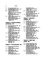
begins to radiate energy in the infrared and visible parts of the spectrum. As the temperature in the core of the gas cloud approaches 20 x 10° K, energy production by hydrogen fusion becomes possible, and a star is born. Most of the stars of a typical galaxy derive energy from this process and therefore plot in a band, called the main sequence, on the Hertzsprung—Russell diagram shown in Figure 2.1. Massive stars, called blue giants, have high luminosities and high surface temperatures. The Sun is a star of intermediate mass and has a surface temperature of about 5800 K. Stars that are less massive than the Sun are called red dwarfs and plot at the lower end of the main sequence. As a Star five times more massive than the Sun converts hydrogen to helium while on the main sequence, the density of the core increases, causing the interior of the star to contract. The core temperature therefore rises slowly during the hydrogen-burning phase. This higher temperature accelerates the fusion reaction and causes the outer envelope of the star to expand. However, when the core becomes depleted in hydrogen, the rate of energy production declines and the star contracts, raising the core temperature still further. The site of energy production now shifts from the core to the surrounding shell. The resulting changes in luminosity and surface temperature cause the star to move off the main sequence toward the realm of the red giants (Figure 2.1). The helium produced by hydrogen fusion in the shell accumulates in the core, which continues

to contract and therefore gets still hotter. The resulting expansion of the envelope lowers the surface temperature and causes the color to turn red. At the same time, the shell in which hydrogen

12

IN THE BEGINNING

Blue giants

Red giants

He burning

10*

103

10?

Solar of Multiples Luminosities White dwarfs

4.5

4.4

4.3

4.2

4.1

4.0

ay

3.8

Da

3.6

log Surface Temperature, K Figure 2.1 Stellar evolution on a Hertzsprung—Russell diagram for stars ranging from | to 9 solar masses. When a star has used up the hydrogen in its core, it contracts and then moves off the main sequence and enters the realm of the red giants, which generate energy by helium fusion. The evolutionary track and the life expectancy of stars are strongly dependent on their masses. Stars five times more massive than the sun are nearly 1000 times brighter, have surface temperatures of about 18,000 K—compared to 5800 K for the Sun—and remain on the main sequence only about 68 million years. Their evolution to the end of the major phase of helium burning takes only about 87 million years (Iben, 1967).

is reacting gradually thins as it moves toward the surface, and the luminosity of the star declines. These changes transform a main-sequence star into a bloated red giant. For example, the radius of a star five times more massive than the Sun increases about 30-fold just before helium burning in the core begins. When the core temperature approaches 100 x 10° K, helium fusion by means of the “triplealpha process” begins and converts three helium nuclei into the nucleus of carbon-12. At the same

time, hydrogen fusion in the shell around the core continues. The luminosities and surface temperatures (color) of red giants become increasingly variable as they evolve, reflecting changes in the rates of energy production in the core and shell. The evolutionary tracks in Figure 2.1 illustrate the importance of the mass of a star to its evolution. A star five times as massive as the Sun is 1000 times brighter while on the main sequence and has a more eventful life as a red giant than stars below about two solar masses (Iben, 1967, 1974).

23° The length of time a star spends on the main sequence depends primarily on its mass and to a lesser extent on the H/He ratio of its ancestral gas cloud. In general, massive stars (blue giants) consume their fuel rapidly and may spend only 10 X 10° years on the main sequence. Small stars (red dwarfs) have much slower “metabolic” rates and remain on the main sequence for very long periods of time exceeding 10 X 10° years. The Sun, being a star of modest magnitude, has enough hydrogen in its core to last about 9 < 10” years at

the present rate of consumption. Since it formed about 4.5 X 10” years ago, the Sun has achieved middle age and will provide energy to the planets of the solar system for a very long time to come. However, ultimately its luminosity will increase, and it will expand to become a red giant, as shown in Figure 2.1. The temperature on the surface of the Earth will then rise and become intolerable to life forms. The expansion of the Sun may engulf the terrestrial planets, including Earth, and vaporize them. When all of its nuclear fuel has been consumed, the Sun will assume the end stage of stellar evolution that is appropriate for a star of its mass and chemical composition. Toward

the

end

of the

giant

stage,

stars

become increasingly unstable. When the fuel for a particular energy-producing reaction is exhausted, the star contracts and its internal temperature rises. The increase in temperature may trigger a new set of nuclear reactions. In stars of sufficient mass, this activity culminates in a gigantic explosion (supernova) as a result of which a large fraction of the outer envelope of the star is blown away. The debris from such explosions mixes with hydrogen and helium in interstellar space to form clouds of gas and dust from which new stars may form. As stars reach the end of their evolution they turn into white dwarfs, or neutron stars (pulsars), or black holes, depending on their masses (Wheeler, 1973). Stars whose mass is less than about 1.2 solar masses contract until their radius is only about 1 x 10* km and their density is between 107 and 10° g/cm®. Stars in this configuration have low luminosities but high surface temperatures and are therefore called white dwarfs (Figure 2.1). They gradually cool and fade from

“NUCLEOSYNTHESIS.

13

view as their luminosities and surface temperatures diminish with time. Stars that are appreciably more massive than the Sun develop dense

cores because of the synthesis of heavy chemical elements by nuclear reactions. Eventually, such stars become unstable and explode as supernovas. The core then collapses until its radius is reduced to about 10 km and its density is of the order of

10'' to 10° g/cm. Such stars are composed of a “neutron gas” because electrons and protons are forced to combine under the enormous pressure and the abundance of neutrons greatly increases as a result. Neutron stars have very rapid rates of rotation and emit pulsed radio waves that were first observed in 1965 by Jocelyn Bell, a graduate student working with A. Hewish at the Cavendish Laboratory of Cambridge University in England (Hewish, 1975). The Crab Nebula contains such a “pulsar,” which is the remnant of a supernova observed by Chinese astronomers in 1054 A.D. (Fowler, 1967). The cores of the most massive stars collapse to form black holes in accordance with Einstein’s theory of general relativity. Black holes have radii of only a few kilometers and densities in

excess of 10'° g/cm’. Their gravitational field is so great that neither light nor matter can escape from them, hence the name “black hole.” Observational evidence supporting the existence of black holes is growing and they are believed to be an important phenomenon in the evolution of galaxies. Stars, it seems, have predictable evolutionary

life cycles. They form, shine brightly for a while, and then die. Hans Bethe (1968, p. 547) put it this way: If all this is true, stars have a life cycle much like animals. They are born, they grow, they go through a definite internal development, and finally die, to give back the material of which they are made so that new stars may live.

2.3

Nucleosynthesis

The origin of the chemical elements is intimately linked to the evolution of stars because the elements are synthesized by the nuclear reactions from which stars derive the energy they radiate into space. Only helium and deuterium, the

14

IN THE BEGINNING

heavy isotope of hydrogen, were synthesized during the initial expansion of the universe. The entire theory of nucleosynthesis was presented in a detailed paper by Burbidge, Burbidge, Fowler and Hoyle (1957) referred to affectionately as B,FH. Subsequent contributions (e.g., Schramm and Arnett, 1973) have been concerned with specific aspects of the theory and its application to the evolution of stars of different masses and initial compositions. The otheory, ypresented, by «BjEHy (1937) evolved from the work of several other scientists, among whom George Gamow deserves special recognition. Gamow received his doctorate from the University of Leningrad and came to the University of G6ttingen in the spring of 1928 for some postdoctoral studies. There he met Fritz Houtermans, with whom he spent many hours in a café making calculations (Gamow, 1963). Subsequently, Houtermans moved to the University of Berlin where he met the British astronomer Robert Atkinson. Houtermans and Atkinson used Gamow’s theory of alpha decay to propose that stars generate energy in their interiors by the formation of helium nuclei from four protons captured by the nucleus of another light element. The initial title of their paper was “Wie kann man einen Heliumkern im Potentialtopf kochen.” (How one can cook a helium nucleus in a pressure cooker.) Needless to say, the editors of the Zeitschrift fur Physik insisted that the title be changed (Atkinson and Houtermans, 1929). Ten years later, in April of 1938, Gamow organized a conference in Washington, D.C., to discuss the internal constitution of stars. The conference stimulated one attendee, Hans Bethe, to examine the possible nuclear reactions between protons and the nuclei of the light elements in order of increasing atomic number. Bethe (1939) found that the “pressure cooker” of Atkinson and Houtermans was the nucleus of '2C and made it the basis of his famous CNO cycle for hydrogen fusion in stars (to be presented later in this section) (Bethe, 1968). Gamow influenced the evolution of the theory of nucleosynthesis in many other ways. In 1935 he published a paper in the Ohio Journal of

Science (an unlikely place for a nuclear astrophysics paper) on the buildup of heavy elements by neutron capture and subsequently championed the idea that the chemical elements were synthesized during the first 30 min after the Big Bang. In the mid-1940s Alpher and Gamow wrote a paper detailing the origin of the chemical elements based on that assumption. At Gamow’s suggestion, Hans Bethe’s name was added “in absentia,” thus creating the famous triumvirate Alpher, Bethe, and Gamow (1948). The abundance of the chemical elements and their naturally occurring isotopes is the blueprint for all theories of nucleosynthesis. For this reason, geochemists and stellar spectroscopists have devoted much time and effort to obtaining accurate analytical data on the concentrations of the elements in the Sun and other nearby stars from the wavelength spectra of the light they emit. Information on the abundances of nonvolatile elements has come also from chemical analyses of stony meteorites, especially the carbonaceous chondrites, which are the most undifferentiated samples of matter in the solar system available to us (Mason, 1962). Table 2.1 lists the abundances of the elements in the solar system compiled by Anders and Ebihara (1982). The abundances are expressed in terms of the number of atoms relative to 10° atoms of silicon. Figure 2.2 is a plot of these data and illustrates several important observations about the abundances of the elements. 1. Hydrogen and helium are by far the most abundant elements in the solar system, and the atomic H/He ratio is about 12.5.

2. The abundances of the first 50 elements decrease exponentially. 3. The abundances of the elements having atomic numbers greater than 50 are very low and do not vary appreciably with increasing atomic number. 4, Elements having even atomic numbers are more abundant than their immediate neighbors with odd atomic numbers (Oddo-Harkins rule).

Table 2.1. Abundances of the Elements in the Solar System in Units of Number of Atoms per

10° Atoms of Silicon

Atomic no. 1 2

Element

Symbol

hydrogen helium

H He

DY DAs

Abundance SNe Se UO?

Atomic no.

Element

53 54

iodine xenon

Symbol I Xe

Abundance‘ OM ABS

9 1d $< TOY

3

lithium

Li

So

S< NO

55

cesium

4 5 6

beryllium boron carbon

Cs

a2

Be B G

Ws Dek NL

SO S€ INO} S< io?

56 57 58

barium lanthanum cerium

Ba ILA Ce

ASOme 448 eGie

i

nitrogen

N

2.48

x 10°

3)

praseodymium

lee

1.74

xX 107

8

oxygen

OL 8.43 376)

S< aly x 10? < OF

84

polonium

Po

a)

33

arsenic

As

6.79

x 10°

85

astatine

At

~0

34 35 36 yi 38 3g) 40

selenium bromine krypton rubidium strontium yttrium zirconium

Se Br Kr Rb Sr Ne Tbe

Gal 118 453 TO 238 4.64 Oy

3He + y + 5.493 MeV

(2.6) (2.7)

3He + 3He — 5He + jH + 7H + 12.859 MeV (2.8) The direct proton—proton fusion to form helium-4 can only take place at a temperature of about 10 X 10° K, and even then the probability of its occurrence (or its “reaction cross section”) is very small. Nevertheless, this process was the only source of nuclear energy for first-generation stars that formed from the primordial mixture of hydrogen and helium after the Big Bang. Once the first generation of stars had run through their evolutionary cycles and had explod-

NUCLEOSYNTHESIS

17

ed, the interstellar gas clouds contained elements of higher atomic number. The presence of carbon-

12 (%.C) synthesized by the ancestral stars has made it easier for subsequent generations of stars to generate energy by hydrogen fusion. This alternative mode of hydrogen fusion was discovered by Hans Bethe and is known as the CNO cycle:

UG + TH > BN +

(2.9)

AN > BC + pt t+ v

BC+ iH

PN

~4N+ y

es Oa

5,

5bO 3 EN + pt +p

EN + 1H > 2C + He

(2.10)

(2.11)

(x12) (213)

(2.14)

The end result is that four protons are fused to form one nucleus of 5He, as in the direct proton— proton chain. The nucleus of '2C acts as a sort of catalyst and is released at the end. It can then be reused for another revolution of the CNO cycle. The Sun contains elements of higher atomic

number than helium including '¢C and therefore carries on hydrogen fusion by the CNO cycle. In fact, most stars in our Milky Way Galaxy are second-generation stars because our Galaxy is so old that only the very smallest first-generation stars could have survived to the present time. The low reaction cross section of the proton— proton chain by which the ancestral stars generated energy has been a source of concern to nuclear astrophysicists. When this difficulty was pointed out to Sir Arthur Eddington, who proposed hydrogen fusion in stars in 1920, he replied (Fowler, 1967): We do not argue with the critic who urges that the stars are not hot enough for this process; we tell him to go and find a hotter place.

After the hydrogen in the core has been converted to helium “ash,” hydrogen fusion ends, and the core contracts under the influence of gravity. The core temperature rises toward 100 x 10° K, and the helium “ash” becomes the fuel for the next set of energy-producing nuclear reactions. The critical reaction for helium burning is the fusion of three

18

IN THE BEGINNING

alpha particles (triple-alpha

process) to form a

nucleus of '2C:

sHe + ;He > {Be

(2.15)

"Be + }3He

(2.16)

9 2C + y

This is the critical link in the chain of nucleosynthesis because it bridges the gap in nuclear stability of the isotopes of lithium, beryllium, and boron. The crux of the problem is that the nucleus of {Be is very unstable and decays quickly with a “halflife”ofabout 10'°sec. Therefore, {Be must absorb a third helium nucleus very soon after its formation

to make it safely to stable '2C (Fowler, 1967). An alternative reaction involving the addition of a proton to the nucleus of }He has an even smaller chance to succeed because the product, }Li, has a

half-life of only 10*'sec and decomposes to form helium and hydrogen:

SeNi+

jn —>S3Ni+ y

O21)

neutron

indicates that the nucleus of $;Ni absorbs a neutron, which changes it to an excited state of $3Ni, which then deexcites by emitting a gamma ray.

Nickel-63 is radioactive and decays to stable $3Cu by emitting a B particle: S3Ni

> $3Cu + B + v + 0.0659 MeV

(2.22)

where v is an antineutrino. $5Cu is a stable isotope of copper and can absorb another neutron

to form $Cu:

4He + {H > 3Li

SLi

‘He + 1H

(2.17) (2.18)

The triple-alpha process is indeed the key to the synthesis of all elements beyond helium. Without it, stellar evolution would be shortcircuited, and the universe would be composed only of hydrogen and helium. Helium burning sustains red giants only for a few tens of millions of years or less. With increasing temperature in the core, alpha particles fuse with the nuclei of '2C to produce nuclei of still higher atomic number:

4G

are the neutron-capture reactions, which produce a large number of the atoms having atomic numbers greater than 26 (Fe). These reactions involve the addition of a neutron to the nucleus of an atom to produce an isotope having the same atomic number but a large mass number. For example, the equation:

He.

2O

0 + 3He > {Ne

(2.19) (2.20)

etc.

However, electrostatic repulsion between positively charged nuclei and alpha particles limits the size of the atoms that can form in this way. The heaviest atom produced by the addition of alpha particles is 56 3,Ni, which decays to 3$Co and then to stable 3°Fe. These nuclear reactions therefore cause the enhanced abundance of the elements in the iron group illustrated in Figure 2.2. During the final stages of the evolution of red giants, several other kinds of nuclear reactions occur (B,FH, 1957). The most important of these

seCu

ian — > egCu

y

(223)

Copper-64 is radioactive and undergoes branched

decay to form $iZn and ${Ni, both of which are stable:

SCus Zn +B

+ 2 +0575 MeV

(2.24)

Cu > $3Ni + Bt + v + 1.678 MeV

(2.25)

This process of successive additions of neutrons is illustrated in Figure 2.3. It takes place during the red giant stage of stellar evolution when the neutron flux is low enough to permit the product nucleus to decay before the next neutron is added. This process therefore is characteristically slow and is therefore referred to as the s-process. By examining Figure 2.3 closely we see that

the track of the s-process bypasses {i}Zn, which is one of the stable isotopes of zinc. In order to make this isotope by neutron capture reactions, the pace must be speeded up so that unstable

30ZN can pick up a neutron to form {°Zn before it decays to stable {/Ga:

Zn + on > Zn + ¥

(2.26)

An even more rapid rate of neutron capture is

required to make {jZn from $3Cu by addition of five neutrons in succession to form 38Cu, which then decays by B emission to stable {)Zn:

2.3. ) NUCLEOSYNTHESIS

19

34 p-process —

33

32

att

Ga

30

Number (Z) Proton 2g

a SS

Paes

—

28

35

38

39

40

A

42

Neutron Number (N) Figure 2.3 Nucleosynthesis in red giants by neutron capture on a slow time scale (s- process) followed by beta decay. The dark squares are stable isotopes, whereas the unshaded ones are radioactive. The process starts with stable $;Ni, which absorbs a neutron to form unstable S3Ni, which decays to stable §3Cu by ee a B particle. The main line of the s-process, as indicated

by arrows, proceeds from $;Ni to {{Se and beyond but bypasses MZn and {4Se. 3)Zn is produced by neutron capture which captures five 4Se is a proton-rich the addition of two

Cura on

(Ci 7a

on a rapid time scale (r-process) from $°Zn via unstable $jZn and from 2 Cu; neutrons in rapid succession to form {Cu followed by decay to stable Le nuclide that cannot form by either the s-process or the r-process and requires protons (p-process) to stable BGe:

> 4,00

pop,

oy

~12MevV

(2.27)

(2.28)

Capture of neutrons at such rapid rates is characteristic of the r-process, which requires a much greater neutron flux than the s-process and therefore takes place only during the last few minutes in the life of a red giant when it explodes as a supernova. However, no neutron capture on any time scale can seco for the formation of some atoms such as stable {jSe shown also in Figure 2.3. This nuclide is synthesized by the addition of two protons to stable {5Ge in the so-called p-process:

UGe + 24H — 2Se

(2.29)

This process also takes place at the very end of the giant stage of stellar evolution. The system of nuclear reactions originally proposed by B,FH (1957) can account for the observed abundances of the chemical elements in the solar system and in nearby stars. Nucleosynthesis is taking place at the present time in the stars of our galaxy and in the stars of other galaxies throughout the universe. We have good evidence in the wavelength spectra of light from distant galaxies that the chemical elements we find on Earth also occur everywhere else in the universe.

20

IN THE BEGINNING

However, pulsars and black holes have high internal pressures and temperatures that cause atomic

nuclei to disintegrate into more primitive constituents. The relative proportions of the chemical elements in other stars are different because local conditions may affect the yields of the many nuclear reactions that contribute to their synthesis.

2.4

Summary

We live in an expanding universe whose future is uncertain. The universe started with a Big Bang about 15 x 10” years ago and has evolved since then in accordance with the laws of physics. Stars are the basic units in the hierarchy of heavenly bodies. They form by contraction of clouds of interstellar gas and dust until their core

temperatures are sufficient to cause hydrogen fusion. Stars evolve through predictable stages depending on their masses and initial compositions. They generate energy by nuclear reactions that synthesize other elements from primordial hydrogen and helium. In the end, stars explode, and the remnants become solid objects of great density. The abundances of the chemical elements in the solar system can be explained by the nuclear reactions that energize the stars. These reactions progress from fusion of hydrogen and helium to neutron capture and to other reactions, most of which occur only for a short time at the end of the active life of a star. The chemical elements we know on Earth occur throughout the universe, but their abundances vary because local conditions affect the yields of the nucleosynthesis processes.

Problems* 1. How has the abundance of hydrogen (H) in the universe changed since the Big Bang?

7. Why is lead (Pb) more abundant than we might have expected?

2. Why are elements with even atomic numbers more abundant than their neighbors with odd atomic numbers?

8. Check the abundance of argon (Ar) and determine whether it is greater than expected. If so, suggest an explanation.

3. How do we know that the Sun is at least a “sec-

9. How did lithium (Li), beryllium (Be), and boron (B) form?

ond-generation” star?

4. Why do technetium (Tc) and promethium (Pm) lack stable isotopes? 5. What other elements also lack stable isotopes?

10. Compare the abundances of the “rare earths” (lanthanum to lutetium) to such well-known metals as Ta, W, Pt, Au, Hg, and Pb. Are the rare earths really all that “rare”?

6. Why do the elements of Problem 5 exist on the Earth, whereas Tc and Pm do not? *Not all of these questions have unequivocal answers.

References ALPHER, R. A., H. BETHE, and G. GAMow, 1948. The origin of the chemical elements. Phys. Rev., 73:803-804. ANDERS,

E., and M. EBIHARA, 1982. Solar-system dances of the elements. Geochim. Cosmochim. 46:2363-2380.

abun-

Acta,

ATKINSON, R. d’E., and F. G. HOUTERMANS, 1929. Zur Frage der Aufbauméglichkeit der Elemente in Sternen. Zeit. Phys., 54:656-665. BAADE, W., 1968. Evolution of Stars and Galaxies. Harvard University Press, Cambridge, MA.

REFERENCES BETHE, H. A., 1939. Energy production in stars. Phys. Rev.,

55:434-456. BeTHE,

Energy

production

in stars. Science,

161:541-547.

HUuBBLE, E., 1936. The Realm of the Nebulae. Yale University

Press, New Haven, CT. Reprinted 1958 by Dover Pub., Inc.,

BURBRIDGE, E. M., G. R. BURBRIDGE, W. A. FOWLER, and F, Hoy_e, 1957. Synthesis of the elements in stars. Rev. Mod. Phys., 29:547-650. FOWLER, W. A., 1967. Nuclear astrophysics. Amer. Phil. Soc. Mem. 67, 109 pp. Gamow, G., 1935. Nuclear transformations and the origin of the chemical elements. Ohio J. Sci., 35:406-413. Gamow, G., 1952. The Creation of the Universe. Viking Press,

New York, 144 pp. Gamow, G., 1963. My early memories of Fritz Houtermans. In and

Hewisn, A., 1975. Pulsars and high density physics. Science,

188:1079-1083.

H. A., 1968.

J. Geiss

21

E. D. Goldberg

(Eds.), Earth

Science and

Meteoritics. North-Holland Publ. Co., Amsterdam, 312 pp. Gort, J. R., Ill, 1982. Creation of open universes from de Sitter space. Nature, 295:304-307. HAINEBACH, K., D. KAZANAS, and D. N. SCHRAMM, 1978. A consistent age for the universe. Short papers of the Fourth International Conference, Geochronology, Cosmochronology and Isotope Geology. U.S. Geol. Sur. Open-File Rept., 78-701, 159-161.

New York.

IBEN, I., Jr., 1967. Stellar evolution: Comparison of theory with observation. Science, 155:785-796. IBEN, I., Jr., 1974. Post main sequence evolution of single stars. Ann. Rey. Astron. and Astrophys., 12:215-256. MAson, B., 1962. Meteorites. Wiley, New York, 274 pp. PENZIAS, A. A., and R. W. WILSON, 1965. A measurement of excess antenna

temperature

at 4,080 Mc/s. Astrophys. J.,

142:419. SCHRAMM, D. N., and W. D. ARNnetT, 1973. Explosive Nucleosynthesis. University of Texas Press, Austin and London, 301 pp. WEINBERG, S., 1977. The First Three Minutes. Bantam Books, New York, 177 pp. WHEELER,

J. C., 1973.

Scientist, 61:42-51.

After

the

supernova,

what?

Amer.

3 The Solar System The Sun formed from a cloud of gas and dust particles, as did all other stars in the Milky Way Galaxy and elsewhere in the universe. Sometimes the process leads to the formation of two companion stars. However, in the case of the Sun a small fraction of the original cloud accreted to form a set of nine planets, including the Earth. Compared to stars, these planets are insignificant objects, but to us they are the very basis of existence. The human race appeared on the Earth only two or three million years ago and, after a slow start, learned to fly and to explore the solar system within a span of a mere century. Geochemistry today not only encompasses the study of the composition and chemical processes occurring on the Earth, but is also concerned with all of the planets and their satellites. Information for geochemical studies of the solar system is derived by analysis of meteorites and rock samples from the Moon and by remote sensing of planetary surfaces. The exploration of the solar system has expanded our horizon and has provided the basis for comparative planetary geochemistry. The satellites of the large gaseous planets are of special interest in this new field of study because some of them are larger than our Moon and have very different chemical compositions and surface features than the Earth. We therefore need to become acquainted with the new worlds we must explore before we concentrate our attention on the conventional geochemistry of the Earth.

stellar gas and dust known as the solar nebula. It had formed about six billion years ago as a result of the

terminal

explosions

of ancestral

stars,

which added the elements they had synthesized to the primordial hydrogen and helium that originated from the Big Bang. The chemical composition of the solar nebula was given in Chapter 2

(Table 2.1). The dust cloud was rotating in the same sense of the Milky Way Galaxy and was acted upon by gravitational, magnetic, and electrical forces. As soon as the main mass of the solar nebula began to contract, order began to be imposed on it by the physical and chemical conditions that existed during this phase of star formation. These included the development of pressure and temperature gradients and an increase in the rate of rotation. Certain kinds of solid particles that had formed in the nebula evaporated as the temperature increased in order to maintain equilibrium between solids and gases. As a result, only the most refractory particles (Fe—-Ni alloys, AlO;, CaO, etc.) survived in the hottest part of the contracting nebula, whereas in the cooler outer regions a larger variety of compounds remained

in the solid state. The increase in the rate of rotation caused part of the nebula outside of the protosun to form a central disk. The solid particles congregated in this disk and made it sufficiently opaque to absorb infrared radiation. The temperature in the central disk therefore increased until it ranged from about 2000 K at the center to

about 40 K at approximately 7.5 x 10’ km from

3.1

Origin of the Solar System

The origin of the planets of the solar system is intimately linked to the formation of the Sun. In the beginning there was a diffuse mass of inter-

22

the protosun. The pressure ranged from less than

0.1 atm to about 10°’ atm near the edge of the disk (Cameron, 1978; Cameron and Pine, 1973). The development of pressure and temperature gradients within the disk caused the first

3.1.

major chemical differentiation of the solar nebula. Compounds with low vapor pressures persisted throughout the nebula and formed “dust” particles, whereas compounds with high vapor pressures could exist only in the cooler outer regions. The condensation temperatures of various compounds that existed in the solar nebula are listed in Table 3.1. The condensates accreted to form larger bodies as a result of selective adhesion caused by electrostatic and magnetic forces. The resulting solid bodies, called planetesimals, had diameters ranging from about 10 m to more than 1000 km, and their chemical compositions varied with distance from the center of the planetary disk. The planetesimals close to the protosun were composed of refractory compounds dominated by oxides and metallic iron and nickel; farther out were Mg and Fe silicates and farthest out, ices composed of water, ammonia, methane, and other

volatiles. The initial rate of evolution of the solar system was remarkably fast. The time required for the Sun to reach the ignition temperature for

Table 3.1

ORIGIN OF THE SOLAR SYSTEM

hydrogen fusion was less than 100,000 years. The Sun’s initial luminosity was two to three times greater than is consistent with the main sequence because the Sun contained excess thermal energy generated during the initial contraction. This “superluminous” phase of the Sun lasted about 10 million years and resulted in the expulsion of about 25% of its original mass in the form of “solar wind” composed of a proton/electron plasma. This is called the “T-Tauri stage” of stellar evolution after the star that is the prototype for this process. All gaseous matter in the vicinity of the Sun was blown away during this period, and only the solid planetesimals having diameters larger than about 10 m remained. The planetesimals in the inner region of the planetary disk subsequently accreted to form the so-called earthlike planets—Mercury, Venus, Earth, and Mars—and

the parent bodies of the

meteorites now represented by asteroids. Instabilities in the outer part of the disk resulted in the formation of the gaseous outer planets: Jupiter, Saturn, Uranus, Neptune, and Pluto.

Condensates from the Solar Nebula at Different Temperatures

Temperature, °C

Condensates

1525

refractory oxides: CaO, Al,O;, TiO,, REE oxides

1025

metallic Fe and Ni

925

enstatite (MgSiO,)

925-220

Fe forms FeO, which reacts with enstatite to form olivine [(Fe,Mg),SiO,]

Wa

Na reacts with Al,O, and silicates to form feldspar and related minerals.

400

HS reacts with metallic Fe to form troilite (FeS)

Condensation of K and other alkali metals 280

150 OO =125

H,O vapor reacts with Ca-bearing minerals to make tremolite

=150 210"

H,O vapor reacts with olivine to form serpentine H,O vapor condenses to form ice NH, gas reacts with water ice to form solid NH, - H,O CH, gas reacts with water ice to form solid CH, - 7H,O Ar and excess CH, condense to form Ar and CH,

=Y50"

Ne, H, and He condense

*These reactions probably did not occur because the temperature in the planetary disk did not decrease to such low values.

SOURCE: Glass (1982), based on Lewis (1974).

23

24

THE SOLAR SYSTEM The descriptive physical properties of the solar system listed in Table 3.2 indicate that 99.87% of the total mass of the solar system (2.052 x 10*° g) is concentrated in the Sun. The remaining 0.13% is distributed among the nine major planets, among which Jupiter is by far the largest with about 71% of the planetary masses. The densities and sizes of the planets, shown in Figure 3.1, vary widely and imply the existence of large differences in their chemical compositions. The inner planets (Mercury, Venus, Earth, and Mars), as well as the Moon and the asteroids, are solid objects composed primarily of elements and compounds having low vapor pressures. The outer

The origin and chemical composition of Pluto are still not well known because this planet is difficult to observe from Earth. Pluto also does not conform to the so-called 7Titius—Bode law, which appears to govern the distances of the planets from the Sun when these are expressed in astronomical units (A. U.), defined as the average distance between the Earth and Sun. The Titius-Bode law was published in 1772 by J. E. Bode, director of the Astronomical Observatory in Berlin, and is based on a series of numbers discovered by J. D. Titius of Wittenberg in 1766. The series is composed of the numbers 0.4, 0.7, 1.0, A Cae aN which are obtained by writing 0, 3, 6, Ne adding 4 to each number, and dividing by 10. The resulting numbers match the distances of the planets from the Sun remarkably well up to and including Uranus (Mehlin, 1968). However, the radius of the orbit of Neptune is only 30.1 A.U., whereas the Titius-Bode value is 38.8 and the discrepancy in the case of Pluto is even greater (Table 3.2). The Titius—Bode law predicts a value of 77.2, but the actual orbital radius of Pluto is only 39.4 A.U. The discrepancy may suggest that Pluto did not form in the orbit it now occupies.

planets (Jupiter, Saturn, Uranus, and Neptune) have

low densities

and

are essentially

gaseous,

although all of them probably have condensed cores. The inner planets resemble the Earth in chemical composition and are therefore referred to as the ferrestrial or earthlike planets. The outer planets consist primarily of hydrogen and helium with small amounts of the other elements and resemble the Sun in chemical composition. The earthlike planets (plus the Moon and asteroids), taken together, make up only 0.0006% of the total mass of the solar system and only

Table 3.2 Properties of the Sun and Her Planets Mean solar distance

Object Sun Mercury

10°km

ANU!

—

Equatorial diameter, km

Mass, g

1,391,400

1.987 x 10°

Sy)

0.387

4.878

Venus

108.2

0.723

Earth

149.6

1.00

Moon

=

Mars

227.9

Ie52

330

Density g/cm

1.4

Number of satellites

—

108

5.44

0

12,100

4.87 x 10?

5.25

0

12756

5.98107

SSW

3,476

7.39510"

3.34

6,786

6.44 x 107

3.94

i

— 2

Ceres (asteroid)

414.0

Dae

1,020

ei

Oe

2D,

Jupiter

778.3

5.20

142,984

1.90’

10”

3s)

16

Saturn

1,427.0

9.54

120,536

5.69 x 10°

0.70

21

Uranus

2,869.6

19.2

Dlelales

8.66 X 10°

1.30

1S)

Neptune

4.504

30.1

49,562

110

1.76

8

Pluto

5,900

39.4

3,000

i0e

itt

|

[O123 Lee

SOURCE: Carr et al. (1984), Glass (1982), and fact sheet, Jet Propulsion Laboratory.

=

oe 0.44% of the planetary masses. All of these objects are so close to the Sun that the orbital radius of the outermost asteroid is only about 7% of the total radius of the solar system. Evidently, the terrestrial planets are not typical of the solar system and owe their existence to the special conditions in the planetary disk close to the Sun. Earth is the largest of the inner planets with about 50.3% of the mass, followed by Venus

(40.9%), Mars (5.4%), and Mercury (2.8%). The earthlike planets, viewed in Figure 3.1 in the perspective of the entire solar system, are a physical and chemical anomaly. The Earth is unique among its earthlike neighbors in having about 71% of its surface covered by liquid water within which life developed early in its history and evolved into the multitude of species of the plant and animal kingdoms. Insofar as we know, life forms do not exist at the present time anywhere else in the solar system.

ORIGIN OF THE EARTHLIKE PLANETS

3.2

Origin of the Earthlike Planets

Our current understanding of the origin of the solar system indicates that the earthlike planets were hot when they formed and that their internal geochemical differentiation may have begun with the sequential accretion of planetesimals of differing compositions (Murray et. al., 1981). Planetesimals composed of metallic iron and oxides accreted first to form a core that was subsequently buried by the planetesimals composed of silicates. The earthlike planets were initially molten because of the heat generated by the rapid capture of the planetesimals and because of radioactive heating. The last phase of formation of Earth, Venus, and Mars involved the capture of planetesimals composed of volatile compounds that had formed in the outer reaches of the planetary disk, perhaps

g/cm? Density,

Pluto

Gaseous planets

Earthlike planets

—»>

58.9 X 108 km

Jupiter

Saturn

12

16

20

25

24

©

O

Uranus

Neptune

28

By

36

40

44

Mean Distance from the Center of the Sun, 108 km Figure 3.1 A: Variation of density of the planets with mean distance from the highest density among the earthlike planets, which, as a group, are more planets. B: The planets of the solar system magnified 2000 times relative to planets are very small in relation to the Sun and the gaseous planets of the

the Sun. Note that the Earth has dense than the outer gaseous the distance scale. The earthlike solar system.

26

THE SOLAR SYSTEM

beyond the orbit of Jupiter. These volatile-rich planetesimals, also known as cometesimals, deposited solids composed of water, ammonia, methane, and other volatiles on the surfaces of the planets. The water and other volatiles deposited on the Earth promptly evaporated to form a dense atmosphere from which water ultimately condensed as the surface of the Earth cooled. Mercury and the Moon do not have atmospheres partly because they are too small to retain gaseous elements of low atomic number and their compounds. According to this scenario, the earthlike planets have been cooling since the time of their formation. Mercury and the Moon have cooled sufficiently to become geologically “inactive” in the sense that their interiors no longer interact with their surfaces. Venus and Earth, being the largest of the earthlike planets, have retained more of the initial heat than their neighbors in the solar system and are still active. Mars is intermediate in size and has had volcanic eruptions in the not-too-distance geologic past. However, the age of the last martian volcanism is not known. In spite of the similarity in size and overall composition of Venus and Earth, their surfaces have evolved very differently. Venus has a dense atmosphere composed of CO, that has caused its surface to become extremely hot and dry. The surface of Earth cooled rapidly, allowing oceans

to form more than 4 X 10” years ago by condensation of water vapor in the atmosphere. The presence of a large volume of water on the surface of Earth permitted geological processes to operate and created conditions conducive to the development. and evolution of life. Neither the Earth nor any of the earthlike planets ever had atmospheres composed of the hydrogen and helium of the solar nebula because these gases were expelled from the inner region of the solar system during the T-Tauri stage of the Sun.

3.3

Satellites of the Outer Planets

All of the outer planets have satellites, some of which are larger than the Moon and the planet Mercury. In addition, these satellites have a wide range of chemical compositions and have responded in very different ways to the forces acting on them. The large satellites of Jupiter were seen by Galileo Galilei on January 7, 1610, with his newly built telescope. Actually, they may have been observed even earlier by Simon Marius. However, detailed images of their surfaces were obtained only recently during “flybys” of the American Pioneer and Voyager space probes. A chronology of these events in Table 3.3 reveals the sudden burst of activity in the exploration of the solar system between 1973 and 1989.

Table 3.3. Chronology of Exploration of the Satellites of Jupiter and Saturn Planet

Encounter date

Spacecraft

Jupiter

Dec

aiO7s

Pioneer 10

left solar system on June 14, 1983

Jupiter

Dec. 2, 1974

Pioneer 11

continued to Saturn

Jupiter

March 5, 1979

Voyager |

1408 images ofjovian satellites

Jupiter

July 9, 1979

Voyager 2

1364 images ofjovian satellites

Jupiter Saturn Saturn Saturn Uranus

Dec, 7, 1995 Sepiale a7 Nov. 13, 1980 Aug. 26, 1981 Jan. 25, 1986

Galileo Pioneer Voyager Voyager Voyager

mission in progress in 1997

Neptune

Aug. 25, 1989

Voyager 2

After Greeley (1985).

Comments

11

low-resolution images

1

900 images of saturnian satellites

2

1150 images of saturnian satellites

2

images of all satellites as well as the rings images of the planet and its satellite Triton

3.3

The planet Jupiter has 16 satellites and a ring guarded by two small satellites. The so-called Galilean satellites lo, Europa, Ganymede, and Callisto were actually named by Marius after mythological lovers of the Greek god Zeus whose Latin name was Jupiter. A fifth satellite was discovered 282 years later by Barnard who named it Amalthea after a nymph who once nursed Jupiter. These satellites, together with three small ones found in 1979, move in nearly circular orbits close to the equatorial plane of Jupiter. Four small satellites (Leda, Himalia, Lysithea, and Elara) are located about 11 million km from Jupiter and have eccentric orbits that are inclined nearly 30° to its equatorial plane. A third group

(Ananke, Carme, Pasiphaé, and Sinope) at a distance of about 22 million km from Jupiter have retrograde orbits whose inclination is between 150° and 160°. The Galilean satellites form in effect a small-scale planetary system of their own with Jupiter as their central “star.” Their densities, listed in Table 3.4 and displayed in Figure 3.2, decrease with increasing orbital radius from

3.53 (Io) to 1.79 (Callisto) g/cm*; therefore they are believed to have significantly different chemical compositions. Io is composed primarily of silicate material and may have an iron sulfide core. Before the encounters with the Voyager spacecraft, Peale et al. (1979) calculated the amount of heat generated within Io by tidal friction caused by the gravitational pull of Jupiter and Europa and predicted that active volcanoes may be present. This prediction was supported by images sent back by Voyager 1 on March 9, 1979, which indicated that the surface of this planet was not cratered as had been expected. Subsequently, Morabito et. al. (1979) discovered a huge volcanic eruption on Io that was obliterating impact craters and all other topographic features in a large area surrounding the

were

volcano.

Eventually,

identified

nine

and named

active

volcanoes

after mythological

deities associated with fire (Amirani, Loki, Marduk, Masubi, Maui, Pele, Prometheus, Surt,

and Voland). The volcanic plumes contain sulfur dioxide and the lava flows may be composed of liquid sulfur, consistent with the fact that the sur-

SATELLITES OF THE OUTER

PLANETS

27

face of Io is yellow to red in color. The surface heat flow of Io is about 48 microcalories/cm?/sec and is therefore about 30 times greater than that of the Earth. Io is clearly the most volcanically active object in the solar system. The other Galilean satellites of Jupiter (Europa, Ganymede, and Callisto) have lower densities than Io and are composed of silicate material with crusts of water ice and mantles of liquid water. They are not volcanically active at the present time, and their surfaces are cratered. Europa appears to be completely covered by a frozen ocean 75-100 km deep. The icy crust may be underlain by liquid water that does not freeze because of heat generated by tidal friction. The surface of Europa is crisscrossed by a multitude of curving

bands,

some

of which

have

been

traced for more than 1000 km. The bands appear to be fractures in the crust caused by internal tectonic activity and by meteorite impacts. The fractures were subsequently filled with subcrustal water that froze to form ice dikes. Ganymede is larger than the planet Mercury and appears to be composed of water and silicate material in about equal proportions. Its surface is composed of water ice mixed with impurities that cause it to darken in color. The dark terrains are fragmented and more heavily cratered than the light-colored terrain in which they are embedded. The ice crust is about 100 km thick and is underlain by a mantle of liquid water between 400 and 800 km deep. The water may have intruded the crust locally in the form of ice slush to produce intrusive bodies of water ice. Callisto is the outermost of the Galilean satellites. It is darker in color than the others and has a heavily cratered icy crust about 200 km thick. A prominent feature on its surface is a very large multiringed basin called Valhalla whose diameter is nearly 2000 km. A second ringed basin near the north pole is called Asgard. The icy crust may be underlain by a liquid mantle about 1000 km thick composed of water. Callisto apparently became inactive very early in its history partly because the amount of heat generated by tidal friction is less than that of the other Galilean satellites. In

28

THE SOLAR SYSTEM

Table 3.4 Physical Properties of the Major Satellites of Jupiter, Saturn, Uranus, and Neptune Name

Mean distance

Diameter,

Mass,

BRU

from planet, km

km

g

g/cnv

Jupiter

lo Europa Ganymede Callisto

421,600 670,900 1,070,000 1,883,000

3,640 3,130 5,280 4,840

te SOll 4.8m dOe 1.49 x 10° 1.06 x10”

188,000 240,000 297,000 379,000 528,000 1,221,000

390 500 1,050 1,120 1,530 5,140

(BieEO tyr ai0(74 234)96107 (6.262017) x10" (TOS s2010S S10 (2.16= O71) x 10” (1.348+ 0.017) x 10°

eyes! 3.03 1.93 1.79

Saturn

Mimas Enceladus Tethys Dione Rhea Titan Hyperion

lapetus Phoebe

1,502,000

1.2 1a 1.0 1.42 igs: 1.9(+)

ea)

3,559,000 10,583,000

1,440 160

Miranda Ariel

130,000 192,000

470 1,150

Umbriel Titania Oberon

267,000 438,000 586,000

L170 1,580 1,520

40" 134 U2: 1:26 1074 SAT oO! 20S A10e

354,000 5,510,000

3,000 940

0278

j '

3)

\

6

aD

Mohorovicic discontinuity

pont PR 2 |Seep 0

2000

Sema

Core

4000

Depth, km

6000

12

°o

nearly 10 g/cm’, and then continues to increase to values in

excess of 12 g/cm? at the bound-

jee)

Core (liquid)

g/cm? Density, 6 4

0

2000

4000

Depth, km plate boundaries. Estimates of the chemical composition of the mantle must meet certain geophysical requirements regarding density, seismic velocities, and heat production by the decay of U, Th, and K. In addition, the mantle

must be capable of forming the major types of

6000

ary between the outer and inner core. The variation of these physical properties leads to the conclusion that the mantle is solid and is composed primarily of silicates and oxides of Mg and Fe. The core consists of an alloy of Fe, Ni, and other siderophile elements and is liquid except for the

inner part which is solid (after Bullen, 1963).

basaltic magmas by partial melting under the physical conditions likely to prevail in that region of the Earth. These requirements are generally satisfied by arock called pyrolite invented by Ringwood (1966) by combining peridotite and basalt in the ratio of 3

4.1

Table 4.1

INTERNAL STRUCTURE OF THE EARTH

45

Physical Dimensions of the Earth Including the Continental

Crust Average Thickness, km

Volume, 107’ cm?

density,

Mass,

Mass,

g/cm

1077 g

%

Whole Earth

6371"

1.083

Sa

5.976

Core

BYAT ts

0.175

10.7

1.876

Bille

Mantle

2883

0.899

4.5

4.075

68.1

Crust”

40

0.008 42

2.8

0.023 6

0.4

0.001 37

1.03

0.001 41

0.024

=

—

0.000 005

0.000 09

Hydrosphere

3.8 (av.)

Atmosphere

=

100

“Radius.

>Continental crust. Source: Parker (1967) and Taylor and McLennan (1985).

Table 4.2

Estimates of the Chemical

Composition of the Mantle of the Earth

SiO, MgO FeO ALO; CaO Na,O Cr,0; MnO P.O; K,O TiO, NiO Sum

Sample 1*

Sample 2°

Sample 3°

45.2 Sues 8.0 ce Sil 0.57 0.43 0.14 0.06 0.13 0.17 — 98.8

48.1 SHE! Oe, al We: Tait 0.55 0.42 0.34 OV? 0.12 — 99195

45.0 39.0 8.0 32 Bes 0.28 0.41 0.11 = 0.04 0.09 O25 99.93

Pyrolite (Ringwood, 1966). >Mantle plus crust based on meteorites (Mason, 1966). °Undepleted mantle based on Iherzolites (Hutchison, 1974).

to 1. The resulting chemical composition of the mantle is similar to one proposed by Mason (1966), which was based on meteorites, and also resembles

the estimate made by Hutchison (1974), which was derived from ultramafic lherzolite inclusions in igneous rocks. The estimates of the chemical composition of the mantle are compiled in Table 4.2.

The great interest by the scientific community in the chemical composition of the mantle and in the Moho caused one of the more colorful episodes in the history of science. In the course of a gathering of some members of the American Miscellaneous Society (AMSOC) in Washington, D.C., chaired by Professor Harry Hess of Princeton University, someone casually suggested that a hole should be drilled through the oceanic crust to find out what causes the Moho. The idea ignited the enthusiastic support of the group, and a proposal was promptly submitted to the National Science Foundation to determine the feasibility of this idea. Thus began the so-called Mohole Project, which received much attention in the popular press but never achieved its objective. Nevertheless, engineering studies were made with support from the National Science Foundation, a drilling ship was outfitted, and some test holes were drilled. These tests demonstrated that it was indeed possible to drill in deep water from a ship positioned over the selected site. Eventually AMSOC disbanded, but the equipment was taken over by the Deep-Sea Drilling Program, which has been exploring the history of the ocean basins by drilling first from the Glomar Challenger and later from the Glomar Explorer. The AMSOC gave up the quest to drill to the Moho partly because it became apparent that this important boundary is actually exposed in some deep-sea trenches and that rocks from the

46

CHEMICAL DIFFERENTIATION OF THE EARTH

upper mantle could be, and in fact had been, recovered by dredging.

4.2

large numbers of chemical analyses, (2) com-

The Continental Crust:

Major Elements The crust of the Earth is important because it contains all of the natural resources that sustain us. It includes the atmosphere, hydrosphere, and biosphere, as well as part of the lithosphere. The term lithosphere is now defined as the rigid outer portion of the Earth consisting of the crust and upper mantle in contrast to the underlying asthenosphere, which deforms plastically in response to tectonic stress. The study of the chemical composition of the continental crust, and of the different types of rocks of which it is composed, has been a major objective of geochemistry (Wedepohl, 1969: Taylor and McLennan, 1985). The

crust

is the

outer

shell of the

but their occurrence at the surface of the continents enhances their importance. The chemical composition of the continental crust has been estimated by (1) averaging

Earth,

which lies above the mantle. It not only makes up the continents but also occurs under the oceans. The oceanic crust is only 5—8 km thick and differs from the continental crust in chemical composition and origin. The continental crust is composed primarily of igneous and metamorphic rocks. Metamorphic rocks are concentrated in orogenic belts, but the distinction between igneous and metamorphic rocks is not always obvious because most of the igneous rocks in the continental crust have been metamorphosed. Sedimentary and volcanic rocks form at the surface of the Earth and therefore tend to cover the underlying igneous and metamorphic rocks. Sedimentary and volcanic rocks may also become folded into elongated masses by compression of tectonic basins in which they were originally

deposited. Clarke and Washington (1924) estimated that the continental crust consists of 95% igneous and metamorphic rocks and 5% sedimentary rocks. The latter include 4% shale, 0.75% sandstone, and 0.25% limestone. Evidently, sedimentary rocks make up only a minor portion of the continental crust,

bining chemical analyses of different rock types weighted in terms of their abundances, (3) analyzing sediment derived from the continent, (4) combining the compositions of acidic and mafic rocks in varying proportions, and (5) by modeling. The results of these different methods are surprisingly similar as indicated in Table 4.3. Clarke and Washington (1924) estimated the chemical composition of the crust not only by averaging a large number of chemical analyses of igneous rocks from all continents and from the ocean basins, but also by combining the average chemical composition of igneous rocks with those of shale, sandstone, and limestone in accordance with their observed abundances. The results in columns | and 2 of Table 4.3 are very similar. An enormous amount of work was required to collect and analyze the well over 5000 rock samples on which the estimate in column | is based. Therefore, V. M. Goldschmidt decided in the early 1930s to analyze the clay-size fraction of till in southern Norway because, he argued, glacial sediment of Pleistocene age was produced by mechanical erosion of bedrock in Scandinavia with little chemical weathering. In addition, transport at the base of the ice sheet and subsequent deposition by meltwater caused glacial clay to be well mixed, making it a representative sample of the rocks in the path of the ice sheet. The average chemical composition of 77 samples of glacial clay from southern

Norway (column 3, Table 4.3) is, in fact, quite similar to the estimates of Clarke and Washington.We note, however, that the concentrations of CaO and

Na,O of the glacial clay are somewhat /ower than their values in columns 1 and 2, presumably because these elements were partially lost from the clay by leaching. In addition, the glacial clays have a lower TiO, content than the crustal averages of Clarke and Washington, which may be a regional characteristic of the rocks of Scandinavia.

4.2

THE CONTINENTAL

CRUST: MAJOR ELEMENTS

47

Table 4.3 Estimates of the Average Chemical Composition of the Continental Crust in Weight Percents

SiO, TiO, ALO, Fe,O, FeO MnO MgO CaO Na,O K,O PO, CO; H,O Sum

ie

a

st

59.12 1.05 15.34 3.08 3.80 0.12 3.49 5.08 3.84 3.13 0.30 = iiss 99.50

59.07 1.03 1522 3.10 3.71 0.11 3.45 5.10 3.71 3.11 0.30 0.35 1.30 99.56

59.19 0.79 15.82 3.41 o58 0.11 3.30 3.07 2.05 3.93 0.22 0.54 3.02 99.03

44

60.06 0.90 15.52 3.55 4.06 0.21 3.56 5.62 3.28 2.88 0.36 = = 100.00

Ge

6

78

59.4 iL 15.6 2.3 5.0 0.1 42 6.6 3.1 28 0.2 = = 100.0

59.3 0.7 15.0 2.4 5.6 0.1 4.9 72 ONS 24 0.2 — = 100.0

57.3 0.9 15.9 = 9.1 = 5.3 7.4 3.1 it = a = 100.1

8

68.4 0.4 14.8 i 32 = sea 3.4 3.1 3.6 0.1 = = 100.0

“Clarke and Washington (1924) based on the average of 5159 analyses of igneous rocks from all continents and the oceans. Clarke and Washington (1924) based on 95% igneous rocks, 4% shale, 0.75% sandstone, 0.25% limestone. “Goldschmidt (1954) based on 77 analyses of glacial clay from southern Norway.

“Daly (1914) based on 1 : 1 mixture of average granite and basalt. “Poldervaart ‘Ronoy and “Taylor and "Sederholm

(1955), based on the average of young folded belts and continental shield region shown in Table 4.4. Yaroshevsky (1976) based on a detailed model like that of Poldervaart (1955). McLennan (1985, Table 3.4, No. 10) based on 75% Archean crust and 25% andesite crust. (1925) based on the Precambrian rocks of Finland.

SOURCE: Parker (1967); Taylor and McLennan (1985).

Columns 4-8 of Table 4.3 contain estimates of the chemical composition of the continental crust

derived by various methods. Daly (1914) estimated its composition by combining analyses of granite

and basalt in equal proportions (column 4,Table 4.3) because these rock types were thought to originate from fundamental magmas of granitic and basaltic compositions. Poldervaart (1955) constructed a detailed model by dividing the crust into the continental shields, young folded belts, the suboceanic region, and the deep oceanic region. He assigned each region certain lithologic compositions (indicated in Table 4.4) and combined the chemical compositions of the different rock types according to their abundances. Column 5 of Table 4.3 contains his estimate of the chemical composition of the continental

crust as a whole. Poldervaart’s estimates of the chemical composition of each of the four structural units are shown separately in Table 4.4. These results illustrate the differences in the chemical composition of the continental crust (continental shield + young folded belts) and the oceanic crust (deep oceanic region). It is evident that the oceanic crust has higher average concentrations of Fe,O, + FeO, MgO, CaO, MnO, P,O,, and TiO, and lower concentrations of SiO,, Al,O;, Na,O, and K,O than

the continental crust (column 5, Table 4.4). These differences arise because the continental crust is composed primarily of granitic rocks (granodiorite?), whereas the oceanic crust was assumed by

Poldervaart (1955) to consist largely of olivine basalt. However, the study of ophiolite complexes,

48

CHEMICAL

DIFFERENTIATION

OF THE EARTH

Table 4.4 Estimates of the Chemical Composition of Four Major Structural Units of the Lithic Crust of the Earth in Weight Percent Ronov and Yaroshevsky

Poldervaart

1 Continental shields*

2 Young folded belts”

3 Suboceanic regions”

4 Deep oceanic"

2) Oceanic crust

SiO, TiO; ALO, FeO;

59.8 12 15.5 Zl

58.4 1.1 15.6 2.8

49.4 i) ileal 3.4

46.6 p58) 15.0 3.8

49.4 1.4 15.4 Ds,

FeO MnO MgO CaO Na,O

Sul 0.1 4.1 6.4 3.1

4.8 0.2 4.3 Tee 3.1

6.4 0.2 6.2 13s pa

8.0 0.2 7.8 {iro Do

18 0.3 7.6 125 2.6

K,O PO;

2.4 0.2

DAG) 0.3

3 0.3

1.0 0.3

0.3 0.2

100.0

100.1

100.0

Sum

100.0

100.0

“Sedimentary cover ~0.5 km: 41% shale, 43 % sandstone, 16% limestone. Igneous rocks vary in composition with depth such that there are 22 km of granodiorite, 3 km of diorite, and 10.5 km of basalt. 20

*Sedimentary cover ~5 km: 52% shale, 13% sandstone, 22% limestone, 5% greywacke, 6% andesite, 2% rhyolite. Igneous rocks: 22.5 km of granodiorite, 2.7 km of diorite, and 7.3 km of basalt. In addition, 40% of the sediment layer is assumed to be granodiorite based on the outcrop area of granitic batholiths. “Shelf sediment ~4 km, similar in composition to that of folded mountain belts. In addition: 74% terrigenous mud, 22% coral mud, 4% volcanic mud. Igneous rocks: 4 km of diorite, 2 km of tholeiite, and 5 km of olvine basalt. “Sediment thickness ~0.3 km: 72% calcareous sands and oozes, 19% red clay, 9% siliceous ooze. Igneous rocks: 5.57 km of olivine basalt.

SOURCE: Poldervaart (1955); Ronov and Yaroshevsky (1976).

summarized by Moores (1982), indicates that the oceanic crust is actually composed of mafic and ultramafic rocks, whose average composition may approach that of basalt, although trace element concentrations have been altered by interaction with heated seawater. Ronov and Yaroshevsky (1976) also modeled the continental and oceanic crust and arrived at compositions that are similar to those of Poldervaart (1955). Their estimate of the chemical composition of the continental crust is listed in column 6 of Table 4.3, whereas column 5 of Table 4.4 contains their estimate for the oceanic crust.

Taylor (1964) revived Daly’s method of estimating the chemical composition of the continental crust by demonstrating that the average concentrations of rare earth elements (REEs) in sedimentary

rocks can be duplicated by combining chemical analyses of mafic and felsic igneous rocks in the proportions 1:5. The resulting chemical composition resembles that of diorite or andesite, which is why this crustal model is generally referred to as the andesite model. Subsequently, Taylor and McLennan (1985) proposed that the continental crust consists of 75% average Archean rocks and 25% andesite crust. The resulting composition is shown in column 7 of Table 4.3. It differs from all other estimates listed in Table 4.3 by having somewhat lower concentrations of SiO, TiO,, Na,O, and K,0 and higher concentrations of Al,O;, Fe as FeO, MgO, and CaO. Accordingly, the chemical composition of the continental crust proposed by

Taylor and McLennan (1985) is somewhat more

4.3.

DIFFERENTIATION

mafic than those of their predecessors. However, it does meet the following important constraints. 1. It satisfies the observed

rate of heat flow

based on the decay of U, Th, and K. 2. It is capable of generating the more highly differentiated granodiorites of the upper crust by partial melting. 3. It restricts crustal growth by andesitic island—arc volcanism to post-Archean time. 4. It recognizes that 75% of the continental crust is composed of rocks that are more than 2500 million years old, which did not necessarily form by the same tectonicmagmatic processes that became important in post-Archean time. In conclusion, we note that the chemical composition of the continental crust of the Earth is very different from that of the solar nebula and stony meteorites. The nine most abundant elements and their average concentrations in the continental crust are: Wt. %

Wt. %

O

45.5

Mg

Si

26.8

3)

Na

De

Al

8.40

K

0.90

Fe

7.06

Ti

0.5

Ca

528

All of the remaining elements make up only a very small fraction of the crust of the Earth.

4.3

Differentiation of Igneous and Sedimentary Rocks

The chemical compositions of igneous rocks vary widely because of geochemical differentiation that takes place during their formation. The differentiation starts during magma formation by partial melting of rocks in the lower crust or upper mantle. The chemical composition of the resulting magma

depends on the composition of the source rocks and

OF IGNEOUS AND SEDIMENTARY

ROCKS

49

on the extent of melting, which is controlled by the pressure and temperature at the source. The composition of magmas may be modified subsequently by assimilation of country rocks or by mixing with magmas derived from different sources. The crystallization of magmas depends on their chemical compositions and on the physical conditions in the magma chamber. The rocks produced by fractional crystallization of magma may vary widely in their mineral composition from ultramafic cumulates of early-formed ferromagnesian minerals (olivine or pyroxene) to quartz-rich late-stage differentiates. The most comprehensive compilation of the chemical compositions of the highly diverse igneous rocks can be found in the Handbook of Geochemistry, edited by K.H.Wedepohl from 1969 to 1978. The compilation of data in Table 4.5 is based on earlier compilations by Turekian and Wedepohl (1961) and Vinogradov (1962). The data are grouped into ultramafic rocks, basalt, high-Ca granite, and low-Ca granite and therefore represent most of the compositional spectrum of igneous rocks. The category “basalt” includes both volcanic and plutonic rocks of basaltic composition, whereas the “high-Ca granites” represent igneous rocks of intermediate composition, which may not actually be granites in the strict sense of that term. The sedimentary rocks are just as highly diversified in their chemical compositions as igneous rocks. However, the processes that cause this diversification operate on the surface of the Earth rather than at depth and include weathering, transport,

deposition,

and lithification. The

study of these processes encompasses a major portion of the subject of geochemistry and will occupy the remainder of this book. Sedimentary rocks can be divided into two groups depending on whether they are composed of mineral and rock particles of preexisting rocks or whether they precipitated from aqueous solution. This division is not completely justified because clastic sedimentary rocks may contain chemically precipitated mineral cements, whereas the chemical precipitates may contain a component of detrital sediment. Moreover, the chemical compositions of rocks in both groups are modified

50

CHEMICAL

Table 4.5

DIFFERENTIATION

OF THE EARTH

Chemical Composition of Igneous and Sedimentary Rocks (in parts per million

unless otherwise indicated) Element,

i 4 Be 5B QF 11 Na (%) 12 Mg (%) 13 Al (%) 14 Si (%) LP 16S IZAEl 19 K (%) 20 Ca (%) ZAGSC 220i 2B, 24 Cr 25 Mn 26 Fe (%) AEE 28 Ni 29 Cu 30 Zn 31 Ga 321Ge 33 As 34 Se 35 Br 37 Rb 38 Sr BOY 40 Zr 41 Nb 42 Mo 47 Ag 48 Cd 49 In 50 Sn 51 Sb Sail sa) C8 56 Ba

Z — Ultramafic’

0.5 OD 2 100 0.49 23.2 2 19.8 195 200 45 0.017 1.6 10 300 40 1800 1560 9.64 175 2000 15 40 L8 iss 0.8 0.05 0.8 ili S30 — 38 9 0.3 0.05 0.05 0.012 0.5 0.1 0.3 0.1 0.7

fi.La

13°

58 Ce 59 Pr

35 0.49°

—_Basalt*

High-Ca Low-Ca granites” _—_granites”

16 0.7 5 385 1.87 4.55 8.28 2305 1130 300 35 0.83 v2 2 11400 225 185 1750 8.60 47 145 94 118 18 1.4 22 0.05 3.3 38 452 21 120 20 IES 0.11 0.21 0.22 IRS 0.6 0.5 1.1 315

24 2 9 520 2.84 0.94 8.20 31.40 920 300 130 252 253 14 3400 88 7} 540 2.96 7 iL 3 60 167 1.3 1.9 0.05 4.5 110 440) 35 140 20 1 0.051 0.13 — IES) 0.2 0.5 2 420

ca 16° Pg

45 81 Well

Shale”

40 3 10 850 2.58 0.16 YAO 34.70 600 300 200 4.20 0.51 7 1200 44 4.1 390 1.42 l 4.5 10 39 ly 1.3 1S 0.05 iL 170 100 40 17s 21 1.3 0.037 0.13 0.26 3 0.2 0.5 4 840

66 3 100 740 0.96 1.50 8 WO 700 2400 180 2.66 DIPA| 13 4600 130 90 850 4.72 19 68 45 95 19 1.6 3 0.6 4 140 300 26 160 ili 2.6 0.07 0.3 0.1 6 eS eg 5 580

2 8.8

59 V6)

55

92

Sandstone”

Carbonate rocks”

— Deep-sea clay”

BS) — 20 330 0.04 4.70 0.42 2.40 400 1200 150 0.27 30.23 1 400 20 11 1100 0.33 0.1 20 4 20 4 On 1 0.08 6.2 3 610 30 19 0.3 0.4 0.01 0.035 = 0.1 0.2 162 0.1 10 1 InIES) Heal

ai) 2.6 230 1300 4 2.10 8.40 Ps) 1500 1300 21000 2.50 2.90 19 4600 120 90 6700 6.50 74 225 250 165 20 2 ABS) 0.17 70 100 180 90 150 14 Zh 0.11 0.42 0.08 1.5 1 0.05 6 2300 1S 345 33

4.3

DIFFERENTIATION

OF IGNEOUS AND SEDIMENTARY

ROCKS

51

Table 4.5 (continued) Element,

60 Nd 62 Sm

63 Eu

Z — Ultramafic*’

[soe 0.42°

Basalt"

High-Ca _ granites’

14¢ AB:

Low-Ca granites”

ae 8.8

3H 10

— Shale’

24 6.4

— Sandstone”

Carbonate rocks”

— Deep-sea clay?

37 10

4.7 3}

140 38

0.14°

oe

1.4

64 Gd

0.54°

65 Tb

6.28

0.12°

8.8

ills

1.4

1.6

1

66 Dy 67 Ho 68 Er 69 Tm 70 Yb 71 Lu I Vabit 73 Ta 74 W 79 Au 80 Hg 81 Tl 82 Pb 90 Th S200)

1.6

0.2

Oi 0.12° 0.30° 0.041° 0.38° 0.036° 0.4 0.5 0.5 0.006 0.01 0.04 0.5 0.0045 0.002

5.94 yas S.Ge 0.60% Bes O55" IBS 0.8 0.9 0.004 0.09 0.21 7 35) 0.75

6

6.3 1.8 3,9 0.3 3.5) hil oe 3.6 3 0.004 0.08 Owe ibs 8.5 3

Y2 2 4 0.3 4 il? 3 4.2 Up 0.004 0.08 223 19 17 3

4.6 Le 29 0.2 2.6 0.7 2.8 0.8 1.8

V2 2 4 0.3 4 122 39 0.01 LS

0.9 0.3 0.5 0.04 0.5 0.2 0.3 0.01 0.6 —0.04 0.01 9 oy Den

ay} WS 15 TED ils) 4.5 4.1 0.1 1 = 0.1 0.8 80 1 Hes}

1.6

1

10

1.6

6.4

—

10

—

0.4 1.4 20 12 SoH

0.03 0.82 7 Le 0.45

0.2

6

1.3

38

“Average of Turekian and Wedepohl (1961) and Vinogradov (1962).

®Turekian and Wedepohl (1961). “Calculated from data listed by Herrmann (1970).

“Average values calculated by Hermann (1970). “Krauskopf (1979) listed a value of 23.8%.

by ion exchange processes associated with electrical surface charges of mineral grains regardless of whether they are detrital or formed as chemical precipitates. The compilation of data in Table 4.5 includes two rock types that are predominantly detrital (shale and sandstone), one that is predominantly precipitated (carbonate rocks), and deep-sea clay, which is a mixture of detrital grains and chemical precipitates. The selection of these rock types has an additional virtue because it includes rocks that form in shallow marine basins in the vicinity of continents as well as sediment deposited in deep ocean basins far from land. The apparent geochemical differentiation indicated by these data reflects the way in which geological processes operating on the surface of

the Earth “sort” the elements on the basis of their chemical properties. We can think of the surface environment of the Earth as a giant machine that processes igneous and metamorphic rocks into a wide variety of sedimentary rocks. The products of this machine are highly diversified because the chemical

elements, and the minerals

they form,

respond differently to the treatment they experience as they pass through the machine. The representation of geological processes operating on the surface of the Earth as a machine is helpful because it emphasizes the coherence of these processes and because it promotes a global view of the geochemistry of the Earth’s surface. We return to this theme in Part V of this book, where we consider the geochemical cycles of selected elements (Chapter 22).

52

4.4

CHEMICAL DIFFERENTIATION OF THE EARTH

Differentiation of the

Hydrosphere The hydrosphere consists of a number of reservoirs of water that are connected by means of the hydrologic cycle. Table 4.6 indicates that the oceans are by far the largest reservoirs of water with 97.25% of the total volume, followed by ice sheets and glaciers (2.05%) and deep groundwater (0.38% ).That leaves a very small fraction of the water in the hydrosphere in shallow groundwater (0.30%), lakes (0.01%), and _ rivers (0.0001%) where it is accessible to humans for

municipal and industrial use (see also Chapter 20). When igneous, metamorphic, or sedimentary rocks come in contact with water at or near the surface of the Earth, different kinds of chemical reactions occur, which collectively constitute chemical weathering or water—rock interaction. The outcome of these reactions depends not only on the chemical and physical conditions at the site but also on the properties of the minerals. Minerals vary widely in their susceptibility to chemical weathering although most are quite insoluble in water. Therefore, the chemical elements do not enter the aqueous phase in the same proportions in which they occur in the rocks of the continental crust. As a result, the chemical composition of surface water or groundwater differs from that of the rocks of the upper continental crust in ways that reflect the geochemical properties of the elements and of the minerals they form. Whitfield and Turner (1979) actually expressed these differences in terms of

partition coefficients (water/upper crust) and showed that they are related to the ionic character of the metal-oxygen bonds in the minerals. Once an element has entered the hydrosphere, it is subjected to other kinds of processes that may affect its concentration. For example, some ions are selectively adsorbed on the charged surfaces of clay minerals or particles of oxides and hydroxides of Fe, Mn, and Al. Other elements may enter the biosphere as nutrients and become

associated with organisms and biogenic carbon compounds. The noble gases are released into the atmosphere, whereas oxygen, carbon dioxide, and

Table 4.6 Inventory of Water in the Hydrosphere Reservoir Oceans

Ice sheets and glaciers

Volume,

Percent,

10° km>

of total

1370

MAS

29

ZnO

Deep groundwater

aS

0.38

Shallow groundwater

4.2

0.30

(Meg

10.00

24.985 837

Mg

11.01

25.982 593 (Answer: 24.305)

3. Calculate the formula weight of orthoclase feldspar (KAISi,O,) using the atomic weights in Table 6.2.

(Answer: 278.332)

(Answer: 3.953 X 10°” g) 6. How many atoms of iron are present in 5.00 g of 7. What

(Answer: 3.77 < 10” atoms)

is the concentration

of Cr in the mineral

chromite (FeCr,O,)?

(Answer: 46.5%)

8. If the concentration of SO7” is 2.5 x 10 * mol/L, how many grams of SO; are present in one liter?

(Answer: 0.24 g) 9. A solution of Al,(SO,), contains 2 x 10°* mol/L of AP*. How many grams of SO; does it contain per

liter?

(Answer: 0.029 g/L)

10. How many gram-equivalent weights of Al’* and

SO?” are in 2 mol of AL,(SO,);? (Answer: Al": 12; S07": 12)

4. How many moles of Na’ are present in one liter of an aqueous solution of Na,SO, containing 4.760 g of

the compound?

(Answer: 0.0670 mol)

References AsIMoV, I., 1965. A Short History of Chemistry. Doubleday, Garden City, NY, 263 pp. FAuRE, G., 1986. Principles of Isotope Geology. 2nd ed. Wiley, New York, 589 pp. GREENWOOD, N.N., and A. EARNSHAW, 1984. Chemistry ofthe Elements. Pergamon Press, Oxford, England, 1542 pp.

Mazurs, E. G., 1974. Graphic Representation of the Periodic System During One Hundred Years. University of Alabama Press, Tuscaloosa.

VAN SPROSEN, J. W., 1969. The Periodic System ofthe Elements. Elsevier, Amsterdam, 368 pp. WEAST,

R. C., M. J. ASTLE,

Handbook

of Chemistry

and W. H. BEYER,

and Physics.

CRC

1986.

CRC

Press, Boca

Raton, FL.

WEEKS, M. E., 1956. Discovery of the Elements, Chem. Ed. Pub., 910 pp.

6th ed. J.

/ Chemical Bonds, lonic Radii, and Crystals The physical and chemical properties of the elements vary with increasing atomic number in accordance with the periodic law. Some of these properties are neatly summarized in periodic tables available in university book stores. It will be helpful to use such a table to study the topics presented in this chapter.

the nonmetals. If a complete transfer of electrons

is achieved,

the

electron-donor

atoms

become positively charged ions called cations, whereas the electron-acceptor atoms acquire a negative charge and form anions. Oppositely charged ions are attracted to each other and may form an electrostatic or ionic bond. Most minerals are chemical compounds composed of

cations (metals) and anions (nonmetals) held

7

Electron Donors Versus

Acceptors We can divide the elements in the periodic table into two groups based on their tendency to give up electrons or to attract them. In general, the elements on the left side of the periodic table are the electron donors because their electronic orbitals are largely empty. The elements on the right side of the periodic table have orbitals that are nearly full, which causes them to be electron acceptors. The elements that are located between the alkali metals on the left and the halogens on the right vary progressively in their tendencies to be electron donors or acceptors, depending on how close they are to filling their orbitals with electrons. The

electron

donors

are

the metals,

whereas the electron acceptors are the nonmetals. The metallic character of the elements generally decreases from left to right in the periods as the orbitals are filling up with electrons. The properties of metals and nonmetals are complementary in the sense that the electrons given up by metallic elements are picked up by

together by ionic bonds. When two elements having similar metallic or nonmetallic character interact, electrons are not actually transferred, but are shared by the atoms. The sharing of electrons among the atoms of two or more different elements establishes a covalent bond between them. The elements do not necessarily share the electrons equally, which causes covalent bonds to have a certain amount of ionic character. Similarly, the transfer of elec-

trons among atoms of elements on opposite sides of the periodic table is never complete. As a result, ionic bonds have covalent character whose magnitude depends on the difference in the tendency of the atoms to attract electrons to themselves. As atoms become more equal in their ability to attract electrons, the covalent character of the bond increases. The distinction between ionic and covalent bonds is therefore an over-simplification of a very complex interaction among atoms of different elements (Pauling, 1960). The only truly covalent bonds occur when two atoms of the same element combine to form diatomic molecules such as H,, O,, or N,.

83

CHEMICAL

84

7.2.

BONDS,

IONIC RADII, AND CRYSTALS

Measures of Metallic Character

Although we can appreciate the difference between electron donors and electron acceptors qualitatively, we need to measure these tendencies quantitatively in order to be able to predict what kind of a bond the atoms of two elements are likely to form. Several parameters have been defined that, in fact, permit us to do this. They are identified and defined as follows. First ionization potential is the energy required to remove one electron from a neutral atom ina

vacuum

and to place it at rest an infinite dis-

tance away.

Electronegativity is a measure of the ability of an atom

in a molecule

to attract electrons to itself

(Pauling, quoted in Cotton and Wilkinson, 1962,

p. 89). Standard electrode potential is the voltage generated when one mole of electrons is removed from one mole of an element or ion “in the standard state.”

We deal with the standard electrode potential in Section 14.3 and consider here how the first ionization potentials and the electronegativities can be used to compare the metallic character of different elements. The first ionization potential indicates how strongly the nucleus of a neutral atom attracts an electron in a partially filled orbital. Figure 7.1A indicates that the first ionization potentials increase With increasing atomic number in each period. The increase coincides with the progressive filling of the electronic orbitals and reflects the reluctance of atoms to give up electrons from orbitals that are nearly full. For example, we see that in periods 2 and 3 the first ionization potentials increase sharply with increasing atomic number toward the noble gas elements that terminate each period. We can even recognize the effect on the first ionization potential of filling the s-orbitals or half-filling the p-orbitals. This explains why the first ionization potential of B is less than that of Be and why it takes less energy to remove an electron from O than from N. The

same effect can be seen in period 3 in the first ionization potentials of Mg and Al and of P and S. The first ionization potentials of the transition metals of period 4, which have partially filled 3d orbitals, vary much /ess than those in the first three periods. Period 4 starts out well enough with K and Ca, but then the first ionization potentials change little as we complete the sequence ending with Zn. Gallium starts to fill the 4p orbitals, which causes it to have a lower

ionization potential than Zn. However, the first ionization potentials then rise rapidly with increasing atomic number until period 4 ends with Kr. The next period, 5, starting with Rb and ending with Xe, likewise illustrates the lack of differentiation among the elements with electrons in the 4d orbitals. The first ionization potentials for these and all other elements are listed in Table 7.1. Evidently, the systematic variation of the first ionization potentials confirms that the metallic character of the elements in each period decreases with increasing atomic number. The first ionization potentials even reflect the reduction in the energy of atoms that have completely filled or half-filled orbitals and, in general, permit us to rank the elements throughout the periodic table in terms of their metallic character, which arises from their tendency to be electron donors. Ionization potentials required to remove additional electrons rise to high values because it takes extraordinary amounts of energy to remove electrons from atoms that have acquired a positive charge because they have already lost one electron or because the remaining electrons completely fill the orbital they occupy. Therefore, during chemical reactions in nature elements generally lose only their “valence electrons,” that is, those

that reside outside of filled orbitals. The problem with ionization potentials as predictors of chemical properties is that the chemical reactions we want to study do not occur in a vacuum but take place in mixtures of gases, in

aqueous solutions, in silicate melts, and even in the solid state. Therefore, we need a parameter that is appropriate for the environments in which chemical reactions actually take place.

MEASURES OF METALLIC CHARACTER

Tica

Figure 7.1 A: Variation of the first ionization potential with increasing atomic number in the first four periods. The first ionization potentials increase as the electronic orbitals are filling up in each period. Note that Be and N have exceptionally high ionization potentials consistent with filling or half-filling of electronic orbitals. The ionization potentials of elements in period 4 with partially filled d-orbitals vary little with atomic number. In general, the data show that the character of the elements in each period changes from metallic (low ionization potential, hence electron donor) to nonmetallic (high ionization potential,

Periods and Orbitals

Te

4

d

Ss

First lonization Potential

25

85

15

hence electron acceptor).

Potential (eV) lonization First

B: Variation of the electronegativity of the elements with increasing atomic number. The diagram shows that the electronegativity increases as the available orbitals become filled with electrons. This pattern, therefore, reflects the increasing tendency of elements in the periods to fill their orbitals by attracting electrons to themselves. Note that metallic elements have low electronega-

Electronegativity

tivities, whereas nonmetallic elements have high

alogens

H.

——

——

—

10

/

/

Covalent Bond Character

Covalent Character, %

Br

—-e

20

25

30

35

Atomic Number

40

values. Therefore, the electronegativities also reflect the progressive decrease of the metallic character of elements with increasing atomic number in each period. C: Variation of the covalent character of single bonds with oxygen based on electronegativity differences (Table 7.2). As the elements lose their metallic character and become increasingly reluctant electron donors, the bonds they form with oxygen are increasingly covalent in character. In general, the alkali metal-oxygen bonds are highly ionic, whereas the halogen—oxygen bonds are highly covalent. All other elements in the periodic table form bonds with oxygen whose character is intermediate between these extremes.

The electronegativities, proposed by Pauling

tronegativity (4.0) and is the strongest electron

(1960), are a set of dimensionless numbers calcu-

acceptor. The electronegativities of all naturally occurring elements are listed in Table 7.1 and are displayed in Figure 7.1B. As expected, we find that the electronegativities rise with increasing atomic number in each period. The electronegativities of the noble gases are shown as “zero” because these elements do not attract electrons to themselves. The alkali metals and the halogens demonstrate that the electronegativities of group A elements decrease with increasing atomic number. The first ionization potentials of these elements also decrease with

lated from the known strengths of bonds between atoms in molecules. They are a measure of the ionic character of covalent bonds and therefore indicate the extent to which two atoms in a molecule actually share their valence electrons equally. Elements having a low electronegativity act as electron donors, whereas elements with high electronegativity act as electron acceptors. Cesium

has the lowest electronegativity (0.7) and therefore has the strongest tendency to be an electron donor, whereas fluorine has the highest elec-

Table 7.1 First lonization Potentials and Electronegativities of the Elements First tonization

First ionization potential,"

l 2 3 4 > 6 7 8 9 10 11 I? 13

Element

eV

Electronegativity °

Yb,

Element

H He Li Be B G N O F Ne Na Mg Al

13.598 24.587 5.392 9.322 8.298 11.260 14.534 13.618 17.422 21.564 5.139 7.646 5.986

Dal

Cd

0.9 1.2 IBS

48 49 50 oul 52 58) 54 55 56 Sy 58 59 60

1.0 iis 20) 25 3.0 3.5 4.0

14

Si

8.151

1.8

61

1S 16 7) 18 19 20 Pal 22 23 24 25 26 PH 28 29 3) 31 32 83 34 85 36 Bi 38 39 40 4] 42 43 44 45 46 AT

1p S Cl Ar K Ca Se Ti V Cr. Mn Fe Co Ni Cu Zn Ga Ge As Se Br Kr Rb Sr We Zt Nb Mo ite Ru Rh Pd Ag

10.486 10.360 12.967 15.759 4.341 6.113 6.54 6.82 6.74 6.766 TEA35 7.870 7.86 7.635 7.726 9.394 5.999 7.899 9.81 9.752 11.814 13.999 4.177 5.695 6.38 6.84 6.88 7.099 7.28 Wc3H 7.46 8.34 7.576

Dall DS 3.0

62 63 64 65 66 67 68 69 70 ial 72 73 74 75 76 Wi 78 79 80 81 82 83 84 85 86 87 88 89 90 91 92 93 94

“Weast et al. (1986).

Pauling (1960).

0.8 1.0 iss iS: 1.6 1.6 lie5 1.8 1.8 1.8 1.9 1.6 1.6 1.8 2.0 2.4 2.8 0.8 1.0 ile3} 1.4 1.6 1.8 1.9 th) Deo) DP 1.9

In

Sn Sb alle

potential," eV 8.993 5.786 7.344 8.641 9.009 10.451 12.130 3.894 DP S017) 5.47 542 5.49 505) 5.63 5.67 6.14 5.85 5.93 6.02 6.10 6.18 6.254 5.426 7.0 7.89 7.98 7.88 8.7 9.1 9.0 9.225 10.437 6.108 7.416 7.289 8.42

Electronegativity ° We Il7/ 1.8 1.9 De ORS 0.7 0.9 ili 1.1 pal 12 il? ital ee? iL? Ne? le? ill 2 3 Ss oy 1.9 Ws) D0) DD) Dak 1.9 Ls 1.8 1.9 2.0 D2

10.748 5.279 6.9

0.7 0.9 1.1

5.8

153 eS Loe 13 1.3

7.3. increasing atomic number in each group. This indicates that the binding energy of the first valence electron of elements in a given group decreases as the volume of the atoms in that group increases. In other words, the larger an atom, the more loosely it holds its valence electrons. Consequently, the metallic character of the group A elements increases with increasing atomic number. In the B groups, where d- and f-orbitals are being filled, the electronegativities change much less dramatically with increasing atomic number than they do in the A groups. As a result, the chemical properties of these elements are more uniform than those of the elements in the A groups. Moreover, the electronegativities of elements in B groups do not decrease with increasing atomic number as they generally do in the A groups. For example, the electronegativities of the congeners of group VITIB (Fe, Co, and Ni) actually rise with increasing atomic number. The concept of electronegativity has merit because the differences in the electronegativities of elements are related to the ionic character of the bond formed by their atoms. Accordingly, two elements with similar electronegativities form covalent bonds with little ionic character, whereas

elements having different electronegativities form bonds whose ionic character is proportional to the magnitude of the electronegativity difference. The relationship between the electronegativity difference and the ionic character of chemical bonds is expressed quantitatively by the data in Table 7.2. In Figure 7.1C we see how the bond character varies with increasing atomic number when elements form bonds with oxygen. Note that the graph shows the percent covalent character in order to emphasize the relationship between bond character and electronegativity (Figure 7.1B) or

first ionization potential (Figure 7.1A). We see that the oxygen bonds of the elements become increasingly covalent in each period. The halogens form the most covalent oxygen bonds, whereas the alkali metals form oxygen bonds that are largely ionic. The transition metals in the fourth period show less variation in bond character than elements with valence electrons in s- and p-orbitals.

BONDING IN MOLECULES

87

The data in Tables 7.1 and 7.2 permit us to predict the ionic character of the bond between any two elements in the periodic table. In general, we find that bonds between neighboring elements in the periodic table are highly covalent. For example, the nonmetals on the right side of the periodic table form many familiar compounds and anion complexes that are covalently bonded. The H—O bond in the H,O, the C—O bond in

CO; , the N—O bond in NO;, the S—O bond in SO}, and the Si—O bond in SiO} are all strongly covalent. In addition, we can demonstrate that bonds between elements from opposite ends of the periodic table are highly ionic. The best examples are

the alkali halides (e.g., NaCl, KCl, and CsF). In fact, the

Cs —F

bond is the most ionic bond we

know because Cs has the strongest tendency to be an electron donor (lowest electronegativity) and F is the strongest electron acceptor (highest electronegativity). Bonds with well-developed ionic character also occur between the cations of metals and complex anions exemplified by CaCO,, NaNO, MgSO,, and Fe,SiO,, all of which occur naturally as minerals. Although the electronegativities of complex anions are not defined, we nevertheless know that the bonds between the cation of the metals and the complex anions are highly ionic because these compounds dissociate into ions when they dissolve in water.

7.3

Bonding in Molecules

We now come to the question: What difference does it make in geochemistry whether chemical bonds are covalent or ionic? The answer is that the physical and chemical properties of all compounds depend on the character of the bonds that hold them together. An important property of most minerals is that they dissociate into ions when they dissolve in water. For example, when calcite (CaCO,) dissolves in water, it forms Ca** ions and CO$" ions:

CacO;> Ca”

CO;

(7.1)

88

CHEMICAL BONDS, IONIC RADII, AND CRYSTALS Table 7.2 Percent Ionic Character of a Single Chemical Bond with Oxygen Difference in electronegativity

Tonic character, %

Difference in electronegativity

character, %

Tonic

0.1

0.5

1.7

Dl

0.2

|

1.8

55

0.3

2

19

oY)

0.4

4

2.0

63

0.5

6

Bol

67

0.6

9

Nef

70

0.7

I?

Des

74

0.8

15

2.4

76

0.9

19

DD

79

1.0

DP)

2.6

82

1.1

26

1.2

30

2.7 2.8

84 86

iS

34

29

88

1.4

39

se

89

IES

43

Rall

9]

1.6

47

Bo

oD

SOURCE: Sargent—Welch (1980).

The carbonate anion does not dissociate into carbon and oxygen ions because the C — O bonds are highly covalent, whereas the Ca— CO, bond is largely ionic. Why should that make a difference? The answer has to do with the interactions between the molecules of the solvent (water in this case) and the calcite “molecules.” The H—O bond in the water molecule is about 60% covalent as can be seen from Figure 7.1C. In addition, the electronegativity

of oxygen (3.5) is larger than that of hydrogen (2.1).

Consequently,

we

conclude

that

O

attracts the electrons of the H atoms to itself. The unequal sharing of the electron between H and O therefore causes a net negative charge to develop on the O atoms of water molecules, whereas the H atoms have a net positive charge. In other words, the water molecule has

electrical polarity and is therefore said to be “polar.” The manner in which the covalent H — O bonds form also determines the shape of the water molecule. A quick review of the electronic structure of O indicates that it has four electrons in the 2p orbitals, whereas H has one electron in the ls orbital. The bond between them forms by sharing of the unpaired electrons. In accordance

with rule 3 of the Aufbau principle (Chapter 5), one of the p-orbitals of oxygen contains two electrons with paired spins, whereas the other two p-orbitals of oxygen contain one electron each. We can represent the p-orbitals of oxygen as circles and the electrons they contain by arrows that point up or down depending on the spin.

O

O

O

7.4 The angle between these p-orbitals of oxygen is 90° because they are symmetrical about the x-, y-, and z-axes. Therefore, we expect that the angle between the H—O bonds in the water molecule should also be 90°. However, the observed angle is 104.45° (Fyfe, 1964). The discrepancy arises because the s- and p-orbitals of O are merged in such a way that the angles between the “hybridized” orbitals are no longer 90°. Hybridization of orbitals is a common phenomenon in covalently bonded molecules and is the key to understanding the shapes or stereochemistry of covalently bonded molecules (Greenwood and Earnshaw, 1984;

Pauling, 1960). The polarity of the water molecule therefore arises not only because of the unequal sharing of the electrons between H and O but also because one of the hybridized p-orbitals of O containing the two paired electrons points away from the other two, which are involved in the bonding. In addition, the H,O molecule is inherently polar because the O atom has more electrons than the H atoms. Because of their electrical polarity, water molecules are attracted to electrical charges on the surface of an ionic crystal such as CaCQO,. The resulting electrostatic interactions weaken the

ionic bonds between the Ca** and the CO%~ ions, but have no effect on the covalent C—O bonds of the carbonate ions. The ions that form by dissociation attract water molecules to themselves and thereby become “hydrated.” The number of water molecules bound to an ion depends primarily on its radius but also on its charge. For example, Be**

(radius = 0.35 water

A; Ahrens,

molecules

to

form

1952) holds the

hydrated

four ion

Be(OH,)3;* whereas Al* (radius = 0.51 A) holds six water molecules and forms Al(OH,)?*. Note that we represent the hydrated Be’* ion as

Be(OH,);* because the Be** is attracted to the negatively charged O atoms of the water molecule. Anions are also hydrated by attracting the positively charged hydrogen atoms of water. In some cases the water molecules are held so

IONIC CRYSTALS

89

strongly that they are incorporated into crystals as

water

of

hydration,

as,

for

example,

in

CaSO, 2H,O (gypsum). Therefore, the answer to the original question is that water is able to dissolve ionic solids because

it dissociates

them

into ions, which

are

then separated from each other by becoming hydrated. However, covalent bonds do not dissociate in water or in other polar solvents. Therefore, water is generally not an effective solvent for covalently bonded compounds.

7.4

lonic Crystals

When ions come together to form a crystal they assemble in regular patterns dictated by the requirement of “closest packing.” This requirement arises because the strength of the electrostatic bond (F) between cations and anions is inversely proportional to the square of the dis-

tance (r) between them:

F=

2

ATS)

(Ez)

where e, and e, are the charges of the ions. Evidently, the magnitude of F increases as r decreases. Therefore, the ions in a crystal arrange themselves in such a way that the interionic distances are minimized, hence the tendency for closest packing. In this context, ions are assumed to be incompressible spheres like billiard balls. A second requirement is that crystals must be electrically neutral. This requirement determines the ratio of cations to anions and is reflected in the chemical formulas of minerals. In addition, the requirement for electrical neutrality must be obeyed whenever substitutions occur in ionic crystals. The arrangement of ions in a crystal can be understood in terms of the magnitudes of the radii of the cations and anions expressed by the radius ratio, which is defined as the ratio of the radius of the cation to that of the anion. In calculating radius ratios one commonly uses O?~ as the anion

90

CHEMICAL

BONDS,

IONIC RADII, AND CRYSTALS Coordination

Figure 7.3 Derivation of the critical radius ratio for threefold coordination. R, and R, are the ionic radii of the cation and anion, respectively. The critical relation-

ship is sin 60° = R,/(R, + R.) from which it follows that R,/R, = 0.155.

Figure 7.2 Examples of closest packing of anions around cations at increasing values of the radius ratio. When &,/R, > 0.155, three anions fit around the cation and when R,/R, > 0.414, fourfold coordination occurs. Coordination numbers 6, 8, and 12 are also important in mineral structures and are pictured in Figure 7.4.

because oxygen is the most abundant chemical element in the crust of the Earth. The geometrical arrangements of ions in a crystal are described by the coordination number, which is the number of anions that surround a particular cation in an ionic crystal. It turns out that the coordination numbers of elements in ionic crystals can be predicted based on their radius ratios. We see from Figure 7.2 that only two large anions can fit around a very small cation. The smallest coordination number therefore is 2. If the cation is larger than in the case just considered and the radius ratio exceeds a critical value,

the coordination number rises to 3. At a still higher value of the radius ratio, four anions can be packed around the cation. The critical value of the radius ratio at which threefold coordination is possible in a planar structure can be derived from geometrical considerations pictured in Figure 7.3. Let R, and R, be the radii of the cation and anion, respectively. By examining Figure 7.3 we find that:

“caela K, Sagi Ce eoe

(73)

since 6 = 60° and sin 60° = 0.8660:

R,

“— rate

= (),8660

(7.4)

By cross multiplying and collecting terms we obtain:

R. _ 0.134 Cc

R,

0.866

=

(7.5)

Therefore, threefold coordination becomes possible in a planar structure when the radius ratio is

7.5 equal to or greater than 0.155. A similar argument indicates that fourfold coordination occurs when the radius ratio is 0.414. All of the packing arrangements shown in Figure 7.2 are two dimensional or planar. Since crystals are actually three-dimensional bodies, we must also consider three-dimensional patterns of fitting anions around cations. For example, fourfold coordination occurs when the anions occupy the corners of a tetrahedron with the cation in its center. Similarly, sixfold coordination is realized in an octahedron where six anions occupy the corners and the cation resides in the center. Higher coordination numbers of 8 and 12 are common and involve the cubic structures shown in Figure 7.4.

Other

coordination

numbers,

Radius

IONICRADI

Coordination

Arrangement of ions

ratio t : (OM , and F’*

has

only

two

electrons.

Similarly, the ions:

GAN

Oem and Fs

form an isoelectronic series in which each ion contains 10 electrons. Other isoelectronic series in periods 3, 4, and S are indicated in Figure 7.5. We will find it helpful later to have a mental image of the ionic radii and to recall some gener-

96

CHEMICAL

BONDS,

IONIC RADII, AND CRYSTALS

Si

pe

Bit

ee ee | oa

see

ae

Ge

ee

— 4

so

|

Negative valences

|

a

4

a

Zoe

iene

ot

re

oS

tae

eee

4

Ze eee

et

7

SS See

: K

_Alkali metals __—_-

a

eS

>

6) ‘e i

Se

S

Rage

o~

‘

SE

Na

Ce Lii

=

geal‘

ae

+1 0.5

aes

Ly] Ch

#3 ee +4,

+

Loe

Si

ee

+6

—

—_

fr

Nee

\;

43° en

Sea

+2 ° 3°

dk

Nee \

°

e

ale ZENG

+4

Rees

Aen SLRS S Cl +62>e——

_—

Positive valences +1,Ga

peal eee

1.0

oe ele BiG

ae ee

2

PAG

= 3 ye N

7

ee Lane

ee

ee. aN G =

+7

“e

Mn

_——

WS Nb

+4°x As

4 5ent6 Br

SS

sie

Halogens

ememer

0

0)

5

10

15

20

25

30

35

40

Atomic Number

Figure 7.5 Variation of ionic radii with atomic number and valence. Note that ions having negative charges are larger than those having positive charges. Note also that the radii of ions forming isoelectronic series decrease with increasing atomic number (e.g., Li’ to F’*, Na‘ to Cl’”, etc). The radii of ions in the same group that have the same charge increase with atomic number (e.g., Li’ to Rb*,F to Br , etc) [based on the ionic radii reported by

Ahrens (1952) for sixfold coordination]. alizations about the way they vary within the periodic table. We therefore derive a number of conclusions about the ionic radii of the elements by examining Figure 7.5.

3. The radii of ions of the same element decrease with increasing positive charge and increase with increasing negative charge.

1. The ionic radii of isoelectronic series decrease with increasing atomic number for both positively and negatively charged ions.

The radii of ions with charges of +2 and +3 among the transition metals of the fourth period decrease with increasing atomic number, thereby implying a contraction of the electron cloud as the 3d orbitals are filled.

2. The radii of ions with the same charge ina group increase with increasing atomic number, that is, downward in the periodic table.

Ions of different elements may have similar ionic radii.

PROBLEMS Examples to illustrate the last observation can be found in Figure 7.5 or by consulting Table 7.3.

INagaiGar

Cds Y?*,

TI*, REE(+3), Th**

Baeza

~ 1.00A (sixfold coordination)

~ 0.80 A (sixfold coordination)

Revtyco"* Nit

~ 0.65 A (sixfold coordination)

The similarity of the ionic radu of different elements is an important phenomenon because it may permit the ion of one element to substitute for an ion of another element in ionic crystals

(Goldschmidt et al., 1926). The radii of ions in aqueous solution may be significantly changed by hydration. In this connection it is helpful to define the ionic potential as the ratio of the charge of an ion in electronic charges to its radius measured in angstrom units. The ionic potential is a measure of the density of the electrical charge on the surface of an ion and reflects the strength of the electrostatic bond the ion can form with another ion of the opposite charge or with a polar molecule like water. Ions with high ionic potential attract more water molecules and form hydrated ions that are larger than those of ions having lower ionic potentials. For example, the radii of the hydrated ions of the alkali metals

decrease from Li’ to Cs” even though their ionic radii in crystals increase with atomic number (Table 7.3). This can be explained by considering the ionic potentials of the alkali metals: Li* = 1.2. Na* = 0.91. K* = 0.68. Rb* = 0.64. and Cs* =

0.56. Therefore, even though Li* (radius = 0.82 A) is much smaller than Cs* (radius = 1.78 A), it forms a /arger hydrated ion than Cs* because of its higher ionic potential.

7.6

97

Summary

The chemical elements can be divided into electron donors and electron acceptors, depending on whether their valence orbitals are nearly empty or nearly full. The tendencies of elements to be electron donors, and therefore to act like metals, is reflected by their first ionization potentials and electronegativities. Elements with low ionization potentials and low electronegativities have strongly developed metallic character. In general, the metallic character of the elements decreases from left to right across the periodic table and increases downward in those groups in which the elements have valence electrons in s- and p-orbitals. Chemical bonds can be classified into ionic or covalent bonds, depending on whether the valence electrons are effectively transferred or shared, respectively. In reality, all ionic bonds have varying degrees of covalent character as indicated by the magnitude of their electronegativity difference. Polar solvents such as water are able to break ionic bonds because of electrostatic interactions between ions in the solid phase and charges on the water molecules. The hydration of cations and anions further enhances the solubility of ionic solids in water. The radius ratio of a cation with respect to the surrounding anions determines its coordination number and hence affects the three-dimensional patterns the ions form in ionic crystals. The ionic radii of the elements in the periodic table vary predictably, depending on the atomic numbers of the elements, the electrical charges of the ions, and on the coordination number. The metallic character of the elements, the kinds of bonds they form with each other, and the radii of ions are all related to their position in the periodic table and thus to their electronic configurations.

Problems 1. Determine the percent ionic character of the following bonds, based on the electronegativity differences: (a) NaCl; (b) FeCl; (c) CuCl; (d) AICI; (e) CClj.

2. Look up the ionization potentials of silicon in a recent edition of the CRC Handbook of Chemistry and

Physics (Weast et al., 1986) and plot them in coordi-

98

CHEMICAL BONDS, IONIC RADII, AND CRYSTALS

nates of electron volts (eV) versus the number of electrons removed. 3. Explain why the third and fifth ionization potentials of silicon are significantly higher than those that immediately precede them. 4, Explain why the first ionization potential of sulfur (Z = 16) is less than that of phosphorus (Z = 15). 5. Write an equation to represent the dissociation of (NH,),SO, into ions in an aqueous solution.

6. Calculate the volume of an ion of Na‘ in cubic

meters (assume sixfold coordination). 7. Calculate the radius ratio for a planar structure with fourfold coordination.

8. Determine the ionic potentials of the ions in the isoelectronic series K* to Mn’* and derive a conclusion about the size of the hydrated ions in the isoelectronic series (use sixfold and fourfold coordination depending on the availability of data in

Table 7.3).

References AHRENS, L. H., 1952. The use of ionization potentials Part 1. Ionic radu of the elements.

Geochim.

Cosmochim.

Acta,

2:155. CoTTon, F. A., and G. WILKINSON, 1962. Advanced Inorganic Chemistry. Wiley, New York, 959 pp. FYFE, W. S., 1964. Geochemistry of Solids. York, 199 pp.

McGraw-Hill, New

SHANNON, R. D., and C.T. PREwITT, 1969. Effective crystal radii

GOLDSCHMIDT, V. M., T. BARTH, G. LUNDE, and W. ZACHARIASEN, 1926. Geochemische Verteilungsgesetze der Elemente. VII. Skrifter Norske Videnskaps.-Akad. Oslo, I. Mat.-Naturv. Klasse, No.2. GREENWOOD, N.N., and A. EARNSHAW, 1984. Chemistry of the

Elements. Pergamon Press, Oxford, England, 1542 pp.

HEYDEMANN, A., 1969. Tables. In K. H. Wedepohl Handbook of Geochemistry, Verlag, Berlin, 442 pp.

vol.

1, 376-412.

PAULING, L., 1927. The sizes of ions and the structure of ionic crystals.J.Amer. Chem. Soc., 49:763. PAULING, L., 1960. Nature of the Chemical Bond, 3rd ed. Cornell University Press, Ithaca, NY. SARGENT-WELCH SCIENTIFIC Co., 1980. Periodic Table of the Elements. 7300 Linder Ave., Skokie, IL 60076.

(Ed.),

Springer-

in oxides and fluorides. Acta Crystallogr., Sect. B, 25:925—946. SHANNON, R. D., 1976. Revised effective ionic radii and systematic studies of interatomic distances in halides and chalcogenides. Acta Crystallogr. Sect. A, 32:751-767. WEAsT, R. C., M. J. ASTLE, and W. H. BEYER, 1986. CRC Handbook of Chemistry and Physics. CRC Press, Boca Raton, FL.

WHITTACKER, E. J. W., and R. MuntUus, 1970. Ionic radii for use in geochemistry. Geochim. Cosmochim. Acta, 34:945-956.

6) lonic Substitutions in

Crystals One of the principal objectives of geochemistry has been to explain the distribution of chemical elements in the Earth (Chapter 1). Before this objective could be achieved, it was first necessary to determine how the elements are actually distributed by analyzing large numbers of rocks and minerals from all over the Earth. F. W. Clarke took a giant step in that direction by his own efforts as an analytical chemist and by presenting the data of geochemistry in his book, first published in 1908. In subsequent years, geochemists continued to analyze geological materials in order to determine the chemical composition of the Earth and to understand the reasons for the observed variation in chemical composition of different kinds of rocks. This was by no means an idle exercise because the information contributed directly to the understanding of the origin of metallic and nonmetallic ore deposits. The search for ore deposits of all kinds continues to be one of the principal tasks of geologists in society. In a very real sense, geologists are still expected to know where to find “the good rocks” that are the foundation of our modern industrial society.

8.1

Goldschmidt’s Rules of Substitution

An important objective of Goldschmidt’s work in geochemistry was to discover the laws of distribution of the chemical elements (Goldschmidt,

1937). He and Pauling (1927) saw perhaps more clearly than their contemporaries that the internal

structure of crystals could be understood in terms of the size and charge of the ions and that an ion of one element can replace the ion of another if it is similar in size and charge. These insights are summarized by a set of generalizations known as Goldschmidt’s rules of substitution. 1. The ions of one element can extensively replace those of another in ionic crystals if their radii differ by less than about 15%.

2. Ions whose charges differ by one unit substitute readily for one another provided electrical neutrality of the crystal is maintained. If the charges of the ions differ by more than one unit, substitution is gener-

ally slight. 3. When two different ions can occupy a particular position in a crystal lattice, the ion with the higher ionic potential forms a stronger bond with the anions surrounding the site.

4. Substitution may be limited, even when the size and charge criteria are satisfied,

when the competing ions have different electronegatives and form bonds of different ionic character. The fourth rule was actually formulated by Ringwood (1955) in order to explain discrepancies that arose from the three rules proposed by Goldschmidt. For example, Na* and Cu” have the same charge and their radii are virtually identical (Ahrens, 1952). Hence, according to Goldschmidt’s

rules, Cu’ should replace Na* in sodium minerals

99

100

= IONIC SUBSTITUTIONS IN CRYSTALS

such as albite (NaAISi,O,) or halite (NaCl). We know, of course, that this substitution does not occur. The reason is that copper forms more covalent bonds than sodium, as indicated by their electronegatives. The occurrence of elements in minerals and rocks either as major or minor constituents depends on their abundances and chemical properties. In general, the most abundant elements form the mineral compounds within which the minor elements may be accommodated by ionic substitution, in interstitial lattice positions, in fluid inclusions, or as exsolved mineral phases. Some minor elements also occur in accessory minerals such as zircon or apatite. The tendencies of elements to form minerals are most clearly displayed during the crystallization of a cooling magma. Therefore, Goldschmidt’s rules primarily apply during this process, which was thought to “sort” the ions according to their size and charge. Those ions that do not fit into the major rock-forming minerals are said to be incompatible and therefore accumulate in the residual magma. Consequently, the incompatible elements are concentrated in late-stage differentiates of magmas, including aplite dikes, pegmatites, and hydrothermal veins. The elements in this category

include K*, Rb*, Cs*, Sr**, Ba’*, the rare earth elements (REE), Zr**, Hf**, Nb°*, Ta>* ,Th**, and U**. All of these elements ultimately associate themselves with rocks composed of silicate minerals and, for that reason, are also referred to as the

large ion lithophile (LIL) group. Goldschmidt’s rules were critically reviewed by many geochemists, including Shaw (1953) and

Burns and Fyfe (1967). The rules are at best a first approximation to which there are many exceptions that arise because the replacement of one ion by another is generally site-specific, especially in complex compounds. The problem is magnified because the ionic radii, used as a criterion in Goldschmidt’s rules, depend on the site where the replacement takes place. In spite of these limitations, Goldschmidt’s rules still serve a useful purpose by identifying some of the major factors that must be considered in the possible replacement of ions in crystals forming in a cooling magma or from an aqueous solution.

8.2

Camouflage, Capture, and Admission

According to Goldschmidt’s first rule, ions that have similar radii and equal charges replace each other extensively in ionic crystals. The extent of substitution that actually takes place depends on the concentration of the ions in the medium in which the crystals are forming, on the temperature, and on the compatibility of their bonds and coordination numbers. Crystals forming at high temperature are more tolerant of foreign ions than crystals forming at a low temperature. Therefore, the concentration of trace elements in crystals can be used to estimate the temperature of formation of certain minerals. For example,

the concentration of Fe** in sphalerite (Fe, ZnS) increases with the temperature provided that enough iron was available to saturate the spha-

lerite (Kullerud, 1959). The second rule applies to substitution of ions of similar size but having different charges. When the charge difference is greater than one, substitution is limited because of the difficulty in maintaining electrical neutrality. Charge deficiencies that result from substitution of ions of unequal charge must be compensated by a second substitution involving an ion having a different charge. This process of coupled substitution contributes to the diversification of chemical compositions of many minerals. An alternative to coupled substitution displayed by the clay minerals is adsorption of ions on the charged surfaces of small crystals. The third rule describes the effect of the ionic potential on the relative strengths of ionic bonds of ions competing for the same site. Ions having a higher ionic potential (charge/radius ratio) forma stronger bond than their competitors and are therefore preferentially incorporated into the crystal. Similarly, competing ions with lower ionic potentials are discriminated against and are initially excluded from crystals forming from a magma. Consequently, ions with high ionic potentials are concentrated in early-formed crystals in a cooling magma, whereas those with low ionic potentials are concentrated in the residual magma and enter late-forming crystals.

8.2.

CAMOUFLAGE, CAPTURE, AND ADMISSION

According to the fourth rule, a minor ion can replace a major ion only if their electronegativities are similar. When two minor ions that are similar in size and charge compete for the same site, the one whose electronegativity is more similar to that of the major ion is preferred because the bonds are more compatible. We see that Goldschmidt’s rules of substitution provide criteria for predicting the extent to which minor elements can replace major elements in the minerals they form. As a result, we can predict how minor elements distribute themselves when minerals crystallize from a cooling magma or from a supersaturated aqueous solution. Some elements are selectively concentrated into the solid phase, whereas others remain in the liquid phase. The different ways in which the ions of minor elements are partitioned between the solid and liquid phases are described by the terms that form the heading of this section. Camouflage occurs when the minor element has the same charge and a similar ionic radius as the major element it is replacing.

In this case, the minor element does not form its

own minerals but is hidden in the crystals of another element. Camouflage is displayed by

Zr** (0.80 A) and Hf**(0.79 A) because hafnium rarely forms its own minerals and is always present in the mineral zircon (ZrSiO,). We could say that zircon crystals do not distinguish between Zr** and Hf** ions and accept both with equal ease.

101

in order to preserve the electrical neutrality of the crystal lattice. Admission involves the entry of a foreign ion that has a lower ionic potential than the major ion because it has either a lower charge or a larger radius, or both.

The occurrence of Rb” in K-feldspar and other potassium minerals is an example of admission

because Rb* (1.57 A) has a smaller ionic potential than K* (1.46 A). Other examples are the replace-

ment of Ca?* (1.08 A) by Sr?* (1.21 A) in calcite,

and the substitution of Cl” (1.72 A) by Br’ (1.88 A) in chlorides. The extent to which ions are admitted into a particular lattice site decreases as the difference in the radii of competing ions increases. For

example, I” (2.13 A) replaces Cl” (1.72 A) much

less than Br (1.88 A) and Ba?* (1.44 A) is less abundant in calcite than Sr?* (1.21 A). Evidently, admission of foreign ions into the crystal of a major element is ultimately controlled by the size criterion expressed in Goldschmidt’s first rule. The third rule makes a statement about the relationship between the ionic potentials of cations and the strength of the bonds they form with anions. This relationship manifests itself in some cases in the melting temperatures of the compounds they form. For example, the Mg sili-

cate forsterite (Mg,SiO,) has a higher melting temperature (1910°C) than the Fe silicate fayalite (Fe,SiO,), which melts at 1503 °C. The two minerals

form a solid solution

known

as the

mineral olivine ((Mg, Fe), SiO,), which crystallizes from cooling magmas of basaltic composition. Early formed olivine is enriched in the

Capture takes place when a minor element enters a crystal preferentially because it has a higher ionic potential than the ions of the major element.

forsterite (Mg) end member, whereas olivine

Examples of capture occur in the formation of feldspar crystals, which may capture Ba**

is that early formed olivine captures Mg?* (0.67 A) in favor of Fe?* (0.74 A) because it has a higher

(1.44 A) or Sr?* (1.21 A) in place of K* (1.46 A). As a result, the concentrations of these elements

ionic potential (Ahrens, 1952). Similarly, the feldspar anorthite (CaALSi,O,) has a higher

in the residual magma decrease during the crystallization of K-feldspar. However, the replace-

melting temperature than albite (NaAISi,O,) presumably because Ca** (1.08 A) has a higher

ment of the univalent K* ion by a divalent ion requires a coupled substitution of Al* for Si**

ionic potential

forming at lower temperatures is enriched in the fayalite (Fe) end member. A possible explanation

than Na‘

(1.10 A) (Ahrens,

1952). As a result, early-formed

plagioclase is

102

IONIC SUBSTITUTIONS IN CRYSTALS

Table 8.1

Classification of Silicate Minerals Based on Their Structures as Illustrated in

Figure 8.1 Shared corners

Silicate anion

Si/O

0 l

SiO} Sis”

Lie oa,

fayalite Fe,SiO, akermanite Ca,MgSi,O,

Cyclo

2

SiO;

ihe

benitoite BaTiS1,0,

Ino single

2,

SiO3

lees

enstatite MgSiO,

Ino double Phyllo Tekto

25 3 4

Si,.07, SLOn SiO,

4:11 235 es

anthophyllite Mg,(Si,O,,),(OH), kaolinite Al,Si,0;(OH), quartz SiO,

Class

Neso Soro

initially enriched in calcium relative to sodium. The ionic potential by itself, however, is not a reliable predictor of the melting temperatures of solid compounds and the examples presented above are more the exception than the rule

(Burns and Fyfe, 1967).

8.3.

Coupled Substitution: Key to the Feldspars

When the ion of a major element is replaced by a foreign ion having a different charge, the electrical neutrality of the crystal must be preserved by a complementary substitution elsewhere in the crystal lattice. This phenomenon helps to explain the chemical diversity of silicate minerals such as the feldspars, zeolites, and micas. Silicate minerals contain a framework of silica tetrahedra \inked together to form different

kinds of structures. The silicate anion (SiO}) forms a tetrahedron in which the Si atom is located in the center and is bonded to the four O atoms that occupy the corners of the tetrahedron. The Si—O bonds are about 50% covalent based on the difference in their electronegativities. Each O atom at the corner of a tetrahedron has an unpaired electron in a hydridized p-orbital that can form ionic bonds with cations in orthosilicates, such as Mg,SiO,, Fe,SiO,, or Li,SiO,. The silica tetrahedra can also form bonds with each other by sharing O atoms at the corners to form

Examples

rings, chains, double chains, sheets, and threedimensional networks listed in Table 8.1 and illustrated in Figure 8.1. The feldspars are “tektosilicates” composed of a three-dimensional network of silica tetrahedra linked at their corners. In this arrangement, the two unpaired electrons of O atoms form bonds with different Si atoms and thereby link the tetrahedra together. When all of the O atoms are shared in this manner, each silicon atom “owns” only half of each of the four O atoms located at the corners of its tetrahedron. Therefore,

in a three-dimensional

network

the

ratio of Sito O is reduced from 1 : 4 to 1 : 2 and its formula is SiO,. This framework of linked silica tetrahedra can admit a limited number of Al** ions in place of Si**. The substitution is restricted because in

fourfold coordination Al’* (0.47 A) is significantly larger than Si** (0.34 A) and actually violates Goldschmidt’s first rule. On the other hand,

the radius ratio of AP* to O?~ is 0.36, which allows it to have a coordination number of 4 like

Si™*, whose radius ratio with O?~ is 0.26 (see Figure 7.4). As a result, one in four Si atoms is replaced to form the aluminosilicate anion AlSi,0,. This anion does not actually exist in discrete form because the lattice extends continuously in all directions. However, the formula of the aluminosilicate anion allows us to recognize that the replacement of one out of every four Si atoms by Al°* causes a charge imbalance of —1

8.4

103

DISTRIBUTION COEFFICIENTS AND GEOTHERMOMETERS

in the lattice. This excess negative charge is neutralized by the introduction of Na” or K*. The resulting compounds are known to us as the alkali feldspars:

NaAlSi,O,

KAIS1,O0, orthoclase, microcline

albite

When two out of four Si atoms are replaced by Al**, the aluminosilicate anion has a charge of —2, which is neutralized by the

addition of Ca** or Ba** to form: CaAlL,S1,O, anorthite

BaALSi,O, celsian

Albite and anorthite form a solid solution known as plagioclase, which is subdivided into six mineral species, depending on the molar concentrations

of albite (Ab) or anorthite (An). Mineral

Ab, %

Albite

An, %

100-90

0-10

Oligoclase

90-70

10-30

Andesine

70—S0

30-50

Labradorite

50-30

50-70

Bytownite

30-10

70—90

Anorthite

10-0

90-100

The series is divided into 20% increments of Ab or An, except at the ends, where the increments are 10%. The names of the plagioclase series can be remembered by noting that the first letters spell the name of the fictitious geochemist A. O. Alba.

8.4 Figure 8.1 Two-dimensional networks of silica tetrahedra connected in different ways by sharing oxygen atoms

at their corners. (a) Nesosilicates, (b) sorosilicates, (c) cyclosilicates, (d) inosilicates (single chain), (e) inosilicates (double chain), and (f) phyllosilicates. The tektosilicate structure, consisting of a three-dimensional network of tetrahedra in which all four oxygen atoms are shared, is not shown. More details are given in Table 8.1.

Distribution Coefficients and Geothermometers

Goldschmidt’s rules provide a rational basis for predicting how minor elements may enter crystals forming from a cooling melt or from an aqueous solution. These effects are described qualitatively as “camouflage,” “capture,” and “admission.” However,

describe

words

the

alone

partitioning

are

not

sufficient

of minor

to

elements

104

IONIC SUBSTITUTIONS IN CRYSTALS

between crystals and the liquid from which they formed. We therefore define the distribution coefficient (D):

anes ——

(8.1)

Cc

where C* is the concentration of a minor element in the crystal (x) of a mineral and C! is the con-

centration of that element in the liquid (1) from which the crystal formed under equilibrium conditions. The distribution coefficient of a particular element in a specific mineral may be > 1, < l,or =1. The magnitude of D is related to the verbal descriptors as follows: DS

I,

capture

D NaCl(s)

(9.2)

| Saturation

| Disequilibrium ———>— Equilibrium —>

CHEMICAL REACTIONS AND EQUILIBRIA

changes in the physical and chemical conditions, it responds by reestablishing a new state of equilibrium. This property of chemical reactions was expressed by Henry Le Chdtelier in 1888 in these words: Any change in one of the variables that determine the state of a system in equilibrium causes a shift in the position of equilibrium in a direction that tends to counteract the change in the variable under consideration

———> Concentration Na*

0

Time——>

Figure 9.1 Increase of the concentration of Na* with time after the addition of solid NaCl to pure water at 25°C. This experiment illustrates the point that chemical reactions progress toward a state of equilibrium in which the concentrations of reactants and products are invariant with time. In this illustration the reaction reaches equilibrium when the solution becomes saturated with respect to NaCl. While reactions are at disequilibrium they effectively convert reactants into products. When reactions reach equilibrium, the rate at which products are converted back to reactants equals the forward reaction rate and, as a result, the net change in the concentrations of reactants and products is zero.

111

(Moore, 1955,

pp. 79-80). In other words, when a reaction at equilibrium is disturbed, it reestablishes equilibrium by counteracting the disturbance. This is the essence of Le Chdtelier’s principle. This principle will be very useful in the interpretation of equations representing chemical reactions. Our experiment leads us also to understand the meaning of the concept of solubility, which is defined as the amount of a compound that dissolves to form a saturated solution. Therefore, in

order to measure or calculate the solubility of a compound the reaction by which it dissolves must be at equilibrium. This is an important point to which we will return when we discuss solubility calculations. The reaction we used in our experiment involves the dissociation of a solid into ions. Therefore, in this reaction no chemical bonds are

occur at the same rates. We represent this state by means of double arrows:

NaCl(s) =Na* + Cl7 That

is, double

arrows

mean

(9.3)

that the reaction

expressed by an equation is ina state of equilibrium. Our experiment illustrates the important point that chemical reactions have a natural tendency to progress toward equilibrium. In order to reach this condition the reactants are consumed and products are formed such that the amounts of both change with time. We can think of this disequilibrium condition as the active mode of a reaction. After a reaction has reached equilibrium it becomes inactive in the sense that the amounts of reactants and products per unit weight or unit volume of water become constant. In fact, when a

chemical reaction at equilibrium is disturbed by

actually formed by close encounters between ions or molecules. We chose that reaction mainly because it is familiar to all of us. Another reaction that is familiar to geologists is the decomposition of calcium carbonate by hydrochloric acid. This reaction can be represented by the following equation:

CaCOt

HCLs Gar ero Cl

HOF

(COs (9.4)

The carbon dioxide that is produced escapes in the form of bubbles when the reaction is carried out in contact with the atmosphere. Under these conditions the reaction cannot reach equilibrium because the CO, does not accumulate. Therefore, the reaction will continue in the direction indicated by the arrow in equation 9.4 until either the HCI or the CaCO, is used up. In this case, the reaction is prevented from reaching equilibrium and instead runs to completion.

112

~— ACIDS AND BASES

Here we encounter the first of many differences between geochemistry and chemistry. In the chemistry laboratory the dissolution of CaCO, by

The rate of the forward reaction 1s:

HCl can be carried out in such a way that the CO, cannot escape. In this case, the reaction will achieve equilibrium and excess CaCO, and HCI will then coexist without appearing to react with each other. However, when this reaction occurs under natural conditions, it does not achieve equilibrium because the CO, escapes into the atmosphere. Similarly, chemical reactions on the surface of the Earth may not achieve equilibrium because some of the products continually escape either because they are gases or because ions and molecules are carried away by the movement of groundwater. Another reason why some reactions in nature fail to achieve equilibrium is that their reaction rates are slow. This is especially true of reactions involving the transformation of a solid compound into another solid. Such reactions require a complex chain of events and their rates are determined by the slowest or the rate-determining step in the process. However, we will see that the failure of some reactions in nature to achieve equilibrium does not diminish the importance of this condition as an aid to understanding the geochemistry of the surface of the Earth.

and the rate of the backward reaction 1s:

v, = k(A)(B)

(9.6)

v, = k(C)(D) where

(A), (B), (C), and

(97)

(D) are the molar

amounts or concentrations of the compounds or elements symbolized by A, B, C, and D and k; and k, are proportionality constants. At equilibrium Vv; = V,. Therefore: k,(A)(B) = k,(C)(D)

(9.8)

which can be rewritten as:

kate (OD) pe

ine)

sem

co?

where K is the equilibrium constant. In the general case of a reaction at equilibrium represented by:

CMSe Nee) oO a aN)

(9.10)

the Law of Mass Action, first formulated Guldberg and Waage in 1863, takes the form:

(CD)! _

(A)(B)* =K where

by

(9.11)

a, b, c, and d are the molar

coefficients

taken from a balanced equation representing the

9.2.

reaction, and (A), (B), (C), and (D) are the con-

The Law of Mass Action

The alchemists originally believed that chemical reactions occur becuse certain elements and compounds Jove each other. Robert Boyle expressed reservations about this idea in 1661 and Claude Louis de Berthollet pointed out about 150 years later that the direction of chemical reactions can be reversed by adding excess amounts of one of the products (Moore, 1955). The apparent reversibility of chemical reactions ultimately led to the conclusion that reactions achieve a state of equilibrium when the rate of forward reaction is equal to the rate of the backward reaction. For a simple reaction such as:

ESR So 23

(9.5)

centrations of reactants and products of the reaction at equilibrium. The left side of equation 9.11 is the reaction quotient, which changes continuously as a reaction proceeds toward equilibrium. When a reaction has achieved equilibrium, the concentrations of reactants and products do not change and the reaction quotient becomes a constant known as the equilibrium constant K

(Moore, 1955). Although it is true that at equilibrium the rate of the forward reaction is equal to that of the backward

reaction,

the

Law

of Mass

Action

expressed in equation 9.11 cannot be derived from kinetics. The reason is that chemical reactions consist of sequences of discrete steps occurring at their own rates. Therefore, the overall rate of a

9.2 reaction is not necessarily a linear function of the molar concentrations of reactants and products, but may vary as the square, the cube, or even the square root of the concentrations. Therefore, the Law of Mass Action was initially stated only as a generalization of experimental results and did not have the force of a scientific law. It turns out, however, that the Law of Mass Action can be derived from the first and second laws of thermodynamics for reactions among ideal gases at equilibrium. In order to apply it to reactions among ions and molecules in aqueous solutions we must replace their molar concentrations by their activities. The activity a of an ion in solution is related to its molar concentration c by the activity coefficient y such that:

a=

yc

(9.12)

The activity coefficients correct the molar concentration of ions for the interference by other ions in real solutions. In most cases, the values of activity coefficients are less than one, which indicates that the effective concentration (or activity) of ions is Jess than their actual concentration. Numerical values of activity coefficients can be calculated from the Debye—Hiickel theory and its extensions, which we will discuss later. The Law of Mass Action stated in equation 9.11 must now be restated in terms of activities: If a reaction represented by equation 9.10 is at equilibrium, then:

[c}1D]" [A}*[B]’

ene

Sue

(9.13)

where the brackets [] symbolize activities, wheras parentheses ( ) symbolize concentrations of ions and molecules. Unfortunately, there is no uniform convention to represent activities. We use brackets for activities and parentheses for concentrations following the example of Garrels and Christ

(1965) and Krauskopf (1979), whereas Stumm and Morgan (1970) used the opposite convention and Drever (1988) symbolized activities by a lowercase a with appropriate subscripts. The difference between activity and concentration is unimpor-

THELAW OF MASS ACTION

113

tant in very dilute solutions and vanishes at infinite dilution when y= 1.0. We will treat the activity coefficient as a dimensionless number, which enables us to express activities in the same units as concentration. The units of concentration of ions and molecules in aqueous solutions are based on amounts expressed in moles but differ in terms of weight or volume of solvent or solution. Molality (m) is the number of moles of solute per kg of water.

Formality (F) is the number of moles of solute per kg of solution. Molarity (M) is the number of moles of solute per liter of solution.

Normality (N) is the number of equivalent weights of solute per liter of solution.

The molarity and normality are expressed in terms of volumes of solution, whereas molality and formality are based on weight of the solvent or solution, respectively. The latter are to be preferred because they are independent of the temperature, whereas molarity and normality vary with temperature because of the expansion of water with increasing temperature. The data in Table 9.1 indicate that the volume of 1 g of water increases from 1.000 13 mL at 0°C to 1.043 42 mL at 100°C or about 4.3%. Moreover, the specific volume of water has a minimum value of 1.00000 mL at 3.98°C. Therefore, concentrations based on volumes must specify the temperature at which the volume was measured. On the other hand, it is more convenient to measure volumes of liquid than it is to weigh them. Therefore, both kinds of concentration units are in use. When a chemical reaction between a solid and its ions and molecules in solution has achieved equilibrium, the Law of Mass Action applies with the following conventions: 1. The activities of ions and molecules must be expressed in terms of moles but may be

referred to a unit weight of solvent (molality), a unit of weight of solution (formality), or a unit of volume of solution (molarity).

114

ACIDS AND BASES

Table 9.1. Density and Specific Volume of Pure Water Free of Air Volume, mL/g

solutions in which the ratio of water to solute is significantly reduced. The convention to express the partial pressures of gases in units of atmospheres is arbitrary but affects the numerical values of equilibrium constants. The temparature and pressure at equilibrium must be specified because equilibriium constants vary with temperature. The effect of pressure on equilibrium constants is negligible under Earth-surface conditions.

t Badoe

Density, g/mL

0

0.99987

1.000 13

3.98

1.00000

1.000 00

5

0.999 99

1.00001

10

0.99973

1.000 27

15

0.999 13

1.000 87

20

0.998 23

1.001 77

25

0.99707

1.002 93

30

0.995 67

1.004 34

35

0.99406

1.005 97

40

0.99224

1.007 82

45

0.99025

1.009 84

50

0.98807

1.01207

55

0.98573

1.01447

60

0.98324

1.01704

65

0.98059

1.01979

70

0.97781

1.022 69

prefer Br@nsted’s definition that an acid is any sub-

TS

0.97489

1.02575

80

0.97183

1.028 98

85

0.96865

1.032 36

90

0.965 34

1.035 90

95

0.96192

1.03958

stance that can donate a proton to another substance and a base is a substance that can accept a proton. Strictly speaking, protons or hydrogen ions (H*) cannot exist unattached in water and interact with water molecules to form hydronium

100

0.95838

1.043 42

ions (H,0*). We adopt the Arrhenius concept of

SouRCE: Weast et al. (1986), p. F-10.

2. The activities of pure solids and of water are equal to one. 3. The concentration of gases are expressed as partial pressures in atmospheres. 4. Reactions are assumed to take place at the

standard temperature (25°C) and pressure (1 atm) unless otherwise indicated.

The use of moles as the unit of mass is required because chemical reactions result from the interactions of individual ions or molecules whose number per mole is specified by Avogadro’s number. The convention that solids and water have unit activities eliminates them from the equation of the Law of Mass Action. The activity of water may, however, be less than unity in very concentrated

9.3.

Dissociation of Weak Acids and Bases

Following the tradition of the Swedish chemist Svante Arrhenius, we define an acid as a compound that releases hydrogen ions when it is dissolved in water. Similarly, a base is a compound that releases hydroxyl ions in aqueous solution. These definitions are no longer accepted by chemists who now

acids and bases because in geochemistry we deal only with aqueous solutions of eletrolytes and we will represent protons as H” regardless of whether they actually occur in this form. Some acids are said to be strong because they release all or most of the available hydrogen ions when they are dissolved in water, whereas weak acids release only a small fraction of their hydrogen ions. Bases are classified similarly by the extent to which they release hydroxyl ions (OH ) in aqueous solutions. However, the behavior of bases is more complicated because some bases do not readily dissolve in water. For example, Mg(OH), is so insoluble in water that it occurs naturally as the mineral brucite. Therefore, a saturated solution of brucite has a low concentration of OH even though Mg(OH), is a strong base and dissociates extensively into Mg** and OH .Some common strong acids and bases are:

9.3. Strong

acids

Hydrochloric acid (HCl) Nitric acid (HNO,) Sulfuric acid (H,SO,)

DISSOCIATION OF WEAK ACIDS AND BASES

Strong bases

hydroxides of alkali metals hydroxides of alkaline earths (except Be) lanthanum hydroxide (La(OH),)

(1.e., y= 1.0) and that an unknown fraction x dissociated into ions. Therefore, at equilibrium:

(CH. COOH] =

KSHO@O

=a

os [sesh

Substituting into equation 9.15 we obtain a quadratic equation: 2

The common weak acids include acetic acid

(CH,COOH), carbonic acid (H,CO,), phosphoric acid (H,PO,), and silicic acid (H,SiO,). Among the weak bases we mention ammonium hydrox-

ide (NH,OH), nickel hydroxide (Ni(OH),), copper hydroxide (Cu(OH),) and the hydroxides of the REEs except La. A clear distinction must be made between the strength of an acid or base and its concentration. For example, hydrochloric acid remains a strong acid even in dilute solution because it is completely dissociated. Similarly, acetic acid remains a weak acid even ina concentrated solution because it is only partially dissociated. Many elements form hydroxides that can release either HX or OH depending on the concentration of H” in the water in which they dissolve. These hydroxides are said to be amphoteric. Among the more that 20 elements whose hydroxides are amphoteric we find Be, Al, Si, Ti, V, Fe,

Co, Zn, Ag, Au, Sn, Pb, and U. When a weak acid such as acetic acid is dissolved in water, it dissociates into ions:

CH,COOH > CH,COO~ + H*

(9.14)

Dissociation reactions like this one reach equilibrium very quickly and are then subject to the Law of Mass Action:

[H*][CH,COO} ='K [CH,COOH]

(9.15)

where K = 1:76 x10 at 25°C and 1 atm. The small value of K indicates that at equilibrium most of the acetic acid will remain in the undissociated molecular form. In order to solve equation 9.15 we now specify that 0.1 mol of the compound was dissolved in 1 L of pure water

115

= 1) hee

(sil -Sso5¢

he

:

(9.16)

This equation can be solved by putting it into the standard form:

at tape

ce)

(9.17)

which then yields the quadratic formula:

=

Dara (Da

x= sie

tac)

ide

ie

2a

(9.18)

In our case, we find that a = 1, b = 1.76 xX 10>,

and c= —1.76 xX 10° and that equation 9.18 yieldsix, |=4h132 X10F° andix, = —133 x10— We discard the negative root of the quadratic equation and conclude that at equilibrium a 0.1 molar solution of acetic acid contains:

(E32)

10c2.mol/1

[GELEOOr | 15325107 mole

[CH COOH) = 01 = 13251050

1 mol/p

The degree of dissociation (D) of a 0.1 molar solution of acetic acid is:

e210 0.1

100

= 1.32%

(9.19)

Evidently, acetic acid is a weak acid because only 1.32% of the molecules in solution are dissociated into ions. The first application of the Law of Mass Action has already taught us that even simple problems can result in complicated algebraic equations that are tedious to solve. We therefore resolve to make approximations whenever possible in order to reduce the effort required to work through to the answer. For example, going back to equation 9.16, we note that K is a very small number, which implies that only a small fraction of the

116

ACIDS AND BASES

acetic acid molecules will dissociate. Therefore, we assume that x < 0.1 and that 0.1 — x =~ 0.1.

Equation 9.16 now reduces to:

a = 176

10>

(9.20)

progress of chemical reactions that may be occurring in an aqueous solution and because it can be measured by eletrical methods (Stumm and Morgan, 1970). Therefore, the activity of hydrogen ions is commonly expressed as the pH value, defined by:

from which it follows immediately that:

Ail 76.

lOe =

ee

On

pH = —log, LH” ]

OO)

Therefore, x really is much less than 0.1 and our assumption was justified. The final result is indistinguishable from the value we obtained by solving a quadratic equation. Another lesson we can learn here is that most numerical problems in geochemistry are based on conceptual models whose validity as representations of reality is limited. For this reason, it is inappropriate to extend numerical solutions of problems to more than two or three significant figures. Similarly, a difference of 10% between approximate and exact solutions is acceptable in many cases. In fact, approximate solutions have a special virtue because they force the investigator to develop some insight into a problem before attempting to solve it. We have seen that acetic acid releases hydrogen ions when it is dissolved in water. However, water is itself dissociated into ions:

H,O= H* + OH”

(9.22)

and the dissociation constant at 25 °C is, to a very

good approximation,K, = 1 x 10°'*. According to equation 9.22, pure water contains equal concentrations of hydrogen and hydroxyl ions whose activities are derivable from the Law of Mass Action:

[H"][OH ma ] _

10-“

(9.23)

(9.25)

It follows from equation 9.24 that the pH of pure water at 25°C is equal to 7.0. When the hydrogen ion activity of a solution is greater than 10°’ mol/L, its pH is less than 7, and when

its

activity is less than 10’ mol/L, the pH is greater that 7. These statements therefore define the pH scale according to which pH < 7.0 at 25°C indicates acidic conditions and pH > 7.0 indicates basic conditions. In conclusion, we can now calculate the pH of a 0.1 molar solution of acetic acid. According to

equation 9.21, [H*] = 1.32 x 10°? mol/L from which we calculate the pH by applying equation 9.25:

pH = —log(1.32 x 10°37) = 2.88

(9.26)

The hydrogen ions released by the acetic acid affect the activity of hydroxyl ions that must remain in equilibrium with water. Therefore, from equation 9.23:

4

POO

[OH’] = 12

_

10

= 0.757 X 10°" mol/L

(9.27)

The hydroxyl ion activity can be expressed pOH defined by:

pOH = =log,,[0H||

as

(9.28)

In the solution of acetic acid pOH = —log(0.757 x

10°'') = 11.12. Evidently, it follows from equaSince [H,O]=1.0 by convention and _ since [H~] = [OH], we find that in pure water: ae | =>

0 amo Ts

tion 9.23 that at 25°C:

pH + pOH = 140

(9.29)

(9.24) The dissociation

The activity of hydrogen ions is a useful parameter because it reflects directly or indirectly the

constant

of water, like all

other equilibrium constants, varies with temperature, as shown in Table 9.2. Therefore, the “neutral

9.3.

DISSOCIATION OF WEAK ACIDS AND BASES

Table 9.2 Dissociation Constant (K,) of Water at Different Temperatures inal &

—log K,

f pele

—log Ky,

14.9435

30

13.8330

35

13.6801

5

14.7338

10

14.5346

40

13.5348

15

14.3463

45

13.3960 13.2617

20

14.1669

50

24

14.0000

0)

13.1369

DIS

13.9965

60

13.0171

LUZ

have the same concentration in both of the equilibria in which they occur. However, the amount of H® produced by the first equilibrium (9.30) is much greater than that contributed by the second

equilibrium (9.31) because K, is about 1 million

times larger than K,,. The problem is to calculate the activities of all ionic and molecular species in a solution containing 0.1 mol of H,S dissolved in 1 L of pure water at 25°C. We will demonstrate two strategies for solving problems involving two or more simultaneous equilibria:

SOURCE: Weast et al. (1986), p. D-164.

1. Stepwise solution.

2. Simultaneous equations. point” of the pH scale is at pH = 7.0 only at 25°C. Actually, the data in Table 9.2 indicate that

K, = 10°'*° at 24°C and at 25°C it is slightly /arg-

er than this value. Several weak acids are capable of yielding two or more hydrogen ions or protons per molecule of acid. When such acids dissolve in water they dissociate stepwise such that each step has a different degree of dissociation. Many bases behave exactly the same way when they dissociate in water to form OH In order to illustrate the application of the Law of Mass Action to weak diprotic acids we choose hydrosulfuric acid (H,S).This compound is a gas that dissolves in water to form H,S molecules in aqueous solution, represented by H,S(aq), which then dissociate in two steps:

HS(aq)=H? +.HS>

HSt—

os.

1K,

(9.30)

Ks

(9.31)

The stepwise method applies to the dissociation of weak acids and bases, where the dissociation constants of successive steps differ by orders of magnitude. However, the use of simultaneous equations is more exact and applies to all situations in which several reactions are involved. The stepwise method is based on simplifying assumptions that the reactions reach equilibrium in sequence. Therefore, we turn first to reaction 9.30

and let x be the number of moles of H,S(aq) that dissociate. At equilibrium we then have:

[H,S(aq)] = 0.1. -— x

[Tieslie te [HS

From the Law of Mass Action we obtain: 2 =

ee J = 4-70

(9.32)

(Hal See ee ae

(9.33)

Here we encounter for the first time two simultaneous equilibria that have two ions in common (H* and HS_). Obviously, these ions must each

=

1077

OL = ae

where K, = 10"° and K, = 10° '*? (Krauskopf, 1979). The reactions rapidly achieve equilibrium and then satisfy the Law of Mass Action:

lex

(9.34)

Since K, is a very small number, we predict that only a small fraction of H,S(aq) will be dissociated at equilibrium, which justifies the assumption that x < 0.1 and that 0.1 — x ~ 0.1. Therefore, equation 9.34 becomes:

ev)

ARE 0.1 fromi)

“which,

sat.)

9.35 (9.35)

ea follows.

‘that

2=d0nr72

[H*] = [HS~] = 10-*° mol/L, and pH = 4.0. The degree of dissociation of H,S(aq) is:

118

ACIDS AND BASES D, =

Pree

100

= 0.1%

0.1

(9.36)

Therefore, the assumption that x < 0.1 was justified in this case. A certain number of HS” molecules dissociate further to form S* and additional H*. We let y be the number of moles of HS~ that dissociate and set:

Then, from the equation 9.33: (107-4 + y)(y)

= 19°?

(10-* — y)

(9.37)

We again simplify the problem with the assump-

tion that y 10°’ because Mg(OH), is a base. When we try [OH] = 10*” in equation 9.68, we obtain: 10 2 10g

2h eS ele

(9169)

which is less than 1.26 x 10~'!. Further trials indicate that equation 9.68 is solved satisfactorily

when

[OH ]= 10°

mol/L. Therefore,

the

activities of the Mg-bearing ions from the equations 9.65 and 9.66 are: [Mg(OH)*]

108

=

107497

1073-93

Oe

= 1 26p< 100

LOS

the Mg ions in a saturated solution of Mg(OH),

197112

[OH |’

=

The relationship between

[OH= |

Sr

1077-26

Mg(OH), is strongly basic.

10°-*°[Mg(OH*)]

[Mg-*} g |=

[Mg**]

96

TMs(oH)] > 10

= 10-'*°

197112

(9.70)

log [Mg’*] = 16.8 — 2pH

(9.74)

Each of these equations has been plotted in Figure 9.2 in coordinates of the log of the activity

and pH. The total solubility of Mg(OH), is the sum of the concentrations of Mg(OH)* and Mg?* at different values of the pH. Equations 9.73 and 9.74 are straight lines that intersect at pH = 11.4. We see by inspection of

Figure 9.2 that Mg** is the dominant ion at pH values Fe?* + 3. CIFe** + 30H — Fe(OH),(s)

(10.41) (10.42)

Solutions that contain a weak acid and a salt of that acid are buffered because they resist changes in their pH. Consider, for example, a solution containing carbonic acid and K,CO,. The carbonic acid is only partially dissociated, as indicated by equations 10.30 and 10.31. By adding K,CO,, which releases additional CO; , the dissociation of the acid is even more inhibited and the concentration of molecular H,CO,

10.3.

Activities and Concentrations

We have assumed so far that the ions in electrolyte solutions do not interfere with each other. This can only be true in very dilute solutions because, in general, oppositely charged ions in a solution attract each other. Therefore, cations in

an electrolyte solution are surrounded by anions and vice versa. The result is that the ions of a particular compound are less able to interact with each other than expected from their concentrations. We express this condition by saying that the activity of the ions in electrolyte solutions is Jess than their concentration. It is plausible to expect that the interference by the other ions increases with their concentrations and charges. Similarly, the effect of a given suite of ions on a particular ion depends on the charge of that ion and its radius, which together determine the charge density on the surface

of the ion. In addition, the

molecules of the solvent play a role because, if they have electrical polarity, they also interact with both anions and cations. All of these factors are included in the Debye—Hiickel theory, on the basis on which the relationship between activity and concentration of ions in a solution of electrolytes can be estimated. The concentrations and charges of ions in a solution are expressed by means of its ionic strength, defined as:

P=! mz

(10.43)

where m, are the concentrations expressed in moles and z, are the charges of the ions. The ionic strength of aqueous solutions on the surface of

140

SALTS AND THEIR IONS

the Earth generally ranges from about | x Om in rivers and lakes to 1 X 10°! in old groundwater. Seawater has an ionic strength of 7 x 10°! and oilfield brines and brine lakes may have ionic strengths of 5 or more. In order to calculate the ionic strength of a water sample, we must have a complete chemical analysis, such as the analysis of water from the Mississippi River at New Orleans in Table 10.2. The concentrations of the ions are converted from parts per million (ppm) to moles per kilogram before they are entered into equa-

tion 10.43. The result is J = 4.4 x 10°. Note that SiO, does not contribute to the ionic strength of this water because its charge is zero and that H* and OH are omitted because their concentra-

tions are very low (about 10°’ mol/kg) unless the water is highly acidic or basic. Note also that the concentrations of H,CO, and CO were not reported in the analysis in Table 10.2 because

HCO;

is the dominant ion when the pH is

between 6.35 and 10.3. The ionic strength is used in_ the Debye-Hiickel theory to estimate values of the activity coefficient y defined by the equation:

[activity] = y(concentration)

For

dilute

HCO3, H,PO,,

eyes

3

HSO;, Hg)", SOZ-, SeO2-, CrO?-, HPO2~, PO?

St aba oka (Cd

eS

WOOL

5.0

Li*, Ca", Cu**, Zn**, Sn2*, Mn2*, Fe2*, Ni2*, Co2+ Mg’*, Be** HE AR

The Zt

Ge

4.0-4.5 6 8

REE?

9

Ge. Sn

11

SOURCE: Garrels and Christ (1965).

coefficients for ions of different charges and hydrated radii shown in Figure 10.2. A third equation developed by Davies yields reliable results up tol = 0.5: 1/2

Se

= AZ|ere

0.21| (10.47)

electrolyte solutions can be attributed to “crowding” of the ions, which counteracts the “interference” that occurs at lower ionic strengths. The interference of other ions in the solution with the ions of a salt causes the solubility of the salt to increase. For example, the ulus ie of

CaSO, in pure water at » "Ci Further extensions

of these methods

by Pitzer

(1973) enabled Harvie and Weare (1980) to calculate the solubilities of minerals in brines having ionic strengths greater than 20. Activity coefficients for ions of different charges in solutions of varying ionic strengths, as

determined from the Davies equation (10.47), are listed in Table 10.5. Note that the values of the activity coefficients in Table 10.5 decrease with increasing ionic strength of the solution and with increasing charge of the ion. For example, we find by interpolating in Table 10.5 that the activity of Na* in water of the Mississippi River

(1 = 4.4 x 10°*) is about 0.936, whereas that of Ca** is 0.759, and that of La** is only 0.543. In other words, the presence of other ions reduces the effective concentration of Na‘ in the Mississippi

River by 6.4%, that of Ca’* by 24.1%, and that of La** by 45.7%. In general, activity coefficients decrease. with increasing ionic strength, but increase again at high values of J and may become larger than one (Garrels and Christ, 1965). The increase of the activity coefficient in highly saline

10s =

Ke

is 10s on5.6.< 106 mol/l Howeverin

water of the Mississippi River (J = 4.4 x 10-3,

Y+2 = 0.759) the concentration of Ca?* in equilibrium with anhydrite is: ica

(Ca)

a

|2

107225

SS

= 7.4 x 10? mol/L

(10.48)

which implies an increase of the solubility of anhydrite of 32.1%. This result illustrates the point that the Law of Mass Action yields inaccurate results unless the concentrations of reactants and products of a reaction at equilibrium are converted to activities by means of activity coefficients in order to correct them for the nonideality of electrolyte solutions. Conversely, the results of calculations based on the Law of Mass Action are expressed in terms of activities and must be converted to concentrations before they are interpreted. The solubility calculation of anhydrite in Mississippi River water indicates that the presence of other ions in a solution must not be ignored.

142

SALTS AND THEIR IONS

1.0

lit, a=

Nat,a= 4.25A

° fon) Cc

Rbt,So

6.0 A

a=2.5A

i

(y) Coefficient Activity @a25 rai —

0.2

610) A

SO) a= '4.25,A Abt,

10°

TOF

Oz

a= 9.0A

1

lonic Strength (/) Figure 10.2 Variation of the activity coefficients of ions having different charges and hydrated radii with the ionic strength of aqueous solutions at 25°C. The curves were calculated from the Debye—Hiickel theory expressed by equation 10.46 with data from Tables 10.3 and 10.4. Note that the magnitude of hydrated radii of ions of equal

charge becomes important at / > 10°.

Table 10.5 Activity Coefficients for Ions of Different Charges in Electrolyte Solutions of Varying Ionic Strengths Based on Equation 10.47 by Davies

/j ie Ome Sale tex 1062 Sex a0 1510= 210 5x 100

10.4

Solubility of Calcium Carbonate

We are now ready to calculate the solubility of calcite, which is one of the most common minerals on the face of the Earth. The calculation requires all of the skills we have developed in applying the Law of Mass Action and is by no means trivial

ae

BE,

aE}

0.97 0.93 0.90 0.82 0.78 0.73 0.69

0.87

OMS

(Butler, 1982; Garrels and Christ, 1965). We start

0.74

0.51

0.66

0.40

0.45

0.16

with the dissociation of calcite into ions at 25°C and the subsequent hydrolysis of the carbonate and bicarbonate ions to form carbonic acid:

0.36

0.10

0.28

0.06

0.23

0.04

SOURCE: Krauskopf (1979).

CaCO,=Ca** + COZ

COs

HO

t1CO

K,, = 10°®*°

(10.49)

© Hat

tek an 050)

HCO 7H Od CO nO

ake a(lO.oi)

10.4

If the solution is open to the atmosphere, carbonic acid is in equilibrium with carbon dioxide, which has a partial pressure of 3 x 10~4 atmosphere:

H,CO,=CO,(g) +H,O

K = 322

CO, CO

FCO, COL’ -OH=

However, the partial pressure of CO, is fixed by the composition of the atmosphere, although soil gases may contain up to ten times as much CO, as the open atmosphere. Therefore, we need only six independent equations in order to specify the concentrations of all ions and molecules in a saturated solution of calcite. We obtain five equations by applying the Law of Mass Action to equations 10.49 through 10.52 and to the dissociation equilibrium of water. From equation 10.49:

lez

[CO2-]-=105=

(10.53)

heO.-|

i a7

fal

[HCO;]

K

,=

ere

(10.59)

= 9.3 x 10°° mol/L Evidently, the activity of carbonic acid is fixed by the partial pressure of CO,. We can use this result in equation 10.55 to express [HCO] as a func-

tion of [OH]:

[HCo;] = EaCOuOH| (9.3 x 10~°)[OH-] = =

From

equation

(10.60)

10-75 10°

Ore]

10.54 we derive a relationship

between [CO3~] and [OH]:

2-) | =_ Switoc [HCO3][OH ] _

[CO;

107°"

fe an ia

=

1

(OH ep ae

(4061)

10°°"[OH

197193

197835

(10.54) =

[CO eer l0e 322 Wo

eej=— = [cos]

ee el)

3

[H,CO,][OH"]

[H,CO,] =

From equations 10.61 and 10.53 we obtain:

From equations 10.50 and 10.51:

[HCO;][OH ]

143

We notice that according to equation 10.56:

(10.52)

When calcite crystals are in equilibrium with their ions in pure water open to the atmosphere at 25°C, seven ions and molecules are present:

a

SOLUBILITY OF CALCIUM CARBONATE

io"

OreS

=

1077.

(10.55)

107835

10°?"*[ OE

107 14.668

|2

(10.62)

- [OH Finally, from equation 10.57: 107149

[H*] = [OH]

(10.63)

Finally, from equation 10.52:

TEEEGR = 322 2-3

(10.56)

and for water:

ET (Ore

= a0e4"

(10.57)

The sixth equation arises from the requirement for electrical neutrality:

AEx*) = (Hy )'=2(CO?)4-(HCO;s) + OH*) (10.58)

We now convert the activities of the ions to their corresponding concentrations for substitution into equation 10.58. In order to do so we must know the ionic strength of the solution, which depends on the concentrations of the ions it contains. Strictly speaking, we cannot determine the ionic strength without first completing the calculation. However, we cannot complete the calculation without knowing the ionic strength. We deal with this Catch-22 situation by iteration. That is, we assume that all activity coefficients are equal

144 ~~ SALTS AND THEIR IONS to one, make the calculation, and then use the results to determine the ionic strength and hence the activity coefficents from the Davies equation (10.47) or from Table 10.5. We then return to equation 10.58, convert the activities of all ions to the appropriate concentrations, and solve the problem a second time. If necessary, the process can be repeated several times to achieve a desired level of accuracy. Therefore, we now proceed with the solution of the problem by substituting equations 10.60, 10.61, 10.62, and 10.63 into equation 10.58, assuming that all activity coefficients are equal to one:

We can now calculate the activities of the other ions in the solution by substituting

[OH ] = 10° into equations 10.60-10.63. The results are: LHeO

al =

(€Ozs

1074"

=

100°?

=

10°°*|ORr

fs [Ca?*]

14.668

1907149

[oH [OH|

a + 107°'8[OH-] + [OH7]

and by combining 10°°'*[OH ]+ [OH ] as 10°°[OH_]. Next, we clear the fractions by multiplying all remaining terms by [OH |]? and collect terms: Lo?”

(OH

| de 107°2

(OH a=

1Q~ 14:36

(10.65)

Dividing each term by 10°°"? yields: LOlte ice 1004

Oe ls=10528=

- (110.66)

x

SZ 1971132

e 10" mole

10°"

S10

107>:%°

molt

19°348

10~ 14.668 RRs

1907149

[H*]

(10.64)

We simplify equation 10.64 by eliminating the term for (H’™) because the solution will be basic

= 0955

(oH

= (2-10) (ORs?

102-618

=

|(On 14.668 —=

=

=

99, 08107

= 10.

SAAS Dein

|OE]

=

1073348

mol/L 197149

~ [OH]

1075

amo

= 10

We check the correctness of these results by calculating the IAP of calcite in this solution: IAP

=

(9.95 x

102)

x (4.48 4

10-*) i022

(10.68) which is identical to K,, for calcite and therefore confirms the correctness of the calculation. The

ionic strength of the solution is J = 1.4 x 107%, and the activity coefficients of the ions from Table 10.5 are y., = 0.966 and y... = 0.857. Returning to equations 10.60-10.63, we now convert the activities to concentrations:

We solve this equation by trial and error starting

with [OH | = 10°°° because we predict that the solution will be basic. Substituting into equation

10.66 yields 10°** + 10°-”, which is about 10 times smaller than 10 *°**°. Therefore, [OH~] must be larger than 10°°°. We note that 10° «< 10°~ and therefore eliminate the first term from equation 10.66 to get: 107

(Ons |? =

1007 20:985

10°°8/OH

MOOS)

(co?) = lee Olga ; x2 = (Ca?)

ing this value into equation 10.66 we find that the

vi

Ors

2066

= 107°3[OH™ |

(10.67)

which yields [OH ] = 10->°° mol/L. By substitut-

| no 1OP ss

vs

0. (Olgh, 0.857

10°35[|OH- [2 107 14.668

197 14.668

y.lOH 2 0.857[0H--

term we omitted is only 2.2% of 10-*°"[OH-—]*,

1907 14-600

which is acceptable.

(Oral?

10.4

Substituting

(H"), and

into

equation

combining

the

10.58,

[OH]

dropping

terms

as

before, we obtain: BE

1Q7 14-600

;

ns

Tore > 2 x 10° )[OHP

(10.69)

reOn | Note that this equation is stated in terms of the activities of OH, which express the concentrations of the other ions. By solving equation 10.69

as before, we obtain [OH ] = 10-*°4 mol/L. This

value yields for the other ions:

[COs | = 9.42510; “mol/L Ona

= 07%

[eae 10269

10 mol 10 mol/L ort

pr =" 836

The ionic strength, based on these results, is = 1.3 X 10°, which does not differ enough from the previous estimate to justify a repetition of the calculation. Therefore, the concentration of Ca’* in the solution is:

(Cac)

Aria clea: = eoexlOr moll y LO857

or 19.5 mg/L. The solubility (S) of calcite in water in equilibrium with CO, of the atmosphere at DaAe is:

S = 4.86 x 107-* x 100.0787 = 4.86 x 10°? g/L In addition, note that the pH of this solution is 8.36, thus confirming our prediction based on the effect of hydrolysis of the carbonate ion of calcite. The chemical analysis in Table 10.2 indicates that the water in the Mississippi River has a Ca concentration of 34 ppm, which is nearly 75% larger than the value we obtained above. The difference is partly due to the higher ionic strength of water in the Mississippi River (J = 4.4 x 10~°) and to the correspondingly lower activity coeffi-

cients

(y., = 0.936,

y.. = 0.759).

However,

allowance for the higher ionic strength increases

SOLUBILITY OF CALCIUM CARBONATE

145

the predicted Ca concentration in the Mississippi River only to 22.0 mg/L and therefore does not resolve the discrepancy. The water in the Mississippi River, like all natural solutions, contains a mixture of ions and molecules derived from different sources. Its Ca?* content originates from the solution of calcium carbonate (calcite and aragonite), calcium sulfate (anhydrite and gypsum), and calcium phosphate (apatite) and from the transformation of plagioclase to kaolinite or other clay minerals. In addition, Ca** may be adsorbed on clay minerals and on the surfaces of other small mineral particles in suspension in the water. Finally, calcium occurs in many complex ions and molecules whose presence permits the calcium concentration of natural waters to exceed the concentration of Ca** based on the solubility of its principal minerals. A partial list of the complex ions of Ca includes CaHCO3, CaCO},

CaCl Cach CanOu Cal NOs) EG2OHia Ca(OH)5y MCaPOs") (CaniePO Cane POr. Oak O77) (Cale, O; , i CaOHP O25: CaSO! (Lindsay, 1979). The point is that natural waters are very complex and their compositions are not explainable by the solubility of a few common minerals. We therefore abandon the effort to explain the concentration of calcium or any other element in the Mississippi River. Instead, we use the discrepancy between the Ca’* concentration of a saturated calcite solution and the calcium concentration in the water of the Mississippi River to consider how the solubility of calcite is affected by variations in the partial pressure CO,, the pH, and the temperature.

The reaction of calcite with carbonic acid between pH values of 6.35 and 10.3 can be represented by the equation:

CaCO,

HCO;Ca = 2HICO;

(10970)

where carbonic acid is also in equilibrium with aqueous CO,, which in turn is in equilibrium with CO, gas:

H,@O,—CO(aq)

CO,(aq)=CO,(g)

HO

(10.71) (10.72)

146

— SALTS AND THEIR IONS

Note that equation 10.52 is the sum of 10.71 and 10.72 and that molecular CO, dissolved in water is thereby eliminated from consideration. We can

use these equations to predict qualitatively how the solubility of calcite is affected by changes in the partial pressure of CO,. An increase in the partial pressure of CO, at constant temperature increases the concentration of carbonic acid in the solution. Consequently, more calcite dissolves by equation 10.70 in accordance with Le Chatelier’s principle. Similarly, a decrease in the partial pressure of CO, causes a saturated solution of calcite to become supersaturated and results in the precipitation of calcite until equilibrium is restored. The partial pressure of CO, at a site on the surface of the Earth may decrease as a result of photosynthesis of aquatic plants, which has the effect of combining CO, and H,O to produce glu-

cose (C,H,,O0,) and O, with the help of ultraviolet radiation. Consequently, communities of aquatic

plants can lower the concentration of CO,(aq) in the water during daylight hours. This may cause calcite to precipitate if the water becomes supersaturated with respect to calcite. Certain colonial algae are capable of precipitating calcite by this mechanism, thereby forming thinly laminated calcite mounds called stromatolites (Walter, 1977). A similar process in limestone caverns results in the deposition of calcite speleothems in the form of stalactites and stalagmites. Limestone caverns form by the solution of calcite by water containing carbonic acid in accordance with equation 10.70. This process occurs primarily below the water table, and the solution cavities are initially filled with water. However, if the groundwater table is lowered because of uplift of the crust or a decrease in meteoric precipitation, the solution cavities above the water table become filled with air. Meteoric water percolating through the soil may equilibrate with CO, at a higher partial pressure than exists in the atmosphere and thus becomes a more effective solvent of calcite than it would have been had it equilibrated with CO, of the atmosphere. When this water forms a drop on the ceiling of a limestone cavern, the excess CO, escapes, the solution therefore may become supersaturated, and calcite may then precipitate

to form a stalactite hanging from the roof of the cavern. When the rate of flow of groundwater is so rapid that the solution does not reach equilibrium on the roof of the cavern, additional calcite may precipitate after the water has dripped onto the floor of the cavern, thereby forming a stalagmite. Ultimately, stalactites and stalagmites may join to become pillars or curtains of calcite. The effect of the partial pressure of CO, on the solubility of calcite is shown quantitatively in Figure 10.3. Here we see that the concentration of Ca** in a saturated solution of calcite at 25°C increases from about 20 mg/L to about 45 mg/L when the partial pressure of CO, increases from

3 x 10-4 atm in the air to 3 X 10°? atm in soil gases. Consequently, each liter of water appearing on the roof of a cavern could, under ideal conditions, deposit 25 mg of calcite. The amount of calcite that is actually deposited depends on the partial pressure of CO, in the soil above a given cavern, on the temperature, and on the establishment of equilibrium between calcite and the groundwater before the water reaches the cavern. Nevertheless, stalactites and stalagmites can grow

mg/L Concentration, Ca?**

3x 10-4 3) 28 110 Oe Partial Pressure of CO,, atm Figure 10.3 Increase of the solubility of calcite in water at 25°C with increasing partial pressure of CO, from 3 X 10-* to3 X 10°? atm. The solubility of calcite is expressed as the concentration of Ca?*in a saturated solution based on ionic strengths, which rise from 1.3 X 10°-* to 6.3 X 1073, whereas the pH decreases, as more CO, dissolves.

10.4

to large size over thousands or tens of thousands of years. The solubility of calcite increases very significantly with increasing acidity of the solution, if the pH is controlled independent of the carbonate equilibria. Equation 10.62 provides a relationship between the activity of Ca** in a saturated solution of calcite in equilibrium with CO, of the atmosphere of 25°C and the activity of OH~.

Replacing [OH| by K,,[H*] gives: 10m 14.668

[Ca?*]

Oe pH

[OH |’ =

|

(Ky)?

el

(10.73)

asia Ul ldi

Taking logarithms of both sides and converting

[H*] to pH, we obtain:

log [Ca**] = 13.332 - 2pH

(10.74)

This equation indicates that the solubility of calcite changes by a factor of 100 when the pH is varied by one unit. For example, at pH = 7,

[Ca**] = 2.15 x 107! mol/L, whereas at pH = 6, [Ca**] = 2.15 x 10*! mol/L. Evidently, when calcite reacts with an excess amount of a strong acid, its solubility is very high. Similarly, calcite cannot persist as a stable phase in natural environments that are even mildly acidic. For example, calcite in till of Wisconsin age in the midcontinent area of North America has been removed by leaching to depths of about one meter or more in only 15,000 years. The solubility of calcite is also affected by the temperature because of changes in the numerical values of all of the equilibrium constants. Garrels and Christ (1965) compiled the set of values of the relevant equilibrium constants between 0 and 50°C that is listed in Table 10.6. We see by inspection that the dissociation constants of carbonic acid increase with increasing temperature, whereas the solubility product constants of calcite and CO, decrease. As a result, the solubility of calcite

SOLUBILITY OF CALCIUM CARBONATE

147

of Ca** at 5°C but only 40 mg/L at 30°C. Such changes in the environmental conditions may occur when cold water from the bottom of the oceans rises to the surface and is warmed in a shallow lagoon. As a result, seawater may become supersaturated with respect to calcite (or aragonite) because of the increase in temperature as well as the decrease in the partial pressure of CO,. However, carbonate sediment in the oceans is primarily of biogenic origin and results from the secretion of carbonate skeletons by plants and animals living in the water. The opposite environmental changes are experienced by skeletal carbonate grains sinking through the ocean toward the bottom. Oceanic bottom water is colder than surface water and contains more dissolved CO, produced by decay of organic material. Consequently, the solubility of calcite (or aragonite) rises with increasing depth, and skeletal carbonate particles dissolve as they sink in the oceans. Whether such particles survive the trip through the water column and reach the bottom of the oceans depends on the

Table 10.6 Equilibrium Constants of Carbonate Equilibria as a Function of Temperature® Temperature,

°C

PK qi

PK a>

pk,

PK eo,

0

6.58

10.62

8.02

iLJe2

5

652

10.56

8.09

(127)?

10

6.47

10.49

8.15

(1.28)

5)

6.42

10.43

8.22

(35) (1.41)

20

6.38

10.38

§.28

XS

6.35

10.33

8.34

1.47

30

6.33

10.29

8.40

(1.52)

40

6.30

10.22

8.52

1.64

50

6.29

10.17

8.63

(1.74)

in pure water in equilibrium with CO, of the PE = log Ki pKig — — log Kia; DK, = log i PKco, = —log Keo, for CO, + HO=H,CO,

atmosphere actually decreases with increasing temperature, as shown in Figure 10.4. For example, a saturated solution of calcite in equilibrium

Values in parentheses were obtained by graphical interpolation.

with CO, at3 x 10° atm contains about 75 mg/L

SOURCE: Garrels and Christ (1965), Table 3.2.

148

SALTS AND THEIR IONS are the dissociation of the compound into ions as it dissolves in the water, accompanied by hydrolysis of the carbonate ion. The point here is that calcite and many other naturally occurring chemical compounds dissolve congruently, that is, without forming another compound. However, the AI silicate minerals generally dissolve incongruently; that is, they react with water to form another solid compound as well as ions and molecules. The process of chemical weathering not only includes the congruent and incongruent solution of minerals but also encompasses all kinds of interactions of water and atmospheric gases with minerals at or near the surface of the Earth. Chemical weathering also includes oxidation—

80

70

60

50

40

reduction reactions, which we will take up in Chapter 14. The reactions that constitute chemical weathering are not restricted to the surface of the

30

mg/L Concentration, Ca?* 20

Earth where minerals are actually exposed to the weather, but also operate effectively in soils and below the groundwater table where minerals are continuously in contact with water. The products

of chemical weathering consist of (1) new minerals such as clay minerals, oxides, and hydroxides; (2) 0

20

40 60 80 Temperature, °C

100

Figure 10.4 Decrease of the concentration of Gas in a saturated solution of calcite in pure water with increasing temperature at two partial pressures of CO,. Activity coefficients were taken from Table 10.5 for the ionic strengths of the solutions, which range

from about 5 X 10°? (Pao, = 3 * 10°° atm, 5°C) to

05 x 105, = 3X 10°“atm, 80°C):

rates at which they sink and dissolve. If the water is deep enough, carbonate particles dissolve before they reach the bottom. Therefore, no carbonate sediment can accumulate in the oceans below this critical depth, which is known as the carbonate compensation depth (CCD).

10.5

Chemical Weathering

The solution of calcite as limestone or as mineral grains in soil is a form of chemical weathering. The chemical reactions that take place in this case

ions and molecules that dissolve in the water; and (3) grains of minerals that are unreactive such as quartz, garnet, zircon, muscovite, and native gold. The solid weathering products, including new compounds and resistant minerals, are a major source of “sediment” that may accumulate in residual deposits at the site of weathering or is transported to the oceans where it is deposited and ultimately forms clastic sedimentary rocks. The ions and molecules in solution determine the chemical composition or “quality” of water and make up the solution load that is transported to the oceans by streams. Ultimately, as noted in Chapter 4, these ions and molecules are removed from the oceans by precipitation of compounds or by adsorption on solid particles. Evidently, chemical weathering is part of the geochemical machine that operates on the surface of the Earth. Chemical and mechanical forms of weathering cause the destruction of rocks, thereby releasing the elements for a trip to the ocean. We recognize, of course, that the trip to the ocean may be delayed by deposition of sediment or of dissolved constituents in basins on the continents and

10.6

TRANSFORMATION

OF POTASSIUM

that chemical weathering occurs also in the oceans themselves. Some of these complexities will become the subject of more detailed consideration in Part V of this book. For the time being, we attempt to apply the Law of Mass Action to the chemical weathering of acommon AI silicate such as K-feldspar.

10.6

4. Any H”* ions consumed

5. After the equation has first been balanced with respect to Al, Si, and soluble cations, we balance oxygen by adding H,O as necessary.

6. We then balance hydrogen by adding H* as needed.

7. The equation must be balanced both in terms of matter and in terms of electrical charges.

Feldspar to Kaolinite

1. In reactions involving Al-silicates the Al is conserved:

that

is, it does

not

appreciably but is transferred solid product of the reaction.

dissolve

into

the

2. Excess Si forms silicic acid, which does not

dissociate unless the environment is very

basic (pH > 9.0). 3. Alkali metals and alkaline earth elements form ions in solution.

by the reaction

originate from the environment.

Transformation of Potassium

When K-feldspar (orthoclase or microcline) in igneous or high-grade metamorphic rocks is exposed to chemical weathering, it develops a “chalky” appearance caused by the formation of kaolinite. This mineral belongs to the large group of clay minerals (Chapter 13) that can form by chemical weathering of Al-silicate minerals of igneous and metamorphic rocks, by reactions involving volcanic glass, by hydrothermal processes, and by transformations from other clay minerals. In order to apply the Law of Mass Action to the reaction that causes K-feldspar to form kaolinite, we must first write the equation that represents this reaction. The construction of such equations requires an understanding of the chemical properties of the elements that may participate in the reaction and of the environment in which the reaction takes place. Therefore, we set up a list of guidelines that will govern the way in which we construct equations for chemical reactions in nature. We start by placing the reactant on the left and the known product on the right side of the equation and then proceed to balance the equation based on the following conventions and requirements, provided that the valence numbers of the elements do not change during the reaction.

149

FELDSPAR TO KAOLINITE

Note that oxygen cannot be balanced by O, unless the reaction involves oxidation-reduction. In balancing oxidation-reduction reactions the electrons that are exchanged must be balanced first before a balance of matter and electrical charges is accomplished. The rules listed above now permit us to construct an equation for the conversion of K-feldspar to kaolinite. We start by writing down the known reactant and its product: KAISi1,0, — ALSi,O,(OH), K-feldspar

(10.75)

kaolinite

Next, we balance Al and then take care of K and Si:

2 KAISi,O, > ALSi,O.(OH),

+ 2K* + 4H,SiO, We 9 + add ance

(10.76)

now have 16 oxygens on the left and 16 = 25 oxygens on the right. Therefore, we 9 H,O to the left side of the equation to baloxygen:

2 KAISi,O, + 9 H,O > ALSi,0,(OH), LOS

Pel ee AH SiO),

(

)

Finally, we have 18 hydrogens on the left and 4 + 16 = 20 hydrogens on the right. Therefore, equation 10.77 is balanced in all respects by

adding two H“ to the left side:

DKAISLOM

OL

ALSi,O;(OH), +

Oe

=>

.

2K* + 4H,SiO,

(10.78)

This equation also satisfies the requirement for electrical neutrality because we have two positive charges on the left and two on the right side.

150

~~ SALTS AND THEIR IONS

We now examine the equation we have constructed to learn by the application of Le Chatelier’s principle how the reaction at equilibrium responds to changes in certain environmental parameters. We recall that reactions in nature may not achieve equilibrium but run to completion if one of the products escapes from the system. In the case we are considering, this could occur if K” and H,SiO, are removed by the movement of the water in which the reaction is taking place. Therefore, the conversion of K-feldspar to kaolinite is favored by the movement of groundwater or surface water in response to a hydraulic or topographic gradient. We also note that nine moles of water are consumed for each mole of kaolinite that is produced. Therefore, the formation of kaolinite is favored by an abundance of water, which, in addition, must be acidic to provide the H™ needed by the reaction. We conclude, therefore, that K-feldspar is converted into kaolinite in places where an abundance of acidified water is available and where the water flows at a sufficient rate to remove the soluble products of the reaction. Also, since reaction rates generally double for every 10°C increase in temperature, the formation of kaolinite is likely to be favored by tropical climatic conditions near the equator of the Earth. The reaction between K-feldspar and water involves the hydrolysis of a salt derived from a weak acid and strong base. We predict that such a reaction should remove H™ from the solution and increase its pH. This is indeed the case here because

tially valuable mineral deposit and, in that sense, is not desirable from our point of view. The probability that a chemical reaction in nature, such as equation 10.78, can achieve equilibrium depends, among other things, on the water/rock ratio. If there is an abundance of water compared to the volume of rock, reactions are likely to run to completion because the environ-

H”* is consumed by the reaction. However, the predicted increase of the pH can only be demonstrated in the laboratory because natural waters are buffered (Wollast, 1967). Therefore, when this reaction occurs in nature, the H” originates from the environment by the dissociation of carbonic or hydrosulfuric acid, or some other reaction. If the supply of H™ is large and if the soluble products are removed, the reaction can run to completion. If, however, the water is basic and the soluble products remain at the site, the reaction can achieve equilibrium. In that case, the conversion of K-feldspar to kaolinite stops and the reaction becomes unproductive. Therefore, the establishment of chemical equilibrium may prevent the formation of a poten-

We “linearize” this equation by taking logarithms:

ment controls the reaction. If, on the other hand, the water/rock ratio is small, the reactions control

the environment and equilibrium is possible, provided reaction rates are adequate. Therefore, reactions taking place in large bodies of water and in aquifers with high percolation rates having large water/rock ratios are more likely to run to completion than to achieve equilibrium, whereas reactions in small volumes of pore water (small water/rock ratios) may achieve a localized state of equilibrium between ions and their solids. Such restricted environments occur in the pore spaces of rocks in which mineral cements may be deposited by reactions that maintain a state of equilibrium. The Law of Mass Action enables us to determine the activities of ions and molecules required for equilibrium in a chemical reaction represented by a balanced equation. Therefore, we return to equation 10.78 and place that reaction at equilibrium. By applying the Law of Mass Action we obtain:

[H,SiO,}'[K* =K LE 4 log{H,SiO,] + 2 log [K*] — 2 log [H*] =

log K

(10.79)

(10.80)

In order to reduce the number of variables to two,

we combine K* and H’* as the [K*]/[H*] ratio: :

Ke

4 log [H,SiO,] + 2 log 1S = log K

(10.81)

We rewrite this equation as:

tl log fat]

ele2 log

3 K — 2 log[H,SiO,]

—_(10.82)

which is the equation of a straight line in coordi-

nates of log [K*]/[H*] and log [H,SiO,] having a

10.6

TRANSFORMATION

Slope m = —2 and an intercept of b = +log K. It is the locus of all points whose coordinates are the

logarithms of the [K*]/[H*] ratio and of [H,SiO,]

required for equilibrium of reaction 10.78. Thus, any point P on the line in Figure 10.5 (equation 10.82) represents an environment in which Kfeldspar and kaolinite coexist in equilibrium with the ions and molecules in equation 10.78. Further, any point that is not on the line represents an environment in which K-feldspar and kaolinite are not at equilibrium. In that case, the reaction

BS

Solubility of

= = (11.33)

where a,b, and c are constants derived by fitting an algebraic equation to experimentally determined data in coordinates of Cp and 7. Substituting equa-

tion (11.33) into equation 11.31 yields: a

I

[an =a] ar +x ip

Helos wo"

ie

ip.

10° TdT if

reat

161 (11.34)

By integrating this equation we obtain:

H,— H,.=a(T — T°) + ee

— (T°)]

xe [3 - (ry)

(1138)

fi

By carrying out the integration we obtain:

THESECONDLAW

Equation 11.35 can be applied to the reactants and products of a chemical reaction as specified by equation 11.19. As a result, we calculate Aa, Ab, and Ac for the reaction and then evaluate the enthalpy change of the reaction at temperature

T (AH, ,) from the equation:

AH, »— AH®, = Aa(T - T°) (11.36) Ne ae care eh Ac x 107° : Sel ces) 2 The relationship between C, and T is sometimes expressed in ways that differ from equation 11.33, but the application of these equations is limited by the availability of experimental data.

11.6

The Second Law

In the 19th century much work was done by means of steam engines in which hot steam expands in a cylinder and pushes a piston. The steam cools as it expands and is returned to the reservoir at a lower temperature. An important scientific problem of that time was to understand the factors that limit the efficiency of steam engines. This problem was solved in 1824 by the French engineer Sadi Carnot

(1796-1832). Without going into the details, we can say that the efficiency of steam engines can never be 100% because some of the heat added to the system must be discharged when the expanded steam returns to the reservoir. The work of Carnot was a very important contribution to thermodynamics and from it arose a new principle known as the second law of thermodynamics. The essence of the second law is

162

THERMODYNAMICS

that all systems possess a property called entropy, named by the German physicist Rudolf Clausius (1822-1888). One way to explain entropy is to say that a certain fraction of the enthalpy of a system is not convertible into work because it is consumed by an increase in the entropy. Another way to explain the meaning of entropy is to compare it to the property of “randomness” recognized in statistical mechanics. When one tries to predict the behavior of a collection of particles, one comes to the conclusion that they will most probably assume a condition of maximum randomness. This conclusion leads to the generalization that every system that is left to itself will, on the average, change toward a condition of maximum randomness. The implication of this statement is that the entropy of a system increases spontaneously and that energy must be spent to reverse this tendency. When entropy is thought of as randomness, it can be recognized in many natural phenomena. We have all learned from the common experiences of life that work must be done to counteract the natural tendency toward disorder. Many popular science books have been written about entropy and its manifestations in everyday life including one by Rifkin (1980) who claimed that “entropy is the supreme law of nature and governs everything we do.” The second law introduces entropy by the statement:

of the system. However, unlike internal energy and enthalpy, the absolute value of the entropy of a system can be determined by virtue of the third law of thermodynamics. Measurements indicate that the heat capacities of pure crystalline materials decrease with decreasing temperature and approach zero at absolute zero. This evidence has been elevated into the third law of thermodynamics, which states: The heat capacities of pure crystalline substances become zero at absolute zero.

Since dq=CdT (equation 11.28) dS = dq/T (equation 11.37), it follows that:

dS = adT

ia

(reversible process)

(11.37)

In any spontaneous irreversible process the change in entropy is greater than this amount: as>

dq

T

;

(irreversible process)

(11.38)

Entropy, like internal energy and enthalpy, is a property whose magnitude depends on the state

(11.39)

If the heat capacity is equal to zero at absolute zero, then dS = 0. Therefore, when a system composed of pure crystalline substances undergoes a reversible change in state at absolute zero, the entropy change AS is equal to zero. The German physicist Walther Hermann Nernst (1864-1941) expressed these insights by stating that at absolute zero the molar entropies of pure crystalline solids are equal to zero. Therefore, the third law enables us to calculate entropies by integrating equation 11.39 from absolute zero to some higher temperature (7):

per |ielen) 1

0

In any reversible process the change in the entropy of the system (dS) is equal to the heat received by the system (dq) divided by the absolute temperature (7):

and

it

0

(11.40)

uf

In order to calculate the entropy of an element or compound in the standard state from equation 11.40, the temperature dependence of its heat capacity must be determined experimentally. The standard molar entropies of many elements and compounds have been determined and are listed in reference books including the CRC Handbook of Chemistry and Physics (Weast et al., 1986). Molar entropies are expressed in “entropy units” or calories per degree (cal/deg). When the standard molar entropies of the reactants and products of a chemical reaction are known, the change in the entropy

(AS‘*) of a chemical reaction or phase transforma-

tion can be calculated from the statement:

11.7.

AS, = >) n;S°(products) — S n,S°(reactants)

(11.41) When AS‘, is positive, the entropy of the system increases as a result of the change in state, whereas when AS‘, is negative, it decreases. For example, when liquid water evaporates in the standard state to form water vapor:

H,O(1) > H,O(g)

(11.42)

GIBBS FREEENERGY

163

where /7/ is the enthalpy and S is the entropy. The change in the Gibbs free energy of a chemical reaction in the standard state is:

AG

=A

2a LAS,

(11.47)

The Gibbs free energy is a function of the state of the system like the internal energy and the enthalpy. It is therefore subject to the same conventions regarding the standard state as enthalpy and is measured in kilocalories per mole:

the change in entropy is (Krauskopf, 1979):

AS® = 45.10 — 16.71 = +28.39 cal/deg (11.43) The increase in the entropy is consistent with our expectation that water molecules in the gas phase are more randomly distributed than molecules of liquid water. Similarly, when solid NaCl dissociates to form ions:

NaCl(s) > Na* + Clo

(11.44)

the change in entropy is (Krauskopf, 1979):

AS® = 14.0 + 13.5 — 17.2 = +10.3 cal/deg (11.45) Evidently, the entropy increases when NaCl dissolves to form ions in aqueous solution because the ions occupy fixed lattice positions in the crystal whereas the ions in the solution are mobile. However, for other reactions AS; may be negative, which implies a reduction in the entropy of the system.

11.7.

Gibbs Free Energy

The second law of thermodynamics implies that the increase in the enthalpy of a system during a reversible change in its state at constant temperature is diminished because a certain amount of the enthalpy is consumed by an increase in the entropy of the system. This insight was used by J. Willard Gibbs (1839-1903) to define a new form of energy, now known as the Gibbs free energy (G):

G=H-TS

(11.46)

The standard Gibbs free energy of formation of a compound (G*) is the change in the free energy

of the reaction by which it forms from the elements in the standard state.

Numerical values of G* for compounds and ions in aqueous solution are listed in Appendix B together with values of H’. The value of AG§ for a reaction is calculated by summing the values of G*, of the products, each multiplied by its molar coefficient, and by subtracting from it the sum of the G*, values of the reactants:

AG =>) n,G%;(products) —) n,G%, (reactants)

(11.48) The algebraic sign and magnitude of AG depend on the sign and magnitude of AH® and AS®, in equation 11.47. If the forward reaction is

exothermic (AH% is negative) and the entropy increases (AS%, is positive), then the two terms of equation 11.47 combine to make AG*% negative. If, however, the entropy decreases (AS% is negative), then 7AS®, in equation 11.47 is positive. If AH is negative, AG will be less negative than AH*, and may even become positive if TAS > AH. Note that TAS is in fact a form of enthalpy because AS = AH/T at constant pressure and temperature (equations 11.16 and = 11.37). Therefore, TAS has the dimensions of AH and the two terms can be added or subtracted from each other. When AG of a reaction is negative, the forward reaction has excess energy when it occurs 1n the standard state. When AG‘ is positive, there is

164

THERMODYNAMICS

a deficiency of energy for the forward reaction in the standard state and the reaction will therefore run in the backward direction. In general, AG is a measure of the driving force of a chemical reaction such as equation 11.17:

If AG, of this reaction is negative, the reaction proceeds as written from left to right in the standard state. When the reaction ultimately reaches equilibrium, the product is more abundant than the reactants so that the equilibrium constant K is large:

(11.49)

If, however, AG® for reaction 11.17 in the standard State is positive, the reaction runs the other way:

2A+3B A,B;

[A, B,] = APIEE

We can also calculate AH and AS‘, for reaction 11.51 using values of H", from Appendix B

1 269.9) (die52)

Since AG is positive, the reaction runs from right to left in the standard state and calcite precipitates. The equilibrium constant for reaction 11.51 should therefore be a small number, as we know it

to be. It is not surprising that the reaction (equation 11.51) runs to the left in the standard state because the activities of the ions in the standard state are each equal to one and the ion activity product is therefore much larger than the equilibrium constant.

=

+11.43 kcal calculated from equation 11.52. Note that AG*, for the dissociation of calcite into ions is positive even though the reaction is exothermic, that is, AH, is negative. This occurs because more heat energy is consumed to decrease the entropy than is produced by the dissociation. Therefore, in this case AH® is not a reliable predictor of the direction in which the reaction runs in the standard state. The sign of AH®, does, however, enable us to use Le Chatelier’s principle to predict how the equilibrium constant of reaction 11.51 varies with temperature. Since the reaction is exothermic as written, it produces heat which increases the tem-

perature. Therefore, if reaction 11.51 is at equilibrium and the temperature is decreased, the reaction

moves to the right because that tends to increase

11.8

the temperature. When equilibrium is reestablished at a lower temperature, the equilibrium constant is larger than it was before. Therefore, the solubilityproduct constant of calcite increases with decreasing temperature and calcite becomes more soluble. As we discussed in Section 10.4, thermodynamics provides a rational explanation for the temperature dependence of the solubility of calcite and aliows us to predict the course of other chemical reactions provided the necessary data are available.

11.8

Derivation of the Law of Mass Action

Because the Gibbs free energy is defined in terms of both the first and second laws of thermodynamics, we can express it in terms of directly measurable properties. We can replace H in equation 11.46 by equation 11.13 and obtain:

Be

TO

1S

(11.57)

For an infinitesimal change in state at constant temperature dT = 0 and therefore:

dG = dE + PdV + VaP — TdS

dG = dq — PdV + PaV + VaP — TdS (11.59) Since dS = dq/T, dq = TdS and equation 11.59 therefore reduces to:

(11.60)

We can use equation 11.60 to calculate the change in the Gibbs free energy of one mole of an ideal

gas as a function of pressure at constant temperature. Since the volume of gases varies with pressure, we must express the volume in equation 11.60 by an equation that relates volume to pressure. According to the ideal gas law, for one mole of gas:

RT V=—: where R is the gas constant.

Substituting into equation 11.60 yields:

ice rr]

(11.61)

(11.62)

Integrating from the standard pressure (P°) to some other pressure (P): Ie

IP

AG Sa

bE

vt

dP

(11.63)

es [4

yields:

Ga

G = Ria Pe sine

anes)

Since P® = 1 atm, In P° = 0. Therefore, equation 11.64 reduces to:

Ga GT Rimini

(11.65)

where G;p is the molar free energy of the ideal gas at pressure P, G° is the molar free energy in the standard

state, and

T is the temperature

of the

standard state in kelvins. The molar free energy is also called the chemical potential (2), and equation 11.65 can be written as: f=

(11.58)

Substituting equation 11.8 for dE yields:

dG = VaP

165

DERIVATION OF THE LAW OF MASS ACTION

pb we RT Iin P

(11.66)

The free energy of n moles of an ideal gas can be calculated by multiplying equation 11.65 by n:

nGp-nG°=nRTInP

(11.67)

According to Dalton’s law, the total pressure of a mixture of ideal gases is the sum of the partial pressures exerted by each gas in the mixture. Therefore, for a mixture of 7 ideal gases:

SnG,-

>n,Go= RT> nin P,

(11.68)

Next, we assume that the mixture of ideal gases is the result of a chemical! reaction and specify that

the molar coefficients (n) of the products are positive and those of the reactants are negative. The provision is not new or arbitrary but goes back to the convention regarding the algebraic sign of heat. If we choose to represent the chemical reaction by the equation:

pAPTD BES ecCdD

mn 1169)

166

THERMODYNAMICS

then we can evaluate what equation 11.68 tells us to do. For example, 2,G, means:

S n,G,(products) —

S n,G(reactants) = AGp (11.70)

Similarly, &n,G? means: > n,G3(products) —S) n,G°(reactants) = AG

(11.71) and RT Xin,ln P,; means: ein

Poe ddr

Paul

= RT(In BaRe = In P4P2)

PS

Cc

= RT]

je)

(11.72)

d

Were ¢ 2

= RT|

nQ

where Q is the reaction quotient. Therefore, we now restate equation 11.68 as:

AG,—AG2=RTiInO@

(11.73)

which is valid for a reacting mixture of ideal gases. The reaction quotient (Q) varies continuously as the reaction proceeds until the reaction reaches a state of equilibrium. After equilibrium has been established, the partial pressures of the reactant and product gases become constant because the forward and backward reactions are occurring at the same rate. Therefore, at equilibrium the reaction quotient becomes constant and is known to us as the equilibrium constant. Next, we consider a very important point: the free energy change of a chemical reaction at equilibrium is equal to zero. This statement becomes obvious if we recall that AG, is regarded as the driving force of a chemical reaction. When a reaction is in equilibrium, there is no driving force

> 0, When the reaction reaches equilibrium, AGp

but AG*®, remains the same. Returning to equation 11.73 we can now state that for a mixture of ideal gases at equilibrium AG p = 0 and therefore:

AG? = —RTInK

(11.74)

where K is the equilibrium constant at the standard temperature. This remarkable equation establishes the functional relationship that exists between AG’, and K, both of which are constants that apply to chemical reactions in the standard state and at equilibrium, respectively. In the process of deriving this relationship we have also proved the validity of the Law of Mass Action for reactions among ideal gases. These two results are among the most important contributions thermodynamics has made to science. Equation 11.74 allows us to calculate the numerical values of equilibrium constants at 25°C for all chemical reactions for which we can calculate AG*, from existing measurements of the standard free energies of formation. We reduce equation 11.74 to a formula by converting the equation to logarithms to the base 10 and by substituting R = 1.987 cal/deg-: mol and T = 298.15 K:

AG? =

mo2a

987 xX 29S 1000

log K (11.75)

= —1.364 log K

(11.76)

The right side of equation 11.75 must be divided by 1000 because R is expressed in calories, whereas AG¥ is in kilocalories. Therefore, the equilibrium constant K is related to AG%, by the formula: K =

1074 2/1364

(11.77)

This is a very useful result, but it applies only to reactions among ideal gases unless we take steps to make it applicable to real gases and to ions and molecules in aqueous solutions.

pushing it one way or the other. However, note

that AG is not zero because it is the change in the Gibbs free energy when the reaction takes place in the standard state. Therefore, AG® is a constant, whereas AG varies as the reaction proceeds from the standard state toward equilibrium.

11.9

Fugacity and Activity

In order to make equations 11.74 and 11.77 applicable to reactions among real gases we define the fugacity as the partial pressure a real

11.9 gas would have if it were ideal. Therefore, fugaci-

ties satisfy equation 11.74. In order to apply equation 11.74 to real solutions of any kind we define

the activity (a) of a solute as:

A (m,) by converting n(B) to kilograms of B: Hb =

(11.78)

where fis the fugacity of the solute in the solution and f° is its fugacity when the vapor is in equilibrium with the pure substance in the standard state. Since fugacities are measured in atmospheres or other units of pressure, the activity as defined by equation 11.78 is a dimensionless number. It also follows from equation 11.78 that for a pure substance:

ASA

fx = FaNa

(11.80)

where JN, is the mole fraction ofA defined as: n(A)

ae carey

11.81

n(B) X MW(B)

(11.85)

where MW(B) is the gram-molecular weight of B. Since n(A)/n(B) = Nz in dilute solutions of A in B: Nx X 1000

Ah 2 Sa MW(B)

=N,k'

(11.86)

and k’ is a constant equal to 1000/MW(B). When we substitute equation 11.86 into equation 11.83, we obtain:

(11.79)

because the fugacity f of a pure substance is equal to f°. Binary mixtures of two nonelectrolytes A and B obey Raoult’s law, which states that the fugacity of component A is given by:

167

The mole fraction ofA in a dilute solution can be transformed into the molal concentration of

n(A) x 1000

Bir a Belts

Ne

FUGACITY AND ACTIVITY

k

a

ae =

—

km,

—

(11.87)

By combining the three constants in equation 11.87 we obtain:

ax = Yanan where yz, is the activity This relationship regardless of the vapor of the solvent. If the volatile nonelectrolytes

(11.88)

coefficient. applies to all solutions pressures of the solutes or solution is a mixture of such as acetone dissolved

in water, we have no difficulty detecting the pres-

where n(A) and n(B) are the numbers of moles of A and B, respectively. When the solution is dilute,

that is, n(A) H,SiO’

(11.98)

The change in Gibbs free energy of this reaction in the standard state is:

AG = [(—312.66)] — [(—203.33) + 2(-56.687)]

+ 4.044 kcal

(11.99)

11.12 and the equilibrium constant K 7 is: Ke

=

1Q~ 4.044/1.364)

=

O59

Gr ila teukare))

The change in enthalpy in the standard state is:

AH, = —349.1 — [—215.94 + 2(-68.315)] + 3.47 kcal (11.101) The reaction is endothermic, suggesting that its equilibrium constant increases with temperature.

From the van’t Hoff equation (11.97): log K; = 2.96

347 10° . D072. 987 VE

1 2085

ee ae

SUMMARY

169

Consequently at 0°C, K;=10°'°'?, whereas at 100°C, K; = 10-*°*. Once again, the equilibrium constant increases with rising temperature because reaction 11.104 is endothermic. These calculations illustrate the point that thermodynamics not only confirms our qualitative predictions based on Le ChAtelier’s principle but actualiy permits us to determine the numerical values of the equilibrium constants of all kinds of chemical reactions between temperatures of 0 and 100°C or other appropriate temperature limits. Although this is a very important advance in geochemistry, the calculations can become quite tedious. Therefore, it is helpful to summarize the results of thermodynamic calculations by means of suitable diagrams. In the case at hand, we want

where

R = 1.987 cal/deg- mol. Note that AH®,

must be converted to calories in order to be com-

patible with R. Equation 11.102 reduces to: | log Kk == 2.96.— 758.4{5 = 0.00335

(11.103) When T > 298.15 K, 1/7— 0.003 35 is negative and the algebraic sign of the second term in equation 11.103 changes to plus. Therefore, at

T= 273.15

K

(0°C)

equation

11.103

yields

Ken Ose Pwhereas’ -at® 373,15: Ky (100°C) K,= 10 **. Evidently, the equilibrium constant of reaction 11.98 increases with increasing temperature as predicted. The first dissociation of silicic acid forms

FE SiO)-and Hi":

H,SiO, > H,SiO; + H*

(11.104)

The standard free energy change is AGR = + 13.24 kcal, and the standard enthalpy change is AH’, = +7.0 kcal. Note that the G* and H* of

H* are both equal to zero. The equilibrium con-

stant of reaction 11.104 at 25°C is K = 10 *”! and

varies with temperature in accordance with the van’t Hoff equation:

1 log Kp = -9.71 - 1530.03( 5= 0.00835) (11.105)

to depict the concentration of SiO, in saturated solutions of amorphous silica at different values of the pH and temperature. We therefore carry out the calculations first made in Section 9.6 at a series of temperatures for selected pH values and plot the results in Figure 11.1 as a set of curves in coordinates of the concentration of SiO, and temperature. The diagram depicts the increase in the solubility of amorphous SiO, with increasing temperature at specified values of the pH. Such diagrammatic representations of chemical reactions are widely used in geochemistry and therefore are the subject of Chapter 12.

11.12

Summary

Thermodynamics is based on three statements regarding the relationship between heat and other forms of energy that do not require proof because they are self-evident. Starting from these basic premises, thermodynamics has grown into a large body of knowledge by rigorous deductive reasoning aided by mathematics. The products of this development include the concepts of enthalpy and Gibbs free energy and a proof of the Law of Mass Action for reacting mixtures of ideal gases. These results of thermodynamics have great practical value in geochemistry because they permit us to calculate the equilibrium constants of

170

THERMODYNAMICS

chemical reactions at any desired temperature, limited only by the availability of the necessary thermodynamic parameters and constrained by the stabilities of the reactants and products. Consequently, we can now explore the behavior of chemical reactions on the surface of the Earth and use the results to specify the stability limits of the common rock-forming minerals. Many of the reactions that take place in the natural environment can be studied in the laboratory only with great difficulty because these reactions are so slow. Thermodynamics enables us to make predictions about the outcome of these reactions that can be tested by evidence in the field.

240

220

200

180

160

140

120

of mg/L Concentration SiO,, Figure 11.1 Solubility of amorphous silica as a function of temperature at different pH values. The equilibrium constants at 25°C were calculated from equation 11.77 using the standard free energies of formation from Appendix B. Equilibrium constants at other temperatures were derived from the van’t Hoff equation

100

80

(11.97) based on K and AH%,. The activity coefficients of all ions and molecules were assumed to be equal to one. The resulting curves indicate that the concentration of SiO, in milligrams per liter in saturated solutions of amorphous silica in water increases both with increasing temperature and pH.

60

0

20 40 60 Temperature, °C

80

Problems 1. Calculate

the

enthalpy

change

when

fluorite

(CaF,) dissolves in water in the standard state. 2. Based on the result in Problem 1, predict how the solubility of fluorite varies with temperature. 3. Calculate the standard free energy change of the reaction by which fluorite dissociates into ions.

4. Calculate the solubility of fluorite in water at 10, 20, and 30°C and express each in terms of the concentration of Ca** in mg/L. (Assume y = 1 for all species.)

5. Calculate

K;. for the reaction between

(NaAISi,O,), water, and H* (ALSi,O,(OH),) and silicic acid.

to

form

albite

kaolinite

6. Apply the Law of Mass Action to the reaction in Problem 5, take logarithms to the base 10, and express

the resulting equation in terms of log [Na*]/[H*] and

log [H,SiO,].

7. The water of the Mississippi River at Baton Rouge, Louisiana, has the following chemical composition at pH = 7.2.

REFERENCES ppm

ppm

HCO,

101

Mg?"

SO;

41

Nat

Ele NO;

15 1.9

ke SiO,

Ca”

34

7.6

i cml 5.9 :

Calculate log [Na‘]/[H*] and log [H,SiO,] for this

water using the necessary activity coefficients. the

8. Use the results of Problems 6 and 7 to determine direction of the reaction in Problem 5 in the

171

Mississippi River at Baton Rouge; that is, determine whether albite or kaolinite is produced.

9. Make

the

necessary

calculation

(assuming

T = 25°C) to determine whether the Mississippi River at Baton Rouge is saturated or undersaturated with

respect to (a) calcite, (b) gypsum, (c) amorphous silica, (d) quartz, and (e) dolomite. 10. Calculate the value of G*, for BaF, given that the concentration of Ba** in a saturated solution at 25°C, having an ionic strength of 0.01, is 1.12 x 10°? m/L. Assume that Ba’* and F~ are derived entirely from BaF, and that hydrolysis is negligible.

References ANDERSON, G. M., 1996. Thermodynamics of Natural Systems. Wiley, New York, 382 pp.

Thermodynamics. Blackwell Scientific, Palo Alto, 477 pp. RIFKIN, J., 1980. Entropy. Bantam, New York, 302 pp.

BARIN, I., F. SAUERT, E. SCHULTZE-RHONHOF, and W. S. SHENG,

Rosig,

1989.

Thermochemical

Data

of Pure

Substances,

VCH

Publishers, New York, 1739 pp. FRASER,

D. G. (Ed.),

1977.

Thermodynamics

in Geology.

Reidel. Amsterdam, 410 pp. KELLEY, K. K., 1962. Heats of free energies of formation of anhydrous silicates. U.S. Bureau of Mines Rept. Invest. 5901. KERN, R., and A. WEISBROD, 1967. Thermodynamics for Geologists. W. H. Freeman, New York, 304 pp. KRAUSKOPF, K. B., 1979. Introduction to Geochemistry, 2nd ed.

McGraw-Hill, New York, 617 pp. Moore, W. J., 1955. Physical Chemistry, 2nd ed. Prentice-Hall, Upper Saddle River, NJ, 633 pp. NorpDstTrRomM,

D. K., and

J. L. Munoz,

1986.

Geochemical

R. A., B. S. HEmMiINGway,

and

J. R. FIsHER,

1978.

Thermodynamic properties of minerals and related substances at 298.15 K and 1 bar pressure and at higher temperatures. U.S. Geol. Survey Bull. 1452.

WeEAasT, R. C., M. J. AsTLe, and W. H. BEYER CRC

Handbook

of Chemistry

and Physics.

(Eds.), 1986. CRC

Press,

Boca Raton, FL.

Woop, B. J. and D. G. FRASER, 1976. Elementary Thermodynamics for Geologists. Oxford University Press, Oxford, England, 303 pp. Woops, T. L., and R. S. GARRELS, 1987. Thermodynamic Values at Low Temperature for Natural Inorganic Materials. Oxford University Press, New York, 242 pp.

eZ Mineral Stability Diagrams When minerals participate in chemical reactions as reactants or products, they are either consumed or produced depending on the direction in which the reaction is moving. We can therefore say that reactant minerals are unstable, whereas product minerals are stable while the reaction is in progress. If the reaction ultimately reaches equilibrium, both reactant and product minerals become stable. Thus, we can investigate the stability of minerals under two kinds of conditions: 1. We can determine the environmental conditions necessary for minerals to coexist at equilibrium. 2. We can determine which minerals are stable and which are unstable in a particular geochemical environment.

The theoretical basis for these kinds of studies is provided by the Law of Mass Action and by the relationship between the standard free energy change of a chemical reaction and its equilibrium constant at 25°C. The activity diagrams we want to construct are based on the incongruent solution of certain aluminosilicate minerals in igneous and highgrade metamorphic rocks. The reactions on which the diagrams are based contribute to chemical weathering and result in the formation of oxides, hydroxides, clay minerals, or zeolites, depending on the geochemical environment. Transformations among minerals that form only at elevated temperature and pressure are inappropriate in activity diagrams drawn at the tem-

172

perature and pressure of the Earth’s surface. However, the stability of minerals can also be defined by equations arising from their congruent solution in dilute aqueous solutions. Both kinds of activity diagrams present complex chemical interactions in a form that is especially appropriate for geologists accustomed to using phase diagrams in igneous petrology.

12.1.

Chemical Weathering of Feldspars

The feldspars in igneous rocks crystallize from silicate melts at high temperature, but can also form on the surface of the Earth by reactions of aqueous solutions with other aluminosilicates such as the clay minerals. In Section 10.6 we discussed how to construct the equations that represent the reactions among aluminosilicates, but we were unable to proceed because we did not know the equilibrium constants of the reactions we wanted to investigate. Now we can restate the equation for the conversion of microcline to kaolinite:

2 KAISi,O, + 9H,O +2H* = ALSi,O,(OH), + 2K* + 4H,SiO,

(12.1)

Using the standard free energies of formation from Appendix B we obtain:

AG& = [-(906.84) + 2(-67.70) + 4(—312.66)] —[2(-894.9) + 9(-56.687)]

= +7.103 kcal

(12.2)

(el Therefore, the equilibrium constant of the reaction at 25°C is: k=

1Q~{7-103/1.364)

=

10-52!

(12.3)

Applying the Law of Mass Action when the reaction is at equilibrium gives:

[H,SiO,}#[K*P (etal?

= 10-4

(12.4)

where the square brackets signify activities or fugacities of reactants and products. Next, we take logarithms of equation 12.4:

4 log [H,SiO,] + 2 log [K*] — 2 log [H*] Sas) ALOU Ss) Collecting terms:

4 log [H,SiO,] + 2(log [K*] — log [H*])

CHEMICAL WEATHERING

OF FELDSPARS

173

We might have chosen to write an equation for the conversion of microcline to gibbsite instead of kaolinite. The resulting line plots to the left of the microcline-kaolinite equilibrium in Figure 12.1. This means that microcline is reacting to form gibbsite under conditions in which kaolinite, not microcline, is stable. Consequently, the transformation of microcline to gibbsite is metastable and must be excluded from the diagram. When reaction 12.1 occurs in a closed environment

having

a

small

water/rock

ratio,

log [H,SiO,] and log [K*]/[H*] may change as the reaction progresses until equilibrium is established. In that case, kaolinite and microcline coexist in equilibrium with the aqueous solution,

provided the temperature remains constant and the activities of the ions and molecules remain unchanged. On the other hand, if the environment is open or the water/rock ratio is large, the reaction may not achieve equilibrium because it is unable to change the activity of H,SiO, and the

ee)

212.6)

[K*] = —5.21 4 log [H,SiO,] + 2 logit

G27)

make them compatible with equation 12.8. In this

= —2 log [H,SiO,] — 2.60 (12.8)

or microcline is used up, depending on the direction in which it is moving; that is, the reaction goes to completion. We can investigate the effect of a temperature change on reaction 12.1 by calculating AH3,:

from which it follows that:

case, the reaction continues until either kaolinite

SS

and:

ae

[H"]

Equation

12.8 is a straight line, shown

ure 12.1,

along

which

log

[K*]/[H*] ratio of the environment enough to

[K*]/[H*]

in Fig-

and

log [H,SiO,] have the values required for equilibrium between microcline and kaolinite. If the two parameters have values that place the environment off the line, the reaction is not at equilibrium. In that case, we can determine

the direction

AH? = [(—983.5) + 2(-60.32) + 4(—348.3)]

—[2(—948.7) + 9(68.315)] = +14.895 kcal

(12.9)

in which the reaction proceeds by applying Le Chatelier’s principle to equation 12.1. If

We see that the reaction is endothermic when it occurs in the standard state, which means that it consumes heat in the forward direction.

log [H,SiO,] of the environment is greater than

Therefore, an increase in temperature favors the

required for equilibrium at a particular value of

conversion of microcline to kaolinite and causes

log [K*]/[H‘], reaction 12.1 moves to the left,

the equilibrium constant to increase. The relationship between K,. and Kis given by the van’t Hoff equation:

thereby

converting

kaolinite

into microcline.

Therefore, microcline is stable under these condi-

tions, whereas kaolinite is unstable. The same reasoning indicates that if log [H,SiO,] is /ess than required for equilibrium, kaolinite is stable and

microcline is unstable at 25°C.

log K, = log Kp. —

AH®, x 10° 1 7 2.3025R 5

0.003 35]

(12.10)

174

MINERAL STABILITY DIAGRAMS

Microcline + amorph. silica

Microcline

Muscovite

—

5

| |

+4 [K*]/[H*] log aro)

ae

aha

Kaolinite + amorph. silica

Kaolinite

=e

=)

a.

=

=

=

log [H,SiO,]

Figure 12.1 Stabilities of microcline, muscovite (proxy for illite), kaolinite, gibbsite, and amorphous silica in equilibrium with K~, H”, and H,SiO, in aqueous solution at 25°C and | atm pressure. The equations for the

stability boundaries are based on the standard free energy values from Appendix B and are listed in Table 12.1. Note that K-smectite, pyrophyllite, and quartz are omitted from the diagram in order to keep it simple. Note also that the diagram lies in the upper left quadrant of the coordinate system. The reaction path was adapted from Steinmann et al. (1994).

0

12:1

bince Ke. = 10-2! , AH? = +14.895 keal, and if

T = 308.15

K (35°C):

log K, = —5.21— 14,895 (0.003 24 — 0.003 35) 4.575

Kies °C) = 104"

(1210)

Since 10-4 > 1075?! the equilibrium does shift to the right in favor of kaolinite with increa sing

temperature, as predicted.

When reaction 12.1 proceeds from left to right as written, it produces K* ions and H 4siO, molecules while consuming H* and lel(Q) There fore, if the system is closed, the chemical composition of the water changes in such a way that

log [H,SiO,] and log [K*]/[H*] become

more

compatible with the values required for equilibrium. Therefore, chemical weathering alters the chemical composition of water and hence its quality as a natural resource. Moreover, reactions such as 12.1 take place not only on the surface of the Earth but also below the surface where groundwater is in contact with minerals that are unstable in the presence of water. Chemical “weathering” is not restricted to places that are exposed to the weather, but occurs at varying depth below the surface depending on the location of the water table and the porosity and permeability of the rocks. We can now complete the construction of the stability diagram for microcline (Figure 12.1) by adding other crystalline or amorphous compounds that can occur in the system composed of Si0,—Al,O,-K,O-HCI-H,O. These include gibbsite, muscovite (proxy for illite), K-smectite, pyrophyllite, and amorphous silica. Note that “HCI” serves as a source of hydrogen ions and is not actually present in natural environments. Note also that the stability fields of K-smectite and pyrophyllite are not shown in Figure 12.1, but they do occur between kaolinite and microcline. The equations required to define the stability limits of the solid phases in this system are derivable by the same procedure we demonstrated above for reaction 12.1 and are therefore listed in Table 12.1. The boundaries in Figure 12.1 are the loci of points whose coordinates have the values required

CHEMICAL WEATHERING

OF FELDSPARS

175

for equilibrium between the solids in adjoining fields. Each field is labeled to indicate which solid is stable within its boundaries. The solids are stable only within their stability fields. When they are exposed to an environment that lies outside their own stability field, they are converted into the solid that is stable in that environment. For example, if a

grain of inicrocline is placed into an environment within the stability field of kaolinite, reaction 12.1 will run from left to right and convert the microcline into kaolinite, provided enough time is available to allow the reaction to run to completion. Similarly, if kaolinite is placed into an environment within the stability field of microcline, it forms secondary K-feldspar known as adularia (Kastner, 1971; Kastner and Siever, 1979; Mensing and Faure, 1983).

Most natural waters plot within the stability field of kaolinite in Figure 12.1, whereas seawater

straddles the boundary between muscovite (illite)

and microcline. Therefore, microcline

and other

feldspars in igneous and metamorphic rocks on the continents weather to form clay minerals

(kaolinite and smectite). When these clay miner-

als are deposited in the oceans, they tend to take up K* and may be converted into illite (represented by muscovite in Figure 12.1) or low-temperature feldspar, given sufficient time. The evolution of the chemical composition of water as a result of chemical weathering of minerals such as microcline can be predicted by numerical modeling (Helgeson et al., 1969). The progress of such reactions produces curved reaction paths on activity diagrams. An example of such a path is shown in Figure 12.1 based on mod-

eling by Steinmann et al. (1994). Their calculations were based on the assumptions that: 1. The system is closed and the water/rock ratio is small.

2. The secondary minerals are in equilibrium with ions in the solution even though the primary minerals are not in equilibrium. 3. Temperature and pressure remain constant. 4. Aluminum is conserved in the reactions.

5. The solutions remain dilute such that all activity coefficients are close to unity.

176

MINERAL STABILITY DIAGRAMS Table 12.1 Stability Relations Among Microcline, Kaolinite, Gibbsite, and Amorphous Silica in the Presence of Water at 25°C and | atm pressure® Microcline—kaolinite

2 KAISi,O, + 9H,O + 2H* = ALSi,O,(OH), +

K = 1054!

AG? = +7.1038 kcal log

[K*]—=

[H

|

2K* + 4H,SiO,

= —2 log [H,SiO,] — 2.60 4 4

Kaolinite—gibbsite +5H,0=2

ALSi,O(OH),

AGH

Al(OH), i

Kea

12755 keale

EL SiO}

lO=

log [H,SiO,] = —4.68

Microcline—muscovite

3 KAISi,O, + 12H,O + 2H* = KALSi,O,,(OH), + AG

2K* + 6 H,SiO,

ik =nli0me

is 16.184 keal

| — 5.93 log —— = —3 log [H,SiO,] [5 [H

|

&

[

4

H|

Muscovite—kaolinite

2 KAI,Si,O,,(OH), + 3H,O + 2H* = 3 AL,Si,O.(OH), + 2K AG® = -11.059kcal K = 10*8"! Kt

log ue = +4.05

[H"]

Muscovite—gibbsite

H); + K* + 3 H,SiO 4 + 9H,O +03H"keal’= 3 Al(O KAISi,0;(OH),AGY= K-= 107°" +13.6 [K*]

log fa] > —3 log [H,SiO,] — 9.97 Solubility limit of amorphous silica

SiO,(amorph.) + 2H,O = H,SiO,

AG; = £3,604 kcal Ki =a0524 log [H,SiO,] = —2.64 “Based on the thermodynamic data in Appendix B.

(6)

el

CHEMICAL WEATHERING

When microcline is exposed to an envir onment represented by the coordinates of point A in

Figure 12.1 (ie., log [H,SiO,] = —6.0, log [K*]/ [H”] = —2.0,pH = 4),itwill react to form gibbsi te:

KAISi;0, + 7H,O + H* > Al(OH)

+ 3H,SiO, + Kt

(12.12)

As a result, the [K*]/[H“] ratio and [H,SiO,] of

the water both increase because the system 1s assumed to be closed and the water/rock ratio is small. Therefore, the chemical composition of the aqueous phase changes along the reaction path from A to B. When the chemical composition of the aqueous phase reaches point B, kaolinite becomes the stable phase. Therefore, the previously formed gibbsite reacts with silicic acid in the water to form kaolinite:

2 Al(OH), + 2H,SiO, > ALSi,0,(OH), + 5 H,O

(12.13)

affect the [K~]/[H*] ratio of the water. At the time,

microcline

incongruently Table 12.1):

to form

continues

kaolinite

represented

by equation

177

12.15 cause

the [K*]/[H*] ratio of the water to rise along the gibbsite-kaolinite boundary from point B to point C, which is reached when all of the gibbsite has been converted to kaolinite. Subsequently, microcline reacts with ions in the water te form kaolinite in accordance with

equation 12.14. As a result, the [K*]/[H‘] ratio as well as [H,SiO,] both increase along the reaction path between points C and D, provided that enough microcline is available to allow reaction 12.14 to continue. If the chemical composition of the water reaches the stability boundary between kaolinite and muscovite (illite), kaolinite becomes unstable and reacts with the ions in the water to form mus-

covite (equation 4, Table 12.1):

3 ALSi,O,(OH), + 2K* > ne 2 KALSi,O,,(OH), +

(12.16)

3H,O + 2 H*

This reaction causes a decrease of the [K*]/[H*]

This reaction consumes silicic acid, but does not same

reactions

OF FELDSPARS

to

dissolve

(equation

2 KAISi,;O, + 9H,O + 2H* > ALSi,O,(OH), +2 K* + 4H, SiO,

1,

(12.14)

ratio of the water without affecting the activity

of [H,SiO,]. However, if microcline is still available, it will now

form muscovite

(equation 3,

Table 12.1):

3 KAS On 12 ELOe 2M : KAI,Si,0,) (OH), + 2 K* + 6 H,SiO,

G217)

This reaction increases both the [K*]/[H*] ratio

This reaction releases silicic acid and also causes

and [H,SiO,]. Since the composition of the water

the [K~]/[H*] ratio of the water to increase. If

must remain on the stability boundary between kaolinite and muscovite until all of the previously formed kaolinite has been converted to mus-

equilibrium

between

gibbsite

and

kaolinite

is

maintained, the concentration of silicic acid in the

water must remain constant until all of the previously formed gibbsite has been converted to kaolinite. Under these conditions, the reactions at point B in Figure 12.1 can be represented by one equation written in such a way that Si is con-

served (Steinmann et al., 1994):

+ 2 Al(OH);

+ H” >

PSEADSCOF(OH) Er Kk

0.5 0

KAISi,O,

covite, the [K*]/[H*] ratio of the solution must remain constant. Therefore, equations 12.16 and 12.17 can be combiied to yield:

KAISi,Q, + AlL,Si,O; (OH), + 3 H,O > KAi,$i,O,, (OH), + 2 H,SiO,

(12.18)

(12.15)

This reaction increases [H,SiO,] without affect-

This equation can be constructed by multiplying

the chemical composition of the water moves along the kaolinite-muscovite boundary in Figure 12.1 from point D toward point EF.

equation 12.14 by 1/2 and adding it to 12.13. The

ing the [K*]/[H*] ratio of the water. Therefore,

178

MINERAL STABILITY DIAGRAMS

If sufficient microcline is available to drive reaction 12.18 until the chemical composition of the water reaches point F, all three minerals

diagrams for many different systems at different temperatures and pressures was published by Bowers et al. (1984).

(microcline, kaolinite, and muscovite) coexist in

The stability limits of albite (NaAISi,O,) and anorthite (CaAISi,O,) are shown in Figure 12.2,

equilibrium with the ions in the solution. Consequently, the chemical weathering reactions stop at point F provided that the temperature remains constant and the system remains closed. The reaction path shown in Figure 12.1 is one of an infinite number of possible paths whose course depends on the initial chemical composition and pH of the water. The work of Steinmann et al. (1994) indicated that the shape of reaction paths in Figure 12.1 is especially sensitive to the initial pH of the water. If pH > 5, the reaction paths proceed from point A to the gibbsite-muscovite boundary without entering the kaolinite field. The purpose of this discourse is to emphasize that the reactions between microcline (or another mineral) and acidified water not only cause transformations among the solid phases but also affect the chemical composition of the water. These reactions therefore contribute significantly to the chemical evolution of water both on the surface and below the surface of the Earth. Therefore, activity diagrams like Figure 12.1 provide useful information about several geochemical questions:

1. What environmental conditions are required to allow a particular mineral to form? 2. What minerals are stable in a given geochemical environment? 3. What ions or molecules are consumed or produced when an unstable mineral reacts in a given geochemical environment?

4. How does the water evolve chemically when reactions occur in a closed system with a small water/rock ratio? The answers to these kinds of questions provide information that is useful in hydrogeology, sedimentary petrology, soil science, geochemical prospecting, economic geology, clay mineralogy, and other important applications of inorganic aqueous geochemistry. A large number of activity

and the relevant equations are listed in Table 12.2. These diagrams can be interpreted in the same way as the microcline diagram. They are, in fact, complementary to Figure 12.1 because they not

only introduce Na* and Ca**, respectively, but also involve H* and H,SiO,. In most natural environments all three minerals are likely to be present. Therefore, the activities of H” and H,SiO, of natural solutions reflect the progress of all three chemical reactions occurring simultaneously. In addition, other reactions may be taking place involving other silicate minerals, as well as carbonates, phosphates, sulfides, or sulfates. As a result, predictions about the progress of one particular reaction occurring in such complex natural environments may be affected by the other reactions that are occurring simultaneously. The stability diagram of albite in Figure 12.2A includes the Na-mica paragonite and therefore is similar to that of microcline. The solubility limit of magadiite (Surdam and Eugster, 1976) is listed in Table 12.2 but is not shown in Figure 12.2A. The stability of analcime is discussed in Section 12.2 with other zeolite minerals, whereas reactions among the clay minerals are discussed in Chapter 13. The stability field of the Ca-mica margarite is not shown in Figure 12.2B because it is a rare mineral and its standard free energy of formation is not well known. In addition, the activity of Ca** in aqueous solutions reacting with anorthite is limited by the solubility of calcite, which depends on the fugacity of CO, of the environment and on the H® activity. The equation that governs the solubility limit of calcite can be constructed as follows. We know that calcite dis-

solves to form Ca** and HCO; at pH values between 6.4 and 10.3 (Section 9.5). However, the bicarbonate ion is also in equilibrium with mole-

cular H,COS, which equilibrates with CO,(g) +

HO. Therefore, we express the solubility of cal-

cite in terms of Ca** and CO,(g) because we

12.1

CHEMICAL WEATHERING

OF FELDSPARS

179

log [Na*]/[H*] Figure 12.2 Stability of albite (A) and anorthite (B) in the presence of acidi-

+16

fied water at 25°C and 1 atm pressure based on equations listed in Table 12.2. Ab = albite, K = kaolinite, G = gibbsite, Pa = paragonite, Py = pyrophyllite, Si = amorphous silica,An = anorthite, C = calcite. Na- and Ca-smectite and the solubility limits of quartz and magadiite are not shown, but the magadiite solubility limit is given by equation 9 in Table 12.2A. The solubility limit of calcite (equation 7, Table 12.2B) in B is based on a fugacity of

|

CO, = 3 x 10 *atm. The solubility limits

| :

Py + C + Si

+14 Calcite

log [Ca?*]/[H*]? =e 2

of amorphous silica and calcite restrict the compositions of natural solutions to the lower left corner of B. Point P in that area represents an environment in which anorthite alters to gibbsite, a reaction that can cause the composition of the water to change. When the reaction path reaches

line 5 (Table 12.2B), calcite begins to precipitate and the path turns to the right but does not advance beyond ihe

gibbsite—kaolinite border (equation 2, +10

Table 12.2B). Because of the way in which the solubility limit of calcite restricts the

[Ca**]/[H*} ratio of water, authigenic anorthite cannot form by reactions of natural solutions with gibbsite, kaolinite, or pyrophyllite at 25°C.

180

MINERAL STABILITY DIAGRAMS

Table 12.2 Stability Relations for Albite and Anorthite in Contact with Aqueous Solutions at 25°C and | atm pressure" A. Albite Albite—kaolinite

2 NaAlSi,O, + 9 H,O + 2H*= ALSi,O,(OH), + 2Na* + 4H,SiO, log

[Na‘]

[H"]

= —2 log [H,SiO,] — 0.19

(1)

Kaolinite—gibbsite

ALSi0O(0OH),

+ 5Hj,0—2 Al(OH), +2 H,Si0, log [H,SiO,] = —4.68

(2)

Albite—paragonite

3 NaAISi,O, + 12 HO + 2 [Na*]

H*=NaAl,Si,O,.(OH), + 2.Na* + 6 H,SiO, ;

;

logOg——~ jog [H,SiO,] (H*] = —3 D168 [T1451 | — 4.10

(3)

Paragonite—kaolinite

2 NaAl,Si,O,)(OH), +

3H,O + 2H*=3

ALSi,O,(OH), + 2 Nat

log [Nat] _ +7.63 pee

(4)

Paragonite—gibbsite

NaAl,Si;O,,(OH), + 9 H,O + H*=3 AI(OH), + Na* + 3H,SiO,

geal Jai Nee] 9 108 [H,SiO,] [FAystO, — 6.40 :

(S)

Albite-pyrophyllite

2 NaAISi;O, + 4H,O + 2 H*= ALSi,O,,(OH), + 2Na* + 2H,SiO [Na‘]

log TH] = —log [H,SiO,] + 2.48

4

(6)

Pyrophyllite—Kaolinite

AL,Si,O,.(OH), + 5 H,O= AL,Si,O,(OH), + 2 H,SiO, log [H,SiO,] = —2.67

(7)

12.1

CHEMICAL WEATHERING

OF FELDSPARS

Table 12.2 (continued) Solubility limit of amorphous silica

SiO,(amorph.) + 2 H,O= H,SiO,

log [H,SiO,] = —2.64

(8)

Solubility limit of magadiite

NaSi,O,,(OH), + 12H,O + H'=Na* + 7H,SiO, | AG, = +18.88kcal Na*

ee

K = 10-3

a = —7 log [H,SiO,] — 13.84

(9)

[H"]

B. Anorthite

Anorthite-kaolinite

CaALSi,O, + H,O + 2H*= ALSi,0O,(OH), + Ca?*

[Ca**]

1 (1)

log (H’ |? = + 16.17 Kaolinite—gibbsite

ALSO

OH), + 5H,0=2 Al(OH), + 2 H,Si0,

log [H,SiO,] = —4.68

(2)

Anorthite—gibbsite

CaAlsO,

7 6H,O 7 2H lo

Ca

ap =

=2 AllOM), + Ca

—2 log [H,SiO,]

=e 2 SiO, (3)

+ 6.82

Anorthite-pyrophyllite

CaAl SiO, + 2H SiO,-

2H

—ALSsiO,,(OW), + Ca

log ies J= 2 log [H,SiO,] + 21.50

[Ey

= 44.0

(4)

Solubility limit of calcite

CxO,

20

log ag = 13.38

— Caz

+ COLO

if [CO,] =3 x 10°“ atm

4Based on the thermodynamic data in Appendix B.

(S)

181

182

MINERAL STABILITY DIAGRAMS

thereby avoid having to introduce the bicarbonate ion into the equations:. CaCO.(s)

+ 2H

=Ca**

+ CO,(s)

> H

( In the standard state, AG

= —13.441

kcal and

hence K = 10’*°. If [CO,] = 3 x 10~* atm: (esa

fe

19? ee

Sec 0

=

13.38

(12.20)

and log [Ca**|/[H* |? = 13.38. Therefore, calcite precipitates

when

log

[Ca’*]/[H*]* > 13.88.

Consequently, the decomposition of anorthite can result in the formation of gibbsite + calcite, kaolinite + calcite, or kaolinite + calcite + amorphous silica, depending on the environment to which anorthite is exposed. For example, if anorthite is placed into an environment represented by point P in the stability field of gibbsite, anorthite is converted to gibbsite in accordance with reaction 3 in Table 12.2B. If the system is closed and the water/rock ratio is small, the composition of the water changes because Ca** and H,SiO, are released. If the fugacity of CO, is 3 X 10 + atm, calcite begins to precipitate when the reaction path reaches the solubility boundary of calcite. As a result, the reaction path moves along the solubility boundary of calcite (line 5 in Figure 12.2B) because the activity of H,SiO, increases as anorthite continues to be converted to gibbsite. When the reaction path reaches the stability boundary between gibbsite and kaolinite (line 2 in Figure 12.2B), the remaining anorthite reacts to form kaolinite by reaction | in Table 12.2B.

This reaction tends to increase the [Ca**]/[H*}’ ratio of the solution and therefore causes more calcite to precipitate. The reaction path does not advance beyond the gibbsite—kaolinite boundary because the conversion of anorthite to kaolinite does not increase the activity of H,SiO, of the

solution and because the [Ca**]/[H*]’ activity ratio cannot exceed the solubility limit of calcite. Therefore, the solubility limits of calcite and amorphous silica in Figure 12.2B restrict the compositions of natural waters to the lower left corner of the diagram.

Another consequence of the calcite solubility limit is that neither gibbsite nor kaolinite can be

converted into anorthite because log [Ca?*]/[H*]’

of the solution cannot rise above 13.38. Therefore,

the reactions between acidified water and anorthite that produce either kaolinite or gibbsite are not reversible at 25°C. If the fugacity of CO, is

increased by a factor of 10 to 3 x 10° atm, log [Ca?*]/[H*]’ = 12.38 (equation 12.20), which causes calcite to precipitate at even lower values

of the [Ca’*]/[H*] ratio. Therefore, anorthite is not formed from clay minerals or aluminum hydroxide at Earth-surface temperatures, whereas albite and K-feldspar do form because their carbonates, oxides, and hydroxides are much more soluble than those of Ca or Mg and therefore do not impose limits on the activities of their ions in

aqueous solutions.

12.2

Formation of Zeolites

The zeolites are a large and highly diversified group of aluminosilicates that occur in certain igneous, metamorphic, and sedimentary rocks (Gottardi and Galli, 1985). They can form by direct precipitation from aqueous solution in vesicles and fractures of lava flow. However, zeolites

also form in sedimentary rocks by reactions between volcanic glass, feldspars, feldspathoids, and other silicate minerals with saline solutions of high pH (Lisitzina and Butuzova, 1982: Petzing and Chester, 1979). The zeolites contain water of hydration, which is gradually forced out by increases in pressure and temperature. Hence, zeolites have been used to determine the depth of burial of lava flows and of volcaniclastic sedimentary rocks (Coombs et al., 1959; Walker, 1960: Sutherland, 1977). The crystal structures of zeolites contain channels and cavities that make these minerals useful as molecular sieves. Therefore, zeolites are used in the purification of water and other liquids and gases, for chemical separations, and for decontamination of radioactive waste (Barrer, 1978). Because of their many industrial uses, Zeolites are synthesized for specific applica-

12.2 tions, but natural materials recovered from large

sedimentary deposits are also used (Hay, 1966). Zeolites are tektosilicates (Section 8.3) com-

posed of silica tetrahedra linked at the corners by sharing oxygen atoms so that the ratio of Si to O is 1:2. The replacement of some Si atoms by Al atoms creates a deficiency of positive charge in the lattice because AI is trivalent whereas Si is tetravalent. The resulting excess negative charge is neutralized by incorporation of Na* or Ca2* and, more

ing proportions of Na*, K*, Ca**, Ba?*, and Sr?*, and because the amount of water may vary depending on pressure and_ temperature. Nevertheless, the chemical formulas of zeolites can be rationalized by normalizing the Al to two atoms, regardless of the numbers of SiO, “units” or water molecules. For example, the formula of stilbite (CaALSi,O,, °6H,O) can be understood in terms of coupled substitution:

S(SiO» et 2 AL =AL,Si,07, + 281°" (12.21) ASV Ons Cag OrLOr

CaAL$i,O;,°6H,O

(12.22)

The composition of zeolites in sedimentary rocks may change continuously in response to changes in the physical and chemical state of their environment. The complexity of the chem1cal compositions of zeolites and their sensitivity to environmental change make it difficult to determine their standard free energies of formation (Johnson et al., 1982; Hemingway and Robie,

183

1984). Hence, thermodynamic constants of only a few zeolites (analcime, wairakite, laumontite, and leonhardite) are listed in Appendix B. We begin by modifying the stability diagram

of albite (Figure 12.2A) by including the zeolite analcime (NaAlSi,O,:H,O). The reaction by which albite is transformed into analcime is easily constructed:

NaAlSi,O, + 3H,O=

rarely, of K*, Ba’*, and Sr?* ions. The zeolites have

a more open lattice than other tektosilicates, such as the feldspars and feldspathoids, which allows them to contain water and makes them useful as molecular sieves. Some zeolites (chabazite) can be dehydrated by heating without permanently damaging the crystal lattice. Dehydrated chabazite can reabsorb the same amount of water it contained originally. Other zeolites (phillipsite and gismondine) experience major structural changes during dehydration below 200°C. The chemical compositions of zeolites range widely because of variations in the number of Si atoms that are replaced by Al atoms, because the resulting charge deficiency is neutralized by vary-

FORMATION OF ZEOLITES

NaAlS,O7°H,O + ESiO, | (1223) AG =o.

41 kcal

1 One

log [H,SiO,] = —4.21

(12.24)

When equation 12.24 is plotted as line 1 in Figure 12.3A, it becomes apparent that analcime must also react to form paragonite. Therefore, we construct the equation to represent this reaction:

3 NaAlSi,O,-H,O

+3H,O+2Ht*=

NaALSi,O,)(OH), + 2Na* + 3H,SiO, (12.25)

AG? = 6045 kcal ¢K = 10 log [Na‘] = ~1.5 log [HSi0,| + 2.22,

[H*]

(12296)

The remainder of Figure 12.3A is identical to Figure 12.2A. We see that analcime is stable in environments having high activities of Na* but low activities of H*, which is typical of saline brines formed by evaporative concentration of surface water. Therefore, analcime commonly occurs in playa-lake deposits and in soils and volcaniclastic sediment in arid regions of the world. It occurs in very small crystals ranging from 5 to 100 wm but can be detected by x-ray diffraction (Hay, 1966). Next, we consider the Ca-zeolites: CaALsi,0O,,°2H,0 wairakite

CaAI,Si,O,, °3.5H,O leonhardite

CaAlLS1,0,,°4H,O laumontite

184

MINERAL STABILITY DIAGRAMS

10

+8

Ste

+4 [Na*]/[H*] log

+2

+18

ar Cap si

Figure 12.3 Stability of albite (A) and anorthite (B) with respect to analcime and Calcite

a 1G

log [H,SiO,]

laumontite, respectively, in the presence of acidified water at 25°C at 1 atm pressure. Ab = albite, Ac = analcime, Pa = paragonite, K = kaolinite, G = gibbsite, Si = amorphous silica, An = anorthite, L = laumontite. The equations for the numbered boundaries are given in the text and the others are the same as in Figure 12.2. Analcime can form when any of the solids in Figure 12.3A reacts with Na-rich brines of high pH. However, the brine compositions required to form laumontite at 25°C are restricted by the solubility limits of calcite and amorphous silica to the small area in Figure 12.3B labeled L.

12.2 all of which have identical molar Si/AI ratios of 2:1 but differ in the number of water molecules they contain. Therefore, we choose laumontite to represent these minerals on the stability diagram in Figure 12.3B because it forms in near-surface environments and may subsequently convert to leonhardite or wairakite. Leonhardite forms by dehydration of laumontite upon exposure to the atmosphere, whereas wairakite becomes stable between 150 and 300°C at 1 atm pressure (Bowers et al., 1984). The transformation of anorthite to lau-

montite proceeds as follows (line 1, Figure 12.3B):

CaAl,Si,O, + 2 H,SiO,= CaALSi,O,,-4H,O (12.27) AG. =—1132 kcal

K = 10°%

log [H,SiO,] = —4.15

(12.28)

The decomposition of laumontite to kaolinite is represented by the equation:

CaALSi,O,,:4H,O + H,O + 2H*= AL,Si,0,(OH), + Ca?* + 2 H,SiO, (12.29) NG= 10.73 heal = 40" a (12.30) log ae = —2 log [H,SiO,] + 7.87 Equation 12.30 has been plotted as line 2 in Figure 12.3B. Finally, the laumontite-pyrophyllite equilibrium is represented by:

CaALSi,O,,-4H,O + 2H*= =18,.00\keal

(12.31)

K = 1071320

lea" | irae ae ate log Tra

: ( 12:32)

Equation 12.32 forms line 3 in Figure 12.3B. All other boundaries are the same as in Figure 12.2B. We see that laumontite has a large stability field in Figure 12.3B, but only a very small part of it lies within the compositional range of natural solutions. Therefore, anorthite, or any other

Al-bearing compound, can alter to laumontite at

185

25°C only in those environments that lie within the small triangular field labeled “L.” In addition, the conversion of anorthite to laumontite is irreversible because the calcite solubility boundary at atmospheric values of the fugacity of CO,

prevents the [Ca**]/[H*}* ratio of natural solutions from increasing to values within the anorthite field. We can combine the stability diagrams of analcime and laumontite (Figure 12.3) by specifying that the solutions are saturated with respect to amorphous silica. This presents no problem for laumontite, which can be in equilibrium with such a soiution. However, analcime, paragonite, and gibbsite are not stable in contact with silica-saturated solutions. Therefore, we anticipate that kaolinite is the stable phase in silica-saturated

solutions having low activities of Na* and Ca’* and that kaolinite can coexist in equilibrium with

albite and laumontite as the activities of Na~ and Ca** in the solution increase. Actually, pyrophyllite forms from kaolinite just below the silica-saturation limit (Figure 12.2). However, we prefer kaolinite because it is far more abundant as a weathering product of aluminosilicate minerals than pyrophyllite. Accordingly, we begin the construction of this diagram with the conversion of kaolinite to albite in a silica-saturated solution:

A1LSi,0,(OH), + 2 Na* + 4 SiO,(amorph.)=

2NaAlSi,0,+ HO +2H* AG? =

Al,Si,O,(OH), + Ca** + 4H,O AGp=

FORMATION OF ZEOLITES

log a

13/899 kcal

= +5.09

(1233)

pK =10)

(line 1, Figure 12.4)

(12.34)

The reaction of kaolinite with Ca’* to form laumontite is represented by:

ALSEOLOM) 74 Ca’ => 2 SiO, (amorph.) + 3 Om

CaAlLsi,O7.44,0)2

INGaps

[Ca]

og (H*P

nd SU

= +13.15

2."

(2.35)

Meerila el omen NE 2 (line 2, Figure 12.4) (12.36)

186

MINERAL STABILITY DIAGRAMS

+10

Applying the Law tion 12.37 yields:

| |

—>--

| +8

5

ettt®,

had

ii

5

Bin

ee

|

a

‘|

aes

cn

=

[Na*]?

| | Abe site

Ab + Si

i)

[Ca**]

| la Siete

sae

|

2 OSs

=U

a

+10

T

|

r=

ema

+12 +14 log [Ca2+]/[H+]?

[CO,] = 3 x 10“ atm (Table 12.2B, equation 5). The numbered lines (1, 2, and 3) were derived from equations 12.33, 12.35, and 12.37, respectively.

Equilibrium between albite and laumontite in silica-saturated solutions is based on: PNaAISi

Ope a.

a 4 HO)

CaALSi,0,,°4H,0

+ 2 Na“

+ 2SiO,(amorph.) AG

= +4.042 kcal

K = 107°”

We note that reaction 12.37 is independent of the

pH and therefore must be modified before it can be plotted in the coordinates of Figure 12.4.

=

lo

[Gate]

5

°” (Ht?

(12.39)

12.39 yields the

=

—2.96 (12.40)

and hence:

+16

Figure 12.4 Stability diagram for albite (Ab), kaolinite (K), laumontite (L), and calcite (C) in contact with solutions saturated with respect to amorphous S10, (Si) at 25°C. Analcime, paragonite, anorthite, and gibbsite were excluded from this diagram because they are unstable in silica-saturated solutions as shown in Figure 12.3. However, pyrophyllite is probably stable, but was excluded because kaolinite is more abundant as a weathering product of Al-silicates than pyrophyllite. The calcite-saturation limit is based on

[Na*]

TH]

le Calcite

+8

(12.38)

=—wOaeee

Taking logarithms of equation desired equation:

|

0)

to equa-

= slpene

[Na*}*/[H*] [Ca”*]/[H*}

2

Action

We now divide the [Na*]}’ and [Ca’**] in equation 12.38 by [H*]?:

| eis

Kes Si

of Mass

log

[Na*] : [Ca?*] —— = 0.5 lo =

[H"]

oi ized

LAs

(line 3, Figure 12.4)

The

three

lines

derived

from

reactions

(12.41) 12.33,

12.35, and 12.37 have been plotted in Figure 12.4 together with the solubility limit of calcite

(Table 12.2B, equation 5) for [CO,] =3 x 10~* atm. The resulting diagram delineates the conditions under which albite decomposes to kaolinite + silica or laumontite + silica. Its virtue lies in the fact that the environmental conditions are described in terms of both Na* and

Ca°*, but it is limited by the instability of certain solids in the presence solutions.

12.3.

of silica-saturated

Magnesium Silicates

Magnesium forms a variety of silicate minerals, some of which include Al (phlogopite, cordierite, vermiculite, chlorite, and Mg-smectite), whereas others lack Al (forsterite, enstatite, serpentine, talc, and sepiolite). Some Mg silicates contain other

cations, such as K* (phlogopite), Fe?*, Ca?*, and K* (vermiculite), and Fe** (Mg-montmorillonite). Therefore, these minerals can be shown only on

diagrams that assume a specified activity of silicic

12.3 acid or require other assumptions. For this reason,

Figure 12.5A includes the Stability fields only of

chlorite (Ct) together with pyrophyllite (Py), kaolinite (K), gibbsite (G), amorphous silica (Si), and magnesite (Ms). Brucite and periclase have

solubility limits of log [Mg**]/[H*}? = 16.71 and log [Mg’*]/[H*}’ = 21.59, respectively, and are unstable

in Figure

12.5A. Therefore, magnesite

effectively limits the [Mg**]/[H*} ratio of natural

solutions to values less than 10'**?, assuming that [CO,] =3 x 10“ atm. The equations for these

reactions are listed in Table 12.3A. The Al-bearing silicates of Mg dissolve incongruently because gibbsite, kaolinite, and pyrophyllite are highly insoluble. This situation does not occur when the Mg silicates that lack Al dissolve in acidified water. These minerals therefore dissolve H,S10,. Mg?* and congruently and form Consequently, the stabilities of the Mg-silicates are

limited by the activities of Mg**, H*, and H,SiO, of the solution with which they come in contact. The equations defining the solubilities of the Mg

silicates in coordinates of log [Mg**]/[H*}’ and log [H,SiO,] are listed in Table 12.3B and have been plotted as dashed lines in Figure 12.5B. The solubilities of magnesite, serpentine, sepiolite, and amorphous silica outline a region in Figure 12.5B in which all of the minerals are soluble and are therefore unstable. When the

activity ratio [Mg?*]/[H*}* and/or [H,SiO,] of solutions in that region increase, either magnesite, serpentine, sepiolite, or amorphous silica precipitates, depending on which solubility line is contacted. The composition of a solution may change either because a soluble Mg silicate such as forsterite, talc, enstatite, or anthophyllite is dissolving in the water in a closed system with a small water/rock ratio, or because of evaporative concentration of surface water, or both. For example, if enstatite dissolves in acidified water represented by the point P in Figure 12.5B, the reaction path intersects the serpentine solubility line. Therefore, serpentine precipitates from the solution as enstatite dissolves. In effect, serpentine replaces enstatite by the reactions:

MAGNESIUM

SILICATES

187

MgSiO, + H,O + 2H*= Mg? + H,SiO, (12.42) 3 Mg?* + 2H,SiO, + HO= (12.43) Mg,Si,O,(OH), + 6 H* If Mg*" is conserved by multiplying equation 12.42 by 3 before adding it to equation 12.43, the net result is:

3 MgSiO, +

4H,O=

Mg,Si,0;(OH), + H,SiO,

(12.44)

Therefore, the conversion of enstatite to serpentine increases the activity of silicic acid. If enstatite continues

to dissolve, the activity of silicic

acid may increase until the solubility limit of sepiolite is reached. Continued solution of enstatite causes sepiolite to precipitate, and so on, until the solution becomes saturated with amorphous silica. However, the suggested sequence of events depends on assumptions about the reactions (i.e., Mg is conserved, enstatite continues to dissolve, no other reactions are taking place) and about the environment (closed, with small

water/rock

erosion, satisfied The reaction

ratio, stable

with

respect

to

constant temperature) that are rarely in nature. replacement of enstatite by serpentine in 12.44 can, in principle, achieve equilibri-

um at a specific value of log [H,SiO,]. Since AG% = —2.63 kcal and K = 10'°?, equilibrium between

enstatite

and

serpentine

occurs

at

log [H,SiO,] = 1.93. This value exceeds the solubility limit of amorphous silica, which means that enstatite and serpentine cannot coexist in equiiibrium in contact with natural solutions at 25°C. This is true also of enstatite—talc, serpentine-talc, forsterite-talc, serpentine—anthophyllite, and anthophyllite—talc because, in each case, the activity

of H,SiO, required for equilibrium is greater than that of a saturated solution of amorphous silica. Similarly, forsterite cannot coexist in equilibrium with enstatite, sepiolite, or anthophyllite because

the [Mg**]/[H*} ratios required for equilibrium in each case exceed the solubility limit of magnesite.

188

MINERAL

STABILITY DIAGRAMS

+16

| Ct + Ms | Gir Se dM | AEE | ee aoe Magnesite

Im

A ar Sh

3

Ct

Py + Si

Figure 12.5 A: Stability diagram of Mg chlorite (Ct) (aluminosilicate) with respect to gibbsite (G), kaolinite (K), pyrophyllite (Py), amorphous silica (Si), and magnesite (Ms)

at [CO,] = 3 x 10“ atm in the pres+8 Silica

ence of acidified water at 25°C. B: Solubility limits of pure Mg-silicates in acidified water at 25°C, based on equations in Table 12.3. Each of the minerals shown here dissolves

in solutions whose [Mg?*]/[H*} ratios and H,SiO, activities are /ess than those of their respective solubility lines. Conversely, when these parameters increase in a solution in the lower left corner of the diagram, magnesite, serpentine, sepiolite, or amorphous silica precipitates, depending on which solubility line is reached by the solution. Consequently, these are the only stable minerals in contact with natural solutions on the surface of the Earth. The combination of solution and reprecipitation causes the replacement of forsterite, enstatite, talc, and anthophyllite by magnesite, serpentine, sepiolite, or amorphous silica. If amorphous silica precipitates first, and if one of the more soluble Mg silicates

stalo

+14

log [Mg?*]/[H*}? 12

solutions

continues to dissolve, the [Mg?*]/[H*}? tO

log [H,SiO,]

of the solution rises until sepiolite coprecipitates with silica. Similarly, the initial precipitation of magnesite may eventually result in the formation of serpentine, provided the activity of H,,SiO, increases sufficiently.

12.3.

MAGNESIUM SILICATES

189

Table 12.3 Stability Relations among Mg Silicates in the Presenc e of Acidified Water at 25°C and 1 atm pressure* A. Mg-Al Silicates Kaolinite—chlorite

Al,Si,0,(OH), + 5 Mg>* + H,SiO, + M

5H,O= Mg,ALSi,O,,(OH), 8 + 10 H* 10°”

K =

+85.235 kcal

AG, = 2+

108 Ae = —0.2 log [H,SiO,] + 12.50

()

Gibbsite—chlorite

2 Al(OH), + 5 Mg** + 3 H,SiO,= Mg, ALSi,O,,(OH), + 10 H* >

AG, = +72.48 keal

roe ee 5

ber ap

K = 10°°"

= —0.6 log [H,SiO,] + 10.62

(2)

Pyrophyllite—chlorite

ALSi,O,)(OH), + 5 Mg?* + 10 H,O= Mg,ALSi,O,,(OH), + H,SiO, + 10 H* Sikcal

=o)

AG

l0r?

Ka

[Mg? al

8 TP =

= +0.2 log [H,SiO,] + 13.56

(3)

Solubility limit of brucite Me(OH),

=iMe”

AG: = +15.40keal loa

a

2 OH=

K = 10°"”

ae ee OM al

(4)

Solubility limit of periclase

MgO + 2H*= Mg"? + H,O ING ee)

ASK Cale

a NQF eee

log van = +21.59

We conclude that the Mg-silicates whose solutibilities are shown as dashed lines in Figure 12.5B are unstable in the presence of acidified water and therefore dissolve in it. As a

(5)

the solutions may rise until they reach the solubility limits of magnesite, serpentine, sepiolite, | or amorphous silica, which are the only stable phases that can coexist with natural solutions at

result, the [Mg*]/[H‘]? and [H,SiO,] values of = 25°C.

190

MINERAL STABILITY DIAGRAMS Table 12.3

(continued)

B. Solubility of Mg Silicates Forsterite Mzg,siO,

+ 4H’

iO, = 5»)Mg?" + H,S

K = 10°?”

AG®, = —38.76 kcal

[Mg**]

logog—=-— (HP

=

(it)

| + 142 —0.5 oglog |H,SiO, 4l 4

Enstatite

MgSiO, + H,O +

2H*=Mg"" + H,SiO, K = 10"

AG®, = -15.31 kcal

ne

Me-*

:

(2)

= J = —log [H,SiO,] + 11.23

ea

Serpentine

Mg,Si,0,(OH), + 6 H*=3 Moe** = 2 SiO,

AG®, = —43.31 kcal

+ EO

K = 10"

. log [Mg] aaa _ _ 0.67 log [H,SiO,| + 10.58

(3)

Anthophyllite

+ 8H,SiO, + 14H*K=7= Mg” Mg,Si,O,,(OH), += 8H,O 10°** —93.95kcal AG?,

8p eo

7h Ss

va

og [H,SiO,] + 9.84

(4)

Talc

Mg,Si,O,,(OH), + 4H,O + 6 H*=3 Mg”* + 4H,Si0, KGS =

29 Ol eal

Me?"

ke = 1008

log ;“an = —2 log [H,SiO,] + 10.96

12.4

Solubility

Diagrams

All minerals dissolve congruently when placed in

(5)

Al* ions in the solution increase sufficiently to stabilize gibbsite. Subsequently, microcline dissolves incongruently to form gibbsite plus K* and

pure water. For example, microcline dissolves — H,SiO,. We therefore need to know how gibbsite congruently in pure water until the activities of — dissolves and under what conditions it is stable

12.4.

SOLUBILITY DIAGRAMS

191

Table 12.3 (continued) Sepiolite (see Appendix B)

(a)

Mg,Si,O,(OH),-6H,O + H,O + 8 H*=4 Mg?* + 6 H,SiO,

AG% = —43.28keal log a

(b)

K = 10373

= —1.5 log [H,SiO,] + 7.93

(6)

Mg,Si,0,(OH), + 2H,O + 4H*=2Me"* + 3 H,SiO, AG®, = —21.26 kcal K = 10'558 loo

= ~1.5 log [H,SiO,] + 7.79

(7)

“Based on the thermodynamic data in Appendix B.

with respect to the different Al ions that can form in an aqueous solution.

a. Gibbsite Since gibbsite is the insoluble hydroxide of Al, we recall the discussion of the dissociation of bases and their amphoteric character from Section 9.4. At that stage in our discussion we were restricted to known dissociation constants, whereas we can

now calculate them from values of AG% for any reaction we wish to study. The Appendix B con-

tains G% values for Al’*, Al(OH)’*, Al(OH), Al(OH)8, AI(OH);, and Al(OH)8 and +=

i

5

a4 Bo ao

Al

i

A

|

| |>

|

|2} AKOH) | ALOH)g | 9

(3)

| T

p=

2

4

aan

a

6

8

7—+—

10

12

pH

_K = 107°”

(4)

AI(OH),(s) + H,O= AK(OH),; + H' AGH = 0 kewl hil log [Al(OH),] = pH — 15.1

(5)

Al(OH),(s) + 2H,O= Al(OH)? + 2 H* AGS = +35.41 kcal K = 10776° log [Al(OH)2"| = 2pH — 26.0

(6)

“Based on the thermodynamic data in Appendix B.

point, microcline forms kaolinite and the previously formed gibbsite is converted to kaolinite:

2 KAISi,O, +

13 |pe |

AB+

2

Al(OH),(s)= AI(OH)$

log [Al(OH)3] = —6.72

ca

oe.

140) =:

AG? = +9.16kcal

/

ze

Figure 12.6

Congruent solubility of gibbsite as a

function of the environmental pH at 25°C, based on the equations in Table 12.4. The lines define the stability field of gibbsite where it precipitates from saturated solutions. The environments in which gibbsite is soluble have been subdivided by identifying the dom1nant Al species depending on the pH. Note that

Al(OH)*” is not dominant at any pH according to the standard free energy values used to construct this diagram. The amphoteric character of Al causes the solubility of a gibbsite to increase with both decreasing and increasing pH. Its solubility is at a minimum at pH values between 6 and 8, which justifies the assumption that Al is conserved during the incongruent solution of aluminosilicates.

9H,O + 2H*=

ALSi,O.(OH), + 2K* + 4H,SiO,

4 Al(OH), + 4 H,SiO,= 2 ALSi,O.(OH), + 10H,O

(12.48)

(12.49)

If the conversion of gibbsite to kaolinite keeps pace with the incongruent solution of microcline

to kaolinite, then [H,SiO,] remains constant and only [K*|/[H’*] increases. Consequently, the reaction path moves “up” along the gibbsite-kaolinite boundary until all of the gibbsite is converted to kaolinite. If more microcline dissolves, the path

then traverses the kaolinite field as discussed before. Therefore the solubility diagram of gibbsite in Figure 12.6 complements the stability diagram of microcline in Figure 12.1. The pH dependence of the solubility of gibbsite and of other Al-bearing minerals causes the abundance of Al species in aqueous solution to rise at both high and low environmental pH values. High concentrations of dissolved Al in soil tend to inhibit the growth of rooted plants for reasons that are not yet fully understood. The Al toxicity associated with strongly acidic or basic

12.4 environments

contributes

SOLUBILITY

DIAGRAMS

193

to the “infertility” of

such environments. In addition, we note that Al is mobile in strongly acidic and basic environments because it can be transported by the movement of water. Moreover, gibbsite can precipitate when strongly acidic or basic solutions are neutralized. When other Al-bearing minerals such as kaolinite, pyrophyllite, feldspars, feldspathoids, zeolites, or clay minerals dissolve congruently in aqueous solutions, the abundances of the aqueous Al species depend on the environmental pH as shown in Figure 12.6. However, these minerals also produce H,SiO, and the equilibria therefore involve three variables: the Al species, pH, and H,SiO,. The stabilities of these minerals in equilibrium with their ions can be represented either in three-dimensional diagrams or in coordinates

of log [AI species] and log [H,SiO,] at a series of pH values.

b. Hematite Iron, like Al, is amphoteric and forms hydroxyl complexes whose standard free energies are listed in Appendix B. Equations for the congruent solution of hematite as a function of pH are easily derived and have been plotted in Figure 12.7. The results define the stability field of hematite where it precipitates from aqueous solutions. The environments in which hematite dissolves have been subdivided according to the dominant Fe species in solution at different pH ranges. The solubility of hematite has a minimum between pH

values of about 4.3-8.7 when Fe(OH) is the dominant ion. The Fe** ion is dominant only at

pHiz22 The solubilities of all oxides, hydroxides, carbonates, and sulfides of iron are strongly dependent on the pH of the environment. At pH ]

(octahedral) Cao

(tetrahedral) 16° Naoo7 > Mgo.04

This formula can be readily interpreted in terms of the three-layer model if we determine the electrical charges in each of the layers. The octahedral

layer contains 1.77 Al’* + 0.03 Fe** + 0.20 Mg?", which adds up to +5.8 electronic charges. Since the octahedral layer is supposed to contain six positive charges, there is a deficiency of 0.2 positive charge, which is equivalent to an excess of 0.2 negative charge. In the tetrahedral layer replacement of some Si** by Al’* causes a deficiency of positive charge equivalent to a charge of —0.26. Evidently, the substitutions in the two kinds of layers have caused a total charge of

—0.2 + (—0.26) = —0.46. In the example before the

negative

charges

are

neutralized

by

adsorption of 0.16 Ca** + 0.07 Na* + 0.04 Mg?*, which together provide 0.47 positive charge. The agreement between the negative charges in the layers (—0.46) and the positive charges of the additional ions (+0.47) is well within the uncertainty of the chemical analysis of this mineral. The overall

charge

distribution

for this monimorillonite

is

given by adding up the ionic charges of all elements that make up this mineral:

1.77(AP*) + 0.03(Fe3*) + 0.20(Mg?*) 3 74(Si ee 020UAl")

interlayer cations are replaced by molecules of water, which have much smaller net positive charges than metal ions. Consequently, a larger number of water molecules is required to neutralize excess negative charges generated within the layers. As a result, the interlayer distances increase as water molecules crowd in and the clay expands.

The swelling of clay minerals in the smectite group is a characteristic property that is used to identify them. For example, when natural montmorillonite is heated at 300°C for an hour or more, the interlayer distance decreases from

about 15 angstroms (A) to about 9 A because adsorbed water molecules are expelled. When the clay is subsequently exposed to the vapor of ethylene glycol (HOCH,CH,OH) for several hours, the interlayer distance expands to 17 or 18 A. Montmorillonite commonly forms by alteration of volcanic ash and therefore is the principal mineral of bentonite beds, which form by alteration of volcanic ash deposits. The well-known swelling of bentonite, when it is placed in water, is actually caused by the expansion of the interlayer distances of montmorillonite. The mineral also occurs in soils of arid regions where leaching is limited by lack of water and the pH is above 7. Beidellite is a dioctahedral smectite contain-

ing little if any Fe** or Mg?* and in which nega-

+ 0.16(Ca?*) + 0.07(Na*)

+ 0.04(Mg?*) — 10(07-) — 2(0H7)

= +0.01

by imperfect substitu-

tions within the layers, are adsorbed on the surfaces of the mineral grains and on_ the tetrahedral layers of the clay units. Therefore, they are partly or completely exchangeable and can be replaced by other cations or by the polar molecules of water in the environment. The adsorbed ions located on the outer surfaces of the tetrahedral layers bond the structural units together. When the bonding involves the cations of metals, the interlayer distances between adjacent structural units are short. However, when certain clay minerals are immersed in water, the

(exchangeable)

us,

The additional cations, which neutralize the negative charges caused

(13.4)

tive charges originate primarily by replacement

of Si” by AP* in the tetrahedral layer. According to Grim (1968), its formula can be written as:

13.2 [(AL, 17)(Si5,Al) g,)O 16OH),] - Nagas

CLASSIFICATION AND CHEMICAL COMPOSITION (1315)

Note that the replacement of Si** by Al* in the

tetrahedral layer has caused a net charge of —0.83, which is partly compensated by the positive charg e

(+0.51) generated by an excess of 0.17 Al** in the

octahedral

layer. The rematming excess negative

charge (—0.83 + 0.51 = —0.32) is neutralized by

adsorption of 0.33 moles of Na‘ per formula weight of beidellite. Nontronite, the third dioctahedral smectite in Table 13.1, contains Fe** in the octahedral layer

in place of AP* with minor amount of Fe2* and

Meg?~. The net charge imbalance arises from sub-

stitutions of Si** by Al’ in the tetrahedral layer. Therefore, the formula of nontronite is:

The smectite mineral sauconite is character-

ized by the presence of Zn’* in the octahedral layer and by limited replacement of Sit* by A*

in the tetrahedral layer. Carroll (1970) recalculated a chemical analysis of sauconite to obtain the following formula: (Zins oMeaneAlyooFe.) (SipAlj) On (OLN |\aee

(13.6)

As in beidellite, the negative charge generated in the tetrahedral layer may be partly compensated

by the presence of additional Fe**, Fe?*, or Mg* in the octahedral layer. When Al’* in the octahedral layer is replaced by Cr**, the resulting dioctahedral smectite is known as volkhonskoite. The trioctahedral smectites include the mineral species saponite, hectorite, and sauconite. In saponite, the octahedral layer is composed pri-

marily of Mg** in place of AP* with minor amounts of Fe** and Fe**. Negative charges arise in the tetrahedral layer by replacement of Si** by AP* and may be partly compensated by additional cations in the octahedral layer. The formula of saponite according to Grim (1968) is: [(Mg,(Sis.67A]p33)O10(OH)

Nao 33

(37)

Hectorite is a Li-bearing smectite in which Mg?* and Li* occur together in the octahedral layer, but no substitutions occur in the tetrahedral layer. Thus the formula for hectorite is:

[(Mgp67Lipss)(Sig)Oj(OH)2]

(13.8)

The smectite mineral stevensite is similar to hectorite because it is Mg-rich and lacks Al in the tetrahedral layer. However, stevensite also lacks Li in the octahedral layer.

(8.9)

The charge imbalance in the octahedral layer of this clay mineral is +0.33, that of the tetrahedral

layer is —0.53 for a net charge of —0.20, which is neutralized by the adsorption of exchangeable cations in interlayer sites. The word vermiculite is derived from the Latin verb

fires") (See Als )0}(OH),] * Nao33

205

vermiculari,

which

means

to breed

worms. The clay mineral vermiculite occurs both in dioctahedral and trioctahedral varieties with other clay minerals and as an alteration

product of micas. According to Gruner (1934), vermiculite from Bare Hills, Maryland, has the formula: [rere Mg>70 Fey Nig.o1) (Sip7 Alia.) OOH)

[Men

Can a,

(13.10)

Evidently, Mg** dominates in the octahedral layer, and the Si** in the tetrahedral layer is extensively replaced by AlP’*. The octahedral layer has an excess positive charge of +0.22, which partly compensates for the strong negative charge of —1.30 in the tetrahedral layer. The remaining negative charge of —1.08 is neutralized by adsorbed Mg** and Ca’ in the interlayer position. Vermiculite characteristically contains both Mg** and water molecules in the interlayer sites. The water can be expelled by heating at 500°C, which causes the interlayer distance to decrease from about 14 A to about 9 A. After heating at 500°C or less, vermiculite rehydrates spontaneously; however, heating at 700°C causes irreversible dehydration. In addition, when vermiculite is treated with a solution of KCl, the interlayer Mg’* ions are replaced by K*, and it becomes nonexpandable. Vermiculite differs from smectites by having a higher charge in the tetrahedral layer, by commonly containing

206

CLAY MINERALS

Mg’’ in the exchangeable interlayer sites, and by being less expandable.

3. ILLITE The power of K” ions to stabilize clay minerals is well illustrated by i/lite, which 1s listed in Table 13.1 with the mica minerals. Actually, illite could also be regarded as a special member of the smectite group. However, it differs from typical smectites by having a nonexpandable lattice because of the presence of K* ions in interlayer sites. Illite was named by Grim et al. (1937) after the state of Illinois in the United States. They intended it to represent mica-like clay minerals as a group, rather than a specific clay mineral, and expressed the formula of illite as:

[(AL, Fe,, Mg,, Mg3)(Si,_, Al,)O,,.(OH),] - K, (San) The formula indicates that the octahedral layer may contain Al, Fe, or Mg and that illites may be

dioctahedral (2 Al’* or 2 Fe**) or trioctahedral (3 Mg°*). The value of x is less than one and usually varies between 0.5 and 0.75. The negative charge generated in the tetrahedral layer is compensated by K”™ ions, which fit into hexagonal holes formed by the silica tetrahedra of the tetrahedral layers. As a result, the K” ions are not exchangeable, the spacing of the interlayers is fixed, and the mineral is not expandable. However, illites may be interlayered with montmorillonite or other clay minerals that are expandable. Illite is a common weathering product of muscovite and differs from it primarily by the

extent of substitution of Si** by Al’* in the tetrahedral layer. Muscovite and its Na-analog paragonite are dioctahedral and have the formula:

[(Al,)(Si;AI)O,,(OH),|K,Na

(13.12)

The charge deficiency in the tetrahedral layer of —1is neutralized by K~ in muscovite and by Na‘ in paragonite. The stacking of adjacent mica units in muscovite can occur in different ways, giving rise to polymorphs designated as 1M, 1Md,2M,,2M,, and 3T (Smith and Yoder, 1956). Illite in the smallest grain-size fraction (](Mg, Al);(OH), (13.15)

chlorites

may

contain

Fe**

ions,

which replace Al** in the brucite layer. Chamosite, one of the Fe-rich chlorites, is an

important

constituent

of Fe-rich

sedimentary

rocks of marine origin described by James (1966). Another Fe-rich phyllosilicate called berthierine has a 1: | kaolinite-type lattice, but has also been called “chamosite” (Brindley, 1961, Brindley et al.,

1968). This mineral has the formula: (Fem Mg),5(Fe**, Al)o7Si;,4Al),0;(OH), (13.16)

and is structurally related to kaolinite but compositionally similar to serpentine. However, it differs from serpentine by containing Fe in the octahe-

dral layer and by limited substitution of Sit” by Al°* in the tetrahedral layer. Both chamosite and berthierine are authigenic minerals that form in the ocean and may

208

CLAY MINERALS

recrystallize during low-grade regional metamorphism to the Fe-chlorite thuringite.

c. Mixed-Layer Clays The clay minerals we have described occur as interstratified layers in the so-called mixed-layer clays, which are very common in soils and in about 70% of clay-rich sedimentary rocks (Weaver, 1956). To some extent the principal types of mixed-layer clays depend on climatic factors that affect the environment within which chemical weathering occurs. Under moist and tropical conditions the stratification in mixed-layer clays is montmorillonite—halloysite-kaolinite, whereas in humid temperature regions the mixed-layer clays consist of montmorillonite—chlorite—mica or mica-intermediate products-illite (Carroll, 1970). The crystallographic properties of mixed-layers clays have been discussed by Zen (1967), Reynolds (1967, 1980), and Corbato and Tettenhorst (1987).

of hydrothermal alteration of pyroxene and amphibole. One of the largest accumulations is in the Hawthorn Formation of Miocene age in Georgia and Florida, which was deposited in fresh to brackish water lagoons. Sepiolite is also composed of chains of silica tetrahedra but it differs from palygorskite in specific details. Grim (1968) reported two different structural formulas for this mineral based on a review of the literature available at the time. The formulas currently in use (see Appendix B) are

Mg,Si;O,(OH),

and

Mg,Si,O,;(OH), :6H,0.

Carroll (1970) reported that a chemical analysis of sepiolite from Little Cottonwood, Utah, yields the formula: (Mg, > Mn¢53 Fe) (Si 11.67 Alp.o4 Fe me) Oe Cugas (13.18)

Evidently, Mg** is partly replaced by Mn** and Fe**, whereas Si** is replaced by AlP’* and Fe**. The structure has a net charge of —0.37, which is largely neutralized by exchangeable Cu**.

d. Fibrous Clay Minerals The fibrous clay minerals palygorskite and sepiolite are composed of double chains of silica tetrahedra with an Si/O ratio of 4: 11. The channel between the double chains is occupied by water molecules that are lost stepwise during heating up to 850°C, at which temperature the structure is destroyed. Neither palygorskite nor sepiolite expand when treated with organic liquids. Palygorskite is a Mg-silicate with some

replacement of Mg** and Si** by Al**. Its structure was worked

out by Bradley (1940), who

reported the formula:

Mg. SigO)(OH),(OH,), - 4H,O

(13.17)

where OH, is bound water and H,O is water in channels like that of zeolites. The structure presented above is electrically neutral but may contain exchangeable Ca** to compensate charge imbalances caused by limited substitutions in this structure. Palygorskite is called attapulgite in the United States after an occurrence of this clay in Attapulgus, Georgia. Palygorskite is an authigenic mineral that occurs in alkaline, unleached soils and as a product

13.3.

Gibbs Free Energies of Formation

The thermodynamic properties of the three-layer and mixed-layer clay minerals are difficult to establish because of their highly variable chemical compositions. As a result, standard free energies or enthalpies of formation are available only in certain specific cases or apply only to idealized compositions that do not reflect the true chemical diversity of real clay minerals. In order to overcome this problem, Tardy and

Garrels (1974), Chen (1975), and Nriagu (1975) proposed empirical methods for estimating standard free energies of formation of clay minerals. Tardy

and Garrels (1976, 1977), Tardy and Gartner (1977), Tardy and Vieillard (1977), and Tardy (1979) subsequently generalized this approach to estimate the standard free energies of formation of other kinds of compounds and their ions in aqueous solution. The method of Tardy and Garrels (1974) is based on the premise that the standard free energy of a phyllosilicate can be treated as the sum of

33 the free energies of its oxide and hydroxide com-

ponents. The numerical values of the free energies of the components must reflect the fact that they exist in a silicate lattice and not in free form. Therefore, they must first be determined from phyllosilicate minerals whose standard free energies of formation are known from experimental determinations. The first step toward that end is to restate the structural formulas of phyllosilicates in terms of oxide components, except that Mg is converted to the hydroxide until all of the hydroxyl ion in the formula has been assigned to Mg(OH),. For example, serpentine is rewritten:

Mg;Si,0,(OH), = 2Mg(OH), - MgO -2Si0,

GIBBS FREE ENERGIES OF FORMATION

209

Equations 13.22-13.24 can be solved by substitution and yield the standard free energies of formation in the silicate lattice of the three components listed in Table 13.2. Other components can be added by considering the AI silicates kaolinite, pyrophyllite, and muscovite,

which yield values for G}(Al,O%), G¢(H,0’),

and GAK, O’).Tardy and ree (1974) also determined the standard free energies of formation in the silicate lattice of exchangeable cations and water. These values are listed in Table 1322. In order to illustrate their method of estimating standard free energies of formation of a real

(13.19) Similarly, tale becomes:

Table 13.2 Standard Free Energies of

Mg,Si,O,)(OH), = Mg(OH), -2MgO - 4SiO, (13.20) and sepiolite, which is not a phyllosilicate, nevertheless is recast into the form:

Mg,Si;O,(OH), = 2Mg(OH),-3SiO,

(13.21)

The three Mg-silicates are composed of Mg(OH),, MgO, and SiO,, whose standard free energies in the silicate lattice are to be determined. This is done by assuming that the known standard free energies of the three minerals can be expressed as the sums of the unknown standard free energies of the components in the silicate lattice. Therefore, we can write appropriate equations for each of the three minerals. For serpentine:

2G3(Mg(OH)s) =F Gi(MgO*) + 2G4(SiO5)

= —965.1 kcal/mol

(43°22)

Formation of Oxide and Hydroxide Components in the Lattice of Phyllosilicate Minerals at 25°C Component

G* (silicated), kcal/mol

K,O Na,O MgO

~188.0 ~162.8 ~149.2

FeO

— 64.1

Fe,O,

A/G

ALO,

—382.4

SiO, H,O Me(OH), Al(OH),

~204.6 =59,0 = 2083 ~280.0

FeOOH

SW)

KOH

= W230

NaOH

cealblole()

Exchangeable Ions Expressed as Oxides

For talc:

G°(Mg(OH);) + 2G9(MgO*) + 4G;(SiO5) = —1320.38 kcal/mol

(13.23)

And for sepiolite:

2G*(Mg(OH);) + 3G7(SiO3) = —1020.95 kcal/mol

(13.24)

K,O CaO Na,O MgO H,O ki SOURCE: Tardy and Garrels (1974).

~188.0 182.8 -175.4 ~159.5 ~58.6 ~190.6

210

CLAY MINERALS

clay mineral, Tardy and Garrels (1974) chose a typical montmorillonite: [(Al, sre, Mgys)(SigsAl)5)Oi9( OH) aI -Mgo.4

(13.25)

Table 13.4 Standard Free Energies of Formation of Clay Minerals Based on Experimental Determinations and Estimates

by the Method of Tardy and Garrels (1974) Gy (measured), kcal/mol

Gy (estimated), kcal/mol

The formula is electrically neutral, which is important because the exchangeable cations do contribute to the free energy of the mineral and therefore cannot be omitted. In Table 13.3 the formula for this montmorillonite has been recast in terms of molar amounts of the oxide components. These are then multiplied by their respective G¥ (silicated) values from Table 13.2 and the products

Illite Fithian

SWOT

= Difexts:

Beavers Bend

SI ECIF

2H

Goose Lake

= U2 TBE

—1273.4

are

Montmorillonite

Aberdeen

=O)

= hey.)

Belle Fourche

—1240.6°

—1236.4

Colony, Wyoming

= 124i

— 1240.6

AOS

summed.

The

result

is —1282.5

kcal/mol,

which is a reasonable value for the standard free energy of formation of montmorillonite. For example, Appendix B contains a value of — 1258.84 kcal/mol listed by Lindsay (1979) for a Mg-montmorillonite. More specific comparisons between free energies of formation, estimated by the method of Tardy and Garrels (1974), and experimentally determined values are presented in Table 13.4. The experimental determinations were made by

Table 13.3 Estimate of the Standard Free Energy of Formation of a Typical Montmorillonite with the Formula Stated in

Equation 13.25 1

y,

Component, moles

3

G*; (silicated), kcal/mol

HX 2. kcal

1.0 Al,O,

= Soy

=382;4

0.1 FeO,

Sue

Eshehi

0.3 Mg(OH),

= PAN3).3)

—60.99

35) SIO),

—204.6

OWE.O=

0.4 MgO(exch.)

HNO

oe

—41.44

= IISS)5)

—63.8 Sum

—1282.5 kcal

“0.3 Mg(OH), uses up 0.6 hydrogen atom, leaving 1.4 hydrogen atoms to make 0.7 mole of H,O. SOURCE:

Tardy and Garrels (1974).

Mineral or locality

Other Phyllosilicates

Annite (1) Annite (2)

NS IL

a1 WS tO2 iio)

Clinochlore

SS LIOIES

= 8)sye4,7/

Phlogopite

—1410.9

— 1400.7

Greenalite

a

= HAVO)

Minnesotaite

—

= OS520)

Illite formulas Fithian, [CA], s4Fe559M 85 19) (Sis 5;Alp 49) Oig(OH)s|Ky 4 Beavers Bend, [(Al, sF ep,50MBo.13)(Sis.62A1p 33) O 19(OH),JK Goose Lake, [(A], ssFej34Mo,15)(Sis.65Ap 35) O1o(OH),]K

0.53

0.59

Montmorillonite formulas

Aberdeen, [(Al, 29F €0 535M 89,445) (Siz 9 Aly 19) O 1 olOH),] Ko Belle Fourche,

ais

[(Al, s15F€p.52sMgq 29)(Sis,935A lp 065) O49(OH),|Ho.29

Colony, r

34+ (AL, soFe)5M0

29)(Si5, 5: Alp 19) Oyp(OH) 2]Ko ap

“Routson and Kittrick (1971).

*Kittrick (1971a). “Kittrick (1971b).

“Weaver et al. (1971).

13.4 dissolving resulting Weaver et morillonite

the minerals and by analyzing the saturated sclutions. For example, al. (1971) dissolved a sample of montfrom Colony, Wyoming:

[CA], 52Fep.3Mg029)(Sis,5

+ 6.10H* + 3.57H,O= IMAP ea SiH SiO,

£0.20

2°)

+ 0.11 Fe,0;(s) + 0.49 Mg?+ At equilibrium in a saturated solution the Law of Mass Action applies: [Mg?* ]°[H, SiO,

P![AB*].7

Vere

(13.27) where Fe,O,(s) and H,O(1) were given activities of one. The value of the equilibrium constant, calculated from equation 13.27 using the measured activities of the ions and molecules, was found to

be K = 10°". Since log K = —AG®,/1.364, it follows that AG = —1.352 kcal. The standard free energy change that takes place during the dissociation of the montmorillonite from Colony, Wyoming, in accordance with equation 13.26 can be expressed as:

MG — 1 71G CA“) + 3.81G;(H,SiO,) + 0.11 G}(Fe,O;) + 0.49 G3(Mg’*)

= 357 GAO)

211

other direct comparisons in Table 13.4 are also impressive.

13.4 Alp 1g) O,9(OH),]M

STABILITY DIAGRAMS

Stability Diagrams

The three-layer clays are more sensitive to the geochemical environment in which they exist than most other minerals because of the presence of exchangeable ions and molecules. Their approach to equilibrium takes place by exchange of the adsorbed ions with ions or molecules from the environment, by transformations involving the chemical composition of the layers and their stacking, and perhaps even by the formation of mixed-layer clays. Although ion exchange is rapid, reactions that require adjustments in the chemical compositions of the octahedral and tetrahedral layers, and in the bonding between individual clay units, are slow. Consequently, natural materials commonly contain mixtures of several clay minerals that cannot be in equilibrium with each other under one set of environmental conditions. For this reason, we now turn

to the construction and use of activity diagrams for clay minerals in order to identify the stable phases and to indicate the direction of reactions among the clay minerals in a given geochemical environment.

a. Aluminosilicate Clay Minerals

6.10G.(H" )— G(mont.) (13.28)

Since AG® for this reaction is known from the measured equilibrium constant, G; of the montmorillonite can be calculated from the G* values of the other constituents. Tardy and Garrels

In order to simplify the construction of stability diagrams, we restrict ourselves to a suite of montmorillonites in which negative charges in the tetrahedral layers are compensated by different adsorbed cations, whereas the octahedral layers consist of unaltered gibbsite sheets. These idealized montmorillonites and their standard free energies of formation were proposed by Helgeson

(1974) obtained a value of G?= —1241.5 kcal

(1969) and Helgeson et al. (1978), and are listed in

per mole for the Colony montmorillonite from the solubility data, whereas their own method yields G? = —1240.6 kcal per mole. The agreement is excellent. However, Weaver et al. (1971)

Table 13.5 together with a standardized illite. These data permit us to explore the stabilities of montmorillonites in the same coordinates we used in Chapter 12 to depict the stability fields of other aluminosilicate minerals. Real montmorillonites and other smectites should react similarly after

obtained G*¢(mont.) = —1255.8 + 0.6 kcal/mol for

the

Mg-substituted

montmorillonite.

The

212

CLAY MINERALS

Table 13.5 Formulas and Standard Free Energies of Formation of Standardized Montmorillonites and Illite Formula

G%, kcal/mol

PAT (Ste Alen JOP (ORL) 1Gann (Aven (Sip etl, a) On (Olt) Nap. [CAL oo) (Siggy Alo ss) O1( OH) sIK oa,

—1279.24 =1277,76 — 1279.60

[(AL, o9)(Si 67Alo 3)0,9(OH)

1273.34

Montmorillonite

IM gp167

Illite [(AL, go!

age) (Steeple

|O

(Ol)

|Kaas

SS

OUKIS

(—1307.485)* “Estimated by the method of Tardy and Garrels (1974). SOURCE: Helgeson (1969).

allowance is made for their more complex chemical compositions. Based on the stability diagrams we derived in Chapter 12, we can say that kaolinite is the stable aluminosilicate clay mineral in environments where product ions are removed by leaching. If

the activity of H,SiO, is less than 10~*” mol/L, even kaolinite breaks down to form gibbsite. Therefore, we can reverse the decomposition of aluminosilicate minerals and inquire how montmorillonite and illite might form from kaolinite when the activities of their ions increase in solutions that are saturated with respect to amorphous silica. Figure 13.2 is an example of such a

[K*]/[H*] log Na-mont.

stability diagram in coordinates of log [K*]/[H*] and log [Na*|/[H*], assuming saturation with respect to amorphous silica. The equations for the

10

boundaries are based on the thermodynamic data in Table 13.5 and in Appendix B. The reaction to

form K-montmorillonite from kaolinite is easily constructed based on the conservation of Al:

7 AL,Si,O.(OH), + 8SiO, + 2K*=

12 14 log [Na*]/[H*]

16

Figure 13.2 Stability of kaolinite, K-montmorillonite, and Na-montmorillonite in the presence of amorphous silica based on data in Table 13.5 and Appendix B.

6[(AL: 99) (Sis 6741p 33)O0(OH)2] Ko33

+ 7H,O + 2H*

(13.29)

If we multiply kaolinite by 7 and K-montmorillonite by 6, we can balance Al to a good approximation. As a result, we must add 8 moles of SiO, (amorphous)

to the left side of the equation to balance Si and 2 moles of K” to balance K. Finally, we need 7 moles of H,O on the right side to balance O and 2 moles of

H”

to

balance

H.

Equation

13.29

yields

13.4

AG, Sar

213

STABILITY DIAGRAMS

os all keallind Ki= 1072": prom the

Law of Mass Action:

Dee

[KTP=

ne 1977603

13.30 ee Ph

and therefore (line 1, Figure 13.2): =

fee

el = 13.02

(1331)

[Ee

log [K*]/[H*]

Equation 13.29 indicates that K-montmorilionite is favored over kaolinite in environments where

[H*] is low and [K*] is high. Such conditions occur

in poorly drained soils under arid climatic conditions or in the oceans where seawater provides a source of K~ at a pH of about 8.2. The formation of Na-montmorillonite from kaolinite takes place by a reaction that is analogous to equation 13.29

(line 2, Figure 13.2, log [Na*]/[H*] = 13.32).

The direct conversion of K-montmorillonite to Na-montmorillonite involves only an exchange of the two elements:

3[(Ab oo) Sis. 67Alp 33)Oi0(OH).]Ky33

+ Na*=

3[(Ab; oo)(Sis 67Alp33)O1p(OH),]Nao33 + K*

AG = +0413 kcal

7

gldgeeens Mg4

6

8

10

[2

log [Mg?*]/[H*]2

Figure 13.3 Stability of selected minerals in the system K,O-MgO-A1L,O,-SiO,-H,O-HCI at 25°C at 1 atm pressure in the presence of amorphous silica. The positions of the lines were adjusted as indicated in the footnotes to Table 13.6 to overcome internal inconsisiencies in the thermodynamic data. Nevertheless, the diagram shows that the clay minerals kaolinite (K),

illite (I), montmorillonite (Mg-mont.), and chlorite (Ct) can form as weathering products of microcline (Mi),

muscovite (Mu), and phlogopite (Ph), which crystallize

(13.32)

from cooling magma or grow by metamorphic recrystallization of clay minerals at elevated temperatures and pressures.

(13.33)

value of AG, of a reaction changes its equilibrium constant by a factor of 10 and displaces the corresponding stability boundary in the activity diagram. In order to avoid some of the resulting inconsistencies, the standard free energy of formation of illite of Helgeson (1969) in Table 13.5 was recalculated by the method of Tardy and Garrels

K = 10703”

Therefore, at equilibrium:

UCT = groan

[Na*]

and hence (line 3, Figure 13.2):

log [K*]— = lo [Na*] =).30)

Ate pee aise

(1324)

We can also construct a stability diagram in

coordinates of log [K* ]/[H*] and log [Mg?"]/[H*f,

(1974), which

increased

it from

—1300.98

to

which includes kaolinite, illite, muscovite, micro-

— 1307.49 kcal/mol. In addition, the value of G* of Mg-montmorillonite was changed from — 1275.34

cline, phlogopite, and chlorite in contact with amorphous silica. The equations for such a diagram are listed in Table 13.6 and have been plotted im Figure 13.3. During the construction of Figure 13.3 we encountered difficulties caused by the lack of internal consistency of some of the thermodynamic data. A difference of 1.364 kcal in the calculated

to —1279.61 kcal/mol. These and other adjustments are listed at the bottom of Table 13.6. The resulting stability diagram in Figure 13.3 indicates that in acidic low-K environments phlogopite (or biotite) alters to chlorite, Mg-montmorillonite, or kaolinite, depending on the activity of Mg**. Although phlogopite may be transformed directly into each of the alteration products, sys-

214

CLAY MINERALS

Table 13.6 Equations for Mineral Stability Diagram (Figure 13.3) in the System K,O-MgO-AI,O,-SiO,—HCI-H,O at 25°C, | atm Pressure, and in Equilibrium with Amorphous Silica Kaolinite—muscovite

2 ALSLOAON)

pr 2K 2

KALSi,AIO,,(OH),

AGS, = +10.959 keal

Stra

Ores

ed

K = 107°”

log re = 4.02 Illite—muscovite

1.3 [(A], g§Mo95)(Sis 5A lp59)O19(OH) 1Kyo) + 0.22 Kt + 0.43 Ht*= KAI,Si,;A1O,,(OH), + 1.55 SiO,(amorph.) + 0.325 Mg?* + 0.5 H,O

AG, = —1.658*keal

K= 10°

log [K’] — = 1.48 log [Me] == — 5.52 Og

fH’ |

Og

(2)

[Atl

Kaolinite-Mg-montmorillonite

7 Al,Si,O;(OH), + 8 SiO, (amorph.)

+ Mg?*=

6 [(AL ~)(Sis.67Alp.33)O10(OH)s]Mgy167 + NG

eo: kcal ooe) ga

7H,O + 2 H*

oes hOye

[Me] =" — 6 4 ee

(3)

Hlite-—Mg-montmorillonite

1.013[(A], s6Mgo25)(Sis sop s9)Oo(OH) Koy + 0.1245 SiO,(amorph.) + 0.781 H*= [(AL, 09)(Siz.67Alp33)O19(OH),|Mg,147+ 0.608 K* + 0.086 Mg** + 0.405 H,O

AG = —3.28° kcal

[K*}

log [A] = SDA

K = 10*4!

[Me?*]

oye [HE

STS

Om

Mg-montmorillonite—chlorite

[(Ab;0)(Sis.67\p.33)O19(OH)]Mgo167+ 5.658 Mg?* + 9.32 HO= 1.165 Mg;Al,Si;0,)(OH), + 0.175 SiO,(amorph.) + 11.316 H* AGR = +87.67" kcal K = 107627

(4)

13.4.

STABILITY DIAGRAMS

215

Table 13.6 (continued) Chlorite-phlogopite

MgsAl,Siz0o(OH)s + Mg’* + 3 SiO,(amorph.) +

AG = +26.60° kcal

ail

es Phlogopite-illite =~ 2 DB) KMg;Si;Al0,.(OH),

2K*=2 KMg,Si,Al0,,(OH), + 4 H*

K = 1071950

oe te) te?

(6)

| | Se se ISO TEI = [Aly soMg55)(Si, pA, 3) O,,( OF), Kae,

+ 1.70 K* + 6.65 Mg?* + 3.40 SiO,(amorph.) + 8.8 HO UK = 10° 2!

AG? = —113.98 keali [K*]

[M

ae

log psy = ~3.91 log an + 49.15

(7)

Microline-illite

2.3 KAISi,0,

+ 0.25 Me** + 0.4 l5L©O) +P iQ ar Ss [CAL geMienss)(Sizqp Alga) O;, (OH) AG. = 14.67 kcal

he

Kas + 1.7 K* + 3.4 SiO,(amorph.) lO

log a = 0.147 log ean x0.33

(8)

Muscovite—microcline

KALSi,A10,,(OH),

NG

+ 6 SiO,(amorph.) + 2K"=3

Ads kcal log

KAISi,O, + 2 H*

marke Salm?

[K*] 7 329 mH]

(9)

Microcline—phlogopite

KAISi,O, + 3 Mg** + 4H,O=KMg;,Si,AlO,,(OH),

+ 6 H*

NG} = 544.948 Kcalyk i= 10

log Pe = 10.98 “Based on G* (illite) = —1307.485 kcal/mol, according to Tardy and Garrels (1974). >G* (Mg-montmorillonite) = — 1279.61 kcal/mol adjusted so that the kaolinite-Mg-montmorillonite line goes

through log [K*]/[H*] = 4.02 and log [Mg**]/[H*} = 6.42. ‘Increased intercept to 4.86 to force line through log [K*]/[H*] = 4.02 and log [Mg**]/[H*}’ = 6.42. ‘G%(chlorite) = —1974.0 kcal/mol (Zen, 1972). °G° (phlogopite) = —1400.7 kcal/mol (Tardy and Garrels, 1974). ‘Reduced to 9.0 to improve the fit.

(10)

216

CLAY MINERALS

tematic variations in the chemical composition of the fluid in the immediate vicinity of a mineral

Table 13.7 Solubility Equations of Pure FeSilicate Minerals in Pure Water at 25°C°

grain may cause a sequence of reactions to occur

such that phlogopite first alters to chlorite, which changes to Mg-montmorillonite, which ultimately decomposes to kaolinite or even gibbsite. Similarly, illite may form either microcline or

Fayalite

Fe,SiO, + 4H* =2 Fe** + H,SiO, AG?, = —20:76kcal K = 10°” alee = —0.5 log [H,SiO,] + 7.61 le [H | le

muscovite by a reduction of [K*] or decrease in pH. Depending on the existence of the appropriate chemical gradients, muscovite flakes may alter to kaolinite or illite, which may transform into illite-montmorillonite or illite-kaolinite mixedlayer clays. However, predictions of reaction products based on thermodynamics alone are not always reliable because unfavorable kinetics may prevent the reactions from reaching equilibrium or from going to completion.

Ferrosilite

FeSiO; + HO +2 H'—Fe* AG®, = —7.663 kcal Fe?"

+ H,s10,

K = 10°

©

(ae

= —log [H,SiO,] + 5.62

log a

Fe,Si,O,(OH), + 6H*= 3 Fe?* + 2H,SiO, + H,O AG. = 18577 kcall

The ferrous silicates include fayalite (Fe,SiO,), ferrosilite (FeSiO,), and the two-layer phyllosili-

log ey = —0.67 log [H,SiO,] + 0.53

siderite (FeCO,) and the hydroxide [Fe(OH)2] may form. We assume that Fe is predominantly in the divalent state and that minerals containing Fe** do not occur in the system. The ferrous silicates dissolve congruently much like the Mg-silicates we discussed in Chapter 12 (Figure 12.5).The solution of the ferrous silicates is expressed by the equation in Table 13.7, which have been plotted in Figure 13.4 in coordinates of log

[Fe°*]/[H*} and log [H,SiO,]. The lines are the boundaries between solutions that are undersaturated or supersaturated with respect to each mineral. For example, fayalite dissolves in solutions represented by points lying to the left of the equilibrium line (equation 1, Table 13.7). Evidently, greenalite (equation 3, Table 13.7) is less soluble, and therefore more stable, than either fayalite or ferrosilite in contact with water at 25°C. However, the composition of natural solutions in contact with the atmosphere is restricted by the solubility boundaries of siderite (equation 4, Table 13.7) and amorphous silica (equation 6, Table 13.7). Therefore, even greenalite dissolves in natural solutions and precipitates only from solutions that have low bicarbonate ion activities.

(2)

Greenalite

b. Solubility of Ferrous Silicates cate greenalite. In addition, the carbonate mineral

(1)

(KG=a0n

F Re

(3)

Siderite

re€O,

ot re

AG = +0.509 kcal F

CO

tO)

K = 107997

2+

log a

=

35

ai [eos]

=3>x

10“atm

(4)

Ferrous hydroxide

Fe(OH),G) 4+ 2H =e"

AG = —15.924kcal

+ 2 HO

K = 10'1°7

[Fe?*]

log Tarp7 1167

(5)

Amorphous silica

SiO,(amorph.) + 2H,O=H,SiO, AGR = +4.044 kcal K = 10°2% log [H,SiO,] = —2.96

(6)

“Based on thermodynamic constants in Appendix B.

The solubility data in Figure 13.4 indicate that greenalite could precipitate in place of siderite if

log [Fe**]/[H*}’ is greater than about 7. The

fugacity of CO, that would permit this can be calculated from the solubility equation for siderite in Table 13.7:

13.4

eae

te

oS N

LOR


Fe” + 2Cl. ith ‘etme

Valence numbers

H=+1 O=-2 S = +6 O=-2 S=+4 staat Si=—2 S=0 O=-2 Ca = +2 C= +4 OS) C= +4 O=-2 C= +2 H= +1 C=-4

e

graphite

C10

FeCrO;

chromite

O=-2

MnO,

permanganate ion

MnO,

pyrolusite

Fe = +2 Cr = +3 O=—7 Mn = +7

O=-2

ame

Cle Fe

Mn,O,

hausmannite

O=-2 Mn = +3 Mn = +2

HNO,

nitric acid

NH,

ammonia

NH;

ammonium

Oj =2 H=+1 N= +5 H=+1 =-3 =+1 = -3

(14.2) trons are in balance, and we can proceed with the

where an arrow pointing down means /oss and an arrow pointing up means gain. In order to balance the loss and gain of electrons, we cross multiply:

Cee

Compound

Mn = +4

Be? Cl

Bic

Formula

4a Ole

(14.3)

The Fe now gives up 2 X 3 = 6 electrons and the Cl, gains 3 x 2 = 6 electrons. Therefore, the elec-

mass balance of this equation:

Diker

as Gly

ke

OG

m4)

Note that the equation is electrically balanced as it must be. Equation 14.4 represents an oxidation-reduction reaction because both oxidation and reduction take place. The metallic Fe loses

228

OXIDATION-—REDUCTION

REACTIONS

three electrons and is thereby oxidized, whereas the Cl,(g) gains two electrons and is reduced. The electrons picked up by Cl, originate from the Fe, which acts as the reducing agent. The Cl,(g) picks up the electrons given up by Fe and thereby acts

An important oxidation-reduction reaction in nature is the conversion of pyrite (FeS,) into a

precipitate of Fe(OH), and SO; ions in solution. In order to construct the equation for this reaction we treat FeS, as a reactant and Fe(OH), and

as the oxidizing agent. In general, metals are reducing agents (electron donors) and nonmetals are oxidizing agents

SO; as products:

(electron acceptors). However, the anions of nonmetals can also act as electron donors (reducing agents) because they may give up the electrons they acquired during their formation. Similarly, the cations of metals can be electron acceptors (oxidizing agents) to make up for the loss of electrons that occurred during their formation. These relationships are summarized in Table 14.2. The oxidation—reduction reaction represented by equation 14.4 can be divided into two complementary half-reactions:

Equation 14.7 indicates that Fe experiences a change in its valence number from +2 in pyrite to +3 in ferric hydroxide. Therefore, the reaction liberates electrons that must be taken up by an

2 Fe

> 2Fe** +6e

(14.5)

and

3 Cleat 66 = 6 Cl(14.6) Equation 14.5 is the electron-donor (oxidation) half-reaction and equation 14.6 is the electronacceptor (reduction) half-reaction. When the two half-reactions are added, the electrons cancel and we obtain equation 14.4 for the complete oxidation-reduction reaction.

Table 14.2 Schematic Representation of the Properties of Elements in Oxidation— Reduction Reactions

Elements

Metals

Electron donors, reducing agents

Electron acceptors, oxidizing agents

FeS, — Fe(OH); + SO77

electron

acceptor

x x

Natural

nonmetals like NO;, SO}, or PO}. Some of these potential electron acceptors may not be “strong” enough to take an electron away from Fe*", but we leave that question for later consideration. Diatomic O, molecules are the most common oxidizing agents in all natural environments in contact with the atmosphere. Therefore, we add O, as a reactant to equation 14.7:

Pes, + O; > Fe(OH); +-SO

(148)

Next, we assign valence numbers and determine the number of electrons released and taken up in the reaction. Compound

Element

Valence number

Fes,

Fe

ae

@F Fe(OH) ,

S O Fe

=a 0 +3 =2 ail

SOn5

O H S

x

Nonmetals Anions of nonmetals

agent).

environments may contain several different electron acceptors, which may be nonmetals like O,(g) of the atmosphere, or cations such as Fe**, or complex ions containing oxidized forms of

x

Cations of metals

(oxidizing

(14.7)

O

+6 =2

Nonmetals in complex anions

(NOP SO,

PO)

x

Nonmetals in complex

cations (NH;)

x

Note that the valence number of S in Pyiiteis —1, whereas in the SO; ion it is +6. Therefore, the S in the pyrite is an electron donor and provides

14.2. seven electrons per atom. The transformation of

Fe** to Fe** provides an additional electron per

atom of Fe. Therefore, the conversion of one mole of pyrite into Fe(OH), and SO; ions releases (7 X 2) + 1 = 15 moles of electrons. The O, molecules accept four electrons per molecule because each O atom can take two electrons, which fill vacancies in its 2p orbitalThe . resulting electronic

configuration of O* is 1s’2s?2p°, which is identical to that of Ne (Chapter 5). The electrons given off and accepted are indicated by means of arrows:

FeS, + O, > Fe(OH), + SO% L ih Sue

(14.9)

ALS

nied by deposition of ferric hydroxide and even gypsum (CaSO, :2H,O) where sufficient Ca’* is present. Even a complicated oxidation—reduction reaction like 14.13 can be divided into two complementary half-reactions representing oxidation and reduction, respectively:

4 FeS, + 44H,O > 4 Fe(OH), + 8 SO77

+76H* +606 15 O, + 60H* + 60e° > 30H,0

4FeS, + 150, > Fe(OH), + SOjn

(14.10)

+ 150, >4 Fe(OH), TOL) ie

(14.11)

In order to balance O, we add 14 H,O to the left side:

Aves, = 15 ©. 7 14:1,0 —

4 Fe(OH), + 8 SO7”

(14.12)

In order to balance H, we add 16 H™ to the right side:

Ares,

15 Oo 4 Fe(OH),

1450 > + 8SO}7 +

(14.14) (14.15)

The Fe** and S'~ of pyrite are the electron donors (reducing agents) and are themselves oxidized to Fe** and S°*. The O, is the electron acceptor (oxi-

Next, we balance Fe and S:

4FeS,

229

commonly causes acidification of local surface and groundwater because of the oxidation of pyrite (or its polymorph marcasite) by exposure to oxygenated water. The uncontrolled discharge of acid mine waters into streams or lakes is harmful to plant and animal life and may be accompa-

In order to balance the transfer of electrons, we

cross multiply.

THE ELECTROMOTIVE SERIES

16H*

(14.13)

Equation 14.13 indicates that the conversion of one mole of pyrite into solid ferric hydroxide and sulfate ion releases four moles of H”™ into the environment. The reaction occurs naturally when pyrite weathers by exposure to oxygenated water at or near the surface of the Earth. This process is greatly accelerated when pyrite-bearing rocks are exposed to weathering as a result of mining or quarrying. Pyrite occurs not only in sulfide ores associated with igneous and metamorphic rocks but also in shales that may be interbedded with

coal seams, especially those that formed in marine coastal swamps. Stripmining of such coal seams

dizing agent) and is reduced to O*. An oxidation-reduction reaction can, of course, achieve a state of chemical equilibrium, in which case it obeys the Law of Mass Action. The value of the equilibrium constant can be calculated from the standard free energy change of the reaction using data from Appendix B. However, in reality the oxidation of pyrite commonly does not reach equilibrium at or near the surface of the Earth because SO; and H* are lost from the system by the movement of water. Moreover, the amount of O, available to the reaction is commonly unlimited, allowing the reaction to continue until all of the available pyrite is consumed.

14.2.

The Electromotive Series

In the preceding section we alluded to the fact

that an oxidizing agent (electron acceptor) may not be strong enough to remove electrons from a particular reducing agent (electron donor). The ability of elements to act as electron donors or electron acceptors arises basically from the extent to which their orbitals are filled with electrons.

230

OXIDATION-REDUCTION

REACTIONS

More specifically, this property depends on the decrease in the energy of the atoms that results from having only completely filled orbitals. Metallic elements empty partially filled orbitals, whereas nonmetals add electrons to orbitals that are nearly filled. For example, Na” and F- both have the same electronic structure as Ne, but Na achieves this condition by losing an electron, whereas F must gain an electron. Thermodynamics enables us to rank the elements in terms of their strengths as reducing agents or oxidizing agents. In order to maintain a consistent point of view in this presentation, we consider all elements to be reducing agents of varying strengths. Since metals have a natural tendency to be reducing agents, we consider how metals interact with each other. For example, suppose we place metallic Zn into a solution contain-

ing Fe**: Zn + Fe** + Zn?* + Fe

(14.16)

If the reaction proceeds as written, Zn atoms are able to force Fe** to accept two electrons. Consequently Zn atoms dissolve as Zn’* and the Fe** ions precipitate as metallic Fe. However, the reaction could also run in the opposite direction, in which case metallic Fe could displace Zn** from the solution. We resolve the question by calculating AG = —16.29 kcal for reaction 14.16 as written. Since free energy is released by this reaction, we conclude that in the standard state Zn is a stronger reducing agent than Fe because it is able to force Fe** to accept its two electrons. Next, we consider the reaction:

Fe + Cu** > Fe** + Cu and find that AG displaces Cu** ions state. Therefore Fe than Cu. Finally, we

(14.17)

= —34.51 kcal. Evidently, Fe from solution in the standard is a stronger reducing agent add metallic Cu to a solution

containing Ag”:

Cu + 2Ag* > Cuw*+2Ag

(14.18)

In this case, two Ag” ions are needed to take the two electrons that Cu atoms can give up. For this reaction, AGS, = —21.21 kcal, which means that Cu is a stronger reducing agent than Ag.

The displacement reactions we have considered (14.16-14.18) permit us to rank the metals in order of decreasing strength as reducing agents in the so-called electromotive series: Zn > Zn’* + 2e

Fe > Fe**

(strongest reducing agent)

+2e7

Gus Cut cr iew Ag > Ag’

+e

(weakest reducing agent)

Zinc is the strongest reducing agent in this group of metals and displaces the ions of all metals located below it in the electromotive series. Silver is the weakest reducing agent in this group of elements, but it does displace ions of elements below it in the electromotive series. Conversely, because Ag atoms are the weakest reducing agent in the series of metals listed, Ag” is the strongest oxidizing agent among the ions we are considering. The displacement reactions 14.16-14.18 are oxidation-reduction reactions involving the transfer of electrons from an electron donor to an electron acceptor and can be expressed as two complementary half-reactions. For example, when metallic Zn displaces Cu’* from solution:

Zn + Cw the reaction reactions:

can

be

7a + Cu divided

into

(14:19) two

_half-

Zn > Zn** +2e7

(14.20)

Cue

(14.21)

eu

These half-reactions can be separated from each other in an experimental setup called an electrochemical cell, which, in this case, consists of a Zn

electrode and a Cu electrode dipping into an electrolyte solution containing Cu** ions. Figure 14.1 shows that the two electrodes are connected by a conducting wire through a voltmeter, which measures the electrical potential or voltage difference between the two electrodes. The voltage arises because electrons are produced at the Zn electrode according to equation 14.20, whereas electrons are consumed at the Cu electrode as shown by equation 14.21. The electrical potential generated by the half-reactions is called the electromotive force

14.2 change

Voltmeter

Cathode

THE ELECTROMOTIVE SERIES of the reaction.

231

In this case, AG

=

—50.8 kcal and K = 10°’*4. Evidently, when most of the Cu** ions have been driven out of the solu-

tion such that [Zn?*]/[Cu?*] = 10°74, the emf of the Zn—Cu cell becomes equal to zero. Note that at equilibrium the free energy change of the reaction is also equal to zero and that both AG, and the emi change from fixed values in the standard state to zero at equilibrium. The relationship between AG, of an oxidation— reduction reaction in any state and the corre-

Porous

partition

sponding emf (£) is given by: Taese S\Ovs

FN

Sy FEE? Se 2

GUTS

AGp = nFE

O75

(GUE

sr VG = Cy

Figure 14.1 Schematic diagram of a Zn—Cu electrochemical cell. The two metal electrodes dip into solutions of ZnSO, and CuSO,, which are prevented from mixing by a porous partition. Metallic Zn gives up two electrons per atom and dissolves as Zn**. The electrons flow to the Cu electrode where Cu** ions pick up two electrons each and plate out as metallic Cu. Sulfate ions migrate through the porous partition to maintain the electrical neutrality of the solutions. As electrons flow from the Zn electrode to the Cu electrode, the activity of Zn** increases, whereas that of Cu*~ decreases until equilibrium is achieved at which time the flow of electrons stops.

(emf). The magnitude of the emf varies with time as the oxidation—reduction reaction composed of the half-reactions electrode complementary two When the reaction is in the approaches equilibrium.

standard state ([Zn?*] = [Cu?*] = 1.0, T = 25°C

P = 1 atm) the value of the emf is fixed by the def-

inition of the standard state. When the reaction proceeds from the standard state toward equilibrium, the emf decreases and becomes equal to zero when equilibrium is achieved. At equilibrium the Zn—Cu electrochemical cell obeys the Law of Mass Action and:

[Zn?*] 26 [Cur"]

(14.22)

The magnitude of the equilibrium constant (K) can be calculated from the standard free energy

(14.23)

where # is the Faraday constant and n is the number of electrons transferred in the reaction. The value of # is 96,489 + 20 coulombs per mole or 23.06 kcal per volt per gram equivalent. Since we can calculate the free energy change of an oxidation-reduction reaction in the standard state, we can use equation 14.23 to determine the corresponding standard emf (E°). For the Zn—Cu cell, AG = —50.8 kcal and therefore: {e)

VAG “Ss0ise eae Sia

1.10 volts (V)

(14,24)

The minus sign originates from the sign of AG and contains information about the electrical polarity of the electrodes. The relationship between AG*®, and E® can be used to rank the elements and their ions in terms of their strengths as reducing agents. In order to establish such a ranking, the emf generated by the

dissociation of H, gas into H* in the standard state 1s arbitrarily set equal to zero:

He)

OH eh De

Bo0.00

V5)

If E° = 0.00 V, then AG® for this half-reaction must also be zero, which requires that we adopt the convention that the standard free energies of formation H* and e~ are equal to zero:

G°(H*) = G5(e-) = 0.00

(14.26)

The standard hydrogen electrode can be connected to any metal electrode in the standard state to

232

OXIDATION-REDUCTION

REACTIONS

form an electrochemical cell represented by an oxidation—reduction reaction that is obtained by adding the half-reactions. For example, it Zn is the metal electrode: Zi

Zi

ee

Dat anediee cr

las)

(14.28)

Zn +2H* = Zn** + H,

(14.29)

Equation 14.29 represents a displacement reaction and implies that Zn atoms can displace H* from solution and force it to form bubbles of H, gas. The value of AG of equation 14.29 is calculated in the conventional manner: AG

= GZ)

Geen)

+ GH)

= 2H

dl 4.30)

However, G(H,) and Gi(H~) are both equal to zero by convention, so that AG, of reaction 14.29 arises entirely from the standard free energy change of the Zn electrode:

NG

GZ)

—3G?(Zn)

= —35.14 —0 = —35.14kcal

(14.31)

Hence, the emf generated by the Zn—-H, cell in the standard state is based only on the magnitude of the standard free energy change of the Zn electrode:

0.76V

(14.32)

When the Cu electrode is connected to the H, electrode in the standard state:

Cu = Cir’ 2 ew 2H Oe = Cit 2H Cr =Hs AG? = G3(Cu?*) = +15.66 kcal

The positive sign indicates that reaction 14.35 actually proceeds in the opposite direction, that is, from right to left. Therefore, equation 14.35 should be reversed:

Cu" +

= Cu

2

(14.37)

This means that H, is a stronger reducing agent than Cu because it forces Cu** from solution in the standard state. Therefore, the Cu electrode lies

below the hydrogen electrode in the electromotive series. The standard electrode potential of the Cu electrode is calculated from the value of AG of equation 14.35 by means of equation 14.23:

+ 15.66 = +03 Bors rls ge

(14.38)

Note again that the H, electrode is “inert” and does not enter into the calculation. We can now recombine the Zn and Cu electrodes knowing that Zn is a stronger reducing agent than Cu:

Zn > Zn

2e"

Cu*++2e>Cu Zn

The emf generated by an electrode in the standard state relative to the H, electrode in the standard state is called the standard electrode potential. The standard electrode potential of the Zn electrode is —0.76 V, where the minus sign originates from the sign of AG® of the half-reaction. It indicates that when the Zn electrode is connected to the H, electrode in the standard state, the reaction proceeds in the direction indicated by the arrow in equation 14.29. In other words, Zn atoms force H* to accept its electrons; thus Zn is the stronger reducing agent and lies above H, in the electromotive series.

81483) (14.34) "dasa (14.36)

Cur

Fe = 076 V (1439) £%, = -0.34V

(14.40)

ne

(14.41)

eu

Eon+cu = EZ, + EG, = —0.76 + (—0.34)

= 110) V;

(14.42)

Note that we change the sign of EG, when we inverted the Cu electrode half-reaction because it acts as the electron acceptor in this case. The manipulation of electrode half-reactions, illustrated above, indicates that the electromotive series can be derived from standard free energy changes of the half-reactions, provided these are written with the electrons on the right side. When this convention is obeyed, the algebraic sign of

14.2

AG‘, indicates the position of the electrode above or below the H, electrode in the electromotive

series. A minus sign means that the electrode is a stronger reducing agent than H,, whereas a positive sign indicates that it is weaker than the hydrogen electrode as a reducing agent. The numerical values of E° of the electrode half-reactions then permit us to rank elements such that the strongest reducing agent is at the top and the weakest reducing agent is at the bottom of the electromotive series. The electromotive series in Table 14.3 is a listing of electrode half-reactions in order of decreasing strength of the reducing agents in the standard state. All of the reducing agents above the H, electrode are stronger than H,, and their half-reactions have negative standard electrode potentials. Those below the H, electrode are weaker reducing agents than H,. The algebraic sign and magnitude of the standard electrode potentials of the electrodes are derived from the sign and magnitude of AG. Note that the alkali metals and alkaline earths are all strong reducing agents because these metals are good electron donors. Some members of the transition groups are moderate to weak reducing agents compared to H, (Zn, Cr, Fe, Ni, and Pb), whereas others are actually weaker than H, (Bi, Cu, Hg, Ag, and Pt). The electrodes with positive standard electrode potentials act as electron acceptors in the standard state and therefore are oxidizing agents. For example, the standard electrode potential of the fluorine electrode in Table 14.3 is +2.88 V. The positive sign and large value indicate that F_ has only a weak tendency to give up electrons to form F, gas, whereas F, has a strong tendency to act as an electron acceptor or oxidizing agent:

ae ce ae) Evidently,

the

standard

electrode

(14.43) potentials

reflect the same property of the elements as elec-

tronegativities (Section 7.2), and both arise from

the tendencies of atoms to have completely filled orbitals by either giving up or accepting electrons.

THE ELECTROMOTIVE SERIES

230

Table 14.3 Electromotive Series Presented as Electrode Half-reactions in Order of

Decreasing Strengths as Reducing Agents* Reducing agent

Ovxidizing agent

Cs

— Cs*

ee

Li

=

are

—3.04

K Ba Sr

= IK —> Ba” = Sr

+e +2e ee

—2.94 OOH —2())

Li”

Standard electrode

potential, V

= 3.08

Ca

= Cae

2

Na Rb

= Na” — Rb™

+e7 +e.

e”

=) Si]

il = 100

iY

=

Ye"

aig one

—2.40

Mg La Ce Sc Be

—> Mg Sue ies | = Sc > Be**

2) e+3e +3e, poe +2e

= DAG —2.36 —2.32 —2.03 —1.97

Ta Al WI

= itien ass /NIP* Suet

aPale 463 © +4e

= 1483) = 11.70 =138

= {LIS

Mn

— Mn-*

+2e

Nb

= Nib”

+

V Zn

as we = Ai

+3e +2e

—0.87 —().76

3€

=TLAG

Cr

sere

+36

=(74

Sa Fe Cd

2S — Fe" Cd

Pe Om aE aE

—0.44 —0.41 —0.40

—(0.28

Co

2 Co

+2e7

Ni

= Nis

+2e7

—0.24

Mo

=} Mo-*

+3e

—0.20

Sn Pb

= Sa 4 = Ph

+2e° +2e7

—0.14 —0.13

HH,

= 2 1B”

+2e7

0.00

Bi

Bit

+367

+0.29

Cu

Gu

Tae

40) 34!

Cu

=> Cu"

+e7

+ OLo2

Se?~ Ag

=\ Se — Ag”

+2e, oe

+ (0.67 + 0.80

Hg Pd

— Hg?* eds

coe +2e7

+0.85 +0.92

DAB

— Br,

2S

+ 1.08

Pt

=P

+2e7

+1.19

Au

= Au”

+e7

+1.69

Pt ie

—> Pt” > F,

+e see

Sen +2.88

me

DG

=A,

Ler

A er

Der

“Based on G; values in Appendix B.

+0.53

+1.36

234

OXIDATION—REDUCTION

REACTIONS

The Emf of

14.3

Electrochemical Cells The relationship between the free energy change of a chemical reaction and the activities of the reactants and products is given by an equation derived in Section 11.8 (equation 11.73):

AG, — AGZ = RTInQ

(14.44)

where AG, is the free energy change of the reaction in any state, AG% is the free energy change in the standard state, R is the gas constant, 7 is the standard temperature in kelvins, and Q is the reaction quotient. We now convert AG values to emf by substituting equation 14.23 into equation 14.44. After rearranging terms and converting to logarithms to the base 10, we have:

2.303RT

Non) i

(14.45)

Since R = 1.987X10-* kcal/deg-mol,

T = 298.15

|, SAE 4

== ns

K, # = 23.06 kcal/V - number of electrons transferred: 7

—

E°

+

2308.50 (1987 S (rhombic) + 2H* + 2e7 AG, + 6.66kcal E° = +0144 V

Eh = 0.174 — 0.0592 pH_ HS”

> S (rhombic)

AG? = —2.93 kcal

+ H*

+ 2e—

E° = —0.0635 V

Eh = 0.034 — 0.0296 pH S (rhombic) AG

=

+

=

+ 6e7

E° = +0.333 V

Eh = 0.323 — 0.0690 pH

AG

when [HS~] = 107! mol/L

4H,O — HSO; + 7H*

+ 46.058kcal

S (rhombic) +

when [H,S°] = 10°! mol/L

when [HSO;]| = 107! mol/L

4H,O > SO7 + 8H* + 6e7

+ 48.998 kcal

E° = +0.0354 V

Eh = 0.344 — 0.0789 pH_ when [SO2-] = 107! mol/L

HSO,, and SO;. Therefore, ferrous sulfides may be stable under a wide range of Eh and pH conditions, whereas ferric sulfides cannot form because Fe*~ is dominant only under highly oxidizing and acidic conditions in the area of HSO, dominance. The ferrous sulfides that may form include

FeS (amorphous), pyrrhotite, mackinawite, troilite, pyrite, and marcasite. However,

only pyrrhotite

(Fe, ;S) and pyrite (FeS,) are stable and need to be considered here. The others may form as intermediate metastable products that recrystallize to form either pyrrhotite or pyrite in the course of geologic time.

(7)

In order to introduce ferrous sulfides into the Eh-pH diagram for the oxides of Fe, we guess that pyrite can occur with hematite in the SO7 field. The transformation of pyrite into hematite plus SO} requires changes in the valence numbers of both Fe and S and therefore can be expressed as an electrode half-reaction:

2 FeS, + 19H,O > FeO, + 4S02+ 38H* + 30e> In

this

electrode,

the

valence

(14.121)

numbers

of S

change from —1 in pyrite to +6 in sulfate, which causes

the release of 28 electrons. In addition,

14.5.

each of the Fe** ions in Pyrite gives up one electron for a total of 30 electrons. For this reacti on AGR = +266.453 kcal and E° = +0.385 V. If we

set [SO2| = 10 mol/L, the Eh-pH boundary equation is:

Eh = +0.377 — 0.0749 pH

(14.122) This line establishes the boundary between pyrite and hematite in that part of the stability field of

hematite where SO} is dominant.

The further development of this Eh-—pH diagram is best done by plotting each new line on Figure 14.11, which already contains the stability fields of the Fe-oxides as well as the distribution of S species. The pyrite-hematite boundary intersects

the

magnetite—hematite

boundary,

plot equation 14.126 because we have entered the field where hematite is soluble with respect

to Fe". Therefore, we must now consider the solubility of pyrite with respect to Fe’* and the various S species. In the SO} -dominated Eh-pH region, the electrode-half reaction is:

FeS, + 8H,O > Fe?* + 2S02+16H*+14e> (14.127) AG? = +118.146 kcal E° = +0366V 0 ee ean monlos

which

implies that pyrite and magnetite can also coexist. Therefore, we construct a pyrite-magnetite electrode reaction in which the S appears as SO7":

3 FeS, + 28 H,O > Fe,0, + 6 SO?” + 56H* + 44e7 (14.123) AG? = +395.136 kcal E° = +0,389 V Eh = 0.381 — 0.0753 pH ([SO}-] = 107!’ mol/L) (14.124) By plotting equation 14.124 in Figure 14.11 we find that magnetite retains a small stability field

247

STABILITY OF IRON COMPOUNDS

|p |SO7m| (ie s|)autale)

By converting [H*] to pH, setting [SO7~] = 10°! mol/L and [Fe**] = 10~° mol/L, equation 14.128 reduces to:

Eh = 0.322 — 0.067pH

= (14.129)

In the HSO,-dominated field the electrode halfreaction 1s:

Bese

SHO

Fe> a 2HSO7

+ 14H*++14e~ (14.130) AG2= 112 266 kcalll i? = 20348Vv Eh = 0.316 — 0.0592 pH (14.131)

in strongly reducing (Eh < —0.30 V) and basic (pH > 11.5) environments where it can precipi-

where

tate from sulfate-dominated solutions. The pyrite—hematite boundary continues into the HSO;, field by virtue of the electrode halfreaction and the corresponding Eh—pH equation:

10° mol/L. Because this line (equation 14.131) enters the stability field of native S at a very low angle we must consider the solubility of pyrite with respect

2 FeS, + 19 H,O > Fe,O, + 4 HSO; + 34H* + 30e7 (14.125) NGFo 204.093 Kea)!

EB i= 20: 303 V

Eh = +0.360 — 0.0670 pH ([HSO;] = 10°' mol/L) (14.126) Equation 14.126 extends the pyrite-hematite boundary from SOj -dominated environments into HSO,-dominated environments with only a slight change in slope. However, we do not

[HSO;Z] = 107!

mol/L

and

[Fe?*] =

to Fe** and native S.

FeS, > Fe’* +2S+2e AG? = +2015 kcal Eh = +0.437 +

0.05916

(14.132)

E° = +0.437V log [Fe?*]

(14.133)

[i] Pea | =3105° mol) Ibn = 0.259 va The construction of Figure 14.11 indicates that pyrite is stable in the Eh-pH region lying below the boundaries based on equations 14.122, 14.124, 14.129, 14.131, and 14.133. Therefore,

alae)

+0.8

+0.6

Fe,©5 ci Oze +0.4

ee

acl Or

Eh, V =U)

=0,2

H,S° + Fe

—0.4

—OXe

AN)x8)

Figure 14.11

Composite Eh-pH diagram for Fe oxides and sulfides in the presence of water at

25°C containing ©S = 10 ' mol/L. In addition, the dashed lines indicate the conditions under which the different S species become dominant. The numbers adjacent to some of the boundaries identify equations in the text. An even more comprehensive diagram including oxides, sulfides, and the carbonate of Fe was published by Garrels and Christ (1965).

1455) ) STABILITY OF IRON COMPOUNDS

pyrite occurs in the area where H,S° is dominant

and could be soluble with respect to Fe?* and

H,S". The relevant electrode half-reaction is:

2 HS” + Fe** > FeS, + 4H* + 2e7

(14.134)

AG

= —6.83 kcal

f=

1A

Eh = +0.088 — 0.118 pH where

[H,S°]= 107!

mol/L

and

a

(14.135) [Fe2*] =

10°° mol/L. Since pyrite also occurs where HS~ is the dominant S species, we write the electrode halfreaction:

2 HS” + Fe** > FeS, + 2H* + 2e7

(14.136)

AG2=26.01 kcal

E° = —0.564V

Eh = —0.327 — 0.0591 pH where.

“|HS*|= 107!

mol/l

and

(14.137) [Fe?*]=

10°° mol/L. Evidently this line lies outside the stability field of water, which implies that pyrite is not appreciably soluble with respect to Fe** under conditions where HS_ is the dominant S species. Finally, we consider the relationship between pyrite and pyrrhotite, which does require a change in the valence number of S from —1 in pyrite to —2 in pyrrhotite. The relevant electrode reaction in the HS -dominated Eh-pH region is:

Fest NG

Bin

Hoe

Fes,

eats kealy

Je

(142138)

Vi = "0389.

—0.359 — 00296 pH ((HS-] = 10°! mol/L)

(14.139)

Note that the formula for pyrrhotite in equation 14.138 is given as FeS for the sake of simplicity even though its standard free energy value in Appendix B is for Feo 9;S. Equation 14.139 delineates a small stability field for pyrrhotite under extremely basic (pH > 12) and

reducing (Eh < —0.52 V) conditions, which explains why this mineral is rarely, if ever, found

as an authigenic mineral in sedimentary rocks.

249

Figure 14.11 contains a great deal of information about the geochemistry of Fe on the surface of the Earth. It identifies the environments in which hematite, magnetite, pyrite, pyrrhotite, and native S are stable in the presence of water containing 10°' mol/L of S species. In addition, the diagram delineates environmental conditions that cause the Fe-minerals to dissolve sig-

nificantly to form

Fe** or Fe** and which

therefore favor the transport of Fe in aqueous solutions at 25°C. In general, we see that Fe is mobile primarily under acidic and oxidizing conditions and that it becomes immobile when Febearing solutions are neutralized or enter reducing environments containing dissolved S. The minerals that form by precipitation from aqueous solutions depend on the Eh and pH conditions as shown in Figure 14.11. However, intermediate compounds may form initially, which may subsequently recrystallize to form the stable phases having the lowest standard free energies of formation. All natural solutions contain not only Fe and S but also carbonate ions. Therefore, natural systems may precipitate siderite, which is not shown in Figure 14.11 in order to avoid overcrowding. An Eh-pH diagram including the oxides, sulfides, and the carbonate of Fe was worked out

by Garrels and Christ (1965, Fig. 7.21) for a sys-

tem at 25°C containing 2S = 10°° mol/L and > carbonates = | mol/L. The methods illustrated here can be used to develop Eh-pH diagrams for all elements in the periodic table with the exception of the noble gases, which do not change their oxidation state. Such diagrams are useful in the study of metallic mineral deposits, in geochemical prospecting, and in environmental geochemistry. The most comprehensive treatment of this subject is by

Brookins (1988).

14.6

Summary

The elements and their ions can be ranked by their tendency to give up electrons as expressed in displacement reactions that involve the transfer of electrons from the electron donor (reducing

250

OXIDATION-REDUCTION

REACTIONS

agent) to the electron acceptor (oxidizing agent). The resulting oxidation—reduction reactions must be balanced by use of valence numbers to assure that the number of electrons given up by the reducing agent is equal to the number of electrons gained by the oxidizing agent. Oxidation-reduction reactions can be divided into two complementary half-reactions that may be separated physically to form an electrochemical cell. The electromotive force (emf) exerted by such a cell is measurable as a voltage between the electrodes dipping into an electrolyte solution. The emf of an electrochemical cell in the standard state is related to the standard free energy change of the reaction by Faraday’s constant. When the cell is not in the standard state, the emf is related to the reaction quotient and decreases to zero as the oxidation—reduction reaction approaches equilibrium. A systematic scale of emf values is created by arbitrarily assigning a value of zero to the emf of the H, electrode in the standard state. This is accomplished by setting the standard free energies of formation of H” ande- equal to zero. The standard electrode potentials of all other electrodes can be calculated from their standard free energy change alone when they are connected to the standard H, electrode. When the electrode half-reactions are written with the electrons on the right side of the equation, the algebraic sign and magnitude of their standard electrode potentials become the basis for ranking them relative to the standard H, electrode. Such a ranked list of electrode half-reactions is called the electromotive series. A negative sign of the standard electrode potential indicates that the half-reaction is a

stronger electron donor (reducing agent) than the standard H, electrode, whereas a positive sign indicates that the electrode is a weaker reducing agent and is therefore a stronger oxidizing agent than the standard H, electrode. As expected from their electronic configurations, the alkali metals and alkaline earths are strong reducing agents, whereas the halogens and other nonmetallic elements are strong oxidizing agents. However, the cations of a metal can act as

electron acceptors (oxidizing agents) and the anions of a nonmetal can function as electron

donors (reducing agents). In order to facilitate the application of electrochemistry to natural environments a special emf is defined as the voltage generated by any electrode in any state relative to the H, electrode in the standard state (Eh). Natural environments on the surface of the Earth are restricted to a range of Eh and pH conditions determined by the dissociation of liquid water into H* and O,, which releases electrons and therefore constitutes an electrode half-reaction. The limits on the stability of water result from the requirement that the fugacity of O, in an environment open to the atmosphere must be less than 1.0 but greater than

10-**! atm. The Eh and pH values of natural environments depend on their chemical compositions and on the reactions that are taking place within them. Therefore, the Eh and the pH are both environmental parameters that are imposed on any specific reaction occurring in the environment. The algebraic sign of measured environmental Eh values gives meaning to the widely used concept of oxidizing and reducing conditions. Oxidizing environments have positive Eh values, so they are weaker reducing agents than the standard H, electrode. Reducing environments have negative Eh values and are therefore stronger reducing agents than the standard H, electrode. The capacity of an environment to be a reducing agent results from the presence of potential electron donors that can force the standard H, electrode to accept electrons. Organic compounds of biological origin containing reduced forms of C, such as CH,, where the C has a valence number of —4, are a common source of electrons in natural environments. Similarly, the oxidizing character of an environment results from the presence of potential electron acceptors or oxidizing agents. A common oxidizing agent in natural environments

is molecular

O,, which

can

accept

four electrons per molecule. However, many other compounds and ions have an effect on the Eh of a particular environment.

The Eh and pH of natural environments can be used to define relationships between solids,

PROBLEMS between solids and ions, and among 10ns in aqueous solution of elements that can have different valence numbers. The Eh-pH stability diagrams of Fe compounds, including oxides, carbonates, and sulfides, are constructed from appropriate electrode half-reactions that define compatible relationships between Eh and pH for these electrodes. The resulting diagrams can be used to understand the geochemistry of Fe and S and to predict the

251

effect of environmental changes on the compounds and ions of these elements. Such diagrams have been constructed for most of the elements. The Eh—pH diagrams are useful in studying the origin of metallic mineral deposits and the subsequent dispersal of metals during chemical weathering. For this reason they are relevant also in hydrogeology, environmental geochemistry, and soil chemistry.

Problems 1. Write electronic formulas for S*~, Ti**, P?~, Zr**, and Cl’. Note the tendency of these elements achieve the electronic configuration of noble gases.

to

2. Balance the following oxidation—reduction reactions.

(oe) C02

I

Cr + 1,

ClO=—

Cro,

pH using a full sheet of graph paper, add the stability limits of water, and label all fields.

3. Calculate the abundance of CO} in moles per liter at pH = 9, 10, 11 in two different systems. a fixed

total carbonate

valence numbers of Mn in each compound and order them in terms of increasing valence number of Mn.

(b) Plot these equations in coordinates of Eh and

+ Cl

(e) CH® + SO?- = HCO; + HS

(a) Having

forms the following oxide minerals:

8. (a) Derive Eh-pH equations based on the progressive oxidation of Mn to form oxides starting with metallic Mn.

(a) MnO; + Cl” > Mn** + CL (b) As,S, + NO, — HAsO, + S + NO Gc,

7. Manganese

manganite (MnOOH), manganosite (MnO), pyrolusite (MnO,), and hausmannite (Mn,O,). Determine the

content

of

10°-* mol/L. (b) In equilibrium with CO, gas at a fugacity of 10°? atm. 4. Complete the following electrode half-reactions in the conventional form and calculate their standard electrode potentials.

(a) PbO (red)—PbO, (b) Cu,O>Cu

(c) Is metallic Mn stable at the surface of the Earth?

9.(a) Derive equations in terms of Eh and pH for the solution of the oxide minerals of Mn to form Mn?*. (b) Plot the equations for [Mn**] = 107° mol/L on the diagram constructed in Problem 8b. 10. What is the fugacity of O, of an environment having pH = 7.0 and Eh = +0.2 V?

11. A solution containing 10° mol/L of Fe** and Mn?* at Eh = +0.2 V is neutralized such that its pH changes from 4 to 6. What effect will this have on the

(c) UGZ” > U* (qjeen — C0;

concentrations of Fe** and Mn?" in the solution? Refer

(e) Si

12. Based on the insight gained above, explain why Fe-oxide deposits in near shore marine environments have low Mn concentrations and speculate about the fate of Mn in the oceans.

SiFZ

5. Combine the Ag and Cu electrode half-reactions

and calculate the emf when [Cu?*]/[Ag* ? = 10~*. 6. Combine

the Al and Ni electrodes and calculate

the emf when [Ni2*]}*/[AP*} = 10~.

to the appropriate Eh-pH diagrams.

252

OXIDATION-REDUCTION

REACTIONS

References BAAS-BECKING, L. G. M., I]. R. KAPLAN, and O. Moore, 1960. Limits of the natural environment in terms of pH and oxidation—-reduction potentials. /. Geol., 68:243-284. Brookins, D. G., 1978. Eh-pH diagrams for elements from Z = 40 to Z = 52: Application to the Oklo natural reactor. Chem. Geol., 23:324-342. BROOKINS,

D. G., 1988. Eh-pH

Diagrams

in Geochemistry.

Springer-Verlag, New York, 200 pp. GARRELS,

R. M., 1960. Mineral Equilibria.

New York, 244 pp.

Harper & Row,

GaARRELS, R. M., and C. L. Curist, 1965. Solutions, Minerals and Equilibria. Harper & Row, New York, 450 pp. Hoaness, T. R., and W. C. JOHNSON, 1954. Qualitative Analysis and Chemical Equilibrium, 4th ed. Henry Holt, New York, 621 pp. POURBAIX, M. J. N., 1949. Thermodynamics of Dilute Aqueous

Solutions. Arnold, London. STUMM, W., and J. J. MORGAN, 1996. Aquatic Chemistry, 3rd ed. Wiley, New York, 1022 pp.

15 Rates of Geochemical Processes The progress of chemical reactions depends on their rates, which are controlled by a variety of factors, including the temperature, the concentrations of reactants and products, and the rate of mass transfer into and out of a fixed reaction site. In some cases, the transformation that we observe is the end product of several intermediate reactions each of which proceeds at its own rate. As a result, the rate of the complete reaction may be controlled by the slowest of the intermediate reactions, which becomes the ratedetermining step. Therefore, the study of the kinetics of chemical reactions leads to insights about what really happens during such familiar processes as the formation of a crystalline precipitate in aqueous solution, the incongruent solution of minerals, or the formation of concretions during diagenesis of sediment. The explanations of reaction mechanisms and the mathematical descriptions of the rates of chemical transformations are often complex and are,

in many cases, not as well understood as the thermodynamic treatment of chemical reactions. In general, thermodynamics allows us to predict what should happen, whereas kinetics determines whether it actually does occur in a reasonable interval of time.

15.1.

s al of Chemic Rate Reactions

The first quantitative study of chemical kinetics was undertaken by L. Wilhelmy in 1850. It was followed in 1863 by the important work of

Guldberg and Waage, who derived the Law of Mass Action from the concept that at equilibrium the rate of the forward reaction is equal to the rate of the backward reaction. The principles of chemical kinetics and other rate-dependent processes such as diffusion and advection have been combined with thermodynamics only recently in comprehensive mathematical descriptions of the rates of geochemical processes

(Berner,

1971,

1980;

Hofmann

et al., 1974;

Lerman, 1979; Lasaga and Kirkpatrick, 1981). The rate of a chemical reaction can be expressed in terms of the consumption of one of the reactants or in terms of the formation of one of the products. Whatever method is used, the rates of chemical reactions decline with time from some initial value until they become virtually equal to zero as the reaction is either reaching equilibrium or is going to completion. We first encountered this idea in Section 9.1, where we

described the dissolution of NaCl(s) in water as a function of time (Figure 9.1).

a. Order of the Reaction The rate of change of the concentration of a reactant or product of a chemical reaction generally varies aS some power of its concentration. For example, in the reaction:

Svea

(15.1)

the rate of consumption of reactant X is given by an equation of the form:

cee k(X)" ee

(1522)

253

254 where

RATES OF GEOCHEMICAL PROCESSES (X) is the concentration

of reactant

X at

any time f, 7 is a number whose value indicates the order of the reaction, k is the specific rate constant, and the minus sign is needed to indicate that the rate decreases with time. The numerical values of n and k for a specific reaction must be determined experimentally. If n = 1.0, the reaction is said to be a first-order reaction, and so on. The value of n may also be a fraction like > in which case the order is one half. The order of the reaction represented by equation 15.1 can be determined by measuring

how the initial rate of the reaction (R*) varies with the initial concentration of reactant X represented by (X)). For this purpose we rewrite equation 15.2 as:

Re = constant.Y+Z

(diss)

may take the form:

z= d(X) = dt

kX)" CY)”

it a second-order

(15.6) reaction.

X+ YZ

If the

(5.7)

the rate equation may take the form:

d(X -W9 oy

(58)

This is also a second-order reaction, but it is said to be first order with respect to X, first order with respect to Y, and second order overall. In general, the rate equation of a chemical reaction:

eh

OD,

(15.9)

(15.10)

and the order of such a reaction is n, + n,. Note that the exponents of the rate equation do not necessarily agree with the molar coefficients of the balanced equation of the reaction.

b. Rate Constant The value of the specific rate constant (A) must also be determined experimentally by measuring the concentration of reactant X at known intervals of time as the reaction runs its course. For this purpose we rearrange equation 15.2 for a firstorder reaction:

_ aX) _ kdt Coy

(15.11)

which we can integrate:

(15.12) In(X) = —k¢t + constant of integration

(15.13)

If t = 0, the integration constant is In (X), where (X), is the initial concentration of X. Therefore,

In (X) = In (X), — kt

d(X , = oe = k(X) which makes reaction Is:

may be expressed as:

fa = Eee) Oi

(rene

(15.14)

(15.15) (15.16)

Equation 15.14 is a straight line in coordinates of In (X) and t whose slope is negative because the concentration of reactant X decreases with time. The absolute value of the slope is the specific rate constant (k) of the reaction. Equation 15.16 has the same form as equation 16.9 in Chapter 16, which expresses the law of radioactive decay. The rate of decay of a radioactive nuclide can be stated in terms of the half-life, which is the time required for one half of an initial number of radioactive atoms to decay. We therefore define the reaction half-life (¢,9)in a similar manner and

15.1.

RATES OF CHEMICAL REACTIONS

can show (see Chapter 16) that for a first-order reaction:

1S

2 ine

es

(Tonle)

es) as Sel Meee

(x),

Sh,

a(X)/de _ Sena)

mol/L

=sec

mol/L X sec

(15.18)

For second-order reactions the units of k are:

fae d(X)dt |

mol/L

(X)?

(mol/L)? X sec

L ace

mol X sec

mol

=I

sces iil (15.19)

The rate of a first-order reaction may also be expressed in terms of the increase of the concentration of one of the products. For example, for the reaction represented by equation 15.1 the rate of formation of product Y can be expressed as follows. If x moles of reactant X have reacted at time f, the concentration of products Y and Z is equal to x and the concentration of reactant X is (X), — x. Therefore, the rate of formation OLY 1s:

a ole paed

15.20 (15.20)

By rearranging this equation and by integration we obtain:

—In [(X), — x] = kt + constant

(15.21)

If ¢ = 0, then x = 0, and the constant of integra-

tion is —In (X)). Therefore:

COs

(15.22)

a (a, = 4 os (X)o

(X)o - x

=

ek

(15.23)

15.24 Cee

and thus

x = (X),0 —e*) When time is measured in seconds and concentrations are expressed in moles/liter, the units of the rate constant (k) of a first-order reaction are:

255

(15225)

Equation 15.22 is a straight line in coordinates of

In (X),/{CX)) — x] and t whose slope is equal to k. Equation 15.25 has the same form as equation 16.19 for the growth of a stable radiogenic daughter. Therefore, the consumption of a reactant and the formation of a product in a /firstorder chemical reaction are governed by the same equations as the decay of a radioactive parent nuclide and the resulting growth of a radiogenic daughter. Both are illustrated in Figure 15.1 fora hypothetical reaction whose rate constant k = 0.0693 sec_',which corresponds to a reaction half-life of 10 sec.

c. Temperature Dependence of Rate Constants Before a reaction of the form:

Mea 7

(15.26)

can take place, the atoms or molecules of the reactants X and Y must collide with sufficient energy to allow them to form a bond. The minimum energy required for two atoms or molecules to react is called the activation energy. When X and Y are molecules, the chemical bonds they contain may have to break before the atoms can recombine to form an intermediate activated complex, which subsequently decomposes to from the product. The activation

energy

(E,) acts as a barrier, illustrated

in

Figure 15.2, between the reactants and products that must be overcome before the reactants can form the desired product. The rates of chemical reaction ultimately depend on the frequency with which atoms or molecules of the reactants acquire the necessary activation energy that enables them to form bonds. Therefore, the rates of chemical reactions increase with increasing temperature because the fraction of atomic ox

256

RATES OF GEOCHEMICAL

PROCESSES

Time, sec O

10 |

20

30

40

1

=|

[ae

50 al!

————=3

12

age 8 ay = = ie)

E c

Cc

5)

a

60

wee

oe

°

8

6

product Y accumulating ®

S

S 4

Reactant X

S

remaining

(e)

°

UO

Sa i Fen Sage

Figure 15.1 Kinetics of a hypothetical first-order chemical reaction represented by XY + Z. The consumption of reactant X follows equation 15.16 where the specific rate constant k = 0.0693 sec |, corresponding to a reaction half-life of 10 sec. The formation of products Y and Z is given by equation 15.25. The graph shows that the rate of consumption of reactant X and the rate of formation of product Y both decrease with time from their initial values at ¢ = 0. In this example the concentration of reactant X apporaches zero, indicating that the reaction is going to completion. If a finite amount of X remains when the reaction rates approach zero, then the reaction is in equilibrium. Note that both curves represent the forward reaction. The consumption of a reactant and the formation of a product in a first-order chemical reaction are governed by the same equations as the decay of a radioactive parent nuclide to a stable radiogenic daughter discussed in Chapter 16.

~~

molecular collisions that are sufficiently energetic to provide the activation energy increases with temperature. The relationship between the specific rate constant (k) of a chemical reaction, the tempera-

ture (7) in kelvins, and the activation energy (E,) in kilocalories is given by an equation derived by Svante Arrhenius in 1889 (Moore, 1955):

Ps Aig Ee

(15.27)

where A is a constant that has a characteristic value for each reaction, and K is the gas constant. The constant A is called the frequency factor and

e

-/8T is known as the Boltzmann factor, which

is the fraction of atoms or molecules that manages to acquire the necessary activation energy from the energy liberated by collisions. By taking base 10 logarithms of equation 15.27 we can transform it into a straight line in coordinates of log k and 1/T:

logk = logA —

E. 1 2.303R Gl

pape

A plot of experimentally determined values of the rate constant of a chemical reaction at differ-

ent temperatures should therefore yield a straight line whose slope is equal to: Mm

oe 2.303R

(15.29 oe

from which the activation energy of the reaction can be calculated. The intercept on the log k axis is equal to the logarithm of the frequency factor A. The activation energy is itself slightly dependent on temperature, but the slope of equation 15.28 is not perceptibly changed by this effect. The formation of the activated complex and its deactivation to form the product of a chemical reaction each have their own rate constants. As a result, even a straightforward first-order reaction involves internal mechanisms that are difficult to express mathematically. The problem can be solved only for the condition of steady state when the rate of formation of the activated complex is equal to the rate of its deactivation and the number of activated complexes remains constant. Although the concept of the activated complex was initially developed for reactions in the gas phase, it also applies to reactions among ions in aqueous solution.

15:2

TRANSPORT OF MATTER: ADVECTION

F = dv

(15.30)

When the density is expressed in grams per cubic centimeter and the velocity in centimeters per second, the units of the flux are:

Activated complex

WSC

hes

@ xX cm Cities

Ce

=O CMe SCO

Reactants

jie (OG Products

Progress of the Reaction —»

satin “Ree

Transport of Matter: Advection

The equations describing the rates of chemical reactions discussed above apply to stationary systems such as a cylinder of gas or an aqueous electrolyte solution in a beaker. However, chemical reactions in nature commonly require the movement of reactants or products and therefore depend on the applicable transport mechanism. Transport of a solute in a solution can occur primarily by advection or by diffusion. Advection involves the displacement of matter in response to the action of a force. Examples of advection include the flow of water in the channel of a stream or in subsurface in response to a hydraulic gradient. In addition, rain falling from a cloud, sediment settling out of water, and the movement of lithospheric plates on the surface of the Earth are all examples of advection. The displacement of matter produces a

flux(F), which is the product of the density of the material (d) and its velocity (v):

(15.32)

In general, typical velocities of advective trans-

port processes are (Lerman, 1979):

Schematic representation of the activa-

tion energy (E,,) that must be acquired by the reactants of a chemical reaction to form the activated complex, which subsequently decomposes to form the products.

15.2

mo.)

When the material in motion contains another substance X in solution at a concentration (X) expressed in grams per cubic centimeter, then the flux of X ts:

Energy —»

Figure 15.2

257

Meters per year

Particles settling in water

2107 tos

Groundwater flow

1-100

Upwelling in the oceans

1-2

Sedimentation in oceans

Be

10s “tous

10;

a0.

and lakes

The flow of water through the pore spaces of sediment or rocks in the subsurface (i.e., an aquifer) is an important advective transport mechanism that affects chemical reactions occurring within the aquifer because the water may supply some of the reactants or remove some of the products. The movement of water, or of another liquid such as petroleum, through a porous medium is governed by a law that was stated by Henry Darcy in 1856. Darcy’s law expresses the flux of water (F) flowing through unit area (a) of an aquifer in unit time as a function of the hydrostatic pressure difference, which is equivalent to the hydraulic gradient (5):

F = KS where K ty whose The flux area/unit

(15.33)

is the coefficient of hydraulic conductividimensions are centimeters per second. F has the dimensions of volume/unit time (em* cm” sec '),which reduces to

258

RATES OF GEOCHEMICAL PROCESSES

centimeter per second and is therefore equivalent to the velocity of the water. The hydraulic gradient S is given by:

_ Ah att

(15.34)

where Ah is the difference in elevation between two points within the aquifer and L is the distance between these points measured along the flow path. Equation 15.33 can be modified to yield the discharge (D) in units of cubic centimeters per second:

D = KSa = Fa

(1535)

where a is the cross-sectional area of the aquifer shown schematically in Figure 15.3. When the

dip of the aquifer is zero (Ah = 0), flow occurs only when a pressure difference is imposed on the aquifer. The hydraulic conductivity (K) is related to

the coefficient of hydraulic permeability (k) by the equation:

K _ kdg n

from 10° cm? for clean gravel to 10°'° cm? for granite and unweathered clay. The hydraulic conductivity (K) varies similarly. Good aquifers composed of clean sand or sand-gravel mixtures characteristically have K ~10°' cm/sec and

k ~ 10 ©cm? (Lerman, 1979). We can now consider an aquifer within which a chemical reaction is occurring (Moore, 1955, p. 544). A solution containing reactant X at concentration (X) mol/L flows through a volume

element dV (the reactor) of the aquifer with a discharge rate D (L/sec) and leaves the reactor with

a concentration (X) — d(X). If no mixing occurs, then the net change in the number of moles of X with time in the reactor is the sum of two terms. One of these is the effect of the chemical reaction in the reactor, and the other is the difference in the concentration of X between the inflow and outflow. Hence: dn,

—* -s — RdV — Dd(X)

(15.36)

where g is the acceleration due to gravity and 7 is the viscosity of the fluid. For water at 20°C, n =

0.01

porosity of the aquifer and to the radius of the particles of which it is composed (Lerman, 1979). Values of k range over 12 orders of magnitude

where R is the reaction rate per unit volume. For a first-order reaction with respect to reactant X:

—R = k(X)

gem! sec ',d = 1.0 g/cm, and since g = 980

cm/sec’:

K ~ 10°k

(15.37)

(15.38)

(15.39)

After the system has operated for some time, it achieves a steady state such that:

The coefficient of hydraulic permeability has the dimension of length squared and is related to the

ti)

Figure 15.3

(15.40)

Schematic representation of a

volume increment of a porous bed (aquifer) in subsurface. The movement of water through the aquifer is governed by Darcy’s law expressed by equation 15.33 in terms of the flux F and the gradient S. The flux has units of mass (or volume) per unit area per unit time, which reduce to cm/sec. The flux F

Discharge D=FXa

times the area a yields the discharge D, which is the volume of water leaving the system in unit time.

hoes

TRANSPORT OF MATTER: DIFFUSION

259

Under conditions of steady state and after substituting the rate equation for R, equation 15.38 becomes:

where D here represents the diffusion coefficient and the minus sign indicates that the concentra-

—k(X)dV = Dd(X)

and molecules move from points of high concentration toward points of low concentration within the medium. Equation 15.47 was formulated by the German chemist Adolf Fick in the 1850s and is known as Fick’s first law. The diffusion coefficient for ions and molecules in water are of the order of 10-° cm?/sec, whereas for diffusion of ions in solids at temperatures around 1000°C, D

(15.41)

which can be integrated between the inlet and

outlet of the reactor (dV): \é

k

-—|

D

d=

0

(x)

. 'd(X)

;

(X),

(15.42)

(X)

where (X), and (X), are the molar concentrations of X at the entrance and exit of volume dV, respectively. The result is:

2

(15.43)

Note that V/D has the dimensions of time called the contact time: V

volume

X time

ee

D

volume

tC

15.44) ( }

and therefore represents the average time mole-

tion gradient has a negative slope; that is, the ions

has values around 10'°cm?/sec. Diffusion coefficients for selected ions in dilute aqueous solutions are tisted in Table 15.1. In case a solute is transported both by advec-

tion and by diffusion, the total flux (F) of an ion or molecule X is the sum of the advective flux (F,) and the diffusive flux (F,) (Lerman, 1979, p. 58):

F=F,+F,

If the solvent moves with velocity v and the con-

centration of component X is (X), the advective flux according to equation 15.32 1s:

cule of X spends in the reactor. If we let V/D = 1,

f= (Xv

equation 15.43 becomes:

In Cor. 0, kt (X), = (X),e™

(15.45) (15.46)

Thus, equation 15.43 reduces to a first-order rate equation when it is applied to a static system.

15.3.

Transport of Matter: Diffusion

Molecules or ions of a solute in a solution tend to disperse throughout a stationary solvent by a process known as diffusion. If the medium is itself in turbulent motion, then the dispersion of the solute is called turbulent or eddy diffusion. The

flux (F) of ions or molecules diffusing through a stationary medium is proportional to the concen-

tration gradient (dc/dx): F= -0( 5]

(15.47)

(15.48)

(15.49)

Table 15.1 Diffusion Coefficients for Ions in Dilute Aqueous Solutions at 25 °C Cation

itia Na* KG Rb* Mere Cae Sr’* Bae Mn?* Fe** Cor) Ni?* Cue Tie =

D, cm? /sec

Anion

D, cm?/sec

M3 10e° 123) I ipgee or ee

1) (16.29)

The Rb-Sr method is used to date Rb-rich minerals such as muscovite, biotite, and K-feldspar in

igneous

and

metamorphic

rocks

based

on

assumed values of the initial *’Sr/*°Sr ratio, that

This method of dating is rarely used because “’Ca

is, 0.704 + 0.001, which is representative of Sr in the source regions of oceanic basalt. The resulting dates may indicate the time elapsed since the minerals cooled through their respective blocking

is the most abundant isotope of Ca (96.94%) and because its isotopic composition is difficult to

temperatures for radiogenic *’Sr, which lie above those for radiogenic “Ar. Therefore, Rb-Sr dates

measure by mass spectrometry.

of slowly cooled minerals tend to be older than their K—Ar dates and are better estimates of their crystallization ages. The Rb-Sr method is most often used to date suites of cogenetic igneous and high-grade metamorphic rocks by means of the isochron technique illustrated in Figure 16.4. Whole-rock samples of igneous and metamorphic rocks may retain Rb and Sr quantitatively even though radi-

| Ga

The

K—Ar

Gays

method

/ (=)4K (e* — 1) (16.28)

is widely used to date

K-bearing minerals that retain “’Ar quantitatively such

as muscovite,

biotite, and

hornblende

in

igneous and metamorphic rocks. The dates calculated from equation 16.27 represent the time elapsed since the mineral being dated cooled through its blocking temperature below which 40Ar is quantitatively retained. Therefore, K—-Ar dates of slowly cooled minerals underestimate their ages. The K-Ar method has also been used

ogenic *’Sr may have been redistributed among their constituent

minerals

by diffusion

during

286

ISOTOPIC GEOQCHRONOMETERS

SE] Cor

&7RD/PSt

Figure 16.4

Rb-Sr isochron diagram for three whole-rock samples of igneous rocks (R1, R2, and R3)

and two minerals (M1 and M2) of rock R3. The two axes in this diagram have equal scale to enhance the

clarity of this illustration. Initially, all rock and mineral samples lie on isochron A1, which has a slope of zero and an intercept equal to b,. As time passes, all rocks and minerals on Al move along straight lines indicated by arrows and, at some time after crystallization, they form isochron A2. The slope of A2 is a measure of the amount of time that has passed since crystallization, but the intercept is still at b,. The isotopic compositions of Sr in minerals M1 and M2 are changed at this time by diffusion of radiogenic *’Sr

caused by thermal metamorphism so that both minerals and R3 have the same *’Sr/*°Sr ratio equal to b,, at the end of this episode. As a result, the rock R3 and its constituent minerals M1 and M2 now lie on isochron B1, but rock R3 also lies on isochron A2. After the passage of additional time, the whole-rock samples form isochron A3 whose slope is a function of the time elapsed since crystallization and whose intercept is still equal to b,. However, minerals M1 and M2 now form isochron B2 whose slope is less than

that of isochron A3 and measures the time elapsed since their isotopic reequilibration. The intercept of isochron B2 at b,, is greater than b, because it is the *’Sr/*°Sr ratio of R3 and its constituent minerals after isotopic reequilibration. This hypothetical example suggests that whole-rock Rb-Sr isochrons can yield the crystallization age of igneous and high-grade metamorphic rocks, whereas their constituent minerals form

isochrons that indicate the time elapsed since the last episode of isotopic reequilibration.

16.3. thermal metamorphism. The date derived from the slope of a whole-rock isochron is therefore regarded as a reliable indicator of the crystallization age of igneous and metamorphic rocks. The intercept is the initial ‘’Sr/*°Sr ratio, which reflects the geochemical history of the Sr before it was incorporated into the rocks that form the isochron. The initial *’Sr/®°Sr is, therefore, an important parameter for the study of the petrogenesis of igneous rocks and of the geochemical differentiation of the continental crust froin the underlying mantle (Faure and Powell, 1972).

c. The Sm-—Nd, Methods

La-Ce,

and

Lu-Hf

These rare earth geochronometers are useful for dating Ca-rich igneous and high-grade metamorphic rocks of Precambrian age. The relevant equations (equations 16.30-16.32), follow directly from equation 16.24 and are written in terms of isotopic ratios: 143NIq

143

q

479m

(16.30)

aNd esa 0 + Tigges Ce

V\

1I38C@

Ce =

fa

THF

7644 ¢

™p Hf

\i7 Hf/,

a

88 a

(“3 ace(ee ~

1)

(16.31)

— 1) Hf e Ta

(16.32)

All three methods are used to construct isochrons by analysis of suites of cogenetic mafic or even ultramafic rocks. These geochronometers can be used to date rocks that are not datable by the K—Ar and Rb-Sr methods. In addition, the initial isotope ratios are important for studies of the petrogenesis of igneous rocks and of crustal evolution.

d. The Re-Os Method The Re-Os method has become easier to use because of improvements in the isotopic analysis

of Os (Creaser et al., 1991). The average concentrations of Re and Os in rocks are very low and amount to only fractions of parts per billion. Both elements are siderophile and are strongly concentrated in the Fe-Ni phases of meteorites. In addition, Re occurs in molybdenite (MoS,), whereas

287

Os is concentrated with other Pt-group metals in the naturally occurring alloy osmiridium. The geochronometry equation takes the form: 1870

fa

IGOg

187pR

(1860, ,

ale" “o

* 1) (16.33)

It is used to construct isochrons for dating of meteorites, ultramafic rocks, and molybdenite-

bearing ore samples. An advantage of the Re-Os decay scheme is that crustal rocks have high Re/QOs ratios. For example, the average

Re/Os

ratio of tholeiite basalts is 28 and that of granites is about 10. This means that crustal rocks of

Precambrian age have high '’’Os/'*°Os ratios, which is useful to igneous petrologists who study the contamination of basalt magma by assimilation of crustal rocks.

e. The U, Th-Pb Methods The decay of 3U, °U, and*’Th runs through separate series of intermediate radioactive daughters to stable isotopes of Pb. These decay chains can achieve a condition of secular equilibrium when the rates of decay of the parents are imposed on all of their intermediate daughters. Under these conditions the geochronometry equations are: 206Ph

oly

METHODS OF DATING

206Ph

Bh

(spp), ZS ict 207Ph

207Ph

204

(2Ph

=

gate ;

2351 J

= aah As pp

208Ph

204Db

238, J

= il)

(16.35)

Fr 1)

(16.36)

2327

oral = Dippy

The three decay schemes can yield three independent age determinations of minerals or rocks containing both U and Th, provided they did not gain or lose U, Th, or Pb after the date of their formation. In most cases, however, the dates indi-

cated by these geochronometers do not agree with each other and are said to be discordant. Most commonly, the discordance results from loss of Pb or of intermediate daughters. The loss of daughter nuclides from U, Th-bearing minerals is caused in part by the radiation damage resulting from the energy released during alpha decay.

288

ISOTOPIC GEOQCHRONOMETERS

In such cases, a fourth date can be calculated by combining equations 16.34 and 16.35 for the U-Pb geochronometers:

207Pb 204 Pb

a71P ans POG.

206Ph 204

This

lines

206Ph

con strongly excludes Pb, which can form both 2257

ee

ienst

Pb?* (1.26 A) and Pb** (0.86 A) ions. Since Pb is

l

id 2387 J

20s

Pb/ ] 5

Pb

equation

represents

in coordinates

a family of straight

of *”’Pb/**Pb

(y) and

“Pb /?4Pb (x) that intersect in a point whose coordinates are the initial *’’Pb/°"Pb and Pb /?4Pb ratios. Therefore, the left side of equation 16.37 is the slope of these straight lines, which are known as Pb—Pb isochrons: ae

|

sales

a

200Ph

(sree)

204Dh

204Db

0

Section 8.1) because their radii in sixfold coordi-

nated sites are similar (Zr** =0.80 A, U** = 0.97 A, and Th** = 1.08 A). However, zir-

ae oa (a Pb

a =a slope

(16.38

)

‘

excluded from zircon, it must occur as Pb**, which cannot replace Zr** because it is too large and its charge differs too much from that of Val Therefore, Goldschmidt’s rules help to explain why zircon crystals exclude Pb but accept U and Th, thereby making zircon one of the most useful geological chronometers. However, not even zircon is perfectly retentive and, in most cases, U, Th—Pb dates of zircons are discordant. This problem was solved brilliantly by Wetherill (1956) by means of the concordia diagram, which is constructed by calculating the pp* /U andi’ Pb*/-U ratios of U-Pb sys: tems that yield concordant dates. From equation 16.34 we have:

where the asterisk (*) indicates that the slope of

206Ph

the Pb—Pb isochrons ts the ratio of the radiogenic Pb isotopes. Equation 16.37 relates the ratio of the radiogenic Pb isotopes to the age t of the rock or mineral based on/y on the isotopic composition of Pb. However, the equation is transcendental and cannot be solved for t by ordinary algebraic methods. Solutions can be obtained most conveniently by interpolating in a table of calculated

204Ph a

(°°°’Pb/*"°Pb)* ratios and ¢ (Faure, 1986, Table 18.3, p. 290). In cases where equations 16.34-16.36 yield discordant dates, the 207/206 date derived from equation 16.37 is commonly older than the U-Pb and Th—Pb dates because the Pb—Pb date is not affected by recent Pb loss that does not change the isotopic composition of the remaining Pb. Although the number of known U- and Th-bearing minerals is very large, only a few are suitable for dating by the U, Th-Pb methods because they retain radiogenic Pb and because they are common. Zircon (ZrSiO,) meets these criteria better than all other minerals, although monazite (rare earth phosphate) and apatite (Ca

phosphate) are used occasionally. Zircon permits

the replacement of Zr** by U** and Th** in accordance with Goldschmidt’s first rule (Table 7.3 and

206Ph (ara a

238]

>

206Ph *

.

2a

eo eel)

(1G 39)

204Dh

Similarly, 207 Pp *

TT

(16.40)

sill

Compatible sets of ?°Pb*/?8U and 7°’Pb*/?>U ratios, calculated from equations 16.39 and 16.40 for selected values of t, are the coordinates of points that form the concordia curve. In other words, the concordia curve is the locus of all points representing U-Pb systems that yield concordant U-Pb dates. Any U-bearing rock or mineral that does not plot on concordia yields discordant U-Pb dates. Zircon crystals or other U-Pb systems that remain closed to U and Pb, and to the intermediate daughters, move along the concordia curve in Figure 16.5 as they age. When they lose Pb as a result of an episode of thermal metamorphism, they leave concordia and move along a straight line toward the origin. When all accumulated

radiogenic

Pb

is lost,

the

7Pb/8U

and

16.3.

METHODS OF DATING

289

1.0

0.8

Crystallization age

S ro

Pb loss U gain /238{ 206P[y* J o ‘pS

Examples of discordant zircons

0.2

O

2

4

6

8

10

ile

14 207

LG peepOre

On

a2

224

Ol

Same)

Ins 122518)

Figure 16.5 Concordia diagram used in dating minerals such as zircon, monazite, apatite, and others by the U-Pb method. The coordinates of points on concordia are generated by solving equations 16.38 and 16.39 for selected values of ¢. During episodic Pb loss or U gain, minerals are displaced from concordia and move along the discordia line toward the origin. Zircons, or other U-bearing minerals, which yield discordant U—Pb dates by solution of equations 16.33 and 16.34, are represented by points that define discordia. The upper point of intersection of discordia with concordia is the crystallization age of the zircons that define discordia. Loss of U causes U-Pb minerals to be represented by points on discordia above concordia. The effect of Pb gain is not predictable unless the isotopic composition of the added Pb is known. U-Th-Pb concordias are possible but have been rarely used because differences in the geochemical properties of U and Th may produce discordias that do not pass through the origin.

201PH/?U ratios approach zero along a chord

yields

directed toward the origin. When only a fraction of Pb is lost from zircons, they are represented by points on the straight line. Such U-Pb systems yield discordant dates, which is why the chord is called discordia. When zircon crystals from a large sample of granitic rock are sorted according to their color, magnetic properties, or shape prior to analysis, they commonly form points that define a straight line on the concordia diagram. The upper point of intersection of this discordia line with concordia

because, if the zircons had not lost Pb, they would

the

time

elapsed

since

crystallization

have resided on concordia at that point. The lower point of intersection may be the time elapsed since the end of episodic Pb loss, because this is where zircon crystals would now be located on concordia if they had lost all of the accumulated Pb during the episode of thermal metamor-

phism (see Section 19.5). The significance of the lower point of intersection of discordia with concordia is uncertain because Pb loss may be continuous rather than

290

= ISOTOPIC GEOCHRONOMETERS

episodic, or it may be caused by the relaxation of lithostatic pressure as a result of erosion of the overlying rocks following crustal uplift. In addition, zircon crystals and other U-bearing minerals may suffer not only loss of Pb but may also lose or gain U. Gain of U has the same effect on U-Pb systems as loss of Pb, whereas loss of U causes them to move away from the origin and places them on discordias above concordia. This kind of behavior is sometimes seen in monazite and other U-bearing phosphate minerals. In such cases, the age of the minerals is indicated by the upper point of intersection as before, but the lower point of intersection does not have a unique interpretation. Use of highly selected and purified samples consisting of only a small number of zircon crystals (or fragments of a single crystal) can reduce the statistical error of ages determined by this method to +2 million years (Ma) for zircons

whose age is 2700 Ma (Krogh, 1982a,b). The decay of U and Th to stable isotopes of Pb permits still more elaborate interpretations that go beyond the limits of this book. We have already mentioned the fission-track method of dating, which arises from the spontaneous fission

decay of *3$U. In addition, the growth of radiogenic Pb in the Earth is the subject of plumbology, which seeks to interpret the isotopic composition of Pb in Pb-bearing minerals that do not contain U or Th. Therefore, plumbology is concerned with the study of Pb in ore deposits containing galena (PbS) and minerals of other metals (Stacey and Kramers, 1975). Before we leave this subject, however, we consider briefly the so-called U-series disequilibrium methods of dating.

1. A member of the decay chain is separated from its parent and therefore “dies” at a rate determined by its half-life. 2. A member of the decay chain is separated from its daughter and subsequently regenerates its own daughter.

Both

conditions

occur

between

*“U

and _ its

daughter *’Th (ionium) in the decay series of **U. Uranium can assume valences of +4 and whereas Th has only one valence of +4. The son for this difference is that U atoms (Z = have two more electrons than Th atoms (Z = Their electron configurations (Table 5.2) are:

U: Th:

+6, rea92) 90).

[Rn|5f*6d*7s? > +4,+6 [Rn]5f°6d?77s? > +4

The tetravalent (+4) ions of U and Th form compounds that are insoluble in water. In addition, their high ionic potentials (charge-to-radius ratio) cause them to be strongly adsorbed on the charged surface of small particles. However, in the presence of molecular O at or near the surface of the Earth, U

is oxidized to the hexavalent state (+6) and forms

the uranyl ion (UO5*), which has a smaller ionic potential than U** and therefore is not scavenged from aqueous solutions by small particles as is Th**. Therefore, when U-bearing minerals decompose as

a result of chemical weathering, **"U forms the uranyl ion and remains in solution, whereas **°Th forms a tetravalent ion and is strongly adsorbed on

sedimentary particles. As a result, *°Th (ionium) is separated from its parent by being concentrated in sediment deposited in the oceans or in lakes. After deposition of the sediment, the adsorbed

f. The lonium (7°°Th) Methods

“excess” *’Th decays by emitting alpha particles with its characteristic half-life (J. = 7.52 X 104 a, A = 9.217 X 10° a ') in accordance with the law of radioactivity. The number of *°Th atoms remaining

The daughters of **°U, shown in Figure 16.2, form

in a unit weight of dry sediment is measured by

a decay chain that can be broken by geological processes because the daughters of U are isotopes of different elements and therefore have different geochemical properties. Two different situations may arise:

observing the rate of disintegration (A) using an alpha spectrometer of known efficiency. When sam-

ples are taken from a piston core, the **°Th activity (Th), of a particular sample is related to its age (1) by equation 16.15:

16.3. Garhi

=

CeTh)) e

METHODS

OF DATING

291

(16.41 )

where (*°Th)! is the activity of °Th at the top of the core. For practical reasons, the activity of 7°Th is divided by the activity of adsorbed 2’Th, whose activity is virtually independent of time because

of its long half-life (Table 16.1). When the rate of

we Secoo) ro)

5

sedimentation s is defined as: (2°Th/222Th),, n

(16.42) where / is the depth below the top of the core, t = h/s, and the ratio of the activities of the Th isotopes is: 230 230 fy

odin

=

(16.43)

[nl e Anis

® ke Ty a

We linearize the equation by taking natural logarithms: 20Th

sel SE In ==)

20Th

—

0

— In al.

Ah

a

:

A (16.44)

Figure 16.6 illustrates how sediment samples taken at different depths from a core generate an

array of points in coordinates of In (**’Th/*Th) , and h to which a straight line can be fitted. The

intercept of that line with the In (*’Th/*”Th), (y) axis is the *’Th/?”Th activity ratio at the sediment—water interface and the slope of the line is:

(16.45) Since the slope also has a negative value, it follows that the sedimentation rate is:

ayste m

(16.46)

This method of dating works best when it is applied to sediment samples taken from known depths below the sediment—water interface. It can yield not only the ages of individual samples

based on the extrapolated value of (*°Th/**’Th)}

but also indicates sedimentation rates. The method is limited by the eventual regrowth of

230Th from small amounts of **U adsorbed on the

sediment particles, which causes data points to

0

20h

40 6092 e000 Depth in the Core, cm

E120

Figure 16.6 Decay of excess *’Th in a core of detrital sediment at increasing depths below the water— sediment interface according to equation 16.44. The slope of the line fitted to the hypothetical data points ism = —0.0355. According to equation 16.46, the sed-

imentation rate is s = A/m = (9.217

10-°)/0.0355 =

2.60 x 10 *cm/a or 2.60 mm/10° yr. This value is fairly typical of the rate of deposition of detrital sediment in the oceans.

deviate from the linear relationship required by equation 16.44. The differences in geochemical properties of U and Th come into play in yet another way. The

water-soluble uranyl ion (UO$*) may enter calcite or aragonite by replacement of Ca’*, whereas Th** is strongly excluded. Therefore, freshly

deposited calcium carbonate contains *“U that has been separated from its daughter *’Th. The daughter is then regenerated in the calcite or aragonite at a rate determined by the difference between the rate of decay of its parent and its own decay rate. The differential equation governing the decay of a radionuclide to a radioactive

daughter was solved by Bateman (1910). When the solution of that equation is adapted to the

decay of **°Th that is forming by decay of *U, we obtain (Faure, 1986, ch. 21, sec. 3):

al

This equation is similar to equation 16.19, which relates the number of daughters to the number of

292

ISOTOPIC GEOCHRONOMETERS

parent atoms present initially. In equation 16.47 the parent is **U, which is assumed to be in secu-

lar equilibrium with its daughter *“4U. Since ***U has a very long half-life (7, = 4.468 x 10’ a,

because of the dynamics of its orbit around the

Sun (Broecker et al., 1968). Equation

16.47 is inexact

because

*“'U is

actually not in secular equilibrium with ***U in

Table 16.2), its activity is virtually constant on a time scale of | million years. Therefore, the growth

water on the surface of the Earth. The reason is

curve of the activity of **°Th in calcium carbonate

minerals because it resides in lattice sites that were damaged by the decay of ***U and of the two

in Figure 16.7 has the same shape as the one in Figure 16.3B, which is a plot of equation 16.19.

The **U~*’Th method of dating is useful for dating calcium carbonate deposited in the oceans in the past 150,000 years or less. It has been used to date coral reefs related to sea-level fluctuations and the results have supported the Milankovitch hypothesis that the global climate is affected by periodic variations in the amount and timing of solar radiation received by the Earth

that 7“U is leached preferentially from U-bearing daughters that precede *“U (Figure 16.2). As a result, the disintegration rate of *“U in the oceans is 15% greater than that of **°U. The discrepancy is even greater in groundwater, where the activity

ratio *U/*5U may be as high as 10. A complete description of the growth of *°Th in systems containing excess *'U can be found in Faure (1986, p. 370) and in the references cited therein.

The decay of **U and *°U through chains of unstable daughters has permitted the development of several other geochronometers. All of them are used to study the rates of sedimentation and other geological processes on the surface of the Earth. These applications of radiochemistry to geology have grown into a large subdivision of isotope geochemistry.

16.4 o

as

(eon 220),

©

N

Ones MON e151) 20p elo" 6 308 Time, 104 years

ess

Figure 16.7 Growth of *’Th by decay of *U, which is in secular radioactive equilibrium with 7*U, in accordance with equation 16.47. During the formation of calcium carbonate from aqueous solution U is admitted as

the uranyl ion (UO3* ), whereas Th is excluded. Therefore, the decay chain of ***U is thereby broken and 7*4U in the carbonate regenerates the daughter **°Th until their activity ratio reaches a value of one and secular equilibrium is reestablished. The diagram assumes that

““U is in equilibrium with **U, but in reality the oceans and water on the continents contain excess **U because it is leached preferentially from U-bearing minerals. A derivation of the equation representing cases where

(™“U/**U),, > 1 was given by Faure (1986, pp. 370-371).

Cosmogenic Radionuclides

A large group of radionuclides is produced by nuclear reactions between cosmic rays and the stable atoms of the atmosphere and in rocks exposed at the surface of the Earth. Cosmic rays originate primarily from the Sun and consist predominantly of highly energetic protons. The products of these nuclear reactions may be removed from the atmosphere by meteoric precipitation or they may remain in the atmosphere for long periods of time, depending on their chemical properties. Many of the product nuclides have half-lives measured in hours or days and therefore are not useful for geologic research. However, a surprisingly large number of these nuclides decay sufficiently slowly to be of interest in geology. The radionuclides listed in Table 16.2 are becoming increasingly useful because of dramatic improvements in the equipment used to detect them. The traditional measurement technique is low-level counting using heavily shielded radia-

16.4

Table 16.2 Physical Constants of Some

iH (tritium) ‘Be 2C aSAl TAS |

Ty,

3sAr >3Mn 33Ni ake

269 8.703 8 x 10* 0.213°

110°

BOSS. 0.462 0.1209 0.968 Ope D5

293

cific disintegration rate of '*C in modern plants is

Nea

12.26 1.5 x 10° 5730 0.716 x 10° 276 0.308 x 10°

RADIONUCLIDES

Arnold and Libby (1949). Two years later, Anderson and Libby (1951) reported that the spe-

Cosmogenic Radionuclides Nuclide

COSMOGENIC

GLO ire x 10° x 10-5 x 10~° alae alOne

0257 «10/7 0.187 x 10°° 0.086 x 10-¢ S253 10

constant worldwide and has an average value of 15.3 + 0.5 disintegrations per minute per gram (dpm/g) of carbon. This value was later revised to 13.56 + 0.07 dpm/g of carbon. These measurements therefore established the feasibility of the

C method of dating, which Libby described in a book published in 1952. The method was widely acclaimed and earned W. F. Libby the Nobel Prize in chemistry in 1960. In 1959 a journal was founded called Radiocarbon in which all age determinations and many research papers dealing with the distribution of 'C continue to be published

(Mook, 1980). tion detectors. In recent years, ultrasensitive highenergy tandem mass spectrometers, which literally count ions, have greatly improved the sensitivity with which cosmogenic radionuclides can be detected. The atmospheric inventories of the cosmogenic radionuclides depend on the rates at which they are produced and on the rates at which they decay or are removed from the atmosphere by meteoric precipitation or by other processes. Once a particular radionuclide has been removed from its atmospheric reservoir, decay becomes the dominant process and its activity declines with time in accordance with equation 16.15. The measured disintegration rate of a particular cosmogenic radionuclide in a geological sample can be used to solve equation 16.15 for ¢, provided the initial disintegration rate is known or can be derived from a set of data.

The carbon-14 method of dating was developed in the late 1940s by a group of scientists working at the University of Chicago. The group included A. V. Grosse,

who

E. C. Anderson,

successfully

trons, derived from cosmic rays, with stable '2N:

neutron + ‘IN > '4C + proton

and

demonstrated

the presence of “C in methane from a sewagetreatment plant. The first age determinations of archaeological objects of known age were made by

(16.48)

The radioactive ''C so produced is incorporated into CO, molecules and is rapidly mixed throughout the atmosphere. From there it is absorbed by green plants during photosynthesis and enters cellulose and other carbon compounds manufactured by them. It is transmitted further up the food chain by herbivorous and carnivorous animals so that

virtually all living organisms contain C at about the same specific concentration expressed in terms of disintegrations per minute per gram of carbon. As long as a plant is alive, it continues to absorb '*C from the atmosphere. However, when

it dies, the concentration of '*C in its tissue begins to decline at a rate dependent on the half-life of

''C as shown in Figure 16.8. The decay of '4C takes place by B” emission to stable '5N:

MCoUN+ 8 +v+O

a. The Carbon-14 Method

W. F. Libby, J. R. Arnold,

The dominant nuclear reaction producing '*C in the atmosphere involves the interaction of neu-

(16.49)

where the symbols have the same meaning as in

equation 16.1. The half-life of '4C is 5730 years. However, C dates are based on a value of 5568 years for the decay constant. The basic principle and measurement technique of the carbon-14 method of dating are quite

simple. The specific activity of '*C in a sample containing biogenic carbon is measured by converting

ISOTOPIC GEOCHRONOMETERS

No O ps

contain CO, derived partly from the atmosphere. The initial activity of “C in calcium carbonate samples, however, is likely to be different from that observed in plant material. Therefore, it must be evaluated at each locality. The limit of the carbon-14 method based on standard counting techniques is about 35,000 years. Use of ultrasensitive mass spectrometers can more than double this limit. Dates are sometimes expressed in terms of years before present (B.P.), where the present is taken to be 1952. Historical dates are also referred to the Christian calendar by subtracting 1952 years from dates adjusted to that point of reference. Thus a date of 2000 years B.P.

becomes 48 B.c. (before Christ), whereas a date of

of dpm/g C'*C, Rate Disintegration O37

25)

OS F201 525-. Time, 103 years

G0"

35

Figure 16.8 Decay curve of '*C in accordance with equation 16.15. The initial decay rate of '“C is 13.56 + 0.07 dpm/g of C. The C date is calculated from equation 16.50 based on the measured disinte-

1500 years B.P. is equivalent to 452 A.D. (anno

domini). Although the principles of the '‘C method of dating appear to be straightforward, many complications do, in fact, occur. These arise from three main sources:

gration rate of the remaining '"C. This method can be

1. Variations in the production rate of '4C

used to date plant remains and calcium carbonate formed in equilibrium with CO, of the atmosphere. The limit of the technique based on radiation detectors is about 35,000 years but can be doubled by using ultrasensitive mass spectrometers. Although the carbon-14 dating method is simple in principle, it is complex in reality because the initial activity of '4C has varied with time in the past and because of fractionation of the isotopes of C.

caused by fluctuations in the cosmic-ray flux and by changes in the magnetic field of the Earth, which interacts with the cosmic rays.

the carbon to CO,, or another carbon compound, and by counting it in a well-shielded ionization chamber or scintillation counter. The measured

activity (A) is substituted into equation 16.15, which

is solved for f using the assumed

initial

activity of “C (A,):

(16.50) The materials suitable for dating include char-

2. Variations of the “C content

of plant

materials and calcium carbonate caused by isotope fractionation and other local environmental effects.

3. Lowering of the 'C content of the atmosphere by dilution with CO, derived by combustion of fossil fuel and increases caused by the explosion of nuclear devices and the operation of nuclear reactors. The changes in the '*C content of the atmosphere since the start of the industrial revolution around 1860 are so profound that the carbon-14 method of dating is no longer applicable to samples formed since that time.

b. The '°Be and *°Al Methods

nuts, grasses, cotton

Although the presence of '’Be in rainwater has

cloth, paper, leather, and peat. In addition, calcium carbonate in mollusk shells and in marine or lacustrine sediment can be dated because such deposits

been known since 1955, its use in geological research was retarded by the technical difficulties in measuring its decay rate with radiation detec-

coal and

wood,

seeds

and

16.4

tors. The same is true for *°Al, Cl, and most of

the other cosmogenic radionuclides listed in Table 16.2. All this changed dramatically in the late 1970s when ultrasensitive mass spectrometers were developed by means of which the abundances of these nuclides can now be measured

accurately (Purser et al., 1982).

Both

'Be and *Al are produced in the

atmosphere by highly energetic cosmic rays that fragment stable isotopes of O and N in spallation reactions. Both isotopes are rapidly removed from the atmosphere in the form of rain and snow. When they enter the oceans, both radionuclides are scavenged from the water by adsorption on inorganic and organic sediment particles that carry them down to the bottom of the oceans. After deposition, the concentrations (or disinte-

gration rates) of '’Be and *°Al decrease with time as they decay with their characteristic half-lives

(Table 16.2). The same is true when '°Be and *°Al are deposited on the continental ice sheets of Greenland and Antarctica. In addition, these and other radionuclides are produced in meteorites and in rocks on other planets exposed to cosmic rays. After meteorites fall to the Earth, the production of cosmogenic radionuclides virtually stops. This makes it possible to determine their terrestrial residence ages by measuring the

remaining concentrations or activities of '"Be and *°Al. The decay of !"Be to stable '°B by beta (8) decay obeys the law of radioactivity expressed by equation 16.9:

Be = Be e™

(16.51)

This equation can be solved for t based on mea-

COSMOGENIC

295

RADIONUCLIDES

radionuclides can be combined by taking the ratio of their concentrations or disintegration rates: 26

26

—Aail

a ‘id (igs), So

Equation 16.52 can be reduced to: 26 26 = = eae

(16.52)

(16.53)

where NS

ye

= (0.968 — 0.462) x 10° a

(16.54)

= 0.506 x 10° a! Tj. = 1.37 X 10°a

According to equation 16.53, the °Al/'’Be ratio decreases with depth in a sediment or ice core at a rate that depends on the rate of deposition. By substituting ¢ = h/s and by taking natural logarithms of equation 16.53 we obtain: In

oN | Dp Saal

ZN Be

Mh i ae

(16.55)

This is the equation of a straight line in coordi-

nates of In(°Al/'’Be) and h whose slope m = —X'/s and whose intercept is In(*°Al/'Be),.A limited number of data reviewed by Faure (1986)

suggest that the initial °°Al/'’Be ratio may be a constant equal to about 0.018 = 0.010.

c. Exposure Dating of Rock Surfaces High-energy neutrons associated with cosmic rays produce radionuclides by nuclear spallation reactions involving atoms in rocks and soils

exposed at the surface of the Earth (Lal, 1988). The products of these nuclear reactions include

surements of '°Be and '’Be,. When samples are

$He, “Be, “2C, 75Neé, 72Al, and’ ?SCl, which accu-

taken from a core of sediment or ice, ¢ can be

mulate in the target rocks as a function of time. The decay constants and half-lives of the radionuclides are included in Table 16.2, except for ;He

expressed in terms of depth (/) and the sedimentation rate (s) as in equation 16.42. When

data

points are plotted in coordinates of In '’Be and

and 7;,Ne, which are stable.

h, they define a straight line whose slope yields the sedimentation rate (s) and whose intercept is

Although nuclear spallation reactions occur in all rocks and minerals that are exposed to cosmic rays, quartz is an especially favorable target

In principle, the same suite of samples can be

for the production of '"Be and *°A] because of its

In Bey, as exemplified by equation 16.44.

analyzed for both '’Be and “Al, which act as independent chronometers. On the other hand, the two

simple chemical composition (SiO,), its resistance to mechanical and chemical weathering, and its

296

= ISOTOPIC GEOCHRONOMETERS

abundance in different kinds of rocks and because cosmogenic radionuclides deposited by meteoric precipitation can be eliminated by a chemical cleaning procedure (Lal and Arnold, 1985; Nishiizumi et al., 1986). In addition, in-situ-produced cosmogenic “Cl has been used successfully to determine exposure ages of lacustrine sediment and glacial deposits of Pleistocene age (Phillips et al., 1986; Phillips et al., 1990; Jannik et al., 1991). The accumulation of a radionuclide formed by a nuclear reaction is governed by an equation derivable from the law of radioactivity (Faure, 1986, Section 4.4):

:

R

P=—-(1-e”%)

16.56 (16.56)

where P = number of product atoms per gram; R = production rate of the product nuclide in atoms

per gram

per year; A = decay constant

of

the product in reciprocal years; and ¢ = duration of the irradiation in years. The production rates of "Be and *°Al in quartz at sea level and at geomagnetic latitude >S0° have been determined by Nishiizumi et al. (1989) who reported rates of

6.0 atoms g 'y ' for "Be and 36.8 atoms g | y ! for °°Al. The production rates rise with increasing altitude above sea level because of decreased atmospheric shielding and also vary with geomagnetic latitude. When equation 16.56 is used to determine the exposure age of quartz based on the measured

concentrations of '’Be or *°Al, several assumptions must be made: 1. The quartz in the target rock did not contain residual cosmogenic radionuclides left over from a previous exposure.

2. The target rock was not shielded from cosmic rays by nearby topographic features. 3. The target rock was irradiated continuously since its initial exposure to cosmic rays. 4. The rate of erosion of the target rock was negligibly low. These assumptions cannot be evaluated in most cases and therefore introduce uncertainty into the exposure dates calculated from equation 16.56.

The erosion rate of the target rock can be taken into consideration provided it remained constant during the exposure. The relevant equa-

tion was derived by Lal (1991): P =

R ee ABTA

————

—_

(A+ pe/A)t

‘

)

(16.57)

where ¢ = erosion rate of the target in centimeters per year; p = density of the target mineral in grams per cubic centimeters; A = absorption mean free path of neutrons in the target rock.

Nishiizumi et al. (1991) used a value of 165 g/cm? for this parameter. Note that the decay constant of the product nuclide in equation 16.57 has been increased by the term pe/A and that the apparent half-life has therefore been shortened. In other words, the effect of erosion is to make the product nuclide appear to decay more rapidly than it actually does. Therefore, a longer exposure time is required to achieve the observed concentration of the cosmogenic radionuclide, meaning that the exposure age calculated from equation 16.57 increases with increasing erosion rate. Equation 16.57 can be used to calculate a minimum exposure date and a maximum erosion rate based on the measured concentrations of

"Be or *°Al in a sample of quartz that was exposed to cosmic rays. If the erosion rate is assumed to be negligibly small, equation 16.57 approaches the form of equation 16.56 and yields a minimum exposure age. However, at higher erosion rates the corresponding exposure ages calculated from equation 16.57 rapidly approach infinity as the erosion rate reaches a maximum. Therefore, the cosmic-ray-exposure date calculated from equation 16.56 is an underestimate of the true exposure age. The discrepancy between the calculated minimum date and the true exposure age rises with increasing values of the erosion rate of the target and with the duration of the exposure. In addition, the sensitivity of this method of dating decreases as the concentration of the product nuclide approaches equilibrium when the rate of production of the radionuclide is equal to its rate of decay. This condition is achieved when the irradiation time is equal to about four half-lives of the

PROBLEMS product nuclide. Since 'Be has a half-life of

1.5 X 10° years, equilibrium is reached in about 6 million years, assuming that the erosion rate of the target is negligibleThis . means that a calculated exposure date of that magnitude may actually be older by amounts of time that cannot be specified. However, exposure ages of less than about one mil-

lion years, calculated from in-situ-produced !Be in

quartz, are reliable, provided that the erosion rates are low (i.e. less than about 10> cm/year) and that the other assumptions listed above are satisfied. Therefore, the most desirable material for exposure dating are quartz crystals, vein quartz, chert, quartz concretions or agate geodes, quartzite, or well-cemented quartz arenites. Age determinations based on in-situ-produced Be in quartz have been reported by Nishiizumi

(1991a,b), Brook et al. (1993), Gosse et al. (1995).

16.5

Summary

The discovery of the radioactivity of the salts of U in 1896 has had a profound effect on geology because radioactivity liberates heat and because it provides clocks that tell geologic time. These geochronometers are based on the slow rate of decay of long-lived radioactive isotopes of K, Rb,

297

Sm, La, Lu, Re, U, and Th. The interpretation of the measurements is based on the law of radioactivity, which yields information not only about time but also about the past histories of the daughter elements within the Earth. Therefore, isotopic methods of dating based on long-lived radioactive isotopes provide information not only about the history of the Earth but also about the origin of igneous rocks and the chemical differentiation of the crust and mantle.

The short-lived radioactive daughters of 7*U and **U enable us to determine sedimentation rates and ages of minerals that formed within 1 million years of the present. The study of geologic processes of the recent past is especially important because it contributes to our understanding of the terrestrial environment, including variations in climate. Cosmogenic radionuclides are becoming increasingly important for dating events on the surface of the Earth within the past million years.

The nuclides include not only the well-known '4C but also '"Be, *°Al, and *°Cl produced by exposure of rocks and minerals to ing emphasis on dating the recent past reflects that we must understand Earth in order to predict

cosmic rays. The increasevents that occurred in the growing conviction the recent history of the its future.

Problems* ‘Problems

2-10 are based on data from Baadsgaard

et al. (1976), and

Problems 11 and 12 are from Baadsgaard (1973) concerning the geologic history of the Amitsoq gneiss of Greenland, which is one of the oldest rocks known on Earth.

1. Calculate the atomic *’Rb/*°Sr ratio of a rock sample containing Rb = 125 we/g and Sr = 275 pg/g. Atomic weights: Rb = 85.46,Sr = 87.62; isotopic abundances: *’Rb = 27.83%, *°Sr = 9.90%.

(Answer: 1.31) 2. Calculate a K-Ar date for a sample of biotite from the Amitsoq gneiss containing K,O = 9.00%,

0 Ar = 2.424 ug/g. Decay constants: A, = 0.581 x 107" at =543 < 10" a: isotopic abundance of 4K = 0.01167%; atomic weights: K = 39.098, O =

15.999, ®Ar = 39.96.

(Answer: 2308 X 10° a) 3. Calculate a Rb-Sr date for the same sample of biotite from the Amitsoq gneiss given _ that

"Rb/*Sr = 107.1, *’Sr/*°Sr = 3.093. Decay constant: N= A210, ae St °Sr) 10.7030) (Answer: 1554 x 10° a) 4. Calculate the slope and intercept of a Rb-Sr isochron by the method of least squares using data for micas from the Amitsog gneiss.

298

ISOTOPIC GEOQCHRONOMETERS Samples

TRb/“Sr

la

763

lb

7. Plot the whole-rock isochron from Problem 5 and the mineral isochron from Problem 6 and use the dia-

os Sh

gram to interpret the dates obtained in Problem 5 and 6.

Sey

41.52

1.739

2

107.12

3.093

5)

166.7

4.543

4

138.7

3.858

5

330.7

8.057

6

SoH)

2.741

8. Calculate U-Pb and Th-Pb dates for a sample of sphene from the Amitsoq gneiss in Green-

land.

Use the slope to calculate a date for these samples (Ne eAD Se Om ar ot), (Answer: intercept = 0.8806, slope = 0.021 59, t=

1504 X 10° a)

5. Calculate the Rb-Sr isochron age and initial “Sr/*Sr ratio of a suite of whole-rock samples from the Amitsoq gneiss near Godthaab, Greenland, based on the following data (A = 1.42 x 10°'' a‘'). Rb /*Sr

87S7 [Sr

2.098

0.8245

2 3 4

0.198 7s 2.033

0.7096 0.7668 0.8191

5

1.364

0.7791

6

0.319

0.7163

Sample

of

a

rock

and

its constituent

9. Calculate the U/Th concentration ratio of the sphene in Problem 8 given that **U/*“Pb = 88.746

and *°Th/7“Pb = 55.38. Atomic weights: U = 238.029, Th = 232.038.

Abundance

of **U = 99.28%.

(Answer: U/Th = 1.655) 10. Calculate the 207/206 date of sphene from the

11. Plot

that

*Pb/**Pb = 140.8, C&P?" Pb), = 312.97.

a= 1A a concordia

curve

for values

of ¢ from

12. Determine the age of zircons from the Amitsoq gneiss by plotting the data given below on the diagram constructed above (Baadsgaard, 1973).

minerals

aalieaor yn

Sample

appr /eoU)

2071p /235U

l 2 3 4 > 6

0.732 Hl 0.714 0.673 0.643 0.625

3005 205 2155 29.75 27.50 27.00

Sample

I RD/ St

21Sr/ St

Whole rock

RIGS

0.7668

7

().600

25.50

4.543

8 9

0.595 0.500

25.60 20.00

Biotite

116.7

2)

ZO5< 10° to3:.7 «10 a:

a Rb-Sr date from the following analy-

whole

USO

(ANsW6r: Loyang = 2512 X10? a)

consult the paper by Baadsgaard et al. (1976)]

CRENED

t=

(28P by Pb

t = 4119 X 10° a. For a discussion of these results

ses

2b 2" Pb = 20516;

(Answer: ty, = 2445 X 10° a, to97 = 2456 X Oe

Amitsoq gneiss given 207 Py /7*Pb = 65.86,

[Answer: (*’Sr/*°Sr), = 0.6971, slope = 0.0060 22,

6. Calculate

206Pb /24 Pb = 53.90,

208Pb /24Ph = 36.94, 8U/2™Pb = 88.746, 8U/?°U = 137.88, 27h Pb = 55.36,c. Pb)PD enor, CUPp/- Pb); =a Pb) PD)oea 3300 CN ae L551 OS x 107 tae Ay 08485 LOY Pacer AAS Selma.

K-feldspar

0.6437

0.7822

Plagioclase

0.0633

0.7344

Xy = 1.551 25 X10 a A Note that the whole rock is sample 3 in Problem 5 and the biotite is sample 3 in Problem 4.

[Answer: (*’Sr/*°Sr) = 0.7468, slope = 0.022 77, t= 1586 X 10° a)]

9.8485 Deuterium symbolized by D. SOURCE: Weast et al. (1986).

differences in the rates of certain chemical reactions and physical processes. For example, an important exchange reaction involving two isotopic molecules of CO, and H,O is:

CO.

HO = 5.C"0, 4 H,°O

In this reaction

'°O and

(ia)

'*O are exchanged

between the two molecules and the factor of5 is needed to reduce the number of O atoms in CO, to one. Isotope exchange reactions progress from some initial state toward equilibrium much like ordinary chemical reactions. At equilibrium the Law of Mass Action applies: (ES O,)i2 (H, OQ)

(Ge Oy

Ne (ED ©)

a

(17.2)

where K is the equilibrium constant. The amounts of reactants and products are expressed in terms of molar concentrations rather than activities because the activity coefficients of isotopic varieties of a molecule cancel in equations like 17.2. If

CO, and H,O molecules accept '°O and !8O without discrimination, then K = 1.00 and no isotope fractionation takes place. In fact, the equilibrium

constant of reaction 17.1 at 25°C is K = 1.0412, which implies that the molecules do favor one of the O isotopes over the other. The standard free energy change of isotope exchange reactions is of the order of —0.020 kcal, which is quite low compared to free energy changes of chemical reactions (Valley et al., 1986). Nevertheless, isotope exchange reactions can achieve equilibrium in spite of the low driving force, and the existence of isotopic equilibrium generally implies that the chemical reactions are also in equilibrium. The equilibrium constant of the isotope exchange reaction represented by equation 17.1

differs from unity at 25°C because '8O forms a stronger covalent bond with C than '°O does. The explanation for this fact arises from the quantum mechanical treatment of the energy of a diatomic

Zee)

moleculeThe . strength of the covalent bond in such a molecule arises from the reduction of the energy of the molecule as the two atoms approach each other. At room temperature, most molecules of a gas are in the ground vibrational state (quantum

number

PRINCIPLES OF ISOTOPE FRACTIONATION

Kinetic energy is equal to }mv, the ratio of the velocities (v) of two isotopic molecules of mass (m) of the same compound is:

oe (Zu)

= 1) and their vibrational energy () is:

E = hv

(73)

where / is Planck’s constant and vis the frequency of vibration. When the heavy isotope of an element replaces the light isotope, the energy of the molecule decreases because the increase in the mass of the molecule decreases its vibrational frequency. Consequently, the heavy isotope forms a stronger bond than the light isotope and molecules containing the heavy isotope of an element are more stable than those containing the light isotope. The general rule regarding isotope

exchange reactions stated by Bigeleisen (1965) is

“The heavy isotope goes preferentially to the chemical compound in which the element is bound most strongly.” The second cause for isotope fractionation is related to the differences in the masses of isotopes and of the molecules in which they occur. For example, the data in Table 17.1 indicate that

deuterium (jH) is 99.8% heavier than protium ({H). The mass differences for the isotopes of the other elements are less than that, but still average ~ 8.6% and decrease with increasing atomic number of the elements. The molecular weights of compounds also vary depending on the isotopes they contain. For example, the molecular weight

of 7H,'°O (or D,'°O) is 11.1% greater than that of in Om (oun EL. ©) Sinilarly, &HO qisicalso ~ 11.1% heavier than H,'°O. Such differences in the molecular weights of compounds affect the rates of certain physical and chemical processes like diffusion, evaporation, and dissociation. The fractionation of isotopes during diffusion and evaporation is caused by differences in the velocities of isotopic molecules of the same compound. According to statistical mechanics, all molecules of an ideal gas have the same kinetic energy depending on the temperature. Since the

303

Un

UA

(17.4)

where ihe subscripts L and H identify the molecule containing the light and heavy isotopes, respectively. In the case of the carbon monoxide

molecules

’C'O

and °C!%O, the ratio of the

velocities is:

ape [aus Li vy \27.994 915

1/2

= 10077

wias)

This means that the velocity of '*C!°O is 1.0177 times greater than that of '°C'°O regardless of the temperature. Velocity differences among isotopic molecules of the same compound contribute to isotope fractionation in a number of ways. For example, molecules containing the light isotope of an element may diffuse out of a system more rapidly than the molecules containing the heavy isotope, thereby enriching the system in the heavy isotope. Therefore, during evaporation of water, H,'°O molecules escape into the vapor phase more

rapidly than H,'*O and thus enrich the vapor in '°O leaving the remaining water enriched in /8O. Differences in bond strengths among isotopic molecules of the same compound affect the kinetics of reactions in which they participate. Since the lighter of two isotopes forms weaker bonds than the heavier isotope, molecules containing the lighter isotope react more rapidly and are concentrated preferentially into the products of the reaction. Therefore, unidirectional chemical reactions can be very effective in fractionating isotopes. Such reactions occur in open systems where the products can escape and equilibrium is unattainable. For example, certain bacteria (Desulfovibrio desulfuricans) reduce sulfate ions to H,S° or HS~, which may be removed from the reaction by precipitation of metal sulfides. The sulfides produced

by this process are enriched in *’S relative to 4S

304

ISOTOPE FRACTIONATION

because the *S—O bonds of the sulfate ions are more easily broken by the bacteria than the

4S—O bonds. The equilibrium constants of isotope exchange reactions in the gas phase can be calculated from so-called partition functions, which are defined in statistical mechanics. However, the fractionation of isotopes by reactions involving solids or liquids must be studied under controlled conditions in the laboratory or by analysis of natural systems believed to have achieved isotopic equilibrium. The magnitude of equilibrium constants of isotope exchange reactions depends primarily on the temperature and approaches 1.00 as the temperature rises to high values because at high temperature the small differences in the strengths of bonds formed by different isotopes of an element in a molecule are not as effective in causing isotope fractionation as they are at low temperature.

17.2

Mathematical

Relations

The equilibrium constant of an isotope exchange reaction involving the replacement of only one atom in a molecule by two different isotopes of an element is identical to the isotope fractionation

its vapor is defined in terms of the D/H ratios and has a value of 1.074 at 25°C. The data in Table 17.1 indicate that the

I80/'°O

ratio

of

average

terrestrial

O

is

(0.200/99.762 = 0.00200 and that the D/H ratio is 0.00015. Because it is difficult to measure small differences in such small ratios, the isotope compositions of H, C, N, and S are expressed as the per mille difference of the isotope ratios of a sample (spl) and a standard (std). For O we have:

R. — R, O.= ee

AG or eS)

std

where K is the ratio of the heavy to the light iso-

tope, that is, R = 'SO/'°O. Similarly for C: CO

13

=

Ry

=

ere

Rea

30

all Canag

(17.9)

std

where R = °C/"C.The standard for O is standard mean ocean water (SMOW), whereas that for C is the calcite of a belemnite from the Peedee Formation in South Carolina known as PDB. SMOW also serves as the standard for H, whereas the isotope composition of O in carbonate rocks and minerals is commonly expressed relative to

PDB. The relationship between 5'8O (SMOW) and 6'°O (PDB) is:

factor, which is defined by:

R.

oats

Ci

17.6 (17.6)

where A, is the ratio of the heavy to the light isotope of an element in a molecule or phase a, R,, is the same in molecule or phase b, and the reaction is in equilibrium at a specific temperature. For example, when water is in equilibrium with its

vapor at 25°C, the fractionation of O isotopes in water molecules is expressed by: al =—

Some

e

= 1.0092

(Goce

where R, = '°O/'°O in the liquid phase and R, = '8O/'°O in the vapor phase. The corresponding fractionation factor for H between water and

5'SO (SMOW)

= 1.030 868!8O (PDB) + 30.86

(17.10)

The standard for N is N, of the atmosphere, whereas the isotopic composition of § is expressed relative to the S in troilite (FeS) of the Canyon Diablo meteorite from Meteor Crater, Arizona. In

all cases, a positive 6-value indicates that the sample is enriched in the heavy isotope relative to the standard, whereas a negative 6-value indicates depletion in the heavy isotope. The 6-values are determined on specially designed mass spectrometers using gases prepared from the samples. The practical problems associated with the determina-

tion of d-values are discussed by Hoefs (1996).

The relationship between the fractionation factor a, for an element whose isotopes are dis-

17.2. tributed between molecules or phases a and b and the corresponding 6-values can be derived from their definitions. Since a = R,/R,, we use equation 17.8 to express R, and R, in terms of 8-values: S=.

ae

OW we d

ie

R, AO;

€

Reed =

ar 10°)

103

(17.11)

MATHEMATICAL RELATIONS

where A and B are constants and T is the temperature in kelvins. Values of A and B for many mineral-water systems were compiled by Friedman

and O’Neil (1977) and Faure (1986). The natural logarithms of small numbers like 1.00x have the interesting property that: 10° In 1.00x ~ x

Therefore, Roo. std E + 10 )10.

—_—

Co

ely)

‘a

= 10°

A

Cae

For (12)

example,

approximation

calculate the 5'*O value of water vapor in the air

10° In 1.005 = 4.987;

=

LO

eats)

a,

'

+ 10°

SO. = “are The

minus

Sods

X a—ys——pf=—2*— R, R,

that water

vapor

is

*

a

1 ae R, ay Ry

Ry

ee (6, ai 10°) A

Since

a!(D) = 1.074

and

(17.18) which reduces to:

6D, = 0.0%0, 6D, = —68.9%0, which means that the vapor is depleted in deuterium by 68.9% or 6.89%. In reality, water vapor over the oceans is

even more depleted in '*O and D than predicted by these calculations because the air over the oceans is undersaturated with respect to water vapor, which means that seawater is not in equilibrium with its vapor. As a result, the rate of evaporation exceeds the rate of condensation and kinetic isotope fractionation takes place. The temperature variation of isotope fractionation factors for specific exchange reactions is usually determined experimentally and is expressed by equations of the form:

-

6

A XSoba 10 i 39>) ecu

Ife) (17.15)

(5, =i 10°)

(6, + 10)

calculate 6D of water vapor in equilibrium with

103 In a? =

((4717 )

10° = —9.1%o (17.14)

sign indicates

at 25°C.

2

Next, we use equation 17.11 to relate R, and R, to their respective 6-values and substitute them into equation 17.17. After simplifying the resulting expression we obtain:

depleted in 'SO relative to SMOW. We can also

seawater

the

mation does apply to the fractionation of C, N, O, and S in many natural systems, and we can therefore use it to simplify equation 17.15. We start with the equation:

equilibrium is maintained. Since a!(O) = 1.0092 and 8'°O, = 0.0%o relative to SMOW: 580, + 10°

but

deteriorates when x > 10, since

over the oceans at 25°C, assuming that isotope

:

(17.16)

10° In 1.010 = 9.950. Nevertheless, the approxi-

Equation 17.12 enables us to calculate either Os, 6,, or 6, when any two of the three variables are known. For example, we can use equation 17.12 to

oO, =

305

O, =

= foo

©

ee 6, + 10°

ial Ee

If a; is less than 1.010, 6, + 10° ~ 10° and therefore:

:

hee

ia

= 6

ary :

(17.20)

and

Oar apie

ake

(17.21)

Therefoie, we can state that:

10°(a4 - 1) = 10° In a? = 8, — 8, (17.22)

If we let 6, — 6, = Aj, then:

107 In a? ~ A?

a AL:

oi

+ B (17.23)

306

ISOTOPE FRACTIONATION

This equation indicates that the difference in the é-values of C, N, O, and S in coexisting compounds in isotopic equilibrium decreases with increasing temperature. Ultimately, as 7 becomes very large, A approaches zero because the two coexisting compounds have virtually the same isotope composition. However, in the normal temperature range at or near the surface of the Earth, coexisting compounds of H, C, N, O, and S$ have different isotope compositions when the respective exchange reactions are in equilibrium.

17.3

Isotope Fractionation in the Hydrosphere

Evaporation of water from the surface of the oceans in the equatorial region of the Earth causes the formation of air masses containing water

vapor that is depleted in '*O and D compared to seawater. In the northern hemisphere the moist air from the tropics is displaced in a northeasterly direction by the circulation of the atmosphere and therefore enters cooler climatic zones. As a result of the decrease in temperature, the air becomes saturated with water vapor, which causes condensation and precipitation of water as rain, snow, or hail. The condensate is enriched in the heavy isotopes of O and H because condensation is the opposite of evaporation. However, whereas evaporation may take place under disequilibrium conditions, the condensation of water from its vapor occurs at equilibrium. Therefore, we can calculate

5'SO and SD of the first condensate that forms from water vapor of known isotopic composition at a specified temperature. According to equation 17.12, the 6'SO value of the condensate is:

S"Oy= alaOF 10°) — 10°) (17.24) If

6°O, = —13.1%0

‘rélative

to

SMOW

and

a'(O) = 1.0092 at 25°C, then:

5180, = 1.0092(—13.1 + 10°) — 10? = —4.0% (17.25)

Similarly, the 5D value of the condensate that forms at 25°C from vapor having 6D, = —94.8%0 is:

5D, = 1.074(—94.8 + 10°) — 10° = —27.8%0

(720) Note that the condensate is enriched in '*O and D relative to the vapor in the air. However, the isotopic composition of the first condensate is not the same as that of the original seawater because we assumed that the isotope fractionation during evaporation was enhanced by kinetic effects. When the first droplets of condensate fall out of the air mass

as rain or snow, the water

vapor remaining in the cloud is further depleted

in 'SO and D. As a result of continuing condensation and loss of water or snow from an air mass, the remaining water vapor becomes pro-

gressively more depleted in 'SO and D as air masses in the northern hemisphere

move

in a

northeasterly direction. Consequently, the 5'°O and 6D values of meteoric precipitation become progressively more negative with increasing geographic latitude. The resulting /atitude effect on the isotope composition of meteoric water is caused by

(1) progressive isotope fractionation associated with condensation of water vapor and the removal of water droplets from the air mass, (2) the increase of the isotope fractionation factors caused by a decrease in temperature, (3) the reevaporation of meteoric water from the surface of the Earth, and

(4) evapotranspiration of water by plants. Since H and O occur together in water molecules and since both experience the same sequence of events dur-

ing the migration of air masses, the 5D and 6'8O values of meteoric water are strongly correlated and satisfy an empirical equation known as the

meteoric-water line (Figure 17.1):

8D = 8580 + 10

(on

The slope of the meteoric-water line is related to the isotopic fractionation factors of H and O during evaporation or condensation of water:

ew(A

OTe o

a(O)-—1

0.0092 —

80

(17.28)

17.3,

ISOTOPE FRACTIONATION

307

IN THE HYDROSPHERE

5°O, = (6"O% + 10°) fF? “= 10? (1730) Similarly, for H:

6D, = (d5D° ae Ope

— 10°

GL7S1)

When f= 1.0 in equation 17.30, 6°O, = 60°. However, when f varies from 1.0 to 0.0, 5'°O of the remaining vapor decreases as shown in Figure 17.2. As the process continues, the isotopic abundances

of 'SO and D in the condensate must also decrease at

T

T

50

40

T

30

i

20

T

T

10

0

O18@, %

Figure 17.1

because the isotope ratios of O and H in the liguid are bound to those in the remaining vapor by equation 17.6, that is,a, = R,/R,. Since R, = R,/a, we obtain from equation 17.29:

Relationship between SD and 5'°O of

R, = aR® fe!

meteoric precipitation expressed by equation 17.27. Snow in the polar regions is strongly depleted in SO and D as a result of progressive isotope fractionation of water vapor in air masses moving toward the polar regions.

The intercept at 5D = +10%o for 5!8O = 0%o is called the deuterium excess. Both the slope and the intercept vary depending on local climatic conditions (Hoefs, 1996). Nevertheless, meteoric

precipitation is progressively depleted in ‘SO and D with increasing geographic latitude such that winter snow at the South Pole is characterized by

d°O = —55%o and 6D = —430%p.

0 40 ss ,5S —20 oS

ro) 30 Ss) jo oO

Ss

S —40 Oo eo

The isotope fractionation of water vapor in an air mass described above can be modeled by Rayleigh distillation, provided that the isotopic composition of the water vapor in the air mass is not modified by evaporation of water from the surface of the Earth, or by evapotranspiration, or by partial evaporation of raindrops falling through the cloud. In accordance with Rayleigh distillation, the isotope ratio (R,) of the remaining vapor is related to its original isotope ratio

(R°) by the equation: Re SrRoFee

(17.32)

(17.29)

i

—50 60 0.8 0.6 0.4 0.2 Fraction of vapor remaining (f)

Figure 17.2

0

Effect of Rayleigh distillation on the

5'*O value of water vapor remaining in an air mass and of meteoric precipitation falling from it at a constant temperature of 25°C and a! = 1.0092. Note that meteoric precipitation becomes strongly depleted in 'SO as the fraction of vapor remaining in the air mass

decreases. Such '*O-depleted snow occurs in the polar

where a! = R,/R, and f is the fraction of vapor remaining. We can use equation 17.11 to convert equation 17.29 to the 6-notation:

regions and at high elevations in mountain ranges, but the effect is probably caused more by condensation at decreasing temperature than by Rayleigh distillation.

308

ISOTOPE FRACTIONATION 580 (SMOW)

and by analogy to equation 17.30:

SO, = a0

Of 4 10)

oe ee

a3) >)

This equation yields the 6'*O value of meteoric precipitation in Figure 17.2 that forms by progressive condensation of vapor at constant temperature.

The results help to explain why meteoric water is depleted in '*O and D compared to seawater. However, in reality the process is complicated because of the addition of vapor to the air mass by reevaporation of fresh water and because the isotope fractionation factors of O and H in water are not constant but increase with decreasing temperature. The temperature dependence of the isotope fractionation factor for oxygen during the evaporation/condensation of water from 0 to 100°C has been studied experimentally and is expressed by an equation stated by Friedman and O’Neil (1977): na 10° Ina =

1.584 < 10°" T2.

3206 < 10°

+ 2.644 (17.34)

where 7 is the temperature in kelvins. The fractionation of H in water from 0 to 50°C is: 10° Ina =

24.844 x 10° ; iis

76.248 X 10° | ih

= (0.521 + 0.014)t — 14.96 + 0.21 (17.36)

52,012 (735)

The condensation of water vapor in air masses to form snow takes place at temperatures below 0°C. The variation of the isotope fractionation factors for ice and its vapor in this temperature range was discussed by Fritz and Fontes (1980b). The strong dependence of the isotope fractionation factors of O and H in meteoric water on the temperature of evaporation/condensation

gives rise to a relationship between the 6'°O value of meteoric precipitation and average monthly temperatures. The relationship was expressed by Yurtsever (1975) in the form of an empirical equation based on data from northern Europe and Greenland:

where ¢ is the average monthly temperature in degrees Celsius.

The temperature dependence of 5'*O and 6D values of snow accumulating in the polar regions is reflected in seasonal variations of these parameters, which thereby record long-term changes in climatic conditions. For example, the climatic warming at the Pleistocene-Holocene boundary about 15,000 years ago is recorded in ice cores recovered from Greenland and Antarctica by a

5-10%o

shift in the 65'°O values

of the ice

(Johnsen et al., 1972; Moser and Stichler, 1981;

Lorius et al., 1985).

17.4

Oxygen Isotope

Composition of Calcite After the end of World War I, Harold C. Urey, the discoverer of deuterium, set up a laboratory at the University of Chicago where he began to study the fractionation of O isotopes between calcite and water. This work soon led to the development of a paleothermometer based on the isotope composition of O in marine calcite and aragonite. In addition, Urey assembled a group of gifted students and postdoctoral collaborators whose research has contributed significantly to the systematic study of the isotope compositions of H, C, N, O, and S in terrestrial and extraterrestrial samples. Harold Urey’s former colleagues and their students are still at the forefront of the study of isotope fractionation and its applications to geochemistry and cosmochem-

istry (Valley et al., 1986). Calcite and aragonite are enriched in 'SO compared to the water from which they precipitated. When the reaction takes place in isotopic

equilibrium in the oceans, the 5!8O value of the calcite (6,) is related to the 5'°O of seawater (6,) and the temperature (¢) in degrees Celsius by the equation:

t= 16.9 —4.2(6 r0s\

t0d3(O) =. 0)

eae)

17.4

OXYGEN

where 6, is 5'°O of CO, prepared by reacting calcium carbonate with 100% H,3PO, at 25°C and 6, is 0 Oop CO, in equilibrium with the water at 25°C and both 6-values are based on the same standard. Anderson and Arthur (1983) recast equation 17.37 by expressing 6, on the SMOW scale, whereas 6. is on the PDB scale:

t(°C)'= 16.0 — 4.14(5,— 6,) + 0.13(8, = 5.) (17.38)

ISOTOPE COMPOSITION

OF CALCITE

309

The complications described above make it impractical to use equation 17.37 or 17.38 to determine the numerical values of paleotemperatures in the oceans. Nevertheless, variations in the

5'°O (PDB) values of selected foraminiferal tests from different depths in a sediment core can reveal changes of the water temperature in the past at the site where the core was taken. An increase in 'SO enrichment of calcite may be caused either by a decrease in the temperature, or

It is customary to express the 6!8O values of carbonate minerals relative to the PDB standard (Peedee Formation, belemnite) originally chosen

by an increase in the '*O content of the water, or both. A decrease in the 'SO enrichment of calcite

carbonates are close to 0%o on the PDB scale, whereas those of nonmarine carbonates are negative because fresh water is depleted in '8O. The 6'°O value of seawater is included in equations 17.37 and 17.38 because the isotope composition of water in the oceans is variable on a regional scale, depending on the rate of evaporation from the surface, and because of mixing of seawater with fresh water discharged by rivers or

temperature of the oceans and the 6!*O value of seawater may be related because a decrease in the temperature of seawater may be caused by the onset of continental glaciation, which also

by Urey. Consequently, the 5'SO values of marine

may be caused by the opposite changes in the

temperature and the 6'*O value of water. The

causes the oceans to become enriched in '8O. Unfortunately, equations 17.37 or 17.38 cannot be used to determine both the temperature and the

5'“O value of seawater because they contain three

of seawater has varied by up to 1.5%o from +0.09%o on the SMOW scale (full-scale continen-

variables, only one of which can be measured. This difficulty could be overcome by analyzing other authigenic O-bearing minerals such as Ca phosphate or chert. However, the temperature dependence of the isotope fractionation factors for these materials is very similar to that of the carbonates. Therefore, it is not possible to determine both the temperature and isotopic composition of seawater by presently available isotopic

tal glaciation) to ~0%o (present state) to —0.60%o

methods (Faure, 1986; Hoefs, 1996).

by melting icebergs. Moreover, the 6'O value of the oceans has varied in the past depending on the extent of continental glaciation. At the height of the Pleistocene glaciation, the oceans became

enriched in 'SO because the continental ice sheets were strongly depleted in '*O. Therefore, the 5'°O

(no continental ice sheets). The oxygen-isotope paleothermometer is also based on the assumption that biogenic calcites or aragonites were precipitated in isotopic equilibrium with seawater. This requirement is met only by a few carbonate-secreting organisms including mollusks and the foraminifera. The latter include both benthic (bottom dwelling) and pelagic (floating) species whose habitats have quite different temperatures. Other complications to be considered are the seasonality of shell growth of mollusks and the mineralogy of the shells because calcite and aragonite have slightly different O isotope fractionation factors.

The 5'*O values of recently formed marine limestones are close to zero on the PDB scale but

tend to be slightly negative. The small 'SO depletion of calcite in modern coral reef deposits occurs during the recrystallization of the carbonate particles in the presence of fresh water that may accumulate in the subsurface in coral atolls and in coastal reef complexes.

The average 5'*O values of marine carbonate rocks of Phanerozoic age become increasingly more negative with age (Veizer and Hoefs, 1976). The apparent '*O depletion of these rocks has

been attributed to (1) the long-term effects of oxygen-isotope exchange between

carbonate

rocks

310

ISOTOPE

and meteoric

FRACTIONATION

water, (2) the existence

of higher

temperatures in the oceans of the Paleozoic Era than at present, and (3) a ower '*O content of seawater in Paleozoic time compared to the modern oceans. The explanation for the observed secular

because tillite is a glacial deposit. If the temperature was 0°C, equation 17.39 yields the fractionation factor for oxygen in calcite and water: 10° In’a2(O) =

2.78 x 10°

changes in the 5'SO values of marine carbonate rocks may have far-reaching consequences to our understanding of the history of the Earth, but there is as yet no consensus on this important question. Nonmarine carbonate rocks are variably depleted in 'SO compared to marine carbonates and commonly have negative 5'*O values on the PDB scale because they formed from meteoric water. Some nonmarine carbonate rocks, such as those of the Flagstaff and Green River formations in the western United States, formed by precipitation of calcite in large lakes that became saline as a result of evaporative concentration under arid or semiarid climatic conditions. If the precipitates formed in isotopic equilibrium, the fractionation of O isotopes between calcite and water varies with temperature between 0 and 500°C in accordance with the equation (Friedman and

O’Neil, 1977):

Therefore,

— — 2.89 = 34.36 (273.15)° (17.41)

In aS(O) = 0.03436

and

as(O)=

1.03495.Next, we use equation 17.12 to calculate 6-O::

1.03495 =

10.2510? O°O,, Fle

(17.42)

which yields 5'*O,, = —23.9%o on the SMOW scale. The approximation represented by equation 17.22:

5, — 5, ~ 10° In ag

(17.43)

leads to 6, = 10.2 — 34.36 = —24.16%o, which differs from the precise value (—23.9%o0) by only about 1%. The results of this calculation indicate that the concretions in the Pagoda Tillite of Antarctica were deposited by water that was strongly deplet-

ed in '*O. This result implies that the water 2

6

lines = cae

TE=

2 69

(L739)

where letters c and w refer to calcite and water, respectively, and 7 is the temperature in kelvins.

This equation can be used to determine the 5'SO value of the water from which calcite precipitated, as illustrated in the following example. Calcite concretions in the Pagoda Tillite of Permian age in the Queen Alexandra Range of the Transantarctic Mountains have an average 5'$O value of about —20%o on the PDB scale

(Lord et al., 1988). In order to calculate 5'*O of the water from which the concretion was deposited, we convert 6'*O of the concretion from the PDB to the SMOW scale by means of equation (17.10).

10.2%o

6D = 8(— 23.9)

#10 =—1812%

(17.40)

The temperature at which the calcite precipitated was probably just above the freezing point

(17.44)

The O and H isotope compositions of the Gondwana ice sheet are similar to those of snow that is presently forming in the coastal areas of Antarctica and in Greenland. The average monthly temperature of the area of accumulation of the Gondwana ice sheet can be estimated from equation 17.36:

—23.9 = 0.521t — 14.96

ll 1.03086(—20) + 30.86 580, (SMOW) = =-+

formed by melting of the Gondwana ice sheet, which also deposited the sediment of the Pagoda Tillite. Evidently, the 5'*O value of the Gondwana ice sheet, which existed more than 245 million years ago, has been preserved in the calcite concretion. The isotopic composition of H in the glacial meltwater is given by equation 17.27:

(17.45)

which yields ¢= —17.2°C.This temperature applies to the area of accumulation of the Gondwana ice sheet and not to its margin in Antarctica where the ice was melting during the Permian Period.

ees

17.5

OXYGEN

Oxygen and Hydrogen in Clay Minerals

Oxygen in the silicate and aluminosilicate minerals of igneous and metamorphic rocks and their sedimentary derivatives is enriched in '8O relative to SMOW. When these aluminosilicate minerals react with acidified water to form kaolinite or other clay minerals (Chapter 16), the isotopic compositions of O and H in the clay minerals depend on several factors: 1. The isotope composition of the water. 2. The isotopic composition of the reactant minerals. 3. The amount of water compared to the amount of reactant minerals (water/rock

ratio).

AND HYDROGEN

the water/rock ratio is large. Therefore, the isotope composition of O and H in clay minerals depends on the water rather than on the reactant

minerals. Since 6'*O and 6D of meteoric water vary depending on geographic latitude and climatic temperatures, the clay minerals formed on the continents inherit the relationship between

dD and 6'*O expressed by the meteoric-water line. However, clay minerals are enriched in '8O and depleted in D relative to the water at the site of the reaction. Therefore, the equations relating

5°O and 6D of clay minerals have similar slopes but different intercept values than the meteoricwater line. According to Savin and Epstein

(1970), the equations are:

5D = 7.365'°O — 260 (montmorillonite) (17.46)

6D = 7.56'°O — 220 (kaolinite)

4. The temperature.

5. The isotopic fractionation and H.

factors

of O

The reactions between feldspar and acidified meteoric water to form clay minerals take place in the presence of an excess of water such that

311

IN CLAY MINERALS

(17.47)

These equations have been plotted in Figure 17.3 in order to illustrate the relationship between the isotopic composition of clay minerals and meteoric water. When clay minerals that formed on land are transported and redeposited in the oceans, the

Figure 17.3. Schematic representation of the isotope compositions of O and H in clay minerals and Al, Fe hydroxides of soils and the local meteoric water. The meteoric-water line is equation 17.27, whereas the montmorillonite and kaolinite lines are equations 17.46 and 17.47, respectively. The isotope compositions of meteoric water and soil from Hawaii and the Montana-—Idaho area of the

—40 mou

(SMOW), 6D %o 20)

United States illustrate the 'SO

= 160)

enrichments and D depletion of clay minerals relative to local meteoric precipitation. The diagram also depicts the latitude effect on the isotopic composition of meteoric precipitation

Montmorillonite

lid)

0

AAO

6 '8O (SMOW), %o

Ore

ba 30

(based on data by Lawrence and Taylor, 1971).

312

ISOTOPE FRACTIONATION

isotope compositions of H and O remain unchanged. Other detrital minerals associated with clay minerals in marine muds likewise do not equilibrate isotopically at the time of deposition. The oxygen isotope fractionation factors of clay minerals at Earth-surface temperatures listed in Table 17.2 range from 1.0236 for illite to 1.027 for kaolinite and montmorillonite. Therefore, the 5'SO value of kaolinite that forms from microcline in the presence of meteoric water having

does not mean that all minerals then contain O or H of the same isotope composition. In order to illustrate this point we use the data in Table 17.3 to calculate O-isotope fractionation factors and 6'SO values of detrital illite, smectite, quartz, and calcite in contact with seawater (5'°O = 0.0%) at 100°C, assuming that sufficient time is available to achieve isotope equilibrium.

5'5O = —10%o is given by equation 17.12:

5°O (kaolinite) = 1.027(—10 + 10°) — 10° =-+

The corresponding equation 17.46:

16.7%o

6D value

(17.48)

is obtained

6D = 7.3(+ 16.7) — 260 = —138.1%0

from (17.49)

These values are typical of clay-rich soils as indicated in Figure 17.3 based on measurements by

Lawrence and Taylor (1971). The mineral particles of clastic sedimentary rocks approach isotopic equilibrium only at elevated temperatures when the rates of the respective isotope exchange reactions become significant. According to O’Neil and Kharaka (1976), temperatures of ~100°C are required to equilibrate H, whereas a temperature of 300°C or more is required to equilibrate O between clay minerals and water. However, note that the achievement of isotopic equilibrium by a clastic sedimentary rock

Mineral

ay

5'8O, %o

Illite Smectite

1.0127 1.0144

hh +14.4

Quartz

1.0210

tpl ll

Calcite

1.0167

+16.7

Evidently, each mineral has a different 5'*O value even though all were assumed to have equilibrated O with water of the same isotopic composition at the same temperature. Clastic sedimentary rocks are generally composed of mineral particles whose H and O isotope compositions may have been only partly reset

Table 17.3 Temperature Dependence of the O-Isotope Fractionation Factor Between Minerals and Water in the Form

10° In a= A X 10°/T? + B?

Mineral

A

B

Clay Minerals

Table 17.2 Isotope Fractionation Factors

Kaolinite

Des

=)

for Hydrogen and Oxygen Between Clay Minerals (Including Gibbsite) and Water at Earth-Surface Temperatures

Illite

2.43

—4,82

Smectite

2.67

—4.82

Chlorite

1.56

—4,70

Mineral

Hydrogen

Oxygen

Other Minerals Quartz

3.38

—3.40

Calcite

2.78

=2.89°

Montmorillonite

0.94

1.027

Kaolinite

0.97

1.027

Dolomite

3.14

=I

Dl

—4.72

Glauconite

0.93

1.026

Anhydrite

Illite

=

1.0236

Gibbsite

0.984

1.018

“Compiled from the literature and recalculated by Anderson and Arthur (1983) to be consistent with Friedman and O'Neil

SOURCE: Faure (1986), Table 25.3.

(1977).

From Friedman and O’Neil (1977).

17.6

GROUNDWATER

during burial and diagenesis depending on the temperature and available time. The 8'8O values of marine shales range from +14 to +19% (Savin and Epstein, 1970), whereas their 5D values lie

between —33 and —73%o (Yeh, 1980). The 880

values of marine limestones decrease with their depositional age from about +30%o (SMOW) for

Quaternary rocks to +21%0 (SMOW)

in speci-

mens of Cambrian age (Keith and Weber, 1964: Veizer and Hoefs, 1976). Since Ca carbonate does

not contain H, the 6D values of limestones are not defined. Note that this section deals with systems having large water/rock ratios. Under such conditions the water contains a virtually infinite reservoir of H and O whose isotope compositions are not affected by exchange reactions with minerals in contact with them. Such environments occur primarily on the surface of the Earth where mineral particles are exposed to large quantities of water. The situation below the surface of the Earth is commonly quite different because in this environment relatively small quantities of water are in contact with large volumes of rock for long periods of time and at elevated temperatures. In such

from

AND GEOTHERMAL

several

different

BRINES

sources

313

defined

by

Kharaka and Carothers (1986): Meteoric water was derived from rain, snow, water courses, and other bodies of surface water that percolates through pore spaces in the rocks and displaces the interstitial water they contain regardless of its origin.

Connate water was deposited with sediments and has been out of contact with the atmosphere since ihe time of deposition. In the case of sedimentary rocks of marine origin the connate water was derived from seawater trapped in the pore spaces of the sediment. Diagenetic water is released from solid phases as a result of reactions among minerals during diagenesis, such as the transformation of gypsum to anhydrite and smectite to illite both of which release water. Formation water is the water that exists in layers of sedimentary rocks prior to drilling regardless of its origin.

Brine is water whose salinity, expressed in terms of total dissolved solids (TDS), exceeds that of seawater, which is 35,000 mg/L.

cases the water/rock ratio is small and therefore

the isotope compositions of O and H in the water change significantly, whereas those of the rocks change much less.

17.6

Groundwater and Geothermal Brines

The isotope compositions of O and H in groundwater are altered by isotope exchange reactions with the rocks in which the water occurs. The magnitude of this effect increases primarily with temperature and with the subsurface residence age of the water, but depends also on the mineral composition of the rocks and on the presence of other substances such as hydrocarbons and H,S(g). Several of these environmental properties, including temperature and residence age of the water, may increase with depth below the surface. Water occurring in the pore spaces and fractures of rocks in the subsurface may originaie

When meteoric water moves through the pore spaces of subsurface rocks, isotope exchange reactions take place that alter the isotope composition of this water in a systematic way. Figure 17.4 illustrates the case where meteoric water having

dO = —10%o, 5D = —70%o on the SMOW scale

interacts with shale having 5'°O = +14%o and 5D between —33 and —73%0 (SMOW). If the water/rock ratio is small, the 6'*O and 8D values of the water change along linear trajectories toward the isotope composition of the shale. The location of a particular water sample on such a trajectory depends primarily on the temperature, which controls the values of the isotope fractionation factors. Since the fractionation factors

decrease with increasing temperature, 5'°O and 6D of the water move closer toward the isotope composition of the rocks as the equilibrium temperature rises. In order to illustrate this relationship we consider two points, A and B, in Figure 17.4, which

314

ISOTOPE FRACTIONATION +20

Connate

& = —40 © = 2

Reequilibrated

Q

meteoric water

ba)

OU

—80

—100

sha.

+10

ar 115)

+20

6'°O (SMOW), %o Figure 17.4 Schematic view of the changes in the isotopic composition of groundwater caused by isotope reequilibration with rocks at increasing temperature in systems having low water/rock ratios. Points A and B are samples of meteoric water (5'°O = —10%o) that reequilibrated with illite at 100°C (point A) and 200°C (point B) assuming that 5'*O of illite is +14%o (SMOW) and remains constant. The diagram shows that both meteoric water and seawater may be altered isotopically by this process. As a result of isotope reequilibration groundwater may be displaced from the meteoricwater line to form linear trajectories directed toward the isotope composition of the host rocks. Alternatively, such trajectories may also be the result of mixing between old isotopically reequili-

brated brines and meteoric water from the surface of the Earth.

represent meteoric water that has equilibrated O

where

with illite at 100 and 200°C, respectively. The 5'°O

between illite (i) and water (w). We assume that

of the water was calculated from the appropriate equation in Table 17.3:

the water/rock ratio is small, that isotopic equilibrium between illite and water has been estab-

(On

2 ASN0F

a, is the

fractionation

factor

for O

lished, and that 6'°O of illite is +14%o (SMOW).

ESO)

The 5'°O of the water can be calculated by solv-

ing equation 17.50 for a\, at the desired temper-

(Ieee

atures and by substituting these equation 17.12. The results are OF at 100°C (point A in Figure

values into OSTEO 17.4) and

OO,, = +7.9%o at 200°C (point B). Evidently, dO

of the

meteoric

water

is shifted

from

—10%o at the surface toward 8'%O of the rocks

by an amount that increases with increasing temperature. In the case illustrated in Figure 17.4 the isotope composition of H of the meteoric water changes very little because the water and the rock were assumed to have similar 5D values. In general, the 6D values of reequilibrated groundwaters do change with increasing temperature depending on the presence of H-bearing compounds, including not only clay minerals but also hydrocarbons and H,S. However, the temperature dependence of the applicable fractionation factors for H is not yet known. We conclude that the isotopic compositions of groundwater derived from meteoric precipitation may be displaced from the meteoric-water

line by enrichment in '*O and D. Water samples collected at increasing depth below the surface tend to le along linear trajectories directed

toward the 5'°O and 6D values of the subsurface rocks with which the water is equilibrating at varying temperatures depending on the depth. Such linear trajectories are commonly observed by isotope analyses of oilfield brines (Clayton et al., 1966; Hitchon and Friedman, 1969). Seawater originally trapped in the pore spaces of sediment is likewise altered isotopically by isotope exchange reactions with the host rocks.

Figure 17.4 outlines the area in the 5'*O—-6D plane

ISOTOPE FRACTIONATION OF CARBON.

315

Evidently, the isotope composition of groundwater can be understood also as a result of mixing of waters of differing compositions and origins. Meteoric water percolating downward from the Earth’s surface may mix at depth with brines that may themselves be mixtures of connate water and highly reequilibrated old meteoric water. The resulting water compositions also lie in the area of reequilibrated meteoric water in Figure 17.4. Therefore, mixing is an important process affecting the isotopic and chemical composition of groundwater in ways that may be indistinguishable from the results of progressive chemical and isotopic equilibration between rocks and water in

the subsurface (Lowry et al., 1988).

17.7

Isotope Fractionation of Carbon

Carbon is the principal element in the biosphere, but it occurs also in the lithosphere, hydrosphere, and atmosphere of the Earth. It has two stable iso-

topes (°C and °C, Table 17.1) whose abundances in terrestrial samples vary by ~10% as a result of isotope fractionation by exchange reactions and kinetic effects. The isotopic composition of carbon

is expressed in terms of the 6'°C parameter defined by equation 17.9 relative to the PDB standard. The fractionation of C isotopes occurs primarily during photosynthesis reactions in green plants. As a result, biogenic C compounds are

strongly depleted in °C and have negative 6'°C values. However, CaCO, precipitated in equilibrium with the CO, of the atmosphere iis enriched in 'SC relative to CO} and has 5'°C values near 0%bo because the PDB standard is itself a marine car-

where such waters are located, provided they equilibrated with shale over a range of elevated temperatures in environments having low water/ rocks ratios. Therefore, connate water in rock formations of marine origin is ancient seawater whose isotopic and chemical composition has changed as a result of water—rock interactions. Formation waters may be mixtures of connate water and meteoric water, both of which had previously reequilibrated H and O depending on the composition of the rocks, the temperature, and

on the proportions of mixing of biogenic and inorganic C. The photosynthesis process starts with diffusion of CO, gas from the atmosphere into the cells of green plants and causes the internal CO,

residence age of the water.

to be depleted in °C. The internal CO, is subse-

bonate.

However,

under

certain

circumstances,

biogenic C may be oxidized to bicarbonate ions which may be incorporated into CaCO,, giving it

negative 6'°C values whose magnitude depends

316

ISOTOPE FRACTIONATION

quently converted into phosphoglyceric acid containing three C atoms (Calvin cycle) or into dicarboxylic acid with four C atoms (Hatch—Slack cycle). These transformations are irreversible and cause further depletion in °C amounting to 17—40%o or more in C; plants but only 2—3%o in Cy plants. The subsequent synthesis of organic compounds causes additional isotope fractionation with maximum '°C-depletion in lipids (oils, fats, and waxes). Consequently, those land plants which use the C, metabolic process are strongly

changing because of the addition of biogenic C released by the combustion of fossil fuel. When CO, dissolves in water to form carbonic acid and its ions, isotope exchange reactions occur that enrich HCO, in '°C relative to atmospheric CO, (Table 17.4). When CaCO, precipitates from such solutions the solid phase is further enriched in

‘SC. According to Deines et al. (1974), the resulting fractionation of C-isotopes in CaCO, relative to CQ, varies with the temperature such that:

depleted in ‘SC and have 6'°C values between —23 and —34%o (PDB), whereas C, plants (corn and tropical grasses) are less depleted in °C than GC.ee and their 5'°C values range from —6 to %o (PDB). Note that the 5'°C values of C, and C,ode do not overlap (Deines, 1980). Fossil fuels (coal, petroleum, and natural gas) are strongly depleted in '°C because they originated primarily from the remains of C, plants. The 5°C values of coal range from about —20 to —30%bo (PDB) and average about —25%o. Petroleum is

slightly more depleted in “C than coal, and its 5'°C values cluster between —27 and —30%o (PDB) The isotopic composition of hydrocarbon gases depends on their molecular composition and origin. In general, methane (CH,) is the most abundant constituent of natural gas and tends to be

more depleted in ‘°C than ethane (C,H,), propane

LOF0° Int

avs

alta 10: PP5

(17.51)

3:63

where s and g Heise to solid CaCO, and gaseous CO,, respectively. Therefore, the isotope fractionation factor for C in the CaCO,—-CO, system at

20°C is 1.0103. If 5°C of the CO, = —7.0%., then CaCO, formed in isotopic equilibrium at 20°C has

53C = +3.2%o (PDB) based on equation 17.12. The 5'°C values of marine carbonate rocks of Phanerozoic age are actually close to 0%o. For example, Keith and Weber (1964) reported an average value of +0.56 + 1.55% (PDB) for 321 selected samples of marine limestones of Phanerozoic age. The C in nonmarine carbonate rocks tends to be depleted in '“C and has more variable isotope compositions than marine carbonates. Keith and Weber (1964) reported an

average 6°C = —4,93 + 2.75%. (PDB) for 183

(C;Hy), or butane (C,H,,)). Methane formed by bacterial decomposition of cellulose under reducing conditions in soil and recently deposited sediment

has strongly negative 5'°C values ranging to about —80%o (PDB). Methane produced by cracking of larger hydrocarbon molecules or during the formation of coal or petroleum is depleted in °C relative

to its source material, such that its 6'°C values vary between —25 and —50%o (PDB). Deines (1980) showed that methane recovered from relatively shallow depths between 100 and ~2000 m is more

depleted in '°C than methane that originated from greater depths. The greater 'C-depletion of methane originating from near-surface sources may be caused by the presence of varying proportions of bacteriogenic methane.

Carbon dioxide of the atmosphere has a 6°C value of —7.0%o, but its isotopic composition is

Table 17.4 Fractionation of Carbon Isotopes Between Aqueous Carbonate Ions

and Calcium Carbonate Relative to CO,(g) Carbonate species ECO,

A*

Be

0.0063

=O.

HCO,

1.099

—4,54

COl

0.87 (approx.)

—3.4 (approx.)

CaCo,(s)

1.194

= OOS

“A and B are constants in the equation

10? Ine = oe

6

+.B

where a is defined as R(carbonate species) /R((CO,(g)) and

R is the atomic °C/'C ratio.

SOURCE: Deines et al. (1974).

17.8

|ISOTOPE COMPOSITIONS OF STRONTIUM

IN CARBONATE

ROCKS

317

selected samples of nonmarine limestones. The 'C-depletion of nonmarine carbonate rocks is attributable to the presence of biogenic carbon formed by oxidation of plant debris to hCOain the environment of deposition. However, nonmarine carbonates deposited where no plant

Instead, the isotope composition of Sr in calcite deposited in the oceans results from mixing of different isotopic varieties of Sr that enter the oceans. The principal sources of marine Sr having

indistinguishable from those of marine carbon-

basement

debris was present have 8'°C values that are ates (Lord et al., 1988).

Calcite cements in sandstones may also be depleted in '‘C where CH, escapes from petroleum pools or coal seams and is oxidized to HCO; (Donovan et al., 1974). Similarly, the calcite in the

cap rocks of salt domes has negative 8'°C values

because it precipitated from HCO; ions that formed by the bacterial oxidation of petroleum in pools along the flanks of the salt domes. Cheney average an reported (1967) Jensen and

d°C = —36.2 + 6.2% (PDB) for calcites associated with salt domes in Louisiana and Texas. They also found '*C-depleted calcites in the sandstone-

hosted U deposits in the Wind River Formation (Lower Eocene), Gas Hills, Wyoming. Isotope analyses of O and C in calcite can now be made by releasing CO, from “zap pits” or microscopic traverses using a laser. Hence, it is possible to study mineral cements or carbonate concretions in great detail on a scale of about 10 wm by means of laser-released CO, gas.

17.8

lsotope Compositions of Strontium in Carbonate Rocks

Carbonate rocks contain not only O and C but also include trace amounts of Sr whose isotope composition is variable because of the decay of

naturally occurring radioactive *’Rb to stable *’Sr (Section 16.3b) Therefore, we digress briefly to

not significantly altered by radioactive decay of

“Rb to ‘’Sr after deposition (Section 16.3b).

distinctive *’Sr/*°Sr ratios are (1) old granitic rocks of the continental

crust

(high

Rb/Sr, high *’Sr/*°Sr); (2) young volcanic rocks along midocean ridges, in oceanic islands, and along continental margins (low Rb/Sr, low

*7§r/*Sr); and (3) marine carbonate rocks on the continents (low Rb/Sr, intermediate *’Sr/*°Sr). The isotopes of Sr are not fractionated during precipitation of calcite or aragonite from aqueous solutions because the mass difference between

*’Sr and *°Sr (defined in Table 17.1) is only 1.2%. Because of the absence of isotope fractionation effects and the negligibly small production of

radiogenic *’Sr by decay of *’Rb in carbonate rocks, we conclude that marine and nonmarine carbonate rocks, as well as calcite cements and concretions, record the isotope composition of Sr in the fluid phase at the time of deposition. Isotope analyses of Sr in a large number of marine limestones of Precambrian and Phanerozoic

age have revealed that the */Sr/*°Sr ratio of seawater has varied systematically with time (Burke et al., 1982). These variations must have been caused by changes in the isotopic compositions of Sr that entered the oceans from various sources and by changes in the relative proportions of these inputs. The systematic variation of the isotope composition of Sr in the oceans therefore reflects the operation of the “geochemical machine” mentioned first in Section 14.5. However, we still do not have a complete explanation of the specific reasons for the way

in which the *’Sr/*°Sr ratio in the oceans has varied with time (Faure, 1986).

The steady rise in the *’Sr/*°Sr ratios of the

discuss the isotope composition of Sr in carbonate rocks even though the isotopes of Sr are not fractionated by exchange reactions or by kinetic

oceans during the Tertiary period is shown in Figure 17.5 based on measurements by DePaolo

effects (Faure, 1986).

for dating marine carbonate samples of Tertiary age and for stratigraphic correlations (Hurst, 1986). The isotope composition of Sr in the modern oceans is constant throughout the oceans

Calcium carbonate permits Sr** to replace Ca** but excludes Rb~. As a result, calcite has a

very low Rb/Sr ratio, and its *’Sr/*°Sr ratio is

and Ingram (1985). This phenomenon can be used

318

ISOTOPE

FRACTIONATION

Holocene carbonates 0.7092

M = 0.709234 + 0.000009 (10)

0.7090

10 20 30 40 50 60

0.7088 S oO N D oS

795

St,

NS

CS

0.7086

/®Sr 87Sr

0.7084

0.7082

0.7080

0.7078

@ Fossils oO Chalk or mar!

Age, millions of years Figure 17.5 Variation of the *’Sr/*°Sr ratio of marine carbonates with age during the Tertiary Period based on measurements by DePaolo and Ingram (1986). The continuous increase of this ratio since the end of the Eocene epoch can be used to date samples of marine carbonate of Tertiary age. Note

that the rate of change of the *’Sr/*°Sr ratio has varied with time and that the present value of this ratio in the oceans is 0.709234 + 0.000009. However, the *’Sr/**Sr ratio measured by DePaolo and Ingram (1986) are higher than those reported by Burke et al. (1982) by 0.00017. The time scale includes P = Pleistocene, Pi = Pliocene, M = Miocene,O = Oligocene, E = Eocene, and Ba — Paicocene:

(N02)

because its residence time is ~4000 times longer than the time required for mixing. Measurements by DePaolo and Ingram (1986) indicate that the

average *’Sr/*°Sr ratio of modern seawater is

0.709 234 + 0.000 009. However, this value must be reduced by 0.00017 to make it compatible with measurements by Burke et al. (1982) and with a compilation of data from the literature by Faure (1982).

The *’Sr/*°Sr ratios of nonmarine limestones reflect the ages and Rb/Sr ratios of the rocks exposed to weathering in the drainage basin in which the carbonates were deposited. Therefore,

stratigraphic variations of the *’Sr/*°Sr ratios of nonmarine carbonate rocks can only be caused by changes in the geology or hydrology of the

drainage basin (Neat et al., 1979).

The *’Sr/*°Sr ratios of carbonate cements in arkosic or lithoclastic sandstones and conglomerates are affected by the release of *’Sr from Rb-bearing minerals in the sediment during diage-

nesis. Therefore, the homogeneity of *’Sr/*°Sr ratios of calcite cements in a lithologic unit is a reflection of the rate of flow of formation water through the lithologic unit or aquifer. Relatively

ISOTOPE FRACTIONATION OF SULFUR

319

Meteor Crater, Arizona. The isotope composition of S is determined by analyzing SO, gas prepared from samples on a multicollector gas-source mass spectrometer (Hoefs, 1996). The most important process causing isotope fractionation of S is associated with the metabolism of the bacteria Desulfovibrio and Desulfatomaculum. These bacteria flourish in anoxic environments by oxidizing organic matter using O derived from sulfate ions. In this process, the S is reduced from +6 to —2 and is subsequently

expelled as H,S, which is enriched in “S compared to the sulfate. We can approximate this transformation by constructing an equation to represent this oxidation-reduction reaction occurring without the aid of bacteria:

SO; + CH? + 2H” 3H,S°+ CO! +240 (1753) The standard free energy change of this reaction is AG = —26.324 kcal and its equilibrium con-

stant at 25°C is K = 10°. Evidently, SO7” and aqueous CH, react to form H,S°, CO$, and H,O, which

dominate

at equilibrium.

However,

the

reduction of SO” by bacteria is not at equilibri-

rapid throughput of water tends to make *’Sr/*°Sr

um and the isotope fractionation of S is caused by

ratios homogeneous, whereas stagnant conditions caused by low permeability or a low hydrostatic gradient permit local variations to develop in the isotope composition of Sr of calcite or zeolite

kinetic effects (Fry et al., 1986).

cements (Stanley and Faure, 1979).

17.9

Isotope Fractionation of Sulfur

The stable isotopes of S listed in Table 17.1 are fractionated during the reduction of sulfate ions by bacteria and as a result of isotope exchange reactions among S-bearing ions and molecules in aqueous solution. The isotope composition is expressed in the 6-notation as:

=

CSS)

es eal (48/75)

CSP),

a!0; 4(17.62)

where the standard is the S in troilite (FeS) of the iron meteorite Canyon Diablo collected at

The extent of fractionation of S isotopes by bacteria is inversely proportional to the rate of metabolism and depends on the composition and abundance of the food supply, on the size of the sulfate reservoir, on the temperature, and on the rate of removal of the H,S. In general, bacterial isotope fractionation of S depends on the environmental conditions represented by three alternative scenarios: 1. In closed systems, which become anoxic because vertical mixing is inhibited, the concentration of H,S may rise until it ultimately poisons the bacteria. Such environments exist in the Black Sea, in isolated depressions in the oceans, and in some

lakes where H,S is strongly depleted in *'S. 2. In open systems in which the sulfate reservoir is virtually infinite, but H,S is continually removed by degassing or by precipitation

320

== ISOTOPE FRACTIONATION

as insoluble sulfides, the metabolic S_ is depleted in “S but the isotope composition of S remains nearly constant. 3. Systems containing a limited amount of sulfate, but from which the metabolic H,S can escape, are subject to Rayleigh distillation. Therefore, both the remaining sulfate as well as the H,S become enriched in “'S because of the systematic and irreversible

The metabolic H,S excreted by bacteria in anoxic marine and nonmarine basins may be precipitated as hydrotroilite (FeS -nH,O), which ultimately recrystallizes as pyrite (FeS,). The S in such sedimentary sulfide minerals is generally

values may vary

stratigraphically, and may even become positive, depending on the extent of Rayleigh distillation. The wide range of variation of 5S values and the commonly observed depletion in “'S distinguish sedimentary sulfides from those in igneous rocks whose 5°'S values cluster close to 0.0%o. However, the isotope composition of S alone is not a reliable criterion for distinguishing between sulfides of sedimentary and magmatic origin because:

1. The 5°'S values of some sedimentary sulfides may be near 0.0% or may even be positive. 2. The 5“S values of some magmatic sulfides may be negative because the S originated from sedimentary rocks in the vicinity of igneous intrusions.

3. The

5°S values of sulfide minerals

values of coexisting sulfide minerals may indicate the isotope equilibration temperature based on the experimentally determined calibration equations listed in Table 17.5. Fractionation of S isotopes between sphalerite and galena has been investigated several times with somewhat different results. For example, at 200°C the equation of Grootenboer and

Schwarcz (1969) yields a3? = 1.00285, whereas that of Kajiwara and Krouse (1971) yields

loss of *°S from the system.

depleted in “S, but the 5S

tions achieved equilibrium, differences in 6°'S

in

metamorphosed igneous or sedimentary rocks may be altered by isotope exchange reactions at elevated temperatures. When sulfide minerals form by precipitation from a hot aqueous fluid or by crystallization from immiscible sulfide liquids in magmas, the S they contain may have different isotope compositions because of isotope exchange reactions with a common S reservoir. The magnitude of the dif-

ferences in the 5“S values of pairs of coexisting sulfide minerals increases with decreasing temperature. If the relevant isotope exchange reac-

as? = 1.00360, where sp and gn refer to sphalerite and galena, respectively. Since in the exam-

ple cited above (a — 1)10° < 10, we can use the approximation:

lO Ina

2 =o

So

gn

S gn

—

IX

gn

(17.54)

Ohmoto and Rye (1979) used this relationship to express the temperature dependence of S-isotope fractionation between sphalerite and galena: SOs ) en Evidently,

Av,

which

5"S(sphalerite) —

ea)le is

(L755) defined

as

6“S(galena), decreases

with

increasing equilibration temperature. Asen = 4.0, equation 17.55 yields:

ui z x 10° an

1/2

When

= 424.3 424.3 KK = = 151°C151° (17.56)

Such isotope equilibration temperatures can be checked by determining the filling temperatures of fluid inclusions in sphalerite. We now return to S-isotope fractionation in the oceans and to the variation of the 6“S parameter in marine sulfate minerals throughout geological time. Marine sulfate in present-day seawater

has 5"S = +20.0%o throughout the oceans. When gypsum precipitates from sulfate-bearing solutions at Earth-surface temperatures, the solid is enriched

in “S by only ~1.65%o. Therefore, marine gypsum and anhydrite effectively record the 6S value of

sulfate ions in the oceans. Measurements of 5S

values of marine gypsum/anhydrite deposits indicate that the 5S value of sulfate ions in the oceans has varied systematically throughout Phanerozoic and Precambrian time.

17.9

ISOTOPE FRACTIONATION OF SULFUR

Table 17.5 Sulfur Isotope Fractionation Between Sulfide Minerals That Equilibrated Sulfur with the Same Reservoir at Elevated Temperatures in Kelvins Reference*

Pyrite—galena

LOM (tee)? Pyrite-sphalerite (or pyrrhotite)

(1)

107 ina = (310 Kal0>)/T=

(1)

Pyrite—chalcopyrite

Une Chalcopyrite—galena

(4A5

10 )/72

(1)

10th w= (65 310 Pr?

(1)

Sphalerite—chalcopyrite and pyrrhotite-chalcopyrite

tO ine— (5

A110) /7

(1)

Sphalerite—galena

10° In a = (8.9 x 10°)/T?— 0.57

(2)

10° In a = (8.0 x 10°)/T?

(1)

107 in @ = (7.0 x 10°)/T* 107 Inve = (6.6-« 10°)/7?— 0.1

(3) (4)

Molybdenite—-galena (experimental)

10° In @ = (1.3 X 10°)/T7= 0.80

(5)

Molybdenite-sphalerite (experimental)

10? In w= (0.71% 10°)?= 0.45 Molybdenite—pyrite (calculated, 400-750°C) 107 In @ = (0:48 & 10°)/T?= 0.75

(5) (5)

Molybdenite-chalcopyrite (calculated, 400-750°C)

10° In a = (0.72 X 10°)/T?— 0.70

(5)

Molybdenite—pyrrhotite (calculated, 400-750°C) 107 In a = (0.65 X 10°)/T?— 1.65

(5)

SO,(g)-H,S(g) (287-1000 °C) 10° In a = (4.54

10°)/T?— 0.30

(experimental)

10° In a = (3.65 x 10°)/T? (calculated)

(6)

(6)

HSO,(aq)—H,S(g) (200-320°C) 10° In a = (5.1 X 10°)/T?+ 6.3

(7)

Sphalerite-HS (aq) (S0-340°C) 103 In @ = (1.11 x 10°)/T?+ 1.36

(2)

Galena—HS (aq) (50-340°C)

fOn cr (782-107)

Pee

“(1)Kajiwara and Krouse (1971); (2) Kiyosu (1973); (3) Czamanske and Rye (1974): (4) Grootenboer and Schwarcz (1969): (5) Suvorova (1974); (6) Thode et al. (1971); (7) Robinson (1973). SOURCE: Friedman and O’Neil (1977).

(2)

321

30

25

I sulfur |

| :

: \ | \

|

|

len

|

|

|

|

|

20

|

|

|

|

|

|

|

|

|

|

|

|

|

| |

|

| |

| |

|

|

|

15

10

!

|

|

0.7080

!

0.7070

|

500

|

|

| Strontium | | |

| | | |

\

| 60

|

|

|

|

l

|

|

| = ALSi,O,(OH),

+

2K* + 6 Mg?*

+ 14HCO,; + 4Si0,

(20.6)

Evidently, | mole of phlogopite releases 1 mole of K*, 3 moles of Mg?*, 7 moles of HCO;, and 2 moles of SiO, into solution. . In biotite, some of the K* may be replaced by Na”, and the octahedral layer may contain AP*,

Ti**, Fe**, Fe?*, Mn2* as well as Mg”*. Moreover,

more than one Si** in the tetrahedral layers may be replaced by Al’* (Garrels, 1967). However, for

20.4

NORMATIVE MINERALS FROM WATER COMPOSITIONS

the sake of simplicity, we simulate the incongruent dissolution of biotite by the equation:

2 K(Mg,Fe?*)AISi,O,.(OH), + 10:0; +50, 4 8H0 > Al,Si,O,(OH), + 2 Fe(OH), eek oP 4Me- + 10HCOs +-4.Si0;:

(20.7)

2 CaMgFeALSi,O,, + 50, + 11H,O +8 CO, >

2 ALSi,O,(OH), + 2 Fe(OH), + 2 Ca?* (20.8)

Each mole of this pyroxene releases 1 mole of Ca**, 1 mole of Mg"*, 1 mole of SiO,, and 4 moles of

HCO,.The reactions of other minerals can be written in the same way, and the number of moles of ions released per mole of mineral are listed in Table 20.4. We are now ready to examine the chemical composition of a sample of spring water from the

Sierra Nevada Mountains in California (Garrels and Mackenzie, 1967), which has reacted with granitic igneous rocks composed primarily of feldspars, biotite, and quartz. The analysis of this

water in Table 20.5 indicates that Ca** and HCO, are the dominant ions, that the concentration of

Na = Kooand Ga.

Cl” in the groundwater are thereby accounted for as well as 29% of K*, 24% of Mg**, 18% of Na‘, and 13% of Ca**. Before we can distribute the remaining amounts of the ions among the minerals from which they originated, we check the solution

In this example, 1 mole of biotite reacts to form 1 mole of K*,2 moles of Mg**,5 moles of HCO;, and 2 moles of SiO,. Note that +mole of molecular oxygen is required to act as the acceptor of the electrons (oxidizing agent) released by Fe’. Magnesium is also released by the incongruent dissolution of other ferromagnesian minerals such as the pyroxenes and amphiboles. The weathering of proxene is represented by the equation:

+ 2Mg?* + 2SiO, + 8HCOZ

379

Me. TDS = 45.83 me/l

and SiO, = 16.4 mg/L, which is unusually high compared to river water in Table 20.1, We begin by converting the concentrations from milligrams per liter to micromoles per liter, followed by rounding to whole numbers. Next, we subtract the micromolar quantities of ions in meltwater derived from local snow (Garrels and Mackenzie, 1967). The concentrations of SO{” and

for electrical neutrality. We find a small excess of negative charge (Table 20.5), which we correct by reducing HCO, by 2 uwmol/L, leaving 308 wmol/L. Now we convert the 108 wmol of Na* in one liter of water into 108 uwmol of albite. Therefore,

we reduce SiO, in Table 20.5 by 216 mol and HCO, by 108 pmol, in accordance with the data in Table 20.4. The resulting amount of albite dissolved in one liter of water is: 108

0

0

0

|

it

1

4

0

Enstatite,

0

0

l

0

i

Z

0

MgSiO, Diopside,

0

0

l

1

Zz

-

0

CaMg(Si0,), Calcite,

0

0

0

1

0

2

0

Dolomite,

0

0

l

1

0

4

0

CaMg(CO,), Gypsum,

0

0

0)

1

0

0

i

CaSO, -2H,O Pyrite Pes,

0

0

0

0

0

2

Albite,

Mg?*

tas One

NaAIlSi,O,

CaMgFeALSi,O,,

CaCO,

0 Formula Weights

albite

262.2

pyroxene (eq. 20.8)

biotite (eq. 21.7) K-feldspar

448.7 278.3

calcite

100.1

dolomite

anorthite diopside

184.4

278.1

anhydrite

136.1

216.5

pyrite

120.0

450.3

“Note that aluminosilicates are assumed to dissolve incongruently to kaolinite and that Fe-bearing minerals form Fe(OH),.

Recalling the fictitious geochemistA. O. Alba from Section 8.3 we identify the plagioclase that dis-

solved in the water as andesine (Abs) to Abj)). However, the plagioclase in the rocks probably was more Na-rich than andesine because anorthite is more susceptible to dissolution than albite (Section 19.3). In addition, the rock may well have contained quartz, magnetite, zircon, and other accessory minerals that resist chemical weathering.

The reconstruction of the minerals dissolved in a sample of water provides a clue to the kinds of rocks with which the water has interacted. In the water from the Sierra Nevada, the composition of the solute is consistent with the expected weathering products of granitic igneous or metamorphic rocks when allowance is made for differences in the relative suscept ibilities of rock-forming silicate minerals.

20.4

Table 20.5

NORMATIVE

MINERALS FROM WATER COMPOSITIONS

381

Reconstruction of the Minerals That Contributed Ions to a Sample of

Groundwater from the Sierra Nevada Mountains, California

Nat

Le

Wile

10a?

SiO, HCO, SO," “Cla

3.03 132

1.09 28

0.70 29

Sali 164 20:07 0 Ie 213. 828 10

0:5 14

10

14

ame

Wes

Analysis

mg/L pmol/L Snow, wmol/L

Net «mol/L Electric neutrality, weq/L Adjusted «mol/L Albite, umol/L Biotite, w~mol/L K-feldspar, ~mol/L Anorthite, wmol/L Amorph. silica, umol/L

24

8

108

20

108 0 0 0 0 0

20 20 9 0 0 0

7

22 308+ 22 22 0 0 0 0

3

6S 52 0

18

10

e100 310= 683572270 3084 50 68 54. 200 0 68 S2upel4s: 9 iro 68 14 136) 600 0 14 Oo +0 0 0 oO ¢

0 0 Oe) 0 0 OF) 0

28.35 4.9 25 Mls 0.8

Sis 9.0 4.6 OSA6 —

54.6 100 “Excluding the amorphous silica.

SOURCE: Garrels and Mackenzie (1967),

Bedrock containing significant amounts of sulfide minerals causes water that interacts with it to become enriched in sulfate and in certain chalcophile and siderophile elements identified in Table 8.2, such as Cu, Co, Ni, Zn, Mo, Ag, As, Sb, Se,

and Te, which form soluble salts with the most abundant anions in groundwater. The presence of unusual concentrations of these elements in water samples is used in geochemical prospecting surveys (discussed in Chapter 22) to locate deposits of “mineralized” rocks below the surface ofthe Earth. In order to demonstrate the relationship between the mineral composition of the rocks in a watershed and the resulting chemical composition of water, we consider a water sample of as yet unidentified origin in Table 20.6. The water conforms to the normal pattern in the sense that

Ca2+ and HCO; are dominant, Na* > K*, and Ca** > Mg?*; however, TDS = 430 mg/L compared to only 46 mg/L in the spring water from the Sierra Nevada, and the concentration of SiO, is low at 6.0 mg/L. In addition, the analysis

includes NO; and PO; and the pH = 7.7. We correct the analysis for meteoric precipitation using the composition of average inland rain

in the United States in Table 20.2. The concentration of HCO, in average inland rain was estimat-

ed from equation 20.2 for [CO,] = 3 x 10-* atm to be 2 wmol/L. A check of the electrical balance among the remaining ions reveals an excess of 15 weq of negative charge, which we correct by arbitrarily decreasing HCO; by that amount, thereby decreasing its concentration by only 0.3%. The small amount of SiO, in this water is assigned to 50 uwmol of albite, and the chloride is combined with Na* to make 1060 wmol of NaCl. The large amount of Mg’* in the water suggests the

presence of dolomite, but its amount is limited by HCO, to 1118.5 wmol, which leaves a residue of

871.5 wmol of Ca** and 152.5 wmol of Mg**. We combine the remaining Ca** with SO; to make

871.5 wmol of anhydrite (CaSO,) and use up the K* as 41 wmol K,SO,, which is acommon ingredient in mixed fertilizers. Similarly, the 58 wzmol of PO} are attributed to fertilizer in the form of NH,H,PO,, where the NH; is assumed to have oxidized to NO, after applicaton. The small amounts of Na’, Mg?*,SO; ,and NO, are nowarbitrarily assigned to 29 wmol NaNO, and 152.5 wmol of MgSO,, although other choices are certainly possible. These

382 Table

CHEMICAL COMPOSITION

20.6

OF SURFACE WATER

Reconstruction of Minerals Dissolved in the Water of an Unidentified Stream

Nat

Kt

Mg?*

SiOj-s

3

6.0

NOSPO:

Cl

HCOsa SO

Analysis

mg/L

31

3.4

101

38 1072

106

12

19

0

1060

87

58

1066 1066

1060 1060

87 87

58 58

58

2021 3k

100 0

449] 2)

1097

1986

100

4489

1066

1271 W27Al

1990 1990

100 0

4474 4474

1271

1990

0

4474

1066

0

87

58

0

0

1066

0

87

58

Svi5

0

0

194.5

0

87

58

0

15255

0

0

153.5

0

87

58

221

0

[S285

0

0

DSi,5

0

BS)

192

0

Sas

0

0

ISD

0

0

ibe

0

0

0

0

1

0

0

1348 17

87 S

is

Rain, wmol/L

Net xmol/L

133

82

1271

1331 1281

82 82

NaCl, wmol/L

AP

By

Dolomite, wmol/L

221

82

ISy-5)

Anhydrite, wmol/L

PR

fey

K,SO,, «mol/L

221

NH,H,PO,, nmol/L NaNO,, uwmol/L MgSo,, wmol/L

noe

35)

6.6

274

4

Sil

Electrical neutrality,

peg/L Adjusted nmol/L Albite, umol/L

TS2ar

7942—

»

0

0 0

“The apparent excess of positively charged ions was caused in part by our choice to treat NO, as NH;.

alternatives do not affect the clear evidence that the water in Table 20.6 originated by dissoiution of very different minerals than that in Table 20.5. This point is emphasized in Table 20.7 in which the micromolar amounts of the minerals are expressed in terms of weight percent. The results indicate that dolomite, anhydrite, and halite contributed 89% of the solute and an additional 3% was derived from silicate minerals represented by albite. The remaining 8% can be attributed to various kinds of fertilizers, implying that the watershed of this stream is being farmed. The dominant minerals reflected in the chemical composition of the water are characteristic of carbonate-evaporite rocks of marine origin. Soluble minerals like halite and anhydrite may be present in subsurface, and their ions may enter the stream as effluent of saline groundwater. The SiO, may have been contributed by weathering of detrital silicate minerals in the carbonate rocks or in shale, by weathering of volcanic ash or igneous rocks, or by dissolution of silicate minerals in transported regolith such as till.

In fact, the water sample we have been discussing was collected from the Great Miami River at West Carrollton is southwestern Ohio. The river drains marine carbonate—evaporite rocks of early to middle Paleozoic age that are overlain by Wisconsinan and Illinoian till and

Table 20.7

Abundances of Minerals That

Dissolved to Form the Water Presented in Table 20.6. Mineral

pmol/L

mg/L

Weight %

albite

50

13.1

3.0

halite

1060

61.9

14.2

dolomite

1118.5

206.2

47.5

anhydrite

871.5

118.6

DiS

71 6.7 2.5

1.6 1.5 0.6

K,SO, NH,H,PO, NaNO, MgSO,

Totals

41 58 29 ISS)

18.4

434.5

4.2

99.9

20.5 outwash deposits derived from the Precambrian Shield of Canada north of Ohio. Evidently, the chemical composition of the water in the Great Miami River does reflect the geology of its watershed. Reconstructions of minerals are most appropriate for surface water whose chemical composition has not been altered by ion exchange and/or precipitation of insoluble compounds. However, mixed waters that have interacted with different kinds of rocks also provide meaningful information about the geology of the watershed from which they originated.

EVAPORATIVE CONCENTRATION

383

concentrations of the dissolved ions and molecules in natural water but also the composition of the solute (see Section 18.3). As a result, evaporative concentration of surface water may result in the formation of brines of widely differing chemical compositions and can lead to the deposition of minerals that may form nonmarine evaporite rocks. These rocks may be composed of calcite, dolomite, anhydrite, and a wide variety of other evaporative minerals of potential economic value. Some lacustrine carbonate rocks in the Green River Formation of Wyoming and its correlatives in Colorado and Utah contain kerogen in sufficient concentrations to warrant calling them oil shale

(Eugster, 1985).

20.5

Evaporative Concentration

Since the chemical composition of water in streams depends on the minerals that have dissolved in it, we now consider whether these minerals can precipitate if the water is subjected to evaporative concentration. We already know that chemical weathering of most minerals is an irreversibe process, and therefore we do not expect that evaporative concentration of water can reverse weathering. We recall that silicate minerals containing Al and Fe dissolve incongruently. Therefore, the ions that go into solution represent only a fraction of the original minerals. Although we can use these ions and molecules to calculate the amounts

of the minerals

that dissolved, the

process is not reversible unless the ions are able to react with the appropriate secondary minerals that formed during incongruent dissolution. The weathering of sulfide minerals is commonly accompanied by the oxidation of S*~ to SO; and by the precipitation of some of the metals, so that these minerals also weather irreversibly. Even the carbonate mineral dolomite does not precipitate

The carbonate ions of groundwater discharged by springs are not in equilibrium with CO, of the atmosphere. Therefore, the activities of the carbonate ions and the pH of spring water change rapidly as equilibrium is established after the water is discharged by the spring. Subsequently, the activities of all ions may increase as a result of the progressive evaporation of water, and ultimately compounds may precipitate when their ion activity products (IAP) exceed the solubility prod-

uct constants (K,,). Garrels and Mackenzie (1967) carried out the necessary calculations to model the evaporative concentration of spring water from the Sierra Nevada Mountains of California and concluded that the compounds most likely to form are calcite, gypsum, sepiolite, and amorphous sili-

ca. As a result, the water is depleted in Ca**, Mg", HCO,, SO;, and SiO, (H,SiO,). In addition, it is enriched in Na‘, K*,and Cl, and its pH rises to 10 or higher. The changes in the chemical composition of

spring water from the Sierra Nevada Mountains as a result of evaporative concentration are displayed graphically in Figure 20.4 according to

from aqueous solutions, except under unusual con-

Garrels and Mackenzie

(1967). Calcite precipi-

ditions defined in terms of the salinity and Mg/Ca ratio of the solution (Folk and Land, 1975). Other examples of the irreversibility of mineral dissolution reactions occur in the geochemistry of SiO,

tates first and, as water

continues

(Section 9.6) and CaSO, (Section 10.1).

Nevertheless, evaporative concentration is an important process that can change not only the

to evaporate,

the concentration of Ca’* declines, whereas that of HCO, increases because the original water contained more HCO; than Ca**. Sepiolite precipitates next after the concentrations of Mg?* and SiO, have tripled. Dolomite does not form under these conditions because of unfavorable

10.0

ae o: 9.0

8.0

2S

Or

HCO;

\

GOs i) OS

er

=

2

©

Calcite

=

PA 7

C

O5

et

Sepiolite

\

10

Oo

=

2

5

10 30 Concentration

100 Factor

1000

Figure 20.4 Evolution of spring water from the Sierra Nevada Mountains, California, as a result of evaporative concentration and the precipitation of calcite, sepiolite, and amorphous silica. Note that calcite precipitation caused by continuing loss of water depletes the water in

Ca?* but enriches it in carbonate ions because the mole ratio Ca**/(CO} + HCO;) of the spring water is less than one. Similarly, the water is depleted in Mg* but enriched in SiO, by

sepiolite precipitation because the Mg-’ /SiO, ratio is less than one. The concentration of SiO, in the brine is ultimately held constant by the precipitation of solid amorphous SiO,. The result of a 1000-fold increase in the concentration of dissolved species caused by loss of water is a Na + K + carbonate + sulfate + chloride brine (adapted from Garrels and Mackenzie, 1967).

20.5

EVAPORATIVE CONCENTRATION

385

kinetics, even though the solution becomes supersaturated with respect to dolomite. Progressive evaporation and continuing precipitation of sepiolite force Me** out of the solution but cause the concentration of SiO, to rise. The solution ultimately becomes supersaturated with respect to amorphous SiO, (concentration factor = 10). Subsequently, the concentration of SiO, in the solution remains constant in equilibrium with

brines of widely diverging chemical compositions can form by progressive evaporation of water and precipitation of compounds. The evolutionary paths depend on the operation of several geochemical divides (Section 10.1) associated with the precipitation of calcite, gypsum, and sepiolite. The subject was summarized by Eugster and

solid amorphous SiO, (Section 9.6).

ciples and resulting computational schemes have been used to explain the chemical compositions of many saline lakes, including Great Salt Lake in

In this case the concentrations of Na", K*,Cl

,

and SO} increase continuously with progressive evaporation because the chlorides, sulfates, and carbonates of the alkali metals are very soluble in water. Gypsum cannot form in this case because the water was depleted in Ca** by the precipitation of calcite. The pH of the water in the spring rises initially from 6.8 to 8.2 as the water equilibrates with

CO, ofthe atmosphere (Poo, = 10°*° atm) at 25°C and stabilizes temporarily at about 8.5 while sepiolite precipitates because that reaction releases H™:

2 Me?* + 3 H,SiO, + nH,O > Mg,Si,0,:7H,O + 4H,O0 + 4H*

(20.11)

sepiolite

After sepiolite precipitation ceases, the pH rises and reaches a value of about 10.1 at a concentration factor of 1000. The increase in the pH causes the concentration of CO} to rise even more rapidly than the progress of the evaporation because of the dissociation of bicarbonate ion. The calculation of Garrels and Mackenzie (1967) are based on familiar concepts of aqueous geochemistry and lead to plausible conclusions regarding the evolution of the water they treated. Compounds of Na* and K” precipitate only after the brines have become so highly concentrated that the Debye—Hiickel theory no longer applies and the more complete treatment of ion interactions by Pitzer (1973) must be used. Alternatively, the crystallization of minerals from highly concentrated brines may be predicted by means of the appropriate ternary phase diagrams used by

Hardie and Eugster (1970). The results of these initial attempts to model the evolution of saline lakes demonstrate that

Hardie (1978), Eugster and Jones (1979), AlDroubi et al. (1980), and Drever (1982). The prin-

Utah (Spencer et al., 1985a,b), Lake Magadi in Kenya (Jones et al., 1977), Lake Chad in west central Africa (Al-Droubi

et al., 1976; Eugster

and Maglione, 1979), and many others included in the study of Hardie and Eugster (1970). The concept of a geochemical divide was first discussed in Section 10.1 in connection with the precipitation of gypsum. We now return to this topic to consider more specifically how such a geochemical divide works based on an illustration by Drever (1982). We assume that the concentra-

tions of Ca** and SO} in a saturated solution of gypsum are such that:

(G2) =2(SO7)

(20.12)

and that the applicable activity coefficients are both equal to unity. Since the solubility product

constant of gypsum is 10 *° (Table 10.1), the application of the Law of Mass Action yields: XSOBNSOP

= 10*

(20.13)

from which it follows that:

(SO?7) =854 (Gar)

10 mols

7.00 SA0e mole

When one liter of this solution is evaporated until the volume of the remaining water is 1/n, where n is the concentration factor, x moles of gypsum are forced to precipitate and the concentrations of the ions in equilibrium with gypsum are modified accordingly:

(SO; = l(654-< 107) — xeon) (Cx

09x

105 al

20115)

386

CHEMICAL COMPOSITION OF SURFACE WATER

If the ions remain in equilibrium with gypsum,

and therefore: b

= 105? which yields the quadratic equation:

10"

[HCOs | s

:

107212

(GO; => TP

1071

ol

=

i)

decisive criterion is the cation/anion ratio of the solution at the initial point of saturation. The ion that dominates initially is ultimately concentrated

& aS)

in the brine, whereas the less abundant ion is depleted. Hence we can justifiably describe this phenomenon as a geochemical divide. The computations required to predict the chemical evolution of spring water to form brines begin with the equilibrium of the carbonate species in water with CO, gas of the atmosphere. For this purpose we assume that T = 25°C, P =

S

1 atm, [CO,] = 10°*° atm, and [H,O] = 1.0, following Hardie and Eugster (1970). Therefore, the bicarbonate ion is related to carbon dioxide by:

HCO;.. HK

(20.18)

Since [CO,] = 107>> atm, HCO; | = i] [HCO;]

(20.19)

and

1071132 HCO)

= :

20.20

yi[H

|

(

)

Similarly,

HOO;

CO7

HK

= 100"

£ 102

© oO O iS

o)

Oso.

10-4 ‘fe

10)=

1971132

(20.23)

en 20)br)

is enriched in Ca?* and depleted in SO}. The

tO

(2022)

aD,

This equation was solved for x for preselected values of nranging from 1 to 100. The resulting values of x were then used to calculate the concentrations of Ca** and SO} from equations 20.14 and 20.15. The results in Figure 20.5 show that the molar concentration of Ca’* increases, whereas that of SO; decreases, with increasing values of n. In other words, as gypsum continues to precipitate in the course of evaporative concentration, the brine

COP

mp

(20;16)

n’[x? — (10.63 X 1073)x + (25.1 x 10°°)]

=i

10721:

[Coe] = aw

n{(3.54 X 1073) — x]n[(7.09 x 1073) — x]

(2021)

SYP

Ow

Concentration

720

50

100

Factor (n)

Figure 20.5 Operation of a geochemical divide caused by the precipitation of gypsum from a saturated solution as a result of progressive loss of water by evaporation. The concentration of Ca?* increases and that of SO7- decreases because the concentration of Ca* in the saturated solution before any gypsum precipitated (n = 1) was twice that of the SO; concentration. The concentrations of the ions were calculated by solving equation 20.17 for selected values of n and substituting the resulting values of xinto equations 20.14 and 20.15.

20.5

EVAPORATIVE CONCENTRATION

387

to

late / from the analysis of the water and hence determine the activity coefficients, which then allow us to solve equation 20.26 for [H”]. We then

(20.24)

use that value to calculate (HCO;),(CO3"), and

Since the water must maintain electrical neutrality as the carbonate ions equilibriate with CO, of the atmosphere, we have the requirement that the major ions must always satisfy the equation:

respectively. These values are then used to recalculate /and anew set of activity coefficients until the

In addition, the dissociation the relation:

of water

10°

(OHS) =

leads

one (LG

(OH_)

NCO;+) (HCO;) = (OH) = 2(Ca**) + 2(Me?*) + (Nat) + (K*)

—2(SO2-) — (CI-)

(20.25)

Note that all of the pH-dependent ions are assembled on the /eft side and that the molar concentrations of SO{, Cl”, and any other anions not related to the carbonate equilibria are moved to the right side of the electrical-neutrality equation. The concentrations of all of the ions on the right side of equation 20.25 are known from the chemical analysis of the water. By substituting equations 20.20, 20.23, and 20.24 into equation 20.25, we obtain: y; x

19721:

sels

=

]

1Q7 1132

10714

rit

vel

Hee ETA On |

from

20.20, 20.23, and 20.24,

|H*] and the resulting concentrations of HCO;, CO; ,and OH, determined by successive iterations, become constant. Only after this computation has been carried out are we able to proceed with the calculations of the effects of evaporative concentration. We begin this process by doubling the concentrations of all ions. Next, we repeat the calculations required to maintain the carbonate ions and pH in equilibrium with CO, of the atmosphere. Then we calculate the IAPs of compounds that may precipitate and compare them to the respective K,, values. When calcite begins to precipitate from the water, the ions must maintain equilibrium with it: Gac@;—

Cae

CO-s

Ke

10

(2028)

and therefore:

(20.26)

10-834

[ears

Fi

where

equations

= [coz]

(20.29)

Substituting equation 20.22 yields:

Ae (Gare ee (Mig?)

— 2(s0*7) — (c-)

(Na)

(Ko)

(20.27)

In order to solve equation 20.26 for [H*] we must first determine the activity coefficients for

‘

en

.

(20:30)

and A

CO2-, HCO;, and OH” from the Debye-Hiickel theory (Section 10.3) based on the ionic strength (I) of the solution. However, we cannot calculate the ionic strength accurately because the concentrations of the ions related by the carbonate equilibria change as a result of the equilibration of the water with CO, of the atmosphere. We are therefore confronted by a dilemma: in order to calculate the concentrations of the carbonate ions and the pH of the water we must Anow their concentrations. The impasse is circumvented by making a series of successive approxiinations. We first calcu-

10-84fq+ 2

[carr] = ET = 108 p-P 1913-28 H*

2

(Gaza = es

(20.31)

Y+2

Evidently, Ca** is now a pH-dependent species and must be transferred to the left side of the

electrical neutrality equation (20.25):

2(CO2>)

4 (HCO3)

= 2(Me~ ) = (kK)

(OH = 2(Ga**)

1(Na™) = 2(SO7) — (1 ) (20.32)

Once again we must determine activity coefficients from the Debye—Hiickel theory by recalcu-

388

CHEMICAL COMPOSITION

OF SURFACE WATER

lating the ionic strength of the solution until the H* ion activity indicated by equation 20.32 reaches a constant value. The entire calculation must be repeated each time the concentrations are doubled until a second salt begins to precipitate. If that salt is gypsum, we must include it in the equation for electrical neutrality:

CaSO, -2H,O= Ca®* + SO2- + 2H,O Konesees (20.33) 5 See4

[

|

(Oss ee an ea

20.34

(

)

Since Ca’* is also in equilibrium with calcite, it must satisfy equation 20.30:

[soy] =

107*6

10525,

10°

* Pa

17.88

(a? P

Therefore, equation 20.35 expresses the activity of SO} in equilibrium with both calcite and gypsum in a solution that is also in equilibrium with CO, of the atmosphere. The equation for electrical neutrality is now written:

2(CO)

(HCO; ) + (OH) = 2(Ca?*)

(Me?*) =

10°"[H + /’

(20.39)

Y+ ARSON

If calcite and sepiolite precipitate together, the equation for electrical neutrality becomes:

2(CO2-) + (HCO;) + (OH~) — 2(Ca**)

=O(Mg" If calcite,

= (Na) 2(SOg) sepiolite,

and

together, (SO; ) expressed

gypsum

= (Cl) (20.40) precipitate

by equation 20.35

must be included among the pH-dependent species of the left side of equation 20.40. This procedure requires knowledge of activity coefficients of the ions in brines formed by evaporative concentration. In addition, it is clear that the computations are unmanageable without the aid of a computer. In fact, Hardie and Eugster (1970) wrote a computer program to carry out the calculations outlined above and applied it to more than 60 water samples. The chemical evolution predicted by Hardie and Eugster (1970) for average North American

river water (Livingstone, 1963) is illustrated in Figure 20.6 by means of two equilateral trian-

gles similar to those devised by Piper (1944).

+ 2(SO7") = 2(Mg’*) + (Na*) + (K*) - (CI) (20.36)

The diagram shows that calcite precipitates first, causing the water to become depleted in Ca?*

which is then solved by iteration for the [H*] of the solution. If sepiolite begins to precipitate after the onset of calcite formation, it is included in the calculation. According to Hardie and Eugster (1970),

tion of the water initially moves away from the Ca** and carbonate corners or the cation and anion triangles, respectively. Since the molar

Mg,si,0,°-”H,O

Tee

2 Mg**

+

4H*=

+ 3SiO,(aq) + (n + 2) H,O

(20.37)

where K,, = 10**. Therefore: ;

1088+ ]}*\12

Mes s(t

Me

| [sio,

and

Ca’* /(HCO; + CO2-) ratio of this water is greater than one, calcite precipitation virtually eliminates carbonate ions from the solution before all of the Ca** has been removed. The cation path then turns away from the Mg’* corner because sepiolite precipitates next. As evaporation continues, the concentration of Ca?* rises until gypsum begins to precipitate. Continued precipitation of gypsum and sepiolite eventually depletes

the water in Ca** and Mg’*, leaving Na* and K*

as the principal cations. When gypsum precipita-

TOE

= ‘{sio,)2.

and CO} + HCO;. As a result, the composi-

(20.38)

tion started, the mole ratio of Ca’*/SO?- was

less than one. Therefore, an excess of SO," remains after Ca** has been virtually chanted

20.5 Cl

SO?

NatesrK*

CO

Figure 20.6

EVAPORATIVE

CONCENTRATION

389 Ca?*

HCO; wi Me?

Chemical evoiution of average North American river water (Livingstone, 1963) as a result of evap-

orative concentration according to Hardie and Eugster (1970). Calcite precipitates first, depleting the water in

Ca?* and carbonate ions. Since the molar Ca** /(CO} + HCO;) ratio of the water was initially greater than one, some Ca*~ remains when the carbonate ions are exhausted. Sepiolite precipitates next, causing the composition of the water to move away from the Mg** corner but not altering the anion composition. The abundance of Ca*~ rises because of the continuing loss of water until gypsum begins to precipitate. Continuing precipitation of sepiolite and gypsum depletes the water in Ca** and Mg” and enriches it in Na* and K*. At the end (ionic

strength = 5.0) some SO; remains because the molar SO; /Ca** ratio at the onset of gypsum precipitation was greater than one. The final result is Na

+ K + Cl + SO, brine depleted in Ca’*, Mg**, and carbonate ions (adapt-

ed from Hardie and Eugster, 1970).

end result is a Na +

(path IA), or all silica may be removed (path IIA), as

K + Cl + SO, brine depleted in Ca**, Mg**, and

more and more water evaporates. Water that follows paths I and IA becomes depleted in alkaline earths and forms an alkali metal-carbonate-sulfate— chloride brine exemplified by Lake Magadi in Kenya. Note that water that becomes enriched in

from

the solution. The

carbonate ions. The chemical evolution of surface water as a result of evaporative concentration was represented by Hardie and Eugster (1970) by a flowsheet, as shown in Figure 20.7A. Calcite precipitates first, either depleting the brine in Ca’* and enriching

it in carbonate ions (path I) or enriching the brine in

Ca’* and depleting it in carbonate (path II), depend-

ing on the initial molar Ca**/(CO} + HCO;) ratio. If the water takes path I, it may become supersaturated with respect to sepiolite as evaporation continues. In that case, all Mg?~ may be removed

Ca** (path IH) may also precipitate sepiolite, but this is not shown explicitly in the diagram. If the water takes either path I or I plus ILA, continued evaporative concentration may enrich it in alkaline earths to the point of gypsum precipitation. As a result, the water may evolve into a sulfate-rich and Ca-poor brine (path IH) or into a Ca + Mg-rich but sulfate-poor brine (path IV). Path II leads to

390

CHEMICAL COMPOSITION

OF SURFACE WATER

brines that are enriched in alkali metals, sulfate, and chloride like Great Salt Lake in Utah, whereas path IV produces alkali metal-alkaline earth— chloride brines exemplified by Bristol Dry Lake in California. The evolutionary pathways in Figure 20.7A do not explain the origin of certain Mg-rich brines found in Little Manitou Lake in Saskatchewan and Poison Lake in Washington. For Mg-rich brines to be produced, the formation of sepiolite must be inhibited either by a process that removes silicic acid from the water or by a failure

tion of surface water. The mechanism depends on the operation of geochemical divides associated with the precipitation of compounds that deplete the water in either the cation or the anion, depending on their molar ratio. As a result of this process, small differences in the initial chemical composition of surface water in neighboring drainage basins may

A

of sepiolite to nucleate. If Mg** is nor removed, then two kinds of Mg-rich brines may form, as suggested in Figure 20.7B. Path II leads to gypsum precipitation and produces either a Mg sulfate (Ca-poor) brine (path II, Poison Lake) ora

Mg + Ca+ Cl (sulfate-poor)

brine (path IV).

Alternatively, gypsum precipitation may be bypassed and a Mg + Na + SO, + Cl brine may form directly after calcite precipitation (broken arrow). The point of this discussion is that a wide variety of brines may form by evaporative concentra-

O Calcite precipitation

Sepiolite precipitation

Na*-CO?--SO2--ClLake Magadi

Gypsum precipitation

O

IV Figure 20.7 A. Chemical evolution of surface water as a result of precipitation of calcite, sepiolite, and gypsum during evaporative concentration. Calcite precipitates first, and the water becomes depleted in Ca** (path I) or enriched in Ca* (path II) as evaporation of water continues. Sepiolite may precipitate next, causing the water to become depleted in Mg** (path IA) or enriched in Mg*~ (path IIA). The diagram implies, but does not show explicitly, that water enriched in Ca?* (path I) may also precipitate sepiolite. Ultimately such waters (paths II and IIA) become supersaturated with respect to gypsum and are then either enriched in sulfate and depleted in Ca*~ (path III) or depleted in sul-

fate and enriched in Ca?* (path IV). B. Flowsheet devised to explain the formation of Mg-rich brines. If sepiolite does not form because it does not nucleate or because the concentration of H,SiO, is too low, then Mg-rich brines can form by precipitation of calcite and gypsum (path II). After gypsum has precipitated, path II leads to Mg sulfate brines, whereas path IV produces Mg + Ca + Cl brines. AMg sulfate brine may also form directly after removal of Ca** by calcite precipitation as indicated by the dashed arrow (adapted from Hardie and Eugster, 1970).

Na*-Ca?*—Mg?*—Cl-

Nat-SO2—CIGreat Salt Lake

Bristol Dry Lake

O Calcite Va \ precipitation

Na*t-CO3--SO2--ClLake Magadi

Gypsum precipitation O

\ Ai Nat-Mg2*-SQ2--ClPoison Lake

IV

Meg2*—Ca2+-Cl(sulfate depleted)

20.5

be amplified to produce brines of quite different chemical compositions. The treatment of this process by Hardie and Eugster (1970) was limited by the failure of the Debye-Hiickel theory to account for ion interactions in concentrated electrolyte solutions. Recent advances in the quantitative treatment of ion interactions by Pitzer (1973, 1979, and 1987) have made it possible to predict the solubilities of compounds in electrolyte solutions having ionic strengths of up to 20. Such calculations are exem-

EVAPORATIVE

CONCENTRATION

plified by the work of Harvie et al. (1982, 1984),

Weare (1987), and Mller (1988), which permit the study of brine evolution under a wide range of chemical and geological conditions. The computations required to make these kinds of calculations are quite time-consuming and therefore require the use of computers. In fact, the study of the geochemistry of natural waters is so complex that computer-based models are required to carry out the necessary computations. Several such programs are listed in Table 20.8.

Table 20.8 Computer Programs for Modeling the Chemical Compositions of Water Name

WATEQ

Purpose

chemical equilibria of natural

Reference

Truesdell and Jones (1974)

waters WATEQOF

chemical equilibria of natural

Plummer et al. (1976)

waters (Fortran IV) EVAPOR

chemical composition of water

Al-Droubi et al. (1976)

and amount of salt precipitated

by progressive concentration POUIE

ionic speciation and degree of

Al-Droubi et al. (1976)

saturation with respect to selected minerals and salts DISSOL

incongruent dissolution of

Al-Droubi et al. (1976)

minerals in water and formation of secondary minerals MINEQL

chemical equilibria in aqueous

Westall et al. (1976)

solution

ISOTOP

modeling of '*C and "C

Reardon and Fritz (1978)

in groundwater GEOCHEM

ionic speciation of soil water

PoaREE®©

chemical equilibria in aqueous

WATEQ2

major and trace-element

Sposito and Mattigod (1980) Parkhurst et al. (1980)

solution

Ball et al. (1980)

speciation in aqueous solution EQCALC

thermodynamic properties of

SALTNORM

calculation of normative salts from

Flowers (1985)

reactions at elevated P and T chemical composition of natural water

391

Bodine and Jones (1986)

392

CHEMICAL COMPOSITION

OF SURFACE WATER

The mineral deposits that form by the evaporation of water in saline lakes and in isolated marine basins are important sources of certain industrial raw material including compounds of Li, B, Na, Mg, S, Cl, K, and Ca. In addition, such deposits may contain kerogen, zeolites, and cer-

Total dissolved solids (TDS) is determined either by weighing the residue after evaporating a known weight of the water or by summing the concentrations of ions and molecules based on a complete chemical analysis.

tain clay minerals that have desirable chemical or physical properties. The occurrence, composition, and origin of evaporite rocks have been described

Specific conductance reflects the concentration of ions in a water sample and is therefore related to TDS. However, the relationship is only empirical and does not hold for complex solutions like

by Stewart (1963), Braitsch (1971), Kirkland and

seawater.

Evans (1973), and Sonnenfeld (1984).

20.6

Water Quality

The chemical composition of water determines its suitability for human consumption, for use in the operation of household appliances, as drinking water for domestic animals, for irrigation of agricultural land, and for its many uses in the manufacturing industry. Each of these uses requires the water to meet certain standards that define its quality. The chemical composition is one of the principal criteria of the quality of water. Also considered are biological oxygen demand, chemical oxygen demand, specific conductance, hardness, alkalinity, presence of harmful trace metals and organic compounds, turbidity, temperature, and other properties as required for specific uses (Hem, 1985). Biological oxygen demand (BOD) is the weight of oxygen consumed per unit volume of sample by the oxidation of organic matter in the water when oxygenated water is added.

Alkalinity is defined as the ability of a water sample to react with H” ions and is based primarily on the presence of carbonate and bicarbonate ions. The determination is made by titration and depends on the pH of the solution because of its effect on the distribution of carbonate species Section 10.4). Hardness is expressed in terms of the concentra-

tions of Ca** and Mg?* because these ions react with soap to form insoluble compounds and precipitate as carbonates and sulfates when the water is heated. The hardness is the sum of the mil-

liequivalent weights of Ca** and Mg** per liter, which is then converted to milligrams of CaCO, per liter: 9)

hardness =

2+

2+

AoE | + oe at.wt.Ca at. wt. Mg . mol. wt. CaCO,

(20.41)

2 where (Ca**) and (Mg?*) are the concentrations in mg/L. The hardness has no geochemical significance but helps to evaluate the quality of water for domestic use.

Total organic carbon (TOC) includes all forms of organic matter such as live microorganisms, suspended particles, and dissolved molecules. It is determined by measuring the amount of CO, produced by burning of the dry residue of the water sample.

Acidity is the capacity of water to react with hydroxyl ions and reflects the presence of H’*, Fe**, and HSO, ions. It may be expressed as the equivalent concentration of H~ or H,SO,.

Chemical oxygen demand (COD) is a measure of the amount of oxidizable organic matter in a water sample that reacts with a strong oxidizing agent. The amount of oxidizing agent consumed by the reaction, expressed in equivalents of oxygen, 1s the COD of the sample.

The quality of water for human consumption not only is affected by the concentrations of the major ions but depends also on the presence of frace amounts of other metals, nonmetals, and organic compounds, many of which become toxic above certain levels. These trace

20.6 elements and compounds may dissolve in the water as a result of chemical weathering of

rocks and minerals (Salomons and Forstner, 1984). They may also be released into the hydrologic cycle by human activities, in which case they are called contaminants. When the concen-

tration of a contaminant is large enough to make the water unfit for use, the contaminant is classified as a pollutant. The contamination of surface water in lakes and streams takes many forms, most of which degrade its quality. For example, Beeton (1965) documented a 36% increase of TDS in Lake Ontario and Lake Erie from 1900 to 1960. The increase was caused by discharges of various kinds of wastewaters, dumping of solid waste into the lakes, and deposition of particles from the air. In addition deforestation, farming, and construction projects increase the rate of erosion, which in turn increases the amount of sediment in suspension and accelerates chemical weathering. The introduction of nutrients such as P, N, and

K by agricultural and urban runoff stimulates growth of plants, especially algae, and other unicellular organisms. The subsequent decay of organic matter in the water consumes dissolved oxygen and the lack of sufficient oxygen may ultimately kill fish and other organisms in the water. The process leading to this condition is called eutrophication. Lakes and streams affected by this process are degraded because of the unpleasant odor that emanates from the water, because of the accumulation of dead fish and algal slime on the beaches, and because these conditions detract from the recreational use of the water bodies. The consequences of the contamination of the environment were brought to our attention by Rachel L. Carson through her popular books

(Carson, 1951, 1962). Although her warnings initially went unheeded, others eventually took up the cause of environmental science and helped us to become aware that our activities are changing the world in ways we had not anticipated (Turk et al., 1972). The growing public concern about the possible deterioration of the environment is

WATER QUALITY

393

expressed in many forms including the annual publication of the State of the World by the World Watch Institute of Washington, D.C. (Brown Cuale

1988). The Environmental Protection Agency (EPA) of the Unites States government now sets and enforces standards for the purity of drinking water that cover not only metals and nonmetals and their ions but also organic compounds used as pesticides, industrial solvents, fuels, dyes, etc. (U.S.

Environmental Protection Agency, 1975, 1976). The authority of the EPA to set standards for the quality of drinking water is based on the

Safe Drinking Water Act (U.S. Public Law 93523). The maximum

contaminant

levels (mcl)

established by the EPA are based on the known toxicity to humans of elements and compounds at a daily rate of consumption of 2 L/day per person and include appropriate safety factors. In addition, the EPA has specified analytical procedures for the determination of each contaminant. The Congress has further directed each state to set standards for the quality of water in lakes, streams, and bodies of seawater (Public

Law 92-500, Section 302). These standards are intended to protect recreational users of such water bodies, the animals that live in or on them, and the persons who hunt and fish these waters.

The

consumers

of fish, shellfish,

and

waterfowl may be “at risk” because of the phenomenon of bioaccumulation of toxic elements and compounds in the food chain. The waterquality standards for surface water are supposed to take this phenomenon into consideration, based on what is called the “latest scientific knowledge.” Virtually all elements become toxic or detrimental to human

health at some

level of intake,

especially in cases of prolonged exposure. Therefore, the permissible concentrations of the most toxic elements in drinking water listed in Table 20.9 have been set at conservative levels. Among the most toxic elements and compounds in drinking water are arsenic, cadmium, chromium, lead, manganese, mercury, silver, selenium;

the chlorinated hydrocarbons endrin, lindane, and toxaphene; the chlorophenoxys 2,4-D and

394

CHEMICAL COMPOSITION OF SURFACE WATER Table 20.9 Primary and Secondary Water-Quality Standards and Sources of Contamination for Selected Elements and Compounds in Drinking Water Element or compound

Acceptable concentration, mg/L

Sources of contamination

Cations and anions

Arsenic

0.05

herbicide used on

Barium

1.0

barite (BaSO,) and witherite (BaCO,)

Cadmium

0.01

Chromium

0.05

land and water

Copper

1.0

mine tailings and industrial effluents industrial effluents aquatic herbicide

Iron

0.3

minerals of Fe

Lead

0.05

industrial effluents

Manganese Mercury

0.05 0.002

minerals of Mn minerals of Hg, antifungal agent,

and uses

combustion of coal and

Silver

0.05

Zinc

5

Fluoride

2.0

Chloride

pH

Nitrate (as N) Selenium

Sulfide Sulfate

TDS

250

6.5-8.5

10 0.01

petroleum, mining and smelting of Hg bactericide natural occurrence natural occurrence, industrial effluent industrial effluent natural occurrence NaCl brines acid rain, mine drainage, industrial effluent

farm runoff natural occurrence, fertilizer, combustion of coal and paper

0.002 250

oxidation of organic matter oxidation of sulfides,

oilfield brines, brine lakes

500

evaporative concentration, discharge of brines

20.7. Table 20.9

SUMMARY

395

(continued)

Element or

Acceptable

compound

Sources of

concentration, mg/L

contamination

Chlorinated hydrocarbons Endrin Lindane Methoxychlor Toxaphene Chlorophenoxys

pesticides 0.0002 0.004 0.1 0.005

herbicides

2,4-D

0.1

2,4,5-TP (Silvex)

0.01

Radioactivity

Ra Gross alpha Gross beta

Spi Ie lope: 4 millirem/yr

souRCE: U.S. Environmental Protection Agency (1986).

2.4,5-TP (Silvex); and the radioactivity in terms of Ra and emitters of a and B radiation. The dispersion of Pb is discussed in Chapter 25. These elements and compounds are present in water partly or entirely because they are released into the environment by the activities of the human population and are therefore classified as anthropogenic contaminants. However, virtually all elements and many compounds also occur naturally as a consequence of chemical weathering of rocks or as a result of chemical reactions in nature. These natural contaminants may constitute a natural hazard to humans and other life forms living in areas where they are present.

tems whose chemical compositions vary as a function of both time and space. Moreover, the chemical load of streams takes many forms that need to be considered in selecting appropriate methods of sampling and analysis. The information available for many of the major rivers is not as good as we would like it to be. The chemical composition of surface water varies because of geological factors and because of the discharge of domestic, agricultural, and industrial wastewaters. Several different schemes have been devised to classify surface waters based on their chemical composition. However, genetic classifications are troubled by the problem that the chemical composition of surface water cannot be attributed to a unique source. The chemical composition of rainwater on the continents depends on the abundance of

20.7

salts derived from seawater, which decreases with distance from the coast; the dissolution of

Summary

In order to assess the rate of movement of elements and compounds from the continents into the oceans, we need to know the average chemical compositions of the world’s major rivers and their total annual discharge. This information is not easy to obtain because streams are complex sys-

mineral particles in the atmosphere; and the presence of anthropogenic contaminants. In general, rain in the interior of the United States is

strongly enriched in K*, Ca’*, and SO" relative to Cl” in seawater and slightly enriched in Na*

and Mg?*.

396

CHEMICAL COMPOSITION

OF SURFACE WATER

The chemical composition of surface water can be used to calculate the abundances of the rock-forming minerals that dissolved in it. The results are instructive because they provide information about the geology of the watershed and about the agricultural and industrial activity on it. When water at the surface of the Earth evaporates, the concentrations of ions increase until salts begin to precipitate. The removal of ions by precipitation causes major changes in the chemical composition of the evolving brines. In most cases, calcium carbonate is the first compound to precipitate, followed by sepiolite and sometimes by gypsum, depending on the chemical composition of the brine and the extent of evaporative concentration. The precipitation of a compound as a result of progressive evaporative concentration constitutes a geochemical divide. If the initial molar ratio of the cation and anion of a particular salt in the water was greater than the ratio in that compound, then the water ultimately becomes enriched in the cation and is depleted in the anion, and vice versa. The occurrence of geochemical divides during evaporative concentration explains why brines of widely differing chemical compositions can form from seemingly

similar surface waters. The minerals precipitated in saline lakes may accumulate to form valuable nonmarine evaporite deposits containing salts of Li, B, Na, K, Ca, Mg, and other elements. The computations necessary to predict the chemical evolution of brines during evaporative concentration are virtually unmanageable without the aid of computers. The same is true of calculations to determine the ionic speciation of natural waters, the composition of salts they contain, and the ion activity coefficients for electrolyte solutions whose ionic strength exceeds the range at which the Debye—Hiickel theory applies. The quality of water is expressed in terms of certain defined parameters and by the concentrations of toxic elements or compounds whose presence may constitute a health hazard to humans, domestic animals, and wildlife. The toxic elements and compounds may have natural and/or anthropogenic sources. The natural sources of many trace elements are rocks that contain minerals of these elements, some of which have economic value. Therefore, in the next chapter we discuss the presence of these metals in water, soil, vegeta-

tion, and atmospheric or soil gases and how they may be used to discover mineral deposits.

Problems 1. Calculate the total amount of Ca** transported annually to the oceans from North America based on the data in Table 20.1. Express the result in grams per year. 2. Write an equation for the chemical weathering of hornblende to kaolinite and ions, including HCO ,. The formula for hornblende is: (Cay gaNao oe Kos) (Tip 6Me3 a5 F 65 coh epoA) 14)

X Six(Si;o4A19,96) Or 24(OH) 57 Assume that Ti forms solid Ti(OH), and that Fe forms Fe(OH), (Garrels, 1967).

3. Calculate the abundances of minerals that reacted with water from the Tsurukabato area of Japan to give it the following chemical composition (Takamatsu et al.,

1981)> (Nav = 72" mele Ke 097- mne/i Cae 13.2 mg/L,Me"* = 0.79 mg/L, SiO;,= 15:5 me/L,Cl. = 6.5 mg/L,SO7 = 10.4 mg/L, HCO; = 33.6 mg/L. Use an appropriate analysis of rainwater from Table 20.2. What kinds of rocks interacted with this water? 4. Calculate the variations of the concentrations of 2+, = 7 . aes . Ca°* and SO; as a result of progressive precipitation of gypsum during evaporative concentration of a solu-

REFERENCES tion saturated with respect to gypsum in which initially

(Ca*") = 3(SO}). Plot the results for a range of con-

centration factors from 1 to 100. 5. What should be the pH of the water in Problem 3

after it has equilibrated with [CO,] = 3 x 10-4 atm?

397

6. At what value of the enrichment factor n does the water in Problem 3 first reach saturation with respect to calcite as a result of evaporative concentration? 7. Calculate the “hardness” of the water in Problem 3.

References AL-DRouBI, A., C. CHEVERRY, B. FRITZ, and Y. TARDY, 1976. Geochemie des eaux et des sels dans les sols des polders du Lac Tchad: application d’un modéle thermodynamique de simulation de l’évaporation. Chem. Geol., 17:165-177. AL-DrouBl, A., B. Fritz, J.-Y. GAc, and Y. Tarby, 1980. Generalized residual alkalinity concept; application to prediction of natura! waters by evaporation. Amer. J. Sci., 280:560-572. BALL, J. W., D. K. NorDsTRoM, and E. A. JENNE, 1980. Additional and revised thermochemical data and computer code for WATEQ2. A computerized chemical model for trace and major element speciation and mineral equilibria

Carson, R. L., 1962. Boston, 368 pp. Drever,

J. I., 1982.

Silent

The

Spring.

Geochemistry

Houghton

Mifflin,

of Natural

Waters.

Prentice-Hall, Upper Saddle River, NJ, 388 pp. EAsTIN, R., and G. FAurRE, 1970. Seasonal variation of the

solute content and the *’Sr/*°Sr ratio of the Olentangy and Scioto rivers at Columbus, Ohio. Ohio J. Sci., 70: 170-179.

EucstTer, H. P., 1985. Oil shales, evaporites and ore deposits. Geochim. Cosmochim. Acta, 49:619-636. EucstTer, H. P., and L. A. HARDIE, 1978. Saline lakes, 237-293.

In A. Lerman (Ed.), Lakes—Chemistry, Springer-Verlag, New York, 363 pp.

Geology, Physics.

Invest.,

EucsTER, H. P., and B. F. Jones, 1979. Behavior of major solutes during closed-basin brine evolution. Amer. J. Sci., 279:609-631.

BEETON, A. M., 1965. Eutrophication of the St. Lawrence Great Lakes. Limnol. Oceanog., 10:240-254.

EuGsTER, H. P.,and G. MAGLIONE, 1979. Brines and evaporites of the Lake Chad basin, Africa. Geochim. Cosmochim. Acta, 43:973-982.

of natural

waters.

U.S.

Geol.

Surv.,

Water

Res.

78(116):109 pp.

BERNER, E. K., and R. A. BERNER, 1987. The Global Water Cycle. Prentice-Hall, Upper Saddle River, NJ, 397 pp.

BopDINE, M. W., JR., and B. F. JONEs, 1986. The SALT-NORM: A quantitative chemical-mineralogical characterization of natural waters. US. Geol. Survey, Water Resources Investigations Rept. 86-4086, 130 pp. BrAITscH, O., 1971. Salt Deposits: Their Origin Composition. Springer-Verlag, New York, 297 pp. Brown,

E., M. W.

SKOUGSTAD,

and

M.

S. FISHMAN,

and

Brown,

L. R., W.

U. CHANDLER,

C. FLAVIN,

of Water

J. JACOBSON,

C. POLLOCK, S. POSTEL, L. STARKE, and E. C. WOLFE, 1988.

State of the World 1988. Norton, New York, 268 pp. CARSON, R. L., 1951. The Sea Around Us. Oxford Univ. Press,

New York, 230 pp.

FeTH, J. H., C. E. ROBERSON, W. L. POLZER, 1964. Sources of mineral

constituents

Nevada,

California

in water

from granitic rocks, Sierra

and Nevada.

U.S. Geol.

Surv.

Water-

Supply Paper, 1535-1. FETTER, C. W., Jr., 1988. Applied Hydrogeology, 2nd ed. Merrill

1970.

Methods for collection and analysis of water samples for

dissolved minerals and gases. In Techniques Resources Investigations, U.S. Geol. Survey.

FeTH, H. J., 1971. Mechanisms controlling world water chemistry: Evaporation-crystallization process. Science, 172:870-871.

Publ. Co., Columbus, OH, 488 pp. FLOWERS, G.C., 1985. EQCALC:a

BASIC program designed

to calculate the thermodynamic properties of reactions at elevated temperatures and pressures. Tierra Consulting, Inc., P. O. Box

15585, New

Orleans,

LA. 70175

(Tel. 504-861-0494). FOLK, R. L., and L. S. LAND, 1975. Mg/Ca ratio and salinity: Two controls over crystallization of dolomite. Amer. Assoc. Petrol. Geol. Bull., 59:60-68

398

CHEMICAL COMPOSITION

OF SURFACE WATER

GARRELS, R. M., 1967. Genesis of some ground waters from igneous

rocks.

In

P. H. Abelson

(Ed.),

Researches

in

Geochemistry, 405-420. Wiley, New York, 663 pp.

GARRELS, R. M., and F. T. MACKENZIE, 1967. Origin of the chemical composition of some springs and lakes, 222-242.

tions. U.S. Geol. Rept. 80.

Survey,

Water

Resources

Investigations,

Piper, A. M., 1944. A graphic procedure in the geochemical interpretation of water analyses. Trans. Amer. Geophys. Union, 25:914-923.

In W. Stumm (Ed.), Equilibrium Concepts in Natural Water Systems. Advances in Chemistry Series No. 67, Amer.

Pirzer, K. S., 1973. Thermodynamics of electrolytes, I. Theoretical basis and general equations. J. Phys. Chem.,

Chem. Soc., Washington, DC. Gipss, R. J., 1970. Mechanisms controlling world water chemistry. Science, 170:1088—1090. GorretL, H. A., 1953. Classification of formation waters

77:268-277. Pitzer, K. S., 1979. Theory: ion interaction approach. In R. Pytkowitez (Ed.), Activity Coefficients in Electrolyte Solutions, pp. 157-208. CRC Press, Inc., Boca Raton, FL.

based

on sodium

chloride

content.

Amer. Assoc.

Petrol.

Geol. Bull., 42:2513. Haroie, L. A., H. P. EuGstrer, 1970. The evolution of closed-

basin brines. Mineral. Soc. Amer. Spec. Paper, 3:273-290. Harvie, C. E., and H. P. EuGsTer, and J. H. WEARE, 1982. Mineral equilibria in the six-component seawater system, Na-K-Mg-SO,-CI-H,O at 25°C. II. Compositions of saturated solutions. Geochim. Cosmochim. Acta, 46:1603-1618. HARVIE,C.E.,N. MOLLER, and J.W. WEARE, 1984. The prediction of mineral solubilities in natural waters: the Na-K-Mg-CaH-Cl-SO,-OH-HCO,-CO,-CO,-H,O system to high tonic strengths at 25°C. Geochim. Cosmochim. Acta, 48:723-751. Hem, J. D., 1985. Study and interpretation of the chemical

characteristics of natural waters, 3rd ed. U.S. Geol. Survey Water-Supply Paper No. 1473, 363 pp.

oss,

13. le. Ish, Je Jewegmsi,

Hydrogeochemistry

eiel

of the Lake

(S, IL, Weenie, Magadi

yi

basin, Kenya.

Geochim. Cosmochim. Acta, 41:53-72. JUNGE, C. E., and R. T. WERBY, 1958. The concentrations of chloride, sodium, potassium, calcium and sulfate in rainwater over the United States. J. Meteorol., 15:417-425.

KIRKLAND, D. W., and R. EvANs (Eds.), 1973. Marine evaporites:

Origin,

diagenesis

and

geochemistry.

Benchmark

Papers in Geology. Dowden, Hutchinson and Ross, Inc., Stroudsburg, PA, 426 pp. LIVINGSTONE, D. A., 1963. Chemical composition of rivers and lakes. In M. Fleischer (Ed.), Data of geochemistry, 6th ed. U.S. Geol. Surv. Prof. Paper 440. MeyYBECK, M., 1979. Concentrations des eaux fluviales en éléments majeurs et apports en solution aux océans. Rev. Géol. Dyn. Geogr. Phys., 21(3):215-246. MOLLER, N., 1988. The prediction of mineral solubilities in nat-

ural waters:

A chemical equilibrium model for the Na-CaCl-SO,-H,O system, to high temperature and concentration. Geochim. Cosmochim. Acta, 52:821-837.

MUNGER, J. W., and S. J. EISENREICH, 1983. Continental-scale variations in precipitation chemistry. Environ. Sci. Technol. 17:32A42A. PARKHURST, D. L., C. T. DONALD, and L. N. PLUMMER, 1980. PHREEO: a computer program for geochemical calcula-

PITZER, K. S., 1987. Thermodynamic model for aqueous solutions of liquid-like density. In I. S. E. Carmichael and H. P. Eugster (Eds.), Thermodynamic Modeling of Geological Materials: Minerals, Fluids and Melts. Rev. Mineral., 17:97-142. Mineral Soc. Amer., Washington, DC. PLUMMER,

L. N., B. F JONES, and A. H. TRUESDELL,

1976.

WATEOF—a Fortran IV version of WATEQ, a computer program for calculating chemical equilibrium of natural waters. U.S. Geol. Survey, Water Resources Investigations,

Rept. 76-13, 61 pp. REARDON,

E., and P. Fritz,

1978. Computer

modelling of

groundwater '°C and C isotope compositions. J. Hydrol., 36:201-224. SALOMONS,

W.,

and

U.

FORSTNER,

1984.

Metals

in the

Hydrocycle. Springer-Verlag, Berlin, 349 pp. SONNENFELD, P., 1984. Brines and Evaporites. Academic Press, New York, 613 pp.

SPENCER, R. J., H. P. EuGsTer, and B. F JONES, 1985a. Geochemistry of Great Salt Lake, Utah I. PleistoceneHolocene evolution. Geochim. Cosmochim. Acta, 49:739-748. SPENCER, R. J., H. P. EUGSTER, B. F. JoNEs, and S. L. RETTIG,

1985b.

of

Hydrochemistry

Geochemistry since 49:727-738.

1850. Geochim.

Great

Salt

Lake,

Utah, I. Acta,

Cosmochim.

Sposiro, G., and S. V. MatTticop, 1980. GEOCHEM: A Computer Program for the Calculation of Chemical Equilibria

in Soil

Solutions

and

Other

Natural

Water

Systems. Kearney Foundation of Soil Science, University of California, Riverside. STALLARD, R. F., 1985. River chemistry, geology, geomorphology and soils in the Amazon and Orinoco basins. In J. I. Drever (Ed.), The Chemistry of Weathering, 293-316. Reidel, Boston. STALLARD, R. F., and J. M. EDMonpb, 1981. Chemistry of the Amazon, precipitation chemistry and the marine contribution to the dissolved load at the time of peak discharge. J.

Geophys. Res., 86(C10):9844-9858. STALLARD, R. F., and J. M. EpMonp, 1983. Geochemistry of the Amazon 2: The influence of the geology and weather-

REFERENCES ing environment on the dissolved load. J. Geophys. Rev.,

88:9671—-9688. STEWART, F, J., 1963. Marine evaporites. In M. Fleischer (Ed.), Data of geochemistry (6th ed.). U.S. Geol. Survey, Prof. Paper 440-Y, 53 pp. TAKAMATSU, N., K. SHIMODAIRA, M. IMAHASHI, and R. YOSHIOKA, 1981.A study on the chemical composition of groundwaters from granitic areas. Geochemistry, 15:69-76. TRUESDELL, A. H., and B. F. Jones, 1974. WATEQ:a computer program for calculating chemical equilibria of natural waters. U.S. Geol. Survey, J. Research, 2:233-248. TurK, A., J. TURK, and J. T. Wirtes, 1972. Ecology, Pollution,

Environment. Saunders, Philadelphia, PA, 217 pp. UNITED STATES ENVIRONMENTAL PROTECTION AGENCY, 1975. National interim primary drinking water regulations.

Federal Register, 40(248):59,566-88.

399

UNITED STATES ENVIRONMENTAL PROTECTION AGENCY, 1976.

Quality

Criteria

for Water.

U.S.

Government

Printing

Office, Washington, DC, 256 pp.

UNITED STATES ENVIRONMENTAL PROTECTION AGENCY, 1986.

Environmental Protection Agency national drinking water regulations. Code of Federal Regulations, 40(143), Appendix V, p. 187, and 40(265), Appendix V, p. 621. WEARE, J. H., 1987. Models of mineral solubility in concentrated brines with application to field observations. Amer. Mineral Soc. Short Course on Thermodynamic Modeling of Geologic Systems, Oct. 26-29, 1987, Phoenix, Arizona. WESTALL, J. C., J. L. ZACHARY,

and F. M. M. Moret,

1976.

MINEQL, a computer program for the calculation of chemical equilibrium composition of aqueous systems. Dept. Civil Eng., M.I.T., Technical Note No. 18,91 pp.

21 Chemical Weathering of Mineral Deposits Mineral deposits of all kinds are distinguished from ordinary rocks by the fact that they contain certain valuable minerals in uncommon concentrations. When these kinds of rocks are exposed to chemical weathering, the elements they contain can be dispersed by geological and geochemical processes. The presence of some of these elements in surface water or soil can constitute a health hazard. On the other hand, their dispersal patterns in soil or surface water can also be used to locate the rocks from which they originated. Many geochemists are engaged in the search for mineral deposits by means of geochemical surveys because the metals or compounds that can be recovered from them are of vital importance to society (Chapter 1). In this chapter, we want to apply all of the relevant information available to us to consider the dispersal of a few selected metals and to outline how such knowledge is used to search for mineral deposits. The principles of geochemical exploration will then lead us to consider questions regarding the present and future availability of mineral resources.

21.1.

Metallic Mineral Deposits

The term mineral deposit is applied to rocks that

contain minerals that either have useful intrinsic physical or chemical properties or from which metals can be extracted by appropriate metallurgical procedures. Such rocks may be igneous, sedimentary, or metamorphic in origin. In addition, some mineral deposits form by filling of fractures

400

or cavities within the host rock, by replacement of the original minerals, or by the accumulation of chemical weathering products (Park and MacDiarmid, 1970; Cox and Singer, 1986; Barnes, 1988; Dennen, 1989). The dispersal of elements from mineral deposits depends primarily on the solubility of their minerals under the conditions that can occur at the surface of the Earth and at shallow depth. Since we have already considered the solubility of the common rock-forming silicate and oxide minerals in Chapters 12 and 19, we concentrate our attention in this chapter on the sulfides. Consequently, we will discuss the geochemical properties of the chalcophile elements identified in Figure 8.3 (including Cu, Zn, Ag, Hg, Pb, As, and Sb) as well as some siderophile elements (Fe, Co, Ni, and Mo), which also form sulfide minerals. The elements we have just listed are important industrial metals that are recovered by mining their ore deposits and by smelting their ore minerals. In this connection, an ore deposit is defined as a volume of rock containing one or more ore minerals in sufficient concentration that one or several metals can be recovered from it at a profit. Evidently, the distinction between a metallic mineral deposit and an ore deposit is based partly on economic considerations, such as the price of the metals to be recovered, the cost of the mining operation, and the initial investment of funds needed to bring the mine into production. Each of these factors depends on a multitude of other geological, geographical, economic, legal, and

21.2

©OXIDATION OF IRON SULFIDES AND THE ROLE OF BACTERIA

even political circumstances that determine whether a mineral deposit can be mined prof-

itably (Harris, 1984).

addition, pyrite occurs in many hydrothermal vein deposits formed over a wide range of tem-

The shape of the orebody.

peratures, it occurs in coal and associated carbonaceous shale, and it is a common accessory mineral in carbonate rocks (limestone and dolomite), which may be quarried as building stone, for road construction, or for metallurgical applications. The oxidation of pyrite to solid ferric hydroxide can be subdivided into a series of steps

The hardness of the surrounding rocks.

(Stumm and Morgan, 1981):

The geologic aspects that must be considered in the evaluation of a mineral deposit include: 1. The amount of ore in the deposit. The concentrations of recoverable metals. The depth of the orebody below the surface.

The availability of water at the site. od The presence of elements whose release ad al TE RS NO Pi may be harmful to the environment.

8. The disposal of waste rock and necessary treatment of water. These geological factors affect the choice of the mining method to be used and hence the investment of capital required to bring a mine into production. The mining method that is chosen also plays a role in determining the cost of operating the mine and hence the profit margin. The chemical weathering of sulfide minerals is accompanied by the oxidation of the sulfide ions to sulfate

or to native

sulfur. In addition,

some metals (Fe, Cu, Hg, As, etc.) also change oxidation state. Hence, we are concerned here with oxidation-reduction reactions presented in Chapter 14. In Section 14.1 we considered the oxidation of pyrite or marcasite to solid ferric hydroxide and sulfate ions, whereas in Section 14.5 we constructed stability diagrams for the oxides, carbonate, and sulfides of Fe in coordinates of Eh and pH

(Figures 14.5-14.11).

FeS, + 5 O, + H,O > Fe?* + 2S02- + 2H* (21.1) Fe** + 70, + H* > Fe?* +4H,O

(212)

Fe’* +3H,O > Fe(OH),

(213)

FeS,2 +

4

Oxidation of Iron Sulfides and the Role of Bacteria

We now resume the discussion of the oxidation of pyrite because it is commonly associated with sulfides of other metals in mineral deposits hosted in igneous, sedimentary, and metamorphic rocks. In

+3H*

20, 2 + 2H,O > Fe(OH), 3 + 2 SO2-4 2 2 +4H* (21.4)

Equation 21.4, which is equivalent to equation 14.13, illustrates several important points regarding the oxidation of pyrite: 1. Ferric hydroxide is an insoluble base, which means that pyrite is ultimately converted to limonite by the transformation of ferric hydroxide: 2) Fe(OH), — te OL limonite

(21.5)

The limonite may accumulate to form a special type of saprolite known as gossan.

2. The oxidation of Fe** to Fe** is a slow process having a half-time of ~1000 days at

pH=3

21.2

401

(Stumm

and

Morgan,

1981).

Therefore, Fe’ may be transported by the movement of water before precipitation of ferric hydroxide takes place. This means that gossans may be displaced from the mineralized rocks in which the pyrite resides. However, in spite of the slowness of the oxidation of Fe**, iron is generally nota mobile element except in acidic environ-

ments with low O, fugacities (Eh < +0.6 V, Figure 14.6).

402

CHEMICAL WEATHERING

OF MINERAL DEPOSITS

3. The oxidation of pyrite releases H™ into the environment and causes acidification of surface waters.

4. The

sulfate

ion goes

into solution

and

serves as a messenger that the water in which it occurs has interacted with sulfide minerals.

The oxidation of pyrite can also take place in the absence of O, by the action of Fe°*, which serves as the electron acceptor (oxidizing agent):

southern New Jersey, which Crerar et al. (1979) attributed to the oxidation of Fe** by Thioba-

cillus ferrooxidans and other species. One of these is Metallogenium, which occurs abundantly in acid mine waters at pH > 3.5. In more acidic waters Thiobacillus ferrooxidans and others become dominant, including Sulfolobus ferrooxidans, which can attack sulfide minerals like

chalcopyrite (CuFe,) and molybdenite (MoS,) by

FeS, + 14 Fe** + 8H,O >

15 Fe?* + 2S02- + 16H*

ing (Puchelt et al., 1973). Another example of bacterial Fe oxidation is the deposition of Fe oxides in the Pine Barrens on the coastal plain of

(21.6)

This reaction is fast and releases additional H* into the environment (Stumm and Morgan, 1981). The Fe** required for this reaction is provided by the oxidation of Fe** and by the dissolution of solid Fe(OH),. The decomposition of pyrite is also accelerated by the activity of the bacterium Thiobacillus ferrooxidans and others that oxidize Fe** to Fe** and thereby promote reaction 21.6 (Ehrlich, 1981, ch. 12; also Section 19.7). Thiobacillus is a rod-shaped microorganism that feeds on Fe** and CO, in acid environments. It is the best known of a group of bacteria that interact with Fe in a variety of ways: (1) enzymatic oxidation of

Fe** to Fe**; (2) nonenzymatic oxidation of Fe** to Fe*~ by localized changes in Eh, or pH, or

both; (3) adsorption of Fe(OH), on cell walls; (4) synthesis of organic chelators for Fe** that prevent its precipitation and increase its mobility; and (5) enzymatic and nonenzymatic reduction of Fe** by Bacillus polymyxa and others

discussed by Ehrlich (1981). Bacteria contribute to the deposition of ochre and other varieties of Fe oxides and hydroxides that form in pipes and channels draining waterlogged soils as well as in swamps and marshes. Such places appear to be the habitat of Gallion-

ella ferruginea (Section 19.7), which thrives in neutral environments (pH = 6-7) containing Fe** and CQ,. This bacterium has also been identified in a bay of the Greek island Palaea Kameni, where Fe oxide is presently accumulat-

oxidizing the sulfide ions (Brierley and Murr, 1973). When pyrite and other sulfide minerals are in contact with sulfate-rich solutions as a result of evaporation of water or for other reasons, minerals of the alunite group may precipitate. Lronbearing species of that group are called jarosite and

have the general formula M*Fe;*(OH),(SO,), where the place of the metal ion M* may be taken by K*, Na*, NH}, or Ag”. Jarosite can also accom-

modate Pb** (plumbojarosite) in the form PbFe,(OH),(SO,),. The solubility product constant of potassium jarosite can be calculated from the dissolution reaction:

KFe,(OH),(SO,), >

K* + 3Fe3+ + 6 OH + 2S02AG

(21.7)

= +140.596 kcal (Appendix B)

K_= sp

1Q7 193-07

The mineral ranges in color from bright yellow to brown and occurs near hot springs and fumaroles around volcanic craters and as an alteration product of sulfide minerals where it may form from

Fe(OH):

K* + 3 Fe(OH), + 2SO2> + 3H* > KFe,(OH),(SO,), +

3H,O (21.8)

Therefore, jarosite may occur in gossans together with the insoluble weathering products of other metals that may be associated with Fe in a particular mineral deposit.

Palle

21.3.

Eh-pH DIAGRAM

Eh-pH Diagram for Copper Minerals

The oxidation of sulfide minerals at or near the surface of the Earth depends on the Eh and the PH of the environment (Chapter 14). The pH is controlled largely by the presence of pyrite or other iron-bearing sulfides because the formation of insoluble Fe(OH), causes the release of H*. The Eh is effectively controlled by the availability of molecular O,, which is the principal, but not the only, oxidizing agent at the surface of the Earth. The oxidation depends on the weathering and conditions. Copper is

mineral

of sulfide minerals ultimately availability of water at the site of hence on climatic and hydrologic

commonly associated with Fe in deposits where it occurs either as the

pure sulfides chalcocite (Cu,S) or covellite (CuS)

metal, as cuprite (Cu,O), and as tenorite (CuO). We begin with the most reduced form of copper, which is the native metal, and write an electrode

half-reaction for the oxidation of metallic Cu to

tenorite (Cu,O), which contains Cu*:

200 + HOt

(Ag, Cu),S, carrollite (CuS-Co,S;), enargite (3Cu,S - As,S,;), bournonite (2PbS - Cu,S - Sb,S,), and many others. The dissolution of chalcocite can be expressed by the equations:

crs

2c

+S

S77 +2 O,— SO2-

160 tO

2d

(21.9) (21.10)

2 Cu + HO

2111)

Cu,S +30, + 2H* > 2Cu”* + SO? +H,0 Q112) The products of these reactions are Cu’' and SO; , both of which go into solution and are therefore mobile in the presence of water. The oxidation of Cu* to Cu** by molecular oxygen consumes H”* and is favored in acid environments,

which

can

result from

the oxidation

of

coexisting pyrite. The oxidation of chalcocite and covellite can be depicted in coordinates of Eh and pH by the

ClO

2H

2c, 1 lis)

From Appendix B,

AG = —35.1 — (—56.687) = +21.587 kcal and therefore, 21587 E ° = ————_= 7 x 23.06

+ 0.468 (), V

14 ) (21.1

Hence:

Eh = 0.468 +

nite (CusFeS,), cubanite (Cu,Fe,S,), and other Pb, Mo, Ag, As, and Sb and may also be combined with them in sulfide minerals: stromeyrite

403

procedures presented in Chapter 14. We consider first a very simple system composed of only Cu, O,, and H,O in which Cu appears as the native

and as mixed sulfides: chalcopyrite (CuFeS,), borrare minerals. In addition, Cu sulfides may coexist with sulfides of other metals, including Ni, Co, Zn,

FOR COPPER MINERALS

0.0591

log [Ea

&

(24015)

and Eh = 0.468 — 0.0591pH

(21.16)

This line is the locus of points whose coordinates are the Eh and pH generated by the electrode in equation 21.13. When the Eh and pH are imposed on the electrode by the environment, equation 21.13 can be used to predict which phase is stable. If the point representing an environment in the Eh—-pH plane lies to the /eft of the line represented by equation 21.16, an excess of H” for the particular Eh is present in the environment and therefore metallic Cu is stable. Therefore, equation 21.16 is a boundary between metallic Cu and cuprite on the Eh—pH diagram in Figure 21.1A. The Eh-pH equation for the cuprite—-tenorite boundary is derived similarly:

CLO 2Cu0'+ 2H) 2e* (21.17) AG®, = +30.387 kcal E° = +0.659V Eh = 0.659 — 0.0591pH (21.18) Next, we consider the solubility of native Cu to

form Cu’: Cu > Cu + €

(21.19)

404

CHEMICAL WEATHERING OF MINERAL DEPOSITS

CuO + SO? +1

Eh

X 10° mol/L

(Cur se SOR Malachite + SO?

=

Figure 21.1

Cu,S + SO?

A. Eh-pH diagram for metallic Cu and its oxides cuprite (Cu,O) and tenorite (CuO). The solids dis-

solve in acid solutions to form Cu**, which is more abundant than Cu*.The solubility boundaries are at [Cu’*] = 1 x

10° mol/L. The diagram is based on equations 21.16 (Cu-Cu,O), 21.18 (Cu,;O-CuO), and 21.24 (Cu-Cu**). The solubilities of Cu,O and CuO are the subject of Problems | and 2. The standard free energies are compiled in Appendix B. B. Eh-pH diagram for Cu superimposed on the Eh—pH diagram for S. The dashed lines indicate the distribution of S species taken from Figure 14.10. The sulfides of Cu that can form in this system are shown in C. C. The stability fields of chalcocite (Cu,S) and covellite (CuS) in a system containing 2S = 1 x 10°! mol/L. The boundaries are defined by equations 21.27, 21.29, 21.31, and 21.33 for chalcocite and by equations 21.35, 21.37, and 21.39 for covellite. The sulfates of Cu are soluble and occur naturally only under arid climatic conditions. D. When the fugacity of CO, > 1 x 10°-*°" atm, tenoriie becomes unstable with respect to malachite (equation 21.40). which takes its place on the Eh—-pH diagram. Malachite dissolves to form Cu** in accordance with equation 21.42.

21

AG& = +11.95 kcal

E° = 0.518 V

0.0591

Eh = 0.518 +

Eh-pH DIAGRAM

log [Cu*]

(21.20)

If [Cu*] = 10-° mol/L is taken as the limiting solubility of metallic Cu and its compounds in geo-

logic settings (Section 14.4), Eh = 0.518 + 0.0591(--6) = 0.163

Cu > Cu?* + 2e7 AG

= +15.66 kcal

(21.22)

E° = +0.340 V

0.0591

2Cu + H,S° > CuS +2Ht+2e

AG®, = —13.94 kcal

E° = —0,302 V 0.0591

Eh = —0.302 — 0.0591 pH

log [H,S°]

(21.26) Eh = —0.272 — 0.0591pH — (21.27) Because this equation plots below the lower stacannot coexist with water and Cu,S is the stable

0.1163)

(21.24)

Evidently, metallic Cu dissolves to form almost equal concentrations of Cu* and Cu** at

Ingifact) (Cuen| (Cute:

phase in the field labeled Cu + H,S’. The reaction between metallic Cu and HS” in aqueous solution yields the electrode:

2. CU tele

at

Eh = 0.161 V. Therefore, at Eh = 0.163 V the concentration of Cu** is greater than that of Cu”. that metallic Cu as dissolve to form Cu** in Figure 21.1A (see same diagram was

derived by Garrels and Christ (1965) and by Brookins (1988). The stability limits of the sulfides chalcocite

(Cu,S) and covellite

(21.25)

bility limit of water H, = 1 atm), Cu and H,S°

0.0591 Eh = 0.340 + 5 (=O)

Consequently, we conclude well as cuprite and tenorite rather than Cu” as shown also Problems 1-3). The

field a reaction should

electrode reaction 1s:

,

log (Gur? lite (21.23)

If [Cu2*] = 107° mol/L.

Ehe=Os630-V5

In the Cu+H,S"

occur to form chalcocite (Cu,S). The applicable

When [H,S°] = 107! mol/L, we obtain:

and hence,

Eh = 0.340 +

because it is the only form of Cu considered in Figure 21.1A that shares its stability field with reduced forms of S.

(211)

The oxidation of metallic Cu to Cu’* is represented by the electrode half-reaction:

405

FOR COPPER MINERALS

(CuS) can be added to

Figure 21.1A by adding S to the system such that >S = 107! mol/L, which is sufficient for native S

AG

Cu

Site tl

= —23.53 kcal

Zee © aou23)

E&* = —0510 V

Bhi=—04380

= 010296pH

(HS sie

2105 mol/l)

This line also lies below the lower stability limit of water; thus chalcocite is stable in the Cu + HS” field as well. The boundary between chalcocite and native

Cu may lie in the Cu + SO{~ field, in which case the electrode half-reaction is:

Cu.S + 4H,O >2Cu+ SO? + 8H* + 6e7

(21.30)

to precipitate (Section 14.5d). In order to determine the speciation of S in the Eh—pH plane, the lines governing the distribution of different forms of S (Table 14.5) have been superimposed in Figure 21.1B on the Cu—O,-H,O system. It becomes apparent that native copper is associat-

AG®, = +69.648 kcal

E° = +0.503 V

Eh = 0.493 — 0.0788pH (ISOj |= dx 10" mol/E))

ed with native S, H,S°, HS, and SO{" in different

The

parts of its Eh—-pH stability field, whereas cuprite,

[Cu?*] = 107° mol/L is given by:

tenorite and Cu’* lie in the SO} field. Therefore, the Eh—pH boundaries for the Cu sulfides must be based on reactions involving native Cu

(21-29)

solubility

limit

of Cu,S

with

2131) respect

to

Cu.s + 4H,O > MOEA

SOR

eae

MOE

TIS)

406

CHEMICAL WEATHERING

AG®, = +100.968 kcal

OF MINERAL

-E° = +0.438 V

Eh = 0.361 — 0.0473pH ((SQ7

| =x

(Cor =i

T0rmoly 1);

0s nol)

(2133)

The stability field of chalcocite delineated by these equations is outlined in Figure 21.1C. Finally, we consider electrode half-reactions based on the conversion of chalcocite (Cu,S) to

covellite (CuS) and H,S°, HS, and SO;. In the H,S field we obtain:

Cus + HS > 2 CuS +2H+2¢€7° AG

= +1.66 kcal

|(21.34)

E° + 0.0360 V

At pH>7.0 species:

t=

where

10 mol/is))) HS

is the

(21:35)

dominant

S

Gas tis =e Gus He es ele) AG? = -7,93'keal E® =.-0.172 V Eh = —0.142 — 0.0296pH (iS=| =) CuS + SO2- + 8H* + 6e7 (21.38) AG® = +54.048kcal

E° = +0391 V

Eh = 0.381 — 0.0788pH ([SO;-] =1 X10 mol/L)

The sulfates of Cu are quite soluble and occur naturally only under arid climatic conditions. Therefore, the oxides of Cu are stable in the presence of water under oxidizing conditions in systems containing insufficient carbonate ions to precipitate the Cu carbonates malachite (CuCO,

Cu(OH),) and azurite (2CuCO, - Cu(OH),). The largest deposit of Cu sulfates occurs in the orebody of the Chuquicamata Mine in the Atacama Desert of Chile, which formed by oxidation of enargite, bornite, chalcopyrite, and other sulfide minerals. The Cu-sulfate minerals in the oxidized

ore include antlerite (CuSO,- 2Cu(OH)),), brochantite (CuSO,- 3Cu(OH),), kréhnkite (Na,Cu(SO,),:2H,O), chalcanthite (CuSO,5H,O), atacamite (Cu,Cl(OH),), and several others described by Jarrell (1944). An Eh-pH dia-

Eh = 0.00645 — 0.0591pH

ELS

DEPOSITS

(21.39)

Equations 21.35, 21.37, and 21.39 outline the stability field of covellite in Figure 21.1C, which includes the Eh-pH region in which native S is dominant in systems having a total S content of 1 x 107! mol/L.

gram for some Cu minerals including brochantite was constructed by Hem (1977). We complete the development of the Eh—pH diagram for Cu by adding CO, to the system. The carbonates malachite and azurite should now be stable depending on the fugacity of CO,, as shown in Figure 12.10. Since malachite contains divalent Cu and requires a lower fugacity of CO, than azurite, it should displace tenorite (CuO) from its stability field in Figure 21.1A by the reaction:

2 CuO + CO, + H,O > CuCO, : Cu(OH), (21.40)

AGR = —4.099 kcal

K = 10°

Therefore, tenorite can coexist with malachite only when:

in equilibrium

[CO,] = 10° atm

(21.41)

Partial pressures of CO, of this magnitude do occur in soil gases, indicating that malachite is stable with respect to tenorite in such environments. The solubility of malachite with respect to Cu’* is given by:

CuCO;- Cu(OH), + 4H* >

Cu "CO, = SLO AGR = —16.555 kcal

(21.42)

K = 1012137

21.4

SUPERGENE

ENRICHMENT OF Fe-Cu SULFIDE DEPOSITS

Therefore, the activity of Cu’* = 10~° mol/L at pH = 6.78, if [CO,] = 1 x 1073 atm. The Eh-pH diagrams in Figure 21.1 indicate that the sulfides of Cu, as well as the native element, are unstable under oxidizing conditions at the surface of the Earth and form insoluble oxides or carbonates at pH > 6.8. In addition, the oxides and carbonates become increasingly soluble with increasing acidity of the environment, and Cu becomes mobile in environments where pH < 6.8. Since the oxidation of pyrite, which is commonly associated with Cu sulfide minerals, acidifies the environment, the presence ofpyrite enhances the mobility of Cu°* ions at the site of weathering. Therefore, Cu°* ions may be removed from the site of weathering by the movement of acidic groundwaters, but may precipitate elsewhere to form oxides or carbonates as the pH of the solution increases. The pH of acid groundwater rises because of hydrolysis reactions with silicate and carbonate minerals that consume H” to form silicic and carbonic acid, respectively.

21.4

Supergene Enrichment of Fe—Cu Sulfide Deposits

407

sulfides such as chalcopyrite or bornite. The oxidation of pyrite and other Fe-bearing sulfides creates a localized acid environment (equations 21.1-21.4). Consequently, Cu** remains in solution and is carried downward to the water table. The Cu** ions may precipitate as oxides or carbonates if the pH increases sufficiently as a result of hydrolysis of carbonate or silicate ions in the country rock. However, under ideal conditions, the Cu’* is transported to the water table where it is reduced to Cu* and comes in contact with Fe sulfides of the unweathered rock called the protore. When pyrite is exposed to a solution

having a large Cu*/Fe**

ratio, equilibrium is

reestablished by the precipitaiton of Cu sulfide and

dissolution

of Fe sulfide.

pyrite is replaced

In other

by, or converted

words,

into, chal-

cocite. As a result, the rock below the water table

is significantly enriched in Cu derived from the Cu sulfide minerals above the water table. This process has resulted in the enrichment of Cu and Ag deposits but rarely those of Pb and Zn because the latter elements form insoluble carbonate and sulfate minerals that precipitate in the zone of oxidation. Therefore, supergene enrichment of an Fe—Cu-Pb—Zn sulfide deposit may cause differentiation of the deposit into an Fe-rich gossan, Pb—Zn carbonates or sulfates in the zone

Some of the largest ore deposits of Cu and Ag were significantly enriched as a result of chemical weathering by a process called supergene

former water table. In addition, the Cu carbonates malachite and azurite may occur with cerus-

enrichment (Garrels, 1954). Such deposits typical-

site (PbCO,) and smithsonite (ZnCO,) and attract

ly include mineralized breccia pipes, granitic stocks, or irregular veinlets forming stockworks. Igneous rocks of granitic composition in the form of small plutons or stocks, which contain dissem-

the attention of prospectors by their brilliant color. The effectiveness of supergene enrichment depends on the occurrence of favorable geologic,

inated

hydrologic, and climatic conditions:

Cu sulfide minerals, are

known

as por-

phyry copper deposits. Such deposits are the source of most of the Cu (and Mo) mined in the southwestern United States. In addition, Ag was recovered from supergene enrichment deposits in a belt extending from the western United States through Mexico to southern Chile (Park and MacDiarmid, 1970). The supergene enrichment of disseminated

Cu deposits depends on the common association of Cu sulfides with pyrite and other Fe-bearing

of oxidation, and Cu sulfides below the present or

1. The presence of pyrite or other Fe sulfides in the protore. 2. Sufficient porosity and permeability of the protore to allow movement of solutions.

3. A slow rate of erosion to provide the time required for the process to run to completion.

4. A deep water table that determines the volume of protore exposed to oxidation.

408

CHEMICAL

WEATHERING

OF MINERAL

5. A low rate of annual precipitation, which provides the water required for the reactions and for transport of ions, but keeps the water table low and prevents flushing of ions released by weathering. 6. Low topographic relief, which affects the rate of erosion and controls the hydraulic gradient of the groundwater. The ideal conditions include a semiarid climate, a deep or decreasing water table, low topographic relief, and low hydraulic gradients in rocks having good porosity and permeability. Such conditions exist in the southwestern United States and have caused significant supergene enrichment of porphyry copper deposits at Miami, Arizona (Peterson, 1962); Ely, Nevada (Bauer et al., 1966); and Bingham Canyon, Utah (Stringham, 1953). Figure 21.2 is a schematic

and

idealized

DEPOSITS

EEE coc jaDROBAoRG

(aaa

oxides + hydroxides)

oxidizing

Oxidized ore (oxides + carbonates)

eX \ Enriched ore oe (sulfides)

SN QOSLY

Replacement of Pyrite by Chalcocite

The reactions of pyrite and Cu—Fe sulfides in the oxidized zone above the water table are embodied in the Eh-pH diagrams for Fe (Figure 14.11) and Cu (Figure 21.1C). Therefore, we consider next reactions that occur when water containing Cu** in solution percolates from the acid and oxidizing environment close to the surface to the water table where conditions are less acid and frequently reducing. The migration of the solution is marked on the combined Fe—Cu Eh-pH diagram in Figure 21.3. At point P in Figure 21.3, pyrite and chalcocite are unstable. Pyrite is transformed into hematite

and SO; +H ions (equation 21.4), whereas chalcocite is oxidized to Cu** + SO77 in solution:

Y

Leached and altered rocks

cross section of a porphyry-Cu deposit that was modified by oxidation of sulfides and supergene enrichment.

21.5

Surface

Exposed ore body

reducing

(sulfides)

Figure 21.2 Schematic and hypothetical representation of oxidation and supergene enrichment of a lowgrade mineral deposit containing disseminated sulfides of Fe, Cu, and other metals. As a result of oxidation of Cu sulfide in an acid environment caused by the oxida-

tion of pyrite to solid Fe(OH),, Cu’* ions are transported from the zone of oxidation to the water table. Secondary oxides and carbonates may be precipitated on the way. The Cu?* ions that reach the water table “displace” Fe** from pyrite, chalcopyrite or bornite, thereby converting them to chalcocite (Cu,S). As a result, the low-grade protore is significantly enriched in Cu and may be converted into Cu ore that is minable at

a profit (adapted from Batemen, 1950, p. 245).

2CuS + 50, + 4H" > AG

SO,

2 HO)

(2143)

Note that the dissolution and oxidation of chalin acid environments created

cocite are favored

by the oxidation

of pyrite. Therefore,

the reac-

tions at point P form a solution containing Cu’*,

SO}, H*, and a small amount of Fe2* that is in equilibrium with hematite (or ferric hydroxide).

Pleo

REPLACEMENT OF PYRITE BY CHALCOCITE

409

depleted in O,. The pH begins to rise slowly with depth because H* ions in the solution are consumed by hydrolysis of aluminosilicate minerals that are converted to kaolinite or other clay minerals. For example, the reaction of microcline to form kaolinite consumes H”* ions by the reaction:

Fe?" Cu? ™ HSO,

2 KAISi,O, +

9H,O + 2H* >

ALSi,O,(OH),

+ 2K* + 4H,SiO,

(21.45)

At point 1 along the path in Figure 21.3, the activity of Fe’* in equilibrium with hematite has

increased fromm, LOT CuyS, FerO3, SOF CuyS, FeS>, SO4 CUS Fesp mom 0

]

2

3

4

5

T

T

T

6

7

8

Minol esate pomters ta

1 xX 10°° mol/L. Consequently, the solution is able to dissolve a small amount of hematite as it moves from point P to point 1 and to transport 9

Figure 21.3 Combined Eh-pH diagram for Fe and

Cu with 3S = 1 X 107! mol/L, based on Figures 14.11 and 21.1D, and simplified in the area where native S precipitates. Point P represents a near-surface environment in which both pyrite and chalcocite are unstable. Iron is precipitated as Fe,O;, whereas Cu** and SO; are transported in solution to the water table. As a result, the ions enter an environment represented by point Q where both chalcocite and pyrite are stable. Equilibrium is established by reactions that cause pyrite to dissolve and chalcocite to precipitate, thereby enriching the rock in Cu. The water table is assumed to be a major discontinuity in the Eh and pH conditions such that the environmental conditions change rapidly between points 2 and 3 on the migration path.

Fe** ions downward. The activities of Cu’* and SO; are not directly affected by the dissolution of hematite, which continues as the solution percolates into environments having decreasing Eh and increasing pH values.

At point 2 along the path, Cu** is converted into Cu’ by the electrode reaction:

Cun

Cu

AG?, = +3.71 kcal Eh = 0.161 4 Therefore,

ee,

(21.46)

Eo =e! ONS0

es

log

[Cu’*] =[Cu*]

V

eeu

items Dey a

when

the

Eh=

+0.161 V. At point 2 on the solubility boundary of chalcocite, Cu’* is still the dominant Cu ion,

but its activity is now limited by equation 21.33.

fa |S©, | aales0m Sano) Pathan (Cue |= 1 < 107° mol/L. The activity of Fe** at point 2 The activity of Fe** in equilibrium with hematite depends on the Eh and pH of the environment at point P in accordance with equation 14.89:

Eh = 0.65 — 0.177pH — 0.05916 log [Fe?*] (21.44) Since at P we have pH = 2.75 and Eh = +0.95 V,

we obtain [Fe?*] = 10° '°*? mol/L.

The solution percolates downward, thereby entering environments that are progressively

(Eh = +0.190 V, pH = 3.8) in equilibrium with hematite has increased by about 10 orders of

magnitude to [Fe?*] = 10 °°? mol/L since the solution left the original site of weathering at point P. Therefore, the amount of hematite dissolved between point P and point 2 in Figure 21.3 is approximately:

(10 2

l0R S596) 2

2

NO a1

(21.48)

410

CHEMICAL

WEATHERING

OF MINERAL

provided that equilibrium was maintained. This explains why the Fe-rich gossan in Figure 21.2 1s underlain by a leached zone, which is depleted in Fe and in which aluminosilicate minerals are altered to kaolinite and other clay minerals. We assume that point 2 is close to the water table and that the Eh—pH conditions now change so rapidly with depth that chemical equilibria between ions and solids are not maintained. Consequently, the solution approaches the environment represented by point Q in Figure 21.3 after it enters the zone of saturation below the water table. At point 3 along the route, SO} is converted to H,S”, which is now the dominant S species. In addition, pyrite and chalcocite in the protore are stable in this environment, but may be out of equilibrium with Fe’* and Cu‘ in the solution. Point Q represents the Eh—pH conditions of the environment in the zone of saturation where pyrite and chalcocite of the protore react

to achieve equilibrium with Fe**,Cu*,and H,S°. The activity of Fe°* in equilibrium with pyrite at Eh = —0.2 V and pH = 5.0 (point Q, Figure 21.3) in a system in which H,S’ = 1 x 107! mol/L is derivable from equation 14.134: Eh =

—0.148

+

0.0591

log

-

2° *[Fe*|[H,9°P

If [H,S°] = 1 x 107' mol/L,

Eh = —0.0889 — 0.1182pH — 0.029 55 log [Fe*] (21.50) Therefore, at point Q in equilibrium with pyrite:

Boy =

mol/L

(21.51)

The solubility of chalcocite with respect to Cu” is given by:

Cups AG

2.2

= +37.84 kcal

Cur

ES) =

.(21552)

Oe

Therefore, at equilibrium:

[Cu* }°[H,s"] ae

iP

253 ee

DEPOSITS

and at pH = 5.0 and [H,S"] = 1 x 107! mol/L: je [Cu]

=

ye

10)- —)"

1071

= 10% mol/l

(21.54)

Evidently, the [Cu*]/[Fe**] ratio of a solution in equilibrium with both chalcocite point Q in Figure 21.3 is: +

and pyrite at

Sky si7/

Kew = nae 10nd

ea

Biss)

In other words, pyrite is about 270 times as soluble as chalcocite, if we include the fact that each mole of chalcocite produces two moles of Cu’. Equation 21.55 explains why pyrite can be replaced by chalcocite during supergene enrich-

ment. If the [Cu*]/[Fe**] ratio of a solution at point QO in Figure 21.3 is greater than 7.41 * 10°°, chalcocite must precipitate and pyrite must dissolve in order to establish equilibrium between the solids and their ions. Hence, pyrite is replaced by chalcocite and the Cu ions, derived by oxidation of chalcocite at point P, are thus precipitated at point Q. The Cu concentration of the protore 1s thereby increased significantly. The process we have outlined does not include the formation of carbonate or oxide minerals of Cu because the path PQ does not enter their stability fields in Figure 21.3. In reality, the physical and chemical conditions to which a solution, formed by oxidation of sulfides of Fe and Cu, is exposed as it percolates downward may vary widely. As a result, tenorite, cuprite, native Cu, malachite, azurite, and the Cu silicate chryso-

colla

(CuSiO,:2H,O)

may

precipitate

under

appropriate conditions, thereby preventing some of the Cu ions from reaching the water table. In addition, the solution may precipitate hematite (or limonite), jarosite, or pyrite, as well as covellite and native S, depending on environmental conditions. Evidently, the outcome of this process depends on the geologic, hydrologic, and climatic factors (listed in Section 21.3), which may be highly site-specific.

21.6

21.6

OXIDATION

Oxidation of Ore Minerals of Other Metals

We conclude from the foregoing discussion that the supergene enrichment of low-grade Cu deposits occurs because chalcocite is less soluble than pyrite under the reducing conditions that prevail in the zone of saturation below the water table. We can calculate the solubilities of the sulfides of other metals that may coexist with pyrite and thereby predict whether supergene enrichment is possible for them. The results in Table 21.1 are ordered in terms of decreasing activities of metal ions in equilibrium with their sulfides at the conditions represented by point Q in Figure 21.3, namely, Eh =

Sen

Si

ES)

OF ORE MINERALS OF OTHER METALS

411

Schiirmann series, which was derived experimentally more than 100 years ago on the basis of the affinity of metals for sulfur (Schiirmann, 1888). The geochemical properties of Ag, Hg, Mo, and U are illustrated by means of their Eh-pH diagrams in Figure 21.4. Silver sulfide deposits containing argentite (Ag,S), are oxidized under near-surface conditions, and the resulting Ag” ions may be reduced to native Ag or may replace metals whose sulfides are more soluble than argentite. Therefore, supergene enrichment has significantly increased the value of the many Ag deposits in the Cordilleran ranges of North, Central, and South America (Park and

MacDiarmid, 1970).

dex 10s mol/L,

In contrast to the sulfides of Cu and Ag, ore

T = 25°C, and P = 1.0 atm. The solubilities of the sulfides included in Table 21.1 range over 44 orders

deposits of Hg containing HgS (cinnabar) are not significantly enriched as a result of oxidation. For example, at the Mt. Jackson mine in Sonoma County, California, secondary cinnabar apparently did not form by replacement of pyrite and is not

of magnitude from 7.46 x 10-*’ mol/L for cinnabar (HgS) to 3.97 x 107-° mol/L for alabandite (MnS). The sulfides of Hg, Ag, Cu, and Cd are less soluble than pyrite and therefore could replace

economically important (Tunnel, 1970). The aque-

it under favorable conditions. The sulfides of Pb,

ous geochemistry of Hg is affected by the stability

Zn, Ni, Co, and Mn are more soluble than pyrite in the specified environment and therefore could

of complex ions such as HgCl;~ and HgS3-, that

replace it only when the [metal ion|/[Fe** |activity

that can occur

ratio in the solution exceeds the equilibrium value. The listing of metals in Table 21.1 resembles the

Consequently, cinnabar deposits form by precipitation from aqueous solutions at low temperature

significantly increase the amount of this element

in solution

(Krauskopf,

Table 21.1 Listing of the Activities of Metal Ions in Equilibrium

with Their Sulfides (Eh = —0.20 V, pH = 5.0, =S = [H,S°] = ie On mol 0). and Py ek--atny) Metal

Mineral

Hg Ag Cu Cd Fe Pb Zn Ni Co

cinnabar (HgS) argentite (Ag,S) chalcocite (Cu,S) greenockite (CdS) pyrite (FeS,) galena (PbS) sphalerite (ZnS) millerite (NiS) cobaltite (CoS)

Mn

alabandite (MnS)

Activity of the ion, mol/L

(toss PAvewi [ean (edn [ea [Pe (Zn

Ie AG x10 g2) lan 53exa 1 ae” 4 275.105" ila 10. |= 5.75105" = 2 0s = 2ST 0n* [Sieg =98.80,< 102 [Con } "7.80% 10" (Ma "307 10.

1951).

412

CHEMICAL WEATHERING OF MINERAL DEPOSITS

ines ar SOK

HMoO,;

+ SOj-

Ey

SO +MoO?

UO? 10-6 mol/L

Ena.

Ss3

Figure 21.4 A. Eh-pH diagram for metallic Ag and its sulfide argentite in a system containing SS = 10°* mol/L

at 25°C and | atm. The solubility boundary is drawn at [Ag*] = 10-8 mol/L. B. Eh-pH diagram for metallic Hg, the sulfide cinnabar and the oxide montroydite in a system containing

=S = 10~ mol/L at 25°C and | atm. The solubility boundaries are drawn at [Hg’*] and [Hg}] = 10-* mol/L. C. Eh-pH diagram for molybdenite (MoS,) and ilsemannite (Mo,O,) in a system containing YS = 10~* mol/L

at 25°C and 1 atm. The solubility boundaries are drawn at [MoO3"* ], [HMoO,], and [MoO2-] = 1078 mol/L.

D. Eh-pH diagram for uraninite (UO,), the uranyl ion (UO$), and its carbonate complexes in a system containing SC = 10 *mol/L and YS = 10° mol/L at 25°C and 1 atm. The solubility boundaries are at 10° mol/L of the respective ions and molecules (after Brookins, 1988).

21.7. (epithermal) and thereby become separated from the sulfides of Fe, Cu, Mo, and other metals that are deposited at higher temperatures

GEOCHEMICAL EXPLORATION

413

and carnotite (IK,(UO,),(VO,), - 1-3H,O) (Rogers and Adams, 1969).

(hypothermal—mesothermal). Molybdenum is an important element that occurs as the sulfide molybdenite (MoS,) and is commonly associated with Cu sulfides. Molybdenum is a member of the Cr group (group VIB, Figure 8.3), which also includes W and U. These elements may be oxidized to the +6 state and then combine with O to form oxy ions. Molybdenite dissolves under oxidizing conditions to form the

bimolybdate (HMoO, ) ion, which gives way to the molybdate (MoO; ) ion at a pH above ~10 (Brookins, 1988). In addition, Mo forms MoO+ ions under strongly acidic conditions in which Mo has a valence of +5. Consequently, Mo ions released by the oxidation of molybdenite tend to be dispersed, but may be reprecipitated under reducing conditions with secondary U minerals. The mobility of Mo under oxidizing conditions makes it useful in geochemical exploration surveys as an indicator of both Cu-Mo and secondary U

deposits. The bimolybdate ion reacts with Pb** to form the mineral wulfenite (PbMoO,), which is much less soluble than the molybdates of other metals (Landergren and Manheim, 1978). The aqueous geochemistry of U and its deposits has been studied intensively because of the importance of this element as a source of energy and as an explosive based on induced fission of

351) (Rich et al., 1977). All aspects of the geochemistry and technology of U are the subject matter of the scientific journal Uranium. The element forms complex ions with O, hydroxyl, carbonate, phosphate, and other ions under oxidizing conditions where U assumes a valence of +6 (Langmuir, 1978). Therefore, U is mobile under oxidizing conditions but can be precipitated in the tetravalent

state as uraninite (UO,), coffinite (USiO,), and a few other compounds not all of which have miner-

al names. In addition, the uranyl ion (UO}$)forms a very large number of insoluble oxides, carbonates, sulfates, phosphates, arsenates, vanadates, silicates, and molybdates, including rutherfordine (UO,CO,), autunite (Ca(UO,),(PO,), * 8-12H,O),

21.7

Geochemical Exploration

When certain kinds of mineral deposits weather, ions may be released into the ambient groundwater or saprolite in unusual concentrations. The resulting geochemical anomalies can be detected by analyzing systematically collected samples of water, soil, colluvium, or plants. Once geochemical anomalies have been located, they become the targets for more detailed exploration based on geological, geophysical, and additional geochemical methods. The ultimate objective is to discover the sources of the geochemical anomalies and to determine the economic potential of the mineral deposits. Therefore, geochemical exploration is one of the techniques geologists use in their quest

to discover new ore deposits (Chapter 1). Geochemical prospecting requires an understanding of the geological processes that apply to the formation of mineral deposits and that come into play during their eventual alteration at the surface of the Earth. In addition, information is

required regarding the chemical properties of the elements and how these properties affect the migration and dispersion of selected elements under a given set of environmental circumstances. Geochemical exploration is the principal occupation of a large number of geologists and geochemists working in the mineral industry. They have organized several professional societies, hold national and international symposia, and publish the results of their research in specialized journals, including the Journal of Geochemical Exploration, Mineralium Deposita, and Economic Geology. The principles of geochemical exploration have been summarized in many textbooks and monographs, e.g. Hawkes and Webb (1962), Brooks

(1972), Levinson (1974), Fletcher (1981), Boyle (1982), Howarth (1982), Govett (1983), Davy and Mazzucchelli

(1984),

Thornton

and

Howarth

(1986), and Wignall and de Geoffrey (1987). In addition,

the

Proceedings

of the

International

414

CHEMICAL WEATHERING

Geochemical reprinted

Exploration

from

the

Symposia

Journal

of

OF MINERAL have

been

Geochemical

Exploration under the general title: Geochemical Exploration . . . published annually by Elsevier Science Publishers in Amsterdam. Geochemical methods of exploration are appropriate in areas where the bedrock is not exposed because of the accumulation of weathering products or because of the presence of alluvial sediment or till. In addition, these methods can be used in areas that are inaccessible because of rugged topography, heavy vegetation, or the absence of adequate roads. Such conditions prevail in many areas of the world, including some parts of Africa, South America, Asia, Australia, and Antarctica. Geochemical surveys are relatively inexpensive and can be adapted to achieve specific objectives under a given set of circumstances. Before any work is done in the field, available sources of information should be thoroughly studied to determine the bedrock geology and overburden of the area to be investigated, as well as its vegetation and climate, roads and settlements, existing mines and smelters, legal requirements to obtain permits, and the availability of housing, food, and fuel. Such preliminary work is necessary not only because the study area may be in a remote location in a foreign country, but also because the most appropriate method of collecting and analyzing samples must be selected. The preliminary study of the geology of the area to be surveyed will suggest what kinds of deposits may be present and what minerals they may contain. For example, low-Ca granites are enriched in Sn, Hg, Li, and Be, whereas Fe, Co, Ni, and Cr are associated with ultramafic rocks. Sedimentary rocks may contain fossil fuels as well as deposits of Fe, Mn, P, U, and more rarely Cu, Pb, or Zn. All of the information gathered by geochemists about the chemical compositions of different kinds of rocks finds direct practical application when it becomes necessary to predict the composition of potential mineral deposits in an area. After ihe metals to be searched for have been identified, the solubility of the minerals in

DEPOSITS

which they occur and the properties of their ions and molecules that form during dissolution of these minerals need to be reviewed. According to information in Chapter 19, some minerals resist chemical weathering and are ultimately concentrated in deposits of sand and gravel. The valuable minerals in this category include Au, Pt group metals, diamonds, rutile, various phosphate minerals, magnetite, corundum, and others. The mobility of some elements is limited by the formation of secondary minerals and the extent to which their ions may be adsorbed on clay minerals, oxide and hydroxide particles or grain coatings, and organic matter. The geochemical properties of the elements to be included in a survey must also be considered in choosing appropriate methods of sampling and analysis. In addition, the geochemist planning a survey must consider the objectives and budgetary limitations when deciding what kinds of samples to collect. In general, a wide variety of materials can be collected for study: 1. Rock samples from outcrops or boulders embedded in the regolith. 2. Soil in bulk or from specific horizons in which the elements of interest may be concentrated. 3. Stream or lake water. 4. Sediment carried in suspension in the water or from the bottom of streams or lakes. 5. Organic matter in streams or lakes including molluscs, fish, larvae, and aquatic plants in bulk, or selectively. 6. Water from springs and water wells. 7. Land plants, including leaves, pine needles, twigs, seeds, or soil humus. 8. Selected land animals, their feces, and solid

body parts such as antlers, bones, or hair. 9. Soil gases and air.

Each of these is appropriate for certain elements, represents a different part of the environment, and can be collected in ways that reflect the scope of the survey to be undertaken.

21.7. Geochemical methods of exploration may be used to evaluate the resource potential of an area in a preliminary manner. In this case, water and/or sediment samples can be collected from streams in existing drainage basins. Metal ions may enter a stream through its tributaries or as effluent from the groundwater. Therefore, samples should be taken at the confluence of each tributary and along the main stream. Alternatively, preliminary surveys may be carried out by sampling soil along the existing network of roads. In both cases, the objective is to identify areas that warrant more detailed investigation. For a detailed survey, samples are collected at regular intervals either based on surveyed lines or by reference to topographic maps or aerial photographs of the area. The spacing of sampling sites must reflect the size of the deposit being searched for. Samples may consist of soil, vegetation, or soil gases, aS appropriate for the elements being sought. If the bedrock is well exposed, rock samples can also be taken. The samples collected in the field should be analyzed while the survey is still in progress so that the sampling can be extended based on the initial results. The analysis of the samples should be done by experts, but the pretreatment of the samples requires careful consideration by the geochemists in charge of the survey. For example, soil samples may be collected selectively from the A, B, or C horizons, they may be analyzed by complete dissolution of the bulk sample or of a selected grainsize fraction, or they may be leached with acids or other solvents to selectively extract elements that are adsorbed or exist in secondary acid-soluble compounds. In some cases, certain minerals may be selectively concentrated prior to analysis based on differences in specific gravity, magnetic susceptibility, or electrical conductivity. Whatever pretreatment procedure and analytical method is chosen, must be applied uniformly to all samples in order to generate an internally consistent data set. The interpretation of the results of a systematic geochemical survey usually starts with the preparation of a contoured map for each of the elements included in the survey. In the ideal case, such a map

GEOCHEMICAL EXPLORATION

415

describes a geochemical landscape within which may occur geochemical anomalies. An anomaly is an area on the contoured geochemical map in which the concentration of a selected element is consistently and significantly above the background based on systematically collected and analyzed samples of a certain kind. Therefore, the background must be

defined for each element included in the survey. The geochemical background depends on the lithologic composition of the bedrock in the study area and therefore may change at geological contacts. This principle has been used in geologic mapping of areas where bedrock is covered by overburden that formed in place. Certain kinds of igneous or sedimentary rocks may give rise to high geochemical backgrounds in surficial deposits because the rocks are enriched in certain elements. For example, carbonaceous shales and phosphate rocks commonly produce high geochemical backgrounds in saprolite or soil formed from them. Ultramafic igneous rocks and certain syenites also give rise to high background values of elements that are concentrated in them

(Table 4.5). Therefore, such elevated local backgrounds must be distinguished from the somewhat lower regional background. In addition, the range of random variations of the concentrations of elements in the background must be known. Large geochemical anomalies have resulted from the dispersal of contaminants released as a consequence of human activity. Some common sources of such anthropogenic contamination of the environment include:

1. Effluent from piles of waste rock or tailings ponds associated with mining operations. 2. Particles deposited from plumes of smoke and gases emitted by smelters. 3. Effluent from chemical or manufacturing plants. 4. Leachate from municipal landfills and effluent from sewage-treatment facilities.

The geochemical anomalies that can be attributed to anthropogenic causes must be identified and removed from further consideration. The

416

CHEMICAL

WEATHERING

OF MINERAL

remaining natural anomalies become targets for further evaluation. Natural geochemical anomalies can be classified on the basis of their formation into clastic, hydromorphic, and biogenic dispersion patterns. However, all three processes of dispersal may contribute to the formation of a particular geochemical anomaly (Hawkes and Webb, 1962). Clastic dispersion patterns result primarily from the movement of solid particles under the influence of gravity or by entrainment in moving water or ice. Hydromorphic dispersal is caused by the transport of ions and molecules in solution and their ultimate deposition by adsorption on solid particles or by precipitation of compounds. Biogenic patterns result from the absorption of ions by plant roots, the accumulation of metals in leaf litter and soil humus, or from the dispersal of elements in the metabolic products of animals. The contrast between an anomaly in the concentration of a particular element in soil samples and the local background or threshold depends on the geochemical properties of the element and the environmental conditions in the soil. High contrast between anomalies and the background result from the following conditions occurring singly or in combination: 1. Shallow depth of chemical weathering. 2. Incomplete soil development.

3. Basic conditions (pH > 7). 4. Presence of carbonates and/or Fe oxides. >.

Presence of clay minerals and other adsorbers of ions.

6. Low rainfall. 7. Poor drainage.

8. Rapid erosion. Conversely, the opposite conditions promote the mobility of ions and result in /ow contrast between anomalies and the local background. Differences in the geochemical properties of metals occurring together in a deposit may affect the contrast of the anomalies they cause in soil. In general, metals whose compounds are soluble are more mobile under a given set of environmental

DEPOSITS

conditions than metals whose compounds are insoluble. Such metals therefore form large, but low-contrast, anomalies compared to the. more insoluble metals with whom they may be associated in the deposit. For example, when Cu, Zn, and Pb occur together in a mineral deposit, the contrast of the resulting anomalies in soil may be Pb > Zn > Cu, regardless of their abundances in the deposit. Similarly, when Cu and Mo occur together, the contrast of the Cu anomaly is commonly greater than that of Mo because the latter is more mobile under oxidizing conditions than Cu. However, Mo is dispersed more widely in a low-contrast anomaly that can be found more easily by a geochemical survey than the high-contrast more localized Cu anomaly. Therefore, Mo acts as a pathfinder for deposits that contain both Cu and Mo. In general, pathfinders are elements that are more easily detected in geochemical surveys than the valuable metals with which they are commonly associated in different kinds of mineral deposits. The list of pathfinders in Table 21.2 includes not only Mo, but also SO,, As, Hg, Se, and Ag. One of the most important aspects of the evaluation of geochemical anomalies is to discover their sources, which, in many cases, are not exposed to direct observation. The first step toward that objective is to recognize the process by which an anomaly was produced. In general, the sources of clastic dispersal patterns are located upslope of the anomaly, whereas the sources of hydromorphic patterns lie upstream or in the up-gradient direction of the water table. Consequently, the sources of geochemical anomalies are commonly not located in the rocks that underlie them. This insight is helpful in planning the evaluation of geochemical anomalies by means of more detailed geochemical surveys, by geophysical methods, and ultimately by core drilling. If the further exploration of a deposit yields positive results, a thorough drilling program is undertaken to determine its volume and tenor, which must be known in order to determine whether the deposit can be mined at a profit. Most natural geochemical anomalies do not result in the discovery of a

2156

PRODUCTION

AND CONSUMPTION

OF MINERAL RESOURCES

417

Table 21.2 Pathfinders of the Ore Deposits from Which They Originate Pathfinder

SO7

Samples taken

Type of mineral deposit

water

all sulfide deposits

Mo

water, sediment, soil

porphyry Cu deposits

As

soil, sediment

Au-bearing veins

Hg

soil

Pb-Zn—Ag deposits

Se

soil

hydrothermal sulfide deposits (epithermal)

Ag

soil

Au—Ag deposits

SOURCE: Hawkes and Webb (1962).

minable deposit because the volume of mineralized rock, or the concentrations of metals, or both, are insufficient to warrant the expense of bringing the deposit into production. However, some large but low-grade deposits may ultimately become minable if the market value of the metals it contains rises or if large-scale surface mining methods are adopted.

21.8

Production and Consumption of Mineral Resources

Atthe start of the 20th century, when the population of the Earth was 1.6 billion, the natural resources of the world appeared to be inexhaustible. As we approach the end of this century, the situation has changed dramatically. The world population is rapidly approaching 6.0 billion, and serious questions have been raised about the future availability of adequate natural resources. Alarming predictions have been made about the decline of living standards based on extrapolations of present rates of consumption of natural resources. These concerns are based in part on our instinctive urge to assure the survival of the human species on Earth, not just for another century, but for all time. Ore deposits, in the present sense of the term, are rocks whose chemical composition differs greatly from that of the average continental crust.

Consequently, such rocks are relatively rare and their total volume, in that part of the crust that is accessible to us, is small. In addition, metallic and

nonmetallic deposits are nonrenewable. These facts combine to confront geologists with the challenging task of finding new deposits to replace those that have been mined out and thereby to assure an adequate supply of all kinds of natural resources for the future. The limited volume and the nonrenewable character of metallic and nonmetallic mineral deposits affect the way in which the rate of production can vary as a function of time. The rates of production of all mineral commodities have increased with time since the middle of the 19th century. When these rates are projected into the future, the total amount produced increases and approaches infinity, which is obviously inconsistent with reality. Therefore, the rates of production of mineral commodities cannot continue to increase indefinitely, but eventually must reach a peak and must then decline. In spite of short-term fluctuations, a plot of annual

production

versus

time must form a bell-shaped curve, sometimes irreverently called Hubbert’s pimple after M. King Hubbert, who first drew attention to these essential facts of mineral economics (Hubbert, 1969; 1973). Hubbert was concerned primarily with the production of fossil fuels at a time when the energy supply of the United States had become a matter of

418

CHEMICAL WEATHERING

OF MINERAL

growing concern. He prefaced one of his papers

with a quotation from James B. Cabell (1926,p.129). The optimist proclaims that we live in the best of all possible worlds; and the pessimist fears that this is true.

Hubbert (1969) estimated that the total amount of petroleum that wiil ultimately be produced in the United States (excluding Alaska) is about 165 X 10° barrels and used this result to predict

+

DEPOSITS

the complete cycle of petroleum production in the United States. Figure 21.5 shows that 80% of all recoverable petroleum will be consumed in 65 years between 1934 and 1999 and that the highest production rate occurred around 1970. The decline of the rate of petroleum production in the United States was slowed temporarily by the discovery of oil on the North Slope of Alaska in 1968 and may be further slowed by improvements in the efficiency of oil recovery, which presently is less than 50%. However, Hubbert’s

Se

ael

[-

WwW

Peak petroleum J production

bbl/year Production 10° Rate, —_

\ ©)

1860

1880

1900

1920

1940

1960

65 yt ————

1980

Ie

2000

ns 2020

Time, calendar years Figure 21.5 Forecast of petroleum production in the United States and its continental shelf excluding Alaska based on the estimate that the total amount of recoverable petroleum in the United States is 165 X 10° barrels (bbl). Therefore, the annual production rate must reach a peak and subsequently decline so that the area under the curve equals the total amount of available petroleum. Adding the expected production in Alaska raises the total amount of recoverable petroleum to about 190 X 10” bbl, which slows the rate of decline, but does not alter the forecast significantly. The shape of the annual prodicacn curve indicates that the United States will consume 80% of the available petroleum in 65 years and that by the year 2000 only 10% of the original amount will remain. The dashed line rising from the bell-shaped curve indicates the increase of the production rate based on an annual growth rate of 5.68%, which occurred between 1935 and

1955. This rate of growth cannot be sustained because it allows the total amount of petroleum to approach infinity (based on Hubbert, 1969).

21.8

PRODUCTION

AND CONSUMPTION

model predicts the ultimate exhaustion of this and other nonrenewable natural resources. The implications of the requirement that the rates of production of all nonrenewable mineral commodities must ultimately decline has given rise to a new genre of books on mineral economics. Some of these have quite alarming titles, as, for example, Affluence in Jeopardy (Park, 1968), Earthbound (Park, 1975), and At the Crossroads (Cameron, 1986). However, the basic facts regarding production and consumption of metals, nonmetallic minerals, and fossil fuels can be found in the Minerals Yearbook published annually in three volumes by the U.S. Bureau of Mines. In addition, the Bureau issues annual summaries of production and consumption of nonfuel miner-

al commodities (Bureau of Mines, 1988). An important aspect of mineral economics is the extent to which the demand for mineral commodities can be met by domestic sources. Since no country is entirely self-sufficient, trade with other nations is required. Consequently, mineral economics affects foreign policy as nations develop alliances with trading partners who can provide the raw materials needed for industrial development. The position of the United States in this regard is shown in Table 21.3, which indicates that in 1987 more than 50% of the demand for 24 commodities was met by imports from other countries. In addition to the 37 metals and industrial minerals listed in Table 21.3, the United States also imported significant amounts of andalusite, Sb. Bi, Ga, Ge, L ilmenite, He, Re rutile, and V.

The imports originated from 50 countries, 11 of which contributed 5 or more commodities. The list

is led by Canada (24 commodities), Mexico (16), Republic of South Africa (13), Australia (9), Brazil (9), China (9), United Kingdom (6), Spain (6), Japan (5), Belgium (5), and Peru (5). The value of imports of mineral commodities in 1987 was $4 billion for ores and raw materials and $33 billion for metals and processed compounds. Exports from the United States in 1987 of raw materials, metals, and processed compounds were valued at $24 billion, which resulted in a trade imbalance of about $13 billion (Bureau of Mines,

1988).

OF MINERAL RESOURCES

419

The consumption of metals and industrial minerals has increased throughout most of the 20th century following the rise of the world’s population and

increases in per capita consumption (Park, 1968). However, between 1964 and 1985 the annual rates of production of most metals and industrial minerals in Table 21.4 declined in spite of the continuing growth of the population (Figure 19.6). The changes in production rates take the form of progressively smaller gains (Al, Cr, Fe, Ni, cement, phosphate, and potash), as well as actual reductions in the amounts produced, especially in the period 1981-1985 (Co, Mo, Sn, Hg,W, barite, fluorite, ilmenite/rutile, baux-

ite, and salt). Such declines in the amounts of these commodities may represent short-term fluctuations that will reverse in the future. Some evidence of such fluctuations can be seen in the production rates of Cu, Pb, Mn, Hg, W, barite, and feldspar. Nevertheless, fluctuations in the production of metals and industrial minerals are partly driven by prices and reflect the state of the balance between supply and demand. Such short-term fluctuations are a property of the world mineral economy and do not provide a reliable basis for predicting the availability of mineral resources in the distant future. Even the rational analysis of the petroleum production in the United States by Hubbert (1969) cannot be used to predict the future availability of metals because the definition of what constitutes an ore deposit has changed and is continuing to do so. In the past, the nonferrous metals were typically recovered from high-grade deposits mined by underground methods. Most of the richest deposits have been mined out or are becoming unprofitable because the cost of underground mining has increased, whereas the prices of metals fluctuate and were depressed in the 1980s because of overproduction. Consequently, the industry has concentrated on mining low-grade deposits at shallow depth that can be recovered by less expensive open-pit methods. The trend toward large-scale mining of low-grade deposits began in 1907 when D.C. Jackling and R. C. Gemmell began open-pit mining of the porphyry-copper deposit in Bingham

Canyon in Utah (Skinner, 1987). As a result of the decrease in the minimum tenor of ore deposits, the volume of ore available

CHEMICAL WEATHERING OF MINERAL DEPOSITS

420

Table 21.3 Imports of Mineral Commodities to the United States in 1987 Expressed as Percent of Apparent Consumption Commodity Arsenic

Sources

Imports, % 100

Sweden, Canada, Mexico

Niobium

100

Brazil, Canada, Thailand, Nigeria

Graphite

100

Mexico, China, Brazil, Madagaskar

Manganese

100

S. Africa, France, Gabon, Brazil

Mica

100

India, Belgium, Japan, France

Celestite

100

Mexico, Spain, China

Yttrium

100

Australia

Gem stones

99

Belgium, Luxembourg, Israel, India, S. Africa

Bauxite

OF

Australia, Guinea, Jamaica, Suriname

Tantalum

SP

Thailand, Brazil, Australia, Canada

Diamond (industrial)

89

S. Africa, United Kingdom, Ireland, Belgium, Luxembourg

Fluorite

88

Mexico, S. Africa, Spain, Italy, China

Platinum group metals

88

S. Africa, United Kingdom, Russia

Cobalt

86

Zaire, Zambia, Canada, Norway

Tungsten

80

China, Canada, Bolivia, Portugal

Chromium

75

S. Africa, Zimbabwe, Turkey, Yugoslavia

Nickel

74

Canada, Australia, Norway, Botswana

Tin

73

Brazil, Thailand, Indonesia, Bolivia Canada, Israel, Germany, Russia

Potassium salts

W2.

Zinc

69

Canada, Mexico, Peru, Australia

Cadmium Barite

66

Canada, Australia, Mexico, Germany

63

Silver

i

China, Morocco, India Canada, Mexico, United Kingdom, Peru

Asbestos

Sl

Canada, S. Africa

Gypsum

of

Canada, Mexico, Spain

Silica Fe ore

33

Brazil, Canada, Norway, Venezuela Canada, Brazil, Venezuela, Liberia

28

Copper Aluminum

24

25

Cement

D)

Iron + steel

19

Lead

ls

Salt (NaCl) Beryllium

11

12

Canada, Chile, Peru, Zaire, Zambia, Mexico Canada, Japan, Venezuela, Brazil Canada, Mexico, Spain Europe, Japan, Canada, Rep. Korea Canada, Mexico, Peru, Australia, Honduras

Titanium

8

Canada, Mexico, Bahamas, Chile, Spain Brazil, China, Switzerland, S. Africa Japan, Russia

Nitrogen

7

Canada, Russia, Trinidad and Tobago, Mexico

Sulfur

6

Canada, Mexico

SOURCE: Bureau of Mines (1988).

21.9 Table 21.4 Annual Growth Rates of Production of Selected Mineral

Commodities in Percent per Year Commodity

1964-1973

1973-1980

1981-1985

Metals

Al

Sale

3.45

0.28

Cr

Sel

Sell

1.86

Fe (steel)

Sol

0.24

0.24

Co

5.96

0.87

—0.14

Cu

4.87

1.01

4.33

Pb

3.87

0.13

0.53

Mn

B30

= dss

Mo

7.74

42

SUMMARY

421

rocks aided by bacteria that decompose sulfide minerals and thereby increase their solubility in aqueous solutions. The long-range outlook for the availability of metals and industrial minerals depends more on the cost and availability of the energy required for mining and processing of ore than on the volume of minable rocks. The mineral resources of the Earth become very large if metals and industrial compounds can be recovered from certain kinds of sedimentary rocks such as carbonaceous shale, phosphorite, or carbonate rocks of marine and nonmarine origin.

1.00 2A

Ni

6.5

26

1.42

Sn

Dea

0.48

= B08

Hg W

0.88 3.43

S513 2s)

=e) =(V2Y

Barite

3.96

Feds

DT)

Cement Feldspar

SL. 4.26

3.44 Bale

4.11

Fluorite

6.55

0.29

—1.24

Ilmenite/rutile

Oe

2.91

=Lo4

Bauxite

MIS

4.25

—0.05

Phosphate

6.24

4.88

Salt

Sls

0.91

Potash

6.26

4.01

Industrial Minerals

1.92

1.64

Os ails

(K,O eq.)

SOURCE: Cameron (1986), Table 6.2; Bureau of Mines (1985).

for mining has increased and continues to grow. Therefore, predictions based on the ore reserves available at one time must be revised later when large amounts of previously unprofitable deposits are reclassified as ore. Mining technology has changed greatly during the 20th century and is likely to continue to develop methods that are relatively inexpensive, can recover groups of metals from low-grade deposits, and do not alter the environment irreversibly. Such methods may include solution mining of artificially fractured

21.9

Sunimany

The principles of geochemistry and the accumulated information about the properties of the elements and their compounds are applied in the search for ore deposits from which metals can be extracted at a profit. The applicable principles concern the oxidation-reduction reactions that occur during the chemical weathering of sulfide minerals of the transition metals, including those of Fe, Cu, Pb, Zn, Hg, Ag, and Mo.

The oxidation of pyrite and the subsequent formation of solid Fe(OH;) causes acidification that enhances the solubility of the compounds of other metals. The process is greatly accelerated by the metabolic activities of certain bacteria, some

of which can also attack sulfide minerals. Copper is commonly associated with either in the form

of discrete

Fe

sulfide minerals,

such as chalcocite and pyrite, or in mixed compounds, such as chalcopyrite, bornite, or cubanite. Under acidic and oxidizing conditions, these min-

erals dissolve to form solutions of Cu?* and SO;, which percolate downward towards the water table. If the solutions encounter basic environments, they may precipitate Cu oxides (cuprite or

tenorite) or the carbonates (malachite or azurite). However, if the Cu** ions reach the reducing environment below the water table, they are reduced to Cu* and may replace Fe** in pyrite. As a result of the formation of secondary chalcocite

422

CHEMICAL WEATHERING

OF MINERAL DEPOSITS

by replacement of pyrite, the concentration of Cu in the rock is increased. This process of supergene enrichment has played an important role in the formation of minable deposits of Cu and Ag. In principle, one can rank the sulfides of different metals in terms of increasing solubility and predict, on that basis, that the ions of one metal can replace the ions of another in a mineral that is more soluble. The effectiveness of supergene enrichment is enhanced when the water table is low, the rocks are permeable, hydrologic gradients and erosion rates are low, and carbonate rocks are absent. Supergene enrichment is ineffective for Pb and Zn, because these metals form insoluble sulfates and carbonates, and for Mo because its ions remain in solution over a wide range of environmental conditions. The mobility of ions released by oxidation of sulfide deposits determines their dispersion and hence the contrast of the geochemical anomaly they form in surficial deposits. Geochemical exploration, which is based on this phenomenon, is an effective and widely practiced technique for locating mineral deposits. However, some of the anomalies identified by such surveys may be of

anthropogenic origin and most of the natural anomalies do not actually result in the discovery of minable deposits because either the tenor or the volume of the deposit, or both, are insufficient to warrant the expense of bringing it into production. The consumption of mineral resources has increased historically in step with the growing population of the world. However, the average annual rates of production of some important metals and industrial minerals decreased in the second half of the 20th century and some have actually become negative. The shortages that may occur in the future may spur production, thereby contributing to the fluctuations in supply and demand that are characteristic of the mining economy of the world. The trend appears to be toward mining of low-grade near-surface deposits that can be worked by open-pit methods and by leaching metals from rocks either on the surface or below it. As a result of the changing definition of what constitutes a minable deposit, the volume of ore

reserves is expanding. The ultimate limitation on the production of natural mineral resources is the cost of the necessary energy.

Problems 1. Derive the Eh—pH equation for the dissolution of

cuprite (Cu,O) to Cu**. 2. Derive the Eh—pH equation for the dissolution of tenorite (CuO) to Cu’. 3. Calculate the ration of [Cu**]/[Cu*] in an aqueous solution at Eh = +0.80 V.

4. Derive an Eh-pH diagram for sphalerite (ZnS)

and zincite (ZnO) and their ions Zn?* and ZnO2> in a system at 25°C and 1 atm, where SS = 107? mol/L (i.e., native S does not occur). Draw the solubility limits at activities of 10° mol/L (see Brookins, 1988,

p:5)).

5. Calculate the solubility of molybdenite (MoS,) dissolving to form HMoO,, at Eh = —0.20 V, pH = 5.0, BS = 10mm) 15,2576 at leat:

6. Calculate the solubility of wulfenite (PbMoO,) in

pure water at pH = 7 and express it in terms of [Pb?*] at equilibrium (check Figure 21.4C). 7. If the

system

([CO,] = 3 x 10*

is open

atm), would

to

the

atmosphere

cerussite

(PbCO,)

replace wulfenite assuming pH = 7.0 and [HMoO, | as calculated in Problem 6?

8. If the activity ratio [Ag*]/[Pb**] = 10-2 in contact with galena, how many moles of Ag,S will form per liter of solution before equilibrium is restored?

(Assume that the data in Table 21.1 apply.)

9. Consider whether supergene enrichment of Cd can occur by replacement of Zn in sphalerite in systems having 2S = 10° mol/L, if pH = 5.0, Eh = —0.20 V, 25°C and 1 atm (consult Brookins, 1988).

REFERENCES

423

References BARNES,J.W., 1988. Ores and Minerals. Open University Press, New York, 192 pp.

GovetT?r,

BATEMAN, A. M., 1950. Economic Wiley, New York, 916 pp.

Harris, D. P., 1984. Mineral Resources Appraisal. Oxford University Press, New York, 448 pp. Hawkes, H. E., and J.S. WeBB, 1962. Geochemistry in Mineral Exploration. Harper & Row, New York, 415 pp. Hem, J. D., 1977. Reactions of metal ions at surfaces of hydrous iron oxide. Geochim. Cosmochim. Acta, 41:527-538. Howarth, R. J. (Ed.), 1982. Statistics and Data Analysis in Geochemical Prospecting. Elsevier, Amsterdam, 438 pp.

Mineral Deposits, 2nd ed.

BAUER, H. L., Jr., R. A. BREITRICK, J. J. COOPER, and J. A. ANDERSON, 1966. Porphyry copper deposits in the Robinson mining district, Nevada, 233-244. In S. R. Titley and C. L. Hicks (Eds.), Geology of the Porphyry Copper Deposits. University of Arizona Press, Tucson. BOYLE, R. W., 1982. Geochemical Prospecting for Thorium and Uranium Deposits. Elsevier, Amsterdam, 498 pp.

BRIERLEY, C. L., and L. E. Murr, 1973. Leaching: Use of a thermophilic and chemoautotrophic microbe. Science, 179:488—499, BROOKINS, D. G., 1988. Eh-pH Diagrams for Geochemistry. Springer-Verlag, New York, 176 pp. Brooks, R. R., 1972. Geobotany and Biogeochemistry in Mineral Exploration. Harper & Row, New York, 290 pp. BUREAU

OF

MINES,

1985.

Minerals

Yearbook;

Minerals, vol. 1. U.S. Government Washington, DC, 1104 pp.

Metals

Printing

and

Office,

BUREAU OF MINES, 1988. Mineral Commodity Summaries. U.S. Government Printing Office, Washington, DC, 193 pp. CABELL, J. B., 1926. The Silver Stallion. McBride, New York.

CAMERON,

E. N.,

1986.

At

the

Crossroads:

The

Mineral

Problems ofthe United States. Wiley, New York, 320 pp. Cox, D. P, and D. A. SINGER (Eds.), 1986. Mineral Deposit Models. U.S. Geol. Survey Bulletin, 1693, 379 pp. CRERAR,

D.

Aw

G

W.

Knox,

‘and

J) L.

Biogeochemistry of bog iron in the New Barrens. Chem. Geol., 24:111-135.

MmANs,

Jersey

1979:

Pine

Davy, R., and R. H.MAZZUCCHELLI (Eds.), 1984. Geochemical Exploration in Arid and Deeply Weathered Environments. Elsevier, Amsterdam, 376 pp. DENNEN, W. H., 1989. Mineral Resources. Taylor and Francis, New York, 300 pp. Eur vic, H. L., 1981. Geomicrobiology. Marcel Dekker, New York, 393 pp. FLETCHER, W. K., 1981. Analytical Methods in Geochemical

Prospecting. Elsevier, Amsterdam, 256 pp. GARRELS, R. M., 1954. Mineral species as functions of pH and oxidation-reduction potentials, with special reference to the zone of oxidation and secondary enrichment of sulphide ore deposits. Geochim. Cosmochim. Acta, 5:153-168. GARRELS, R. M., and C. L. Curist, 1965. Solutions, Minerals and Equilibria. Harper & Row, New York, 450 pp.

G. J. S.

1983.

Rock

Geochemistry

in Mineral

Exploration. Elsevier, Amsterdam, 462.

Hussert, M. K., 1969. Energy resources. In P. Cloud (Ed.), Resources and Man, 157-242. Committee on Resources and Man, National Academy of Sciences—National Research Council. W. H. Freeman, San Francisco, 259 pp. Hussert, M. K., 1973. Survey of world energy resources. Can. Min. Metall. Bull., 66(753):37-S4. JARRELL, O. W., 1944. Oxidation at Chuquicamata, Chile. Econ. Geol., 39:215-286. KRAuSKOPF, K. B., 1951. Physical chemistry of quicksilver transportation in vein fluids. Econ. Geol., 46:498-523. LANDERGREN, S., and F. T. MANHEIM, 1978. Molybdenum. In K. H. Wedepohl (Ed.), Handbook of Geochemistry, vol. 1

(4). Springer-Verlag, Berlin, ch. 42. LANGMUIR, D., 1978. Uranium solution—mineral equilibria at low temperatures with applications to sedimentary ore deposits. Geochim. Cosmochim. Acta, 4:547-569. Levinson, A. A., 1974. Introduction to Exploration Geochemistry. Applied Publ. Calgary, 612 pp. ParK, C. F, Jr., 1968. Affluence in Jeopardy: Minerals and the Political Economy. Freeman, Cooper and Co., San Francisco, 368 pp. Park, C. F, Jr., and R. A. MACDIARMID, 1970. Ore Deposits, 2nd ed. W. H. Freeman, New York, 522 pp. Park, C. F., 1975. Earthbound: Minerals, Energy, and Mans Future. W. H. Freeman, San Francisco, 270 pp. PETERSON, N. P., 1962. Geology and ore deposits of the Globe—Miami district, Arizona. U. S. Geol. Surv. Prof. Paper 342. PUCHELT, H., H. H. ScHocK, and H. HANERT, 1973. Rezente marine Eisenerze auf Santorin, Griechenland. Geol. Rundschau, 62:786-812. RicH, R. A., H. D. HOLLAND, and U. PETERSON, 1977. Hydrothermal Uranium Deposits. Elsevier, Amsterdam, 264 pp. Rocers, J. J. W., and J. A. S. ADAMS, 1969. Uranium. In K. H. Wedepohl (Ed.), Handbook of Geochemistry, vol. IL(5). Springer-Verlag, Berlin, ch. 92 (D-O).

424

CHEMICAL WEATHERING

SCHURMANN, E., L888.

OF MINERAL

Uber die Verwandtschaft der Schwermetalle

zum Schwefel. Justus Liebigs Ann.

Chem., 249:326-350.

SKINNER, B. J., 1987. Changing thoughts about mineral deposits: The Sth to 28th IGC. Episodes, 10(4):297-301. STRINGHAM, B., 1953. Granitization and hydrothermal alteration at Bingham, Utah. Geol. Soc. Amer. Bull., 64:945-991. STUMM, W., AND J. J. Morgan, 1981. Aquatic Chemistry, 2nd ed. Wiley, New York, 780 pp.

DEPOSITS THORNTON, I. and R. J. HowarrH, 1986. Applied Geochemistry in the 1980s. Wiley, New York, 347 pp. TUNNEL, G., 1970. Mercury. In K. H. Wedepohl (Ed.), Handbook of Geochemistry, B to O, vol. II(5). SpringerVerlag, Berlin, ch. 80.

WIGNALL, T. K., and J. DE GEOFFREY, 1987. Statistical Models for Optimizing Mineral Exploration. Plenum Pub. Corp., New York, 444 pp.

22 Geochemical Cycles The geochemical processes on the surface of the Earth work like a machine through which matter is cycled continuously (Section 4.3). The plumbing system of the machine consists of several reservoirs of different volumes connected by pipes through which matter moves from one reservoir to another. All chemical elements are continually being processed by this geochemical machine. However, the volumes of the reservoirs and the period of time a particular element resides in each reservoir depend on the geochemical properties of the element. Therefore, each element has a characteristic geochemical cycle that reflects its particular set of geochemical properties. The geochemical cycles of the elements have influenced the environment on the surface of the Earth and have, in turn, been affected by changes that have occurred on that surface. The most recent perturbation of geochemical cycles has been caused by

human activities (Stumm, 1977). The rock cycle in Figure 22.1 illustrates how the major rock types are related to each other by geological and geochemical processes. For example, chemical and mechanical weathering convert igneous rocks into sediment and ions in solution that are transported to the oceans where they are deposited (Sections 4.3 and 4.4). The resulting layers of sediment are lithified into sedimentary rocks that may be altered to metamorphic rocks or may be partially melted to form magma from which new igneous rocks crystallize. Since the rock cycle has operated throughout the history of the Earth, we can assume that it has achieved a steady state. Consequently, the chemical compositions of the conduits through which the ele-

ments pass and the reservoirs in which they reside for varying periods of time should have remained constant. This generalization is helpful because it implies that the chemical composition of sedimentary rocks, averaged over sufficiently long intervals of geologic time, is constant and that the chemical composition of seawater has likewise been constant. The chemical composition of seawater and sedimentary rocks is, however, affected by longterm changes such as the evolution of life and the related changes in the chemical composition of

the atmosphere (Holland, 1984). The reservoirs also respond to orogenies on continents, volcanic activity in subduction zones and along midocean ridges, and to the resulting chemical as well as isotopic exchange between seawater and basalt

(Wolery and Sleep, 1988). Moreover, the geochemical differentiation of the mantle and continental crust in the course of geologic time has allowed differences to develop in the isotopic abundances of stable, radiogenic daughters of

long-lived

radioactive

parents

(Section 16.3).

Consequently, the isotopic compositions of the nonvolatile elements Ca, Sr, Nd, Hf, Os, and Pb in

the oceans and in clastic sedimentary rocks have changed over geologic time in response to variations in the inputs from the continental crust and

the mantle of the Earth (Faure, 1986). Some important contributions to the literature on geochemical cycles include the books by Garrels and Mackenzie (1971), Garrels et al.

(1975), Salomons and Foérstner (1984), Berner and Berner (1987), Gregor et al. (1988), and Lerman and Meybeck (1988).

425

426

GEOCHEMICAL CYCLES

Igneous rocks

Magma formation Intrusion

Crystallization

|

a os YN

|

|

2%\\.

| |

| Metamorphic rocks

Weathering Transport

Deposition

\

Weathering, etc.

Sediment

| | |

Deformation Recrystallization Segregation

Subduction

nS

Burial Diagenesis Lithification

Sedimentary rocks Figure 22.1 The rock cycle consisting of igneous, sedimentary, and metamorphic rocks. The arrows indicate the geological and geochemical processes that cause the required transformations of matter.

22.1.

The Principle of Mass

M,,, =

mass of water in the oceans

Balance

C\, =

concentration of element i in seawater

If the geochemical cycles of the elements are ina steady state, the total mass of a nonvolatile element released by weathering of igneous rocks must be equal to its mass in sedimentary rocks and in the oceans. This postulate is expressed by

the equation (Drever et al., 1988):

M,, Cie= Mey > GC where

sed

slay Coy 22a)

M,;, =

mass of all igneous rocks in the con-

C;, =

tinental crust that have weathered concentration of element 1 in

=

igneous rocks of the crust mass of all sedimentary rocks in existence at the present time, including sediment in the oceans concentration of element i in sedimentary rocks and sediment in the oceans

a. =

mass fractions of different kinds of

sedimentary rocks and sediment in the oceans

Equation 22.1 neglects groundwater, surface water, and ice sheets because together they constitute only 2.75% of the water in the hydrosphere

(Table 4.6) and because the concentrations of most elements they contain are low compared to seawater (Table 4.7). The equation does include the clay minerals, oxides, and hydroxides that form during incongruent dissolution of aluminosilicate minerals because they are ultimately incorporated into sedimentary rocks. The equation can be expanded to include saprolite, till, and soil on the continents and sediment in suspension in rivers, lakes, and in the oceans, if desired.

22.1 The

masses of the various been estimated as follows:

Mig =

reservoirs

have

2.5 £0.4 X 10% (Li, 1972; Ronov and

Yaroshevsky, 1976) Mi, = 0.88 M,.g, where M,., includes volatile elements and compounds degassed from the interior of the Earth, such as H,O,

CO,, and the noble gases (Li, 1972) M,,, = 1.4 X 10* g (Sverdrup et al., 1942)

THE PRINCIPLE OF MASS BALANCE

tion about the chemical composition of terrestrial rocks summarized in Chapter 4. In order to assess the state of the mass balance of the elements, it is convenient to evaluate each side of equation 22.3 separately and then to form the ratio of the results. If the right side of equation 22.3 is represented by C,, a perfect balance is indicated when the ratio:

SW

C,

The

mass

of sediment

in the oceans

0.88C,

is about

0.12 x 10° g (Drever et al., 1988) distributed in approximately equal proportions between pelagic clay (deep-sea sediment) and calcareous ooze. The abundances of the different kinds of sedimentary rocks have been estimated in various ways with somewhat different results (Sections 4.2

and 4.3). Garrels and Mackenzie (1971) estimated the proportions of shale/sandstone/carbonates/evaporites to be 74:11:15:2. These pro-

portions indicate that the mass fractions (a;) are:

a,, (shale) = 0.725

a,, (carbonate) = 0.147

a,, (sandstone) = 0.108

a,, (evaporite) = 0.020

427

=

(22.4)

me

However, because of the uncertainties in the magnitudes of the concentrations and mass fractions in equation 22.3, we can be satisfied with values between 0.8 and 1.30, as suggested by Drever

et al. (1988). The state of the mass balance for Mg can be evaluated by using data from Table 4.5. For this purpose we estimate the average Mg concentration of igneous rocks by combining low-Ca and high-Ca granites in equal proportions to obtain an average value for granite and by defining C igas follows:

Cc. = 0.35C} basalt Oe:

granite

(22:5)

Drever et al. (1988) treated oceanic pelagic (op) and oceanic carbonate (oc) separately and adjust-

The necessary data for the assessment of the Mg balance based on Table 4.5 (rocks) and Table 4.7

ed the mass fractions in equation 22.1 accordingly:

(seawater) are:

M,, Ci, = M,q(0.702C}, + 0.108C}, PO012C) SOO2Ch + 01024C op 1 OO24C™ \aa Cl

(22.2)

Since M,.4 = M,,/0.88 = 2.5 + 0.4 x 10% g, we

divide equation 22.2 by M. sed*

0.88C!, = 0.702Ci, + 0.108C), + 0.122Ci, + 0.02Ci, + 0.024C: op + 0.24Ci, + 0.56Ci, (22.3) This equation can be used to calculate the chemical composition of seawater or to assess the geochemical balance of individual elements by substituting appropriate estimates of the concentrations in the different kinds of rocks and in seawater. In doing so, we make use of all of the accumulated informa-

%

CARE CMe Ce

F PTEOS 1.50 0.70

CMs

4.70

Ss

%

CMs (Gras Ge

4.70 (?) 2.10 4.70 (2)

Based on these data, C{* = 1.645%, 0.88CM" = 1.716%, and the ratio:

CP) 1645

——s—_ = ~~ = 0.96 0.88CM8 1.716 S

(22.6)

which confirms the mass balance for this element. The result for Ca does not work out this well.

Using the data listed below from Tables 4.5 and 4.7 we find excess Ca in sedimentary rocks and seawater:

428

GEOCHEMICAL CYCLES

Table 22.1 Ce

Sia

ce

GS

22)

Ce

2.90

Ge

391

Ee

30.23

ON

30.23

Ge esi Gal ae

0.88C;,"

30.23

and in the oceans.) 7.061 3.088

=

2.3

(227)

The Ca imbalance can be resolved either by questioning the validity of the data used in the calculation or by postulating the existence of additional sources for Ca that are not represented in equation 22.3, such as:

1. Leaching of Ca from volcanogenic sediment (Garrels and Mackenzie, 1971). 2. Preferential exchange of Mg** and Na‘ in seawater with Ca°* in basalt in convecting hydrothermal systems along midocean ridges (Wolery and Sleep, 1976; Edmond et al., 1979), followed by precipitation of the Ca as calcite. These and other suggestions were evaluated by Drever et al. (1988) without resolving the dilemma. Nevertheless, 43 elements listed in Table 22.1 have acceptable mass balances, whereas 18 elements do not. The balance ratios of these elements range from ~1.5 for U to 151 for Cl. Evidently, there is much more Cl in the oceans and in sedimentary rocks than can be accounted for by weathering of igneous rocks in the crust.

22.2

State of the Geochemical Mass

Balance for the Chemical Elements (Based on the requirement that the amount supplied by weathering of igneous rocks is equal to the amounts in sedimentary rocks

Mass Balance for Major Elements in the Ocean

The ocean plays an important role in the operation of geochemical cycles because both solid particles and ions/molecules pass through it. In Section 4.4, we calculated the mean oceanic residence times (MORT, Table 4.7) of the elements and discussed the importance of solid particles in selectively removing the ions of some elements

Element

Balance ratio"

Element

Balance ratio

A. Satisfactory balance Be EF Na Mg Al Si Fe K Sc lit Vv Gr Mn Fe Co Ni Cu Zn Ga Ge Rb Sr

1.26 1.24 0.84 1.02 0.91 0.94 0.81 0.96 0.81 0.87 0.88 1.18 27 0.94 0.90 1.24 EOD 25) 1.06 Hels 1.20 1S

B. Unsatisfactory balance Li 2 AWD B 11.9 S 16.5 Cl Sil Ca As Se

Br Mo SS

rll 6.1 10.1

oy 2.34 ee

Ye Zr Nb Pd Ag Cd In Ba La Ge Nd Sm Eu Tb Yb Hf Ta W Au Tl Th

1.05 1.07 0.81 =~ 0.92 1.29 0.91 1202) LEO iNals} 1.24 0.97 25) 1.00 Lill 1.02 0.99 1.26 0.98 ALi 105

Sn 2.44 Sb 6.28 Te 10.4 I Vo? Cs 1.79 Hg Sil Pb (less Bi 8.5 U 1.47 es Te eee

“The balance ratio is defined in equation 22.4. A value between 0.80 and 1.30 implies a satisfactory mass balance, Whereas a value >1.30 implies an imbalance between the mass of an element in sedimentary rocks (including the oceans) and crustal igneous rocks that have weathere d.

SOURCE: Drever et al. (1988).

MASS BALANCE FOR MAJOR ELEMENTS IN THE OCEAN

222

from seawater. We now return to this subject in order to assess the mass balance of elements entering and leaving the oceans by considering the relevant inputs and outputs of both major and trace elements. The major elements enter the oceans primarily by discharge of river water and to some extent by ion exchange reactions between seawater and suspended sediment, and between seawater and hot basalt along midocean ridges. The input of major elements to the ocean by rivers has been evaluated by Meybeck (1979) based on estimates of the average chemical compositions and discharges of the

rivers of the world (Sections 20.1 and 20.2 and Table 20.1). The amounts of each element discharged into the oceans as a result of chemical weathering of rocks on the continents must be reduced by subtracting cyclic marine salts and anthropogenic contaminants as shown in Table 22.2. Note that anthropogenic contamination contributes ~30% of the Na*, Cl”, and SO{~

and from 7 to 10% of the Mg**, Ca’*, and K* dissolved in rivers at the present time (Section 20.2). In addition, marine salts represent an additional 32% of the Cl” and 20% of Na” dissolved in rivers, which means that only ~40-50% of the Cl” and Na‘ in solution in river water was released by chemical weathering. If the ocean is in a steady state, the inputs must be equal to the outputs for each element. The principal outputs of major elements from the ocean include: 1. Burial of pore water. 2. Ion exchange interactions.

reactions

and

water-—rock

3. Diagenesis. 4. Chemical fides,

precipitates of carbonates, sul-

oxides,

phosphates,

silica, sulfates,

and chlorides.

429

Table 22.2 Inputs of Major Elements in Solution in River Water That Enter the

Oceans Each Year in Units of 10'* mol/yr Based on a Total Discharge of 37.4 x 10! L/yr Ton or compound

Total flux

Na*

Wily

Marine salt

Anthropogenic contaminant

Net flux

OS)

Bey

K*

IL HG;

0.05

0.13

ly

Me?*

5.59)

0.29

0.41

4.85

ed 8.69

0.05 282

1.18 2.63

12.36 S27),

4.49

0.16

1.29

307

33.4 6.47

— —

1.64 —

32.09 6.47

Cie Cla

SO; EEeOr EysiOy

Suill

SOURCE: Drever et al. (1988); Meybeck (1979).

that it could range up to 50%. Ion exchange of suspended clay minerals entering the oceans is relatively unimportant for the major elements

and involves primarily Na* replacing Ca’* on adsorption sites. However, water-rock interaction may be a source for some elements and a sink for

others. Chemical reactions between mineral particles in the sediment and trapped seawater (diagenesis) also release some ions while consuming others. An evaluation by Sayles (1979) indicated that K* and Mg’* are consumed, whereas Na‘, Ca’*, and HCO; are released by diagenetic reactions. Seawater is close to being saturated with respect to several types of compounds (listed above), which may precipitate from it under favorable physical/chemical conditions or as a result of biological activity. The quantitative estimates of outputs from the oceans in Table 22.3 (Drever et al., 1988) can be compared to the inputs by rivers to test the balance

for each major element.

For example,

Each year a certain amount of seawater is removed from the oceans because it occupies pore spaces in sediment. The porosity of the sediment decreases as a result of compaction and therefore cannot be stated precisely. Drever et al.

Na‘ is removed from seawater by burial of pore water and by ion exchange reactions, but is added by diagenetic reactions in the sediment. The sum of the inputs and outputs for Na” is

(1988) adopted a value of 30%, but considered

is the sum of the errors of the estimated fluxes in

+5.9 + 2.4 x 10° mol/yr, where the uncertainty

430

GEOCHEMICAL CYCLES

Table 22.3

Inputs and Outputs of Major Elements in Solution in the Ocean* in

Units of 10'? mol/yr Ton or compound

River? input

Na

+5.91

Burial, pore water

Oj Se OMe

Ton exchange

NS}

ae OKO

Precipitates

Net balance

E25) 22 Ib,7/

—

+5.9 42.4

Ke

aeledlon

SANO2 Se ONO

Mg”*

$4.85:

0.090.040.3222 0.08

—23 206

"06s 002"

1

Ca? Cl

srilZ 3 seal

= (OO2 2 OO = 1109) 22 OETA

=125 ze Ie —

+45+ 4.9 sah = (ONT)

SO;

+3.07

—0.06 + 0.04

HGO@x

+32.09

—

H,SiO,

+6.47

=

{() AQ) SE (0)(0%ss

Diagenetic reactions

=)

= OS

= =OMH

ONO

s3O2230

= 0142

OO

4

—

-

—

aAOHOB) 25 6)

= (60ize 2 c= 0

=

4

0er 1k7

+2.4 Oe

leona es

-7.0+0.09

—0.5 + 0.09

a ee sign indicates gain by and a minus sign means loss from the ocean. SOURCE: ee er et al. (1988)

Table 22.3. Evidently, more Na* appears to be entering the ocean than is leaving it, which may indicate either that the estimates of the input or output fluxes are incorrect or that the ocean is not in a steady state with respect to Na’; that is, the Na* concentration of seawater is increasing. Similar positive imbalances exist for Ca**, Cl,

HCO,, SO; ,and Mg’*, whereas K* and H,SiO,

appear to be in balance. The excess Ca** in the ocean is partly matched by an excess of SO}, whereas the Na* excess correlates with the excess in Cl. Therefore, we may conclude that the concentrations of these elements in seawater are rising in preparation for the next episode of deposition of CaSO, and NaCl in marine evaporite basins. The last such episode occurred ~5.5 X 10° yr ago when the Mediterranean basin was isolated from the Atlantic Ocean (Hsii, 1983). However, the imbalances for Na” and Ca** persist even after allowances are made for the future precipitation of gypsum and halite. This difficulty serves as a reminder that the estimates of inputs and outputs in Table 22.3 do not include the interactions of seawater with hot basalt along midocean ridges. According to studies cited by Drever et al. (1988), these reactions involve the conversion of anorthite (CaALSi,O,)

to talc (Mg,Si,O,,(OH),) by the uptake of Mg?* from seawater:

6 Mg** + 4 CaALSi,O,

+

4H,O >

2 Mg;3Si,O;9(OH), + 4 ALO, +4 Ca

4

28)

Complex interactions of fayalite (Fe,SiO,) with SO; and Mg** form sepiolite (Mg,Si,O,(OH),), pyrite, amorphous silica, and magnetite:

2Mg** + 2SO7" + 11 Fe,SiO, + 2H,O >

Mg,Si,0,(OH), + FeS, 1788107417 Fe,”

(22:9)

In addition, Na* replaces Ca** and Kt as a result of the albitization of Ca-plagioclase and K-feldspar, respectively:

2Na* + CaALSi,O, + 4 SiO, > Gal =) NaAlISi,O,

(22.10)

Na’ + KAISi,O, > K* + NaAISi,O,

(22.11)

and:

These

reactions

reduce

the

concentrations

of

Mg**,SO7", and Na* in seawater and i increase the

concentrations

of Ca?*

and

Kt.

However,

the

22.3

MASS BALANCE FOR TRACE ELEMENTS IN THE OCEAN

Ca’* released by this process precipitates as calcite in fractures and cavities in the basalt and does not remain in seawater. Moreover, the fluxes of the major elements leaving and entering the ocean as a result of water—rock interactions have not been quantified. Therefore, we can say only

muds. The annual input of trace element i by rivers can be represented by:

INDUC where

that these reactions probably remove Na*, Mg?*, and SO; from the oceans and that some K* may be released. However, water-rock interaction

input natural

to

the

of 3.39 x 10" flux.

mol/yr

However,

Ci, = concentration of element i in river water

The output from the oceans is given by:

output, = M,.Ci, + MyCi, where

pogenic input of SOZ~ (1.29 x 10’ mol/yr) would saturate seawater with respect to gypsum, assuming that the concentration of Ca’* in the ocean remains constant. The ocean resists change because it is a very large reservoir of the major elements compared to the annual inputs by rivers.

Mass Balancerter irace Elements in the Ocean

Trace elements in solution in river water and adsorbed on suspended particles are generally deposited in estuaries and on the continental shelves or accumulate in deep-sea clay (Sections 4.3 and 4.4). Therefore, the annual riverine input of a trace element to the oceans must be equal to the output of that element associated with marine

(22.13)

clay deposited

M,, = mass of mud deposited annually in estuaries and on continental shelves Ci, = concentration of element i in deepsea clay

is

ocean. For example, Drever et al (1988) reported that it would take 300 x 10° yr before the anthro-

D230

M,,= mass of deep-sea annually

& sh

anthro-

pogenic contamination has a negligible effect on the concentrations of the major elements in the

entering the

Ge = concentration of element i in suspended particles

present time is not 5.91 X 10'° mol/yr (Table 22.2) but is actually 9.30 x 10’? mol/yr when the added

C mm 22112)

M,,, = mass of river water ocean annually

Ca** in the oceans.

anthropogenic

eer

M,, = mass of suspended sediment transported annually by rivers into the ocean

does not help to explain the apparent excess of The attempt to balance inputs and outputs of major elements in the oceans is only partly successful. This could mean that the ocean is not ina steady state and that the composition of seawater is changing due to natural causes and probably has done so in the geologic past. The imbalances discussed above become Jarger when anthropogenic contamination of rivers is included. For example, the riverine Na’ flux to the ocean at the

431

= concentration

of element

i in shelf

sediment (shale)

The mass of sediment deposited near shore each year is equal to the input by rivers in the form of suspended particles and dissolved ions minus the mass of deep-sea clay:

M,, = M,, + M,, >» Ce 2M

0214)

The term =C',, in equation 22.14 is the sum of the concentrations of all ions in river water, excluding Ca** and HCO;, after reducing the concentrations by the amount of recycled marine chloride.

Drever et al. (1988) excluded Ca** and HCO; because they precipitate as calcite in the ocean and because calcite concentrates only a few of the trace elements. By substituting equation 22.14 in equation 22.13 and by letting input; = output,, we obtain the complete mass balance equation

(Drever et al., 1988): MeO.

ait MC

a

=

[My cs My

MasCis

S

OF

fine Ma) a

(22.15)

432

= GEOCHEMICAL CYCLES

The masses of sediment entering and leaving the ocean annually have been estimated and can be specified as follows:

M,,

=18+3x 10% ¢/yr (Holeman, 1968; Meybeck, 1979)

M.

= 11

04 X10 9/yn

= 33. 3 x10"* s/yr

C00

1971)

10” aiyi

(Drever et al., 1988) Substituting yields:

ise

these

0 Jer

values

Gs

into

equation

22.15

10"),

= (1.1 x 10*)c',ds + [18 x 10%)

O21)

I

el) (Co

(2216)

which reduces to:

Cals

310)Ce

and Deep-Sea Clay) Output/input

=Element

~~Output/input

A. Satisfactory Balance (Output ~ Input)

(Garrels and Mackenzie,

Wie

Mass Balance of Elements 22.20) Entering the Ocean by of Rivers (in Solution and in Particles) and Leaving the

Ocean by Deposition of Sediment (as Shale Element

(Ku et al., 1968)

M..,

Table 22.4 (Equation Discharge Suspended

0.06Ch = 0.99C%,

(22.17) where the concentrations are expressed in parts

per million. We now define the input (M},) as:

Li

2.26

Ga

0.80

B

1S

As

1.58

Meg

0.83

Rb

1.43

Al

0.89

Sr

1.07

Si

0.97

Mo

1.0

K

1.14

Cs

0.89

@as

1.02

Ba

ikea

Sc

0.78

La

0.96 0.93

Th

0.86

@e

V

0.79

Nd

1.14

Cr

0.93

sm

AS}

Mn

2

Eu

(Lil

le

1.05

Lu

ea,

Co

1.2

Th

0.90

Ni

0.89

U

1.02

B. Unsatisfactory Balance (Input > Output)

0.65

Ag

0.11

0.66

Cd

0.29

S

0.37

Sb

0.25

(22.19)

Cl Cu

0.10

I

0.30

0.53

Au

0.026

If the ocean is in a steady state with respect to a particular element, the ratio of its output and input functions must be:

Zn

0.27

Hg

On2

Br 0.20 Pb C. Not Classified (Nonvolatile) Be Pd Ho

0.16

Ma

In

C1810

C1)

(2218)

and the output M),,, as:

Mi,,out = 0.06Ci, + 0.99C' sh

Mi = 1.00 Mow

(22.20)

in

As before, we accept values of this ratio between 0.80 and 1.30 as evidence of a satisfactory balance between output and input and use this criterion to classify the elements. Data assembled from the literature by Drever et al. (1988) indicate that 30 elements identified in Table 22.4A have satisfactory input-output balances. Lithium, As, and Rb, whose output/input

Na

Re

FE

In

Er

Os

Tm

Ir

Ge

ile

Zr

ene

Yb

Pr

Nb

Gd

Hf

Tl

Ru

Tb

Ta

Rh

Dy

W

“Oceanic carbonate included by adding 0.08 C}, to the right side of equation 22.17 (Drever et al., 1988)

SOURCE: Drever et al. (1988).

22.4 ratios (equation 22.20) are actually greater than 1.30 are, nevertheless, included in this group. A second group of 14 elements are out of balance because their inputs to the ocean are significantly greater than their outputs. A large number of elements are not listed at all, either because they are volatile or because the information necessary for an evaluation is lacking. Table 22.4 contains 26 unclassified nonvolatile elements without including the noble gases, C, H, N, O, and the radioactive elements in the decay chains of U and Th: Po, At, Fr, Ra, Ac, and Pa. The apparent imbalance of the inputs and outputs of elements in Table 22.4B may be caused by inaccurate analytical data or by the existence of outputs that are not included in equation 22.17. Drever et al. (1988) considered the possible removal of these elements from the ocean by water-rock interactions in the hydrothermal systems along midocean ridges. However, they concluded that only a small fraction of the excess can be removed in this way. Another possibility is that the apparent excess in the riverine input may be caused by the recycling of marine aerosols. In other words, elements are removed from the ocean in aerosols, are washed

out of the atmosphere by rain or snow deposited on the continents, and are then returned to the oceans in solution in river water. Additional sources of the excess riverine input of some of the Table 22.4B elements may be volcanic gases, exhalations by plants, and anthropogenic contamina-

tion. Drever

et al. (1988) concluded

that the

apparent excess of Cl, Br, I, Na, Cd, and Hg can be accounted for by recycling of marine aerosols. However, the apparent excess in the riverine input of Na and Cl may also be an indication, already suggested by the data in Table 22.3, that these elements as well as Br, I, and S are actually

accumulating

in the ocean. Therefore, the mass

balance on the basis of particulate fluxes through the ocean (equation 22.17) confirms conclusions regarding these elements based on the rock cycle (equation 22.3; 1.e., weathered igneous rocks = sedimentary rocks + seawater). Moreover, these elements all have long oceanic residence times expressed in years (Table 4.7):

THECYCLESOFC-H-O-N Na

BO)

OP

S

S052

1G?

Cl

6.3 X 108

Br

WS

NOP

AN)

Se IOP

I

433

as expected, if they are accumulating in the ocean. Although Hg and Cd may be supplied to the rivers by marine aerosols, the excess may also originate from exhalations by volcanoes and plants on the continents. In this case, they should have been accumulating in the ocean because the known outputs are unable to remove them completely. However, their short oceanic resi-

dence times (Cdy7.9 x 10" yr He, 7.9 x 10° yr, Table 4.7), indicate that the apparent excess input is probably caused by anthropogenic contamination or by bad data. The other elements of Table 22.4B (P, Cu, Zn, Ag, Sb, Au, and Pb) are not explainable by recycling of marine aerosols or by natural emissions by volcanoes and plants. Moreover, only Sb and Au have long oceanic residence times of

1.3 X 10° yr and 1.6 X 10° yr, respectively. Drever et al. (1988) concluded that the apparent excess of the riverine inputs of all of these elements is caused either by anthropogenic contamination of streams or by inaccurate data.

22.4

The Cycles of C-H-O-N

The geochemical cycles of the volatile elements, including C-H-O-N and the noble gases, cannot be represented adequately in terms of solids and ions in solution because these elements occur in the gas phase and together constitute the atmosphere, the biosphere, and the hydrosphere of the Earth. The geochemical cycles of these elements are therefore of paramount importance because they create the environment in which we live and of which we are an integral part. The C-H-O-N elements dominate the exogenic cycle, which operates on the surface of the Earth. Their principal reservoirs and the processes that move them from one reservoir to another are

434

GEOCHEMICAL CYCLES

22.2 by boxes and arrows, depicted in Figure 22.2 respectively. The resulting “plumbing system” shows that the exogenic cycle is connected to the endogenic cycle, which operates in the interior of the Earth and involves magma, igneous rocks, sedimentary rocks, and metamorphic rocks

Solar system

Exogenic Cycle

tale 4 |

Rare

Rare

(Wolery and Sleep, 1976). The principal connection between the cycles occurs in sediment and soil because both are the result of weathering of endogenic rocks and also interact with the biosphere, the hydrosphere, and the atmosphere. Additional connections take the form of water— rock interactions along midocean ridges and the exhalation of volcanic gases. The nonvolatile elements tend to reside preferentially in the reservoirs of the endogenic cycle, whereas the volatile and the water-soluble elements occupy reservoirs in the exogenic cycle. However, all elements occur in all of the available reservoirs even though their residence times may be short and their concentrations may be low. We have already considered parts of this geochemical machine by evaluating the rates at which nonvolatile elements enter and leave the ocean and by calculating their mean oceanic resi-

dence times (Table 4.7). We have also specified the volumes of the reservoirs of the hydrologic cycle (Table 4.6) and made an inventory of the composition of the atmosphere (Table 4.8). The geochemical cycles of C-H-O-N are interconnected because these elements form compounds involving two or more of the elements in

Endogenic Cycle Figure 22.2 Interactions between the exogenic and endogenic cycles of the elements. The boxes are reservoirs in which elements reside for varying periods of time depending on their geochemical properties. The

v Metamorphic

| = ee

eee

——

e | [sem t

json

|

arrows are processes that move elements from one

reservoir to another. The two cycles are connected primarily through sediment and soil, which interact directly with the atmosphere, the biosphere, and the hydrosphere. Other connections take the form of subduction and partial melting of sedimentary rocks or their metamorphic descendents and the exchange of elements between hot basalt and seawater. The mantle of the Earth is the ultimate source of all matter in the two cycles except for a small amount derived from the solar system as meteorites, interplanetary dust, and the solar wind. Some of the processes that make the geochemical cycles work are reversible as indicated by double arrows, whereas others are unidirectional and are irreversible.

224 this group, such as H,O, CO,, CH,, CH,O, and NO,. These elements also occur in minerals and therefore participate in the endogenic cycle. For example, O is the most abundant chemical element in the rocks of the continental crust (Table 4.3), whereas C occurs in mantle-derived kimberlites as diamond.

a. The Carbon Cycle The geochemistry of C is dominated by the reduction of C in CO, during photosynthesis and by its eventual reoxidation to CO,, some of which may react with water to form bicarbonate ions and hence CaCO,. The movement of C through the endogenic and exogenic cycles can be traced in Figure 22.3. The amounts of C in the reservoirs and the magnitudes of the fluxes are listed in Fable 22S: Reduced C enters the crust from the mantle by the intrusion of magma and resides in igneous rocks or is exhaled through volcanoes directly into the atmosphere primarily as CO,. The CO, of the atmosphere dissolves in the water of the hydrosphere and also enters the biosphere by photosynthesis and by absorption of carbonate ions through plant roots. The hydrosphere and biosphere in Figure 22.3 are each divided into oceanic and continental reservoirs. The bicarbonate ions of the hydrosphere are incorporated into sediment in the form of CaCQO;, whereas a fraction of the biospheric C is deposited as organic matter in sediment and soil. Sediment composed primarily of CaCO, forms limestone, whereas sediment composed of plant debris forms coal. In addition, the organic matter in shale may alter to kerogen from which petroleum and natural gas may form. Once it has entered the endogenic cycle, the C in sedimentary rocks may be transformed into anthracite or graphite by thermal metamorphism of its sedimentary host, whereas limestones may

recrystallize to form marble. Some C in sedimentary rocks may be incorporated into magma during partial melting and thus enters igneous rocks of the crust. In addition, C may return to the mantle by subduction of sedimentary and volcanic rocks.

THECYCLESOFC-H-O-N

435

The pathways of C in the exogenic cycle are reversible, whereas those of the endogenic cycle are generally unidirectional and irreversible. Once C has become enclosed in sedimentary, igneous, or metamorphic rocks, it can return to the exo-

genic cycle only as a result of weathering of its host, by venting of magma through volcanoes, or by decarbonation reactions of carbonate rocks at elevated temperatures. If the geochemical machine in Figure 22.3 is in a steady state, the amounts of C in the various reservoirs and the fluxes between them are invariant with respect to time, with the exception of the long-term changes discussed before. Therefore, the present magnitudes of these reservoirs and fluxes can provide a valid description of how the C-cycle works at the present time and how it has worked in the not-too-distant geologic past. The data listed in Table 22.5 indicate that sediment in the oceans and on the continents, and the sedimentary rocks derived from them, together form

the largest reservoir with 7643 x 10'S moles of C. The ocean contains only 3.3 x 10'* moles of C, whereas the oceanic and continental biospheres

together contain even less at ~0.39 x 10'* moles of C. The atmosphere, with only 0.058 x 10'* moles of C, nevertheless plays an important role in the C-cycle because it allows C to pass between the hydrosphere and the biosphere. Therefore, it acts more as a conduit of C than as a reservoir and is the point of entry of C released into the atmosphere by volcanoes and by the combustion of fossil fuel by humans. The fluxes of C between the atmosphere and the ocean are very large (~8000 x 10” mol/yr), which favors the establishment of a steady state. Similarly, the fluxes between the atmosphere and

the continental biosphere (~4800 x 10’* mol/yr) and between the ocean and the marine biomass

(~3100 x 10’ mol/yr) are quite large and likewise permit C to move freely among these reservoirs. As a result, changes in the C-content of one reservoir are rapidly transmitted to the others. For example, a reduction of the continental biomass releases C into the atmosphere as a result of bacterial degradation of organic matter. Consequently, the C-content of the atmosphere rises temporarily

436

GEOCHEMICAL

CYCLES

Atmosphere

calem *min|, 0.0012%). The amount of heat received by the Earth from the Sun must be equal to heat losses in order to maintain the thermal balance. According to Berner and Berner (1987), ~30% of the solar energy received by the Earth is reflected back into space as short-wave radiation (A4NO; + 8H* +4H,0 (22.23) ENO? 8 20) NO. e201)

HNO,

small

2-3 wk

The NO, and NO; as well as NH; are assimilat-

N,O

OTe 110"

ets van)

ed by plants through their roots and are incorporated into cell material as the amino radical NH). However, NO, may also be reduced to N, by de-

Biosphere

Continents Ocean Hydrosphere (oceans) Dissolved N,

Dissolved organic

ee at 6A. 10°

nitrifying bacteria (e.g., Pseudomonas):

4NO; + 2H,O >2N,+50,+40H™ (22.25)

157:

Mantle

Figure 22.6 The natural geochemical cycle of sulfur. The exogenic cycle of S is dominated by the reduction of dissolved sulfate to sulfide by anaerobic bacteria (Desulfovibrio) living just below the sediment—water interface in the oceans and in bodies of fresh water. The sulfide is precipitated as pyrite in the presence of an adequate supply of Fe*~. In addition, sulfate salts may form in marine and continental evaporite basins. The return flow of the S from sedimentary rocks to the hydrosphere takes place by chemical weathering. In the endogenic cycle, S from the mantle is brought into the crust by basalt and other mafic rocks from which it may be released by weathering and by alteration of basalt on the floor of the ocean. A third outlet for S from the interior of the Earth is by volcanic activity that may release a mixture of S derived partly from the mantle and partly from igneous, sedimentary, and metamorphic rocks of the continental and oceanic crust. The S released by volcanic activity may enter the hydrosphere directly or may enter the atmosphere first and be subsequently removed as sulfate in meteoric precipitation. The igneous and metamorphic rocks contain S derived

primarily from oceanic or continental sediment with contributions from the mantle via volcanic rocks of basaltic composition. Anthropogenic effects on the S cycle are not shown here.

22.5

Table 22.8 Principal Reservoirs of Sulfur in the Endogenic and Exogenic Cycles Reservoir

Ocean Atmosphere Fresh water

Moles ofS

Principal form

40 x 1018 56°< 10" 407 10>

sulfate SO, sulfate

Sediment

Oceanic Continental, reduced Continental, oxidized,

8 x 108 145. x 10° RSP Sates

sulfide sulfide sulfate

Oceanic basalt, altered Mafic rocks, unaltered

SS Oe 106 x 10'°

sulfide sulfide

Igneous and metamorphic

430 x 10'*

sulfide

evaporite

rocks

SOURCE: Holser et al. (1988).

Figure 22.6 does not show that even seawater or continental brines may contribute part of the S that is recycled by volcanic activity. Volcanic emissions of S may contain HS, but it is rapidly oxidized during the eruption and enters the atmosphere as SQ). The atmosphere contains S derived primarily by volcanic activity, by exhalation from the biosphere, and by recycling of sulfates from the surface water of the ocean, from surficial salt deposits, and from brine lakes. Sulfur compounds of volcanic or biogenic origin are oxidized by reactions with O, and H,O in the atmosphere to form sulfuric acid. The resulting acidification of rain and snow is a natural phenomenon that commonly follows large volcanic eruptions. Evidence for this process is preserved in the ice sheets of Antarctica and Greenland in the form of layers of ice containing tephra overlain by ice containing excess sulfate. Evidently, the S emitted by major volcanic

eruptions remains in the atmosphere somewhat longer than the tephra, which are deposited downwind from their source (Palais and Kyle, 1988). The S cycle has been significantly disturbed by the emission of SO, into the atmosphere from coal-burning electric power plants and by roasting

THESULFURCYCLE

445

of sulfide ores. In addition, mining operations and construction projects cause exposure of sulfidebearing rocks, which accelerates chemical weathering and causes localized release of H,SO, into streams, lakes, and groundwater (Sections 14.5d

and 21.2). The isotope composition of S processed by bacteria is altered because of the preferential

enrichment

of

the

metabolic

H,S

in

~S

(Section 17.9). As a result, sedimentary sulfide

deposits may be variably enriched in “S, whereas marine sulfate deposits are enriched in “'S and depleted in *S. The 5S values of marine sulfate deposits have varied systematically throughout geologic time (Figure 17.6) in response to secular variations in the isotope compositions of the inputs and outputs of S to and from the ocean. The models that have been proposed to account for the observed variation of the 5S value of marine sulfate deposits were reviewed by Holser et al. (1988). We focus attention here on the possibility that the alteration of the isotope composition of S by bacteria can be used to detect the first appearance of S-reducing bacteria on the Earth in Early Archean time.

Measurement by Monster et al. (1979) indicate that sulfide minerals in different facies of the banded iron formation at Isua in Greenland have an average 5°'S value of +4.5 + 0.90%p relative to S in the Canyon Diablo troilite. Associated tuffa-

ceous amphibolites have 5°S = +0.27 + 0.91%bo, and sulfide veins in the iron formation and amphi-

bolite yielded 5S = +0.78 + 0.63%o. These values are indistinguishable from each other and from meteoritic S, which represents S in igneous rocks derived from the mantle. Therefore, Monster et al.

(1979) concluded that sulfate-reducing bacteria had not yet evolved 3.7 X 10” years ago. The reason may be that these bacteria require an ample supply of sulfate, which was not available until photosyn-

thetic organisms had begun to release O, into solution in standing bodies of water. The first appearance of S-reducing bacteria occurred prior to about 2.0 billion years ago, but the precise timing of this event is still controversial (Schidlowski, 1979; Cameron, 1983).

446

22.6

GEOCHEMICAL CYCLES

Summary

Geological and geochemical processes have been operating on the surface of the Earth throughout geologic time. Therefore, we may assume that these processes are in a steady state such that the chemical compositions of the major reservoirs have remained constant except for long-term changes caused by the evolution of life, convection in the mantle, and the decay of long-lived radioactive nuclides to stable daughters. The assumptions can be tested by equating the mass of an element released by chemical weathering of igneous rocks with the sum of its masses in sedimentary rocks and in the ocean at the present time. The resulting mass-balance equation can be evaluated for each element using its average concentrations in the three principal reservoirs. The results yield satisfactory balances for many elements with some notable exceptions, including S, Cl, Ca, Hg, and 14 other elements. All of these elements have higher concentrations in the oceans and in sedimentary rocks than can be accounted for by the mass of igneous rocks that has weathered. Another kind of balance involves a comparison of the mass of an element entering the ocean annually and its rate of removal from the ocean. The annual inputs by rivers must be corrected for recycling of marine salts, which are transported to the continents as atmospheric aerosols, and for anthropogenic contamination of river water. Outputs from the ocean take the form of burial of pore water, ion exchange reactions, diagenesis and precipitation of salts all of which are difficult to evaluate quantitatively. Nevertheless, satisfactory input-output balances can be demonstrated for 30 elements, whereas 14 elements have larger inputs than outputs. The group of elements with unsatisfactory oceanic input-output balances includes some of

the same elements that have unsatisfactory mass balances (weathered granite = sedimentary rocks + oceans): S, Cl, Hg, as well as Na, P, Cd, and Pb. These results suggest that the concentrations of Na, Cl, and S in seawater are actually

increasing at the present time. The excess inputs of other elements may only be apparent because they may be caused by recycling of marine salt (Hg and Cd), by anthropogenic contamination of river water, or by bad data. The geochemical balances of the volatile ele-

ments

(C-H-O-N

and noble gases) cannot

be

evaluated in terms of their concentrations in rocks or water alone because significant proportions of these elements reside in the atmosphere and in the biosphere. Their complete geochemical cycles include both an endogenic (magma, igneous, sedimentary, and metamorphic rocks) and an exogenic (atmosphere, biosphere, ocean, sediment/soil) subcycle. If the amounts of an element in all of the available reservoirs and the fluxes between them are known, then it is possible to describe the complete geochemical cycle of that element and to calculate residence times in each reservoir. Such complete descriptions of geochemical cycles are difficult to achieve partly because of the complex interactions among reservoirs and partly because of anthropogenic intervention in the natural operation of the geochemical cycles of many elements. Nevertheless, even qualitative descriptions of the circulation of an element among its exogenic and endogenic reservoirs promote understanding of the interactions among the reservoirs. The discussion of the exogenic cycles of the C-H-O-N group of elements leads to important questions about the CO, content of the atmosphere, the history of outgassing of the Earth, and the role of bacteria in the global circulation of N. The exogenic cycle of S is likewise dominated by the bacterial reduction of sulfate to sulfide, which is accompanied by significant fractionation of the stable isotopes of S. A study of the isotope composition of S in pyrite in rocks of Archean age indicates that bacterial reduction of sulfate postdates photosynthesis because the bacteria require sulfate ions that could not form until after green plants had begun to release O, into solution in standing bodies of water on the surface of the Earth.

REFERENCES

447

Problems 1. Check equation 22.9 for proper exchange of electrons and material balance. 2. Determine whether this reaction can be in equilibrium in seawater at 25°C and 1 atm pressure (use

7. Calculate the output/input ratio for Fe entering and leaving the ocean using equations 22.18 and 22.19

data from Table 4.7 and Appendix B). 3. Calculate

the total amount

6. Calculate a mass balance for K using data from Tables 4.5 and 4.7. Assume that average granitic rocks consist of 35% basalt and 65% granite and that granite is the average of high-Ca and low-Ca granite.

of Na* in the ocean

(Table 4.7), mass of seawater = 1.4 x 10% g).

and the following data (Drever et al., 1988): ppm

4. How long would it take to increase the concentration of Na” in seawater by 10% based on the present anthropogenic flux (Table 22.2), assuming that the increase was not counteracted by increases in the output? 5. Calculate the average residence time of water (liquid equivalent) in the atmosphere based on data in Table 22.6.

Fe,,

48,000

Fes

0.0388

Fe,,

65,000

Fe,,

47272

8. Draw the endogenic and exogenic cycles of P including its major reservoirs and pathways.

References APPEL, P. W. U., 1980. On the Early Archean Isua iron-formation. Precamb. Res., 11:73-87.

BAADSGAARD, H., A. P. NUTMAN, and D. BRIDGWATER, 1986. Geochronology and isotopic variation of the Early Archaean Amitsoq gneisses of the Isukasis area, southern West Greenland. Geochim. Cosmochim. Acta, 50:2173-2184. BERNER,

E. K., and R. A. BERNER,

1987. The Global Water

Cycle. Prentice-Hall, Upper Saddle River, NJ, 397 pp.

CAMERON, E. M., 1983. Genesis of Proterozoic iron formation: Sulphur isotopic evidence. Geochim. Cosmochim. Acta, 47:1069-1074. DAMON, P.E.,and J. L. KuLp, 1958. Inert gases and the evolution of the atmosphere. Geochim. Cosmochim. Acta, 13:280-292. DELWICHE, C. C., 1970. The nitrogen cycle. Sci. Amer. Sept.,

137-146.

R. M. Garrels, F. T. Mackenzie, and J. B. Maynard (Eds.), Chemical Cycles in the Evolution ofthe Earth,

17-53. Wiley,

New York, 276 pp. Epmonp; J. M., J. B. Coruiss, and L. I. GoRDON,

hydrothermal

American Geophysical Union, Washington, DC. FANALE, F. P., 1971. A case for catastrophic early degassing of the Earth. Chem. Geol., 8:79-105.

Faure, G., 1986. Principles of Isotope Geology, 2nd ed. Wiley,

New York, 589 pp. FISHER, D. E., 1978. Terrestrial potassium and argon abundances as limits to models of atmospheric evolution. In E. C. Alexander, Jr., and M. Ozima (Eds.), Terrestrial Rare Gases, 173-183. Japanese Scientific Societies Press, Tokyo. GARRELS,

R. M., and F. T. MACKENZIE,

1971. Evolution

of

Sedimentary Rocks. A New Approach to the Study of Material Transfer and Change Through Time. Norton, New York, 397 pp.

DREVER, J. I., Y.-H. Li, and J. B. MAYNARD, 1988. Geochemical cycles: the continental crust and the oceans. In C. B. Gregor,

crest

spreading center and reverse weathering. In M. Talwani, C. G. Harrison, and D. E. Hayes (Eds.), Deep Drilling Results in the Atlantic Ocean: Ocean Crust, 383-390.

metamorphism

at

the

1979. Ridge-

Galapagos

GARRELS,

Chemical

R. M.,

F. T. MACKENZIE,

and

C. Hunt,

1975.

Cycles and the Global Environment: Assessing

Human Influences. Kaufmann, Los Altos, CA, 206 pp. GOLDHABER, M. B., and I. R. KAPLAN, 1974. Mechanisms of sulfur incorporation and isotope fractionation during early diagenesis in sediments of the Gulf of California. Marine Chem., 9:95-143.

448

GEOCHEMICAL CYCLES

Grecor. C. B.. R. M. GARRELS, F. T. MACKENZIE, and Chemical Cycles in the J. B. MAYNARD (Eds.), 1988. Evolution of the Earth. Wiley, New York, 276 pp.

HAMANO, Y., and M. OziMa, 1978. Earth-atmosphere evolution Jr.,and model based on Ar isotopic data. In E. C. Alexander, M. Ozima

(Eds.), Terrestrial Rare Gases,

155-171. Japanese

Scientific Societies Press, Tokyo. Harr, R.,and L. HoGAN, 1978. Earth degassing models and the heterogeneous ys. homogeneous mantle. In E. C. Alexander, Jr., and M. Ozima

(Eds.), Terrestrial Rare Gases,

193-206.

Japanese Scientific Societies Press, Tokyo. HOLEMAN, J. N., 1968. The sediment yield of major rivers of the world. Water Resources Res., 4:737-747. HoLLANp,

H.

Atmosphere

D.,

1984.

and

The

Oceans.

Chemical

Evolution

of the

Princeton

University

Press,

Princeton, NJ, 568 pp. HOoLserR, W. T., M. SCHIDLOWSKI, F. T. MACKENZIE, and J.B. MAYNARD, 1988. Geochemical cycles of carbon and sulfur. In C. B. Gregor, R. M. GARRELS, F. T. Mackenzie, and J. B. Maynard (Eds.), Chemical Cycles in the Evolution of the Earth, 105-173. Wiley, New York, 276 pp. Hsw. K. J., 1983. The Mediterranean Was a Desert. Princeton University Press, Princeton, NJ, 197 pp. Ku, T. L., W. B. BROECKER, and N. OppDYkE, 1968. Comparison of sedimentation rates measured by paleomagnetic and the ionium methods of age determination. Earth Planet. Sci. Lett., 4:1-16.

KurRzZ, M. D.,W. J. JENKINS, J.-G. SCHILLING, and S. R. HART, 1982. Helium isotopic variations in the mantle beneath the central North Atlantic Ocean. Earth Planet. Sci. Lett., 58:1-14. LERMAN,

A., and

M. MEYBECK

(Eds.), 1988. Physical and

Chemical Weathering in Geochemical

Cycles. NATO ASI Series, Mathematical and Physical Sciences, vol. 251. Kluwer Acad. Publishers, Dordrecht. The Netherlands, 375 pp.

Li, Y.-H., 1972. Geochemical! mass balance among lithosphere, hydrosphere and atmosphere. Amer. J. Sci., 272:119-137. MeyBEck, M., 1979. Concentrations des eaux fluviales en éléments majeurs et apports en solution aux oceans. Rev. Geol. Dyn. Geogr. Phys., 21:215-246. Monster, J., P. W. U. APPEL, H. G. THODE, M. SCHIDLOWSKI, C. M. CARMICHAEL, and D. BRIDGWATER, 1979. Sulfur isotope studies in early Archean sediments from Isua, West Greenland: Implications to the antiquity of bacterial sulfate reduction. Geochim. Cosmochim. Acta, 43:405-413. PALAIS, J. M., and P. R. KYLE, 1988. Chemical composition of ice containing tephra layers in the Byrd Station ice core, Antarctica. Quat. Res., 30:315-330. RAISWELL, R., and R. A. BERNER, 1986. Pyrite and organic matter in Phanerozoic normal marine shales. Geochim. Cosmochim. Acta, 50:1967-1976.

Ronov, A. B.,and A.A.YAROSHEVSKY, 1976. A new model for the chemical structure of the Earth’s crust. Geochem. Int., 13(6):89-121. Rusey, W. W., 1951. Geologic history of seawater: An attempt to state the problem. Geol. Soc. Amer. Bull., 62:1111-1147.

SALOMONS, W., and U. FORSTNER, 1984. Metals Hydrocycle. Springer-Verlag, Berlin, 349 pp.

in

the

SAYLES, F.L., 1979. The composition and diagenesis ofinterstitial solutions: I. Fluxes across the seawater-sediment interface in the Atlantic Ocean. Geochim. Cosmochim. Acta, 43:527-546. SCHIDLOWSKI, M., 1979. Antiquity and evolutionary status of bacterial sulfate reduction: Sulfur isotope evidence. In Origins of Life, 9:299-311. Reidel, Dordrecht and Boston.

ScHIDLOWSKI, M., P. W. U. AppeL, R. EICHMANN, and C. E. JUNGE, 1979. Carbon isotope geochemistry of the

3.7

x

10’-yr

old

Isua

sediments,

West

Greenland:

Implications for the Archaean carbon and oxygen cycles. Geochim. Cosmochim. Acta, 43:189-200.

SCHWARTZMAN, D. W., 1978. On the ambient mantle *He/*Ar ratio and the coherent model of degassing of the Earth. In

E. C. Alexander, Jr., and M. Ozima (Eds.), Terrestrial Rare Gases, 185-191. Japanese Scientific Societies Press, Tokyo. StumM, W. (Ed.), 1977. Global Geochemical Cycles and Their Alterations by Man. Heyden & Son, Inc., Philadelphia, 347 pp. SVERDRUP, H. N.,M. W. JOHNSON, and R. H. FLEMING, 1942. The Oceans. Prentice-Hall, Upper Saddle River, NJ, 1087 pp. TUREKIAN, K. K., 1959. The terrestrial economy of helium and

argon. Geochim. Cosmochim. Acta, 17:37—43.

TUREKIAN, K. K. 1964. Degassing of argon and helium from the Earth. In P. J. Brancazio and A. G. W. Cameron (Eds.), The Origin and Evolution of Atmospheres and Oceans, 74-82. Wiley, New York. WALKER, J. C. G., 1977. Evolution Macmillan, New York, 318 pp. WALKER, J. C. G., and J. 1 DREVER, of atmospheric gases. In C. B. F.T. Mackenzie, and J. B. Maynard the Evolution ofthe Earth, 55-76.

of the Atmosphere.

1988. Geochemical cycles Gregor, R. M. Garrels, (Eds.), Chemical Cycles in Wiley, New York, 276 pp.

WLOTZKA, F., 1972. Nitrogen. In K. H. Wedepohl (Ed.), Handbook of Geochemistry, Sections E and K. SpringerVerlag, Berlin. WoLery, T. J.,and N. H. SLEEP, 1976. Hydrothermal circulation and geochemical flux at mid-ocean ridges. J. Geol. 84:249-275. Wo_ery, T. J., and N. H. SLEEP, 1988. Interactions of geochemical cycles with the mantle. In C. B. Gregor,

R. M. Garrels, F. T. Mackenzie, and J. B. Maynard (Eds.), Chemical Cycles in the Evolution of the Earth, 77-103. Wiley, New York, 276 pp.

23 Chemistry of the Atmosphere Until recently, the atmosphere of the Earth has not received the attention from geochemists it deserves, even though our very lives depend on the availability of oxygen in the air we breathe. Our complacency about the atmosphere was shattered by the publication of a paper by Farman et al. (1985) in which they reported a

drastic decline in the ozone (O;) content of the stratosphere in the austral spring (October to November) at Halley Bay in Antarctica. This discovery raised worldwide concern because ozone contributes significantly to the absorption of ultraviolet light, which can cause skin cancer in humans and may have other harmful biological effects. Another danger signal is the steady increase of the carbon dioxide (CO,) concentration of the atmosphere recorded continuously since 1958 at the Mauna Loa observatory in Hawaii (Keeling et al., 1982). Ice cores collected at Siple Station in Antarctica (Friedli et al., 1986) extended this geochronological record to about 1750 A.p. and demonstrate that the concentration of carbon dioxide in the atmosphere has been rising at an accelerating rate from about

emitted by the surface of the Earth, thus causing the atmosphere to heat up in the so-called greenhouse effect. A third reason for the rising interest in the atmosphere of the Earth is the exploration of the earthlike planets and the satellites of the gaseous planets of the solar system. The atmospheres of Venus and Mars are different from that of Earth in composition, temperature, and density, whereas Mercury and the Moon lack atmospheres altogether (excluding very small concentrations

of He on the former, Lewis and

Prinn, 1983, p. 121). The exploration of the solar system has therefore focused attention on the evolution of planetary atmospheres (Lewis and

Prinn, 1983; Chamberlain

and Hunten, 1987)

and on the origin of the atmosphere

of Earth

(Holland, 1979, 1984; Holland et al., 1986). Our increased awareness of the place of the Earth in the solar system has added urgency to the study of impacts by meteoroids, asteroids, and comets on the Earth. The energy released by such events cause catastrophic temporary changes in the atmosphere, including an increase in the dust content, global fire storms, and acid

in

rain (Prinn and Fegley, 1987). The traumatic

1750 A.D. to about 350 ppmv in 1988. Increases have also been recorded in the concentrations of

carbon monoxide (CO) (Zander et al., 1989), and nitrous oxide (NO,) (Pearman et al., 1986).

effect on the biosphere of such sudden environmental changes may have been responsible for large-scale extinctions of species that were unable to cope with the environmental consequences of these celestial accidents. (Silver and

These gases, as well as water vapor and ozone,

Schultz,

275 ppmv

(parts per million

by volume)

methane (CH,) (Khalil and Rasmussen, 1987),

absorb infrared radiation (A > 750 nanometers)

1982; Alvarez

et al., 1984; Fassett and

Rigby, 1987).

449

450

CHEMISTRY OF THE ATMOSPHERE

The growing realization of the importance of atmospheric processes is reflected in the publication of monographs on the chemistry of the atmosphere (Warneck, 1988) and of interdisciplinary textbooks concerned with climate change on

the Earth (Graedel and Crutzen, 1993).

Structure and Composition

23.1

The vertical structure of the atmosphere in Figure 23.1 is based on the observed variation of the temperature as a function of altitude above sea level and consists of the troposphere (0-12 km), stratosphere (12-50 km), mesosphere (50-100 km), and

the thermosphere (100 to >1000 km). The boundaries between these atmospheric shells are called the tropopause, stratopause, etc. The chemical compositions of the troposphere and the stratosphere affect the climate and hence the living conditions on the surface of the Earth in ways to be discussed in this chapter. The temperature in the troposphere

decreases with altitude from 288.15 K (15.0°C) at the surface to 216.65 K (—56.5°C) at the tropopause (12 km) (Anonymous, 1976). The temperature in the stratosphere actually increas-

es with altitude and reaches 270.65 K (—2.5°C) at the stratopause 50 km above the surface of the Earth. In the overlying mesosphere the tempera-

ture decreases again to 186.87 K (—86.28°C), but rises in the thermosphere to values in excess

of 373.15

1000

500}

Thermosphere

=

with altitude from 1010 millibars (mbar) at the

ZOO = 100F

Mesopause

——4

Mesophere

=

30)\=

= ae}

10) =

at the stratopause (50 km). In other words, the number of molecules in a cubic centimeter of space 50 km above the surface of the Earth is about 1200 times smaller than at the surface of the Earth. The lower number density of the stratosphere reduces the frequency of molecular collisions and hence affects the rates of chemical reactions. The chemical composition of the atmosphere can be described in terms of only 10 constituents

listed in Table 23.1. (See also Table 4.8.) The data indicate that N, and O, make up 99.0% of the atmosphere

followed

by the

noble

gases

at

23.2

Table 23.1

Chemical Composition of Dry

Air at the Surface in Remote Continental Areas Symbol or formula

Constituent Nitrogen

INE

Concentration, %

78.1

Oxygen

O,

20:9

Argon

At

0.93

Carbon dioxide

ULTRAVIOLET RADIATION

451

The energy (£) transmitted by electromagnetic radiation is related the equation:

to its wavelength

E = hp

through

(23.1)

where fi is Planck’s constant (6.626 x 10°** Js) and vis the frequency, equal to c/A, where c is the speed of light (2.998 x 10° m/s). Therefore, the energy of electromagnetic radiation of wavelength A, stated in Chapter 5 equation 5.16, is:

OXY,

0.035

Neon

Ne

0.0018

Helium

He

0.0005

Methane

Csi

0.00017

Krypton

Kr

0.00011

Hydrogen

lak,

0.00005

into UV-A(400-320 nm), UV-B(320-290 nm), and UV-C( 750 nm

Crutzen (1993, p. 262) indicate that many plants

ultraviolet,

A < 400 nm

452

CHEMISTRY OF THE ATMOSPHERE increases the UV-B flux at the surface of the Earth by 2% which raises the incidence of basal-cell carcinomas by 4% and the occurrence of squamouscell carcinomas by 6%. In addition, exposure to UV-B also causes the more dangerous melanoma skin cancers.

10 --

2 ded aaa 200

220

240

| 260

Ozone in the Stratosphere

When molecular O, in the stratosphere absorbs

| 280

300

Wavelength (nm)

UV-C, it dissociates into two atoms of O: O,

Figure 23.2 Efficiency of absorption of the most energetic ultraviolet light (UV-C) by ozone expressed here as the absorption cross section. The diagram demonstrates that the ozone of the stratosphere helps to shield the surface of the Earth from UV-C. The effi-

form ozone (O,): O,+0+M>O0O,+M

for photosynthesis to penetrate. An increase in the UV-B flux may force plankton to live at greater depth, thereby causing a reduction of the food supply for organisms higher in the food chain, including invertebrates, fish, and whales. Whether the increase in UV-B radiation caused by the present ozone depletion of the stratosphere over Antarctica has affected plankton in the Southern Ocean is not yet known. Exposure of unprotected humans to UV-B causes cancer, increases the occurrence of cataracts, and weakens the immune system. According to Graedel and Crutzen (1993, p. 262), a 1% reduction in the concentration of stratospheric ozone

(23.4)

resulting in a net transformation of:

30, +hv>20, are adversely affected by exposure to UV-B, showing reductions in the size of leaves, in the length of shoots, and in the rate of photosynthesis. For example, a 25% reduction in the concentration of stratospheric ozone is projected to cause a 50% reduction in soybean yields. Since planktonic organisms in the oceans are likewise sensitive to UV-B, they live at a depth below the surface that permits only long-wave UV radiation needed

(23.3)

where /fivis the energy of the UV radiation having A < 240 nm. Each of the two free oxygen atoms then reacts with diatomic oxygen molecules to

ciency of ozone as an absorber of UV-B (290-320 nm) is much less than for the more damaging UV-C.

[Modified from Graedel and Crutzen (1993) who reproduced it from Brasseur and Solomon (1986).|

+ hv>0O0+0

Reaction

23.4 requires the presence

(23-5)) of a mole-

cule (M), such as N, or O,, that absorbs the energy liberated by this reaction and disperses it by collisions with other molecules in the surrounding space. The ozone produced by this process absorbs UV-C most effectively at \ = 250 nm (Hartley band). As a result, the ozone dissociates:

O,+ hv>O,+0O

(23.6)

followed by:

O+

0,520,

(23:7)

for a net change of:

Zon

10;

(23.8)

The process outlined above is modified by the catalytic destruction of ozone in the stratosphere caused by the presence of certain trace constituents, symbolized by X+ and XO-, where X = NO, HO, or Cl. For example, N,O emitted by

soil bacteria passes through the troposphere with a residence time of 150-200 years. Once it reaches

23.4

the stratosphere, the N,O molecules are decomposed into NO by several processes, including:

OZONE HOLE ABOVE ANTARCTICA

453

thereby causing the conversion of 2 O; into 3 O,

(Molina and Rowland, 1974).

(23.9)

The catalytic “ozone killers” may be neutralized in reactions such as:

where O('D) is an oxygen atom that has been energized by ultraviolet radiation. The NO radical then reacts with ozone in a sequence of steps that transform it into diatomic

HO: + NO,+M-—>HNO,+M _~ (23.13) ClO: +NO,+M—>CIONO, + M (23.14)

N,O + OCD)

> 2NO

oxygen”

NO

On

INO}

O.. 7 hy

OFFO;5

ONO

2 QO. el oe | =a

©;

NOP

hve

NO

= Os

13 05. (23.10)

where CIONO, is a molecule of chorine nitrate. However, these compounds are short-lived reservoirs of HO* and ClO: because the HNO; and CIONO, molecules are decomposed by ultraviolet radiation. Chlorine is supplied to the stratosphere by sea spray, volcanic eruptions, and in the form of methyl chloride gas (CH;Cl) released by seaweed. According to Graedel and Crutzen

The net result (step 4) is the same as that of reactions (23.6-23.8). Although the catalysts listed above (NO, HO, and Cl) are present in the stratosphere in very small concentrations under natural conditions, the destruction of ozone in the stratosphere is accelerated when the concentrations of these catalysts are increased as a result of anthropogenic activities. For example, NO may be injected into the stratosphere by high-flying aircraft or by nuclear explosions in the atmosphere. In addition, the catalytic destruction of ozone in the stratosphere is linked to the release of chlorofluorocarbon gases used in refrigerators and as propellants in aerosol spray cans. These compounds, exemplified by CFCI, and CF CL, are very stable and are not soluble in water. The socalled “CFCs” are not removed from the troposphere by meteoric precipitation, but rise to altitudes of about 25 km in the stratosphere where they are decomposed by UV-C in reations such as:

OE

23.4

Ozone Hole Above Antarctica

The abundance of ozone in a column of air having a diameter of 1.0 cm’ varies seasonally and with latitude. In the equatorial region of the Earth, the

ozone

content of the atmosphere

is about 250

Dobson units (DU), where:

1 DU = 2.69 x 10'° molecules of O,/cm?

2CFCI, + hv + $0, + HO >

260,

(1993,

p. 143), the Cl concentration of the stratosphere has increased by a factor of five, from 0.6 to about 3 ppbv (parts per billion by volume), as a consequence of anthropogenic emissions of CFCs and other Cl-bearing industrial gases. The increase in the Cl concentration of the stratosphere caused by the release of CFC gases has contributed to a decrease of the ozone concentration of the atmosphere, especially over Antarctica.

OC!

(23.11)

The Cl acts as a catalyst in the destruction ozone by the sequence of reactions:

PCa Os. ClO: tOp 2 OL hy > OF O; BuGlOr SFOS CEE OF

of

(23:12)

The DU is defined by the statement that 100 DU corresponds to a layer of ozone 10 mm thick at a pressure of 1.0 atmosphere and a temperature of 0°C. The amount of ozone in the polar regions varies seasonally. In the Arctic the range is from about 300 DU in the early fall up to about 460 DU in the spring. In the Antarctic the ozone levels in the spring reach only about 400 DU under natural

454

— CHEMISTRY OF THE ATMOSPHERE

conditions. However, the measurements by Farman et al. (1958) shown in Figure 23.3 demonstrated that the average ozone concentration in October over Halley Bay, Antarctica, declined from about 330 DU in 1957 to about 200 Du in 1984. The monthly average ozone content for October has continued to decline since then and fell to just over 120 DU in 1989, The cause for this alarming phenomenon was ultimately deduced from the following observa-

tions: (1) Direct measurements by a high-flying ER-2 plane on September 21, 1987 (Anderson et al., 1989), demonstrated a strong anticorrelation between the concentrations of ClO and O, in the stratosphere over Antarctica at latitudes greater than about 70°S; (2) a balloon launched from McMurdo on October 27, 1987, detected a significant decrease in the ozone profile in the lower stratosphere between altitudes of about 12

and 21 km (Hofmann et al., 1989); (3) balloon

:

launches demonstrated a 20-degree increase in the temperature at 21 km in the stratosphere over McMurdo between August 29 and October 27, 1987. These direct observations indicated that the reduced ozone concentrations in Antarctica occur in the early austral spring (September—October), coincide with elevated concentrations of ClO, and

are associated with an increase in ture of the lower stratosphere. These cipal clues that were used to development of the ozone hole over

the temperaare the prinexplain the Antarctica.

During the austral winter months

(June—

September), the atmosphere over Antarctica is isolated from the global circulation by the polar vortex and the stratosphere receives no direct sunlight. As a result, the temperature of the stratosphere over Antarctica declines to —80°C. This permits the formation of ice crystals composed of a mixture of water and nitric acid. The absence of UV radiation caused by the absence of solar radiation retards the reactions that produce and destroy ozone in the stratosphere. Under

these conditions, chlorine nitrate (CIONO,) is

300

all

incorporated into the ice crystals and is adsorbed on their surfaces where it reacts with HCI to form Cl, and HNO;:

]

CIONO, + HCI 5 Cl, + HNO, (23.15) |

Ozone, DU Nm So eS

|

|

eae 1960

Te Te ne (NR 70

Figure 23.3 Average ozone concentrations of the stratosphere during the month of October over Halley Bay, Antarctica, from 1957 to 1989. The data show that the average ozone concentrations for October at this site declined from 330 DU in 1957 to about 120 DU in 1989, or about 64% in 33 years. [Modified from Graedel and Crutzen (1993) who

adapted it from Farman et al. (1985).]

Cl

EN 80

The Cl, molecules are released into the air of the stratosphere, whereas the HNO, remains in the ice crystals. When sunlight returns to Antarctica in the early spring, the ice crystals sublime and the chlorine molecules are dissociated by UV (A < 450 nm), thus releasing the Cl catalyst:

90

i

2cle

(23.16)

Consequently, the return of the Sun to Antarctica triggers rapid catalytic destruction of ozone by the Cl+stored in the stratosphere. However, as the stratosphere warms up, the circumpolar circulation breaks down and the ozone-depleted air over Antarctica mixes with ozone-rich air at lower latitudes. This phenomenon causes the “ozone hole” to spread to populated areas in the southern hemisphere until normal transport

Dean)

INFRARED RADIATION AND THE GREENHOUSE

processes in the stratosphere restore the global distribution of ozone. The potential hazard to the biosphere of increased exposure to UV-B caused by the largescale destruction of ozone by CFCs was considered in 1987 by an international conference in Montreal (Graedel and Crutzen, 1993, p. 372). The protocol arising from that conference called for a voluntary 50% reduction in the manufacture of CFCs by 1998. This recommendation was strengthened at a subsequent conference in 1990 in London by specifying maximum allowable production of CFCs relative to 1986: 80% by 1993; 50% by 1995; 15% by 1997; and 0% by 2000. In addition, the production of methylchloroform

(CH;CCI,) and carbon tetrachloride (CCl) is to end in 2005. Although the production of CFCs in Europe and North America has been reduced, the targets have not been met by some major industrial nations. Model calculations by Briihl and Crutzen

(1988) predict a significant 28%

reduction

of

stratospheric ozone (relative to 1965) in the southern hemisphere by the year 2030 even if the production targets of London are actually realized. However, if CFC production continues at 1974 levels, the ozone depletion of the southern hemisphere will reach 48% of the 1965 level in 2030. If the recommendations for reduced production of CFCs are not implemented and production rises above 1974 levels, the ozone depletion will be greater than 48% and the resulting health hazard to humans may become quite serious. For this reason, Cicerone et al. (1991) considered the feasibility of reducing the chlorine content of the stratosphere over Antarctica by

injecting ethane (C,H,) and propane (C,Hy). These gases react with Cl - to form HCl, thus sequestering it and preventing the destruction of ozone:

Cl + CH. HCl + GH: Cl: + C,H, > HCl + C,H,

(2347) (23.18)

Unfortunately, a fleet of high-flying aircraft would be required to disperse about 50,000 tons of the hydrocarbons annually. In addition, the gas must be dispersed widely within the atmosphere

EFFECT

455

encompassed by the polar vortex whose position and integrity vary unpredictably. It is probably better to stop production of chlorine-bearing gases worldwide than to attempt to repair the atmosphere. However, even in the unlikely event that production of these gases is actually stopped in 2005, ozone depletion in the southern hemisphere will continue for many decades until the atmosphere gradually cleans itself up. Ozone

depletion

by CFCs

is, of course,

a

world-wide phenomenon that is aggravated in the Southern Hemisphere because of the isolation of Antarctica during the winter months by the polar vortex. In the Northern Hemisphere the problem is not as severe because the Arctic region does not develop a polar vortex. Consequently, the ozone content of the stratosphere in the Arctic is reduced by only 10-20% of normal levels when the sun returns at the end of the winter.

2325

Infrared Radiation and the Greenhouse Effect

Ninety percent of the sunlight reaching the Earth is in the visible (A 400-750 nm) and infrared (A > 750 nm) part of the spectrum. The radiation that reaches the surface is converted into heat and causes the surface to emit infrared radiation consistent with its temperature. This radiation is not sufficiently energetic to break chemical bonds, but it is absorbed by molecules of the air and increases their vibrational and rotational energies. The excess energy is transformed into kinetic energy and results in an increase in the frequency of molecular collisions (heat). The principal constituents of the atmosphere, O, and N,, are not efficient absorbers of infrared radiation. Instead, minor constituents including H,O, CO, and O, are primarily responsible for absorption of infrared radiation emitted from the surface of the Earth. The radiation budget of the Earth indicates that almost 30% of the incoming solar radiation is reflected back into space, approximately 25% is absorbed by the atmosphere, and the rest (about 47%) is absorbed at the surface. Most of that radiation is consumed as latent heat of evaporation of

456

— CHEMISTRY OF THE ATMOSPHERE

water and is released back into the atmosphere when water vapor condenses in the troposphere. In addition, some of the secondary infrared radiation is absorbed by H,O and CO,. The recycling of solar energy between the surface of the Earth and its atmosphere increases the temperature of the surface quite significantly compared to what it would be without this natural greenhouse effect. Certain trace constituents of the atmosphere (O,, N,O, CH,, CFCL,, etc.) play a sensitive role in the heat budget of the atmosphere because they absorb infrared radiation in the wavelength band 8000-12,000 nm where H,O and CO, are not effective. Therefore, these trace gases trap some of the infrared radiation that would otherwise escape and thereby enhance the greenhouse warming of the atmosphere. The effective radiation temperature of the Earth (7;.) depends on the amount of solar energy the Earth receives from the Sun (E£,) and the amount of energy emitted by the Earth as infrared radiation. This balance is expressed by the equation: ie

q

—a)=

alk

where E, = 1380W m ° (solar constant) is the solar energy received by the Earth at the average Sun—Earth distance in units of watts per square meter;a@ = 0.28 (planetary albedo) is the fraction of solar radiation reflected into space; a = 5.67 X 10 “Wm °K “(Stefan—Boltzmann constant); and the factor 1/4 is the ratio of the planetary disk to its surface area, required because the solar radiation is

intercepted by the area of the disk. Substituting the appropriate values into equation 23.19: 1380

(= 028) =5.67 x10 75

yields:

tiga 2o) Koor =16°€

The recycling of infrared radiation emitted by the surface of the Earth can be taken into account by means of the effective atmospheric infrared transmission factor,f= 0.61; that is, only about 61% of the secondary infrared radiation actually escapes

from the Earth. Therefore, equation 23.19 is modified to include the infrared transmission factor:

Es 4

(=o)

=tioke

(23.20)

where 7, is the temperature of the Earth’s surface as before. The result is:

T, = 291 K or 18 -C which is close to the observed global temperature of about 15°C. This calculation demonstrates the importance of the greenhouse effect of the natural atmosphere, which increases the average global surface temperature of the Earth by 34°C compared to what it would otherwise be. The beneficial effects of energy recycling in the atmosphere are amplified by increases in the concentrations of the so-called greenhouse gases. These gases have different heating powers depending partly on their concentrations in the natural atmosphere. For example, an increase in the concentration of methane from 0 to 2 ppmv

adds about the same amount of heat to the atmosphere as an increase in the CO, content from 275 to 375 ppmy. The reason is that CO, is already absorbing most of the infrared radiation in its spectral region because of its high natural concentration. Therefore, the heating power of the greenhouse gas (called radiative forcing) can be expressed in terms of the reduction of the amount of infrared radiation leaving the Earth caused by a unit increase in the concentration of the gas in the atmosphere. A comparison by Houghton et al. (1990) of atmospheric heating by greenhouse gases indicates that the effect of CFCs, CH,, N,O, and stratospheric water vapor has been rising and nearly equalled the heating caused by CO, in the decade of the 1980s. The climatic consequences of the release of different greenhouse gases into the atmosphere depend not only on their concentration and hence on their radiative forcing but also on their residence time in the atmosphere. Therefore, the global warming potential (GWP) of a greenhouse gas is computed by including its atmospheric lifetime and by comparing the resulting heating function to that of CO,. Houghton et al. (1990) listed

23.6

PREDICTION OF THE FUTURE GLOBAL CLIMATE

values of the global warming potentials per kg of the principal greenhouse gases relative to CO;: Greenhouse gas

=GWP

CO; Cr N,O CEES

I 21 290 3000-8000

The global warming potential of 1 kg of CH, causes 21 times as much absorption of infrared radiation as the release of 1 kg of CO,. The heating potentials of the CFCs are obviously very large compared to that of CO, because their concentration in the natural atmosphere is zero, because they absorb infrared radiation in the wavelength band between 8000 and 12,000 nm where CO, is ineffective, and because they have long atmospheric residence times. The global warming potentials of greenhouse gases help to quantify the effect these gases have on the average global temperature. Predictions of the increase in the surface temperature to be expected during the 21st century vary depending on the assumed rate of release of greenhouse gases, on the uptake of the resulting heat by the oceans, and on other factors such as changes 1n the planetary albedo caused by increased cloudiness, etc. Nevertheless, virtually all models predict an increase in the average global surface temperature during the 21st century (Houghton et al., 1990): Temperature increase, °C by 2050 A.D. by 2100 A.D.

High estimate

SS

6:29

Best estimate

2.15

4.25

Low estimate

1.75

3.00

Even the lowest estimate predicts an increase of 1.75°C in the average global temperature by the year 2050. Changes in the surface temperature of the Earth have certainly occurred in the past. For example, the Little Ice Age (1450-1890) was caused by a decrease in the average global tem-

457

perature of about 1°C, and the end of the last ice

age about 15,000 years ago was accompanied by an increase in the average global temperature of about 3°C. However, the warming at the end of the last ice age occurred gradually over a period of many centuries, whereas the expected global warming caused by the release of greenhouse gases will take only a few decades.

23:6

Prediction of the Future Global Climate

The geological record contains clear evidence that the global climate has changed significantly during the Earth’s history as a result of both terrestrial and extraterrestrial factors. The extraterrestrial causes of global climate change include: 1. The variation of the luminosity of the Sun in

the past 4.5 x 10°’ years (Graedel et al., 1991). 2. Periodic changes in the celestial mechan-

ics of the Earth (Milankovitch theory) that affect the amount

of sunlight it receives

(Berger, 1988). The terrestrial causes of climate change include:

1. The chemical evolution of the atmosphere. 2. The amount of dust emitted by volcanic eruptions and meteoroid impacts.

3. Changes in the circulation pattern of the oceans. 4. Changes in the albedo caused by the formation of continental ice sheets. 5. Anthropogenic emissions of CO, and other gases. However, even though the average global temperature has undoubtedly changed significantly in the course of geologic time, life on the Earth has continued without interruption since its first recorded presence about 3.5 10° years ago. The extraterrestrial factors affecting the average global temperature (solar luminosity and celestial mechanics) will continue to do so in the future. Volcanic eruptions and infrequent meteoroid impacts will also continue to cause

458

CHEMISTRY OF THE ATMOSPHERE

short-term catastrophic climate perturbations. An evaluation by Lamb (1977) of the effects of orbital changes on the amount of solar radiation reaching the top of the atmosphere of the Earth suggests that episodic decreases in the winter temperatures will occur during the next several tens of thousands of years. The effectiveness of celestial mechanics to cause global temperature fluctuations was clearly demonstrated by Prell and Kutzbach (1987). Therefore, the orbital parameters are likely to cause a decrease in the average global temperature with minima at 5 and 22 kyr after the present (AP), leading to continental glaciation at about 50 kyr AP (Berger, 1987). However, the climate predictions based on Milankovitch theory (celestial mechanics) must be modified to include the anthropogenic emission of greenhouse gases. Continued combustion of fossil fuel, deforestation, and other factors may increase concentrations of CO, and other greenhouse gases in the atmosphere by up to a factor of four in the next 1000 years or less. Broecker (1987) in his book How to Build a Habitable Planet predicted that in the next 5000 years global temperature could rise by about 4.5°C above normal values, but would then decline as predicted by Milankovitch theory. The extent of global warming depends significantly on the response of the C-cycle (Section 22.4, Figure 22.3) to the release of greenhouse gases. If the increase in the concentration of atmospheric CO, stimulates the growth of marine organisms, the increase in the oceanic biomass will result in the burial of a portion of the carbon in marine sediment, thus taking it out of circulation for long periods of geologic time. Therefore, the anthropogenic greenhouse warming of the Earth may be a short-lived episode on the geological time scale, producing an “anthropogenic superinterglacial” epoch to be followed by the next glaciation mandated by celestial mechanics (Broecker, 1987). However, this longrange prediction provides little comfort to humans who must cope with the effects of global warming and increased sea level in the next several centuries.

23.7

Summary and Prognosis for the Future

The atmosphere of the Earth is composed primarily of N, and O, with minor concentrations of Ar, CO), Ne, He, CH Skt, Hi, and! O;. Phe structure:of the atmosphere consists of the troposphere (0-10 km), stratosphere (10-50 km), mesosphere (50-100 km), and the thermosphere (100-1000 km).The pressure of the atmosphere decreases exponentially from 1.0 atmosphere at sea level to 10° + atmospheres close to 70 km above the surface of the Earth. The temperature in the troposphere decreases with increasing altitude and reaches about —50°C at the tropopause located at an altitude of 10 km at the equator. Subsequently, the temperature rises in the stratosphere, decreases in the mesosphere, but rises

again in the thermosphere. The gases of the atmosphere absorb ultraviolet radiation and thereby protect the surface of the Earth from it. The wavelength spectrum of ultravi-

olet radiation includes UV-C (A < 290 nm), UV-B (290-320 nm), and UV-A (320-400 nm). The most

energetic form of ultraviolet radiation (UV-C) is absorbed by N,O, O,, and O, in the stratosphere. However, UV-B does reach the surface and can cause biological damage unless precautions are taken to limit exposures. Ozone plays an important role in reducing the fluxes of UV-C and UV-B that reach the surface of Earth. Ozone is produced in the stratosphere when UV-C breaks the bond of O, molecules. The resulting oxygen atoms then react

with O, to form ozone (O,). Under natural conditions the inventory of O, in the stratosphere is maintained in a steady state by the production and destruction of this molecule. The introduction into the atmosphere of

Cl-bearing anthropogenic gases (CFCs and others) has resulted in an acceleration of the destructive reactions causing the ozone content of the stratosphere to decline. The effect is especially severe over Antarctica during the spring (September—October) because of the combination of factors related to the geographic location and atmospheric circulation during the austral winter.

REFERENCES The reduction in the ozone content of the Stratosphere over Antarctica (ozone hole) has caused an increase in the UV-B flux to that region, and this increase endangers all life forms that are exposed to it. The increase in the flux of UV-B also raises concerns about the increased risk to life on a global scale. The release of excess amounts of CO,, CH,, and certain other gases (e.g., CFCs) has increased the ability of the atmosphere to absorb infrared radiation (A > 750 nm) emitted by rocks and soil on the surface of the Earth. The expected increase in the average annual global temperature will change weather patterns and may increase the frequency and severity of storms. Global warming may also lead to an increase in sea level caused by

459

the recession of glaciers and polar ice sheets and by an increase in the temperature of seawater. Existing models all predict an increase in the average annual global temperature, but differ in the effect that the increase in temperature will have on the albedo of the Earth and the response of the polar ice sheets. Long-range predictions suggest that global warming will be a relatively short-lived phenomenon ona time scale of 10* years because the excess C in the atmosphere will be buried in marine sediment. Subsequently, changes in the celestial mechanics of the Earth will cause cooling, leading to another ice age at about 50,000 years after the present.

Problems 1. Given that 100 Dobson units (DU) correspond to a layer of ozone

1mm

thick at atmospheric pressure

and 0°C, demonstrate that 1 DU = 2.69 x 10!° molecules of O, cm*. 2. Calculate the number density of air at 1 atm and O°C assuming that it is composed of N, = 78.15%, O, = 20.95%. Express the result in molecules per cm’,

(Answer: 2.66 X 10'? molecules/cm*) 3. Using equation 23.2, calculate the energy of a photon of ultraviolet light (UV-C) having a wavelength

of 250 nm (= 250 x 10°? m).

4. Use equation 23.19 to calculate the effective radiation temperature of the Earth if the albedo of the Earth increases by 10% to 0.31, assuming that the solar

constant remains 1380 W m °. (Answer: —18.6°C) 5. Explain why the average annual global temperature at the surface of the Earth is significantly higher than the radiation temperature.

6. How will the atmosphere infrared transmission factor (f) change when anthropogenic emissions of greenhouse gases cause an increase in global temperatures?

(Answer: 7.94 x 10718J)

References

F. Asaro, and H. V. MICHEL, 1984. Impact theory of mass

Anonymous, 1976. U.S. standard atmosphere. Atmosph. Admin., Washington, D. C.

extinctions

BERGER, A., 1987. The Earth’s future climate at the astronom-

ALVAREZ,

W., E. G. KAUFFMAN,

and

the

F. SURLYK,

invertebrate

fossil

L.W. ALVAREZ,

record.

Science,

223:1135-1141. ANDERSON, J. G., W. H. BRUNE, AND M. H. PROFFITT, 1989. Ozone destruction by chlorine radicals within the Antarctic

vortex: The spatial and temporal evolution of ClO-O, anticorrelation based in situ ER-2 data. J. Geophysics, Res., 94:11,465-11,479.

ical time scale. In C. Goodess Future,

Climate

Change

Nat. Ocean

and S. Pakstikof (Eds),

and Radioactive

Waste Disposal.

Norwich, U.K. BERGER,

A.,

1988. Milankovitch

Geophys.,26:624—657.

theory

and climate.

Rev.

460 BROECKER,

CHEMISTRY OF THE ATMOSPHERE W. S., 1987. How

to Build a Habitable

Eldigio Press, Palisades, NY. BRASSEUR, G., and S. SOLOMON, 1986. Aeronomy Middle Atmosphere, 2nd ed. Kluwer Acad. Pub.

Planet.

HOLLAND,

of the

Evolution of the atmosphere and oceans. Nature, 320:27-33. HouGutTon, J. T., G. J. JENKINS, and J. J. EPHRAUMS, (Eds.), 1990. Climate Change: The IPCC Scientific Assessment.

BRUHL, C., and P. J. CRUTZEN, 1988. Scenarios for possible changes in atmospheric temperatures and ozone concentrations due to man’s activities as estimated with a onedimensional climate model. coupled photochemical Climate Dynamics, 2:173-203. CHAMBERLAIN, J. W., and D. M. HUNTEN,

1987. Theory of to their Physics and Chemistry, 2nd ed. Internat. Geophys. Series, vol. 36. Planetary Atmospheres: An

Introduction

Academic Press, San Diego, CA. CHAMEIDES, W. L., and D. D. DAvis, 1982. Chemistry in the tro-

posphere. Chem. Eng. News, 60(40):38-S2. CICERONE, R. J., S. ELLIOTT, and R. P. TuRco, 1991. Reduced Antarctic ozone depletions in a model with hydrocarbon injections. Science, 254:1191-1193.

FARMAN, J. C., B. G. GARDINER, and J. D. SHANKLIN, 1985. Large losses of total ozone in Antarctica reveal seasonal interaction. Nature, 315:207-210. Fassett, J. E., and J. K. RicBy, Jr., 1987. The CretaceousTertiary boundary in the San Juan and Raton basins, New Mexico and Colorado. Geol. Soc. Amer. Spec. Paper 209:200 pp. FRIEDLI, H., H. LOTSCHER, H. OESCHGER, U. SIEGENTHALER,

and B. STAUFER,1986. Ice core record of the °C/'’C ratio of atmospheric 324:237-238.

CO,

in

the

past

two

centuries.

Nature,

GRAEDEL,T. E., and P. J. CRUTZEN, 1993. Atmospheric Change:

an Earth System Perspective. W. H. Freeman, New York. GRAEDEL, T. E., I.-J. SACKMAN, and A. I. BOOTHRoyD, 1991. Early solar mass loss: a potential solution to the weak sun paradox. Geophy. Res. Letters, 18:1881-1884. HOFMANN, D. J., J. W. HARDER, J. M. ROSEN, J. V. HEREFORD, and J. R. CARPENTER, 1989. Ozone profile measurements at McMurdo Station, Antractica, during the spring of 1987. J. Geophys. Res., 94:16,527-16,536. HOLLAND,

H. D., 1979. The chemisty of the atmosphere and

oceans. Wiley, New York. HOLLAND, H. D., 1984. The chemical evolution of the atmosphere and oceans. Princeton University Press, 582 pp.

H. D., B. LAZAR,

and M. M. McCaAFFREY,

1986.

Cambridge Univ. Press, New York. KEELING, C. D., R. B. BACAsTow, and T. P. WHoRF, 1982. Measurements of the concentrations of carbon dioxide at Mauna Loa Observatory, Hawaii. In W. C. Clark (Ed.), Carbon Dioxide Review 1982, 377-385. Oxford University Press, New York. KHALIL, M. A. K., and R. A. RASMUSSEN, 1987. Atmospheric methane: trends over the last 10,000 years. Atmospheric Environment, 21:2445-2452. Lamp, H. H., 1977. Climate: present, past, and future, vol. 2, Methuen Co., London. Lewis, J. S., and R. G. PRINN, 1983. Planets and their atmospheres: origin and evolution. /nternat. Geophys. Series, vol. 33. Academic Press, San Diego, CA. Mo una, M. J., and F.S. ROWLAND, 1974. Stratospheric sink for chlorofluoromethanes: chlorine atom catalized destruction of ozone. Nature, 249:810-812. PEARMAN, G. E., D, ETHERIDGE, F. DE SILVA, and P. J. FRASER, 1986. Evidence of changing concentrations of atmospheric CO,, N,O, and CH, from air bubbles in the Antarctic ice. Nature, 320:248-250. PRELL, W. L. and J. E. KurzBacn, 1987. Monsoon variability over the past 150,000 years. J.Geophys. Res., 92:8411-8425. PRINN, R. G., and B. FEGLEY JR., 1987. Bolide impacts, acid rain, and biospheric traumas at the Cretaceous—Tertiary boundary. Earth Planet. Sci. Letters, 83:1-15. SILVER, L.T., and P. H. SCHULTZ, 1982. Geological implications of impacts of large asteroids and comets on Earth. Geol. Soc. Amer., Spec. Paper 190:528 pp. WARNECK, P., 1988. Chemistry of the natural atmosphere. Internat. Geophys. Series. vol. 41, Academic Press, San Diego, CA. ZANDER, R., PH. DEMOULIN,

D. H. EHHALT, U. SCHMIDT, and

C. P. RINSLAND, 1989. Secular increase of the total vertical column abundance of carbon monoxide above central Europe since 1950. J. Geophys. Res. 94:11021-11028.

24 Environmental

Geochemistry: Disposal of Radioactive Waste We now return to the idea that geochemists have a role to play in the struggle of the human race to survive on the Earth. Although we have succeeded in controlling the environment on a local scale, we cannot escape the fact that the capacity of the Earth to support the human population is limited. Moreover, our efforts to improve the quality of life worldwide have unexpectedly caused the environment to deteriorate in ways that threaten the very quality of life we seek to improve. This dilemma can be avoided only by prudent management of all of the Earth’s resources based on an understanding of the natural processes that make the Earth “an abode fitted for life.”

24.1

The Big Picture

Life on the Earth has always been hazardous because of the occurrence of violent geological events, including volcanic eruptions, earthquakes, floods, and landslides. In addition, we are exposed

to geochemical hazards associated with the ionizing radiation emitted by naturally occurring longlived radionuclides, by the unstable daughters of U and Th, and by cosmogenic radionuclides

including tritium, '"Be, and ''C (Faure, 1986). Other natural geochemical hazards consist of anomalous concentrations of certain elements whose presence or absence in our diet can cause

medical problems (Cannon, 1974). In addition, our individual survival is endangered by toxins

generated by bacteria and by certain plants and animals of the biosphere. We even face danger from outer space in the form of meteorite impacts, ultraviolet radiation, and cosmic rays. All of these hazards are a natural property of the environment on the surface of the Earth and ultimately control our life expectancy. Some of these natural hazards can be minimized by a judicious choice of life style and habitat. However, all forms of life are exposed to these natural risks and have adapted themselves to survive as long as possible. The subject of this chapter.concerns new anthropogenic hazards that threaten not only the human population but could affect the entire biosphere on the surface of the Earth. Geologists and geochemists have studied the natural hazards of life for many years and have attempted to inform the public by pointing out that the loss of life and property resulting from natural disasters was predictable and could have been and therefore should have been avoided in many cases. Inevitably, the subject matter of environmental geology and environmental geochemistry has been presented in the form of case studies of natural disasters in the hope that the horror stories of the past will not be repeated in the future. In addition to the natural geological and geochemical hazards, we now face threats that are a direct consequence of our own actions. These threats were not anticipated in many cases because we believed that the capacity of the Earth

461

462

ENVIRONMENTAL

GEOCHEMISTRY:

DISPOSAL OF RADIOACTIVE WASTE

to provide the resources we require and to absorb our waste products is virtually unlimited. We have begun to realize only recently that nonrenewable natural resources are limited (Section 21.8) and that the improper disposal of waste products can cause a deterioration of the environment in which we live. Instead of presenting the evidence for these newly recognized threats in another series of horror stories, we attempt here to integrate them into a big picture. We begin by asserting that all human beings have a right to live and are therefore entitled to have access to the natural resources required to provide the necessities of life: food, water, air, housing, tools and utensils, transportation, and energy. The consumption of natural resources inevitably creates waste products, which must be disposed of in such a way that they do not threaten the quality of life of future generations. Therefore, the problem to be addressed includes both the supply of natural resources and the disposal of the resulting waste products. The severity of the problem we face is increased by the rapid increase of the population during the 20th century, by the uneven distribution of natural resources, and by the need to transport food products and mineral commodities to population centers. All of these activities require the use of energy, which also must be provided from natural sources, resulting in additional waste products that aggravate the potential for environmental degradation. The role of geochemists in this formidable task centers increasingly on evaluations of the environmental consequences arising both from the exploitation of natural resources and from the disposal of waste products. We have already considered some aspects of

the production of food (Section 19.8), water (Section 20.6), and mineral resources (Section 21.8). These can be treated as global abstractions but are expressed directly at the local level where they affect the quality of life of the peopie and the environment in which they live. In this chapter we draw attention to problems of waste disposal, which can also be treated on a global scale as well as at the local level. We select for discussion the consequences of energy production

by induced fission of *°U because the resulting

waste products remain harmful to life for very long periods of time. The uncontrolled dispersal of radioactive isotopes on the surface of the Earth, and the safe disposal of nuclear waste have become important problems that require the attention of geochemists throughout the world.

24.2

High-Level Radioactive Waste

Nuclear power reactors generate heat by means of a controlled chain reaction based on the fission of

°U by thermal neutrons (Section 16.1c). The resulting fission-product nuclides accumulate in the fuel rods of nuclear reactors together with transuranium elements, including plutonium (Pu),

neptunium (Np), americium (Cm), which

are produced

(Am), and curium by neutron-capture

reactions starting with ***U and *°U. The fuel rods of nuclear reactors therefore become highly radioactive as a result of the decay of the fission products, of the transuranium elements, and of their unstable daughters. The activity of spent fuel elements decreases s/owly with time and reaches the level of U ore only after 10,000-100,000 years, depending on whether or not the fuel elements are reprocessed. The radioactive wastes generated by nuclear power reactors not only are highly radiotoxic but also release significant amounts of heat. For these reasons, such wastes must be isolated in repositories designed to contain them safely until the rate of decay has diminished to levels encountered in U ore. The rate of decay of a radioactive nuclide is expressed in the becquerel (Bq), defined as one disintegration per second (dis/s). Alternatively, the rate of decay may be stated in curies (Ci),

where

1 Ci = 3.70 X 10'° Bg. The decay rates

encountered in nuclear waste are of the order of

terabecquerels (1 TBq = 10'* Bq) and petabec-

querels (1 PBq = 10'° Bq). The exposure to ionizing radiation (a-, B-, y-, and x-rays) is measured in terms of the energy that is released when the radiation interacts with a unit weight of the absorber such as biological

24.2

tissues. The basic unit of measurement of the radiation dose is called the gray (Gy), which is equal to 1 J/kg or to 100 rad (radiation absorbed dose). One rad is the amount of radiation required to liberate 1 x 10° J of energy per gram of absorbing material (Roxburgh, 1987, p. 18). In order to make the radiation dose relevant to humans, the rem (roentgen equivalent man) is defined as one rad of x-rays or y-rays. The sievert (Sv) is defined as 100 rem. All forms of ionizing radiation are harmful, but the amount of tissue damage depends on the intensity and energy of the radiation, on the distance between the source of the radiation and the object being irradiated, on the shielding provided by the matter between the source and the object, on the duration of the exposure, on the type of radiation, and on the tissue that is irradiated. The natural, whole-body, background radiation from rocks, cosmic rays, and atmospheric gases is ~0Q.1 rem per year, depending on the composition of the rocks, the elevation of the site, and other circumstances. Anthropogenic sources of radiation, such as medical or dental x-rays, just about double the average exposure to 0.2 rem per year, although wide variations occur here as well, depending on the circumstances. The physiological effects of full-body irradiations described in Table 24.1 require much larger doses than are provided by the natural environment. However,

Table 24.1

Physiological Effects of Whole-

Body Irradiation Dose, rem 0-25 25-100 100-200

Effects reduction of white blood cells nausea, fatigue, changes in blood nausea, vomiting, fatigue, susceptible to infection due to low count of

white blood cells; death possible 200-400

fatal in 50% of cases, especially without treatment; damage to bone marrow and spleen

>600

fatal, even with treatment

SOURCE: Roxburgh (1987).

HIGH-LEVEL RADIOACTIVE WASTE

463

high-level radioactive waste from nuclear reactors can administer large doses of ionizing radiation in a short time that severely affect tissues, the digestive system, and the nervous

system. As a

result, a deficiency of white blood cells (leukopenia) occurs, followed by hemorrhaging, fever, vomiting, and death. The radioactive waste generated in the course of the fuel cycle is indicated in Figure 24.1. The waste rock and mineral residues produced during the mining and extraction of U from the ore are commonly stored at the mine in tailings ponds and piles of waste rock (Brookins, 1984, ch. 10). The mine tailings are radioactive because of the presence of the unstable daughters of U and Th, including the isotopes of the noble gas radon (Rn). In addition, the mine tailings may contain pyrite and other minerals that create an environmental hazard when they react with water and oxygen (Sections 14.1 and 21.2). Chemical weathering of mine tailings may also release potentially toxic elements into the local groundwater including Mo, Se, and As. The environmental hazards of mine tailings of any kind are magnified when such sites are later used to construct housing developments and shopping malls. The most dangerous high-level waste (HLW) in the U-fuel cycle is produced during the initial fabrication of the fuel elements, during their subsequent reprocessing after use in a reactor, and by discarding the spent fuel elements without reprocessing them. When the U fuel of a nuclear reactor has been

depleted in *°U, the fuel rods are removed from the core of the reactor and are stored at the reactor site for up to five years in order to allow the intensity of the radioactivity to decrease. Subsequently, the fuel elements may be reprocessed to recover the U and Pu they contain. For this purpose, the U fuel is separated from the metal containers into which it is packed and is then dissolved in nitric acid. The U and Pu are separated from this solution by solvent extractions with tributyl phosphate

(TBP) and odorless kerosene (OK). The residual nitric acid solution contains 99.9% of the nonvolatile fission products, 0.1% of the U,

Fuel fabrication

Disposal,

high-level waste Spent fuel

Reactor

storage

B-decay (Roxburgh, 1987). The heat liberated by the decay of these radionuclides is used to remove excess water by boiling. After further cooling, the residue is converted into a borosilicate glass, which is poured into steel containers for ultimate disposal in a geological repository. The U recovered in this process can be reused after some additional enrichment of the remaining **°U. The *’Pu pro-

duced from **SU during the operation of the reactor is itself fissionable and is used in nuclear weapons (Blasewitz et al., 1983). The volume of HLW produced by reprocess-

Figure 24.1

stored at the reactor site for up to five years in order to allow the short-lived fission-product nuclides and some of the transuranium elements to decay. Subsequently, the spent fuel may be reprocessed or discarded. Radioactive waste products arise during the initial mining and milling of U-ore, during the reprocessing of spent fuel elements, and by discarding spent fuel without reprocessing. The spent fuel and high-level waste remain radiotoxic for more than 10,000 years.

the year 2000 the discharge fuel annually. result in 750

According

Nuclear fuel cycle

starting with the mining and milling of U-ore leading to the fabrication of fuel elements and their use in nuclear power reactors. In the United States the spent fuel is

will be 600 GWe, which will result in of about 15,000 metric tons of spent If half of that is reprocessed, it would m* of HLW per year worldwide.

to data cited

by Roxburgh

(MCi) or 4662 x 10'S Bq. Various other forms of radioactive waste (radwaste) will have a volume of

2.28 X 10° m* and a total activity of 1980 MCi, which is equivalent to 73.26 x 10'S Bq and will

ing one metric ton (1 t = 10° kg) of spent fuel is

raise the total accumulated

about

United States alone to 4735 x 10'S Bq.

5 m*, according

to an

estimate

by the

Nuclear Energy Agency (NEA) of the Organization for Economic

Cooperation and Develop-

(1987,

Table 1.9), the total amount of HLW in the United States by the year 2000 will have a volume of 10,500 m° with an activity of 126,000 megacuries

radioactivity in the

The radiochemical composition of the fission products in HLW can be predicted from the

1984). To put it

isotopic abundance of **°U in the fuel, from the

another way, the generation of 1GW (1 GW = 10”

energy spectrum of the neutrons in the reactor, from possible neutron-capture reactions of product nuclides, and from the decay time since the fuel was removed from the reactor. The results of such a calculation are listed in Table 24.2 for a reactor that operated for one year at one MWe

ment

(OECD)

(Anonymous,

W) of electric power (GWe) produces 6 m°* of

HLW in vitrified form and ~50 m® of additional highly radioactive waste containing high concentrations of alpha emitters. The NEA has estimated that the nuclear generating capacity of the world in

24.35

GEOLOGICAL DISPOSAL OF RADIOACTIVE WASTE

Table 24.2 List of Fission-Product Nuclides and Their Activities in Terabecquerels

(1 TBq = 10" Bq) at Different Times After

Removal from a Reactor That Operated for One Year at One MWe Radionuclide

OKT SE ST ays ony EE Nb? Ru EAR Ru eoRh orl 3Xe eis SEAR Ae Ba Ola a Ge BPE 4Ce od 2a 4Nd 47Pm?

t=0

Ton 1413.40 52.91 52.91 1809.30 1820.40 1783.40 1143.30 1143.3 80.66 80.66 932.40 2046.10 39.96 38.11 1912.90 1912.90 1768.60 1676.10 987.90 987.90 806.60 181.30

t= 100days

6.92 381.10 52.54 52.54 536.50 629.00 1061.90 219.04 219.04 66.60 66.60 0.15 0 39.59 37.74 8.51 9.99 175.38 10.73 769.60 769.60 1.48 177.60

t=5

years

4.88 0 44.40 44.40 0 0 0 0 0 2.59 2.59 0 0 35.89 34.04 0 0 0 0 9,99 9,99 0 50.32

“Daughter of a fission-product nuclide.

SOURCE: Roxburgh (1987) after Pentreath (1980).

465

The principal radionuclides remaining in HLW after a cooling period of 5 years are isotopes of some of the rare earth elements (Pm, Pr,

and Ce), platinum group metals (Ru and Rh), the alkaline earths (Sr and Ba), plus Kr, Y, and Cs. In addition, spent unreprocessed fuel (SURF) contains isotopes of the actinide elements, including

specifically “Pu

(Ty, =2.44 x 10° yr), Pu

(Ti = 6.54 X 10° yr), “'Am

(Tryp = 433

yr),

=I NDE pee 1 ty) gare emTiyan 447 X10" yt), and sresiduale “"U (7 ),5)— 7.04 x 10° yr). All of these nuclides have long half-lives and give rise to series of unstable daughters whose decay augments the activity of their parents. As a result, SURF not only contains more radioactivity than HLW but also remains active longer than reprocessed HLW (Roxburgh, 1987). This point is illustrated in Figure 24.2, which shows that the fission-product nuclides of HLW and SURF decay to less than one TBq in 1000 years, whereas the actinides of SURF require more than 100,000 years to decay to the same level of activity. The radioactivity of HLW, SURF, and of the cladding hulls of spent nuclear fuel elements releases very substantial amounts of heat for about 10,000 years after they were removed from a power reactor. The heat output decreases with time, as shown in Figure 24.3; but even after

100,000 years, HLW produces ~1 W/metric ton of nuclear fuel, whereas SURF gives off about six times that much heat.An even more graphic illustration of the thermal energy produced by SURF is to note that the spent fuel removed annually from the Pickering A power reactor in Canada produces the same amount of heat as the combus-

tion of 25 million barrels ofoil (Barnes, 1979). (Roxburgh, 1987, after Pentreath, 1980). The data indicate that the activity and hence the radiotoxicity of the principal fission-product nuclides and their daughters decrease rapidly with time. After a “cooling time” of 100 days, the total activity of the radionuclides decreases to about 23% of its original value and is further reduced to 0.84% of its initial value in 5 years when its activity is about

190 TBq.

24.3.

Geological Disposal of Radioactive Waste

The radwaste that is accumulating at nuclear reactors is a threat to all life forms for more than 10,000 years after its removal from the reactor. Therefore, this material must be isolated from the biosphere in

ENVIRONMENTAL GEOCHEMISTRY: DISPOSAL OF RADIOACTIVE WASTE

466

Total activity |

ae.

Figure 24.2 Decay rate of reprocessed

Se cfSURF (actinides + fission products)

high-level waste (HLW) and spent unre-

processed fuel (SURF) in units of ter-

abecquerels (1 TBq = 10!° dis/s) and Actinides Bd

time in years. The data pertain to a pressurized water reactor generating 33 GW

day tonne '(1 GW = 10’ W) after five years of cooling and are normalized to one metric tonne of heavy metal in the original fuel elements. The fission-product nuclides in both HLW and SURF decay to e)

im 8

9.6 ug/g at about

HEALTH

LEAD ON HUMAN

a

°

lobo

—

ale mile

LOS OE a x102:9 X10" 26105 13 x 107 AT S107 eS < 10" eect] 14x10

26 27 28 29

Fe Co Ni Cu

TA* 10 ie x10 Or Ae 2.6: 107

(B?) (Cs) (B) (B)

74 75 76 Ta

Ww Re Os Ir

Zn Ga Ge Rb Sr a La

6.3 X 10° 14x 10° ale 0: 8.9 al st 2.8 1334103

(C) (C) (©) (B) (B) (D) (D)

78 79 80 81 82 83 90 92

Pt Au Hg Tl Pb Bi Th U

ite 2a dX el0