Numerical methods for chemical engineers using Excel, VBA, and MATLAB 9781466575356, 1466575352, 9781466575363, 1466575360, 9781466579408, 1466579404, 9781482201598, 1482201593, 9781628707465, 1628707461

Citation preview

NUMERICAL METHODS for CHEMICAL ENGINEERS ®

Using Excel , VBA, and MATLAB

®

NUMERICAL METHODS for CHEMICAL ENGINEERS ®

Using Excel , VBA, and MATLAB

VICTOR J. LAW

Boca Raton London New York

CRC Press is an imprint of the Taylor & Francis Group, an informa business

®

MATLAB® is a trademark of The MathWorks, Inc. and is used with permission. The MathWorks does not warrant the accuracy of the text or exercises in this book. This book’s use or discussion of MATLAB® software or related products does not constitute endorsement or sponsorship by The MathWorks of a particular pedagogical approach or particular use of the MATLAB® software.

CRC Press Taylor & Francis Group 6000 Broken Sound Parkway NW, Suite 300 Boca Raton, FL 33487-2742 © 2013 by Taylor & Francis Group, LLC CRC Press is an imprint of Taylor & Francis Group, an Informa business No claim to original U.S. Government works Version Date: 20130313 International Standard Book Number-13: 978-1-4665-7535-6 (eBook - PDF) This book contains information obtained from authentic and highly regarded sources. Reasonable efforts have been made to publish reliable data and information, but the author and publisher cannot assume responsibility for the validity of all materials or the consequences of their use. The authors and publishers have attempted to trace the copyright holders of all material reproduced in this publication and apologize to copyright holders if permission to publish in this form has not been obtained. If any copyright material has not been acknowledged please write and let us know so we may rectify in any future reprint. Except as permitted under U.S. Copyright Law, no part of this book may be reprinted, reproduced, transmitted, or utilized in any form by any electronic, mechanical, or other means, now known or hereafter invented, including photocopying, microfilming, and recording, or in any information storage or retrieval system, without written permission from the publishers. For permission to photocopy or use material electronically from this work, please access www.copyright.com (http://www.copyright.com/) or contact the Copyright Clearance Center, Inc. (CCC), 222 Rosewood Drive, Danvers, MA 01923, 978-750-8400. CCC is a not-for-profit organization that provides licenses and registration for a variety of users. For organizations that have been granted a photocopy license by the CCC, a separate system of payment has been arranged. Trademark Notice: Product or corporate names may be trademarks or registered trademarks, and are used only for identification and explanation without intent to infringe. Visit the Taylor & Francis Web site at http://www.taylorandfrancis.com and the CRC Press Web site at http://www.crcpress.com

Dedication To my wonderful family: Penny (wife) Preston (elder son) Sandy (younger son) Vicki (daughter) Jo (daughter-in-law) CeCe (granddaughter) Blake (grandson) They make even writing a book worthwhile.

Contents Preface.................................................................................................................... xiii Author ...................................................................................................................... xv Notes to the Instructor ...........................................................................................xvii Chapter 1

Roots of a Single Nonlinear Equation ..................................................1 1.1 1.2

Introduction ...............................................................................1 Algorithms for Solving f(x) = 0 .................................................2 1.2.1 Plotting the Equation ....................................................2 1.2.2 Fixed-Point Iteration (Direct Substitution) ...................2 1.2.3 Bisection .......................................................................4 1.2.4 Newton’s Method..........................................................6 1.2.5 Secant Method ..............................................................7 1.3 Using Excel® to Solve Nonlinear Equations (Goal Seek)..........8 1.4 A Note on In-Cell Iteration ..................................................... 16 Exercises............................................................................................. 16 References ..........................................................................................20 Chapter 2

Visual Basic® for Applications Programming ................................... 21 2.1 2.2 2.3 2.4 2.5 2.6

Introduction ............................................................................. 21 Algorithm Design .................................................................... 21 VBA Coding ............................................................................24 Example VBA Project .............................................................24 Getting Help and Documentation on VBA ............................. 29 VBA Statements and Features ................................................. 29 2.6.1 Assignment Statement ................................................ 30 2.6.2 Expressions ................................................................. 30 2.6.2.1 Numerical Expressions ............................... 30 2.6.2.2 Logical (Boolean) Expressions ................... 31 2.7 Objects and OOP ..................................................................... 31 2.8 Built-In Functions of VBA ...................................................... 33 2.9 Program Control ...................................................................... 35 2.9.1 Branching ................................................................... 35 2.9.1.1 If-Then-Else ................................................ 35 2.9.2 Looping ...................................................................... 35 2.9.2.1 For…Next.................................................... 35 2.9.2.2 While…Wend Statement ............................. 36 2.10 VBA Data Types ...................................................................... 36 2.11 Subs and Functions .................................................................. 37

vii

viii

Contents

2.12 Input and Output ...................................................................... 38 2.12.1 Getting Data from the Worksheet .............................. 38 2.12.2 Putting Data onto the Worksheet ............................... 39 2.13 Array Data Structures.............................................................. 39 2.13.1 Array Arguments .......................................................40 2.13.2 Dynamic Arrays in VBA............................................ 42 2.14 Alternative I/O Methods.......................................................... 43 2.14.1 Using Range.Select .............................................. 43 2.14.2 Using Message Box .................................................... 43 2.14.3 Using Input Box.......................................................... 43 2.15 Using Debugger .......................................................................44 Exercises............................................................................................. 50 References .......................................................................................... 54 Chapter 3

Linear Algebra and Systems of Linear Equations ............................. 55 3.1 3.2 3.3 3.4

3.5 3.6

3.7

3.8 3.9

Introduction ............................................................................. 55 Notation ................................................................................... 55 Vectors ..................................................................................... 56 Vector Operations .................................................................... 57 3.4.1 Vector Addition and Subtraction ................................ 57 3.4.1.1 Multiplication by a Scalar ........................... 57 3.4.2 Vector Transpose ........................................................ 57 3.4.3 Linear Combinations of Vectors ................................ 58 3.4.4 Vector Inner Product .................................................. 58 3.4.5 Vector Norm ............................................................... 58 3.4.6 Orthogonal Vectors .................................................... 59 3.4.7 Orthonormal Vectors.................................................. 59 Matrices ...................................................................................60 Matrix Operations ...................................................................60 3.6.1 Matrix Addition and Subtraction ...............................60 3.6.2 Multiplication by a Scalar ..........................................60 3.6.3 Transposition of Matrices ........................................... 61 3.6.4 Special Matrices ......................................................... 61 3.6.5 Matrix Multiplication ................................................. 61 3.6.6 Matrix Determinant ................................................... 62 3.6.7 Matrix Inverse ............................................................ 62 3.6.8 More Special Matrices ............................................... 63 Solving Systems of Linear Algebraic Equations ..................... 63 3.7.1 Gaussian Elimination ................................................. 63 3.7.2 Determinant Revisited................................................66 3.7.3 Gauss–Jordan Elimination ......................................... 67 3.7.4 Rank of Matrix ........................................................... 68 3.7.5 Existence and Uniqueness of Solutions for Ax = b..... 69 Linear Equations and Vector/Matrix Operations in Excel® .... 69 More about Matrix.xla............................................................. 71

ix

Contents

3.10 SVD and Pseudo-Inverse of a Matrix...................................... 73 Exercises............................................................................................. 76 Reference ............................................................................................80 Chapter 4

Numerical Differentiation and Integration......................................... 81 4.1

Numerical Differentiation ....................................................... 81 4.1.1 Approximation of a Derivative in One Variable ........ 81 4.1.2 Approximation of Partial Derivatives ........................84 4.2 Numerical Integration ............................................................. 86 4.2.1 Trapezoidal Rule ........................................................ 86 4.2.2 Simpson’s Rule ........................................................... 87 4.2.3 Gauss Quadrature ....................................................... 88 4.3 Curve Fitting for Integration ................................................... 91 Exercises............................................................................................. 93 Chapter 5

Ordinary Differential Equations (Initial Value Problems).................99 5.1

Introduction .............................................................................99 5.1.1 General Statement of the Problem .............................99 5.2 Euler-Type Methods.................................................................99 5.2.1 Euler’s Method for Single ODE .................................99 5.2.2 Stability of Numerical Solutions of ODEs ............... 102 5.2.3 Euler Backward Method........................................... 102 5.2.4 Trapezoidal Method (Modiied Euler) ..................... 103 5.2.5 Accuracy of Euler-Type Methods ............................. 105 5.3 RK Methods .......................................................................... 105 5.3.1 Second-Order RK Method ....................................... 106 5.3.2 Fourth-Order RK Method ........................................ 107 5.4 Stiff ODEs ............................................................................. 108 5.5 Solving Systems of ODE-IVPs.............................................. 109 5.6 Higher-Order ODEs............................................................... 111 Exercises........................................................................................... 116 Chapter 6

Ordinary Differential Equations (Boundary Value Problems) ........ 123 6.1 Introduction ........................................................................... 123 6.2 Shooting Method ................................................................... 124 6.3 Split BVPs Using Finite Differences ..................................... 125 6.4 More Complex Boundary Conditions with ODE-BVPs ........ 127 Exercises........................................................................................... 129 Reference .......................................................................................... 135

Chapter 7

Regression Analysis and Parameter Estimation............................... 137 7.1

Introduction and the General Method of Least Squares ....... 137

x

Contents

7.2

Linear Regression Analysis ................................................... 139 7.2.1 Straight Line Regression .......................................... 139 7.2.2 Curvilinear Regression............................................. 142 7.3 How Good Is the Fit from a Statistical Perspective? ............. 145 7.3.1 Residual Plots ........................................................... 145 7.3.2 Correlation Coeficient ............................................. 146 7.3.3 Parameter Standard Deviations ................................ 146 7.3.4 Parameter Conidence Intervals ............................... 147 7.3.5 Using t-Ratios (t-Statistics) for Individual Parameter Signiicance ............................................. 148 7.4 Regression Using Excel’s® Regression Add-In ...................... 153 7.5 Numerical Differentiation and Integration Revisited ............ 155 Exercises........................................................................................... 156 Chapter 8

Partial Differential Equations .......................................................... 161 8.1 8.2

Introduction ........................................................................... 161 Parabolic PDEs ...................................................................... 161 8.2.1 Explicit Method (Centered Difference in x, Forward Difference in θ) .......................................... 163 8.2.2 Centered Difference in x, Backward Difference in θ ............................................................................ 165 8.2.3 Crank–Nicholson Method (Centered Difference in x, Centered Difference in θ) ................................. 165 8.3 Thomas Algorithm for Tridiagonal Systems ......................... 167 8.4 Method of Lines .................................................................... 172 8.5 Successive Overrelaxation for Elliptic PDEs ........................ 173 Exercises........................................................................................... 177

Chapter 9

Linear Programming, Nonlinear Programming, Nonlinear Equations, and Nonlinear Regression Using Solver......................... 179 9.1 Introduction ........................................................................... 179 9.2 Linear Programming ............................................................. 179 9.3 Nonlinear Programming ....................................................... 184 9.4 Nonlinear Equations .............................................................. 186 9.5 Nonlinear Regression Analysis ............................................. 189 Exercises........................................................................................... 191

Chapter 10 Introduction to MATLAB® .............................................................. 195 10.1 Introduction ........................................................................... 195 10.2 MATLAB® Basics ................................................................. 196 10.2.1 MATLAB® Colon Operator ..................................... 201 10.2.2 MATLAB®, M-Files, and Input from Command Window ..................................................202

Contents

xi

10.3 MATLAB® Programming Language Statements .................204 10.3.1 If-Then-Else Statements ...........................................204 10.3.2 Looping Statements (For, While) .............................205 10.4 MATLAB® Function Arguments ..........................................206 10.5 Plotting in MATLAB® ..........................................................207 10.5.1 Plotting Two Functions on the Same Graph.............207 10.6 Example MATLAB® Programs.............................................208 10.7 Closing Comment Regarding MATLAB® ............................ 216 Exercises ........................................................................................... 217 Appendix: Additional Features of VBA ............................................................. 219 A.1 Introduction ............................................................................. 219 A.2 Calling Excel® Built-In Functions in VBA Macros ................ 219 A.3 Calling Excel® Add-In Functions in VBA Macros ................. 220 A.4 Variant Data Type ................................................................... 221 A.5 VBA Function That Returns an Array .................................... 223 A.6 Creating Excel® Add-Ins ......................................................... 225 Index ...................................................................................................................... 227

Preface This book has been written using notes developed for the course Numerical Methods for Chemical Engineers at Tulane University. The author has written two previous textbooks: one on FORTRAN® programming and one using the language Pascal. On a personal note, when I completed the Pascal book, I asked my wife to break my ingers if I ever decided to write another book! Well, that was a long time ago, and having been granted a sabbatical leave to write this book, my wife decided that she would look the other way. While there are many textbooks whose title would indicate that they are suitable for the course Numerical Methods for Chemical Engineers, every one that has been tried has been a failure in one way or another. Either they were too elementary and the applications and problems were not ideal or they did not offer instruction in Excel® and Visual Basic® for Applications (VBA). This led to the development, over a 6-year period, of detailed notes to be used in place of a textbook. These notes have been enhanced and put into textbook form to produce the present book. The primary reason for using Excel is that it is generally available software, and it comes with every computer system (both PC and Mac) with Microsoft Ofice® installed. VBA is a programming environment that comes with Excel and greatly enhances the capabilities of basic Excel spreadsheets. It is available on systems running Microsoft operating systems and Mac OS. Beware, however, that VBA is available only on the latest (2011) version of Microsoft Ofice for the Mac. Other programming software systems that are often used in chemical and biomolecular engineering numerical methods courses are the following: • • • • • •

MATLAB® Mathematica® MathCad® C/C++ FORTRAN PolyMath

C/C++ and FORTRAN are compiler-based programming languages. Courses that deal with them must devote large amounts of time to learning the language itself rather than emphasizing problem solving. The irst three examples are programming environments with relatively easyto-use interfaces. Mathematica and MathCad offer powerful built-in methods for solving many common problem types, and both are particularly suited to symbolic problem solving (such as performing analytical differentiation or integration and solving differential equations). MATLAB is by far the most popular of the “proprietary” packages, and at least two textbooks have been written that combine chemical engineering problem solving with the MATLAB system. A signiicant dificulty with using MATLAB is that it requires rather expensive licenses. In all likelihood, xiii

xiv

Preface

MATLAB will not be available to practicing engineers in industry. This adds to the attractiveness of using Excel with VBA. PolyMath is a specialized software package and has its roots in academia. It is especially suitable for a number of chemical engineering applications, and at least one textbook has been written using PolyMath as the base programming tool. Obviously, there is no panacea when choosing which programming system to use, and any choice will have both backers and detractors. As a compromise, MATLAB is introduced in the last chapter of this text. This introduction is suficient for students to grasp the basics of MATLAB and how it differs from using Excel and VBA. Also, MATLAB programming is easily mastered by those who know VBA. The vast majority of problems presented in this text, including in-class examples, homework problems, and exam problems, are related to chemical and biomolecular engineering. Application areas include (but are not limited to) • • • • • • • • •

Material and energy balances Thermodynamics Fluid low Heat transfer Mass transfer Reaction kinetics (including biokinetics) Reactor design and reaction engineering Process design Process control

In the course taught by the author, exams (including most of the inal exam) are of the “take-home” variety. It is not practical to give a timed, in-class exam when numerical methods and using a computer are involved. In order to encourage individual work, each student is given a unique set of input data so that no two students are expected to get the same “answers.” In the text, when mentioning a topic for which there is neither time nor space to elaborate, the statement “Google it” appears. This is not a plug for any speciic search engine but an easy way for the author to suggest getting more information if the reader’s interest is sparked. Another feature is the use of “Did You Know” boxes. These are used to remind about features of Excel that are assumed known. MATLAB® is a registered trademark of The MathWorks, Inc. For product information, please contact: The MathWorks, Inc. 3 Apple Hill Drive Natick, MA 01760-2098 USA Tel: 508-647-7000 Fax: 508-647-7001 E-mail: [email protected] Web: www.mathworks.com

Author In the Fall of 2012, Victor J. Law, PhD, FAIC hE, FICH EME, CE, started his 50th year on the faculty of Tulane University. Dr. Law graduated with a BS (ChE) degree from Tulane in 1960, an MS (ChE) degree in 1962, and a PhD degree in 1963. He joined the faculty of the Tulane School of Engineering (Department of Chemical Engineering) on July 1, 1963. Dr. Law’s PhD thesis was in the area of automatic process control. Early on, he taught graduate and upper-level undergraduate courses in process control, transport phenomena, applied mathematics, and applied statistics. He began using computers while still an undergraduate, and his research centered on the use of computers for process control and process simulation. Dr. Law worked for several summers at the Monsanto research campus in St. Louis, Missouri, and was peripherally involved in the development of one of the irst “process simulators” called FLOWTRAN. While working at Monsanto, Dr. Law became interested in numerical optimization methods. He worked with Monsanto colleague Dr. Robert H. Fariss on general-purpose software for nonlinear equations, nonlinear regression, nonlinear programming, and constrained nonlinear regression. In 1967, Dr. Law was promoted to associate professor (with tenure) and in 1970 to professor. In 1973, Dr. Law initiated a program that was to become the Department of Computer Science at Tulane. He was the head of that department from 1979 to 1982. During his tenure in computer science, Dr. Law wrote two textbooks on introductory computer programming (one on FORTRAN77 and another on Pascal). In 1988, Dr. Law returned to the chemical engineering department in order to resume his research career. Since returning to chemical engineering, he has taught classes in process control, transport phenomena, process design, engineering statistics, and numerical methods for chemical engineers. His research has included projects in coastal erosion, methane emissions from rice paddies, thermochemical processes for hydrogen production from water, and butanol production from biomass. Dr. Law is a fellow of the American Institute of Chemical Engineers; a fellow of the Institution of Chemical Engineers; a chartered engineer in the United Kingdom and Europe, No. 20514794; and a registered professional engineer in the State of Louisiana, No. 10961. He is a member of Tau Beta Pi, Sigma Xi, and Omega Chi Epsilon.

xv

Notes to the Instructor HISTORY OF AND THE REASON FOR EXCEL®/VBA The material in this book has been developed over a 6-year period while teaching a class entitled Numerical Methods for Chemical Engineers. The author has taught this class (not continually) for the past 15 years. Early on, the computing platform was FORTRAN® running on a mainframe. At that time, students (as freshmen) took a required course in FORTRAN programming. By the time they took this class (as juniors), they needed considerable refreshing in FORTRAN. The course concentrated on linear algebra and the solution of ordinary differential equations. Many of the problems were generic rather than chemical engineering oriented. When PCs became prevalent, a switch was made to the MATLAB® platform. Considerable time was spent getting students familiar with MATLAB, but the range of problems was greater because of MATLAB’s function availability. However, students returning from summer internships complained that MATLAB was not available at their employer’s sites. They wanted a tool that they could use in any setting. The result was to settle on Excel and VBA. There is no panacea; other students who went to graduate school came back for reunions and complained that MATLAB, MathCad, and Mathematica were the popular computing tools at the institutions they attended. It was then decided to add some MATLAB training to the Numerical Methods for Chemical Engineers class. In recent years, almost all example and homework problems have been related to chemical and biomolecular engineering. Mac Users Beware: The most recent version (2011) of MS Ofice for the Mac does include VBA. Students have reported that the Mac version presents no signiicant differences from the PC version. In Chapter 3, a free software package called Matrix.xla is introduced. It offers a host of matrix-based functions not available directly in Excel. While this package can be downloaded to a Mac, the Matrix.xla functions are not available at the Excel level. They can, however, be utilized in VBA mode. If nothing else, these functions allow students to view very well written code in VBA. At some point, it is hoped that the publishers of Matrix.xla will support its features on the Mac.

MATERIAL AVAILABLE FOR INSTRUCTORS Files with Excel/VBA or MATLAB programs for all of the examples in the book, any concluding comments for those programs, and solutions to all of the end-ofchapter exercises are available on a DVD from the publisher with a qualifying course adoption. Additionally, solutions to all of the end-of-chapter exercises are provided. When possible, concluding comments are included along with the programs.

xvii

xviii

Notes to the Instructor

HOW THE AUTHOR TEACHES THE CLASS All classes are held in a departmental computer lab. Usual class size is about 20, and each student has his or her own computer. At the beginning of coverage of a new chapter, a short lecture (at the chalk board—no PowerPoint) presents the highlights of the material. Chapter examples are then shown on a projector connected to a PC. Sometimes the lecture/example sequence is repeated when appropriate. Finally, students are given an in-class exercise to perform—usually one of the end-of-chapter exercises. They are given time to attempt the solution on their own; after a while, they are given “helpful hints” as to how to proceed. If they do not complete the exercise within the allotted class time, they are encouraged to inish on their own. A homework assignment is given that is again one of the end-of-chapter exercises. Students are usually given about 1 week to complete a homework assignment. They are expected to turn in Excel/VBA or MATLAB iles along with a Word ile if needed. The homework assignments are sent via email to a teaching assistant (TA), who grades the work. The instructor usually spends some time with the TA regarding the assignment and how to grade it. Exams are all of the “take-home” variety. It is not reasonable to give a programming assignment within the time limits of a typical class. In order to discourage collaboration, each student is given his or her own set of data for the exam. In addition, an honor code statement is made at the beginning of the exam document. Students are warned that plagiarism on programs is usually very easy to detect and that the spirit of the honor code will be upheld. The instructor grades all exams. Typically, two exams are given during the semester and often consist of about six problems. The inal exam is usually handed out during the second to last week of the class. The due date of the exam is the day that an in-class inal exam would have taken place (this is pre-scheduled by the university). So, students usually have about 10–14 days to work on the inal exam. Enterprising students can complete the exam well before other inal exams begin (students are encouraged to do this). The inal exam usually consists of about 10–12 problems. Again, each student is given his or her own set of data required for the exam problems. Since MATLAB is the last subject covered, there are several MATLAB problems on the inal exam.

1 1.1

Roots of a Single Nonlinear Equation

INTRODUCTION

Many engineering problems require the solution of a single nonlinear equation. Such an equation can always be cast into the form f(x) = 0

(1.1)

The objective of this chapter is to study methods and learn of Excel® tools for inding the root(s) of a nonlinear equation, that is, for inding x such that f(x) = 0. Simple algebra provides the root for a linear equation. However, for more complex (nonlinear or transcendental) equations, it is often the case that no analytical solution is available, or is dificult to obtain, so that numerical methods must be used. An example of a nonlinear equation is the van der Waals equation of state, which is given by  a   P + V 2  (V − b) = RT

(1.2)

where a=

27  R 2Tc2  64  Pc 

b=

RTc 8 Pc

with subscript c referring to the “critical” values of temperature and pressure for the gas. Note that, if a and b are zero, this reduces to the ideal gas equation of state. A typical problem is to ind the molar volume, V, given the temperature and pressure (and the type of gas). While it is possible to ind analytic solutions to the van der Waals equation of state for V (this is simply a cubic equation), a numerical solution is often preferred. The equation of state in the form f(x) = 0 is obtained by simple rearrangement:

1

Numerical Methods for Chemical Engineers Using Excel®, VBA, and MATLAB®

2

 a  f (V ) =  P + 2  (V − b) − RT = 0  V 

(1.3)

Note that this particular form f(x) = 0 is not unique, and other algebraic rearrangements are possible.

1.2

ALGORITHMS FOR SOLVING f(x) = 0

Clearly there is a need to ind good methods for determining roots. Four such methods are now presented (though many more have been developed): ixed-point iteration (direct substitution), bisection, Newton’s method, and the secant method. These methods are iterative. That is, given a guess of a root, or the interval in which a root lies, the algorithm reines that guess repeatedly, obtaining (hopefully) better and better guesses, until a value “close enough” to the true root is found. Also, graphing the equation can add insight into the roots of interest and can provide good initial estimates of the roots for the iterative algorithms. It is recommended to always prepare a graph of the function to give insight into possible solutions.

1.2.1

PLOTTING THE EQUATION

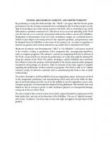
Excel has very good plotting capabilities. Unfortunately, it is not possible in Excel to simply give a command such as plot(f(x)). It is necessary to produce a list or table of x and f(x) values and to graph the resulting data. This is best illustrated by an example. Example 1.1: Plotting the Equation A table of data and an Excel graph of the van der Waals equation for ammonia at 250°C and 10 atm are shown in Figure 1.1. From the graph, it is easy to see that there is one real root between 0 and 5 (the other roots are complex conjugates). Remember that the van der Walls equation of state is an attempt to model the nonideality of the gas. Since the given temperature and pressure are not severe, it is expected that the calculated molar volume from the equation of state should not be greatly different from that predicted by the ideal gas law. From the ideal gas law, the molar volume is 4.29 L/gmol, which is very close to the root shown in the graph.

1.2.2 FIXED-POINT ITERATION (DIRECT SUBSTITUTION) To apply this method, the equation must be cast into the form x = g(x) or, more generally,

3

Roots of a Single Nonlinear Equation

f(V) 10

f(v)

0 –10

0

1

2

3

4

5

6

–20 –30 –40

Molar volume

FIGURE 1.1 Roots of the van der Walls equation for ammonia at 250°C and 10 atm.

xk+1 = g(xk)

(1.4)

where k is an iteration counter. Example 1.2: Direct Substitution Note that this can always be accomplished by adding x to each side of f(x) = 0, if necessary. The van der Walls equation can be cast into the following form:

V = b+

RT  a   P + V 2 

(1.5)

The pertinent data for ammonia are shown in Figure 1.1. If a value for V = 4 is guessed (based on the graph of Figure 1.1) and is used on the right-hand side, a new (and hopefully better) value is calculated from Equation 1.5. The iterations produce the following sequence: 4.00000 4.21854 4.22946 4.22996 4.22998.

The solution is 4.22998 L/gmol. If more significant digits are required, then more iterations can be carried out.

Numerical Methods for Chemical Engineers Using Excel®, VBA, and MATLAB®

4

It should be noted that direct substitution can be a divergent process. That is, the successively calculated values actually get worse rather than closer to the correct value. Without proof, the following statements apply: Let gʹ be the irst derivative of the function g in Equation 1.4. Then, • • • •

If |gʹ| < 1, the error will decrease with each iteration. If |gʹ| > 1, the error grows at each iteration. If gʹ > 0, the error will have the same sign at each iteration. If gʹ < 0, the error will alternate signs at each iteration.

Clearly, the equation should be arranged so that the magnitude of gʹ is less than 1. This might take some experimentation. Often, a form of g is tried, and if the process does not converge, then other forms are attempted.

1.2.3

BISECTION

If it is (somehow) known that a root lies in the interval [a, b], then by simply halving the interval in which the root lies, the interval can be reduced to an acceptable level. This idea is at the heart of the bisection method as shown in Figure 1.2. The restriction is that f(a) and f(b) must have opposite signs—one of them must be positive, the other negative (it does not matter which). Then, because f is assumed to be continuous, it must be a zero somewhere in [a, b]. Let c be the midpoint of [a, b]. Either c is the root, or the root lies in [a, c] or in [a, b]. If f(c) is close enough to zero (see below regarding tolerance), then the root has been found. Otherwise, one pair of [f(a),f(c)]or [f(c),f(b)] has opposite signs. Keep the half-interval with opposite signs and discard the other. Repeat the process until either (1) f, evaluated at the midpoint of the interval, is suficiently small or (2) the interval has been shrunk to a suitably small value.

f(x)

a c

FIGURE 1.2 Bisection: c = (a + b)/2.

b

x

5

Roots of a Single Nonlinear Equation

The term “suficiently small” is usually tested using a “tolerance,” which represents a number small enough to be considered zero based on the application. This can be stated more formally as follows: If |f(x)| =, =, < > and the logical operators are And, Or, and Not (these are VBA keywords). Here are a few examples: a < b And c = a

In the operator hierarchy, comparative operators come before logical operators, so this is the same as the next one. Putting parentheses around the comparatives makes the meaning clear and this practice is encouraged. (a < b) And (c = a) The expression is True only if both comparisons are True. (a < b) Or (c = a) The expression is True if either or both comparisons are True. Not (a = b) Same as a b.

2.7

OBJECTS AND OOP

OOP may be seen as a collection of cooperating objects, as opposed to a traditional view in which a program may be seen as a list of instructions to the computer. In OOP, each object is capable of receiving messages, processing data, and sending messages to other objects. Each object can be viewed as an independent little machine with a distinct role or responsibility. A thorough treatment of OOP is far beyond what can or need be covered in this text. It is only important to grasp the basic ideas and know where to get help when it is needed. Some examples of VBA objects are the Workbook object, the Worksheet object, the Chart object, and the Range object. To get an alphabetic list of objects, when in the VBA editor, click the question mark and then select Microsoft Visual Basic Reference/Objects. Objects have methods, which are invoked in the traditional syntax of OOP using a period separator. To get an alphabetic list of methods, when in the VBA editor, click the question mark and then select Microsoft Visual Basic Reference/Methods. As an example, the following is a commonly used invocation of an object. method command: Worksheets(ActiveSheet.Name).Activate

The object Worksheets (ActiveSheet.Name) takes on the identity of the active worksheet (the one that is currently showing when the Excel window is active).

32

Numerical Methods for Chemical Engineers Using Excel®, VBA, and MATLAB®

The Activate method tells the current VBA program that any further references to an object (Range, for example) refer to cells of the active worksheet. Effectively, this statement makes the current worksheet the “active” one. For Excel iles with multiple worksheets, this can be an important distinction. A VBA program with this statement in it can then be invoked from any of the worksheets, and all references to, for example, Cells(I, J) refer to objects within the worksheet from which the VBA program is executed. In other words, if the VBA program was created while Sheet 1 was active and later it is used when Sheet 2 is active, then Cells(I, J) refers to cells on Sheet 2. Without the Activate command, the cells in Sheet 1 would be referred to by default. Here is another example: Range(“A1:E150”).Sort “Last Name”, xlAscending

This says sort the data contained in the range A1:E150 in ascending order using as the sort key the values in the column headed by the label Last Name. The label xlAscending is one of the many VBA built-in constants. A list of all of the VBA objects and associated “members” can be viewed by clicking on View/Object Browser when in the VBA Editor. The Object Browser looks like this:

Notice that the Worksheet object is selected, so its members appear in the righthand column (and among these members is Activate). There are two Activate entries: one is a “subroutine” and one is an “event.” Right clicking on the one with the “lightning bolt” and selecting “Help” gives the following:

Visual Basic® for Applications Programming

33

By selecting “Activate method as it applies to the Worksheet object,” the following window appears:

Thus, Worksheet.Activate does the same as clicking on the sheet’s tab, but it is done under program control instead of with the mouse pointer.

2.8

BUILT-IN FUNCTIONS OF VBA

There are many built-in functions in VBA, but only a small number of them apply to scientiic and engineering applications. Table 2.1 shows a list of just a few of them.

34

Numerical Methods for Chemical Engineers Using Excel®, VBA, and MATLAB®

TABLE 2.1 Short List of VBA Functions and Their Excel® Counterparts Purpose

VBA Function

Excel Function

Absolute value Truncate to integer Round x to n digits after decimal Square root Exponential Natural log Base 10 log Base b log Value of π Sine Cosine Tangent ArcSine ArcCosine ArcTangent ArcTangent (4 quadrant) Degrees to radians Radians to degrees Remainder (x modulo y) Random number

Abs(x) Int(x) Round(x, n) Sqr(x) Exp(x) Log(x) Sin(x) Cos(x) Tan(x) Atn(x) x Mod y Rnd()

ABS(x) INT(x) ROUND(x, n) SQRT(x) EXP(x) LN(x) LOG10(x) LOG(x, b) PI() SIN(x) COS(x) TAN(x) ASIN(x) ACOS(x) ATAN(x) ATAN2(x, y) RADIANS(x) DEGREES(x) MOD(x, y) RAND()

To see the entire list, click the question mark for help. Then choose Microsoft Visual Basic Documentation/Visual Basic Language Reference/Functions. The functions are grouped alphabetically. Also shown in Table 2.1 are the corresponding Excel functions (ones that can be accessed directly from a Worksheet). Note that the VBA functions are capitalized. Perhaps the most confusing one is Sqr for taking the square root. The corresponding Excel function is the more usual SQRT. Excel functions that have no VBA counterpart can be called from VBA. For example, if it is desired to use the Pi() function within a VBA program, the Application method can be used as in the following Function:

This code produces the value of π when the Function PiCalc is called.

Visual Basic® for Applications Programming

2.9

35

PROGRAM CONTROL

Program control statements include those for decision making (branching) and for looping. Many such statements available in VBA are discussed below. Ones less frequently used (or ones that are repetitious) are not covered.

2.9.1

BRANCHING

Two popular branching or decision making statements in VBA are the If-Then-Else and the Select Case statements. Since anything that can be done with the Select Case statement can be implemented just as well using If-Then-Else, Select Case is not presented here. 2.9.1.1 If-Then-Else The syntax of the If-Then-Else statement is If Logical Expression Then statements 1 ‘this can be any number of statements on separate lines Else

statements 2

‘this can be any number of statements on separate lines

End If

Simpler forms of this statement are possible, but it is easier to always use this form, which is more formally called the Block If statement. The Else clause can be omitted if there is no else “branch” in the program logic. It is good programming practice to indent the statements in each branch. Here is a simple example: IF a < b Then c = a + b Else c = a – b End If

The amount of indentation to use is up to the programmer. The simplest thing is to use the Tab key to provide indentation, but at least two space indentation is recommended.

2.9.2 LOOPING There are four looping statements in VBA (For...Next, Do While...Loop, Do...Loop While, For Each...Next). Only the irst two of these are presented since the other two are repetitious (or can be confusing). 2.9.2.1 For…Next This is a simple “counting” loop and it has the following syntax: For Counter = Start To End [Step Increment] Statements Next [Counter]

36

Numerical Methods for Chemical Engineers Using Excel®, VBA, and MATLAB®

Counter is a variable name (usually of an integer type). On entering the loop (executing Statements the irst time), Counter is initialized to the variable (or expression) Start. After the Statements are executed the irst time, Counter is incremented by 1 unless the optional Step Increment is used. For example, using Step 2 means that Counter is incremented by 2 instead of 1. The Increment can be negative so that counting is backward. Looping continues until Statements are executed with Counter having the value of End. Note that if Counter is not an integer type, there can be some questions about its value the last time through the loop. Here is a very typical example: For i = 1 To n x(i) = i Next i

In the example, the Counter is the variable i, Start is 1, and End is the value of the variable n. So, i takes on the values 1, 2, …, n, after which control passes to the statement after the loop. 2.9.2.2 While...Wend Statement This looping statement executes a series of statements as long as a given condition is True. The syntax of this statement is While condition statements Wend

If condition (a logical expression) is True, all statements are executed until the Wend statement is encountered. Control then returns to the While statement and condition is again checked. If condition is still True, the process is repeated. If it is not True, execution resumes with the statement following the Wend statement. While...Wend loops can be nested to any level. Each Wend matches the most recent While.

2.10

VBA DATA TYPES

All of the VBA data types are shown in Table 2.2. For loating point numbers, it is best to always use Double, which provides about 15 signiicant digits. Most modern computers are equipped with loating point processors, so using Double (as opposed to Single) costs essentially nothing. For integers, it is best to use Long (instead of Integer) since integers outside the range +/– 32,767 occur sometimes. Boolean data types can be useful in some applications. The keyword DIM is used to specify the data type of a variable. When Option Explicit is used (as is always recommended), the type of every variable in the program must be speciied explicitly. Later it will be seen that DIM is also used to specify an Array data structure. Table 2.2 summarizes some of the VBA built-in data types. Only the types most often used are included. A full list of data types can be viewed via the Help system.

37

Visual Basic® for Applications Programming

TABLE 2.2 VBA Built-In Data Types Storage Required

Data Type Boolean (logical) Integer Long Real (single precision) Double (double precision)

String Variant

2.11

2 bytes 2 bytes 4 bytes 4 bytes 8 bytes

1 byte/char. 16 bytes + 1/char.

Range of Values True or False –32,767 to 32,768 –2,147,283,648 to 2,147,283,647 –3.402823E+38 to –1.401298E-45 for negatives 1.401298E-45 to 3.402823E+38 for positives –1.79769313486232E+308 to –4.94065645841247E-324 for negatives 4.94065645841247E-324 to 1.79769313486232E+308 for positives Delimited by quote marks (“). Any numeric value up to the range Double or any text.

SUBS AND FUNCTIONS

A VBA program is automatically a “Sub” or Subroutine. The introductory VBA example program for getting the average of a list of numbers began with Sub CalcAverage()

In addition to Subs, VBA also has Function subprograms. Here are the differences between the two: 1. A Sub can receive information (properties) and it can change or set properties. 2. A Function can only receive properties. 3. A Sub is invoked by a “Call” statement. 4. A Function is invoked simply by using its name. A Sub has the following syntax: Sub name ([arglist]) Statements End Sub

Things within square brackets are optional. The deinition of arglist is as follows: arglist:

A list of variables representing arguments that are passed to the Sub procedure when it is called. Multiple arguments are separated by commas.

Numerical Methods for Chemical Engineers Using Excel®, VBA, and MATLAB®

38

In its simplest form, arglist consists of variable names separated by commas. Consider for example Call Alpha(Beta, Gamma)

The name of the subroutine is Alpha. Beta and Gamma are the arguments or parameters (often called the actual arguments) of the subroutine in the calling program. When the subroutine is coded, it might appear as follows: Sub Alpha (Delta, Epsilon)

Here, Delta and Epsilon are what we call dummy parameters since they take on information provided by the actual arguments when Alpha is called. The actual parameters can be “sent” to the subroutine in one of two modes: • By reference: What is sent to the subroutine is the memory location of the parameter. Therefore, if the parameter is altered by the subroutine, such changes will be known to the caller when control is passed back at the end of the subroutine (often called “returning” from the subroutine). This is the default mode for parameter passing. • By value: If an actual argument is a constant, then it is automatically passed by value (it would be chaotic if the constant 2 suddenly represented the number 3, for example). It is rare that a variable name used as an argument is to be passed by value, but if so, simply enclose it in parentheses as in Call Alpha((Beta), Gamma)

Here, only the current value of Beta is sent to the subroutine. Using the same dummy variables as previously (Delta, Epsilon), any changes made to Delta by the subroutine are not transmitted back to the calling program.

2.12 2.12.1

INPUT AND OUTPUT GETTING DATA FROM THE WORKSHEET

In traditional programming (such as with C++), the source of input data is usually either the keyboard or (usually when there are lots of data) a ile. When using VBA, which is an integral part of Excel, the natural source of input is from the Worksheet itself. In Example Program 2.1, the following statement appeared: InputNumber = ActiveSheet.Cells(ActRow, 1)

The Cells method treats the spreadsheet as a two-dimensional array representing the rows and columns. If the variable ActRow is 3, for example, then the variable

Visual Basic® for Applications Programming

39

InputNumber is assigned whatever value is contained in the cell in the third row and irst column. It is possible using the Range object to write a statement that inputs values from a collection of cells (but this tends to make things more complex than they need be).

2.12.2

PUTTING DATA ONTO THE WORKSHEET

The procedure for “writing” output data to the active worksheet simply reverses the assignment used for input. Another example taken from the sample program is as follows: ActiveSheet.Cells(ActRow + 1, 2) = Average

The value currently stored in the variable Average is written into the cell referenced on the left of the assignment.

2.13

ARRAY DATA STRUCTURES

An Array is the equivalent of a subscripted variable. There are one-, two-, or even higher-dimensional arrays. As with scalar variables, arrays are declared in a Dim statement as in Dim x(4) as Double

In this example, the array x consists of 5 elements: x(0), x(1), x(2), x(3), and x(4). By default, the irst subscript is 0. However, starting at zero can lead to confusion, and it is recommended to always include Option Base 1

Then subscripts begin with 1, which many ind more natural. For those comfortable with subscripts starting at zero, this option need not be used. For all programs in this book use, Option Base 1 is used. For a two-dimensional array (matrix), an example declaration is as follows: Dim y (3, 4)

The matrix y has 3 rows and 4 columns (assuming subscripts start at 1). Example Program 2.2: Using an Array The following is a modified version of the program of Example Program 2.1. Here an Array is used to store the numbers to the averaged. A “For” loop is then used to compute the Sum of the numbers. An additional “check” is included to be sure that the number of data items does not exceed 20, which is an arbitrary hardcoded dimension for the array InputNumbers.

40

Numerical Methods for Chemical Engineers Using Excel®, VBA, and MATLAB®

2.13.1

ARRAY ARGUMENTS

Each of the next two versions of the example program uses a subroutine to do some of the work. The subroutine is named Summer and is declared as follows: Sub Summer(N, Nums, Avg)

The “dummy” parameters N, Nums, and Avg do not appear in a Dim statement. They “inherit” the data type and structure of the actual argument when the subroutine is called. The calling statement in the next two examples is Call Summer(NumNumbers, InputNumbers(), Average)

The empty parentheses after InputNumbers identify it as an array argument, and the dummy Nums becomes an array structure of whatever length InputNumbers happens to be. These parentheses are not essential but they help to document the array argument.

Visual Basic® for Applications Programming

Example Program 2.3: Using a Subroutine The same program is changed again, this time using a Sub with arguments to perform the summing and averaging operations:

41

42

Numerical Methods for Chemical Engineers Using Excel®, VBA, and MATLAB®

2.13.2

DYNAMIC ARRAYS IN VBA

It is often the case that it is not known ahead of time how large an array’s dimensions need to be. It is wasteful of memory (and poor programming practice) to simply make the dimensions arbitrarily large. To circumvent this problem, VBA provides the ReDim statement so that the dimensions of an array do not have to be “hard coded” in the program. Example Program 2.4: Use of ReDim To illustrate the use of ReDim, one more version of the example program is shown. The input data format is changed so that the very first number in the list is not one of the numbers to be averaged, but it indicates how many numbers there are (and thus the required size of the array that holds the numbers). In this version, the dimension of InputNumbers is left blank (note the empty parentheses), and then the following statement makes the dimension what it needs to be: ReDim InputNumbers(NumNumbers)

Another approach that does not require the number of data items known in advance is to again use a While loop to detect a zero or sentinel value and put a ReDim statement within the While loop. When designing a program, it is wise to think of different ways in which to accomplish the same task.

Visual Basic® for Applications Programming

43

2.14 ALTERNATIVE I/O METHODS Using the Cells method is straightforward and the one that is most often used for input and output. There are other methods worthy of mention, however.

2.14.1

USING RANGE.SELECT

The Range.Select combined with the ActiveCell object can accomplish essentially the same thing that Cells does. Here is an example: Range(“b10”).Select v = ActiveCell.Value

This inputs into the variable v whatever value is in cell B10. The .Value method is actually the default for ActiveCell and can be omitted. This technique of input is more unwieldy than the Cells method.

2.14.2

USING MESSAGE BOX

The built-in function MsgBox can be used to send a message to the user without it appearing in a worksheet cell. Here is an example: MsgBox “This program finds the average of a list of numbers”

This pops up a box containing the quoted message overlaid onto the active worksheet.

2.14.3

USING INPUT BOX

The built-in function InputBox can be used to both send a message to the user and to obtain data from the user without it appearing in a worksheet cell. Consider the example: a = InputBox(“Please enter the first value to be added”)

A box pops up on the worksheet with the quoted prompt and a place for the user to type in the value requested (in this case, for the variable a). Example Program 2.5: Using MsgBox and InputBox for Input/Output Another version of the example program for finding the average of a list of numbers is shown below. In this case, MsgBox and InputBox are used for input and output. Note that three consecutive quote marks are required for one quote mark to appear.

44

Numerical Methods for Chemical Engineers Using Excel®, VBA, and MATLAB®

The & symbol is the “concatenation” operator. It appends the value of the variable Average to the preceeding text.

2.15

USING DEBUGGER

The Debugger allows many operations that assist in inding errors in programs or in the input data. When opening an Excel spreadsheet ile that contains a VBA macro then going to Tools/Macros and Edit, the Debug menu is among those that appear. By selecting from the Debug menu Step Into, the Sub statement is highlighted (in yellow). The program is now running but under your control. To view the Debug Toolbar, go to View/Toolbars and select Debug. The following is what the screen looks like for the CalcAverage4 VBA example:

Visual Basic® for Applications Programming

45

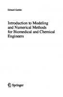
To single step through the program, use F8 or the Step tool button, which is the one just to the right of the “Hand” icon in the Debug Toolbar. Here is what the screen looks like after stepping down to the ReDim statement. Here the Debug/Add Watch menu was used to display at the bottom the values of the variables ActRow and NumNumbers. From the Debug menu, several useful operations can be invoked to aid in tracking down a programming error. For example, a “breakpoint” can be placed on any statement so that when Run (instead of single stepping) is chosen, execution halts when that statement with a breakpoint is reached. At that time, the value of any variable can be viewed. Note that in addition to using the Set Watch feature, values of a scalar variable can be observed simply by placing the cursor over the variable’s name. Using the Debugger can provide a powerful tool in tracking down programming errors and errors in input data. This discussion has only touched on a few features of the Debugger. Example Program 2.6: Modified False Position The method of false position is a “hybrid” of the bisection and secant methods. This method assumes two starting points having opposite function signs. A new point is found by drawing a straight line between the bracketing points. One of the old points is discarded depending on the sign of the function at the new point. This is depicted in Figure 2.4.

46

Numerical Methods for Chemical Engineers Using Excel®, VBA, and MATLAB® f(x)

f(xR)

0

xL xM

xR

x

f(xL)

FIGURE 2.4 Modiied false position method. The formula for finding improved values for x using the notation of Figure 2.4 is as follows:

x m = xL −

( xR − xL )f ( xL ) . f ( xR ) − f ( xL )

(2.1)

An inefficiency of the method of false position is that one of the end points tends to become stagnant. That is, the end point remains unchanged for several iterations. A modification to overcome stagnation is to detect when it occurs and to take action to avoid it. An effective modification is to simply halve the stagnated f(x) value in the update formula. While the modified false position method can be implemented directly in Excel, the logic required is sufficiently complex to make using VBA a better choice. Program specification, algorithm design, coding, and testing are now given where the problem is to find the root between 0.4 and 1.2 of the function f(x) = tan x − x − 0.5

(2.2)

SPECIFICATION It is necessary to place on the spreadsheet user interface the two initial values of x that bracket the root. If the initial values do not bracket the root, the program should terminate with an error message. It is desired that at each iteration the values of xL, xR, f(xL), f(xR), xm, and f(xm) be displayed along with an iteration counter. Shown below is one way the spreadsheet might appear before program execution:

Visual Basic® for Applications Programming The program then computes and displays the remaining values for Iteration 1. The update formula, Equation 2.1, is used to compute xm. Next, either xL or xR is replaced by xm (based on the sign of f(xm)), and a new iteration is performed. When the absolute value of the difference between xL and xR is less than a tolerance (1.E-8), the following message is shown: Solution is within tolerance

To prevent continued iterations when convergence is very slow, a maximum number of iterations (100) is invoked, and the following error message is displayed: Maximum iteration reached; Solution might not be valid

If the initial values of xL and xR do not bracket a root, the following error message is displayed: Root is not bracketed, please try again

ALGORITHM DESIGN An “outline” summary of the logic for this program is as follows: 1. Get input data and fill out the first line of the output. 2. Compute xm and f(xm). 3. If f(xm) has the same sign as f(xR), then replace xR with xm and set a repetition counter for xR to zero while incrementing a repetition counter for xL. 4. Otherwise, f(xm) has the same sign as f(xL) so replace xL with xm and set a repetition counter for xL to zero while incrementing a repetition counter for xR. 5. Output a line on the spreadsheet. This process is repeated until the absolute value of the difference between xL and xR is less than the tolerance or the maximum number of iterations has occurred (Figure 2.5). Coding could be attempted using the brief outline summary of the algorithm, but by using a structure chart, even more detail can be displayed and envisioned unambiguously prior to coding. Such a structure chart appears below, accompanied by a list of variable names used within the chart. DICTIONARY OF VARIABLES Name Tol iMax xL xR fxL fxR

Definition Tolerance to detect small differences between x values Maximum iteration before terminating with error message One of the x values The other of the x values f(xL) f(xR)

47

48

Numerical Methods for Chemical Engineers Using Excel®, VBA, and MATLAB® Modified false position Get xL and xR from Excel

Tol