Murach's SQL Server 2019 for Developers [1 ed.] 9781943872572

Citation preview

MASTER THE SQL STATEMENTS that every application developer needs to retrieve and update the data in a Microsoft SQL Server database

DESIGN DATABASES LIKE A DBA and implement them with SQL statements or the Management Studio

GAIN PROFESSIONAL SKILLS like working with views, scripts, stored procedures, functions, triggers, transactions, locking, security, XML, and BLOBs

murach's

S L Server 2019

for developers

Bryan Syverson Joel Murach

TRAINING & REFERENCE

murach's

S L Server 2019

for developers

Bryan Syverson Joel Murach

lh

•111

MIKE MuRACH & AssociATEs, INc. 4340 N. Knoll Ave. • Fresno, CA 93722

www.murach.com • murachbooks@ murach.com

Authors:

Bryan Syverson Joel Murach

Editor:

Anne Boehm

Production:

Juliette Baylon

Books for database developers Murach's SQL Server for Developers Murach 's Oracle SQL and PUSQLfor Developers Murach 's MySQL

Books for .NET developers Murach 's C# Murach 's Visual Basic Murach's ASP.NET Web Programming with C# Murach 's ASP.NET Core MVC

Books for Python, C++, and Java developers Murach's Python Programming Murach 's C++ Programming Murach 's Java Programming Murach 's Java Servlets and JSP

Books for web developers Murach 's HTML5 and CSS3 Murach 's JavaScript andjQuery Murach 's PHP and MySQL

For more on Murach books, please visit us at www.murach.com © 2020, Mike Murach & Associates, Inc. All rights reserved. Printed in the United States of America 1098765432 1 ISBN-13: 978-1-943872-57-2

Content xvii

Introduction

Section 1 An introduction to SQL Chapter I Chapter 2

An introduction to relational databases and SQL How to use the Management Studio

3

49

Section 2 The essential SQL skills Chapter 3 Chapter 4 Chapter 5 Chapter 6 Chapter 7 Chapter 8 Chapter 9

How to retrieve data from a single table How to retrieve data from two or more tables How to code summary queries How to code subqueries How to insert, update, and delete data How to work with data types How to use functions

85 125 159 183 215 239 261

Section 3 Database design and implementation Chapter 10 Chapter II Chapter 12

How to design a databa~e How to create a database and its tables with SQL statements How to create a database and its tables with the Management Studio

303 333 375

Section 4 Advanced SQL skills Chapter Chapter Chapter Chapter Chapter Chapter Chapter

13 14 IS

16 17 18 19

How to work with views How to code scripts How to code stored procedures, functi ons, and triggers How to manage transactions and locking How to manage database security How to work with XML How to work with BLOBs

395 417 457 509 535 587 619

Reference aids Appendix A Index

How to set up your computer for this book

647

659

Expanded contents

Expanded contents Section 1 An introduction to SQL Chapter 1

--------------------

An introduction to relational databases and SQL

An introduction to client/server systems ......................................... 4 The hardware components of a client/server system ......................................... ............ .4 The software components of a client/server system ........................................................ 6 Other clie nt/server system architectures ......................................................................... 8

An introduction to the relational database model......................... 10 How a database table is organized ................................................................................ 10 How the tables in a relational database are related ....................................................... 12 How the columns in a table are defined ........................................................................ 14 How relational databases compare to other data models .............................................. 16

An introduction to SOL and SOL-based systems ......................... 18 A brief history of SQL .................................................................................................. 18 A comparison of Oracle, DB2, MySQL, and SQL Server ............................................ 20

The Transact-SOL statements ......................................................... 22 An introduction to the SQL statements ......................................................................... 22 Typical statements for working with database objects .................................................. 24 How to query a single table ........................................................................................... 26 How to j oin data from two or more tables .................................................................... 28 How to add, update, and delete data in a table .............................................................. 30 SQL coding guidelines .................................................................................................. 32

How to work with other database objects ...................................... 34 How to work with views ............................................................................................... 34 How to work with stored procedures, triggers, and user-defined functions .................. 36

How to use SOL from an application program .............................. 38 Common data access models ......................... .................................... ................ ........... 38 How to use ADO.NET from a .NET application ......................................................... .40 Visual Basic code that retrieves data from a SQL Server database ............................... 42 C# code that retrieves data from a SQL Server database .............................................. 44

Chapter 2

How to use the Management Studio An introduction to SOL Server 2019 ............................................... 50 A summary of the SQL Server 2019 tools .................................................................... 50 How to start and stop the database engine ............................................... ., ................... 52 How to enable remote connections ............................................................................... 52

An introduction to the Management Studio ................................... 54 How to connect to a database server .............. .................................... ................ ........... 54 How to navigate through the database objects .............................................................. 56

How to manage the database files .................................................. 58 How to attach a database ............................................................................................... 58 How to detach a database .............................................................................................. 58 How to back up a database ............................................................................................ 60 How to restore a database.............................................................................................. 60 How to set the compatibility level for a database ......................................................... 62

Vii

Viii

Expanded contents

How to view and modify the database ............................................54 How How How How How

to create database diagrams .................................................................................. 64 to view the column definitions of a table .............................................................. 66 to modify the column definitions .......................................................................... 66 to view the data of a table ..................................................................................... 68 to modify the data of a table ................................................................................. 68

How to work with queries ................................................................. 70 How to enter and execute a query ................................................................................. 70 How to handle syntax errors .......................................................................................... 72 How to open and save queries ....................................................................................... 74 An introduction to the Query Designer ......................................................................... 76

How to view the documentation for SQL Server ...........................78 How to display the SQL Server documentation ............................................................ 78 How to look up information in the documentation ....................................................... 78

Section 2 The essential SQL skills Chapter 3

How to retrieve data from a single table An introduction to the SELECT statement .....................................86 The basic syntax of the SELECT state ment.. ................................................................ 86 SELECT statement examples ........................................................................................ 88

How to code the SELECT clause ..................................................... 90 How How How How How How How

to code column specifications............................................................................... 90 to name the columns in a result set.. ........................................ ............................. 92 to code string expressions ..................................................................................... 94 to code arithmetic expressions ................................................. ............................. 96 to use functions ................................ ..................................................................... 98 to use the DISTINCT keyword to eliminate duplicate rows .............................. 100 to use the TOP clause to return a subset of selected rows .................................. 102

How to code the WHERE clause ................................................... 104 How How How How How How

to to to to to to

use comparison operators ............................................................................... 104 use the AND, OR, and NOT logical operators ............................................... 106 use the IN operator ......................................................................................... 108 use the BETWEEN operator .......................................................................... 110 use the LIKE operator .................................................................................... 112 use the IS NULL clause.................................................................................. ll4

How to code the ORDER BY clause .............................................. 116 How to sort a result set by a column name .. .................................... ........................... 116 How to sort a result set by an al ias, an expression, or a column number .................... 118 How to retrieve a range of selected rows .................................................................... 120

Chapter 4

How to retrieve data from two or more tables How to work with inner joins ......................................................... 126 How to code an inner j oin ........................................................................................... 126 When and how to use correlation names ..................................................................... l 28 How to work with tables from different databases ...................................................... 130 How to use compound join conditions ........................................................................ 132 How to use a self-join.................................................................................................. l 34 Inner joins that join more than two tables ................................................................... 136 How to use the impl icit inner join syntax ................................................................... 138

Expanded contents

How to work with outer joins ......................................................... 140 How to code an outer j oin .................................................................. ......................... 140 Outer j oin examples .................................................................................................... 142 Outer j oins that join more than two tables .................................................................. 144

Other skills for working with joins ................................................ 146 How to combine inner and outer joins ........................................................................ 146 How to use cross j oins ................................................................................................. l48

How to work with unions ................................................................ 150 T he syntax of a union .................................................................................................. l50 Unions that combine data from different tables .......................................................... 150 Unions that combine data from the same table ........................................................... 152 How to use the EXCEPT and INTERSECT operators ............................................... 154

Chapter 5

How to code summary queries How to work with aggregate functions ......................................... 160 How to code aggregate functions ................................................................................ 160 Queries that use aggregate functions ........................................................................... 162

How to group and summarize data ............................................... 164 How to code the GROUP BY and HAVING clauses .................................................. 164 Queries that use the GROUP BY and HAVING clauses .................................... ......... l66 How the HAVING clause compares to the WHERE clause........................................ l68 How to code complex search conditions ........ .................................... ................ ......... 170

How to summarize data using SQL Server extensions .............. 172 How to use the ROLLUP operator .............................................................................. 172 How to use the CUBE operator ................................................................................... l74 How to use the GROUPING SETS operator............................................................... 176 How to use the OVER clause ...................................................................................... 178

Chapter 6

How to code subqueries An introduction to subqueries ...................................................... 184 How to use subqueries ................................................................................................. 184 How subqueries compare to joins ............................................................................... 186

How to code subqueries in search conditions ............................ 188 How to use subqueries with the IN operator ...................................... ................ ......... 188 How to compare the result of a subquery with an expression ..................................... 190 How to use the ALL keyword ............................................................................ ......... 192 How to use the ANY and SOME keywords ................................................................ 194 How to code correlated subqueries ............................................................................. 196 How to use the EXISTS operator ................................................................................ 198

Other ways to use subqueries ....................................................... 200 How to code subqueries in the FROM clause ............................................................. 200 How to code subqueries in the SELECT clause .......................................................... 202

Guidelines for working with complex queries ............................. 204 A complex query that uses subqueries ........................................................................ 204 A procedure for building complex queries .................................................................. 206

How to work with common table expressions ............................. 208 How to code a CTE ..................................................................................................... 208 How to code a recursive CTE ...................................................................................... 210

ix

X

Expanded contents

Chapter 7

How to insert, update, and delete data How to create test tables ............................................................... 216 How to use the SELECT INTO statement .................................................................. 2 16 How to use a copy of the database .............................................................................. 2 16

How to insert new rows .................................................................. 218 How How How How

to to to to

insert a single row ........................................................................................... 2 18 insert multiple rows ........................................................................................ 2 18 insert default values and null values ............................................................... 220 insert rows selected from another table .......................................................... 222

How to modify existing rows ......................................................... 224 How to perform a basic update operation ................................................................... 224 How to use subqueries in an update operation ............................................................ 226 How to use j oins in an update operation ..................................................................... 228

How to delete existing rows ........................................................... 230 How to perform a basic delete operation .................................................................... 230 How to use subqueries and joins in a delete operation ............................................... 232

How to merge rows ......................................................................... 234 How to perform a basic merge operation .................................................................... 234 How to code more complex merge operations ............................................................ 234

Chapter 8

How to work with data types A review of the SQL data types .....................................................240 Data type overview ...................................................................................................... 240 The numeric data types ............................................................................................... 242 The string data types ................................................................................................... 244 The date/time data types .............................................................................................. 246 The large value data types ........................................................................................... 248

How to convert data ........................................................................ 250 How How How How How

Chapter 9

data conversion works ........................................................................................ 250 to convert data using the CAST function ........................................................... 252 to convert data using the CONVERT function ................................................... 254 to use the TRY _CONVERT fu nction ................................................................. 256 to use other data conversion functions ................................................................ 258

How to use functions How to work with string data ......................................................... 262 A summary of the string functions .............................................................................. 262 How to solve common problems that occur with string data ...................................... 266

How to work with numeric data ..................................................... 268 A summary of the numeric functions .......................................................................... 268 How to solve common problems that occur with numeric data .................................. 270

How to work with date/time data ................................................... 272 A summary of the date/time functions ........................................................................ 272 How to parse dates and times ...................................................................................... 276 How to perform operations on dates and times ........................................................... 278 How to perform a date search ..................................................................................... 280 How to perform a time search ..................................................................................... 282

Other functions you should know about ...................................... 284 How to use the CASE function ................................................................................... 284 How to use the IIF and CHOOSE fu nctions .................................... ........................... 286

Expanded contents

How to use the COALESCE and IS NULL functions ................................................. 288 How to use the GROUPING fu nction ................................................................ ......... 290 How to use the ranking functions ................................................................................ 292 How to use the analytic functions ............................................................................... 296

Section 3 Database design and implementation Chapter 10

How to design a database How to design a data structure ..................................................... 304 The basic steps for designing a data structure ............................................................. 304 How to identify the data elements ............................................................................... 306 How to subdivide the data elements ............................................................................ 308 How to identify the tables and assign columns ........................................................... 3 10 How to identify the primary and foreign keys ............................................................ 3 12 How to enforce the relationships between tables ............................................... ......... 3 14 How normalization works .................................................................................. ......... 3 16 How to identify the columns to be indexed .... .................................... ................ ......... 3 18

How to normalize a data structure ................................................ 320 T he seven normal forms ................................. .................................... ................ ......... 320 How to apply the fi rst normal form ............................................................................. 322 How to apply the second normal form ........................................................................ 324 How to apply the third normal form ................................................................... ......... 326 When and how to denormalize a data structure .......................................................... 328

Chapter 11

How to create a database and its tables with SQL Statements An introduction to DOL .................................................................. 334 T he SQL stateme nts for data definition ...................................................................... 334 Rules for coding object names ........................................................... ................ ......... 336

How to create databases, tables, and indexes ............................ 338 How to create a database ................................ .................................... ................ ......... 338 How to create a table ................................................................................................... 340 How to create an index ....................................................................... ................ ......... 342 How to use snippets to create database objects ........................................................... 344

How to use constraints .................................................................. 346 An introduction to constraints ..................................................................................... 346 How to use check constraints ...................................................................................... 348 How to use foreign key constraints ................ .................................... ................ ......... 350

How to change databases and tables ........................................... 352 How to delete an index, table, or database .................................................................. 352 How to alter a table ........................................ .................................... ................ ......... 354

How to work with sequences ......................................................... 356 How How How How

to create a sequence ............................................................................................ 356 to use a sequence ................................................................................................ 356 to delete a sequence ............................................................................................ 358 to alter a sequence .............................................................................................. 358

How to work with collations ........................................................... 360 An introduction to encodings ......................... .................................... ................ ......... 360 An introduction to collations ....................................................................................... 362 How to view collations ................................... .................................... ................ ......... 364 How to specify a collation ........................................................................................... 366

Xi

Xi i

Expanded contents

The script used to create the AP database .................................. 368 How the script works ................................................................................................... 368 How the DDL statements work ................................................................................... 368

Chapter 12 How to create a database and its tables with the Managment Studio How to work with a database ......................................................... 376 How to create a database ............................................................................................. 376 How to delete a database ............................................................................................. 376

How to work with tables ................................................................. 378 How How How How How

to create, modify, or delete a table ...................................................................... 378 to work with foreign key relationships ............................................................... 380 to work with indexes and keys ............................................................................ 382 to work with check constraints ........................................................................... 384 to examine table dependencies ........................................................................... 386

How to generate scripts ................................................................. 388 How to generate scripts for databases and tables ........................................................ 390 How to generate a change script when you modify a table ......................................... 392

Section 4 Advanced SQL skills Chapter 13 How to work with views An introduction to views ................................................................396 How views work ............................................................................... ........................... 396 Benefits of using views ............................................................................................... 398

How to create and manage views.................................................. 400 How to create a view ................................................................................................... 400 Examples that create views ......................................................................................... 402 How to create an updatable view ................................................................................ 404 How to delete or modify a view .................................................................................. 406

How to use views ............................................................................408 How How How How

to update rows through a view ........................................................................... .408 to insert rows through a view .............................................................................. 4 10 to delete rows through a view ............................................................................ .4 10 to use the catalog views ........................................................... ........................... 4 12

How to use the View Designer ....................................................... 414 How to create or modify a view .................................................................................. 4 14 How to delete a view ................................................................................................... 414

Chapter 14 How to code scripts An introduction to scripts .............................................................. 418 How to work with scripts ............................................................................................ 418 The Transact-SQL statements for script processing ................................................... .420

How to work with variables and temporary tables ...................... 422 How to work with scalar variables .............................................................................. 422 How to work with table variables ............................................................................... .424 How to work with temporary tables ............................................................................ 426 A comparison of the fi ve types ofTransact-SQL table objects .................................. .428

How to control the execution of a script ...................................... 430 How to perform conditional processing ...................................................................... 430 How to test for the existence of a database object ..................................................... .432

Expanded contents

How to perfonn repetitive processing ........................................................................ .434 How to use a cursor ............................................................................................ ......... 436 How to handle errors ................................................................................................... 438 How to use surround-with snippets ............................................................................. 440

Advanced scripting techniques .................................................... 442 How to use the system functions ................................................................................. 442 How to change the session settings .................................................... ........................ .444 How to use dynamic SQL ........................................................................................... 446 A script that summarizes the structure of a database .................................................. 448 How to use the SQLCMD utility................................................................................. 452

Chapter 15

How to code stored procedures, functions, and triggers Procedural programming options in Transact-SQL ....................458 Scripts ..................... ........................................ .................................... ................ ......... 458 Stored procedures, user-defined functions, and triggers ............................................ .458

How to code stored procedures .................................................... 460 An introduction to stored procedures .......................................................................... 460 How to create a stored procedure ....................................................................... ......... 462 How to declare and work with parameters .................................................................. 464 How to call procedures with parameters ........ .................................... ................ ........ .466 How to work with return values .................................................................................. 468 How to validate data and raise errors ................................................................. ........ .470 A stored procedure that manages insert operations ............................ ................ ......... 472 How to pass a table as a parameter .................................................... ................ ........ .478 How to delete or change a stored procedure ............................................................... 480 How to work with system stored procedures ..................................................... ........ .482

How to code user-defined functions ............................................ 484 An introduction to user-defined functi ons ...... ............................................................. 484 How to create a scalar-valued function ....................................................................... 486 How to create a simple table-valued function ............................................................ .488 How to create a multi-statement table-valued function ............................................... 490 How to delete or change a function ............................................................................. 492

How to code triggers ......................................................................494 How How How How How How

Chapter 16

to create a trigger ....................................................................... ......................... 494 to use AFTER triggers ........................................................................................ 496 to use INSTEAD OF triggers .................................................... ................ ........ .498 to use triggers to enforce data consistency ................................ ................ ......... 500 to use tr iggers to work with DDL statements ............................ ................ ......... 502 to delete or change a trigger .................. .................................... ................ ......... 504

How to manage transactions and locking How to work with transactions ...................................................... 510 How transactions maintain data integrity .................................................................... 5 10 SQL statements for handling transactions ...... .................................... ................ ......... 5 12 How to work with nested transactions ........................................................................ 514 How to work with save points ........................ .................................... ................ ......... 5 16

An introduction to concurrency and locking ............................... 518 How concurrency and locking are related ................................................................... 5 18 The four concurrency problems that locks can prevent .............................................. 520 How to set the transaction isolation level... ........................................ ......................... 522

Xiii

XiV

Expanded contents

How SQL Server manages locking ............................................... 524 Lockable resources and lock escalation ...................................................................... 524 Lock modes and lock promotion ................................................................................. 526 Lock mode compatibil ity ............................................................................................ 528

How to prevent deadlocks ............................................................. 530 Two transactions that deadlock ................................................................................... 530 Coding techniques that prevent deadlocks .................................................................. 532

Chapter 17

How to manage database security How to work with SQL Server login IDs ....................................... 536 An introduction to SQL Server security ...................................................................... 536 How to change the authentication mode ..................................................................... 538 How to create logi n IDs .............................................................................................. 540 How to delete or change logi n IDs or passwords .................................. oo .. oooooo .......... oo542 How to work with database users ................................................................................ 544 546 How to work with schemas .......................... 00 . . 000000 . . . . . . . . . . . . . . . . . . . . . . . . . . . . . . 00 . . 00 . . . . . . . . . . 00 . . . . .

How to work with permissions ...................................................... 548 How to grant or revoke object permissions ................................................................. 548 T he SQL Server object permjssions ............................................................................ 550 How to grant or revoke sche ma permissions ............................................................... 552 How to grant or revoke database permissions ............................................................. 554 How to grant or revoke server perrrussions ................................................................. 556

How to work with roles ................................................................... 558 How How How How How How How How

to work with the fixed server roles ..................................................................... 558 to work with user-defined server roles ................................................................ 560 to display information about server roles and role members ................ 562 to work with the fixed database roles ...................................... ........................... 564 to work with user-defined database roles ........................................................... 566 to display information about database roles and role members ......................... 568 570 to deny permissions granted by role membership .................... to work with application roles ............................................................................ 572 00 . . . . . . . . . . .

00 . . 00 00 00 . . . . . . . . . . 00 . . 00

How to manage security using the Management Studio ............ 574 to work with login IDs ........................................................................................ 574

How How How How How

to work with the server roles for a login ID ....................................................... 576 to assign database access and roles by login ID ................................................. 578 to assign user permissions to database objects ................................................... 580 to work with database perrrussions ..................................................................... 582

Chapter 18 How to work with XM L An introduction to XML .................................................................. 588 An XML document ..................................................................................................... 5 88 An XML schema .. .................................... ........................................ ........................... 590

How to work with the xml data type .............................................. 592 How to store data in the xml data type ........................................................................ 592 How to work with the XML Editor ............................................................................. 594 How to use the methods of the xml data type ............................................................. 596 An example that parses the xml data type ................................................................... 600 Another example that parses the xml data type........................................................... 602

How to work with XML schemas ................................................... 604 How How How How

to add an XML schema to a database ................................................................. 604 to use an XML schema to validate the xml data type......................................... 606 to view an XML schema.............................................................................. 608 to drop an XML schema .................. ........................................ ........................... 608 00 00 00 .

Expanded contents

Two more skills for working with XML .......................................... 610 How to use the FOR XML clause of the SELECT statement.. .......... ......................... 610 How to use the OPENXML statement.. ...................................................................... 614

Chapter 19

How to work with BLOBs An introduction to BLOBs .............................................................. 620 Pros and cons of storing BLOBs in files ..................................................................... 620 Pros and cons of storing BLOBs in a column ............................................................. 620 When to use FILESTREAM storage for BLOBs ........................................................ 620

How to use SQL to work with a varbinary(max) column ............ 622 How to create a table with a varbinary(max) column ........................ ................ ......... 622 How to insert, update, and delete binary data .................................... ................ ......... 622 How to retrieve binary data ............................ .................................... ................ ......... 622

A .NET application that uses a varbinary(max) column ............. 624 The user interface for the application.......................................................................... 624 The event handlers for the form .................................................................................. 626 A data access class that reads and writes binary data ................................................. 628

How to use FILESTREAM storage ................................................. 634 How to enable FILESTREAM storage on the server ......................... ................ ......... 634 How to create a database with FILESTREAM storage ...................................... ......... 636 How to create a table with a FILESTREAM column ........................ ................ ......... 638 How to insert, update, and delete FILESTREAM data ...................... ................ ......... 638 How to retrieve FILESTREAM data .................................................. ................ ......... 638 A data access class that uses FILESTREAM storage ........................ ................ ......... 640

Appendix A How to set up your computer for this book Three editions of SQL Server 20 19 Express ............................................................... 648 The tool for working with all editions of SQL Server ....................................... ......... 648 How to install SQL Server 20 19 Express.................................................................... 650 How to install SQL Server Management Studio ................................................ ......... 650 How to install the fi les for this book .............. .................................... ................ ......... 652 How to create the databases for this book .......................................... ................ ......... 654 How to restore the databases for this book .... .................................... ................ ......... 654 How to install Visual Studio 20 19 Community .................................. ................ ......... 656

XV

Introduction If you want to learn SQL, you've picked the right book. And if you want to learn the specifics of SQL for SQL Server 2019, you've made an especially good choice. Along the way, you'lllearn a lot about relational database management systems in general and about SQL Server in particular. Why learn SQL? First, because most programmers would be better at database programming if they knew more about SQL. Second, because SQL programming is a valuable specialty in itself. And third, because knowing SQL is the first step toward becoming a database administrator. In short, knowing SQL makes you more valuable on the job.

Who this book is for This book is the ideal book for application developers who need to work with a SQL Server database. It shows you how to code the SQL statements that you need for your applications. It shows you how to code these statements so they run efficiently. And it shows you how to take advantage of the most useful advanced features that SQL Server has to offer. This book is also a good choice for anyone who wants to learn standard SQL. Since SQL is a standard language for accessing database data, most of the SQL code in this book will work with any database management system. As a result, once you use this book to learn how to use SQL to work with a SQL Server database, you can transfer most of what you have learned to another database management system such as Oracle, DB2, or MySQL. This book is also the right .first book for anyone who wants to become a database administrator. Although this book doesn' t present all of the advanced skills that are needed by a top DBA, it will get you started. Then, when you have finished this book, you'll be prepared for more advanced books on the subject.

4 reasons why you'll learn faster with this book •

Unlike most SQL books, this one starts by showing you how to query an existing database rather than how to create a new database. Why? Because that's what you're most likely to need to do first on the job. Once you master those skills, you can learn how to design and implement a database, whenever you need to do that. Or, you can learn how to work with other database features like views and stored procedures, whenever you need to do that.

XViii

Introduction

•

Like all our books, this one includes hundreds of examples that range from the simple to the complex. That way, you can quickly get the idea of how a feature works from the simple examples, but you'll also see how the feature is used in the real world from the complex examples.

•

Like most of our books, this one has exercises at the end of each chapter that give you hands-on experience by letting you practice what you' ve learned. These exercises also encourage you to experiment and to apply what you've learned in new ways.

•

If you page through this book, you'll see that all of the information is presented in "paired pages," with the essential syntax, guidelines, and examples on the right page and the perspective and extra explanation on the left page. This helps you learn more with less reading, and it is the ideal reference format when you need to refresh your memory about how to do something.

What you'll learn in this book •

In section 1, you' ll learn the concepts and terms you need for working with any database. You'll also learn how to use Microsoft SQL Server 2019 and the Management Studio to run SQL statements on your own PC.

•

In section 2, you'll learn all the skills for retrieving data from a database and for adding, updating, and deleting that data. These chapters move from the simple to the complex so you won't have any trouble if you're a SQL novice. And they present skills like using outer joins, summary queries, and subqueries that will raise your SQL expertise if you already have SQL expenence.

•

In section 3, you'll learn how to design a database and how to implement that design by using either SQL statements or the Management Studio. When you're done, you'll be able to design and implement your own databases. But even if you're never called upon to do that, this section will give you perspective that will make you a better SQL programmer.

•

In section 4, you'll learn the skills for working with database features like views, scripts, stored procedures, functions, triggers, and transactions. In addition, you'll learn the skills for working with database security, XML, and BLOBs. These are the features that give a database much of its power. So once you master them, you'll have a powerful set of SQL skills.

Prerequisites Although you will progress through this book more quickly if you have some development experience, everything you need to know about databases and SQL is presented in this book. As a result, you don' t need to have any programming background to use this book to learn SQL.

Introduction

However, if you want to use C# or Visual Basic to work with a SQL Server database as described in chapter 19, you need to have some experience using C# or Visual Basic to write ADO.NET code. If you don't already have that experience, you can refer to the appropriate chapter in the current edition of Murach's C#or Murach's Visual Basic.

What software you need for this book All of the software you need for this book is available from Microsoft 's website for free. That includes: • SQL Server 2019 Express (only runs on Windows 10 and later •

SQL Server Management Studio

•

Visual Studio Community (only necessary for chapter 19)

In appendix A, you'll find complete instructions for installing these items on your PC. However, SQL Server 2019 only runs on Windows 10 and later. As a result, if you have an earlier version ofWindows, such as Windows 8, you'll need to upgrade your operating system to Windows 10 or later.

What you can download from our website You can download all the source code for this book from our website. That includes: • Scripts that create the databases used by this book •

The source code for all examples in this book

•

The solutions for all exercises in this book

In appendix A, you'll find complete instructions for installing these items on your PC.

Support materials for trainers and instructors If you're a corporate trainer or a college instructor who would like to use this book for a course, we offer these supporting materials: (1) a complete set of PowerPoint slides that you can use to review and reinforce the content of this book; (2) instructional objectives that describe the skills a student should have upon completion of each chapter; (3) test banks that measure mastery of those skills; (4) additional exercises for each chapter that aren' t in this book; and (5) solutions to those exercises. To learn more about these materials, please go to our website at www.murachforinstructors.com if you're an instructor. If you're a trainer, please go to www.murach.com and click on the Courseware for Trainers link, or contact Kelly at 1-800-221-5528 or [email protected].

XiX

XX

Introduction

Please let us know how this book works for you

--

When we started working on this book, our goal was ( 1) to provide a SQL Server book for application developers that will help them work more effectively; (2) to cover the database design and implementation skills that application developers are most likely to use; and (3) to do both in a way that helps you learn faster and better than you can with any other SQL Server book. Now, if you have any comments about this book, we would appreciate hearing from you. If you like this book, please tell a friend. And good luck with your SQL Server projects!

~~ Joel Murach Author [email protected]

Section 1 An introduction to SQL Before you begin to learn the fundamentals of programming in SQL, you need to understand the concepts and terms related to SQL and relational databases. That's what you'lllearn in chapter 1. Then, in chapter 2, you' ll learn about some of the tools you can use to work with a SQL Server database. That will prepare you for using the skills you'llleam in the rest of this book.

1 An introduction to relational databases and SQL Before you can use SQL to work with a SQL Server database, you need to be familiar with the concepts and terms that apply to database systems. In particular, you need to understand what a relational database is. That's what you' lllearn in the first part of this chapter. Then, you 'lllearn about some of the basic SQL statements and features provided by SQL Server.

An introduction to client/server systems ........................... .4 The hardware components of a client/server system ..................................... .4 The software components of a client/server system ........................................ 6 Other client/server system architectures ......................................................... 8

An introduction to the relational database model ............ 10 How a database table is organized ................................................................ 10 How the tables in a relational database are related ....................................... 12 How the columns in a table are defined ........................................................ 14 How relational databases compare to other data models .............................. 16

An introduction to SQL and SQL-based systems ............. 18 A brief history of SQL.. ................................................................................. 18 A comparison of Oracle, DB2, MySQL, and SQL Server ............................20

The Transact-SaL statements ............................................ 22 An introduction to the SQL statements .........................................................22 Typical state ments for working with database objects ................................. 24 How to query a single table ...........................................................................26 How to j oin data from two or more tables .....................................................28 How to add, update, and delete data in a table ..............................................30 SQL coding guidelines .................................................................................. 32

How to work with other database objects .........................34 How to work with views ............................................................................... .34 How to work with stored procedures, triggers, and user-defined fu nctions .......................................................................... ...36

How to use SQL from an application program ..................38 Common data access models .........................................................................38 How to use ADO.NET from a .NET application ......................................... 40 Visual Basic code that retrieves data from a SQL Server database ............. .42 C# code that retrieves data from a SQL Server database ............................ 44

Perspective ...........................................................................46

4

Section 1

An introduction to SQL

An introduction to client/server systems In case you aren' t familiar with client/server systems, the first two topics that follow introduce you to their essential hardware and software components. These are the types of systems that you're most likely to use SQL with. Then, the last topic gives you an idea of how complex client/server systems can be.

The hardware components of a client/server system Figure 1-1 presents the three hardware components of a client/server system: the clients, the network, and the server. The clients are usually the PCs that are already available on the desktops throughout a company. And the network is the cabling, communication lines, network interface cards, hubs, routers, and other components that connect the clients and the server. The server, commonly referred to as a database server, is a computer that has enough processor speed, internal memory (RAM), and disk storage to store the files and databases of the system and provide services to the clients of the system. This computer is usually a high-powered PC, but it can also be a midrange system like an IBM Power System or a Unix system, or even a mainframe system. When a system consists of networks, midrange systems, and mainframe systems, often spread throughout the country or world, it is commonly referred to as an enterprise system. To back up the files of a client/server system, a server usually has a disk drive or some other form of offline storage. It often has one or more printers or specialized devices that can be shared by the users of the system. And it can provide programs or services like e-mail that can be accessed by all the users of the system. In a simple client/server system, the clients and the server are part of a local area network (LAN). However, two or more LANs that reside at separate geographical locations can be connected as part of a larger network such as a wide area network (WAN). In addition, individual systems or networks can be connected over the Internet.

Chapter 1

An introduction to relational databases and SQL

A simple client/server system

~Database Server

I

D I

Network

D

Client

I

Client

I

D I

Client

The three hardware components of a client/server system •

The clients are the PCs, Macs, or workstations of the system.

•

The server is a computer that stores the files and databases of the system and provides services to the clients. When it stores databases, it's often referred to as a database server.

•

The network consists of the cabling, communication lines, and other components that connect the clients and the servers of the system.

Client/server system implementations •

In a simple client/server system like the one shown above, the server is typically a high-powered PC that communicates with the clients over a local area network (LAN).

•

The server can also be a midrange system, like an IBM Power System or a Unix system, or it can be a mainframe system. Then, special hardware and software components are required to make it possible for the clients to communicate with the midrange and mainframe systems.

•

A client/server system can also consist of one or more PC-based systems, one or more midrange systems, and a mainframe system in dispersed geographical locations. This type of system is commonly referred to as an enterprise system.

•

Individual systems and LANs can be connected and share data over larger private networks, such as a wide area network (WAN) , or a public network like the Internet.

Figure 1-1

The hardware components of a client/server system

5

6

Section 1

An introduction to SQL

The software components of a client/server system

---

Figure 1-2 presents the software components of a typical client/server system. In addition to a network operating system that manages the functions of the network, the server requires a database management system (DBMS) like Microsoft SQL Server or Oracle. This DBMS manages the databases that are stored on the server. In contrast to a server, each client requires application software to perform useful work. This can be a purchased software package like a financial accounting package, or it can be custom software that's developed for a specific application. Although the application software is run on the client, it uses data that's stored on the server. To do that, it uses a data access API (application programming inteiface) such as ADO.NET. Since the technique you use to work with an API depends on the programming language and API you're using, you won't learn those techniques in this book. Instead, you'lllearn about a standard language called SQL, or Structured Query Language, that lets any application communicate with any DBMS. (In conversation, SQL is pronounced as either S-Q-L or sequel.) Once the software for both client and server is installed, the client communicates with the server via SQL queries (or just queries) that are passed to the DBMS through the API. After the client sends a query to the DBMS, the DBMS interprets the query and sends the results back to the client. As you can see in this figure, the processing done by a client/server system is divided between the clients and the server. In this case, the DBMS on the server is processing requests made by the application running on the client. Theoretically, at least, this balances the workload between the clients and the server so the system works more efficiently. By contrast, in a file-handling system, the clients do all of the work because the server is used only to store the files that are used by the clients.

Chapter 1

An introduction to relational databases and SQL

Client software, server software, and the SQL interface

Q

. -- SQ-L-que-r ie-s - - -1.

_

I.

Results

Client

Database Server

Application software Data access API

Database management system Database

Server software •

To store and manage the databases of the client/server system, each server requires a database management system (DBMS) like Microsoft SQL Server.

•

The processing that's done by the DBMS is typically referred to as back-end processing, and the database server is referred to as the back end.

Client software •

The application software does the work that the user wants to do. This type of software can be purchased or developed.

•

The data access API (application programming interface) provides the interface between the application program and the DBMS. The current Microsoft API is ADO.NET, which can communicate directly with SQL Server. Older APis required a data access model, such as ADO or DAO, plus a driver, such as OLE DB or ODBC.

•

The processing that's done by the client software is typically referred to as front-end processing, and the client is typically referred to as the f ront end.

The SQL interface •

The application software communicates with the DBMS by sending SQL queries through the data access API. When the DBMS receives a query, it provides a service like returning the requested data (the query results) to the client.

•

SQL stands for Structured Query Language, which is the standard language for working with a relational database.

Client/server versus file-handling systems •

In a client/server system, the processing done by an application is typically divided between the client and the server.

•

In a file-handling system, all of the processing is done on the clients. Although the clients may access data that's stored in files on the server, none of the processing is done by the server. As a result, a file-handling system isn' t a client/server system.

Figure 1-2

The software components of a client/server system

7

8

Section 1

An introduction to SQL

Other client/server system architectures In its simplest form, a client/server system consists of a single database server and one or more clients. Many client/server systems today, though, include additional servers. In figure 1-3, for example, you can see two client/server systems that include an additional server between the clients and the database server. The first illustration is for a simple Windows-based system. With this system, only the user interface for an application runs on the client. The rest of the processing that's done by the application is stored in one or more business components on the application server. Then, the client sends requests to the application server for processing. If the request involves accessing data in a database, the application server formulates the appropriate query and passes it on to the database server. The results of the query are then sent back to the application server, which processes the results and sends the appropriate response back to the client. Similar processing is done by a web-based system, as illustrated by the second example in this figure. In this case, though, a web browser running on the client is used to send requests to a web application running on a web server somewhere on the Internet. The web application, in turn, can use web services to perform some of its processing. Then, the web application or web service can pass requests for data on to the database server. Although this figure should give you an idea of how client/server systems can be configured, you should realize that they can be much more complicated than what's shown here. In a Windows-based system, for example, business components can be distributed over any number of application servers, and those components can communicate with databases on any number of database servers. Similarly, the web applications and services in a web-based system can be distributed over numerous web servers that access numerous database servers. In most cases, though, it's not necessary for you to know how a system is configured to use SQL. Before I go on, you should know that client/server systems aren't the only systems that support SQL. For example, traditional mainframe systems and newer thin client systems also use SQL. Unlike client/server systems, though, most of the processing for these types of systems is done by a mainframe or another high-powered machine. The terminals or PCs that are connected to the system do little or no work.

Chapter 1

An introduction to relational databases and SQL

A Windows-based system that uses an application server

D

User request

~ SQ~

Response

I

I

~

queries

~

Results

L__j

I

Client

Application Server

Database Server

User interface

Business components

DBMS Database

A simple web-based system

I I

Usen eq""'

~- ....

•--·,!!!!!!!~-•· • Respoose ~

U._s_e_ r r_eq_u_es_t_

Respoose

B

a "•'"'"

SQL queries

~@

~[

Client

Web Server

Database Server

Web browser

Web applications Web services

DBMS Database

Description •

In addition to a database server and clients, a client/server system can include additional servers, such as application servers and web servers.

•

Application servers are typically used to store business components that do part of the processing of the application. In particular, these components are used to process database requests from the user interface running on the client.

•

Web servers are typically used to store web applications and web services. Web applications are applications that are designed to run on a web server. Web services are like business components, except that, like web applications, they are designed to run on a web server.

•

In a web-based system, a web browser running on a client sends a request to a web server over the Internet. Then, the web server processes the request and passes any requests for data on to the database server.

•

More complex system architectures can include two or more application servers, web servers, and database servers.

Figure 1-3

Other client/server system architectures

9

10

Section 1

An introduction to SQL

An introduction to the relational database model In 1970, Dr. E. F. Codd developed a model for a new type of database called a relational database. This type of database eliminated some of the problems that were associated with standard files and other database designs. By using the relational model, you can reduce data redundancy, which saves disk storage and leads to efficient data retrieval. You can also view and manipulate data in a way that is both intuitive and efficient. Today, relational databases are the de facto standard for database applications.

How a database table is organized

--------------------

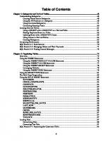
The model for a relational database states that data is stored in one or more tables. It also states that each table can be viewed as a two-dimensional matrix consisting of rows and columns. This is illustrated by the relational table in figure 1-4. Each row in this table contains information about a single vendor. In practice, the rows and columns of a relational database table are often referred to by the more traditional terms, records and fields. In fact, some software packages use one set of terms, some use the other, and some use a combination. This book uses the terms rows and columns because those are the terms used by SQL Server. In general, each table is modeled after a real-world entity such as a vendor or an invoice. Then, the columns of the table represent the attributes of the entity such as name, address, and phone number. And each row of the table represents one instance of the entity. A value is stored at the intersection of each row and column, sometimes called a cell. If a table contains one or more columns that uniquely identify each row in the table, you can define these columns as the primary key of the table. For instance, the primary key of the Vendors table in this figure is the VendoriD column. In this example, the primary key consists of a single column. However, a primary key can also consist of two or more columns, in which case it's called a composite primary key. In addition to primary keys, some database management systems Jet you define additional keys that uniquely identify each row in a table. If, for example, the VendorName column in the Vendors table contains unique data, it can be defined as a non-primary key. In SQL Server, this is called a unique key. Indexes provide an efficient way of accessing the rows in a table based on the values in one or more columns. Because applications typically access the rows in a table by referring to their key values, an index is automatically created for each key you define. However, you can define indexes for other columns as well. If, for example, you frequently need to sort the Vendor rows by zip code, you can set up an index for that column. Like a key, an index can include one or more columns.

Chapter 1

An introduction to relational databases and SQL

The Vendors table in an Accounts Payable database Primary key

I

~

VendoriD

1

Columns

r·;··. . . . . . . . . . . ] 2

~

VendorAddress1 Attn: Supt. Window Services

VendorAddress2 PO Box 7005

VendorOty

Nationl!l Information Dati! Qr

PO Box 96621

NULL

Wl!shington

~............... ,,,,,,,,,,,,,,i

2

I

VendorName US Postal Service

Madison

3

3

Register al Copyrights

Library Of Congress

NULL

Washington

4

4

Jo~k

5 6

5 6

Newbrige Book Oubs

1990 Westwood Blvd Ste 260 3000 Cndel Drive

NULL NULL

Los Nlgeles Washington

CaiWomil! Oll!mber Of Commerce

3255 Rllmos Or

NULL

Sl!cn!mento

7

7

Towne Advertiser's Ml!iling Svcs

Kevin M1nder

3441 W Ml!cl!rthur Blvd

Sl!fltahll!

8

8

BFl Industries

PO Box 9369

NULL

Fresno

9 10

9 10

Pi!cif'IC Gl!s & Bectrlc Robbins Mobile Lock h1d Key

Box 52001

Sl!n Frl!Odsc

4669 N Fresno

NULL NULL

11

11

Bill Mllrvin Bectric Inc

4583 E Home

NULL

Fresno

12

12

City Of Fresno

PO Box 2069

NULL

Fresno

13

13

Golden Eagle lnsun~nce Co

PO Box 85826

NULL

Sl!n Diego

14

14

4420 N. Rrst Street. SUte 108

NULL

Fresno

15

15

Expedatl! Inc ASC Signs

1528 N Siem~ Vistll

NULL

Fresno

16

16

lnleml!l Revenue Service

NULL

NULL

Fresno

-

r-- Rows

Fresno

.., >




T

"' •

Foreign key

Concepts •

The tables in a relational database are related to each other through their key columns. For example, the VendoriD column is used to relate the Vendors and Invoices tables above. The VendoriD column in the Invoices table is called a foreign key because it identifies a related row in the Vendors table. A table may contain one or more foreign keys.

•

When you define a foreign key for a table in SQL Server, you can 't add rows to the table with the foreign key unless there's a matching primary key in the related table.

•

The relationships between the tables in a database correspond to the relationships between the entities they represent. The most common type of relationship is a one-to-many relationship as illustrated by the Vendors and Invoices tables. A table can also have a one-to-one relationship or a many-to-many relationship with another table.

Figure 1-5

"

Fresno

How the tables in a relational database are related

"'

13

14

Section 1

An introduction to SQL

How the columns in a table are defined When you define a column in a table, you assign properties to it as indicated by the design of the Invoices table in figure 1-6. The most critical property for a column is its data type, which determines the type of information that can be stored in the column. With SQL Server 2019, you typically use one of the data types listed in this figure. As you define each column in a table, you generally try to assign the data type that will minimize the use of disk storage because that will improve the performance of the queries later. In addition to a data type, you must identify whether the column can store a null value. A null represents a value that's unknown, unavailable, or not applicable. If you don' t allow null values, then you must provide a value for the column or you can't store the row in the table. You can also assign a default value to each column. Then, that value is assigned to the column if another value isn't provided. You' lllearn more about how to work with nulls and default values later in this book. Each table can also contain a numeric column whose value is generated automatically by the DBMS. In SQL Server, a column like this is called an identity column, and you establish it using the Is Identity, Identity Seed, and Identity Increment properties. You'lllearn more about these properties in chapter 11. For now, just note that the primary key of both the Vendors and the Invoices tables-VendoriD and InvoiceiD-are identity columns.

Chapter 1

An introduction to relational databases and SQL

The columns of the Invoices table • .; MMA17\SQLEXPRESS.AP - dbo.lnvo~ees- MICrosoft SQL Server Management Studoo Fole

Voe.~

Edot

Project

,J •

0 •

Table Desogner

"

Tools

Wondow

.Jil .Iii Ne.~Query .Iii

.~

f '¥ G -Jo. i5 localhost\ SQLEXPRESS (SQLServer 15.0.2000- murach\Anno)

"

Databasos

8

8

Ill Ill IE Ill Ill Ill

Database Diagrams Tables Systom Tablos FileTables Extornal Tables Graph Tablos !Ill dbo.ContactUpdates !Ill dbo.GLAccounts

Iii dbo.lnvoicMrchive & dbo.lnvoicelineltems 13 !Ill dbo.lnvoicos IE III

l3

OJ t.J

~

p

I:

X

00:00:00

Data Type

·~ ~~~~~~~~~=~~==~~ int

ii AP ctl 9

VondoriD

int

lnvoiceNumber

varchar(SO)

InvoiceDate

date

lnvoice:Total

money

PaymentTotal

money

CroditTotal

money

TermsiO

int

lnvoiceDueDate

datt~

PaymentOate

date

Allow Nulls

0 0 0 0 0 0 0 0 0 0

Column Properties

J:l1!

Columns

ldentrty SpecrfJcatJOn

.. lnvoiceiD (PK, in~ not null) \!>" VondoriD (FK, in~ not null) l3 lnvoicoNumbor (varchar(SO), not nuiQ l3 lnvoiceDate (dot.. not nuiQ 13 lnvoicoTotal (money, not null) 13 PaymontTotal (money, not null) l3 CroditTotal (money, not nuiQ ~ TormsiD (FK, in~ not null)

0

cl(,

System Databases Database Snapshots

1.tJ l!l

-

MMA17\SQLEXPRESS.AP - dbo.lnvoiCes X Column Name

Connect ·

13

----------------

,0 ,o;., ,?,.

• q X

Object Explorer

p

Quock launch (Ctri•Ql

Help

Iv I

(Is Identity)

Yos Yos

Identity Increment

ldontity s..d lndoxablo

Yos

Identity Specification

Ready

Common SQL Server data types Type

Description

bit

A value of I or 0 that represents a True or False value.

int, bigint, smallint, tinyint

Integer values of various sizes.

money, smallmoney

Monetary values that are accurate to four decimal places.

decimal, numeric

Decimal values that are accurate to the least significant digit The values can contain an integer portion and a decimal portion.

float, real

Floating-point values that contai n an approximation of a decimal value.

date, time, datetime2

Dates and times.

char, varchar

A string of letters, symbols, and numbers in the ASCII character set

nc har, nvarchar

A string of letters, symbols, and numbers in the Unicode character set.

Description •

The data type that's assigned to a column determines the type and size of the information that can be stored in the column.

•

Each column definition also indicates whether or not it can contain null values. A null value indicates that the value of the column is unknown.

•

A column can also be defined with a default value. Then, that value is used if another value isn't provided when a row is added to the table.

•

A column can also be defined as an identity column. An identity column is a numeric column whose value is generated automatically when a row is added to the table.

Figure 1-6

How the columns in a table are defined

15

16

Section 1

An introduction to SQL

How relational databases compare to other data models Now that you understand how a relational database is organized, you're ready to learn how relational databases differ from other data models. Specifically, you should know how relational databases compare to conventional file systems, hierarchical databases, and network databases. Figure 1-7 presents the most important differences. To start, you should realize that because the physical structure of a relational database is defined and managed by the DBMS, it's not necessary to define that structure within the programs that use the database. Instead, you can simply refer to the tables and columns you want to use by name and the DBMS will take care of the rest. By contrast, when you use a conventional file system, you have to define and control the files of the system within each application that uses them. That's because a conventional file system is just a collection of files that contain the data of the system. In addition, if you modify the structure of a file, you have to modify every program that uses it. That's not necessary with a relational database. The hierarchical and network database models were predecessors to the relational database model. The hierarchical database model is limited in that it can only represent one-to-many relationships, also called parent/child relationships. The network database model is an extension of the hierarchical model that provides for all types of relationships. Although hierarchical and network databases don't have the same drawbacks as conventional file systems, they still aren't as easy to use as relational databases. In particular, each program that uses a hierarchical or network database must navigate through the physical layout of the tables they use. By contrast, this navigation is automatically provided by the DBMS in a relational database system. In addition, programs can define ad hoc relationships between the tables of a relational database. In other words, they can use relationships that aren't defined by the DBMS. That's not possible with hierarchical and network databases. Another type of database that's not mentioned in this figure is the object database. This type of database is designed to store and retrieve the objects that are used by applications written in an object-oriented programming language such as C#, C++, or Java. Although object databases have some advantages over relational databases, they also have some disadvantages. In general, object databases have not yet become widely used. However, they have acquired a niche in some areas such as engineering, telecommunications, financial services, high energy physics, and molecular biology.

Chapter 1

An introduction to relational databases and SQL

A comparison of relational databases and conventional file systems Feature

Conventional file system

Relational database

Definition

Each program that uses the file must define the fil e and the layout of the records within the file

Tables, rows, and columns are defined within the database and can be accessed by name

Maintenance

If the definition of a file changes, each program that uses the file must be modified

Programs can be used without modification when the definition of a table changes

Validity checking

Each program that updates a file must include code to check for valid data

Can include checks for valid data

Relationships

Each program must provide for and enforce relationships between files

Can enforce relationships between tables using foreign keys; ad hoc relationships can also be used

Data access

Each 1/0 operation targets a speci fic record in a file based on its relative position in the file or its key value

A program can use SQL to access selected data in one or more tables of a database

A comparison of relational databases and other database systems Feature

Hierarchical database

Network database

Relational database

Supported relationships

One-to-many only

One-to-many, one-to-one, and many-to-many

One-to-many, one-to-one, and many-to-many; ad hoc relationships can also be used

Data access

Programs must include code to navigate through the physical structure of the database

Programs must include code to navigate through the physical structure of the database

Programs can access data without knowing its physical structure

Maintenance

New and modified relationships can be difficult to implement in application programs

New and modified relationships can be difficult to implement in application programs

Programs can be used without modification when the definition of a table changes

Description •

To work with any of the data models other than the relational database model, you must know the physical structure of the data and the relationships between the files or tables.

•

Because relationships are difficult to implement in a conventional file system, redundant data is often stored in these types of files.

•

The hierarchical database model provides only for one-to-many relationships, called parent/child relationships.

•

The network database model can accommodate any type of relationship.

•

Conventional files, hierarchical databases, and network databases are all more efficient than relational databases because they require fewer system resources. However, the flexibility and ease of use of relational databases typically outweigh this inefficiency.

Figure 1-7

How relational databases compare to other data models

17

18

Section 1

An introduction to SQL

An introduction to SQL and SQL-based systems In the topics that follow, you'll learn how SQL and SQL-based database management systems evolved. In addition, you'lllearn how some of the most popular SQL-based systems compare.

A brief history of SQL

----

Prior to the release of the first relational database management system (RDBMS), each database had a unique physical structure and a unique programming language that the programmer had to understand. That all changed with the advent of SQL and the relational database management system. Figure 1-8lists the important events in the history of SQL. In 1970, Dr. E. F. Codd published an article that described the relational database model he had been working on with a research team at IBM. By 1978, the IBM team had developed a database system based on this model, called System/R, along with a query language called SEQUEL (Structured English Query Language). Although the database and query language were never officially released, IBM remained committed to the relational model. The following year, Relational Software, Inc. released the first relational database management system, called Oracle. This RDBMS ran on a minicomputer and used SQL as its query language. This product was widely successful, and the company later changed its name to Oracle to reflect that success. In 1982, IBM released its first commercial SQL-based RDBMS, called SQUDS (SQUData System). This was followed in 1985 by DB2 (Database 2). Both systems ran only on IBM mainframe computers. Later, DB2 was ported to other systems, including those that ran the Unix, Linux, and Windows operating systems. Today, it continues to be IBM's premier database system. During the 1980s, other SQL-based database systems, including SQL Server, were developed. Although each of these systems used SQL as its query language, each implementation was unique. That began to change in 1989, when the American National Standards Institute (ANSI) published its first set of standards for a database query language. These standards have been revised a few times since then, most recently in 2016. As each database manufacturer has attempted to comply with these standards, their implementations of SQL have become more similar. However, each still has its own dialect of SQL that includes additions, or extensions, to the standards. Although you should be aware of the SQL standards, they will have little effect on your job as a SQL programmer. The main benefit of the standards is that the basic SQL statements are the same in each dialect. As a result, once you've learned one dialect, it's relatively easy to learn another. On the other hand, porting applications that use SQL from one database to another isn' t as easy as it should be. In fact, any non-trivial application will require at least modest modifications.

Chapter 1

An introduction to relational databases and SQL

Important events in the history of SQL Year

Event

1970

Dr. E. F. Codd developed the relational database model.

1978

IBM developed the predecessor to SQL, called Structured English Query Language (SEQUEL). This language was used on a database system called System/R, but neither the system nor the query language was ever released.

1979

Relational Software, Inc. (later renamed Oracle) released the first relational DBMS, Oracle.

1982

IBM released their first relational database system, SQL!DS (SQL!Data System).

1985

IBM released DB2 (Database 2).

1987

Microsoft released SQL Server.

1989

The American National Standards Institute (ANSI) published the first set of standards for a database query language, called ANSI/ISO SQL-89, or SQLl. Because they were not stringent standards, most commercial products could claim adherence.

1992

ANSI published revised standards (ANSI/ISO SQL-92, or SQL2) that were more stringent than SQLl and incorporated many new features. These standards introduced levels of conformance that indicated the extent to which a dialect met the standards.

1999

ANSI published SQL3 (ANSI/ISO SQL: 1999), which incorporated new features, including support for objects. Levels of conformance were dropped and were replaced by a core specification along with specifications for nine additional packages.

2003

ANSI published SQL:2003, which introduced XML-related features, standardized sequences, and identity columns.

2006

ANSI published SQL:2006, which defined how SQL can be used with XML. The standards also allowed applications to integrate XQuery into their SQL code.

2008

ANSI published SQL:2008, which introduced INSTEAD OF triggers and the TRUNCATE statement.

2011

ANSI published SQL:2011 , which included improved support for temporal databases.

2016

ANSI published SQL:2016, which introduced polymorphic table functions, row pattern recognition, and support for JSON.

Description •

SQL-92 initially provided for three levels of conformance: entry, intermediate, and full . A transitional level was later added between the entry and intermediate levels.

•

SQL: 1999 includes a core specification that defines the essential elements for conformance, plus nine packages. Each package is designed to serve a specific market niche.

•

Although SQL is a standard language, each vendor has its own SQL dialect, or variant, that may include extensions to the standards. SQL Server's SQL dialect is called Transact-SQL.

How knowing "standard SQL'' helps you •

The most basic SQL statements are the same for all SQL dialects.

•

Once you have learned one SQL dialect, you can easily learn other dialects.

How knowing "standard SQL'' does not help you •

Any non-trivial application will require modification when moved from one SQL database to another.

Figure 1-8

A brief history of SOL

19

20

Section 1

An introduction to SQL

A comparison of Oracle, DB2, MySQL, and SQL Server Although this book is about SQL Server, you may want to know about some of the other SQL-based relational database management systems. Figure 1-9 compares SQL Server with three of the most popular: Oracle, DB2, and MySQL. Oracle has a huge installed base of customers and continues to dominate the marketplace, especia11y for servers running the Unix or Linux operating system. Oracle works well for large systems and has a reputation for being extremely reliable, but also has a reputation for being expensive and difficult to use. DB2 was originally designed to run on IBM mainframe systems and continues to be the premier database for those systems. It also dominates in hybrid environments where IBM mainframes and newer servers must coexist. Although it has a reputation for being expensive, it also has a reputation for being reliable and easy to use. MySQL runs on all major operating systems and is widely used for web applications. MySQL is an open-source database, which means that any developer can view and improve its source code. In addition, the MySQL Community Server is free for most users, although Oracle also sells other editions of MySQL that include customer support and advanced features. SQL Server was designed by Microsoft to run on Windows and is widely used for small- to medium-sized departmental systems. It has a reputation for being inexpensive and easy to use. Until2016, SQL Server ran only under the Windows operating system. By contrast, Oracle and MySQL ran under most modern operating systems. As a result, if a company used Linux as the operating system for its database servers, it couldn't use SQL Server and had to use Oracle or MySQL. However, in 2016, Microsoft released a preview version of SQL Server that runs under Linux, and it released a final version in 2017. This should allow SQL Server to compete with Oracle and MySQL when a company prefers to use Linux, not Windows, for its database servers. Although this book focuses on using SQL Server with Windows, the database engine is basically the same for Linux. If you search the Internet, you'll find that dozens of other relational database products are also available. These include proprietary databases like Informix, SQL Anywhere, and Teradata. And they include open-source databases like PostgreSQL.

Chapter 1

An introduction to relational databases and SQL

A comparison of Oracle, 082, MySQL, and SQL Server Oracle

082

MySQL

SQL Server

Released

1979

1985

2000

1987

Platforms

Unix/Linux z/OS Windows macOS

OS/390, z/OS, and AIX Unix/Linux Windows macOS

Unix/Linux Windows macOS

Windows Linux

Description •

Oracle is typically used for large, mission-critical systems that run on one or more Unix servers.

•

DB2 is typically used for large, mission-critical systems that run on legacy IBM mainframe systems using the z/OS or OS/390 operating system.

•

MySQL is a popular open-source database that runs on all major operating systems and is commonly used for web applications.

•

SQL Server is typically used for small- to medium-sized systems that run on one or more Windows servers. However, SQL Server 2017 and later are designed to run on Linux as well as Windows.

Figure 1-9

A comparison of Oracle, 0 82, MySQL, and SOL Server

21

22

Section 1

An introduction to SQL

The Transact-SQL statements In the topics that follow, you'llleam about some of the SQL statements provided by SQL Server. As you'll see, you can use some of these statements to manipulate the data in a database, and you can use others to work with database objects. Although you may not be able to code these statements after reading these topics, you should have a good idea of how they work. Then, you'll be better prepared to learn the details of coding these statements when they're presented in sections 2 and 3 of this book.

An introduction to the SQL statements Figure 1-10 summarizes some of the most common SQL statements. As you can see, these statements can be divided into two categories. The statements that work with the data in a database are called the data manipulation language (DML). These four statements are the ones that application programmers use the most. You'll see how these statements work later in this chapter, and you'lllearn the details of using them in section 2 of this book. The statements that work with the objects in a database are called the data definition language (DDL). On large systems, these statements are used exclusively by database administrators, or DBAs. It's the DBA's job to maintain existing databases, tune them for faster performance, and create new databases. On smaller systems, though, the SQL programmer may also be the DBA. You'll see examples of some of these statements in the next figure, and you'lllearn how to use them in chapter 11.

Chapter 1

An introduction to relational databases and SQL

SQL statements used to work with data (DML) Statement

Description

SELECT

Retrieves data from one or more tables.

INSERT

Adds one or more new rows to a table.

UPDATE

Changes one or more existing rows in a table.

DELETE

Deletes one or more existing rows from a table.

SQL statements used to work with database objects (DOL) Statement

Description

CREATE DATABASE

Creates a new database.

CREATE TABLE

Creates a new table in a database.

CREATE INDEX

Creates a new index for a table.

ALTER TABLE

Changes the structure of an existing table.

ALTER INDEX

Changes the structure of an existing index.

DROP DATABASE

Deletes an existing database.

DROP TABLE

Deletes an existing table.

DROP INDEX

Deletes an existing index.

Description •

The SQL statements can be divided into two categories: the data manipulation language (DML) that lets you work with the data in the database and the data definition language (DDL) that lets you work with the objects in the database.

•

SQL programmers typically work with the DML statements, while database administrators (DBAs) use the DDL statements.

Figure 1-10

An introduction to the SOL statements

23

24

Section 1

An introduction to SQL

Typical statements for working with database objects To give you an idea of how you use the DDL statements you saw in the previous figure, figure 1-11 presents five examples. The first statement creates an accounts payable database named AP. This is the database that's used in many of the examples throughout this book. The second statement creates the Invoices table you saw earlier in this chapter. If you don't understand all of this code right now, don't worry. You' ll learn how to code statements like this later in this book. For now, just realize that this statement defines each column in the table, including its data type, whether or not it allows null values, and its default value if it has one. In addition, it identifies identity columns, primary key columns, and foreign key columns. The third statement in this figure changes the Invoices table by adding a column to it. Like the statement that created the table, this statement specifies all the attributes of the new column. Then, the fourth statement deletes the column that was just added. The last statement creates an index on the Invoices table. In this case, the index is for the VendoriD column, which is used frequently to access the table. Notice the name that's given to this index. This follows the standard naming conventions for indexes, which you '11 learn about in chapter 11 .

Chapter 1

An introduction to relational databases and SQL

A statement that creates a new database CREATE DATABASE AP;

A statement that creates a new table CREATE TABLE Invoices (

InvoiceiD VendoriD InvoiceNwnber InvoiceDate InvoiceTotal PaymentTotal CreditTotal TermsiD InvoiceDueDate PaymentDate

INT INT VARCHAR (50) DATE MONEY MONEY MONEY INT DATE DATE

NOT NULL IDENTITY PRIMARY KEY, NOT NULL REFERENCES Vendors(VendoriD), NOT NULL, NOT NULL, NOT NULL, NOT NULL DEFAULT 0 , NOT NULL DEFAULT 0 , NOT NULL REFERENCES Terms(TermsiD), NOT NULL, NULL

) ;

A statement that adds a new column to the table ALTER TABLE Invoices ADD BalanceDue MONEY NOT NULL;

A statement that deletes the new column ALTER TABLE Invoices DROP COLUMN BalanceDue;

A statement that creates an index on the table CREATE INDEX IX_ Invoices_VendoriD ON Invoices (VendoriD);

Description •

The REFERENCES clause for a column indicates that the column contains a foreign key, and it names the table and column that contains the primary key. Because the Invoices table includes foreign keys to the Vendors and Terms tables, these tables must be created before the Invoices table.

•

Because default values are specified for the PaymentTotal and CreditTotai columns, these values don't need to be specified when a row is added to the table.

•

Because the PaymentDate column accepts nulls, a null value is assumed if a value isn't specified for this column when a row is added to the table.

Figure 1-11

Typical statements for working with database objects

25

26

Section 1

An introduction to SQL

How to query a single table Figure 1-12 shows how to use a SELECT statement to query a single table in a database. At the top of this figure, you can see some of the columns and rows of the Invoices table. Then, in the SELECT statement that follows, the SELECT clause names the columns to be retrieved, and the FROM clause names the table that contains the columns, called the base table. In this case, six columns will be retrieved from the Invoices table. Notice that the last column, BalanceDue, is calculated from three other columns in the table. In other words, a column by the name of BalanceDue doesn't actually exist in the database. This type of column is called a calculated value, and it exists only in the results of the query. In addition to the SELECT and FROM clauses, this SELECT statement includes a WHERE clause and an ORDER BY clause. The WHERE clause gives the criteria for the rows to be selected. In this case, a row is selected only if it has a balance due that's greater than zero. And the returned rows are sorted by the InvoiceDate column. This figure also shows the result table, or result set, that's returned by the SELECT statement. A result set is a logical table that's created temporarily within the database. When an application requests data from a database, it receives a result set.

Chapter 1

An introduction to relational databases and SQL

The Invoices base table lnvoiceiD 1 2 3 4 5 6 7 8 9 10 11 12

VendoriD

!.·.·.·.·.·.·.·.·.·.-·. -.··. ·.-·. ·.~·.·.~] 122

[ ...

2 3 4 5 6 7 8 9 10 11 12

13

13

14 15

14 15

123 123 123 123 123 123 89 121 123 123 96 95 115 48

Invoice Number 989319-457 263253241 963253234 2.()00.2993 963253251 963253261 963253237 125521}1 97/ 488 263253250 963253262 177271.001 111-92R-10096 25022117 P02-88DnS7

Invoice Date 2019-1().08 2019-11}10 2019-11}13 2019-11}16 2019-11}16 2019-11}16 2019-11}21 2019-11}24 2019-11}24 2019-11}24 2019-11}25 2019-11}26 2019-11}30 2019-11-()1 2019-11-()3

InvoiceTotal 3813.33 40.20 138.75 144.70 15.50 42.75 m .50 95.00 601.95 42.67 42.50 662.00 16.33 6.00 856.92

PaymentTotal 3813.33 40.20 138.75 144.70 15.50 42.75 172.50 95.00 601.95 42.67 42.50 662.00 16.33 6.00 856.92

CreditTotal

0.00 0.00 0.00 0.00 0.00 0.00 0.00 0.00 0.00 0.00 0.00 0.00 0.00 0.00 0.00


0 order by invoicedate

A SELECT statement that's coded with a readable style Select InvoiceNumber, InvoiceDate, InvoiceTotal, InvoiceTotal - PaymentTotal - CreditTotal As BalanceDue From Invoices Where InvoiceTotal - PaymentTotal - CreditTotal > 0 Order By InvoiceDate;

A SELECT statement with a block comment /* Author: Joel Murach Date: 1/22/2020 *I SELECT InvoiceNumber, InvoiceDate, InvoiceTotal, InvoiceTotal - PaymentTotal - CreditTotal AS BalanceDue FROM Invoices;

A SELECT statement with a single-line comment SELECT InvoiceNumber, InvoiceDate, InvoiceTotal, InvoiceTotal - PaymentTotal - CreditTotal AS BalanceDue -- The fourth column calculates the balance due for each invoice FROM Invoices;

Coding recommendations •

Start each new clause on a new line.

•

Break long clauses into multiple lines and indent continued lines.

•

Capitalize the fi rst letter of each keyword and each word in column and table names.

•

End each statement with a semicolon (;).

•

Use comments only for portions of code that are difficult to understand.

How to code a comment •

To code a block comment, type/* at the start of the block and */ at the end.

•

To code a single-line comment, type -- followed by the comment.

Description •

Line breaks, white space, indentation, and capitalization have no effect on the operation of a statement.

•

Comments can be used to document what a statement does or what specific parts of a statement do. They are not executed by the system.

Note •

Throughout this book, SQL keywords are capitalized so they're easier to identify. However, it's not necessary or customary to capitalize SQL keywords in your own code.

Figure 1-1 5

SOL coding guidelines

33

34

Section 1

An introduction to SQL

How to work with other database objects In addition to the tables you've already learned about, relational databases can contain other objects. In the two topics that follow, you'll be introduced to four of those objects: views, stored procedures, triggers, and user-defined functions. Then, in section 4, you'll learn more about how to code and use these objects.

How to work with views A view is a predefined query that's stored in a database. To create a view, you use the CREATE VIEW statement as shown in figure 1-16. This statement causes the SELECT statement you specify to be stored with the database. In this case, the CREATE VIEW statement creates a view named VendorsMin that retrieves three columns from the Vendors table. Once you've created the view, you can refer to it instead of a table in most SQL statements. For this reason, a view is sometimes referred to as a viewed table. For example, the SELECT statement in this figure refers to the VendorsMin view rather than to the Vendors table. Notice that this SELECT statement makes use of the * operator, which causes all three of the columns defined by the view to be returned. If you choose to, you can let a user query certain views but not query the tables on which the views are based. In this way, views can be used to restrict the columns and rows of a table that the user can see. In addition, you can simplify a user's access to one or more tables by coding complex SELECT queries as views.

Chapter 1

An introduction to relational databases and SQL

A CREATE VIEW statement for a view named VendorsMin CREATE VIEW VendorsMin AS SELECT VendorName, VendorState, VendorPhone FROM Vendors;

The virtual table that's represented by the view VendorName

VendorState

VendorPhone

L·.Q.S.~~.P..~.~.~.i~~~.~~·.·.·.·~~.·~~.·~~.·~~~~~~~~~.·~~.·~~.·~~.·~~.·~.·.·~] wI

(800) 555-1205

Register of Copyrights

DC DC

(301) 555-8950 NULL

4

Jobtrak

CA

(800) 55S.Sn5

5

Newbrige Book Oubs

NJ

(800) 555-9980

6 7

California Olamber Of Commerce

CA

(916) 555-6670

Towne Advertiser's Maning Svcs

CA

NULL

8

BFl Industries

CA

(559) 555-1551

9 10

Pacific Gas & Bectric

CA

Robbins MobUe Lock hid Key

CA

(800) 555-6081 (559) 555-9375

1 2 3

National Information Data Ctr

"""'

A SELECT statement that uses the VendorsMin view SELECT * FROM VendorsMin WHERE VendorState = 'CA' ORDER BY VendorName ;

The result set that's returned by the SELECT statement VendorName 1

L·~·~·~··.?.f.ii.~.~.·.·.F.~F..i.~~~~~.·.·.·.·.·.·~·.·.~·.·~ .·~.·.·.·.·.·.J

VendorState

VendorPhone

CA

(559) 555-8300 (800) 555-3344

2 3

American Express

CA

ASC Signs

CA

NULL

4

Aztek Label

CA

5

Bertelsmann Industry Svcs. Inc

CA

(714) 555-9000 (805) 555-0584

6

BFIIndustries

CA

(559) 555-1551

7

Bin Jones

CA

NULL

8

BiQ Marvin Electric Inc

CA

9

Blanchard &Johnson Associates

CA

(559) 555-5106 (214) 555-3647

Description •

A view consists of a SELECT statement that's stored with the database. Because views are stored as part of the database, they can be managed independently of the applications that use them.

•

A view behaves like a virtual table. Since you can code a view name anywhere you'd code a table name, a view is sometimes called a viewed table.

•

Views can be used to restrict the data that a user is allowed to access or to present data in a form that's easy for the user to understand. In some databases, users may be allowed to access data only through views.

Figure 1-1 6

How to work with views

35

36

Section 1

An introduction to SQL

How to work with stored procedures, triggers, and user-defined functions A stored procedure is a set of one or more SQL statements that are stored together in a database. To create a stored procedure, you use the CREATE PROCEDURE statement as shown in figure 1-17. Here, the stored procedure contains a single SELECT statement. To use the stored procedure, you send a request for it to be executed. One way to do that is to use the Transact-SQL EXEC statement as shown in this figure. You can also execute a stored procedure from an application program by issuing the appropriate statement. How you do that depends on the programming language and the API you're using to access the database. When the server receives the request, it executes the stored procedure. If the stored procedure contains a SELECT statement like the one in this figure, the result set is sent back to the calling program. If the stored procedure contains INSERT, UPDATE, or DELETE statements, the appropriate processing is performed. Notice that the stored procedure in this figure accepts an input parameter named @State from the calling program. The value of this parameter is then substituted for the parameter in the WHERE clause so that only vendors in the specified state are included in the result set. When it's done with its processing, a stored procedure can also pass output parameters back to the calling program. In addition, stored procedures can include control-of-flow language that determines the processing that's done based on specific conditions. You'll learn more about how to code stored procedures in chapter 15. A trigger is a special type of stored procedure that's executed automatically when an insert, update, or delete operation is executed on a table or when a DOL statement is executed on a database. Triggers are used most often to validate data before a row is added or updated, but they can also be used to maintain the relationships between tables or to provide information about changes to the definition of a database. A user-defined function, or UDF, is also a special type of procedure. After it performs its processing, a UDF can return a single value or an entire table to the calling program. You' llleam how to code and use user-defined functions and triggers in chapter 15.

Chapter 1

An introduction to relational databases and SQL

A CREATE PROCEDURE statement for a procedure named spVendorsByState CREATE PROCEDURE spVendorsByState @StateVar char(2) AS SELECT VendorName, VendorState, VendorPhone FROM Vendors WHERE VendorState = @Statevar ORDER BY VendorName;

A statement that executes the spVendorsByState stored procedure EXEC spVendorsByState 'CA';

The result set that's created when the stored procedure is executed VendorName 1 2

3 4

VendorState

VendorPhone

American Express

CA CA

(559) 555-8300 (800) 555-3344

ASC Signs

CA

NULL

Aztek label

CA

(714) 555-9000

[_·~.b..~i..·.~.~.~.·~.F.~~.~.~~~~~~.·.·~.·.·~ .·~ .·~ .·~ .·.·~.·]

5

Bertelsmann Industry Svcs. Inc

CA

(805) 555-0584

6

BFI Industries

CA

(559) 555-1551

7

Bift Jones

CA

NULL

8

BiD Marvin Bectric Inc

CA

(559) 555-5106

"""""'

"""

Concepts •

A stored procedure is one or more SQL statements that have been compiled and stored with the database. A stored procedure can be started by application code on the client.

•

Stored procedures can improve database performance because the SQL statements in each procedure are only compiled and optimized the first time they're executed. By contrast, SQL statements that are sent from a client to the server have to be compiled and optimized every time they're executed.

•

In addition to SELECT statements, a stored procedure can contain other SQL statements such as INSERT, UPDATE, and DELETE. It can also contain control-of-flow language, which lets you perform conditional processing within the stored procedure.

•

A trigger is a special type of procedure that's executed when rows are inserted, updated, or deleted from a table or when the definition of a database is changed. Triggers are typically used to check the validity of the data in a row that's being updated or added to a table.

•

A user-defined function (UDF) is a special type of procedure that can return a value or a table.

Figure 1-17

How to use stored procedures, triggers, and user-defined functions

37

38

Section 1

An introduction to SQL

How to use SQL from an application program This book teaches you how to use SQL from within the SQL Server environment. However, SQL is commonly used from application programs too. So in the topics that follow, you'll get a general idea of how that works. And you'll see that it's easy to recognize the SQL statements in an application program because they're coded just as they would be if they were running on their own.

Common data access models Figure 1-18 shows two common ways for an application to access a SQL Server database. First, you can access a SQL Server database from a .NET application written using a .NET language such as C# or Visual Basic. To do that, you can use ADO. NET. This is a data access model developed by Microsoft, and it can communicate directly with SQL Server. Because ADO.NET uses a disconnected data architecture, its use has become widespread, particularly for web-based applications. That's because web-based applications by necessity work with disconnected data. That means that once an application has sent a response to the client, it doesn't maintain its connection to the database. The second data access model in this figure is JDBC, which is used by Java applications. Unlike ADO.NET, JDBC requires additional software, called a driver, to communicate with SQL Server. Although it's not shown here, another option for accessing SQL Server data that's becoming more and more popular is using an object-relational mapping (ORM) framework. When you use an ORM framework, the data in a relational database is mapped to the objects used by an object-oriented programming language such as C# or Java. Then, the application can make requests against the object model, and those requests are translated into ones that can be executed by the database. This simplifies the code that's needed to communicate with the database. Before you start developing an application that works with a database, then, you should consider using an ORM framework such as Entity Framework (EF) for .NET applications and Hibernate for Java applications.

Chapter 1

An introduction to relational databases and SQL

Two common options for accessing SQL Server data

Description •

To work with the data in a SQL Server database, an application uses a data access model. For an application written in a .NET language such as C# or Visual Basic that model is typically ADO.NET. For an application written in Java, that model is typically JDBC (Java Database Connectivity).

•

Each data access model defines a set of objects you can use to connect to and work with a SQL Server database. For example, both of the models shown above include a connection object that you can use to specify the information for connecting to a database.

•

Some of the data access models require additional software, called drivers, to communicate with SQL Server. For example, JDBC requires a Java driver.

•

ADO.NET, a data access model developed by Microsoft, includes its own driver so it can communicate directly with SQL Server.

•

In addition to working with ADO.NET and JDBC directly, you can use an objectrelational mapping (ORM) framework. An ORM framework works by mapping the data in a relational database to the objects used by an object-oriented programming language. Then, the ORM translates requests to retrieve, insert, update, and delete data so the DBMS will understand them.

•

The most popular ORM framework for use with .NET applications is Entity Framework (EF), which was developed by Microsoft. The most popular ORM framework for use with Java is Hibernate. Both of these frameworks are open-source.

Figure 1-18

Common data access models

39

40

Section 1

An introduction to SQL

How to use ADO.NET from a .NET application -~--~

To illustrate how you use a data access model, figure 1-19 introduces you to the basic ADO.NET objects that you use in a .NET application. Then, in the next two figures, you' ll see some actual code that creates and uses these objects. Keep in mind, though, that there's a lot more you need to know about ADO.NET than what's presented here. When you develop a .NET application, you can choose from several languages, but the most popular are Visual Basic and C#. Although C# has become more popular than Visual Basic over the past few years, the language you choose is largely a matter of personal preference. To access a database using the objects shown here, you execute command objects. Then, a connection object is used to connect to the database, perform the requested operation, and return the result. If you execute a command that contains a SELECT statement, the result is a result set that contains the rows you requested. Then, you can read the rows in the result set using a data reader object. If you execute a command that contains an INSERT, UPDATE, or DELETE statement, the result is a value that indicates if the operation was successful.

Chapter 1

An introduction to relational databases and SQL

Basic ADO. NET objects in a .NET application .NET data provider Data reader

i Select command

1i

Database server

Connection

i

Insert, Delete, or Update command

Description •

To work with the data in a SQL Server database from a .NET application, you can use ADO.NET objects like the ones shown above.

•

A .NET data provider provides the classes that let you create the objects that you use to retrieve data from a database and to store data in a database.

•

To retrieve data from a database, you execute a command object that contains a SELECT statement. Then, the command object uses a connection object to connect to the database and retrieve the data. You can then read the results one row at a time using a data reader object.

•

To insert, update, or delete data in a database, you execute a command object that contains an INSERT, UPDATE, or DELETE statement. Then, the command object uses a connection to connect to the database and update the data. You can then check the value that's returned to determine if the operation was successful.

•

After data is retrieved from a database or updated in a database, the connection is closed and the resources used by the connection are released. This is referred to as a disconnected data architecture.

Figure 1-19

How to use ADO. NET from a .NET application

41

42

Section 1

An introduction to SQL

Visual Basic code that retrieves data from a SQL Server database Figure 1-20 presents a Visual Basic function that uses the ADO.NET objects shown in the previous figure. This function is from a simple application that accepts a vendor ID from the user, retrieves the information for the vendor with that ID from the Vendors table, and then displays that information. Although I don' t expect you to understand this code, I hope it will give you a feel for how you use SQL from an application program. This function starts by creating a new Vendor object. Although it's not shown here, this object contains properties that correspond to the columns in the Vendors table. Then, this function creates the connection object that will be used to connect to the database and sets the connection string for that object. The connection string provides ADO.NET with the information it needs to connect to the database. Once the connection string is set, the next group of statements defines the Command object that will be executed to retrieve the data from the database. The first statement in this group creates the command object. Then, the next statement assigns the connection object to the command object. That means that when the statement that this object will contain is executed, it will use the connection string in the connection object to connect to the database. The next statement in this group specifies the SELECT statement to be executed. If you review this statement, you'll see that the WHERE clause includes a parameter named @VendoriD that will contain the value of the vendor ID. This value is set by the last statement in this group. The next statement opens the connection to the database. Then, the next group of statements retrieves the vendor row and stores it in a Vendor object. To do that, it starts by executing the command to create a data reader. Then, if the vendor is found, it assigns the values of the columns in the row to the properties of the Vendor object. Otherwise, the Vendor object is set to Nothing. After all of the rows are processed, the data reader and connection are closed. Then, the Vendor object is returned to the calling procedure. Now that you've reviewed this code, you can see that there's a lot involved in accessing a SQL Server database from an application program. However, you can also see that only one statement in this figure actually involves using SQL. That's the statement that specifies the SELECT statement to be executed. Of course, if the program also provided for updating the data in the Vendors table, it would include INSERT, UPDATE, and DELETE statements. With the skills that you'lllearn in this book, though, you won't have any trouble coding the SQL statements you need for your applications.

Chapter 1

An introduction to relational databases and SQL

A Visual Basic function that uses ADO.NET objects to retrieve data from a SQL Server database Public Share d Function GetVendor (vendoriD As Integer) As Vendor Dim vendor As New Vendor 1 Create the c onnec tion objec t Dim connection As New SqlConnection() connection.ConnectionString = " Data Source=localhost \ SqlExpress; " & "Initial Catalog=AP;Integrated Security=True"

Create the command object and set the connection, SELECT statement, and parame ter value Dim sele ctCommand As New SqlCommand selectCommand.Connection = connection selectCommand.CommandText = "SELECT VendoriD, " & " VendorName, VendorAddressl, VendorAddress2, " & "VendorCity, VendorState, VendorZipCode " & "FROM Vendors WHERE VendoriD • ~VendoriD" selectCommand.Parameters.AddWithValue ( "@VendoriD", vendoriD ) 1 1

1 Open the connection to the database connection.Open ( )

Retrieve the row specified by the SELECT statement and load it into the Vendor object Dim reader As SqlDataReader = selectCommand.ExecuteReader If reader . Read Then vendor.Vendor iD = Cint(reader ( "VendoriD")) vendor.VendorName = reader("VendorName" ) .ToString vendor.VendorAddressl = reader ( "VendorAddressl" ) .ToString vendor.VendorAddress2 = reader("VendorAddress2").ToString vendor.VendorCity = reader("VendorCity" ) .ToString vendor.VendorState = reader ( "VendorState").ToString vendor.VendorZipCode = reader ( "VendorZipCode " ).ToString Else vendor = Nothing End If reader . Close() 1 1

Close the connection to the database connection.Close() 1

Return vendor End Function

Description •

To issue a SQL statement from a Visual Basic program, you can create ADO.NET objects like the ones shown above.

•

After you create the ADO.NET objects, you have to set the properties of those objects that define how they work. For example, the ConnectionString property of a connection object contains the information ADO.NET needs to connect to a database.

Figure 1-20

Visual Basic code that retrieves data from a SOL Server database

43

44

Section 1

An introduction to SQL

C# code that retrieves data from a SQL Server database Figure 1-21 presents C# code that uses the ADO.NET objects to retrieve data from a SQL Server database. This code provides the same functionality as the Visual Basic code presented in figure 1-20. If you compare the code presented in these two figures, you'll see that both Visual Basic and C# use the same ADO.NET objects that are provided as part of the .NET Framework. The main difference is that the C# language uses a different syntax than Visual Basic. This syntax is similar to the syntax that's used by C++ and Java. As a result, if you already know C++ or Java, it should be relatively easy for you to learn C#. Conversely, once you learn C#, it's easier to learn C++ or Java.

Chapter 1

An introduction to relational databases and SQL

A C# method that uses ADO.NET objects to retrieve data from a SQL Server database public static Vendor GetVendor(int vendoriD) {

Vendor vendor = new Vendor();

II Create the connection object SqlConnection connection = new SqlConnection(); connection.ConnectionString = "Data Source=localhost\\SqlExpress;" + "Initial Catalog=AP;Integrated Security=True"; II II

Create the command object and set the connection, SELECT statement, and parameter value SqlCommand selectCommand = new SqlCommand(); selectCommand.Connection = connection; selectCommand.CommandText = "SELECT VendoriD, " + " VendorName , VendorAddressl, Ve ndorAddress 2, " + "VendorCity, VendorState, VendorZipCode " + " FROM Vendors WHERE VendoriD • @VendoriD" ; selectCommand.Parameters.AddWithValue("@VendoriD", vendoriD);

II Open the connection to the database connection.Open(); II II

Retrieve the row specified by the SELECT statement and load it into the Vendor object SqlDataReader reader= selectCommand.ExecuteReader(); if (reader.Read()) {

vendor. VendoriD = ( int) reader [ "VendoriD"] ; vendor.VendorName = reader["VendorName"] .ToString(); vendor.VendorAddressl = reader["VendorAddressl"].ToString(); vendor.VendorAddress2 = reader["VendorAddress2"].ToString(); vendor.VendorCity = reader["VendorCity"] .ToString(); vendor.VendorState = reader["VendorState"] .ToString(); vendor.VendorZipCode = reader["VendorZipCode"].ToString(); }

else {

vendor = null; }

reader.Close();

II Close the connection to the database connection.Close(); return vendor; }

Description •

To issue a SQL statement from a C# application, you can use ADO.NET objects like the ones shown above.

Figure 1-21

C# code that retrieves data from a SOL Server database

45

46

Section 1

An introduction to SQL

Perspective To help you understand how SQL is used from an application program, this chapter has introduced you to the hardware and software components of a client/server system. It has also described how relational databases are organized and how you use some of the basic SQL statements to work with the data in a relational database. With that as background, you're ready to start using SQL Server. In the next chapter, then, you ' 11 learn how to use some of the tools provided by SQL Server.

Terms client server database server network client/server system local area network (LAN) enterprise system wide area network (WAN) network operating system database management system (DBMS) back end application software data access API (application programming interface) front end SQL (Structured Query Language) SQL query query results application server web server business component web application web service web browser thin client relational database table row column record field cell

primary key composite primary key non-primary key unique key index foreign key one-to-many relationship one-to-one relationship many-to-many relationship data type null value default value identity column hierarchical database parent/child relationship network database object database relational database management system (RDBMS) Oracle DB2 (Database 2) ANSI (American National Standards Institute) levels of conformance core specification package SQL dialect extension SQL variant Transact-SQL open-source database data manipulation language (DML) data definition language (DDL)

Chapter 1

database administrator (DBA) base table result table result set calculated value J Oin

inner join outer join cross JOin action query comment block comment single-line comment view viewed table

An introduction to relational databases and SQL

stored procedure input parameter output parameter control-of-flow language user-defined function (UDF) trigger data access model ADO.NET JDBC (Java Database Connectivity) disconnected data architecture driver command connection data source

47

2 How to use the Management Studio In the last chapter, you learned about some of the SQL statements you can use to work with the data in a relational database. Before you learn the details of coding these statements, however, you need to become familiar with a tool that you can use to execute these statements against a relational database. Since this book is about SQL Server 2019, this chapter will teach you about the primary tool for working with SQL Server 2019, the SQL Server Management Studio.

An introduction to SQL Server 2019 ...................................50 A summary of the SQL Server 2019 tools ....................................................50 How to start and stop the database engine ....................................................52 How to e nable remote connections ................................................................ 52

An introductionto the Management Studio ....................... 54 How to connect to a database server .............................................................54 How to navigate through the database objects ..............................................56

How to manage the database files ..................................... 58 How to attach a database ...............................................................................58 How to detach a database ..............................................................................58 How to back up a database ........................................................................... 60 How to restore a database ............................................................................. 60 How to set the compatibility level for a database ..........................................62

How to view and modify the database ...............................64 How to c reate database diagrams ................................................................. 64 How to view the column defin itions of a table ............................................. 66 How to mod ify the column defin itions ......................................................... 66 How to view the data of a table .....................................................................68 How to mod ify the data of a table .................................................................68

How to work with queries ....................................................70 How to e nter a nd execute a query ..................................................................70 How to handle syntax errors ..........................................................................72 How to open and save queries ....................................................................... 74 An introduction to the Query Designer .........................................................76

How to view the documentationfor SQL Server ................78 How to display the SQL Server documentation ............................................78 How to look up information in the documentation .......................................78

Perspective ...........................................................................80

50

Section 1

An introduction to SQL

An introduction to SQL Server 2019 The current version of Microsoft SQL Server, SQL Server 2019, is a complete database management system. It consists of a database server that provides the services for managing SQL Server databases and client tools that provide an interface for working with the databases. Of these client tools, the Management Studio is the primary tool for working with a database server. Before I go on, you should know that you can follow along with the skills presented in this chapter if you have access to SQL Server 2019. If that's not the case, you can refer to appendix A of this book to learn how to download and install it. In addition, you can refer to appendix A to download all of the database and source code files used in this book. Once you do that, you can work along with the book examples. If you install SQL Server as described in appendix A of this book, a free edition of SQL Server, called the SQL Server 20 19 Express, will be installed on your machine. Although the Express Edition restricts the number of processors, the amount of memory, and the amount of data that SQL Server can manage, it provides a realistic testing environment that is 100% compatible with the other versions of SQL Server 2019. In fact, SQL Server Express is adequate for many small and medium sized applications. And since it's free and easy to use, it's perfect for learning about SQL Server. For example, I used SQL Server Express to create and test all of the statements presented in this book. Note, however, that SQL Server Express is strictly a database server, or database engine. In other words, it doesn' t provide some of the client tools you may need. In particular, it doesn' t include the Management Studio. That's why appendix A describes how to install the Management Studio, which is also available for free.

A summary of the SQL Server 2019 tools Figure 2- 1 summarizes the SQL Server 2019 client tools that you' ll learn how to use in this book: the Management Studio and the Configuration Manager. Although other tools exist for working with a SQL Server 2019 database, they are commonly used by database administrators and other specialists, not application developers. That's why they aren' t presented in this book.

Chapter 2

How to use the Management Studio

A summary of the SQL Server 2019 tools Tool

Description

SQL Server Management Studio

The primary graphical tool that a developer uses to work with a SQL Server 2019 database. You can use this tool to work directly with database objects and to develop and test SQL statements.

SQL Server Configuration Manager

A graphical tool that you can use to start and stop the database server.

Description •

To work with a SQL Server database and the data it contains, you can use the SQL Server 2019 tools described above.

•

After you install SQL Server 2019, you can access the Management Studio from the Start-7Microsoft SQL Server Tools 18 program group, and you can access the Configuration Manager from the Start-7Microsoft SQL Server 2019 program group. To start one of these tools, just select it from its group.

•

To make either of these tools easier to access, you can pin it to the Start menu by right-clicking on it and selecting Pin to Start. Then, it will appear as a tile in the Start menu and you can click on it to start it.

Figure 2-1

The SOL Server 2019 tools

51

52

Section 1

An introduction to SQL

How to start and stop the database engine If you've installed SQL Server Express on your own system, you can use the SQL Server Configuration Manager to start and stop the database engine as described in figure 2-2. By default, the database engine starts automatically when the operating system starts, which is usually what you want. However, you may occasionally need to stop and then restart the engine. For example, some changes you make to the database server won' t go into effect until you restart the engme. By the way, if you simply want to find out if the database engine is running, you can do that by selecting SQL Server 2019 Services in the left pane. Then, you can look at the State column in the right pane. In this figure, for example, the Configuration Manager shows that the SQL Server Express database engine . . IS runmng.

How to enable remote connections When you install SQL Server 2019, remote connections are disabled by default. This is a security precaution that prevents other computers from connecting to this instance of SQL Server before it has been properly secured. As a result, if you have installed SQL Server 2019 and you want to allow other computers to be able to access this instance of SQL Server, you must enable remote connections. To do that, you can use the SQL Server Configuration Manager tool as described in figure 2-2. Of course, if databases that contain sensitive data are running under this instance of SQL Server, you'll want to secure the database properly before you enable remote connections.

Chapter 2

How to use the Management Studio

The SQL Server Configuration Manager (Services) 0

Sql Server Configuration Manager

~ SQL Server Configuration Manager (locaij

Cl

Name

SQL Server Services

State

·a SOL Server (SQLEXPRESS)

Runmng ,.[, SQL Server Network Configuration (32bit f.tj SQL Full-text Fiker Daemon Launc ... Running > -~·SOL Native Client 11.0Configuration (321 11'.>.-.sQL S R · Se · (SQ R · .[ SOL Server Network Configuration li1V erver eportlng rv~ces "' unnlng ·~· SQL Native Client 11.0 Configuration ! SOL Server Agent (SQLEXPRfSS) Stopped ·

~.!J SOL

·

Server Browser

Stopped

X

Start Mode

Log On As

Proc6s 10

Automatoc Manual Automatic Other (Boo~ Syste... Other (Boo~ Syste...

NT Servoce\MSSQLSSQLEXPRESS NT Service\ MSSQLFDLauncherSS... NT Service\ ReportServerSSQLEXP ... NT AUTHORITY\NETWORKSERVI... NT AUTHORITY\LOCALSERVICE

3068 3800 3024 0 0

>
2.01 202CH>1-28

90.36

224.00

3 4

Data Reproductions Corp

39104

202CH>1-10

Federal Express Corporation

5

Federal Express Corporation

263253273 963253264

202CH>1·22 202CH>1-18

6 7

Federal Express Corporation

263253268 263253270

202CH>1·21 202CH>1·22

59.97 67.92

InvoiceNumber

InvoiceDate

UnekemMlount

Accolx1t Description

202CH>2.01

224.00

Group Insurance

Direct Mail Advertising Book Printing Costs

Federal Express Corporation

85.31 30.75 52.25

(11 rows )

The final result set VendorName

1

r.·.~~~~-~-~-~·.·.·~~:.·.·.·~~-·.··~~--.·~~~--.·~~-·.··~~~-"'''"'''"'''1 547480102

2

Cardinal Business Media. Inc.

134116

202CH>1-28

90.36

3 4

Data Reproductions Corp Federal Express Corporation

39104 263253270

202CH>1-10 202CH>1·22

85.31 67.92

Freight

5

Federal Express Corporation

263253268

59.97

Freight

6 7

Federal Express Corporation

963253264 263253273

202CH>1-21 202CH>1·18

52.25 30.75

Freight

Federal Express Corporation

202CH>1·22

Freight

(11 rows)

Description •

You can think of a multi-table join as a series of two-table joins proceeding from left to right. The first two tables are joined to produce an interim result set or interim table. Then, the interim table is joined with the next table, and so on.

Figure 4-6

Inner joins that join more than two tables

137

138

Section 2

The essential SQL skills

How to use the implicit inner join syntax -----~-

Earlier in this chapter, I mentioned that SQL Server provides an implicit syntax for joining tables. This syntax was used prior to the SQL-92 standards. Although I recommend you use the explicit syntax, you should be familiar with the implicit syntax in case you ever need to maintain SQL statements that use it. Figure 4-7 presents the implicit syntax for an inner join along with two statements that use it. As you can see, the tables to be joined are simply listed in the FROM clause. Then, the join conditions are included in the WHERE clause. The first SELECT statement, for example, joins data from the Vendors and Invoices table. Like the SELECT statement you saw back in figure 4-1, these tables are joined based on an equal comparison between the VendoriD columns in the two tables. In this case, though, the comparison is coded as the search condition of the WHERE clause. If you compare the result set shown in this figure with the one in figure 4-1, you' 11 see that they' re identical. The second SELECT statement uses the implicit syntax to join data from four tables. This is the same join you saw in figure 4-6. Notice in this example that the three join conditions are combined in the WHERE clause using the AND operator. In addition, an AND operator is used to combine the join conditions with the search condition. Because the explicit syntax for joins lets you separate join conditions from search conditions, statements that use the explicit syntax are typically easier to read than those that use the implicit syntax. In addition, the explicit syntax helps you avoid a common coding mistake with the implicit syntax: omitting the join condition. As you' ll learn later in this chapter, an implicit join without a join condition results in a cross join, which can return a large number of rows. For these reasons, I recommend you use the explicit syntax in all your new SQL code.

Chapter 4

How to retrieve data f rom two or more tables

The implicit syntax for an inner join SELECT s ele ct_ lis t FROM t able_ l, table_ 2 [ , table_ 3 ] ••. WHERE table_ l . column_ name operator table_ 2.column_ name [AND table_ 2.column_ name operator table_ 3.column_ name] . .•

A SELECT statement that joins the Vendors and Invoices tables SELECT Invoi c e Number, VendorName FROM Vendors, Invoices WHERE Vendors . VendoriD = Invoices.VendoriD;

The result set InvoiceNumber

1 2

[§~~:~·.·.·~.·.·.·.·.·~.·.·.·~~] Q54544J

VendocName IBM IBM

3

547481328

4

547479217

5

547480102

Blue Cross

6

P02-88DnS7

Fresno County Tax Collector

7

40318

Data Reproductions Corp

Blue Cross Blue Cross

A statement that joins four tables SELECT Vendo rName, Invo iceNumber, InvoiceDate, InvoiceLineitemAmount AS LineitemAmount , Ac c ountDesc ription FROM Vendors, Invoic es, InvoiceLi neitems, GLAc counts WHERE Vendo rs .VendoriD = Invoices . Ve ndoriD AND Invo i c es.InvoiceiD = InvoiceLine items .Invo i c eiD AND Invoic eLineitems.AccountNo = GLAccounts.Acc ountNo AND InvoiceTotal - PaymentTotal - CreditTotal > 0 ORDER BY VendorName, LineitemAmount DESC;

The result set InvoiceNumber

Invoice Date

UnelemAmotr.t

Pcccxxt Desaiption

202!Hl2.()1

224.00

Group Insurance

Cardinal Business Media, Inc.

547480102 134116

202!Hl1-28

90.36

3

Data Reproductions Corp

39104

202!Hl1-10

85.31

Direct Mail Advertising Book Printing Costs

4

Federal Express Corporation

263253270

202!Hl1-22

67.92

Freight

5

Federal Express Corporation

263253268

202!Hl1-21

59.97

Freight

6

Federal Express Corporation

963253264

202!Hl1-18

52.25

Freight

7

Federal Express Corporation

263253273

202!Hl1-22

30.75

VendorName 1

r.·.~~~~·~.~·~ .·.·~~~.·.·.·~~.·.·.·~~.·.·.·~~.·.·.·~~.·.·~~.·.·.·~~.·.·.·~~.·.·~~~]

2

Freight ~

Description •

Instead of coding a join condition in the FROM clause, you can code it in the WHERE clause along with any search conditions_ Then, you simply list the tables you want to join in the FROM clause separated by commas_

•

This syntax for coding joins is referred to as the implicit syntax, or the theta syntax. It was used prior to the SQL-92 standards, which introduced the explicit syntax.

•

If you omit the join condition from the WHERE clause, a cross join is performed. You 'Illearn about cross joins later in this chapter.

Figure 4-7

How to use the implicit inner join syntax

139

140

Section 2

The essential SQL skills

How to work with outer joins Although inner joins are the type of join you'll use most often, SQL Server also supports outer joins. Unlike an inner join, an outer join returns all of the rows from one or both tables involved in the join, regardless of whether the join condition is true. You'll see how this works in the topics that follow.

How to code an outer join Figure 4-8 presents the explicit syntax for coding an outer join. Because this syntax is similar to the explicit syntax for inner joins, you shouldn' t have any trouble understanding how it works. The main difference is that you include the LEFT, RIGHT, or FULL keyword to specify the type of outer join you want to perform. As you can see in the syntax, you can also include the OUTER keyword, but it's optional and is usually omitted. The table in this figure summarizes the differences between left, right, and full outer joins. When you use a left outer join, the result set includes all the rows from the first, or left, table. Similarly, when you use a right outer join, the result set includes all the rows from the second, or right, table. And when you use afull outer join, the result set includes all the rows from both tables. The example in this figure illustrates a left outer join. Here, the Vendors table is joined with the Invoices table. Notice that the result set includes vendor rows even if no matching invoices are found. In that case, null values are returned for the columns in the Invoices table. When coding outer joins, it's a common practice to avoid using right joins. To do that, you can substitute a left outer join for a right outer join by reversing the order of the tables in the FROM clause and using the LEFT keyword instead of RIGHT. This often makes it easier to read statements that join more than two tables. In addition to the explicit syntax for coding outer joins, earlier versions of SQL Server provided for an implicit syntax. This worked much the same as the implicit syntax for coding inner joins. For outer joins, however, you used the *= operator in the WHERE clause to identify a left outer join, and you used the =* operator to identify a right outer join. Although you can't use these operators in SQL Server 2005 and later, you should at least be aware of them in case you come across them in older queries.

Chapter 4

How to retrieve data f rom two or more tables

The explicit syntax for an outer join SELECT s e lect _ lis t FROM table_ l {LEFTIRIGHTIFULL} [OUTER] JOIN table_ 2 ON join_ condition_ l [{LEFT IRIGHTIFULL} [OUTER] JOIN table_ 3 ON join_ condition_ 2] •••

What outer joins do Joins of this type

Keep unmatched rows from

Left outer join

The first (left) table

Right outer join

The second (right) table

Full outer join

Both tables

A SELECT statement that uses a left outer join SELECT Vendo rName, Invoic eNumber, Invoic eTotal FROM Vendors LEFT JOIN Invoic es ON Vendors.VendoriD = Inv oices.VendoriD ORDER BY VendorName; VendorName

1 2

lnvoiceNunber

[.§.~.·-~-~-~~--~~~·.·.·.:.·~··=··] 20333~13 American

Booksell~

Assoc

InvoiceTotal

NULL

17.50 NULL

3

American Express

NULL

NULL

4

ASC Signs

NULL

NULL

5

Ascom Hasler Mailing Systems

NULL

NULL

6

AT&T

NULL

NULL

( 202 rows )

Description •

An outer j oin retrieves all rows that satisfy the j oin condition, plus unmatched rows in one or both tables.

•

In most cases, you use the equal operator to retrieve rows with matching columns. However, you can also use any of the other comparison operators.

•

When a row with unmatched columns is retrieved, any columns from the other table that are included in the result set are given null values.

Notes •

The OUTER keyword is optional and typically omitted.

•

Prior to SQL Server 2005 , you could also use the implicit syntax to code left outer and right outer joins. To do that, you listed the tables to be j oined in the FROM clause, and you used the *= (left) and =* (right) operators in the WHERE clause to specify the join condition.

Figure 4-8

How to code an outer join

141

142

Section 2

The essential SQL skills

Outer join examples To give you a better understanding of how outer joins work, figure 4-9 presents three more examples. These examples use the Departments and Employees tables shown at the top of this figure. In each case, the join condition joins the tables based on the values in their DeptNo columns. The first SELECT statement performs a left outer join on these two tables. In the result set produced by this statement, you can see that department number 3 is included in the result set even though none of the employees in the Employees table work in that department. Because of that, a null value is assigned to the LastName column from that table. The second SELECT statement uses a right outer join. In this case, all of the rows from the Employees table are included in the result set. Notice, however, that two of the employees, Watson and Locario, are assigned to a department that doesn't exist in the Departments table. Of course, if the DeptNo column in this table had been defined as a foreign key to the Departments table, this would not have been allowed. In this case, though, a foreign key wasn't defined, so null values are returned for the DeptName column in these two rows. The third SELECT statement in this figure illustrates a full outer join. If you compare the results of this query with the results of the queries that use a left and right outer join, you' ll see that this is a combination of the two joins. In other words, each row in the Departments table is included in the result set, along with each row in the Employees table. Because the DeptNo column from both tables is included in this example, you can clearly identify the row in the Departments table that doesn' t have a matching row in the Employees table and the two rows in the Employees table that don't have matching rows in the Departments table.

Chapter 4

The Departments table DeptName

The Employees table EmployeeiD

DeptNo

[.~~·::::~J

How to retrieve data from two or more tables

Last Name

LT:·. ::·.·::.·. : .·.: ·.·.·:·_·] Snmh

PntN;,me

Dept No

Ondy

1

1

2

Payroll

2

2

2

3 4 5

Operi!lions

3

3

3

Simoni!ll'l

Ri!lph

2 4 2

Personnel

4 5

4

4

HemCIOdez

Olivia

1

5 6

5 6

Aaronsen

Robert

2

WC!Ison

Denise

6

7 8

7 8

Hardy

Thomas

5

O'Leary

Rhea

4

9

9

l..ocario

Paulo

6

1

Maintenance

-

Jones

Bmer

"""

A left outer join SELECT DeptName, Departments.DeptNo, LastName FROM Departments LEFT JOIN Employees ON Departments.DeptNo = Employees.DeptNo;

DeptName

DeptNo

L..astName

l'"'"'""'''""'""'""'"""'l

1

l. ~~~. . . ..J1

Hernandez

2

Payroll

2

3

Payroll

2

Smlh Simonian

4

Payroll

2

Aaronsen

5

Operations

3

NULL

6

PefSOmel

4

Jones

7

PefSOmel

4

O'leary

8

Maintenance

5

Hardy

A right outer join SELECT DeptName, Employees.DeptNo, LastName FROM Departments RIGHT JOIN Employees ON Departments.DeptNo Employees.DeptNo;

DeptName DeptNo .....................................

1 2

l...P..~. . . . . . . . . ..J2

LastName Smlh

5

Payroll

4 2 1 2

6

NULL

6

7 8

Maintenance

5

Hardy

Personnel

4

O'Leary

9

NULL

6

l..ocario

DeptNo

LastName

1

Hernandez

3 4

Personnel Payroll

kcounting

Jones

WC!Ison

Simonian Hernandez Aaronsen

A full outer join SELECT DeptName, Departments . DeptNo, Employees . DeptNo, LastName FROM Departments FULL JOIN Employees ON Departments.DeptNo = Employees.DeptNo;

DeptName

1

DeptNo

[_~;~·::·::·_]1 Payroll

2 3 4 5 7

Personnel

2 2 2 3 4 4

Operi!lions

6

Personnel

8

Maintenance

5

9

NULL

NULL

5 6

10

NULL

NULL

6

Payroll Payroll

2 2 2 NULL

NULL Jones O'le;,ry WC!Ison l..oc;,rio

From these examples, you can see that none of the employees in the Employees table work in the Operations department, and two of the employees (Watson and Locario) work in a department that doesn't exist in the Departments table.

Figure 4-9

Outer join examples

Simonian Aaronsen

4 4

Description •

Smlh

Hardy

143

144

Section 2

The essential SQL skills

Outer joins that join more than two tables Like inner joins, you can use outer joins to join data from more than two tables. The two examples in figure 4-10 illustrate how this works. These examples use the Departments and Employees tables you saw in the previous figure, along with a Projects table. All three of these tables are shown at the top of this figure. The first example in this figure uses left outer joins to join the data in the three tables. Here, you can see once again that none of the employees in the Employees table are assigned to the Operations department. Because of that, null values are returned for the columns in both the Employees and Projects tables. In addition, you can see that two employees, Hardy and Jones, aren't assigned to a project. The second example in this figure uses full outer joins to join the three tables. This result set includes unmatched rows from the Departments and Employees table just like the result set you saw in figure 4-9 that was created using a full outer join. In addition, the result set in this example includes an unmatched row from the Projects table: the one for project number Pl014. In other words, none of the employees are assigned to this project.

Chapter 4

The Departments table DeptName

1

The Employees table

DeptNo

EmployeeiD

[_'§.~"'.'] 1

2

Payroll

2

3

Ope!Mions

3

4

Personnel

4

5

Mairienance

5

LastName

r1.. · · · · · ·1. Smith

The Projects table ProjectNo

EmployeeiD

F'rstName

DeptNo

Qndy

2

P1011

4

3 4

P1012

3

P1012

1

['~5§!5'"'''":'] 8

2

Jones

Bmer

3

Simonian

Ralph

4

Hernandez

Olivia

2 4 2 1

5 6

5 6

Aaronsen

Robert

2

5

P1012

5

Watson

Denise

7

Hardy

Thomas

6 7

P1013

6 9

8 9

8 9

O'leary

Rhea

8

P1014

10

l.ocario

Paulo

6 5 4 6

P1013

7

1

=

How to retrieve data f rom two or more tables

2 3 4

~

=

1

=

A SELECT statement that joins the three tables using left outer joins SELECT DeptName, LastName, ProjectNo FROM Departments LEFT JOIN Employees ON Departments.DeptNo = Employees.DeptNo LEFT JOIN Projects ON Employees.EmployeeiD = Proj ects.EmployeeiD ORDER BY DeptName, LastName, ProjectNo; DeptName 1

[~~·_'.'.'.-]

2

Maintenance

LastName

ProjectNo

Hernandez Hardy

NULL

P1011

3

Opel'llllons

NULL

NULL

4

Payroll

Al!ronsen

P1012

5

Payroll

Simonian

P1012

6 7 8

Payroll

Smith

P1012

Personnel

Jones

NULL

Personnel

O'leary

P1011

A SELECT statement that joins the three tables using full outer joins SELECT DeptName, LastName, ProjectNo FROM Departments FULL JOIN Employees ON Departments.DeptNo = Employees.DeptNo FULL JOIN Projects ON Employees.EmployeeiD = Projects.EmployeeiD ORDER BY DeptName; DeptName 1

[.~'_g.~~.-. ~:~.'_'_'~.'.'.]

LastName

ProjectNo

Watson

P1013

2

NULL

l.ocario

P1013

3

NULL

NULL

P1014

4

Accounting

Hernandez

P1011

5

Mainteniilnce

Hii!rdy

NULL

6 7 8

Operations

NULL

NULL

Payroll

Smith

P1012

Payroll

Simonian

P1012

9 10

Payroll

Aaronsen

P1012

Personnel

Jones

NULL

11

Personnel

O'Leary

P1011

Figure 4-1 0

Outer joins that join more than two tables

145

146

Section 2

The essential SQL skills

Other skills for working with joins The two topics that follow present two additional skills for working with joins. In the first topic, you'lllearn how to use inner and outer joins in the same statement. Then, in the second topic, you'lllearn how to use another type of join, called a cross join.

How to combine inner and outer joins Figure 4-11 shows how you can combine inner and outer joins. In this example, the Departments table is joined with the Employees table using an inner join. The result is an interim table that includes departments with one or more employees. Notice that the EmployeeiD column is shown in this table even though it's not included in the final result set. That's because it's used by the join that follows. After the Departments and Employees tables are joined, the interim table is joined with the Projects table using a left outer join. The result is a table that includes all of the departments that have employees assigned to them, all of the employees assigned to those departments, and the projects those employees are assigned. Here, you can clearly see that two employees, Hardy and Jones, haven' t been assigned projects.

Chapter 4

The Departments table DeptName

1

The Employees table

DeptNo

[~0.~~--~~~]

EmployeeiD

1

1 2 3

2

Peyrol

3

Operations

4

Persomel

4

5

Maintenance

5

How to retrieve data f rom two or more tables

=

r 1· · · · · t

.

•

.

LastName

·1 Smith .:

The Projects table

FrstName

DeptNo

Ondy

2 4 2 1

2

2

Jones

Bmer

3 4

3

Simonian

Ralph

4

Hernandez

Olivia

5

Aaronsen

Robert

6

5 6 7 8

Watson

Denise

2 6

7

Hardy

Thomas

5

8

O'leary

Rhea

9

9

l..ocario

Paulo

4 6

Project No

1

2 3 4 5 6 7 8

EmployeeID

L.P.5.~if~~- ~ ~.-.J 8 P1011

4

P1012

3

P1012

1

P1012 P1013

5 6 9

P1014

10

P1013

A SELECT statement that combines an outer and an inner join SELECT DeptName, LastName, ProjectNo FROM Departments JOIN Employees ON Departments.DeptNo = Employees.DeptNo LEFT JOIN Projects ON Employees.EmployeeiD = Proj ects.EmployeeiD ORDER BY DeptName;

The interim table DeptName

LastName

[.£.~~ -·.·.:~ -~ :.·.·.~:·.] 2

EmployeeiD

Smith

1

pe!SOfll1el

Jones

2

3

Payrol

Simonian

3

4

Accounting

Hernandez

4

5 6

Payrol

Aaronsen

5

Maintenance

Hardy

7

Persomel

O'Leary

7 8 ~

The result set DeptName

LastName

ProjedNo

Maintenance

Hema'ldez Hardy

NULL

1

["~0.i.·.·~~~:J

2

P1011

3

Payrol

Smith

P1012

4

Payrol

Simonian

P1012

5 6

Payrol

Aaronsen

P1012

Persomel pe!SOfll1el

Jones

NULL

O'Leary

P1011

7

• Description •

You can combine inner and outer joins within a single SELECT statement using the explicit join syntax. You can' t combine inner and outer joins using the implicit syntax.

Figure 4-11

How to combine inner and outer joins

147

148

Section 2

The essential SQL skills

How to use cross joins A cross join produces a result set that includes each row from the first table joined with each row from the second table. The result set is known as the Cartesian product of the tables. Figure 4-12 shows how to code a cross join using either the explicit or implicit syntax. To use the explicit syntax, you include the CROSS JOIN keywords between the two tables in the FROM clause. Notice that because of the way a cross join works, you don't include a join condition. The same is true when you use the implicit syntax. In that case, you simply list the tables in the FROM clause and omit the join condition from the WHERE clause. The two SELECT statements in this figure illustrate how cross joins work. Both of these statements combine data from the Departments and Employees tables. As you can see, the result is a table that includes 45 rows. That's each of the five rows in the Departments table combined with each of the nine rows in the Employees table. Although this result set is relatively small, you can imagine how large it would be if the tables included hundreds or thousands of rows. As you study these examples, you should realize that cross joins have few practical uses. As a result, you'll rarely, if ever, need to use one.

Chapter 4

How to retrieve data from two or more tables

How to code a cross join using the explicit syntax The explicit syntax for a cross join SELECT sel e c t _ list FROM table_ l CROSS JOIN table_ 2

A cross join that uses the explicit syntax SELECT De p a r t ments. De p t No , DeptName, EmployeeiD, LastName FROM Departments CROSS JOIN Employees ORDER BY De p a rtments .DeptNo;

How to code a cross join using the implicit syntax The implicit syntax for a cross join SELECT s e lect_ list FROM table_ l, table_2

A cross join that uses the implicit syntax SELECT Departments.DeptNo, DeptName, EmployeeiD, LastName FROM Departments, Emplo yees ORDER BY Departments.Dept No;

The result set created by the statements above Dept No

1

['!··~················]

2 3 4 5 6 7

(4 5 rows )

Dept Name

Accountng Accountng Accountng Accountng Accournng Accountng Accountng

EmployeeiD 1

2

Last Name Smith Jones

3 4

Simonian

5

Aaronsen W 500 ORDER BY InvoiceQty DESC; VendorName

1

. ...............................................................................

r·~~ p:;;~i~~~~··························! ~

lnvoiceOty 9

lnvoiceAvg

;

2575.3288

2

Zylka Design

8

867.5312

3

Manoy Lithographing Inc

5 2 2

23978.482

4

Data Reproductions Corp

5

IBM

109&3.655 600.06

(19 rows)

A summary query with a search condition in the WHERE clause SELECT VendorName, COUNT(*) AS InvoiceQty, AVG(InvoiceTotal) AS InvoiceAvg FROM Vendors JOIN Invoices ON Vendors.VendoriD = Invoices.VendoriD WHERE InvoiceTotal > 500 GROUP BY VendorName ORDER BY InvoiceQty DESC; VendorName 1 2

lnvoiceOty

lnvoiceAvg

Zylka Design

9 7

2575.3288 946.6714

r.·.~.~~~¥..~·.·.~.~.~~~.:~.·~~~~~~~~~~~~~~~~]

3

Manoy Lithographing Inc

5

23978.482

4

Ingram

2

1077.21

5

Pollstar

1750.00

(20 rows)

Description •

When you include a WHERE clause in a SELECT statement that uses grouping and aggregates, the search condition is applied before the rows are grouped and the aggregates are calculated. That way, only the rows that satisfy the search condition are grouped and summarized.

•

When you include a HAVING clause in a SELECT statement that uses grouping and aggregates, the search condition is applied after the rows are grouped and the aggregates are calculated. That way, only the groups that satisfy the search condition are included in the result set.

•

A HAVING clause can only refer to a column included in the SELECT or GROUP BY clause. A WHERE clause can refer to any column in the base tables.

•

Aggregate functions can only be coded in the HAVING clause. A WHERE clause can't contain aggregate functions.

Figure 5-5

How the HAVING clause compares to the WHERE clause

169

170

Section 2

The essential SQL skills

How to code complex search conditions You can code compound search conditions in a HAVING clause just as you can in a WHERE clause. This is illustrated by the first query in figure 5-6. This query groups invoices by invoice date and calculates a count of the invoices and the sum of the invoice totals for each date. In addition, the HAVING clause specifies three conditions. First, the invoice date must be between 11112020 and 1131/2020. Second, the invoice count must be greater than 1. And third, the sum of the invoice totals must be greater than $100. Because the second and third conditions in the HAVING clause in this query include aggregate functions, they must be coded in the HAVING clause. The first condition, however, doesn't include an aggregate function, so it could be coded in either the HAVING or WHERE clause. The second statement in this figure, for example, shows this condition coded in the WHERE clause. Note that the query returns the same result set regardless of where you code this condition. So how do you know where to code a search condition? In general, I think your code will be easier to read if you include all the search conditions in the HAVING clause. If, on the other hand, you prefer to code non-aggregate search conditions in the WHERE clause, that's OK, too. Since a search condition in the WHERE clause is applied before the rows are grouped while a search condition in the HAVING clause isn' t applied until after the grouping, you might expect a performance advantage by coding all search conditions in the HAVING clause. However, SQL Server takes care of this performance issue for you when it optimizes the query. To do that, it automatically moves search conditions to whichever clause will result in the best performance, as long as that doesn' t change the logic of your query. As a result, you can code search conditions wherever they result in the most readable code without worrying about system performance.

Chapter 5

How to code summary queries

A summary query with a compound condition in the HAVING clause SELECT InvoiceDate, COUNT(*) AS InvoiceQty, SUM(InvoiceTotal) AS InvoiceSum FROM Invoices GROUP BY InvoiceDate HAVING InvoiceDate BETWEEN '2020-01-01' AND '2020-01-31' AND COUNT(*) > 1 AND SUM(InvoiceTotal) > 100 ORDER BY InvoiceDate DESC;

The same query coded with a WHERE clause SELECT InvoiceDate, COUNT(*) AS InvoiceQty, SUM(InvoiceTotal) AS InvoiceSum FROM Invoices WHERE I nvoiceDate BETWEEN '2020-01-01' AND '2020-01-31' GROUP BY InvoiceDate HAVING COUNT(*) > 1 AND SUM(InvoiceTotal) > 100 ORDER BY InvoiceDate DESC;

The result set returned by both queries lnvoiceQty

Invoice Sum

1"'2020:o'1=24"'' 1

4

2020-()1-23 2020-(}1-21 2020-()1-19 202Q.OHl8 202Q.OHl7 202Q.OHl6

3 2 2 2 2 2

27777.77 22647.21 639.39 27481.40 207.25 897.20 150.77

InvoiceDate

1 2 3 4 5 6

7

t .................... .............";

= Description •

You can use the AND and OR operators to code compound search conditions in a HAVING clause just as you can in a WHERE clause.

•

If a search condition includes an aggregate function, it must be coded in the HAVING clause. Otherwise, it can be coded in either the HAVING or the WHERE clause.

•

In most cases, your code will be easier to read if you code all the search conditions in the HAVING clause, but you can code non-aggregate search conditions in the WHERE clause if you prefer.

Figure 5-6

How to code complex search conditions

171

172

Section 2

The essential SQL skills

How to summarize data using SQL Server extensions So far, this chapter has discussed standard SQL keywords and functions. However, you should also know about four extensions SQL Server provides for summarizing data: the ROLLUP, CUBE, and GROUPING SETS operators and the OVER clause.

How to use the ROLLUP operator ----------------~------

You can use the ROLLUP operator to add one or more summary rows to a result set that uses grouping and aggregates. The two examples in figure 5-7 illustrate how this works. The first example shows how the ROLLUP operator works when you group by a single column. Here, the invoices in the Invoices table are grouped by VendoriD, and an invoice count and invoice total are calculated for each vendor. Notice that because the ROLLUP operator is included in the GROUP BY clause, an additional row is added at the end of the result set. This row summarizes all the aggregate columns in the result set. In this case, it summarizes the InvoiceCount and InvoiceTotal columns. Because the VendoriD column can' t be summarized, it's assigned a null value. The second query in this figure shows how the ROLLUP operator works when you group by two columns. This query groups the vendors in the Vendors table by state and city and counts the number of vendors in each group. Notice that in addition to a summary row at the end of the result set, summary rows are included for each state. You should also notice the ORDER BY clause in this query. It causes the rows in the result set to be sorted by city in descending sequence within state in descending sequence. The reason these columns are sorted in descending sequence is that the sort is performed after the summary rows are added to the result set, and those rows have null values in the VendorCity column. In addition, the final summary row has a null value in the VendorS tate column. So if you sorted these columns in ascending sequence, the rows with null values would appear before the rows they summarize, which isn' t what you want. You can also use another function, the GROUPING function, to work with null columns in a summary row. However, this function is typically used in conjunction with the CASE function , which you' llleam about in chapter 9. So I'll present the GROUPING function in that chapter. The syntax of the ROLL UP operator shown in these two examples was introduced with SQL Server 2008. The syntax that was used with earlier versions of SQL Server is shown below both of the examples. To use this syntax, you code the WITH ROLLUP phrase at the end of the GROUP BY clause. Because the syntax that was introduced with SQL Server 2008 is more consistent with other SQL Server extensions, you should use it for new development unless you're using a version of SQL Server before 2008.

Chapter 5

How to code summary queries

A summary query that includes a final summary row (SQL Server 2008 or later) SELECT VendoriD, COUNT ( * ) AS InvoiceCount , SUM ( I nvoiceTotal) AS Inv oic eTotal FROM Invoices GROUP BY ROLLUP (Vendor iD ) ; lrwoiceColrt

InvoiceTotal

119

1

16.62 4901.26

32

121

8

6940.25

33

34

122 123

9 47

23177.96 4378.02

35

NULL

114

214290.51

VendorlD

30

117

31

Summary row

Another way to code the GROUP BY clause GROUP BY VendoriD WITH ROLLUP

A summary query that includes a summary row for each grouping level (SQL Server 2008 or later) SELECT Ve ndorSt a t e, Vendor City, COUNT (*) AS QtyVe ndors FROM Ve ndor s WHERE VendorSt ate I N (' IA ', ' NJ' ) GROUP BY ROLLUP (Ve ndo rState , Ve ndorCity) ORDER BY VendorState DESC, Vendo r City DESC; VendorState 1

VendorQy

OtyVendors

[~J::: :.·: : :.·: : : : : : .·:J Wasllngton Fairfield East Bru1swick

2

NJ

NULL

4

6

lA lA

Washington Faifleld

7

lA

8

NULL

NULL NULL

2

NJ

3

NJ

4 5

1

Summary row for state 'NJ'

1 2 6

Summary row for state 'lA' Summary row for all rows

Another way to code the GROUP BY clause GROUP BY Vendo r St a t e, Ve ndo r City WITH ROLLUP

Description •

The ROLLUP operator adds a summary row for each group specified. It also adds a summary row to the end of the result set that summarizes the entire result set. If the GROUP BY clause specifies a single group, only the final summary row is added.

•

The sort sequence in the ORDER BY clause is applied after the summary rows are added. Because of that, you'll want to sort grouping columns in descending sequence so the summary row for each group, which can contain null values, appears after the other rows in the group.

•

When you use the ROLLUP operator, you can't use the DISTINCT keyword in any of the aggregate functions.

•

You can use the GROUPING function with the ROLLUP operator to determine if a summary row has a null value assigned to a given column. See chapter 9 for details.

Figure 5-7

How to use the ROLLUP operator

173

174

Section 2

The essential SQL skills

How to use the CUBE operator Figure 5-8 shows you how to use the CUBE operator. This operator is similar to the ROLLUP operator, except that it adds summary rows for every combination of groups. This is illustrated by the two examples in this figure. As you can see, these examples are the same as the ones in figure 5-7 except that they use the CUBE operator instead of the ROLLUP operator. In the first example, the result set is grouped by a single column. In this case, a single summary row is added at the end of the result set that summarizes all the groups. In other words, this works the same as it does with the ROLLUP operator. In the second example, however, you can see how CUBE differs from ROLLUP when you group by two or more columns. In this case, the result set includes a summary row for each state just as it did when the ROLL UP operator was used. In addition, it includes a summary row for each city. The eighth row in this figure, for example, indicates that there are two vendors in cities named Washington. If you look at the first and fifth rows in the result set, you'll see that one of those vendors is in Washington, New Jersey and one is in Washington, Iowa. The same is true of the city named Fairfield. There are also two vendors in the city of East Brunswick, but both are in New Jersey. As with the ROLLUP operator, the syntax of the CUBE operator shown in these examples was introduced with SQL Server 2008. The syntax that was used prior to SQL Server 2008 is shown below both of the examples. If you understand how this syntax works for the ROLLUP operator, you shouldn' t have much trouble understanding how it works for the CUBE operator. Although this syntax won't work for versions of SQL Server prior to 2008, you can use it for new development. Now that you 've seen how the CUBE operator works, you may be wondering when you would use it. The fact is, you probably won't use it except to add a summary row to a result set that's grouped by a single column. And in that case, you could just as easily use the ROLLUP operator. In some unique cases, however, the CUBE operator can provide useful information that you can' t get any other way.

Chapter 5

How to code summary queries

A summary query that includes a final summary row (SQL Server 2008 or later) SELECT VendoriD, COUNT(*) AS InvoiceCount, SUM(InvoiceTotal) AS InvoiceTotal FROM Invoices GROUP BY CUBE(VendoriD); 31 32 33 34 35

VendorlD

lrwoiceColrt

InvoiceTotal

119 121 122 123

1 8 9 47 114

4901.26 6940.25 231n.96 4378.02 214290.51

NULL

Summary row

Another way to code the GROUP BY clause GROUP BY VendoriD WITH CUBE

A summary query that includes a summary row for each set of groups (SQL Server 2008 or later) SELECT VendorState, VendorCity, COUNT(*) AS QtyVendors FROM Vendors WHERE VendorState IN ('IA', 'NJ') GROUP BY CUBE (VendorState, VendorCity) ORDER BY VendorState DESC, VendorCity DESC; VendorS!ate

1 2 3 4 5 6 7

8 9 10 11

VendooOy

[~L.:.::::=:.::.:~.:J Washington NJ

Fairfield

NJ

East Bn.nswick

NJ lA

NULL Washington

lA

Farfield

lA NULL

NULL Washington

NULL

Fairfield

NULL NULL

East Bn.nswick NULL

QtyVendors

1 1 2 4 1 1 2 2 2 2 6

Summary row for state 'NJ' Summary row for state 'lA' Summary row for city 'Washington' Summary row for city 'Fairfield' Summary row for city 'East Brunswick' Summary row for all rows

Another way to code the GROUP BY clause GROUP BY VendorState, VendorCity WITH CUBE

Description •

The CUBE operator adds a summary row for every combination of groups specified. It also adds a summary row to the end of the result set that summarizes the entire result set.

•

When you use the CUBE operator, you can' t use the DISTINCT keyword in any of the aggregate functions.

•

You can use the GROUPING function with the CUBE operator to determine if a summary row has a null value assigned to a given column. See chapter 9 for details.

Figure 5-8

How to use the CUBE operator

175

176

Section 2

The essential SQL skills

How to use the GROUPING SETS operator ~------

Figure 5-9 shows you how to use the GROUPING SETS operator that was introduced with SQL Server 2008. This operator is similar to the ROLLUP and CUBE operators. However, the GROUPING SETS operator only includes summary rows, it only adds those summary rows for each specified group, and it uses a syntax that's similar to the 2008 syntax for the ROLLUP and CUBE operators. The first example in this figure is similar to the second example that's presented in the previous two figures. However, this example uses the GROUPING SETS operator instead of the CUBE or ROLLUP operator. Here, the result set only includes summary rows for the two grouping elements: state and city. To start, it displays the summary rows for the states. Then, it displays the summary rows for the cities. The second example in this figure shows some additional features that are available when you use the GROUPING SETS operator. To start, within the parentheses after the GROUPING SETS operator, you can add additional sets of parentheses to create composite groups that consist of multiple columns. In addition, you can add an empty set of parentheses to add a group for a summary row that summarizes the entire result set. In this example, the first group is the vendor's state and city, the second group is the vendor's zip code, and the third group is an empty set of parentheses that adds a summary row for the entire result set. When you use composite groups, you should know that you can add additional summary rows by applying the ROLLUP and CUBE operators to a composite group. To do that, you code the ROLLUP or CUBE operator before the composite group. In this figure, for instance, the third example shows a GROUPING SETS clause that applies the ROLLUP operator to the composite state/city group. This adds a summary row for each state, and it adds a summary row for the entire result set, much like the second example in figure 5-7. Although this may seem confusing at first, with a little experimentation, you should be able to get the result set you want.

Chapter 5

How to code summary queries

A summary query with two groups SELECT Vendo rStat e , Ve ndorCity, COUNT (*) AS QtyVendors FROM Vendors WHERE Vendo rState IN ( 'IA', 'NJ' ) GROUP BY GROUPING SETS (VendorState , VendorCity ) ORDER BY VendorSt a te DESC, Vendo rCity DESC; OtyVendors

4 3

NULL

Washington

2 2

4

NULL

Fairfield

2

5

NULL

East Brunswick

2

A summary query with a composite grouping SELECT Vendo rState , VendorCity, VendorZipCo de , COUNT (*) AS QtyVendors FROM Vendors WHERE VendorSta te IN ('IA', 'NJ' ) GROUP BY GROUPING SETS(( VendorState , VendorCity), VendorZipCode, () ) ORDER BY Vend orState DESC, Vendo rCity DESC ; VendorState

1 2 3

L.ti.L.·.·~.·.·~.·.·~.·.·~ .·~ .·.:~~.·~~.J NJ

VendO!Oy

VendorZipCode

Wasrnngton Fairfield

NULL

1

NULL

1

2

NJ

East Brunswick

NULL

4

lA

Washington

NULL

5 6 7

lA

Fairfield

NULL

NULL

NULL

NULL

NULL

8

NULL

NULL

9

NULL

NULL

10 11 12

NULL

NULL

NULL

NULL

07004 07882 08810 08816 52353 52556

NULL

NULL

NULL

~

"""""'

OtyVendors

1 6

"""""'

A summary query with a group that uses the ROLLUP operator GROUP BY GROUPING SETS( ROLLUP (VendorState, Ve ndorCity) , Vendor ZipCod e )

Description •

The GROUPING SETS operator creates a summary row for each specified group.

•

Within the parentheses after the GROUPING SETS operator, you can add additional sets of parentheses to create composite groups.

•

Within the parentheses after the GROUPING SETS operator, you can add an empty set of parentheses to add a summary row that summarizes the entire result set.

•

For a composite group, you can add the ROLLUP or CUBE operator to add additional summary rows. This performs the ROLLUP or CUBE operation on the composite group, which also adds a summary row that summarizes the entire result set.

Figure 5-9

How to use the GROUPING SETS operator

177

178

Section 2

The essential SQL skills

How to use the OVER clause So far in this chapter, you've learned how to code summary queries that return just the summarized data. But what if you want to return the individual rows that are used to calculate the summaries along with the summary data? To do that, you can use the OVER clause as shown in figure 5-10. In the syntax at the top of this figure, you can see that you code the OVER clause after the aggregate function, followed by a set of parentheses. Within the parentheses, you can code a PARTITION BY clause, an ORDER BY clause, or both of these clauses. This is illustrated by the three examples in this figure. The first example calculates the total, count, and average of the invoices in the Invoices table. Here, I used the PARTITION BY clause to indicate that the invoices should be grouped by invoice date. If you look at the results of this query, you'll see that the Invoices table contains a single invoice for the first three dates. Because of that, the total, count, and average columns for those dates are calculated based on a single invoice. By contrast, the next three invoices are for the same date. In this case, the total, count, and average columns are calculated based on all three invoices. The second example is similar, but it uses the ORDER BY clause instead of the PARTITION BY clause. Because of that, the calculations aren't grouped by the invoice date like they are in the first example. Instead, the summaries accumulate from one date to the next. For example, the total and average columns for the first invoice are the same as the invoice total because they're calculated based on just that total. The total and average columns for the second invoice, however, are calculated based on both the first and second invoices. The total and average columns for the third invoice are calculated based on the first, second, and third invoices. And so on. In addition, the count column indicates the sequence of the invoice date within the result set. A total that accumulates like this is called a cumulative total, and an average that's calculated based on a cumulative total is called a moving average. If the result set contains more than one invoice for the same date, the summary values for all of the invoices are accumulated at the same time. This is illustrated by the fourth, fifth, and sixth invoices in this example. Here, the cumulative total column for each invoice includes the invoice totals for all three invoices for the same date, and the moving average is based on that cumulative total. Because the cumulative total now includes six rows, the count column is set to 6. In other words, the summary values for all three rows are the same. The last example in this figure uses both the PARTITION BY and ORDER BY clauses. In this case, the invoices are grouped by terms ID and ordered by invoice date. Because of that, the summaries for each invoice date are accumulated separately within each terms ID. When one terms ID ends and the next one begins, the accumulation starts again.

Chapter 5

How to code summary queries

The syntax of the OVER clause aggregate_ function OVER ([partition_ by_ clause]

[order_ by_ clause])

A query that groups the summary data by date SELECT InvoiceNumber, InvoiceDate, InvoiceTotal, SUM(InvoiceTotal) OVER (PARTITION BY InvoiceDate) AS DateTotal, COUNT(InvoiceTotal) OVER (PARTITION BY InvoiceDate) AS DateCount, AVG(InvoiceTotal) OVER (PARTITION BY InvoiceDate) AS DateAvg FROM Invoices; InvoiceNumber

1

InvoiceDate ['~?3.1'~'~!'''_''''''] 2019-1G{)S

2

263253241

3 4

963253234 2.()00.2993

5 6

963253251 963253261

InvoiceTotal 3813.33

DateTotal 3813.33

DateCount

DateAvg 3813.33

2019-10.10 2019-10.13

40.20 138.75

40.20 138.75

1

40.20 138.75

2019-10.16

144.70

202.95

1 3

2019-10.16 2019-10.16

15.50 42.75

202.95 202.95

3 3

,..

67.65 67.65 67.65

""

A query that calculates a cumulative total and moving average SELECT InvoiceNumber, InvoiceDate, InvoiceTotal, SUM(InvoiceTotal) OVER (ORDER BY InvoiceDate) AS CumTotal, COUNT(InvoiceTotal) OVER (ORDER BY InvoiceDate) AS Count, AVG(InvoiceTotal) OVER (ORDER BY InvoiceDate) AS MovingAvg FROM Invoices; InvoiceNumber

InvoiceDate

1"'98931'94'5'7'"""""1 2019-1G{)S l . o oOOO OOOOOOOOOOOO,OOOO' " '' ' "' OMOOOOOOO;

InvoiceTotal

CumTotal

CoiXll

MovilgAvg

3813.33 40.20

3813.33 3853.53

1 2

3813.33 1926.765

138.75

3992.28

3

1330.76

4195.23 4195.23

6

699.205 699.205

4195.23

2

263253241

2019-10.10

3

963253234 2.()00.2993

2019-10.13 2019-1().16

963253251

2019-10.16

144.70 15.50

963253261

2019-10.16

42.75

4 5 6

6 6

,..

699.205

The same query grouped by TermsiD SELECT InvoiceNumber, TermsiD, InvoiceDate, SUM(InvoiceTotal) OVER (PARTITION BY TermsiD ORDER BY COUNT(InvoiceTotal) OVER (PARTITION BY TermsiD ORDER BY AVG(InvoiceTotal) OVER (PARTITION BY TermsiD ORDER BY FROM Invoices; 22 23 24 25 26 27

InvoiceTotal, InvoiceDate) AS CumTotal, InvoiceDate) AS Count, InvoiceDate) AS MovingAvg

InvoiceNumber 97-1024A

TermsiD 2

InvoiceDate 202M1-20

InvoiceTotal 356.48

CumTotal 9415.08

Count

MovingAvg

16

588.4425

31361833 134116

2 2

579.42 90.36

9994.50 10084.86

17 18

587.9117 560.27

989319-457 263253241

3

202M1-21 202M1-28 2019-1G{)S

3813.33 40.20

3813.33

2019-10.10

1 2

3813.33 1926.765

2019-10.13

138.75

3

1330.76

3 3

963253234

3853.53 3992.28

,.. L

'Y

"""

Description •

When used with the aggregate functions, the OVER clause lets you summarize the data in a result set while still returning the rows used to calculate the summary.

Figure 5-10

How to use the OVER clause

179

180

Section 2

The essential SQL skills

Perspective In this chapter, you learned how to code queries that group and summarize data. In most cases, you'll be able to use the techniques presented here to get the summary information you need. If not, you may want to find out about another tool provided by SQL Server 2019 called Analysis Services. This tool provides a graphical interface that lets you build complex data models based on cubes. Then, you can use those models to analyze the database using complex patterns and correlations. You can find out more about this tool by searching for "Analysis Services" in the documentation for SQL Server.

Terms scalar function aggregate function column function summary query

scalar aggregate vector aggregate cumulative total movmg average

1.

Write a SELECT statement that returns two columns from the Invoices table: VendoriD and PaymentSum, where PaymentSum is the sum of the PaymentTotal column. Group the result set by VendoriD.

2.

Write a SELECT statement that returns two columns: VendorName and PaymentSum, where PaymentSum is the sum of the PaymentTotal column. Group the result set by VendorName. Return only 10 rows, corresponding to the 10 vendors who've been paid the most. Hint: Use the TOP clause and join Vendors to Invoices.

3.

Write a SELECT statement that returns three columns: VendorName, InvoiceCount, and InvoiceSum. InvoiceCount is the count of the number of invoices, and InvoiceSum is the sum of the InvoiceTotal column. Group the result set by vendor. Sort the result set so the vendor with the highest number of invoices appears first.

4.

Write a SELECT statement that returns three columns: AccountDescription, LineltemCount, and LineltemSum. LineltemCount is the number of entries in the InvoiceLineitems table that have that AccountNo. LineitemSum is the sum of the InvoiceLineitemAmount column for that AccountNo. Filter the result set to include only those rows with LineitemCount greater than 1. Group the result set by account description, and sort it by descending LineltemCount. Hint: Join the GLAccounts table to the InvoiceLineltems table.

5.

Modify the solution to exercise 4 to filter for invoices dated from October 1, 2019 to December 31, 2019. Hint: Join to the Invoices table to code a search condition based on InvoiceDate.

Chapter 5

6.

How to code summary queries

Write a SELECT statement that answers the following question: What is the total amount invoiced for each AccountNo? Use the ROLLUP operator to include a row that gives the grand total. Hint: Use the InvoiceLineitemAmount column of the InvoiceLineltems table.

7.

Write a SELECT statement that returns four columns: VendorName, AccountDescription, LineitemCount, and LineitemSum. LineltemCount is the row count, and LineltemSum is the sum of the InvoiceLineltemAmount column. For each vendor and account, return the number and sum of line items, sorted first by vendor, then by account description. Hint: Use a four-table join.

8.

Write a SELECT statement that answers this question: Which vendors are being paid from more than one account? Return two columns: the vendor name and the total number of accounts that apply to that vendor's invoices. Hint: Use the DISTINCT keyword to count InvoiceLineitems.AccountNo.

9.

Write a SELECT statement that returns six columns: VendoriD From the Invoices table InvoiceDate

From the Invoices table

InvoiceTotal VendorTotal VendorCount

From the Invoices table The sum of the invoice totals for each vendor The count of invoices for each vendor

VendorAvg

The average of the invoice totals for each vendor

The result set should include the individual invoices for each vendor.

181

6 How to code subqueries A subquery is a SELECT statement that's coded within another SQL statement. As a result, you can use subqueries to build queries that would be difficult or impossible to do otherwise. In this chapter, you' llleam how to use subqueries within SELECT statements. Then, in the next chapter, you'll learn how to use them when you code INSERT, UPDATE, and DELETE statements.

An introduction to subqueries .......................................... 184 How to use subqueries ................................................................................. 184 How subqueries compare to joins ................................................................ 186

How to code subqueries in search conditions ................ 188 How to use subq ueries with the IN operator ............................................... 188 How to compare the result of a subquery with an expression ..................... 190 How to use the ALL keyword .................................................................... . 192 How to use the ANY and SOME keywords ................................................ 194 How to code correlated subqueries .............................................................. l96 How to use the EXISTS operator ................................................................ 198

Other ways to use subqueries ..........................................200 How to code subque ries in the FROM clause ............................................ 200 How to code subque ries in the SELECT clause ......................................... 202

Guidelines for working with complex queries ................. 204 A complex query that uses subqueries ....................................................... 204 A procedure for building complex queries ................................................. 206

How to work with common table expressions ................ 208 How to code a CTE ..................................................................................... 208 How to code a recursive CTE ...................................................................... 210

Perspective ......................................................................... 212

184

Section 2

The essential SQL skills

An introduction to subqueries Since you know how to code SELECT statements, you already know how to code a subquery. It's simply a SELECT statement that's coded within another SQL statement. The trick to using subqueries, then, is knowing where and when to use them. You' ll learn the specifics of using subqueries throughout this chapter. The two topics that follow, however, will give you an overview of where and when to use them.

How to use subqueries In figure 6-1, you can see that a subquery can be coded, or introduced, in the WHERE, HAVING, FROM, or SELECT clause of a SELECT statement. The SELECT statement in this figure, for example, illustrates how you can use a subquery in the search condition of a WHERE clause. When it's used in a search condition, a subquery can be referred to as a subquery search condition or a subquery predicate. The statement in this figure retrieves all the invoices from the Invoices table that have invoice totals greater than the average of all the invoices. To do that, the subquery calculates the average of all the invoices. Then, the search condition tests each invoice to see if its invoice total is greater than that average. When a subquery returns a single value as it does in this example, you can use it anywhere you would normally use an expression. However, a subquery can also return a single-column result set with two or more rows. In that case, it can be used in place of a list of values, such as the list for an IN operator. In addition, if a subquery is coded within a FROM clause, it can return a result set with two or more columns. You'lllearn about all of these different types of subqueries in this chapter. You can also code a subquery within another subquery. In that case, the subqueries are said to be nested. Because nested subqueries can be difficult to read and can result in poor performance, you should use them only when necessary.

Chapter 6

How to code subqueries

Four ways to introduce a subquery in a SELECT statement 1. In a WHERE clause as a search condition 2. In a HAVING clause as a search condition 3. In the FROM clause as a table specification 4. In the SELECT clause as a column specification

A SELECT statement that uses a subquery in the WHERE clause SELECT InvoiceNumber, Inv oiceDate, InvoiceTotal FROM Inv o ices WHERE Inv oiceTot al > (SELECT AVG(InvoiceTotal) FROM Invoices) ORDER BY InvoiceTota l;

The value returned by the subquery 1879.74 13

The result set Invoice Number

1 2 3 4

5

InvoiceDate

InvoiceTotal

2019-12·28 2020-01-23 2019-12-16

1927.54 1962.13 2051.59 2115.81 2184.11

. . ]2019-12-20

[~?.~.!~~!~.·.·~ 97/ 522 989319-417 989319-427 989319-4n

2019-1 2~

( 2 1 rows)

Description •

A subquery is a SELECT statement that's coded within another SQL statement.

•

A subquery can return a single value, a result set that contains a single column, or a result set that contains one or more columns.

•

A subquery that returns a single value can be coded, or introduced, anywhere an expression is allowed. A subquery that returns a single column can be introduced in place of a list of values, such as the values for an IN phrase. And a subquery that returns one or more columns can be introduced in place of a table in the FROM clause.

•

The syntax for a subquery is the same as for a standard SELECT statement. However, a subquery doesn't typically include the GROUP BY or HAVING clause, and it can't include an ORDER BY clause unless the TOP phrase is used.

•

A subquery that's used in a WHERE or HAVING clause is called a subquery search condition or a subquery predicate. This is the most common use for a subquery.

•

Although you can introduce a subquery in a GROUP BY or ORDER BY clause, you usually won' t need to.

•

Subqueries can be nested within other subqueries. However, subqueries that are nested more than two or three levels deep can be difficult to read and can result in poor performance.

Figure 6-1

How to use subqueries

185

186

Section 2

The essential SQL skills

How subqueries compare to joins In the last figure, you saw an example of a subquery that returns an aggregate value that's used in the search condition of a WHERE clause. This type of subquery provides for processing that can't be done any other way. However, most subqueries can be restated as joins, and most joins can be restated as subqueries. This is illustrated by the SELECT statements in figure 6-2. Both of the SELECT statements in this figure return a result set that consists of selected rows and columns from the Invoices table. In this case, only the invoices for vendors in California are returned. The first statement uses a join to combine the Vendors and Invoices table so the VendorState column can be tested for each invoice. By contrast, the second statement uses a subquery to return a result set that consists of the VendoriD column for each vendor in California. Then, that result set is used with the IN operator in the search condition so that only invoices with a VendoriD in that result set are included in the final result set. So if you have a choice, which technique should you use? In general, I recommend you use the technique that results in the most readable code. For example, I think that a join tends to be more intuitive than a subquery when it uses an existing relationship between two tables. That's the case with the Vendors and Invoices tables used in the examples in this figure. On the other hand, a subquery tends to be more intuitive when it uses an ad hoc relationship. As your queries get more complex, you may find that they're easier to code by using subqueries, regardless of the relationships that are involved. On the other hand, a query with an inner join typically performs faster than the same query with a subquery. So if system performance is an issue, you may want to use inner joins instead of subqueries. You should also realize that when you use a subquery in a search condition, its results can't be included in the final result set. For instance, the second example in this figure can't be changed to include the VendorName column from the Vendors table. That's because the Vendors table isn' t named in the FROM clause of the outer query. So if you need to include information from both tables in the result set, you need to use a join.

Chapter 6

How to code subqueries

A query that uses an inner join SELECT InvoiceNumber, InvoiceDate, InvoiceTotal FROM Invoices JOIN Vendors ON Invoices.VendoriD = Vendors.VendoriD WHERE VendorState = 'CA' ORDER BY InvoiceDate;

The same query restated with a subquery SELECT InvoiceNumber, InvoiceDate, InvoiceTotal FROM Invoices WHERE VendoriD IN (SELECT VendoriD FROM Vendors WHERE VendorState = 'CA ' ) ORDER BY InvoiceDate;

The result set returned by both queries Invoice Number ,........................................... ! InvoiceDate

InvoiceTotal

. 12552(}.1 ' '······························~···········; 97/ 488

201~1 (}.24

95.00

201~1 (}.24

601.95

3

111-92R-10096

201 ~1 (}.30

16.33

4

25022117

201~1 1 -01

6.00

1 2

II

(40 rows)

Advantages of joins •

The result of a join operation can include columns from both tables. The result of a query that includes a subquery can only include columns from the table named in the outer query. It can't include columns from the table named in the subquery.

•

A join tends to be more intuitive when it uses an existing relationship between the two tables, such as a primary key to foreign key relationship.

•

A query with a join typically performs faster than the same query with a subquery, especially if the query uses only inner joins.

Advantages of subqueries •

You can use a subquery to pass an aggregate value to the outer query.

•

A subquery tends to be more intuitive when it uses an ad hoc relationship between the two tables.

•

Long, complex queries can sometimes be easier to code using subqueries.

Description •

Like a join, a subquery can be used to code queries that work with two or more tables.

•

Most subqueries can be restated as joins and most joins can be restated as subqueries.

Figure 6-2

How subqueries compare to joins

187

188

Section 2

The essential SQL skills

How to code subqueries in search conditions You can use a variety of techniques to work with a subquery in a search condition. You' lllearn about those techniques in the topics that follow. As you read these topics, keep in mind that although all of the examples illustrate the use of subqueries in a WHERE clause, all of this information applies to the HAVING clause as well.

How to use subqueries with the IN operator In chapter 3, you learned how to use the IN operator to test whether an expression is contained in a list of values. One way to provide that list of values is to use a subquery. This is illustrated in figure 6-3. The example in this figure retrieves the vendors from the Vendors table that don't have invoices in the Invoices table. To do that, it uses a subquery to retrieve the VendoriD of each vendor in the Invoices table. The result is a result set like the one shown in this figure that contains just the VendoriD column. Then, this result set is used to filter the vendors that are included in the final result set. You should notice two things about this subquery. First, it returns a single column. That's a requirement when a subquery is used with the IN operator. Second, the subquery includes the DISTINCT keyword. That way, if more than one invoice exists for a vendor, the VendoriD for that vendor will be included only once. Note, however, that when the query is analyzed by SQL Server, this keyword will be added automatically. So you can omit it if you'd like to. In the previous figure, you saw that a query that uses a subquery with the IN operator can be restated using an inner join. Similarly, a query that uses a subquery with the NOT IN operator can typically be restated using an outer join. The first query shown in this figure, for example, can be restated as shown in the second query. In this case, though, I think the query with the subquery is more readable. In addition, a query with a subquery will sometimes execute faster than a query with an outer join. That of course, depends on a variety of factors. In particular, it depends on the sizes of the tables and the relative number of unmatched rows. So if performance is an issue, you may want to test your query both ways to see which one executes faster.

Chapter 6

How to code subqueries

The syntax of a WHERE clause that uses an IN phrase with a subquery WHERE test_ expression [NOT] IN (subquery)

A query that returns vendors without invoices SELECT VendoriD, VendorName, VendorState FROM Vendors WHERE VendoriD NOT IN (SELECT DISTINCT VendoriD FROM Invoices);

The result of the subquery VendorlD

1 2

r.·~:.·.·.·.·:.·.·.·::.·.·.·::.·.·.] 37

3

48

4 5 6

80

72

81

(34 rows)

The result set VendorlD

VendorName

VendorStllte

32

33

Nielson

OH

33

35 36

Cal Stille Termite

CA

Graytjft

CA

Venture Communiclltions In!1

NY

34 35 36 37

38 39 40

Custom Printing Company

MO

Nllt Assoc of CoHege Stores

OH

[

(88 rows)

The query restated without a subquery SELECT Vendors.VendoriD, VendorName, VendorState FROM Vendors LEFT JOIN Invoices ON Vendors.VendoriD = Invoices.VendoriD WHERE Invoices.VendoriD IS NULL;

Description •

You can introduce a subquery with the IN operator to provide the list of values that are tested against the test expression.

•

When you use the IN operator, the subquery must return a single column of values.

•

A query that uses the NOT IN operator with a subquery can typically be restated using an outer join.

Figure 6-3

How to use subqueries with the IN operator

189

190

Section 2

The essential SQL skills

How to compare the result of a subquery with an expression -----

Figure 6-4 illustrates how you can use the comparison operators to compare an expression with the result of a subquery. In the example in this figure, the subquery returns the average balance due of the invoices in the Invoices table that have a balance due greater than zero. Then, it uses that value to retrieve all the invoices that have a balance due that's less than the average. When you use a comparison operator as shown in this figure, the subquery must return a single value. In most cases, that means that it uses an aggregate function. However, you can also use the comparison operators with subqueries that return two or more values. To do that, you use the SOME, ANY, or ALL keyword to modify the comparison operator. You'lllearn more about these keywords in the next two topics.

Chapter 6

How to code subqueries

The syntax of a WHERE clause that compares an expression with the value returned by a subquery WHERE expression comparison_ operator [SOMEIANYIALL]

(subquery)

A query that returns invoices with a balance due less than the average SELECT InvoiceNumber, InvoiceDate, InvoiceTotal, InvoiceTotal - PaymentTotal - CreditTotal AS BalanceDue FROM Invoices WHERE InvoiceTotal - PaymentTotal - CreditTotal > 0 AND InvoiceTotal - PaymentTotal - CreditTotal < (SELECT AVG(InvoiceTotal - PaymentTotal - CreditTotal) FROM Invoices WHERE InvoiceTotal - PaymentTotal - CreditTotal > 0) ORDER BY InvoiceTotal DESC;

The value returned by the subquery 2910.9472

The result set InvoiceNumber

!"........................................., !

31361833

!

l.........................................i

2

9982n1

3 4

547480102 134116

5

39104

InvoiceDate

InvoiceTotal

BalanceDue

202().01·21

579.42

579.42

202().01-24 202().02.{)1

503.20

503.20

224.00

224.00

90.36 85.31

90.36 85.31

202().01-28 202().01-10

Ll!

(9 rows)

Description •

You can use a comparison operator in a search condition to compare an expression with the results of a subquery.

•

If you code a search condition without the ANY, SOME, and ALL keywords, the subquery must return a single value.

•

If you include the ANY, SOME, or ALL keyword, the subquery can return a list of values. See figures 6-5 and 6-6 for more information on using these keywords.

Figure 6-4

How to compare the result of a subquery with an expression

191

192

Section 2

The essential SQL skills

How to use the ALL keyword Figure 6-5 shows you how to use the ALL keyword. This keyword modifies the comparison operator so the condition must be true for all the values returned by a subquery. This is equivalent to coding a series of conditions connected by AND operators. The table at the top of this figure describes how this works for some of the comparison operators. If you use the greater than operator (>), the expression must be greater than the maximum value returned by the subquery. Conversely, if you use the less than operator ( (SELECT MAX(InvoiceTotal) FROM Invoices WHERE VendoriD = 34)

Whenever you can, then, I recommend you replace the ALL keyword with an equivalent condition.

Chapter 6

How to code subqueries

How the ALL keyword works Condition

Equivalent expression

Description

> ALL (1, 2)

X

> 2

x must be greater than all the values returned by the subquery, which means it must be greater than the maximum value.

X
ALL (SELECT InvoiceTotal FROM Invoices WHERE Ve ndoriD = 34) ORDER BY VendorName;

The result of the subquery

I :~~:= The result set VendorName

1 2 3

[·.·:.~.~.~~·.~~~.·~. ·~·~!::·:.~.·.·.] Cahners Publishng Company

InvoiceNumber

InvoiceTotal

509786

6940.25

587056

2184.50

Computerworld

367447

2433.00

4

Data Reproductions Corp

40318

21842.00

5

Dean Witter Reynolds

75C-90227

1367.50

I!

li

(25 rows)

Description •

You can use the ALL keyword to test that a comparison condition is true for all of the values returned by a subquery. This keyword is typically used with the comparison operators,=.

•

If no rows are returned by the subquery, a comparison that uses the ALL keyword is always true.

•

If all of the rows returned by the subquery contain a null value, a comparison that uses the ALL keyword is always false.

Figure 6-5

How to use the ALL keyword

193

194

Section 2

The essential SQL skills

How to use the ANY and SOME keywords Figure 6-6 shows how to use the ANY and SOME keywords. You use these keywords to test if a comparison is true for any, or some, of the values returned by a subquery. This is equivalent to coding a series of conditions connected with OR operators. Because these keywords are equivalent, you can use whichever one you prefer. The table at the top of this figure describes how these keywords work with some of the comparison operators. The example in this figure shows how you can use the ANY keyword with the less than operator. This statement is similar to the one you saw in the previous figure, except that it retrieves invoices with invoice totals that are less than at least one of the invoice totals for a given vendor. Like the statement in the previous figure, this condition could be rewritten using the MAX function like this: WHERE InvoiceTotal < (SELECT MAX(InvoiceTotal) FROM Invoices WHERE VendoriD = 115)

Because you can usually replace an ANY condition with an equivalent condition that's more readable, you probably won' t use ANY often.

Chapter 6

How to code subqueries

How the ANY and SOME keywords work Condition

Equivalent expression

Description

X >

ANY (1 , 2)

X

> 1

x must be greater than at least one of the values returned by the subquery list, which means that it must be greater than the minimum value returned by the subquery.

X
1.

6.

Write a SELECT statement that returns a single value that represents the sum of the largest unpaid invoices submitted by each vendor. Use a derived table that returns MAX(InvoiceTotal) grouped by VendoriD, filtering for invoices with a balance due.

7.

Write a SELECT statement that returns the name, city, and state of each vendor that's located in a unique city and state. In other words, don' t include vendors that have a city and state in common with another vendor.

8.

Write a SELECT statement that returns four columns: VendorName, InvoiceNumber, InvoiceDate, and InvoiceTotal. Return one row per vendor, representing the vendor's invoice with the earliest date.

9.

Rewrite exercise 6 so it uses a common table expression (CTE) instead of a derived table.

213

7 How to insert, update, and delete data In the last four chapters, you learned how to code the SELECT statement to retrieve and summarize data. Now, you' lllearn how to code the INSERT, UPDATE, and DELETE statements to modify the data in a table. When you're done with this chapter, you' ll know how to code the four statements that are used every day by professional SQL programmers.

How to create test tables ................................................... 216 How to use the SELECT INTO statement .................................................. 216 How to use a copy of the database ............................................................... 2 16

How to insert new rows ..................................................... 218 How to insert a single row ........................................................................... 2 18 How to insert multiple rows ......................................................................... 218 How to insert defau lt va lues and nu ll va lues ............................................... 220 How to insert rows selected from another table .......................................... 222

How to modify existing rows ............................................. 224 How to perform a basic update operation................................................... 224 How to use subqueries in an update operation ............................................ 226 How to use joins in an update operation ..................................................... 228

How to delete existing rows .............................................. 230 How to perform a basic delete operation .....................................................230 How to use subq ueries and joins in a delete operation ................................ 232

How to merge rows ............................................................234 How to perform a basic me rge operation .................................................... 234 How to code more complex merge operations ............................................ 234

Perspective .........................................................................236

216

Section 2

The essential SQL skills

How to create test tables As you learn to code INSERT, UPDATE, and DELETE statements, you need to make sure that your experimentation won' t affect "live" data or a classroom database that is shared by other students. Two ways to get around that are presented next.

How to use the SELECT INTO statement Figure 7-1 shows how to use the SELECT INTO statement to create test tables that are derived from the tables in a database. Then, you can experiment all you want with the test tables and delete them when you're done. When you use the SELECT INTO statement, the result set that's defined by the SELECT statement is simply copied into a new table. The three examples in this figure show some of the ways you can use this statement. Here, the first example copies all of the columns from all of the rows in the Invoices table into a new table named InvoiceCopy. The second example copies all of the columns in the Invoices table into a new table, but only for rows where the balance due is zero. And the third example creates a table that contains summary data from the Invoices table. For the examples in the rest of this chapter, I used the SELECT INTO statement to make copies of the Vendors and Invoices tables, and I named these tables VendorCopy and InvoiceCopy. If you do the same, you' ll avoid corrupting the original database. Then, when you're done experimenting, you can use the DROP TABLE statement that's shown in this figure to delete the test tables. When you use this technique to create tables, though, only the column definitions and data are copied, which means that definitions like those of primary keys, foreign keys, and default values aren' t retained. As a result, the test results that you get with the copied tables may be slightly different than the results you would get with the original tables. You'll understand that better after you read chapters 10 and 11.

How to use a copy of the database If you download the files for this book as described in appendix A, you can create copies of the databases used in this book on your local server by running the provided database creation scripts. As a result, you can modify the tables within these databases without worrying about how much you change them. Then, when you're done testing, you can restore these databases by running the database creation scripts again. However, when you create a copy of the entire database instead of making copies of tables within a database, the definitions of primary keys, foreign keys, and default values are retained, so your results may be slightly different than the ones shown in the examples. If, for example, you try to add a row with an invalid foreign key, SQL Server won' t let you do that. You' lllearn more about that in chapters 10 and 11.

Chapter 7

How to insert, update, and delete data

The syntax of the SELECT INTO statement SELECT select_ list INTO table_name FROM table_ source [WHERE search_ condition] [GROUP BY group_ by_ list] [HAVING search_ condition] [ORDER BY order_ by_ list]

A statement that creates a complete copy of the Invoices table SELECT * INTO InvoiceCopy FROM Invoices; (114 rows affected)

A statement that creates a partial copy of the Invoices table SELECT * INTO Oldinvoices FROM Invoices WHERE InvoiceTotal - PaymentTotal - CreditTotal = 0; (103 rows affected)

A statement that creates a table with summary rows SELECT VendoriD, SUM(InvoiceTotal) AS SumOfinvoices INTO VendorBalances FROM Invoices WHERE InvoiceTotal - PaymentTotal - CreditTotal 0 GROUP BY VendoriD; (7 rows affected)

A statement that deletes a table DROP TABLE InvoiceCopy;

Description •

The INTO clause is a SQL Server extension that lets you create a new table based on the result set defined by the SELECT statement. Since the definitions of the columns in the new table are based on the columns in the result set, the column names assigned in the SELECT clause must be unique.

•

You can code the other clauses of the SELECT INTO statement just as you would for any other SELECT statement.

•

If you use calculated values in the select list, you must name the column since that name is used in the definition of the new table.

•

The table you name in the INTO clause must not exist. If it does, you must delete it using the DROP TABLE statement before you execute the SELECT INTO statement.

Warning •

When you use the SELECT INTO statement to create a table, only the column definitions and data are copied. That means that definitions of primary keys, foreign keys, indexes, default values, and so on are not included in the new table.

Figure 7-1

How to use the SELECT INTO statement to create test tables

217

218

Section 2

The essential SQL skills

How to insert new rows To add new rows to a table, you use the INSERT statement. This statement lets you insert a single row or multiple rows.

How to insert a single row Figure 7-2 shows how to code an INSERT statement to insert a single row. The two examples in this figure insert a row into the InvoiceCopy table. The data this new row contains is defined near the top of this figure. In the first example, you can see that you name the table in which the row will be inserted in the INSERT clause. Then, the VALUES clause lists the values to be used for each column. You should notice three things about this list. First, it includes a value for every column in the table except for the InvoiceiD column. This value is omitted because the InvoiceiD column is defined as an identity column. Because of that, its value will be generated by SQL Server. Second, the values are listed in the same sequence that the columns appear in the table. That way, SQL Server knows which value to assign to which column. And third, a null value is assigned to the last column, PaymentDate, using the NULL keyword. You' ll learn more about using this keyword in the next topic. The second INSERT statement in this figure includes a column list in the INSERT clause. Notice that this list doesn' t include the PaymentDate column since it allows a null value. In addition, the columns aren' t listed in the same sequence as the columns in the InvoiceCopy table. When you include a list of columns, you can code the columns in any sequence you like. Then, you just need to be sure that the values in the VALUES clause are coded in the same sequence. When you specify the values for the columns to be inserted, you must be sure that those values are compatible with the data types of the columns. For example, you must enclose literal values for dates and strings within single quotes. However, you don' t need to enclose literal values for numbers in single quotes. You' lllearn more about data types and how to work with them in the next chapter. For now, just realize that if any of the values aren't compatible with the data types of the corresponding columns, an error will occur and the row won't be inserted.

How to insert multiple rows SQL Server 2008 extended the syntax for the INSERT statement to allow a single INSERT statement to insert multiple rows. To do that, you just use a comma to separate the multiple value lists as shown in the third INSERT statement in figure 7-2. Although this syntax doesn' t provide a performance gain, it does provide a more concise way to write the code than coding multiple INSERT statements.

Chapter 7

How to insert, update, and delete data

The syntax of the INSERT statement INSERT [INTO] table_ name [(column_ list)] [DEFAULT] VALUES (expression_1 [, expression_2] .•• ) [, (expression_ 1 [, expression_ 2] ••• ) ••• ]

The values for a new row to be added to the Invoices table Column

Value

Column

Value

InvoiceiD

(Next available unique ID)

PaymentTotal

0

VendoriD

97

CreditTotal

0

InvoiceNUmber

456789

TermsiD

1

InvoiceDate

3/01/2020

InvoiceDueDate

3/31/2020

InvoiceTotal

8,344.50

PaymentDate

null

An INSERT statement that adds the new row without using a column list INSERT INTO InvoiceCopy VALUES (97, 1 456789 1 , 1 2020-03-01 1 ,

8344.50, 0, 0, 1,

1

2020-03-31 1 ,

NULL);

An INSERT statement that adds the new row using a column list INSERT INTO InvoiceCopy (VendoriD, InvoiceNumber, InvoiceTotal, PaymentTotal, CreditTotal, TermsiD, InvoiceDate, InvoiceDueDate) VALUES (97 1 I 456789 I 1 8344 o 50, 0, 0, 1, I 2030-03-01 I 1 I 2020-03-31 I ) ;

The response from the system (1 row affected)

An INSERT statement that adds three new rows INSERT INTO InvoiceCopy VALUES (95, I 111-10098 I I I 2020-03-01 I I 219.50, 0, 0, 1, I 2020-03-31 I I NULL) (102, 1 109596 1 , 1 2020-03-01 1 ,22.97, 0, 0, 1, 1 2020-03-31 1 , NULL), (72, 1 40319 1 , 1 2020-03-01 1 , 173.38 , 0, 0, 1, 1 2020-03-31 1 , NULL);

The response from the system (3 rows affected)

Description •

You specify the values to be inserted in the VALUES clause. The values you specify depend on whether you include a column list.

•

If you don' t include a column list, you must specify the column values in the same order as they appear in the table, and you must code a value for each column in the table . The exception is an identity column, which must be omitted.

•

If you include a column list, you must specify the column values in the same order as they appear in the column list. You can omit columns with default values and columns that accept null values, and you must omit identity columns.

Figure 7-2

How to insert one or more rows

I

219

220

Section 2

The essential SQL skills

How to insert default values and null values If a column allows null values, you'll want to know how to insert a null value into that column. Similarly, if a column is defined with a default value, you'll want to know how to insert that value. The technique you use depends on whether the INSERT statement includes a column list, as shown by the examples in figure 7-3. All of these INSERT statements use a table named ColorSample. This table contains the three columns shown at the top of this figure. The first column, ID, is defined as an identity column. The second column, ColorNumber, is defined with a default value of 0. And the third column, ColorName, is defined so it allows null values. The first two statements illustrate how you assign a default value or a null value using a column list. To do that, you simply omit the column from the list. In the first statement, for example, the column list names only the ColorNumber column, so the ColorName column is assigned a null value. Similarly, the column list in the second statement names only the ColorName column, so the ColorNumber is assigned its default value. The next three statements show how you assign a default or null value to a column without including a column list. As you can see, you do that by using the DEFAULT and NULL keywords. For example, the third statement specifies a value for the ColorName column, but uses the DEFAULT keyword for the ColorNumber column. Because of that, SQL Server will assign a value of zero to this column. The fourth statement assigns a value of 808 to the ColorNumber column, and it uses the NULL keyword to assign a null value to the ColorName column. The fifth statement uses both the DEFAULT and NULL keywords. Finally, in the sixth statement, the DEFAULT keyword is coded in front of the VALUES clause. When you use the DEFAULT keyword this way, any column that has a default value will be assigned that value, and all other columns (except the identity column) will be assigned a null value. Because of that, you can use this technique only when every column in the table is defined as either an identity column, a column with a default value, or a column that allows null values.

Chapter 7

How to insert, update, and delete data

The definition of the ColorSample table Column name

Data Type

Length

Identity

Allow Nulls

Default Value

ID

Int

4

No

No

ColorNumber

Int

4

Yes No

No

0

Co lorNarne

VarChar

10

No

Yes

No

Six INSERT statements for the ColorSample table INSERT INTO ColorSample (ColorNumber) VALUES (606); INSERT INTO ColorSample (ColorName) VALUES ( 'Yellow•); INSERT INTO ColorSample VALUES (DEFAULT, 'Orange'); INSERT INTO ColorSample VALUES (808, NULL); INSERT INTO ColorSample VALUES (DEFAULT, NULL); INSERT INTO ColorSample DEFAULT VALUES;

The ColorSample table after the rows are inserted 10

1

2 3 4 5 6

ColorNunber

[.'!~.··~··] 606 2 0 3 0 4 5 6

ColorName NULL

Yellow Orange

808

NULL

0 0

NULL NULL

""""

Description •

If a column is defined so it allows null values, you can use the NULL keyword in the list of values to insert a null value into that column.

•

If a column is defined with a default value, you can use the DEFAULT keyword in the list of values to insert the default value for that column.

•

If all of the columns in a table are defined as either identity columns, columns with default values, or columns that allow null values, you can code the DEFAULT keyword at the beginning of the VALUES clause and then omit the list of values.

•

If you include a column list, you can omit columns with default values and null values. Then, the default value or null value is assigned automatically.

Figure 7-3

How to insert default values and null values

221

222

Section 2

The essential SQL skills

How to insert rows selected from another table Instead of using the VALUES clause of the INSERT statement to specify the values for a single row, you can use a subquery to select the rows you want to insert from another table. Figure 7-4 shows you how to do that. Both examples in this figure retrieve rows from the InvoiceCopy table and insert them into a table named InvoiceArchive. This table is defined with the same columns as the InvoiceCopy table. However, the InvoiceiD column isn' t defined as an identity column, and the PaymentTota] and CreditTotal columns aren't defined with default values. Because of that, you must include values for these columns. The first example in this figure shows how you can use a subquery in an INSERT statement without coding a column list. In this example, the SELECT clause of the subquery is coded with an asterisk so that all the columns in the InvoiceCopy table will be retrieved. Then, after the search condition in the WHERE clause is applied, all the rows in the result set are inserted into the InvoiceArchive table. The second example shows how you can use a column list in the INSERT clause when you use a subquery to retrieve rows. Just as when you use the VALUES clause, you can list the columns in any sequence. However, the columns must be listed in the same sequence in the SELECT clause of the subquery. In addition, you can omit columns that are defined with default values or that allow null values. Notice that the subqueries in these statements aren't coded within parentheses as a subquery in a SELECT statement is. That's because they're not coded within a clause of the INSERT statement. Instead, they're coded in place of the VALUES clause. Before you execute INSERT statements like the ones shown in this figure, you'll want to be sure that the rows and columns retrieved by the subquery are the ones you want to insert. To do that, you can execute the SELECT statement by itself. Then, when you're sure it retrieves the correct data, you can add the INSERT clause to insert the rows in the derived table into another table.

Chapter 7

How to insert, update, and delete data

The syntax of the INSERT statement for inserting rows selected from another table INSERT [INTO] table_ name [(column_ list)] SELECT column_list FROM table_source [WHERE search_condition]

An INSERT statement that inserts paid invoices in the lnvoiceCopy table into the lnvoiceArchive table INSERT INTO InvoiceArchive SELECT * FROM InvoiceCopy WHERE InvoiceTotal - PaymentTotal - CreditTotal = 0; (103 rows affected)

The same INSERT statement with a column list INSERT INTO InvoiceArchive (InvoiceiD, VendoriD, InvoiceNumber, InvoiceTotal, CreditTotal, PaymentTotal, TermsiD, InvoiceDate, InvoiceDueDate) SELECT InvoiceiD, VendoriD, InvoiceNumber, InvoiceTotal, CreditTotal, PaymentTotal, TermsiD, InvoiceDate, InvoiceDueDate FROM InvoiceCopy WHERE InvoiceTotal - PaymentTotal - CreditTotal = 0; (103 rows affected)

Description •

To insert rows selected from one or more tables into another table, you can code a subquery in place of the VALUES clause. Then, the rows in the derived table that result from the subquery are inserted into the table.

•

If you don' t code a column list in the INSERT clause, the subquery must return values for all the columns in the table where the rows will be inserted, and the columns must be returned in the same order as they appear in that table. The exception is an identity column, which must be omitted.

•

If you include a column list in the INSERT clause, the subquery must return values for those columns in the same order as they appear in the column list. You can omit columns with default values and columns that accept null values, and you must omit identity columns.

Figure 7-4

How to insert rows selected from another table

223

224

Section 2

The essential SQL skills

How to modify existing rows To modify the data in one or more rows of a table, you use the UPDATE statement. Although most of the UPDATE statements you code will perform simple updates like the ones you'll see in the next figure, you can also code more complex UPDATE statements that include subqueries and joins. You' ll learn how to use these features after you learn how to perform a basic update operation.

How to perform a basic update operation Figure 7-5 presents the syntax of the UPDATE statement. As you can see in the examples, most UPDATE statements include just the UPDATE, SET, and WHERE clauses. The UPDATE clause names the table to be updated, the SET clause names the columns to be updated and the values to be assigned to those columns, and the WHERE clause specifies the condition a row must meet to be updated. Although the WHERE clause is optional, you' ll almost always include it. If you don' t, all of the rows in the table will be updated, which usually isn' t what you want. The first UPDATE statement in this figure modifies the values of two columns in the InvoiceCopy table: PaymentDate and PaymentTotal. Because the WHERE clause in this statement identifies a specific invoice number, only the columns in that invoice will be updated. Notice in this example that the values to be assigned to the two columns are coded as literals. You should realize, however, that you can assign any valid expression to a column as long as it results in a value that's compatible with the data type of the column. You can also use the NULL keyword to assign a null value to a column that allows nulls, and you can use the DEFAULT keyword to assign the default value to a column that's defined with one. The second UPDATE statement modifies a single column in the InvoiceCopy table: TermsiD. This time, however, the WHERE clause specifies that all the rows for vendor 95 should be updated. Because this vendor has six rows in the InvoiceCopy table, all six rows will be updated. The third UPDATE statement illustrates how you can use an expression to assign a value to a column. In this case, the expression increases the value of the CreditTotal column by 100. Like the first UPDATE statement, this statement updates a single row. Before you execute an UPDATE statement, you'll want to be sure that you've selected the correct rows. To do that, you can execute a SELECT statement with the same search condition. Then, if the SELECT statement returns the correct rows, you can change it to an UPDATE statement. In addition to the UPDATE, SET, and WHERE clauses, an UPDATE statement can also include a FROM clause. This clause is an extension to the SQL standards, and you' ll see how to use it in the next two figures.

Chapter 7

How to insert, update, and delete data

The syntax of the UPDATE statement UPDATE table_ name SET column_name_l =expression_! [, column_name_2 = expression_2] ... [FROM table_ source [[AS] table_ alias] [WHERE search_ condition]

An UPDATE statement that assigns new values to two columns of a single row in the lnvoiceCopy table UPDATE InvoiceCopy SET PaymentDate = '2020 - 03 - 21', PaymentTotal = 19351.18 WHERE InvoiceNumber = '97/522'; (1 row affected)

An UPDATE statement that assigns a new value to one column of all the invoices for a vendor UPDATE InvoiceCopy SET TermsiD = 1 WHERE VendoriD = 95; (6 rows affected)

An UPDATE statement that uses an arithmetic expression to assign a value to a column UPDATE InvoiceCopy SET CreditTotal = CreditTotal + 100 WHERE InvoiceNumber = '97/522'; (1 row affected)

Description •

You use the UPDATE statement to modify one or more rows in the table named in the UPDATE clause.

•

You name the columns to be modified and the value to be assigned to each column in the SET clause. You can specify the value for a column as a literal or an expressiOn.

•

You can provide additional criteria for the update operation in the FROM clause, which is a SQL Server extension. See figures 7-6 and 7-7 for more information.

•

You can specify the conditions that must be met for a row to be updated in the WHERE clause.

•

You can use the DEFAULT keyword to assign the default value to a column that has one, and you can use the NULL keyword to assign a null value to a column that allows nulls.

•

You can' t update an identity column.

Warning •

If you omit the WHERE clause, all the rows in the table will be updated.

Figure 7-5

How to perform a basic update operation

225

226

Section 2

The essential SQL skills

How to use subqueries in an update operation

----

Figure 7-6 presents four more UPDATE statements that illustrate how you can use subqueries in an update operation. In the first statement, a subquery is used in the SET clause to retrieve the maximum invoice due date from the InvoiceCopy table. Then, that value is assigned to the InvoiceDueDate column for invoice number 97/522. In the second statement, a subquery is used in the WHERE clause to identify the invoices to be updated. This subquery returns the VendoriD value for the vendor in the VendorCopy table with the name "Pacific Bell." Then, all the invoices with that VendoriD value are updated. The third UPDATE statement also uses a subquery in the WHERE clause. This subquery returns a list of the VendoriD values for all the vendors in California, Arizona, and Nevada. Then, the IN operator is used to update all the invoices with VendoriD values in that list. Note that although the subquery returns 80 vendors, many of these vendors don't have invoices. As a result, the UPDATE statement only affects 51 invoices. The fourth example in this figure shows how you can use a subquery in the FROM clause of an UPDATE statement to create a derived table. In this case, the subquery returns a table that contains the InvoiceiD values of the ten invoices with the largest balances of $100 or more. (Because this UPDATE statement will apply a credit of $100 to these invoices, you don't want to retrieve invoices with balances less than that amount.) Then, the WHERE clause specifies that only those invoices should be updated. You can also use a column from a derived table in an expression in the SET clause to update a column in the base table.

Chapter 7

How to insert, update, and delete data

An UPDATE statement that assigns the maximum due date in the lnvoiceCopy table to a specific invoice UPDATE InvoiceCopy SET CreditTotal = CreditTotal + 100, InvoiceDueDate = (SELECT MAX(InvoiceDueDate) FROM InvoiceCopy) WHERE InvoiceNumber = '97/522'; (1 row affected)

An UPDATE statement that updates all the invoices for a vendor based on the vendor's name UPDATE InvoiceCopy SET Te:rmsiD = 1 WHERE VendoriD = (SELECT VendoriD FROM VendorCopy WHERE VendorName = 'Pacific Bell'); (6 rows affected)

An UPDATE statement that changes the terms of all invoices for vendors in three states UPDATE InvoiceCopy SET Te:rmsiD = 1 WHERE VendoriD IN (SELECT VendoriD FROM VendorCopy WHERE VendorState IN ('CA',

'AZ',

'NV'));

(51 rows affected)

An UPDATE statement that applies a $100 credit to the 10 invoices with the largest balances UPDATE InvoiceCopy SET CreditTotal = CreditTotal + 100 FROM (SELECT TOP 10 InvoiceiD FROM InvoiceCopy WHERE InvoiceTotal - PaymentTotal - CreditTotal >= 100 ORDER BY InvoiceTotal - PaymentTotal - CreditTotal DESC) AS Topinvoices WHERE InvoiceCopy.InvoiceiD = Topinvoices.InvoiceiD; (5 rows affected)

Description •

You can code a subquery in the SET, FROM, or WHERE clause of an UPDATE statement.

•

You can use a subquery in the SET clause to return the value that's assigned to a column.

•

You can use a subquery in the FROM clause to identify the rows that are available for update. Then, you can refer to the derived table in the SET and WHERE clauses.

•

You can code a subquery in the WHERE clause to provide one or more values used in the search condition.

Figure 7-6

How to use subqueries in an update operation

227

228

Section 2

The essential SQL skills

How to use joins in an update operation In addition to subqueries, you can use joins in the FROM clause of an UPDATE statement. Joins provide an easy way to base an update on data in a table other than the one that's being updated. The two examples in figure 7-7 illustrate how this works. The first example in this figure updates the TermsiD column in all the invoices in the InvoiceCopy table for the vendor named "Pacific Bell." This is the same update operation you saw in the second example in the previous figure. Instead of using a subquery to retrieve the VendoriD value for the vendor, however, this UPDATE statement joins the InvoiceCopy and VendorCopy tables on the VendoriD column in each table. Then, the search condition in the WHERE clause uses the VendorName column in the VendorCopy table to identify the invoices to be updated. The second example in this figure shows how you can use the columns in a table that's joined with the table being updated to specify values in the SET clause. Here, the VendorCopy table is joined with a table named ContactUpdates. As you can see in the figure, this table includes VendoriD, LastName, and FirstName columns. After the two tables are joined on the VendoriD column, the SET clause uses the LastName and FirstName columns from the ContactUpdates table to update the VendorContactLName and VendorContactFName columns in the VendorCopy table.

Chapter 7

How to insert, update, and delete data

An UPDATE statement that changes the terms of all the invoices for a vendor UPDATE InvoiceCopy SET TermsiD = 1 FROM InvoiceCopy JOIN VendorCopy ON InvoiceCopy.VendoriD = VendorCopy.VendoriD WHERE VendorName = ' Pacific Bell'; (6 rows affected)

An UPDATE statement that updates contact names in the VendorCopy table based on data in the ContactUpdates table UPDATE VendorCopy SET VendorContactLName = LastName, VendorContactFName = FirstName FROM VendorCopy JOIN ContactUpdates ON VendorCopy.VendoriD = ContactUpdates.VendoriD; (8 rows affected)

The ContactUpdates table VendoriD

LastNli!Tle

[·~.·.····.·.··.-··.··:·.·.··.-··.·] Da~son 2

F'IISIName

MicheDe

12 17

Onandonga

Bruce

4 5

44

Antavius

Anthony

76

Bradlee

Danny

6

94

Suscipe

Reynaldo

7 8

101 123

O'SuDivan

Geraldine

Bucket

Olar1es

3

Mayteh

Kendal

Description •

If you need to specify column values or search conditions that depend on data in a table other than the one named in the UPDATE clause, you can use a join in the FROM clause.

•

You can use columns from the j oined tables in the values you assign to columns in the SET clause or in the search condition of a WHERE clause.

Figure 7-7

How to use joins in an update operation

229

230

Section 2

The essential SQL skills

How to delete existing rows To delete one or more rows from a table, you use the DELETE statement. Just as you can with the UPDATE statement, you can use subqueries and joins in a DELETE statement to help identify the rows to be deleted. You' lllearn how to use subqueries and joins after you learn how to perform a basic delete operation.

How to perform a basic delete operation Figure 7-8 presents the syntax of the DELETE statement, along with three examples that illustrate some basic delete operations. As you can see, you specify the name of the table that contains the rows to be deleted in the DELETE clause. You can also code the FROM keyword in this clause, but this keyword is optional and is usually omitted. To identify the rows to be deleted, you code a search condition in the WHERE clause. Although this clause is optional, you'll almost always include it. If you don' t, all of the rows in the table are deleted. This is a common coding mistake, and it can be disastrous. You can also include a FROM clause in the DELETE statement to join additional tables with the base table. Then, you can use the columns of the joined tables in the search condition of the WHERE clause. The FROM clause is an extension to the standard SQL syntax. You'll see how to use it in the next figure. The first DELETE statement in this figure deletes a single row from the InvoiceCopy table. To do that, it specifies the InvoiceiD value of the row to be deleted in the search condition of the WHERE clause. The second statement is similar, but it deletes all the invoices with a VendoriD value of 37. In this case, three rows are deleted. The third DELETE statement shows how you can use an expression in the search condition of the WHERE clause. In this case, the InvoiceTotal, PaymentTotal, and CreditTotal columns are used to calculate the balance due. Then, if the balance due is zero, the row is deleted. You might use a statement like this after inserting the paid invoices into another table as shown in figure 7-4. Finally, the fourth DELETE statement shows how easy it is to delete all the rows from a table. Because the WHERE clause has been omitted from this statement, all the rows in the InvoiceCopy table will be deleted, which probably isn't what you want. Because you can't restore rows once they' ve been deleted, you' ll want to be sure that you've selected the correct rows. One way to do that is to issue a SELECT statement with the same search condition. Then, if the correct rows are retrieved, you can be sure that the DELETE statement will work as intended.

Chapter 7

How to insert, update, and delete data

The syntax of the DELETE statement DELETE [FROM] table_ name [FROM table_ source] [WHERE search_ condition]

A DELETE statement that removes a single row from the lnvoiceCopy table DELETE InvoiceCopy WHERE InvoiceiD = 115; (1 row affected)

A DELETE statement that removes all the invoices for a vendor DELETE InvoiceCopy WHERE VendoriD = 37; (3 rows affected)

A DELETE statement that removes all paid invoices DELETE InvoiceCopy WHERE InvoiceTotal - PaymentTotal - CreditTotal = 0; (103 rows affected)

A DELETE statement that removes all the rows from the lnvoiceCopy table DELETE InvoiceCopy; (114 rows affected)

Description •

You can use the DELETE statement to delete one or more rows from the table you name in the DELETE clause.

•

You specify the conditions that must be met for a row to be deleted in the WHERE clause.

•

You can specify additional criteria for the delete operation in the FROM clause. See figure 7-9 for more information.

Warning •

If you omit the WHERE clause from a DELETE statement, all the rows in the table will be deleted.

Figure 7-8

How to perform a basic delete operation

231

232

Section 2

The essential SQL skills

How to use subqueries and joins in a delete operation The examples in fi gure 7-9 illustrate how you can use subqueries and joins in a DELETE statement. Because you've seen code like this in other statements, you shouldn' t have any trouble understanding these examples. The first two examples delete all the invoices from the InvoiceCopy table for the vendor named "Blue Cross." To accomplish that, the first example uses a subquery in the WHERE clause to retrieve the VendoriD value from the VendorCopy table for this vendor. By contrast, the second example joins the InvoiceCopy and VendorCopy tables. Then, the WHERE clause uses the VendorName column in the VendorCopy table to identify the rows to be deleted. The third DELETE statement deletes all vendors that don't have invoices. To do that, it uses a subquery to return a list of the VendoriD values in the InvoiceCopy table. Then, it deletes all vendors that aren't in that list. The fourth DELETE statement shows how you can use the FROM clause to join the base table named in the DELETE clause with a derived table. Here, the subquery creates a derived table based on the InvoiceCopy table. This subquery groups the invoices in this table by vendor and calculates the total invoice amount for each vendor. Then, after the derived table is joined with the VendorCopy table, the results are filtered by the total invoice amount. Because of that, only those vendors that have invoices totaling $100 or less will be deleted from the VendorCopy table.

Chapter 7

How to insert, update, and delete data

A DELETE statement that deletes all invoices for a vendor based on the vendor's name DELETE InvoiceCopy WHERE VendoriD = (SELECT VendoriD FROM VendorCopy WHERE VendorName

'Blue Cross');

(3 rows affected)

The same DELETE statement using a join DELETE InvoiceCopy FROM InvoiceCopy JOIN VendorCopy ON InvoiceCopy.VendoriD = VendorCopy.VendoriD WHERE VendorName = 'Blue Cross'; (3 rows affected)

A DELETE statement that deletes vendors that don't have invoices DELETE VendorCopy WHERE VendoriD NOT IN (SELECT DISTINCT VendoriD FROM InvoiceCopy); (88 rows affected)

A DELETE statement that deletes vendors whose invoices total $100 or less DELETE VendorCopy FROM VendorCopy JOIN (SELECT VendoriD, SUM(InvoiceTotal) AS TotalOfinvoices FROM InvoiceCopy GROUP BY VendoriD) AS InvoiceSum ON VendorCopy.VendoriD = InvoiceSum.VendoriD WHERE TotalOfinvoices ia.PaymentTotal THEN UPDATE SET ia.PaymentTotal = ic.PaymentTotal, ia.CreditTotal = ic.CreditTotal, ia.PaymentDate = ic.PaymentDate WHEN NOT MATCHED THEN INSERT (InvoiceiD, VendoriD, InvoiceNumber, InvoiceTotal, PaymentTotal, CreditTotal, Ter.msiD, InvoiceDate, InvoiceDueDate) VALUES (ic.InvoiceiD, ic.VendoriD, ic.InvoiceNumber, ic.InvoiceTotal, ic.PaymentTotal, ic.CreditTotal, ic.TermsiD, ic.InvoiceDate, ic.InvoiceDueDate) ;

A WHEN clause that deletes rows that aren't matched by the source WHEN NOT MATCHED BY SOURCE THEN DELETE

Description •

The MERGE statement merges multiple rows from one table into another table. Since this often involves updating existing rows and inserting new rows, the MERGE statement is sometimes referred to as the upsert statement.

•

When coding search conditions, you can use the AND keyword to create compound search conditions.

•

You can code one or more WHEN clauses that control when and how a row is inserted, updated, or deleted.

•

Within a WHEN clause, you can code a simplified INSERT, UPDATE, or DELETE statement that doesn' t include a table name or a WHERE clause.

•

To signal the end of a MERGE statement, you must code a semicolon (;).

Figure 7-10

How to perform a merge operation

235

236

Section 2

The essential SQL skills

Perspective In this chapter, you learned how to use the INSERT, UPDATE, and DELETE statements to modify the data in a database. Now, if you want to practice using these statements, please use one of the two options presented at the start of this chapter so you won't corrupt a live database or a database shared by others. In chapters 10 and 11, you'lllearn more about the table definitions that can affect the way these statements work. If, for example, you delete a row in a Vendors table that has related rows in an Invoices table, SQL Server may delete all of the related rows in the Invoices table. But that depends on how the relationship is defined. So, to complete your understanding of the INSERT, UPDATE, and DELETE statements, you need to read chapters 10 and 11. Finally, you should know that you can use the TOP clause with the INSERT, UPDATE, and DELETE statements to limit the number of rows that are inserted, updated, or deleted. This works similarly to using the TOP clause with a SELECT statement as described in chapter 3. As a result, if you read chapter 3, you shouldn' t have much trouble using the TOP clause with the INSERT, UPDATE, and DELETE statements. For coding details, you can search for "TOP (Transact-SQL)" in the documentation for SQL Server.

1.

Write SELECT INTO statements to create two test tables named VendorCopy and InvoiceCopy that are complete copies of the Vendors and Invoices tables. If VendorCopy and InvoiceCopy already exist, first code two DROP TABLE statements to delete them.

2.

Write an INSERT statement that adds a row to the InvoiceCopy table with the following values: VendoriD: 32 InvoiceTotal: $434.58 TermsiD: 2 InvoiceNumber: AX-014-027 PaymentTotal: $0.00 InvoiceDueDate: 05/8/2020 InvoiceDate: 4/2112020 CreditTotal: $0.00 PaymentDate: null

3.

Write an INSERT statement that adds a row to the VendorCopy table for each non-California vendor in the Vendors table. (This will result in duplicate vendors in the VendorCopy table.)

4.

Write an UPDATE statement that modifies the VendorCopy table. Change the default account number to 403 for each vendor that has a default account number of 400.

Chapter 7

How to insert, update, and delete data

5.

Write an UPDATE statement that modifies the InvoiceCopy table. Change the PaymentDate to today's date and the PaymentTotal to the balance due for each invoice with a balance due. Set today's date with a literal date string, or use the GETDATE() function.

6.

Write an UPDATE statement that modifies the InvoiceCopy table. Change TermsiD to 2 for each invoice that's from a vendor with a DefaultTermsiD of 2. Use a subquery.

7.

Solve exercise 6 using a join rather than a subquery.

8.

Write a DELETE statement that deletes all vendors in the state of Minnesota from the VendorCopy table.

9.

Write a DELETE statement for the VendorCopy table. Delete the vendors that are located in states from which no vendor has ever sent an invoice. Hint: Use a subquery coded with "SELECT DISTINCT VendorState" introduced with the NOT IN operator.

237

8 How to work with data types So far, you have been using SQL statements to work with the three most common types of data: strings, numbers, and dates. Now, this chapter takes a more in-depth look at the data types that are available with SQL Server and shows some basic skills for working with them. When you complete this chapter, you' ll have a thorough understanding of the data types, and you' ll know how to use some functions to convert one data type to another.

A review of the SQL data types......................................... 240 Data type overview ..................................................................................... 240 The numeric data types ...............................................................................242 The string data types .................................................................................. 244 The date/time data types ............................................................................ 246 The large value data types .......................................................................... 248

How to convert data ........................................................... 250 How data conversion works .................... .................................................... .250 How to convert data using the CAST function ............................................ 252 How to convert data using the CONVERT function...................................254 How to use the TRY_CONVERT function ................................................. 256 How to use other data conversion functions ................................................ 258

Perspective ......................................................................... 260

240

Section 2

The essential SQL skills

A review of the SQL data types A column's data type specifies the kind of information the column is intended to store. In addition, a column's data type determines the operations that can be performed on the column.

Data type overview The SQL Server data types can be divided into the four categories shown in the first table in figure 8-1. The string data types are intended for storing a string of one or more characters, which can include letters, numbers, symbols, or special characters. The terms character, string, and text are used interchangeably to describe this type of data. The numeric data types are intended for storing numbers that can be used for mathematical calculations. As you'll see in the next topic, SQL Server can store numbers in a variety of formats. The temporal data types are used to store dates and times. These data types are typically referred to as date/time, or date, data types. Historically, most databases have stored string, numeric, and temporal data. That's why this book focuses on working with these data types. However, it's becoming more common to store other types of data such as images, sound, and video in databases. That's why SQL Server 2005 introduced new data types for working with these types of data. For more information about working with large character and binary values, see figure 8-5. SQL Server 2005 also introduced a rowversion data type. This data type is meant to replace the timestamp data type, which has been deprecated. The rowversion data type is used to store unique 8-byte binary values that are generated by SQL Server and that are typically used to identify various versions of the rows in a table. The value of a column with the rowversion data type is updated any time a row is inserted or updated in the table. Finally, SQL Server 2005 introduced an xml data type that provides new functionality for storing XML in a database. To learn more about working with the xml data type, see chapter 18. Beyond that, SQL Server 2008 introduced several more data types. It introduced several new date/time data types that are described later in this chapter. In addition, it introduced a geometry data type for storing geometric data such as points, lines, and polygons. It introduced a geography data type that works similarly to the geometry type, except that it uses longitude and latitude to specify points on the earth's surface. And, it introduced the hierarchyid data type for storing hierarchical data such as organization charts. Most of the SQL Server data types correspond to the ANSI-standard data types. These data types are listed in the second table in this figure. Here, the second column lists the SQL Server data type names, and the first column lists the synonyms SQL Server provides for the ANSI-standard data types. Although you can use these synonyms instead of the SQL Server data types, you're not likely to do that. If you do, SQL Server simply maps the synonyms to the corresponding SQL Server data types.

Chapter 8

How to work with data types

The four data type categories Category

Description

String

Strings of character data

Numeric

Integers, floating point numbers, currency, and other numeric data

Temporal (date/time)

Dates, times, or both

Other

Large character and binary values, XML, geometric data, geographic data, hierarchical data

ANSI-standard data types and SQL Server equivalents Synonym for ANSI-standard data type

SQL Server data type used

binary varying

varbinary

char varying character varying

varchar

character

char

dec

decimal

double precision

float

float

real or float

integer

int

national char national character

nchar

national char varying national character varying

nvarchar

national text

ntext

timestamp

row version

Description •

SQL Server defines dozens of data types that are divided into the four categories shown above.

•

The temporal data types are typically referred to as date/time data types, or simply date data types.

•

SQL Server supports most, but not all, of the ANSI-standard data types.

•

SQL Server provides a synonym for each of the supported ANSI-standard data types. Although you can use these synonyms, I recommend you use the SQL Server data types instead.

•

When you use the synonym for an ANSI data type, it's mapped to the appropriate SQL Server data type indicated in the table above.

Figure 8-1

Data type overview

241

242

Section 2

The essential SQL skills

The numeric data types Figure 8-2 presents the numeric data types supported by SQL Server. As you can see, these can be divided into three groups: integer, decimal, and real. Integer data types store whole numbers, which are numbers with no digits to the right of the decimal point. The five integer data types differ in the amount of storage they use and the range of values they can store. Notice that the bigint, int, and smallint data types can store positive or negative numbers. By contrast, the tinyint and bit data types can store only positive numbers or zero. To store numbers with digits to the right of the decimal point, you use the decimal data types. These data types have a fixed decimal point, which means that the number of digits to the right of the decimal point doesn' t vary. The number of digits a value has to the right of the decimal point is called its scale, and the total number of digits is called its precision. Notice that the money and smallmoney data types have a fixed precision and scale. These data types are intended for storing units of currency. By contrast, you can customize the precision and scale of the decimal and numeric data types so they' re right for the data to be stored. Although the decimal and numeric data types are synonymous, decimal is more commonly used. In contrast to the fixed-point numbers stored by the decimal data types, the real data types are used to store floating-point numbers. These data types provide for very large and very small numbers, but with a limited number of significant digits. The real data type can be used to store a single-p recision number, which provides for numbers with up to 7 significant digits. And the float data type can be used to store a double-precision number, which provides for numbers with up to 15 significant digits. Because the real data type is equivalent to float(24), the float data type is typically used for fl oating-point numbers. To express the value of a floating-point number, you can use scientific notation. To use this notation, you type the letter E followed by a power of 10. For instance, 3.65E+9 is equal to 3.65 x 109, or 3,650,000,000. If you have a mathematical background, of course, you're already familiar with this notation. Because the precision of all the integer and decimal data types is exact, these data types are considered exact numeric data types. By contrast, the real data types are considered approximate numeric data types because they may not represent a value exactly. That can happen, for example, when a number is rounded to the appropriate number of significant digits. For business applications, you will most likely use only the exact numeric types, as there's seldom the need to work with the very large and very small numbers that the real data types are designed for.

Chapter 8

How to work with data types

The integer data types Type

Bytes

Description

bigint

8

Large integers from -9,223,372,036,854,775,808 through 9 ,223,372,036,854,775,807.

int

4

Integers from -2, 147,483,648 through 2, 147,483,647.

smallint

2

Small integers from -32,768 through 32,767.

tinyint

Very small positive integers from 0 through 255.

bit

Integers with a value of 1 or 0.

The decimal data types Type

Bytes

decimal[(p[,s])]

5-17

Description Decimal numbers with fixed precision (p) and scale (s) from

-1038+ I through 1038- 1. The precision can be any number between I and 38; the default is 18. The scale can be any number between 0 and the precision; the default is 0. numeric[(p[,s])]

5- 17

Synonymous with decimal.

money

8

Monetary values with four decimal places from -922,337,203,685,477.5808 through 922,337,203,685,477.5807. Synonymous with decimal( l9,4).

smallmoney

4

Monetary values with four decimal places from -214,748.3648 through 2 14,748.3647. Synonymous with decimal(l0,4).

The real data types Type

Bytes

Description

float [ (n) ]

4 or 8

Double-precision floati ng-point numbers from - I .79x I 0 308 through 1.79x 10308• n represents the number of bits used to store the decimal portion of the number (the mantissa): n=24 is single-precision; n=53 is double-precision. The default is 53.

real

4

Single-precision floati ng point numbers from -3.4x 1038 through 3.4x l 038• Synonymous with float(24).

Description •

The integer data types are used to store whole numbers, which are numbers without any digits to the right of the decimal point.

•

The decimal data types are used to store decimal values, which can include digits to the right of the decimal point. The precision of a decimal value indicates the total number of digits that can be stored, and the scale indicates the number of digits that can be stored to the right of the decimal point.

•

The integer and decimal data types are considered exact numeric data types because their precision is exact.

•

The real data types are used to store floating-point numbers, which have a limited number of significant digits. These data types are considered approximate numeric data types because they may not represent a value exactly.

Figure 8-2

The numeric data types

243

244

Section 2

The essential SQL skills

The string data types Figure 8-3 presents the four most common string data types supported by SQL Server. The number of bytes that are used to store each character for these data types depends on the collation that's used. You'lllearn more about collations in chapter 11. For now, we'll assume you're using the default collation. With the default collation for SQL Server, the char and varchar data types use one byte per character. This allows them to store most characters used by Western European languages. On the other hand, the nchar and nvarchar data types use two bytes per character. This allows them to store most Unicode characters, which include most characters used by the world's writing systems. In the ANSI standards, two-byte characters are known as national characters. That's why the names of these data types start with the letter n, and that's why you prefix string literals with an N when working with these data types. You use the char and nchar data types to store fixed-length strings. These data types always use the same number of bytes regardless of the length of the string. To make that possible, SQL Server appends spaces to the string whenever necessary. These data types are typically used to define columns that have a fixed number of characters. For example, the VendorS tate column in the Vendors table is defined with the char(2) type because it always contains two characters. You use the varchar and nvarchar data types to store variable-length strings. These data types only use the number of bytes needed to store the string, plus two bytes to store the length of the string. They're typically used to define columns whose lengths vary from one row to the next. In general, variable-length strings use less storage than fixed-length strings. As a result, you should only use fixed-length strings when the length of the string is always going to be the same. Although you typically store numeric values using numeric data types, the string data types may be a better choice for some numeric values. For example, you typically store zip codes, telephone numbers, and social security numbers in string columns even if they contain only numbers. That's because their values aren't used in arithmetic operations. In addition, if you stored these numbers in numeric columns, leading zeros would be stripped, which isn' t what you want. As I said, the char and varchar types store each character with a single byte when you use the default collation. Because a byte consists of eight bits and because eight bits can be combined in 256 different ways, each byte can represent one of 256 different characters. These characters are assigned numeric codes from 0 to 255. Most systems use the same codes for the first 128 characters. These are the codes defined by the ASCII (American Standard Code for Information Interchange) system. The other codes, however, may be unique on your system. When you use the nchar and nvarchar types to store Unicode characters with the default collation, each character is stored in two bytes (16 bits). This provides for 63,536 different characters, which allows for most characters used by the world's writing systems. Because of that, you should use the nchar and nvarchar data types if your database needs to support a multi-language environment. However, if your database primarily needs to support Western European languages, you should use the char and varchar data types to keep storage requirements to a minimum.

Chapter 8

How to work with data types

The string data types used to store standard characters Type

Bytes

Description

char(n)

n

Fixed-length string of characters where n is the number of bytes ranging from 1 to 8000. Variable-length string of characters where n is the maximum number of bytes ranging from 1 to 8000.

varchar(n)

The string data types used to store Unicode characters Type

Bytes

Description

nchar(n)

2xn

Fixed-length string of Unicode characters where n is the number of byte-pairs ranging from 1 to 4000. Variable-length string of Unicode characters where n is the maximum number of byte-pairs ranging from 1 to 4000.

nvarchar(n)

The string data types with the default collation for most systems Type

Original value

Value stored

Bytes used

CHAR(2)

'CA'

'CA'

2

CHAR( 10)

'CA'

'CA

10

VARCHAR ( 2 0 )

'CA'

'CA'

4

VARCHAR ( 2 0 )

'New York'

'New York'

10 (8 + 2)

NCHAR(2)

N'CA'

N'CA'

4

NCHAR(10)

N'CA'

N'CA

20

NVARCHAR ( 2 0)

N'CA'

N'CA'

6

NVARCHAR ( 2 0)

N'New York'

N'New York'

18 (16 + 2)

(2 + 2)

(4 + 2)

Description •

The number of bytes that are used to store characters depends on the collation that's used. For more information about collations, see chapter 11.

•

With the default collation, the char and varchar types use one byte per character. This allows these types to store the characters used by most Western European languages.

•

With the default collation, the nchar and nvarchar types use one byte-pair, or two bytes, per character. This allows these types to store most Unicode characters, which includes most characters used by the world's writing systems.

•

The char and nchar types store fixed-length strings that use the same amount of storage for each value. To do that, they append spaces to the end of the string whenever necessary.

•

The varchar and nvarchar types store variable-length strings that use a varying amount of storage for each value. To do that, they store the characters for the string plus two bytes that store the length of the string.

•

With the default collation, the number specified within the parentheses for a data type matches the number of characters that can be stored in the data type. However, that's not true for collations that allow these data types to store the full range of Unicode characters.

Figure 8-3

The string data types

245

246

Section 2

The essential SQL skills

The date/time data types Figure 8-4 starts by presenting the two date/time data types supported prior to SQL Server 2008. These data types differ by the amount of storage they use and the range of values they can store. In particular, the datetime type supports a wider range of dates and more precise time values than the smalldatetime type. However, it also requires more bytes. After the older data types, this figure presents the four date/time data types that were introduced with SQL Server 2008. These data types offer several advantages over the older date/time types. As a result, for new development, you will probably want to use the data types that were introduced with SQL Server 2008 instead of the older date/time data types. Of course, for existing databases, you can continue to use the older date/time types. If you want to store date values without storing a time component, you can use the date data type. This data type is appropriate for many date/time values where the time component isn' t necessary such as birthdays. In addition, compared to the datetime type, the date type reduces storage requirements, allows for a wider range of dates, and makes it easier to search a range of dates. Conversely, if you want to store a time value without storing a date component, you can use the time data type. When you work with this type, you can specify the precision for the fractional seconds from 0 to 7 digits. Then, the amount of disk space that's required varies from 3 to 5 bytes depending on the precision that's specified. For example, the time(l) type can only store 1 digit of fractional seconds and requires 3 bytes. At the other end of the spectrum, the time(7) type can store 7 digits of fractional seconds and requires 5 bytes. The datetime2 data type combines the date and time data types into a single type that stores both a date and a time component. This allows you to use the techniques for specifying the precision for fractional seconds with the datetime2 data type. For example, compared to the datetime type, the datetime2(3) type stores a wider range of date values with more precise time values and uses less storage (only 6 bytes). The datetimeoffset data type works like the datetime2 data type. However, this data type also stores a time zone offset that specifies the number of hours that the value is ahead or behind Greenwich Mean Time (GMT), which is also known as Universal Time Coordinate (UTC). Although this can make it easier to work with time zones, it requires another 2 bytes of storage. When you work with date/time values, you need to know how to code date and time literals. This figure presents some of the most common formats for dates and times. All SQL Server systems recognize dates in the yyyy-mm-dd format, which is why I've used this format in most of the examples in this book. Most systems recognize the other date and time formats shown here as well. Since the supported formats depend on system settings, however, you may need to check and see which ones are acceptable on your system. You also need to be aware of the two-digit year cutoff that's defined on your system when you work with date literals. When you code a two-digit year, the two-digit year cutoff determines whether the year is interpreted as a year

Chapter 8

How to work with data types

The date/time data types prior to SQL Server 2008 Type

Bytes

Description

datetime

8

Dates and times from January I, 1753 through December 31, 9999, with an accuracy af 3.33 milliseconds.

smalldatetime

4

Dates and times from January 1, 1900 through June 6, 2079, with an accuracy of one minute.

The date/time data types introduced with SQL Server 2008 Type

Bytes

Description

date

3

Dates only (no time part) from January 1, 0001 through December 31, 9999.

time(n )

3-5

Times only (no date part) from 00:00:00.0000000 through 23:59:59.9999999, with an accuracy of .0000001 seconds. n is the number of digits from 0 to 7 that are used for fractional second precision.

datetime2(n)

6-8

Dates from January 1, 0001 through December 31, 9999 with time values from 00:00:00.0000000 through 23:59:59.9999999.

d a tetimeoffset (n)

8-10

An extension of the datetime2 type that also includes a time zone offset from -14 to +14.

Common date and time formats Date format

Example

yyyy-JIDII-dd

2020-04-30

JIDII/ dd/ yyyy

4 / 30/ 202 0

JIDII-dd-yy

4-30-20

Month dd, yyyy

April 30, 2020

Mon dd, yy

Apr 30, 20

dd Mon yy

30 Apr 20

Time format

Example

hh : mi

16 :2 0

hh:mi am/pm

4 : 20 pm

hh : mi:ss

4 : 20 : 36

hh : mi : ss : mmm

4 : 20 : 36 : 12

hh : mi : ss.nnnnnnn

4 : 20 : 36 . 1234567

Description •

You can specify a date/time value by coding a date/time literal. To code a date/time literal, enclose the date/time value in single quotes.

•

If you don' t specify a time when storing a date/time value, the time defaults to 12:00 a.m. If you don't specify a date when storing a date/time value, the date defaults to January 1, 1900.

•

By default, the two-digit year cutoff is 50, which means that 00 to 49 are interpreted as 2000 to 2049 and 50 through 99 are interpreted as 1950 through 1999.

•

You can specify a time using either a 12-hour or a 24-hour clock. For a 12-hour clock, am is the default.

Figure 8-4

The date/time data types

247

248

Section 2

The essential SQL skills

in the 20th or the 21st century. By default, SQL Server interprets the years 00 through 49 as 2000 through 2049, and it interprets the years 50 through 99 as 1950 through 1999. Because the two-digit year cutoff can be modified, however, you'll want to find out what it is on your system before you use date literals with two-digit years. Then, if you code a date literal outside the range, you'll have to use a four-digit year. Of course, you can always code all of your date literals with four-digit years, just to be sure.

The large value data types Figure 8-5 presents the data types introduced in SQL Server 2005 that make it easier to work with large values, such as image and sound files. To start, SQL Server provides a max specifier that can be used with the varchar and nvarchar data types described in figure 8-3. This allows you to store up to 2 gigabytes of character data in a column. In addition, the max specifier can be used with the varbinary data type. This allows you to store up to 2 gigabytes of binary data in a column. Since these data types allow you to store large values, they're known as the large value data types. Prior to SQL Server 2005, you could use the text, ntext, and image data types to store this type of data. However, these data types have been deprecated and will be removed in a future version of Microsoft SQL Server. As a result, you should avoid using these data types for any new development. Instead, you should use the corresponding large value data type. One advantage of the large value data types is that they work like their smaller counterparts. As a result, once you learn how to use the smaller counterparts, you can use the same skills to work with the large value data types. For example, once you understand how to work with the varchar data type, you can use the same skills for working with the varchar(max) data type. However, since the large value data types may store up to 2 gigabytes of data in a column, you may not want to read or write the entire value at once. In that case, you can use the SUBSTRING function that you' lllearn about in the next chapter to read the data in chunks, and you can use the .WRITE clause of the UPDATE statement to update the value in chunks. For more information about using the .WRITE clause of the UPDATE statement, you can look up the UPDATE statement in the documentation for SQL Server. A second advantage of the large value data types is that they don't have as many restrictions as the old text, ntext, and image data types. For example, they can be used as variables in batches and scripts. In recent years, it has become increasingly common to store large binary values such as images, sounds, and video within a database. That's why chapter 19 shows how to use the varbinary(max) type to store large binary values within a database. Once you learn how to work with this type, you can apply similar skills to the varchar(max) and nvarchar(max) types if you need to do that.

Chapter 8

How to work with data types

The large value data types for SQL Server 2005 and later Type

Description

varchar(max)

Works the same as the varchar type described in figure 8-3, but the max specifi er allows this data type to store up to 2,147,483,648 bytes of data.

nvarchar(max)

Works the same as the nvarchar type described in figure 8-3, but the max specifier allows this data type to store up to 2,147,483,648 bytes of data.

varbinary(max)

Stores variable-length binary data up to a maximum of 2, 147,483,648 bytes. The number of bytes used to store the data depends on the actual length of the data.

How the large value data types map to the old large object types SQL Server 2005 and later

Prior to 2005

varchar(max)

text

nvarchar(max)

ntext

varbinary(max)

image

Description •

The max specifier can be used with the varchar, nvarchar, and varbinary data types to increase the storage capacity of the column so it can store up to 2 gigabytes of data.

•

The varchar(max), nvarchar(max), and varbinary(max) data types are known as the large value data types, and these data types can be used to store images and other types of large character or binary data. For more information about working with the varbinary(max) data type, see chapter 19.

•

The text, ntext, and image data types that were used prior to SQL Server 2005 have been deprecated and will be removed in a future version of Microsoft SQL Server. As a result, you should avoid using these data types for any new development.

•

The large value data types work like their smaller counterparts. As a result, once you learn how to use the smaller counterparts, you can use the same skills to work with the large value data types. In addition, the large value data types don' t have as many restrictions as the old text, ntext, and image data types.

Figure 8-5

The large value data types

249

250

Section 2

The essential SQL skills

How to convert data As you work with the various data types, you'll find that you frequently need to convert a value with one data type to another data type. Although SQL Server does many conversions automatically, it doesn't always do them the way you want. Because of that, you need to be aware of how data conversion works, and you need to know when and how to specify the type of conversion you want to do.

How data conversion works Before SQL Server can operate on two values, it must convert those values to the same data type. To do that, it converts the value that has the data type with the lowest precedence to the data type of the other value. Figure 8-6 presents the order of precedence for some common SQL Server data types. To illustrate how this works, consider the three expressions shown in this figure. The first expression multiplies the InvoiceTotal column, which is defined with the money data type, by a decimal value. Because the decimal data type has a higher precedence than the money data type, the value in the InvoiceTotal column is converted to a decimal before the multiplication is performed. Then, the result of the operation is also a decimal value. Similarly, the integer literal in the second expression is converted to the money data type before it's subtracted from the PaymentTotal column, and the result of the operation is a money value. The third example shows that data conversion is also used when a value is assigned to a column. In this case, a date literal is assigned to the PaymentDate column. Because this column is defined with the date data type, the literal must be converted to this data type before it can be assigned to the column. When SQL Server performs a conversion automatically, it's called an implicit conversion. However, not all conversions can be done implicitly. Some of the conversions that can't be done implicitly are listed in this figure. These conversions must be done explicitly. To perform an explicit conversion, you use the CAST and CONVERT functions you'lllearn about in the next two topics. Before I go on, you should realize that you won't usually code expressions with literal values like the ones shown in this figure. Instead, you'll use column names that contain the appropriate values. I used literal values here so it's clear what data types are being evaluated.

Chapter 8

How to work with data types

Order of precedence for common SQL Server data types Precedence

Category

Data type

Highest

Date/ time

datetime2 date time

Numeric

float real decimal money smallmoney int smallint tinyint bit

Stri ng

nvarchar nchar varchar

Lowest

cha r

Conversions that can't be done implicitly From data type

To data type

char, v a r c har , ncha r, nvarcha r

money, smallmoney

money, smallmoney

char, v a rcha r, nchar, nva rcha r

Expressions that use implicit conversion InvoiceTotal * . 0775 PaymentTotal - 1 00 PaymentDate = ' 2 0 2 0-04-05'

InvoiceTotal (mone y) c onverte d to decimal Numeric l i teral c onv erted to money Date liter al c onverte d t o date value

Description •

If you assign a value with one data type to a column with another data type, SQL Server converts the value to the data type of the column using implicit conversion. Not all data types can be converted implicitly to all other data types.

•

SQL Server also uses implicit conversion when it evaluates an expression that involves values with different data types. In that case, it converts the value whose data type has lower precedence to the data type that has higher precedence. The result of the expression is returned in this same data type.

•

Each combination of precision and scale for the decimal and numeric values is considered a different data type, with higher precision and scale taking precedence.

•

If you want to perform a conversion that can' t be done implicitly or you want to convert a data type with higher precedence to a data type with lower precedence, you can use the CAST or CONVERT function to perform an explicit conversion.

•

Not all data types can be converted to another data type. For example, the datetime2, date, and time data types can' t be converted to any of the numeric data types.

Figure 8-6

How data conversion works

251

252

Section 2

The essential SQL skills

How to convert data using the CAST function Figure 8-7 presents the syntax of the CAST function. This function lets you convert, or cast, an expression to the data type you specify. The SELECT statement in this figure illustrates how this works. Here, the third column in the result set shows that when the date values that are stored in the InvoiceDate column are cast as varchar values, they're displayed the same as they are without casting. If you want to display them with a different format, then, you can use the CONVERT function as shown in the next figure. The fourth column in the result set shows what happens when the money values in the InvoiceTotal column are cast as integer values. Before the digits to the right of the decimal point are dropped, the numbers are rounded to the nearest whole number. Finally, the last column in the result set shows the values from the InvoiceTotal column cast as varchar values. In this case, the result looks the same even though the data has been converted from the money type to the varchar type. This figure also illustrates a problem that can occur when you perform integer division without explicit conversion. In the first example, the number 50 is divided by the number 100 giving a result of 0. This happens because the result of the division of two integers must be an integer. For this operation to return an accurate result, then, you must explicitly convert one of the numbers to a decimal. Then, because the data type of the other value will be lower in the order of precedence, that value will be converted to a decimal value as well and the result will be a decimal. This is illustrated in the second example, where the value 100 is converted to a decimal. As you can see, the result is .5, which is what you want.

Chapter 8

How to work with data types

The syntax of the CAST function CAST(expression AS data_ type )

A SELECT statement that uses the CAST function SELECT InvoiceDate , InvoiceTotal , CAST(Invoi ceDate AS varc har) AS varcharDate, CAST(Invoi ceTota l AS int) AS integerTotal, CAST(Invoi ceTotal AS varc har ) AS varc harTotal FROM Invoic e s ; Invoice Date 1

2

InvoiceTotal

1"""201"S:10.00" .., 3813.33 ·······························~···;

2019-10-10

varcharDate

integerTotal

varcharTotal

2019-1().08

3813

3813.33

40

2019-10-13

40.20 138.75

2019-10-10

3

2019-10-13

139

40.20 138.75

4

2019-10-16

144.70

2019-10-16

145

144.70

~

Ill 'I

"'

How to convert data when performing integer division Operation

Result

50/100

0

50/CAST(lOO AS dec imal ( 3))

.500000

Description •

You can use the CAST function to explicitly convert, or cast, an expression from one data type to another.

•

When you perform a division operation on two integers, the result is an integer. To get a more accurate result, you can cast one of the integer values as a decimal. That way, the result will be a decimal.

•

CAST is an ANSI-standard function and is used more frequently than CONVERT, which is unique to SQL Server. You should use CONVERT when you need the additional formatting capabilities it provides. See figure 8-8 for details.

Figure 8-7

How to convert data using the CAST function

253

254

Section 2

The essential SQL skills

How to convert data using the CONVERT function Although the CAST function is an ANSI-standard function, SQL Server provides another function you can use to convert data: CONVERT. Figure 8-8 shows you how to use this function. In the syntax at the top of this figure, you can see that the CONVERT function provides an optional style argument. You can use this argument to specify the format you want to use when you convert date/time, real, or money data to character data. Some of the common style codes are presented in this figure. For a complete list of codes, please refer to the documentation for SQL Server. The SELECT statement in this figure shows several examples of the CONVERT function. The first thing you should notice here is that if you don't code a style argument, the CONVERT function works just like CAST. This is illustrated by the first and fourth columns in the result set. Because of that, you'll probably use CONVERT only when you need to use one of the formats provided by the style argument. The second and third columns both use the CONVERT function to format the InvoiceDate column. The second column uses a style code of 1, so the date is returned in the mrn/dd/yy format. By contrast, the third column uses a style code of 107, so the date is returned in the Mon dd, yyyy format. Finally, the fifth column uses the CONVERT function to format the InvoiceTotal column with two digits to the right of the decimal point and commas to the left.

Chapter 8

How to work with data types

The syntax of the CONVERT function CONVERT(data_ type, expression [, style])

A SELECT statement that uses the CONVERT function SELECT CONVERT(varchar, InvoiceDate) AS varcharDate, CONVERT(varchar, InvoiceDate, 1) AS varcharDate_1, CONVERT(varchar, InvoiceDate, 107) AS varcharDate_107, CONVERT(varchar, InvoiceTotal) AS varcharTotal, CONVERT(varchar, InvoiceTotal, 1) AS varcharTotal_1 FROM Invoices; varcharDate varcharDate_1 ,.............. .....................,

l..~.~.?.:~.~......i 10/ 08/19

2 3 4

2019-10-10 2019-10-13 2019-10-16

10/ 10/ 19 10/ 13119 10/ 16/19

varchar0ate_107 Oct 08. 2019 Od 10.2019 Oct 13. 2019 Oct 16. 2019

varcharTalai 3813.33 40.20 138.75 144.70

varcharTotal_1 3.813.33 40.20 138.75 144.70

I\

Ill 'V

Common style codes for converting date/time data to character data Code

Output format

0 or 100

Mon dd yyyy hh:miAM/PM

1 or 101

rrrm/dd/yy or rrrm/dd/yyyy

7 or 107

Mon dd, yy or Mon dd, yyyy

8 or 108

hh:mi:ss

10 or 110

rrrm-dd-yy or rrrm-dd-yyyy

12 or 112

yyrrrmdd or yyyyrrrmdd

14 or 114

hh:mi:ss:mmm (24-hour clock)

Common style codes for converting real data to character data Code

Output

0 (default)

6 digits maximum

1

8 digits; must use scientific notation

2

16 digits; must use scientific notation

Common style codes for converting money data to character data Code

Output

0 (default)

2 digits to the right of the decimal point; no commas to the left

1

2 digits to the right of the decimal point; commas to the left

2

4 digits to the right of the decimal point; no commas to the left

Description •

You can use the CONVERT function to explicitly convert an expression from one data type to another.

•

You can use the optional style argument to specify the format to be used for date/time, real, and money values converted to character data. For a complete list of codes, search for "cast and convert" in the SQL Server documentation.

Figure 8-8

How to convert data using the CONVERT function

255

256

Section 2

The essential SQL skills

How to use the TRY_CONVERT function When you use the CAST or CONVERT function, SQL Server returns an error if the expression can' t be converted to the data type you specify. If that's not what you want, you can use the TRY_CONVERT function instead. Figure 8-9 shows how this function works. If you compare the SELECT statement in this figure to the one in figure 8-8, you' ll notice two differences. First, it uses the TRY_CONVERT function instead of the CONVERT function. If you look at the results of the first five columns, you'll see that they're identical to the results of the CONVERT function. Second, a sixth column has been added to the SELECT clause. This column uses a TRY_CONVERT function that attempts to convert an invalid date to the date data type. As you can see, this function returns a value of NULL instead of generating an error. This is particularly useful if you need to test the value of a variable within a script. For more information on coding scripts, please see chapter 14. Note that you can only use the TRY_CONVERT function with a data type that can be converted to the specified data type. As mentioned earlier, for example, the datetime2, date, and time data types can't be converted to any of the numeric data types. If you try to perform this type of conversion, SQL Server will return an error just like it does if you use the CAST or CONVERT function.

Chapter 8

How to work with data types

The syntax of the TRY_CONVERT function TRY_ CONVERT(data_ type , expression[, style] )

A SELECT statement that uses the CONVERT function SELECT TRY_CONVERT(varchar, InvoiceDate ) AS varcha rDate , TRY_ CONVERT (varchar, InvoiceDate, 1) AS varcharDate_ 1, TRY_ CONVERT (varchar, InvoiceDate , 107 ) AS varcha rDa te_ 107, TRY_ CONVERT (varchar , Invoi ceTotal ) AS varcharTotal, TRY_ CONVERT (varchar, Invoi c e Total, 1) AS varcharTotal_ 1, TRY_ CONVERT (date , 'Feb 29 2019') AS invalidDate FROM Invoice s ; varcharOate

varcharOate_1

r:~_,_·~-~= '2019-10-28' AND StartDate < '2019-10-29';

A SELECT statement that searches for month, day, and year components SELECT * FROM DateSample WHERE MONTH(StartDate) = 10 AND DAY(StartDate) = 28 AND YEAR(StartDate) = 2019;

A SELECT statement that uses the CAST function to remove time values SELECT * FROM DateSample WHERE CAST(CAST(StartDate AS char(11)) AS datetime) = '2019-10-28';

A SELECT statement that uses the CONVERT function to remove time values SELECT * FROM DateSample WHERE CONVERT(datetime, CONVERT(char(10), StartDate, 110)) = '2019-10-28';

The result set ID

StartDate

r.·~.·~· ··J 2019-10.28 13:58:32.823

Description •

If you perform a search using a date string that doesn' t include the time, the date string is converted implicitly to a date/time value with a zero time component. Then, if the date columns you're searching have non-zero time components, you have to accommodate the times in the search condition.

Figure 9-8

How to perform a date search

281

282

Section 2

The essential SQL skills

Note that the second technique (searching for a range of dates) is the only technique that doesn't use any functions in the WHERE clause. Because of that, this is the most efficient technique for searching for dates. As a result, you may want to use it even if you're using SQL Server 2008 or later.

How to perform a time search When you search for a time value without specifying a date component, SQL Server automatically uses the default date of January 1, 1900. That's why neither of the first two SELECT statements in figure 9-9 return any rows. Even though at least one row has the correct time value for each search condition, those rows don't have the correct date value. To solve this problem, you can use a SELECT statement like the one shown in the third or fourth example. In the third example, the CONVERT function is used to convert the datetime value to a time value. Of course, since the time data type was introduced with SQL Server 2008, this won't work for earlier versions of SQL Server. As a result, if you need to use an earlier version of SQL Server, you can use a SELECT statement like the one shown in the fourth example. In this statement, the search condition uses the CONVERT function to convert the datetime values in the StartDate column to string values without dates. To do that, it uses a style argument of 8. Then, it converts the string values back to datetime values, which causes the default date to be used. That way, the date will match the dates that are added to the date literals.

Chapter 9

How to use functions

The contents of the DateSample table ID

1 2 3 4 5 6

StartDate

['.~.... .. ..] 1990-11-01 00:00:00.000 2 3

2010-10-28 00:00:00.000 201£.0G-30 00:00:00.000

4 5 6

201&-10-28 10:00:00.000 2019-10-28 13:58:32.823 2019-11-01 09:02:25.000

Two search conditions that fail to return a row SELECT * FROM DateSample WHERE StartDate = CAST ( '10:00:00' AS datetime); SELECT * FROM DateSample WHERE StartDate >= ' 09:00:00' AND StartDate < '12:59:59:999';

Two SELECT statements that ignore date values A SELECT statement that removes date values (SQL Server 2008 or later) SELECT * FROM DateSample WHERE CONVERT(time, StartDate) >= '09:00:00' AND CONVERT(time, StartDate) < ' 12:59:59:999 ' ;

A SELECT statement that removes date values (prior to SQL Server 2008) SELECT * FROM DateSample WHERE CONVERT(datetime , CONVERT(char(12 ) , StartDate , 8)) >= '09:00 : 00 ' AND CONVERT(datetime , CONVERT(char(12 ) , StartDate, 8) ) < '12:59:59 : 999';

The result set ID

2

StartDate

[ . ~. . . .] 201&-10-28 10:00:00.000 6 2019-11-01 09:02:25.000

Description •

If you perform a search using a date string that includes only a time, the date is converted implicitly to a date/time value with a default date component of 1900-01-01. Then, if the date columns you're searching have other dates, you have to accommodate those dates in the search condition.

Figure 9-9

How to perform a time search

283

284

Section 2

The essential SQL skills

Other functions you should know about In addition to the conversion functions and the functions for working with specific types of data, SQL Server provides some other general purpose functions you should know about. Several of these functions are described in the topics that follow.

How to use the CASE function Figure 9-10 presents the two formats of the CASE function. This function returns a value that's determined by the conditions you specify. The easiest way to describe how this function works is to look at the two examples shown in this figure. The first example uses a simple CASE function. When you use this function, SQL Server compares the input expression you code in the CASE clause with the expressions you code in the WHEN clauses. In this example, the input expression is a value in the TermsiD column of the Invoices table, and the when expressions are the valid values for this column. When SQL Server finds a when expression that's equal to the input expression, it returns the expression specified in the matching THEN clause. If the value of the TermsiD column is 3, for example, this function returns the value "Net due 30 days." Although it's not shown in this example, you can also code an ELSE clause at the end of the CASE function. Then, if none of the when expressions are equal to the input expression, the function returns the value specified in the ELSE clause. The simple CASE function is typically used with columns that can contain a limited number of values, such as the TermsiD column used in this example. By contrast, the searched CASE function can be used for a wide variety of purposes. For example, you can test for conditions other than equal with this function. In addition, each condition can be based on a different column or expression. The second example in this figure illustrates how this function works. This example determines the status of the invoices in the Invoices table. To do that, the searched CASE function uses the DATEDIFF function to get the number of days between the current date and the invoice due date. If the difference is greater than 30, the CASE function returns the value "Over 30 days past due." Similarly, if the difference is greater than 0, the function returns the value "1 to 30 days past due." Notice that if an invoice is 45 days old, both of these conditions are true. In that case, the function returns the expression associated with the first condition since this condition is evaluated first. In other words, the sequence of the conditions is critical to getting logical results. If neither of the conditions is true, the function returns the value "Current." Because the WHEN clauses in this example use greater than conditions, this CASE function couldn't be coded using the simple syntax. Of course, CASE functions can be more complicated than what's shown here, but this should give you an idea of what you can do with this function.

Chapter 9

How to use functions

The syntax of the simple CASE function CASE input_ expression WHEN when_ expression_ 1 THEN result_ expression_ 1 [WHEN when_ expression_ 2 THEN result_ expression_ 2] ••• [ELSE else_ result_ expression] END

The syntax of the searched CASE function CASE WHEN conditional_expression_1 THEN result_expression_1 [WHEN conditional_expression_2 THEN result_expression_2] ... [ELSE else_result_expression] END

A SELECT statement that uses a simple CASE function SELECT InvoiceNumber, TermsiD, CASE TermsiD WHEN 1 THEN 'Net due 10 WHEN 2 THEN 'Net due 20 WHEN 3 THEN 'Net due 30 WHEN 4 THEN 'Net due 60 WHEN 5 THEN 'Net due 90 END AS Terms FROM Invoices; Invoice Number

TermsiD

Terms

6 7

963253261 963253237

3

Net due 30 days Net due 30 days

8

12552G-1

3

days' days' days' days' days'

I'.

-

Net due 10 days

I!

'I

A SELECT statement that uses a searched CASE function SELECT InvoiceNumber, InvoiceTotal, InvoiceDate, InvoiceDueDate, CASE WHEN DATEDIFF(day, InvoiceDueDate, GETDATE()) > 30 THEN 'Over 30 days past due' WHEN DATEDIFF(day, InvoiceDueDate, GETDATE()) > 0 THEN '1 to 30 days past due• ELSE 'Current' END AS Status FROM Invoices WHERE InvoiceTotal - PaymentTotal - CreditTotal > 0; Invoice Number

InvoiceTotal

InvoiceDate

InvoiceDue Date

Status

9 10

134116 1}.2436

90.36 10976.06

202G-01-28

202G-02-17 202G-02-29

Current Current

11

547480102

224.00

202G-01-31 202G-02.()1

202G-02-29

Current

I'.

_ I! 'I

Description •

The simple CASE function tests the expression in the CASE clause against the expressions in the WHEN clauses. Then, the function returns the result expression associated with the first test that results in an equal condition.

•

The searched CASE function tests the conditional expression in each WHEN clause in sequence and returns the result expression for the first condition that evaluates to true.

Figure 9-10

How to use the CASE function

285

286

Section 2

The essential SQL skills

How to use the IIF and CHOOSE functions Figure 9-11 shows how to use the two Logical functions that were introduced with SQL Server 2012. The IIF function returns one of two values depending on the result of a conditional expression, and the CHOOSE function returns a value from a list of values depending on the index you specify. The SELECT statement in the first example in this figure illustrates how the IIF function works. This statement groups the rows in the Invoices table by the VendoriD column and returns three columns. The first column contains the VendoriD for each vendor, and the second column contains the sum of the invoice totals for that vendor. Then, the third column contains a value that indicates if the sum of invoice totals is less than 1000 or greater than or equal to 1000. To do that, the first argument of the IIF function tests if the sum of invoice totals is less than 1000. If it is, a value of "Low" is returned. Otherwise, a value of "High" is returned. If you compare the IIF function with the searched CASE function in the previous figure, you' ll see that it provides another way to test a conditional expression that can result in one of two values. In fact, SQL Server translates IIF functions to CASE functions before processing them. For example, SQL Server would translate the IIF function in this figure so it looks something like this: SELECT VendoriD, SUM(InvoiceTotal) AS Suminvoices, CASE WHEN SUM(InvoiceTotal) < 1000 THEN 'Low' ELSE 'High' END AS InvoiceRange FROM Invoices GROUP BY VendoriD;

The technique you use is mostly a matter of preference. The second SELECT statement in this figure illustrates how to use the CHOOSE function. Although this function isn' t as useful as some of the other functions presented in this book, it can be useful in certain situations. In this example, it's used to return a description of the due days for the invoices in the Invoices table with a balance due based on the value of the TermsiD column. This works because the TermslD column is an int type.

Chapter 9

How to use functions

The syntax of the IIF function IIF (conditional_ expression, true_ value , false_ value)

The syntax of the CHOOSE function CHOOSE(index, value1, value2 [,value3] ••• )

A SELECT statement that uses the IIF function SELECT VendoriD, SUM(InvoiceTotal ) AS Suminvoices, IIF(SUM(InvoiceTotal) < 1000, 'Low•, 'High') AS InvoiceRange FROM Invoices GROUP BY VendoriD; VendoriD

r.·~--~- - ~- - ~- - ~- - ~ - ~ J

Sum Invoices

InvoiceRa119e

1200.12

High

2

37

564.00

3

48 72 80 81 82

856.92

Low Low

21927.31

High

265.36

600.00

Low Low Low

83

2154.42

High

4 5 6 7 8

936.93

'

A SELECT statement that uses the CHOOSE function SELECT InvoiceNumber, InvoiceDate, InvoiceTotal, CHOOSE(Ter.msiD, '10 days•, '20 days•, '30 days•, AS NetDue FROM Invoices WHERE InvoiceTotal - PaymentTotal - CreditTotal > 0; Invoice Number Invoice Date 1"""391"04""""""""""""""""""""""""! 2020-01·10 t ..........................................;

2

963253264

2020-01·18

3 4

31361833

2020-01·21

263253268 263253270

2020-01·21 2020-01·22

5

InvoiceTotal

Net Due

85.31 52.25

JOdays JOdays

579.42 59.97

20days JOdays

67.92

JOdays

'60 days•, '90 days')

L

'

Description •

The IIF and CHOOSE functions are known as logical functions, and they were introduced with SQL Server 2012.

•

The IIF function lets you test an expression and return one value if the expression is true and another value if the expression is false. It provides a shorthand way of coding a searched CASE function with a single WHEN clause and an ELSE clause.

•

The CHOOSE function provides an index into a list of values. The index value must be a type that can be converted to an int value and it must range from 1 to the number of values in the list.

Figure 9-11

How to use the IIF and CHOOSE functions

287

288

Section 2

The essential SQL skills

How to use the COALESCE and ISNULL functions Figure 9-12 presents two functions that you can use to work with null values: COALESCE and ISNULL. Both of these functions let you substitute non-null values for null values. Although these two functions are similar, COALESCE is more flexible because it lets you specify a list of values. Then, it returns the first non-null value in the list. By contrast, the ISNULL function uses only two expressions. It returns the first expression if that expression isn't null. Otherwise, it returns the second expression. The examples in this figure illustrate how these functions work. The first example uses the COALESCE function to return the value of the PaymentDate column, if that column doesn' t contain a null value. Otherwise, it returns the date 1900-01-01. The second example performs the operation using the ISNULL function. Note that when you use either of these functions, all of the expressions must have the same data type. So, for example, you couldn't substitute the string "Not Paid" for a null payment date. The third example shows how you can work around this restriction. In this example, the value of the InvoiceTotal column is converted to a character value. That way, if the InvoiceTotal column contains a null value, the COALESCE function can substitute the string "No invoices" for this value. Notice that this example uses an outer join to combine all of the rows in the Vendors table with the rows for each vendor in the Invoices table. Because of that, a null value will be returned for the InvoiceTotal column for any vendor that doesn't have invoices. As you can see, then, this function is quite useful with outer joins.

Chapter 9

How to use functions

The syntax of the COALESCE function COALESCE(expression_ 1 [ , expression_ 2] .•• )

The syntax of the IS NULL function ISNULL(check_ expression, replacement_ value)

A SELECT statement that uses the COALESCE function SELECT PaymentDate, COALESCE(PaymentDate, '1900-01-01') AS NewDate FROM Invoices ;

The same SELECT statement using the ISNULL function SELECT PaymentDate, ISNULL(PaymentDate, FROM Invoices;

'1900-01-01') AS NewDate

The result set PaymentDale

New Date

111 112

202t).Ol.OJ

2020-03-03 19()().{)1-{)1

113 114

NULL

NULL

_II

19()().{)1-{)1 2020-{)3-04

2020-{)3-04

A SELECT statement that substitutes a different data type SELECT VendorName, COALESCE(CAST(InvoiceTotal AS varchar), 'No invoices') AS InvoiceTotal FROM Vendors LEFT JOIN Invoices ON Vendors.VendoriD = Invoices.VendoriD ORDER BY VendorName; VendorName

1

..

InvoiceTotal

. . . . . . . . . .l 11.so

r·;.;t;b;;·Offi~~ F~;;:;;;t;i~ij;

t ...............................................................................;

2

American Booksellers hsoc

No invoices

3

American Express

No invoices

4

ASC Signs

5

Ascom Hasler Mailing Systems

No invoices No invoices

Description •

The COALESCE and ISNULL functions let you substitute non-null values for null values.

•

The COALESCE function returns the first expression in a list of expressions that isn' t null. All of the expressions in the list must have the same data type. If all of the expressions are null, this function returns a null value.

•

The ISNULL function returns the expression if it isn' t null. Otherwise, it returns the value you specify. The expression and the value must have the same data type.

•

COALESCE is not an ANSI-standard function, but it's more widely supported than ISNULL, which is unique to SQL Server.

Figure 9-1 2

How to use the COALESCE and ISNULL functions

289

290

Section 2

The essential SQL skills

How to use the GROUPING function In chapter 5, you learned how to use the ROLLUP and CUBE operators to add summary rows to a summary query. You may recall that when you do that, a null value is assigned to any column in a summary row that isn' t being summarized. If you need to, you can refer back to figures 5-7 and 5-8 to refresh your memory on how this works. If you want to assign a value other than null to these columns, you can do that using the GROUPING function as illustrated in figure 9-13. This function accepts the name of a column as its argument. The column you specify must be one of the columns named in a GROUP BY clause that includes the ROLLUP or CUBE operator. The example in this figure shows how you can use the GROUPING function in a summary query that summarizes vendors by state and city. This is the same summary query you saw back in figure 5-7. Instead of simply retrieving the values of the VendorState and VendorCity columns from the base table, however, this query uses the GROUPING function within a CASE function to determine the values that are assigned to those columns. If a row is added to summarize the VendorState column, for example, the value of the GROUPING function for that column is 1. Then, the CASE function assigns the value "All" to that column. Otherwise, it retrieves the value of the column from the Vendors table. Similarly, if a row is added to summarize the VendorCity column, the value "All" is assigned to that column. As you can see in the result set shown here, this makes it more obvious what columns are being summarized. This technique is particularly useful if the columns you're summarizing can contain null values. In that case, it would be difficult to determine which rows are summary rows and which rows simply contain null values. Then, you may not only want to use the GROUPING function to replace the null values in summary rows, but you may want to use the COALESCE or ISNULL function to replace null values retrieved from the base table.

Chapter 9

How to use functions

The syntax of the GROUPING function GROUPING(column_ name)

A summary query that uses the GROUPING function SELECT CASE WHEN GROUPING(VendorState) = 1 THEN 'All' ELSE VendorState END AS VendorState, CASE WHEN GROUPING(VendorCity) = 1 THEN 'All' ELSE VendorCity END AS VendorCity, COUNT(*) AS QtyVendors FROM Vendors WHERE VendorState IN ('IA', 'NJ') GROUP BY VendorState, VendorCity WITH ROLLUP ORDER BY VendorState DESC, VendorCity DESC;

The result set VendorState 1

VendorOty

[H~~····~··················J Washington

QtyVendoB 1

2

NJ

Fairfield

1

3 4

NJ

East Brunswick

NJ

All

2 4

5

lA

Washington

6

lA

Failfield

7

lA

All

8

All

All

2 6

Description •

You can use the GROUPING function to determine when a null value is assigned to a column as the result of the ROLLUP or CUBE operator. The column you name in this function must be one of the columns named in the GROUP BY clause.

•

If a null value is assigned to the specified column as the result of the ROLLUP or CUBE operator, the GROUPING function returns a value of 1. Otherwise, it returns a value ofO.

•

You typically use the GROUPING function with the CASE function. Then, if the GROUPING function returns a value of 1, you can assign a value other than null to the column.

Figure 9-13

How to use the GROUPING function

291

292

Section 2

The essential SQL skills

How to use the ranking functions Figure 9-14 shows how to use the four ranking functions. These functions provide a variety of ways that you can rank the rows that are returned by a result set. All four of these functions have a similar syntax and work similarly. The first example shows how to use the ROW_NUMBER function. Here, the SELECT statement retrieves two columns from the Vendors table. The first column uses the ROW_NUMBER function to sort the result set by VendorName and to number each row in the result set. To show that the first column has been sorted and numbered correctly, the second column displays the VendorName. To accomplish the sorting and numbering, you code the name of the ROW_NUMBER function, followed by a set of parentheses, followed by the OVER keyword and a second set of parentheses. Within the second set of parentheses, you code the required ORDER BY clause that specifies the sort order that's used by the function. In this example, for instance, the ORDER BY clause sorts by VendorNarne in ascending order. However, you can code more complex ORDER BY clauses whenever that's necessary. In addition, when necessary, you can code an ORDER BY clause that applies to the entire result set. In that case, the ORDER BY clause within the ranking function is used to number the rows and the ORDER BY clause outside the ranking function is used to sort the rows after the numbering has been applied. The second example shows how to use the optional PARTITION BY clause of a ranking function. This clause allows you to specify a column that's used to divide the result set into groups. In this example, for instance, the PARTITION BY clause uses a column within the Vendors table to group vendors by state and to sort these vendors by name within each state. However, you can also use the PARTITION BY clause when a SELECT statement joins one or more tables like this: SELECT VendorName, InvoiceNumber, ROW_NUMBER() OVER(PARTITION BY VendorName ORDER BY InvoiceNumber) As RowNUmber FROM Vendors JOIN Invoices ON Vendors.VendoriD = Invoices .VendoriD;

Here, the invoices will be grouped by vendor and sorted within each vendor by invoice number. As a result, if a vendor has three invoices, these invoices will be sorted by invoice number and numbered from 1 to 3.

Chapter 9

How to use functions

The syntax for the four ranking functions ROW_ NUMBER ( )

OVER OVER OVER DENSE_ RANK ( ) NTILE(integer_ expression) OVER

RANK()

([partition_ by_ clause] ([partition_by_clause] ([partition_ by_ clause] ([partition_by_clause]

order_ by_ clause) order_by_clause) order_ by_ clause) order_ by_ clause)

A query that uses the ROW_ NUMBER function SELECT ROW_NUMBER() OVER(ORDER BY VendorName) AS RowNumber, VendorName FROM Vendors;

The result set RowNumber 1 2

[!~::~~.·.:~~.·.:~~.·.:~~.·.:~~.·]

VendorName

2

Abbey Off~e Flmstwlgs American BookseUm Assoc

3

3

American Express

4

4

ASC Signs

5

5

Ascom Hasler Marting Systems

A query that uses the PARTITION BY clause SELECT ROW_NUMBER() OVER(PARTITION BY VendorState ORDER BY VendorName) As RowNumber, VendorName, VendorState FROM Vendors;

The result set VendorState ~

~

3 4

3

5 6

2 3

Wens Fargo Bark

~

Abbey Office Furnishings

CA

American Express

CA

ASC Signs

CA

Description •

The ROW _NUMBER, RANK, DENSE_RANK, and NTILE functions are known as ranking functions.

•

The ROW _NUMBER function returns the sequential number of a row within a partition of a result set, starting at 1 for the first row in each partition.

•

The ORDER BY clause of a ranking function specifies the sort order in which the ranking function is applied.

•

The optional PARTITION BY clause of a ranking function specifies the column that's used to divide the result set into groups.

Figure 9-14

How to use the ranking functions (part 1 of 2)

293

294

Section 2

The essential SQL skills

The third example shows how the RANK and DENSE_RANK functions work. You can use these functions to rank the rows in a result set. In this example, both the RANK and the DENSE_RANK functions sort all invoices in the Invoices table by the invoice total. Since the first three rows have the same invoice total, both of these functions give these three rows the same rank, 1. However, the fourth row has a different value. To calculate the value for this row, the RANK function adds 1 to the total number of previous rows. In other words, since the first three rows are tied for first place, the fourth row gets fourth place and is assigned a rank of 4. The DENSE_RANK function, on the other hand, calculates the value for the fourth row by adding 1 to the rank for the previous row. As a result, this function assigns a rank of 2 to the fourth row. In other words, since the first three rows are tied for first place, the fourth row gets second place. The fourth example shows how the NTILE function works. You can use this function to divide the rows in a partition into the specified number of groups. When the rows can be evenly divided into groups, this function is easy to understand. For example, if a result set returns 100 rows, you can use the NTILE function to divide this result set into 10 groups of 10. However, when the rows can' t be evenly divided into groups, this function is a little more difficult to understand. In this figure, for example, the NTILE function is used to divide a result set that contains 5 rows. Here, the first NTILE function divides this result into 2 groups with the first having 3 rows and the second having 2 rows. The second NTILE function divides this result set into 3 groups with the first having 2 rows, the second having 2 rows, and the third having 1 row. And so on. Although this doesn' t result in groups with even numbers of rows, the NTILE function creates the number of groups specified by its argument. In this figure, the examples for the RANK, DENSE_RANK, and NTILE functions don' t include PARTITION BY clauses. As a result, these functions are applied to the entire result set. However, whenever necessary, you can use the PARTITION BY clause to divide the result set into groups just as shown in the second example for the ROW_NUMBER function.

Chapter 9

How to use functions

A query that uses the RANK and DENSE_ RANK functions SELECT RANK() OVER (ORDER BY InvoiceTotal) As Rank, DENSE_ RANK () OVER (ORDER BY Inv oiceTotal ) As DenseRank, InvoiceTotal , InvoiceNumber FROM Invoice s;

The result set 1

Rank DenseRank r.·;~·.··~~···~~-] 1

2

InvoiceTotal 6.00

lnvoiceNunber 250221 17

1

6.00 6.00 9.95

24863706 24780512

3 4

4

2

5

4

2

6

6

3

21-4923721

9.95 10.00

21-4748363 4·321·2596

~

Description •

The RANK and DENSE_RANK functions both return the rank of each row within the partition of a result set.

•

If there is a tie, both of these functions give the same rank to all rows that are tied.

•

To determine the rank for the next distinct row, the RANK function adds 1 to the total number of rows, while the DENSE_RANK function adds 1 to the rank for the previous row.

A query that uses the NTILE function SELECT TermsDes c riptio n, NTILE ( 2) OVER (ORDER BY TermsiD) AS Tile2, NTILE ( 3) OVER (ORDER BY TermsiD) AS Ti le3, NTILE ( 4) OVER (ORDER BY TermsiD ) AS Tile4 FROM Terms;

The result set Tenns Description 1

Tre2

Tile3

Tile4

1

1 1

1 1

1

2

2

2 2

2 3

3 4

r.·.~- -~-."5~--~~--~·] 1

2 3 4

Net due 20 days

5

Net due 90 days

Net due 30 days Net due 60 days

Description •

The NTILE function divides the rows in a partition into the specified number of groups.

•

If the rows can't be evenly divided into groups, the later groups may have one less row than the earlier groups.

Figure 9-14

How to use the ranking functions (part 2 of 2)

295

296

Section 2

The essential SQL skills

How to use the analytic functions Figure 9-15 shows how to use the analytic functions that were introduced with SQL Server 2012. These functions let you perform calculations on ordered sets of data. Note that all of the examples in this figure use the SalesReps and SalesTotals tables that are summarized in this figure. These tables are related by the RepiD column in each table. The FIRST_ VALUE and LAST_ VALUE functions let you return the first and last values in an ordered set of values. The first example in this figure uses these functions to return the name of the sales rep with the highest and lowest sales for each year. To do that, the OVER clause is used to group the result set by year and sort the rows within each year by sales total in descending sequence. Then, the expression that's specified for the functions causes the name for the first rep within each year to be returned. For the LAST_VALUE function to return the value you want, you also have to include the RANGE clause as shown here. This clause indicates that the rows should be unbounded within the partition. In other words, all of the rows in the partition should be included in the calculation. If you don't include this clause, the LAST_ VALUE function will return the last value for each group specified by the ORDER BY clause. In this case, that means that the function would return the last rep name for each sales total. Since all of the sales totals are different, though, the function would simply return the name of the rep in each row, which isn' t what you want. So, you would typically use this clause only if you sorted the result set by a column that contains duplicate values. In that case, you can typically omit the PARTITION BY clause. Instead of the RANGE clause, you can code a ROWS clause on a FIRST_VALUE or LAST_VALUE function. This clause lets you specify the rows to include relative to the current row. For more information on how to code this clause and the RANGE clause, please search for it in the SQL Server documentation.

Chapter 9

How to use functions

The syntax of the analytic functions {FIRST_ VALUE ILAST_ VALUE}(scalar_ expression ) OVER ([partition _ b y _ clause] o rder_ b y_ clause [rows _ range_ clause]) {LEADILAG} ( s c alar_ expressio n [ , offset [ , default]] ) OVER ( [p artition _ by_ clause] order_ by_ clause ) {PERCENT_ RANK () ICUME_ DIST} OVER ( [pa rti t i on_ by_ cla use] order_ by_ clause ) {PERCENTILE_ CONTIPERCENTILE_ DISC} (numer i c _ liter al ) WITHIN GROUP (ORDER BY e xpressi on [ASCIDESC] ) OVER (partition_by_ clause )

The columns in the SalesReps and SalesTotals tables Column name

Data type

Column name

Data type

RepiD

int

RepiD

int

RepFirstName

varchar(50)

SalesYear

char(4)

RepLastName

varchar(SO)

SalesTotal

money

A query that uses the FIRST_VALUE and LAST_VALUE functions SELECT Sale sYe a r, RepFir stName + 1 1 + Re pLastName AS Re pName, Sale s Total, FIRST_VALUE (Re pFir stName + 1 1 + Re pLastName ) OVER ( PARTITION BY SalesYear ORDER BY SalesTotal DESC ) AS Highe s t Sales , LAST_VALUE( Re p FirstName + 1 1 + Re pLastName ) OVER ( PARTITION BY SalesYear ORDER BY Sa l e sTotal DESC RANGE BETWEEN UNBOUNDED PRECEDING AND UNBOUNDED FOLLOWING ) AS LowestSa les FROM Sales Totals JOIN Sa les Reps ON SalesTotals . RepiD = SalesReps . RepiD ; SalesYear

[_'?§1..?.·.·.·~ .·.·.·~~.·.·.·] 2 3 4 5 6 7 8 9 10 11 12

2017 2017 2018 2018 2018 2018 2018 2019 2019 2019 2019

RepiD

SalesTotal

PdRank

CumeDist

PercentUeCont

Percertile Disc

2 3 1 5 4

978465.99 1032875.48 1274856.38 422847.86 655786.92 923746.85 974853.81 1132744.56 45182.44 72443.37 887695.75 998337.46

0 0.5 1 0 0.25 0.5 0.75 1 0 0.3333... 0.6666...

0.333333333333333 0.666666666666667 1 0.2 0.4 0.6 0.8 1 0.25 0.5 0.75

1032875.48 1032875.48 1032875.48 923746.85 923746.85 923746.85 923746.85 923746.85 480069.56 480069.56 480069.56 480069.56

1032875.48 1032875.48 1032875.48 923746.85 923746.85 923746.85 923746.85 923746.85 72443.37 72443.37

2 3 5 4 2

72443.37 72443.37

Description •

The FIRST_VALUE, LAST_VALUE, LEAD, LAG, PERCENT_RANK, CUME_DIST, PERCENTILE_CONT, and PERCENTILE_DISC functions are known as analytic functions. They were introduced with SQL Server 2012.

•

The FIRST_VALUE function returns the first value in a sorted set of values, and the LAST_ VALUE function returns the last value in a sorted set of values. When you use the PARTITION BY clause with LAST_VALUE, you typically include the ROWS or RANGE clause as well.

Figure 9-1 5

How to use the analytic functions (part 1 of 2)

297

298

Section 2

The essential SQL skills

The LEAD and LAG functions let you refer to values in other rows of the result set. The LAG function is illustrated in the second example in this figure. Here, the OVER clause is used to group the result set by rep ID and sort it by year. Then, the LAG function in the fourth column gets the sales total from one row prior to the current row (the offset). Since the rows are sorted by year for each sales rep, that means that the function retrieves the sales rep's sales for the previous year. The fifth column uses the same function, but it subtracts the result of this function from the current sales to show the change in sales from the previous year. The LEAD function is similar, but it lets you refer to values in following rows rather than preceding rows. Notice that the value of the LAG function for the first row for each sales rep is 0.00. That's because there isn' t a row for the prior year. By default, this value is NULL. Because I wanted to calculate the change for each row in the result set, though, I set the third argument of the LAG function (default) to 0. The third example in this figure shows how to use all four of the remaining functions. Each of these functions groups the rows by year and sorts them by sales total in ascending sequence. Notice, though, that the ORDER BY clause for the PERCENTILE_CONT and PERCENTILE_DISC functions isn' t specified on the OVER clause. Instead, it's specified on the WITHIN GROUP clause, which, unlike the OVER clause, allows for the result set to be sorted only by a single column. The PERCENT_RANK function calculates a percent that indicates the rank of each row within a group. The result of this function is always a value between 0 and 1. If you study the results in this example, you shouldn't have any trouble understanding how this function works. The CUME_DIST function is similar, but it calculates the percent of values that are less than or equal to the current value. This function represents the cumulative distribution of the values. The cumulative distribution is calculated by dividing the number of rows with the current value or a lower value by the total number of rows in the group. The PERCENTILE_CONT and PERCENTILE_DISC functions calculate the value at the percentile you specify. The difference between these two functions is that PERCENTILE_CONT is based on a continuous distribution of values, and PERCENTILE_DISC is based on a discrete distribution of values. This means that the value returned by PERCENTILE_CONT doesn' t need to appear in the result set, but the value returned by PERCENTILE_DISC does. In this example, these functions are used to calculate the median of the sales totals for each year (the value in the middle). Because there are an odd number of rows for 2017 and 2018, both functions return the value in the middle row. Because there are an even number of rows for 2019, though, there isn' t a middle value. In that case, the PERCENTILE_CONT function calculates the median by adding the two middle values together and dividing by 2. As you can see, the resulting value doesn't exist in the result set. By contrast, the PERCENTILE_DISC function uses the CUME_DIST function to identify the row with a cumulative distribution of .5 (the same percentile specified by the PERCENTILE_DISC function), and it uses the value of that row as the result.

Chapter 9

How to use functions

A query that uses the LAG function SELECT RepiD, SalesYear , SalesTotal AS CurrentSales, LAG ( SalesTotal, 1 , 0) OVER ( PARTITION BY RepiD ORDER BY Sales Ye ar) AS LastSales , SalesTotal - LAG ( Sa lesTotal, 1 , 0 ) OVER ( PARTITION BY REPID ORDER BY SalesYear) AS Change FROM Sales Totals ; RepiD

1

SalesYear

c.r :.·.·.·.·.·::.·:::J 2017

Current Sales

Last Sales

Oiange

1274856.38

0.00

1274856.38 -351109.53

2

2018

923746.85

1274856.38

3

2019

998337.46

923746.85

74590.61

2017

978465.99

0.00

978465.99

4

2

5

2

2018

974853.81

978465.99

·3612.18

6

2

2019

887695.75

974853.81

-8715806

I\

A query that uses the PERCENT_ RANK, CUME_ DIST, PERCENTILE_CONT, and PERCENTILE DISC functions SELECT SalesYear, RepiD, SalesTo tal, PERCENT_ RANK () OVER (PARTITION BY Sa lesYear ORDER BY SalesTotal ) AS PctRank, CUME_ DIST () OVER (PARTITION BY SalesYear ORDER BY SalesTotal ) AS CumeDist, PERCENTILE_ CONT(.S ) WITHIN GROUP (ORDER BY SalesTota l ) OVER ( PARTITION BY SalesYear) AS PercentileCo nt, PERCENTILE_ DISC (. S ) WITHIN GROUP (ORDER BY SalesTotal ) OVER ( PARTITION BY SalesYear) AS Percenti leDi s c FROM SalesTotals; SalesYear

RepName

[}iJ.i. .?.·.·.·~··.·.·~··.·~~] Jonathon Thomas

Sales Total

HighestSales

lowestSales

Jonathon Thomas

Sonja Marmez

Jonathon Thomas

Sonja Martinez

2 3

2017 2017

Andrew Marl= 0)));

Description •

Constraints are used to enforce the integrity of the data in a table by defining rules about the values that can be stored in the columns of the table. Constraints can be used at the column level to restrict the value of a single column or at the table level to restrict the value of one or more columns.

•

You code a column-level constraint as part of the definition of the column it constrains. You code a table-level constraint as if it were a separate column definition, and you name the columns it constrains within that definition.

•

Constraints are tested before a new row is added to a table or an existing row is updated. If the new or modified row meets all of the constraints, the operation succeeds. Otherwise, an error occurs and the operation fails.

Figure 11-7

An introduction to constraints

347

348

Section 3

Database design and implementation

How to use check constraints To code a check constraint, you use the syntax presented in figure 11-8. As you can see, you code the CHECK keyword followed by the condition that the data must satisfy. This condition is evaluated as a Boolean expression. The insert or update operation that's being performed is allowed only if this expression evaluates to a True value. The first example in this figure uses a column-level check constraint to limit the values in the InvoiceTotal column to numbers greater than zero. This is similar to the constraints you saw in the previous figure. Notice that if you try to store a negative value in this column as illustrated by the INSERT statement in this example, the system responds with an error and the insert operation is terminated. The second example shows how you can use a check constraint to limit a column to values that have a specific format. Note that although this constraint limits the values in a single column, it's coded at the table level because it refers to a column other than the one being constrained. The first part of the condition in this check constraint uses a LIKE expression to restrict the VendorCode column to six characters, consisting of two alphabetic characters followed by four numeric characters. Then, the second part of the condition restricts the first two characters of the YendorCode column to the first two characters of the VendorName column. In general, you should use check constraints to restrict the values in a column whenever possible. In some situations, however, check constraints can be too restrictive. As an example, consider a telephone number that's constrained to the typical "(000) 000-0000" format used for US phone numbers. The problem with this constraint is that it wouldn't let you store phone numbers with extensions (although you could store extensions in a separate column) or phone numbers with an international format. For this reason, check constraints aren't used by all database designers. That way, the database can store values with formats that weren' t predicted when the database was designed. However, this flexibility comes at the cost of allowing some invalid data. For some systems, this tradeoff is acceptable. Keep in mind, too, that application programs that add and update data can also include data validation. In that case, check constraints may not be necessary. Because you can't always assume that an application program will check for valid data, though, you should include check constraints whenever that makes sense.

Chapter 11

How to create a database and its tables with SQL statements

The syntax of a check constraint CHECK (condition)

A column-level check constraint that limits invoices to positive amounts A statement that defines the check constraint CREATE TABLE Invoices3 (InvoiceiD INT NOT NULL IDENTITY PRIMARY KEY, InvoiceTotal MONEY NOT NULL CHECK (InvoiceTotal > 0));

An INSERT statement that fails due to the check constraint INSERT Invoices3 VALUES (-100);

The response from the system The INSERT statement conflicted with the CHECK constraint "CK__ Invoices3 Invoi OBC6C43E". The conflict occurred in database "New_AP", table "dbo. Invoices3", column ' InvoiceTotal'. The statement has been terminated.

A table-level check constraint that limits vendor codes to a specific format A statement that defines the check constraint CREATE TABLE Vendorsl (VendorCode CHAR(6) NOT NULL PRIMARY KEY, VendorName VARCHAR ( 50 ) NOT NULL, CHECK ((VendorCode LIKE '[A-Z][A-Z] [0-9] [0-9][0-9] [0-9]') AND (LEFT(VendorCode,2) = LEFT(VendorName,2))));

An INSERT statement that fails due to the check constraint INSERT Vendorsl VALUES ('Mc4559','Castle Printers, Inc.');

The response from the system The INSERT statement conflicted with the CHECK constraint "CK__ Vendors1 __164452B1". The conflict occurred in database "New_AP", table "dbo.Vendorsl". The statement has been terminated.

Description •

Check constraints limit the values that can be stored in the columns of a table.

•

The condition you specify for a check constraint is evaluated as a Boolean expression. If the expression is true, the insert or update operation proceeds. Otherwise, it fails.

•

A check constraint that's coded at the column level can refer only to that column. A check constraint that's coded at the table level can refer to any column in the table.

Figure 11-8

How to use check constraints

349

350

Section 3

Database design and implementation

How to use foreign key constraints Figure 11-9 presents the syntax of a foreign key constraint, also known as a reference constraint. This type of constraint is used to define the relationships between tables and to enforce referential integrity. To create a foreign key constraint at the column level, you code the REFERENCES keyword followed by the name of the related table and the name of the related column in parentheses. Although you can also code the FOREIGN KEY keywords, these keywords are optional and are usually omitted. After the REFERENCES clause, you can code the ON DELETE and ON UPDATE clauses. I'll have more to say about these clauses in a moment. The first two statements in this figure show how to create two related tables. The first statement creates the primary key table, a table named Vendors9. Then, the second statement creates the foreign key table, named Invoices9. Notice that the VendoriD column in this table includes a REFERENCES clause that identifies the VendoriD column in the Vendors9 table as the related column. The next statement in this figure is an INSERT statement that attempts to insert a row into the Invoices9 table. Because the Vendors9 table doesn' t contain a row with the specified VendoriD value, however, the insert operation fails. Before I go on, you should realize that although the foreign key of one table is typically related to the primary key of another table, that doesn' t have to be the case. Instead, a foreign key can be related to any unique key. For the purposes of this topic, though, I'll assume that the related column is a primary key column. By default, you can' t delete a row from the primary key table if related rows exist in a foreign key table. Instead, you have to delete the related rows from the foreign key table first. If that's not what you want, you can code the ON DELETE clause with the CASCADE option. Then, when you delete a row from the primary key table, the delete is cascaded to the related rows in the foreign key table. Because a cascading delete can destroy valuable data if it's used improperly, you should use it with caution. The ON UPDATE clause is similar. If you code the CASCADE keyword in this clause, a change to the value of a primary key is automatically cascaded to the related rows in the foreign key table. Otherwise, the change isn' t allowed. Since most tables are designed so their primary key values don' t change, you won' t usually code the ON UPDATE clause. When you code a foreign key constraint at the column level, you relate a single column in the foreign key table to a single column in the primary key table. If the keys consist of two or more columns, however, you have to code the constraint at the table level. For example, suppose that a foreign key consists of two columns named CustomeriD2 and CustomeriD4 and that the foreign key is related to two columns with the same name in a table named Customers. Then, you would define the foreign key constraint like this: FOREIGN KEY (CustomeriD2, CustomeriD4) REFERENCES Customers (CustomeriD2, CustomeriD4)

In this case, you must include the FOREIGN KEY keywords.

Chapter 11

How to create a database and its tables with SQL statements

The syntax of a column-level foreign key constraint [FOREIGN KEY] REFERENCES ref_ table_ name (ref_ column_ name) [ON DELETE {CASCADEINO ACTION}] [ON UPDATE {CASCADEINO ACTION}]

The syntax of a table-level foreign key constraint FOREIGN KEY (column_name_1 [, column_name_2] • • • ) REFERENCES ref_table_name (ref_column_name_1 [, ref_column_name_2] ••• ) [ON DELETE {CASCADEINO ACTION}] [ON UPDATE {CASCADEINO ACTION}]

A foreign key constraint defined at the column level A statement that creates the primary key table CREATE TABLE Vendors9 (VendoriD INT NOT NULL PRIMARY KEY, VARCHAR(SO) NOT NULL); VendorName

A statement that creates the foreign key table CREATE TABLE Invoices9 (InvoiceiD INT NOT NULL PRIMARY KEY, VendoriD INT NOT NULL REFERENCES Vendors9 (VendoriD), MONEY NULL) ; InvoiceTotal

An INSERT statement that fails because a related row doesn't exist INSERT Invoices9 VALUES (1, 99, 100);

The response from the system The INSERT statement conflicted with the FOREIGN KEY constraint "FK_Invoices9_Vendo 1367E606". The conflict occurred in database " New_AP" , table "dbo .Vendors9", column 'VendoriD'. The statement has been terminated.

Description •

You use the FOREIGN KEY clause to define a foreign key constraint, also called a reference constraint. A foreign key constraint defines the relationship between two tables and enforces referential integrity.

•

A foreign key constraint that's coded at the column level can only relate a single column in the new table to a single column in the related table. A constraint that's coded at the table level can relate two tables by two or more columns.

•

Typically, a foreign key constraint refers to the primary key of the related table. However, it can also refer to a unique key.

•

The ON DELETE clause specifies what happens to rows in the table if the row in the related table with the same key value is deleted. The ON UPDATE clause specifies what happens to rows in the table if the key of the related row is updated.

•

The CASCADE keyword causes the rows in this table to be deleted or updated to match the row in the related table. This is known as a cascading delete or a cascading update.

•

The NO ACTION keyword prevents the row in the related table from being deleted or updated and causes an error to be raised. This is usually the preferred option.

Figure 11-9

How to use foreign key constraints

351

352

Section 3

Database design and implementation

How to change databases and tables After you create a database, you may need to change it. For example, you may need to add a new table or index. To do that, you can use the CREATE statements that you've already learned. If you need to modify an existing table, however, or if you need to delete an existing index, table, or database, you'll need to use the statements that follow.

How to delete an index, table, or database Figure 11-10 presents the syntax of the three DROP statements you use to delete an index, a table, or a database. You can use these statements to delete one or more indexes, tables, or databases on the current server. If other objects depend on the object you're trying to delete, SQL Server won' t allow the deletion. For example, you can't delete a table if a foreign key constraint in another table refers to that table, and you can' t delete an index if it's based on a primary key or a unique key. In addition, you can' t drop a database that's currently in use. You should also know that when you delete a table, many of the objects related to that table are deleted as well. That includes any indexes, triggers, or constraints defined for the table. By contrast, any views or stored procedures that are associated with a deleted table are not deleted. Instead, you have to delete these objects explicitly using the statements you'lllearn in chapter 15. Because the DROP statements delete objects permanently, you' ll want to use them cautiously. In fact, you may want to create a backup copy of the database before using any of these statements. That way, you can restore the database if necessary.

Chapter 11

How to create a database and its tables with SQL statements

The syntax of the DROP INDEX statement DROP INDEX index_ name_ l ON table_ name_ l

[, index_ name_ 2 ON table_ name_ 2] •••

The syntax of the DROP TABLE statement DROP TABLE table_ name_ l

[, table_ name_ 2] •••

The syntax of the DROP DATABASE statement DROP DATABASE database_ name_ l

[, database_ name_ 2] ...

Statements that delete database objects A statement that deletes an index from the Invoices table DROP INDEX IX_ Invoices ON Invoices;

A statement that deletes a table from the current database DROP TABLE Vendorsl;

A statement that qualifies the table to be deleted DROP TABLE New_ AP.dbo.Vendorsl;

A statement that deletes a database DROP DATABASE New_ AP;

Description •

You can use the DROP INDEX statement to delete one or more indexes from one or more tables in any database on the current server.

•

You can use the DROP TABLE statement to delete one or more tables from any database on the current server. To delete a table from a database other than the current database, you must qualify the table name with the database name.

•

You can use the DROP DATABASE statement to delete one or more databases from the current server.

•

You can' t delete a table if a foreign key constraint in another table refers to that table.

•

When you delete a table, all of the data, indexes, triggers, and constraints are deleted. Any views or stored procedures associated with the table must be deleted explicitly.

•

You can't delete an index that's based on a primary key or unique key constraint. To do that, you have to use the ALTER TABLE statement. See figure 11-11 for details.

Warnings •

You can' t undo a delete operation. For this reason, you may want to back up the database before you use any of these statements so you can restore it if necessary.

•

You should never use these statements on a production database without first consulting the DBA.

Figure 11-1 0

How to delete an index, table, or database

353

354

Section 3

Database design and implementation

How to alter a table Figure 11-11 presents the basic syntax of the ALTER TABLE statement. You can use this statement to modify an existing table in one of several ways. The clauses shown here are the ones you're most likely to use. The first example in this figure shows how to add a new column to a table. As you can see, you code the column definition the same way you do when you create a new table: You specify the column name, followed by its data type and its attributes. The second example shows how to drop an existing column. Note that SQL Server prevents you from dropping some columns. For example, you can't drop a column if it's the primary key column, if it's used in a check constraint or a foreign key constraint, or if an index is based on it. The third and fourth examples show how to add constraints to a table. The third example adds a check constraint, and the fourth example adds a foreign key constraint. You can use the same technique to add a primary key or unique constraint. Note that you use this technique regardless of whether the constraint refers to a single column or to two or more columns. That's because the ALTER COLUMN clause only lets you change the data type or the NULL or NOT NULL attribute of an existing column. You can't use it to add column constraints. When you add a table constraint, SQL Server automatically checks that existing data meets the constraint. If that's not what you want, you can include the WITH NOCHECK keywords in the ALTER statement. This is illustrated in the third example. In addition to adding constraints, you can use the ALTER TABLE statement to delete constraints. To do that, you have to know the name of the constraint. Although you can name a constraint when you create it, you don't usually do that. That's why I didn't include that information in the syntax for creating constraints. Instead, you usually let SQL Server generate a constraint name for you. Then, if you need to delete the constraint, you can use the Management Studio as described in the next chapter to find out what name SQL Server assigned to it. The last example shows how to modify the data type of an existing column. In this case, a column that was defined as VARCHAR(lOO) is changed to VARCHAR(200). Because the new data type is wider than the old data type, you can be sure that the existing data will still fit. However, that's not always the case. Because of that, SQL Server checks to be sure that no data will be lost before it changes the data type. If the change will result in a loss of data, it's not allowed.

Chapter 11

How to create a database and its tables with SQL statements

The basic syntax of the ALTER TABLE statement ALTER TABLE table_ name [WITH CHECKIWITH NOCHECK] {ADD new_ column_ name data_ type [column_ attributes] DROP COLUMN column_ name I ALTER COLUMN column_ name new_ data_ type [NULLINOT NULL] ADD [CONSTRAINT] new_ constraint_ definition I DROP [CONSTRAINT] constraint_ name}

Examples of the ALTER TABLE statement A statement that adds a new column ALTER TABLE Vendors ADD LastTranDate DATE NULL;

A statement that drops a column ALTER TABLE Vendors DROP COLUMN LastTranDate;

A statement that adds a new check constraint ALTER TABLE Invoices WITH NOCHECK ADD CHECK (InvoiceTotal >= 1);

A statement that adds a foreign key constraint ALTER TABLE InvoiceLineitems WITH CHECK ADD FOREIGN KEY (AccountNo) REFERENCES GLAccounts(AccountNo);

A statement that changes the data type of a column ALTER TABLE InvoiceLineitems ALTER COLUMN InvoiceLineitemDescription VARCHAR(200);

Description •

You use the ALTER TABLE statement to modify an existing table. You can use this statement to add columns or constraints, drop columns or constraints, or change the definition of an existing column, including changing the column's data type.

•

Before SQL Server changes the data type of a column, it checks to be sure that no data will be lost. If it will, the operation isn't performed.

•

You can modify a column to allow null values as long as the column isn' t defined as the primary key. You can modify a column so it doesn' t allow null values as long as none of the existing rows contain null values in that column.

•

You can add a column that doesn't allow null values only if you specify a default value for that column.

•

To delete a constraint, you must know its name. If you let SQL Server generate the name for you, you can use the Management Studio as shown in the next chapter to look up the name.

•

By default, SQL Server verifies that existing data satisfies a new check or foreign key constraint. If that's not what you want, you can code the WITH NOCHECK keywords.

Warning •

You should never alter a table in a production database without first consulting the DBA.

Figure 11-11

How to alter a table

355

356

Section 3

Database design and implementation

How to work with sequences A sequence is a type of database object introduced with SQL Server 2012 that automatically generates a sequence of integer values. Because you can use the IDENTITY attribute for the primary key of a table to generate a simple sequence of numbers that starts with 1 and is incremented by 1, you won't typically use a sequence for that purpose. Instead, you'll use a sequence only if you want to generate a more complex sequence of numbers or if you want to share the sequence between multiple tables.

How to create a sequence Figure 11-12 shows how to create a sequence. Most of the time, you can create a sequence by coding the CREATE SEQUENCE statement followed by the name of the sequence and the starting value. In the first example, for instance, the CREATE SEQUENCE statement creates a sequence named TestSequencel. This sequence starts with a value of 1, is incremented by a value of 1, has minimum and maximum values that are determined by the data type (bigint by default). In addition, this sequence doesn't cycle back to the minimum value when it reaches the last number in the sequence, and it doesn' t cache any sequence numbers. (Although CACHE is the default, a cache size must be specified to use it.) In most cases, these settings are adequate. If you need to create a sequence that works differently, you can use any of the other clauses of the CREATE SEQUENCE statement to modify the sequence. For example, you can use the INCREMENT BY clause as shown in the second example to increment the sequence numbers by a value other than 1. Although you'll typically code a positive increment value to create an ascending sequence, you can also code a negative value to create a descending sequence. The third example shows how to create a sequence using all of the optional clauses. This example generates a sequence of int values that begins with 100, is incremented by a value of 10, has a minimum value of 0, has a maximum value of 1,000,000, stores 10 values in the cache at a time, and cycles back to the beginning of the sequence when it reaches the end. Note that a sequence cycles back to the minimum value for the sequence (the maximum value for a descending sequence) even if a starting value is specified. Because of that, you'll want to be sure to specify a minimum value when you use the CYCLE keyword.

How to use a sequence Once you've created a sequence, you can use it in a variety of ways. For example, you can use it to specify the default value for a column in a table. You can also use it in an INSERT statement as the value for a column. This is illustrated in the second set of examples in figure 11-12. Here, the first example creates a table that contains an int column named SequenceNo. Then, the second example inserts two rows into the table. Here, the NEXT VALUE FOR function

Chapter 11

How to create a database and its tables with SQL statements

How to create a sequence The syntax of the CREATE SEQUENCE statement CREATE SEQUENCE sequence_name [AS integer_type] [START WITH starting_integer] [INCREMENT BY increment_integer] [{MINVALUE minimum_integer I NO MINVALUE}] [ {MAXVALUE maximum_integer I NO MAXVALUE}] [{CYCLEINOCYCLE}] [{CACHE cache_ sizeiNOCACHE}]

A statement that creates a sequence that starts with 1 CREATE SEQUENCE TestSequence1 START WITH 1;

A statement that specifies a starting value and an increment for a sequence CREATE SEQUENCE TestSequence2 START WITH 10 INCREMENT BY 10;

A statement that specifies all optional parameters for a sequence CREATE SEQUENCE TestSequence3 AS int START WITH 100 INCREMENT BY 10 MINVALUE 0 MAXVALUE 1000000 CYCLE CACHE 10;

How to use a sequence A statement that creates a test table CREATE TABLE SequenceTab1e( SequenceNo INT, VARCHAR(SO)); Description

Statements that get the next value for a sequence INSERT VALUES INSERT VALUES

INTO SequenceTable (NEXT VALUE FOR TestSequence3, 'First inserted row') INTO SequenceTable (NEXT VALUE FOR TestSequence3, 'Second inserted row');

A statement that gets the current value of the sequence SELECT current_value FROM sys.sequences WHERE name= 'TestSequence3'; value !"c:urrent_ ..................................... !

11 0 l'....................................... J'

Description • You use the CREATE SEQUENCE statement to generate integer values for a column in one or more tables. •

By default, the CREATE SEQUENCE statement creates a sequence with the bigint data type that starts with the minimum value for the data type, is incremented by a value of 1, has minimum and maximum values based on the data type, doesn' t specify the cache size, and doesn't restart the sequence when the end is reached.

•

You can use the NEXT VALUE FOR function to get the next value in the sequence.

•

You can query the sys.sequences table to get information about a sequence.

Figure 11-12

How to create and use a sequence

357

358

Section 3

Database design and implementation

gets the next value from the sequence named TestSequence3 so it can be inserted into the SequenceNo column. The last example in figure 11-12 shows how to use the sys.sequences catalog view to get information about a sequence. You'lllearn about catalog views in chapter 13. For now, just realize that the SELECT statement shown here retrieves the current value for the sequence from this view. If you review the starting value and the increment for the sequence, you'll see how this works.

How to delete a sequence When you delete a table, the sequences that are used by the table aren't deleted since they' re independent of any table. As a result, if you want to delete a sequence, you must use the DROP SEQUENCE statement shown in figure 11-13. Here, the first example drops the sequence named TestSequence2 that was created in figure 11-12.

How to alter a sequence Once you've created a sequence, you can use the ALTER SEQUENCE statement to alter the attributes of the sequence as shown in figure 11-13. This statement is similar to the CREATE SEQUENCE statement. The two differences are that you can' t change the data type for a sequence, and you use the RESTART clause to set a new starting number for the sequence. In addition, you can't set the minimum and maximum values so they don't make sense. For example, if the starting value of the sequence is 1, you can't set the minimum value to 2 without resetting the starting value so it's greater than or equal to 2. Similarly, if the current value of the sequence is 99, you can' t set the maximum value to 98 without resetting the starting value so it's less than or equal to 98.

Chapter 11

How to create a database and its tables with SQL statements

The syntax of the DROP SEQUENCE statement DROP SEQUENCE sequence_ namel[, sequence_ name2] .••

A statement that drops a sequence DROP SEQUENCE TestSequence2;

The syntax of the ALTER SEQUENCE statement ALTER SEQUENCE sequence_ name [RESTART [WITH starting_ integer]] [INCREMENT BY increment_ integer] [{MINVALUE minimum_integer I NO MINVALUE}] [ {MAXVALUE maximum_ integer I NO MAXVALUE}] [{CYCLEINOCYCLE}] [{CACHE cache_sizeiNOCACHE}]

A statement that alters a sequence ALTER SEQUENCE TestSequencel INCREMENT BY 9 MINVALUE 1 MAXVALUE 999999 CACHE 9 CYCLE;

Description •

You can use the DROP SEQUENCE statement to delete a sequence. A sequence can't be deleted if it's used as the default value for a column.

•

You can use the ALTER SEQUENCE statement to alter the attributes of a sequence. However, you can't change the data type, and you can't set the minimum and maximum values so they don't make sense based on existing values.

•

If you omit the WITH value of the RESTART clause, the sequence is restarted based on the current definition of the sequence.

Figure 11-1 3

How to delete and alter a sequence

359

360

Section 3

Database design and implementation

How to work with collations So far, this book has assumed that you're using the default collation for SQL Server. Now, you'll learn more about collations and why you might want to use a collation that's different from the default. But first, you need to learn a little about encodings.

An introduction to encodings A character set refers to a set of characters and their numeric codes. An encoding refers to the representation of these numeric codes. For example, Unicode is a character set that defines numeric codes for characters from most of the world's writing systems, and UTF-8 and UTF-16 are encodings of Unicode that provide two different ways to represent these characters. Figure 11-14 begins by presenting four encodings that are commonly used by SQL Server. The Latini encoding, technically known as ISO/IEC 8859-1, is the default encoding used for the char and varchar types. It uses 1 byte per character to represent 256 of the most commonly used characters in Western European languages. That includes the 128 characters in the older ASCJ/ character set. The UCS-2 encoding is the default encoding used for the nchar and nvarchar types. It uses 2 bytes per character and can be used to represent the first 65,536 Unicode characters. SQL Server 2012 introduced support for the supplementary characters provided by Unicode that go beyond the original 65,536 characters. To provide for these characters in nchar and nvarchar types, SQL Server uses the UTF-16 encoding. This encoding uses 4 bytes per character to store supplementary characters such as emojis. SQL Server 2019 introduced support for the UTF-8 encoding, which can be used to store Unicode characters, including the supplementary characters, in char and varchar data types. This encoding requires from 1 to 4 bytes per character and is widely used when working with the Internet. The second table in this figure should help you understand the differences in the bytes required to store characters using the three Unicode encodings. To store an ASCII character, for example, UTF-8 requires 1 byte, but UCS-2 and UTF-16 require 2 bytes. On the other hand, to store Asian ideographs, UTF-8 requires 3 bytes but UCS-2 and UTF-16 require only two. Both UTF-8 and UTF-16 require 4 bytes to store supplementary characters, and these characters aren't supported by UCS-2. This is important to keep in mind when you decide what collation to use.

Chapter 11

How to create a database and its tables with SQL statements

Common character encodings Name

Bytes

Supported characters

Latinl

1

The letters, digits, and punctuation for most Western European languages.

UCS - 2

2

The first 65,536 Unicode characters, with 2 bytes for each character.

UTF-8

1-4

All Unicode characters, with I to 3 bytes for the first 65,536 characters and 4 bytes for the supplementary characters.

UTF- 1 6

2 or 4

All Unicode characters, with 2 bytes for the first 65,536 characters and 4 bytes for the supplementary characters.

Bytes required for Unicode characters Numeric code range

Characters

UCS-2

0-127

ASCII

2

128-2047

European letters and Middle Eastern script

2

2

2

2048-65,535

Korean, Chinese, and Japanese ideographs

2

3

2

65,536-1,114,111

Supplementary characters

N/A

4

4

UTF-8

UTF-16 2

Description •

Character sets and encodings map a numeric code to each character. In practice, these terms are used interchangeably.

•

One byte consists of eight bits, which can be combined in 256 different ways. Two bytes, or 16 bits, can be combined in 65,536 different ways.

•

Most systems use the same numeric codes for the first 128 characters. These are the codes defined by the ASCII (American Standard Code for Information Interchange) character set.

•

The Latini (ISO/IEC 8859-1) encoding starts with the 128 ASCII characters and adds another 128 characters commonly used by Western Europe languages.

•

Unicode begins by defining 65,536 Unicode characters from most of the world's writing systems. The first 256 ofthese characters are the ones in the Latin1 character set.

•

To work with Unicode characters, you use an encoding such as UCS-2, UTF-8, or UTF-16. All three of these encodings allow you to access the first 65,536 Unicode characters.

•

Unicode also defines supplementary characters that go beyond the first 65,536 characters. SQL Server 2012 and later provide support for these characters, and you can work with them using either the UTF-8 encoding with the char or varchar data type (SQL Server 2019 or later) or the UTF-16 encoding with the nchar or nvarchar data type.

•

The Latini and UCS-2 encodings are known as fixed-length encodings, since they always use the same number of bytes per character.

•

The UTF-8 and UTF-16 encodings are known as variable-length encodings, since the number of bytes per character varies depending on the character.

Figure 11-14

An introduction to character sets and encodings

361

362

Section 3

Database design and implementation

An introduction to collations A collation determines how character data is stored in a server, database, or column and how that data can be sorted and compared. You specify a collation by coding the collation name, followed by one or more collation options. SQL Server's default collation, for example, uses _Latini to specify that the Latin1 encoding should be used for the char and varchar types and the UCS-2 encoding should be used for the nchar and nvarchar types. Then, the _CI option specifies that sorting should be case-insensitive. This means that SQL Server sorts uppercase letters such as A and lowercase letters such as a at the same level, which is usually what you want. Finally, the _AS option specifies that character accents are used when sorting. This means that Latin letters that have accents such as A are not sorted at the same level as characters such as A that don' t have accents, which is usually what you want. Figure 11-15 begins by describing three collation sets supported by SQL Server. Then, it describes some of the collation options. If SQL Server isn' t storing or sorting characters the way you want, you can change the collation as described in figure 11-17. If you're creating a new database, for example, you probably want to use a collation from the Windows set, not the SQL Server set. That's because the collations in the Windows set are newer and provide sorting that's compatible with Windows sorting. In most cases, you only want to use a collation from the SQL Server set for backwards compatibility with existing SQL Server databases. When sorting, you may want to include one or more of the sorting options. To perform a case-sensitive sort, you can use a collation that includes the _CS option. Similarly, to perform an accent-sensitive sort, you can use a collation that includes the _AS option. Or, to perform a sort as quickly as possible, you can use a collation that includes the _BIN or _BIN2 option. Here, bin stands for binary, and it means that SQL Server sorts characters by their numeric codes. This results in a case-sensitive and accent-sensitive sort. When specifying the collation, the _SC and _UTF8 options change how SQL Server stores data. To start, the _SC option allows supplementary characters to be stored in the nchar and nvarchar types using UTF-16 encoding. Similarly, using both the _SC and _UTF8 options allows Unicode characters, including supplementary characters, to be stored in the char and varchar types using UTF-8 encoding. Note that if you use the _SC or the _SC and _UTF8 collation options, your string data types may not be able to store as many characters as they would without these options. That's because, as you learned in the last figure, many of the Unicode characters require more than one byte with UTF-8 encoding, and all of the supplementary characters require four bytes with both UTF-8 and UTF-16 encoding. When you use these collation options, then, you need to be sure to declare string columns with the appropriate size. You' ll learn more about that in a minute.

Chapter 11

How to create a database and its tables with SQL statements

Collation sets supported by SQL Server Set

Description

Windows

Collations in this set store data based on an associated Windows system locale and provide sorting that's completely compatible with Windows.

SQL Server

The collations in this set have a prefi x of SQL_. They provide sorting that's not compatible with Windows for non-Unicode data. This set is older than the Windows set and is provided for backwards compatibility with existing SQL Server databases.

Binary

The collations in this set have a suffix of _ BIN or _BIN2. They can onl y be used for sorting. Because they sort by numeric code, they always perform a case-sensitive and accent-sensitive sort. They are also the fastest collations for sorting.

Some collation options Option

Name

Description

_CS

Case Sensitive

Case is used when sorting.

_CI

Case Insensitive

Case is not used when sorting. This is the default.

AS

Accent Sensitive

C haracter accents are used when sorting.

_ AI

Accent Insensitive

C haracter accents are not used when sorting. This is the default.

_BIN

Binary (legacy)

Sorts based on the numeric codes of the characters.

_BIN2

Binary (new)

Sorts based on the Unicode codes of the characters.

_sc

Supplementary Characters

Allows supplementary characters to be stored. Can be used only with version 90 and 100 Windows collations. Version 140 collati ons automatically provide for supplementary characters.

_ UTF8

UTF-8

Uses UTF-8 for the char and varchar data types.

Collation examples The default server collation for the English (United States) locale SQL_Latinl_General_CPl_CI_AS

The closest Windows equivalent to this collation Latinl_ General_ lOO_ CI_ AS

A collation that provides for supplementary characters using UTF-8 Latinl_ General_ 100_ CI_ AS_ SC_ UTF8

Description •

A collation determines how character data is stored in a server, database, or column and how that data can be sorted and compared. You specify a collation by coding the collation name, followed by one or more collation options.

•

For the Latin1_General_ IOO_CI_AS collation, the char and nchar types use the 1-byte Latin i character set, and the nchar and nvarchar types use the 2-byte UCS-2 encoding to access most of the Unicode characters.

•

With SQL Server 2012 and later, you can use a collation that supports supplementary characters. Then, the nchar and nvarchar types use UTF-16 encoding, not UCS-2.

•

With SQL Server 2019 and later, you can use a collation that supports UTF-8 encoding. Then, the char and varchar types use UTF-8 encoding, not Latin 1.

Figure 11-1 5

An introduction to collations

363

364

Section 3

Database design and implementation

How to view collations Figure 11-16 starts by showing how to view the default collation for a server. Here, the first example shows the collation that's the default for many locales, including the United States. The second example shows how to view all collations that are available on the current server. To do that, you can use a SELECT statement to view all rows and columns returned by a system function named FN_HELPCOLLATIONS. As the result set shows, this function returns the name and a description for each collation. The third example shows how to view collations with a specific name. To do that, you can add a LIKE clause that uses the % wildcard character to limit the number of rows that are returned. Here, the SELECT statement uses the % wildcard character to return all rows that have a name that starts with Latin1_General_l00. The fourth example shows how to view the collation for a specific database. To do that, you can use a SELECT statement that queries the data that's returned by the sys.databases catalog view. As you'lllearn in chapter 13, you can use catalog views to retrieve information about database objects. In this example, the SELECT statement displays the name of the database and its collation where the database name is AP. Here, the result set shows that the collation for the AP database has been changed from the collation used by the server. You'lllearn how to specify a different collation in the next figure. The fifth example shows how to view the collations for each column in a table. To do that, you can query the tables that are returned by the sys.tables and sys.columns catalog views. Here, the SELECT statement returns the table name, column name, and collation for each column in the current database. In this figure, the current database happens to be the AP database, but this SELECT statement works for any database. This result set shows that a collation is assigned to each string column, but not to columns that store other data types such as numbers and dates. Now that you have a basic understanding of collations, you may wonder which collation you should use. For new development, it's generally considered a good practice to use a collation from the Windows set, not one from the SQL Server set, which is provided mainly for backwards compatibility. Beyond that, the answer depends on the nature of the string data that you need to store in your database. If your string data consists entirely of characters from Western European languages, using the Latin 1 encoding allows you to minimize storage by using the char and varchar types to store these characters using 1 byte per character. If your string data consists mostly of characters from Western European languages but you need to support Unicode characters too, using UTF-8 encoding allows you to minimize storage. However, if your string data contains a high percentage of characters that are Asian ideographs, using the UCS-2 or UTF-16 encodings and the nchar and nvarchar types minimizes storage requirements by using 2 bytes for Asian ideographs instead of the 3 bytes required by UTF-8. Of course, if you use UTF-8 or UTF-16, you need to make sure your columns specify enough bytes to avoid data truncation errors.

Chapter 11

How to create a database and its tables with SQL statements

How to view the default collation for a server SELECT CONVERT(varchar, SERVERPROPERTY( 1 collation 1 ) ) ;

How to view all available collations for a server SELECT* FROM sys.fn_ helpcollations(); name

description

3137

latin 1_Generai_1 00_CI_AS_SC

latin H>eneral-100, case4nsensitive, accert-sensitive,...

3138

latin 1_Generai_100_CI_AS_ws_sc latin 1_Generai_100_CI_AS_KS_SC

3139 3140

l.atin l -General-100. case1nsensitive. accent-sensitive....

latin1_Generai_1 00_CI_AS_Ks_ws_sc

latin l -General-100. case1nsensitive. accent-sensitive.... latin l {leneral-100. case4nsensitive. accert-sensitive....

3141

latin 1_Generai_100_CS_AI_SC

latin l {leneral-100, case-sensitive , accert1nsensitive....

3142

latin 1_Generai_100_CS_AI_WS_SC

latin 1-General-100, case-sensitive, accert-insenslive,...

3143

latin 1_Generai_100_CS_AI_KS_SC latin 1_Genera1_1 oo_cs_AI_KS_ws_sc

latin l {leneral-100. case-sensitive. accert-insensitive....

3144 3145 3146

[

latin 1-General-100, case-sensitive. accent-insensitive.. .. latin l {leneral-100, case-sensitive. accent-sensitive....

latin 1_Generai_1 00_CS_AS_SC latin 1_General_1oo_cs_AS_ws_sc

latin l {leneral-100, case-sensitive, accert-sensitive, ...

v

~

How to view all collations with a specific name SELECT * FROM sys.fn_ helpcollations() WHERE name LIKE 1 Latinl_ General_ 100%1

;

How to view the collation for a database SELECT name, collation_name FROM sys.databases WHERE name = 1 AP 1 ; name

conation_name

r···················· l..~..........J latin1_Genera1_100_CI_AS

How to view the collations for the columns in a database SELECT sys.tables.name AS TableName , sys.columns.name AS ColumnName, collation_ name FROM sys.columns inner join sys.tables ON sys.columns.object_ id = sys.tables.object_ id; Table Name Terms

Column Name TermsiD

collation_name NULL

32

Terms

Terms Description

33

Terms

Terms Due Days

34 35 36

Vendors

VendoriD

Vendors

VendorName

Vendors

VendorAddress 1

37

Vendors

38

Vendors

VendorAddress2 Vendo!City

latin 1_Genenll_l 00_CI_AS NULL NULL latin1_Genera1_100_CI_AS latin1_Genera1_100_CI_AS latin 1_General_l 00_CI_AS latin 1_General_! 00_CI_AS

31

~

""

l "

Note •

When you install SQL Server, the default collation is based on the operating system locale.

Figure 11-16

How to view collations

365

366

Section 3

Database design and implementation

How to specify a collation Figure 11-17 shows how to specify a collation at three levels: database, column, and expression. In most cases, you want to specify the collation at the database level as shown in the first example. Then, all the columns that store string data are defined with that collation. If necessary, though, you can override collation that's set at the database level by setting it at the column or expression level as shown by the second and third examples. To specify a collation, you use the COLLATE clause. For a new database or table, you add this clause to the CREATE statement for the database or columns in the table. For an existing database or table, you add these clauses to the ALTER statement for the database or columns in the table. When you specify a collation for a database, it sets the encoding that's used for the columns of the database that store string data. In the first example, the CREATE DATABASE statement specifies a collation that uses Latin 1 encoding for char and varchar types and UCS-2 encoding for nchar and nvarchar types. Then, the ALTER DATABASE statement specifies a collation that uses UTF-8 encoding for char and varchar types and UTF-I6 encoding for nchar and nvarchar types. The second example works similarly, except that the collation only applies to the EmployeeName column, not the entire AR database. In other words, the column-level collation overrides the database-level collation. The third example specifies an expression-level collation for an ORDER BY clause of a SELECT statement. More specifically, it uses the _BIN2 option to specify a binary collation. Binary collations provide the fastest sorting, but you can only use them in expressions such as this ORDER BY clause. In other words, you can' t use them at the database or column level. If you switch from Latini to UTF-8, you may need to quadruple the maximum number of bytes for any char and varchar types impacted by the new collation. Otherwise, these data types may not be able to support as many characters as they did previously. For example, if you attempt to store characters that use more than I byte per character, you may get a truncation error like the one shown in the fourth example. Here, the Message column was defined with the varchar(lO) type, so it can store 10 bytes. Then, the user attempted to insert 7 characters, but the last three characters are emojis. Because emojis require 4 bytes per character, the string requires a total of I6 bytes (4x I+ 3x4 ), which causes an error. In the second example, the CREATE TABLE statement uses the Latini encoding for the EmployeeName column that's defined with the varchar(50) type. Then, when the ALTER TABLE statement changes the collation for this column to one that uses UTF-8, it also changes the data type to varchar(200). That way, this column can store at least 50 characters, even if all characters use 4 bytes. The same principles apply if you switch from UCS-2 to UTF-I6. In this case, however, you only need to double the maximum number of bytes for any nchar and nvarchar types impacted by the new collation. That's because a column with the nchar(lO) type can store 20 bytes. As a result, to make sure you don' t get a truncation error, you only need to double it to nchar(20) so it can store 40 bytes.

Chapter 11

How to create a database and its tables with SQL statements

The clause used to specify a collation [COLLATE collation]

How to specify a collation at the database level For a new database CREATE DATABASE AR COLLATE Latinl_ General_ lOO_ CI_AS;

For an existing database ALTER DATABASE AR COLLATE Latinl_ General_ lOO_ CI_AS_ SC_ UTFS;

How to specify a collation at the column level For a column in a new table CREATE TABLE Employees (

EmployeeiD EmployeeName

INT VARCHAR (50)

PRIMARY KEY, COLLATE Latinl_ General_ lOO CI AS

);

For a column in an existing table ALTER TABLE Employees ALTER COLUMN EmployeeName VARCHAR(200) COLLATE Latinl_General_lOO_CI_AS_SC_UTFS;

How to specify a collation for an expression SELECT * FROM Employees ORDER BY EmployeeName COLLATE Latinl_ General_ l00_ BIN2;

A possible error message after switching to UTF-8 or UTF-16 String or binary data would be truncated in table 'Test', column 'Message'. Truncated value: 'Hi! @@@ •.

Description •

You can use the COLLATE clause to set the collation at the database level, at the column level, or for an expression in an ORDER BY clause.

•

The default collation for a database is the collation for the server, and the default collation for a column in a table is the collation for the database.

•

You can use a binary collation only to specify that a binary sort is to be performed on an expression.

•

To use UTF-8 encoding, a collation must also provide for supplementary characters.

•

If you switch from Latin 1 to UTF-8, you may need to quadruple the maximum number of bytes for any char and varchar types impacted by the new collation. Otherwise, these data types may not be able to support as many characters as they did previously.

•

If you switch from UCS-2 to UTF-16, you may need to double the maximum number of bytes for any nchar and nvarchar types impacted by the new collation. Otherwise, these data types may not be able to support as many characters as they did previously.

Figure 11-17

How to specify a collation

367

368

Section 3

Database design and implementation

The script used to create the AP database To complete this chapter, figure 11-18 presents the DOL statements that I used to create the AP database that's used in the examples throughout this book. By studying these DDL statements, you'll get a better idea of how a database is actually implemented. Note, however, that these statements are coded as part of a script. So before I describe the DOL statements, I'll introduce you to scripts.

How the script works In this figure, all of the DDL statements are coded as part of a script, which consists of one or more SQL statements that are stored in a file. This is typically the way that all of the objects for a database are created. In chapter 14, you'll learn the details of coding scripts, but here are some basic concepts. A script consists of one or more batches. The script shown in the two parts of this figure, for example, consists of two batches. Each batch consists of one or more SQL statements that are executed as a unit. To signal the end of a batch and execute the statements it contains, you use the GO command. As you can see, then, the first batch shown in this figure consists of a single CREATE DATABASE statement, and the second batch consists of several CREATE TABLE and CREATE INDEX statements. Notice that a GO command isn't required at the end of the second batch, which is the last batch in this script. To create and execute a script, you can use the Management Studio. Although you may not be aware of it, you're creating a script each time you enter a SQL statement into the Management Studio. So far, though, the scripts you've created have consisted of a single batch. The reason for breaking a script like the one shown here into batches is that some of the statements must be executed before others can execute successfully. Before any tables can be created in the AP database, for example, the database itself must be created. The only other statement used in this script that you're not familiar with is the USE statement. You use this statement to change the current database. That way, after the script creates the AP database, the statements that follow will operate on that database rather than on the one that's selected in the Management Studio toolbar.

How the DDL statements work Notice that each CREATE TABLE statement in this script lists the primary key column (or columns) first. Although this isn' t required, it's a conventional coding practice. Also note that the order in which you declare the columns defines the default order for the columns. That means that when you use a SELECT * statement to retrieve all of the columns, they're returned in this order. For that reason, you'll want to define the columns in a logical sequence.

Chapter 11

How to create a database and its tables with SQL statements

The SQL script that creates the AP database

Page 1

CREATE DATABASE AP; GO

USE AP ; CREATE TABLE Terms (TermsiD TermsDescription TermsDueDa ys

INT VARCHAR ( 50) SMALL INT

NOT NULL PRIMARY KEY, NOT NULL , NOT NULL);

CREATE TABLE GLAccounts (Acc ountNo INT Acc ountDescript i on VARCHAR ( 50)

NOT NULL PRIMARY KEY, NOT NULL ) ;

CREATE TABLE Vendors (Ven doriD VendorName Ven d orAddre ssl VendorAddress2 VendorCity Vendor St a te Vendor ZipCo d e Vendor Phone VendorContactLName VendorContactFName Defau ltTermsiD De f a ultAccountNo

INT NOT NULL IDENTITY PRIMARY KEY I VARCHAR (50) NOT NULL, VARCHAR ( 50 ) NULL, VARCHAR ( 50 ) SPARSE NULL, VARCHAR ( 50 ) NOT NULL, CHAR ( 2 ) NOT NULL, VARCHAR (2 0 ) NOT NULL, VARCHAR ( 50 ) NULL, VARCHAR (50) NULL, VARCHAR (50) NULL, INT NOT NULL REFERENCES Terms (TermsiD ), INT NOT NULL REFERENCES GLAccounts (AccountNo ) );

Basic script concepts •

Instead of creating database objects one at a time, you can write a script that contains all of the statements needed to create the database and its tables and indexes.

•

A script is a set of one or more batches that can be stored in a file. A batch is a sequence of SQL statements that are executed as a unit. You can use the Management Studio to create and execute script files.

•

The GO command signals the end of the batch and causes all of the statements in the batch to be executed. You should issue a GO command when the execution of the next statement depends on the successful completion of the previous statements.

•

SQL Server executes the last batch in a script automatically, so a final GO command isn' t required.

•

To change the current database within a script, you use the USE statement.

Note •

The Terms and GLAccounts tables are created first so the other tables can define foreign keys that refer to them. Similarly, the Vendors table is created before the Invoices table, and the Invoices table is created before the InvoiceLineltems table (see part 2).

Figure 11 -18

The script used to create the AP database (part 1 of 2)

369

370

Section 3

Database design and implementation

Also notice that most of the columns in this database are assigned the NOT NULL constraint. The exceptions are the VendorAddress1, VendorAddress2, VendorPhone, VendorContactLName, and VendorContactFName columns in the Vendors table and the PaymentDate column in the Invoices table. Because not all vendor addresses will require two lines and because some vendors won' t provide a street address at all, a null value can be assigned to both address columns to indicate that they're not applicable. Similarly, you may not have a phone number and contact information for each vendor. For this reason, you could assign a null value to one of these columns to indicate an unknown value. Finally, an invoice wouldn't be assigned a payment date until it was paid. Until that time, you could assign a null value to the PaymentDate column to indicate that it hasn' t been paid. I could also have used a default date to indicate an unpaid invoice. To do that, I could have defined the PaymentDate column like this: PaymentDate DATE NOT NULL DEFAULT '1900-01-01'

In this case, the date January 1, 1900 would be stored in the PaymentDate column unless another value was assigned to that column. Usually, a null value is a more intuitive representation of an unk nown value than a default such as this, but either representation is acceptable. Keep in mind, though, that the technique you use will affect how you query the table. Since at least 60% of the values for the VendorAddress2 column are likely to contain a null value, this column uses the SPARSE attribute to optimize storage of null values. Although this attribute isn' t critical, it can significantly reduce the amount of storage required for this column. The Vendors, Invoices, and InvoiceLineltems tables also define the appropriate foreign key constraints. Notice that the foreign key constraint in the InvoiceLineltems table that defines the relationship to the Invoices table includes the ON DELETE CASCADE clause. That way, if an invoice is deleted, its line items are deleted too. Because each of the five tables in this database has a primary key, SQL Server creates a clustered index for each table based on that key. In addition, this script creates seven additional indexes to improve the performance of the database. The first five of these indexes are based on the foreign keys that each referring table uses to relate to another table. For example, since the VendoriD column in the Invoices table references the VendoriD column in the Vendors table, I created a nonclustered index on VendoriD in the Invoices table. Similarly, I created indexes for TermsiD in the Invoices table, DefaultTermsiD and DefaultAccountNo in the Vendors table, and AccountNo in the InvoiceLineitems table. Finally, I created indexes for the VendorName column in the Vendors table and the InvoiceDate column in the Invoices table because these columns are frequently used to search for rows in these tables. As you may have noticed, I created an index for each column that appears in a foreign key constraint except one: the InvoiceiD column in the InvoiceLineitems table. Since this column is part of the composite primary key for this table, it's already included in the clustered index. For this reason, the addition of a nonclustered index on InvoiceiD by itself won' t improve performance.

Chapter 11

How to create a database and its tables with SQL statements

The SQL script that creates the AP database CREATE TABLE Invoices (InvoiceiD VendoriD InvoiceNumber InvoiceDate InvoiceTotal PaymentTotal Credit Total TermsiD InvoiceDueDate PaymentDate

Page2

INT NOT NULL IDENTITY PRIMARY KEY, INT NOT NULL REFERENCES Vendors(VendoriD), VARCHAR(SO) NOT NULL, DATE NOT NULL, MONEY NOT NULL, MONEY NOT NULL DEFAULT 0, MONEY NOT NULL DEFAULT 0, INT NOT NULL REFERENCES Terms (TermsiD), DATE NOT NULL, DATE NULL);

CREATE TABLE InvoiceLineitems (InvoiceiD INT NOT NULL REFERENCES Invoices(InvoiceiD) ON DELETE CASCADE, InvoiceSequence SMALLINT NOT NULL, AccountNo NOT NULL INT REFERENCES GLAccounts(AccountNo), InvoiceLineitemAmount MONEY NOT NULL, InvoiceLineitemDescription VARCHAR(lOO) NOT NULL, PRIMARY KEY (InvoiceiD, InvoiceSequence)); CREATE ON CREATE ON CREATE ON CREATE ON CREATE ON CREATE ON CREATE ON

INDEX IX_Invoices_VendoriD Invoices (VendoriD); INDEX IX_Invoices_TermsiD Invoices (TermsiD); INDEX IX_Vendors_TermsiD Vendors (DefaultTermsiD); INDEX IX_ Vendors_AccountNo Vendors (DefaultAccountNo); INDEX IX_ InvoiceLineitems_ AccountNo InvoiceLineitems (AccountNo); INDEX IX_ VendorName Vendors (VendorName); INDEX IX_ InvoiceDate Invoices (InvoiceDate DESC);

Notes •

The InvoiceLineltems table has a composite primary key that consists of the InvoiceiD and InvoiceSequence columns. For this reason, the PRIMARY KEY constraint must be defined as a table-level constraint.

•

In addition to the five indexes that SQL Server automatically creates for the primary key of each table, this script creates seven additional indexes. The first five are indexes for the foreign keys that are used in the REFERENCES constraints. The last two create indexes on the VendorName column and the InvoiceDate column since these columns are used frequently in search conditions.

Figure 11-18

The script used to create the AP database (part 2 of 2)

371

372

Section 3

Database design and implementation

Perspective Now that you've completed this chapter, you should be able to create and modify databases, tables, and indexes by coding DDL statements. This provides a valuable background for working with any database. In practice, though, you may sometimes want to use the Management Studio to perform the functions that are done by DDL statements, so that's what you'lllearn to do in the next chapter.

Terms data definition language (DDL) database objects identifier transaction log file attach a database full-table index filtered index snippet snippet picker constraint column-level constraint table-level constraint check constraint foreign key constraint reference constraint cascading delete cascading update

sequence character set encoding Unicode UTF-8 UTF-16 Latini ASCII (American Standard Code for Information Interchange) UCS-2 supplementary characters fixed-length encoding variable-length encoding collation script batch

Chapter 11

How to create a database and its tables with SQL statements

1.

Create a new database named Membership.

2.

Write the CREATE TABLE statements needed to implement the following design in the Membership database. Include foreign key constraints. Define IndividualiD and GroupiD as identity columns. Decide which columns should allow null values, if any, and explain your decision. Define the Dues column with a default of zero and a check constraint to allow only positive values. Individuals lndividuaiiD, int FirstName, varchar LastName, varchar Address, varchar Phone, varchar

GroupMembership .....,

Y

GroupiD, int lndividuaiiD, int

Groups • • -....... ~ Group iD, int GroupName, varchar Dues, money

3.

Write the CREATE INDEX statements to create a clustered index on the GroupiD column and a nonclustered index on the IndividualiD column of the GroupMembership table.

4.

Write an ALTER TABLE statement that adds a new column, DuesPaid, to the Individuals table. Use the bit data type, disallow null values, and assign a default Boolean value of False.

5.

Write an ALTER TABLE statement that adds two new check constraints to the Invoices table of the AP database. The first should allow (1) PaymentDate to be null only if PaymentTotal is zero and (2) PaymentDate to be not null only if PaymentTotal is greater than zero. The second constraint should prevent the sum of PaymentTotal and CreditTotal from being greater than InvoiceTotal.

6.

Delete the GroupMembership table from the Membership database. Then, write a CREATE TABLE statement that recreates the table, this time with a unique constraint that prevents an individual from being a member in the same group twice.

7.

Write a SELECT statement that displays the collation name for the collation that's used by the Membership database. If NULL is displayed for the collation name, it means that there isn' t an active connection to the Membership database. To fix that, select the Membership database from the Available Databases combo box in the SQL Editor toolbar.

8.

Write an ALTER TABLE statement that changes the collation for the GroupName column in the Groups table to Latinl _General_ lOO_CI_AS_ SC_UTF8. Be sure to account for extra bytes that may be required to store Unicode characters with the UTF-8 encoding.

373

12 How to create a database and its tables with the Management Studio Now that you've learned how to code all of the essential SQL statements for data definition, you're ready to learn how to use the Management Studio to generate this code for you. The Management Studio makes it easy to perform common tasks, and you' ll use it frequently to create, modify, and delete the objects of a database. Once you learn how to use the Management Studio to create or modify the design of a database, you can decide when it makes sense to use it and when it makes sense to code the DDL statements yourself.

How to work with a database ............................................376 How to c reate a database ............................................................................. 376 How to delete a database ............................................................................ .376

How to work with tables..................................................... 378 How to c reate, modi fy, or delete a table ...................................................... 378 How to work with foreign key relationships................................................ 380 How to work with indexes and keys ............................................................ 382 How to work with check constraints ........................................................... 384 How to examine table dependencies ........................................................... 386

How to generate scripts .....................................................388 How to generate scripts for databases and tables ........................................ 388 How to generate a change script when you modify a table ......................... 390

Perspective ......................................................................... 392

376

Section 3

Database design and implementation

How to work with a database In chapter 2, you learned how to use the Management Studio to attach the files for an existing database to the SQL Server engine. Now, you' lllearn how to use the Management Studio to create a new database from scratch.

How to create a database Figure 12-1 shows the New Database dialog box that's used to create a new database. To display this dialog box, you can start the Management Studio, right-click on the Databases folder, and select the New Database command. Then, you can use the New Database dialog box to enter a name for the database. When you do, the names for the data and log files are automatically updated in the Database Files pane. In this figure, for example, I entered New_AP for the database name. As a result, the New Database dialog box automatically changed the name for the data file to New_AP, and it changed the name of the log file to New_AP_log. Although it's possible to alter these names, I recommend using this naming convention. Since the default properties for a database are set correctly for most databases, that's usually all you need to do to create a new database. However, if necessary, you can use the New Database dialog box to change any default properties that are used by SQL Server. If you want to change the initial size for the data file for a database, you can click in the Initial Size column and enter a new initial size. If you want to change the owner of the database from the default owner, you can click on the button to the right of the Owner text box. If you want to change other properties, you can display the Options page and change the properties that are available from this page. And so on. By default, the data and log files for a new database are stored in the directory shown in this figure, which is usually what you want. If it isn' t, you can detach, move, and reattach the database files as described in chapter 2.

How to delete a database If you want to delete a database, you can right-click on the database in the Management Studio, select the Delete command, and click OK in the resulting dialog box. Keep in mind, however, that this permanently deletes the data and log files for the database. Because of that, you may want to create a backup copy of the database before you delete it as described in chapter 2. That way, you can restore the database later if necessary. Alternatively, you may want to detach the database from the server instead of deleting it. That way, the database files aren' t deleted and can be attached again later if necessary.

Chapter 12

How to create a database and its tables with the Management Studio

The New Database dialog box Iii

0

N 3 000 BREAK; END;

Sometimes, though, the CONTINUE statement can clarify the logic of an IF statement, as it does in the example in this figure. In addition, since this statement returns control to the beginning of the loop, it can be used in an IF clause to bypass the remaining statements in the loop. However, like the BREAK statement, this makes your code confusing to read, so I recommend you code your IF statements in such a way that you avoid using the CONTINUE statement whenever possible.

Chapter 14

How to code scripts

The syntax of the WHILE statement WHILE expression {statementiBEGIN ... END} [BREAK)

[CONTINUE)

A script that tests and adjusts credit amounts with a WHILE loop USE AP; IF OBJECT_ ID('tempdb •• #InvoiceCopy') IS NOT NULL DROP TABLE #InvoiceCopy; SELECT * INTO #InvoiceCopy FROM Invoices WHERE I n voiceTotal - CreditTotal - PaymentTotal > 0; WHILE (SELECT SUM(InvoiceTotal - CreditTotal - PaymentTotal) FROM #InvoiceCopy) >= 20000 BEGIN UPDATE #Invoic eCopy SET CreditTotal = CreditTotal + . OS WHERE InvoiceTotal - CreditTotal - PaymentTotal > 0; IF (SELECT MAX(CreditTotal) FROM #InvoiceCopy) > 3000 BREAK; ELSE --(SELECT MAX(CreditTotal) FROM #InvoiceCopy) 0 AND InvoiceTotal > 1000

However, if you encounter a situation where it makes sense to use a cursor, the skills presented in this figure should help you do that.

Chapter 14

How to code scripts

The syntax Declare a cursor DECLARE cursor_name CURSOR FOR select_statement;

Open the cursor OPEN cursor_name;

Get column values from the row and store them in a series of variables FETCH NEXT FROM cursor_name INTO @variable1[, @variable2] [, @variable3] ••• ;

Close and deallocate the cursor CLOSE cursor_name; DEALLOCATE cursor_ name;

A script that uses a cursor USE AP; DECLARE @InvoiceiDVar int, @InvoiceTotalVar money, @UpdateCount int; SET @UpdateCount = 0; DECLARE Invoices_ Cursor CURSOR FOR SELECT InvoiceiD, InvoiceTotal FROM Invoices WHERE InvoiceTotal - PaymentTotal - CreditTotal > 0; OPEN Invoices_ Cursor; FETCH NEXT FROM Invoices Cursor INTO @InvoiceiDVar, @InvoiceTotalVar; WHILE @@FETCH_STATUS -1 BEGIN IF @InvoiceTotalVar > 1000 BEGIN UPDATE Invoices SET CreditTotal = CreditTotal + (InvoiceTotal * .1) WHERE InvoiceiD = @InvoiceiDVar; SET @UpdateCount = @UpdateCount + 1; END; FETCH NEXT FROM Invoices_ Cursor INTO @InvoiceiDVar, @InvoiceTotalVar; END; CLOSE Invoices_ Cursor; DEALLOCATE Invoices_ Cursor; o PRINT I PRINT CONVERT(varchar, @UpdateCount) + ' row(s) updated.'; I

I

The response from the system when the script is run 2 row(s) updated.

Description •

The @ @FETCH_STATUS system function returns 0 if the row was fetched successfully or - 1 if the row can' t be fetched because the end of the result set has been reached.

Figure 14-1 0

How to use a cursor

437

438

Section 4

Advanced SQL skills

How to handle errors To handle errors in a SQL Server script, you can use the TRY ... CATCH statement shown in figure 14-11. Handling errors is often referred to as error handling or exception handling, and the TRY ... CATCH statement works similarly to the exception handling statements that are available from the .NET languages such as C# and Visual Basic. To start, you code the TRY block around any statements that might cause an error to be raised. A TRY block begins with the BEGIN TRY keywords and ends with the END TRY keywords. In this figure, for example, you can see that a TRY block is coded around an INSERT statement and a PRINT statement. Immediately following the TRY block, you must code a single CATCH block. A CATCH block begins with the BEGIN CATCH keywords and ends with the END CATCH keywords. Within the CATCH block, you can include any statements that handle the error that might be raised in the TRY block. In this figure, for example, the first statement in the CATCH block uses a PRINT statement to display a simple message that indicates that the INSERT statement in the TRY block did not execute successfully. Then, the second PRINT statement uses two functions that are designed to work within a CATCH block to provide more detailed information about the error. All four of the functions you can use within a CATCH block are presented in this figure. Although it's common to use a CATCH block to display information to the user, you can also use a CATCH block to perform other error handling tasks such as writing information about the error to a log table or rolling back a transaction. In this figure, the INSERT statement that's coded within the TRY block provides a vendor ID that doesn' t exist. As a result, when SQL Server attempts to execute this statement, a foreign key constraint will be violated and an error will be raised. Then, program execution will skip over the PRINT statement that follows the INSERT statement and jump into the CATCH block. This causes the message that's shown in this fi gure to be displayed. However, if the INSERT statement had executed successfully, program execution would have continued by executing the PRINT statement immediately following the INSERT statement and skipping the CATCH block. In that case, this code would have displayed a message indicating that the INSERT statement executed successfully. When coding TRY .. .CATCH statements, you may find that some types of errors aren' t handled. In particular, errors with a low severity are considered warnings and aren't handled. Conversely, errors with a high severity often cause the database connection to be closed, which prevents them from being handled. Another thing to keep in mind when coding TRY ... CATCH statements is that they must be coded within a single batch, stored procedure, or trigger. In other words, you can' t code a TRY block that spans multiple batches within a script. However, you can nest one TRY .. . CATCH statement within another. For example, if a CATCH block contains complex code that inserts error data into a log table, you may want to code a TRY ... CATCH statement within that CATCH block to catch any errors that might occur there.

Chapter 14

How to code scripts

The syntax of the TRY...CATCH statement BEGIN TRY {sql_ statementlstatement_ block} END TRY BEGIN CATCH {sql_ statementlstatement_ block} END CATCH

Functions you can use within a CATCH block Function

Description

ERROR_ NUMBER ( ) ERROR_MESSAGE()

Returns the error number. Returns the error message.

ERROR_ SEVERITY()

Returns the severity of the error.

ERROR_ STATE()

Returns the state of the error.

A script that uses a TRY...CATCH statement BEGIN TRY INSERT Invoices VALUES (799, 'ZXK-799', '2020-03 - 07', 299.95, 0, 0, 1, I 2020-04-06 I I NULL); PRINT 'SUCCESS: Record was inserted.'; END TRY BEGIN CATCH PRINT 'FAILURE: Record was not inserted.'; PRINT 'Error ' + CONVERT(varchar, ERROR_ NUMBER(), 1) + ': ' + ERROR_MESSAGE(); END CATCH;

The message that's displayed FAILURE: Record was not inserted. Error 547: The INSERT statement conflicted with the FOREIGN KEY constraint "FK_ Invoices_ Vendors". The conflict occurred in database "AP", table "dbo.Vendors", column 'VendoriD'.

Description •

You can use the TRY ... CATCH statement to provide error handling (also known as exception handling). This works similarly to exception handling statements provided by C# and Visual Basic.

•

A TRY block must be followed immediately by a single CATCH block.

•

When an error occurs in a statement within a TRY block, control is passed to the CATCH block where the error can be processed. If no error occurs inside the TRY block, the CATCH block is skipped.

•

Errors that have a severity of 10 or lower are considered warnings and are not handled by TRY ... CATCH blocks. Errors that have a severity of 20 or higher and cause the database connection to be closed are not handled by TRY ... CATCH blocks.

•

Within a CATCH block, you can use the functions shown in this figure to return data about the error that caused the CATCH block to be executed.

Figure 14-11

How to handle errors

439

440

Section 4

Advanced SQL skills

How to use surround-with snippets In chapter 11, you learned how to use snippets to help you code statements for creating database objects. In addition to these snippets, you can use surround-with snippets to enclose a block of statements in a BEGIN ... END, IF, or WHILE statement. Figure 14-12 shows how surround-with snippets work. The first screen in this figure shows part of the code from the script in figure 14-9. If you look back at that fi gure, you' ll see that the UPDATE and IF ... ELSE statements were executed within a WHILE loop. In this fi gure, I used a surround-with snippet to add the WHILE statement. To do that, I selected the statements I wanted to include in the loop and then selected the snippet for the WHILE statement as described in this figure. When you insert a snippet for an IF or WHILE statement, a BEGIN ... END statement is added automatically. That's true regardless of the number of statements you selected. That makes it easy to add statements to the block later on. After you insert a snippet for an IF or WHILE statement, you have to enter a condition for the statement. To make that easy to do, the placeholder for the condition is highlighted. Then, you can just replace the placeholder with the appropriate condition.

Chapter 14

How to code scripts

The list of surround-with snippets r:J SELECT INTO #Invoi ceCopy FROM Invoices fWHERE I nvoiceTotal - CreditTotal - Payment Total

1 l El

0;

UPDATE #InvoiceCopy SET CreditTotal • CreditTotal + .05 \~ERE I nvoiceTotal - CreditTotal Payment Total

0,

IF

SELECT ~lAX Credi tTotal FROM #InvoiceCopy 3000 BREAK, ELSE --(SELECf _MAX(Creditiatall_EBOM #Invnire(nnv) 0; r-]WHI LE Conditio j, -;] BEGIN

1 1

UPDATE #Invoi ceCopy SET Cr editTotal • Cr editTotal + .05 \~ERE I nvoiceTotal - Cr editTotal - PaymentTotal

0;

I F (SELECT ~ ( C reditTotal ) FROM #InvoiceCopy) > 3000 BREAK, ELSE -- (SELECT ~(CreditTota l) FROM #InvoiceCopy) 0 ORDER BY VendorName;

The response from the system Commands completed successfully.

A statement that calls the procedure EXEC spinvoiceReport;

The result set created by the procedure VendorName

1

InvoiceNI.ITlber

[~~.~.·.·~~~.~·.·.·.·~ .~·~ .··.·.·.·.·~~.·.·~~~~.·.·..·.··.·.·.·~ ~.·~ ~ ~.·.·. .·.·] 547480102

InvoiceDate

Invoice Total

202 0 GROUP BY VendorName HAVING SUM(InvoiceTotal) >=@Cut Off);

A SELECT statement that invokes the function SELECT * FROM dbo.fnTopVendorsDue ( SOOO );

The result set VendorName

I

1

TotaiDue

L.~.~_n_;;y~~~~-~-i-~-~~~-i-~~~~]

31527.24

A SELECT statement that uses the function in a join operation SELECT Vendors . VendorName, VendorCity, TotalDue FROM Vendors JOIN dbo.fnTopVendorsDue (DEFAULT ) AS TopVendors ON Vendors.VendorName = TopVendors.VendorName;

The result set VendorName

r.·.~-~-~--~~-~~-~~·.··~:~·.··~~~---~~~---~~~- ~~~~- ~~~~--~~~~-~~~~-·]

VendotOty

Total Due

Oxnard

224.00

2

Cardinal Business Media. Inc.

Pht1adelphia

90.36

3 4

Data Reproductions Corp

1\Jbum Hills

Federal Express Corporation

Memphis

85.31 210.89

5 6 7

Ford Motor Credit Company

Los klgeles

503.20

Ingram

Dalas

Manoy l.ithogaphing Inc

l>nn Mlor

579.42 31527.24

Description •

You create a simple table-valued function, also called an inline table-valued function, by coding the table data type in the RETURNS clause of the CREATE FUNCTION statement. Then, you code a SELECT statement that defines the table in the RETURN statement.

•

To use a simple table-valued function, code the function name in place of a table name or a view name. If you use a table-valued function in a join operation, you' ll want to assign a correlation name to it as shown above.

Figure 15-14

How to create and use a simple table-valued function

489

490

Section 4

Advanced SQL skills

How to create a multi-statement table-valued function Figure 15-15 presents the syntax for creating a multi-statement table-valued function. Although you should know about this syntax, you 'll probably never need to use it. That's because a single SELECT statement with joins and subqueries can fulfill almost every query need. Since a multi-statement table-valued function creates a new table, you must define the structure of that table. To do that, you declare a table variable in the RETURNS clause and then define the columns for the new table. The syntax you use to define the columns is similar to the syntax you use to define the columns of a table variable. You code the SQL statements that create the table within a BEGIN .. .END block. This blocks ends with a RETURN keyword with no argument. This terminates the function and returns the table variable to the invoking program. The function shown in this figure returns a table with one row for each invoice with a balance due. This function calculates the credit adjustment that would be necessary to reduce the total balance due to the threshold amount that's passed to the function. This function is similar to the script you saw in figure 14-9 in chapter 14 that uses a temporary table. This function starts by using an INSERT statement to copy all the rows in the Invoices table with a balance due to the @OutTable table variable. Then, a WHILE statement is used to increment the CreditTotal column of each row in this table by one cent until the total amount due for all invoices falls below the threshold. The SELECT statement that uses this function summarizes the CreditTotal column by vendor.

Chapter 15

How to code stored procedures, functions, and triggers

The syntax for creating a multi-statement table-valued function CREATE FUNCTION [schema_ name.]function_ name ([@parameter_name data_type [=default]] [, • •• ] ) RETURNS @return_ variable TABLE (column_ name_ l data_ type [column_ attributes] [, c olumn_ name_ 2 data_ type [column_ a ttributes]] • • • ) [WITH [ENCRYPTION] [, SCHEMABINDING] [, EXECUTE_ AS_ clause]] [AS] BEGIN sql_ statements RETURN END

A statement that creates a multi-statement table-valued function CREATE FUNCTION fnCreditAdj (@HowMuch money) RETURNS @OutTable table (InvoiceiD int, VendoriD int, InvoiceNUmber varchar(SO), InvoiceDate date, InvoiceTotal money, PaymentTotal money, CreditTotal money) BEGIN INSERT @OutTable SELECT InvoiceiD, VendoriD, InvoiceNUmber, InvoiceDate, InvoiceTotal, PaymentTotal, CreditTotal FROM Invoices WHERE InvoiceTotal - CreditTotal - PaymentTotal > 0; WHILE (SELECT SUM(InvoiceTotal - CreditTotal - PaymentTotal) FROM @OutTable) >= @HowMuch UPDATE @OutTable SET CreditTotal = CreditTotal + .01 WHERE InvoiceTotal - CreditTotal - PaymentTotal > 0; RETURN; END;

A SELECT statement that uses the function SELECT VendorName, SUM(CreditTotal) AS CreditRequest FROM Vendors JOIN dbo.fnCreditAdj(25000) AS CreditTable ON Vendors.Vendo riD = CreditTable.VendoriD GROUP BY VendorName;

The response from the system VendorName

1 2

L.~.~~~~-~-~-~ ~- -·~:~.·- ~ ~ - ~ ~ - ~~~~--·~ ~- ~~~~--~~~~~~~~~~]

Cred~ Request

Cardinal Business Media, Inc.

224.oo 90.36

3

Data Reproductions Corp

85.31

4 5 6

Federal Express Corporation Ford Motor Cred~ Company Ingram

210.89 503.20 579.42

7

MaUoy Uthographing Inc

6527.26

Warning •

Because this code must loop through the Invoices table thousands of times, this function can take several seconds or more to execute.

Figure 15-1 5

How to create and use a multi-statement table-valued function

491

492

Section 4

Advanced SQL skills

How to delete or change a function Figure 15-16 presents the syntax of the DROP FUNCTION and ALTER FUNCTION statements. The DROP FUNCTION statement permanently deletes one or more user-defined functions from the database. In addition, it drops any security permissions defined for the function along with any dependencies between the function and the tables and views it uses. The ALTER FUNCTION statement modifies the definition of a user-defined function. You should use this statement if you need to preserve permissions and dependencies that would be lost if you dropped the function and then recreated it. Just like the CREATE FUNCTION statement, the ALTER FUNCTION statement has three syntax variations for the three types of functions you can create.

Chapter 15

How to code stored procedures, functions, and triggers

The syntax of the DROP FUNCTION statement DROP FUNCTION [schema_ name.]function_ name [, ..• ]

The syntax of the ALTER FUNCTION statement for a scalar-valued function ALTER FUNCTION [schema_name.]function_name ([@parameter_name data_type [=default]] [, ••• ]) RETURNS data_ type [WITH [ENCRYPTION] [, SCHEMABINDING] [, EXECUTE_ AS_ clause]] BEGIN [sql_ statements] RETURN scalar_ expression END

The syntax for altering a simple table-valued function ALTER FUNCTION [schema_ name.]function_ name ([@parameter_ name data_ type [=default]] [, ••• ]) RETURNS TABLE [WITH [ENCRYPTION] [ , SCHEMABINDING]] RETURN [(] select_ statement [)]

The syntax for altering a multi-statement table-valued function ALTER FUNCTION [schema_name.]function_name ([@parameter_name data_type [=default]] [, • •• ]) RETURNS @return_variable TABLE (column_ name_ l data_ type [column_ attributes] [, column_name_2 data_type [column_attributes]] •• • ) [WITH [ENCRYPTION] [, SCHEMABINDING] [, EXECUTE_ AS_ clause]] BEGIN sql_ statements RETURN END

Description •

To delete a user-defined function from the database, use the DROP FUNCTION statement.

•

To modify the definition of a function, you can delete the function and then create it again, or you can use the ALTER FUNCTION statement to specify the new definition.

•

When you delete a function, any security permissions that are assigned to the function and any dependencies between the function and the tables and views it uses are also deleted. If that's not what you want, you can use the ALTER FUNCTION statement to modify the function and preserve the permissions and dependencies.

Figure 15-1 6

How to delete or change a function

493

494

Section 4

Advanced SQL skills

How to code triggers A trigger is a special type of procedure that's invoked, or fired , automatically when an action query is executed on a table or view. Triggers provide a powerful way to control how action queries modify the data in your database. If necessary, you can use triggers to enforce design rules, implement business logic, and prevent data inconsistency. However, triggers can cause locking and performance problems. In addition, there's often a better way to accomplish a task than by using a trigger. As a result, I recommend you use them sparingly.

How to create a trigger Figure 15-17 presents the syntax of the CREATE TRIGGER statement you use to create a trigger. Notice in this syntax that a trigger can't use parameters. In addition, a trigger can' t return a value. The CREATE TRIGGER statement provides for two types of triggers: AFfER triggers and INSTEAD OF triggers. Both types of triggers can be defined to fire for an insert, update, or delete operation or any combination of these operations. If an action query has an AFfER trigger, the trigger fires after the action query. If an action query has an INSTEAD OF trigger, the trigger is fired instead of the action query. In other words, the action query is never executed. In addition to AFTER and INSTEAD OF, you can code the FOR keyword in the CREATE TRIGGER statement. A FOR trigger is identical to an AFTER trigger. FOR is an ANSI-standard keyword and is more commonly used than AFfER. However, this book uses AFTER since it more clearly describes when the trigger fires. Each trigger is associated with the table or view named in the ON clause. Although each trigger is associated with a single table or view, a single table can have any number of AFfER triggers. Since two or more triggers for the same table can be confusing to manage and debug, however, I recommend you have no more than one trigger for each action. Each table or view can also have one INSTEAD OF trigger for each action. A view can't have AFfER triggers. The CREATE TRIGGER statement in this figure defines an AFTER trigger for the Vendors table. Notice that the name of this trigger reflects the table it's associated with and the operations that will cause it to fire . This is a common naming convention. In this case, the trigger fires after an insert or update operation is performed on the table. As you can see, the trigger updates the VendorState column so state codes are in uppercase letters. Notice that the WHERE clause in the trigger uses a subquery that's based on a table named Inserted. This is a special table that's created by SQL Server during an insert operation. It contains the rows that are being inserted into the table. Since this table only exists while the trigger is executing, you can only refer to it in the trigger code.

Chapter 15

How to code stored procedures, functions, and triggers

The syntax of the CREATE TRIGGER statement CREATE TRIGGER trigger_ name ON {table_namelview_ name} [WITH [ENCRYPTION] [,] [EXECUTE_ AS_ clause]] {FORIAFTERIINSTEAD OF} [INSERT] [,] [UPDATE] AS sql_ statements

[,]

[DELETE]

A CREATE TRIGGER statement that corrects mixed-case state names CREATE TRIGGER Vendors_ INSERT_ UPDATE ON Vendors AFTER INSERT, UPDATE AS UPDATE Vendors SET VendorState = UPPER(VendorState) WHERE VendoriD IN (SELECT VendoriD FROM Inserted);

An INSERT statement that fires the trigger INSERT Vendors VALUES ('Peerless Uniforms , Inc.•, '785 S Pixley Rd', NULL, 'Piqua•, 'Oh', '45356', '(937) 555-8845' , NULL , NULL, 4, 550);

The new row that's inserted into the Vendors table VendoriD

1

VendorName

!""1'25.................] Peerless Unifoons. Inc.

VendorAddress1 785 S Pbdey Rd

VendorAddress2 NULL

VendOIOty P'~qua

VendorState OH

Vendorllpi 45356

; .............................!




Description •

A trigger is a special kind of procedure that executes, or fires, in response to an action query. Unlike a stored procedure, you can't invoke a trigger directly, you can't pass parameters to a trigger, and a trigger can' t pass back a return value.

•

A trigger is associated with a single table or view, which you identify in the ON clause. The trigger can be set to fire on INSERT, UPDATE, or DELETE statements or on a combination of these statements.

•

A trigger can be set to fire after the action query (AFTER) or instead of the action query (INSTEAD OF). A FOR trigger is the same as an AFfER trigger.

•

A table can have multiple AFfER triggers, even for the same action. A view can't have an AFTER trigger. A table or view can have only one INSTEAD OF trigger for each action.

•

To hide the code for the trigger from the user, include the ENCRYPTION option.

•

To execute a trigger under a specific security context, include the EXECUTE_AS_clause option.

•

It's a common programming practice to name triggers based on the table or view and the actions that will cause the trigger to fire.

•

Within a trigger, you can refer to two tables that are created by the system: Inserted and Deleted. The Inserted table contains the new rows for insert and update operations. The Deleted table contains the original rows for update and delete operations.

Figure 15-17

How to create a trigger

495

496

Section 4

Advanced SQL skills

Similarly, a table named Deleted that contains the rows that are being deleted is created by SQL Server during a delete operation. For an update operation, SQL Server creates both tables. In that case, the Inserted table contains the rows with the updated data, and the Deleted table contains the original data from the rows that are being updated.

How to use AFTER triggers Figure 15-18 shows another example of an AFfER trigger. This trigger archives all rows deleted from the Invoices table by inserting the deleted rows into another table named InvoiceArchive. The CREATE TRIGGER statement shown in this fi gure begins by specifying a name of Invoices_DELETE. Then, it specifies that this trigger should execute after a DELETE statement is executed against the Invoices table. The body of this trigger uses an INSERT statement to insert the rows that have been deleted from the Invoices table into the InvoiceArchive table. To accomplish this, this trigger uses a SELECT statement to retrieve columns from the Deleted table. The DELETE statement shown in this figure deletes three rows from Invoices table. This causes the Invoices_DELETE trigger to fire. As a result, the trigger inserts these three rows into the InvoiceArchive table after the DELETE statement executes. Because an AFfER trigger fires after the action query is executed, the trigger doesn' t fire if the action query causes an error. Usually, that's what you want. In this figure, for example, you wouldn' t want to archive deleted rows if the DELETE statement caused an error and didn' t execute successfully.

Chapter 15

How to code stored procedures, functions, and triggers

An AFTER trigger that archives deleted data CREATE TRIGGER Invoices_ DELETE ON Invoices AFTER DELETE AS INSERT INTO InvoiceArchiv e (InvoiceiD, VendoriD, InvoiceNumber, InvoiceDate, InvoiceTotal, PaymentTotal, CreditTotal, TermsiD, InvoiceDueDate, PaymentDate) SELECT InvoiceiD, VendoriD, InvoiceNumber, InvoiceDate, InvoiceTotal, PaymentTotal, CreditTotal, TermsiD, InvoiceDueDate, PaymentDate FROM Deleted

A DELETE statement that causes the AFTER trigger to fire DELETE Invoic es WHERE VendoriD = 37

The rows inserted into the lnvoiceArchive table lnvoiceiD

1 2 3

VendoriD

[55·~.·~.·.·~.·.·~.·.·~~.·~~.] 37 50 46

37 37

InvoiceNumber

InvoiceDate

InvoiceTotal

PaymentTotal

CreditTotal

Tern

547480102 547479217 547481328

20164Hl1

224.00 116.00 224.00

0.00 116.00 224.00

0.00 0.00 0.00

3 3 3

2016-02~7

201 6-02~3




Description •

An AFTER trigger fires after the action query is executed. If the action query causes an error, the AFTER trigger never fires.

•

AFTER triggers can be used to archive deleted data.

Figure 15-18

How to use AFTER triggers

497

498

Section 4

Advanced SQL skills

How to use INSTEAD OF triggers An INSTEAD OF trigger can be associated with either a table or a view. However, INSTEAD OF triggers are used most often to provide better control of updatable views. Figure 15-19 presents an INSTEAD OF trigger that's used to control an insert operation through a view named IBM_Invoices. This view selects the InvoiceNumber, InvoiceDate, and InvoiceTotal from the Invoices table for the vendor named "IBM." If you look at the design of the Invoices table you' ll see that there are six additional columns that don' t allow null values. The problem is, how do you insert values into these six additional columns when the view isn' t aware of their existence? Three of the six columns (InvoiceiD, PaymentTotal , and CreditTotal) don' t need to be inserted through the view. That's because the design of the Invoices table automatically handles null values for these columns. InvoiceiD is an identity column, so the database automatically inserts the value for that column. The other two columns have a default value of 0, so the database uses this default value. This leaves three columns (VendoriD, TermsiD, and InvoiceDueDate) that must be updated when you insert data through the view. If you attempt to insert a row through the view, you can' t specify these required columns, and the insert operation fails. This trigger accommodates these missing columns by calculating their values based on three logical assumptions. First, the VendoriD can be assumed because this view is explicitly for invoices for vendor "IBM." Second, the terms for the invoice can be assumed to be the default terms for the vendor. Third, the due date for the invoice can be calculated based on the invoice date and the terms. After it declares the variables it uses, the trigger queries the Inserted table to get a count of the number of rows that are being inserted. Since this trigger will work only if a single row is being inserted, an error is raised if the row count is greater than one. Otherwise, the trigger queries the Inserted table to get the values of the three columns that were specified in an INSERT statement like the one shown in this figure. The SELECT statement assigns these values to three of the variables. Then, if all three variables contain values other than null, the trigger calculates the values of the missing columns. Since an INSTEAD OF trigger is executed instead of the action query that caused it to fire, the action will never occur unless you code it as part of the trigger. For this reason, the last statement in this trigger is an INSERT statement that inserts the new row into the Invoices table. Without this statement, the row would never be inserted.

Chapter 15

How to code stored procedures, functions, and triggers

An INSTEAD OF INSERT trigger for a view CREATE TRIGGER IBM_ Invoices_ INSERT ON IBM_Invoices INSTEAD OF INSERT AS DECLARE @InvoiceDate date, @InvoiceNumber varchar(SO), @InvoiceTotal money, @VendoriD int, @InvoiceDueDate date, @TermsiD int, @DefaultTerms smallint, @TestRowCount int; SELECT @TestRowCount = COUNT(*) FROM Inserted; IF @TestRowCount = 1 BEGIN SELECT @InvoiceNumber = InvoiceNumber, @InvoiceDate InvoiceDate, @InvoiceTotal = InvoiceTotal FROM Inserted; IF (@InvoiceDate IS NOT NULL AND @InvoiceNumber IS NOT NULL AND @InvoiceTotal IS NOT NULL) BEGIN SELECT @VendoriD = VendoriD, @TermsiD = DefaultTermsiD FROM Vendors WHERE VendorName 'IBM'; SELECT @DefaultTerms = TermsDueDays FROM Terms WHERE TermsiD = @TermsiD; SET @InvoiceDueDate = DATEADD(day, @DefaultTerms , @InvoiceDate); INSERT Invoices (VendoriD, InvoiceNumber, InvoiceDate, InvoiceTotal, TermsiD, InvoiceDueDate, PaymentDate ) VALUES (@VendoriD, @InvoiceNumber, @InvoiceDate, @InvoiceTotal, @TermsiD, @InvoiceDueDate, NULL); END; END; ELSE THROW 50027, 'Limit INSERT to a single row.•, 1;

An INSERT statement that succeeds due to the trigger INSERT IBM_ Invoices VALUES (I RA23988 I ' I 2 020-03-09 I ' 417.34) i

Description •

An INSTEAD OF trigger is executed instead of the action query that causes it to fire. Because the action query is never executed, the trigger typically contains code that performs the operation.

•

INSTEAD OF triggers are typically used to provide for updatable views. They can also be used to prevent errors, such as constraint violations, before they occur.

•

Each table or view can have only one INSTEAD OF trigger for each type of action. However, if a table is defined with a foreign key constraint that specifies the CASCADE UPDATE or CASCADE DELETE option, INSTEAD OF UPDATE and INSTEAD OF DELETE triggers can't be defined for the table.

Figure 15-19

How to use INSTEAD OF triggers

499

500

Section 4

Advanced SQL skills

How to use triggers to enforce data consistency

---

Triggers can also be used to enforce data consistency. For example, the sum of line item amounts in the InvoiceLineltems table should always be equal to the invoice total for the invoice in the Invoices table. Unfortunately, you can't enforce this rule using a constraint on either the Invoices table or the InvoiceLineltems table. However, you can use a trigger like the one in figure 15-20 to enforce this rule when a payment amount is updated. The trigger shown here fires after an update operation on the Invoices table. Since you can assume that posting a payment is likely to be the last action taken on an invoice, firing a trigger on this action is a good way to verify that all of the data is valid. If an update operation changes the PaymentTotal column, the rest of the trigger verifies that the sum of the line items is equal to the invoice total. If the data isn' t valid, the trigger raises an error and uses the ROLLBACK TRAN statement to roll back the update. You' ll learn more about using this statement in the next chapter. Notice the two IF statements shown in this figure. They use the EXISTS operator to test for the existence of the data specified by the subqueries that follow. In chapter 6, you saw how to use the EXISTS operator in the WHERE clause. Because this keyword returns a Boolean value, however, you can use it in an IF statement as well. You can use triggers like the one shown here to enforce business rules or verify data consistency. Since you can program a trigger to accommodate virtually any situation, triggers are more flexible than constraints. As a result, some programmers prefer to use triggers rather than constraints to enforce data consistency and sometimes even check constraints and defaults.

Chapter 15

How to code stored procedures, functions, and triggers

A trigger that validates line item amounts when posting a payment CREATE TRIGGER Inv oices_ UPDATE ON Invoices AFTER UPDATE AS IF EXISTS --Test whether PaymentTotal was changed (SELECT * FROM Deleted JOIN Invoices ON Deleted.InvoiceiD = Invoices.InvoiceiD WHERE Deleted.PaymentTotal Invoices.PaymentTotal) BEGIN IF EXISTS --Test whether line items total and InvoiceTotal match (SELECT * FROM Invoices JOIN (SELECT InvoiceiD, SUM(InvoiceLineitemAmount) AS SumOfinvoices FROM InvoiceLineitems GROUP BY Invoic eiD) AS Lineitems ON Invoices.InvoiceiD = Lineitems.InvoiceiD WHERE (Invoices.InvoiceTotal Lineitems.SumOfinvoices) AND (Lineitems.InvoiceiD IN (SELECT Invoi c eiD FROM Deleted))) BEGIN THROW 50113, 'Correct line item amounts before posting payment. ' , 1; ROLLBACK TRAN; END; END;

An UPDATE statement that fires the trigger UPDATE Invoices SET PaymentTotal = 662, PaymentDate = '2020 - 03 - 09' WHERE InvoiceiD = 98;

The response from the system Msg 50113 , Level 16, State 1, Procedure Invoices_ UPDATE, Line 23 Correct line item amounts before posting payment.

Description •

Triggers can be used to enforce database rules for data consistency that can' t be enforced by constraints.

•

Triggers can also be used to enforce the same rules as constraints, but with more flexibility.

Figure 15-20

How to use triggers to enforce data consistency

501

502

Section 4

Advanced SQL skills

How to use triggers to work with DDL statements So far, this chapter has only shown you how to create triggers for DML statements such as the INSERT, UPDATE, and DELETE statements since that's typically how triggers are used. However, you can also create triggers for DDL statements such as the CREATE TABLE statement. For example, figure 15-21 shows a trigger that is executed when any CREATE TABLE or DROP TABLE statement is executed on the current database. Although the syntax for this trigger is similar to a trigger for a DML statement, the ON clause works a little differently. To start, you can code the DATABASE keyword after the ON keyword to fire the trigger when the specified DDL actions are executed on the current database. Or, you can code the ALL SERVER keywords after the ON keyword to fire the trigger when the specified DDL actions are executed on any database on the current server. However, only a handful of DDL actions apply to a server-level trigger. As a result, a server-level trigger can only be fired by certain actions that apply to the server such as the CREATE DATABASE statement. To specify the DDL actions for the trigger, you begin by coding the AFTER or INSTEAD OF keywords just as you do for any type of trigger. Then, you specify one or more DDL statements, separated by commas. When you code the name of the DDL statement, replace any spaces with underscores. In this figure, for example, the statement uses CREATE_TABLE and DROP_TABLE to specify that the trigger fires after a CREATE TABLE or DROP TABLE statement is executed. Next, two variables are declared, @EventData with an xml data type and @EventType with a varchar data type. Then, the @EventData variable is filled using a special function called EVENTDATA. This function is available from within the body of a trigger for a DDL statement, and it returns an XML document that contains data about the event that caused the trigger to fire. After that, the @EventType variable is filled by parsing the character data that's stored in the @EventData variable. This returns information about what type of DDL statement was executed. For now, don't worry if you don' t understand the code that parses the @EventData variable. It should make more sense after you've read chapter 18. Finally, the code inserts the data stored in the @EventData and @EventType variables into the corresponding columns in the AuditDDL table. This figure shows the data in the AuditDDL table after a user has created a table named VendorsTest. If you are using Management Studio and you click on the XML in the EventData column, Management Studio displays the XML for the event. This XML should be similar to the XML shown in this figure. If you want to make it easier to access any of this data, you can store it in the columns of the AuditDDL table. To do that, create the necessary columns in the AuditDDL table. Then, use the techniques described in chapter 18 to parse the @EventData variable and store each piece of data in the appropriate column. For example, you might want to store the PostTime and UserName values in their own columns. That way, you could easily query the AuditDDL table to determine when the DDL statement was executed and who executed it.

Chapter 15

How to code stored procedures, functions, and triggers

A trigger that works with DOL statements CREATE TRIGGER Database_ CreateTable_ DropTable ON DATABASE AFTER CREATE_ TABLE, DROP_ TABLE AS DECLARE @EventData xml; DECLARE @EventType varchar(20 ) ; SELECT @EventData = EVENTDATA() ; SET @EventType = @Ev entData.value(' ( / EVENT_ INSTANCE / EventType) [1] ',

'varchar(100)');

INSERT INTO AuditDDL (EventType, EventData) VALUES(@EventType, @EventData);

A CREATE TABLE statement that fires the trigger CREATE TABLE VendorsTest (VendoriD int, VendorName varc har(SO));

The row inserted into the AuditDDL table EventType

Event Data

!"'''"''""'""'"""'"'"''""'"'"""')

i

CREATE_TABLE ! CREATE TABLE 54 MMA17 \ SQLEXPRESS murach\anne dbo< /UserName > AP< /DatabaseName> dbo< /SchemaName> VendorsTest TABLE< /ObjectType>

CREATE TABLE VendorsTest (VendoriD int, VendorName varchar(SO));

< /EVENT_ INSTANCE>

Description •

In the ON clause, you can specify the DATABASE keyword to fire the trigger only for the current database, or you can specify the ALL SERVER keywords to fire the trigger for any database on the current server.

•

To specify a DDL statement for a trigger, you can code the name of the DDL statement, replacing any spaces with underscores.

•

The EVENTDATA function returns an XML document of the xml data type. If necessary, you can use the skills presented in chapter 18 to parse this document.

Figure 15-21

A trigger that works with DOL statements

503

504

Section 4

Advanced SQL skills

How to delete or change a trigger Figure 15-22 presents the syntax of the DROP TRIGGER and ALTER TRIGGER statements. DROP TRIGGER permanently deletes one or more triggers along with any security permissions associated with the trigger. If you want to change the definition of a trigger without affecting permissions, you can use the ALTER TRIGGER statement. The statement shown in this figure, for example, modifies the trigger you saw in figure 15-17. This trigger now removes spaces from the beginning and end of the address columns in addition to converting the state code to upper case.

Chapter 15

How to code stored procedures, functions, and triggers

The syntax of the DROP TRIGGER statement DROP TRIGGER trigger_ name [, .•• ]

The syntax of the ALTER TRIGGER statement ALTER TRIGGER trigger_ name ON {table_ namelview_ name} [WITH [ENCRYPTION] [,] [EXECUTE_ AS_ clause]] {FORIAFTERIINSTEAD OF} [INSERT] [,] [UPDATE] [,] AS sql_ statements

[DELETE]

A statement that modifies the trigger in figure 15-17 ALTER TRIGGER Vendors_ INSERT_ UPDATE ON Vendors AFTER INSERT, UPDATE AS UPDATE Vendors SET VendorState = UPPER(VendorState ), VendorAddressl = TRIM(VendorAddressl), VendorAddress2 = TRIM (VendorAddress2) WHERE VendoriD IN (SELECT VendoriD FROM Inserted) ;

A statement that deletes the trigger DROP TRIGGER Vendors_ INSERT_ UPDATE;

Description •

To delete a trigger from the database, use the DROP TRIGGER statement.

•

To modify the definition of a trigger, you can locate the trigger in the Object Explorer of SQL Server Management Studio by expanding the table the trigger is associated with and then expanding the Triggers folder. Finally, you can right-click on the trigger and choose modify.

•

To modify the definition of a DDL trigger, you can locate the trigger in the Object Explorer by expanding the Programmability folder and then expanding the Database Triggers folder. Finally, you can right-click on the trigger and choose modify.

•

When you delete a trigger, any security permissions that are assigned to the trigger are also deleted. If that's not what you want, you can use the ALTER TRIGGER statement to modify the trigger and preserve the permissions.

•

Unless a trigger and its corresponding table or view belong to the default schema, you must include the schema name on the DROP TRIGGER and ALTER TRIGGER statements.

Figure 15-22

How to delete or change a trigger

505

506

Section 4

Advanced SQL skills

Perspective In this chapter, you've learned how to create the three types of executable database objects supported by SQL Server using SQL statements. Stored procedures are the most flexible of the three because you can use them in so many different ways. You can code procedures to simultaneously simplify and restrict a user's access to the database, to verify data integrity, and to ease your own administrative tasks. Although they're generally less flexible than stored procedures, functions and triggers are powerful objects. You can use them to solve problems that otherwise would be difficult or impossible to solve. In particular, table-valued functions are one of the most useful extensions provided by Transact-SQL because they behave like views but can accept parameters that can change the result set. In addition to using SQL statements to work with stored procedures, functions, and triggers, you can use the Management Studio. You'll find all three of these object types in folders within the Programmability folder for a database. Then, you can add, modify, and delete objects using the menus that appear when you right-click on a folder or object. You can use this same technique to work with the user-defined table types you use with stored procedures.

Terms stored procedure user-defined function (UDF) trigger sproc call a procedure precompiled execution plan recursive call recursion temporary stored procedure local procedure global procedure parameter input parameter output parameter

required parameter optional parameter passing parameters by position passing parameters by name return value data validation user-defined table type system stored procedure scalar-valued function table-valued function simple table-valued function multi-statement table-valued function invoke a function inline table-valued function fire a trigger

Chapter 15

How to code stored procedures, functions, and triggers

Exercises 1.

Create a stored procedure named spBalanceRange that accepts three optional parameters. The procedure should return a result set consisting of VendorName, InvoiceNumber, and Balance for each invoice with a balance due, sorted with largest balance due first. The parameter @VendorVar is a mask that's used with a LIKE operator to filter by vendor name, as shown in figure 15-5. @BalanceMin and @BalanceMax are parameters used to specify the requested range of balances due. If called with no parameters or with a maximum value of 0, the procedure should return all invoices with a balance due.

2.

Code three calls to the procedure created in exercise 1: (a) passed by position with @VendorVar='M%' and no balance range (b) passed by name with @VendorVar omitted and a balance range from $200 to $1000 (c) passed by position with a balance due that's less than $200 filtering for vendors whose names begin with C or F

3.

Create a stored procedure named spDateRange that accepts two parameters, @DateMin and @DateMax, with data type varchar and default value null. If called with no parameters or with null values, raise an error that describes the problem. If called with non-null values, validate the parameters. Test that the literal strings are valid dates and test that @DateMin is earlier than @DateMax. If the parameters are valid, return a result set that includes the InvoiceNumber, InvoiceDate, InvoiceTotal, and Balance for each invoice for which the InvoiceDate is within the date range, sorted with earliest invoice first.

4.

Code a call to the stored procedure created in exercise 3 that returns invoices with an InvoiceDate between October 10 and October 20, 2019. This call should also catch any errors that are raised by the procedure and print the error number and description.

5.

Create a scalar-valued function named fnUnpaidinvoiceiD that returns the InvoiceiD of the earliest invoice with an unpaid balance. Test the function in the following SELECT statement: SELECT VendorName, InvoiceNumber, InvoiceDueDate, InvoiceTotal - CreditTotal - Pay.mentTotal AS Balance FROM Vendors JOIN Invoices ON Vendors . VendoriD Invoices.VendoriD WHERE InvoiceiD dbo.fnUnpaidinvoiceiD();

=

6.

=

Create a table-valued function named fnDateRange, similar to the stored procedure of exercise 3. The function requires two parameters of data type date. Don't validate the parameters. Return a result set that includes the InvoiceNumber, InvoiceDate, InvoiceTotal, and Balance for each invoice for which the InvoiceDate is within the date range. Invoke the function from within a SELECT statement to return those invoices with InvoiceDate between October 10 and October 20, 2019.

507

508

Section 4

Advanced SQL skills

7.

Use the function you created in exercise 6 in a SELECT statement that returns five columns: VendorName and the four columns returned by the function.

8.

Create a trigger for the Invoices table that automatically inserts the vendor name and address for a paid invoice into a table named ShippingLabels. The trigger should fire any time the PaymentTotal column of the Invoices table is updated. The structure of the ShippingLabels table is as follows: CREATE TABLE ShippingLabels (VendorName varchar(SO), VendorAddressl varchar(SO), VendorAddress2 varc har(SO), VendorCity varchar(SO), VendorState char(2) , VendorZipCode varchar(20));

Use this UPDATE statement to test the trigger: UPDATE Invoices SET PaymentTotal = 67.92, PaymentDate = '2020-02-23' WHERE InvoiceiD 100 ;

=

9.

Write a trigger that prohibits duplicate values except for nulls in the NoDupName column of the following table: CREATE TABLE TestUniqueNulls (RowiD int IDENTITY NOT NULL, NoDupName varchar(20) NULL);

(Note that you can't do this by using a unique constraint because the constraint wouldn't allow duplicate null values.) If an INSERT or UPDATE statement creates a duplicate value, roll back the statement and return an error message. Write a series of INSERT statements that tests that duplicate null values are allowed but duplicates of other values are not.

16 How to manage transactions and locking If you've been working with a stand-alone copy of SQL Server, you've been the only user of your database. In the real world, though, a database is typically used by many users working simultaneously. Then, what happens when two users try to update the same data at the same time? In this chapter, you' ll learn how SQL Server manages concurrent changes. But first, you' ll learn how to combine related SQL statements into a single unit, called a transaction. By learning these skills, you'll be able to write code that anticipates these conflicts.

How to work with transactions ......................................... 510 How transactions maintain data integrity ................................................... 510 SQL statements for handling transactions ................................................... 512 How to work with nested transactions ......................................................... 514 How to work with save points ...................................................................... 5 16

An introduction to concurrency and locking .................. 518 How concurrency and locking are related ................................................... 518 The four concurre ncy proble ms that locks can prevent .............................. 520 How to set the transaction isolation level .................................................... 522

How SQL Server manages locking ...................................524 Lockable resources and lock escalation ...................................................... 524 Lock modes and lock promotion ................................................................. 526 Lock mode compatibi lity ............................................................................. 528

How to prevent deadlocks ................................................. 530 Two transactions that deadlock ................................................................... 530 Coding techniques that prevent deadlocks ................................................. .532

Perspective ......................................................................... 534

510

Section 4

Advanced SQL skills

How to work with transactions A transaction is a group of database operations that you combine into a single logical unit. By combining operations in this way, you can prevent certain kinds of database errors. In the topics that follow, you' lllearn the SQL statements for managing transactions.

How transactions maintain data integrity Figure 16-1 presents an example of three INSERT statements that are good candidates for a transaction. As you can see, the first INSERT statement adds a new invoice to the Invoices table. Next, a SET statement assigns the identity value for the newly inserted invoice to the @InvoiceiD variable. Then, the last two INSERT statements insert rows into the InvoiceLineltems table that represent the two line items associated with the invoice. What would happen if one or more of these INSERT statements failed? If the first statement failed, @InvoiceiD wouldn' t be assigned a valid value, so the last two insertions would also fail. However, if the first statement succeeded and one or both of the other INSERT statements failed, the Invoices and InvoiceLineltems tables wouldn' t match. Specifically, the total of the InvoiceLineitemAmount columns in the InvoiceLineitems table wouldn' t equal the InvoiceTotal column in the Invoices table, so the data would be invalid. Now, suppose that these three INSERT statements were executed as part of the same transaction as illustrated in the second example in this figure. Here, you can see that a BEGIN TRAN statement is executed before the first INSERT statement. Then, after all three INSERT statements are executed, a COMM£T TRAN statement commits the changes to the database making them permanent. Because these statements are coded within a TRY block, however, the COMMIT TRAN statement is never executed if any of the INSERT statements fail. Instead, execution jumps into the CATCH block. This block executes a ROLLBACK TRAN statement to undo, or rollback, all of the changes made since the beginning of the transaction. By grouping these SQL statements together in a single transaction, you can control whether and how changes are made to the database. Since all three INSERT statements must succeed for the transaction to be committed, a failure of any of the statements will cause the entire transaction to be rolled back. Note, however, that once you commit the transaction, you can' t roll it back. Likewise, once you roll a transaction back, you can' t commit it. In this particular example, an error in one of the INSERT statements wouldn't be catastrophic. If a statement failed because you coded it incorrectly, you could easily correct the error by resubmitting the failed INSERT statement. If the failure was due to a system error such as a server crash, however, you wouldn' t discover the error unless you looked for it after the server was restored.

Chapter 16

How to manage transactions and locking

Three INSERT statements that work with related data DECLARE @InvoiceiD int; INSERT Invoices VALUES (34, 'ZXA-080', '2020-03-01',14092.59,0,0,3, '2020-03-31',NULL); SET @InvoiceiD = @@IDENTITY; INSERT InvoiceLineitems VALUES (@InvoiceiD,1,160,4447.23, 'HW upgrade'); INSERT InvoiceLineitems VALUES (@InvoiceiD,2,167,9645.36, 'OS upgrade');

The same statements coded as a transaction DECLARE @InvoiceiD int; BEGIN TRY BEGIN TRAN; INSERT Invoices VALUES (34, 'ZXA-080', '2020-03-01',14092.59,0,0,3, '2020-03-31',NULL); SET @InvoiceiD = @@IDENTITY; INSERT InvoiceLineitems VALUES (@InvoiceiD,1,160,4447.23,'HW upgrade'); INSERT InvoiceLineitems VALUES (@InvoiceiD,2,167,9645.36,'0S upgrade'); COMMIT TRAN; END TRY BEGIN CATCH ROLLBACK TRAN; END CATCH;

When to use explicit transactions •

When you code two or more action queries that affect related data

•

When you update foreign key references

•

When you move rows from one table to another table

•

When you code a SELECT query followed by an action query and the values inserted in the action query are based on the results of the SELECT query

•

When a failure of any set of SQL statements would violate data integrity

Description •

A transaction is a group of database operations that are combined into a logical unit. By default, each SQL statement is treated as a separate transaction. However, you can combine any number of SQL statements into a single transaction as shown above.

•

When you commit a transaction, the operations pelformed by the SQL statements become a permanent part of the database. Until it's committed, you can undo all of the changes made to the database since the beginning of the transaction by rolling back the transaction.

•

A transaction is either committed or rolled back in its entirety. Once you commit a transaction, it can't be rolled back.

Figure 16-1

How transactions maintain data integrity

511

512

Section 4

Advanced SQL skills

For some systems, however, a violation of data integrity such as this one is critical. For instance, consider the classic example of a transfer between two accounts in a banking system. In that case, one update reduces the balance in the first account and another update increases the balance in the second account. If one of these updates fails, either the bank or the customer gets an unexpected windfall. Because an error like this could cause problems even during the short period of time it may take to fix it, these two updates should be coded as a transaction.

SQL statements for handling transactions Figure 16-2 summarizes the SQL statements used to process transactions. As you can see, you can code either the TRAN or the TRANSACTION keyword in each of these statements, although TRAN is used more commonly. You can also omit this keyword entirely from the COMMIT and ROLLBACK statements. However, it's customary to include this keyword since it makes your code easier to read. The BEGIN TRAN statement explicitly marks the starting point of a transaction. If you don't code this statement, SQL Server implicitly starts a new transaction for each SQL statement you code. If the statement succeeds, the implicit transaction is committed automatically. For this reason, this mode is called autocommit mode. Note that you can't use the COMMIT TRAN statement to commit an implicit transaction. However, you can code a ROLLBACK TRAN statement to roll back an implicit transaction. You saw an example of that in the trigger in figure 15-20. That trigger rolled back an UPDATE statement if it caused the data in the Invoices and InvoiceLineltems tables to be inconsistent. You can also use the SAVE TRAN statement to declare one or more save points within a transaction. Then, you can roll back part of a transaction by coding the save point name in the ROLLBACK TRAN statement. You' ll learn more about how that works in a moment. This figure presents another script that uses a transaction. This script deletes the invoices for a particular vendor and then deletes the vendor. Notice that the script tests the value of the@ @ROWCOUNT system function after rows are deleted from the Invoices table to see if more than one invoice was deleted. If so, the transaction is rolled back, so the deletion from the Invoices table is undone. If only one invoice was deleted, however, the transaction is committed, so the deletion is made permanent. Before I go on, you should realize that you can also name a transaction in the BEGIN TRAN statement, and you can refer to that name in the COMMIT TRAN and ROLLBACK TRAN statements. Since there's usually no reason to do that, however, I've omitted that option from the syntax shown in this figure and from the examples shown in this chapter.

Chapter 16

How to manage transactions and locking

Summary of the SQL statements for processing transactions Statement

Description

BEGIN {TRANITRANSACTION}

Marks the starting point of a transaction.

SAVE {TRANITRANSACTION} save_point

Sets a new save point within a transaction.

COMMIT [TRANITRANSACTION1

Marks the end of a transaction and makes the changes within the transaction a permanent part of the database.

ROLLBACK [[TRANITRANSACTION1 [save_point 1 1

Rolls back a transaction to the starting point or to the specified save point.

A script that performs a test before committing the transaction BEGIN TRAN; DELETE Invoices WHERE VendoriD = 34; IF @@ROWCOUNT > 1 BEGIN ROLLBACK TRAN; PRINT 'More invoices than expected. Deletions rolled back.' ; END; ELSE BEGIN COMMIT TRAN; PRINT 'Deletions committed to the database.'; END;

The response from the system (3 rows affected) More invoices than expected. Deletions rolled back.

Description •

Although you can omit the TRAN keyword from the COMMIT and ROLLBACK statements, it's generally included for readability.

•

By default, SQL Server is in autocommit mode. Then, unless you explicitly start a transaction using the BEGIN TRAN statement, each statement is automatically treated as a separate transaction. If the statement causes an error, it's automatically rolled back. Otherwise, it's automatically committed.

•

Even if you don' t explicitly start a transaction, you can roll it back using the ROLLBACK TRAN statement. However, you can' t explicitly commit an implicit transaction.

•

When you use save points, you can roll a transaction back to the beginning or to a particular save point. See figure 16-4 for details on using save points.

•

Although you can name a transaction in the BEGIN TRAN statement and you can refer to that name in the COMMIT TRAN and ROLLBACK TRAN statements, you' re not likely to do that.

Figure 16-2

SOL statements for handling transactions

513

514

Section 4

Advanced SQL skills

How to work with nested transactions A nested transaction is a transaction that's coded within another transaction. In other words, a BEGIN TRAN statement is coded after another BEGIN TRAN statement but before the COMMIT TRAN or ROLLBACK TRAN statement that ends the first transaction. Since there are few problems that can only be solved using nested transactions, it's unlikely that you'll ever need to code them. However, you should understand how the COMMIT TRAN statement behaves when you code it within a nested transaction. Figure 16-3 presents a script that illustrates how this works. This example uses the @ @TRANCOUNT system function, which returns the number of explicit transactions that are active on the current connection. If you haven' t coded a BEGIN TRAN statement, @ @TRANCOUNT returns zero. Then, each BEGIN TRAN statement increments @ @TRANCOUNT by one, so its value indicates how deeply you've nested the transactions. If the current value of @ @TRANCOUNT is one, the COMMIT TRAN statement closes the current transaction and commits the changes to the database as you've seen in the last two figures. But if @ @TRANCOUNT is greater than one, COMMIT TRAN simply decrements @ @TRANCOUNT by 1. In other words, within a nested transaction, the COMMIT TRAN statement doesn' t commit a transaction. This counterintuitive behavior is illustrated by the script in this figure. Here, the COMMIT TRAN statement that follows the DELETE statement that deletes all the rows in the Vendors table decrements @ @TRANCOUNT, but doesn' t commit the deletion. That's because this COMMIT TRAN statement is coded within a nested transaction. On the other hand, the ROLLBACK TRAN statement always rolls back all of the uncommitted statements, whether or not they're coded within a nested transaction. In this script, for example, the ROLLBACK TRAN statement rolls back both DELETE statements. As you can see from the results of the last five statements in this script, neither DELETE statement was committed.

Chapter 16

How to manage transactions and locking

A script with nested transactions BEGIN TRAN; PRINT 'First Tran @@TRANCOUNT: ' + CONVERT(varchar 1 @@TRANCOUNT); DELETE Invoices; BEGIN TRAN; PRINT 'Second Tran @@TRANCOUNT: ' + CONVERT(varchar 1 @@TRANCOUNT); DELETE Vendors; COMMIT TRAN; -- This COMMIT decrements @@TRANCOUNT. - - I t doesn't commit 'DELETE Vendors'. PRINT 'COMMIT @@TRANCOUNT: ' + CONVERT(varchar 1 @@TRANCOUNT); ROLLBACK TRAN; PRINT 'ROLLBACK @@TRANCOUNT: ' + CONVERT(varchar 1 @@TRANCOUNT); PRINT I I Io DECLARE @VendorsCount inti @InvoicesCount int; SELECT @VendorsCount = COUNT (*) FROM Vendors; SELECT @InvoicesCount = COUNT (*) FROM Invoices; PRINT 'Vendors Count: ' +CONVERT (varchar @VendorsCount); PRINT 'Invoices Count: ' + CONVERT (varchar 1 @InvoicesCount);

The response from the system First Tran

@@TRANCOUNT: 1

(114 rows affected) Second Tran @@TRANCOUNT: 2 (122 rows affected) COMMIT @@TRANCOUNT: 1 ROLLBACK @@TRANCOUNT: 0 Vendors count : 122 Invoices count: 114

Description •

You can nest transactions by coding nested BEGIN TRAN statements. Each time this statement is executed, it increments the @ @TRANCOUNT system function by 1. Then, you can query this function to determine how many levels deep the transactions are nested.

•

If you execute a COMMIT TRAN statement when @ @TRANCOUNT is equal to 1, all of the changes made to the database during the transaction are committed and @@TRANCOUNT is set to zero. If @@TRANCOUNT is greater than 1, however, the changes aren't committed. Instead, @ @TRANCOUNT is simply decremented by 1.

•

The ROLLBACK TRAN statement rolls back all active transactions regardless of the nesting level where it's coded. It also sets the value of @ @TRANCOUNT back to 0.

•

Since there are few programming problems that you can only solve using nested transactions, you probably won't use them often.

Figure 16-3

How to work with nested transactions

515

516

Section 4

Advanced SQL skills

How to work with save points You can create save points within a transaction by coding the SAVE TRAN statement. In that case, you can roll back the transaction to that particular point by coding the save point name in the ROLLBACK TRAN statement. Figure 16-4 presents a script that shows how this works. First, this script creates a temporary table named #VendorCopy that contains a copy of the vendor IDs and names for the vendors in the Vendors table with vendor IDs 1, 2, 3, and 4. After beginning a transaction, the script deletes a row and then sets a save point named Vendorl. Then the script deletes a second row, sets another save point named Vendor2, and deletes a third row. The result of the first SELECT statement that follows illustrates that only one row is left in the #VendorCopy table. Next, a ROLLBACK TRAN statement rolls back the transaction to the Vendor2 save point. This rolls back the third delete, as illustrated by the second SELECT statement in this figure. The next ROLLBACK TRAN statement rolls the transaction back to the Vendorl save point, which rolls back the second delete. At that point, the #VendorCopy table contains three rows, as illustrated by the third SELECT statement. Finally, a COMMIT TRAN statement commits the transaction. Since the only statement that hasn' t already been rolled back is the statement that deleted the first row, this row is deleted permanently. The last SELECT statement illustrates the final result of this code. You should note that if you don't code a save point name in the ROLLBACK TRAN statement, it ignores any save points and rolls back the entire transaction. In addition, you should notice that you can't code a save point name in a COMMIT TRAN statement. This means that you can't partially commit a transaction. Instead, a COMMIT TRAN statement ignores save points completely and commits the entire transaction. As with nested transactions, you'll probably never need to use save points since there are few problems that can be solved by using them. Unlike the way that nested transactions work, however, save points work in an intuitive way, so coding them is less confusing.

Chapter 16

How to manage transactions and locking

A transaction with two save points IF OBJECT_ ID('tempdb .. #VendorCopy') IS NOT NULL DROP TABLE tempdb .. #VendorCopy; SELECT VendoriD, VendorName INTO #VendorCopy FROM Vendors WHERE VendoriD < 5; BEGIN TRAN; DELETE #VendorCopy WHERE VendoriD = 1; SAVE TRAN Vendorl ; 2; DELETE #VendorCopy WHERE VendoriD SAVE TRAN Vendor2; DELETE #VendorCopy WHERE VendoriD = 3; SELECT * FROM #VendorCopy; ROLLBACK TRAN Vendor2; SELECT * FROM #VendorCopy; ROLLBACK TRAN Vendorl; SELECT * FROM #VendorCopy; COMMIT TRAN; SELECT * FROM #VendorCopy;

The response from the system VendoriD

VendorName

[·~.·.·.·: .·.·: :.·.·: :.·.·: .·.·.] VendoriD

[~:::.::::.::::.:::::::::.] 2

4

[·?.··::.····:·:·.··

Register af Copyrights

Jobtrak

VendoriD

1

Jobtrak VendorName

VendorName

.···1 NC!!ionllllnforme!lion DC!Ill Or

2

3

Register af Copyrights

3

4

Jobtrak

VendoriD

VendorName

1

!"'2. . . . . . . . . . . .] NC!!ionllllnforme!lion OC!Il! Or ~..........

l

2

3

Register af Copyrights

3

4

Jobtrak

I

Description •

You can partially roll back a transaction if you use save points. If you code a save point name in the ROLLBACK TRAN statement, the system rolls back all of the statements to that save point.

•

If you don' t code a save point name, the ROLLBACK TRAN statement rolls back the entire transaction.

•

Since you can't code a save point name in a COMMIT TRAN statement, the system always commits the entire transaction.

•

As with nested transactions, there are few practical programming problems that you can solve using save points.

Figure 16-4

How to work with save points

517

518

Section 4

Advanced SQL skills

An introduction to concurrency and locking When two or more users have access to the same database, it's possible for them to be working with the same data at the same time. This is called concurrency. Concurrency isn' t a problem when two users retrieve the same data at the same time. If they then try to update that data, however, that can be a problem. In the topics that follow, you'lllearn more about concurrency and how SQL Server uses locking to prevent concurrency problems. You'll also learn how you can control the types of problems that are allowed.

How concurrency and locking are related Figure 16-5 presents two transactions that select and then update data from the same row in the same table. If these two transactions are submitted at the same time, the one that executes first will be overwritten by the one that executes second. Since this means that one of the two updates is lost, this is known as a lost update. This figure shows the result if the update operation in transaction A is executed first, in which case its update is lost when the update in transaction B is executed. Because transaction A is unaware that its update has been lost, however, this can leave the data in an unpredictable state that affects the integrity of the data. For the AP database, it's unlikely that a lost update will adversely affect the system. For some database systems, however, this sort of unpredictability can be disastrous. If your database has a relatively small number of users, the likelihood of concurrency problems is low. However, the larger the system, the greater the number of users and transactions. For a large system, then, you should expect concurrency, and therefore concurrency problems, to occur more frequently. One way to avoid concurrency problems is to use locking. By holding a lock on the data, the transaction prevents others from using that data. Then, after the transaction releases the lock, the next transaction can work with that data. Since SQL Server automatically enables and manages locking, it may prevent most of the concurrency problems on your system. If the number of users of your system grows, however, you may find that the default locking mechanism is insufficient. In that case, you may need to override the default locking behavior. You'lllearn how to do that in a moment. But first, you need to understand the four concurrency problems that locks can prevent.

Chapter 16

How to manage transactions and locking

Two transactions that retrieve and then modify the data in the same row Transaction A BEGIN TRAN; DECLARE @InvoiceTotal money, @PaymentTotal money, @CreditTotal money; SELECT @InvoiceTotal InvoiceTotal, @CreditTotal = CreditTotal, @PaymentTotal = PaymentTotal FROM Invoices WHERE InvoiceiD = 112; UPDATE Invoices SET InvoiceTotal = @InvoiceTotal, CreditTotal = @CreditTotal + 317.40, PaymentTotal = @PaymentTotal WHERE InvoiceiD = 112; COMMIT TRAN;

Transaction 8 BEGIN TRAN; DECLARE @InvoiceTotal money, @PaymentTotal money, @CreditTotal money; SELECT @InvoiceTotal = InvoiceTotal, @CreditTotal = CreditTotal, @PaymentTotal = PaymentTotal FROM Invoices WHERE InvoiceiD = 112; UPDATE Invoices SET InvoiceTotal = @InvoiceTotal, CreditTotal = @CreditTotal, PaymentTotal = @InvoiceTotal - @CreditTotal, PaymentDate = GetDate() WHERE InvoiceiD = 112; COMMIT TRAN;

The initial values for the row PaymentTotal

PaymentDate

0.00

NULL

The values after transaction A executes lnvoiceTotal

L.!.:~.?.~;.!?~r·.·.·.·~:.J

CredHotal

PaymentTotal

PaymentDate

317.40

o.oo

NULL

The values after transaction 8 executes, losing transaction A's updates InvoiceTotal

[5:~.!.~.:.~::.·.·.·.·~:.:-.J

CredHotal 317.40

PaymentTotal 10658.66

Payment Date 2020-{)2.05

Description •

Concurrency is the ability of a system to support two or more transactions working with the same data at the same time.

•

Because small systems have few users, concurrency isn' t generally a problem on these systems. On large systems with many users and many transactions, however, you may need to account for concurrency in your SQL code.

•

Concurrency is a problem only when the data is being modified. When two or more transactions simply read the same data, the transactions don't affect each other.

•

You can avoid some database concurrency problems by using locks, which delay the execution of a transaction if it conflicts with a transaction that's already running. Then, the second transaction can't use the data until the first transaction releases the lock.

•

Although SQL Server automatically enforces locking, you can write more efficient code by understanding and customizing locking in your programs.

Figure 16-5

An introduction to concurrency and locking

519

520

Section 4

Advanced SQL skills

The four concurrency problems that locks can prevent Figure 16-6 describes the four types of concurrency problems. You 've already learned about the first problem: lost updates. In a moment, you'll see how locking can be used to prevent all four of these problems. Like lost updates, the other three problems may not adversely affect a database. That depends on the nature of the data. In fact, for many systems, these problems happen infrequently. Then, when they do occur, they can be corrected by simply resubmitting the query that caused the problem. On some database systems, however, these problems can affect data integrity in a serious way. Although locks can prevent the problems listed in this figure, SQL Server's default locking behavior won't. If your transaction could adversely affect data integrity on your system, then, you should consider changing the default locking behavior by setting the transaction isolation level.

Chapter 16

How to manage transactions and locking

The four types of concurrency problems Problem

Description

Lost updates

Occur when two transactions select the same row and then update the row based on the values originally selected. Since each transaction is unaware of the other, the later update overwrites the earlier update.

Dirty reads (uncommitted dependencies)

Occur when a transaction selects data that isn' t committed by another transaction. For example, transaction A changes a row. Transaction B then selects the changed row before transaction A commits the change. If transaction A then rolls back the change, transaction B has selected a row that doesn' t exist in the database.

Nonrepeatable reads (inconsistent anal ysis)

Occur when two SELECT statements of the same data result in different values because another transaction has updated the data in the time between the two statements. For example, transaction A selects a row. Transaction B then updates the row. When transaction A selects the same row again, the data is different.

Phantom reads

Occur when you perform an update or delete on a set of rows when another transaction is performing an insert or delete that affects one or more rows in that same set of rows. For example, transaction A updates the payment total for each invoice that has a balance due. Transaction B inserts a new, unpaid invoice while transaction A is still running. After transaction A finishes, there is still an invoice with a balance due.

Description •

In a large system with many users, you should expect for these kinds of problems to occur. In general, you don' t need to take any action except to anticipate the problem. In many cases, if the query is resubmitted, the problem goes away.

•

On some systems, if two transactions overwrite each other, the validity of the database is compromised and resubmitting one of the transactions will not eliminate the problem. If you're working on such a system, you must anticipate these concurrency problems and account for them in your code.

•

You should consider these locking problems as you write your code. If one of these problems would affect data integrity, you can change the default locking behavior by setting the transaction isolation level as shown in the next figure.

Figure 16-6

The four concurrency problems that locks can prevent

521

522

Section 4

Advanced SQL skills

How to set the transaction isolation level The simplest way to prevent concurrency problems is to reduce concurrency. To do that, you need to change SQL Server's default locking behavior. Figure 16-7 shows you how. To change the default locking behavior, you use the SET TRANSACTION ISOLATION LEVEL statement to set the transaction isolation level for the current session. As you can see, this statement accepts one of five options. The table in this figure lists which of the four concurrency problems each option will prevent or allow. For example, if you code the SERIALIZABLE option, all four concurrency problems will be prevented. When you set the isolation level to SERIALIZABLE, each transaction is completely isolated from every other transaction and concurrency is severely restricted. The server does this by locking each resource, preventing other transactions from accessing it. Since each transaction must wait for the previous transaction to commit, the transactions are executed serially, one after another. Since the SERIALIZABLE isolation level eliminates all possible concurrency problems, you may think that this is the best option. However, this option requires more server overhead to manage all of the locks. In addition, access time for each transaction is increased, since only one transaction can work with the data at a time. For most systems, this will actually eliminate few concurrency problems but will cause severe performance problems. The lowest isolation level is READ UNCOMMITTED, which allows all four of the concurrency problems to occur. It does this by performing SELECT queries without setting any locks and without honoring any existing locks. Since this means that your SELECT statements will always execute immediately, this setting provides the best performance. Since other transactions can retrieve and modify the same data, however, this setting can' t prevent concurrency problems. The default isolation level, READ COMMITTED, is acceptable for most applications. However, the only concurrency problem it prevents is dirty reads. Although it can prevent some lost updates, it doesn' t prevent them all. The REPEATABLE READ level allows more concurrency than the SERIALIZABLE level but less than the READ COMMITTED level. As you might expect, then, it results in faster performance than SERIALIZABLE and permits fewer concurrency problems than READ COMMITTED. The SNAPSHOT isolation level uses a feature called row versioning. With row versioning, any data that's retrieved by a transaction that uses SNAPSHOT isolation is consistent with the data that existed at the start of the transaction. To accomplish that, SQL Server stores the original version of a row in the tempdb database each time it's modified. You can also use row versioning with the READ COMMITTED isolation level. Then, each statement within a transaction works with a snapshot of the data as it existed at the start of the statement. When you use row versioning, locks are not required for read operations, which improves concurrency. However, the need to maintain row versions requires additional resources and can degrade performance. In most cases, then, you'll use row versioning only when data consistency is imperative.

Chapter 16

How to manage transactions and locking

The syntax of the SET TRANSACTION ISOLATION LEVEL statement SET TRANSACTION ISOLATION LEVEL {READ UNCOMMITTEDIREAD COMMITTEDIREPEATABLE READISNAPSHOTISERIALIZABLE}

The concurrency problems prevented by each transaction isolation level Dirty reads

Lost updates

Nonrepeatable reads

Phantom reads

READ UNCOMMITTED

Allows

Allows

Allows

Allows

READ COM\1ITTED

Prevents

Allows

Allows

Allows

REPEATABLE READ

Prevents

Prevents

Prevents

Allows

SNAPSHOT

Prevents

Prevents

Prevents

Preve nts

SERIALIZABLE

Prevents

Preve nts

Preve nts

Preve nts

Isolation level

Description •

Since SQL Server manages locking automatically, you can' t control every aspect of locking for your transactions. However, you can set the isolation level in your code.

•

The transaction isolation level controls the degree to which transactions are isolated from one another. The server isolates transactions by using more restrictive locking behavior. If you isolate your transactions from other transactions, concurrency problems are reduced or eliminated.

•

You specify the transaction isolation level by changing the ISOLATION LEVEL session setting. The default transaction isolation level is READ COMMITTED. At this level, some lost updates can occur, but this is acceptable for most transactions.

•

The READ UNCOMMITTED isolation level doesn' t set any locks and ignores locks that are already held. Setting this level results in the highest possible performance for your query, but at the risk of every kind of concurrency problem. For this reason, you should only use this level for data that is rarely updated.

•

The REPEATABLE READ level places locks on all data that's used in a transaction, preventing other users from updating that data. However, this isolation level still allows inserts, so phantom reads can occur.

•

The SNAPSHOT level uses row versioning rather than locks to provide read consistency. To use this level, you use the ALTER DATABASE statement to set the ALLOW_SNAPSHOT_ISOLATION option on.

•

The SERIALIZABLE level places a lock on all data that's used in a transaction. Since each transaction must wait for the previous transaction to commit, the transactions are handled in sequence. This is the most restrictive of the five isolation levels.

•

You can also use row versioning with the READ COMMITTED isolation level. To do that, you must set the READ_COMMITTED_SNAPSHOT database option on.

•

With row versioning, each time a transaction modifies a row, SQL Server stores an image of the row as it existed before the modification. That way, read operations that use row versioning retrieve the row as it existed at the start of the transaction (SNAPSHOT) or statement (READ COMMITTED).

Figure 16-7

How to set the transaction isolation level

523

524

Section 4

Advanced SQL skills

How SQL Server manages locking SQL Server automatically manages locking by setting a lock on the data used by each transaction. By understanding how this process works, you'll be able to write better SQL code.

Lockable resources and lock escalation A transaction like the one shown in figure 16-5 affects only one row in one table. By contrast, a transaction that uses DDL statements to change the design of a database can affect every object in the database. To accommodate these differences, SQL Server can lock data resources at ten different levels. These levels are presented in figure 16-8. A resource's granularity refers to the relative amount of data it includes. For example, a row is a fine-grain resource and has higher granularity than a database, which is a coarse-grain resource. As you can see, the resources listed in this figure are listed in order of increasing granularity. The SQL Server lock manager automatically assigns locks for each transaction. Since a coarse-grain lock will lock out more transactions than a fine-grain lock, the lock manager always tries to lock resources at the highest possible granularity. However, it takes greater server resources to maintain several fine-grain locks compared to one coarse-grain lock. For this reason, the lock manager detects when several fine-grain locks apply to a single coarse-grain resource. Then it converts, or escalates, the fine-grain locks to a single coarse-grain lock.

Chapter 16

How to manage transactions and locking

The ten levels of lockable resources Granularity Coarse

Fine

Resource

Description

Database

Locks an entire database.

Allocation unit

Locks a collection of pages that contains a particular type of data.

Metadata

Locks the data in the system catalog.

File

Locks an entire database file.

Table

Locks an entire table, including indexes.

Heap orB-tree

Locks the index pages (B-tree) for a table with a clustered index or the data pages (heap) for a table with no clustered index.

Extent

Locks a contiguous group of eight pages.

Page

Locks one page (8 KB) of data.

Key

Locks a key or range of keys in an index.

Row

Locks a single row within a table.

Description •

SQL Server can lock data at various levels, known as lockable resources. The ten levels form a hierarchy based on granularity, which refers to the amount of data the resource encompasses. A resource that encompasses more data than another resource is said to be less granular, or coarser, than the other resource.

•

A coarse-grain lock affects more data than a fine-grain lock. For this reason, more transactions are locked out when the lock is less granular. Since this slows database performance, the server assigns locks of the finest possible granularity.

•

Locking is automatically enabled and controlled by a SQL Server application called the lock manager. This program generates locking events and handles the setting and releasing of locks.

•

Maintaining several fine-grain locks requires greater server resources than maintaining one coarse-grain lock. For this reason, the lock manager will automatically convert multiple fine-grain locks on the same resource into a single coarse-grain lock. This is known as lock escalation.

Figure 16-8

Lockable resources and lock escalation

525

526

Section 4

Advanced SQL skills

Lock modes and lock promotion In addition to assigning a resource level, the lock manager also assigns a lock mode to your transaction. Figure 16-9 presents the most common lock modes used by SQL Server. Although nine different lock modes are listed, each mode can be categorized as either a shared lock or an exclusive lock. A shared lock doesn't prevent other shared locks from being granted on the same resource. For example, if you submit the query SELECT * FROM Invoices; the lock manager grants your transaction a Shared (S) lock on the Invoices table. If, while your query is executing, another user submits a query on the same table, your lock doesn't prevent the lock manager from granting a secondS lock on the same table. An exclusive lock on a resource, however, is granted exclusively to a single transaction. If another transaction requests a lock on the same resource, it must wait until the transaction that holds the exclusive lock has finished and its lock is released. If you submit an INSERT statement against the Invoices table, for example, the lock manager requests an Exclusive (X) lock on the Invoices table. If no other transaction has an exclusive lock on that table, the lock is granted. While that transaction holds that lock, no other transaction can be granted a lock. A single transaction can include various SQL statements that each require a different lock mode. In that case, a shared lock may need to be promoted to an exclusive lock. If, while the transaction is still executing, an exclusive lock can't be acquired, the transaction must wait until the lock is available. If the lock never becomes available, the transaction can never commit. To prevent this problem, an Update (U) lock is assigned for some transactions. For example, consider the locks needed for an UPDATE query. First, the query must determine which row or rows are being updated based on the WHERE clause. For this part of the query, only a shared lock is needed. Then, when the actual update takes place, the lock must be promoted to an exclusive lock. Since this kind of lock promotion occurs with virtually every action query, the lock manager first assigns aU lock, which prevents another transaction from gaining a shared lock. The Schema lock modes place a lock on a table's design. For this reason, they can't be placed at resource levels other than the table level. Interestingly, these lock modes represent both the least restrictive and the most restrictive mode. A Schema Stability (Sch-S) lock is placed when a query is compiling to prevent changes to the table's design. A Schema Modification (Sch-M) lock is placed when a query includes DDL statements that modify a table's design. If another transaction requests a lock on the same resource but at a lower granularity, your finer-grain lock must still be honored. In other words, if your transaction holds an X lock on a page of data, you wouldn't want the lock manager to grant another transaction an X lock on the entire table. To manage this, the three intent lock modes are used as placeholders for locks on finer-grained resources.

Chapter 16

How to manage transactions and locking

Common SQL Server lock modes Category

Lock mode

What the lock owner can do

Shared

Schema Stability (Sch-S)

Compile a query

Intent Shared (IS)

Read but not change data

Shared (S)

Read but not change data

Update (U)

Read but not change data until promoted to an Exclusive (X) lock

Shared with Intent Exclusive (SIX)

Read and change data

Intent Exclusive (IX)

Read and change data

Exclusive (X)

Read and change data

Bulk Update (BU)

Bulk-copy data into a table

Schema Modification (Sch-M)

Modify the database schema

Exclusive

Description •

SQL Server automatically determines the appropriate lock mode for your transaction. In general, retrieval operations acquire shared locks, and update operations acquire exclusive locks. As a single transaction is being processed, its lock may have to be converted, or promoted, from one lock mode to a more exclusive lock mode.

•

An Update (U) lock is acquired during the first part of an update, when the data is being read. Later, if the data is changed, the Update lock is promoted to an Exclusive (X) lock. This can prevent a common locking problem called a deadlock.

•

An intent lock indicates that SQL Server intends to acquire a shared lock or an exclusive lock on a finer-grain resource. For example, an Intent Shared (IS) lock acquired at the table level means that the transaction intends to acquire shared locks on pages or rows within that table. This prevents another transaction from acquiring an exclusive lock on the table containing that page or row.

•

Schema locks are placed on a table's design. Schema Modification (Sch-M) locks are acquired when the design is being changed with a DOL statement. Schema Stability (Sch-S) locks are acquired when compiling a query to prevent a schema change while the query is compiling.

•

The Bulk Update (BU) lock mode is acquired for the BULK INSERT statement and by the bulk copy program (bcp). Since these operations are typically done by DBAs, neither is presented in this book.

Figure 16-9

Lock modes and lock promotion

527

528

Section 4

Advanced SQL skills

The three intent locks differ based on the portion of the resource and the type of lock that the transaction intends to acquire. An Intent Shared (IS) lock indicates that the transaction intends to acquire a shared lock on some, but not all, of the finer-grained resource. Likewise, an Intent Exclusive (IX) lock indicates an intent to acquire an exclusive lock on some, but not all, of the resource. Finally, a Shared with Intent Exclusive (SIX) lock indicates an intent to acquire both an exclusive lock on some of the resource and a shared lock on the entire resource. The Bulk Update (BU) lock mode is used exclusively for copying large amounts of data in bulk into a database using either the BULK INSERT statement or the bulk copy program. Since bulk copies are usually done by DBAs to create databases based on other sources, they're not presented in this book.

Lock mode compatibility Figure 16-10 presents a table that shows the compatibility between the different lock modes. When a transaction tries to acquire a lock on a resource, the lock manager must first determine whether another transaction already holds a lock on that resource. If a lock is already in place, the lock manager will grant the new lock only if it's compatible with the current lock. Otherwise, the transaction will have to wait. For example, if a transaction currently holds a U lock on a table and another transaction requests a U lock on the same table, the lock manager doesn' t grant the second transaction's request. Instead, the second transaction must wait until the first transaction commits and releases its lock. As you can see, Sch-S lock mode is compatible with every other lock mode except Sch-M. For this reason, the only lock that can delay the compilation of a query is the lock placed by a DDL statement that's changing the table's design. Notice that the IS and S locks are compatible. This means that any number of SELECT queries can execute concurrently. All of the other locks, however, are incompatible to some extent. That's because each of these other modes indicates that data is already being modified by a current transaction. Although the intent locks are similar to the standard shared and exclusive locks, they result in improved performance. That's because when the lock manager grants an intent lock, it locks a resource at a higher level than it would if it granted shared or exclusive locks. In other words, it grants a more coarse-grained lock. Then, to determine if a resource is already locked, the lock manager needs to look only at the coarse-grained resource rather than every fine-grained resource it contains.

Chapter 16

How to manage transactions and locking

Compatibility between lock modes

Intent Shared Shared

s

Update

u

Shared w/lntent Exclusive

SIX

Intent Exclusive

IX

Exclusive

X

Bulk Update

BU

Schema Modification

Sch-M

Description •

If a resource is already locked by a transaction, a request by another transaction to acquire a lock on the same resource will be granted or denied depending on the compatibility of the two lock modes.

•

For example, if a transaction has a Shared (S) lock on a table and another transaction requests an Exclusive (X) lock on the same table, the lock isn' t granted. The second transaction must wait until the first transaction releases its lock.

•

Intent locks can help improve performance since the server only needs to examine the high-level locks rather than examining every low-level lock.

Figure 16-1 0

Lock mode compatibility

529

530

Section 4

Advanced SQL skills

How to prevent deadlocks A deadlock occurs when two transactions are simultaneously holding and requesting a lock on each other's resource. Since deadlocks can occur more frequently at higher isolation levels, you need to understand how they come about and how you can prevent them.

Two transactions that deadlock Figure 16-11 presents two transactions that are executed simultaneously. As you can see, transaction A queries the InvoiceLineltems table to determine the sum of all line item amounts for a specific invoice. Then, the WAITFOR DELAY statement causes the transaction to wait five seconds before continuing. (This statement is included only so you can actually cause the deadlock to occur.) Next, an UPDATE statement updates the InvoiceTotal column in the Invoices table with the value retrieved by the SELECT statement. When this transaction executes, it requests several different locks. In particular, when the SELECT statement is executed, it requests an S lock on one page of the InvoiceLineltems table. And when the UPDATE statement is executed, it requests an X lock on a page of the Invoices table. Now take a look at transaction B, which queries the Invoices table and then updates the InvoiceLineltems table for the same invoice as transaction A. In this case, the transaction requests an S lock on the Invoices table when the SELECT statement is executed, and it requests an X lock on the InvoiceLineltems table when the UPDATE statement is executed. Because transaction A has an S lock on the InvoiceLineitems table, however, the X lock isn't granted. Similarly, the X lock on the Invoices table isn't granted to transaction A because transaction B has an S lock on it. Because neither UPDATE can execute, neither transaction can commit and neither can release the resource needed by the other. In other words, the two transactions are deadlocked. SQL Server automatically detects deadlocks and keeps them from tying up the system. It does this by selecting one of the transactions as the deadlock victim, which is rolled back and receives an error message. The other transaction runs to completion and commits. In the example in this figure, transaction B is the deadlock victim, as you can see by the system response. Note that these two transactions will deadlock only if you set the transaction isolation level to REPEATABLE READ or SERIALIZABLE. Otherwise, the S lock acquired by each transaction is released after the SELECT statement completes. Since this doesn't prevent the other transaction from acquiring an X lock, each transaction can commit but causes the other to suffer from a dirty read.

Chapter 16

How to manage transactions and locking

Two transactions that deadlock

A

SET TRANSACTION ISOLATION LEVEL REPEATABLE READ;

8

SET TRANSACTION ISOLATION LEVEL REPEATABLE READ;

DECLARE @InvoiceTotal money;

DECLARE @InvoiceTotal money;

BEGIN TRAN; SELECT @InvoiceTotal SUM(InvoiceLineitemAmount) FROM InvoiceLineitems WHERE InvoiceiD = 101;

BEGIN TRAN; SELECT @InvoiceTotal = InvoiceTotal FROM Invoices WHERE InvoiceiD = 101;

=

WAITFOR DELAY '00 : 00:05'; UPDATE Invoices SET InvoiceTotal = @InvoiceTotal WHERE InvoiceiD = 101;

COMMIT TRAN;

UPDATE InvoiceLineitems SET InvoiceLineitemAmount = @InvoiceTotal WHERE InvoiceiD = 101 AND InvoiceSequence = 1; COMMIT TRAN;

The response from the system

I

(1 row(s) affected)

Msg 1205, Level 13, State 51, Line 11 Transaction (Process ID 53) was deadlocked on lock resources with another process and has been chosen as the deadlock victim. Rerun the transaction.

How the deadlock occurs 1. Transaction A requests and acquires a shared lock on the InvoiceLineltems table. 2. Transaction B requests and acquires a shared lock on the Invoices table. 3. Transaction A tries to acquire an exclusive lock on the Invoices table to perform the update. Since transaction B already holds a shared lock on this table, transaction A must wait for the exclusive lock. 4. Transaction B tries to acquire an exclusive lock on the InvoiceLineltems table, but must wait because transaction A holds a shared lock on that table.

Description •

A deadlock occurs when neither of two transactions can be committed because they each have a lock on a resource needed by the other.

•

SQL Server automatically detects deadlocks and allows one of the transactions to commit. The other transaction is rolled back and raises error number 1205. This transaction is known as the deadlock victim.

Note •

To test this example, you must execute transaction A first and then execute transaction B within five seconds.

Figure 16-11

Two transactions that deadlock

531

532

Section 4

Advanced SQL skills

Coding techniques that prevent deadlocks Deadlocks slow system performance and cause transactions to become deadlock victims. For these reasons, you should try to avoid deadlocks as much as possible. Figure 16-12 presents a summary of the techniques you can use to do that. First, you shouldn' t leave transactions open any longer than is necessary. That's because the longer a transaction remains open and uncommitted, the more likely it is that another transaction will need to work with that same resource. Second, you shouldn' t use a higher isolation level than you need. That's because the higher you set the isolation level, the more likely it is that two transactions will be unable to work concurrently on the same resource. Third, you should schedule transactions that modify a large number of rows to run when no other transactions, or only a small number of other transactions, will be running. That way, it's less likely that the transactions will try to change the same rows at the same time. Finally, you should consider how a program you code could cause a deadlock. To illustrate, consider the UPDATE statements shown in this figure that transfer money between two accounts. The first example transfers money from a savings to a checking account. Notice that the savings account is updated first. The second example transfers money from a checking to a savings account. In this example, the checking account is updated first, which could cause a deadlock if the first transaction already has an X lock on the data. To prevent this situation, you should always update the same account first, regardless of which is being debited and which is being credited. This is illustrated by the third example in this figure.

Chapter 16

How to manage transactions and locking

Don't allow transactions to remain open for very long •

Keep transactions short.

•

Keep SELECT statements outside of the transaction except when absolutely necessary.

•

Never code requests for user input during an open transaction.

Use the lowest possible transaction isolation level •

The default level of READ COMMITTED is almost always sufficient.

•

Reserve the use of higher levels for short transactions that make changes to data where integrity is vital.

Make large changes when you can be assured of nearly exclusive access •

If you need to change millions ofrows in an active table, don't do so during hours of peak usage.

•

If possible, give yourself exclusive access to the database before making large changes.

Consider locking when coding your transactions •

If you need to code two or more transactions that update the same resources, code the updates in the same order in each transaction.

UPDATE statements that transfer money between two accounts From savings to checking UPDATE Savings SET Balance = Balance - @TransferAmt; UPDATE Checking SET Balance = Balance + @TransferAmt;

From checking to savings UPDATE Checking SET Balance = Balance - @TransferAmt; UPDATE Savings SET Balance = Balance + @TransferAmt;

From checking to savings in reverse order to prevent deadlocks UPDATE Savings SET Balance = Balance + @TransferAmt; UPDATE Checking SET Balance = Balance - @TransferAmt;

Figure 16-12

Coding techniques that prevent deadlocks

533

534

Section 4

Advanced SQL skills

Perspective In this chapter, you've learned the ways that SQL Server protects your data from the problems that can occur on a real-world system. Since the failure of one or more related SQL statements can violate data integrity, you learned how to prevent these problems by grouping the statements into transactions. Since multiple transactions can simultaneously modify the same data, you learned how to prevent concurrency problems by setting the transaction isolation level to change the default locking behavior. And since changing the isolation level can increase the chances of deadlocks, you learned defensive programming techniques to prevent deadlocks.

Terms transaction commit a transaction roll back a transaction autocommit mode nested transactions save point concurrency locking lost update dirty read nonrepeatable read phantom read transaction isolation level lockable resource

row vers10nmg granularity fine-grain lock coarse-grain lock lock manager lock escalation lock mode shared lock exclusive lock intent lock schema lock lock promotion deadlock deadlock victim

Exercises 1.

Write a set of action queries coded as a transaction to reflect the following change: United Parcel Service has been purchased by Federal Express Corporation and the new company is named FedUP. Rename one of the vendors and delete the other after updating the VendoriD column in the Invoices table.

2.

Write a set of action queries coded as a transaction to move rows from the Invoices table to the InvoiceArchive table. Insert all paid invoices from Invoices into InvoiceArchive, but only if the invoice doesn't already exist in the InvoiceArchive table. Then, delete all paid invoices from the Invoices table, but only if the invoice exists in the InvoiceArchive table.

17 How to manage database security If you've been using a stand-alone copy of SQL Server installed on your own computer, the security of the system hasn' t been of concern. When you install SQL Server for use in a production environment, however, you must configure security to prevent misuse of your data. In this chapter, you' lllearn how to do that using either the Management Studio or Transact-SQL.

How to work with SQL Server login 1Ds ...........................536 An introduction to SQL Server security ......................................................536 How to change the authentication mode ...................................................... 538 How to c reate login IDs .......................... .................................................... 540 How to delete or change login IDs or passwords ........................................ 542 How to work with database users ............................................................... 544 How to work with schemas ..................... .................................................... 546

How to work with permissions .......................................... 548 How to grant or revoke object permissions ................................................. 548 The SQL Server obj ect permissions ............................................................ 550 How to grant or revoke sche ma permissions ............................................... 552 How to grant or revoke database permissions ............................................. 554 How to grant or revoke server permissions ................................................. 556

How to work with roles ......................................................558 How to work with the fixed server roles ...................................................... 558 How to work with user-defi ned server roles ................................................ 560 How to display information about server roles a nd role members .............. 562 How to work with the fixed database roles ................................................. 564 How to work with user-defi ned database roles ............................................ 566 How to display information about database roles and role members ......... 568 How to deny permissions granted by role me mbership .............................. 570 How to work with application roles ............................................................. 572

How to manage security using the Management Studio .......................................... 574 How to work with login IDs ........................................................................ 574 How to work with the server roles for a logi n ID ........................................ 576 How to assign database access and roles by login ID ................................. 578 How to assign user permissions to database objects ................................... 580 How to work with database permissions ..................................................... 582

Perspective .........................................................................584

536

Section 4

Advanced SQL skills

How to work with SQL Server login IDs Before a user can work with the data in a database, he must have a valid login ID so he can log on to SQL Server. Then, he must have access to the database itself. In the topics that follow, you 'll leam how to work with login IDs and how to give a user access to a database. But first, I'll present an overview of how SQL Server manages database security.

An introduction to SQL Server security Figure 17-1 illustrates how a user gains access to a SQL Server database. First, the user must connect and log on to the server using either an application program or the Management Studio. As you can see, the login ID can be authenticated in one of two ways, which I'll discuss in a moment. Once the user is logged on to SQL Server, the data he has access to and the operations he can perform depend on the permissions that have been granted to him. You can grant object permissions so the user can perform specific actions on a specific database object, you can grant schema permissions so the user can perform actions on every object in the schema, you can grant database permissions so the user can perform specific database operations, and you can grant server permissions so the user can perform specific actions at the server level. In addition, you can define a collection of permissions called a role. Then, you can assign users to that role to grant them all of the permissions associated with that role. This reduces the number of permissions you must grant each user and makes it easier to manage security. For this reason, roles are used on most systems. This figure also summarizes the two ways you can manage SQL Server security. First, you can do that by executing SQL statements and system stored procedures from the Query Editor or using the SQLCMD utility. Second, you can use the graphical interface of the Management Studio. You'lllearn how to use both of these techniques in this chapter. The technique you use is mostly a matter of preference. However, even if you intend to use the Management Studio, you should still read the topics on using the SQL statements and stored procedures. These topics will help you understand the underlying structure of SQL Server security, which will help you use the Management Studio better. Although the Management Studio's graphical interface makes it easier to work with security, it can also slow you down. For example, if you need to set up a new database with hundreds of users, you'll have to create those users one at a time using the Management Studio. On the other hand, if you've read chapter 14 and know how to code dynamic SQL, you can code a script that will manage the entire process. For this reason, many experienced system administrators prefer to manage security using Transact-SQL. Before I go on, you should know about two terms that are used frequently when talking about security. The first term, principal, refers to a user, group, login, or role that has access to a database. The second term, securable, refers to a SQL Server entity that can be secured. That includes tables, schemas, databases, and the server itself. You' lllearn more about principals and securables as you progress through this chapter.

Chapter 17

How to manage database security

How users gain access to a SQL Server database Users

Security

Connection and Login

Database

Windows authentication