Modern Compiler Implementation in C [1 ed.] 052158390X

Citation preview

Modern Compiler Implementation in C

Modern Compiler Implementation in C

ANDREW W. APPEL Princeton University

with MAIA GINSBURG

PUBLISHED BY THE PRESS SYNDICATE OF THE UNIVERSITY OF CAMBRIDGE The Pitt Building, Trumpington Street, Cambridge, United Kingdom CAMBRIDGE UNIVERSITY PRESS The Edinburgh Building, Cambridge CB2 2RU, UK 40 West 20th Street, New York NY 10011–4211, USA 477 Williamstown Road, Port Melbourne, VIC 3207, Australia Ruiz de Alarcón 13, 28014 Madrid, Spain Dock House, The Waterfront, Cape Town 8001, South Africa http://www.cambridge.org Information on this title: www.cambridge.org/9780521583909

© Andrew W. Appel and Maia Ginsburg 1998 This book is in copyright. Subject to statutory exception and to the provisions of relevant collective licensing agreements, no reproduction of any part may take place without the written permission of Cambridge University Press. First published 1998 Revised and expanded edition of Modern Compiler Implementation in C: Basic Techniques Reprinted with corrections, 1999 First paperback edition 2004 Typeset in Times, Courier, and Optima A catalogue record for this book is available from the British Library Library of Congress Cataloguing-in-Publication data Appel, Andrew W., 1960– Modern compiler implementation in C / Andrew W. Appel with Maia Ginsburg. – Rev. and expanded ed. x, 544 p. : ill. ; 24 cm. Includes bibliographical references (p. 528–536) and index. ISBN 0 521 58390 X (hardback) 1. C (Computer program language) 2. Compilers (Computer programs) I. Ginsburg, Maia. II. Title. QA76.73.C15A63 1998 005.4´53—dc21 97-031089 CIP ISBN 0 521 58390 X hardback ISBN 0 521 60765 5 paperback

Contents

Preface

ix

Part I Fundamentals of Compilation 1 Introduction 1.1 Modules and interfaces 1.2 Tools and software 1.3 Data structures for tree languages

3 4 5 7

2 Lexical Analysis 2.1 Lexical tokens 2.2 Regular expressions 2.3 Finite automata 2.4 Nondeterministic finite automata 2.5 Lex: a lexical analyzer generator

16 17 18 21 24 30

3 Parsing 3.1 Context-free grammars 3.2 Predictive parsing 3.3 LR parsing 3.4 Using parser generators 3.5 Error recovery

39 41 46 56 69 76

4 Abstract Syntax 4.1 Semantic actions 4.2 Abstract parse trees

88 88 92

5 Semantic Analysis 5.1 Symbol tables 5.2 Bindings for the Tiger compiler

103 103 112 v

CONTENTS

5.3 Type-checking expressions 5.4 Type-checking declarations

115 118

6 Activation Records 6.1 Stack frames 6.2 Frames in the Tiger compiler

125 127 135

7 Translation to Intermediate Code 7.1 Intermediate representation trees 7.2 Translation into trees 7.3 Declarations

150 151 154 170

8 Basic Blocks and Traces 8.1 Canonical trees 8.2 Taming conditional branches

176 177 185

9 Instruction Selection 9.1 Algorithms for instruction selection 9.2 CISC machines 9.3 Instruction selection for the Tiger compiler

191 194 202 205

10 Liveness Analysis 10.1 Solution of dataflow equations 10.2 Liveness in the Tiger compiler

218 220 229

11 Register Allocation 11.1 Coloring by simplification 11.2 Coalescing 11.3 Precolored nodes 11.4 Graph coloring implementation 11.5 Register allocation for trees

235 236 239 243 248 257

12 Putting It All Together

265

Part II Advanced Topics 13 Garbage Collection 13.1 Mark-and-sweep collection 13.2 Reference counts vi

273 273 278

CONTENTS

13.3 13.4 13.5 13.6 13.7

Copying collection Generational collection Incremental collection Baker’s algorithm Interface to the compiler

280 285 287 290 291

14 Object-Oriented Languages 14.1 Classes 14.2 Single inheritance of data fields 14.3 Multiple inheritance 14.4 Testing class membership 14.5 Private fields and methods 14.6 Classless languages 14.7 Optimizing object-oriented programs

299 299 302 304 306 310 310 311

15 Functional Programming Languages 15.1 A simple functional language 15.2 Closures 15.3 Immutable variables 15.4 Inline expansion 15.5 Closure conversion 15.6 Efficient tail recursion 15.7 Lazy evaluation

315 316 318 319 326 332 335 337

16 Polymorphic Types 16.1 Parametric polymorphism 16.2 Type inference 16.3 Representation of polymorphic variables 16.4 Resolution of static overloading

350 351 359 369 378

17 Dataflow Analysis 17.1 Intermediate representation for flow analysis 17.2 Various dataflow analyses 17.3 Transformations using dataflow analysis 17.4 Speeding up dataflow analysis 17.5 Alias analysis

383 384 387 392 393 402

18 Loop Optimizations 18.1 Dominators

410 413 vii

CONTENTS

18.2 18.3 18.4 18.5

viii

Loop-invariant computations Induction variables Array-bounds checks Loop unrolling

418 419 425 429

19 Static Single-Assignment Form 19.1 Converting to SSA form 19.2 Efficient computation of the dominator tree 19.3 Optimization algorithms using SSA 19.4 Arrays, pointers, and memory 19.5 The control-dependence graph 19.6 Converting back from SSA form 19.7 A functional intermediate form

433 436 444 451 457 459 462 464

20 Pipelining and Scheduling 20.1 Loop scheduling without resource bounds 20.2 Resource-bounded loop pipelining 20.3 Branch prediction

474 478 482 490

21 The Memory Hierarchy 21.1 Cache organization 21.2 Cache-block alignment 21.3 Prefetching 21.4 Loop interchange 21.5 Blocking 21.6 Garbage collection and the memory hierarchy

498 499 502 504 510 511 514

Appendix: Tiger Language Reference Manual A.1 Lexical issues A.2 Declarations A.3 Variables and expressions A.4 Standard library A.5 Sample Tiger programs

518 518 518 521 525 526

Bibliography

528

Index

537

Preface

Over the past decade, there have been several shifts in the way compilers are built. New kinds of programming languages are being used: object-oriented languages with dynamic methods, functional languages with nested scope and first-class function closures; and many of these languages require garbage collection. New machines have large register sets and a high penalty for memory access, and can often run much faster with compiler assistance in scheduling instructions and managing instructions and data for cache locality. This book is intended as a textbook for a one- or two-semester course in compilers. Students will see the theory behind different components of a compiler, the programming techniques used to put the theory into practice, and the interfaces used to modularize the compiler. To make the interfaces and programming examples clear and concrete, I have written them in the C programming language. Other editions of this book are available that use the Java and ML languages. Implementation project. The “student project compiler” that I have outlined is reasonably simple, but is organized to demonstrate some important techniques that are now in common use: abstract syntax trees to avoid tangling syntax and semantics, separation of instruction selection from register allocation, copy propagation to give flexibility to earlier phases of the compiler, and containment of target-machine dependencies. Unlike many “student compilers” found in textbooks, this one has a simple but sophisticated back end, allowing good register allocation to be done after instruction selection. Each chapter in Part I has a programming exercise corresponding to one module of a compiler. Software useful for the exercises can be found at http://www.cs.princeton.edu/˜appel/modern/c

ix

PREFACE

Exercises. Each chapter has pencil-and-paper exercises; those marked with a star are more challenging, two-star problems are difficult but solvable, and the occasional three-star exercises are not known to have a solution.

Activation Records

1. Introduction

10.

9.

Liveness Analysis 17.

7.

4.

Abstract Syntax

Translation to Intermediate Code

Instruction Selection 11.

Dataflow Analysis

5.

8.

Semantic Analysis

Basic Blocks and Traces 12.

Putting it All Together

Register Allocation 18.

Loop Optimizations

Semester

6.

3. Parsing

Static Single19. Assignment Form

15.

Functional Languages

16.

Polymorphic Types

20.

Pipelining, Scheduling

13.

Garbage Collection

14.

Object-Oriented Languages

21.

Memory Hierarchies

Semester

Lexical Analysis

Quarter

2.

Quarter

Course sequence. The figure shows how the chapters depend on each other.

• A one-semester course could cover all of Part I (Chapters 1–12), with students implementing the project compiler (perhaps working in groups); in addition, lectures could cover selected topics from Part II. • An advanced or graduate course could cover Part II, as well as additional topics from the current literature. Many of the Part II chapters can stand independently from Part I, so that an advanced course could be taught to students who have used a different book for their first course. • In a two-quarter sequence, the first quarter could cover Chapters 1–8, and the second quarter could cover Chapters 9–12 and some chapters from Part II. Acknowledgments. Many people have provided constructive criticism or helped me in other ways on this book. I would like to thank Leonor AbraidoFandino, Scott Ananian, Stephen Bailey, Max Hailperin, David Hanson, Jeffrey Hsu, David MacQueen, Torben Mogensen, Doug Morgan, Robert Netzer, Elma Lee Noah, Mikael Petterson, Todd Proebsting, Anne Rogers, Barbara Ryder, Amr Sabry, Mooly Sagiv, Zhong Shao, Mary Lou Soffa, Andrew Tolmach, Kwangkeun Yi, and Kenneth Zadeck.

x

PART ONE

Fundamentals of Compilation

1 Introduction

A compiler was originally a program that “compiled” subroutines [a link-loader]. When in 1954 the combination “algebraic compiler” came into use, or rather into misuse, the meaning of the term had already shifted into the present one. Bauer and Eickel [1975]

This book describes techniques, data structures, and algorithms for translating programming languages into executable code. A modern compiler is often organized into many phases, each operating on a different abstract “language.” The chapters of this book follow the organization of a compiler, each covering a successive phase. To illustrate the issues in compiling real programming languages, I show how to compile Tiger, a simple but nontrivial language of the Algol family, with nested scope and heap-allocated records. Programming exercises in each chapter call for the implementation of the corresponding phase; a student who implements all the phases described in Part I of the book will have a working compiler. Tiger is easily modified to be functional or object-oriented (or both), and exercises in Part II show how to do this. Other chapters in Part II cover advanced techniques in program optimization. Appendix A describes the Tiger language. The interfaces between modules of the compiler are almost as important as the algorithms inside the modules. To describe the interfaces concretely, it is useful to write them down in a real programming language. This book uses the C programming language.

3

Canonicalize

Instruction Selection

Assem

Translate

IR Trees

Semantic Analysis

IR Trees

Tables

Translate

Parsing Actions

Abstract Syntax

Reductions

Parse

Environments

Frame

Linker

Machine Language

Assembler

Relocatable Object Code

Code Emission

Assembly Language

Register Allocation

Register Assignment

Data Flow Analysis

Interference Graph

Control Flow Analysis

Flow Graph

Frame Layout

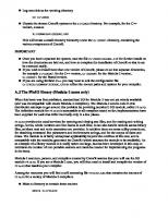
FIGURE 1.1.

1.1

Tokens

Lex

Assem

Source Program

CHAPTER ONE. INTRODUCTION

Phases of a compiler, and interfaces between them.

MODULES AND INTERFACES Any large software system is much easier to understand and implement if the designer takes care with the fundamental abstractions and interfaces. Figure 1.1 shows the phases in a typical compiler. Each phase is implemented as one or more software modules. Breaking the compiler into this many pieces allows for reuse of the components. For example, to change the target-machine for which the compiler produces machine language, it suffices to replace just the Frame Layout and Instruction Selection modules. To change the source language being compiled, only the modules up through Translate need to be changed. The compiler can be attached to a language-oriented syntax editor at the Abstract Syntax interface. The learning experience of coming to the right abstraction by several iterations of think–implement–redesign is one that should not be missed. However, the student trying to finish a compiler project in one semester does not have

4

1.2. TOOLS AND SOFTWARE

this luxury. Therefore, I present in this book the outline of a project where the abstractions and interfaces are carefully thought out, and are as elegant and general as I am able to make them. Some of the interfaces, such as Abstract Syntax, IR Trees, and Assem, take the form of data structures: for example, the Parsing Actions phase builds an Abstract Syntax data structure and passes it to the Semantic Analysis phase. Other interfaces are abstract data types; the Translate interface is a set of functions that the Semantic Analysis phase can call, and the Tokens interface takes the form of a function that the Parser calls to get the next token of the input program.

DESCRIPTION OF THE PHASES Each chapter of Part I of this book describes one compiler phase, as shown in Table 1.2 This modularization is typical of many real compilers. But some compilers combine Parse, Semantic Analysis, Translate, and Canonicalize into one phase; others put Instruction Selection much later than I have done, and combine it with Code Emission. Simple compilers omit the Control Flow Analysis, Data Flow Analysis, and Register Allocation phases. I have designed the compiler in this book to be as simple as possible, but no simpler. In particular, in those places where corners are cut to simplify the implementation, the structure of the compiler allows for the addition of more optimization or fancier semantics without violence to the existing interfaces.

1.2

TOOLS AND SOFTWARE Two of the most useful abstractions used in modern compilers are contextfree grammars, for parsing, and regular expressions, for lexical analysis. To make best use of these abstractions it is helpful to have special tools, such as Yacc (which converts a grammar into a parsing program) and Lex (which converts a declarative specification into a lexical analysis program). The programming projects in this book can be compiled using any ANSIstandard C compiler, along with Lex (or the more modern Flex) and Yacc (or the more modern Bison). Some of these tools are freely available on the Internet; for information see the World Wide Web page http://www.cs.princeton.edu/˜appel/modern/c

5

CHAPTER ONE. INTRODUCTION

Chapter Phase 2 Lex 3 Parse 4 Semantic Actions 5 Semantic Analysis 6 7

Frame Layout Translate

8

Canonicalize

9

Instruction Selection Control Flow Analysis Dataflow Analysis

10

10

11

Register Allocation

12

Code Emission

TABLE 1.2.

Description Break the source file into individual words, or tokens. Analyze the phrase structure of the program. Build a piece of abstract syntax tree corresponding to each phrase. Determine what each phrase means, relate uses of variables to their definitions, check types of expressions, request translation of each phrase. Place variables, function-parameters, etc. into activation records (stack frames) in a machine-dependent way. Produce intermediate representation trees (IR trees), a notation that is not tied to any particular source language or targetmachine architecture. Hoist side effects out of expressions, and clean up conditional branches, for the convenience of the next phases. Group the IR-tree nodes into clumps that correspond to the actions of target-machine instructions. Analyze the sequence of instructions into a control flow graph that shows all the possible flows of control the program might follow when it executes. Gather information about the flow of information through variables of the program; for example, liveness analysis calculates the places where each program variable holds a still-needed value (is live). Choose a register to hold each of the variables and temporary values used by the program; variables not live at the same time can share the same register. Replace the temporary names in each machine instruction with machine registers.

Description of compiler phases.

Source code for some modules of the Tiger compiler, skeleton source code and support code for some of the programming exercises, example Tiger programs, and other useful files are also available from the same Web address. The programming exercises in this book refer to this directory as $TIGER/ when referring to specific subdirectories and files contained therein.

6

1.3. DATA STRUCTURES FOR TREE LANGUAGES

Stm → Stm ; Stm (CompoundStm) Stm → id := Exp (AssignStm) Stm → print ( ExpList ) (PrintStm) Exp → id (IdExp) Exp → num (NumExp) Exp → Exp Binop Exp (OpExp) Exp → ( Stm , Exp ) (EseqExp) GRAMMAR 1.3.

1.3

ExpList → Exp , ExpList (PairExpList) ExpList → Exp (LastExpList) Binop → + (Plus) Binop → − (Minus) Binop → × (Times) Binop → / (Div)

A straight-line programming language.

DATA STRUCTURES FOR TREE LANGUAGES Many of the important data structures used in a compiler are intermediate representations of the program being compiled. Often these representations take the form of trees, with several node types, each of which has different attributes. Such trees can occur at many of the phase-interfaces shown in Figure 1.1. Tree representations can be described with grammars, just like programming languages. To introduce the concepts, I will show a simple programming language with statements and expressions, but no loops or if-statements (this is called a language of straight-line programs). The syntax for this language is given in Grammar 1.3. The informal semantics of the language is as follows. Each Stm is a statement, each Exp is an expression. s1 ; s2 executes statement s1 , then statement s2 . i :=e evaluates the expression e, then “stores” the result in variable i. print(e1 , e2 , . . . , en ) displays the values of all the expressions, evaluated left to right, separated by spaces, terminated by a newline. An identifier expression, such as i, yields the current contents of the variable i. A number evaluates to the named integer. An operator expression e1 op e2 evaluates e1 , then e2 , then applies the given binary operator. And an expression sequence (s, e) behaves like the C-language “comma” operator, evaluating the statement s for side effects before evaluating (and returning the result of) the expression e.

7

CHAPTER ONE. INTRODUCTION

.

CompoundStm AssignStm a

OpExp

NumExp

Plus

5

CompoundStm AssignStm NumExp

b

PrintStm LastExpList

EseqExp

IdExp

3

PrintStm

OpExp b

PairExpList

NumExp Times

IdExp

LastExpList

a

OpExp IdExp a

10

IdExp a

Minus NumExp 1

a := 5 + 3 ; b := ( print ( a , a - 1 ) , 10 * a ) ; print ( b )

FIGURE 1.4.

Tree representation of a straight-line program.

For example, executing this program a := 5+3; b := (print(a, a-1), 10*a); print(b)

prints 8 7 80

How should this program be represented inside a compiler? One representation is source code, the characters that the programmer writes. But that is not so easy to manipulate. More convenient is a tree data structure, with one node for each statement (Stm) and expression (Exp). Figure 1.4 shows a tree representation of the program; the nodes are labeled by the production labels of Grammar 1.3, and each node has as many children as the corresponding grammar production has right-hand-side symbols. We can translate the grammar directly into data structure definitions, as shown in Program 1.5. Each grammar symbol corresponds to a typedef in the data structures:

8

1.3. DATA STRUCTURES FOR TREE LANGUAGES

Grammar Stm Exp ExpList id num

typedef A stm A exp A expList string int

For each grammar rule, there is one constructor that belongs to the union for its left-hand-side symbol. The constructor names are indicated on the right-hand side of Grammar 1.3. Each grammar rule has right-hand-side components that must be represented in the data structures. The CompoundStm has two Stm’s on the righthand side; the AssignStm has an identifier and an expression; and so on. Each grammar symbol’s struct contains a union to carry these values, and a kind field to indicate which variant of the union is valid. For each variant (CompoundStm, AssignStm, etc.) we make a constructor function to malloc and initialize the data structure. In Program 1.5 only the prototypes of these functions are given; the definition of A_CompoundStm would look like this: A_stm A_CompoundStm(A_stm stm1, A_stm stm2) { A_stm s = checked_malloc(sizeof(*s)); s->kind = A_compoundStm; s->u.compound.stm1=stm1; s->u.compound.stm2=stm2; return s; }

For Binop we do something simpler. Although we could make a Binop struct – with union variants for Plus, Minus, Times, Div – this is overkill because none of the variants would carry any data. Instead we make an enum type A_binop. Programming style. We will follow several conventions for representing tree data structures in C: 1. Trees are described by a grammar. 2. A tree is described by one or more typedefs, corresponding to a symbol in the grammar. 3. Each typedef defines a pointer to a corresponding struct. The struct name, which ends in an underscore, is never used anywhere except in the declaration of the typedef and the definition of the struct itself. 4. Each struct contains a kind field, which is an enum showing different variants, one for each grammar rule; and a u field, which is a union.

9

CHAPTER ONE. INTRODUCTION typedef typedef typedef typedef typedef

char *string; struct A_stm_ *A_stm; struct A_exp_ *A_exp; struct A_expList_ *A_expList; enum {A_plus,A_minus,A_times,A_div} A_binop;

struct A_stm_ {enum {A_compoundStm, A_assignStm, A_printStm} kind; union {struct {A_stm stm1, stm2;} compound; struct {string id; A_exp exp;} assign; struct {A_expList exps;} print; } u; }; A_stm A_CompoundStm(A_stm stm1, A_stm stm2); A_stm A_AssignStm(string id, A_exp exp); A_stm A_PrintStm(A_expList exps); struct A_exp_ {enum {A_idExp, A_numExp, A_opExp, A_eseqExp} kind; union {string id; int num; struct {A_exp left; A_binop oper; A_exp right;} op; struct {A_stm stm; A_exp exp;} eseq; } u; }; A_exp A_IdExp(string id); A_exp A_NumExp(int num); A_exp A_OpExp(A_exp left, A_binop oper, A_exp right); A_exp A_EseqExp(A_stm stm, A_exp exp); struct A_expList_ {enum {A_pairExpList, A_lastExpList} kind; union {struct {A_exp head; A_expList tail;} pair; A_exp last; } u; };

PROGRAM 1.5.

Representation of straight-line programs.

5. If there is more than one nontrivial (value-carrying) symbol in the right-hand side of a rule (example: the rule CompoundStm), the union will have a component that is itself a struct comprising these values (example: the compound element of the A_stm_ union). 6. If there is only one nontrivial symbol in the right-hand side of a rule, the union will have a component that is the value (example: the num field of the A_exp union). 7. Every class will have a constructor function that initializes all the fields. The malloc function shall never be called directly, except in these constructor functions.

10

1.3. DATA STRUCTURES FOR TREE LANGUAGES

8. Each module (header file) shall have a prefix unique to that module (example, A_ in Program 1.5). 9. Typedef names (after the prefix) shall start with lowercase letters; constructor functions (after the prefix) with uppercase; enumeration atoms (after the prefix) with lowercase; and union variants (which have no prefix) with lowercase.

Modularity principles for C programs. A compiler can be a big program; careful attention to modules and interfaces prevents chaos. We will use these principles in writing a compiler in C: 1. Each phase or module of the compiler belongs in its own “.c” file, which will have a corresponding “.h” file. 2. Each module shall have a prefix unique to that module. All global names (structure and union fields are not global names) exported by the module shall start with the prefix. Then the human reader of a file will not have to look outside that file to determine where a name comes from. 3. All functions shall have prototypes, and the C compiler shall be told to warn about uses of functions without prototypes. 4. We will #include "util.h" in each file: /* util.h */ #include typedef char *string; string String(char *); typedef char bool; #define TRUE 1 #define FALSE 0 void *checked_malloc(int);

The inclusion of assert.h encourages the liberal use of assertions by the C programmer. 5. The string type means a heap-allocated string that will not be modified after its initial creation. The String function builds a heap-allocated string from a C-style character pointer (just like the standard C library function strdup). Functions that take strings as arguments assume that the contents will never change. 6. C’s malloc function returns NULL if there is no memory left. The Tiger compiler will not have sophisticated memory management to deal with this problem. Instead, it will never call malloc directly, but call only our own function, checked_malloc, which guarantees never to return NULL:

11

CHAPTER ONE. INTRODUCTION

void *checked_malloc(int len) { void *p = malloc(len); assert(p); return p; }

7. We will never call free. Of course, a production-quality compiler must free its unused data in order to avoid wasting memory. The best way to do this is to use an automatic garbage collector, as described in Chapter 13 (see particularly conservative collection on page 296). Without a garbage collector, the programmer must carefully free(p) when the structure p is about to become inaccessible – not too late, or the pointer p will be lost, but not too soon, or else still-useful data may be freed (and then overwritten). In order to be able to concentrate more on compiling techniques than on memory deallocation techniques, we can simply neglect to do any freeing.

PROGRAM

STRAIGHT-LINE PROGRAM INTERPRETER Implement a simple program analyzer and interpreter for the straight-line programming language. This exercise serves as an introduction to environments (symbol tables mapping variable-names to information about the variables); to abstract syntax (data structures representing the phrase structure of programs); to recursion over tree data structures, useful in many parts of a compiler; and to a functional style of programming without assignment statements. It also serves as a “warm-up” exercise in C programming. Programmers experienced in other languages but new to C should be able to do this exercise, but will need supplementary material (such as textbooks) on C. Programs to be interpreted are already parsed into abstract syntax, as described by the data types in Program 1.5. However, we do not wish to worry about parsing the language, so we write this program by applying data constructors: A_stm prog = A_CompoundStm(A_AssignStm("a", A_OpExp(A_NumExp(5), A_plus, A_NumExp(3))), A_CompoundStm(A_AssignStm("b", A_EseqExp(A_PrintStm(A_PairExpList(A_IdExp("a"), A_LastExpList(A_OpExp(A_IdExp("a"), A_minus, A_NumExp(1))))), A_OpExp(A_NumExp(10), A_times, A_IdExp("a")))), A_PrintStm(A_LastExpList(A_IdExp("b")))));

12

PROGRAMMING EXERCISE

Files with the data type declarations for the trees, and this sample program, are available in the directory $TIGER/chap1. Writing interpreters without side effects (that is, assignment statements that update variables and data structures) is a good introduction to denotational semantics and attribute grammars, which are methods for describing what programming languages do. It’s often a useful technique in writing compilers, too; compilers are also in the business of saying what programming languages do. Therefore, in implementing these programs, never assign a new value to any variable or structure-field except when it is initialized. For local variables, use the initializing form of declaration (for example, int i=j+3;) and for each kind of struct, make a “constructor” function that allocates it and initializes all the fields, similar to the A_CompoundStm example on page 9. 1. Write a function int maxargs(A_stm) that tells the maximum number of arguments of any print statement within any subexpression of a given statement. For example, maxargs(prog) is 2. 2. Write a function void interp(A_stm) that “interprets” a program in this language. To write in a “functional programming” style – in which you never use an assignment statement – initialize each local variable as you declare it.

For part 1, remember that print statements can contain expressions that contain other print statements. For part 2, make two mutually recursive functions interpStm and interpExp. Represent a “table,” mapping identifiers to the integer values assigned to them, as a list of id × int pairs. typedef struct table *Table_; struct table {string id; int value; Table_ tail}; Table_ Table(string id, int value, struct table *tail) { Table_ t = malloc(sizeof(*t)); t->id=id; t->value=value; t->tail=tail; return t; }

The empty table is represented as NULL. Then interpStm is declared as Table_ interpStm(A_stm s, Table_ t)

taking a table t1 as argument and producing the new table t2 that’s just like t1 except that some identifiers map to different integers as a result of the statement.

13

CHAPTER ONE. INTRODUCTION

For example, the table t1 that maps a to 3 and maps c to 4, which we write {a $ → 3, c $ → 4} in mathematical notation, could be represented as the linked list a 3 . c 4 Now, let the table t2 be just like t1 , except that it maps c to 7 instead of 4. Mathematically, we could write, t2 = update(t1 , c, 7) where the update function returns a new table {a $ → 3, c $ → 7}. On the computer, we could implement t2 by putting a new cell at the head of the linked list: c 7 as long as we assume a 3 c 4 that the first occurrence of c in the list takes precedence over any later occurrence. Therefore, the update function is easy to implement; and the corresponding lookup function int lookup(Table_ t, string key)

just searches down the linked list. Interpreting expressions is more complicated than interpreting statements, because expressions return integer values and have side effects. We wish to simulate the straight-line programming language’s assignment statements without doing any side effects in the interpreter itself. (The print statements will be accomplished by interpreter side effects, however.) The solution is to declare interpExp as struct IntAndTable {int i; Table_ t;}; struct IntAndTable interpExp(A_exp e, Table_ t) · · ·

The result of interpreting an expression e1 with table t1 is an integer value i and a new table t2 . When interpreting an expression with two subexpressions (such as an OpExp), the table t2 resulting from the first subexpression can be used in processing the second subexpression.

FURTHER READING Hanson [1997] describes principles for writing modular software in C.

14

EXERCISES

EXERCISES 1.1

This simple program implements persistent functional binary search trees, so that if tree2=insert(x,tree1), then tree1 is still available for lookups even while tree2 can be used. typedef struct tree *T_tree; struct tree {T_tree left; String key; T_tree right;}; T_tree Tree(T_tree l, String k, T_tree r) { T_tree t = checked_malloc(sizeof(*t)); t->left=l; t->key=k; t->right=r; return t; } T_tree insert(String key, T_tree t) { if (t==NULL) return Tree(NULL, key, NULL) else if (strcmp(key,t->key) < 0) return Tree(insert(key,t->left),t->key,t->right); else if (strcmp(key,t->key) > 0) return Tree(t->left,t->key,insert(key,t->right)); else return Tree(t->left,key,t->right); }

a. Implement a member function that returns TRUE if the item is found, else FALSE. b. Extend the program to include not just membership, but the mapping of keys to bindings: T_tree insert(string key, void *binding, T_tree t); void * lookup(string key, T_tree t);

c. These trees are not balanced; demonstrate the behavior on the following two sequences of insertions: (a) t s p i p f b s t (b) a b c d e f g h i *d. Research balanced search trees in Sedgewick [1997] and recommend a balanced-tree data structure for functional symbol tables. Hint: To preserve a functional style, the algorithm should be one that rebalances on insertion but not on lookup, so a data structure such as splay trees is not appropriate.

15

2 Lexical Analysis

lex-i-cal: of or relating to words or the vocabulary of a language as distinguished from its grammar and construction

Webster’s Dictionary

To translate a program from one language into another, a compiler must first pull it apart and understand its structure and meaning, then put it together in a different way. The front end of the compiler performs analysis; the back end does synthesis. The analysis is usually broken up into Lexical analysis: breaking the input into individual words or “tokens”; Syntax analysis: parsing the phrase structure of the program; and Semantic analysis: calculating the program’s meaning.

The lexical analyzer takes a stream of characters and produces a stream of names, keywords, and punctuation marks; it discards white space and comments between the tokens. It would unduly complicate the parser to have to account for possible white space and comments at every possible point; this is the main reason for separating lexical analysis from parsing. Lexical analysis is not very complicated, but we will attack it with highpowered formalisms and tools, because similar formalisms will be useful in the study of parsing and similar tools have many applications in areas other than compilation.

16

2.1. LEXICAL TOKENS

2.1

LEXICAL TOKENS A lexical token is a sequence of characters that can be treated as a unit in the grammar of a programming language. A programming language classifies lexical tokens into a finite set of token types. For example, some of the token types of a typical programming language are: Type

Examples foo n14 73 0 00 66.1 .5 if , != ( )

ID NUM REAL IF COMMA NOTEQ LPAREN RPAREN

last 515 082 10. 1e67

5.5e-10

Punctuation tokens such as IF, VOID , RETURN constructed from alphabetic characters are called reserved words and, in most languages, cannot be used as identifiers. Examples of nontokens are comment preprocessor directive preprocessor directive macro blanks, tabs, and newlines

/* try again */ #include #define NUMS 5 , 6 NUMS

In languages weak enough to require a macro preprocessor, the preprocessor operates on the source character stream, producing another character stream that is then fed to the lexical analyzer. It is also possible to integrate macro processing with lexical analysis. Given a program such as float match0(char *s) /* find a zero */ {if (!strncmp(s, "0.0", 3)) return 0.; }

the lexical analyzer will return the stream FLOAT LBRACE

ID (match0) IF

LPAREN

LPAREN BANG

CHAR

STAR

ID (strncmp)

ID (s) LPAREN

RPAREN ID (s)

17

CHAPTER TWO. LEXICAL ANALYSIS

COMMA

STRING (0.0)

RETURN

REAL (0.0)

COMMA SEMI

NUM (3)

RBRACE

RPAREN

RPAREN

EOF

where the token-type of each token is reported; some of the tokens, such as identifiers and literals, have semantic values attached to them, giving auxiliary information in addition to the token type. How should the lexical rules of a programming language be described? In what language should a lexical analyzer be written? We can describe the lexical tokens of a language in English; here is a description of identifiers in C or Java: An identifier is a sequence of letters and digits; the first character must be a letter. The underscore _ counts as a letter. Upper- and lowercase letters are different. If the input stream has been parsed into tokens up to a given character, the next token is taken to include the longest string of characters that could possibly constitute a token. Blanks, tabs, newlines, and comments are ignored except as they serve to separate tokens. Some white space is required to separate otherwise adjacent identifiers, keywords, and constants.

And any reasonable programming language serves to implement an ad hoc lexer. But we will specify lexical tokens using the formal language of regular expressions, implement lexers using deterministic finite automata, and use mathematics to connect the two. This will lead to simpler and more readable lexical analyzers.

2.2

REGULAR EXPRESSIONS Let us say that a language is a set of strings; a string is a finite sequence of symbols. The symbols themselves are taken from a finite alphabet. The Pascal language is the set of all strings that constitute legal Pascal programs; the language of primes is the set of all decimal-digit strings that represent prime numbers; and the language of C reserved words is the set of all alphabetic strings that cannot be used as identifiers in the C programming language. The first two of these languages are infinite sets; the last is a finite set. In all of these cases, the alphabet is the ASCII character set. When we speak of languages in this way, we will not assign any meaning to the strings; we will just be attempting to classify each string as in the language or not. To specify some of these (possibly infinite) languages with finite descrip-

18

2.2. REGULAR EXPRESSIONS

tions, we will use the notation of regular expressions. Each regular expression stands for a set of strings. Symbol: For each symbol a in the alphabet of the language, the regular expression a denotes the language containing just the string a. Alternation: Given two regular expressions M and N, the alternation operator written as a vertical bar | makes a new regular expression M | N. A string is in the language of M | N if it is in the language of M or in the language of N. Thus, the language of a | b contains the two strings a and b. Concatenation: Given two regular expressions M and N, the concatenation operator · makes a new regular expression M · N. A string is in the language of M · N if it is the concatenation of any two strings α and β such that α is in the language of M and β is in the language of N. Thus, the regular expression (a | b) · a defines the language containing the two strings aa and ba. Epsilon: The regular expression ϵ represents a language whose only string is the empty string. Thus, (a · b) | ϵ represents the language {"","ab"}. Repetition: Given a regular expression M, its Kleene closure is M ∗ . A string is in M ∗ if it is the concatenation of zero or more strings, all of which are in M. Thus, ((a | b) · a)∗ represents the infinite set { "" , "aa", "ba", "aaaa", "baaa", "aaba", "baba", "aaaaaa", . . . }.

Using symbols, alternation, concatenation, epsilon, and Kleene closure we can specify the set of ASCII characters corresponding to the lexical tokens of a programming language. First, consider some examples: (0 | 1)∗ · 0 Binary numbers that are multiples of two. ∗ ∗ ∗ b (abb ) (a|ϵ) Strings of a’s and b’s with no consecutive a’s. ∗ ∗ (a|b) aa(a|b) Strings of a’s and b’s containing consecutive a’s. In writing regular expressions, we will sometimes omit the concatenation symbol or the epsilon, and we will assume that Kleene closure “binds tighter” than concatenation, and concatenation binds tighter than alternation; so that ab | c means (a · b) | c, and (a |) means (a | ϵ). Let us introduce some more abbreviations: [abcd] means (a | b | c | d), [b-g] means [bcdefg], [b-gM-Qkr] means [bcdefgMNOPQkr], M? means (M | ϵ), and M + means (M·M ∗ ). These extensions are convenient, but none extend the descriptive power of regular expressions: Any set of strings that can be described with these abbreviations could also be described by just the basic set of operators. All the operators are summarized in Figure 2.1. Using this language, we can specify the lexical tokens of a programming language (Figure 2.2). For each token, we supply a fragment of C code that reports which token type has been recognized.

19

CHAPTER TWO. LEXICAL ANALYSIS

a ϵ M|N M·N MN M∗ M+ M? [a − zA − Z] . "a.+*"

FIGURE 2.1.

An ordinary character stands for itself. The empty string. Another way to write the empty string. Alternation, choosing from M or N. Concatenation, an M followed by an N . Another way to write concatenation. Repetition (zero or more times). Repetition, one or more times. Optional, zero or one occurrence of M. Character set alternation. A period stands for any single character except newline. Quotation, a string in quotes stands for itself literally. Regular expression notation.

if [a-z][a-z0-9]* [0-9]+ ([0-9]+"."[0-9]*)|([0-9]*"."[0-9]+) ("--"[a-z]*"\n")|(" "|"\n"|"\t")+ .

FIGURE 2.2.

{return IF;} {return ID;} {return NUM;} {return REAL;} { /* do nothing */ } {error();}

Regular expressions for some tokens.

The fifth line of the description recognizes comments or white space, but does not report back to the parser. Instead, the white space is discarded and the lexer resumed. The comments for this lexer begin with two dashes, contain only alphabetic characters, and end with newline. Finally, a lexical specification should be complete, always matching some initial substring of the input; we can always achieve this by having a rule that matches any single character (and in this case, prints an “illegal character” error message and continues). These rules are a bit ambiguous. For example, does if8 match as a single identifier or as the two tokens if and 8? Does the string if 89 begin with an identifier or a reserved word? There are two important disambiguation rules used by Lex and other similar lexical-analyzer generators: Longest match: The longest initial substring of the input that can match any regular expression is taken as the next token. Rule priority: For a particular longest initial substring, the first regular expres-

20

2.3. FINITE AUTOMATA

a-z

a-z 1 i

2

1

2

3

ID

0-9

.

0-9

.

0-9

3 5

0-9

REAL FIGURE 2.3.

1

2

-

-

0-9 2

NUM 3

\n

4

a-z

2 4

1

0-9

IF

1

0-9

f

blank, etc. 5

0-9

blank, etc.

1

white space

any but \n

2

error

Finite automata for lexical tokens. The states are indicated by circles; final states are indicated by double circles. The start state has an arrow coming in from nowhere. An edge labeled with several characters is shorthand for many parallel edges.

sion that can match determines its token type. This means that the order of writing down the regular-expression rules has significance.

Thus, if8 matches as an identifier by the longest-match rule, and if matches as a reserved word by rule-priority.

2.3

FINITE AUTOMATA Regular expressions are convenient for specifying lexical tokens, but we need a formalism that can be implemented as a computer program. For this we can use finite automata (N.B. the singular of automata is automaton). A finite automaton has a finite set of states; edges lead from one state to another, and each edge is labeled with a symbol. One state is the start state, and certain of the states are distinguished as final states. Figure 2.3 shows some finite automata. We number the states just for convenience in discussion. The start state is numbered 1 in each case. An edge labeled with several characters is shorthand for many parallel edges; so in the ID machine there are really 26 edges each leading from state 1 to 2, each labeled by a different letter.

21

CHAPTER TWO. LEXICAL ANALYSIS

a-e, g-z, 0-9 ID

IF

f

2

3

ID

0-9, a-z

4

a-h j-z

i

error

0-9 a-z

5

. 7

.

NUM

blank, etc.

12

blank, etc.

white space

FIGURE 2.4.

REAL

0-9

6

0-9

0-9

0-9

1

0-9

8 REAL

other 9 13 error

-

10

error

\n

11

white space

a-z

Combined finite automaton.

In a deterministic finite automaton (DFA), no two edges leaving from the same state are labeled with the same symbol. A DFA accepts or rejects a string as follows. Starting in the start state, for each character in the input string the automaton follows exactly one edge to get to the next state. The edge must be labeled with the input character. After making n transitions for an n-character string, if the automaton is in a final state, then it accepts the string. If it is not in a final state, or if at some point there was no appropriately labeled edge to follow, it rejects. The language recognized by an automaton is the set of strings that it accepts. For example, it is clear that any string in the language recognized by automaton ID must begin with a letter. Any single letter leads to state 2, which is final; so a single-letter string is accepted. From state 2, any letter or digit leads back to state 2, so a letter followed by any number of letters and digits is also accepted. In fact, the machines shown in Figure 2.3 accept the same languages as the regular expressions of Figure 2.2. These are six separate automata; how can they be combined into a single machine that can serve as a lexical analyzer? We will study formal ways of doing this in the next section, but here we will just do it ad hoc: Figure 2.4 shows such a machine. Each final state must be labeled with the token-type

22

2.3. FINITE AUTOMATA

that it accepts. State 2 in this machine has aspects of state 2 of the IF machine and state 2 of the ID machine; since the latter is final, then the combined state must be final. State 3 is like state 3 of the IF machine and state 2 of the ID machine; because these are both final we use rule priority to disambiguate – we label state 3 with IF because we want this token to be recognized as a reserved word, not an identifier. We can encode this machine as a transition matrix: a two-dimensional array (a vector of vectors), subscripted by state number and input character. There will be a “dead” state (state 0) that loops to itself on all characters; we use this to encode the absence of an edge. int edges[][256]={ /* · · ·0 1 2· · ·-· · ·e f g h i j· · · */ /* state 0 */ {0,0,· · ·0,0,0· · ·0· · ·0,0,0,0,0,0· · ·}, /* state 1 */ {0,0,· · ·7,7,7· · ·9· · ·4,4,4,4,2,4· · ·}, /* state 2 */ {0,0,· · ·4,4,4· · ·0· · ·4,3,4,4,4,4· · ·}, /* state 3 */ {0,0,· · ·4,4,4· · ·0· · ·4,4,4,4,4,4· · ·}, /* state 4 */ {0,0,· · ·4,4,4· · ·0· · ·4,4,4,4,4,4· · ·}, /* state 5 */ {0,0,· · ·6,6,6· · ·0· · ·0,0,0,0,0,0· · ·}, /* state 6 */ {0,0,· · ·6,6,6· · ·0· · ·0,0,0,0,0,0· · ·}, /* state 7 */ {0,0,· · ·7,7,7· · ·0· · ·0,0,0,0,0,0· · ·}, /* state 8 */ {0,0,· · ·8,8,8· · ·0· · ·0,0,0,0,0,0· · ·}, et cetera }

There must also be a “finality” array, mapping state numbers to actions – final state 2 maps to action ID, and so on.

RECOGNIZING THE LONGEST MATCH It is easy to see how to use this table to recognize whether to accept or reject a string, but the job of a lexical analyzer is to find the longest match, the longest initial substring of the input that is a valid token. While interpreting transitions, the lexer must keep track of the longest match seen so far, and the position of that match. Keeping track of the longest match just means remembering the last time the automaton was in a final state with two variables, Last-Final (the state number of the most recent final state encountered) and Input-Positionat-Last-Final. Every time a final state is entered, the lexer updates these variables; when a dead state (a nonfinal state with no output transitions) is reached, the variables tell what token was matched, and where it ended. Figure 2.5 shows the operation of a lexical analyzer that recognizes longest matches; note that the current input position may be far beyond the most recent position at which the recognizer was in a final state.

23

CHAPTER TWO. LEXICAL ANALYSIS

Last Final 0 2 3 3 0 12 12 0 9 9 9 9 9 9 0 9 9 FIGURE 2.5.

2.4

Current State 1 2 3 0 1 12 0 1 9 10 10 10 10 0 1 9 0

Current Input ⊤ |if --not-a-com ⊥ |i⊤ ⊥f --not-a-com |if⊤ ⊥ --not-a-com |if⊤⊥--not-a-com ⊤ if| ⊥ --not-a-com if| ⊤ ⊥--not-a-com if| ⊤-⊥-not-a-com |--not-a-com if ⊤ ⊥ if |-⊤ ⊥-not-a-com if |-⊤-⊥not-a-com if |-⊤-n⊥ot-a-com if |-⊤-no⊥t-a-com if |-⊤-not⊥-a-com if |-⊤-not-⊥a-com ⊤ if -| ⊥-not-a-com if -|-⊤ ⊥not-a-com if -|-⊤n⊥ot-a-com

Accept Action

return IF

found white space; resume

error, illegal token ‘-’; resume

error, illegal token ‘-’; resume

The automaton of Figure 2.4 recognizes several tokens. The symbol | indicates the input position at each successive call to the lexical analyzer, the symbol ⊥ indicates the current position of the automaton, and ⊤ indicates the most recent position in which the recognizer was in a final state.

NONDETERMINISTIC FINITE AUTOMATA A nondeterministic finite automaton (NFA) is one that has a choice of edges – labeled with the same symbol – to follow out of a state. Or it may have special edges labeled with ϵ (the Greek letter epsilon), that can be followed without eating any symbol from the input. Here is an example of an NFA: a

a

a

24

a

a

a a

2.4. NONDETERMINISTIC FINITE AUTOMATA

In the start state, on input character a, the automaton can move either right or left. If left is chosen, then strings of a’s whose length is a multiple of three will be accepted. If right is chosen, then even-length strings will be accepted. Thus, the language recognized by this NFA is the set of all strings of a’s whose length is a multiple of two or three. On the first transition, this machine must choose which way to go. It is required to accept the string if there is any choice of paths that will lead to acceptance. Thus, it must “guess,” and must always guess correctly. Edges labeled with ϵ may be taken without using up a symbol from the input. Here is another NFA that accepts the same language: a

a

a

∋

∋

a a

Again, the machine must choose which ϵ-edge to take. If there is a state with some ϵ-edges and some edges labeled by symbols, the machine can choose to eat an input symbol (and follow the corresponding symbol-labeled edge), or to follow an ϵ-edge instead.

CONVERTING A REGULAR EXPRESSION TO AN NFA Nondeterministic automata are a useful notion because it is easy to convert a (static, declarative) regular expression to a (simulatable, quasi-executable) NFA. The conversion algorithm turns each regular expression into an NFA with a tail (start edge) and a head (ending state). For example, the single-symbol regular expression a converts to the NFA a

The regular expression ab, made by combining a with b using concatenation is made by combining the two NFAs, hooking the head of a to the tail of b. The resulting machine has a tail labeled by a and a head into which the b edge flows.

25

CHAPTER TWO. LEXICAL ANALYSIS

a

a

∋

ϵ

M|N

M?

constructed as M | ϵ

[abc] N

M·N

constructed as M · M ∗

∋

M

∋

M+

∋

"abc"

N

M

∋

a b c

constructed as a · b · c

∋

M∗

FIGURE 2.6.

M

∋

Translation of regular expressions to NFAs.

a

b

In general, any regular expression M will have some NFA with a tail and head: M

We can define the translation of regular expressions to NFAs by induction. Either an expression is primitive (a single symbol or ϵ) or it is made from smaller expressions. Similarly, the NFA will be primitive or made from smaller NFAs. Figure 2.6 shows the rules for translating regular expressions to nondeterministic automata. We illustrate the algorithm on some of the expressions in Figure 2.2 – for the tokens IF, ID , NUM , and error. Each expression is translated to an NFA, the “head” state of each NFA is marked final with a different token type, and the tails of all the expressions are joined to a new start node. The result – after some merging of equivalent NFA states – is shown in Figure 2.7.

26

2.4. NONDETERMINISTIC FINITE AUTOMATA

2

f

IF

4

i

a-z

a

3

.. .

5

6

.. .

z

0-9

0

0

ID

7

8

1 any 14

.. .

error

15

9

.. .

10

9

11

.. .

NUM

12

13

9

character

FIGURE 2.7.

Four regular expressions translated to an NFA.

CONVERTING AN NFA TO A DFA As we saw in Section 2.3, implementing deterministic finite automata (DFAs) as computer programs is easy. But implementing NFAs is a bit harder, since most computers don’t have good “guessing” hardware. We can avoid the need to guess by trying every possibility at once. Let us simulate the NFA of Figure 2.7 on the string in. We start in state 1. Now, instead of guessing which ϵ-transition to take, we just say that at this point the NFA might take any of them, so it is in one of the states {1, 4, 9, 14}; that is, we compute the ϵ-closure of {1}. Clearly, there are no other states reachable without eating the first character of the input. Now, we make the transition on the character i. From state 1 we can reach 2, from 4 we reach 5, from 9 we go nowhere, and from 14 we reach 15. So we have the set {2, 5, 15}. But again we must compute ϵ-closure: from 5 there is an ϵ-transition to 8, and from 8 to 6. So the NFA must be in one of the states {2, 5, 6, 8, 15}. On the character n, we get from state 6 to 7, from 2 to nowhere, from 5 to nowhere, from 8 to nowhere, and from 15 to nowhere. So we have the set {7}; its ϵ-closure is {6, 7, 8}. Now we are at the end of the string in; is the NFA in a final state? One of the states in our possible-states set is 8, which is final. Thus, in is an ID token. We formally define ϵ-closure as follows. Let edge(s, c) be the set of all NFA states reachable by following a single edge with label c from state s.

27

CHAPTER TWO. LEXICAL ANALYSIS

For a set of states S, closure(S) is the set of states that can be reached from a state in S without consuming any of the input, that is, by going only through ϵ edges. Mathematically, we can express the idea of going through ϵ edges by saying that closure(S) is smallest set T such that ! # " T =S∪ edge(s, ϵ) . s∈T

We can calculate T by iteration: T ←S repeat T ′ ← T $ T ← T ′ ∪ ( s∈T ′ edge(s, ϵ)) until T = T ′

Why does this algorithm work? T can only grow in each iteration, so the final T must include S. If T = T ′ after an iteration step, then T must also in$ clude s∈T ′ edge(s, ϵ). Finally, the algorithm must terminate, because there are only a finite number of distinct states in the NFA. Now, when simulating an NFA as described above, suppose we are in a set d = {si , sk , sl } of NFA states si , sk , sl . By starting in d and eating the input symbol c, we reach a new set of NFA states; we’ll call this set DFAedge(d, c): " DFAedge(d, c) = closure( edge(s, c)) s∈d

Using DFAedge, we can write the NFA simulation algorithm more formally. If the start state of the NFA is s1 , and the input string is c1 , . . . , ck , then the algorithm is: d ← closure({s1 }) for i ← 1 to k d ← DFAedge(d, ci )

Manipulating sets of states is expensive – too costly to want to do on every character in the source program that is being lexically analyzed. But it is possible to do all the sets-of-states calculations in advance. We make a DFA from the NFA, such that each set of NFA states corresponds to one DFA state. Since the NFA has a finite number n of states, the DFA will also have a finite number (at most 2n ) of states. DFA construction is easy once we have closure and DFAedge algorithms. The DFA start state d1 is just closure(s1 ), as in the NFA simulation algo-

28

2.4. NONDETERMINISTIC FINITE AUTOMATA

ID

2,5,6,8,15 i

1,4,9,14

ID

a-h j-z

NUM

10,11,13,15

ID

a-z 0-9

5,6,8,15

0-9

other

a-e, g-z, 0-9 IF f 3,6,7,8 a-z 0-9 6,7,8

a-z 0-9

NUM

0-9

11,12,13

0-9

error

15

FIGURE 2.8.

NFA converted to DFA.

rithm. Abstractly, there is an edge from di to d j labeled with c if d j = DFAedge(di , c). We let $ be the alphabet. states[0] ← {}; states[1] ← closure({s1 }) p ← 1; j ←0 while j ≤ p foreach c ∈ $ e ← DFAedge(states[ j ], c) if e = states[i] for some i ≤ p then trans[ j, c] ← i else p ← p + 1 states[ p] ← e trans[ j, c] ← p j ← j +1

The algorithm does not visit unreachable states of the DFA. This is extremely important, because in principle the DFA has 2n states, but in practice we usually find that only about n of them are reachable from the start state. It is important to avoid an exponential blowup in the size of the DFA interpreter’s transition tables, which will form part of the working compiler. A state d is final in the DFA if any NFA-state in states[d] is final in the NFA. Labeling a state final is not enough; we must also say what token is recognized; and perhaps several members of states[d] are final in the NFA. In this case we label d with the token-type that occurred first in the list of

29

CHAPTER TWO. LEXICAL ANALYSIS

regular expressions that constitute the lexical specification. This is how rule priority is implemented. After the DFA is constructed, the “states” array may be discarded, and the “trans” array is used for lexical analysis. Applying the DFA construction algorithm to the NFA of Figure 2.7 gives the automaton in Figure 2.8. This automaton is suboptimal. That is, it is not the smallest one that recognizes the same language. In general, we say that two states s1 and s2 are equivalent when the machine starting in s1 accepts a string σ if and only if starting in s2 it accepts σ . This is certainly true of the states labeled 5,6,8,15 and 6,7,8 in Figure 2.8; and of the states labeled 10,11,13,15 and 11,12,13 . In an automaton with two equivalent states s1 and s2 , we can make all of s2 ’s incoming edges point to s1 instead and delete s2 . How can we find equivalent states? Certainly, s1 and s2 are equivalent if they are both final or both non-final and for any symbol c, trans[s1 , c] = trans[s2 , c]; 10,11,13,15 and 11,12,13 satisfy this criterion. But this condition is not sufficiently general; consider the automaton a a 1

2

b

a

3

a 4

a

5

Here, states 2 and 4 are equivalent, but trans[2, a] ̸ = trans[4, a]. After constructing a DFA it is useful to apply an algorithm to minimize it by finding equivalent states; see Exercise 2.6.

2.5

Lex: A LEXICAL ANALYZER GENERATOR DFA construction is a mechanical task easily performed by computer, so it makes sense to have an automatic lexical analyzer generator to translate regular expressions into a DFA. Lex is a lexical analyzer generator that produces a C program from a lexical specification. For each token type in the programming language to be lexically analyzed, the specification contains a regular expression and an action.

30

2.5. LEX: A LEXICAL ANALYZER GENERATOR

%{ /* C Declarations: */ #include "tokens.h" /* definitions of IF, ID, NUM, ... */ #include "errormsg.h" union {int ival; string sval; double fval;} yylval; int charPos=1; #define ADJ (EM_tokPos=charPos, charPos+=yyleng) %} /* Lex Definitions: */ digits [0-9]+ %% /* Regular Expressions and Actions: */ if {ADJ; return IF;} [a-z][a-z0-9]* {ADJ; yylval.sval=String(yytext); return ID;} {digits} {ADJ; yylval.ival=atoi(yytext); return NUM;} ({digits}"."[0-9]*)|([0-9]*"."{digits}) {ADJ; yylval.fval=atof(yytext); return REAL;} ("--"[a-z]*"\n")|(" "|"\n"|"\t")+ {ADJ;} . {ADJ; EM_error("illegal character");}

PROGRAM 2.9.

Lex specification of the tokens from Figure 2.2.

The action communicates the token type (perhaps along with other information) to the next phase of the compiler. The output of Lex is a program in C – a lexical analyzer that interprets a DFA using the algorithm described in Section 2.3 and executes the action fragments on each match. The action fragments are just C statements that return token values. The tokens described in Figure 2.2 are specified in Lex as shown in Program 2.9. The first part of the specification, between the %{· · ·%} braces, contains includes and declarations that may be used by the C code in the remainder of the file. The second part of the specification contains regular-expression abbreviations and state declarations. For example, the declaration digits [0-9]+ in this section allows the name {digits} to stand for a nonempty sequence of digits within regular expressions. The third part contains regular expressions and actions. The actions are fragments of ordinary C code. Each action must return a value of type int, denoting which kind of token has been found.

31

CHAPTER TWO. LEXICAL ANALYSIS

In the action fragments, several special variables are available. The string matched by the regular expression is yytext. The length of the matched string is yyleng. In this particular example, we keep track of the position of each token, measured in characters since the beginning of the file, in the variable charPos. The EM_tokPos variable of the error message module errormsg.h is continually told this position by calls to the macro ADJ. The parser will be able to use this information in printing informative syntax error messages. The include file tokens.h in this example defines integer constants IF, ID, NUM, and so on; these values are returned by the action fragments to tell what token-type is matched. Some tokens have semantic values associated with them. For example, ID’s semantic value is the character string constituting the identifier; NUM’s semantic value is an integer; and IF has no semantic value (any IF is indistinguishable from any other). The values are communicated to the parser through the global variable yylval, which is a union of the different types of semantic values. The token-type returned by the lexer tells the parser which variant of the union is valid.

START STATES Regular expressions are static and declarative; automata are dynamic and imperative. That is, you can see the components and structure of a regular expression without having to simulate an algorithm, but to understand an automaton it is often necessary to “execute” it in your mind. Thus, regular expressions are usually more convenient to specify the lexical structure of programming-language tokens. But sometimes the step-by-step, state-transition model of automata is appropriate. Lex has a mechanism to mix states with regular expressions. One can declare a set of start states; each regular expression can be prefixed by the set of start states in which it is valid. The action fragments can explicitly change the start state. In effect, we have a finite automaton whose edges are labeled, not by single symbols, but by regular expressions. This example shows a language with simple identifiers, if tokens, and comments delimited by (* and *) brackets: (* [a-z]+

INITIAL

COMMENT *)

if

32

.

PROGRAMMING EXERCISE

Though it is possible to write a single regular expression that matches an entire comment, as comments get more complicated it becomes more difficult, or even impossible if nested comments are allowed. The Lex specification corresponding to this machine is .. . the usual preamble ... %Start INITIAL COMMENT %% if {ADJ; return IF;} [a-z]+ {ADJ; yylval.sval=String(yytext); return ID;} "(*" {ADJ; BEGIN COMMENT;} . {ADJ; EM_error("illegal character");} "*)" {ADJ; BEGIN INITIAL;} . {ADJ;} . {BEGIN INITIAL; yyless(1);}

where INITIAL is the “outside of any comment” state. The last rule is a hack to get Lex into this state. Any regular expression not prefixed by a operates in all states; this feature is rarely useful. This example can be easily augmented to handle nested comments, via a global variable that is incremented and decremented in the semantic actions.

PROGRAM

LEXICAL ANALYSIS Use Lex to implement a lexical analyzer for the Tiger language. Appendix A describes, among other things, the lexical tokens of Tiger. This chapter has left out some of the specifics of how the lexical analyzer should be initialized and how it should communicate with the rest of the compiler. You can learn this from the Lex manual, but the “skeleton” files in the $TIGER/chap2 directory will also help get you started. Along with the tiger.lex file you should turn in documentation for the following points: • • • • •

how you handle comments; how you handle strings; error handling; end-of-file handling; other interesting features of your lexer.

33

CHAPTER TWO. LEXICAL ANALYSIS

Supporting files are available in $TIGER/chap2 as follows: tokens.h Definition of lexical-token constants, and yylval. errormsg.h, errormsg.c The error message module, useful for producing error messages with file names and line numbers. driver.c A test scaffold to run your lexer on an input file. tiger.lex The beginnings of a real tiger.lex file. makefile A “makefile” to compile everything.

When reading the Tiger Language Reference Manual (Appendix A), pay particular attention to the paragraphs with the headings Identifiers, Comments, Integer literal, and String literal. The reserved words of the language are: while, for, to, break, let, in, end, function, var, type, array, if, then, else, do, of, nil. The punctuation symbols used in the language are: , : ; ( ) [ ] { } . + - * / = < >= & | := The string value that you return for a string literal should have all the escape sequences translated into their meanings. There are no negative integer literals; return two separate tokens for -32. Detect unclosed comments (at end of file) and unclosed strings. The directory $TIGER/testcases contains a few sample Tiger programs. To get started: Make a directory and copy the contents of $TIGER/chap2 into it. Make a file test.tig containing a short program in the Tiger language. Then type make; Lex will run on tiger.lex, producing lex.yy.c, and then the appropriate C files will be compiled. Finally, lextest test.tig will lexically analyze the file using a test scaffold.

FURTHER READING Lex was the first lexical-analyzer generator based on regular expressions [Lesk 1975]; it is still widely used. Computing ϵ-closure can be done more efficiently by keeping a queue or stack of states whose edges have not yet been checked for ϵ-transitions [Aho et al. 1986]. Regular expressions can be converted directly to DFAs without going through NFAs [McNaughton and Yamada 1960; Aho et al. 1986]. DFA transition tables can be very large and sparse. If represented as a simple two-dimensional matrix (states × symbols) they take far too much mem-

34

EXERCISES

ory. In practice, tables are compressed; this reduces the amount of memory required, but increases the time required to look up the next state [Aho et al. 1986]. Lexical analyzers, whether automatically generated or handwritten, must manage their input efficiently. Of course, input is buffered, so that a large batch of characters is obtained at once; then the lexer can process one character at a time in the buffer. The lexer must check, for each character, whether the end of the buffer is reached. By putting a sentinel – a character that cannot be part of any token – at the end of the buffer, it is possible for the lexer to check for end-of-buffer only once per token, instead of once per character [Aho et al. 1986]. Gray [1988] uses a scheme that requires only one check per line, rather than one per token, but cannot cope with tokens that contain end-of-line characters. Bumbulis and Cowan [1993] check only once around each cycle in the DFA; this reduces the number of checks (from once per character) when there are long paths in the DFA. Automatically generated lexical analyzers are often criticized for being slow. In principle, the operation of a finite automaton is very simple and should be efficient, but interpreting from transition tables adds overhead. Gray [1988] shows that DFAs translated directly into executable code (implementing states as case statements) can run as fast as hand-coded lexers. The Flex “fast lexical analyzer generator” [Paxson 1995] is significantly faster than Lex.

EXERCISES 2.1 Write regular expressions for each of the following. a. Strings over the alphabet {a, b, c} where the first a precedes the first b. b. Strings over the alphabet {a, b, c} with an even number of a’s. c. Binary numbers that are multiples of four. d. Binary numbers that are greater than 101001. e. Strings over the alphabet {a, b, c} that don’t contain the contiguous substring baa. f. The language of nonnegative integer constants in C, where numbers

35

CHAPTER TWO. LEXICAL ANALYSIS

beginning with 0 are octal constants and other numbers are decimal constants. g. Binary numbers n such that there exists an integer solution of a n +bn = cn .

2.2 For each of the following, explain why you’re not surprised that there is no regular expression defining it.

a. Strings of a’s and b’s where there are more a’s than b’s. b. Strings of a’s and b’s that are palindromes (the same forward as backward). c. Syntactically correct C programs.

2.3 Explain in informal English what each of these finite state automata recognizes. 0

1

1

2

1

a.

1

3

0

0

0

8 1

a

a

9

0

7 1

0 1

0

6

4

10 1 a

a

b. a 1

*c.

0

0

0

1

1

2

1

0

2.4 Convert these regular expressions to nondeterministic finite automata. a. (if|then|else) b. a((b|a∗ c)x)∗|x∗ a

2.5 Convert these NFAs to deterministic finite automata. 1

a.

x

∋

2

z

5

∋ ∋

1

∋

∋

6

a b

36

∋

4

y

a

b.

3

7 a

a 3

2 b

a 4

b

a 5

b

6 b

EXERCISES

c

1

a

2

3

t

4

∋ c

5

c.

a

6

7

t

8

s

9

∋ c

10 ∋

11

c

14

15

a

12

a

16

r

r

13

17

s

18

2.6 Find two equivalent states in the following automaton, and merge them to produce a smaller automaton that recognizes the same language. Repeat until there are no longer equivalent states. 1

0 1

0

2

1

0 4 1 1 0 8

3

0

1 5

1 0

6 1

1

7 0

0

Actually, the general algorithm for minimizing finite automata works in reverse. First, find all pairs of inequivalent states. States X, Y are inequivalent if a a X is final and Y is not or (by iteration) if X → X ′ and Y → Y ′ and X ′ , Y ′ are inequivalent. After this iteration ceases to find new pairs of inequivalent states, then X, Y are equivalent if they are not inequivalent. See Hopcroft and Ullman [1979], Theorem 3.10.

*2.7 Any DFA that accepts at least one string can be converted to a regular expression. Convert the DFA of Exercise 2.3c to a regular expression. Hint: First, pretend state 1 is the start state. Then write a regular expression for excursions to state 2 and back, and a similar one for excursions to state 0 and back. Or look in Hopcroft and Ullman [1979], Theorem 2.4, for the algorithm.

37

CHAPTER TWO. LEXICAL ANALYSIS

*2.8 Suppose this DFA were used by Lex to find tokens in an input file. 0-9 a-z 1

+ 3

4

a-z

2 0-9 5

e

6

8 0-9 +

0-9 0-9

7

0-9

a. How many characters past the end of a token might Lex have to examine before matching the token? b. Given your answer k to part (a), show an input file containing at least two tokens such that the first call to Lex will examine k characters past the end of the first token before returning the first token. If the answer to part (a) is zero, then show an input file containing at least two tokens, and indicate the endpoint of each token.

2.9 An interpreted DFA-based lexical analyzer uses two tables, edges indexed by state and input symbol, yielding a state number, and final indexed by state, returning 0 or an action-number. Starting with this lexical specification, (aba)+ (a(b*)a) (a|b)

(action 1); (action 2); (action 3);

generate the edges and final tables for a lexical analyzer. Then show each step of the lexer on the string abaabbaba. Be sure to show the values of the important internal variables of the recognizer. There will be repeated calls to the lexer to get successive tokens.

**2.10 Lex has a lookahead operator / so that the regular expression abc/def matches abc only when followed by def (but def is not part of the matched string, and will be part of the next token(s)). Aho et al. [1986] describe, and Lex [Lesk 1975] uses, an incorrect algorithm for implementing lookahead (it fails on (a|ab)/ba with input aba, matching ab where it should match a). Flex [Paxson 1995] uses a better mechanism that works correctly for (a|ab)/ba but fails (with a warning message) on zx*/xy*. Design a better lookahead mechanism.

38

3 Parsing

syn-tax: the way in which words are put together to form phrases, clauses, or sentences.

Webster’s Dictionary

The abbreviation mechanism in Lex, whereby a symbol stands for some regular expression, is convenient enough that it is tempting to use it in interesting ways: digits = [0 − 9]+ sum = (digits “+”)* digits These regular expressions define sums of the form 28+301+9. But now consider digits = [0 − 9]+ sum = expr “+” expr expr = “(” sum “)” | digits

This is meant to define expressions of the form: (109+23) 61 (1+(250+3))

in which all the parentheses are balanced. But it is impossible for a finite automaton to recognize balanced parentheses (because a machine with N states cannot remember a parenthesis-nesting depth greater than N), so clearly sum and expr cannot be regular expressions. So how does Lex manage to implement regular-expression abbreviations such as digits? The answer is that the right-hand-side ([0-9]+) is simply

39

CHAPTER THREE. PARSING

substituted for digits wherever it appears in regular expressions, before translation to a finite automaton. This is not possible for the sum-and-expr language; we can first substitute sum into expr, yielding expr = “(” expr “+” expr “)” | digits

but now an attempt to substitute expr into itself leads to expr = “(” ( “(” expr “+” expr “)” | digits ) “+” expr “)” | digits

and the right-hand side now has just as many occurrences of expr as it did before – in fact, it has more! Thus, the notion of abbreviation does not add expressive power to the language of regular expressions – there are no additional languages that can be defined – unless the abbreviations are recursive (or mutually recursive, as are sum and expr). The additional expressive power gained by recursion is just what we need for parsing. Also, once we have abbreviations with recursion, we do not need alternation except at the top level of expressions, because the definition expr = ab(c | d)e can always be rewritten using an auxiliary definition as aux = c | d expr = a b aux e In fact, instead of using the alternation mark at all, we can just write several allowable expansions for the same symbol: aux = c aux = d expr = a b aux e The Kleene closure is not necessary, since we can rewrite it so that expr = (a b c)∗ becomes expr = (a b c) expr expr = ϵ

40

3.1. CONTEXT-FREE GRAMMARS

1 2 3

S→S; S S → id := E S → print ( L )

4 5 6 7

GRAMMAR 3.1.

E E E E

→ id → num →E + E → (S , E )

8 9

L→E L→L, E

A syntax for straight-line programs.

What we have left is a very simple notation, called context-free grammars. Just as regular expressions can be used to define lexical structure in a static, declarative way, grammars define syntactic structure declaratively. But we will need something more powerful than finite automata to parse languages described by grammars. In fact, grammars can also be used to describe the structure of lexical tokens, although regular expressions are adequate – and more concise – for that purpose.

3.1

CONTEXT-FREE GRAMMARS As before, we say that a language is a set of strings; each string is a finite sequence of symbols taken from a finite alphabet. For parsing, the strings are source programs, the symbols are lexical tokens, and the alphabet is the set of token types returned by the lexical analyzer. A context-free grammar describes a language. A grammar has a set of productions of the form symbol → symbol symbol · · · symbol where there are zero or more symbols on the right-hand side. Each symbol is either terminal, meaning that it is a token from the alphabet of strings in the language, or nonterminal, meaning that it appears on the left-hand side of some production. No token can ever appear on the left-hand side of a production. Finally, one of the nonterminals is distinguished as the start symbol of the grammar. Grammar 3.1 is an example of a grammar for straight-line programs. The start symbol is S (when the start symbol is not written explicitly it is conventional to assume that the left-hand nonterminal in the first production is the start symbol). The terminal symbols are id print num , + ( ) := ;

41

CHAPTER THREE. PARSING

S S; S S ; id := E id := E ; id := E id := num ; id := E id := num ; id := E id := num ; id := E id := num ; id := id id := num ; id := id id := num ; id := id id := num ; id := id id := num ; id := id id := num ; id := id

+ + + + + + + +

E (S , E ) (S , E ) (id := E , E ) (id := E + E (id := E + E (id := num + (id := num +

, E) , id ) E , id ) num , id )

DERIVATION 3.2.

and the nonterminals are S, E, and L. One sentence in the language of this grammar is id := num; id := id + (id := num + num, id)

where the source text (before lexical analysis) might have been a := 7; b := c + (d := 5 + 6, d)

The token-types (terminal symbols) are id, num, :=, and so on; the names (a,b,c,d) and numbers (7, 5, 6) are semantic values associated with some of the tokens.

DERIVATIONS To show that this sentence is in the language of the grammar, we can perform a derivation: start with the start symbol, then repeatedly replace any nonterminal by one of its right-hand sides, as shown in Derivation 3.2. There are many different derivations of the same sentence. A leftmost derivation is one in which the leftmost nonterminal symbol is always the one expanded; in a rightmost derivation, the rightmost nonterminal is always next to be expanded.

42

3.1. CONTEXT-FREE GRAMMARS

.

S

S id

:=

; E

S id

num

E

:=

E +

id

E

(

S

,

id

:=

E

E

+

num

FIGURE 3.3.

E

)

id

E num

Parse tree.

Derivation 3.2 is neither leftmost nor rightmost; a leftmost derivation for this sentence would begin, S S; S id := E ; S id := num ; S id := num ; id := E id := num ; id := E + E .. .

PARSE TREES A parse tree is made by connecting each symbol in a derivation to the one from which it was derived, as shown in Figure 3.3. Two different derivations can have the same parse tree. AMBIGUOUS GRAMMARS A grammar is ambiguous if it can derive a sentence with two different parse trees. Grammar 3.1 is ambiguous, since the sentence id := id+id+id has two parse trees (Figure 3.4). Grammar 3.5 is also ambiguous; Figure 3.6 shows two parse trees for the sentence 1-2-3, and Figure 3.7 shows two trees for 1+2*3. Clearly, if we use

43

CHAPTER THREE. PARSING

.

.

S

id

E

:=

E

E

+

+

E

id

id

:=

E

E

E

+

E

id

id

E

+

id

E

id

id

Two parse trees for the same sentence using Grammar 3.1.

FIGURE 3.4.

E E E E E E E

S

→ id → num →E ∗ E →E/E →E + E →E − E →(E)

GRAMMAR 3.5.

.E

E

E

-

-

E

1

.E E

E

3

1

2

FIGURE 3.7.

44

E

-

2

.E

1

E E 3

Two parse trees for the sentence 1-2-3 in Grammar 3.5.

FIGURE 3.6.

E

-

E

*

+

E 2

.E E

E

3

1

+

E

E

*

2

E 3

Two parse trees for the sentence 1+2*3 in Grammar 3.5.

3.1. CONTEXT-FREE GRAMMARS

E→E + T E→E − T E→T

T →T ∗ F T →T /F T →F

F → id F → num F →(E)

GRAMMAR 3.8.

.

.

?X +

FIGURE 3.9.

?U ?Y

?V

+

+

*

Parse trees that Grammar 3.8 will never produce.

parse trees to interpret the meaning of the expressions, the two parse trees for 1-2-3 mean different things: (1 − 2) − 3 = −4 versus 1 − (2 − 3) = 2. Similarly, (1 + 2) × 3 is not the same as 1 + (2 × 3). And indeed, compilers do use parse trees to derive meaning. Therefore, ambiguous grammars are problematic for compiling: in general we would prefer to have unambiguous grammars. Fortunately, we can often transform ambiguous grammars to unambiguous grammars. Let us find an unambigous grammar that accepts the same language as Grammar 3.5. First, we would like to say that * binds tighter than +, or has higher precedence. Second, we want to say that each operator associates to the left, so that we get (1 − 2) − 3 instead of 1 − (2 − 3). We do this by introducing new nonterminal symbols to get Grammar 3.8. The symbols E, T , and F stand for expression, term, and factor; conventionally, factors are things you multiply and terms are things you add. This grammar accepts the same set of sentences as the ambiguous grammar, but now each sentence has exactly one parse tree. Grammar 3.8 can never produce parse trees of the form shown in Figure 3.9 (see Exercise 3.17). Had we wanted to make * associate to the right, we could have written its production as T → F ∗ T . We can usually eliminate ambiguity by transforming the grammar. Though there are some languages (sets of strings) that have ambiguous grammars but no unambiguous grammar, such languages may be problematic as programming languages because the syntactic ambiguity may lead to problems in writing and understanding programs.

45

CHAPTER THREE. PARSING

S →E$ T →T ∗ F T →T /F T →F

E→E + T E→E − T E→T

F → id F → num F →(E)

GRAMMAR 3.10.

S → if E then S else S S → begin S L S → print E

L → end L →; SL E → num = num

GRAMMAR 3.11.

END-OF-FILE MARKER Parsers must read not only terminal symbols such as +, -, num, and so on, but also the end-of-file marker. We will use $ to represent end of file. Suppose S is the start symbol of a grammar. To indicate that $ must come after a complete S-phrase, we augment the grammar with a new start symbol S ′ and a new production S ′ → S$. In Grammar 3.8, E is the start symbol, so an augmented grammar is Grammar 3.10.

3.2

PREDICTIVE PARSING Some grammars are easy to parse using a simple algorithm known as recursive descent. In essence, each grammar production turns into one clause of a recursive function. We illustrate this by writing a recursive-descent parser for Grammar 3.11. A recursive-descent parser for this language has one function for each nonterminal and one clause for each production.

46

3.2. PREDICTIVE PARSING

enum token {IF, THEN, ELSE, BEGIN, END, PRINT, SEMI, NUM, EQ}; extern enum token getToken(void); enum token tok; void advance() {tok=getToken();} void eat(enum token t) {if (tok==t) advance(); else error();} void S(void) {switch(tok) { case IF: eat(IF); E(); eat(THEN); S(); eat(ELSE); S(); break; case BEGIN: eat(BEGIN); S(); L(); break; case PRINT: eat(PRINT); E(); break; default: error(); }} void L(void) {switch(tok) { case END: eat(END); break; case SEMI: eat(SEMI); S(); L(); break; default: error(); }} void E(void) { eat(NUM); eat(EQ); eat(NUM); }

With suitable definitions of error and getToken, this program will parse very nicely. Emboldened by success with this simple method, let us try it with Grammar 3.10: void S(void) { E(); eat(EOF); } void E(void) {switch (tok) { case ?: E(); eat(PLUS); T(); break; case ?: E(); eat(MINUS); T(); break; case ?: T(); break; default: error(); }} void T(void) {switch (tok) { case ?: T(); eat(TIMES); F(); break; case ?: T(); eat(DIV); F(); break; case ?: F(); break; default: error(); }}

There is a conflict here: the E function has no way to know which clause to use. Consider the strings (1*2-3)+4 and (1*2-3). In the former case, the initial call to E should use the E → E + T production, but the latter case should use E → T . Recursive-descent, or predictive, parsing works only on grammars where the first terminal symbol of each subexpression provides enough information

47

CHAPTER THREE. PARSING

Z →d Z→XY Z

Y → Y →c

X →Y X →a

GRAMMAR 3.12.

to choose which production to use. To understand this better, we will formalize the notion of FIRST sets, and then derive conflict-free recursive-descent parsers using a simple algorithm. Just as lexical analyzers can be constructed from regular expressions, there are parser-generator tools that build predictive parsers. But if we are going to use a tool, then we might as well use one based on the more powerful LR(1) parsing algorithm, which will be described in Section 3.3. Sometimes it’s inconvenient or impossible to use a parser-generator tool. The advantage of predictive parsing is that the algorithm is simple enough that we can use it to construct parsers by hand – we don’t need automatic tools.

FIRST AND FOLLOW SETS Given a string γ of terminal and nonterminal symbols, FIRST(γ ) is the set of all terminal symbols that can begin any string derived from γ . For example, let γ = T ∗ F. Any string of terminal symbols derived from γ must start with id, num, or (. Thus, FIRST(T ∗ F) = {id, num, (}. If two different productions X → γ1 and X → γ2 have the same lefthand-side symbol (X ) and their right-hand sides have overlapping FIRST sets, then the grammar cannot be parsed using predictive parsing. If some terminal symbol I is in FIRST(γ1 ) and also in FIRST(γ2 ), then the X function in a recursive-descent parser will not know what to do if the input token is I . The computation of FIRST sets looks very simple: if γ = X Y Z , it seems as if Y and Z can be ignored, and FIRST(X ) is the only thing that matters. But consider Grammar 3.12. Because Y can produce the empty string – and therefore X can produce the empty string – we find that FIRST(X Y Z ) must include FIRST(Z ). Therefore, in computing FIRST sets, we must keep track of which symbols can produce the empty string; we say such symbols are nullable. And we must keep track of what might follow a nullable symbol. With respect to a particular grammar, given a string γ of terminals and nonterminals,

48

3.2. PREDICTIVE PARSING

• nullable(X) is true if X can derive the empty string. • FIRST(γ ) is the set of terminals that can begin strings derived from γ . • FOLLOW(X) is the set of terminals that can immediately follow X. That is, t ∈ FOLLOW(X) if there is any derivation containing Xt. This can occur if the derivation contains X Y Zt where Y and Z both derive ϵ.

A precise definition of FIRST, FOLLOW, and nullable is that they are the smallest sets for which these properties hold: For each terminal symbol Z , FIRST[Z ] = {Z }. for each production X → Y1 Y2 · · · Yk for each i from 1 to k, each j from i + 1 to k, if all the Yi are nullable then nullable[X ] = true if Y1 · · · Yi−1 are all nullable then FIRST[X ] = FIRST[X ] ∪ FIRST[Yi ] if Yi+1 · · · Yk are all nullable then FOLLOW[Yi ] = FOLLOW[Yi ] ∪ FOLLOW[X ] if Yi+1 · · · Y j −1 are all nullable then FOLLOW[Yi ] = FOLLOW[Yi ] ∪ FIRST[Y j ] Algorithm 3.13 for computing FIRST, FOLLOW, and nullable just follows from these facts; we simply replace each equation with an assignment statement, and iterate. Of course, to make this algorithm efficient it helps to examine the productions in the right order; see Section 17.4. Also, the three relations need not be computed simultaneously; nullable can be computed by itself, then FIRST, then FOLLOW. This is not the first time that a group of equations on sets has become the algorithm for calculating those sets; recall the algorithm on page 28 for computing ϵ-closure. Nor will it be the last time; the technique of iteration to a fixed point is applicable in dataflow analysis for optimization, in the back end of a compiler. We can apply this algorithm to Grammar 3.12. Initially, we have: X Y Z

nullable no no no

FIRST

FOLLOW

In the first iteration, we find that a ∈ FIRST[X ], Y is nullable, c ∈ FIRST[Y ], d ∈ FIRST[Z ], d ∈ FOLLOW[X ], c ∈ FOLLOW[X ],

49

CHAPTER THREE. PARSING

Algorithm to compute FIRST, FOLLOW, and nullable. Initialize FIRST and FOLLOW to all empty sets, and nullable to all false. for each terminal symbol Z FIRST[Z ] ← {Z } repeat for each production X → Y1 Y2 · · · Yk for each i from 1 to k, each j from i + 1 to k, if all the Yi are nullable then nullable[X ] ← true if Y1 · · · Yi−1 are all nullable then FIRST[X ] ← FIRST[X ] ∪ FIRST[Yi ] if Yi+1 · · · Yk are all nullable then FOLLOW[Yi ] ← FOLLOW[Yi ] ∪ FOLLOW[X ] if Yi+1 · · · Y j −1 are all nullable then FOLLOW[Yi ] ← FOLLOW[Yi ] ∪ FIRST[Y j ] until FIRST, FOLLOW, and nullable did not change in this iteration. ALGORITHM 3.13. Iterative computation of FIRST, FOLLOW, and nullable.

d ∈ FOLLOW[Y ]. Thus: X Y Z

nullable no yes no

FIRST a c d

FOLLOW cd d

In the second iteration, we find that X is nullable, c ∈ FIRST[X ], {a, c} ⊆ FIRST[Z ], {a, c, d} ⊆ FOLLOW[X ], {a, c, d} ⊆ FOLLOW[Y ]. Thus: X Y Z

nullable yes yes no

FIRST ac c acd

FOLLOW acd acd

The third iteration finds no new information, and the algorithm terminates. It is useful to generalize the FIRST relation to strings of symbols: FIRST(X γ ) = FIRST[X ] FIRST(X γ ) = FIRST[X ] ∪ FIRST(γ )

50

if not nullable[X ] if nullable[X ]

3.2. PREDICTIVE PARSING

X

a X →a X →Y

c

d

X →Y

X →Y

Y

Y →

Y → Y →c

Y →

Z

Z → XY Z

Z → XY Z

Z →d Z → XY Z

FIGURE 3.14.

Predictive parsing table for Grammar 3.12.

and similarly, we say that a string γ is nullable if each symbol in γ is nullable.

CONSTRUCTING A PREDICTIVE PARSER Consider a recursive-descent parser. The parsing function for some nonterminal X has a clause for each X -production; it must choose one of these clauses based on the next token T of the input. If we can choose the right production for each (X, T ), then we can write the recursive-descent parser. All the information we need can be encoded as a two-dimensional table of productions, indexed by nonterminals X and terminals T . This is called a predictive parsing table. To construct this table, enter production X → γ in row X , column T of the table for each T ∈ FIRST(γ ). Also, if γ is nullable, enter the production in row X , column T for each T ∈ FOLLOW[X ]. Figure 3.14 shows the predictive parser for Grammar 3.12. But some of the entries contain more than one production! The presence of duplicate entries means that predictive parsing will not work on Grammar 3.12. If we examine the grammar more closely, we find that it is ambiguous. The sentence d has many parse trees, including: .

.

Z d

Z

X Y

Y

Z d

An ambiguous grammar will always lead to duplicate entries in a predictive parsing table. If we need to use the language of Grammar 3.12 as a programming language, we will need to find an unambiguous grammar. Grammars whose predictive parsing tables contain no duplicate entries

51

CHAPTER THREE. PARSING

are called LL(1). This stands for Left-to-right parse, Leftmost-derivation, 1-symbol lookahead. Clearly a recursive-descent (predictive) parser examines the input left-to-right in one pass (some parsing algorithms do not, but these are generally not useful for compilers). The order in which a predictive parser expands nonterminals into right-hand sides (that is, the recursivedescent parser calls functions corresponding to nonterminals) is just the order in which a leftmost derivation expands nonterminals. And a recursive-descent parser does its job just by looking at the next token of the input, never looking more than one token ahead. We can generalize the notion of FIRST sets to describe the first k tokens of a string, and to make an LL(k) parsing table whose rows are the nonterminals and columns are every sequence of k terminals. This is rarely done (because the tables are so large), but sometimes when you write a recursive-descent parser by hand you a need to look more than one token ahead. Grammars parsable with LL(2) parsing tables are called LL(2) grammars, and similarly for LL(3), etc. Every LL(1) grammar is an LL(2) grammar, and so on. No ambiguous grammar is LL(k) for any k.

ELIMINATING LEFT RECURSION Suppose we want to build a predictive parser for Grammar 3.10. The two productions E→E + T E→T are certain to cause duplicate entries in the LL(1) parsing table, since any token in FIRST(T ) will also be in FIRST(E + T ). The problem is that E appears as the first right-hand-side symbol in an E-production; this is called left recursion. Grammars with left recursion cannot be LL(1). To eliminate left recursion, we will rewrite using right recursion. We introduce a new nonterminal E ′ , and write E → T E′ E′ → + T E′ E′ → This derives the same set of strings (on T and +) as the original two productions, but now there is no left recursion.

52

3.2. PREDICTIVE PARSING

S →E$ T → F T′ E → T E′ T′ → ∗ F T′ T′ → / F T′ T′ →

E′ → + T E′ E′ → − T E′ E′ →

F → id F → num F →(E)

GRAMMAR 3.15.

S E E′ T T′ F

nullable no no yes no yes no

TABLE 3.16.

FIRST ( id num ( id num +( id num */ ( id num

FOLLOW )$ )$ )+-$ )+-$ )*/+-$

Nullable, FIRST, and FOLLOW for Grammar 3.8.

In general, whenever we have productions X → X γ and X → α, where α does not start with X , we know that this derives strings of the form αγ ∗, an α followed by zero or more γ . So we can rewrite the regular expression using right recursion:     X → α1 X ′ X → X γ1  X → α X′     2   X → X γ2      *⇒  X ′ → γ1 X ′    ′  X → α1   X → γ2 X ′  X → α2 X′ → Applying this transformation to Grammar 3.10, we obtain Grammar 3.15. To build a predictive parser, first we compute nullable, FIRST, and FOLLOW (Table 3.16). The predictive parser for Grammar 3.15 is shown in Table 3.17.

LEFT FACTORING We have seen that left recursion interferes with predictive parsing, and that it can be eliminated. A similar problem occurs when two productions for the

53

CHAPTER THREE. PARSING

+ S E E′ T T′ F

*

id S → E$ E → T E′

( S → E$ E → T E′

E ′ → +T E ′

TABLE 3.17.

T → FT′ ′

T →

′

T → ∗F T

$

E′ →

E′ →

T′ →

T′ →

T → FT ′

′

F → id

)

F → (E)

Predictive parsing table for Grammar 3.15. We omit the columns for num, /, and -, as they are similar to others in the table.

same nonterminal start with the same symbols. For example: S → if E then S else S S → if E then S In such a case, we can left factor the grammar – that is, take the allowable endings (“else S” and ϵ) and make a new nonterminal X to stand for them: S → if E then S X X→ X → else S The resulting productions will not pose a problem for a predictive parser.

ERROR RECOVERY Armed with a predictive parsing table, it is easy to write a recursive-descent parser. Here is a representative fragment of a parser for Grammar 3.15: void T(void) {switch (tok) { case ID: case NUM: case LPAREN: F(); Tprime(); break; default: error! }} void Tprime(void) {switch (tok) { case PLUS: break; case TIMES: eat(TIMES); F(); Tprime(); break; case EOF: break; case RPAREN: break; default: error! }}

54

3.2. PREDICTIVE PARSING

A blank entry in row T , column x of the LL(1) parsing table indicates that the parsing function T() does not expect to see token x – this will be a syntax error. How should error be handled? It is safe just to raise an exception and quit parsing, but this is not very friendly to the user. It is better to print an error message and recover from the error, so that other syntax errors can be found in the same compilation. A syntax error occurs when the string of input tokens is not a sentence in the language. Error recovery is a way of finding some sentence similar to that string of tokens. This can proceed by deleting, replacing, or inserting tokens. For example, error recovery for T could proceed by inserting a num token. It’s not necessary to adjust the actual input; it suffices to pretend that the num was there, print a message, and return normally. void T(void) {switch (tok) { case ID: case NUM: case LPAREN: F(); Tprime(); break; default: printf("expected id, num, or left-paren"); }}

It’s a bit dangerous to do error recovery by insertion, because if the error cascades to produce another error, the process might loop infinitely. Error recovery by deletion is safer, because the loop must eventually terminate when end-of-file is reached. Simple recovery by deletion works by skipping tokens until a token in the FOLLOW set is reached. For example, error recovery for T ′ could work like this: int Tprime_follow [] = {PLUS, TIMES, RPAREN, EOF, -1}; void Tprime(void) { switch (tok) { case PLUS: break; case TIMES: eat(TIMES); F(); Tprime(); break; case RPAREN: break; case EOF: break; default: printf("expected +, *, right-paren, or end-of-file"); skipto(Tprime_follow); }}

A recursive-descent parser’s error-recovery mechanisms must be adjusted (sometimes by trial and error) to avoid a long cascade of error-repair messages resulting from a single token out of place.

55

CHAPTER THREE. PARSING

3.3

LR PARSING The weakness of LL(k) parsing techniques is that they must predict which production to use, having seen only the first k tokens of the right-hand side. A more powerful technique, LR(k) parsing, is able to postpone the decision until it has seen input tokens corresponding to the entire right-hand side of the production in question (and k more input tokens beyond). LR(k) stands for Left-to-right parse, Rightmost-derivation, k-token lookahead. The use of a rightmost derivation seems odd; how is that compatible with a left-to-right parse? Figure 3.18 illustrates an LR parse of the program a := 7; b := c + (d := 5 + 6, d)

using Grammar 3.1, augmented with a new start production S ′ → S$. The parser has a stack and an input. The first k tokens of the input are the lookahead. Based on the contents of the stack and the lookahead, the parser performs two kinds of actions: Shift: move the first input token to the top of the stack. Reduce: Choose a grammar rule X → A B C; pop C, B, A from the top of the stack; push X onto the stack.

Initially, the stack is empty and the parser is at the beginning of the input. The action of shifting the end-of-file marker $ is called accepting and causes the parser to stop successfully. In Figure 3.18, the stack and input are shown after every step, along with an indication of which action has just been performed. The concatenation of stack and input is always one line of a rightmost derivation; in fact, Figure 3.18 shows the rightmost derivation of the input string, upside-down.

LR PARSING ENGINE How does the LR parser know when to shift and when to reduce? By using a deterministic finite automaton! The DFA is not applied to the input – finite automata are too weak to parse context-free grammars – but to the stack. The edges of the DFA are labeled by the symbols (terminals and nonterminals) that can appear on the stack. Table 3.19 is the transition table for Grammar 3.1. The elements in the transition table are labeled with four kinds of actions:

56

3.3. LR PARSING

Stack 1 1 1 1 1 1 1 1 1 1 1 1 1 1 1 1 1 1 1 1 1 1 1 1 1 1 1 1 1 1

a := 7 ; := 7 ; 7 ; ; ; ;

id4 id4 :=6 id4 :=6 num10 id4 :=6 E 11 S2 S2 ;3 S2 ;3 id4 S2 ;3 id4 :=6 S2 ;3 id4 :=6 id20 S2 ;3 id4 :=6 E 11 S2 ;3 id4 :=6 E 11 +16 S2 ;3 id4 :=6 E 11 +16 S2 ;3 id4 :=6 E 11 +16 S2 ;3 id4 :=6 E 11 +16 S2 ;3 id4 :=6 E 11 +16 S2 ;3 id4 :=6 E 11 +16 S2 ;3 id4 :=6 E 11 +16 S2 ;3 id4 :=6 E 11 +16 S2 ;3 id4 :=6 E 11 +16 S2 ;3 id4 :=6 E 11 +16 S2 ;3 id4 :=6 E 11 +16 S2 ;3 id4 :=6 E 11 +16 S2 ;3 id4 :=6 E 11 +16 S2 ;3 id4 :=6 E 11 +16 S2 ;3 id4 :=6 E 11 +16 S2 ;3 id4 :=6 E 11 +16 S2 ;3 id4 :=6 E 11 S2 ;3 S5 S2

FIGURE 3.18.

b b b b b b b

:= := := := := := := :=

c c c c c c c c c

+ + + + + + + + + + +

( ( ( ( ( ( ( ( ( ( ( (

Input d := d := d := d := d := d := d := d := d := d := d := d := d := :=

(8 (8 id4 (8 id4 :=6 (8 id4 :=6 num10 (8 id4 :=6 E 11 (8 id4 :=6 E 11 +16 (8 id4 :=6 E 11 +16 num10 (8 id4 :=6 E 11 +16 E 17 (8 id4 :=6 E 11 (8 S12 (8 S12 ,18 (8 S12 ,18 id20 (8 S12 ,18 E 21 (8 S12 ,18 E 21 )22 E 17

5 5 5 5 5 5 5 5 5 5 5 5 5 5 5

+ + + + + + + + + + + + + + + + +

6 6 6 6 6 6 6 6 6 6 6 6 6 6 6 6 6 6

, , , , , , , , , , , , , , , , , , , , , ,

d d d d d d d d d d d d d d d d d d d d d d d

) ) ) ) ) ) ) ) ) ) ) ) ) ) ) ) ) ) ) ) ) ) ) ) )

$ $ $ $ $ $ $ $ $ $ $ $ $ $ $ $ $ $ $ $ $ $ $ $ $ $ $ $ $ $

Action shift shift shift reduce reduce shift shift shift shift reduce shift shift shift shift shift reduce shift shift reduce reduce reduce shift shift reduce shift reduce reduce reduce reduce accept

E → num S → id:=E

E → id

E → num

E → num E→E+E S → id:=E

E → id E → (S, E) E→E+E S → id:=E S → S; S

Shift-reduce parse of a sentence. Numeric subscripts in the Stack are DFA state numbers; see Table 3.19.

sn gn rk a

Shift into state n; Goto state n; Reduce by rule k; Accept; Error (denoted by a blank entry in the table).

To use this table in parsing, treat the shift and goto actions as edges of a DFA, and scan the stack. For example, if the stack is id := E, then the DFA goes from state 1 to 4 to 6 to 11. If the next input token is a semicolon, then the “;” column in state 11 says to reduce by rule 2. The second rule of the

57

CHAPTER THREE. PARSING

1 2 3 4 5 6 7 8 9 10 11 12 13 14 15 16 17 18 19 20 21 22 23

id s4

num

1 2

;

,

+

:=

(

)

s3 s4

$

S g2

E

L

a

s7

g5 s6 r1

s20

r1

r1

s10

s4

s8 s9

g11

s7

g12 g15 r5 r2 s3 r3

s20

r5 r2 s18 r3 s19 r8

r5 s16

r6

s16

r3

s10 s10

S ′ → S$ S →(L) S →x

g14

r5 r2

s8 r6

s20 s20

r5

s13 r8

s10

TABLE 3.19.

0

print s7

g17 r6

r6

s8 s8 r4

r4

r4

r7

r7 r9

r7 s16

g21 g23 r4 s22 r7 r9

r4 r7

LR parsing table for Grammar 3.1.

3 4

L→S L→L, S

GRAMMAR 3.20.

grammar is S → id:= E, so the top three tokens are popped from the stack and S is pushed. The action for “+” in state 11 is to shift; so if the next token had been + instead, it would have been eaten from the input and pushed on the stack. Rather than rescan the stack for each token, the parser can remember instead the state reached for each stack element. Then the parsing algorithm is:

58

3.3. LR PARSING

Look up top stack state, and input symbol, to get action; If action is Shift(n): Advance input one token; push n on stack. Reduce(k): Pop stack as many times as the number of symbols on the right-hand side of rule k; Let X be the left-hand-side symbol of rule k; In the state now on top of stack, look up X to get “goto n”; Push n on top of stack. Accept: Stop parsing, report success. Error: Stop parsing, report failure.

LR(0) PARSER GENERATION An LR(k) parser uses the contents of its stack and the next k tokens of the input to decide which action to take. Table 3.19 shows the use of one symbol of lookahead. For k = 2, the table has columns for every two-token sequence and so on; in practice, k > 1 is not used for compilation. This is partly because the tables would be huge, but more because most reasonable programming languages can be described by L R(1) grammars. LR(0) grammars are those that can be parsed looking only at the stack, making shift/reduce decisions without any lookahead. Though this class of grammars is too weak to be very useful, the algorithm for constructing LR(0) parsing tables is a good introduction to the LR(1) parser construction algorithm. We will use Grammar 3.20 to illustrate LR(0) parser generation. Consider what the parser for this grammar will be doing. Initially, it will have an empty stack, and the input will be a complete S-sentence followed by $; that is, the right-hand side of the S ′ rule will be on the input. We indicate this as S ′ → .S$ where the dot indicates the current position of the parser. In this state, where the input begins with S, that means that it begins with any possible right-hand side of an S-production; we indicate that by 1

S ′ → .S$ S → .x S → .(L) Call this state 1. A grammar rule, combined with the dot that indicates a position in its right-hand side, is called an item (specifically, an LR(0) item). A state is just a set of items.

59

CHAPTER THREE. PARSING

Shift actions. In state 1, consider what happens if we shift an x. We then know that the end of the stack has an x; we indicate that by shifting the dot past the x in the S → x production. The rules S ′ → .S$ and S → .(L) are irrelevant to this action, so we ignore them; we end up in state 2:

S → x.

2

Or in state 1 consider shifting a left parenthesis. Moving the dot past the parenthesis in the third item yields S → (.L), where we know that there must be a left parenthesis on top of the stack, and the input begins with some string derived by L, followed by a right parenthesis. What tokens can begin the input now? We find out by including all L-productions in the set of items. But now, in one of those L-items, the dot is just before an S, so we need to include all the S-productions: 3

S L L S S

→ (.L) → .L , S → .S → .(L) → .x

Goto actions. In state 1, consider the effect of parsing past some string of tokens derived by the S nonterminal. This will happen when an x or left parenthesis is shifted, followed (eventually) by a reduction of an S-production. All the right-hand-side symbols of that production will be popped, and the parser will execute the goto action for S in state 1. The effect of this can be simulated by moving the dot past the S in the first item of state 1, yielding state 4: 4

S ′ → S.$ Reduce actions. In state 2 we find the dot at the end of an item. This means that on top of the stack there must be a complete right-hand side of the corresponding production (S → x), ready to reduce. In such a state the parser could perform a reduce action. The basic operations we have been performing on states are closure(I ), and goto(I, X ), where I is a set of items and X is a grammar symbol (terminal or nonterminal). Closure adds more items to a set of items when there is a dot to the left of a nonterminal; goto moves the dot past the symbol X in all items.

60

3.3. LR PARSING

Closure(I ) = repeat for any item A → α.Xβ in I for any production X → γ I ← I ∪ {X → .γ } until I does not change. return I

Goto(I, X ) = set J to the empty set for any item A → α.Xβ in I add A → α X.β to J return Closure(J )

Now here is the algorithm for LR(0) parser construction. First, augment the grammar with an auxiliary start production S ′ → S$. Let T be the set of states seen so far, and E the set of (shift or goto) edges found so far. Initialize T to {Closure({S ′ → .S$})} Initialize E to empty. repeat for each state I in T for each item A → α.Xβ in I let J be Goto(I, X ) T ← T ∪ {J} X

E ← E ∪ {I → J } until E and T did not change in this iteration However, for the symbol $ we do not compute Goto(I, $); instead we will make an accept action. For Grammar 3.20 this is illustrated in Figure 3.21. Now we can compute set R of LR(0) reduce actions: R ← {} for each state I in T for each item A → α. in I R ← R ∪ {(I, A → α)}

We can now construct a parsing table for this grammar (Table 3.22). For X

each edge I → J where X is a terminal, we put the action shift J at position (I, X ) of the table; if X is a nonterminal we put goto J at position (I, X ). For each state I containing an item S ′ → S.$ we put an accept action at (I, $). Finally, for a state containing an item A → γ . (production n with the dot at the end), we put a reduce n action at (I, Y ) for every token Y . In principle, since LR(0) needs no lookahead, we just need a single action for each state: a state will shift or reduce, but not both. In practice, since we

61

CHAPTER THREE. PARSING

1

S' S S

2

x

.S$ .(L) .x

S

(

S

S L L S S

( 4

S'

x. x

L,.S .(L) .x

S

9

L

L,S.

, 5

L

S L

(L.) L.,S )

S.

S

6

(L).

LR(0) states for Grammar 3.20. )

x s2 r2 s2

r2

,

$

r2

r2

S g4

L

g7

g5

a r1 r3 s3 r4

s6 r1 r3

r1 r3 s2 r4

r4

TABLE 3.22.

1

(

7

FIGURE 3.21.

0

L S S

S

S.$

( s3 r2 s3

3

(.L) .S .L,S .(L) .x

L

1 2 3 4 5 6 7 8 9

8

x

s8 r1 r3

r1 r3

r4

r4

g9

LR(0) parsing table for Grammar 3.20.

S →E$ E→T + E

2 3

E→T T →x

GRAMMAR 3.23.

need to know what state to shift into, we have rows headed by state numbers and columns headed by grammar symbols.

SLR PARSER GENERATION Let us attempt to build an LR(0) parsing table for Grammar 3.23. The LR(0) states and parsing table are shown in Figure 3.24. In state 3, on symbol +, there is a duplicate entry: the parser must shift into state 4 and also reduce by production 2. This is a conflict and indicates that

62

3.3. LR PARSING

1

S E E T

.E$ .T+E .T .x

E T

x 5

T

x.

FIGURE 3.24.

x

1 2 3 4 5 6

2

S

E.$ 3

E E +

T.+E T. T

E E E T

T+.E .T+E .T .x

x s5

+

$

r2 s5 r3 r1

s4,r2

a r2

r3 r1

r3 r1

E g2

T g3

g6

g3

4

E

6

E

T+E.

LR(0) states and parsing table for Grammar 3.23.

the grammar is not LR(0) – it cannot be parsed by an LR(0) parser. We will need a more powerful parsing algorithm. A simple way of constructing better-than-LR(0) parsers is called SLR, which stands for Simple LR. Parser construction for SLR is almost identical to that for LR(0), except that we put reduce actions into the table only where indicated by the FOLLOW set. Here is the algorithm for putting reduce actions into an SLR table: R ← {} for each state I in T for each item A → α. in I for each token X in FOLLOW( A) R ← R ∪ {(I, X, A → α)}

The action (I, X, A → α) indicates that in state I , on lookahead symbol X , the parser will reduce by rule A → α. Thus, for Grammar 3.23 we use the same LR(0) state diagram (Figure 3.24), but we put fewer reduce actions into the SLR table, as shown in Figure 3.25. The SLR class of grammars is precisely those grammars whose SLR parsing table contains no conflicts (duplicate entries). Grammar 3.23 belongs to this class, as do many useful programming-language grammars.

63

CHAPTER THREE. PARSING

1 2 3 4 5 6

x s5

+

$

s4

a r2

s5

FIGURE 3.25.

r3

E g2

T g3

g6

g3

r3 r1

SLR parsing table for Grammar 3.23.

LR(1) ITEMS; LR(1) PARSING TABLE Even more powerful than SLR is the LR(1) parsing algorithm. Most programming languages whose syntax is describable by a context-free grammar have an LR(1) grammar. The algorithm for constructing an LR(1) parsing table is similar to that for LR(0), but the notion of an item is more sophisticated. An LR(1) item consists of a grammar production, a right-hand-side position (represented by the dot), and a lookahead symbol. The idea is that an item (A → α.β, x) indicates that the sequence α is on top of the stack, and at the head of the input is a string derivable from βx. An LR(1) state is a set of LR(1) items, and there are Closure and Goto operations for LR(1) that incorporate the lookahead: Goto(I, X ) = Closure(I ) = J ← {} repeat for any item (A → α.Xβ, z) in I for any item (A → α.Xβ, z) in I add (A → α X.β, z) to J for any production X → γ return Closure(J ). for any w ∈ FIRST(βz) I ← I ∪ {(X → .γ , w)} until I does not change return I The start state is the closure of the item (S ′ → .S $, ?), where the lookahead symbol ? will not matter, because the end-of-file marker will never be shifted. The reduce actions are chosen by this algorithm: R ← {} for each state I in T for each item ( A → α. , z) in I R ← R ∪ {(I, z, A → α)}

64

3.3. LR PARSING

The action (I, z, A → α) indicates that in state I , on lookahead symbol z, the parser will reduce by rule A → α. Grammar 3.26 is not SLR (see Exercise 3.9), but it is in the class of LR(1) grammars. Figure 3.27 shows the LR(1) states for this grammar; in the figure, where there are several items with the same production but different lookahead, as at left below, I have abbreviated as at right: S′ → . S & S →.V = E S →.E E →.V V →.x V →.*E V →.x V →.*E

? $ $ $ $ $ = =

S′ S S E V V

→.S& →.V = E →.E →.V →.x →.*E

? $ $ $ $, = $, =

The LR(1) parsing table derived from this state graph is Table 3.28a. Wherever the dot is at the end of a production (as in state 3 of Figure 3.27, where it is at the end of production E → V ), then there is a reduce action for that production in the LR(1) table, in the row corresponding to the state number and the column corresponding to the lookahead of the item (in this case, the lookahead is $). Whenever the dot is to the left of a terminal symbol or nonterminal, there is a corresponding shift or goto action in the LR(1) parsing table, just as there would be in an LR(0) table.

LALR(1) PARSING TABLES LR(1) parsing tables can be very large, with many states. A smaller table can be made by merging any two states whose items are identical except for lookahead sets. The result parser is called an LALR(1) parser, for Look-Ahead LR(1). For example, the items in states 6 and 13 of the LR(1) parser for Grammar 3.26 (Figure 3.27) are identical if the lookahead sets are ignored. Also, states 7 and 12 are identical except for lookahead, as are states 8 and 11 and states 10 and 14. Merging these pairs of states gives the LALR(1) parsing table shown in Figure 3.28b. For some grammars, the LALR(1) table contains reduce-reduce conflicts where the LR(1) table has none, but in practice the difference matters little.

65

CHAPTER THREE. PARSING

S′ → S $ S →V = E S →E

0 1 2

3 4 5

E→V V →x V →*E

GRAMMAR 3.26. A grammar capturing the essence of expressions, variables, and pointer-dereference (by the *) operator in the C language.

S.$

?

.S$ .V=E .E .V .x .* E

? $ $ $ $,= $,=

2

S E

V.=E V.

$ $

S

E.

$

3

=

V

S'

1

E

x

x *

V E V T

x s8

* s6

=

s4 s11

$

E

E

V.

$

V

x.

$,= 8

x.

$

E

V.

$.=

V

*E .

$.=

S g2

E g5

V g3

s13

g9

g7

r2 s8

s6

g10 r4 r5 r3

s11

TABLE 3.28.

11

V

a r3

g12

r3 r4 r1 r5 r4 r3

s13

*

E S

V x

12 10

V E V V

*.E .V .x .*E E *E.

V

4

$

V=E. $ $ $ $ $

g14

1 2 3 4 5 6 7 8 9 10

x s8

s8

* s6

=

$

s4

a r3

S g2

s6

9

13

* 14

E g5

V g3

g9

g7

g10

g7

r2 s8

s6 r3 r4 r5

r3 r4 r1 r5

g7

r5

(a) LR(1)

66

V

V 7

$ $ $ $

LR(1) states for Grammar 3.26.

FIGURE 3.27.

1 2 3 4 5 6 7 8 9 10 11 12 13 14

$,= $,= $,= $,=

*. E .V . x . *E

6

5

V=.E .V .x .*E

x

S' S S E V V

S E V V

(b) LALR(1)

LR(1) and LALR(1) parsing tables for Grammar 3.26.

3.3. LR PARSING

Unambiguous Grammars LL(k)

LR(k)

LL(1)

LR(1)

Ambiguous Grammars

LALR(1) SLR LL(0)

FIGURE 3.29.

LR(0)

A hierarchy of grammar classes.

What does matter is that the LALR(1) parsing table requires less memory to represent than the LR(1) table, since there can be many fewer states.

HIERARCHY OF GRAMMAR CLASSES A grammar is said to be LALR(1) if its LALR(1) parsing table contains no conflicts. All SLR grammars are LALR(1), but not vice versa. Figure 3.29 shows the relationship between several classes of grammars. Any reasonable programming language has a LALR(1) grammar, and there are many parser-generator tools available for LALR(1) grammars. For this reason, LALR(1) has become a standard for programming languages and for automatic parser generators.

67

CHAPTER THREE. PARSING

LR PARSING OF AMBIGUOUS GRAMMARS Many programming languages have grammar rules such as S → if E then S else S S → if E then S S → other which allow programs such as if a then if b then s1 else s2

Such a program could be understood in two ways: (1) (2)

if a then { if b then s1 else s2 } if a then { if b then s1 } else s2

In most programming languages, an else must match the most recent possible then, so interpretation (1) is correct. In the LR parsing table there will be a shift-reduce conflict: S → if E then S . S → if E then S . else S

else (any)

Shifting corresponds to interpretation (1) and reducing to interpretation (2). The ambiguity can be eliminated by introducing auxiliary nonterminals M (for matched statement) and U (for unmatched statement): S S M M U U

→M →U → if E then M else M → other → if E then S → if E then M else U

But instead of rewriting the grammar, we can leave the grammar unchanged and tolerate the shift-reduce conflict. In constructing the parsing table this conflict should be resolved by shifting, since we prefer interpretation (1). It is often possible to use ambiguous grammars by resolving shift-reduce conflicts in favor of shifting or reducing, as appropriate. But it is best to use this technique sparingly, and only in cases (such as the dangling-else described here, and operator-precedence to be described on page 73) that are

68

3.4. USING PARSER GENERATORS

1

2 3 4 5 6

P→L S S S S S

→ id := id → while id do S → begin L end → if id then S → if id then S else S

7 8

L→S L→L; S

GRAMMAR 3.30.

well understood. Most shift-reduce conflicts, and probably all reduce-reduce conflicts, should not be resolved by fiddling with the parsing table. They are symptoms of an ill-specified grammar, and they should be resolved by eliminating ambiguities.

3.4

USING PARSER GENERATORS The task of constructing LR(1) or LALR(1) parsing tables is simple enough to be automated. And it is so tedious to do by hand that LR parsing for realistic grammars is rarely done except using parser-generator tools. Yacc (“Yet another compiler-compiler”) is a classic and widely used parser generator; Bison and occs are more recent implementations. A Yacc specification is divided into three sections, separated by %% marks: parser declarations %% grammar rules %% programs

The parser declarations include a list of the terminal symbols, nonterminals, and so on. The programs are ordinary C code usable from the semantic actions embedded in the earlier sections. The grammar rules are productions of the form exp :

exp PLUS exp

{ semantic action }

where exp is a nonterminal producing a right-hand side of exp+exp, and PLUS is a terminal symbol (token). The semantic action is written in ordinary C and will be executed whenever the parser reduces using this rule.

69

CHAPTER THREE. PARSING %{ int yylex(void); void yyerror(char *s) { EM_error(EM_tokPos, "%s", s); } %} %token ID WHILE BEGIN END DO IF THEN ELSE SEMI ASSIGN %start prog %% prog: stmlist stm : | | | |

ID ASSIGN ID WHILE ID DO stm BEGIN stmlist END IF ID THEN stm IF ID THEN stm ELSE stm

stmlist : stm | stmlist SEMI stm

GRAMMAR 3.31. Yacc version of Grammar 3.30. Semantic actions are omitted and will be discussed in Chapter 4.

Consider Grammar 3.30. It can be encoded in Yacc as shown in Grammar 3.31. The Yacc manual gives a complete explanation of the directives in a grammar specification; in this grammar, the terminal symbols are ID, WHILE, etc.; the nonterminals are prog, stm, stmlist; and the grammar’s start symbol is prog.

CONFLICTS Yacc reports shift-reduce and reduce-reduce conflicts. A shift-reduce conflict is a choice between shifting and reducing; a reduce-reduce conflict is a choice of reducing by two different rules. By default, Yacc resolves shift-reduce conflicts by shifting, and reduce-reduce conflicts by using the rule that appears earlier in the grammar. Yacc will report that this Grammar 3.30 has a shift-reduce conflict. Any conflict is cause for concern, because it may indicate that the parse will not be as the grammar-designer expected. The conflict can be examined by reading the verbose description file that Yacc produces. Figure 3.32 shows this file. A brief examination of state 17 reveals that the conflict is caused by the familiar dangling else. Since Yacc’s default resolution of shift-reduce conflicts is to shift, and shifting gives the desired result of binding an else to the nearest then, this conflict is not harmful.

70

3.4. USING PARSER GENERATORS

state 0: prog : . stmlist ID WHILE BEGIN IF prog stm stmlist .

state 7: stmlist : stmlist SEMI . stm

shift 6 shift 5 shift 4 shift 3 goto 21 goto 2 goto 1 error

ID WHILE BEGIN IF stm .

state 1: prog : stmlist . stmlist : stmlist . SEMI stm SEMI .

shift 7 reduce by rule 0

state 2: stmlist : stm . .

reduce by rule 6

state 3: stm : IF . ID THEN stm stm : IF . ID THEN stm ELSE stm ID .

shift 8 error

state 4: stm : BEGIN . stmlist END ID WHILE BEGIN IF stm stmlist .

shift 6 shift 5 shift 4 shift 3 goto 2 goto 9 error

state 6: stm : ID . ASSIGN ID

FIGURE 3.32.

THEN .

shift 13 error

state 9: stm : BEGIN stmlist . END stmlist : stmlist . SEMI stm END SEMI .

shift 14 shift 7 error

state 10: stm : WHILE ID . DO stm DO .

shift 15 error

state 11: stm : ID ASSIGN . ID shift 16 error

state 12: stmlist : stmlist SEMI stm . . reduce by rule 7

shift 10 error

ASSIGN shift 11 . error

state 8: stm : IF ID . THEN stm stm : IF ID . THEN stm ELSE stm

ID .

state 5: stm : WHILE . ID DO stm ID .

shift 6 shift 5 shift 4 shift 3 goto 12 error

state 13: stm : IF ID THEN . stm stm : IF ID THEN . stm ELSE stm ID WHILE BEGIN IF stm .

shift 6 shift 5 shift 4 shift 3 goto 17 error

state 14: stm : BEGIN stmlist END . .

reduce by rule 3

state 15: stm : WHILE ID DO . stm ID WHILE BEGIN IF stm .

shift 6 shift 5 shift 4 shift 3 goto 18 error

state 16: stm : ID ASSIGN ID . .

reduce by rule 1

state 17: shift/reduce conflict (shift ELSE, reduce 4) stm : IF ID THEN stm . stm : IF ID THEN stm . ELSE stm ELSE .

shift 19 reduce by rule 4

state 18: stm : WHILE ID DO stm . .

reduce by rule 2

state 19: stm : IF ID THEN stm ELSE . stm ID WHILE BEGIN IF stm .

shift 6 shift 5 shift 4 shift 3 goto 20 error

state 20: stm : IF ID THEN stm ELSE stm . .

reduce by rule 5

state 21: EOF

accept

.

error

LR states for Grammar 3.30.

71

CHAPTER THREE. PARSING

1 2 3 4 5 6 7 8 9 10 11 12 13 14 15

id s2

s2

s2 s2 s2 s2

TABLE 3.33.

num s3

+

-

*

/

r1 r2

r1 r2

r1 r2

r1 r2

s3

( s4

)

$

r1 r2

r1 r2

s4 r7 s8

r7 s10

r7 s12

r7 s14

s8,r5

s10,r5

s12,r5

s14,r5

s8,r6

s10,r6

s12,r6

s14,r6

s8,r3

s10,r3

s12,r3

s14,r3

s8,r4

s10,r4

s12,r4

s14,r4

s3

g5 s6 r7

r7 a

s4

s3

g9 r5

r5

r6

r6

r3

r3

r4

r4

s4

s3

g11

s4

s3

E g7

g13

s4

g15

LR parsing table for Grammar 3.5.

Shift-reduce conflicts are acceptable in a grammar if they correspond to well understood cases, as in this example. But most shift-reduce conflicts, and all reduce-reduce conflicts, are serious problems and should be eliminated by rewriting the grammar.

PRECEDENCE DIRECTIVES No ambiguous grammar is LR(k) for any k; the LR(k) parsing table of an ambiguous grammar will always have conflicts. However, ambiguous grammars can still be useful if we can find ways to resolve the conflicts. For example, Grammar 3.5 is highly ambiguous. In using this grammar to describe a programming language, we intend it to be parsed so that ∗ and / bind more tightly than + and −, and that each operator associates to the left. We can express this by rewriting the unambiguous Grammar 3.8. But we can avoid introducing the T and F symbols and their associated “trivial” reductions E → T and T → F. Instead, let us start by building the LR(1) parsing table for Grammar 3.5, as shown in Table 3.33. We find many conflicts. For example, in state 13 with lookahead + we find a conflict between shift into state 8 and reduce by rule 3. Two of the items in state 13 are:

72

3.4. USING PARSER GENERATORS

E→E ∗ E. E→E. + E

+ (any)

In this state the top of the stack is · · · E ∗ E. Shifting will lead to a stack · · · E ∗ E+ and eventually · · · E ∗ E + E with a reduction of E + E to E. Reducing now will lead to the stack · · · E and then the + will be shifted. The parse trees obtained by shifting and reducing are: .

.

E

E

E

*

E

E

+

E

Shift

E

E

+

*

E

E

Reduce

If we wish ∗ to bind tighter than +, we should reduce instead of shift. So we fill the (13, +) entry in the table with r3 and discard the s8 action. Conversely, in state 9 on lookahead ∗, we should shift instead of reduce, so we resolve the conflict by filling the (9, ∗) entry with s12. The case for state 9, lookahead + is E→E + E. E→E. + E

+ (any)

Shifting will make the operator right-associative; reducing will make it leftassociative. Since we want left associativity, we fill (9, +) with r5. Consider the expression a − b − c. In most programming languages, this associates to the left, as if written (a − b) − c. But suppose we believe that this expression is inherently confusing, and we want to force the programmer to put in explicit parentheses, either (a − b) − c or a − (b − c). Then we say that the minus operator is nonassociative, and we would fill the (11, −) entry with an error entry. The result of all these decisions is a parsing table with all conflicts resolved (Table 3.34). Yacc has precedence directives to indicate the resolution of this class of shift-reduce conflicts. A series of declarations such as %nonassoc EQ NEQ %left PLUS MINUS %left TIMES DIV %right EXP

73

CHAPTER THREE. PARSING

+

-

*

/

s12 s12 r3

s14 s14 r3

.. . 9 11 13 15

r5

r5

r3 r4

r3 r4

···

···

.. .

TABLE 3.34.

Conflicts of Table 3.33 resolved.

indicates that + and - are left-associative and bind equally tightly; that * and / are left-associative and bind more tightly than +; that ˆ is right-associative and binds most tightly; and that = and ̸ = are nonassociative, and bind more weakly than +. In examining a shift-reduce conflict such as E→E ∗ E. E→E. + E

+ (any)

there is the choice of shifting a token and reducing by a rule. Should the rule or the token be given higher priority? The precedence declarations (%left, etc.) give priorities to the tokens; the priority of a rule is given by the last token occurring on the right-hand side of that rule. Thus the choice here is between a rule with priority * and a token with priority +; the rule has higher priority, so the conflict is resolved in favor of reducing. When the rule and token have equal priority, then a %left precedence favors reducing, %right favors shifting, and %nonassoc yields an error action. Instead of using the default “rule has precedence of its last token,” we can assign a specific precedence to a rule using the %prec directive. This is commonly used to solve the “unary minus” problem. In most programming languages a unary minus binds tighter than any binary operator, so −6 ∗ 8 is parsed as (−6) ∗ 8, not −(6 ∗ 8). Grammar 3.35 shows an example. The token UMINUS is never returned by the lexer; it is merely a placeholder in the chain of precedence (%left) declarations. The directive %prec UMINUS gives the rule exp: MINUS exp the highest precedence, so reducing by this rule takes precedence over shifting any operator, even a minus sign.

74

3.4. USING PARSER GENERATORS %{ declarations of yylex and yyerror %} %token INT PLUS MINUS TIMES UMINUS %start exp %left PLUS MINUS %left TIMES %left UMINUS %% exp : | | | |

INT exp PLUS exp exp MINUS exp exp TIMES exp MINUS exp %prec UMINUS

GRAMMAR 3.35.

Precedence rules are helpful in resolving conflicts, but they should not be abused. If you have trouble explaining the effect of a clever use of precedence rules, perhaps instead you should rewrite the grammar to be unambiguous.

SYNTAX VERSUS SEMANTICS Consider a programming language with arithmetic expressions such as x + y and boolean expressons such as x + y = z or a&(b = c). Arithmetic operators bind tighter than the boolean operators; there are arithmetic variables and boolean variables; and a boolean expression cannot be added to an arithmetic expression. Grammar 3.36 gives a syntax for this language. The grammar has a reduce-reduce conflict, as shown in Figure 3.37. How should we rewrite the grammar to eliminate this conflict? Here the problem is that when the parser sees an identifier such as a, it has no way of knowing whether this is an arithmetic variable or a boolean variable – syntactically they look identical. The solution is to defer this analysis until the “semantic” phase of the compiler; it’s not a problem that can be handled naturally with context-free grammars. A more appropriate grammar is: S → id := E E → id E→E&E E→E = E E→E + E Now the expression a + 5&b is syntactically legal, and a later phase of the compiler will have to reject it and print a semantic error message.

75

CHAPTER THREE. PARSING %{ declarations of yylex and yyerror %} %token ID ASSIGN PLUS MINUS AND EQUAL %start stm %left OR %left AND %left PLUS %% stm : ID ASSIGN ae | ID ASSIGN be be

: | | |

be OR be be AND be ae EQUAL ae ID

ae

: ae PLUS ae | ID

GRAMMAR 3.36.

3.5

ERROR RECOVERY LR(k) parsing tables contain shift, reduce, accept, and error actions. On page 59 I claimed that when an LR parser encounters an error action it stops parsing and reports failure. This behavior would be unkind to the programmer, who would like to have all the errors in her program reported, not just the first error.

RECOVERY USING THE ERROR SYMBOL Local error recovery mechanisms work by adjusting the parse stack and the input at the point where the error was detected in a way that will allow parsing to resume. One local recovery mechanism – found in many versions of the Yacc parser generator – uses a special error symbol to control the recovery process. Wherever the special error symbol appears in a grammar rule, a sequence of erroneous input tokens can be matched. For example, in a Yacc grammar for Tiger, we might have productions such as

76

3.5. ERROR RECOVERY

state 5: reduce/reduce conflict between rule 6 and rule 4 on EOF be : ID . ae : ID .

state 0: stm : . ID ASSIGN ae stm : . ID ASSIGN be ID stm .

shift 1 goto 14 error

PLUS AND EQUAL EOF .

state 1: stm : ID . ASSIGN ae stm : ID . ASSIGN be ASSIGN shift 2 . error

state 6: be : ae EQUAL . ae

state 2: stm : ID ASSIGN . ae stm : ID ASSIGN . be ID be ae .

ID ae .

shift 5 goto 4 goto 3 error

shift 10 goto 9 error

state 7: ae : ae PLUS . ae ID ae .

state 3: stm : ID ASSIGN ae . be : ae . EQUAL ae ae : ae . PLUS ae

shift 10 goto 11 error

state 8: be : be AND . be

PLUS shift 7 EQUAL shift 6 . reduce by rule 0 state 4: stm : ID ASSIGN be . be : be . AND be AND .

reduce by rule 6 reduce by rule 4 reduce by rule 6 reduce by rule 4 error

ID be ae .

shift 5 goto 13 goto 12 error

state 9: be : ae EQUAL ae . ae : ae . PLUS ae PLUS .

shift 7 reduce by rule 3

state 10: ae : ID . .

reduce by rule 6

state 11: ae : ae . PLUS ae ae : ae PLUS ae . .

reduce by rule 5

state 12: be : ae . EQUAL ae ae : ae . PLUS ae PLUS shift 7 EQUAL shift 6 . error state 13: be : be . AND be be : be AND be . .

reduce by rule 2

state 14: EOF .

accept error

shift 8 reduce by rule 1

FIGURE 3.37.

LR states for Grammar 3.36.

exp → ID exp → exp + exp exp → ( exps ) exps → exp exps → exps ; exp

Informally, we can specify that if a syntax error is encountered in the middle of an expression, the parser should skip to the next semicolon or right parenthesis (these are called syncronizing tokens) and resume parsing. We do

77

CHAPTER THREE. PARSING

this by adding error-recovery productions such as exp → ( error ) exps → error ; exp What does the parser-generator do with the error symbol? In parser generation, error is considered a terminal symbol, and shift actions are entered in the parsing table for it as if it were an ordinary token. When the LR parser reaches an error state, it takes the following actions: 1. Pop the stack (if necessary) until a state is reached in which the action for the error token is shift. 2. Shift the error token. 3. Discard input symbols (if necessary) until a state is reached that has a nonerror action on the current lookahead token. 4. Resume normal parsing.

In the two error productions illustrated above, we have taken care to follow the error symbol with an appropriate synchronizing token – in this case, right parenthesis or semicolon. Thus, the “non-error action” taken in step 3 will always shift. If instead we used the production exp → error, the “non-error action” would be reduce, and (in an SLR or LALR parser) it is possible that the original (erroneous) lookahead symbol would cause another error after the reduce action, without having advanced the input. Therefore, grammar rules that contain error not followed by a token should be used only when there is no good alternative. Caution. One can attach semantic actions to Yacc grammar rules; whenever a rule is reduced, its semantic action is executed. Chapter 4 explains the use of semantic actions. Popping states from the stack can lead to seemingly “impossible” semantic actions, especially if the actions contain side effects. Consider this grammar fragment: statements: | |

statements exp SEMICOLON statements error SEMICOLON /* empty */

exp : increment exp decrement | ID increment: decrement:

78

LPAREN RPAREN

{nest=nest+1;} {nest=nest-1;}

3.5. ERROR RECOVERY

“Obviously” it is true that whenever a semicolon is reached, the value of nest is zero, because it is incremented and decremented in a balanced way according to the grammar of expressions. But if a syntax error is found after some left parentheses have been parsed, then states will be popped from the stack without “completing” them, leading to a nonzero value of nest. The best solution to this problem is to have side-effect-free semantic actions that build abstract syntax trees, as described in Chapter 4.

GLOBAL ERROR REPAIR What if the best way to recover from the error is to insert or delete tokens from the input stream at a point before where the error was detected? Consider the following Tiger program: let

type a := intArray [ 10 ] of 0

in . . .

A local technique will discover a syntax error with := as lookahead symbol. Error recovery based on error productions would likely delete the phrase from type to 0, resynchronizing on the in token. Some local repair techniques can insert tokens as well as delete them; but even a local repair that replaces the := by = is not very good, and will encounter another syntax error at the [ token. Really, the programmer’s mistake here is in using type instead of var, but the error is detected two tokens too late. Global error repair finds the smallest set of insertions and deletions that would turn the source string into a syntactically correct string, even if the insertions and deletions are not at a point where an LL or LR parser would first report an error. In this case, global error repair would do a single-token substitution, replacing type by var. Burke-Fisher error repair. I will describe a limited but useful form of global error repair, which tries every possible single-token insertion, deletion, or replacement at every point that occurs no earlier than K tokens before the point where the parser reported the error. Thus, with K = 15, if the parsing engine gets stuck at the 100th token of the input, then it will try every possible repair between the 85th and 100th token. The correction that allows the parser to parse furthest past the original reported error is taken as the best error repair. Thus, if a single-token substitution of var for type at the 98th token allows the parsing engine to proceed past the 104th token without getting stuck, this repair is a successful one.

79

CHAPTER THREE. PARSING

a

Old num10 Stack :=6 id4 ↓ ; := 7 !

FIGURE 3.38.

Current (8 Stack +16 E 11 :=6 id4 ;3 S2 ↓ b := c + ( d "# $ 6-token queue

:=

5

+

6

,

d

)

$

Burke-Fisher parsing, with an error-repair queue. Figure 3.18 shows the complete parse of this string according to Table 3.19.

Generally, if a repair carries the parser R = 4 tokens beyond where it originally got stuck, this is “good enough.” The advantage of this technique is that the LL(k) or LR(k) (or LALR, etc.) grammar is not modified at all (no error productions), nor are the parsing tables modified. Only the parsing engine, which interprets the parsing tables, is modified. The parsing engine must be able to back up K tokens and reparse. To do this, it needs to remember what the parse stack looked like K tokens ago. Therefore, the algorithm maintains two parse stacks: the current stack and the old stack. A queue of K tokens is kept; as each new token is shifted, it is pushed on the current stack and also put onto the tail of the queue; simultaneously, the head of the queue is removed and shifted onto the old stack. With each shift onto the old or current stack, the appropriate reduce actions are also performed. Figure 3.38 illustrates the two stacks and queue. Now suppose a syntax error is detected at the current token. For each possible insertion, deletion, or substitution of a token at any position of the queue, the Burke-Fisher error repairer makes that change to within (a copy of) the queue, then attempts to reparse from the old stack. The success of a modification is in how many tokens past the current token can be parsed; generally, if three or four new tokens can be parsed, this is considered a completely successful repair. In a language with N kinds of tokens, there are K + K · N + K · N possible deletions, insertions, and substitutions within the K -token window. Trying

80

3.5. ERROR RECOVERY

this many repairs is not very costly, especially considering that it happens only when a syntax error is discovered, not during ordinary parsing. Semantic actions. Shift and reduce actions are tried repeatly and discarded during the search for the best error repair. Parser generators usually perform programmer-specified semantic actions along with each reduce action, but the programmer does not expect that these actions will be performed repeatedly and discarded – they may have side effects. Therefore, a Burke-Fisher parser does not execute any of the semantic actions as reductions are performed on the current stack, but waits until the same reductions are performed (permanently) on the old stack. This means that the lexical analyzer may be up to K + R tokens ahead of the point to which semantic actions have been performed. If semantic actions affect lexical analysis – as they do in C, compiling the typedef feature – this can be a problem with the Burke-Fisher approach. For languages with a pure context-free grammar approach to syntax, the delay of semantic actions poses no problem. Semantic values for insertions. In repairing an error by insertion, the parser needs to provide a semantic value for each token it inserts, so that semantic actions can be performed as if the token had come from the lexical analyzer. For punctuation tokens no value is necessary, but when tokens such as numbers or identifiers must be inserted, where can the value come from? The ML-Yacc parser generator, which uses Burke-Fischer error correction, has a %value directive, allowing the programmer to specify what value should be used when inserting each kind of token: %value ID ("bogus") %value INT (1) %value STRING ("")

Programmer-specified substitutions. Some common kinds of errors cannot be repaired by the insertion or deletion of a single token, and sometimes a particular single-token insertion or substitution is very commonly required and should be tried first. Therefore, in an ML-Yacc grammar specification the programmer can use the %change directive to suggest error corrections to be tried first, before the default “delete or insert each possible token” repairs. %change |

EQ -> ASSIGN | ASSIGN -> EQ SEMICOLON ELSE -> ELSE | -> IN INT END

81

CHAPTER THREE. PARSING

Here the programmer is suggesting that users often write “; else” where they mean “else” and so on. The insertion of in 0 end is a particularly important kind of correction, known as a scope closer. Programs commonly have extra left parentheses or right parentheses, or extra left or right brackets, and so on. In Tiger, another kind of nesting construct is let · · · in · · · end. If the programmer forgets to close a scope that was opened by left parenthesis, then the automatic singletoken insertion heuristic can close this scope where necessary. But to close a let scope requires the insertion of three tokens, which will not be done automatically unless the compiler-writer has suggested “change nothing to in 0 end” as illustrated in the %change command above.

PROGRAM

PARSING Use Yacc to implement a parser for the Tiger language. Appendix A describes, among other things, the syntax of Tiger. You should turn in the file tiger.grm and a README. Supporting files available in $TIGER/chap3 include: makefile The “makefile.” errormsg.[ch] The Error Message structure, useful for producing error messages with file names and line numbers. lex.yy.c The lexical analyzer. I haven’t provided the source file tiger.lex, but I’ve provided the output of Lex that you can use if your lexer isn’t working. parsetest.c A driver to run your parser on an input file. tiger.grm The skeleton of a file you must fill in.

You won’t need tokens.h anymore; instead, the header file for tokens is y.tab.h, which is produced automatically by Yacc from the token specification of your grammar. Your grammar should have as few shift-reduce conflicts as possible, and no reduce-reduce conflicts. Furthermore, your accompanying documentation should list each shift-reduce conflict (if any) and explain why it is not harmful. My grammar has a shift-reduce conflict that’s related to the confusion between variable [ expression ] type-id [ expression ] of expression

In fact, I had to add a seemingly redundant grammar rule to handle this confusion. Is there a way to do this without a shift-reduce conflict?

82

FURTHER READING

Use the precedence directives (%left, %nonassoc, %right) when it is straightforward to do so. Do not attach any semantic actions to your grammar rules for this exercise. Optional: Add error productions to your grammar and demonstrate that your parser can sometimes recover from syntax errors.

FURTHER READING Conway [1963] describes a predictive (recursive-descent) parser, with a notion of FIRST sets and left-factoring. LL(k) parsing theory was formalized by Lewis and Stearns [1968]. LR(k) parsing was developed by Knuth [1965]; the SLR and LALR techniques by DeRemer [1971]; LALR(1) parsing was popularized by the development and distribution of Yacc [Johnson 1975] (which was not the first parser-generator, or “compiler-compiler,” as can be seen from the title of the cited paper). Figure 3.29 summarizes many theorems on subset relations between grammar classes. Heilbrunner [1981] shows proofs of several of these theorems, including LL(k) ⊂ LR(k) and LL(1) ̸ ⊂ LALR(1) (see Exercise 3.14). Backhouse [1979] is a good introduction to theoretical aspects of LL and LR parsing. Aho et al. [1975] showed how deterministic LL or LR parsing engines can handle ambiguous grammars, with ambiguities resolved by precedence directives (as described in Section 3.4). Burke and Fisher [1987] invented the error-repair tactic that keeps a K token queue and two parse stacks.

EXERCISES 3.1 Translate each of these regular expressions into a context-free grammar. a. ((x y ∗ x)|(yx ∗ y))? b. ((0|1)+"."(0|1)∗)|((0|1)∗"."(0|1)+) *3.2 Write a grammar for English sentences using the words time, arrow, banana, flies, like, a, an, the, fruit

83

CHAPTER THREE. PARSING

and the semicolon. Be sure to include all the senses (noun, verb, etc.) of each word. Then show that this grammar is ambiguous by exhibiting more than one parse tree for “time flies like an arrow; fruit flies like a banana.”

3.3 Write an unambigous grammar for each of the following languages. Hint: One way of verifying that a grammar is unambiguous is to run it through Yacc and get no conflicts.

a. Palindromes over the alphabet {a, b} (strings that are the same backward and forward). b. Strings that match the regular expression a∗b∗ and have more a’s than b’s. c. Balanced parentheses and square brackets. Example: ([[](()[()][])]) *d. Balanced parentheses and brackets, where a closing bracket also closes any outstanding open parentheses (up to the previous open bracket). Example: [([](()[(][])]. Hint: First, make the language of balanced parentheses and brackets, where extra open parentheses are allowed; then make sure this nonterminal must appear within brackets. e. All subsets and permutations (without repetition) of the keywords public final static synchronized transient. (Then comment on how best to handle this situation in a real compiler.) f. Statement blocks in Pascal or ML where the semicolons separate the statements: ( statement ; ( statement ; statement ) ; statement )

g. Statement blocks in C where the semicolons terminate the statements: { expression; { expression; expression; } expression; }

3.4 Write a grammar that accepts the same language as Grammar 3.1, but that is suitable for LL(1) parsing. That is, eliminate the ambiguity, eliminate the left recursion, and (if necessary) left-factor.

3.5 Find nullable, FIRST, and FOLLOW sets for this grammar; then construct the LL(1) parsing table. 0

S′ → S $ 5

1 2

S → S →X S

6 7 8

3 4

84

B → \ begin { WORD } E → \ end { WORD }

9 10

X X X X X X

→ → → → → →

BSE {S} WORD begin end \ WORD

EXERCISES

3.6 a. Calculate nullable, FIRST, and FOLLOW for this grammar: S B B D E E F F

→u B Dz →Bv →w →E F →y → →x →

b. Construct the LL(1) parsing table. c. Give evidence that this grammar is not LL(1). d. Modify the grammar as little as possible to make an LL(1) grammar that accepts the same language.

*3.7 a. Left-factor this grammar. 0 1 2

S →G$ G→P G→PG

3 4 5

P → id : R R→ R → id R

b. Show that the resulting grammar is LL(2). You can do this by constructing FIRST sets (etc.) containing two-symbol strings; but it is simpler to construct an LL(1) parsing table and then argue convincingly that any conflicts can be resolved by looking ahead one more symbol. c. Show how the tok variable and advance function should be altered for recursive-descent parsing with two-symbol lookahead. d. Use the grammar class hierarchy (Figure 3.29) to show that the (leftfactored) grammar is LR(2). e. Prove that no string has two parse trees according to this (left-factored) grammar.

3.8 Make up a tiny grammar containing left recursion, and use it to demonstrate that left recursion is not a problem for LR parsing. Then show a small example comparing growth of the LR parse stack with left recursion versus right recursion.

3.9 Diagram the LR(0) states for Grammar 3.26, build the SLR parsing table, and identify the conflicts.

3.10 Diagram the LR(1) states for the grammar of Exercise 3.7 (without left-factoring), and construct the LR(1) parsing table. Indicate clearly any conflicts.

3.11 Construct the LR(0) states for this grammar, and then determine whether it is an

85

CHAPTER THREE. PARSING

SLR grammar. 0

3

S →B$

4 1 2

B → id P B → id ( E ]

5 6

P→ P →(E) E→B E→B, E

3.12 a. Build the LR(0) DFA for this grammar: 0

1 2 3

S →E$ E → id E → id ( E ) E → E + id

b. Is this an LR(0) grammar? Give evidence. c. Is this an SLR grammar? Give evidence. d. Is this an LR(1) grammar? Give evidence.

3.13 Show that this grammar is LALR(1) but not SLR: 0 1 2

3.14

S →X$ X →Ma X →bMc

3 4 5

X →dc X →bda M→d

Show that this grammar is LL(1) but not LALR(1): 1 2 3 4

S S S X

→(X →E] →F) →E)

5 6 7 8

X E F A

→F] →A →A →

*3.15 Feed this grammar to Yacc; from the output description file, construct the LALR(1) parsing table for this grammar, with duplicate entries where there are conflicts. For each conflict, show whether shifting or reducing should be chosen so that the different kinds of expressions have “conventional” precedence. Then show the Yacc-style precedence directives that resolve the conflicts this way. 0

1 2 3 4

86

S →E$ E E E E

→ while E do E → id := E →E + E → id

EXERCISES

*3.16 Explain how to resolve the conflicts in this grammar, using precedence directives, or grammar transformations, or both. Use Yacc as a tool in your investigations, if you like. 3 1 2

E → id E→E B E

4 5 6

B B B B

→+ →− →× →/

*3.17 Prove that Grammar 3.8 cannot generate parse trees of the form shown in Figure 3.9. Hint: What nonterminals could possibly be where the ?X is shown? What does that tell us about what could be where the ?Y is shown?

87

4 Abstract Syntax

ab-stract: disassociated from any specific instance

Webster’s Dictionary

A compiler must do more than recognize whether a sentence belongs to the language of a grammar – it must do something useful with that sentence. The semantic actions of a parser can do useful things with the phrases that are parsed. In a recursive-descent parser, semantic action code is interspersed with the control flow of the parsing actions. In a parser specified in Yacc, semantic actions are fragments of C program code attached to grammar productions.

4.1

SEMANTIC ACTIONS Each terminal and nonterminal may be associated with its own type of semantic value. For example, in a simple calculator using Grammar 3.35, the type associated with exp and INT might be int; the other tokens would not need to carry a value. The type associated with a token must, of course, match the type that the lexer returns with that token. For a rule A → B C D, the semantic action must return a value whose type is the one associated with the nonterminal A. But it can build this value from the values associated with the matched terminals and nonterminals B, C, D.

RECURSIVE DESCENT In a recursive-descent parser, the semantic actions are the values returned by parsing functions, or the side effects of those functions, or both. For each terminal and nonterminal symbol, we associate a type (from the implementation

88

4.1. SEMANTIC ACTIONS

enum token {EOF, ID, NUM, PLUS, MINUS, · · · }; union tokenval {string id; int num; · · · }; enum token tok; union tokenval tokval; int lookup(String id) {

···

}

int F_follow[] = { PLUS, TIMES, RPAREN, EOF, -1 }; int F(void) {switch (tok) { case ID: {int i=lookup(tokval.id); advance(); return i;} case NUM: {int i=tokval.num; advance(); return i;} case LPAREN: eat(LPAREN); { int i = E(); eatOrSkipTo(RPAREN, F_follow); return i; } case EOF: default: printf("expected ID, NUM, or left-paren"); skipto(F_follow); return 0; }} int T_follow[] = { PLUS, RPAREN, EOF, -1 }; int T(void) {switch (tok) { case ID: case NUM: case LPAREN: return Tprime(F()); default: printf("expected ID, NUM, or left-paren"); skipto(T_follow); return 0; }} int Tprime(int a) {switch (tok) { case TIMES: eat(TIMES); return Tprime(a*F()); case PLUS: case RPAREN: case EOF: return a; default: · · · }} void eatOrSkipTo(int expected, int *stop) { if (tok==expected) eat(expected); else {printf(· · ·); skipto(stop);} }

PROGRAM 4.1.

Recursive-descent interpreter for part of Grammar 3.15.

89

CHAPTER FOUR. ABSTRACT SYNTAX %{ declarations of yylex and yyerror %} %union {int num; string id;} %token INT %token ID %type exp %start exp %left PLUS MINUS %left TIMES %left UMINUS %% exp : | | | |

INT {$$ = $1;} exp PLUS exp {$$ = $1 + $3;} exp MINUS exp {$$ = $1 - $3;} exp TIMES exp {$$ = $1 * $3;} MINUS exp %prec UMINUS {$$ = - $2;}

PROGRAM 4.2.

Yacc version of Grammar 3.35.

language of the compiler) of semantic values representing phrases derived from that symbol. Program 4.1 is a recursive-descent interpreter for Grammar 3.15. The tokens ID and NUM must now carry values of type string and int, respectively. We will assume there is a lookup table mapping identifiers to integers. The type associated with E, T, F, etc. is int, and the semantic actions are easy to implement. The semantic action for an artificial symbol such as T ′ (introduced in the elimination of left recursion) is a bit tricky. Had the production been T → T ∗ F then the semantic action would have been {int a,b; a = T(); eat(TIMES); int b=F(); return a*b;}

With the rearrangement of the grammar, the production T ′ → ∗F T ′ is missing the left operand of the ∗. One solution is for T to pass the left operand as an argument to T ′ , as shown in Program 4.1.

Yacc-GENERATED PARSERS A parser specification for Yacc consists of a set of grammar rules, each annotated with a semantic action that is a C statement. Whenever the generated parser reduces by a rule, it will execute the corresponding semantic action fragment.

90

4.1. SEMANTIC ACTIONS

Stack

Input

Action

1 + 2 * 3 $

shift

1 INT

+ 2 * 3 $

reduce

1 exp

+ 2 * 3 $

shift

2 * 3 $

shift

1 exp

+

1 exp

+

2 INT

* 3 $

reduce

1 exp

+

2 exp

* 3 $

shift

1 exp

+

2 exp

*

3 $

shift

1 exp

+

2 exp

*

3 INT

$

reduce

1 exp

+

2 exp

*

3 exp

$

reduce

1 exp

+

6 exp

$

reduce

$

accept

7 exp

FIGURE 4.3.

Parsing with a semantic stack.

Program 4.2 shows how this works for Grammar 3.35. The semantic action can refer to the semantic values of the ith right-hand-side symbol as $i . It can produce a value for the left-hand-side nonterminal symbol by assigning to $$. The %union declaration declares different possible types for semantic values to carry; each terminal or nonterminal symbol declares which variant of the union it uses by means of the notation. In a more realistic example, there might be several nonterminals each carrying a different type. A Yacc-generated parser implements semantic values by keeping a stack of them parallel to the state stack. Where each symbol would be on a simple parsing stack, now there is a semantic value. When the parser performs a reduction, it must execute a C-language semantic action; it satisfies each reference to a right-hand-side semantic value by a reference to one of the top k elements of the stack (for a rule with k right-hand-side symbols). When the

91

CHAPTER FOUR. ABSTRACT SYNTAX

parser pops the top k elements from the symbol stack and pushes a nonterminal symbol, it also pops k from the semantic value stack and pushes the value obtained by executing the C semantic action code. Figure 4.3 shows an LR parse of a string using Program 4.2. The stack holds states and semantic values (in this case, the semantic values are all integers). When a rule such as E → E + E is reduced (with a semantic action such as exp1+exp2), the top three elements of the semantic stack are exp1, empty (a place-holder for the trivial semantic value carried by +), and exp2, respectively.

AN INTERPRETER IN SEMANTIC ACTIONS Program 4.2 shows how semantic values for nonterminals can be calculated from the semantic values of the right-hand side of the productions. The semantic actions in this example do not have side effects that change any global state, so the order of evaluation of the right-hand-side symbols does not matter. However, an LR parser does perform reductions, and associated semantic actions, in a deterministic and predictable order: a bottom-up, left-to-right traversal of the parse tree. In other words, the (virtual) parse tree is traversed in postorder. Thus, one can write semantic actions with global side effects, and be able to predict the order of their occurrence. Program 4.4 shows an interpreter for the straight-line program language. It uses a global variable for the symbol table (a production-quality interpreter would use a better data structure than a linked list; see Section 5.1).

4.2

ABSTRACT PARSE TREES It is possible to write an entire compiler that fits within the semantic action phrases of a Yacc parser. However, such a compiler is difficult to read and maintain. And this approach constrains the compiler to analyze the program in exactly the order it is parsed. To improve modularity, it is better to separate issues of syntax (parsing) from issues of semantics (type-checking and translation to machine code). One way to do this is for the parser to produce a parse tree – a data structure that later phases of the compiler can traverse. Technically, a parse tree has exactly one leaf for each token of the input and one internal node for each grammar rule reduced during the parse.

92

4.2. ABSTRACT PARSE TREES

%{ typedef struct table *Table_; Table_ {string id; int value; Table_ tail}; Table_ Table(string id, int value, struct table *tail); (see page 13) Table_ table=NULL; int lookup(Table_ table, string id) { assert(table!=NULL); if (id==table.id) return table.value; else return lookup(table.tail, id); } void update(Table_ *tabptr, string id, int value) { *tabptr = Table(id, value, *tabptr); } %} %union {int num; string id;} %token INT %token ID %token ASSIGN PRINT LPAREN RPAREN %type exp %right SEMICOLON %left PLUS MINUS %left TIMES DIV %start prog %% prog: stm stm : stm SEMICOLON stm stm : ID ASSIGN exp stm : PRINT LPAREN exps RPAREN

{update(&table,ID,$3);} {printf("\n");}

exps: exp exps: exps COMMA exp

{printf("%d ", $1);} {printf("%d ", $3);}

exp exp exp exp exp exp exp exp

{$$=$1;} {$$=lookup(table,$1);} {$$=$1+$3;} {$$=$1-$3;} {$$=$1*$3;} {$$=$1/$3;} {$$=$3;} {$$=$2;}

: : : : : : : :

INT ID exp PLUS exp exp MINUS exp exp TIMES exp exp DIV exp stm COMMA exp LPAREN exp RPAREN

PROGRAM 4.4.

An interpreter in imperative style.

93

CHAPTER FOUR. ABSTRACT SYNTAX

S S S E E E E

→S; S → id := E → print L → id → num →E BE →S, E

GRAMMAR 4.5.

L → L →LE B B B B

→+ →− →× →/

Abstract syntax of straight-line programs.

Such a parse tree, which we will call a concrete parse tree representing the concrete syntax of the source language, is inconvenient to use directly. Many of the punctuation tokens are redundant and convey no information – they are useful in the input string, but once the parse tree is built, the structure of the tree conveys the structuring information more conveniently. Furthermore, the structure of the parse tree depends too much on the grammar! The grammar transformations shown in Chapter 3 – factoring, elimination of left recursion, elimination of ambiguity – involve the introduction of extra nonterminal symbols and extra grammar productions for technical purposes. These details should be confined to the parsing phase and should not clutter the semantic analysis. An abstract syntax makes a clean interface between the parser and the later phases of a compiler (or, in fact, for the later phases of other kinds of program-analysis tools such as dependency analyzers). The abstract syntax tree conveys the phrase structure of the source program, with all parsing issues resolved but without any semantic interpretation. Many early compilers did not use an abstract syntax data structure because early computers did not have enough memory to represent an entire compilation unit’s syntax tree. Modern computers rarely have this problem. And many modern programming languages (ML, Modula-3, Java) allow forward reference to identifiers defined later in the same module; using an abstract syntax tree makes compilation easier for these languages. It may be that Pascal and C require clumsy forward declarations because their designers wanted to avoid an extra compiler pass on the machines of the 1970s. Grammar 4.5 shows the abstract syntax of a straight-line-program language. This grammar is completely impractical for parsing: the grammar is

94

4.2. ABSTRACT PARSE TREES

quite ambiguous, since precedence of the operators is not specified, and many of the punctuation keywords are missing. However, Grammar 4.5 is not meant for parsing. The parser uses the concrete syntax (Program 4.6) to build a parse tree for the abstract syntax. The semantic analysis phase takes this abstract syntax tree; it is not bothered by the ambiguity of the grammar, since it already has the parse tree! The compiler will need to represent and manipulate abstract syntax trees as data structures. In C, these data structures are organized according to the principles outlined in Section 1.3: a typedef for each nonterminal, a unionvariant for each production, and so on. Program 1.5 shows the data structure declarations for Grammar 4.5. The Yacc (or recursive-descent) parser, parsing the concrete syntax, constructs the abstract syntax tree. This is shown in Program 4.6.

POSITIONS In a one-pass compiler, lexical analysis, parsing, and semantic analysis (typechecking) are all done simultaneously. If there is a type error that must be reported to the user, the current position of the lexical analyzer is a reasonable approximation of the source position of the error. In such a compiler, the lexical analyzer keeps a “current position” global variable, and the errormessage routine just prints the value of that variable with each message. A compiler that uses abstract-syntax-tree data structures need not do all the parsing and semantic analysis in one pass. This makes life easier in many ways, but slightly complicates the production of semantic error messages. The lexer reaches the end of file before semantic analysis even begins; so if a semantic error is detected in traversing the abstract syntax tree, the current position of the lexer (at end of file) will not be useful in generating a linenumber for the error message. Thus, the source-file position of each node of the abstract syntax tree must be remembered, in case that node turns out to contain a semantic error. To remember positions accurately, the abstract-syntax data structures must be sprinkled with pos fields. These indicate the position, within the original source file, of the characters from which these abstract syntax structures were derived. Then the type-checker can produce useful error messages. The lexer must pass the source-file positions of the beginning and end of each token to the parser. Ideally, the automatically generated parser should maintain a position stack along with the semantic value stack, so that the beginning and end positions of each token and phrase are available for the

95

CHAPTER FOUR. ABSTRACT SYNTAX %{ #include "absyn.h" %} %union {int num; string id; A_stm stm; A_exp exp; A_expList expList;} %token INT %token ID %token ASSIGN PRINT LPAREN RPAREN %type stm prog %type exp %type exps %left SEMICOLON %left PLUS MINUS %left TIMES DIV %start prog %% prog: stm {$$=$1;} stm : stm SEMICOLON stm stm : ID ASSIGN exp stm : PRINT LPAREN exps RPAREN

{$$=A_CompoundStm($1,$3);} {$$=A_AssignStm($1,$3);} {$$=A_PrintStm($3);}

exps: exp exps: exp COMMA exps

{$$=A_ExpList($1,NULL);} {$$=A_ExpList($1,$3);}

exp exp exp exp exp exp exp exp

{$$=A_NumExp($1);} {$$=A_IdExp($1);} {$$=A_OpExp($1,A_plus,$3);} {$$=A_OpExp($1,A_minus,$3);} {$$=A_OpExp($1,A_times,$3);} {$$=A_OpExp($1,A_div,$3);} {$$=A_EseqExp($1,$3);} {$$=$2;}

: : : : : : : :

INT ID exp PLUS exp exp MINUS exp exp TIMES exp exp DIV exp stm COMMA exp LPAREN exp RPAREN

PROGRAM 4.6.

Abstract-syntax builder for straight-line programs.

semantic actions to use in reporting error messages. The Bison parser generator can do this; Yacc does not. When using Yacc, one solution is to define a nonterminal symbol pos whose semantic value is a source location (line number, or line number and position within line). Then, if one wants to access the position of the PLUS from the semantic action after exp PLUS exp, the following works:

96

4.2. ABSTRACT PARSE TREES

%{ extern A_OpExp(A_exp, A_binop, A_exp, position); %} %union{int num; string id; position pos; · · · }; %type pos pos : exp :

{ $$ = EM_tokPos; } exp PLUS pos exp { $$ = A_OpExp($1,A_plus,$4,$3); }

But this trick can be dangerous. With pos after PLUS, it works; but with pos too early in the production, it does not: exp :

pos exp PLUS exp { $$ = A_OpExp($2,A_plus,$4,$1); }

This is because the LR(1) parser must reduce pos → ϵ before seeing the PLUS. A shift-reduce or reduce-reduce conflict will result.

ABSTRACT SYNTAX FOR Tiger Figure 4.7 shows for the abstract syntax of Tiger. The meaning of each constructor in the abstract syntax should be clear after a careful study of Appendix A, but there are a few points that merit explanation. Figure 4.7 shows only the constructor functions, not the typedefs and structs. The definition of A_var would actually be written as /* absyn.h */ typedef struct A_var_ *A_var; struct A_var_ {enum {A_simpleVar, A_fieldVar, A_subscriptVar} kind; A_pos pos; union {S_symbol simple; struct {A_var var; S_symbol sym;} field; struct {A_var var; A_exp exp;} subscript; } u; };

This follows the principles outlined on page 9. The Tiger program (a := 5; a+1)

translates into abstract syntax as

97

CHAPTER FOUR. ABSTRACT SYNTAX

/* absyn.h */ A_var A_SimpleVar(A_pos pos, S_symbol sym); A_var A_FieldVar(A_pos pos, A_var var, S_symbol sym); A_var A_SubscriptVar(A_pos pos, A_var var, A_exp exp); A_exp A_exp A_exp A_exp A_exp A_exp A_exp A_exp A_exp A_exp A_exp A_exp A_exp A_exp A_exp

A_VarExp(A_pos pos, A_var var); A_NilExp(A_pos pos); A_IntExp(A_pos pos, int i); A_StringExp(A_pos pos, string s); A_CallExp(A_pos pos, S_symbol func, A_expList args); A_OpExp(A_pos pos, A_oper oper, A_exp left, A_exp right); A_RecordExp(A_pos pos, S_symbol typ, A_efieldList fields); A_SeqExp(A_pos pos, A_expList seq); A_AssignExp(A_pos pos, A_var var, A_exp exp); A_IfExp(A_pos pos, A_exp test, A_exp then, A_exp elsee); A_WhileExp(A_pos pos, A_exp test, A_exp body); A_BreakExp(A_pos pos); A_ForExp(A_pos pos, S_symbol var, A_exp lo, A_exp hi, A_exp body); A_LetExp(A_pos pos, A_decList decs, A_exp body); A_ArrayExp(A_pos pos, S_symbol typ, A_exp size, A_exp init);

A_dec A_FunctionDec(A_pos pos, A_fundecList function); A_dec A_VarDec(A_pos pos, S_symbol var, S_symbol typ, A_exp init); A_dec A_TypeDec(A_pos pos, A_nametyList type); A_ty A_NameTy(A_pos pos, S_symbol name); A_ty A_RecordTy(A_pos pos, A_fieldList record); A_ty A_ArrayTy(A_pos pos, S_symbol array); A_field A_Field(A_pos pos, S_symbol name, S_symbol typ); A_fieldList A_FieldList(A_field head, A_fieldList tail); A_expList A_ExpList(A_exp head, A_expList tail); A_fundec A_Fundec(A_pos pos, S_symbol name, A_fieldList params, S_symbol result, A_exp body); A_fundecList A_FundecList(A_fundec head, A_fundecList tail); A_decList A_DecList(A_dec head, A_decList tail); A_namety A_Namety(S_symbol name, A_ty ty); A_nametyList A_NametyList(A_namety head, A_nametyList tail); A_efield A_Efield(S_symbol name, A_exp exp); A_efieldList A_EfieldList(A_efield head, A_efieldList tail); typedef enum {A_plusOp, A_minusOp, A_timesOp, A_divideOp, A_eqOp, A_neqOp, A_ltOp, A_leOp, A_gtOp, A_geOp} A_oper;

FIGURE 4.7.

98

Abstract syntax for the Tiger language. Only the constructor functions are shown; the structure fields correspond exactly to the names of the constructor arguments.

4.2. ABSTRACT PARSE TREES

A SeqExp(2, A ExpList(A AssignExp(4,A SimpleVar(2,S Symbol(“a”)),A IntExp(7,5)), A ExpList((A OpExp(11,A plusOp,A VarExp(A SimpleVar(10, S Symbol(“a”))), A IntExp(12,1))), NULL)))

This is a sequence expression containing two expressions separated by a semicolon: an assignment expression and an operator expression. Within these are a variable expression and two integer constant expressions. The positions sprinkled throughout are source-code character count. The position I have chosen to associate with an AssignExp is that of the := operator, for an OpExp that of the + operator, and so on. These decisions are a matter of taste; they represent my guesses about how they will look when included in semantic error messages. Now consider let var a := 5 function f() : int = g(a) function g(i: int) = f() in f() end

The Tiger language treats adjacent function declarations as (possibly) mutually recursive. The FunctionDec constructor of the abstract syntax takes a list of function declarations, not just a single function. The intent is that this list is a maximal consecutive sequence of function declarations. Thus, functions declared by the same FunctionDec can be mutually recursive. Therefore, this program translates into the abstract syntax, A LetExp( A DecList(A VarDec(S Symbol(“a”),NULL,A IntExp(5)), A DecList(A FunctionDec( A FundecList(A Fundec( S Symbol(“f”),NULL,S Symbol(“int”), A CallExp(S Symbol(“g”), · · ·)), A FundecList(A Fundec( S Symbol(“g”), A FieldList(S Symbol(“i”),S Symbol(“int”),NULL), NULL, A CallExp(S Symbol(“f”), · · ·)), NULL))), NULL)), A CallExp(S Symbol(“f”), NULL))

99

CHAPTER FOUR. ABSTRACT SYNTAX

where the positions are omitted for clarity. The TypeDec constructor also takes a list of type declarations, for the same reason; consider the declarations type tree = {key: int, children: treelist} type treelist = {head: tree, tail: treelist}

which translate to one type declaration, not two: A TypeDec( A NametyList(A Namety(S Symbol(“tree”), A RecordTy( A FieldList(A Field(S Symbol(“key”),S Symbol(“int”)), A FieldList(A Field(S Symbol(“children”), S Symbol(“treelist”)), NULL)))), A NametyList(A NameTy(S Symbol(“treelist”), A RecordTy( A FieldList(A Field(S Symbol(“head”),S Symbol(“tree”)), A FieldList(A Field(S Symbol(“tail”),S Symbol(“treelist”)), NULL)))), NULL)))

There is no abstract syntax for “&” and “|” expressions; instead, e1 &e2 is translated as if e1 then e2 else 0, and e1 |e2 is translated as though it had been written if e1 then 1 else e2 . Similarly, unary negation (−i) should be represented as subtraction (0 − i) in the abstract syntax.1 Also, where the body of a LetExp has multiple statements, we must use a seqExp. An empty statement is represented by A_seqExp(NULL). By using these representations for &, |, and unary negation, we keep the abstract syntax data type smaller and make fewer cases for the semantic analysis phase to process. On the other hand, it becomes harder for the typechecker to give meaningful error messages that relate to the source code. The lexer returns ID tokens with string values. The abstract syntax requires identifiers to have symbol values. The function S_symbol (from symbol.h) converts strings to symbols, and the function S_name converts back. The representation of symbols is discussed in Chapter 5. 1 This might not be adequate in an industrial-strength compiler. The most negative two’s complement integer of a given size cannot be represented as 0 − i for any i of the same size. In floating point numbers, 0 − x is not the same as −x if x = 0. We will neglect these issues in the Tiger compiler.

100

PROGRAMMING EXERCISE

The semantic analysis phase of the compiler will need to keep track of which local variables are used from within nested functions. The escape component of a varDec or field is used to keep track of this. This escape field is not mentioned in the parameters of the constructor function, but is always initialized to TRUE, which is a conservative approximation. The field type is used for both formal parameters and record fields; escape has meaning for formal parameters, but for record fields it can be ignored. Having the escape fields in the abstract syntax is a “hack,” since escaping is a global, nonsyntactic property. But leaving escape out of the Absyn would require another data structure for describing escapes.

PROGRAM

ABSTRACT SYNTAX Add semantic actions to your parser to produce abstract syntax for the Tiger language. You should turn in the file tiger.grm. Supporting files available in $TIGER/chap4 include: absyn.h The abstract syntax declarations for Tiger. absyn.c Implementation of the constructor functions. prabsyn.[ch] A pretty-printer for abstract syntax trees, so you can see your results. errormsg.[ch] As before. lex.yy.c Use this only if your own lexical analyzer still isn’t working. symbol.[ch] A module to turn strings into symbols. makefile As usual. parse.[ch] A driver to run your parser on an input file. tiger.grm The skeleton of a grammar specification.

FURTHER READING Many compilers mix recursive-descent parsing code with semantic-action code, as shown in Program 4.1; Gries [1971] and Fraser and Hanson [1995] are ancient and modern examples. Machine-generated parsers with semantic actions (in special-purpose “semantic-action mini-languages”) attached to the grammar productions were tried out in 1960s [Feldman and Gries 1968]; Yacc [Johnson 1975] was one of the first to permit semantic action fragments to be written in a conventional, general-purpose programming language.

101

CHAPTER FOUR. ABSTRACT SYNTAX

The notion of abstract syntax is due to McCarthy [1963], who designed the abstract syntax for Lisp [McCarthy et al. 1962]. The abstract syntax was intended to be used writing programs until designers could get around to creating a concrete syntax with human-readable punctuation (instead of Lots of Irritating Silly Parentheses), but programmers soon got used to programming directly in abstract syntax. The search for a theory of programming-language semantics, and a notation for expressing semantics in a compiler-compiler, led to ideas such as denotational semantics [Stoy 1977]. The denotational semanticists also advocated the separation of concrete syntax from semantics – using abstract syntax as a clean interface – because in a full-sized programming language the syntactic clutter gets in the way of understanding the semantic analysis.

EXERCISES 4.1 Write type declarations and constructor functions to express the abstract syntax of regular expressions.

4.2 Implement Program 4.4 as a recursive-descent parser, with the semantic actions embedded in the parsing functions.

102

5 Semantic Analysis

se-man-tic: of or relating to meaning in language

Webster’s Dictionary

The semantic analysis phase of a compiler connects variable definitions to their uses, checks that each expression has a correct type, and translates the abstract syntax into a simpler representation suitable for generating machine code.

5.1

SYMBOL TABLES This phase is characterized by the maintenance of symbol tables (also called environments) mapping identifiers to their types and locations. As the declarations of types, variables, and functions are processed, these identifiers are bound to “meanings” in the symbol tables. When uses (nondefining occurrences) of identifiers are found, they are looked up in the symbol tables. Each local variable in a program has a scope in which it is visible. For example, in a Tiger expression let D in E end all the variables, types, and functions declared in D are visible only until the end of E. As the semantic analysis reaches the end of each scope, the identifier bindings local to that scope are discarded. An environment is a set of bindings denoted by the ! → arrow. For example, we could say that the environment σ0 contains the bindings {g ! → string, a ! → int}; meaning that the identifier a is an integer variable and g is a string variable. Consider a simple example in the Tiger language:

103

CHAPTER FIVE. SEMANTIC ANALYSIS

1 2 3 4 5 6 7 8

function f(a:int, b:int, c:int) = (print_int(a+c); let var j := a+b var a := "hello" in print(a); print_int(j) end; print_int(b) )

Suppose we compile this program in the environment σ0 . The formal parameter declarations on line 1 give us the table σ1 equal to σ0 + {a ! → int, b ! → int, c ! → int}, that is, σ0 extended with new bindings for a, b, and c. The identifiers in line 2 can be looked up in σ1 . At line 3, the table σ2 = σ1 + {j ! → int} is created; and at line 4, σ3 = σ2 + {a ! → string} is created. How does the + operator for tables work when the two environments being “added” contain different bindings for the same symbol? When σ2 and {a ! → string} map a to int and string, respectively? To make the scoping rules work the way we expect them to in real programming languages, we want {a ! → string} to take precedence. So we say that X + Y for tables is not the same as Y + X ; bindings in the right-hand table override those in the left. Finally, in line 6 we discard σ3 and go back to σ1 for looking up the identifier b in line 7. And at line 8, we discard σ1 and go back to σ0 . How should this be implemented? There are really two choices. In a functional style, we make sure to keep σ1 in pristine condition while we create σ2 and σ3 . Then when we need σ1 again, it’s rested and ready. In an imperative style, we modify σ1 until it becomes σ2 . This destructive update “destroys” σ1 ; while σ2 exists, we cannot look things up in σ1 . But when we are done with σ2 , we can undo the modification to get σ1 back again. Thus, there is a single global environment σ which becomes σ0 , σ1 , σ2 , σ3 , σ1 , σ0 at different times and an “undo stack” with enough information to remove the destructive updates. When a symbol is added to the environment, it is also added to the undo stack; at the end of scope (e.g., at line 6 or 8), symbols popped from the undo stack have their latest binding removed from σ (and their previous binding restored). Either the functional or imperative style of environment management can be used regardless of whether the language being compiled, or the implementation language of the compiler, is a “functional” or “imperative” or “objectoriented” language.

104

5.1. SYMBOL TABLES structure M = struct structure E = struct val a = 5; end structure N = struct val b = 10 val a = E.a + b end structure D = struct val d = E.a + N.a end end

package M; class E { static } class N { static static } class D { static }

(a) An example in ML

(b) An example in Java

FIGURE 5.1.

int a = 5;

int b = 10; int a = E.a + b;

int d = E.a + N.a;

Several active environments at once.

MULTIPLE SYMBOL TABLES In some languages there can be several active environments at once: each module, or class, or record, in the program has a symbol table σ of its own. In analyzing Figure 5.1, let σ0 be the base environment containing predefined functions, and let σ1 = {a ! → int} σ2 = {E ! → σ1 } σ3 = {b ! → int, a ! → int} σ4 = {N ! → σ3 } σ5 = {d ! → int} σ6 = {D ! → σ5 } σ7 = σ2 + σ4 + σ6

In ML, the N is compiled using environment σ0 + σ2 to look up identifiers; D is compiled using σ0 + σ2 + σ4 , and the result of the analysis is {M ! → σ7 }. In Java, forward reference is allowed (so inside N the expression D.d would be legal), so E, N, and D are all compiled in the environment σ7 ; for this program the result is still {M ! → σ7 }.

EFFICIENT IMPERATIVE SYMBOL TABLES Because a large program may contain thousands of distinct identifiers, symbol tables must permit efficient lookup.

105

CHAPTER FIVE. SEMANTIC ANALYSIS struct bucket {string key; void *binding; struct bucket *next;}; #define SIZE 109 struct bucket *table[SIZE]; unsigned int hash(char *s0) {unsigned int h=0; char *s; for(s=s0; *s; s++) h = h*65599 + *s; return h; } struct bucket *Bucket(string key, void *binding, struct bucket *next) { struct bucket *b = checked_malloc(sizeof(*b)); b->key=key; b->binding=binding; b->next=next; return b; } void insert(string key, void *binding) { int index = hash(key) % SIZE; table[index] = Bucket(key, binding, table[index]); } void *lookup(string key) { int index = hash(key) % SIZE; struct bucket *b; for(b=table[index]; b; b=b->next) if (0==strcmp(b->key,key)) return b->binding; return NULL; } void pop(string key) { int index = hash(key) % SIZE; table[index] = table[index]->next; }

PROGRAM 5.2.

Hash table with external chaining.

Imperative-style environments are usually implemented using hash tables, which are very efficient. The operation σ ′ = σ + {a ! → τ } is implemented by inserting τ in the hash table with key a. A simple hash table with external chaining works well and supports deletion easily (we will need to delete {a ! → τ } to recover σ at the end of the scope of a). Program 5.2 implements a simple hash table. The ith bucket is a linked list of all the elements whose keys hash to i mod SIZE.

106

5.1. SYMBOL TABLES

bat

1

dog

3

camel 2

(a) FIGURE 5.3.

mouse 4

(b)

Hash tables.

Consider σ + {a ! → τ2 } when σ contains a ! → τ1 already. The insert function leaves a ! → τ1 in the bucket and puts a ! → τ2 earlier in the list. Then, when pop(a) is done at the end of a’s scope, σ is restored. Of course, pop works only if bindings are inserted and popped in a stacklike fashion. An industrial-strength implementation would improve on this in several ways; see Exercise 5.1.

EFFICIENT FUNCTIONAL SYMBOL TABLES In the functional style, we wish to compute σ ′ = σ + {a ! → τ } in such a way that we still have σ available to look up identifiers. Thus, instead of “altering” a table by adding a binding to it we create a new table by computing the “sum” of an existing table and a new binding. Similarly, when we add 7 + 8 we don’t alter the 7 by adding 8 to it; we create a new value 15 – and the 7 is still available for other computations. However, nondestructive update is not efficient for hash tables. Figure 5.3a shows a hash table implementing mapping m 1 . It is fast and efficient to add mouse to the fifth slot; just make the mouse record point at the (old) head of the fifth linked list, and make the fifth slot point to the mouse record. But then we no longer have the mapping m 1 : we have destroyed it to make m 2 . The other alternative is to copy the array, but still share all the old buckets, as shown in Figure 5.3b. But this is not efficient: the array in a hash table should be quite large, proportional in size to the number of elements, and we cannot afford to copy it for each new entry in the table. By using binary search trees we can perform such “functional” additions to search trees efficiently. Consider, for example, the search tree in Figure 5.4,

107

CHAPTER FIVE. SEMANTIC ANALYSIS

dog

bat

3

dog

1

3

mouse 4

camel 2

(a)

FIGURE 5.4.

(b)

Binary search trees.

which represents the mapping m 1 = {bat ! → 1, camel ! → 2, dog ! → 3}. We can add the binding mouse ! → 4, creating the mapping m 2 without destroying the mapping m 1 , as shown in Figure 5.4b. If we add a new node at depth d of the tree, we must create d new nodes – but we don’t need to copy the whole tree. So creating a new tree (that shares some structure with the old one) can be done as efficiently as looking up an element: in log(n) time for a balanced tree of n nodes. This is an example of a persistent data structure; a persistent red-black tree can be kept balanced to guarantee log(n) access time (see Exercise 1.1c, and also page 292).

SYMBOLS IN THE Tiger COMPILER The hash table of Program 5.2 must examine every character of the string s for the hash operation, and then again each time it compares s against a string in the ith bucket. To avoid unnecessary string comparisons, we can convert each string to a symbol, so that all the different occurrences of any given string convert to the same symbol object. The Symbol module implements symbols and has these important properties: • Comparing two symbols for equality is very fast (just pointer or integer comparison).

108

5.1. SYMBOL TABLES

/* symbol.h */ typedef struct S_symbol_ *S_symbol; S_symbol S_Symbol(string); string S_name(S_symbol); typedef struct TAB_table_ *S_table; S_table S_empty(void); void S_enter(S_table t, S_symbol sym, void *value); void *S_look(S_table t, S_symbol sym); void S_beginScope(S_table t); void S_endScope(S_table t);

PROGRAM 5.5.

symbol.h, the interface for symbols and symbol tables.

• Extracting an integer hash-key is very fast (in case we want to make hash table mapping symbols to something else). We will use the Symbol-pointer itself as the integer hash-key. • Comparing two symbols for “greater-than” (in some arbitrary ordering) is very fast (in case we want to make binary search trees).

Even if we intend to make functional-style environments mapping symbols to bindings, we can use a destructive-update hash table to map strings to symbols: we need this to make sure the second occurrence of “abc” maps to the same symbol as the first occurrence. Program 5.5 shows the interface of the Symbol module. Environments are implemented in symbol.c as S_Tables mapping S_Symbols to bindings. We want different notions of binding for different purposes in the compiler – type bindings for types, value bindings for variables and functions – so we let the bindings be void*, though in any given table every binding should be a type binding, or every binding should be a value binding, and so on. To implement S_Symbol (Program 5.6), we use hashing much as in Program 5.2. For the Tiger compiler in C we choose to use destructive-update environments. The S_empty() function of the symbol module makes a new S_Table. To handle the “undo” requirements of destructive update, the interface function S_beginScope remembers the current state of the table, and S_endScope restores the table to where it was at the most recent beginScope that has not already been ended. An imperative table is implemented using a hash table. When the binding

109

CHAPTER FIVE. SEMANTIC ANALYSIS

#include #include #include #include

"util.h" "symbol.h"

struct S_symbol_ {string name; S_symbol next;}; static S_symbol mksymbol(string name, S_symbol next) { S_symbol s=checked_malloc(sizeof(*s)); s->name=name; s->next=next; return s; } #define SIZE 109 static S_symbol hashtable[SIZE]; static unsigned int hash(char *s0) {. . . as in Program 5.2} S_symbol S_Symbol(string name) { int index= hash(name) % SIZE; S_symbol syms = hashtable[index], sym; for(sym=syms; sym; sym=sym->next) if (0==strcmp(sym->name,name)) return sym; sym = mksymbol(name,syms); hashtable[index]=sym; return sym; } string S_name(S_symbol sym) { return sym->name; } S_table S_empty(void) { return TAB_empty(); } void S_enter(S_table t, S_symbol sym, void *value){TAB_enter(t,sym,value);} void *S_look(S_table t, S_symbol sym) {return TAB_look(t,sym);} static struct S_symbol_ marksym = {"",0}; void S_beginScope(S_table t) { S_enter(t,&marksym,NULL); } void S_endScope(S_table t) { S_symbol s; do s=TAB_pop(t); while (s != &marksym); } .. .

PROGRAM 5.6.

110

Symbol table (symbol.c) implementation.

5.1. SYMBOL TABLES

/* table.h - generic hash table */ typedef struct TAB_table_ *TAB_table; TAB_table TAB_empty(void);

/* Make a new table */

void TAB_enter(TAB_table t, void *key, void *value); /* Enter key→ value into table t , shadowing any previous binding for key . */ void *TAB_look(TAB_table t, void *key);

/* Look up key in t */

void *TAB_pop(TAB_table t); /* Pop the most recent binding and return its key. This may expose another binding for the same key. */

PROGRAM 5.7.

The table.h interface.

x ! → b is entered (S_enter(table,x,b)), x is hashed into an index i, and a Binder object x ! → b is placed at the head of the linked list for the ith bucket. If the table had already contained a binding x ! → b′ , that would still be in the bucket, hidden by x ! → b. This is important because it will support the implementation of undo (beginScope and endScope). The key x is not a character string, but is the S_symbol pointer itself. Module table implements generic pointer hash tables (TAB_table), mapping a key type (void*) to a binding type (also void*). Program 5.7 shows the table.h interface. Since using so many void*’s can easily lead to programming mistakes, the symbol module will encapsulate these operations with functions S_empty, S_enter, and so on, where the key type is S_symbol instead of void*. There must also be an auxiliary stack, showing in what order the symbols were “pushed” into the symbol table. When x ! → b is entered, then x is pushed onto this stack. A beginScope operation pushes a special marker onto the stack. Then, to implement endScope, symbols are popped off the stack down to and including the topmost marker. As each symbol is popped, the head binding in its bucket is removed. The auxiliary stack can be integrated into the Binder by having a global variable top showing the most recent Symbol bound in the table. Then “pushing” is accomplished by copying top into the prevtop field of the Binder. Thus, the “stack” is threaded through the binders.

111

CHAPTER FIVE. SEMANTIC ANALYSIS

FUNCTIONAL-STYLE SYMBOL TABLES If we wanted to use functional-style symbol tables in the Tiger compiler, the S_table interface might look like this: typedef struct TAB_table_ *S_table; S_table S_empty(void); S_table S_enter(S_table t, S_symbol sym, void *value); void *S_look(S_table t, S_symbol sym);

The S_enter function would return a new table without modifying the old one. We wouldn’t need beginScope and endScope, because we could keep an old version of the table even as we use the new version.

5.2

BINDINGS FOR THE Tiger COMPILER With what should a symbol table be filled – that is, what is a binding? Tiger has two separate name spaces, one for types and the other for functions and variables. A type identifier will be associated with a Ty_ty. The Types module describes the structure of types, as shown in Program 5.8. The primitive types in Tiger are int and string; all types are either primitive types or constructed using records and arrays from other (primitive, record, or array) types. Record types carry additional information: the names and types of the fields. Arrays work just like records: the Ty_array constructor carries the type of the array elements. For array and record types, there is another implicit piece of information carried by the Ty_array or Ty_record object: the address of the object itself. That is, every Tiger-language “record type expression” creates a new (and different) record type, even if the fields are similar. We can encode this in our compiler by using == to compare record types to see if they are the same. If we were compiling some other language, we might have the following as a legal program: let type a = {x: type b = {x: var i : a := var j : b := in i := j end

112

int, y: int} int, y: int} ··· ···

5.2. BINDINGS FOR THE TIGER COMPILER

/* types.h */ typedef struct typedef struct typedef struct typedef struct

Ty_ty_ *Ty_ty; Ty_tyList_ *Ty_tyList; Ty_field_ *Ty_field; Ty_fieldList_ *Ty_fieldList;

struct Ty_ty_ {enum {Ty_record, Ty_nil, Ty_int, Ty_string, Ty_array, Ty_name, Ty_void} kind; union {Ty_fieldList record; Ty_ty array; struct {S_symbol sym; Ty_ty ty;} name; } u; }; Ty_ty Ty_ty Ty_ty Ty_ty

Ty_Nil(void); Ty_Int(void); Ty_String(void); Ty_Void(void);

Ty_ty Ty_Record(Ty_fieldList fields); Ty_ty Ty_Array(Ty_ty ty); Ty_ty Ty_Name(S_symbol sym, Ty_ty ty); struct Ty_tyList_ {Ty_ty head; Ty_tyList tail;}; Ty_tyList Ty_TyList(Ty_ty head, Ty_tyList tail); struct Ty_field_ {S_symbol name; Ty_ty ty;}; Ty_field Ty_Field(S_symbol name, Ty_ty ty); struct Ty_fieldList_ {Ty_field head; Ty_fieldList tail;}; Ty_fieldList Ty_FieldList(Ty_field head, Ty_fieldList tail);

PROGRAM 5.8.

Module Types.

This is illegal in Tiger, but would be legal in a language where structurally equivalent types are interchangeable. To test type equality in a compiler for such a language, we would need to examine record types field by field, recursively. However, the following Tiger program is legal, since type c is the same as type a:

113

CHAPTER FIVE. SEMANTIC ANALYSIS

let type a = {x: int, y: int} type c = a var i : a := · · · var j : c := · · · in i := j end

It is not the type declaration that causes a new and distinct type to be made, but the type expression {x:int,y:int}. In Tiger, the expression nil belongs to any record type. We handle this exceptional case by inventing a special “nil” type. There are also expressions that return “no value,” so we invent a type Ty_Void. When processing mutually recursive types, we will need a place-holder for types whose name we know but whose definition we have not yet seen. We can create a Ty_Name(sym,NULL) as a place-holder for the type-name sym and later on fill in the ty field of the Ty_Name object with the type that sym is supposed to stand for.

ENVIRONMENTS The table type of the Symbol module provides mappings from symbols to bindings. Thus, we will have a type environment and a value environment. The following Tiger program demonstrates that one environment will not suffice: let type a = int var a : a := 5 var b : a := a in b+a end

The symbol a denotes the type “a” in syntactic contexts where type identifiers are expected, and the variable “a” in syntactic contexts where variables are expected. For a type identifier, we need to remember only the type that it stands for. Thus a type environment is a mapping from symbol to Ty_ty – that is, a S_table whose S_lookup function always returns Ty_ty pointers. As shown in Figure 5.9, the Env module will contain a base_tenv value – the “base” or “predefined” type environment. This maps the symbol int to Ty_Int and string to Ty_String. We need to know, for each value identifier, whether it is a variable or a function; if a variable, what is its type; if a function, what are its parameter and result types, and so on. The type enventry holds all this information, as

114

5.3. TYPE-CHECKING EXPRESSIONS typedef struct E_enventry_ *E_enventry; struct E_enventry_ {enum {E_varEntry, E_funEntry} kind; union {struct {Ty_ty ty;} var; struct {Ty_tyList formals; Ty_ty result;} fun; } u; }; E_enventry E_VarEntry(Ty_ty ty); E_enventry E_FunEntry(Ty_tyList formals, Ty_ty result); S_table E_base_tenv(void); S_table E_base_venv(void);

FIGURE 5.9.

/* Ty_ ty environment */ /* E_ enventry environment */

env.h: Environments for type-checking.

shown in Figure 5.9; and a value environment is a mapping from symbol to environment-entry. A variable will map to a VarEntry telling its type. When we look up a function we will obtain a FunEntry containing: formals The types of the formal parameters. result The type of result returned by the function (or UNIT).

For type-checking, only formals and result are needed; we will add other fields later for translation into intermediate representation. The base_venv environment contains bindings for predefined functions flush, ord, chr, size, and so on, described in Appendix A. Environments are used during the type-checking phase. As types, variables, and functions are declared, the type-checker augments the environments; they are consulted for each identifier that is found during processing of expressions (type-checking, intermediate code generation).

5.3

TYPE-CHECKING EXPRESSIONS The Semant module (semant.h, semant.c) performs semantic analysis – including type-checking – of abstract syntax. It contains four functions that recur over syntax trees: struct expty transVar(S_table venv, S_table struct expty transExp(S_table venv, S_table void transDec(S_table venv, S_table struct Ty_ty transTy ( S_table

tenv, tenv, tenv, tenv,

A_var v); A_exp a); A_dec d); A_ty a);

115

CHAPTER FIVE. SEMANTIC ANALYSIS

The type-checker is a recursive function of the abstract syntax tree. I will call it transExp because we will later augment this function not only to type-check but also to translate the expressions into intermediate code. The arguments of transExp are a value environment venv, a type environment tenv, and an expression. The result will be an expty, containing a translated expression and its Tiger-language type:

struct expty {Tr_exp exp; Ty_ty ty;}; struct expty expTy(Tr_exp exp, Ty_ty ty) { struct expty e; e.exp=exp; e.ty=ty; return e; }

where Tr_exp is the translation of the expression into intermediate code, and ty is the type of the expression. To avoid a discussion of intermediate code at this point, let us define a dummy Translate module:

typedef void *Tr_exp;

and use NULL for every value. We will flesh out the Tr_exp type in Chapter 7. Let’s take a very simple case: an addition expression e1 + e2 . In Tiger, both operands must be integers (the type-checker must check this) and the result will be an integer (the type-checker will return this type). In most languages, addition is overloaded: the + operator stands for either integer addition or real addition. If the operands are both integers, the result is integer; if the operands are both real, the result is real. And in many languages if one operand is an integer and the other is real, the integer is implicitly converted into a real, and the result is real. Of course, the compiler will have to make this conversion explicit in the machine code it generates. Tiger’s nonoverloaded type-checking is easy to implement:

116

5.3. TYPE-CHECKING EXPRESSIONS

struct expty transExp(S_table venv, S_table tenv, A_exp a) { switch(a->kind) { .. . case A_opExp: { A_oper oper = a->u.op.oper; struct expty left =transExp(venv,tenv,a->u.op.left); struct expty right=transExp(venv,tenv,a->u.op.right); if (oper==A_plusOp) { if (left.ty->kind!=Ty_int) EM_error(a->u.op.left->pos, "integer required"); if (right.ty->kind!=Ty_int) EM_error(a->u.op.right->pos,"integer required"); return expTy(NULL,Ty_Int()); } .. . } } assert(0); /* should have returned from some clause of the switch */ }

This works well enough, although we have not yet written the cases for other kinds of expressions (and operators other than +), so when the recursive calls on left and right are executed, an assertion will fail. You can fill in the other cases yourself (see page 122).

TYPE-CHECKING VARIABLES, SUBSCRIPTS, AND FIELDS The function transVar recurs over A_var expressions just as transExp recurs over A_exp. struct expty transVar(S_table venv, S_table tenv, A_var v ) { switch(v->kind) { case A_simpleVar: { E_enventry x = S_look(venv,v->u.simple); if (x && x->kind==E_varEntry) return expTy(NULL, actual_ty(x->u.var.ty)); else {EM_error(v->pos,"undefined variable %s", S_name(v->u.simple)); return expTy(NULL,Ty_Int());} } case A_fieldVar: .. . }

The clause of transVar that type-checks a SimpleVar illustrates the use of environments to look up a variable binding. If the identifer is present in the

117

CHAPTER FIVE. SEMANTIC ANALYSIS

environment and is bound to a VarEntry (not a FunEntry), then its type is the one given in the VarEntry (Figure 5.9). The type in the VarEntry will sometimes be a “Name type” (Program 5.8), and all the types returned from transExp should be “actual” types (with the names traced through to their underlying definitions). It is therefore useful to have a function, perhaps called actual_ty, to skip past all the Names. The result will be a Ty_ty that is not a Name, though if it is a record or array type it might contain Name types to describe its components. For function calls, it is necessary to look up the function identifier in the environment, yielding a FunEntry containing a list of parameter types. These types must then be matched against the arguments in the function-call expression. The FunEntry also gives the result type of the function, which becomes the type of the function call as a whole. Every kind of expression has its own type-checking rules, but in all the cases I have not already described the rules can be derived by reference to the Tiger Language Reference Manual (Appendix A).

5.4

TYPE-CHECKING DECLARATIONS Environments are constructed and augmented by declarations. In Tiger, declarations appear only in a let expression. Type-checking a let is easy enough, using transDec to translate declarations: struct expty transExp(S_table venv, S_table tenv, A_exp a) { switch(a->kind) { .. . case A_letExp: { struct expty exp; A_decList d; S_beginScope(venv); S_beginScope(tenv); for (d = a->u.let.decs; d; d=d->tail) transDec(venv,tenv,d->head); exp = transExp(venv,tenv,a->u.let.body); S_endScope(tenv); S_endScope(venv); return exp; } .. .

118

5.4. TYPE-CHECKING DECLARATIONS

Here transExp marks the current “state” of the environments by calling beginScope(); calls transDec to augment the environments (venv, tenv) with new declarations; translates the body expression; then reverts to the original state of the environments using endScope().

VARIABLE DECLARATIONS In principle, processing a declaration is quite simple: a declaration augments an environment by a new binding, and the augmented environment is used in the processing of subsequent declarations and expressions. The only problem is with (mutually) recursive type and function declarations. So we will begin with the special case of nonrecursive declarations. For example, it is quite simple to process a variable declaration without a type constraint, such as var x := exp. void transDec(S_table venv, S_table tenv, A_dec d) { switch(d->kind) { case A_varDec: { struct expty e = transExp(venv,tenv,d->u.var.init); S_enter(venv, d->u.var.var, E_VarEntry(e.ty)); } .. . }

What could be simpler? In practice, if d->typ is present, as in var x : type-id := exp

it will be necessary to check that the constraint and the initializing expression are compatible. Also, initializing expressions of type Ty_Nil must be constrained by a Ty_Record type.

TYPE DECLARATIONS Nonrecursive type declarations are not too hard: void transDec(S_table venv, S_table tenv, A_dec d) { .. . case A_typeDec: { S_enter(tenv, d->u.type->head->name, transTy(d->u.type->head->ty)); }

119

CHAPTER FIVE. SEMANTIC ANALYSIS

The transTy function translates type expressions as found in the abstract syntax (A_ty) to the digested type descriptions that we will put into environments (Ty_ty). This translation is done by recurring over the structure of an A_ty, turning A_recordTy into Ty_Record, etc. While translating, transTy just looks up any symbols it finds in the type environment tenv. The program fragment shown is not very general, since it handles only a type-declaration list of length 1, that is, a singleton list of mutually recursive type declarations. The reader is invited to generalize this to lists of arbitrary length.

FUNCTION DECLARATIONS Function declarations are a bit more tedious: void transDec(S_table venv, S_table tenv, A_dec d) { switch(d->kind) { .. . case A_functionDec: { A_fundec f = d->u.function->head; Ty_ty resultTy = S_look(tenv,f->result); Ty_tyList formalTys = makeFormalTyList(tenv,f->params); S_enter(venv,f->name,E_FunEntry(formalTys,resultTy)); S_beginScope(venv); {A_fieldList l; Ty_tyList t; for(l=f->params, t=formalTys; l; l=l->tail, t=t->tail) S_enter(venv,l->head->name,E_VarEntry(t->head)); } transExp(venv, tenv, d->u.function->body); S_endScope(venv); break; } .. .

This is a very stripped-down implementation: it handles only the case of a single function; it does not handle recursive functions; it handles only a function with a result (a function, not a procedure); it doesn’t handle program errors such as undeclared type identifiers, etc; and it doesn’t check that the type of the body expression matches the declared result type. So what does it do? Consider the Tiger declaration function f(a: ta, b: tb) : rt = body.

First, transDec looks up the result-type identifier rt in the type environment. Then it calls the local function makeFormalTyList, which traverses

120

5.4. TYPE-CHECKING DECLARATIONS

the list of formal parameters and returns a list of their types (by looking each parameter type-id in the tenv). Now transDec has enough information to construct the FunEntry for this function and enter it in the value environment. Next, the formal parameters are entered (as VarEntrys) into the value environment; this environment is used to process the body (with the transExp function). Finally, endScope() discards the formal-parameters (but not the FunEntry) from the environment; the resulting environment is used for processing expressions that are allowed to call the function f.

RECURSIVE DECLARATIONS The implementations above will not work on recursive type or function declarations, because they will encounter undefined type or function identifiers (in transTy for recursive record types or transExp(body) for recursive functions). The solution for a set of mutually recursive things (types or functions) t1 , ..., tn is to put all the “headers” in the environment first, resulting in an environment e1 . Then process all the “bodies” in the environment e1 . During processing of the bodies it will be necessary to look up some of the newly defined names, but they will in fact be there – though some of them may be empty headers without bodies. What is a header? For a type declaration such as type list = {first: int, rest: list}

the header is approximately type list =. To enter this header into an environment tenv we can use a Ty_Name type with an empty binding : S_enter(tenv, name, Ty_Name(name,NULL));

Now, we can call transTy on the “body” of the type declaration, that is, on the record expression {first: int, rest: list}. It’s important that transTy stop as soon as it gets to any Ty_Name type. If, for example, transTy behaved like actual_ty and tried to look “through” the Ty_Name type bound to the identifier list, all it would find (in this case) would be NULL – which it is certainly not prepared for. This NULL can be replaced only by a valid type after the entire {first:int, rest:list} is translated.

121

CHAPTER FIVE. SEMANTIC ANALYSIS

The type that transTy returns can then be assigned into the ty field within the Ty_Name struct. Now we have a fully complete type environment, on which actual_ty will not have a problem. Every cycle in a set of mutually recursive type declarations must pass through a record or array declaration; the declaration type type type type

a b c d

= = = =

b d a a

contains an illegal cycle a → b → d → a. Illegal cycles should be detected by the type-checker. Mutually recursive functions are handled similarly. The first pass gathers information about the header of each function (function name, formal parameter list, return type) but leaves the bodies of the functions untouched. In this pass, the types of the formal parameters are needed, but not their names (which cannot be seen from outside the function). The second pass processes the bodies of all functions in the mutually recursive declaration, taking advantage of the environment augmented with all the function headers. For each body, the formal parameter list is processed again, this time entering the parameters as VarEntrys in the value environment.

PROGRAM

TYPE-CHECKING Write a type-checking phase for your compiler, a module semant.c matching the following header file: /* semant.h */ void SEM_transProg(A_exp exp);

that type-checks an abstract syntax tree and produces any appropriate error messages about mismatching types or undeclared identifiers. Also provide the implementation of the Env module described in this chapter. Make a module Main that calls the parser, yielding an A_exp, and then calls SEM_transProg on this expression. You must use precisely the Absyn interface described in Figure 4.7, but you are free to follow or ignore any advice given in this chapter about the internal organization of the Semant module. You’ll need your parser that produces abstract syntax trees. In addition, supporting files available in $TIGER/chap5 include:

122

EXERCISES

types.h, types.c Describes data types of the Tiger language.

and other files as before. Modify the makefile from the previous exercise as necessary. Part a. Implement a simple type-checker and declaration processor that does not handle recursive functions or recursive data types (forward references to functions or types need not be handled). Also don’t bother to check that each break statement is within a for or while statement. Part b. Augment your simple type-checker to handle recursive (and mutually recursive) functions; (mutually) recursive type declarations; and correct nesting of break statements.

EXERCISES 5.1

Improve the hash table implementation of Program 5.2:

a. Double the size of the array when the average bucket length grows larger than 2 (so table is now a pointer to a dynamically allocated array). To double an array, allocate a bigger one and rehash the contents of the old array; then discard the old array. b. Allow for more than one table to be in use by making the table a parameter to insert and lookup. c. Hide the representation of the table type inside an abstraction module, so that clients are not tempted to manipulate the data structure directly (only through the insert, lookup, and pop operations).

***5.2 In many applications, we want a + operator for environments that does more than add one new binding; instead of σ ′ = σ + {a !→ τ }, we want σ ′ = σ1 + σ2 , where σ1 and σ2 are arbitrary environments (perhaps overlapping, in which case bindings in σ2 take precedence). We want an efficient algorithm and data structure for environment “adding.” Balanced trees can implement σ + {a !→ τ } efficiently (in log(N) time, where N is the size of σ ), but take O(N) to compute σ1 + σ2 , if σ1 and σ2 are both about size N. To abstract the problem, solve the general nondisjoint integer-set union prob-

123

CHAPTER FIVE. SEMANTIC ANALYSIS

lem. The input is a set of commands of the form, s1 = {4} (define singleton set) s2 = {7} s3 = s1 ∪ s2 (nondestructive union) 6 s4 s5 s6

?

∈ s3 (membership test) = s1 ∪ s3 = {9} = s4 ∪ s5 ?

7 ∈ s2 An efficient algorithm is one that can process an input of N commands, answering all membership queries, in less than o(N 2 ) time.

*a. Implement an algorithm that is efficient when a typical set union a ← b∪c has b much smaller than c [Brown and Tarjan 1979]. ***b. Design an algorithm that is efficient even in the worst case, or prove that this can’t be done (see Lipton et al. [1997] for a lower bound in a restricted model).

*5.3 The Tiger language definition states that every cycle of type definitions must go through a record or array. But if the compiler forgets to check for this error, nothing terrible will happen. Explain why.

124

6 Activation Records

stack: an orderly pile or heap

Webster’s Dictionary

In almost any modern programming language, a function may have local variables that are created upon entry to the function. Several invocations of the function may exist at the same time, and each invocation has its own instantiations of local variables. In the Tiger function, function f(x: int) : int = let var y := x+x in if y < 10 then f(y) else y-1 end

a new instantiation of x is created (and initialized by f’s caller) each time that f is called. Because there are recursive calls, many of these x’s exist simultaneously. Similarly, a new instantiation of y is created each time the body of f is entered. In many languages (including C, Pascal, and Tiger), local variables are destroyed when a function returns. Since a function returns only after all the functions it has called have returned, we say that function calls behave in lastin-first-out (LIFO) fashion. If local variables are created on function entry and destroyed on function exit, then we can use a LIFO data structure – a stack – to hold them.

125

CHAPTER SIX. ACTIVATION RECORDS fun f(x) = let fun g(y) = x+y in g end

int (*)() f(int x) { int g(int y) {return x+y;} return g; }

val h = f(3) val j = f(4)

int (*h)() = f(3); int (*j)() = f(4);

val z = h(5) val w = j(7)

int z = h(5); int w = j(7);

(a) Written in ML

(b) Written in pseudo-C

PROGRAM 6.1.

An example of higher-order functions.

HIGHER-ORDER FUNCTIONS But in languages supporting both nested functions and function-valued variables, it may be necessary to keep local variables after a function has returned! Consider Program 6.1: This is legal in ML, but of course in C one cannot really nest the function g inside the function f . When f (3) is executed, a new local variable x is created for the activation of function f . Then g is returned as the result of f (x); but g has not yet been called, so y is not yet created. At this point f has returned, but it is too early to destroy x, because when h(5) is eventually executed it will need the value x = 3. Meanwhile, f (4) is entered, creating a different instance of x, and it returns a different instance of g in which x = 4. It is the combination of nested functions (where inner functions may use variables defined in the outer functions) and functions returned as results (or stored into variables) that causes local variables to need lifetimes longer than their enclosing function invocations. Pascal (and Tiger) have nested functions, but they do not have functions as returnable values. C has functions as returnable values, but not nested functions. So these languages can use stacks to hold local variables. ML, Scheme, and several other languages have both nested functions and functions as returnable values (this combination is called higher-order functions). So they cannot use stacks to hold all local variables. This complicates the implementation of ML and Scheme – but the added expressive power of higher-order functions justifies the extra implementation effort. For the remainder of this chapter we will consider languages with stackable

126

6.1. STACK FRAMES

local variables and postpone discussion of higher-order functions to Chapter 15.

6.1

STACK FRAMES The simplest notion of a stack is a data structure that supports two operations, push and pop. However, it turns out that local variables are pushed in large batches (on entry to functions) and popped in large batches (on exit). Furthermore, when local variables are created they are not always initialized right away. Finally, after many variables have been pushed, we want to continue accessing variables deep within the stack. So the abstract push and pop model is just not suitable. Instead, we treat the stack as a big array, with a special register – the stack pointer – that points at some location. All locations beyond the stack pointer are considered to be garbage, and all locations before the stack pointer are considered to be allocated. The stack usually grows only at the entry to a function, by an increment large enough to hold all the local variables for that function, and, just before the exit from the function, shrinks by the same amount. The area on the stack devoted to the local variables, parameters, return address, and other temporaries for a function is called the function’s activation record or stack frame. For historical reasons, run-time stacks usually start at a high memory address and grow toward smaller addresses. This can be rather confusing: stacks grow downward and shrink upward, like icicles. The design of a frame layout takes into account the particular features of an instruction set architecture and the programming language being compiled. However, the manufacturer of a computer often prescribes a “standard” frame layout to be used on that architecture, where possible, by all compilers for all programming languages. Sometimes this layout is not the most convenient one for a particular programming language or compiler. But by using the “standard” layout, we gain the considerable benefit that functions written in one language can call functions written in another language. Figure 6.2 shows a typical stack frame layout. The frame has a set of incoming arguments (technically these are part of the previous frame but they are at a known offset from the frame pointer) passed by the caller. The return address is created by the CALL instruction and tells where (within the calling function) control should return upon completion of the current function. Some local variables are in this frame; other local variables are kept in

127

CHAPTER SIX. ACTIVATION RECORDS

↑ higher addresses

incoming arguments

frame pointer →

argument n . . . argument 2 argument 1 static link

previous frame

local variables return address temporaries saved registers

outgoing arguments

stack pointer →

current frame

argument m . . . argument 2 argument 1 static link next frame ↓ lower addresses

FIGURE 6.2.

128

A stack frame.

6.1. STACK FRAMES

machine registers. Sometimes a local variable kept in a register needs to be saved into the frame to make room for other uses of the register; there is an area in the frame for this purpose. Finally, when the current function calls other functions, it can use the outgoing argument space to pass parameters.

THE FRAME POINTER Suppose a function g(. . .) calls the function f (a1 , . . . , an ). We say g is the caller and f is the callee. On entry to f , the stack pointer points to the first argument that g passes to f . On entry, f allocates a frame by simply subtracting the frame size from the stack pointer SP. The old SP becomes the current frame pointer FP. In some frame layouts, FP is a separate register; the old value of FP is saved in memory (in the frame) and the new FP becomes the old SP. When f exits, it just copies FP back to SP and fetches back the saved FP. This arrangement is useful if f ’s frame size can vary, or if frames are not always contiguous on the stack. But if the frame size is fixed, then for each function f the FP will always differ from SP by a known constant, and it is not necessary to use a register for FP at all – FP is a “fictional” register whose value is always SP+framesize. Why talk about a frame pointer at all? Why not just refer to all variables, parameters, etc. by their offset from SP, if the frame size is constant? The frame size is not known until quite late in the compilation process, when the number of memory-resident temporaries and saved registers is determined. But it is useful to know the offsets of formal parameters and local variables much earlier. So, for convenience, we still talk about a frame pointer. And we put the formals and locals right near the frame pointer at offsets that are known early; the temporaries and saved registers go farther away, at offsets that are known later. REGISTERS A modern machine has a large set of registers (typically 32 of them). To make compiled programs run fast, it’s useful to keep local variables, intermediate results of expressions, and other values in registers instead of in the stack frame. Registers can be directly accessed by arithmetic instructions; on most machines, accessing memory requires separate load and store instructions. Even on machines whose arithmetic instructions can access memory, it is faster to access registers. A machine (usually) has only one set of registers, but many different procedures and functions need to use registers. Suppose a function f is using

129

CHAPTER SIX. ACTIVATION RECORDS

register r to hold a local variable and calls procedure g, which also uses r for its own calculations. Then r must be saved (stored into a stack frame) before g uses it and restored (fetched back from the frame) after g is finished using it. But is it f ’s responsibility to save and restore the register, or g’s? We say that r is a caller-save register if the caller (in this case, f ) must save and restore the register, and r is callee-save if it is the responsibility of the callee (in this case, g). On most machine architectures, the notion of caller-save or callee-save register is not something built into the hardware, but is a convention described in the machine’s reference manual. On the MIPS computer, for example, registers 16–23 are preserved across procedure calls (callee-save), and all other registers are not preserved across procedure calls (caller-save). Sometimes the saves and restores are unnecessary. If f knows that the value of some variable x will not be needed after the call, it may put x in a caller-save register and not save it when calling g. Conversely, if f has a local variable i that is needed before and after several function calls, it may put i in some callee-save register ri and, save ri just once (upon entry to f ) and fetch it back just once (before returning from f ). Thus, the wise selection of a caller-save or callee-save register for each local variable and temporary can reduce the number of stores and fetches a program executes. We will rely on our register allocator to choose the appropriate kind of register for each local variable and temporary value.

PARAMETER PASSING On most machines whose calling conventions were designed in the 1970s, function arguments were passed on the stack.1 But this causes needless memory traffic. Studies of actual programs have shown that very few functions have more than four arguments, and almost none have more than six. Therefore, parameter-passing conventions for modern machines specify that the first k arguments (for k = 4 or k = 6, typically) of a function are passed in registers r p , ..., r p+k−1 , and the rest of the arguments are passed in memory. Now, suppose f (a1 , . . . , an ) (which received its parameters in r1 , . . . , rn , for example) calls h(z). It must pass the argument z in r1 ; so f saves the old contents of r1 (the value a1 ) in its stack frame before calling h. But there is the memory traffic that was supposedly avoided by passing arguments in registers! How has the use of registers saved any time? 1 Before about 1960, they were passed not on the stack but in statically allocated blocks of memory, which precluded the use of recursive functions.

130

6.1. STACK FRAMES

There are four answers, any or all of which can be used at the same time: 1. Some procedures don’t call other procedures – these are called leaf procedures. What proportion of procedures are leaves? Well, if we make the (optimistic) assumption that the average procedure calls either no other procedures or calls at least two others, then we can describe a “tree” of procedure calls in which there are more leaves than internal nodes. This means that most procedures called are leaf procedures. Leaf procedures need not write their incoming arguments to memory. In fact, often they don’t need to allocate a stack frame at all. This is an important savings. 2. Some optimizing compilers use interprocedural register allocation, analyzing all the functions in an entire program at once. Then they assign different procedures different registers in which to receive parameters and hold local variables. Thus f (x) might receive x in r1 , but call h(z) with z in r7 . 3. Even if f is not a leaf procedure, it might be finished with all its use of the argument x by the time it calls h (technically, x is a dead variable at the point where h is called). Then f can overwrite r1 without saving it. 4. Some architectures have register windows, so that each function invocation can allocate a fresh set of registers without memory traffic.

If f needs to write an incoming parameter into the frame, where in the frame should it go? Ideally, f ’s frame layout should matter only in the implementation of f . A straightforward approach would be for the caller to pass arguments a1 , ..., ak in registers and ak+1 , ..., an at the end of its own frame – the place marked outgoing arguments in Figure 6.2 – which become the incoming arguments of the callee. If the callee needed to write any of these arguments to memory, it would write them to the area marked local variables. The C programming language actually allows you to take the address of a formal parameter and guarantees that all the formal parameters of a function are at consecutive addresses! This is the varargs feature that printf uses. Allowing programmers to take the address of a parameter can lead to a dangling reference if the address outlives the frame – as the address of x will in int *f(int x){return &x;} – and even when it does not lead to bugs, the consecutive-address rule for parameters constrains the compiler and makes stack-frame layout more complicated. To resolve the contradiction that parameters are passed in registers, but have addresses too, the first k parameters are passed in registers; but any parameter whose address is taken must be written to a memory location on entry to the function. To satisfy printf, the memory locations into which register arguments are written must all be

131

CHAPTER SIX. ACTIVATION RECORDS

consecutive with the memory locations in which arguments k + 1, k + 2, etc. are written. Therefore, C programs can’t have some of the arguments saved in one place and some saved in another – they must all be saved contiguously. So in the standard calling convention of many modern machines the calling function reserves space for the register arguments in its own frame, next to the place where it writes argument k + 1. But the calling function does not actually write anything there; that space is written into by the called function, and only if the called function needs to write arguments into memory for any reason. A more dignified way to take the address of a local variable is to use callby-reference. With call-by-reference, the programmer does not explicitly manipulate the address of a variable x. Instead, if x is passed as the argument to f (y) where y is a “by-reference” parameter, the compiler generates code to pass the address of x instead of the contents of x. At any use of y within the function, the compiler generates an extra pointer dereference. With call-byreference, there can be no “dangling reference,” since y must disappear when f returns, and f returns before x’s scope ends.

RETURN ADDRESSES When function g calls function f , eventually f must return. It needs to know where to go back to. If the call instruction within g is at address a, then (usually) the right place to return to is a + 1, the next instruction in g. This is called the return address. On 1970s machines, the return address was pushed on the stack by the call instruction. Modern science has shown that it is faster and more flexible to pass the return address in a register, avoiding memory traffic and also avoiding the need to build any particular stack discipline into the hardware. On modern machines, the call instruction merely puts the return address (the address of the instruction after the call) in a designated register. A nonleaf procedure will then have to write it to the stack (unless interprocedural register allocation is used), but a leaf procedure will not. FRAME-RESIDENT VARIABLES So a modern procedure-call convention will pass function parameters in registers, pass the return address in a register, and return the function result in a register. Many of the local variables will be allocated to registers, as will the intermediate results of expression evaluation. Values are written to memory (in the stack frame) only when necessary for one of these reasons:

132

6.1. STACK FRAMES

• the variable will be passed by reference, so it must have a memory address (or, in the C language the & operator is anywhere applied to the variable); • the variable is accessed by a procedure nested inside the current one;2 • the value is too big to fit into a single register;3 • the variable is an array, for which address arithmetic is necessary to extract components; • the register holding the variable is needed for a specific purpose, such as parameter passing (as described above), though a compiler may move such values to other registers instead of storing them in memory; • or there are so many local variables and temporary values that they won’t all fit in registers, in which case some of them are “spilled” into the frame.

We will say that a variable escapes if it is passed by reference, its address is taken (using C’s & operator), or it is accessed from a nested function. When a formal parameter or local variable is declared, it’s convenient to assign it a location – either in registers or in the stack frame – right at that point in processing the program. Then, when occurrences of that variable are found in expressions, they can be translated into machine code that refers to the right location. Unfortunately, the conditions in our list don’t manifest themselves early enough. When the compiler first encounters the declaration of a variable, it doesn’t yet know whether the variable will ever be passed by reference, accessed in a nested procedure, or have its address taken; and doesn’t know how many registers the calculation of expressions will require (it might be desirable to put some local variables in the frame instead of in registers). An industrial-strength compiler must assign provisional locations to all formals and locals, and decide later which of them should really go in registers.

STATIC LINKS In languages that allow nested function declarations (such as Pascal, ML, and Tiger), the inner functions may use variables declared in outer functions. This language feature is called block structure. For example, in Program 6.3, write refers to the outer variable output, and indent refers to outer variables n and output. To make this work, the function indent must have access not only to its own frame (for variables i and s) but also to the frames of show (for variable n) and prettyprint (for variable output). 2 However, with register allocation across function boundaries, local variables accessed by inner functions can sometimes go in registers, as long as the inner function knows where to look. 3 However, some compilers spread out a large value into several registers for efficiency.

133

CHAPTER SIX. ACTIVATION RECORDS

1 2 3 4 5 6 7 8 9 10 11 12 13 14 15 16 17 18 19 20 21 22

type tree = {key: string, left: tree, right: tree} function prettyprint(tree: tree) : string = let var output := "" function write(s: string) = output := concat(output,s) function show(n:int, t: tree) = let function indent(s: string) = (for i := 1 to n do write(" "); output := concat(output,s); write("\n")) in if t=nil then indent(".") else (indent(t.key); show(n+1,t.left); show(n+1,t.right)) end in show(0,tree); output end

PROGRAM 6.3.

Nested functions.

There are several methods to accomplish this: • Whenever a function f is called, it can be passed a pointer to the frame of the function statically enclosing f ; this pointer is the static link. • A global array can be maintained, containing – in position i – a pointer to the frame of the most recently entered procedure whose static nesting depth is i. This array is called a display. • When g calls f , each variable of g that is actually accessed by f (or by any function nested inside f ) is passed to f as an extra argument. This is called lambda lifting.

I will describe in detail only the method of static links. Which method should be used in practice? See Exercise 6.7. Whenever a function f is called, it is passed a pointer to the stack frame of the “current” (most recently entered) activation of the function g that immediately encloses f in the text of the program. For example, in Program 6.3: Line # 21 prettyprint calls show, passing prettyprint’s own frame pointer as show’s static link.

134

6.2. FRAMES IN THE TIGER COMPILER

10 show stores its static link (the address of prettyprint’s frame) into its own frame. 15 show calls indent, passing its own frame pointer as indent’s static link. 17 show calls show, passing its own static link (not its own frame pointer) as the static link. 12 indent uses the value n from show’s frame. To do so, it fetches at an appropriate offset from indent’s static link (which points at the frame of show). 13 indent calls write. It must pass the frame pointer of prettyprint as the static link. To obtain this, it first fetches at an offset from its own static link (from show’s frame), the static link that had been passed to show. 14 indent uses the variable output from prettyprint’s frame. To do so it starts with its own static link, then fetches show’s, then fetches output.4

So on each procedure call or variable access, a chain of zero or more fetches is required; the length of the chain is just the difference in static nesting depth between the two functions involved.

6.2

FRAMES IN THE Tiger COMPILER What sort of stack frames should the Tiger compiler use? Here we face the fact that every target machine architecture will have a different standard stack frame layout. If we want Tiger functions to be able to call C functions, we should use the standard layout. But we don’t want the specifics of any particular machine intruding on the implementation of the semantic analysis module of the Tiger compiler. Thus we must use abstraction. Just as the Symbol module provides a clean interface, and hides the internal representation of S_table from its clients, we must use an abstract representation for frames. The frame interface will look something like this:

4 This program would be cleaner if show called directly, but it would not be as instructive.

write here instead of manipulating output

135

CHAPTER SIX. ACTIVATION RECORDS

/* frame.h */ typedef struct F_frame_ *F_frame; typedef struct F_access_ *F_access; typedef struct F_accessList_ *F_accessList; struct F_accessList_ {F_access head; F_accessList tail;}; F_frame F_newFrame(Temp_label name, U_boolList formals); Temp_label F_name(F_frame f); F_accessList F_formals(F_frame f); F_access F_allocLocal(F_frame f, bool escape); .. .

The abstract interface frame.h is implemented by a module specific to the target machine. For example, if compiling to the MIPS architecture, there would be a file mipsframe.c containing #include "frame.h" .. .

In general, we may assume that the machine-independent parts of the compiler have access to this implementation of frame.h; for example, /* in translate.c */ #include "frame.h" .. . F_frame frame = F_newFrame(· · ·);

In this way the rest of the compiler may access the Frame module without knowing the identity of the target machine. The type F_frame holds information about formal parameters and local variables allocated in this frame. To make a new frame for a function f with k formal parameters, call F_newFrame( f , l), where l is a list of k booleans: true for each parameter that escapes and false for each parameter that does not. The result will be a F_frame object. For example, consider a threeargument function named g whose first argument escapes (needs to be kept in memory). Then F_newFrame(g,U_BoolList(TRUE, U_BoolList(FALSE, U_BoolList(FALSE, NULL))))

136

6.2. FRAMES IN THE TIGER COMPILER

returns a new frame object. The F_access type describes formals and locals that may be in the frame or in registers. This is an abstract data type, so the contents of struct F_access_ are visible only inside the Frame module: /* mipsframe.c */ #include "frame.h" struct F_access_ {enum {inFrame, inReg} kind; union { int offset; /* InFrame */ Temp_temp reg; /* InReg */ } u; }; static F_access InFrame(int offset); static F_access InReg(Temp_temp reg);

InFrame(X) indicates a memory location at offset X from the frame pointer; InReg(t84) indicates that it will be held in “register” t84 . F_access is an abstract data type, so outside of the module the InFrame and InReg con-

structors are not visible. Other modules manipulate accesses using interface functions to be described in the next chapter. The F_formals interface function extracts a list of k “accesses” denoting the locations where the formal parameters will be kept at run time, as seen from inside the callee. Parameters may be seen differently by the caller and the callee. For example, if parameters are passed on the stack, the caller may put a parameter at offset 4 from the stack pointer, but the callee sees it at offset 4 from the frame pointer. Or the caller may put a parameter into register 6, but the callee may want to move it out of the way and always access it from register 13. On the Sparc architecture, with register windows, the caller puts a parameter into register o1, but the save instruction shifts register windows so the callee sees this parameter in register i1. Because this “shift of view” depends on the calling conventions of the target machine, it must be handled by the Frame module, starting with newFrame. For each formal parameter, newFrame must calculate two things: • How the parameter will be seen from inside the function (in a register, or in a frame location); • What instructions must be produced to implement the “view shift.”

For example, a frame-resident parameter will be seen as “memory at offset

137

CHAPTER SIX. ACTIVATION RECORDS

1 Formals 2 3 View Shift

TABLE 6.4.

Pentium

MIPS

Sparc

InFrame(8)

InFrame(0)

InFrame(68)

InFrame(12)

InReg(t157 )

InReg(t157 )

InFrame(16)

InReg(t158 )

InReg(t158 )

M[sp + 0] ← f p fp ← sp sp ← sp − K

sp ← sp − K M[sp + K + 0] ← r2 t157 ← r4 t158 ← r5

save %sp,-K,%sp

M[fp + 68] ← i0 t157 ← i1 t158 ← i2

Formal parameters for g(x1 , x2 , x3 ) where x1 escapes.

X from the frame pointer,” and the view shift will be implemented by copying the stack pointer to the frame pointer on entry to the procedure.

REPRESENTATION OF FRAME DESCRIPTIONS The implementation module Frame is supposed to keep the representation of the F_frame type secret from any clients of the Frame module. But really it’s a data structure holding: • • • •

the locations of all the formals, instructions required to implement the “view shift,” the number of locals allocated so far, and the label at which the function’s machine code is to begin (see page 141).

Table 6.4 shows the formals of the three-argument function g (see page 136) as newFrame would allocate them on three different architectures: the Pentium, MIPS, and Sparc. The first parameter escapes, so it needs to be InFrame on all three machines. The remaining parameters are InFrame on the Pentium, but InReg on the other machines. The freshly created temporaries t157 and t158 , and the move instructions that copy r4 and r5 into them (or on the Sparc, i1 and i2) may seem superfluous. Why shouldn’t the body of g just access these formals directly from the registers in which they arrive? To see why not, consider function m(x:int, y:int) =

(h(y,y); h(x,x))

If x stays in “parameter register 1” throughout m, and y is passed to h in parameter register 1, then there is a problem. The register allocator will eventually choose which machine register should hold t157 . If there is no interference of the type shown in function m, then (on

138

6.2. FRAMES IN THE TIGER COMPILER

the MIPS) the allocator will take care to choose register r4 to hold t157 and r5 to hold t158 . Then the move instructions will be unnecessary and will be deleted at that time. See also pages 172 and 267 for more discussion of the view shift.

LOCAL VARIABLES Some local variables are kept in the frame; others are kept in registers. To allocate a new local variable in a frame f , the semantic analysis phase calls F_allocLocal( f ,TRUE)

This returns an InFrame access with an offset from the frame pointer. For example, to allocate two local variables on the Sparc, allocLocal would be called twice, returning successively InFrame(-4) and InFrame(-8), which are standard Sparc frame-pointer offsets for local variables. The boolean argument to allocLocal specifies whether the new variable escapes and needs to go in the frame; if it is false, then the variable can be allocated in a register. Thus, F_allocLocal( f ,FALSE) might create InReg(t481). The calls to allocLocal need not come immediately after the frame is created. In a language such as Tiger or C, there may be variable-declaration blocks nested inside the body of a function. For example, function f() = let var v := 6 in print(v); let var v := 7 in print (v) end; print(v); let var v := 8 in print (v) end; print(v) end

void f() {int v=6; print(v); {int v=7; print(v); } print(v); {int v=8; print(v); } print(v); }

In each of these cases, there are three different variables v. Either program will print the sequence 6 7 6 8 6. As each variable declaration is encountered in processing the Tiger program, allocLocal will be called to allocate a temporary or new space in the frame, associated with the name v. As each end (or closing brace) is encountered, the association with v will be forgotten

139

CHAPTER SIX. ACTIVATION RECORDS

– but the space is still reserved in the frame. Thus, there will be a distinct temporary or frame slot for every variable declared within the entire function. The register allocator will use as few registers as possible to represent the temporaries. In this example, the second and third v variables (initialized to 7 and 8) could be held in the same temporary. A clever compiler might also optimize the size of the frame by noticing when two frame-resident variables could be allocated to the same slot.

CALCULATING ESCAPES Local variables that do not escape can be allocated in a register; escaping variables must be allocated in the frame. A FindEscape function can look for escaping variables and record this information in the escape fields of the abstract syntax. The simplest way is to traverse the entire abstract syntax tree, looking for escaping uses of every variable. This phase must occur before semantic analysis begins, since Semant needs to know whether a variable escapes immediately upon seeing that variable for the first time. The traversal function for FindEscape will be a mutual recursion on abstract syntax exp’s and var’s, just like the type-checker. And, just like the type-checker, it will use environments that map variables to bindings. But in this case the binding will be very simple: it will be the boolean flag that is to be set if the particular variable escapes: /* escape.h */ void Esc_findEscape(A_exp exp);

/* escape.c */ static void traverseExp(S_table env, int depth, A_exp e); static void traverseDec(S_table env, int depth, A_dec d); static void traverseVar(S_table env, int depth, A_var v);

Whenever a variable or formal-parameter declaration is found at static function-nesting depth d, such as A_VarDec{name=symbol(“a”), escape=r ,...}

then EscapeEntry(d,&(x->escape)) is entered into the environment, and x->escape is set to FALSE. This new environment is used in processing expressions within the scope of the variable; whenever a is used at depth > d, then the escape field of x is set to TRUE.

140

6.2. FRAMES IN THE TIGER COMPILER

For a language where addresses of variables can be taken explicitly by the programmer, or where there are call-by-reference parameters, a similar FindEscape can find variables that escape in those ways.

TEMPORARIES AND LABELS The compiler’s semantic analysis phase will want to choose registers for parameters and local variables, and choose machine-code addresses for procedure bodies. But it is too early to determine exactly which registers are available, or exactly where a procedure body will be located. We use the word temporary to mean a value that is temporarily held in a register, and the word label to mean some machine-language location whose exact address is yet to be determined – just like a label in assembly language. Temps are abstract names for local variables; labels are abstract names for static memory addresses. The Temp module manages these two distinct sets of names. /* temp.h */ typedef struct Temp_temp_ *Temp_temp; Temp_temp Temp_newtemp(void); typedef S_symbol Temp_label; Temp_label Temp_newlabel(void); Temp_label Temp_namedlabel(string name); string Temp_labelstring(Temp_label s); typedef struct Temp_tempList_ *Temp_tempList; struct Temp_tempList_ {Temp_temp head; Temp_tempList tail;} Temp_tempList Temp_TempList(Temp_temp head, Temp_tempList tail); typedef struct Temp_labelList_ *Temp_labelList; struct Temp_labelList_{Temp_label head; Temp_labelList tail;} Temp_labelList Temp_LabelList(Temp_label head, Temp_labelList tail); ··· /* Temp˙map type, and operations on it, described on page 207 */

Temp_newtemp() returns a new temporary from an infinite set of temps. Temp_newlabel() returns a new label from an infinite set of labels. And Temp_namedlabel(string) returns a new label whose assembly-language

name is string. When processing the declaration function f(· · ·), a label for the address of f’s machine code can be produced by Temp_newlabel(). It’s tempt-

141

CHAPTER SIX. ACTIVATION RECORDS

ing to call Temp_namedlabel("f") instead – the assembly-language program will be easier to debug if it uses the label f instead of L213 – but unfortunately there could be two different functions named f in different scopes.

TWO LAYERS OF ABSTRACTION Our Tiger compiler will have two layers of abstraction between semantic analysis and frame-layout details: semant.c translate.h translate.c frame.h temp.h µframe.c temp.c

The frame.h and temp.h interfaces provide machine-independent views of memory-resident and register-resident variables. The Translate module augments this by handling the notion of nested scopes (via static links), providing the interface translate.h to the Semant module. It is essential to have an abstraction layer at frame.h, to separate the source-language semantics from the machine-dependent frame layout (µ stands for a target machine such as mips, sparc, pentium). Separating Semant from Translate at the translate.h interface is not absolutely necessary: we do it to avoid a huge, unwieldy module that does both type-checking and semantic translation. In Chapter 7, we will see how Translate provides C functions that are useful in producing intermediate representation from abstract syntax. Here, we need to know how Translate manages local variables and static function nesting for Semant. /* translate.h */ typedef struct Tr_access_ *Tr_access; typedef · · · Tr_accessList · · · Tr_accessList Tr_AccessList(Tr_access head, Tr_accessList tail); Tr_level Tr_outermost(void); Tr_level Tr_newLevel(Tr_level parent, Temp_label name, U_boolList formals); Tr_accessList Tr_formals(Tr_level level); Tr_access Tr_allocLocal(Tr_level level, bool escape);

142

6.2. FRAMES IN THE TIGER COMPILER

In the semantic analysis phase of the Tiger compiler, transDec creates a new “nesting level” for each function by calling Tr_newLevel. That function in turn calls F_newFrame to make a new frame. Semant keeps this level in its FunEntry data structure for the function, so that when it comes across a function call it can pass the called function’s level back to Translate. The FunEntry also needs the label of the function’s machine-code entry point: /* new versions of VarEntry and FunEntry */ struct E_enventry_ { enum {E_varEntry, E_funEntry} kind; union {struct {Tr_access access; Ty_ty ty;} var; struct {Tr_level level; Temp_label label; Ty_tyList formals; Ty_ty result;} fun; } u; }; E_enventry E_VarEntry(Tr_access access, Ty_ty ty); E_enventry E_FunEntry(Tr_level level, Temp_label label, Ty_tyList formals, Ty_ty result);

When Semant processes a local variable declaration at level lev, it calls Tr_allocLocal(lev,esc) to create the variable in this level; the argument esc specifies whether the variable escapes. The result is a Tr_access, which is an abstract data type (not the same as F_access, since it must know about static links). Later, when the variable is used in an expression, Semant can hand this access back to Translate in order to generate the machine code to access the variable. Meanwhile, Semant records the access in each VarEntry in the value-environment. The abstract data type Tr_access can be implemented as a pair consisting of the variable’s level and its F_access: /* inside translate.c */ struct Tr_access_ {Tr_level level; F_access access;};

so that Tr_allocLocal calls F_allocLocal, and also remembers what level the variable lives in. The level information will be necessary later for calculating static links, when the variable is accessed from a (possibly) different level.

MANAGING STATIC LINKS The Frame module should be independent of the specific source language being compiled. Many source languages do not have nested function declara-

143

CHAPTER SIX. ACTIVATION RECORDS

tions; thus, Frame should not know anything about static links. Instead, this is the responsibility of Translate. Translate knows that each frame contains a static link. The static link is passed to a function in a register and stored into the frame. Since the static link behaves so much like a formal parameter, we will treat it as one (as much as possible). For a function with k “ordinary” parameters, let l be the list of booleans signifying whether the parameters escape. Then l ′ = U_BoolList(TRUE, l) is a new list; the extra TRUE at the front signifies that the static link “extra parameter” does escape. Then newFrame(label, l ′ ) makes the frame whose formal parameter list includes the “extra” parameter. Suppose, for example, function f (x, y) is nested inside function g, and the level (previously created) for g is called levelg . Then transDec (inside semant.c) can call Tr_newLevel(levelg , f , U_BoolList(FALSE, U_BoolList(FALSE, NULL)))

assuming that neither x nor y escapes. Then Tr_newLevel(label,fmls) adds an extra element to the formal-parameter list (for the static link), and calls F_newFrame(label,U_BoolList(TRUE, fmls))

What comes back is a F_frame. In this frame are three frame-offset values, accessible by calling F_formals(frame). The first of these is the staticlink offset; the other two are the offsets for x and y. When Semant calls Tr_formals(level), it will get these two offsets, suitably converted into access values.

KEEPING TRACK OF LEVELS With every call to Tr_newLevel, Semant must pass the enclosing level value. When creating the level for the “main” Tiger program (one not within any Tiger function), Semant should pass a special level value, obtained by calling Tr_outermost(). This is not the level of the Tiger main program, it is the level within which that program is nested. All “library” functions are declared (as described at the end of Section 5.2) at this outermost level, which does not contain a frame or formal parameter list. Tr_outermost() returns

144

PROGRAMMING EXERCISE

the same level every time it is called; it is a function just because initializing global variables to heap-allocated values is difficult in C. The function transDec will make a new level for each Tiger function declaration. But Tr_newLevel must be told the enclosing function’s level. This means that transDec must know, while processing each declaration, the current static nesting level. This is easy: transDec will now get an additional argument (in addition to the type and value environments) that is the current level as given by the appropriate call to newLevel. And transExp will also require this argument, so that transDec can pass a level to transExp, which passes it in turn to transDec to process declarations of nested functions. For similar reasons, transVar will also need a level argument.

PROGRAM

FRAMES Augment semant.c to allocate locations for local variables, and to keep track of the nesting level. To keep things simple, assume every variable escapes. Implement the Translate module as translate.c. If you are compiling for the Sparc, implement the SparcFrame module (matching frame.h) as sparcframe.c. If compiling for the MIPS, implement MipsFrame, and so on. Try to keep all the machine-specific details in your machine-dependent Frame module, not in Semant or Translate. To keep things simple, handle only escaping parameters. That is, when implementing newFrame, handle only the case where all “escape” indicators are TRUE. If you are working on a RISC machine (such as MIPS or Sparc) that passes the first k parameters in registers and the rest in memory, keep things simple by handling only the case where there are k or fewer parameters. Optional: Implement FindEscape, the module that sets the escape field of every variable in the abstract syntax. Modify your transDec function to allocate nonescaping variables and formal parameters in registers. Optional: Handle functions with more than k formal parameters. Supporting files available in $TIGER/chap6 include: temp.h, temp.c The module supporting temporaries and labels.

145

CHAPTER SIX. ACTIVATION RECORDS

FURTHER READING The use of a single contiguous stack to hold variables and return addresses dates from Lisp [McCarthy 1960] and Algol [Naur et al. 1963]. Block structure (the nesting of functions) and the use of static links are also from Algol. Computers and compilers of the 1960s and ’70s kept most program variables in memory, so that there was less need to worry about which variables escaped (needed addresses). The VAX, built in 1978, had a procedure-call instruction that assumed all arguments were pushed on the stack, and itself pushed program counter, frame pointer, argument pointer, argument count, and callee-save register mask on the stack [Leonard 1987]. With the RISC revolution [Patterson 1985] came the idea that procedure calling can be done with much less memory traffic. Local variables should be kept in registers by default; storing and fetching should be done as needed, driven by “spilling” in the register allocator [Chaitin 1982]. Most procedures don’t have more than five arguments and five local variables [Tanenbaum 1978]. To take advantage of this, Chow et al. [1986] and Hopkins [1986] designed calling conventions optimized for the common case: the first four arguments are passed in registers, with the (rare) extra arguments passed in memory; compilers use both caller- and callee-save registers for local variables; leaf procedures don’t even stack frames of their own if they can operate within the caller-save registers; and even the return address need not always be pushed on the stack.

EXERCISES 6.1 Using the C compiler of your choice (or a compiler for another language), compile some small test functions into assembly language. On Unix this is usually done by cc -S. Turn on all possible compiler optimizations. Then evaluate the compiled programs by these criteria:

a. Are local variables kept in registers? b. If local variable b is live across more than one procedure call, is it kept in a callee-save register? Explain how doing this would speed up the following program: int f(int a) {int b; b=a+1; g(); h(b); return b+2;}

146

EXERCISES

c. If local variable x is never live across a procedure call, is it properly kept in a caller-save register? Explain how doing this would speed up the following program: void h(int y) {int x; x=y+1; f(y); f(2);}

6.2 If you have a C compiler that passes parameters in registers, make it generate assembly language for this function: extern void h(int, int); void m(int x, int y) {h(y,y); h(x,x);}

Clearly, if arguments to m(x, y) arrive in registers rarg1 and rarg2 , and arguments to h must be passed in rarg1 and rarg2 , then x cannot stay in rarg1 during the marshalling of arguments to h(y, y). Explain when and how your C compiler moves x out of the rarg1 register so as to call h(y, y).

6.3 For each of the variables a, b, c, d, e in this C program, say whether the variable should be kept in memory or a register, and why. int f(int a, int b) { int c[3], d, e; d=a+1; e=g(c, &b); return e+c[1]+b; }

*6.4 How much memory should this program use? int f(int i) {int j,k; j=i*i; k=i?f(i-1):0; return k+j;} void main() {f(100000);}

a. Imagine a compiler that passes parameters in registers, wastes no space providing “backup storage” for parameters passed in registers, does not use static links, and in general makes stack frames as small as possible. How big should each stack frame for f be, in words? b. What is the maximum memory use of this program, with such a compiler? c. Using your favorite C compiler, compile this program to assembly language and report the size of f ’s stack frame. d. Calculate the total memory use of this program with the real C compiler. e. Quantitatively and comprehensively explain the discrepancy between (a) and (c). f. Comment on the likelihood that the designers of this C compiler considered deeply recursive functions important in real programs.

147

CHAPTER SIX. ACTIVATION RECORDS

*6.5 Some Tiger functions do not need static links, because they do not make use of a particular feature of the Tiger language.

a. Characterize precisely those functions that do not need a static link passed to them. b. Give an algorithm (perhaps similar to FindEscape) that marks all such functions.

*6.6 Instead of (or in addition to) using static links, there are other ways of getting access to nonlocal variables. One way is just to leave the variable in a register! function f() : int = let var a := 5 function g() : int = (a+1) in g()+g() end

If a is left in register r7 (for example) while g is called, then g can just access it from there. What properties must a local variable, the function in which it is defined, and the functions in which it is used, have for this trick to work?

*6.7

A display is a data structure that may be used as an alternative to static links for maintaining access to nonlocal variables. It is an array of frame pointers, indexed by static nesting depth. Element Di of the display always points to the most recently called function whose static nesting depth is i . The bookkeeping performed by a function f , whose static nesting depth is i , looks like:

Copy Di to save location in stack frame Copy frame pointer to Di · · · body of f · · · Copy save location back to Di

In Program 6.3, function prettyprint is at depth 1, write and show are at depth 2, and so on.

a. Show the sequence of machine instructions required to fetch the variable output into a register at line 14 of Program 6.3, using static links. b. Show the machine instructions required if a display were used instead. c. When variable x is declared at depth d1 and accessed at depth d2 , how many instructions does the static-link method require to fetch x? d. How many does the display method require?

148

EXERCISES

e. How many instructions does static-link maintenance require for a procedure entry and exit (combined)? f. How many instructions does display maintenance require for procedure entry and exit? Should we use displays instead of static links? Perhaps; but the issue is more complicated. For languages such as Pascal and Tiger with block structure but no function variables, displays work well. But the full expressive power of block structure is obtained when functions can be returned as results of other functions, as in Scheme and ML. For such languages, there are more issues to consider than just variable-access time and procedure entry-exit cost: there is closure-building cost, and the problem of avoiding useless data kept live in closures. Chapter 15 explains some of the issues.

149

7 Translation to Intermediate Code

trans-late: to turn into one’s own or another language

Webster’s Dictionary

The semantic analysis phase of a compiler must translate abstract syntax into abstract machine code. It can do this after type-checking, or at the same time. Though it is possible to translate directly to real machine code, this hinders portability and modularity. Suppose we want compilers for N different source languages, targeted to M different machines. In principle this is N · M compilers (Figure 7.1a), a large implementation task. An intermediate representation (IR) is a kind of abstract machine language that can express the target-machine operations without committing to too much machine-specific detail. But it is also independent of the details of the source language. The front end of the compiler does lexical analysis, parsing, semantic analysis, and translation to intermediate representation. The back end does optimization of the intermediate representation and translation to machine language. A portable compiler translates the source language into IR and then translates the IR into machine language, as illustrated in Figure 7.1b. Now only N front ends and M back ends are required. Such an implementation task is more reasonable. Even when only one front end and one back end are being built, a good IR can modularize the task, so that the front end is not complicated with machine-specific details, and the back end is not bothered with information specific to one source language. Many different kinds of IR are used in compilers; for this compiler I have chosen simple expression trees.

150

7.1. INTERMEDIATE REPRESENTATION TREES

Java ML

Sparc MIPS

Pascal

Sparc

Java ML Pascal

MIPS IR

Pentium C C++ FIGURE 7.1.

7.1

Pentium C

Alpha

C++

Alpha

Compilers for five languages and four target machines: (left) without an IR, (right) with an IR.

INTERMEDIATE REPRESENTATION TREES The intermediate representation tree language is defined by the interface tree.h, as shown in Figure 7.2. A good intermediate representation has several qualities: • It must be convenient for the semantic analysis phase to produce. • It must be convenient to translate into real machine language, for all the desired target machines. • Each construct must have a clear and simple meaning, so that optimizing transformations that rewrite the intermediate representation can easily be specified and implemented.

Individual pieces of abstract syntax can be complicated things, such as array subscripts, procedure calls, and so on. And individual “real machine” instructions can also have a complicated effect (though this is less true of modern RISC machines than of earlier architectures). Unfortunately, it is not always the case that complex pieces of the abstract syntax correspond exactly to the complex instructions that a machine can execute. Therefore, the intermediate representation should have individual components that describe only extremely simple things: a single fetch, store, add, move, or jump. Then any “chunky” piece of abstract syntax can be translated into just the right set of abstract machine instructions; and groups of abstract machine instructions can be clumped together (perhaps in quite different clumps) to form “real” machine instructions. Here is a description of the meaning of each tree operator. First, the ex-

151

CHAPTER SEVEN. TRANSLATION TO INTERMEDIATE CODE

/* tree.h */ typedef struct T_stm_ *T_stm; struct T_stm_ {enum {T_SEQ, T_LABEL, T_JUMP, . . ., T_EXP} kind; union {struct {T_stm left, right;} SEQ; .. . } u; }; T_Seq(T_stm left, T_stm right); T_Label(Temp_label); T_Jump(T_exp exp, Temp_labelList labels); T_Cjump(T_relOp op, T_exp left, T_exp right, Temp_label true, Temp_label false); T_stm T_Move(T_exp, T_exp); T_stm T_Exp(T_exp); T_stm T_stm T_stm T_stm

typedef struct T_exp_ *T_exp; struct T_exp_ {enum {T_BINOP, T_MEM, T_TEMP, . . ., T_CALL} kind; union {struct {T_binOp op; T_exp left, right;} BINOP; .. . T_exp T_exp T_exp T_exp T_exp T_exp T_exp

} u; }; T_Binop(T_binOp, T_exp, T_exp); T_Mem(T_exp); T_Temp(Temp_temp); T_Eseq(T_stm, T_exp); T_Name(Temp_label); T_Const(int); T_Call(T_exp, T_expList);

typedef struct T_expList_ *T_expList; struct T_expList_ {T_exp head; T_expList tail;}; T_expList T_ExpList (T_exp head, T_expList tail); typedef struct T_stmList_ *T_stmList; struct T_stmList_ {T_stm head; T_stmList tail;}; T_stmList T_StmList (T_stm head, T_stmList tail); typedef enum {T_plus, T_minus, T_mul, T_div, T_and, T_or, T_lshift, T_rshift, T_arshift, T_xor} T_binOp ; typedef enum {T_eq, T_ne, T_lt, T_gt, T_le, T_ge, T_ult, T_ule, T_ugt, T_uge} T_relOp;

FIGURE 7.2.

152

Intermediate representation trees.

7.1. INTERMEDIATE REPRESENTATION TREES

pressions (T_exp), which stand for the computation of some value (possibly with side effects): The integer constant i. Written in C as T_Const(i). NAME (n) The symbolic constant n (corresponding to an assembly language label). Written in C as T_Name(n). TEMP (t) Temporary t. A temporary in the abstract machine is similar to a register in a real machine. However, the abstract machine has an infinite number of temporaries. BINOP (o, e1 , e2 ) The application of binary operator o to operands e1 , e2 . Subexpression e1 is evaluated before e2 . The integer arithmetic operators are PLUS, MINUS , MUL , DIV; the integer bitwise logical operators are AND, OR , XOR ; the integer logical shift operators are LSHIFT, RSHIFT; the integer arithmetic right-shift is ARSHIFT. The Tiger language has no logical operators, but the intermediate language is meant to be independent of any source language; also, the logical operators might be used in implementing other features of Tiger. MEM(e) The contents of wordSize bytes of memory starting at address e (where wordSize is defined in the Frame module). Note that when MEM is used as the left child of a MOVE, it means “store,” but anywhere else it means “fetch.” CALL ( f, l) A procedure call: the application of function f to argument list l. The subexpression f is evaluated before the arguments which are evaluated left to right. ESEQ(s, e) The statement s is evaluated for side effects, then e is evaluated for a result. CONST (i)

The statements (T_stm) of the tree language perform side effects and control flow: t, e) Evaluate e and move it into temporary t. e2 ) Evaluate e1 , yielding address a. Then evaluate e2 , and store the result into wordSize bytes of memory starting at a. EXP(e) Evaluate e and discard the result. JUMP (e, labs) Transfer control (jump) to address e. The destination e may be a literal label, as in NAME (lab), or it may be an address calculated by any other kind of expression. For example, a C-language switch(i) statement may be implemented by doing arithmetic on i. The list of labels labs specifies all the possible locations that the expression e can evaluate to; this is necessary for dataflow analysis later. The common case of jumping to a known label l is written as MOVE ( TEMP

MOVE ( MEM(e1 ),

T_Jump(l,Temp_LabelList(l,NULL));

f ) Evaluate e1 , e2 in that order, yielding values a, b. Then compare a, b using the relational operator o. If the result is true, jump to

CJUMP (o, e1, e2 , t,

153

CHAPTER SEVEN. TRANSLATION TO INTERMEDIATE CODE

t; otherwise jump to f . The relational operators are EQ and NE for integer equality and nonequality (signed or unsigned); signed integer inequalities LT, GT , LE , GE ; and unsigned integer inequalities ULT , ULE , UGT , UGE . SEQ(s1 , s2 ) The statement s1 followed by s2 . LABEL (n) Define the constant value of name n to be the current machine code address. This is like a label definition in assembly language. The value NAME (n) may be the target of jumps, calls, etc.

It is almost possible to give a formal semantics to the Tree language. However, there is no provision in this language for procedure and function definitions – we can specify only the body of each function. The procedure entry and exit sequences will be added later as special “glue” that is different for each target machine.

7.2

TRANSLATION INTO TREES Translation of abstract syntax expressions into intermediate trees is reasonably straightforward; but there are many cases to handle.

KINDS OF EXPRESSIONS What should the representation of an abstract syntax expression A_exp be in the Tree language? At first it seems obvious that it should be T_exp. However, this is true only for certain kinds of expressions, the ones that compute a value. Expressions that return no value (such as some procedure calls, or while expressions in the Tiger language) are more naturally represented by T_stm. And expressions with Boolean values, such as a > b, might best be represented as a conditional jump – a combination of T_stm and a pair of destinations represented by Temp_labels. Therefore, we will make a union type (with kind tag, as usual) in the Translate module, to model these three kinds of expressions:

/* in translate.h */ typedef struct Tr_exp_ *Tr_exp;

154

7.2. TRANSLATION INTO TREES

/* in translate.c */ struct Cx {patchList trues; patchList falses; T_stm stm;}; struct Tr_exp_ {enum {Tr_ex, Tr_nx, Tr_cx} kind; union {T_exp ex; T_stm nx; struct Cx cx; } u; }; static Tr_exp Tr_Ex(T_exp ex); static Tr_exp Tr_Nx(T_stm nx); static Tr_exp Tr_Cx(patchList trues, patchList falses, T_stm stm);

Ex stands for an “expression,” represented as a Tr_exp. Nx stands for “no result,” represented as a Tree statement. Cx stands for “conditional,” represented as a statement that may jump to a truelabel or false-label, but these labels have yet to be filled in. If you fill in a true-destination and a false-destination, the resulting statement evaluates some conditionals and then jumps to one of the destinations (the statement will never “fall through”).

For example, the Tiger expression a>b|cb|cu.SEQ.left->u.CJUMP.true, PatchList(&s1->u.SEQ.right->u.SEQ.right-> u.CJUMP.true, NULL)); patchList falses= PatchList(&s1->u.SEQ.right->u.SEQ.right-> u.CJUMP.false, NULL); Tr_exp e1 = Tr_Cx(trues, falses, s1);

Sometimes we will have an expression of one kind and we will need to convert it to an equivalent expression of another kind. For example, the Tiger statement flag := (a>b | cb|cu.cs.stm; it will jump to t if true, and f if false. If the condition is false, then 0 is moved into r; if true, then execution proceeds at t and the second move is skipped. The result of the whole thing is just the temporary r containing zero or one.

156

7.2. TRANSLATION INTO TREES

static T_exp unEx(Tr_exp e) { switch (e->kind) { case Tr_ex: return e->u.ex; case Tr_cx: { Temp_temp r = Temp_newtemp(); Temp_label t = Temp_newlabel(), f = Temp_newlabel(); doPatch(e->u.cx.trues, t); doPatch(e->u.cx.falses, f); return T_Eseq(T_Move(T_Temp(r), T_Const(1)), T_Eseq(e->u.cx.stm, T_Eseq(T_Label(f), T_Eseq(T_Move(T_Temp(r), T_Const(0)), T_Eseq(T_Label(t), T_Temp(r)))))); } case Tr_nx: return T_Eseq(e->u.nx, T_Const(0)); } assert(0); /* can’t get here */ }

PROGRAM 7.3.

The conversion function unEx.

By calling doPatch(e->u.cx.trues,t) we fill in all the label-holes in the trues patch list with the label t, and similarly for the falses list with doPatch(e->u.cx.trues,f). The doPatch function is one of two useful utility functions on patch lists: void doPatch(patchList tList, Temp_label label) { for (; tList; tList=tList->tail) *(tList->head) = label; } patchList joinPatch(patchList first,patchList second) { if (!first) return second; for (; first->tail; first=first->tail); /* go to end of list */ first->tail = second; return first; }

The functions unCx and unNx are left as an exercise. It’s helpful to have unCx treat the cases of CONST 0 and CONST 1 specially, since they have particularly simple and efficient translations. Also, unCx should never expect to see a Tr_exp with a kind of Tr_nx – such a case should never occur in compiling a well typed Tiger program.

157

CHAPTER SEVEN. TRANSLATION TO INTERMEDIATE CODE

SIMPLE VARIABLES The semantic analysis phase has a function that type-checks a variable in the context of a type environment tenv and a value environment venv. This function transVar returns a struct expty containing a Tr_exp and a Ty_ty. In Chapter 5 the exp was merely a place-holder, but now Semant must be modified so that each exp holds the intermediate-representation translation of each Tiger expression. For a simple variable v declared in the current procedure’s stack frame, we translate it as . MEM BINOP PLUS

TEMP fp

CONST k

MEM ( BINOP ( PLUS, TEMP fp, CONST

k))

where k is the offset of v within the frame and TEMP fp is the frame pointer register. For the Tiger compiler we make the simplifying assumption that all variables are the same size – the natural word size of the machine. Interface between Translate and Semant. The type Tr_exp is an abstract data type, whose Ex and Nx constructors are visible only within Translate. The manipulation of MEM nodes should all be done in the Translate module, not in Semant. Doing it in Semant would clutter up the readability of that module and would make Semant dependent on the Tree representation. We add a function Tr_Exp Tr_simpleVar(Tr_Access, Tr_Level);

to the Translate interface. Now Semant can pass the access of x (obtained from Tr_allocLocal) and the level of the function in which x is used and get back a Tr_exp. With this interface, Semant never gets its hands dirty with a T_exp at all. In fact, this is a good rule of thumb in determining the interface between Semant and Translate: the Semant module should not contain any direct reference to the Tree or Frame module. Any manipulation of IR trees should be done by Translate.

158

7.2. TRANSLATION INTO TREES

The Frame module holds all machine-dependent definitions; here we add to it a frame-pointer register FP and a constant whose value is the machine’s natural word size: /* frame.h */ .. . Temp_temp F_FP(void); extern const int F_wordSize; T_exp F_Exp(F_access acc, T_exp framePtr);

In this and later chapters, I will abbreviate BINOP (PLUS , e1 , e2 ) as +(e1 , e2 ), so the tree above would be shown as . MEM + TEMP fp

CONST k

+(TEMP fp, CONST k)

The function F_Exp is used by Translate to turn an F_access into the Tree expression. The T_exp argument is the address of the stack frame that the F_access lives in. Thus, for an access a such as InFrame(k), we have F_Exp(a, T_Temp(F_FP())) returns

MEM( BINOP( PLUS, TEMP( FP), CONST(k)))

Why bother to pass the tree expression T_Temp(F_FP()) as an argument? The answer is that the address of the frame is the same as the current frame pointer only when accessing the variable from its own level. When accessing a from an inner-nested function, the frame address must be calculated using static links, and the result of this calculation will be the T_exp argument to F_Exp. If a is a register access such as InReg(t832), then the frame-address argument to F_Exp will be discarded, and the result will be simply TEMP t832 . An l-value such as v or a[i] or p.next can appear either on the left side or the right side of an assignment statement – l stands for left, to distinguish from r-values that can appear only on the right side of an assignment. Fortunately, only MEM and TEMP nodes can appear on the left of a MOVE node.

159

CHAPTER SEVEN. TRANSLATION TO INTERMEDIATE CODE

FOLLOWING STATIC LINKS When a variable x is declared at an outer level of static scope, static links must be used. The general form is MEM (+(CONST kn , MEM (+(CONST kn−1 , . . . MEM (+(CONST k1 , TEMP FP )) . . .))))

where the k1 , ..., kn−1 are the various static link offsets in nested functions, and kn is the offset of x in its own frame. To construct this expression, we need the level l f of the function f in which x is used, and the level lg of the function g in which x is declared. As we strip levels from l f , we use the static link offsets k1 , k2 , ... from these levels to construct the tree. Eventually we reach lg , and we can stop. Tr_simpleVar must produce a chain of MEM and + nodes to fetch static links for all frames between the level of use (the level passed to simpleVar) and the level of definition (the level within the variable’s access).

ARRAY VARIABLES For the rest of this chapter I will not specify all the interface functions of Translate, as I have done for simpleVar. But the rule of thumb just given applies to all of them; there should be a Translate function to handle array subscripts, one for record fields, one for each kind of expression, and so on. Different programming languages treat array-valued variables differently. In Pascal, an array variable stands for the contents of the array – in this case all 12 integers. The Pascal program var a,b : array[1..12] of integer begin a := b end;

copies the contents of array a into array b. In C, there is no such thing as an array variable. There are pointer variables; arrays are like “pointer constants.” Thus, this is illegal: {int a[12], b[12]; a = b; }

but this is quite legal:

160

7.2. TRANSLATION INTO TREES

{int a[12], *b; b = a; }

The statement b = a does not copy the elements of a; instead, it means that b now points to the beginning of the array a. In Tiger (as in Java and ML), array variables behave like pointers. Tiger has no named array constants as in C, however. Instead, new array values are created (and initialized) by the construct ta [n] of i, where ta is the name of an array type, n is the number of elements, and i is the initial value of each element. In the program let type intArray = array of int var a := intArray[12] of 0 var b := intArray[12] of 7 in a := b end

the array variable a ends up pointing to the same 12 sevens as the variable b; the original 12 zeros allocated for a are discarded. Tiger record values are also pointers. Record assigment, like array assignment, is pointer assigment and does not copy all the fields. This is also true of modern object-oriented and functional programming languages, which try to blur the syntactic distinction between pointers and objects. In C or Pascal, however, a record value is “big,” and record assigment means copying all the fields.

STRUCTURED L -VALUES An l-value is the result of an expression that can occur on the left of an assignment statement, such as x or p.y or a[i+2]. An r-value is one that can only appear on the right of an assignment, such as a+3 or f(x). That is, an l-value denotes a location that can be assigned to, and an r-value does not. Of course, an l-value can occur on the right of an assignment statement; in this case the contents of the location are implicitly taken. We say that an integer or pointer value is a “scalar,” since it has only one component. Such a value occupies just one word of memory and can fit in a register. All the variables and l-values in Tiger are scalar. Even a Tiger array or record variable is really a pointer (a kind of scalar); the Tiger Language Reference Manual does not say so explicitly, because it is talking about Tiger semantics instead of Tiger implementation.

161

CHAPTER SEVEN. TRANSLATION TO INTERMEDIATE CODE

In C or Pascal there are structured l-values – structs in C, arrays and records in Pascal – that are not scalar. To implement a language with “large” variables such as the arrays and records in C or Pascal requires a bit of extra work. In a C compiler, the access type would require information about the size of the variable. Then, the MEM operator of the TREE intermediate language would need to be extended with a notion of size: T_exp T_Mem(T_exp, int size);

The translation of a local variable into an IR tree would look like MEM (+(TEMP fp, CONST kn ),

S)

where the S indicates the size of the object to be fetched or stored (depending on whether this tree appears on the left or right of a MOVE). Leaving out the size on MEM nodes makes the Tiger compiler easier to implement, but limits the generality of its intermediate representation.

SUBSCRIPTING AND FIELD SELECTION To subscript an array in Pascal or C (to compute a[i]), just calculate the address of the ith element of a: (i −l) × s + a, where l is the lower bound of the index range, s is the size (in bytes) of each array element, and a is the base address of the array elements. If a is global, with a compile-time constant address, then the subtraction a − s × l can be done at compile time. Similarly, to select field f of a record l-value a (to calculate a. f ), simply add the constant field offset of f to the address a. An array variable a is an l-value; so is an array subscript expression a[i], even if i is not an l-value. To calculate the l-value a[i] from a, we do arithmetic on the address of a. Thus, in a Pascal compiler, the translation of an l-value (particularly a structured l-value) should not be something like . MEM + TEMP fp

CONST k

but should instead be the Tree expression representing the base address of the array: . + TEMP fp

162

CONST k

7.2. TRANSLATION INTO TREES

What could happen to this l-value? • A particular element might be subscripted, yielding a (smaller) l-value. A “+” node would add the index times the element size to the l-value for the base of the array. • The l-value (representing the entire array) might be used in a context where an r -value is required (e.g., passed as a by-value parameter, or assigned to another array variable). Then the l-value is coerced into an r -value by applying the MEM operator to it.

In the Tiger language, there are no structured, or “large,” l-values. This is because all record and array values are really pointers to record and array structures. The “base address” of the array is really the contents of a pointer variable, so MEM is required to fetch this base address. Thus, if a is a memory-resident array variable represented as MEM (e), then the contents of address e will be a one-word pointer value p. The contents of addresses p, p + W, p + 2W, ... (where W is the word size) will be the elements of the array (all elements are one word long). Thus, a[i] is just .

MEM + MEM e

BINOP MUL

i

CONST W

MEM (+( MEM(e), BINOP ( MUL ,

i, CONST W )))

L-values and MEM nodes. Technically, an l-value (or assignable variable) should be represented as an address (without the top MEM node in the diagram above). Converting an l-value to an r-value (when it is used in an expression) means fetching from that address; assigning to an l-value means storing to that address. We are attaching the MEM node to the l-value before knowing whether it is to be fetched or stored; this works only because in the Tree intermediate representation, MEM means both store (when used as the left child of a MOVE) and fetch (when used elsewhere).

163

CHAPTER SEVEN. TRANSLATION TO INTERMEDIATE CODE

A SERMON ON SAFETY Life is too short to spend time chasing down irreproducible bugs, and money is too valuable to waste on the purchase of flaky software. When a program has a bug, it should detect that fact as soon as possible and announce that fact (or take corrective action) before the bug causes any harm. Some bugs are very subtle. But it should not take a genius to detect an outof-bounds array subscript: if the array bounds are L ..H , and the subscript is i, then i < L or i > H is an array bounds error. Furthermore, computers are well-equipped with hardware able to compute the condition i > H . For several decades now, we have known that compilers can automatically emit the code to test this condition. There is no excuse for a compiler that is unable to emit code for checking array bounds. Optimizing compilers can often safely remove the checks by compile-time analysis; see Section 18.4. One might say, by way of excuse, “but the language in which I program has the kind of address arithmetic that makes it impossible to know the bounds of an array.” Yes, and the man who shot his mother and father threw himself upon the mercy of the court because he was an orphan. In some rare circumstances, a portion of a program demands blinding speed, and the timing budget does not allow for bounds checking. In such a case, it would be best if the optimizing compiler could analyze the subscript expressions and prove that the index will always be within bounds, so that an explicit bounds check is not necessary. If that is not possible, perhaps it is reasonable in these rare cases to allow the programmer to explicitly specify an unchecked subscript operation. But this does not excuse the compiler from checking all the other subscript expressions in the program. Needless to say, the compiler should check pointers for nil before dereferencing them, too.1 ARITHMETIC Integer arithmetic is easy to translate: each Absyn arithmetic operator corresponds to a Tree operator. The Tree language has no unary arithmetic operators. Unary negation of integers can be implemented as subtraction from zero; unary complement can be implemented as XOR with all ones. Unary floating-point negation cannot be implemented as subtraction from zero, because many floating-point representations allow a negative zero. The 1 A different way of checking for nil is to unmap page 0 in the virtual-memory page tables, so that attempting to fetch/store fields of a nil record results in a page fault.

164

7.2. TRANSLATION INTO TREES

negation of negative zero is positive zero, and vice versa. Some numerical programs rely on identities such as −0 < 0. Thus, the Tree language does not support unary negation very well. Fortunately, the Tiger language doesn’t support floating-point numbers; but in a real compiler, a new operator would have to be added for floating negation.

CONDITIONALS The result of a comparison operator will be a Cx expression: a statement s that will jump to any true-destination and false-destination you specify. Making “simple” Cx expressions from Absyn comparison operators is easy with the CJUMP operator. However, the whole point of the Cx representation is that conditional expressions can be combined easily with the Tiger operators & and |. Therefore, an expression such as x b else 0 As shown above, x < 5 translates into Cx(s1 ); similarly, a > b will be translated as Cx(s2 ) for some s2 . The whole if-statement should come out approximately as . SEQ CJUMP LT

x

CONST 5

SEQ (s1 (z,

SEQ z

f

LABEL z

CJUMP GT

a

b

t

f

f ), SEQ(LABEL z, s2 (t, f )))

for some new label z. The shorthand s1 (z, f ) means the Cx statement s1 with its trues labels filled in with z and its falses labels filled in with f . String comparison. Because the string equality operator is complicated (it must loop through the bytes checking byte-for-byte equality), the compiler should call a runtime-system function stringEqual that implements it. This function returns a 0 or 1 value (false or true), so the CALL tree is naturally contained within an Ex expression. String not-equals can be implemented by generating Tree code that complements the result of the function call.

STRINGS A string literal in the Tiger (or C) language is the constant address of a segment of memory initialized to the proper characters. In assembly language a label is used to refer to this address from the middle of some sequence of instructions. At some other place in the assembly-language program, the definition of that label appears, followed by the assembly-language pseudoinstruction to reserve and initialize a block of memory to the appropriate characters. For each string literal lit, the Translate module makes a new label lab, and returns the tree T_NAME(lab). It also puts the assembly-lan-guage fragment F_string(lab,lit) onto a global list of such fragments to be handed to the code emitter. “Fragments” are discussed further on page 172; translation of string fragments to assembly language, on page 269.

166

7.2. TRANSLATION INTO TREES

All string operations are performed in functions provided by the runtime system; these functions heap-allocate space for their results, and return pointers. Thus, the compiler (almost) doesn’t need to know what the representation is, as long as it knows that each string pointer is exactly one word long. I say “almost” because string literals must be represented. But how are strings represented in Tiger? In Pascal, they are fixed-length arrays of characters; literals are padded with blanks to make them fit. This is not very useful. In C, strings are pointers to variable-length, zero-terminated sequences. This is much more useful, though a string containing a zero byte cannot be represented. Tiger strings should be able to contain arbitrary 8-bit codes (including zero). A simple representation that serves well is to have a string pointer point to a one-word integer containing the length (number of characters), followed immediately by the characters themselves. Then the string function in the machine-specific Frame module (mipsframe.c, sparcframe.c, pentiumframe.c, etc.) can make a string with a label definition, an assemblylanguage pseudo-instruction to make a word containing the integer length, and a pseudo-instruction to emit character data.

RECORD AND ARRAY CREATION The Tiger language construct a{ f 1 = e1 , f 2 = e2 , ..., f n = en } creates an nelement record initialized to the values of expressions ei . Such a record may outlive the procedure activation that creates it, so it cannot be allocated on the stack. Instead, it must be allocated on the heap. There is no provision for freeing records (or strings); industrial-strength Tiger systems should have a garbage collector to reclaim unreachable records (see Chapter 13). The simplest way to create a record is to call an external memory-allocation function that returns a pointer to an n-word area into a new temporary r. Then a series of MOVE trees can initialize offsets 0, 1W, 2W, ..., (n − 1)W from r with the translations of expressions ei . Finally the result of the whole expression is TEMP (r), as shown in Figure 7.4. In an industrial compiler, calling malloc (or its equivalent) on every record creation might be too slow; see Section 13.7. Array creation is very much like record creation, except that all the fields are initialized to the same value. The external initArray function can take the array length and the initializing value as arguments.

167

CHAPTER SEVEN. TRANSLATION TO INTERMEDIATE CODE

.

ESEQ SEQ

TEMP

MOVE TEMP r

SEQ

CALL

MOVE

NAME CONST malloc

n*W PLUS

FIGURE 7.4.

r

MEM

SEQ e1

MOVE

BINOP

MEM

TEMP

CONST

r

0*W

... e2

MOVE

BINOP PLUS

MEM

TEMP

CONST

r

1*W

en

BINOP PLUS

TEMP

CONST

r

(n-1)*W

Record allocation.

Calling runtime-system functions. To call an external function named initArray with arguments a, b, simply generate a CALL such as CALL (NAME(Temp_namedlabel("initArray")),

T_ExpList(a, T_ExpList(b, NULL)))

This refers to an external function initArray which is written in a language such as C or assembly language – it cannot be written in Tiger because Tiger has no mechanism for manipulating raw memory. But on some operating systems, the C compiler puts an underscore at the beginning of each label; and the calling conventions for C functions may differ from those of Tiger functions; and C functions don’t expect to receive a static link, and so on. All these target-machine-specific details should be encapsulated into a function provided by the Frame structure: /* frame.h */ .. . T_exp F_externalCall(string s,T_expList args);

where F_externalCall takes the name of the external procedure and the arguments to be passed.

168

7.2. TRANSLATION INTO TREES

The implementation of externalCall depends on the relationship between Tiger’s procedure-call convention and that of the external function. The simplest possible implementation looks like T_exp F_externalCall(string s, T_expList args) { return T_Call(T_Name(Temp_namedlabel(s)), args); }

but may have to be adjusted for static links, or underscores in labels, and so on.

WHILE LOOPS The general layout of a while loop is test: if not(condition) goto done body goto test done:

If a break statement occurs within the body (and not nested within any interior while statements), the translation is simply a JUMP to done. So that transExp can translate break statements, it will have a new formal parameter break that is the done label of the nearest enclosing loop. In translating a while loop, transExp is called upon body with the done label passed as the break parameter. When transExp is recursively calling itself in nonloop contexts, it can simply pass down the same break parameter that was passed to it. The break argument must also be added to the transDec function.

FOR LOOPS A for statement can be expressed using other kinds of statements:

for i := lo to hi do body

let var i := lo var limit := hi in while i u.BINOP.left, ExpRefList(&exp->u.BINOP.right,NULL))), exp); case T_MEM: return StmExp(reorder(ExpRefList(&exp->u.MEM,NULL)), exp); case T_ESEQ: { struct stmExp x = do_exp(exp->u.ESEQ.exp); return StmExp(seq(do_stm(exp->u.ESEQ.stm), x.s), x.e); } case T_CALL: return StmExp(reorder(get_call_rlist(exp)), exp); default: return StmExp(reorder(NULL), exp); }}

The function seq(s1 , s2 ) just returns a statement equivalent to SEQ (s1 , s2 ), but in the very common case that s1 or s2 is a no-op, we can so something simpler: static T_stm seq(T_stm x, T_stm y) { if (isNop(x)) return y; if (isNop(y)) return x; return T_Seq(x,y); }

181

CHAPTER EIGHT. BASIC BLOCKS AND TRACES

.e .l 2

.e

1

2

l1

.. .

.e .l 3

3

. BINOP +

CONST 343

FIGURE 8.2.

. . MEM

.

List-of-refs argument passed to reorder.

The ESEQ case of do_exp must call do_stm, which pulls all the ESEQs out of a statement. It also works by making a list of all the subexpression references and calling reorder: static T_stm do_stm(T_stm stm) { switch (stm->kind) { case T_SEQ: return seq(do_stm(stm->u.SEQ.left), do_stm(stm->u.SEQ.right)); case T_JUMP: return seq(reorder(ExpRefList(&stm->u.JUMP.exp,NULL)), stm); case T_CJUMP: return seq(reorder(ExpRefList(&stm->u.CJUMP.left, ExpRefList(&stm->u.CJUMP.right,NULL))), stm); case T_MOVE: .. . see below case T_EXP: if (stm->u.EXP->kind == T_CALL) return seq(reorder(get_call_rlist(stm->u.EXP)), stm); else return seq(reorder(ExpRefList(&stm->u.EXP, NULL)), stm); default: return stm; }}

The left-hand operand of the MOVE statement is not considered a subexpression, because it is the destination of the statement – its value is not used

182

8.1. CANONICAL TREES

by the statement. However, if the destination is a memory location, then the address acts like a source. Thus we have, static T_stm do_stm(T_stm stm) { .. . case T_MOVE: if (stm->u.MOVE.dst->kind == T_TEMP && stm->u.MOVE.src->kind == T_CALL) return seq(reorder(get_call_rlist(stm->u.MOVE.src)), stm); else if (stm->u.MOVE.dst->kind == T_TEMP) return seq(reorder(ExpRefList(&stm->u.MOVE.src, NULL)), stm); else if (stm->u.MOVE.dst->kind == T_MEM) return seq(reorder(ExpRefList(&stm->u.MOVE.dst->u.MEM, ExpRefList(&stm->u.MOVE.src, NULL))), stm); else if (stm->u.MOVE.dst->kind == T_ESEQ) { T_stm s = stm->u.MOVE.dst->u.ESEQ.stm; stm->u.MOVE.dst = stm->u.MOVE.dst->u.ESEQ.exp; return do_stm(T_Seq(s, stm)); } .. .

With the assistance of do_exp and do_stm, the reorder function can pull the statement si out of each expression ei on its list of references, going from right to left.

MOVING CALLS TO TOP LEVEL The Tree language permits CALL nodes to be used as subexpressions. However, the actual implementation of CALL will be that each function returns its result in the same dedicated return-value register TEMP (RV). Thus, if we have BINOP (PLUS , CALL (. . .), CALL (. . .))

the second call will overwrite the RV register before the PLUS can be executed. We can solve this problem with a rewriting rule. The idea is to assign each return value immediately into a fresh temporary register, that is CALL (fun, args)

→

ESEQ (MOVE (TEMP

t, CALL (fun, args)), TEMP t)

Now the ESEQ-eliminator will percolate the MOVE up outside of its containing BINOP (etc.) expressions.

183

CHAPTER EIGHT. BASIC BLOCKS AND TRACES

This technique will generate a few extra MOVE instructions, which the register allocator (Chapter 11) can clean up. The rewriting rule is implemented as follows: reorder replaces any occurrence of CALL ( f, args) by ESEQ (MOVE (TEMP tnew , CALL ( f, args)), TEMP tnew )

and calls itself again on the ESEQ. But do_stm recognizes the pattern MOVE (TEMP tnew , CALL ( f, args)),

and does not call reorder on the CALL node in that case, but treats the f and args as the children of the MOVE node. Thus, reorder never “sees” any CALL that is already the immediate child of a MOVE. Occurrences of the pattern EXP (CALL( f, args)) are treated similarly.

A LINEAR LIST OF STATEMENTS Once an entire function body s0 is processed with do_stm, the result is a tree s0′ where all the SEQ nodes are near the top (never underneath any other kind of node). The linearize function repeatedly applies the rule SEQ (SEQ (a, b), c)

= SEQ (a, seq(b, c))

The result is that s0′ is linearized into an expression of the form SEQ (s1 , SEQ (s2 , . . . , SEQ (sn−1 , sn ) . . .))

Here the SEQ nodes provide no structuring information at all, and we can just consider this to be a simple list of statements, s1 , s2 , . . . , sn−1 , sn where none of the si contain SEQ or ESEQ nodes. These rewrite rules are implemented by linearize, with an auxiliary function linear: static T_stmList linear(T_stm stm, T_stmList right) { if (stm->kind == T_SEQ) return linear(stm->u.SEQ.left, linear(stm->u.SEQ.right, right)); else return T_StmList(stm, right); } T_stmList C_linearize(T_stm stm) { return linear(do_stm(stm), NULL); }

184

8.2. TAMING CONDITIONAL BRANCHES

8.2

TAMING CONDITIONAL BRANCHES Another aspect of the Tree language that has no direct equivalent in most machine instruction sets is the two-way branch of the CJUMP instruction. The Tree language CJUMP is designed with two target labels for convenience in translating into trees and analyzing trees. On a real machine, the conditional jump either transfers control (on a true condition) or “falls through” to the next instruction. To make the trees easy to translate into machine instructions, we will rearrange them so that every CJUMP(cond, lt , l f ) is immediately followed by LABEL (l f ), its “false branch.” Each such CJUMP can be directly implemented on a real machine as a conditional branch to label lt . We will make this transformation in two stages: first, we take the list of canonical trees and form them into basic blocks; then we order the basic blocks into a trace. The next sections will define these terms.

BASIC BLOCKS In determining where the jumps go in a program, we are analyzing the program’s control flow. Control flow is the sequencing of instructions in a program, ignoring the data values in registers and memory, and ignoring the arithmetic calculations. Of course, not knowing the data values means we cannot know whether the conditional jumps will go to their true or false labels; so we simply say that such jumps can go either way. In analyzing the control flow of a program, any instruction that is not a jump has an entirely uninteresting behavior. We can lump together any sequence of non-branch instructions into a basic block and analyze the control flow between basic blocks. A basic block is a sequence of statements that is always entered at the beginning and exited at the end, that is: • The first statement is a LABEL. • The last statement is a JUMP or CJUMP. • There are no other LABELs, JUMPs, or CJUMPs.

The algorithm for dividing a long sequence of statements into basic blocks is quite simple. The sequence is scanned from beginning to end; whenever a LABEL is found, a new block is started (and the previous block is ended); whenever a JUMP or CJUMP is found, a block is ended (and the next block is started). If this leaves any block not ending with a JUMP or CJUMP, then

185

CHAPTER EIGHT. BASIC BLOCKS AND TRACES

a JUMP to the next block’s label is appended to the block. If any block has been left without a LABEL at the beginning, a new label is invented and stuck there. We will apply this algorithm to each function-body in turn. The procedure “epilogue” (which pops the stack and returns to the caller) will not be part of this body, but is intended to follow the last statement. When the flow of program execution reaches the end of the last block, the epilogue should follow. But it is inconvenient to have a “special” block that must come last and that has no JUMP at the end. Thus, we will invent a new label done – intended to mean the beginning of the epilogue – and put a JUMP(NAME done) at the end of the last block. In the Tiger compiler, the function C_basicBlocks implements this simple algorithm.

TRACES Now the basic blocks can be arranged in any order, and the result of executing the program will be the same – every block ends with a jump to the appropriate place. We can take advantage of this to choose an ordering of the blocks satisfying the condition that each CJUMP is followed by its false label. At the same time, we can also arrange that many of the unconditional JUMPs are immediately followed by their target label. This will allow the deletion of these jumps, which will make the compiled program run a bit faster. A trace is a sequence of statements that could be consecutively executed during the execution of the program. It can include conditional branches. A program has many different, overlapping traces. For our purposes in arranging CJUMPs and false-labels, we want to make a set of traces that exactly covers the program: each block must be in exactly one trace. To minimize the number of JUMPs from one trace to another, we would like to have as few traces as possible in our covering set. A very simple algorithm will suffice to find a covering set of traces. The idea is to start with some block – the beginning of a trace – and follow a possible execution path – the rest of the trace. Suppose block b1 ends with a JUMP to b4 , and b4 has a JUMP to b6 . Then we can make the trace b1 , b4 , b6 . But suppose b6 ends with a conditional jump CJUMP (cond, b7 , b3 ). We cannot know at compile time whether b7 or b3 will be next. But we can assume that some execution will follow b3 , so let us imagine it is that execution that we are simulating. Thus, we append b3 to our trace and continue with the rest

186

8.2. TAMING CONDITIONAL BRANCHES

Put all the blocks of the program into a list Q. while Q is not empty Start a new (empty) trace, call it T . Remove the head element b from Q. while b is not marked Mark b; append b to the end of the current trace T . Examine the successors of b (the blocks to which b branches); if there is any unmarked successor c b←c (All the successors of b are marked.) End the current trace T . ALGORITHM 8.3. Generation of traces.

of the trace after b3 . The block b7 will be in some other trace. Algorithm 8.3 (which is similar to C traceSchedule) orders the blocks into traces as follows: It starts with some block and follows a chain of jumps, marking each block and appending it to the current trace. Eventually it comes to a block whose successors are all marked, so it ends the trace and picks an unmarked block to start the next trace.

FINISHING UP An efficient compiler will keep the statements grouped into basic blocks, because many kinds of analysis and optimization algorithms run faster on (relatively few) basic blocks than on (relatively many) individual statements. For the Tiger compiler, however, we seek simplicity in the implementation of later phases. So we will flatten the ordered list of traces back into one long list of statements. At this point, most (but not all) CJUMPs will be followed by their true or false label. We perform some minor adjustments: • Any CJUMP immediately followed by its false label we let alone (there will be many of these). • For any CJUMP followed by its true label, we switch the true and false labels and negate the condition. • For any CJUMP (cond, a, b, lt , l f ) followed by neither label, we invent a new false label l ′f and rewrite the single CJUMP statement as three statements, just to achieve the condition that the CJUMP is followed by its false label:

187

CHAPTER EIGHT. BASIC BLOCKS AND TRACES

prologue statements JUMP( NAME test) LABEL(test) CJUMP(>, i, N, done, body) LABEL(body) loop body statements JUMP( NAME test) LABEL(done) epilogue statements

prologue statements JUMP( NAME test) LABEL(test) CJUMP(≤, i, N, body, done) LABEL(done) epilogue statements LABEL(body) loop body statements JUMP( NAME test)

prologue statements JUMP( NAME test) LABEL(body) loop body statements JUMP( NAME test) LABEL(test) CJUMP(>, i, N, done, body) LABEL(done) epilogue statements

(a)

(b)

(c)

FIGURE 8.4.

Different trace coverings for the same program.

CJUMP (cond, a, b, lt , l ′f ) LABEL l ′f JUMP ( NAME l f )

The trace-generating algorithm will tend to order the blocks so that many of the unconditional JUMPs are immediately followed by their target labels. We can remove such jumps.

OPTIMAL TRACES For some applications of traces, it is important that any frequently executed sequence of instructions (such as the body of a loop) should occupy its own trace. This helps not only to minimize the number of unconditional jumps, but also may help with other kinds of optimization such as register allocation and instruction scheduling. Figure 8.4 shows the same program organized into traces in different ways. Figure 8.4a has a CJUMP and a JUMP in every iteration of the while-loop; Figure 8.4b uses a different trace covering, also with CJUMP and a JUMP in every iteration. But 8.4c shows a better trace covering, with no JUMP in each iteration. The Tiger compiler’s Canon module doesn’t attempt to optimize traces around loops, but it is sufficient for the purpose of cleaning up the Treestatement lists for generating assembly code.

FURTHER READING The rewrite rules of Figure 8.1 are an example of a term rewriting system; such systems have been much studied [Dershowitz and Jouannaud 1990].

188

EXERCISES

Fisher [1981] shows how to cover a program with traces so that frequently executing paths tend to stay within the same trace. Such traces are useful for program optimization and scheduling.

EXERCISES *8.1

The rewriting rules in Figure 8.1 are a subset of the rules necessary to eliminate all ESEQs from expressions. Show the right-hand side for each of the following incomplete rules:

a. MOVE (TEMP t, ESEQ(s, e)) ⇒ b. MOVE (MEM (ESEQ(s, e1 )), e2) ⇒ c. MOVE (MEM (e1 ), ESEQ(s, e2 )) ⇒ d. EXP (ESEQ(s, e)) ⇒ e. EXP (CALL(ESEQ(s, e), args)) ⇒ f. MOVE (TEMP t, CALL(ESEQ(s, e), args)) ⇒ g. EXP (CALL(e1 , [e2 , ESEQ(s, e3 ), e4 ])) ⇒ In some cases, you may need two different right-hand sides depending on whether something commutes (just as parts (3) and (4) of Figure 8.1 have different right-hand sides for the same left-hand sides).

8.2 Draw each of the following expressions as a tree diagram, and then apply the rewriting rules of Figure 8.1 and Exercise 8.1, as well as the CALL rule on page 183.

a. MOVE (MEM(ESEQ(SEQ(CJUMP (LT, TEMPi , CONST 0 , L out , L ok ), LABELok ), TEMP i )), CONST 1 ) b. MOVE (MEM (MEM(NAMEa )), MEM(CALL(TEMP f , []))) c. BINOP (PLUS , CALL(NAME f , [TEMP x ]), CALL ( NAME g , [ESEQ( MOVE ( TEMP x , CONST 0 ), TEMP x )]))

*8.3

The directory $TIGER/chap8 contains an implementation of every algorithm described in this chapter. Read and understand it.

8.4 A primitive form of the commute test is shown on page 179. This function is conservative: if interchanging the order of evaluation of the expressions will change the result of executing the program, this function will definitely return false; but if an interchange is harmless, commute might return true or false. Write a more powerful version of commute that returns true in more cases, but is still conservative. Document your program by drawing pictures of (pairs of) expression trees on which it will return true.

189

CHAPTER EIGHT. BASIC BLOCKS AND TRACES

*8.5 The left-hand side of a

MOVE node really represents a destination, not an expression. Consequently, the following rewrite rule is not a good idea: MOVE (e1 , ESEQ(s, e2 ))

→ SEQ(s, MOVE(e1 , e2 ))

if s, e1 commute

Write an statement matching the left side of this rewrite rule that produces a different result when rewritten. Hint: It is very reasonable to say that the statement MOVE(TEMPa , TEMPb ) commutes with expression TEMPb (if a and b are not the same), since TEMPb yields the same value whether executed before or after the MOVE. Conclusion: The only subexpression of MOVE(TEMPa , e) is e, and the subexpressions of MOVE(MEM(e1 ), e2 ) are [e1 , e2 ]; we should not say that a is a subexpression of MOVE(a, b).

8.6

Break this program into basic blocks. 1 2 3 4 5 6 7 8

m←0 v←0 if v ≥ n goto 15 r ←v s←0 if r < n goto 9 v ←v+1 goto 3

9 10 11 12 13 14 15

x ← M[r ] s ←s+x if s ≤ m goto 13 m←s r ←r +1 goto 6 return m

8.7 Express the basic blocks of Exercise 8.6 as statements in the Tree intermediate form, and use Algorithm 8.3 to generate a set of traces.

190

9 Instruction Selection

in-struc-tion: a code that tells a computer to perform a particular operation

Webster’s Dictionary

The intermediate representation (Tree) language expresses only one operation in each tree node: memory fetch or store, addition or subtraction, conditional jump, and so on. A real machine instruction can often perform several of these primitive operations. For example, almost any machine can perform an add and a fetch in the same instruction, corresponding to the tree . MEM BINOP PLUS

e

CONST c

Finding the appropriate machine instructions to implement a given intermediate representation tree is the job of the instruction selection phase of a compiler.

TREE PATTERNS We can express a machine instruction as a fragment of an IR tree, called a tree pattern. Then instruction selection becomes the task of tiling the tree with a minimal set of tree patterns. For purposes of illustration, we invent an instruction set: the Jouette architecture. The arithmetic and memory instructions of Jouette are shown in Figure 9.1. On this machine, register r0 always contains zero.

191

CHAPTER NINE. INSTRUCTION SELECTION

Name —

Effect ri

ADD

ri ← r j + rk

MUL

ri ← r j × rk

SUB

ri ← r j − rk

DIV

ri ← r j /rk

ADDI

Trees

. .+

TEMP

.* ../ .+

.+

ri ← r j + c .- CONST

SUBI

CONST

ri ← r j − c . CONST MEM

LOAD

.

+

ri ← M[r j + c]

CONST . MOVE

STORE

.

CONST

M[r j + c] ← ri

.

MEM

MEM

+

CONST

CONST . MOVE

.

MOVE

MEM

MEM

MEM

+

+

CONST

.

MEM

.

MOVE MEM

CONST CONST . MOVE

MOVEM

FIGURE 9.1.

M[r j ] ← M[ri ]

MEM

MEM

Arithmetic and memory instructions. The notation M[x] denotes the memory word at address x.

Each instruction above the double line in Figure 9.1 produces a result in a register. The very first entry is not really an instruction, but expresses the idea that a TEMP node is implemented as a register, so it can “produce a result in a register” without executing any instructions at all. The instructions below the double line do not produce results in registers, but are executed only for side effects on memory. For each instruction, the tree-patterns it implements are shown. Some instructions correspond to more than one tree pattern; the alternate patterns are obtained for commutative operators (+ and *), and in some cases where a register or constant can be zero (LOAD and STORE). In this chapter we abbre-

192

CHAPTER NINE. INSTRUCTION SELECTION

9

MOVE

9

MOVE MEM MEM

8

6 6

+ 7

2 7 5

MEM

*

3

+

FP

FP

5

MEM

CONST x

*

3

+

4

+

FP

CONST x

4

TEMP i CONST 4

TEMP i CONST 4 1

1

8

+

+

2

MEM

MEM

FP

CONST a

2

LOAD

4

ADDI

CONST a

2

LOAD

4

ADDI

5

MUL

6

ADD

8

LOAD

9

STORE

r1 ← M[fp + a] r2 ← r0 + 4 r2 ← ri × r2 r1 ← r1 + r2 r2 ← M[fp + x] M[r1 + 0] ← r2 (a)

FIGURE 9.2.

5

MUL

6

ADD

8

ADDI

9

MOVEM

r1 ← M[fp + a] r2 ← r0 + 4 r2 ← ri × r2 r1 ← r1 + r2 r2 ← fp + x M[r1 ] ← M[r2 ] (b)

A tree tiled in two ways.

viate the tree diagrams slightly: BINOP(PLUS , x, y) nodes will be written as +(x, y), and the actual values of CONST and TEMP nodes will not always be shown. The fundamental idea of instruction selection using a tree-based intermediate representation is tiling the IR tree. The tiles are the set of tree patterns corresponding to legal machine instructions, and the goal is to cover the tree with nonoverlapping tiles. For example, the Tiger-language expression such as a[i] := x, where i is a register variable and a and x are frame-resident, results in a tree that can be tiled in many different ways. Two tilings, and the corresponding instruction sequences, are shown in Figure 9.2 (remember that a is really the frame offset of the pointer to an array). In each case, tiles 1, 3, and 7 do not correspond to any machine instructions, because they are just registers (TEMPs) already containing the right values. Finally – assuming a “reasonable” set of tile-patterns – it is always possible to tile the tree with tiny tiles, each covering only one node. In our example, such a tiling looks like this:

193

CHAPTER NINE. INSTRUCTION SELECTION

ADDI ADD LOAD ADDI MUL ADD ADDI ADD LOAD STORE

r1 ← r0 + a r1 ← fp + r1 r1 ← M[r1 + 0] r2 ← r0 + 4 r2 ← ri × r2 r1 ← r1 + r2 r2 ← r0 + x r2 ← fp + r2 r2 ← M[r2 + 0] M[r1 + 0] ← r2

For a reasonable set of patterns, it is sufficient that each individual Tree node correspond to some tile. It is usually possible to arrange for this; for example, the LOAD instruction can be made to cover just a single MEM node by using a constant of 0, and so on.

OPTIMAL AND OPTIMUM TILINGS The best tiling of a tree corresponds to an instruction sequence of least cost: the shortest sequence of instructions. Or if the instructions take different amounts of time to execute, the least-cost sequence has the lowest total time. Suppose we could give each kind of instruction a cost. Then we could define an optimum tiling as the one whose tiles sum to the lowest possible value. An optimal tiling is one where no two adjacent tiles can be combined into a single tile of lower cost. If there is some tree pattern that can be split into several tiles of lower combined cost, then we should remove that pattern from our catalog of tiles before we begin. Every optimum tiling is also optimal, but not vice versa. For example, suppose every instruction costs one unit, except for MOVEM which costs m units. Then either Figure 9.2a is optimum (if m > 1) or Figure 9.2b is optimum (if m < 1) or both (if m = 1); but both trees are optimal. Optimum tiling is based on an idealized cost model. In reality, instructions are not self-contained with individually attributable costs; nearby instructions interact in many ways, as discussed in Chapter 20.

9.1

ALGORITHMS FOR INSTRUCTION SELECTION There are good algorithms for finding optimum and optimal tilings, but the algorithms for optimal tilings are simpler, as you might expect.

194

9.1. ALGORITHMS FOR INSTRUCTION SELECTION

Complex Instruction Set Computers (CISC) have instructions that accomplish several operations each. The tiles for these instructions are quite large, and the difference between optimum and optimal tilings – while never very large – is at least sometimes noticeable. Most architectures of modern design are Reduced Instruction Set Computers (RISC). Each RISC instruction accomplishes just a small number of operations (all the Jouette instructions except MOVEM are typical RISC instructions). Since the tiles are small and of uniform cost, there is usually no difference at all between optimum and optimal tilings. Thus, the simpler tiling algorithms suffice.

MAXIMAL MUNCH The algorithm for optimal tiling is called Maximal Munch. It is quite simple. Starting at the root of the tree, find the largest tile that fits. Cover the root node – and perhaps several other nodes near the root – with this tile, leaving several subtrees. Now repeat the same algorithm for each subtree. As each tile is placed, the instruction corresponding to that tile is generated. The Maximal Munch algorithm generates the instructions in reverse order – after all, the instruction at the root is the first to be generated, but it can only execute after the other instructions have produced operand values in registers. The “largest tile” is the one with the most nodes. For example, the tile for ADD has one node, the tile for SUBI has two nodes, and the tiles for STORE and MOVEM have three nodes each. If two tiles of equal size match at the root, then the choice between them is arbitrary. Thus, in the tree of Figure 9.2, STORE and MOVEM both match, and either can be chosen. Maximal Munch is quite straightforward to implement in C. Simply write two recursive functions, munchStm for statements and munchExp for expressions. Each clause of munchExp will match one tile. The clauses are ordered in order of tile preference (biggest tiles first). Programs 9.3 and 9.4 sketch a partial example of a Jouette code-generator based on the Maximal Munch algorithm. Executing this program on the tree of Figure 9.2 will match the first clause of munchStm; this will call munchExp to emit all the instructions for the operands of the STORE, followed by the STORE itself. Program 9.3 does not show how the registers are chosen and operand syntax is specified for the instructions; we are concerned here only with the pattern-matching of tiles.

195

CHAPTER NINE. INSTRUCTION SELECTION static void munchStm(T_stm s) { switch(s->kind) { case T_MOVE: { T_exp dst = s->u.MOVE.dst, src = s->u.MOVE.src; if (dst->kind==T_MEM) { if (dst->u.MEM->kind==T_BINOP && dst->u.MEM->u.BINOP.op==T_plus && dst->u.MEM->u.BINOP.right->kind==T_CONST) { T_exp e1 = dst->u.MEM->u.BINOP.left, e2=src; /* MOVE(MEM(BINOP(PLUS, e1, CONST(i))), e2) */ munchExp(e1); munchExp(e2); emit("STORE"); } else if (dst->u.MEM->kind==T_BINOP && dst->u.MEM->u.BINOP.op==T_plus && dst->u.MEM->u.BINOP.left->kind==T_CONST) { T_exp e1 = dst->u.MEM->u.BINOP.right, e2=src; /* MOVE(MEM(BINOP(PLUS, CONST(i), e1)), e2) */ munchExp(e1); munchExp(e2); emit("STORE"); } else if (src->kind==T_MEM) { T_exp e1 = dst->u.MEM, e2=src->u.MEM; /* MOVE(MEM(e1), MEM(e2)) */ munchExp(e1); munchExp(e2); emit("MOVEM"); } else { T_exp e1 = dst->u.MEM, e2=src; /* MOVE(MEM(e1), e2) */ munchExp(e1); munchExp(e2); emit("STORE"); } } else if (dst->kind==T_TEMP) { T_exp e2=src; /* MOVE(TEMP˜i, e2) */ munchExp(e2); emit("ADD"); } else assert(0); /* destination of MOVE must be MEM or TEMP */ break; case T_JUMP: · · · case T_CUMP: · · · case T_NAME: · · · .. .

PROGRAM 9.3.

Maximal Munch in C.

If, for each node-type in the Tree language, there exists a single-node tile pattern, then Maximal Munch cannot get “stuck” with no tile to match some subtree.

196

9.1. ALGORITHMS FOR INSTRUCTION SELECTION static void munchStm(T_stm s) MEM( BINOP( PLUS, e1, CONST(i))) ⇒ munchExp(e1); emit("LOAD"); MEM( BINOP( PLUS, CONST(i), e1)) ⇒ munchExp(e1); emit("LOAD"); MEM( CONST(i)) ⇒ emit("LOAD"); MEM(e1) ⇒ munchExp(e1); emit("LOAD"); BINOP( PLUS, e1, CONST(i)) ⇒ munchExp(e1); emit("ADDI"); BINOP( PLUS, CONST(i), e1) ⇒ munchExp(e1); emit("ADDI"); CONST(i) ⇒ munchExp(e1); emit("ADDI"); BINOP( PLUS, e1, CONST(i)) ⇒ munchExp(e1); emit("ADD"); TEMP(t) ⇒ {}

PROGRAM 9.4.

Summary of the C function munchStm.

DYNAMIC PROGRAMMING Maximal Munch always finds an optimal tiling, but not necessarily an optimum. A dynamic-programming algorithm can find the optimum. In general, dynamic programming is a technique for finding optimum solutions for a whole problem based on the optimum solution of each subproblem; here the subproblems are the tilings of the subtrees. The dynamic-programming algorithm assigns a cost to every node in the tree. The cost is the sum of the instruction-costs of the best instruction sequence that can tile the subtree rooted at that node. This algorithm works bottom-up, in contrast to Maximal Munch, which works top-down. First, the costs of all the children (and grandchildren, etc.) of node n are found recursively. Then, each tree-pattern (tile kind) is matched against node n. Each tile has zero or more leaves. In Figure 9.1 the leaves are represented as edges whose bottom ends exit the tile. The leaves of a tile are places where subtrees can be attached. For each tile t of cost c that matches at node n, there will be zero or more subtrees si corresponding to the leaves of the tile. The cost ci of each subtree has already been computed (because the algorithm works bottom-up). So the ! cost of matching tile t is just c + ci . Of all the tiles t j that match at node n, the one with the minimum-cost match is chosen, and the (minimum) cost of node n is thus computed. For example, consider this tree: . MEM + CONST 1

CONST 2

197

CHAPTER NINE. INSTRUCTION SELECTION

The only tile that matches CONST 1 is an ADDI instruction with cost 1. Similarly, CONST 2 has cost 1. Several tiles match the + node: Tile .

Instruction Tile Cost

+

Leaves Cost

Total Cost

ADD

1

1+1

3

ADDI

1

1

2

ADDI

1

1

2

.

+

.

CONST

+

CONST

The ADD tile has two leaves, but the ADDI tile has only one leaf. In matching the first ADDI pattern, we are saying “though we computed the cost of tiling CONST 2, we are not going to use that information.” If we choose to use the first ADDI pattern, then CONST 2 will not be the root of any tile, and its cost will be ignored. In this case, either of the two ADDI tiles leads to the minimum cost for the + node, and the choice is arbitrary. The + node gets a cost of 2. Now, several tiles match the MEM node: Tile .

Instruction Tile Cost

MEM

Leaves Cost

Total Cost

LOAD

1

2

3

LOAD

1

1

2

LOAD

1

1

2

.

MEM +

.

CONST

MEM + CONST

Either of the last two matches will be optimum. Once the cost of the root node (and thus the entire tree) is found, the instruction emission phase begins. The algorithm is as follows: Emission(node n): for each leaf li of the tile selected at node n, perform Emission(li ). Then emit the instruction matched at node n.

Emission(n) does not recur on the children of node n, but on the leaves of the tile that matched at n. For example, after the dynamic programming

198

9.1. ALGORITHMS FOR INSTRUCTION SELECTION

algorithm finds the optimum cost of the simple tree above, the Emission phase emits ADDI

r1 ← r0 + 1 ← M[r1 + 2]

LOAD r1

but no instruction is emitted for any tile rooted at the + node, because this was not a leaf of the tile matched at the root.

TREE GRAMMARS For machines with complex instruction sets and several classes of registers and addressing modes, there is a useful generalization of the dynamic programming algorithm. Suppose we make a brain-damaged version of Jouette with two classes of registers: a registers for addressing, and d registers for “data.” The instruction set of the Schizo-Jouette machine (loosely based on the Motorola 68000) is shown in Figure 9.5. The root and leaves of each tile must be marked with a or d to indicate which kind of register is implied. Now, the dynamic programming algorithm must keep track, for each node, of the min-cost match as an a register, and also the min-cost match as a d register. At this point it is useful to use a context-free grammar to describe the tiles; the grammar will have nonterminals s (for statements), a (for expressions calculated into an a register), and d (for expressions calculated into a d register). Section 3.1 describes the use of context-free grammars for source-language syntax; here we use them for quite a different purpose. The grammar rules for the LOAD, MOVEA, and MOVED instructions might look like this: d d d d d a

→ MEM (+(a, CONST )) → MEM (+(CONST , a)) → MEM (CONST ) → MEM (a) →a →d

Such a grammar is highly ambiguous: there are many different parses of the same tree (since there are many different instruction sequences implementing the same expression). For this reason, the parsing techniques described in Chapter 3 are not very useful in this application. However, a generalization of the dynamic programming algorithm works quite well: the

199

CHAPTER NINE. INSTRUCTION SELECTION

Name —

Effect ri

ADD

di ← d j + dk

Trees

. . d+

TEMP

d

d

.

d*

MUL

di ← d j × dk

d

d

.

d-

SUB

di ← d j − dk d

d

.

d/

DIV

di ← d j /dk

d

d

.

.

d+

ADDI

di ← d j + c

d

.

d+

CONST

d CONST

CONST

d

. dSUBI MOVEA MOVED

LOAD

di ← d j − c

d

CONST

. da . ad

d j ← ai a j ← di

.

.

d MEM

d MEM

+

+

CONST

a

di ← M[a j + c] .

CONST

CONST

MEM

MOVE d

MEM

+ a

CONST CONST

.

FIGURE 9.5.

200

M[a j ] ← M[ai ]

MEM

MEM

a

a

The Schizo-Jouette architecture.

.

MEM CONST

a

.

MOVE d

+

MOVE

MOVEM

a

.

MOVE

M[a j + c] ← di

.

d MEM

a

STORE

.

d MEM

MOVE d MEM a

d

9.1. ALGORITHMS FOR INSTRUCTION SELECTION

minimum-cost match at each node for each nonterminal of the grammar is computed. Though the dynamic programming algorithm is conceptually simple, it becomes messy to write down directly in a general-purpose programming language such as C. Thus, several tools have been developed. These codegenerator generators process grammars that specify machine instruction sets; for each rule of the grammar, a cost and an action are specified. The costs are used to find the optimum tiling, and then the actions of the matched rules are used in the emission phase. Like Yacc and Lex, the output of a code-generator generator is usually a program in C that operates a table-driven matching engine with the action fragments (written in C ) inserted at the appropriate points. Such tools are quite convenient. Grammars can specify addressing modes of treelike CISC instructions quite well. A typical grammar for the VAX has 112 rules and 20 nonterminal symbols; and one for the Motorola 68020 has 141 rules and 35 nonterminal symbols. However, instructions that produce more than one result – such as autoincrement instructions on the VAX – are difficult to express using tree patterns. Code-generator generators are probably overkill for RISC machines. The tiles are quite small, there aren’t very many of them, and there is little need for a grammar with many nonterminal symbols.

FAST MATCHING Maximal Munch and the dynamic programming algorithm must examine, for each node, all the tiles that match at that node. A tile matches if each nonleaf node of the tile is labeled with the same operator (MEM, CONST, etc.) as the corresponding node of the tree. The naive algorithm for matching would be to examine each tile in turn, checking each node of the tile against the corresponding part of the tree. However, there are better approaches. To match a tile at node n of the tree, the label at n can be used in a case statement: match(n) { switch (label(n)) { case MEM: · · · case BINOP: · · · case CONST: · · · }

Once the clause for one label (such as MEM) is selected, only those patterns

201

CHAPTER NINE. INSTRUCTION SELECTION

rooted in that label remain in consideration. Another case statement can use the label of the child of n to begin distinguishing among those patterns. The organization and optimization of decision trees for pattern matching is beyond the scope of this book. However, for better performance the naive sequence of clauses in function munchExp should be rewritten as a sequence of comparisons that never looks twice at the same tree node.

EFFICIENCY OF TILING ALGORITHMS How expensive are Maximal Munch and dynamic programming? Let us suppose that there are T different tiles, and that the average matching tile contains K nonleaf (labeled) nodes. Let K ′ be the largest number of nodes that ever need to be examined to see which tiles match at a given subtree; this is approximately the same as the size of the largest tile. And suppose that, on the average, T ′ different patterns (tiles) match at each tree node. For a typical RISC machine we might expect T = 50, K = 2, K ′ = 4, T ′ = 5. Suppose there are N nodes in the input tree. Then Maximal Munch will have to consider matches at only N/K nodes because, once a “munch” is made at the root, no pattern-matching needs to take place at the nonleaf nodes of the tile. To find all the tiles that match at one node, at most K ′ tree nodes must be examined; but (with a sophisticated decision tree) each of these nodes will be examined only once. Then each of the successful matches must be compared to see if its cost is minimal. Thus, the matching at each node costs K ′ + T ′ , for a total cost proportional to (K ′ + T ′ )N/K . The dynamic programming algorithm must find all the matches at every node, so its cost is proportional to (K ′ + T ′ )N . However, the constant of proportionality is higher than that of Maximal Munch, since dynamic programming requires two tree-walks instead of one. Since K , K ′ , and T ′ are constant, the running time of all of these algorithms is linear. In practice, measurements show that these instruction selection algorithms run very quickly compared to the other work performed by a real compiler – even lexical analysis is likely to take more time than instruction selection.

9.2

CISC MACHINES A typical modern RISC machine has

202

9.2. CISC MACHINES

1. 2. 3. 4. 5. 6. 7.

32 registers, only one class of integer/pointer registers, arithmetic operations only between registers, “three-address” instructions of the form r1 ← r2 ⊕ r3 , load and store instructions with only the M[reg+const] addressing mode, every instruction exactly 32 bits long, one result or effect per instruction.

Many machines designed between 1970 and 1985 are Complex Instruction Set Computers (CISC). Such computers have more complicated addressing modes that encode instructions in fewer bits, which was important when computer memories were smaller and more expensive. Typical features found on CISC machines include 1. few registers (16, or 8, or 6), 2. registers divided into different classes, with some operations available only on certain registers, 3. arithmetic operations can access registers or memory through “addressing modes,” 4. “two-address” instructions of the form r1 ← r1 ⊕ r2 , 5. several different addressing modes, 6. variable-length instructions, formed from variable-length opcode plus variablelength addressing modes, 7. instructions with side effects such as “auto-increment” addressing modes.

Most computer architectures designed since 1990 are RISC machines, but most general-purpose computers installed since 1990 are CISC machines: the Intel 80386 and its descendants (486, Pentium). The Pentium, in 32-bit mode, has six general-purpose registers, a stack pointer, and a frame pointer. Most instructions can operate on all six registers, but the multiply and divide instructions operate only on the eax register. In contrast to the “3-address” instructions found on RISC machines, Pentium arithmetic instructions are generally “2-address,” meaning that the destination register must be the same as the first source register. Most instructions can have either two register operands (r1 ← r1 ⊕ r2 ), or one register and one memory operand, for example M[r1 + c] ← M[r1 + c] ⊕ r2 or r1 ← r1 ⊕ M[r2 + c], but not M[r1 + c1 ] ← M[r1 + c1 ] ⊕ M[r2 + c2 ] We will cut through these Gordian knots as follows: 1. Few registers: we continue to generate TEMP nodes freely, and assume that the register allocator will do a good job.

203

CHAPTER NINE. INSTRUCTION SELECTION

2. Classes of registers: The multiply instruction on the Pentium requires that its left operand (and therefore destination) must be the eax register. The highorder bits of the result (useless to a Tiger program) are put into register edx. The solution is to move the operands and result explicitly; to implement t1 ← t2 × t3 : mov eax, t2 mul t3 mov t1 , eax

eax ← t2 eax ← eax × t3 ; t1 ← eax

edx ← garbage

This looks very clumsy; but one job that the register allocator performs is to eliminate as many move instructions as possible. If the allocator can assign t1 or t3 (or both) to register eax, then it can delete one or both of the move instructions. 3. Two-address instructions: We solve this problem in the same way as we solve the previous one: by adding extra move instructions. To implement t1 ← t2 + t3 we produce mov t1 , t2 add t1 , t3

t1 ← t2 t1 ← t1 + t3

Then we hope that the register allocator will be able to allocate t1 and t2 to the same register, so that the move instruction will be deleted. 4. Arithmetic operations can address memory: The instruction selection phase turns every TEMP node into a “register” reference. Many of these “registers” will actually turn out to be memory locations. The spill phase of the register allocator must be made to handle this case efficiently; see Chapter 11. The alternative to using memory-mode operands is simply to fetch all the operands into registers before operating and store them back to memory afterwards. For example, these two sequences compute the same thing: mov eax, [ebp − 8] add eax, ecx mov [ebp − 8], eax

add [ebp − 8], ecx

The sequence on the right is more concise (and takes less machine-code space), but the two sequences are equally fast. The load, register-register add, and store take 1 cycle each, and the memory-register add takes 3 cycles. On a highly pipelined machine such as the Pentium Pro, simple cycle counts are not the whole story, but the result will be the same: the processor has to perform the load, add, and store, no matter how the instructions specify them. The sequence on the left has one significant disadvantage: it trashes the value in register eax. Therefore, we should try to use the sequence on the right when possible. But the issue here turns into one of register allocation, not of instruction speed; so we defer its solution to the register allocator.

204

9.3. INSTRUCTION SELECTION FOR THE TIGER COMPILER

5. Several addressing modes: An addressing mode that accomplishes six things typically takes six steps to execute. Thus, these instructions are often no faster than the multi-instruction sequences they replace. They have only two advantages: they “trash” fewer registers (such as the register eax in the previous example), and they have a shorter instruction encoding. With some work, treematching instruction selection can be made to select CISC addressing modes, but programs can be just as fast using the simple RISC-like instructions. 6. Variable-length instructions: This is not really a problem for the compiler; once the instructions are selected, it is a trivial (though tedious) matter for the assembler to emit the encodings. 7. Instructions with side effects: Some machines have an “autoincrement” memory fetch instruction whose effect is r2 ← M[r1 ]; r1 ← r1 + 4 This instruction is difficult to model using tree patterns, since it produces two results. There are three solutions to this problem: (a) Ignore the autoincrement instructions, and hope they go away. This is an increasingly successful solution, as few modern machines have multipleside-effect instructions. (b) Try to match special idioms in an ad hoc way, within the context of a tree pattern-matching code generator. (c) Use a different instruction algorithm entirely, one based on DAG-patterns instead of tree-patterns.

Several of these solutions depend critically on the register allocator to eliminate move instructions and to be smart about spilling; see Chapter 11.

9.3

INSTRUCTION SELECTION FOR THE Tiger COMPILER Pattern-matching of “tiles” is simple (if tedious) in C, as shown in Program 9.3. But this figure does not show what to do with each pattern match. It is all very well to print the name of the instruction, but which registers should these instructions use? In a tree tiled by instruction patterns, the root of each tile will correspond to some intermediate result held in a register. Register allocation is the act of assigning register-numbers to each such node. The instruction selection phase can simultaneously do register allocation. However, many aspects of register allocation are independent of the particular target-machine instruction set, and it is a shame to duplicate the register-

205

CHAPTER NINE. INSTRUCTION SELECTION

allocation algorithm for each target machine. Thus, register allocation should come either before or after instruction selection. Before instruction selection, it is not even known which tree nodes will need registers to hold their results, since only the roots of tiles (and not other labeled nodes within tiles) require explicit registers. Thus, register allocation before instruction selection cannot be very accurate. But some compilers do it anyway, to avoid the need to describe machine instructions without the real registers filled in. We will do register allocation after instruction selection. The instruction selection phase will generate instructions without quite knowing which registers the instructions use.

ABSTRACT ASSEMBLY-LANGUAGE INSTRUCTIONS We will invent a data type for “assembly language instruction without register assignments,” called AS_instr: /* assem.h */ typedef struct {Temp_labelList labels;} *AS_targets; AS_targets AS_Targets(Temp_labelList labels); typedef struct { enum {I_OPER, I_LABEL, I_MOVE} kind; union {struct {string assem; Temp_tempList dst, src; AS_targets jumps;} OPER; struct {string assem; Temp_label label;} LABEL; struct {string assem; Temp_tempList dst, src;} MOVE; } u; } *AS_instr; AS_instr AS_Oper(string a, Temp_tempList d, Temp_tempList s, AS_targets j); AS_instr AS_Label(string a, Temp_label label); AS_instr AS_Move(string a, Temp_tempList d, Temp_tempList s); void AS_print(FILE *out, AS_instr i, Temp_map m); .. .

An OPER holds an assembly-language instruction assem, a list of operand registers src, and a list of result registers dst. Either of these lists may be empty. Operations that always fall through to the next instruction have

206

9.3. INSTRUCTION SELECTION FOR THE TIGER COMPILER

jump=NULL; other operations have a list of “target” labels to which they

may jump (this list must explicitly include the next instruction if it is possible to fall through to it). A LABEL is a point in a program to which jumps may go. It has an assem component showing how the label will look in the assembly-language program, and a label component identifying which label-symbol was used. A MOVE is like an OPER, but must perform only data transfer. Then, if the dst and src temporaries are assigned to the same register, the MOVE can later be deleted. Calling AS_print( f, i, m) formats an assembly instruction as a string and prints it to the file f ); m is a temp mapping that tells the register assignment (or perhaps just the name) of every temp. The temp.h interface describes functions for operating on temp mappings: /* temp.h */ .. . typedef struct Temp_map_ *Temp_map; Temp_map Temp_empty(void); /* create a new, empty map */ Temp_map Temp_layerMap(Temp_map over, Temp_map under); void Temp_enter(Temp_map m, Temp_temp t, string s); string Temp_look(Temp_map m, Temp_temp t); Temp_map Temp_name(void);

A Temp_map is just a table whose keys are Temp_temps and whose bindings are strings. However, one mapping can be layered over another; if σ3 = layer(σ1 , σ 2), this means that look(σ3 , t) will first try look(σ1 , t), and if that fails it will try look(σ2 , t). Also, enter(σ3 , t, a) will have the effect of entering t ( → a into σ2 . The primary users of these Temp_map operations will be the register allocator, which will decide which register name to use for each temporary. But the Frame module makes a Temp_map to describe the names of all the preallocated registers (such as the frame-pointer, stack-pointer, etc.); and for debugging purposes it’s useful to have a special Temp_name mapping that just maps each temporary (such as t182 ) to its “name” (such as "t182"). Machine-independence. The AS_instr type is independent of the chosen target-machine assembly language (though it is tuned for machines with only one class of register). If the target machine is a Sparc, then the assem strings

207

CHAPTER NINE. INSTRUCTION SELECTION

will be Sparc assembly language. I will use Jouette assembly language for illustration. For example, the tree . MEM + TEMP fp

CONST 8

could be translated into Jouette assembly language as AS_Oper("LOAD ‘d0 a)->(a->a)), n: poly((b->b)->(b->b))) : poly(c->c)->(c->c) = let function g(f: d->d) : d->d = md>(n(f)) in g end

The reason is that the function mult has formal parameters m and n that are explicitly polymorphic. But the only place that the Algorithm 16.10 introduces a poly type is in generalization, which only occurs at function declarations, never at formal parameters. On the other hand, any ImplicitPoly-Tiger program can be translated directly into Poly-Tiger.3 Algorithm 16.10 can be augmented to perform this translation as it does type-checking; it would then fit in the “Type Inference” box of Figure 16.1. No Hindley-Milner-style type inference algorithm exists – or can exist – for a Poly-Tiger-like type system (one that can handle functions such as mult). If we wish to use the full power of second-order lambda calculus we will have to write our types out in full. It is not clear whether the extra expressive power of Poly-Tiger is necessary, or whether it outweighs the convenience of type inference available in implicitly typable languages. ML and Haskell, which use implicit polymorphic types, have been quite successful as general-purpose functional programming languages in the research community; no explicitly typed polymorphic language has caught on in the same way. But explicitly typed languages are becoming the state of the art in intermediate representations for polymorphic languages.

16.3

REPRESENTATION OF POLYMORPHIC VARIABLES After type-checking, the program can be translated into an explicitly typed intermediate language similar in structure to Poly-Tiger. Canonicalization (translation into functional intermediate form, as described in Section 19.7) and optimization (as in Chapters 17–19) can be performed on this typed IR. Finally, we must prepare for instruction selection. The basic problem that must be solved for polymorphic languages is that the compiler cannot know the type – and size – of the data held in a polymorphic variable. 3 Well, almost any; see Exercise 16.7.

369

CHAPTER SIXTEEN. POLYMORPHIC TYPES

Consider the append function, rewritten with variables x and y to model compiler-generated temporaries: function append(a: list, b: list) : list = if a=nil then b else let var x : e := a.head var y : list := a.tail in list{head=x, tail=append(y,b)} end

What is the type of x? If it is a pointer (i.e., a record or array type), then it should serve as a root for garbage collection; if is an integer, then it should not. If it is a double-precision floating-point number (in a Poly-Tiger enhanced with floating-point types) then it is eight bytes long; if it is a pointer, it is (typically) four bytes. It is obvious why the compiler needs to know the size of a value such as a.head: it must copy the data from the a record to the newly created list record, and it needs to know how many bits to copy. But the garbagecollection issue is also important: if the allocation call that creates the new list finds that a garbage collection is necessary, then all the local variables and compiler temporaries of append are roots of garbage collection (see Section 13.7). If a.head is an integer i, then attempting to trace reachable data from heap-address i will lead to disaster.4 But the compile-time type of a.head is simply e, which is a type variable that will be instantiated differently at different call sites of append. How can the machine code deal with different types and sizes of data for a.head? There are several solutions to this problem: Expansion: Don’t generate code for the general-purpose append function; instead, for each different type at which e is instantiated, generate an append function specific to that type. Boxing, tagging: Make sure that every value is the same size (typically one word) and can serve as a root of garbage collection. Coercions: Allow differently typed values to be different sizes, but coerce them into a uniform-size representation when they are passed to polymorphic functions. Type-passing: Allow differently typed values to be different sizes, and pass type information to polymorphic functions along with the values so that the polymorphic functions know how to handle them. 4 Only a conservative collector (see page 296) doesn’t need to be told which fields are pointers.

370

16.3. REPRESENTATION OF POLYMORPHIC VARIABLES

Each of these is a complete solution that can handle every case – some compilers use only expansion, others use only boxing/tagging, and so on. But a compiler can best optimize programs by using tagging for some types, coercions for other types, type-passing to handle other cases, and expansion where convenient. The next few sections describe these techniques in more detail.

EXPANSION OF POLYMORPHIC FUNCTIONS A simple approach to polymorphism is to inline-expand all polymorphic functions until everything is monomorphic. This is the way that Ada generics and C++ templates work. The advantage of this approach is a simple and efficient compilation model; the disadvantage is that functions are replicated, which can cause code bloat. Section 15.4 describes the inline expansion of functions: the body of a function is copied, but with the actual parameters of the call substituted for the formal parameters of the definition. This technique works just as well when the parameters are types instead of values. Given a function definition function f (x1 : t1 , . . . , xn : tn ) : tr = e and a function call f (a1 , . . . , an ), we can replace the call by let function f (x1 : t1′ , . . . , xn : tn′ ) : tr′ = e′ in f (a1 , . . . , an ) end where ti′ = subst(ti , {z 1 " → u 1 , . . . , z k " → u k ]) and e′ is formed by replacing any occurrence of a z i within e by u i . This works very straightforwardly for nonrecursive functions: we just do it bottom-up, so that in the case of function f the expression e would have been processed already, so that it contains no polymorphic function definitions or calls to polymorphic functions. But if e contains a recursive call to f , then we have two cases to consider: 1. The call to f within e is of the form f (. . .), where the actual type parameters of the call match the formal type parameters of f ’s definition. In this case, we can just delete the parameters as we rewrite e to use the monomorphic function f introduced by the let described above. This is, in fact, a very common case; all recursive function-calls introduced by Algorithm 16.10 follow this pattern. 2. The recursive call to f has different actual type parameters.

371

CHAPTER SIXTEEN. POLYMORPHIC TYPES

The latter situation is called polymorphic recursion, and is illustrated by the following program: let function blowup(i:int, x:e) : e = if i=0 then x else blowup(i-1,list{head=x,tail=nil}).head in blowup(N, 0) end

The blowup function will be called at N different types: int, list, list, and so on. No finite amount of inline expansion of blowup can cover all possible values of N. Because ImplicitPoly-Tiger (and languages like ML and Haskell) do not permit polymorphic recursion, this kind of blowup cannot occur, so complete expansion into monomorphic code is possible. But total inline-expansion will not work for Poly-Tiger; and in languages where it does work, there’s still a difficulty with separate compilation: often we’d like to compile a function where it is declared, not recompile it at every place where it’s called.

FULLY BOXED TRANSLATIONS Another way to solve the polymorphic-variable problem is to use fully boxed representations, in which all values are the same size, and each value describes itself to the garbage collector. Usually we put each value in one word; when its natural representation is too large to fit, we allocate a record, and use the pointer as the word. This technique is called boxing, and the pointer is a boxed value. As described in Section 13.7, the record representing the boxed value usually starts with a descriptor indicating how large the record is and whether it contains pointers. The basic Tiger compiler described in Chapters 2–12 represents everything in one word, but the data objects do not describe themselves to the garbage collector. The garbage-collection descriptor format described at the end of Chapter 13 does better, but still cannot not support polymorphism. Boxing and tagging. An integer value fits into a word but doesn’t describe itself to the garbage collector, so it must also be boxed. In this case, we create a one-word record (preceded by a descriptor, as usual) to hold the integer, and the boxed value is the pointer to this record. To compile arithmetic such as c ← a + b on boxed values requires that a be fetched from its box (unboxed), b be fetched, the addition performed, then a new record be allocated to hold the boxed value c. This is quite expensive.

372

16.3. REPRESENTATION OF POLYMORPHIC VARIABLES

For values (such as characters) whose natural representation is smaller than one word, there is an alternative to boxing called tagging. Suppose, for example, that all record pointers on a byte-addressed machine are aligned at multiple-of-4 boundaries; then any word ending with a 1 bit will be recognizably not a pointer. So we can represent character values by shifting them left and adding 1: c

1

To compile c ← a +b on tagged values requires that a be shifted right (untagged), b be shifted right, the addition performed, then c be shifted left and incremented (tagged). This is much cheaper than allocating a new (garbagecollectable) record. In fact, many of the shifts cancel out (see Exercise 16.8). Tagging is so much cheaper than boxing that many implementations of polymorphic languages use tagging for their ordinary integer variables, with the disadvantage that integers cannot use the full word size of the machine because one bit must be reserved for the tag.

COERCION-BASED REPRESENTATION ANALYSIS The problem with full boxing is that the entire program uses (expensive) boxed representations, even in places where the programmer has not used any polymorphic functions. The idea of coercion-based representation analysis is to use unboxed (and untagged) representations for values held in monomorphic variables, and boxed (or tagged) representations for values held in polymorphic variables. That way the monomorphic parts of the program can be very efficient, with a price paid only when polymorphic functions are called. In Poly-Tiger, or in an ImplicitPoly-Tiger program that the type-checker has converted into Poly-Tiger, the conversion from unboxed to boxed values must occur at the call to a polymorphic function. Consider the definition of f as function f (x : a) : a = . . . x . . . x . . . with some call-site that calls f (y), where y is an integer variable. The type of y is int, and the type of x is a, which is a polymorphic type variable. In this case we can convert from int to “polymorphic” by boxing y. The type of the formal parameter will always be at least as general as the type of the actual parameter; that is, the actual type can be derived from the formal type by substitution. Based on this substitution, the compiler will always be able to construct a sort of boxing function appropriate for the task.

373

CHAPTER SIXTEEN. POLYMORPHIC TYPES

Type int

Representation 32-bit word

char

8 bits

float

64 bits

(t1 , t2 )

t1 (n words) catenated with t2 (m words) 2-word closure: code pointer and env. pointer pointer to record pointer to characters

a→b

{a : t1 , b : t2 } string

TABLE 16.12.

How to wrap and unwrap wrapint allocate 1-word record unwrapint fetch 1 word wrapchar shift left and add 1 unwrapchar shift right wrapfloat allocate 8-byte record unwrapfloat fetch 8 bytes wraptuple allocate (n + m)-word record unwraptuple wrapclosure

fetch n + m words allocate 2-word record

unwrapclosure wraprecord unwraprecord wrapstring unwrapstring

fetch 2 words leave it as is leave it as is leave it as is leave it as is

Wrapping and unwrapping of primitive types.

Table 16.12 shows how to wrap values of primitive types (int, char, string) by boxing or tagging. Records by value or by reference? A Tiger-language record, like a Java object or a C pointer-to-struct, allows several kinds of operations: 1. 2. 3. 4.

Is a value there or is it nil? Is it the same record (by pointer-equality) as that one? What are the field values? Let me update one of the fields!

But a C struct or ML record value has no pointer and cannot be “nil.” Therefore, only operation (3) applies. The essential difference is between a reference and a pure value. The importance of this for representation analysis is that we can take advantage of concept (3) especially when (1), (2), and (4) don’t get in the way: we can copy the record into a different format – we can keep a two-word C struct or ML record in two registers if we want to, and pass the record as a function-parameter in registers. That is, representation analysis can do more on pure values than it can on references.

374

16.3. REPRESENTATION OF POLYMORPHIC VARIABLES

To give an example of a record-style language construct that is a pure value, I have introduced tuple types into Table 16.12. The type (t1 , t2 ), for example, is the type of two-element tuples whose first element has type t1 and whose second has type t2 . Tuples are just like records without field names. However, I have given these tuples a pure-value semantics: one cannot test a tuple for nil, update a field of a tuple value, or test pointer-equality on tuples. This is a design choice; the fact that records have field names and tuples do not is actually irrelevant to the distinction between references and pure values. Recursive wrapping. For structured types such as (int, char) or (int → char), primitive wrapping (as shown in Table 16.12) can convert the value into a single boxed word. But this is not enough, as shown by this example: let function get(l) = l.head.1 function dup(x) = list{head=x,tail=list{head=x,tail=nil}} var tuple = (3,’a’) in extract(dup(tuple)) end

If we primitive-wrap tuple by making a boxed tuple containing an unboxed integer and an untagged character, then the polymorphic function get will be directly handling the unboxed integer – which is not allowed. To solve this problem we recursively wrap: we first wrap the components (bottom-up), then build a tuple of wrapped types. When a function is to be wrapped, we must recursively wrap its argument and result. Recursive wrapping is summarized in Table 16.13. Note that to recursively wrap a function f of type (int → char), we make a new function f that takes a boxed argument, unwraps the argument, applies f, and wraps the result. Thus, the recursive definition of wrap relies on unwrap for function-parameters, and vice versa. These primitive wrapping functions will suffice when the actual parameter is a polymorphic variable. But when the type of the formal parameter is something like a → int or (int, a) where a is a polymorphic type variable, then we cannot simply box the entire actual parameter. Instead, we must make an unboxed function (or tuple, respectively) whose argument (or component, respectively) is boxed. Let us use • as the symbol for a type variable holding a boxed value. We can do this because coercion-based analysis doesn’t care which type variable has been used: they all have the same, boxed, representation.

375

CHAPTER SIXTEEN. POLYMORPHIC TYPES

Type (t1 , t2 ) t1 → t2

How to wrap and unwrap wrap(t1 ,t2 ) (x) wraptuple(wrapt1 (x.1), wrapt1 (x.2)) unwrap(t1 ,t2 ) (x) y = unwraptuple(x); (unwrapt1 (y.1), unwrapt1 (y.2)) wrapt1 →t2 ( f ) wrapclosure(let function fw(a)= wrapt2 (f(unwrapt1 (a))) in fw end) unwrapt1 →t2 ( f ) let function fu(a) = unwrapt2 (unwrapclosure(f)(wrapt1 (a))) in fu end

{a : t1 , b : t2 }

TABLE 16.13.

Type of actual y:• y : int y : char y : (t1 , t2 ) y : (t1 , t2 ) y : (t1 , t2 ) f : t1 → t2 f : t1 → t2 f : t1 → t2 TABLE 16.14.

wrap{a:t1 ,b:t2 } (r) unwrap{a:t1 ,b:t2 } (r)

wraprecord (r) unwraprecord (r)

Recursive wrapping and unwrapping of structured types.

Type of formal • • • • (t1 , •) (•, •) • • → t2 •→•

Transformation y wrapint (y) wrapchar (y) wrap(t1 ,t2 ) (y) (y.1, wrapt2 (y.2)) (wrapt1 (y.1), wrapt2 (y.2)) wrapt1 →t2 ( f ) let function fw(a)= f(unwrapt1 (a)) in fw end let function fw(a)=wrapt2 (f(unwrapt1 (a))) in fw end

Wrapping for partially polymorphic formal parameters.

To convert variable y from type (int, char) to (int, •) we must create a new record whose first component is copied from the first component of y, and whose second component is wrapchar applied to the second component of y. To wrap a function f : t1 → t2 into a boxed •, we recursively wrap f into a single pointer as shown in Table 16.13. But when the formal parameter is x : • → t2 , then that won’t do: the called function expects a functionclosure, not a box, and the return-value must be t2 , not a box. The compiler must construct a new function as shown in Table 16.14. When a polymorphic function returns a result into a monomorphic con-

376

16.3. REPRESENTATION OF POLYMORPHIC VARIABLES

text, the return value must be unwrapped. If the result is completely polymorphic, then we can use an unwrapper from Table 16.12 or 16.13. But if it is something like (t1 , t2 → •), then we must pick it apart, unwrap some of the components, and rebuild it; the process is complementary to the one shown in Table 16.14. Performance advantage. Coercion-based representation analysis relies on the fact that in typical programs, instantiation of polymorphic variables (which is where the coercions must be inserted) is rarer than ordinary execution. Representation analysis is particularly useful for programs that heavily use floating point numbers (which need lots of boxing/unboxing in the fully boxed translation scheme) or other data types for which tagging or boxing is expensive.

PASSING TYPES AS RUN-TIME ARGUMENTS Another approach to the implementation of polymorphism is to keep data always in its natural representation. A function f with a polymorphic formal parameter x will tolerate different representations of x depending on the type of the actual parameter. To do this, f must be told the actual type of each instance. Descriptions of the types of actual parameters can be passed exactly in those places where Poly-Tiger (or, equivalently, second-order lambda calculus) passes a type parameter. Consider the randomzap function as an example; its representation in Poly-Tiger is function randomzap(x:a) : a = let function f(y:a) : a = if random() then y else x in f end

and a sample use of it is let var i0 := randomzap(0) var s0 := randomzap("zero") in i0(3)+size(s0("three")) end

So far we have seen three ways to deal with the parameter : substitute for it (expansion of polymorphic functions), ignore it (fully boxed translations), or treat it as a black box (coercion-based representation analysis). But the most explicit thing we could do is to take it at face value: that is, to pass at run time a description of the type a.

377

CHAPTER SIXTEEN. POLYMORPHIC TYPES

The compiler can build run-time descriptions of types, not so different from the data structures summarized in Figure 16.3b. The primitive types can be statically bound to specific labels (such as L_int_type). Then the function randomzap(x:a) can actually be translated as something like, function randomzap(a:type,x:a) : a = let function f(y:a) : a = let var s = sizeof(a) in if random() then copy s bytes from y to result else copy s bytes from x to result end in f end

The type-description a is a free variable of the inner function f, and must be handled using closures as described in Section 15.2. The code in the thenclause inside f that moves a value of type a from its argument y to the returnvalue register must examine a to see how many words to move, and from what kind of register. An interesting aspect of type passing is that the descriptions of types can also be used in the garbage-collector interface. The data does not need to describe itself using boxing, because each function knows the type of all its variables – and the polymorphic functions know which variables describe the types of other variables. Type passing also enables the introduction of a typecase facility (see Table 14.6 on page 307). Type passing has certain implementation challenges. Descriptions of types must be constructed at run time, as in the append function (page 353), which receives a type-description e and must construct the description list. One must take care that constructing these descriptions does not become too costly. Also, a polymorphic function must treat its variables differently depending on what the type parameters say, and this can become costly.

16.4

RESOLUTION OF STATIC OVERLOADING Some languages permit overloading: different functions of the same name but different argument types. The compiler must choose between function-bodies based on the types of the actual parameters. This is sometimes known as ad hoc polymorphism, as opposed to the parametric polymorphism described in the previous sections.

378

FURTHER READING

Static overloading is not difficult to implement. When processing the declaration of an overloaded function f , the new binding bn must not hide the old definitions b1 , . . . , bn−1 . Instead, the new binding maps f to a list of different implementations, f " → [b1 , . . . , bn ]. Depending on the language semantics, it may be necessary to give an error message if bn has identical parameter types to one of the bi . Then, when looking up f in a place where it is called with actual parameters, the types of the actual parameters will determine which of the bindings bi should be used. Some languages allow functions of identical argument types (but different result type) to be overloaded; some languages allow forms of dynamic overloading; see the Further Reading section.

FURTHER READING One of the first “polymorphic” languages was Lisp [McCarthy 1960], which has no static (i.e., compile-time checkable) type system at all. Consequently, the fully boxed implementation of data was used, so that the data could describe itself to the run-time type-checker as well as to the garbage collector. The Hindley-Milner type system was invented for combinatory logic by Hindley [1969] and for the ML programming language by Milner [1978]. Similarly, second-order lambda calculus was invented for logic by Girard [1971] and for programming by Reynolds [1974]. Harper and Mitchell [1993] show how programs using Hindley-Milner types can be translated into secondorder lambda calculus (e.g., how ImplicitPoly-Tiger can be automatically translated into Poly-Tiger). Mitchell [1990] explains the theoretical aspects of polymorphic type systems. The first programming language to use implicit parametric polymorphism was ML, which was originally the MetaLanguage of the Edinburgh theorem prover [Gordon et al. 1978] but was later developed into a general-purpose programming language [Milner et al. 1990]. Cardelli [1984] describes a fully boxed implementation of ML. Leroy [1992] describes coercion-based representation analysis, Shao and Appel [1995] describe a variant that does recursive wrapping only when necessary, and Shao [1997] shows a more general scheme that combines coercion-based and type-passing styles, and also works on explicitly typed languages such as Poly-Tiger. Harper and Morrisett [1995] and Tolmach [1994] describe type-passing style.

379

CHAPTER SIXTEEN. POLYMORPHIC TYPES

Type inference for ML takes exponential time in the worst case [Mairson 1990], but in practice it runs quickly: the particular arrow-type structures that cause the worst-case behavior have not been observed in real programs. When polymorphic recursion is permitted, then type inference is no longer a computable problem [Henglein 1993; Kfoury et al. 1993]. In the Ada programming language [Ada 1980], the generic mechanism allows a function (in fact, an entire package) to be parameterized over types; but full type-checking is done at each call site after the generic is applied to actual parameters, and the expansion technique of implementation must be used. Overloading. Ada allows different functions with the same parameter types to be overloaded, as long as the result types are different. When the output of such a function is an argument to another overloaded identifier, then there may be zero, one, or many possible interpretations of the expression; the Ada semantics say that the expression is legal only if there is exactly one interpretation. Aho et al. [1986, section 6.5] discuss this issue and give a resolution algorithm. But Ada-style overloading has not been widely imitated in recent language designs, perhaps because it can confuse the programmer. Dynamic overloading allows different implementations of a function to be chosen based on the run-time type of an actual parameter; another name for this is overriding, and it is a fundamental concept of object-oriented programming (see Chapter 14). Type classes in the Haskell language allow overloading and parametric polymorphism to interact in a useful and expressive way [Hall et al. 1996].

EXERCISES 16.1 Show the steps in type-checking the declaration of append on page 353 using Algorithm 16.8.

*16.2 Algorithm 16.8 shows how to type-check the declarations and calls of singleargument functions and records. Write a version (in the same notational style) that covers the cases where there are multiple type arguments, multiple value arguments, and multiple record fields; that is, complete these clauses: transdec(σv , σt , function f (x 1 : t1 , . . . , x n : tn ) : tr = ebody) = transexp(σv , σt , e f (e1 , . . . , en )) = transexp(σv , σt , rcrd{fld1 = e1 , . . . , fldn = en }) =

380

EXERCISES

16.3 Show the results of calling unify on the following pairs of arguments: Is the result OK or error? What bindings are added to σm ? The symbols α, β, . . . stand for Meta types, and in each case σm is initially empty.

a. (α, int → γ ) and (int → γ , β). b. α → α and α. c. (list, α → string) and (list, β → string). d. α → α and int → string. e. (α, α, α, β, β) and (δ, int, γ , γ , δ).

*16.4 Show an algorithm for composing two substitutions. That is, given σ1 and σ2 , construct σ12 such that subst(t, σ12 ) = subst(subst(t, σ1 ), σ2 ) for any type t. Then show how Algorithm 16.4 can be written more efficiently.

*16.5 Show the steps in type-inferencing the declaration of randomzap (page 364) followed by the expression randomzap(0), using Algorithm 16.10.

16.6 Translate the following declarations from ImplicitPoly-Tiger to Poly-Tiger. a.

type list = {head: e, tail: list} function map(f,l) = if l=nil then nil else list{head=f(l.head),tail=map(f,l.tail)}

b.

type list = {head: e, tail: list} function fold(f,z) = let function helper(l) = if l=nil then z else f(l.head,helper(l.tail)) in helper end function add(i,j) = i+j var x := fold(add,0)(list{head=3,tail= list{head=5,tail=nil}})

*16.7 There is a difficulty in translating the following program from ImplicitPoly-Tiger to Poly-Tiger: let function f(s) = let function g(y) = y in print(s); g end var f1 := f("beep") in size(f1("three"))+f1(3) end

a. What integer does this expression return, and what gets printed during the evaluation of the expression?

381

CHAPTER SIXTEEN. POLYMORPHIC TYPES

b. Apply Algorithm 16.10 to this program to demonstrate that it is well typed in ImplicitPoly-Tiger. (Remember that print takes a string argument; it is not polymorphic.) Hint: The type of f is Poly([z], App(String, [ ]) → (Var(z) → Var(z))). c. Show how the declaration function f(s)=. . . is translated to Poly-Tiger. Hint: Because the type of f is Poly([z], . . .), the explicitly typed function should begin function f(s:string) = . . . d. Translate var f1 := f("beep"). Hint: Somewhere in that process you’ll have f("beep"); but where does t come from? The usual solution is to make up a new function var f1: ? = let function h(): ? = f("beep") in h end

but I’ll let you fill the omitted types. The function h has a type parameter but no value parameter! e. Translate the expression size(f1("three"))+f1(3). f. What gets printed during the evaluation of the translated expression? Hint: It’s not the same as what’s printed in part (a). One way to avoid this problem [Wright 1995] is to restrict the implicitly polymorphic language (such as ML or ImplicitPoly-Tiger) such that expressions containing top-level effects (such the function call f("beep")) must not be polymorphic.

16.8 On a 32-bit machine, let us represent pointers with the last two bits 00 (because they point to word-aligned data), and integers with the last bit 1. The 31-bit integer value x will be represented as x ′ = 2x + 1. Show the best sequence of ordinary machine instructions to implement each of the following expressions on tagged values. In each case, compare the length of this instruction sequence with the instructions needed to implement the same expression on 32-bit untagged values.

a. c′ ← a ′ + b′ b. c′ ← a ′ + 3 c. c′ ← a ′ × b′ . d. A conditional branch on a ′ < b′ . e. The basic block c′ ← a ′ × b′ ; s ′ ← s ′ + c′ with c′ dead afterwards. f. Now suppose you wish to have the computer’s overflow flags set if any computation computes a value that cannot fit in a 31-bit signed integer. But your computer only calculates this for its 32-bit calculations. Analyze each of the instruction sequences above to see whether it sets the overflow appropriately in all cases.

382

17 Dataflow Analysis

anal-y-sis: an examination of a complex, its elements, and their relations

Webster’s Dictionary

An optimizing compiler transforms programs to improve their efficiency without changing their output. There are many transformations that improve efficiency: Register allocation: Keep two nonoverlapping temporaries in the same register. Common-subexpression elimimination: If an expression is computed more than once, eliminate one of the computations. Dead-code elimination: Delete a computation whose result will never be used. Constant folding: If the operands of an expression are constants, do the computation at compile time. This is not a complete list of optimizations. In fact, there can never be a complete list.

NO MAGIC BULLET Computability theory shows that it will always be possible to invent new optimizing transformations. Let us say that a fully optimizing compiler is one that transforms each program P to a program Opt(P) that is the smallest program with the same input/output behavior as P. We could also imagine optimizing for speed instead of program size, but let us choose size to simplify the discussion. For any program Q that produces no output and never halts, Opt(Q) is short and easily recognizable: L 1 : goto L 1

383

CHAPTER SEVENTEEN. DATAFLOW ANALYSIS

Therefore, if we had a fully optimizing compiler we could use it to solve the halting problem; to see if there exists an input on which P halts, just see if Opt(P) is the one-line infinite loop. But we know that no computable algorithm can always tell whether programs halt, so a fully optimizing compiler cannot be written either. Since we can’t make a fully optimizing compiler, we must build optimizing compilers instead. An optimizing compiler transforms P into a program P ′ that always has the same input/output behavior as P, and might be smaller or faster. We hope that P ′ runs faster than the optimized programs produced by our competitors’ compilers. No matter what optimizing compiler we consider, there must always exist another (usually bigger) optimizing compiler that does a better job. For example, suppose we have an optimizing compiler A. There must be some program Px which does not halt, such that A(Px ) ̸ = Opt(Px ). If this were not the case, then A would be a fully optimizing compiler, which we could not possibly have. Therefore, there exists a better compiler B: B(P) = if P = Px then [L : goto L] else A(P) Although we don’t know what Px is, it is certainly just a string of source code, and given that string we could trivially construct B. The optimizing compiler B isn’t very useful – it’s not worth handling special cases like Px one at a time. In real life, we improve A by finding some reasonably general program transformation (such as the ones listed at the beginning of the chapter) that improves the performance of many programs. We add this transformation to the optimizer’s “bag of tricks” and we get a more competent compiler. When our compiler knows enough tricks, we deem it mature. This theorem, that for any optimizing compiler there exists a better one, is known as the full employment theorem for compiler writers.

17.1

INTERMEDIATE REPRESENTATION FOR FLOW ANALYSIS In this chapter we will consider intraprocedural global optimization. Intraprocedural means the analysis stays within a single procedure or function (of a language like Tiger); global means that the analysis spans all the statements or basic blocks within that procedure. Interprocedural optimization is more global, operating on several procedures and functions at once.

384

17.1. INTERMEDIATE REPRESENTATION FOR FLOW ANALYSIS

Each of the optimizing transformations listed at the beginning of the chapter can be applied using the following generic recipe: Dataflow analysis: Traverse the flow graph, gathering information about what may happen at run time (this will necessarily be a conservative approximation). Transformation: Modify the program to make it faster in some way; the information gathered by analysis will guarantee that the program’s result is unchanged.

There are many dataflow analyses that can provide useful information for optimizing transformations. Like the liveness analysis described in Chapter 10, most can be described by dataflow equations, a set of simultaneous equations derived from nodes in the flow graph.

QUADRUPLES Chapter 10’s liveness analysis operates on Assem instructions, which clearly indicate uses and defs but whose actual operations are machine-dependent assembly-language strings. Liveness analysis, and register allocation based on it, do not need to know what operations the instructions are performing, just their uses and definitions. But for the analyses and optimizations in this chapter, we need to understand the operations as well. Therefore, instead of Assem instructions we will use Tree-language terms (Section 7.2), simplified even further by ensuring that each Exp has only a single MEM or BINOP node. We can easily turn ordinary Tree expressions into simplified ones. Wherever there is a nested expression of one BINOP or MEM inside another, or a BINOP or MEM inside a JUMP or CJUMP, we introduce a new temporary using ESEQ : . BINOP .

BINOP +

e1

+ BINOP e2

e3

ESEQ

MOVE

⇒ *

e1

TEMP t

TEMP t BINOP

*

e2

e3

and then apply the Canon module to remove all the ESEQ nodes. We also introduce new temporaries to ensure that any store statement (that

385

CHAPTER SEVENTEEN. DATAFLOW ANALYSIS

.

MOVE a

BINOP

binop

b

.

c

.

JUMP

LABEL

L

L

goto L

a ← b binop c

L:

.

.

MOVE

MOVE

.

MOVE a

a

MEM

MEM

b

a

b

a←b

a ← M[b]

.

EXP

.

MOVE

CALL relop

a

b

L1

b

L2 f

if a relop b goto L 1 else goto L 2 TABLE 17.1.

M[a] ← b

.

CJUMP

b

...

f (a1 , . . . , an )

CALL f

...

b ← f (a1 , . . . , an )

Quadruples expressed in the Tree language. Occurrences of a, b, c, f, L denote TEMP, CONST, or LABEL nodes only.

is, a MOVE whose left-hand side is a MEM node) has only a TEMP or a CONST on its right-hand side, and only a TEMP or CONST under the MEM. The statements that remain are all quite simple; they take one of the forms shown in Table 17.1. Because the “typical” statement is a ← b ⊕ c with four components (a, b, c, ⊕), these simple statements are often called quadruples. We use ⊕ to stand for an arbitrary binop. A more efficient compiler would represent quadruples with their own data type (instead of using Tree data structures), and would translate from trees to quadruples all in one pass. Intraprocedural optimizations take these quadruples that come out of the Canon phase of the compiler, and transform them into a new set of quadruples. The optimizer may move, insert, delete, and modify the quadruples. The resulting procedure-body must then be fed into the instruction-selection phase

386

17.2. VARIOUS DATAFLOW ANALYSES

of the compiler. However, the tree matching will not be very effective on the “atomized” trees where each expression contains only one BINOP or MOVE. After the optimizations are completed, there will be many MOVE statements that define temporaries that are used only once. It will be necessary to find these and turn them back into nested expressions. We make a control flow graph of the quadruples, with a directed edge from each node (statement) n to its successors – that is, the nodes that can execute immediately after n.

17.2

VARIOUS DATAFLOW ANALYSES A dataflow analysis of a control flow graph of quadruples collects information about the execution of the program. One dataflow analysis determines how definitions and uses are related to each other, another estimates what values a variable might have at a given point, and so on. The results of these analyses can be used to make optimizing transformations of the program.

REACHING DEFINITIONS For many optimizations we need to see if a particular assignment to a temporary t can directly affect the value of t at another point in the program. We say that an unambiguous definition of t is a particular statement (quadruple) in the program of the form t ← a ⊕ b or t ← M[a]. Given such a definition d, we say that d reaches a statement u in the program if there is some path of control flow edges from d to u that does not contain any unambiguous definition of t. An ambiguous definition is a statement that might or might not assign a value to t. For example, if t is a global variable, and the statement s is a CALL to a function that sometimes modifies t but sometimes does not, then s is an ambiguous definition. But our Tiger compiler treats escaping variables as memory locations, not as temporaries subject to dataflow analysis. This means that we never have ambiguous definitions; unfortunately, we also lose the opportunity to perform optimizations on escaping variables. For the remainder of this chapter, we will assume all definitions are unambiguous. We can express the calculation of reaching definitions as the solution of dataflow equations. We label every MOVE statement with a definition-ID, and we manipulate sets of definition-IDs. We say that the statement d1 : t ← x ⊕ y generates the definition d1 , because no matter what other definitions reach

387

CHAPTER SEVENTEEN. DATAFLOW ANALYSIS

Statement s d : t ← b⊕c d : t ← M[b] M[a] ← b if a relop b goto L 1 else goto L 2 goto L L: f (a1 , . . . , an ) d : t ← f (a1 , . . . , an ) TABLE 17.2.

gen[s] {d} {d} {} {} {} {} {} {d}

kill[s] defs(t) − {d} defs(t) − {d} {} {} {} {} {} defs(t) − {d}

Gen and kill for reaching definitions.

the beginning of this statement, we know that d1 reaches the end of it. And we say that this statement kills any other definition of t, because no matter what other definitions of t reach the beginning of the statement, they do not reach the end (they cannot directly affect the value of t after this statement). Let us define defs(t) as the set of all definitions (or definition-IDs) of the temporary t. Table 17.2 summarizes the generate and kill effects of the different kinds of quadruples. Using gen and kill, we can compute in[n] (and out[n]) the set of definitions that reach the beginning (and end) of each node n:

in[n] =

!

out[ p]

p∈pred[n]

out[n] = gen[n] ∪ (in[n] − kill[n])

These equations can be solved by iteration: first in[n] and out[n] are initialized to the empty set, for all n; then the equations are treated as assignment statements and repeatedly executed until there are no changes. We will take Program 17.3 as an example; it is annotated with statement numbers that will also serve as definition-IDs. In each iteration, we recalculate in and out for each statement in turn:

388

17.2. VARIOUS DATAFLOW ANALYSES

1: a←5 2: c←1 3 : L 1 : if c > a goto L 2 4: c ←c+c 5: goto L 1 6 : L2 : a ← c − a 7: c←0 PROGRAM 17.3.

Iter. 1 n gen[n] kill[n] in[n] out[n] 1 1 6 1 2 2 4,7 1 1,2 3 1,2 1,2 4 4 2,7 1,2 1,4 5 1,4 1,4 6 6 1 1,2 2,6 7 7 2,4 2,6 6,7

Iter. 2 in[n] out[n] 1 1 1,2 1,2,4 1,2,4 1,2,4 1,4 1,4 1,4 1,2,4 2,4,6 2,4,6 6,7

Iter. 3 in[n] out[n] 1 1 1,2 1,2,4 1,2,4 1,2,4 1,4 1,4 1,4 1,2,4 2,4,6 2,4,6 6,7

Iteration 3 serves merely to discover that nothing has changed since iteration 2. Having computed reaching definitions, what can we do with the information? The analysis is useful in several kinds of optimization. As a simple example, we can do constant propagation: only one definition of a reaches statement 3, so we can replace the test c > a with c > 5.

AVAILABLE EXPRESSIONS Suppose we want to do common-subexpression elimination; that is, given a program that computes x ⊕ y more than once, can we eliminate one of the duplicate computations? To find places where such optimizations are possible, the notion of available expressions is helpful. An expression x ⊕ y is available at a node n in the flow graph if, on every path from the entry node of the graph to node n, x ⊕ y is computed at least once and there are no definitions of x or y since the most recent occurrence of x ⊕ y on that path. We can express this in dataflow equations using gen and kill sets, where the sets are now sets of expressions.

389

CHAPTER SEVENTEEN. DATAFLOW ANALYSIS

Statement s t ←b⊕c t ← M[b] M[a] ← b if a > b goto L 1 else goto L 2 goto L L: f (a1 , . . . , an ) t ← f (a1 , . . . , an )

TABLE 17.4.

gen[s] {b ⊕ c} − kill[s] {M[b]} − kill[s] {} {} {} {} {} {}

kill[s] expressions containing t expressions containing t expressions of the form M[x] {} {} {} expressions of the form M[x] expressions containing t, and expressions of the form M[x]

Gen and kill for available expressions.

Any node that computes x ⊕ y generates {x ⊕ y}, and any definition of x or y kills {x ⊕ y}; see Table 17.4. Basically, t ← b + c generates the expression b + c. But b ← b + c does not generate b + c, because after b + c there is a subsequent definition of b. The statement gen[s] = {b ⊕ c} − kill[s] takes care of this subtlety. A store instruction (M[a] ← b) might modify any memory location, so it kills any fetch expression (M[x]). If we were sure that a ̸ = x, we could be less conservative, and say that M[a] ← b does not kill M[x]. This is called alias analysis; see Section 17.5. Given gen and kill, we compute in and out almost as for reaching definitions, except that we compute the intersection of the out sets of the predecessors instead of a union. This reflects the fact that an expression is available only if it is computed on every path into the node.

in[n] =

"

out[ p]

if n is not the start node

p∈pred[n]

out[n] = gen[n] ∪ (in[n] − kill[n])

To compute this by iteration, we define the in set of the start node as empty, and initialize all other sets to full (the set of all expressions), not empty. This is because the intersection operator makes sets smaller, not bigger as the union operator does in the computation of reaching definitions. This algorithm then finds the greatest fixed point of the equations.

390

17.2. VARIOUS DATAFLOW ANALYSES

REACHING EXPRESSIONS We say that an expression t ← x ⊕ y (in node s of the flow graph) reaches node n if there is a path from s to n that does not go through any assignment to x or y, or through any computation of x ⊕ y. As usual, we can express gen and kill; see Exercise 17.1. In practice, the reaching expressions analysis is needed by the commonsubexpression elimination optimization only for a small subset of all the expressions in a program. Thus, reaching expressions are usually computed ad hoc, by searching backward from node n and stopping whenever a computation x ⊕ y is found. Or reaching expressions can be computed during the calculation of available expressions; see Exercise 17.4.

LIVENESS ANALYSIS Chapter 10 has already covered liveness analysis, but it is useful to note that liveness can also be expressed in terms of gen and kill. Any use of a variable generates liveness, and any definition kills liveness:

Statement s t ←b⊕c t ← M[b] M[a] ← b if a > b goto L 1 else goto L 2 goto L L: f (a1 , . . . , an ) t ← f (a1 , . . . , an )

gen[s] kill[s] {b, c} {t} {b} {t} {b} {} {a, b} {} {} {} {} {} {a1 , . . . , an } {} {a1 , . . . , an } {t}

The equations for in and out are similar to the ones for reaching definitions and available expressions, but backward because liveness is a backward dataflow analysis:

in[n] = gen[n] ∪ (out[n] − kill[n]) ! in[s] out[n] = s∈succ[n]

391

CHAPTER SEVENTEEN. DATAFLOW ANALYSIS

17.3

TRANSFORMATIONS USING DATAFLOW ANALYSIS Using the results of dataflow analysis, the optimizing compiler can improve the program in several ways.

COMMON-SUBEXPRESSION ELIMINATION Given a flow-graph statement s : t ← x ⊕ y, where the expression x ⊕ y is available at s, the computation within s can be eliminated. Algorithm. Compute reaching expressions, that is, find statements of the form n : v ← x ⊕ y, such that the path from n to s does not compute x ⊕ y or define x or y. Choose a new temporary w, and for such n, rewrite as

n:w←x⊕y n′ : v ← w Finally, modify statement s to be s: t ←w We will rely on copy propagation to remove some or all of the extra assignment quadruples.

CONSTANT PROPAGATION Suppose we have a statement d : t ← c where c is a constant, and another statement n that uses t, such as n : y ← t ⊕ x. We know that t is constant in n if d reaches n, and no other definitions of t reach n. In this case, we can rewrite n as y ← c ⊕ x. COPY PROPAGATION This is like constant propagation, but instead of a constant c we have a variable z. Suppose we have a statement d : t ← z. and another statement n that uses t, such as n : y ← t ⊕ x. If d reaches n, and no other definition of t reaches n, and there is no definition of z on any path from d to n (including a path that goes through n one or more times), then we can rewrite n as n : y ← z ⊕ x.

392

17.4. SPEEDING UP DATAFLOW ANALYSIS

A good graph-coloring register allocator will do coalescing (see Chapter 11), which is a form of copy propagation. It detects any intervening definitions of z in constructing the interference graph – an assignment to z while d is live makes an interference edge (z, d), rendering d and z uncoalesceable. If we do copy propagation before register allocation, then we may increase the number of spills. Thus, if our only reason to do copy propagation were to delete redundant MOVE instructions, we should wait until register allocation. However, copy propagation at the quadruple stage may enable the recognition of other optimizations such as common-subexpression elimination. For example, in the program a ← y+z u←y c ←u+z the two +-expressions are not recognized as common subexpressions until after the copy propagation of u ← y is performed.

DEAD-CODE ELIMINATION If there is a quadruple s : a ← b ⊕ c or s : a ← M[x], such that a is not live-out of s, then the quadruple can be deleted. Some instructions have implicit side effects. For example, if the computer is configured to raise an exception on an arithmetic overflow or divide by zero, then deletion of an exception-causing instruction will change the result of the computation. The optimizer should never make a change that changes program behavior, even if the change seems benign (such as the removal of a run-time “error”). The problem with such optimizations is that the programmer cannot predict the behavior of the program – and a program debugged with the optimizer enabled may fail with the optimizer disabled.

17.4

SPEEDING UP DATAFLOW ANALYSIS Many dataflow analyses – including the ones described in this chapter – can be expressed using simultaneous equations on finite sets. So also can many of the algorithms used in constructing finite automata (Chapter 2) and parsers (Chapter 3). The equations can usually be set up so that they can be solved by iteration: by treating the equations as assignment statements and repeatedly

393

CHAPTER SEVENTEEN. DATAFLOW ANALYSIS

executing all the assignments until none of the sets changes any more. There are several ways to speed up the evaluation of dataflow equations.

BIT VECTORS A set S over a finite domain (that is, where the elements are integers in the range 1 – N or can be put in an array indexed by 1 – N ) can be represented by a bit vector. The ith bit in the vector is a 1 if the element i is in the set S. In the bit-vector representation, unioning two sets S and T is done by a bitwise-or of the bit vectors. If the word size of the computer is W , and the vectors are N bits long, then a sequence of N/W or instructions can union two sets. Of course, 2N/W fetches and N/W stores will also be necessary, as well as indexing and loop overhead. Intersection can be done by bitwise-and, set complement can be done by bitwise complement, and so on. Thus, the bit-vector representation is commonly used for dataflow analysis. It would be inadvisable to use bit vectors for dataflow problems where the sets are expected to be very sparse (so the bit vectors would be almost all zeros), in which case a different implementation of sets would be faster. BASIC BLOCKS Suppose we have a node n in the flow graph that has only one predecessor, p, and p has only one successor, n. Then we can combine the gen and kill effects of p and n and replace nodes n and p with a single node. We will take reaching definitions as an example, but almost any dataflow analysis permits a similar kind of combining. Consider what definitions reach out of the node n: out[n] = gen[n] ∪ (in[n] − kill[n]) We know in[n] is just out[ p]; therefore out[n] = gen[n] ∪ ((gen[ p] ∪ (in[ p] − kill[ p])) − kill[n]) By using the identity (A∪ B)−C = (A−C)∪(B −C) and then (A− B)−C = A − (B ∪ C), we have out[n] = gen[n] ∪ (gen[ p] − kill[n]) ∪ (in[ p] − (kill[ p] ∪ kill[n])) If we want to say that node pn combines the effects of p and n, then this last

394

17.4. SPEEDING UP DATAFLOW ANALYSIS

equation says that the appropriate gen and kill sets for pn are: gen[ pn] = gen[n] ∪ (gen[ p] − kill[n]) kill[ pn] = kill[ p] ∪ kill[n] We can combine all the statements of a basic block in this way, and agglomerate the gen and kill effects of the whole block. The control-flow graph of basic blocks is much smaller than the graph of individual statements, so the multipass iterative dataflow analysis works much faster on basic blocks. Once the iterative dataflow analysis algorithm is completed, we may recover the dataflow information of an individual statement (such as n) within a block (such pn in our example) by starting with the in set computed for the entire block and – in one pass – applying the gen and kill sets of the statements that precede n in the block.

ORDERING THE NODES In a forward dataflow problem (such as reaching definitions or available expressions), the information coming out of a node goes in to the successors. If we could arrange that every node was calculated before its successors, the dataflow analysis would terminate in one pass through the nodes. This would be possible if the control-flow graph had no cycles. We would topologically sort the flow graph – this just gives an ordering where each node comes before its successors – and then compute the dataflow equations in sorted order. But often the graph will have cycles, so this simple idea won’t work. Even so, quasi-topologically sorting a cyclic graph by depth-first search helps to reduce the number of iterations required on cyclic graphs; in quasisorted order, most nodes come before their successors, so information flows forward quite far through the equations on each iteration. Depth-first search (Algorithm 17.5) topologically sorts an acyclic graph graph, or quasi-topologically sorts a cyclic graph, quite efficiently. Using sorted, the order computed by depth-first search, the iterative solution of dataflow equations should be computed as repeat for i ← 1 to N n ← sorted[i] # in ← p∈pred[n] out[ p] out[n] ← gen[n] ∪ (in − kill[n]) until no out set changed in this iteration

There is no need to make in a global array, since it is used only locally in

395

CHAPTER SEVENTEEN. DATAFLOW ANALYSIS

Topological-sort: N ← number of nodes for all nodes i mark[i] ← false DFS(start-node)

function DFS(i) if mark[i] = false mark[i] ← true for each successor s of node i DFS(s) sorted[N ] ← i N ← N −1

ALGORITHM 17.5. Topological sort by depth-first search.

computing out. For backward dataflow problems such as liveness analysis, we use a version of Algorithm 17.5 starting from exit-node instead of start-node, and traversing predecessor instead of successor edges.

USE-DEF AND DEF-USE CHAINS Information about reaching definitions can be kept as use-def chains, that is, for each use of a variable x, a list of the definitions of x reaching that use. Use-def chains do not allow faster dataflow analysis per se, but allow efficient implementation of the optimization algorithms that use the results of the analysis. A generalization of use-def chains is static single-assignment form, described in Chapter 19. SSA form not only provides more information than use-def chains, but the dataflow analysis that computes it is very efficient. One way to represent the results of liveness analysis is via def-use chains: a list, for each definition, of all possible uses of that definition. SSA form also contains def-use information. WORK-LIST ALGORITHMS If any out set changes during an iteration of the repeat-until loop of an iterative solver, then all the equations are recalculated. This seems a pity, since most of the equations may not be affected by the change. A work-list algorithm keeps track of just which out sets must be recalculated. Whenever node n is recalculated and its out set is found to change, all the successors of n are put onto the work-list (if they’re not on it already). This is illustrated in Algorithm 17.6. The algorithm will converge faster if, whenever a node is removed from

396

17.4. SPEEDING UP DATAFLOW ANALYSIS

W ← the set of all nodes while W is not empty remove a node n from W old ← out[n] # in ← p∈pred[n] out[ p] out[n] ← gen[n] ∪ (in − kill[n]) if old ̸ = out[n] for each successor s of n if s ∈ /W put s into W ALGORITHM 17.6. A work-list algorithm for reaching definitions.

W for processing, we choose the node in W that occurs earliest in the sorted array produced by Algorithm 17.5. The coalescing, graph-coloring register allocator described in Chapter 11 is an example of a work-list algorithm with many different work-lists. Section 19.3 describes a work-list algorithm for constant propagation.

INCREMENTAL DATAFLOW ANALYSIS Using the results of dataflow analysis, the optimizer can perform program transformations: moving, modifying, or deleting instructions. But optimizations can cascade: • Removal of the dead code a ← b ⊕ c might cause b to become dead in a previous instruction b ← x ⊕ y. • One common-subexpression elimination begets another. In the program x y u v

← b+c ←a+x ← b+c ← a+u

after u ← b + c is replaced by u ← x, copy propagation changes a + u to a + x, which is a common subexpression and can be eliminated.

A simple way to organize a dataflow-based optimizer is to perform a global flow analysis, then make all possible dataflow-based optimizations, then repeat the global flow analysis, then perform optimizations, and so on until no

397

CHAPTER SEVENTEEN. DATAFLOW ANALYSIS

more optimizations can be found. At best this iterates two or three times, so that on the third round there are no more transformations to perform. But the worst case is very bad indeed. Consider a program in which the statement z ← a1 + a2 + a3 + · · · + an occurs where z is dead. This translates into the quadruples x1 x2 xn−2 z

← a1 + a2 ← x1 + a3 .. . ← xn−3 + an−1 ← xn−2 + an

Liveness analysis determines that z is dead; then dead-code elimination removes the definition of z. Then another round of liveness analysis determines that xn−2 is dead, and then dead-code elimination removes xn−2 , and so on. It takes n rounds of analysis and optimization to remove x1 and then determine that there is no more work to do. A similar situation occurs with common-subexpression elimination, when there are two occurrences of an expression such as a1 + a2 + a3 + · · · + an in the program. To avoid the need for repeated, global calculations of dataflow information, there are several strategies: Cutoff: Perform no more than k rounds of analysis and optimization, for k = 3 or so. Later rounds of optimization may not be finding many transformations to do anyway. This is a rather unsophisticated approach, but at least the compilation will terminate in a reasonable time. Cascading analysis: Design new dataflow analyses that can predict the cascade effects of the optimizations that will be done. Incremental dataflow analysis: When the optimizer makes a program transformation – which renders the dataflow information invalid – instead of discarding the dataflow information, the optimizer should “patch” it. Value numbering. The value numbering analysis is an example of a cascading analysis that, in one pass, finds all the (cascaded) common subexpressions within a basic block. The algorithm maintains a table T , mapping variables to value numbers, and also mapping triples of the form (value number, operator, value number) to value numbers. For efficiency, T should be represented as a hash table. There is also a global number N counting how many distinct values have been seen so far.

398

17.4. SPEEDING UP DATAFLOW ANALYSIS

T ← empty N ←0 for each quadruple a ← b ⊕ c in the block if (b ) → k) ∈ T for some k nb ← k else N ← N +1 nb ← N put b ) → n b into T if (c ) → k) ∈ T for some k nc ← k else N ← N +1 nc ← N put c ) → n c into T if ((n b , ⊕, n c ) ) → m) ∈ T for some m put a ) → m into T mark this quadruple a ← b ⊕ c as a common subexpression else N ← N +1 put (n b , ⊕, n c ) ) → N into T put a ) → N into T ALGORITHM 17.7. Value numbering.

Using T and N , the value-numbering algorithm (Algorithm 17.7) scans the quadruples of a block from beginning to end. Whenever it sees an expression b + c, it looks up the value number of b and the value number of c. It then looks up hash(n b , n c , +) in T ; if found, it means that b + c repeats the work of an earlier computation; we mark b + c for deletion, and use the previously computed result. If not found, we leave b + c in the program and also enter it in the hash table. Figure 17.8 illustrates value numbering on a basic block: (a) is the list of quadruples, and (b) is the table (after the algorithm is finished). We can view the table as a directed acyclic graph (DAG), if we view an entry (m, ⊕, n) ) → q as a node q with edges to nodes m and n, as shown in Figure 17.8c.

399

CHAPTER SEVENTEEN. DATAFLOW ANALYSIS

g h i x u v w

←x+y ←u−v ←x+y ←u−v ←g+h ←i +x ←u+v

(a) FIGURE 17.8.

x )→ 1 y )→ 2 (1, +, 2) ) → 3 g )→ 3 u )→ 4 v )→ 5 (4, −, 5) ) → 6 h )→ 6 i )→ 3 x )→ 6 (3, +, 6) ) → 7 u )→ 7 v )→ 7 (7, +, 7) ) → 8 w )→ 8 (b)

w

8 +

v 7

u

x

+

i

h

g

3

_

+

6

y

x0

1

y0

2 u0

4

v0

5

(c)

An illustration of value numbering. (a) A basic block; (b) the table created by the value-numbering algorithm, with hidden bindings shown crossed out; (c) a view of the table as a DAG.

Value numbering is an example of a single dataflow analysis that calculates the effect of cascaded optimizations: in this case, cascaded commonsubexpression elimination. But the optimizer would like to perform a wide variety of transformations – especially when the loop optimizations described in the next chapter are included. It is very hard to design a single dataflow analysis capable of predicting the results of many different optimizations in combination. Instead, we use a general-purpose dataflow analyzer and a general-purpose optimizer; but when the optimizer changes the program, it must tell the analyzer what information is no longer valid. Incremental liveness analysis. For example, an incremental algorithm for liveness analysis must keep enough information so that if a statement is inserted or deleted, the liveness information can be efficiently updated. Suppose we delete this statement s : a ← b ⊕ c from a flow graph on which we have live-in and live-out information for every node. The changes to the dataflow information are as follows: 1. a is no longer defined here. Therefore, if a is live-out of this node, it will now be live-in where it was not before.

400

17.4. SPEEDING UP DATAFLOW ANALYSIS

2. b is no longer used here. Therefore, if b is not live-out of this node, it will no longer be live-in. We must propagate this change backwards, and do the same for c.

A work-list algorithm will be useful here, since we can just add the predecessor of s to the work-list and run until the work-list is empty; this will often terminate quickly. Propagating change (1) does the same kind of thing that the original (nonincremental) work-list algorithm for liveness does: it makes the live-sets bigger. Thus, our proof (Exercise 10.2) that the algorithm finds a least fixed point of the liveness equations also applies to the propagation of additional liveness caused by the deletion of the definition of a. Even the proof that the liveness analysis terminates was based on the idea that any change makes things bigger, and there was an a priori limit to how big the sets could get. But change (2) makes live-sets smaller, not bigger, so naively running our original algorithm starting from the previously computed in and out sets may find a fixed point that is not a least fixed point. For example, suppose we have the following program: 0 1 2 3 3a 4 5 6

d←4 a←0 L1 : b ← a + 1 c ←c+b a←d a ←b·2 if a < N goto L 1 return c

Liveness analysis shows that d is live-in at statements 1, 2, 3, 3a, 4, 5. But a is not live-out of statement 3a, so this statement is dead code, and we can delete it. If we then start with the previously computed dataflow information and use Algorithm 10.4 (page 221) until it reaches a fixed point, we will end up with the column Y of Table 10.7, which is not the best possible approximation of the actual liveness information. A more refined liveness analysis. Therefore, we must use a better algorithm. The solution is that at each point where a variable d is defined, we must keep track of exactly what uses it might have. Our liveness calculation will be very much like Algorithm 10.4, but it will operate on sets of uses instead of sets of variables. In fact, it is just like the reaching definitions algorithm in

401

CHAPTER SEVENTEEN. DATAFLOW ANALYSIS

reverse. Let uses(v) be the set of all uses of variable v in the program. Given a statement s : a ← b ⊕ c, the set live-out[s] ∩ uses(a) contains all the uses of a that could possibly be reached by this definition. Now, when we delete a quadruple that uses some variable b, we can delete that use of b from all the live-in and live-out sets. This gives the least fixed point, as we desire. Cascades of dead code After deleting statement 3a from the program above, the incremental liveness analysis will find that statement 0 is dead code and can be deleted. Thus, incremental liveness analysis cooperates well with deadcode elimination. Other kinds of dataflow analysis can similarly be made incremental; sometimes, as in the case of liveness analysis, we must first refine the analysis.

17.5

ALIAS ANALYSIS The analyses we have described in this chapter consider only the values of Tree-language temporaries. Variables that escape are represented (by the front end of the compiler) in memory locations with explicit fetches and stores, and we have not tried to analyze the definitions, uses, and liveness of these variables. The problem is that a variable or memory location may have several different names, or aliases, so that it is hard to tell which statements affect which variables. Variables that can be aliases include: • variables passed as call-by-reference parameters (in Pascal, C++, Fortran); • variables whose address is taken (in C, C++); • l-value expressions that dereference pointers, such as p.x in Tiger or *p in C; • l-value expressions that explicitly subscript arrays, such as a[i]; • and variables used in inner-nested procedures (in Pascal, Tiger, ML).

A good optimizer should optimize these variables. For example, in the program fragment p.x := 5; q.x := 7; a := p.x

402

17.5. ALIAS ANALYSIS

we might want our reaching definitions analysis to show that only one definition of p.x (namely, 5) reaches the definition of a. But the problem is that we cannot tell if one name is an alias for another. Could q point to the same record as p? If so, there are two definitions (5 and 7) that could reach a. Similarly, with call-by-reference parameters, in the program function f( ref i: int, ref j: int) = (i := 5; j := 7; return i)

a naive computation of reaching definitions would miss the fact that i might be the same variable as j, if f is called with f(x,x). The may-alias relation We use alias analysis, a kind of dataflow analysis, to learn about different names that may point to the same memory locations. The result of alias analysis is a may-alias relation: p may-alias q if, in some run of the program, p and q might point to the same data. As with most dataflow analyses, static (compile-time) information cannot be completely accurate, so the may-alias relation is conservative: we say that p may-alias q if we cannot prove that p is never an alias for q.

ALIAS ANALYSIS BASED ON TYPES For languages with strong typing (such as Pascal, Java, ML, Tiger) where if two variables have incompatible types they cannot possibly be names for the same memory location, we can use the type information to provide a useful may-alias relation. Also in these languages the programmer cannot explicitly make a pointer point to a local variable, and we will use that fact as well. We divide all the memory locations used by the program into disjoint sets, called alias classes. For Tiger, here are the classes we will use: • For every frame location created by F_allocLocal(true), we have a new class; • For every record field of every record type, a new class; • For every array type a, a new class.

The semantic analysis phase of the compiler must compute these classes, as they involve the concept of type, of which the later phases are ignorant. Each class can be represented by a different integer. The Translate functions must label every fetch and store (that is, every MEM node in the Tree language) with its class. We will need to modify the Tree data structure, putting an aliasClass field into the MEM node.

403

CHAPTER SEVENTEEN. DATAFLOW ANALYSIS type list = {head: int, tail: list} var p : list := nil var q : list := nil q := list{head=0, tail=nil}; p := list{head=0, tail=q}; q.head := 5; a := p.head

{int *p, *q; int h,i; p = &h; q = &i; *p = 0; *q = 5; a = *p; }

(b) C program

(a) Tiger program PROGRAM 17.9. p and q are not aliases.

Given two MEM nodes Mi [x] and M j [y], where i and j are the alias classes of the MEM nodes, we can say that Mi [x] may-alias M j [y] if i = j . This works for Tiger and Java. But it fails in the presence of call-byreference or type casting.

ALIAS ANALYSIS BASED ON FLOW Instead of, or in addition to, alias classes based on types, we can also make alias classes based on point of creation. In Program 17.9a, even though p and q are the same type, we know they point to different records. Therefore we know that a must be assigned 0; the definition q.head:=5 cannot affect a. Similarly, in Program 17.9b we know p and q cannot be aliases, so a must be 0. To catch these distinctions automatically, we will make an alias class for each point of creation. That is, for every different statement where a record is allocated (that is, for each call to malloc in C or new in Pascal or Java) we make a new alias class. Also, each different local or global variable whose address is taken is an alias class. A pointer (or call-by-reference parameter) can point to variables of more than one alias class. In the program 1 2 3 4 5

p := list q := list if a=0 then p.head :=

{head=0, tail=nil}; {head=6, tail=p}; p:=q; 4;

at line 5, q can point only to alias class 2, but p might point to alias class 1 or 2, depending on the value of a.

404

17.5. ALIAS ANALYSIS

Statement s t←b t ←b+k (k is a constant) t ←b⊕c t ← M[b] M[a] ← b if a > b goto L 1 else L 2 goto L L: f (a1 , . . . , an ) d : t ← allocRecord(a) t ← f (a1 , . . . , an ) TABLE 17.10.

transs (A) (A − !t ) ∪ {(t, d, k)| (b, d, k) ∈ A} (A − !t ) ∪ {(t, d, i)| (b, d, i − k) ∈ A} (A − !t ) ∪ {(t, d, i)| (b, d, j ) ∈ A ∨ (c, d, k) ∈ A} A ∪ !t A A A A A (A − !t ) ∪ {(t, d, 0)} A ∪ !t

Transfer function for alias flow analysis.

So we must associate with each MEM node a set of alias classes, not just a single class. After line 2 we have the information p ) → {1}, q ) → {2}; out of line 4 we have p ) → {2}, q ) → {2}. But when two branches of control flow merge (in the example, we have the control edges 3 → 5 and 4 → 5) we must merge the alias class information; at line 5 we have p ) → {1, 2}, q ) → {2}. Algorithm. The dataflow algorithm manipulates sets of tuples of the form (t, d, k) where t is a variable and d, k is the alias class of all instances of the kth field of a record allocated at location d. The set in[s] contains (t, d, k) if t − k might point to a record of alias class d at the beginning of statement s. This is an example of a dataflow problem where bit vectors will not work as well as a tree or hash table representation better suited to sparse problems. Instead of using gen and kill sets, we use a transfer function: we say that if A is the alias information (set of tuples) on entry to a statement s, then transs (A) is the alias information on exit. The transfer function is defined by Table 17.10 for the different kinds of quadruples. The initial set A0 includes the binding (FP, frame,0) where frame is the special alias class of all frame-allocated variables of the current function. We use the abbreviation !t to mean the set of all tuples (t, d, k), where d, k is the alias class of any record field whose type is compatible with variable t. Cooperation from the front end in providing a “small” !t for each t makes the analysis more accurate. Of course, in a typeless language, or one with type-casts, !t might have to be the set of all alias classes.

405

CHAPTER SEVENTEEN. DATAFLOW ANALYSIS

The set equations for alias flow analysis are: in[s0 ] = A0 where s0 is the start node # in[n] = p∈pred[n] out[ p] out[n] = transn (in[n]) and we can compute a solution by iteration in the usual way. Producing may-alias information. Finally, we say that p may-alias q at statement s

if there exists d, k such that ( p, d, k) ∈ in[s] and (q, d, k) ∈ in[s].

USING MAY-ALIAS INFORMATION Given the may-alias relation, we can treat each alias class as a “variable” in dataflow analyses such as reaching definitions and available expressions. To take available expressions as an example, we modify one line of Table 17.4, the gen and kill sets: Statement s gen[s] kill[s] M[a] ← b {} {M[x]| a may alias x at s} Now we can analyze the following program fragment: 1: 2: 3: 4:

u ← M[t] M[x] ← r w ← M[t] b ←u+w

Without alias analysis, the store instruction in line 2 would kill the availability of M[t], since we would not know whether t and x were related. But suppose alias analysis has determined that t may alias x at 2 is false; then M[t] is still available at line 3, and we can eliminate the common subexpression; after copy propagation, we obtain: 1: 2: 4:

406

z ← M[t] M[x] ← r b ←z+z

FURTHER READING

What I have shown here is intraprocedural alias analysis. But an interprocedural analysis would help to analyze the effect of CALL instructions. For example, in the program 1: 2: 3: 4: 5:

t ← fp + 12 u ← M[t] f (t) w ← M[t] b ←u+w

does the function f modify M[t]? If so, then M[t] is not available at line 4. However, interprocedural alias analysis is beyond the scope of this book.

ALIAS ANALYSIS IN STRICT PURE-FUNCTIONAL LANGUAGES Some languages have immutable variables that cannot change after their initialization. For example, const variables in the C language, most variables in the ML language, and all variables in PureFun-Tiger (see Chapter 15) are immutable. Alias analysis is not needed for these variables. The purpose of alias analysis is to determine whether different statements in the program interfere, or whether one definition kills another. Though it is true that there could be many pointers to the same value, none of the pointers can cause the value to change, i.e. no immutable variable can be killed. This is a good thing for the optimizer, and also for the the programmer. The optimizer can do constant propagation and loop-invariant detection (see Chapter 18) without being bothered by aliases; and the programmer can understand what a segment of the program is doing also without the confusion and complexity introduced by stores through aliased pointers.

FURTHER READING G¨odel [1931] proved the full employment theorem for mathematicians. Turing [1937] proved that the halting problem is undecidable, and Rice [1953] proved the full employment theorem for compiler writers, even before there were any compiler writers. Ershov [1958] developed value numbering. Allen [1969] codified many program optimizations; Allen [1970] and Cocke [1970] designed the first global dataflow analysis algorithms. Kildall [1973] first presented the fixedpoint iteration method for dataflow analysis.

407

CHAPTER SEVENTEEN. DATAFLOW ANALYSIS

Landi and Ryder [1992] give an algorithm for interprocedural alias analysis.

EXERCISES 17.1

Show the dataflow equations for reaching expressions (page 391). Be specific about what happens in the case of quadruples such as t ← t ⊕ b or t ← M[t] where the defined temporary also appears on the right-hand side. The elements of the gen and kill sets will be definition-IDs, as in reaching definitions. Hint: If the definition on page 391 is not clear enough to formulate a precise definition, be guided by the role that reaching expressions must play in common-subexpression elimination (page 392).

17.2 Write down the control-flow graph of basic blocks (not just statements) for Program 17.3, and show the gen and kill sets (for reaching definitions) of each block.

*17.3 Show how to combine the gen and kill effects of two adjacent statements in the same basic block for each of:

a. Available expressions b. Liveness analysis **17.4 Modify the algorithm for computing available expressions to simultaneously compute reaching expressions. To make the algorithm more efficient, you may take advantage of the fact that if an expression is not available at statement s, then we do not need to know if it reaches s or not (for purposes of commonsubexpression elimination). Hint: For each available expression a + b that is propagated through statement s, also propagate a set representing all the statements that define a + b and reach s. 17.5 Consider the calculation of reaching definitions on the following program: x := 1; y := 1; if z 0 then x := 2 else y := 2; w := x+y

a. Draw a control-flow graph for this program. b. Show the sorted array that results from running Algorithm 17.5 on the program. c. Calculate reaching definitions, showing the result of each iteration in tabular format as on page 389. How many iterations are required?

408

EXERCISES

*d. Prove that when reaching definitions is computed by iteration on an acyclic graph, taking the nodes in the order given by Algorithm 17.5, only one iteration is necessary (the second iteration merely verifies that nothing has changed). Hint: Prove, and make use of, the lemma that each node is visited after all of its predecessors. e. Suppose we order the nodes according to the order they are first visited by depth-first search. Calculate reaching definitions using that order, showing the results in tabular format; how many iterations are required?

*17.6 Write down a work-list algorithm for liveness analysis, in a form similar to that of Algorithm 17.6.

409

18 Loop Optimizations

loop: a series of instructions that is repeated until a terminating condition is reached

Webster’s Dictionary

Loops are pervasive in computer programs, and a great proportion of the execution time of a typical program is spent in one loop or another. Hence it is worthwhile devising optimizations to make loops go faster. Intuitively, a loop is a sequence of instructions that ends by jumping back to the beginning. But to be able to optimize loops effectively we will use a more precise definition. A loop in a control-flow graph is a set of nodes S including a header node h with the following properties: • From any node in S there is a path of directed edges leading to h. • There is a path of directed edges from h to any node in S. • There is no edge from any node outside S to any node in S other than h. Thus, the dictionary definition (from Webster’s) is not the same as the technical definition. Figure 18.1 shows some loops. A loop entry node is one with some predecessor outside the loop; a loop exit node is one with a successor outside the loop. Figures 18.1c, 18.1d, and 18.1e illustrate that a loop may have multiple exits, but may have only one entry. Figures 18.1e and 18.1f contain nested loops.

REDUCIBLE FLOW GRAPHS A reducible flow graph is one in which the dictionary definition of loop corresponds more closely to the technical definition; but let us develop a more precise definition.

410

CHAPTER EIGHTEEN. LOOP OPTIMIZATIONS

1

1

2

2

1

3

3 (a)

2

1

(b)

3

2 1

1 2

3

(c) FIGURE 18.1.

4

2

3

(d)

4

3

5

4

6

(e)

(f)

Some loops; in each case, 1 is the header node.

Figure 18.2a does not contain a loop; either node in the strongly connected component (2, 3) can be reached without going through the other. Figure 18.2c contains the same pattern of nodes 1, 2, 3; this becomes more clear if we repeatedly delete edges and collapse together pairs of nodes (x, y), where x is the only predecessor of y. That is: delete 6 → 9, 5 → 4, collapse (7, 9), (3, 7), (7, 8), (5, 6), (1, 5), (1, 4); and we obtain Figure 18.2a. An irreducible flow graph is one in which – after collapsing nodes and deleting edges – we can find a subgraph like Figure 18.2a. A reducible flow graph is one that cannot be collapsed to contain such a subgraph. Without such subgraphs, then any cycle of nodes does have a unique header node. Common control-flow constructs such as if-then, if-then-else, while-do, repeat-until, for, and break (even multilevel break) can only generate reducible flow graphs. Thus, the control-flow graph for a Tiger or Java function, or a C function without goto, will always be reducible. The following program corresponds to flow graph 18.1e, assuming Tiger were augmented with repeat-until loops:

411

CHAPTER EIGHTEEN. LOOP OPTIMIZATIONS

1 1 4

5

6

2 1 2

3 3

4

(a) FIGURE 18.2.

(b)

2

3

7

9

8 (c)

None of these contains a loop. Dotted lines indicate reduction of graph (c) by deleting edges and collapsing nodes. function isPrime(n: int) : int = (i := 2; repeat j := 2; repeat if i*j=n then return 0 else j := j+1 until j=n; i := i+1 until i=n; return 1)

In a functional language, loops are generally expressed using tail-recursive function calls. The isPrime program might be written as: 0

function isPrime(n: int) : int = tryI(n,2)

1

function tryI(n: int, i: int) : int = tryJ(n,i,2)

2 3 4

function tryJ(n: int, i: int, j: int) : int = if i*j=n then 0 else nextJ(n,i,j+1)

5

6

412

function nextJ(n: int, i: int, j: int) : int = if j=n then nextI(n,i+1) else tryJ(n,i,j) function nextI(n: int, i: int) : int = if i=n then 1 else tryI(n,i)

18.1. DOMINATORS

where the numbers 1–6 show the correspondence with the flow-graph nodes of Figure 18.1f. Because the programmer can arrange these functions in arbitrary ways, flow graphs produced by the tail-call structure of functional programs are sometimes irreducible. Advantages of reducible flow graphs. Many dataflow analyses (presented in Chapter 17) can be done very efficiently on reducible flow graphs. Instead of using fixed-point iteration (“keep executing assignments until there are no changes”), we can determine an order for computing the assignments, and calculate in advance how many assignments will be necessary – that is, there will never be a need to check to see if anything changed. However, for the remainder of this chapter we will assume that our controlflow graphs may be reducible or irreducible.

18.1

DOMINATORS Before we optimize the loops, we must find them in the flow graph. The notion of dominators is useful for that purpose. Each control-flow graph must have a start node s0 with no predecessors, where program (or procedure) execution is assumed to begin. A node d dominates a node n if every path of directed edges from s0 to n must go through d. Every node dominates itself.

ALGORITHM FOR FINDING DOMINATORS Consider a node n with predecessors p1 , . . . , pk , and a node d (with d ̸ = n). If d dominates each one of the pi , then it must dominate n, because every path from s0 to n must go through one of the pi , but every path from s0 to a pi must go through d. Conversely, if d dominates n, it must dominate all the pi ; otherwise there would be a path from s0 to n going through the predecessor not dominated by d. Let D[n] be the set of nodes that dominate n. Then ⎛ ⎞ # D[s0 ] = {s0 } D[n] = {n} ∪ ⎝ D[ p]⎠ for n ̸ = s0 p∈pred[n]

The simultaneous equations can be solved, as usual, by iteration, treating each equation as an assignment statement. However, in this case each set D[n] (for

413

CHAPTER EIGHTEEN. LOOP OPTIMIZATIONS

n ̸ = s0 ) must be initialized to hold all the nodes in the graph, because each assignment D[n] ← {n} ∪ . . . makes D[n] smaller (or unchanged), not larger. This algorithm can be made more efficient by ordering the set assignments in quasi-topological order, that is, according to a depth-first search of the graph (Algorithm 17.5). Section 19.2 describes a faster algorithm for computing dominators. Technically, an unreachable node is dominated by every node in the graph; we will avoid the pathologies this can cause by deleting unreachable nodes from the graph before calculating dominators and doing loop optimizations. See also Exercise 18.4.

IMMEDIATE DOMINATORS Theorem: In a connected graph, suppose d dominates n, and e dominates n. Then it must be that either d dominates e, or e dominates d. Proof: (By contradiction.) Suppose neither d nor e dominates the other. Then there is some path from s0 to e that does not go through d. Therefore any path from e to n must go through d; otherwise d would not dominate n. Conversely, any path from d to n must go through e. But this means that to get from e to n the path must infinitely loop from d to e to d . . . and never get to n. This theorem tells us that every node n has no more than one immediate dominator, idom(n), such that 1. idom(n) is not the same node as n, 2. idom(n) dominates n, and 3. idom(n) does not dominate any other dominator of n.

Every node except s0 is dominated by at least one node other than itself (since s0 dominates every node), so every node except s0 has exactly one immediate dominator. Dominator tree. Let us draw a graph containing every node of the flow graph, and for every node n an edge from idom(n) to n. The resulting graph will be a tree, because each node has exactly one immediate dominator. This is called the dominator tree. Figure 18.3 shows a flow graph and its dominator tree. Some edges in the dominator tree correspond single flow-graph edges (such as 4 → 6), but others do not (such as 4 → 7). That is, the immediate dominator of a node is not necessarily its predecessor in the flow graph.

414

18.1. DOMINATORS

1

1

2

2

3

4 5

8

3 6

11 12

10

5

12

11

9 10

(a) FIGURE 18.3.

7

6

8

7

9

4

(b)

(a) A flow graph; (b) its dominator tree.

A flow-graph edge from a node n to a node h that dominates n is called a back edge. For every back edge there is a corresponding subgraph of the flow graph that is a loop. The back edges in Figure 18.3a are 3 → 2, 4 → 2, 10 → 5, 9 → 8.

LOOPS The natural loop of a back edge n → h, where h dominates n, is the set of nodes x such that h dominates x and there is a path from x to n not containing h. The header of this loop will be h. The natural loop of the back edge 10 → 5 from Figure 18.3a includes nodes 5, 8, 9, 10 and has the loop 8, 9 nested within it. A node h can be the header of more than one natural loop, if there is more than one back edge into h. In Figure 18.3a, the natural loop of 3 → 2 consists of the nodes 3, 2 and the natural loop of 4 → 2 consists of 4, 2. The loop optimizations described in this chapter can cope with any loop, whether it is a natural loop or not, and whether or not that loop shares its header with some other loop. However, we usually want to optimize an inner loop first, because most of the program’s execution time is expected to be in

415

CHAPTER EIGHTEEN. LOOP OPTIMIZATIONS

the inner loop. If two loops share a header, then it is hard to determine which should be considered the inner loop. A common way of solving this problem is to merge all the natural loops with the same header. The result will not necessarily be a natural loop. If we merge all the loops with header 2 in Figure 18.3a, we obtain the loop 2, 3, 4 – which is not a natural loop.

Nested loops If A and B are loops with headers a and b respectively, such that a ̸ = b and b is in A, then the nodes of B are a proper subset of the nodes of A. We say that loop B is nested within A, or that B is the inner loop. We can construct a loop-nest tree of loops in a program. The procedure is, for a flow graph G:

Compute dominators of G. Construct the dominator tree. Find all the natural loops, and thus all the loop-header nodes. For each loop header h, merge all the natural loops of h into a single loop, loop[h]. 5. Construct the tree of loop headers (and implicitly loops), such that h 1 is above h 2 in the tree if h 2 is in loop[h 1 ]. 1. 2. 3. 4.

The leaves of the loop-nest tree are the innermost loops. Just to have a place to put nodes not in any loop, we could say that the entire procedure body is a pseudo-loop that sits at the root of the loop-nest tree. The loop-nest tree of Figure 18.3 is shown in Figure 18.4.

LOOP PREHEADER Many loop optimizations will insert statements immediately before the loop executes. For example, loop-invariant hoisting moves a statement from inside the loop to immediately before the loop. Where should such statements be put? Figure 18.5a illustrates a problem: if we want to insert statement s into a basic block immediately before the loop, we need to put s at the end of blocks 2 and 3. In order to have one place to put such statements, we insert a new, initially empty, preheader node p outside the loop, with an edge p → h. All edges x → h from nodes x inside the loop are left unchanged, but all existing edges y → h from nodes y outside the loop are redirected to point to p.

416

18.1. DOMINATORS

1 6, 7, 11, 12

2 3, 4

5 10

8 9

The loop-nest tree for Figure 18.3a. Each loop header is shown in the top half of each oval (nodes 1, 2, 5, 8); a loop comprises a header node (e.g. node 5), all the other nodes shown in the same oval (e.g. node 10), and all the nodes shown in subtrees of the loop-nest-tree node (e.g. 8, 9).

FIGURE 18.4.

2 2

3 P

3 4

4

5

5

6

7

6

7 8

8

(a) FIGURE 18.5.

(b) (a) A loop; (b) the same loop with a preheader.

417

CHAPTER EIGHTEEN. LOOP OPTIMIZATIONS

18.2

LOOP-INVARIANT COMPUTATIONS If a loop contains a statement t ← a ⊕ b such that a has the same value each time around the loop, and b has the same value each time, then t will also have the same value each time. We would like to hoist the computation out of the loop, so it is computed just once instead of every time. We cannot always tell if a will have the same value every time, so as usual we will conservatively approximate. The definition d : t ← a1 ⊕ a2 is loopinvariant within loop L if, for each operand ai 1. ai is a constant, 2. or all the definitions of ai that reach d are outside the loop, 3. or only one definition of ai reaches d, and that definition is loop-invariant.

This leads naturally to an iterative algorithm for finding loop-invariant definitions: first find all the definitions whose operands are constant or from outside the loop, then repeatedly find definitions whose operands are loop-invariant.

HOISTING Suppose t ← a ⊕ b is loop-invariant. Can we hoist it out of the loop? In Figure 18.6a, hoisting makes the program compute the same result faster. But in Figure 18.6b, hoisting makes the program faster but incorrect – the original program does not always execute t ← a ⊕ b, but the transformed program does, producing an incorrect value for x if i ≥ N initially. Hoisting in Figure 18.6c is also incorrect, because the original loop had more than one definition of t, and the transformed program interleaves the assignments to t in a different way. And hoisting in Figure 18.6d is wrong because there is a use of t before the loop-invariant definition, so after hoisting, this use will have the wrong value on the first iteration of the loop. With these pitfalls in mind, we can set the criteria for hoisting d : t ← a ⊕ b to the end of the loop preheader: 1. d dominates all loop exits at which t is live-out; 2. and there is only one definition of t in the loop, 3. and t is not live-out of the loop preheader. Implicit side effects. These rules need modification if t ← a ⊕ b could raise some sort of arithmetic exception or have other side effects; see Exercise 18.7. Turning while loops into repeat-until loops. Condition (1) tends to prevent many computations from being hoisted from while loops; from Figure 18.7a

418

18.3. INDUCTION VARIABLES

L0

L0 t

←0

←t (a) Hoist

FIGURE 18.6.

L0 t

←0

L1 if i ≥ N goto L 2 i ←i +1 t ←a⊕b M[i] ← t goto L 1

i ←i +1 t ←a⊕b M[i] ← t if i < N goto L 1 x

←0

L1

L1

L2

L0 t

x

←t

←0

L1 i ←i +1 t ←a⊕b M[i] ← t t ←0 M[ j ] ← t if i < N goto L 1

L2

t

M[ j ] ← t i ←i +1 t ←a⊕b M[i] ← t if i < N goto L 1 L2 x

L2

(b) Don’t

(c) Don’t

←t (d) Don’t

Some good and bad candidates for hoisting t ← a ⊕ b.

it is clear that none of the statements in the loop body dominates the loop exit node (which is the same as the header node). To solve this problem, we can transform the while loop into a repeat loop preceded by an if statement. This requires duplication of the statements in the header node, as shown in Figure 18.7b. Of course, all the statements in the body of a repeat loop dominate the loop exit (if there are no break or explicit loop-exit statements), so condition (1) will be satisfied.

18.3

INDUCTION VARIABLES Some loops have a variable i that is incremented or decremented, and a variable j that is set (in the loop) to i ·c+d where c and d are loop-invariant. Then we can calculate j ’s value without reference to i; whenever i is incremented by a we can increment j by c · a. Consider, for example, Program 18.8a, which sums the elements of an array. Using induction-variable analysis to find that i and j are related induction variables, strength reduction to replace a multiplication by 4 with an addition, then induction-variable elimination to replace i ≥ n by k ≥ 4n + a, followed by miscellaneous copy propagation, we get Program 18.8b. The transformed loop has fewer quadruples; it might even run faster. Let us now take the series of transformations one step at a time. We say that a variable such as i is a basic induction variable, and j and k

419

CHAPTER EIGHTEEN. LOOP OPTIMIZATIONS

1 x i+3 if x < n goto 2 else goto 3 1 x i+3 if x < n goto 2 else goto 3 2 y i+a z M[y] w y+1 M[w] z goto 1

2 y i+a z M[y] w y+1 M[w] z 1a x i+3 if x < n goto 2 else goto 3 3

3

(a) FIGURE 18.7.

A while loop (a), transformed into a repeat loop (b).

s ←0 i ←0 L 1 : if i ≥ n goto L 2 j ←i ·4 k ← j +a x ← M[k] s ←s+x i ←i +1 goto L 1 L2 (a) Before

(b)

s ←0 k′ ← a b ←n·4 c ←a+b L 1 : if k ′ ≥ c goto L 2 x ← M[k ′ ] s ←s+x k′ ← k′ + 4 goto L 1 L2 (b) After

PROGRAM 18.8. A loop before and after induction-variable optimizations.

420

18.3. INDUCTION VARIABLES

s ←0 L 1 : if s > 0 goto L 2 i ←i +b j ←i ·4 x ← M[ j ] s ←s−x goto L 1 L2 : i ← i + 1 s ←s+ j if i < n goto L 1 (a) Before FIGURE 18.9.

s ←0 j′ ← i · 4 b′ ← b · 4 n′ ← n · 4 L 1 : if s > 0 goto L 2 j ′ ← j ′ + b′ j ← j′ x ← M[ j ] s ←s−x goto L 1 L2 : j ′ ← j ′ + 4 s ←s+ j if j ′ < n ′ goto L 1 (b) After

The basic induction variable i is incremented by different amounts in different iterations; the derived induction variable j is not changed in every iteration.

are derived induction variables in the family of i. Right after j is defined (in the original loop), we have j = a j + i · b j , where a j = 0 and b j = 4. We can completely characterize the value of j at its definition by (i, a, b), where i is a basic induction variable and a and b are loop-invariant expressions. If there is another derived induction variable with definition k ← j + ck (where ck is loop-invariant), then k is also in the family of i. We can characterize k by the triple (i, ck , b j ), that is, k = ck + i · b j . We can characterize the basic induction variable i by a triple in the same way, that is (i, 0, 1), meaning that i = 0 + i · 1. Thus every induction variable can be characterized by such a triple. If an induction variable changes by the same (constant or loop-invariant) amount in every iteration of the loop, we say it is a linear induction variable. In Figure 18.9a, the induction variable i is not linear: incremented by b in some iterations and by 1 in other iterations. Furthermore, in some iterations j = i · 4 and in other iterations the derived induction variable j gets (temporarily) left behind as i is incremented.

421

CHAPTER EIGHTEEN. LOOP OPTIMIZATIONS

DETECTION OF INDUCTION VARIABLES Basic induction variables. The variable i is a basic induction variable in a loop L with header node h if the only definitions of i within L are of the form i ← i + c or i ← i − c where c is loop-invariant. Derived induction variables. The variable k is a derived induction variable in loop L if: 1. There is only one definition of k within L, of the form k ← j ·c or k ← j +d, where j is an induction variable and c, d are loop-invariant; 2. and if j is a derived induction variable in the family of i, then: (a) the only definition of j that reaches k is the one in the loop, (b) and there is no definition of i on any path between the definition of j and the definition of k.

Assuming j is characterized by (i, a, b), then k is described by (i, a · c, b · c) or (i, a + d, b), depending on whether k’s definition was j · c or j + d. Statements of the form k ← j − c can be treated as k ← j + (−c) for purposes of induction-variable analysis (unless −c is not representable, which can sometimes happen with two’s complement arithmetic). Division. Statements of the form k ← j/c can be rewritten as k ← j · ( 1c ), so that k could be considered an induction variable. This fact is useful for floating-point calculations – though we must beware of introducing subtle numerical errors if 1/c cannot be represented exactly. If this is an integer division, we cannot represent 1/c at all.

STRENGTH REDUCTION On many machines, multiplication is more expensive than addition. So we would like to take a derived induction variable whose definition is of the form j ← i · c and replace it with an addition. For each derived induction variable j whose triple is (i, a, b), make a new variable j ′ (although different derived induction variables with the same triple can share the same j ′ variable). After each assignment i ← i + c, make an assignment j ′ ← j ′ + c · b where c · b is a loop-invariant expression that may be computed in the loop preheader. If c and b are both constant, then the multiplication may be done at compile-time. Replace the (unique) assigment to j with j ← j ′ . Finally, it is necessary to initialize j ′ at the end of the loop preheader, with j ′ ← a + i · b.

422

18.3. INDUCTION VARIABLES

We say two induction variables x, y in the family of i are coordinated if (x − ax )/bx = (y − a y )/b y at every time during the execution of the loop, except during a sequence of statements z i ← z i + ci , where ci is loop-invariant. Clearly, all the new variables in the family of i introduced by strength reduction are coordinated with each other, and with i. When the definition of an induction variable j ← · · · is replaced by j ← ′ j , we know that j ′ is coordinated but j might not be. However, the standard copy propagation algorithm can help here, replacing uses of j by uses of j ′ where there is no intervening definition of j ′ . Thus, instead of using some sort of flow analysis to learn whether j is coordinated, we just use j ′ instead, where copy propagation says it is legal to do so. After strength reduction there is still a multiplication, but it is outside the loop. If the loop executes more than one iteration, then the program should run faster with additions instead of multiplication, on many machines. The results of strength reduction may be disappointing on processors that can schedule multiplications to hide their latency. Example. Let us perform strength reduction on Program 18.8a. We find that j is a derived induction variable with triple (i, 0, 4), and k has triple (i, a, 4). After strength reduction on both j and k, we have

s ←0 i ←0 j′ ← 0 k′ ← a L 1 : if i ≥ n goto L 2 j ← j′ k ← k′ x ← M[k] s ←s+x i ←i +1 j′ ← j′ + 4 k′ ← k′ + 4 goto L 1 L2 We can perform dead-code elimination to remove the statement j ← j ′ . We would also like to remove all the definitions of the useless variable j ′ , but

423

CHAPTER EIGHTEEN. LOOP OPTIMIZATIONS

technically it is not dead, since it is used in every iteration of the loop.

ELIMINATION After strength reduction, some of the induction variables are not used at all in the loop, and others are used only in comparisons with loop-invariant variables. These induction variables can be deleted. A variable is useless in a loop L if it is dead at all exits from L, and its only use is in a definition of itself. All definitions of a useless variable may be deleted. In our example, after the removal of j , the variable j ′ is useless. We can delete j ′ ← j ′ + 4. This leaves a definition of j ′ in the preheader that can now be removed by dead-code elimination. REWRITING COMPARISONS A variable k is almost useless if it is used only in comparisons against loopinvariant values and in definitions of itself, and there is some other induction variable in the same family that is not useless. An almost-useless variable may be made useless by modifying the comparison to use the related induction variable. If we have k < n, where j and k are coordinated induction variables in the family of i, and n is loop-invariant; then we know that ( j − a j )/b j = (k − ak )/bk , so therefore the comparison k < n can be written as ak +

bk ( j − aj) < n bj

Now, we can subtract ak from both sides and multiply both sides by b j /bk . If b j /bk is positive, the resulting comparison is: j − aj


bj (n − ak ) bk

instead. Finally, we add a j to both sides (here we show the positive case): j
j goto L 1 else goto L 2 ≤ j goto L 2 else goto L 1

where L 2 is out of the loop. 2. There is a statement s2 of the form if k 0.

Often, n will be an array length. In a language with static arrays an array length n is a constant. In many languages with dynamic arrays, array lengths are loop-invariant. In Tiger, Java, and ML the length of an array cannot be dynamically modified once the array has been allocated. The array-length n will typically be calculated by fetching the length field of some array-pointer v. For the sake of illustration, assume the length field is at offset 0 in the array object. To avoid the need for complicated alias analysis, the semantic analysis phase of the compiler should mark the expression M[v] as immutable, meaning that no other store instruction can possibly update the contents of the length field of the array v. If v is loop-invariant, then n will also be loopinvariant. Even if n is not an array length but is some other loop invariant, we can still optimize the comparison k ,=,,=,=ord("0") & ord(buffer)0 then (f(i/10); print(chr(i-i/10*10+ord("0")))) in if i0 then f(i) else print("0") end function printlist(l: list) = if l=nil then print("\n") else (printint(l.first); print(" "); printlist(l.rest)) /* BODY OF MAIN PROGRAM */ in printlist(merge(readlist(), readlist())) end

527

Bibliography

A DA 1980. Military standard: Ada programming language. Tech. Rep. MIL-STD-1815, Department of Defense, Naval Publications and Forms Center, Philadelphia, PA. A HO , A. V., G ANAPATHI , M., AND T JIANG , S. W. K. 1989. Code generation using tree matching and dynamic programming. ACM Trans. on Programming Languages and Systems 11(4), 491–516. A HO , A. V., J OHNSON , S. C., AND U LLMAN , J. D. 1975. Deterministic parsing of ambiguous grammars. Commun. ACM 18(8), 441–452. A HO , A. V., S ETHI , R., AND U LLMAN , J. D. 1986. Compilers: Principles, Techniques, and Tools. Addison-Wesley, Reading, MA. A IKEN , A. AND N ICOLAU , A. 1988. Optimal loop parallelization. In Proc. SIGPLAN ’88 Conf. on Prog. Lang. Design and Implementation. SIGPLAN Notices 23(7), 308–17. A LLEN , F. E. 1969. Program optimization. Annual Review of Automatic Programming 5, 239–307. A LLEN , F. E. 1970. Control flow analysis. SIGPLAN Notices 5(7), 1–19. A LPERN , B., W EGMAN , M. N., AND Z ADECK , F. K. 1988. Detecting equality of variables in programs. In Proc. 15th ACM Symp. on Principles of Programming Languages. ACM Press, New York, 1–11. A MIEL , E., G RUBER , O., AND S IMON , E. 1994. Optimizing multi-method dispatch using compressed dispatch tables. In OOPSLA ’94: 9th Annual Conference on Object-Oriented Programming Systems, Languages, and Applications. SIGPLAN Notices 29(10), 244–258. A PPEL , A. W. 1992. Compiling with Continuations. Cambridge University Press, Cambridge, England. A PPEL , A. W., E LLIS , J. R., AND L I , K. 1988. Real-time concurrent collection on stock multiprocessors. In Proc. SIGPLAN ’88 Conf. on Prog. Lang. Design and Implementation. SIGPLAN Notices 23(7), 11–20. A PPEL , A. W. AND S HAO , Z. 1996. Empirical and analytic study of stack versus heap cost for languages with closures. J. Functional Programming 6(1), 47–74. A RNOLD , K. AND G OSLING , J. 1996. The Java Programming Language. Addison Wesley, Reading, MA. AUGUSTSSON , L. 1984. A compiler for lazy ML. In Proc. 1984 ACM Conf. on LISP and Functional Programming. ACM Press, New York, 218–27. BACKHOUSE , R. C. 1979. Syntax of Programming Languages: Theory and Practice. Prentice-Hall International, Englewood Cliffs, NJ. BAKER , H. G. 1978. List processing in real time on a serial computer. Commun.

528

BIBLIOGRAPHY

ACM 21(4), 280–294. BALL , T. AND L ARUS , J. R. 1993. Branch prediction for free. In Proc. ACM SIGPLAN ’93 Conf. on Prog. Lang. Design and Implementation. SIGPLAN Notices 28(6), 300–313. BAUER , F. L. AND E ICKEL , J. 1975. Compiler Construction: An Advanced Course. Springer-Verlag, New York. B IRTWISTLE , G. M., DAHL , O.-J., M YHRHAUG , B., AND N YGAARD , K. 1973. Simula Begin. Petrocelli/Charter, New York. B OBROW, D. G., D E M ICHIEL , L. G., G ABRIEL , R. P., K EENE , S. E., K ICZALES , G., AND M OON , D. A. 1989. Common Lisp Object System specification. Lisp and Symbolic Computation 1(3), 245–293. B OEHM , H.-J. 1993. Space efficient conservative garbage collection. In Proc. ACM SIGPLAN ’93 Conf. on Prog. Lang. Design and Implementation. SIGPLAN Notices 28(6), 197–206. B OEHM , H.-J. 1996. Simple garbage-collector-safety. In Proc. ACM SIGPLAN ’96 Conf. on Prog. Lang. Design and Implementation. SIGPLAN Notices 31(5), 89–98. B OEHM , H.-J., D EMERS , A. J., AND S HENKER , S. 1991. Mostly parallel garbage collection. In Proc. ACM SIGPLAN ’91 Conf. on Prog. Lang. Design and Implementation. SIGPLAN Notices 26(6), 157–164. B OEHM , H.-J. AND W EISER , M. 1988. Garbage collection in an uncooperative environment. Software—Practice and Experience 18(9), 807–820. B RANQUART, P. AND L EWI , J. 1971. A scheme for storage allocation and garbage collection in Algol-68. In Algol 68 Implementation, J. E. L. Peck, Ed. North-Holland, Amsterdam. B RIGGS , P., C OOPER , K. D., AND T ORCZON , L. 1994. Improvements to graph coloring register allocation. ACM Trans. on Programming Languages and Systems 16(3), 428–455. B ROWN , M. R. AND TARJAN , R. E. 1979. A fast merging algorithm. Journal of the Association for Computing Machinery 26(2), 211–226. B UMBULIS , P. AND C OWAN , D. D. 1993. RE2C: A more versatile scanner generator. ACM Letters on Programming Languages and Systems 2(1–4), 70–84. B URKE , M. G. AND F ISHER , G. A. 1987. A practical method for LR and LL syntactic error diagnosis and recovery. ACM Trans. on Programming Languages and Systems 9(2), 164–167. C ALLAHAN , D., C ARR , S., AND K ENNEDY, K. 1990. Improving register allocation for subscripted variables. In Proc. ACM SIGPLAN ’90 Conf. on Prog. Lang. Design and Implementation. SIGPLAN Notices 25(6), 53–65. C ARDELLI , L. 1984. Compiling a functional language. In 1984 Symp. on LISP and Functional Programming. ACM Press, New York, 208–17. C ARR , S. AND K ENNEDY, K. 1994. Improving the ratio of memory operations to floating-point operations in loops. ACM Trans. on Programming Languages and Systems 16(6), 1768–1810. C ATTELL , R. G. G. 1980. Automatic derivation of code generators from machine descriptions. ACM Trans. on Programming Languages and Systems 2(2), 173–190. C HAITIN , G. J. 1982. Register allocation and spilling via graph coloring. SIGPLAN Notices 17(6), 98–105. Proceeding of the ACM SIGPLAN ’82 Symposium on Compiler Construction. C HAMBERS , C. AND L EAVENS , G. T. 1995. Typechecking and modules for multimethods. ACM Trans. on Programming Languages and Systems 17(6), 805–843. C HAMBERS , C., U NGAR , D., AND L EE , E. 1991. An efficient implementation of SELF, a dynamically-typed object-oriented language based on prototypes. Lisp and Symbolic

529

BIBLIOGRAPHY

Computation 4(3), 243–281. C HEN , W. AND T URAU , B. 1994. Efficient dynamic look-up strategy for multi-methods. In European Conference on Object-Oriented Programming (ECOOP ’94). C HENEY, C. J. 1970. A nonrecursive list compacting algorithm. Commun. ACM 13(11), 677–678. C HOW, F., H IMELSTEIN , M., K ILLIAN , E., AND W EBER , L. 1986. Engineering a RISC compiler system. In Proc. COMPCON Spring 86. IEEE, 132–137. C HURCH , A. 1941. The Calculi of Lambda Conversion. Princeton University Press, Princeton, NJ. C OCKE , J. 1970. Global common subexpression elimination. SIGPLAN Notices 5(7), 20–24. C OCKE , J. AND S CHWARTZ , J. T. 1970. Programming languages and their compilers: Preliminary notes. Tech. rep., Courant Institute, New York University. C OHEN , J. 1981. Garbage collection of linked data structures. Computing Surveys 13(3), 341–367. C OHEN , N. H. 1991. Type-extension type tests can be performed in constant time. ACM Trans. on Programming Languages and Systems 13(4), 626–629. C OLLINS , G. E. 1960. A method for overlapping and erasure of lists. Commun. ACM 3(12), 655–657. C ONNOR , R. C. H., D EARLE , A., M ORRISON , R., AND B ROWN , A. L. 1989. An object addressing mechanism for statically typed languages with multiple inheritance. SIGPLAN Notices 24(10), 279–285. C ONWAY, M. E. 1963. Design of a separable transition-diagram compiler. Commun. ACM 6(7), 396–408. C ORMEN , T. H., L EISERSON , C. E., AND R IVEST, R. L. 1990. Introduction to Algorithms. MIT Press, Cambridge, MA. C OUSINEAU , G., C URIEN , P. L., AND M AUNY, M. 1985. The categorical abstract machine. In Functional Programming Languages and Computer Architecture, LNCS Vol. 201, J. P. Jouannaud, Ed. Springer-Verlag, New York, 50–64. C YTRON , R., F ERRANTE , J., ROSEN , B. K., W EGMAN , M. N., AND Z ADECK , F. K. 1991. Efficiently computing static single assignment form and the control dependence graph. ACM Trans. on Programming Languages and Systems 13(4), 451–490. C YTRON , R., L OWRY, A., AND Z ADECK , K. 1986. Code motion of control structures in high-level languages. In Proc. 13th ACM Symp. on Principles of Programming Languages. ACM Press, New York, 70–85. D E R EMER , F. L. 1971. Simple LR(k) grammars. Commun. ACM 14, 453–460. D ERSHOWITZ , N. AND J OUANNAUD , J.-P. 1990. Rewrite systems. In Handbook of Theoretical Computer Science, J. van Leeuwen, Ed. Vol. B. Elsevier, Amsterdam, 243–320. D IJKSTRA , E. W., L AMPORT, L., M ARTIN , A. J., S CHOLTEN , C. S., AND S TEFFENS , E. F. M. 1978. On-the-fly garbage collection: An exercise in cooperation. Commun. ACM 21(11), 966–975. D IWAN , A., M OSS , E., AND H UDSON , R. 1992. Compiler support for garbage collection in a statically typed language. In Proc. ACM SIGPLAN ’92 Conf. on Prog. Lang. Design and Implementation. SIGPLAN Notices 27(7), 273–282. D IWAN , A., M OSS , J. E. B., AND M C K INLEY, K. S. 1996. Simple and effective analysis of statically typed object-oriented programs. In OOPSLA ’96: 11th Annual Conference on Object-Oriented Programming Systems, Languages, and Applications. SIGPLAN Notices 31, 292–305. D IWAN , A., TARDITI , D., AND M OSS , E. 1994. Memory subsystem performance of

530

BIBLIOGRAPHY

programs using copying garbage collection. In Proc. 21st Annual ACM SIGPLAN-SIGACT Symp. on Principles of Programming Languages. ACM Press, New York, 1–14. D IXON , R., M C K EE , T., S CHWEIZER , P., AND VAUGHAN , M. 1989. A fast method dispatcher for compiled languages with multiple inheritance. In OOPSLA ’89: Object-Oriented Programming: Systems, Languages, and Applications. SIGPLAN Notices 24(10), 211–214. E RSHOV, A. P. 1958. On programming of arithmetic operations. Commun. ACM 1(8), 3–6. F ELDMAN , J. AND G RIES , D. 1968. Translator writing systems. Commun. ACM 11(2), 77–113. F ENICHEL , R. R. AND YOCHELSON , J. C. 1969. A LISP garbage-collector for virtual-memory computer systems. Commun. ACM 12(11), 611–612. F ERRANTE , J., OTTENSTEIN , K. J., AND WARREN , J. D. 1987. The program dependence graph and its use in optimization. ACM Trans. on Programming Languages and Systems 9(3), 319–349. F ISHER , J. A. 1981. Trace scheduling: A technique for global microcode compaction. IEEE Transactions on Computers C-30(7), 478–490. F ISHER , J. A. 1983. Very long instruction word architectures and the ELI-512. In Proc. 10th Symposium on Computer Architecture. 140–150. F LANAGAN , C., S ABRY, A., D UBA , B. F., AND F ELLEISEN , M. 1993. The essence of compiling with continuations. In Proceedings of the ACM SIGPLAN ’93 Conference on Programming Language Design and Implementation. ACM Press, New York, 237–247. F ORD , L. R. AND F ULKERSON , D. R. 1962. Flows in Networks. Princeton University Press, Princeton, NJ. F RASER , C. W. AND H ANSON , D. R. 1995. A Retargetable C Compiler: Design and Implementation. Benjamin Cummings, Redwood City, CA. F RASER , C. W., H ENRY, R. R., AND P ROEBSTING , T. 1992. BURG—fast optimal instruction selection and tree parsing. SIGPLAN Notices 24(4), 68–76. F RIEDMAN , D. P. AND W ISE , D. S. 1976. Cons should not evaluate its arguments. In Automata, Languages and Programming, S. Michaelson and R. Milner, Eds. Edinburgh University Press, 257–284. G AREY, M. R. AND J OHNSON , D. S. 1979. Computers and Intractability: A Guide to the Theory of NP-completeness. W. H. Freeman, New York. G EORGE , L. AND A PPEL , A. W. 1996. Iterated register coalescing. ACM Trans. on Programming Languages and Systems 18(3), 300–324. G IRARD , J.-Y. 1971. Une extension de l’interpr´etation de G¨odel a` l’analyse, et son application a` l’´elimination des coupures dans l’analyse et la th´eorie des types. In Proc. 2nd Scandinavian Logic Symposium, J. E. Fenstad, Ed. North-Holland, Amsterdam, 63–92. G LANVILLE , R. S. AND G RAHAM , S. L. 1978. A new method for compiler code generation. In Fifth ACM Symposium on Principles of Programming Languages. 231–40. ¨ ¨ G ODEL , K. 1931. Uber formal unentscheidbare S¨atze der Principia Mathematica and verwandter Systeme I. Monatshefte f¨ur Mathematik und Physik 38, 173–198. G OLDBERG , A., ROBSON , D., AND I NGALLS , D. H. H. 1983. Smalltalk-80: The Language and Its Implementation. Addison-Wesley, Reading, MA. G ONC¸ ALVES , M. J. R. AND A PPEL , A. W. 1995. Cache performance of fast-allocating programs. In Proc. Seventh Int’l Conf. on Functional Programming and Computer Architecture. ACM Press, New York, 293–305.

531

BIBLIOGRAPHY

G ORDON , M. J. C., M ILNER , A. J. R. G., M ORRIS , L., N EWEY, M. C., AND WADSWORTH , C. P. 1978. A metalanguage for interactive proof in LCF. In Fifth ACM Symp. on Principles of Programming Languages. ACM Press, New York. G OVINDARAJAN , R., A LTMAN , E. R., AND G AO , G. R. 1996. A framework for resource-constrained rate-optimal software pipelining. IEEE Transactions on Parallel and Distributed Systems 7(11), 1133–1149. G RAY, R. W. 1988. γ -GLA—a generator for lexical analyzers that programmers can use. In USENIX Conference Proceedings. USENIX Association, Berkeley, CA, 147–160. G RIES , D. 1971. Compiler Construction for Digital Computers. John Wiley & Sons, New York. H ALL , C. V., H AMMOND , K., P EYTON J ONES , S. L., AND WADLER , P. L. 1996. Type classes in Haskell. ACM Trans. on Programming Languages and Systems 18(2), 109–138. H ANSON , D. R. 1997. C Interfaces and Implementations: Techniques for Creating Reusable Software. Addison-Wesley, Reading, Mass. H AREL , D. 1985. A linear time algorithm for finding dominators in flow graphs and related problems. In Proc. 7th Annual ACM Symp. on Theory of Computing. ACM Press, New York, 185–194. H ARPER , R. AND M ITCHELL , J. C. 1993. On the type structure of Standard ML. ACM Trans. on Programming Languages and Systems 15(2), 211–252. H ARPER , R. AND M ORRISETT, G. 1995. Compiling polymorphism using intensional type analysis. In Twenty-second Annual ACM Symp. on Principles of Prog. Languages. ACM Press, New York, 130–141. H EILBRUNNER , S. 1981. A parsing automata approach to LR theory. Theoretical Computer Science 15, 117–157. H ENDERSON , P. AND M ORRIS , J. H. 1976. A lazy evaluator. In Third ACM Symp. on Principles of Prog. Languages. ACM Press, New York, 123–142. H ENGLEIN , F. 1993. Type inference with polymorphic recursion. ACM Trans. on Programming Languages and Systems 15(2), 253–289. H ENNESSY, J. L. AND PATTERSON , D. A. 1996. Computer Architecture: A Quantitative Approach, Second ed. Morgan Kaufmann, San Mateo, CA. H INDLEY, J. R. 1969. The principal type-scheme of an object in combinatory logic. Trans. AMS 146, 29–60. H OPCROFT, J. E. AND U LLMAN , J. D. 1979. Introduction to Automata Theory, Languages, and Computation. Addison-Wesley, Reading, MA. H OPKINS , M. E. 1986. Compiling for the RT PC ROMP. In Tutorial, Reduced Instruction Set Computers, W. Stallings, Ed. IEEE Computer Society, Los Angeles, 196–203. H UDAK , P., P EYTON J ONES , S., AND WADLER , P. 1992. Report on the programming language Haskell, a non-strict, purely functional language, version 1.2. SIGPLAN Notices 27(5). H UGHES , J. 1989. Why functional programming matters. Computer Journal 32(2), 98–107. J OHNSON , S. C. 1975. Yacc – yet another compiler compiler. Tech. Rep. CSTR-32, AT&T Bell Laboratories, Murray Hill, NJ. J ONES , R. AND L INS , R. 1996. Garbage Collection: Algorithms for Automatic Dynamic Memory Management. John Wiley & Sons, Chichester, England. K ANE , G. AND H EINRICH , J. 1992. MIPS RISC Architecture. Prentice-Hall, Englewood Cliffs, NJ. K ELSEY, R. A. 1995. A correspondence between continuation passing style and static single assignment form. In Proceedings ACM SIGPLAN Workshop on Intermediate

532

BIBLIOGRAPHY

Representations. SIGPLAN Notices 30(3), 13–22. K EMPE , A. B. 1879. On the geographical problem of the four colors. American Journal of Mathematics 2, 193–200. K FOURY, A. J., T IURYN , J., AND U RZYCZYN , P. 1993. Type reconstruction in the presence of polymorphic recursion. ACM Trans. on Programming Languages and Systems 15(2), 290–311. K ILDALL , G. A. 1973. A unified approach to global program optimization. In Proc. ACM Symp. on Principles of Programming Languages. ACM Press, New York, 194–206. K NUTH , D. E. 1965. On the translation of languages from left to right. Information and Control 8, 607–639. K NUTH , D. E. 1967. The Art of Computer Programming, Vol. I: Fundamental Algorithms. Addison Wesley, Reading, MA. KOOPMAN , P. J., L EE , P., AND S IEWIOREK , D. P. 1992. Cache behavior of combinator graph reduction. ACM Trans. on Programming Languages and Systems 14(2), 265–297. K RANZ , D., K ELSEY, R., R EES , J., H UDAK , P., P HILBIN , J., AND A DAMS , N. 1986. ORBIT: An optimizing compiler for Scheme. SIGPLAN Notices (Proc. Sigplan ’86 Symp. on Compiler Construction) 21(7), 219–33. L ANDI , W. AND RYDER , B. G. 1992. A safe approximation algorithm for interprocedural pointer aliasing. In Proc. ACM SIGPLAN ’92 Conf. on Prog. Lang. Design and Implementation. SIGPLAN Notices 26(6), 235–248. L ANDIN , P. J. 1964. The mechanical evaluation of expressions. Computer J. 6(4), 308–320. L ENGAUER , T. AND TARJAN , R. E. 1979. A fast algorithm for finding dominators in a flowgraph. ACM Trans. on Programming Languages and Systems 1(1), 121–141. L EONARD , T. E., Ed. 1987. VAX Architecture Reference Manual. Digital Press, Bedford, MA. L EROY, X. 1992. Unboxed objects and polymorphic typing. In 19th Annual ACM Symp. on Principles of Prog. Languages. ACM Press, New York, 177–188. L ESK , M. E. 1975. Lex—a lexical analyzer generator. Tech. Rep. Computing Science Technical Report 39, Bell Laboratories, Murray Hill, NJ. L EWIS , P. M. I. AND S TEARNS , R. E. 1968. Syntax-directed translation. Journal of the ACM 15, 464–488. L IEBERMAN , H. AND H EWITT, C. 1983. A real-time garbage collector based on the lifetimes of objects. Commun. ACM 26(6), 419–429. L IPPMAN , S. B. 1996. Inside the C++ Object Model. Addison Wesley, Reading, MA. L IPTON , R. J., M ARTINO , P. J., AND N EITZKE , A. 1997. On the complexity of a set-union problem. In Proc. 38th Annual Symposium on Foundations of Computer Science. IEEE Computer Society Press, Los Alamitos, CA, 110–115. L OWRY, E. S. AND M EDLOCK , C. W. 1969. Object code optimization. Commun. ACM 12(1), 13–22. M AIRSON , H. G. 1990. Deciding ML typability is complete for deterministic exponential time. In 17th Annual ACM Symp. on Principles of Prog. Languages. ACM Press, New York, 382–401. M C C ARTHY, J. 1960. Recursive functions of symbolic expressions and their computation by machine – I. Commun. ACM 3(1), 184–195. M C C ARTHY, J. 1963. Towards a mathematical science of computation. In Information Processing (1962). North-Holland, Amsterdam, 21–28. M C C ARTHY, J., A BRAHAMS , P. W., E DWARDS , D. J., H ART, T. P., AND L EVIN , M. I. 1962. LISP 1.5 Programmer’s Manual. M.I.T., RLE and MIT Computation Center, Cambridge, MA.

533

BIBLIOGRAPHY

M C NAUGHTON , R. AND YAMADA , H. 1960. Regular expressions and state graphs for automata. IEEE Trans. on Electronic Computers 9(1), 39–47. M ILNER , R. 1978. A theory of type polymorphism in programming. J. Comput. Syst. Sci. 17, 348–75. M ILNER , R., T OFTE , M., AND H ARPER , R. 1990. The Definition of Standard ML. MIT Press, Cambridge, MA. M ITCHELL , J. C. 1990. Type systems for programming languages. In Handbook of Theoretical Computer Science, J. van Leeuwen, Ed. Vol. B. Elsevier, Amsterdam, 365–458. M OON , D. A. 1984. Garbage collection in a large LISP system. In ACM Symposium on LISP and Functional Programming. ACM Press, New York, 235–246. M OWRY, T. C., L AM , M. S., AND G UPTA , A. 1992. Design and evaluation of a compiler algorithm for prefetching. In Proc. 5rd Int’l Conf. on Architectural Support for Programming Languages and Operating Systems. SIGPLAN Notices 27(9), 62–73. NAUR , P., BACKUS , J. W., BAUER , F. L., G REEN , J., K ATZ , C., M C C ARTHY, J., P ERLIS , A. J., RUTISHAUSER , H., S AMELSON , K., VAUQUOIS , B., W EGSTEIN , J. H., VAN W IJNGAARDEN , A., AND W OODGER , M. 1963. Revised report on the algorithmic language ALGOL 60. Commun. ACM 6(1), 1–17. N ELSON , G., Ed. 1991. Systems Programming with Modula-3. Prentice-Hall, Englewood Cliffs, NJ. PATTERSON , D. A. 1985. Reduced instruction set computers. Commun. ACM 28(1), 8–21. PAXSON , V. 1995. Flex—Fast lexical analyzer generator. Lawrence Berkeley Laboratory, Berkeley, CA, ftp://ftp.ee.lbl.gov/flex-2.5.3.tar.gz. P ELEGRI -L LOPART, E. AND G RAHAM , S. L. 1988. Optimal code generation for expression trees: An application of BURS theory. In 15th ACM Symp. on Principles of Programming Languages. ACM Press, New York, 294–308. P EYTON J ONES , S. AND PARTAIN , W. 1993. Measuring the effectiveness of a simple strictness analyser. In Functional Programming: Glasgow 1993, K. Hammond and M. O’Donnell, Eds. Springer Workshops in Computer Science. Springer, New York, 201–220. P EYTON J ONES , S. L. 1987. The Implementation of Functional Programming Languages. Prentice-Hall, Englewood Cliffs, NJ. P EYTON J ONES , S. L. 1992. Implementing lazy functional languages on stock hardware: The Spineless Tagless G-machine. Journal of Functional Programming 2(2), 127–202. R AU , B. R. 1994. Iterative modulo scheduling: An algorithm for software pipelining loops. In Proc. 27th Annual International Symposium on Microarchitecture. ACM Press, New York, 63–74. R EINHOLD , M. B. 1994. Cache performance of garbage-collected programs. In Proc. SIGPLAN ’94 Symp. on Prog. Language Design and Implementation. SIGPLAN Notices 29(6), 206–217. R EYNOLDS , J. C. 1974. Towards a theory of type structure. In Proc. Paris Symp. on Programming. Lecture Notes in Computer Science, vol. 19. Springer, Berlin, 408–425. R ICE , H. G. 1953. Classes of recursively enumerable sets and their decision problems. Transactions of the American Mathematical Society 89, 25–59. ROSE , J. R. 1988. Fast dispatch mechanisms for stock hardware. In OOPSLA ’88: 3rd Annual Conference on Object-Oriented Programming Systems, Languages, and Applications. SIGPLAN Notices 23(11), 27–35. ROSEN , B. K., W EGMAN , M. N., AND Z ADECK , F. K. 1988. Global value numbers and redundant computations. In Proc. 15th ACM Symp. on Principles of Programming

534

BIBLIOGRAPHY

Languages. ACM Press, New York, 12–27. S CHEIFLER , R. W. 1977. An analysis of inline substitution for a structured programming language. Commun. ACM 20(9), 647–654. S EDGEWICK , R. 1997. Algorithms in C, Third ed. Addison Wesley, Reading, MA. S ETHI , R. AND U LLMAN , J. D. 1970. The generation of optimal code for arithmetic expressions. J. Assoc. Computing Machinery 17(4), 715–28. S HAO , Z. 1997. Flexible representation analysis. In Proc. 1997 ACM SIGPLAN International Conference on Functional Programming (ICFP ’97). ACM Press, New York, 85–98. S HAO , Z. AND A PPEL , A. W. 1994. Space-efficient closure representations. In Proc. 1994 ACM Conf. on Lisp and Functional Programming. ACM Press, New York, 150–161. S HAO , Z. AND A PPEL , A. W. 1995. A type-based compiler for Standard ML. In Proc 1995 ACM Conf. on Programming Language Design and Implementation. SIGPLAN Notices 30(6), 116–129. S HAW, R. A. 1988. Empirical analysis of a Lisp system. Ph.D. thesis, Stanford University, Palo Alto, CA. S ITES , R. L., Ed. 1992. Appendix A: Software Considerations. Digital Press, Boston. S OBALVARRO , P. G. 1988. A lifetime-based garbage collector for LISP systems on general-purpose computers. Tech. Rep. 1417, MIT Artificial Intelligence Laboratory. S TEELE , G. L. 1975. Multiprocessing compactifying garbage collection. Commun. ACM 18(9), 495–508. S TEELE , G. L. 1978. Rabbit: a compiler for Scheme. Tech. Rep. AI-TR-474, MIT, Cambridge, MA. S TOY, J. E. 1977. Denotational Semantics: The Scott-Strachey Approach to Programming Language Theory. MIT Press, Cambridge, MA. S TRACHEY, C. AND WADSWORTH , C. 1974. Continuations: A mathematical semantics which can deal with full jumps. Technical Monograph PRG-11, Programming Research Group, Oxford University. S TROUSTRUP, B. 1997. The C++ Programming Language, Third ed. Addison-Wesley, Reading, MA. TANENBAUM , A. S. 1978. Implications of structured programming for machine architecture. Commun. ACM 21(3), 237–246. TARDITI , D. 1997. Design and implementation of code optimizations for a type-directed compiler for Standard ML. Ph.D. thesis, Carnegie Mellon University, Pittsburgh, PA. T OLMACH , A. 1994. Tag-free garbage collection using explicit type parameters. In Proc. 1994 ACM Conf. on Lisp and Functional Programming. ACM Press, New York, 1–11. T URING , A. M. 1937. On computable numbers, with an application to the Entscheidungsproblem. Proceedings of the London Mathematical Society 42, 230–265. U LLMAN , J. D. 1975. NP-complete scheduling problems. Journal of Computer and System Sciences 10, 384–393. U NGAR , D. M. 1986. The Design and Evaluation of a High Performance Smalltalk System. MIT Press, Cambridge, MA. WADLER , P. 1990. Deforestation: Transforming programs to eliminate trees. Theoretical Computer Science 73, 231–248. WADLER , P. 1995. How to declare an imperative. In International Logic Programming Symposium, J. Lloyd, Ed. MIT Press, Cambridge, MA. W EGMAN , M. N. AND Z ADECK , F. K. 1991. Constant propagation with conditional branches. ACM Trans. on Programming Languages and Systems 13(2), 181–210. W ENTWORTH , E. P. 1990. Pitfalls of conservative collection. Software—Practice and

535

BIBLIOGRAPHY

Experience 20(7), 719–727. W ILSON , P. R. 1997. Uniprocessor garbage collection techniques. ACM Computing Surveys, (to appear). W OLF, M. E. AND L AM , M. S. 1991. A data locality optimizing algorithm. In Proc ACM SIGPLAN ’91 Conf. on Prog. Lang. Design and Implementation. SIGPLAN Notices 26(6), 30–44. W OLFE , M. 1996. High Performance Compilers for Parallel Computing. Addison Wesley, Redwood City, CA. W RIGHT, A. K. 1995. Simple imperative polymorphism. Lisp and Symbolic Computation 8(4), 343–355. YOUNG , C., J OHNSON , D. S., K ARGER , D. R., AND S MITH , M. D. 1997. Near-optimal intraprocedural branch alignment. In Proc. ACM SIGPLAN ’97 Conf. on Prog. Lang. Design and Implementation. SIGPLAN Notices 32(5), 183–193. YOUNG , C. AND S MITH , M. D. 1994. Improving the accuracy of static branch prediction using branch correlation. In ASPLOS VI: Sixth International Conference on Architectural Support for Programming Languages and Operating Systems. SIGPLAN Notices 29(11), 232–241.

536

Index

abstract data type, 5 abstract syntax, see syntax, abstract access link, see static link activation record, 6, 125–134 Ada, 350, 351, 371, 380 addressing mode, 199, 203 ADT, see abstract data type Aiken-Nicolau algorithm, 478–482, 493 alias analysis, 390, 402–407, 426 in coalescing register allocation, 250 alignment, see cache alignment alloca, 213 allocation of activation records, 125, 127, 171 of arrays and records, 167 of heap data, 291 register, see register allocation alphabet, 18 ambiguous grammar, see grammar analysis dataflow, see dataflow analysis liveness, see liveness antidependence, see dependence, write-afterread approximation dataflow analysis, 224, 227, 385 in garbage collection, 273 of spill effect, 236 of strictness, 345 argument, see parameter array, 160, 162, 167 bounds check, 164, 425–429 Assem module, 206

associativity, see right-associative, leftassociative, nonassociative attribute grammar, 13 available expressions, 389 Baker’s algorithm, 290 basic block, 185, 187, 394, 398, 416 beta reduction, see inline expansion binding, 103–111, see also precedence in FindEscape module, 140 in type environment, 112 in value environment, 115 Bison, 5, 69, 96 blacklist, 297 block structure, see function, nested blocking, 511–514, 516 boxing, 372–377 branch prediction, 490–493 buffered input, 35 bypass datapaths, 476, 478 C programming language, 95 linking to, 168 writing compiler for, 18, 94, 125, 126, 131, 139, 153, 160–162, 166, 167, 213, 265, 338, 402, 404, 407, 411 writing compiler in, 5, 9–11, 145 C++, 265, 308, 350, 351, 371, 402 cache, 498–501 alignment, 502–504 and garbage collection, 283, 514–515 cache alignment, 515 CALL , 176, 177, 183 call by name, 338 by need, 339

537

INDEX

by reference, 132, 133 callee-save, see register, callee-save caller-save, see register, caller-save Canon module, 177 canonical tree, see intermediate representation, canonical card marking, 286 CISC, 195, 203–205, 493 class descriptor, 303–306, 309–314 classless language, 310 cloning, 310 closure conversion, 332–334, 336 ϵ, 27, 28, 34 function, 318, 320, 347 Kleene, 19, 40 of LR state, 60, 64 coalescing, 239–256, 261, 336, 393 conservative, 239 of SSA variables, 463 code generation, see instruction selection code-generator generator, 201 Codegen module, 212 coercion, 307, 373 coloring, see graph coloring comma operator, see expression sequence common-subexpression elimination, 389, 392 commute, 179–189 complex instruction set, see CISC computer, see CISC and RISC conditional jump, 154, 165, 176, 185 conditional move, 488 conflict in predictive parser, 47 reduce-reduce, 69, 70, 72, 75, 97 resolution of, 72–75 shift-reduce, 62, 68–70, 72, 74, 97 conservative approximation, see approximation constant folding, 453 constant propagation, 389, 452–453 conditional, 453–456 constraint functional-unit, 475, 477 constructor, 9 continuation, 323, 348 continuation-passing style, 469

538

control dependence, 459–460 graph, 460 control flow, 185, see also flow graph control-flow graph, see flow graph coordinated induction variable, 423–426 copy propagation, 392, 453, see also coalescing dangling else, 68 dangling reference, 131 data type, abstract, see abstract data type dataflow, see also liveness, reaching definitions, available expressions, etc. analysis, 6 bit vector, 394 equations, 220–225, 385, 387, 389, 401, 406, 413 iteration, see iteration algorithms work-list algorithms, 396 dead state, 23 dead code, 329, 342, 393, 397, 398, 401, 402, 423, 428, 451, 461 def (of variable), 220 def-use chain, 433, 472 deforestation, 342–344 dependence control, see control dependence data, 457, 476, 510 loop-carried, 479 memory and array, 457–459, 479 read-after-write, see dependence, data write-after-read, 457, 475, 510 write-after-write, 457, 475, 510 depth-first search for dataflow analysis, 222, 224, 395, 396 garbage collection, 273, 283, 295 spanning tree, 444–445 derivation, 42 descriptor class, 292, 303–306, 309–314 level, 170 record, 292, 294 DFA, see finite automaton display, 148 class hierarchy, 307, 312, 313 dominance frontier, 438, 470

INDEX

dominance property, see static single-assignment form dominator, 413–416, 418, 426–428, 430, 470 efficient calculation of, 444–450, 468 dynamic programming for instruction selection, 197–201 for register allocation, 257–260 dynamic scheduling, see out-of-order execution edge splitting, 442 edge-split SSA, see static single-assignment form else, dangling, 68 emission in instruction selection phase, 198, 201 of assembly code, 5, 6, 214, 260 encapsulation, 299 end-of-file marker, 46 Env module, 115 environment, 12, 103–112, 114, 115, 123, 140, 302, 318, 333 functional, 107 imperative, 105 multiple, 105 equational reasoning, 315–319, 324, 337, 464 error message, 95, 99 error recovery, 54 escape, 101, 133, 140–141, 265, 319, 337, 347, see also FindEscape Escape module, 140 ESEQ, 176–184 expression sequence, 99, see also ESEQ

FindEscape module, 140 finite automaton, 18, 21–30 deterministic, 22 minimization, 37 nondeterministic, 24 converting to DFA, 27–32 FIRST set, 48–53, 64 fixed point, 49, 221, 390, 407 least, 224, 233, 401, 453 Flex, 5, 35 flow graph, 218 reducible, 411 flow, data, see dataflow FlowGraph module, 231

FOLLOW set, 49–51, 53, 55, 63 forward reference, see recursion, mutual forwarding, 281–284 fragmentation, 277 frame, see activation record Frame module, 136, 268 frame pointer, 127–129, 148, 158, 159, 170, 213, 215 on Pentium, 203 freeze, 240, 249, 255 function dead, 329 declaration, 122 header, 122 higher-order, 126, 315 integration, see inline expansion leaf, 131 nested, 101, 126–127, 133–135, 143, 144, 148, 159, 265, 315, 318–319, 402, 521 functional intermediate form, 369, 464– 469 functional programming, 13, 104, 315–349, see also side effect impure, 316–317 pure, 319–325 symbol tables, 107–108 functional unit, 475, 476 multiple, 476 garbage collection, 12, 167, 273–298, 318, 337, 349 and cache, 283, 514–515 Baker’s algorithm, 290 compiler interface, 291–294, 370, 372, 378 concurrent, 288 conservative, 296 copying, 280–285 cost, 275, 279, 284, 287, 290 flip, 290 generational, 285–287, 514 incremental, 287–291 mark-sweep, 273–277 reference counts, 278–280 generic, 350, 380 grammar, 5, 41–46, see also syntax ambiguous, 43, 51, 52, 68–69, 94, 199 attribute, 13

539

INDEX

factoring, 54 for intermediate representation, 7, 9 for parser generator, 90–92 hierarchy of classes, 67 LALR, 65, 67, 69 LL(1), 52 of straight-line programs, 7 to specify instruction set, 199–201 transformations, 52, 90, 94 unambiguous, 51 graph coloring, 235–239, 266, 304, 393 optimistic, 237 with coalescing, 239–256, 261, 336 work-list algorithm, 248–256 interference, see interference graph Graph module, 230 graph, flow, see flow graph halting problem, 384, 407 hash table, 106, 123 hazard, 475, see also constraint, functionalunit Hindley-Milner type system, 362, 368, 379 IBM 360/91, 489 ImplicitPoly-Tiger, 362 induction variable, 419–425 coordinated, 423, 424, 426 linear, 421 inheritance, 299, 302 multiple, 304 single, 302, 311, 312 inline expansion, 292, 326–332, 348, 466 of polymorphic functions, 371 instantiation of variable, 125 instruction fetch, 490, 504 instr representation of, 206 pipeline, see pipeline resource usage of, 476 selection of, 6, 191–217 side effect of, 203, 213 three-address, 203 two-address, 203, 209 variable-length, 203 instruction set, see CISC and RISC instruction-level parallelism, 474 Intel, see Pentium interfaces, 5

540

interference graph, 227–248, 260 construction of, 228, 231–233, 252 for SSA form, 463 from SSA form, 463, 472 intermediate representation, 6, 151–154, see also Tree canonical, 176–184 functional, 369, 464–469 interpreter, 92, 93 invariant, see loop invariant IR, see intermediate representation item LR(0), 59 LR(1), 64 iteration algorithms alias analysis, 406 dominators, 413 ϵ-closure, 28 efficient, 393–397 first and follow sets, 49 invention of, 407 liveness analysis, 221–222 LR parser construction, 61 minimization of finite automata, 37 reaching definitions, 388 iterative modulo scheduling, see modulo scheduling Java, 351 writing compiler for, 18, 94, 105, 161, 265, 292, 298, 307–309, 314, 338, 403, 404, 426, 427 Jouette, 191–195, 208–210 Schizo, 199 Kleene closure, 19, 40 label, 141 lambda calculus, 347, 464 second-order, 368, 369, 377, 379 landing pad, 469 lattice, 454 lazy evaluation, 337–342, 469 leaf function, 131 left factoring, 53 left recursion, 52 left-associative operator, 73, 74, 524 Lengauer-Tarjan algorithm, 444–450, 468, see also dominator level, static nesting, 143, 144

INDEX

Lex, 5, 30, 34 lexical analyzer, 6, 16–38, 95 generator, 30 lexical scope, see function, nested Lisp, 379 live range, 218, 228 live-in, 220 live-out, 220 liveness, 6, 218–234, 252, 391, 393, 396, 398, 400, 401 in SSA form, 463 of heap data, 273 Liveness module, 231 LL(k), see parser, LL(k) local variable, 125 locality of reference, see cache lookahead, 38 loop, 410 header, 410, 415–416 inner, 415 interchange, 510–511 invariant, 330, 341, 416, 418–424, 432 natural, 415–416 nested, 416 postbody, see postbody node scheduling, 478–490 unrolling, 429–430, 478, 508 LR(k), see parser, LR(k) l-value, 161–163 macro preprocessor, 17 Maximal Munch, 195 memory allocation, see allocation and garbage collection method, 299 instance, 302 lookup, 303, 311–313 multi-, 313 private, 310 replication, 314 static, 303 MIPS, 476, 493 MIPS computer, 138, 145 ML, 94, 350, 379 writing compiler for, 105, 126, 133, 149, 161, 316, 338, 348, 402, 403, 407, 426, 427 Modula-3, 94, 292, 350

modularity, 11, 299 modulo scheduling, 482–490 Motorola 68000, 199 MOVE , 182 multimethod, 313 negation, 100, 164 NFA, see finite automaton nonassociative operator, 73, 524 nonterminal symbol, 41 nullable symbol, 48–51, 53 object-oriented classless language, 310 language, 161, 292, 299–314, 380 occs parser generator, 69 occurs check, 364 out-of-order execution, 489, 505 output dependence, see dependence, writeafter-write overloaded operator, 116 overloading, 350, 378–380 parallel processing instruction-level, 474 parameter, see also view shift actual, 212, 328, 335 address of, 131 allocating location of, 133 by-reference, 132, 141, 402, 404 declaration, 120, 122 formal, 115, 138, 176 in frame, 131, 136, 137 in Tiger, 520, 521, 523 lazy, 338 nesting level of, 140 of method, 300 outgoing, 129, 212, 269 register, 130, 138, 145 self, 300, 301 static link, 144, 319, 333 substitution, 328 type-checking, 118 variable number of, 131 parse tree, 43, 92 abstract, 96 parser, 6, 95 dynamic programming, 199 error recovery, 54 generator, 69

541

INDEX

LL(1), 47–55 LL(k), 52, 56 LR, 92 LR(0), 59–63 LR(1), 56–59 LR(k), 56–59 predictive, 47–55 construction, 51 recursive-descent, 46–48, 51–55, 88 SLR, 62–64 Pascal, 94, 125, 126, 133, 149, 160–162, 167, 292, 338, 402, 403 pattern, see tile Pentium, 138, 203, 204, 213 persistent data structure, 15, 108 phases of a compiler, 4, 351 order of, 5 φ-function, 434 pipeline, 476 software, see scheduling pointer derived, 293 reversal, 276 Poly-Tiger, 352 polymorphism, 350 pos, 95 position in source code, 95 postbody node, 431, 432, 437, 469 postdominance, 460 precedence, 45 precedence directive, 72–75 predicated execution, 488 prediction, see branch prediction predictive parser, see parser prefetching, 504–509, 514, 515 preheader, 329–330, 416, 422, 426, 431, 432, 469, 492 preprocessor, 17 procedure, see function profile-based optimization, 492, 494 pure functional language, see functional programming, pure quadruple, 386, 464 RAW, see dependence, data reachable data, 273 reaching definitions, 311, 387, 403

542

reaching expressions, 391 recursion mutual, 94, 99 tail, see tail recursion recursive descent, see parser red-black tree, 108 reduce-reduce conflict, see conflict reduced instruction set, see RISC reducible flow graph, 411 reference counts, 278–280 reference parameter, see call by reference register allocation, 6, 204, 393 for trees, 257–260 Sethi-Ullman algorithm, 258 callee-save, 129–130, 171, 172, 215, 243–244, 267, 293, 335, 347 caller-save, 129–130, 147, 212, 244, 336 classes of, 199, 203, 204 windows, 131, 137, 138 zero, 215 register allocation for SSA form, 462 regular expression, 18–21, 34 converting to NFA, 25–26 remembered set, 286, 295 representation analysis, 373–377, 379 reservation table, 488, 506 reserved word, 17 return address, 215 right-associative operator, 73, 74, 316 RISC, 145, 195 roots of garbage-collected heap, 273, 280, 282, 286, 297 rule priority, 20, 30 runtime system, 167 scalar replacement, 512, 516 scanner, see lexical analyzer scheduling, 478–490, 505 modulo, see modulo scheduling Scheme, 126, 149, 316, 348 Schizo-Jouette, 199 scope, 103–108, 132, 142, 464, 520–525 lexical, see function, nested nested, 160 search tree, 15

INDEX

balanced, 15 semantic action, 31, 88–97, 101–102 analysis, 6, 103 stack, 91, 92, 95 value, 18, 42, 90, 91 semantics, 13, 92 semidominator, 446 sentinel, 35 Sethi-Ullman algorithm, 258 shift of view, see view shift shift-reduce conflict, see conflict side effect, 13, 92, 315 in semantic action, 92 of instruction, 203, 213 significant degree, 236, 239–249, 264 Simula, 312 Sparc, 137–139, 145 sparse conditional constant, see constant propagation spill, 204, 235–237, 239, 242, 260, 267 cost, 261 potential, 236, 240, 242, 263, 264 work-list, 249–251 splitting, see edge splitting SSA, see static single-assignment form stack frame, see activation record illustration of, 128 of activation records, 127–129 pointer, 127–129, 171, 213, 215 on Pentium, 203 semantic, 91, 92, 95 start state, 32 state LR(0), 61, 62 LR(1), 64 static link, 134, 142, 143, 148, 159, 160, 170, 171, 215, 318, 319, 332, 333 static single-assignment form, 433–436 converting from, 462–463 converting to, 436–442 data structures for, 451 dominance property, 438, 456, 463 edge-split, 443, 456 optimizations using, 451–457 size of, 471, 472 unique successor or predecessor property, 442, 456

straight-line program, 7–9, 94 interpreter, 12 strength reduction, 419, 422–424 strictness analysis, 344–347 string literal, 166 substitution, 337, see type substitution superscalar, 475 Symbol, 100 symbol in Tiger compiler, 108 Symbol module, 109, 110 symbol table, see environment symbol, grammar, 41 syntax, 39, see also grammar abstract, 5, 6, 92–95 of straight-line programs, 8–9 of Tiger, 97–101 tree, 95 concrete, 94, 95 vs. semantics, 75 table compression, 34 tableau, 480 tagging values, 373 tail recursion, 335–336 Temp module, 141 template, 350 temporary variable, 141 terminal symbol, 41 thunk, 338–341, 344, 348 Tiger abstract syntax, 97–101 instruction selection, 205–214 language, 518–525 tile, 191–206, 212, 257–259 cost, 197 optimum vs. optimal, 194 tools, compiler generation, 5, 201 trace, 186–188 trace scheduling, 489, 493 Translate module, 142, 154 tree canonical, see intermediate representation, canonical data structures, 7 intermediate representation, 6 parse, see parse tree pattern, see tile pattern matching, 201

543

INDEX

red-black, 108 register allocation for, 257–260 search, see search tree Tree intermediate represention, 151–154, 266 Tree module, 152 type checking, 115–122, 354–359 constructor, 352 equivalence, 114, 355, 357 generalization, 364 hierarchy analysis, 311 Hindley-Milner, 362, 368, 379 inference, 359–369 instantiation, 365 metavariable, 362 passing, 377, 379 polymorphic, 352 propagation, 311 recursive, 114, 359 substitution, 355, 373 unification, 357, 362–364 Types module, 113

unification, see type unification union-find, 468 unique successor or predecessor property, 462 unreachable code, 428, 453 unroll and jam, 513, 516 unrolling, see loop unrolling use (of variable), 220 use-def chain, 472 factored, 469 useless variable, 424 value numbering, 398, 407, 434, 468 varargs, 131 variable escaping, see escape free, 332 in frame, 132 live, see liveness local, 125 useless, 424 view shift, 137, 139, 266 VLIW, 493 WAR, see dependence, write-after-read WAW, see dependence, write-after-write work-list algorithms, 249, 396, 441, 452, 455 Yacc, 5, 69–90, 92, 96

544