Loss Data Analysis: The Maximum Entropy Approach 9783110516074, 9783110516043
This volume deals with two complementary topics. On one hand the book deals with the problem of determining the the prob
265 10 4MB
English Pages 210 Year 2018
Preface
Contents
1 Introduction
2 Frequency models
3 Individual severity models
4 Some detailed examples
5 Some traditional approaches to the aggregation problem
6 Laplace transforms and fractional moment problems
7 The standard maximum entropy method
8 Extensions of the method of maximum entropy
9 Superresolution in maxentropic Laplace transform inversion
10 Sample data dependence
11 Disentangling frequencies and decompounding losses
12 Computations using the maxentropic density
13 Review of statistical procedures
Index
Bibliography
Recommend Papers


- Author / Uploaded
- Henryk Gzyl
- Silvia Mayoral
- Erika Gomes-Gonçalves
File loading please wait...
Citation preview
Henryk Gzyl, Silvia Mayoral and Erika Gomes-Gonçalves Loss Data Analysis De Gruyter STEM
Also of Interest Environmental Data Analysis. Methods and Applications Zhihua Zhang, 2016 ISBN 978-3-11-043001-1, e-ISBN (PDF) 978-3-11-042490-4, e-ISBN (EPUB) 978-3-11-042498-0
Stochastic Finance. An Introduction in Discrete Time Hans Föllmer, Alexander Schied, 2016 ISBN 978-3-11-046344-6, e-ISBN (PDF) 978-3-11-046345-3, e-ISBN (EPUB) 978-3-11-046346-0
Risk Management Thomas Wolke, 2017 ISBN 978-3-11-044052-2, e-ISBN (PDF) 978-3-11-044053-9, e-ISBN (EPUB) 978-3-11-043245-9
Advanced Data Statistics & Risk Modeling with Applications in Finance and Insurance Robert Stelzer (Editor-in-Chief) ISSN 2193-1402, e-ISSN 2196-7040
Scientific Computing. For Studies in Nonlinear Dynamics & Econometrics Bruce Mizrach (Editor-in-Chief) e-ISSN 1558-3708
Henryk Gzyl, Silvia Mayoral and Erika Gomes-Gonçalves
Loss Data Analysis
| The Maximum Entropy Approach
Mathematics Subject Classification 2010 62-07, 60G07, 62G32, 62P05, 62P30, 62E99, 60E10, 60-80, 47N30, 97K80, 91B30 Authors Prof. Dr. Henryk Gzyl Instituto de Estudios Superiores de Administración IESA San Bernardino Caracas 1010 Venezuela [email protected] Prof. Dr. Silvia Mayoral Universidad Carlos III de Madrid Department of Business Administration Calle Madrid 126 28903 Getafe Spain [email protected] Dr. Erika Gomes-Gonçalves Independent Scholar Calle Huertas 80 Piso 2 A. 28014 Madrid Spain [email protected]
ISBN 978-3-11-051604-3 e-ISBN (PDF) 978-3-11-051607-4 e-ISBN (EPUB) 978-3-11-051613-5 Library of Congress Cataloging-in-Publication Data A CIP catalog record for this book has been applied for at the Library of Congress. Bibliographic information published by the Deutsche Nationalbibliothek The Deutsche Nationalbibliothek lists this publication in the Deutsche Nationalbibliografie; detailed bibliographic data are available on the Internet at http://dnb.dnb.de. © 2018 Walter de Gruyter GmbH, Berlin/Boston Cover image: Stefan Gzyl Typesetting: le-tex publishing services GmbH, Leipzig Printing and binding: CPI Books GmbH, Leck ♾ Printed on acid-free paper Printed in Germany www.degruyter.com
On making mistakes “The higher up you go, the more mistakes you are allowed. Right at the top, if you make enough of them, it’s considered to be your style.” Fred Astaire “A person who never made a mistake never tried anything new.” Albert Einstein “Mistakes are the portals of discovery.” James Joyce “Testing can show the presence of errors, but not their absence.” Edsger Dijkstra “Makin’ mistakes ain’t a crime, you know. What’s the use of having a reputation if you can’t ruin it every now and then?” Simone Elkeles “If you are afraid to take a chance, take one anyway. What you don’t do can create the same regrets as the mistakes you make.” Iyanla Vanzant
And to finish the list, the following is just great: “We made too many wrong mistakes.” Yogi Berra
Preface This is an introductory course on loss data analysis. By that we mean the determination of the density of the probability of cumulative losses. Even though the main motivations come from applications to the insurance, banking and financial industries, the mathematical problem that we shall deal with appears in many application in engineering and natural sciences, where the appropriate name would be accumulated damage data analysis or systems reliability data analysis. Our presentation will be carried out as if the focus of our attention is operational risk analysis in the banking industry. Introductory does not mean simple: because the nature of the problems to be treated is complicated, some sophisticated tools may be required to deal with it. Even though the main interest, which explains the title of the book, is to develop a methodology to determine probability densities of loss distributions, the final numerical problem consists of the determination of the probability density of a positive random variable. As such, the problem appears in a large variety of fields. For example, for the risk management of a financial institution, the nature of the problem is complicated because of the very large variety of risks present. This makes it hard to properly quantify the risks as well as to establish the cause-effect relationships that may allow preventive control of the risk or the damage the risk events may cause. For risk analysts, the complication comes from the fact that the precise attribution of losses to risk events is complicated, due to the variety and nature of the risk events. Historically speaking, in the engineering sciences there has been a large effort directed to developing methods that can identify and manage risks and quantify the damage in risk events. In parallel, in the insurance business, a similar effort has led to a collection of techniques developed to quantify damages (or losses) for the purpose of the determination of risk premia. In the banking and financial industries, during the last few decades, there has been a collective effort to develop a precise conceptual framework in which to characterize and quantify risk, and in particular, operational risk, which basically describes losses due to the way in which business is carried out. This was done so that banks would put money aside to cover possible operational risk losses. This has resulted in a typification of risks according to a list of business types. Such typification has resulted in systematic procedures to aggregate losses in order to compute their distribution. Similar mathematical problems also appear in systems reliability and operations research in the insurance industries; in the problem of finding the distribution of a positive random variable describing some threshold in structural engineering; and in describing the statistics of the escape time from some domain when modeling reaction rates in physical chemistry. In all of these problems, one eventually ends up with the need to determine a probability density from the knowledge of its Laplace transform, which may be known https://doi.org/10.1515/9783110516074-201
VIII | Preface
either analytically, as the solution of some (partial) differential equation, or numerically, as the result of some simulation process or calculated from empirical data. The problem of inverting the Laplace transform can be transformed into a fractional moments problem on the unit interval, and we shall see that the method of maximum entropy provides an efficient and robust technique to deal with these problems. This is what this book is really about. This volume is written with several possible classes of readers in mind. First and foremost, it is written for applied mathematicians that need to address the problem of inverting the Laplace transform of probability density (or of a positive function). The methodology that we present is rather effective. Additionally, with the banking and insurance industries in mind, risk managers should be aware of the potential and effectiveness of this methodology for the determination of risk capital and the computation of premia. To conclude, we mention that all numerical examples were produced using R. The authors wish to thank the copy-editor and the typesetters for their professional and careful handling of the manuscript. Erika Gomes-Gonçalves, Silvia Mayoral, Madrid Henryk Gzyl, Caracas
Contents Preface | VII 1 1.1 1.2
Introduction | 1 The basic loss aggregation problem | 1 Description of the contents | 2
2 2.1 2.1.1 2.1.2 2.1.3 2.1.4 2.2 2.3 2.3.1 2.3.2
Frequency models | 5 A short list of examples | 6 The Poisson distribution | 6 Poisson mixtures | 7 The negative binomial distribution | 8 Binomial models | 9 Unified version | 9 Examples | 10 Determining the parameter of a Poisson distribution | 10 Binomial distribution | 18
3 3.1 3.1.1 3.1.2 3.1.3 3.1.4 3.1.5 3.1.6 3.2 3.2.1
Individual severity models | 23 A short catalog of distributions | 23 Exponential distribution | 23 The simple Pareto distribution | 24 Gamma distribution | 24 The lognormal distribution | 25 The beta distribution | 25 A mixture of distributions | 26 Numerical examples | 26 Data from a density | 27
4 4.1 4.2 4.3 4.4 4.5
Some detailed examples | 31 Claim distribution and operational risk losses | 31 Simple model of credit risk | 32 Shock and damage models | 36 Barrier crossing times | 36 Applications in reliability theory | 37
5 5.1 5.1.1 5.2
Some traditional approaches to the aggregation problem | 39 General remarks | 39 General issues | 40 Analytical techniques: The moment generating function | 41
X | Contents
5.2.1 5.3 5.3.1 5.3.2 5.3.3 5.4 5.4.1 5.4.2 5.4.3 5.5 5.6
Simple examples | 42 Approximate methods | 45 The case of computable convolutions | 45 Simple approximations to the total loss distribution | 45 Edgeworth approximation | 47 Numerical techniques | 49 Calculations starting from empirical or simulated data | 49 Recurrence relations | 50 Further numerical issues | 50 Numerical examples | 51 Concluding remarks | 61
6 6.1 6.2 6.3 6.4 6.5 6.5.1 6.5.2 6.6 6.6.1 6.6.2
Laplace transforms and fractional moment problems | 63 Mathematical properties of the Laplace transform and its inverse | 63 Inversion of the Laplace transform | 65 Laplace transform and fractional moments | 67 Unique determination of a density from its fractional moments | 68 The Laplace transform of compound random variables | 68 The use of generating functions and Laplace transforms | 69 Examples | 71 Numerical determination of the Laplace transform | 73 Recovering a density on [0, 1] from its integer moments | 74 Computation of (6.5) by Fourier summation | 75
7 7.1 7.2 7.3 7.4 7.4.1 7.4.2 7.5 7.5.1 7.5.2 7.5.3
The standard maximum entropy method | 77 The generalized moment problem | 78 The entropy function | 79 The maximum entropy method | 81 Two concrete models | 83 Case 1: The fractional moment problem | 83 Case 2: Generic case | 83 Numerical examples | 84 Density reconstruction from empirical data | 84 Reconstruction of densities at several levels of data aggregation | 88 A comparison of methods | 96
8 8.1 8.1.1 8.1.2 8.1.3
Extensions of the method of maximum entropy | 99 Generalized moment problem with errors in the data | 100 The bounded error case | 100 The unbounded error case | 101 The fractional moment problem with bounded measurement error | 102
Contents | XI
8.2 8.2.1 8.3 8.4 8.4.1 8.4.2 9 9.1 9.2 9.3 9.4
Generalized moment problem with data in ranges | 103 Fractional moment problem with data in ranges | 106 Generalized moment problem with errors in the data and data in ranges | 106 Numerical examples | 107 Reconstruction from data in intervals | 108 Reconstruction with errors in the data | 110 Superresolution in maxentropic Laplace transform inversion | 115 Introductory remarks | 115 Properties of the maxentropic solution | 116 The superresolution phenomenon | 117 Numerical example | 119
10 Sample data dependence | 121 10.1 Preliminaries | 121 10.1.1 The maximum entropy inversion technique | 122 10.1.2 The dependence of λ on μ | 124 10.2 Variability of the reconstructions | 125 10.2.1 Variability of expected values | 129 10.3 Numerical examples | 130 10.3.1 The sample generation process | 130 10.3.2 The ‘true’ maxentropic density | 131 10.3.3 The sample dependence of the maxentropic densities | 132 10.3.4 Computation of the regulatory capital | 136 11 Disentangling frequencies and decompounding losses | 139 11.1 Disentangling the frequencies | 139 11.1.1 Example: Mixtures of Poisson distributions | 141 11.1.2 A mixture of negative binomials | 146 11.1.3 A more elaborate case | 146 11.2 Decompounding the losses | 149 11.2.1 Simple case: A mixture of two populations | 151 11.2.2 Case 2: Several loss frequencies with different individual loss distributions | 152 12 Computations using the maxentropic density | 155 12.1 Preliminary computations | 155 12.1.1 Calculating quantiles of compound variables | 156 12.1.2 Calculating expected losses given that they are large | 157 12.1.3 Computing the quantiles and tail expectations | 157 12.2 Computation of the VaR and TVaR risk measures | 158
XII | Contents
12.2.1 12.2.2 12.3
Simple case: A comparison test | 158 VAR and TVaR of aggregate losses | 161 Computation of risk premia | 163
13 Review of statistical procedures | 165 13.1 Parameter estimation techniques | 165 13.1.1 Maximum likelihood estimation | 165 13.1.2 Method of moments | 166 13.2 Clustering methods | 167 13.2.1 K-means | 167 13.2.2 EM algorithm | 168 13.2.3 EM algorithm for linear and nonlinear patterns | 169 13.2.4 Exploratory projection pursuit techniques | 171 13.3 Approaches to select the number of clusters | 172 13.3.1 Elbow method | 173 13.3.2 Information criteria approach | 173 13.3.3 Negentropy | 174 13.4 Validation methods for density estimations | 174 13.4.1 Goodness of fit test for discrete variables | 175 13.4.2 Goodness of fit test for continuous variables | 175 13.4.3 A note about goodness of fit tests | 177 13.4.4 Visual comparisons | 178 13.4.5 Error measurement | 178 13.5 Beware of overfitting | 179 13.6 Copulas | 180 13.6.1 Examples of copulas | 181 13.6.2 Simulation with copulas | 190 Index | 191 Bibliography | 193
1 Introduction In this short chapter we shall do two things. First, we briefly describe the generic problem that eventually leads to the same typical numerical Laplace inversion problem, and second, we give a summary of the contents of this book.
1.1 The basic loss aggregation problem Consider the following compound random variable: N
S = ∑ Xn ,
(1.1)
n=1
in which N is an integer valued random variable and the X n are supposed to be positive random variables, independent identically distributed and independent of N, all of which are defined on a common probability space (Ω, F, P). The product space structure from the underlying probability space comes to mind as the obvious choice. That is, we may consider Ω = ℕ × [0, ∞)ℕ , with typical sample point ω = (n, x1 , x2 , . . . ) and coordinate maps N : Ω → ℕ defined by N(ω) = n, and X n (ω) = x n . All questions that we can ask about this model are contained in the σ-algebra F generated by N and the X n . Here, we suppose that the distributions p n = P(N = n), n = 0, 1, . . . and F(x) = P(X n ≤ x), x ∈ (0, ∞) are supposed to be known, and the problem that we are interested in solving is to determine P(S ≤ x), x ∈ (0, ∞). Since in many of the applications of interest to us the X n have a density, the problem we want to solve is to find the probability density of S from the information available about N and the X n , or as may be the case in many applications, from the empirical knowledge of S. In the list below we mention a few concrete examples. These will be further explained and amplified in Chapter 4. – In the insurance industry: N is the total number of claims in a given time period, and X n is the amount claimed by the n-th claimant. – In the banking industry: N stands for the number of risk events of a certain type, say credit card frauds or typing mistakes authorizing a money transfer at certain branch of the bank. In this case X n may stand for the loss in each theft or the cost of each typing mistake. In this case, S will stand for the total loss due to each risk type. – Again, in the banking industry, consider the following simplified model of credit risk. At the beginning of the year, the bank concedes a certain number of loans, some of which are not paid by the end of the year. Now, N stands for the total number of customers that do not return a loan at the end of the year. In this case N is a random number between 0 and the total number of loans that the bank has https://doi.org/10.1515/9783110516074-001
2 | 1 Introduction
–
given, which are due within the period. This time X n is the amount not returned by the n-th borrower. If all borrowers are supposed to be statistically equivalent, we are within the framework of our basic model. In operations research: Let N be the number of customers taken care of at a certain business unit, and X n the total money that each of them spends, or the time that it takes to serve each of them. Then, S will denote either the total receipt for the period or the total service time, and the management might be interested in its probability distribution.
Some of these problems lead to subproblems that are interesting in themselves, and important to solve as part of the general problem at hand. Consider for example the following situation. Suppose that we record global losses that result from the aggregation of some other, more basic losses. Furthermore, suppose that the number of possible risk sources is also known. A question of interest is the following: Can anything be said about the individual loss frequencies and the individual severities at lower levels of aggregation? We mention two specific examples. An insurance company suspects that the frequency of claims and cost of the claims incurred by male or female claimants are different, and wants to know by how much. Or consider typing errors at a bank, which when made by male or female clerks may cause different losses. These examples pose the problem of determining what kind of individual information can be extracted from the aggregate data. It is one of the purposes of this book to propose a methodology to solve the various problems that appear when trying to determine the probability distribution of S from the distribution of N and that of the X n , and then to determine the probability distribution resulting from aggregating such collective risks. This is an old problem, which has been addressed in many references. The other aim is to examine some related questions, like how the methodology that we propose depend on the available data, or why it works at all.
1.2 Description of the contents The initial chapters follow a more or less traditional approach, except for the fact that we do not review the very basic notions of probability, calculus and analysis. We start the book by devoting Chapter 2 to describing some of the integer valued random variables that are used to model the frequency of events. As we shall be considering events that take place during a fixed interval of time (think of a year, to be specific), we will not be considering integer valued random processes, just plain integer valued random variables. In Chapter 3 we consider a variety of the standard examples to describe individual severities. The reason for considering this in two blocks was mentioned previously. We want to obtain the statistical properties of the compound variable S from the proper-
1.2 Description of the contents | 3
ties of its building blocks. Before reviewing some of the traditional ways of doing that in Chapter 5, we devote Chapter 4 to looking in more detail at the examples mentioned after (1.1), that is, we will describe several possible problems leading to the need to determine the statistical nature of a compound random variable. This is a good point to say that readers familiar with the contents of Chapters 2, 3, and 5 (take a glimpse at the table of contents), can skip the first five chapters and proceed directly to Chapter 6. These chapters are meant to fill in some basic vocabulary in probability theory for professionals from other disciplines, so the material is included for completeness sake. Chapter 6 is devoted to the Laplace inversion problem, because many traditional approaches rely on it. From the knowledge of a model for the frequency of events N and a model for the individual loss distribution losses X, the Laplace transform on the aggregate loss can be simply computed if the independence assumption is brought in. Then the problem of determining the density of the aggregate loss becomes a problem of inverting a Laplace transform. That is why we review many of the traditional methods for inverting Laplace transforms. The methodology that we shall develop to invert Laplace transforms to the density of S relies on the connection between the problem of inverting the Laplace transform of a positive random variable and the fractional moment problem. As we shall see, the applicability of the methodology that we propose goes beyond that of finding the density of compound random variables. We shall describe that connection in Section 6.4. In Chapters 7 and 8 we consider the basic aspects of mathematical techniques for solving the fractional moment problem, namely the standard method of maximum entropy. This method is useful for several reasons. First, it does not depend on the knowledge of underlying models and therefore it is nonparametric. Second, it requires little data. In fact, eight fractional moments (or the values of the Laplace transform at eight points) lead to quite good reconstructions of the density. We explain why that might be so in Chapter 9. Last but not least, the method allows for extensions to cases in which the data is known to fall in ranges instead of being point data, or extensions to incorporate error measurements in the available data. Since the reconstructions fit the data rather well, that is the Laplace transform of the maxentropic density coincides with the given values of the Laplace transform regardless of how the transform was calculated, we can easily study how the transform depends on the available data. We examine this issue both theoretically and by means of simulations in Chapter 10. In Chapter 11 we address a natural converse problem: If we are given aggregate data, besides being able to determine the probability density of the aggregate distribution, we shall see that to some extent, we can determine the underlying statistical nature of the frequency of events and that of the individual losses. In Chapter 12 we consider some standard applications, one of the more important being the computation of some risk measures, like value at risk (VaR) and tail value at risk (TVaR). To finish, in Chapter 13 we review some of the statistical procedures used throughout the
4 | 1 Introduction
book. In particular, we emphasize the statistical procedures used to check the quality of the maxentropically reconstructed density functions, and the concept of copula, which is used to produce joint distributions from individual distributions.
2 Frequency models One of the two building blocks that make up the simplest model of aggregate severity is the frequency of events during the modeling period. We shall examine here some of the most common examples of (positive) integer valued random variables and some of their properties. An integer valued random variable is characterized by its probability distribution P(N = k) = p k ; k = 0, 1, . . . . Whether we consider bounded or unbounded random variables depends on the application at hand: If we consider the random number N of defaults among a ‘small’ number M of borrowers, it is reasonable to say that 0 ≤ N ≤ M. But if M is a large number, it may be convenient to suppose that N can be modeled by an unbounded random variable. To synthesize properties of the collection {p k , k ≥ 0} and to study statistical properties of collections of random variables, it is convenient to make use of the concept of the generating function. It is defined by: Definition 2.1. Consider an integer valued random variable, and let z be a real or complex number with |z| < 1. The series G N (z) = ∑ p k z k = E [z N ] k≥0
is called the generating function of the sequence {p k , k ≥ 0}. In many of the models used to describe the frequency of events, there exists a relationship among every p k that makes it possible to compute explicitly the generating function G(z). Clearly, the series defining G(z) converges and (1/k!)d k G/dz k (0) = p k . One of the main applications of the concept comes through the following simple lemma: Lemma 2.1. Suppose that N1 , . . . , N K are independent integer valued random variables. With the notation just introduced, if N = N1 + N2 + ⋅ ⋅ ⋅ + N K , then K
G N (z) = ∏ G N j (z) . j=1
The proof is simple: Just note that G N (z) = E [z N ] = ∏j E [z N j ] = ∏j G N j (z). We leave it for the reader to verify that: Lemma 2.2. With the notations introduced above, the moments of N are E [N k ] = (z
https://doi.org/10.1515/9783110516074-002
d k . ) G N (z) dz z=1
6 | 2 Frequency models
2.1 A short list of examples We shall briefly describe some common examples. We will make use of them later on.
2.1.1 The Poisson distribution This is one of the most common models. It has interesting aggregation properties. We say that N is a Poisson random variable with parameter λ if P(N = k) = p k =
λe−λ ; k!
k≥0.
(2.1)
It takes an easy computation to verify that G N (z) = E [z N ] = e λ(z−1) is actually defined for all values of z. From this it is simple to verify that E[N] = λ ;
Var(N) = λ .
That is, estimating the mean of a Poisson random variable amounts to estimating its variance. Suppose that we are interested in the frequency of events in a business line at a bank. Suppose as well that the different risk types have frequencies of Poisson type. Then the collective or aggregate risk in that business line is Poisson. Formally, Theorem 2.1. If N1 , N2 , . . . , N K are Poisson with parameters λ1 , λ2 , . . . , λ K , then N = N1 + N2 + ⋅ ⋅ ⋅ + N K is Poisson with parameter λ = ∑Ki=1 λ i . Proof. According to Lemma 2.1, G(z) = E [z N ] = E [z∑ N i ] = E [∏ z N i ] = ∏ E [z N i ] = ∏ e λ i (z−1) = e∑ λ i (z−1) = e λ(z−1) . As the generating function determines the distribution, the conclusion emerges. What about the opposite situation? That is, suppose that you have recorded the annual frequency of a certain type of event resulting from the aggregation of independent events, each of which occurs with known probability. For example, car crashes are the result of aggregating collisions caused by either male or female drivers, each proportional to their frequency in the population; or credit card fraud according to some idiosyncratic characteristic. What can be said about the frequency within each group from the global observed frequency? A possible way to answer this question is contained in the following result.
2.1 A short list of examples |
7
Theorem 2.2. Suppose that N is Poisson with parameter λ. Suppose that each event can occur as one of K possible types that occur independently of each other with probabilities p1 , . . . ., p K . The number N j of events of type j = 1, . . . , K can be described by a Poisson frequency of parameter λ j = p j λ and N = ∑Kj=1 N j . Proof. Given that the event {N = n} occurs, the individual underlying events occur according to a possibility like {N1 = n1 , . . . , N K = n K }. As the individual events in the curly brackets are independent with probabilities p1 , . . . , p K , the joint probability of that event is P(N1 = n1 , . . . , N K = n K | N = n) = (
n n n )p 1 . . . p KK . n1 , . . . , n k 1
Therefore, since ∑ n k = n and P(N = n) = e−λ λ n /n!, P(N1 = n1 , . . . , N K = n K ) = P(N1 = n1 , . . . , N K = n K | N = n)P(N = n) =(
n n n n λ )p11 . . .p KK e−λ . n1 , . . . , n k n!
Therefore, since ∑ n k = n and ∑ p k = 1, we have λ n = ∏ j λ n j and e−λ = ∏j e−p j λ . In other words, we can rewrite the last identity as K
P(N1 = n1 , . . . , N K = n K ) = ∏ j=1
(p j λ)n j e−p j λ , nj !
Which is equivalent to saying that we can regard N as a sum of independent Poisson random variables with parameters λ j = p j λ.
2.1.2 Poisson mixtures Consider the following interesting situation. Suppose that it is reasonable to model the frequency of some event by means of a Poisson distribution, but that regretfully its frequency is unknown, and it may itself be considered to be a random variable. The risk event is observed, but its source (which determines its frequency) is inaccessible to observation. To model this situation we proceed as follows: We suppose that the values of the parameter determining the frequency are modeled by a random variable Λ, and that when the event takes place {Λ = λ}, the probability law of N is known to be P(N = k | λ). That is, to be really proper we should write P(N = k | Λ = λ), which we furthermore suppose to be given by (2.1). For the model to be complete, we should provide the distribution function P(Λ ≤ λ) = F Λ (λ) of the underlying variable. Once this is specified, we can obtain the unconditional probability distribution of N by P(N = k) = ∫ P(N = k | λ)dF Λ (λ) .
8 | 2 Frequency models
Consider the following examples. Example 1. Suppose that Λ is distributed according to a Γ(r, β) law. That is, Λ has a r−1 −λ/β e probability density given by f Λ (λ) = λ β r Γ(r) where, as usual, Γ(r) denotes the Euler gamma function. Then, ∞
∞
P(N = k) = ∫ P(N = k | λ)f Λ (λ)dλ = ∫ 0
λ k e−λ λ r−1 e−λ/β dλ k! β r Γ(r)
0 ∞
=
−1 Γ(k + r)β k 1 1 ∫ e−λ(1+β ) λ k+r−1 dλ = r k! β Γ(r) k!Γ(r)(1 + β)(k+a)
0
=(
k r k+r−1 β 1 )( ) ( ) . k 1+β 1+β
Example 2. Let us suppose that Λ is a binary random variable. Suppose that there are two types of drivers, of ‘aggressive’ and ‘defensive’ types. The insurance company only knows the statistical frequency with which they exist in the population of drivers. Or think perhaps about property damage, which may be ‘intentional’ or ‘unintentional’. Let us model this by saying that P(Λ = λ1 ) = p and P(Λ = λ0 ) = 1 − p describes the probability distribution of Λ. Therefore, in a self explanatory notation P(N = k) = P(N = k | λ0 )P(Λ = λ0 ) + P(N = k | λ1 )P(Λ = λ1 ) , or equivalently λ0k −λ 0 λk + p 1 e−λ 1 . e k! k! Of course, the remaining problem is to determine p, λ0 and λ1 from the data. P(N = k) = (1 − p)
2.1.3 The negative binomial distribution A few lines above we explained how the following distribution appears as a mixture of Poisson random variables when the intensity is distributed according to a gamma law. An integer valued random variable is said to have a negative binomial distribution with parameters r > 0 and β > 0 whenever P(N = k) = p k = (
k r k+r−1 1 β )( ) ( ) . k 1+β 1+β
(2.2)
It is not difficult to verify that the generating function of this probability law is G(z) = ∑ p n z n = [1 − β(z − 1)]−r , n≥0
which converges for |z| < 1. Using this result, one can verify that E[N] = rβ ;
Var(N) = rβ(1 + β) ,
which relates the parameter r and β to standard statistical moments.
2.2 Unified version
| 9
Note that the geometrical distribution is a particular case of the negative binomial corresponding to setting r = 1. In this case we obtain P(N = k) = p k =
k β 1 ( ) = pq k , 1+β 1+β
(2.3)
where at the last step we set p = 1/(1 + β) and q = 1 − p. If we think of N as describing the number of independent trials (at something) before the first success, clearly N will have such a law. Note as well that P(N ≥ k) = q k ,
and
P(N ≥ m + k | N ≥ k) = q m = P(N ≥ m) .
It is also interesting to note that when r is a positive integer and p k is given by (2.2), then N can be interpreted as the r-th event occurring for the first time at k + r attempts.
2.1.4 Binomial models This is the simplest model to invoke when one knows that a maximum number n of independent events can occur within the period, all with the same probability of occurrence. In this case probability of occurrence of k events is clearly given by n P(N = k) = ( )p k (1 − p)n−k . k
(2.4)
The generating function of this law is given by G(z) = [1 − p(z − 1)]n , from which it can easily be obtained that E[N] = pn ;
Var(N) = np(1 − p) .
Now, there is only one parameter to be estimated, and it is related to the mean.
2.2 Unified version There is an interesting way of describing the four families of variables that we have discussed above. The reason is more than theoretical, because the characterization provides an inference procedure complementary to those described above, in which we related the moments of the variables to the parameters of their distributions. Definition 2.2. Denote by p k the probability P(N = k). We shall say that it belongs to the Panjer (a, b, 0) class if there exist constants a, b such that p k /p k−1 = a + b/k ,
for
k = 1, 2, 3, . . . .
Note that the value of p0 has to be adjusted in such a way that ∑n≥0 p n = 1.
(2.5)
10 | 2 Frequency models Tab. 2.1: The Panjer (a, b, 0) class. Distribution
a
b
p0
Poisson
0
λ
e −λ
p − 1−p
p (n + 1) 1−p
(1 − p)n
Neg. Binomial
β 1+β
(r − 1) 1+β
(1 + β)−r
Geometric
β 1+β
0
(1 + β)−r
Binomial
β
The relationship between a, b and the standard parameters is described in Table 2.1. The interesting feature of the characterization mentioned above is the following: Suppose that we have a ‘reasonable amount’ N of observations so that we can estî k = nnk , where n k is the number of time periods in which exactly k risk events mate p occurred; then (2.5) can be rewritten as ̂ k−1 = ka + b ; ̂ k /p kp
k = 1, 2, . . . .
The beauty about this is that it can be reinterpreted as linear regression data, from which the parameter a, b can be estimated and the standard parameters of the distribution can be obtained as indicated in Table 2.1.
2.3 Examples In this section we examine in more detail the process of fitting a model to empirical data about the frequency of events of some (risk) type. The usual first choices that come to mind are the binomial, negative-binomial and Poisson models. We mention at this point that we shall make extensive use of this class in Chapter 12 when studying the disentangling problem. For the time being we shall illustrate the most direct applications of this class.
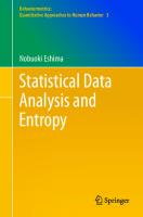
2.3.1 Determining the parameter of a Poisson distribution Suppose we have data about daily system failures at a given bank, and that we have organized the data as shown in Table 2.2. In the left column of Table 2.2 we list the possible number of failures and in the second column we list the number of days in which that number of failures occurred. Clearly, during the data gathering period, more than 14 failures were never observed during one day. The histogram corresponding to that data is displayed in Figure 2.1.
2.3 Examples |
Tab. 2.2: Daily system failures of some bank. Number of events (k) 0 1 2 3 4 5 6 7 8 9 10 11 12 13 14
Frequency (n k ) 11 50 112 169 190 171 128 82 46 23 10 5 2 1 0
Total
1000
Relative frequency (p k ) 0.011 0.050 0.112 0.169 0.190 0.171 0.128 0.082 0.046 0.023 0.010 0.005 0.002 0.001 0.000 1
Frequency n(k)
150
100
50
0 0
5 10 Number of events k
Fig. 2.1: Failures versus time.
15
11
12 | 2 Frequency models
Tab. 2.3: Daily system failures in some bank. Number of events (k) 0 1 2 3 4 5 6 7 8 9 10 11 12 13 14 Total
nk
kn
Frequency (n k ) 11 50 112 169 190 171 128 82 46 23 10 5 2 1 0
k−1
– 4.545 4.480 4.527 4.497 4.500 4.491 4.484 4.488 4.500 4.348 5.500 4.800 6.500 0.000
1000
–
The first step in the risk modeling process is to determine a model for the frequency of losses. So, let us suppose that the frequency model belongs to the (a, b, 0) family. Thus, we shall consider the characterization k
̂k p = ak + b ̂ k−1 p
̂ k = ∑n kn , and n k is the frequency with which k losses are obwhere, to be explicit, p k k served. Let us now consider Table 2.3, a variant of the first table in which the last column ̂k k is replaced by a column displaying k p̂pk−1 = k nnk−1 . nk Next, we plot k n k−1 versus k to obtain Figure 2.2. Clearly the values appear to be constant about 4.5 except for the three last values. This would suggest that we are in the presence of a Poisson distribution, because a appears to be 0 and b (which for the Poisson coincides with λ) seems to be about 4.5. One easy test of the ‘Poissonness’ of the distribution is the comparison of the mean and the variance of the data. Both the mean and the variance of the data in Table 2.2 equal 4.5. This reinforces the possibility of its being a Poisson distribution. To be really sure, we would need to apply tests like the chi-square (χ2 ), maximum likelihood or Kolmogorov–Smirnov tests, in case we were dealing with continuous data.
2.3 Examples | 13
6
n ( k)
k+
n(k – 1)
4
2
0 0
5 10 Number of events (k)
k Fig. 2.2: Plot of k versus k nnk−1 .
χ 2 goodness of fit test This is a standard hypothesis test. Here we shall apply it to the data in Table 2.2 to decide whether the data comes from a Poisson of parameter λ = 4.5. The first step consists of establishing the null and alternative hypotheses: (1) H0 : the random variable is distributed according to a Poisson law (2) H1 : the random variable is not distributed according to a Poisson law. In Figure 2.1 we display the frequency histogram of the daily data. The number of categories (bins) is k = 14 and the total number of data points is n = 1000 (roughly 40 months of data) and there is only one parameter (λ) to be estimated. We already did that, but we can also obtain it from the estimated sample mean. The observed frequency O i in each of the bins {0, 1, . . . , 14} is shown in Table 2.2. The expected frequency E i for each of the k categories can be estimated by E i = nP(X = i) = n(e −λ λ i /i!), with λ = 4.5. In Table 2.4 we gather all the steps necessary to compute the value of χ 2o . As a practical rule, it is advised that the theoretical expected frequency in each category is not less than 5. In case it is to be applied, one may combine successive intervals until the minimal frequency is achieved. In Table 2.4 we see that the practical rule suggests that we should combine intervals to form a new category. In our case, this will correspond to 11 or more events. In Table 2.5 we see the resulting new dataset, in which the number of categories is 12. Therefore the new degree of freedom for the χ2 test is 12 − 1 − 1 = 10. If we set the level of significance to α = 0.05, the critical value of χ(0.05, 10) can be obtained from the tables of the χ2 distribution or using your favorite software. 2 i) Therefore, χ 2o = ∑ki=1 (O i −E = 0.2922061. The value of χ 20.05,10 = 18.307045 Ei using the R command qchisq(1 − 0.05, 10). Since 0.2922061 < 18.30704 we do not reject the null hypothesis and we conclude that the data is distributed according to a Poisson(4.5) law.
14 | 2 Frequency models
Tab. 2.4: Absolute and relative frequencies in each category. Number of events (k) 0 1 2 3 4 5 6 7 8 9 10 11 12 13 or more Total
Absolute frequency (O k ) 11 50 112 169 190 171 128 82 46 23 10 5 2 1 1000
Relative frequency (E k ) 11.1089965 49.9904844 112.4785899 168.7178849 189.8076205 170.8268585 128.1201439 82.3629496 46.3291592 23.1645796 10.4240608 4.2643885 1.5991457 0.8051379 1000
Tab. 2.5: Absolute and expected frequencies. Number of events (k) 0 1 2 3 4 5 6 7 8 9 10 11 or more Total
Absolute frequency (O k ) 11 50 112 169 190 171 128 82 46 23 10 8 1000
Expected frequency (E k ) 11.1089965 49.9904844 112.4785899 168.7178849 189.8076205 170.8268585 128.1201439 82.3629496 46.3291592 23.1645796 10.4240608 6.6686721 1000
The procedure just described can be carried out in R using the command goodfit available in the vcd library. This command allows us to verify whether a dataset does or does not fit some of the discrete distributions (binomial, negative binomial or Poisson) via a χ2 or a maximum likelihood procedure. Organizing the data in a matrix x, the code for the R procedure for the goodness of fit test is displayed in Table 2.6 The results of applying the code in Table 2.6 are displayed in Table 2.7. As we mentioned above, the dataset in Table 2.2 fits a Poisson quite well.
2.3 Examples | 15
Tab. 2.6: R code for the goodness of fit test. # the original data is grouped, the following instructions ungroup them: xpoi=NULL for (k in min(x[,1]):max(x[,1])) xpoi=c(xpoi,rep(k,x[k+1,2])) xpoi #apply the χ 2 test: library(vcd) gf=goodfit(xpoi,type= "poisson",method= "MinChisq") summary(gf) plot(gf,main="Frequency vs. Poisson dist.",xlab = 'Number of failures', ylab = 'days')
Tab. 2.7: Results of applying the goodness of fit test. Goodness of fit test for Poisson distribution X 2 df P(> X 2 ) Pearson 0.291703 12 1 In summary.goodfit(gf) : Chi-squared approximation may be incorrect
Comment. Note that the number of degrees of freedom in Table 2.7 is different from its true value because the procedure ‘does not know’ that we are estimating a parameter. We mention as well that in R there exists another command that produces similar results, namely the command chisq.test. A simpler but not so rigorous numerical procedure consists of plotting the probability distribution that is supposed to describe the data along with a histogram of the data, and comparing the result visually. For the dataset in Table 2.5, such a procedure yields Figure 2.3. The display suggests that the proposed distribution seems to be the right one. Computation of the P-value The P-value is usually used in hypothesis testing. It is defined as the smallest significance level that can be chosen to possibly reject the null hypothesis about a given dataset. Any significance level smaller than the P-value implies not rejecting the null hypothesis. In the present case it can be defined by: Pvalue ≈ P (χ2α,k−p−1 > χ 20 ) 0 ≤ Pvalue ≤ 1 . The null hypothesis is rejected when: α > Pvalue .
16 | 2 Frequency models
Frequency n(k)
150
100
50
0 0
Fig. 2.3: Frequency data and theoretical distribution.
5 10 Number of events k
Thus, in our example it happens that Pvalue ≈ P (χ 20.5,10 > 0.2922061) = 0.9999995 . Observe that the results using R, displayed in Table 2.7, show that the Pvalue is approximately 1, which coincides with the previously obtained result. The Pvalue can be computed using R by 1 − pchisq(0.29, 10). Comment. This test is independent of the sample size, so it is always possible to reject a null hypothesis with a large enough sample, even though the true difference is very small. This situation can be avoided by complementing the analysis with the calculation of the power of the test and the optimal sample space, as suggested, for example, in [2]. Determination of the parameter by maximum likelihood The basic philosophy of the maximum likelihood estimation procedure is the following: We suppose that the distribution belongs to some parametric distribution family, and then we determine the parameter that makes the dataset most probable. Then, the goodness of fit test may be applied to complement the analysis. So, consider the data in Table 2.2 once more. We begin by supposing that the dis−θ k tribution underlying the data is Poisson P(X = k) = e k!θ , and the likelihood function is defined by e−θ θ k i ki! i=1
n
n
L(θ; k 1 , k 2 , . . . , k n ) = ∏f(k i | θ) = ∏ i=1 n
=
∑ ki e−nθ θ i=1 n
∏ ki! i=1
.
2.3 Examples | 17
In our example n = 1000. The log-likelihood function is defined by n
n
log L(θ; x1 , x2 , . . . , x n ) = −nθ + log θ ∑ x i − log (∏x i !) , i=1
i=1
log(∏ ni=1
x i !) can be ignored because the likelihood function is maxiwhere the term mized with respect to θ. To find the value of θ that maximizes the likelihood, we differentiate the log-likelihood function with respect to θ and equate the result to zero, obtaining n
∂ log L(θ; x1 , x2 , . . . , x n ) = −n + ∂θ
∑ xi i=1
=0.
θ
Therefore, n
θ̂ =
∑ xi i=1
, n which happens to be the sample mean of the data, with a value of 4.505. To verify that ̂θ really minimizes the likelihood function, we compute its second derivative and substitute in the value of ̂θ, obtaining n
∂2 log L(θ; x
1 , x2 , . . . ∂2 θ
, xn )
∑ xi =−
i=1 θ2
=−
n2 n
0 by ∞
ϕ(α) = E [e
−αX
] = ∫ e−αx f X (x)dx . 0
A widely used and related concept is the moment generating function, given by M(t) = ϕ(−t). Those who get annoyed by the minus sign when computing derivatives prefer this notation. Even though sometimes the range of the definition can be extended to a larger subset of the real line, we shall not bother about this too much. Further properties of the Laplace transform will be explored in Chapter 6. The definition given is all we need for the time being. In all cases we will make explicit the relationship between the moments of the variable and the parameters of the distribution.
3.1 A short catalog of distributions The densities considered below are characterized by parameters that are easily related to moments of the variables, making the problem of their estimation easy. The reader is supposed to finish the incomplete computations.
3.1.1 Exponential distribution The exponential distribution is characterized by a single parameter λ. The density is given by f(x) = λe−λx , M(t) = λ(λ − t)−1 , F(x) = 1 − e−λx , k! E [X k ] = k ; k ∈ ℕ , λ https://doi.org/10.1515/9783110516074-003
ϕ(α) =
λ . λ+α
(3.1)
24 | 3 Individual severity models
The reader should verify that for any pair of positive numbers t, s the following holds: P(X > t + s | X > t) = P(X > s). This property actually characterizes the exponential density.
3.1.2 The simple Pareto distribution This density is characterized by two positive parameters λ and θ (which is usually supposed to be known because it denotes a cutoff point), f(x) = λθ λ x−(λ+1) ;
x>θ,
λ
F(x) = 1 − (θ/x) , E [X k ] =
λθ k ; (λ − k)
k ∈ ℕ, k < λ ,
(3.2)
ϕ(α) = λ(θα)λ Γ(−λ, α) . This is one of the simplest examples in which the Laplace cannot be given by a close analytic expression. The series expansion (in α) of the incomplete gamma functions is nevertheless convergent. This makes the need for the approach that we favor apparent, as the computations to obtain aggregate losses involving individual severities of the Pareto type have to be carried out numerically. Note as well that when θ is known, λ can be obtained by estimating the mean.
3.1.3 Gamma distribution The density of such variables is characterized by λ > 0 and β > 0, and its simple properties are: (xβ)λ e−xβ f(x) = , xΓ(λ) β −k Γ(λ + k) ; k > −λ , E [X k ] = Γ(λ) k
E [X k ] = β −k ∏ (λ + k − 1) ; j=1
ϕ(α) = (
λ β ) ; β+α
α>0.
when k ∈ ℕ ,
3.1 A short catalog of distributions
|
25
3.1.4 The lognormal distribution This is a very widely used model. It is also interesting for us since its Laplace transform has to be dealt with numerically. When X is lognormal, the ln(X) is distributed according to a normal distribution, hence its name. The basic properties of the variable are: ln x−μ
ϕ( σ ) 1 ln x − μ 2 1 ) )= , exp (− ( f(x) = 2 σ xσ xσ √2π ln −μ ) , F(x) = Φ ( σ 1 E [X k ] = exp [kμ + k 2 σ 2 ] . 2
(3.3)
The Laplace transform of this density is a complicated affair. Try summing the series expansion of ∞ (−α)k E [e−αX ] = ∑ E [X k ] , k! k=0 where the moments are given a few lines above. Again, it may be easier to proceed numerically: Simulate a long sequence of values of X and compute the integral by invoking the law of large numbers.
3.1.5 The beta distribution This is a standard example of a continuous distribution on a bounded interval. It is described by two shape parameters a, b, and a parameter L that specifies its range, which we chose to preserve as generic, for when it is unknown it can be randomized. Otherwise, it can be scaled to L = 1. The properties of the beta density are: f(x) =
Γ(a + b) x a−1 (L − x)b−1 ; Γ(a)Γ(b) L a+b−1 k
E [X k ] = L k ∏ j=1
(a + k − j) ; (a + b + k − j)
L k Γ(a + b)Γ(a + k) ; E [X ] = Γ(a)Γ(a + b + k) k
∞
k−1
k=1
j=0
ϕ(α) = ∑ (∏
0 0 of not returning the money. If a customer does not pay their loan, then the bank looses the amount lent (plus the interest rate) that it was going to collect. To examine the alternatives to lending money at risk, we note that instead of granting individual loans the bank could have lent the money to the central bank, receiving n(1 + r b )L with certainty. Hence the name risk free rate for r b . We will denote by D i , i = 1, . . . , n a binary random variable such that D i = 1 means the i-th customer defaults, and D i = 0 means the customer pays their debt. The loss to the bank (given that) the i-th customer defaults is (1 + r l )L, which written as a random variable is (1 + r l )D i L. This means the total (random) loss (or money not collected at the end of the year) is given by ∑i D i (1 + r l )L, and the distribution of this variable is easy to obtain because it is essentially distributed according to a binomial law. At this point we come across a couple of interesting issues in risk management. First: Is there a fair way to choose r l ? One possible interesting way to answer the question is that the bank chooses r l in such a way that the money it expects to receive in each of the two possible investment alternatives is the same. As in this simple model E[∑i D i ] = np, we have n
E [ ∑ (1 − D i )(1 + r l )L] = n(1 − p)(1 + r l )L = n(1 + r b )L . i=1
That is, the bank adjusts the lending rate to a level at which the expected amount to be received from lending at risk to individual borrowers equals the amount received by lending at zero risk (at the rate r b ). A simple calculation shows that the spread (the difference in rates) is p rl − rb = (1 + r b ) 1−p But this is not a good managerial decision, because the number of defaults may fluctuate about its mean (np) in a way that makes large losses highly probable. A criterion for designing a better way to determine the lending rate r l goes as follows: Fix a large fraction 0 < f < 1 of sure earnings and a large probability 0 < α < 1 with which you want your earnings to overtake fn(1 + r b )L and choose r l such that this is true. That is, choose r l so that n
P ( ∑ (1 − D i )(1 + r l )L > fn(1 + r b )L) ≥ α . i=1
34 | 4 Some detailed examples As ∑ni=1 (1 − D i ) is a binomial distribution with parameters n, (1 − p), it is easy to see that such an r l can be found. Even though the example is too simple, we already see that the need to compute the distribution of losses (or defaults) is an important part of the analysis. To make the model a bit more realistic, suppose that the bank has several categories of creditors, for example large corporations, middle size corporations, small businesses and individual borrowers. Suppose as well that the creditors within each category have the same probability of default. It is reasonable to suppose that the number of large corporations and middle size corporations is not very large, and it is also reasonable to suppose that the random number among them that default may be described by a binomial model. For small businesses and individual borrowers, if the individual probabilities of default are small, it may make sense to model the number of defaults by variables of the Poisson type. The total loss to a bank caused by defaulting creditors may be described by M Nk
S = ∑ ∑ X k,n ,
(4.2)
k=1 n=1
where N k is the random number of defaults of the creditors in the k-th category, and X k,n is the loss to the bank produced by the n-th borrower in the k-th category. As mentioned, each of the M summands has some internal structure and the necessary modeling involves quite a bit of analysis. For example, if we consider large corporations, there is information about their credit ratings from which an individual probability of default may be extracted. As the corporations function in a common economic environment, the probabilities of default may not be independent. Other sources of credit losses to aggregate may come from loans to small corporations or small businesses, the residential mortgage loans, the standard consumer loans via credit card, and so on. Clearly each group has internal similarities and possible dependencies. Besides that, the notion of the occurrence of default depends on the type of borrower. To model the default by a corporation, or by a collection of them in a credit portfolio, a variety of ways have been proposed to model the occurrence of default, and then to model the probability of default of a collection of corporations. Such details have to be taken into account when trying to determine the distribution of credit losses affecting a bank. For details about such modeling process, the reader may consult chapters 8 and 10 in [90]. We mention as well that the model in (4.2) is the starting point for a methodology (called Credit Risk+, CR+) proposed by the Credit Suisse Bank, which extends the simple model presented at the beginning of this section into a slightly more elaborate model, and still leads to an analytic computation of the Laplace transform of the total loss. The extension involves several changes. Instead of allowing all obligors to have (or to cause) independent and identically distributed (IID) individual losses, it maintains a given fixed number of obligors, which may have independent but non identically
4.2 Simple model of credit risk
| 35
distributed losses. The variation on the theme described above proposes a random number of defaults, which are grouped into classes such that the individual losses within each class are IID. To continue with the CR+ model proposal we write N
S = ∑ Dn En , n=1
where D n is the default indicator introduced above and E n = LGDn × EADn is the loss caused by the n-th obligor, where LGD n stands for ‘loss given default’ and EAD n stands for ‘exposure at default’. It is decomposed into two factors: an exposure at default, which quantifies the maximum loss, and the loss given default, which is sometimes written as 1 − f n , where f n stands for the fraction recovered after the default of the n-th obligor. But let us stick to the simpler notation and let E n denote the random variable modeling the loss caused by the default of the n-th obligor. Usually a base unit E of loss is introduced and we set ν n = E n /E for the number of units of loss caused by the n-th obligor. Denoting S/E by S once more we have N
N
S = ∑ Dn νn = ∑ λn , n=1
n=1
where λ n denotes the loss (in units of E) produced by the n-th obligor. The second part of the CR+ proposal consists of supposing that the default frequencies are Poisson instead of Bernoulli. That is justified by the proponents of the model as follows: If P(D n = 1) = p n is very small, then ψ λ n (α) = E [e−αλ n ] = (1 − p n + p n E [e−αν n ]) eln(1−p n +p n E[e
−αν n
]) ≈ e−p n (1−E[exp(−αν n )]) .
That is, the default indicators now are now supposed to be integer valued random variables distributed according to a Poisson(p n ). Since in a real economy, the defaults may in some way be affected by a common factor, in order to introduce dependence and still keep a simple analytical model the last extension to the simple model consists of replacing p n by the following simple possible mixture model: K
K
p n ( ∑ w nk X k , )
with w nk ≥ 0 ,
k=0
∑ w nk = 1 ,
and
k=1
where the random factors X k ∼ Γ(ξ k , 1/ξ k ), and X0 = 1. This means the random factor is positive and has a mean equal to 1. But, to add to the unpalatable nature of the model, as it admits possible multiple defaults by the same obligor, there is also the possibility of the default probability to being larger than 1. To finish, let us introduce the notation P k (α) = ∑Nn=1 p n w nk E[e−αν n ]. With this, the Laplace transform of the total loss can be easily seen to be given by K
E [e−αS ] = ∏ ( k=1
ξk 1 ) . 1 + ξ k P k (α)
Again, the problem is now to invert this Laplace transform.
36 | 4 Some detailed examples
4.3 Shock and damage models These are restricted versions of a model that is inherently dynamical. The accumulation of damage produced by shocks is a stochastic process, which at any given time is described by a compound random variable like those described above. Considering only the accumulated damage in a given fixed period of time is a very small aspect of the problem. The literature on this type of problems is large. As an introduction to the field, consider [96]. Consider N to be the number of events, or shocks, that affect a structure during a fixed period of time. At the time that the n-th shock occurs an amount of wear (or damage) W n is accumulated. It is natural to suppose that the W n are independent and identically distributed. Actually, and like in the case of credit risk, there is some internal structure to W n . The resulting damage occurs when the intensity of the shock is larger than some threshold, and we may think of W n as the response of the system to the intensity of the shock. Anyway, the ‘severity’ of the accumulated damage is again given by a compound variable N
S = ∑ Wn . n=0
Even though the question is more natural in a dynamical setup, the reason that the distribution of S is relevant is because as soon as the accumulated damage becomes larger than some critical value K, the effect of the damage entails serious losses of some kind, and this involves the computation of the distribution of accumulated damage.
4.4 Barrier crossing times Let us examine a few dynamical versions of the problems described above. Let us denote by N(t) an integer valued process, usually supposed to have independent, identically distributed increments, and let {X n | n ≥ 1} be a collection of independent identically distributed positive random variables. Consider either of the following processes: N(t)
S(t) = s0 + ∑ X n − rt n=1
or N(t)
S(t) = s0 + rt − ∑ X n . n=1
When r = 0, the first example can be used to describe accumulated damage in time. When r > 0, we can think of S(t) as the savings in an account, or the water level in a dam, in which there is an ‘input’ of money or rain at random times described by N(t), and r quantifies the spending or release rates. The constant (or perhaps random) term s0 models the initial amount of whatever it is that S(t) denotes. The second example is
4.5 Applications in reliability theory
| 37
used in the insurance industry to denote the capital of the insurance company. Naturally, s0 is the initial capital, r the rate at which premia are collected and the compound variable is the amount paid in claims. Apart from the simplifications present in each of the models, for us the interest is in a question that appears in all of them: When is the first time some critical barrier is reached? Ths is defined by T = inf{t ≥ 0 | S(t) ≥ K} or perhaps T = inf{t ≥ 0 | S(t) ≤ K} for some level K related to the nature of the problem. The problem of interest in many applications is to determine the distribution (usually a probability density) of T. The relationship of this problem with the problems described in the three sections above is that the methodology to solve it is similar to the methodology of determining the density of the compound variables. In many cases, the nature of the inputs in the problem is such that a differential or integral equation to compute ϕ(α) = E [e −αT ] can be established and solved. An important class of such problems appears when dealing with the distribution of defaults of corporations to compute credit losses. A class of models, called structural models, proposes that defaults occur when the value of a corporation falls below a certain threshold related to the liabilities of the corporation. When dealing with a portfolio of corporations we have a many-dimensional barrier crossing problem.
4.5 Applications in reliability theory Another branch of applied mathematics in which the problem of determining the distribution of a positive random variable crops up in a natural way is reliability theory. The failure rate of a complex system is a function of the failure rates of its components. The components are chained in groups of series and/or parallel blocks, which may or may not fail independently. If a module consists of K-blocks placed in series, and their times to failure are random variables T i (not necessarily identically distributed), the time to failure of the block is given by min{T i : i = 1, . . . , K}. Similarly, if a component is made up of kblocks connected in parallel, and their times to failure are denoted by T i , and if the system does not fail until all subcomponents have stopped working, then the time to failure of the component is given by max{T i : i = 1, . . ., k}. c are the failure times of the subcomponents of It is then clear that if T1c , . . . , T M a system, the failure time of the system is some more or less complicated function
38 | 4 Some detailed examples c H(T1c , . . . , T M ) of the failure times of the components. Note that even when we know the distributions of the blocks, and are lucky enough that the distribution of failure time of the subsystems can be computed, our luck does not usually extend to the computation of the distribution of the failure time of the system. For that we can now resort c to the Monte Carlo simulation of a large sample of H(T1c , . . . , T M ) and try to obtain the distribution that fits the resulting histogram, or to use the Laplace transform based techniques that we propose in this volume. Of course, we may have empirical data and we may start from that, without having to resort to simulations.
5 Some traditional approaches to the aggregation problem 5.1 General remarks In Chapters 2 and 3 we considered some standard models for the two basic building blocks for modeling the compound random variables used to model risk. First, we considered several instances of integer valued random variables used to model the frequency of events, then some of the positive continuous random variables used to model individual losses or damage each time a risk event occurs. From these we obtain the first level of risk aggregation, which consists of defining the compound random variables that model loss. Higher levels of loss aggregation are then obtained by summing the simple compound losses. As we mentioned in the previous chapter, the first stage of aggregation has been the subject of attention in many areas of activity. In this chapter we shall review some of the techniques that have been used to solve the problem of determining the distribution of losses at the first level of aggregation. This is an essential step prior to the calculation of risk capital, risk premia, or breakdown thresholds of any type. The techniques used to solve the problem of determining the loss distribution can be grouped into three main categories, which we now briefly summarize and develop further below. – Analytical techniques: There are a few instances in which explicit expressions for the frequency of losses and for the probability density of individual losses are known. When this happens, there are various possible ways to obtain the distribution of the compound losses. In some cases this is by direct computation of the probability distribution, in other cases by judicious use of integral (mostly Laplace) transforms. Even in these cases, in which the Laplace transform of the aggregate loss can be obtained in close form from that of the frequency of events and that of the individual severities, the final stage (namely the inversion of the transform) may have to be completed numerically. – Approximate calculations: There are several alternatives that have been used. When the models of the blocks of the compound severities are known, approximate calculations consisting of numerical convolution and series summation can be tried. Sometimes some basic statistics, like the mean, variance, skewness, kurtosis or tail behavior or so are known, in this case these parameters are used as starting points for numerical approximations to the aggregate density. – Numerical techniques: When we only have numerical data, or perhaps simulated data, obtained from a reliable model, we can only resort to numerical procedures.
https://doi.org/10.1515/9783110516074-005
40 | 5 Some traditional approaches to the aggregation problem
5.1.1 General issues As we proceed, we shall see how the three ways to look at the problem overlap each other. Under the independence assumptions made about the blocks of the model of total severity given by the compound variable S = ∑Nn=1 X n , it is clear that ∞
P(S ≤ x) = ∑ P(S ≤ x | N = k) P(N = k) k=0 ∞
k
k=0
n=1
∞
k
k=0
n=1
= ∑ P ( ∑ X n ≤ x | N = k) P(N = k) = ∑ P ( ∑ X n ≤ x) P(N = k) ∞
k
k=1
n=1
= P(N = 0) + ∑ P ( ∑ X n ≤ x) P(N = k) .
(5.1)
We halt here and note that if P(N = 0) = p0 > 0, or to put it in words, if during the year there is a positive probability that no risk events occur, or there is a positive probability of experiencing no losses during the year, in order to determine the density of total loss we shall have to condition out the no-loss event, and we eventually concentrate on ∞
k
k=1
n=1
P(S ≤ x; N > 0) = ∑ P ( ∑ X n ≤ x) P(N = k) . To avoid trivial situations, we shall also suppose that P(X n > 0) = 1. This detail will be of importance when we set out to compute the Laplace transform of the density of losses. From (5.1) we can see the nature of the challenge: First, we must find the distribution of losses for each n, that is given that n risk events took place, and then we must sum the resulting series. In principle, the first step is ‘standard procedure’ under the IID hypothesis placed upon the X n . If we denote by F X (x) the common distribution function of the X n , then for any k > 1 and any x ≥ 0 we have F ∗k X (x)
x
k
∗(k−1)
= P ( ∑ X n ≤ x) = ∫ F X n=1
(x − y)dF X (y) ,
(5.2)
0
where F ∗k X (x) denotes the convolution of F X (x) with itself k times. This generic result will be used only in the discretized versions of the X n , which are necessary for numerical computations. For example, if the individual losses were modeled as integer multiples of a given amount δ, and for uniformity of notation we put P(X1 = nδ) = f X (n), in this case (5.2) becomes n
∗(k−1)
P(S k = n) = f X∗k (n) = ∑ f X m=1
(n − m)f X (m) .
(5.3)
5.2 Analytical techniques: The moment generating function | 41
Thus, the first step in the computation of the aggregate loss distribution (5.1), consists of computing these sums. If we suppose that F X (x) has a density f X (x), then differentiating (5.2) we obtain the following recursive relationship between densities for different numbers of risk events: x
f X∗k (x)
∗(k−1)
= ∫ fX
(x − y)f X (y)dy ,
(5.4)
0
where f X∗k (x) is the density of F ∗k X (x), or the convolution of f X (x) with itself k times. This is the case with which we shall be concerned from Chapter 6 on. Notice now that if we set p0k ≡ p k /P(N > 0), then ∞
k
k=1
n=1
P(S ≤ x | N > 0) = ∑ P ( ∑ X n ≤ x) p0k . We can now gather the previous comments as Lemma 5.1. Lemma 5.1. Under the standard assumptions of the model, suppose furthermore that the X k are continuous with common density f X (x), then, given that losses occur, S has a density f S (x) given by f S (x) =
∞ ∞ d (k) P(S ≤ x | N > 0) = ∑ f S k (x)p0k = ∑ f X (x)p0k . dx k=1 k=1
This means, for example, that the density obtained from empirical data should be thought of as a density conditioned on the occurrence of losses. The lemma will play a role below when we relate the computation of the Laplace of the loss distribution to the empirical losses. This also shows that in order to compute the density f S from the building blocks, a lot of work is involved, unless the model is coincidentally simple.
5.2 Analytical techniques: The moment generating function These techniques have been developed because of their usefulness in many branches of applied mathematics. To begin with, is it usually impossible, except in very simple cases, to use (5.2) or (5.4) to explicitly compute the necessary convolutions to obtain the distribution or the density of the total loss S. The simplest example that comes to mind is the case in which the individual losses follow a Bernoulli distribution with X n = 1 (or any number D) with probability P(X n = 1) = q or X n = 0 with P(X n = 0) = 1 − q. In this case ∑kn=1 X k has binomial distribution B(k, q) and the series (5.2) can be summed explicitly for many frequency distributions.
42 | 5 Some traditional approaches to the aggregation problem
A technique that is extensively used for analytic computations is that of the Laplace transform. It exploits the compound nature of the random variables quite nicely. It takes a simple computation to verify that k
ϕ S k (α) = E [e−αS k ] = (E [e−αX1 ]) . For the simple example just mentioned, E[e−αX1 ] = 1−q+qe−α and therefore E[e−αS k ] = (1 − q + qe−α )k from which the distribution of S n can be readily obtained. To continue, the Laplace transform of the total severity is given by: Lemma 5.2. With the notations introduced above we have ∞
∞
k=0
k=1
k
ψ S (α) = E [e−αS ] = ∑ E [e−αS k ] p k = ∑ (E [e−αX1 ]) p k = G N (E [e−αX1 ]) where
∞
G N (z) := ∑ z n P(N = n) ,
(5.5)
for |z| < 1 .
n=0
We shall come back to this theme in Chapter 6. For the time being, note that for z = e−α with α > 0, G N (e−α ) = ψ N (α) is the Laplace transform of the a discrete distribution.
5.2.1 Simple examples Let us consider some very simple examples in which the Laplace transform of the compound loss can be computed and its inverse can be identified. These simple examples complement the results from Chapters 2 and 3. The frequency N has geometric distribution In this case p k = P(N = k) = p(1 − p)k for k ≥ 0. Therefore ψ S (α) = E [e−αS ] = p [1 +
1 ] . 1 − pE [e−αX1 ]
For the Bernoulli individual losses, ψ S (α) = p [1 +
1 ] . 1 − p(1 − q + qe−α )]
The frequency N is binomial B(M, p) M M k M ψ S (α) = E [e−αS ] = ∑ ( ) (E [e−αX1 ]) = [1 + pE [e−αX1 ]] . k k=0
5.2 Analytical techniques: The moment generating function
| 43
The frequency N is Poisson (λ) Since we shall be using this model for the frequency of events, we shall explore this example in some detail. Now p k = λ k e λ /k!, and the sums mentioned above can be computed in closed form, yielding ∞ n −λ λ e −αX1 k ψ S (α) = E [e−αS ] = ∑ (E [e−αX1 ]) = e λ(E[e ]−1) . k! k=0 Some computations with this example are straightforward. For example E[N] = V(N) = E [(N − E[N])3 ] = λ . Therefore, if we put μ = E[X], σ 2S = λμ 2 + λσ 2X = λE[X 2 ] .
E[S] = λμ , In particular, from (5.9)
E[(S − E[S])3 ] = λE [X1 ]3 + 3λμσ 2X1 + λE [(X1 − E [X1 ])3 ] we obtain that E [(S − E[S])3 ] = λE [X13 ] . Thus, the coefficient of asymmetry of the accumulated loss is given by E [(S − E[S])3 ] σ 3S
=
E [X13 ] √λE [X12 ]
. 3
Note that this quantity is always positive (X1 is a positive random variable) regardless of the sign of the asymmetry of X1 . N is Poisson with a random parameter Let us build upon the previous model and suppose now that the parameter of the frequency is random, but that the frequency still is Poisson, conditional on the value of the parameter. We shall see how this allows us to modify the skewness in the total losses. Suppose that the intensity parameter λ is given by the realization of a positive random variable Λ with distribution H(dλ) such that P(N = k | Λ = λ) =
λ k −λ e . k!
In this case the results obtained above can be written as E[S | Λ = λ] = λμ ,
V(S | Λ = λ) = λμ 2 + λσ 2X = λE[X 2 ]
44 | 5 Some traditional approaches to the aggregation problem
and, in particular
E [ (S − E[S])3 Λ = λ] = λE[X 3 ] .
Now, integrating with respect to H(dλ) we obtain E[S] = E[Λ]μ σ 2S = V(Λ)μ 2 + E[Λ]σ 2X and furthermore, E [(S − E[S])3 ] = E [(Λ − E[Λ])3 ] μ 3 + 3σ 2Λ μE [X 2 ] + E[Λ]E [X 3 ] . Clearly, if the asymmetry in the distribution of Λ is large and negative, then S can be skewed to the left. It is also easy to verify that ψ S (α) = E [E [ e−αS Λ]] = E [e Λ(ϕ X (α)−1) ] = G Λ (ϕ X (α) − 1) . We leave it up to the reader to verify that the moments of S are obtained by differentiating with respect to α at α = 0. Gamma type individual losses To complete this short list of simple examples, we suppose that X n ∼ Γ(a, b), that is, f X1 (x) = b a x(a−1) e−bx /Γ(a). Observe that, in the particular case when a = 1, the gamma distribution becomes the exponential distribution. In the generic gamma case, E [e−αX1 ] = (
a ak b b k ) ⇒ E [e−αS k ] = E [e−αX1 ] = ( ) . b+α b+α
Or to put it in words, the sum of k random variables distributed as Γ(a, b) is distributed according to a Γ(ka, b) law. For any frequency distribution we have ∞
ψ S (α) = ∑ p k ( k=0
ak b ) , b+α
which can be explicitly summed for the examples that we considered above. But more important than that, according to Lemma 5.1, f S (x) =
d b k x(ak−1) P(S ≤ x | N > 0) = ∑ p0k ( ) e−bx . dx Γ(ak) k≥1
This sum does not seem to easy to evaluate in closed form except in very special cases, but it is easy to deal with it numerically. Notice now that if, for example, N is geometrical with distribution p k = p(1 − p)k , and a = 1 (that is the individual losses are exponentially distributed) then the former sum becomes f S (x) = ∑ p0k ( k≥1
b k x(k−1) ) e−bx = pbe−pbx . (k − 1)!
That is, the accumulated losses are again exponential with a smaller intensity (a larger mean equal to 1/bp).
5.3 Approximate methods |
45
5.3 Approximate methods Many different possible methods exist under this header. Let us explore a few.
5.3.1 The case of computable convolutions In some instances it may be natural or plain easier to use (5.4) or (5.3) in order to calculate the distribution of aggregate losses. This happens when the density of a finite number of losses can be explicitly calculated or at least reasonably well approximated. This possibility is important because, even when the density of any finite number of losses can be calculated exactly, the resulting series cannot be explicitly summed. In this case one must determine how many terms of the series to choose to determine the losses in some range to a good approximation, and then deal numerically with the resulting approximate sum. Simple example A few lines above we considered a simple example of this situation. Suppose that the frequency of losses N is Poisson with parameter (λ) and that the joint distribution of the X k is Γ(a, b). We have already mentioned that the X1 + X2 + ⋅ ⋅ ⋅ + X k is distributed according to a Γ(ka, b), and in Lemma 5.1 we saw that the density f S (x) of accumulated losses is given by ∞ λ n x na−1 b na −bx 1 ∑ e−λ . f S (x) = e −λ n! Γ(na) 1 − e n=1 As mentioned at the outset, the pending issue is now how to chose the range within which we want to obtain a good approximation to that sum. The answer depends on what we want to do. For example, we may just want to plot the values of the function up to a certain range, or we may want to compute some expected values, or we may want to compute some quantiles at the tail of the distribution.
5.3.2 Simple approximations to the total loss distribution Something that uses simple calculations involving the mean, variance, skewness and kurtosis of the frequency of events and of the individual losses and the independence assumptions of the basic model, is to compute the mean, variance and kurtosis of the total severity and use them to approximate the density of aggregate losses. It is simple to verify that (−1)k d k ln ψ S (α)α=0 = E [(S − E[S])k ] , dα k
for
k = 2, 3 .
(5.6)
46 | 5 Some traditional approaches to the aggregation problem When k = 1
−d (5.7) ln ψ S (α)α=0 = E[N]E[X] , dα where E[X] denotes the expected value of a random variable X whose distribution coincides with that of the X k . When k = 2 we have V(S) = V[N]E[X]2 + E[N]V(X) ,
(5.8)
in which we use V(Y) to denote the variance of a random variable Y. Another identity that we use below is that for k = 3 E [(S − E[S])3 ] = E [(N − E[N])3 ] E[X]3 + 3V(N)E[X]V(X) + E[N]E [(X − E[X])3 ] . (5.9) And to finish this preamble, for k = 4 it happens that d4 ln ψ S (α)α=0 = E [(S − E[S])4 ] − 3V(S) . dα 4
(5.10)
We shall now see how moments up to order three of N and X can be used to obtain approximations to the accumulated losses using some simple approximate procedures. Gaussian approximation The underlying intuition behind this approximation is that when the expected number of events is large, one can invoke the central limit theorem to obtain an approximation to the density of S. The starting point is the identity P(S ≤ x) = P (
S − E[S] x − E[S] ≤ ) . σS σS
From the computations mentioned above, we know that E[S] = E[N]E[X] ;
and that
V(S) = σ 2S = σ 2N (E[X])2 + σ 2X E[N] .
We can thus prove that when N is large, the former identity can be rewritten (and it is here that the CLT (central limit theorem) comes in) as P(S ≤ x) = Φ (
x − E[S] ) . σS
Here we use the usual Φ(x) to denote the cumulative distribution of the N(0, 1) random variable. The translated gamma approximation The Gaussian approximation is simple and based on basic ideas, but it has two handicaps. First, it assigns positive probability to negative losses, and second, it is symmetric. An alternative based on the generic shape of the gamma density consists of
5.3 Approximate methods |
47
supposing the distribution of losses is a translated gamma, and to identify its parameters by a moment matching procedure. That is, we have to determine the parameters (a, b) of a Γ(a, b) distributed random variable Y, and a positive number k such that the three first moments of the random variable k+Y coincide with those of the random variable S. If we denote by γ the coefficient of asymmetry of S, the identities that determine the parameters of k + Y are E(k + Y) = k +
a = σS b2
V(k + Y) = 3
E [(k + Y − E(k + Y)) ] [V(k +
Y)]3/2
=
a = E[S] b
2 =γ. √a
It is important to keep in mind that this computation makes sense only when β > 0. Once k, a and b are determined, one can use the translated gamma k+Y to carry out all sorts of computations. A complementary approximation occurs when 2a is an integer, because in this case 2aY ∼ χ 22a .
5.3.3 Edgeworth approximation Let us now consider the standardized version of the aggregate loss S, that is, consider S − E[S] . σS
Z=
The Taylor expansion of ln ϕ Z (t) begins as follows: ln ϕ Z (α) = a0 − a1 α + a2
α2 α3 α4 − a3 + a4 . . . , 2 6 24
where a k = (−1)k d k ln ϕ Z (α)/dα k α=0 . As the variable Z is standardized, clearly a0 = 0 ,
a2 = σ 2Z = 1 ,
a1 = E[Z] = 0 ,
a3 = E [Z 3 ] ,
and the fourth moment is a4 = E [Z 4 ] − 3 =
E [(S − E[S])4 ] σ 4S
−3.
Let us now note that if we truncate the series at the fourth term, we obtain ϕ Z (α) ≈ e α
2
/2 −a 3 α3 /6+a 4 α4 /24
e
.
If we now expand the second exponential and retain the terms up to the sixth order in α, 2 α3 α4 α6 ϕ Z (α) ≈ e α /2 (1 − a3 + a4 + a23 ) . 6 24 72
48 | 5 Some traditional approaches to the aggregation problem If we replace α by −α we obtain the usual moment generating function M Z (α) ≈ e α
2
/2
(1 − a3
We know that e
α2 /2
= ∫e
−xα e
ℝ
−x 2 /2
√2π
α3 α4 α6 + a4 + a23 ) . 6 24 72
dx = ∫ e−αx ℝ
dΦ(x) dx , dx
where Φ(x) is cumulative distribution function of an N(0, 1) random variable, therefore 2 2 d n e−αx e−x /2 d n+1 Φ(x) (−α)n e α /2 = ∫ dx , dx = (−1)n ∫ e−αx n dx dx n+1 √2π ℝ
ℝ
where the last step follows from an integration by parts. That is, ϕ Z (α) ≈ ∫ e−αx (dΦ(x) − ℝ
a2 a3 a4 dΦ(3) (x) + dΦ(4) (x) + 3 dΦ(6) (x)) . 6 24 72
As both sides of the equation are Laplace transforms, it follows that P(Z ≤ x) ≈ Φ(x) −
a2 a4 (4) a3 (3) Φ (x) + Φ (x) + 3 Φ(6) (x) . 6 24 72
Now, undoing the standardization Z → (S − μ S )/σ S , we obtain P(S ≤ x) = P ( ≈ Φ(
S − μS x − μS ≤ ) σS σS a2 x − μS a3 (3) x − μ S a4 (4) x − μ S x − μS )− )+ ) + 3 Φ(6) ( ) . Φ ( Φ ( σS 6 σS 24 σS 72 σS (5.11)
A very common situation in practice consists of the case in which S is a compound variable, with frequency N being Poisson(λ). In this case, it is simple to compute the coefficients a k . It takes a simple computation to verify that μ S = λμ X ,
σ S = √λμ X (2) ,
and in general
ak =
λμ X (k) , (λμ X (2))k/2
where we have put μ X (k) = E[X k ]. In this case, (5.11) becomes P(S ≤ x) ≈ Φ ( +
x − μS x − μS μ X (3) Φ(3) ( )− ) √λμ X (2) √ λμ X (2) 6√λμ X (2)3
μ X (3)2 x − μS x − μS μ X (4) Φ(4) ( Φ(6) ( )+ ) . 2 24λμ X (2) 72μ X (2)2 √λμ X (2) √λμ X (2)
5.4 Numerical techniques |
49
5.4 Numerical techniques In this section we review some direct numerical techniques for computing the distribution of losses when models for the frequency of losses and for the individual losses are at our disposal, or if not, when empirical data about each block is available. We shall examine how to use that information to compute the distribution of S using (5.4) or from (5.3) plus a direct numerical procedure.
5.4.1 Calculations starting from empirical or simulated data The procedure described in (5.3) to compute the distribution of losses when the blocks are discrete can be used to deal with empirical or simulated data, for in this case the convolutions have to be carried out numerically. In both cases we shall suppose that the postanalysis data is of the following two types. First, the relative frequency of events is presented as a distribution with em̂ n describing the probability that n events occurred during a cerpirical frequencies p tain number of years. We furthermore suppose that the number of events is finite, 0 ≤ n ≤ M where M is the maximum number of observed events. Second, we shall suppose that the frequency of individual losses has been organized in cells, chosen as multiples of a monetary unit δ and we interpret the histogram P(X = kδ) = ̂f X (k) as the probability of having observed a loss of size kδ. Observe that if losses occur, then it is necessary that X > 0. We must therefore keep in mind that if the empirical (or simulated range of X is δ, 2δ, . . . , Nδ, then the range of the aggregate sum S n = X1 + ⋅ ⋅ ⋅ + X n is nδ ≤ S n ≤ nNδ. This detail has to be kept in mind when computing the distribution of S n , that is, when carrying out the computation of k
̂f ∗n (k) = ∑ ̂f ∗(n−1) (k − j)̂f X (j) ; X X
n ≤ k ≤ nN .
j=1
Once we have computed the ̂f X∗n , we can compute their cumulative distribution as follows: ̂ ∗n (x) = ∑ ̂f ∗n (k) , F X X kδ≤x
and after that we can estimate the total distribution of losses by M
̂ ∗n (x) . ̂nF ̂0 + ∑ p F̂ S (x) = p X
(5.12)
n=1
Comment. When the losses are modeled by a discrete random variable, and no analytical procedure can be implemented, we have to resort to something like what we
50 | 5 Some traditional approaches to the aggregation problem
described before. If the individual losses are modeled by an unbounded random variable, then there will be no upper limit to the partial sums and the numerical issues must include an analysis of the choice of a truncation point.
5.4.2 Recurrence relations An important technique, less demanding computationally and very much used in the insurance business, is based on the following recurrence methodology. Suppose that the frequency of events is of the (a, b, 0) class. Recall that this means that for n ≥ 1 the recurrence relation p n = (a + b/n)p n−1 holds, where p n is the probability of observing n events. Suppose furthermore that the individual losses occur in multiples of δ, then the aggregate losses take values that are multiples of δ and the probabilities p S (n) = P(S = nδ) satisfy the following recurrence relation: n
p S (n) = ∑ (a + k=1
bk p X (k)p S (n − k) ) ; n 1 − ap X (0)
n ≥1.
(5.13)
That is, starting from some given P(S = 0) = P(N = 0) and having computed p X (n) for n ≥ 0, by iterating the recurrence (5.13) we can find the loss distribution. For more about this, see [100] and [132].
5.4.3 Further numerical issues We have already mentioned several times that most of the time we may have to resort to numerical procedures to calculate sums like (5.3) and (5.4), that is to evaluate series like ∞
F S (x) = p0 + ∑ p n F ∗n X (x) . n=1
There are two complementary issues here. First, there is the choice of the number of terms of the series to be summed, and second the range [0, L] in which we want F S (x) to be determined. To answer the first question is easy due to the uniform boundedness of the F ∗n X (x). To state it formally, consider: Lemma 5.3. For every ϵ > 0 there exists an integer K > 0 such that ∞
F S (x) − ∑ p n F ∗n X (x) < ϵ n=0
uniformly in x ∈ [0, ∞). The proof is simple. Since ∑n≥0 p n = 1, there is an M such that ∑n≥M+1 p n < ϵ, from which the conclusion emerges. It is implicit in the proof that the F ∗n X are known.
5.5 Numerical examples |
51
When we are forced to compute the F ∗n X , what to do depends on the starting point. If we have a reliable model for F X (x), then we can compute the iterated integrals either using integral transforms, or numerically using some discretization procedure. If all we have is empirical data, and cannot reduce to the previous case by fitting a distribution to the data, then we have to proceed numerically. We shall consider all these alternatives below, but for the time being, let us begin by recalling some direct approximations that have been used in actual practice.
5.5 Numerical examples In this section we present a collection of detailed examples. It is a vital section for students that must come up with this material through worked examples. The examples covered are part of the daily life of a risk analyst confronted with small sized empirical data. Example 1 Consider to begin with the following simple example. Let us suppose that the average monthly frequency of events of a certain type is eight events per month and that its standard deviation is of three events per month. Suppose as well that the average loss per event is 150 000, with a standard deviation of 30 000 in some monetary units. If we apply (5.6) we obtain that E[S] = μ S = 8 × 150 000 $ = 12 × 105 , V(S) = 9 × (15 × 105 )2 + 8 × (3 × 104 )2 ≈ (3 × 15)2 × 10¹⁰ ⇒ σ S = 45 × 105 . Let us suppose furthermore that the distribution that better fits this data is the lognormal with parameters (μ, σ), and we want to determine its parameters from the data. We know that 2 2 E[S] = e μ+σ /2 and that E [S2 ] = e2μ+2σ . With the numbers given above, we have to solve μ + σ 2 /2 = 5 + log10 (12) μ + σ 2 = 5 + log10 (54) all of which yields
μ = 5.51 ,
σ = 1.07 .
Solving for (μ, σ) we know that the aggregate loss is given by S = exp(μ + σZ) with Z ∼ N(0, 1). Once we have reached this point, we can answer questions like: What is the probability that the losses exceed the mean by a certain number of standard deviations? That is, we want to compute P(S > μ S + aσ S ), or perhaps quantities like E[S | S > v] where v is some large quantile. We leave it as an exercise for the reader to answer a few such questions.
52 | 5 Some traditional approaches to the aggregation problem
Tab. 5.1: Loss distribution.
Tab. 5.2: Frequency distribution.
x
p X (x)
F X (x)
k
0
1
2
3
4
1 2 3 4 5 6
0.01024 0.07680 0.23040 0.34560 0.25920 0.07776
0.01024 0.08704 0.31744 0.66304 0.92224 1.00000
pk
0.05
0.10
0.20
0.25
0.4
2
3 x
4
5
6
0.2
p(k) 1
0.0
0.30 0.15
p(x)
0.0
0
Frequencies
0.40
Losses
1
0
1
2 k
3
4
Fig. 5.1: Histograms of data in Tables 5.1 (left panel) and 5.2 (right panel).
Example 2 In the next example we illustrate several aspects of the routine that should be carried out in a real situation. We want to illustrate how equation (5.1) is used as a technique of loss aggregation. Suppose that the individual losses in a small business, in thousands of some monetary unit, are given in Table 5.1. Suppose as well that the frequency of the losses is as in Table 5.2 and the recorded frequencies are listed in Table 5.2. In Figure 5.1 we display the values of p X (x) according to Table 5.1 and the histogram of the frequency of events shown in Table 5.2. From the data in Tables 5.1 and 5.2 we want to know the probability that the aggregate loss is larger or smaller than 10 (in units of 1000) as well as the expected aggregate loss E[S] and its variance V[S]. Since S = X1 + X2 + ⋅ ⋅ ⋅ + X N (recall that S = 0 whenever N = 0), the probability P(S ≤ 10) is computed like ∞
P(S ≤ x) = F S (x) = ∑ p k F ∗k X (x) , k=0
with x = 10 (corresponding to 10 000) and p k = P(N = k) being given in Table 5.2.
5.5 Numerical examples | 53
Tab. 5.3: F X∗0 (x) and F X∗1 (x). x
0
1
2
3
4
5
F X∗0 (x) F X∗1 (x)
1.00000 0
1.00000 0.01024
1.00000 0.08704
1.00000 0.31744
1.00000 0.66304
1.00000 0.92224
x
6
7
8
9
10
11
F X∗0 (x) F X∗1 (x)
1.00000 1.00000
1.00000 1.00000
1.0000 1.00000
1.00000 1.00000
1.00000 1.00000
1.0000 1.00000
Tab. 5.4: F ∗k (x) and F S (x). x
F X∗0 (x)
F X∗1 (x)
F X∗2 (x)
F X∗3 (x)
F X∗4 (x)
F S (x)
0 1 2 3 4 5 6 7 8 9 10 11
1 1 1 1 1 1 1 1 1 1 1 1
0.00000 0.01024 0.08704 0.31744 0.66304 0.92224 1.00000 1.00000 1.00000 1.00000 1.00000 1.00000
0.00000 0.00000 0.00010 0.00168 0.01229 0.05476 0.16624 0.36690 0.61772 0.83271 0.95364 0.99395
0.00000 0.00000 0.00000 0.00000 0.00003 0.00028 0.00193 0.00935 0.03383 0.09505 0.21310 0.39019
0.00000 0.00000 0.00000 0.00000 0.00000 0.00000 0.00001 0.00005 0.00032 0.00161 0.00647 0.02103
0.05000 0.05102 0.05872 0.08208 0.11877 0.15325 0.18373 0.22574 0.28213 0.34095 0.39659 0.45475
pn
0.05
0.10
0.20
0.25
0.40
–
When k = 0, the value of F ∗0 X (x) is obtained as follows: {0 , F ∗0 X (x) = { 1, {
if x < 0 if x ≥ 0 .
∗0 ∗1 For k = 1 we have F ∗1 X (x) = F X (x). In Table 5.3 we show the values of F (x) and F (x). Nothing new so far. Since X is discrete and its values are consecutive integers, from the knowledge of p X (x) for x = {0, 1, 2, . . . , 10}, we can obtain the value F ∗k X (x) for k = {2, 3, 4} by simple iteration, that is x
∗(k−1)
F ∗k X (x) = ∑ F X
(x − y)p X (y) .
y=0
The cumulative distribution function F ∗k X (x) for losses up to $ 11.000 are collected in Table 5.4, along with the values of F S (x). That is, the value of P(S ≤ 10) = F S (10) = ∑4k=0 p k F ∗k X (10) happens to be 0.39659, as can be seen from Table 5.4.
54 | 5 Some traditional approaches to the aggregation problem Another possible way to compute P(S ≤ 10) is to directly compute the probability function P(S = k) of S, and then simply use it to calculate whatever we need. In this case (5.1) has to be modified a bit. To unify notations we shall write P(X = x) as f X (x), P(S k = x) = f X∗k (x). Then clearly ∞
f S (x) = ∑ p k f X∗k (x) , k=0
where now {1 , f X∗0 (x) = { 0, {
whenever x = 0 for x ≠ 0 .
For k = 1 clearly {f X (x) , when 1 ≤ x ≤ M f X∗1 (x) = { 0, otherwise , { where in our numerical example M = 6. And for k > 1, since the range of S k is [k, kM], {∑x f ∗k (x − y)f X∗1 (y) , f X∗k (x) = { y=1 X 0, { x
∗(k−1)
f X∗k (x) = ∑ f X
(x − y)f X (y) ;
for k ≤ x ≤ kM otherwise k = 2, 3, 4 . . .
y=0
The results of the computations are displayed in Table 5.5. In the rightmost column we display the values of P(S = x) ≡ f S (x) for x = 0, . . . 10 instead of the values of the cumulative distribution. Tab. 5.5: Values of f ∗k (x) and f S (x). x
f X∗0 (x)
f X∗1 (x)
f X∗2 (x)
f X∗3 (x)
f X∗4 (x)
f S (x)
0 1 2 3 4 5 6 7 8 9 10 11
1 0 0 0 0 0 0 0 0 0 0 0
0.00000 0.01024 0.07680 0.23040 0.34560 0.25920 0.07776 0.00000 0.00000 0.00000 0.00000 0.00000
0.00000 0.00000 0.00010 0.00157 0.01062 0.04247 0.11148 0.20066 0.25082 0.21499 0.12093 0.04031
0.00000 0.00000 0.00000 0.00000 0.00002 0.00025 0.00165 0.00742 0.02449 0.06121 0.11806 0.17708
0.00000 0.00000 0.00000 0.00000 0.00000 0.00000 0.00000 0.00004 0.00027 0.00129 0.00485 0.01456
0.05000 0.00102 0.00770 0.02335 0.03669 0.03448 0.03049 0.04200 0.05639 0.05882 0.05564 0.05816
pn
0.05
0.10
0.20
0.25
0.40
–
5.5 Numerical examples |
55
From the results in the last column we see that P(S ≤ 10) = ∑10 s=0 f S (s) is 0.39659, which coincides with the result determined above. The first two moments of S are easy to estimate as well. Note that E[N] = 2.85 σ(N) = 1.1945, E[X] = 3.9972, and σ(X) = 1.142926. Therefore, E(S) = E(N)E(X) = 11.3972 V(S) = E(N)V(X) + (E(X))2 V(N) = 22.8082 ⇒ σ(S) = 4.7770 . These will be used as inputs in the following example, in which we compare the exact calculation carried out above with the procedures examined in the first example. Example 3 Consider a small financial institution that has some data, but not in very large quantities, so that its technicians cannot infer individual loss and frequency distributions with high confidence. In this case, the analyst, before attempting computations like those in the previous example, can try using approximate methods to extract interesting information for the risk managers. One possibility may consist of using simple analytical approximation techniques to estimate the probability that losses are smaller than some threshold, say 10, in some appropriate units. Suppose that from the data the technician can confidently infer a few moments of N and X from data and since she is not carrying out the convolutions, she computes a few moments instead to answer questions that interests risk management. For example, what is P(S < 10) if we regard 1000 as the unit of measurement? She will answer it using the normal, gamma, and lognormal approximations. We shall suppose that the only data available is that reported at the end of the previous example. With that we compute the first two moments to obtain P(S ≤ 10) ≈ P (
S − E(S) 10 − 11.3972 ≤ ) = P(Z ≤ −0.2925) = 0.3850 . 4.7758 √Var(S)
Clearly, in this case, the Gaussian approximation underestimates the probability of loss. Supposedly the Gaussian approximation is to be trusted when E[N] is large, and perhaps this is the cause of the poor approximation in our example. The risk manager may mistrust the previous approximation and decides to examine a lognormal and a translated gamma for the sake of comparison. To determine the parameters of the lognormal we must solve for (μ, σ) in E(S) = exp (μ +
1 2 σ ) 2
and
E (S2 ) = V(S) + E[X]2 = exp (2μ + 2σ 2 ) .
56 | 5 Some traditional approaches to the aggregation problem The solution of this system of equation is simple and it yields: μ = 2.3115 and σ = 0.2442: ln(10) − 2.3115 P(S ≤ 10) = Φ [ ] ≈ 0.4854 , 0.2442 which overestimates the probability. Perhaps exponentiating a normal makes the tail too heavy. However, for this approximation one only needs the mean and the variance of the total loss, quantities which are easily obtainable from he empirical data. The other approximate method, described in Section 5.3.2, is the translated gamma approximation. Recall that this consists of replacing S with k + Y, where Y ∼ Γ(a, b), and the coefficients k, a, b have to be determined to match the mean, variance and the asymmetry coefficients of S. We explained there how to compute these from the data about the frequency of events N and the individual losses X. From the information provided in Example 2 we can easily do that. Explicitly, E(S) = E(N)E(X) = μ = 11.3972 V(S) = E(N)V(X) + V(N)(E(X))2 = σ 2 = 28.8081 E [(S − E(S))3 ] = γ = 1.0178 . [V(S)]3/2 Recall as well that in terms of the block data, E [(S − E(S))3 ] = E(N)E [(X − E[X])3 ] + 3V(N)E(X)V(X) + E [(N − E[N])3 ] (E(X))3 . To determine the coefficients we have to solve the system μ=k+
α β
α β2 2 γ= . √α
σ2 =
Carrying out the computations we obtain γ = 1.0178, and we have already seen that E[S] = 11.4 and V(S) = 35.953. From this we obtain the coefficients of the gamma as α = 3.861 and β = 0.4145 and for the translation coefficient we get k = 2.008. Now to use this to estimate P(S ≤ 10) we proceed as follows: P(S ≤ 10) = P(k + Y ≤ 10) = P(Y ≤ 7.9992) ≈ 1 . For the last step use your favorite spreadsheet. Here the overestimation is clear. Example 4 Consider the following slightly more elaborate version of Example 2. Suppose that the frequency of losses is Poisson with λ = 0.8, and that individual losses take only three
5.5 Numerical examples | 57
Tab. 5.6: Individual losses (in thousands). x
p X (x)
F X (x)
1 2 3
0.250 0.375 0.375
0.250 0.625 1
Tab. 5.7: Distribution of frequencies. k
0
1
2
3
4
5
6
p(k)
0.4493
0.3595
0.1438
0.0383
0.0077
0.0012
0.0002
∑6k=1 p k = 1
Tab. 5.8: Values of F ∗k (x) and F S (x). x
F X∗0 (x)
F X∗1 (x)
F X∗2 (x)
F X∗3 (x)
F X∗4 (x)
F X∗5 (x)
F X∗6 (x)
F S (x)
0 1 2 3 4 5 6 7 8
1 1 1 1 1 1 1 1 1
0.000 0.250 0.625 1.000 1.000 1.000 1.000 1.000 1.000
0.000000 0.000000 0.062500 0.250000 0.578125 0.859375 1.000000 1.000000 1.000000
0.0000000 0.0000000 0.0000000 0.0156250 0.0859375 0.2617188 0.5253906 0.7890625 0.9472656
0.00000000 0.00000000 0.00000000 0.00000000 0.00390625 0.02734375 0.10351562 0.26171875 0.49243164
0.0000000000 0.0000000000 0.0000000000 0.0000000000 0.0000000000 0.0009765625 0.0083007812 0.0375976562 0.1145019531
0.0000000000 0.0000000000 0.0000000000 0.0000000000 0.0000000000 0.0000000000 0.0002441406 0.0024414062 0.0128784180
0.4493000 0.5391750 0.6829750 0.8453484 0.8952559 0.9426137 0.9735295 0.9848819 0.9928120
0.0383
0.0077
0.0012
0.0002
–
p n 0.4493 0.3595 0.1438
values as indicated in Table 5.6. We want to estimate the probability of not losing more than 8000 in some monetary unit, or that the losses do no exceed 8 in thousands of that unit. k −λ We know that P(N = k) = λ k!e , for k = {0, 1, . . . }. In Table 5.7 we list the probabilities for various values of N. We see from this that considering time lapses in which more than six events occur is not necessary. With the data on these two tables we can perform computations similar to those performed in Example 2 and we arrive at Table 5.8. There we list the values of the cumulative loss distribution function. From that it is clear that the probability that we are after is 99.3%. Example 5 This time we examine the use of the recurrence relations instead of carrying out the convolutions. The underlying model is that considered in the previous example, namely, the individual losses are given in Table 5.6, and the frequency of losses are
58 | 5 Some traditional approaches to the aggregation problem modeled by a Poisson of intensity λ = 0.8. Again we want to estimate the probability of losing no more than 8 (in thousands) of the chosen monetary unit. Since p X (0) = 0, clearly P(S = 0) = P(N = 0) = e−0.8 = 0.4493 is the probability of no losses taking place. As the frequencies are modeled by a Poisson law, according to the results in Section 5.1.1 we have a = 0, b = λ = 0.8. For n > 0, the recurrence relation is n bk p X (k)p S (n − k) ) . p S (n) = ∑ (a + n 1 − ap X (0) k=1 Therefore, p S (1) = λp X (1)p S (0) = 0.8 × 0.250 × 0.4493 = 0.089866 λ p X (1)p S (1) + λp X (2)p S (0) 2 = (0.8) × (0.25) × (0.0898) + (0.8) × (0.375) × (0.4493) = 0.1437
p S (2) =
.. . In Table 5.9 we show the result of carrying out this process a few more times. Tab. 5.9: Loss distribution. S
0
1
2
3
4
5
6
7
8
∑8n=1 p S (n)
p S 0.4493 0.0898 0.1437 0.1623 0.0499 0.0473 0.0309 0.0011 0.0079 0.9928
As indicated P(S ≤ 8) = ∑8s=0 p S (s) = 0.9928 as observed in the previous example. The difference between the two cases consists of the number of computations to be performed. The recurrence methodology is quite efficient in this regard. Example 6 In Table 5.10 we show the individual loss data of a large company (in millions of some monetary unit). Suppose that the losses are arbitrary, but the data is collected in ‘bins’. In the table we show the collection bins and their middle points, which play the role of discrete values of the variable. This data will be refined below, when we prepare it for the convolution procedure. The data is plotted in the histogram in Figure 5.2 in which it is apparent that the distribution is bimodal. This can occur for example if there were two sources of risk and the data comes in aggregated across sources. Suppose furthermore that the frequency of losses during the time lapse of interest is rather simple as specified in Table 5.11. The risk manager needs to estimate the probability that the losses are larger than 50 million.
5.5 Numerical examples |
Tab. 5.10: Distribution of losses in millions in some monetary unit. X (in mills.)
M.P
p X (x)
F(x)
(4,6] (6,8] (8,10] (10,12] (12,14] (14,16] (16,18] (18,20] (20,22] (22,24] (24,26] (26,28] (28,30] (30,32] (32,34] (34,36]
5 7 9 11 13 15 17 19 21 23 25 27 29 31 33 35
0.04802111 0.09498681 0.13403694 0.11029024 0.07176781 0.04010554 0.02638522 0.02849604 0.04010554 0.05593668 0.07387863 0.07968338 0.06965699 0.06385224 0.04538259 0.01741425
0.04802111 0.14300792 0.27704485 0.38733509 0.45910290 0.49920844 0.52559367 0.55408971 0.59419525 0.65013193 0.72401055 0.80369393 0.87335092 0.93720317 0.98258575 1
Fig. 5.2: Histogram of values in Table 5.10. Tab. 5.11: Frequency distribution. k
0
1
2
3
4
pk
0.05
0.10
0.20
0.25
0.40
1
59
60 | 5 Some traditional approaches to the aggregation problem
Tab. 5.12: Discretized individual probability loss distribution (in millions). x
0
1
2
3
4
5
6
7
8
9
10
11
px
0
0
0
0
0
0.048
0
0.095
0
0.1341
0
0.1103
x
12
13
14
15
16
17
18
19
20
21
22
23
px
0
0.072
0
0.040
0
0.026
0
0.028
0
0.04
0
0.056
x
24
25
26
27
28
29
30
31
32
33
34
35
px
0
0.074
0
0.079
0
0.07
0
0.064
0
0.045
0
0.017
The data collection procedure allows us to apply the techniques employed in the examples described above. In principle, we need to compute x
P(S ≥ x) = 1 − F S (x) = 1 − ∑ f S (s) , s=0
where
∞
f S (x) = ∑ p k f X∗k (x) , k=0
where again we use f X (x) instead of P(X = x). To perform the convolutions, we think of the middle points of the bins in Table 5.10 as the observed losses. Their probabilities obtained from that table are listed below in Table 5.12. We chose the maximum number of losses to be rather small so that performing the convolutions as in Example 1 is easy. Doing that produces Table 5.13 shown below, in which we compute P(S = x) ≡ f S (x) from x = 0 up to x = 50. Tab. 5.13: Distribution of S. x 0 5 7 9 10 11 12 13 14 15 16 17
f S (x) 0.0500000000 0.0048021110 0.0094986810 0.0134036940 0.0004612054 0.0110290240 0.0018245488 0.0071717678 0.0043791399 0.0040382385 0.0072112004 0.0028028036
x 18 19 20 21 22 23 24 25 26 27 28 29
f S (x) 0.0091612125 0.0034063732 0.0094105720 0.0053326462 0.0083253624 0.0080263849 0.0069377001 0.0110389771 0.0062920016 0.0126125059 0.0069800025 0.0121461642
x 30 31 32 33 34 35 36 37 38 39 40 41
f S (x) 0.0090830433 0.0116687812 0.0120890097 0.0097607880 0.0150529158 0.0071159614 0.0171836458 0.0060405021 0.017954198 0.0073014853 0.0173115923 0.0089810793
x 42 43 44 45 46 47 48 49 50
f S (x) 0.0155757319 0.0107128249 0.0136841256 0.0120876057 0.0126616145 0.0127897115 0.013019472 0.0127169534 0.0144556153
5.6 Concluding remarks
|
61
Summing up the entries along the even columns of Table 5.13 we obtain F S (50) = ∑50 s=0 f S (s) = 0.473539. Therefore, P(S > 50) = 1 − F S (50) = 0.526461, that is the probability that losses exceed 50 million is about 53%.
5.6 Concluding remarks There are two main conclusions to be obtained from these examples. First, performing the computations according to basic theory may be lengthy and time consuming, but in some cases is the only thing that we can do. Therefore, there is real need for methods of approximation. It is also clear from the examples that the obvious and simple methods of approximation may yield the wrong estimate of the relevant probabilities. Additionally, these methods need some further theoretical support to determine when and when not to apply them. In the references at the end of the book other methods are considered along with applications to problems in loss data analysis and operational risk. Also, the examples presented in this section all have their reason of being, and are intended as an appetizer for the methods presented from Chapter 7 on.
6 Laplace transforms and fractional moment problems This chapter is a detour from the track were were on, but as it is an essential part of the methodology that we are to use to deal with the problem of loss data analysis, we decided to gather the material under one heading. Since the Laplace transform technique is rather important we shall try to weave a line between generality and the particular applications that we have in mind. To make it generic, let us denote by X a positive random variable, and throughout this chapter we suppose that it is continuous and has a density f X (x), with respect to the usual Lebesgue measure on [0, ∞) unless otherwise specified. Its Laplace transform is defined by ∞
ϕ(α) = E [e−αX ] = ∫ e−αx f X (x)dx .
(6.1)
0
The representation of the Laplace transform of f X as an expected value is useful because in many cases there is information about X that allows us to compute its Laplace transform ϕ(α), but not its probability density f X (x) directly. We have already mentioned the fact that ϕ(α) may solve some equation, or that X is a compound random variable and we may know the Laplace transform of its building blocks, or that we may have a sample of values of X from which to compute E[exp(−αX)]. Our goal is thus to use the knowledge of ϕ(α) given by (6.1) to obtain the density f X .
6.1 Mathematical properties of the Laplace transform and its inverse The ubiquitousness and importance of the Laplace transform has motivated much research about the properties of the mapping f(x) → ϕ(α) and, especially, the inverse mapping. As a matter of fact, below we shall verify that f(x) → ϕ(α) is continuous and injective, but that its inverse is not continuous. This fact is related to many numerical instability issues. From the mathematical point of view, the f X (x)dx = dF X (x) appearing in (6.1) might be a very general distribution. As we are concerned with probability densities on [0, ∞), our aims are much more modest, nevertheless for the statements of some general properties of the Laplace transform throughout much of this section we shall not care too much whether f ≥ 0 and whether it integrates to 1. By L p we shall denote the class of Borel measurable functions on [0, ∞) such that ∫ |f(x)|p dx < ∞. The first thing to note is that for f ∈ L1 , the transform can actually be extended to the right half complex plane {z = α + iβ | α > 0, β ∈ ℝ}. Not only that, but an easy application of Morera’s theorem shows that ϕ(z) is analytic there and the standard Laplace inversion technique can be invoked to invert it and obtain f(x). The analyticity https://doi.org/10.1515/9783110516074-006
64 | 6 Laplace transforms and fractional moment problems
property will be related below to the determinacy of the fractional moment problem. This is because analytic functions can be recovered from their values at a sequence of points with an accumulation point. The fact that the standard inversion formula consists of a contour integration of an analytic function in the right half complex plane has given rise to a lot of interesting mathematics related to the complex interpolation problem. See for example [65] or [9]. All the comments made above are important to us on several accounts. First, ϕ(α) can only be determined numerically at a few, positive, values of α. Second, this usually means that ϕ(α) is known up to some error, and as mentioned, the inverse Laplace transformation is not continuous, so our methods will need to be robust. And third, even if we knew ϕ(α) exactly at few points and we wanted to use classical inversion formulae, we would still need to extend it to the right half complex plane as an analytic function, which is a major problem in itself. Thus, in order to avoid the complex interpolation problem, we shall propose inversion methods that make use of the data directly. Let us now examine the issue of continuity of the direct and inverse Laplace transforms. Let f1 (x), f2 (x) both satisfy |f i (x)| ≤ Me ax for some M, a > 0, or let both be in L1 ([0, ∞)) ⋂ L2 ([0, ∞)). Then for ℜz > a ∞ −zx ϕ1 (z) − ϕ2 (z) = ∫ (f1 (x) − f2 (x))e dx 0 ∞
≤ ∫ |f1 (x) − f2 (x)| e ax e−(z−a)x dx 0 ∞
≤ sup |f1 (x) − f2 (x)| e ax ∫ e−(ℜz−a)x dx x>0
0
ε < . ℜz − a Thus if supx>0 |f1 (x) − f2 (x)|e−ax ≤ ε, the difference in Laplace transforms stays small in ℜz − a > σ for every σ > 0. A similar computation shows that when ‖f1 − f2 ‖p < ε then |ϕ1 (z) − ϕ2 (z)| < Mε uniformly in compact regions of the right half complex plane. That is, the Laplace transform is continuous in many setups. Consider now the two following examples. First f ω (t) = A sin(ωt). Its Laplace transform is ϕ ω (z) = z2ωA for ℜz > 0. +ω2 Even though f ω (x) has constant amplitude A, which can be small or large, its oscillations get higher and higher as ω increases, but |ϕ ω (z)| ≤ ωA (for ℜz > 0). Thus small changes in ϕ ω (z) can produce wildly different reconstructions. −3/2 2 e−a /4x together with ϕ a (α) = Ae−a√α with α > 0. Consider now f a (x) = A ax 2√π Notice that for small a, ϕ a (α) stays bounded by A but f a (x) has a maximum at
6.2 Inversion of the Laplace transform
| 65
x = a2 /6, of size cA/a2 , with c > 0. Thus even if A were a small number, the hump in f a (x) can be large if a is small. Therefore, even though the direct Laplace transform is continuous, its inverse is not, and this is the reason why inverting Laplace transforms is a terribly complicated problem from the numerical point of view. There exists a large body of literature proposing different techniques devised to deal with the problem of inverting Laplace transforms. In the references at the end of the book we mention only a small sample of the large literature on this subject.
6.2 Inversion of the Laplace transform To better appreciate the methodology that we propose below, let us examine some classical results. The first one is from [29], but consider as well [131] or [38]. ̃ be an analytic function in the strip α < ℜ(z) < β of the complex Theorem 6.1. Let ϕ(z) plane. Suppose furthermore that in the narrower strip α + δ < ℜ(z) < β − δ, for some ̃ appropriate δ, we have ϕ(z) ≤ k(|z|), for some k ∈ L1 (0, ∞). Then for any x ∈ ℝ and fixed y, y+i∞
1 ϕ(s)e xs ds ϕ(x) = ∫ ̃ 2πi
(6.2)
y−i∞
is well defined, and furthermore, in the strip α < ℜ(z) < β, the following identity holds: +i∞
1 ̃ ϕ(x) = ∫ ϕ(x)e−xz dx . 2πi
(6.3)
−i∞
The case that is of interest to us corresponds to: Corollary 6.1. If in the statement of the theorem, β = ∞, and ̃ ϕ(z) is analytic on the right half complex plane ℜ(z) > 0, then i∞ xs ̃ = ∫ ϕ(s)e ̃ ϕ(z) ds ,
for
ℜ(z) > 0 ,
(6.4)
0
and
y+i∞
1 ϕ(s)e xs ds , ϕ(x) = ∫ ̃ 2πi
(6.5)
y−i∞
for y such that all possible poles of ̃ ϕ have real parts less that y. Observe that if we wanted to use the inversion formula provided in these statements, and the only information available to us consisted of the value of ̃ ϕ at a finite number
66 | 6 Laplace transforms and fractional moment problems
of points on the real axis, first we would have to extend it to an analytic function on vertical strip or to the right of a vertical line in the complex plane, such that all of its poles lie to the left of that line. As previously mentioned, this has given rise a lot of mathematics on the complex interpolation problem, some of which is mentioned in the references. When studying the Laplace transform of measures on [0, ∞) there exist alternative inversion procedures. Let us begin with: Definition 6.1. A function ϕ(λ) defined on (0, ∞) is completely monotone if it possesses derivatives of all orders and (−1)n
dϕ (λ) ; dλ
λ>0.
An interesting result is contained in: Lemma 6.1. If ϕ is completely monotone, and if ψ is positive with completely monotone first derivative, then ϕ(ψ) is completely monotone. In particular, e−ψ is completely monotone. The following results taken from [44] provide a characterization of Laplace transform of measures as well as an inversion procedure. Theorem 6.2. A function ϕ(λ), defined on (0, ∞) is completely monotone if and only if it is of the form ∞
ϕ(λ) = ∫ e−xλ dF(x) , 0
where F(x) is the cumulative mass function of a (possibly σ-finite) measure on [0, ∞). Furthermore, F(x) can be obtained from ϕ(λ) as (−λ)n (n) ϕ (λ) . n! λ→∞ n≤λx
F(x) = lim ∑
To close, a potentially useful result is contained in: Corollary 6.2. For ϕ(λ) to be of the form ∞
ϕ(λ) = ∫ e−λx f(x)dx 0
it is necessary and sufficient that 0≤
(−a)n ϕ(n) (a) C ≤ n! a
for some positive constant C.
for all
a>0
(6.6)
6.3 Laplace transform and fractional moments | 67
Note that when F(x) is the cumulative distribution of a random variable X, having finite moments E[X n ] = μ n for all n ≥ 0, and the domain of analyticity of ϕ(λ) includes the point λ = 0, then (−1)n ϕ(n) (0) = μ n , and the theorem asserts that the Laplace transform and the integer moments determine each other. The extension of this result to fractional moments is the content of Section 6.4 below. But this is not always the case as the following famous example shows. Let X = e Z with Z ∼ N(0, 1), and let consider the two densities f(x) = e−x
2
/2
/ (x√2π)
g(x) = f(x)(1 + a sin (2mπ(ln(x))) .
along with
Here m is an integer and |a| < 1. It only takes a change of variables to verify that ∞
∞
∫ x n f(x)dx = e n
2
/2
= ∫ x n g(x)dx .
0
0
That is, the lognormal density is not determined by its moments. See [81] for more on this issue. Actually, the issue lies with the analyticity of the Laplace transform of the lognormal at λ = 0, apart from the fact that it is quite hard to compute. Consider [77] or [10].
6.3 Laplace transform and fractional moments Recall that problem (6.1) consists of finding a density f X (x) of [0, ∞) such that ∞
ϕ(α) = E [e
−αX
] = ∫ e α x f X (x)dx . 0
The idea of regarding the values of the Laplace transform of X as fractional moments of Y = e−X is not new. See for example the lecture notes in [8]. Notice that the change of variable y = e−x maps [0, ∞) bijectively onto (0,1]. The Jacobian 1/y of the transformation will be made part of the new density as f Y (y) = f X (− ln y)/y, and (6.1) becomes a fractional moment problem consisting of: 1
Find a density f Y (y) on [0, 1] such that
ϕ(α i ) = ∫ y α i f Y (y)dy;
i = 1, . . . , K. (6.7)
0
Once such f Y is determined, the desired density is f X (x) = e−x f Y (e−x ). In Chapter 4 we listed some typical problems in which the unifying theme was that ϕ(α) could be calculated indirectly, be it analytically, or numerically by solving some equation or by simulation. Except in the case in which ϕ(α) can be determined as a function of α > 0, in all other cases that we deal with, it will be known only at a
68 | 6 Laplace transforms and fractional moment problems finite collection α i , i = 1, . . . , K of values of the transform parameter. That is, we only have at hand a few values of the transform (or a few fractional moments), and to make the problem close to real applications, the values may be known up to a range or have error built into them. The method that we propose to deal with (6.7) has the flexibility of dealing with the two issues just mentioned. The possibility of using the method of maximum entropy in this framework was explored in [122].
6.4 Unique determination of a density from its fractional moments Since an analytic function defined in a domain of the complex plane is determined by its values on a sequence of points having an accumulation point in the domain, it is natural to ask whether there is a connection between this fact and the Laplace inversion problem. The answer is yes, and it comes via the connection between the Laplace inversion problem and the fractional moment problem. Before getting into that, let us recall the statement of the determinateness of the fractional moment problems in [80]: Theorem 6.3. Let F Y be the distribution of a positive random variable Y. Let α n be a sequence of positive and distinct numbers in (0, A) for some A, satisfying limn→∞ α n = α 0 < A. If E[Y A ] < ∞, the sequence of moments E[Y α n ] characterizes F Y . Theorem 6.4. Let F Y be the distribution of a random variable Y taking values in [0, 1]. Let α n be a sequence of positive and distinct numbers satisfying limn→∞ α n = 0 and ∑n≥1 α n = ∞. Then the sequence of moments E[Y α n ] characterizes F Y . So, the issue of whether values of the Laplace transform along the real axis only suffice to uniquely determine a probability density is settled. The question is now how to go about determining the density.
6.5 The Laplace transform of compound random variables Since we are going to be using Laplace transform to determine loss distributions, it will be convenient to gather in one place some basic results and examples about the first step in the process, namely that of the computation of the Laplace transform of a compound random variable. We shall also complete here some pending computations mentioned in Section 5.3. For the sake of ease of presentation, we shall repeat some of the material introduced in Chapters 3 and 4.
6.5 The Laplace transform of compound random variables
|
69
6.5.1 The use of generating functions and Laplace transforms Let us begin with the following definition: Definition 6.2. When N is a random variable that assumes only positive integer values, with probabilities p k = P(N = k), its generating function and Laplace transform were defined by ∞
G N (z) = E [z N ] = ∑ z n p n ,
with
z∈ℂ,
|z| < 1 ,
n=0
and for z = e−α with α > 0, the Laplace transform of N is defined by ∞
ϕ N (α) = G N (e−α ) = ∑ e−nα p n . n=0
We also mentioned that the functions G N (z) and/or ϕ N (α) have the following interesting properties: Lemma 6.2. (1) If we know G N (z) or ϕ(α), the p n are obtained from pn =
1 dn G N (z) . n z=0 n! dz
(2) If N1 , N2 , . . . is a finite or infinite collection of independent random variables such that ∑k N k is well defined, then G∑k N k (Z) = ∏ G N k (z) . k≥1
ϕ∑k N k (α) = ∏ ϕ N k (α) . k≥1
Definition 6.3. If X is a positive random variable with cumulative distribution function F X (x) = P(X ≤ x), its Laplace transform is defined by ∞
ϕ X (α) = E [e
−αX
] = ∫ e−αx dF X (x) ,
with
α>0,
0
and when X has a density f X the former becomes ∞
ϕ X (α) = E [e−αX ] = ∫ e−αx f X (x)dx . 0
Clearly when the values of X are integers, we reobtain the previous definition. The properties of ϕ X (α) are similar to those of the generating function. Consider the following statement to record this fact:
70 | 6 Laplace transforms and fractional moment problems
Lemma 6.3. With the notations introduced above (1) ϕ X (α) determines F X (x). (2) The function ϕ X (α) is continuously differentiable on (0, ∞) and E [X n ] = (−1)n
dn ϕ (α) . X α=0 dα n
(3) If X1 , X2 , . . . is a finite or infinite collection of positive random variables, such that ∑k X k is well defined, ϕ∑k X k (α) = ∏ ϕ X k (α) . k≥1
To complete the preamble we recall the following result: Lemma 6.4. Let N be a positive integer valued random variable and {X k : k ≥ 1} a collection of positive, IID random variables, independent of N, and let S = ∑Nk=1 X k . Then ∞
∞
k=0
k=1
k
ψ S (α) = E [e−αS ] = ∑ E [e−αS k ] p k = ∑ (E [e−αX1 ]) p k = G N (E [e−αX1 ]) .
(6.8)
The proof is simple and uses the independence properties and the tower property of conditional expectations: ∞
E [e−αS ] = E [E[e−αS | N]] = ∑ E [e−αS k ] P(N = k) . k=1
To obtain the results necessary for the gamma approximation, note that after taking natural logarithms in the previous identity, the successive derivatives up to order 3 of the left-hand side yield the centered moments of S. To compute the derivative of the logarithm of the right-hand side, just apply the chain rule and keep in mind that G N (ϕ(α)) = E[ϕ(α)N ]. In order to prove the following identities, we need some work to justify that differentiation can be exchanged with integration at all stages. That is systematic but somewhat tedious and we shall skip it. It takes a computation to verify that −
N ϕ (α) dϕ S (α) E [Nϕ X (α) ] = (− X ) . dα ϕ S (α) ϕ X (α)
This identity computed at α = 0 yields E[S] = E[N]E[X]. To compute (−1)2
d2 ϕ S (α) dα 2
note that −
N E [Nϕ(α)N ] ϕ (α) ϕ (α) d E [Nϕ(α) ] E [N 2 ϕ X (α)] = (− X ) − (− X ) , dα ϕ S (α) ϕ S (α)ϕ X (α) ϕ X (α) ϕ S (α) ϕ X (α)
6.5 The Laplace transform of compound random variables |
71
which, multiplied by −ϕX (α)/ϕ X (α) and evaluated as α = 0, yields V(N)E[X 2 ]. The derivative of the remaining term is −
d ϕX (α) , dα ϕ X (α)
where we already know that at α = 0 it equals the variance V(X). This, when multiplied by E[Nϕ X (α)N ]/ϕ S (α) evaluated at α = 0, yields E[N]V(X). Putting all of this together we obtain E[(S − E[S])2 ] = V(N)E [X 2 ] + E[N]V(X) . We leave the verification of the case of the third derivative for the reader. Just differentiate all terms of the second derivative, use the chain rule and evaluate at α = 0.
6.5.2 Examples Using the examples considered in Chapters 2 and 3, we can compute the Laplace transform of some compound random variables. We already know that the Laplace transform of a compound variable is the composition of the moment generating function of the frequency variable with the Laplace transform of the individual losses. The result of that composition provides the input for the maxentropic methodology to compute the cumulative distribution function F S or the probability density f S of the compound losses. Preliminary remark At this point we mention again our aim is determine the probability density of aggregate losses given that loss occurs. According to Lemma 5.1, in the examples to obtain the Laplace transform of that conditioned random variable we should consider ϕ S (α) =
ψ S (α) − P(N = 0) . 1 − P(N = 0)
(6.9)
That is why in the examples presented below we consider P(N = k)/(1 − P(N = 0)). Example: Poisson frequency and gamma individual losses Suppose that the frequency is modeled by a Poisson(λ) and the individual loses are modeled by a Γ(a, b). In this case the Laplace transform of the compound random variable is a b −(1−( b+α ) ) ψ S (α) = e . (6.10) As we mentioned, this is an example that is easy to study, because the convolution of a gamma density with itself is again a gamma density. This example was already mentioned in Section 5.3.1. There we pointed out that the probability density, conditioned
72 | 6 Laplace transforms and fractional moment problems
on the occurrence of losses, is given by f S (x) = ∑ p0k ( k≥1
b k x(ak−1) ) e−bx Γ(ak)
and we saw there that the Laplace transform of this density is given by ψ(α) − e−λ . 1 − e−λ This is a series representation of the density of aggregate loses, which can be used to compare with the result of the maxentropic procedure. Example: Poisson frequency and binary individual loses This is a very simple example that illustrates the use of the composition law of generating functions. Suppose that the number of losses during a time period is random, with a Poisson(λ) frequency, and when a loss event occurs, either we lose 0 with probability p or we lose 1 with probability 1 − p. Now G N (z) = exp(−λ(1 − z)) and ϕ X (α) = p + (1 − p)e −α ). In this case it is easy to see that ψ S (α) = exp ( − (1 − p)λ (1 − e −α ) ) , which is the Laplace transform of an integer valued random variable of Poisson type with frequency (1 − p)λ. Example: binomial frequency and gamma individual losses Suppose this time that there is a finite number of losses, occurring according to a B(n, p) distribution and that individual losses are as above. This time the Laplace transform of the compound variable looks like n
ψ S (α) = (p (
a b ) + (1 − p)) . b+α
(6.11)
Now the series expansion of the compound density has a finite number of terms, and the analysis and comparisons with the output of the maxentropic procedure are even easier to carry out. It is not hard to see that n
f S (x) = ∑ 1
p k (1 − p)(n−k) n b k x(ak−1) ( )( ) e−bx . n k 1 − (1 − p) Γ(ak)
Example: binomial frequency and uniform losses In the simple model of credit risk, in which there are n independent borrowers, each having a probability p of defaulting, in which case the bank will sustain a loss uniformly distributed on [0, 1], the Laplace transform of the loss sustained by the bank
6.6 Numerical determination of the Laplace transform
| 73
is given by ψ S (α) = (p (
n n 1 − e−α 1 − e−α k ) + (1 − p)) = ∑ p k (1 − p)(n−k) ( ) . α α k=0
(6.12)
Here we made use of the fact that the Laplace transform of a U[0, 1] random variable is ϕ X (α) = (1 − e−α )/α. Again, there is not much numerical nor practical difficulty here. To invert this Laplace transform note that (
1 k k 1 − e−α k ) = k ∑ (−1)j ( )e−jα j α α j=0
and note as well that
∞
1 −jα (x − j)+k−1 −xα e = ∫ e dx , (k − 1)! αk 0
where we use the notation (a)+ to denote the positive part of the real number a. Putting these two remarks together, it follows that the sum of k independent random variables uniformly distributed on [0, 1] has a density (on [0, k]) given by f k (x) =
1 k ∑ (−1)j ( )(x − j)(k−1) j (k − 1)! 0≤j≤x
for 0 < x < k and it equals 0 otherwise. A finite weighted sum of such polynomials presents no difficulty and can be used for comparison purposes. As there is a probability (1 − p)n of no default occurring, the conditional density of losses, given that losses occur, according to Lemma 5.1 is given by n
f S (x) = ∑ k=1
p k (1 − p)(n−k) n ( )f k (x) , 1 − (1 − p)n k
where the f k (x) are given a few lines above.
6.6 Numerical determination of the Laplace transform To repeat ourselves once more, the motivation for this section is the fact that we may not be able to compute a Laplace transform, even if we happen to know the distribution function of a random variable, like in the case of the lognormal density, or we may only know a differential equation satisfied by the density, or by the Laplace transform itself, or as in the case to be considered, we may just have a sample of the random variable itself. The sample may come from actual measurements or be the result of a simulation process. Let us now examine how to determine the value of the Laplace transform of a positive random variable from real or simulated data. So, let us suppose that S is a positive
74 | 6 Laplace transforms and fractional moment problems random variable. Suppose that we have a sample {s1 , . . . ., s M } of size M of S, which is the result of M independent observations of S. The estimated Laplace transform is defined by 1 M −αs j ̂ ψ(α) = ∑e . (6.13) M j=1 There is nothing special about this definition. It just relies on the law of large numbers for its verification, and on the central limit theorem for a measure of the quality of the approximation, or of the error in the approximation, if you prefer. With a eye on what comes below, that is the determination of the probability density of the losses, notice that if S models losses in a given time period, and if there might periods in which no losses occur, we have to weed out this part of the above computation. For that, let M0 be the number of sample points at which s j = 0, and let M+ be the number of nonzero sample points. Certainly, M = M0 + M+ . Notice now that 1 M −αs j M0 M+ 1 ̂ ψ(α) = + ∑e = ∑ e−αs j , M j=1 M M M+ s >0 j
which can be rewritten as follows: ̂ ̂ = 0) ψ(α) − P(N 1 ̂ ϕ(α) = = ∑ e−αs j . ̂ = 0) M+ s >0 1 − P(N j
(6.14)
̂ = 0) = M0 /M. This is the empirical analogue of Lemma 5.1, and Here we have set P(N this will be the input for the fractional moment problem in the numerical procedures to determine the density of losses from actual data. In Chapter 11 we shall take up the problem of the influence of the sample dependence on the reconstructed density.
6.6.1 Recovering a density on [0, 1] from its integer moments We have already mentioned that a Laplace inversion problem can be mapped onto a fractional moment problem for a density on [0, 1]. This will be useful when we only know the Laplace transform at a few, nonintegral values of the variable. We have also related the problem of the inversion of the Laplace transform when the values of the moments E[X n ] are available to us. Here we describe a technique based on the knowledge of the Laplace transform at integral values of the parameter, which can be invoked to invert it. It also relies on the mapping of the Laplace transform X at α = n to the moment of order n of Y = e −X . Let us consider a continuous probability density g(y) on [0, 1]. Notice that it can be uniformly approximated by a step function N
g N (y) = ∑ g N (i)I((i−1)/N,i/N](y) . i=1
6.6 Numerical determination of the Laplace transform
| 75
The method we examine consists of relating the values of g N (i) to the integral moments of Y, and it is made explicit below. But first, let us introduce some notations. Write 1
μ n = ∫ y n g(y)dy 0
for the integer moments of Y, then the result that we want is contained in: Theorem 6.5. Let g be a continuous density on [0, 1] with moments μ n , for n ≥ 1. Then for 0 < δ < 1, and, given N we set N N−i N − i )(−1)k μ k−i g N (i) = (N + 1)( ) ∑ ( i k=0 k and the function g N is defined as above, then ‖g − g N ‖ ≤ ∆(g, δ) +
2‖g‖ , δ(M + 2)
where ∆(g, δ) := sup{|g(y) − g(y )| | |y − y | < δ}. Comment. We use ‖h‖ for the uniform or L∞ norm of h. This result is proved in [93]. See as well [94] for the case in which the change of variables f(x) = e−x g(e−x ) is undone as part of the process on inversion.
6.6.2 Computation of (6.5) by Fourier summation Here we present an approximate method for evaluating (6.5). This is useful when the Laplace transform of a density is known to be, or can be extended to, an analytic function on the right half complex plane, and all of its singularities are poles on the left half complex plane. Note that a simple change of sign in the integration variable allows us to write +∞
∫ e
+∞
0 x(α+is)
μ(α + is)ds = ∫ e
−∞
x(α+is)
μ(α + is)ds + ∫ e x(α+is) μ(α + is)ds
−∞
0 +∞
= 2e xα ∫ ℜ (eixs μ(α + is)) ds . 0
Therefore, the classical inversion formula becomes +∞
f(x) =
1 xα e ∫ ℜ (eixs μ(α + is)) ds . π 0
76 | 6 Laplace transforms and fractional moment problems
This is the starting point for Crump’s approximation of the contour integral by a Fourier series; see [32]. An application of the trapezoidal rule, with steps of size π/T transforms the previous integral into f(x) =
kπ kπ e xα μ(α) ∞ ( + ∑ ℜ {μ (α + i exp (i ))}) . T 2 T T k=1
(6.15)
Concluding Remark. The methods described in the last two sections, useful as they are, depend on the knowledge of μ(n) (or ψ(α)) at quite a large number of points. In the next chapter, we shall compare the reconstructions based on the these two methods with the reconstructions obtained using the maxentropic technique, which makes use of a very small number of data points.
7 The standard maximum entropy method We begin this chapter with some historical remarks about the concept of entropy of a probability distribution. We decided to do this because now and then a reviewer of a paper, or a colleague who vaguely remembers his high school chemistry classes, has asked us what the problems addressed here have to do with problems in physical chemistry. The answer is nothing of course, even though the origin of the name comes from the natural sciences. We find these comments pertinent and we hope that they are welcome by colleagues in the banking and the insurance industries. The concept, or should we better say, the name ‘entropy’ has been used (and misused) in many different contexts: in art, economics, politics, besides being an important concept in information theory (the transmission of information), statistics and in natural sciences. And there is even an open access journal, Entropy, devoted to all sort of applications of the concept and of the method of maximum entropy. We mention two interesting expository books, [20] and [11], in which the concept of entropy plays a central role. From the historical point of view, the concept of entropy originates in physical chemistry, and the notion of entropy as a function of some probability distribution comes from Boltzmann around 1875. He was studying the dynamics of the approach to equilibrium of a gas. There he proposed understanding the macroscopic behavior of a system with a very large number of particles through the study of a density f(t, x, v), which describes the number of particles in a volume dxdv ∈ V × ℝ3 of the ‘configuration space’ (position and velocities of the system). We denote by V the volume that the particles occupy. Boltzmann proposed a ‘dynamics’ for f(t, x, v), that is an equation that explains how it changes due to the action of internal and external forces on the particles and due to the collisions of the particles among themselves. To understand the approach to equilibrium, Boltzmann noticed that the function S(f t ) = − ∫ f(t, x, v) ln f(t, x, v)dxdv V×ℝ3
behaved as a Lyapunov function. That is, he noticed that under the proposed dynamics, S(f t ) increased to the static (equilibrium) solution of the equation. Later on, at the turn of the 20th century, came the work by Gibbs on the foundation of statistical mechanics. He used the same functional form, but he considered the probability densities to be defined in ‘phase space’, which is V N × ℝ3N . Again, the state of equilibrium of the system corresponds to the density that maximizes the entropy function. The same concept appeared in the late 1940s in the work of Shannon [116], who was designing efficient ways to deal with the noise in the transmission of messages. During the late 1950s the same concept appeared in the field of statistics; see [76]. But it seems that an implementation of Gibbs’ ideas by Jaynes [70] led to the variational https://doi.org/10.1515/9783110516074-007
78 | 7 The standard maximum entropy method
method in the way that it is used nowadays. It is a procedure to solve the generalized moment problem, which consists of determining a probability distribution or a probability density from the knowledge of the expected values of a few random variables. The volumes [30] and [71] collect much of the work done on applications of the concept of entropy in information theory, statistics, and physics. Besides that, the concept of entropy appears in a curious and perhaps unexpected way in large deviations theory; see [42].
7.1 The generalized moment problem Let us state the problem that we want to solve in its simplest and direct form. In probabilistic modeling one starts with a collection of observed quantities X i : i = 1, . . . , M that assume values in subsets I i ⊂ ℝ, i = 1, . . . , M. Usually, such subsets are (bounded or unbounded) intervals, and with them we form the sample space Ω = ∏M i=1 I i , along with a σ-algebra F of subsets of Ω. The questions that one asks about experiments involving the random quantities are of the following type: What is the fraction of observations in which {X i ∈ J i }, where J i ∈ F? To answer these questions, one needs to have a probability on (Ω, F), and it is at this point where the maximum entropy methodology comes in. The way this goes is as follows. Instead of measuring P(X i ∈ J i ) for all possible J i we set up a reduced problem to solve, but which provides us with a good answer. We are thus led to a problem that can be stated as: Determine a probability P on a measure space (Ω, F), from the knowledge of the expected values of a few random variables, that is from E P [h i (X)] = μ i , for i = 1, . . . , K , (7.1) where the functions h i : Ω → ℝ; i = 1, . . . , K are chosen by the modeler to be as informative about X as possible. This problem is called the generalized moment problem, and it is in solving that problem that the method of maximum entropy comes in. In order to make our life simpler, and to not start in a vacuum, we suppose that the probability P is absolutely continuous with respect to a measure m defined on (Ω, F), which we call the reference measure. That is, we constrain our quest to densities f such that dP = fdm. In many problems, when Ω is an open or closed subset of ℝd , m is chosen to be the Lebesgue measure, (the usual dx), or when Ω is a countable set, it is just the counting measure. Sometimes we may find it convenient to let m be a probability on (Ω, F) in which some prior information about the law P is incorporated. When we limit our search to probabilities having a density f with respect to m, the statement of the problem becomes: Find a density f such that E P [h i (X)] = ∫ h i (X(ω))f(ω)m(dω) = μ i , Ω
for
i = 1, . . . , K .
(7.2)
7.2 The entropy function
|
79
It is rather simple to verify the following lemma: Lemma 7.1. With the notations introduced above we have: (1) The set of probabilities satisfying (7.1) is convex in the class of probabilities that are absolutely continuous with respect to the measure m. (2) The set of densities satisfying (7.2) are convex sets in the class of all L1 (m) integrable functions. Here we use the usual notation L1 (m) to refer to the class of all F measurable functions h on Ω such that ∫Ω |h|dm < ∞. But we mention at this point that the class of densities (or the class of nonnegative integrable functions for that matter) is not an open set in the topology defined by the L1 (m) norm. To see this, just add a small (in norm) nonpositive perturbation to a positive function. The perturbed function stays inside any small ball in L1 (m), but it is not positive. This is an important technical detail overlooked in many applications of the method. The basic intuition behind the method of maximum entropy is that in order to determine a density satisfying (7.2), it suffices to define a concave function of the class of all densities and prove that it achieves a maximum in the class satisfying (7.2). Certainly there are many possible functions to propose, and it so happens that the entropy function has proven to be a good choice. In order to solve the generalized moment problem, we need to properly define the entropy functions and examine their properties, and then use them to solve the problem.
7.2 The entropy function We shall suppose that all measures and probabilities that we talk about are defined on a measurable space (Ω, F). We begin with a general definition and then consider variations on the theme. Definition 7.1. The entropy of a probability P relative to a measure m is defined by dP {−E P [ln ( dm )] = − ∫ S m (P) = { −∞ , {
dP dm
dP ln ( dm ) dm ,
if P ≪ m, and the integral is finite otherwise . (7.3)
The standing convention here is that 0 ln 0 = 0. Also, if m is a counting measure concentrated on a set {ω1 , ω2 , . . . }, and if P(ω i ) ≠ 0, then the definition becomes S m (P) = − ∑ P(ω i ) ln P(ω i ) . i≥1
80 | 7 The standard maximum entropy method
But, as we are going to be dealing with problem (7.2), we shall be more concerned with the following version of (7.3). Let dP = fdm. The entropy of the density f is defined as follows: {− ∫ f ln (f ) dm , if the integral is finite (7.4) S m (f) = { −∞ , otherwise . { We call it the entropy of f without further reference to m when it stays fixed. For some applications it is convenient to consider m as a probability measure; let us denote it by Q and say that its choice is up to the modeler. In this case (7.3) is replaced by dP {−E P [ln ( dQ )] = − ∫ S Q (P) = { −∞ , {
dP dQ
dP ln ( dQ ) dQ ,
if P ≪ Q, and the integral is finite otherwise .
(7.5) In this case one usually writes S(P, Q) and calls it the entropy of P with respect to Q. As last variation on the theme, consider the case in which P ≪ Q and both P and Q have densities with respect to a reference measure m, that is, dP/dm = f and dQ/dm = g. In this case S(P, Q) becomes dP {−E P [ln ( dQ )] = − ∫ gf ln ( gf ) gdm , S m (P, Q) = { −∞ , {
if the integral is finite otherwise .
(7.6)
Now we call S m (f, g) the entropy of f with respect to g. At this point we mention that beginning with the work of Kullback, in statistics and information theory it is customary to work with K(f, g) = −S m (f, g), which then is convex in f . Theorem 7.1. With the notations introduced above, we have: (1) The function f → S m (f, g) is strictly concave. (2) S m (f, g) ≤ 0, and S m (f, g) = 0 if and only if f = g almost everywhere with respect to m. (3) When S m (f, g) is finite, we have (Kullback’s inequality) 1 ‖f − g‖2 ≤ −S m (f, g) = K(f, g) . 4 This result is proved in several places, for example in [76], [17] or [30]. A sketch of the proof goes as follows: First note that the function t → −t ln t is strictly concave. This property is preserved when t is replaced by a function and integrated. The second property is an easy consequence of Jensen’s inequality. The third assertion is a guided exercise in Chapter III of [76]. Let us now introduce some more notation. With the notations introduced for (7.1) or (7.2), P = {P ≪ m | (7.1) or (7.2) holds} . (7.7)
81
7.3 The maximum entropy method |
Consider now the following exponential family of densities (called the Hellinger arc of X): e−⟨λ,h(X)⟩ Z(λ)
(7.8)
Z(λ) = ∫ e−⟨λ,h(X)⟩ dm .
(7.9)
ρλ =
Ω
The normalization factor is defined on D(m) = { λ ∈ ℝK Z(λ) < ∞} .
(7.10)
The first important property of Z(λ) is contained in: Proposition 7.1. With the notations just introduced we have: (1) The set D(m) is convex and the function λ → ln Z(λ) is convex on D(m). (2) For f ∈ P and λ ∈ D(m), S m (f) ≤ Σ(λ, μ) ≡ ln Z(λ) + ⟨λ, μ⟩ . The proof of the first assertion emerges from Hölder’s inequality, and the proof of the second consists of an invocation of Theorem 7.1 applied to f and g replaced by ρ λ , and the fact that f satisfies (7.2). Note that if ρ λ ∈ P, then Σ(λ, μ) = S m (ρ λ ).
7.3 The maximum entropy method We have already mentioned the intrinsic difficulty in doing calculus on the space of densities, in particular if we tried to find the maximum of a convex function defined on a convex subset of the class of densities. The difficulty lies in the fact that an arbitrarily small (in the L1 (m)-norm) variation f → f + δf takes the function out of the class of densities. This makes the application of the concepts of calculus hard to apply in this infinite dimensional setup. But there is a way out of this difficulty. Notice that the inequality in Proposition 7.1 asserts that the entropy S m (f) of any density f satisfying the constraints is bounded above by the entropy S m (ρ λ ). The problem is that we do not know whether ρ λ satisfies (7.2). If we were able to prove that for some λ∗ , the density ρ λ satisfies (7.2) or is in P, then we will be done. Then the natural thing to do is to minimize Σ(λ, μ) and verify that for the λ∗ at which the minimum is reached, the density ρ λ∗ ∈ P. So, let us study some of its properties. We begin with the following assumption: Assumption A. Suppose that the convex set D(m) has a nonempty interior in ℝK .
82 | 7 The standard maximum entropy method
Thus it is clear that ∫ e−⟨λ,h(X)⟩ dm
(7.11)
Ω
is continuously differentiable in D(m) as many times as we need, but all that we need for the applications that come below is: Proposition 7.2. As function of (λ, μ), the function Σ(λ, μ) has two continuous derivatives in D(m), and −
∂ e−⟨λ,h(X)⟩ ln Z(λ) = ∫ h i (X) dm . ∂λ i Z(λ) Ω
∂2 e−⟨λ,h(X)⟩ dm ln Z(λ) = ∫ h i (X)h j (X) ∂λ i ∂λ j Z(λ) Ω
− ∫ h i (X)
e−⟨λ,h(X)⟩ e−⟨λ,h(X)⟩ dm ∫ h j (X) dm . Z(λ) Z(λ)
Ω
(7.12)
Ω
The dependence of Σ(λ, μ) on μ will come into focus below, when we study problems with data in intervals. The result that we need for the time being is the following: Theorem 7.2. With the notations introduced above and under Assumption A, suppose that the minimum of Σ(λ, μ) as function of λ is achieved at λ∗ in the interior of D(m), then − ∇λ ln Z(λ ∗ ) = μ . (7.13) Then the density
∗
ρλ
∗
e−⟨λ ,h(X)⟩ = Z(λ ∗ )
(7.14)
solves the entropy maximization problem, and furthermore S(ρ λ∗ ) = Σ(λ ∗ , μ) = ln Z(λ∗ ) + ⟨λ∗ , μ⟩ .
(7.15)
Proof. Notice that if λ∗ is the minimizer of Σ(λ, μ) for fixed μ, then, invoking the first identity in (7.12), we have ∇λ Σ(λ ∗ , μ) = 0
⇔
−∇λ ln Z(λ∗ ) = μ .
In particular, this asserts that ρ ∗λ is a density that solves (7.2). The third assertion is obtained by a simple computation. Not only that, according to the comment right after the proof of Proposition 7.1, we conclude that at ρ ∗λ the entropy attains its maximum possible value. Comment. In the statement of the theorem we considered the nicest possible case. We can be a bit more general and suppose that the optimal λ ∗ is achieved at the relative interior of D(m), and still obtain the same result. But it may happen that for fixed
7.4 Two concrete models |
83
μ, the function λ → Σ(λ, μ) is not bounded below. In this case, which may occur when there is inconsistency of the data, the maximum entropy method breaks down. Rigorous proofs of all these assertions appear in [17]. As to the use of duality to obtain the result as we did, it seems that it was in [91] that a connection to duality theory was first mentioned.
7.4 Two concrete models To close, we shall make explicit the choice of (Ω, F) for two possible cases. Let us begin by the simplest case.
7.4.1 Case 1: The fractional moment problem This example is a particular case of the example just described. Here we shall consider M = 1 and Ω = [0, 1] with the σ-algebra F = B([0, 1]) and the reference measure dm(y) = dy, the standard Lebesgue measure on the interval. To vary the notation a bit, now (7.2) becomes: Find a density f(y) on [0, 1] such that 1
∫ y α i f(y)dy = μ i ;
i = 1, . . .K .
(7.16)
0
That is, in this case h i (y) = y α i . We already saw that the solution of the associated maximum entropy problem is explicitly given by K
f ∗ (y) =
∗ αi
e− ∑i=1 λ i y Z(λ ∗ )
,
(7.17)
where λ∗ is obtained as described, and the particular aspect of Z(λ) is now 1 K
Z(λ) = ∫ e− ∑i=1 λ i y dy . αi
0
7.4.2 Case 2: Generic case In this case, the random vector X can be regarded as a vector variable taking values in ℝK , and we can think of (Ω, F) as (ℝK , B(ℝK )). This time we suppose that the information available to the modeler is about the expected values of the X i , i = 1, . . . , K themselves, that is h i (X) = X i . We are not placing any restrictions on the range of the X i , besides the knowledge of their mean values. Furthermore, we suppose that the modeler knows that the unknown probability distribution has an unknown density
84 | 7 The standard maximum entropy method ρ(x) with respect to a probability dQ(x) on ℝK . From the maximum entropy procedure, we know that the unknown density is of the form ∗
ρ λ∗ (x) =
e−⟨λ ,x⟩ Z(λ ∗ )
(7.18)
and, for λ ∈ D(Q), the normalization factor is given by Z(λ) = ∫ e−⟨λ,x⟩ dQ(x) . Notice that it is the choice of the reference probability dQ(x) that makes the problem nontrivial. Actually, the solution to be obtained may depend strongly on the choice of the dQ(x), and a theory of best choice of such reference measure is, as far as we know, an unstudied problem. Again, the notations and the procedure to determine the λ∗ is as described in the previous section.
7.5 Numerical examples In this section we shall consider several types of examples. First, we shall consider the problem of reconstructing a density from simulated data from a known distribution. Next we shall determine a distribution of losses with several levels of aggregation, and to finish we shall compare the output of the maxentropic procedure versus two other reconstruction methods. In the first case, after explaining how the data is generated, we display the maxentropic reconstructions obtained by an application of the standard maximum entropy (SME) procedure described above, and compare the result obtained with the true distribution by means of several measures of discrepancy. For the case in which the data is obtained as a result of several levels of aggregation, we shall compare with the empirical distribution for a case in which the amount of data is moderately large. And to finish, to compare with two nonmaxentropic procedures, we shall consider an example discussed in Chapter 5.
7.5.1 Density reconstruction from empirical data We shall consider next a quite simple case, consisting of reconstructing the density of a positive random variable when we have a sample from its distribution. But more importantly, to illustrate the power of the method, we shall only use eight values of its Laplace transform determined from the data. The sample that we shall consider comes from a lognormal density. This example is chosen because neither its Laplace transform nor its characteristic function can be determined analytically, and we have to rely on numerical estimation. Moreover, and this is the beauty of the example, the
7.5 Numerical examples | 85
reconstructed density function can be compared to the true one after the maxentropic procedure is carried out. The data generation process In order to test the robustness of the maxentropic procedure, we shall consider two samples {s1 , . . . , s N }, one of size N = 200 and the other of size N = 1000, from a lognormal density with parameters μ = 1 and σ = 0.1. The fractional moments (or the Laplace transform) at α i = 1.5/i for i = 1, . . . , 8, is computed according to μ̄ i =
1 N −s j α i ∑e , N k=1
α i = 1.5/i ;
i = 1, . . . , 8 .
(7.19)
The empirical moments obtained are listed in Table 7.1. Tab. 7.1: Moments of S for different sample sizes. Moments of S
Size 200 1000
μ1
μ2
μ3
μ4
μ5
μ6
μ7
μ8
0.0176 0.0181
0.1304 0.1319
0.2562 0.2579
0.3596 0.3612
0.4409 0.4424
0.5051 0.5066
0.5568 0.5581
0.5990 0.6002
In the next chapter we shall list the confidence intervals for these moments. They will play a role in the reconstruction procedure carried out there when the data is specified to be in an interval. The maxentropic density In Figure 7.1 we present the histograms of the two sets of data points. In the left panel we present the histogram of the sample of size N = 200 and to its right that of the sample of size N = 1000. In the two panels of Figure 7.2 we display the maxentropic densities, and then in the two panels of Figure 7.3 the cumulative distribution functions for the two sample sizes. In both figures the left-hand panel corresponds to the reconstruction obtained from N = 200 data points and the right-hand panel to the corresponding reconstruction obtained from N = 1000 data points. In the plots of the cumulative distribution functions, the jagged line corresponds to the cumulative distribution of the empirical density of the data. This shows the amount of discrepancy between the data and the reconstructed density better than the visual comparison between the density and the histogram, which is bin dependent. In Tables 7.2 and 7.3 shown below, we present some numerical measures of quality of reconstruction. In Table 7.2 we present the comparison of the L1 and L2 norms
86 | 7 The standard maximum entropy method 1.5
1.0
1.0
Density
Density
1.5
0.5
0.5
0.0
0.0
2.4
2.8 S
3.2
2.0
(a) N = 200
2.5
3.0 S
3.5
4.0
(b) N = 1000
Fig. 7.1: Histograms of the two samples.
1.5
1.5 TRUE SME
TRUE SME
Density
1.0
Density
1.0
0.5
0.5
0.0
0.0 2.0
(a) N = 200
2.5
3.0 S
3.5
4.0
2.0
2.5
3.0 S
3.5
4.0
(b) N = 1000
Fig. 7.2: Density distributions for different sample sizes.
between the true density and the histogram to stress the fact that this measure of discrepancy between the reconstructed density and the empirical density is bin dependent. Note that the L1 and L2 distances between the true and the empirical density as well as the L1 and L2 distances between the maxentropic and the empirical densities are quite similar. Also note that the L1 and L2 distances between the true and the maxentropic densities are considerably smaller. Of course, this type of comparison is not possible in ‘real life’ situations because we do not have the true density to begin with.
1.00
1.00
0.75
0.75
CDF
CDF
7.5 Numerical examples |
0.50 DATA TRUE SME 0.25
87
0.50 DATA TRUE SME 0.25
0.00
0.00 2.5
3.0
3.5
2.0
2.5
S
(a) N = 200
3.0 S
3.5
4.0
(b) N = 1000
Fig. 7.3: Cumulative distribution functions for different sample sizes. Tab. 7.2: Quality of reconstruction using L1 and L 2 distances.
Size 200 1000
Hist. vs. true density
Hist. vs. maxent.
True density vs. maxent.
L1-norm
L2-norm
L1-norm
L2-norm
L1-norm
L2-norm
0.1599 0.1042
0.1855 0.1077
0.1449 0.0973
0.1727 0.1044
0.0668 0.0307
0.0761 0.0289
Tab. 7.3: Quality of reconstruction according to MAE and RMSE.
Size 200 1000
Hist. vs. true density
Hist. vs. maxent.
True density vs. maxent.
MAE
RMSE
MAE
RMSE
MAE
RMSE
0.0158 0.0064
0.0199 0.0076
0.0089 0.0043
0.0103 0.0056
0.0105 0.0053
0.0115 0.0060
As an alternative to the L1 and L2 distances between densities, in Table 7.3 we present the mean absolute error (MAE) and root mean square error (RMSE) as an alternative measure of error. These two discrepancy measures are not bin dependent, and capture the closeness between the cumulative densities displayed in Figures 7.2 and 7.3. Clearly, the results seem to be pretty good using either measure. For L1 and L2 norms, the reconstruction is close to the true density. This result seems to be better because we are directly comparing two densities instead of the histogram. For the MAE and RMSE measures the reconstruction is closer to the simulated data. It is important
88 | 7 The standard maximum entropy method
to clarify that for this calculations we obtain the cumulative distribution for each available data point, not just the centers of the bins as in the case of L1 and L2 norms (see Figure 7.3). To finish, we mention a complementary result. The minimization of the dual entropy Σ(λ, μ) is carried out with a step reducing Newton gradient method available in the R library under the name B&B-package. The norm of the gradient of the dual entropy, which measures the degree with which the maxentropic density reproduces the data, was of the order of 10−7 for the sample of size N = 200 and 10−8 for the sample of size N = 1000.
7.5.2 Reconstruction of densities at several levels of data aggregation In this section we address the problem of numerically determining the density of a positive random variable, which results from an underlying multistage aggregation process. Think of a bank that during a given period of time is aggregating losses of risks of different types into risk in a line of business, and then aggregating the risk of the different business lines into one total loss for the time period. Or think of an insurance company that aggregates liability payments produced by different types of claims during a given period. In these cases, depending on how it was collected, the empirical data may or may not come with the dependencies among the different losses built in. From the point of view of evaluating the capabilities of the method of maximum entropy, the comments in the previous paragraph have to be taken into account to be sure that the right input is fed into the maxentropic reconstruction procedure. The aggregation process that we consider has three levels. We might think of the total loss as aggregations of losses in several business lines, each of which is the result of aggregating losses of different type in each of them, and finally (or to begin with), the losses of each type result from aggregating individual severities according to the number of times that they occur during some preassigned lapse of time. In the context of claims to be paid by an insurance company, the total amount paid is the sum of claims paid by accidents, which may be of different types. The numerical example that comes was developed in [58]. To put it in symbols, for each b = 1, 2 . . . , B consider h = 1, 2, . . . , H b and put Hb
B
S = ∑ Sb ,
with
S b = ∑ S b,h ,
b=1
(7.20)
h=1
where, for each pair (b, h), N b,h
S b,h = ∑ X b,h,k k=1
(7.21)
7.5 Numerical examples | 89
describes the loss at the first level of aggregation. Here we suppose that all the individual losses are independent among themselves and of the numbers of losses in each time period, and those of the same (b, h, k) type are identically distributed. Next we describe how the data is generated. Once the data for S is available we proceed as in the previous section, that is, we compute numerically the Laplace transform at eight values of the parameter and then compute maxentropic density from the associated moments. The data generation process We shall consider B = 3 and H b = 7 for all b. We shall consider several possible frequency models for the N b,h and, to create a first level of dependency, we shall couple them by means of Gaussian copulas with different values of the correlation coefficient. Below we describe the coupling procedure in more detail. Tab. 7.4: Inputs for the simulation of S1 . S bh
N bh
X bh
S11 : S12 : S13 : S14 : S15 : S16 : S17 :
POISSON (λ = 20) POISSON (λ = 40) BINOMIAL (n = 70, p = 0.5) BINOMIAL (n = 62, p = 0.5) BINOMIAL (n = 50, p = 0.5) BINOMIAL (n = 56, p = 0.5) NEGATIVE BINOMIAL (r = 60, p = 0.3)
CHAMPERNOWNE (α = 25, M = 85, c = 15) PARETO (shape = 10, scale = 85) PARETO (shape = 10, scale = 85) CHAMPERNOWNE (α = 10, M = 100, c = 45) GAMMA (shape = 1500, rate = 15) GAMMA (shape = 4000, rate = 35) WEIBULL (shape = 100, scale = 15)
Tab. 7.5: Additional inputs for the simulation of S2 .
TAIL:
N bh
X bh
NEGATIVE BINOMIAL (r = 90, p = 0.8)
PARETO (shape = 5.5, scale = 2100)
Tab. 7.6: Inputs for the simulation of S3 . S bh
N bh
X bh
S31 : S32 : S33 : S34 : S35 : S36 : S37 : Tail:
POISSON (λ = 80) POISSON (λ = 60) BINOMIAL(n = 70, p = 0.5) BINOMIAL (n = 62, p = 0.5) BINOMIAL (n = 50, p = 0.5) BINOMIAL (n = 76, p = 0.5) NEGATIVE BINOMIAL (r = 80, p = 0.3) NEGATIVE BINOMIAL (r = 90, p = 0.8)
CHAMPERNOWNE (α = 20, M = 85, c = 15) LogNormal (μ = −0.01, σ = 2) PARETO (shape = 10, scale = 85) CHAMPERNOWNE (α = 10, M = 125, c = 45) GAMMA (shape = 4500, rate = 15) GAMMA (shape = 9000, rate = 35) WEIBULL (shape = 200, scale = 50) PARETO (shape = 5.5, scale = 5550)
90 | 7 The standard maximum entropy method
1.5 Density 1.0 0.5 1.5
1.1 1.2 1.3 1.4 1.5 1.6 1.7 1.8 S
(a) S1
0.0
0
1
Density 2
3
4
Density 0.0 0.5 1.0 1.5 2.0 2.5 3.0
In Table 7.4, we list all the frequency models considered. To generate S1 and S2 we use almost the same inputs. S2 consists of two pieces. One is a sample with the same distributions as, but independent of, S1 , and the other is an additional compound variable generated as explained in Table 7.5. The frequency was modeled by a negative binomial and the individual losses were chosen to be Pareto. This is done to add kurtosis to a sample like S1 . Not only that, we generated a very large amount of data, but in order to have relatively large numbers, we filtered out the losses smaller than 11 000 and retained over 9000 of those points. To fatten the tail behavior of S2 , from the Pareto data we filtered out values smaller than 32 000 and again kept the same total number of points as for S1 and S2 . Let us now explain how we added dependency among the S1,h . We supposed that there was some sort of dependence among the frequencies. This amounts to supposing that whatever it is that causes the dependence affects only the frequency at which events occur but not the individual severities. The frequencies shown in Table 7.4 proceed as follows: We use a copula with correlation ρ = 0.8 to couple N1,1 , N1,2 and N1,3 , a copula of ρ = 0.5 to couple N1,4 , N1,5 and a copula of ρ = 0.3 for N1,6 , N1,7 . And of course, a similar procedure applies to the part of S2 generated similarly to S1 . For S3 , we use the distributions described in Table 7.6, here we considered the compound variables S3,h for h = 1, . . . , 7 as independent among themselves, and, as usual, the N3,h as independent of the individual losses X3,h,k with k ≥ 1 independent and identically distributed. The size of the samples in each case are of 9000 data points. Once S1 , S2 , S3 are obtained, we apply the maximum entropy technique as explained above to obtain their densities f1∗ (s), f2∗ (s), f3∗ (s). These are plotted in Figure 7.4. The scale in the abscissa axis in all three plots is 105 . The scale in each case is in thousands. This time we measure the quality of the reconstruction using the MAE and RSME distances between the reconstructed densities f S i and the histogram. We show the results in Table 7.7. The agreement is quite good. Once we have the f i∗ (s) and the data, there are a variety of things that we can do to compute the distribution of the sum S = S1 + S2 + S3 .
(b) S2
2.0 S
2.5
3.0
4.0 4.5 5.0 5.5 6.0 6.5 7.0 S
(c) S3
Fig. 7.4: Losses for each line of activity reconstructions reconstructed by SME.
7.5 Numerical examples | 91
Tab. 7.7: MAE and RMSE distances between the histogram and the S i . Error
S S1 S2 S3
MAE
RMSE
0.0054 0.0241 0.0061
0.0072 0.0282 0.0071
(1) First, we can suppose that the S i are independent, and use the data to generate a sample of S = S1 + S2 + S3 to determine the distribution of total losses using SME. (2) Use a sequential coupling combined with convolution to determine a density of total losses. (3) There are several possible copulas that we can invoke to produce a joint distribution. Then we can sample from that distribution to generate joint samples (s1 , s2 , s3 ) from which we can produce s = s1 + s2 + s3 and then use SME to determine the density of total losses. As the notion of copula is essential for what follows, we say a few words about the subject here and direct the interested reader to Chapter 13 for some more about the subject. A copula is the joint distribution function of n ≥ 1 random variables Y 1 , . . . , Y n that take values in [0, 1]. We shall denote it by the customary C(u 1 , . . . , u n ) : [0, 1]n → [0, 1], and suppose that it is continuously differentiable in all variables. Given a copula (there is a large catalog of them), if one knows the cumulative distribution functions F i (x i ) of the random variables X1 , . . . , X n , then a candidate for joint distribution for (X1 , . . . , X n ) is given by F X x ,...,X n (x1 , . . . , x n ) = C(F1 (x1 ), . . . , F n (x n )) .
(7.22)
If, furthermore, we suppose that the given variables are continuous with densities f i (x i ) with respect to the Lebesgue measure, from our assumption on C it follows that the joint density of (X1 , . . . , X n ) is given by n ∂n f X1 ,...X n (x1 , . . .x n ) = C(u 1 , . . .u n ) ∏ f i (x i ) . (7.23) u i =F i (x i ) ∂u 1 , . . . , ∂u n i=1 Now we come back to our problem. For us, n = 3 and the f i (x i ) are the maxentropic densities of the S i that we determined above. Once we settle on a copula, we generate a sample (s1 , s2 , s3 ) from the joint distribution given by (7.22), and for each sample point we form s = s1 + s2 + s3 , which will be the inputs for the determination of the maxentropic density of the total aggregate loss, then carry on the standard business, that is, we implement the maxentropic procedure and perform a few comparisons. To take care of the first issue in the itemized list a few lines above we consider the independent copula C(u 1 , u 2 , u 3 ) = u 1 u 2 u 3 , which amounts to saying that we consider the (s1 , s2 , s3 ) as independent and just generate s = s1 + s2 + s3 from the data
92 | 7 The standard maximum entropy method
that we already have. In this case, since there are only three densities, the computations to determine the joint density by convolution are not that heavy, namely s1
s
f S (s) = ∫ f1 (s − s1 ) (∫ f2 (s1 − s2 )f3 (s2 )ds2 ) ds1 . 0
(7.24)
0
For the second item, we shall suppose that there is dependence between S1 and S2 modeled by a copula c(u 1 , u 2 ) and then suppose that L1,2 = S1 + S2 is independent of S3 . To obtain the total loss in two steps, we first obtain f S1 ,S2 according to (7.23), and then generate a sample for L1,2 with density ℓ
f L1,2 (ℓ) = ∫ f S1 ,S2 (s, ℓ − s)ds .
(7.25)
0
This sequential procedure seems to have been first introduced by Alexander in [6]. With this and the sample for S3 we generate a sample for s = ℓ+ s3 , which is then used as input for the maximum entropy procedure. Note that also in this case the density of the total loss can be obtained by convolution of f L1,2 and f3 , namely s
f S (s) = ∫ f L1,2 (s − ℓ)f3 (ℓ)dℓ .
(7.26)
0
This and the three term convolution will be used below to compare the output of the maxentropic procedure when the data is generated according to the assumed densities. Finally, for the third item in the list we consider a pair of copulas from the catalog and generate the necessary data from the resulting joint density. Let us now describe the numerical results and some comparisons among them. Independent copula versus partial coupling Let us first compare the results provided by the maxentropic techniques when the partial losses are either independent or only the first two of them are dependent but independent of the third. The copulas that were used to construct a joint density of (S1 , S2 ) were the following (see Figure 7.5). To generate the data for panel (a) we supposed that S1 , S2 and S3 were independent. For the data for (b)–(c) we used Gaussian copulas with ρ = 0.5 and ρ = 0.8, whereas to generate the data in panel (d) we used a Student copula with parameters ρ i = 0.7, ν = 10. This one is usually used to generate long tailed data.
93
SME Convolution
0.0
0.0
0.5
0.5
Density
Density
1.0
1.0
SME Convolution
1.5
1.5
7.5 Numerical examples |
7
8 S
6
9
7
8 S
9
(b) Gaussian, ρ i = 0.5
1.5
(a) Independent Copula
SME Convolution
0.0
0.0
0.5
0.5
Density
Density
1.0
1.0
SME Convolution
1.5
6
6
7
(c) Gaussian, ρ i = 0.8
8 S
9
6
7
8 S
9
(d) t-copula, ρ i = 0.7, ν = 10
Fig. 7.5: Density of the sum obtained by convolution and SME approaches for different types of copulas and correlations.
The results are plotted in Figure 7.5 along with the results of calculating the densities by direct convolution. The contents of the four panels in Figure 7.5 are as follows: In panel (a) we show the result of applying the maxentropic procedure to the empirical data obtained by simply summing the samples of each of the losses as well as the result of obtaining the density numerically by convolution according to (7.24). In panels (b)–(d) we show the maxentropic density obtained when the input data was s = ℓ1,2 + s3 where ℓ1,2 was sampled from the joint F S1 ,S2 couple by the copula indicated, and regarding S3 independent of that partial total loss. There we also show the density of total loss computed as indicated in (7.26).
94 | 7 The standard maximum entropy method
Tab. 7.8: MAE and RMSE distances between SME and the convolution approaches. Error
Copula Independent Gaussian, ρ = 0.5 Gaussian, ρ = 0.8 t-Student, ρ = 0.7, ν = 10
MAE
RMSE
0.027 0.004 0.004 0.004
0.039 0.005 0.005 0.005
To compare the maxentropic density to the true density we measured the discrepancy between them using the MAE and the RSME. The results are displayed in Table 7.8. These results confirm the visual results apparent in Figure 7.5. Fully dependent risks The numerical experiments in this section go as follows. We shall consider a few copulas that will provide us with a joint density for (S1 , S2 , S3 ). Recall that above we mentioned that since the maximum entropy method provides us with reliable partial loss distributions, we can use them to determine a joint distributions or joint density as in (7.22) and (7.23). So, the problem of determining a density of the total loss will be solved, because from that one can compute the distribution of S1 + S2 + S3 . The actual computation goes as follows. From the joint density f S1 ,S2 ,S3 one can compute the probability (cumulative distribution function) by P(S1 + S2 + S3 ≤ x) =
∫
f S1 ,S2 ,S3 (s1 , s2 , s3 )ds1 ds2 ds3 ,
{s 1 +s 2 +s 3 ≤x}
which after the change of variables s1 + s2 + s3 = s, s2 + s3 = u, s3 = v, differentiation with respect to x and renaming variables, becomes s
u
f S (s) = ∫ (∫ f S1 ,S2 ,S3 (s − u, u − v, v)dv) du . 0
(7.27)
0
This is the ‘exact’ density against which we shall compare the output of the maxentropic procedure. Of course, for the comparison to be fair, the input data has to be well collected, that is, we suppose that s = s1 + s2 + s3 is obtained from a well collected sample, that is a sample generated from the true distribution F S1 ,S2 ,S3 obtained by coupling according to (7.22). For the numerical examples we considered a several copulas. For the first example we considered a Gumbel and a Clayton copula, with parameters 3 and 2 respectively. We carried out the maxentropic approach with the data provided by the Gumbel copula, and computed the ‘exact’ densities according to (7.27) for the densities obtained from the Gumbel and Clayton copulas. The result obtained is plotted in Figure 7.6. In the plot we also show the histogram of the data.
1.0
7.5 Numerical examples |
95
0.0
0.2
Density 0.4 0.6
0.8
SME (Gumbel) Convolution (Clayton) Convolution (Gumbel)
6.0
6.5
7.0
7.5
8.0
8.5
9.0
9.5
S Fig. 7.6: Densities for the Gumbel and Clayton copulas.
The plot may be read as follows. First, to exemplify the fact that when the data is well collected (that is, the different random variables are collected jointly, or in such a way that the dependencies are preserved), the maximum entropy method provides a reliable reconstruction of the true density. Second, we exemplify the effect of the choice of the wrong copula to determine the density of the total loss, and finally, the effect of the numerical convolution procedure, which may be the cause of the wiggle in the curves obtained as in (7.27). As a measure of the quality of the reconstruction in Table 7.9, we consider the MAE and RMSE between the histogram and the three other curves. In this experiment, the maxentropic reconstruction has the smallest error. In [58] we present further examples of a similar analysis carried out with Gaussian copulas with positive and negative correlation and one obtained with t-Student based copula. Also, in Chapter 12, where we carry out computations made with the maxentropic densities, we present the bearing of the copula choice on the computation of quantiles and tail conditional Tab. 7.9: Errors of SME versus convolution approaches. Error
SME
Convolution (Gumbel)
Convolution (Clayton)
MAE RMSE
0.005107 0.006291
0.005453 0.007283
0.02512 0.03088
96 | 7 The standard maximum entropy method
expectations, that is, the influence of the choice of the copula on the computation of regulatory capital.
7.5.3 A comparison of methods This section is devoted to a comparison of the four different methods in a case in which an analytic solution to the problem is at hand. The model we shall consider for the compound losses is the following: The frequency is to be modeled by a Poisson distributed random variable and the individual losses are supposed to be distributed according to a gamma density. In this case, we saw in Chapter 5 that the exact densities for any number of losses are again gamma distributions and that the problem boils down to a summation of an infinite series of gamma densities. Not only that, but the Laplace transform of the density of the compound variable can be explicitly computed, and different methods of inverting it can be compared. We consider the maxentropic method, which depends on a small number of data points versus an integer moment based method and a Fourier inversion method, which in this case is easy to implement because the Laplace transform is simple to extend to the right half complex plane. If the intensity parameter of the Poisson is denoted by ℓ and the individual losses have densities Γ(a, b), we saw that the density of the total loss (given that losses occur) is given by e−ℓ e−bx ∞ ℓn x na−1 b na f S (x) = . ∑ 1 − e−ℓ n=1 n!Γ(na) To chose a truncation point for the sum, we determine an nℓ such that e−ℓ ∞ ℓn ≥1−ϵ ∑ 1 − e−ℓ n=1 n! 0.25
S(N)
(x)
0.15 0.1 0.05 0
Maxent Crump RM Stand
0.2
f
S(N)
(x)
0.2
f
0.25
Maxent Crump RM Stand
0.15 0.1 0.05
0
1
2
3
4
0 0
5
x
(a) Short range
(b) Wider range
Fig. 7.7: A comparison of density reconstruction methods.
5
10 x
15
20
7.5 Numerical examples | 97
for ϵ = 10−5 . For the numerical example developed in [62], from which we took Figure 7.7, the parameters chosen were ℓ = 1, a = 2 and b = 1 and two ways of assigning the eight Laplace transform parameters α were considered. Note that the maxentropic method and the Fourier inversion method give quite good approximations to the (approximate) true density obtained by summing nℓ = 500 terms. The difference being of course that to implement the Fourier summation we need to have an analytic expression for the Laplace transform. Similarly, for the integer based method we need a large number of integer moments whereas for the maxentropic method we need only eight fractional moments. Again, consider Chapter 9 for an explanation of this phenomenon. To conclude we should mention an important numerical issue that comes up when minimizing the dual entropy function to determine the Lagrange multipliers. The function Σλ is in most cases quite flat near the minimum. Thus to find the minimum when using gradient type methods it is convenient to couple such methods with a step reducing procedure. Such a method exists, and it is called the Barzilai and Borwein algorithm (BB-method), which is a nonmonotone gradient method. This is a low-cost computational method, easy to implement and very effective for large-scale problems [109].
8 Extensions of the method of maximum entropy In this chapter we consider two extensions of the maximum entropy method to cover two somewhat related cases: (1) There may be errors in the data. This means that the moments μ i that appear in the right-hand side of (7.1)–(7.2) are exactly known, but up to errors in the measurement. (2) The moments μ i are not known. What is known is an interval, say [a i , b i ], in which the moment μ i falls. (3) There is error in the measurement and the data is specified to lie in an interval. Let us state the three possible generalized moment problems. The first one consists of finding a probability density f of an unknown probability P with respect to a reference measure m on a sample space (Ω, F), and to estimate a K-vector η, such that ∫ h i (X(ω))f(ω)dm(ω) + η i = μ i ;
i = 1, . . . , K .
(8.1)
Ω
Observe that in this problem the error η i is known to be there, but is an unknown quantity that has to be estimated as well. At this point some modeling is necessary to further specify the problem. This shall be done below. We shall maintain a general notation for a while, but eventually replace Ω by [0, ∞), P by F X , etc., when we come down to our specific application. The second problem can be stated as consisting of finding a density f such that: ∫ h i (X(ω))f(ω)dm(ω) ∈ [a i , b i ] ;
i = 1, . . . , K ,
(8.2)
Ω
where the a i , b i , i = 1, . . . , K, are to be provided by the modeler. Here we suppose that the left-hand side can be computed exactly, but its value is specified or known to lie in a given interval. This way of looking at the problem is natural in some cases in which what is known is a bid-ask range for the price of a risk or an asset, and we are interested in determining the probability distribution implied in that price. The case in which the expected values of the X i are estimated by ‘experts’ to lie in ranges is also typical. To finish, we also have the problem in which not only is there a possible measurement error in the evaluation or determination of the left-hand side of (7.2), but also that the data is specified up to a range. That is, we want to find a density f and a vector η such that ∫ h i (X(ω))f(ω)dm(ω) + η i ∈ [a i , b i ] ; i = 1, . . . , K . (8.3) Ω
The work in this chapter is based on [54], although we mention that there are proposals different from ours to infer probabilities from data in ranges, like that of [1]. https://doi.org/10.1515/9783110516074-008
100 | 8 Extensions of the method of maximum entropy
8.1 Generalized moment problem with errors in the data Let us consider (8.1). If we are to think of the μ i as expected values of h i (X), that is as possible average values over some sample values, then it is consistent to think of the error in the specification of μ i as the average of the errors incurred in the observations of the X i themselves or perhaps errors in the numerical estimation of the expected values. That is, we may suppose that η i = ∫ y j f n (y)dν(y) , Ωn
where the model for the sample space (Ω n , Fn ) has to be specified as well as that of the measure dν. There are two extreme cases to consider for the range of the random variables Y i modeling the measurement error. Either they have a finite range, that is, Y i ∈ [−δ i , δ i ], where the δ i is to be provided by the modeler, or they have an infinite range, that is, either Y i ∈ ℝ. Let us consider a simple version of both cases separately.
8.1.1 The bounded error case Notice now that as any number in [−δ i , δ i ] can be written as a convex combination of the two end points, it suffices to consider measures that are absolutely continuous with respect to K
dν(y) = ∏ (ϵ−δ i (dy i ) + ϵ δ i (dy i )) . i=1
Here ϵ a (dy) denotes the unit point mass concentrated at the point a, also called the Dirac measure concentrated at a. Observe that any probability P n on Ω n = ∏Ki=1 [−δ i , δ i ] that is absolutely continuous with respect to dν(y) has the form K
dP n (y) = ∏ (p i ϵ−δ i (dy i ) + (1 − p i )ϵ δ i (dy i )) , i=1
and the expected value of any Y i is given by E P n [Y i ] = −p i δ i + (1 − p i )δ i . Having said this, our problem consists now of finding a product probability dP(x)dP n (y) on Ω × Ω n such that E P×P n [h i (X) + Y i ] = ∫ h i (X)dP + ∫ Y i dP n = μ i .
(8.4)
As it is easy to see that the entropy of a product measure is the sum of the entropies of the factor measures, our problem now is to find density f(x) and numbers 0 < p i < 1 such that K
S m (f, p) = S m (f) − ∑ (p i ln p i − (1 − p i ) ln(1 − p i )) i=1
8.1 Generalized moment problem with errors in the data |
101
achieves its maximum values over the class satisfying (8.4). The procedure for this case is the same as above, except that now the function Z(λ) has more structure built into it. This time Z(λ) = ∫ e −⟨λ,h(X)⟩ dm × ∏ (e λ i δ i + e−λ i δ i ) (8.5) i=1
and the dual entropy function stays the same, that is K
Σ(λ, μ) = ln Z(λ) + ⟨λ, μ⟩ = ln Z X (λ) + ∑ ln (e λ i δ i + e−λ i δ i ) + ⟨λ, μ⟩ , i=1
except that Z(λ) is given by the expression displayed two lines above, and we now use Z X = ∫ e−⟨λ,h(X)⟩ dm. The result that we need looks similar to Theorem 7.2, and it is stated next. Theorem 8.1. With the notations introduced above and under Assumption A, suppose that the minimum of Σ(λ, μ) as function of λ is achieved at λ∗ in the interior of D(m), then − ∇λ ln Z(λ∗ ) = μ . (8.6) Then the density
∗
ρ λ∗ =
e−⟨λ ,h(X)⟩ Z(λ∗ )
and the probability
(8.7)
∗
e δi λi
p∗i =
∗
(8.8)
∗
e δ i λ i + e−δ i λ i solve the entropy maximization problem, and furthermore S(ρ λ∗ ) = Σ(λ ∗ , μ) = ln Z(λ∗ ) + ⟨λ∗ , μ⟩ .
(8.9)
Comment. The proof proceeds like the proof of Theorem 7.2. We only add that the estimate of the observational error in this model is given by ∗
ϵ∗i = −δ i
e δi λi e
δ i λ ∗i
+e
−δ i λ ∗i
∗
+ δi
e−δ i λ i e
δ i λ ∗i
∗
+ e−δ i λ i
.
8.1.2 The unbounded error case The underlying logic in this case is the same as in the previous case, except that now we suppose that as a reference measure on the error sample space we consider a Gaussian measure, that is K 2 dy dν(y) = ∏ e−y /2 . K/2 (2π) i=1
102 | 8 Extensions of the method of maximum entropy
A probability absolutely continuous with respect to this reference measure has a density f n (y), which will be required to satisfy (8.4) with dP n (y) = f n (y)dν(y). The entropy function of the product density f(ω)f n (y) is S m×ν (f, f n ) = S m (f) + S ν (f n ) . Again, instead of maximizing the entropy, we minimize the dual entropy, and for that the first step is to compute the normalization factor Z(λ). A simple calculation shows that K
Z(λ) = ∫ e−⟨λ,h(X)⟩ dm × ∏ e‖λ‖
2
/2
.
(8.10)
i=1
Therefore, the dual entropy is given by Σ(λ, μ) = ln Z(λ) + ⟨λ, μ⟩ = ln Z X (λ) +
1 K 2 ∑ λ + ⟨λ, μ⟩ . 2 i=1 i
There is a slight change in notation in the statement of the main result for this case. Theorem 8.2. With the notations introduced above and under Assumption A, suppose that the minimum of Σ(λ, μ) as function of λ is achieved at λ∗ in the interior of D(m), then − ∇λ ln Z(λ ∗ ) = μ . (8.11) Then the densities
∗
ρ λ∗ = and
K
f n (y)∗ ∏ i=1
e−⟨λ ,h(X)⟩ Z(λ ∗ )
(8.12)
K 1 −‖y‖2 /2 1 −‖y+λ∗ ‖2 =∏ e e √2π √ i=1 2π
(8.13)
solve the entropy maximization problem, and furthermore S m×ν (ρ λ∗ f n∗ ) = Σ(λ ∗ , μ) = ln Z X (λ ∗ ) +
1 ∗ 2 ‖λ ‖ + ⟨λ∗ , μ⟩ . 2
(8.14)
8.1.3 The fractional moment problem with bounded measurement error As an application of the first case, we consider now the fractional moment problem considered in Section 7.4.1 when there is a measurement error to be taken into account. We already explained that to do that, all we have to do is to modify the notations appropriately. We pointed out that in this case Ω = [0, 1] and F = B([0, 1]), that is dm = dy. Instead of X we have Y(y) = y and h i (y) = y α i . According to (8.1), the maxentropic density is given by ∗ e−⟨λ ,h(y)⟩ ρ λ∗ = , (8.15) Z(λ ∗ )
8.2 Generalized moment problem with data in ranges
|
103
where Z(λ) is detailed in Section 7.4.1, and the errors are to be estimated as ∗
ϵ∗i
= −δ i
∗
e δi λi ∗
∗
e δ i λ i + e−δ i λ i
+ δi
e−δ i λ i ∗
.
∗
e δ i λ i + e−δ i λ i
Also (8.9) holds, that is S(ρ λ∗ f n∗ ) = Σ(λ ∗ , μ) = ln Z(λ∗ ) + ⟨λ∗ , μ⟩ where now Z(λ) is given by 1 K
αi
K
Z(λ) = ∫ e− ∑i=1 λ i y dy ∏(e λ 1 δ i + e−λ 1 δ i ) . 0
i=1
Note that the normalization factor is finite for all λ ∈ ℝK
8.2 Generalized moment problem with data in ranges This section is devoted to the solution of the problem (8.2), namely to find a density (with respect to dm) such that ∫ h i (X(ω))f(ω)dm(ω) ∈ [a i , b i ] ;
i = 1, . . . , K ,
Ω
where the a i , b i , i = 1, . . . , K must be specified as part of the statement of the problem. The intuition behind the method that we propose next goes as follows. For each μ i ∈ [a i , b i ] we solve a maximum entropy problem. The entropy of the resulting density depends on μ; denote it by S m (μ). Then we determine the μ that maximizes the set {S m (μ) | μ ∈ ∏Ki=1 [a i , b i ]}. Let us put K
P(μ) = {Densities f such that (7.2) holds for μ ∈ ∏[a i , b i ]} . i=1
And let us now set P = {Densities f such that (8.2) holds} =
⋃
P(μ) .
μ∈∏ Ki=1 [a i ,b i ]
Then clearly we have K sup{S m (f) | f ∈ P} = sup {sup{S m (f) | f ∈ P(μ)} μ ∈ ∏[a i , b i ] } . i=1
104 | 8 Extensions of the method of maximum entropy Now recall from (8.9) in Theorem 7.2 that at the density at which sup{S m (f) | f ∈ P(μ)} is reached we have S m (μ) = inf{ln Z(λ) + ⟨λ, μ⟩ | λ ∈ D(m)} , which we substitute in the previous identity to obtain K sup{S m (f) | f ∈ P} = sup {inf{ln Z(λ) + ⟨λ, μ⟩ | λ ∈ D(m)} μ ∈ ∏[a i , b i ] } . i=1 Recall that under Assumption A, we have: Lemma 8.1. The function Σ(λ, μ) : D(m) × ℝK → ℝ given by (λ, μ) → ln Z(λ) + ⟨λ, μ⟩ is convex in λ and concave in μ, and in the interior of D(m) × ℝK we have ∇μ ∇λ Σ(λ, μ) = I . Here I is the K × K identity matrix, which is clearly a positive definite matrix. The proof of this fact is trivial, and the consequence of the lemma is that the maximum and the minimum in the last identity of the chain can be exchanged and we have K sup{S m (f) | f ∈ P} = inf { sup {ln Z(λ) + ⟨λ, μ⟩ μ ∈ ∏[a i , b i ] } λ ∈ D(m)} , i=1 which can be restated as K sup{S m (f) | f ∈ P} = inf { ln Z(λ) + sup {⟨λ, μ⟩ μ ∈ ∏[a i , b i ] } λ ∈ D(m)} . i=1 To compute the inner maximum, we begin with the following result: Lemma 8.2. For λ ∈ ℝK we have K
sup {⟨λ, μ⟩ μ ∈ [−1, 1]K } = ‖λ‖1 = ∑ |λ i | . i=1
To complete the maximization we map [−1, 1]K homotetically onto ∏Ki=1 [a i , b i ] by means of ξ → μ = κ + T(ξ ), where κ i = (a i + b i )/2 and T is diagonal with entries T ii = (b i − a i )/2. Therefore, ⟨λ, μ⟩ = ⟨λ, κ⟩ + ⟨Tλ, ξ ⟩ , and it follows from Lemma 8.2 that K K (a i + b i ) (b i − a i ) sup {⟨λ, μ⟩ μ ∈ ∏[a i , b i ] } = ⟨λ, κ⟩ + ‖Tλ‖ = ∑ (λ i + |λ i | ) . 2 2 i=1 i=1 (8.16)
8.2 Generalized moment problem with data in ranges
| 105
Therefore, the chain of identities becomes sup{S m (f) | f ∈ P} = inf {ln Z(λ) + ⟨λ, κ⟩ + ‖Tλ‖ | λ ∈ D(m)} . Due to the presence of the absolute values in (8.16), to state the analogue of Theorem 7.2 we have to recall the extension of the notion of derivatives. As motivation note that the slope of the standard absolute value function x at 0 is any number in [−1, 1], which are the possible slopes of the tangent lines to the function x at 0. The generic definition goes as follows (see [16]). Definition 8.1. Let f : D → (0, ∞] be a convex function defined on a convex domain in ℝK . The subgradient ∂f(x 0 ) is the set of all those vectors ξ ∈ ℝK such that ⟨ξ , x − x0 ⟩ ≤ f(x) − f(x 0 ) . If x0 ∉ D, we set ∂f(x 0 ) = 0. The subgradient is a closed convex set. The important result that we need is the following: Proposition 8.1. Suppose that the domain D has a nonempty interior, then x0 ∈ D is a global minimizer of the convex function f : D → (0, ∞], if and only if the extended first order condition 0 ∈ ∂f(x 0 ) holds. We can now state the analogue of Theorem 7.2 as: Theorem 8.3. Suppose that the function ln Z(λ) + ⟨λ, κ⟩ + ‖Tλ‖ achieves its minimum at λ∗ . At the minimum we have ∂ ln Z(λ ∗ ) = bi ∂λ i ∂ ln Z(λ ∗ ) − ∈ [a i , b i ] ∂λ i ∗ ∂ ln Z(λ ) = ai − ∂λ i
if λ∗i > 0 ,
−
if λ∗i = 0 ,
(8.17)
if λ∗i < 0 .
In this case the maxentropic density has the usual representation, namely ∗
ρ λ∗ =
e−⟨λ ,X⟩ Z(λ∗ )
(8.18)
solves the entropy maximization problem, and furthermore S(ρ λ∗ ) = ln Z(λ ∗ ) + ⟨λ∗ , κ⟩ + ‖Tλ∗ ‖ .
(8.19)
106 | 8 Extensions of the method of maximum entropy
8.2.1 Fractional moment problem with data in ranges This time we consider another variation on the fractional moment problem addressed in Section 7.4.1, except that now we shall suppose that the data is known up to a range. We shall particularize for this situation the results just obtained. Now, as in Section 8.1.3, we have only one random variable that takes values in [0, 1], and K functions h i (y) = y α i for i = 1 . . . , K. Therefore, the setup will be as in that section. But the problem that we consider now consists of finding a density f(y) on [0, 1] such that 1
∫ y α i f(y)dy ∈ [a1 , b i ] ;
i = 1, . . . , K .
0
We saw that the solution to this problem can be represented by ∗
f ∗ (y) =
e−⟨λ ,h(y)⟩ , Z(λ)
where the vector λ ∗ is obtaining minimizing the dual entropy K
Σ(λ) = ln Z(λ) + ∑ (λ i i=1
with
(a i + b i ) (b i − a i ) + |λ i | ) 2 2
1
Z(λ) = ∫ e−⟨λ
∗
,h(y)⟩
dy .
0
The normalization factor is again finite for λ ∈ ℝK , and the minimizer differs from that of the previous example because the dual entropy is different.
8.3 Generalized moment problem with errors in the data and data in ranges This section will be devoted to problem (8.3), that is, of determining a density f such that ∫ h i (X(ω))f(ω)dm(ω) + η i ∈ [a i , b i ] ; i = 1, . . . , K . (8.20) Ω
In this problem, the data ranges [a i , b i ] and the nature of the measurement error are provided by the model builder. Its should be clear that to solve this problem by means of the method of maximum entropy, we just have to put together the two techniques developed in Sections 8.1 and 8.2. To take care of the measurement error we had to augment the sample space and extend the entropy to the class of densities on the extended space, and the rest of the procedure is as described in Chapter 7.
8.4 Numerical examples |
107
To take care of the data in ranges, we proceeded through a nested double maximization process, which eventually resulted in the minimization of a more elaborate dual entropy function. The notations and the assumptions made above will stay in force now. We shall consider only the case in which the measurement error is bounded. Let us first recall the normalization factor given by (8.5) K
Z(λ) = ∫ e−⟨λ,h(X)⟩ dm × ∏ (e λ i δ i + e−λ i δ i ) .
(8.21)
i=1
This normalization factor is to be incorporated into the dual entropy function given by (8.19), to obtain K
K
i=1
i=1
Σ(λ) = ∫ e −⟨λ,h(X)⟩ dm × ∏ (e λ i δ i + e−λ i δ i ) + ∑ (λ i
(a i + b i ) (b i − a i ) + |λ i | ) . (8.22) 2 2
The formal result can be stated as: Theorem 8.4. Suppose that the dual entropy has a minimizer λ∗ lying in the interior of its domain. Then, the maximum entropy density f ∗ and weights p∗i that solve (8.20) are given by ∗ e−⟨λ ,h(X)⟩ f∗ = (8.23) Z(λ ∗ ) as well as ∗ e δi λi p∗i = δ λ ∗ (8.24) ∗ . e i i + e−δ i λ i
8.4 Numerical examples Here we shall consider two variants on the example considered in Section 7.5, namely the problem of reconstructing a density from its Laplace transform regarded as a fractional moment problem, except that now we shall suppose that the data is only given in an interval or it is noisy data. We shall generate the data as in Section 7.5. Recall that we considered two samples from a lognormal density with parameters μ = 1 and σ = 0.1, of sizes N = 200 and N = 1000. The moments of these samples are given in Table 8.1. The corresponding confidence intervals are listed in Table 8.2. These will be the input for the first of the maxentropic reconstruction that we shall carry out below and were computed in the standard fashion, that is, using (μ̄ i − z∗
sd i sd i , μ̄ i + z∗ ) , √n √n
(8.25)
with upper (1 − C)/2 critical value and with lower 1 − (1 − C)/2 critical value determined by the confidence interval at level C. For our example we considered a confidence level of C = 10%. In this case (μ̄ i − z0.55 sd i /√n, μ̄ i + z0.45 sd i /√n), where sd i is
108 | 8 Extensions of the method of maximum entropy
Tab. 8.1: Moments of S for different sample sizes. Moments of S
Size 200 1000
μ1
μ2
μ3
μ4
μ5
μ6
μ7
μ8
0.0176 0.0181
0.1304 0.1319
0.2562 0.2579
0.3596 0.3612
0.4409 0.4424
0.5051 0.5066
0.5568 0.5581
0.5990 0.6002
Tab. 8.2: Confidence intervals of μ̄ for different sample sizes. μi
Sample size 200
Sample size 1000
μ1 μ2 μ3 μ4 μ5 μ6 μ7 μ8
[0.0175, 0.0177] [0.1302, 0.1307] [0.2559, 0.2565] [0.3592, 0.3599] [0.4405, 0.4412] [0.5048, 0.5054] [0.5565, 0.5570] [0.5987, 0.5992]
[0.0181, 0.0182] [0.1318, 0.1321] [0.2578, 0.2581] [0.3611, 0.3614] [0.4423, 0.4426] [0.5065, 0.5068] [0.5580, 0.5583] [0.6001, 0.6004]
the sample standard deviation and μ̄ i is the sample mean of Y α i of the simulated samples. Using tables of the normal distribution we obtain |z0.45 | = |z0.55 | = 0.1256. Using the statistical tool R, this involves invoking the commands abs(qnorm(0.45)) or abs(qnorm(0.55)).
8.4.1 Reconstruction from data in intervals Here we apply the result described in Section 8.2, namely the reconstruction from data in ranges. The results are displayed in Figure 8.1. In the left panel we present the density from the data of the sample of size N = 200 and in the right panel that of the data of size N = 1000. For comparison purposes, in both cases we plot the lognormal density from which the data was sampled and the histograms of the sample for comparison. Along with the curves, we plotted the histogram of the data to emphasize that the difference between the reconstructed densities and the histogram is not due to bad quality of the reconstruction. This assertion is borne by the discrepancy measures that we present below. Again, in order to better visualize the reconstructions against the data, in Figure 8.2 we display the plots of the cumulative distribution function of the empirical data, the true distribution function and the maxentropic reconstruction. In the left panel we show the case of N = 200 and in the right panel that of N = 1000 data points.
8.4 Numerical examples | 109
1.5 1.5 TRUE R SME M 1.0
1.0
Density
Density
TRUE R SME M
0.5
0.5
0.0
0.0 2.0
2.5
3.0 S
3.5
2.0
(a) N = 200
2.5
3.0 S
3.5
(b) N = 1000
1.00
1.00
0.75
0.75
CDF
CDF
Fig. 8.1: Density distributions for different sample sizes.
0.50 DATA TRUE SME
0.50 DATA TRUE SME
0.25
0.25
0.00
0.00 2.5
3.0
3.5
2.0
S
(a) N = 200
2.5
3.0
3.5
S
(b) N = 1000
Fig. 8.2: Cumulative distribution functions for different sample sizes.
Below we examine the discrepancies quantitatively. Let us also mention that once the maxentropic density is obtained, we can compute what the ‘true’ (or implied) moments must be. These are listed in Table 8.3 below. Let us repeat the results of the discrepancy analysis similar to that performed in Section 7.5. We consider again three quality reconstruction tests with two kinds of discrepancy measures, and perform three pairwise comparisons as is shown in Tables 8.4
110 | 8 Extensions of the method of maximum entropy
Tab. 8.3: Moments of the maxentropic densities. Moments of S
Size 200 1000
μ1
μ2
μ3
μ4
μ5
μ6
μ7
μ8
0.0176 0.0181
0.1302 0.1319
0.2559 0.2579
0.3592 0.3612
0.4405 0.4424
0.5048 0.5066
0.5565 0.5581
0.5987 0.6002
Tab. 8.4: L 1 and L 2 distances between densities and histograms.
Approach 200 1000
Hist. vs. true density
Hist. vs. maxent.
True density vs. maxent.
L1-norm
L2-norm
L1-norm
L2-norm
L1-norm
L2-norm
0.1599 0.1042
0.1855 0.1077
0.1504 0.1052
0.1753 0.1158
0.0527 0.0619
0.0583 0.0577
Tab. 8.5: Discrepancy tests according MAE and RMSE.
Approach 200 1000
Hist. vs. true density
Hist. vs. maxent.
True density vs. maxent.
MAE
RMSE
MAE
RMSE
MAE
RMSE
0.0158 0.0064
0.0199 0.0076
0.0104 0.0072
0.0149 0.0090
0.0106 0.0104
0.0115 0.0119
and 8.5. It is clear that the L1 and L2 discrepancies between the histogram and the true density are quite similar to those for the histogram relative to the maxentropic densities. Also, the norm distances between the true density and the maxentropic densities are smaller than those between the histogram and the density. The results in Table 8.5 confirm the visual analysis of Figure 8.2. This time, as the computations do not depend on the bin size but on the data, the agreement of the pairwise comparisons is much better. Notice as well that, as intuitively expected and as is confirmed by the results displayed in Tables 8.4 and 8.5, the larger the size of the sample the better the estimation results for both methods. To conclude we add that the size of the gradient of the dual entropy, which measures the quality of the reconstructions, was of the order 1 × 10⁻⁴ for both sample sizes. This value can be made much smaller by increasing the number of iterations.
8.4.2 Reconstruction with errors in the data In this section we shall consider the moments generated by the two samples as we did in Section 7.5, but we shall now assume that the difference between them and the true moments is due to a measurement error, and solve the problem posed in (8.1).
8.4 Numerical examples | 111
Tab. 8.6: Moments of S for different sample sizes. Moments of S
Size 200 1000
μ1
μ2
μ3
μ4
μ5
μ6
μ7
μ8
0.0176 0.0181
0.1304 0.1319
0.2562 0.2579
0.3596 0.3612
0.4409 0.4424
0.5051 0.5066
0.5568 0.5581
0.5990 0.6002
Tab. 8.7: ‘True’ moments provided by the maxentropic procedure. Moments of S
Size 200 1000
μ1
μ2
μ3
μ4
μ5
μ6
μ7
μ8
0.2409 0.2516
0.4577 0.4640
0.5820 0.5858
0.6607 0.6631
0.7146 0.7163
0.7538 0.7550
0.7835 0.7844
0.8069 0.8076
Tab. 8.8: Weights and estimated errors.
N N N N
N N N N
= 200 = 200 = 1000 = 1000
= 200 = 200 = 1000 = 1000
k
1
2
3
4
pk ϵk pk ϵk
0.5184 −5.11 × 10⁻⁵ 0.5081 −1.13 × 10⁻⁵
0.4587 1.30 × 10⁻⁴ 0.4793 3.13 × 10⁻⁶
0.5066 −1.91 × 10⁻⁵ 0.5084 −1.16 × 10⁻⁵
0.5185 −4.82 × 10⁻⁵ 0.5088 −1.089×10⁻⁵
k
5
6
7
8
pk ϵk pk ϵk
0.5148 −3.44 × 10⁻⁵ 0.5039 −4.30 × 10⁻⁶
0.5055 −1.14 × 10⁻⁵ 0.4996 4.05 × 10⁻⁷
0.4946 1.03 × 10⁻⁵ 0.4969 2.84 × 10⁻⁶
0.4837 2.83 × 10⁻⁵ 0.4955 3.75 × 10⁻⁶
That is, instead of considering the data as given up to an interval, we shall search for the distribution that estimates true moments and a distribution in an auxiliary error range, which provides us with an estimate of the error measurement. We shall apply the results obtained in Section 8.2 without further ado. Let us recall the moments generated by the two samples considered in Section 7.5, which are listed below in Table 8.6 for ease of access. Let us also mention that the intervals chosen for the error ranges were obtained by centering the confidence intervals obtained in (8.25), that is sd i sd i (8.26) , z∗ ) . (−δ i , δ i ) = (−z∗ √n √n As said, the application of the maxentropic procedure produces ‘true’ moments, which we collect in Table 8.7. The procedure provides us with an estimate of the measurement errors for each moment. These are listed in Table 8.8 for the two samples.
112 | 8 Extensions of the method of maximum entropy
1.5
1.5 TRUE SME
TRUE SME
Density
1.0
Density
1.0
0.5
0.5
0.0
0.0 2.0
(a) N = 200
2.5
3.0 S
3.5
4.0
2.0
2.5
3.0 S
3.5
4.0
(b) N = 1000
Fig. 8.3: Cumulative distribution functions for different sample sizes.
Recall that the estimated error plus the reconstructed moment should add up to the observed moment. In our case the estimated errors turn out to be rather small, and both the reconstructed moments and the measured moments coincide. Next we display the true and the maxentropic densities along with the histogram in Figure 8.3. Again, the same comments that we made before apply, that is the visual discrepancy between the densities and the histogram is an artifact of the histogram generation process. This will be borne out by the numerical estimation of the distance between the densities as compared with the discrepancies between the cumulative distributions. In Figure 8.4 we display the cumulative distributions. The assertions made above are certainly borne out by looking at the plots. The numerical measures of the discrepancies for both cases yield results similar to those of the previous cases. A measure of discrepancy between the densities among themselves and between the densities and the histogram are presented in Table 8.9 and Table 8.10 respectively.
1.00
1.00
0.75
0.75
0.50 DATA TRUE SME
CDF
CDF
8.4 Numerical examples | 113
0.50 DATA TRUE SME 0.25
0.25
0.00
0.00 2.5
2.0
3.0
2.0
3.5
2.5
3.0 S
S
(a) N = 200
3.5
(b) N = 1000
Fig. 8.4: Cumulative distribution functions for different sample sizes. Tab. 8.9: L1 and L 2 distances.
Approach 200 1000
Hist. vs. true density
Hist. vs. maxent.
True density vs. maxent.
L1-norm
L2-norm
L1-norm
L2-norm
L1-norm
L2-norm
0.1939 0.1703
0.0005 0.0005
0.1919 0.1663
0.0005 0.0005
0.1289 0.0803
0.0003 0.0002
Tab. 8.10: Discrepancies among cumulative distributions according to MAE and RMSE.
Approach 200 1000
Hist. vs. true density
Hist. vs. maxent.
True density vs. maxent.
MAE
RMSE
MAE
RMSE
MAE
RMSE
0.0158 0.0065
0.0199 0.0077
0.0151 0.0101
0.0195 0.0119
0.0211 0.0065
0.0278 0.0075
4.0
9 Superresolution in maxentropic Laplace transform inversion 9.1 Introductory remarks We have proposed the method of maximum entropy to determine a probability density of a positive random variable from the knowledge of its Laplace transform. In Chapter 4 we provided several examples of situations in which the problem appears, and in Chapters 7 and 8 we presented a collection of numerical examples in which we applied the method. The problem was stated as ∞
Find f S (s) such that E [e−Sα i ] = ∫ e−sα i f S (s)ds = μ i ;
i = 1, . . . , K .
(9.1)
0
In Chapter 6 we mentioned that this problem can be solved by transforming it into a fractional moment problem on [0, 1], which can then be solved applying the maximum entropy technique. In the examples considered in Chapters 7 and 8, we saw that a small number of moments (eight to be precise) suffices to determine f S with high accuracy. This fact was observed in [62] in the context of a comparison between maximum entropy based methods and other techniques for density reconstruction. In our numerical work we have observed that in some situations the entropy of the reconstructed density with four moments does not change (actually does not decrease) very much when we considered eight moments. This happens to be relevant because the convergence in entropy and the convergence in the L1 norm are related. The fact that the entropy stabilizes rapidly as the number of fractional moments increases may be responsible for the high accuracy in the reconstructions. To make these statements more precise, let us denote by f K the density reconstructed by means of the maxentropic procedure, determined by a collection of K moments. Below we shall see that as the number of moments increases, the difference in entropies between successive density reconstructions f K becomes smaller and the f K converge in L1 to a limit density f∞ , which in our case it will be proven to coincide with the true density f S . This argument was used in [47], in which the authors noted that successive integer moments lead to densities having entropies that decreased and became quite close. What we shall do below is make this argument precise. This is rather curious and important. Observe that when using the maximum entropy method to invert Laplace transform we do not have to use complex interpolation to extend the data to an analytic function in the right half complex plane, but we only need to know the value of the transform at a small number of points to invert it. The fact that very few fractional moments provide a very good approximation to the true density is called superresolution.
https://doi.org/10.1515/9783110516074-009
116 | 9 Superresolution in maxentropic Laplace transform inversion
The superresolution phenomenon has been noted in several applications of the maximum entropy method. To mention just a few references devoted to this matter using a related maxentropic procedure – the method of maximum entropy in the mean – consider for example [48], [79] and more recently [134]. The name superresolution is also used to describe the situation in which fine detail in a signal is obtained from a response in which much less detail is available. As examples of works along this line, consider [39], [22] and [21].
9.2 Properties of the maxentropic solution So you do not have to flip pages back and forth, let us recall some properties of the solution to (9.1). Recall that after a change of variable y = e−s problem (9.1) becomes 1
Find f Y (y) such that
E [Y ] = ∫ y α i f Y (y)dy = μ i ; αi
i = 1, . . . , K ,
(9.2)
0
and once the f Y (y) is obtained, f S (s) = e−s f Y (e−s ) provides us with the desired f S . We also explained in Chapter 6 under what conditions fractional moments determined a solution to (9.2), and in Chapter 7 what the standard form of the solution to such a problem looks like. We saw that the maxentropic solution is given by ∗
f K (y) =
α
e−⟨λ ,y ⟩ . Z(λ ∗ )
(9.3)
As we are going to be working with different versions of f Y , corresponding to different numbers of assigned moments, we drop the subscript Y and add the subscript K to emphasize that f K solves (9.2) and satisfies the constraint given by the K moments. Here we denote by y α the K-vector with components y α i : i = 1, . . . , K, and by ⟨a, b⟩ the standard Euclidean product of the two vectors. We also explained that λ∗ is to be obtained by minimizing the (strictly) convex function Σ(λ, μ) = ln Z(λ) + ⟨λ, μ⟩ ,
(9.4)
overall λ ∈ ℝK . Not only that, if the minimum of Σ(λ, μ) is reached at λ ∗ , we then have 1
S(f K ) = − ∫ f K (y) ln f K (y)dy = Σ(λ ∗ , μ) = ln Z(λ ∗ ) + ⟨λ∗ , μ⟩ .
(9.5)
0
In Chapter 7 we introduced the notion of the relative entropy of a density f with respect to a density g, defined in the class of densities on [0, 1] by 1
For densities f and g ∈ L1 ([0, 1]) set
S(f, g) = − ∫ f(y) ln (f(y)/g(y)) dy . 0
(9.6)
9.3 The superresolution phenomenon | 117
From Chapter 7 we recall that the two S(f, g) relevant for what comes below are contained in: Lemma 9.1. The relative entropy satisfies (1) S(f, g) ≤ 0 and S(f, g) = 0 ⇔ f = g a.e. (2) (1/2)‖f − g‖2 ≤ −S(f, g). We mentioned there that first emerges from Jensen’s inequality and the second is an exercise in [76].
9.3 The superresolution phenomenon Let us begin by rephrasing the previous lemma as follows: Lemma 9.2. Let M > K and let f M and f K be the maxentropic solution of the truncated moment problems (9.2), with M and K moments, respectively. Then S(f M , f K ) = S(f M ) − S(f K ) ≤ 0 . ‖f M − f K ‖2 ≤ −2S(f M , f K ) . The second assertion is part of Lemma 9.1, and the first identity in the first assertion follows from (9.5). The inequality is backed by Lemma 9.1, but more importantly, it follows from the fact that both f K and f M share the first K moments and S(f K ) has the largest entropy among such densities. Let the fractional moments {μ(α i ) | i ≥ 1} be determined by a sequence {α i | i ≥ 1} satisfying the conditions of Lin’s Theorem (Chapter 6). We now state a key assumption for the rest of the section: Assumption A. The density f with moments μ(α i ) has finite entropy S(f) . This assumption is similar to the finiteness assumption in corollary 3.2 to theorem 3.1 in [16]. Before stating the result that we are after, let us comment on the intuition behind it and the practical application of the result. If the entropies on the truncated moment problems decrease to the entropy of the true density, we start with a problem with a few moments, say four, then find the maxentropic density and compute its entropy. Next, we increase the number of moments, one at a time say, and repeat the process. When the entropies of the successive densities change very little (one has to decide what that means), we stop and say that we got a satisfactory approximation at the density. Of course, a strict mathematical minded critic may say that the decreasing sequence of entropies as the number of moments increases may have local clusters of very similar values, and then start to decrease again before the last cluster at the limit. Particularly if we are talking about small numbers (say eight moments) that criticism is true, but in the examples that we considered, eight moments provide quite a good
118 | 9 Superresolution in maxentropic Laplace transform inversion
approximation to the empirical density obtained from a very large number of data points. The result that describes the superresolution property is contained in the following theorem: Theorem 9.1. Suppose that Assumption A holds true. Then, with the notations introduced above we have: 1. S(f K ) decreases to S(f) as K → ∞ . 2. ‖f K − f‖ → 0 as K → ∞ . Proof. Using an argument similar to the one used to prove Lemma 9.2, and from Assumption A, the following argument is clear. Since S(f K ) ≥ S(f), then the decreasing sequence S(f K ) converges. Therefore, from the second assertion in (9.2) and the completeness of L1 , it follows that there is a function f∞ such that ‖f K − f∞ ‖ → 0. That f∞ integrates to 1 is clear, and by taking limits along a subsequence if need be, we conclude that f∞ ≥ 0, and therefore that f∞ is a density. Observe now that for any fixed K and the corresponding α i , 1 ≤ i ≤ K, we have 1 1 α i αi ) − ∫ y f (y)dy ∫ y (y) − f (y)) dy = μ(α (f M ≤ ‖f M − f∞ ‖ → 0 . i ∞ ∞ 0 0 That is, the moments of f∞ coincide with those of f , and according to Lin’s Theorem in Chapter 6, we obtain that f∞ = f , thus concluding the proof. Comment. That this result is similar to Theorem 3.1 in [16], and Assumption A is what allows us to make sure that the sequence of decreasing entropies S(f K ) is actually a Cauchy sequence. This detail closes the gap in the argument in [47], and provides another approach to the problem considered in [79]. As far as the application of Theorem 9.1 to our numerical experiments goes, what we observed is that in going from four to eight decreasing fractional moments, the entropy of the reconstructed densities changed very little. Particularly if all we have to begin with is a histogram (of a dataset), and the fit of the maxentropic density to the histogram was quite good with four moments, and when you consider for eight moments the improvement is not that large, you may wonder whether there is something missing. The theorem says that no, there is nothing missing. This makes the application of the maxentropic procedure to the problem of reconstructing densities from Laplace transforms (converted into fractional moment problems) quite a convenient procedure compared to other numerical inversion techniques.
9.4 Numerical example |
119
9.4 Numerical example As a numerical example we consider a density reconstruction problem from numerical data. As with some of the previous examples, we consider a compound random variable S = ∑∞ k=1 X k , where N is a Poisson random variable of parameter ℓ = 1, and the X k are independent identically distributed random variables, all distributed according to a lognormal of parameters m = 0, σ = 0.25. Again, the lognormal model for the individual losses, or individual accumulated damages, was chosen because the Laplace transform of its density cannot be computed in closed form and one is forced to proceed numerically. We considered a sample of size M = 8000 in order to compare the resulting density to the empirical density, and so that the numerical computation of the Laplace transform proceeds according to ψ(α i ) =
1 M −α i S k ∑e ; n k=1
i = 1, . . . , M .
That this approximates E[exp(−αS)] well is a consequence of the law of large numbers. Keep in mind that for each random value n of N, describing the number of losses during the time lapse, we have to aggregate a sample of n lognormals and sum them to obtain the corresponding total loss/damage. These total loss/damage measurements are the inputs for the computation of the Laplace transform. There are a certain number of samples (time lapses) in which no shocks occur. This is taken into account by the fact that P(N = 0) = exp(−ℓ > 0). This means that the distribution of total losses has a nonzero probability of being zero. To account for that before computing the density of the accumulated damage, from the Laplace transform we note that ∞
ψ(α) − e −ℓ μ(α) = E [ e αS N > 0] = = ∫ e−αx f S (x)dx . 1 − e−ℓ
(9.7)
0
As fractional moments, or values of the transformed variable, we consider α i = 1.5/i for i = 1, . . . 8 when reconstructing from eight values of the Laplace transform. For the reconstruction from four values of α we considered every second one of these values, or the four even labeled ones if you prefer. Once the μ i ≡ μ(α i ) have been determined, we apply the maxentropic procedure to determine the density of the aggregate damage distribution. The results are presented in Figure 9.1, in which the densities obtained from four and eight moments are plotted along with the histogram. In Table 9.1 we present the estimated reconstruction differences between the two reconstructions and the histogram. The L1 and L2 errors are computed in the obvious way, by discretizing the integral in such a way as to coincide with the bins of the histogram. The MAE (mean absolute error) and RMSE (root mean square error) are two
120 | 9 Superresolution in maxentropic Laplace transform inversion 0.8 4 8
Density
0.6
0.4
0.2
0.0 0
2
4
6 S
8
10
12
Fig. 9.1: Density reconstructions and histogram. Tab. 9.1: Errors and entropies for four and eight moments. Error
Eight moments
Four moments
L 1 -norm L2 -norm MAE RMSE Entropy
0.2649 0.2099 0.0216 0.0257 − 0.567984
0.2653 0.2091 0.02244 0.02671 − 0.565490
common discrepancy measures between data and observations. The results suggest that the maximum entropy method applied to the empirically computed Laplace transform of the aggregate damage severity yields a rather good result with eight points, in case one feels that reconstructing from four data points may not be that good.
10 Sample data dependence 10.1 Preliminaries In practice, the situation is closer to the examples considered in the previous chapters. That is, the situation in which all we know about the losses observed is that they can be modeled by compound random variables of the type S = ∑Nn=1 X n , but where we do not necessarily have an explicit mathematical model for the frequency of losses N nor for the individual losses X n . All that we have is empirical data about the total loss S during each observation period. To be specific, the data that we have at the end of each observation period consists of a collection {n; x1 , . . . , x n }, where n is the number of risk events and each x k denotes the loss occurring at the k-th risk event. The aggregate loss for that observation period is s = ∑nk=0 x k . When n = 0 there were no losses, the sum is empty and s = 0. nj When we need to specify the year j we shall write (n j , x1 , . . . , x n j ) and s j = ∑k=0 x k . Suppose that the record consists of M years of data, therefore an observed sample (of losses) will be an (M) vector ω = (s1 , . . . , s M ), in which each s j is as just described. We saw that the first thing to do to estimate the probability density of the losses is to compute the empirical Laplace transform by ψ(α) =
1 M −αs j ∑e . M j=1
(10.1)
Later on we shall consider the moments corresponding to K values of the parameter α. Since the distribution function of S has a probability P(N = 0) = P(S = 0) > 0 at S = 0, to determine the probability density of the losses we have to condition out this event and replace ψ(α) by μ(α) =
ψ(α) − P(N = 0) , 1 − P(N = 0)
(10.2)
where P(N = 0) is estimated as the fraction of the number of years of observation in which there were no losses. Recall that to transform the Laplace inversion problem into a fractional moment problem we use the change of variables y = e−s , after which we can rewrite (10.1) as 1 M α ψ(α) = ∑y , (10.3) M j=1 which is the empirical version of 1
∞
ψ(α) = ∫ y α dF Y (y) = ∫ e−αx dF S (x) . 0
https://doi.org/10.1515/9783110516074-010
0
122 | 10 Sample data dependence With this notation, we know that our problems consists of finding a density f Y (y) on [0, 1] such that 1
∫ y α f Y (y)dy = μ(α) 0
in which the relationship between the ψ(α) and the μ(α) is as detailed a few lines above. Once f Y (y) has been obtained, we know that the change of variables f S (x) = e−x f Y (e x ) provides us with the desired density. As we have to emphasize the dependence of f Y on the size M of the sample, we shall drop the Y and simply write f for it, and we shall use the notation f M (ω, x) to denote the maxentropic density reconstructed from the collection of K moments given in (10.2). We already saw that f M can be obtained with the maxentropic method. What is interesting for us is that the maxentropic representation of the density obtained from the Laplace transform data can be used to study the sample dependence. The sample dependence is expected to be larger when the size of the sample is smaller. This is clear from (10.1). The convergence of the empirical Laplace transform to the true Laplace transform for each value of the parameter α is guaranteed by the law of large numbers, and the fluctuations of the empirical Laplace transform about its true value are described by the central limit theorem. Therefore, the reconstructed density f M has to reflect the variability of the input somehow. The maxentropic representation of the solution will help us to understand how.
10.1.1 The maximum entropy inversion technique Here we shall recall some results from Chapter 7 and Chapter 8, so that you, dear reader, do not have to flip pages back and forth. There we saw that the standard method of maximum entropy (SME) and the method of standard entropy with errors in the data (SMEE), provided us with a way to solve the following fractional moment problem: 1
∫ y α k f(y)dy = μ(α k )
for
k = 0, 1, . . . , K .
(10.4)
0
We set α 0 = 0 and μ 0 = 1 to take care of the natural normalization requirement on f(y). We know that the solution to problem (10.4) provided by the SME method is given by K
f ∗ (y) = exp (− ∑ λ∗k y α k ) ,
(10.5)
k=0 ∗
which depends on the αs (or the μ(α)s) through the λs. It is customary to write e−λ 0 = Z(λ∗ )−1 , where λ = (λ∗1 , . . . , λ∗K ) is a K-dimensional vector.
10.1 Preliminaries
|
123
The generic form of the normalization factor is given by 1 K
Z(λ) = ∫ e− ∑k=1 λ k y dy . αk
(10.6)
0
With this notation the generic form of the solution looks like f ∗ (y) =
K K ∗ αk ∗ αk 1 e− ∑k=1 λ k y = e− ∑k=0 λ k y . Z(λ ∗ )
(10.7)
To finish, it remains to recall how the vector λ∗ is to be determined. For that, one has to minimize the dual entropy Σ(λ, μ) = ln Z(λ) + ⟨λ, μ Y ⟩
(10.8)
with respect to λ for each fixed μ. There ⟨a, b⟩ denotes the standard Euclidean scalar product and μ is the K-vector with components μ k , and obviously, the dependence on α is through μ Y . We mention that when the solution of this dual problem exists; then we have 1
H(f ) := − ∫ f ∗ (y) ln f ∗ (y)dy = Σ(λ ∗ , μ) = ln Z(λ ∗ ) + ⟨λ∗ , μ Y ⟩ . ∗
(10.9)
0
There is an extended version of (10.4) that goes as follows. Determine f Y and a Kvector η representing possible measurement errors by solving the following system: 1
∫ y α k f(y)dy + η k = μ(α k )
for
k = 0, 1, . . . , K .
(10.10)
0
To simplify, we may suppose that measurement errors lie in a bounded interval η k ∈ [−c, c], which we take to be symmetric about 0. All these suppositions can be relaxed considerably at the expense of complicating the notation. Under this assumption and consistent with the rest of the problem, we write η k = −p k c + (1 − p k )c, that is as an expected value with respect to a measure that puts mass (1 − p k ) at −c and mass p k at c. Now our problem consists of determining a density f Y on [0, 1] and parameters 0 < p k < 1 such that 1
∫ y α k f(y)dy − p k c + (1 − p k )c = μ(α k )
for
k = 1, . . . , K .
(10.11)
0
We already know from Chapter 8 that the maxentropic (SMEE) solution to this problem is given by K ∗ α e− ∑k=1 λ k y k f ∗ (y) = Z(λ ∗ ) (10.12) ∗ e cλ k p k = cλ ∗ ∗ . e k + e−cλ k
124 | 10 Sample data dependence Here, the normalization factor Z(λ) is as above. This time the vector λ∗ of Lagrange multipliers is to be found by minimizing the dual entropy K
Σ(λ, μ) = ln Z(λ) + ∑ ln (e cλ k + e−cλ k ) + ⟨λ, μ⟩ .
(10.13)
k=1
As a side remark, notice that once λ∗ is found, the estimator of the measurement error is, as is implicit in (10.11), given by ∗
ηk =
∗
−ce cλ k + ce−cλ k e
cλ ∗k
+e
−cλ ∗k
.
(10.14)
Notice that, although the formal expression for f ∗ (y) is the same as that for the first method, the result is different because the λ∗ is found by minimizing a different function.
10.1.2 The dependence of λ on μ Since we are keeping α 1 , . . . , α K fixed, and the variability of the μ(α k ) will come from the variability of the sample used to estimate it, we are going to write μ k for μ(α k ) from now on. As the dependence of the reconstructed density on the sample μ comes in through λ, in order to study the sample variability we must begin establishing the dependence of λ on μ. To do that, we examine some properties of Σ(λ, μ) related to the minimization process. First, observe that in our setup, Σ(λ, μ) is a strictly convex and twice continuously differentiable function, defined on all ℝK . If we introduce {−∇λ ln Z(λ) Ψ(λ) = { −∇ (ln Z(λ) + ∑Kk=1 ln (e cλ k + e−cλ k )) , { λ
(10.15)
then the first order condition for λ∗ to be a minimizer is that Ψ(λ ∗ ) = μ. Notice that Ψ(λ) is differentiable and its Jacobian (the negative of the Hessian matrix of ln(Z(λ)) is the negative of the covariance matrix of the fractional powers y α i , that is of the positive definite matrix with components μ(α i + α j ) − μ(α i )μ(α j ) with respect to the maximum entropy density. Observe as well that μ has all of its components bounded by 1, thus the image of [0, 1] by Ψ −1 , which is continuous due to the continuity and boundedness of the Hessian matrix, is compact. Thus the following assumption, which plays a role in the analysis carried out in the next section, is natural:
10.2 Variability of the reconstructions
|
125
Assumption A. Suppose that there is a ball B(0, R) in ℝK such that all solutions to Ψ(λ ∗ ) = μ lie there for every μ ∈ [0, 1]K . Suppose as well that the Hessian matrix ∂2 Σ(λ ∗ , μ) ∂Ψ i ∗ =− (λ ) ∂λ i ∂λ j ∂λ j has its upper eigenvalue uniformly bounded above and its minimum eigenvalues uniformly bounded away from 0 in B(0, R). The next result could have been stated in several places, but is related to the notation just introduced. Lemma 10.1. Let f(y) be the density given by (10.7) (or (10.12)). Let Z(λ) be as above, then the Hessian matrix of ln(Z) satisfies ∇λ ∇λ ln (Z(λ)) = Cf , where Cf is the covariance matrix of y α with respect to f , i.e., 1
Cf (i, j) = ∫ y
1 α i +α j
f(y)dy − ∫ y f(y)dy ∫ y α i f(y)dy
0 ∞
= ∫e 0
1 αj
0
0 ∞
−(α i +α j )s
f(x)dx − ∫ e
∞ −α j s
f(x)dx ∫ e−α i s f(x)dx ,
0
0
where f(y)dy = e −x f(x)dx for the change of variables y = e−x . The proof is just a simple computation and it is left for the reader.
10.2 Variability of the reconstructions The questions that we are interested in answering are: (1) What is the limit of the f M as M → ∞? (2) What is the mean of f M ? (3) How does f M fluctuate around its mean? To establish the first result, denote by μ M (α) the vector of moments computed for a sample of size M, as in (10.2), and by μ e (α) the exact moments. Denote as well by λ∗M and λ∗e the corresponding minimizers of (10.8). Denote as well by f M (x) and f e (x) the corresponding maxentropic densities.
126 | 10 Sample data dependence
Lemma 10.2. With the notations just introduced, suppose that the risks observed during M consecutive years are independent of each other. Then μ M (α) → μ e (α) and λ ∗M → λ∗e , and therefore f M (x) → f e (x) when M → ∞. Proof. The first assertion emerges from an application of the law of large numbers to (10.1) and (10.2). Actually, the convergence is almost everywhere. The second assertion emerges from the continuity of Ψ −1 , which is a consequence of Assumption A. For the third assertion we invoke representations (10.7) and (10.12) as well as the first two assertions. To relate the sample variability of f M to the sample variability of the μ(α), starting from λ∗M = Ψ −1 (μ), and applying the chain rule, it follows that up to terms of o(δμ), δλ ∗M = Dδμ ,
(10.16)
where D is the inverse matrix of the Jacobian of Ψ evaluated at λ∗M . Actually, since the Jacobian of Ψ is the Hessian matrix appearing in the statement of Assumption A, then the Jacobian D of Ψ −1 is the inverse of the Hessian. Recall that the maxentropic solution to the inverse problem is f M (y) =
K M ∗ αk ∗ αk 1 e− ∑k=1 λ k y = e− ∑k=0 λ k y , Z(λ ∗M )
in which a reference to the sample size M is made explicit. It is in the statement of the following results where the independence of the parameter c from the sample enters. Had we considered the intervals [−c, c] to be sample dependent, the function Ψ defined in (10.15) would be sample dependent and the arguments that follow would not be true. With these notations another application of the chain rule leads to the proof of the following lemma: Lemma 10.3. With the notations introduced above, up to terms that are o(δμ), using the computation in (10.16), K
f M (x) − f e (x) = ∑ (μ(α i ) − e−xα i ) f e (x)D i,j δμ j .
(10.17)
i,j=1
Here K is the number of moments used to determine the density and δμ j = μ M (α j ) − μ e (α j ). Let us carry out the necessary computations to verify the claim. To shorten the notation let us write y α for the K-vector with components y α i , i = 1, . . . , K, and δλ = λ M − λ e . Let us begin by rewriting (10.7) as α
f M (x) =
α
α
α
e−⟨λM ,y ⟩ e−⟨λe +δλ,y ⟩ e−⟨λe ,y ⟩ e−⟨δλ,y ⟩ = = . Z(λ M ) Z(λ e + δλ) Z(λ e ) Z(λ e + δλ)/Z(λ e )
10.2 Variability of the reconstructions
|
127
Notice that the first factor in the last term on the right-hand side is the maxentropic solution f e (x) to the problem with exact moments μ e . To continue, expand the numerator in the second factor up to the first order (or neglecting terms of second order) in δλ as α e−⟨δλ,y ⟩ = 1 − ⟨δλ, y α ⟩ . To take care of the denominator, note that up to first order in δλ we have Z(λ ∗e δλ) = 1 + ⟨∇λ ln Z(λ∗ ), δλ⟩ . Z(λ e ) Therefore, up to terms of first order in δλ we have f M (x) = f e (x) ((1 + ⟨∇λ ln Z(λ ∗ ), δλ⟩)(1 − ⟨δλ, y α ⟩)) . We know that for the exact density we have ∇λ ln Z(λ ∗ ) = −μ(α). Using this fact and invoking (10.16) we obtain the desired result. The result in this lemma makes explicit the deviation of f M from its exact value f e up to first order in the δμ. Notice that δμ is where all the randomness in the right-hand side lies, thus the result not only explains (or confirms) where the randomness comes from, but also quantifies it. Observe that if we integrate both sides of (10.17) with respect to x we get 0 on both sides. Also, if we multiply both sides both e−xα k integrate to δμ k . This is due to the fact that D = −Cf ∗ according to Lemma 10.1. If we think of the f M as random realizations of a density, they happen to be vectors in a convex set in L1 (dx). The values f M (x) at each point can be thought as the components of those vectors, and results of the type of the central limit theorem for such values bear out in the simulations that we carried out. However, these results are of not much use for direct applications because the exact moments μ e (α) are unknown, nor is the maxentropic density f e that they determine. But, a result that is potentially useful for the banking industry, goes along the following lines. Suppose that a bank has a relatively large number of branches, call it N A , and that each of them has been collecting data for the last M years. If all the losses recoded by these agencies could be considered identically distributed, the computations in Lemma 10.2 lead to an interesting consequence. To establish it, we need to introduce extra labeling. Denote by μ M,m (α i ) the i-th moment computed from the M-year data at branch m = 1, . . . , N A of the bank. Denote as well by f M,m (x) the density reconstructed from the dataset at the branch m of the bank using a sample of size M. We then have:
128 | 10 Sample data dependence
Lemma 10.4. Set NA ̂f M = 1 ∑ f M,m (x) . N A m=1
(10.18)
Then, up to terms of o(δμ), we have ̂f M = f e (x). Proof. Let us rewrite (10.17) in the proposed notation: K
f M,m (x) − f e (x) = ∑ (μ e (α i ) − e−xα i ) f e (x)D i,j (μ M,m (α j ) − μ e (α j )) . i,j=1
Summing over m we obtain K
̂f M (x) − f e (x) = ∑ (μ e (α i ) − e−xα i ) f e (x)D i,j (μ e (α j ) − μ e (α j )) = 0 i,j=1
up to terms of order o(δλ), which concludes the proof of this intuitive result. To measure of the variability we shall estimate the L1 difference between the approximate reconstruction f M for each sample and the true f e density. For that we need the bound on the norm of the L1 difference between densities by their relative entropy. Recall from Chapter 7 that the relative entropy of a density f with respect to a density g is defined by 1
f, g ∈ L1 ([0, 1]) set
S(f, g) = − ∫ f(y) ln (f(y)/g(y)) dy .
(10.19)
0
In Chapter 7 we mentioned that some interesting properties of S(f, g) relevant for what comes below are contained in the following result: Lemma 10.5. The relative entropy satisfies (1) S(f, g) ≤ 0 and S(f, g) = 0 ⇔ f = g almost everywhere (2) (1/2)‖f − g‖2 ≤ S(f, g) . To estimate the relative entropy in terms of the entropies of the density we make use of (10.9) and Definition 10.19 to obtain S(f e , f M ) = ln Z(λ∗e ) − ln Z(λ ∗M ) + ⟨λ∗e , μ e ⟩ − ⟨λ∗M , μ e ⟩.⟨λ ∗e , μ e ⟩ .
(10.20)
Combining this with Lemma 10.2, we can easily verify the proof of the following assertion: Proposition 10.1. With the notations introduced above we have ‖f M − f e ‖1 ≤ (−4S(f e , f M ))1/2 → 0 as M → ∞ .
(10.21)
10.2 Variability of the reconstructions
|
129
Observe that a similar result would have been obtained had we considered S(f M , f e ). Of interest to us is that (10.21) allows us to estimate the sample size variability of the reconstruction for a given sample. Actually, we can combine Lemma 10.2, equation (10.20) and Lemma 10.1 to further relate the deviations ‖f M − f e ‖1 to the deviations of μ M from μ e . Proposition 10.2. With the notations introduced above we have ‖f M − f e ‖1 ≤ (2⟨δμ, Dδμ⟩)
1/2
→ 0 as M → ∞ .
(10.22)
Here δμ and D are as above. The proof is simple, and emerges from the fact that up to terms of order o((δμ)2 ), −S(f e , f M ) = ⟨δμ, Dδμ⟩.
10.2.1 Variability of expected values Let us examine a few results that will be of use in Chapter 12 when we consider the application of the maxentropic densities to the computation of risk premiums. As expected values are to be computed using densities obtained from data samples, it is of interest to examine how sample variability is transferred from the sample to the expected values. Let us begin with a simple consequence of Proposition 10.1 or Proposition 10.2. Lemma 10.6. Let H be a bounded, measurable function. Then, with the notations introduced above, E f M [H(S)] → E f e [H(S)] as M → ∞ . The proof is easy. If K denotes any number such that H(x) ≤ K, then ∞
E f M [H(S)] − E f e [H(S)] ≤ ∫ |H(x)| |f M (x) − f e (x)| dx ≤ K ‖f M − f e ‖1 . 0
Now, invoke Proposition 10.1 or Proposition 10.2 to obtain the desired conclusion. For the next result we need the notation and conclusion in Lemma 10.3. Lemma 10.7. Let H be a bounded, measurable function. With the notations used in Lemma 10.3 we have E f M [H(S)] − E f e [H(S)] = ∑ E f e [H(S) (μ(α i ) − e−α i S )] D i,j δμ j . i,j
The proof consists of substituting the claim in Lemma 10.3 in E f M [H(S)]. We shall examine the empirical behavior of E f M [H(S)] in Chapter 12.
130 | 10 Sample data dependence
10.3 Numerical examples The numerical example presented below is organized as follows: (1) We describe how the sample is generated. (2) We use the standard method of maximum entropy to determine a true density, which is to serve as reference for the sample variability analysis. (3) Then we analyze numerically the sample variability with subsamples of the original sample. (4) To conclude we analyze the effect of the sample variability on two possible ways to compute regulatory capital: value at risk (VaR) and tail value at risk (TVaR).
10.3.1 The sample generation process To provide a touch of reality to the data, we consider a random variable resulting from summing eight compound variables, that is, the result of a double aggregation level. As models for the frequency of events we chose two Poisson random variables with parameters ℓ1 = 80 and ℓ2 = 60, four binomial frequencies of parameters (n3 = 70, p3 = 0.5), (n4 = 62, p4 = 0.5), (n5 = 50, p5 = 0.5) and (n6 = 76, p6 = 0.5). We considered as well two negative binomial frequencies with parameters (n7 = 80, p7 = 0.3) and (n8 = 90, p8 = 0.8). To describe the individual risks, we denote by X k the type of the individual loss compounded according to the k-th frequency in the previous list. The list goes as follows: X1 and X4 are chosen to be Champernowne densities with parameters (α 1 = 20, M1 = 85, c1 = 15) and (α4 = 10, M4 = 125, c4 = 45). X2 was chosen as a lognormal of parameters (−0.01, 2). The variables X3 and X8 were chosen to have fat tails and to follow a Pareto distribution with (shape, scale) parameters given by (10, 85) and (5.5, 5550) respectively. Next in the list are X5 and X6 , which were chosen to be gamma distributions with (shape, scale) parameters given respectively by (4500, 15) and (900, 35). Finally, X7 was chosen to be a Weibull of type (200, 50). A moderately sized sample of M = 5000 was chosen. This is to insure a large enough sample to obtain a ‘true’ density to serve as the basis for comparison. To study the sample variability we chose different subsamples of sizes 10, 20, 50, 100, 500, 1000, and to numerically compute the Laplace transform we considered K = 8 moments determined by α k = 1.5/k, k = 1, . . . , 8. As before, since the size of the resulting aggregate losses has order of magnitude 104 , and since the maxentropic methods use the Laplace transforms of the aggregate loss as starting point, to avoid numerical over(under)-flow, we scale the data prior to the application of the procedure, and reverse the scaling to plot the resulting densities. The simplest scaling consists of dividing the empirical losses by 104 as we did. Another possibility could be to introduce a scaled variable defined by
10.3 Numerical examples | 131
(s − min(s))/(max(s) − min(s)), where of course, max(s) and min(s) stand for the maximum and minimum values realized in the sample. Anyway, with all of this we are ready for the next stage.
10.3.2 The ‘true’ maxentropic density Let us recall that by ‘true’ density we shall mean the density obtained from the large sample, which will be used for comparison. To obtain such density we apply the two maxentropic procedures mentioned above. We included the SMEE in the analysis to examine the possible effect of the numerical approximations involved in the computation of the fractional moments. In Figure 10.1 we plot the maxentropic densities obtained applying the SME and the SMEE procedures to the full dataset. The histogram of dataset is plotted along for the sake of comparison. We have already mentioned that, since the dataset is very large, the maxentropic reconstructions will agree quite well with the empirical data. Clearly the continuous densities are close enough to the histogram, and are closer to themselves. As the input data for both maxentropic techniques is the same, this means that the potential effect of the ‘measurement’ error is small. To quantify how close the curves are to the histogram, it is easier to use discrepancy measures like the mean absolute error (MAE) and the square root mean error (RMSE). Recall that these ̂ s denotes the empirical distribution function and F e deare computed as follows: If F notes the ‘exact’ (reconstructed) distribution function, the measures of reconstruction error is to be estimated by MAE =
1 N ̂ ∑ F(x n ) − F e (x n ) N n=1
RMSE = √
1 N ̂ 2 ∑ (F(x n ) − F e (x n )) , N n=1
1.5 SME SMEE
Density
1.0
0.5
0.0 4.0
4.5
5.0
5.5 S
6.0
6.5
7.0
Fig. 10.1: Histogram of the (scaled) total losses and maxentropic density.
132 | 10 Sample data dependence where N is generic and stands for the size of the sample and the {x n : n = 1, . . . , N} are the sample points. We do not compare the histogram to the continuous densities using standard L1 and L2 , because the integration process will be bin dependent, resulting in a poorer estimate of the error. In Table 10.1 we show the results of the computation of MAE and RSME to the full dataset and how the well the maxentropic densities fit the empirical data. Clearly, both maxentropic procedures yield quite good reconstructions. Tab. 10.1: MAE and RMSE for a sample size of 5000. Approach
MAE
RMSE
SMEE SME
0.005928 0.006395
0.006836 0.009399
We also mention that the reconstruction error in the maxentropic procedure, that is the norm of the gradient of the dual entropy (8), was less than 10−6 in all reconstructions. This value is used as a criterion for stopping the iterations in the process of minimization of the dual entropy.
10.3.3 The sample dependence of the maxentropic densities In this section we do several things. First, we examine the variability of the maxentropic density due to the variability of the sample. As we said above, the maxentropic techniques provide us with a density that has the given fractional moments. Thus, if the moments are not the true moments (as is the case with moments estimated from a small sample) the density may be quite different from the true density. We begin by displaying the variability of the density reconstructed using the SME method. The results displayed in the panels of Figure 10.2 should be understood as follows. To produce each panel of the figure, we applied the maxentropic procedures to 200 samples of the indicated sizes. For example, in the first panel the gray shadow consists of the plot of the 200 densities produced as outputs of the maxentropic procedure estimated from the moments produced by 200 samples of size M = 10. In each panel we also plot the average density ̂f M as well as the true density. Also, for each panel we average the moments and use them as input for the maximum entropy method, and we display the density obtained from such average moments along with the density obtained from the exact moments. That the last two coincide is no surprise according to the results in the previous section.
10.3 Numerical examples |
Density 1.0 1.5 0.5 0.0
0.5 0.0
(b) M = 20
(c) M = 50
1.5
True AVERAGE Reconstructions
0.0
0.0
0.5
0.5 0.0 3.5 4.0 4.5 5.0 5.5 6.0 6.5 7.0 Losses
(d) M = 100
True AVERAGE Reconstructions
0.5
Density 1.0
Density 1.0
1.5
True AVERAGE Reconstructions
3.5 4.0 4.5 5.0 5.5 6.0 6.5 7.0 Losses
Density 1.0
2.0
(a) M = 10
3.5 4.0 4.5 5.0 5.5 6.0 6.5 7.0 Losses
1.5
3 Density 2 1 0 3.5 4.0 4.5 5.0 5.5 6.0 6.5 7.0 Losses
True AVERAGE Reconstructions
2.0
2.5
True AVERAGE Reconstructions
Density 1.0 1.5 2.0
4
True AVERAGE Reconstructions
133
3.5 4.0 4.5 5.0 5.5 6.0 6.5 7.0 Losses
(e) M = 500
3.5 4.0 4.5 5.0 5.5 6.0 6.5 7.0 Losses
(f) M = 1000
Fig. 10.2: SME reconstructions with different sample sizes.
An important procedural matter is worth noting. Let us denote each of the 200 fractional moments of a sample of size M by μ kM (α i ), where i = 1, . . . , 8 and k = k 1, . . . , 200, and let us denote by f M (x) the corresponding maxentropic density satisfying ∞
k ∫ e−α i s f M (x)dx = μ kM (α i ) . 0 1 k Note that from the linearity of that identity it follows that 200 (x) is a density hav∑ fM k 1 ing moments 200 ∑ μ M (α i ). But, even though the average density has the average moment (which may coincide with the true moment), it may not be the maxentropic density having that moment as a constraint, for the simple reason it may not maximize the entropy for that constraint. This is why we solve the maxentropic density for the average moment. This side remark has importance in the case where we collect data from different but equivalent sources. Say different but equivalent branches of a bank have collected data independently for a short number of years. According to the results of the plots, if we estimate the same moments in each case and apply the maxentropic procedure to the average moments, we will obtain something quite close to the true density. This is in line with Lemma 10.2, for it means that we have a sample of a larger size to apply the maxentropic procedure (of size 200 × M) in our example. As we move from panel to panel, the amount of data used to compute the moments increases and they become closer to their true values. This is the law of large numbers
134 | 10 Sample data dependence
Tab. 10.2: MAE and RMSE of SME for different sample sizes. Size (M)
Error Meas.
1st Qu.
Mean
3rd Qu.
Area
Average
10
MAE RMSE
0.0500 0.0590
0.0880 0.1010
0.1150 0.1310
2.625
0.0092 0.0120
20
MAE RMSE
0.0359 0.0400
0.0619 0.0702
0.0811 0.0915
1.523
0.0089 0.0116
50
MAE RMSE
0.0203 0.0237
0.0377 0.0429
0.0510 0.0575
0.9545
0.0082 0.0106
100
MAE RMSE
0.0144 0.0169
0.0266 0.0304
0.0343 0.0393
0.696
0.0053 0.0066
200
MAE RMSE
0.0126 0.0148
0.0194 0.0225
0.0247 0.0285
0.5375
0.0053 0.0067
500
MAE RMSE
0.0081 0.0101
0.0128 0.0153
0.0163 0.0194
0.3258
0.0055 0.0076
1000
MAE RMSE
0.0067 0.0087
0.0093 0.0115
0.0108 0.0132
0.2033
0.0054 0.0078
in action. Therefore, the spread in the indeterminacy of the true density decreases, as is apparent from the shrinking size of the gray shadow. As a quantitative measure of the variability of the reconstructions, consider Table 10.2, the entries of which are to be understood as follows. The first two columns describe the size of the sample and the error measure being listed. To obtain the numbers listed in the next three columns, we listed the MAE and RSME errors computed as described in the previous section for the 200 samples of each size, and the percentiles mentioned were computed. In column number six we list the area of the gray shadow, computed in the obvious way. That is, for a fine enough partition of the horizontal (abscissa) axis find the maximum and minimum of the densities at the midpoint of the axis, and carry on from there. To obtain the last column, we averaged the moments over the 200 samples, obtained the corresponding maxentropic density, and computed the average discrepancies between that density and the densities in the sample. To obtain the next figure, we repeat the same procedure as before, except that this time the densities were obtained using the SMEE method. This is to test whether specifying a measurement error improves the reconstructions. In the six panels of Figure 10.3 we did as described above. Similar to the previous case, as we increased the amount of data the reconstructions improved, but as shown in Table 10.3 the improvement (relative to the results obtained using SME) as the sample size increase is small. The entries in Table 10.3 were produced and have the same meaning as those in Table 10.2.
1.5 0.5 3.5 4.0 4.5 5.0 5.5 6.0 6.5 7.0 Losses
(b) M = 20
3.5 4.0 4.5 5.0 5.5 6.0 6.5 7.0 Losses
(c) M = 50
2.0
(a) M = 10
True AVERAGE Reconstructions
1.0
Density
1.5
3.5 4.0 4.5 5.0 5.5 6.0 6.5 7.0 Losses
135
0.0
0
0.0
0.5
1
Density 2
Density
2.0
2.5
True AVERAGE Reconstructions
1.0
3
True AVERAGE Reconstructions
2.0
10.3 Numerical examples |
(d) M = 100
1.5 1.0 0.0
0.0 3.5 4.0 4.5 5.0 5.5 6.0 6.5 7.0 Losses
True AVERAGE Reconstructions
0.5
Density 1.0
Density
1.5
True AVERAGE Reconstructions
0.5
1.0 0.0
0.5
Density
1.5
True AVERAGE Reconstructions
3.5 4.0 4.5 5.0 5.5 6.0 6.5 7.0 Losses
(e) M = 5000
3.5 4.0 4.5 5.0 5.5 6.0 6.5 7.0 Losses
(f) M = 10 000
Fig. 10.3: SMEE reconstructions with different sample sizes.
Tab. 10.3: MAE and RMSE of SMEE results for different sample sizes. Size (M)
Error Meas.
1st Qu.
Mean
3rd Qu.
Area
Average
10
MAE RMSE
0.0419 0.0514
0.0690 0.0784
0.0898 0.1030
2.619
0.0069 0.0110
20
MAE RMSE
0.0360 0.0420
0.0620 0.0705
0.0820 0.0918
1.759
0.0066 0.0109
50
MAE RMSE
0.0198 0.0240
0.0378 0.0430
0.0500 0.0582
1.044
0.0065 0.0102
100
MAE RMSE
0.0142 0.0168
0.0267 0.0306
0.0353 0.0398
0.690
0.0060 0.0082
200
MAE RMSE
0.0125 0.0147
0.0196 0.0229
0.0247 0.0270
0.552
0.0063 0.0072
500
MAE RMSE
0.0083 0.0101
0.0131 0.0156
0.0165 0.0199
0.294
0.0058 0.0083
1000
MAE RMSE
0.0068 0.0082
0.0093 0.0114
0.0109 0.0133
0.200
0.0057 0.0082
136 | 10 Sample data dependence
Tab. 10.4: Summary of results. 10
SME SMEE
100
1000
Mean (MAE)
Area
Mean (MAE)
Area
Mean (MAE)
Area
0.0880 0.0690
2.625 2.619
0.0266 0.0267
0.696 0.690
0.0092 0.0093
0.2033 0.2000
In Table 10.4 we summarize the variability of the reconstructions depending on the size of the sample in a slightly different way. There we show how the mean MAE and the area of the gray shadow vary with the sample size. The improvement of the reconstructions as the sample size increases is apparent.
10.3.4 Computation of the regulatory capital This section is devoted to the computation of the two most used risk measures, namely the VaR and the TVaR, which are used to determine the regulatory capital. We explained how to compute these risk measures as in [57]. The idea is that this analysis should provide us with insight into the possible variability of quantities essential in risk measurement. In Table 10.5 we present a comparison of the values of the VaR and the TVaR computed from an empirical sample of size 5000, and the VaR and the TVaR computed using the SME and SMEE densities at the 95% and the 99% confidence levels. In the table, γ stands for the confidence level. The sample used to build Table 10.5 might be considered large for operational risk purposes, and datasets corresponding to large disasters may comprise even smaller datasets. Therefore, computations like those leading to this table will have to take into account sample variability. In Table 10.6 we consider two measures of variability of the VaR and the TVaR computed from the maxentropic densities obtained for 200 samples of the indicated sizes. In each cell we present the mean and the variance (within parentheses) of each risk measure, for each sample size. We do this at the 95% and the 99% confidence levels. To finish, consider Table 10.7, in which we compute the ‘true’ VaR and the ‘true’ TVaR of small samples. Recall that the ‘true’ density of a small sample of size M was obtained by averaging the densities of the 200 samples of size M, and was shown to become closer to the true density of the total loss as M increased. We see that the same happens to the VaR and the TVaR, as described in Table 10.7. Besides the relevance of the table for possible applications, we note that as the sample gets larger, the VaR and the TVaR become closer to their true values.
10.3 Numerical examples | 137
Tab. 10.5: Comparison of VaR and TVaR at 95% and 99% for a unique sample of size 5000.
VaR
TVaR
γ
Empirical
SME
SMEE
0.950
5.05
4.935
5.004
0.990
5.72
5.755
5.772
0.950
5.45
5.443
5.461
0.990
6.05
6.0207
6.014
Tab. 10.6: Mean and standard deviation of the VaR and TVaR for 200 samples of different sizes. VaR(95%)
Size(M)
TVaR(95%)
VaR(99%)
TVaR(99%)
SME
SMEE
SME
SMEE
SME
SMEE
SME
SMEE
10
4.96 (0.4530)
4.87 (0.6740)
5.30 (0.5678)
5.156 (0.7984)
4.331 (1.083)
5.283 (0.8597)
4.328 (0.995)
5.634 (1.3138)
20
4.96 (0.4536)
4.91 (0.5200)
5.30 (0.5678)
5.282 (0.6515)
4.518 (1.004)
5.502 (0.7537)
4.633 (1.004)
5.818 (0.8053)
50
4.97 (0.2902)
4.925 (0.3254)
5.39 (0.382)
5.386 (0.4286)
5.003 (0.988)
5.688 (0.5463)
5.162 (1.069)
6.058 (0.5617)
100
4.96 (0.1994)
4.931 (0.2258)
5.44 (0.251)
5.43 (0.2794)
5.457 (0.705)
5.779 (0.3626)
5.694 (0.768)
6.016 (0.3476)
200
4.97 (0.1537)
5.013 (0.1828)
5.45 (0.1902)
5.46 (0.1995)
5.624 (0.395)
5.766 (0.2343)
5.871 (0.417)
6.016 (0.2498)
500
4.95 (0.08963)
4.93 (0.1038)
5.45 (0.1136)
5.45 (0.1249)
5.708 (0.153)
5.822 (0.1539)
5.972 (0.159)
6.017 (0.1385)
1000
4.95 (0.05815)
4.95 (0.07033)
5.45 (0.07088)
5.45 (0.07765)
5.729 (0.109)
5.828 (0.1065)
5.977 (0.107)
6.064 (0.09838)
Tab. 10.7: VaR and TVaR for the average of the maxentropic densities for different sample sizes.
Size(M) 10 100 500 1000
VaR(95%)
TVaR(95%)
VaR(99%)
TVaR(99%)
SME
SMEE
SME
SMEE
SME
SMEE
SME
SMEE
4.81 4.95 4.95 5.01
4.82 4.92 4.95 4.95
5.32 5.42 5.49 5.50
5.35 5.38 5.45 5.45
4.54 5.67 5.78 5.78
5.64 5.72 5.79 5.79
5.97 5.99 6.09 6.05
5.97 6.05 6.09 6.05
11 Disentangling frequencies and decompounding losses Even though today’s data collection tools may allow for a high level of discrimination, it is still plausible that in many fields loss data comes in aggregate form. For example, when recording losses due to mistyped transaction orders, the information about the person typing the order or the nature of the transmission error is not recorded. Or consider for example the losses due to fraud, where the total fraud events at some location or fraud events of some type are known, but they may have different causes. Or an insurance company may record all claims due to collisions but only keep the data about the car owner and not about the person(s) causing the accident. It may be important for the purpose of risk management, risk control or risk mitigation, to be able to determine from the total risk recorded the sources of the risk events and the individual losses at each event. To state the problem to solve more precisely, we are presented with a total loss severity S, and we know it may be the result of an aggregation like M
Nh
S = ∑ ∑ X h,n ,
(11.1)
h=1 n=1
where M is the (unknown) number of risk types. For each possible risk type, N h is the (unknown) risk frequency, and X h,n denotes the (unknown) individual losses when the risk event of type h occurs. In order to disaggregate the total loss we have to perform two tasks. The first consists of determining the number M of risk types and their statistical nature and then to determine their statistical nature. The second task is to determine the statistical nature of the individual losses. We shall see that under certain circumstances these tasks can be satisfactorily solved. In particular, in the simple cases in which the number of risk types is low and the frequencies belong to the Panjer (a, b, 0) class, quite a bit can be said. The problem of determining the nature of the individual losses is a bit more complicated, but something can be said as well. This chapter is split into two sections, in each of which we shall address one of the two issues mentioned above.
11.1 Disentangling the frequencies Certainly, if we are given the total number of risk events (or of any number of events) that took place during some time, even if we knew the sum of the numbers of events of different nature that occurred during that time, to determine how many events of each type took place seems a hopeless task. But it so happens that if the events can be modhttps://doi.org/10.1515/9783110516074-011
140 | 11 Disentangling frequencies and decompounding losses eled distributions of the Panjer (a, b, 0) class, a reasonable answer can be obtained, especially when we know the number of different types that are being aggregated. For ease of access, we shall review here some material about the (a, b, 0) Panjer class first introduced in Chapter 2. This is a very interesting class of models, comprising four of the standard parametric distributions: Poisson, binomial, negative binomial and geometric. The formal definition goes as follows: Definition 11.1. Let N be a random variable taking positive integer values, and write p k = P(N = k) for k ∈ ℕ. We shall say that N is in the class (a, b, 0) if there exist constants a, b such that p k /p k−1 = a + b/k ,
for
k = 1, 2, 3, . . . .
(11.2)
Comment. The 0 in the definition of the class refers to the fact that the recurrence relation requires p(0) to be specified so that ∑n≥0 p n = 1. We have already mentioned that this class plays an important role in the modeling process, since they are a key part of a recursive method for the computation of the full probability distribution of the compound random variable. The reader should consult [100] to learn all about these matters. In Table 11.1 we display the relationship between the parameters a and b along with the parameters of the four families of probability distributions mentioned above. Tab. 11.1: Relation between parameters (a, b) and the discrete family distributions. Distribution
a
b
p0
Poisson
0
λ
e −λ
Binomial
p − 1−p
p (n + 1) 1−p
(1 − p)n
Neg. binomial
β 1+β
(r − 1) 1+β
(1 + β)−r
Geometric
β 1+β
0
(1 + β)−r
β
The key observation for the disentangling process is that the recurrence relation (11.2) can be rewritten as p(k)/p(k − 1) = a + b/k . (11.3) Observe now that the ratio defined by r(k) = p(k)/p(k − 1) satisfies kr(k) = ka + b. Therefore, if the parameters a and b are known, the plot of kr(k) versus k is a straight line, or to phrase it differently, that knowing the parameters and p(0) we can use the recurrence to determine p(k) for all ≥ 1. That is that nice, but just as nice is the fact that this may be turned around. That is, we may combine the (k, kr(k)) plot with a linear regression procedure to infer the coefficients a and b, from which the probabilities p k may be obtained.
11.1 Disentangling the frequencies
|
141
But even nicer, this plot may suggest whether there is more than one regression present. Thus, with the problem of disentangling a frequency model, if we have any means of determining these regressions present in the collective plot we might be able to determine the mixture. It is also clear from (11.1) that, except in the last case, if the values of a, b are known, the value p0 is completely determined. For example, if the plot consists of a line with negative slope a, this suggests that the underlying probability distribution is binomial. From a we determine the probability p of success, and then use b to determine n. In Chapter 13 we devote several sections to the various statistical techniques that can be used either to determine the straight lines in a mixture or the number of clusters in a population. The last may be used to determine the possible number of lines, and the former to determine the equations of the lines. Below we shall present only a few simple cases of the methodology, thus complementing the examples developed in Chapter 2.
11.1.1 Example: Mixtures of Poisson distributions Let us now consider the following dataset corresponding to the (daily) frequency of errors by an unknown number of typists transcribing data. The details are shown in Table 11.2. The meaning of the columns is the following: In the first column we show the number of errors occurring and, in the second, the frequency of that event. In the third column we show the relative frequency (the empirical estimate of p(k)), and k in the last column we show the result of computing k nnk−1 . The data was obtained by simulating two Poisson distributions of parameters five and 16 respectively. The routine carried out to produce Table 11.2 will be carried out in all examples treated below, except that we shall not display the tables anymore. This routine was used in the simple examples treated in Chapter 5, but it is here that the usefulness of modeling with the class (a, b, 0) is essential. In Figure 11.1 we display the histogram (bar diagram) determined by that data as well as the Panjer plot for the data in Table 11.2. Clearly, the underlying data is separated into two populations. It appears that there are two typists, one making errors with a Poisson intensity of five and the other with a Poisson intensity of 16. In Figure 11.2 we can see how the EM algorithm separates the two groups of data points contained in the sample described in Table 11.2. To each of these groups we apply a goodness of fit test to verify whether they do belong to a Poisson distribution of parameters λ1 = 5 and λ2 = 16, which furthermore coincide with the sample mean of each group obtained by means of the maximum likelihood technique.
142 | 11 Disentangling frequencies and decompounding losses
Tab. 11.2: Number of errors made by two typists. # of events (typos) 0 1 2 3 4 5 6 7 8 9 10 11 12 13 14 15 16 17 18 19 20 21 22 23 24 25 26 27 28 29 30 Total
Frequency 4 20 51 84 105 105 88 63 39 22 11 30 40 49 56 60 60 56 50 42 34 26 19 13 9 6 3 2 1 1 0 1149
nk
Relative frequency (p k )
kn
0.003481288 0.017406440 0.044386423 0.073107050 0.091383812 0.091383812 0.076588338 0.054830287 0.033942559 0.019147084 0.009573542 0.026109661 0.034812881 0.042645779 0.048738033 0.052219321 0.052219321 0.048738033 0.043516101 0.036553525 0.029590949 0.022628372 0.016536118 0.011314186 0.007832898 0.005221932 0.002610966 0.001740644 0.000870322 0.000870322 0.000000000
– 5.00 5.10 4.94 5.00 5.00 5.02 5.01 4.95 5.07 5.00 30.00 16.00 15.92 16.00 16.07 16.00 15.86 16.07 15.96 16.19 16.05 16.07 15.73 16.61 16.66 13.00 18.00 14.00 29.00 –
k−1
1
As a perhaps more realistic example, consider the case treated in [55]. The aim of the example is to show the work involved in determining both the number of groups in the mixture and their statistical nature. For this case we suppose that the aggregate risk has two sources, the frequencies of each of them being a Poisson distribution with parameters ℓ1 = 2, ℓ2 = 8, and that the individual severities X1 , X2 follow a common lognormal distributions, X ∼ LogNormal(−1, 0.25). All the variables are supposed independent. Besides this, we consider a sample of size 500 to compute S = S1 + S2 , and all that we record, or consider as given data, is the total number of risk events and the total loss in each sample.
|
143
0
5
20
10
15
20
Frequencies 40 60 80
25
30
100
11.1 Disentangling the frequencies
0
#errors
(a) Histogram
5
10
15 k
20
25
30
(b) Lines
5
10
15
20
25
30
Fig. 11.1: Histogram and Panjer plot for data in Table 11.2.
0
5
10
15 k
20
25
30 Fig. 11.2: Result of applying the EM algorithm.
This is the first step in our methodology and we shall describe it in much detail. In the left panel of Figure 11.3 we show a histogram of the frequency of losses. It is clearly suggestive of the existence of more that one subpopulation. In order to determine it, we plot the Panjer lines in the right-hand panel of Figure 11.3. There we observe a group of values around the value two, and another group of points that is more dispersed. Also, towards the right end of the abscissa axis we observe some larger values. Additionally, the groups observed in Figure 11.3 b show little slope, and the only significant increase in the values occurs at the end. This seems to indicate that the underlying distribution could be a mixture of Poisson distributions. By rescaling the vertical axis of Figure 11.3 b, the slope of the points would look steeper, and a univariate negative binomial distribution can also be a possible candidate. But this possibility is not borne out by the shape of the histogram of Figure 11.3 a.
20
kr(k) 30
100 0
0
10
50
Frequency
40
50
150
144 | 11 Disentangling frequencies and decompounding losses
5
Number of Losses (a) Histogram
10 k
15
(b) Lines
Fig. 11.3: Histogram and Panjer plot example 2. Tab. 11.3: AIC, AIC3, BIC, ICL-BIC & negentropy values (Case 1). No. of components
AIC
AIC3
BIC
ICL-BIC
Negentropy
1 2 3 4 5 6
255.2 253.6 231.5 229.4 228.4* 229.8
259.2 260.6 241.5* 242.4 244.4 248.8
259.0 260.2 240.9* 241.7 243.5 247.7
259.0 266.1 244.9 243.7* 247.8 251.4
1 0.7763 0.9043 0.9616* 0.9292 0.9458
* Value of g given by criterion AIC = −2loglik + 2H, AIC3 = −2loglik + 3H BIC = −2loglik + H log(n), ICL = BIC + 2 ∗ ENT n
H
∑ ∑ −p il ⋅ ln(p il ) Negentropy = 1 −
i=1 l=1
n ⋅ ln(H) p il is the posterior probability of the element i being in group l H: number of groups, n: number of elements in the data
To get a better idea of the number of groups that are present in the data sample, it is customary to utilize a variety of information criteria measures like the AIC, AIC3, BIC and ICL-BIC values (further detail about this is provided in Chapter 13, and a short explanation at the bottom of Table 11.3). These measures address the goodness of fit of the clustering method (in our case, the EM method), and they are defined so that bigger is better. Additionally, we estimate the negentropy measure, which indicates how well discriminated or separated the classes seem to be, based on posterior probabilities (as before the higher the measure, the better). The results of these estimations are listed in Table 11.3, where we consider a number of subpopulations between one and six. This range was selected according to the result obtained with the sum of squared errors (SSE) for a broad number of clusters. This methodology is known in the clustering
145
15
Frequency 50 100
150
20 25 30 35
|
0
0
5
10
kr(k)
11.1 Disentangling the frequencies
5
10 k
15
20
(a) Disentangled lines
Number of Losses
(b) Mixture
Fig. 11.4: Disentangled lines and detailed mixture.
literature as the Elbow method (see Chapter 13), which consists of calculating the sum of the squared distance between each member of a cluster to its cluster centroid. This methodology also provides a possible number of clusters. Table 11.3 shows that the information criterion is not very conclusive; these values indicate that the number of groups is between three and five. On the basis of the negentropy measure one may suppose that there are four subpopulations present. Additionally, more advanced methodologies may be brought into the analysis. For example, the projection pursuit method of Peña and Prieto [102, 103] gives us a possible clustering without the need to introduce in advance the number of groups. This algorithm detects four groups in our data, two of them being clusters and the other two being isolated points or outliers (the largest values). This result is equivalent to the one obtained with the EM algorithm when the input is the discrete data and the number of groups is H = 4. The results are displayed in Figure 11.4 a. There we see that the two largest clusters have almost zero slope, which indicates that the two groups follow a Poisson distribution. Combining the results with the k-mean, the Poisson parameters are the centers with values of 2.08 and 7.64 for each group. Rounding these values, the density obtained is shown in Figure 11.4 b as a mixture of Poisson distributions in which the weights of the mixture are the proportions of points in each group provided by the disentangling procedure. Looking at Figure 11.4 b we conclude that this density mixture provides a satisfactory fit to the data. Considering the χ2 goodness of fit test statistic we find a satisfactory fit (χ 2o =9.512, ρ=0.5747, 11 degrees of freedom). Additionally, when comparing this result with a simple Poisson and a simple negative binomial model, the mixture model always gives superior fit.
kr(k) 20 25 15
25 kr(k) 20
20
10
10
40
15
80 60
30
30
35
35
146 | 11 Disentangling frequencies and decompounding losses
0
5 10 15 20 25 30 35 40
(a) Fraud frequency
(a)
5 10 15 20 25 30 35 40
(b)
(b) Plot of kr(k) vs k
Fig. 11.5: Disentangled lines and detailed mixture.
11.1.2 A mixture of negative binomials The negative binomial, which after the Poisson distribution is probably the most popular in operational risk, and perhaps the frequency models that use the negative binomial to model risk events in operational risk, will fit the available data better than the Poisson. This is due to the fact that it has two parameters, which provides more flexibility in shape; see for example [33], [95] or [45], where it has been used to explain the frequency of fraud. In particular, in this case it is also conceivable that different perpetrators take part in the process, which might show up in the presence of several modes in the frequency histogram. Suppose for example that yearly fraud data frequency yields a histogram like that in Figure 11.5 a, where one group has parameters p1 = 0.5 and r1 = 10, and the other one p2 = 0.4 and r2 = 20 (here p = β/(β + 1)). When the (k, kr(k)) plot is produced, we obtain a histogram like that in Figure 11.5 b. The usefulness of the plot is again clear. It certainly suggests the presence of two different straight lines. The EM procedure tells them apart for us, yielding the plot in Figure 11.5 b. The resulting parameters are b 1 = 4.54(0.057519), a1 = 0.49(0.00486) and b 2 = 13.10(0.94896), a2 = 0.54679(0.03203). Then, using the identities in Table 11.1, we obtain β 1 = 0.9739, r1 = 10.21639, p1 = 0.506 and β 2 = 1.2064, r2 = 24.96817, p2 = 0.453.
11.1.3 A more elaborate case Let us now consider a case studied in [55], in which there are more sources of risk involved. The data we present below comes from a sample generated from the following four binomial distributions: N1 ∼ binomial(15, 0.50), N2 ∼ binomial(30, 0.65),
11.1 Disentangling the frequencies
|
147
Tab. 11.4: Binomial parameters of each group (original values). μ
σ2
p
n
Group1 Group2 Group3 Group4
7.5 19.5 27 32
3.75 6.825 2.7 6.4
0.5 0.65 0.90 0.8
15 30 30 40
0
0
50
10
20
kr(k) 30
Frequency 100 150
40
200
50
250
–
5
10
15
Number of Losses
(a) Frequencies of losses
20 k
25
30
35
(b) Plot of kr(k) versus k
Fig. 11.6: Histogram and plot of kr(k) versus k.
N3 ∼ binomial(30, 0.90) and N4 ∼ binomial(40, 0.8). Somewhat more detailed information about the four frequencies is specified in Table 11.4. These are listed for comparison with the results of the disentangling process. The histogram of the data and the plot of the Panjer relation appears in Figures 11.6 a and 11.6 b. To determine the number of subpopulations we applied the criteria summarized in Table 11.5. We settled for five groups according to the result suggested by the negentropy measure, as the other four criteria do not seem to be consistent. In the left panel of Figure 11.7 a we observe the five groups obtained by the EM procedure. The first set of points is excluded and for the calculations the other four sets of data are used. The parameters obtained by an application of the EM method are listed in Table 11.6 and should be compared with the original parameters listed in Table 11.4. The curve shown in Figure 11.7 b is that of the mixed density, that is P(N = k) = ∑4j=1 P(N j = k)f j , where f j is the proportion of data points assigned to the j-th group by the disentangling procedure. We can say that the agreement is quite reasonable. To sum up, results presented in these examples show that when we can model the frequency of losses by distributions in the Panjer (a, b, 0) class, and when the number
148 | 11 Disentangling frequencies and decompounding losses
Tab. 11.5: AIC, AIC3, BIC, ICL-BIC and negentropy values (Case 5). No. of components
AIC
AIC3
BIC
ICL-BIC
negentropy
1 2 3 4 5 6
573.8 564.2 561.1 560.5 557.8* 558.7
577.8 572.2* 573.1 576.5 577.8 582.7
580.4 577.5* 581.1 587.1 591.1 598.7
580.4 586.0* 593.6 597.2 597.8 608.0
1 0.8330 0.8457 0.9011 0.9434* 0.9291
* Value of g given by criterion AIC = −2loglik + 2H, AIC3 = −2loglik + 3H BIC = −2loglik + H log(n), ICL = BIC + 2 ∗ ENT n
H
∑ ∑ −p il ⋅ ln(p il ) Negentropy = 1 −
i=1 l=1
60
0
0
20
100
40
kr(k)
80
Frequency 200 300
100
400
n ⋅ ln(H) p il is the posterior probability that the element i being in group l H: number of groups, n: number of elements in the data
0
10
20 k
30 Number of Losses
(a) Disentangling Result
(b) Mixture of binomial distributions
Fig. 11.7: Disentangled lines and distribution. Tab. 11.6: Disentangled parameters for each group. –
μ
σ2
p
n
Group1 Group2 Group3 Group4
7.67 19.2 27.3 32.37
4.94 7.68 2.457 5.50
0.36 0.60 0.91 0.83
22 32 30 39
of risk sources is small, we can make use of various statistical techniques to determine the properties of the underlying distributions.
11.2 Decompounding the losses
|
149
11.2 Decompounding the losses In this section we address the remainder of the disaggregation problem, namely to determine the individual losses of each type. As that certainly turns out to be too much to ask for, we shall first examine some aspects of the problem and then present some examples. Recall that what we are observing is samples from the distribution of M
Nh
S = ∑ ∑ X h,n . h=1 n=1
Keeping in mind some of the examples presented in the previous section, clearly, unless the X h,n with the same value of h are identically distributed, that is, unless within each type of risk the individual losses have the same distribution, there is not much hope to solve the problem. Let us begin by examining the problem in the simplest possible case, in which there are two types of risk with frequencies N1 and N2 and let us suppose that there is independence among all the random variables involved. In this case, the Laplace transform of the aggregate loss is related to the Laplace transforms of each partial loss as follows: ψ S (α) = ψ S1 (α)ψ S2 (α)
⇔
G N1 (ϕ1 )(α)G N2 (ϕ2 )(α) .
(11.4)
Here we set ϕ h (α) = E[e −αX h ] where X h is a generic variable distributed like the X h,n . From this it is clear that if the X h have the same distribution, then the ϕ h (α) coincide and we may regard (11.4) as an equation in ϕ(α). Once we solve that equation and we have determined ϕ(α), then we can invert the Laplace transform (at least numerically as shown in Chapter 7), and thus determine f X (s). This idea can readily be extended to the case in which there are more risk types as long as all the ϕ h (α) coincide. But this is certainly too much to hope for. The question is: What is the next best that we can do? An interesting possibility presents itself when all the risk event frequencies are of the Poisson type. To be specific, suppose that N i ∼ Poisson(λ i ), for i = 1, . . . , H, and that the individual severities are distributed according to f X i . In this case, it is clear that (11.4) becomes ̂ H −αX h −λ(E[e −αX ]−1) ψ(α) = e− ∑h=1 λ i (E[ e ]−1) = e , (11.5) where we put λ = ∑H h=1 λ h and manipulate the exponent as follows: H
H
h=1
h=1
∑ λ h E [e−αX h ] = λ ( ∑ E [e−αX h ]
λh ) . λ
(11.6)
̂ is a random variable whose density is the mixture f ̂ = ∑H λ h f X . Thus, in (11.5) X h h=1 λ X In other words, the aggregated risk is the result of compounding a risk produced with
150 | 11 Disentangling frequencies and decompounding losses
a Poisson intensity equal to the sum of the individual intensities and individual loss whose probability density equals that of a weighted average of the individual densities, where weights are given by the proportion of the individual frequency relative to the total frequency. That idea was eventually extended by Wang in [129] into a result that we now state and prove. Proposition 11.1. Suppose that the H compound risks to be aggregated have Poisson frequencies N i with a common mixing distributions F(θ) such that, given θ, the conditional distributions of the frequencies are given by N|θ ∼ P(θλ i ), and we suppose them to be independent. Let S = ∑H h=1 S i be as above. ̂ n have ̂ n with N|θ ∼ P(θλ), where λ = ∑H λ i , and as above, the X Then S ∼ ∑Nn=1 X h=1 H λh common density ∑h=1 λ f X h . i Proof. The proof is computational, and hinges on the fact that λλi = θλ θλ is independent of the mixing parameter θ. A simple computation like in (11.6) would take us from (11.5) to ̂ N ̂ −θλ(E[e −αX ]−1) ψ(α) = ∫ e dF(θ) = E [e−α ∑n=1 X n ]
as claimed. Notice that for the proposed mixing we have λ i / ∑j λ j = E[N i ]/ ∑j E[N j ]. The class of frequencies for which this is valid includes the Poisson and negative binomial random variables. The result contained in the proposition suggests what the best one can do regarding the decompounding problem is. That is, consider the total risk to be the compounding of individual risks that are distributed according to an equivalent individual loss defined as follows: Definition 11.2. Let f X h denote the common probability density of the individual losses for the compound losses of the h-th type, h = 1, . . . , H, and let N h denote the respective loss frequency. The aggregated individual loss has a density given by H
E[N h ] f Xh , E[N agg ] h=1
f X̂ = ∑
(11.7)
which we shall refer to as the ‘equivalent mixture’. Here we set E[Nagg ] = ∑H h=1 E[N j ] to ̂ we denote the individual loss, be the mean of the aggregate loss frequency. That is, by X which, compounded according to Nagg , yields the total aggregate risk S. Our goal is now more realistic and our original problem becomes first to determine the distributions of the N i , and using that, to determine the distribution of the equivalent mixture of densities, from the knowledge of the aggregate risk data. In the general case we are within the scope of the identifiability problem considered for example in chapter 3 of [127]. The importance of that work for us being that unless we know that the individual losses in the risk sources are identically distributed, from the aggregate loss we shall not be able to obtain the individual losses of
11.2 Decompounding the losses
|
151
the different risk types. At most, we shall be able to obtain the equivalent mixture of densities given (11.7). At this point it is interesting to note that the equivalent mixture coincides reasonably well with the distribution obtained by the decompounding procedure in the numerical experiments that we carried out. We shall next examine a couple of examples considered in [56]. In each of these, part of the work consists of disentangling the frequencies. We shall now concentrate on the decompounding aspect of the problem.
11.2.1 Simple case: A mixture of two populations We shall consider first the case of total losses produced by two sources. We shall suppose that the frequencies of each of them are a Poisson distribution with parameters ℓ1 = 2, ℓ2 = 8. We already saw above how to go about disentangling the two underlying frequencies. Again, just to emphasize the power of the maxentropic procedure, we suppose that the individual severities X1 , X2 follow a common lognormal distribution, X ∼ LogNormal(−1, 0.25), which amounts to saying that their Laplace transforms can only be estimated numerically. All the variables are supposed independent. We consider a relatively small sample of size 500 to compute S = S1 + S2 , and we only record the total number of risk events and the total loss in each sample. Observe as well that since we are supposing that the individual losses in both cases are identically distributed, the equivalent mixture coincides with the individual loss density, f X̂ =
E(N1 ) E(N1 ) × f X1 + × f X2 ∼ LogNormal(−1, 0.25) . E(N1 ) + E(N2 ) E(N1 ) + E(N2 )
To solve for the Laplace transform of the individual density when the frequency model is Poisson is easy now. We list in Tables 11.7–11.8 below the values of ψ S (α) and those of ϕ X (α), obtained numerically as in Chapter 7 and using (11.4). Since we will apply both maxentropic methods, that is SME and SMEE, we also compute the confidence interval for the data about ϕ X (α). Tab. 11.7: Laplace transform of the aggregate losses and individual losses (Case 1). k
1
2
3
4
5
6
7
8
ψ(α k ) ϕ(α k )
0.0064 0.4959
0.0515 0.7034
0.1229 0.7903
0.1978 0.8380
0.2671 0.8680
0.3284 0.8886
0.3818 0.9037
0.4283 0.9152
The confidence interval for ϕ X (α) is determined by a bootstrapping procedure at the 5% confidence level.
152 | 11 Disentangling frequencies and decompounding losses
Tab. 11.8: Intervals for the Laplace of the simulated individual losses (Case 1). ϕ(α k )
Confidence Interval
ϕ(α 1 ) ϕ(α 2 ) ϕ(α 3 ) ϕ(α 4 ) ϕ(α 5 ) ϕ(α 6 ) ϕ(α 7 ) ϕ(α 8 )
[0.4948, 0.4966] [0.7032, 0.7039] [0.7903, 0.7907] [0.8380, 0.8383] [0.8680, 0.8682] [0.8886, 0.8888] [0.9037, 0.9038] [0.9151, 0.9153]
Once we have reached this point, we apply the techniques proposed in Chapters 7 and 8 to obtain the maxentropic densities. The result obtained is plotted in Figure 11.8.
4
5
3
EquivMix SMEE
1
2
Density 2
3
EquivMix SME
0
0
1
Density
4
0.2
0.4
0.6 Values
0.8
(a) Results with SME
1.0
0.2
0.4
0.6 Severity
0.8
1.0
(b) Results with SMEE
Fig. 11.8: Maxentropic individual densities.
Even though the description of the panels in Figure 11.8 is clear, let us emphasize that in the left panel we plot both the histogram of a sample of the true population as well as the reconstructed density. To measure the quality of the approximation we compute the MAE and RMSE between the density and the empirical cumulative density. The results are listed in Table 11.9 displayed below.
11.2.2 Case 2: Several loss frequencies with different individual loss distributions Let us now consider a more elaborate example. The loss frequencies are those described and disentangled in the last example of the previous section. As individual loss densities generate the data, we consider the following four densities: X1 ∼
11.2 Decompounding the losses
|
153
Tab. 11.9: MAE and RMSE distances between reconstructed densities, original histogram and true densities.
Approach SME SMEE
Hist. vs. true density
Hist. vs. maxent.
True density vs. maxent.
MAE
RMSE
MAE
RMSE
MAE
RMSE
0.0024 0.0024
0.0029 0.0029
0.0129 0.0143
0.0143 0.0162
0.0129 0.0142
0.0143 0.0159
beta(1, 25), X2 ∼ Weibull(1, 0.1), X3 ∼ Frechet(0.01, 2) and X4 ∼ gamma(0.1, 3). They are associated in the same order with the binomials listed above in last example of the previous section. This time we considered a sample of size 1000 and we recorded the total number of events and the total loss in each cycle of the simulation. In Table 11.10 we list the numerical values of the Laplace transform of the total loss ψ S (α) and that of the Laplace transform of the equivalent mixture computed as suggested in Proposition 11.1, which is to be the Laplace transform of the equivalent mixture (11.7). For the purpose of implementing the SMEE detailed in Chapter 8, using a bootstrapping procedure we compute the confidence intervals for ϕ X̂ (α). The results are listed in Table 11.11. With this we are all set to apply the procedures presented in Chapters 7 and 8 once more. The result is plotted in the two panels of Figure 11.9; the left panel corresponding to the reconstruction using SME as in Chapter 7 and the right panel using SMEE as proposed in Chapter 8. Tab. 11.10: Laplace transform of the aggregate losses and individual losses (Case 2). m
1
2
3
4
5
6
7
8
ψ(α k ) ϕ(α k )
0.0062 0.9425
0.0688 0.9694
0.1624 0.9791
0.2524 0.9841
0.3302 0.9872
0.3957 0.9893
0.4506 0.9908
0.4971 0.9919
Tab. 11.11: Confidence intervals for the Laplace of the simulated individual losses (Case 2). ϕ(α k )
Confid. interval
ϕ(α 1 ) ϕ(α 2 ) ϕ(α 3 ) ϕ(α 4 ) ϕ(α 5 ) ϕ(α 6 ) ϕ(α 7 ) ϕ(α 8 )
[0.9425, 0.9426] [0.9694, 0.9695] [0.9791, 0.9792] [0.9841, 0.9842] [0.9871, 0.9872] [0.9892, 0.9893] [0.9908, 0.9909] [0.9919, 0.9920]
4
EquivMix SMEE
2
4
Density
EquivMix SME
0
0
2
Density
6
6
8
8
154 | 11 Disentangling frequencies and decompounding losses
0.0
0.2
0.4 0.6 Values
0.8
1.0
(a) Results with SME
0.0
0.2
0.4 0.6 Values
0.8
1.0
(b) Results with SMEE
Fig. 11.9: Maxentropic individual densities (Case 2). Tab. 11.12: MAE and RMSE distances between reconstructed densities, original histogram and densities.
Approach SME SMEE
Hist. vs. equiv. mix
Hist. vs. maxent.
Equiv. mix vs. maxent.
MAE
RMSE
MAE
RMSE
MAE
RMSE
0.2120 0.2120
0.2474 0.2474
0.1270 0.1772
0.1355 0.1854
0.1052 0.0894
0.1285 0.1009
We only add that the histogram of the equivalent mixture is not available in a real situation. It is available for us to construct from the simulated data, and we compute it according to (11.7) for comparison purposes. To asses the quality of the reconstructions, in Table 11.12 we show the MAE and RMSE distances between the reconstructed densities, original histogram of the mixture and densities computed from the input data. Clearly, at least when the suspected number of risk types is small, the combination of the disentangling technique plus the maxentropic procedure yields an efficient approach to determining the frequencies of the risk events as well as that of an equivalent mixture of densities that plays the role of individual risk density for the aggregated loss.
12 Computations using the maxentropic density In the previous chapters we devoted much effort to solving the problem of determining probability density from a few values of its Laplace transform, and to testing the quality of these reconstructions. In particular, we supposed that the unknown density is that of a positive compound random variable used to model losses. In this chapter we carry out some numerical computations with the maxentropic densities obtained in the previous chapters to answer some typical questions. As one of the important applications of the methodology is to describe operational risk losses in a bank, or accumulated claims in an insurance company, the important applications to be considered include the VaR (value at risk) and the TVaR (tail value at risk), which are two of the standard measures required by a regulator to determine the capital to be set apart to cover potential losses. After that we shall consider some of the standard computations needed to compute the risk premium, that is, we shall compute the expected values of typical random variables. But we shall once more begin with a theme treated in Chapter 5, related to the fact that in most loss models there is a positive probability that there are no losses.
12.1 Preliminary computations Recall from Chapter 5 that in Lemma 5.1 we established that the density of losses was obtained by conditioning on the occurrence of losses according to f S (x) =
d P(S ≤ x | N > 0) . dx
(12.1)
When we want to compute expected values of quantities related to the total loss, we need to take that detail into account. Let us begin with a generic result. The following is essentially a corollary of Lemma 5.1, but of more applicability: Proposition 12.1. Let H : (0, ∞) → ℝ be a bounded or positive measurable function. Then ∞
E[H(S)] = H(0)P(N = 0) + (1 − P(N = 0)) ∫ H(s)f S (s)ds . 0
Proof. Since {N = 0} = {S = 0}, we have E[H(S)] = E[H(S) | S = 0]P(S = 0) + E[H(S) | S > 0](1 − P(S = 0)) = H(0)P(N = 0) + (1 − P(N = 0))E[H(S) | S > 0] . To conclude the proof, invoke (12.1).
https://doi.org/10.1515/9783110516074-012
(12.2)
156 | 12 Computations using the maxentropic density
This means that computations made with the maxentropic densities have to be scaled when one wants to obtain unconditional expected values of quantities of interest. In the remaining sections of the chapter we shall see how these remarks influence the computation of the quantiles of S from the knowledge of f S .
12.1.1 Calculating quantiles of compound variables Recall that if S denotes a continuous positive random variable, with density f S , its q-quantile V q is obtained by solving the equations ∞
Vq
∫ f S (x)dx = 1 − q
⇔
∫ f S (x)dx = q 0
Vq
where, of course, 0 < q < 1. But when we deal with random variables like the compound variable S that describes total loss, we have to be a bit more careful. Let us now establish the relationship between the quantiles of S and the quantiles of S|{S>0} , that is, the quantiles of the random variable with density f S . Note that from (12.1) or Proposition 12.1 it follows that the V q quantile of S can be related to the V q∗ -quantile of f S as follows. Note that if V q is defined by P(S ≤ V q ) = q, from Proposition 12.1 we know that Vq
P(S ≤ V q ) = P(S = 0) + (1 − P(S = 0)) ∫ f S (s)ds = q 0
Or, if we define q∗ =
Vq
⇔
∫ f S (s)ds = 0
q − P(S = 0) . 1 − P(S = 0)
q − P(N = 0) 1 − P(N = 0)
and the V q∗ -quantile of f S as the number such that ∞
∫ f S (s)ds = V q∗
q − P(N = 0) = 1 − q∗ , 1 − P(N = 0)
we can state: Proposition 12.2. Let q > P(N = 0), then the q-quantile V q of S (or of P(S ≤ x)) is the same as the q∗ -quantile V q∗ of f S , where q∗ = (q − P(N = 0))/(1 − P(N = 0)) < q. Once more, the condition q > P(N = 0) reflects the fact that for compound random variables describing accumulated loss or damage, the distribution function P(S ≤ s)
12.1 Preliminary computations |
157
has a jump of size P(N = 0) at 0. Notice that even though q∗ < q, this does not imply any relationship between V q and V q∗ because they are quantiles of different (although related) distributions. Notice as well that since the maxentropic densities f S are positive, we do not bother about right or left quantiles. The result in the lemma has to be taken into account when using empirical data to determine the quantiles of S and the threshold probability, say q = 0.999, and when the probability of no loss is small, say P(S = 0) = 10−4 , then q∗ = 0.9989. In the numerical examples below we shall compute the quantile of f S from the data and from its maxentropic representation.
12.1.2 Calculating expected losses given that they are large The object of this example is to point out how to use the loss density to compute the expected loss beyond a given threshold, that is, we want to compute E[S | S > V] for some V > 0 using the density f S . We shall verify that actually the natural calculations can be carried out. Observe that ∞
E [SI(V,∞) (V)] E [SI(V,∞) (V) | S > 0] P(S > 0) ∫V sf S (s)ds = = ∞ E[S | S > V] = . P(S > V) P(S > V | S > 0)P(S > 0) ∫V f S (s)ds (12.3) According to the comments in the previous section, when we use (12.3) we have to be careful when identifying V with a quantile. It is either the q-quantile of S (if P(S > V q ) = 1 − q) or the q∗ -quantile of S|{S>0} , with q and q∗ related as above.
12.1.3 Computing the quantiles and tail expectations Lets us now present a result taken from [110], which allows us to compute the quantile and the tail expected value in one single computation: Proposition 12.3. Let f S (s) be a strictly positive and continuous density on [0, ∞), and consider for any 0 < γ < 1 the function U defined on (0, ∞) by ∞
1 U(t) = t + ∫ (s − t)f S (s)ds . 1−γ t
Then, U(t) is convex, twice continuously differentiable, achieves its minimum at the γ quantile V γ of f S and its minimum equals E[S | S > V γ ]. The proof is simple and it involves taking two derivatives.
158 | 12 Computations using the maxentropic density The quantity E[S | S > V] is called the tail expected value of S. If the α-quantile V α of f S is called the VaR (value at risk) at (confidence) level α, then E[S | S > V α ] is called the TVaR (tail value at risk) of f S . Comment. For the computations described below, the upper limit of the integral was set equal to 10 max(S), that is, ten times the maximum value in the sample obtained for S. (That is, the possible range of t was chosen as (0, 10 max(S).) Besides this analytical procedure, we can use the standard method to determine VaR and TVaR from the empirical data. In order to compute the empirical VaR we consider the values of S > 0 ordered in increasing size (s1 ≤ s2 ≤ s n ), and then we estimate it ̂ γ (S) ≈ x([N(γ)]), where [a] denotes the integer part of the real number a. The as VaR estimation of the TVaR is obtained from the same ordered list of values as ̂γ = TVaR
1 N − [Nγ] + 1
N
∑
sj .
j=[N(γ)]
The confidence intervals for the VaR and TVaR were calculated by resampling without replacement with random subsamples between 50% and 90% of the total data size.
12.2 Computation of the VaR and TVaR risk measures 12.2.1 Simple case: A comparison test In this section we shall compute the VaR and the TVaR of a known density (in our case a lognormal density of parameters (1, 0.1)) computed in three different ways: First from a sample of the distribution; second, using the true density and the procedure described in Proposition 12.3; and third, using the maxentropic density calculated using the procedures described in Chapters 7 and 8, using the empirical data as the input. Again, and to emphasize once more, remember that there is no analytical expression for the Laplace transform of the lognormal density but its exact density is known, so here we shall actually test the power of the maxentropic approach as well. The details of this example were described in Chapters 7 and 8 in the context of the determination of the density. Recall that we considered two samples, one of size 200 and one of size 1000, and we carried out the reconstruction and a study of its quality supposing that the data was exact, or when it was given up to a range or that it was collected with measurement errors. Here we shall just determine the VaR and TVaR as mentioned above. Exact data This corresponds to the first numerical example treated in Chapter 7. Below we present four tables, one for each risk measure and each sample size, in which VaR and TVaR are computed as specified above.
12.2 Computation of the VaR and TVaR risk measures
| 159
Tab. 12.1: VaR: Sample size 200. γ
Empirical
VaRinf
VaRsup
True density
SME
0.950 0.960 0.970 0.975 0.990 0.995 0.999
3.1884282 3.2437457 3.3136158 3.3451934 3.3892554 3.4561725 3.4561725
3.1473332 3.1857360 3.2162549 3.2437457 3.3491837 3.3892554 3.4239602
3.2437457 3.3136158 3.3491837 3.3779235 3.4239602 3.4561725 3.4561725
3.1986397 3.2346469 3.2766553 3.3006601 3.4266853 3.5107021 3.6967393
3.1926385 3.2286457 3.2706541 3.2946589 3.4146829 3.4926985 3.6607321
Tab. 12.2: TVaR: Sample size 200. γ
Empirical
TVaRinf
TVaRsup
True density
SME
0.950 0.960 0.970 0.975 0.990 0.995 0.999
3.3268312 3.3571341 3.3840441 3.3941053 3.4342822 3.4481195 3.4561725
3.2425054 3.2627653 3.2905055 3.3084260 3.3653890 3.3835894 3.3892554
3.3891441 3.4073819 3.4257257 3.4352135 3.4561725 3.4561725 3.4561725
3.3379850 3.3684512 3.4066716 3.4303371 3.5437877 3.6246062 3.8002637
3.3277078 3.3572957 3.3941155 3.4167206 3.5230580 3.5965116 3.7488995
In the left column of Tables 12.1 and 12.2 we display the confidence levels at which VaR and TVaR were computed. In the next three columns we list, respectively, the empirical quantity as well as its confidence interval at the 95% confidence. In the last two columns we list, respectively, the VaR and the TVaR computed with the true density and with the maxentropic density. We add that in the two tables mentioned above and in the next tables, the empirical confidence intervals are determined by resampling from the datasets, with samples of size up to 90% of the original sample size. Next we present Tables 12.3 and 12.4, in which everything is as above, except that the sample size used is 1000. Tab. 12.3: VaR: Sample size 1000. γ
Empirical
VaRinf
VaRsup
True density
SME
0.950 0.960 0.970 0.975 0.990 0.995 0.999
3.2360580 3.2473619 3.3106142 3.3220161 3.4239602 3.4717304 3.6898073
3.1938743 3.2283227 3.2473619 3.2770023 3.3837184 3.4239602 3.4717304
3.2458468 3.2856532 3.3283750 3.3754777 3.4385691 3.5427976 3.6898073
3.2006401 3.2326465 3.2726545 3.3046609 3.4246849 3.5127025 3.6967393
3.2086417 3.2486497 3.2886577 3.3206641 3.4406881 3.5367073 3.7287457
160 | 12 Computations using the maxentropic density
Tab. 12.4: TVaR: Sample size 1000. γ
Empirical
TVaRinf
TVaRsup
True density
SME
0.950 0.960 0.970 0.975 0.990 0.995 0.999
3.3547538 3.3821343 3.4191905 3.4394590 3.5373198 3.6208459 3.8343980
3.2968652 3.3181586 3.3443793 3.3600881 3.4138775 3.4291698 3.4471884
3.4185504 3.4559391 3.4966896 3.5232593 3.6834803 3.8357996 3.9789886
3.3379840 3.3684504 3.4067017 3.4303656 3.5437671 3.6246247 3.8002637
3.3553835 3.3868917 3.4265035 3.4510622 3.5689433 3.6531619 3.8370929
Risk measures when the data is given up to a range Let us now present the tables containing the results of the computation of the VaR and the TVaR when the data is given in ranges. Numerical examples of density reconstruction in this case were given in Section 8.4.1. The results presented in Tables 12.5 and 12.6 fare or a sample size of 200. The description of the entries of these two tables is as for the previous examples. To examine the effect of the sample size in the determination of the risk measures, we repeated the computation for a sample size of 1000. That there is an improvement is clear from the entries of Tables 12.7 and 12.8. Tab. 12.5: VaR: Sample size 200. γ
Empirical
VaRinf
VaRsup
True density
SME
0.950 0.960 0.970 0.975 0.990 0.995 0.999
3.1884282 3.2437457 3.3136158 3.3451934 3.3892554 3.4239602 3.4561725
3.1884282 3.2437457 3.3136158 3.3451934 3.3892554 3.4239602 3.4561725
3.2162549 3.2770023 3.3451934 3.3491837 3.4239602 3.4561725 3.4561725
3.1986397 3.2346469 3.2766553 3.3006601 3.4266853 3.5107021 3.6967393
3.1986397 3.2346469 3.2826565 3.3126625 3.4446889 3.5407081 3.7567514
Tab. 12.6: TVaR: Sample size 200. γ
Empirical
TVaRinf
TVaRsup
True density
SME
0.950 0.960 0.970 0.975 0.990 0.995 0.999
3.3386299 3.3659274 3.3897737 3.3988697 3.4390701 3.4549336 3.4561725
3.3121873 3.3412500 3.3725905 3.3846290 3.4211680 3.4400664 3.4561725
3.3574699 3.3817269 3.4010767 3.4118711 3.4473142 3.4561725 3.4561725
3.3379850 3.3684512 3.4066716 3.4303371 3.5437877 3.6246062 3.8002637
3.3515103 3.3846741 3.4266536 3.4529036 3.5810123 3.6749027 3.8869329
12.2 Computation of the VaR and TVaR risk measures
| 161
Tab. 12.7: VaR: Sample size 1000. γ
Empirical
VaRinf
VaRsup
True density
SME
0.950 0.960 0.970 0.975 0.990 0.995 0.999
3.2360580 3.2473619 3.3106142 3.3220161 3.4239602 3.4717304 3.6898073
3.1938743 3.2283227 3.2473619 3.2770023 3.3837184 3.4239602 3.4717304
3.2458468 3.2856532 3.3283750 3.3754777 3.4385691 3.5427976 3.6898073
3.2006401 3.2326465 3.2726545 3.3046609 3.4246849 3.5127025 3.6967393
3.2486497 3.2886577 3.3366673 3.3686737 3.5287057 3.6407281 3.8887778
Tab. 12.8: TVaR: Sample size 1000. γ
Empirical
TVaRinf
TVaRsup
True density
SME
0.950 0.960 0.970 0.975 0.990 0.995 0.999
3.3547538 3.3821343 3.4191905 3.4394590 3.5373198 3.6208459 3.8343980
3.2968652 3.3181586 3.3443793 3.3600881 3.4138775 3.4291698 3.4471884
3.4185504 3.4559391 3.4966896 3.5232593 3.6834803 3.8357996 3.9789886
3.3379840 3.3684504 3.4067017 3.4303656 3.5437671 3.6246247 3.8002637
3.4191404 3.4572513 3.5056193 3.5358641 3.6842614 3.7935868 4.0422850
We only add that similar tables corresponding to the examples in Section 8.4.2, in which the data was contaminated with a small measurement error, yield very similar results, which we refrain from presenting to the reader.
12.2.2 VAR and TVaR of aggregate losses In this section we show the results of the computation of the VaR and TVaR of the densities of losses that comprise several levels of aggregation. Independent and partially coupled risks The numerical example of density determination for this case was treated in Section 7.5.2. Let us begin with the first case depicted in Figure 7.5. To have a few numbers as references for comparisons, we first compute the empirical VaR and TVaR for each case using a large sample of size 9000 at confidence levels equal to 95% and 99%. The result is presented in Table 12.9. Besides each empirical value, in Table 12.9 we show as well the confidence intervals obtained by resampling (or bootstrapping) with a large subsample. For the comparison to be fair, in this case we computed the integral (12.3) using as the upper limit of integration the maximum value of the sample. Since the maximum
162 | 12 Computations using the maxentropic density
Tab. 12.9: VaR, TVaR and confidence intervals for the simulated S of size 9000. VaR S
TVaR
0.95
0.99
0.95
0.99
Emp.
Conf. int.
Emp.
Conf. int.
Emp.
Conf. int.
Emp.
Conf. int.
7.877
7.849–7.910
8.601
8.560–8.652
8.301
8.239–8.363
8.888
8.799–8.979
Tab. 12.10: Comparison of VaR and TVaR for the SME, and convolution approaches for several cases. VaR Copula
TVaR
0.95
Independent Gaussian, ρ = 0.5 Gaussian, ρ = 0.8 t-Student, ρ = 0.7, ν = 10
0.99
0.95
0.99
SME
Conv.
SME
Conv.
SME
Conv.
SME
Conv.
7.793 7.560 7.682 7.672
7.828 7.672 7.672 7.707
8.698 8.045 8.136 8.138
8.603 7.983 8.138 7.983
8.527 7.868 7.9568 7.936
8.332 7.850 7.978 7.914
9.190 8.272 8.379 8.348
8.922 8.292 8.435 8.317
entropy method provides us with an analytic expression for the density, we can use a much larger interval to obtain a better estimate of the VaR and the TVaR. In Table 12.10 we show the result of computing the VaR and the TVaR for the densities corresponding to Figure 7.5. If need be, the reader should go back to Chapter 7 to review how the different densities plotted in that figure were obtained. Fully coupled risks This case corresponds to the second example treated in Section 7.5.2. The densities obtained in this case are plotted in Figure 7.6. In Table 12.11 we present the VaR at various confidence levels (indicated in the first column), obtained from the maxentropic densities as with the densities obtained by the copula based convolution approach. In the last two columns of Table 12.11 we list the endpoints of the confidence interval for the different values of γ, computed at the 95% confidence level by bootstrapping from the empirical data. Tab. 12.11: Comparison of VaR for the SME, and convolution approaches. Approaches
γ 0.900 0.950 0.990 0.995 0.999
Errors
Confidence interval 95%
SME
Conv.
Empirical
SME err.
Conv. err.
VaRinf
VaRsup
7.431 7.707 8.259 8.397 8.810
7.569 7.707 8.259 8.397 8.672
7.491 7.704 8.231 8.672 8.999
0.060 0.003 0.028 0.275 0.189
0.078 0.003 0.028 0.275 0.327
7.442 7.641 8.102 8.231 8.689
7.522 7.757 8.603 8.804 9.065
12.3 Computation of risk premia | 163
Tab. 12.12: Comparison of TVaR for the SME, and convolution approaches. Approaches
γ 0.900 0.950 0.990 0.995 0.999
Errors
Confidence interval 95%
SME
Conv.
Empirical
SME err.
Conv. err.
TVaRinf
TVaRsup
7.817 8.032 8.498 8.687 9.092
7.834 8.030 8.408 8.499 8.896
7.836 8.091 8.769 8.875 9.160
0.019 0.059 0.271 0.188 0.068
0.002 0.061 0.361 0.371 0.264
7.718 7.922 8.344 8.473 8.650
7.963 8.262 8.974 9.147 9.254
The description of Table 12.12 is similar to that of Table 12.11, so there is no need to add much to this. We end this section by mentioning the results of computing the VaR and the TVAR at various levels of confidence using (12.3) with 10 max(S) as indicated there.
12.3 Computation of risk premia Actually, the thrust of this section is not the computation of the risk premia, but to examine the dependence of the risk premia on the sample size. In our case this is easy because the maxentropic procedure produces a density, which is consistent with the data even when the data is scarce. This problem was analyzed in the previous section. Here we just examine the influence of the variability of the reconstructed density on the expected values calculated using those densities. The few definitions that we consider were taken from [72]. We direct the reader to chapter 5 in that volume in which premium principles are explained. In what follows, S will denote the total severity that the insurance company has to cover. Consider to begin with the mean value principle: Let U(s) be a concave function defined on (0, ∞) and define π(S) = U −1 (E[U(S)]) .
(12.4)
Here U −1 stands for the compositional inverse of U. In utility theory, that quantity can be thought of as the certain equivalent of the risk S. Note that according to the material in Section 12.1, E[U(S)] = U(0)P(S = 0) + (1 − P(S = 0)) ∫ f S (s)U(s)ds . When U(0) = 0 and only when P(S = 0) can be neglected relative to 1, we obtain π(S) = U −1 (∫ f S (s)U(s)ds) .
(12.5)
As we want to illustrate the variability of the π(S) due to the variability of the f S , let us use two of the examples contained in the list (12.5) and suppose that our utility
164 | 12 Computations using the maxentropic density
function is either of the two following cases: U(x) = 1 − e−as
or
U(x)√ x .
Then, according to (12.5) the risk premia in each case are, respectively, given by 1 π(S) = − ln (∫ f S (s)e−as ds) a
2
∞
or
π(S) = ( ∫ √(s)f S (x)) dx . 0
Besides that we may also consider the stop loss with a cap given by K+d
∞
π(S) = E [max (K, (S − d)+ )] = ∫ (s − d)f S (s)ds + K ∫ f S (s)ds . d
K+d
Now we use the densities plotted in Figure 10.2, in which the samples sizes were M = 10, 20, 50, 100, 500, 1000, to compute π M (S) = E f M [max(K, (S − d)+ )] for each f M , and then we plot the results in a bar diagram. In Figure 12.1 we present the results computing the risk premiums as the certain equivalent of the two possible utility functions mentioned above, as well as that premium with stop loss and cap.
(a) Utility function 1 − e −as
(b) Utility function √(s)
(c) Stop loss with a cap
Fig. 12.1
As indicated in the figure, the left panel describes the variability of the premium for the exponential utility function, the center panel that of the square root function, and the right panel the stop loss premium. As expected, the boxes shrink when the sample size increases. The data used for the figures is as follows: For the exponential utility function we used a = 1. We considered d = E[S] + σ S , and we set K = VaR95 (S). In each case, that is for every sample size, we use the corresponding density f M to compute these values.
13 Review of statistical procedures Even though we assumed at the outset that the readers of this book are familiar with basic probability theory, we do not assume that they are necessarily familiar with most statistical techniques and concepts that are necessary for the examples analyzed in this volume. Even though statistical estimation and hypothesis testing are tools that most applied mathematicians are familiar with, we review that material anyway. There are several sections devoted to cluster analysis and the EM method. These are important for the disentangling problems discussed in Chapter 11. There are various sections devoted to different methods to quantify the quality of the maxentropic reconstructions and the different goodness of fit methods and the error measurement. Also, there is a lengthy section devoted to copulas in which a collection of examples is examined.
13.1 Parameter estimation techniques Here we rapidly review two standard techniques: the maximum likelihood method and the method of moments. This last method is related to the Laplace transform methodology that we proposed for dealing with densities of positive random variables.
13.1.1 Maximum likelihood estimation Maximum likelihood estimation, also known by its acronym MLE, is used in statistics when we suspect that a given dataset follows some parametric distribution, or that the data is sampled from such a distribution. Is this case only the parameters characterizing the distribution need to be determined. The choice of the family of distributions is in most cases determined by a comparison between the theoretical and the empirical distributions, and/or from some previous knowledge about the underlying process that generated the data. Suppose we have a sample X = {x1 , x2 , . . . , x n } of n independent observations from f(x | θ), x ∈ X, with θ being an unknown vector of parameters. We must estimate ̂ which is as close as possible to the true value θ, using the sample {x1 , x2 , . . . , x n }. a θ, The maximum likelihood estimation method begins with the definition of a mathematical expression known as the likelihood function, which depends on the data and the unknown parameters. The parameter values that maximize the likelihood function are known as maximum likelihood estimators. The likelihood function is defined as n
L(θ; x1 , x2 , . . . , x n ) = f(x1 | θ) ⋅ f(x2 | θ) ⋅ . . . ⋅ f(x n | θ) = ∏f(x i | θ) . i=1
https://doi.org/10.1515/9783110516074-013
166 | 13 Review of statistical procedures
In practice, the logarithm of this function is used to facilitate calculations. Thus, the maximum likelihood estimator θ̂ is the one that maximizes the likelihood function, i.e., θ̂ = argmax L(θ; x1 , x2 , . . . , x n ) , θ∈Θ
where Θ stands for the range of the parameters. To find the extremal points, analytical methods are usually used when the likelihood function is simple, that is, the partial derivatives ( ∂L(θ,x) ∂θ ) are equated to 0 and the resulting system of equations is solved. But we may have to resort to numerical optimization methods. It may also happen that the maximum is not unique. In R we can use the maximum likelihood method using any of these two commands: (1) mle() is included in the library stats4 and it requires as one of its parameters the negative likelihood function. (2) fitdistr() is included in the library or package MASS.
13.1.2 Method of moments The simplest version of this method is based on the relationship that may exist between the parameters of a distribution and its moments. It also depends on the possibility of estimating the moments accurately (invoking the law of large numbers). To put it simply, the idea goes as follows: Once the relation between moments and parameters has been established, estimate the sample moments from a large sample X of size n. In this way the parameters of interest may be obtained solving a nonlinear system of equations. In order to understand the method, suppose that we want to estimate the parameters p and m of a binomial distribution using the method of moments. The relation between the first two moments and the parameters is given by μ 1 = E[X] = mp
and
μ 2 = E [X 2 ] = m2 p2 + mpq .
Now each of the theoretical moments is equated to its corresponding sampling moments, obtaining a system of two equations with two unknowns: mp = m2 p2 + mpq =
1 n ∑ xi = X n i=1 1 n 2 ∑ x = X2 . n i−1 i
13.2 Clustering methods | 167
Finally, m=
X
2
2
X + X − X2 2
p=
X + X − X2 X
=
X . m
Comment. We close this section by mentioning once again that one of the most widely used applications of the maximum entropy method is to solve this type of moment problem.
13.2 Clustering methods Consider a situation in which we cannot distinguish between two or more subpopulations of risk sources. It is then necessary to separate those subpopulations in order to calculate the underlying distributions as well as the different measures of risk. That can be done using clustering methods, for example K-means, which group observations in such a way that the data within any two groups are similar while data across groups are different. Those similarities and differences can be characterized mathematically in terms of distance metrics, which provides different segmentation solutions. There are many statistical methods in the literature that are used to separate groups of observations. In practice, one may use various approaches and then select the most robust solution. Here, we discuss two widely used methods named K-means and EM algorithms. Later, we present another advanced methodology called projection pursuit, which is an alternative method to take in account. Other methods that we do not discuss here, but that may be of interest for the reader, are K-medians, hierarchical clustering, and T-SNE. Before proceeding with the separation of the data in clusters, a few steps are required. It is necessary to decide which variables to use, then decide whether to scale or standardize the data and later perform an initial analysis of the data in order to check for any inconsistencies. This procedure may vary depending on the particular application and its success in similar situations.
13.2.1 K-means K-means is a well-known partitioning method, and the most popular clustering algorithm used in scientific and business applications. The method was proposed in [63] and improved in [64]. It consists of partitioning the observations of a dataset X into K groups, such that the sum of squares of the observations assigned to the same cluster
168 | 13 Review of statistical procedures
center is minimal. This means that each observation is assigned to the cluster with the smallest within-group sum of squared errors (SSE): n
p
SSE(k) = ∑ ∑ (x ij − ̄x kj )2 , i=1 j=1
where k is the label or identification of the cluster, p is the number of variables used, x ij is the value of the j-th variable for the i-th observation, and x̄ kj is the mean of the j-th variable for the k-th cluster. Briefly, the algorithm starts after choosing a number k ≤ K of initial centroids (the mean of a group of points), where K is specified by the user. Then, each point is assigned to the closest centroid, and each collection of points assigned to a centroid is a cluster. The centroid of each cluster is then updated based on the points assigned to the cluster. We repeat the procedure and update the steps until no point changes clusters, or until the centroids remain the same.
13.2.2 EM algorithm The EM algorithm is a technique widely used to deal with incomplete or missing data. Briefly, this method consists of finding the maximum likelihood estimates of the parameters of a distribution from a given incomplete dataset and it requires two steps: the computation of the expectation (the E-step) and the maximization (M-step) of the likelihood. The EM algorithm is useful when data values are missing due to limitations in the observation process or due to the nature of the data. Here, we may assume that there is an unobserved variable that indicates the group to which a given datum belongs. At the end of each iteration cycle of the EM method we end up with a probability vector that indicates the likelihood that a data point belongs to a given group. In this way, the point ends up being assigned to the group of higher probability of belonging. To better describe the algorithm, consider X as the observed data generated by a mixture of H distributions, each having a probability π h with density function f h and parameter(s) θ h such that H
f(x; Θ) = ∑ π h f h (x; θ h ) ,
(13.1)
h=1
where Θ = {(π h , θ h ) : h = 1, . . . , H} is used to denote the unknown parameters, with 0 ≤ π h ≤ 1 and ∑H h=1 π h for any number H of groups. The log-likelihood of (13.1) can be written as n
H
ln L(Θ) = ∑ log ( ∑ π h f h (x i ; θ h )) i=1
h=1
(13.2)
13.2 Clustering methods |
169
for any given data vector X = {x i : i = 1, . . . , n}. Introducing the variable Z, which represents the unobserved data, the log-likelihood of the augmented or completed data {X, Z} is n
H
ln L c = ln L(Θ) = ∑ ∑ z ih log(π h f h (x i ; θ h )) .
(13.3)
i=1 h=1
The E-step consists of the computation of the expected value of the log-likelihood with respect to the distribution of the unobserved variable. The result is denoted by Q: n
H
(m)
Q(Θ; Θ(m) ) = E Θ(m) (ln L c | X) = ∑ ∑ τ ih log(π h f h (x i ; θ h )) ,
(13.4)
i=1 h=1
where Θ(m) represents the parameters to be estimated at the m-th iteration. In the M-step the estimated parameters that maximize Q are updated. Both steps are repeated until convergence is clear. Note that the relationship between z and τ is contained in ̂1, . . . π ̂H ] . τ ih = E [z hi x j , θ̂1 , . . . , θ̂ H ; π (13.5) ̂1, . . . π ̂ H } are obtained. These At the end of the process the parameters {θ̂1 , . . . , θ̂ H ; π are the maximizers of the expected log-likelihood of a mixture of distributions of H components (see [88]): ̂ = argmaxΘ log L(Θ) . Θ A handicap of the EM and K-means algorithms is that the number of groups must be specified in advance. There are some criteria that can be used to overcome this limitation, as for example those denoted by their acronyms AIC, AIC3, BIC and ICL-BIC, and thoroughly described in Section 13.3 of this chapter. These metrics are computed for different values of the number of groups H, and the number yielding the lowest value of the metric is chosen as the number of clusters.
13.2.3 EM algorithm for linear and nonlinear patterns Let us consider a few concrete applications of the EM method to disentangle linear and nonlinear regressions. In Chapter 11 we used this methodology to separate lin̂ = E(̂y ) = β̂ o + ∑i β̂ i x, ear regressions of the type ̂y = β̂ o + ∑i β̂ i x, which means μ 2 ̂ h }. In that case the set of parameters to esparametrized by θ̂ h = {β̂ oh , β̂ 1h . . ., β̂ mh , σ 2 ̂ ̂ ̂ ̂ ̂ timate are {β oh , β 1h . . ., β mh , σ h ; π h } for h = 1, . . . , H with H the number of groups. To determine the exact positioning of the lines, it is easy modify the EM algorithm to differentiate between linear and nonlinear regressions. In the examples described below, we compare the modified EM algorithm with the algorithm Mclust from the library mclust of R, in order to see the differences between the original method and the modified EM method for the cases of linear and nonlinear patterns.
170 | 13 Review of statistical procedures
Fig. 13.1: Linear patterns.
(a) EM: Mclust in R
(b) EM: modified algorithm
Fig. 13.2: Result of applying the EM algorithm.
Example 1. In this example we consider a case in which there five groups that appear to follow linear patterns. Looking at Figure 13.1 is it not clear at first sight what the number of groups is or which points correspond to a particular cluster. In Figure 13.2 we can see the differences between the results produced by the Mclust algorithm of R (left panel) and the modified algorithm (right panel). Here, it is clear that the modified algorithm performs better at finding linear patterns as was expected. Clearly, this methodology has a certain error, but in general works well. Example 2. Now, consider a nonlinear case as in Figure 13.3. In Figure 13.4 we can see the differences between the output of the Mclust algorithm of R and that of the modified algorithm for this example; again the modified EM algorithm performs better.
13.2 Clustering methods | 171
Fig. 13.3: Nonlinear patterns.
(a) EM: Mclust in R
(b) EM: modified algorithm
Fig. 13.4: Result of applying the EM algorithm.
13.2.4 Exploratory projection pursuit techniques Imagine you have a cloud of points that you know belong to two or more distributions with unknown mean and variance as can be seen in the left panel of Figure 13.5. One way to find such distributions is to project the data onto one of the coordinate axes, rotating the data points α degrees, so that the data is grouped into two or more distributions with the greatest possible distance between them, as is shown in the right panel of Figure 13.5. Then, the search for the α direction that produces the maximum gap or separation between the projected data is what it is known as ‘projection pursuit’. The projection pursuit technique is very useful to complement exploratory analysis, since it aims to reveal visually hidden structures, such as outliers in high or low di-
172 | 13 Review of statistical procedures
(a) Cloud of points
(b) Projected clouds
Fig. 13.5: Projection pursuit.
mensional data, and helps to assess the number of clusters, if any (see [23]). Basically, this method seeks projection directions (or weight vectors) by optimizing a function called the projection index I(⋅), which serves to capture nonlinear structures in a big volume of data. Principal component analysis (PCA) is a technique of this kind where the index I(⋅) represents the variance of the projected data [119]. Peña and Prieto [102, 103] use this technique and look for projection directions that minimize or maximize a kurtosis index. Viewing the data along those univariate projections it is possible to detect outliers or find groups of clusters. This is because the kurtosis coefficient is inversely related to bimodality. The presence of outliers would thus cause heavy tails and a large kurtosis coefficient, while clusters or larger number of outliers may introduce multimodality and the kurtosis would decrease (see [130]). Thus, the detection of clusters is achieved by minimizing this function while maximizing outlier detection. Additionally, the presence of significant groups or clusters is controlled through the spacing of the projected points and a readjustment procedure, based on the Mahalanobis distance to verify the quality of the resulting groups. The advantage of this method is that no preliminary knowledge of the number of groups is required. However, this method should be used with caution, since it tends to produce a relatively large number of false positives in some cases. Alternative methods of clustering methods may then be used to complement and verify the results. Consult with [102, 103] or [130].
13.3 Approaches to select the number of clusters Let us now address one of the most controversial issues in clustering and describe some statistical criteria that can help in this task. Several approaches have been pro-
13.3 Approaches to select the number of clusters
|
173
posed to determine the correct number of clusters H, a value that it is necessary for the implementation of algorithms like K-means and EM. Determining the true number of clusters or groups present in a dataset is often difficult, and there is no one true method that works best in all possible cases. In the end, it is always necessary to use the best judgment of the analyst. Among the methods we consider the following approaches: (1) elbow method, (2) information criterion approach, (3) negentropy, and (4) projection pursuit, which we already described in the previous section.
13.3.1 Elbow method This is a visual method; specifically the method consists of calculating the withingroup sum of squares of errors (WSSE) for each group or partition given after applying the K-means, EM or any other procedure and looking for an elbow (value where WSSE drops dramatically) in the resulting curve. This method can be ambiguous, because is not always clear what the best answer is.
13.3.2 Information criteria approach It is customary to utilize a multiplicity of information criteria like the information criterion (AIC) of [3], modified AIC criterion (AIC3) of [18], Bayesian information criterion (BIC) of [115] and the integrated classification likelihood BIC-type approximation (ICLBIC) of [15] to select the best model. In order to determine the number of groups present in the mixture, the clustering procedure must be executed for several values of classes or groups. These measures employ the log-likelihood at convergence of a specific clustering method for each number of classes or groups (H), sample size (n) and number of parameters. These measures address goodness of fit of a specific method, where the lowest value is best. Each of these measures penalizes models with more parameters, promoting parsimony; conversely, the BIC (Bayesian information criterion) penalizes increases in the sample size. In summary, this methodology yields a table that contains the metrics mentioned before for each possible value. The criteria to select the number of clusters will be that with the lowest value in the majority of the criteria. The Akaike information criterion [4] takes the form AIC = −2loglik + 2H . Many authors observed that AIC tends to overestimate the correct number of components. Thus, in order to correct that limitation, this criteria leads to the modified AIC criterion or AIC3: AIC3 = −2loglik + 3H .
174 | 13 Review of statistical procedures
The Bayesian information criterion (BIC) penalizes complex models more heavily than AIC, whose penalty term H does not depend on the sample size. The BIC is given by BIC = −2loglik + H log(n) , where loglik is the likelihood of the mixture model. Finally, the integrated classification likelihood criterion (ICL-BIC) includes an entropy measure to improve its ability to estimate the correct number of components: ICL = BIC + 2 ∗ ENT , where ENT is the entropy measure, calculated as − ∑ni=1 ∑H l=1 p il ⋅ ln(p il ) ≥ 0, where the classification matrix p il gives the posterior probabilities that each data point belongs to a specific group; this may be obtained by Bayes’ theorem.
13.3.3 Negentropy Another measure of interest is negentropy or negative entropy, which is a measure varying from 0 to 1, and indicates how well discriminated or separated the classes seem to be, based on the posterior probabilities. If the model’s assignment mechanism is indistinguishable from random assignment, the negentropy will therefore zero; on the contrary if the classes are well distinguished, the negentropy will be nearer to one ([108] and [121]). The negentropy is expressed as n
H
∑ ∑ −p il ⋅ ln(p il ) Negentropy = 1 −
i=1 l=1
n ⋅ ln(H)
,
where H is the number of groups, n is the number of elements in the data and p il is the posterior probability that the element i is in group l; this can be obtained by Bayes’ theorem.
13.4 Validation methods for density estimations Once a density function has been obtained, it is necessary to test whether it is consistent with the data. The evaluation process is inherently a statistical problem, which involves exploring, describing, and making inferences about datasets containing observed and estimated values. Exploratory tests to asses the quality of a reconstruction include visual comparisons, through the use of graphical tools like reliability and calibration plots, which measures the agreement between the estimation and the observed data, statistical tests and error measurement. In this section we describe several of the tests that have been proposed to assess the quality of a probability distributions estimated from available data. We applied
13.4 Validation methods for density estimations
| 175
them to evaluating the quality of the output of the procedures in the numerical examples that we considered in the previous chapters.
13.4.1 Goodness of fit test for discrete variables Chi-squared test This is a simple test that is used to verify whether a given discrete distribution fits the data appropriately or not. Here, the test statistic is calculated as 2
(E j − O j ) , Ej j=1 k
χ 2o = ∑
̂j where k is the number of categories, discrete values or partitions, the value E j = n p is the expected number of observations for a specific discrete value or category (assuming that the hypothesized model is true) and O j = np nj is the observed number of values in a given partition or category. The critical value for this test comes from the chi-square distribution with degrees of freedom equal to the number of terms is the sum k minus the number of estimated parameters p minus 1. The null hypothesis H o of no difference between the data population and the stated model has to be rejected at the chosen significance level α of 0.1, 0.05 or 0.01, whenever χ 2o > χ 2α,k−1−p or if pvalue < α. More detailed information may be seen in [100].
13.4.2 Goodness of fit test for continuous variables Probability integral transform (PIT) based analysis This methodology relies on the fact that F S (S) is uniformly distributed in [0, 1]. Thus, if the s j are the sample points examining the collections F ∗S (s j ), for uniformity, or deviation thereof, we decide whether reconstruction may have failed to capture some aspect of the underlying data generation process. To test for uniformity and independence using the PIT test, a visual inspection of a PIT histogram and autocorrelation plots are used along with additional tests like the KS-test, the Anderson–Darling test, and the Cramér–Von Mises test, [124]. Additionally, we may also consider the Berkowitz back test approach, which consists of taking the inverse normal transformation of the PIT and then applying a joint test for normality and independence, which is sometimes combined with the normality test of Jarque–Bera. Let us briefly describe some of these tests now. Kolmogorov–Smirnov test The Kolmogorov–Smirnov test is a test of uniformity based on the differences of fit between the empirical distribution function (EDF) and the estimated (reconstructed)
176 | 13 Review of statistical procedures
distribution function. The quality of fit is measured by calculating the largest absolute observed distance between them, as D n = sup F n (s j ) − F ∗S (s j ) , s
where n is the number of data points, {s j | j = 1, . . . , n} are the sample data points of the total losses S, F n (⋅) is the (cumulative) empirical distribution function, and F ∗S (⋅) is the maxentropic (cumulative) distribution function. The statistic to be used to perform the test is √nD n . A problem with this test is that the KS statistic depends on the maximum difference without considering the whole estimated distribution. This is important when the differences between distributions are suspected to occur only at the upper or lower end of their range. This may be particularly problematic in small samples. Besides, little is known about the impact of the departures from independence on D n . That is, if we are not sure about the independence of the sample, we would not be sure of the meaning of the results of the test. There exist other EDF tests, which in most situations are more effective than the simple Kolmogorov–Smirnov test. Further details about the K-S test can be seen in [118] or in [113]. Anderson–Darling test This is a more sophisticated version of the KS approach, which emphasizes more the tails of the distribution than the KS test, and ]is based on the quadratic difference between F n (s) and F ∗S (s). Here the Anderson–Darling (AD) statistic is computed as follows: ∞
A2n
2 = n ∫ F n (s) − F ∗S (s) Ψ(s)f ∗ (s)ds , −∞
is a weight function, n is the number of data points, where Ψ(s) = {s j | j = 1, . . . , n} is the observed (simulated in our case) total loss S sample, F n (⋅) is the empirical (cumulative) distribution function and F ∗S (⋅) is the (cumulative) maxentropic distribution function. When Ψ(s) = 1 the AD statistic reduces to the statistic that is today known as the Cramér–von Mises statistic. The AD statistic behaves similarly to the Cramér–von Mises statistic, but is more powerful for testing whether F ∗S (s) departs from the true distribution in the tails, especially when there appear to be many outlying values. For goodness of fit testing, departure in the tails is often important to detect, and A2n is the recommended statistic. For this, see [87] and [126]. 1 F ∗S (s)(1−F ∗S (s))
Berkowitz back test sn ∗ Berkowitz [14] proposed the transformation z n = Φ−1 (∫−∞ f S (s)ds) = Φ−1 (F(s n )), to make the data IID standard normal under the null hypothesis. This allows one to make use of a powerful battery of available normality tests, instead of relying on uniformity
13.4 Validation methods for density estimations
| 177
tests. Besides that, the Berkowitz back test provides a joint test of normality and independence. See [25] for more details. It is usually convenient to supplement the Berkowitz test with at least one additional test for normality, for example the Jarque–Bera test. This extra test ensures that we test for the predicted normal distribution and not just for the predicted values of the parameters ρ, μ and σ. Jarque–Bera test The standard Jarque–Bera (JB) test is a test of normality. This test uses the empirical skewness coefficient and the empirical kurtosis in a statistic to test deviations from the normal distribution. Unfortunately, the standard JB statistic is very sensitive to extreme observations, due to the fact that the empirical moments are known to be very sensitive to outliers, and that the sample variance is more affected by outliers than the mean, disturbing the estimations of the sample skewness and kurtosis. To solve the problem a robust modification of the Jarque–Bera test was proposed in [50], which utilizes the robust standard deviation (namely the average absolute deviation from the median (MAAD)) to estimate a more robust kurtosis and skewness from the sample. For this, see [50] and consider [113]. Correlograms Tests like KS and AD do not prove independence, so to asses whether the probability integral transformation (PIT) of the data is IID, we use a graphical tool, the correlogram, which helps in the detection of particular dependence patterns and can provide information about the deficiencies of the density reconstructions [37].
13.4.3 A note about goodness of fit tests To close this section, let us note that the KS, AD, and the Cramér–von Mises tests are the most used goodness of fit tests in the context of operational risk. These tests are more powerful than the chi-squared test, in the sense that they are less likely to reject a null hypothesis when the null hypothesis is true. However, these tests are dependent on the sample size, so it is always possible to reject a null hypothesis with a large enough sample, even if the true difference is trivially small. The solution here is estimate the effect size (magnitude of the differences) that we want to test and calculate a measure of its precision (confidence intervals and power) to guarantee that there is a real difference between the distributions that we are comparing [2].
178 | 13 Review of statistical procedures
13.4.4 Visual comparisons Let us now examine some ‘visual comparison’ tests. That is, let us go a bit beyond the ‘it looks nice’ approach. Reliability diagram or PP-plots This plot serves to determine the quality of a fit by the proximity of the fitted curve to the diagonal. The closer to the diagonal the better the approximation; deviations from the diagonal give the conditional bias. Additionally, this plot could indicate the existence of problems like overfitting when the fitted curve lies below the diagonal line, and underfitting when the fitted curve lies above the line (see [68]). Marginal calibration plot The calibration plot is based in the idea that a system is marginally calibrated when its estimations and observations have the same (or nearly the same) marginal distribution. Then, a graphical device consists of making a plot of F ∗S (s j ) − F n (s j ) versus s j . Under the hypothesis of marginal calibration, we expect minor fluctuations about zero. The same information may be visualized in terms of the quantiles Q(F ∗S (⋅), q) − Q(F n (⋅), q), q ∈ (0, 1) of the functions F ∗S (⋅) and F n (⋅); see [53].
13.4.5 Error measurement In order to analyze the quality of the numerical results, we might use measures of error, such as L1, L2, MAE and RMSE distances. The first two measure the distance between the fitted density and the histogram of the data sample. The second two consider the cumulative distribution function (CDF) to calculate the difference between the fitted CDF and the sample CDF. Distances in L1 and L2 norms This assessment error is based on the evaluation of the distances between the histogram and the fitted density by means of G−1
∞
b k+1
L1 = ∑ ∫ f S∗ (s) − f n (s) ds + ∫ f S∗ (s) ds k=0 b k G−1
bG ∞
b k+1
L2 = √ ∑ ∫ (f S∗ (s) − f n (s)) ds + ∫ (f S∗ (s)) ds , k=0 b k
2
2
bG
13.5 Beware of overfitting |
179
where b k and b k+1 are the boundary points of the bins of the histogram, G is the number of bins, f S∗ is the reconstructed density and f n is the empirical density obtained from the data (i.e., frequency in the bin k/size of the dataset). This measure has the disadvantage of depending on the location and the number of bins of the histogram. MAE and RMSE To overcome the bin dependency we can compute the mean absolute error (MAE) and the root mean squared error (RMSE), which measures the distance between the cumulative distribution functions of the empirical and the CDF of the reconstructed densities. These measures are computed as follows: MAE =
1 n ∗ ∑ F (s j ) − F n (s j ) n j=1 S
RMSE = √
1 n 2 ∑ (F ∗ (s j ) − F n (s j )) . n j=1 S
Note that the computations do not depend on the choice of bins to create the histogram, but only on the sample data; see [67]. The measure RMSE is more sensitive to outliers because it gives a relatively high weight to large errors. So, the greater the difference between MAE and RMSE, the greater the variance of the individual errors in the sample.
13.5 Beware of overfitting One important question when we are in the process of modeling is: Which is the best criteria to use when we have to select a model among a set of competing models? A short answer is that a model should be selected based on its generalizability, by which we mean the model’s ability to fit current data and also perform well on new data. This is important in order to avoid the problem of overfitting, which occurs when the model gives better results for the set than for other datasets that come from the same population. A good fit is a necessary, but not a sufficient condition to ensure that an approximation correctly captures the underlying distribution. This is because a model can achieve a superior fit than its competitors for reasons that may have nothing to do with the model’s faithfulness to the underlying data. So, using a set of values that come from the same underlying population, but that was not used in the modeling process, is a good additional element to test the quality of the results.
180 | 13 Review of statistical procedures
13.6 Copulas A copula is a tool used to create statistical dependence among a collection of random variables whose individual distribution functions are known. Its main purpose is to describe a possible interrelationship between several random variables. The idea of a function that characterizes the dependence structure between different random variables goes back the work of Hoeffding in the mid 1940s, although it was Sklar in 1959 who defined and established the name of copula ([97] and [41]). Copulas are a very useful not only for modeling, but also for the estimation or simulation of random variables. As we have made extensive use of this technique when working out the problem of aggregating risk with several levels of aggregation, we shall devote the rest of this chapter to the underlying examples. Definition A copula is a joint distribution function of a collection {U1 , U2 , . . . , U n } of random variables taking values in [0, 1] having uniform one dimensional marginals. Formally, it can be expressed as: C(u 1 , u 2 , . . . , u n ) = P [U1 ≤ u 1 , U2 ≤ u 2 , . . . , U n ≤ u n ] .
(13.6)
Properties Since a copula is a d-dimensional distribution function, it satisfies the following: (1) C : [0, 1]d → [0, 1] (2) For any u j ∈ [0, 1] on j ∈ {1, . . . , d}, it holds that C(0, 0, . . . , u j , . . . , 0) = 0. (3) For any u j ∈ [0, 1] on j ∈ {1, . . . , d}, it holds that C(1, 1, . . . , u j , . . . , 1) = u j . (4) C is d-ascending, i.e., for all (u 1 , . . . , u n ), (v1 , . . . , v n ) ∈ [0, 1]d with u j ≤ v j we have 2
2
i 1 =1
i d =1
∑ . . . ∑ (−1)i1 +...+i d C(g1i1 , . . . , g di d ) ≥ 0 ,
(13.7)
where g j1 = u j and g j2 = v j for all j ∈ {1, . . . , d} Conversely, a function that satisfies these properties is a copula. Clearly, it is natural to think that each distribution function in (R)d determines a copula. Reciprocally, if we start from a copula along with some marginal distributions and combine them appropriately we will obtain a multivariate distribution function. This is the content of the following result.
13.6 Copulas | 181
Sklar’s theorem Let F be a joint distribution function with marginal F1 , . . . , F d . Then there is a copula C such that for all x1 , . . . , x d ∈ ℜ F(x1 , . . . , x d ) = C(F1 (x1 ), . . . , F d (x d )) . If the F i are continuous, then C is unique. Conversely, if F1 , . . . , F d are distribution functions, then the function defined by F(x1 , . . . , x d ) = C(F1 (x1 ), . . . , F d (x d )) is a joint distribution function with marginals F1 , . . . , F d . This is an important theorem that states that any multivariate distribution admits a representation through a copula function. In addition, if the marginal distributions are continuous, the copula function is unique. Reciprocally, it asserts that given any copula function and a collection of marginal distributions, we obtain a multivariate distribution. This fact is what has made the use of copulas an important tool to generate dependence among random variables with given marginals.
13.6.1 Examples of copulas Let us examine a few examples. Many of them were used in the previous chapters to generate dependence among the variables describing partial risks. We direct the reader to [41], [97] and to the scattered references for more on the properties of these copulas and further examples. Maximum copula This is named this way because it corresponds to the case where the negative maximum dependence occurs. This copula has the following form: W(u 1 , u 2 , . . . , u n ) = max(u 1 + u 2 + . . . + u n − n + 1, 0) .
(13.8)
Minimum copula This is the case where the positive maximum dependence occurs. This copula has the following form: M(u 1 , u 2 , . . . , u n ) = min(u 1 , u 2 , . . . , u n ) .
(13.9)
Equations (13.8) and (13.9) are part of the well-known Fréchet inequality for copulas, which states that: W(u 1 , u 2 , . . . , u n ) ≤ C(u 1 , u 2 , . . . , u n ) ≤ M(u 1 , u 2 , . . . , u n ) .
(13.10)
182 | 13 Review of statistical procedures
Independent copula This clearly describes the case in which there is no dependence between variables: n
C(u 1 , u 2 , . . . , u n ) = ∏ u i .
(13.11)
i=1
Let us now consider some elliptical copulas, so named because they are derived from elliptical distributions. The advantage of these copulas is that you can specify different levels of correlation between the marginal distributions. The disadvantages are that the elliptic copulas have complicated expressions and are restricted to a radial symmetry [82]. The two most important copulas in this family are the normal copula (or Gaussian) and t-Student copula (or simply t-copula), which are derived from the multivariate distribution functions that have these same names. Gaussian copula The copula corresponding to the normal distribution, n-dimensional with linear correlation matrix Σ, is: n −1 −1 CGa Σ (u) = Φ Σ (Φ (u 1 ), . . . , Φ (u n )) ,
(13.12)
where Φ nΣ denotes the joint distribution function of the standard normal distribution n-dimensional, with linear correlation matrix Σ and Φ−1 the inverse distribution function of the univariate normal distribution [82]. For example, for the bivariate case, equation (13.12) is rewritten as: Φ −1 (u1 ) Φ −1 (u2 )
CGa Σ (u 1 , u 2 )
=
∫
∫
−∞
−∞
1 (2π(1 − Σ2 ))
1/2
⋅
s2 − 2Σst + t2 dsdt . 2(1 − Σ2 )
(13.13)
In Figure 13.6 we show the dependency structure imposed by the Gaussian copula on two simulated normal marginal distributions, each of which has a total of 2000 data points. These two random variables are named X1 and X2 . Each panel in the figure represents the copula for different values of correlation between the marginal ones. These correlations are − 0.8, 0.0, 0.5 and 0.8 respectively. It is clear in Figure 13.6 that most of the observations are concentrated at the center of the distribution. The figure shows the clear elliptical symmetry of the Gaussian copula. t-Student copula This copula is related to the n-dimensional t-Student distribution, with ν degrees of freedom and linear correlation matrix Σ: −1 C tν,Σ (u) = Φ nν,Σ (t−1 ν (u 1 ), . . . , t ν (u n )) ,
(13.14)
13.6 Copulas | 183
(a) Coeff. = − 0.8
(b) Coeff. = 0
(c) Coeff. = 0.5
(d) Coeff. = 0.8
Fig. 13.6: Gaussian copulas, bivariate case.
where Φ nν,Σ denotes the joint distribution of an n-dimensional t-Student distribution, with linear correlation matrix Σ, ν degrees of freedom and t−1 ν the univariate, inverse t-Student distribution, [82]. In the bivariate case we have: −1 t −1 ν (u 1 ) t ν (u 2 )
C tν,Σ (u 1 , u 2 )
=
∫
∫
−∞
−∞
1 (2π(1 − Σ2 ))
1/2
⋅ (1 +
s2 − 2Σst + t2 ) ν(1 − Σ2 )
−(ν+2)/2
dsdt .
(13.15) In Figures 13.7 and 13.8 we show the results of applying a t-copula to two random variables of 2000 points each, with different correlation coefficients, where it is clear that the dependence relation is stronger at the extremes. In Figure 13.7 we show a t-copula or copula t-Student with fixed degrees of freedom ν and different correlation values, whereas in Figure 13.8 the correlation value is fixed and the number of degrees of freedom (ν) are different.
184 | 13 Review of statistical procedures
(a) Coeff. − 0.8, ν = 3
(b) Coeff.= 0, ν = 3
(c) Coeff.=0.5, ν = 3
(d) Coeff.=0.8, ν = 3
Fig. 13.7: t-copula, bivariate case with three degrees of freedom.
Figure 13.7 shows how the observations are concentrated at the center of the distribution, which seems to be more dispersed for correlation values lower than 0.5 (and values greater than − 0.5) and less dispersed for values closer to 1 (or − 1), without losing the radial symmetry that characterizes this type of distributions. In Figure 13.8 it is observed that larger values of ν (for example ν = 1000) make the copula approximate the Gaussian distribution. In contrast, small values of ν (for example ν = 1 and ν = 2) increase the dependence at the ends of the distribution. Note that in the case when ν = 1, we observe a wing effect in the distribution, an effect that may not be desired in the case of a simulation. This effect can be observed more clearly in Figure 13.9. The relation of dependence on the extremes exists and tends to zero as the degrees of freedom tend to infinity. This means that as degrees of freedom increase, the t-copula approaches a Gaussian copula.
13.6 Copulas | 185
(a) Coeff.=0.8, ν = 1
(b) Coeff.= 0, ν = 2
(c) Coeff.=0.8, ν = 5
(d) Coeff.=0.8, ν = 1000
Fig. 13.8: t-copula, bivariate case with different degrees of freedom.
Despite their complicated expressions elliptic copulas are easy to implement, but they do have some limitations such as that their dependence structure is symmetric. Depending on the application and the data with which you want to work, this feature may not be convenient. However, another advantage of the Gaussian and Student t-copulas with respect to the distribution functions from which they originate is that from these copulas it is possible to use random variables that follow marginal distributions and are not Gaussian or t-Student (see [82]). Let us now direct our attention to Archimedean copulas. There are situations in which it is necessary to capture dependence between random variables with some form of asymmetry. For these cases it is convenient to use these copulas. They comprise a large family of functions. The majority of the copulas that belong to this family are functions with one or two parameters. This fact allows us to represent different types of dependence easily, but it also imposes limitations, since it is complicated to
186 | 13 Review of statistical procedures
Fig. 13.9: Undesired effect for the t-copula function.
describe complex dependency relations with a reduced number of parameters, especially in high dimensions [125]. Unlike the elliptical copulas, the Archimedean copulas are not obtained directly from multivariate distributions and the Sklar theorem. Because of this, much attention is needed on how copulas of this kind can be built. For this consider [125] for example. Next we consider three of the most relevant Archimedean copulas, namely the Gumbel, Clayton, and Frank copulas. These copulas have the form: C(u 1 , u 2 , . . . , u n ) = Φ−1 (Φ(u 1 ) + Φ(u 2 ) + . . . + Φ(u n )) ,
(13.16)
where Φ is a decreasing function that maps [0, 1] and [0, ∞) [82]. Gumbel copula It is an asymmetric copula that presents dependence only at the upper or lower tail of the distribution. This copula is given by the following expression: 1/θ
θ θ θ CGu θ (u 1 , u 2 , . . . , u n ) = exp (−(− ln u 1 ) + (− ln u 2 ) + . . . + (− ln u n ) )
,
(13.17)
where ΦGu (u) = (− ln u)θ with u = {u 1 , u 2 , . . . , u n } (see equation (13.16) with θ ∈ [1, ∞). Notice that: – For θ = 1 we obtain the independent copula. – For θ → +∞ the expression is reduced to M(u 1 , u 2 , . . . , u n ) = min(u 1 , u 2 , . . . , u n ). Gumbel’s copula is an example of an asymmetric copula that has great dependence on the upper end, as can be seen in Figure 13.10, considering different values for the association parameter.
13.6 Copulas | 187
(a) Theta = 2
(b) Theta = 3
(c) Theta = 4
(d) Theta = 5
Fig. 13.10: Gumbel copula, bivariate case.
Clayton copula This is also known as the Cook–Johnson copula. It was initially proposed in [26] and studied later in [98] and [27, 28]. The Clayton copula is given by: θ θ 1/θ CCl , θ (u 1 , u 2 , . . . , u n ) = (max(u 1 + . . . + u n − 1), 0)
(13.18)
with ΦCl (u) = 1θ (u −θ − 1) (see equation (13.16)) where u = {u 1 , u 2 , . . . , u n }, is the interval θ ∈ [−1, ∞) \ {0}. Notice as well that: – For θ → 0 the expression is reduced to the independence copula, C(u 1 , . . . , u n ) = ∏ni=1 u i – For θ = −1 the expression is reduced to W(u 1 , u 2 , . . . , u n ) = max(u 1 + u 2 + . . . + u n − 1, 0), which was indicated before as the maximum negative dependence.
188 | 13 Review of statistical procedures
(a) Theta = − 0.9
(b) Theta = 2
(c) Theta = 5
(d) Theta = 10
Fig. 13.11: Clayton copula, bivariate case.
–
For θ → +∞ the expression is reduced to M(u 1 , u 2 , . . . , u n ) = min(u 1 , u 2 , . . . , u n ), corresponding to the maximum positive dependence.
Clayton’s copula is an asymmetrical Archimedean copula that exhibits a large dependence at the lower tail [82], as is clear from Figure 13.11. As the association parameter increases this dependence becomes larger. Frank copula This copula does not present dependence at the extremes as in the Gumbel and Clayton copulas. It was first proposed in [46] and later studied in [51] and [125], see Fig-
13.6 Copulas | 189
(a) Theta = − 10
(b) Theta = − 2
(c) Theta = 2
(d) Theta = 10
Fig. 13.12: Frank copula, bivariate case.
ure 13.12 for some examples. This copula is symmetrical and it is specified by: 1 (e−θu1 − 1)(e−θu2 − 1) . . . (e −θu n − 1) ) , (u , u , . . . , u ) = − ln (1 + CFr 1 2 n θ θ e−θ − 1 where ΦFr (u) = − ln
e−θu − 1 with θ ∈ ℜ \ {0} (equation (13.16)). In addition: e−θ − 1
(13.19)
190 | 13 Review of statistical procedures n
–
θ → 0 the expression becomes C(u 1 , . . . , u n ) = ∏ u i
–
For θ → +∞ the expression is reduced to M(u 1 , u 2 , . . . , u n ) = min(u 1 , u 2 , . . . , u n ) (maximum positive association). For θ → −∞ the expression is reduced to W(u 1 , u 2 , . . . , u n ) = max(u 1 + u 2 + . . . + u n − 1, 0) (maximum negative association).
i=1
–
13.6.2 Simulation with copulas In many instances, from the available data we are able to infer only the marginal distributions of a collection of random variables. In this case, in order to simulate the joint distribution of the variables, the possibility of using copulas comes in handy. The use of copulas allows us to try different dependence structures, e.g., [82]. In general the steps for the simulation process are: (1) Estimate marginal distributions F1 , . . . , F n . (2) Estimate a pairwise correlation matrix. (3) Choose a n-copula C. (4) Simulate random vectors (U1 , . . . , U n ) from a distribution C. (5) Apply the transformation u i → F −1 i (U i ), i = 1, . . . , n. To finish, we emphasize that we actually carried out all of these steps in the numerical examples developed to aggregate losses with some form of dependence built in. After simulating the loss data with the dependence built in, we computed the Laplace transform of the aggregated loss, from which we obtained its density, and then carried out the computations like those exemplified in Chapter 12.
Index A Aggregation of Poisson distributions 6 Anderson–Darling test 176 Approximate methods 45 Archimedean copulas 185 B Barrier crossing times 36 Berkowitz back test 176 Beta distribution 25 Binomial distribution 18 Binomial models 9 C Chi-squared test 175 Claim distribution 31 Clayton copula 187 Clustering methods 167 Compound random variable 1 Convolution of distribution functions 40 Cook–Johnson copula 187 Copulas 180 Correlograms 177 Credit risk losses 32 D Decompounding losses 139, 149 Disentangling frequencies 139 E Edgeworth approximation 47 Elbow method 173 Elliptical copulas 182 EM algorithm 168 Entropy function 79 Equivalent mixture 150 Error measurement 178 Exponential distribution 23 F Fractional moment problem – with data in ranges 106 – with errors in the data 102 Fractional moments 67 Fréchet inequality 181 https://doi.org/10.1515/9783110516074-014
G Gamma density 8 Gamma distribution 24 Gaussian approximation 46 Gaussian copula 182 Generalized moment problem 78 – with data in ranges 103 – with errors in the data 100 Generating function 5 Goodness of fit test 13, 30 Goodness of fit: continuous variables 175 Goodness of fit: discrete variables 175 Gumbel copula 186 I Information criteria approach 173 J Jarque–Bera test 177 K K-means 167 Kolmogorov–Smirnov test 30, 175 L Laplace transform 23, 63 Laplace transform of compound random variables 68 Likelihood function 30 Lognormal distribution 25 Loss aggregation 1 M Marginal calibration plot 178 Maximum copula 181 Maximum entropy method 81 Maximum likelihood estimation 16, 30, 165 Maximum negative association 190 Maximum positive association 190 Mean absolute error (MAE) 179 Method of moments 17, 166 Minimum copula 181 Mixture of distributions 26 Mixture of negative binomials 146 Mixture of Poisson distributions 141 Moment generating function 17, 23, 41
192 | Index
N Negative binomial 8 Negentropy 174 O Operational risk losses 31 Outliers 171, 172 Overfitting 179 P Panjer (a, b, 0) class 9 Panjer class 140 Panjer recurrence relations 50 Pareto distribution 24 Poisson distribution 6 Poisson mixtures 7 PP-plots 178 Projection pursuit technique 171 P-value 15 Q Quantile (Q-Q) plot 29
R Regulatory capital 136 Reliability diagram 178 Reliability models 37 Root mean squared error (RMSE) 179 S Sample data dependence 121 Sample dependence of the maxentropic density 132 Shock and damage models 36 Sklar’s theorem 181 Standard maximum entropy method 77 Standard maximum entropy method extended 99 Superresolution 115 T Time to failure 37 Translated gamma approximation 46 t-Student copula 182
Bibliography [1]
[2] [3]
[4] [5] [6] [7] [8] [9] [10] [11] [12]
[13] [14] [15] [16] [17] [18] [19] [20] [21] [22]
Abbas, A. Maximum Entropy Distributions with Upper and Lower Bounds, in Bayesian Inference and Maximum Entropy Methods in Science and Engineering, K. H. Knuth, A. E. Abbas, R. D. Morris, J. P. Castle (eds.), AIP Conference Proceedings 803, Am. Inst. Phys., Melville NY, 2005, 25–42. Abbott, M. L. and McKinnney, J. Understanding an Applying Research Design, John Wiley & Sons., New York, 2013. Akaike, H. Information theory and an extension of the maximum likelihood principle. In B. N. Petrov and F. Caski (eds.), Proceedings of the Second International Symposium on Information Theory. Akademiai Kiado, Budapest, 1973. Akaike, H. A new look at the statistical model identification. IEEE Trans. Autom. Control, 19 (1974), 716–723. Al-Suaibi, A. On the inversion of the Laplace transform by the use of a regularized displacement operator, Inv. Prob., 13 (1997), 1153–1160. Alexander, C. Operational Risk Aggregation. Operational Risk 4(4) (2003). URL: http://www. carolalexander.org/publish/download/JournalArticles/PDFs/OpRiskAgg.pdf. Alexander, C. Operational Risk: Regulation Analysis and Management Prentice Hall, New Jersey, 2003. Ang, D., Lund, J. and Stenger, F. Complex variable and regularization methods of inversion of the Laplace transform, Math. Comp., 53 (1989), 589–608. Antolín, J. Maximum entropy formalism and analytic extrapolation, J. Math. Phys., 31 (1990), 791–797. Asmussen, S., Jensen, J. L. and Rojas-Nandayapa, L. On the Laplace transform of the lognormal distribution, Methodol. Comput. Appl. Probab. 18 (2016), 441. Atkins, P. W. The Second Law, W. H. Freeman & Co, New York, 1994. Behan D., Cox S. A procedure for simulation with constructed copulas. 2007, retrieved from https://www.soa.org/Files/Research/Projects/rsrch-final-instr-copula.pdf, accessed 26.11.2017. Bellman, R., Kallaba, R. and Locket, J. Numerical inversion of the Laplace Transform, Elsevier, New York, 1996. Berkowitz, J. Testing density forecasts, with applications to risk management. J. Bus. Econ. Stat., 19 (2001), 465–474. Biernacki, C., Celeux, G. and Govaert, G. Assessing a mixture model for clustering with the integrated completed likelihood. IEEE Trans. Pattern Anal. Mach. Intell., 22 (2000), 719–725. Borwein, J. and Lewis, A. Convergence of best entropy estimates, SIAM J. Optim. 1 (1991), 191– 205. Borwein, J. and Lewis, A. Convex Analysis and Nonlinear Optimization, CMS–Springer, 2000. Bozdogan, H. Model selection and Akaike’s information criterion (AIC): The general theory and its analytical extensions. Psychometrika, 52 (1987), 345–370. Brianzi, P. and Frontini, M. On the regularized inversion of the Laplace transform, Inverse Probl., 7 (1991), 355–368. Campbell, J. The Grammatical Man, Simon and Schuster, New York, 1982. Candes, E. and Fernández-Granda, C. Towards a mathematical theory of superresolution, Comm. Pure and Appl. Math., 67 (2012), 906–956. Candes, E., Romberg, J. and Tao, T. Robust uncertainty principles: exact signal reconstruction from highly incomplete frequency information, IEEE Trans. Inf. Theory, 52 (2006), 489–509.
https://doi.org/10.1515/9783110516074-015
194 | Bibliography
[23] [24] [25] [26] [27]
[28] [29] [30] [31] [32] [33] [34] [35] [36] [37] [38] [39] [40] [41] [42] [43] [44] [45] [46] [47] [48] [49]
Caussinus, H. and Ruiz-Gazen, A. Exploratory projection pursuit, in Data Analysis, in Govaert, G. (ed.), ISTE, London, 2009. doi: 10.1002/9780470611777.ch3 Chernobai, A., Rachev, S. and Fabozzi, F. Operational Risk: a guide to Basel II capital requirements, models and analysis Wiley, New York, 2007. Christoffersen, P. F. Elements of financial risk management, Springer-Verlag, Berlin, 2012. Clayton, D. G. A model for association in bivariate life tables and its application in epidemiological studies of familial tendency in chronic disease incidence. Biometrika (1978), 141–151. Cook, R. D. and Johnson, M. E. A family of distributions for modeling non-elliptically symmetric multivariate data. Journal of the Royal Statistical Society. Series B (Methodological) (1981), 210–218. Cook, R. D. and Johnson, M. E. Generalized Burr–Pareto-logistic distributions with applications to a uranium exploration data set. Technometrics, 28(2) (1986), 123–131. Courant, R. and Hilbert, D. Methods of Mathematical Physics Vol. 2, J. Wiley Interscience, New York, 1962. Cover, T. M. and Thomas, J. A. Elements of Information Theory, 2nd edn., John Wiley, New York, 2006. Craig, I. and Thompson, W. Why Laplace transform are difficult to invert, Comp. Phys., 8 (1994), 648–659. Crump, K. S. Numerical inversion of the Laplace transform using a Fourier series approximation, Jour. Assoc. Comput. Mach., 23 (1976), 89–96. Cruz, M. G. Modeling, measuring and hedging operational risk, Wiley, New York, 2002. Da Costa Lewis, N. Operational Risk. Applied Statistical Methods, Wiley, New York, 2007. Davies, B. and Martin, B. Numerical inversion of the Laplace transform: a survey and comparison of methods, J. Comp. Phys., 33 (1979), 1–32. Day, A., Martin, C. and Ruymgaart, F. H. Input recovery from noise output data, using regularized inversion of the Laplace transform, IEEE Trans. Inf. Theory, 44 (1998), 1125–1130. Diebold, F. X., Gunther, T. A. and Tay, A. S. Evaluating density forecasts with applications to financial risk management, International Economic Review, 39 (1998), 863–883. Doetsch, G. Introduction to the Theory and Applications of the Laplace Transformation, Springer-Verlag, Berlin, 1974. Donoho, D. and Stark, P. Uncertainty principles and signal recovery, SIAM J. Appl. Math., 49 (1989), 906–931. Dorey, M. and Joubert, P. Modeling copulas: an overview, The Staple Inn Actuarial Society, 2005. Durante, F. and Sempi, C. Principles of Copula Theory, CRC Press, Boca Raton, 2016. Ellis, R. Entropy, Large Deviations and Statistical Physics Springer-Verlag, New York, 1985. Essah, W. and Delves, L. On the numerical inversion of the Laplace transform, Inv. Prob., 4 (1998), 705–724. Feller, W. T. Introduction to Probability and its Applications, Vol. II, J. Wiley, New York, 1971. Fontnouvelle, P. Rosengren, E. and Jordan, J Implications of alternative operational risk modeling techniques. Technical Report, Federal Reserve Bank of Boston and Fitch Risk, 2005. Frank, M. J. On the simultaneous associativity of F(x, y) and x + y − F(x, y), Aequ. Math., 19(1) (1979), 194–226. Frontini M. and Tagliani A. Entropy-convergence in Stieltjes and Hamburger moment problem, Appl. Math. Comp., 88 (1997), 39–51. Gamboa, F. and Gassiat, E. Sets of superresolution and maximum entropy in the mean, SIAM J. Math. Anal., 27 (1996), 1129–1152. Gaver, D. Observing stochastic process and approximate transform inversion, Operat. Res., 14 (1966), 444–456.
Bibliography | 195
[50] [51] [52] [53] [54] [55] [56] [57] [58] [59] [60] [61] [62] [63] [64] [65] [66] [67] [68] [69] [70] [71] [72] [73] [74] [75] [76] [77]
Gel, Y. R. and Gastwirth, J. L. A robust modification of the Jarque–Bera test of normality, Econ. Lett., 99(1) (2008), 30–32. Genest, C. Frank’s family of bivariate distributions. Biometrika (1987), 549–555. Genest, C. and Favre, A. C. Everything you always wanted to know about copula modeling but were afraid to ask. Journal of Hydrologic Engineering, 12(4) (2007), 347–368. Gneiting, T., Balabdaoui, F. and Raftery, A. E. Probabilistic forecasts, calibration and sharpness. J. Royal Stat. Soc.: Ser. B (Stat. Methodology), 69 (2007), 243–268. Gomes-Gonçalves, E. Gzyl, H. and Mayoral, S. Density reconstructions with errors in the data, Entropy, 16 (2014), 3257–3272. Gomes-Gonçalves, E. and Gzyl, H. Disentangling Frequency models, Jour. of Operational Risk, 9 (2014), 3–21. Gomes-Gonçalves, E., Gzyl, H. and Mayoral, S. Maxentropic approach to decompound aggregate risk losses, Insur.: Math. and Econ., 64, 326–336. (2015). Gomes-Gonçalves, E. Gzyl, H. and Mayoral, S. Loss data analysis: Analysis of the sample dependence in density reconstructions by maxentropic methods, Insur.: Math. Econ., 2016. Gomes-Gonçalves, E., Gzyl, H and Mayoral, S. Maximum entropy approach to the loss data aggregation problem, J. Oper. Risk, 11, 49–70. (2016) Gordon E. W., Panjer, H. and Stuart A. K. Loss Models: From Data to Decisions, 4th edn., John Wiley and Sons, New York, 2012. Gzyl, H. and Tagliani, Determination of the probability of ultimate ruin by maximum entropy applied to fractional moments, Insurance: Math. Econ., 53 (2013), 457–463. Gzyl, H. ter Horst, E. and Villasana, M. Numerical determination of hitting time distributions: from their Laplace transforms: One dimensional diffusions, Physica A, 419 (2015), 594–602. Gzyl, H., Novi-Inverardi, P. L. and Tagliani, A. A comparison of numerical approaches to determine the severity of losses, J. Oper. Risk, 1 (2013), 3–15. Hartigan, J. A. Clustering algorithms (Vol. 209). Wiley, New York, 1975. Hartigan, J. A. and Wong, M. A. Algorithm AS 136: A k-means clustering algorithm. J. Royal Stat. Soc.: Ser. C (Appl. Stat.), 28(1) (1979), 100–108. Henrici, P. Applied computational complex analysis, Vol. 2, J. Wiley& Sons, New York, 1977. Hull, J. Risk Management and Financial Institutions, Prentice Hall, 2007. Hyndman, R. J. and Koehler, A. B. Another look at measures of forecast accuracy. Intern. J. Forecast., 22(4) (2006), 679–688. Härdle, W., Kleinow, T. and Stahl, G. Applied quantitative finance, Springer-Verlag, Berlin, 2002. Jacod, J. and Protter, P. Probability Essentials, Springer-Verlag, New York, 2004. Jaynes, E. Information theory and statistical mechanics, Phys. Rev. 106 (1957), 171–197). Jaynes, E. Probability Theory: The Logic of Science, Cambridge Univ. Press, Cambridge, 2002. Kaas, R., Goovaerts, M. Dhaene, J. and Denuit, M. Modern Actuarial Theory, Kluwer Acad. Pubs., Boston/Dordrecht, 2001. Karlin S. and Shapley L. S. Geometry of moment spaces, Providence RI, AMS Memoirs, 12 (1953). Kleiber, C. and Kotz, S. Statistical Size distributions in Economics and Actuarial Sciences John Wiley, New York, 2003. Koç, Ç. and Chen, G. A fast algorithm for scalar Nevanlina–Pick interpolation, Numer. Math., 64 (1993), 115–126. Kullback, S. Information Theory and Statistics, John Wiley, New York, 1959. Leipnik, R. B. On lognormal Random Variables: I The Characteristic Function, Journal of the Aust. Math. Soc.: Ser. B, 32 (1991), 327–347.
196 | Bibliography
[78]
[79] [80] [81] [82] [83] [84] [85] [86] [87] [88]
[89] [90] [91] [92] [93] [94] [95] [96] [97] [98] [99] [100] [101] [102] [103]
Levin, D. Numerical inversion of the Laplace transform by accelerating the convergence of Bromwick’s integral, Journal of Computational and Applied Mathematics, 1(4) (1975), 247– 250. Lewis, A. Superresolution in the Markov moment problem, J. Math. Anal. & Appl., 197 (1996), 774–780. Lin, G. D. Characterizations of distributions via moments, Sankhya: Indian J. Stat. 54 (1992), 128–132. Lin, G. D. and Stoyanov, J. The logarithmic skew-normal distributions are moment indeterminate, J. Appl. Prob., 46 (2009), 909–916. Lindskog F. Modeling dependence with copulas and applications to risk management, Master’s Thesis. Swiss Federal Institute of Technology Zürich 2000. Lindskog, F. and McNeil, A. Common Poisson Shock Models: Applications to Insurance and Credit Risk Modeling, ASTIN Bulletin, 33 (2003), 209–238. Longman, I. Application of best rational function approximation for Laplace transform inversion, J. Comp. Apply. Math., 1 (1975), 17–23. Lyness, J.N. and Giunta, G. A modification of the Weeks method for numerical inversion of the Laplace transform, Mathematics of Computation, 47(175) (1986), 313–322. MATLAB R2016a. The Mathworks, Natick, Massachusetts, USA. Marsaglia, G. and Marsaglia, J. Evaluating the Anderson–Darling distribution. J. Stat. Softw., 9 (2004), 1–5. McLachlan, G.J. and Peel, D. Mixtures of factor analyzers. In Langley, P. (Ed.), Proceedings of the Seventeenth International Conference on Machine Learning. Morgan Kaufmann, San Francisco, 599–606. McLachlan, G. J. and Peel, D. Finite mixture models, Wiley, New York, 2000. McNeil, A. J., Frey, R. and Embrechts, P. Quantitative Risk Management, Princeton Series in Finance, Princeton, 10 (2005), 4. Mead, L. R. and Papanicolau, N. Maximum entropy in the moment problem. J. Math. Phys., 25 (1984), 2404–2417. Mignola, G., Ugoccioni, R. and Cope, E. Comments on the BCBS proposal for the new standardized approach, arxiv:1607.00756. Mnatsakanov, R. Hausdorff moment problems: reconstructions of probability densities, Stats. Prob. Lett., 78 (2008), 1869–1877. Mnatsakanov, R. and Sarkisian, K. A note on recovering the distributions from exponential moments, Stats. Prob. Lett., 219 (2013), 8730–8737. Moscadelli, M. The modeling of operational risk: Experience with the data collected by the Basel Committee. Technical Report, Bank of Italy, 2004. Nakagawa, T. Shock and Damage models in Reliability Theory, Springer Verlag, London, 2007. Nielsen, R. An Introduction to Copulas, Springer-Verlag, New York, 2006. Oakes, D. A model for association in bivariate survival data. J. Royal Stat. Soc.: Ser. B (Methodol.) 44(3) (1982), 414–422. Panjer, H. Recursive evaluation of a family of compound distributions,ASTIN Bulletin:The Journal of the IAA, 12(1) (1981), 22–26. Panjer, H. Operational Risk: Modeling Analytics, Wiley, New York, 2006. Papoulis, A. A new method of inversion of the Laplace transform, Q. Apply. Math., 14 (1956), 405–414. Peña D. and Prieto F. J. Cluster identification using projections, J. Am. Stat. Assoc., 96(456) (2001), 1433–1445. Peña, D. and Prieto, F. J. Multivariate outlier detection and robust covariance matrix estimation. Technometrics, 43(3) (2001), 286–310.
Bibliography |
197
[104] Piessens, R. A bibliography on numerical inversion of the Laplace transform and applications, J. Comp. Appl. Math. 2 (1975), 115–126. [105] Piessens, R. and Dang, N. A bibliography on numerical inversion of the Laplace transform and applications: a supplement, J. Comp. Appl. Math., 2 (1976), 225–227. [106] Protter, M. H and Morrey, C. B. A first Course in Real Analysis, Springer-Verlag, New York, 1997. [107] R Development Core Team R: A language and environment for statistical computing. R Foundation for Statistical Computing, Vienna, Austria. (2015). ISBN 3-900051-07-0, URL: www.R-project.org, accessed 26.11.2017. [108] Ramaswamy, V., Wayne Desarbo, D. Reibstein and W. Robinson An Empirical Pooling Approach for Estimating Marketing Mix Elasticities with PIMS Data, Mark. Sci., 12 (1993),103– 124. [109] Raydan, M. On the Barzilai and Borwein choice of step length for the gradient method, IMA J. Numer. Anal., 13 (1993), 321–326. [110] Rockafellar, R. T. and Uryasev, S. Conditional value at risk for general loss distributions, J. Bank. Fin., 26 (2002), 1443–1471. [111] Rodriguez, G. and Seatzu, S. On the numerical inversion of the Laplace transform with equally spaced data, Atti. Sem. Fis. Univ. Modena, XL (1992), 539–548. [112] Royden, H. L. Real Analysis, Macmillan, London (1968). [113] Ruppert, D. Statistics and data analysis for financial engineering, Springer, New York, 2011, 183–216. [114] Schonberg, I. Remarks concerning a numerical inversion of the Laplace transform due to Bellman, Kallaba and Locket, J.M.A.A., 43 (1973), 823–828. [115] Schwarz, G. Estimating the dimension of a model. Ann. Stat., 6(2) (1978), 461–464. [116] Shannon, C. E. A mathematical theory of communication, Bell Syst. Tech. J., 27 (1948), 379– 423 and 623–666. [117] Shohat J. A., Tamarkin, J. D. The problem of moments, Math. Surveys, 1 (1970), American Mathematical Society, Providence, RI. [118] Stephens, M. A. EDF statistics for goodness of fit and some comparisons. J. Am. Stat. Assoc., 69(347) (1974), 730–737. [119] Stone, J. V. Independent component analysis: a tutorial introduction, Massachusetts Institute of Technology, 2004. [120] Sundt, B. and Jewell, W. S. Further results of recursive evaluation of compound distributions, Astin Bull., 12 (1981), 27–39. [121] Swait, J. D. Discrete choice theory and modeling. The Oxford Handbook of the Economics of Food Consumption and Policy, 119 (2011). [122] Tagliani, A. and Velásquez, Y. Numerical inversion of the Laplace transform via fractional moments, App. Math. and Comp., 143 (2003), 99–107. [123] Talenti, G. Recovering a function from a finite number of moments, Inv. Probs., 3 (1987), 501– 517. [124] Tay, A. S. and Wallis, K. F. Density forecasting: a survey. J. Forec., 19(4) (2000), 235–254. [125] Tenney M. S. Introduction to Copulas. In Enterprise Risk Management Symposium. Mathematical Finance Company, Virginia, 2003. [126] Thas, O. Comparing distributions. Springer, New York, 2010. [127] Titterington, D. M., Smith, A. F. M. and Markov, U. E. Statistical analysis of finite mixture models, Wiley, Chichester, 1985. [128] Wagner, U. and Geyer, A. A maximum entropy method for inverting Laplace transforms of probability density functions, Biometrika, 82 (1981), 888–892.
198 | Bibliography
[129] Wang, A. S. Aggregation of correlated risk portfolios: Models and Algorithms, Casualty Actuarial Soc. 85 (1998), 848–939. [130] Werner, M. Identification of multivariate outliers in large data sets, Doctoral dissertation, University of Colorado, Denver, 2003. Available at http://math.ucdenver.edu/graduate/thesis/ werner_thesis.pdf [131] Widder, D. An Introduction to Transform Theory, Acad. Press, New York, 1971. [132] Willmot, G. E, Panjer, H. H. and Klugman, S. A. Loss Models: From Data to Decisions, 4th edn., John Wiley &,Sons, New York, 2012. [133] d’Motoni, P. Stabilization and error bounds for the inverse Laplace transform, Num. Funct. Anal. and Optim. 3 (1981), 65–283. [134] de Castro, Y., Gamboa, F. Henrion, D. and Lasserre, J. B. Exact solutions to super resolution on semi-algebraic domains in higher domains, IEEE Trans. Inf. Th. 63 (2015), 621–630.