Introduction to Object-Oriented Modeling and Simulation with OpenModelica

Citation preview

TUTORIAL Introduction to Object-Oriented Modeling and Simulation with OpenModelica Peter Fritzson

Copyright (c) by Peter Fritzson Version 2006

Abstract Object-Oriented modeling is a fast-growing area of modeling and simulation that provides a structured, computer-supported way of doing mathematical and equation-based modeling. Modelica is today the most promising modeling and simulation language in that it effectively unifies and generalizes previous objectoriented modeling languages and provides a sound basis for the basic concepts. The Modelica modeling language and technology is being warmly received by the world community in modeling and simulation with major applications in virtual prototyping. It is bringing about a revolution in this area, based on its ease of use, visual design of models with combination of lego-like predefined model building blocks, its ability to define model libraries with reusable components, its support for modeling and simulation of complex applications involving parts from several application domains, and many more useful facilities. To draw an analogy, Modelica is currently in a similar phase as Java early on, before the language became well known, but for virtual prototyping instead of Internet programming. The tutorial presents an object-oriented component-based approach to computer supported mathematical modeling and simulation through the powerful Modelica language and its associated technology. Modelica can be viewed as an almost universal approach to high level computational modeling and simulation, by being able to represent a range of application areas and providing general notation as well as powerful abstractions and efficient implementations. The tutorial gives an introduction to the Modelica language to people who are familiar with basic programming concepts. It gives a basic introduction to the concepts of modeling and simulation, as well as the basics of object-oriented component-based modeling for the novice, and an overview of modeling and simulation in a number of application areas. The tutorial has several goals: • • • • •

Being easily accessible for people who do not previously have a background in modeling, simulation. Introducing the concepts of physical modeling, object-oriented modeling and component-based modeling and simulation. Giving an introduction to the Modelica language. Demonstrating modeling examples from several application areas. Giving a possibility for hands-on exercises.

Presenter’s data Peter Fritzson is a Professor and Director of the Programming Environment Laboratory (Pelab), at the Department of Computer and Information Science, Linköping University, Sweden. He holds the position of Director of Research and Development of MathCore Engineering AB. Peter Fritzson is chairman of the Scandinavian Simulation Society, secretary of the European simulation organization, EuroSim; and vice chairman of the Modelica Association, an organization he helped to establish. His main area of interest is software engineering, especially design, programming and maintenance tools and environments.

1. Useful Web Links The Modelica Association Web Page http://www.modelica .org Modelica publications http://www.modelica.org/publications.shtml Modelica related research and the OpenModelica open source project at Linköping University with download of the OpenModelica system and link to download of MathModelica Lite. http://www.ida.liu.se/~pelab/modelica/OpenModelica.html The Proceedings of 5th International Modelica Conference, September 4-5, 2006, Vienna, Austria http://www.modelica.org/events/Conference2006/ The Proceedings of 4th International Modelica Conference, March 7-8, 2005, Hamburg, Germany http://www.modelica.org/events/Conference2005/ The Proceedings of 3rd International Modelica Conference, November 3-4, 2004, Linköping, Sweden http://www.modelica.org/events/Conference2003/ The Proceedings of 2nd International Modelica Conference, March 18-19, 2002, "Deutsches Zentrum fur Luft- und Raumfahrt" at Oberpfaffenhofen, Germany. http://www.modelica.org/events/Conference2002/ The Proceedings of Modelica Workshop, October 23 - 24, 2000, Lund University, Lund, Sweden http://www.modelica.org/events/workshop2000/

2. Contributors to the Modelica Language, version 2.2 Bernhard Bachmann , University of Applied Sciences, Bielefeld, Germany John Batteh, Ford Motor Company, Dearborn, MI, U.S.A. Dag Brück, Dynasim, Lund, Sweden Francesco Casella, Politecnico di Milano, Milano, Italy Christoph Clauß, Fraunhofer Institute for Integrated Circuits, Dresden, Germany Jonas Eborn, Modelon AB, Lund, Sweden Hilding Elmqvist, Dynasim, Lund, Sweden Rüdiger Franke, ABB Corporate Research, Ladenburg, Germany Peter Fritzson, Linköping University, Sweden Anton Haumer, Technical Consulting & Electrical Engineering, St.Andrae-Woerdern, Austria Christian Kral, arsenal research, Vienna, Austria Sven Erik Mattsson, Dynasim, Lund, Sweden Chuck Newman, Ford Motor Company, Dearborn, MI, U.S.A. Hans Olsson, Dynasim, Lund, Sweden Martin Otter, German Aerospace Center, Oberpfaffenhofen, Germany Markus Plainer, Arsenal Research, Vienna, Austria Adrian Pop, Linköping University, Sweden Katrin Prölß, Technical University Hamburg-Harburg, Germany André Schneider, Fraunhofer Institute for Integrated Circuits, Dresden, Germany Christian Schweiger, German Aerospace Center, Oberpfaffenhofen, Germany Michael Tiller, Ford Motor Company, Dearborn, MI, U.S.A. Hubertus Tummescheit, Modelon AB, Lund, Sweden Hans-Jürg Wiesmann, ABB Switzerland Ltd.,Corporate Research, Baden, Switzerland

Principles of Object-Oriented Modeling and Simulation with Modelica Peter Fritzson Peter Bunus Linköping University, Dept. of Comp. & Inform. Science SE 581-83, Linköping, Sweden {petfr,petbu}@ida.liu.se

Course Based on Recent Book, 2004 Peter Fritzson Principles of Object Oriented Modeling and Simulation with Modelica 2.1 Wiley-IEEE Press 940 pages

2

Copyright © Peter Fritzson

pelab

Acknowledgements, Usage, Copyrights • If you want to use the Powerpoint version of these slides in your own course, send an email to: [email protected] • Thanks to Emma Larsdotter Nilsson for contributions to the layout of these slides • Most examples and figures in this tutorial are adapted with permission from Peter Fritzson’s book ”Principles of Object Oriented Modeling and Simulation with Modelica 2.1”, copyright Wiley-IEEE Press • Some examples and figures reproduced with permission from Modelica Association, Martin Otter, Hilding Elmqvist • Modelica Association: www.modelica.org • OpenModelica: www.ida.liu.se/projects/OpenModelica 3

Copyright © Peter Fritzson

pelab

Outline • Introduction to Modeling and Simulation • Modelica - The next generation modeling and Simulation Language • Classes • Components, Connectors and Connections • Equations • Discrete Events and Hybrid Systems • Algorithm and Functions • Modeling and Simulation Environments • Demonstrations 4

Copyright © Peter Fritzson

pelab

Why Modeling & Simulation ? • • • •

Increase understanding of complex systems Design and optimization Virtual prototyping Verification Build more complex systems

5

pelab

Copyright © Peter Fritzson

What is a system? • A system is an object or collection of objects whose properties we want to study • Natural and artificial systems • Reasons to study: curiosity, to build it Collector

Hot water

Storage tank Heater

Electricity Cold water

6

Copyright © Peter Fritzson

Pump

pelab

Examples of Complex Systems • • • • • • •

7

Robotics Automotive Aircrafts Satellites Biomechanics Power plants Hardware-in-the-loop, real-time simulation

Copyright © Peter Fritzson

pelab

Experiments An experiment is the process of extracting information from a system by exercising its inputs Problems • Experiment might be too expensive • Experiment might be too dangerous • System needed for the experiment might not yet exist

8

Copyright © Peter Fritzson

pelab

Model concept A model of a system is anything an experiment can be applied to in order to answer questions about that system

Kinds of models: • • • •

Mental model – statement like “a person is reliable” Verbal model – model expressed in words Physical model – a physical object that mimics the system Mathematical model – a description of a system where the relationships are expressed in mathematical form – a virtual prototype • Physical modeling – also used for mathematical models built/structured in the same way as physical models

9

Copyright © Peter Fritzson

pelab

Simulation A simulation is an experiment performed on a model Examples of simulations: • Industrial process – such as steel or pulp manufacturing, study the behaviour under different operating conditions in order to improve the process • Vehicle behaviour – e.g. of a car or an airplane, for operator training • Packet switched computer network – study behaviour under different loads to improve performance

10

Copyright © Peter Fritzson

pelab

Reasons for Simulation • Suppression of second-order effects • Experiments are too expensive, too dangerous, or the system to be investigated does not yet exist • The time scale is not compatible with experimenter (Universe, million years, …) • Variables may be inaccessible. • Easy manipulation of models • Suppression of disturbances

11

Copyright © Peter Fritzson

pelab

Dangers of Simulation Falling in love with a model The Pygmalion effect (forgetting that model is not the real world, e.g. introduction of foxes to hunt rabbits in Australia)

Forcing reality into the constraints of a model The Procrustes effect (e.g. economic theories)

Forgetting the model’s level of accuracy Simplifying assumptions

12

Copyright © Peter Fritzson

pelab

Building Models Based on Knowledge System knowledge • The collected general experience in relevant domains • The system itself

Specific or generic knowledge • E.g. software engineering knowledge

13

Copyright © Peter Fritzson

pelab

Kinds of Mathematical Models • Dynamic vs. Static models • Continuous-time vs. Discrete-time dynamic models • Quantitative vs. Qualitative models

14

Copyright © Peter Fritzson

pelab

Dynamic vs. Static Models A dynamic model includes time in the model A static model can be defined without involving time Resistor voltage – static system

Input current pulse

Capacitor voltage - dynamic

time

15

pelab

Copyright © Peter Fritzson

Continuous-Time vs. Discrete-Time Dynamic Models Continuous-time models may evolve their variable values continuously during a time period Discrete-time variables change values a finite number of times during a time period

Continuous Discrete

time

16

Copyright © Peter Fritzson

pelab

Quantitative vs. Qualitative Models Results in qualitative data Variable values cannot be represented numerically Mediocre = 1, Good = 2, Tasty = 3, Superb = 4

Superb Tasty Good Mediocre time

Quality of food in a restaurant according to inspections at irregular points in time 17

pelab

Copyright © Peter Fritzson

Using Modeling and Simulation within the Product Design-V Level of Abstraction Experience Feedback Maintenance

System requirements Calibration

Specification

Product verification and deployment

Preliminary feature design Design

Architectural design and system functional design

Integration Design Refinement

Verification

Detailed feature design and implementation

Subsystem level integration test calibration and verification Subsystem level integration and verification

Component verification Realization

Documentation, Version and Configuration Management

18

Copyright © Peter Fritzson

pelab

Principles of Equation-Based Modeling • Each icon represents a physical component i.e. Resistor, mechanical Gear Box, Pump • Composition lines represent the actual physical connections i.e. electrical line, mechanical connection, heat flow • Variables at the interfaces describe interaction with other component

Component 1

• Physical behavior of a component is described by equations

Component 3

Component 2

Connection

• Hierarchical decomposition of components

19

pelab

Copyright © Peter Fritzson

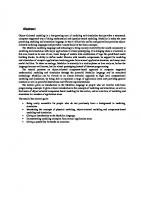
Application Example – Industry Robot k2 i qddRef

qdRef

qRef

1

1

S

S

k1

cut joint

r3Control r3Motor

axis6

tn

r3Drive1 1

i

qd

axis5

l qdRef

Kd

S rel

0.03 Jmotor=J

pSum

-

Kv 0.3

sum

w Sum

+1 +1

-

rate2

rate3

b(s)

340.8

a(s)

S

joint=0

axis4

S

iRef

gear=i

fric=Rv0

qRef

spring=c

axis3 rate1

tacho2

b(s)

b(s)

a(s)

a(s)

tacho1 PT1

axis2

g5

q

C=0.004*D/w m

Rd1=100

Rp1=200

Rd2=100 Ri=10

-

-

+ diff

+ pow er

+ OpI

Ra=250 La=(250/(2*D*wm))

Rp2=50

qd

axis1

Vs

Rd4=100

emf

y x inertial

Rd3=100

Srel = n*transpose(n)+(identity(3)- n*transpose(n))*cos(q)skew(n)*sin(q); g3 wrela = n*qd; g1 zrela = n*qdd; Sb = Sa*transpose(Srel); r0b = r0a; hall1 vb = Srel*va; wb = Srel*(wa + wrela); g4 ab = Srel*aa; qd g2 zb = Srel*(za + zrela + cross(wa, wrela)); hall2

w

r

q

Courtesy of Martin Otter

20

Copyright © Peter Fritzson

pelab

GTX Gas Turbine Power Cutoff Mechanism

Hello

Courtesy of Siemens Industrial Turbomachinery AB

21

Copyright © Peter Fritzson

Developed by MathCore for Siemens

pelab

Modelica – The Next Generation Modeling Language

22

Copyright © Peter Fritzson

pelab

Stored Knowledge Model knowledge is stored in books and human minds which computers cannot access “The change of motion is proportional to the motive force impressed “ – Newton

23

Copyright © Peter Fritzson

pelab

The Form – Equations • Equations were used in the third millennium B.C. • Equality sign was introduced by Robert Recorde in 1557

Newton still wrote text (Principia, vol. 1, 1686)

“The change of motion is proportional to the motive force impressed ” CSSL (1967) introduced a special form of “equation”: variable = expression v = INTEG(F)/m Programming languages usually do not allow equations! 24

Copyright © Peter Fritzson

pelab

Modelica – The Next Generation Modeling Language Declarative language Equations and mathematical functions allow acausal modeling, high level specification, increased correctness

Multi-domain modeling Combine electrical, mechanical, thermodynamic, hydraulic, biological, control, event, real-time, etc...

Everything is a class Strongly typed object-oriented language with a general class concept, Java & MATLAB-like syntax

Visual component programming Hierarchical system architecture capabilities

Efficient, non-proprietary Efficiency comparable to C; advanced equation compilation, e.g. 300 000 equations, ~150 000 lines on standard PC 25

Copyright © Peter Fritzson

pelab

Modelica – The Next Generation Modeling Language High level language MATLAB-style array operations; Functional style; iterators, constructors, object orientation, equations, etc.

MATLAB similarities MATLAB-like array and scalar arithmetic, but strongly typed and

efficiency comparable to C.

Non-Proprietary • Open Language Standard • Both Open-Source and Commercial implementations

Flexible and powerful external function facility • LAPACK interface effort started

26

Copyright © Peter Fritzson

pelab

Modelica Language Properties • Declarative and Object-Oriented • Equation-based; continuous and discrete equations • Parallel process modeling of real-time applications, according to synchronous data flow principle • Functions with algorithms without global side-effects (but local data updates allowed) • Type system inspired by Abadi/Cardelli • Everything is a class – Real, Integer, models, functions, packages, parameterized classes.... 27

Copyright © Peter Fritzson

pelab

Object Oriented Mathematical Modeling with Modelica • The static declarative structure of a mathematical model is emphasized • OO is primarily used as a structuring concept • OO is not viewed as dynamic object creation and sending messages • Dynamic model properties are expressed in a declarative way through equations. • Acausal classes supports better reuse of modeling and design knowledge than traditional classes 28

Copyright © Peter Fritzson

pelab

Brief Modelica History • First Modelica design group meeting in fall 1996 • International group of people with expert knowledge in both language design and physical modeling • Industry and academia

• Modelica Versions • 1.0 released September 1997 • 2.0 released March 2002 • Latest version, 2.2 released March 2005

• Modelica Association established 2000 • Open, non-profit organization 29

Copyright © Peter Fritzson

pelab

Modelica Conferences • The 1st International Modelica conference October, 2000 • The 2nd International Modelica conference March 1819, 2002 • The 3rd International Modelica conference November 5-6, 2003 in Linköping, Sweden • The 4th International Modelica conference March 6-7, 2005 in Hamburg, Germany • The 5th International Modelica conference planned September 4-5, 2006 in Vienna, Austria

30

Copyright © Peter Fritzson

pelab

Modelica Classes and Inheritance

1

pelab

Copyright © Peter Fritzson

Simplest Model – Hello World! A Modelica “Hello World” model Equation: x’ = - x Initial condition: x(0) = 1

class HelloWorld "A simple equation" Real x(start=1); equation der(x)= -x; end HelloWorld;

Simulation in OpenModelica environment 1

simulate(HelloWorld, stopTime = 2) plot(x)

0.8 0.6 0.4 0.2

0.5

2

1

Copyright © Peter Fritzson

1.5

2

pelab

Another Example Include algebraic equation Algebraic equations contain no derivatives

class DAEexample Real x(start=0.9); Real y; equation der(y)+(1+0.5*sin(y))*der(x) = sin(time); x - y = exp(-0.9*x)*cos(y); end DAEexample;

Simulation in OpenModelica environment 1.20

simulate(DAEexample, stopTime = 1) plot(x)

1.15 1.10 1.05

time

1.0 0.95

0.2

0.4

0.6

0.8

1

0.90

3

pelab

Copyright © Peter Fritzson

Example class: Van der Pol Oscillator class VanDerPol "Van der Pol oscillator model" Real x(start = 1) "Descriptive string for x"; // Real y(start = 1) "y coordinate"; // parameter Real lambda = 0.3; equation der(x) = y; // This is the der(y) = -x + lambda*(1 - x*x)*y; /* This is the end VanDerPol;

x starts at 1 y starts at 1

1st diff equation // 2nd diff equation */

2

simulate(VanDerPol,stopTime = 25) plotParametric(x,y)

1

-2

-1

1

2

-1

-2

4

Copyright © Peter Fritzson

pelab

Small Exercise • Locate the HelloWorld model in DrModelica using OMNotebook! • Simulate and plot the example. Do a slight change in the model, re-simulate and re-plot. class HelloWorld "A simple equation" Real x(start=1); equation der(x)= -x; end HelloWorld;

simulate(HelloWorld, stopTime = 2) plot(x)

• Locate the VanDerPol model in DrModelica and try it! 5

Copyright © Peter Fritzson

pelab

Variables and Constants Built-in primitive data types Boolean true or false Integer Integer value, e.g. 42 or –3 Real Floating point value, e.g. 2.4e-6 String String, e.g. “Hello world” Enumeration Enumeration literal e.g. ShirtSize.Medium

6

Copyright © Peter Fritzson

pelab

Variables and Constants cont’ • • • •

Names indicate meaning of constant Easier to maintain code Parameters are constant during simulation Two types of constants in Modelica • constant • parameter constant constant constant parameter

7

Real String Integer Real

PI=3.141592653589793; redcolor = "red"; one = 1; mass = 22.5;

pelab

Copyright © Peter Fritzson

Comments in Modelica 1) Declaration comments, e.g. Real x "state variable"; class VanDerPol "Van der Pol oscillator model" Real x(start = 1) "Descriptive string for x”; // Real y(start = 1) "y coordinate”; // parameter Real lambda = 0.3; equation // This is the der(x) = y; der(y) = -x + lambda*(1 - x*x)*y; /* This is the end VanDerPol;

x starts at 1 y starts at 1

1st diff equation // 2nd diff equation */

2) Source code comments, disregarded by compiler 2a) C style, e.g. /* This is a C style comment */ 2b) C++ style, e.g. // Comment to the end of the line…

8

Copyright © Peter Fritzson

pelab

A Simple Rocket Model apollo13

thrust mg

new model parameters (changeable before the simulation) floating point type

differentiation with regards to time

9

thrust − mass ⋅ gravity mass mass ′ = − massLossRate ⋅ abs ( thrust ) acceleration =

Rocket

altitude′ = velocity velocity ′ = acceleration

class Rocket "rocket class" parameter String name; Real mass(start=1038.358); Real altitude(start= 59404); Real velocity(start= -2003); Real acceleration; Real thrust; // Thrust force on rocket Real gravity; // Gravity forcefield parameter Real massLossRate=0.000277; equation (thrust-mass*gravity)/mass = acceleration; der(mass) = -massLossRate * abs(thrust); der(altitude) = velocity; der(velocity) = acceleration; end Rocket;

declaration comment

start value

name + default value mathematical equation (acausal)

pelab

Copyright © Peter Fritzson

Celestial Body Class A class declaration creates a type name in Modelica class CelestialBody constant Real parameter Real parameter String parameter Real end CelestialBody;

g = 6.672e-11; radius; name; mass;

An instance of the class can be declared by prefixing the type name to a variable name

... CelestialBody moon; ...

The declaration states that moon is a variable containing an object of type CelestialBody

10

Copyright © Peter Fritzson

pelab

Moon Landing Rocket

apollo13

thrust

apollo. gravity =

mg altitude

CelestialBody

only access inside the class access by dot notation outside the class

11

moon. g ⋅ moon.mass (apollo.altitude + moon.radius )2

class MoonLanding parameter Real force1 = 36350; parameter Real force2 = 1308; protected parameter Real thrustEndTime = 210; parameter Real thrustDecreaseTime = 43.2; public Rocket apollo(name="apollo13"); CelestialBody moon(name="moon",mass=7.382e22,radius=1.738e6); equation apollo.thrust = if (time < thrustDecreaseTime) then force1 else if (time < thrustEndTime) then force2 else 0; apollo.gravity=moon.g*moon.mass/(apollo.altitude+moon.radius)^2; end MoonLanding;

pelab

Copyright © Peter Fritzson

Simulation of Moon Landing simulate(MoonLanding, stopTime=230) plot(apollo.altitude, xrange={0,208}) plot(apollo.velocity, xrange={0,208}) 30000 50 25000

100

150

200

-100

20000 -200

15000 10000

-300

5000

-400 50

100

150

200

It starts at an altitude of 59404 (not shown in the diagram) at time zero, gradually reducing it until touchdown at the lunar surface when the altitude is zero 12

Copyright © Peter Fritzson

The rocket initially has a high negative velocity when approaching the lunar surface. This is reduced to zero at touchdown, giving a smooth landing

pelab

Restricted Class Keywords • The class keyword can be replaced by other keywords, e.g.: model, record, block, connector, function, ... • Classes declared with such keywords have restrictions • Restrictions apply to the contents of restricted classes • Example: A model is a class that cannot be used as a connector class • Example: A record is a class that only contains data, with no equations • Example: A block is a class with fixed input-output causality model CelestialBody constant Real parameter Real parameter String parameter Real end CelestialBody; 13

g = 6.672e-11; radius; name; mass;

pelab

Copyright © Peter Fritzson

Modelica Functions • Modelica Functions can be viewed as a special kind of restricted class with some extensions • A function can be called with arguments, and is instantiated dynamically when called • More on functions and algorithms later in Lecture 4 function sum input Real arg1; input Real arg2; output Real result; algorithm result := arg1+arg2; end sum;

14

Copyright © Peter Fritzson

pelab

Inheritance parent class to Color restricted kind of class without equations

child class or subclass keyword denoting inheritance

record ColorData parameter Real red = 0.2; parameter Real blue = 0.6; Real green; end ColorData; class Color extends ColorData; equation red + blue + green = 1; end Color;

class ExpandedColor parameter Real red=0.2; parameter Real blue=0.6; Real green; equation red + blue + green = 1; end ExpandedColor;

Data and behavior: field declarations, equations, and certain other contents are copied into the subclass

15

pelab

Copyright © Peter Fritzson

Inheriting definitions

record ColorData parameter Real red = 0.2; parameter Real blue = 0.6; Real green; end ColorData; class ErrorColor extends ColorData; parameter Real blue = 0.6; parameter Real red = 0.3; equation red + blue + green = 1; end ErrorColor;

16

Copyright © Peter Fritzson

Legal! Identical to the inherited field blue

Illegal! Same name, but different value

Inheriting multiple identical definitions results in only one definition

Inheriting multiple different definitions of the same item is an error

pelab

Inheritance of Equations class Color parameter Real red=0.2; parameter Real blue=0.6; Real green; equation red + blue + green = 1; end Color;

Color is identical to Color2 Same equation twice leaves one copy when inheriting

class Color2 // OK! extends Color; equation red + blue + green = 1; end Color2;

class Color3 // Error! extends Color; equation red + blue + green = 1.0; // also inherited: red + blue + green = 1; end Color3;

17

Color3 is overdetermined Different equations means two equations!

pelab

Copyright © Peter Fritzson

Multiple Inheritance Multiple Inheritance is fine – inheriting both geometry and color class Color parameter Real red=0.2; parameter Real blue=0.6; Real green; equation red + blue + green = 1; end Color;

class Point Real x; Real y,z; end Point;

multiple inheritance

class ColoredPointWithoutInheritance Real x; Real y, z; parameter Real red = 0.2; parameter Real blue = 0.6; Real green; equation red + blue + green = 1; end ColoredPointWithoutInheritance;

18

Copyright © Peter Fritzson

class ColoredPoint extends Point; extends Color; end ColoredPoint;

Equivalent to

pelab

Multiple Inheritance cont’ Only one copy of multiply inherited class Point is kept class Point Real x; Real y; end Point;

class VerticalLine extends Point; Real vlength; end VerticalLine;

Diamond Inheritance

class HorizontalLine extends Point; Real hlength; end HorizontalLine;

class Rectangle extends VerticalLine; extends HorizontalLine; end Rectangle;

19

pelab

Copyright © Peter Fritzson

Simple Class Definition – Shorthand Case of Inheritance • Example: class SameColor = Color;

Equivalent to: inheritance

20

class SameColor extends Color; end SameColor;

Copyright © Peter Fritzson

• Often used for introducing new names of types: type Resistor = Real; connector MyPin = Pin;

pelab

Inheritance Through Modification • Modification is a concise way of combining inheritance with declaration of classes or instances • A modifier modifies a declaration equation in the inherited class • Example: The class Real is inherited, modified with a different start value equation, and instantiated as an altitude variable: ... Real altitude(start= 59404); ...

21

pelab

Copyright © Peter Fritzson

The Moon Landing Example Using Inheritance Rocket thrust

apollo13

mg altitude

CelestialBody

model Body "generic body" Real mass; String name; end Body; model CelestialBody extends Body; constant Real g = 6.672e-11; parameter Real radius; end CelestialBody;

22

Copyright © Peter Fritzson

model Rocket "generic rocket class" extends Body; parameter Real massLossRate=0.000277; Real altitude(start= 59404); Real velocity(start= -2003); Real acceleration; Real thrust; Real gravity; equation thrust-mass*gravity= mass*acceleration; der(mass)= -massLossRate*abs(thrust); der(altitude)= velocity; der(velocity)= acceleration; end Rocket;

pelab

The Moon Landing Example using Inheritance cont’ inherited parameters

model MoonLanding parameter Real force1 = 36350; parameter Real force2 = 1308; parameter Real thrustEndTime = 210; parameter Real thrustDecreaseTime = 43.2; Rocket apollo(name="apollo13", mass(start=1038.358) ); CelestialBody moon(mass=7.382e22,radius=1.738e6,name="moon"); equation apollo.thrust = if (time