Introduction to Differential Geometry and Riemannian Geometry 0802015018, 9780802015013

Citation preview

INTRODUCTION TO DIFFERENTIAL GEOMETRY AND RIEMANNIAN GEOMETRY ERWIN KREYSZIG

Erwin Kreyszig has held mathematical teaching and research positions at universities in Germany, Canada, and the United States and now is teaching at the University of Windsor, Windsor, Ontario. He has published many papers on mathematical research in North American and European journals, in the fields of both pure and applied mathematics. This book provides an introduction to the differential geometry of curves and surfaces in three-dimensional Euclidean space and to n-dimensional Riemannian geometry. Based on Kreyszig's earlier book Differential Geometry, it is presented in a simple and understandable manner with many examples illustrating the ideas, methods, and results. Among the topics covered are vector and tensor algebra, the theory of surfaces, the formulae of Weingarten and Gauss, geodesies, mappings of surfaces and their applications, and global problems. A thorough investigation of Reimannian manifolds is made, including the theory of hypersurfaces. Interesting problems are provided and complete solutions are given at the end of the book together with a list of the more important formulae. Elementary calculus is the sole prerequisite for the understanding of this detailed and complete study in mathematics.

MATHAMATICAL EXPOSITIONS Editorial Board H.S.M. COXETER, G.F.D. DUFF, D.A.S. FRASER, G. de B. ROBINSON (Secretary), P.G. ROONEY Volumes Published 1 The Foundations of Geometry G. de B. ROBINSON 2 Non-Euclidean Geometry H.S.M. COXETER 3 The Theory of Potential and Spherical Harmonics WJ. STERNBERG and T.L. SMITH 4 The Variational Principles of Mechanics CORNELIUS LANCZOS 5 Tensor Calculus J.L. SYNGE and A.E. SCHILD 6 The Theory of Functions of a Real Variable R.L. JEFFERY 7 General Topology WACLAW SIERPINSKI (translated by C. CECILIA KRIEGER) (out of print) 8 Bernstein Polynomials G.G. LORENTZ (out of print) 9 Partial Differential Equations G.F.D. DUFF 10 Variational Methods for Eigenvalue Problems S.H. GOULD 11 Differential Geometry ERWIN KREYSZIG (out of print) 12 Representation Theory of the Symmetric Group G. de B. ROBINSON 13 Geometry of Complex Numbers HANS SCHWERDTFEGER 14 Rings and Radicals N.J. DIVINSKY 15 Connectivity in Graphs W.T. TUTTE 16 Introduction to Differential Geometry and Riemannian Geometry ERWIN KREYSZIG 17 Mathematical Theory of Dislocations and Fracture R.W. LARDNER 18 n-gons FRIEDRICH BACHMANN and ECKART SCHMIDT (translated by CYRIL W.L. GARNER) 19 Weighing Evidence in Language and Literature: A Statistical Approach BARRON BRAINERD 20 Rudiments of Plane Affine Geometry P. SCHERK and R. LINGENBERG

MATHEMATICAL EXPOSITIONS No. 16

Introduction to

Differential Geometry and

Riemannian Geometry ERWIN KREYSZIG

UNIVERSITY OF TORONTO PRESS

ORIGINAL GERMAN EDITION PUBLISHED BY AKADEMISCHE VERLAGSGESELLSCHAFT, LEIPZIG, ENGLISH TRANSLATION © UNIVERSITY OF TORONTO PRESS TORONTO AND BUFFALO

ISBN 0-8020-1501-8 LC 68-108147

1968

1967

DEDICATED TO

PROFESSOR S. BERGMAN Stanford University

This page intentionally left blank

PREFACE THIS BOOK provides an introduction to the differential geometry of curves and surfaces in three-dimensional Euclidean space and to n-dimensional Riemannian geometry. Elementary calculus is the sole prerequisite. The elements of vector algebra and vector calculus are considered in Chapter I and are then used throughout the book. Chapter II is devoted to the theory of space curves. Then we introduce the notion of a surface and develop the foundations of the theory of surfaces, starting with considerations related to the first and second fundamental forms (Chapters III and IV). In Chapter V we define and explain the notion of a tensor and the basic operations of tensor algebra, which constitutes a convenient tool in the further chapters on surface theory and Riemannian geometry. These geometrical applications of tensors will lead to a better understanding of the ideas involved in tensor methods, and will also be profitable for certain branches of physics and engineering in which tensors are of increasing importance. Of course we should always keep in mind that the purpose of tensor algebra and calculus lies in its applications to certain problems. It is a tool only, albeit a very powerful one. The remaining part of surface theory includes the important formulae of Weingarten and Gauss (Chapter VI), geodesies (Chapter VII), mappings of surfaces and their applications (Chapters VIII and IX), global problems (Chapter X), tensor calculus on surfaces and the parallelism of Levi-Civita (Chapter XI), and special surfaces (Chapter XII) such as minimal surfaces, modular surfaces, and envelopes of families of surfaces. The last four chapters of the book are devoted to Riemannian geometry. The notions of a differentiate manifold and a Riemannian manifold are introduced and explained in Chapter XIII. Absolute differentiation and affine connections on differentiable manifolds are considered in Chapter XIV. Chapter XV includes an investigation of geometrical properties of submanifolds of Riemannian manifolds. The theory of hypersurfaces is developed in Chapter XVI, and the reader will see that several concepts and methods in that chapter are generalizations resulting from the theory of surfaces. Differential geometry is a particularly attractive subject because of its relation to differential equations, the calculus of variations, complex analysis, topology, and other fields of mathematics. It is of practical importance in that it constitutes an essential part of the foundation of some applied sciences, for instance physics, geodesy, and geography. We shall illustrate the universal character of differential geometry on several occasions.

viii

PREFACE

The book will have a German counterpart, which is now in press at the Akademische Verlagsgesellschaft, Leipzig, and will be included in the series "Mathematik und ihre Anwendungen in Physik und Technik." In preparing the book I evaluated the results of various discussions with colleagues, in particular O. Biberstein, H. S. M. Coxeter, G. F. D. Duff, R. C. Fisher, C. Loewner, H.-W. Pu, T. Rado, P. Scherk, and J. P. Spencer. Valuable suggestions were made by M. Earner, H. Behnke, S. Bergman, R. Domiaty, H. Florian, H. Graf, H. Kneser, M. Pinl, M. Riesz, P. Tschupik, and H. Wielandt. I wish to thank all these gentlemen for their help. Last but not least I wish to thank the University of Toronto Press for their helpful cooperation. E. K. Columbus, Ohio February 1967

CONTENTS PREFACE

vii

IMPORTANT NOTATIONS

3

I. PRELIMINARIES 1. Nature and purpose of differential geometry 2. Topological and metric spaces. Mappings 3. Coordinates in R3. Transformation groups. Equivalence 4.Vectors in Euclidean spave R3 5. Basic rules of vector algebra and calculus in R3

5 5 8 12 14

II. THEORY OF CURVES 6. 7. 8. 9. 10. 11. 12. 13. 14. 15.

Concept of a curve in differential geometry Examples Some remarks on the concept of a curve Arc length Tangent vector, principal normal vector, and binormal vector. Curvature Torsion. Formulae of Frenet Local shape of a curve (canonical representation) Natural equations of a curve Contact. Circle of curvature, osculating sphere Involutes and evolutes

20 23 25 28 31 36 40 42 47 52

III. NOTION OF A SURFACE. FIRST FUNDAMENTAL FORM 16. 17. 18. 19. 20.

Portion of a surface Surface Examples Curves on a surface, Tangent plane. Normal Measurement of lengths and angles. First fundamental form. Summation convention 21. Area 22. Remarks on the definition of area

55 58 61 63 67 72 75

IV. SECOND FUNDAMENTAL FORM. GAUSSIAN AND MEAN CURVATURE 23. 24. 25. 26. 27. 28. A*

Second fundamental form Arbitrary and normal sections of a surface Elliptic, parabolic, and hyperbolic points of a surface Asymptotic lines Principal curvature, lines of curvature, Gaussian and mean curvature Euler's theorem. Dupin's indicatrix

78 81 84 88 89 95

x

CONTENTS

V. TENSORS 29. Allowable coordinate transformations 30. Contravariant and covariant vectors 31. Tensors of second order 32. Tensors of arbitrary order 33. Addition, multiplication, and contraction 34. Special tensors on surfaces 35. Vectors in the tangent plane of a surface 36. Vector spaces and their tensor products

101 102 106 109 111 113 115 119

VI. FORMULAE OF WEINGARTEN AND GAUSS 37. Formulae of Weingarten 38. Formulae of Gauss 39. Properties of the Christoffel symbols 40. Transformation behaviour of the Christoffel symbols 41. Riemann curvature tensor

125 127 128 131 133

VII. GEODESIC CURVATURE. GEODESICS 42. Geodesic curvature 43. Geodesies 44. Arcs of minimum length 45. Geodesic parallel coordinates 46. Geodesic polar coordinates 47. Surfaces of constant Gaussian curvature 48. Spherical surfaces of revolution 49. Pseudospherical surfaces of revolution

137 140 143 145 148 151 153 155

VIII. ISOMETRIC MAPPING OF SURFACES 50. Preliminaries 51. Isometric mapping 52. Isometry of surfaces of constant Gaussian curvature 53. Bending. Intrinsic geometry 54. Ruled surfaces, developable surfaces 55. Spherical image. Isometric mapping of developable surfaces 56. Conjugate directions. Developable surfaces having contact with a given surface IX. FURTHER MAPPINGS OF SURFACES 57. Conformal mapping 58. Conformal mapping of surfaces in the plane 59. Isotropic curves and isothermic coordinates 60. Conformal mapping of a sphere into a plane. Stereographic and Mercator projection 61. The Bergman metric 62. Equiareal mapping 63. Equiareal mapping of spheres into planes. Mappings of Lambert, Sanson, and Bonne 64. Geodesic mapping

161 161 164 165 167 172 175

180 182 186 188 192 196 198 201

CONTENTS

xi

X. TOPICS FROM GLOBAL DIFFERENTIAL GEOMETRY 65. Compact and complete surfaces 66. Umbilics 67. Hilbert's lemma 68. Characteristic properties of spheres 69. Theorem of Gauss and Bonnet. Integral curvature 70. Generalizations of the theorem of Gauss and Bonnet 71. Application of the theorem of Gauss and Bonnet to closed surfaces

204 206 207 208 209 210 213

XI. ABSOLUTE DIFFERENTIATION AND CONNEXIONS ON SURFACES 72. Absolute differentiation of contravariant vectors 73. Absolute differentiation of covariant vectors 74. Absolute differentiation of arbitrary tensors 75. Properties of absolute differentiation 76. Interchange of the order of absolute differentiation 77. Differential operators of Beltrami 78. Connexion of Levi-Civita 79. Properties of the connexion of Levi-Civita 80. Geometrical interpretation of the connexion of Levi-Civita

215 218 220 222 223 225 228 231 233

XII. SPECIAL SURFACES 81. Minimal surfaces 82. Examples of minimal surfaces 83. Minimal surfaces and complex analysis 84. Minimal surfaces as translation surfaces with isotropic generators 85. Modular surfaces of analytic functions 86. Envelope of a one-parameter family of surfaces 87. Developable surfaces as envelopes of families of planes 88. Envelope of the osculating, normal, and rectifying planes of a curve, polar surface 89. Centre surfaces of a surface 90. Surfaces of constant Gaussian curvature and non-Euclidean geometry 91. Geodesic mapping of surfaces of constant Gaussian curvature

261 263 265 272

XIII. FOUNDATIONS OF RIEMANNIAN GEOMETRY 92. Differentiate manifolds 93. Submanifolds 94. Curves in a manifold 95. Tangent spaces of a manifold 96. Riemannian manifolds

275 277 277 278 280

XIV. ABSOLUTE DIFFERENTIATION AND CONNEXION 97. Absolute differentiation of tensors 98. Affine connexions 99. Curvature tensor, interchange of the order of differentiation 100. Displacement around closed curves 101. Autoparallel curves 102. Riemannian connexion

283 286 289 292 295 298

236 238 241 244 246 252 259

xii

CONTENTS

XV. FURTHER PROPERTIES OF RIEMANNIAN MANIFOLDS 103. Submanifolds of Riemannian manifolds 104. Connexion in submanifolds 105. Generalization of the formulae of Frenet 106. Riemannian curvature 107. Mean curvature of a manifold 108. Identities of Bianchi 109. Riemannian manifolds of constant curvature

301 303 305 306 309 311 311

XVI. HYPERSURFACES 110. Formulae of Gauss and second fundamental form of a hypersurface 111. Formulae of Weingarten for a hypersurface 112. Generalized covariant derivative in a hypersurface 113. Application to the formulae of Gauss and Weingarten 114. Normal curvature of a hypersurface 115. Principal directions of a tensor. Principal curvatures

314 316 318 320 322 323

ANSWERS TO ODD-NUMBERED PROBLEMS

327

COLLECTION OF FORMULAE

338

BIBLIOGRAPHY

359

INDEX

365

INTRODUCTION TO DIFFERENTIAL GEOMETRY AND RIEMANNIAN GEOMETRY

This page intentionally left blank

IMPORTANT NOTATIONS (For a collection of formulae, see the end of the book.) Page 8 x1 x 2, x3 : Cartesian coordinates in Euclidean space R3. 12 Boldface letters a, y, etc.: Vectors in space R3. The components of these vectors will be denoted by al9 a2, a3 ; yi9 y29 y3 ; etc. 29 s: Arc length of a curve. Derivatives with respect to s will be denoted by primes, e.g. An arbitrary parameter in the representation of a curve will usually be denoted by t and derivatives with respect to t will be characterized by dots, e.g. 31 33 33 32 36 58

t -= x' : Unit tangent vector of a curve C: \(s). p = x'7|x"|: Unit principal normal vector of that curve. b = t x p: Unit binormal vector of that curve. K = |t'| = 1/p: Curvature, p being the radius of curvature of a curve. T : Torsion of a curve. w 1 , u2 : Coordinates on a surface,

56

n : Unit normal vector to a surface, n j = 8n/8uJ, etc. Summation convention. If a letter appears twice, once as superscript and once as subscript, summation must be carried out with respect to that letter. The summation sign S will then be omitted. In the theory of surfaces this summation runs from 1 to 2, and in the case of w-dimensional spaces it runs from 1 to n. See examples in Section 20. 102 Superscript: Contravariant index. 104 Subscript: Covariant index. 68 dx-dx = gjk dujduk: First fundamental form. 68 gjk : Metric tensor, fundamental tensor. 70 g: Discriminant of the first fundamental form. In the case of a surface, g = 811822 -fen) 2 jk 1 1 3 g : Contravariant components of the metric tensor, 64 69

4

DIFFERENTIAL AND RIEMANNIAN GEOMETRY

Page

79 172 82 91 91 307 92 137 127 127 284 134 218

—dx'dn = bjk dujduk: Second fundamental form. dn-dn = cjk dujduk : Third fundamental form. KH = l/R: Normal curvature of a surface. Ki9 K2: Principal curvatures of a surface. K = iq K2 : Gaussian curvature of a surface. K: Riemannian curvature. H=(Ki + K2)/2: Mean curvature of a surface. Kg : Geodesic curvature of a curve on a surface. Tijk: Christoffel symbols of the first kind. r f y k : Christoffel symbols of the second kind. Gtjk: Components of a connexion. Rijkh Wjki'- Curvature tensors. aj k, ajk, etc. : Covariant derivatives.

I PRELIMINARIES

SECTION 1 will give the reader some idea and first impression of the field to which this book is devoted. The other sections of this chapter include some basic notions from topology and a collection of formulae from vector algebra and calculus which we shall use frequently. 1. Nature and purpose of differential geometry. Differential geometry is concerned with the application of differential and integral calculus to the investigation of geometric properties of point sets (curves and surfaces in Euclidean space R3 and similar point sets in spaces of higher dimension). A geometric property is called local if it does not pertain to the geometric configuration as a whole but depends only on the shape of the configuration in an (arbitrarily small) neighbourhood of a point under consideration. For instance, the curvature of a curve is a local property. Since differential geometry is concerned mainly with local properties, it is primarily a geometry in the small or a local geometry. This does not exclude the possibility of considering a geometric configuration as a whole. Such an investigation belongs to what is called global differential geometry or differential geometry in the large. We may say that global problems are problems in which "macroscopic" properties are related to "microscopic" ones. Chapter X will be devoted to this subject. The study of differential geometry was begun very early in history because it was obvious that calculus could be applied to geometrical problems. Practical tasks in cartography and geodesy caused and influenced the creation of the classical theory of surfaces. Riemannian geometry became of great practical interest because of the theory of relativity, in which it serves as a basic tool. Its modern development is strongly influenced by progress in topology and in complex analysis of functions of several variables. In this book we shall, in general, confine ourselves to real configurations but shall occasionally extend our methods to the complex domain also. 2. Topological and metric spaces. Mappings. We shall now consider some general basic definitions, starting with point sets in three-dimensional Euclidean space R3. Let P be an arbitrary point in Rz. The set of all points whose distance from P is smaller than a positive number 77 is called an open spherical neighbourhood of

6

DIFFERENTIAL AND R I E M A N N I A N GEOMETRY

P. Obviously this set consists of all the points in the interior of a sphere of radius y with centre at P. A point set N in R3 is called a neighbourhood of a point P if N contains an open spherical neighbourhood of P. A point set M in R3 is called open if each point of M has a neighbourhood all of whose points belong to M". The union of arbitrarily many open sets is an open set, and so is the intersection of finitely many open sets. Using these properties we may now introduce a very general concept of space, as follows. A set X, together with a collection Q of subsets of X, called open sets, is called a topological space if Q satisfies the following axioms: Al. The set X and the empty set (i.e. the set that has no element) belong to Q. A2. The union of arbitrarily many sets ofCl belongs to Q. A3. The intersection of finitely many sets of£l belongs to Q. The elements of X are called the points of the topological space, and the collection Q is called a topology for X. Let P be any point of X. Then a set N containing an open set to which P belongs is called a neighbourhood of P. A neighbourhood of P need not be open, but it contains an open neighbourhood of P. Every open set is a neighbourhood of all of its points. If any two distinct points P and Q of a topological space X have disjoint neighbourhoods NP and NQ9 respectively, then X is called a Hausdorff space. The Euclidean space R3 is a Hausdorff space. In fact, if any two points P and Q in R3 have the distance d(P, 0, we obtain two corresponding disjoint neighbourhoods by choosing 77 = d(P, 0/3 in the above definition. In R3 the distance d(P, Q) of two points P and Q has the following properties: Ml. d(P, 0 is real,finite,and non-negative. M2. d(P9 0 - 0 if and only ifP = Q. M3.d(P,Q) = d(Q,P). M4. d(P, Q) < d(P, R) + d(R, Q\ where R is any other point in R3. The inequality in M4 is called the triangle inequality. The function d(P9 Q) depends on P and Q and is called the distance function. It defines a metric in ^3. These four properties may be used for introducing another important notion of space in an axiomatic fashion as follows. Suppose that with any two elements P and Q of a set X there is associated a number d(P9 Q) satisfying the axioms M1-M4. Then A" is called a metric space. Its elements are called points. d(P, Q) is called the distance between the points P and Q.

PRELIMINARIES

7

Let P be any point of a metric space X. Then the set of all points of X whose distance from P is less than a positive number 77 is called an open spherical neighbourhood of P, and 77 is called the radius of this neighbourhood. A set N containing an open spherical neighbourhood of P is called a neighbourhood of P. A point set M of a metric space Xis said to be open if each point of M has a neighbourhood all of whose points belong to M. Using this definition of open sets in a metric space X it can be shown that the totality Q of these sets in X satisfies the axioms A1-A3. Hence a metric space is a topological space, even a Hausdorff space. We shall now consider the notion of mapping and related concepts which are of basic importance in differential geometry. Let M and M* be two point sets. Suppose that there is given a rule T which associates with every point P of M a point P* of M*. Then we say that a mapping or a transformation of the set M into the set M* is given. We write and P* = TP. The point P* is called the image point of P, and P is called an inverse image point of P*. The set M of the image points of all the points of M is called the image of M . We write If every point of M* is an image point of at least one point of M, the mapping is called a mapping of M onto M* or a surjective mapping. A mapping of M into M * is said to be infective if any two distinct points of M have distinct image points in M*. If T is both surjective and injective, it is called a bijective mapping or a 0/je/0-0«e mapping of A/ onto M*. Then there exists the inverse mapping of T, denoted by T"1, which maps M* onto M such that every point P* of M* is mapped onto that point P of M which corresponds to P* with respect to the mapping T. We write andP- j-ip*. Let X and 7 be topological spaces. Suppose that there is given a mapping which maps A" into Y. This mapping T is said to be continuous at a point P of X if, for every neighbourhood NP* of the image P* of P, there exists a neighbourhood NP of P whose image is contained in NP*. The mapping is said to be continuous if it is continuous at every point of X. A one-to-one continuous mapping whose inverse is also continuous is called a topological mapping or a homeomorphism. Point sets in topological spaces

8

DIFFERENTIAL AND RIEMANNIAN GEOMETRY

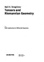
which can be mapped topologically onto each other are said to be homeomorphic. Topology may now be described as the study of the properties of configurations which are unaffected by topological mappings. A one-to-one mapping of two point sets in a metric space is called a motion if any two image points have the same distance as the corresponding inverse image points. Motions in ^3 will be considered in the next section. 3. Coordinates in R3. Transformation groups. Equivalence. For representing curves and surfaces in real Euclidean space ^3 we need suitable coordinate systems. We shall use right-handed orthogonal parallel coordinates xi9 x29 x3, as shown in Fig. 3.1 (a). Such a right-handed coordinate system will be called a Cartesian coordinate system in R3. The term right-handed is suggested by the fact that if the positive .^-direction is rotated into the positive x2-direction through the angle ir/2, the positive x3direction is the direction in which a right-handed screw would advance if turned in the same fashion. Similarly, a left-handed coordinate system (Fig. 3.1(6)) is such that if the positive jq-direction is rotated into the positive x2-direction through the angle 7r/2, the positive jc3-direction is the direction in which a left-handed screw would advance if turned in the same fashion.

(a) Right-handed system

(b) Left-handed system

Fig. 3.1. Orthogonal parallel coordinates

A Cartesian coordinate system being given, to each point P in R3 there corresponds an ordered triple (xl9 x2, x3) of real numbers xi9x29 x3 which are called the coordinates of P. Instead of (jq, x2, x3), we may also write (#,-). The coordinate system being fixed, the correspondence between the points in R3 and those triples of real numbers is one-to-one. Two points P and Q with coordinates (xj) and (yj), respectively, have the distance

(3.1) The Euclidean space R3 is a metric space with metric defined by the distance function (3.1).

PRELIMINARIES

9

Any other Cartesian coordinate system xl9 x2, x3 is related to that Cartesian *i *2 *3-system by a special linear transformation of the form (3.2) whose coefficients satisfy the conditions (3.3)

and

(3.4) 8kl is called the Kronecker symbol or Kronecker delta. The transition from one Cartesian coordinate system to another can be effected by a certain rigid motion of the axes of the original system. Such a motion is composed of a suitable translation and a suitable rotation. It is called a direct congruent transformation (or displacement). Special cases are the identity transformation

(3.5) under which the transformed coordinates are the same as the original ones, the translation or parallel displacement

(3.6) and the rotation represented by (3.2) with b^ = 0, b2 = 0, b3 = 0. This last transformation is also known as a direct orthogonal transformation. We also mention the notion of an opposite orthogonal transformation, which is composed of a rotation about the origin and a reflection in a plane. It is represented by (3.2) with b± = 0, b2 = 0, b3 = 0, satisfying (3.3) and det(a,k) = — 1. It transforms a right-handed coordinate system into a left-handed one and vice versa. A simple example is xl = —xl9x2 = x2, x3 = x3. Direct and opposite orthogonal transformations are called orthogonal transformations. A transformation which is composed of translations, rotations, and an odd number of reflections is called an opposite congruent transformation. Direct and opposite congruent transformations are called congruent transformations. The coefficients ajk in (3.2) form a three-rowed square matrix

(3.7)

10

DIFFERENTIAL AND R I E M A N N I A N GEOMETRY

A square matrix satisfying (3.3) and (3.4) (or (3.3) and det(a;k) = — 1) is called an orthogonal matrix. If we wish to investigate geometric facts analytically, we have to introduce a coordinate system. Consequently, a coordinate system is a useful tool but no more. A property of a geometric configuration consisting of points in R3 will be called geometric (in the sense of Euclidean geometry) if it is independent of the special choice of the Cartesian coordinates. In other words, a property of a configuration is called a geometric property if it is an invariant with respect to direct congruent transformations of the coordinate system, or, what is the same thing, with respect to direct congruent transformations of the configuration being considered. The notion of a geometric property may be considered from a more general point of view. For this purpose we shall use the concept of a group and mention an important connexion between geometry and group theory. We consider mappings of the form (3.8)

which are assumed to be one-to-one mappings of a three-dimensional space onto itself. If we apply two such mappings successively, for example (3.8) and we obtain the composite mapping A set G of mappings (3.8) is called a group of mappings or a transformation group if G has the following properties: 1. The identity mapping Xj = Xj (j = 1, 2, 3) is contained in G. 2. The inverse mapping T'1 of any mapping T contained in G is also an element ofG. 3. For any two (not necessarily distinct) mappings Tl9 T2 contained in G the composite mappings of these mappings are elements of G. A subset of mappings of a group G which constitutes a group is called a subgroup of G. For example, the congruent transformations form a group, and the direct congruent transformations form a subgroup of that group. By means of a transformation group G we may classify the geometric configurations (point sets) in R3 into equivalence classes, as follows. A configuration A is said to be equivalent or congruent to a configuration B with respect to G if G contains a mapping that maps A onto B. Then we write A ~ B(G) or simply

PRELIMINARIES

11

Then the equivalence class containing A consists of all the configurations that are equivalent to A with respect to G. Each such configuration is called a representative of that class. From the viewpoint of classification of configurations A, B, C,... into equivalence classes the group axioms become identical with the axioms of equivalence: 1. A~A.

2. If A ~ B, then B ~ A. 3. If A ~ B andB ~ C, then A ~ C. A property of a configuration is said to be geometric with respect to a transformation group G if it remains unaffected by every mapping contained in G, that is, if it is an invariant of G. In this fashion to each group G there corresponds a geometry which may be regarded as the theory of invariants of that group. This is the basic idea of the so-called Erlanger Programm of F. Klein [1],| which had considerable influence on the development of geometry. For example, Euclidean geometry is the theory of the invariants of the group of the afore-mentioned congruent transformations. Affine geometry corresponds to the group of affine transformations, i.e., transformations of the form (3.2) satisfying the condition det(ajk) 7^ 0, etc. An example of an invariant in Euclidean geometry is the distance (3.1). If a congruent transformation is imposed, the coordinates of P and Q will, in general, change their values while d(P, Q) remains unaffected. We should mention that the Erlanger Programm has certain limits. While it is useful for classical geometries (Euclidean, affine, projective, non-Euclidean, etc.) it does not apply to many Riemannian geometries (cf. Sec. 20) because in these cases the transformation groups that leave the metric invariant may consist of the identity transformation only. Attempts to generalize the Erlanger Programm by using holonomy groups (cf. Sec. 100) and invariants of connexions were made by E. Cartan [1], J. A. Schouten [1], and O. Veblen [1]. Problems 3.1-3.5. Do the following transformations form a group? 3.1. Translations. 3.2. Rotations about a fixed axis, the angle of every rotation being an integral multiple of 120°. 3.3. Opposite congruent transformations. 3.4. Translations x\ = x\, xi = *2, *3 = *3 + t where / > 0. 3.5. Orthogonal transformations. t Cf. the bibliography at the end of this book.

12

DIFFERENTIAL AND RIEMANNIAN GEOMETRY

3.6. Interpret the following transformations geometrically:

Determine the composite transformation. Compose the transformations in the opposite order (using a suitable change of notation). Is this composite transformation the same as before?

4. Vectors in Euclidean space R3. We shall now consider some basic facts about vectors in jR3 which we shall use in the theory of curves and surfaces. A line segment in R3 is uniquely determined by its end points. The segment is said to be directed if we designate one of those two points as the initial point and the other as the terminal point. A directed segment with initial point P and —> terminal point Q will be denoted by PQ. The correspondence between the ordered pairs of points (P9 Q) and the directed segments PQ in R3 is one-to-one. These directed segments may be classified into equivalence classes, as follows. A directed segment in R3 is said to be equivalent to another directed segment in R3 if both segments are parallel and have the same length and the same sense. An equivalence class consists of a directed segment and all the directed segments that are equivalent to that segment. Such an equivalence class of directed segments in R3 is called a vector in R3. The length of the segments is called the length of that vector. Each directed segment of the class is called a representative or a representation of the vector. Vectors in R3 will be denoted by lower-case bold-face letters, e.g. a, v, z, etc. The length of a vector a will be denoted by |a|. A vector of length 1 is called a unit vector. Let z be a given vector and let P be any point in R3. Then there exists precisely one directed segment PQ which represents z, and the transition to another representation of z corresponds to a translation of that segment. We may therefore say that a vector can be arbitrarily displaced parallel to itself] or, what amounts to the same thing, its initial point may be chosen arbitrarily. We now introduce in R3 a fixed Cartesian coordinate system and denote the coordinates of those points P and Q by (Xj) and (yj)9 respectively. From (3.6) we see that the differences (4.1) are invariant with respect to translations. These three numbers are called the components of the vector z represented by PQ with respect to that coordinate system, and we write z = (zl9 z2, z3). The coordinate system being fixed, to each vector there corresponds an ordered triple of real numbers. Conversely, to each such triple, except for the

PRELIMINARIES

13

triple (0, 0, 0), there corresponds a vector. To (0, 0, 0) we let correspond the so-called null vector, which is denoted by 0 and, by definition, has components 0, 0, 0 and length 0. This definition is independent of the particular choice of the coordinates, as we shall now see.

Fig. 4.1. Components of a vector in R$

To the transformation (3.2)-(3.4) of the coordinates there corresponds the transformation (4.2)

of the components of a vector z. Here zl9 z2, z3 are the components of z with respect to the jcj x2 Jc3-coordinate system. The transformation behaviour (4.2) is characteristic for vectors in R3 because it can be used for defining such vectors, as follows. By definition, a vector in ^3 is given if with every Cartesian coordinate system in R3 there is associated an ordered triple of real numbers (called the components of the vector in the corresponding coordinate system) such that two such triples corresponding to the coordinates in (3.2)-(3.4) are related by (4.2). While our above definition may be easier to grasp, the present definition has the advantage that it can be extended to more general spaces, as we shall see in Section 30. We have stated earlier in this section that a vector may be translated arbitrarily and that its initial point may be chosen arbitrarily. It is sometimes advantageous, however, to choose a certain fixed point P as the initial point of a vector. Then the vector is said to be bound at P. A vector whose initial point is left unspecified is sometimes called a free vector. A fixed Cartesian coordinate system being given, any point Q in space R3 is uniquely determined by its coordinates xl9 x29 x3. Now xi9 x2, x3 may be regarded as the components of a vector x whose initial point is the origin of that

14

DIFFERENTIAL AND R I E M A N N I A N GEOMETRY

coordinate system. Then Q is the terminal point of x, and x is called the position vector of Q with respect to that coordinate system (cf. Fig. 4.2). Note that the components of the position vector transform according to (3.2)-(3.4) and not (4.2) because under a coordinate transformation (3.2)-(3.4) the origin will change, in general.

Fig. 4.2. Position vector

5. Basic rules of vector algebra and calculus in ^3. A fixed Cartesian coordinate system in R3 being given, the correspondence between the vectors and the ordered triples of their components is one-to-one. It follows that two vectors a = (al9 a2, #3) and b = (bi9 b2, b3) are equal if and only if a^ = bl9 a2 — b29 a3 = b3. Hence a single vector equation is equivalent to three equations for the components. Addition of vectors is defined as follows. Represent two given vectors a and b —>• —> by directed segments PQ and QR, respectively (cf. Fig. 5.1). Then the vector represented by PR is called the sum of a and b and is denoted by a + b. has components This sum (5.1) Vector addition is commutative and associative, that is, For any vector a, Subtraction of vectors is defined to be the inverse operation of addition. Two vectors a and b being given, there exists a unique vector v such that a + v = b. This "difference vector" is denoted by v = b — a.

Fig. 5.1. Addition of vectors

Fig. 5.2. Multiplication of a vector by a number

PRELIMINARIES

15

Multiplication of a vector a by a number k is defined as follows. If a = 0 or k = 0, then the product A:a of k and a is the null vector 0. In any other case to is a vector of length \k\ |a| which has the direction of a if k is positive and has the direction opposite to that of a if k is negative. If a = («!, a2, a3), then fca = (kai9 ka2, ka3). Furthermore,

We mention that the vectors in R3 form a vector space. This notion will be considered in Section 36. The scalar product, dot product, or inner product of two vectors a and b is denoted by a • b and is defined as follows:

(5.2) Here a (0 < a < TT) is the angle between a and b (cf. Fig. 5.3).

Fig. 5.3. Scalar product of two vectors

Scalar multiplication is commutative and distributive with respect to addition, that is If a = (al9 a2, a3) and b = (bi9 b2, 63), then

(5.3)

Setting b = a in (5.2), we have (5.4)

If a 7^ 0 and b ^ 0, we thus obtain from (5.2) (5.5)

16

DIFFERENTIAL AND RIEMANNIAN GEOMETRY

Finally (5.2) yields the important Theorem 5.1 (Orthogonality). Two vectors, which are not equal to the null vector, are orthogonal if and only if their scalar product is zero. The vector product, cross product, or outer product of two vectors a and b is denoted by a x b and is a vector v defined as follows. If a and b have the same or opposite direction or one of these vectors is the null vector, then v = 0. In any other case, v is the vector whose length is

(5.6) and whose direction is orthogonal to both a and b and is such that a, b, v, in this order, form a right-handed triple or right-handed triad, as shown in Fig. 5.4. Here a is the angle between a and b. From (5.6) we see that |v| is equal to the area of the parallelogram with a and b as adjacent sides (cf. Fig. 5.4). Cross-multiplication of vectors is not commutative but anticommutative, because (5.7)

It is not associative. This follows from (5.8)

It is distributive with respect to addition, that is,

(5.9) Furthermore, from the definition it follows that (5.10) If with respect to Cartesian coordinates (which are right-handed, by definition), a = (al9 a29 a3) and b = (bl9 b2, 63), then (5.11) where e j is the unit vector in the positive direction of the jth coordinate axis. Hence v has the components In the case of a left-handed system of orthogonal parallel coordinates we must write a minus sign in front of the determinant in (5.11).

PRELIMINARIES

17

The scalar product of two vector products satisfies the following identity of Lag range: (5.12)

(a x b) • (c x d) = (a • c)(b • d) - (a • d)(b • c).

From this and (5.4) we obtain (5.13)

Fig. 5.4. Vector product

Fig. 5.5. Geometrical interpretation of the scalar triple product

The scalar product of a vector a by a vector b x c is denoted by |a b c| and is called the scalar triple product or mixed product (sometimes the determinant) of a, b, c. From (5.11) and (5.3) we obtain (5.14) The absolute value of this product can be interpreted geometrically as the volume of the parallelepiped having the edge vectors a, b, and c (cf. Fig. 5.5). From the rules governing determinants we find

Furthermore, (5.15) p vectors a(1), a(2),..., a(p) having the same number of components are said to be linearly dependent if there exist/? real numbers k^k2,.-*kp, not all zero, such that (5.16) If kt = 0, k2 = 0,..., kp = 0 is the only set of numbers for which (5.16) holds, then those vectors are said to be linearly independent.

18

DIFFERENTIAL AND RIEMANNIAN GEOMETRY If one of those vectors is the null vector, the vectors are linearly dependent.

Theorem 5.2. Two vectors are linearly dependent if and only if their vector product is the null vector. Then these two vectors are said to be collinear because they can be represented by directed segments which lie in the same straight line. Theorem 5.3. Three vectors in R3 are linearly dependent if and only if their scalar triple product is zero. Then these three vectors are said to be coplanar because they can be represented by directed segments which lie in the same plane. Theorem 5.4. Four and more vectors in R3 are always linearly dependent. The basic concepts of calculus can be generalized to vectors in a natural fashion, as follows. If to each real t in an interval /there corresponds a unique vector a, then we say that a vectorfunction with interval of definition /is given. This function is denoted by a(f). a(0 is said to have the limit 1 as t approaches f 0 , if a(/) is defined in some neighbourhood of fo (possibly except at f 0 ) and Then we write a(f) is said to be continuous at t = t0 if it is defined in some neighbourhood of /0 and It is said to be differentiable at t = t0 if the limit

exists. a'('o) is called the derivative of a(0 at t = tQ. If a(/) = (at(0, a2(t)9 a3(t)), then Furthermore, (5.17) Differentiating a • a = const we have a' • a — 0. Hence we obtain

PRELIMINARIES

19

Theorem 5.5. If the derivative of a vector of constant length (for example, a unit vector) is not the null vector, it is orthogonal to the vector. Problems

5.1. Let a - (1, 0, 5), b = (3, 1, 4), and c = (1, -1, 2). Find 2a, a + b, a - b, |a|, a • b, a x b, b x a, |a x b|, and |a b c|. 5.2. Determine k such that a = (3, —2, 0) and b = (4, £, 0) are orthogonal. 5.3. Are the vectors in Problem 5.1 linearly dependent or independent? 5.4. Prove that if one of a set of vectors is the null vector, then the vectors are linearly dependent. 5.5. Show that the length of the vector x(/) = (a cos /, a sin f, 0) is constant and verify that x and x' are orthogonal. (Here a is a constant.) 5.6 (Normal form of Hesse). Show that a plane a\ x\ + 02 X2 + 03 *3 = c can be represented in the form a • x = c, where a = (a\9 #2, 03) and x = (jci, *2, ^3). Show that if a is a unit vector, then |c| is the distance of the plane from the origin. Show that a is perpendicular to the plane. 5.7. Prove (5.17).

II THEORY OF CURVES

IN THIS CHAPTER we shall consider curves in three-dimensional Euclidean space R3. We shall define the notion of a curve (Sees. 6-8) such that the arc length (Sec. 9), the tangent, and the curvature K (Sec. 10) exist. At points at which K > 0 we can associate with a curve a right-handed triple of orthogonal unit vectors (unit tangent vector, unit principal normal vector, unit binormal vector). If the derivatives of these vectors exist, they may be represented as linear combinations of these vectors. The corresponding formulae are called the Frenet formulae (Sec. 1 1) and are of basic importance. These formulae can be used to prove that a curve is uniquely determined by its curvature K and its torsion r (Sec. 13), except for its position in space. From those formulae we shall also obtain information about the geometric shape of a curve in the small (Sec. 12). In Section 14 we shall consider the concept of contact between curves and between a curve and a surface. Section 15 will be devoted to involutes and evolutes of a curve. Most of the material in this chapter will be needed in the theory of surfaces. Important concepts in this chapter: Parametric representations x(f), x(j) (Sec. 6), arc length s (Sec. 9), vectors t, p, b of the moving trihedron (Sec. 10), curvature K (Sec. 10), torsion r (Sec. 11), Frenet formulae (Sec. 11). 6. Concept of a curve in differential geometry. A point set M in space R3 which is a topological image (cf. Sec. 2) of an open| segment / of a straight line is called a Jordan arc (after the French mathematician C. Jordan, 1838-1922). This notion of an arc of a curve is appropriate in topology, but is much too general in differential geometry. In fact, the mapping is merely topological (cf. Sec. 2), and since we want to apply differential calculus we have to make suitable additional differentiability assumptions. For this purpose we introduce Cartesian coordinates xi9 x2, x3 in ^3 and a coordinate t on /. Then we may represent the mapping / -> M by a single-valued real vector function (6.1) f That is, a segment whose end points are not regarded as points belonging to the segment, in contrast to the closed segment whose end points are regarded as points belonging to the segment.

THEORY OF CURVES

21

which associates with each t on /: a < t < b a point of M with position vector x(t). Representation (6.1) is called a parametric representation of M, and t is called the parameter of this representation. For example, the vector function represents the portion of the parabola x2 = x±2 (0 < x± < 1) in the xl x2-plane. Parametric representations are quite natural in mechanics, t may then be the time, and x(t) may represent the path of a moving particle. Differentiability assumptions can be formulated conveniently if we use the following notion. A function that is defined in a domain G of Rn is said to be a function of class r in G, where r may have one of the values if it has the following properties: r = 0: The function is continuous in G. r = a natural number: The function has continuous derivatives up to and including the rth derivatives in G. r = oo: The function has derivatives of any order in G. r = co: The function is analytic in G. For the time being we shall use this definition only in the case of a function of a single variable. Then G is an interval /. A representation of the form (6.1) is called an allowable representation of class r if it satisfies the following Assumptions

0. The mapping T: I -> M defined by (6.1) is one-to-one. 1. The vector function (6.1) 75 of class r > 1 in the interval I. 2. Its derivative is different from the null vector everywhere in I. The value of r in Assumption 1 depends on the problem and will be specified in each case, r = 3 will be sufficient in all considerations. Assumption 2 implies the existence and uniqueness of the tangent, as we shall see in Section 10. Obviously, (6.1) is not the only possible parametric representation of that point set M. In fact, from (6.1) we may obtain other vector functions by imposing a transformation (6.2) For example, in the case of the above representation of a portion of a parabola B

22

DIFFERENTIAL AND R I E M A N N I A N

GEOMETRY

we may set t = —2t* and obtain the new representation x(f*) = (—2t*, 4t*29 0), -£ < f* < 0, of that portion. If (6.1) represents the path of a moving particle, then (6.2) corresponds to a change of the motion in time. In each individual case there are many functions (6.2) that we might choose. However, we wish to admit only those transformations that lead from an allowable representation (6.1) of class r to a representation x = x(f*) which is allowable of class r and represents the entire point set M represented by (6.1). This suggests the following notion. A transformation (6.2) is called an allowable parametric transformation of class r if it satisfies the following Assumptions

0*. The function (6.2) is defined (at least) in an interval /*: a* < t* < b* such that the corresponding range of values is L 1*. The function (6.2) is of class r > 1 in I*. 2*. The derivative dtjdt* is different from zero everywhere in /*. By means of the allowable parametric transformations we may classify the allowable parametric representations of the form (6.1) into equivalence classes, as follows. An allowable representation of class r is said to be equivalent to an allowable representation of class r if there is an allowable transformation of class r which transforms the one representation into the other. In this fashion each allowable representation (6.1) belongs to an equivalence class consisting of that representation and all the representations that are equivalent to that representation. It is easily seen that the axioms of equivalence (Sec. 3) are satisfied. Definition 6.1 (Arc of a curve). An equivalence class of allowable representations of class r is called an arc of a curve of class r. The points of the point set represented by that class are called the points of the arc. An arc C of a curve in the sense of this definition is a Jordan arc. In fact, if C is represented by (6.1), then it is a topological image of the above interval / on the /-axis. However, not every Jordan arc is an arc of a curve in the sense of our definition. We shall now introduce the notion of a curve, starting with the following definition. A representation of the form (6.1) is called a general allowable representation of class r if it has the following properties. It satisfies Assumptions 1 and 2 but not necessarily 0. Its interval of definition /is not necessarily finite but the restriction of (6.1) to a sufficiently small subinterval of / represents an arc of a curve. A general allowable representation T: I -> M of class r is said to be equivalent

T H E O R Y OF C U R V E S

23

to a general allowable representation T*: /* -> M of class r if for each of those subintervals the restriction f of T to such a subinterval 7 is equivalent to the restriction T* of T* to the subinterval /* for which T*/* = fl in the sense defined before. This yields a classification of the general allowable representation into equivalence classes which we may use for defining the notion of a curve. Definition 6.2 (Curve). An equivalence class of general allowable representations of class r is called a curve of class r. The points of the point set represented by this class are called the points of the curve. Assumption 0 guarantees that an arc of a curve does not have self-intersections. This is convenient for local considerations. Since this assumption is not requested for general allowable representations, a curve C may very well have a point that corresponds to more than one value of the parameter t in (6.1). Such a point is called a multiple point of C. Curves without multiple points are known as simple curves. A curve is said to be closed if it can be represented by a vector function x(f) which, when considered for all values of t, is periodic, that is, and is such that each t corresponds to a point of C with position vector \(t). It follows that a simple curve is closed if and only if it is a topological image of a circle. A curve is said to be plane if all of its points lie in a plane. A curve that is not plane is called a twisted curve. 7. Examples Example 7.1 (Straight line). A linear vector function (a, b constant vectors) represents a straight line L through the point with position vector a = (#1,#2, 03). The vector b = (b\, 62, £3) determines the direction of L. Its components bi are proportional to the direction cosines of L, that is, the cosines of the angles between b and the positive coordinate axes. It is known that the sum of the squares of the direction cosines is equal to 1. Hence we may obtain these cosines by dividing the components b{ by the length of b. If we insert the components of a and b, our vector function takes the form (7.1)

Example 7.2 (Ellipse, circle). A parametric representation of the ellipse

in the x\ *2-p1ane is (7.2)

24

D I F F E R E N T I A L A N D R I E M A N N I A N GEOMETRY

In fact, in (7.2) we have x\ = a cos t and X2 = b sin t. Dividing this by a and b, respectively, squaring, and adding we obtain the first formula. The ellipse is a simple, closed, and plane curve. (7.2) is periodic. When b = a = r, (7.2) represents the circle of radius r (7.3)

Example 7.3 (Folium of Descartes). Figure 7.1 shows the folium of Descartes

introduced by R. Descartes in 1638. This plane curve is not simple because it has a double point at the origin corresponding to the two values t = 0 and t — —\.

Fig. 7.2. Circular helix

Fig. 7.1. Folium of Descartes

Example 7.4 (Circular helix). An important twisted curve is the circular helix (7.4)

where r and c are constants. It lies on the cylinder of revolution If c is positive, it looks like a right-handed screw, as shown in Fig. 7.2. If c is negative, it looks like a left-handed screw. Problems 7.1.Find a parametric representation of the straight line through the points(1,3,2) and (6,4,5). 7.2 Find a parametric representation of the intersection of the planes 7x1 - 3x2+x3 =14 and 4x1-3x2-2x3=-1. 7.3. Represent the curve(x1-1) + 4(x2-2)2=4,x3=0 in parametric form.

THEORY OF CURVES

25

7.4. Represent the following curves in terms of Cartesian coordinates x\ = r cos 0, X2 = r sin 6: Spiral of Archimedes: r Cissoid of Diodes: r Conchoid of Nicomedes: r Trisectrix of Maclaurin: r

Fig.7.3.Spiral of Archimedes

Fig.7.4.Cissoid of Diocles

Fig. 7.5. Conchoid of Nicomedes

Fig. 7.6. Trisectrix of Maclaurin

7.5. Determine the orthogonal projections of the circular helix (7.4) into the coordinate planes. 8. Some remarks on the concept of a curve. Suppose that the point set in Fig. 8.1 (a) can be represented by a general allowable representation if it is traversed in the order A BCD BE. However, this certainly does not hold if the set is traversed in

26

DIFFERENTIAL AND RIEMANNIAN GEOMETRY

the order ABDCBE, because then the corresponding vector function is not differentiable at B. The circular arcs AC, CD, and DE in Fig. 8.1(i) can be traversed in the order ABCDBE or in the order ABDCBE. To both cases there correspond general allowable representations. However, we shall see in Section 10 that the curvature is continuous at B only if the first order is chosen. These examples illustrate that a point set may correspond to several curves with different properties.

(a)

(b) Fig. 8.1. Concept of a curve

If (6.1) is allowable, then x 7^ 0. Hence for each t in the interval / at least one of the three components of x is not zero. Suppose that for a certain t we have xi ^ 0. Then on some interval / containing that value of t the inverse function t(xt) exists. By inserting this function into (6.1) we obtain a representation of the form (8.1) valid for the portion of the curve corresponding to /. The first of these functions represents the orthogonal projection of that portion in the xl #2'plane» anc^ ^e other function represents the projection of that portion in the x^ x3-plane. Cf. Fig. 8.2.

Fig. 8.2. Representation (8.1)

THEORY OF CURVES

27

Example 8.1 (Circle). In (7.3) we have x\ = r cos /. Hence The first interval corresponds to the upper semicircle, and a representation of the form (8.1) is The other interval corresponds to the lower semicircle To represent the entire circle we must admit a double-valued function, writing However, note that xi is not differentiate at x\ = ±r. No such difficulties arise in the case of suitably chosen parametric representations, and our example shows that these representations are more general than (8.1) or similar representations with x2 or x3 as the independent variable. The reason is that in a parametric representation all three coordinates xl9 x2, x3 are dependent variables. In this sense parametric representations are more "symmetrical" and therefore more suitable than other representations. For this reason we shall use parametric representations in almost all of our considerations. The sense corresponding to increasing values of the parameter t of a parametric representation x(t) is called the positive sense on the corresponding curve C. In this fashion a parametric representation defines a certain orientation of C. Obviously, there are two ways of orienting C, and it is not difficult to see that the transition from one orientation to the opposite orientation can be effected by a parametric transformation whose derivative is negative. For the sake of completeness we mention that curves in R3 may also be represented by pairs of equations

(8.2) Each equation represents a surface, and the curve is the intersection of these surfaces. For example, represents the circle (7.3). We should note that not every curve is the complete section of two surfaces. In fact, there are cases in which (8.2) holds not only for the points of the curve C to be represented but also for further points not on C. The earliest investigations of curves by means of analysis were made by R. Descartes [1] in 1637, who also gave the first precise definition of the notion of a curve. This definition corresponds to what we now call an algebraic curve, that is, a curve that can be represented by two algebraic equations relating the Cartesian coordinates (or one such equation in the case of a curve in a plane).

28

D I F F E R E N T I A L AND R I E M A N N I A N G E O M E T R Y

Parametric representations of (some special) curves were already used by Euler [2], Later on, the historical development of the concept of a curve was closely related to that of the concept of a function. 9. Arc length. To define the length of an arc C of a curve we may proceed as follows. We inscribe in C a polygon of n chords joining the two end points of C as illustrated in Fig. 9.1. This we do for each positive integer n in an arbitrary way but such that the maximum chord length approaches zero as n approaches infinity. The lengths of these polygons can be obtained from the theorem of Pythagoras. If the sequence of these lengths is convergent with the limit /, then C is said to be rectifiable, and / is called the length of C.

Fig. 9.1. Arc of a curve and polygon of chords

We shall now see that from Assumption 1 in Section 6 it follows that an arc i rectifiable, even when r = 1. Theorem 9.1 (Length of an arc of a curve). An arc C of class r ^ 1 is rectifiable. IfC is represented by x(f), a < t < b, its length is (9.1)

/15 independent of the particular choice of the allowable parametric representation. Proof. We consider a polygon Zn of n chords with vertices Zn has length lm is the length of the mth chord, x is continuous. Hence we may apply the mean value theorem of differential calculus, finding where vm is a vector with components

(9.2)

THEORY OF C U R V E S

29

Adding and subtracting |xj, we may write Summation over m from 1 to n yields

(9.3) rjm is the difference of the distances of the points xw and vm from the origin. From the triangle inequality we conclude that r?m is at most equal to the distance Dm — lv/n ~~ *m| between these points. Since x is continuous, an e > 0 being given, we can find a S(e) > 0 such that (cf. (9.2)) Hence if the maximum chord length is less than S, then

This shows that as the maximum chord length approaches zero the last sum in (9.3) approaches zero while the first sum in (9.3) approaches the integral in (9.1) because x is continuous. If /(/*) is an allowable parametric transformation such that /*: a* < r* < b* corresponds to a < t < b, then dt/dt* is continuous in /* (cf. Assumptions 1 * and 2* in Sec. 6), and by substituting t* into (9.1) we find

This proves the last statement of Theorem 9.1. If we replace the fixed value b in (9.1) by a variable t, then / becomes a function of f, say s(t). Replacing a by any other fixed value t0 in /, we thus obtain

(9.4) This function s(t) is called the arc length of C. It has a simple geometric interpretation, as follows. If t > t0, then s(t) is the length of the portion of C with initial point x(t0) and terminal point x(t). Ift< t0, then s(t) is negative, and that length is given by —s(t) (>0). Lemma 9.2 (Arc length as parameter). The arc length s(t) may be used as a parameter in parametric representations of curves. The transition from t to s preserves the class of the representation. B*

30

DIFFERENTIAL AND R I E M A N N I A N GEOMETRY

Proof. s(t) is continuous. By Assumption 2 in Section 6,

(9.5) Hence s(t) is a strictly monotone increasing function of t. Furthermore, from (9.5) and Assumption 1 we see that s(t) is not zero and is of class r — 1. Since x(t) is of that class,

is of that class and not equal to the null vector, so that x(s) is of class r. This completes the proof. s is called the natural parameter. We shall see that the use of representations with s as a parameter simplifies many investigations. The point corresponding to s = 0 (that is, t = tQ) may be chosen arbitrarily. The positive sense (cf. Sec. 8) of the new representation x(s) is the same as that of the original representation x(t). To obtain the opposite orientation we may use s* = —s as another parameter. We may write symbolically dx = (dxi9 dx2, dx3) and (9.6)

ds is called the linear element of C. Notation. Derivatives with respect to s will be denoted by primes, while derivatives with respect to an arbitrary parameter t will be denoted by dots, as before. For instance,

Example 9.1 (Circular helix). From (7.4) we obtain

Problems 9.1. Find s in Example 9.1 by a method of elementary geometry. Find a representation of the helix with s as a parameter. 9.2. Find the arc length of the catenary x = (/, cosh /, 0). 9.3. Find the length of the hypocycloid x = (r cos3/, r sin3/, 0). 9.4. Derive from (9.1) the familiar formula

for the length of a plane arc

THEORY OF CURVES

31

9.5. Continuity of x(t) is not sufficient for the existence of the arc length. To illustrate this prove that the point set represented by

(cf. Fig. 9.2) does not have a finite length. 9.6. Show that with respect to polar coordinates r arc tan (*2/*i),

Fig. 9.2. The point set in Problem 9.5

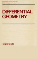
10. Tangent vector, principal normal vector, and binormal vector. Curvature. With a curve C we may associate certain unit vectors which are of basic importance. In this connexion we shall also introduce the important notion of curvature. Let C be represented by x(s) with arc length s as a parameter. Two points x(s) and x(s + h) of C determine a chord (cf. Fig. 10.1). This chord has the direction of the vector x(s + K) — x(s) or of the vector

If we let h approach zero, we obtain the derivative (10.1) t(s) is called the unit tangent vector of C at the point x(s). It exists because of Assumption 1 in Section 6, is tangent to C, and points in the direction of increasing parametric values. Hence its sense depends on the orientation of C (cf. Sec. 8). From (9.5) with t = s it follows that t is a unit vector. If x(0 represents C, then x' = xt' = x/s. Consequently, (10.2)

DIFFERENTIAL AND RIEMANNIAN GEOMETRY

32

The straight line through a point x(s) in the direction of t(s) is called the tangent of C at the point \(s). It is the limiting position of the straight line through that point and another point Q of C as Q approaches that point along C. This follows from our above consideration. A parametric representation of the tangent is (10.3) |u| is the distance of the corresponding point from the point \(s) on C. Since x is tangent to C, another representation of the tangent is (10.4)

Fig. 10.1. Tangent vector

Fig. 10.2. Moving trihedron

Example 10.1 (Straight line, helix). Straight lines are the only curves whose unit tangent vector is constant. This follows by integrating the vector equation x' = const. The unit tangent vector of the circular helix (7.4) is

We see that it makes a constant angle with the xa-axis. Representation (10.4) takes the form Curves whose tangents make a constant angle with a fixed direction in space are called general helices. The derivative of the unit tangent vector with respect to the arc length s is (10.5) and is called the curvature vector of the curve C at the point x(s). Its length (10.6) is called the curvature of C at the point x(s). The reciprocal value (10.7)

THEORY OF CURVES

33

is called the radius of curvature of C at that point. If C is represented by x(0, then (cf. Problem 10.5) (10.8) Straight lines are the only curves whose curvature is identically zero, because from K — 0 we have x" = 0 and \(s) = as + c, where a and c are constant vectors. K measures the arc rate of change of the tangent vector and therefore the deviation of C from the tangent in some neighbourhood of the corresponding point. If K ^ 0, then k = t' ^ 0. Then t' is orthogonal to t (cf. Theorem 5.5). The same is true for the corresponding unit vector (10.9) p(s) is called the unit principal normal vector of C at the point x(s). It exists, if C is of class r > 2, at every point of C at which K is not zero (that is, is positive). Its sense is independent of the orientation of the curve (why?), in contrast to the sense of the unit tangent vector, which depends on that orientation. The straight line through the point x(,s) in the direction of p(s) is called the principal normal of C at that point. With each point of a curve C at which K > 0, we now have associated the two orthogonal unit vectors t and p. The unit vector (10.10) is called the unit binormal vector of C at the point x(s). It is orthogonal to both t and p. The straight line through that point in the direction of b(s) is called the binormal of C at that point. The three vectors t, p, b form a right-handed triple (cf. Sec. 5) of orthogonal unit vectors. This triple is called the moving trihedron of C. Figure 10.2 shows the trihedron and three planes spanned by its vectors, which are listed in the following table: Table 10.1. Normal plane, osculating plane, and rectifying plane Name Normal plane N Osculating plane O Rectifying plane R

Spanned by

Normal vector

Representation

pandb tandp tandb

t b P

(z- x)-t = 0 (z- x)-b = 0 (z-x)-p = 0

In the case of a plane curve with positive curvature the tangents and the

34

DIFFERENTIAL AND R I E M A N N I A N GEOMETRY

principal normals lie in the plane E of the curve, and the unit binormal vector is constant and perpendicular to E. Example 10.2 (Ellipse, circle). In the case of the ellipse (7.2) we have

From (10.8) we thus obtain The case a = b = r corresponds to a circle of radius r. Then K = r2/r3 = 1/r, and the radius of curvature p = l//c is equal to the radius r of the circle. Example 10.3 (Circular helix). From (7.4) and Example 9.1 we obtain

Hence the curvature of the circular helix is constant, Furthermore,

The unit principal normal vector is parallel to the x\ *2-plane. If we insert x, b, and z = (zi, Z2, ^3) in the representation of the osculating plane and use / = sjw, we find

We want to show that the osculating plane of a curve C is the limiting position of a plane E through three points P: x(s), Pl: \(s + 7^), and P2: x(s + h2) of C, as PI and P2 approach P along C in a suitable fashion. We assume that the curvature of C at P is not zero. Figure 10.3 shows the vectors If these vectors are linearly independent, they span E. Then E is also spanned by or by and

THEORY OF CURVES

35

If C is of class r > 2, then by Taylor's formula we have (10.11) Here o(/j/) is a vector whose components are 0(/*/), and this so-called Landau symbol is defined as follows. Let/(z) be a function which is different from zero in an interval containing the point z = 0. Let g(z) be another function defined in this interval. Suppose that g(z)/f(z) ->Q as z ->Q. Then g(z) is said to be o(f(z)\ which is to be read as "small o off(z)" From (10.11) we obtain

Hence if we let hl and h2 approach zero such that o(A2) — o(hi) = o(h2 — /*i), then Y! approaches x'(s) and w approaches x"(s). This completes the proof.

Fig. 10.3. Plane E through three points of a curve

In antiquity only tangents of special curves (conic sections, the spiral of Archimedes) were known. The general concept of a tangent was introduced during the seventeenth century, in connexion with the basic concepts of calculus. Fermat, Descartes, and Huyghens made important contributions to the tangent problem, and a complete solution was obtained by Leibniz [1] in 1677. The first analytical representation of a tangent was given by Monge [1] in 1785. The name "osculating plane" was introduced by Tinseau (1780), and the name "binormal" by Saint Venant [1]. Problems 10.1. Determine the intersection between the tangents to the curve x(0 = (t, Bt2, Ct"), n ^ 0, and the x\ *2-plane, where B and C are constant. 10.2. Show that the osculating plane of the circular helix (7.4) can be represented in the form z\ c sin t — 22 c cos t + (73 — cf)r = 0. 10.3. Show that if the vectors x(0 and x(0 are linearly dependent for all t, then the corresponding curve represented by x(/) is a straight line. 10.4. Show that the osculating plane of a curve C at a point P is the limiting position of a plane through the tangent of C at P and a point g of C, as Q approaches P along C.

36

D I F F E R E N T I A L AND R I E M A N N I A N G E O M E T R Y

10.5. Derive (10.8) from (10.6). 10.6. Derive from (10.8) the formula for the curvature of a plane curve y = /(*), where a prime denotes the derivative with respect to x. 10.7. Verify the expression for the curvature of the ellipse (7.2) in Example 10.2.

11. Torsion. Formulae of Frenet. The curvature K of a curve Cat a point P measures the deviation of C from a straight line (the tangent at P) in a neighbourhood of P, because it is related to the arc rate of change of the tangent direction. We shall now introduce the torsion r. We want r to measure the deviation of C from a plane (the osculating plane O at P) in a neighbourhood of P. We shall therefore consider the arc rate of change of the position of O. This position is determined by the unit binormal vector b because b is perpendicular to O, and its arc rate of change is measured by the derivative b' = db/ds. This vector exists if we assume that the representation x(s) of C with arc length s as parameter is of class r > 3 and K > 0 at P. We shall prove that if b' is not the null vector, it must have the direction of the principal normal; consequently, (11.1') where a is a scalar. Clearly, it suffices to show that b' is perpendicular to both b and t. The orthogonality of b and b' follows from Theorem 5.5. To complete the proof we differentiate b • t = 0, finding b7 • t + b • t' = 0. The last scalar product is zero. This follows from (10.9) because p and b are orthogonal. Thus b' • t = 0, and (ll.T) is proved. It is conventional to set a = — r. Then (11.1') takes the form (11.1) Scalar multiplication of both sides by p yields (11.2) r(s) is called the torsion of the curve C at the point x(s). This name was first used by L. I. de la Vallee [1]. The quantity x = 1/T is called the radius of torsion. Theorem 11.1 (Plane curves). A curve C of class r > 3 with nonzero curvature is plane if and only if its torsion is identically zero. Proof. If C is plane, then b is constant. Then b' = 0 and r = 0, as follows from (11.2). Conversely, if r = 0, it follows from (11.1) that b must be constant. Hence, by integrating b • t = 0 we obtain b • x(s) = const. This means that the curve

T H E O R Y OF CURVES

37

represented by x(s) lies in the plane perpendicular to the constant vector b. This completes the proof. Curvature and torsion are also known as first and second curvature, and a twisted curve is called a curve of double curvature. x/(/c2 + r2) is sometimes called the third curvature or total curvature of a curve. Example 11.1 (Circular helix). From Example 10.3 we find

If we insert this into (11.2) and simplify, we obtain the constant value

Hence the torsion of a right-handed helix (c > 0) is positive while the torsion of a lefthanded helix (c < 0) is negative. Our result is typical, as we shall see in the next section.

Fig. 11.1. Right-handed and left-handed circular helix

The torsion can be expressed in terms of the position vector x(s) of the curve and its derivatives. In (11.2) we have b = t x p. Hence The mixed product — |pt'p| is zero. In the last mixed product, t = x' and p = t'/K = /ox"; cf. (10.9) and (10.7). Simplifying the determinant by the usual elementary rules, we thus obtain Since p2 = l//c2 = 1/x" • x", we finally have (11.3)

38

D I F F E R E N T I A L AND R I E M A N N I A N GEOMETRY

In the case of a representation x(t) involving an arbitrary parameter / we obtain (cf. Problem 11.1) (11.4) In addition to (11.1) there are two similar formulae for the derivatives t' and p'. From (10.9) we find t' = /cp. We shall derive the formula for p'. From the definition of a vector product it follows that Differentiating the first of these formulae and using the formulae for t' and b', we obtain Altogether, (11.5) These are the so-called formulae of Frenet [1]. They are probably the most important relations in the theory of curves. Basic consequences resulting from these formulae will be considered later. For the time being we shall use these formulae to obtain a geometrical interpretation of the sign of the torsion r. We consider a curve C of class r > 3 in a neighbourhood of a point P: x(s) of C at which K > 0. The curve C is said to be right-handed at P if, for increasing values of s, it leaves the osculating plane O(P) to the positive side of this plane which is determined by the sense of the unit binormal vector b. Then C looks locally like a right-handed helix. C is said to be left-handed at P if, for increasing s, it leaves O(P) to the opposite side. Note that this definition is independent of the orientation. In fact, if we change the orientation, then the sense oft is reversed, but the same is true for b = t x p. The sign of r is independent of the orientation, too, because under that change both x' and x'" reverse their sense while the sense of x" remains unaffected. Theorem 11.2 (Sign of the torsion). If the torsion r of a curve C of class r > 3 at a point P at which K > 0 is positive, then C is right-handed at P; ifr is negative, then C is left-handed at P. Proof. Let x(s) represent C. Let P correspond to s = 0. The Taylor formula yields

01.6) where the subscript 0 denotes the value of the corresponding quantity at P and o

THEORY OF CURVES

39

is defined in the last section. We have x 0 ' = t0. From (11.5) we obtain By inserting this into (11.6) we find (11.7) x0 is the position vector of P. The other vectors lie in the osculating plane O(P\ except for the vector If s > 0 and TO > 0, then s3K0 r0/6 > 0, and s3K0 TO b0/6 points in the direction of b0. The vector v is continuous. Hence for sufficiently small positive s it has almost the direction of b0, and C is right-handed at P. If TO < 0, then for sufficiently small positive s the vector v has almost the direction of — b0, and C is left-handed at P. This completes the proof. Problems

11.1. Derive (11.4) from (11.3). 11.2-11.4. Find the torsion of the following curves: 11.2. (/, cosh /, sinh t). 11.3. (cos t, sin /, el). 11.4. (t, /2/2, /3/6). 11.5 (Vector of Darboux). Let x(s) represent a curve of class r > 3 with positive curvature K. To the motion along the curve with constant speed 1 there corresponds a rotation of the trihedron (and a translation of the trihedron, which will not be considered here). Show that the corresponding rotation vector is d = rt + Kb. This vector is called the vector of Darboux. (A rotation vector d is defined as follows. Its direction is that of the axis of rotation and such that the rotation appears clockwise if one looks from the initial point of d towards its terminal point. The length of d is equal to the angular speed & (>0) of the rotation, that is, the linear (or tangential) speed of a point B divided by its distance from the axis of rotation.) 11.6. Using d in Problem 11.5, show that (11.5) can be written 11.7 (Spherical images of a curve). If we let the vectors of the trihedron of a curve undergo a parallel displacement such that they are bound at the origin O of the coordinate system in space, their terminal points lie on the unit sphere S with centre O and generate, in general, three curves on S, which are called the tangent indicatrix (generated by t), the principal normal indicatrix (generated by p), and the binormal indicatrix (generated by b) of the curve. Show that for the linear elements dsj, dsp, dss of these indicatrices or spherical images of the curve the following formulae hold: (Equation of Lancret).

40

DIFFERENTIAL AND R I E M A N N I A N GEOMETRY

12. Local shape of a curve (canonical representation). We shall now consider an interesting consequence of (11.7). For this purpose we choose a Cartesian xi x2 -x3-coordinate system with centre P such that the positive x^, x2-> and #3-direction is the direction of t0, p0, and b0, respectively. Then (12.1)

x0 = 0,

t0 - (1, 0, 0),

po = (0, 1, 0),

b0 = (0,0, 1),

and (11.7), written in terms of components, takes the form (12.2) This is the so-called canonical representation of our curve C. Let T0 96 0, as before. When we discard all the terms in each series except the first term, we obtain the vector function (12.3) which represents an approximation curve C of C in a neighbourhood of P. By eliminating s we obtain the following representations of the orthogonal projections of £(cf. Fig. 12.1): (quadratic parabola) (cubical parabola) (semicublcal parabola).

(in the osculating plane O) (in the rectifying plane R) (in the normal plane N)

Figure 12.2 shows C in space. C is right-handed if TO > 0 and is left-handed if TO < 0. Note that the projection in the normal plane has a cusp at P. Problems

12.1. Let / (< TTT) be the length of an arc C of a circle of radius r with end points PQ and P. Then the corresponding chord PQ P has the length

If C is sufficiently small, the difference / — /* is of order /3. Prove that the difference of the lengths of a sufficiently small arc of any curve (with K > 0) and the corresponding chord is always of order /3. 12.2. Determine and graph the curve (12.3) in the case of the point (1, 0, 0) on the circle xC?) = (cos 5-, sin s, 0). 12.3. Determine and graph the curve (12.3) in the case of the point (1, 0, 0) on the helix x(/) = (cos /, sin /, t).

THEORY OF CURVES

Fig. 12.1. Orthogonal projections of the approximation curve (12.3) in the osculating plane O, the rectifying plane R, and the normal plane N

Fig. 12.2. Approximation curve (12.3) in space

41

42

D I F F E R E N T I A L AND R I E M A N N I A N G E O M E T R Y

13. Natural equations of a curve. We know that a curve C may be given by a parametric representation x(t) or x(s). Of course such a representation depends on the choice of the coordinate system and changes if the coordinate system is changed. We may ask whether C can be characterized by equations which do not refer to the coordinate system. This question was first raised by L. Euler [1]. It is clear that quantities appearing in such equations must be independent of the coordinate system. The arc length s, the curvature /c, and the torsion r are of this type. Two independent functional relations between these quantities are called natural equations or intrinsic equations of the corresponding curve. We shall consider the natural equations (13.1) We shall prove that these two functions determine C uniquely, except for its position in space. If these functions are analytic, this follows immediately from the Taylor series development of the function x(s) representing C, because from (11.5) we see that the coefficients of this series involve only those functions and their derivatives. However, our statement remains true under much weaker assumptions, as follows. Theorem 13.1 (Existence and uniqueness theorem). Let K(S) (>0) and r(s) be functions of a real variable s which are defined and continuous in an interval I: 0 < s < a. Then there exists an arc C of a curve whose arc length is s and whose curvature K and torsion r are given by those functions. C is unique, except for its position in space. (r(s) satisfies (11.2). If K(S) is of class r > 1, then (11.3) holds.) Proof, (a) Existence. We apply Picard's method to the formulae (11.5) of Frenet. These formulae are nine differential equations for the nine components of the vectors t, p, and b. We use the simpler notation (13.2) Then (11.5), written in terms of components, takes the form The subscript /indicates the fth component of the corresponding vector. We drop this subscript, for the sake of simplicity, and write (13.3) The elements of the coefficient matrix

THEORY OF CURVES

43

are continuous functions in the closed interval / and therefore bounded in /, say (13.4)

We want to show that (13.3) has a solution in / satisfying given initial conditions (13.5) Here \Vj°\ < I because we are dealing with components of unit vectors. Integrating (13.3) and using (13.5), we obtain (13.6) A solution of (13.6) is a solution of (13.3), (13.5) and conversely. We replace vk(a) by vk°. Then we obtain from (13.6) three first approximations (13.7) If we replace vk(d) in (13.6) by vk(l\ then (13.6) yields three second approximations Vj(2\ etc. If we insert the (n — l)th approximations vk(n"1\ then (13.6) yields three nth approximations (13.8) We shall prove that the limits (13.9) exist and satisfy (13.3) and (13.5). Because of \Vj°\ < 1 and (13.4) we obtain from (13.6) In a similar fashion it follows that

etc., and in general, (13.10)

Now (13.11)

44

DIFFERENTIAL AND R I E M A N N I A N GEOMETRY

From (13.10) we see that the absolute value of each of these terms is at most equal to the corresponding term in the sum (13.12) As n approaches infinity, (13.12) approaches Hence the series (13.13) converges uniformly in /, and the limits (13.9) exist in /. These limit functions are continuous in / because the Vj(n) are differentiable and therefore continuous in / and (13.13) converges uniformly in /. (13.8) can be written in the form (13.14) The functions vfn) — Vj and vk(n 1} — vk approach zero uniformly in /as n -> oo. From (13.14) we thus obtain (13.6). Hence the limit functions (13.9) satisfy (13.6) and therefore also (13.5). They are differentiable because the right-hand side of (13.6) is differentiable. Hence they are solutions of the formulae of Frenet in /. (b) We shall now prove that if the initial vectors v^, v2°, v3° form a righthanded orthogonal triple of unit vectors (cf. Sec. 5), the same is true for the solution vectors v/s) = (vjk(s)) in /. We have to show that if the matrix V with row vectors v l9 v2, v3 is orthogonal at s = 0, it is orthogonal for all s in /. It suffices to show that the column vectors of that matrix satisfy the relations (13.15) Then the same is true for the row vectors. We prove that the derivative of the lefthand side of (13.15) with respect to s is equal to zero. Then the left-hand side must be constant and, for reasons of continuity, equal to the initial value 8a/3. Using (11.5) we obtain

We interchange./ and k in the second member of each term of this double sum. Using ckj = —cjk, we then obtain

This completes the present part of the proof. When s = 0, then det V = 1.

THEORY OF CURVES

45

Because of continuity, det V = 1 in /. This means that the solution vectors form a right-handed triple. The corresponding arc of a curve has the representation (13.16) It is determined except for a translation, because the position vector x0 of the point corresponding to s = 0 is arbitrary. (c) Uniqueness of solution. Let Vj = t*, v2 = p*, v3 = b* be another solution of (13.3) satisfying (13.5). Then

Addition of these three equations yields Integrating we have (13.17) because at s = 0 we have t • t* = t • t = 1, etc. From part (b) of the proof it follows that all the vectors are unit vectors. Hence each scalar product can be equal at most to 1. Consequently, t* = t, p* = p, b* = b, and uniqueness is proved. Furthermore, two right-handed triples of orthogonal initial unit vectors being given, there is a unique direct orthogonal transformation that carries one of the triples into the other. Under this transformation, K(S) and T(S) do not change. Hence the arcs corresponding to the two triples are congruent. This completes the proof of Theorem 13.1. Example 13.1 (Plane curves). The natural equations of a plane curve C are K = K(S), T = 0. The unit tangent vector is (13.18) where 3 with positive curvature K is a general helix if and only if its torsion r is proportional to its curvature K, that is, T(S)/K(S) = const.

Fig. 13.1. Spiral of Cornu Problems 13.1. Prove Theorem 13.2. 13.2. Determine the curve corresponding to the natural equations K — \\a — const, r = 0 directly from (11.5) by solving a differential equation of second order for t. 13.3. Find the curve whose natural equations are ic = 1/cosh s, r = 0. 13.4 (Cycloids). Let KQ be a fixed circle of radius ro and let K be a circle of radius r, which lies in the same plane and has a common tangent with #0 at a point. K is assumed to lie exterior to KQ and vice versa. Now, when drolls on KQ without sliding, a fixed point P of K generates a plane curve which is called an ordinary epicycloid. Show that this curve can be represented in the form

THEORY OF CURVES 47 where R = r$ + r, and find the natural equations. (If r < r$ and K lies interior to KQ, then that path of P is called an ordinary hypocycloid. If .£ rolls on a straight line, then that path is called an ordinary cycloid. General cycloids are obtained if P does not lie on the circumference of a circular disk but in the interior.) 14. Contact. Circle of curvature, osculating sphere. If two curves C and C* have a common point P0, then in a neighbourhood of P0 they may differ "more or less" from each other. We shall investigate this situation in detail and characterize it in a precise manner by introducing the concept of contact. First of all there are two possible cases: Either (a) the tangents to C and C* at P0 are different from each other or (b) they coincide. Without loss of generality we may choose the representations (14.1) where s is the arc length of C and s* is the arc length of C*. Let P0 correspond to s — SQ on C and to s* — s0* on C*. Then in both cases (a) and (b), Furthermore, in case (b) the unit tangent vectors of C and C* at P0 coincide or are opposite to each other. We may assume that the orientations of C and C* are such that for the representations (14.1) those vectors coincide. This assumption will be made throughout this section. Then in case (b),

While we can visually distinguish only between the two cases (a) and (b), we are able to characterize the case (b) in more detail by analytical methods, namely, by taking into account the higher derivatives of \(s) and x(s*). For this purpose we introduce the following notion. Definition 14.1 (Contact of curves). A curve C of class r > m has contact of order m (exactly) with a curve C* of class r* > m at a point P0 if, with respect to (14.1), atP0, (14.2a) and, if the (m + l)th derivatives at P0 exist, at P0, (14.2b) It follows that in the above case (a) the curve C has contact of order 0 with the

48

DIFFERENTIAL AND RIEMANNIAN GEOMETRY

curve C* at P0. Contact of first order is also known as ordinary contact, contact of second order as stationary contact or osculation, and contact of third order as stationary osculation or superosculation. Definition 14.1 may be interpreted geometrically as follows. Using the Taylor formula we develop x(s) in a power series involving powers of s — s0. The curve represented by the sum of the first terms of that development up to and including the term containing the power (s — s0)k is called the kth approximating curve of CatP0. For example, the tangent at P0 is the first approximating curve, and so on. Then contact of order m is equivalent to the coincidence of the first, second, ..., wth approximating curves of the curves under consideration at the point of contact. Particularly interesting is the contact between curves and simple surfaces, such as planes and spheres. The general definition of a surface will be given in Sections 16 and 17. At this stage it suffices to say that surfaces are point sets in Euclidean space ^3, which, at least in a sufficiently small neighbourhood of any of their points, can be represented in the form G(xi9 x2, x3) = 0 where G is a function of class m > 1 and is such that at every point at least one of the three first partial derivatives is not zero. Definition 14.2 (Contact of a surface with a curve). A surface S has contact of order m (exactly) with a curve C of class r > m at a point PQ if there exists a curve C* of class r* *>manS which has contact of order m with C at PQ but there does not exist a curve on S which has contact of order greater than m with C at P0. We first consider planes that have contact with a curve C at a point PQ. If that contact is of first order, the plane must contain the tangent to C at P0. Obviously, there exists a whole pencil of planes of this type. It contains the osculating plane of C at P0. Theorem 14.1 (Osculating plane). The osculating plane of a curve at a point PQ has contact of second order (at least) with the curve at P0. Proof. Let x(s) represent that curve C and let P0 correspond to s = s0. Then

The sum x*(s) of the first three terms represents a curve C* in the osculating plane of C at PQ because this plane is spanned by X'(SQ) and x"(%)- Representing C* by y(s*) = x*(/z(,y*)), where s = h(s*) and s* is the arc length of C*, we obtain y(^0*) = x(5-0), y'fao*) = x'(j0)» y"0o*) = x"0o)> where s* = s0* corresponds to P0. This proves the theorem. If C is of class r ^ 3 and r(P0) ^ 0, then the contact is precisely of second order. This follows from (12.2). Lemma 14.2 (Contact of a surface with a curve). Let C be a curve of class r ^ m represented by (14.1) where s is the arc length. Let PQ : s = s0 be a point of C which lies on a surface S, and let G(x^ x2, x3) = 0 be a representation of S of

THEORY OF CURVES

49

class r* > m valid in some neighbourhood of P0. Then S has contact of order m (exactly) with C at P0 if and only if the function and its derivatives up to and including the mth derivative are zero at s = s0, while the (m + Y)th derivative—if it exists—is not zero at s = s0, that is (14.3)

Proof, (a) Suppose that S has contact of order m (exactly) with C at P0. Then, by definition, there is a curve C* on 5 which has contact of order m (exactly) with C at P0. Let C* be represented as in (14.1) where s* is the arc length of C* and C and C* have the same orientation at P0. Let P0 correspond to s* = s0*. Since C* lies on S9 we have (14.4a) By differentiation,

(14.4b)

etc. Since C and C* have contact of order m (exactly) at P0, it follows from (14.2a) that (14.5a) and, if the (m + l)th derivative exists, (14.5b) In (14.4) we set 5* = 50*. Then we may replace the values of ftj and its derivatives at P0 with the values of the corresponding c^ and its derivatives at P0. This yields (14.3). (b) We prove the converse. By assumption, dG/dXj =£ 0 at any point for at least one value of 7 = 1, 2, 3. Suppose that at P0 we have 8G/dx3 ^ 0. Then we may represent S in a neighbourhood of P0 in the form x3 = (xl9 x2\ In consequence of (14.3) this equation and the equations obtained by differentiating it m times are satisfied by the values of a^s) and its derivatives at P0. Let C* : x*(^*) = (Pi(s*)9 /?2C?*), j83(j*)) be a curve on S with arc length j* passing through P0 (s* = s0*) and satisfying j8y(|l)(j0*) = aj(»\s0)9 p, = 0, ..., m\j = 1, 2. Since C* is on 5, we have Gtf^s*), p2(s*)9 j83(j*)) = 0 and £3C?*) = ^i^*), 02(j*)). Differentiation and use of (14.3) gives j33(^l)(^0*) = m + 1 at a point P0. Ifm is even, then C pierces S at P0. Ifm is odd, then, in a sufficiently small neighbourhood 0/P0, the curve C lies on one side of S. Proof. Let C be represented by x = («/$)) and let S be represented by G(xi9 x29 x3) = 0. Let P0 correspond to s = 0. Then from the Taylor formula and (14.3) we have

At s = 0 the (m + l)th derivative of p is not zero. Since it is continuous, it is different from zero for all sufficiently small \s\ and has constant sign. Let m be even. Then sm+i >0 when s > 0 and y +1 < 0 when s < 0. If m is odd, then sm+1 > 0 for all values of s. From this the statement follows, and the proof is complete. We shall now consider spheres that have contact with an arbitrary curve C, represented by x(s) where s is the arc length. A sphere S of radius R with centre M can be represented in the form (14.6) where a is the position vector of M. In order that C and S should have contact of order zero they must have a point P in common. For the contact to be of first order we must have, at P, (14.7) That is, M must lie in the normal plane of C at P. If /c(P) > 0, the vectors p and b exist, and the position vector of M is of the form (14.8) The corresponding radius R is obtained from (14.6). For the contact to be of second order, in addition to (14.7) we must have, at P, (14.9) By substituting (14.8) into (14.9) we obtain the condition 1 — a/c = 0 or « = I/* = p. Hence the centre of such a sphere lies on the straight line (14.10) This line is called the polar axis of C at P. It is normal to the osculating plane 0(P)

THEORY OF CURVES

51

and intersects it at a point Q with position vector (14.11) Q is called the centre of curvature of C at P. The circle of radius p with centre Q in the osculating plane is called the circle of curvature or osculating circle of C at P. It has contact of second order (at least) with C at P. In order that our sphere S should have contact of third order (at least) with C at P, in addition to (14.7) and (14.9) we must have [cf. (11.5)] (14.12) Substituting (14.10) into (14.12) we obtain the condition If K(P) ^ 0 and r(P) -=£ 0, then j3 = —PK'/KT = +p'/r. Hence that sphere has centre (14.13) and radius (14.14) It is called the osculating sphere of the curve C at P. If /c' = 0, then p = 0 and the centre of the osculating sphere lies in the osculating plane O(P) and coincides with the centre of curvature. From (14.14) we see that curves of constant curvature have constant radius of the osculating spheres. Osculating spheres were first considered by N. Fuss [1]. Formula (14.13) was first obtained by B. de Saint Venant [1]. We may sum up our results as follows. Theorem 14.4 (Contact of spheres with a curve). The centres of the spheres that have contact of first order (at least) with a curve C at a point P lie in the normal plane N(P) of C at P. The centres of the spheres that have contact of second order (at least) with C at P lie on the polar axis of Cat P, and these spheres intersect the osculating plane O(P) ofCatP along the circle of curvature ofC at P. This circle has contact of second order (at least) with C at P. The osculating sphere with centre (14.13) and radius (14.14) has contact of third order (at least) with C at P. Problems

14.1-14.4. Determine the order of contact in the following cases: 14.1. The curve *2 = *i3, *3 = 0 and the xi-axis. 14.2. Two circles with a common point P and common tangents at P. 14.3. The sphere x\2 + *22 + x$2 = r2 and the straight line x(s) = (s, r, 0).

52

DIFFERENTIAL AND RIEMANNIAN GEOMETRY

14.4. The sphere (xi + I)2 + X22 + *32 = 4 and the circular helix x(f) = (cos t, sin /, t). 14.5. Prove that, in general, the osculating plane is the only plane that has contact of second order (at least) with the corresponding curve at the corresponding point. 14.6. Let C and C* be plane curves that have contact of /nth order (exactly) at a point P. Show that if mis even, then the curves intersect each other.

15. Involutes and evolutes. Involutes and evolutes are curves associated with a given curve, as follows. In general, the tangents to a curve C generate a surface S which is called the tangent surface of C and will be considered in more detail in Section 54. If C is represented by x(s) where s is the arc length, it follows from (10.3) that S can be represented in the form (15.1) t is the unit tangent vector of C, and u is a real parameter. \u\ is the distance of a point P of S from the point of contact B of the corresponding tangent with the curve C. The value of u is positive if the directed segment BP has the same sense as t and is negative otherwise. Involutes of C are curves on S which are orthogonal to the generating tangents. The angle y (0 < y < TT) between two intersecting curves is defined to be the angle between the unit tangent vectors of the curves at the point of intersection. From (15.1) we see that an involute of C can be represented in the form where u(s) is such that the vector which is tangent to the involute, is orthogonal to the unit tangent vector t of C. Thus z' • t = 0. It follows that 1 + u' — 0. Integration yields u = c — s where c is an arbitrary constant. Consequently an involute of a curve C, represented by \(s), has the representation (15.2) We see that there is a one-parameter family of such involutes, each of which corresponds to a certain value of the constant c in (15.2). If K > 0 and s 7^ c, then z' ^ 0. If C is plane, the involutes are plane curves also. We may interpret (15.2) in a geometrical manner, as follows. If a thread lying on C is wound off so that the unwound portion of it is always held taut in the direction of the tangent to C, while the rest of it lies on C, then every point of the thread generates an involute of C during this motion.

THEORY OF CURVES

Fig. 15.1. Tangent surface of a circular helix (C) with an involute (/)

53

Fig. 15.2. Notion of evolute

In our consideration we started from a given curve and determined its involutes. We shall now treat the converse problem: Let a curve C be given and determine a curve C* so that the given curve C is an involute of C*. The curve C* is then called an evolute of C. The names "involute" and "evolute" were introduced by C. Huyghens (1629-95) in 1673 ;cf.[l]. We shall now derive a representation y(s) of the evolutes C* of the curve C: x(X), assuming that C is of class r > 3 and has non-zero curvature K(S). By the definition of an involute, the tangents to C* must intersect the given curve C orthogonally. Hence C* may be represented in the form (15.3) where a(j) is a unit vector in the normal plane of C at x(s); then \q(s)\ is the distance between that point and the corresponding point y(s) of the evolute. From the definition of the involute we see that a must be tangent to the curve C*. Thus y' = Aa, or written at length,

where A is a scalar. Since t and a' are orthogonal to a, we must have q' = A and (15.4) a is of the form (cf. Fig. 15.2) (15.5)

where a is the angle between a and the unit binormal vector b of C. Differentiating (15.5) with respect to s, substituting the result into (15.4), and using (11.5), we find c

54

DIFFERENTIAL AND R I E M A N N I A N GEOMETRY

t, p, and b are linearly independent. Hence the coefficient of each of these vectors must be zero. This yields and furthermore Since cos a and sin a have no common zeros, we obtain a' = r. By integration, (15.6) By inserting this into (15.3) we see that the evolutes of a curve C: \(s) may be represented in the form (15.7) where a(s) is given by (15.6) and p and b are the unit principal normal vector and the unit binormal vector, respectively, of C. Because of (11.5) the condition y' 7^ 0 is equivalent to p' — pr cot a 7^ 0. Comparing this with (14.10) we see that each point of an evolute C* lies on the polar axis of the curve at the corresponding point. If C is plane, then r = 0 and a is constant. Then c = ir/2 in (15.6) yields an evolute of C in the plane of C which is the locus of the centres of curvature of C and is the intersection of that plane with the cylinder on which the other evolutes of C lie. Problems (1)

2

15.1. Let y (-s) and y^ \s) be two evolutes of the same curve x(s). Show that their tangents corresponding to the same s intersect at a constant angle. 15.2 (Bertrand curves). Two curves whose principal normals at corresponding points coincide are called Bertrand curves; cf. J. Bertrand [1], Show that, a plane curve C being given, there is a curve C* such that C and C* are Bertrand curves. (Hint: Consider an involute of the plane evolute of C.) Show that the distance of corresponding points on these curves is constant. (For this reason, Leibniz [2] called these parallel curves.) 15.3. Show that, a circular helix being given, there is a circular helix such that the two curves are Bertrand curves. 15.4. Show that for a twisted curve C there is a curve C* such that C and C* are Bertrand curves if and only if the curvature K and the torsion T of C satisfy a linear relation with constant coefficients c\ and 02 of the form c\K.(f) + C2r(t) = 1. 15.5. Show that the tangents of the circular helix \(t) = (cos t, sin /, /) intersect the jci *2-plane along an involute of the unit circle.

Ill

NOTION OF A SURFACE. FIRST FUNDAMENTAL FORM WE SHALL NOW consider real surfaces in three-dimensional Euclidean space R3. In the present chapter we first define the concepts of a portion of a surface (Sec. 16) and a surface (Sec. 17) in a fashion suitable for the purpose of differential geometry. This will involve a particular case of a differentiable manifold. The tangent plane and the normal of a surface will be considered in Section 19. Then we shall introduce the so-called first fundamental form, which defines a metric on a surface so that we are able to measure lengths, angles, and areas on surfaces. Important concepts in this chapter: Parametric representation x(u*9 u2) (Sec. 16), portion of a surface (Sec. 16), surface (Sec. 17), tangent plane and normal (Sec. 19), first fundamental form (Sec. 20), summation convention (Sec. 20), area (Sec. 21). 16. Portion of a surface. In topology one can define a portion of a surface to be a point set M in Euclidean space ^3 which is a topological image (cf. Sec. 2) of a simply connected! domain G in a plane. This notion is much too general in differential geometry. In fact the mapping

G->M is merely topological, and we have to request additional differentiability properties. This is similar to the situation in Section 6. We introduce Cartesian coordinates xl9 x2, x3 in R3 and Cartesian coordinates n1, u2 in the plane of G. The reason for writing ii1, u2 instead of w l5 u2 will be explained later, in Section 30; this is a standard notation in tensor calculus. We may now represent the mapping G -> M by a single-valued real vector function (16.1)

x - X(MI, u2)

which associates with each point (w1, w2) in G a point of M with position vector X(MI, w2). Representation (16.1) is called a parametric representation of M. The variables w1, u2 are called the parameters of this representation, and the ulu2plane is called the parametric plane. t That is, a domain G such that every closed curve in G can be shrunk continuously to any point in G without leaving G. For example, the interior of a circle is simply connected while the domain bounded by two concentric circles is not simply connected.

DIFFERENTIAL AND R I E M A N N I A N GEOMETRY

56

Fig. 16.1. Portion of a surface

For example, the vector function represents the portion of the circular cylinder in the first octant between the jq jc2-plane (;c3 = 0) and the plane jt3 = 1. Partial derivatives of x (w1, u2) will be characterized by subscripts, for instance

(16.1) is called an allowable representation of class r if it satisfies the following Assumptions:

0. The mapping G -> M given by (16.1) is one-to-one. 1. The vector function (16.1) is of class r > 1 (for definition see Sec. 6) in its domain of definition G. 2. The vector product x t x x2 is different from the null vector everywhere in G. The value of r in Assumption 1 will be specified in each particular consideration. r = 3 will be sufficient in most cases. In Section 19 we shall see that from Assumption 2 the existence and uniqueness of the tangent plane and the surface normal follow. From (16.1) we may obtain other vector functions representing M by imposing a transformation of the form (16.2) For example, the vector function

SURFACES. FIRST FUNDAMENTAL FORM 1

57

2

represents the xi x2-plane, and w , u are Cartesian coordinates. Setting we obtain a new representation of the x1 jc2-plane, and w1, u2 are polar coordinates. Of course we shall admit only those transformations (16.2) which transform an allowable representation (16.1) of class r into a representation x(w1, f/2) which is allowable of class r and represents the entire set M (see above). For this reason we introduce the following notion. A transformation (16.2) is called an allowable parametric transformation of class r if it satisfies the following

Assumptions: 0*. The functions (16.2) are defined in a domain G* of the ulu2-plane such that the corresponding range of values is the domain G in the U1u2-plane in which (16.1) is defined. 1*. The functions (16.2) are of class r > 1 in G*. 2*. The transformation (16.2) is one-to-one. The corresponding Jacobian

(16.3)

is different from zero everywhere in G*. Note that the two conditions in 2* are independent. For example, the transformation is not one-to-one in a sufficiently large domain, although its Jacobian is nowhere zero. On the other hand the transformation

is one-to-one in the real domain, although its Jacobian is zero when w1 = 0. By means of the allowable parametric transformations we may classify the allowable representations (16.1) into equivalence classes, as follows. An allowable

58

DIFFERENTIAL AND RIEMANNIAN GEOMETRY

representation of class r is said to be equivalent to an allowable representation of class r if there is an allowable transformation (16.2) of class r which transforms the one representation into the other. Definition 16.1 (Portion of a surface). An equivalence class of allowable representations (16.1) of class r is called a portion of a surface of class r. The points of the point set represented by that class are called the points of that portion of a surface. If r = o> (cf. Sec. 6), then that portion is called an analytic portion of a surface. The parameters w1, u2 in (16.1) are called coordinates on that portion. The curves i/1 = const and u2 = const are called the coordinate curves of the ulu2coordinate system. Sometimes we shall represent portions of surfaces by an implicit representation of the form (16.4)

G(*i,*2,*3) = 0.

Then we shall assume that G is of class r > 1 and at each point at least one of the three first partial derivatives is not zero. 17. Surface. The notion of a portion of a surface (cf. Sec. 16) will be sufficient for local investigations. For global considerations we shall need the concept of a surface. We shall define this concept in a fashion suitable for the purposes of differential geometry. Roughly speaking a surface is a point set S in Euclidean space R3 each point of which has a neighbourhood f/such that S n U is a portion of a surface as defined before. To arrive at the definition of a surface we shall proceed stepwise, starting from the notion of a topological space (cf. Sec. 2). Such a space is said to be connected if it cannot be represented as the union of two disjoint non-empty open sets. A connected Hausdorff space Mn (cf. Sec. 2) is called an ^-dimensional topological manifold if each point of MH has a neighbourhood which is homeomorphic to an open set in w-dimensional Euclidean space, for example, the interior of the sphere In this section we shall need only the case n = 2. A two-dimensional topological manifold M2 is a connected Hausdorff space each point P of which has a neighbourhood Up homeomorphic to an open set in the plane, for example an open circular disk. Examples of such manifolds are planes, cylinders, spheres in R3, and so on. On M2 we may introduce local coordinate systems. We first define the following notion. A system {£/,} of open sets is called a covering ofM2 if each point of M2 is an

SURFACES. FIRST F U N D A M E N T A L FORM

59

element of at least one of these sets and if the union of all of these sets is equal to M2. Suppose that to each set Ut there corresponds a topological mapping where At is an open plane circular disk. Then for every point P in the intersection of two sets Ut and Uj we have (cf. Fig. 17.1) Hence and therefore This mapping Tj 1Ti maps the shaded portion of Ai onto the shaded portion of Aj. These shaded portions are the inverse images of the intersection of Ut and Uj with respect to the mappings Tt and Tjf If for every non-empty intersection of pairs of sets Uh Uj from the system {U t } the mapping Tfl Tt is given by functions

Fig. 17.1. Differentiable manifold

of class r (cf. Sec. 6) and if the corresponding Jacobian is not zero, then the system {Ut}, together with the mappings {Tt}9 is called an atlas of class r or a differential structure of class r on M2. This atlas is denoted by [U^ Tt}. A differential structure of class r = w is also called an analytic structure. Using the mapping Tl we may introduce Cartesian coordinates in Al as co-

60

DIFFERENTIAL AND R I E M A N N I A N GEOMETRY

ordinates in Ut = TlAi. These coordinates in Ut are called local coordinates on Af2. Their domain of validity Ut is called a coordinate neighbourhood or a cA0rf of our atlas. An atlas {Ut; Tt} of class r is said to be equivalent to an atlas {£//*; Tj*} of class r if the composite system {Ut, Uj*; Ti9 Tj*} is an atlas of class r on M2. The reader may show that this is an equivalence relation in the sense of the definition given in Section 3. A topological manifold M29 together with a fixed equivalence class of atlases of class r on Af2, is called a two-dimensional differentiable manifold of class r or an (abstract) surface of class r. Each of these atlases is called an allowable atlas, and its charts are called allowable charts of that manifold. A two-dimensional differentiable manifold of class r = to (cf. Sec. 6) is also known as an analytic manifold or analytic surface. Note that in this definition we do not refer to a space in which the manifold might lie. However, the surfaces we shall consider are embedded in threedimensional Euclidean space R3. For this reason let us finally introduce the notion of a surface in R3. We start from a two-dimensional differentiable manifold M2 of class r. We assume that there is a mapping V: M2 -> R3 of M2 into R3 such that for each allowable chart the mapping Fis given locally by a vector function of class r, say x = X(M I , w2). Here w1, u2 are local coordinates on M2, and the components xi9 x2, x3 of the vector x are Cartesian coordinates in R3. Then the image VM2 of M2 is called a two-dimensional differentiable manifold of class r embedded in R3. This embedding and the embedded manifold VM2 are said to be regular if the corresponding Jacobian matrix

(17.1)

has rank 2. We remember that a matrix is said to be of rank R if it contains an /{-rowed square submatrix with not identically vanishing determinant, while the determinant of any square submatrix having R + 1 or more rows, possibly contained in that matrix, is identically zero.

SURFACES. FIRST F U N D A M E N T A L FORM

61

A two-dimensional differentiable manifold S of class r which is regularly embedded in Euclidean space R3 is called a surface of class r in ^3. Sometimes we shall have to admit that at finitely many isolated points or along finitely many curves on S the matrix / has rank less than 2. Then such a point or curve is called a singular point or curve, respectively, of S. The other points of S are called regular points of S. Singular points and curves may arise from the geometrical shape of S and are then called geometrical singularities of S. Or they may result merely from the particular choice of the representation of S and are then called singularities of that representation. The reader may show that the condition rank / — 2 is equivalent to Assumption 2 in the previous section. 18. Examples Example 18.1 (Plane). The XL *2-plane can be represented in the form (IS.la) ul and u2 are Cartesian coordinates. The corresponding matrix (17.1) has rank 2 at each point. Polar coordinates u1, u2 may be introduced by setting Then we obtain the representation (IS.lb) The corresponding matrix (17.1) is

J has rank 1 at the origin x = 0 (u1 = 0) and rank 2 otherwise. This means that polar coordinates are singular at the origin. Example 18.2 (Sphere). The vector function (18.2) represents a sphere of radius r with centre at the origin. It has the components Squaring these components and adding, we have This w^-coordinate system is used on the globe. nl measures the longitude and u2 the latitude of the corresponding point. The curves u1 = const and u2 = const are the meridians and parallels, respectively, u2 = 0 represents the equator. The representation c*

62 DIFFERENTIAL AND R I E M A N N I A N GEOMETRY is singular at the poles u2 = iw/2, because at these points the matrix

has rank 1. If we interchange sin u2 and cos u2 in (18.2), then we obtain another representation of the sphere which is frequently used in mathematics.

Fig. 18.1. "Geographical coordinates" on the sphere

Fig. 18.2. Cone of revolution

Example 18.3 (Cone of revolution). The vector function

(18.3) represents a cone of revolution. From (18.3) we obtain The coordinate curves u1 = const and u2 = const in (18.3) are circles and straight lines (the generators), respectively. The matrix (17.1) has rank 1 at u = 0; the apex is a geometric singularity of the cone. A set of curves on a surface S which depend continuously on a real parameter is called a one-parameter family of curves on S. Two one-parameter families of simple curves on S are called a net of curves if through every point P of S there passes one and only one curve of each of these families such that these two curves have distinct direction at P. If 5 is represented by X(M I , w2), then the coordinate curves w 1 = const and 2 u = const form a net. Problems

18.1-18.3. What surface is represented by the given vector function? Is Assumption 2 in Section 16 satisfied? What type of curves are the coordinate curves w1 = const and u2 = const! 18.1. 18.2. 18.3.

SURFACES, FIRST F U N D A M E N T A L FORM

63

18.4. Show that an allowable parametric transformation preserves Assumption 2, Section 16. 18.5. What type of curves are the coordinate curves w1 = const and u2 = const on the following surfaces? In each case find a representation G(;CI, #2, *a) = 0. Ellipsoid (a cos u2 cos w1, b cos u2 sin w1, c sin u2). Elliptic paraboloid (au1 cos u2, bul sin w2, (w1)2). Hyperbolic paraboloid (aw1 cosh w2, &/1 sinh w2, (w1)2). Hyperboloid of two sheets (a sinh w1 cos «2, 6 sinh w1 sin «2, c cosh w1). 18.6. Find a parametric representation of the surface formed by the tangents of the curve x(/) = (t, t2, f3).

19. Curves on a surface. Tangent plane. Normal. We shall see later that many investigations of geometric properties of a surface involve suitable curves on that surface. Suppose that a surface S of class r > 1 is represented by xCw1, u2). Then a curve C on S may be represented in the form (19.1)

M 1 - U\t\

U2 = U\t).

Here t is a real parameter. In fact, by inserting (19.1) into x^1, u2) we obtain a parametric representation (19.2)

xdAOVCO)

of C which is of the form (6.1). Suppose that the functions (19.1) are of class r > 1 and that for each t at least one of the first derivatives w1 and #2 is not zero. Then (19.2) is a general allowable representation of class r (cf. Sec. 6). Other representations of C on S are u2 = wV)

(19.3) and the implicit representation

(19.4)

h(u\ u2) = 0.

Example 19.1 (Circular helix on a cylinder of revolution). The vector function (19.5)

x(wi, u2) = (r cos «i, r sin «i, w2)

represents a cylinder of revolution 5 whose radius is r and whose axis of revolution is the *3-axis. A circular helix C on S may be represented in the form «i = t,

u2 = c/.

In fact, if we substitute this in (19.5), we obtain (7.4).

64

DIFFERENTIAL AND R I E M A N N I A N GEOMETRY

Let a surface S be represented by X(M I , w2), and let a curve C on 5 be given by (19.1). Then we see from (19.2) that the vector (W.6) is tangent to C at the corresponding point P. This vector is a linear combination of the vectors x t and x2. The latter are tangent to the coordinate curves u2 = const and w1 = const, respectively, at P and are linearly independent (cf. Sec. 16). Hence they span a plane E(P). This plane is called the tangent plane of S at the point P. It contains the tangents to all curves through P on S. E(P) can be represented in the form (19.7) Here x is the position vector of the "point of contact" P, which is the origin of the qiq2~coordmatQ system on E(F). Note that Xj and x2 depend on the particular choice of the representation x(u{9 u2) of S. Since y — x lies in £(P)(cf. Fig. 19.1), the vectors y — x, x l5 and x2 are linearly dependent. Hence, by Theorem 5.3, another representation of E(P) is (19.8)

Fig. 19.1. Tangent plane and unit normal vector of a surface

The vector (19.9) is a unit vector and is perpendicular to E(P). It is called the unit surface norms

SURFACES. FIRST FUNDAMENTAL FORM

65

vector of S at P. The straight line through P in the direction of n is called the surface normal of S at P. Another formula for n will be included in Section 23. With each regular point of a surface S we now have associated a triple of linearly independent vectors x1? x2, and n. In contrast to the vectors of the trihedron of a curve the vectors x x and x2 are in general neither unit vectors nor orthogonal. The sense of n depends on the representation of the surface S. A transformation (16.2) whose Jacobian D is negative reverses the sense of n. An example is the transformation (19.10) A transformation (16.2) whose Jacobian is positive preserves the sense of n. This follows from

that is, (19.11a) Conversely, (19.11b) where D is the Jacobian of the inverse transformation. If we insert (19.1 Ib) into (19.11 a), we see that (19.12) in agreement with the multiplication theorem for Jacobians. Example 19.2 (Cylinder of revolution). In the case of the cylinder (19.5) we obtain from (19.9) (19.10) yields the new representation The corresponding unit surface normal vector is opposite to the original unit surface normal vector. The direction of the unit surface normal vector n is called the positive normal direction of the surface S at the point P under consideration. S is said to be

66

DIFFERENTIAL AND R I E M A N N I A N GEOMETRY

orientable if the positive normal direction, when given at an arbitrary point P ofS, can be continued in a unique and continuous way to the entire surface. If 5 is orientable, there does not exist a closed curve on S through P such that the positive normal direction reverses when it is displaced continuously from P along C and back to P. A sufficiently small portion of a surface is always orientable. In the large this may not hold. There are non-orientable surfaces. A well-known example of such a surface is the Mobius strip shown in Fig. 19.2. When a normal vector, which is given at P0> is displaced continuously along the curve C in this figure, the resulting normal vector upon returning to P0 is opposite to the original vector at P0. (A model of a Mobius strip can be made by taking a long rectangular piece of paper and sticking the shorter sides together so that the two points A and the two points B in Fig. 19.2 coincide.)

Fig. 19.2. Mobius strip

Clearly the allowable representations of a portion of a surface may be subdivided into two classes each of which corresponds to one of the two possible orientations of that portion. Two such representations belong to the same class if they are related by a transformation whose Jacobian is positive. If a surface S is represented in the form G(xl9 x29 x3) = 0 (cf. (16.4)) and if x ;(s) represents a curve C on S, then Differentiation with respect to the arc length s of C yields (19.13) We see that this may be written as the scalar product of the unit tangent vector x' = (#/, *2', x3') of C and the vector (19.14)

erad G

that is, x' • grad G = 0. The vector grad G is called the gradient of G. In connexion with (16.4) we made the assumption that grad G ^ 0. Since (19.13) holds

SURFACES. FIRST F U N D A M E N T A L FORM

67

for every curve on S passing through P, the vector grad G is orthogonal to the tangent plane E(P) of S at P. The corresponding unit vector is (19.15) Furthermore we see that the tangent plane may be represented in the form (19.16) Here x is the position vector of the point of contact, as before. jrroDiems

19.1-19.2. Find what curve is determined by the representations: 19.1. x = (cos w1, sin u1, u2), ul = t, u2 = sin /. 19.2. x = (w1 cos u29 u1 sin w2, u1), ul = t, u2 = arc sin (1/019.3. Determine the tangent plane of x\2 + *22 + x$2 = 1 at the point (1/V3, 1/V3, 1/V3). 19.4. Show that if two surfaces F(x\, #2, ^3) = 0 and G(x\, X2, ^3) = 0 intersect along a curve C and if (grad F) x (grad G) ^ 0, then this vector is tangent to C. 19.5. Cut a model of a Mobius strip along the curve C (cf. Fig. 19.2). 19.6. Show that a unit normal vector of a surface *3 = f(x\, #2) is

19.7. Sketch the surface ^3 = *i2 + X22 and determine a unit normal vector at the point (*i,*2) = (1, 1).

20. Measurement of lengths and angles. First fundamental form. Summation convention. We shall now derive a formula for the length / of an arc of a curve C on a surface S. Suppose that S is represented by x(u*9 u2) and C has the representation (20.1)

u1 = ul(t), I

u2 = u\f)

(a < t < b).

2

By inserting (20.1) into X(M , u ) we obtain the vector function which represents C, regarded as an arc in space. In (9.1) we now have Since scalar multiplication is distributive, it follows that

68

D I F F E R E N T I A L AND R I E M A N N I A N G E O M E T R Y

For the scalar products on the right-hand side we shall use the standard notation (20.2) that is, We see that Using this notation we obtain (20.3) This and (9.1) yield the desired formula (20.4) Furthermore, from (20.3) we see that (9.6) now takes the form (20.5)

i.e. This important quadratic form is called the first fundamental form. Some authors still use the older notation which was introduced by Gauss. The advantage of the notation (20.2) will soon become obvious. Example 20.1 (Sphere). From (18.2) we obtain

Hence to the representation (18.2) of the sphere there corresponds the first fundamental form (20.6) In the course of our further considerations, multiple summations will occur quite frequently. To make formulae of this type more manageable we shall now introduce the following

SURFACES. FIRST FUNDAMENTAL FORM

69

SUMMATION CONVENTION. If a letter appears twice, once as superscript and once as subscript, summation must be carried out with respect to that letter. The summation sign S will be omitted. In the theory of surfaces this summation runs from 1 to 2. (Later on, in the case of ^-dimensional spaces, corresponding summations will run from 1 to n.) An index with respect to which summation must be carried out is called a summation index or dummy index. The other indices are called free indices. Summation indices may be changed during an investigation, while a change of free indices is not allowed. Of course, letters which already denote other indices must not be used as dummy indices. In different independent summations different dummy indices must be used. Example 20.2 (Summation convention).

/ and m are free indices. (20.5) now takes the form (20.5) In \j = dx/duj, duk/dnj, and similar expressions the letter/ is regarded as a subscript For example,

Returning to the first fundamental form, we want to show that the angle y between two intersecting curves C and C* on a surface S: x(ul9 u2) can be expressed using the coefficients gjk of that form, y is defined to be the angle between two vectors which are tangent to C and C* at the point of intersection and whose sense corresponds to the positive sense on C and C*, respectively. Let C and C* be represented on S by respectively, and let P be a point of intersection of C and C*. Then a vector tangent to C at P is

70

D I F F E R E N T I A L AND R I E M A N N I A N

GEOMETRY

This vector points in the positive direction on Cat P. A corresponding vector for C*is From (5.5) and (20.2) we thus obtain the desired formula (20.7) It follows that in the case of the coordinate curves ul = const and u2 = const we have simply (20.8) This yields the following important result. Theorem 20.1 (Orthogonal coordinates). The ulu2-coordinates on a surface S represented by x^1, u2) are orthogonal if and only if (20.9) The coordinates in Example 20.1 are orthogonal (except at the poles, where the representation is singular). We shall see that the use of orthogonal coordinates simplifies various considerations and corresponding formulae. We shall now consider some important properties of the first fundamental form. A quadratic form of two real variables x and y is said to be positive definite if F > 0 for every (x, y) ^ (0, 0). The form is positive definite if and only if #n > 0 and the discriminant In the case of the first fundamental form, This follows from (20.2) and Assumption 2 in Section 16. The discriminant is (20.10) From (5.13), (20.2), and Assumption 2 in Section 16 we find that (20.11) Our result may be formulated as follows. Theorem 20.2 (Positive definiteness). At regular points of a surface the first fundamental form (20.5) is positive definite.

SURFACES. FIRST FUNDAMENTAL FORM

71

Furthermore, we have the following theorem. Theorem 20.3 (Transformation of the coefficients gjk). If two allowable representations x(ul, u2) and x(itl, u2) of a surface are related by an allowable transformation (16.2), then the corresponding coefficients gjk and gjk of the first fundamental forms are related by the formulae (20.12a) and conversely (20.12b) Proof. Using (20.2), the chain rule, and the notation xj = dx/du1, we obtain

Since X, • x^ = gtm, formula (20.12a) follows. (20.12b) can be proved by the same argument. In Chapter V we shall see that because of the transformation behaviour (20.12) the coefficients gjk are the components of a tensor, which is called the metric tensor. From (19.11) and (20.12) we readily obtain Theorem 20.4 (Transformation of the discriminant g). The discriminants g andg of the fundamental forms in Theorem 20.3 are related by the formulae (20.13) where D is given by (16.3) and D is the Jacobian of the inverse transformation. We have seen that the first fundamental form enables us to measure lengths and angles on a surface S, and the measurement of areas using that form will be considered in the next section. This form therefore defines a "metric'" on S. A metric that is defined by a quadratic differential form is called a Riemannian metric. The corresponding geometry is called a Riemannian geometry, and the space in which such a metric has been introduced is called a Riemannian space or a Riemannian manifold. It follows from (20.5) that surfaces are two-dimensional Riemannian spaces. Riemannian spaces of arbitrary dimension n will be considered later (in Chaps. XIII-XVI).

72

DIFFERENTIAL AND R I E M A N N I A N GEOMETRY Problems

20.1-20.4. Determine the first fundamental form for the following: 20.1. Representation of a plane in terms of polar coordinates. 20.2. The cylinder x(«i, «2) = (f(ui)9 /^i), tt2). 20.3. *3=/(*i,*2). 20.4. The ellipsoid in Problem 18.5. 20.5 (Surface of revolution). A surface obtained by rotating a curve C about a fixed straight line A in space is called a surface of revolution, and A is called the axis of 5. Find a parametric representation of such a surface and determine the corresponding first fundamental form.

Fig. 20.1. Surface of revolution

Fig. 20.2. Right conoid

20.6 (Right conoid). A surface S is called a right conoid if it can be generated by moving a straight line G intersecting a fixed straight line GO so that G and GO are always orthogonal. Find a parametric representation of a right conoid and determine the corresponding first fundamental form. 20.7 (General helicoid). A surface S is called a general helicoid if it can be generated by rotating a (plane or twisted) curve C about a fixed axis A and, at the same time, displacing it parallel to A so that the velocity of displacement is always proportional to the angular velocity of rotation. Find a parametric representation of S. 21. Area. We shall now define the notion of area of an arbitrary surface, assuming that the notion of area of plane regions is defined in the usual way known from elementary calculus. This consideration will parallel that in Section 9 to some extent. In Section 9 we approximated a given arc by chords. We shall now approximate a given surface by portions of tangent planes. This is not the exact analogue of our method for curves. The reason for the difference will be explained in the next section.

SURFACES. FIRST F U N D A M E N T A L FORM I

73

2

Let X(M , w ) represent a portion H of a surface 5 such that the orthogonal projection T: H -+HofHmto the x^ *2-plane is one-to-one and the normal to H is nowhere parallel to that plane. Suppose that H is bounded by finitely many arcs. Then the same is true for H = TH, and the area of H exists. We subdivide H into finitely many portions hn so that every portion has an area. To this subdivision of H there corresponds a subdivision ofH= T~^H into finitely many portions hn = T~*hn. Let Pn be any point on hn, and let T*: hn -> hn* be the parallel projection into the tangent plane of H at Pn9 the projecting straight lines being parallel to the x3-axis. Note that the smaller the maximum distance of the points of hn is, the less hn* will differ from hn.

Fig. 21.1. hn and its projections hn and hn*

Let oc(Pn) < 7T/2 be the angle between the normal to H at Pn and the ^3-axis. Then cos a(Prt) > 0. Noting that a = xl x x2 is normal to Hand using (5.5) and (20.11), we thus obtain

where k is a unit vector in the positive x3-direction and

74

D I F F E R E N T I A L AND R I E M A N N I A N GEOMETRY

Hence the areas A(hn*) of hn* and A(hn) of hn are related by the formula

We now define the area A(H) of H by the formula (21.1) where N is the number of portions of subdivision, Pn = TPn9 and the limit process is such that the maximum distance of the points of hn* approaches zero as N -> oo. Let us show that (21.2) Since the representation of H is allowable, Q = \/gl\D\ is continuous and bounded in G. By applying the mean value theorem for double integrals we thus obtain (21.3) where Pn' is a point of hn. Since H is closed, Q is uniformly continuous in H. Hence, an e > 0 being given, we can make all hn so small that the variation of Q on every hn becomes smaller than e. Consequently, for the difference between the finite sum in (21.1) and the sum in (21.3) we have

This shows that the limit in (21.1) exists and is equal to (21.2). In (21.2) we may introduce the coordinates n1, u2 on H as new variables of integration. Then, by the general rule for transforming double integrals, (21.4) where C/is the region in the M1M2-plane corresponding to H. Note that the integral is invariant with respect to any allowable parametric transformation, because then the integrand is multiplied by the absolute value \D\ of the Jacobian while ^/g is multiplied by | D\, cf. Theorem 20.4, and DD = 1, cf. (19.12). Our result suggests the following definition.

SURFACES. FIRST F U N D A M E N T A L FORM

75 l

Definition 21.1 (Area). The area A(H) of a portion H of a surface S: x(u , u2) is defined by the double integral (21.5) over the region U in the u^u2-plane corresponding to H. The expression (21.6) is called the element of area of S. jg Aw 1 Aw 2 can be interpreted geometrically as the area of a parallelogram with sides Xj Aw1 and x2 Aw 2 . This follows from (5.6) and (20.11).

Integrating over the rectangle 0 < w1 < 2v9 -ir/2 < u2 < ir/2 (cf. (18.2)), we find the total area of the sphere A = 47rr2. Another simple example is included in Section 25. The area in (21.5) is positive because we take the positive sign of the square root yjg. Sometimes it is convenient to consider also areas of oriented portions of surfaces. Then the area of//corresponding to one of the two possible orientations is defined by (21.5), and the area of//corresponding to the opposite orientation is defined to be the negative of (21.5). In this and the last section we have seen that the coefficients gjk of the first fundamental form enable us to measure lengths, angles, and areas in a surface', that is, this form defines a metric on the surface. Problems

21.1. Find a formula for the element of area of a surface *3 = F(x\, ^2). 21.2. Find the area of the portion of the cone (18.3) between x$ = 0 and x$ = B. 21.3. Find a formula for the element of area of a surface of revolution and apply the formula for computing the area of the sphere. 22. Remarks on the definition of area. In Section 9 we approximated an arc of a curve by polygons of chords. The exact analogue would be to approximate a portion H of a surface by polyhedra with vertices on //. However, unless certain restrictions are imposed the method would not lead to a unique limit. This surprising fact can be illustrated with a classical example by H. A. Schwarz [1, pp. 309-11]. The portion H of the cylinder x^2 + x22 = 1 between the planes x3 = 0 and x3 = 1 has area 2-n. Let us show that there are sequences of polyhedra with vertices on H whose areas approach other limits or no limit at all.

76

DIFFERENTIAL AND RIEMANNIAN GEOMETRY

We start from k + 1 equidistant circles (22.1) on H. Note that H is bounded by the first and the last circle. We divide each circle into n congruent arcs so that the end points of the arcs on one circle lie vertically above the mid-points of the arcs on the preceding circle, as shown in Fig. 22.1. If we join those end points on each circle, we obtain regular «-sided polygons. We now join the end points of every side S of these polygons with those two vertices of the neighbouring polygons which are at a minimum distance from 5; cf. Figure 22.1. This yields a polyhedron P consisting of 2kn congruent isosceles triangles T. The sides S have length 2 sin (TT/W), and T has altitude

Hence the polyhedron P has area

The limit of this expression depends on the fashion in which we let k and n approach infinity. In fact, if we set k = n\ then

If s = 1, the limit is ITT. If s = 2, it is 277^(1 + ?r4/4). If s = 3, then A approaches infinity.

Fig. 22.1. Two neighbouring circles (22.1) and the corresponding triangles

SURFACES. FIRST F U N D A M E N T A L FORM

77

Similar difficulties do not arise in connexion with the definition of arc length, because from the mean value theorem of differential calculus it follows that the direction of a chord AB of a curve C approaches the direction of the tangent of C at A as B approaches A along C. We mention without proof that if a sequence of areas of polyhedra with vertices on a portion H of a surface has a limit, this limit is greater than or equal to the area of H. Hence our example is typical. We may consider the lower limits of various sequences of areas of these polyhedra. This is a set of numbers, and the area of H can be defined as the lower limit of this set.

IV SECOND FUNDAMENTAL FORM. GAUSSIAN AND M E A N CURVATURE THE FIRST FUNDAMENTAL FORM determines the metric on the corresponding surface. Two surfaces may have the same first fundamental form but look entirely different, regarded as surfaces in R3. (Examples are the plane (18.la) and the cylinder (19.5) with r = 1. Both surfaces have the first fundamental form ds2 = (du1)2 -r (du2)2.) This important fact and the resulting notion of intrinsic geometry will be considered later, in connexion with the so-called isometric mappings (Chap. VIII). At the present instant it suffices to note that for characterizing the local geometrical shape of a surface in space R3 the first fundamental form is not enough but we shall need another form in addition, which is called the second fundamental form (Sec. 23). In Section 27 we shall introduce suitable measures for the curvature of a surface, namely the so-called Gaussian curvature K and the mean curvature H. We shall prove the surprising fact that K depends on the first fundamental form only. As we shall proceed to the definitions of K and H we shall have to consider curves on surfaces, in particular the asymptotic curves (Sec. 26) and the lines of curvature (Sec. 27). Another type of curve, called geodesic, will be investigated later after we have developed convenient tools. We shall see that the three cases K > 0, K = 0, and K < 0 correspond to three different types of the local shape of a surface (Sees. 25, 28). Important concepts and results in this chapter: Second fundamental form (23.6), normal curvature Kn (Sec. 24), elliptic, parabolic, and hyperbolic points of a surface (Sec. 25), asymptotic curves (Sec. 26), principal curvatures Kl9 *2, Gaussian curvature K, mean curvature H (all in Sec. 27), Theorema egregium (Sec. 27). 23. Second fundamental form. If a curve C of class r > 2 with non-zero curvature K lies on a surface S, then at each point of C the tangent lies in the corresponding tangent plane of S. Hence the normal plane of C passes through the normal of S. But only in special cases will the unit principal normal vector p or the unit binormal vector b of C lie in the normal of 5, that is, will it be equal to the unit surface normal vector n (or equal to —n). In general p and n make a non-zero angle y which varies along C and depends on both the curve C and the surface S. Since p and n are unit vectors, (5.5) yields (23.1)

SECOND F U N D A M E N T A L FORM. CURVATURE 1

Let S be of class r* > 2 and be represented by x(u represented on S by

9

79

2

u ). Furthermore, let C be

From (11.5) we have p = \"/K. Hence from (23.1) we obtain (23.2) We differentiate x(ul(s), w2(s)) with respect to s, denote partial derivatives by subscripts (cf. Sec. 16), and use the summation convention (Sec. 20). Then (23.3) The vectors x7- and n are orthogonal. Hence their scalar product is zero, and we find (23.4)

Fig. 23.1. Curve on different surfaces (plane, spherical cap, hemisphere)

For the scalar product on the right we shall use the standard notation (23.5) that is. The quadratic form (23.6)

having those scalar products as coefficients is called the second fundamental form. The discriminant of the form is (23.7) It will be considered in Section 25.

80

DIFFERENTIAL AND RIEMANNIAN GEOMETRY

The advantage of the notation (23.5) will soon become obvious. Nevertheless, some authors still use the older notation which was introduced by Gauss. From (19.9) and (20.11) it follows that (23.8) From (23.5) we thus obtain the representation (23.9) Example 23.1 (Sphere). Using the representation (18.2) and the formulae in Example 20.1, we find xii = (—r cos u2 cos w1, — r cos u2 sin u1, 0), xi2 = (r sin u2 sin w1, — r sin u2 cos w1, 0), X22 = (—r cos u2 cos u1, —r cos u2 sin u1, —r sin u2).

We have ^g = r2 cos u2 (cf. Example 20.1), and (23.9) yields b\\ = — r cos2 «2,

b\2 = 0,

622 = —r.

Taking the partial derivative of xy- • n = 0 with respect to wk, we find

xjk • n + xy • nk = 0.

Comparing this and (23.5) we obtain the formula (23.10) which we shall need in our further consideration. From (9.6) and (20.5) we have (23.11) Similarly from (23.10) we obtain (23.12) By inserting (23.4) and (23.5) into (23.2) we find that If we introduce an arbitrary allowable parameter t, then

SECOND F U N D A M E N T A L FORM C U R V A T U R E

81

and (23.13) The transformation behaviour of the coefficients gjk of the first fundamental form is characterized in Section 20 (Theorems 20.3 and 20.4). The following corresponding theorem for the second fundamental form can be proved in a similar fashion. Theorem 23.1 (Transformation of the coefficients bjk and the discriminant b). If two allowable representations X(M I , u2) andxfi1, w2) of a surface S of class r > 2 are related by an allowable transformation (16.2) of class r, then the corresponding coefficients bjk and bjk of the second fundamental form are related by the formulae (23.14a) and conversely (23.14b) where the plus sign corresponds to a transformation that preserves the sense of the unit normal vector of S and the minus sign corresponds to a transformation that reverses that sense. The discriminants b and b are related by the formulae (23.15) where D and D are given in Theorem 20.4. Problems 23.1-23.4. Find the second fundamental form for the following: 23.1. JC3 = F(XI, x12). 2 1 23.2. The plane (w cos w , w sin w2,0). 23.3. The cylinder (r cos w1, r sin w1, «2). 23.4. The sphere (18.2). 23.5. Apply to (18.2) a coordinate transformation which reverses the sense of the unit normal vector and verify (23.14) for this case by direct calculation. 24. Arbitrary and normal sections of a surface. We are going to study the geometric shape of a surface S in the neighbourhood of any of its points. For this purpose we have considered curves on S passing through a point of S. This led to the important formula (24.1) (cf. (23.13)) where K = K(S) is the curvature of a curve C: w1 = w1^), u2 = u2(s)

82

DIFFERENTIAL AND RIEMANNIAN GEOMETRY

on a surface 5: X(MI, w2) and y = y(s) is the angle between the unit principal normal vector p(s) of C and the corresponding unit normal vector n(ul(s)9 u2(s)) of S. We shall now interpret this formula geometrically. For this purpose we consider any point P of C on S. At this fixed point P the coefficients gjk and bjk of the first and second fundamental form have certain fixed values. Then K in (24.1) depends only on the tangent direction u2': u1' of C at P and on y. If a certain position of the osculating plane at P is given, then both that direction and that angle y are fixed. Hence we obtain the following result. Theorem 24.1 (Curves having the same osculating plane). All curves of class r > 2 on a surface S of class r* > 2 which pass through any fixed point P of S and have at P the same osculating plane O(P\ which does not coincide with the tangent plane of S at P, also have the same curvature at P. Those curves through P on S contain a plane curve, namely the intersection of S and O(P). Hence we may restrict our further consideration to plane curves passing through P. We can draw further conclusions from (24.1). For this purpose we consider all curves on S passing through P and having at P the same tangent. If this tangent is fixed, the right-hand side of (24.1) is constant. This constant value will be denoted by Kn9 that is, we set (24.2) Kn is called the normal curvature of S at P, for the following reason. From (24.1) and (24.2) we have (24.3)

If y = 0, then K = Kn. If y = TT, then K = —Kn. Hence \Kn\ is the curvature of the intersection of S and a plane passing through both that tangent and the normal to S at P. Such a curve is called a normal section of S. The sign of Kn has no geometrical significance because it is equal to the sign of cos y, which depends on the orientation of S and is reversed if a transformation of the coordinates t/1, u2 on S reverses the sense of the unit normal vector. However, there will be no difficulty, because all we shall do is to compare the values of Kn at P corresponding to the various tangent directions at P. Directions for which Kn = 0 are called asymptotic directions. A curve whose direction is asymptotic at each of its points is called an asymptotic curve on S. These concepts will be considered in Section 26. In the present section we shall only consider directions for which *„ ^ 0. Then we may set Obviously, \R\ is the radius of curvature of the corresponding normal section.

SECOND F U N D A M E N T A L FORM. C U R V A T U R E

83

Since /> = l//c (cf. Sec. 10), we may now write (24.3) in the form (24.4) This yields the following result. Theorem 24.2 (J. B. M. Meusnier [1]). The centre of curvature of all curves on a surface S which pass through an arbitrary (fixed) point P and whose tangents at P have the same direction, different from an asymptotic direction, lie on a circle K of radius %\R\ which lies in the normal plane of those curves and has contact of first order (at least) with S at P. Cf. Fig. 24.1.

Fig. 24.1. Meusnier's theorem

Example 24.1 (Sphere). The normal sections of a sphere are great circles. Arbitrary plane sections through a point P of the sphere are small circles. The circles of curvature at P are identical with those small circles. Example 24.2 (Cylinder of revolution). We consider the cylinder S represented by (19.5) and those plane sections of S which pass through a fixed point P of S and whose tangents at P are parallel to the x\ Ari-plaiie. The normal section is a circle of radius r while the other sections are ellipses whose principal axes have the lengths la — 2r/cos y and 2b = 2r, respectively, where y is the angle between the plane of the section and the x\ X2-plane. From Meusnier's theorem we conclude that the radius of curvature of these ellipses at P is p = r cos y. Together with the preceding formulae this yields the wellknown expression p = b2ja for the radius of curvature of an ellipse at the vertex lying on the principal axis of length 2a. (24.3) is a simple relation between the curvature of arbitrary sections and normal sections. Hence in our further consideration we may concentrate on normal sections. Problems (0)

24.1. Consider a point P: x$ = JC3 on a paraboloid of revolution S: x^ = x\2 + X22Find the radius and centre of the circle of curvature of that normal section through P whose tangent at P is parallel to the x\ *2-plane. 24.2. What types of plane sections do we obtain in the case of a cylinder of revolution and a cone of revolution?

DIFFERENTIAL AND RIEMANNIAN GEOMETRY

84

25. Elliptic, parabolic, and hyperbolic points of a surface. The normal curvature

(cf. (24.2)) of a surface S at a fixed point P depends on the tangent direction du2jdul of the normal section of S at P, and we shall now consider this dependence. We exclude the case in which the coefficients bjk of the second fundamental form are all zero at P and Kn is identically zero at P. We shall return to this case at the end of the present section. From the last section we know that \Kn\ is the curvature of the normal section in the corresponding direction, and a direction for which Kn = 0 is called an asymptotic direction. According to Theorem 20.2 the first fundamental form is positive definite. Hence the sign of Kn depends on the second fundamental form only. This form is (positive or negative) definite if at P its discriminant (25.1)

b = det(6.-,) = 2i

22

is positive. In this case Kn has the same sign for all possible directions of the normal sections at P, that is, the centres of curvature of all normal sections lie on the same side of the surface 5. Then P is called an elliptic point of S. Cf. Fig. 25.1. There are no (real) asymptotic directions at P. For example any point of the ellipsoid (25.2) is an elliptic point.

Fig. 25.1. Example of a surface in the neighbourhood of an elliptic point

Fig. 25.2. Example of a surface in the neighbourhood of a parabolic point

SECOND FUNDAMENTAL FORM. CURVATURE

85

If b = 0 at a point P of a surface S, the sign of *„ does not change, but there is exactly one direction for which Kn = 0, that is, exactly one (real) asymptotic direction. P is then called a parabolic point of S. Cf. Fig. 25.2. For example, any point of a cylinder or a cone (apart from the apex) is a parabolic point; Kn is zero in the direction of the generators. If b < 0 at a point P of 5, the normal curvature Kn does not have the same sign for all directions du2/dul. More precisely, there are two (real) asymptotic directions for which KH = 0. These directions separate the directions for which Kn is positive from those for which Kn is negative. P is then called a hyperbolic point or saddle point of S. Cf. Fig. 25.3. For example, any point of a hyperbolic paraboloid is a hyperbolic point.

Fig. 25.3. Example of a surface in the neighbourhood of a hyperbolic point and the tangent plane at that point

Since the conditions 6 > 0, b = Q, b 0 b 6= = 00 bo + r cos u2] cos w1, [ro + r cos «2] sin u1, r sin «2) where r is the radius of C and ro is the distance of the centre of C from the axis of revolution. The latter is the *3-axis. w1 is the angle of rotation, measured from the xi-axis, and u2 is an angular coordinate on C. From (20.2) we obtain

Fig. 25.4. Torus

From Theorem 20.1 we see that the w^-coordinates are orthogonal. From (23.9) we find that Since rQ > r, the expression in parentheses is positive. Hence the discriminant

SECOND F U N D A M E N T A L FORM. CURVATURE

87

u2. 2

has the same sign as the factor cos It follows that the points of the two circles of radius ro on S which correspond to u = ± n/2 are parabolic points. The points which are farther away from the axis of revolution correspond to — rr/2 < u2 < 7TJ2 and are elliptic points. The other points of S are hyperbolic points. From (21.5) we find that the torus has the area

This result can be obtained more simply by the theorem of Pappus, which states that the area of a surface of revolution is equal to the product of the length /of a meridian M and the length L of the path of the centre of gravity of M when M is rotated through the angle 2ir. In our case, / = 2irr and L = ZTTTQ. Our classification of points on surfaces does not include points at which all the coefficients bjk of the second fundamental form are zero. Such a point of a surface is called a flat point, planar point, or parabolic umbilic. We mention this notion for the sake of completeness and confine ourselves to two typical examples. Example 25.2. If we rotate the curve #3 = *i4, which lies in the x\ *3-plane, about the X3-axis in space, we obtain the surface of revolution

Hence the origin x = 0 (u1 = 0, u2 = 0) is a planar point. The other points are elliptic. The surface lies entirely above the tangent plane at the origin, which coincides with the x\ *2-plane. Example 25.3 (Monkey saddle). Figure 25.5 shows the surface A parametric representation of the surface is From (23.9) we obtain

where A is defined in the previous example and # = 1 + 9A2. At the origin we have b = 0. The corresponding tangent plane intersects the surface 5 along the three straight lines X2 = 0, X2 = ±\j3x\. This yields a saddle point of higher type having three upward and three downward slopes. This is called a monkey saddle, two of the downward slopes being for the legs of the monkey and one for his tail (cf. Fig. 25.5). Note that at an ordinary saddle point there are only two upward and two downward slopes. The origin is a flat point and the other points are hyperbolic points of the surface.

88

DIFFERENTIAL AND R I E M A N N I A N GEOMETRY

Fig. 25.5. Monkey saddle

Fig. 25.6. Saddle point of higher type of the the surface #3 = x\ *2(*i2 — *22) Problems

25.1-25.4. Find whether the points of the following surfaces are elliptic, parabolic, or hyperbolic. 25.1. Paraboloid (ul cos w2, w1 sin w2, (w1)2). 25.2. Elliptic cylinder (a cos ul9 b sin u1, u2). 253. Helicoid (ul cos w2, ul sin w2, u2). 25.4. Hyperbolic paraboloid x$ = x\ X2-

26. Asymptotic lines. We consider a surface S of class r > 2. A direction at a point P of S for which the normal curvature *cn is zero is called an asymptotic direction. A curve on S whose direction is asymptotic at each of its points is called an asymptotic curve or asymptotic line. This was already mentioned in Section 24, and we shall now consider some basic properties of asymptotic curves. From (24.1) we see that asymptotic curves are solution curves of the differential equation (26.1) The existence of (real) asymptotic curves, that is, the existence of real solutions of (26.1), depends on the shape of the surface S. In fact, from the last section it follows that on a portion of S whose points are elliptic there are no asymptotic

SECOND F U N D A M E N T A L FORM. CURVATURE

89

curves at all. At a portion of S whose points are parabolic there passes precisely one asymptotic curve through each point and these curves form a one-parameter family of curves (cf. Sec. 18). On a portion of 5 whose points are hyperbolic there pass precisely two asymptotic curves through each point, the angle between these curves being different from zero. Hence these curves form a net and may therefore be used as coordinate curves. Then (26.1) must be satisfied for dul = 0 as well as for du2 = 0. This yields the following result. Theorem 26.1 (Asymptotic curves as coordinate curves). The coordinate curves u1 = const and u2 = const of an allowable representation xfa1, u2) of class r > 3 are asymptotic curves if and only if (26.2)

and

From (23.2), (24.1), and (26.1) we obtain (26.3) In the case of a straight line, x" = 0. Hence we have Theorem 26.2 (Straight lines as asymptotic curves). Every straight line on a surface S of class r > 2 is an asymptotic curve on S. (26.3) also holds for a curve for which the unit principal normal vector p is orthogonal to the unit normal vector n of the surface. This yields the following property of asymptotic curves. Theorem 26.3 (Osculating plane of an asymptotic curve). Let C be an asymptotic curve on a surface S of class r > 2. Then at each point P of C at which K is not zero the osculating plane of C and the corresponding tangent plane of S coincide. The name "asymptotic direction" will be explained in Section 28 in connexion with the Dupin indicatrix. Problems

26.1. Find the asymptotic curves of the helicoid (u1 cos u2, u1 sin u2, cu2). 26.2. Determine the asymptotic curves of a cylinder of revolution from (26.1). 26.3. Suppose that a surface of revolution is given by the representation in the answer to Problem 20.5. What form does (26.1) have in this case? Characterize the location of the elliptic, parabolic, and hyperbolic points on the surface. 26.4. Find a representation of the hyperbolic paraboloid ^3 = x\ X2 such that the coordinate curves are asymptotic curves. 27. Principal curvature, lines of curvature, Gaussian and mean curvature. In Section 25 we considered the normal curvature Kn at an arbitrary (fixed) point P

90

DIFFERENTIAL AND RIEMANNIAN GEOMETRY

on a surface S as a function of the direction du2/dul of the normal sections at P. The result was as follows. At an elliptic point (b > 0) the normal curvature is not zero and has constant sign. At a parabolic point (b = 0) there is precisely one asymptotic direction (/cn = 0); otherwise Kn has constant sign. At a hyperbolic point (b < 0) there are two asymptotic directions which separate directions for which Kn is positive from directions for which KH is negative. We shall now determine the directions du2jdul for which Kn has extreme values and then later determine these values. This is a natural problem whose solution will be of great importance. Of course in this connexion we are not interested in points at which Kn is the same for all directions. Such a point is called a navel point or umbilic. Obviously a point P on a surface S is an umbilic if and only if bjk is proportional to gjk, that is

This can be seen from (24.2). Then b = X2g. If A ^ 0, then b > 0, because g > 0, and P is called an elliptic umbilic. If A = 0, then b = 0, and P is called a parabolic umbilic or planar point. For example the points of a sphere are elliptic umbilics while the points of a plane are parabolic umbilics. Cf. also Section 25. Let P be any point on S, not an umbilic. To determine the directions du2jdul at P for which Kn has an extreme value we write (24.2) in the form (27.1) where hj = duj. Furthermore, we set

If we differentiate (27.1) with respect to hr, treating Kn as a constant (because dKn = 0 is a necessary condition for Kn to be a maximum or minimum), we obtain

Since gjk and bjk are symmetric, we have ark = akr and therefore (27.2) If we eliminate «„ we find (27.3)

SECOND F U N D A M E N T A L FORM. C U R V A T U R E

91

This is equivalent to (27.4) Directions for which *„ has an extremum must satisfy (27.3). In the next section we shall see that the two roots of this quadratic equation do correspond to directions for which KH has extreme values. These directions are called principal directions of normal curvature of S at P or, briefly, principal directions of S at P. The corresponding values of the normal curvature Kn are called the principal curvatures of S at P and are denoted by K± and /c2. Their product K = K± K2 is called the Gaussian curvature and is very important. We shall prove later in this section that (27.5) It looks as if K depends on both fundamental forms. But this is not true, because the following famous result obtained by Gauss [1] holds. Theorem 27.1 (Theorema egregium). The Gaussian curvature Kofa surface does not depend on the second fundamental form but depends only on the coefficients gjk of the first fundamental form and their first and second derivatives. In fact, (27.6) where

This theorem will be proved at the end of this section, and another, more elegant proof will be given in Section 41. From (27.5) and our considerations in Section 25 we immediately have Theorem 27.2 (Sign of the Gaussian curvature). At elliptic points K is positive. At parabolic and fiat points K is zero. At hyperbolic points K is negative.

92

DIFFERENTIAL AND RIEMANNIAN GEOMETRY

The arithmetic mean (KI + K2)/2 of the principal curvatures is called the mean curvature of the corresponding surface and is denoted by H. Later in this section we shall prove that (27.7) A curve on a surface S whose direction at each of its points is a principal direction is called a line of curvature on S. Obviously such a curve is a solution curve of the differential equation (27.4). Theorem 27.3 (Orthogonality of the lines of curvature). The equation (27.2) has real roots. At any point which is not an umbilic the principal directions are orthogonal. Hence the lines of curvature on a surface of class r > 3 are real curves. Apart from umbilics they form an orthogonal net. Proof, (a) Setting q = du2ldul, we may write (27.4) in the form where

Let qi and q2 denote the roots of the equation. Then (27.8) as is well known. Since a and p are real, the sum qi + q2 is also real. Hence the sum of the two quantities is real. Furthermore, by direct calculation we find (27.9) If we insert (27.8) into (27.9), we see that B = 0. From this and g > 0 we obtain A± A2 < 0. Hence Ai and A2 have a real sum and a negative real product and must therefore be real. Consequently ql and q2 are real, (b) We set q} = du(j)2ldu(j)l. Then B = 0 is equivalent to From this and (20.7) it follows that the principal directions are orthogonal. (c) Since S is of class r > 3, the coefficients of the differential equation (27.4) are of class 1 at least. This yields the last statement of Theorem 27.3, and the proof is complete. While asymptotic curves form a net only on portions consisting of hyperbolic

SECOND FUNDAMENTAL FORM. CURVATURE

93

points, lines of curvature always form a net. To Theorem 26.1 there corresponds the following Theorem 27.4 (Lines of curvature as coordinate curves). The coordinate curves w1 = const and u2 = const of an allowable representation x(t/1, u2) of class r > 3 are lines of curvature on the corresponding surface if and only if (27.10) Proof. If the coordinate curves are lines of curvature, then (27.4) must be satisfied for du1 = 0 as well as for du2 = 0. Hence the coefficients of (du1)2 and (du2)2 in (27.4) must be zero, that is, The determinant of this homogeneous system of linear equations in the unknowns gi2 and bi2 is D = b22 gil — blt g22. This determinant is zero only at umbilics, which we have excluded. Hence the system has only the trivial solution (27.10). Conversely, if (27.10) holds, then (27.4) reduces to Dduldu2 = 0. This is satisfied for w1 = const as well as for u2 = const, and the proof is complete. It is clear that the use of the lines of curvature as coordinate curves on a surface S entails many simplifications. For example, from (27.5), (27.7), and (27.10) we obtain (27.11) To complete our present consideration we now have to derive the formulae (27.5) and (27.6). For this purpose we write (27.1) in the form (27.12)

(b22 - Kng22)q2 + 2(bl2 -

Kngl2)q

+ (6n - Kngli) = 0.

Here *„ is a function of q. We differentiate (27.12) with respect to q and use the fact that for an extremum, dujdq = 0. Then we obtain (27.13a) If we insert this into (27.12), we find (27.13b) Elimination of q from the system (27.13) yields

that is, (27.14) D*

94

DIFFERENTIAL AND R I E M A N N I A N GEOMETRY

Hence the principal curvatures KI and /c2 are the solutions of this equation. It follows that Comparing this with (27.14), we obtain (27.5) as well as (27.7). (27.6) is obtained from (27.5) by straightforward calculation, as follows. From (27.5) and (23.9) we have

Performing the multiplication and using (20.2), we find (27.15) Taking the partial derivative of (20.2) with respect to ul, we obtain (27.16) In particular, if k = j9 (27.17) Differentiating (27.16), we find Similarly, from (27.17) we obtain the formulae and

By subtraction we find from the last three formulae (27.18) The subdeterminants of second order in the left upper corner of the two determinants in (27.15) are the same. Hence we may transfer the element x12 • x 12 from the right lower corner of the last determinant to the right lower corner of the first determinant. Then in the latter corner we have the left-hand side of (27.18). From (27.16)-(27.18) we see that (27.15) is identical with (27.6). This proves (27.6) and the Theorema egregium. Another proof of that important theorem will follow in Section 41.

SECOND F U N D A M E N T A L FORM. CURVATURE

95

If the coordinates are orthogonal, we have g12 = 0 and (27.6) yields (27.19)

This is equivalent to (27.20) We shall need this formula in our later considerations. Problems

27.1. Prove that on a surface of revolution of class r > 2 the meridians and parallels are lines of curvature. 27.2. Give some examples of umbilics on a surface. 27.3. Find the Gaussian curvature of the hyperbolic paraboloid *3 = *i *227.4. Find the mean curvature of a plane, a cylinder of revolution, a cone of revolution, and a sphere. 27.5. Show that in the case of a surface *3 = F(x\, #2) we have

where

and

27.6. Find the mean curvature of the hyperbolic paraboloid *3 = x\ X2* 27.7. Using the theorem in Problem 27.1 find the Gaussian curvature of the paraboloid *3 = jci2 + #22, expressed as a function of #3. Check the result by means of the formula in Problem 27.5. 28. Eider's theorem. Dupin's indicatrix. The normal curvature *„ corresponding to any direction may be represented in terms of the principal curvatures Ki and *2, as follows. Theorem 28.1 (L. Euler [3]). Let P be any point on a surface S, not an umbilic, and let a be the angle between a direction at P and the principal direction at P corresponding to /q. Then (28.1) Proof. We choose coordinates on S such that the coordinate curves are lines of

96

DIFFERENTIAL AND RIEMANNIAN GEOMETRY

curvature on S. Then, according to (24.2), (27.10), and (27.11), we have (28.2) The direction corresponding to du2/du1 is determined by the vector x' = \j ujf, and the principal direction corresponding to jq is determined by x x . Since |x'| = 1 and the coordinates are orthogonal, we obtain (cf. (5.5))

where a is the angle defined in the theorem. By inserting this into (28.2) we obtain (28.1), and the proof is complete.

(A)

(B)

(C)

Fig. 28.1. Dupin indicatrix in the case of (A) an elliptic point, (B) a parabolic point, (C) a hyperbolic point, where a and

SECOND FUNDAMENTAL FORM. CURVATURE

97

This theorem and Theorem 24.2 give complete information on the curvature of any curve on a surface. Furthermore, from (28.1) we see that the extrema of Kn correspond to the principal directions (a = 0 and a = ?r/2), as was stated in the last section. Theorem 28.1 may be illustrated in a geometrical fashion, as follows. Let z1, z2 be Cartesian coordinates in a plane. In each direction we lay off a segment of length ^I\R\ = lA/l^l from the origin; in this process we let the positive z1 and z2 directions correspond to the principal directions. Then the end point of the segment has the coordinates sin a This we insert into (28.1) and multiply by

Then we obtain

(28.3) This is the so-called Dupin indicatrix; cf. Dupin [1]. The clearest illustration is obtained if we imagine that the indicatrix lies in the tangent plane at the corresponding point P of the surface S under consideration and the z1- and z2-axes correspond to the principal directions. If P is an elliptic point of 5, then K^ and K2 have the same sign, and the indicatrix is an ellipse (cf. Fig. 28.1(A)). At an elliptic umbilic (at which a is not defined) the indicatrix is a circle. In the case of a parabolic point with KI = 0 the representation (28.3) reduces to (z2)2 = ±l//c2, and the indicatrix is a pair of straight lines which are parallel to the z^axis, as shown in Fig. 28.1(B). If P is a hyperbolic point of 5, then K± and /c2 have opposite sign, and the indicatrix consists of two hyperbolas which have the same asymptotes; cf. Fig. 28.1(C). This justifies the terms "asymptotic direction" and "hyperbolic point." By construction the directions in the z1z2-plane correspond to those on the surface. This yields the following result. Theorem 28.2 (Principal directions and asymptotic directions). The directions of equal normal curvature lie symmetric with respect to the principal directions. At a saddle point the latter bisect the angle between the asymptotic directions. The Dupin indicatrix is closely related to the curve of intersection of S at P and planes which are parallel and close to the tangent plane of S at P. To verify this we first prove Lemma 28.3 (Distance from the tangent plane). Suppose that P: x(ul9 u2) is a point on a surface S of class r > 2 at which the second fundamental form is not identically zero. Then the distance of a point Q*: x(ul + A1, u2 + h2) on Sfrom the tangent plane T(P) of S at P is approximately equal to where "approximately" means that we neglect terms of third and higher order in \hl\ + \h2\. Cf. Fig. 28.2 on the next page.

98

DIFFERENTIAL AND RIEMANNIAN GEOMETRY

Proof. From the Taylor formula we see that that distance A(Q*) is

This completes the proof.

Fig. 28.2. Lemma 28.3

It follows that planes parallel to T(P) at a distance ±€ intersect S approximately along the curve (or curves) (28.4) If we choose the coordinates such that the coordinate curves are lines of curvature on S, this becomes Then according to (27.11) we have The similarity transformation zj = hjj(gjj/2€) proves the following result.

Hence carries this into (28.3). This

Theorem 28.4 (Dupin indicatrix and curves of intersection). The intersection of a surface S of class r > 2 and a plane which is parallel and sufficiently close to the tangent plane T(P) of S at a point P, not aflat point, is approximately a conic section which is similar to the Dupin indicatrix of S at P9 or, if P is a hyperbolic point , to one of the two hyperbolas of that indicatrix. We see that at an elliptic, hyperbolic, or parabolic point a surface looks approximately the same as a portion of an elliptic or hyperbolic paraboloid or a cylinder, respectively. This is illustrated, for instance, by a torus (cf. Example 25.1).

SECOND F U N D A M E N T A L FORM. C U R V A T U R E

99

Problems 28.1. Prove that the sum of the normal curvatures corresponding to two orthogonal directions at a point P is constant. 28.2-28.4. Determine and sketch the Dupin indicatrix of the following surfaces at the origin: 28.2. 28.3. 28.4.

V

TENSORS TENSORS PLAY AN important role in the theory of surfaces as well as in «-dimensional Riemannian geometry, which is a generalization of the theory of surfaces. To prepare for both fields we shall drop the restriction of the dimension (n = 2) and in the present chapter consider spaces of any dimension n. This will not cause additional difficulties. Of course we now have to modify the SUMMATION CONVENTION. If a letter appears twice, once as superscript and once as subscript, summation must be carried out with respect to that letter from 1 to n. The summation sign S will be omitted. (Cf. Sec. 20).

The advantage of vectors in the theory of curves is obvious. Similarly, tensors are useful in the theory of surfaces. In this theory various geometric properties correspond to invariants which are composed of quantities having a certain transformation behaviour. A typical example is the first fundamental form (20.5). If we transform the coordinates w1, u2 and introduce new coordinates w1, w 2 , then the chain rule yields the transformation formula

for the coordinate differentials in the form, and the coefficients of the form transform according to (20.12). These are examples of tensors. Roughly speaking, tensors are quantities, "bricks" of invariants, which are characterized by their transformation behaviour. The notation will be such that the transformation behaviour can be seen immediately from the number and position of the indices of a tensor; details are included in Sections 30-32. We shall develop tensor algebra and calculus from its very beginning, assuming no previous knowledge and proceeding in steps and slowly. The most important section is Section 30, which contains the basic ideas. The definition of tensors of second and higher order (Sees. 31 and 32) is merely a simple generalization of these ideas. In Section 33 we define and explain the basic operations of tensor algebra. Section 34 includes some important special tensors. Geometrical applications to vectors in a surface will be considered in Section 35. The last section of the chapter is concerned with an algebraic approach to tensors, using vector spaces, their duals, and tensor products of such spaces. The beginner should not be afraid of the "many indices" of tensors because he can soon convince himself that the rules governing these indices are very simple.

TENSORS

101

Important concepts in this chapter: Contra variant vector (Def. 30.1), covariant vector (Def. 30.2), contravariant, covariant, and mixed tensor of second order (Sec. 31), arbitrary tensor (Sec. 32), operations of tensor algebra (Sec. 33), contravariant metric tensor (34.2), contravariant and covariant components of a vector in a surface (Sec. 35), vector spaces (Sec. 36), tensor products of vector spaces (Sec. 36). 29. Allowable coordinate transformations. We know that a surface S can be represented locally by a vector function x(ul, w2). The real parameters w1, u2 are called coordinates on 5. New coordinates w1, w2 may be introduced on S by means of a transformation (cf. (16.2)). Similarly in an ^-dimensional space we need n coordinates w1, w 2 ,..., un. New coordinates w1, w 2 ,..., w" may be introduced by means of a coordinate transformation (29.1) Such a transformation is said to be allowable if it is one-to-one and has a non-zero Jacobian and if both the transformation and its inverse (29.2) are of class r > 1. The transformations appearing in this chapter are assumed to be allowable and to form a group (cf. Sec. 3). If we write (29.1) and (29.2) in the form then we obtain the identities

Differentiation yields

Since uj and uk (j ^ k) are independent, the left-hand side is zero when./ ^ k. It is 1 if j = k. The same is true for the last formula. This yields the important relations (29.3)

102

D I F F E R E N T I A L AND R I E M A N N I A N G E O M E T R Y

where m is a summation index and (29.4) is the so-called Kronecker symbol or Kronecker delta. 30. Contra variant and covariant vectors. If coordinates ul,..., un and u1,..., un are related by an allowable transformation (29.1), then the differentials du1,..., dun and e/w1,..., du" are related by the formulae

where according to the summation convention we have to sum over i from 1 to n. These formulae are known to us from calculus. Conversely,

We see that to the transformation (29.1) of the coordinates there corresponds a linear transformation of the coordinate differentials. We say that (29.1) induces such a linear transformation of the differentials. Quantities that transform like the differential of the coordinates are called contravariant vectors; more precisely: Definition 30.1 (Contravariant tensor of first order or contravariant vector). Let G be a group of allowable coordinate transformations in an n-dimensional space Rn (cf. Sec. 29). Let an n-tuple of real numbers a1, a2,..., a" be associated with a point P with coordinates ul,u2,...,un in Rn. Furthermore, let there be associated with P an n-tuple of real numbers dl,d29...,dn with respect to any coordinate system ul9u29...9un which can be obtained from the other coordinate system by a transformation contained in G. Suppose that these numbers satisfy the relations (30.1a) and conversely (30.1b) where the derivatives are evaluated at P. Then we say that at P there is given a contravariant tensor of first order or contravariant vector with respect to G. The numbers ai9a29...9cf and dl,d29...9dn are called the components of this vector in the respective coordinate system. This vector is denoted by aj or dj in the respective coordinate system uj or uj. The contravariant transformation behaviour (30.1) is indicated by a superscript.

TENSORS

103

The relations (30.Ib) can be obtained from (30.la) in a simple fashion. Multiplying (30.la) by duJ/du"1, summing with respect to m from 1 to n, and using (29.3a), we find that

Since the notation aj in the text of Definition 30.1 is merely an abbreviation for the «-tuple a1,..., a", we may equally well denote this vector by cf or aa or choose any other letter as superscript. Any ordered w-tuple of real numbers may be taken as the components of a contravariant vector at P with respect to the coordinates w*,..., un. The components of this vector with respect to the coordinates M 1 ,..., if1 are then obtained from (30.la). Note that while in the special case of Euclidean spaces the notion of a free vector is appropriate, in general spaces the concept of a bound vector is appropriate because while the transformation (3.2) is linear, in general the transformation (29.1) is nonlinear and the derivatives in (30.1) therefore are not constant, in contrast to the ajk in (4.2). This does not exclude the fact that in general the components of a contravariant vector will be given not merely at a single point but at every point of a point set in space (for example, along a curve or on a surface). These components will then be functions of the coordinates in that set. In such a case we say that a contravariant vector field or contravariant tensor field of first order in that set is given. For the sake of simplicity we shall use the name "tensor" (instead of "tensor field") in this case also. We shall now introduce the notion of a covariant vector. Let a1 be any contravariant vector and consider a linear form

in the components of this vector. Suppose that L has a geometric meaning. Then it must be invariant with respect to allowable coordinate transformations (29.1). We may now ask how the coefficients bl9...,bn must transform in order that L be invariant. This transformation behaviour will be called the covariant transformation behaviour, and the numbers bl9...,bn will be called the components of a covariant vector. Let bm denote the coefficients of the transformed form L and let dm denote the vector in the w 1 ,..., un coordinates. Then

Using (30.Ib) we obtain

104

DIFFERENTIAL AND RIEMANNIAN GEOMETRY

Since this relation should hold for any contravariant vector, corresponding components ff" must have the same coefficient on both sides. Thus (30.2a) (where i is a summation index). Using (30.la) we obtain the inverse relations (30.2b) Note that (30.2b) may be obtained from (30.2a) by multiplying by titF/dii*, summing over m, and using (29.3). Definition 30.2 (Covariant tensor of first order or covariant vector). Let G be a group of allowable coordinate transformations in an n-dimensional space Rn. Let an n-tuple of real numbers bl9 62,..., ^« be associated with a point P with coordinates w1,..., un in Rn. Furthermore, let there be associated with P an n-tuple of real numbers Bl9 5 2 ,.--> bn with respect to any coordinate system w1,..., w" which can be obtained from the other coordinate system by a transformation contained in G. Suppose that these numbers satisfy the relations (30.2) where the derivatives are evaluated at P. Then we say that at P there is given a covariant tensor of first order or covariant vector with respect to G. The numbers are called the components of this vector in the respective coordinate system. The vector is denoted by bj or bj in the respective coordinate system uj or uj. The covariant transformation behaviour (30.2) is indicated by a subscript. This is again a vector bound at a point. We see that the position of an index (superscript or subscript) characterizes the transformation behaviour, and we must distinguish carefully between superscripts and subscripts. Example 30.1 (Tangent vector). The vector (19.6) is tangent to the curve (19.1) on a surface x(ul, «2). The quantities ii1, u2 in (19.6) are the components of a contravariant vector. In fact, setting aj = duj/dt, we obtain

This transformation law is of the form (30.1). Example 30.2 (Gradient of a scalar function). A scalar function $ in a region B with respect to a group G of allowable transformations (29.1) is a real function ^(w1,..., «") which is defined in B and whose function values are invariant with respect to each transformation in G. The first partial derivatives df/du1,..., 0^/d«wof a scalar of class r > 1 are the components of a covariant vector, because from the chain rule we have

This vector is called the gradient of and is denoted by d/Bul.

TENSORS

105

Hence to memorize the two types of transformation behaviour we may keep in mind that the coordinate differentials have a contravariant transformation law while the first partial derivatives of a scalar have a covariant transformation law. Since the differentials of the coordinates are the components of a contravariant vector and such a vector is characterized by a superscript, our use of superscripts for those coordinates is justified. Example 30.3 (Work done by a force). Tensors are useful tools in physics, too. As a first illustration let us consider the work done by a force in space R$. Let n1, u2, «3 be coordinates in R$ and let p\, P2,P3 be the corresponding components of a force. Then the work done by PJ in an infinitesimal displacement dd is dW = PJ duJ.

Since dW is independent of the choice of coordinates and duj is a contravariant vector, the force pj must be a covariant vector to make dW invariant. We shall say that a geometric object is given at a point P of a space if the following conditions hold: 1. With respect to every allowable coordinate system one and only one ordered set of N real numbers, called the components of the object in the respective coordinate system, is given. 2. A law is given according to which the components of the object can be represented in terms of (a) the components of the object with respect to any other coordinate system and (b) the functions representing the corresponding coordinate transformation and the derivatives of these functions, both evaluated at P. Geometric objects can be classified according to their transformation law, as follows: 0. Scalars or invariants are objects with one component which is invariant with respect to those coordinate transformations. 1. Tensors of first order or vectors are objects with n components which transform according to (30.1) ("contravariant vectors") or (30.2) ("covariant vectors"). Further classes of objects (tensors of second and higher order) will be introduced in the next section. Problems 2

30.1. Let a\ = 2, a = 1 be the components of a contravariant vector at a point P with coordinates ul = 1, u2 = 1. Find the components a1, a2 of this vector with respect to the coordinates

30.2. Find the components of the covariant vector field a\ = (u1)2 — («2)2, 02 == 2w1«2 with respect to the coordinates w1, u2 in Problem 30.1. 30.3. Find the components of the contravariant vector field a1 = (u1)2 — («2)2, 2 l 2 1 2 a = 2u u with respect to the coordinates w , u in Problem 30.1.

106

DIFFERENTIAL AND R I E M A N N I A N GEOMETRY

31. Tensors of second order. Tensors of first order or vectors were introduced in the last section, and we know that there are two different types of such tensors. Before we state the definition of a tensor of arbitrary order we shall first define tensors of second order, which will be of particular importance in our further considerations. We shall see that there are three different types of tensors of second order. The definitions will be obtained by a slight generalization of the ideas contained in the last section. In that section we considered linear forms in the components of a single vector, assuming that the forms are invariant with respect to a group of allowable transformations (29.1). Similarly, we shall now consider invariant bilinear forms in the components of two vectors and determine the transformation law of the coefficients of the forms. By definition, because of their transformation law, these coefficients will form the components of a tensor of second order. This programme will now be carried out in detail. We take two arbitrary covariant vectors bj and ck at a point P and consider the bilinear form in the components of these vectors. B is a double sum. We assume B to be invariant with respect to a group of allowable coordinate transformations (29.1). Characterizing the quantities corresponding to the coordinates w1,..., if1 by a bar, we must have From this and (30.2) we obtain

Since this should hold for any pair of covariant vectors, corresponding products bm cp must have the same coefficient on both sides. Thus (31.1a) In a similar fashion we obtain conversely (31.1b) These relations (31.1b) can also be obtained by multiplying (31.1 a) by (dtfl/dff*)(Bi/ldiF), summing with respect to m and/7, and using (29.3), that is,

TENSORS

107

Definition 31.1 (Contravariant tensor of second order). Let G be a group of allowable coordinate transformations in an n-dimensional space Rn (cf. Sec. 29). Let an ordered set ofn2 real numbers ajk (j = 1,...,«; k = 1,..., n) be associated with a point P with coordinates w 1 ,..., un in Rn. Furthermore, let there be associated with P an ordered set of n2 real numbers dmp (m = 1,..., n\p = 1,..., n) with respect to any coordinate system M 1 ,..., utl which can be obtained from the other coordinate system by a transformation contained in G. Suppose that these numbers are related by (31.1), where the derivatives are evaluated at P. Then we say that at P there is given a contravariant tensor of second order with respect to G. The numbers are called the components of this tensor in the respective coordinate system. The tensor (in the coordinates uj) is denoted by ajk. Note that the structure of (31.1) is quite simple. In (31.1 a), m and p are free indices of quantities that have a bar, and no further indices appear on the left. Hence j and k on the right must be dummy indices. They belong to quantities without a bar. m and j are the first indices of a and d\ hence they must appear in the same derivative on the right, p and k are the last indices and must therefore also appear in the same derivative. The reader may check (31.1b) in a similar fashion. Again the contravariant transformation behaviour is indicated by superscripts. The n2 components of a second-order tensor ajk may be arranged in the form of a square matrix,

Example 31.1 (Tensor product of vectors). If vq and w* are contravariant vectors at a point P, we may form the n2 products These are the components of a contravariant tensor of second order, because from (30.1) we immediately have This tensor is called the tensor product of those two vectors. It should be noted that, conversely, not every tensor of second order can be represented as the tensor product of two vectors. The next type of tensor of second order is obtained by considering the bilinear form

108

DIFFERENTIAL AND R I E M A N N I A N GEOMETRY

in the components of two contravariant vectors at a point P in space. We assume C to be invariant with respect to a group of allowable coordinate transformations (29.1) Characterizing the quantities corresponding to the coordinates w1,..., un by a bar, we must have From this and (30.1) we obtain

Since this should hold for any pair of contravariant vectors, corresponding products bmcp must have the same coefficient on both sides. This yields (31.2a) Similarly, the converse formulae are (31.2b) Definition 31.2 (Covariant tensor of second order). Let Gbea group of allowable coordinate transformations in an n-dimensional space Rn. Let an ordered set of n2 real numbers aqr (q = !,...,«; r = !,...,«) be associated with a point P with coordinates u1,..., un in Rn. Furthermore, let there be associated with P an ordered set of n2 real numbers amp (m = 1,..., n; p = 1,..., n) with respect to any coordinate system w1,..., un which can be obtained from the other coordinate system by a transformation contained in G. Suppose that these numbers are related by (31.2), where the derivatives are evaluated at P. Then we say that at P there is given a covariant tensor of second order with respect to G. The numbers are called the components of this tensor in the respective coordinate system. The tensor (in the coordinates uj) is denoted by aqr. Again the covariant transformation behaviour is indicated by subscripts. Example 31.2 (First and second fundamental form). The coefficients gjk of the first fundamental form are the components of a covariant tensor of second order with respect to the group of all allowable coordinate transformations at a point P. This tensor is called the covariant metric tensor. The coefficients bjk of the second fundamental form are the components of a covariant tensor of second order with respect to the group of all those transformations at P which leave the sense of the unit normal vector of the surface invariant. In fact, (20.12) and (23.14) with the plus sign are of the form (31.2). Finally, the third type of tensor of second order, the so-called mixed tensor, is obtained by considering a bilinear form

TENSORS

109 j

in the components of an arbitrary contravariant vector b and an arbitrary co variant vector ck9 assuming that this form is invariant with respect to a group of allowable transformations (29.1). From the invariance and (30.1) and (30.2) we obtain

Comparing coefficients of corresponding products bmcp9 we see that the coefficients of the form have the transformation law (31.3a) Conversely, (31.3b) Definition 31.3 (Mixed tensor of second order). Let G be a group of allowable coordinate transformations in an n-dimensional space Rn. Let an ordered set of n2 real numbers aqr (q = 1,..., n; r = 1,..., n) be associated with a point P with coordinates M 1 ,..., un in Rn. Furthermore, let there be associated with P an ordered set of n2 real numbers dmp (m = 1,..., n; p = 1,..., n) with respect to any coordinate system w1,..., wn which can be obtained from the other coordinate system by a transformation contained in G. Suppose that these numbers are related by (31.3), where the derivatives are evaluated at P. Then we say that at P there is given a mixed tensor of second order with respect to G. The numbers are called the components of this tensor in the respective coordinate system. The tensor (in the coordinates uj) is denoted by aqr. Problems 31.1. Determine the metric tensor g^ for the representation (cos w1, sin w1, u2) of a cylinder of revolution. Set w1 = ul — u2, u2 = w1 + u2. What curves are the coordinate curves of the new representation x(«!, w2)? Determine the corresponding metric tensor (a) by direct calculation and (b) by means of the transformation formulae. 31.2. Let a11 = 1, a12 = — 1, a21 = 1, a22 = 4 be the components of a tensor a'* 1 2 at the point (w , u ) = (2, 2). Find the components of this tensor with respect to the 1 coordinates w , w2 in Problem 30.1. 31.3. Find the components am* of the tensor in Problem 31.2, assuming that the tensor is given at the point (u1, u2) = (1, 1). 32. Tensors of arbitrary order. We shall now introduce the notion of an arbitrary tensor, which includes the previous definitions as particular cases. For this purpose we consider a multilinear form

110 DIFFERENTIAL AND R I E M A N N I A N GEOMETRY in the components of r arbitrary contravariant vectors bjl9cj',...9fjr and s arbitrary covariant vectors gki, hkt,..., wka and assume that this form is invariant with respect to a group of allowable coordinate transformations in ^-dimensional space. We apply the appropriate transformation law to each vector and equate corresponding coefficients, as before. Then we find that the coefficients of the form have the transformation law (32.1a) Multiplying this by

summing with respect to ml9...9 mr,pl9...,ps, and applying (29.3), we obtain the inverse formulae (32.1b) Definition 32.1 (Tensor of arbitrary order). Let G be a group of allowable coordinate transformations in an n-dimensional space Rn (cf. Sec. 29). Let an ordered set of nr+s real numbers alr^lrqi'q* (l^ = !,...,«; /2 = !,...,«; ...; qs =!,...,«) be associated with a point P with coordinates ul,...,un in Rn. Furthermore, let there be associated with P an ordered set ofnr+s real numbers ami...mrpl'"ps (wi = !>•••> "'> t"2 = I,---, n\ ...;ps = 1,..., n) with respect to any coordinate system u1 ,...,&" which can be obtained from the other coordinate system by a transformation contained in G. Suppose that these numbers are related by (32.1), where the derivatives are evaluated at P. Then we say that at P there is given a tensor of order r + s with respect to G. The tensor is said to be covariant of order r and contravariant of order s. These numbers are called the components of this tensor in the respective coordinate system. The tensor (in the coordinates uj) is denoted by ^...j/1'"**. We see that the total number of indices of a component of a tensor is called the order of the tensor. A tensor is said to be covariant if it has only subscripts. It is said to be contravariant if it has only superscripts. If it has both types of indices it is said to be mixed. A scalar is also called a tensor of order zero. A vector is also called a tensor of first order. Definition 32.1 includes the definitions in the last two sections as particular cases. Note that, although (32.1) looks complicated, it really is very simple. Consider (32. la). To each index there corresponds precisely one derivative in the (r + s)-

TENSORS

111

fold sum on the right. This derivative involves that index and the corresponding index of the transformed tensor component. If the index is contravariant (a superscript) the derivative is of the same form as that in (30.1). If it is covariant (a subscript) the derivative is like that in (30.2). It is clear that the position of an index (subscript or superscript) must be noted quite carefully. At the beginning of an investigation we may choose the order of the indices in an arbitrary fashion, but this order must then be carefully retained during that particular investigation. In general the components of a tensor will be given not merely at a point P but at every point of a point set S in space (for example, along a curve or on a surface). These components are then functions of the coordinates in S satisfying (32.1) at each point of S. Then we say that a tensor field of order r + s is given in S. Physical examples of a tensor field of order 0,1, and 2 are the field of temperature, the field of a force, and the field of the tensions in an elastic solid, respectively. A tensor is said to be symmetric with respect to two covariant or two contravariant indices when the two components obtained from each other by interchanging the two indices are equal. A covariant or contravariant tensor is said to be symmetric if it is symmetric with respect to every pair of indices. For example, the metric tensor is symmetric, that is, gjk = gkj. A tensor of second order has n2 components. If it is symmetric, at most n(n + l)/2 components can be different. A tensor is said to be skew-symmetric (or alternating) with respect to two covariant or two contravariant indices when the two components obtained from each other by interchanging these indices differ only in sign. A covariant or contravariant tensor is said to be skew-symmetric or alternating if it is skewsymmetric with respect to every pair of indices. If a tensor is skew-symmetric with respect to two indices, say j and fc, then all components for which j = k are zero. From (32.1) it follows that the properties of symmetry and skew-symmetry are independent of the particular choice of coordinates. 33. Addition, multiplication, and contraction. Two tensors are said to be of the same type if they have the same number of subscripts and the same number of superscripts. Addition is defined only for tensors of the same type. By definition the sum of two such tensors a^...^'"*' and b^^*1"'9' is the tensor with components Multiplication of tensors is defined without restriction. By definition the product or tensor product of two tensors ahi.. h il'"iq and bjimtj*l'"k' is the tensor with components

112

DIFFERENTIAL AND RIEMANNIAN GEOMETRY

We see that these components are obtained if we multiply every component of the first tensor by every component of the last tensor. From the transformation law of the given tensors it follows that the product is a tensor of order p + q + r + s, covariant of order/? + r and contravariant of order q + s. This definition includes the multiplication of a tensor by a scalar (tensor of order zero) as a particular case. In consequence of this multiplication and the above addition all tensors of a certain type form a vector space. We shall return to this fact in Section 36. Example 33.1 (Tensor product). The tensor product of two vectors was considered in Example 31.1. The components of the tensor product of two tensors atj and bklm have the transformation law

Hence this product is a tensor of fifth order, covariant of third order and contravariant of second order.

In the case of a mixed tensor we may equate a subscript and a superscript and sum with respect to this pair of indices. This process is called contraction. From (32.1) and (29.3) it follows that it yields a tensor of order one less contravariant and one less covariant. Example 33.2 (Contraction). If we contract a mixed tensor af- we obtain This is a scalar. In fact, from (31.3) and (29.3) we find that

By contracting the tensor aijklm we obtain a^11"1 or a,-/1"1, etc. The reader may find out how many possibilities of contraction we have in the present case, and he may show that the resulting tensors are of third order, covariant of first order and contravariant of second order. By repeated contraction of a$lm we obtain contravariant vectors ay1"-'1", 0 j/y, 0i///2, a = V > ^ ^ transformation law and (b) from the new representation x(wj, u2) and the formulae in Problem 35.1. 35.4. Derive the covariant components of the vector v in Problem 35.2 from the contravariant components a1 = ^2, a2 = ^J2. 36. Vector spaces and their tensor products. We shall now consider another way of introducing the notion of a tensor. A set V of elements a, b,... is called a vector space (or linear space) over the field of real numbers if in V there are defined two algebraic operations, called vector addition and multiplication by a scalar, which have the following properties. I. Vector addition 10. To each pair a, b of elements of V there corresponds a unique element of K, which is called the sum of a and b and is denoted by a + b. II. For any two elements a and b in V9 a + b = b + a.

12. For any three elements a, b, and c of K, a + (b + c) = (a + b) + c.

120

DIFFERENTIAL AND R I E M A N N I A N G E O M E T R Y

13. There exists a unique element in V9 called the zero element and denoted by 0, such that a + 0 = a for every a in V. 14. To each element a in V there exists a unique element in K, denoted by —a, such that a + (—a) = 0. II. Multiplication by a scalar

HO. To each element a of V and each real number k there corresponds a unique element of V9 which is called the product of k and a and is denoted by fca. III. For any real number k and any two elements a and b in K, 112. For any real numbers k and / and any element a in K, 113. For any real numbers k and / and any a in V, 114. For every element a in V, The elements of V are called vectors, and the real numbers are also known as scalars. p vectors v lv .., vp are said to be linearly independent if implies that the/? numbers A:1,..., kp are all zero. Otherwise these vectors are said to be linearly dependent. A vector space Kis said to be n-dimensional if it contains n linearly independent vectors but any set of n + 1 or more vectors of V is linearly dependent. In this case a set of n linearly independent vectors of V is called a basis of V. Suppose that Vis ^-dimensional, and let e lv .., en be a basis of V. Then any vector a of Fhas a unique representation as a linear combination of the vectors of the basis, say (36.1) The real numbers a1,..., a11 are called the components of a with respect to that basis. Let e t ,..., en be another basis of V. Then its vectors can be represented as linear combinations of the vectors e lv .., en, say (36.2) Furthermore, a has a unique representation with respect to the new basis, say (36.3)

TENSORS

121

From this, (36.1), and (36.2) we obtain Since the basis vectors are linearly independent, the coefficient of e7- in both expressions must be the same. We thus obtain the transformation law (36.4) of the components of a. Conversely, let (36.5) Then from this, (36.1), and (36.3) we have By comparing the coefficients of efc we obtain the transformation law (36.6) By substituting (36.5) into (36.2), we find Since the basis vectors are linearly independent, this implies (36.7) where / is the «-rowed unit matrix. The elements of the vector space V under consideration are called contravariant vectors. This agrees with our earlier considerations. In fact, in the case of a surface 5, represented by x^1, w2), a basis at a point P of S is

the derivatives being evaluated at P. Representation (36.1) then becomes (36.1') To another representation x(w1, i/2) of S there corresponds the basis and

Relations (36.2) take the form (36.2')

where

122

DIFFERENTIAL AND RIEMANNIAN GEOMETRY

The vector a has the new representation (36.3') From (36.4) and (36.2') we see that (36.4') The converse of (36.2') is (36.5')

where

This shows that (36.6) now becomes (36.6') Relations (36.4') and (36.6') are of the form (30.1). Hence the above term "contravariant vector" is in agreement with our earlier considerations. Note that in Section 30 we defined contravariant vectors to be sets of ordered w-tuples of numbers which transform according to (30.1). In this section vectors are at first defined without reference to bases. After a basis has been introduced they take the form (36.1) involving the basis vectors. This is a slight difference of the present approach. From the practical point of view the definition in Section 32 is preferable. The same remark applies to covariant vectors, which we shall now introduce, and to tensors of higher order to be considered at the end of this section. A real function y(a) of the vectors of an n-dimensional vector space Kis called a linear form defined on V if for any two vectors a and b of Fand any real number k we have (36.8) Xa + b) = Xa) + XW, X**) = *X»)The set of all linear forms defined on V constitutes a vector space K* if we define addition of forms and multiplication of forms by a real number as follows. The sum y + z of two forms y and z is the form s such that

*(a) = Xa) + z(t) for every a in V. The product ky of a form y by a real number k is the form/? such that p(a) = fcXa) for every a in V. The vector space V* is called the dual vector space of V. To each basis e lv .., e B in V there corresponds linear forms e1,..., e"in K*such that (36.9)

TENSORS

123

From this and (36.1) we have and every linear form y in V* can be expressed as a linear combination of those forms, because (36.10) Those forms are linearly independent, because the validity of the equation for an arbitrary vector a implies that all ck are zero. Hence those forms e1,..., en form a basis of V*9 which is called the dual basis of the basis e^..., en, and V* has dimension n. The elements of V* are called covariant vectors. The numbers yj in (36.10) are called the components of such a vector y with respect to the basis e1 ,..., ecn. e Let e1,..., en be the dual basis of the basis e l5 ..., en, which is related to the basis e lv .., en by (36.2). Let the corresponding representations of y be From (36.2) we see that in this representation, This yields the transformation law (36.11) This is the analogue of the formula (36.6) for contravariant vectors, but note that (36.11) has the same coefficients as (36.4) (not (36.6)). Conversely, (36.12) This is the analogue of (36.4), but the coefficients are the same as in (36.6). Using (36.7) and (36.9) the reader may show that (36.13) The term "covariant vectors" agrees with our earlier considerations because for the coefficients Akj and Bf in (36.2') and (36.5') the formulae (36.11) and (36.12) take the form (30.2). We shall now see how the present approach can be used to define tensors of second order. Let U and W be vector spaces of dimension n. The tensor product U ® W of U and W is defined to be a vector space of dimension n2 whose elements are called tensors of second order and have the following properties:

124

DIFFERENTIAL AND R I E M A N N I A N GEOMETRY

(a) To each pair (u, w) of a vector u of U and a vector w of W there corresponds a unique element of U ® W, which is called the tensor product of u and w and is denoted by u ® w. (b) For every u, Uj, u2 of U, every w, w t , w2 of W, and every real number fc,

(c) If u lv .., un is a basis in U and w lv .., wn is a basis in H^, then u; ® w* 0" = !,.••> n; k = 1,..., H) is a basis in t/ ® W. Using the vector space V and its dual space V* previously considered we may form three tensor products V ® V, V ® V*, and V* ® V*9 whose elements are called contravariant, mixed, and covariant tensors of second order, respectively. To the basis e lv .., en in Vthere corresponds the basis e7- ® efc (j, k = 1,..., ri) in V ® V. To the contravariant vectors

and there corresponds the contravariant tensor The n2 quantities cjk = ajbk are called the components of c with respect to that basis. To another basis e^..., ew in Vthere corresponds the representation From (36.2) and (36.5) we obtain the transformation formulae (36.14) These formulae hold for all tensors in V ® V, not merely for those that are tensor products of elements of V. For the coefficients in (36.2') and (36.5') they become identical with (31.1), except for notation. In the case of V ® V* and V* ® V* the situation is similar. For defining tensors contravariant of order r and covariant of order s we would have to take the tensor product consisting of r factors V and s factors V*. Since this would not involve new ideas, we shall not enter into the details.

VI

FORMULAE OF WEINGARTEN AND GAUSS THE FORMULAE of Weingarten and Gauss are the analogues of the formulae of Frenet in the theory of curves. The formulae of Gauss involve the ChristorTel symbols whose properties will be considered in Sections 39 and 40. The integrability conditions for those formulae lead to the Riemann curvature tensors, which are of fundamental importance. Important formulae and concepts in this chapter: Formulae of Weingarten (37.1), formulae of Gauss (38.7), Christoffel symbols (Sees. 39, 40), curvature tensors (Sec. 41). 37. Formulae of Weingarten. Any vector in Euclidean space R3 can be represented as a linear combination of three linearly independent vectors. In the theory of curves we may use the vectors t, p, b of the trihedron of a curve C at a point P at which the curvature of C is not zero. These are linearly independent vectors, even orthogonal unit vectors. Any vector can be represented as a linear combination of these vectors. In particular, if the derivatives t', p', and b' exist, they may be represented in that fashion. The corresponding formulae are called the formulae of Frenet; cf. Section 11.

Fig. 37.1. Trihedron in the theory of curves and in the theory of surfaces

In the theory of surfaces the situation is similar. At any regular point P of a surface S: X(M I , u2) of class r > 2 we have the linearly independent vectors

(cf. (23.8)). Any vector can be represented as a linear combination of these vectors. In particular, the partial derivatives of these vectors with respect to the E

126

DIFFERENTIAL AND RIEMANNIAN GEOMETRY

coordinates w 1 and w 2 can be represented in this way. The corresponding formulae are named after Weingarten and Gauss and will now be derived. We first consider the unit normal vector n of S. Since it is a unit vector, it follows from Theorem 5.5 that its derivatives n x = dn/du1 and n2 = dn/du2 lie in the tangent plane of S at P. This plane is spanned by x t and x2. Hence n x and n2 are linear combinations of xi and x2, say

We determine the coefficients c/. Taking the scalar product by xm gmp and using (34.4), we find From (23.10) we see that the left-hand side equals This yields the formulae of Weingarten [1] (37.1) where These are two vector equations, that is, six equations for the components of the two first partial derivatives of n. If we choose coordinates on 5 so that the coordinate curves are lines of curvature on S, then g12 = 0, bl2 = 0 (cf. Theorem 27.4); hence gli = l/gu, g22 = Vg22 (cf. Sec. 34) and

In this case (37.1) takes the simple form (37.2) These are the formulae of O. Rodriguez (1816), which are characteristic for the lines of curvature. We may formulate our result as follows. Theorem 37.1 [O. Rodrigues]. I f x ( u l 9 u2) represents a surface S of class r > 2 such that the coordinate curves are lines of curvature on S, then the derivative n7of the unit normal vector n of S is parallel to the vector \j (j= 1, 2), which is tangent to the ^-coordinate curve. The geometrical interpretation of this theorem must be postponed until Section 89.

FORMULAE OF WEINGARTEN AND GAUSS

127

Problems 37.1. Prove that if the coefficients bjk of the second fundamental form of a surface S are identically zero, then S is a plane. 37.2. Consider the sphere (18.2) and verify (37.1) by direct calculation. 38. Formulae of Gauss. We consider a surface S of the class r > 2, represented by x(w1, M2). The second derivatives

exist, and from the last section we know that they can be represented as linear combinations of the vectors x x , x2, and n, say (38.1) We first determine the coefficients a^. Taking the scalar product of xi7- and n and using (cf. (23.5)), we have immediately (38.2) Let us determine the coefficients F f /. Taking the scalar product of (38.1) and xm and using xm • n = 0 as well as (20.2), we find that For the scalar product on the left we introduce the standard notation (38.3) Then we simply have (38.4) Taking the inner product of (38.4) and glm and using (34.4), we obtain (38.5) In the next section we shall prove that (38.6) The quantities Tijm are called Christoffel symbols of the first kind, and the coefficients F-/ in (38.1) are called Christoffel symbols of the second kind; cf. E. B. Christoffel [1]. In Section 40 we shall see that these symbols are not the

128

DIFFERENTIAL AND R I E M A N N I A N

GEOMETRY

components of a tensor. According to (38.2) our result may be formulated as follows. The second partial derivatives of a vector function x(ul, u2) representing a surface S of class r > 2 can be represented in the form (38.7) where bi^ are the coefficients of the second fundamental form of S. The Christoffel symbols of the second kind in (38.7) can be expressed in terms of the Christoffel symbols of the first kind by means of (38.5), and the latter are related to the metric tensor by means of (38.6). The formulae (38.7) are called the formulae of Gauss. Problems

38.1-38.2. Find the Christoffel symbols for the following: 38.1. The sphere (18.2). 38.2. The cylinder (cos w1, sin w1, u2). 38.3. Consider the sphere (18.2) and verify (38.7) with i= 1, j= 1 by direct calculation.

39. Properties of the Christoffel symbols. In the last section we introduced the Christoffel symbols in connexion with the formulae of Gauss. These symbols will play a basic role in our further consideration of the theory of surfaces as well as in the Riemannian geometry of spaces of arbitrary dimension. For this reason we shall now derive various properties of these symbols. The second partial derivatives in (38.3) are assumed to be continuous. Hence the order of differentiation is immaterial. This implies that the Christoffel symbols are symmetric with respect to the first two indices, that is, (39.1) We shall now prove (38.6). From (20.2) we have gim — Xj • xm. Differentiating and using (38.3), we obtain (39.2) Note that the first two subscripts on the right are those corresponding to the second partial derivatives; their order is immaterial because of (39.1). From (39.2) and (39.1) we find that (39.3) (39.4)

FORMULAE OF WEINGARTEN AND GAUSS

129

Adding (39.2), (39.3), and (39.4), we obtain (38.6). Surfaces are spaces of dimension n = 2, and each of the three indices of the corresponding Christoffel symbols may assume the value 1 or 2. Hence in the theory of surfaces there are 23 = 8 Christoffel symbols of the first kind, namely Because of (39.1), at most six of them can be different. From (38.6) we find that

(39.5)

Furthermore, in the case of a surface there are eight Christoffel symbols of the second kind, namely p 11i > pM l2* p i p * r 2 P 2 p 1 P 2 L 1 12 — L 21 9 L 12 — x 21 > x 22 > 1 2 2 From (38.5), (34.2), and (39.5) we obtain the corresponding formulae

(39.6)

(Since in the case of a surface an index can only take the value 1 or 2, it is clear what is meant by "y ^ k" in the first line of (39.6).) If the coordinates are orthogonal, then gl2 = 0; cf. Theorem 20.1. This simplifies (39.6). In fact, then g = gll g22 and

(39.7)

130

DIFFERENTIAL AND RIEMANNIAN GEOMETRY

The analogue of (39.2) for the contravariant metric tensor is (39.8) To prove this formula we start from (cf. (34.4)). Differentiation yields

Taking the inner product by gip and using (34.4), we find that

From this and (39.2) we obtain

Using (38.5) and (39.1), we obtain (39.8). We shall now derive a similar formula for the first partial derivatives of the discriminant g. We have

From this and (34.2) we obtain

Furthermore, using (39.2) and (38.5), we find that

Since summation indices may be changed, we can replace j by /. Then (39.9) From this we obtain another useful formula, namely (39.10)

FORMULAE OF WEINGARTEN AND GAUSS

131

40. Transformation behaviour of the Christoffel symbols. The Christoffel symbols are not the components of a tensor. This follows from the transformation law of these symbols, which will now be derived and will play a basic role in our later considerations of the connexion of Levi-Civita (Chap. XI) and its generalizations (Chap. XIV). We consider an allowable coordinate transformation uj = u^u1, ii2\j =1,2, on a surface S: x(w1, w 2 ) of class r > 2 and want to find out how the Christ off el symbols corresponding to the original representation are related to those corresponding to the new representation x(w1, w2). The latter will be characterized by a bar. According to (38.7), (40.1) Similarly, with respect to the new representation, (40.2) On the other hand, by differentiating the relation

with respect to uj9 we have

From this and (40.2) we obtain (40.3) The tangential component of xtj in (40.1) and (40.3) must be the same. This yields (40.4) On the left-hand side,

If we insert this, we obtain a formula which involves XY and \2 on both sides. Since at a regular point of a surface these vectors are linearly independent, each of them must have the same coefficients on both sides of our formula. This yields the desired result (40.5)

132

DIFFERENTIAL AND R I E M A N N I A N GEOMETRY

In consequence of (29.3), this is equivalent to (40.6) These relations are sometimes called the formulae of Christoffel. If we take the inner product of (40.6) by

we obtain

Hence the transformation law for the Christoffel symbols of the first kind is (40.7)

In the plane there exist coordinate systems with respect to which the Christoffel symbols are zero at every point. On an arbitrary surface S of class r > 2 we can introduce coordinate systems such that the corresponding Christoffel symbols are zero at an arbitrarily chosen fixed point P0. In fact, let w1, u2 be any allowable coordinates on S, and suppose that P0 has the coordinates Wo1, u02. Furthermore let (r7fc% denote the values of the Christoffel symbols at P0. Then the coordinates w*1, w*2 defined by (40.8) have the desired property. Indeed, P0 is the origin of the w*y-coordinate system, and by differentiation we see that at P0 (40.9) (40.9a) shows that the transformation (40.8) is allowable in a neighbourhood of P0. From (40.9b) and (40.5) we find that at P0

Hence, by (40.9a), This proves our statement. The coordinates w*1, w*2 are called geodesic coordinates with centre PQ. This terminology will be justified in the next chapter.

F O R M U L A E OF WEINGARTEN AND G A U S S

133

Problems

40.1-40.3. Find the Christoffel symbols for the following: 40.1. A plane, represented in terms of polar coordinates. 40.2. The surface of revolution (u2 cos ul, u2 sin ul, f(u2)). 40.3. *3 = F(xi, x2\ 40.4. Show that for a sphere, / = ^J(r2 — (u2)2) in Problem 40.2 and Tz22 = u2r2/[r2 — (u2)2]2. Find the transformation that relates this representation and the representation \(ul, u2) = (r cos u2 cos w1, r cos u2 sin u1, r sin u2). Then, using (40.7), determine ^22 from the Christoffel symbols corresponding to xO/1, u2). 41. Riemann curvature tensor. We know that the formulae of Weingarten and Gauss are the analogues of the formulae of Frenet for curves. Using the latter we proved that if continuous functions K(S) (>0) and r(s) are given there exists an arc of a curve whose arc length is s and whose curvature and torsion are determined by those functions K(S) and r(s). The corresponding problem in the theory of surfaces is as follows. Let gjk(ul9 u2) and bjk(ul, u2) be functions which are of sufficiently high class and are such that gjk = gkj, bjk = bkj9 and gjk vjvk > 0 for all (t?1, v2) 7^ (0, 0). Does it follow from the formulae of Weingarten and Gauss that there exists a portion of a surface whose coefficients of the first and second fundamental forms are given by those functions ? For surfaces of class r >3 the answer is negative unless certain integrability conditions are satisfied. These conditions will now be derived ; see (41.5) and (41.6) below. From the theory of systems of partial differential equations it follows that if the functions gjk and bjk are of class r* ^2 and r > 1, then these integrability conditions are sufficient for the existence of that portion of a surface. The portion is even unique, except for its position in space. Suppose that x(u19 u2) represents a surface S of class r > 3. Then we must have

This we may write more briefly as (41.1) Differentiating (38.7) we obtain

We insert xpk and nk according to (38.7) and (37.1), respectively, finding

134

D I F F E R E N T I A L AND R I E M A N N I A N G E O M E T R Y

Interchanging some terms and changing some dummy indices, we have (41.2) If we interchange k and /, we obtain (41.3)

We insert this and (41.2) into (41.1). The resulting equation involves the three vectors \l9 x2, and n. Since at a regular point of a surface these vectors are linearly independent, the coefficient of each of these vectors in this equation must be zero. The coefficient of Xj can be written in a simple fashion if we introduce the quantities (41.4) Then, equating that coefficient to zero, we get (41.5) Equating the coefficient of n to zero, we obtain (41.6) From the right-hand side of (41.5) we see that the quantities Rljkl are the components of a tensor of fourth order, contravariant of first order and covariant of third order. This tensor is called the mixed Riemann curvature tensor. Its components are sometimes called Riemann symbols of the second kind. The formulae (41.6) are called the formulae of Mainardi [1] and Codazzi [1], They already occur implicitly in the famous "Disquisitiones" of Gauss [1]. Writing (41.6) at length, we have

(41.6')

Another form of these formulae will be included in Section 75. Taking the inner product of (41.4) and gih, we obtain the tensor (41.7) which is called the covariant Riemann curvature tensor. The components of this

FORMULAE OF WEINGARTEN AND GAUSS

135

tensor are sometimes called the Riemann symbols of the first kind. Conversely, taking the inner product of (41.7) and ghm and using (34.4) we find that (41-8) We insert (41.4) into (41.7) and use

(cf. (39.2)) and

Then we obtain the representation (41.9) From (41.5) and (41.7) it follows that Hence (41.10) From this we see that the first pair and the second pair of indices can be interchanged without altering the value of the components, that is (41.11) Furthermore, the covariant curvature tensor is skew-symmetric with respect to the last two indices, (41.12) as well as with respect to the first two indices (41.13) Both formulae follow from (41.10). In an w-dimensional space the tensor has n4 components. Hence in the theory of surfaces (n = 2) it has 24 = 16 components. Because of (41.12) and (41.13) at most four of these components are not zero, namely those components for which k ^ /as well as h ^j. These components are (41.14)

Hence the formula (27.5) for the Gaussian curvature may also be written (41.15)

136

DIFFERENTIAL AND RIEMANNIAN GEOMETRY

Since the Christoffel symbols depend only on the coefficients of the first fundamental form and their first partial derivatives, it follows that ^1212 depends only on the first and second partial derivatives of these coefficients. Clearly this yields another proof of the famous Theorema egregium (Theorem 27.1). This is one of the main reasons for the fundamental importance of (41.14). From (41.14) we may obtain simple expressions for the components of the mixed Riemann curvature tensor. Using (41.8) we have etc. Hence, by (34.2),

(41.16)

All the other components are zero. Hence in the case of a surface the mixed Riemann curvature tensor has at most eight components which are not zero. If the coordinates are orthogonal, then g12 = 0, and (41.16) yields (41.17) The importance of the curvature tensors will become obvious in Chapter XI where we shall consider absolute differentiation and the connexion of Levi-Civita. The formulae (37.1) of Weingarten lead to integrability conditions. A direct calculation using the formulae of Gauss shows that these conditions are equivalent to (41.6). Problems

41.1-41.4. Find the components of the curvature tensors for the following: 41.1. *3 = F(xi, x2). 41.2. The sphere (18.2). 41.3. The torus (25.3). 41.4. The general helicoid (cf. Prob. 20.7).

VII GEODESIC CURVATURE. GEODESICS THE CONCEPT of geodesic curvature Kg originates from the problem of determining a shortest arc on a surface S joining any two fixed points Pl and P2 on S. Of course, there are infinitely many arcs on S with end points Pt and P2. The question is whether this set of arcs includes an arc C of minimum length and what conditions C must satisfy in order to be the shortest of all those arcs. Obviously this is a problem of the calculus of variations. It was first considered by Johann Bernoulli (1697). The problem becomes very simple if S is a plane. Then there is a unique shortest arc joining Pl and P2, namely, the segment of a straight line with end points P1 and P2. It is understandable that on an arbitrary surface the arcs of minimum length will play a role similar to that of segments of straight lines in a plane. Straight lines can be characterized by the property that their curvature K is identically zero. In Section 44 we shall see that arcs of minimum length are arcs of so-called geodesies (Sec. 43), which are characterized by the property that their geodesic curvature Kg (Sec. 42) is identically zero. Using geodesies on a surface S we may introduce coordinate systems on S which are analogues of rectangular and polar coordinates in a plane (Sees. 45,46) and are useful in various considerations. An application of such coordinates in connexion with surfaces of constant Gaussian curvature will be included in Sections 47-49. Important concepts in this chapter: Geodesic curvature Kg (Sec. 42), geodesies (Sec. 43), arcs of minimum length (Sec. 44), geodesic field (Sec. 45), geodesic parallels (Sec. 45), spherical surfaces (Sec. 48), pseudosphere (Sec. 49). 42. Geodesic curvature. The geodesic curvature Kg of a curve C of class r > 2 on a surface S at a point P is defined as follows (cf. Fig. 42.1): 1. \Kg\ is equal to the curvature K* of the curve C* at P where C* is the orthogonal projection of C into the tangent plane E(P) of S at P. 2. In the case K* > 0 the geodesic curvature Kg is positive if the unit principal normal vector p* of C* at P is equal to (42.1)

e = n x t,

where n is the unit normal vector of S and t is the unit tangent vector of C at P. The geodesic curvature *g is negative if p* = — e.

138

DIFFERENTIAL AND RIEMANNIAN GEOMETRY

We see that the sign of Kg does not have a geometric significance because it depends on the orientation of S as well as on the orientation of C. The name "geodesic curvature" was introduced by Liouville in 1850.

Fig. 42.1. Notion of geodesic curvature

The curvature vector (10.5) of C at P may now be represented as the sum of a normal component kn and a tangential component k^, that is (cf. Fig. 42.1) (42.2) k n is called the normal curvature vector, and kff is called the geodesic curvature vector. We find that (42.3) In fact, from (10.5) and (10.6) we have |k| = /c, and (42.3a) follows from (24.3). The formula (42.3b) is obtained by noting that C* is a normal section of the cylinder which projects C orthogonally into E(P). From (42.1W42.3) we obtain Since t = x' and t' = x", we thus have (42.4) where primes denote derivatives with respect to the arc length s of the curve C which is represented on S by functions ul(s), u2(s). Clearly, in general, Kg depends not only on C but also on the surface S on which Clies. An exception occurs iff = x" = 0. Then Kg = 0. This holds at any point of a straight line. If C is a circle of radius r on a sphere of radius r, then C is a great circle, and Kg = 0 because the vectors in (42.4) lie in a plane (which passes through the centre of the sphere). However, if that circle C is regarded as a curve in a plane, then \Kg\ = K = l/r.

GEODESIC C U R V A T U R E . GEODESICS

139

There is a fundamental difference between the geodesic curvature Kg and the normal curvature Kn. While *„ depends on both fundamental forms, Kg depends on the first fundamental form only. In fact, the following theorem holds. Theorem 42.1 (Independence of the geodesic curvature of the second fundamental form). The geodesic curvature Kg of a curve C on a surface S depends on the first fundamental form of S only (and also, of course, on C).

Proof. It suffices to derive a representation of Kg in terms of quantities depending on C and the coefficients gjk of the first fundamental form on S only. In (42.4), Using (38.7) we thus have (42.5) We insert this and the expression for x' into the vector product x' X x" and the result into (42.4). Since, by (23.8), and furthermore we obtain

i.e. (42.6) This completes the proof. In (42.6) we may easily replace the arc length s with any allowable parameter t. Then where dots denote derivatives with respect to t. Similarly, all the other terms in (42.6) are multiplied by t'3 = 1/s3. We therefore obtain a common factor t'3 = 1/s3 on the right-hand side of (42.6) and have merely to replace the primes by dots. From (42.6) we shall now derive formulae for the geodesic curvature of the coordinate curves, which we shall need later. Along the curves w1 = const we We thus have and Hence obtain (42.7a)

140

DIFFERENTIAL AND R I E M A N N I A N GEOMETRY

Similarly the geodesic curvature of the lines u2 = const is (42.7b) In the case of orthogonal coordinates we have from (39.7)

Consequently,

(42.8)

Problems

42.1-42.3. Find the geodesic curvature of the following: 42.1. Circular helix on a cylinder of revolution. 42.2. Circle of radius r0 on the cone of revolution x^2 = x\_2 + X22. 42.3. Circle of radius r0 on a sphere of radius r. 42A. Show that Kg = |x x n|/(x • x)3/2, where dots denote derivatives with respect to the parameter / in the representation uj\t) of the curve on a surface x(ul9 u2). 43. Geodesies. A curve C on a surface S is called a geodesic on S or geodesic curve on S if its geodesic curvature Kg is identically zero. From (42.4) we see that the differential equation of the geodesies on S is (43.1) If x" = 0, this holds. Suppose that x" ^ 0. Then, since x' and n are linearly independent, x" must be a linear combination of x' and n in order that (43.1) be satisfied. From |x'| = 1 and Theorem 5.5 we conclude that x" must be a multiple of n only. This means that the principal normal of C and the normal of S coincide, and we have the following result. Theorem 43.1 (Geodesies). Straight lines on a surface S are geodesies on S. A curve C of class r > 2 on S is a geodesic on S if and only if at every point of C at which the curvature ofC is not zero the corresponding osculating plane of C passes through the normal of S. Note that while along an asymptotic curve the osculating planes coincide with the tangent planes of the surface S (cf. Theorem 26.3), along a geodesic line they are perpendicular to the tangent planes. We have seen that for a geodesic the vector x" either must be the null vector or must have the direction of the surface normal. Hence the coefficients of Xj and

GEODESIC CURVATURE. GEODESICS

141

x2 in (42.5) must be zero. This is necessary and sufficient for the curve under consideration to be a geodesic. We thus obtain the following differential equations of the geodesies: (43.2) If the surface S is of class r > 3, then the coefficients Ttjk in (43.2) are of class r — 2 > 1, and (43.2) has precisely one solution satisfying given initial conditions This means that there is precisely one geodesic on S passing through a given point P on S and having at P a given direction. In order that (43.2) yields representations of geodesies involving the arc length s as a parameter, we have to choose the initial conditions such that gt j uiruj' = 1 when s = s0. Then this relation holds for any s. In fact, from (39.3), (43.2), and (38.4) we obtain

Hence gi} ul'ujf is constant and therefore equal to its value at 5- = s09 which value isl. In Section 46 we shall see that through any two points on a sufficiently small portion of a surface there passes precisely one geodesic. In a plane this property holds also in the large. On other surfaces the situation will, in general, be different. For example, two diametrically opposite points on a sphere can be joined by infinitely many great circles. Another simple example is furnished by a cylinder of revolution. On this surface the generators, the circles, and the circular helices are geodesies. Hence any two points which do not lie on the same circle can be joined by infinitely many arcs of circular helices. From (42.7) and (42.8) we obtain the following result. Theorem 43.2 (Geodesies as coordinate curves). The coordinate curves u1 = const and u2 = const on a portion of a surface S: x(w1, u2) of class r > 2 are geodesies on S if and only if at every point ofS respectively. In the case of orthogonal coordinates this holds if and only ifg22 does not depend on u1 while gi l does not depend on u2. Example 43.1 (Sphere). If we represent a sphere by (18.2), then £12 = 0 (cf. Example 20.1). Hence the coordinates are orthogonal. Furthermore #22 = r2, which does not

142

DIFFERENTIAL AND R I E M A N N I A N GEOMETRY

depend on u1. Consequently, the curves ul = const are geodesies. These are the meridians. If we differentiate gu = r 2 cos 2 # 2 with respect to w2, we have (43.3) This is zero when u2 = 0 (also when u2 = ± w/2, but for these values the coordinates are no longer allowable; cf. Example 18.2). This means that the equator is the only geodesic among the curves u2 = const. Except for the equator these are small circles on the sphere. We shall now investigate the torsion of a geodesic G on a surface S. Let S be represented by x(w1, u2). Suppose that G is not a straight line and, regarded as a curve in space, has the representation x(s) where s is the arc length of G. From Theorem 43.1 we see that we may orient S so that the unit normal vector n of S is equal to the unit principal normal vector p of G, that is, p = n at every point of G. Then the unit binormal vector of G is The torsion of the geodesic G will be denoted by rg. Using (11.5) we find that Since x" and n are parallel, the first vector product equals the null vector. Hence Taking the scalar product of rg n and n we obtain (43.4) We see that rg depends only on the point P under consideration and on the tangent direction of G at P. We may thus define: The geodesic torsion rg of a curve C on a surface S at a point P is the torsion of the geodesic through P which touches C at P. rg is given by (43.4). From (37.2) we obtain the following result. Theorem 43.3 (Geodesic torsion of the lines of curvature). The geodesic torsion of a line of curvature is identically zero. If a geodesic C is a line of curvature on a surface S9 then C is plane. Every plane geodesic on S is a line of curvature on S. Problems 43.1-43.4. Show that the given curves are geodesies on the given surface: 43.1. Circular helices on a cylinder of revolution. 43.2. The coordinate curves on (cos w1, sin w1, u2). 43.3. The curve u2 = w1 on (w1, u2, ulu2). 43.4. The curve corresponding to X2 = 0 on a surface #3 = F(x\, X2) for which F(*i, — x2) = F(x\, x2). 43.5. Integrate (43.2) with k — 1 in the case of a surface of revolution (u2 cos w1, 2 u sin ul9f(u2)) and show that the meridians are geodesies.

GEODESIC CURVATURE. GEODESICS

143

44. Arcs of minimum length. We shall now consider arcs of minimum length joining two given points on a surface. This will lead to geodesies. Let S be a surface of class r > 2 which is represented by x^1, w2), and let P1 and P2 be any two points on S. We assume that there exists an arc C of class r > 2 on S which joins P1 and P2 and has minimum length among all arcs of class r on S which join Pi and P2 and lie sufficiently close to C. We shall prove that then C must be an arc of a geodesic. Suppose that C is represented in the form and C* is represented in the form Let Pl and P2 correspond to t± and /2, respectively. We put (44.1) For each sufficiently small value of |e| this represents an arc C* of a curve on S which lies close to C and joins P^ and P2. We assume all occurring functions of t to be of class r > 2. According to (20.4) the arc C has the length

where (44.2) and dots denote derivatives with respect to t. Similarly, C* has the length

Clearly /(O) = /(C). In order that /(c) have an extreme value for c = 0 we must necessarily have Differentiation yields

Because of (44.1) we thus obtain

144

DIFFERENTIAL AND RIEMANNIAN

GEOMETRY

Applying integration by parts to the last sum in the integrand, we get

Since £>'(fi) = ^'(^2) — 0» the first sum on the right-hand side is zero. Hence

Since C is assumed to have minimum length compared with all the neighbouring arcs, the integral on the right must be zero for any pair of functions v1 which are zero at t1 and t2. Therefore (44.3)

where h is given by (44.2). These two equations (44.3) are called the EulerLagrange equations of the variational problem under consideration. In order that the arc C: ul = f1(t), u2 =f2(t)9 compared with any above arc C* in a neighbourhood of C, have minimum length, it is necessary that these equations be satisfied. Now comes the final step, the insertion of (44.2) into (44.3). Instead offl(t) we may simply write ul(t). Moreover, we choose a special parameter t, namely the arc length s of C. Then in (44.3)

and furthermore

Differentiating this with respect to s, we find that

Hence (44.3) takes the form

GEODESIC C U R V A T U R E . GEODESICS

145

Using (38.6) and

we see that the last equation may be written

If we multiply this by — 1 and take the inner product by gik, then because of (34.4) and (38.5) we obtain

This is identical with (43.2). We may summarize our result as follows. Theorem 44.1 (Minimum arcs). In order that an arc C of class r > 2, which lies on a surface S: X(M I , w2) of class r >2 and has end points Pi andP2, have minimum length among all neighbouring arcs of class r on S which join Pl and P2, it is necessary that C satisfy the Euler-Lagrange equations (44.3). These differential equations are satisfied if and only if C is an arc of a geodesic on S. In the case of a plane the condition that C be an arc of a geodesic is also sufficient for C to be of minimum length. In fact, the geodesies in a plane are straight lines, and any segment of such a line is the arc of minimum length joining the two end points of the segment. On a more general surface this condition will not be sufficient, as may be illustrated by a sphere S. Any two points Pi and P2 on 5, not on the same diameter, determine a unique great circle G. But only one of the two arcs of G with end points Pj and P2 is an arc of minimum length joining Pl and P2 on S. A sufficient condition for an arc to be of minimum length will be stated in the next section. But first some preliminary considerations, which are also of general interest, are required. 45. Geodesic parallel coordinates. A one-parameter family of geodesies on a surface Sis called a field of geodesies in a portion S' of S if the geodesies are simple curves and if through every point of S' there pdsses one and only one of these geodesies. The name "field of geodesies" was introduced by Weierstrass. For example, a family of parallel straight lines is a field of geodesies in a plane. A pencil of straight lines through a point P of a plane £ is a field of geodesies in any portion of E which does not contain P. There does not exist a field of geodesies on the whole sphere, since any two geodesies (great circles) intersect each other. The generating straight lines of a cylinder Z constitute a field of geodesies on Z. Using a geodesic field we may introduce coordinates on a portion of a surface such that the first fundamental form becomes particularly simple. For this

146

DIFFERENTIAL AND R I E M A N N I A N GEOMETRY

purpose we start from any curve C on a surface S, which is assumed to be of class r > 3. From our considerations in connexion with (43.2) we see that at each point P of C there is precisely one geodesic which passes through P and is orthogonal to C. These geodesies form a field of geodesies in a sufficiently small portion S' of S, where S' contains C. Hence we may choose these geodesies as coordinate curves w2* = const and their orthogonal trajectories as coordinate curves w1* = const. The coordinates thus obtained are called geodesic parallel coordinates. They are orthogonal. Consequently, g*2 = 0. For the geodesies w2* = const we have Kg = 0, and (42.8) yields BgJJdu2* = 0. This means that g* is a function of w1* only. We introduce new coordinates

These coordinates have the same coordinate curves as the original coordinates; of course the value w1* = const of a curve will be transformed into another value ul = const. The corresponding first fundamental form is (45.1) which is characteristic for geodesic coordinates. It follows that then (27.20) also becomes very simple; we find (45.2) Important applications of this formula will be included in Sections 47-49. Let us again consider a curve C on a surface 5 and the field of geodesies that intersect C at right angles. The points that lie on these geodesies to the same side of C and at the same distance from C (measured along the geodesies) form a curve, which is called a geodesic parallel of C. On the other hand we see from (45.1) that the arcs of our geodesies u2 = const between two orthogonal trajectories u1 =-cl and w1 = c2 have the same length

This yields the following result of Gauss: Theorem 45.1 (Geodesic parallels of a curve). The geodesic parallels of a curve C on a surface of class r > 3 are the orthogonal trajectories in the field of the geodesies that are orthogonal to C. For example the geodesic parallels of the "equator" on a sphere are the "parallels" that intersect the "meridians" at right angles.

GEODESIC CURVATURE. GEODESICS

Fig. 45.1. Notation in Theorem 45.2

147

Fig. 45.2. Arc of minimum length on a sphere

The notion of field of geodesies may also be used for formulating sufficient conditions in order that an arc have minimum length, as follows. Theorem 45.2 (Arc of minimum length). Let G be a geodesic arc on a surface S of class r > 3 with end points P1 and P2. If there exists a geodesic field F on S such that G is an arc of the field and is the only geodesic arc in F joining P^ and P2, then G is the arc of minimum length joining Pl and P2 compared with any other arc on S which lies entirely in F and joins Pi and P2. Proof. Let 5" be represented by X(M I , u2). Let w1, u2 be geodesic parallel coordinates which are allowable in a neighbourhood of G and are such that G is given by u2 = uQ2 = const. An arbitrary arc x(w1(0» M2(0)> *i < f < *2> which lies in the field F and joins Pl and P2 has length (cf. (45.1))

The second equality sign holds if and only if g22(u2)2 = 0, that is, u2 = 0 because g22 > 0. Then u2 = const, which corresponds to G, and the proof is complete. For example, two points P± and P2 on a sphere, not diametrically opposite, determine a great circle C and divide C into two arcs. The shorter of these arcs can be embedded in a geodesic field (cf. Fig. 45.2), while the longer arc cannot be embedded in such a field. Problems 45.1. Apply Theorem 45.1 to a circle on a sphere and on a cone of revolution. 45.2. Show that two points on a cylinder of revolution, not on the same circle, can be joined by infinitely many geodesic arcs. Which of these arcs is the shortest? 45.3. Find examples of representations of surfaces for which ds2 has the form (45.1).

148

DIFFERENTIAL AND RIEMANNIAN GEOMETRY

46. Geodesic polar coordinates. Geodesic parallel coordinates, as defined in the last section, are a generalization of orthogonal parallel coordinates in a plane. In this section we shall introduce geodesic polar coordinates, which are a generalization of polar coordinates in a plane. In connexion with (43.2) it was stated that on a surface S of class r > 3 there passes precisely one geodesic through a given point in a given direction. We shall now prove that the geodesies through a point P on S constitute a field of geodesies in U — P where U is a sufficiently small neighbourhood of P. For this niirnnse we intrndnre nn .