Intelligent robotic systems : design, planning, and control 0306469677, 9780306469671

Citation preview

INTELLIGENT ROBOTIC SYSTEMS DESIGN, PLANNING, AND CONTROL

International Federation for Systems Research International Series on Systems Science and Engineering Series Editor: George J. Klir State University of New York at Binghamton Editorial Board Gerrit Broekstra Erasmus University, Rotterdam, The Netherlands John L. Casti Santa Fe Institute, New Mexico Brian Gaines University of Calgary, Canada Volume 8 Volume 9 Volume 10 Volume 11 Volume 12 Volume 13 Volume 14

Ivan M. Havel Charles University, Prague, Czech Republic Manfred Peschel Academy of Sciences, Berlin, Germany Franz Pichler University of Linz, Austria

THE ALTERNATIVE MATHEMATICAL MODEL OF LINGUISTIC SEMANTICS AND PRAGMATICS Vilém Novák CHAOTIC LOGIC: Language, Thought, and Reality from the Perspective of Complex Systems Science Ben Goertzel THE FOUNDATIONS OF FUZZY CONTROL Harold W. Lewis, III FROM COMPLEXITY TO CREATIVITY: Explorations in Evolutionary, Autopoietic, and Cognitive Dynamics Ben Goertzel GENERAL SYSTEMS THEORY: A Mathematical Approach Yi Lin PRINCIPLES OF QUANTITATIVE LIVING SYSTEMS SCIENCE James R. Simms INTELLIGENT ROBOTIC SYSTEMS: Design, Planning, and Control Witold Jacak

IFSR was established “to stimulate all activities associated with the scientific study of systems and to coordinate such activities at international level.” The aim of this series is to stimulate publication of high-quality monographs and textbooks on various topics of systems science and engineering. This series complements the Federation’s other publications. A Continuation Order Plan is available for this series. A continuation order will bring delivery of each new volume immediately upon publication. Volumes are billed only upon actual shipment. For further information please contact the publisher. Volumes 1–6 were published by Pergamon Press.

INTELLIGENT ROBOTIC SYSTEMS DESIGN, PLANNING, AND CONTROL

WITOLD JACAK Johannes Kepler University Linz, Austria and Polytechnic University of Upper Austria Hagenberg, Austria

KLUWER ACADEMIC PUBLISHERS NEW YORK, BOSTON, DORDRECHT, LONDON, MOSCOW

eBook ISBN: Print ISBN:

0-306-46967-7 0-306-46062-9

©2002 Kluwer Academic Publishers New York, Boston, Dordrecht, London, Moscow Print ©1999 Kluwer Academic / Plenum Publishers New York All rights reserved

No part of this eBook may be reproduced or transmitted in any form or by any means, electronic, mechanical, recording, or otherwise, without written consent from the Publisher

Created in the United States of America

Visit Kluwer Online at: and Kluwer's eBookstore at:

http://kluweronline.com http://ebooks.kluweronline.com

Preface Robotic systems are effective tools for the automation necessary for industrial modernization, improved international competitiveness, andeconomic integration. Increases in productivity and flexibility and the continuous assurance of high quality are closely related to the level of intelligence and autonomy required of robots and robotic systems. At the present time, industry is already planning the application of intelligent systems to various production processes. However, these systems are semiautonomous and need some human supervision. New intelligent, flexible, and robust autonomous systems are key components of the factory of the future, as well as in the service industries, medicine, biology, and mechanical engineering. A robotic system that recognizes the environment and executes the tasks it is commanded to perform can achieve more dexterous tasks in more complicated environments. Integration of sensory data and the building up of an internal model of the environment, action planning based on this model and learning-based control of action are topics of current interest in this context. System integration is one of the most difficult tasks whereby sensors, vision systems, controllers, machine elements, and software for planning, supervision, and learning are tied together to give a functional entity. Moreover, robot intelligence needs to interact with a dynamic world. Cognition, perception, action, and learning are all essential components of such systems, and their integration into real systems of different levels of complexity should help to clarify the nature of robotic intelligence. In a complex robotic agent system, knowledge about the surrounding environment determines the structure and methodologies used to control and coordinate the system, which leads to an increase in the intelligence of the individual system components. Full or partial knowledge of an agent’s environment, as in industry, leads to an intelligent robotic workcell. Because of the rather high level of this knowledge, all the planning activities can be performed off-line, and only task execution needs to be done on-line. A different approach is needed when little or no information about the environment is available. In this situation, a robotic multiagent system that shows no clear v

vi

Preface

grouping of components is better suited to develop plans and to react to changes in a dynamic environment. All the calculations have to be done on-line. This requires more processing power and faster algorithms than the organized structure, where only the operations in the execution phase have to be computed in real time. This book only treats the intelligent robotic cell and its components; the fully autonomous robotic multiagent system is not covered here. However, the on-line components, methods, and algorithms of the intelligent robotic cell can be used in multiagent systems as well. The book deals with the basic research issues associated with each subsystem of an intelligent robotic cell and discusses how tools and methods from different discrete system theory, artificial intelligence, fuzzy set theory, and neural network analysis can address these issues. Each unit of design and synthesis for workcell control needs different mathematical and system engineering tools such as graph searching, optimization, neural computing, fuzzy decision making, simulation of discrete dynamic systems, and event-based system methods. The material in the book is divided into two parts. The first part gives detailed formal descriptions and solutions of problems in technological process planning and robot motion planning. The methods presented here can be used in the offline phase of design and synthesis of the intelligent robotic system. The chapters present the methods and algorithms which are used to obtain the executable plan of robot motions and manipulations and device operations based only on the general description of the technological task. The second part treats real-time events based on multilevel coordination and control of robotic cells using neural network computing. The components of such control systems use discrete-event, neural-network, and fuzzy logic-based coordinators and controllers. Different on-line planning, coordination, and control methods are described depending on the knowledge about the surrounding environment of robotic agent. These methods call on different degrees of autonomy of the robotic agent. Possible solutions to obtain the required intelligent behavior of robotic system are presented. In writing this book, a formal approach has been adopted. The usage of mathematics is limited to the level required to maintain the clarity of the presentation. The book should contribute to the better understanding, advancement, and development of new applications of intelligent robotic systems.

Acknowledgments This book would not have been possible without the help of numerous friends, colleagues, and students. On the professional side, I am most grateful to my colleagues at the University of Linz for the level of support they showed through all these years. In particular, I would like to thank Prof. Franz Pichler, Prof. Gerhard Chroust, and Prof. Bruno Buchberger for providing me with an academic home in Austria. Much of the work included here was taught in lectures at the University of Linz and at the Technical University of Wroclaw, and several improvements can be attributed through feedback from my students there. Other parts of the theory were developed in cooperation with my Ph.D. students and colleagues, in particular with Dr. Ireneusz Sierocki, Dr. Stephan Dreiseitl, Dr. Gerhard Jahn, Dr. Robert Dr. Ignacy and Dr. Tomasz Kubik, who should also be mentioned for providing valuable input on several topics. Finally let me thank my family for their continuous support during weekends and late nights when this text was written.

vii

This page intentionally left blank

Contents 1

1. Introduction . . . . . . . . . . . . . . . . . . . . . . . . . . . . . . . . . . . . . . . . . . . . . . . 1.1. The Modern Industrial World: The Intelligent Robotic Workcell ......................................... 1.2. How to Read this Book . . . . . . . . . . . . . . . . . . . . . . . . . . . . . . .

2 7

2. Intelligent Robotic Systems . . . . . . . . . . . . . . . . . . . . . . . . . . . . . . . . . . 2.1. The Intelligent Robotic Workcell . . . . . . . . . . . . . . . . . . . . . . . . 2.2. Hierarchical Control of the Intelligent Robotic Cell . . . . . . . . . . 2.3. Centralization versus Autonomy of the Robotic Cell Agent . . . . . 2.4. Structure and Behavior of the Intelligent Robotic System . . . . . .

9 9 12 15 17

I. Off-Line Planning, Programming, and Simulation of Intelligent Robotic Systems 3. Virtual Robotic Cells . . . . . . . . . . . . . . . . . . . . . . . . . . . . . . . . . . . . 3.1. Logical Model of the Robotic Cell . . . . . . . . . . . . . . . . . . . . . . . 3.2. Geometrical Model of the Robotic Cell . . . . . . . . . . . . . . . . . . . 3.3. Basic Methods of Computational Geometry . . . . . . . . . . . . . . . .

23 24 24 26

4. Planning of Robotic Cell Actions . . . . . . . . . . . . . . . . . . . . . . . . . . . . .................................. 4.1. Task Specification 4.2. Methods for Planning Robotic Cell Actions . . . . . . . . . . . . . . . . 4.3. Production Routes — Fundamental Plans of Action . . . . . . . . . .

33 33 38 43

5. Off-Line Planning of Robot Motion . . . . . . . . . . . . . . . . . . . . . . . . . . 5.1. Collision-Free Path Planning of Robot Manipulator . . . . . . . . . . 5.2. Time-Trajectory Planner . . . . . . . . . . . . . . . . . . . . . . . . . . . . . . . . . 5.3. Planning for Fine Motion and Grasping . . . . . . . . . . . . . . . . . . . .

55 55 99 126

ix

x

Contents

6. CAP/CAM Systems for Robotic Cell Design . . . . . . . . . . . . . . . . . . . 6.1. Structure of the CAP/CAM System ICARS . . . . . . . . . . . . . . . . 6.2. Intelligent Robotic Cell Design with ICARS . . . . . . . . . . . . . . . 6.3. Structure of the HyRob System and Robot Design Process . . . . . . .

141 141 143 148

II. Event-Based Real-Time Control of Intelligent Robotic Systems Using Neural Networks and Fuzzy Logic

7. The 7.1. 7.2. 7.3. 7.4.

Execution Level of Robotic Agent Action . . . . . . . . . . . . . . . . . . Event-Based Modeling and Control of Workstation . . . . . . . . . . Discrete Event-Based Model of Production Store . . . . . . . . . . . . Event-Based Model and Control of a Robotic Agent . . . . . . . . . . Neural and Fuzzy Computation-Based Intelligent Robotic Agents . . . . . . . . . . . . . . . . . . . . . . . . . . . . . . . . . . . . . . . . . . . . .

155 157 164 165

8. The Coordination Level of a Multiagent Robotic System . . . . . . . . . . . 8.1. Acceptor: Workcell State Recognizer . . . . . . . . . . . . . . . . . . . . 8.2. Centralized Robotic System Coordinator . . . . . . . . . . . . . . . . . . 8.3. Distributed Robotic System Coordinator . . . . . . . . . . . . . . . . . . 8.4. Lifelong-Learning-Based Coordinator of Real-World Robotic Systems ..........................................

211 211 213 219

9. The 9.1. 9.2. 9.3.

241 241 242 246

Organization Level of a Robotic System . . . . . . . . . . . . . . . . . . . The Task of the Robotic System Organizer . . . . . . . . . . . . . . . . . Fuzzy Reasoning System at the Organization Level . . . . . . . . . . The Rule Base and Decision Making . . . . . . . . . . . . . . . . . . . . .

169

221

. . . . . . . . . . . . . . . . . . . . . . . . . . . . . . . . . . . 255 10. Real-Time Monitoring 10.1. Tracing the Active State of Robotic Systems . . . . . . . . . . . . . . . 255 10.2. Monitoring and Prediagnosis . . . . . . . . . . . . . . . . . . . . . . . . . . 256 11. Object-Oriented Discrete-Event Simulator of Intelligent Robotic Cells ................................................ 11.1. Object-Oriented Specification of Robotic Cell Simulator . . . . . . . 11.2. Object Classes of Robotic Cell Simulator . . . . . . . . . . . . . . . . . . 11.3. Object-Oriented Implementation of Fuzzy Organizer . . . . . . . . .

References

261 262 269 285

........... . . . . . . . . . . . . . . . . . . . . . . . . . . . . . . . . . . . . . . . . . 295

Index . . . . . . . . . . . . . . . . . . . . . . . . . . . . . . . . . . . . . . . . . . . . . . . . . . 303

CHAPTER 1

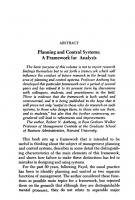
Introduction In a complex system using robotic agents, knowledge about the surrounding environment determines the structure and methodologies used to control and coordinate the system, which leads to an increase in the intelligence of the individual system components. Full or partial knowledge of the agents’ environment, as is found in industry, leads to an intelligent robotic workcell. Because of the rather high level of this knowledge, all the planning activities can be performed off-line, and only taskexecution needs to be done on-line. A different approach is needed when little or no information about the environment is available. In this situation, a robotic multiagent system that shows no clear grouping ofcomponents is better suited to develop plans and to react to changes in a dynamic environment. All the calculations have to be done on-line. This requires more processing power and faster algorithms than the organized structure, where only the operations in the execution phase have to be computed in real time. The distinction between these two paradigms is shown in Figure 1.1. This book will treat only the intelligent robotic cell and its components (shown on the left side of Figure 1.1). Fully autonomous robotic multiagent systems are not covered here. However, the on-line components and algorithms for an intelligent robotic cell can be used in multiagent systems as well. The knowledge it will have about the environment determines the requirements of robotic agent intelligence. Depending on the uncertainty in the work space of a robotic agent in a workcell (existence of dynamic objects), the agent can be classified as belonging to one of the following three classes: Nonautonomous agents require a central processing module to perform off-line and on-line calculations for them. Partially autonomous agents (reactive agents) can react independently to dynamic changes in the environment by calculating new path and trajectory segments on line. Autonomous agents require the least amount of supervision by a coordinator and that can change or adopt a given plan of action based on experience learned during their whole life cycle. 1

2

Chapter 1

Figure 1.1. Degree of autonomy of a robotic system as a function of the amount of knowledge it has about its environment.

1.1. The Modern Industrial World: The Intelligent Robotic Workcell Modern manufacturing is characterized by low-volume, high-variety production and close-tolerance, high-quality products. In response to the ever-increasing competition in the global market, major efforts have been devoted to the research and development of various technologies to improve productivity and quality. The economic pressure for increases in quality, productivity, and efficiency of manufacturing processes has motivated the development of more complex and intelligent flexible manufacturing systems (FMS) (Buzacott, 1985; Kusiak, 1990; Lenz, 1989; Meystel, 1988). The flexible and economic production of goods requires a new level of automation. Intelligent robotic workcells, integrating manufacturing stations (workstations) and robots, form the basis of a flexible manufacturing process. Intelligent robotic workcells and computer integrated manufacturing are effective tools to increase manufacturing competitiveness.

Introduction

3

Figure 1.2. General structure of FMS.

In a manufacturing environment, FMS are generally constructed based on a hierarchical architecture (Buzacott, 1985; Jones and McLean, 1986). The FMS hierarchy consists of the following levels: facility, cell, and workstation and equipment. The levels in the hierarchical architecture have the following functions:

The facility level implements the manufacturing engineering, resource, and task management functions. The control functions at the cell level are job sequencing, scheduling, material handling, supervision, and coordination of the physical activities of workstations and robots. Machining operations are performed at the workstation level. The structure of the FMS control system is shown in Figure 1.2. In the above architecture, the control mechanisms are established in such a way that the

4

Chapter 1

Figure 1.3. Basic definition of the manufacturing process.

upper-level components issue commands to lower-level ones and receive feedback upon the completion of command execution by these lower-level components. The physical components at each level are computer systems and control devices, connected by a communication network such as a local area network (LAN) with a manufacturing automation protocol (MAP) (Buzacott, 1985; Jones and McLean, 1986). Control software is a key component in achieving a high degree of FMS flexibility. The design of robotic cell control software involves the application and implementation of concepts and methods from different scientific disciplines. For a robotic workcell one has to define theprocess according to which the goods are to be manufactured. This process should be defined, designed, and then loaded into the components of the manufacturing cell and executed. The synthesis of the manufacturing process and its enactment have to be performed off-line and thus executed in a radically different environments, in contrast to software engineering, which has largely the luxury to be able to design, quality assure, and execute the programs in roughly the same environment (Chroust, 1992; Pichler, 1989). With respect to the above hierarchy of manufacturing activities, we list the major subtasks to be performed and provide a process model for it (Saridis, 1983; Black, 1988; Jacak and Rozenblit, in press; Jacak and Rozenblit, 1994). On the highest level of abstraction we have (Figure 1.3): Preparation of the Basic Operating Plan: In this step the sequence of processing steps (as defined by the processing

Introduction

5

Off-line phase (Part I) Off line planning and programming

Figure 1.4. Organization of Part I of the book.

6

Chapter 1

On-line phase (Part II) On-line control and coordination

Figure 1.5. Organization of Part II of the book. NN, neural network.

requirements of the product and the applied technology) are defined and the individual processing steps assigned to machines (or machine classes). The subtasks of this process step are: (1) material selection, (2) technological operation selection, (3) machine and tool selection, (4) machining parameter selection, and (5) machining process sequencing (Black, 1988; Wang and Li, 1991).

Modeling of the Processing Workcell: It is necessary for there to be an easy way to describe the physical layout of the cell and specify its components, and easy ways to change it and to provide a large repository of standardized models in a library. The result is a so-called virtual cell, a complete description of the real cell and its components.

Introduction

7

Task Planning and Programming of Cell Equipment: The automatic programming and task planning is based on logical and geometric models of the cell and robots, mathematical algorithms, and to a certain extent experiments. The generation of a robot action sequence is only one phase in the hierarchy of steps required to plan the robot’s behavior in programmable robotic cells. To make the generation of the robot plan applicable to practical problems, more systematic approaches to the design and planning of actions are needed to enhance their performance and enable their cost-effective implementation. At the implementation level, the system for generating the action plan should be capable of reasoning about the geometry and times of actions. Special attention must be focused on questions of directional approach (“what is the best orientation under which a partial product is to be moved toward the machine?”), on collision-freeness, and on optimization of the desired attributes (be it time, energy consumption, speed, etc.) (Prasad, 1989; Bedworth et al., 1991; Maimon, 1987; Lozano-Perez, 1989; Latombe, 1991; Shin and McKay, 1986; Shin and McKay, 1985). Materials Flow — Event-Based Emulation: Only for very simple producer/consumer models can the actual behavior of the product flow be computed in a closed analytical form. In practically all interesting cases only simulation can provide a solution (Ranky and Ho, 1985; Wloka, 1991; Rozenblit and Zeigler, 1988; Jacak and Rozenblit, 1993).

The basic manufacturing process specification is shown in Figure 1.3. For most of the presented steps no closed solution or construction method exists, and thus we are forced to verify and validate the results of our engineering efforts heuristically.

1.2. How to Read this Book In this book we introduce basic research issues associated with each subsystem of the intelligent robotic cell and discuss how different discrete system theory, artificial intelligence, fuzzy set theory, and neural network tools and methods can address these issues. Each block of a workcell control synthesis system need different mathematical and system engineering tools such as graph searching, optimization, neural computing, fuzzy decision making, simulation of the discrete dynamic system, and event based system methods. The book is organized as follows:

8

Chapter 1

Part I gives detailed descriptions and solutions of problems relating to planning the technological process and robots motions. The methods presented here are used in off-line synthesis of the intelligent robotic cell (Chapters 2–6). Methods and algorithms are given to obtain executable plans of robot motions and manipulations based only on general descriptions of the technological task or on the final state of the assembly process. Examples of software systems are given for the design of intelligent control of robotic systems. The plan of this part of book is shown in Figure 1.4. Part II treats the real-time, event-based multilevel coordination and control of robotic system (Chapters 7–11). The components of such control systems use discrete event, neural network, and fuzzy-logic based controllers. Different coordination methods are described depending on the state of knowledge about the surrounding environment of the robotic agent. These methods need different degrees of autonomy for the robotic agent. Possible solutions for obtaining the required intelligent behavior of robotic systems are presented. Chapter 10 describes the synchronized simulation of the manufacturing process performed in a virtual cell parallel to the real technological process, which allows rapid monitoring and diagnosis. The object-oriented specification of an intelligent organizer, coordinator, and executor of cell actions is described in Chapter 11. The plan of this part of the book is shown in Figure 1.5.

CHAPTER 2

Intelligent Robotic Systems A robotic system and its control are termed intelligent if the system can selfdetermine its decision choices based upon the simulation of needed solutions or upon experience stored in the form of rules in its knowledge base. The required level of intelligence depends on how the complete its knowledge is about its environment. The different classes of intelligent robotic systems are shown in Figure 2.1. One such system is the intelligent robotic workcell. Intelligent robotic cells are effective tools to increase productivity and quality in modern industry.

2.1. The Intelligent Robotic Workcell In recent years, the use of flexible manufacturing systems has enabled partial or complete automation of machining and assembly of products. The flexible manufacturing system (FMS) is an efficient production system which can be directly integrated with production functions (Prasad, 1989; Bedworth et al., 1991; Black, 1988). The basic building block of the system is the robotic manufacturing cell, called the robotic workcell. The parts processed in the system are selected and grouped into families based on the similarity of operations (Prasad, 1989; Bedworth et al., 1991). The machines related to these families are grouped and allocated to the cells. This provides benefits such as reduced setup and flow times and lower in-process inventory levels through simplified work flows. They consist of three main components: a production system (technological devices) a material handling system (robots) a hierarchical computer-assisted control system Robotic cellular manufacturing systems are data-intensive systems. The robotic workcell integrates all aspects of manufacturing. The intelligent robotic 9

10

Chapter 2

Figure 2.1. Intelligent robotic systems: Classes, structures, and methods.

Intelligent Robotic Systems

11

workcell, and consequently intelligent cellular manufacturing systems, represent the direction of the development of modern manufacturing (Kusiak, 1990; Prasad, 1989; Saridis, 1983; Meystel, 1988). Definition 2.1.1 (Intelligent Robotic Cell). The robotic cell and its control are termed intelligent if it can self-determine its decisions choices based upon the simulation of needed solutions in virtual world or upon experience gained in the

past both from failures and successful solutions which are stored in the form of rules in the system knowledge base (Kusiak, 1990; Sacerdot, 1981; McDermott, 1982; Saridis, 1989; Yoshikawa and Holden, 1990). An intelligent robotic system in the industrial world is a computer-integrated cellular system consisting of partially or fully intelligent robotic workcells. The planning and control within a cell is done off-line and on-line by a hierarchical controller which itself is regarded as an integral part of the cell. Such a structured robotic manufacturing cell will be called a computer-assisted robotic cell (CARC). The main purpose of the CARC is to synthesize and execute a sequence of actions so that the overall system objectives are achieved even under circumstances which may require replanning. The control system should tie all the data available to the solutions required to run the manufacturing system effectively. Some of the problems to be solved in such an environment are grouping, machine choice and process and motion planning. Definition 2.1.2 (Control Task of CARC). The intelligent computer-assisted robotic cell should be able to self-determine for given technological task the control of workcell actions such that:

the task is realized deadlocks are avoided maximal flow time is minimal work-in-process factor is minimal geometric constraints are satisfied

collisions between robotic agents are avoided Design and control of intelligent robotic manufacturing systems involves the application and implementation of concepts, methods, and tools from different disciplines of science, mathematics, and engineering. To synthesize a completely autonomous or semiautonomous computer-assisted robotic cell operating in dynamic environment we use concepts, ideas, and tools from artificial intelligence,

12

Chapter 2

computational intelligence, and general systemtheory, such as hierarchical decomposition of control problems, the hierarchy of specification models, and discrete and continuous simulation from system theory, and action planning methods, graph-searching of the model’s state, neural computation, learning, and fuzzy decision making from artificial and computational intelligence.

2.2. Hierarchical Control of the Intelligent Robotic Cell The control problem of a computer-assisted robotic cell is a complicated one. Due to the large number of possible solutions (which differ depending on the sequence of technological operations, sequence of sensor-dependent robot actions, geometric forms of manipulator paths, and dynamics of movements along the paths), it is necessary to apply a a stratified methodology. This is possible since robot actions can be modeled in terms of different conceptual frameworks, namely, operational, geometrical, kinematic, and dynamic. Thus, to reduce the complexity of the control problem, we propose to apply a hierarchical decomposition process to break down the original problem into a set of subproblems. In this way, the solution of the control synthesis problem is formulated in terms of successive levels ofa model ofa flexible production system behavior. The control laws which govern the operation of a CARC are structured hierarchically. We distinguish three basic levels of control: the execution (workstation) level the coordination (cell) level

the organization level This follows the classification of intelligent control systems often cited in the literature (Kusiak, 1990; Lenz, 1989; Saridis, 1983; Meystel, 1988; Maimon, 1987). The organization level accepts and interprets related feedback from the lower levels, defines the strategy of task sequencing to be executed in real-time

and processes large amounts of information with little or no precision. Its functions are defined to be reasoning, decision making, learning feedback, and long-term memory exchange. The coordination level defines the routing of the part in logical and geometric terms and coordinates the activities of workstations and robots, which in turn coordinate the activities of the equipment in the workstation. It is concerned with the formulation of the actual control task to be executed by the lowest level.

Intelligent Robotic Systems

13

Figure 2.2. Functional structure of an intelligent robotic system.

The execution level is composed of device controllers, and executes the action programs issued by the coordinator. An intelligent CARC (with the hierarchical structure shown in Figure 2.2) composed of the three interactive levels of organization, coordination, and execution, is modeled with the aid the theory of intelligent systems (Sacerdot, 1981; Saridis, 1989). Figure 2.3 presents the knowledge base and the different classes of formal models which are needed for the planning and control of cell action. All planning and decision making actions are performed within the higher levels. In general, the performance of such systems is improved through self-planning with different planning methods and through self-modification with learning algorithms and schemes interpreted as interactive procedures for the determination of the best possible cell action. There are two major problems in the planning and synthesis of such complex control laws. The first depends on coordination and integration

14

Chapter 2

Figure 2.3. Structure of a knowledge base for an intelligent robotic cell.

at all levels in the system, from that of the cell, where a number of machine must cooperate, to that of the whole manufacturing workshop, where all cells must be coordinated. The second problem is that of automatic action planning and programming of the elements of the system. Thus, the control problem of a robotic cell can be considered as having two main elements.

The first, which we shall call logical control or operational control, relates to the coordination of events, for example, the loading of a part into a machine and the starting of the machine program cycle. Logical control acts to satisfy ordering constraints on event sequences. The second, termed geometric and dynamic control, relates to the determination of the geometric and dynamic parameters of motions for the elements of the system. Geometric control ensures that the position, path,

Intelligent Robotic Systems

15

and time of movement of all elements of the system and its environment satisfy the geometric and dynamic constraints at all times.

2.3. Centralization versus Autonomy of the Robotic Cell Agent For a multirobot system forming a robotic cell, there are two extreme possibilities a centralized or a distributed system. In a centralized robotic system, each robot is only a collection of sensors, actuators and some local feedback loops. Almost all tasks are processed in a coordinator (central controller). The communication between the coordinator and the robots only involves sending data from sensors to the coordinator and receiving detailed commands from the coordinator. Conversely, in a distributed robotic system, each robot plans and solves a problem (task) “independently” and communicates its information, which is processed in each robot.

2.3.1. Centralized Control of the Intelligent Robotic Cell A multirobot system which aims at cooperative work always has some tasks which are common to the whole system rather than to individual robots, e.g., a task for planning the manipulation, or a task for global cooperation, etc. These tasks are suited for processing in a coordinator rather than in each robot. However, in a centralized system, defects such as the limitation of processing ability or lack of fault tolerance might become more significant as the system becomes larger, because the processing of all of tasks is performed by the coordinator. Moreover, since the robots are distributed physically, it is more suitable to process some tasks separately rather than concentrating them at the coordinator. Centralized systems, due to the limits on available computational power and the existence of overhead in transferring data between the robots and the central system (coordinator), are not appropriate for other than small groups of robots. Thus, centralized processing is not quite suitable for cooperative work via multiple robots.

2.3.2. Distributed Control of the Intelligent Robotic Cell The trend in studies of distributed autonomous robotic systems seems to indicate that this approach is superior to centralized system from the view points of flexibility, robustness and fault-tolerance ability. In a pure distributed system, the processing of a cooperative manipulation task which is common to the whole

16

Chapter 2

system is also done separately. In this situation, cooperation among distributed agents becomes necessary to perform the task. This kind of cooperation requires excessive robot intelligence, excessive communication, and tautological processing. These are unnecessary and unnatural for constructing a multirobot system and can be thought of as a type of loss to the whole system (Ahmadabi and Nakano,

1996; Lambrinos and Scheier, 1996; Wang et al., 1996; Kosuge and Oosumi,

1996). A mixed form, rather than aiming at constructing a pure distributed robotic system, is a multirobot system which maintains a coordinator as its leader, and incorporates homogeneous behavior-based robots which have limited abilities for manipulation. In contrast to the coordinator in a centralized system, the coordinator here acts as a leader and an organizer which coordinates robot behavior, generates goals for the robots, and offers some global position information to each robot to modify its own data. It does not perform any calculation of target object dynamics

or force distribution for dynamic cooperation, and does not do any path planning for each robot. In contrast to collision avoidance among moving robots, in this system, the robots which are working on a manipulation interfere with each other dynamically through the target object. For cooperation, some information about the target object and other robots can be obtained from sensors on each robot. Then, with the information obtained from the coordinator by communication and from sensors, cooperation with other robots for manipulation work can be realized, and the necessity of communication among robots vanishes. A system without communication among robots has the advantage of avoiding a rapid increase of communication quantity when the number of robots in the system increases. Such a system is not just a simple mixture of the two types of systems, centralized and distributed, in order to obtain an average of the advantages of each system. The coordinator, the leader of the system, not only compensates for the incompleteness of each robot’s ability, but also serves to organize robots whose behavioral attributes include limited manipulating ability and cooperative ability. As an illustration, consider that even among human beings, a better quality of cooperation often appears in a group with a leader or a supervisor when a difficult task is being performed.

2.3.3. Cooperation in the Robot Group Various researchers on multirobot systems have different targets in mind, and thus there are various definitions of cooperation. The most basic and essential point of the cooperation between multiple robots is that they perform a task together without conflict. For performing different tasks, the information and factors involved in achieving cooperation will be different. This gives different characteristics to the different

Intelligent Robotic Systems

17

cooperation strategies. Cooperation in a group of robots can be defined such that both the information obtained or exchanged by each robot and the elements of the task which the cooperation is working to achieve, include dynamic factors (such as accelerations of forces). In general, dynamic cooperation is only necessary when performing a task with a dynamic system, whether in a model-based or in a behavior-based approach. Of course, behavior-based cooperation strategy is different from the strategy applied in a model-based cooperating robotic system. In the model-based approach, cooperation in a group of robots is achieved in two steps: generating a set of the desired physical parameters (e.g., the desired path and torque of each robot) by using a model-based planner (off-line phase)

controlling the robot mechanisms to realize the desired parameters. Therefore, a dynamic cooperation strategy in the model-based approach is required to consider dynamic factors of the system in the planning stage and to guarantee that its controller is able to cope with the dynamic characteristic of the system. On the contrary, the behavior-based approach is based on the idea that robot control can be realized by constructing a robot’s behavioral attributes from a certain quantity of behavioral elements. Each behavioral element constructs a behavior control mechanism to act on the world in some situation. Cooperation among robots emerges from robot behavioral attributes and their interaction through the object and the environment. Thus a dynamic cooperation strategy must be such that a robot’s behavior acts on the object and on the environment dynamically. Also, each robot’s behavioral attributes must be able to cope with the dynamic interaction (Wang et al., 1996; Kosuge and Oosumi, 1996; Haddadi, 1995; Wooldridge et al., 1996).

2.4. Structure and Behavior of the Intelligent Robotic System The intelligent control of a computer-assisted robotic cell is synthesized and executed in two phases, namely: Planning and off-line simulation On-line simulation based monitoring and intelligent control

In the first phase a hierarchical simulation model of a robotic workcell termed a virtual cell is created. Because the computer-assisted robotic cell has to make too

18

Chapter 2

Figure 2.4. Structure of computer-assisted robotic cell (CARC).

many subjective decisions on the basis of deterministic programming methods, the knowledge database and knowledge-based decision support system need to act as an adviser. Such a knowledge database is represented by the virtual workcell. The are two basic types of simulation employed for modeling manufacturing systems: discrete and continuous simulation. Discrete simulation is event oriented and is based on the concept of a complex discrete events system (DEVS) (Zeigler, 1984; Rozenblit and Zeigler, 1988). Workcell components such as NC-machine tools, robots, conveyors, etc., are modeled as elementary DEVS systems. Discrete changes of state of these systems are of interest. This type of simulation is used for verification and testing different variant of workcell task realizations, called processes, obtained from the Process Planner. Process planning is based on the description of task operations and their precedence relations. The resulting fundamental planes of cell action describe different ways to decompose the cell

Intelligent Robotic Systems

19

task into ordered sequences of technological operations. To simulate the variants of a process the system know how individual robot actions are carried out. For the detailed modeling of cell components the continuous simulation approach and motion planning methods are used. The geometrical interpretations of cell actions obtained from the Motion Planner and tested in a geometric cell simulator allow us to select the optimal task realizations which establish the logical control unit of the control system. The motion trajectories of robots obtained by continuous simulation create the geometric control unit of the control system. In the second phase the real-time discrete event simulator of a CARC generated in the first phase is used to generate a sequence of future events of a virtual cell in a given time window. These events are compared with the current states of a real cell and are used to predict motion commands for the robots and to monitor the process flow. The simulation model is modified at any time when the states of the real cell change, and current real states are introduced into the model. The structure of a computer-assisted robotic cell is shown in Figure 2.4.

This page intentionally left blank

PART I

Off-Line Planning, Programming, and Simulation of Intelligent Robotic Systems

This page intentionally left blank

CHAPTER 3

Virtual Robotic Cells Robotic cells are formed by group technology clustering techniques such as the rank order clustering (ROC) method (Black, 1988; King, 1980; Wang and Li, 1991); improved methods also exist (Black, 1988). The problem of grouping parts and machines has been extensively studied. The available approaches can be classified as follows: evaluative methods clustering algorithms similarity coefficient-based methods bond energy algorithms cost-based heuristics within-cell utilization-based heuristics neural network-based approaches A real cell is a fixed physical group of machines and a virtual cell is a formal representation (computer model) of a machine group in the central computer of a control system. Each cell is designated for the production of a small family of parts. The production related to one type of part is called a technological task. More specifically, an intelligent robotic cell is a set of NC (or CNC)-programmable machines (technological devices) D called workstations and production stores M, connected by a flexible material handling facility R (such as robots or automated guided vehicles), and controlled by a computer net (LAN) connected with a sensory system. Each workstation has its own control and programming system. A workstation (machine) can have a buffer. Parts are automatically loaded into the machine from the buffer. Then they are machined and subsequently can be stored in the buffer. Depending on the type of technological operation to be carried out on a part, various tooling programs can be used to control the workstation’s machining process. 23

24

Chapter 3

The virtual robotic cell has a hierarchical structure of models. The robotic cell modeling process proceeds in two phases, namely (1) modeling of the logical structure of the cell and (2) modeling of the geometry of the cell.

3.1. Logical Model of the Robotic Cell In the first phase, the workcell entity structure needs to be designed, i.e., a logical structure of the cell must be created. The group of machines is divided into

subgroups, called machining centers, which are serviced by separate robots. Parts are transferred between machines by the robots from set R, which service the cell. A robot can service only those machines within its service space is the Cartesian base frame). The set of devices which lie in the rth robot service space is denoted by More specifically, the device belongs to a group serviced by robot r [i.e., if all positions of its buffer lie in the service space of robot r. Consequently, the logical model of a workcell is represented by Example 3.1.1. Consider Example_Cell. To perform the technological tasks the following machines are grouped: NC-millers WHD 25 (d01) and FYD 30 (d03), NC-lathes TNS 26e (d02) and Weiler 16 (d04), a quality inspection center (d05), a feeder conveyor (m01), conveyor (m02), and an output conveyor (m03). The workcell is serviced by two IRb ASEA robots {r01, r02}. The machining center serviced by robot r01 consists of the following devices: The machining center of robot r02 has the following equipment:

The logical structure of the manufacturing workcell is shown in Figure 3.1.

3.2. Geometrical Model of the Robotic Cell In the second phase of the modeling process the geometry of the virtual cell must be created. Formally the geometry of the cell is defined as follows (Brady, 1986; Yoshikawa and Holden, 1990; Jacak, in press; Ranky and Ho, 1985; Wloka, 1991):

Virtual Robotic Cells

25

Figure 3.1. Logical structure of a virtual cell.

The first component of the cell geometry description

represents the set of geometrical models of the cell’s objects. Ed is the coordinate frame of the object (device) d, and Vi is the polyhedral approximation of geometry dth object in Ei (Ranky and Ho, 1985; Wloka, 1991). The second component of the geometrical model

represents the cell layout as a set of transformations between an object’s coordinate frame Ed and the base coordinate frame E0 (Brady, 1986). Consequently, a geometry modeling process has two phases: (1) workcell object modeling and (2) workcell layout modeling.

3.2.1. Workcell Object Modeling The geometric model of each object is created through solid modeling (Bedworth et al., 1991; Yoshikawa and Holden, 1990), Which incorporates the design and analysis of virtual objects created from primitives of solids stored in a geometric database. Constructive solid geometry handles primitives of solids, which are bounded intersections of closed half-spaces defined by planes or shapes. More complex objects (such as technological devices, auxiliary devices or static obstacles) can be built by composition using set operations, such as the union, intersection, and difference of solid bodies. As an example of virtual object synthesis, the modeling of the NC-lathe WH64 VF is shown in Figure 3.2.

3.2.2. Workcell Layout Modeling Workcell objects Vd can be placed in a robot’s workscene in any position and orientation. The transformation between the object frame Ed and the base frame E0 is used to calculate the location of virtual objects (devices, stores,

26

Chapter 3

Figure 3.2. The geometric model of the NC-lathe WH64 VF.

robots). The virtual objects (devices, stores) are loaded from a catalogue into the Cartesian base frame and can be located anywhere in the cell using translation and rotation operations in the base coordinate frame (Jacak, in press). The layout of the manufacturing workcell considered in the example Example_ Cell is presented in Figure 3.3. Major drawbacks of such graphics modeling include the following: Unless already stored in the catalogue, the graphics images of the robots, devices, and other components of the cell must be designed by the user. This is often time-consuming.

Using three-dimensional polyhedral approximation of objects, collisions can be detected by complex time-consuming computer geometry algorithms.

3.3. Basic Methods of Computational Geometry We focus on defining tools for the efficient computation of distances between bodies of objects in three-dimensional space.

3.3.1. Distance Computing Problem The most natural measure of the proximity is the Euclidean distance between two objects, i.e., the length of the shortest line segment joining the two objects.

Virtual Robotic Cells

27

Figure 3.3. The geometric model of the robotic workcell Example_Cell.

There is an extensive computational geometry literature concerning the distance calculation problem (Gilbert et al., 1988). Many algorithms have been specifically designed to achieve bounds on the form of the asymptotic time. For twodimensional problems, Schwartz (1981) gives an O(log2 M) algorithm, and more recently, O(log M) has been used (Schwartz, 1981) (M is the number of vertexes). The three-dimensional problem has been considered (Red, 1983) with a time of O(M log M). Because of their complexity and special emphasis on asymptotic performance, it is not clear that the algorithms are efficient for practical problems. Other schemes have also been described: Red (1983) presents a program which uses a projection approach for polyhedra with facial representation, Gilbert (1988) considers negative distances for polytopes, Mayer (1986) considers boxes and their distances, and Lumelsky (1985) considers line segments. Let O1 and O2 denote two convex solids, x and z two points belonging respectively to O1 and O2, and n a unit vector. The notation (n|x) refers to the inner product of vectors n and x. The Euclidean distance between O1 and O2, equal to

can be computed by alternatively projecting a point of O1 onto O2, the point of O2 that we obtain onto O1, etc., until the distance between the points converges. For

28

Chapter 3

nonoverlapping objects the Euclidean distance can be defined as

where

If they do overlap, such a distance becomes negative and measures how far objects interpenetrate. The interesting point in this definition is that is always lower than Let us define the influence distance as the threshold on interactions between objects. Then, if is greater than for some value n, the same stands for the exact distance and we can declare these objects to be noninteracting. Note that the computation of can be decomposed into

for an arbitrary point o. Based on such a definition of procedure for distance estimation:

we can use the following

1. Select an arbitrary point x in O1 and project it on O2. 2. With

compute the first point x' of O1 in direction –n.

3. Then

and we have

It can be shown that converges toward if the procedure is repeatedly applied (Faverjon, 1986). It is also possible to convert the distance problem into a quadratic programming problem and apply a feedback neural network to solve it (Lee and Bekey, 1991; Jacak, 1994b). Obstacles are modeled as unions of convex polyhedra in 3D Cartesian space. A polyhedral obstacle can be represented by a set of linear inequalities where The polyhedral object is modeled by a connectionist network with three units in the bottom layer which represent the x,y,z coordinates of the point. Each unit in the second layer corresponds to one inequality constraint of the object: The connections between the bottom and the second layer have their weights equal to the coefficients aj, bj of the corresponding face. Then the jth face of the polyhedral object is represented by a neuron with a sigmoid function

Virtual Robotic Cells

29

When a point is given to the bottom-layer units, each of the second-layer neurons decides whether the given point satisfies its constraints. To reduce the training time we can apply hybrid techniques which automatically create the full network topology and values of neural weights based on symbolic computation of the polyhedral object’s faces. Let M, N denote the number of neurons representing the objects O1 and O2, respectively. The distance between objects O1 and O2, i.e., is the solution of the following optimization problem:

with constraints

The above problem can be transformed into a problem without constraints by

introducing the penalty function r(x,z) defined as

where is the neuron activation function given by Equation (3.9). Then the modified criterion function is

The solution of the above problem can be obtained by attaching a feedback around a feedforward network to form a recurrent loop. This coupled neural network is the neural implementation of the gradient method of distance calculation (Lee and Bekey, 1991; Park and Lee, 1990; Han and Sayeh, 1989; Jacak, 1994b). Let then

where

30

Chapter 3

Figure 3.4. Neural computation of the distance between objects O1 and O2.

and c(d) is called the update ratio and can be chosen as

where

is the Hessian of w.

It should be noted that the Hessian of w is easy to compute based on the output of the neurons The structure of a neural network realizing the distance calculation is shown in Figure 3.4. The above method can be easy extended for nonpolyhedral objects (Jacak, 1994b).

3.3.2. Intersection Detection Problem In many cases of collision detection it is possible to avoid calculating the minimal distance between two objects by testing the intersection only. The most important problem is the detection of an intersection between a line segment and a convex solid.

Virtual Robotic Cells

31

To obtain fast and fully computerized methods for intersection detection we can use the additional geometrical representation of each cell’s object. Each volume representation decomposes objects into primitive volumes such as cylinders, boxes, or cubes. We introduce the ellipsoidal representation of 3D objects, which uses ellipsoids for filling the volume. Instead of planes that are in polyhedral approximation, the surface of the object is modeled by parts of ellipsoids. The accuracy of representation depends on the number of ellipsoids and their distribution in the object. The algorithm for packing primitive volumes with touching ellipsoids or spheres has the following major stages: (1) distance calculation, (2) search for the local centers of the ellipsoids, and (3) selection of ellipsoids. The steps are repeated performed until sufficient accuracy is reached. The ellipsoid packing algorithm transforms each primitive solid into a union of ellipsoids, and consequently the geometry of the virtual object is represented by

and ri represents the centers of the ellipsoids, Di is the matrix of the major axes, and Ai is the matrix of the axis lengths. As an example, a parallelepiped is packed by a bigger central ellipsoid and eight smaller spheres in the corners. The packed ellipsoids are a hierarchical representation in the sense that for gross representation only the biggest ellipsoids are used. 3.3.2.1. Intersection of an ellipsoid with a line segment. The ellipsoidal representation of a virtual object can be used to test the feasibility of a robot configuration, represented by the robot’s skeleton. Checking for the collision-free nature of a robot configuration can be reduced to the “broken line–ellipsoid” intersection detection problem, which in this case has the following analytical solution. Let a point from the given line segment [P, Q] be given by

Plugging the point p into the equation of the ellipsoid [Equation (3.16)] gives the following condition of nonintersection between the line segment the and ellipsoid

where

It is easy to show that:

32

Chapter 3

Figure 3.5. Hierarchy of virtual cell models.

Fact 3.3.1. The line segment [P, Q] does not intersect with the ellipsoid if

The virtual robotic workcell is represented by a multilayer system of models which can be used as a knowledge base for planning systems. The hierarchy of workcell models is shown in Figure 3.5.

CHAPTER 4

Planning of Robotic Cell Actions Small-batch production requires complex control systems with reasonably high flexibility; not only with regard to manufacturing equipment, but also in connection with planning, scheduling, handling, and management decision-making procedures. The computer integrated manufacturing (CIM) system integrates all aspects of manufacturing. The key to a successful CIM implementation is “integration”. Every component in a manufacturing system has to be an integral part of the system. The various components of a system such as CAD (computer-aided design), CAM (computer-aided manufacturing), FMS (flexible manufacturing system), CAT (computer-aided testing), and so on must be integrated (Prasad, 1989; Bedworth et al., 1991; Yoshikawa and Holden, 1990; Black, 1988; Wang and Li, 1991). The communication between CAD and CAM is a key link which to a great extent determines the success of CIM. Computer-aided process planning (CAPP) serves as the bridge between CAD and CAM. CAPP determines how a design will be made in a manufacturing system. The manufacturing process includes not only processes acting directly upon the manufactured objects, but also preparatory processes (such as production planning, process planning, production scheduling, etc.) and auxiliary processes (such as equipment maintenance, workpiece handling, quality inspection, etc.).

4.1. Task Specification To begin the synthesis of a computer-assisted robotic cell (CARC) control, one specifies the family of technological tasks to be realized in the cell. Machining Task: All activities that consist of material-removal operations constitute machining. Examples are turning, drilling, and face milling. Assembly Task: Assembly involves assembling the manufactured parts to form the required products. In order to perform this task, the parts have to be machined according to the required specifications and tolerances. 33

34

Chapter 4

Depending on how the parts arrive at the machines, there are two modes of processing (machining or assembly), flow shop and job shop. In the flow shop, all parts flow in one direction, whereas in the job shop, the parts may flow in different directions; also, a machine can be visited more than once by the same part. In both cases, a part does not have to visit all machines.

4.1.1. Machining Task Specification In this section we focus on issues involved in the machining process. The machining process of part may include various machining operations, such as turning, milling, drilling, grinding, broaching, gear-cutting, etc., depending on the required shape, dimensions, tolerance, and surface quality of the part.

The basic components of the machining process are operations. An operation is a complete portion of the machining process for cutting, grinding, or otherwise treating a workpiece at a single workplace. The operation is characterized by unchanged equipment, unchanged workpiece, and continuity. Each operation is to be processed by a most one machine at a time. Process planning for CARCs is critically dependent on the task representation. Several task representation schemes have been proposed (Sacerdot, 1981; Lifschitz, 1987; Homem De Mello and Sanderson, 1990; Sanderson et al., 1990; Maimon, 1987), and include lists of operations, triangle tables, and AND/OR graphs. Here, we use a general description of a workcell machining task, formally specified as follows.

Definition 4.1.1 (The Machining Task). The machining task realized by a robotic cell is represented by a three-tuple:

where O is a finite set of technological operations (machine, test, etc.) required to process the parts, is the partial order precedence relation on the set O, and is the relation of device or store assignment.

The partial order represents an operational precedence, i.e., means that the operation q is to be completed before the operation o can begin. means that the operation o can be performed on the workstation d, and if then m is the production store from the set M where the parts can be stored after the operation o has been completed. The parts are transferred between devices by the robots. Based on the previously defined logical model of the cell and the description of the set Group(r), we can define the relation which describes the transfer of

Planning of Robotic Cell Actions

35

Figure 4.1. The machining task.

parts after each technological operation of the task

where

and and We assume that for each operation oi there exists a robot ri which can transfer parts between the workstation di and stores mi from the set Group(ri). In a special case is a partial function, i.e., Example 4.1.1. In the example Example_Cell, the manufacturing cell should perform a task consisting of the following operations: {A,D,E} mill operations {B,C,F} turn operations {G} quality test operation

The precedence relation is shown in Figure 4.1. To perform this task the following machines are grouped: the NC-millers WHD 25 (d01) and FYD 30 (d03), the NC-lathes TNS 26e (d02) and Weiler 16 (d04), and quality inspection center (d05), a feeder conveyor (m01), a conveyor (m02) and an output conveyor (m03). The symbols in brackets represent the logical names of the cell devices. The allocation relation α is illustrated in Figure 4.2. Such a task is realized in robotic cells based on the group technology concept, which groups parts together based on their similarities. Such a cellular manufacturing approach organizes machines and robots into groups responsible for producing a family of parts.

36

Chapter 4

Figure 4.2. The allocation relation.

4.1.2. Assembly Task Specification The second type of technological task is the assembly task. All operations which lead from parts to the required final product constitute assembly. Definition 4.1.2 (The Assembly Task). The assembly task is the partial ordered set of the assembly operations over the parts:

where A is a finite set of assembly operations required to process the final product,

is the partial orderprecedence relation on the set A,

is

the relation of machining task assignment (where MTasks is the set of machining tasks), and is the relation of assembly station assignment.

The precedence relation among operations for the final product can be represented by a complex directed graph (digraph). In this digraph any node of degree 1, i.e., with the number of edges incident to the node equal to 1, denotes the initial operation The initial operation is directly connected with the appropriate machining task Taski which prepared the initial part,

Any node of degree greater than 1 denotes a subassembly operation and the root node denotes a final assembly operation. The arcs of the digraph correspond to precedence constraints. The partial order represents an operational precedence, i.e., means that the assembly operation a is to be completed before the assembly operation b can begin. Based on this description we can use the previously defined digraph as a representation of the final product. The nodes of the graph

Planning of Robotic Cell Actions

37

represent the parts or subassemblies. Each initial node denotes a part (and corresponds to a machining task that prepared this part) and the rest of the nodes denote a subassembly or a final product. Each part is connected to one subassembly. The mapping between initial operations (initial nodes, parts) and machining tasks is described by the relation means that the part (initial

operation) can be obtained as a result of the machining task Taski. The graph representation allows assembly at a particular node of only one subassembly with any number of parts or any number of subassemblies without parts at all. Then each subassembly node can be represented by the set of initial parts, which are the initial nodes in the subassembly tree expanded from the subassembly node. Given two subassemblies ai and aj characterized by their sets of parts Pai, respectively, and Paj, we say that joining ai and aj is an assembly operation if the set characterizes a new subassembly ak. The subassemblies ai and aj are input subassemblies of the assembly operation, and ak (with is the output subassembly of the assembly operation. Due to the assumption of unique geometry, an assembly operation can be characterized by its input subassemblies only, and it can be represented by a set of two subsets of parts. The set of connections in the representation of an assembly operation corresponds to a cut-set of the graph ofconnections of the operation’s output subassembly. Conversely, each cut-set of a subassembly’s graph of connections corresponds to an assembly operation (Homem De Mello and Lee, 1991; Homem De Mello and Sanderson, 1990). Given the set of all cut-sets of a subassembly’s graph of connections, the set of their corresponding assembly operations is referred to as the operations of the subassembly. An example of an assembly task is shown in Figure 4.3.

38

Chapter 4

4.2. Methods for Planning Robotic Cell Actions Process planning for a mechanical product involves preparation of a plan that outlines the routes, operations, machine tools, and fixtures required to produce the part. In the last decade there has been the trend to automate process planning, since it increases production efficiency. Examples of such systems are CAPP, CPPP, MIPLAN, and GenPLAN. There are two basic approaches to process planning: (1) variant approaches and (2) generative approaches (Kusiak, 1990). In the variant approach each part is classified based on a number of attributes and coded using a classification and coding system. The code determines the process plan. The variant approach can be useful in a case where there is a great deal of similarity between parts (Kusiak, 1990).

4.2.1. Assembly Task Planning Assembling a mechanical structure is typically performed by a series of operations, such as insertions of a peg into a hole. Under this model, the first stage in the design of an assembly system must be to identify the operations necessary to manufacture the given assembly and to specify the sequence in which they are to be performed. The selection of such a sequence of operations is called the assembly planning process. Definition 4.2.1 (The Assembly Process). Given an assembly task Assembly (Definition 4.3) that has I parts, an ordered set of I – 1 assembly operations Assembly_Process = (a 1, a2, ... aI–1) is an assembly sequence or an assembly process if:

no two operations have a common input subassembly

the output subassembly of the last operation is the whole assembly the input subassembly to any operation ai is either a one-part subassembly or the output subassembly of an operation that precedes ai To any assembly sequence Assembly_Sequence = (a1, a2, ... aI–1) there corresponds an ordered sequence

Assembly_Trace = (as1, as2, ..., asI) of I assembly states of the assembly process.

Planning of Robotic Cell Actions

39

The state as1 is the state in which all parts are separated. The state asI is the state in which all parts are joined forming the whole assembly. Any two consecutive states asi and asi+1 are such that only the two input subassemblies of the operation ai are in asi and not in asi+1, and only the output subassembly of operation ai is in asi+1 and not in asi. Therefore, an assembly sequence can also be characterized by an ordered sequence of states. The assembly sequence states the assembly process. A computer system for assembly planning must have a way to represent the assembly plans it generates. Several methodologies for representing assembly plans have been utilized. These include representations based on directed graphs, on AND/OR graphs, on establishment conditions, and on precedence relationships (Homem De Mello and Lee, 1991; Homem De Mello and Sanderson, 1990). An AND/OR graph can also be use to represent the set of all assembly sequences. The nodes in this graph are the subsets of parts that characterize stable subassemblies. The hyperarcs correspond to the geometrically and mechanically feasible assembly operations. Each hyperarc is an ordered pair in which the first element is a node that corresponds to a stable subassembly ak and the second element is a set of two nodes {ai, aj} such that and the assembly operation characterized by ai and aj is feasible. Each hyperarc is associated to a decomposition of the subassembly that corresponds to its first element and can also be characterized by this subassembly and the subset of all its connections that are not in the graphs of connections of the subassemblies in the hyperarc’s second element. This subset of connections associated to a hyperarc corresponds to a cut-set in the graph of connections of the subassembly in the first elements of the hyperarc. The formal definition of an assembly AND/OR graph can be found in (Homem De Mello and Lee, 1991; Kusiak, 1990). Every feasible assembly sequence in the directed graph of an assembly task (Definition 4.3) corresponds to a feasible assembly tree in the AND/OR graph of assembly sequences, and every feasible assembly tree in the graph AND/OR corresponds to one or more feasible assembly sequences in the directed graph of a feasible assembly task. Assembly planning is a computationally intensive task. The problem of generating the assembly sequences for a product can be transformed into the problem of generating the disassembly sequences for the same product. Since assembly task are not necessarily reversible, the equivalence of the two problems will hold only if each operation used in disassembly is the reverse of a feasible assembly operation, regardless of whether this reverse operation itself is feasible or not. In the disassembly problem each operation splits one subassembly into smaller subassemblies, maintaining all contacts between the parts in either of the smaller subassemblies. This transformation leads to a decomposition approach in which the problem of disassembling one assembly is decomposed into distinct subproblems, each being to disassemble one subassembly. It is assumed that exactly two parts or

40

Chapter 4

subassemblies are joined at each time, and that whenever parts are joined forming a subassembly all contacts between the parts in that subassembly are established. The decomposition algorithm returns the AND/OR graph representation of the assembly process. The correctness of the algorithm is based on the assumption that it is always possible to decide correctly whether or not two subassemblies can be joined, based on geometrical and physical criteria. Based on this approach, different computer aided assembly planning systems have been implemented, including LEGA, GRASP, XAP, BRAEN, COPLANNER, and DFA. More exact descriptions are given in (Homem De Mello and Lee, 1991). In this chapter we focus on the machining planning problem in which only the general description of a task is provided (Definition 4.1.1).

4.2.2. Machining Task Planning Machining process planning can be divided into two stages (Wang and Li, 1991):

machining operations design: i.e., selection of machining methods and machine tools for each operation, and specification of each operation process route planning:

i.e., determination of the sequence of machining operations

Process route planning is the overall planning of a part manufacturing process. The objective is to determine the sequence of operations in a process plan. The precedence of operations is based on operation constraints, tooling constraints andpart geometry constraints. Several alternative process plans are evaluated and compared so that the best plan can be selected. The evaluation of the alternatives should be a synthetic analysis from the technological and manufacturing efficiency points of view. Then the main purpose of an intelligent control of autonomous robotic workcell (CARC) for the machining process is to synthesize and execute a sequence of machine and robot actions so that the all operations are realized. Such systems should enable automatic generation and interpretation of robot and NC machine actions. There are two major problems in designing such complex control systems (Sacerdot, 1981; Saridis, 1983; Meystel, 1988). The first depends on coordination and integration at all levels in the manufacturing system. The second problem is that of automatic programming of the elements of the system. The control of manufacturing can be considered as having two elements. The first, which we shall call logical control relates to the coordination of events required to satisfy ordering constraints on event sequences and is adequate for a sequence of process operations. The second, termed geometric and dynamic control, relates to the

Planning of Robotic Cell Actions

41

determination of the geometry and dynamic parameters of motion of the elements of the system. In this chapter we focus on the production route planning problem in which only a general description of a task is provided (Definition 4.1.1). In other words, the route planning problem is to find for a given task the most efficient sequence of machines through which parts must flow during repetitive task executions. Such a route is called the fundamental plan of the workcell action. Searching for the most efficient plan requires that we define plan comparison criteria. One such criterion is that the sequence of operations and robot/machine actions related to it should minimize the mean flow time of parts (Kusiak, 1990; Bedworth et al., 1991). The information necessary to evaluate the efficiency of a plan is usually available during the actual execution of the plan in a real workcell or in its simulation model (Maimon, 1987; Jacak and Rozenblit, in press; Jacak and Rozenblit, 1994). The flow time of every job is the sum of the processing time, the waiting time, and the time of interoperational moves, called the transfer time. The waiting and transfer times depend on the order of operations in a task and on the interpretation of robot movements. Each route determines different topology of robot motion trajectories, different deadlock avoidance conditions, and a different

job flow time. Therefore, route planning is a critical issue in all manufacturing problems. 4.2.2.1. Basic terminology of concurrent technological process planning. In the process planning phase, we must find an ordered sequence of technological operations from Task (Definition 4.1.1), called aprocess, with a minimum number of deadlock cases. This problem is related to operations scheduling (Kusiak, 1990; Jones and McLean, 1986). To explain it in more detail, we introduce some additional notions. Definition 4.2.2 (The Machining Process). The ordered execution sequence of L operations of Task (Definition 4.1.1) is called a pipeline sequential machining process

if the following conditions hold:

if for two operations oi and oj from Task,

then i < j

for each i = 1, ..., L – 1 there exists a robot which can transfer a part from machine di (or store mi) assigned to operation oi to machine di+1 assigned to operation oi+1, i.e.,

42

Chapter 4

A process can be realized by different sequences of technological devices (called resources) required by successive operations from the list at the time of their execution. This set of new sequences, denoted P, is called the production route. A production route is an ordered list of resources which has at most 2L + 1 stages, where L denotes the length of the list The route is created on-line during the execution of the technological operations. Definition 4.2.3 (The Production Route). The production route is denoted by

where if there exists a robot which can transfer parts directly from di to di+1 and res(oi) = (di,mi) if the robot r can transfer parts only from the production store mi to di+1. We assume that there always exists a

robot transferring parts from di to mi. By mf and mo we denote the feeder and the output conveyor, respectively. Each execution of a process is called a job. A job Jb is characterized by a production route p, its start time tJb, and two status functions:

and

defined as follows: The stage function indicates the stage of job Jb with respect to production route p at time t, where means that the first resource in the production route p(1) has not yet been allocated to the job. indicates that the job has been completed. means that the operation oj is being executed and that a part is currently being processed by the workstation p(i) from the route p (or is at a store). The wait function indicateswhether the job Jb is waiting for the next resource in the production route. If the operation oj has finished at the workstation (where i = 2j or i = 2j – 1) and the job is waiting for the next resource (workstation) p(i + 1). Otherwise, Transitions in the wait function (from 0 to 1) occur when a job finishes using the resource for the current stage. The production route p has L stages. During the stage i, the operation oi is executed and thus the resource (machine) is required for a finite period of time. After this interval, if it is not possible to allocate the store to the job for some waiting time units, the next machine must be assigned to the job. This allocation strategy places a higher priority on the allocation of machines than on the allocation of stores. The job continues to hold the resource

Planning of Robotic Cell Actions

43

di or mi and cannot advance to stage i + 1 until the machine di+1 is allocated to it. This creates a potential for deadlocks among a set of successive executions of processes in the cell. As we noted previously, the process being planned should minimize the number of deadlock cases. Avoiding deadlock causes an increase in job waiting time and consequently an increase in the makespan. Therefore, in designing the cell planning and control algorithm one needs to examine carefully the deadlock-avoidance conditions and their effects on the entire process. A quality criterion of process planning should be defined to assess how well the algorithm performs. In the workcell considered in this chapter, the so-called circular-wait deadlock among pipeline processes can occur. Definition 4.2.4 (Circular-Wait Deadlock). Circular wait occurs if there is a closed chain of jobs in which each job is waiting for a machine held by the next job in the chain (Coffman et al., 1971; Deitel, 1983).

4.3. Production Routes — Fundamental Plans of Action The route planning algorithm should take into account the conditions for deadlock avoidance. In order to formulate a quality criterion of process planning, we first describe the procedure of deadlock avoidance presented in (Banaszak and Roszkowska, 1988; Krogh and Banaszak, 1989).

4.3.1. Quality Criterion for Route Planning To avoid blocking, the production route p is partitioned into a unique set of Z sublists called zones,

where every zone has the form zk = (skuk), where is the sublist of resources which appear only once in a production route. Such resources are called unshared resources. In addition, if p(i) = p(i + 1) and there exists no then p(i) and p(i + 1) are unshared resources, too. In addition, is the sublist of resources which are used more than once in a route. The sublists uk and sk of the zone zk are referred to as the unshared and shared subzones of zk, respectively. I(k) and J(k) denote the number of unshared and shared resources in subzones uk and sk, respectively. Now we consider the deadlock problem for a machining system and an algorithm for preventing the occurrence of deadlocks based on the method described

44

Chapter 4

in (Banaszak and Roszkowska, 1988; Krogh and Banaszak, 1989). The deadlockavoidance algorithms proposed for computer operating systems (Coffman et al., 1971; Deitel, 1983) are notefficient forpipelineprocesses. They donot incorporate the production route information which indicates the specific order in which resources of a cell must be allocated and deallocated tojobs. According to the definition of a production route p, we can specify the function NextJb(p(i), t) = p(i + 1). This function determines the next resource required by the job Jb holding the resource p(i). A resource allocation policy is a rule which assigns a resource d to ajob Jb for which NextJb (t) = d. In general, unrestricted allocation of an available resource required by a job can lead to a deadlock among a set of jobs in the system. To avoid deadlocks, we use the restricted allocation policy proposed in (Banaszak and Roszkowska, 1988; Krogh and Banaszak, 1989). Let C(d) denote the capacity of a machine, i.e., the maximum number of jobs to which the machine (or store) can be allocated. h(d) denotes the number of jobs which are currently allocated to the machine d. Assume that the machine NextJb(t) = v belongs to the zone zk, i.e.,

The restricted allocation policy is defined by the following rules:

A. If

B. If

and

or and or and then resource can be allocated to job Jb, i.e.,

and

then resource can be allocated to job Jb if and

C. If if

and

then resource can be allocated to job Jb

Here It means that if the current capacity of the required resource is then the resource can be allocated to job Jb, or if the capacity of the required resource is then the resource can be allocated to job Jb only if there does not exist another fully allocated resource in the zone. In both cases the entire unshared zone is treated as one resource. The complete formal explanation of the restriction allocation policy is presented in (Krogh and Banaszak, 1989).

Fact 4.3.1. The circular-wait deadlock can never occur under the restricted allocation policy described in rules A–C) (Krogh and Banaszak, 1989).

Planning of Robotic Cell Actions

45

We use the above conditions to formulate the planning quality criterion. Our goal is to optimize the production rate, i.e., minimize the job waiting times. Fact 4.3.1 can be derived. Let zone zk have n(k) = J(k) + 1 elements. J(k) is the number of shared machines and 1 denotes all the unshared devices. Assume that the probability of a machine being completely full is equal to w, i.e., Fact 4.3.2. If there exists a job Jb such that then the probability that the job Jb waits for processing is

and h(x) < C(x),

Proof A job Jb will have to wait if the resource required by it has only one

place free in its input buffer and there exists a second, completely full resource in its zone. Thus

The more elements (machines) that belong to a zone (the subzone uk is treated as one element), the higher is the probability that a job will wait for resource allocation. Thus, the production routes should contain zones with a minimum

number of elements. Based on previous remarks, we introduce the measure of route quality. Let p = (zk|k = 1, ..., Z) be the production route of the process

where

zk = (s k u k ), with the unshared subzone and the shared subzone. In several cases the first zone may contain only an unshared subzone (i.e., z1 = u1) and the last subzone may contain only a shared subzone (i.e., zZ = sZ). By n(k) we denote the number of elements in the zone zk. If z k = (skuk), then n(k) = J(k) + 1; if zk = uk, then n(k) = 1, and if zk = sk then n(k) = J(k). Also, if there exist resources and in the subzone sk such that

then n(k) = (J(k) – l) + l. The measure of route quality is defined as

Fact 4.3.3. If a production route is composed of only unshared resources, then the measure of route quality is minimal (v1 = 1). If it contains only shared resources, then the measure of route quality has a maximum value.

46

Chapter 4

Another way to construct a heuristic measure of deadlock cases in the production route is to approximate the probability that the job will wait for processing, called the probability of waiting (Rogalinski, 1994). In order to calculate the probability of waiting, let us define the probability that the device d is completely full as a function of the capacity of this device and of the times of the technological operations performed by it. The probability that device d is completely full is given by

where and denotes the processing time of operation o. The definition just proposed of the probability that device d is completely full satisfies the property,

i.e., the probability of an impossible event

(filling up a device which has a limitless capacity or does not perform any timeconsuming operation) equals 0, and the probability of a certain event (filling up a device which has capacity equal to 1 and performs the most time-consuming operations) equals 1. When the probability of waiting for the zone zk is calculated the whole nonempty unshared subzone is treated as one resource d* which has a capacity given by

and Time(d*) is given by

Thus, the probability that the nonempty unshared subzone uk is completely full, i.e.,

takes the form

If the unshared subzone uk is empty, the probability of filling it up equals zero. The state of possible deadlock in the zone zk occurs when there are at least two resources completely full in the zone zk. Because one device can belong to various zones or to various production routes we assume that different resources are filled up independently. To calculate the deadlock factor of the zone zk three cases are considered:

Planning of Robotic Cell Actions

47

There is no device in the zone z k for which the probability of filling up equals 1 There is exactly one resource in the zone zk for which the probability of filling up equals 1

There are at least two devices in the zone zk for which the probability of filling up equals 1 Let w(i) denote the probability that the ith resource in the zone zk is completely full and w(0) denote the probability that resource d* which replaces the unshared subzone uk is completely full. According to the assumption that resources are filled up independently, the waiting probability of the zone zk takes the form

where w(0) = w(d*).

Fact 4.3.4. It is easy to prove the following facts (Rogalinski, 1994):

i. Exchange of a succession of resources in the unshared subzone uk or in the shared subzone sk does not change the probability of waiting

ii. Increase of the probability of filling up any resource in the zone zk (all unshared resources are treated as one resource d*) can at most increase the probability of waiting iii. Adding to the shared subzone sk a new resource for which the probability of filling up is different from 0 can at most increase the probability of waiting

Now we can state the production process planning problem with the minimization of the probability of waiting. The production route p can be partitioned into a unique set of zk zones. Then the quality measure of the production route p is as follows:

48

Chapter 4

The function v(p) (v1 or v2) is used to evaluate the technological process being planned. Our task is to find an ordered sequence of operations from Task which is feasible and which minimizes the function v(p). This problem may have more than one solution.

4.3.2. Process Route Planning Algorithm The function v(p) is used to evaluate the technological process being planned. The Process planning problem can be formulated as follows:

Find a feasible, ordered sequence of operations from Task (Definition 4.1.1) and production route p which minimizes the function v(p). This is a permutation problem which may have more than one solution. To solve it, we proceed as follows: Task is represented by a directed acyclic graph. Let (K < L) be a subprocess of and pK = (zk|k = 1, ..., ZK) be a subroute of minimal route p. Let START denote the list of operations which have no immediate predecessors in relation To solve the planning problem under consideration, we propose the backtracking procedure in Figure 4.4. The evaluation function f(q) is calculated as follows: Let PATH be a list (o1, ..., o j). Let Create temporarily the subprocess

production subroute

Calculate its

and decompose it into zones (zk|k = 1, ..., Zj+1).

Calculate the measure of route quality

and the

The output list PROCESSES in the route planning procedure contains only feasible, ordered sequences of technological operations realizing the Task. The procedure expands the OR-graph of operations depthwise, one at a time, along one path with different possible choices of the return point in the case of failure. The backtracking node lies either at the next higher level, if operations at the level are not admissible, or at a much higher level, if a contradiction occurs.

Fact 4.3.5. If there exists a production route for a given Task, then the backtracking procedure finds the optimal ordered sequence of operations computed by the function v. Proof Let

j

be a subprocess of

and pj =

(zk|k = 1, ..., Z ) be a subroute of route p. It can be seen that According to step (*) of the procedure, we eliminate the subprocess

Planning of Robotic Cell Actions

Figure 4.4. Route planning procedure.

49

50

Chapter 4

(o1, o2, ..., oj, q) if v(pj+l) > v(p*), where p* is a previously obtained optimal route. It is clear that

In step (**) the suboptimal solutions are eliminated. Each from the set PROCESSES determines a different fundamental plan of robot and machine actions and a different law of workcell control. To minimize the flow time of jobs, variants of the fundamental plan should be tested. Example 4.3.1. For the task of the Example_Cell the following routes, among others, can be computed, with different values of quality measure function v:

where | ... | denotes a zone. The route planner generates only one optimal production route p* for which v1(p*) = 2:

The optimal route p* is shown in Figure 4.5.

4.3.3. Process Route Interpreter Based on a sequence of operations and its route p the fundamental plan of workcell actions is first created. This fundamental plan describes the decomposition of a technological task into an ordered sequence of robot and machine actions which are used to realize the task. The model of the robotic agent is reduced to a fundamental transfer action: Action_robot(r) = Transfer part From a To b

which denotes the transfer of a part from a workstation or a store a to a workstation or a store b. The machine’s activity is represented by

Action_machine(d) = Execute o On b which is interpreted as the beginning of the execution of an operation o from the set O on the machine b.

Planning of Robotic Cell Actions

51

Figure 4.5. Optimal production route p*.

Based on the sequence of operations obtained through task planning, we create a fundamental plan of actions for the cell’s components, i.e.,

Each Actioni consists of three parts which determine: (1) the preconditions of an action, (2) the robot’s motion parameters to execute the ith operation of and (3) the action execution parameters. The ith action has the following form:

The Cond(oi) segment describes the preconditions which must be satisfied in order for the operation oi to be executed. It also establishes the geometric parameters for the robot’s motion trajectories. The preconditions are formulated as a function of both the workcell and job state. Let i-B(d) denote the state of the ith position of the workstation d’s buffer B(d), where This state can be characterized as follows:

i-B(d) = (0,0): the position is free i-B(d) = (j, 0): the position is occupied by a part before the operation oj

i-B(d) = (j, 1): the position is occupied by a part after the operation oj

52

Chapter 4

Figure 4.6. Interpretation of a fundamental action.

Planning of Robotic Cell Actions

53

Using the above specification, the Cond(oi) segment can be defined by the follow-

ing instructions of the task-oriented robot programming language (Figure 4.6): LOOP FOR(i=1,...,L)

IF there exists j-Buffer(d(i))=(0,0) THEN IF there exists k-Buffer(d(i-1))=(i-1,1) THEN SET Pickup-position=Frame_k-Buffer (d(i-1)) ELSE IF there exists k-Store (m(i-1))=(i-1,1) THEN SET Pickup_position=Frame_k-Store(m(i-1)) ELSE go to LOOP SET Place_position =Frame_j-Buffer (d(i)) IF PROCEDURE (Deadlock_Av(d(i)) =True THEN BEGIN Transfer & Execution ELSE

ELSE

IF there exists k-Buffer(d(i-1))=(i-1,1) THEN IF there exists j-Store(m(i-1))=(0,0) THEN SET Pickup_position=Frame_k-Buffer (d(i-1)) SET Place_position =Frame_j-Store(m(i-1))

ELSE go to LOOP ELSE go to LOOP END LOOP

By d(i) and m(i) we denote respectively the workstation and store assigned to the operation oi. The call PROCEDURE (Deadlock_Av (d(i))) checks to see if the deadlock avoidance conditions for device d(i) are satisfied. If they are satisfied, then the subactions Transfer and Execution are activated. In addition, the geometrical parameters of the Transfer subaction are established and stored in Frames_Table.

The Frames_Table determines the geometrical initial and final positions and orientations of the robot’s effector for each robot movement. For movements which realize the transfer of parts, the initial and final positions result directly from the sequence of machines in route p. The parameters indicate the geometrical places between which Transfer has to be performed. This subaction is realized by a robot servicing the workstation d(i). The elementary robot actions can be expressed as basic macro-instructions. The basic macro-instructions are (Jacak and Rozenblit, 1992a; Jacak and Rozenblit, 1992b; Jacak and Rozenblit, in press): MOVE (EMPTY, HOLDING) TO position PICKUP AT position PLACE ON position WAIT FOR sensor input signal INITIALIZE output signal GRASP, OPEN GRIPPER, and CLOSE GRIPPER The basic instructions may be combined into higher level macros, e.g., the PICK-AND-PLACE instruction (Jacak and Rozenblit, 1992b). In this set of instructions, the action Transfer(oi–1, oi) is interpreted as the PICK-AND-PLACE part FROM x TO y macro, where x denotes the geometrical data of a workstation’s buffer (store), and y is the position and orientation

54

Chapter 4

of the buffer of the next workstation. The parameters x and y are determined by segment Cond(oi), namely

x = Pickup_frame y = Place_frame This macroinstruction is decomposed into a sequence of more primitive instructions as illustrated below and in Figure 4.6: [ PICK-AND-PLACE part FROM x TO y :=]

MOVE EMPTY TO x+v (x=position of buffer of machine d and v is approach vector) PICKUP AT x := [begin PICKUP] CENTER GRIPPER (grasp orientation of effector) OPEN GRIPPER MOVE EMPTY FROM x+v TO x WITH APPROACH = v CLOSE GRIPPER

WAIT FOR contact signal with part MOVE HOLDING FROM x TO x+v WITH DEPARTURE = v

[end PICKUP]

MOVE HOLDING FROM x+v TO y+v (y=position of the

next machine buffer) PLACE ON y [end PICK-AND-PLACE]

The above sequence of instructions is used to synthesize automatically the robot’s motion program. The instructions for the action Execute can be translated in a similar manner. The instructions may be interpreted in various ways. The implementation and interpretation of the fundamental plan is carried out using the automatic task-level programming approach in which detailed paths and trajectories, gross and fine motion, and grasping and sensing instructions are specified. Each route determines a specific topology of robot motion tracks, distinct deadlock-avoidance conditions, and a certain job flow time. Therefore, route planning is critical for problems such as the maximum-rate and minimum-jobs-in-process optimization problems. Consequently, the automatic design of a geometrical motion route must determine, for each robot r servicing the process, a set of cell-state-dependent time trajectories of the robot’s motions. To generate trajectories of robot motions, a geometrical model of the virtual robotic system as well as models of the robot’s kinematics and dynamics need to be available.

CHAPTER 5

Off-Line Planning of Robot Motion The production route p for a machining task determines the parameters of the robot’s movements and manipulations (such as initial and final positions) needed to carry out this task. The set of all of a robot’s motions between devices and stores needed to perform a given process is called a geometric route or geometric control. Consequently, the automatic design of a geometric route must determine, for each robot r servicing the process, a set of cell-state-dependent time trajectories of the robot’s motions. To generate trajectories of robot motions, a geometrical model of the virtual robotic system as well as models of the robot’s kinematics and dynamics need to be available. Based on the sequence of operations and its route p the positions table (Frames_Table) for all motions of each robot is first created. The FramesTable determines the geometrical initial and final positions and orientations of the robot’s effector for each robot movement. For movements which realize the transfer of parts, the initial and final positions result directly from the sequence of machines in route p. The robot motion trajectory planning process is performed in two stages: (1) planning of the geometrical track of the motion, and (2) planning of the motion dynamics along a computed track.

5.1. Collision-Free Path Planning of Robot Manipulator The path planner creates variants of the geometric tracks of the manipulator which executes a given action. It uses robot-dependent planning techniques and a discrete system formalism (Jacak, 1989b; Jacak, 1989a; Jacak, 1991). Such a path planner should be able to determine the collision-free track of robot motion from the initial to the final effector locations based on geometric and kinematic descriptions of the robot and its environment and the initial and final positions of the effector end. 55

56

Chapter 5

The problem of moving in space while avoiding collisions with the environment is known as obstacle avoidance or path planning. For the robot’s manipulator, the problem is more complicated than for a mobile robot. Not only must the effector end move to the desired destination without collisions with obstacles, but the links of the arm must also avoid collisions. This problem has been addressed in various ways and is widely reported in the literature (Brooks, 1983; Barraquand et al., 1992; Jacak, 1991; Kircanski and Timcenko, 1992; Latombe, 1991; Lozano-Perez, 1989). Research in the area of obstacle avoidance can be broadly divided into two classes of methodologies: global and local. Global methods rely on the description of the obstacles in the configuration space of a manipulator (Latombe, 1991; Lozano-Perez, 1989). Local methods rely on the description of the obstacles and the manipulator directly in the Cartesian workspace (Brooks, 1983; Barraquand et al., 1992; Kircanski and Timcenko, 1992; Jacak, 1989b; Jacak, 1990; Latombe, 1991). Global methodologies require that two main problems be addressed. First, the obstacles must be mapped into the configuration space of the manipulator. Second, a path through the configuration space must be found for the point representing the robot arm. To obtain a uniform representation of the robot and its environment, a transformation of the geometrical model of the work scene from the base Cartesian frame into the joint space is often performed (Latombe, 1991; Lozano-Perez, 1989). Transformations called configuration-space methods are very complex and inefficient, particularly for the redundant robots. Such methodologies have several disadvantages. The algorithms necessary for configuration space generation are computationally intensive, and the computational costs increase quickly as a function of the robot’s degrees of freedom, at least exponentially for geometric search techniques (Latombe, 1991; Lozano-Perez, 1989). Thus, they are suited only for off-line path planning and cannot be used for real-time obstacle avoidance. An immediate consequence is that global methods are difficult to use for obstacle avoidance in dynamic environments. Also, it is very difficult to describe complicated motion planning task using such algorithms, such as those tasks arising when two manipulators cooperate. An alternative to global methodologies is provided by local ones (Latombe, 1991). The main advantage of local techniques is that they are less computationally intensive than global ones. Thus they can be used in real time control. Further, they provide the necessary framework to deal with dynamic environments. Most planning methods are based on arbitrary discretization of either the joint space or the Cartesian space of the robot’s manipulator. This discretization decides the accuracy with which the terminal point of motion can be reached, as well as the exactness of the relation between the manipulator and the obstacle (Jacak, 1989b; Jacak, 1989a; Jacak, 1991).

Off-Line Planning of Robot Motion

57

Due to the discretization, the number of possible manipulator configurations is finite. The search through the whole set of configurations requires a huge computational effort and is unrealistic in real time. However, the process of a local (partial) search of the configuration set, directed toward finding a path which is not always the shortest one, can be described by an implicit graph of configurations. The computational efficiency of such graph-searching methods depends first on the ease of generating new nodes (configurations) of the implicitly extended graph, the ease of testing whether the generated nodes are feasible and nonrepeatable, and the ease of calculating the cost and heuristic evaluation functions. Hence, a model of robot kinematics should be a mathematical system endowed with an ability to produce a new configuration of the manipulator on the basis of an old configuration and a desired input signal. The model should facilitate direct analysis of a robot location with respect to objects in its real world environment and should be not too complex computationally.

5.1. 1. Neural and Discrete Models of Robot Kinematics The most suitable model of robot kinematics is a discrete dynamic system M defined as

where:

The set Q denotes the state of the manipulator. The state determines the position of the manipulator, called the manipulator’s configuration, in the real space in which the physical robot operates. The most frequently used description of a state of the manipulator with n degrees of freedom is its representation as a vector of joint variables:

where

is the range of change of the ith joint angle.

U denotes the set of input signals of M. The output Y ensures the possibility of geometrically representing the robot’s body in a 3D base frame. For this purpose it is convenient to use a skeleton model of the manipulator described as the vector

where is the point in the base coordinate frame describing the current position of the ith joint and is the position of the effector end.

58

Chapter 5

The function the form

is a discrete one-step transition function of

where k is the discrete moment of time. is an output function of the form

The properties of such a model of the robot kinematics depend on the method of specification of its components, specifically on the input set U. There are two ways to construct such a model. The first one involves discretely changing the state in the joint space and then translating it into the base Cartesian space. The second one involves constructing a model operating on the robot arm directly in the discretized base frame. These two approaches to the trajectory planning problem are referred to as joint space planning and Cartesian

space planning, respectively.

5.1.2. Neural Network-Based Path Planning in Joint Space One way to construct a model of the robot’s kinematics is based on an arbitrary discretization of angle increments of the manipulator joints (Jacak, 1989b). 5.1.2.1. Discrete model of robot kinematics. In order to specify the input set U of the model M the discretization of the robot’s joint space Q is performed,

where Using the fact that all the angles can change only by a define increment, we define the input set U of the model M as

where is the set of possible (admissible) directions of changes of the ith joint angle. Having defined the set U, it is possible to describe the changes of successive configurations of the robot’s link as a discrete linear dynamic system of the form

Off-Line Planning of Robot Motion

59

where is the vector of increments of angles of the joint, and is a diagonal matrix describing the length of the angle’s step changes at each joint, i.e., In order to make it possible to check the configuration with respect to obstacle locations, it is necessary to create an output function g. As stated previously, the manipulator’s position in the base frame is represented by the skeleton of the robot arm. Recall that the ith joint position in Cartesian base space, assuming that all the joint variables are known, is described by the Denavit–Hartenberg matrix (Brady, 1986).

where is the transformation matrix between the coordinate frame of the ith joint and the coordinate frame of the (i – 1)th joint, is the rotation matrix, and is the translation vector. The last column of the matrix i.e., can be used to determine the output function of model M as

where is the last column of the matrix The components of the output function g are highly nonlinear trigonometric functions. Path planning and next control based on the computation of such forward kinematics is computationally expensive and requires frequent calibration to maintain accuracy. In particular, the use of multiple and redundant robot arms makes path planning based on numerical computation extremely difficult. Therefore it is attractive to develop a neural network which automatically generates the robot kinematics. Neural networks can be used to reduce the computational complexity of the model of robot kinematics. Additionally, neural network can give robots the ability to learn and to self-calibrate (Jacak, 1994b; Kung and Hwang, 1989; Lee and Bekey, 1991). Neural network approach to the modeling of the output function g. The recent surge of interest in massively parallel algorithms has prompted researchers to investigate the use of neural networks for robotics applications. While not as accurate as traditional numerical methods, these new approaches promise speedups for problems where accuracy is not a fundamental issue. The main idea is to use these methods to obtain good initial values for more accurate finetuning operations or to use external feedback loops to increase the accuracy of these methods (Guez and Ahmad, 1998a). Many researchers in the field of robotics have used neural networks to implement kinematics calculations. The theoretical basis for the applicability of neural networks to computationally complex problems can be found in reports on function approximation by the superposition of elementary functions. This research [(Gallant and White, 1988; Hornik et al., 1990; White, 1990; Hornik,

60

Chapter 5

Figure 5.1. Skeleton model of two-dimensional manipulator.

1991; Kreinovich, 1991), among others] shows that any function can be approximated arbitrarily closely by a feedforward neural network with only one hidden layer. To reduce the size of the network, it is sometimes beneficial to introduce a second hidden layer (Lippman, 1987; Chester, 1991). Using this notion of neural networks as universal approximators, there have been several attempts to apply them to solve robot kinematics problems, e.g., (Elsley, 1988; Guez and Ahmad, 1998b; Josin et al., 1988). Further research has shown that the networks used for these problems (mostly feedforward networks trained by backpropagation) provide adequate behavior for small robots, but do not scale up well for larger problems, i.e., to robots with more than three degrees of freedom. Various improvements have been suggested to remedy this situation. Yeung and Bekey (1989) used context-sensitive networks to achieve better scale-up properties. Guo and Cherkassy (1989) proposed the use of Hopfield-type networks. Kung and Hwang (1989) discussed possible neural implementations by a ring VLSI systolic architecture. SIGMOIDAL NEURAL NETWORK APPROACH: Most neural networks that are used to learn mapping problems (as is the case for the robot kinematics problem) are multilayer feedforward networks composed of sigmoidal units. The terms multilayer and feedforward describe the topology of the network — in this case, the activation values propagate forward from an input through at least one hidden layer to the output layer. The term sigmoidal refers to the activation function of these neurons, which is monotonic, bounded, and differentiated. Such networks can be trained by the most widely used network training algorithm, the backpropagation algorithm. Example 5.1.1. As an example, we investigate the forward and inverse kinematics of a simple two-dimensional 3-DOF manipulator. Such a manipulator is

Off-Line Planning of Robot Motion

61

the simplest redundant robot in two dimensions. Figure 5.1 shows the skeleton of such a robot. For this example, the joint angles and were all chosen in the interval The Cartesian position (x,y) can be calculated from the joint angles as follows (using trigonometric simplifications):

The Jacobian matrix of partial derivatives can easily be calculated as

Preliminary testing of the backpropagation algorithm on highly nonlinear functions (Chester, 1991; Lee and Bekey, 1991) revealed that an architecture with two hidden layers shows better performance than one with only one hidden layer. Experiments with the algorithm have also shown it to be advantageous to use a decoupled network architecture. In such a network, the hidden units are divided into disjoint subsets, each subset connecting to only one output neuron. For large networks, this would also allow each subnet to be trained separately, thus reducing the total training times. Comparing the equations for direct and inverse kinematics, one can immediately see the similarity. We therefore start our investigations on the mathematically “easier” problem of direct kinematics, since the results obtained there can be extended to the “harder” problem of inverse kinematics. In the neural network approach, the only difference lies in the size of the network needed to represent the solution. The three topologies on which we focus in the present experiment have 8, 10, and 12 hidden neurons, respectively, for each output neuron, arranged into two hidden layers of 4, 5, and 6 neurons each. Figure 5.2 shows the topology of the decoupled network with 10 hidden units per output neuron. The behavior of the network with only 8 hidden units per output neuron proved to have inferior behavior to the other two networks (both in the training and the testing phase). To study the effect that the size of the training set has on the performance of the network, we trained each network topology with two different pattern sets.

62

Chapter 5

Figure 5.2. The topology of a decoupled network.

For the first set, seven equidistant sample points were chosen in the joint range interval For three joints, this results in a total of patterns. Likewise, one can also pick 13 equidistant points in obtaining a larger pattern set with elements. In the remainder of this section, these two pattern sets will be referred to as “small” and “regular,”

respectively. Since the network should not only display acceptable behavior (i.e., small errors) on the patterns it has used for training, but also interpolate reasonably well between those patterns, a network is generally tested with a pattern set that is different from the one used in training. To this end, 1000 patterns were created, of which the input components were chosen randomly in It should be kept in mind that networks which use the logistic activation function in all neurons can only produce output values in the range between 0 and 1. Therefore, the pattern sets were all scaled to this range. The standard backpropagation algorithm was used to train the networks. Table 5.1 displays the result of training the two network topologies with the two pattern sets. The error values in the table are the average Euclidean distances between desired and actual outputs. The rows in this table are to be read as follows: In the rows labeled “Training,” the average error of the network on the pattern set with which it was trained is given. In the rows labeled “Testing,” the results of testing the networks with a randomly generated pattern set are displayed. The labels “small” and “regular” indicate which pattern set was used to train the network. The table shows how the behavior of the network gets better (i.e., the average error decreases) as training times increase. A surprising, albeit satisfactory result is that the network seems to interpolate

Off-Line Planning of Robot Motion

63

very well, as the average errors for the random testing set are even smaller than the errors for the training sets. It can also be seen that the “capacity” of the network with only 10 hidden neurons per output unit is already reached after 250,000 epochs. Further training for this net did not result in a noticeable decrease in the error. On the other hand, the network with 12 hidden neurons per output unit still shows an improvement of about 10% in the last 200,000 training cycles. These training runs also verified the expectation that error size is dependent on the size of the training set. It can be seen that networks which used the larger training set have much better behavior than those that used the smaller set. JACOBIAN MATRIX CALCULATIONS BASED ON A SIGMOID NEURAL NETWORK: The Jacobian matrix of a kinematic equation is necessary to compute the inverse of the kinematics. For this reason we analyze briefly the possibilities for the neural modeling of the Jacobian components. The functions that appear in the Jacobian matrix of the end effector are very similar in nature to the equations that describe the forward kinematics. Example 5.1.2. For Jacobian network training we fixed a topology—using hidden neurons for each output neuron—and limited our attention to comparing how the average error grew for a larger network. The problem scaled up very well, as Table 5.2 shows. In this table, the third column from Table 5.1 is compared with the average error of a network calculating the Jacobian matrix of the end effector. Both networks use 10 hidden neurons per output unit and were trained for 250,000 cycles. Considering that there are three times as many output neurons in the Jacobian network as in the direct kinematic network, the results are satisfactory in the sense that the average error does indeed grow less than linearly. For the Euclidean distance between desired and actual outputs as error measure, it can easily be seen that the theoretical growth of the error is the square root of the number of output neurons. SINUSOIDAL NEURAL NETWORK FOR DIRECT KINEMATIC MODELING: It can be seen from the equations describing the position of the end effector of a manipulator that in general the position of a robot manipulator can be described by trigonometric

64

Chapter 5

functions. In the case of a two-dimensional manipulator, the position is determined by the weighted sum of such functions. For three-dimensional manipulators, the equations can involve multiplication of trigonometric functions as well.

We can use a multilayer feedforward neural network with hidden units having sinusoidal activation functions (Kung and Hwang, 1989; Lee and Bekey, 1991; Lee and Kil, 1989; Lee and Kil, 1990). To reduce the training time we can apply hybrid techniques which automatically create the full network topology and values of the neural weights based on symbolic computation of forward kinematic model components. Each component of an output function g can be represented in the form of

where is either or 1 Then, after simplification, the output function g representing the forward kinematics of a robot manipulator with n rotaryjoints can be described by the weighted sum of sinusoidal functions

where defines the (i, s) output representing the sth Cartesian variable of ith joint position; q is the joint state vector; and represents the weight vector of the jth sinusoidal function with The parameter I is understood to be large enough that the sum can accommodate all summands for each i. If the manipulator has prismatic joints, some of the will have to be treated as constants, with some taking their place as variables. From this description, it can be seen that a network with one hidden layer of sinusoidal units can implement such a function. There are two restrictions that have to be kept in mind: First, the size of the net needed to implement the functions in Equation (5.12) depends on the complexity of the manipulator, and cannot be determined beforehand.

Off-Line Planning of Robot Motion

65

Figure 5.3. Symbolic computation system for neural kinematics and Jacobian model design.

Second, the weights need to be calculated (the vectors can be determined directly and are not changed). There are two possibilities to deal with the task of obtaining the appropriate network topology for such a network: One is to start with the largest possible network, learn all the values, and then “prune” those parts of the network which do not contribute to the output, i.e., cut those sinusoidal units that have links of weight zero connecting them to the output. The maximal number of sinusoidal units for a manipulator with n rotary joints is as there are possibilities to weight the inputs with values in {–1,0,1}. The otherpossibility is to use an algorithm that starts with a small number of sinusoidal units and dynamically creates more as they are needed. As a another method, we can use symbolic computation methods to create the neural networks implementing the kinematic models. The structure of the system for neural kinematics and Jacobian model design is presented in Figure 5.3. The systemconsists of six elements grouped into two levels. The symbolic computation level consists of the following modules: the procedure for computation of the direct kinematics the procedure for computation of the Jacobian matrix the set of simplification and expansion rules

The neural network level is made up of the neural network synthesizer the neural network trainer the calibration module

66

Chapter 5

Figure 5.4. Generation of the real Jacobian and the real kinematic models.

The input to the symbolic computation level is the set of Denavit–Hartenberg parameters (Paul, 1981), which describe the robot’s geometry. The symbolic output from this level goes to the neural network level, where the neural network implementation of the kinematic and the Jacobian matrices is generated and the calibration process is performed.

Figure 5.4 shows how the parameters of a manipulator are transformed step by step into the neural kinematic and Jacobian models. The procedure is started by calculating the standard nominal kinematic matrix (by the kinematic model generator). The matrix entries are then transformed into a weighted sum-of-sines

format which can directly be implemented as a neural network. This implementation is done in the neural network synthesizer. Next, the neural model is trained, using some measurement data, to implement the actual kinematics. The trained kinematic matrix is now expressed in Cartesian and RPY coordinates (Paul, 1981). Based on this model, the Jacobian generator computes the Jacobian matrix, which is also expressed in Cartesian and RPY coordinates. In the next step, this matrix is transformed into a weighted sum-of-sines format and implemented as a neural

Off-Line Planning of Robot Motion

67

network. Example 5.1.3 (Symbolic computation-based neural model of the kinematics). Recall that the whole model of the robot kinematics can be calculated as (Paul, 1981)

where

and

As the example manipulator we use a rotary planar manipulator with four joints. For such a manipulator, the kinematic matrix generated by the kinematic model generator has the form

where

and for Note that this model takes into account only the nonzero parameters of the manipulator. In general, multiplications of sines and cosines can occur in the kinematic matrix obtained from the kinematic model generator. In order to allow a neural network implementation using only linear and sinusoidal neurons, we have to transform multiplicative expressions into the weighted sum-of-sines format. Here,

68

Chapter 5

sums of input angles are used as arguments to the sine functions. More precisely, the ikth element of the kinematic matrix is transformed into the weighted sum-of-sines format

Notice the similarity of this equation to Equation (5.12). Here we also use as the weight vector of the joint angles and

as the weight vector of the sines; ik

however, we use explicit biases and a , whereas Equation (5.12) used an augmented weight vector The difference is negligible when calibrating a neural implementation of fik(q), but Equation (5.14) allows an exact representation

of the symbolic expression returned by the transformation module. Again, the

parameter I is understood to be large enough that the sum can accommodate all summands for each ik. Using the neural representation of such a sum, the calibration can be performed by additional training for relearning the weights in the network. Using trigonometric identities, one can write

These expressions are used as the transformation rules in the expression form converter to obtain the required format of the kinematic elements. In the presented example the kinematic matrix for the 4-DOF manipulator takes the form

with

for

Off-Line Planning of Robot Motion

69

Figure 5.5. Neural network designed for Equation (5.16).

The x coordinate of the translation vector

(the last column of ) is given by

with and as defined in Equation (5.15). This is the form of the matrix entry when only nonzero nominal elements are considered. To compare the effects of calibration for different complexities of networks, two neural networks are investigated. One was constructed for the

Equation (5.16) and the other for the equation where all length parameters of the manipulator are taken into account. The

topologies of these neural networks are shown in Figures 5.5 and 5.6. For the RPY-angles, the resulting network has a slightly different form. CALIBRATION OF NEURAL NETWORK KINEMATIC MODEL: Robot calibration is a necessary step in realizing a true on-line robot programming environment on a modem factory floor. Calibration is a process by which the accuracy of the manipulator is improved by modifying its control software. The model of kinematics encoded in a typical controller software refers to some standard geometry of the manipulator’s mechanisms. Such a model is usually called nominal. Due to inevitable deviations of the kinematics from the standard mentioned above (caused by link parameter errors, clearances in the mechanism’s connections, thermal effects, flexibility of the links and the gear train, gear backlash, and encoder resolution errors), the actual kinematics may differ from the nominal kinematics. The problem of recovering the actual kinematics on the basis of the nominal

kinematics and some measurements is referred to in the robotic literature as the kinematic calibration problem.

70

Chapter 5

Figure 5.6. Neural network designed for Equation (5.17).

Since the network implementing the nominal robot kinematics is a network with one hidden layer of sinusoidal units, it is possible to train either only the set of weights connecting the hidden to the output layer, or the weights between the input and hidden layer as well. The former approach is considerably simpler than the latter, as it only involves training of the outermost layer of the network. For such a task, the delta rule (Yeung and Bekey, 1989) learning algorithm which minimizes the mean square distance between actual and nominal kinematics is sufficient. In mathematical formulation, the update rule for the weights can be stated as

with the step size (usually between 0 and 1) and the ikth actual entry in the matrix of kinematic values. The meaning of the other symbols is as in Equation (5.14). This update process sequentially changes the such that the difference between the and tends to zero. Example 5.1.4. Now we describe experiments for two types of neural kinematic models to illustrate the importance of selecting the proper model. In the first experiment we take into account only nonzero manipulator parameters (the simple model), and in the second one (the extended model) we consider all length parameters of the manipulator. We present the results of applying the calibration procedure to the neural model of the x component of the translation vector For this purpose two output data types are compared: thelocation predictedby theneural model, andthe actual location The equations describing the x component of the translation vector in

Off-Line Planning of Robot Motion

71

the kinematic matrix for the simple and the extended model are given in Equations (5.16) and (5.17), respectively. The topologies of the networks for the two types of models for and are shown in Figures 5.5 and 5.6. The results in Table 5.3 show improvements in mean

error and maximum error when various error sources are present. The first column in the table defines the combination of error sources by using the following binary coding: errors in the link lengths errors in the link offsets errors in the joint offsets errors in the transducers’ convergence rates errors in the robot’s base system noise in the location measurements

The absolute error

000001 000010 000100 001000 010000 100000

is defined as

Similarly, the mean absolute error

is given by

with Num being the number of control points. In these experiments 1000 points from a uniform grid in the workspace of the manipulator were taken as the control points for testing the calibration results. One

72

Chapter 5

Figure 5.7. The mean error of effector position in the XY plane for (a) noncalibrated and (b) calibrated neural-based robot kinematics.

hundred points, also from the uniform grid, were used as the learning patterns. The number of learning cycles was 1000. The mean error of end-effector position in XY plane is shown in Figure 5.7. In each case it was possible to reduce the maximal error after calibration to the level of To compare the calibration method presented above with results obtained by calibration based on identification methods, let us recall some other researchers’ results. Wu and Young (1993) proposed to use a robot accuracy compensator. With this compensator applied to a PUMA 560 manipulator they reduced the PUMA’s position errors from 7.1 mm to 0.4 mm. The theoretical value of the position error they obtained was 0.2 mm. Mooring et al. (1991) used two different manipulator models (modified Denavit–Hartenberg model and zero-reference-position model) for a PUMA 560 robot and reduced the position error from 43 mm to 0.8 mm. Borm and Menq (1991) pointed out the importance of determining the optimal measurement configuration. Using an iterative least square based estimation algorithm with a set of optimal measured positions for an RM-501 robot, they reduced the position errors from 28 mm to 0.6 mm. Duelen and Schröer (1991) presented a calibration procedure which allows the automatic determination of all kinematic parameters, i.e., those of geometric origin as well as nongeometric ones. For a SCARA robot, their method reduced the mean position error from 5.7 mm to 0.4 mm. As we can see, the methods mentioned above reduce the position errors of manipulators to tenths of a millimeter. The accuracy of our method seems to be limited only by measurement equipment precision. APPLYING THE CALIBRATED KINEMATIC MODEL TO NEURAL JACOBIAN CALCULATION: Similarly as in the previous section, we analyze now the possibility of modeling the Jacobian matrix with sinusoidal neuron networks. One well-known method for calculating the Jacobian matrix of a robot’s manipulator is described by Spong and Vidyasagar (1989). This method calculates the Jacobian matrix

Off-Line Planning of Robot Motion

73

without taking derivatives of the kinematic equations. However, the algorithm requires all partial kinematic matrices of the manipulator, described in terms of Denavit–Hartenberg parameters, to be known beforehand. The Jacobian obtained from this algorithm describes the dependence

where v is the vector of linear velocities and the vector of angular velocities. For the linear velocities it is not difficult to find the coordinate frame, as they are described in the base coordinate frame. It is, however, impossible to do so for the angular velocities, because there does not exist an orientation vector whose first derivatives are equal to these velocities. Due to this fact, we can express the Jacobian matrix in Cartesian RPY coordinates. Although there exists a method that directly calculates the Jacobian matrix in these coordinates, we will calculate it using a method that yields a form that is more useful for neural network implementation. Each of the elements and of the translation part of the kinematic matrix has a form given by Equation (5.14). The partial derivative of with respect to is described by

where is the ith component of the weight vector associated with The partial derivatives of and are similar to that for as only the weights and bias need to be changed. It is easy to observe that the structure of a neural network for such elements of Jacobian matrix is the same as for the corresponding kinematic matrix elements. The difference lies only in the parameters of the net. For the RPY angles we obtain

where are the elements of the rotation part of the kinematic matrix Note that only the five elements and from the rotation part of the matrix [Equation (5.13)] are used.

74

Chapter 5

In order to show the weighted sum-of-sines format of the above derivatives, we can use the corresponding format of the rotation elements from our example of the manipulator (Example 5.1.3), to write, e.g.,

The scalar factor cannot be implemented by the neural network and needs to be calculated with the help of additional parallel hardware. Repeating this calculation for the derivatives of leads to an expression of the same form, but with different indexes. The derivative of is similar to the right-hand side of Equation (5.18), again with appropriate weights and bias. It can be seen that the topologies of the neural networks implementing the denominators of these derivatives are much more complicated than those implementing the corresponding elements of the kinematic matrix. Given the form of the above expressions, it can be seen that they are already in the weighted sum of sines format and need no further transformation. The overall structure of the resulting system that calculates the Jacobian matrix elements in RPY Cartesian coordinates is shown in Figure 5.8. It can be seen in Equations (5.18) and (5.19) how the weights and of the Jacobian matrix elements can be calculated from the corresponding weights and biases of the kinematic networks. The discrete model of robot kinematics based on neural network computation is shown in Figure 5.9. Such a form, obtained from the symbolic level of network generation, represents the input–output function of a neural network with sinusoidal hidden units. 5.1.2.2. Finite-state machine model of robot kinematics. In order to apply fast methods of geometricalpathplanning,therobotkinematicsmodelshouldfacilitate the direct analysis of robot location with respect to objects in its environment modeled in Cartesian space. The discrete model of a robot’s kinematics with n degrees of freedom can be simplified when the robot has a planar manipulator, i.e., all the joints lie on a plane which can rotate around the Z axis (Jacak, 1989b; Jacak, 1991).

Off-Line Planning of Robot Motion

75

Figure 5.8. Neural and numerical processing system for Jacobian calculation.

In this case the model of robot kinematics is reduced to the following finite state machine:

where: Y denotes the set of robot configurations in the Cartesian base frame, i.e., the configuration

where is the point in the Cartesian base frame describing the actual position of the ith joint. For such a specification the state of the robot model is equal to the skeleton of the manipulator and the output function g can be omitted. U is the input signal set. Recall that in order to specify the set U the discretization of the robot’s joint space Q is performed [Equation (5.6)]. In this case the input signal set and denotes the increase (decrease) of the appropriate joint angle (Jacak, 1991).

76

Chapter 5

Figure 5.9. Neural network-based model of robot kinematics.

is the one-step state transition function of a finite-state machine of the form

and is defined as follows (Jacak, 1991): Let then

where

and

where is the transformation between the base frame and the manipulator arm plane. The component is recursively calculated as follows:

Off-Line Planning of Robot Motion

77

Figure 5.10. Finite-state machine model of robot kinematics.

and each

is a constant matrix,

The construction of the transition function f of the robot kinematics model allows us to obtain, by simple computations, successive configurations of the robot with respect to the Cartesian base frame. The complete formal explanation of the FSM model of robot kinematics, shown in Figure 5.10, is presented in (Jacak, 1989b; Jacak, 1991). 5.1.2.3. Searching strategies for collision-free robot movements. The problem of collision-free robot movement planning based on a discrete model M amounts

to finding a sequence

of input signal vectors such that:

a. The terminal configuration reaches the effector’s final position

where

i.e.,

and

b. Every configuration q(i) for

in the robot’s environment.

does not collide with any obstacle

78

Chapter 5

c. The sequence

should minimize the motion-cost function

expressing, e.g., the length of the effector path. In order to solve the path planning problem we apply a graph searching procedure to the manipulator’s state transition graph. The development of the search graph will start from the node (configuration) q(0) by the action f for all possible input signals from the set U. Then the successor set of the node q(k) is as follows:

Every node of the graph has

successors. Thus, it becomes essential to check

rapidly for the nonrepeatability of the nodes generated and their feasibility. Configuration feasibility testing. A configuration q is said to be feasible if does not collide with any obstacle in the work scene. The space occupied by the robot manipulator at configuration q can be approximated by rotary cylinders whose axes are individual links of the skeleton model. In order to check, using only its skeleton model, whether the manipulator moves in a collision-free way, we extend the objects in each direction by the value of the maximal radius of the cylinders which approximate the links. To obtain fast and fully computerized methods for collision detection, we use additional geometric representations of each object on the scene. We introduce the ellipsoidal representation of 3D objects [Equation (3.16)], which uses ellipsoids for filling the volume. The ellipsoidal representation of a virtual object is convenient to test the feasibility of robot configurations. Checking for the collision-freeness of the robot configuration can be reduced to the “broken line-ellipsoid” intersection

detection problem, which in this case has easy analytical solution (Fact 3.3.1). Let for denote an obstacle in the scene. Taking into account the above statements, we define the set of feasible configurations as

where Seg(q) is a broken line joining points Search technique for the track of the motion. In order to solve the reachability problem of the terminal configuration, we apply a graph search procedure to the state-transition graph of the model M. This procedure generates (makes explicit) part of an implicit specified graph. For this purpose we exploit the state-transition graph of model M generated implicitly by applying the function f. The process of applying the transition function to the start node (the initial configuration) we call expanding the node. Expanding

successors of

etc., ad infinitum makes

Off-Line Planning of Robot Motion

79

explicit the graph that is implicitly defined by and the function f. The graph search control strategy is a process of making explicit a portion of an implicit graph sufficient to include a goal node. The way of expanding the graph will depend on the form of the cost function, the evaluation function, and the way of expanding the node. The cost of a path between two nodes is the sum of the cost of all the arcs connecting the nodes along the path. Let the function c(q) give the actual cost of the path in the search tree from start node to the node q for all q accessible from and the function h(q) give the cost estimate of the path from node q to the goal node We call h the heuristic function. The evaluation function v(q) at any node q gives the sum of the cost of the part from to q plus the cost of the part from q to the goal node i.e.,

A configuration q is said to be feasible if it does not collide with any object in the cell. The development of the search graph will start from the initial position, represented by the or configuration, by the action of function f for all possible inputs u.

To find the shortest path in the state-transition graph connecting the initial node and the final node (such that nth component of the final node is), we use the A* algorithm with penalty function (Pearl, 1984; Pearl, 1988; Nilsson, 1980; Jacak, 1989b). As the cost function between two nodes q, q′ joined by an arc, we shall assume the distance traveled by the effector while passing from configuration q to q′ , i.e.,

or

or

Let denote the center of gravity of the ith obstacle, and let Any motion of the effector toward the obstacle will be penalized by increasing the value of the evaluation function at configuration This is realized by adding the value of a penalty function p. The value of p will depend only on those obstacles that potentially may be found between the actual position and the goal point The set of potentially active obstacles for configuration q is defined as

80

Chapter 5

Denote by

the vector joining the center of gravity of the jth obstacle to the actual position of the end of the effector in configuration q, and by

the translation vector of the end of the effector while passing from configuration q to q′ . The component of the penalty function generated by the jth obstacle from the set VO(q) upon passing from configuration q to q′ can be expressed as

where the angle

defines a cone around the direction along which the motion is

performed, and the penalty function is in effect. The penalty function for approaching the obstacles is equal to the sum of

functions

i.e.,

The heuristic function h is defined as the rectilinear distance between the current effector position and the final position

Fact 5.1.1. It is also easily seen that the heuristic function h satisfies the monotone restriction whenever The structure of such a path planner is shown in Figure 5.11. Remarks. The basic advantages of a such technique lie in the possibility of

expressing successive robot configurations immediately in the basic Cartesian frame by means of a computationally simple recurrent transition function of the

finite-state model M or neural implementation of the manipulator’s kinematics. This function can be calculated using only the operations of addition, multiplication by constant matrices, and taking square roots. Some obvious disadvantages of

this approach come from restricting the modeling only to planar robots. However, an extension of the model to nonplanar manipulators complicates only the state transition function by introducing an additional coordinate frame. In this case, the

Off-Line Planning of Robot Motion

81

Figure 5.11. Structure of a path planner based on joint space discretization.

general model [Equation (5.1)] can be applied with the neural implementation of the output function g. The possibility of expressing the robot’s configuration directly in the Cartesian space allows one to abandon the transformation of the workspace with obstacles into the joint space. This fact becomes of particular importance from the viewpoint of effectiveness of testing solution feasibility. Checking for the collision-freeness of the configuration has been reduced to the broken line–ellipsoid intersection detection problem. which has a simple analytical solution (Fact 3.3.1). The technique of searching for collision-free paths has been reduced to the problem of model state graph searching. Due to the cardinality of the model’s input set, this planning technique is especially applicable to robots that do not have a large number of degrees of freedom n — typically, Indeed the number of discrete configurations that are the successors of the given configuration q increases exponentially with the number of degrees of freedom. Testing all would be too time consuming for robots with many degrees of freedom. As long as this raises no difficulty. However, when n becomes too big, the size of the successor set becomes too large. In this case, at each step of the expanding node process, a limited

82

Chapter 5

(and relatively small) number of configurations in the successor set of the current configuration q is iteratively considered. Each iteration consists of randomly

selecting the successors of q using a uniform probability distribution law. The number of configurations is limited. As the algorithm uses a random procedure to build the search graph, it is not guaranteed to find a solution whenever one exists. Such a method is only probabilistically complete.

5.1.3. Neural Network Based Path Planning in Cartesian Space Due to the discretization of the joint space, the number of possible states of the robot arm is finite, but too large to be determined explicitly. Thus, it is very

important to find a method to reduce the number of possible states. This can be done by performing the discretization of the Cartesian space. This leads to the assumption that an input signal of M has to be a generalized vector of displacement of the effector end. The location of the effector end is generally described as a

vector

where is the position of the effector end and are the Euler angles (or RPY angles representing the orientation of the effector (Brady, 1986; Jacak, 1991;Sciavicco and Siciliano, 1988). By a generalized vector of the effector’s displacement in the base frame we mean a vector

which consists of the displacement vector of the work point and the orientation

change vector. Assuming that the effector position and orientation can change only by a defined increment we can construct the set of inputs of the model M as

where is the set of possible increments of the effector displacement along the X axis. Similarly, we define the sets The number of elements of the set U depends on the type of task and the type of discrete geometry used to discretize the base frame.

5.1.3.1. Inverse model of robot kinematics. For the above reasons the model of manipulator kinematics must be able to generate a sequence of robot configurations which realize the motion along the desired effector displacement. To determine the one-step transition function f, the inverse kinematics of the robot manipulator is needed. We can use the relationship between the joint and the Cartesian velocity.

Off-Line Planning of Robot Motion

83

The direct kinematic equation allows us to establish the relationship between the joint configuration q and the generalized position of the effector end:

where is the last column of the matrix [Equation (5.13)]. This equation can be transformed into an equation describing the relationship between joint velocities and Cartesian velocities:

where J(q) is the Jacobian matrix For a kinematically redundant manipulator the dimension of the joint space is greater than the dimension of the Cartesian space: Consequently, the Jacobian matrix J(q) is rectangular, and there exists no unique inverse velocity transformation. A rectangular matrix J does not have an unique inverse but it is possible

to find a generalized inverse so that In fact, there exists an infinite number of matrices with the above property. The problem then is choosing one of these. The most commonly used generalized inverse is the pseudo-inverse, or the Moore–Penrose inverse (Klein and Huang, 1983; Nakamura and Hanafusa, 1987; Luca et al., 1991). For this is

where a null vector to the specific solution

A general solution can be found by adding

where is the joint velocity vector minimizing the performance function h, and is its projection into the null space of J corresponding to a self-motion of the linkage that does not move the effector end. Recall that adding a null vector does not affect the Cartesian space velocity vector Most of the approaches to the kinematic control of a redundant manipulator focus on resolving redundancy by applying the generalized inverse to the manipulator Jacobians based on a performance function such as the manipulability measure (Yoshikawa, 1985), condition number, manipulator-velocity ratio (Dubey and Luh, 1987), compatibility index, or minors of the Jacobian matrix (Dubey and Luh, 1987; Nakamura and Hanafusa, 1987; Chung et al., 1992). However, when a manipulator with a large number of redundant degrees of freedom is required, the pseudo-inverse approaches have great difficulty in formulating a performance function and finding its gradient vector even with the aid of symbolic calculations. It makes real-world applications unrealistic. For these reasons we will use a method which requires only the computation of direct kinematics based on neural

84

Chapter 5

processing. Such a solution of inverse kinematic problems can be obtained by at-

taching a feedback network around a feedforward network to form a recurrent loop such that, given the desired Cartesian location of the feedforward network, the feedback network iteratively generatesjoint angle correction terms to move the output of the forward network toward the given location (Kung and Hwang, 1989; Lee and Bekey, 1991). This coupled neural network is the neural implementation of the gradient method (Goldenberg et al., 1985; Chang, 1987) of position error minimization. Let

denote the location error between the current position and orientation of the

effector-end calculated by forward kinematics and a desired Cartesian location Then the inverse kinematic problem can be transformed to an optimization

problem with constraints as follows: For a given Cartesian location find the joint configuration q* that minimizes the performance criterion

The performance criterion v can be treated as a Lyapunov error function. Calculating the time derivative of v,we obtain

With the choice of

the dynamic system ensures that e converges to zero, and the time derivative of v

is negative if is positive. The dynamic system given by Equation (5.39) can be transformed into the following discrete dynamic system:

Off-Line Planning of Robot Motion

85

Convergence. It is easy to observe that the above solution represents a so-called gradient system of the form

The function v(q) is positive definite and

For positive such a system is stable and it can easily be shown that isolated minima are asymptotically stable (Hirsch and Smale, 1974). The speed of convergence is strongly influenced by the parameter To find the best parameter we can calculate the generalized least square solution as the solution of the discrete dynamical system:

where C(q) is the normal equation matrix of the form

We present three different possibilities for calculating the parameter values for in Equation (5.40).

A. The system (5.41) may be regarded as the system (5.40) with the parameter taken as the inverse of the normal equation matrix, i.e.,

Such a generalized least squares procedure will often fail to converge because the errors of the initial approximations are too large. Moreover, such a system needs to calculate the inverse of matrix C(q(k)) for each iteration step. B. The system (5.40) is equivalent to the gradient method. The parameter

is

generally referred to as the convergence rate and should be selected at each step of the iterative process to minimize

The solution obtained in this way is

86

Chapter 5

More exactly,

where is the Hessian matrix. This choice of parameter requires the computation of the Hessian of t(q), which is generally numerically intensive.

C. Let us try setting the parameter

to

It can be shown (Lee and Bekey, 1991) that the dynamic system (5.39) with such a parameter has an equilibrium point in q* if and only if q* is a solution vector of the error e, i.e., iff The formula for updating determined by Equation (5.40) and guarantees the convergence as long as exists.

Neural processing-based inverse kinematics for redundant manipulators. We apply the discrete dynamical system presented above to calculate the inverse kinematics by neural processing. The system needs only to calculate the direct kinematics of a robot manipulator. Recall that the equations for the forward kinematics of a manipulator can be reduced to a weighted sum of sines through trigonometric transformations. More precisely, the kth element of the kinematic matrix (a function of joint angles q) is transformed into the weighted sum-of-sines format

Here we use as the weight vector of the joint angles and as the weight vector of the sinusoidal units, as well as biases and Neural networks can be used to reduce the computational complexity of the robot kinematic model. Additionally, neural networks can give robots the ability to self-calibrate in a learning-like manner. The solution of the inverse kinematic problem can be obtained by attaching a feedback network around a feedforward network to form a recurrent loop. Given a desired Cartesian location the feedback network iteratively generates joint angle correction terms to move the output of the forward network toward the given location. This coupled neural network, shown in Figure 5.12, is the neural

Off-Line Planning of Robot Motion

87

Figure 5.12. Coupled neural network for unconstrained inverse calculation.

implementation of the gradient method [Equation (5.40)] (Goldenberg et al., 1985; Chang, 1987) of position error minimization. In the case of a redundant manipulator with joint-range constraints, the inverse kinematic problem can be transformed into an optimization problem with constraints as follows: For a given Cartesian location find the joint configuration q* that minimizes the performance criterion v,

The above problem can be transformed into a problem without constraints by introducing a penaltyfunction to obtain the joint limits. To this purpose we use additional errors for each degree of freedom, i.e.,

88

Chapter 5

The penalty function is defined as

where entries

and

is a diagonal matrix with is a diagonal matrix with entries

Then the modified performance function is given by

By using the sigmoid function in the penalty function with a large value of β , we activate the errors and only if or respectively. The modified function v can be interpreted as the Lyapunov function of a dynamic system. Error dynamics is involved to ensure convergence of to With the choice of

the error e converges to zero when the constraints are satisfied. This issue can be recognized by considering the time derivative of the Lyapunov function for which the time derivative of v is negative if α is positive. The gradient of v has the following form:

where is the Jacobian matrix, is the diagonal matrix with entries and is the diagonal matrix of first derivatives of It can easily be seen that The discrete form of Equation (5.46) represents the variant of an iterative gradient method (Han and Sayeh, 1989) written as

In our case

Off-Line Planning of Robot Motion

89

The solution of the inverse kinematic problem with limited joint ranges presented here uses only direct kinematic models, namely and Jacobian The computational burden can be drastically reduced by neural implementation of the performance function and its gradient. The Jacobian can be obtained directly from the output of sinusoidal units of a feedforward neural network in a similar way as for the forward kinematics

The penalty function and its gradient can be computed by a neural network that implements the joint range limits. Each joint’s limit is represented by two neurons with the sigmoid activation function The outputs of these neurons are used directly to calculate the gradient of A neural implementation of Equation (5.46) defining the update rule for a feedback network is shown in Figure 5.13. The update of q based on guarantees the convergence of the feedback network output to a given location if this location lies in the joint’s range. The control unit of the network stops the iterative calculations when the location error e is less than a given limit or if the number of iterations exceed some other given limit. The above approach corresponds with the method developed by Sciavicco and Siciliano (1988) and used by Lee (1991). When the neural network implementation of the inverse kinematic solution is extended to the case of redundant manipulators, constraints on the joint variables can be automatically incorporated in the solution algorithm. Neural implementation of the inverse kinematics yields the continuity of the solution, drastic reduction of computational time, and generation of joint velocities without additional cost. The end point of the manipulator keeps tracking the desired trajectory and the resulting joint trajectories avoid violating the mechanical limits on the joint variable. The activation and deactivation of constraints are automatically performed by the neural subnetwork representing the limit constraints. Example 5.1.5. The Figure 5.14 presents the behavior of the neural gradient algorithm in the case of the three-link and 2D arm model with link length equal to 0.5 (the column length is 0.8). In the simulation run the algorithm had to move the manipulator end from the start point S = (0.8, 1.5) to the final point F = (0.0, 1.8).

It can be seen in Figure 5.14 that only 12 iterations were necessary to achieve a solution with error value less than 0.01 (see Table 5.4). The error measure is the Euclidean distance between the current and desired positions of the arm end.

90

Chapter 5

Figure 5.13. Inverse kinematics for manipulators constrained with joint ranges.

Off-Line Planning of Robot Motion

91

Figure 5.14. Experimental results.

5.1.3.2. State transition f of the system M. Based on the above method we can define the state transition function f of the system M as follows:

where The output function g is the same as in the previous model M [Equation (5.10)], i.e.,

This completes the full description of the model M with respect to the Cartesian space discretization. 5.1.3.3. Search for collision-free path. Recall that the problem of collisionfree robot movement planning amounts to finding a sequence

92

Chapter 5

of input signals of the model M such that the terminal configuration reaches the effector’s final position no configuration collides with any obstacle in the robot’s environment, and the input sequence minimizes the motion-cost function, expressing, e.g., the length of the effector path. In order to solve the path planning problem we apply the same graph-searching procedure to the state transition graph of the model M as for the previously presented model specification. The development of the search graph starts from the node (configuration) by the action f for all possible input signals from the set U, i.e., the successor set of each node is given by

The number of successors of the node q depends on the type of discrete geometry used to discretize the Cartesian space. When the 6-conjunctive discrete geometry is used, the generalized displacement vector has one of the forms

Then, for a given configuration q, the state transition function f generates 12 successors of q, independent of the number of degrees of freedom of the manipulator. It reduces greatly the computational complexity of the graph-searching procedure. The successor set generation using the kinematic model. For a kinematically redundant manipulator the dimension of the joint space is greater than the dimension of the Cartesian space These extra degrees of freedom of a redundant manipulator can be used to achieve some subgoals such as singularity avoidance or obstacle avoidance (Maciejewski and Klein, 1985; Chirikjian and Budrick, 1990; Lee and Lee, 1990). Although one or two degrees of redundancy can be used to satisfy the above subgoals, the use of hyperredundancy becomes very attractive because of the flexibility and dexterity in motion, it offers for given tasks in a complex environment. However, studies on the kinematic control of redundant manipulators with a large number of degrees of redundancy have not been performed extensively because of the lack of appropriate techniques (Lee and Lee, 1990). Note that a link avoids a joint’s range limit if its distance from the limit is greater than some epsilon distance depending on the value of of the sigmoid function If all links satisfy this condition, there is no reason to modify the current solution, and the model will select one of the possible configurations, depending on the initial joint configuration. Such a configuration is said to be not feasible if it collides with the obstacles in the work scene, but this does not mean that there does not exist another collision-free configuration from the possible configurations.

Off-Line Planning of Robot Motion

93

COLLISION-FREE ROBOT CONFIGURATIONS: Since the inverse kinematic algorithm provides joint configurations which are adjacent to each other as the manipulator proceeds through the successive effector-end locations, one or more constraints need to be introduced directly during the calculation of the successor set in order to avoid collisions with obstacles. One of the potential advantages of a kinematically redundant manipulator is the use of the extra (redundant) degrees of freedom to maneuver in a complex workspace and avoid contact with obstacles. It can be assumed that a link has avoided a convex obstacle if its minimum distance from the obstacle is greater than a preplanned threshold distance (Sciavicco and Siciliano, 1988). If the distance between one of the links and an obstacle becomes less than the threshold, the current solution is to be modified. It is understood that at most n – m constraints of such type can be activated. The coupled neural network realizing the gradient algorithm [Equation (5.47)] calculates a joint configuration that is a solution to the inverse kinematic problem. Nevertheless, it can happen that even though the end-effector position is collisionfree, collisions occur on some of the manipulator links. In this case the manipulator configuration has to be changed. To do so, we can use the same gradient algorithm with a modified performance function. Such a function can be defined similarly to the performance function for joint limitation. Below we briefly present the definition of the distance performance function. Let indicate the position of a point situated on the ith link of the robot skeleton, and denote the point of an obstacle at a minimum distance from the link to the obstacle, i.e., the ith link-obstacle distance is (see Figure 5.15). Additionally, let be the threshold distance. If the distance becomes less than the threshold distance there is a danger of collision, and the joint changes need to be modified according to the new constraints. In analogy to the penalty function definition for the avoidance of joint limits, we use the additional errors for each link The penalty function can be defined as

where functions

and

is the vector of sigmoid

94

Chapter 5

Figure 5.15. Distance between an obstacle and a link of the manipulator.

Then the modified performance function is

By using the sigmoid function in the penalty function we activate the error only if

with a large value of

The gradient of the modified function w has the following form:

where is the Jacobian s matrix of the point closest to the obstacle. If there are many obstacles in the scene, we consider only the obstacle which is closest to the link. Such a penalty function corresponds to the approach proposed in (Sciavicco and Siciliano, 1988). For computational experiments we use the neural network representation of the function Example 5.1.6. The simulation results are presented in Figure 5.16. The task of the manipulator was to trace a path (from a start point Start to the end point Final) that had been specified by a linear path planner. The gradient algorithm used for the simulations is

Off-Line Planning of Robot Motion

95

Figure 5.16. Skeleton tracks of collision-free movements.

where is the weight of the gradient of The length of each manipulator link was set to 1.0. The parameter values used in the gradient algorithm were and and the initial manipulator configuration was

As can be seen in Figure 5.16, the neural-processed gradient algorithm produced collision free manipulator configurations. In each step of the algorithm the pairs of nearest link-to-obstacle points were calculated and then used in the parametrized Jacobian calculation. As mentioned, the gradient algorithm is not able to find a solution if too many constraints are active. Testing revealed that in such cases the gradient algorithm produces undesirable solutions. One more disadvantage of the proposed method is that the configurations obtained during path tracing depend on the initial configuration. This sometimes leads the algorithm to a bad solution, even if a

correct solution exists. Search process. To find the shortest path in the state-transition graph connecting the initial node and the final node we use the A* algorithm (Pearl, 1984; Pearl, 1988;Nilsson, 1980). As the cost function between two nodes joined by an arc, we shall assume the Euclidean distance in Cartesian space traveled by the effector while passing from configuration q to [Equation (5.29)]. The function which estimates the distance from the actual configuration q to the final position is defined as the rectilinear distance between the effector end in configuration q and the terminal position. It is easily seen that the heuristic function is the lower bound of the function calculated for the path between q and the goal node. Let configuration q be chosen as the best node from the list OPEN (Nilsson,

1980; Jacak, 1989b). For q let us find the set of collision free successors based on

96

Chapter 5

the above kinematic model M. Remove from this set the configurations which are ancestors of q. In order to simplify the procedure of successor generation, we can additionally introduce a list of initially empty forbidden nodes FORBID and add to it the nodes for which there does not exist a collision-free configuration. From the reduced set of successors, we choose those configurations which have not been present until now on the list OPEN or CLOSED, and introduce the configuration into OPEN, establishing q as their predecessor. For all new and newly marked nodes of the list OPEN we calculate the evaluation function, and order the list according to increasing values of it. Then we repeat the procedure. Remarks. In this chapter we have presented two search methods for collisionfree robot motion planning using two different models of robot kinematics, with neural processing as the background. Both models have the form of a discrete dynamical system which can be directly used for search-graph generation. The first model, based on joint space discretization, allows us to use a few efficient algorithms of graph searching (Pearl, 1984; Pearl, 1988; Nilsson, 1980) with different costs and heuristic functions. Basic advantages of such a model lie in the possibility of expressing successive robot configurations in the basic Cartesian frame by means of neural implementation of its output function. Due to the cardinality of the model’s input set, this planning technique is well applicable to robots that do not have a large number of degrees of freedom—typically, Indeed the number of discrete configurations that are successors of the given configuration q increases exponentially with the number of degrees of freedom. An illustration of this approach of planning a collision-free path for the manipulator is shown in the top part of Figure 5.17, where simulation results are presented for a robot with 4 degrees of freedom in macromovements. Figure 5.17 visualizes the track of the skeleton from initial to final position and shows the expanded planning search tree. However, when n becomes too big, the size of the successor set becomes too large. In this case, the second method, employing a kinematic model based on Cartesian space discretization, is more efficient. The simulation results for the same manipulator are shown in the bottom part of Figure 5.17. The scene is identical to the scene in the previous example. Figure 5.17 illustrates successively selected configurations of the whole manipulator and the expanded planning search tree. To increase the efficiency of the search procedure we can additionally introduce to the heuristic function precomputed values of the numerical potential field using the wavefront expansion algorithm (Barraquand et al., 1992; Latombe, 1991). However, since it is a heuristic method, it does not always guarantee finding the optimal track. The second model also can be a good tool for searching for the robot motion trajectory in the presence of obstacles in the real world, by using proximity sensors (Espiau and Boulic, 1985).

Off-Line Planning of Robot Motion

Figure 5.17. Skeleton tracks of collision-free robot movements.

97

98

Chapter 5

Figure 5.18. Voxel tracks of collision-free motion.

5.1.3.4. Continuous track calculation. From the path planner, we obtain an ordered sequence

of configurations which defines how to move the effector end from the initial to the final position. Then a geometric track can be constructed by connecting configurations from track*. This is accomplished by using cubic splines (Jacak et al., 1992). Finally, the geometric track is given in the form of a parametrized curve:

where the initial and final configurations of the track and correspond to the points and respectively. Additionally, we introduce the raster representation of the geometric track of robot movement. The service space of each robot can be discretized in the form of a cubic raster, i.e.,

The path planner generates all possible geometric tracks of robot movements. For a given track we can establish the subset of raster elements (voxels) which are visited by the robot manipulator during the motion (see Figure 5.18):

Off-Line Planning of Robot Motion

99

where Seg is the broken line joining the points of the output function g of model M [Equation (5.1)] and represents the robot’s skeleton. The set of volume elements Tor is a gross approximation of the geometric track of robot movement and can be used for fast collision detection between two moving robots. Based on the methods presented above, the CARC path planner is capable of automatically calculating collision-free tracks for all motions of the robots in a cell with respect to a given production route p, as well as for one selected movement. Example 5.1.7. The result shown in Figure 5.19 demonstrate the collision-free paths for the holding motions from the optimal route p* calculated by the process planner for Example_Cell. Now the optimal speed and acceleration of movements along the computed tracks can be found by the trajectory planning package of CARC.

5.2. Time-Trajectory Planner The trajectory planner receives the geometrical tracks as input and determines a time history of position, velocity, acceleration, and input torques which then can be fed to the trajectory tracker. In the trajectory planner, the robot is represented by a model of the manipulator dynamics (Brady, 1986; Shin and McKay, 1986; Shin and McKay, 1985).

5.2.1. Modeling of Robot Dynamics There are a number of ways to obtain the dynamic equations of the robot manipulator. The trajectory planner uses the Lagrange description, which yields a set of differential equations in the form

or

where is the (n×n) inertia matrix of the robot, is the (n × n ×n) array of centrifugal and Coriolis terms for the robot, R is the (n × n) diagonal matrix of viscous friction coefficients for the robot, is the (n × 1) vector of the robot’s center-of-gravity terms, F is the (n × 1) vector of the robot’s input torques and forces, q is the (n × 1) vector of generalized coordinates (configuration), and n is the number of degrees of freedom (DOF).

100

Chapter 5

Figure 5.19. Collision-free motion realizing the optimal route p*.

Off-Line Planning of Robot Motion

101

The first step to obtain the equations consists of modeling the robot body. The body can be considered as a set of elementary parts (cones, cylinders, cubes, etc.) that make up the links of the robot. Then the dynamic parameters of the robot’s links (masses, inertia matrix coefficients, centers of gravity) are determined as functions of the parameters of elementary parts (lengths, radii, heights, etc.). The equations of the robot’s dynamics can be obtained by applying the Euler– Lagrange formalism or the Newton’s approach. In the first approach the principle of minimal action is exploited to derive the Euler–Lagrange equation:

where is the Lagrange function (difference between kinetic and potential energy of a robot) and F denotes the external forces/torques acting on the robot. In this approach the equations of the robot’s dynamics are obtained in closed form. In the second approach, Newton equations of motion are formulated for each component of the robot. In this approach the resulting equations offer the robot’s dynamics most often take a recursive form. The two approaches are equivalent not only in the sense that they lead to the same equations, but also in that the computational effort to calculate them is almost the same. In the past, the Newton approach was preferred when calculations were performed on sequential computers. For modeling the robot’s dynamics we will take advantage of the Euler– Lagrange approach. There are many schemes to compute the dynamics in such a manner as to get the resulting equations as quickly as possible. We concentrate on the scheme described by Luh et al. (1986), in which the equations of the robot’s dynamics take the form:

where

102

Chapter 5

if joint k is rotational

if joint k is translational

where is the 4 × 4 matrix transforming coordinates from the kth frame to the jth frame, i.e., is the pseudo-inertia matrix for the ith link (expressed in the ith coordinate frame); is the gravity vector; is the mass of the ith link; is the vector connecting the center of gravity of the ith link with the origin of the ith coordinate frame (and expressed in the ith coordinate frame), and tr is the trace operator. Fact 5.2.1. The components

are

and

Computing partial derivatives can be avoided by multiplying subchain matrices by the matrix Q.

In order to derive Equation (5.64), the kinematic and dynamic parameters should be known. The kinematic parameters influence the transformation matrices [Equation (5.13)] while the dynamic ones (together with the kinematic parameters) influence the pseudo-inertia matrices (where Kinematic parameters were discussed in the previous chapter, so here we concentrate on dynamic ones. There are two possible ways to obtain these parameters: by modeling the robot’s body, and by doing measurements on its parts. The first method is usually applied in CAD/CAM systems while the second is used by robot manufacturers and when doing research on robots. We follow the first route and model the robot. As a rule, some primitive objects are needed to model the robot’s body. Primitives need to be simple in shape and appropriate for approximating any volume. The most popular elementary objects are balls, ellipsoids, cones, and cylinders. The derivation of the pseudo-inertia matrix for

Off-Line Planning of Robot Motion

103

every primitive object (expressed in its own coordinate frame attached to its center of gravity) is a simple task. As can be seen from Equation (5.64), pseudo-inertia matrices should be expressed in appropriate frames, usually different from the frames attached to the center of gravity (CG) of each link. The Steiner Theorem can be used to transform pseudo-inertia matrices from the CG frame to the link frame:

where is the pseudo-inertia matrix in the frame attached to the CG, I is the pseudo-inertia matrix in the link’s frame, and T is the transformation matrix from the CG frame to the link’s frame. Superscript T denotes matrix transposition. It should be pointed out that equation (5.64) is an idealized version of the equation of a real robot. There are at least two main sources of differences between the two sets of equations:

The formalism to derive equation (5.64) is based on an energy-preserving principle, so dissipative phenomena are not taken into account (e.g.,

viscous friction is determined by doing experiments on a real robot).

When modeling a robot’s body by simple (unified) components, any irregularity in material density or shape cannot be properly modeled; additionally, real robot parameters can vary from one item to another and even parameters of the robot as given by a manufacturer can be used only as approximate values. Moreover, some parameters can vary over the usage time in an unpredictable manner.

The coefficients of Equation (5.62) are not independent of one another. Coriolis and centripetal terms can be obtained as follows (McKerrow, 1991):

Below we list the most important properties of the coefficients:

Example 5.2.1. Following the Euler–Lagrange formalism, we modeled the PUMA-like robot depicted in Figure 5.20; it kinematic parameters are presented in Table 5.5 and a complete list of parameters of the PUMA-like robot is presented

104

Chapter 5

Figure 5.20. A PUMA-like robot with coordinate axes.

in Table 5.6. The pseudo-inertia matrices for the PUMA-like robot modeled as a set of cylinders (cf. Figure 5.20) are

Off-line Planning of Robot Motion

105

The following equations connect the robot parameters with the terms of the pseudoinertia matrices. Link No. 1:

106

Chapter 5

Link No. 3 and an object:

The pseudo-inertia matrix for an object is defined as

where dm is an infinitesimal element of a mass, and (x,y,z) are the coordinates of the elements in the frame in which the pseudo-inertia matrix is calculated. We assume that the cylinder has a height a radius and a constant density For a cylinder with a mass distributed uniformly (mass density is a constant) and a coordinate frame attached at the cylinder center of gravity, and for the z-axis lying along the height of the cylinder, the matrix takes the form

The following examples give the coefficients of the equations of the robot’s dynamics derived using the Euler–Lagrange approach and technical data for a PUMA-like robot:

Off-Line Planning of Robot Motion

107

5.2.2. Symbolic and Neural Network-Computed Robot Dynamics In order to fully utilize a robot’s capability its dynamics should be taken into account. Because a robot’s controllers have to calculate the dynamics in each control interval (usually tens of milliseconds), steps need to be taken to make the calculations possible. Approaches used to reduce the computational complexity of calculating the dynamic model include the following: Ignore terms which are in some sense small. The omission can be general in scope or only local, valid for particular trajectories or points. Leaving out some terms may cause problems in preserving the robot structure (e.g., symmetry and positive definiteness of its inertia matrix). Measure some quantities instead of calculating some terms. Some dynamic parameters can be estimated on the basis of the measurements.

108

Chapter 5

Unfortunately these methods introduce new error sources. Computation on parallel computers significantly reduces the amount of time needed to compute a robot’s dynamics. The true solution of the problem of implementing the dynamics will come through the use of powerful integrated chips, which will make it possible to apply neural network techniques that can exploit the speed of optoelectronics and give flexibility and robustness. For robotic applications the most promising activation function of a single neuron is the sinusoidal function (Jacak et al., 1994b; Lee and Bekey, 1991), although general (not specialized) structures are in use as well (Miller et al., 1990). The reason for this is that the main robotic transformations — kinematic, dynamic, Jacobian matrix — use sine and cosine (sines with biases in neural terms) functions as elementary blocks of expressions. It is worth noting here that by knowing the structure of a robot’s kinematics or dynamics in advance,

the problem of deriving the equations governing the behavior of a real robot reduces to merely identifying coefficients. In this way the problem of structure identification is reduced to the much simpler problem of parameter estimation. First let us observe that having fixed the structure of a robot’s dynamics, the whole information about the dynamics is found in its coefficients So it is enough to transform the coefficients into neural network form to get the neural representation of the robot’s dynamics. As can easily be seen, the coefficients are functions of the robot configuration q and are in fact kinematic-like in nature. The transformation assumes that the robot has only rotary joints, so the motion variables enter into coefficients only as functions of sines or cosines. Therefore any coefficient can be expressed as follows:

where

is an expression from the set and is the number of coefficients. It is a simple exercise to transform any expression in the form of a multiplication of sines/cosines into the form described by Equation (5.75). Assuming that a sinusoidal neuron is available (a neuron with sinusoidal activation function), any of the coefficients can be implemented as a neural network. The structure of the neural network model of a robot’s dynamics is shown in Figure 5.21. Because any neural network learning algorithm is sensitive to the choice of some parameters, there is a need to normalize the coefficients of the robot’s dynamics in order to avoid a decrease in the effectiveness of the learning process due to the parameters of a particular robot. An advantage of the normalization lies in making the process of learning independent of a robot’s parameters, so that the learning procedure can be treated in quite a general way. The normalization consists in dividing any coefficient of the robot’s dynamics by a properly chosen

Off-Line Planning of Robot Motion

109

Figure 5.21. Neural network structure for robot dynamics.

constant value, a normalization factor (NormF). It is natural to take the value

So the normalized coefficients take the form

5.2.2.1. Calibration of neural model of robot dynamics. Calibration is performed to model properly a real object (robot), using as input data a rough model (e.g., obtained with some simplifying assumption). In our case the calibration process is carried out in two main steps: the active and passive modes of the robot’s dynamics learning. The main difference between the two modes lies in the

ability (active mode) or inability (passive mode) to perform active experiments on the robot, i.e., the robot can be controlled by allowable controls. The active mode of learning requires that one perform experiments on the robot manipulator for which the networks were built. From this step of calibration the real dynamics of the robot with zero payload is obtained. The passive mode of learning is applied to tune the net coefficients while performing a real task in the robotic workcell. It has to be done because of change in the work conditions of a manipulator (i.e., different payloads). Active mode of learning. The aim of the active mode of learning is to obtain the real dynamics of a robot with zero payload (RD0). RD0 is the dynamics of a robot when no external forces/torques act on it and its gripper does not hold any object. A characteristic feature of this mode is that active experiments on a real robot are allowed as well. An active experiment relies on forcing a robot to follow prescribed trajectories and measuring important robotic data during this

110

Chapter 5

process: configurations, velocities, accelerations and resulting torques/forces. The trajectories in the active mode can be chosen freely, but in such a way as to make identification of the robot’s dynamic parameters as easy as possible. A trajectory can be shrunk just to a single point in phase space. The hypothesis for the active mode of learning is as follows: By choosing appropriate trajectories (points) in phase space, the problem of identifying dynamic parameters of a robot can be decomposed into a set of simpler kinematic problems.

This is of great importance when neural techniques are used to derive the robot’s dynamics. Looking back at Equation (5.62), it is easy to observe that many of the parameters depending on the configuration q are multiplied by velocities or accelerations. The classical algorithm used to train neural networks (backpropagation method) does not work in this case. Other algorithms for training fail as well. By taking advantage of the possibility to choose freely a measuring (identification) point, we can avoid the difficulties. A RD0 is identified in terms of four subsequent submodes: A. Quasistatic submode: In this submode

so Equation (5.62) becomes

and gravitational terms can be identified. By performing a set of experiments we get patterns ready to be used to train the gravitational net, B. Constant-velocity submodes: Two submodes are characterized by a condition of constant velocity. In the viscous friction submode a robot passes a trajectory with velocities chosen to be Then

This way, viscous friction coefficients and centripetal terms are identified. Let us observe that F is measured, while G(q) is computed based on results of the previous submode. Other Coriolis terms are identified in accordance with the following formula

Off-Line Planning of Robot Motion

111

C. Inertia submode: Having identified G(q),R, and N(q), only M(q) remains to be identified. The identification is easier when while j = 1,…, i – l, i + l,…, n. In this case the equations of the robot’s dynamics can be written as follows:

A direct measurement of accelerations is hardly ever possible. Therefore the following procedure to get values for the is suggested: Rotate a single axis when measuring forces/torques F acting in the joint configuration for q and velocity over an interval of time. The measurement is accurate and easy to perform. Then approximate the value of by examining in the interval. The approximate acceleration value is better than when the ordinary approximation of acceleration is used (division of the differences of velocity at two time points by the time interval between them).

Experiments for the submodes are performed using as input the data for the training neural network which realize the coefficients of Equation (5.62). By choosing proper values for velocities and accelerations, the identification of dynamic parameters has been decomposed into a set of kinematic problems that can easily be solved by applying a standard backpropagation algorithm. Example 5.2.2. In this example only the active mode of learning is considered. Some tests were performed in order to evaluate the active mode of learning. We distinguish among noncalibrated dynamics, calibrated dynamics, and real dynamics taken as a pattern dynamics. The nominal dynamics (noncalibrated dynamics) can be uniquely described by the following set of parameters:

The variation of the nominal dynamics was taken as the real dynamics. The parameters differ by approximately of their nominal values:

To evaluate the learning process, some indices need to be introduced such as the mean of the difference between an identified coefficient of the neural dynamics

112

Figure 5.22. The mean error for (a) noncalibrated and (b) calibrated dynamics.

Chapter 5

term of the model of robot

and its real value,

Superscripts net and real are abbreviated forms of neural network and real dynamics, respectively, and pr stands for a particular identified parameter. The chosen test results for the coefficient of the neural-based dynamics model are shown in Figure 5.22. Passive mode of learning. Although after performing the active mode of learning, the dynamics of a robot with zero payload is known, the coefficients of the robot dynamics depend on the payload parameters. The coefficients can vary when different payloads are carried. So there is a need for tuning the coefficients while a real task is being performed in the robotic cell. In classical robotics, the tuning is performed as an adaptation algorithm (Craig, 1981; Spong and Vidyasagar, 1989). In the approach here based on neural techniques we propose an algorithm to change the weights of the network to react properly to different payloads. The algorithm is not as simple as in the active mode of learning when, by proper choice of learning sequences, neural network-modeled coefficients were obtained. When doing real work, we can only get information about coefficients

by passive experiments, i.e., by following trajectories prescribed by a user. We consider two approaches to identify properly dynamic coefficients, both of which take advantage of the neural representation. In Figure 5.23, the general idea of the approaches is depicted. Index d denotes the desired value of a particular variable. The robot’s dynamics will be properly modeled when and In the case when at least one of the above conditions is not satisfied, some weights of the network have to be changed to satisfy the conditions. The tuning can be performed either by a backpropagation algorithm adapted for our purposes or by a tuning process based on a negative gradient method coupled

Off-Line Planning of Robot Motion

113

Figure 5.23. Passive training of neural dynamics.

with an optimization procedure for finding the minimum of a goal function along particular lines in parameter space. PARAMETER TUNING BASED ON OPTIMIZATION PRINCIPLE: The idea behind the method is as follows: when obtaining the nominal dynamics a payload is modeled as well (the robot dynamics with zero payload is just the dynamics obtained by zeroing all the payload parameters, masses, inertia terms, and center of gravity positions), so the information about which parameter of the payload influences which coefficient of the robot dynamics is kept. When an unknown payload is identified, an algorithm modifying the parameter values is applied. Let us assume that the parameters are independent of each other and call them where np is the number of payload parameters. The algorithm is based on a numerical negative gradient method combined with a procedure for minimizing a goal function along the negative gradient. The algorithm consists in the following steps: Step 1. Read in the parameter space:

Step 2. Set the iteration counter to zero,

Step 3. Read in the state

and read in the initial value for

and the torques

acting on the robot.

Step 4. Numerically determine the negative gradient of the goal function GJ defined as follows: where are the measured torques acting on the robot, while F(p) is the output of the neural networks, given state as input. Obviously the value depends on the current set of parameters p. The negative gradient is determined in a sequential manner. Two values are taken for each parameter (j = 1,…, n) to determine the gradient:

114

Chapter 5

and

Then

Inverse_Dynamics and Inverse_Dynamics are computed by a neural network with weights set according to the value of the parameter vector. The smallest value from the set is found and the appropriate (leading to the smallest values) is stored. The procedure is repeated for all parameters. As a result a vector of is obtained. Step 5. Along a line in parameter space starting at the point and passing through the point a minimization is performed (e.g., golden division method). As a result, a new point in parameter space is obtained. Step 6. Set

Step 7. Check the stop condition: if set of parameters has been found; otherwise, after incrementing

then STOP; the best goto Step 4.

The metric used in Step 7 can be any metric, although from a numerical standpoint, metrics of types 1 and are preferable. Step 5 is introduced to allow global search and to penetrate more promising areas of parameter space. The algorithm can be executed for different states (in Step 3 the state was fixed). Any intermediate result can influence the neural network immediately. Example 5.2.3. In order to examine the method of parameter tuning based on the optimization principle, the following test was performed. Let us assume that in a state q = (1,1,1), the robot (Figure 5.20) running till then without any payload grabs a cylinder with a mass of 1.5 kg, height 0.3 m, and radius 0.05 m. The algorithm presented in the previous section, generates the sequence of points in parameter space as depicted in Figure 5.24. The parameter space was chosen to be

The process of parameter change has the following phases: iteration 1, the starting point; iterations 2–4, establishment of the negative gradient, iterations 5–14, traveling along the negative gradient direction. The number of iteration can be decreased by finishing computations when the error becomes less than a given minimal value.

Off-Line Planning of Robot Motion

115

Figure 5.24. Passive learning of a parameter of the dynamics.

NEURAL NETWORK TUNING BASED ON A VARIANT OF THE BACKPROPAGATION ALGORITHM: The other method of performing passive learning applies a slightly modified backpropagation algorithm for training the neural network. In order to apply the backpropagation algorithm, the error must be known for each neural

network modeling a coefficient of the robot’s dynamics. Unfortunately, the only parameters available to measure on a real robot are the current state (i.e., configuration, velocity, and acceleration of each joint) and torques/forces F acting on the robot. To get the error in terms of F, the current state is entered into the neural network as input data. After computing the inverse dynamics, the network gives an output When the robot’s dynamics is modeled correctly, otherwise the difference between the two values can be treated as an error. Then the error, now expressed in terms of F, must be transformed into a set of errors for particular networks. The classical backpropagation algorithm uses the following rule: (Classical backpropagation rule).

As the simplest possible rule, it has an obvious drawback. If we add all errors coming from nets and weight them by appropriate terms, we get

and the last expression is usually different than The rule should respect the common-sense rule that (Common-sense rule). Let us define

116

Chapter 5

Then the error transformation is governed by

It is easy to check that the total error is just the sum of weighted errors coming from the nets. This rule is not unique and any metric can be used. Being more natural, this rule leads to obvious errors when applied to robot dynamics. Let us consider the branch From theoretical considerations we know that this entry is constant at zero. But the common-sense rule prompts us to use the value of which is bigger than zero for nonzero velocity The next rule tries to avoid such situations: (Proportional excitement rule). Let us define as

where is the output coming from the ith net; then the error transformation is governed by

For comparison we define the final rule as:

(Null rule). The error on a net is assumed to be constant and equal to zero. The existence of many rules is a consequence of the fact that the number of errors on a net is bigger than the number of outputs. Example 5.2.4. The following test was performed to judge the effectiveness of each rule. For conditions different from the nominal ones 0.05 m, and m fixed for the time of the experiment, and randomly generated points in configuration space, an error was introduced to the patterns and examined. The error was defined as follows:

where

is the value of the error prompt by the kth error propagation rule for the ith neural network modeling the robot’s coefficients, is the value of the error prompt for the ideal error propagation algorithm, and s denotes the sth experimental item. The number of experiments is taken as Num = 100 and the performance index is defined as

Off-Line Planning of Robot Motion

117

Results for a given coefficient are summarized in Table 5.7, which compares the classical backpropagation rule (rule 1), the common-sense rule (rule 2), the proportional excitement rule (rule 3), and the null rule (rule 0). Now it is reasonable to couple symbolic computations with classical mathematical apparatus in order to get domain (robotic)-specific knowledge without performing tedious and very complicated computations. The specialized structure of neural nets can be treated with a known (after performing symbolic computations of the robot’s dynamics) and small number of neurons, so the dynamics is easy to implement within a chip with relatively small capacity. The active mode of learning should be performed very carefully because the number of variables decreases significantly (in fact only object parameters remain) and the starting point for the passive mode of learning can be established properly. The most important step in active mode of learning is to detect gravity terms properly. This is because in the next submodes, the gravity terms are frozen [cf. Equations (5.78)– (5.82)] and errors in gravity identification propagate to other components of the robot’s dynamics. In fact, the passive mode of learning in static conditions lead to the conclusion that learning based on tuning is more efficient than that based on backpropagation algorithms and has the following advantages:

It bears more domain specific information (not only the structure of robot dynamics, but also how unknown variables, object parameters, enter into the weights of nets). It works well even when an error at a single point in state space is available (just opposite to the backpropagation algorithms). As a straightforward consequence of the previous remark one might suspect that an error cannot accumulate while the process of learning is being performed, The complexity of the tuning algorithm grows linearly with the number of varied parameters; when the antigradient is established the optimization is performed for one variable function. The main disadvantage of this method is that a parameter-dependent function needs to be be known for any weight depending on the variable parameters.

118

Chapter 5

5.2.3. Optimal Trajectory Planning Problem Because of the nonlinearity and highly coupled nature of the manipulator dynamics, the conventional optimal control approach is complicated and too time consuming for on-line implementation. Instead a two-stage optimization approach has been commonly used to tackle the problem. The first stage involves an off-line trajectory planning model, which yields a time history of the joint angles and joint velocities (as well as joint accelerations) to be followed by the robot’s arm to carry out a prescribed task. The time trajectory of robot motion is planned with the objective of achieving minimum cost or minimum time. The second stage is the on-line path tracking problem. This section treats the problem of the first stage, that is, minimum-cost trajectory planning for manipulators with general minimum-cost objectives. Particular solutions for minimum criteria have been found (Shin and McKay, 1986; Shin and McKay, 1985). Minimum-time task is especially easy to solve because of the existence of a local law for global optimal control (i.e., minimum/maximum acceleration rule (Shin and McKay, 1986)). For a general criterion there does not exist such a law. The trajectory planner receives as input some sort of geometric path description from which it calculates the time history of the desired positions and velocities. One possible approach to the solution of the stated trajectory planning problem is to apply one of the standard tools of optimal control theory, Pontryagin’s maximum principle. Since the trajectory planning problem frequently requires state or mixed state-control constraints, the maximum principle is not usually applicable even if appropriate equations can be formulated. Therefore we take a more intuitive approach to develop optimal planning methods. The early trajectory planning methods presented by Luh and Lin (1986) use a nonlinear programming approach to solve the planning problem. These methods suffer from the deficiency that the manipulator dynamics is not taken into account so that the robot’s joint actuators are likely to be underutilized. In more recent publications [e.g., (Shin and McKay, 1986; 1985)] the robot’s dynamics is taken into account. Shin and McKay (1985) adopt a dynamic programming approach to the trajectory planning problem. They consider a general form of the joint torque constraints and general minimum-cost objectives such as minimum energy loss. Dynamics programming has the advantage that it is a well-established method and also gives the control law for any point on the curve (path). On the other hand, if it is implemented in the most obvious and straightforward manner (on the discretized phase plane), it uses a large amount of computer memory and time for computation. The computation time also increases quickly as the density of the discretization and hence the solution accuracy are made finer. For this reason other methods or modifications of existing ones are being sought in an attempt to achieve considerably increased speed. One modification, namely the method of optimal cost trajectory planning, is based on the graph-searching algorithm of this chapter. It is purpose of this chapter to extend the work done

Off-Line Planning of Robot Motion

119

in (Shin and McKay, 1985; Jacak et al., 1992) and present a trajectory planner based on a discrete robot model and heuristic search methods applied to the state graph of the model of the dynamics. Before discussing the proposed method of trajectory planning based on the graph-searching algorithm, I first describe briefly the optimal trajectory planning problem and its standard solutions. 5.2.3.1. Optimal trajectory of motion. For the trajectory planning problem we have to consider the effects of restricting the manipulator’s motions to a preplanned collision-free geometrical path which specified by the (collision-free) path planner. The path planner usually yields a sequence of manipulator configurations described in joint space by the joint position vector. A smooth geometric path can be constructed by connecting intermediate configurations with means such as cubic splines. Then the smooth geometric path of the motion is given by a parametrized curve comprising a set of n functions of a single parameter s [Equation (5.58)]. We assume that the joint vector varies continuously with s. Since the parameter s along with the functions completely describe the joint positions, s will be referred to as the “position” variable. The ith joint velocity then becomes

where is the pseudo-velocity of the manipulator. It is also assumed that the derivatives and exist, and that the derivatives are never all zero simultaneously. In order to present the dynamic model of the robot the Einstein summation convention is used and all indices run from 1 to n. Plugging this into the known dynamic equation of the robot’s manipulator [Equation (5.61)] gives the following equations of motion along the geometric path:

where is the torque or force applied at the ith joint. is the n × n inertia matrix, is the Coriolis force array, is the matrix representing viscous friction, is the gravitational force, and n is the number of robot joints. Introducing shorthand notation (Shin and McKay, 1985) equations (5.90) can be expressed as follows

where the quantities are functions of s.

120

Chapter 5

The goal of automation is to produce at as low a cost as possible. Such cost depends upon the cost of driving the robot, which varies with the robot motion. Let the functional C given by

(L is the objective function and T is the time of motion) describe the cost of the robot motion. Using the parametrized curve, the cost functional can be transformed into

More exactly, the cost of motion along a track is assumed to be

where

for general minimal energy motion. For minimal time motion, and Then the minimum-cost control problem can be stated as follows:

Trajectory planning problem. Given a curve in the robot’s joint space, a model of the robot’s dynamics, and the robot’s actuator characteristics, find the set of signals to the actuators that will drive the robot from its initial configuration to the desired final one with minimum cost. More formally, assume that the constraints of the input torques can be expressed in terms of the state of the robot, i.e.,

The optimal trajectory planning problem is to find the control F(s) which minimize the functional C of cost (5.93). In such cases the standard tools of optimal control theory, such as the maximum principle, are not applicable. This problem is solved using a discretization of the parameter s into intervals where Assuming that in each interval thepseudo-acceleration one can express the pseudovelocity in this interval as a function of s as follows (Shin and McKay, 1985)

Off-Line Planning of Robot Motion

121

where denotes and Given the formulas for the velocity the incremental cost of motion in the interval under consideration can be found using the formula

where

With these formulas at hand it is possible to solve our optimization problem using the dynamic programming algorithm (Shin and McKay, 1985). To use dynamic programming, a grid is set up so that the position parameter s is used as the state variable. Thus a column of the grid corresponds to a fixed value of s, while a row corresponds to a fixed value. One starts at the desired final state (the last column of the grid, with the row corresponding to the desired final value) and assigns that state zero cost. All other states with position are given

a cost of infinity. Once costs have been computed, the dynamic programming algorithm can be applied with respect to the following recursive form:

where is the optimal cost from to The standard algorithm starts at the last column. For each point in the previous column one finds all the accessible points in the current column, determines the minimum cost to go from the previous to the current column, and the increments cost accordingly. The point is accessible if there exists a realizable torque which achieves this point. It can be easily checked by the condition given in (Shin and McKay, 1985). Determining which points are accessible from one column to the next is simply a matter of checking to see if the slope of the curve connecting the two points gives a feasible value. The slope limits can be found from the constraints on the actuator torques. For each point in the previous grid points, the optimal choice of the next grid point is recorded. When the initial state is reached, the optimal trajectory is found by following the pointer chain which starts at the given initial state. The incremental cost is computed for the minimum-cost problem so that a running sum can be kept for the total cost.

5.2.4. Neural Network-Computed Dynamics for Time-Trajectory Planning The application of the dynamical programming method leads to the analysis of all the nodes of the grid starting from the node It is easy to

122

Chapter 5

observe that the pair describes the state of the reduced dynamical system (5.90). Assuming that at the kth step of the discretization the state of system (5.90) is (k = 0, 1,..., N), we can reach the next nodes of the grid by using the feasible input F(s) on the interval such that the obtained pseudo-velocity is feasible at point i.e., there must exist F(s) such that where is described by formula (5.96). The feasibility of for the given is easy to prove by applying the rules proposed in (Shin and McKay, 1985). Hence, we can establish that each state [node of the grid can be expanded into the following set of states (nodes):

where is given by formula (5.96). The set is called the set of successors of the node Such a definition allows one to expand locally the state graph of the discretized system (5.90). The optimization task (5.93) now can be reformulated into the task of finding the minimum-cost path on the state graph connecting the starting node with the final node The dynamical programming method can create the full graph of states. To reduce the computational complexity of the problem we propose a method based on methods applied in AI. The method relies on sequentially expanding the state graph of the dynamical system (5.90). Expanding successors of etc., ad infinitum makes explicit the graph that is implicitly defined by the rules (5.99) of creating a successor set. A graph-search control strategy is a process of making explicit the portion of the implicit graph sufficient to reach the goal node The way of expanding the graph will depend on the form of the cost function and the evaluation function. As noted previously, the cost of transition from node to node is equal to defined by formula (5.97). This means that there exists F(s) for which and the cost of an arc directed from node to node is equal to The cost of a path between two nodes is then the sum of the costs of all the arcs connecting the nodes along the path. Let the function give the actual cost of the path in the search tree from the start node to the node for all accessible from and let the function give the cost estimate of the path from the node to the goal node We call h the heuristic function. The evaluation function at any node consists of the cost of the path from to and the estimated cost of the path from to the goal node. Our problem can be solved using a more effective bidirectional search strategy as well. The other direction is evaluated by the same procedure with the starting

Off-Line Planning of Robot Motion

123

node For calculating the optimal path we check all points belonging to both direction trees and choose the path on which the sum of the cost functions in both directions is minimal. The bidirectional process expands many fewer nodes than does the unidirectional one. The choice of evaluation function to order nodes in the list OPEN critically determines the search results. 5.2.4.1. The evaluation function e. As we saw previously, the evaluation function consists of two components, namely

where w(v) gives the cost of the path in the search tree from the start node for the forward direction for the backward direction] to the node and the heuristic function h(v) gives the cost estimate of the path from the node v to the goal node for the forward direction for the backward direction]. The cost function w(v) can be calculated with the help of the cost of transition from node to node described by formula (5.97). The cost of path w(v) between the start node and node v is then the sum of the costs of all

the arcs connecting the nodes along path,

The selection of the heuristic function h(v) is critical in determining the heuristic power of the search algorithm. The heuristic function h. The heuristic function h estimates the cost of movement from the present node to the goal node for a forward procedure for a backward procedure]. The heuristic function h is a lower bound of the optimal cost of movement from to (Nilsson, 1980). An admissible heuristic function is the optimal cost of robot movement, without imposing limitations on its geometric shape, from the state to the state i.e.,

where and Such a function meets the condition of being a lower bound. Finding such a function, however, cannot be solved for the general case.

Because of this we will show another method for estimating the cost of movement to the goal node which allows us to construct a nontrivial heuristic function. The idea is to use the knowledge about local minima gathered in subsequent steps of evaluating the cost of searching.

124

Chapter 5

Suppose that we are in the node of the forward searching procedure. Let denote the minimal current cost of transition from node to node if such a transition is calculated in the expansion process. Otherwise the current cost is equal to zero. By we denote the current cost for the forward/backward searching direction. Denote by the current estimation of the cost of the path in the interval it is given by Then the heuristic function

is defined as follows:

where and denote the minimal current cost of transition from the layer to the layer in the forward (backward) search tree if such a transition is calculated during the expansion process. Otherwise it is set to zero. Observe that such a function meets the condition of the lower bound of the actual optimal cost of searching restricted to current information about the search process. At the beginning, and are both equal to zero and they become nontrivial during the execution of the procedure. The construction of the function h requires bidirectional searching. Fact 5.2.2. The heuristic function defined in Equation (5.103) is monotonic and lower-bound of real cost of achieving the goal node. While the properties are met the solution is optimal.

The heuristic function based on learning allows for an essential reduction of the number of extended nodes slightly worsening the quality of the results. The number of extended nodes can be used as the evaluation criterion of the power of heuristic function, as can the relative deviation of the current value of the criterion function obtained by the proposed graph search from its optimal value obtained by dynamic programming. Tests lead to the conclusion that a heuristic function based on learning allows for an essential reduction of the number of extended nodes and leads to results which differ slightly from optimal. Also, different heuristic functions can be used to improve the power of the algorithm. Such results are presented in (Jacak et al., 1992). The trajectory planner generates the sequence of optimal pseudo-velocity values, i.e.,

Off-Line Planning of Robot Motion

125

Figure 5.25. Minimum-time trajectory of the first movement along the optimal route

for each for Based on equation (5.96) it is easy to compute the sequence of optimal pairs for which approximates the optimal function Plugging this function into (5.58) for q(s) gives the optimal time trajectory of robot motion. Hence, the trajectory planner yields an optimal trajectory, the time and energy needed for robot movement along each geometrical track. The motion planner is capable of automatically calculating the optimal trajectories with respect to desired quality criteria for all holding movements resulting from the production route as well as the optimal trajectory for all empty movements. Example 5.2.5. The trajectory planner results shown in Figure 5.25 demonstrate the minimum-time trajectory of the first movement from the optimal route calculated by the process and path planner for the Example_Cell. To generate automatically the cell-control program, the process planner determine the succession of technological operations. Then, for each robot r servicing

126

Chapter 5

the process, a set of time trajectories of the robot’s motions for all transfer operations of a given route is established,

and

where the trajectory is a function mapping the time interval into the joint space Q(r) of the robot r (Brady, 1986; Jacak and Rozenblit, 1992a). These functions realize the transfer of parts between machines of the cell and, for each part, they ensure that all the operations from Task are executed in a preplanned order. The set is called the geometric and dynamic control of the robotic agents in the flexible workcell. The structure of the motion planner is shown in Figure 5.26. The time trajectories of motions provide the basis for computing the times of each elementary action. For each motion command, we can change the geometry of movement or change the motion dynamics by selecting criteria for optimal trajectory planning. Variant interpretations obtained from the motion planning allow us to test and select the logical control law which minimizes the makespan. To calculate the makespan for different sequences of operations and different selection rules, we use the DEVS simulator, which is described in the Part II of this book. Consequently, we can test and select the logical control of a cell with respect to different criteria. The intelligent robotic cell planning system is capable of calculating and automatically choosing the best logical control (production route) which minimize the global quality criterion in the form

Example 5.2.6. In the Example_Cell the best route has the following dynamic parameters: length = 14.87m, time of motion = 9.76s, energy of motion = 1837J. The geometrical route planner completes the description of the CAPP/CAM components of the intelligent autonomous robotic cell CARC.

5.3. Planning for Fine Motion and Grasping When the workspace is too densely occupied by obstacles, the robot may not attain the goal configuration with the desired precision and orientation. In such

Off-Line Planning of Robot Motion

Figure 5.26. Structure of the motion planner.

127

128

Chapter 5

cases some additional preplanning of the motion path in the goal region and online sensing must be explicitly incorporated into the motion plans. Such motion is called fine motion. Precise control of the effector end is crucial to accomplishing advanced robot tasks.

5.3.1. Fine Motion Planner Given two regions IR and GR in the workspace called the initial region and the goal region, respectively, the fine motion planning problem is to generate a motion strategy whose execution is guaranteed to return success with a final configuration in GR whenever the initial configuration is in IR. The motion between the both regions, called gross motion, can be realized less precisely and can be planned using the previous presented planner. 5.3.1.1. Conditional geometric path planning. In both regions it is very important to create a geometric path of motion that satisfies the additional conditions concerning the geometrical relationships between the manipulated object OM and

objects from its environment. Such a type of path will be called a conditional geometric path of motion. For determining the degree of additional conditions between the object OM and its environment we select a set of l test points from the object (or from the gripper). For the ith test point the motion conditions can be defined as where the constraint function is a positive function, i.e.,

and

is the vector of current distances between the ith test point and objects Conditional path planning can be transformed into an optimization problem with two constraints. One is to minimize the length of the path achieving the final position and the other is to satisfy the distance constraints along the path from the beginning of the goal (or initial region). 5.3.1.2. Neural computation-based conditional path planning. These two constraints can be implemented by a neural network representation of the penalty function associated with the ith test point in the following form:

where

is the neuron with sigmoid function representing the constraint

Off-Line Planning of Robot Motion

129

p is the current position of the ith test point, and is the neuron representing the goal region GR (d is the range of the goal region and is the center point of the goal region).

We present two methods to solve the conditional fine motion planning problem. The first is based on the artificial potential field approach, and the second on minimizing the energy of motion. 5.3.1.3. Potential field method. Let p be a point in the base coordinate frame The field of artificial forces F(p) is produced by a differentiable potential function (Latombe, 1991; Lee and Bekey, 1991)

with forces

U is constructed as the sum of two elementary potential functions: where is the attractive potential associated with the goal position and is the repulsive potential associated with the conditional geometric path. Attractive potential. We use the parabolic-well attractive field to compute the attractive potential field:

where and Repulsive potential. To model the repulsive potential we use the conditional geometric path potential

Using the above relationships which describe the value of the potential field at point p, we deduce the following equation of motion of point p.

where and each test point, respectively.

are the attractive and repulsive forces for

130

Chapter 5

Figure 5.27. Fine motion of a six-DOF manipulator.

Example 5.3.1 (Problem of keeping a fixed distance). In experiments with fine motion planning the potential field method was used. The problem we seek to solve is specified as follows: For a given initial configuration of a six-DOF manipulator on the plane and for a given placement of the object that has to be picked up, find the manipulator track that ensures a good (center) grasp.

Introducing the test point p in the center of the gripper (tool center point) we can define the constraint function f in the goal region as follows:

where and are two points situated symmetrically near the object OM (see Figure 5.27). Assuming the parabolic attractive potential field in the form

where and the potential field-based path planner is able to produce the desired path. This path can be treated as the input to the inverse kinematics module. In this way the manipulator configurations to achieve a given task are calculated. The result of such a simulation is shown in Figure 5.27.

5.3.1.4. Minimal energy method. The fine motion planning algorithm presented here is based on minimizing the energy of the path lengths and the constraint penalty. Let p represent the reference point from the object OM for which the path is to be planned. Then the energy of the path length is defined as the sum

Off-Line Planning of Robot Motion

131

of the squares of all the lengths of the line segments connecting the route points

of motion p(k) for The total energy E of the path is defined as

where l is the number of test points. This implies that individual route points should move in directions that minimize the energy. Based on the gradient of the energy function the path planning algorithm can be implemented as a coupled connectionist network (Lee and Bekey, 1991). It should be noted that the gradient of the total energy is easy to compute based on the output of neurons and The sequence of optimal route points represents the effector path in the goal (initial) region and is the input data for the robot movement track planner presented in the previous section.

5.3.2. Grasp Planner In order to control properly the position and the attitude of a grasped object a suitable set of contact forces must always be applied by the manipulating structure in accord with the following basic specifications: the resultant wrench must be appropriate to the assigned object motion, and the set of applied contact forces must satisfy the appropriate physical constraint. Because the contacts are not restricted to the end areas on the individual fingers of the gripper, therefore sensing capability on the whole surface is needed. Distributed tactile elements suitable to give a detailed map of contact areas with relative pressure distribution are necessary in case of large or segmented contact areas on the same finger. If distributed tactile sensors are mounted all over the finger links, the robot can detect any touch between finger and object. Several works have discussed the shape recognition of an object using finger tactile sensors. The design of grasp planning systems has been greatly conditioned by the large amount of sensory information which needs to be acquired and elaborated in real time. This heavy computational burden led to the design of neural network-based grasp planners. We assume that the fingers of the gripper are equipped with distributed tactile sensors (touch sensors) organized in matrix form. The object is grasped in a fixed specified sequence, depending on the solid contour. An approximation of the contour of the object can be obtained by sequentially grasping and interpreting of the sensor signals. For the approximation of the contour it is divided into a constant number, say K, of segments and for each ith segment grip points are chosen. Some of these

132

Chapter 5

Figure 5.28. Symbolic computation-based training of a neural network for grasping.

points are used for contour approximation. The set of grip points is grouped in pairs. The signals from the sensors create the input vector for the feedforward neural network which calculates the best pair of points and the grasping forces to be used for grip realization. 5.3.2.1. Symbolic computation-based grasp learning. The training of this network is performed with the simulation approach, using symbolic representation of the object to be grasped. The object is represented by a geometric model built up through solid modeling techniques. Based on the contour segmentation the pair of grip points is generated. For every pair of grip points we simulate the touch sensor signals for each finger, and so model the input vector of patterns. For a given pair of grip points a mathematical analysis of grasping forces is performed and the feasibility of the forces is tested. The best pair according to the criterion of minimal grasp force is used as the pattern output of the neural network together with the generated grasp forces. The idea of such a grasp planner is shown in Figure 5.28. The objects considered in the learning phase are sums of convex polyhedra. In addition, the physical characteristics of each object, i.e., mass, coefficient of

Off-Line Planning of Robot Motion

133

friction and the stiffness R, are given. We assume that the object is placed on a table and a two-finger parallel jaw is used to pick it up. Each jth link of a finger is equipped with an l × k touch sensor matrix with the values 0 or 1. Before analyzing feasible grip points using mating surfaces, all the forbidden surfaces which the gripper cannot reach should be avoided. Since initial and final grasp configurations are known beforehand, this can be done by analyzing the geometrical constraints of the object and the environment with respect to the gripper constraints. The analysis is based on two criteria. Initially, feasible gripping points are found by analyzing the geometrical characteristics of the object to be picked up and the gripper’s geometry. Then one finds gripping points such that the object is in equilibrium in the gripper using the given forces, and then one obtains the optimal gripping points by analyzing the rigidity of the object with respect to the gripper. 5.3.2.2. Optimal grasping forces. Most authors (Wolter et al., 1985; LozanoPerez, 1981; Gatrell, 1989) find grip points by considering the rotational and slippage effects when the gripper forces are applied against the surface of the object. Though this approach seems to be an extension of the work of (Wolter et al., 1985), the analysis of the stability of the object in the gripper is considered using concepts described in (Kumar and Waldron, 1991). As in many applications, the gripper is made of metal and the gripping points are relatively point contacts, and by simply verifying the rigidity of the object we find effective optimal gripping points. The object is considered as the sum of convex polyhedra. An object OM to be grasped and moved has an intrinsic coordinate system with respect to which points in it can be specified. The physical characteristics of each object are its mass, coefficient of friction, and rigidity. The grasping activity is analyzed assuming a two-finger parallel jaw and that the object to be grasped stays on the workstation serviced by the robot. The solution uses a the top-down structure. The problem can be divided into two subproblems.

A. Find feasible grip points using the geometrical characteristics of the object, gripper, and the workstation serviced by the robot. B. Find the best pair of grip points for each pair of surface points of the object by analyzing the stability and rigidity of object with respect to the gripper.

Selecting feasible gripping points. All possible gripping points can be analyzed using the geometrical characteristics of the object, gripper, and workstation serviced by the robot. This analysis is carried out by first finding all possible gripping surfaces of the object. Before finding these surfaces, excluded surfaces should be avoided.

134

Chapter 5

UNREACHABLE SURFACES: Let be the set of all of the surfaces of the object OM, i.e., All the surfaces which the gripper cannot reach are called excluded surfaces (Feddema and Ahamed, 1985). There are two types of excluded surfaces, unreachable and coexcluded surfaces. Unreachable surfaces are those already in contact with other surfaces from the environment at the initial position, and coexcluded surfaces are parallel for the unreachable surfaces for the proposed parallel jaw. From the set we eliminate the subset of surfaces already in contact with other surfaces from the environment’ and all surfaces nearly parallel to each of the surfaces of After analyzing excluded surfaces, all the grip points can be found using individual surfaces that belong to the set of feasible surfaces.

SELECTION OF MATING SURFACES OF THE GRIPPER: Based on the “grasp view” (approach view of the object, typically top view or side view) the contour of the object is established. In the next step we select a pair of surface elements which connect to the contour and are nearly parallel, facing away from and opposite to each other. Each such pair determines an orientation vector. This can be easily analyzed using the symbolic surface equation

The vectors A, B, C have unit length and point outward from the face. Each pair of faces belonging to the contour passes through a series of filters which eliminate geometrically infeasible pairs. To ensure that two faces are parallel within an angle the angle between normal vectors must be within the range Selection of contact points of the robot gripper. After selecting a pair of surfaces, specific grip positions must be chosen on these surfaces. In order to ensure that a grip can be found in as many run-time situations as possible, a diverse set of grips is proposed. These vectors are selected using the raster method. This is done by selecting contact points from all pairs of surfaces. The selection of a pair of contact points is done starting from the middle point of the chosen face. In this way, various points are selected along all symmetries of the face and along the edges of the face. Each point is analyzed with appropriate point from the other surface which is nearly parallel to the chosen face. The selected points are grouped according to the fixed segmentation of the “grasp contour” of the object. Additionally, the simulated values of the sensors signals are stored. For each surface two types of vectors are found: one parallel to the considered edge on a specific surface, the second perpendicular to the surface on which the position vectors for gripping will be selected. This pair of gripping points should lie on the plane formed between these two points and the resultant force vector in order to avoid a rotational effect in the initial configuration (Figure 5.29).

Off-Line Planning of Robot Motion

135

Figure 5.29. Grasping plane.

Calculation of optimal grip points. From the feasible grip points, semioptimal grip points can be obtained by analyzing the stability of the object with respect to the gripper, considering the forces distributed between them and the rigidity of the object. The best (optimal) pair of grip points for each pair of mating surfaces can

be obtained by finding the maximum angle between the position vector of each grip point with respect to the resultant external force of the object. STABILITY OF THE OBJECT IN THE GRIPPER: Gripper–object contacts are modeled as point contacts, which means that the gripper can apply any three force components, but no moments. A quasistatic approach to the problem has been adopted which considers the resultant of the inertial forces and moments on the object, and all external forces and moments excluding the grasping forces are always balanced by the grasping forces. The contact forces of these grip points can be divided into two types of forces: equilibrating and interaction forces:

Equilibrating forces are forces required to maintain the object in equilibrium without squeezing it, while the interaction forces squeeze the object with zero resultant force. The interaction forces are defined by the geometry in the two-fingers grasp, as the component of the difference of the contact forces projected along the line joining the two contact points (Cutkosky, 1985). Thus the object–gripper system is required to maintain the object in equilibrium while the interaction forces ensure that the friction angle at each contact point is within allowable limits. For further calculation, we denote by the position vector of ith grip point, by n the number of grip points (in this case n = 2), by the grasping force at the ith contact point, and by 0 the center of n contact points. The equilibrium equation for the grasped object may be written as follows:

136

Chapter 5

where w is the 6 × 1 external force vector consisting of the inertial forces and torques and the weight of the object, F is the unknown 3n × 1 contact force vector, and G is the 6 × 3n coefficient matrix. G is analogous to the Jacobian matrix encountered in the kinematics of the serial chain manipulator. Each column vector is a zero-pitch screw through a point contact in screw coordinates. If and are zero-pitch screw axes parallel to the X, Y, and Z axes through the ith contact point, then

EQUILIBRATING FORCES: It has been shown (Cutkosky, 1985; Kumar and Waldron, 1989) that the pseudo-inverse solution for the force system can be found through an equilibrating force calculation. In this case w always belongs to the column space of G. The pseudo-inverse, then, is a right inverse which yields a minimum norm solution,

Since the solution vector must belong to the row space of G (Noble, 1976), we have

where c is a 6 × 1 constant vector. If is the equilibrating force at the ith contact point and 3 × 1 vectors such that then

and

are two

where is the position vector of the ith contact point. The above equilibrium equation may be rewritten as where Q and T are external force and moment components of the load vector w. INTERACTION FORCES: The interaction forces are determined by the geometry. They are equal and opposite along the line (e) joining two grip points as shown in Figure 5.30. The problem of determining the forces at grip points may be decomposed into two subproblems: I. Determination of the equilibrating forces required to maintain the equilibrium of the gripped body assuming that the finger interaction forces

are absent. II. Determination of the interaction forces violating the constraints.

needed to produce

without

Off-Line Planning of Robot Motion

137

Figure 5.30. Interaction forces.

STABLE GRASP: If is the coefficient of friction and is the maximum allowable grasping force, the following two conditions should be satisfied for a

stable grasp. 1. Friction condition:

2. Maximum force condition:

If and are unit normal vectors and and are the angles between the resultant contact force vector and the normal on each contact point respectively, the necessary and sufficient condition for producing a stable grasp is

where is the friction coefficient. In order to obtain a stable grasp, the valid range of interaction force factor a must be chosen such that

satisfies the inequalities (5.127) and (5.129). If is the interaction force, then it should satisfy the following equality:

138

Chapter 5

where E is a constant unit vector. Hence, the force is a function of i.e.,

3. Deforming condition: Assuming that the gripper is sufficiently rigid in order to grasp any object, we evaluate the rigidity of the object. The rigidity of any material can be evaluated by

where As is the cross-sectional area, L is the length over which the force is applied, and F is the force applied in the specified cross-sectional area

Evaluating the rigidity condition gives the limit on the range of interaction force from the above stability condition.

where R is the rigidity of the material used to construct the object. The force depends on the hardness of the gripper and the material of the object. If the above conditions are satisfied, then the gripper can take the object at the contact points without deforming the object’s shape. Determination of the gripping forces can be realized using a helicoidal velocity field. The interaction forces should be chosen in such a way that the grasp forces for a given pair of contact points are maximal inside a friction cone. This depends on the proper choice of the force factor BEST INTERACTION FORCE FACTOR The best α is that for which the angle formed between the normal n and the resultant contact force vector at the considered grip point is minimum. To find such an it is necessary to calculate the first derivative of the following criterion:

Local extreme values of the derivative of this expression give the whose forms the minimum angle with the normal n. If this value lies inside the range of obtained from the stability condition, it is considered the best choice. Otherwise we must consider extreme values in order to find the best for the smaller angle formed between and n. It is obvious that sometimes two different values of are given for two-finger grasping.

Off-line Planning of Robot Motion

139

Figure 5.31. Contact forces for a cone. Left: Mass = 2 kg, friction coefficient = 0.5, rigidity = 0.7; best Resultant contact forces: Right: Mass = 2 kg, friction coefficient = 0.5, rigidity = 0.3; best α does not exist. Resultant contact forces: do not exist.

Example 5.3.2. The analysis of grasping forces for a cone-shaped object is considered without selecting the best choice for grasping, to show how the resultant contact force is increased along the edge when the distance between contact points is decreased. Based on the rigidity concept, the force is inversely proportional to this distance. It can be shown that no grasping exists when the distance between

two contact points is too large. We analyze two cases: Case 1. A cone with mass = 2.0 kg, friction coefficient = 0.5, and rigidity = 0.7. Case 2. A cone with mass = 2.0 kg, friction coefficient = 0.5, and rigidity = 0.3. The forces are shown in Figure 5.31. This example shows that, for the contact points in Figure 5.31, when rigidity decreases it is impossible to grasp the object because the maximum grasping force decreases and therefore the interaction force factor does not lie inside a valid range obtained from the equilibrium conditions. In other words, when the rigidity decreases and when the distance between the pair of grasping points increases, the object tends to be deformed. BEST GRASPING FORCES: The best solution is found for the largest angle formed between the resultant contact force and the net external force vector acting on the object for each pair of grip points such that the stability condition is not violated and there is no collision with nearby objects during the movement of the object to its destination. In this form, we can obtain a pair of grip points for every pair of surfaces of any object. Training pattern preparation. The method presented above finds the optimal solution for two-finger grasping and also finds the best choice for grasping at each pair of nearly parallel surfaces of the object. The analysis is performed for all chosen contact points, and for each pair of points the grasping forces are

140

Chapter 5

calculated. From all points we choose a pair for which the grasping forces are minimal. The best grasping point is calculated as

Based on the above grasp planning algorithm, the pattern pair for neural network training is taken as the following set:

The symbolic calculation-based grasp planning process is performed for many fully modeled virtual objects. The best grasp points and model signals from finger sensors create the pattern set using to train the neural network.

CHAPTER 6

CAP/CAM Systems for Robotic Cell Design There is currently a great deal of research and development effort aimed at integrating CAD/CAP/CAM systems and generating production process robot and machine programs using graphics simulation (Prasad, 1989; Bedworth et al., 1991; Faverjon, 1986; Speed, 1987; Ranky and Ho, 1985; Wloka, 1991). In this chapter we give a brief description of the CAD/CAP/CAM systems ICARS (intelligent control of autonomous robotic system) and HyRob (hybrid calculation-based robot modeler), experimental process engineering environments, which provides many of the automatic planning and simulation tools for the synthesis of manufacturing processes and their control in CARC (Jacak and Rozenblit, 1992a; Jacak, in press). ICARS and HyRob are complete structured software systems which, based on the specification of technological tasks, technical data, and cell models, allow the development, design, programming, execution, and testing of logical and geometric control of the machining process in a flexible robotic workcell as well as the fuzzyneural control of individual robotic agents.

6.1. Structure of the CAP/CAM System ICARS Possible robot and machine actions are modeled in ICARS in terms of different conceptual frameworks, namely logical, geometrical, kinematic, and dynamic. ICARS, which enables automatic generation of logical and geometric control of manufacturing cell, has a modular structure consisting of three basic modules:

1. Process sequencing module (Taskplan) 2. Graphics modeling and simulation module (Grim) 3. Optimal and collision-free motion planning module (Groplan) 141

142

Chapter 6

Process planning in the Taskplan (task planner) module is carried out based on description of the technological operations of the underlying machining process, of the manufacturing cell and its resources such as devices, robots, stores, or fixtures, and of the precedence relation over the set of technological operations. Task specification data are used to synthesize a geometrical model of the cell (virtual workcell) and simulate it in the 3D graphics simulation module Grim (graphic representation of industrial-robot motions). The software of the Grim system enables the geometric modeling of each object of the cell and planning of the cell layout. Moreover, Grim can simulate different robots with direct/inverse kinematics and their dynamics and provide a “teach-in” method in an on-line mode. These models are imported from the HyRob system, which enables the design of any robot manipulator with neuralbased kinematic and dynamic models obtained in an automatic way. In this implementation the graphic simulation system is presented using the example of IRb ASEA and Adept robots. Grim allows 3D graphical display of the robot and its movement with free choice of the viewpoint, including zooming and the performance of the collision tests. Such a robot simulation makes it possible to test the realization of the technological process and estimate the geometrical parameters of each transfer operation. The process planner (Taskplan) then uses the geometrical data from Grim

simulator for logical control (production route) planning. The basic problem here is the derivation of an ordered sequence of robot actions that can be used to perform the task. It is solved by finding an ordered and feasible sequence of technological operations which can be transformed directly into a sequence of robot actions. Such a fundamental action plan for a technological task determines the programs of robot manipulations which service the process. Every program is a sequence of motion and grasp actions. The interpretation of the fundamental plan (logical control) is carried out using an automatic motion planning approach in which the detailed paths and trajectories are specified using both gross and fine motions. The main unit of the ICARS modules is the motion planner Groplan (geometrical route planning). The motion planner automatically creates variants of collision-free time trajectories of the manipulator movements which execute the individual robot actions. Such a planner is based on robot-dependent planning techniques and a discrete dynamical system formalism. The Groplan unit automatically generates collision-free geometric paths of robot movements for the whole production route obtained from the Taskplan system. Moreover, Groplan allows one to optimize the dynamics of motion along paths with respect to time or energy criteria. Each of the planned movements is transferred automatically to the simulator Grim, which performs 2D and 3D animated computer simulation of cell actions. Automatically generated time trajectories of robot motions can be used as geometric control routines of a robotic cell when they are compiled with a postprocessor into a specified control code. The detailed ICARS system architecture is shown in Figure 6.1.

CAP/CAM Systems for Robotic Cell Design

143

Figure 6.1. Structure of the CAP/CAM system ICARS.

6.2. Intelligent Robotic Cell Design with ICARS

6.2.1. Task Specification Process To begin the design of an intelligent robotic workcell with ICARS, one specifies the technological task to be realized by the cell being designed. The technological task consists of a finite set of machining operations, an operations precedence relation, and operations allocation relation (Definition 4.1.1). Moreover, the workcell entity structure needs to be created. The first module of ICARS (Taskplan) allows the description of the technological task and cell structure in standard form. Taskplan includes a special editor that enables the easy specification of each task and cell components. The logical names of operations (A, B, C,...) and cell devices [such as machines (d0l, d02,...), stores (m01, m02,...), robots (r01, r02,...)] are automatically assigned by the Taskplan editor. The sample display of the Taskplan editor package shown in Figure 6.2 demonstrates the operations precedence relation.

144

Chapter 6

Figure 6.2. Example of an input screen of the Taskplan editor — the operations precedence relation.

6.2.2. Cell Geometry Modeling and Design Task and cell specification data are used to synthesize a geometric model of the workcell (virtual workcell) in the graphics modeling module Grim. The software of the Grim module enables the geometric modeling of each object of the workcell and planning of the workcell layout.

6.2.2.1. Workcell object modeling. Complex objects such as technological devices, auxiliary devices, or static obstacles, are composed of solid primitives such as cuboids, pyramids, regular polyhedra, prisms, and cylinders. The main Grim menu allows the operator to load primitives from a catalog into the object’s own base frame and rotate and transfer them for complex object composition. The geometric models of the objects can be stored in an open catalog. 6.2.2.2. Workcell layout modeling. The objects can be placed in a robot’s workscene in any position and orientation. The transformations between the object frames and the base frame are performed automatically. Grim allows the user to transfer the model of an object from the catalog to the workscene (edited on screen) and to locate it in the desired position and orientation with a user-friendly screen management system. Grim presents a 3D graphic display of the robot and its environment with a free choice of the viewpoint, including zoom, and of a window system (up to four windows each with its own viewpoint and zoom). Figure 6.3 shows examples of models of the object and the workcell layout, created with Grim.

CAP/CAM Systems for Robotic Cell Design

145

Figure 6.3. Model of a virtual object and of the cell layout.

6.2.3. Route Planning Taskplan package of ICARS automatically sequences operations based on the task and cell descriptions, including allocation, specification of machining parameters (processing time), partial ordering of operations, and the logical structuring of a cell. Taskplan creates optimal sequences of machines (there can be more than one solution) called production routes along which the parts flow during the machining process. Figure 6.4 shows the result of the process planning, i.e., a sample output screen of Taskplan, and an example of the calculated optimal logical route.

6.2.4. Geometrical Route Planning and Programming The ICARS module Groplan automatically generates geometric paths of robot movements for the whole production route obtained from the Taskplan system. Moreover, Groplan allows one to optimize the dynamics of motion along paths with respect to time or energy criteria. Groplan can simulate robots with direct/ inverse kinematics and their dynamics and provide a teaching method in an online teach-in mode. The different robot models are imported from the HyRob system. The standard version of ICARS is equipped with geometric, kinematic,

146

Chapter 6

Figure 6.4. Output screen of Taskplan — the production route.

and dynamic models of IRb ASEA and Adept robots. The Groplan module consists of two packages: a path planner package and a trajectory package. 6.2.4.1. Path planner package. Based on the graphic model of the cell, the path planner allows the operator to establish precisely the position and orientation of the robot’s effector end at each location of the machine’s buffer or store. The operator can place the robot manipulator in the desired position on the screen and can move the robot’s effector end in Cartesian base space as well as the robot’s skeleton in the internal joint space. For each robot position a collision test is automatically performed. The Groplan path planner facilitates motion programming and planning for any two given points along the following paths:

straight line in Cartesian base frame

circle in Cartesian base frame linear path in the joint coordinate frame linear path in the cylinder coordinate frame automatic collision-free path

The sequence of movements can be stored as an off-line programmed robot motion program.

CAP/CAM Systems for Robotic Cell Design

147

Figure 6.5. Collision-free track of a robot movement.

Groplan offers automatic collision-free path planning for all motions of a cell’s robots with respect to a given production route, as well as for the one selected movement. Each planned movement is transferred automatically to the graphics simulator, which allows the demonstration of each path of an effector’s movement by computer animation in a 3D representation of the cell layout. Additionally, Groplan enables the display of geometric tracks of the skeleton or the whole track of the robot’s body for all motions on the geometric route. The package offers the possibility of computer animation for the whole geometric route or only for the selected movement. The sample display of the path planner package shown in Figure 6.5 demonstrates the collision-free geometric track of one selected robot movement. 6.2.4.2. Time-trajectory planning. The Groplan trajectory planner optimizes the motion dynamics with respect to time or energy criteria. Moreover, the dynamic parameters of motion along a given path, including the length of effector motion, the time of motion, and the global energy of motion, are calculated and displayed. The graphics editor of Grim allows the 2D display of such function graphs as the following: the optimal joint trajectories joint velocities

148

Chapter 6

Figure 6.6. Multiwindows screen of the trajectory planner package.

joint accelerations drive currents joint jerks Figure 6.6 presents the sample display of an optimal trajectory. Automatically generated time trajectories of robot motions can be used as geometric control routines of a robotic workcell. Moreover, Groplan can calculate and automatically choose the best production route (logical control of the cell) which minimizes a global quality criterion.

6.3. Structure of the HyRob System and Robot Design Process The structure of the HyRob system is shown in Figure 6.7. The kinematics and dynamics modelers are the main parts of the HyRob system. When starting a new project, the modules of the kinematics and dynamics modelers should be executed in the order presented in Figure 6.7. This is due to the fact that some modules require the output of other modules as their input, and cannot be executed before this input is available.

CAP/CAM Systems for Robotic Cell Design

149

Figure 6.7. HyRob modules.

6.3.1. Robot Kinematic Data Specification Module This is one of the top-level specification modules in the system. It queries the user for the Denavit–Hartenberg (and other) parameters of a robot to be used in the system and stores them in a special format. The first step is the specification of the Denavit–Hartenberg parameters d, s, and as well as the range limits and for each joint (the value of has to be given in radians). The Denavit– Hartenberg parameter file of the robot is created after all link information is entered by the user. This module is one of the centerpieces of the whole system. It has to be selected first when using the kinematics modeler for the first time because it is used to select or create the robot types that should be used in the ICARS project. The nominal data for each robot is not project-specific and therefore can be used in more than one project.

6.3.2. Symbolic Calculation-Based Kinematics Builder With the information from the nominal kinematic parameters file, the module calls the computer algebra system Mathematica (possibly on a remote computer) and creates a file with the kinematic equations of the robot.

150

Chapter 6

Figure 6.8. Example of a neural network synthesizer output.

6.3.3. Neural Network Synthesizer for Robot Kinematics The module calls the computer algebra system Mathematica once more and transforms the kinematic equations of the robot into the form of a sinusoidal neural network. It produces the kinematic equations in a sum-of-sines format. The values of the all network weights are calculated. The resulting network is then displayed on the screen (see Figure 6.8). The number of neurons in the network is displayed in the title bar of the window.

6.3.4. Measurement Data Interface The measurement data interface is used to generate data on the pattern for the robot kinematics trainer. The user is then queried for the number of cycles. This value is needed in the training (calibration) module, an item in the kinematics modeler. The number of cycles determines how many times the kinematics neural network has to go through the list of measurement points in the calibration process. This module is used to calculate the differences between symbolic calculation based nominal kinematic parameters and the slightly different “real” values of these parameters obtained from a measurement system.

6.3.5. Training Module for Direct Kinematics The calibration (training) process is started by selecting a “real” data file of robot kinematics. The symbolic calculation based nominal kinematics of the robot

CAP/CAM Systems for Robotic Cell Design

151

is now trained (using a backpropagation method and delta rule) based on the information specified in the measurement data interface module. Depending on the parameter values of learning items and learning cycles (specified in the measurement data interface module), the calibration process can take several minutes.

6.3.6. Calibrated Jacobian Neural Network Builder After the calibration process, the calibrated neural network is transformed back to a symbolic expression format by the Mathematica function builder. The symbolic representation of the calibrated kinematics is then processed by Mathematica to calculate the Jacobian matrix. This matrix is also transformed into a neural network format, resulting in a parallel neural implementation of the calibrated Jacobian matrix.

6.3.7. Inverse Kinematics Builder The inverse kinematics builder is a stand alone module and can also be called from outside the HyRob system. The neural-implemented robot direct kinematics and its Jacobian matrix can be loaded from the ICARS project database. After selecting a robot, a wireframe model of the robot is displayed on the screen. Next, the module calls the neural network synthesizer to create a coupled neural network for the inverse kinematics, which consists of neural networks for the direct kinematics and the Jacobian calculation together with a numerical part for calculation of the parameters by the gradient method. After selecting the gradient method parameter values, the simulation can be run. The robot is animated and shown proceeding along the path specified by the sequence of route points in Cartesian space. The modules of the HyRob system for synthesizing the neural implementation of the robot dynamics have similar properties.

6.3.8. Remark The ICARS and HyRob systems have been developed in cooperation between the University of Linz (Austria) and the University of Wroclaw (Poland) and are available at the Research Institute for Symbolic Computation, University of Linz, Austria.

This page intentionally left blank

PART II

Event-Based Real-Time Control of Intelligent Robotic Systems Using Neural Networks and Fuzzy Logic

This page intentionally left blank

CHAPTER 7

The Execution Level of Robotic Agent Action Process planning based on the description of task operations and their precedence relation creates a fundamental plan of cell action by decomposing the task into an ordered sequence of technological operations. In the next phase a real-time event-based controller of the computer-assisted robotic cell (CARC) is synthesized which generates via simulation a sequence of future events of a virtual cell in a given time window. These events are compared with the current states of the real cell and are used to predict motion commands for the robots and to monitor the process flow. The simulation model is modified any time the states of the real cell change and current real states are introduced into the model. The simulation used to create a control system is event oriented and is based on complex DEVS (discrete event system) concept introduced by B. Zeigler (Figure 7.1). Such a model has the following structure:

where X is the set of external input events S is the set of the sequential states Y is the output value set is the internal transition specification function is the external transition specification function is the output specification function ta is the time advance function function with the following constraints: 155

156

Chapter 7

Figure 7.1. Structure of DEVS and its control database.

a. The total state set of the system specified by Dev is

b.

is a mapping from S to S:

c.

is a function:

d. ta is a mapping from S to the nonnegative reals with infinity:

e.

is a mapping from S to Y:

Further explanation of DEVS and its semantics is presented in (Zeigler, 1984; Jacak and Rozenblit, 1992b; Jacak and Rozenblit, in press). Workcell components such as NC-machine tools, robot conveyors, etc., are modeled as elementary DEVS systems. Discrete changes of state of these systems are of interest. We separate the description of the model from simulation data. A

The Execution Level of Robotic Agent Action

157

set of circumstances under which a model is experimented with is called a control database (Zeigler, 1984). The variants of the fundamental plan of actions obtained from the process planner should be tested by a simulator and then controlled in a real workcell. For the simulation, the system must have knowledge of how individual robot actions are carried out in the process. The most important parameters are the time it takes to complete an operation o and the time the robot requires to service a workstation. The time depends on the type of machine on which the operation o is being executed. It is fixed, but can be changed by replacing the machine. Similarly, the times of the PICKUP and PLACE operations are determined by the type of part and the machine on which the part is processed. The times of the robot’s interoperational moves (transfers) depend on the geometry of the workscene and the cost function of the robot’s motion. This function determines the dynamics of motion along the geometric tracks and the duration of the moves. These data must be accessible in order to simulate the entire system and are the database for control. Based on the fundamental plan of actions and its production route p, the posi-

tion table (Frames_Table) for all motions of each robot is created. The production route and Frames_Table determine the geometric parameters ofthe robot’s movements. The path planner computes the shortest collision-free geometric track of motion. Then the optimal speed and acceleration of moves along the precomputed track are calculated. This task is solved by the trajectory planner. The trajectory planner receives the geometric tracks as input and determines the time history of position, velocity, acceleration, and input torques, which are then input to the trajectory tracker. Hence we obtain the optimal trajectory and the times of the manipulator transfer moves. The time trajectories of the motions are the basis for computing the times of each fundamental action. In this way we create the knowledge base of the discrete event-based simulator. The structure of the control database is shown in Figure 7.1.

7.1. Event-Based Modeling and Control of Workstation Each workstation is modeled by two coupled atomic discrete event systems (DEVS) called the active and the passive models of device (Jacak and Rozenblit, 1994; Jacak and Rozenblit, 1993)

where is the active model and is the passive model. The active atomic DEVS performs the simulation process and the passive atomic DEVS represents

158

Chapter 7

the register of real states of the workstation as obtained from sensor signals, and acts as a synchronizer between the real and simulated processes. This complex model is a modified version of the events system proposed by B. Zeigler and has the following structure.

7.1.1. The Active Model of a Workstation We have where (d) is the set of external input virtual event types (d) is the set of sequential virtual states

is the set of internal transition specification functions is the external transition specification function is the time advance function

with the following constraints: a. The total virtual event set of the system specified by

is

b.

is the set of parametrized internal state-transition functions:

c.

is the external state-transition function:

d. ta is a mapping from

to the nonnegative reals with infinity:

We describe now each component of an active workstation model. Each workstation can have a buffer. The capacity of this buffer is denoted by C(d). If a workstation has no buffer, then C(d) = 1. Let NC(d) (NC program register) denote the set of operations performed on the workstation d, i.e.,

The Execution Level of Robotic Agent Action

159

7.1.1.1. The virtual state set of a workstation. The state set of d is defined by

where denotes the state set of the machine and its buffer. The state set is defined as

denotes the state set of

where signifies that the machine is free

and (busy, a) signifies that the machine is busy processing the a-operation and (done, a) signifies that the machine has completed the a-operation and is not free The state set of workstation’s buffer

Let

and

is specified as

then ith position of the buffer is free ith position of the buffer is reserved for a part being currently processed ith position of the buffer is occupied by a part before operation a ith position of the buffer is occupied by a part after operation a

The state of the workstation’s buffer is described by a vector whose coordinates specify the current state of each position in the buffer. We assume that the ith position denotes the location at which a part is placed in the buffer. 7.1.1.2. Event-based workstation controller. Given the virtual state set, we now define the internal state-transition functions These functions represent the model of the workstation controller. The internal state transition function describes the control mechanism which determines the work of the device. Each of these functions is parametrized by the external parameter u which is loaded into the workstation from a higher level of control, namely from the workcell organizer. The parameter u U is the operation’s choice function, and represents the priority strategy of the workstation. The strategy u can be interpreted as a function which determines the current realization priority for each operation from Task.

160

Chapter 7

For the given operation o such a priority is represented by the pair where is the membership function of the fuzzy representation of the priority (see Chapter 9). This function is calculated by the fuzzy decision system based organization level. Then the operation’s choice function is given by

where

such that

The strategy u defines the priority rule under which the operations will be chosen to be processed from the device’s buffer. Let and let

be the set of operations awaiting processing. Then the internal transition function

is specified as follows:

Fact 7.1.1. It is clear that if = (done, a) = (busy, a), then because the workstation cannot process two parts simultaneously. The internal function is used to perform the control process of the workstation. 7.1.1.3. Modeling of workstation–robotic agent interaction. The interaction between robot and workstation is modeled by the external state transition function. The communication between the workstation and robot is realized by exchanging external events. The robot generates events, called the set of the workstation’s external events, which act on the workstation and change its state.

The Execution Level of Robotic Agent Action

The set of external virtual events for the workstation model follows:

161

is defined as

where ON ith position signifies that before the a operation a part is placed on the ith position of the (d-workstation’s buffer

AT ith position signifies that after a operation a part is removed from the ith position of the d-workstation’s buffer

The robot’s influence on the workstation is realized by the exchange of events and is modeled by the external transition function. The external transition function for each workstation d is defined in the following way. Let then

7.1.1.4. Time advance model. The time advance function for determines the time needed to process a part on the dth workstation. It is defined in the following manner. Let then

denotes the tooling/assembly time of operation a for the workstation d. The terms and denote the loading and setup, and unloading times for d, respectively. Let at time the workstation be in the active state s, which began at time moment and such that This means that during the interval of time the state s is active. After this time the workstation transfers its state from s into which will be active in the next time interval

162

Chapter7

Figure 7.2. Active DEVS model of a workstation.

Fact 7.1.2. It is easy to observe that external events are not able to change the

advance time for each active state. Let x = (e, t) be an external event different from which occurs at time The workstation changes its state to state and the advance time of the new state

is equal to

The above is a complete active model of a cell’s workstation.

Example 7.1.1. An example of a discrete event model of a workcell which has only one place in its buffer is shown in Figure 7.2.

The Execution Level of Robotic Agent Action

163

7.1.2. The Passive Model of a Workstation The passive model of a workstation is represented by a finite-state machine (FSM):

where

is the set of the external input real events is the set of the sequential real states is the external real-state transition specification function

is the updating function with the following constraints: a.

b.

is the real-state transition function (one-step transition function):

is the updating function (output function):

where UP = {0,1} and 0 denotes that the updating process is stopped and 1 denotes that updating should be performed. The interaction between external sensors and the workstation is modeled by the state transition function The external sensor system generates real events which can be used to synchronize the simulated technological process with a real technological process. 7.1.2.1. Registration process. The set of real events for the workstation model is defined as follows:

where

signifies that before the a operation a part is placed on the ith position of the d-workstation’s buffer signifies that after the a operation a part is removed from the ith position of the d-workstation’s buffer

164

Chapter 7

signifies that before the a operation a part is loaded into the machine and processing is begun signifies that the machine has completed the a operation, the machine is unloaded, and a part is placed on the ith position of the d-workstation’s buffer

We assume that the state set of the passive model is the same as the state set of the active model, i.e., Then the state transition function for the workstation d can be defined as follows: Let then

Such a state transition function represents the real-state registration mechanism of the workstation. 7.1.2.2. Synchronization. The updating signal set is UP = {0,1}, where 0 denotes that the updating process is stopped and 1 denotes that updating should be performed. The output function is a function which forces the real state in the active model of workstation when updating is needed, i.e., The above is a complete model of a cell’s workstation.

7.2. Discrete Event-Based Model of Production Store We can define a model of a production store in a similar manner. The state set of a store m is specified as a vector of states of each store position, i.e., where if

then

ith position of store is free ith position of store is occupied by a part after operation a The set of external events for m is similar to the set of external events of a workstation. The internal transition is an identity function which can be omitted. The external transition function for each store m can be defined in the same manner as the function The time advance function for is equal to

The Execution Level of Robotic Agent Action

165

7.3. Event-Based Model and Control of a Robotic Agent Each robot r R is modeled by two coupled systems, the active and passive models of the device,

where is the active discrete event model and is the passive model. The active atomic DEVS performs the simulation process and the passive model represents the register of real states of the robot and acts as a synchronizer between the real and simulated processes.

7.3.1. Event-Based Model of a Robotic Agent To create an active model of a robot, we use a discrete event atomic system which generates external events for other devices from the set D. Such an event generator receives as external input events the outputs of the cell state recognizer (acceptor) and the cell controller (selector) (see next section) in order to determine its own state. The model of a robot r is defined by the following DEVS:

The DEVS model of each robot contains the state set

where: is the set of possible goals of the robot’s actions, i.e., (a, (w,j), (v,i)) GOAL denotes the initial (v, i) and final (w, j) effector frames for the robot motion that transfers the part before operation a, and (w, j), (v, i) have the same meaning for POSE. We assume that the empty set GOAL.

is the set of effector frame numbers of the robot’s effector end in the base Cartesian space (effector frame = position and orientation), and (v, i) POSE denotes the effector frame which determines the grasp on the part at the ith position of the v-workstation’s buffer. HS is the set of states of the effector, i.e., HS = {Empty, Holding}.

166

Chapter 7

The set of external events for the model of the robot

is defined as follows:

where: part (a, 0) FROM (v, i) TO (w, j)

signifies that a part before the a operation should be picked from the i position on the v-device’s buffer and placed at the j position of the w-device’s buffer; and

Given the state and external event set, we now define the transition functions. Let Then the internal transition function

is specified as follows:

The external transition function then

for each robot r is defined as follows. Let

for all other states The internal and external state transition functions are shown in Figure 7.3. The time advance functions determine the following times for the Empty and Holding states:

The Execution Level of Robotic Agent Action

167

Figure 7.3. State transition and generated events for the model of the robot.

a. The time of motion to position

b. The time of the pickup operation: c. The motion time from position i to position j: d. The time of the placement operation at the wth workstation: The last component of is the set of functions which generate external events for workstations or stores and the cell controller:

where viced by robot r in process

is the set of devices ser-

The function generates external events for the model of the workstation d. More specifically, this function is defined as follows: For s(r) = ((a, (w, j), (v, i)), (v, i), Holding)

and for s(r) = ((a, (w, j), (v, i)), (w, j), Empty)

168

Chapter 7

and

The model of the robot also generates external events (i.e., PICKUP and PLACE) for machines which trigger their corresponding simulators.

7.3.2. Passive State Register of the Robot Model The passive model of a robot represents the measurement system of the robot’s control. Each robot has own internal sensor system which can measure at every time point the real state of the robot, where:

Int_Sens(r) is the set of the internal sensor signals from the robot control system is the set of the sequential real states

is the input function,

is the updating function with the following constraints:

a.

is the input function:

b.

is the updating function (output function):

where UP = {0,1}, where 0 denotes that the updating process is stopped and 1 denotes that updating should be performed. The interaction between internal sensors and the robot model is described by the input function The internal sensor system generates signals which can be used to synchronize the simulated technological process with the real technological process. We assume that the state set of the passive model is the same as the state set of the active model, i.e., Then the input function for the robot r can be defined as follows:

The Execution Level of Robotic Agent Action

169

where is the joint configuration of robot r. The output function forces the real state in the active model of the robot when updating is needed, i.e.,

The virtual workstations and robots (DEVS models) together with the real devices and robots represent the execution level of the CARC control system. The structure of the CARC execution level is illustrated in Figure 7.4.

7.4. Neural and Fuzzy Computation-Based Intelligent Robotic Agents The execution of the transfer operations is realized by an event-based intelligent controller for each robot. The robot controller receives as input the output signals from the cell controller in order to determine its motion task. Additionally, the robot controller obtains the preplanned collision-free path realizing the transfer task from the coordination level. The principal task of the intelligent local controller of a robotic agent is the execution of the given path of movement so that the robot action does not result in

a collision with currently active dynamic objects (such as other robotic agents) in the cell. While the robot is tracking a preplanned path, some extraneous dynamic objects may enter the work space. These dynamic obstacles are detected by sensors mounted on the links of the manipulator. The sensor readings are analyzed to check for collision (see Figure 7.5). The problem of finding the path of a robot equipped with sensors has been dealt with by Lumelsky and Sun (1989). In this approach the manipulator moves along a specified path and traces the outer boundary of the obstacle when one of the links touches an obstacle. In our case the objective of sensory manipulation is preventive collision avoidance. Recall that we prepared collision-free trajectories of motion for individual robotic agents during the off-line planning phase and the robot controller has local information about static obstacles in the robot’s environment. For preventive collision avoidance we install ultrasonic sensors and a sensitive skin on each manipulator link and then use a neural network to estimate the proximity of objects to the link in question. The resulting distances are compared with the local virtual model of the robot’s environment to recognize the new obstacles. The perception process realized by the neural network can be defined as the process of deriving specific items of information about meaningful structures in the environment from the sensor information. The structure of an intelligent reactive controller is presented in Figure 7.6. The system consists of four main parts:

170

Chapter 7

Figure 7.4. Structure of the execution level of a robotic workcell.

The Execution Level of Robotic Agent Action

171

Figure 7.5. Intelligent robotic agent.

The decision-making system The intelligent reactive one-step geometric path planner based on a multisensor local world model The intelligent one-step trajectory planner with neural-network based dynamics of the robot The intelligent reactive dynamic controller The off-line trajectory planner is used every time a new goal state of the manipulator is set to the motion controller input. Then this planner computes the trajectory that allows one to achieve the manipulator goal state. It is clear that this trajectory does not ensure dynamical obstacle avoidance since we have no a priori information about these objects.

Figure 7.6. Intelligent controller of a robotic agent.

172

Chapter 7

In the case when objects disturbing the off-line trajectory execution are reported via system sensors, the intelligent reactive one-step path planner is used to find new manipulator path segments. At the same time the intelligent one-step trajectory planner is used to calculate a time-trajectory segment corresponding to each path segment found by the path planner. To drive the robot manipulator along desired trajectories, the intelligent reactive dynamic controller is applied. The decision-making system decides what the current mode of the motion controller work should be. Generally there are two possible main kinds of system work modes. The first is Tracing, in which the manipulator traces the trajectory preplanned by the off-line trajectory planner. In this kind of work mode the intelligent reactive controller is the only module used on-line to control the manipulator. In the second kind of work mode, the Detour mode, more system units are involved. When the system is switched to this mode some on-line trajectory

planning is necessary.

7.4.1. Intelligent and Reactive Behavior of a Robotic Agent in the Presence of Uncertainties The intelligent reactive controller allows one to drive a robot arm in the presence of environmental uncertainties. Based on signals coming from external sensors as well as its internal signals, the system produces the robot’s input torques which make the robot perform a prescribed task. 7.4.1.1. Execution steps of the intelligent reactive controller of motion. When the intelligent reactive controller obtains the goal state from a higher layer, the offline trajectory planner (see Chapter 5) uses the knowledge base to plan a trajectory connecting the current state of the robot with the goal state. When the trajectory is preplanned, the decision-making system calls the neural-based intelligent reactive controller to move the robot along this trajectory. The situation changes when the decision system reports (via the sensor system) an object in the scene which

disturbs the trajectory execution. Then it calculates the desired direction of robot movement prohibiting the collision and passes it to the input of the intelligent reactive one-step path planner. The path planner calculates a path segment lying along the desired direction of movement and passes it to the intelligent one-step trajectory planner, which finds the trajectory segment allowing the realization of the path segment just planned. Then the decision making system forces the controller to perform the trajectory planned by the one-step trajectory planner. The data flow corresponding to the above computations is shown in Figure 7.7.

We point out again that the most time consuming calculations in this case, i.e., the computation of the inverse kinematics, can be performed with the use of neural implementation.

The Execution Level of Robotic Agent Action

173

Figure 7.7. Data flow in the on-line trajectory planning stage.

The one-step path planner, in each step of its work, calculates only one point from the path segment along the given direction, which is used as input to the one-step trajectory planner. This planner calculates the trajectory segment leading to this point according to an established algorithm. During these steps the one-step planner and the one-step trajectory planner check whether the point is reachable without collision and without violating limiting constraints on the joint. The on-line calculation steps described so far form the first cyclic loop in the system. This loop can be called the on-line trajectory planning loop since it finds the consecutive trajectory segments. The second loop in the system appears in the path execution stage. Figure 7.8 depicts the data flow in this stage. Here, when the one-step path planner sent the new desired position to the onestep trajectory planner, this generates the sequence of the new states in the joint space. Simultaneously the robot controller is called to drive the robot manipulator according to the desired state. This state continues until the desired position is achieved. When the danger of collision disappears, the decision-making system forces the robot to return to the preplanned trajectory and then to execute the rest of it. Below we describe the calculations performed by the motion controller components during one step of the system process. 7.4.1.2. Path segment planning step. When the motion controller is in one of the on-line modes, the intelligent reactive one-step path planner is used to find

174

Chapter 7

Figure 7.8. Data flow in the on-line trajectory execution stage.

segments of the path along which the manipulator should move. This task relies

every time on finding one path point to which the robot manipulator should move. To this aim, the planner performs the following calculations in every iteration step of its work: It sets an arbitrary point in the workspace lying the direction of the desired

movement. It uses the neural implementation of the inverse kinematics based on

generalized sensor readings to calculate a collision-free position of the manipulator in the joint space.

Workspace point selection. The task to be performed now is to set an arbitrary point in the workspace lying in the direction of the desired movement. The manipulator end effector should travel to this point in the current step of activity. This point is generated by the control unit of the module. The control unit does

this by translating the current manipulator end-effector position in the workspace by a unit vector in the desired movement direction multiplied by a scaling factor. Joint-space position calculation. The point set by the control unit, the generalized sensor readings, and the current manipulator position in the joint space are used as inputs to the inverse kinematics module. This module finds the manipulator position in the joint space at which the manipulator end effector achieves the given point. The calculations are done iteratively. They start from the current manipulator position (which is treated as a temporary position) and follow by updating the temporary position in each step. The updating terms are calculated as a scaled gradient of the performance function to be minimized.

The Execution Level of Robotic Agent Action

175

In each iteration of the algorithm for the inverse kinematics calculation the forward kinematics, the Jacobian matrix, and the terms responsible for the admissibility of the calculated positions (only collision-tree positions within the joint ranges) are calculated. 7.4.1.3. Trajectory-segment planning step. Now the task is to find functions of time that describe changes of the joint’s acceleration, velocity, and position such that they start from the manipulator’s current state and go to the desired position without violating the acceleration and velocity constraints. To do this, the planner performs the following calculations in every iteration step of its work: It uses the neural network dynamic model with zero payload to calculate limits on joint velocities and accelerations. It computes the period of time in which the current move must be performed. It computes the current trajectory segment.

Computation of limits on the joint motions. To calculate the maximal velocities and maximal and minimal accelerations which cannot be violated along the path segment considered in the present iteration, we assume that the move to the next point is to be performed along a straight line in the joint space. Since the present task is only to estimate the limit values, and since for typical situations consecutive points on the joint path lie close to one another, the limits obtained with this assumption are very similar to the real ones. With this assumption we parametrize the joint trajectory by an unknown, strictly monotonic function s(t) where t is time, substitute this trajectory into the dynamic equations of the robot, set the components of input torques to their limiting values, and solve the equations, obtaining the limiting values of and This leads in a straightforward way to the limiting values of the joint velocities and accelerations in the neighborhood ofthe current path segment. Computation of duration of movement. Having computed limits on joint velocities and accelerations, we are in a position to find the time period within which the manipulator is to perform the desired movement. First, based on the value of the desired end-effector velocity, we compute the lower bound of the movement realization time td min. Then for each joint we check if it is possible within time td min to realize the movement from the initial state to the desired position without violating the velocity and acceleration limits. If we can, the time td min is the time we are looking for, if not, then for the joint for which the condition was not satisfied we compute a new value of the time td such that the move is now realizable and check whether it is valid for the rest of the joints. We repeat the procedure until it is possible to perform the movement of each joint within the calculated time.

176

Chapter 7

Trajectory segment computation. The previous steps of the calculation yield the final time within which the movement must be realized, and joint velocity and acceleration limits in the form

Now we are in a position to calculate the current trajectory segment. The parameters are established by a fuzzy logic-based method. The calculations are performed separately for each manipulator joint. The calculated trajectory is in a form ready to be executed by the controller.

7.4.1.4. Trajectory execution step. Both kinds of trajectories, one obtained from the off-line trajectory planner and one from the intelligent one-step trajectory planner are executed by the intelligent reactive dynamic controller. The main computations performed by the dynamic controller are calculation of the sequence of manipulator input torques which will drive the manipulator along the desired trajectories. The most time-consuming calculations, i.e., the computation of the robot inverse dynamics, are performed in this case by neural networks. Additionally, taking advantage of the possibility of neural network learning, some adaptation of the controller is performed (Jacak et al., 1995e; Jacak et al., 1995g). This adaption allows the control system to react to changes of the robot dynamic parameters (for example, different payloads in the gripper).

7.4.2. Multisensor Image Processing-Based World-Modeling and Decision-Making System Instead of assuming only a sensitive skin on each manipulator link which responds only when the obstacle actually touches the manipulator, we install additional r rings of ultrasonic range finders on the links and use the neural network to estimate the proximity of obstacles to the link in question. The sensing process is defined as that by which measurements of sensor readings are obtained. The perception process realized by the neural network is defined as the process of deriving from the sense data specific items of information about meaningful structures in the environment. The inputs of the neural network are the signals from the jth ultrasonic sensors of rth rings mounted on the manipulator links. The outputs of the neural network are vectors representing the minimal distances to objects in the robot’s environment for eachjoint of the manipulator. The sensing process can be interpreted as a mapping of the state of the ultrasonic sensors and the touch sensors into a set of multisensor images of much lower dimension. The neural net performing the sensing process is trained based on a

The Execution Level of Robotic Agent Action

177

Figure 7.9. Sensor system.

geometrical model of the workcell during the off-line planning of movements for the individual robots. The sensor system is shown in Figure 7.9. 7.4.2.1. Physical principles of sonar ranging. Most conventional ranging systems employ a single acoustic transducer that acts as both a transmitter and receiver. After the transmitted pulse encounters an object, an echo may be detected by the same transducer acting as a receiver. The waveform of a typical echo observed as the output of the detection circuit has an oscillatory characteristic with decreasing amplitude (see Figure 7.10). A threshold level, denoted by is included to suppress erroneous readings generated by electronic or acoustic noise. A range measurement is obtained from the round-trip time of flight by

Figure 7.10. Typical echo waveform.

178

Chapter 7

where c is the speed of sound in air and is the time when the echo waveform first exceeds the threshold. The minimum range is determined by the time required for the transducer to switch from being a transmitter to a receiver, and allowing for the large transmitted voltage transients to decay below the threshold value. The maximum range is usually determined by the range in which the amplitude of the echo from a strong reflector falls below the threshold value. The maximal amplitude A of the waveform plays a crucial role in the detection process. In some cases it can be lower than the threshold which can lead to detection errors. It was observed (Kuc and Viard, 1991) that the amplitude A can be described as a function of bearing (the angle with respect to the transducer orientation) and range. Other factors that influence the sensing process include, for example, the resonant frequency of the transducer, beam spreading and absorption, and reflection. 7.4.2.2. Sensor data combination. When a manipulator is equipped with many sensors and these sensors are mounted on different manipulator links the problem arises of how to combine the sensor readings to obtain useful information (Pau, 1988; Aggarwal and Wang, 1991). “Useful information” includes, for example, the distance from the nearest obstacle to the manipulator body, or “the safe” direction of manipulator movements. or the nature of a visible obstacle (dynamic or static). Here, we combine the sensor readings in such a way that a manipulator can perform a given task. To this aim we apply an inverse kinematics algorithm that uses sensor combination methods as described below. Projection method. The inverse kinematics algorithm (see Section 5.1) requires two inputs from the sensor data combination algorithm: a vector from a particular manipulator joint to the nearest obstacle (or equivalently, in the opposite direction, an escape vector), and the distance to it. To find such data we make the following assumptions:

The manipulator model is a skeleton model Sensors are mounted directly onto manipulator links The positions and orientations of the sensing vectors are known The output from the ith sensor is equal to if there is no obstacle within the sensing range and is equal to the distance to the visible obstacle otherwise

Combination is performed only for sensors belonging to the same link Each link has its start position b (joint position) and the position of the link

end is e With these assumptions, let us consider the case of a manipulator link and the set of sensors mounted on it. Such a link (see Figure 7.11) can be interpreted as

The Execution Level of Robotic Agent Action

179

Figure 7.11. Manipulator link with sensors.

part of a line with sensors represented by vectors (we use a 2D representation for clearer explanation of the method). The data combination algorithm combines two operations, namely vector projection and minimum finding. It can be expressed in the form

where is the ith sensor output, is the unit vector int the sensing direction (in the global coordinate frame), is the angle between and the link, l is the link length, and the position of the ith sensor on the link. Figure 7.12 shows a simple example of sensor data combination is shown. The resulting vector w lies on the projection line k which is perpendicular to the link. Linear approximation method. In the previous subsection we made some assumptions about the manipulator and sensor models. We make these assumptions here as well. Now we also assume that when the sensor j “sees” an obstacle, this obstacle is identified with a point In the situation when no obstacle is visible, is identical with the mounting point of sensor j (which, in fact, lies on the link). Knowing the link’s position, the vector and the distance we are able to calculate the position of this point in the global coordinate frame. Let the point be a “brother” of the point created in the following way (see Figure 7.13): if the obstacle is visible, and

otherwise. is the unit vector perpendicular to the link, created from the vector In the next step, using well-known linear approximation methods (based on

180

Chapter 7

Figure 7.12. Example of sensor data combination based on the projection method.

Figure 7.13. Example of sensor data combination based on the linear approximation method.

The Execution Level of Robotic Agent Action

square error minimization), we can find a line

181

approximating the set of points

Now the vector representing the distance of the link to the nearest obstacle may be calculated from the normal projection of the link end e onto the line according to the following equation (see Figure 7.13)

Application of these methods to each manipulator link produces a set of vectors D. Each particular vector from this set can be interpreted as the distance to the obstacle and the direction to it for the appropriate manipulator joint. So it can be used in the decision system and one-step path-planning module. Recall that in the first phase of workcell control development, i.e., during the off-line motion planning, a local model of the environment of the movement path is prepared. In general, the preplanned geometric and dynamic trajectory of motion of a robot r together with a local model of the world can be expressed as

where is the parametrized track created by the path planner of the motion of robot r in the joint space, is the time parameterization of motion along the track, as calculated by the off-line trajectory planner, and is the sensor-image compatible local model of the path environment. represents the minimal distance vector from the ith joint to a static obstacle at point s of the trajectory. 7.4.2.3. Decision-making system. During the motion the local model is compared with the output of a neural network-based sensor-image processor and the following external events for a DEVS-based decision making system are created:

{Path_free, New_obstacle, Danger_increasing, Danger_ decreasing}

The decision-making system is represented by an event-oriented DEVS whose transition function is presented in Figure 7.14. Tracking denotes the state when the robot manipulator is tracking its currently assigned individual collision-free path. Pause is the state when the manipulator is stationary. Detour denotes the state when the manipulator is trying to circumvent an obstacle. Advance denotes the state when the obstacle has been circumvented and the manipulator is approaching its immediate goal. Abandon denotes the abandonment of the assigned path and Deadlock is the state when the environment and the manipulator seem to be static. If the dynamic obstacle comes dangerously near to the link, the manipulator is stopped or is reconfigured to avoid touching the obstacle. Under extreme cases, it might happen that the obstacle cannot be avoided if the end effector is to pursue its preplanned path. The manipulator must now be moved to give way to the obstacle.

182

Chapter 7

Figure 7.14. Event-based decision system for motion planning.

Then the manipulator is made to go through a sequence of actions to bring back the end effector to its original path. To realize such a task the local controller of the robot uses the above event-based decisions as the strategy to change between manipulator motion along the preplanned trajectory and neural calculation-based on-line planning of the motion to adopt at each step. In extreme cases the robot must abandon the preplanned trajectory and find the next collision-free position. This position should be as near as possible to the preplanned path.

7.4.3. Neural Computation-Based On-Line Geometrical Path Planner in the Presence of Unknown Objects in the Environment The one-step path planning and reactive control approach is based on the computation of robot kinematics and dynamics, and is computationally expensive. Therefore it is attractive to develop a neural network which automatically generates a safe configuration of the robot. Neural networks can be used to reduce the computational complexity of the model of robot kinematics. Additionally, neural networks can give robots the ability to learn and self-calibrate. Some neural network models used to attack this problem include the backpropagation network (Guo and Cherkassky, 1989; Martinez and Schulten, 1990), the Hopfield network (Kung and Hwang, 1989; Wu et al., 1993), the context-sensitive network (Lee and Bekey, 1991; Kawato et al., 1987; Yeung and Bekey, 1989), and the twolayer counterpropagation network (Hecht-Nielsen, 1987). Experiments show that

The Execution Level of Robotic Agent Action

183

the forward kinematics models based on these neural network types have many disadvantages. For all of them the training time is too long for on-line relearning and these approaches can only provide approximations of the robot positions in the base frame. For this reason we use a multilayer feedforward neural network with hidden units having sinusoidal activation functions (Lee and Bekey, 1991; Lee and Kil, 1989; Lee and Kil, 1990) (see Chapter 5). To reduce the training time we apply hybrid techniques which automatically create the full network topology and values of the neural weights based on symbolic computation of components of the forward kinematics model. Each component of the direct kinematics can be represented in the form

where defines the (i, m) output of the neural network representing the sth Cartesian variable of the ith joint position, q is the joint state vector, and represents the weight vector of the jth sinusoidal function. Such a form, obtained from symbolic network generation, represents the input– output function of a neural network with sinusoidal hidden units (see Chapter 5). For the above reasons the model of manipulator kinematics must generate a sequence of robot configurations which realizes the motion along the desired effector displacement and avoids obstacles. In Section 7.4.2 we described some methods for combining signals from sensors mounted onto robot links. Using these methods we can obtain the generalized distance and the vector from a particular robot joint to the nearest obstacle. We are going to use this information now and combine it with the inverse kinematics computation (methods for the inverse kinematics computation without obstacle avoidance are described in Chapter 5). The solution of the inverse kinematics problem can be obtained by attaching a feedback network around a forward network to form a recurrent loop such that, given a desired Cartesian location from the path of a feedforward network, the feedback network iteratively generates joint angle correction terms to move the output of the forward network toward the given location. To avoid obstacles, we can add additional conditions combining the information from the local model of the robot’s environment (the values of the neural network outputs with the current position of each robot joint. Let

denote the location-error between the current position of the effector end (in step k) calculated by the forward kinematics and the desired next Cartesian location (in step ) on the path.

184

Chapter 7

Figure 7.15. The ellipse function.

Obstacle avoidance can be achieved by introducing additional errors for each joint, i.e., errors between virtual points and the joint positions

7.4.3.1. Virtual points. The virtual points are the positions of the ith link that achieve collision avoidance and are given by

where is the vector to the nearest obstacle (the generalized output from sensors mounted onto ith link), and is an ellipse function parametrized by a, b (radials of the ellipse; see Figure 7.15). Using formula (7.34), the virtual points are placed on the opposite side of the joint with respect to the obstacle (see Figure 7.16). Note that the parameter b can be interpreted as an emergence threshold. The terms i = 1,... ,n – 1, are defined to avoid collision. But the points cannot be placed too far from the corresponding joints because this would yield a discrepancy from the goals. Therefore the parameters a and b have to be set carefully. The influence of a virtual point on the robot skeleton is shown in Figure 7.17.

Figure 7.16. A virtual point.

The Execution Level of Robotic Agent Action

185

Figure 7.17. Virtual points.

7.4.3.2. Inverse kinematics with on-line obstacle avoidance. To solve the in-

verse kinematic problem in our particular case we transform it into an optimization

problem as follows: For a given end-effector position find a joint configuration q* that minimizes the performance criterion

and for i =1,...,n,

where: position error.

is a coefficient set, and

is the

The above problem can be transformed into a problem without constraints by introducing the penalty function to obtain the limits on the joints. To this purpose we use additional errors for each degree of freedom, i.e.,

The penalty function is defined as (see Chapter 5)

186

where

Chapter7

and

is a diagonal matrix

and

Then the modified performance function is given by

By using the sigmoid function in the penalty function with large value of we activate the error or only if respectively. Method based on a Lyapunov function. Let the performance criterion be such a function candidate. It is easy to see that is a locally positive definite function and if

then is the solution of the inverse kinematic problem. The modified function can be interpreted as the Lyapunov function of the dynamics system. The time derivative of is given by

where the gradient of the function

has the following form:

where

is the Jacobian matrix of the kinematics is the diagonal matrix with and is the diagonal matrix of the first derivative of such that From (7.40) we can formulate an update rule to determine in such a way as to guarantee the convergence to a solution in the sense of Lyapunov. With the choice

becomes nonpositive throughout the convergence process. Updating q with iteratively the errors converge to 0, i.e., the inverse kinematics is calculated. Note that the solution of the inverse kinematics problem presented above uses only direct kinematics models, namely and Jacobians and both of these components can be implemented as neural networks. But the update rule (7.42)

The Execution Level of Robotic Agent Action

187

cannot be implemented in a neural algorithm because it needs some additional terms to assure convergence stability and to increase the convergence rate. Substituting (7.42) into (7.40), we obtain the following differential equation:

with the solution

The exponential convergence dynamics can be modified for faster convergence by modification of So, instead of (7.42), can be calculated as follows:

where α is a positive real constant. It can be seen that if asymptotically. If 1/2