Impacts of point polluters on terrestrial biota: comparative analysis of 18 contaminated areas [1 ed.] 9789048124664, 9048124662

Citation preview

Impacts of Point Polluters on Terrestrial Biota

ENVIRONMENTAL POLLUTION VOLUME 15

Editors Brian J. Alloway, Department of Soil Science, The University of Reading, U.K. Jack. T. Trevors, Department of Environmental Biology, University of Guelph, Ontario, Canada

Editorial Board I. Colbeck, Institute for Environmental Research, Department of Biological Sciences, University of Essex, Colchester, U.K. R.L. Crawford, Food Research Center (FRC) 204, University of Idaho, Moscow, Idaho, U.S.A. W. Salomons, GKSS Research Center, Geesthacht, Germany

For other titles published in this series, go to www.springer.com/series/5929

Impacts of Point Polluters on Terrestrial Biota Comparative Analysis of 18 Contaminated Areas

Mikhail V. Kozlov

Section of Ecology, Department of Biology, University of Turku, Finland

Elena L. Zvereva

Section of Ecology, Department of Biology, University of Turku, Finland

Vitali E. Zverev

Section of Ecology, Department of Biology, University of Turku, Finland

Mikhail V. Kozlov Section of Ecology Department of Biology University of Turku Finland

Elena L. Zvereva Section of Ecology Department of Biology University of Turku Finland

Vitali E. Zverev Section of Ecology Department of Biology University of Turku Finland

ISBN 978-90-481-2466-4 e-ISBN 978-90-481-2467-1 DOI 10.1007/978-90-481-2467-1 Springer Dordrecht Heidelberg London New York Library of Congress Control Number: 2009931555 © Springer Science+Business Media B.V. 2009 No part of this work may be reproduced, stored in a retrieval system, or transmitted in any form or by any means, electronic, mechanical, photocopying, microfilming, recording or otherwise, without written permission from the Publisher, with the exception of any material supplied specifically for the purpose of being entered and executed on a computer system, for exclusive use by the purchaser of the work. Cover illustration: Main photo (part of the color plate 36): industrial barren located 2 km W of smelter at Monchegorsk. Photo by V. Zverev. Top right-hand photo (part of the color plate 30): nickel-copper smelter at Monchegorsk, Russia. Photo by V. Zverev. Printed on acid-free paper Springer is part of Springer Science+Business Media (www.springer.com)

Executive Summary

1

Background

The adverse consequences of pollution impact on terrestrial ecosystems have been under careful investigation since the beginning of the twentieth century. Several thousand case studies have documented the biotic effects occurring in contaminated areas. However, after more than a century of research, ecologists are still far from understanding the effects of pollution on biota. Only a few generalisations have been made on the basis of extensive monitoring programs and numerous experiments with industrial contaminants. The need to reveal general patterns in the responses of terrestrial biota to industrial pollution and to identify the sources of variation in these responses became obvious more than a decade ago. At about that time, our team initiated a quantitative research synthesis of the biotic effects caused by industrial pollution, based on a meta-analysis1 of published data. All meta-analyses conducted so far (covering diversity and abundance of soil microfungi, diversity of vascular plants, diversity and abundance of terrestrial arthropods, and plant growth and reproduction) consistently showed high heterogeneity in the responses of terrestrial biota to industrial pollution. At the same time, they demonstrated an unexpected shortage of information suitable for meta-analyses, as well as a considerable influence of methodology of primary studies on the outcome of the research syntheses. To overcome the identified problems, we designed a comparative study, the results of which are reported in this book. We used a properly replicated sampling design, and applied identical techniques for collecting and processing the data on the same characteristics of organisms and ecosystems around different polluters. In this way we substantially increased the amount of primary data available for research synthesis and minimised the effects of both methodological differences and the quality of primary studies on the outcomes of our analyses. A comparison of our original, uniformly collected data with data from published studies allowed

Meta-analysis is a quantitative synthetic research method that statistically integrates results from individual studies to find common trends and differences.

1

v

vi

Executive Summary

for the identification of biases and the mitigation of their impacts on conclusions based on published data. In this book, we summarise our observations on a number of characteristics reflecting the structure and functions of terrestrial ecosystems, which were conducted in the impact zones of 18 polluters.

2

Materials and Methods

We explored environmental effects imposed by eight non-ferrous smelters, six aluminium plants, one iron pellet plant, one fertilising plant, and two power stations. These polluters differ in the type and amount of emissions and in pollution history, and are situated in localities that differ in climate and vegetation type. Considered together, these polluters are sufficiently representative to detect the effects of industrial pollutants on terrestrial ecosystems of temperate to northern regions of the Northern hemisphere. We briefly describe the history of each polluter, summarise available emission data, and review the results of earlier environmental research. We selected ten study sites around each polluter. These sites were grouped in two blocks (transects) of five, located in two different directions from the polluter. At each site, we measured environmental contamination, soil quality (stoniness, topsoil depth, pH, and electrical conductivity), and functional (soil respiration and consumption of plant foliage by herbivorous insects) and structural parameters of terrestrial ecosystems. Organism-level effects (two parameters of photosynthesis, fluctuating asymmetry, leaf/needle size, shoot length, radial increment, and needle longevity) were explored in 43 species of vascular plants. Community-level effects included cover and diversity of vegetation (separately for different functional groups), stand characteristics, regeneration of woody plants, and abundance of herbivorous insects. We summarised our data by means of meta-analyses. We also linked the observed effects with some characteristics of both polluters and the affected communities. The site-specific values of all measured parameters, reported in this book (about 7,570 data lines), may provide a basis for future comparative studies.

3

Key Findings

1. All measured parameters generally demonstrated substantial intersite variation around all investigated polluters. However, only a small part of this variation was associated with pollution load. The Pearson linear correlation coefficient, calculated between site-specific values of measured parameters and pollution loads, and averaged across all parameters and all impact zones, was around 0.4, suggesting that the effects of pollution on many parameters are weak.

Executive Summary

vii

2. Soil quality generally decreased with pollution. Changes in soil chemical properties (measured by pH and electrical conductivity) were industry-specific, whereas changes in soil morphology or physical properties (measured by topsoil depth and stoniness) were similar across the studied polluters. Both losses of topsoil and overall decreases in soil respiration indicated adverse effects of industrial polluters on ecosystem services. 3. Plant vitality indices responded differently to the impacts of polluters. Radial increment and needle longevity in conifers strongly decreased with pollution. Photosynthesis and shoot length demonstrated slight, albeit significant, adverse effects, while leaf/needle size did not change. No differences in responses were detected between species, life forms, or between evergreen and deciduous plants. 4. It is generally accepted that an increase in fluctuating asymmetry 2 (FA) reflects the development instability and can serve a measure of environmental stress (in particular stress imposed by pollution). However, we did not detect the expected increase of plant FA with increasing levels of pollution. We suggest that either plants persisting in polluted habitats do not experience environmental stress (due to acclimation or selection for pollution resistance), or the hypothesis linking FA and environmental stress requires reformulation and restriction of its scope. 5. Although some point polluters drastically change both the structure and diversity of surrounding vegetation, pollution effects were not uniform across the polluters. Vegetation cover, stand basal area, proportion of conifers among top-canopy plants and diversity of vascular plants significantly decreased near non-ferrous smelters, while the effects of other polluters (including aluminium smelters) on these characteristics were neutral or even positive. 6. Overall decreases in stand basal area and stand height, decline of field layer vegetation, and overall reduction in plant growth suggest that a decrease in net primary productivity with pollution is likely to be a general ecosystem-level phenomenon. 7. Foliar damage to woody plants by insect herbivores showed a slight but significant decrease with pollution, while the densities of selected groups of herbivorous insects did not change. The dome-shaped patterns in herbivory along pollution gradients, earlier considered to be a typical population response to pollution, were rare. We conclude that increases in herbivory at polluted sites are an infrequent phenomenon rather than a general regularity. 8. The direction and magnitude of changes in ecosystem parameters around industrial polluters generally depended on both composition and amount of emissions but were only rarely associated with the duration of the impact. Polluters that caused acidifying effects on soil imposed a stronger impact on biota than polluters that caused alkalifying effects. The impacts of metal-emitting industries (non-ferrous smelters) were generally more detrimental than the impacts of polluters emitting only sulphur dioxide or fluorine.

Fluctuating asymmetry represents small, random deviations from symmetry of a bilaterally symmetrical trait.

2

viii

Executive Summary

9. Pollution-induced changes in some vegetation characteristics were smaller in low diversity plant communities. The adverse effects of pollution on community- and organism-level parameters were stronger in southern ecosystems and increased with mean July temperatures. Variations in responses of the investigated components of terrestrial ecosystems to pollution were not explained by critical loads of sulphur, nickel, or copper. 10. Comparison of outcomes of meta-analyses of our data with the outcomes of meta-analyses of published data allowed us to conclude that published results generally overestimated (by an average factor of 5) the magnitude of the effects of industrial pollution on terrestrial biota. This effect can be explained by both research and publication biases frequently observed in pollution studies.

4

Conclusions

1. Effects of pollution should be considered within the scope of basic ecology and have to be studied in the same manner as any natural ecological phenomena. They require proper documentation, explanation, generalisation through building of theoretical models, and experimental verification of these models followed by practical application. This research requires an understanding of the ecological principles governing ecosystem-level processes in both pristine and contaminated habitats. 2. Short-term experiments with non-adapted organisms in over-simplified laboratory environments are likely to overestimate the adverse effects of pollutants relative to the effects observed in polluted ecosystems. 3. Since the links between the organism-level and ecosystem-level effects appeared weak, pollution impacts on ecosystem-level processes should be explored directly rather than deducted from organism-level studies. Similarly, the importance of indirect and secondary effects in shaping community structure prevents the deduction of community-level responses to pollution from the results of single-species studies. 4. Impact zones of point polluters can be seen as ‘unintentional experiments’ and can serve as suitable models to explore biotic consequences of environmental contamination. Investigation of the effects imposed by point polluters lacks some of the benefits of controlled experiments, but instead allows for the consideration of: (a) the consequences of long-term impacts on abiotic environment and biota, (b) multiple interactions among different organisms and processes, (c) large-scale, landscape- and ecosystem-level effects, and (d) secondary effects, such as modifications of the microclimate. 5. Non-significant overall effects of pollution on many of the explored characteristics primarily resulted from a high diversity in responses, which is linked with variations in characteristics of both polluters and impacted ecosystems. Identification of factors underlying this variation is crucial for understanding and predicting pollution-induced changes in terrestrial ecosystems.

Executive Summary

ix

6. Geographical variation in ecosystem responses to pollution is likely to be a general phenomenon. This variation deserves thorough investigation, since our results support the hypothesis that under a warmer climate the existing pollution loads may become more harmful.

5

Data Gaps and Research Needs

Study objects •฀ Geography: Africa, South-Eastern Asia, South America, Oceania •฀ Biomes and ecosystems: tropical forests, deserts, grasslands, savannah, tundra •฀ Industries: power plants, chemical industries, small polluters Research topics •฀ •฀ •฀ •฀ •฀

Belowground processes Changes in species interactions Functional diversity of communities Spatial structure and demography of populations Ecosystem-level effects

Research approaches •฀ •฀ •฀ •฀

6

Comparisons between polluters, organisms, communities, and ecosystems Long-term studies Exploration of dose-and-effect and cause-and-effect relationships Research synthesis

Methodological Recommendations

1. A high (35%) proportion of studies based on only two or three study sites and a low (25% on average) power of the majority of statistical tests in published studies, reporting effects of industrial polluters on terrestrial biota, emphasise the need to substantially improve the design of impact research. Special attention should be paid to proper replication of sampling on all hierarchical levels. In particular, the impact versus reference sites design should include at least two polluted and two control plots. However, more than 30 study sites are necessary to achieve sufficient statistical power of correlation analysis. Choosing study sites in several directions from the polluter is likely to minimise the impact of confounding variables on the data analysis outcomes. 2. We suggest that more attention be paid to identification of non-linear dose– effect relationships. This requires improvements in research methodology, including an increase in the number of study sites to allow for: (a) an accurate

x

Executive Summary

approximation of data using non-linear functions and (b) statistical comparison of the fit of non-linear and linear models to the data. Exploration of non-linear effects is particularly important to enhance the understanding of causal relationships behind the observed phenomena. 3. Selection of the pollution load measure in studies conducted around point polluters (pollutant concentrations or distance from the pollution source) depends primarily on the research goals. If the study aims at a demonstration of the effect, then the distance from the polluter may appear to be the best proxy of pollution load. Exploration of dose–response relationships requires the use of pollutant concentration (usually log-transformed) instead of distance. 4. Primary studies that detected pollution-induced changes in biotic parameters by calculating correlations with distance, correlations with concentrations of selected pollutant(s), or contrasting polluted and control sites, generally yield similar estimates of effect sizes, and the results of all these studies can therefore be combined in research synthesis. 5. We strongly encourage researchers and editors to publish the quality results that are unexpected or seem strange. Elimination of these results at the pre-publication stage (decision not to submit the manuscript) or by reviewers (frequently due to disagreement with the prevailing paradigm) is likely to bias estimates of overall effects. This process may lead to the dominance of incorrect or exaggerated opinions. ‘Outliers’ are especially important for exploration of the sources of variation in responses of organisms and ecosystems to pollution.

Acknowledgements

The creation of this book was made possible by the consolidated support of several funding bodies, organisations, friends and colleagues. At the data collection stage, we benefited from advice provided by Peter Beckett, Vincas Buda, Tatiana Chernenkova, John Gunn, Jan Kulfan, Pekka Niemelä, Lukasz Przybylowicz, Elena Runova, Vitaly Savchenko, Tatiana Vlasova, Eugene Vorobeichik and Peter Zach. Among the persons who participated fieldwork we are most grateful to Sarah Bogart, Jan Kulfan, Eugene Melnikov, Irina Mikhailova, Anna Sandulskaya, Erik Szkokan, Andrey Vassiliev, Brian Wesolek, Peter Zach, Anna Zvereva and Ljubov Zvereva. Identifications of vascular plants were provided by Sarah Bogart, Viktor Chepinoga, Anna Doronina, Alexandr Egorov, Elena Khantemirova, Galina Konechnaya, Irina Sokolova, Marina Trubina, and Nikolay Tzvelev; plant nomenclature was checked by Anna Doronina. Chemical analyses were conducted under the supervision of Andrey Bakhtiarov, Tamara Gorbacheva, Leena Kuusisto, Katarina Kvapilova, Natalia Lukina and Hannu Raitio. A substantial amount of the measurements for the analyses of fluctuating asymmetry were conducted by Tatjana Koskello and Andrey Stekolshchikov. Assistance in the search for information and the translation of information published in national languages was kindly provided by Valery Barcan, Eduardas Budrys, Janne Eränen, Gottskálk Friðgeirsson, Gísli Már Gíslason, Tatyana Karapetyan, Andrey Kozlovich, Jan Kulfan, Yngvild Lorentzen, Sigurður Magnússon, Tatiana Mikhailova, Marja Roitto, Anna Liisa Ruotsalainen, Nadia Solovieva, and Hans Tømmervik. Andrey Maisov, Astkhik Vinokurova and Ljubov Zvereva contributed to creation of the list of references. We are pleased to thank Valery Barcan, John Gunn, Julia Koricheva, Jan Kulfan, Annamari Markkola, Tatiana Mikhailova, Anders Pape Møller, Pekka Niemelä, Anna Liisa Ruotsalainen, and Eugene Vorobeichik for inspiring discussions, as well as for their perceptive reading and comments on selected chapters. The language was improved by highly qualified editors from ‘American Journal Experts’. The study was primarily supported by several research grants provided by Maj and Tor Nessling Foundation (Finland) to the co-authors. These grants covered both fieldwork and book production, especially publication of the colour section showing both polluted and pristine landscapes. Additional financial support was provided by the Academy of Finland (projects 124152, 209219, and 211734, and several researcher exchange grants to M.V.K. and E.L.Z.), and by EC through the xi

xii

Acknowledgements

BASIS and BALANCE projects carried out under contracts ENV4-CT97-0637 and EVK2-2002-00169, respectively. Work on this book for one of us (M.V.K.) was partially supported by NordForsk through the visiting professorship programme from 2000 to 2007. We are grateful to Ulf Molau and Brian Huntley for their permission to refer to the unpublished report of the DART project, as well as to Elsevier and Natturfræðingurinn for their permissions to reproduce, in a modified form, Tables 2.7 and 2.19, respectively. Finally, we thank the University of Turku, and the staff of Ecology and Biodiversity Sections in particular, for providing an excellent environment for conducting this research. Grateful thanks are given to Erkki Haukioja who, by inviting us to work in Turku, created the basis for the development of our research careers.

Contents

1

2

Introduction ..............................................................................................

1

1.1 1.2 1.3

1 3 4 4 5 6

‘Pollution Science’ – Applied or Basic Ecology? ............................. Pollution, Polluters, and Pollutants ................................................... Extent and Severity of Impacts.......................................................... 1.3.1 Local Scale ............................................................................ 1.3.2 Regional Scale ....................................................................... 1.3.3 Global Scale........................................................................... 1.4 The State of Pollution-Oriented Studies and the Need for Generalization ........................................................ 1.5 Impact Zones of Point Polluters as Models for Ecological and Environmental Research ..................................... 1.6 Summary ...........................................................................................

11 13

Methodology of the Research and Description of Polluters .................

15

2.1 Selection of Polluters ........................................................................ 2.2 History of the Selected Polluters and Their Environmental Impacts ..................................................... 2.2.1 Introduction ........................................................................... 2.2.2 Descriptions of the Polluters ................................................. 2.3 Study Sites and General Sampling Design ........................................ 2.4 Environmental Contamination at Study Sites.................................... 2.4.1 Sampling and Preservation .................................................... 2.4.2 Analyses ................................................................................ 2.5 Statistical Approaches ....................................................................... 2.5.1 Traditional Analyses .............................................................. 2.5.2 Meta-analyses ........................................................................ 2.5.3 Significance of Effects ........................................................... 2.6 Summary ...........................................................................................

15

6

17 17 20 89 102 102 102 103 103 104 106 106

xiii

xiv

3

4

Contents

Soil Quality ...............................................................................................

107

3.1 3.2

Introduction ....................................................................................... Materials and Methods ...................................................................... 3.2.1 Topsoil Depth and Soil Stoniness .......................................... 3.2.2 Soil pH and Electrical Conductivity ...................................... 3.2.3 Soil Respiration ..................................................................... 3.3 Results ............................................................................................... 3.3.1 Interdependence of Soil Quality Indices ............................... 3.3.2 Topsoil Depth and Soil Stoniness .......................................... 3.3.3 Soil pH and Electrical Conductivity ...................................... 3.3.4 Soil Respiration ..................................................................... 3.4 Discussion ......................................................................................... 3.4.1 Soil Erosion ........................................................................... 3.4.2 Changes in Soil pH ................................................................ 3.4.3 Soil Electrical Conductivity................................................... 3.4.4 Changes in Soil Respiration .................................................. 3.4.5 Sources of Variation .............................................................. 3.5 Summary ...........................................................................................

107 108 108 109 110 110 110 110 117 126 127 127 128 129 130 131 131

Plant Growth and Vitality .......................................................................

133

4.1

133 133 134 136 136 136 137 138 139 139 140 140 140 153 166 182 182 188 188

4.2

4.3

4.4

4.5

Introduction ....................................................................................... 4.1.1 The Vitality of Plants ............................................................. 4.1.2 Indices of Plant Vitality Used in Our Study .......................... 4.1.3 Carbon Allocation and Allometric Relationships.................. Materials and Methods ...................................................................... 4.2.1 Selection of Study Objects and Plant Individuals ................. 4.2.2 Chlorophyll Fluorescence ...................................................... 4.2.3 Leaf/Needle Size and Shoot Length ...................................... 4.2.4 Radial Increment ................................................................... 4.2.5 Needle Longevity in Conifers................................................ 4.2.6 Identification of Traits Associated with Sensitivity............... Results ............................................................................................... 4.3.1 Chlorophyll Fluorescence ...................................................... 4.3.2 Leaf/Needle Size ................................................................... 4.3.3 Shoot Growth......................................................................... 4.3.4 Radial Growth........................................................................ 4.3.5 Needle Longevity in Conifers................................................ Discussion ......................................................................................... 4.4.1 Overall Effects of Pollution on Vitality Indices .................... 4.4.2 Sources of Variation in Pollution Impacts on Vitality Indices ................................................................. 4.4.3 Carbon Allocation and Allometric Relationships.................. Summary ...........................................................................................

191 194 194

Contents

5

Fluctuating Asymmetry of Woody Plants ..............................................

197

5.1

Introduction ....................................................................................... 5.1.1 Definitions and Theoretical Background ............................... 5.1.2 Use of Fluctuating Asymmetry in Pollution Research .......... 5.1.3 Misuse and Abuse.................................................................. Materials and Methods ...................................................................... 5.2.1 Sampling and Preservation .................................................... 5.2.2 Measurements ........................................................................ 5.2.3 Analysis and Interpretation.................................................... Results ............................................................................................... 5.3.1 Data Validation ...................................................................... 5.3.2 Variation between Plant Individuals and between Study Sites........................................................ 5.3.3 Overall Effect of Pollution and Sources of Variation ............ Discussion ......................................................................................... 5.4.1 Plants as Study Objects ......................................................... 5.4.2 Data Quality........................................................................... 5.4.3 Pollution Effects on Plant Fluctuating Asymmetry ............... Summary ...........................................................................................

197 197 197 201 201 201 203 206 211 211

Structure of Plant Communities .............................................................

225

6.1 6.2

225 227 227 274 274 275 275 276 277 277 281 282 284 287 287 287 290 290 293 295

5.2

5.3

5.4

5.5 6

xv

Introduction ....................................................................................... Materials and Methods ...................................................................... 6.2.1 Study Areas and Sampling Design ........................................ 6.2.2 Vegetation Cover ................................................................... 6.2.3 Stand Characteristics ............................................................. 6.2.4 Regeneration of Dominant Woody Plants ............................. 6.2.5 Diversity of Vascular Plants .................................................. 6.2.6 Species Composition of Vascular Plants ............................... 6.3 Results ............................................................................................... 6.3.1 Vegetation Cover ................................................................... 6.3.2 Stand Characteristics ............................................................. 6.3.3 Regeneration of Dominant Woody Plants ............................. 6.3.4 Diversity of Vascular Plants .................................................. 6.3.5 Species Composition of Vascular Plants ............................... 6.4 Discussion ......................................................................................... 6.4.1 Vegetation Structure and Productivity ................................... 6.4.2 Stand Regeneration ................................................................ 6.4.3 Diversity of Vascular Plants .................................................. 6.4.4 Temporal Changes in Plant Community Structure ................ 6.5 Summary ...........................................................................................

211 212 212 212 221 222 224

xvi

7

8

9

Contents

Insect Herbivory.......................................................................................

297

7.1 7.2

Introduction ....................................................................................... Materials and Methods ...................................................................... 7.2.1 Density of Birch-Feeding Herbivores.................................... 7.2.2 Foliar Damage to Woody Plants ............................................ 7.3 Results ............................................................................................... 7.3.1 Density of Birch-Feeding Herbivores.................................... 7.3.2 Foliar Damage to Woody Plants ............................................ 7.4 Discussion ......................................................................................... 7.4.1 Herbivory in Polluted Areas .................................................. 7.4.2 Pollution Effects on Insect–Plant Relationships.................... 7.4.3 Dome-Shaped Responses ...................................................... 7.4.4 Insect Feeding Guilds ............................................................ 7.5 Summary ...........................................................................................

297 298 298 300 307 307 318 320 320 321 321 322 322

Methodology of Pollution Ecology: Problems and Perspectives ..........

323

8.1 8.2 8.3 8.4

Importance of Observational Studies ................................................ Interpretation of Experimental Results.............................................. The Amount of Reliable Information ................................................ Quality of Information....................................................................... 8.4.1 Design of Impact Studies....................................................... 8.4.2 Signal to Noise Ratio ............................................................. 8.4.3 Power of Correlation Analyses .............................................. 8.4.4 Correlation with Pollution or Correlation with Distance? ..... 8.4.5 Gradient Approach or the Planned Contrast? ........................ 8.4.6 Importance of Supplementary Information ........................... 8.5 Research and Publication Biases ....................................................... 8.6 Summary ...........................................................................................

323 324 325 326 326 329 330 331 332 333 334 337

Effects of Industrial Polluters: General Patterns and Sources of Variation .........................................................................

339

9.1

The State of Knowledge .................................................................... 9.1.1 Landscape-Level Effects ....................................................... 9.1.2 Ecosystem-Level Effects ....................................................... 9.1.3 Community-Level Effects ..................................................... 9.1.4 Population-Level Effects ....................................................... 9.1.5 Organism-Level Effects ......................................................... 9.2 Myths of Pollution Ecology .............................................................. 9.2.1 Generality of Responses ........................................................ 9.2.2 Uniformity of Responses ....................................................... 9.2.3 Causality of Responses .......................................................... 9.2.4 Linearity of Responses .......................................................... 9.2.5 Gradualness of Responses .....................................................

339 339 341 341 343 345 346 346 348 349 351 353

Contents

Changes of Ecosystem Components Along Pollution Gradients: Structure of Phenomenological Model............. 9.4 Sources of Variation in Biotic Responses to Pollution ...................... 9.4.1 Variation Related to Emission Sources.................................. 9.4.2 Variation Related to Impacted Ecosystems ........................... 9.4.3 Variation Related to Climate ................................................. 9.5 Exploring Effects of Industrial Pollution: Prospects and Limitations.................................................................. 9.6 Summary ...........................................................................................

xvii

9.3

354 359 359 363 365 366 368

Appendix I ......................................................................................................

369

Appendix II .....................................................................................................

371

References .......................................................................................................

403

Geo Index ........................................................................................................

451

Organism Index ..............................................................................................

455

Subject Index ..................................................................................................

459

Chapter 1

Introduction

1.1

‘Pollution Science’ – Applied or Basic Ecology?

We are living in a rapidly changing world. Human domination of the Earth alters the composition, structure and function of ecosystems, emphasising an urgent need to consider ecological principles on a global scale. Knowledge of these principles is necessary to understand ecosystem development and to manage ecosystem services crucial to human survival (Kremen & Ostfeld 2005; Mokany et al. 2006; Grimm et al. 2008). Pollution, the introduction of contaminants into an environment that causes instability, disorder, harm or discomfort to the physical systems or living organisms, is just one of many actors behind global changes. Along with direct toxic impacts, pollution often triggers numerous secondary effects, such as modifications of the microclimate, leading to further disturbance of the contaminated environments. Disturbance-induced changes in ecosystems are of central concern in ecology, and a challenge for ecologists is to understand the factors that affect the resilience of community structures and ecosystem functions (Moretti et al. 2006). The domain of ecology is defined as the spatial and temporal patterns of the distribution and abundance of organisms, including causes and consequences (Scheiner & Willig 2008). This domain obviously incorporates the effects of pollution, which have frequently been reported to affect the distribution and abundance of living beings, both directly, through toxicity of pollutants, and indirectly, through habitat degradation and loss. The effects of pollution on biota were, for example, considered by E. Odum (1969a), who included a chapter on pollution in his book Fundamentals of Ecology and further developed the theoretical basis of ‘stress ecology’ (as defined by Barrett et al. 1976) in several influential papers (Odum et al. 1979; Odum 1985). However, the attitude of ‘basic’ ecologists towards the impacts of pollution on ecosystems has changed since then (Filser 2008), and pollution, at best, is now mentioned in only a few lines of basic ecological textbooks (Dodson et al. 1998; Krebs 2001). Freedman (1989) considered pollution effects among other topics of ‘environmental ecology’, a somewhat odd expression since ecology, by definition, is the study

M.V. Kozlov et al. Impacts of Point Polluters on Terrestrial Biota, DOI 10.1007/978-90-481-2467-1_1, © Springer Science + Business Media B.V. 2009

1

2

1

Introduction

of interactions between organisms and their natural environment. In the Russian literature, some authors discuss ‘ecology of impacted areas’ (Vorobeichik 2002) or even ‘dirty ecology’ (Vorobeichik 2005). Several universities offer course on ‘pollution ecology’ (www.uvm.edu, www.csuchico.edu). Direct effects of pollution are often seen as a topic of ecotoxicology, which aims to study how organisms are affected by chemicals released into the environment due to human activities. For example, the effects of zinc smelters at Palmerton, Pennsylvania, are considered, among other case histories, in the Handbook of Ecotoxicology (Hoffman et al. 1995). However, the toxicological approach is too narrow to adequately describe the complex effects of pollution, since pollution alters not only the fate of individuals but also biotic interactions within and among species. In particular, while changes on a larger scale arise from interactions on a finer scale, it is difficult to predict the effects of chemical contamination across scales. Several ecotoxicologists have argued for putting more ‘eco’ into ecotoxicology (Calow et al. 1997; Chapman 2002), and several new terms have been suggested. These include, for example, ‘community ecotoxicology’, addressing effects of chemicals on species abundance, diversity, and interactions (Clements & Newman 2002), ‘syntropic ecotoxicology’, aimed at multilevel conceptualisation beyond the simple organism-level effects of poisons (Downs & Ambrose 2001), and ‘disturbance ecology’, bridging ecotoxicological studies and ecological theories (Filser et al. 2008). An attempt to properly account for toxicity effects acting on multiple spatial scales resulted in the development of landscape ecotoxicology (Cairns & Niederlehner 1996; Johnson 2002). Chapters on the pollution effects on wildlife also appeared in textbooks on applied ecology (Newman 1993) and conservation biology (Hunter & Gibbs 2007). Development of heavy metal tolerance in plants provides a well-documented example of rapid evolutionary adaptation (Bradshaw & McNeilly 1981), a topic that that belongs to evolutionary ecology. Thus, in spite of several attempts to integrate this research field, different aspects of the pollution impact on biota are still being considered by different scientific disciplines. It is difficult to discern the reasons behind a recent reluctance of ‘basic’ ecologists to consider pollution effects on biota as a part of general ecology, as was common in the 1960–1970s (Odum 1969b; Barrett et al. 1976; Odum et al. 1979). Instead, this ecological approach to pollution-mediated effects is becoming increasingly popular among ecotoxicologists (Clements & Newman 2002; Filser 2008). We think that data from contaminated environments are well suited to advance basic ecology, in particular by exploring the limits of ecological ‘rules’ or ‘laws’ that are usually based on studies of unpolluted habitats. This opinion is also in line with the recent position of the British Ecological Society, which arranged the ‘Ecology of Industrial Pollution’ meeting (2008). This meeting stressed the importance of basic ecology in solving environmental problems. In particular, ecologists were called to answer several vital questions, namely: How do we monitor and assess the ecological status of environments? What constitutes ‘good ecological status’? Does industrial pollution always result in lower biodiversity? How can we use ecology in remediation technologies? (www.britishecologicalsociety.org).

1.2

1.2

Pollution, Polluters, and Pollutants

3

Pollution, Polluters, and Pollutants

It is problematic to define either pollution or a pollutant. Any foreign substance, primarily waste from human activities, that renders the air, soil, water, or other natural resource harmful or unsuitable for a specific purpose, can be classified as a pollutant, especially when it has detrimental effects on living organisms. Harmless or even useful substances become pollutants when they appear where they should not be, for example gasoline in drinking water. Aerial emissions from any polluter consist of an endless number of substances, dozens of which are known to be toxic. In the following text we will only briefly mention the most common groups of pollutants that (a) appear in ambient air due to industrial activities, (b) are common and widespread, and (c) are considered primary drivers of environmental deterioration near industrial enterprises. Historically, sulphur dioxide was the very first pollutant that caused local but severe environmental deterioration several centuries ago (for an early history of air pollution, consult Brimblecombe & Makra 2005). This is the best-studied pollutant, both in experimental and natural conditions. In high concentrations, it causes acute plant damage, which weakens and then kills the trees (please see color plates 32, 33 and 53 in Appendix II); in low concentrations, it contributes to regional acidification. Animals, especially invertebrates, are less susceptible to SO2 than plants. Over the past century, the importance of different sources of sulphur dioxide emissions changed substantially. While in 1940 both smelters and power plants contributed approximately equal parts to global SO2 emissions, by 1990 the contribution of smelters had declined to 5% (Dudka & Adriano 1997). Fluorine emissions into the atmosphere started to increase in the late 1930s, reaching peak values in the late 1960s. These emissions, primarily associated with aluminium production, resulted in severe localised damage (please see color plate 6 in Appendix II). Fluoride causes severe health problems in vertebrates, including humans. However, fluorine emissions strongly decreased between 1970 and 1980 due to effective precautions taken to minimise the release of fluoride from aluminium smelters into the atmosphere. Heavy metals have been common pollutants since ancient times (for an early history of metal pollution, consult Makra & Brimblecombe 2004); luckily, heavy metals generally do not spread far from smelters. Only a few of the largest polluters caused detectable contamination of soils and vegetation at distances exceeding 50 km from the emission source. Although most heavy metals are extremely toxic, they were only rarely reported as proximate causes of the deterioration of landscapes adjacent to polluters. However, while mature trees can withstand extreme soil concentrations of metal pollutants, heavy metals efficiently prevent seedling establishment, thus hampering natural revegetation of contaminated areas long after pollution decline (please see color plate 23 in Appendix II). They also pose toxicity risks to vertebrates, including humans. Increased deposition of nitrogen started to play an important role in European forests several decades ago. Although this pollutant does not create dramatic

4

1

Introduction

landscapes, its effects are insidious and long lasting. In some countries, such as the Netherlands, annual deposition of nitrogen by the late 1980s reached 200 kg/ha, making eutrophication (an increase in chemical nutrients, mostly compounds containing nitrogen and phosphorous, in an ecosystem) more important than the impact of traditional acidifying pollutants. The importance of nitrogen deposition has also been increasing in some parts of North America. It has recently been argued that atmospheric nitrogen deposition may represent a threat to floristic diversity on a global scale (Phoenix et al. 2006). Emissions of nitrogen oxides and volatile organic compounds have significantly increased levels of ozone over large regions of the globe. Ozone has recently been identified as a probable contributor to the observed forest decline and reduction of crop production in Europe and North America. Although unequivocal evidence for O3-induced foliar injury on woody species under field conditions has only been found in a few places, ozone obviously weakens plants, making them vulnerable to other assaults and stresses. Overall, the quantitative risk assessment of the ozone impact on natural ecosystems is vague on a European scale. Finally, carbon dioxide is sometimes listed among pollutants, even as the number one pollutant (Birdsey 2003). However, although CO2 fits the definition of a pollutant and is emitted by industry, its concentrations, distribution, and mode of action differ substantially from other pollutants. In our opinion, the effects of CO2 elevation are outside the scope of pollution ecology.

1.3

Extent and Severity of Impacts

For more than a century, pollution has been recognised as one of the most severe, albeit local, environmental stressors associated with large industrial towns, primarily those housing non-ferrous smelters and iron factories (Haywood 1907; National Research Council of Canada 1939; Gordon & Gorham 1963). However, by the 1960s, both the extent and impact of air pollution were already much greater than previously thought (Likens & Bormann 1974), and air pollution came to represent one of the major factors of environmental disturbance (Freedman 1989; Soulé 1991; Lee 1998). Now pollution affects every part of our planet, and its impacts on ecosystem structure and services have considerable implications for human welfare (Emberson et al. 2003).

1.3.1

Local Scale

Extensive forest mortality around large sources of pollution has sometimes created barren ‘moonscapes’ (please see color plates 9–11, 20–23, 29, 34–39, 45–47, 54, 59 in Appendix II) that, in spite of their relatively small areas, have attracted considerable public

1.3

Extent and Severity of Impacts

5

and scientific attention over the past decades (reviewed by Kozlov & Zvereva 2007a). The most striking examples of severe local pollution have long been associated with Canadian smelters (in Trail, Sudbury, and Wawa). However, after implementation of strong emission controls in most industrial countries in the 1970s, the largest individual polluters remain in Eastern Europe and Russia. Among them, the Norilsk smelter in Northern Siberia (please see color plate 50 in Appendix II) is the largest on a global scale: it causes damage to vegetation over 100–150 km distances. The largest sources of fluorine-containing emissions (Bratsk, Shelekhov) are also situated in Siberia. The most extensive scientific information concerning impacts imposed by an individual polluter, with more than 1,000 published data sources (Kozlov 2006), has been collected around the Monchegorsk nickel-copper smelter (Kola Peninsula, NW Russia). Importantly, local problems do not disappear with emission decline or even with the closure of polluters since natural leaching of some toxic pollutants, e.g., metals from contaminated soils, may last for centuries (Tyler 1978; Barcan 2002a). Therefore, there exists a time lag between emission decline and the start of ecosystem recovery (Tarko et al. 1995), which in the case of the smelter at Monchegorsk, Russia obviously exceeds 20 years (Zverev 2009). This time lag can be shortened only by applying costly remediation efforts (Gunn 1995; Winterhalder 2000).

1.3.2

Regional Scale

While the majority of aerial emissions are deposited near the polluter, some substances are spread over huge areas, leading to increases in pollutant deposition on a regional scale. The best known example of a regional pollution problem is acidification, which is caused mostly by emissions of sulphur and nitrogen compounds that react in the atmosphere to produce acids (Likens & Bormann 1974). Mapping of precipitation pH in the late 1980s identified two regions most affected by acid rain: Western Europe and the Atlantic coast of North America (Newson 1995). Acidification is still widespread and occurs even in remote parts of the Arctic (AMAP 2006). It is of special concern in areas with sensitive geology when deposition exceeds the system’s acid neutralising capacity. Model calculations (Fowler et al. 1999) demonstrate that by 2050, severe regional problems may be expected in rapidly developing regions of South-Eastern Asia, South Africa, Central America, and along the Atlantic coast of South America. Large, primarily forested, areas require rehabilitation as a result of the impacts of acidic deposition and other forms of pollution, including ozone. The problem is particularly apparent in Central Europe, with the most striking example being the ‘Black Triangle’, an area along the German-Czech-Polish border. This region has been heavily affected by industrial pollution for the past 50 years, with severe consequences for forests, landscapes, the environment and public health (Markert et al. 1996; Renner 2002).

6

1.3.3

1

Introduction

Global Scale

In 1985, 8% of the forested areas of the world received >1 kg H+ ha−1 annually due to sulphur deposition, and it is estimated that 17% of the forested areas of the world will reach this pollution load by 2050 (Fowler et al. 1999). Similarly, 24% of global forest was exposed to ozone concentrations exceeding 60 ppb by 1990, and this proportion is expected to increase to 50% of global forest by 2100 (Fowler et al. 1999). Polymetallic dust emitted by large smelters, such as Norilsk and Monchegorsk, can be detected more than 2,000 km away from the emission source (Shevchenko et al. 2003), and significant increases in metal concentrations relative to a pre-industrial period have been reported even from Greenland (Boutron et al. 1995; Johansen et al. 2000) and Antarctica (Wolff et al. 1999). Thus, more and more extensive areas will require specific management, which will account for pollution impacts. Still, current projections of ecosystem responses to global climate change only rarely consider important physiological changes induced by air pollutants that may amplify climatic stress.

1.4

The State of Pollution-Oriented Studies and the Need for Generalization

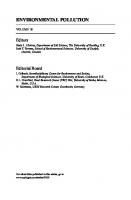
Adverse consequences of the pollution impact on terrestrial ecosystems have been under careful investigation since the very beginning of the twentieth century, and several thousand case studies have documented the biotic effects occurring in contaminated areas. The overall number of studies containing the key word ‘pollut*’ in the title showed steady growth from the beginning of the century until the 1980s (Fig. 1.1a). However, as can be seen from the number of papers that appeared in ‘Nature’ (Fig. 1.1b) and ‘Science’ (Fig. 1.1c), this problem attracted attention of multidisciplinary scientists in the 1970s–1980s, and then the general interest in pollution started to decline. Industrial development, environmental legislation and public attitude have influenced the focal research topics of pollution ecology. Sulphur dioxide is historically the first of the well-known pollutants that was reported to cause health problems and deteriorate the natural environment. Fluorine emissions associated with aluminium production became important in the middle of the last century, and the importance of ozone and nitrogen was appreciated in the 1980s. This process, along with the reversal of the trend in global anthropogenic sulphur emissions (the peak value of 73.2 million tons was achieved in 1989; Stern 2006), naturally shifted research priorities. The proportion of presentations devoted to industrial polluters at bi-annual meetings for specialists in pollution impact on forest ecosystems, conducted by the International Union of Forestry Research Organisations (IUFRO), declined from 20–40% in the early 1990s to 3–7% in 2004–2008. At the same meetings, reported studies of ozone increased from approximately 30% to 70% at the expense of studies on the effects of sulphur dioxide (35–55% in the early 1990s and less than 10% in 2004–2008).

1.4

The State of Pollution-Oriented Studies and the Need for Generalization

7

Fig. 1.1 Temporal trends in proportion (×1,000) of publications containing key word ‘pollut*’ in the title relative to all publications. a, all journals listed in the database of the Institute of Scientific Information; b, ‘Nature’; c, ‘Science’

Thus, pollution ecology, which started from the exploration of acute damage caused by traditional pollutants (such as SO2, fluorine, and metals) associated with large industrial enterprises (Freedman 1989; Treshow 1984), turned towards studies focused on the regional effects of ozone and, to a lesser extent, nitrogen deposition. In line with this pattern, we detected a recent decrease in the number of descriptive studies, providing quantitative information on biotic effects of industrial polluters in a form suitable for meta-analysis (Fig. 1.2). However, ‘traditional’ pollutants should not be forgotten; although the environmental impact of large polluters is gradually declining, especially in high-income OECD member states, overall emission rates of sulphur dioxide and heavy metals still remain high on a global scale, particularly due to the contributions of rapidly developing countries (Fowler et al. 1999; Stern 2006). As a result, large-scale deterioration and the decline of natural ecosystems remain a serious concern both globally and regionally, in particular in the European Community, which recently ‘inherited’ environmental problems from new member states (Freer-Smith 1997; Fowler et al. 1999; Innes & Oleksyn 2000; Innes & Haron 2000; Kozlov & Zvereva 2007a).

8

1

Introduction

Fig. 1.2 Numbers of publications that reported quantitative information suitable for meta-analysis of biotic effects caused by industrial polluters. For selection criteria, consult Zvereva et al. (2008). a, diversity and abundance of soil microfungi (after Ruotsalainen & Kozlov 2006); b, growth and reproduction of vascular plants (after Roitto et al. 2009); c, diversity of vascular plants (after Zvereva et al. 2009); d, abundance and diversity of terrestrial arthropods (after Zvereva & Kozlov 2009); e, four meta-analyses pooled

After more than a century of research on the biotic effects of industrial pollution, ecologists are still far from understanding pollution effects on biota. Even the eternal questions, such as ‘Does industrial pollution always result in lower biodiversity?’,

1.4

The State of Pollution-Oriented Studies and the Need for Generalization

9

are not answered yet. This is in particular due to surprisingly weak links between pollution-oriented environmental studies and development of ecological theories (see above, Section 1.1). Only a few generalizations have been made on the basis of extensive monitoring programs and numerous experiments with industrial contaminants (Odum 1985; Rapport et al. 1985; Freedman 1989; Genoni 1997; Clements & Newman 2002). Environmental scientists clearly prefer a descriptive approach to the testing of research hypotheses (Ormerod et al. 1999), although several models in the field of population and community ecology (Andrén et al. 1997; Doak et al. 1998; Tilman 1999; Scheffer & Carpenter 2003; Orwin et al. 2006; Didham & Norton 2006) are readily available to predict ecosystem behaviour under pollution impacts. On the other hand, researchers addressing basic ecological problems reluctantly use the results of ‘unintentional pollution experiments’ (Lee 1998; Zvereva & Kozlov 2000b, c, 2001, 2004; Clements & Newman 2002). Scientists working around industrial polluters have only rarely addressed the question of causal links between pollution and the recorded effects; therefore, the published case studies are generally narrative and often fail to deliver quantitative information. We were surprised by an acute shortage of information suitable for meta-analyses; although any search for relevant publications brings several hundred ‘hits’, only a small fraction of these studies allow calculation of effect sizes (Fig. 1.2). Moreover, following several trials that have carefully investigated the evidence of causal links between emissions and environmental damage (National Research Council of Canada 1939; Fitzgerald 1980; MacMillan 2000), ordinary people, as well as many scientists, tend to routinely attribute all adverse effects observed in polluted areas to the impact of the largest local polluter (usually a smelter or power plant). Although this approach seems logical, we suggest that a presumption of innocence needs to be accepted by environmental researchers dealing with pollution effects; any environmental change should be considered natural until proof of causal links between pollution and effect have been collected. The majority of studies conducted around point polluters are still aimed at logical rationalisation and an historical explanation of patterns and processes occurring in these contaminated environments. Narrative reviews (we surveyed approximately 50) offer low levels of generalization, frequently just listing selected case studies as examples supporting intuitive conclusions (see, for example, Smith 1974; Linzon 1986; Bååth 1989; Freer-Smith 1997; Klumpp et al. 1999; Rusek & Marshall 2000; Padgett & Kee 2004). Moreover, the accuracy of the conclusions made in these reviews may suffer from the research bias in original studies, i.e., the tendency to perform experiments on organisms or under conditions in which one has a reasonable expectation of detecting significant effects (Gurevitch & Hedges 1999). It was recently found that some historically formed views concerning pollution effects on biota, such as a higher sensitivity of Northern ecosystems, overall decline in biodiversity, or increase in herbivory, lack proper statistical support (Zvereva et al. 2008; Zvereva & Kozlov 2009). Many problems vital for understanding and predicting pollution effects on biota, such as dose–response relationships, separation between specific responses to individual pollutants and general response to pollution, synergic effects of pollutants, effects of climate on bioavailability and toxicity of pollutants, and the role of catastrophic events in the transformation of contaminated communities, remain largely

10

1

Introduction

unexplored (Vorobeichik et al. 1994; Holmstrup et al. 1998; Clements & Newman 2002; Settele et al. 2005; Kozlov & Zvereva 2007a; Zvereva et al. 2008). This may partly explain why the biotic impacts of traditional pollutants, such as sulphur dioxide, fluorine and heavy metals, are not considered in global change scenarios. The need to reveal general patterns in the responses of terrestrial biota to industrial pollution and to identify the sources of variation in these responses became obvious more than a decade ago. At about that time, our research team initiated a quantitative research synthesis of biotic responses to industrial pollution, based on a meta-analysis of published data (Kozlov & Zvereva 2003). This task is extremely time-consuming, and so far we have only been able to summarise the data on the diversity and abundance of soil microfungi (Ruotsalainen & Kozlov 2006), diversity of vascular plants (Zvereva et al. 2008), diversity and abundance of terrestrial arthropods (Zvereva & Kozlov 2009), and plant growth and reproduction (Roitto & Kozlov 2007; Roitto et al. 2009). All these meta-analyses consistently showed high heterogeneity in the responses of terrestrial biota to industrial polluters. Problems with the heterogeneity of primary studies summarised by meta-analyses have been discussed widely, in particular in terms of the contrast between ‘real’ differences in the target phenomena and ‘artefactual’ differences due to the way these phenomena have been studied (Glasziou & Sanders 2002). One continuing criticism is that, because no two studies can ever be perfectly identical, meta-analysts are comparing apples and oranges (Hunt 1997; Glass 2000), thereby calling into question the generalizability of conclusions made by meta-analyses (Markow & Clarke 1997; Matt 2003). However, the same arguments are applicable to comparisons of study objects (or subjects) within a study, since they are never identical. Of course, narrative reviews also compare apples and oranges, although in a different manner than metaanalyses. Thus, all studies differ, and the problem lies in formulating an adequate research question: how study outcomes vary across the factors that we consider important (Glass 2000). Other concerns include the diverse quality of primary studies (Conn & Rantz 2003) and the comparison of results arising from different research designs. The latter source of variation deserves specific attention. First and most importantly, many of the studies reporting pollution effects on biota suffer from pseudoreplication; i.e., statistical conclusions on the effects of pollution are based on comparisons between samples collected from one polluted and one unpolluted site, while true replication requires comparison between several (at least two) polluted and several unpolluted sites. Conclusions based on these two sampling designs may well differ (Zvereva & Kozlov 2009), yet we cannot disregard pseudoreplicated data since the number of correctly designed studies is too small to allow in-depth analyses. Second, the spatial arrangement of study sites varies greatly between studies (Ruotsalainen & Kozlov 2006). The majority of researchers prefer a gradient approach, with several study sites selected at different distances from an emission source. With this design, effects are usually quantified by calculating correlation coefficients, either with the concentration of one ‘major’ or ‘representative’ pollutant, or with the distance from polluter. Whether or not the magnitude of the effect depends on the choice of explanatory variable, had not, to our knowledge, ever been tested statistically.

1.5

Impact Zones of Point Polluters as Models for Ecological and Environmental Research

11

Neither is there any information on whether an ANOVA-oriented design (several polluted vs. several control sites) yields the same conclusions as a gradient design. Last but not least, some researchers, to be on the safe side, select control sites very far from polluters. However, this increases the importance of confounding factors, in particular climatic differences between the impact zone and arbitrarily selected distant control(s). Although many strategies have been proposed to address the heterogeneity of primary studies, no consensus exists on any one set of methods. That is why we decided not only to restrict our research synthesis to meta-analysis of the published data but also to design a comparative study, the results of which are reported in this book. Using a uniform, properly replicated sampling design, and applying identical techniques for data collection and processing, we attempted to minimise the effects of both methodological differences and the quality of primary studies. Of course our data remain biased; as with any data produced by the same team, they share problems and errors. However, we believe that comparison of our original, uniformly collected data with data from published studies would favour distinguishing artefactual differences from real variation in biotic responses to pollution. In this book, we aimed to reveal general patterns in the responses of terrestrial biota to industrial pollution and to identify the sources of variation in these responses. We also intended to provide some numerical estimates that, in terms of building phenomenological models, would allow linking of the observed effects with some characteristics of both the polluter and the affected community. We address the following questions: 1. What are the relative sensitivities of key ecosystem components and services to pollution impacts? 2. Which characteristics of polluters and of impacted ecosystems explain variation in biotic responses among the explored impact zones? 3. Which operational indicators are best suited to detect pollution-induced changes in basic ecosystem properties and services? 4. What are the minimum levels of pollution that cause changes in basic ecosystem properties/services? Answering these questions is necessary to predict the possible fates of the impacted ecosystems under different economic and climatic scenarios.

1.5

Impact Zones of Point Polluters as Models for Ecological and Environmental Research

A point source of pollution is a single identifiable localised source that, relative to the impacted territory, has negligible extent. The sources are called point sources because in modelling they can be approximated as mathematical points to simplify analysis. This is in contrast to non-point pollution sources, the largest of which are agriculture, with huge areas treated by various chemicals, and big cities, with plenty

12

1

Introduction

of small, stationary and mobile sources, the individual impacts of which are impossible to distinguish. We would like to specifically stress the fact that our focus on the data collected around point polluters does not mean that we overestimate the importance of local effects. There is no doubt that relatively minor regional increases in the deposition of pollutants has much larger ecological and economic consequences than the acute impacts of the largest individual emitters, such as Norilsk in Siberia or (earlier) Sudbury in Canada. However, local impacts on biota are well suited to reveal directions and magnitudes of biotic effects and to investigate dose–response relationships, as well as to explore general patterns and sources of variation (including relative sensitivities) in the responses of organisms, communities and ecosystems to pollution. In particular, histories of point polluter impacts are usually documented, effects are well pronounced, environmental gradients are sharp and short, and therefore the unavoidable influence of confounding factors can be accounted for more easily than on a regional scale (Ruotsalainen & Kozlov 2006; Kozlov & Zvereva 2007a; Zvereva et al. 2008). On the other hand, the exploration of impact zones around point polluters allows us to bridge ‘observational’ and ‘experimental’ studies. From a scientific perspective, ecosystems transformed by pollution, for example, unusual landscapes of denuded barren land with lifeless lakes, can be considered opportunistic macrocosms (unique laboratories) for integrated research on the effects of harsh environmental conditions on ecosystem structure and function (Nriagu et al. 1998). This opinion is in line with the perception that ecological effects caused by industrial pollutants are the result of unintentional experiments with terrestrial ecosystems, and this result can be utilised by ecologists (Lee 1998). Environmental gradients created by point polluters share many characteristics with urban-rural gradients (simply because polluters are usually associated with large settlements), which were already considered ‘an unexploited opportunity for ecology’ long ago (McDonnell & Pickett 1990). When studying the impact zone of a given polluter, we know where and when the ‘experimental treatment’ started. We can estimate the amount of pollutants that have been ‘applied’ to study sites. We can compare ‘controls’ and ‘treatments’ after long-term exposure and thus evaluate the effects. Of course, we cannot randomise ‘treatments’ among our study sites, but this is a reasonable cost of harvesting the data from long-term and incredibly expensive experiments established by industries many years ago. Neglect of these field-collected data in favour of simplified shortterm experiments will obviously have detrimental consequences for understanding, predicting, and mitigating consequences of pollution impacts on biota. Instead, ecologists involved in stress-effect evaluation should combine the results obtained from microcosms and seminatural and natural ecosystems in order to properly extrapolate the results of laboratory-type studies to nature itself (Barrett et al. 1976; Filser et al. 2008). It has sometimes been argued that since each impacted area has developed in its own way due to a unique history of events, experience with one system is rarely directly applicable to a prediction of outcome in another (Cairns & Niederlehner 1996; Matthews et al. 1996). However, the same argument can be applied, for example, to forest fires; each fire event is unique, but this is not seen as an obstacle for studying and predicting

1.6

Summary

13

the ecological effects of fires. The difference is that fire ecologists never restrict themselves to the study of a single fire event, while pollution ecologists devote many years of their lives to exploration of the impact zone of a single polluter. Examples of this concentration are endless, while comparisons between at least two polluted areas have only rarely been performed. In a random sample of 1,000 publications reporting the effects of point polluters on terrestrial biota (a history of creation of the collection of primary studies was briefly described by Kozlov & Zvereva 2003; Zvereva et al. 2008; criteria for selecting publications are listed in Section 5.1.2), only 9% of publications reported the effects of two or more polluters; even among these studies, only rarely was the question asked whether some effects were shared among the studied impact zones. We are aware of only two publications (except for those produced by our team) that explicitly address comparative analysis. One of these papers compared the data from two independent projects addressing pollution issues (Grodziński & Yorks 1981), and another reported the results of similarly designed studies conducted in impact zones of four Russian polluters (Chernenkova 2002). Understanding the mechanisms of pollution impacts on biota and predicting the long-term consequences of these impacts require building integrative phenomenological models, i.e., providing some numerical estimates that would allow researchers to link changes in biota with some characteristics of both the polluter and the impacted community (Zvereva et al. 2008). These models would allow prediction of the biotic effects of pollution at local, regional and (to a certain extent) global scales, when they are built on the basis of representative samples of contaminated territories. We appreciate that we are still far from reaching this goal, which was determined to be a major end result of any stress-response analysis decades ago (Barrett et al. 1976). This is due to both low integration between different levels of research of toxic effects (Filser 2008) and geographical biases; most pollution studies originated in Europe and North America, while almost no information is available from the tropics and from the Southern hemisphere (Innes & Oleksyn 2000; Innes & Haron 2000; Padgett & Kee 2004; Ruotsalainen & Kozlov 2006; Zvereva et al. 2008; Zvereva & Kozlov 2009). In this book we did our best to make our sample of impacted areas as representative as possible, given time and resource constrains. Last but not least, a comparison of data on environmental contamination of areas adjacent to selected point polluters (Tables 2.26–2.43) with modelled global deposition of pollutants (Fowler et al. 1999) suggests that an average local effect detected by our study should be higher than any regional effect of pollution. Therefore, our conclusions on overall effects caused by point polluters can be seen as an upper estimate of possible regional effects of pollution on biota of northern and temperate regions of the Northern hemisphere.

1.6

Summary

Effects of pollution should be considered within the scope of basic ecology and need to be studied in the same manner as any natural ecological phenomena. They require proper documentation, explanation, generalization through building theoretical

14

1

Introduction

models, and experimental verification of these models followed by practical applications. This requires an understanding of the ecological principles governing ecosystem-level processes in both pristine and contaminated habitats. We argue that impact zones of point polluters can be seen as ‘unintentional experiments’ and thus serve as suitable models to explore biotic consequences of environmental contamination. By studying changes in structure and functions of ecosystems around point polluters, we aim to reveal general patterns in the responses of terrestrial biota to industrial pollution and to identify the sources of variation in these responses. We also intended to provide some numerical estimates that would allow linking of the observed effects with some characteristics of both the polluter and the impacted community. These models can be further used to predict the biotic effects of pollution on different spatial scales.

Chapter 2

Methodology of the Research and Description of Polluters

2.1

Selection of Polluters

In order to obtain an unbiased estimate of the overall effect of point polluters on terrestrial biota, we needed to explore a random sample from the entire population of polluters. Unfortunately, this task is hardly feasible, keeping in mind obvious financial and time constraints. Therefore we selected a representative sample of point polluters according to the following basic criteria: 1. The explored polluters should represent the entire range of pollution loads, from highest to reasonably low. 2. Basic types of polluters (identified in earlier meta-analyses; Ruotsalainen & Kozlov 2006; Zvereva et al. 2008) should be included. 3. Impact zones should represent the basic vegetation types of the northern and temperate regions of the Northern hemisphere. When other selection criteria were met, the preference was given to impact zones that were best studied either by our team or by other researchers. We explored environmental effects imposed by 18 point polluters (Fig. 2.1; Table 2.1) representing five of six classes that were used in earlier meta-analyses (Ruotsalainen & Kozlov 2006; Zvereva et al. 2008): non-ferrous industries, emitting heavy metals and SO2; aluminium plants, emitting fluorine; iron and steel producing factories, emitting both SO2 and alkaline dust; fertilising and chemical plants, emitting various nitrogen and sulphur containing compounds; and power stations, emitting mostly SO2. Detailed information on these polluters is given below (Section 2.2). Table 2.1 shows classifications of these polluters, listing the variables that are used in categorical meta-analysis (Section 2.5).

M.V. Kozlov et al. Impacts of Point Polluters on Terrestrial Biota, DOI 10.1007/978-90-481-2467-1_2, © Springer Science + Business Media B.V. 2009

15

Fig. 2.1 Location of the investigated polluters

Table 2.1 Values of classificatory variables used in meta-analysis Classificatory variables Locality and polluter

Geographic Polluter typea Effect on soil pHb positionc

Apatity, Russia: power plant Pow B N Bratsk, Russia: aluminium smelter Al B S Harjavalta, Finland: nickel-copper smelter Nf N S Jonava, Lithuania: fertiliser factory Fert N S Kandalaksha, Russia: aluminium smelter Al B N Karabash, Russia: copper smelter Nf A S Kostomuksha, Russia: iron pellet plant Fe B S Krompachy, Slovakia: copper smelter Nf A S Monchegorsk, Russia: nickel-copper smelter Nf A N Nadvoitsy, Russia: aluminium smelter Al B N Nikel, Russia: nickel-copper smelter Nf A N Norilsk, Russia: nickel-copper smelters Nf N N Revda, Russia: copper smelter Nf A S Straumsvík, Iceland: aluminium smelter Al N N Sudbury, Canada: nickel-copper smelter Nf N S Volkhov, Russia: aluminium smelter Al B S Vorkuta, Russia: power plant Pow B N Žiar nad Hronom, Slovakia: aluminium smelter Al B S a Classification follows Zvereva et al. (2008). b A, acidifying; B, alkalysing; N, neutral; classification is primarily based on data reported in Section 3.3. c Classification is based on mean July temperature: below 14°C – northern polluters (N); above 14°C – southern polluters (S). For a map showing location of polluters, consult Fig. 2.1; coordinates of polluters are given in Tables 2.25–2.42; climatic data are summarised in Table 2.2.

2.2

History of the Selected Polluters and Their Environmental Impacts

2.2

17

History of the Selected Polluters and Their Environmental Impacts

2.2.1

Introduction

In this chapter, we provide background information on both polluters selected for our study and their environmental impacts. We also briefly describe the surrounding landscapes (climatic data are summarised in Table 2.2), a history of landscape deterioration under the impacts of pollution, and a history of environmental research conducted around the selected polluters. The amount of information included in this chapter for each polluter depends on its availability to the international scientific community. We do not repeat details easily available from review papers (e.g., on Harjavalta, Monchegorsk, and Sudbury), but we do include more data for less well-known polluters, especially from sources published in national languages. Historical information is referenced only in cases of discrepancies between different data sources. Emission data are of vital importance for understanding changes in the polluted environment, conducting comparative analyses and exploring dose-response relationships (Ruotsalainen & Kozlov 2006; Zvereva et al. 2008). These data are also necessary for re-assessment of regional and global emissions from anthropogenic sources (Nriagu & Pacyna 1988; Pacyna & Pacyna 2001). Therefore, every effort was made to obtain emission data from both published and unpublished sources for

Table 2.2 Temperature and precipitation at the study areas Mean temperatures, °C Polluter

January

July

Annual precipitation, mm

Apatity Bratsk Harjavalta Jonava Kandalaksha Karabash Kostomuksha Krompachy Monchegorsk Nadvoitsy Nikel/Zapolyarnyy Norilsk Revda Straumsvík Sudbury Volkhov Vorkuta Žiar nad Hronom

−13.2 −20.5 −6.8 −5.2 −13.7 −16.4 −12.8 −3.6 −13.8 −11.7 −10.9 −28.9 −15.7 −11.7 −11.9 −10.8 −24.8 −3.3

13.6 17.4 16.4 16.8 14.3 15.4 15.0 19.2 14.1 14.1 11.7 13.8 17.4 14.1 19.1 16.7 14.3 18.7

640 357 545 630 519 666 580 613 561 566 499 528 546 569 811 652 437 644

Climatic data were estimated using New_LocClim (FAO 2006).

18

2

Methodology and Polluters

all the polluters involved in our analysis. Since emission data are very diverse due to a variety of methods for their estimation and reporting, we referenced each value in Tables 2.4–2.24. If values that differ from each other by more than 7% were reported for the same year, they were all included in our tables. If the values differ less than by 7%, then the value reported with higher accuracy was included in the table (i.e., 0.83 was preferred over 0.8). Importantly, the data on both ambient concentrations of pollutants and, later on, emission of pollutants in industrial cities of the USSR (before 1990) and of the Russian Federation (since 1991) have been summarised in annual reports by the Voeikov Main Geophysical Observatory (St. Petersburg) from 1966 until 1995, and by the Research Institute of Ambient Air Protection (St. Petersburg) since 1996. These low-circulation reports (100–250 copies, published in Russian) were, until 1987, ‘for the restricted use only’, with numbered copies deposited into specially authorised departments of the main libraries, and public access to old reports was allowed only in 2007. However, even the accessible reports (for the years 1988–2005) remain unknown to the majority of environmental scientists, leading to large uncertainties in estimation of local and regional depositions of pollutants (Boyd et al. 2009). We were lucky to obtain access to most of these reports (Berlyand 1967, 1968, 1969, 1970, 1971, 1972, 1973, 1974, 1975, 1976, 1979, 1980, 1981, 1982, 1983, 1984, 1985, 1986, 1987, 1988, 1989, 1990, 1991, 1992, 1994; Milyaev & Nikolaev 1996; Milyaev et al. 1997a, b, 1998, 1999, 2000, 2001, 2002, 2003; Milyaev & Yasenskij 2004, 2005, 2006). For reasons of brevity, these reports are later referred to as ‘Emissions of pollutants in Russia (1966–2005)’. Since these reports combine emissions of all polluters within a city, the data should be used with caution, especially for sulphur dioxide and nitrogen oxides that are emitted by many industries. Still, these values are good approximations for the giant polluters (such as Monchegorsk, Nikel, or Karabash, that produce over 95% of a town’s emissions), as well as for pollutants associated with specific industrial processes (such as fluorine-containing substances emitted by aluminium industries). Amounts of both production and emission are reported in metric tons (i.e., 1,000 kg; abbreviated ‘t’ hereafter). The data on pollution loads and the extent of the contaminated territory are even less uniform than the emission data. Therefore, we have chosen to report them in their original form. We paid special attention to the information on the spatial extent of the contaminated territory, i.e., the area with statistically significant increases in pollution load relative to the regional background level. Since this area was often measured from published maps showing ‘pollution zones’, criteria for defining these zones vary across the selected polluters. We provide several estimates reflecting (to a certain extent) the level of knowledge on both environmental contamination around the selected polluters and biotic effects attributable to pollution (Table 2.3). The number of publications known to us is counted from an extensive collection of reprints accumulated by M. Kozlov and E. Zvereva over 25 years of research on pollution ecology; it recently included approximately 5,000 publications reporting pollution effects on terrestrial biota. Potential publications were searched using the ISI Web of Science and several more databases. The publications in Russian were identified by surveying the abstract

2.2

History of the Selected Polluters and Their Environmental Impacts

19

Table 2.3 Amount and quality of available information on environmental impact of the selected polluters Number of publications Polluter

Contaminationa

Biotic effectsa

Number of effect sizes used in meta-analysesb

Totalc

ISId

A

Q

A

Q

1

2

3

4

Apatity, Russia: power plant 3 Bratsk, Russia: 50 aluminium smelter Harjavalta, Finland: 200 nickel-copper smelter Jonava, Lithuania: 60 fertiliser factory Kandalaksha, Russia: 30 aluminium smelter Karabash, Russia: 80 copper smelter Kostomuksha, Russia: 100 iron pellet plant Krompachy, Slovakia: 20 copper smelter Monchegorsk, Russia: 1,000+ nickel-copper smelter Nadvoitsy, Russia: 0 aluminium smelter 100 Nikel, Russia: nickel-copper smelter (and ore-roasting plant in Zapolyarnyy) Norilsk, Russia: 80 nickel-copper smelters Revda, Russia: 300 copper smelter Straumsvík, Iceland: 10 aluminium smelter Sudbury, Canada: nickel-copper smelter 100 Volkhov, Russia: aluminium smelter 5 Vorkuta, Russia: power plant 40 Žiar nad Hronom, Slovakia: 80 aluminium smelter

1 0

1 2

3 3

1 2

3 2

0 1

0 1 0 29

2 5

57

3

3

3

3

3

5 46 13

9

2

3

2

3

1

0

0

3

6

1

2

1

1

1

1

5

9

8

2

3

2

3

0

5

5

2

7

3

3

2

2

4

5

1 13

8

2

2

1

2

0

0

0

91

3

3

3

3

10

0

0

–

0

–

0

0

0

40

2

3

2

3

6

3

6 24

17

2

3

1

1

4

0

0

12

3

3

3

3

4

5 17 21

0

1

3

1

1

0

0

0

0

20 1 8 11

3 1 2 2

3 2 2 2

2 1 2 2

3 3 2 2

1 0 0 0

5 3 0 10 0 0 5 18

0 0 4 3

0

5 58 80 0

0

Numbers of publications may overestimate the level of knowledge on environmental effects due to repeated publication of the same results by several Russian research groups. This especially concerns studies conducted near Kandalaksha, Karabash, Kostomuksha and Monchegorsk. a Evaluation is based on publications available to the authors. Amount of published information (A) scored as: 0 – absent, 1 – insufficient; 2 – sufficient to outline the general picture; 3 – sufficient to represent the detailed picture. Quality of published information (Q), in terms of sampling design (number and distribution of study sites), applied methodology, statistical analysis and presentation form, scored as: 1 – unsatisfactory; 2 – moderate; 3 – high (an overall impression based on all available data sources). b Publication coded as follows: 1 – abundance and diversity of soil fungi (Ruotsalainen & Kozlov 2006), 2 – diversity of vascular plants (Zvereva et al. 2008), 3 – abundance and diversity of arthropods (Zvereva & Kozlov 2009), 4 – growth and reproduction of vascular plants (Roitto et al. 2009). c Only scientific publications were counted (grey literature included, but newspaper reports and web-based data in HTML format excluded); all values exceeding ten are approximate; for the efforts taken to obtain relevant publications, consult text (Section 2.2.1). d ISI Web of Knowledge was searched for location of the polluter, its name, and the type of the industry; all searches were conducted between 25 December 2007 and 10 January 2008.

20

2

Methodology and Polluters

journal Nature protection (1990–2007; code 72 in the series of monthly abstract journals published by the All-Russian Institute of Scientific and Technical Information in Moscow). We also checked reference sections of all obtained data sources, and asked colleagues from many countries for assistance in locating grey literature and publications in national languages. The review of publications describing the effects of each of the polluters on terrestrial biota are by no means exhaustive; additional publications can be located using review papers published by our team (Ruotsalainen & Kozlov 2006; Kozlov & Zvereva 2007a; Zvereva et al. 2008; Zvereva & Kozlov 2009; Roitto et al. 2009). Although a detailed investigation of the perception of environmental and health problems caused by industrial pollution is outside the scope of our study, we still found it interesting to give a brief overview of materials reflecting the degree of public awareness of local environmental problems. For reasons of simplicity, in this review we used a dual referencing system: all individual data sources, such as newspaper reports or individual web-based documents, are included in the list of references, However, overall impressions obtained by surveying some web sites, or small pieces of web-based information that cannot be attributed to an individual author, are referred to by short URLs inserted into the text. All websites mentioned in this chapter were visited between 20 December 2007 and 19 January 2008. An absence of information can be seen as an absence of public interest in local environmental problems.

2.2.2

Descriptions of the Polluters

2.2.2.1

Apatity, Russia: Power Plant (Color Plates 1–3 in Appendix II)

Location and Environment Apatity (population 62,600; data from 2007) is a town in the Murmansk Region, located between Imandra Lake and the Khibiny Mountains 160 km south of Murmansk (Fig. 2.2). Originally it was surrounded by mixed forests of Scots pine (Pinus sylvestris) and mountain birch1 (Betula pubescens subsp. czerepanovii), usually with dwarf shrub and moss cover; stands with ground lichens were relatively infrequent. Pre-industrial History The earliest settlements on Imandra Lake, 15 km east of the current location of Apatity, appeared 7–8,000 years ago. In 1574, a country churchyard, with six huts and 40 inhabitants subsisting on fishing and hunting, existed at about the same locality. 1 Jonsell (2000) considered mountain birch, Betula pubescens subsp. czerepanovii (Orlova) Hämet–Ahti, an ecological form of white birch (Betula pubescens), not a distinct taxon.

2.2

History of the Selected Polluters and Their Environmental Impacts

21

Figs. 2.2–2.7 Distribution of study sites (triangles) around investigated polluters (black circles with white cross inside). Names of larger settlements (usually towns) are capitalised. 2.2, power plant in Apatity, Russia; 2.3, aluminium smelter in Bratsk, Russia; 2.4, nickel-copper smelter in Harjavalta, Finland; 2.5, fertilising factory in Jonava, Lithuania; 2.6, aluminium smelter in Kandalaksha, Russia; 2.7, copper smelter in Karabash, Russia

The first permanent settlement at the current location of the city appeared in 1916 in connection with the building of a railway from St. Petersburg to Murmansk. Colonisation started in 1924 when the village of Byelorechenskij was established close to the place where the power plant was later built. Apatity was granted town status in 1966.

22

2

Methodology and Polluters

Industrial History The intensive growth of Apatity (from seven inhabitants in 1926 to 4,000 in 1939 and 15,200 in 1959) was associated with the development of the apatite mining and processing industry. The main employer of Apatity is the joint stock company ‘Apatit’, the largest mining and concentrating enterprise in Europe. The coal-fired power plant (‘Kirovskaya GRES’, now named ‘Apatitskaya TEC’) was launched in 1959 and reached its full capacity in 1961. For the first 2 decades, it mostly produced electricity (up to 37% of the total output of the Murmansk region), but since the late 1970s, it is used almost exclusively for heating the town. The power plant employed 983 people in 2003, but only 520 people in 2005; it achieves peak capacity (80 MWt) during the winter, when daily coal consumption reaches 2,800–3,000 t. In the summer, the daily coal consumption is around 650 t and the capacity is 10 MWt. The station mainly uses coal from Inta, Northern Ural (sulphur content 1.5–1.9%), but sometimes from Spitsbergen or Khakassia (sulphur content 0.7–1.0%). Emissions Data The power plant is the only local emitter of sulphur dioxide and some metals, such as iron, zinc, chromium, cadmium and lead (Golubeva 1991). The station contributed 99.0% of the sulphur dioxide and 75.4% of the mineral dust to overall emissions of Apatity (summarised in Table 2.4). Pollution Loads and the Extent of the Contaminated Territory Ambient concentrations of pollutants in Apatity have been monitored since 1972; the peak reported values were 1.4 mg/m3 of dust in 1972 and 1.43 mg/m3 of SO2 in 1982 (Emissions of pollutants in Russia 1966–2006). During the period 1987–1989, annual depositions of sulphur and nitrogen in Apatity were 3,100 and 400 kg/km2, respectively (Vasilenko et al. 1991). Concentrations of chromium, arsenic and lead in the leaves of the speckled alder (Alnus incana) in 1992 were below the detection limit (10 mg/kg), even within a few hundred meters of the power plant. Foliar concentrations of nickel, copper and zinc showed no relationship to the distance from the polluter. The peak concentrations of strontium were detected 4–7 km northwest of the power plant and were obviously associated with dust contamination from tailing ponds of the apatite and nepheline-processing factory (located 400–800 m from these sites). Foliar concentrations of iron appeared to be a good measure of pollution load; they exceeded the background level by a factor of 3 within 2 km of the power plant and approached regional background levels at about 5 km (Kozlov 2003). Consistently, soil contamination was detected only within approximately 2 km2 east of the power plant (Kalabin 1999). On the other hand, from 1986 to 1991 a doubling of pollutant deposition (relative to the regional background) was recorded for the 800 km2 around Apatity (Prokacheva et al. 1992).

2.2

History of the Selected Polluters and Their Environmental Impacts

23

Table 2.4 Aerial emissions (t) from industrial enterprises at Apatity, Russia Year

Dust

SO2

1972 1973 1974 1975 1978 1979 1980 1981 1982 1983 1984 1985 1986 1987 1988 1989

14,600 14,600 14,600 18,250 19,500 17,400 17,700 14,400 13,900 15,800 19,000 19,700 15,200 16,300 14,400 13,800

51,800 51,100 51,100 51,100 25,500 31,300 31,200 21,500 31,800 30,800 36,900 35,300 31,000 36,400 30,700 29,400

1990

16,100

31,900

1991

17,600

28,200

1993 1994 1995 1996 1997 1998 1999 2000 2001 2002 2003 2004 2005

10,200 7,100 7,400 7,300 8,900 8,600 8,100 7,300 7,200 5,800 5,300 6,000 5,100

21,400 14,600 11,800 14,700 16,200 17,900 16,800 16,200 14,300 12,000 7,300 10,300 8,200

CO

NOx

– – – – – – 10 200 100 5,000 4,900 5,500 8,300 800 900 600 4,900 a 700 9,200 a 300 8,800 a 700 300 400 200 1,100 700 500 300 300 200 200 100 100

– 12,800 12,800 12,800 2,100 3,300 3,200 2,900 2,500 2,700 2,800 3,300 4,500 4,500 4,100 2,700 3,200 a 3,500 4,400 a 3,200 4,100 a 6,900 5,600 5,500 5,100 5,300 4,500 4,200 4,000 4,200 3,900 3,600 3,900 3,300

Non-referenced values were extracted from Emissions of Pollutants in Russia (1966–2006). Other data sources: a Kryuchkov (1993b).

Habitat Transformation due to Human Activity Forests located 1–3 km from the power plant (please see color plate 3 in Appendix II) are dominated by mountain birch and speckled alder due to selective logging of conifers during the expansion of the settlement (between the 1930s and 1970s). Field layer vegetation is sparse, most likely due to both recreational activities (picking of berries and mushrooms) and dust contamination from the apatiteprocessing plant.

24

2

Methodology and Polluters

Brief History of Environmental Research The data on the environmental impact of the power plant at Apatity are restricted to a study modelling the spatial distribution of sulphur dioxide (Baklanov et al. 1993), a report mentioning (but not quantifying) the contribution of the power plant to soil contamination by some metals (Golubeva 1991), and a paper reporting the results of long-term (1991–2001) monitoring of the population density of a tiny moth, Phyllonorycter strigulatella (Lienig et Zeller) (Lepidoptera, Gracillariidae), whose larvae develop in the leaves of the speckled alder (Kozlov 2003). Perception of the Environmental Situation The local population is most worried by the health effects of dust from tailing ponds of the apatite-processing factory, which affects the quality of ambient air in the city (especially on windy days) and contaminates drinking water (www.liga-rf.ru). 2.2.2.2

Bratsk, Russia: Aluminium Smelter (Color Plates 4–6 in Appendix II)

Location and Environment Bratsk is a large (population 253,200; data from 2007) industrial city in the Irkutsk Region, located on the Angara River near the vast Bratsk Reservoir, 490 km North of Irkutsk (Fig. 2.3). Bratsk is surrounded by southern taiga forests (please see color plate 5 in Appendix II) consisting mostly of Scots pine (56%) and common birch (Betula pendula) (22%); other abundant trees are Siberian larch (Larix sibirica), Siberian spruce (Picea abies ssp. obovata), and Siberian fir (Abies sibirica). Pre-industrial History The area surrounding Bratsk has long been populated by Buryats who subsisted mostly from hunting. Bratsk was founded in 1631, when the stockaded fort was built at the confluence of the Oka and Angara rivers (now submerged by the Bratsk reservoir). In 1702, 128 homesteads were recorded in the Bratsk area. In 1805, the newly established Bratsk administrative unit had 5,210 inhabitants. In 1948, the regional centre, the old village of Bratsk, had 2,247 inhabitants. Town status was granted in 1955. Industrial History The railway reached Bratsk in 1947. The construction of the Bratsk dam and the hydroelectric station was completed in 1961. Construction of the aluminium smelter started in 1961. Production of aluminium was launched in 1966, but extension of the

2.2

History of the Selected Polluters and Their Environmental Impacts

25

facilities continued until 1976; annual production reached 850,000 t in the late 1990s (US Geological Survey 1999). In 2006, the smelter employed approximately 5,000 people and produced 983,000 t of primary aluminium (30% of the aluminium production in Russia and 4% of the world’s output), totalling 30,000,000 t of aluminium since its launch. In the early 1990s, the smelter implemented an ecologically oriented modernisation program, which will continue until 2012 (Ditrikh 2001). The city also houses large-scale timber processing industries and several coal-fired power plants. Emissions Data Although the emission of pollutants from all industries in Bratsk has been reported since 1970 (Table 2.5), emissions from the aluminium smelter were first estimated in 1980 (Ditrikh 2001). All emissions of fluorine-containing gases reported for the city of Bratsk (Emissions of pollutants in Russia 1966–2006) were attributed to the aluminium smelter; contributions from other sources to HF emissions is less than 0.1%, and to fluorine-containing dust emissions is approximately 6% (Lyubashevsky et al. 1996). Data on other pollutants are scarce. Bezuglaya et al. (1991, fig. 2.104) indicated that during the period 1984–1998, emissions of nitrogen oxides from the aluminium smelter were approximately 300 t, i.e., 5% of the overall emissions in Bratsk. Lyubashevsky et al. (1996), referring to local authorities, reported (for an unknown year, presumably 1992 or 1993) emissions of 25,358 t of dust, 3,968 t of SO2, 2,448 t of HF, 2,808 t of fluorine-containing dust (it remains unclear, whether this value is included in an overall estimate of dust emission given above), 274 t of NOx, and 107,199 t of CO. Importantly, these values (totalling 142,055 t) suggest substantially higher emissions than reported by Ditrikh (2001). Pollution Loads and the Extent of the Contaminated Territory Ambient concentrations of pollutants in Bratsk have been monitored since 1969; the peak reported values were 3.18 mg/m3 of SO2 in 1975, 1.39 mg/m3 of NOx in 1971, 7.0 mg/m3 of dust in 1970, and 0.44 mg/m3 of HF in 1978 (Emissions of pollutants in Russia 1966–2006). The peak annual depositions of fluorine near the polluter were 7,200 kg/km2 in the early 1980s and 5,000 kg/km2 in the early 1990s (Morshina 1986; Davydova 2001), i.e., 300–1,000 times as high as the regional background. The increase in sulphur deposition was less extreme, with peak values exceeding the background by a factor of 10–30 (Davydova 2001). In 1987–1989, annual depositions of sulphur and nitrogen in Bratsk were 1,100 and 500 kg/km2, respectively (Vasilenko et al. 1991). The deposition of airborne pollutants in the 1980s exceeded the regional background within approximately 100 km of Bratsk (Morshina 1986). These data suggest that an area of 25,000–30,000 km2 was contaminated by smelter emissions; however, the larger part of this territory (with 3–25 times excess fluorine deposition and 2–10 times excess sulphur deposition over the regional background) did not

26

2

Methodology and Polluters

Table 2.5 Aerial emissions (t) from industrial enterprises at Bratsk, Russia Year

Totala

Dust

SO2

CO

NOx

F-containing dust

HF

1970 1971 1972 1973 1974 1975 1978 1979 1980 1981 1982 1983 1984 1985 1986 1987 1988 1989 1990 1991 1992 1993 1994 1995 1996 1997 1998 1999 2000 2001 2002 2004 2005

– – – – – – – – 181,598 a 172,779 a 168,981 a 161,995 a 149,925 a 132,596 a 125,999 a 111,572 a 99,465 a 55,171 a 52,947 a 73,386 a 92,998 a 78,297 a 73,843 a 64,487 a 58,609 a 46,642 a 43,556 a 42,680 a 82,426 a – – – –

– 5,500 16,400 51,100 73,000 73,000 51,200 49,900 45,500 57,800 60,200 57,600 51,600 51,000 44,400 41,900 41,300 42,400 41,300 50,800 – 41,600 36,700 – 23,700 20,200 22,800 20,800 25,900 21,300 22,200 16,300 19,400

– 8,400 25,600 40,150 43,800 43,800 17,500 21,600 18,200 17,500 22,400 23,900 23,800 22,300 21,100 22,400 20,700 22,700 16,700 18,500 – 15,900 13,800 – 10,300 8,400 9,700 8,900 10,300 9,000 7,600 5,900 7,200

– – – – 186,200 175,200 183,100 188,000 165,500 152,700 147,100 148,200 136,800 118,200 114,800 101,700 85,400 50,900 54,700 59,300 – 56,300 49,000 – 46,600 45,300 45,800 45,300 75,000 62,500 52,000 49,300 55,200

– – – 9,100 14,600 14,600 8,300 9,100 7,400 5,000 5,400 5,600 5,400 5,100 4,600 4,700 5,700 6,100 7,500 7,600 – 5,800 4,800 – 8,300 7,200 7,200 7,500 6,400 5,600 6,100 7,300 8,500

– – – 3,500 – – – – – – 4,000 3,455 3,355 3,061 2,970 2,652 – 2,652 – 3,295 – – – – – – – – – – – – –

730 2,200 7,300 2,800 4,000 4,000 5,490 5,100 6,100 2,600 3,200 2,862 2,960 2,448 2,240 2,020 1,960 b 2,020 2,020 2,155 – 2,463 2,069 2,070 1,714 1,453 1,324 1,299 1,456 1,280 1,070 1,037 1,110

Non-referenced values were extracted from Emissions of Pollutants in Russia (1966–2006); emissions of SO2 from the aluminium smelter comprise approximately 18% of the total emissions reported for Bratsk (proportion based on data of Lyubashevsky et al. 1996). Other data sources: a Ditrikh (2001), values refer to the aluminium smelter only. b Bezuglaya et al. (1991). Note added in proof: Detailed information on the emissions of Bratsk aluminium smelter during 1980–2001 is published by Pavlov (2006).

exhibit visible signs of environmental damage. During the period 1986–1991, a doubling of pollutant deposition (relative to the regional background) was recorded for 3,000 km2 around Bratsk (Prokacheva et al. 1992). Detectable soil contamination by fluorine extended up to 15 km (Morshina 1986), with a peak value of 3,400 mg/kg (Sataeva 1991). On the basis of pollutant deposition and changes in vegetation structure, Davydova (2001) outlined zones of extreme (13.9 km2), strong (82.5 km2), moderate (200 km2), and modest (316 km2) impact.

2.2

History of the Selected Polluters and Their Environmental Impacts

27

Habitat Transformation due to Human Activity Forests have been cut around Bratsk for centuries, while the impact of agriculture was negligible until the 1950s. Recently, pollution has been the leading factor in habitat transformation, although the contribution of recreational activities is also detectable (Alpatov et al. 2001). The first signs of forest damage became apparent in 1968, when 1.36 km2 of Scots pine stands died on the slopes of Mogrudon hill, situated near the smelter. Forest dieback increased to 15–20 km2 by 1976, 50–75 km2 by 1985, and 100–150 km2 by the early 2000s. The extent of damaged forests reached 800 km2 by 1985 (Ugrjumov et al. 1996) and 1,000–1,500 km2 by the late 1990s (Runova 1999); another data source reported damage to 1,400 km2 of forests by the early 1980s (Mikhailova 2003) and 2,000 km2 by the mid-1990s (Mikhailova 1997). Davydova (2001) estimated that landscapes within approximately 70 km were affected by the emissions. The aluminium smelter shares the responsibility for adverse environmental effects with power plants and timber-processing industries, emitting 82% of the sulphur dioxide released in Bratsk. Although fluorine contamination may cause more pronounced environmental effects than sulphur dioxide, it is estimated that only 41.5% of forest damage within 50 km of Bratsk is due to emissions from the aluminium plant (Lyubashevsky et al. 1996). In spite of the extreme pollution loads, we have not found industrial barrens (bleak open landscapes evolved due to deposition of airborne pollutants, with only small patches of vegetation surrounded by bare land) around the Bratsk smelter (Kozlov & Zvereva 2007a). However, trees are nearly absent within the zone of extreme impact, which is mostly covered by herbaceous vegetation and low-stature alder and willow bushes, exhibiting clear signs of pollution-induced damage, i.e., dwarfed growth forms and chlorosis (please see color plate 6 in Appendix II). The surrounding zone of strong impact is mostly covered by white birch (Betula pubescens) and European aspen (Populus tremula); surviving Scots pine and Siberian spruce often have dead upper canopies and stunted growth forms (Davydova 2001).

Brief History of Environmental Research All publications on the environmental impact of the Bratsk aluminium smelter, including five monographs (Rozhkov & Mikhailova 1989; Lyubashevsky et al. 1996; Ugrjumov et al. 1996; Runova 1999; Pavlov 2006), are in Russian. The book by Rozhkov and Mikhailova (1992) was translated to English. The vast majority of publications do not report quantitative data in a form suitable for meta-analysis (Table 2.3). Especially disappointing is a book by Lyubashevsky et al. (1996), which lists a large number of biotic effects, such as smaller size and germinability of the seeds of white and common birches, a decline in species richness of lichens, changed growth of several herbaceous species, and changes in abundances of different groups of insects. However, this book did not provide either supporting

28

2

Methodology and Polluters

numerical information or the results of statistical tests. Majority of these raw data have never been published (N. Lyubashevsky 2006 and M. Trubina, personal communication, 2006) and are, in fact, lost to science. The very first studies of the environmental impacts of the aluminium smelter on forest ecosystems were conducted in the early 1970s by researchers from the Siberian Institute of Plant Physiology and Biochemistry, Irkutsk. In particular, they documented growth of conifers (Sokov & Rozhkov 1975) and listed xylophagous insects in damaged forests (Anisimova 1989). Since 1977, integrated research of the forests affected by emissions from both the aluminium smelter and the timber-processing industry has been conducted (for nearly 20 years) by scientists from the Forest Technical Academy in St. Petersburg. They have documented changes in forest vitality, including decreases in the vertical growth and radial increment of conifers, suppression of regeneration of conifers with simultaneous increases in the density of birch and aspen seedlings, and quantified damage to woody plants by insect herbivores (Kataev et al. 1981; Golutvin et al. 1983; Popovichev & Golutvin 1983; Selikhovkin 1992, 1995). Decreases in the increment of Scots pine near Bratsk (detected by dendrochronological analysis) started in the 1960s and were therefore associated with the beginning of the pollution impact (Lairand et al. 1979). Since the mid-1990s, a research team from Bratsk University has monitored forest damage and developed silvicultural measures for impacted forests (Ugrjumov et al. 1996; Alpatov et al. 2001).

Perception of the Environmental Situation Bratsk was declared an ecological disaster zone in 1993, and the government of the Russian Federation developed plans to improve the situation from 1994–2000. In spite of a substantial decrease in emissions (Table 2.5), the Chekanovskiy settlement (located 1.5 km northeast of the smelter) was evacuated in 2001 due to repeated health emergencies. Bratsk is listed by the 2004 report of the Central Geophysical Laboratory in St. Petersburg among the ten most polluted Russian cities (english. pravda.ru), and by the report of the Blacksmith Institute (2007) among the 30 most polluted places in the world in the category ‘petrochemicals’. The most acute environmental problems have recently been identified as contamination of drinking water by mercury, and not with air pollution (www.pollutedplaces.org). 2.2.2.3

Harjavalta, Finland: Nickel-Copper Smelter (Color Plates 7–11 in Appendix II)

Location and Environment Harjavalta is a small (population 7,700; data from 2007) town in Western Finland, 170 km northwest of Helsinki (Fig. 2.4). Harjavalta is situated on an esker that runs to the southeast of the smelter. The region is part of the southern boreal coniferous

2.2

History of the Selected Polluters and Their Environmental Impacts

29

zone, with the forest consisting mainly of Scots pine (please see color plate 8 in Appendix II). According to the Finnish classification, the forest along the esker varies from the Vaccinium to the Calluna type.

Pre-industrial History The Harjavalta region has been populated since the Iron Age, with the first signs of human settlement dating back to about 1500 BC. Written records mentioning the village of Harjavalta begin in the AD 1400s. Harjavalta was established as a municipality in 1869 and an independent parish in 1878, when it included 1,600 inhabitants. Telephones and railroads reached Harjavalta in the late nineteenth century, but Harjavalta remained a typical countryside village until 1944. By 1950, Harjavalta had a population of 6,000. Town status was granted in 1977.

Industrial History The Outokumpu copper plant was moved to Harjavalta from Imatra in 1944 (at the end of World War II) because of the proximity of Imatra to the Russian border; it started operations in 1945. The Kemira sulphuric acid plant was launched in 1947 and the nickel smelter in 1960; recently, this industrial area has hosted 13 different firms (Heino & Koskenkari 2004). Originally part of Outokumpu, a Finnish company, the copper business is now owned by Boliden (since 2003) and the nickel business by Norilsk Nickel (since 2007). The copper smelter has a nominal annual capacity of 160,000 t. Sulphur is recovered and sold as sulphuric products. The nickel smelter, operating on a tolling basis, produces nickel matte.

Emissions Data Accurate emissions data from the Harjavalta smelters (Table 2.6) have been available through Outokumpu reports and the web-site, as well as from the documents of the Finnish Ministry of Environment, since the mid-1980s; they were partially published in many research reports, including those by Nieminen et al. (2002) and Kiikkilä (2003). Estimates of dust emissions for 5-year periods starting with the beginning of smelting have been published by Nieminen et al. (2002) and are included in Table 2.6; for a detailed history of emissions and for annual production-based estimates of dust emissions (not included in Table 2.6), consult Nieminen (2005). Data on annual emissions of sulphur dioxide in the early 1970s are contradictory: 20,000 t was reported by Levula (1993), while Laaksovirta and Silvola (1975) indicated 4,800 t. Data from 1990 demonstrated that smelters contributed 98.7% of the sulphur dioxide, 90% of the nitrogen oxides (with annual emissions of 180 t), 92.7% of the dust

30

2

Methodology and Polluters

Table 2.6 Annual emissions (t) from Harjavalta smelters, Finland Year 1945 1947 1945–1949 1950 1950–1954 1955–1959 1960–1964 1965–1969 1970 1970–1974 1975–1979 1980–1984 1984 1985 1986 1987 1988 1989 1990 1991 1992 1993 1994 1995 1996 1997 1998 1999 2000 2001 2002 2003 2004 2005

Dust – – 478 c – 534 c 784 c 1,195 c 632 c – 548 c 778 c 903 c 1,100 1,100 1,200 1,800 1,000 1,000 960 640 280 250 190 70 195 355 132 48 36 50 55 – – –

SO2

Cu

30,000 35,000 b – 10,000 a – – – – 20,000 a – – – 11,500 7,800 7,530 6,860 8,500 9,500 8,800 5,200 4,800 4,700 5,000 3,270 3,243 2,980 3,041 3,397 3,002 3,387 3,300 3,000 2,900 2,850

a

– – – – – – – – – – – – 300 98 126 140 104 80 80 80 60 50 40 17 49 69 23 5.9 6.6 7.4 11.6 6.0 f – –

Ni – – – – – – – – – – – – 70 47 46 90 45 33 31 15 10 7.0 6.0 1.4 1.2 2.9 1.7 0.8 1.2 0.8 0.6 0.6 f – –

Pb – – – – – – – – – – – – 50 55 60 94 48 70 80 45 9.0 6.0 3.0 0.5 1.9 3.9 2.4 1.0 0.2 0.7 0.4 0.3 f – –

Zn

Cd

– – – – – – – – – – – – 200 216 232 162 103 190 160 90 12 11 6.0 1.7 5.3 14 6.1 4.2 1.1 3.0 1.5 0.9 f – –

– – – – – – – – – – – – – 1.7 d 7.1 d 3.9 d 3.2 d 3.6 d 4.2 d 1.6 e 1.0 e 0.9 e 0.6 e 0.0 e 0.2 e 0.3 e 0.4 0.3 0.1 0.4 0.1 – – –

As – – – – – – – – – – – – – 15 d 17 d 19 d 19 d 22 d 28 d – – 10 e 5.0 e 0.2 e 4.2 e 10 e 10 1.8 0.8 1.6 0.5 0.4 f – –

Non-referenced values were obtained from Outokumpu Harjavalta Metals Ltd. Other data sources: a Levula (1993). b Poutanen and Kuisma (1998). c Nieminen et al. (2002). d Harjavallan Kaupunki (1991). e Helmisaari (2000). f Nieminen (2005).

and 99.5% of the heavy metals emissions at Harjavalta (Harjavallan Kaupunki 1991). However, before the closure of the fertiliser factory in 1989, the emissions share of the smelter for nitrogen oxides was much lower; 125 t emitted in 1978 constituted only 17.2% of the total emissions at Harjavalta (Helmisaari 2000). Emissions of NO2 in 2002 were 250 t (Outokumpu Harjavalta Metals Ltd.). In 2002, Outokumpu claimed the smelter to be ‘among the cleanest in the world’.

2.2

History of the Selected Polluters and Their Environmental Impacts

31

Pollution Loads and the Extent of the Contaminated Territory Long-term pollution impacts resulted in soil contamination by metals, with peak recorded values of 49,000 mg/kg of copper, 913 mg/kg of nickel, 58 mg/kg of arsenic, 620 mg/kg of zinc, and 204 mg/kg of lead (Helmisaari et al. 1995; Derome & Nieminen 1998; Uhlig et al. 2001; Salemaa et al. 2001; Nieminen et al. 2002; Nieminen 2004). However, due to a substantial decline in emissions, both deposition of pollutants and ambient concentrations of sulphur dioxide have been very low recently. For example, average ambient concentrations of sulphur dioxide near the smelter in 2001–2002 were 0.004–0.006 mg/m3 (Outokumpu Harjavalta Metals Ltd.), i.e., well below sanitary limits. The polluted area, defined by the accumulation of copper in moss bags exceeding the background level by a factor of 5 or more (Hynninen 1986), in 1981–1982 was 70 km2. In 1995, the area contaminated by copper (over 8 mg/kg in green mosses) was 107 km2 (Kubin et al. 2000). Habitat Transformation due to Human Activity The heathland Scots pine forests in the immediate vicinity of the smelter died during the first years of industrial activity, but they were left uncut until the mid-1950s (Poutanen & Kuisma 1998). The very first evaluation, conducted at the beginning of the 1970s, classified 8.8 km2 as a lichen desert, i.e., the area where epiphytic lichens disappeared due to the pollution impact. Visible damage to Scots pine was detected within approximately the same area, and another 52 km2 area was classified as a transitional zone (Laaksovirta & Silvola 1975). In the mid- to late 1950s, the dying forest around the smelter was restored by planting Scots pine seedlings, which had a high rate of survival but stunted growth. They have formed a kind of forest with unusually open canopies and dead or nearly dead ground layer vegetation (please see color plates 9 and 11 in Appendix II). The overall extent of barren and semi-barren habitats around Harjavalta is now approximately 0.5 km2 (Kozlov & Zvereva 2007a). Brief History of Environmental Research The first scientific report known to us about the environmental effects of the Harjavalta smelters is the paper by Laaksovirta and Silvola (1975). Many of the studies conducted near Harjavalta were based on a poorly replicated sampling design, with four study sites, each representing a different pollution load. The studies cover soil microbiota, invertebrates (mostly epigeic fauna and insect herbivores), the structure of plant communities, the growth and vitality of Scots pine, and the performance of insectivorous birds (for a review and references, consult Kiikkilä 2003). Recent declines in emissions have already resulted in ecosystem recovery, which was detected by monitoring bird communities (Eeva & Lehikoinen 2000).

32

2

Methodology and Polluters

Perception of the Environmental Situation The Harjavalta smelter was removed from a ‘hot spot’ list of top Baltic polluters in 2003. A census by the Association of Finnish Local and Regional Authorities in 2004 clearly showed that Harjavalta’s image has changed greatly due to a significant decrease in emissions since 1990; it is no longer perceived as a polluted little town (Rintakoski 2004). In spite of several accidents reported in newspapers (www. turunsanomat.fi), local inhabitants pay little attention to environmental contamination. 2.2.2.4

Jonava, Lithuania: Fertiliser Factory (Color Plates 12–14 in Appendix II)

Location and Environment Jonava (population 34,500; data from 2007) is located in the central part of Lithuania, 30 km northeast of Kaunas (Fig. 2.5). Before the onset of pollution, Scots pine (50%), Norway spruce (Picea abies ssp. abies) (23%), common birch and black alder (Alnus glutinosa) prevailed in the local forests (Armolaitis 1998). Pre-industrial History Jonava (founded in 1740) was an estate until the mid-eighteenth century, owned by the Kosakowski family. In 1750, Jonava received town and market rights, but it did not develop into a city. In 1923, proper city rights were granted, but no substantial growth had occurred prior to World War II. Industrial History Construction of the nitrogen fertiliser factory ‘Achema’ (formerly ‘Azotas’) started near Jonava, at the confluence of the rivers Neris and Sventoji, in 1962. Production of synthetic ammonia was launched in 1965; development of the factory and the launching new departments continued until 1973. The factory became the ‘Achema’ stock company following privatisation in 1994. Recently, the plant has become the biggest producer of nitrogen fertilisers in Lithuania, Latvia and Estonia. It employs 1,600 workers and produces ammonia, ammonium nitrate, urea ammonium nitrate solution, and many other chemicals. Emissions Data In the 1980s, the factory was one of the biggest air pollution sources in Lithuania (Table 2.7), emitting the larger part of all pollutants reported for Jonava. Along with the pollutants included in Table 2.7, emissions of chlorine have been occasionally

2.2

History of the Selected Polluters and Their Environmental Impacts

33

Table 2.7 Annual emissions (t) from all industrial enterprises at Jonava, Lithuania (1974–1989) and from the Achema plant (1980–2005) Year

Dust

1974 1975 1978 1979 1980

7,300 7,300 4,800 14,600 16,400 12,995 a 14,100 13,860 a 12,400 11,476 a 7,300 8,098 a 7,000 6,328 a 7,400 4,477 a 6,700 3,238 a 5,500 1,705 a 4,300 629 a 1,300 271 a 305 a 351 a 246 a 212 a 274 a 292 a 285 a 265 a 203 a 301 a 323 a – – – – –

1981 1982 1983 1984 1985 1986 1987 1988 1989 1990 1991 1992 1993 1994 1995 1996 1997 1998 1999 2000 2001 2002 2003 2004 2005

SO2 11,000 11,000 7,500 4,200 5,400 3,901 a 5,200 4,630 a 4,300 4,079 a 4,400 3,699 a 1,700 3,312 a 1,600 2,635 a 1,700 2,975 a 3,000 2,416 a 2,300 1,991 a 1,600 1,295 a 716 a 450 a 438 a 630 a 379 a 370 a 24 a 541 a 68 a 83 a 8a 50 b 34 b 24 b 7b 0b

CO

NOx

NH4

25,600 25,600 19,600 20,500 28,100 8,548 a 10,000 9,874 a 10,100 10,541 a 10,400 9,711 a 9,800 9,928 a 9,800 9,456 a 9,100 10,291 a 9,400 9,682 a 8,700 8,356 a 8,300 6,608 a 6,143 a 7,318 a 6,904 a 3,924 a 3,013 a 3,475 a 3,450 a 3,510 a 5,704 a 5,362 a 5,770 a 4,282 b 4,192 b 3,527 b 3,639 b 2,598 b

– – 2,200 5,600 6,400 4,148 a 3,900 3,862 a 3,900 3,896 a 4,500 3,595 a 3,600 2,777 a 3,000 2,886 a 2,600 2,730 a 2,500 2,358 a 2,400 2,206 a 2,000 1,824 a 908 a 1,133 a 690 a 243 a 359 a 324 a 122 a 389 a 390 a 381 a 416 a 430 b 428 b 478 b 408 b 514 b

– – 2,420 4,100 5,100 3,622 a 3,734 a 3,700 3,633 a 3,720 3,034 a 3,840 2,591 a 3,870 2,426 a 4,010 2,559 a 2,495 a 1,551 3,658 2,249 a 2,249 a 2,055 a 678 a 720 a 1,287 a 645 a 382 a 257 a 197 a 286 a 420 b 446 b 423 b 416 b 426 b

Non-referenced values extracted from Emissions of Pollutants in Russia (1966–2006). Other data sources: a Juknys et al. (2003, Table 2.1; reprinted, in a modified form, with permission from Elsevier). b Sujetovine× and Stake× nas (2007, and personal communication 2009).

reported (2,030 t in 1981, 1,561 t in 1984, 1,166 in 1987) (Emissions of pollutants in Russia 1966–2006). Small quantities of metals (Zn, Cu, Mn, Cr, Ni, Cd) detected in snow samples (Slavenene et al. 1987) presumably resulted from burning organic fuel.

34

2

Methodology and Polluters

Pollution Loads and the Extent of the Contaminated Territory Ambient concentrations of pollutants in Jonava have been monitored since 1974; the peak reported values were 4.2 mg/m3 of dust in 1975, 4.63 mg/m3 of SO2 in 1979, 0.34 mg/m3 of NOx in 1975, 0.70 mg/m3 of HF in 1979, and 5.00 mg/m3 of NH4 in 1974–1975 (Emissions of pollutants in Russia 1966–2006). In 1987–1989, annual depositions of sulphur and nitrogen in Jonava were 1,900 and 1,100 kg/km2, respectively (Vasilenko et al. 1991). However, according to another data source (Armolaitis 1998), total (wet and dry) annual deposition of sulphur at a distance of 1–2 km from the factory in the mid-1980s comprised 5,000 kg/km2 but was reduced to 1,500 kg/km2 by the mid-1990s. To our knowledge, pollution loads have never been mapped; at the time of peak emissions (in the mid-1980s), the contaminated zone most likely ranged from 500 to 1,000 km2.

Habitat Transformation due to Human Activity Local forest damage was recognised in 1972 and has become extremely acute since 1979, when crown defoliation in conifers was recorded up to 10–12 km in the direction of prevailing winds, and complete dieback occurred within 2–3 km from the polluter (Juknys et al. 2003). By 1983, 20 km2 of forest had been damaged by pollution (Dauskevicius 1984). Despite essential reduction of emissions (Table 2.7), at the end of the 1980s the forest damage expanded to 20–25 km in the direction of prevailing winds. Some signs of recovery appeared only in the 1990s (Juknys et al. 2003).

Brief History of Environmental Research The studies of biotic effects caused by emissions of Achema are generally forestryoriented, with detailed descriptions of the growth and vitality of Scots pine (Augustaitis 1989; Armolaitis 1998; Juknys et al. 2003) and fragmentary data on soil microbiota (Lebedeva & Lugauskas 1985), insect pests (Mastauskis 1987), and birds (Knistautas 1982, 1983).

Perception of the Environmental Situation According to the web-based reports of the mass media, Achema was the first factory in Lithuania to adopt the EU requirement for an environmental management system, and was recently assessed as one of the top ten least polluting big chemical plants of the EU (E. Budrys, personal communication 2008).

2.2

History of the Selected Polluters and Their Environmental Impacts

2.2.2.5

35

Kandalaksha, Russia: Aluminium Smelter (Color Plates 15–17 in Appendix II)

Location and Environment Kandalaksha is a small (population 38,100; data from 2007) town in the Murmansk Region, located on the Kola Peninsula on the coast of the Kandalaksha Gulf on the White Sea, 210 km south of Murmansk (Fig. 2.6). Originally, it was surrounded by mixed forests dominated either by Scots pine or, less frequently, by Norway spruce. Ground vegetation typically consisted of dwarf shrubs and green mosses (please see color plate 16 in Appendix II).

Pre-industrial History Fishing has been the primary business of the local population for millennia. Although Kandalaksha has existed since eleventh century, only 806 inhabitants were recorded there in 1914. Town status was granted in 1938.

Industrial History The industrial development of Kandalaksha started in 1915 with the building of the railway connecting St. Petersburg and Murmansk. The next important events were construction of the Niva hydropower station (completed in 1934) and the mechanical factory (launched in 1936). Building of the aluminium plant started in 1939 but was interrupted by World War II, and the smelter was only commissioned in 1951. Its main products are primary aluminium ingots, aluminium wire rod and billets. Annual production of aluminium in the late 1990s was 63,000 t (US Geological Survey 1999). During the period 2001–2007, the smelter employed 1,400 people and produced 70–75,000 t of aluminium annually (Boltramovich et al. 2003; www.rusal.ru).

Emissions Data The aluminium smelter contributed 70–80% of all aerial emissions reported for the town of Kandalaksha in 1989–1991; in 1993–2000, its share declined to 53–64% (Emissions of pollutants in Russia 1966–2006), in particular due to ‘severe pressure from nature protection agencies, up to demand to reduce production of aluminium by 12%’ (Kruglyashov 2001). All emissions of both aluminium oxide (around 5,000 t in the mid-1990s; Evdokimova et al. 2007) and fluorine-containing substances (Table 2.8) originate from the smelter. In 2005, the new gas-cleaning system was put into operation, and a further decrease in emissions is expected in the coming years.

36 Table 2.8

2

Aerial emissions (t) from industrial enterprises at Kandalaksha, Russia

Year

Dust

SO2

1970 1971 1973 1974 1975 1978 1979 1980 1981 1982 1983 1984 1985 1986 1987 1988 1989

– – 7,300 7,300 7,300 20,100 19,400 20,100 18,000 23,200 23,300 23,700 9,100 8,600 8,400 8,100 8,500

– – 5,500 5,500 5,500 5,500 5,500 4,200 4,100 3,700 5,200 6,600 5,500 5,200 5,000 4,700 5,200

1990

7,600

4,600

1991

Methodology and Polluters

CO – 3,100 1,800 1,800 – 8,300 8,300 7,600 7,200 7,300 8,000 8,900 7,800 7,000 6,900 6,800 7,100 15,500 a 6,600 8,800 a 7,500 19,400 a – 9,300

NOx – – – – – – 800 300 1,500 300 500 200 300 200 900 200 300 600a 200 300 a 200 1,400 a – 600

F-containing dust HF – – – – – – – – – – 836 833 830 824 821 816 814 a 806

>1,300 1,300 1,100 1,100 1,100 1,425 550 790 800 800 795 790 790 800 800 784 780 660 775 a 659 a

5,244 b 3,800 936 9,500 1992 5,193 b – – – 1993 5,198 b 5,800 848 705 10.800 8,700 11,300 800 – 694 b 1994 5,158 b 9,400 848 1995 5,126 b 4,800 7,800 340 – 693 b 8,900 848 1996 5,031 b 5,300 8,100 300 – 688 b 9,000 839 1997 4,992 b 5,100 8,500 300 – 688 b 9,700 839 1998 4,946 b 5,700 8,700 300 – 687 9,700 5,800 8,200 300 – 686 1999 4,950 b 9,300 2000 8,400 6,100 7,100 600 – 686 2001 8,400 6,200 7,300 600 – 672 2002 8,200 5,400 7,200 600 – 670 2003 5,400 5,400 7,100 600 – 383 2004 5,000 5,800 7,400 600 – 349 2005 3,800 6,000 6,700 500 – 274 Non-referenced values extracted from Emissions of Pollutants in Russia (1966–2006); emission of CO in 1983 corrected from the reported 800 to 8,000 t – the typing error presumed. Other data sources: a Kryuchkov (1993b). b Kruglyashov (2001), data refer to the aluminium smelter only.

2.2

History of the Selected Polluters and Their Environmental Impacts

37

Pollution Loads and the Extent of the Contaminated Territory Ambient concentrations of pollutants in Kandalaksha have been monitored since 1967; the peak reported values were 1.60 mg/m3 of dust in 1967, 2.21 mg/m3 of SO2 in 1982, 0.43 mg/m3 of NOx in 1971, and 1.30 mg/m3 of HF in 1970. Importantly, high concentrations of HF (0.30–0.50 mg/m3) were recorded up to 2 km from the smelter in 1971–1973 (Emissions of pollutants in Russia 1966–2006). A local increase in sulphate deposition from 1979–1983 was detected within approximately 300 km2 (Kryuchkov & Makarova 1989). However, by the late 1980s–early 1990s, the sulphur-contaminated territories around major industrial centres of the Murmansk region had merged, and no local increase in sulphur deposition near Kandalaksha was detected in the 1990s (Kalabin 1999). In 1987–1989, annual depositions of sulphur and nitrogen in Kandalaksha were 1,000 and 300 kg/km2, respectively (Vasilenko et al. 1991). The impact of the aluminium smelter on the local geochemistry in the mid-1990s was characterised as ‘surprisingly small’ (Reimann et al. 1998); however, emissions caused a substantial increase in the pH of both snow precipitation and forest litter (Evdokimova et al. 2005). The peak concentrations of fluorine in soils exceeded the regional background by a factor of 25–30 (Evdokimova et al. 2005). During the period 1986–1991, a doubling of pollutant deposition (relative to the regional background) was recorded for 250 km2 around Kandalaksha (Prokacheva et al. 1992). The content of fluorine in forest litter suggests that approximately 500 km2 have been recently contaminated, with the severely contaminated zone (fluorine content increased by a factor of 6–25 relative to the regional background) limited to 2.5 km from the smelter (Evdokimova et al. 1997, 2007). Habitat Transformation due to Human Activity Severe damage to conifers and depression of field layer vegetation were apparent in the early 1980s, when Syroid (1987) classified the habitats next to the smelter as a zone of ‘complete destruction of ecosystems’, with 70–90% of soils void of vegetation. However, felling had been quite intensive around Kandalaksha until at least the 1970s; thus, initial deforestation near the smelter was most likely the result of clearcutting. Moreover, the presence of young Scots pines near the smelter (Syroid 1987) suggests that forest recovery was not prevented even at periods with the highest pollution pressure. Kryuchkov and Makarova (1989, Fig. 18) claimed the presence of 25 km2 of industrial barrens around the aluminium smelter at Kandalaksha; however, this information seems exaggerated. In particular, it contradicts the data by Georgievskij

38

2

Methodology and Polluters

(1990), who reported a decline of epiphytic lichens within 5 km2 only. We repeatedly visited Kandalaksha in the early 1980s and observed Scots pine stands growing 1–3 km from the smelter (please see color plate 17 in Appendix II). We suggest that the acute environmental effects were local and mostly resulted from deposition of fluorinecontaining dust in combination with other kinds of human-induced disturbances. Visible forest damage in the early 1980s was observed within 450 km2 (Syroid 1987); detectable lichen damage was reported within 1,300 km2 (Georgievskij 1990). Brief History of Environmental Research The first reports of the environmental situation around Kandalaksha (Syroid 1987; Georgievskij 1990) were narrative and contained neither numerical estimates of the effects nor statistical analysis. Quantitative information is available only for soil micromycetes (Evdokimova et al. 1997, 2007) and several groups of soil invertebrates (Zainagutdinova 2003). An integrated environmental study (Evdokimova et al. 2005) produced mostly inconclusive results due to methodological flaws, including a poorly replicated sampling design, selective reporting of information (e.g., data on individual taxa of soil mesofauna are given for the most polluted site, but data for the control site are missing), and an absence of proper statistical support for the majority of the conclusions. In particular, the contrast between one polluted and one unpolluted site (e.g., Evdokimova et al. 2007) does not allow to attribute the detected differences to the impact of pollution. Our team recently published information on growth of three species of herbs (Kozlov & Zvereva 2007b) and phenology of mountain birch (Kozlov et al. 2007) in the impact zone of the smelter at Kandalaksha. Perception of the Environmental Situation Recent publications in mass media indicate that the situation in this town is reasonably good in comparison to other towns of the Murmansk Region, and suggest that the existing sanitary zone around the smelter (it is now 1 km wide) is too large (Anonymous 2007). 2.2.2.6

Karabash, Russia: Copper Smelter (Color Plates 18–23 in Appendix II)

Location and Environment Karabash (population 15,400; data from 2007) is an industrial town of the Chelyabinsk Region, located on the eastern slopes of the South Ural Mountains 90 km northwest of Chelyabinsk (Fig. 2.7). The town lies within a flat-bottomed valley, roughly parallel to the prevailing wind direction and surrounded by hills (please see color plate 21 in Appendix II) having an altitude up to 610 m. This valley was originally covered by south taiga forests formed by Scots pine and common birch, with well-developed herbaceous vegetation (please see color plate 19 in Appendix II).

2.2

History of the Selected Polluters and Their Environmental Impacts

39

Pre-industrial History The region has hosted mining and metal production for over 3,000 years. The settlement Sak-Elginskij (later renamed Soimanovskij) was founded in 1822 close to the current location of Karabash by gold-miners; in the early 1900s, the population was around 400. Industrial History For unknown reasons, many publications have reported contradictory dates for the most important events in the industrial history, including in particular the opening of a concentrating mill and a period of temporary closure of the smelter. All the dates below follow the book by Novoselov (2002). The building of the first copper smelter started in 1834 at Sak-Elginskij; from 1837 to 1842, it produced 22 t of copper from local ores, and it was then developed into an iron factory. The second copper smelter was launched at another locality in 1907 and operated for 3 years. The third smelter was built in 1910, again at a new site (approximately between the two earlier works), and the settlement grew around it. This smelter utilised modern technology to produce blister copper, and by 1915, one third of the Russian copper output originated from Karabash. Copper production from 1907 to 1918 totalled 56,000 t. Both mining and smelting operations were discontinued between 1918 and 1925. In 1930, a concentrating mill was built in the eastern part of the settlement. Town status was granted in 1933. Copper production in 1940 reached 22,000 t but declined during the World War II to 6,750 t in 1945 due to a shortage of electricity and workforce. The peak population of 50,000 occurred between the late 1950s and the 1960s, when mining, ore beneficiation and smelting operations were at their peaks. In 1987, Soviet authorities decided to modify the smelter for recycling of nonferrous metals. The concentrating mill and one of the copper furnaces were closed in November 1989. Closures occurred gradually until 1997, when the smelting operations were discontinued totally. The ownership of the plant and of the nearby mine changed in 1998, and a new enterprise, ‘Karabashmed’ (with 1,400 employees), was launched using the existing facilities. Annual copper production reached 30,000 t in 2000 and further increased to 40,000 t in the mid-2000s. Since 2005, the plant has also produced sulphuric acid (31,600 t from May to December of 2005). Emissions Data The emissions history of the smelter is well documented (Table 2.9), although official data (Emissions of pollutants in Russia 1966–2006) have only been available since 1984. During the period 1989–2003, the smelter contributed 98.3–99.9% of all emissions at Karabash (Emissions of pollutants in Russia 1966–2006). It is expected that ongoing modernisation will reduce the annual emissions of sulphur dioxide to less than 5,000 t (www.karmed.ru).

40

2

Methodology and Polluters

Table 2.9 Aerial emissions (t) from industrial enterprises at Karabash, Russia Year

Dust

SO2

CO

NOx

Cu

Pb

Zn

As

1,760 a 1,940 a – – – – – 540 a – – – – 410 a 990 a 1,660 a – 12,100 a – – – 540 a 1,280 a 1,830 a – – – – – 1,030 a 1,060 a 2,130 a – 20,400 a – – – 1,100 a 1,300 a 3,290 a 1,900 b 23,800 a – – – 1,200 a 2,250 a 4,020 a – 10,600 a – – – 1,780 a 1,790 a 3,560 a – 29,400 a – – – 1,600 a 2,300 a 3,820 a 1,610 a 25,600 a – – – 1,350 a 1,990 a 3,410 a 1,850 a 28,600 a – – – 1,340 a 2,880 a 4,410 a 2,070 a 31,700 a – – – 1,360 a 3,280 a 5,370 a 2,420 a 29,900 a – – – 1,440 a 3,820 a 5,140 a 2,600 a 28,800 a 364,500 a – – 1,530 a 2,570 a 4,550 a 1,920 a 25,800 a 281,200 a – – 1,250 a 3,350 a 4,680 a 1,680 a 18,700 a – – – 830 a 3,110 a 3,150 a 1,070 a 27,900 a 273,100 a – – 860 a 3,300 a 3,430 a 1,720 a 27,400 a 259,800 a – – 740 a 2,870 a 3,470 a 1,480 a 27,100 a 252,000 a – – 600 a 2,720 a 2,960 a 1,380 a 25,900 a 233,800 a – – 1,070 a 3,400 a 4,740 a 2,300 a 29,000 a 267,200 a – – 1,370 a 3,930 a 5,140 a 2,400 a 26,000 a 181,100 a – – – 3,410 a – 1,870 a 23,900 a 183,700 a – – – 3,760 a – 2,330 a 20,300 a 184,000 a – – 1,140 a 3,160 a 4,100 b 1,990 a 23,600 137,300 – 100 1,600 2,532 3,200 1,803 23,300 153,500 – 100 1,400 2,130 3,300 1,700 21,300 153,000 – 100 1,200 1,960 3,000 1,670 18,700 148,100 – 100 1,300 1,650 2,600 1,300 20,500 142,500 – 100 – – – – 20,500 142,500 – 100 – 483 – – 3,400 46,900 500 – 435 254 1,363 b 75 3,900 b 485 b 1991 2,200 6,000 100 100 88 119 – 31 1994 200 b 600 b – – 21 b 9b 63 b 4b 1996 200 40 200 100 – – – – 1997 1,200 b 4,500 b – – 100 b 30 b 200 b 20 b 1998 200 5,000 200 100 6 3 – – 2000 10,100 79,000 15,800 400 – 72 – 99 2001 13,800 71,900 12,200 300 – 92 – 110 2002 14,800 67,700 14,800 400 – 63 – 83 2003 – – – – 340 c – – – 2004 2,300 66,300 800 100 – 26 – 7 2005 1,300 38,100 1,600 90 – 20 – 7 Non-referenced values were extracted from Emissions of Pollutants in Russia (1966–2006); note that data for the years 1993–1995, 1997, 1999 and 2003 have not been reported in these publications. Other data sources: a Stepanov et al. (1992). b Chernenkova et al. (2001). c E. Vorobeichik (personal communication, 2008). 1956 1957 1958 1959 1960 1961 1962 1965 1966 1967 1968 1969 1970 1971 1972 1973 1974 1975 1976 1977 1978 1979 1980 1984 1985 1986 1987 1988 1989 1990

2.2

History of the Selected Polluters and Their Environmental Impacts

41

Pollution Loads and the Extent of the Contaminated Territory Ambient concentrations of pollutants in Karabash have been monitored since 1972; the peak reported values were 4.00 mg/m3 of dust in 1973 and 6.20 mg/m3 of SO2 in 1974 (Emissions of pollutants in Russia 1966–2006). The peak ambient SO2 level in 2000 (i.e., after reopening the smelter) reached 20 mg/m3 at a 1 km distance from the smokestack (Udachin et al. 2003). A detailed investigation of total airborne suspended particulates performed in 2000–2001 demonstrated that a large (83–100%) fraction was respirable; these particulates contain high levels of potentially toxic metals and are thought to pose a severe risk to human health (Williamson et al. 2004). From 1987 to 1989, annual depositions of sulphur and nitrogen in Karabash were 16,200 and 1,100 kg/km2, respectively (Vasilenko et al. 1991). In the early 1990s, deposition of heavy metals near the smelter exceeded the regional background by a factor of 45 for copper, 20 for lead, and 5 for cadmium (Bolshakov et al. 2001). In 1981, soils near the smelter contained 2,500 mg/kg of copper and 1,000 mg/kg of zinc (Chernenkova 1986); later, a peak value of 6,744 mg/kg of copper in forest litter was recorded 3 km northwest of the polluter (Stepanov et al. 1992). The peak concentrations of other elements in soils of the industrial barrens were 10,000 mg/kg of zinc, 3,000 mg/kg of lead, and 1,500 mg/kg of arsenic (Makunina 2002). In the mid-1990s, copper concentrations in soils exceeded the background level by a factor of 128 or more for 5.5 km2 (Nesterenko 1997). During the period 1986–1991, a doubling of pollutant deposition (relative to the regional background) was recorded for 250 km2 around Karabash (Prokacheva et al. 1992). In 1998, depositions of arsenic and copper reached the regional background levels between 30 and 40 km from the smelter (Frontasyeva et al. 2004). Metal accumulation in lichens demonstrated a similar extent of the contaminated territory (Purvis et al. 2004). Thus, although the distribution of pollutants has not been properly mapped, we estimate that emissions from the Karabash smelter have contaminated 3–4,000 km2. Habitat Transformation due to Human Activity The occurrence of industrial barrens around Karabash is well documented (Stepanov et al. 1992; Kozlov & Zvereva 2007a). Development of the barrens presumably started in the 1940s, following intensive felling near the town of Karabash. Clearcutting continued until the 1950s, leaving no stands within 5 km of the smelter (Stepanov et al. 1992). The barren sites (please see color plates 20, 21 and 23 in Appendix II) are now surrounded by semi-barren landscapes – birch forests with missing field layer vegetation (please see color plate 22 in Appendix II). The absence of birch seedlings in these stands suggests that their state is transient; these birch forests will likely turn into industrial barrens following either fire or felling (Kozlov & Zvereva 2007a), or when birches will reach their upper age limit (Zverev 2009). In 1983, dead and declining stands occupied 80 km2, surrounded by 210 km2 of damaged forests; in 1992, these

42

2

Methodology and Polluters

areas were 35 and 160 km2, respectively (Butusov et al. 1998). These data are in line with the conclusions of Chernenkova et al. (1989) that birch forests located 10–12 km from the polluter were not modified by pollution. Brief History of Environmental Research Research on pollution impacts of the Karabash smelter started in the early 1980s, when a team from the Severtsev Institute of Evolutionary Morphology and Ecology of Animals (Moscow) collected data on the contamination of soils, water, and plants, as well as on the composition and productivity of plant communities (Chernenkova 1986). This team continued an integrated monitoring (with an emphasis on vegetation) until the mid-1990s (Chernenkova et al. 1999; Chernenkova 2002), involving remote sensing data for outlining the extent of pollution damage (Bugrovskii et al. 1985; Butusov et al. 1998). The results have been summarised in two monographs (Stepanov et al. 1992; Chernenkova 2002). Unfortunately, T. Chernenkova and her colleagues published many of their data sets and conclusions repeatedly. An absence of cross-references and missing sampling dates in these publications create numerous problems for using these data in meta-analyses. Although published data are diverse, changes in plant growth and community structure were much better documented than the effects of pollution on animals. Several data sources (Stepanov et al. 1992, and references therein; Kucherov & Muldashev 2003) reported a decline in the growth of Scots pine, as well as an absence of changes in the radial increment of common birch; however, non-replicated (or poorly replicated) study designs and an absence of statistical analyses diminish the value of this information. Changes in species richness and biomass (i.e., productivity) were reported for soil microbiota (Mukatanov & Shigapov 1997), soil algae (Stepanov et al. 1992), epiphytic lichens (Williamson et al. 2004), vascular plants (Chernenkova et al. 1989), and soil macrofauna (Nekrasova 1993). Studies of vertebrates seem to be restricted to short reports on changes in vole reproduction (Lukyanova 1987; Chernousova 1990) and information on the absence of small mammals in the most polluted habitats (Stepanov et al. 1992). A decrease in emissions due to the closure of the plant in the 1990s resulted in a slight improvement of the environmental situation. The initial stages of the recovery of field layer vegetation were observed in slightly to moderately polluted forests (5–9 km from the smelter), while the state of the most polluted forests (3 km northeast of the smelter) did not change (Chernenkova et al. 1999). Later on, grasses started to colonise barren, heavily eroded slopes of the Zolotaya Mountain next to the smelter (Chernenkova et al. 2001), and the radial increment of Scots pine increased near the polluter (Kucherov & Muldashev 2003). Perception of the Environmental Situation In 1992, the United Nations Environmental Programme designated Karabash as one of the world’s most polluted towns (Anonymous 1999). Newspaper’s descriptions of Karabash resemble apocalyptic nightmares: ‘The sky turned black.

2.2

History of the Selected Polluters and Their Environmental Impacts

43

The snow became black. The withered branches of ailing trees got a new coating of black’ (Filipov 2004). The mountains near Karabash are called ‘bald’ by the locals, as their slopes are almost void of vegetation. The other end of town looks like a lunar landscape, with nothing but dust for hundreds of metres (Anonymous 1999). A plan to hold a referendum on shutting down the smelter faltered after unidentified assailants badly beat one of the initiators (Filipov 2004). Karabash was visited by a team from the Blacksmith Institute in February of 2005. The adverse health effects caused by the smelter were partly acknowledged by local health and municipal authorities. The priorities here are relocating people living in the buffer zone elsewhere and installation of pollution control devices in the smelter (www.pollutedplaces.org). Intriguingly, in 2005 the smelter at Karabash was awarded a medal ‘For achievements in nature protection’. At the ceremony held in the Kremlin, Moscow, it was announced that ‘already now, Karabash can be removed from the list of ecologically unfavourable localities’ (www.elisprom.ru). However, this conclusion seems premature, since in 2007 we have not observed an improvement of the polluted landscapes around Karabash (please see color plates 18–23 in Appendix II). 2.2.2.7

Kostomuksha, Russia: Iron Pellet Plant (Color Plates 24–26 in Appendix II)

Location and Environment Kostomuksha (population 30,000; data from 2007) is a newly built town. It was established in 1977 as an urban-type settlement and populated by people from various regions of the Soviet Union; town status was granted in 1983. Kostomuksha is located in the north-western part of the Republic of Karelia on the shore of Kontoki Lake, 40 km from the border with Finland (Fig. 2.8). In the mid-1970s, two thirds of the territory surrounding Kostomuksha was covered by forest, and about one-quarter by bogs. Some stands were still in an almost virgin state, representing old-growth mid-taiga forests dominated by Scots pine or Norway spruce, with a ground layer formed by dwarf shrubs and green mosses (please see color plate 25 in Appendix II). Pre-industrial History Kostomuksha area is best known for poems of the Finnish epos ‘Kalevala’. When Elias Lönnrot visited Kostomuksha in 1837 to record this epos, the village had only ten houses. Before the Winter War (1939), Kostomuksha (or Kostamus) belonged to the sparsely populated Finnish municipality of Kontokki, with 1,872 inhabitants in 1907. During the war, the village was ruined, and in 1948, only five persons who were capable of working, a few horses, a cow and a sheep were living in Kostomuksha. By the late 1950s, Kostamuksha had become unpopulated, and only a few people were still living in the entire area.

44

2

Methodology and Polluters

Figs. 2.8–2.13 Distribution of study sites (triangles) around investigated polluters (black circles with white cross inside). Names of larger settlements (usually towns) are capitalised. 2.8, iron pellet plant in Kostomuksha, Russia; 2.9, copper smelter in Krompachy, Slovakia; 2.10, nickel-copper smelter in Monchegorsk, Russia; 2.11, aluminium smelter in Nadvoitsy, Russia; 2.12, nickel-copper smelter in Nikel, and ore-roasting factory in Zapolyarnyy, Russia 2.13, nickel-copper smelters in Norilsk, Russia

The presence of iron ores around Kostomuksha has been known for a long time, at least since the beginning of the nineteenth century. In the 1850s, some local inhabitants dug mud from Kostamus Lake, smelted it and made axes and other iron items. Intensive geological exploration of this region started in 1946.

2.2

History of the Selected Polluters and Their Environmental Impacts

45

Industrial History The decision to build the Kostomuksha ore mining and processing enterprise was made in 1969, and a contract with Finnish companies that conducted a substantial part of the work was signed in 1977. Mining of depleted ferruginous quartzite began in 1978, and production of iron-ore pellets (high-grade metallurgical stock) was launched in 1982. Development continued until 1985, when the full capacity had been achieved. In 1993, the enterprise was reorganised into an open joint-stock company, Karelsky Okatysh, which is the principal employer (8,600 persons in 2001) of the town (okatysh.home.spb.ru). In 2004, the company mined 22,320,000 t of ore and produced 7,584,000 t of iron pellets (ru.wikipedia.org). Emissions Data Karelsky Okatysh contributed 99.4–99.8% to the total emissions of pollutants at Kostomuksha (Emissions of pollutants in Russia 1966–2006). Only the amounts of gaseous pollutants have been reported (Table 2.10); no data are available on emissions of either metals (with dust) or organic pollutants. However, metal emissions can be roughly estimated from the amount of dust using concentrations reported by Shiltsova and Lastochkina (2004); 6,900 t of dust (emitted in 2000) is likely to contain approximately 350 t of iron, approximately 27 t of zinc, and approximately 0.6 t of copper. Table 2.10 Aerial emissions (t) from industrial enterprises at Kostomuksha, Russia Year

Dust

SO2

CO

NOx

1987 5,400 61,300 400 2,500 1988 5,100 61,900 400 2,700 1989 4,800 62,500 400 2,700 1990 4,700 62,200 2,200 3,400 1991 5,200 54,700 600 2,500 1992 6,000 a 60,400 a 1,300 a 2,200 a 1993 5,300 53,100 600 1,600 1994 6,400 48,100 600 1,500 1995 5,000 44,600 600 1,300 1996 6,400 47,400 500 1,200 1997 6,000 32,200 900 1,500 1998 6,400 37,700 900 1,600 1999 6,900 34,400 1,000 1,300 2000 6,900 30,200 1,100 1,300 2001 6,500 30,000 1,200 1,400 2002 6,400 32,700 1,300 1,400 2003 6,600 33,500 1,300 1,400 2004 6,400 35,400 1,200 1,400 2005 6,100 36,500 1,400 2,100 Non-referenced values extracted from Emissions of Pollutants in Russia (1966–2006). Other data sources: a Krutov et al. (1998).

46

2

Methodology and Polluters

Pollution Loads and the Extent of the Contaminated Territory During the mid-1990s, sulphur deposition within 2–3 km from the plant was 2,100 kg/ km2, i.e., nearly ten times as high as the regional background of 260 kg/km2 (Shiltsova & Lastochkina 2004). In 1986–1987, the extent of the most contaminated zone (with an approximately 100-fold increase in dust deposition) was 4–5 km, and the extent of the moderately contaminated zone (with an approximately 10–30-fold increase in dust deposition) was 25–30 km (Lazareva et al. 1988). Monitoring of wet precipitation from 1992 to 1994 indicated that to the west of the smelter (nearly opposite the direction of prevailing winds), emissions extend to about 30–40 km. However, a substantial (tenfold) increase in annual deposition of iron was only detected within 5 km, while the deposition at localities 22–38 km from the polluter was only 1.5 times as high as at more distant (63–114 km) plots (Poikolainen & Lippo 1995). The iron content in soils near the polluter in the late 1990s–early 2000s exceeded the regional background by a factor of 60 (Opekunova & Arestova 2005). Levels of Li, B, Al, Fe, Ni, Cu, Zn, Hg, Mn, and Mo, as well as hydrocarbons, phthalates and phenols in snow samples collected near the polluter in 2001, were found to exceed the maximum allowable concentrations (Lebedev et al. 2003). High concentrations of calcium-containing dust in aerial emissions resulted in increased pH values of precipitation near the factory (Potapova & Markkanen 2003). However, at distances exceeding 2 km, a slight acidification of forest litter was detected after 6 years of pollution impact (Lazareva et al. 1988). During the period 1986–1991, a doubling of pollutant deposition (relative to the regional background) was recorded for 390 km2 around Kostomuksha (Prokacheva et al. 1992). However, mapping of the entire territory of Karelia for sulphur and metal contamination in the mid-1990s revealed increases in sulphur and iron content in mosses (by a factor of 2 or more) for approximately 10.1 and 12.9 km2 near Kostomuksha, respectively (Fedorets et al. 1998). On the other hand, the extent of the territory contaminated by manganese, chromium and vanadium was recently estimated as approximately 1,200 km2 (Gulyaeva & Kalieva 2004). Habitat Transformation due to Human Activity Three years of pollution impact appeared sufficient to enhance accumulation of forest litter and reduce the biomass of mosses and field layer vegetation near the factory (Chernenkova 1991). The appearance of dust on plants and litter in the immediate vicinity of the factory, a partial replacement of dwarf shrubs by herbaceous vegetation, and a decline of epiphytic lichens are directly attributable to pollution (please see color plate 26 in Appendix II). However, Scots pine stands at distances exceeding 5 km showed no signs of pollution damage, and no effects on growth of Scots pine had been detected until very recently (Krutov et al. 1998; Sinkevich 2001). Brief History of Environmental Research Environmental and ecological research conducted from 1972 to 1975, i.e., several years prior to launching the factory, provided detailed information on the pre-industrial

2.2

History of the Selected Polluters and Their Environmental Impacts

47

state of many components of the terrestrial and aquatic ecosystems (Biske et al. 1977). Since the launch, environmental monitoring has continued almost uninterrupted until very recently, providing a unique opportunity to follow environmental changes during the first years of pollution impact. The largest body of information is collected on pollution-induced changes in soil quality and microbial activity (Zaguralskaya 1997; Germanova & Medvedeva 2001), soil nematoda (Matveeva et al. 2001), epiphytic lichens (Fadeeva 1999), growth, physiology and vitality of Scots pine (Fuksman et al. 1997; Kaibiyainen et al. 2001; Lamppu & Huttunen 2003; Sazonova et al. 2005), and on the structure and productivity of plant communities (Chernenkova 1991, 2002). Since researchers from the Forest Institute at Petrozavodsk tend to publish the same results repeatedly, less than half of the data sources available to us (Table 2.3) contain original information. Perception of the Environmental Situation Due to the proximity to the Finnish border, emissions from Kostomuksha soon became an international concern. Several research projects established in the early 1990s concluded that the effects of contamination on the Finnish environment and population are relatively minor (Lumme et al. 1997), and the recent report by the Finnish Ministry of the Environment (Ympäristöministeriö 2007) says that there are no ‘direct, continuous, significant environmental threats’ to the Finnish environment from the Karelian side. 2.2.2.8

Krompachy, Slovakia: Copper Smelter (Color Plates 27–29 in Appendix II)

Location and Environment Krompachy (population 8,800; data from 2001) is a town in Slovakia, situated in the central Spiš region, in the valley of the Hornád River, surrounded by three mountain ranges with summits 900–1,100 m above sea level (Fig. 2.9). Norway spruce is the prevailing tree in coniferous and mixed forests between 400 and 800 m above sea level (please see color plate 28 in Appendix II). At lower altitudes, the forests are mostly composed of European beech (Fagus sylvatica) with contributions of Silver fir (Abies alba), Norway spruce, and common birch. Pre-industrial History Metallurgy ranks among the most ancient industries within the territory of Slovakia; local polymetallic ores have been exploited since the Bronze Age. Iron and non-ferrous (copper- and silver-containing) ores have been mined and processed in the area surrounding Krompachy for about 700 years. The first written record of the existence of the settlement is dated 1282, and the town of Krompachy was founded in the mid-fourteenth century.

48

2

Methodology and Polluters

Industrial History During the nineteenth century, the Krompachy Iron Mining Company was gradually formed from smaller iron-mills; iron and copper rolling mills were also built. In the early 1900s, the Krompachy Ironworks, with 3,500 employees (of 6,500 inhabitants of the town), produced 85,000 t of iron annually and was the biggest ironworks of the former Hungary. It was closed after World War I. Production of copper started in 1843. A copperworks built in 1937 on the site of the old ironworks produced 1,500 t of copper annually and operated until early 1945, when it was destroyed by the withdrawing German troops. The present smelter was launched in 1951 for processing ore concentrates and recycled copper materials, with an annual capacity of 20,000 t of copper; 29,000 t was produced in 1995 and 25,000 in both 1996 and 1997. For a long time Krompachy was a flourishing town; however, production was ceased in 1999 due to falling world copper prices, and 1,000 workers were dismissed. The smelter was reopened in September 2000 by the newly established joint-stock company, Kovohuty (Barecz 2000). The town of Krompachy also houses several other industries, including production of alloys, electronic goods, and electromechanical equipment for both industrial and domestic use. Emissions Data While emissions of sulphur dioxide are more or less properly documented (Table 2.11), data on metal emissions are scarce. The composition of dust arising from different technological processes was reported by Hronec (1996); however, contributions of these processes to the total amount of emitted dust remain unknown. Occasional information suggests that annual copper emissions in the 1990s were between 40 and 55 t, lead emissions decreased during the first half of the 1990s from 50 to 20 t (Kalač et al. 1996), and arsenic emissions in 1986 were as high as 90 t (Andersen 2000). Pollution Loads and the Extent of the Contaminated Territory The highest reported concentrations of metals in soil are 8,437 mg/kg of copper, 1,482 mg/kg of zinc, and 3,343 mg/kg of lead (Maňkovská 1984; Banásová & Lackovičová 2004); the regional background levels are reached at 7–12 km from the smelter (Wilcke et al. 1999). Soil acidification was only detected within 3–5 km from the smelter (Hronec 1996; Wilcke et al. 1999). Importantly, a decrease in emissions in early the 1990s did not result in lower metal contamination of edible mushrooms, and concentrations of Hg, Cd, Pb and Cu in many samples collected 3–5 km east of the smelter exceeded the statutory limits (Svoboda et al. 2000). Maňkovská (1984) outlined three zones of environmental contamination around Krompachy. The first zone, with pollutant concentrations exceeding the regional background by a factor of 150 or more, covered 28.4 km2; the second zone (pollution loads 6 to 150 times higher than the background) covered 44.7 km2. The borders of the third, less contaminated zone, were incompletely shown on the map by Maňkovská (1984), but its area still exceeded 150 km2.

2.2

History of the Selected Polluters and Their Environmental Impacts

49

Table 2.11 Aerial emissions (t) from copper smelter at Krompachy, Slovakia Year

SO2

NOx

Dust

1952 1955 1960 1965 1971 1975 1980 1985 1986 1989 1990 1992 1995 1996

5,600 – 11,900 6,800 – 12,220 7,400 – 12,670 7,032 – 10,096 3,040 – 1,387 15,616 – 1,086 19,654 – 1,869 24,341 – 1,724 20,000 a – 1,400 a 13,700 b – – 23,000 – 1,100 10,156 – 73 5,348 b 43 b 86 b 10,187 c 90 d 188 c 9,008 d 1997 7,236 d 99 d 296 e 1998 2,543 e 98 e 151 e 2002 0.5 f 20 f 3.3 f Non-referenced values were extracted from Hronec (1996, Table 2.8). Other data sources: a Andersen (2000). b Lackovičová et al. (1994). c Slovak Environmental Agency (1997). d Slovak Environmental Agency (1998). e Maňkovská (2003). f Ministry of the Environment of the Slovak Republic (2004).

Habitat Transformation due to Human Activity Development of the industrial barrens presumably began in the 1980s, and recently they covered less than 0.5 km2. Extensive soil erosion (please see color plates 27 and 29 in Appendix II) occurs on the north-facing slope of a hill adjacent to the smelter (Maňkovská 1984; Banásová & Lackovičová 2004; Kozlov & Zvereva 2007a). Although Krompachy is surrounded by a ‘lichen desert’ (Lackovičová 1995), a rare lichen species, Cladonia rei Schaer, is abundant on bare, acid soils near the smelter (Hajdúk & Lisiká 1999). Brief History of Environmental Research Information on the environmental effects caused by aerial emissions of the Krompachy smelter is scarce, with contamination patterns documented much better than the biotic effects of pollution. Data on soil pH, as well as concentrations of both macronutrients and pollutants, were published by Hronec (1996) and Wilcke et al. (1999). Deposition of metals with dust was measured at 15 sites between Krompachy and Košice in 1999 (Bobro et al. 2000). The effects of emissions on vegetation were first explored by Kaleta (1982). A detailed description of field layer

50

2

Methodology and Polluters

vegetation at the most polluted, nearly barren, site was provided by Banásová and Lackovičová (2004). Data on animals are restricted to reports on soil nematodes (Sabová & Valocká 1996). 2.2.2.9

Monchegorsk, Russia: Nickel-Copper Smelter (Color Plates 30–39 in Appendix II)

Location and Environment Monchegorsk (population 49,400; data from 2007) is an industrial town in the Murmansk Region, located 115 km south of Murmansk, between Imandra Lake and the Monche-tundra mountain ridge (reaching 965 m above sea level) (Fig. 2.10). Monchegorsk is only 150 km south of the tree line formed by mountain birch; up to the mid–1930s, virgin Scots pine stands and an impenetrable Norway spruce forest with beards of epiphytic lichens covered the area close to the recent position of Monchegorsk (Bobrova & Kachurin 1936). Pre-industrial History Although the Kola Peninsula has been populated since approximately 6000 BC, in 1913 there were only 13,200 inhabitants, mostly in seashore settlements. Until the railway was built in 1916, central parts of the Kola Peninsula were accessible only by foot or by boat. Descriptions of the landscape and vegetation made in the 1920s–1930s reflect a virgin nature, slightly affected by traditional forms of land use such as reindeer herding, fishing and hunting (Kozlov & Barcan 2000). The discovery of apatite ores in the Khibiny Mountains (1920–1926) and of nickel-copper ores in the Monche-tundra (1929–1932), followed by the decision of the Soviet government to develop mining and ore processing factories in the central part of the Kola Peninsula (1929–1935), resulted in rapid changes. The Severonikel smelter and the town of Monchegorsk were built in the mid-1930s on a previously unpopulated territory using forced labour. The population of the Monchegorsk area grew from a single Saami family in 1930 to 200 persons in 1933 and 34,190 persons in 1938, and town status was granted to Monchegorsk in 1937. Intensive development of the town required the clear-cutting of large forest areas, and the rapid population growth resulted in a drastic increase in forest fires. Industrial History Construction of the smelter started in 1934, and it was officially opened in 1937. Operations were discontinued the week after the German attack on the USSR in 1941. The equipment was partially sent to Norilsk, where it served as the basis for the recently operating nickel smelter; another portion of the equipment was moved to Orsk.

2.2

History of the Selected Polluters and Their Environmental Impacts

51

Restoration of the factory started in 1942, the mine was restored in 1943, and nickel production began before the end of World War II. However, regular operations started only in 1946–1947 with ores from the local Nittis-Kumuzhje deposit, which was exhausted in 1977. Later, sinter-roasted ores from Zapolyarnyy and both ores and nickel matte from Norilsk (since 1968) were processed. Recently, the smelter has used a breakage, waste products and raw material from both domestic and foreign suppliers. The smelter had no air-cleaning facilities until 1968, when production of sulphuric acid was launched to utilise converter and roaster gases. The second line of sulphuric acid production was installed in 1979. The last substantial expansion of the smelter took place in the 1980s. One of the most polluting smelting departments was closed in 1998, due to both economic and ecological reasons (Pozniakov 1993, 1999; Alexeyev 1993; Barcan 2002b). Until 1950, nickel and copper production did not exceed 10,000 and 6,300 t, respectively. In the 1980s, annual production reached 140,000 t of nickel and 100–120,000 t of copper (Pozniakov 1993). Production decreased in the 1990s, but it increased in the 2000s to 100–122,000 t of nickel and 74–106,000 t of copper. Other products include concentrates of precious metals and sulphuric acid (www.nornik.ru). Between 2002 and 2007, the number of employees decreased from 16,601 to 11,374. Emissions Data During the first years of smelting, losses were as high as 10–15% of the metal content of the ores, which, in combination with the data on metal production and on sulphur content in ores, allows us to estimate annual emissions for the late 1940s as 60,000 t of sulphur dioxide, 1,000–1,500 t of nickel and 500–1,000 t of copper (Kozlov & Barcan 2000). During the period 1989–1999, the smelter produced 99.6–99.9% of all aerial emissions reported from the town of Monchegorsk (Table 2.12). Along with the pollutants included in this table, emissions of H2SO4 (255 t in 1979, 170 t in 1987) and chlorine (438 t in 1987) have been occasionally reported (Emissions of pollutants in Russia 1966–2006). Both the nature and origin of emissions of the smelter at Monchegorsk are described in details by Barcan (2002b), a professional chemist who worked at this smelter for many years. Recently, Boyd et al. (2009) estimated emissions of As, Cd, Cr, Pb, Sb, V and Zn on the basis of ore chemistry and annual production data. Pollution Loads and the Extent of the Contaminated Territory Ambient concentrations of pollutants in Monchegorsk have been monitored since 1967; the peak reported values were 2.90 mg/m3 of dust in 1970, 6.84 mg/m3 of SO2 in 1973, and 1.12 mg/m3 of NOx in 1967 (Emissions of pollutants in Russia 1966–2006). In 1987–1989, annual depositions of sulphur and nitrogen in Monchegorsk were 2,100 and 400 kg/km2, respectively (Vasilenko et al. 1991). The long-term emissions

52

2

Methodology and Polluters

Table 2.12 Aerial emissions (t) from industrial enterprises at Monchegorsk, Russia Year

Dust

SO2

CO

1960 1961 1962 1963 1964 1965 1966 1967 1968 1969 1970 1971 1972 1973

– – – – – – – – – – – – – 7,300

1974

7,300

1975 1976

9,100 –

1977 1978

– 8,600

1979

8,600

1980

11,800

134,000 139,000 a 136,000 a 147,000 a 148,000 a 200,000 a 191,000 a 199,000 a 76,400 a 94,000 b 101,000 b 117,200 117,200 138,700 215,000 b 138,700 259,000 b 259,200 268,000 b 307,100 c 253,000 c 254,200 237,000 c 254,200 189,000 b 206,100

1981

11,700

1982

13,300

1983 1984 1985

15,500 19,900 17,800

1986 1987 1988 1989

17,600 17,500 17,100 16,600

278,200 257,200 254,500 236,000 b 243,600 224,400 212,200 200,400

1990

15,786 f

232,600

1991

15,422 f

196,200

1992 1993

14,147 f 12,528 f

1994 1995

10,206 f 8,445 f

182,000 b, c 136,900 145,000 f 97,700 129,400

a

204,900 187,000 b 239,200

NOx

Ni

Cu

Co

– – – – – – – – – – – – – –

– – – – – – – – – – – – – –

– – – – – – – – – – – – – –

– – – – – – – – – – – – – –

– – – – – – – – – – – – – –

–

–

–

–

–

– –

– –

– –

– –

– –

– –

– –

– –

– –

– –

–

–

–

–

–

200

1,300

400

2,900

400

3,500

400 400 400

4,000 4,000 4,000

1,200 1,200 1,200 1,300 5,400 e 1,200 6,600 e 1,400 9,700 e – 1,300

5,100 5,100 5,100 5,100 5,500 e 5,100 5,600 e 5,100 6,100 e – 5,100

900 1,000

1,300 1,000

1,619 1,366

3,420 c 5,600 d –

1,370 c

2,970 c 3,200 d 1,560 d 3,110 3,013

1,600 c 2,130 c 2,490 2,420

– 116 b 82 b

6,770 c 7,480 c 2,710 c 3,100

5,000 c 5,670 c 4,110 c 2,200

– – – 100

2,712

1,813

97

2,660

1,739

97

2,118 b 1,960

1,456 b 1,049

91 b 89

–

– – –

933 82 726 56 (continued)

2.2

History of the Selected Polluters and Their Environmental Impacts

53

Table 2.12 (continued) Year

Dust

1996

7,729 9,800 8,092 f 7,246 f 8,500 6,016 f 7,200 9,900 9,100 7,700

1997 1998 1999 2000 2001 2002

f

SO2

CO

NOx

Ni

Cu

Co

110,500

2,300

1,000

1,309

699

41

140,200 88,600

1,500 1,400

700 700

1,348 1,304

761 873

37 35

46,100

2,000

800

1,128

856

32

45,800 43,900 43,900

4,000 3,600 3,800

1,500 1,300 1,200

1,216 873 34 1,200 827 44 b 818 f 696 – 910 2003 7,200 42,100 3,800 800 734 f 699 10 2004 6,500 37,900 2,900 800 687 580 12 2005 6,500 41,100 2,400 700 501 f 608 12 Non-referenced values were extracted from Emissions of Pollutants in Russia (1966–2006). Other data sources: a Alexeyev (1993). b Barcan (2002b). c Mokrotovarova (2003). d V. Nikonov (personal communication, 1998). e Kryuchkov (1993b). f Miroevskij et al. (2001), the data refer to the smelter only. f Severonikel smelter (statistical forms TP-2).

impact resulted in slight soil acidification and severe contamination by metals. The reported peak concentrations in soils were 4,622 mg/kg of copper, 9,288 mg/kg of nickel, and 210 mg/kg of zinc (Barcan & Kovnatsky 1998; V. Barcan, personal communication, 2006). By the time of the first survey (1966), the contaminated area covered approximately 6,000 km (Kozlov & Barcan 2000). In 1983, sulphur deposition exceeded the regional background over 60,000 km2, forming a continuous polluted zone centred at Monchegorsk and extending over Kovdor, Olenegorsk, Kirovsk and Kandalaksha (Kryuchkov & Makarova 1989); however, there still was a gap between this area and the contaminated area around Nikel and Zapolyarnyy. These polluted areas merged by the late 1980s–early 1990s, and a potentially critical deposition of sulphur was exceeded over an area of 150,000 km2, 32,000 km2 of which was in Finland and 19,000 km2 in Norway (Tuovinen et al. 1993). However, according to official reports, a doubling of pollutant deposition (relative to the regional background) during the period 1986–1991 was recorded only for 800 km2 (Prokacheva et al. 1992). Habitat Transformation due to Human Activity Visible signs of forest damage around Monchegorsk appeared immediately after the beginning of smelting. In the early 1950s, clear changes in forest vegetation were detected within 2–3 km from the smelter (Kozlov & Barcan 2000). Industrial barrens

54

2

Methodology and Polluters

(please see color plates 34–39 in Appendix II) appeared in the early 1960s, and by the early 1990s, they were estimated to cover 200–250 km2, surrounded by 400–500 km2 of dead forests (please see color plates 32 and 33 in Appendix II) (Kryuchkov 1993a, c; Tikkanen & Niemelä 1995; Rigina & Kozlov 2000; Kozlov & Zvereva 2007a). Brief History of Environmental Research The effects of emissions of the Monchegorsk smelter on terrestrial ecosystems have been systematically studied since 1971, and the impact zone of this polluter is explored most thoroughly on a global scale. Some 30 research teams have been working in the area affected by the Severonikel smelter since 1970s; the results of the research are reported in over 1,000 publications, including approximately 20 monographs. For the history of environmental research and references for the most important studies of Russian scientists, consult Kozlov et al. (1993) and Kozlov and Barcan (2000); the results of the Finnish project were summarised by Tikkanen and Niemelä (1995). A somewhat outdated list of relevant publications is available at www.ngu.no/Kola/bibliodb.html. In spite of the high number of studies, there remain a number of knowledge gaps (identified by Rigina & Kozlov 2000). The extensive overview of recent findings is given by the AMAP (2006) assessment. Perception of the Environmental Situation Although severe damage to forests around Monchegorsk has been clearly visible for decades, neither the Soviet nor the Russian governments invested money in searching for solutions to the ecological problems of the Kola Peninsula. Even publication of the alarming letter ‘Smoke over the reserve’ by O. I. Semenov-TianSchanskij and A. B. Bragin in the central communist newspaper ‘Pravda’ in 1979 had no effect (Kozlov & Barcan 2000). Later, the distribution of ‘negative’ ecological information was prohibited until 1989, when the appearance of publications warning of the threat to nature led to mass actions by local residents calling for an end to the poisoning of the environment. However, since 1990 the smelter has been privately owned, leaving no hope for governmental funding of nature protection measures. Furthermore, on 12 May 1990, the director of the Severonikel smelter declared in the local newspaper that reducing production is the only realistic way to reduce emissions, but that this would lead to substantial cutting the workforce. Thus, in a town inhabited mainly by smelter workers, every family would be affected (Kryuchkov 1993c). There is no doubt that the inhabitants of Monchegorsk were and continue to be chronically exposed to exceptionally high levels of pollutants. The concentrations of nickel and copper in local vegetables, berries and mushrooms greatly exceed the maximum tolerable limits, and the extensive health problems reported for the residents of these cities are obviously related to the emissions of non-ferrous metallurgy. However, local residents, although regularly informed through the press and other

2.2

History of the Selected Polluters and Their Environmental Impacts

55

mass media of the possible adverse effects of contaminated air and food, continue to collect berries and mushrooms near the smelter and to grow potatoes and vegetables within severely contaminated areas (Kozlov & Barcan 2000). The situation started to change in the late 1990s, with a decrease in smelter emissions and implementation of a municipal re-greening program widely advertised by mass media (Petrov 2004; Timofeeva 2005). The environmental situation at Monchegorsk was recently debated on one of the local web forums (www.hibiny.ru).

2.2.2.10

Nadvoitsy, Russia: Aluminium Smelter (Color Plates 40–42 in Appendix II)

Location and Environment Nadvoitsy is a small (population 10,600; data from 2006) urban-type settlement in the Segezhsky district of the Republic of Karelia. It is located on the shore of Vygozero Lake, 240 km north of Petrozavodsk (Fig. 2.11). Forests around Nadvoitsy (please see color plate 40 in Appendix II) were originally dominated by Scots pine, with a mixture of Norway spruce and frequent occurrences of Sphagnum and aapa mires.

Pre-industrial History The oldest settlements in the area surrounding Nadvoitsy date to the Stone Age. Prior to building of the railway between St. Petersburg and Murmansk, the area was only sparsely populated. The railway station at Nadvoitsy was established in 1915. Neither agriculture nor forestry had affected the surrounding forest prior to the 1930s, when a pulp and paper factory was built in the nearby town of Segezha.

Industrial History The aluminium smelter, located on the southern outskirts of Nadvoitsy, was commissioned in 1954. Its capacities were expanded in 1961, allowing production of 60,000 t of aluminium (in pigs, silumin, powder, and alloys) annually. Annual production of aluminium increased to 68,000 t in the late 1990s (US Geological Survey 1999). The new electrolysis production line, using technology developed by Kaiser (USA), was launched in 1999, leading to both an increase of aluminium production (80,000 t in 2006) and a decrease in emissions. Building of new emission control systems (dry gas-washing) started in 2006. Following implementation of the new technologies, the number of employees decreased from 3,000 in the early 1990s to 2,000 in 2001 (Boltramovich et al. 2003) and 1,458 in 2006 (www.sual.ru). The town’s economy is fully dependent on the smelter.

56

2

Methodology and Polluters

Emissions Data Since there are no other industries in the town, the aluminium smelter is responsible for a vast majority of the total emissions of sulphur dioxide and nitrogen oxides at Nadvoitsy, and for the entire emission of fluorine (Table 2.13). Pollution Loads and the Extent of the Contaminated Territory Ambient concentrations of pollutants in Nadvoitsy have been monitored since 1978; the peak reported values were 0.30 mg/m3 of SO2 in 1981, and 0.27 mg/m3 of HF in 1982 (Emissions of pollutants in Russia 1966–2006). In 1990, ambient air monitored 1,200 m north–northwest of the smelter contained on average 0.037 mg/ m3 of SO2, 0.026 mg/m3 of NOx and 0.0084 mg/m3 of HF, with peak values of 0.15, 0.08 and 0.027 mg/m3, respectively (Ministry of the Environment of Finland 1991b). On the other hand, it was reported (Kozlovich 2006) that ambient fluorine

Table 2.13 Aerial emissions (t) from industrial enterprises at Nadvoitsy, Russia Year 1978 1979 1980 1981 1984 1985 1986 1987 1988 1989 1990

Dust

SO2

CO

NOx

F-containing dust

HF

1,700 12,900 7,200 200 – 360 1,700 12,900 7,200 200 – 360 6,200 – 7,200 200 – 400 4,700 1,500 16,200 200 – 400 5,000 1,500 7,500 100 – 410 4,600 1,500 7,500 100 3,330 400 4,700 1,400 7,500 100 3,330 400 6,100 2,300 5,200 100 4,704 375 5,900 2,300 5,100 100 4,700 373 6,000 2,200 3,700 100 4,487 437 5,700 2,200 3,500 100 690 a 410 a 3,450 a 1991 4,300 1,800 3,300 100 – – 1993 3,900 1,900 3,300 100 445 216 1994 4,100 1,600 4,000 100 – 240 1995 4,100 1,400 3,700 50 – – 1996 4,100 1,200 3,600 40 – – 1997 4,000 1,000 3,000 40 – 246 1998 3,400 1,200 3,000 50 – – 1999 3,500 1,300 3,000 40 – 283 2000 4,300 1,400 3,200 40 – 363 2001 4,300 1,200 3,500 100 – – 2002 3,400 1,200 2,700 40 – 288 2003 3,000 1,200 2,700 70 – 318 2004 4,200 1,000 2,600 60 – 497 2005 3,000 1,200 2,400 70 – 313 Non-referenced values were extracted from Emissions of Pollutants in Russia (1966–2006). Other data sources: a Ministry of the Environment of Finland (1991b).

2.2

History of the Selected Polluters and Their Environmental Impacts

57

in Nadvoitsy during 2 days of measurements in 2005 was 0.021 and 0.230 mg/m3 (i.e., 4 and 46 times higher than the sanitary limit of 0.005 mg/m3). A doubled level of pollutant deposition (relative to the regional background) during the period 1986–1991 was recorded for 40 km2 around Nadvoitsy (Prokacheva et al. 1992). At the same time, the footprint of the plant had not been detected in the course of mapping of the entire territory of Karelia for sulphur and metal concentrations in green mosses and forest litter (Fedorets et al. 1998). Habitat Transformation due to Human Activity Although we have not observed any dead stands near the smelter in 2004–2007, alarming newspaper reports claimed that ‘emissions have turned a 100-m belt of the surrounding taiga into a lifeless zone of dead trees’ (Baiduzhy 1994). Slight signs of forest deterioration (please see color plate 41 in Appendix II) are visible only within 1–2 km from the smelter, but local heating systems and recreation obviously share responsibility for the lower vitality of forests around Nadvoitsy. Brief History of Environmental Research We failed to locate any scientific publication analysing the impact of the aluminium smelter on terrestrial ecosystems. The data from environmental and health surveys conducted by scientists from the Petrozavodsk State University in the early 2000s have not been published and will remain unpublished according to the agreement with the Nadvoitsy aluminium plant that financed the research (T. Karaperyan, personal communication, 2008). On the basis of this study, the smelter administration reported an absence of ecological problems (Lukin & Gavrilova 2004), but it did not disclose the actual results of the research. Perception of the Environmental Situation Since the late 1980s–early 1990s, the Nadvoitsy aluminium plant has become the centre of the Greens’ attention. An inspection (results of which we were unable to trace) produced a shocking report about an extreme excess of fluorine in the drinking water. A furor erupted, with a number of alarming papers published in newspapers and on the web (Baiduzhy 1994; Efron 1994; Kozlovich 2004). These papers claimed that there was a high degree of occupational illness, as well as outstanding development of fluorosis among the younger generation of Nadvoitsy (Efron 1994). However, according to another newspaper’s report (Zlobin 2002), the significant worsening of the ecological situation around the works, which took place in the 1970s, is at present fully overcome. In 2001, emissions of substances detrimental to human health were reported to be within allowable limits. Thus, the ‘ecological catastrophe’ neither exists, nor is it anticipated (Zlobin 2002). However, it seems

58

2

Methodology and Polluters

that these results have not convinced environmental activists (Kozlovich 2006), and the situation in Nadvoitsy was recently publicised in Northern Europe (Lorentzen 2005). 2.2.2.11

Nikel, Russia: Nickel-Copper Smelter, and Zapolyarnyy, Russia: Ore-Roasting Plant (Color Plates 43–47 in Appendix II)

Location and Environment Nikel (the Finnish name is Kolosjoki), the administrative centre of the Pechengsky district, is an urban-type settlement (population 15,900; data from 2005) in the Murmansk Region. It is located on the shores of Kuetsjärvi (Kuets Lake) 195 km northwest of Murmansk and 7 km from the Norwegian border. Zapolyarnyy is a small (population 18,200; data from 2007) town located 25 km east of Nikel, halfway from Nikel to Pechenga (Fig. 2.12). Both Nikel and Zapolyarnyy are situated in the north boreal and low-alpine vegetation regions close to the Arctic tree line. Pre-industrial vegetation of the landscape surrounding the towns, with hills of up to 600 m above sea level, was patchy, with sparse mixed forests of Scots pine and mountain birch to the south of Nikel (please see color plate 45 in Appendix II), and birch woodlands and tundras (please see color plate 44 in Appendix II) to the northeast. Pre-industrial History The ancestors of the indigenous population of Lapland, Saami, appeared in the Pechenga area in approximately 6000 BC. From the beginning of the sixteenth century, Russians (Pomors) built their temporary settlements here for fishing and trade. The Pechenga area (the Finnish name is Petsamo) was part of Russia between 1533 and 1920 and then became part of Finland. Discovery of the nickel ore deposits in the Pechenga Mountains (Petsamo-tunturi) in 1934 made this region very important in a strategic sense because nickel was in demand by military industry. The settlement of Kolosjoki was built 40 km southwest of the Pechenga Monastery, on approximately the same site where Pazrestkij Pogost (the Finnish name is Vanhatalvikylä) existed from the sixteenth century. The area became, again, a part of Russia (the Soviet Union at that time) in 1944. Industrial History In 1934, the Canadian company INCO obtained concessions for the entire orebearing area of 135 km2. Preparatory works started in 1935, and mining was launched in 1940. In 1941, the area was occupied by Germany, and smelting (at the factory built by INCO of Canada) began in 1942. The smelter was very

2.2

History of the Selected Polluters and Their Environmental Impacts

59

modern; it had the biggest convertors and the tallest (165 m) smokestack in Europe at that time. The mine and the smelter worked at full capacity until 1944, producing in total 16,000 t of nickel, 90% of which was exported to Germany. In 1944, there were 1,570 workers, including 360 war prisoners. The smelter was partially destroyed by retreating German troops in 1944, but it was reconstructed soon after (thanks to documentation bought by the Soviet government from the former Finnish owners for USD 20 million) and recommenced operations in 1946. The settlement of Zapolyarnyy was established in 1955 in association with the mining and processing of copper-nickel ores; it was granted town status in 1963. Now Pechenganikel is a subsidiary of Norilsk Nikel, with four open pits, an enrichment plant, a roasting shop, and smelting and sulphuric acid production shops; it employs 10,000 workers. Its principal products are matte (processed on a tolling basis at the Severonikel smelter in Monchegorsk) and sulphuric acid. However, since smelting facilities at Nikel require extensive reparation, it is likely that the smelter will soon be (partially) closed, with simultaneous extension of the smelting facilities at Monchegorsk (BarentsObserver 2007). Emissions Data The smelter in Nikel contributed 98.0–99.9%, and the ore roasting factory in Zapolyarnyy contributed 90.6–99.7%, of aerial emissions reported for these towns during the period 1989–1999 (Tables 2.14, 2.15; Emissions of pollutants in Russia 1966–2006). Pollution Loads and the Extent of the Contaminated Territory Ambient concentrations of pollutants in both Nikel and Zapolyarnyy have monitored since 1967. The peak reported values for Nikel were 5.00 mg/m3 of dust in 1978, 7.14 mg/m3 of SO2 in 1971, and 1.18 mg/m3 of NOx in 1978. The peak reported values for Zapolyarnyy were 3.25 mg/m3 of SO2 in 1979, and 1.87 mg/m3 of NOx in 1967 (Emissions of pollutants in Russia 1966–2006). In spite of a substantial emissions decline (Table 2.14), high levels of ambient sulphur dioxide still occur at Nikel; for example, concentrations of 2.6 mg/m3 (exceeding the sanitary limit of 0.05 mg/m3 by a factor of 52) were officially reported on 4 and 15 July 2007 (www.kolgimet.ru). Importantly, the levels of ambient sulphur dioxide measured by an international research project from 1992 to 2005 were around three times higher than those officially reported by the Murmansk Hydrometeorological service, and they are considered unacceptably high (Stebel et al. 2007). The long-term emissions impact resulted in slight soil acidification and severe contamination by metals. The peak reported metal concentrations in soils were 3,489 and 1,020 mg/kg of copper, and 2,990 and 2,230 mg/kg of nickel (for Nikel and Zapolyarnyy, respectively) (Niskavaara et al. 1996; Reimann et al. 1998; Kozlov & Zvereva 2007a). During the period 1987–1989, annual depositions of sulphur and nitrogen in Nikel were 3,300 and 200 kg/km2, respectively (Vasilenko et al. 1991).

60

2

Methodology and Polluters

Table 2.14 Aerial emissions (t) from industrial enterprises at Nikel, Russia Year

Dust

SO2

1943 1971 1972 1973 1974 1975 1978 1979 1980 1981 1982 1983 1984 1985 1986 1987 1988 1989

– – 7,300 7,300 7,300 7,300 5,200 5,200 5,000 4,800 4,600 4,700 4,700 4,400 4,300 4,000 4,100 3,900

55,000 a 131,800 255,500 255,500 335,800 335,800 339,000 339,000 328,200 290,100 292,800 293,200 290,500 274,900 261,100 257,900 211,400 199,600

1990

3,900

190,100

1991

3,900

189,800

1993 1994 1995 1996 1997 1998 1999 2000 2001 2002 2003 2004 2005

3,500 3,700 3,900 3,300 3,700 2,400 2,500 2,600 2,600 2,800 2,400 2,300 2,200

160,600 129,200 175,400 183,700 183,500 125,500 90,100 85,600 85,600 62,300 60,600 56,400 55,500

CO

NOx

Ni

– – – – – – – – 100 100 100 200 100 200 200 200 200 200 800 b 200 4,200 b 200 3,800 b 300 300 340 300 300 200 700 500 500 200 100 100 70

– – – 14,600 14,600 14,600 14,600 14,600 200 – 200 400 – 100 100 100 100 200

– – – – – – – – – – – 240 220 210 220 190 160 170

– – – – – – – – – – – 170 140 130 150 130 140 110

– – – – – – – – – – – 10 10 10 10 6 20 10

136

92

5

131

88

5

130 136 137 136 155 143 155 171 171 150 149 154 157

87 82 85 92 96 93 100 108 108 83 83 86 88

5 5 5 5 5 5 5 6 – – 5 5 5

200 600 b 200 600 b 200 200 160 100 100 100 200 100 100 200 200 200 10

Cu

Co

Non-referenced values were extracted from Emissions of Pollutants in Russia (1966–2006). Other data sources: a Honkasalo (1989). b Kryuchkov (1993a).

Satellite data showed that the total area affected by air pollution around Nikel increased from 400 km2 in 1973 to more than 3,900 km2 in 1988, and the area remained this size during the early 1990s (Høgda et al. 1995; Tømmervik et al. 1995). According to another estimate, between 1986 and 1991 a doubling of pollutant deposition (relative to the regional background) was recorded for 1,200 km2 (within the Russian Federation only) around Nikel, Zapolyarnyy and Pechenga (Prokacheva et al. 1992).

2.2

History of the Selected Polluters and Their Environmental Impacts

Table 2.15 Year

61

Aerial emissions (t) from industrial enterprises at Zapolyarnyy, Russia Dust

SO2

CO

NOx

Ni

Cu

Co

1971 1972 1973 1974 1975 1978 1979 1980 1981 1982 1983 1984 1985 1986 1987 1988 1989

9,900 52,900 – – – – – 9,900 58,000 – – – – – 10,950 60,200 – 3,700 – – – 10,950 63,900 – 3,700 – – – 10,950 63,900 – 3,700 – – – 5,300 56,700 – – – – – 5,300 60,000 – 8,600 – – – 5,500 70,600 300 300 – – – 6,300 71,300 300 – – – – 5,400 65,100 300 200 – – – 5,500 75,500 300 300 190 90 – 5,200 74,900 300 200 190 90 8 4,600 79,300 300 200 170 90 10 4,100 81,500 200 200 160 4,100 79,700 200 200 200 100 5 4,100 78,600 300 200 200 100 5 4,100 77,800 400 300 130 90 5 4,500 a 3,400 a 1,200 a 1990 4,100 63,700 400 300 165 88 6 4,500 a 5,200 a 1,500 a 1991 4,100 67,600 400 300 148 – – 4,500 a 4,700 a 1,400 a 1993 3,900 66,600 500 300 152 74 5 1994 6,400 69,200 500 300 161 81 5 1995 6,500 70,200 400 300 161 93 6 1996 5,900 52,500 400 200 162 85 5 1997 6,100 69,900 400 300 166 87 6 1998 5,800 65,200 400 200 180 95 6 1999 5,600 62,500 1,000 200 175 93 6 2000 5,500 65,600 900 200 183 98 6 2001 5,500 65,600 900 300 183 98 – 2002 5,500 61,600 70 300 183 86 – 2003 4,600 63,700 60 300 180 84 – 2004 4,300 56,000 100 300 175 82 – 2005 3,900 51,400 200 300 171 84 – Non-referenced values were extracted from Emissions of Pollutants in Russia (1966–2006). Other data sources: a Kryuchkov (1993b).

Habitat Transformation due to Human Activity Since the original vegetation was patchy, with a predominance of birch woodlands, the development of industrial barrens did not modify the landscape as much as in forested regions, such as Monchegorsk or Sudbury. The appearance of barrens is dated to the early 1960s for Nikel and the late 1960s for Zapolyarnyy. The overall extent of barren and semi-barren landscapes (please see color plates 45–47 in Appendix II) around these two towns with overlapping impact zones, was 340 km2 in 1973 and 687 km2 in 1999 (Tømmervik et al. 2003; Kozlov & Zvereva 2007a).

62

2

Methodology and Polluters

Brief History of Environmental Research The effects of aerial emissions arising from Nikel and Zapolyarnyy on terrestrial biota were not properly documented until the late 1980s, in particular due to restricted access to this territory. However, the situation changed in the early 1990s, especially due to international concern about transboundary pollution effects. The studies mostly reported the effects on vegetation, including mosses, lichens, and vascular plants (Aamlid 1992; Tømmervik et al. 1998, 2003; Aamlid et al. 2000; Aamlid & Skogheim 2001; Chernenkova 2002; Bjerke et al. 2006). An extensive overview of recent studies is given by the AMAP (2006), with the most recent data summarised by Stebel et al. (2007). Perception of the Environmental Situation The industrial complex of Nikel and Zapolyarnyy poses its main threat to aquatic and terrestrial environments in the joint Norwegian, Finnish and Russian border area. The awareness of this situation exists both nationally and internationally (Stebel et al. 2007), although the Finnish people have not been concerned as much recently about the emissions from Nikel as they were in the 1980s–1990s. In 2007, pollution at Nikel became the focal point of several alarming publications (Popova 2007), and a criminal investigation was conducted in association with the excess of sulphur dioxide above sanitary limits and subsequent forest damage (nn.gazetazp.ru). The situation was widely debated, especially in Norway, and the Norwegian authorities even recommended evacuating the city (www.Euroarctic.com). People on the Norwegian side were indeed worried by this situation, but there was no panic (H. Tømmervik, personal communication, 2008). 2.2.2.12 Norilsk, Russia: Nickel-Copper Smelters (Color Plates 48–50 in Appendix II) Location and Environment Norilsk (population 209,300; data from 2007) is a heavily industrialised, major city in the Krasnoyarsk Region, located on the Taimyr Peninsula nearly 2,000 km to the north of Krasnoyarsk, and 300 km north of the Arctic Circle (Fig. 2.13). The city is situated on one of the largest nickel deposits on Earth, at the foot of the 1,700 m high Putoran Mountains. It is the northernmost city with a population over 100,000 on the planet, and one of two large cities in the continuous permafrost zone (the second one is Yakutsk, Russia). Norilsk is situated approximately at the border between deciduous shrub tundra and sparse, 200–300 years old sub-tundra forests (please see color plate 48 in Appendix II). A detailed description of plant communities around Norilsk in 1962– 1963 (Moskalenko 1965) to a large extent reflects the pre-industrial situation.

2.2

History of the Selected Polluters and Their Environmental Impacts

63

At about that time, the forests formed by Siberian larch or Gmelinii larch (Larix gmelinii) with white birch and Siberian spruce, covered 43% of the region (Kovalev & Filipchuk 1990). Pre-industrial History Archaeological evidence suggests that the copper ore deposits were first discovered and used in small amounts during the Bronze Age (Kunilov 1994; cited after Blais et al. 1999). For centuries, this area was only sparsely populated by natives who lived from hunting, fishing, and reindeer herding. The first known mining and smelting operations, resulting in production of 3 t of copper, are dated 1868. However, systematic exploration began only in the 1920s, and the first building in this unpopulated area was erected in 1921. The settlement of Norilsk was founded by the end of the 1920s; however, the official date is traditionally set to 1935, when Norilsk was expanded as a settlement for the mining-metallurgic complex. Town status was granted in 1953. Industrial History Initial exploration drilling began in the Norilsk area in 1923. The government of the USSR created in 1935 the Norilsk Combine, which used forced labour until the mid-1950s. The first mine to remove sulphide ores was operational in 1938, and the first copper-nickel matte was produced in 1939. The second line (the recent nickel smelter) was launched in 1942 using equipment evacuated from Monchegorsk; the copper smelter and the coke production plant began operations between 1947 and 1949. The third smelter, Nadezhda, was launched in 1979; it produces copper, fainstein, selenium, tellur, and concentrates of precious metals including platinum, palladium, Ro, Ru, Ir, Os, silver and gold. This smelter also has sulphur-processing facilities. By the late 1990s, these three smelters produced approximately 50% of Russia’s nickel, 40% of its copper, 70% of its cobalt and 90% of its platinum group metals. A joint-stock company, Norilsk Nikel (created in 1993), now employs 56,000 inhabitants of Norilsk. Emissions Data Non-ferrous smelting is responsible for nearly 100% of emissions of sulphur dioxide, 77.5% of dust, and 67.6% of emissions of carbon oxide and nitrogen oxides at Norilsk (Savchenko 1998). The peak annual emissions of sulphur dioxide exceed 2.5 million tons (Table 2.16), contributing nearly 4% of global emissions (estimate after Lefohn et al. 1999). Concentrations of nickel and copper in dust (according to Menshchikov & Ivshin 2006) suggest that metal emissions during the period 1990–1997 were much

64

2

Methodology and Polluters

Table 2.16 Aerial emissions (t) from industrial enterprises at Norilsk, Russia Year

Dust

1965 1970

– 93,100

1971 1972 1973 1974 1975

93,100 143,100 142,350 142,350 142,350

1976 1978

– 44,000

1979

44,000 59,750 c 41,000 69,850 c 41,000 66,650 c 65,100 62,900 c 73,300 64,000 c 52,600 71,450 c

1980 1981 1982 1983 1984 1985

47,400 59,750 c

1986

35,400 54,950 c 33,800 42,150 c 32,800 40,000 c

1987 1988 1989

30,900

1990

31,700

1991

31,700

1992 1993 1994 1995 1996 1997 1998

29,710 a 27,200 26,600 27,500 24,100 26,000 20,100

SO2 400,000 a 1,803,100 750,000 a 1,825,000 1,825,000 1,825,000 1,825,000 1,825,000 1,225,000 a 1,380,000 b 1,580,600 1,490,000 b 1,749,000 1,540,000 b 1,622,700 1,742,000 b 1,994,900 d 1,880,000 b 2,190,000 2,402,000 d 2,520,300 2,195,000 b 2,447,200 2,647,700 d 1,890,000 b 2,418,900 e 2,724,300 d 1,850,000 b 2,327,300 1,760,000 b 2,325,200 e 1,740,000 b 2,244,300 2,350,000 a 1,710,000 b 2,207,500 2,300,000 a 1,690,000 b 2,201,700 1,568,000 b 2,201,700 2,397,000 a 2,118,000 a 1,862,800 1,860,300 1,961,300 2,014,400 2,104,800 2,064,900

CO

NOx

Ni

Cu

– –

– –

– –

– –

– – – – –

– – – – –

– – – – –

– – – – –

– –

– 1,000

– –

– –

23,100

15,000

–

–

27,800

31,800

–

–

29,400

29,400

–

–

44,000

29,400

–

–

58,800

29,000

–

–

31,200

29,100

–

–

20,400

28,000 29,600 e

–

–

20,400

18,700 20,500 e 19,200 20,800 e 16,900 18,600 e

–

–

–

–

–

–

18,800 18,600 12,900

18,400

–

–

15,000

20,200

–

–

7,790 a 15,000

17,990 a 20,200

1,300

3,021

10,040 a 9,900 10,400 8,900 37,400 16,700 15,400

19,280 a 17,300 14,700 16,000 12,200 11,300 11,600

– 1,089 1,284 1,449 1,198 1,432 916

– 2,469 2,382 2,415 2,151 1,958 1,750

(continued)

2.2

History of the Selected Polluters and Their Environmental Impacts

65

Table 2.16 (continued) Year

Dust

1999

20,300

SO2 2,104,000

CO 12,400

NOx 10,700

Ni

Cu

3,000 793 2000 16,800 2,078,800 13,200 10,500 596 2001 15,000 2,050,100 11,500 10,900 595 2002 14,200 1,965,000 12,400 9,300 629 2003 13,900 1,846,600 14,500 8,300 558 2004 – 2,011,200 – 8,200 556 2005 12,400 1,955,300 10,200 9,000 539 Non-referenced values extracted from Emissions of Pollutants in Russia (1966–2006). Other data sources: a Savchenko (1998). b Kharuk (2000). c Kharuk et al. (1996). d Kovalev and Filipchuk (1990). e Bezuglaya et al. (1991). f Koutsenogii et al. (2002). f

8,250 f 1,752 1,069 1,069 – 562 661 626

higher than officially reported (Table 2.16), comprising 3,900 t of copper, 3,100 t of nickel, and 84 t of cobalt annually. Other data sources reported annual emissions of 1,800 t of copper, 4,000 t of nickel, and 65 t of vanadium in the early 1990s (Nilsson et al. 1998; cited after Kharuk 2000) and of 3,000 t of copper and 8,250 t of nickel in 1999 (Koutsenogii et al. 2002). Ore chemistry and annual production data suggest that in 1994 smelters at Norilsk also emitted 150 t of lead, 29 t of zink, and less that 1 t of arsenic and antimony (Boyd et al. 2009). It was even claimed that ‘heavy metal pollution in the area is so severe that the soil itself has platinum and palladium content which is feasible to mine’ (Kramer 2007). All this information casts doubt on the reliability of official emissions data. The strategic goal announced by Norilsk Nikel in 2005 is a fivefold decrease of sulphur dioxide emissions (i.e., to 426,000 t or less) by 2015 (Ershov et al. 2005). By 2010, Norilsk Nikel plans to implement large investment projects aimed at reconstruction of production facilities to reduce the environmental impact. Actions toward the gradual decrease of emissions resulted in 2006 in a decline of SO2 emissions by 0.84%, and of dust emissions by 12.9%, relative to 2005 (Norilsk Nikel 2007). Pollution Loads and the Extent of the Contaminated Territory Ambient concentrations of pollutants in Norilsk have been monitored since 1968; the peak reported values were 8.50 mg/m3 of dust in 1978, 68.4 mg/m3 (sic!) of SO2 in 1981, and 0.43 mg/m3 of NOx in 1978. Even in 1990, the average annual concentration of SO2 exceeded the sanitary limit (0.05 mg/m3) by a factor of 2–3, with a peak value of 19 mg/m3 (Bezuglaya 1991). In 1987–1989, annual depositions of sulphur and nitrogen in Norilsk were 12,200 and 1,200 kg/km2, respectively (Vasilenko et al. 1991). The concentration of copper

66

2

Methodology and Polluters

in the upper soil horizon 600 m from the copper smelter was 20,600 mg/kg (Gorshkov 1997), and soils within approximately 1,350 and 1,000 km2 contained copper and nickel, respectively, in concentrations exceeding the regional background by a factor of 10 or more (Igamberdiev et al. 1994). Dust deposition exceeded the background values by a factor of 100 or more for 70 km2, with peak values (1,000–1,100 t/km2) 750 times higher than the regional background (Chekovich et al. 1993). In spite of extreme emissions of sulphur dioxide, soil, snow and water of local lakes were slightly alkaline due to high concentrations of base cations (Blais et al. 1999; Menshchikov & Ivshin 2006). Still, the lowest pH values of soil in the impact zone were 4.4, compared with 5.3–7.0 in unpolluted areas (Kharuk 2000). Norilsk is the only city whose individual footprint is clearly visible on a map showing the annual deposition of sulphur for the entire territory of the former USSR (Vasilenko et al. 1991). According to this map, the deposition exceeded the regional background (less than 250 kg/km2) over 246,000 km2. According to another estimate, the overall extent of the contaminated zone over a ‘relatively clean’ background in 1989 was approximately 34,200 km2 (including both land and lakes); the strongly contaminated zone covered 2,300 km2 (Klein & Vlasova 1992). At the same time, another report indicated a doubling of pollutant deposition (relative to the regional background) during the period 1986–1991 for 7,000 km2 (Prokacheva et al. 1992). Although the external border of the metal-contaminated area to the north of the smelter extended less than 100 km (Allen-Gil et al. 2002), aerosols emitted by Norilsk smelters were reported to reach both Severnaya Zemlya and Franz Josef Land, thus substantially contributing to regional contamination of the Arctic (Shevchenko et al. 2003). Habitat Transformation due to Human Activity We date the development of the industrial barrens around Norilsk to the mid-1950s. Different data sources suggest that the extent of barren and semi-barren sites around Norilsk in 1990s was around 4,000 km2 (Kozlov & Zvereva 2007a). The initial deforestation, leading to the rapid development of industrial barrens, was created here for a very specific reason; since prisoners were used extensively for construction of the Norilsk plant, a buffer of 3–4 km was cut around each of the prison camps (Kharuk 2000). The first report of forest decline near Norilsk is dated 1968; by this time, 50 km2 of forest was dead (Kharuk et al. 1995). The extent of forest damage increased from 3,384 km2 in 1976 (including 446 km2 of dead forests) to 5,452 km2 in 1986 (Kovalev & Filipchuk 1990). Other data sources suggest that the effects of emissions on vegetation in the late 1980s–early 1990s were detectable over 35,500 km2 (Menshchikov 1992), or even 70,000 km2 (Chekovich et al. 1993). The external border of declining forests (please see color plate 49 in Appendix II) in 1987 was located 60 km to the east and 120 km to the southeast. Visual signs of larch damage, such as needle discoloration, were detected up to 200 km from the polluter (Kovalev & Filipchuk 1990; Kharuk et al. 1995). In 2002, we observed necroses on white

2.2

History of the Selected Polluters and Their Environmental Impacts

67

birch leaves at our most distant plot, located 96 km east of Norilsk. Still, some ‘optimistic’ publications report that ‘60–70 km from Norilsk [one can see] virgin sub-tundra forests in their original beauty’ (Grachev 2004, p. 102). Damage to terricolous lichens was detected at distances of 200–250 km (Kharuk 2000), or even 300 km from the smelters (Otnyukova 1997). The lichen desert area in 1989 was estimated to cover 3,000 km2, and lichens over 6,000 km2 exhibited retarded growth and visual signs of damage (Klein & Vlasova 1992). Brief History of Environmental Research Although scientific exploration of the pollution impact on terrestrial ecosystems around Norilsk started no later than the 1970s, almost no information was published before the early 1990s. The majority of publications about the Norilsk environment are too general and only rarely provide solid conclusions supported by both a description of methodology and statistical analysis. The book by Menshchikov and Ivshin (2006) is especially disappointing due to incomplete presentation of unbalanced data sets (or presentation of relative values only), a messy structure (i.e., distance of some study plots from the polluter remains unknown; data on plant growth and contamination originate from different subsets of study plots), and an absence of straightforward conclusions. The reported biotic effects of pollution are limited to soil microbiota (Raguotis 1989; Kirtsideli et al. 1995), vitality of conifers (measured using an arbitrary index), decline in the radial increment of larch and spruce (albeit without statistically sound comparison between polluted and unpolluted sites; Simachev et al. 1992; Demyanov et al. 1996; Schweingruber & Voronin 1996; Menshchikov & Ivshin 2006), decline in forest biomass (Polyakov et al. 2005), changes in vegetation structure (Varaksin & Kuznetsova 2008), and remote sensing data outlining the extent of the pollution damage (Kharuk et al. 1995, 1996, Tutubalina & Rees 2001; Zubareva et al. 2003). For an overview of the environmental situation around Norilsk, consult Kharuk (2000). The acidity status of soils is discussed in the AMAP (2006) report. Perception of the Environmental Situation The Norilsk phenomenon can be seen as the largest ecological catastrophe on a global scale (Kharuk et al. 1996). The situation in Norilsk has long been attracting public attention on both national and international scales, and many alarming reports have been published in past years. The broad awareness of this particular case is emphasised by description of the pollution problem at Norilsk in Wikipedia (en.wikipedia.org). The Blacksmith Institute (2007) included Norilsk in its list of the ten most polluted places on Earth. Although there is no doubt that the problem is rather acute, some statements that have appeared in mass media, such as, ‘Within 30 mi (48 km) of the nickel smelter there’s not a single living tree’ (Walsh 2007), are incorrect.

68

2

Methodology and Polluters

According to a recent BBC News (2007) report, Norilsk Nikel accepted responsibility for what has happened to the forest, but the company stressed that it was taking action to cut pollution. Voting arranged on a local website (www.norilskinfo. ru) for 2 weeks in January 2008 did not attract much attention; only two of 70 visitors identified local pollution problems as life-threatening. 2.2.2.13

Revda, Russia: Copper Smelter (Color Plates 51–54 in Appendix II)

Location and Environment Revda (population 61,800; data from 2007) is an industrial town in the Sverdlovsk Region, located on the western slopes of the Middle Ural Mountains, 45 km west of Ekaterinburg (Fig. 2.14). Over 60% of the surrounding territory is covered by southern taiga, now represented mostly by secondary stands co-dominated by Siberian fir and Siberian spruce (please see color plate 52 in Appendix II). Pre-industrial History The first settlements on the Revda River, to the south of the recent position of the town, already existed 7–8,000 years ago. However, the territory remained sparsely populated until the beginning of the eighteenth century. Industrial History Development of Revda started in 1734 with the launching of an iron foundry. This factory, owned by Akinfij Demidov, produced 3,300–4,900 t of iron annually by the late 1700s. By 1907, production had increased to 16,000 t. In 1897, Revda had 8,000 inhabitants. The decision by the Soviet government to build a copper smelter between Revda and Pervouralsk was made in 1931. Industrial development started from the building of roads and the railway and constructing a brick factory and wood processing facilities. Town status was acquired in 1935. The concentration mill was launched in 1937 and expanded in 1939. The building of the Middle Ural Copper Smelter started in 1938, and the first copper was produced in 1940. Development of the smelter continued after World War II; it has produced sulphuric acid since 1963 and super phosphate since 1972. Renovation of the smelting facilities began in 1984, and renovation of the shop producing sulphuric acid began in 2004. In 2006, the smelter employed 4,527 workers and produced 95,233 t of copper, 465,015 t of sulphuric acid, and substantial amounts of other chemical products (www.sumz. umn.ru). Revda also hosts iron and non-ferrous processing factories, a brick plant, a mechanical enterprise and several small-scale industries.

2.2

History of the Selected Polluters and Their Environmental Impacts

69

Figs. 2.14–2.19 Distribution of study sites (triangles) around investigated polluters (black circles with white cross inside). Names of larger settlements (usually towns) are capitalised. 2.14, copper smelter in Revda, Russia; 2.15, aluminium smelter in Straumsvík, Iceland; 2.16, nickel-copper smelter in Copper Cliff near Sudbury, Canada; 2.17, aluminium smelter in Volkhov, Russia; 2.18, power plant and cement factory near Vorkuta, Russia; 2.19, aluminium smelter in Žiar nad Hronom, Slovakia

Emissions Data Metallurgy is responsible for 91–99% of all industrial emissions in Revda (Emissions of pollutants in Russia 1966–2006). The contribution of the copper

70

2

Methodology and Polluters

Table 2.17 Aerial emissions (t) from industrial enterprises at Revda, Russia Year

Dust

SO2

CO

NOx

HF

As

Pb

Cu

1980 25,100 201,700 21,100 3,100 1,950 – – – 1981 28,900 143,800 20,200 3,200 1,600 – – – 1982 26,700 137,400 20,400 1,200 1,400 – – – 1983 26,799 136,200 20,300 1,200 1,458 – – – 1984 25,700 142,100 20,500 1,300 1,426 – 913 – 1985 25,300 141,100 20,000 1,100 1,340 – 890 – 1986 24,500 140,800 19,300 1,200 1,300 900 750 – 1987 23,600 139,500 19,300 1,200 1,240 639 565 – 1988 23,900 137,800 20,100 1,200 1,202 639 565 – 1989 23,500 134,400 20,100 1,200 1,016 639 564 – 1990 25,400 131,700 2,600 1,800 – – – – 1993 14,600 91,100 2,400 1,100 191 310 401 – 1994 13,400 86,000 2,200 1,000 78 287 358 1,163 1995 10,400 64,600 2,400 1,100 42 205 292 848 1996 10,100 88,400 2,200 1,100 47 172 344 800 1997 11,500 86,200 2,000 900 84 216 354 761 1998 8,900 64,800 1,700 900 45 121 353 633 1999 7,700 58,200 2,200 200 32 116 353 405 2000 7,300 56,300 1,600 1,100 32 100 324 337 2001 7,300 52,800 1,400 1,000 27 60 302 207 2004 3,600 25,300 1,300 900 19 14 160 37 2005 3,000 24,300 900 600 20 18 146 49 All values were extracted from Emissions of Pollutants in Russia (1966–2006).

Zn – – – – – – – – – – – – 955 804 766 903 812 828 769 561 265 255

Table 2.18 Aerial emissions (t) from the Middle Ural Copper smelter at Revda, Russia Year

Dust

SO2

NOx

HF

As

Pb

Cu

Zn

1,077 a 4,400 a – 1980 – – – – 943 a b b b b b 1986 20,910 140,625 470 1,295 908 754 b – – 1987 16,081 b 139,325 b 485 b 1,242 b 637 b 565 b 2,617 b 1,779 b 1988 16,110 b 137,645 b 485 b 1,016 b 639 b 565 b 2,918 b 1,769 b 1989 16,086 b 134,089 b 479 b 1,011 b 640 b 564 b 2,610 b 1,753 b 1990 15,967 b 130,827 b 477 b 1,014 b 620 b 546 b 2,532 b 1,701 b 1991 – 95,370 b 375 b 935 b 455 b 450 b 1,480 b 1,505 b 1992 – 95,369 b 361 b 375 b 353 b 449 b 1,479 b 1,173 b 1995 – 63,628 c – – – 292 c 842 c 791 c c c c 2003 – 29,600 – – – 217 88 326 c All the values were extracted from publications that refer to the copper smelter as to the sole polluter. Data sources: a Zyrin et al. (1986). b Yusupov et al. (1999). c E. Vorobeichik (personal communication, 2006).

smelter is difficult to evaluate due to a shortage of reliable information. Therefore, we have grouped all the data into two tables, one reporting emissions from all industrial enterprises of Revda (Table 2.17) and the other referring to the copper smelter only (Table 2.18).

2.2

History of the Selected Polluters and Their Environmental Impacts

71

Pollution Loads and the Extent of the Contaminated Territory Ambient concentrations of pollutants in Revda have been monitored since 1972; the peak reported values were 8.70 mg/m3 of dust in 1975, 10.2 mg/m3 of SO2 in 1973, 0.65 mg/m3 of NOx in 1978, and 0.47 mg/m3 of HF in 1975 (Emissions of pollutants in Russia 1966–2006). In the mid-1970s, an average multiyear ambient concentration of SO2 within 2 km from the smelter was 2.04 mg/m3 (Fimushin 1979). From 1987 to 1989, annual depositions of sulphur and nitrogen in Revda were 11,700 and 1,200 kg/km2, respectively (Vasilenko et al. 1991). Maximum annual depositions of metals (presumably in the early 1990s) were 1,044 kg/km2 of copper, 443 kg/km2 of zinc, 244 kg/km2 of lead and 13 kg/km2 of cadmium (Kaigorodova & Vorobeichik 1996). In the late 1990s, SO2 concentrations 2 km from the smelter reached 15 mg/m3 (Koroleva & Shavnin 2000). The pollution impact caused soil acidification (the lowest recorded pH = 2.9). Peak reported metal concentrations in soils were 14,000 mg/kg of copper (Sataeva 1992), 4,194 mg/kg of zinc, 2,348 mg/kg of lead, and 80 mg/kg of cadmium (Vorobeichik 2003a, b; Kozlov & Zvereva 2007a). The first detailed survey of environmental contamination and ecosystem damage around Revda, with maps showing concentrations of metals in soil and plants, was performed in the early 1980s (Zyrin et al. 1986). The overall extent of the ‘damaged’ area was between 21 km2 (soil ‘damage’) and 57 km2 (visible vegetation damage) (Figs. 3.5 and 3.11 in Zyrin et al. 1986). Soil contamination by copper exceeded the regional background over 686 km2 (Zyrin et al. 1986). Data from 1986–1991 provide a similar estimate, suggesting a doubling of pollutant deposition (relative to the regional background) over 700 km2 (Prokacheva et al. 1992). Measurements from 1995–1998 revealed that soil contamination by metals expanded over 1,800 km2 (Vorobeichik 2003b). Habitat Transformation due to Human Activity Development of the industrial barrens around Revda (please see color plates 53 and 54 in Appendix II) is tentatively dated to the early 1950s (Kozlov & Zvereva 2007a); their extent in the early 1960s was outlined by Tarchevskij (1964). Importantly, a part of this barren zone (to 2 km east and between 0.5 and 1.5 km southeast) had (at least until 1945) been used for agricultural purposes. Thus, the industrial barrens in this area differ from the industrial barrens located south and north to northeast of this polluter, which have developed directly from declining coniferous forests (Tarchevskij 1964). In the early 1980s, the extent of the industrial barrens was between 3.7 km2 (as estimated from vegetation damage) and 5 km2 (as estimated from soil erosion) (Zyrin et al. 1986, Figs. 3.5 and 3.11). In the 2000s, the industrial barrens occupied less than 3 km2 (Kozlov & Zvereva 2007a). In the mid-1970s, visible forest damage by pollution occurred over approximately 415 km2 (Fimushin 1979). We are not aware of any publications reporting the overall recent extent of forest damage. However, severe forest damage in the late 1990s was recorded over 90 km2 (Fomin & Shavnin 2001).

72

2

Methodology and Polluters

Brief History of Environmental Research Exploration of the environmental effects caused by emissions of the copper smelter at Revda started in the early 1960s (Tarchevskij 1964). Researchers from the Institute of Plant and Animal Ecology (Ekaterinburg) contributed the most to the exploration of this impact zone. The history of environmental research at this institution has recently been outlined by Vorobeichik (2005), who also listed the most important publications related not only to Revda but also to other polluters in the Ural region. Several monographs are entirely (Vorobeichik et al. 1994; Yusupov et al. 1999; Bezel et al. 2001) or partly (Bezel 1987, 2006; Bezel et al. 1994, 2001; Shebalova & Babushkina 1999; Vasfilov 2002) based on environmental data collected around Revda. As a result, the impact zone of the copper smelter at Revda is one of the best explored polluted regions in the world; most functional and taxonomic groups of terrestrial biota have been studied there. The most detailed information has been accumulated on pollution-induced changes in soil quality and microbiological activity (Kovalenko et al. 1997; Shebalova & Babushkina 1999; Vorobeichik 1995, 2002, 2007), soil-dwelling invertebrates (Vorobeichik 1998; Ermakov 2004), mycorrhizal fungi (Veselkin 2004a, b) and xylotrophic basidiomycetes (Bryndina 2000), epiphytic lichens (Mikhailova & Vorobeichik 1999; Scheidegger & Mikhailova 2000; Mikhailova 2007), structure and productivity of plant communities (Khantemirova 1996; Goldberg 1997; Shavnin et al. 1999; Trubina 2002), and the diversity and breeding success of birds (Belskii & Lyakhov 2003; Eeva et al. 2006a) and small mammals (Lukyanova 1990; Mukhacheva 1996, 2007). Importantly, a substantial number of data were analysed in terms of dose–effect relationships, and this analysis demonstrated non-linearity in ecosystem responses, i.e., the existence of threshold pollution load at which the ecosystems undergo a rapid transition between two alternative, relatively stable, states (Vorobeichik et al. 1994; Vorobeichik & Khantemirova 1994; Vorobeichik 2003b). Unfortunately, the vast majority of the results are published in Russian, largely in low-circulation books. Perception of the Environmental Situation Although the Russian version of Wikipedia (ru.wikipedia.org) and several popular publications (Kočí 2006) claim the existence of a local ecological catastrophe, we did not find signs of specific public anxiety. 2.2.2.14

Straumsvík, Iceland: Aluminium Smelter (Color Plates 55–57 in Appendix II)

Location and Environment The smelter is located on the northwestern coast of the Reykjanes Peninsula, 12 km southwest of Reykjavik, and 2 km outside of Hafnarfjörður (Hafnarfjord), the third largest settlement in Iceland (population 25,000; data from 2007) and one of the

2.2

History of the Selected Polluters and Their Environmental Impacts

73

nation’s largest fishing centres (Fig. 2.15). Although the area was presumably covered by birch woodlands when Iceland was first settled 1,100 years ago, currently the smelter is surrounded by a flat, open, treeless landscape (please see color plates 56 and 57 in Appendix II). Specific vegetation coverings of the lava fields near the smelter are classified as grasslands, grassy heaths, and heathlands (Magnússon & Thomas 2007). Pre-industrial History Cove Straumsvík, located between the smelter and the former farm Straumur, south of the town Hafnarfjörður, was a harbour and a trading post frequented by German traders during the late Middle Ages. Hafnarfjörður was first named in the medieval ‘Book of Settlements’, and the earliest reports of voyages to Hafnarfjörður date from the end of the fourteenth century. The settlement attained official municipal status in 1908. Industrial History In 1966, the Icelandic Parliament permitted the construction of the aluminium smelter. Construction started in 1967, and the smelter was launched in 1969. Soon the smelter at Straumsvík became a major polluter. For about a decade it was the largest industrial firm in Iceland without any pollution control, until dry cleaning was set up in the late 1970s. HF cleaning efficiency remained about 93% until the late 1980s, when it increased to 99.3% (G. M. Gíslason 2008, personal communication). The initial production was 33,000 t of aluminium annually; since then, the smelter has been expanded four times, and its capacity increased to 162,000 t in the late 1990s (US Geological Survey 1999) and 179,000 t in 2006. Recently, the smelter staff included 500 people. A small harbour was constructed for the import of raw materials and the export of aluminium. Electricity is supplied by the hydroelectric power station at Burfell. From the beginning of operations to the end of 2006, the plant has produced 3.7 million tons of aluminium. The area of Straumsvík also houses a steel smelter, an asphalt factory, and several small-scale industries (Magnússon 2002, Magnússon & Thomas 2007). Emissions Data Data from 1980–2006 are summarised in Table 2.19. Tómasson and Thormar (1998) also reported aerial emissions of CF4, which decreased from 62 t in 1988 to 3 t in 1996. Pollution Loads and the Extent of the Contaminated Territory Ambient concentrations of fluorides within 1 km of the smelter from 1977 to1980 exceeded 0.001 mg/m3 (re-calculated for F) in 12 samples out of 16, with a peak

74

2

Methodology and Polluters

Table 2.19 Aerial emissions (t) from the aluminium smelter at Straumsvík, Iceland Year

SO2

Dust

Fluorine (total)

1980 1,444 2,408 1,137 1981 1,447 2,408 1,044 1982 1,577 1,401 681 1983 1,436 330 270 1984 1,489 552 536 1985 1,311 514 499 1986 1,473 588 477 1987 1,587 719 575 1988 1,485 428 576 1989 1,441 625 568 1990 1,480 290 433 1991 1,546 401 – 1992 1,558 70 95 1993 1,610 49 122 1994 1,680 50 139 1995 1,543 48 160 1996 – 68 122 1998 2,435 a 162 a 146 a 1999 2,696 a 100 a 106 a 2000 2,722 a 129 a 97 a 2001 2,524 a 177 a 108 a 2002 2,638 a 160 a 127 a 2003 2,496 a 167 a 113 a 2004 2,391 a 173 a 98 a 2005 2,477 a 151 a 111 a 2006 2,395 a 141 a 106 a Non-referenced data after Tómasson and Thormar (1998, Table 2.1; reprinted, in a modified form, with permission from Natturfræðingurinn). a Environment and Food Agency of Iceland (personal communication, 2008)

value of 0.094 mg/m3. Concentrations of sulphur dioxide exceeded 0.050 mg/m3 in five samples out of nine, with a peak value of 0.090 mg/m3 (Thormar & Jóhannesson 1981; cited after Gíslason & Helgason 1989). In 1994–1995 at Hvaleyrarholt (2.5 km northeast of Straumsvík), the average concentration of HF was 0.00005 mg/m3 (peak value of 0.00049 mg/m3), and that of SO2 was 0.00088 mg/m3 (peak value of 0.0107 mg/m3) (Tómasson & Thormar 1998). Current measurements at this location are available at www.vista.is. Fluorine analyses in vascular plants and mosses suggested that in 1971, the contaminated zone extended 10–11 km from the smelter; the peak concentration of 558 mg/kg was recorded at a distance of 900 m in the moss Hylocomium splendens (Comission on Fluorine Tolerance Limits 1971, cited after Gíslason & Helgason 1989). Concentrations of fluorine in grass have steadily declined since the late 1980s, following a decrease in emissions (Tómasson & Thormar 1998). From 2000–2005, the extent of the metal-contaminated territory was less than 3 km from the smelter. The increased levels of arsenic (three times the regional background), nickel (five times the regional background) and sulphur (10% over the regional background) in mosses were attributed to the smelter, while 1.5–5 fold increases in

2.2

History of the Selected Polluters and Their Environmental Impacts

75

cadmium, copper, lead and zinc most likely resulted from other industrial activities (Magnússon 2002). By 2005, the concentrations of nickel and sulphur near the smelter decreased relative to 2000, although they remained higher than in more distant localities (Magnússon & Thomas 2007). Habitat Transformation due to Human Activity Substantial changes in vegetation structure, including the replacement of declining mosses and lichens by crowberry (Empetrum nigrum), a decrease in plant species richness, and an increase in the area of exposed rock surfaces, were detected close to the smelter (300 m). Sites 2 km away were unaffected in terms of vegetation structure (Kristinsson 1998). Brief History of Environmental Research Very few environmental studies have been conducted in the vicinity of the smelter, and most of them concern concentrations of pollutants in ambient air and plants (Gíslason & Helgason 1989; Magnússon 2002, Magnússon & Thomas 2007). To our knowledge, a survey of plant communities by Kristinsson (1998) is the only publication reporting changes in terrestrial biota near the aluminium smelter at Straumsvík. Perception of the Environmental Situation Discussion of environmental issues has increased considerably in Iceland during 2000s, and Alcoa (the owner of the Straumsvík smelter) is listed as ‘The Nature Killer’ (www.savingiceland.org). Plans to increase production of aluminium at Straumsvík to 400,000 t were blocked by local people with a referendum (88 deciding votes). Inhabitants of Hafnarfjörđur voted against the expansion of the smelter in particular to prevent further hydroelectric development because a valuable area of Thjórsárver in the Central Highlands of Iceland would be partially inundated by a hydroelectric reservoir to supply sufficient electricity for the expanded Straumsvík smelter. Moreover, expansion of the smelter would reduce the area available for housing development in Hafnarfjörđur (G. M. Gíslason 2008, personal communication). Even after a referendum, the people of Hafnarfjörđur continued to protest, including by means of public actions such as blocking the gates of the smelter (Krater 2006). 2.2.2.15

Sudbury, Canada: Nickel-Copper Smelters (Color Plates 58–60 in Appendix II)

Location and Environment Greater Sudbury (population 157,857; data from 2006) is a city in Northern Ontario, about 400 km North of Toronto (Fig. 2.16). It was created in 2001 by amalgamating the cities and towns of the former Regional Municipality of Sudbury.

76

2

Methodology and Polluters

Sudbury lies in the Great Lakes–St. Lawrence forest region. One part of this region was originally covered by stands of red and white pine (Pinus resinosa and P. strobus). In another part, white pine was mixed with hardwoods such as sugar maple (Acer saccharum) and yellow birch (Betula alleghaniensis). Although the pre-industrial state of vegetation within the severely degraded area was not described, stumps and vestiges hint at a mosaic of pine forests on the slopes and white cedar (Thuja occidentalis) swamps in many of the depressions. Pre-industrial History The area around the current location of Sudbury has been populated for at least 7,000 years. In 1824, the Hudson Bay Company established a fur-trading post near what was later to become Sudbury. Originally named Sainte-Anne-des-Pins, the community developed from a small lumber camp in McKim Township. Lumbering started in 1872 and until 1927 remained the dominant business, despite the emergence of the mining industry in the 1880s. Industrial History The first roast yard and smelter were set up in Copper Cliff in 1888, and open-bed roasting continued until 1929. The development of smelting facilities at Copper Cliff started in 1903, and the present smelter has been operating since 1930. An additional smelter was built in Coniston in 1913 (closed in 1972), and the third smelter was opened at Falconbridge in 1928. In 1972, the famous Super Stack, 381 m in height, was built at the Copper Cliff smelter. For more historical details, consult Gunn (1995) and Sudbury Area Risk Assessment (2008); statistics on annual metal production at the INCO and Falconbridge smelters and refineries are summarised in the Canadian Minerals Yearbooks (www.nrcan.gc.ca). Emissions Data By 1949, more than 900,000 t of sulphur dioxide had been discharged into the atmosphere (Linzon 1958; cited after Costescu & Hutchinson 1972). In the early 1960s, Sudbury’s copper-nickel complex with three smelters (listed above) was one of the largest point sources of industrial pollution, contributing approximately 4% of global sulphur dioxide emissions. The peak emission of sulphur dioxide (2,560,000 t) was recorded in 1960, and since then it has steadily declined to approximately 700,000 t in the 1980s and 200,000 t in the 2000s, with 183,000 t in 2006. Annual data on SO2 emission for the years 1960–1994 (total for all Sudbury smelters and separately for the Falconbridge smelter) were published by Gunn (1995, Figs. 4.6 and A4.2). Data for the years 1970–2006 are available on the INCO

2.2

History of the Selected Polluters and Their Environmental Impacts

77

website (www.inco-cc-smelter.com). Average emissions from four different sources at the Copper Cliff smelter and the Falconbridge smelter from 1973–1981, along with annual data for SO2 and particulate emissions through the superstack, were reported by Chan and Lusis (1985); separate data for the Copper Cliff and Falconbridge smelters were published by Pollution Probe (2003). Data on particulate emissions are less detailed. It was estimated that they totalled approximately 35,000 t annually in the 1960s, approximately 10,000 t in 1976– 1977, and approximately 3,500 t annually in the mid-1980s (Freedman & Hutchinson 1980a; Allum & Dreisinger 1987). Dust emissions during the period from 1973–1981 contained 1,800 t of iron, 700 t of copper, 500 t of nickel, 200 t of lead and 125 t of arsenic (Chan & Lusis 1985). Recently, emissions of sulphur dioxide, total particulate matter, and some metals from smelting at Copper Cliff for the period 1930–2003 were summarized by Bouillon (2003; cited after Sudbury Area Risk Assessment 2008). Since the available information greatly differs in both spatial (different emission sources included) and temporal resolution (data are shown for different time periods), we do not provide a summary table for Sudbury emissions. This work remains to be done by someone who has access to the archives of the Sudbury smelters. Pollution Loads and the Extent of the Contaminated Territory The long-term emission impact resulted in soil acidification (the lowest reported pH was 2.0) and severe contamination by metals. The peak reported concentrations in soils were 9,700 mg/kg of copper, 12,300 mg/kg of nickel, 336 mg/kg of zinc, and 92 mg/kg of lead (Hutchinson & Whitby 1974; Hazlett et al. 1983; Dudka et al. 1995). By the 1960s, sulphur dioxide adversely affected 5,300 km2 (Dreisinger & McGovern 1970); increased concentrations of nickel and copper were reported up to 50–70 km from the nearest smelter (Hutchinson & Whitby 1974; Freedman & Hutchinson 1980a). The territory with average mean ambient concentrations of sulphur dioxide over 0.01 ppm (equivalent to approximately 0.013 mg/m3), as estimated from lichen surveys, decreased from 480 km2 in 1968 (LeBlanc et al. 1972) to 230 km2 in 1978 (Beckett 1984) due to an emissions decline and construction of the superstack. Habitat Transformation due to Human Activity Development of industrial barrens on hilltops close to the roast yards started prior to 1920 (Allum & Dreisinger 1987). A combination of lumbering, forest fires, smelter emissions and soil erosion created a barren landscape that, prior to the beginning of reclamation, occupied approximately 100 km2. This ‘moonscape’ was surrounded by 360 km2 of open woodland dominated by stunted and coppiced

78

2

Methodology and Polluters

trees of canoe birch (Betula papyrifera), red maple (Acer rubrum) and Northern red oak (Quercus rubra) (Winterhalder et al. 2001). In total, approximately 1,000 km2 was classified as smelter-damaged lands, of which barren lands (please see color plate 59 in Appendix II) occupied 61.6 km2 in 1970 and 35.7 km2 in 1989. This difference can be attributed to both emissions reduction (that allowed vegetation to recover naturally) and implementation of the land reclamation program (McCall et al. 1995). Brief History of Environmental Research Environmental deterioration in the Sudbury area is perfectly documented (Courtin 1994; Gunn 1995; Munton 2002). Historically, the studies focussed on freshwater ecosystems (Gunn 1995; Nriagu et al. 1998; Yan et al. 2003), while terrestrial biota received less attention. On the other hand, Sudbury is one of only a few contaminated sites where development of metal-tolerant races of grasses (Cox & Hutchinson 1980) and mosses (Beckett 1986) has been properly documented. Studies of forest damage had already started in the 1940s, but their first results were not widely available. Pioneering works by Gorham and Gordon (1960a, b), followed by those by Freedman and Hutchinson (1980a, b), describing both contamination and changes in vegetation structure are among the most cited data sources in the domain of pollution ecology. However, responses of terrestrial biota to pollution are properly documented only for soil microbiota (Anand et al. 2003) and vegetation (mosses: Gignac 1987; lichens: LeBlanc et al. 1972; Beckett 1984; Cox & Beckett 1993; vascular plants: Gorham & Gordon 1960a; Amiro & Courtin 1981; Freedman & Hutchinson 1980b). Although the studies were initiated to evaluate the pollution impact on local forests, no quantitative (i.e., suitable for meta-analysis) plant growth data have been published. Perception of the Environmental Situation Home of one of the world’s largest metal smelting complexes, Sudbury for many years was widely known as a wasteland. However, this reputation has changed recently, with air pollution control efforts and implementation of the largest and most successful municipal land restoration program (Gunn 1995). In the late 1970s, combined private, public, and commercial interests initiated an unprecedented ‘regreening’ effort (Gunn 1995). In 1992, Sudbury was one of 12 world cities given the Local Government Honours Award at the United Nations Earth Summit to recognise the city’s community-based environmental reclamation strategies (en.wikipedia.org). The reclamation effort is described on several web sites (e.g., www.cyberbeach.net, www.inco.com). The emissions problem, although not as acute as it was, is still of importance to the local people, as can be seen from discussions on a local web site (www.northernlife.ca).

2.2

History of the Selected Polluters and Their Environmental Impacts

2.2.2.16

79

Volkhov, Russia: Aluminium Smelter (Color Plates 61–63 in Appendix II)

Location and Environment Volkhov (Volkhovstroy from 1933 to1940) is a small (population 45,800; data from 2007) industrial town in the Leningrad Region, situated on the Volkhov River, 120 km east of St. Petersburg (Fig. 2.17). The region belongs to the mid-taiga zone, with mixed forests that were earlier dominated by Norway spruce.

Pre-industrial History Volkhov is located only 12 km south of Staraya Ladoga (Ladoga before the eighteenth century), the oldest Russian settlement in this part of the country (known from the eighth century). Coniferous forests were repeatedly cut and burned to clear the area for agricultural use. They have now generally been replaced with deciduous forests formed by white and silver birches, black alder, and European aspen, as well as by meadows and agricultural landscapes (please see color plates 62 and 63 in Appendix II).

Industrial History The building of the Volkhov hydroelectric plant was completed in 1926, and in 1932, the first Soviet aluminium plant (constructed with the assistance of the French company Ale Forge Comarg) was launched nearby to take advantage of local bauxite from the Tikhvin deposit. Volkhov acquired town status in 1933. In 1941, soon after the German attack on the USSR, equipment from the smelter was dismantled and sent to the Ural region. Production at Volkhov was restored in 1946, and in the 1950s the plant started integrated processing of nepheline ores transported from the Kola Peninsula. In the 1960s, facilities for production of various chemicals (including soda, potassium carbonate, sulphur acid, and super phosphate) were built to utilise the by-products of aluminium production. Cement and alumina production were suspended in 1995, and super phosphate production was restructured during the same year. Data on the annual production of 45,000 t of aluminium in the late 1990s (US Geological Survey 1999) seem overestimated; other data sources reported an output of 24,000 t in 1994, 21,000 t in 2001, and 23,500 t in 2006 (Boltramovich et al. 2003; www.sual.ru). Since 2004, the smelter has been owned by SUAL Ltd., which in 2007 became a part of RUSAL Ltd., the world’s largest producer of aluminium. Employment decreased from 1,417 in 2001 (Boltramovich et al. 2003) to 514 in 2006 (www.sual.ru).

80

2

Methodology and Polluters

The town also hosts chemical and cement enterprises. Volkhov has a large railway junction, and mooring and cargo handling facilities on the river that provide access to the St. Petersburg and Murmansk sea ports.

Emissions Data To our knowledge, emissions data for the Volkhov aluminium smelter have only rarely been estimated. However, the smelter is responsible for a substantial part of the total emissions of sulphur dioxide and nitrogen oxides at Volkhov, and for the entire emission of fluorine (Table 2.20). Along with these data, emissions of 105 t of insoluble fluorides, 227 t of sulphuric acid, and 54 t of SO3 were reported in 1990 (Ministry of the Environment of Finland 1991a).

Pollution Loads and the Extent of the Contaminated Territory Ambient concentrations of pollutants in Volkhov have been monitored since 1970; the peak reported values were 6.30 mg/m3 of dust in 1975, 4.00 mg/m3 of SO2 in 1974, and 2.66 mg/m3 of HF in 1974. Importantly, high concentrations of HF (0.19–0.21 mg/m3) were recorded up to 2 km, and concentrations of soluble fluorides ranging from 0.08 to 0.10 mg/m3 were recorded up to 15 km from the smelter in 1971 (Emissions of pollutants in Russia 1966–2006). These concentrations are much lower than in the mid-1950s, when up to 30 mg/m3 of SO2 was sometimes observed (Kijamov 1959). An analysis of fluorine in unwashed common birch leaves was conducted at 24 sites in 1989 and at 12 sites in 1994. The peak concentration from 1989 was around 1,000 mg/kg; in 1994, the concentrations of fluorine were only 10–40% of those recorded in 1989. The fluorine-contaminated area extended approximately 4 km north and 15 km south of the smelter (Kozlov & Zvereva 1997, and unpublished, 1994). The area contaminated by fluorine in the late 1980s covered 62 km2, and that contaminated by sulphur covered 280 km2 (Isachenko et al. 1990); however, the quality of the data behind this estimation remains questionable. On the other hand, the data from the period 1986–1991 suggest a doubling (relative to the regional background) of pollutant deposition over 195 km2 (Prokacheva et al. 1992).

Habitat Transformation due to Human Activity The severely contaminated area is densely populated, and plant communities are affected by urbanisation, recreation, and agriculture (please see color plate 63 in Appendix II). It therefore seems impossible to attribute any particular changes in vegetation structure to the effects of pollution.

2.2

History of the Selected Polluters and Their Environmental Impacts

81

Table 2.20 Aerial emissions (t) from industrial enterprises at Volkhov, Russia Year

Dust

SO2

CO

NOx

HF

1971 1972 1973 1974 1975 1978 1979 1980 1981 1982 1983 1984 1985 1986 1987 1988 1989 1990

– 8,750 – – 730 – 8,750 – – 730 – 10,950 – – 730 – 10,950 – – 730 – 10,950 – – 730 9,300 4,600 – 300 240 9,300 4,600 2,300 800 330 9,400 2,600 2,800 900 280 8,900 2,500 2,500 800 222 8,100 2,500 2,800 900 400 9,400 2,900 3,200 1,100 369 7,500 3,000 3,900 900 410 6,700 2,900 2,400 800 320 6,000 3,800 2,300 1,100 360 5,000 3,600 2,100 1,200 250 6,200 3,600 2,100 1,200 – 4,900 3,000 2,000 1,100 378 4,100 2,700 1,200 800 375 1,816 a 1,818 a 1,318 a 296 a 162 a 1991 2,800 2,900 1,900 900 238 1992 2,856 b 2,388 b 1,644 b – 253 b 1993 2,300 2,600 1,500 600 133 1994 1,700 1,400 1,400 400 22 1995 1,400 2,900 1,100 300 7 1996 300 1,300 1,200 200 18 1997 200 1,300 900 100 22 1998 200 1,500 1,200 300 16 1999 200 1,600 1,300 300 16 2000 700 1,300 1,500 300 19 2001 719 b 556 b 1,600 200 16 800 600 2002 2,308 b 938 b 1,400 400 16 2,400 1,500 2003 2,400 1,500 1,400 400 15 2004 2,600 1,100 1,800 300 26 2005 2,000 1,000 3,100 300 24 Non-referenced values were extracted from Emissions of Pollutants in Russia (1966–2006). Other data sources: a Ministry of the Environment of Finland (1991a), data refer to the aluminium plant only. b HELCOM (2004), data refer to the aluminium plant only.

Brief History of Environmental Research Our team started collecting environmental data for bioindication purposes in 1986 and continued monitoring birch-feeding insect herbivores until 2005. However, the information collected in the course of this research remains largely unpublished,

82

2

Methodology and Polluters

except for the data on needle longevity of the Norway spruce (Kozlov 1991), densities of birch-feeding leaf rollers (Kozlov 1991), and abundancies of several groups of flies (Zvereva 1994; Kozlov & Zvereva 1997). We are not aware of any other pollution-related research conducted in this region. Perception of the Environmental Situation Extensive health problems (respiratory diseases, fluorosis) had already been reported in the mid-1950s (Kijamov 1959), but their public perception remains unknown. Over the past decades, international concern about pollution in Volkhov (www. pollutedplaces.org) has been much larger than just a local concern. Volkhov had been identified as a ‘hot spot’ in terms of pollution (mostly discharge of wastewater; www.blacksmithinstitute.org) by the early 1990s, and measures taken by the smelter had positive effects on environmental quality by 2002 (HELCOM 2004). Voting arranged on a Volkhov website (63clan.ru) for 2 weeks in January 2008 did not attract much attention; only three of 82 visitors identified local pollution problems as life-threatening. 2.2.2.17

Vorkuta, Russia: Power Plant and Cement Factory (Color Plates 64–67 in Appendix II)

Location and Environment The industrial city of Vorkuta (population 90,100; data from 2002) is located in the northwestern Russian tundra (Fig. 2.18), within the permanent permafrost zone, 80 km north of the treeline formed by Siberian spruce. The topography in the region is relatively flat, with elevation varying from 100 m above sea level in the deepest river valleys to 250 m atop the smooth hills. Shrub tundra dominated by dwarf birch (Betula nana) is the most common vegetation type, associated with better drained and slightly elevated sites. Depressions are occupied by willow-dominated (Salix glauca, S. phylicifolia, S. lanata), often paludified, vegetation (please see color plate 66 in Appendix II). A detailed description of the pre-industrial state of the plant communities is given by Rebristaya (1977). Pre-industrial History Before the 1930s, the territory was only sparsely populated by aboriginal people subsisting on reindeer herding and hunting. Industrial History The Vorkuta region is the largest industrial centre in the tundras of European Russia. It consists of the main city and more than ten subcentres located near coal mines and other industrial units. The city and the first coal mines were established in the 1930s.

2.2

History of the Selected Polluters and Their Environmental Impacts

83

The population increased from 30,000 in the early 1950s to over 180,000 in the 1960s, to 216,000 in 1991, and then declined to 127,500 by 2005. For a detailed account of the early industrial development and the use of forced labour, consult Negretov (1977). The two main air pollutant sources are the Vorkuta cement factory (established in 1950) and the coal-fired power plant (TEZ-2, established in 1956); both are located about 15 km north of the town of Vorkuta. However, their emissions are included in the total emissions of Vorkuta in government reports (Emissions of pollutants in Russia 1966–2006). Emissions Data Atmospheric pollution in the area surrounding Vorkuta is mainly associated with dust from open coal mines, emissions from the power plant and cement factory, and burning of waste rock near the coal mines (Table 2.21). Contributions from two Table 2.21 Aerial emissions (t) from industrial enterprises at Vorkuta, Russia Year

Dust

SO2

CO

NOx

1975 175,200 51,100 34,700 – 1978 107,300 41,800 13,800 11,700 1979 103,500 54,000 26,700 12,000 1980 141,200 47,000 25,200 8,200 1981 135,700 34,000 18,900 7,200 1982 90,700 35,400 4,100 5,600 1983 91,500 43,900 4,000 5,500 1984 108,800 47,000 4,500 4,900 1985 102,700 41,500 4,500 3,400 1986 67,300 41,100 3,500 2,500 1987 62,800 41,400 4,200 4,600 1988 64,100 44,200 3,900 4,600 1989 118,500 46,300 16,600 5,500 1990 128,700 46,400 18,000 5,500 1991 131,800 47,500 17,700 5,800 1992 130,667 a 50,442 a 16,235 a 6,572 a 1993 111,600 47,500 13,600 6,800 1994 93,500 45,300 11,000 7,400 1995 85,500 46,300 14,100 7,800 1996 79,000 44,100 13,100 7,400 1997 72,100 36,900 10,000 7,300 1998 58,300 36,400 9,400 7,200 1999 58,200 39,900 9,300 7,200 2000 57,900 38,700 9,300 6,900 2001 53,200 33,600 8,600 6,900 2002 53,200 33,600 8,600 6,900 2003 35,000 34,200 7,300 5,900 2004 33,300 33,000 7,100 7,000 2005 26,800 32,300 5,500 6,900 Non-referenced values were extracted from Emissions of Pollutants in Russia (1966–2006). Other data sources: a Solovieva et al. (2002, and personal communication, 2008).

84

2

Methodology and Polluters

power plants and the cement factory to local aerial emissions in the late 1980s-early 1990s were 53–56% and 32–34%, respectively (Emissions of pollutants in Russia 1966–2006). Data from 1999–2000 (Tables 2.22 and 2.23) demonstrated that one of the power plants (TEZ-2) is responsible for two thirds of the sulphur dioxide emissions in the Vorkuta region (summarised in Table 2.21). Annual emissions of SO2 from the two power plants ranged from 37–39,000 t in 1994–1996 (Getsen 2000). Peak emissions from the cement factory reached 60,000 t in the late 1980s (Regional Committee of Nature Protection at Vorkuta, personal communication 2001). Pollution Loads and the Extent of the Contaminated Territory Ambient concentrations of pollutants in and around Vorkuta have been monitored since 1974; the peak reported values were 2.70 mg/m3 of dust in 1978, 1.70 mg/m3 of SO2 in 1975, and 0.36 mg/m3 of NOx in 1978 (Emissions of pollutants in Russia 1966–2006). The peak concentrations of dust measured in snow in the mid-1970s suggests an annual deposition rate of approximately 1,000 t/km2 (Kuliev & Lobanov 1978); values from the late 1990s are about 300 t/km2 (Getsen 2000). Deposition of calciumcontaining dust caused strong alkalisation near the polluters, with soil pH ranging from 6.7 to 8.9 (Getsen et al. 1994), while the soil pH outside of the impacted territory varied from approximately 5 to less than 4.5 (Virtanen et al. 2002). From 1987 to 1989, annual depositions of sulphur and nitrogen in Vorkuta were 1,400 and 700 kg/ km2, respectively (Vasilenko et al. 1991). Pollution caused a strong increase in the soil concentration of strontium (up to 25 times higher than in background regions), along with moderate (two to ten times above the background) increases in zinc, lead, iron, cadmium and chromium concentrations (Krasovskaya 1996). In the 1970s, smoke from the local polluters was visually observed up to 50 km away. A characteristic smell was detected up to 30 km away, and the presence of cement dust was recorded up to 25 km from the factory (Kuliev & Lobanov 1978). During the period 1986–1991, a doubling of pollutant deposition (relative to the regional background) was recorded for 3,000 km2 around Vorkuta and adjacent

Table 2.22 Aerial emissions (t) from the cement factory at Vorkuta, Russia Year

Dust

SO2

NOx

HF

1999 18,887 393 300 6 2000 19,115 415 318 6 Unpublished data received from the Regional Committee of Nature Protection at Vorkuta. Table 2.23 Aerial emissions (t) from the power plant ‘TEZ-2’ at Vorkuta, Russia Year

Dust

SO2

NOx

1999 22,698 26,900 4,122 2000 21,832 25,072 3,932 Unpublished data received from the Regional Committee of Nature Protection at Vorkuta.

2.2

History of the Selected Polluters and Their Environmental Impacts

85

settlements (Prokacheva et al. 1992). At the end of the 1990s, the local gradient in deposition of alkaline ash extended to 25–40 km, with increased concentrations of Ca, Ba, Sr and other alkaline earth metals recorded within approximately 30 km from Vorkuta (Walker et al. 2003a, b). Satellite image analysis (Landsat TM, from 31 July 1988) suggests that the effects of pollution on vegetation are detectable for 600–900 km2, of which 150–200 km2 are strongly affected by pollution (Virtanen et al. 2002). Habitat Transformation due to Human Activity Substantial changes in terrestrial ecosystems around Vorkuta are caused by a combination of different disturbances, including pollution, coal mining, sand and gravel mining for building purposes, the use of track vehicles, and agriculture (mostly pasture) (Druzhinina 1985). The relative importance of other kinds of disturbances is expected to increase with the decline of pollution (Virtanen et al. 2002; Walker et al. 2006). Brief History of Environmental Research Studies on the pollution impact on terrestrial ecosystems around the industrial complex of Vorkuta are scarce, and they are mostly published in Russian (for the list, consult Getsen 2000). Studies from 1976–1978 (Kuliev 1977, 1979; Kuliev & Lobanov 1978) revealed the extent of the pollution impact by analysing the concentration of particles in snow and related these to changes in vegetation structure (in particular, a decline in lichens, accompanied by increases in moss and grass cover) and increased growth of several plants. Studies from the 1990s are summarised in the collection of scientific papers on bioindication (Getsen et al. 1996). A review is given by Virtanen et al. (2002). Perception of the Environmental Situation Although Walker et al. (2006) concluded that ‘Vorkuta’s inhabitants perceived air pollution as the primary environmental threat’, we did not find signs of specific public anxiety in local webpages. 2.2.2.18

Žiar nad Hronom, Slovakia: Aluminium Smelter (Color Plates 68–70 in Appendix II)

Location and Environment Žiar nad Hronom (Svätý Kríž nad Hronom until 1955) is a small (population 19,750; data from 2005) industrial town situated on the northern bank of the river Hron, 150 km northeast of Bratislava (Fig. 2.19). The entire mountainous region belongs to the

86

2

Methodology and Polluters

western Carpathians, with altitudes ranging 300–700 m above sea level. The original vegetation surrounding the polluter (below 600 m above sea level) was oak-beech and beech forest (please see color plates 69 and 70 in Appendix II). Pre-industrial History Although the region was populated long ago, the first written reference to Svätý Kríž dates to 1237. During the Middle Ages, Svätý Kríž was a toll-collecting town on an important trade route. In the early 1950s, it was a village of 1,400 people. Industrial History Construction of the aluminium plant began in 1951, and production of primary aluminium from bauxite ore by electrolysis was launched in 1953; production of anode matter started in 1954. The coal-fired power plant (a source of both sulphur dioxide and heavy metals) was built in 1956, and a second aluminium electrolysis plant was built in 1958. Additional facilities were built in 1967, and a new heating plant has operated since 1986. In 1985, the company running the aluminium plant started a capital expenditure program to invent modern smelting technology. SLOVALCO, founded in 1993, took over construction of the partly built new smelter and ancillary facilities. Production of aluminium reached 60,000 t in 1966, about 110,000 t annually in the late 1990s, and 176,000 t in 2006 (Maňkovská & Steinnes 1995; US Geological Survey 1999; Maňkovská & Kohút 2002). In the 2000s, the smelter employed between 600 and 700 people (www.slovalco.sk). Recently, metallurgy has formed the basis of local economy. Emissions Data Before effective filters were installed, production resulted in the emission of fly ash with high contents of heavy metals and fluorides (gaseous hydrogen fluoride and fluoride minerals such as cryolite), particles of aluminium oxide, sulphur dioxide, and many other substances. Accurate emission records are available starting from 1990 (Table 2.24). The smelter also emitted fluorine-containing dust (from 18 t in 1997 to 0.2 t in 2007: www.slovalco.sk). In the 1990s, the production process was gradually updated, and the closing of the old smelter in 1996 resulted in a reduction of dust emissions. The company also implemented the Environmental Remediation Program (www.slovalco.sk). Pollution Loads and the Extent of the Contaminated Territory In the early 1970s, annual deposition of fluorine exceeded 1,000 kg/km2 up to 2.2 km south of the polluter (Hajdúk 1974), and soils within 16 km2 contained over 200 mg/kg

2.2

History of the Selected Polluters and Their Environmental Impacts

87

Table 2.24 Aerial emissions (t) from aluminium smelter and associated power plant at Žiar nad Hronom, Slovakia Year

Dust

SO2

CO

NOx

HF

1958–1959 1960–1966 1966 1967–1973 1973 1974–1975 1975 1990 1991 1992 1993 1994 1995 1996 1997

– – – – 1,022 a – – – – 1,096 a – 4,723 a – – – – – – – 657 a – 11,315 a – – – – – – – 563 a – 9,606 a – – – 1,580 6,556 840 810 848 1,718 5,557 932 788 809 1,859 3,879 706 616 557 718 3,555 892 596 364 303 3,168 975 588 319 317 1,943 951 360 326 253 2,373 11,160 378 114 195 2,595 10,603 389 60 98 b 1,009 b 10,499 b 39 b 42 b 1998 177 2,267 10,589 321 58 97 b 1,009 b 10,499 b 41 b 40 b 1999 193 2,651 8,503 486 34 119 b 1,511 b 8,439 b 230 b 32 b 2000 186 2,477 7,960 584 30 115 b 1,178 b 7,887 b 293 b 28 b 2001 190 2,431 7,937 577 30 118 b 1,176 b 7,865 b 295 b 28 b 2002 88 b 1,293 b 10,220 b 403 b 22 b b b b b 2003 95 1,334 11,618 474 23 b 2004 104 b 1,107 b 13,010 b 541 b 24 b 2005 146 b 1,310 b 12,994 b 689 b 46 b 2006 104 b 1,324 b 12,956 b 565 b 10 b 2007 98 b 1,326 b 12,942 b 559 b 9b Non-referenced values after ŽSNP, a.s. (personal communication). Other data sources: a Sobocky (1977), the annual emissions of HF are averaged for several years. b www.slovalco.sk, data refer to aluminium smelter only.

of fluorine (Kontrišová 1980, Fig. 2.11). The contaminated area approached 500 km2 (Maňkovská & Steinnes 1995; Krištín & Žilinec 1997). The polluted region was subdivided into zones with different levels of environmental contamination by Maňkovská (1979) and Kontrišová (1980). By the early 2000s, a statistically significant increase in fluorine concentrations over the regional background was detected only within the most polluted zone (61 km2); however, other zones were still distinguished on the basis of sulphur concentrations (Maňkovská & Kohút 2002). According to another data source, the content of water soluble fluorine in soils in the early 1990s exceeded the sanitary limit (10 mg/kg) for 37 km2 (Andersen 2000), i.e., within approximately 3.5 km from the smelter.

88

2

Methodology and Polluters

Habitat Transformation due to Human Activity The pollution impact did not cause deforestation; however, the signs of pollution damage are easily recognisable in forests located close to the smelter (please see color plate 70 in Appendix II). The proportion of dying trees reached 32% near the polluter, compared to 4.4% in a distant (background) site (Cicák & Mihál 1996). In 1990, heavily damaged stands were observed up to 3 km from the smelter (Bucha & Maňkovská 2002).

Brief History of Environmental Research The surroundings of Žiar nad Hronom are among the most contaminated areas of the Slovak Republic (Kellerová 2005). The adverse effects of air pollution on forests had already been detected in the late 1950s (Štefančík 1995), and since then, the accumulation of pollutants (inorganic: Maňkovská & Steinnes 1995; Wilcke & Kaupenjohann 1998; Maňkovská & Kohút 2002; polycyclic aromatic hydrocarbons: Wilcke et al. 1996), soil acidification (Löffler 1983; Wilcke & Kaupenjohann 1998) and biotic responses to pollution have been described. Most studies were forestryoriented, documenting forest vitality (Cicák & Mihál 1996), the occurrence of mycorrhizatl and parasitic fungi (Cicák & Mihál 1996; Mihál & Bučinová 2005), and damage by herbivorous insects (Šušlík & Kulfan 1993; Kulfan et al. 2002). Plant diversity (Hajdúk 1974) as well as abundance, species richness and the breeding success of birds declined near the polluter (Feriancová-Masárová & Kalivodová 1965a, b; Newman 1977; Krištín & Žilinec 1997, and references therein). Data on mammals are restricted to reports on fluorosis in roe deer (Capreolus capreolus) (Hell et al. 1995). A recent decrease in emissions has already resulted in a lower accumulation of pollutants in the foliage of forest trees (Maňkovská 2001, 2004) and in a steady improvement of forest vitality (Bucha & Maňkovská 2002).

Perception of the Environmental Situation Soon after the launch of the smelter, the pollution problem became extremely acute for the inhabitants of the small village of Horné Opatovice, located less than 1 km from the smelter. The emissions first killed bees, then caused the death of cattle and trees, and worsened health conditions of the inhabitants. Although scientific data on this environmental disaster have not been disclosed, the government of the Czechoslovak Socialist Republic decided to abolish the village in 1960, and this name disappeared from official maps in 1969. Inhabitants (1,380 people living in 228 houses) were mostly relocated to Žiar nad Hronom. However, after reconstruction of the smelter in 1995 and the subsequent emissions decline, pollution is not perceived as a life-threatening problem by local people (J. Kulfan 2008, personal communication).

2.3

2.3

Study Sites and General Sampling Design

89

Study Sites and General Sampling Design

We have adopted a uniform sampling design for all investigated impact zones. Around each polluter, we selected ten study sites, grouped in two blocks (transects) of five, located in two different directions from the polluter (Figs. 2.2–2.19). The sites are coded by a transect number followed by the site number, with site 1 being the closest to and site 5 the farthest from the polluter. Deviations from this sampling scheme occurred near Monchegorsk and Žiar nad Hronom. In the impact zone of the Monchegorsk smelter, which was the focus of our research for decades, we chose 17 sampling sites (Fig. 2.10) due to the practical impossibility of collecting all the data (mostly related to plant vigour) from the same set of ten sites; however, each individual analysis is based on ten sites only. Moreover, in this impact zone, we were forced to select both controls to the south of the polluter due to an overlap between the northern part of the impact zone of Monchegorsk smelter with the southern part of the impact zone of the iron ore processing factory in Olenegorsk. In the impact zone of the aluminium plant situated at Žiar nad Hronom, attribution of the study sites to two transects is somewhat arbitrary (Fig. 2.19), since the mountain relief, forestry and agriculture substantially restricted the extent of areas suitable for establishment of study sites. Two impact zones include more than one point polluter. The smelter at Nikel and ore-roasting plant at Zapolyarnyy are located 25 km apart, and their impact zones overlap substantially (Tømmervik et al. 2003; Kozlov & Zvereva 2007a). Similarly, pollution at Norilsk is imposed by three plants located 5–10 km apart. Therefore, two transects selected in these impact zones start from different polluters (Figs. 2.12 and 2.13). We have chosen to consider the Copper Cliff smelter at Sudbury, Canada, as the sole polluter, since the Coniston smelter located nearby was closed in 1972, and the Falconbridge plant emitted into the ambient air about ten times less SO2 and about 10–50 times less metal than the Copper Cliff smelter (Pollution Probe 2003). We started selection of study sites from surveys of all available ecological and environmental information. In particular, at this stage we made a decision on the approximate location of our most distant study sites (5 to 96 km from the polluter), taking into account both the extent of the impact zone under study and its overlap with the impact zones of other polluters. Our intention was to establish the most distant study sites at localities representing the regional background in terms of pollution load. At this stage, we also made a preliminary decision on the type of plant community to be explored. In the course of the reconnaissance work (1–2 days, depending on the size of the impact zone and road network), we usually visited 15–30 localities potentially suitable for establishment of our study sites. Whenever possible, we explored study sites used by other researchers who had been working in these impact zones earlier. In the course of this reconnaissance work, we made pilot observations on the types of plant communities, stand age and composition (for forested habitats), the occurrence of plant species to be sampled for vitality indices, approximate levels of the pollution impact (evaluated, e.g., by needle longevity in conifers), and disturbances other than

90

2

Methodology and Polluters

the pollution impact (e.g., fellings, fires, recreation). This information was summarised in the form of a table and used to make an optimal selection of study sites. Some pictures taken from the sites not selected for detailed survey, included in the colour section of this book, are labelled as taken at additional sites. The positions of study sites (Tables 2.25–2.42) were located using GPS. As a rule, all data were collected within 50 m from the point located using GPS; under specific circumstances, such as rarity of one of the selected plant species, some samples were collected up to 100 m from the central point of the study site. At the time of the first visit, we photographed each study site from its approximate central point toward the main compass directions. Whenever possible, we collected the data over several sampling sessions (Table 2.43); collection of some data over 2 or more years allowed us to account for the repeatability of measurements (discussed in Chapters 3–7). However, due to financial limitations and logistic constrains, two of our impact zones (around Norilsk and Bratsk) were visited only once, and therefore the amount of information collected from these areas is lower than from other (repeatedly visited) study areas. We were unable to measure chlorophyll fluorescence around Sudbury and Vorkuta and soil respiration around Vorkuta. Data collection was performed by the same team. M. Kozlov collected the data in all impact zones except for Vorkuta; V. Zverev collected the data in all impact zones except for Vorkuta and Sudbury; E. Zvereva collected the data around Harjavalta, Kandalaksha, Monchegorsk, Nikel, Straumsvík, Volkhov and Vorkuta.

Table 2.25 Location of study plots and concentrations of pollutants in the impact zone of power plant at Apatity, Russia Pollutant concentrations, mg/kg (mean ± SE)a

Plot position Plot code

Latitude (N)

Altitude, Longitude (E) m a.s.l.

Distance from polluter, km

Fe

Sr

Polluter 67°35¢55″ 33°25¢26″ 160 0 – – 1–1 67°35¢52″ 33°24¢54″ 160 0.4 45.0 ± 3.2 30.0 ± 3.9 1–2 67°36¢36″ 33°24¢00″ 160 1.6 47.8 ± 5.5 20.0 ± 2.3 1–3 67°37¢06″ 33°22¢23″ 170 3.1 32.5 ± 6.0 33.2 ± 6.5 1–4 67°37¢47″ 33°19¢46″ 160 5.3 18.8 ± 1.2 86.2 ± 6.6 1–5 67°38¢22″ 33°17¢11″ 150 7.4 16.0 ± 1.6 37.8 ± 3.2 2–1 67°36¢02″ 33°26¢35″ 150 0.9 32.5 ± 1.2 22.8 ± 4.2 2–2 67°35¢26″ 33°27¢44″ 160 1.9 40.2 ± 4.3 17.2 ± 2.4 2–3 67°35¢08″ 33°28¢57″ 190 2.9 31.8 ± 6.0 10.8 ± 2.3 2–4 67°34¢59″ 33°30¢19″ 190 3.9 17.8 ± 1.2 14.2 ± 2.1 2–5 67°34¢57″ 33°33¢02″ 190 5.7 11.7 ± 1.7 49.3 ± 12.4 a In leaves of speckled alder, Alnus incana (four samples per site; collected in 1992); meta-analyses are based on correlations with iron.

2.3

Study Sites and General Sampling Design

91

Table 2.26 Location of study plots and concentrations of fluorine in the impact zone of aluminium smelter at Bratsk, Russia Plot position Plot code

Latitude (N)

Longitude (E)

Altitude, m a.s.l.

Distance from polluter, km

Fluorine concentrations, mg/kg (mean ± SE)a

Polluter 56°07¢44″ 101°27¢10″ 380 0 – 1–1 56°09¢00″ 101°26¢19″ 340 1.6 97.2 ± 7.2 1–2 56°08¢17″ 101°30¢31″ 400 3.6 52.1 ± 21.5 1–3 56°12¢13″ 101°37¢23″ 520 13.0 21.7 ± 4.8 1–4 56°20¢15″ 101°39¢51″ 460 27.0 13.4 ± 6.6 1–5 56°35¢22″ 101°31¢35″ 400 56.0 2.3 ± 0.1 2–1 56°07¢40″ 101°29¢56″ 420 1.8 283.2 ± 68.8 2–2 56°06¢00″ 101°26¢09″ 480 2.6 35.3 ± 5.2 2–3 56°05¢13″ 101°12¢00″ 400 16.0 11.8 ± 1.9 2–4 55°54¢00″ 101°05¢41″ 520 30.0 4.5 ± 0.4 2–5 55°34¢50″ 101°06¢49″ 460 65.0 3.6 ± 0.8 a In leaves of white birch, Betula pubescens (two samples per site; collected in 2002).

Table 2.27 Location of study plots and concentrations of pollutants in the impact zone of nickel-copper smelter at Harjavalta, Finland Plot position Plot code

Latitude (N)

Distance Altitude, from polluter, km Longitude (E) m a.s.l.

Polluter 61°19¢11″ 22°07¢16″ 30 1–1 61°19¢40″ 22°07¢05″ 30 1–2 61°19¢31″ 22°06¢28″ 30 1–3 61°20¢13″ 22°05¢23″ 25 1–4 61°20¢44″ 22°03¢53″ 20 1–5 61°23¢47″ 21°52¢21″ 25 2–1 61°19¢14″ 22°07¢57″ 30 2–2 61°19¢05″ 22°08¢11″ 30 2–3 61°18¢44″ 22°08¢57″ 30 2–4 61°17¢42″ 22°11¢26″ 50 2–5 61°15¢15″ 22°18¢36″ 35 a In leaves of goat willow, Salix caprea (five samples are based on correlations with nickel.

Pollutant concentrations, mg/kg (mean ± SE)a Ni

Cu

0 – – 0.93 315.8 ± 38.2 27.2 ± 5.7 1.0 903.8 ± 184.7 38.8 ± 6.7 2.6 58.2 ± 6.0 6.0 ± 1.9 4.2 70.4 ± 8.8 4.8 ± 1.2 15.8 20.4 ± 11.7 3.2 ± 0.9 0.6 196.4 ± 18.9 39.0 ± 3.5 0.8 242.2 ± 11.1 42.8 ± 3.3 1.7 154.6 ± 22.0 21.6 ± 4.4 4.6 47.8 ± 3.2 7.8 ± 1.6 12.5 22.4 ± 2.8 6.6 ± 1.2 per site; collected in 1999); meta-analyses

Latitude (N)

Longitude (E)

Plot position Altitude, m a.s.l.

Distance from polluter, km Sr

Zn

– 1.51 ± 0.17 0.87 ± 0.10 1.82 ± 0.28 1.53 ± 0.25 2.51 ± 0.28 1.36 ± 0.05 1.27 ± 0.33 0.86 ± 0.04 2.44 ± 0.33 2.73 ± 0.32

Ni

Pollutant concentrations, mg/kg (mean ± SE)a

Polluter 55°05¢02″ 24°19¢36″ 35 0 – – 1–1 55°04¢25″ 24°19¢21’″ 39 1.2 28.0 ± 1.5 95.6 ± 12.5 1–2 55°03¢46″ 24°18¢60″ 72 2.4 13.0 ± 2.7 176.9 ± 37.0 1–3 55°02¢38″ 24°13¢43″ 69 7.7 18.4 ± 1.5 96.1 ± 1.2 1–4 55°01¢40″ 24°10¢38″ 55 11.4 13.1 ± 3.2 175.9 ± 47.8 1–5 54°57¢40″ 24°01¢47″ 80 24.3 21.7 ± 1.7 183.6 ± 4.8 2–1 55°05¢00″ 24°18¢51″ 33 0.8 13.4 ± 1.4 153.4 ± 39.7 2–2 55°05¢56″ 24°21¢55″ 69 3.0 35.5 ± 10.4 64.7 ± 21.9 2–3 55°06¢32″ 24°25¢31″ 88 6.9 14.3 ± 0.2 88.3 ± 10.0 2–4 55°08¢59″ 24°27¢47″ 69 11.4 37.9 ± 7.4 287.1 ± 32.5 2–5 55°10¢58″ 24°34¢04″ 48 18.9 11.4 ± 1.1 157.0 ± 28.7 a In leaves of common birch, Betula pendula (three samples per site; collected in 2005); meta-analyses are based on correlations with strontium.

Plot code

Table 2.28 Location of study plots and concentrations of pollutants in the impact zone of fertilizing factory at Jonava, Lithuania

92 2 Methodology and Polluters

2.3

Study Sites and General Sampling Design

93

Table 2.29 Location of study plots and concentrations of fluorine in the impact zone of aluminium smelter at Kandalaksha, Russia Fluorine concentrations, mg/kg (mean ± SE)

Plot position Plot code

Latitude (N)

Longitude (E)

Altitude, m a.s.l.

Distance from polluter, km 1998a

2002b

Polluter 67°11¢43″ 32°25¢51″ 80 0 – – 1–1 67°12¢20″ 32°26¢25″ 90 1.2 26.9 ± 9.5 99.4 ± 22.0 1–2 67°12¢57″ 32°26¢09″ 110 2.3 15.1 ± 2.4 117.4 ± 20.0 1–3 67°13¢47″ 32°24¢52″ 150 3.9 15.0 ± 2.1 54.9 ± 1.6 1–4 67°14¢57″ 32°25¢35″ 140 6.0 15.6 ± 5.3 44.0 ± 8.6 1–5 67°16¢53″ 32°27¢12″ 130 9.7 8.0 ± 2.0 27.2 ± 3.6 2–1 67°11¢27″ 32°26¢11″ 70 0.6 21.1 ± 3.7 142 ± 20.5 2–2 67°10¢40″ 32°25¢24″ 80 2.0 19.2 ± 5.3 84.1 ± 9.2 2–3 67°09¢39″ 32°26¢56″ 60 3.9 – 36.6 ± 11.8 2–4 67°08¢42″ 32°26¢01″ 40 5.6 13.3 ± 2.7 20.9 ± 2.7 2–5 67°09¢45″ 32°07¢44″ 85 13.6 – 6.9 ± 1.2 a In needle of Scots pine, Pinus sylvestris (five samples per site; collected in 1998). b In leaves of mountain birch, Betula pubescens ssp. czerepanovii (two samples per site; collected in 2002); meta-analyses are based on correlations with data of 2002.

Table 2.30 Location of study plots and concentrations of pollutants in the impact zone of copper smelter at Karabash, Russia Plot position Plot code

Latitude (N)

Longitude (E)

Altitude, m a.s.l.

Distance from polluter, km

Pollutant concentrations, mg/kg (mean ± SE)a Cu

Zn

Polluter 55°28¢03″ 60°12¢07″ 360 0 – – 1–1 55°29¢00″ 60°13¢17″ 380 2.2 164.6 ± 5.2 1,107 ± 50 1–2 55°30¢01″ 60°15¢35″ 340 5.2 45.8 ± 3.3 327 ± 33 1–3 55°31¢42″ 60°20¢08″ 320 10.8 37.8 ±10.8 312 ± 82 1–4 55°36¢44″ 60°25¢19″ 280 21.3 13.9 ± 1.7 260 ± 92 1–5 55°42¢47″ 60°28¢17″ 260 32.2 14.3 ± 2.2 173 ± 67 2–1 55°27¢13″ 60°12¢20″ 330 1.6 238.2 ± 19.9 1,282 ± 200 2–2 55°26¢18″ 60°13¢05″ 330 3.4 129.2 ± 22.3 517 ± 54 2–3 55°24¢39″ 60°08¢55″ 330 7.1 51.9 ± 2.5 455 ± 162 2–4 55°13¢19″ 60°09¢00″ 320 27.5 15.9 ± 1.8 265 ± 52 2–5 55°06¢47″ 59°57¢11″ 420 42.5 11.3 ± 1.4 175 ± 43 a In leaves of Betula pendula (three samples per site; collected in 2003); meta-analyses are based on correlations with copper.

94

2

Methodology and Polluters

Table 2.31 Location of study plots and concentrations of pollutants in the impact zone of iron pellet plant at Kostomuksha, Russia Pollutant concentrations, mg/kg (mean ± SE)a Plot position Longitude Plot code Latitude (N) (E)

Altitude, m a.s.l.

Polluter 64°38¢52″ 30°45¢07″ 200 1–1 64°39¢04″ 30°43¢55″ 200 1–2 64°41¢42″ 30°45¢15″ 200 1–3 64°42¢31″ 30°52¢26″ 170 1–4 64°45¢14″ 30°47¢50″ 190 1–5 64°49¢46″ 30°42¢36″ 150 2–1 64°38¢52″ 30°45¢40″ 190 2–2 64°37¢53″ 30°43¢08″ 200 2–3 64°37¢06″ 30°39¢46″ 190 2–4 64°34¢26″ 30°53¢19″ 170 2–5 64°29¢49″ 31°07¢32″ 150 a In leaves of white birch, Betula pubescens (three meta-analyses are based on correlations with iron.

Distance from polluter, km Cu

Fe

0 – – 1.0 4.40 ± 0.09 1,296 ± 19 5.3 4.01 ± 0.45 441 ± 14 9.0 3.88 ± 0.18 224 ± 22 12.0 4.24 ± 0.49 805 ± 190 20.4 4.75 ± 0.58 592 ± 158 0.5 5.08 ± 0.49 3,758 ± 160 2.4 8.06 ± 3.08 1,278 ± 249 5.4 4.10 ± 0.56 354 ± 57 10.5 6.27 ± 1.38 170 ± 20 24.6 2.80 ± 0.10 95 ± 7 to five samples per site; collected in 2003);

Table 2.32 Location of study plots and concentrations of pollutants in the impact zone of copper smelter at Krompachy, Slovakia Pollutant concentrations, mg/kg (mean ± SE)a

Plot position Plot code

Altitude, Latitude (N) Longitude (E) m a.s.l.

Polluter 1–1 1–2 1–3 1–4 1–5 2–1 2–2 2–3 2–4 2–5

48°55¢20″ 48°55¢45″ 48°56¢09″ 48°56¢35″ 48°55¢11″ 48°55¢54″ 48°55¢14″ 48°54¢30″ 48°53¢47″ 48°54¢33″ 48°48¢38″

20°52¢56″ 20°52¢52″ 20°50¢43″ 20°49¢33″ 20°46¢49″ 20°43¢10″ 20°54¢04″ 20°53¢16″ 20°53¢16″ 20°56¢32″ 21°00¢25″

370 540 500 410 460 430 450 460 730 390 550

Distance from polluter, km Cu

Ni

0 0.7 3.0 4.7 7.4 12.0 1.5 1.7 2.9 4.6 15.4

– 4.30 ± 0.53 2.30 ± 0.55 2.53 ± 0.19 0.79 ± 0.17 2.62 ± 0.64 2.24 ± 0.47 1.88 ± 0.28 3.11 ± 0.44 2.97 ± 0.51 1.75 ± 0.41

– 15.6 ± 1.98 13.9 ± 1.93 11.2 ± 0.91 6.43 ± 0.61 16.6 ± 7.73 35.6 ± 17.8 11.1 ± 1.46 8.77 ± 0.12 6.50 ± 1.13 7.03 ± 0.24

In leaves of European beech, Fagus sylvatica (three samples per site; collected in 2002); meta-analyses are based on correlations with copper.

a

2.3

Study Sites and General Sampling Design

95

Table 2.33 Location of study plots and concentrations of pollutants in the impact zone of nickel-copper smelter at Monchegorsk, Russia Pollutant concentrations, mg/kg (mean ± SE)b

Plot position Plot code Latitude (N)

Longitude (E)

Altitude, Distance from polluter,a km Ni m a.s.l.

Cu

Polluter 67°55¢15″ 32°50¢18″ 140 0 – – 1–1 67°56¢04″ 32°49¢08″ 180 1.6 237.1 ± 25.2 86.5 ± 13.2 1–2 67°58¢07″ 32°52¢29″ 140 5.0 145.8 ± 24.0 67.5 ± 7.3 1–3 67°59¢37″ 32°54¢57″ 160 8.1 (72.2 ± 5.5) (20.2 ± 1.9) 1–4 68°00¢59″ 32°57¢03″ 180 11.1 44.8 ± 5.4 16.9 ± 1.5 1–5 68°02¢20″ 33°00¢53″ 180 14.6 (32.8 ± 4.5) (10.4 ± 0.7) 2–1 67°54¢49″ 32°48¢30″ 190 1.1 (119.2 ± 8.6) (56.2 ± 5.7) 2–2 67°52¢59″ 32°46¢40″ 210 4.3 318.0 ± 29.4 134.3 ± 14.2 2–3 67°51¢58″ 32°47¢50″ 260 5.7 586.8 ± 92.7 323.9 ± 60.5 2–4 67°51¢01″ 32°48¢10″ 240 7.5 315.8 ± 39.1 147.2 ± 32.8 2–5 67°48¢03″ 32°46¢56″ 140 13.0 163.3 ± 6.4 67.4 ± 4.78 2–6 67°46¢36″ 32°47¢45″ 200 15.6 131.6 ± 5.2 80.3 ± 3.8 2–7 67°45¢31″ 32°48¢29″ 210 17.5 (88.8 ± 5.2) (38.0 ± 4.9) 2–8 67°40¢39″ 32°49¢27″ 220 26.7 52.3 ± 3.3 28.0 ± 1.6 2–9 67°38¢21″ 32°45¢00″ 170 31.1 23.8 ± 2.1 13.2 ± 1.0 2–10 67°34¢38″ 32°32¢54″ 140 39.7 19.3 ± 0.4 10.0 ± 0.4 2–11 67°34¢46″ 33°35¢22″ 220 49.5 (12.0 ± 2.3) (9.6 ± 0.4) 2–12 67°32¢16″ 33°57¢52″ 240 64.0 5.9 ± 0.3 5.7 ± 0.3 a Measured from the nearest smokestack. b In leaves of mountain birch, Betula pubescens ssp. czerepanovii (three samples per site; collected in 2003, except for values in parentheses that are each based on five samples collected in 1993); consult Kozlov (2005a) for comparability of contamination data; meta-analyses are based on correlations with nickel.

Table 2.34 Location of study plots and concentrations of pollutants in the impact zone of aluminium smelter at Nadvoitsy, Russia Plot position Plot code

Latitude (N)

Altitude, Longitude (E) m a.s.l.

Distance from Fluorine concentrations, polluter, km mg/kg (mean ± SE)a

Polluter 1–1 1–2 1–3 1–4 1–5 2–1 2–2 2–3 2–4 2–5

63°52¢50″ 63°53¢15″ 63°53¢44″ 63°54¢31″ 63°55¢44″ 64°01¢45″ 63°53¢08″ 63°52¢31″ 63°52¢47″ 63°52¢28″ 63°51¢30″

34°15¢50″ 34°15¢53″ 34°14¢04″ 34°12¢55″ 34°07¢47″ 34°04¢12″ 34°16¢34″ 34°17¢39″ 34°20¢40″ 34°24¢12″ 34°29¢58″

0 0.8 2.2 3.9 8.5 19.1 0.8 1.6 4.0 6.9 11.8

a

100 100 110 110 100 110 100 100 100 90 80

– 60.7 ± 2.0 59.4 ± 10.8 25.8 ± 2.5 14.8 ± 4.7 11.2 ± 4.2 85.8 ± 20.7 65.4 ± 3.8 15.8 ± 0.2 12.4 ± 3.1 8.6 ± 0.8

In leaves of white birch, Betula pubescens (two samples per site; collected in 2004).

96

2

Methodology and Polluters

Table 2.35 Location of study plots and concentrations of pollutants in the impact zone of nickelcopper smelter at Nikel (Polluter 2) and ore-roasting plant at Zapolyarnyy (Polluter 1), Russia Pollutant concentrations, mg/ kg (mean ± SE)a

Plot position Plot code

Longitude Latitude (N) (E)

Altitude, m a.s.l.

Distance from the nearest polluter, km Ni

Cu

Polluter 1 69°24¢25″ 30°47¢49″ 160 0 – – 1–1 69°24¢40″ 30°47¢51″ 140 0.5 366.3 ± 53.7 175.3 ± 23.8 1–2 69°25¢30″ 30°52¢45″ 70 3.8 67.9 ± 3.9 23.5 ± 1.3 1–3 69°26¢50″ 31°02¢10″ 90 10.4 36.0 ± 3.7 7.8 ± 0.4 1–4 69°27¢46″ 31°29¢44″ 170 28.1 14.8 ± 2.3 6.4 ± 0.2 1–5 69°26¢34″ 31°56¢42″ 160 45.3 7.5 ± 0.5 5.2 ± 0.6 Polluter 2 69°24¢46″ 30°14¢30″ 100 0 – – 2–1 69°24¢42″ 30°16¢32″ 230 1.4 273.3 ± 24.0 139.0 ± 13.2 2–2 69°23¢32″ 30°10¢45″ 70 3.4 96.6 ± 9.4 48.9 ± 5.7 2–3 69°21¢15″ 30°03¢11″ 90 9.9 47.7 ± 7.0 18.6 ± 2.0 2–4 69°16¢14″ 30°04¢56″ 230 17.1 29.2 ± 2.6 16.7 ± 1.8 2–5 69°04¢28″ 30°12¢15″ 200 37.8 33.1 ± 2.1 9.4 ± 0.1 a In leaves of mountain birch, Betula pubescens ssp. czerepanovii (five samples per site; collected in 2001); meta-analyses are based on correlations with nickel.

Table 2.36 Location of study plots and concentrations of pollutants in the impact zone of nickelcopper smelters at Norilsk, Russia Pollutant concentrations, mg/ kg (mean ± SE)a

Plot position Latitude Plot code (N)

Longitude (E)

Altitude, m a.s.l.

Distance from the nearest polluter, km Ni

Cu

Polluter 1 69°19¢25″ 87°58¢20″ 220 0 – – Polluter 2 69°21¢45″ 88°08¢10″ 90 0 – – Polluter 3 69°19¢00″ 88°12¢10″ 100 0 – – 1–1 69°20¢35″ 88°01¢20″ 120 2.5 133.9 ± 10.6 459.6 ± 37.7 1–2 69°21¢55″ 87°37¢20″ 140 14.5 21.5 ± 0.3 31.3 ± 5.5 1–3 69°22¢40″ 87°20¢10″ 120 25.9 12.8 ± 1.1 17.8 ± 2.0 1–4 69°23¢25″ 86°46¢50″ 70 47.5 6.7 ± 0.6 15.6 ± 1.0 1–5 69°25¢00″ 86°23¢05″ 60 64.0 7.6 ± 0.5 10.1 ± 0.9 2–1 69°19¢35″ 88°18¢35″ 50 4.0 82.7 ± 14.0 62.1 ± 4.2 2–2 69°21¢30″ 88°23¢20″ 40 9.0 53.4 ± 9.8 33.9 ± 5.1 2–3 69°32¢40″ 88°19¢30″ 80 21.0 31.0 ± 3.2 22.7 ± 0.8 2–4 69°20¢40″ 89°00¢55″ 50 31.8 12.9 ± 1.1 16.1 ± 1.4 2–5 69°28¢00″ 90°36¢00″ 50 96.0 2.8 ± 0.4 7.0 ± 1.1 a In leaves of woolly willow, Salix lanata (three samples per site; collected in 2002); meta-analyses are based on correlations with nickel.

2.3

Study Sites and General Sampling Design

97

Table 2.37 Location of study plots and concentrations of pollutants in the impact zone of copper smelter at Revda, Russia Pollutant concentrations, mg/kg (mean ± SE)a

Plot position Latitude Plot code (N)

Longitude (E)

Altitude, m a.s.l.

Distance from polluter, km

Cu

Zn

Polluter 56°51¢11″ 59°54¢06″ 360 0 – – 1–1 56°50¢40″ 59°52¢41″ 360 1.7 58.2 ± 1.4 888 ± 183 1–2 56°51¢05″ 59°49¢33″ 380 4.6 13.8 ± 1.5 640 ± 156 1–3 56°51¢15″ 59°46¢23″ 420 7.8 11.3 ± 0.5 649 ± 110 1–4 56°49¢19″ 59°34¢13″ 330 20.5 6.5 ± 0.9 170 ± 16 1–5 56°47¢51″ 59°25¢36″ 380 29.7 5.2 ± 0.5 326 ± 56 2–1 56°50¢15″ 59°54¢17″ 360 1.7 50.3 ± 8.8 576 ± 104 2–2 56°49¢37″ 59°54¢33″ 350 3.0 41.1 ± 5.8 841 ± 130 2–3 56°49¢41″ 59°59¢30″ 340 6.2 33.2 ± 10.6 575 ± 40 2–4 56°43¢47″ 59°53¢00″ 350 13.8 11.3 ± 2.0 309 ± 77 2–5 56°34¢10″ 59°52¢06″ 360 31.7 7.6 ± 0.1 338 ± 33 a In leaves of white birch, Betula pubescens (three samples per site; collected in 2003); meta-analyses are based on correlations with copper.

Table 2.38 Location of study plots and concentrations of fluorine in the impact zone of aluminium smelter at Straumsvík, Iceland Plot position Plot code Polluter 1–1 1–2 1–3 1–4 1–5 2–1 2–2 2–3 2–4 2–5 a

Latitude (N)

Longitude (W)

Altitude, m a.s.l.

Distance from polluter, km

Fluorine concentrations, mg/kg (mean ± SE)a

64°02¢44″ 64°02¢26″ 64°02¢17″ 64°02¢10″ 64°02¢15″ 64°01¢30″ 64°02¢54″ 64°02¢58″ 64°03¢05″ 64°02¢20″ 64°00¢40″

22°01¢39″ 22°02¢17″ 22°02¢48″ 22°03¢12″ 22°04¢19″ 22°07¢22″ 22°00¢48″ 22°00¢28″ 21°59¢59″ 21°58¢58″ 21°56¢35″

15 15 10 20 20 30 15 15 20 25 85

0 0.77 1.26 1.71 2.35 5.19 0.70 1.06 1.51 2.31 5.64

– 24.4 ± 5.0 0.26 ± 0.24 0.81 ± 0.79 1.61 ± 1.51 0.04 ± 0.00 6.0 ± 0.8 4.4 ± 2.4 1.0 ± 0.5 0.9 ± 0.3 0.05 ± 0.02

In leaves of dwarf birch, Betula nana (two samples per site; collected in 2002).

98

2

Methodology and Polluters

Table 2.39 Location of study plots and concentrations of pollutants in the impact zone of nickelcopper smelter at Copper Cliff, Sudbury, Canada Pollutant concentrations, mg/kg (mean ± SE)a

Plot position Plot code Latitude (N)

Longitude (W)

Altitude, Distance from m a.s.l. polluter, km

Ni

Cu

Polluter 1–1 1–2 1–3 1–4 1–5 2–1 2–2 2–3 2–4 2–5

81°03¢33″ 81°02¢37″ 81°04¢47″ 81°12¢00″ 81°12¢43″ 81°32¢38″ 81°04¢39″ 81°06¢28″ 81°12¢59″ 81°24¢56″ 81°51¢24″

300 315 320 315 300 450 285 280 270 260 210

– 192.0 ± 7.4 96.2 ± 17.7 38.6 ± 5.5 20.9 ± 4.2 7.8 ± 0.8 225.3 ± 9.3 180.8 ± 19.2 27.0 ± 1.1 13.2 ± 1.7 4.3 ± 0.3

– 79.4 ± 6.8 35.9 ± 2.6 14.4 ± 1.4 9.0 ± 0.6 21.9 ± 4.3 47.7 ± 5.5 50.9 ± 1.1 10.7 ± 0.6 6.1 ± 0.9 5.4 ± 0.2

46°28¢36″ 46°30¢18″ 46°32¢02″ 46°30¢37″ 46°37¢30″ 46°40¢37″ 46°28¢28″ 46°26¢00″ 46°24¢34″ 46°21¢48″ 46°15¢46″

0 3.4 6.5 11.4 20.2 43.3 1.4 6.1 14.2 30.1 65.8

In leaves of canoe birch, Betula papyrifera (three samples per site; collected in 2007); meta-analyses are based on correlations with nickel.

a

Table 2.40 Location of study plots and concentrations of fluorine in the impact zone of aluminium smelter at Volkhov, Russia Plot position Plot code

Latitude (N)

Longitude (E)

Altitude, m a.s.l.

Distance from polluter, km

Fluorine concentrations, mg/kg (mean ± SE)a

Polluter 59°54¢38″ 32° 21¢22″ 30 0 – 1–1 59°55¢12″ 32° 20¢46″ 30 1.2 38.1 ± 0.9 1–2 59°55¢39″ 32°19¢50″ 30 2.0 17.8 ± 2.3 1–3 59°55¢40″ 32°18¢28″ 40 3.3 13.0 ± 1.6 1–4 59°56¢52″ 32°13¢37″ 40 8.3 5.5 ± 0.2 1–5 59°59¢35″ 32°10¢32″ 40 13.7 5.8 ± 0.6 2–1 59°54¢31″ 32°21¢02″ 30 0.3 146.1 ± 29.4 2–2 59°53¢30″ 32°21¢48″ 30 2.1 54.6 ± 8.4 2–3 59°52¢19″ 32°21¢36″ 30 4.4 16.9 ± 0.3 2–4 59°47¢32″ 32°21¢44″ 20 13.2 7.2 ± 0.7 2–5 59°46¢20″ 32°21¢38″ 20 15.4 6.6 ± 0.5 a In leaves of white birch, Betula pubescens (two samples per site; collected in 2002).

2.3

Study Sites and General Sampling Design

99

Table 2.41 Location of study plots and concentrations of pollutants in the impact zone of power plant at Vorkuta, Russia Pollutant concentrationsa (Mean ± SE), mg/kg

Plot position Latitude Plot code (N)

Longitude (E)

Altitude, m a.s.l.

Distance from polluter, km

Cu

Fe

Polluter 67°37¢20″ 64°05¢30″ 160 0 – – 1–1 67°36¢30″ 64°04¢00″ 160 0.8 5.44 ± 1.32 71.0 ± 10.4 1–2 67°37¢00″ 64°02¢40″ 160 2.0 8.05 ± 0.55 302.3 ± 35.6 1–3 67°36¢30″ 63°59¢35″ 160 4.0 7.37 ± 0.41 163.7 ± 7.9 1–4 67°36¢45″ 63°53¢30″ 160 8.0 6.73 ± 0.74 74.1 ± 4.3 1–5 67°36¢10″ 63°45¢20″ 180 14.0 5.44 ± 1.32 71.0 ± 10.4 2–1 67°37¢40″ 64°04¢30″ 140 0.3 8.49 ± 0.26 414.1 ± 46.3 2–2 67°37¢00″ 64°08¢40″ 180 2.1 7.56 ± 0.40 248.5 ± 32.9 2–3 67°38¢30″ 64°12¢00″ 180 4.6 10.33 ± 0.11 268.3 ± 30.2 2–4 67°40¢20″ 64°21¢30″ 200 12.0 7.32 ± 0.41 83.3 ± 7.4 2–5 67°42¢25″ 64°26¢40″ 160 17.5 5.72 ± 0.41 79.5 ± 6.3 a In leaves of woolly willow, Salix lanata (three samples per site; collected in 2001); meta-analyses are based on correlations with iron.

Table 2.42 Location of study plots and concentrations of fluorine in the impact zone of aluminum smelter at Žiar nad Hronom, Slovakia Plot position Altitude, Plot code Latitude (N) Longitude (E) m a.s.l.

Distance from Fluorine concentrations, polluter, km mg/kg (mean ± SE)a

Polluter 48°34¢00″ 18°50¢50″ 250 0 – 1–1 48°33¢15″ 18°51¢20″ 350 1.5 79.0 ± 4.7 1–2 48°33¢19″ 18°51¢53″ 350 1.7 47.5 ± 3.4 1–3 48°32¢40″ 18°53¢30″ 580 4.1 10.0 ± 0.7 1–4 48°31¢05″ 18°52¢40″ 680 8.4 5.9 ± 0.4 1–5 48°31¢00″ 18°57¢40″ 600 10.0 3.8 ± 0.4 2–1 48°34¢17″ 18°52¢54″ 300 2.6 8.3 ± 0.4 2–2 48°34¢06″ 18°54¢53″ 440 4.9 4.0 ± 0.1 2–3 48°33¢35″ 18°56¢19″ 460 6.7 2.5 ± 0.5 2–4 48°32¢05″ 18°57¢05″ 560 8.5 3.1 ± 2.1 2–5 48°32¢52″ 18°59¢38″ 390 11.0 1.8 ± 0.2 a In leaves of European beech, Fagus sylvatica (two samples per site; collected in 2002).

–

– 17.6–2.8;

2–5.9 14–20.8

–

–

–

–

Nikel

Norilsk

Revda

17.6–6.7.1997

–

–

–

–

10–13.9

–

–

–

–

–

–

17–18.7

–

–

23–30.7

– –

19–21.7

18–19.8 –

– 11–12.6; 29.6–1.7; 12–13.10

2006

–

–

–

–

–

25.7

11.11

21.8

–

12.7

–

7.10

–

– 30.7; 19.8

3–5.9

2005

–

–

5–7.8

23.8

–

–

24–26.6; 8–9.8

18.6

21–27.8 11.7–20.8 10.7–13.8

6–8.10

–

–

5.8

–

–

20–25.1

–

– 31.5; 25–27.7; 25–26.8

12–19.10

–

–

23–25.7

–

–

2004

11.7

12.10

7.11

–

–

24–26.8

–

5–6.7

16.8

–

–

–

31.8–1.9

2007

2

Nadvoitsy

–

16–17.7

26.6,

–

25.8 –

–

2–4.8

–

–

–

2003

11–12.9 20.3, 18.7

15.9

–

26.9

–

–

2002

Dates of sampling sessions by study year

–

–

–

–

–

–

–

–

2001

16.6–5.8

–

–

–

–

–

31.8

–

–

2000

–

–

Krompachy

1999

12–14.7.1993; 10.7–11.8; 22–27.6

–

Monchegorsk a

–

Kostomuksha

10.6.1998

–

26.8.1998

Karabash

Kandalaksha

Jonava

28.8.1997;

Bratsk

Harjavalta

3–7.7.1992; 9.8.1997

Prior 1999

Apatity

Site

Table 2.43 Data collection timetable

100 Methodology and Polluters

8–10.7 –

11.10

8–9.8;

9.6;

18–19.5

11–13.7

–

–

–

– –

–

– –

–

–

–

–

–

–

–

–

–

–

–

–

–

–

5.9.

–

–

Žiar nad Hronom – – – – 29.8–1.9 – 3–5.10 The dates of the principal sampling session (when the majority of the data have been collected) are boldfaced. a In Monchegorsk we also estimated longevity of Scots pine on 12.6.2008.

Vorkuta

–

18.9.1994,

Sudbury

Volkhov

9.9.1998

–

Straumsvík

9.11

8–9.7

17.6

–

–

–

–

17.8

19–21.10

30.10–1.11

2.3 Study Sites and General Sampling Design 101

102

2

Methodology and Polluters

Although assisting personnel changed with sampling year and impact zone, this was not expected to cause variation in the outcomes of our surveys because all measurements that require specific training were performed by the authors, who conducted training sessions to assure the uniformity of methods across the entire study.

2.4

Environmental Contamination at Study Sites

2.4.1

Sampling and Preservation

As the basic estimate of the pollution load at our study sites we used total concentrations of selected pollutants in unwashed samples of plant leaves. Thus, our samples reflect both root and canopy uptake of pollutants (Kozlov et al. 2000). Woody plants with large, preferably pubescent, leaves were selected for analyses of pollutants. We sampled white birch (eight impact zones), common birch (2), European beech (2), woolly willow, Salix lanata (2), goat willow, Salix caprea (1), dwarf birch (1), canoe birch (1), speckled alder (1) and Scots pine (1). Samples were taken from five mature plants randomly selected at each site (the same individuals from which vigour indices were measured; consult Chapter 4), within approximately 25 m from the marked centre of the study plot. One branch with 30–50 shoots was cut at a height of 1.2–1.4 m (except for dwarf birch in Iceland, where the uppermost twig was collected), packed in a plastic bag and transported to the laboratory. The next day after sampling, the leaves were cut by scissors in such a way that the basal parts of petioles and buds were not included in the sample; care was taken to avoid cross-contamination. In birches, only short-shoot leaves (Fig. 5.1) were sampled. Unwashed leaf samples were packed in paper bags, dried for 12–24 h at 80°C, and preserved for analysis. The parts of samples that were not used for our analyses were deposited in the Paljakka Environmental Bank of the Finnish Forest Research Institute.

2.4.2 2.4.2.1

Analyses Metals

Concentrations of metals in samples from 1992–1993 (from Apatity and Monchegorsk) and from 1999 (from Harjavalta) were determined by X-ray fluorescence (Spectrace 5000 spectrometer, Tractor X-Ray, USA) at St. Petersburg State University, Russia. Samples from 2001–2005 were analysed by ICP (Analist 800, Perkin Elmer, USA) at the Institute of North Industrial Ecology, Apatity, Russia. Samples from 2007 (from Sudbury) were analysed by ICP-OES (IRIS Intrepid II XSP, Thermo Electron Corporation, USA) at the University of Joensuu, Finland.

2.5

Statistical Approaches

103

The quality of the analytical data was checked by replicate analyses of the same samples, both by blind tests with the same analytical procedure in the original laboratory and by comparing the results obtained in different laboratories. For more details on sample preparation, analytical procedures and intercalibrations, consult Kozlov et al. (1995, 2000) and Kozlov (1996, 2005a). 2.4.2.2

Fluorine

Total concentrations of fluorine were determined by Enviroservis, s.r.o., Žiar nad Hronom, Slovakia. Foliar samples were pulverised and dried at 75°C to a constant weight. Each sample was subdivided into two parts that were processed independently, according to internal procedure PP OZP 006 cl. 5.7; the results were averaged for a sample-specific value. Fluoride concentrations were measured by potenciometry with a fluoride ion selective electrode (Orion model 96-09, Thermo Electron Corporation, USA) in the automatic system SINTALYZER (SINTEF ADR 7034, Trondheim, Norway) and compared to the blank test conducted with a certified reference material GBW07604 (poplar leaves) with a fluoride concentration of 22 ± 4 mg/kg.

2.5

Statistical Approaches

2.5.1

Traditional Analyses

2.5.1.1

Data Inspection and Transformation

Raw data were first inspected for obvious errors. Then distributions of the data were analysed by SAS UNIVARIATE procedure (SAS Institute 2007). Following removal of the identified outliers (usually less than 0.5% of all measurements), the data were averaged by observational units (sensu Kozlov & Hurlbert 2006) and log-transformed whenever necessary.

2.5.1.2

Variation Between Sites

Distributions of individual measurements, or measurements averaged by observational units (sensu Kozlov & Hurlbert 2006), were used to test the null hypothesis, that there were no differences between the ten study sites within the impact zone of a given polluter. This analysis was performed using either ANOVA for normally distributed variables (SAS GLM procedure) or the Kruskal-Wallis test based on X2 for variables with highly skewed distributions (SAS NPAR1WAY procedure).

104

2

Methodology and Polluters

Since the later analyses were based on plot-specific values, we chose not to include standard errors or other measures of within-plot variation in the data tables. 2.5.1.3

Test for Non-linearity of Responses

We checked whether second-degree polynomial regression fit the data better than linear regression. These tests were only performed using log-transformed distances as explanatory variables, and only for biotic response variables (i.e., concentrations of pollutants and soil quality indices, except for soil respiration, have been excluded from this analysis). For the data sets where the quadratic model had a significant seconddegree component, we compared residual variations for linear and second-degree regression models using F-statistics (Motulsky & Christopoulos 2004; web calculator at http://graphpad.com/quickcalcs/AIC1.cfm), with one degree of freedom subtracted from the second-degree regression model to account for the additional parameter. 2.5.1.4

Correlation Analysis

Relationships between response variables and both distance from the polluter and concentration of pollutants (indicated in Tables 2.25–2.42) were explored by correlation analyses (SAS CORR procedure; SAS Institute 2007); correlations with both explanatory variables are reported in all data tables in Chapters 3–7. Logarithmic transformation was applied to the distance data to make them roughly proportional to the deposition of pollutants. As a rule, we calculated the Pearson linear correlation coefficient; however, if the distribution of response variables was highly skewed (e.g., herbivore density data), the Spearman rank correlation coefficient was calculated instead.

2.5.2 Meta-analyses 2.5.2.1

General Approaches

Meta-analysis is a quantitative synthetic research method that statistically integrates results from individual studies to find common trends and differences (Gurevitch & Hedges 2001). This method has been demonstrated to be a much better tool than traditional narrative review for synthesising results from multiple studies with diverse outcomes. Although meta-analysis is becoming increasingly popular in basic ecology, it is relatively rarely applied to integrate field collected environmental data (but see Ruotsalainen & Kozlov 2006; Menzel et al. 2006; Kozlov & Zvereva 2007b; Zvereva et al. 2008; Zvereva & Kozlov 2009). In this book, we use the meta-analytic approach to summarise collected information, search for general patterns, and identify the sources of variation in changes of structural and functional parameters of terrestrial ecosystems. In general, our approach follows

2.5

Statistical Approaches

105

the methodology described by Zvereva et al. (2008). However, in this book we also explore whether correlations with distance and correlations with pollutant concentrations generally yield the same results, and whether contrast between the two most polluted and two control sites is sufficiently informative in comparison with the gradient approach involving ten study sites. 2.5.2.2

Calculation of Effect Sizes

To calculate effect sizes (ESs) based on the gradient approach involving ten study sites, individual correlation coefficients were z-transformed and weighed by their sample size. Note that the sign of the correlation coefficient between response variables and distance was changed by multiplying by (−1) to make these data consistent with correlations calculated for concentrations of pollutants; in our database, positive ESs denote an increase in the response variable with an increase in pollution. Hedge’s d (another measure of the ES) was calculated as the difference between the means based on the two most polluted and two control plots divided by the pooled standard deviation. It should be stressed that the expressions ‘positive effect of pollution’ and ‘negative effect of pollution’ used throughout the text should not be perceived as ‘beneficial’ and ‘adverse’ effects. These expressions only denote that the parameter under study in polluted site(s) attained higher and lower values than in control site(s), respectively. 2.5.2.3

Overall Effect and Sources of Variation

If not stated otherwise, our analyses are based on ESs calculated from correlations between the measured parameter and the concentration of the selected pollutant (indicated in Tables 2.25–2.42). The mean ESs were calculated and compared using a random effect model with 95% confidence intervals (CIs). If the number of ESs in an individual analysis was seven or less, then we used a bootstrap estimate of the CI. Separate meta-analyses were conducted for each class of response variables. Pollution was considered to have a statistically significant effect if the 95% CI of the mean effect size did not overlap zero (Gurevitch & Hedges 2001). Variation in ES among classes of categorical variables was explored for each response variable by calculating between-class heterogeneity (QB) and testing it against the X2 distribution (Gurevitch & Hedges 2001). All calculations described above were performed using the MetaWin program (version 2.1.4; Rosenberg et al. 2000). 2.5.2.4

Repeatability of Results

When measurements of some index were performed more than once for two or more study areas, we used a meta-analysis to check for repeatability of the observed patterns.

106

2

Methodology and Polluters

For this analysis, we calculated all pairwise Pearson linear correlation coefficients between site-specific values obtained from the same study area and then calculated ES from these coefficients as described above (Section 2.5.2.2). The mean ESs were calculated and compared using a random effect model. A pattern was considered repeatable if the 95% CI of the mean effect size did not overlap zero. 2.5.2.5

Regression Analysis of Effect Sizes

We applied stepwise regression analysis (SAS REG procedure; SAS Institute 2007) to better understand the sources of variation in the responses of selected structural and functional characteristics of terrestrial ecosystems to pollution. In particular, it was used to estimate the contribution of different geographical (latitude of the polluter’s location), climatic (mean July and January temperatures and annual precipitation in the locality) and polluter (emissions of principal pollutants and duration of the impact) characteristics to the variation of the effect size. The distribution of variables was checked, and appropriate transformation (usually logarithmic) was applied whenever necessary.

2.5.3 Significance of Effects Through the entire book, the presence of an effect means that the effect in question was significant at P = 0.05; the absence of an effect means that, for the given test, P > 0.05. Sometimes we use expressions such as ‘tended to be’ for effects whose significance approached P = 0.05; an actual probability level is always reported in these situations.

2.6

Summary

The selected 18 polluters differ in the type and amount of emissions, as well as in pollution history, climate and type of primary vegetation within the impact zone. Considered together, they are sufficiently representative to reveal general patterns in the effects of industrial polluters on terrestrial ecosystems of temperate to northern regions of the Northern hemisphere. Uniformity in sampling design and proper replication at all hierarchical levels allowed us to decrease the impact of methodology-related variation (which is typical in meta-analyses of published data) on the outcome of the comparative analysis. To study possible causal links between pollution impacts and biotic effects, as well as general patterns and sources of variation, we used a combination of traditional statistical procedures (analysis of variance, correlation and regression analyses) and meta-analyses based on correlations with distances, correlations with pollution loads, and relative differences between the most and least polluted sites.

Chapter 3

Soil Quality

3.1

Introduction

Soil, like air and water, is an integral component of our environment. The value of soil is difficult to overestimate. One definition of soil especially stresses that this naturally occurring, unconsolidated or loose covering of broken rock particles and decaying organic matter on the surface of the Earth is capable of supporting life (Voroney 2006). Soil, together with water, constitutes the most important natural resource, and therefore soil quality has been discussed widely within soil science and agronomy. Soil quality was recently defined as ‘the fitness… to function within its capacity and within natural and managed ecosystem boundaries, to sustain plant and animal productivity, maintain air and water quality and support human health and habitation’ (Karlen et al. 1997). Doran (2002) defines soil health similarly, but speaks of the capacity of a living soil to function. Many studies have been conducted concerning soil quality, but there is still no well-defined universal methodology to characterise soil quality by means of a set of clear indicators (Bouma 2002). Different researchers have listed six to 12 physical, chemical and biological indicators to characterise soil quality in agro-ecosystems (Doran & Jones 1996; Gomez et al. 1996; Arshad & Martin 2002). Several of these indicators, such as pH, concentrations of pollutants, total and extractable nitrogen, phosphorous, potassium, calcium and magnesium, are frequently measured in studies addressing the impact of industrial polluters on soils. Some others, such as topsoil depth, infiltration, and electrical conductivity, are reported only occasionally, probably because ecologists generally consider soil as an environment for plant roots and animals, and not as a study object (Kaigorodova & Vorobeichik 1996; Pankhurst et al. 1997). Little is known about changes of soil morphology under pollution impacts (Kryuchkov 1993a, c; Kaigorodova & Vorobeichik 1996), and an integrated approach to soil quality assessment, to our knowledge, has not been used in studies of industrially contaminated terrestrial ecosystems. Moreover, changes in soil quality are only rarely accounted for by researchers exploring pollution effects on biota. For example, we were unable to locate data on changes in soil pH around 12 of 60

M.V. Kozlov et al. Impacts of Point Polluters on Terrestrial Biota, DOI 10.1007/978-90-481-2467-1_3, © Springer Science + Business Media B.V. 2009

107

108

3

Soil Quality

polluters involved in a meta-analysis of pollution impacts on the diversity of vascular plants (Zvereva et al. 2008), and around 23 of 74 polluters in a meta-analysis of changes in diversity, abundance and fitness of terrestrial arthropods (Zvereva & Kozlov 2009). In our study, we recorded five indices of soil quality: topsoil depth, stoniness, pH, electrical conductivity, and soil respiration. These indices, which are relatively easy to measure, provided basic information on changes in soil, which is necessary for understanding ecosystem-level effects of industrial pollution.

3.2 3.2.1

Materials and Methods Topsoil Depth and Soil Stoniness

Topsoil, sometimes referred to as the soil organic layer or the A horizon (although labelling of soil horizons varies among different classificatory systems), is the upper, outermost layer of soil. It has the highest concentration of organic matter and microorganisms, and most of the Earth’s biological soil activity occurs in this layer. The depth of the organic layer is the outcome of litter production and decomposition rates. Both of these parameters depend on site condition, including productivity and climate. Plants generally concentrate their roots in and obtain most of their nutrients from the soil organic layer. The depth of the organic layer (including litter) was measured (by a ruler, to the nearest 2 mm) in soil cores (30 mm diameter; 10–25 per site, depending on intrasite variation) collected at 2 m intervals along a line crossing the study site. If we discovered a surface rock fragment at the selected sampling point, we then considered topsoil depth to be zero (in cases where this fragment was large enough, so there was no topsoil under the stone), or we measured topsoil depth several centimetres away. The boundary between the topsoil and the subsoil was drawn where soil colour and texture changed abruptly, or in the middle of the intermediate layer if soil properties changed gradually. We are aware of the fact that by using this protocol, we may have measured different soil horizons in different regions. However, since we do not compare absolute values obtained around different polluters, but only patterns of changes along pollution gradients, the regional differences in soil morphology are unlikely to influence our conclusions. In some heavily contaminated areas, a high level of stoniness is the main evidence of extensive erosion (please see color plates 34 and 54 in Appendix II). Different researchers define and measure stoniness in an inconsistent way, by percentage of stone cover, using an arbitrarily defined scale with four to six ranks, or by weighing stones after sieving the soil sample (the minimum size of rock fragments varied from 2 to 20 mm). In the present study, we combined two measures of stoniness, the percentage of surface stone cover and average stone depth (i.e., average thickness of the soil layer that does not contain stones) measured using the rod penetration

3.2

Materials and Methods

109

method (Eriksson & Holmgren 1996). We visually estimated the percentage of stone cover in ten 1 × 1 m plots; this was done simultaneously with an evaluation of vegetation cover (consult Section 6.2.2 for details). The depth of the first stone was measured using a pointed stainless steel probe (7 mm diameter, 500 mm length). We forced this probe into the soil (perpendicular to the soil surface) until it was hampered by a stone. These measurements were performed simultaneously with measurements of topsoil thickness (see above), 10 or 25 measurements per site, depending on the variability of the results. Due to a relatively large number of zero values in measurements of stone cover, variation of this characteristic between study sites was explored using a nonparametric Kruskal-Wallis test. In calculation of site-specific stone depths, we estimated summary statistics of these data using the robust method described by Helsel (1990). We excluded five impact zones (Harjavalta, Jonava, Kostomuksha, Revda, and Vorkuta) from the meta-analysis of stoniness because the topsoil in these areas contained almost no stones, and therefore soil erosion could not be explored by measuring stoniness. For example, soil probing detected a stone in 7 of 100 measurement points around Harjavalta, and stone cover equalled zero in all 100 plots around Jonava.

3.2.2

Soil pH and Electrical Conductivity

Samples for measurements of pH and electrical conductivity were collected from the upper part of the subsoil, usually at a depth of 5–15 cm (measuring from the upper surface of litter). We have chosen to measure these parameters in subsoil because topsoil was completely washed out from many barren sites close to large polluters (please see color plates 20, 29, 34, 46 and 54 in Appendix II). A small shovel was used to remove topsoil before collecting approximately 100 g of subsoil. Five samples were taken from each study site, approximately 10 m apart, at least 1 m from the nearest large woody plant. Samples were sieved through a plastic screen with 2.5 mm openings. All samples collected around one polluter were processed and analysed simultaneously. If immediate processing of samples was impossible, they were stored in a refrigerator for a period not exceeding 5 days. Samples (15 cm3 of compacted soil) were extracted by 1 min shaking in distilled water (1:2.5 vol:vol) in plastic bottles and then left for 24 h at room temperature. Then the solid and liquid phases were mixed, and measurements were performed by digital pH- and EC-meters (Nieuwkoop Aalsmeer, The Netherlands). The pHmeter (PH-93), with an epoxy gel electrode, had an accuracy of 0.1 pH within the range from 0 to 14 pH; the EC-meter (EC-93), with an automatic compensation for temperature, had an accuracy of 0.1 mS/cm within the range from 0 to 2,000 mS/cm. Both meters were calibrated prior to each series of measurements. The electrode was kept in the extract for 60 s prior to recording pH and EC values.

110

3.2.3

3

Soil Quality

Soil Respiration

The soil respiration rate (g CO2/m2.h) was measured in situ, by using a soil CO2 flux system (PP Systems International, UK). This system employed the method described by Parkinson (1981); a chamber of known volume (SRC-1, 100 mm diameter) was placed on the soil, and the rate of increase in CO2 within the chamber was monitored. In this system, the air was continuously sampled using a closed circuit through the infrared gas analyser (EGM-2) which calculated, displayed and recorded the soil respiration rate. This system ensured that air within the chamber was carefully mixed without generating pressure differences that would affect the evolution of CO2 from the soil surface. Five measurements were performed at each study site during a sampling session. Representative microsites were selected after surveying of both polluted and control sites in each study area, and then measurements at each study site were conducted in the first five discovered microsites of the selected type that were at least 10 m apart. For example, in the impact zones of the Monchegorsk, Nikel, and Kandalaksha smelters, we measured soil respiration in open microsites covered by crowberry; at sites where pollution killed this species (please see color plate 38 in Appendix II), we conducted measurements in spots that were covered by dead stems of crowberry. This allowed us to minimise variation between individual measurements performed at the same study site, that was outside the scope of the present study. The point selected for measurement was carefully cleaned of green parts of vegetation; however, care was taken not to disturb litter. All measurements were conducted in the daytime, at least 4 h after any heavy rain. Care was taken to randomise the sampling pattern in such a way that distance to the polluter was not confounded by the daily rhythms of illumination and temperature.

3.3 3.3.1

Results Interdependence of Soil Quality Indices

The site-specific values of five indices of soil quality varied independently from each other. At a table-wide probability level of P = 0.05, we discovered only a weak positive correlation between soil pH and electrical conductivity (r = 0.32). This result suggests that separate analyses of the five measured indices of soil quality were not redundant.

3.3.2

Topsoil Depth and Soil Stoniness

Variation in topsoil depth between study sites was significant in all 11 data sets and in stoniness in 16 of 17 data sets. However, only four of 22 individual correlations

3.3

Results

111

(with both distance and pollution) were significant for topsoil depth, and four of 34 were significant for stoniness (Tables 3.1–3.16). Pollution had no overall effect on topsoil depth (Fig. 3.1); this result did not depend on the method used to calculate ES (QB = 1.38, df = 2, P = 0.79). The effect Table 3.1 Soil quality indices in the impact zone of the power plant at Apatity, Russia Site

Topsoil depth, mm

pH

Electrical conductivity, mS/cm

Soil respiration, g CO2/m2·h

1–1 1–2 1–3 1–4 1–5 2–1 2–2 2–3 2–4 2–5

23.8 23.0 20.0 34.2 19.0 16.5 39.8 70.2 76.0 40.2

7.24 7.09 7.41 5.81 7.06 7.67 6.02 6.66 5.66 6.04

47.2 49.6 31.2 23.8 34.2 40.5 38.8 45.8 37.6 53.8

0.33 0.52 0.23 0.86 0.66 0.92 0.32 2.36 0.54 0.76

ANOVA: F/P 42.0/