GIS Applications in Agriculture 0849375266, 9780849375262

Citation preview

 

  

    

 

   

  

 

GIS Applications in Agriculture

 

  

    

 

   

  

 

 

  

    

 

   

  

 

GIS Applications in Agriculture Edited by

Francis J. Pierce David Clay

G I S A P P L I C A T I O N S I N A G R I C U LT U R E S E R I E S

Boca Raton London New York

CRC Press is an imprint of the Taylor & Francis Group, an informa business

 

  

    

 

   

  

 

CRC Press Taylor & Francis Group 6000 Broken Sound Parkway NW, Suite 300 Boca Raton, FL 33487-2742 © 2007 by Taylor & Francis Group, LLC CRC Press is an imprint of Taylor & Francis Group, an Informa business No claim to original U.S. Government works Printed in the United States of America on acid-free paper 10 9 8 7 6 5 4 3 2 1 International Standard Book Number-10: 0-8493-7526-6 (Hardcover) International Standard Book Number-13: 978-0-8493-7526-2 (Hardcover) his book contains information obtained from authentic and highly regarded sources. Reprinte material is quoted with permission, and sources are indicated. A wide variety of references a listed. Reasonable efforts have been made to publish reliable data and information, but the auth and the publisher cannot assume responsibility for the validity of all materials or for the cons quences of their use. No part of this book may be reprinted, reproduced, transmitted, or utilized in any form by a electronic, mechanical, or other means, now known or hereafter invented, including photocopyin microfilming, and recording, or in any information storage or retrieval system, without writt permission from the publishers. For permission to photocopy or use material electronically from this work, please access ww copyright.com (http://www.copyright.com/) or contact the Copyright Clearance Center, Inc. (CC 222 Rosewood Drive, Danvers, MA 01923, 978-750-8400. CCC is a not-for-profit organization th provides licenses and registration for a variety of users. For organizations that have been granted photocopy license by the CCC, a separate system of payment has been arranged. Trademark Notice: Product or corporate names may be trademarks or registered trademarks, a are used only for identification and explanation without intent to infringe. Library of Congress Cataloging-in-Publication Data Pierce, F. J. (Francis J.) GIS applications in agriculture / Francis J. Pierce and David Clay. p. cm. -- (GIS applications for agriculture) Includes bibliographical references and index. ISBN-13: 978-0-8493-7526-2 (alk. paper) ISBN-10: 0-8493-7526-6 (alk. paper) 1. Geographic information systems. 2. Agricultural mapping. 3. Agriculture--Data processing. 4. Agriculture--Remote sensing. I. Clay, David (David E.) II. Title. III. Series. G70.212.P54 2007 630.2085--dc22 Visit the Taylor & Francis Web site at http://www.taylorandfrancis.com and the CRC Press Web site at http://www.crcpress.com

2006025884

 

  

    

 

   

  

 

Preface Agriculture is a business sector ideally suited for the application of Geographic Information Systems (GIS) because it is natural resource based, requires the movement, distribution, and/or utilization of large quantities of products, goods, and services, and is increasingly required to record details of its business operations from the Þeld to the marketplace. Nearly all agricultural data has some form of spatial component, and a GIS allows you to visualize information that might otherwise be difÞcult to interpret. The value of GIS to agriculture continually increases as advances in technology accelerate the need and opportunities for the acquisition, management, and analysis of spatial data on the farm and throughout the agriculture value chain. As a technology, GIS has greatly advanced from its initial use in the 1960s by cartographers who wanted to adopt computer techniques in map-making to the versatile toolkit it is today. The GIS toolkit available today has evolved largely by innovations created in one application of GIS being shared and built upon in subsequent applications. Thus, GIS users, by sharing their innovations and applications formally and informally, were very important to the development of the GIS tools available today. Sharing applications and innovations among users remains an important aspect of GIS both within and across disciplines and business sectors. Those who use GIS in agriculture recognize that the potential application of GIS in agriculture is large. However, the GIS user community in production agriculture is rather small compared to other business sectors. There is a lack of formal opportunities to share applications and innovations of GIS speciÞcally focused on agriculture. To support and advance the use of GIS in agriculture, our intent was to develop a book series to provide a venue for users to share their applications and innovations of GIS in agriculture. The book series is titled GIS Applications for Agriculture and will be published and distributed by CRC Press. Books in this series will be published periodically as need and resources allow. The primary audience for this book series is current users of GIS in an agricultural context including researchers, educators, government agencies, private Þrms, consultants, and growers. The intent is for the infusion of these agricultural applications into standard GIS publications and formal and informal education programs within and external to agriculture. This book is the Þrst in a proposed series of books focusing on relevant applications of GIS for agriculture that will address a range of topics and audiences. It includes 10 chapters with an accompanying CD that provide examples of GIS applications primarily associated with precision agriculture, with one (Chapter 1) dealing with a regional water quality problem. Most chapters provide data and software programs that enable readers to recreate the speciÞc application as part of a formal or informal learning experience in GIS. Ideas for future volumes in the

 

  

    

 

   

  

 

GIS Applications for Agriculture series are welcome. Proposals for new volumes can be submitted either to Dr. Pierce or directly to CRC Press. As editors, we would like to thank those who contributed to the idea of this book series, particularly Max Crandall, and for those who helped organize this Þrst volume, Pierre Robert, Harold Reetz, Jr., and Matthew Yen. We thank all reviewers, particularly Cheryl Reese and Pedro Andrade-Sanchez, whose assistance was invaluable. We thank John Sulzycki of CRC Press for his efforts in gaining approval for this book series.

 

  

    

 

   

  

 

The Editors Francis J. Pierce, Ph.D., has served since 2000 as director of the Center for Precision Agricultural Systems (CPAS) at Washington State University (WSU) located at the Irrigated Agriculture Research and Extension Center in Prosser, Washington. He holds a joint appointment as professor in the Departments of Crop and Soil Sciences and Biological Systems Engineering at WSU. Before that he was professor of soil science in the Department of Crop and Soil Sciences at Michigan State University, East Lansing, Michigan, from 1984 to 2000. He has M.S. and Ph.D. degrees in soil science from the University of Minnesota and a B.S. in geology from the State University of New York at Brockport. His major Þelds of interest have included soil management particularly as it relates to conservation tillage and soil and water quality and has been extensively involved in many aspects of precision agriculture since 1991. His current research at CPAS is focused on the development of wireless sensor networks and remote, real-time monitoring and control systems for production agriculture as well as the assessment and management of spatial variability in agricultural systems. Books he co-edited include Soil Management for Sustainability published by the Soil and Water Conservation Society; Advances in Soil and Water Conservation published by Sleeping Bear Press, Inc.; and The State of Site-SpeciÞc Management published by the American Society of Agronomy. He also co-authored the CRC Press book Contemporary Statistical Models for the Plant and Soil Sciences with Oliver Schabenberger. Dr. Pierce is a recipient of the USDA Distinguished Service Award, is founding member of the North Central Regional Research Committee on Site-SpeciÞc Management, and has served on a number of national committees and review panels. He is a member of the American Society of Agronomy, Soil Science Society of America, the Soil and Water Conservation Society, and the American Society of Agricultural and Biological Engineers. David E. Clay, Ph.D., is a professor of soil science at South Dakota State University where he has teaching and research responsibilities. He received his B.S. degree from the University of Wisconsin in 1976, a M.S. degree in soil fertility from the University of Idaho in 1984, and a Ph.D. in soil biochemistry from the University of Minnesota in 1988. Dr. Clay has published over 100 scientiÞc articles and has served on the editorial boards for the Agronomy Journal and the Site-SpeciÞc Management Guidelines. Dr. Clay is an active member of the honorary societies Sigma Xi and Gamma Sigma Delta, and he has served as chairman of the Agricultural Systems division in the American Society of Agronomy.

 

  

    

 

   

  

 

 

  

    

 

   

  

 

Contributors Viacheslav I. Adamchuk Biological System Engineering Department University of Nebraska Lincoln, Nebraska James Alfonso U.S. Fish & Wildlife Service Devils Lake, North Dakota Pedro Andrade-Sanchez Center for Precision Agricultural Systems Washington State University Prosser, Washington R. Bobbitt GeoSpatial Experts Thornton, Colorado C. Gregg Carlson South Dakota State University Brookings, South Dakota Florence Cassel S. Center for Irrigation Technology California State University Fresno Fresno, California Jiyul Chang Geographic Information Science Center of Excellence South Dakota State University Brookings, South Dakota David E. Clay Plant Science Department South Dakota State University Brookings, South Dakota

Sharon A. Clay Plant Science Department South Dakota State University Brookings, South Dakota David W. Franzen North Dakota State University Fargo, North Dakota N. Kitchen USDA-ARS University of Missouri Columbia, Missouri Jonathan Kleinjan Plant Science Department South Dakota State University Brookings, South Dakota T.G. Mueller Department of Plant and Soil Sciences University of Kentucky Lexington, Kentucky T.S. Murrell Potash & Phosphate Institute (PPI) Woodbury, Minnesota H.F. Reetz, Jr. Foundation for Agronomic Research Monticello, Illinois Q.B. Rund PAQ Interactive, Inc. Monticello, Illinois Bruce Seelig Western Plains Consulting Bismarck, North Dakota

 

  

 

  

 

   

  

 

Shrinivasa K. Upadhyaya Department of Biological and Agricultural Engineering University of California Davis Davis, California

Philip Westra Department of Bioagricultural Sciences and Pest Management Colorado State University Fort Collins, Colorado

Chenguang Wang Statistics Department University of Florida Gainesville, Florida

Lori J. Wiles USDA-ARS, Water Management Research Unit Fort Collins, Colorado

 

  

 

  

 

   

  

 

Contents Chapter 1 Application of GIS to Integrated Pest Management on U.S. Fish and Wildlife Service Land............................................................................................... 1 Bruce Seelig and James Alfonso Chapter 2 Nitrogen Management in Sugar Beet Using Remote Sensing and GIS................ 35 David W. Franzen Chapter 3 Using Historical Management to Reduce Soil Sampling Errors........................... 49 David E. Clay, N. Kitchen, C. Gregg Carlson, Jonathan Kleinjan, and Jiyul Chang Chapter 4 Developing Productivity Zones from Multiple Years of Yield Monitor Data....... 65 Jonathan Kleinjan, David E. Clay, C. Gregg Carlson, and Sharon A. Clay Chapter 5 Site-SpeciÞc Weed Management in Growers’ Fields: Predictions from Hand-Drawn Maps.................................................................................................. 81 Lori J. Wiles, R. Bobbitt, and Philip Westra Chapter 6 Map Quality Assessment for Site-SpeciÞc Fertility Management ...................... 103 T.G. Mueller Chapter 7 Gleaning More Information from Yield Data ...................................................... 121 T.S. Murrell, Q.B. Rund and H.F. Reetz, Jr. Chapter 8 Soil Salinity Mapping Using ArcGIS .................................................................. 141 Florence Cassel S.

 

  

 

  

 

   

  

 

Chapter 9 Using GIS and On-the-Go Soil Strength Sensing Technology for Variable-Depth Tillage Assessment...................................................................... 163 Pedro Andrade-Sanchez and Shrinivasa K. Upadhyaya Chapter 10 Collocating Multiple Self-Generated Data Layers .............................................. 185 Viacheslav I. Adamchuk and Chenguang Wang Index ......................................................................................................................197

1

Application of GIS to Integrated Pest Management on U.S. Fish and Wildlife Service Land Bruce Seelig and James Alfonso

CONTENTS 1.1 1.2 1.3 1.4

Executive Summary.............................................................................................1 Introduction .........................................................................................................2 Methods ...............................................................................................................4 Results ...............................................................................................................11 1.4.1 Soils Data..............................................................................................12 1.4.2 Land-use Data .......................................................................................19 1.4.3 Proximity Data......................................................................................20 1.4.4 Pesticide Application/Properties ...........................................................22 1.4.5 Summation of Delivery Potential Factors ............................................22 1.5 Conclusions .......................................................................................................28 References................................................................................................................32

1.1 EXECUTIVE SUMMARY The U.S. Fish & Wildlife Service (USFWS) has observed a steady reduction in the quality of wildlife habitat due to invasive and noxious weeds in North Dakota. They have taken the Þrst steps in instituting an integrated pest management (IPM) strategy to restore habitat that has been damaged by invasive species. While herbicide application is part of their IPM strategy, the USFWS recognizes that the positive environmental impacts from improved habitat could be outweighed by the negative impacts of pesticide contamination to water resources. Therefore, they also include a systematic assessment of potential pesticide contamination of water resources in their IPM strategy. A geographic information system (GIS) was used to develop an assessment of potential contamination of water resources on land managed for waterfowl production in the Devils Lake area of North Dakota. The results of the water resource assessments are intended as the Þrst level of information for a pesticide management 1

2

GIS Applications in Agriculture

decision tree. Pesticide management in areas with high potential to deliver pesticides to water resources will be managed differently than areas of low potential. The application of the assessment methodology to the IPM strategy was Þrst tested in Ramsey County, North Dakota. Earlier methodologies used to assess for potential delivery of pesticides to water resources in North Dakota were adapted to the Ramsey County study. Critical factors that contribute to pesticide fate and translocation in the environment were determined through access to databases of countywide extent. GIS was used to import, manipulate, and summarize the data so that potential pesticide contamination to water resources could be displayed for all areas in Ramsey County. These results were then available for geographic comparison with wildlife habitat areas and incorporation into USFWS IPM strategy. The scope of this paper is limited to the surface water analysis. Six factors were used to determine the potential delivery of pesticides to surface water resources as follows: soil erodibility, frequency of ßooding, runoff potential, land use, proximity to major streams and/or lakes, and pesticide application/properties. These factors were selected based on their observed effects on contaminant transport. Accessibility of data to measure the value of each factor was also a consideration. The Þrst step in a county analysis for potential pesticide delivery to surface water is acquiring the appropriate tools and databases. Image Analyst, Spatial Analyst, and Soil Data Viewer extensions to ArcView 3.2 (ESRI, Redlands, California) are required. In addition, other tools that allow the user to clip grids, modify grids, and change coordinate systems are also needed. The databases required for this analysis are the Natural Resources Conservation Service Soil Survey Geographic (NRCS SSURGO), North Dakota Department of Transportation Geographic Information Systems (NDDOT GIS), and North Dakota ofÞce of the Agricultural Statistics Service (NDASS) Land-use Image. Once users acquire the GIS tools listed above, they may import the soils, geography, and land use for Ramsey County, and begin the analysis. The results of the analysis provide a view of potential pesticide delivery to surface water resources over a relatively large area. Ramsey County has an area of approximately 1,311 square miles, or 839,040 acres. Data that help evaluate factors of demonstrated importance with respect to pesticide transport and fate were successfully acquired. The results show that these factors could be systematically integrated to provide comparative information important to resource planning decisions. The strength of the analysis lies in the extent and resolution of the databases used. Information regarding potential pesticide delivery can be compared over an area of approximately 1 million acres or between Þelds as small as 5 acres.

1.2 INTRODUCTION The Devils Lake Wetland Management Complex is part of the U.S. Fish & Wildlife Service (USFWS) system in the heart of the Prairie Pothole Region. It is an eightcounty area in northeastern North Dakota with cultivated agriculture as the dominant land use. Although a wide range of crops are grown, small grains are dominant. Prior to cultivation the native plant community was prairie grassland. The wetlands

Application of GIS to Integrated Pest Management

3

of this management complex are used in spring and summer for nesting and feeding by local waterfowl, and hundreds of thousands of migrating waterfowl use these wetlands during spring and fall. The USFWS manages over 200,000 acres of land throughout the eight-county area as waterfowl production areas (WPA), national wildlife refuges, easement refuges, game preserves, and wetland easements. Inßux of nonindigenous plant species (weeds) is one of the most important wildlife management issues, second only to habitat loss. These species contribute to decreased biological diversity of ecosystems with negative impacts to water, energy, nutrient cycles, productivity, and biomass.1 In grassland systems weeds now account for 13–30% of the plant community. The USFWS recognizes that the quality of wildlife habitat has been reduced by the presence of invasive and noxious weeds on land in the Devils Lake Wetland Complex. They have taken the Þrst steps in instituting an integrated pest management (IPM) strategy to restore habitat that has been damaged by invasive species. Herbicide application is one of the tools that will be used within the IPM strategy adopted for the Devils Lake Wetland Management Complex. The USFWS recognizes that the positive environmental impacts from improved habitat could be outweighed by the negative impacts of pesticide contamination to water resources. Included in its IPM strategy is a systematic assessment of potential pesticide contamination of water resources in the complex. The results of the assessment will be used within the context of a decision tree, to determine the management alternatives or if further study is required. Ramsey County was the Þrst in the Devils Lake Wetland Management Complex to test the application of the assessment methodology to the IPM strategy. The methodology used to assess aquifer sensitivity to pesticides2 and potential delivery of pesticides to surface water3 was modiÞed for the Ramsey County assessment. Values for critical factors that contribute to pesticide fate and translocation in the environment were determined through access to databases of countywide extent. GIS was used to import, manipulate, and summarize the data so that potential pesticide contamination to water resources could be displayed for all areas in Ramsey County. These results were then available for geographic comparison with wildlife habitat areas and incorporation into USFWS IPM strategy. Methods and results will only be presented for the surface water analysis. Pesticides are entrained in runoff water in two forms, soluble species and adsorbed species.4–7 As runoff water moves over the surface soil it interacts with the surface both physically and chemically. The depth of interaction inßuences the amount of pesticide that moves off-site, and varies under different circumstances.8 Despite the variability, a 4-inch depth of interaction is often used to estimate edge-of-Þeld losses of contaminants.7,9 These losses include pesticides dissolved in the runoff water and pesticides adsorbed to suspended sediment transported by the runoff. The availability of pesticides to translocation by runoff is strongly inßuenced by the characteristics of application, formulation, and chemistry.4,6,7,10–12 Increased knowledge of these factors has improved the accuracy of predicting edge-of-Þeld losses of pesticides. However, many investigations show that substantial reductions in pesticide concentrations occur between the edge-of-Þeld and streams and lakes.10,13–15

4

GIS Applications in Agriculture

Wauchope’s10 work deÞned a general pattern of pesticide loss from cropland. He concluded that on average 1% of the total foliar-applied organochlorine insecticides was lost to surface runoff. However, this family of insecticides is no longer used. He also estimated for pesticides with wettable powder formulations, such as the triazine herbicides, annual runoff losses would be about 2% of the total applied on land with less than 10% slope, and about 5% of the total applied on land with greater than 10% slope. Non-organochlorine insecticides, incorporated pesticides, and all other herbicides were estimated to have losses of about 0.5% of the total applied.

1.3 METHODS Predicting where and when pesticide use may cause damaging concentrations in surface water environments depends on knowledge of local conditions and processes that rule pesticide fate. Research and study have helped to demonstrate the complexity of pesticide contamination, but have also identiÞed certain critical elements that are regularly found to inßuence surface water contamination. Systematic assessment of these elements cannot predict the exact nature of contamination at any given place for any given time without a large risk of error. However, systematic assessment can estimate ordered results that may be used to prioritize management decisions that attempt to address surface water protection. Six factors were used to determine the potential delivery of pesticides to surface water resources as follows: soil erodibility, frequency of ßooding, runoff potential, land use, proximity to major streams and/or lakes, and pesticide application/properties. These factors were selected based on their observed effects on contaminant transport. Accessibility of data to measure the value of each factor was also a consideration. The criteria used to rate each of these factors are discussed in detail below. Soil erodibility is an important indicator of the potential for transport of pesticides with sediment. In general, erosion control has been demonstrated to reduce the total load of agricultural chemicals that leave cropped Þelds.16–18 The large majority of residual pesticides are adsorbed to soil materials, particularly organic matter. When these soil materials are detached and translocated due to the erosion process, pesticides are also translocated. Although the adsorbed form of a pesticide is not as mobile or active as the soluble form, it is a source of slow-release to the environment. Soils with characteristics that allow greater erodibility have greater potential to allow translocation of adsorbed pesticides. The soil k factor is an indicator of surface erodibility, and ranges from low (0.02–0.2) to intermediate (0.2–0.4) to high (0.4–0.69). In Ramsey County, soil erodibility ranged from low to intermediate. The k factor for the dominant condition for each soil mapping unit was extracted from the NRCS SSURGO database for Ramsey County.19 Values of 3, 2, and 1 were assigned to the “high,” “intermediate,” and “low” potential categories, respectively. Flooding affects the translocation of pesticides to water resources. SCS staff20 and Hornsby21 adjusted upward potential pesticide losses in surface runoff from soils that have greater occurrences of ßooding. Flooding may remove large quantities of

5

Application of GIS to Integrated Pest Management

pesticides in solution or adsorbed to sediments in a single event.20 Soils are rated according to their frequency of ßooding. Soils that are frequently ßooded have a high potential for pesticide transport compared to those that never ßood. The frequency of soil ßooding was extracted from the NRCS SSURGO database for Ramsey County.19 Flooding was determined for the dominant soil in each mapping unit. Values of 3, 2, and 1 were assigned to “common,” “occasional,” and “rare to never” ßooding categories, respectively. Runoff is an important soil factor to the translocation of pesticides both as soluble and sediment phases. It is largely inßuenced by the soil permeability and slope. When water reaches the soil surface as a liquid it must evaporate, inÞltrate, or run off.22 Horton23 deÞned inÞltration as the entry of water through the soil surface. The rate at which water can enter the soil is inßuenced by many factors such as surface cover, vegetation canopy, surface crusting, rainfall energy, slope, and surface texture. The maximum inÞltration capacity generally occurs at the beginning of a storm, and decreases rapidly due to changes in the surface caused by water movement. When the rate of precipitation exceeds the inÞltration rate, water accumulates as surface storage, and when the capacity of the surface storage is exceeded, runoff occurs.22 A positive correlation exists between the slope of land surface (vertical distance/horizontal distance) and the amount of runoff and eroded sediment.16,24,25 Hornsby,21 Goss and Wauchope,26 and Goss27 recognized the need to adjust potential losses of pesticides upward for soils on steeper slopes. The runoff class for a soil is determined by the layer of minimum saturated hydraulic conductivity (Ksat) within the upper meter (Table 1.1). If the lowest Ksat occurs in the layer above 0.5 m, this value is used to estimate runoff. However, if the lowest Ksat is in the 0.5–1.0 m layer, the runoff estimate is reduced by one class. Runoff class ranges from “negligible,” where permeability is high and slope is low, to “very high,” where permeability is very low to impermeable and slope is high (Table 1.2).28 Soil permeability for the dominant soil and slope for the dominant condition of each soil mapping unit were extracted from the NRCS SSURGO database for Ramsey County.19 The runoff class was determined for the dominant soil in each mapping unit. Values of 5, 3, 2, and 1 were assigned to the “very high” and “high,” “medium” and “low,” “very low” and “negligible” runoff categories, respectively. Further classiÞcation grouped classes “negligible,” “very low,” and

TABLE 1.1 NRCS Ksat categories and ranges of values NRCS Ksat Category Impermeable Very slow Slow Moderately slow Moderate Moderately rapid Rapid Very rapid

Ksat (μ/sec) 0–0.01 0.01–0.42 0.42–1.4 1.4–4 4–14 14–42 42–141 141–705

6

GIS Applications in Agriculture

TABLE 1.2 NRCS surface runoff classes index Permeability Class Slope (%) Concave 500 feet from a water resource have low potential for contaminant delivery. The location of streams was extracted from the ND DOT GIS database.39 The location of surface water bodies was extracted from the ND DOT GIS, the NRCS

8

GIS Applications in Agriculture

SSURGO, and NDASS land-use databases. Buffers of 250 and 500 feet were delineated around streams and lakes. Values of 3, 2, and 1 were assigned to the “high,” “intermediate,” and “low” proximity categories, respectively. The USFWS plans to apply a similar buffering protocol to wetlands identiÞed in the National Wetlands Inventory, but this was beyond the scope of this project. Pesticide application/properties affect the mobility and availability of pesticides. This factor is a combination of (1) pesticide formulation and application characteristics, (2) pesticide afÞnity for soil materials, and (3) pesticide afÞnity to water. Pesticide formulation-application has been shown to have signiÞcant effects on the translocation of various pesticides (Table 1.3). Wauchope10 concluded after extensive review of research results that long-term pesticide losses can be grouped into three broad categories based on formulation and application: (1) wettable powders, (2) foliar-applied organochlorine insecticides, and (3) non-organochlorine insecticides, incorporated pesticides, and all other herbicides. He estimated annual edge-of-Þeld losses of 2–5%, 1%, and 0.5%, respectively, of the total pesticide applied within these three categories. He theorized that wettable powder formulations leave a dust coating on the soil surface upon evaporation that is easily entrained in runoff water. Arsenical and cationic pesticides, such as Paraquat, may also be prone to losses via dust entrainment in surface runoff. Wauchope10 determined by comparing many study results a trend in pesticide concentrations from edge-of-Þeld runoff related to modes of application and pesticide formulation. Pesticide concentrations in edge-of-Þeld runoff occurred in the following pattern among Þve pesticide application-formulation categories: incorporated emulsions or granules < insoluble pesticides applied as emulsions to soil surface or crop foliage < soluble pesticides applied as solutions to soil surface < < wettable powders applied to soil surface < soluble pesticides applied to crop foliage. Pesticide afÞnity to soil materials is used to determine the potential for pesticide runoff to occur in the sediment phase. Hornsby,21 Goss and Wauchope,26 and Goss27 demonstrated that pesticide contamination could be addressed systematically by combining selected pesticide and soil properties. Pesticide solubility, half-life (T1/2), and organic carbon adsorption (Koc) are used to determine potential runoff in the sediment phase (Table 1.4). Pesticide afÞnity to water is also characterized by a combination of T1/2, Koc, and solubility (Table 1.5). A composite pesticide mobility

TABLE 1.3 Pesticide mobility rating based on application and formulation Pesticide Application/Formula All other formulation and application combinations Soluble pesticides (>100,000 mg/l) applied to plant foliage Wettable powders applied to soil surface

Delivery Potential Category Low High

Delivery Potential Value 1 3

High

3

9

Application of GIS to Integrated Pest Management

TABLE 1.4 Pesticide mobility rating based on affinity to soil materials Pesticide Properties T1/2 ≤ 1 day or T1/2 ≤ 2 days and Koc ≤ 500 or T1/2 ≤ 4 days and Koc ≤ 900 and solubility ≥ 0.5 mg/l or T1/2 ≤ 40 days and Koc ≤500 and solubility ≥ 0.5 mg/l or T1/2 ≤ 40 days and Koc ≤ 900 and solubility ≥ 2 mg/l Pesticides that do not meet the High or Low criteria T1/2 ≥ 40 days and Koc ≥ 1000 or T1/2 ≥ 40 days and Koc ≥ 500 and solubility ≤ 0.5 mg/l

Delivery Potential Category Low

Delivery Potential Value 1

Intermediate High

2 3

Source: Goss D.W., Screening procedure for soils and pesticides for potential water quality impacts, Weed Tech., 6, 701, 1992.

TABLE 1.5 Pesticide mobility rating based on affinity to water Pesticide Properties Koc ≥ 100,000 or Koc ≥ 1000 and T1/2 ≤ 1 day or solubility < 0.5 mg/l and T1/2 < 35 days Pesticides that do not meet the High or Low criteria Solubility ≥ 1 mg/l and T1/2 > 35 days and Koc < 100,000 mg/l or solubility ≥ 10 mg/l but < 100 mg/l and Koc ≤ 700

Delivery Potential Category Low Intermediate High

Delivery Potential Value 1 2 3

Source: Goss D.W. and Wauchope, R.D., The SCS/ARS/CES pesticide properties database: II Using it with soils data in a screening procedure. In Pesticides in the next decade: the challenges ahead, Weigmann, D.L., Ed., Proc. 3rd National Research Conf. on Pesticides, 8–9 November 1990, Virginia WRRC and Polytechnic Institute and State University, Blacksburg, VA., 1990, 471.

rating is arrived at by summing the values from the three categories discussed above (Table 1.6). Overall potential for pesticide delivery to surface water was determined by summing the six factors. The values for the summation ranged from 6 to 20. These values were grouped into three potential pesticide delivery categories: (1) high (16–20), (2) intermediate (11–15), and (3) low (6–10). The GIS program ArcView 3.2 was used to import, manipulate, and summarize the data. Soils information from Ramsey County SSURGO database19 was extracted as shapeÞles using the Soil Dataviewer 3.0 extension40 to ArcView 3.2. The SSURGO Þles were downloaded from the NRCS website http://www.ncgc.nrcs.usda.gov/products/datasets/ssurgo/. Clicking on Soil Data Mart will bring up the web page http://soildatamart.nrcs.usda.gov/. At this website, the user will enter the state and county, in consecutive screens, and lastly select Select Survey Area to obtain data Þles. Follow

10

GIS Applications in Agriculture

TABLE 1.6 Composite pesticide mobility rating for pesticides used by the USFWS in the Devils Lake Management Complex Pesticide 2,4-D acid 2,4-D amine 2,4-D ester Arsenal (Imazapyr amine) Arsenal (Imazapyr acid) Assure II (quizalofop) Curtail (Clopyralid amine) Curtail (2,4-D amine) Harmony extra XP (Thifensilfuron methyl) Harmony extra XP (Tribenuro methyl) MCPA dimethyl salt MCPA ester Plateau (Imazapic) Poast (Sethoxydim) Redeem (Triclopyr amine) Redeem (Clopyralid amine) Roundup (glyphosate) Transline (Clopyralid amine)

Composite Delivery Potential Category (Value) Low (4) Intermediate (6) Low (4) High (8) Intermediate (6) Intermediate (6) Low (4) Intermediate (6) Low (4) Low (4) Intermediate (7) Intermediate (5) Intermediate (6) Low (4) Intermediate (6) Low (4) High (9) Low (4)

Delivery Potential Value 1 2 1 3 2 2 1 2 2 2 2 2 2 1 2 1 3 1

the instructions on this page to download. Soil data for the area may also be downloaded from http://websoilsurvey.nrcs.usda.gov/app/WebSoilSurvey.aspx. The Soil Data Viewer 3.0 extension may be downloaded at the NRCS website http://www.itc.nrcs.usda.gov/soildataviewer/updates.htm. Computers with Windows XP Professional (Microsoft Corp., Redmond, Washington) are compatible with Soil Data Viewer 4.0, which also may be downloaded from the NRCS site mentioned above. The shapeÞles were converted to raster (grid) format with coordinates expressed in meters, UTM 83 Zone 14 projection, and a resolution of 30 m × 30 m pixels. The land-use data for North Dakota were imported into ArcView 3.2 as an image projected in UTM 83 Zone 14 with a resolution of 30 m × 30 m pixels. The image was clipped using a shapeÞle of Ramsey County in UTM 83 Zone 14 coordinates. The clipped image of Ramsey County was converted to a grid with the same resolution as the image using the Spatial Analyst extension. The buffer function in ArcView 3.2 was used to create shapeÞles of two zones of equal width, 0–250 ft and 250–500 ft, around streams imported from the ND DOT GIS database. The buffer function was also used to create similar zones of the same width around areas of water that were imported from three different databases (ND DOT, NRCS SSURGO, and 2001 NDASS land-use image). The water features from each of the three databases were converted to separate shapeÞles and then merged into a single shapeÞle. This shapeÞle was then buffered and a new shapeÞle created that delineated the two zones of 250-ft width around lakes. The shapeÞles of stream

Application of GIS to Integrated Pest Management

11

and lake buffers were merged into a single buffer shapeÞle that was converted into a grid projected as UTM 83 Zone 14 with 30 × 30 m resolution. For this analysis the pesticide application/properties factor is applied as a constant throughout the county. In other words, the analysis assumes that the pesticide in question is applied everywhere at the same rate. This results in three different potential pesticide contamination maps (each map assuming application of either a high, intermediate, or low value for the pesticide application/properties factor). A grid with coordinates expressed in meters, UTM 83 Zone 14 projection, and a resolution of 30 m × 30 m pixels was created for each of the three mobility categories. The Ramsey County boundary imported from the ND DOT GIS database was used as the template to create the three pesticide application/properties grids. Each data grid was reclassiÞed as needed into the appropriate potential delivery categories. These grid themes were subsequently used in the summation process to determine overall potential for delivery of pesticides to surface water resources. The three summed grid layers were Þltered using the Remove Noise function in the Grid Generalization extension to ArcView 3.2. This step eliminated areas less than 5 acres. A separate map layer was prepared from each factor layer delineating only areas of high potential. This was done by selecting the high-potential categories from the Þve grid coverages (somewhat high was also selected from the land-use grid) and then converting to a shapeÞle. Displaying the overall potential grid with the high-potential shapeÞles helps to explain to resource managers the reasons for landscape variations in delivery potential of pesticides to water resources. The factor layers with high potential are designed to become visible only at a scale of 1:30,000 or larger. Data for Ramsey County highways, towns, sections, townships, county roads, and county boundary were imported from the ND DOT GIS database39 as unprojected shapeÞles. Data from the National Wetlands Inventory were downloaded as UTM 83 Zone 14 projected coordinates for Ramsey County from the website http://www.fws.gov/nwi/. (The following site is an additional resource for locating wetlands data: http://nmviewogc.cr.usgs.gov/viewer.htm.) Using ArcView 3.2, the 36 quad sheets with wetland delineations for Ramsey County were merged into a composite wetland layer. This layer was reprojected to decimal degree coordinates before further use. Wetland methods and techniques of wetland management used by the USFWS depend on the major wetland categories: (1) lacustrine, (2) riverine, (3) temporary, (4) seasonal, and (5) semi-permanent. Wetland management zones were created by querying the wetland layer for each of these major types and creating a new shapeÞle for each category.

1.4 RESULTS The Þrst step in a county analysis for potential pesticide delivery to surface water is acquiring the appropriate tools and databases. Image Analyst, Spatial Analyst, and Soil Data Viewer extensions to ArcView 3.2 are required. In addition, other tools that allow the user to clip grids, modify grids, and change coordinate systems are also needed. The databases required for this analysis are the NRCS SSURGO,

12

GIS Applications in Agriculture

FIGURE 1.1 Window to select the appropriate ArcGIS extensions.

NDDOT GIS, and NDASS Land-use Image. Once the user acquires the GIS tools listed above, they may import the soils, geography, and land use for Ramsey County and begin the analysis. ArcView 3.2 is opened and the extensions mentioned previously are turned on (Figure 1.1). Select Properties in the drop-down menu under View in the top tool bar. Change the projection to UTM 83 Zone 14 with meters as the map units.

1.4.1 SOILS DATA Add the Ramsey County geographic data from the ND DOT GIS database to the view (Figure 1.2). Add the Ramsey County soils data (Nd071_a.shp) from the SSURGO database to the view. The Soil Data Viewer can now be used to create the soil properties layers required for the assessment analysis. Activate the Ramsey County soils shapeÞle and click the Soil Data Viewer button in the top menu (Figure 1.3a). The Soil Data Viewer will open. Select the Options tab and browse to the access template.mdb Þle (Figure 1.3b). This Þle comes with the Soil Data Viewer download. It is a clean template that is required for each SSURGO project. Each time a new SSURGO project is begun, the access template.mdb Þle must be copied and pasted into the project folder. The use of Soil Data Viewer will change the template in that project folder, thereby making it unusable for any other soils project. Select the Description tab and in the

Application of GIS to Integrated Pest Management

13

FIGURE 1.2 View of Ramsey County geographic data from the “ND DOT GIS” data base and soils data (Nd071_a.shp) from the SSURGO database.

left-hand view expand the Soil Erosion Factor folder. Select the K-factor–whole soil Þle. Now go back to the Options tab. In the Data Filter Option window scroll to Dominant Condition. Then click the Produce Map button. Add the theme, Ramseybnd.shp to the view (Figure 1.3c). Select the pull-down menu under Theme in the top toolbar and scroll to convert to a grid. In the following pop-up window, name the Þle and place in the temp directory by default. In the next pop-up window set the grid extent the same as Ramseybnd.shp and the cell size as 30 m. In the conversion Þeld window select SErodWhIDS for cell values. Reclassify the new grid layer into the three potential delivery categories as previously deÞned (Figure 1.4a). This is done by selecting the pull-down menu under Analysis in the top toolbar and scrolling to Reclassify. In the pop-up menu go the classiÞcation Þeld window and scroll to s_value. Then change the values to reßect the three potential delivery categories for the K-factor (Table 1.7, Figure 1.4b). The same procedure is used to create the ßooding delivery potential grid (Table 1.8, Figure 1.5). Determining the potential delivery for the runoff factor is more complicated because the runoff class is not directly available from SSURGO database. Runoff class must be determined by considering both soil permeability and slope, which are available from the SSURGO database. As explained previously, minimum permeability (Ksat) must be determined in both the upper and lower 50 cm of soil. Using

14

GIS Applications in Agriculture

(a)

(b)

FIGURE 1.3 The “Soil Data Viewer” window used to create soil properties layers in the background Ramsey County view. (a) The “description” tab on the right is used to explain the Þle contents selected in the window on the left. (b) The “option” tab on the left allows the user to set summary parameters for soil data selected from the Þles in the left window. (c) A new map is generated for the selected soil property and displayed in the Ramsey County view.

Application of GIS to Integrated Pest Management

15

(c)

FIGURE 1.3 (continued)

the Soil Data Viewer extension, the same initial steps as discussed above are followed to select the options for permeability class in the soil physical properties folder. In the option window (Figure 1.6a), select for the slowest permeability in the 0 to 150 cm of the dominant soil. Do not produce a map. Select the Report tab and in the report window select all records and preview report. The report is previewed in your word processor (Figure 1.6b). The preview is printed for subsequent use in the runoff class determination. The above procedure is repeated to determine the minimum permeability in the 150–300-cm soil depth. Slope information is determined similarly by selecting the options for representative slope in the Soil Qualities and Features folder. In the option window, the dominant condition is selected. Then follow the same steps previously outlined to generate a report. The three tables generated are used to determine the runoff class as deÞned previously. The results of the runoff class determination are recorded in a spreadsheet and saved as a database Þle (.dbf) or delimited text Þle (.txt) that is imported into the ArcView project by adding in the table view. The runoff table (runoff.dbf provided with other data Þles) is then joined to the attribute table for the SSURGO soils map (Nd071_a.shp) using the map unit symbol as the common feature. A runoff class map is created from the shapeÞle, Nd071_a.shp, by changing the legend to the runoff feature. This is saved as a grid and reclassiÞed into the appropriate potential delivery categories following the steps previously outlined (Table 1.9, Figure 1.6c).

16

GIS Applications in Agriculture

(a)

(b)

FIGURE 1.4 ReclassiÞcation of a new grid layer into the three potential pesticide delivery categories based on soil erodibility (k-factor). (a) The “reclassify values” window is used to change and regroup grid values into 3 categories. (b) A map with the regrouped categories is displayed.

17

Application of GIS to Integrated Pest Management

TABLE 1.7 Potential pesticide delivery based on soil erodibility (k-factor) k-factor 0.02–0.2 0.2–0.4 0.4–0.69

Potential Delivery Category Low Intermediate High

Potential Delivery Value 1 2 3

TABLE 1.8 Potential pesticide delivery based on soil flooding frequency Flooding Frequency Never to rare Occasional Common to frequent

Potential Delivery Category Low Intermediate High

Potential Delivery Value 1 2 3

FIGURE 1.5 ReclassiÞcation of a new grid layer into the three potential pesticide delivery categories based on soil ßooding frequency.

18

GIS Applications in Agriculture

(a)

(b)

FIGURE 1.6 ReclassiÞcation of a new grid layer into the three potential pesticide delivery categories based on soil runoff. (a) The “option” job is used to organize the soils’ data by permeability. (b) The “report” tab is used to display the permeability class by mapping unit. (c) The soil reclassiÞed runoff class data is desplayed as a map of polential pesticide delivery.

19

Application of GIS to Integrated Pest Management

FIGURE 1.6 (continued)

(c)

TABLE 1.9 Potential pesticide delivery based on soil runoff Runoff Class Negligible to low Medium High to very high

Potential Delivery Category Low Intermediate High

Potential Delivery Value 1 2 3

1.4.2 LAND-USE DATA The 2001 land use for Ramsey County is available in raster format in the accompanying data Þles. The info and Ramlnduse2001 folders must be placed in a temp directory directly under your root drive (e.g., C:\) or operating system directory (e.g., Windows\). Make sure the Spatial Analyst extension is active for your project. Then click the add theme button in the top tool bar. In the add theme pop-up window, you should select Grid Data Sources and scroll to the temp directory. In the left window you may select the grid theme Ramlnduse2001 to be added to your project. Now you may change the legend to land-use classes by using the legend editor and selecting Class_names in the Values Field window. The grid is reclassiÞed into the appropriate delivery potential categories using the Spatial Analyst extension as described previously. The frame around the land-use grid may be removed by clipping with the shapeÞle Ramseybnd.shp. The land-use layer is Þltered using a

20

GIS Applications in Agriculture

nearest-neighbor technique to include only areas of approximately 5 acres or greater. In the pull-down menu (Figure 1.7a ) under Generalize Grid in the top menu, select remove noise. In the pop-up-window type in 23 cells in the cell count window. The new land-use grid created is used in the summary process. Unfortunately summer fallow and idle land were included in the same land-use unit in the NDASS database. Idle land includes CRP acreages. In terms of surface cover, the CRP acreage would have been better combined with pasture and rangeland. The result is that summer fallow acreage is overestimated, which causes an overestimation of potential delivery of pesticides to surface water resources in some areas (Table 1.10, Figure 1.7b).

1.4.3 PROXIMITY DATA Streams are buffered by activating the stream theme (drain.shp) imported from the ND DOT database. Select the pull-down menu (Figure 1.8a) under Theme in the top tool bar and scroll to create buffer. In the pop-up window select features of a theme and scroll to Drains.shp. In the next window select at a speciÞc distance and type in 250. In the Distance Units are window, scroll to Feet. In the next window select yes to dissolve barriers between buffers. Finish by naming a new theme and saving in the project folder. A similar procedure is used to buffer around the lakes. Combining the water features from the ND DOT, NRCS SSURGO, and NDASS land-use databases using the X-tools extension creates the lakes theme. First, a shapeÞle from the water feature in each of the three themes must be created by selection and creation of a new theme (provided with other data Þles as surfacewater.shp, nrcswater.shp and ndasswater.shp) (Figure 1.8b). Then select the X-tools pull-down menu in the top tool bar and scroll to merge themes. In the pop-up windows that subsequently appear, the appropriate shapeÞles to be merged are selected. The merged theme is named all water.shp (provided in the data Þles for the project). Go back to the X-tools pulldown menu and select convert shape to graphics. In the pop-up window that appears select all water.shp. Go to the Edit pull-down menu in the top tool bar and select all graphics. Go back to the Edit pull-down menu and select union graphics (Figure 1.8c). Go back to the X-tools pull-down menu and select convert graphics to shapes. In the subsequent pop-up windows, highlight 1 graphic polygon and name the new shapeÞle union all water. Activate the union all water theme and scroll to create buffers in the pulldown menu under theme in the top tool bar. Follow the same steps as outlined for the stream buffers, except after the dissolve buffer step, an additional step is taken to select create buffers so they are outside the polygons. You should have created four different shapeÞles of buffers (one for each of the two different buffer distances around streams and around lakes). The shapeÞles for 250-ft buffers around streams and lakes are merged, unioned as graphics, and saved as a composite 250-ft buffer, union 250 buffer.shp, using the same protocol as described previously. The same steps are followed to create a composite 500-ft buffer, union 500 buffer.shp, around streams and lakes. The buffers

Application of GIS to Integrated Pest Management

21

(a)

(b)

FIGURE 1.7 ReclassiÞcation of a new grid layer into the three potential pesticide delivery categories based on land use. (a) The “remove noise” window is used to group cells from the land-use map in the background into areas no smaller than 5 acres. (b) The regrouped landuse map displayed is a better depiction of actual areas.

22

GIS Applications in Agriculture

TABLE 1.10 Potential pesticide delivery based on land use Land-use Category Woodland Pasture, rangeland, hayland Small grains and other crops that form a dense canopy quickly Row crops Urban, summer fallow

Potential Delivery Category Low Somewhat low Intermediate Somewhat high High

Potential Delivery Value 1 2 3 4 5

are created in this way so that odd overlapping areas created when merging stream and lake buffers can be eliminated. You may scroll to erase features in the pulldown menu under X-tools in the top tool bar. In the following windows, select the composite 500-ft buffer shapeÞle as the theme with the features to be erased and the 250-ft shapeÞle as the erase theme. Then use the X-tools extension to merge the erased theme with the 250-ft buffer theme. Create a grid from the merged buffer theme using the same protocol described previously for grid creation. This grid is reclassiÞed into the appropriate delivery potential categories (Table 1.11, Figure 1.8d).

1.4.4 PESTICIDE APPLICATION/PROPERTIES For this analysis the pesticide application/properties factor is applied as a constant throughout the county. In other words the analysis assumes that the pesticide in question is applied everywhere at the same rate. This results in three different potential pesticide contamination maps because each has a different pesticide application/properties delivery potential (high, intermediate, or low) (Table 1.12). Use the Ramsey County boundary Þle (Ramseybnd.shp) to create three grids with 30 × 30 m pixels. Each grid is reclassiÞed to a single unique value for one of the three potential delivery categories (Figure 1.9).

1.4.5 SUMMATION

OF

DELIVERY POTENTIAL FACTORS

The map calculator function in the Spatial Analyst extension sums the six potential delivery factors. In the pull-down menu under Analysis in the upper tool bar, scroll to map calculator (Figure 1.10). Expand the window that appears to the full screen to set up the calculation for summation. Go to the Layers window and double click on the Þrst factor theme to be included in the calculation. Then click the + button. Go back to the Layers window and select the next factor theme. Continue this process until all factor themes have been entered into the equation, remembering that only one of the pesticide application/properties themes should be used. Then click on the evaluate button. The calculation is repeated for each of the three pesticide application/properties themes (Figure 1.11a,b,c). The result is three different summation themes for potential pesticide delivery (Table 1.13). Each of these

Application of GIS to Integrated Pest Management

23

(a)

(b)

FIGURE 1.8 ReclassiÞcation of a new grid layer into the three potential pesticide delivery categories based on proximity to water bodies. (a) The stream theme in the background is buffered using the “create buffer” window. (b) The different water themes displayed in the background are combined using the “merge theme” function. (c) Graphics of the merged water theme (background) are selected and unioned. (d) The Þnal step merges the composite 250 ft. and 500 ft. buffers, streams and lakes into a single shapeÞle.

24

GIS Applications in Agriculture

(c)

FIGURE 1.8 (continued)

(d)

25

Application of GIS to Integrated Pest Management

TABLE 1.11 Potential pesticide delivery based on proximity Distance to Water Resource > 500 ft 250–500 ft 0–250 ft

Potential Delivery Category Low Intermediate High

Potential Delivery Value 1 2 3

TABLE 1.12 Potential pesticide delivery based on chemical/physical properties and mode of application Pesticide Property/Application Score 3–4 5–7 8–9

Potential Delivery Category Low Intermediate High

Potential Delivery Value 1 2 3

FIGURE 1.9 ReclassiÞcation of a new grid layer into the three potential pesticide delivery categories based on pesticide chemical/physical properties.

26

GIS Applications in Agriculture

FIGURE 1.10 ReclassiÞcation of a new grid layer based on summation of all six factors using the map calculator function in the Spatial Analyst extension.

themes is reclassiÞed into the appropriate categories using the methods discussed previously. Open the table for the runoff grid and select the high record. Close the table and select convert to shapeÞle in the pull-down menu under Theme in the top tool bar. Double click on the new theme in the legend. In the legend editor window that appears (Figure 1.12a), double click the colored box. In the window that appears select the Þll palette button and change to a transparent box with a black pattern and apply. In the pull-down menu under Theme in the top tool bar select properties. On the left side of the window that appears, scroll to the display icon and click. In the following window (Figure 1.12b) that appears, type in 60000 in the maximum scale window. This will ensure that this shapeÞle will not appear at smaller scales. Follow the same protocol to create shapeÞles with transparent patterns for the “high” category of the other delivery potential grids (Figure 1.12c). It should be noted that when grids are converted to shapeÞles, angular polygons unlike the square pixels result. The original square shapes can be retained, if the grids are resampled on a pixel size 1/3 the size of the original using the Grid Transformation extension.

Application of GIS to Integrated Pest Management

27

(a)

(b)

FIGURE 1.11 Layers of overall potential pesticide delivery based on summation of all six factors. (a) low potential, (b) intermediate potential, and (c) high potential.

28

GIS Applications in Agriculture

FIGURE 1.11 (continued)

(c)

TABLE 1.13 Overall potential pesticide delivery based on summation of all six factors Summation Value 6–10 11–15 16–20

Potential Delivery Category Low Intermediate High

Potential Delivery Value 1 2 3

1.5 CONCLUSIONS The results of the analysis provide a view of potential pesticide delivery to surface water resources over a relatively large area. Ramsey County has an area of approximately 1,311 square miles or 839,040 acres. Data that help evaluate factors of demonstrated importance with respect to pesticide transport and fate were successfully acquired. The results show that these factors could be systematically integrated to provide comparative information important to resource planning decisions. The strength of the analysis lies in the extent and resolution of the databases used.

Application of GIS to Integrated Pest Management

29

(a)

(b)

FIGURE 1.12 Creating a shapeÞle from the high potential soil runoff grid layer. (a) A transparent Þll is selected in the legend editor so that the high potential factors can be overlayed. (b) The theme properties’ window is used to set a maximum scale to prevent map clutter at small scales. (c) High factor potential themes, each with a different transparent pattern, may be displayed together.

30

FIGURE 1.12 (continued)

GIS Applications in Agriculture

(c)

Information regarding potential pesticide delivery can be compared over an area of approximately 1 million acres or between Þelds as small as 5 acres. The power of the assessment is further demonstrated when displayed with other geographic databases such as the National Wetland Inventory (provided with the data Þles for the project), streams and lakes, or areas of human activity. Areal relationships between these different themes are important to the development of resource management plans, particularly during the initial phases. Whether the area is several hundred thousand acres or a cropped Þeld of a few acres, consideration of these results will make subsequent decisions related to pesticide management more effective. There are limitations to the assessment that need some discussion. Previously mentioned were the summer fallow interpretation and grid/shapeÞle incongruity problems. The summer fallow problem may be overcome in future NDASS landuse images by applying slightly different cataloging methodology during image processing. As mentioned earlier, grid resampling will solve the grid/shapeÞle incongruity problem. Areas of “no data” do present a signiÞcant challenge to planning in those speciÞc locations. The soils factor and land-use coverages contain areas of “no data” and are labeled as such. Some of the soil mapping units simply were not populated with

Application of GIS to Integrated Pest Management

31

data for certain characteristics. There is no solution to this problem. One must take what one gets from the SSURGO download. The land-use database has areas of clouds and water that cannot be assigned a delivery potential value; therefore, they are represented as “no data.” A solution to this problem is the application of statistical smoothing techniques, such as the “neighborhood statistics” function in the Spatial Analyst extension. Smoothing results in a more complete indication of land use in areas covered by clouds, but may be somewhat misleading where land-use values were extended to areas of water. Smoothed values assigned to areas of water are not appropriate; however, displaying the water theme with precedence over the delivery potential themes solves this problem. The “no data” problem is carried forward when the map calculator sums the factor layers. This means that if just one factor layer has areas of “no data,” these areas will not receive a summed value. Pixels originally with no data received a mean value based on pixel values in the surrounding neighborhood. Most discrepancies in the land-use layer should disappear when the water layer is applied to the view. The edges of the map layers appear to be shifted approximately 30 m in some places. This is a problem associated with data clipping, conversion, and differences between vector and raster (grid) formats. Slight edge shifts may occur when grids are created or clipped using polygons (vector) of slightly different spatial extent. In addition, when a grid format is created from a vector format, the pixels created will not fall exactly on the vector boundaries. The larger the pixels, the greater the potential shift or difference with other layers. Following a consistent procedure when creating data layers helps to minimize the shift between layers. All factor layers except the land-use layer can be overlaid with an exact Þt on the edges. However, because the land-use layer must be used to calculate the overall delivery layer, the overall delivery layer also does not agree exactly with the other layers. The landuse layer differs from all other layers in its original format. The land-use layer was imported as an image, whereas all other data layers were either imported or created as shapeÞles. This probably explains much of the shift in the Þnal layers. Finally, the assessment process and results should not be viewed as an attempt to predict pesticide loading to water resources. The determination of potential delivery of pesticides is just that, a relative estimate of potential. The factors used to estimate the potential are based on knowledge gained from scientiÞc studies. The methodology outlined here inventories those factors and places a relative value on their importance. However, it was never intended that values would be measured for inclusion in a calculation that would attempt to model environmental processes. The results of the assessment are a good method to help resource managers decide where and when the application of process models is warranted. For instance, USFWS plans to apply the US EPA GENEEC model in areas where the surface water assessment indicates that two or more factors have high potential to deliver pesticides. In a similar step, the application of the US EPA SCI-GROW model is planned for areas where the aquifer assessment (not shown) indicates that two or more factors have high potential to contribute pesticides to groundwater.

32

GIS Applications in Agriculture

REFERENCES 1. Mac, M.J., et al., Status and trends of the nation’s biological resources, 2 vols, U.S. Dept. Int., USGS, Reston, VA., 1998. 2. Seelig, B.D., An assessment system for potential groundwater contamination from agricultural pesticide use in North Dakota, ER-18, Extension Service, North Dakota State University, Fargo, ND, 1994. 3. Seelig, B.D., Protecting surface water from pesticide contamination in North Dakota–recommendations for assessment and management, ER-37, Extension Service, North Dakota State University, Fargo, ND, 1998. 4. Caro, J.H., Pesticides in agricultural runoff, in Control of Water Pollution from Cropland, Vol. II — An Overview, U.S. Dept. of Ag, ARS, and U.S. Envir. Prot. Agency, Rep. No. ARS-H-5-2 and EPA-600/2-75-026b, U.S. Gov. Printing OfÞce, Washington, D.C., 1976, 91. 5. Dean, J.D., Potency factors and loading functions for predicting agricultural nonpoint source pollution, in Agricultural Management and Water Quality, Schaller, F.W. and Bailey, G.W., Eds., Iowa State University Press, Ames, IA, 1983, 155. 6. Rao, P.S.C. et al., Retention and transformations of pesticides in relation to nonpoint source pollution from croplands, in Agricultural Management and Water Quality, Schaller, F.W. and Bailey, G.W., Eds., Iowa State University Press, Ames, IA, 1983, 126. 7. Leonard, R.A., Movement of pesticides into surface waters, in Pesticides in the Soil Environment: Processes, Impacts, and Modeling, Cheng, H.H., Ed., SSSA Book Series: 2. Soil Sci. Soc. Am. Inc., Madison, WI, 1990, 303. 8. Gaynor, J.D., MacTavish, D.C., and Findlay, W.I., Atrazine and metolachlor loss in surface and subsurface runoff from tillage treatments in corn, J. Environ. Qual., 24, 246, 1995. 9. Knisel, W.G., Foster, G.R., and Leonard, R.A., CREAMS: a system for evaluating management practices, in Agricultural Management and Water Quality, Schaller, F.W. and Bailey, G.W., Eds., Iowa State University Press, Ames, IA, 1983, 178. 10. Wauchope, R.D., The pesticide content of surface water draining from agricultural Þelds — a review, J. Environ. Qual., 7, 459, 1978. 11. Baker, J.L. and Johnson, H.P., Evaluating the effectiveness of BMPs from Þeld studies, in Agricultural Management and Water Quality, Schaller, F.W. and Bailey, G.W., Eds., Iowa State University Press, Ames, IA, 1983, 281. 12. Christensen, B. et al., BMPs for water quality — best management practices to reduce runoff of pesticides into surface water: a review and analysis of supporting research, WQBMP1-0993-.25K, Cons. Tech. Info. Center, West Lafayette, IN, 1993. 13. Rhode, W.A. et al., Trißuralin movement in runoff from a small agricultural watershed, J. Environ. Qual., 9, 37, 1980. 14. Wu, T.L., Correll, D.L., and Remenapp, H.E.H., Herbicide runoff from experimental watersheds, J. Environ. Qual., 12, 330, 1983. 15. Ng, H.Y.F. et al., Dissipation and loss of atrazine and metolachlor in surface and subsurface drain water: a case study, Water Res., 29, 2309, 1995. 16. Stewart, B.A. et al., in Control of Water Pollution from Cropland, Vol. II — An Overview, U.S. Dept. of Ag, ARS, and U.S. Envir. Prot. Agency, Rep. No. ARS-H5-2 and EPA-600/2-75-026b, U.S. Gov. Printing OfÞce, Washington, D.C., 1976, 91. 17. Beyerlein, D.C. and Donigian, A.S., Modeling soil and water conservation practices, in Best management practices for agriculture and silviculture, Loehr, R.C., Haith, D.A., Walter, M.F., and Martin, C.S., Eds., Proc. 1978 Cornell Agricultural Waste Management Conference, Ann Arbor Science Publishers, Inc., Ann Arbor, MI, 1979, 687.

Application of GIS to Integrated Pest Management

33

18. Shoemaker, C.A. and Harris, M.O., The effectiveness of SWCPs in comparison with other methods for reducing pesticide pollution, in Effectiveness of Soil and Water Conservation Practices for Pollution Control, Haith, D.A. and Loehr, R.C., Eds., EPA-600/3-79-106, 1979, 206. 19. NRCS, Soil survey geographic database for Ramsey County, North Dakota, USDANatural Resources Conservation Service, Fort Worth, TX, 2002. 20. SCS Staff, Soil/pesticide interaction rankings for pesticide leaching and surface loss, Nat. Bull. No. 430-1-4. USDA Soil Conservation Service, Washington, D.C., 1991. 21. Hornsby, A.G., Site-speciÞc pesticide recommendations: the Þnal step in environmental impact prevention, Weed Tech., 6, 736, 1992. 22. Branson, F.A., Gifford, G.F., and Owen, J.R., Rangeland hydrology. Soc. Range Man., Range Sci. Series, No. 1, Belke Printing Co., Denver, CO, 1975. 23. Horton, R.E., The role of inÞltration in the hydrologic cycle, Am. Geophys. Union Trans., 14, 446, 1933. 24. Wischmeier, W.H., Cropland erosion and sedimentation, in Control of Water Pollution from Cropland, Vol. II — An Overview, U.S. Dept. of Ag, ARS, and U.S. Envir. Prot. Agency, Rep. No. ARS-H-5-2 and EPA-600/2-75-026b, U.S. Gov. Printing OfÞce, Washington, D.C., 1976, 31. 25. Wischmeier, D.A. and Smith, D.D., Predicting rainfall erosion losses — a guide to conservation planning, USDA, Ag. Hndbk. 537, Science and Education Admin., U.S. Gov. Print. OfÞce, Washington, D.C., 1978. 26. Goss, D.W. and Wauchope, R.D., The SCS/ARS/CES pesticide properties database: II Using it with soils data in a screening procedure, in Pesticides in the Next Decade: The Challenges Ahead, Weigmann, D.L., Ed., Proc. 3rd National Research Conf. on Pesticides 8–9 November 1990, Virginia WRRC and Polytechnic Institute and State University, Blacksburg, VA, 1990, 471. 27. Goss, D.W., Screening procedure for soils and pesticides for potential water quality impacts, Weed Tech., 6, 701, 1992. 28. Soil Survey Staff, National soil survey handbook, Title 430-VI., NRCS, USDA, U.S. Gov. Printing OfÞce, Washington, D.C., 1998. 29. Roose, E.J. and Masson, F.X., Consequences of heavy mechanization and new rotation on runoff and on loessial soil degradation in northern France, in Soil Erosion and Conservation, Il-Swaify, S.A., Moldenhauer, W.C., and Lo, A., Eds., Proc. “Malama ’Aina ‘83,” International Conf. on Soil Erosion and Conservation, 16–22 January, 1983, Honolulu, Hawaii, SCSA, Ankeny, IA, 1985, 24. 30. Wicherek, S.P. and Bernard, C., Assessment of soil movements in a watershed from Cs-137 data and conventional measurements (example: the Parisian Basin), Catena, 25, 141, 1995. 31. Sharpley, A.N. and Smith, S.J., Wheat tillage and water quality in the Southern Plains, Soil Tillage Res., 30, 33, 1994. 32. Coote, D.R., MacDonald, E.M., and DeHaan, R., Relationships between agricultural land and water quality, in Best management Practices for Agriculture and Silviculture, Loehr, R.C., Haith, D.A., Walter, M.F., and Martin, C.S., Eds., Proc. 1978 Cornell Agricultural Waste Management Conference, Ann Arbor Science Publishers, Inc., Ann Arbor, MI, 1979, 79. 33. NDASS Staff, North Dakota agricultural statistics 1998, Ag. Statistics No. 67, North Dakota State University, Fargo, ND, 1998. 34. Wischmeier, W.H., Estimating the soil loss equation’s cover and management factor for undisturbed areas, in Present and Prospective Technology for Predicting Sediment Yield and Sources, ARS-S-40, Ag. Res. Ser., USDA, 1975, 118.

34

GIS Applications in Agriculture 35. NDASS, USDA/NASS Cropland Data Layer for North Dakota, North Dakota Agricultural Statistics Service, Fargo, ND, 2001. 36. Campbell, I.A, The partial area concept and its application to the problem of sediment source areas, in Soil Erosion and Conservation, Il-Swaify, S.A., Moldenhauer, W.C., and Lo, A., Eds., Proc. “Malama ’Aina ’83,” International Conf. on Soil Erosion and Conservation, 16–22 January, 1983, Honolulu, Hawaii, SCSA, Ankeny, IA, 1985, 128. 37. Satterlund, D.R., Wildland Watershed Management, The Ronald Press Co., New York, 1972. 38. Baker, J.L. et al., Nutrient and pesticide movement from Þeld to stream: a Þeld study, in Proc. 1978 Cornell Agricultural Waste Management Conference, Loehr, R.C., Haith, D.A., Walter, M.F., and Martin, C.S., Eds., Ann Arbor Science Publishers, Inc., Ann Arbor, MI, 1979, 213. 39. NDDOT, State of North Dakota GIS base map data–1.1a, North Dakota Department of Transportation, Bismarck, ND, 2001. 40. NRCS-ITC, Customer service toolkit soil data viewer, USDA-NRCS, Information Tech. Center, Fort Collins, CO, 2001.

2

Nitrogen Management in Sugar Beet Using Remote Sensing and GIS David W. Franzen

CONTENTS 2.1 2.2 2.3 2.4

Executive Summary...........................................................................................35 Introduction .......................................................................................................36 Methods .............................................................................................................38 Results ...............................................................................................................40 2.4.1 Using Satellite Images and GIS to Help Solve Sugar Beet Production Problems .................................................................41 2.4.2 Use of a Ground-Based Sensor to Delineate N Management Zones from Sugar Beet Tops .............................................................44 2.5 Summary............................................................................................................47 Acknowledgments....................................................................................................47 References................................................................................................................47

2.1 EXECUTIVE SUMMARY One of the most successful early applications of remote sensing and geographic information systems (GIS) in agriculture has been in improving sugar beet (Beta vulgaris) nitrogen management. Sugar beet is a crop that leaves much of the nitrogen it takes up during the growing season in the Þeld at harvest. A portion of that nitrogen can be credited against the supplemental fertilizer nitrogen required by the following crop. Satellite imagery can be used to delineate areas within sugar beet Þelds where higher or lower nitrogen credits can be applied to the subsequent crop. The amount of nitrogen credits for subsequent crops is directly related to green reßectance of the sugar beet’s canopy. Recent research using a ground-based active sensor has shown promise through Þner image resolution and the opportunity for more timely imagery acquisition.

35

36

GIS Applications in Agriculture

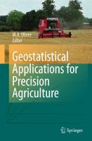
2.2 INTRODUCTION Sugar beet is a foreign crop to many people, although most people in the United States eat the fruits of its production regularly — sugar. Where sugar beet is grown for seed production, it is a biennial crop, grown to full maturity over two years. However, if sugar beet is grown for sugar processing, it is an annual crop; sown in the spring and harvested in the fall. At harvest, there are two components that are important: the green, leafy tops, and the sugar storage component of the root (Figure 2.1). Sugar beet cannot be grown everywhere. The presence of rocks is not good for harvest or processing. A more important component of production is the local availability of sugar beet processing facilities. Without processing plants nearby, sugar beet production would not be proÞtable. Transportation costs can rapidly

FIGURE 2.1 Sugar beet in the month of September, showing harvestable beet, taproot, and tops.

Nitrogen Management in Sugar Beet Using Remote Sensing and GIS

37

consume the value of the product. Conversely, if nearby growers decided not to grow sugar beets, the factories would be in Þnancial trouble, since transportation costs to move more distant production into the factory would make production costs prohibitive. Consequently, there has been a close relationship between sugar beet processors and growers. In some areas, such as the Red River Valley in Minnesota and North Dakota, the relationship has been especially strong due to the development of grower cooperatives. Early in the development of the sugar beet industry, researchers found that there was a unique relationship between nitrogen (N) fertilizer application and sugar beet production. As N fertilizer rates increased, sugar yields decreased.1 During sugar beet reÞning, the nitrogenous impurities within the root also increase the cost of processing. Growers are therefore encouraged not to over-fertilize with N. Sugar beets can use N from fertilizer as well as from residual N in the soil. In the 1970s, the concept of using soil sampling and nitrate analysis of soil as an approach to manage residual N was proposed.2 In a very short time, soil sampling for N management in sugar beets was widespread in the Red River Valley of Minnesota and North Dakota.3 Sugar beet harvest is unique compared to most other crops grown in the United States. In some cultures, sugar beet tops are harvested and removed from the Þeld as a livestock feed before or at root harvest. However, in the United States, the sugar beet tops are removed using a defoliator (Figure 2.2) that cuts the tops off along with a very small part of the root crown and distributes the beaten-up leaves on the soil surface. The lifter (Figure 2.2), which immediately follows the defoliator, lifts the beets from the ground to a truck for shipment to the processor. Distribution of nutrients at sugar beet harvest is different than production of cereal grain and oilseed crops, where most of the plant nutrients move to the grain and seed. When grain and oilseed is harvested, most of the plant nutrients are also removed. In sugar beets, many nutrients, including N, remain in the foliage. The concept of treating sugar beet tops as a green manure was Þrst reported in France.4 The results of this study showed that sugar beet tops provided signiÞcant N to the subsequent crop and should be treated as a green manure crop — a crop that is grown partially to maturity, but is terminated before harvest and all the nutrients returned to the soil for use by the next crop. Organic farmers often use this principle to provide N and other nutrients to subsequent crops to limit the use of commercial fertilizers. The color of leaves at harvest is related to the amount of N contained within the plant.5–9 Yellow sugar beet tops at harvest suggest that the leaves contain low levels of N, while green tops suggest that the plants contain a substantial amount of N. Leaf color can be used as a basis for N credits from sugar beet. For yellow leaves, no N credit is provided, while for dark green leaves, a credit of 90 kg ha–1 is provided. Remote sensing can be used to assess plant color. Low-cost LANDSAT data can be purchased by sugar cooperatives. LANDSAT data have a pixel size of approximately 30 m. These data can be processed to produce a number of different products. One of the most popular is the N Difference Vegetation Index (NDVI) ((red–NIR)/(red + NIR)). The imagery that is most useful for assessing residual N is collected between August and October. Imagery closer to

38

GIS Applications in Agriculture

FIGURE 2.2 Sugar beet defoliator (top) is used within hours of harvest by the sugar beet lifter (bottom).

harvest is preferred, but due to possible interference by cloud cover, imagery obtained earlier in the summer can be used to increase the chance of a successful image in any given area. When the agricultural consultants (agriculturalists) of the sugar cooperatives receive the images from the imagery provider, the agriculturalists visit a few farms in each view and determine whether the NDVI measurement in the image is related to green, yellow-green, or yellow. This relationship is then transferred to other Þelds in the area. The NDVI values within each image are then classiÞed based on that ground-truthed relationship using ArcView (ESRI, Redlands, California) software. The Þelds are classiÞed into three to Þve zones based on the established ground-truth relationship between sugar beet top color and the image NDVI values. From these zones of N credits, a fertilizer-spread map is developed using SGIS® (SOILTEQ, Minnetonka, Minnesota) software, which is ArcView-based. Although about 30% of Red River Valley sugar beet growers in 2005 utilized this zone N credit technique, the development of maps and N credits is still somewhat subjective. The following discussion provides an outline of how the current management recommendations are developed and how a ground-based active sensor can be used.

2.3 METHODS The development of zones in a GIS package such as ArcView or in a non-GIS software such as Surfer© (Golden Software, Golden, Colorado) is subjective, and

Nitrogen Management in Sugar Beet Using Remote Sensing and GIS

39

in terms of imagery, not very easy. If the data came to the user in a raw form as a text (.txt) Þle, either program would handle it well. If the data came to the user as an image, the image must Þrst be converted to a .txt Þle and then imported into the GIS program. The user can then select data intervals for the imagery that might be useful and rely on the software to develop a certain number of zones that Þt the base criteria in what is called “unsupervised classiÞcation,” or the user can manipulate the data intervals within the GIS software to Þt a view that makes sense when compared with other data including topography, yield maps, electrical conductivity, or previous year imagery. In the Red River Valley, much of the zone development is conducted by agriculturalists who are familiar with the farm and grower, so the activity of zone development is mostly a “supervised” classiÞcation, using the image viewing software developed by the supplier (AgriImaGIS, Inc. Maddock, North Dakota). When one data layer, such as imagery, is used to develop zones, classiÞcation is usually chosen as a method to accomplish the task. ClassiÞcation means that the data values (in imagery, the colors or hues are in values from 1 to 256) are divided into categories or classes. The classiÞcation method can vary depending on the experiences and preferences of the user. Common choices for single data layers within ArcView are equal spacing, Jenks10 natural breaks, and some multiple of standard deviation. The equal spacing choice would be appropriate for data that is equally distributed within the histogram of data. Standard deviation is a more statistical approach with normally distributed data. Jenks natural breaks is a procedure that groups data into classes that are relatively separate of the other classes, relying on the natural grouping of the data instead of a more subjective division.10 When an image is added to the ArcView screen, the Þle name of the image appears on a Þle column to the left of the main screen. Under the Þle name will be a red, green, and blue box. By left-clicking on any box, a small window will open with Visible checked. By left-clicking the Visible option of the red box, the check is removed and the image assumes the properties of only the green and blue boxes. This operation is reversible, so if the user wants to see the red layer again, the Visible command is simply rechecked. Sometimes the red-green-blue image is appropriate to work with, while in other images, one or two of the three layers is most representative of differences in the Þeld. Once the proper choice is made, the image can be exported as a tag image Þle format (.tif) Þle by right clicking the Þle name in the column to the left of the viewing area and then choosing Data > Export Data in the choices that appear sequentially. Sometimes the .tif Þle created in this manner is not usable in other formats; one way to ensure a useful .tif Þle after creating the .tif in the manner already described, is to go to File > Export Map, then save as a .tif under the previously used Þle name. To classify an image within ArcView, either the raw numeric data or the numeric data generated from the image through another program are required. ClassiÞcation of imagery within Surfer also must be conducted using numeric data. It is possible to import a .tif Þle into Surfer, but it can then only be viewed, and cannot be classiÞed in that format. One program that has been used to generate these numeric data is Noesys Transform© (Fortner Software LLC, Sterling, Virginia). An 8-bit .tif Þle can be opened in Transform, which then opens a numeric matrix of the user’s choice of

40

GIS Applications in Agriculture

designated columns and rows containing the raw data originally used to make the image. Without further manipulation, the numeric data can only be exported as an ASCII text matrix, which is not usable in GIS formats. However, using the “xyz1” macro, from the Transform toolbar, the data can be transformed from matrix to x, y, and z columns. The resulting Þle can be saved as .txt and imported into both Excel© (Microsoft Corporation, Redmond, Washington) or Surfer. The “xyz1” macro does not automatically appear as a macro choice. However, the “xyz1” macro code is imbedded in the macro archives and can be copied and pasted into an active macro by following the instructions within the program. ClassiÞcation of numeric data within ArcView is relatively easy and meaningful, as long as the classiÞcation results correspond to the user’s knowledge of the Þeld. Sometimes variability in the data is low, and if the data are not enhanced in some way, or the classiÞcation criteria are not Þne enough, ArcView will not automatically search for the criteria required to provide more than two or three classes. In some relatively ßat Red River Valley Þelds, for example, instead of recording feet or meters, use of inches or centimeters is necessary to provide enough numeric range for ArcView to function well. Another trick is to not use the default number for standard deviation, but use a fraction of it. If the results are still not satisfactory, a program such as Surfer might be better suited. Within Surfer, the user can dictate as many classes as are required. In addition, the composition of the classes can be orchestrated by choosing the range of each class, which is very difÞcult to do within ArcView. The resulting map can be exported out of Surfer as a .tif and imported into ArcView through the add data tool bar option. The resulting image can then be registered using the corner georeferences of the data. Another possible way to delineate zones from imagery alone is through the ArcView companion program ERDAS Imagine© (Leica Geosystems Group, Norcross, Georgia). Within ArcView, display a .tif image. In the Þle bar to the left of the screen, left click on the Þle name of the image. Choose Data, then Export Data. Within the three choices is the Image (.img) Þle. Choose the image option and the correct path to save the data. Once the .img Þle is created, it can be opened or manipulated using Imagine software. To create classes in the image, left click on the ClassiÞer icon in the Imagine toolbar at the top of the viewing screen. Choose Unsupervised classiÞcation from the choices of items within the ClassiÞer column. Once the Unsupervised classiÞcation window is opened, enter the image (.img) Þle that will be classiÞed, and create the output Þle and signature Þle that will go with the Þnal classiÞcation. Under the Initializing options button, one can choose the range of standard deviation on which the classiÞcation will be based. Also, the number of classes can be chosen in the space designated classes. The output Þle will have an .img extension, so it will be readable in both Imagine and ArcView.

2.4 RESULTS Two examples are provided to illustrate the use of remote sensing and GIS to deÞne N management zones based on sensing N content of sugar beet tops. The Þrst example describes the mapping of N management zones for wheat (Triticum aestivum L.) in St. Thomas, North Dakota, based on remotely sensed N content of sugar

Nitrogen Management in Sugar Beet Using Remote Sensing and GIS

41

beet tops, and the second example describes the use of a ground-based sensor compared to satellite imagery for zone delineation of N credits following sugar beet in Crookston, Minnesota.

2.4.1 USING SATELLITE IMAGES AND GIS BEET PRODUCTION PROBLEMS

TO

HELP SOLVE SUGAR

The crop rotation at the St. Thomas, North Dakota, site was sugar beet followed by wheat followed by potato (Solanum tuberosum) then back to sugar beet.11 This is a highly proÞtable rotation, but in this Þeld the sugar beets were suffering from high yield with low sugar content, resulting in much lower sugar payments than growers in different areas with different rotations. Although the logical cause of low sugar and high yield would be high residual soil N levels, the site had low soil N levels down to four-foot depths, and nothing out of the ordinary was observed. The decision was made to sample sugar beet tops for N content to assess this as a source of the observed problem. Four Þelds 16–20 ha in size were soil-sampled to a 2-m depth in a 0.2-ha grid in the fall of each year of a four-year study. Sugar beet tops ranged from light to very dark green as illustrated for one Þeld in Figure 2.3. A 3-m length of row within

FIGURE 2.3 Fertilizer application map for the Þeld in Figure 2.4 created using classiÞcation of an image to delineate zones, and soil nitrate data to Þnalize the nitrogen rates. The Þnal zones were hand-drawn, scanned, and geo-registered for use by an applicator. Each hue would receive a different nitrogen rate.

42

GIS Applications in Agriculture

each grid was harvested for root yield and top yield in the sugar beet years. Nitrogen

FIGURE 2.4 Aerial photography in August of a sugar beet Þeld showing darker, more robust areas with more N and biomass than lighter areas.

in the sugar beet tops ranged from 112 kg ha–1 to 448 kg ha–1. A Landsat 5 NDVI satellite image for one sugar beet Þeld showed a range of hue differences corresponding to a range of low to high vigor, while an aerial photograph for the same Þeld showed a range from no growth due to excessive water to high vigor in the darkest areas (Figure 2.4). The aerial image has three advantages over the NDVI satellite image. First, the aerial image has a much Þner resolution than the LANDSAT data. Second, since the relationship between sugar beet top N credit to subsequent crops is based on the level of greenness of the canopy, ground-truth information is much more critical in the NDVI image than in the true-color photograph. Third, areas within the Þeld of poor growth and thin stands are clearly identiÞable in the aerial image. These areas are not clearly identiÞable in the satellite (NDVI) image. In this example, early in the use of remote sensing of sugar beet tops, GIS was only used at the last step to develop the application map for N fertilizer to the subsequent wheat (Triticum aestivum L.) crop. Today, GIS is more easily used to remove subjectivity in delineating the fertilizer management zones from imagery. In this case, N fertilizer management zones were delineated by hand drawing around areas with similar greenness and vigor. The satellite and aerial imagery did not match exactly, and aerial imagery was weighted more than the satellite imagery. The resulting N fertilizer application map (Figure 2.5 shows that N credits ranged from 0 (168 kg N ha–1 rate to wheat) to 78 kg N ha–1 (90 kg N ha–1 to wheat). The farmer applied N fertilizer in the spring as anhydrous ammonia using an applicator equipped with a variable rate controller. The result of the variable N application showed no wheat yield differences between zones where large and small N credits were given (Table 2.1), suggesting that the N credits given to the zones were appropriate. If too great a credit had been given, yields would have been lower at the lower N rates. Since this study, sugar beet quality in the Þelds has dramatically improved as a result of using imagery to identify sugar beet tops with excessive N and reducing N rates accordingly to the subsequent crop. This practice has also helped to reduce residual N levels when the rotation again is planted back to sugar beets. The zones identiÞed during the sugar beet year have also been found to correspond to areas of related residual soil N levels throughout the rotation.11 The zones delineated during the sugar beet year are

Nitrogen Management in Sugar Beet Using Remote Sensing and GIS

43

FIGURE 2.5 Sugar beet images from a single Þeld obtained using aerial photography (left) and satellite imagery (right). The satellite imagery has been processed using viewer software that interpolates the raw image data and groups the data into classes. The raw data in the satellite image still exist within the GIS database, and can be further manipulated into different numbers of classes using different methods.

TABLE 2.1 Wheat yield differences between zones in a field near St. Thomas, North Dakota, that received various N credits from anticipated sugar beet top N contributions from the previous fall Zone –1

168 kg N ha 112 kg N ha–1 90 kg N ha–1 SigniÞcance at P 125.74,1,2) in cell M2 (note: the Þeld average yield is 125.74 bu ac–1). The second column (N) is used to classify variability into two categories, (1) above or (3) below the average standard deviation

22.50

3

4

1

1

22.50 22.50

7

8

9

10

11

12

13

14

15

16

17

18

19

1

1

1

1

1

1

1

1

1

1

1

1

1 22.50

22.50

22.50

22.50

22.50

22.50

22.50

22.50

22.50

22.50

22.50

22.50

1

22.50

5

6

1

22.50

22.50

2

1

Long_Feet 22.50

Column_No 1

Row_No 1

832.50

787.50

742.50

697.50

652.50

607.50

562.50

517.50

472.50

427.50

382.50

337.50

292.50

247.50

202.50

157.50

112.50

67.50

Lat_Feet 22.50

1661.73

1661.10

1660.55

1660.06

1659.63

1659.24

1658.82

1658.42

1658.07

1657.64

1657.23

1657.15

1657.81

1658.46

1659.09

1659.72

1660.28

1660.68

Elevation (ft) 1660.48

101.52

119.06

112.05

110.04

121.23

124.60

124.45

121.93

126.84

136.68

125.86

97.93

140.38

109.43

115.57

114.23

107.71

112.98

Corn96 111.35

144.55

165.14

174.86

183.88

193.17

212.76

219.43

213.91

215.48

216.81

222.65

226.14

207.91

216.24

204.69

212.60

217.89

176.25

Corn98 176.87

123.04

142.10

148.57

145.64

163.22

172.22

170.19

169.01

164.53

170.89

186.52

184.03

183.71

186.51

165.56

153.29

155.27

156.60

Corn00 151.40

104.58

120.78

123.39

124.54

135.32

144.38

145.65

143.04

143.61

110.49

103.47

103.47

105.00

110.30

112.79

106.48

89.88

95.43

Corn02 110.72

118.42

136.77

139.72

141.02

153.23

163.49

164.93

161.97

162.62

158.72

159.62

152.89

159.25

155.62

149.65

146.65

142.69

135.32

Average Yield (bu/ac) 137.59

19.84

21.62

27.96

32.09

31.83

38.22

40.86

39.62

38.47

45.95

54.74

62.71

45.70

54.21

43.98

48.51

57.23

37.50

Standard Deviation (bu/ac) 32.38

16.75

15.81

20.01

22.76

20.77

23.38

24.77

24.46

23.66

28.95

34.29

41.02

28.70

34.84

29.39

33.08

40.11

27.71

Coefficient of Variation (%) 23.53

TABLE 4.2 A portion of a summary file with elevation, seasonal and average yields, standard deviations, and coefficients of variation for four years of corn yield data

70 GIS Applications in Agriculture

Developing Productivity Zones from Multiple Years of Yield Monitor Data

71

FIGURE 4.1 Topography overlaid with average yield zones.

FIGURE 4.2 Topography overlaid with standard deviation zones.

value. This can be accomplished by typing the formula =IF(K2>36.85,1,3) in cell N2 (note: the Þeld average standard deviation is 36.85). When adding the yield and variability categories together, the numbers combine to create four unique zone values. This is accomplished by entering the formula =M2+N2 in cell O2. Columns need to be Þlled down to complete calculations for the entire data set. Grid cells

72

GIS Applications in Agriculture

FIGURE 4.3 Topography overlaid with coefÞcient of variation (CV) zones.

FIGURE 4.4 Topography overlaid with combination average yield and standard deviation zones.

with a combined yield and variability value of 2, 3, 4, and 5 are categorized as high yield and high deviation, low yield and high deviation, high yield and low deviation, and low yield and low deviation, respectively. These functions can be performed in any spreadsheet software package. An example of this data set is shown in Table 4.3.

67.50

112.50

157.50

202.50

247.50

292.50

337.50

382.50

427.50

472.50

517.50

562.50

607.50

652.50

697.50

742.50

787.50

832.50

22.50

22.50

22.50

22.50

22.50

22.50

22.50

22.50

22.50

22.50

22.50

22.50

22.50

22.50

22.50

22.50

22.50

22.50

Lat_Feet 22.50

Long_Feet 22.50

1661.73

1661.10

1660.55

1660.06

1659.63

1659.24

1658.82

1658.42

1658.07

1657.64

1657.23

1657.15

1657.81

1658.46

1659.09

1659.72

1660.28

1660.68

101.52

119.06

112.05

110.04

121.23

124.60

124.45

121.93

126.84

136.68

125.86

97.93

140.38

109.43

115.57

114.23

107.71

112.98

144.55

165.14

174.86

183.88

193.17

212.76

219.43

213.91

215.48

216.81

222.65

226.14

207.91

216.24

204.69

212.60

217.89

176.25

123.04

142.10

148.57

145.64

163.22

172.22

170.19

169.01

164.53

170.89

186.52

184.03

183.71

186.51

165.56

153.29

155.27

156.60

104.58

120.78

123.39

124.54

135.32

144.38

145.65

143.04

143.61

110.49

103.47

103.47

105.00

110.30

112.79

106.48

89.88

95.43

Elevation (ft) Corn96 Corn98 Corn00 Corn02 1660.48 111.35 176.87 151.40 110.72

118.42

136.77

139.72

141.02

153.23

163.49

164.93

161.97

162.62

158.72

159.62

152.89

159.25

155.62

149.65

146.65

142.69

135.32

Average Yield (bu/ac) 137.59

19.84

21.62

27.96

32.09

31.83

38.22

40.86

39.62

38.47

45.95

54.74

62.71

45.70

54.21

43.98

48.51

57.23

37.50

Standard Deviation (bu/ac) 32.38

16.75

15.81

20.01

22.76

20.77

23.38

24.77

24.46

23.66

28.95

34.29

41.02

28.70

34.84

29.39

33.08

40.11

27.71

Coefficient of Variation (%) 23.53

2.00

1.00

1.00

1.00

1.00

1.00

1.00

1.00

1.00

1.00

1.00

1.00

1.00

1.00

1.00

1.00

1.00

1.00

Yield Zone 1.00

3.00

3.00

3.00

3.00

3.00

1.00

1.00

1.00

1.00

1.00

1.00

1.00

1.00

1.00

1.00

1.00

1.00

1.00

Deviation Zone 3.00

5.00

4.00

4.00

4.00

4.00

2.00

2.00

2.00

2.00

2.00

2.00

2.00

2.00

2.00

2.00

2.00

2.00

2.00

Combination Zone 4.00

TABLE 4.3 A portion of a summary file showing the yield, deviation, and combination zones as calculated by the spreadsheet

Developing Productivity Zones from Multiple Years of Yield Monitor Data 73

74

GIS Applications in Agriculture

The data set provided with this case-study can be imported into ArcView or an alternative geographic information systems software package for data viewing, interpretation, and development of shapeÞles for export to variable-rate equipment.

4.3.6 CALCULATING ZONE IMPACTS

ON

YIELD VARIABILITY

Yield variability reductions are calculated with the equation %variance  reduction = 100 × [1 −

s 2pz ] s 2field

(4.1)

where s2pz is the pooled variance of all productivity zones and s2Þeld is the variance of the entire Þeld.8 Pooled variance (s2pz) is calculated with the equation

s

2 pz

∑ (n − 1)s =

2 i

i

(4.2)

N−z

where ni is the number of points in each zone, s2i is the variance of each zone, N is the total number of points in all zones and z is the number of zones.10 Field variance (s2Þeld) is calculated with the equation

s

2 field

∑ (x − x ) = i

( n − 1)

2

(4.3)

where xi are the yield values of each data point, x is the Þeld average yield, and n is the number of data points in the Þeld.10 The yield variability reduction calculations are accomplished by (1) calculating the variance for the entire Þeld (Equation 4.3), (2) sorting the data based on the various productivity zones, (3) calculating the variance for each zone (Equation 4.3), (4) calculating the pooled variance values for each method of zone delineation (Equation 4.2), and (5) calculating the percent reduction in variance (Equation 4.1). The reductions in yield variability for each year using the different productivity zone delineation methods can be seen in Table 4.4.

4.4 RESULTS AND DISCUSSION The four different approaches used to characterize multiple-year yield data had both similarities and differences (Table 4.4). Production zones created from average yields separated the Þeld into areas with low, medium, and high yields. Low yields were observed in the summit or shoulder landscape positions, medium yields were generally observed in the backslope positions, and high yields often were found in footslope or toeslope positions. In eastern South Dakota, where moisture is often

Developing Productivity Zones from Multiple Years of Yield Monitor Data

75

TABLE 4.4 Impact of the four methods to identify productivity zones on the percent reduction in yield variation when compared to whole field variability Method of Productivity Zone Delineation – % Reduction in Yield Variation Year 1996 1998 2000 2002 All years

Average Yields 7 53 48 20 32

Standard Deviations 16 49 37 0 28

Coefficient of Variation 29 27 18 4 22

Average + Standard Deviation 26 63 54 18 43

the limiting factor for crop production, average yields are generally correlated to landscape position. However, this approach does not take into consideration the extremes in variability that may occur on a temporal basis. Areas of high production in one year may have limited production in a different year with different weather conditions. Production zones based solely on yield will improve as additional years are added to the data set. Average yield zones can help producers to set production goals for different Þeld areas and vary inputs to account for the expected differences in production. To improve management, it is necessary to examine the standard deviation of individual grid-cell yields over time. Areas with low standard deviation, typically were summit, shoulder, and backslope. Areas with an average or medium standard deviation are typically located in transition areas, which also occur in backslopes. Toeslope and footslope areas may have a high standard deviation because these areas can have both very high and very low yields, depending on climatic conditions. Areas with high standard deviation may require additional management. For example, in toeslope areas, tile drainage can be installed to remove excess water. By understanding within-Þeld variability, producers may be better able to manage this variability and increase production. The coefÞcient of variation is another way to delineate zones based on variability. However, the CV also takes the Þeld average yields into account. Basically, the CV measures the variability in the values in a population relative to the magnitude of the population mean.10 The zones created with CV values are similar to those created by standard deviations. In order to gain a better understanding of how the average yields and standard deviations in a Þeld interact, it may be necessary to deÞne zones taking both measures into account. In the example Þeld, areas with both high yields and high standard deviations were found in footslope areas that have occasional problems with excess moisture. These areas produce high yields in dry years and low to average yields in wet years. Approximately 32% of the Þeld areas Þt into this category. These areas are good candidates for installing tile drainage. Selecting yield goals for these areas is difÞcult due to the large variability. In relatively dry years theses areas can produce yields in excess of 200 bu ac–1, while in very wet years, yields can be as low as

76

GIS Applications in Agriculture

0 bu ac–1. The areas with low yields and high deviations are typically toeslope areas that are extremely wet or in compacted regions surrounding wet Þeld areas. The yields are usually low due to excess water or compaction and only produce high yields when conditions are ideal. Producers may try to control variability in these areas by limiting compaction, using drainage methods, or planting extremely low areas to grass waterways. Areas of the Þeld with high yields and low deviations are typically backslope areas that have adequate soil moisture but are not prone to ßooding. Producers may wish to increase inputs in these areas, as agronomists report that nutrient depletion often occurs in areas of consistently high production. Finally, the areas of the Þeld with low yields and low deviations are typically summit or shoulder positions with limited soil moisture. These areas may also be eroded with low organic matter contents and limited production capabilities. Producers may wish to cut back inputs in these areas to increase efÞciency. Agronomists often report that due to several years of low yields and correspondingly low crop removal rates, nutrients have accumulated in these areas. A notable trend occurred for all types of production zone delineation processes. Yield variability (s2Þeld) was increased by extremely wet conditions in 1996 and decreased by a severe windstorm during pollination in 2002. In years with extremely high or low variability (s2Þeld), zones based on average values of yield and standard deviation will not perform as well. All methods examined did a better job of explaining yield variability in the years 1998 and 2000, when yield patterns were close to “average” (Table 4.4). There is one exception to this statement. In 1996, when variability was high, the CV approach was the best, reducing yield variability by 29%. However, the zone delineation method that most consistently explained variability was the combination average and standard deviation approach. Over all years, this method reduced yield variability by an average of 43%. The amount of variability reduced was much higher, 63% and 54% in the more “average” years of 1998 and 2000, respectively. The method based on average yields reduced variability by an average of 32%. This approach also performed better in the years 1998 and 2000, reducing yield variability by 53% and 48%, respectively. The standard deviation approach reduced variability by an average of 28% and performed the best in years 1998 and 2000, reducing variability by 49% and 37%, respectively. Finally, the production zones based on CV reduced variability by an average of 22%. This approach performed best in 1996 and 1998, reducing variability by 29% and 27%, respectively.

4.5 CONCLUSIONS There are several ways to use yield data to analyze yield trends both spatially and temporally. Production zones will become more accurate with time as more and more growing seasons are added into a Þeld database. Different maps can be used for different purposes. Average yield maps can be used to deÞne yield goals. However, in areas with high standard deviations, care must be used when using average values. Standard deviation maps are very useful in identifying areas requiring corrective treatments. By comparing yield and standard deviation maps, the costs associated with not implementing a corrective treatment can be determined. For

Developing Productivity Zones from Multiple Years of Yield Monitor Data

77

example, if a 10-acre area in a footslope area has excess water 1 year out of 10 resulting in a 90% yield loss, the loss from that year would be $4,500 (10 acres @ 180 bu ac–1 loss @ $2.50 bu–1). This scenario occurred in 1996 in the example Þeld provided with this case study. In this case study, the best method for explaining yield variability in Þelds was using a combination of average yields and standard deviation to delineate productivity zones. Due to the variability present in any agricultural production system, it is up to producers to analyze and interpret the different zones created for each Þeld and determine how management decisions can be altered to increase production efÞciency.

4.6 EXERCISE: MAPPING PRODUCTIVITY ZONES 4.6.1 OVERVIEW Any GIS package may be used to map the data generated by Field Analyst. In this exercise, ArcView will be used to plot productivity zones. This program may be used to create shapeÞles from Field Analyst data to drive variable rate applications.

4.6.2 FILE FORMATS ArcView uses either text Þles (.txt) or database Þles (.dbf). Files may be converted to this format using Excel or most other spreadsheet programs. Note: If using GPS coordinates, latitude and longitude values must be speciÞcally designated to have six decimal places.

4.6.3 MAPPING PRODUCTIVITY ZONES This section outlines the process used to map productivity zones. To begin, open the ArcView 3.3 software program. 1. As the program starts, a window will pop up asking whether or not to add a new view. Select with a new view and click OK. When the dialogue box asking would you like to add new data to the view appears, click No. 2. In the Untitled window, click on the Tables icon and then click Add. A window entitled Add Table should appear, allowing navigation to the dataÞle.dbf Þle supplied with this exercise. 3. After selecting the dataÞle.dbf Þle, click OK. Remember to select (.dbf) as the Þle type in ArcView. The data table should appear in a new window. 4. Next the data from the table will be added to the view. First, click on the View1 window to make it active. From the toolbar at the top of the screen, select View and then Add Event Theme. 5. A window entitled Add Event Theme appears. Make sure the X Þeld reads Long_feet and the Y Þeld reads Lat_feet. Click OK to continue. 6. A dataÞle.dbf theme should appear in the View1 window. Click on the check box to the left of the theme name to make the map visible. These are the grid points used for productivity zone delineation.

78

GIS Applications in Agriculture

7. In order to see the productivity zones, data points need classiÞcation. To do this, double-click on the box surrounding the dataÞle.dbf theme name. The Legend Editor window should appear. 8. From the Legend Type pulldown menu, select Unique value. 9. In this exercise the combination zones will be mapped. Select Combination zones from the Values Field pull-down menu and then click Apply. The Legend Editor window can now either be closed or minimized. 10. The map should now show four color levels representing the different zones. For zone interpretations, refer back to earlier discussion in the “Identifying productivity zones” section. 11. To change the type of zones on the map, simply reopen the Legend Editor window, change the zone type in the Values Field pulldown menu, and click Apply.

ACKNOWLEDGMENTS Funding was provided by the South Dakota Soybean Research and Promotion Council, Upper Midwest Aerospace Consortium (UMAC) the United Soybean Board, NASA, the North Central Soybean Research Program, the South Dakota Agricultural Experiment Station, and USDA-CREES Grant 2004 51/30–02248.

REFERENCES 1. Chang, J. et al., DeÞning yield goals and management zones to minimize yield and nitrogen and phosphorus fertilizer recommendation errors, Agron. J., 96, 825, 2004. 2. Bakhsh, A. et al., Spatio-temporal analysis of yield variability for a corn-soybean Þeld in Iowa, Trans. ASAE, 43, 31, 2000. 3. Diker, K. et al., Frequency analysis of yield for delineating management zones, in Proceeding of the 6th International Conference on Precision Agriculture, July 14–17, 2002, Robert, P.C. et al., Eds., Bloomington, MN. ASA-CSSA-SSSA, Madison, WI, 2002. 4. Fridgen, J.J., Kitchen, N.R., and Sudduth K.A., Variability of soil and landscape attributes within sub-Þeld management zones, in Proceeding of the 5th International Conference on Precision Agriculture, July 16–19, 2000. Bloomington, MN, Robert, P.C. et al., Eds., ASA-CSSA-SSSA, Madison, WI, 2000. 5. Blackmore, S. and Moore, M., Remedial correction of yield map data, Prec. Agric., 1, 53, 1999. 6. Thylen, L. and Algerbo, P.A., An expert Þlter removing erroneous yield data, in Proceeding of the 5th International Conference on Precision Agriculture, July 16–19, 2000. Bloomington, MN, Robert, P.C. et al., Eds., ASA-CSSA-SSSA, Madison, WI, 2000. 7. Fleming, K.L., Westfall, D.G., and Wiens, D.W., Field testing management zones for VRT, in Site-SpeciÞc Management Guideline, SSMG-21. PPI-FAR, Norcross, GA, 1999. Available online at www.ppi-ppic.org.

Developing Productivity Zones from Multiple Years of Yield Monitor Data

79

8. Kitchen, N. et al., Procedures for evaluation unsupervised classiÞcation to derive management zones, in Proceeding of the 6th International Conference on Precision Agriculture, July 14–17, 2002, Robert, P.C. et al., Eds., Bloomington, MN, ASACSSA-SSSA, Madison, WI, 2002. 9. Walker, T. et al., DeÞning and managing yield zones for rice and soybeans — a case study, Better Crops with Plant Food, 88, 10, 2004. 10. Rao, P.V., Statistical Research Methods in the Life Sciences, Brooks/Cole Publishing Co., PaciÞc Grove, CA, 1998.

5

Site-Specific Weed Management in Growers’ Fields: Predictions from Hand-Drawn Maps Lori J. Wiles, R. Bobbitt, and Philip Westra

CONTENTS 5.1 Executive Summary...........................................................................................81 5.2 Introduction .......................................................................................................82 5.2.1 Site-SpeciÞc Strategies for Weed Management ...................................83 5.2.2 Variability in the BeneÞts of Site-SpeciÞc Weed Management...........83 5.3 Overview of the WeedSite Program..................................................................84 5.4 Evaluating Site-SpeciÞc Weed Management ....................................................85 5.4.1 Creating a Scenario...............................................................................85 5.4.2 Identifying Polygons.............................................................................88 5.4.3 Predicting Outcomes for Simulation Polygons....................................88 5.4.4 Decision Algorithms .............................................................................88 5.4.5 Viewing Results ....................................................................................89 5.5 Examples with Maps Drawn by Agricultural Consultants ...............................90 5.5.1 Predictions: What We Know ................................................................92 5.5.2 Predictions: What We Are Learning.....................................................93 5.6 Limitations: Accuracy and Speed .....................................................................96 5.7 Conclusions .......................................................................................................96 Acknowledgment .....................................................................................................99 References................................................................................................................99

5.1 EXECUTIVE SUMMARY Herbicide use may be reduced 30–80% without impacting crop yield with sitespeciÞc weed management. Herbicide use is varied within a Þeld to match the variation in the weed population. However, growers will not adopt this strategy until they are conÞdent that the reduction in herbicide and other beneÞts of site-speciÞc weed management will justify the cost of implementation and future weed control

81

82

GIS Applications in Agriculture

will not be compromised. Predicting the outcome of site-speciÞc weed management is difÞcult because beneÞts vary with the composition and spatial distribution of the weed population, possible herbicide treatments, and the resolution of variable management. WeedSite software was developed so growers could investigate the potential beneÞts of postemergence site-speciÞc weed management in irrigated corn speciÞcally for their weed populations and implementation of site-speciÞc weed management. Users choose the resolution of patch spraying and may divide a Þeld into management units. Georeferenced weed maps and GIS software are not needed. Net gain from site-speciÞc weed management, area of the Þeld not treated, herbicide use and cost, yield loss from weed competition, and weeds left in the Þeld are all calculated from hand-drawn weed maps and results can be mapped. We think WeedSite can be useful for educating growers, agricultural consultants, and students about the potential beneÞts of postemergence site-speciÞc weed management in irrigated corn in addition to published Þeld experiments. Evaluations are consistent with what is known about variation in the beneÞts of site-speciÞc weed management. Predictions from hand-drawn maps will be less accurate than predictions from Þeld experiments but more germane. General features of spatial distributions may be more representative and users choose the weed species present, the resolution of management, and the candidate herbicides.

5.2 INTRODUCTION Weeds grow in patches of varying size, shape, and composition within Þelds1–5 yet herbicide treatments are usually selected based on the “average” weed population and applied uniformly across a Þeld. Site-speciÞc weed management (SSWM) may reduce herbicide use while still achieving appropriate and economical control.6 This is a strategy of varying weed management within a Þeld to match the variation of the species and density of the weed population. Herbicide use may be reduced because herbicide is applied only where the beneÞts exceed the costs. Further, control may be more cost effective and future weed problems minimized because the type and rate of herbicide can be varied for local weed populations within the Þeld. Growers are aware of the spatial variability of weed populations in their Þelds and many practice simple strategies of site-speciÞc weed management with postemergence herbicides such as spraying Þeld edges with a different herbicide or higher rate than the rest of the Þeld.7 However, few practice the potentially more valuable SSWM with the technology of precision agriculture. Even if a grower already has the technology and knowledge, SSWM may still be more expensive and require more time than uniform management. Using SSWM requires the grower to map the weed population in a Þeld, make many rather than a single management decision for a Þeld, and prescribe the varying management in a format for the sitespeciÞc technology used. Also, growers are concerned that additional weeds left untreated in the Þeld may lead to more serious weed problems in the future. Growers need to know that the reduction in herbicide use and other beneÞts will exceed the costs and that future weed control will not be compromised before investing in the technology, learning the new skills, and committing the additional time needed for site-speciÞc weed management.

Site-Specific Weed Management in Growers’ Fields

5.2.1 SITE-SPECIFIC STRATEGIES

FOR

83

WEED MANAGEMENT

One approach to site-speciÞc weed management is to map weed populations in the Þeld and then divide the Þeld into subunits with the herbicide application for each selected according to the average weed population indicated on the map for each subunit.8 In this scenario, herbicides are applied uniformly in subunits. For the patch spraying strategy of SSWM, subunits may be cells of a sprayer grid with the width and length of cells determined by the size and technology of the sprayer (patch or variable rate) that will be used.9 Cell width is the length of the boom or smaller if sections of the boom or individual nozzles can be operated independently. The length of a sprayer grid cell is determined by how quickly herbicide application can be varied with the sprayer.10 Subunits of a Þeld, called management units, can be either the smallest area that a grower can manage independently11 or an area that a grower needs to manage independently based on the variability of the weed population.12 For growers without global positioning systems (GPS) and patch or variable rate sprayers, management units can be easily identiÞed areas such as a pass of the sprayer or half of a Þeld. The choice of management for each sprayer grid cell or management unit may be spray or no spray, the typical concept of patch spraying, or applying one of several herbicides or herbicide mixtures for the most cost-effective control of different types of weeds such as annuals and perennials.13 Alternatively, a grower may spray the entire Þeld with a single herbicide, but vary the rate depending on the density of the weed population.14 Growers may prefer this latter approach to leaving areas of the Þeld unsprayed to minimize the risk of seed production from uncontrolled weeds.

5.2.2 VARIABILITY

IN THE

BENEFITS

OF

SITE-SPECIFIC WEED MANAGEMENT

Herbicide use may be reduced by 90% or more with SSWM with reductions of 40–70% common in research studies.9,15–21 However, reductions are not consistent. For example, in one study of site-speciÞc compared to uniform weed management, herbicide use was reduced 98% in one corn Þeld but only 11.5% in a nearby Þeld.21 Net gain from site-speciÞc weed management of wild oat (Avena fatua L.) varied from $3.19 to $19.98 ha–1 in four Þelds of dryland spring wheat.22 The beneÞt of SSWM in a particular Þeld is difÞcult to predict because herbicide use with SSWM varies with the size, shape, arrangement, and species composition of patches and the site-speciÞc strategy used.11,23,24 In general, the beneÞt of sitespeciÞc management increases with the patchiness of the weed population because more of a Þeld can be left untreated.6,25 Also, herbicide use is minimized with smaller management units and sprayer cells because more cells or units will be weed-free.24,26 For patch spraying (on/off), the actual reduction depends on the weed-free area at the spatial resolution of the patch sprayer.24 Weed species present11,13 and the choice of herbicides23 also inßuence the beneÞts of SSWM because control with a herbicide and the ability to compete with the crop varies among weed species. The economic beneÞt of SSWM will be greatest with the more expensive herbicides,11 but will vary with the yield potential and selling price of the crop.

84

GIS Applications in Agriculture

With the observed variability of herbicide use and economic and other beneÞts with SSWM in research studies, and the many potential reasons for the variability, growers need estimates for the composition and distributions of weed populations in their Þelds and the site-speciÞc strategies that can potentially Þt their needs. For these reasons, we developed a computer program for growers and agricultural consultants to explore the potential beneÞts of different strategies of SSWM in their irrigated corn Þelds.

5.3 OVERVIEW OF THE WEEDSITE PROGRAM Our objective was to develop an easy-to-use computer program (WeedSite) that growers and agricultural consultants in Colorado, USA, can use to investigate the potential beneÞts of site-speciÞc, postemergence weed management in their irrigated corn Þelds. Our goal was education rather than recommendations and our targeted audience included growers and agricultural consultants who do not own site-speciÞc technology and may not even be familiar with site-speciÞc weed management. To meet this objective, our most important requirements were that georeferenced Þeld or weed data and GIS software would not be needed. Also, we wanted software distribution to be free to reach the most potential users. Most growers and agricultural consultants are aware of variation in the spatial distribution of weeds in their corn Þelds. Few draw maps, but most make management decisions based on their perceptions of the distribution and many will readily draw a weed map if asked.7 The program we developed does not require georeferenced weed maps. Instead, uniform and site-speciÞc weed management are evaluated based on hand-drawn weed maps. The program has three modules: (1) a GIS interface, (2) a simulation model for predicting biological and economic outcomes of weed management, and (3) decision algorithms that identify the optimal site-speciÞc management from the predicted outcomes for the weed populations in the Þeld. Each component of the program performs an essential task for determining the optimal uniform or sitespeciÞc weed management. These tasks are completed sequentially with the results of a task completed by one module written to a database to be retrieved by the next module. WeedSite was developed for the Windows environment using Microsoft Visual Basic 6.0® (Microsoft Corporation, Redmond, Washington, USA) and MapObjects LT 2.0® (ESRI, Redlands, California, USA). MapObjects LT is a Windows ActiveX® (Microsoft Corporation, Redmond, Washington, USA) software control that provides extensive GIS interface tools for map display, analysis, drawing, querying, and navigation, and there are no royalties for distribution of programs developed using this software. Custom programming was necessary for functions not included in MapObjects LT such as map legends. Model parameters and users’ scenarios and results are stored in Microsoft Access 2000 databases® (Microsoft Corporation, Redmond, Washington, USA) and maps are stored as ESRI shapeÞles. Because the MapObjects LT software does not include tools for calculating the intersections of polygons (weed patches, management units, etc.), vector polygons representing weed patches, management units, and sprayer grid cells are converted

Site-Specific Weed Management in Growers’ Fields

85

to a raster data set for analysis. This allows Þnite and discrete calculations for the area of intersection of different layers. The raster size is based on a database parameter that represents the length and width of a raster cell and can be changed by users. Length and width of sprayer grids are limited to multiples of this parameter. Areas of the intersections that need to be identiÞed for an evaluation are calculated by Þnding the number of raster cells that intersect the derived polygons and then multiplying that number by the area of a raster grid cell.

5.4 EVALUATING SITE-SPECIFIC WEED MANAGEMENT WeedSite evaluates uniform and SSWM strategies for a set of tactics speciÞed in a model database and a scenario. A tactic is no control, an application of one or more herbicides at a speciÞed rate, or a sequential application of herbicides. A scenario is the set of Þeld, weed population, production, and strategy information speciÞed by the user. Strategies are uniform management and different methods of implementing site-speciÞc management (Table 5.1). Site-speciÞc strategies are patch spraying with one or two tactics; user-deÞned management units with the model or the user selecting the tactic for each unit; and an estimate of maximum beneÞt from site-speciÞc weed management.

5.4.1 CREATING

A

SCENARIO

The user creates maps and speciÞes information of a scenario through a single screen of the GIS interface. The minimum information needed for a scenario is a Þeld map, a weed map and a sprayer grid, and production and economic information (Figure 5.1). A scenario may also include management units, plus tactics for the management units, and the user may choose to evaluate just a subset of tactics of the program (Figure 5.1).

TABLE 5.1 Site-specific strategies differ by the type of management polygons and method for selecting optimal tactic or tactics Strategy Uniform management Maximum beneÞt

Management Polygons Field Unique weed populations

Patch spraying with one tactic Patch spraying with two tactics Management units

Sprayer grid cells

Grower management

Sprayer grid cells User-deÞned subunits of the Þeld User-deÞned subunits of the Þeld

Method for Selecting Optimal Tactics One tactic for the Þeld One tactic for each unique weed population One tactic or no control for each cell One of two tactics or no control for each cell One tactic for each management unit User selects a tactic for each management unit

86

GIS Applications in Agriculture

FIGURE 5.1 WeedSite users create scenarios that include maps, production information, and choice of tactics for an evaluation.

FIGURE 5.2 Users draw weed maps and may use density or pressure to describe the weed population, include up to six weed species in a patch, and specify weeds that are uniformly distributed through the Þeld.

Fields, weed patches, and management units can be circles, rectangles, or any shape drawn by the user with a GIS polygon tool (Figure 5.2). Populations in a weed patch may include up to six weed species and are described as density [weeds per 100 ft (30.5 m) of row] for each weed species or by choosing from a list of pressure ratings (Figure 5.2). English units are used in the program since these are most appropriate for the intended audience. Pressure ratings indicate expected percent crop yield loss and a pressure rating is converted to density for each weed species based on the competitiveness of the weed species. Weed patches can overlap. For these areas, weed presence is the higher density or weed pressure for a species that is included in more than one of the overlapping patches. Besides weed patches,

Site-Specific Weed Management in Growers’ Fields

87

FIGURE 5.3 Sprayer grids of various sizes and orientation relative to the Þeld can be generated with WeedSite.

FIGURE 5.4 A Þeld can be divided into management units that do not overlap and the user can choose to specify the tactic for each unit.

up to six weed species that are uniformly distributed throughout a Þeld may be speciÞed. Different sprayer grids can be created to compare SSWM with various variable rate or patch sprayers. The user selects the length and width of sprayer grid cells and the angle for orientation of the grid relative to the Þeld (Figure 5.3). Management units, like weed patches, can be circles, rectangles, or polygons but cannot overlap (Figure 5.4). For the site-speciÞc strategy of grower management, the user chooses a tactic for each management unit (Figure 5.4).

88

GIS Applications in Agriculture

5.4.2 IDENTIFYING POLYGONS The Þrst step of an evaluation is identifying weed, management, and simulation polygons of a scenario. Weed polygons are weed patches that do not overlap with other patches and polygons created by overlapping patches. The area of the Þeld without patches is also deÞned as a weed polygon. Management polygons are the entire Þeld (uniform management), weed polygons (maximum beneÞt), sprayer grid cells (patch spraying with one or two tactics), and the management units drawn by the user plus any area of the Þeld not included in management units (management units and grower management) (Table 5.1). Simulation polygons are intersections of weed polygons with management polygons. These are the fundamental units for simulating the outcome of management and calculations of the decision algorithms.

5.4.3 PREDICTING OUTCOMES

FOR

SIMULATION POLYGONS

The second step in an evaluation is simulating biological and economic outcomes for each simulation polygon for all possible tactics or the set of tactics selected by the user. The simulation model in WeedSite is a modiÞed version of an existing weed management decision model, GWM/WEEDCAM,27,28 with herbicide databases updated with information from the Colorado29 and Nebraska30 weed management guides. Outcomes predicted for each simulation polygon/tactic combination are herbicide use (active ingredient), cost of herbicide, weed escapes, crop yield loss from competition with weed escapes, and gross margin. Gross margin (GM) is the value of the crop calculated from the user’s prediction of crop price (Pc) and expected yield with no weeds (Ynw) minus the simulated yield loss from weeds not controlled by the tactic (Yw). Percent yield loss depends on percent control with the tactic, density and estimated competitiveness of the different species of the weed population, and a relationship between weed density and crop yield loss. It is assumed that the weeds emerge with the crop and are controlled at the optimal time. All results are calculated per unit area (acre). GWM/WEEDCAM has been evaluated on 50 farms in a 4-year study in eastern Colorado.31 The model is also suitable for corn production in the panhandle of Nebraska.

5.4.4 DECISION ALGORITHMS The tactics are speciÞed for the grower management strategy. Decision algorithms for the other strategies all identify the tactic that optimizes gross margin for a Þeld, but differ by the number of tactics for optimal management and which simulation polygons must have the same tactic (Table 5.1). For example, the same tactic must be speciÞed for all simulation polygons within a management unit or sprayer grid cell. Gross margin for a Þeld is the weighted sum of the gross margin for each simulation polygon with the proportion of the area of the Þeld of a simulation polygon as the weight. Optimal management may be one tactic to as many tactics as the number of unique weed populations (maximum beneÞt) or management units

Site-Specific Weed Management in Growers’ Fields

89

FIGURE 5.5 WeedSite generates tables of results that include net gain from site-speciÞc weed management, outcomes related to herbicide use, and crop yield loss (summary tab), area of the Þeld for each tactic (management tab), and weeds left in the Þeld (weed escapes tab), and the scenario and tables can be printed (print tab).

in a Þeld (Table 5.1). Gross margin for grower management is calculated in the same method as the other strategies, but with the tactics speciÞed. Herbicide use, weeds not controlled, and yield loss from competition with uncontrolled weeds are calculated for the Þeld for a management strategy with the same method as gross margin. We also calculate net gain from SSWM for easier comparison among the site-speciÞc strategies and with the optimal uniform management. This is the gross margin with optimal management for a site-speciÞc strategy minus the gross margin for the optimal uniform strategy and the site-speciÞc technology cost. A net gain greater than zero indicates net return is greater with sitespeciÞc than uniform management.

5.4.5 VIEWING RESULTS Net gain from SSWM, optimal tactics, herbicide use, area of the Þeld treated, crop yield, and weeds escaping control in the Þeld are displayed in tables on the Summary, Management, and Weed Escapes tabs of the results screen of the GIS interface (Figure 5.5). However, differences among the site-speciÞc strategies and why these occurred can best be understood by viewing maps. Spatial variability of the information in the tables can be displayed on the Maps tab for each management strategy (Figure 5.6). The user can print the scenario, results tables, and maps from the Print tab or copy maps to the Windows clipboard (Figure 5.6).

90

GIS Applications in Agriculture

FIGURE 5.6 Predicted results of uniform and site-speciÞc weed management can be mapped for a better understanding of the outcomes of site-speciÞc weed management.

5.5 EXAMPLES WITH MAPS DRAWN BY AGRICULTURAL CONSULTANTS Use of WeedSite is illustrated with maps drawn by agricultural consultants during interviews about how they make weed management decisions.7 The maps were digitized by the authors and are shown in Figures 5.7 and 5.8 with the uniformly distributed species and the weed polygons, and the species in each, identiÞed. Weed species included in the maps were Echinochloa crus-galli (L.) Beauv., Cenchrus longispinus (Hack.) Fern., Salsola tragus L., Kochia scoparia (L.) Schrad., Amaranthus retroßexus L., Chenopodium album L., Solanum physalifolium Rusby, Cirsium arvense (L.) Scop., and Setaria viridis (L.) Beauv. The interviews were conducted before WeedSite was developed so we did not have all the information needed for an evaluation. Consequently, the authors chose the Þeld size (30.4 ha), crop yield (10 T ha–1), crop price ($168.25 kg–1), two sprayer grids (6 × 18 m and 12 × 36 m), and two management units for both Þelds. Grower management was not included in the evaluations. The larger spraying grid and management units for the Þelds are shown in Figures 5.9 and 5.10. Management units were selected to be a primarily grass unit and a primarily broadleaf unit. Tactics in the WeedSite database are 24 herbicides and herbicide mixtures that are commonly used by corn growers in Colorado. We did the evaluations with all the tactics in the database and with the Þve least expensive tactics excluded to illustrate the effect of herbicide cost on the beneÞts of SSWM. The cost of these tactics was $3.71 to $15.10 ha–1 and the cost of the remaining tactics was $24.00 to $80.28 ha–1. No control was also simulated. No site-speciÞc technology cost was included since this information is not yet available. Without this cost, net gain can be interpreted as the maximum amount that can be spent on SSWM if the objective is to maximize proÞt.

Site-Specific Weed Management in Growers’ Fields

91

FIGURE 5.7 Weed map of Field A drawn by an agricultural consultant with weed species in each weed polygon and uniformly distributed throughout the Þeld identiÞed.

FIGURE 5.8 Weed map of Field B drawn by an agricultural consultant with weed species in each weed polygon and uniformly distributed throughout the Þeld identiÞed.

The predicted outcomes of site-speciÞc and uniform weed management for the agricultural consultants’ hand-drawn maps illustrate both well-established and emerging principles of the beneÞts of site-speciÞc weed management.

92

GIS Applications in Agriculture

FIGURE 5.9 The two management units, indicated by the white line dividing the Þeld, and the 12 × 36 m sprayer grid for Field A.

FIGURE 5.10 The two management units, indicated by the white line dividing the Þeld, and the 12 × 36 m sprayer grid for Field B.

5.5.1 PREDICTIONS: WHAT WE KNOW BeneÞts of patch spraying compared to uniform management predicted from the hand-drawn maps were generally consistent with published results. Herbicide use and cost, and area of the Þeld treated were reduced; economic gain was small; and slightly more weeds were left in the Þeld (indicated by greater crop yield loss

Site-Specific Weed Management in Growers’ Fields

93

and more weed escapes) for the patch spraying with one-tactic strategies (Tables 5.2 and 5.3). Three of the four effects were predicted for the patch spraying with two-tactic strategies. Herbicide use has been typically reduced 30–80% in research studies.9,15–21 For these maps, recommended herbicide use was reduced by 32–43% with the patch spraying strategies for Field A and 41–54% with patch spraying with one tactic for both sets of tactics and patch spraying with two tactics with the most expensive tactics for Field B. Cost of the herbicide and area of application was reduced in all cases. Yield loss from weeds left in the Þeld increased by up to 1.3% with the patch spraying strategies. The maximum yield loss was 3.6% (patch spraying with one tactic, all tactics, Field A). Net gain from patch spraying compared to uniform weed management was $6.57 to $19.29 ha–1 for Þeld A and $3.38 to $17.76 ha–1 for Field B. The beneÞts of patch spraying typically increase with Þner resolution of management24,26 and the predicted outcomes illustrate this effect. Herbicide use and cost, and area of application were smaller with the Þner grid (6 × 18 m) for both of the patch spraying strategies and both sets of tactics (Tables 5.2 and 5.3). Yield loss was the same or increased with grid size. However, decreasing sprayer grid size by half increased net gain by at most $2.84 ha–1 (patch spraying with one tactic, most expensive tactics, Field A). The smallest increase was $0.07 ha–1 (patch spraying with two tactics, all tactics, Field A). The effect of grid size for patch spraying would likely be larger with much smaller weed patches than drawn in these maps. The results also illustrate the observed or expected inßuence of weed population on the value of SSWM. The value of site-speciÞc management increases with weedfree area in a Þeld6,25 and is thought to be more valuable with higher density and greater aggregation of weed populations.6 The maps did not include any weed-free areas, but weed pressure was higher for Field A than Field B. The expected yield loss with no control was 9.8% for Field A and 7.7% for Field B (data not shown). The estimated maximum net gain of SSWM was $9.06 ha–1 (all tactics) and $5.43 (most expensive tactics) greater for Field A than for Field B (Tables 5.2 and 5.3). Net gain also increased with weed pressure for all but two of the patch spraying tactics, but the herbicide-related beneÞts were lower for Field A than Field B. An exception is herbicide use for patch spraying with two tactics when all tactics are considered The value of SSWM is expected to be greater with more expensive herbicides. Maximum beneÞt increased $9.88 ha–1 for Field A and $13.51 ha–1 for Field B when the Þve least expensive tactics were excluded from possible tactics (Tables 5.2 and 5.3). Net gain for all patch spraying and management unit strategies showed the expected increase in net gain with more expensive tactics. The increase was smaller for Field B with the lower weed pressure except with management units. Changes in the herbicide-related outcomes were inconsistent.

5.5.2 PREDICTIONS: WHAT WE ARE LEARNING Predictions for SSWM based on these maps illustrate beneÞts of SSWM that are not widely recognized. First, site-speciÞc management at a very coarse resolution (management units) may be valuable. Net gain from implementing SSWM with

— 100% 0.995 $44.31 1.67%

Net gain ($ ha–1) Area of application (% of Þeld) Herbicide use (kg ai ha–1) Cost of herbicide ($ ha–1) Yield loss (%) $24.13 67% 0.325 $23.61 1.8%

$14.25 71% 0.142 $13.76 2.1%

All Tactics

12 × 36 m

$16.60 57% 0.568 $25.27 2.6%

$13.76 64% 0.636 $28.26 2.5%

$19.29 72% 0.676 $26.95 1.9%

$12.28 76% 0.010 $9.09 2.7%

$16.55 78% 0.733 $28.87 1.9%

$10.40 82% 0.011 $9.90 2.8%

12 × 36 m

Two Tactics

Patch Spraying

6 × 18 m

$7.93 $6.57 57% 64% 0.010 0.011 $8.35 $9.34 3.6% 3.5% Most Expensive Tacticsb

6 × 18 m

One Tactic

Patch Spraying

$0.02 100% 0.989 $44.26 1.6%

$0.00 100% 0.017 $14.65 3.0%

Management Units

ai = active ingredient

Five herbicide or herbicide mixtures that cost $3.71 to $15.00 ha–1 were excluded as possible tactics.

b

Maximum beneÞt from site-speciÞc weed management is estimated with the optimal tactic selected for each unique local weed population in the Þeld.

a

— 100% 0.017 $14.65 3.0%

Net gain ($ ha–1) Area of application (% of Þeld) Herbicide use (kg ai ha–1) Cost of herbicide ($ ha–1) Yield loss (%)

Uniform Application

Maximum Benefit of Site-Specifica

Site-Specific Strategy

TABLE 5.2 Predicted outcomes for site-specific and uniform weed management in Field A for a scenario with all possible tactics and a scenario with the five least expensive tactics excluded

94 GIS Applications in Agriculture

— 100% 0.039 $39.10 1.5%

Net gain ($ ha–1) Area of application (% of Þeld) Herbicide use (kg ai ha–1) Cost of herbicide ($ ha–1) Yield loss (%) $18.70 50% 0.020 $19.24 2.3%

$5.19 100% 0.036 $10.32 1.4% $16.06 53% 0.021 $20.87 2.5%

$3.58 53% 0.009 $7.83 2.6%

6 × 18 m

$15.24 48% 0.018 $17.89 2.8%

$17.76 53% 0.022 $20.35 2.2%

$17.07 56% 0.024 $21.24 2.2%

$4.35 56% 0.059 $7.36 2.5%

12 × 36 m

Two Tactics

Patch Spraying

6 × 18 m

$3.38 $4.42 56% 53% 0.010 0.043 $8.23 $7.24 2.5% 2.6% Most Expensive Tacticsb

All Tactics

12 × 36 m

One Tactic

Patch Spraying

ai = active ingredient

Five herbicide or herbicide mixtures that cost $3.71 to $15.00 ha–1 were excluded as possible tactics.

b

Maximum beneÞt from site-speciÞc weed management is estimated with the optimal tactic selected for each unique local weed population in the Þeld.

a

— 100% 0.017 $14.65 1.5%

Net gain ($ ha–1) Area of application (% of Þeld) Herbicide use (kg ai ha–1) Cost of herbicide ($ ha–1) Yield loss (%)

Uniform Application

Maximum Benefit of SiteSpecifica

Site-Specific Strategy

$12.77 42% 0.015 $16.50 3.4%

$0.00 100% 0.017 $14.65 1.5%

Management Units

TABLE 5.3 Predicted outcomes for site-specific and uniform weed management in Field B with for a scenario with all possible tactics and a scenario with the five least expensive tactics excluded

Site-Specific Weed Management in Growers’ Fields 95

96

GIS Applications in Agriculture

the two management units selected by the authors was $12.77 ha–1 with the most expensive herbicides in Field B. This was more than half of estimated maximum beneÞt of site-speciÞc management (Table 5.3). The management units strategy was not valuable for any other case, but may have been with more than two management units. Multiple tactics may be a valuable site-speciÞc strategy,13 but research on SSWM with multiple tactics in the Þeld is rare besides variable rate of a single herbicide. Adding a second tactic to patch spraying increased net gain from site-speciÞc management by an average of $0.84 to 4.35 ha–1. Two to four tactics were recommended in the three cases for which yield loss was less with site-speciÞc rather than uniform management (maximum beneÞt, all tactics, both Þelds and patch spraying with two tactics, all tactics, Field A). The value of yield loss prevented was $0.38 to $3.38 ha–1. In one case, the beneÞt of SSWM was more cost-effective control of weeds rather than reduced herbicide use (Tables 5.4 and 5.5). Herbicide use was greater, but yield loss and herbicide cost were reduced in the case of the maximum beneÞt with all tactics in Field A.

5.6 LIMITATIONS: ACCURACY AND SPEED WeedSite users will understand that the usefulness of their evaluations will depend on the accuracy of the weed maps they draw. They also should be aware that the detail of the map will inßuence accuracy of the evaluations. For example, the value of SSWM would likely be underestimated if the user chooses to draw a big patch to represent a scattered group of small patches. Underestimation will depend on the size of the small patches relative to the area of the single big patch, raster cell size, and the grid for patch spraying. Besides the error in evaluations due to the inaccuracy and lack of detail of maps, there will be error from predicting outcomes of weed management with a simple simulation model given the many interacting factors inßuencing the choice and outcomes of management. However, the relationships between the beneÞts from SSWM and weed distribution, number of tactics that can be used, and management resolution will likely still be demonstrated. The greatest limitation of WeedSite as a tool to evaluate SSWM is the time required for an evaluation. Users can increase raster cell size for faster, but less accurate evaluations. Evaluations would be faster and likely more accurate with an analysis of polygon intersections rather than the raster-based calculations of polygon size. A web-based version of WeedSite would overcome this limitation because there are libraries of GIS functions for Visual Basic code that calculate polygon intersections and we could eliminate the use of raster cells. Royalties charged for distribution of these libraries would not be a problem with a web-based version since we would not be distributing the program.

5.7 CONCLUSIONS We think WeedSite can be a useful tool to help growers, agricultural consultants, and students learn about the potential beneÞts of SSWM in irrigated corn and how

6% 21% 26%

— — —

5%

—

33% 14%

26% 13%

— —

— 100%

29% 27%

— 100%

Uniform Application

—

—

—

43% 57%

—

— —

43% 57%

—

—

—

36% 64%

—

24%

—

28% 48%

Most Expensive Tacticsb

—

— —

36% 64%

All Tactics

Percentage of Field

—

27% —

24% 50%

6 × 18 m

—

28%

—

22% 50%

—

28% —

17% 55%

12 × 36 m

Two Tactics

12 × 36 m

One Tactic 6 × 18 m

Patch Spraying

Patch Spraying

Five herbicide or herbicide mixtures that cost $3.71 to $15.00 ha–1 were excluded as possible tactics.

b

Maximum beneÞt from site-speciÞc weed management is estimated with the optimal tactic selected for each unique local weed population in the Þeld.

a

No Control 878 g ha–1 rimsulforun + 131 g ha–1 nicosullfuron + 852 g ha–1 atrazine 34 g ha–1 foramsulfuron + 2 g ha–1 iodsulfuron-methyl-sodium 841 g ha–1 bromoxynil + 561 g ha–1 atrazine 39 g ha–1 nicosulfuron + 13 g ha–1 rimsulfuron

No Control 17 g ha–1 rimsulforun + 6 g ha–1 thifensulforun 7 g ha–1 carfentrazsone-ethyl 878 g ha–1 imsulforun + 131 g ha–1 nicosullfuron + 852 g ha–1 atrazine 34 g ha–1 foramsulfuron + 2 g ha–1 iodsulfuron-methyl-sodium

Tactic

Maximum Benefit of SiteSpecifica

Site-Specific Strategy

—

—

—

— 100%

—

— —

— 100%

Management Units

TABLE 5.4 Tactics recommended for site-specific and uniform weed management in Field A for a scenario with all possible tactics and a scenario with the five least expensive tactics excluded

Site-Specific Weed Management in Growers’ Fields 97

50% 4% 46% — —

— 100%

— 4% 50% 46%

— — —

— — — 100%

— 53%

47% — —

47% — — 53%

48% —

52% — —

— —

46% 6% 48%

Most Expensive Tacticsb

44% — — 56%

All Tactics 47% — 5% 48%

6 × 18 m

Percentage of Field

12 × 36 m

— —

44% 8% 48%

44% 8% — 48%

12 × 36 m

Two Tactics

One Tactic 6 × 18 m

Patch Spraying

Patch Spraying

Five herbicide or herbicide mixtures that cost $3.71 to $15.00 ha–1 were excluded as possible tactics.

b

— —

58% — 42%

— — — 100%

Management Units

Maximum beneÞt from site-speciÞc weed management is estimated with the optimal tactic selected for each unique local weed population in the Þeld.

a

No control 105 g ha–1 mesotrione 34 g ha–1 foramsulfuron + 2 g ha–1 iodsulfuron-methyl-sodium 37 g ha–1 foramsulfuron 26 g ha–1 nicosulfuron + 13 g ha–1 rimsulfuron

No Control 645 g ha–1 2,4 D Amine 7 g ha–1 carfentrazsone-ethyl 878 g ha–1 rimsulforun + 131 g ha–1 nicosullfuron + 852 g ha–1 atrazine

Tactic

Uniform Application

Maximum Benefit of SiteSpecifica

Site-Specific Strategy

TABLE 5.5 Tactics recommended for site-specific and uniform weed management in Field B for a scenario with all possible tactics and a scenario with the five least expensive tactics excluded

98 GIS Applications in Agriculture

Site-Specific Weed Management in Growers’ Fields

99

the beneÞts can vary from Þeld to Þeld and with the strategy for implementing sitespeciÞc weed management. We acknowledge the inaccuracy of hand-drawn weed maps but our examples show that much of what is known about variability of beneÞts of SSWM can be demonstrated. Also, the beneÞts of SSWM with multiple tactics or situations for which herbicide use is not reduced, but control is more cost-effective, may be difÞcult to predict without a tool such as WeedSite. Hand-drawn maps are usually the only information about weed distribution available for growers’ Þelds. These maps are reasonable because WeedSite is for education rather than recommendations. Hand-drawn weed maps may be more representative than Þeld experiments of the weed species and distributions in a user’s Þeld. The best feature of WeedSite, however, may be that users can investigate the beneÞts of site-speciÞc weed management for how they would do it. For example, a herbicide application is recommended according to the concept of economic threshold32 in WeedSite and many Þeld experiments.6,8,9,13,21,27,31 However, we know from discussions with growers and agricultural consultants that herbicides may be selected for many reasons other than cost-effectiveness, such as maximum weed control, guarantees on performance, herbicides on sale, herbicides they already have, and personal preference. Also, a grower may want to treat an area of a Þeld with a very low weed population. To accommodate these choices, we included the options of choosing just some of the tactics for an evaluation (Figure 5.1) and selecting the tactic for each management unit (Figure 5.4). With the strategy of grower management, users can choose the whole Þeld as a management unit and specify a particular tactic to compare sitespeciÞc outcomes with a uniform herbicide application they choose. Users also choose the resolution of patch spraying and may draw any number of management units of various sizes and shapes. WeedSite can be downloaded for free from the USDA-ARS website http://arsagsoftware.ars.usda.gov/ and is also provided in the CD included with this book under the Chapter 5 directory. The decision model of WeedSite is structured to be modiÞed for different row crops or regional variation in outcomes or tactics of weed management by changing values in databases.28 We chose parameters to give the same result the postemergence weed management component of the decision model WeedCAM.31 Contact the authors for information on the database structure.

ACKNOWLEDGMENT This research was partially funded by the U.S. Environmental Protection Agency, Region 8, Denver, Colorado. Mention of a trade name or proprietary product does not constitute a guarantee or warranty by the U.S. Department of Agriculture and does not imply approval to the exclusion of other products that may be suitable.

REFERENCES 1. Cardina, J., Johnson, G.A., and Sparrow, D.H., The nature and consequence of weed spatial distribution, Weed Sci., 45, 364, 1997.

100

GIS Applications in Agriculture

2. Colbach, N., Forcella, F., and Johnson, G.A., Spatial and temporal stability of weed populations over Þve years, Weed Sci., 48, 366, 2000. 3. Johnson, G.A., Mortensen, D.A., and Gotway, C.A., Spatial and temporal analysis of weed seedling populations using geostatistics, Weed Sci., 44, 704, 1996. 4. Wiles, L.J. and Schweizer, E.E., Spatial dependence of weed seed banks and strategies for sampling, Weed Sci., 50, 595, 2002. 5. Wyse-Pester, D.Y., Wiles, L.J., and Westra, P., Infestation and spatial dependence of weed seedling and mature weed populations in corn, Weed Sci., 50, 54, 2002. 6. Oriade, C.A., King, R.P., Forcella, F., and Gunsolus, J.L., A bioeconomic analysis of site-speciÞc weed management for weed control, Rev. Agric. Econ., 18, 523–535, 1996. 7. Wiles, L.J., Canner, S.R., and Bosley, D.B., Talking about weed pressure: an interview survey of farmer and crop consultant descriptions of weed density level, Proc. West. Weed Sci. Soc., 51, 117, 1998. 8. Nordbo, E., Christensen, S., Kristensen, K., and Walter, A.M., Patch spraying of weeds in cereal crops, Aspects Appl. Biol., 40, 325, 1994. 9. Brown, R.B. and Steckler, J.-P.G.A., Prescription maps of spatially-variable herbicide application in no-till corn, Trans. Am. Soc. Agric. Eng., 38, 1659, 1995. 10. Paice, M.E.R., Miller, P.C.H., and Day, W., Control requirements for spatially selective herbicide sprayers, Comp. Electr. Agric., 14, 163, 1996. 11. Johnson, G.A., Cardina, J., and Mortensen, D.A., Site-speciÞc weed management: current and future directions, in Site-SpeciÞc Management for Agricultural Systems, Robert, P.C., Rust, R.H., and Larson, W.E., Eds., American Society of Agronomy, Madison, WI, 131, 1997. 12. Mulla, D.J., Mapping and managing spatial patterns in soil fertility and crop yield, in Site-SpeciÞc Crop Management, Robert, P.C., Rust, R.H., and Larson, W.E., Eds., American Society of Agronomy, Madison, WI, 15, 1993. 13. Medlin, C.R. and Shaw, D.R., Economic comparison of broadcast and site-speciÞc herbicide application in nontransgenic and glyphosate-tolerant Glycine max, Weed Sci., 48, 652, 2000. 14. Paice, M.E.R. and Day, W., Using computer simulation to compare patch spraying strategies, in Precision Agriculture ’97, Stafford, J.V., Ed., Bios ScientiÞc Publishers Limited, Oxford, UK, 421, 1997. 15. Colliver, C.T., Maxwell, B.D., Tyler, D.A., Roberts, D.W., and Long, D.S., Georeferencing wild oat infestations in small grains: accuracy and efÞciency of three weed survey techniques, in Precision Agriculture, Robert, P.C., Rust, R.H., and Larson, W.E., Eds., American Society of Agronomy, Madison, WI, 453, 1996. 16. Gerhards, R., Wyse-Pester, D.Y., Mortensen, D.A., and Johnson, G., Characterizing spatial stability of weed populations using interpolated maps, Weed Sci. 45, 108, 1997. 17. Green, H.M., Vencill, W.K., Kvien, C.K., Boydell, B.C., and Pocknee, S., Precision management of spatially variable weeds, in Precision Agriculture ’97, Stafford, J.V., Ed., Bios ScientiÞc Publishers Limited, Oxford, UK, 983, 1997. 18. Heisel, T., Christensen, S., and Walter, A.M., Weed managing model for patch spraying in cereal, in Precision Agriculture, Robert, P.C., Rust, R.H., and Larson, W.E., Eds., American Society of Agronomy, Madison, WI, 999, 1996. 19. Heisel, T., Christensen, S., and Walter, A.M., Validation of weed patch spraying in spring barley — a preliminary trial, in Precision Agriculture ’97, Stafford, J.V., Ed., Bios ScientiÞc Publishers Limited, Oxford, UK, 879, 1997.

Site-Specific Weed Management in Growers’ Fields

101

20. Rew, L.J., Cussans, G.W., Mugglestone, M.A., and Miller, P.C.H., A technique for mapping the spatial distribution of Elymus repens, with estimates of potential herbicide usage from patch spraying, Weed Res., 36, 283, 1996. 21. Williams II, M.M. and Mortensen, D.A., Crop/weed outcomes from site-speciÞc and uniform soil-applied herbicide applications, Prec. Agric., 2, 377, 2001. 22. Luschei, E.C., Van Wychen, L.R., Maxwell, B.D., Bussan, A.J., Buschena, D., and Goodman, D., Implementing and conducting on-farm weed research with the use of GPS, Weed Sci. 49, 536, 2001. 23. Christensen, S., Walter, A.M., and Heisel, T., The patch treatment of weeds in cereals, Brighton Crop Protection Conference — Weeds, British Crop Protection Council, Farnham, UK, 591, 1999. 24. Wallinga, J., Groeneveld, R.W.M., and Lotz, L.A.P., Measures that describe weed spatial patterns at different levels of resolution and their applications for patch spraying of weeds, Weed Res., 38, 351, 1998. 25. Van Wychen, L.R., Bussan, A.J., and Maxwell, B.D., Accuracy and cost effectiveness of GPS-assisted wild oat mapping in spring cereal crops, Weed Sci., 50, 129, 2002. 26. Rew, L.J., Miller, P.C.H., and Paice, M.E.R., The importance of patch mapping resolution for sprayer control, Aspects Appl. Biol., 48, 49, 1997. 27. Lybecker, D.W., Schweizer, E.E., and Westra, P., Computer decision aid for managing weeds in irrigated corn, in Agricultural Research to Protect Water Quality, Soil and Water Conservation Society, Minneapolis, MN, 295, 1993. 28. Wiles, L.J., King, R.P., Schweizer, E.E., Lybecker, D.W., and Swinton, S.M., GWM: General weed management model, Agric. Systems, 50, 355, 1996. 29. Beck, K.G., McDonald, S.K., Nissen, S.J., Oman, C.C., and Westra, P.H., 2004 Colorado Weed Management Guide for Field and Vegetable Crops, Publication XCM205, Colorado State University Cooperative Extension Service, Fort Collins, CO, 2004. 30. Gaussoin, R.E., Kappler, B.F., Klein, R.N., Knezevic, S.Z., Lyon, D.J., Martin, A.R., Roeth, F.W., Wicks, G.A., and Wilson, R.G., 2005 Weed Management Guide, Publication EC04-130-D, University of Nebraska Cooperative Extension, Lincoln, NE, 2005. 31. Lybecker, D.W., Schweizer, E.E., and King, R.P., Weed management decisions in corn based on bioeconomic modeling, Weed Sci., 39, 124, 1991. 32. Coble, H.D. and Mortensen, D.A., The threshold concept and its application to weed science, Weed Technol., 6, 191, 1992.

6

Map Quality Assessment for Site-Specific Fertility Management T.G. Mueller

CONTENTS 6.1 Executive Summary .....................................................................................103 6.2 Introduction ..................................................................................................104 6.3 Materials and Methods.................................................................................105 6.4 Results ..........................................................................................................108 6.5 Summary and Conclusions ..........................................................................110 6.6 GIS Application............................................................................................111 Acknowledgment ...................................................................................................115 References............................................................................................................. 119

6.1 EXECUTIVE SUMMARY Maps of soil and crop properties must be of adequate quality for site-speciÞc fertility management to be effective. Therefore, managers should consider assessing map quality in test Þelds before adopting site-speciÞc fertility management for an entire farm. The objective of this study was to demonstrate how map quality assessment methods could be applied to the site-speciÞc management of a central Kentucky Þeld. Ordinary kriging, inverse distance weighted (IDW), radial basis function, and polynomial interpolation procedures were applied to two soil fertility data sets (200and 300-ft regular grids) from a central Kentucky Þeld. Validation and cross-validation analyses generated substantially different results. Global and local polynomial interpolation procedures produced maps of unreliable quality. Ordinary kriging, IDW interpolation, and radial basis interpolation produced similar maps. Maps obtained using 300-ft grids were generally of poor quality. Substantial improvements occurred only for P soil test values and P fertilizer recommendations with the more intensive 200-ft sampling grids.

103

104

GIS Applications in Agriculture

6.2 INTRODUCTION A fundamental assumption of site-speciÞc fertility management is that economically optimum application rates of lime, P, and K are adequately known across agricultural Þelds.1 To estimate these rates, soil samples obtained from around individual grid points or within zones are composited. The composite samples are then sent to a laboratory for chemical analyses and algorithms are used to determine fertilizer recommendations. With grid sampling, soil properties and fertilizer recommendation maps are created with stochastic (e.g., ordinary kriging) and deterministic (e.g., inverse distance weighted, radial basis function, and polynomial) interpolation procedures (see Johnston et al.2 for more details regarding interpolation techniques). The zone sampling approach involves assigning the test results to the zones from which the subsamples were collected. The quality of fertility and fertilizer recommendation maps is generally not questioned. However, maps created with commonly used sampling and interpolation procedures have been found to be of marginal to poor quality in some studies.3–5 Therefore, managers should evaluate map quality at test sites prior to whole-farm adoption of site-speciÞc P, K, and lime management. Map quality can be evaluated by comparing predicted and observed soil properties. Predicted and measured values can be determined either with validation or cross-validation analyses. Validation analysis involves the collection of an independent data set and comparing estimated and measured values for each validation point. Others6 have referred to validation analysis as “jackknife analysis.” Because validation involves the collection of an additional data set, assessing map quality with this approach is potentially very costly. Cross-validation is often used for map quality assessment because it requires virtually no additional effort or resources. It involves removing an observation from a prediction data set. Next, the reduced data set is used to generate a prediction at the location of the point that had been removed. Then, the data point is added back to the data set. This process is repeated for all observations in the data set. Unfortunately, cross-validation may do a poor job at predicting map errors for data collected on regular grids.3 However, a recent study demonstrated that this method performed well for unaligned grids.5 Validation and cross-validation can be used to assess map quality with plots of predicted versus measured values or maps of residuals. Quantitative measurements include estimates of map error (e.g., the mean absolute error, mean squared error, and bias) and measures of map goodness (e.g., correlation between predicted and measured values, prediction efÞciency). In some cases, cross-validation has been used to select interpolation procedures7–10 although this is generally not recommended.11–15 Current versions of ArcGIS (ESRI, Redlands, California) allow interpolation parameters to be selected with a cross-validation error minimization procedure. One study evaluated the use of cross-validation errors for opimizing IDW interpolation but found that this approach was generally inferior to simply using distance exponent values between 1.5 and 2.0.16

Map Quality Assessment for Site-Specific Fertility Management

105

Below we will demonstrate the application of map quality assessment techniques for the site-speciÞc management of a Þeld in the Outer Bluegrass Region of central Kentucky. Data from a previously published study4 were used for these analyses.

6.3 MATERIALS AND METHODS This study was conducted in a Þeld located in the Outer Bluegrass physiographic region of Kentucky (38°132 N, 85°2740 W). It had been in a no-till 2-year corn(Zea mays. L.) wheat- (Triticum aestivum L.)-double-crop soybean- (Glycine max L. Merr.) rotation for more than 15 years. The soils were primarily derived from limestone residuum overlain by loess. Soil samples obtained from points on a 100-ft regular grid by Mueller et al.4 were used in this analysis. From this data set, one 200-ft (n = 144) and one 300-ft grid (n = 68) subsets were extracted (Figure 6.1) with n indicating the total number of sampling points. In addition to these grids, validation samples were obtained randomly within regular grids (n = 70) (Figure 6.1). At each grid point, Þve subsamples (one at the grid point and four within a 23-ft radius) were obtained using a 2.1-cm-diameter core to a depth of 8 in and these samples were combined to form a composite at each grid or sample point. Soils were air dried at 77°F and ground to pass a 2-mm sieve. Standard soil analyses were conducted by the soil testing laboratory at the Department of Regulatory Services, University of Kentucky. Analyses included pH (1:1 soil:water mixture), Shoemaker-McLean-Pratt buffer pH,17 P, K, Ca, and Mg (Mehlich III extractable18). Soil test P and K are reported in pounds per acre and P and K recommendations are reported in pounds of P2O5 or K2O fertilizer per acre. Tri-state fertilizer recommendations19 for lime were calculated to adjust the pH to 6.4. The University of Kentucky18 recommendations for P and K were used. The 200-ft grid data were explored using the Histogram, Normal Q-Qplot, and Trend Analysis tools available with the ArcGIS Geostatistical Analyst. Lognormal or Box-Cox transformations were performed for all variables with the exception of the lime, P, and K recommendations. Interpolations (inverse distance weighted interpolation, global polynomial interpolation, local polynomial interpolation, radial basis function, and ordinary kriging) were conducted using the Geostatistical Wizard that is found on the Geostatistical Analyst tool bar. Theoretical details and methods for using these interpolation procedures have been described by Johnston et al.2 The 200-ft and 300-ft data sets were used for prediction and the validation data set was used for validation analysis. The radial basis functions included the completely regularized spline, spline with tension, multiquadric, inverse multiquadric, and thin plate spline procedures. Interpolations were conducted with IDW for power values between 1.0 and 5.0. Interpolations were conducted with optimal power values for IDW and optimal parameter values for the radial basis functions. The software employs cross-validation to determine these optimal values. The search radii were set to 400 ft for the 200-ft grid data set and to 800 ft for the 300-ft data set.

106

FIGURE 6.1 Soil data sets.

GIS Applications in Agriculture

107

Map Quality Assessment for Site-Specific Fertility Management

Prediction errors were calculated with validation and cross-validation analyses. The mean provided by geostatistical analysis is referred to as bias and the RMSE is the square root of the mean square error (MSE). The predicted and measured values were used to calculate various measures of map quality. The MSE was the sum of accuracy and precision. It is deÞned in Equation 6.1. 1 nv

MSE = Accuracy + Precision =

nv

∑v

2 i

(6.1)

i =1

where vi was the difference between the predicted and the observed values at location i (I = 1, …, nv), and nv was the number of validation or cross-validation points. Accuracy (the square of bias) is deÞned in Equation 6.2. ⎛ 1 Accuracy = (Bias) = ⎜ ⎝ nv 2

nv

∑ i =1

⎞ vi ⎟ ⎠

2

(6.2)

Precision (the variance of the residuals) is deÞned in Equation 6.3.

Precision =

1 nv

nv

∑ (v − v ) _

2

(6.3)

i

i =1

_

where v represents the mean of the residuals. A one-tailed t-test used to test for bias is deÞned in Equation 6.4.

t=

bias

(6.4)

precision / n v where df = n v – 1. Prediction efÞciency is deÞned in Equation 6.5. Prediction efficiency (%) = 100 ( MSE field average − MSE )( MSE field average )

−1

(6.5)

where MSEÞeld average was the MSE obtained by using the Þeld average values (obtained from the 200-ft grid data sets) as an estimate for all validation data points.

108

GIS Applications in Agriculture

6.4 RESULTS The histograms for soil test pH and buffer pH were bell shaped and points fell along the reference in the QQ plots. This result indicated that these variables did not deviate substantially from normality. However, P and K soil test values were positively skewed and P, K, and lime recommendation values deviated moderately to severely from normality. A log transformation of P improved the shape of this distribution. A Box-Cox transformation with negative parameter values was more appropriate for soil test K. However, lime, P, and K recommendations could not be normalized with ArcGIS. The shapes of these distributions were important to consider because kriging is not optimal if the data are not Gaussian.2,12 The trends were relatively minor for the pH, buffer pH, and lime data. However, there were some spatial trends for P and K soil test value and fertilizer recommendations. Spatial trends are important because they are the basis for global and local polynomial interpolation and are used to make decisions about stationarity assumptions. For unbiased estimates with normally distributed residuals, RMSE values can be meaningfully compared with standard deviations of the raw data. Further, 68%, 95%, and 99% of the mapped values would be expected to be plus or minus one, two, or three RMSEs from the predicted values, respectively. Only pH was both unbiased and had normally distributed residuals. Since the RMSE values for pH were greater than the standard deviations (Table 6.1), the interpolated values were more effective predictors of soil pH than the Þeld average values. Prediction efÞciencies and correlation values indicated that kriged predictions of soil test P and P fertilizer recommendation were substantially better than interpolated values of pH, buffer pH, test K, lime recommendation, and K recommendation. Prediction efÞciency is a standard measure of map quality and reßects the reduction in interpolation error relative to errors that would occur with a Þeld average prediction. While correlation values are frequently used to assess map quality, they reßect only the scatter of the residuals about the regression between predicted and measured values. They do not reßect the scatter about the one-to-one line. While nonlinearity, non-normality, heterogeneous error variances, and spatially dependent errors can impact the signiÞcance tests, the correlation values will still be legitimate indicators of the strength of the linear relationship. Unfortunately, the relationship between prediction efÞciency values and correlation between predicted and measured values appears to be nonlinear (Figure 6.2). Therefore, it is difÞcult to compare predictions from different studies that use these different measures of goodness. The residuals generally did not align well along the one-to-one lines of the plots of predicted versus measured for the 200-ft (Figure 6.3) and 300-ft (Figure 6.4) grid data sets. With the exception of soil test P, increasing sampling intensity from a 300to 200-ft grid did not dramatically improve the quality of the maps. While in most studies map quality is evaluated quantitatively, plots of predicted versus measured should always be examined before adopting a system of sampling and interpolation. Prediction efÞciency calculated with cross-validation did not relate well with prediction efÞciency determined using validation analysis (Figure 6.5), which is consistent with the Þndings of Mueller et al.3 Brouder et al.5 found better relation-

–0.0273 6.47 –8.37 0.250 –3.47 2.41

Buffer pH

P

K

Lime recommendation

P recommendation

K recommendation

*

**

*

2.81

–6.64

0.324

–7.49

10.6

–0.0319

300-ft –0.0346

*

*

**

*

27.5

21.5

1.15

64.4

18.9

0.135

200-ft 0.299

28.3

25.5

1.22

66.8

25.3

0.146

300-ft 0.304

RMSE

*, ** bias values signiÞcantly different from zero at P > 0.05 and 0.01.

200-ft –0.0456

pH

Bias

26.9

33.8

1.23

57.8

33.8

0.158

200-ft 0.337

28.2

32.4

1.49

64.4

35.0

0.19

300-ft 0.37

Standard Deviation

6.9

59.2

18.0

8.3

58.9

20.1

200-ft 15.7

1.5

42.4

7.4

1.1

26.2

6.9

300-ft 13.1

Prediction Efficiency

TABLE 6.1 Statistics for the residuals for ordinary kriging and standard deviation of the raw data

0.27

0.77

0.43

0.30

0.79

0.45

200-ft 0.40

0.20

0.68

0.37

0.19

0.60

0.36

300-ft 0.37

Correlation

Map Quality Assessment for Site-Specific Fertility Management 109

110

GIS Applications in Agriculture

FIGURE 6.2 Prediction efÞciency versus correlation between predicted and measured values for the 200- and 300-ft grid data.

ships but they did not use a validation data set with points that were randomly distributed in space. Rather, the validation points were grid points that were not being used for the interpolations in question. Additionally, they used unaligned grids for their prediction data sets whereas regular grids were used by Mueller et al.3 and in this study. For Þve data sets across Kentucky (including the one used in this study), Mueller et al.16 found that when cross-validation was used to optimize IDW interpolations, prediction efÞciencies were not as large as they would have been if a distance exponent between 1.5 and 2.0 had been used as demonstrated here in Figure 6.6. For regular grids, cross-validation should not be used to optimize the distance exponent value for IDW interpolation. Considering the Þndings of Brouder et al.,5 this practice might be appropriate for data collected on irregular grids. The performance of ordinary kriging for soil test P (Figure 6.7) was not substantially better than that of IDW (Figure 6.6), polynomial, or radial basis interpolation (Figure 6.8). Although P was log normally distributed and there were spatial trends, log normal ordinary kriging and trend removal did not substantially improve prediction quality.

6.5 SUMMARY AND CONCLUSIONS Quantitative and qualitative methods are necessary for effectively evaluating map quality. However, only validation analysis should be used to evaluate the quality of

Map Quality Assessment for Site-Specific Fertility Management

111

FIGURE 6.3 Predicted versus measured values for the 200-ft grid data set.

maps created with data collected on regular grids because cross-validation may lead to incorrect decisions regarding site-speciÞc management practices. In this study, map quality assessment methods were used to determine that log normal kriging and spatial trend removal did not necessarily produce maps of greater quality. Further, it was observed that ordinary kriging, IDW interpolation, and radial basis functions generally yielded maps of similar quality. Polynomial interpolation methods produced maps of inconsistent quality. Finally, maps created with 300-ft grids generally produced maps of marginal quality. Increasing sampling intensity to 200-ft grids only substantially improved prediction quality for soil test P and P fertilizer recommendations.

6.6 GIS APPLICATION To complete this exercise, you must have ArcGIS 9.X and the Geostatisitcal Analyst extension installed. To enable the extension, begin by clicking on tools and then extensions. Make sure that Geostatistical Analyst is checked. Click close. Next,

112

GIS Applications in Agriculture

FIGURE 6.4 Predicted versus measured values for the 300-ft grid data set.

right click on the tool bar at the top of the screen. Then check the Geostatisitcal Analyst tool bar if it is not checked already. Repeat to turn on the 3D Analyst if it is not already available. You will also need to open the geodatabase soils data.mdb from the CD that came with this book. Add the data from Soils data.mdb provided on the CD into an empty ArcMap project. This includes the f16 boundary Þle and the XYField16_200 and XYField16_Val data Þles. The data have been projected into Kentucky State Plane (NAD_1983_StatePlane_Kentucky_North_FIPS_1601_Feet). Click on the Geostatistical Analyst button on the tool bar and choose Explore Data and then select either Histogram or Normal QQ Plot. Figure 6.9 demonstrates how the QQ plots can be used to detect deviations from normality and to test the transformed values. See Johnston et al.2 for more details on the use of these procedures. Trend analysis can also be easily conducted with ArcGIS. Click on the Geostatistical Analyst button. Select Explore Data and then Trend analysis. Observe in the example provided in Figure 6.10 that the trends for soil test P were clearly visible in the east-west (green line) and north-south (blue line) directions. The green

Map Quality Assessment for Site-Specific Fertility Management

113

FIGURE 6.5 Prediction efÞciency determined with validation analysis versus prediction efÞciency versus cross-validation analysis.

and blue dots projected on the side of the graph represented the substantial scatter about the trend lines in a particular direction. Click on the Geostatistical Analyst button and then click on the Geostatistical Wizard button. Under data set 1, click on XYField16_200 (this is a 200-foot grid) and under attribute click on pH. Check the box next to the word Validation. A check should appear. Under Input data, click on XYField16_val (this is the validation data set) and set attribute to pH. Under Methods, make sure Inverse Distance Weighting (IDW) is selected. Click next. Note that the power is set to 2, which is the default because many people use IDW with the distance exponent equal to 2. Click Optimize Power Value. Note that the optimum power is 1.96 (based on cross validation). Note that the default Major and Minor Semiaxis are set to 1055. These deÞne the geometry of the search neighborhood. Change these numbers to 400. Click on optimize power again. Notice that the optimal power is now 1.60. Click Finish. Click OK. Note that the interpolated map does not follow the Þeld boundaries. You can improve the map’s appearance by changing some settings. Right click on Layers and click on Properties. Click on the data frame tab. Under clip to shape, check Enable and click on Specify shape. Note that the polygon layer f16 is selected. Click OK. Click OK again. Note that the interpolation does not completely Þll the boundary Þle. Right click on Inverse Distance Weighting and select Properties. Click on the Extent tab and set the extent to “the rectangular extent of f16.” Click

114

GIS Applications in Agriculture

FIGURE 6.6 Prediction efÞciency (validation analysis) versus IDW distance exponent values with optimal distance exponent values determined with cross validation.

on Symbology and then click on Filled Contours. Change the color ramp to the red to yellow to green ramp like before. Click OK. The screen should look like the graphic in Figure 6.11. Save your work. Click off all the layers. Then click on the xyÞeld16_val and Inverse distance weighting map layers. Now put your cursor over the xyÞeld16_val layer and drag

Map Quality Assessment for Site-Specific Fertility Management

115

FIGURE 6.7 Prediction efÞciency for ordinary kriging for soil test P.

this layer to the top. The validation points will be used to test the quality of the interpolated map. Right click on the inverse distance weighted map and click on method properties. Click next. These are the cross validation results. The Y axis represents the predicted value at each validation data point and the X value represents the measured values for each prediction point. If there is a 1:1 correspondence between predicted and measured, the data will fall along the dashed 1:1 line. A highquality prediction will be clustered very close to this line. The blue line is the regression of the predicted as a function of measured. If the map is of high quality, the blue regression line should be along the dashed 1:1 line and the points should be scattered very close to the dashed line. There are also quantitative values provided. Look under prediction errors. The mean (–0.012 pH units) is the bias of the map. Bias squared is accuracy. Bias in this map is very small (overall very accurate). The root mean squared error (RMSE, 0.32 pH units) is the square root of (precision + accuracy). To view the validation results click next. Note that the slope of the regression line for cross validation is much greater than for validation analysis (0.33 compared to 0.14). The RMSE is also slightly greater for cross-validation than validation analysis (0.33 compared with 0.32). The above exercises can be repeated for each nutrient and with different variables in the data set.

ACKNOWLEDGMENT This material is based upon work supported by the Cooperative State Research, Education and Extension Service, U.S. Department of Agriculture, under Agreement Numbers 99-34408-7561 and 00-34408-9287.

FIGURE 6.8 Prediction efÞciency for global and local polynomial and radial basis function interpolation for soil test P.

116 GIS Applications in Agriculture

Map Quality Assessment for Site-Specific Fertility Management

FIGURE 6.9 QQ plots for (a) raw and (b) log transformed soil P values.

117

118

GIS Applications in Agriculture

FIGURE 6.10 Trend analysis for soil test K values where the colored lines indicate the trends in the cardinal directions. The residuals in each direction are projected onto the sides of the graphs and are represented by the colored dots. The graph can be rotated to observe the trends in other directions.

Map Quality Assessment for Site-Specific Fertility Management

119

FIGURE 6.11 Interpolated soil pH values.

REFERENCES 1. Sawyer, J.E., Concepts of variable rate technology with considerations for fertilizer application, J. Prod. Agric., 7, 195, 1994. 2. Johnston, K. et al., Using ArcGIS Geostatistical Analyst, ESRI Press, Redlands, CA, 2001. 3. Mueller, T.G. et al., Map quality for site-speciÞc management, Soil Sci. Soc. Am. J., 65, 1547, 2001. 4. Mueller, T.G. et al., Site-speciÞc fertility management: a model for map quality, Soil Sci. Soc. Am. J., 68, 2031, 2004. 5. Brouder, S.M., Hofmann, B.S., and Morris, D.K., Mapping soil pH: accuracy of common soil sampling strategies and estimation techniques, Soil Sci. Soc. Am. J., 69, 427, 2005. 6. Deutsch, C.V. and Journel, A.G., GSLIB: Geostatistical Software Library and User’s Guide, 2nd ed., Oxford University Press, New York, 1998. 7. Zhang, R., Myers, D.E., and Warrick, A.W., Estimation of the spatial distribution of soil chemicals using pseudo-cross-variograms, Soil Sci. Soc. Am. J., 56, 1444, 1992. 8. Gotway, C.A. et al., Comparison of kriging and inverse-distance methods for mapping soil parameters, Soil Sci. Am. J., 60, 1237, 1996.

120

GIS Applications in Agriculture

9. Kravchenko, A. and Bullock D.G., A comparative study of interpolation methods for mapping soil properties, Agron. J., 91, 393, 1999. 10. Schloeder, C.A., Zimmermann, N.E., and Jacobs, M.J., Comparison of methods for interpolating soil properties using limited data, Soil Sci. Soc. Am. J., 65, 470, 2001. 11. Chiles, J.P. and DelÞner, P., Geostatistics: Modeling Spatial Uncertainty, Wiley, New York, 1999. 12. Cressie, N., Statistics for Spatial Data, rev. ed. John Wiley & Sons, New York, 1993. 13. Goovaerts, P., Geostatistics for Natural Resource Evaluation, Oxford University Press, New York, NY, 1997. 14. Issaks, E. and Srivastava, R., An Introduction to Applied Geostatistics, Oxford University Press, New York, NY, 1989. 15. Olea, R.A., Geostatistics for Engineers and Earth Scientists, Kluwer Academic Publishers, Norwell, MA, 1999. 16. Mueller, T.G. et al., Optimizing inverse distance weighted interpolation with crossvalidation, Soil Sci., 170, 504, 2005. 17. Shoemaker, H.E., McLean, E.O., and Pratt, P.F., Buffer methods for determining lime requirement of soils with appreciable amounts of extractable aluminum, Soil Sci. Soc. Amer. Proc., 25, 274, 1961. 18. University of Kentucky, 2004–2005 Lime and Nutrient Recommendations, Kentucky Agric. Exp. Stn. Bull. AGR-1, 2004. 19. Vitosh, M.L., Johnston, J.W., and Mengel, D.B., Tri-state Fertilizer Recommendations for Corn, Soybeans, Wheat, and Alfalfa, Michigan State University Ext. Bull E-2567, 1995.

7

Gleaning More Information from Yield Data T.S. Murrell, Q.B. Rund and H.F. Reetz, Jr.

CONTENTS 7.1 Executive Summary.........................................................................................121 7.2 Introduction .....................................................................................................122 7.3 Methods ...........................................................................................................124 7.3.1 Visualizing ProÞtability ......................................................................124 7.3.2 Visualizing Production........................................................................126 7.3.3 Visualizing Partial Nutrient Budgets ..................................................126 7.4 Results .............................................................................................................128 7.4.1 Visualizing ProÞtability ......................................................................128 7.4.2 Visualizing Production........................................................................129 7.4.3 Visualizing Partial Nutrient Budgets ..................................................130 7.5 Conclusions .....................................................................................................131 7.6 Step-by-Step Exercises Using ArcGIS 8.2 .....................................................132 7.6.1 Visualizing ProÞtability ......................................................................133 7.6.2 Categorizing ProÞtability....................................................................134 7.6.3 Visualizing ProÞt Consistency............................................................135 Acknowledgments..................................................................................................139 References..............................................................................................................139

7.1 EXECUTIVE SUMMARY In production agriculture, geospatially referenced yield data are often collected but are many times underutilized. This chapter focuses on analytical techniques that are straightforward to perform and rely on concepts easily explained. Procedures are described for extracting proÞtability, production, and nutrient budget information from yield and other accompanying data commonly available in production settings. Two Þelds, both managed in a maize (Zea mays L.)/soybean (Glycine max L. Merr.) rotation, were selected to demonstrate techniques discussed in this chapter. One Þeld, in Minnesota, was used to show how proÞtability could be visualized if crop prices and total costs were known or could be reasonably estimated. Production 121

122

GIS Applications in Agriculture

levels relative to yield goals were also evaluated. Coding techniques were explained that allowed proÞt and production consistency to be evaluated over time. The second Þeld, in Illinois, was used to demonstrate how to estimate partial nutrient budgets from yield data, nutrient application rates, and soil test levels. These analyses led to practical evaluations of current management practices. In the Minnesota Þeld, soybean was found to be less consistently proÞtable than maize and maize yield goals should be increased. In the Illinois Þeld it was found that phosphorus (P) and potassium (K) fertilizer rates should be reduced in a majority of the Þeld.

7.2 INTRODUCTION So often in production settings, maps of crop yield are the Þnal products delivered in precision agriculture programs. While yield maps do provide valuable information, there is much practical information that can be further gleaned from them. Generating such information is not straightforward, however, and involves several steps. The Þrst step toward using yield data is to “clean” it. Raw yield data contain erroneous observations that need to be removed to improve the accuracy of analytical results. There are many techniques for cleaning yield data,1–3 but these are not discussed here. In addition, software tools are available on the Internet that can help users identify and remove errors in raw yield data Þles.4–6 Data cleaning is discussed in Chapters 4 and 10. Once cleaned, yield data are generally mapped using geographic information system (GIS) software. Maps of individual yield observations are the Þrst maps generated; however, interpolation procedures are usually employed to “Þll in” data gaps using estimates based on surrounding observations or accompanying data.7 The end result is a map of modeled yield for the whole Þeld. Interpolation techniques include inverse distance weighting, ordinary kriging, block kriging, cokriging, simple kriging with varying local means, and kriging with external drift.8–14 The latter three methods have been examined when secondary spatial information is available for a Þeld, such as aerial imagery.9 Accuracy of maps generated by various interpolation methods can be assessed and compared using cross-validation techniques.7 Once yield maps have been generated for a given cropping season, they must be combined with other information to answer practical questions posed by farmers and their advisors. Questions about causes of yield variability in the Þeld may require extensive documentation, such as current and past management practices, historical land use, soil mapping units, and soil fertility, to name just a few.15 Even so, causes of yield variability can be elusive. Other information, however, can be more straightforward to generate. For instance, maps of proÞtability are created through simple mathematical manipulations of yield data.16 Once multiple years of yield data exist for a Þeld, more analytical techniques become available. The focus of such methods is to quantify how yield changes over time at any given point in the Þeld to delineate contiguous areas, or zones, where management practices can be varied. Statistical evaluations have been the thrust of most of the techniques developed to date. Their primary objective is to characterize, over time, production levels and their associated variability.

Gleaning More Information from Yield Data

123

The statistical methods employed have been varied. Many use temporal variance as a basis for classifying stability, where less variable areas are classiÞed as being more consistent.10,11,13,16,17 When delineating management zones, yield levels can be combined with variance estimates. Often, measured yields are transformed to a relative scale, a process termed normalization, as temporal trends are assessed. Cluster analysis techniques have also been employed as a means of delineating zones from yield data.10,12–14 This approach consists of a host of speciÞc analyses, but in general it strives to divide data into separate classes, with each one being homogeneous internally yet distinct from other classes.18 Maps resulting from statistical classiÞcation approaches provide farmers and advisors with valuable information that can be used to change expectations about production levels in various regions within the Þeld; however, they are only part of the information that these practitioners need and that can be generated from multiple years of yield data. A complementary method of analyzing many years of yield data is to use a coding scheme to classify yield data into meaningful categories. Diker et al.8 introduced this method for delineating regions in the Þeld that were either above (assigned a value of 1) or below (assigned a value of 0) the annual Þeld average yield. An ArcView® (ESRI, Redlands, California) script was then used that calculated how many years a particular grid point had been marked with a 1. When this count was mapped, it demonstrated how many years various areas in the Þeld exceeded the annual Þeld average yield. The strength of the coding approach is its simplicity, both in derivation and interpretation. Such a straightforward approach is important in production settings, where techniques are more readily adopted if they can be simply explained. Higher conceptual complexity is a shortcoming of statistical methods in such settings. The weakness of the coding approach is its lack of quantiÞcation. Knowing that an area in the Þeld met or did not meet a speciÞc criterion does not provide any information on the degree to which that area compared to the threshold value. QuantiÞcation, both of yield levels and their associated variability, is the strength of the statistical methods. Consequently, the two techniques are best used together. The purpose of this chapter is to illustrate a few basic techniques that can be used to extract more information from yield data, for both single and multiple years. The target audience is the practitioner (farmer, advisor, government agent, university extension agent/educator) who wants to use yield data to evaluate management practices. Consequently, the emphasis in this chapter is on straightforward yet informative analyses that rely upon only the data that are readily and widely available in production settings. The techniques presented focus on three primary areas of interest: (1) proÞtability, (2) production levels, and (3) nutrient budgets. For multiple years of data, coding approaches were used because of their straightforward concepts. Readers desiring more quantitative assessments of yield trends and associated variability are referred to other chapters in this book. Exercises at the end of the chapter demonstrate essential steps in the analyses. While speciÞc instructions and illustrations were developed for ArcGIS® v. 8.2. (ESRI, Redlands, California) with the Spatial Analyst extension, the general approaches are appropriate for a wide range of GIS software.

124

GIS Applications in Agriculture

7.3 METHODS The methods outlined below use grid, also termed raster, layers. These data layers have a grid structure composed of equally sized square cells. Each cell represents a discretely uniform unit of area. This type of data layer was used for two primary reasons. First, many GIS software packages have tools for incorporating raster layers into mathematical operations. Second, raster layers that have been created with consistent settings ensure the same spatial coordinates for each cell each year, allowing temporal changes to be evaluated. It is assumed that readers are familiar with the techniques needed to generate and manipulate these layers in their own GIS software. In the equations that follow, raster layers are denoted with square brackets and constants with parentheses.

7.3.1 VISUALIZING PROFITABILITY The data in this section and the one that follows came from a 9.7-ha (24-acre) Þeld at the Southwest Research and Outreach Center of the University of Minnesota, located near Lamberton in Redwood County, Minnesota. Maize was grown in 1998 and 2000 and soybean was grown in 1999 and 2001. Crops were harvested using a yield monitor coupled with a GPS receiver. Yield data were cleaned and interpolated using the inverse distance weighting method with a power of 2 and a variable search radius to include the nearest 12 points. Rasters of interpolated yield were created using a 9.144-m (30-ft) cell size. Whole-Þeld production targets, termed yield goals, for this Þeld were 8.8 and 3.0 Mg ha–1 (140 and 45 bu acre–1) for maize and soybean, respectively (Table 7.1). Since actual costs were not available, whole Þeld costs of production for each year were estimated from proÞtability survey data from southwestern Minnesota.19–22 Additionally, historical average prices received by Minnesota farmers, as recorded by the National Agricultural Statistics Service (USDA-NASS),23 were used instead of actual prices received for maize and soybean because these prices were not recorded. ProÞt rasters were created for each crop (i) using Equation 7.1. [ profiti ] = [ yieldi ] × (crop pricei ) − (total costsi )

(7.1)

Although crop price and total costs of production were constants in this example, they can vary across the Þeld. When this is the case, those data layers can be converted to rasters and used instead of constants. Rasters of production costs per unit were calculated for each crop year using Equation 7.2. These rasters allowed ready evaluations of proÞtability across the Þeld under changing market conditions. [ per unit cos tsi ] =

(total costsi ) [ yieldi ]

(7.2)

125

Gleaning More Information from Yield Data

TABLE 7.1 Economic data for each crop year at the Minnesota location (S.I. and U.S. units provided) Year

Commodity

1998 1999 2000 2001

Maize Soybean Maize Soybean

Total Costs19–22

Yield Goal (Mg ha–1) 8.8 3.0 8.8 3.0

(bu acre–1) 140 45 140 45

($ ha–1) 672.45 481.14 624.95 456.38

Price23

($ acre–1) 272.13 194.71 252.91 184.69

($ Mg–1) 67.25 162.26 67.25 158.59

($ bu–1) 1.71 4.42 1.71 4.32

Rasters of proÞtability averaged over years were created for each crop and across both crops. These averages were calculated according to Equation 7.3, where n is the total number of rasters. n

∑ [ profit ] i

i =1

[ average profit ] =

(7.3)

n

In the same manner, average per-unit production costs for each crop were calculated using Equation 7.4. n

∑ [ per unit costs ] i

[ average per unit costsi ] =

i =1

n

(7.4)

To investigate temporal consistency in proÞt, binary rasters of proÞtability were created from each crop’s annual proÞt rasters. Cells were assigned a value of 0 if they were unproÞtable or a 1 if they were proÞtable. Next, annual binary proÞt rasters were added across years for each crop to assess consistency of proÞtability for a given commodity (Equation 7.5). n

[ profit consistency ] =

∑ [binary profit ] i

(7.5)

i =1

Resulting values for each cell were counts of the number of proÞtable years. Possible values were 0, 1, or 2, since only 2 years’ data existed for each crop. Last, annual binary proÞt rasters were added across all years and crops to gain insight into proÞt consistency for the maize/soybean cropping system. The number of proÞtable years in this analysis ranged from 0 to 4.

126

GIS Applications in Agriculture

7.3.2 VISUALIZING PRODUCTION Yield rasters from each year were normalized on the basis of yield goals, using Equation 7.6 and the data in Table 7.1. The resulting rasters expressed yield as a percentage of yield goal. [ normalized yieldi ] =

[ yieldi ] × 100 ( yield goali )

(7.6)

This normalization accomplished two things. First, it provided a ready assessment of how yields compared to production goals. Second, it created a relative scale that allowed different crops to be included in a temporal analysis. Like proÞt rasters, annual normalized yield rasters were converted to binary rasters. If an individual cell in the raster met or exceeded the yield goal (normalized yield >100%) it was coded to a 1. If it did not meet the yield goal (normalized yield -123 to -62

> -50 to -25

> -62 to 0

> -25 to 0

> 0 to 62

> 0 to 25

> 62 to 123

> 25 to 50

> 123

> 50

FIGURE 7.1 ProÞt rasters for each crop year: (a) maize 1998, (b) soybean 1999, (c) maize 2000, and (d) soybean 2001.

Figure 7.4 demonstrates how binary maps of proÞtability were created as precursors to maps of proÞt consistency over time. This coding scheme made the greater extent of maize proÞtability more readily discernable. Consistency of proÞt over time is shown in Figure 7.5. Maize had 75.7% of the Þeld area proÞtable in two of the last two years and 19.6% proÞtable in only one year. The northwest corner (top left) was the most inconsistent and poorest performing area of the Þeld (Figure 7.5a). Soybean was much less consistent, with only 28.1% of the Þeld proÞtable in both years and 30.6% proÞtable in only one year. The best performing areas of the Þeld for soybean were two approximately parallel areas running northwest to southeast (Figure 7.5b). These areas corresponded to two ridges in the Þeld. When analyzed over the entire rotation, these two ridges were the most consistently proÞtable, as shown in Figure 7.5c.

7.4.2 VISUALIZING PRODUCTION How consistently production levels met or exceeded yield goals is shown in Figure 7.6. Approximately 93.8% of the Þeld regularly exceeded (two out of two years) the 8.8 Mg ha–1 (140 bu acre–1) yield goal that had been set for maize production. This result indicated that production goals for maize should be increased for the Þeld. For soybean only 20.7% of the Þeld met or exceeded the production goal of 3.0 Mg ha–1 (45 bu acre–1) in both years. The target level was met or exceeded in one of the two years on 26.7% of the Þeld. As shown in Figure 7.6b, production

130

GIS Applications in Agriculture

a) maize 1998 and 2000

Profit (U.S.$

ha-1)

(U.S.$ acre-1)

< -123

< -50

> -123 to -62

> -50 to -25

> -62 to 0

> -25 to 0

> 0 to 62

> 0 to 25

> 62 to 123

> 25 to 50

> 123

> 50

b) soybean 1999 and 2001

c) maize and soybean 1998-2001

FIGURE 7.2 Average proÞt rasters for (a) maize 1998 and 2000, (b) soybean 1999 and 2001, and (c) maize and soybean 1998–2001.

was consistently higher along the ridges in the Þeld. The poorer performance of soybean than maize across most of the Þeld led to maps of production consistency (compare b and c in Figure 7.6).

7.4.3 VISUALIZING PARTIAL NUTRIENT BUDGETS The Illinois Þeld for which nutrient budgets were examined had been previously used for a P and K rate evaluation study. Consequently, applications had been made in rectangular strips that produced many of the spatial features in the P and K partial budgets in Figure 7.7a,b. The more natural-looking features in these maps originated from variability in nutrient removal, which was directly related to variability in yield. Positive partial budgets for P existed on 55.3% of the Þeld and 31.9% of the area had a negative budget, meaning only 12.8% of the Þeld was balanced (Figure 7.7a). For K, 58.6%, 35.3%, and 6.1% of the Þeld area had a positive, negative, and balanced budget, respectively (Figure 7.7b).

131

Gleaning More Information from Yield Data

a) maize 1998 and 2000 Avg. per-unit costs for maize (U.S.$ Mg-1)

(U.S.$ bu-1)

> 71 to 79

> 1.80 to 2.00

> 63 to 71

> 1.60 to 1.80

> 55 to 63

> 1.40 to 1.60

< 55

< 1.40

b) soybean 1999 and 2001 Avg. per-unit costs for soybean (U.S.$ Mg-1)

(U.S.$ bu-1)

> 202

> 5.50

> 165 to 202

> 4.50 to 5.50

> 128 to 202

> 3.50 to 4.50

< 128

< 3.50

FIGURE 7.3 Average per-unit production rasters for (a) maize 1998 and 2000 and (b) soybean 1999 and 2001.

Soil test levels across the Þeld were generally within target ranges. Desired P soil test levels were observed in 73.5% of the Þeld. Only 4.9% of the Þeld was below the target range, while 21.6% was higher (Figure 7.7c). Potassium was at desired levels on 64.8% of the Þeld. Higher and lower levels were present on 4.8% and 30.4% of the Þeld, respectively (Figure 7.7d). Since the majority of the Þeld had positive budgets of P and K and much of the Þeld was at target soil test levels, rate reductions were called for on the majority of the Þeld (Figure 7.8). Combined codes (Table 7.2) indicated that P reductions were needed on 56.3% of the Þeld and lower K applications were appropriate for 56.9%. Applying rates needed to maintain P and K soil tests at their target levels was recommended for 17.8% and 15.9% of the Þeld area, respectively. That left 25.9% of the Þeld that needed higher rates of P while 27.2% needed increased rates of K.

7.5 CONCLUSIONS The techniques used in this chapter were used to assess proÞtability, production, and nutrient budgets. For the Minnesota Þeld studied, the techniques demonstrated that soybean was not as proÞtable as maize. In addition, target production levels of maize needed to be increased to reßect the yield attained in the last two seasons when maize was grown.

132

GIS Applications in Agriculture

a) maize 1998

c) maize 2000

b) soybean 1999

d) soybean 2001

Binary profit (code)

(interpretation)

0

unprofitable

1

profitable

FIGURE 7.4 Binary rasters of annual proÞt for (a) maize 1998, (b) soybean 1999, (c) maize 2000, and (d) soybean 2001.

For the Illinois Þeld, historical rates applied with the P and K rate studies dominated the nutrient budgets’ spatial features. The majority of the Þeld required rate reductions of both nutrients to help soil test levels stay at or return to desired ranges. This chapter outlined straightforward procedures that are easily explained yet provide valuable assessments of management practices. The procedures do, however, lack quantiÞcation when deciding the degree to which practices need to be altered. Consequently, they are probably best combined with the types of statistical approaches discussed in other chapters of this book.

7.6 STEP-BY-STEP EXERCISES USING ARCGIS 8.2 These exercises require ArcGIS 8.2 with the Spatial Analyst extension activated. For system requirements or software information, visit www.esri.com. Data layers for these exercises are found on the compact disk (CD) under the folder for Chapter 7. Ensure that the Spatial Analyst toolbar is visible. If it is not, click View > Toolbars > Spatial Analyst on the standard toolbar. As a note, U.S. units are used in these exercises.

133

Gleaning More Information from Yield Data

a) maize 1998 and 2000

Profit consistency: Number of profitable years for each crop (code)

(interpretation)

0

0 out of 2 yr

1

1 out of 2 yr

2

2 out of 2 yr

Profit consistency: Number of profitable years across both crops (code)

b) soybean 1999 and 2001

c) maize and soybean 1998-2001

(interpretation)

0

0 out of 4 yr

1

1 out of 4 yr

2

2 out of 4 yr

3

3 out of 4 yr

4

4 out of 4 yr

FIGURE 7.5 ProÞt consistency rasters for (a) maize 1998 and 2000, (b) soybean 1999 and 2001, and (c) maize and soybean 1998–2001.

7.6.1 VISUALIZING PROFITABILITY In this exercise, you will generate a proÞt map from the 2001 soybean data, using Equation 7.1 and the crop price and total costs in Table 7.1. 1. Open ArcMap to a new, empty map. 2. Click File > Add Data. In the Add Data dialog box, navigate to Chapter7\ExerciseA\ on the CD accompanying this book and open Þle ydsoy2001. This is a raster of soybean yield from 2001. 3. Click Spatial Analyst on the Spatial Analyst toolbar and select Raster Calculator. 4. In the Raster Calculator dialog box, double click on ydsoy2001 in the text box under the Layers label (Figure 7.9). Then click the multiplication (*) button on the calculator. Next, enter the unit price of soybeans, 4.32, click the minus button (–) on the calculator, and enter the total costs of

134

GIS Applications in Agriculture

a) maize 1998 and 2000

Production consistency: Number of years the yield goal was met or exceeded for each crop (code)

(interpretation)

0

0 out of 2 yr

1

1 out of 2 yr

2

2 out of 2 yr

Production consistency: Number of years the yield goal was met or exceeded across both crops (code)

b) soybean 1999 and 2001

c) maize and soybean 1998-2001

(interpretation)

0

0 out of 4 yr

1

1 out of 4 yr

2

2 out of 4 yr

3

3 out of 4 yr

4

4 out of 4 yr

FIGURE 7.6 Production consistency rasters for (a) maize 1998 and 2000, (b) soybean 1999 and 2001, and (c) maize and soybean 1998–2001.

184.69. The Raster Calculator dialog box should look like the one in Figure 7.9. Once it does, click the Evaluate button. 5. A new layer appears with proÞt ranging from –$130.26 to $76.31 acre–1 (Figure 7.10). This is the newly created proÞt map. Once you have completed this exercise, close ArcMap.

7.6.2 CATEGORIZING PROFITABILITY This exercise demonstrates how to create binary categorical maps of proÞt for a given crop year. 1. Open ArcMap to a new, empty map. 2. Click File > Add Data. In the Add Data dialog box, navigate to Chapter7\ExerciseB\ on the CD accompanying this book and open Þle psoy2001. This is a raster of soybean proÞtability from 2001.

135

Gleaning More Information from Yield Data

a) P partial budget

c) P soil test levels

b) K partial budget

d) K soil test levels

Nutrient partial budgets (code)

(interpretation)

Soil test levels (code)

(interpretation)

10

negative

0

below target range

20

balanced

1

within target range

30

positive

2

above target range

FIGURE 7.7 Coded rasters for (a) P partial budgets, (b) K partial budgets, (c) P soil test levels, and (d) K soil test levels.

3. Click Spatial Analyst on the Spatial Analyst toolbar and select Raster Calculator. 4. Type CON then press the left parentheses button. Double click on psoy2001 under Layers. Next, press the less than or equal to button ( Add Data. In the Add Data dialog box, navigate to Chapter7\ExerciseC\ on the CD accompanying this book and open Þle cpcrn1998. This is a binary raster of proÞtability for the 1998 maize crop. In the same manner, add the remaining three binary proÞt rasters named cpcrn2000, cpsoy1999, and cpsoy2001. 3. Click Spatial Analyst on the Spatial Analyst toolbar and select Raster Calculator. 4. Double click cpcrn1998 under the label Layers. Press the plus (+) key on the calculator then double click cpcrn2000. Keep pressing the plus key and adding additional layers until all rasters have been added together and the expression matches that in Figure 7.13. Click the Evaluate button. 5. A new layer appears with Þve values, representing the number of years out of the last four that individual cells have been proÞtable, which is a measure of proÞt consistency (Figure 7.14). Once you have completed this exercise, close ArcMap.

FIGURE 7.13 Raster Calculator expression that adds together binary proÞt rasters from all crop years to generate a map of proÞt consistency, according to Equation 7.5.

FIGURE 7.14 A consistency map of proÞtability, where each number represents the number of years, out of the last four, that a cell was proÞtable.

Gleaning More Information from Yield Data

139

ACKNOWLEDGMENTS This material is based upon work supported by the Cooperative State Research, Education, and Extension Service (CSREES), U.S. Department of Agriculture, under agreement No. 00-52103-9679 of the Initiative for Future Agriculture and Food Systems (IFAFS) program. Any opinions, Þndings, conclusions, or recommendations expressed in this publication are those of the authors and do not necessarily reßect the view of the U.S. Department of Agriculture. The authors would also like to acknowledge Mr. Max Crandall, formerly with ESRI, for extending his assistance and expertise to the Potash & Phosphate Institute and the Foundation for Agronomic Research.

REFERENCES 1. Reyniers, M. and De Baerdemaeker, J., Comparison of two Þltering methods to improve yield data accuracy, Trans. ASAE, 48, 909, 2005. 2. Robinson, T.P. and Metternicht, G., Comparing the performance of techniques to improve the quality of yield maps, Agric. Syst., 85, 19, 2005. 3. Simbahan, G.C., Dobermann, A., and Ping, J.L., Screening yield monitor data improves grain yield maps, Agron. J., 96, 1091, 2004. 4. Drummond, S., Yield editor software, http://www.ars.usda.gov/Services/docs.htm ?docid=4776, USDA-ARS, Columbia, MO, 2005. 5. Islam, M.M., Field analyst 1.1: A decision support system for agronomic management intensity, http://plantsci.sdstate.edu/precisionfarm/paper/publicationSoftware.aspx, South Dakota State Univ., Brookings, SD, 2005. 6. Simbahan, G.C. and Dobermann, A., Yield check — an algorithm for Þltering of yield monitor data, http://soilfertility.unl.edu, University of Nebraska, Lincoln, NE, 2004. 7. Isaaks, E.H. and Srivastava, R.M., Applied Geostatistics, Oxford University Press, New York, NY, 1989. 8. Diker, K., Heermann, D.F., and Brodahl, M.K., Frequency analysis of yield for delineating yield response zones, Precision Agric., 5, 435, 2004. 9. Dobermann, A. and Ping, J.L., Geostatistical integration of yield monitor data and remote sensing improves yield maps, Agron. J., 96, 285, 2004. 10. Dobermann, A. et al., ClassiÞcation of crop yield variability in irrigated production Þelds, Agron. J., 95, 1105, 2003. 11. Lauzon, J.D. et al., Assessing the temporal stability of spatial patterns in crop yields using combine yield monitor data, Can. J. Soil Sci., 85, 439, 2005. 12. Ping, J.L. and Dobermann, A., Creating spatially contiguous yield classes for sitespeciÞc management, Agron. J., 95, 1121, 2003. 13. Roel, A. and Plant, R.E., Spatiotemporal analysis of rice yield variability in two California Þelds, Agron. J., 96, 77, 2004. 14. Schepers, A.R. et al., Appropriateness of management zones for characterizing spatial variability of soil properties and irrigated maize yields across years, Agron. J., 96, 195, 2004. 15. Doerge, T.A., Yield map interpretation, J. Prod. Agric., 12, 54, 1999. 16. Blackmore, S., The interpretation of trends from multiple yield maps, Comput. Electron. Agric., 26, 37, 2000.

140

GIS Applications in Agriculture

17. Blackmore, S., Godwin, R.J., and Fountas, S., The analysis of spatial and temporal trends in yield map data over six years, Biosyst. Eng., 84, 455, 2003. 18. Everitt, B.S., Landau, S., and Leese, M., Cluster Analysis, 4th ed., Arnold Publishers, London, 2001. 19. Southwestern Minnesota Farm Business Management Association, 2001 annual report, Staff paper P02-2, Department of Applied Economics, University of Minnesota, St. Paul, http://www.cffm.umn.edu/Publications/MNAnRprtsPrv.aspx, 2002. 20. Southwestern Minnesota Farm Business Management Association, 2000 annual report, Staff paper P01-2, Department of Applied Economics, University of Minnesota, St. Paul, http://www.cffm.umn.edu/Publications/MNAnRprtsPrv.aspx, 2001. 21. Southwestern Minnesota Farm Business Management Association, 1999 annual report, Staff paper P00-2, Department of Applied Economics, University of Minnesota, St. Paul, http://www.cffm.umn.edu/Publications/MNAnRprtsPrv.aspx, 2000. 22. Southwestern Minnesota Farm Business Management Association, 1998 annual report, Staff paper P99-2, Department of Applied Economics, University of Minnesota, St. Paul, http://www.cffm.umn.edu/Publications/MNAnRprtsPrv.aspx, 1999. 23. USDA-NASS, Data and statistics, http://www.nass.usda.gov/Data_and_Statistics/ index.asp, 2005. 24. Hoeft, R.G. and Peck, T.R., Soil testing and fertility, in Illinois Agronomy Handbook, Hoeft, R. and Nafziger, E., Eds., University of Illinois, Champaign, 1995, chap. 11.

8

Soil Salinity Mapping Using ArcGIS Florence Cassel S.

CONTENTS 8.1 Executive Summary........................................................................................ 141 8.2 Introduction .................................................................................................... 142 8.3 Methods .......................................................................................................... 143 8.3.1 Soil Salinity Assessment.....................................................................143 8.3.2 Soil Salinity Mapping.........................................................................144 8.3.2.1 Salinity Data ........................................................................144 8.3.2.2 Field Boundary Data............................................................145 8.3.2.3 Coordinate System...............................................................145 8.3.2.4 Correlating Soil Salinity Data with Other Soil and Crop Parameters................................................................147 8.4 Results ............................................................................................................ 147 8.4.1 Setting the Working Environment ......................................................147 8.4.2 Importing Data Into ArcGIS...............................................................148 8.4.2.1 Salinity Data ........................................................................148 8.4.2.2 Field Boundary Data............................................................150 8.4.2.3 Layer Properties...................................................................150 8.4.3 Spatial Analyses..................................................................................152 8.4.3.1 Spatial Analyst Extension....................................................152 8.4.3.2 Raster Interpolation..............................................................153 8.4.3.3 Contour Maps ......................................................................156 8.4.3.4 Using the Salinity Map for Precision Agriculture ..............157 8.4.3.5 Correlating Soil Salinity Data with Other Soil Parameters.........................................................................159 8.4.4 Map Layout.........................................................................................160 8.5 Conclusions .....................................................................................................161 References..............................................................................................................162

8.1 EXECUTIVE SUMMARY Soil salinity is a critical problem in many arid and irrigated agricultural areas of the United States because of saline parent material, shallow water table, and inadequate

141

142

GIS Applications in Agriculture

drainage that prevents the leaching of soluble salts. Excessive salinity negatively affects crop productivity. Therefore, it is important to evaluate soil salinity levels in agricultural Þelds in order to determine management methods that will help optimize crop production. Soil salinity can be measured remotely and very accurately using the electromagnetic induction (EM) methodology. When coupled with a GPS and data logging capabilities, a mobilized EM system can rapidly provide automated and georeferenced measurements of soil salinity over vast areas. This chapter describes the use of such technology for crop management practices in saline soils and details the methods to incorporate these remote-sensing data into a GIS environment for the development of soil salinity maps. The use of Spatial Analyst for the creation of surface maps is also described. In addition, this chapter explains how the salinity maps can be used to develop prescription maps for precision farming applications in cotton systems.

8.2 INTRODUCTION Soil salinization is an agricultural and environmental concern in many arid and semiarid regions of the United States. In California, salinity affects large areas because of the inherently clayey and saline nature of the soils, intensive irrigation that results in rising water tables, high evapotranspiration, and inadequate drainage.1 Excessive soil salinity adversely impacts crop production, soil and water quality, and eventually results in soil erosion and land degradation. In these areas, characterizing the spatial and temporal changes in soil salinity is essential to sustain land quality, optimize crop and water management practices, and recommend adequate soil reclamation. Over the past decade, electromagnetic induction (EM) has become a very useful and cost-effective technique for monitoring soil salinity over large areas.2–4 Compared to other methods, such as soil sampling and four-electrode probes, the EM technology provides quick, low-cost, and non-invasive measurements of soil salinity.5,6 Several researchers have demonstrated the usefulness of EM surveys as a rapid and economical technique to provide 3-D quantiÞcation of soil salinity levels7,8 as well as to predict potential crop yield reduction due to elevated salinity.9 Additionally, when used with a GPS and mobilized system, the EM technique allows detailed characterization of soil salinity variability across the surveyed area. Electromagnetic induction is based on the principle that current can be applied to the soil through induction and that the magnitude of the induced current loops is directly proportional to the depth-weighted apparent electrical conductivity (EC) of the soil.10,11 The depth of measurement depends on the instrument length, frequency, and orientation relative to the soil surface. Since solid soil particles and rock material have very low EC, the instrument response is primarily inßuenced by the EC of soil water, which is dependent on the concentrations and types of ions in solution, the content and types of soil clays, the volumetric water content, and the soil water temperature. In saline soils, variations in EM measurements are primarily due to changes of ionic concentrations in the soil water. Details on the principle of the EM technology can be found in McNeill.10 In certain instances, EM instruments can also be used to indirectly characterize other soil physical and chemical properties, such as moisture, texture, and nitrate concentrations.

Soil Salinity Mapping Using ArcGIS

143

This chapter describes the use of a mobilized EM-GPS system to assess soil salinity in agricultural Þelds and details methods to incorporate remote-sensing data into a GIS environment to create soil salinity maps. These maps provide vital information to growers by identifying salt-affected areas and can be used to implement precision farming practices for variable seeding, fertilizer, or amendment applications. The use of Spatial Analyst for the creation of surface maps is also described. In addition, this chapter explains how the salinity maps can be used to develop prescription maps for precision farming applications in cotton systems. This chapter shows how to create soil surface maps in ArcGIS® v. 9.1 (ESRI, Redlands, California) using Þeld data collected on the ßy. The example presented here focuses on mapping soil salinity in agricultural Þelds but can be extended to any soil or plant parameters obtained experimentally in any grid pattern.

8.3 METHODS 8.3.1 SOIL SALINITY ASSESSMENT The soil salinity assessment study was conducted in a 64-ha cotton Þeld near Fresno, California. Soil salinity data were obtained by performing Þeld surveys using a Mobile Conductivity Assessment (MCA) system. The MCA system, developed at the Center for Irrigation Technology, California State University, Fresno, comprised four basic components mounted on a Spra-Coupe tractor: (1) EM-38® sensor (Geonics Limited, Mississauga, Ontario, Canada), (2) global positioning system (AgGPS® 132, Trimble Navigation Limited, Sunnyvale, California), (3) computer, and (4) hydraulic soil sampler (Figure 8.1). The EM sensor was placed in a PVC carriersled attached 3 m behind the tractor to avoid any signal interference due to metallic objects. The GPS data were differentially corrected to sub-meter accuracy and collected as decimal degree coordinates. Two digital interfaces connected the EM sensor and GPS receiver to the on-board computer that instantaneously recorded the EM readings along with their GPS location. The ESAP statistical package12 was used to analyze the EM data. The MCA system was driven along transects (Þeld rows) spaced 38 m apart. The EM and GPS data were obtained every 10 m approximately along each transect. The use of the motorized system allowed the survey to be completed in three hours. After the survey, the EM and GPS data were processed and saved into a text Þle; the GPS coordinates were projected to NAD 1983 UTM Zone 10. This Þle was imported into the ESAP statistical package to design an optimum sampling plan for calibrating the EM readings and predicting soil salinity values. The sampling plan encompassed 12 locations that were spatially representative of the EM measurements. Then, soil sampling was conducted at those selected locations using a hydraulic soil sampler. A navigational device was used with GPS to return to the selected Þeld locations. Samples were collected to a depth of 0.5 m and analyzed for electrical conductivity, texture, and moisture. Based on the EM data and soil sample analyses, salinity was estimated at all surveyed locations using stochastic methods.12 These estimated salinity data were used to generate the surface maps described below. Soil

144

GIS Applications in Agriculture

GPS

Laptop

EM-38 placed in a plastic sled

Hydraulic soil sampler

Spra-Coupe

FIGURE 8.1 Mobile conductivity assessment system used to conduct the soil salinity surveys.

samples can also be collected at additional depths to obtain soil salinity estimates and maps at those depths. Depending on speciÞc contamination or production problems encountered by the growers, other soil parameters, such as nitrate or boron, can also be analyzed and mapped.

8.3.2 SOIL SALINITY MAPPING The following applications are needed to produce soil maps: ArcMap with Spatial Analyst extension, Arc Catalog, Arc Toolbox, and Excel (Microsoft Corp., Redmond, Washington). The Spatial Analyst extension is required to create continuous surface maps from discrete sample points. This extension also provides numerous analysis and spatial modeling tools, including converting features (points, lines, polygons) to rasters, performing neighborhood and zone analyses, and modeling and analyzing raster and vector data. Additional optional applications and extensions include ArcPad and Geostatistical Analyst. ArcPad is an application used to delineate and georeference the boundaries of the surveyed Þeld via a handheld device integrated with a GPS. The Geostatistical Analyst extension can be used to deÞne a spatial model that will be integrated in the kriging interpolation. 8.3.2.1 Salinity Data The soil salinity and GPS data need to be saved as a text Þle that will be later imported into ArcMap. The Þle should be tab delimited with three columns: longitude (X), latitude (Y), and estimated salinity data (Z). The headings of each column should be written in the Þrst row. The text Þle can be created easily in Excel or any text editor. Figure 8.2 shows the salinity.txt Þle created for this exercise.

Soil Salinity Mapping Using ArcGIS

145

FIGURE 8.2 Screen shot of the salinity.txt Þle created for this soil salinity exercise.

8.3.2.2 Field Boundary Data Field boundary data were also collected after the EM survey by driving the vehicle around the Þeld using a pocket PC connected to a GPS receiver. Collection of such data is important to help visualize the experimental site and perform the spatial analyses. In this study, the ArcPad application was used to automatically create a shapeÞle of the Þeld boundaries that can be imported into ArcMap and overlaid with the soil salinity map. Other applications, such as HGIS (Starpal, Inc., Fort Collins, Colorado), can also provide shapeÞles of Þeld boundaries. Additionally, geographic maps representing the area where the study was conducted can be added to the soil salinity map to provide more information on the relative location of the Þeld with respect to nearby town or streets, as well as counties and states. Such maps can be downloaded from various local and state agency websites. 8.3.2.3 Coordinate System It is important to know the coordinate system parameters for the data sets you are collecting or downloading. To correctly position source data with respect to each

146

GIS Applications in Agriculture

FIGURE 8.3 Screen shot of ArcMap window illustrating the Þeld—boundary procedure for deÞning the coordinates of the shapeÞle.

other, all data must have the same coordinate system. However, if you have Þles with different coordinate systems, you can project them to one common system using ArcToolbox. Such conversion is performed in a two-step process: (1) deÞne the current coordinate system and (2) project to a new coordinate system. 1. In the ArcToolbox window, click the + signs next to Data Management Tools and Projections and Transformations (Figure 8.3). 2. First, double-click on DeÞne Projection. In the DeÞne Projection window, select the input data set to deÞne and then the Coordinate system using the Open and Map Properties buttons, respectively. 3. In the Spatial Reference Properties window, click on Select a predeÞned coordinate system and browse through the list to select the coordinate system corresponding to your Þle. Click Add and OK twice. Close the DeÞne Projection window once the task has been completed successfully. 4. Second, project the coordinate system of your Þle by double-clicking on Project under Data Management Tools > Projections and Transformations > Feature (Figure 8.4). 5. Select the input data set you want to project and the output dataset location. Enter the name of the new output Þle and click Save. 6. Select the output coordinate system using the Map Properties button. Close the Project window when the task has been completed.

Soil Salinity Mapping Using ArcGIS

147

FIGURE 8.4 Screen shot of ArcMap window for projecting the coordinate system of the Þeld_boundary shapeÞle.

Detailed information on projections and coordinate systems can be found in the ESRI Guide to Map Projections. 8.3.2.4 Correlating Soil Salinity Data with Other Soil and Crop Parameters Soil salinity maps can be overlaid with other soil parameter maps to derive correlations among all measured parameters. Such correlations can be obtained with any other soil/crop/insect parameter of interest. For example, yield data collected with a yield monitor can provide valuable information for comparison with soil salinity. In our study, saturation percentage (SP) was used as an index of texture and data were estimated at all surveyed locations using the ESAP software. To import the data into ArcMap, create a new text Þle with three columns containing the GPS coordinates and SP data (Figure 8.5). The format of the Þle should be identical to the one saved for the salinity data. Since the salinity and SP data were obtained for the same locations, you can also append the new data in the salinity_data Þle. For this chapter, another text Þle was created and saved as SP_data.

8.4 RESULTS 8.4.1 SETTING

THE

WORKING ENVIRONMENT

To set the working environment, perform the following:

148

GIS Applications in Agriculture

FIGURE 8.5 Screen shot of Excel data Þle for import into ArcMap containing GPS coordinates and saturation percentage data.

1. After opening ArcMap, create a working directory where all your Þles will be saved. We set up a directory under C:\ArcGIS\ESRI. Copy all your text Þles and shapeÞles to that directory using Arc Catalog. 2. In the ArcMap View menu, select Data Frame Properties in the dropdown menu to name the layer in the General tab and change the projection to UTM 83 Zone 10N in the Coordinate System tab. The map units will automatically be set as meters.

8.4.2 IMPORTING DATA INTO ARCGIS 8.4.2.1 Salinity Data 1. Choose Tools > Add XY Data from the menu to import your salinity data Þle (Figure 8.6). In the Add XY Data window, choose salinity_data.txt. The headings of the Þrst two columns appear as X Field and Y Field coordinates; make sure X and Y represent the longitude and latitude data, respectively. Click on Edit and select the coordinate system of the soil data, Projected UTM NAD 83 Zone 10N. Then click OK twice. The XY data appear in the Data View and the name of the Þle is shown in the Table of Contents as salinity_data.txt.Events. The map shows the geographical locations where the experimental data were collected (Figure 8.7). 2. To convert the text Þle into a shapeÞle: right-click on the Þle name in the Table of Contents, point to Data and select Export Data (Figure 8.8). In

Soil Salinity Mapping Using ArcGIS

149

FIGURE 8.6 Screen shot of ArcMap window illustrating how to import the salinity—data Þle.

FIGURE 8.7 Screen shot of ArcMap window showing the geographical locations of the experimental data.

150

GIS Applications in Agriculture

FIGURE 8.8 Screen shot of ArcMap window showing how to convert the text Þle into a shapeÞle.

the Export Data window, select use the same coordinate system as this layer’s source data and enter the name of the output shapeÞle, salinity.shp. Click OK and then Yes to add the exported data to the map as a layer. The new shape Þle of the salinity data appears in the Data View and the name of the Þle is shown in the Table of Contents. 3. Save the map document as salinity. 8.4.2.2 Field Boundary Data To import the Þeld boundary shapeÞle, click on the Add Data button. Then, point to the Þle name (Þeld_boundary_projected.shp) and click Add. The Þeld boundary shapeÞle data appear in the Data View and the name of the Þle in the Table of Contents (Figure 8.9). Save the map document. 8.4.2.3 Layer Properties You can change the layer properties (map colors, data intervals, etc.) by doubleclicking on the layer name in the Table of Contents. You will now work on the salinity layer to improve the presentation of the map.

Soil Salinity Mapping Using ArcGIS

151

FIGURE 8.9 Screen shot of ArcMap window showing the Þeld—boundary shapeÞle projected with the data point locations.

1. In the Layer Properties window (Figure 8.10), click on General tab and change the layer name to soil salinity (dS/m). 2. In the Symbology tab, classify the salinity values into graduated color classes. In the Show section, choose Quantities > Graduated colors. Select EC_dS_m for the Þeld value, and choose the green to red color ramp. In the ClassiÞcation section, click on the Classify button. Then, select DeÞne Interval using the drop-down arrow in the Method section and set the interval size to 1 (which refers to 1 dS m–1); this will automatically create 11 intervals based on the salinity values. The break values of the classes will appear at the bottom right corner of the ClassiÞcation window. Click OK. Double-click on Label to set the number formats (you should still be working under the Symbology tab). ArcMap will create a salinity map with colors gradually changing for each class as displayed in the color ramp. Click OK. The map with the new graduated color classes will appear in the Data View (Figure 8.11). The legend is shown in the Table of Contents with the range values of the 11 classes and their corresponding color labels. The map shows areas of high salinity in the northern part of the Þeld and areas of low salinity in the south part of the Þeld.

152

GIS Applications in Agriculture

FIGURE 8.10 Screen shot of the layer properties window used to change the characteristics of the salinity layer.

8.4.3 SPATIAL ANALYSES 8.4.3.1 Spatial Analyst Extension 1. Enable the Spatial Analyst extension. Choose Tools > Extensions from the menu and check the Spatial Analyst box. This extension will enable you to create raster Þles in the ArcGIS environment. Spatial Analyst should then be active any time you start ArcMap. Next, choose View > Toolbars and check Spatial Analyst. The Spatial Analyst toolbar will appear on the ArcMap interface; you can dock it next to the Standard Toolbar. 2. When working with Spatial Analyst, it is important to set a few parameters to save all processing data and output Þles in the same directory, and speed up the analysis process. From the Spatial Analyst toolbar, select Options. 3. In the Options dialog box, click on the General tab and set the working directory to C:\ArcGIS\ESRI. Next to Analysis Mask, select the Þeld_boundary_projected.shp from the drop-down box. This feature will limit all grid operations to the extent deÞned by the selected layer boundaries. In the Analysis Coordinate System section, select the option most

Soil Salinity Mapping Using ArcGIS

153

FIGURE 8.11 Screen shot of ArcMap window showing the salinity map with graduated color classes.

appropriate for you. In this exercise, we want to save the output Þles in the same coordinate systems as the input Þles. 4. Click on the Extent tab, select Same as Layer Þeld_boundary_ projected from the drop-down box. 5. Click on the Cell size tab and select As SpeciÞed Below from the dropdown box, then enter 10 in the Cell Size box. This number indicates the size of our output grid cell, i.e., 10 m. You can choose a smaller cell size if you want to generate a more precise map. Click OK to close the Options window. Save the map document. 8.4.3.2 Raster Interpolation Spatial Analyst is used to create and analyze continuous raster data sets. These data sets are made of individual cells of identical size, each having a Z value, i.e., salinity. Spatial Analyst uses statistical methods to predict the Z values at non-surveyed locations. This procedure is called interpolation and the ArcGIS application provides several options to create surface raster maps: kriging, IDW (inverse-distance weighting), and spline. This chapter focuses on the kriging interpolation. The IDW technique is also chosen for certain agricultural studies. Kriging is a linear unbiased estimation method that provides estimates at unsampled points based on the surrounding data collected at precise locations.13 The intrinsic hypothesis is that the variogram depends on the distance between samples and not on the sampling location. Kriging will thus provide salinity information at any point in the Þeld.

154

GIS Applications in Agriculture

FIGURE 8.12 Screen shot of the kriging windows used by Spatial Analyst to create and analyze continuous raster data sets.

1. Activate the salinity layer in the Data Frame Table of contents. 2. In the Spatial Analysis toolbar, click on Interpolate to Raster and select Kriging (Figure 8.12). 3. In the Kriging window, select the soil salinity (dS/m) layer as the Input points and choose EC_dS_M as the Z value Þeld. Select the Ordinary Kriging method and use the drop-down arrow to specify the semivariogram model. Such a model helps characterize the spatial structure of the salinity data and determine the spatial dependency between salinity measurements (i.e., the distance up to which the salinity data are auto-correlated and likely to be similar). The variogram models are obtained by performing geostatistical analyses using the ArcMap Geostatistical Analyst extension or other applications, such as GS+® (Gamma Design Software, Plainwell, Michigan). Detailed information on semivariogram models and geostatistical analyses can be found in Isaaks and Srivastava,13 Vieira et al.,14 Cambardella et al.,15 and Meirvenne and Hofman.16 For this chapter, we used the GS+ software to determine the semivariogram model that best characterized our salinity data. 4. The spatial structure of the salinity data was described by a spherical model with a range of 1294 m, a sill of 10.72, and a nugget of 0.88. Click Advanced Parameters and enter those values; click OK. In the Search Radius Settings section, enter 12 next to the Number of points and leave the Maximum distance box blank. These settings indicate that one grid cell will be interpolated using the data collected at 12 adjacent surveyed

Soil Salinity Mapping Using ArcGIS

155

FIGURE 8.13 Screen shot of ArcMap window showing the raster map of soil salinity.

locations. The Output cell size should already be set at 10 m. Finally, enter the name of the output raster Þle: soil_salinity. Click OK. The new raster map appears in the Data View with its legend in the Table of Contents (Figure 8.13). Notes: (1) The input kriging parameters will differ for other data sets depending on the spatial structure of the data, number of lag classes desired, etc. (2) When using the kriging interpolation, ArcGIS will not follow exactly the shape of Þeld_boundary_projected shapeÞle; it will create a rectangular surface map. This problem will not appear if you use the IDW or spline interpolations. However, you can easily clip your surface map in Spatial Analyst by setting the analysis map to the Þeld_boundary_projected shapeÞle and generating a new Þle (soil salinity_clipped) using the Raster calculator as shown in Figure 8.14. (3) Using the kriging interpolation under Spatial Analyst is acceptable if you just want to display a surface map of your data. However, if you need to conduct further spatial analyses with your surface maps, it is recommended you use the Geostatistical Analyst extension, which provides more accurate interpolation results. Numerous kriging algorithms can be chosen in Geostatistical Analyst and comprehensive tools are available to analyze your data, including logarithmic transformation, error prediction and characterization, and detrending. 5. Open the Layer Properties window to modify the appearance of the new clipped map. The layer soil salinity_clipped should be activated in the

156

GIS Applications in Agriculture

FIGURE 8.14 Screen shot of ArcMap window showing one method of clipping raster data.

Data Frame Table of contents. Click on the Symbology tab to classify the data into nine classes of deÞned interval size 1 and choose the green to red color ramp. Click OK. Set the label format with no decimals. ArcMap will create a salinity map with colors gradually changing for each class as displayed in the color ramp. Click OK. The map with the new graduated color classes will appear in the Data View. The legend is shown in the Table of Contents with the range values of the nine classes and their corresponding color labels (Figure 8.15). 6. Activate the point and raster layers to verify that the interpolation resulted in correct estimation of the salinity levels across the Þeld. Save the map document. 8.4.3.3 Contour Maps We will create a contour map and layer it above the clipped raster salinity map to help visualize the salinity variability across the Þeld. 1. In the Spatial Analyst toolbar, click on Surface Analysis and select Contour. In the Contour window, select the input surface layer name using the drop-down arrow. Set the contour interval at 1, base contour at 0, and Z factor at 1. Enter the name of the output Þle (soil salinity_contour)

Soil Salinity Mapping Using ArcGIS

157

FIGURE 8.15 Screen shot of ArcMap window showing the new clipped raster map with graduated color classes.

and click OK. The contour map now overlays the clipped salinity raster map. 2. Double-click on the name of the contour layer in the Table of Contents to change the Layer properties. Click on the Symbology tab to modify the size of the contour lines and the legend label. Click on the button in the Symbol section, and change the line size to 1. In the Legend section, enter the unit of the contour data, dS/m, as the label appearing next to the symbol in table of contents. 3. In the Labels tab, check the Label Features in this layer box and choose to Label all the features the same way. In the Text String section, select CONTOUR as the Label Field. Click on the Symbol button in the Text Symbol section to change the font and size of the labels to Arial 9. Click OK. Hit the PlacementProperties button to place all the labels above the lines. A new layer of contours now appear in the Data View (Figure 8.16). Save the map document. 8.4.3.4 Using the Salinity Map for Precision Agriculture Production of cotton is affected by elevated soil salinity levels. As we have seen on the salinity raster maps, high variability in salinity exists across the Þeld. Therefore, certain farmers have started managing their Þelds as different sub-units instead of one homogeneous area. One important concern for growers is the low seed emer-

158

GIS Applications in Agriculture

FIGURE 8.16 Screen shot of ArcMap window showing the new contour map of soil salinity with graduated color classes.

gence in saline areas. To reduce this problem, farmers are now using variable rate seeding technology to plant high seeding rates in saline areas and lower seeding rates in non-affected areas, because it is expected that plant emergence will be reduced in salt-affected soils. The Spatial Analyst application can be used to reclassify the salinity maps into seeding application rates. We selected three salinity level thresholds usually followed by cotton growers in California: 6 dS m–1 and related these levels to seeding application rates of 10, 15, and 18 lbs ac–1, respectively (Table 8.1). 1. Activate the soil salinity_clipped raster layer in the Table of Contents. 2. In the Spatial Analyst toolbar, click on Reclassify. Click on the Classify button, select the Equal Interval classiÞcation method and enter 3 in the Classes box. In the Break Values section, reset the Þrst two values to 3 and 6. Click OK. 3. In the Reclassify window, enter the New Values as 10, 15, and 18; these values represent the seeding rates for each salinity zone. Enter the name of the Output raster Þle (seed_VRT). Click OK. You can use a smaller output cell size (i.e., 1 m) to obtain a smoother and more precise prescription seeding map.

159

Soil Salinity Mapping Using ArcGIS

TABLE 8.1 Reclassification values for seeding application rates Old Values Salinity (dS m–1) 1–3 3–6 6–9.5

New Values Seeding Rates (lbs ac–1) 10 15 18

FIGURE 8.17 Screen shot of ArcMap window showing a prescription seeding map created using reclassiÞcation procedures.

Figure 8.17 illustrates the type of prescription map that can be given to the grower and used in conjunction with guidance and delivery systems to apply the prescribed seeding rates based on the salinity level at any particular location. 8.4.3.5 Correlating Soil Salinity Data with Other Soil Parameters In this study, a soil SP map was also produced based on experimental SP data. The same steps presented for salinity were followed to create the SP map. The map in Figure 8.18 shows similar variability patterns to the salinity map. Areas of high SP, or high clay contents, are found in more saline areas. The salinity and SP data sets obtained from the interpolations can be exported for correlation analyses. Such

160

GIS Applications in Agriculture

FIGURE 8.18 Screen shot of ArcMap window showing the saturation percentage map with graduated color classes.

comparative studies can be done for other soil/crop parameters collected in the Þeld along with the salinity data.

8.4.4 MAP LAYOUT The map layout view needs to be activated to create a layout for printing or exporting. 1. Highlight the map layer you want to print or export. 2. Click View > Layout View. The map appears on a page format (Figure 8.19). 3. Click the Insert menu to add cartographic elements, such as title, text, legend, north arrow, scale bar, picture, or object to the layout view. The font, size, and color of the title can be changed in the Title window. 4. Resize the map by clicking on the Data Frame, selecting the nodes, and dragging the frame nodes to the chosen size. The position of the map can also be changed by clicking on the Data Frame and moving it on the map with the mouse. Right-click on the Data Frame to obtain the Data Frame Properties window and change the color of the border frame to white. Each cartographic element can also be resized and positioned anywhere in the layout.

Soil Salinity Mapping Using ArcGIS

161

FIGURE 8.19 Screen shot of ArcMap window showing the map layout view for printing or exporting.

5. When satisÞed with the layout, save the map. 6. Click on File > Print to print the map or File > Export Map to export the map as an image.

8.5 CONCLUSIONS Assessment of soil properties and applications of precision farming practices are important for optimizing crop productivity in poor quality soils, such as those affected by salinity. Management of soil salinity problems has become easier to implement with the development of remote sensing techniques, GIS, and site-speciÞc tools. In this chapter, you learned how soil salinity data can be collected remotely and integrated into a GIS environment for generating surface maps and developing prescription maps for precision farming applications in cropping systems. You should now be familiar with the use of Spatial Analyst for creating raster Þles and interpolating data into smoothed continuous maps, as well as reclassifying your raster data into new speciÞed intervals for crop management practices. It should be emphasized that surface interpolations need to be conducted very scientiÞcally as each interpolation method takes into account different assumptions of the data and therefore uses different calculations. Selection of the appropriate interpolation method should be based on the nature of your data. Geostatistical methods, such as kriging, usually provide better continuous (prediction) maps because they take into consideration the

162

GIS Applications in Agriculture

spatial relationship among measured data points. These methods can also provide a measure of accuracy and certainty of the predictions. The example chosen for this exercise focused on soil salinity mapping in cotton Þelds but the same approach could be applied to any soil or plant parameters obtained experimentally in any ecosystem.

REFERENCES 1. Letey, J., Soil salinity poses challenges for sustainable agriculture and wildlife, CA Agriculture, 55, 2000. 2. Ceuppens, J., Wopereis, M.C.S., and Miézan, K.M., Soil salinization processes in rice irrigation schemes in the Senegal River Delta, Soil Sci. Soc. Am. J., 61, 1122, 1997. 3. Davis, J.G. et al., Using electromagnetic induction to characterize soils, in Applications of Electromagnetic Methods: Agriculture, Geonics Limited, Mississauga, ON, Canada, 1999. 4. Sudduth, K.A., Kitchen, N.R., and Drummond, S.T., Soil conductivity sensing on clay pans: comparison of electromagnetic induction and direct methods, in Applications of Electromagnetic Methods: Agriculture, Geonics Limited, Mississauga, ON, Canada, 1999. 5. Lesch, S.M., Herrero, J., and Rhoades, J.D., Monitoring for temporal changes in soil salinity using electromagnetic induction techniques, Soil Sci. Soc. Am. J., 62, 232, 1998. 6. McKenzie, R.C. et al., Use of the electromagnetic-induction meter (EM38) as a tool in managing salinisation, Hydrogeol. J., 5, 37, 1997. 7. Hendrickx, J.M.H. et al., Soil salinity assessment by electromagnetic induction of irrigated lands. Soil Sci. Soc. Am. J., 56, 1933, 1992. 8. Lesch, S.M. et al., Mapping soil salinity using calibrated electromagnetic measurements, Soil Sci. Soc. Am. J., 56, 540, 1992. 9. Bennett, D.L. and George, R.J., Using the EM38 to measure the effect of soil salinity on Eucalyptus globulus in south-western Australia, Agric. Water Mgmt., 27, 69, 1995. 10. McNeill, J.D., Electrical conductivity of soils and rocks, Tech. Note TN-5, Geonics Limited, Mississauga, ON, Canada, 1980. 11. Rhoades, J.D. and Corwin, D.L., Determining soil electrical conductivity-depth relations using an inductive electromagnetic soil conductivity meter, Soil Sci. Soc. Am. J., 45, 255, 1981. 12. Lesch, S.M. and Rhoades, J.D., ESAP-95 Software Package Version 2.01R, USDAARS, George E. Brown Jr. Salinity Laboratory, Riverside, CA, 1999. 13. Isaaks, E.H. and Srivastava, R.M., An Introduction to Applied Geostatistics, Oxford Univ. Press, New York, 1989. 14. Vieira, S.R. et al., Geostatistical theory and application to variability of some agronomic properties, Hilgardia, 51, 1, 1983. 15. Cambardella, C.A. et al., Field-scale variability of soil properties in central Iowa soils, Soil Sci. Soc. Am. J., 58, 1501, 1994. 16. Meirvenne, M.V. and Hofman, G., Spatial variability in topsoil micronutrients in a 1-ha cropland plot, Comm. Soil Sci. Plant Anal., 120, 103, 1989.

9

Using GIS and On-the-Go Soil Strength Sensing Technology for Variable-Depth Tillage Assessment Pedro Andrade-Sanchez and Shrinivasa K. Upadhyaya

CONTENTS 9.1 9.2 9.3 9.4 9.5 9.6

Executive Summary.........................................................................................163 Introduction .....................................................................................................164 Literature Review ............................................................................................164 Background Information .................................................................................165 Methods ...........................................................................................................166 Results .............................................................................................................167 9.6.1 Regression Analysis of UCD-SCPS Output and Cone Index Data...167 9.6.2 Tutorial: Visualization of CI-Equivalent Quantities...........................167 9.7 Conclusions .....................................................................................................178 Acknowledgments..................................................................................................179 References..............................................................................................................179 Appendix 9.1 Campbell ScientiÞc CR23X Data Logger Code............................180

9.1 EXECUTIVE SUMMARY In recent years, several soil dynamic research groups have been developing instrumented shanks (i.e., chisels/subsoilers) for the quantiÞcation of soil compaction in real-time. The goal of this research is to develop an alternative to standardized cone penetrometer technology commonly used for measuring soil resistance at selected points.1–6 Compaction sensors are designed to record the mechanical resistance of soil to cutting at different depths of the soil proÞle. However, due to the complex nature of the soil-tool interaction, it has been difÞcult to establish sound relationships between standard measurements, primarily cone index (CI), and soil strength measurements 163

164

GIS Applications in Agriculture

provided by these sensors. This limitation is a clear disadvantage for the new sensors since soil compaction has generally been assessed from standard cone penetrometer measurements. Extensive Þeld tests at the University of California, Davis, have resulted in an empirical relationship that relates sensor-based soil strength measurements with standard CI values for multiple depths and the depth of these measurements within the soil proÞle. This chapter reports on the development of the UC Davis soil compaction proÞle sensor (UCD-SCPS) and an empirical relationship found between the measurements obtained using the UCD-SCPS and standard cone penetrometer.2,7 A method is proposed to transform the sensor output into CI-equivalent quantities that improves soil compaction assessment and mapping. The real-time compaction measurement system consists of a soil compaction proÞle sensor (UCD-SCPS), a DGPS receiver, and a data logger. Techniques are presented to generate and visualize maps of CI-equivalent data and prescribed variable tillage depth for the case of a typical farm located in central Missouri. Data sets and code used for sensor-GPS interfacing are provided.

9.2 INTRODUCTION In recent years, precision agriculture has generated widespread attention and increased interest in the use of real-time sensors for extracting soil and plant information. In the Þeld of soil dynamics, this new trend has resulted in the development of sensors for measuring soil physical properties for the purpose of assessing and managing variability in soil management problems like soil compaction. Measuring soil-reaction forces to obtain soil properties for machine-control purposes, with a particular thrust toward hardpan detection and management, is a common approach adopted by several researchers.1,3,8,9 When these sensors are interfaced with Global Positioning Systems (GPS), they can be used to develop maps of soil strength.1,3,6,9 The within-Þeld variability detected by these sensors indicates that in many situations only certain regions of a Þeld may require corrective management such as sitespeciÞc tillage. However, a signiÞcant problem remains with the proper interpretation of the information generated with these devices. Ongoing research is focused on the analysis of data generated with these new technologies to address management problems like soil compaction. This chapter is targeted to engineers, scientists, and students with particular interest in soil mechanics, power and machinery, and precision agriculture. The tutorial section is intended to serve as an example of interfacing sensors, GPS receivers, and data loggers for Þeld measurements. Moreover, it presents a procedure for using ESRI® ArcGIS v. 9.1 (ESRI, Redlands, California) software for the interpretation of spatial variability of soil cutting resistance data within a Þeld.

9.3 LITERATURE REVIEW The variability in soil compaction can be assessed with the measurement of soil strength indices such as the cone index (CI), which is a composite soil parameter

Using GIS and On-the-Go Soil Strength Sensing Technology

165

that depends on several properties including bulk density, moisture content, and texture. Many plant functions are affected by the compaction state of soil,10–13 in particular, root growth, which gets impeded sharply when soil CI reaches or exceeds 300 psi (2 MPa).12–14 However, CI is a point measurement that exhibits signiÞcant variability,15 is tedious and time consuming to acquire, and may require signiÞcant amounts of labor to obtain sufÞcient spatial measurements. For these reasons, on-the-go soil compaction proÞle sensors are highly desirable to enable the rapid assessment of soil compaction within a Þeld. Several groups have developed systems that will measure soil compaction continuously and in real time using instrumented shanks designed to measure the resultant vertical and horizontal forces acting on the tillage tool to measure average soil compaction in the whole-soil proÞle.4,5,9,16 Others have explored the alternative of measuring soil strength along the tillage tool by using a rigid chisel instrumented with multiple sensors.8,17,18 However, this approach has potential problems in dealing with cross-sensitivity between the sensing elements. Newer developments, such as the UCD-SCPS, make use of shanks instrumented with an array of force transducers that are directly attached to cutting elements assembled in the front of the tillage tool.1–3,6,7 This approach results in fully independent sensing units capable of measuring soil cutting resistance directly ahead of the cutting elements. Even for these improved proÞle sensors, interpreting the output in terms of soil physical properties has been a challenge. Raw measurement data have very limited application and a meaningful analysis procedure is needed to obtain useful information. Andrade et al.2,7 used a step-wise regression approach to show that a relationship exists between horizontal soil reaction forces on the cutting elements located at some depth and soil cone index values corresponding to the same depth provided the depth location of the sensing elements is properly taken into account.

9.4 BACKGROUND INFORMATION The UCD-SCPS is a sensor with unique features in its geometry. The design goal was to develop a thin shank with sufÞcient structural rigidity, combined with a shape that could achieve self-penetration into the ground. The UCD-SCPS design included a 90º rake angle, a shank width of only 2.7 cm, and the use of Þve customized octagonal ring load-sensing units, resulting in an effective sensing range of 7.5–45.7 cm soil depth (Figure 9.1). These load-sensing units were custom-designed based on their relative location along the depth and expected load at that depth in order to maintain similar sensitivity levels among all Þve sensing units. Four strain gauges were installed on each octagonal ring to measure the horizontal component of soil reaction force or draft. An overload protection mechanism consisting of disc springs arranged in series/parallel conÞgurations was installed to become active when the total displacement of the force sensing assembly reached rated load capacity of the individual sensing unit.

166

GIS Applications in Agriculture

FIGURE 9.1 CAD drawing of the UCD-SCPS.

9.5 METHODS Prior to Þeld testing, the sensing elements were individually calibrated using a loading machine I-1122® (Instron, Norwood, Massachusetts). The calibration procedure revealed that the association between the sensor output and the applied static loads was always linear with very high coefÞcients of determination. The compaction proÞle sensor was attached to a three-point hitch frame that was Þtted with a pair of gauge wheels to keep constant depth of operation. The device was satisfactorily tested in an experimental Þeld near the UC Davis campus. The sensor output at a given depth correlated with the cone index values obtained at the same depth. The UCD-SCPS unit was evaluated in a 10-ha Þeld located near Centralia in central-northern Missouri. Flags were installed on a 27.5-m square grid to mark CI measurement sites and to guide the path of the UCD-SCPS unit to ensure that sensor measurements intersected the grid points. Triplicate soil cone penetrometer readings were obtained at each grid point using an ASAE standard cone with a narrow-base (129 mm2)19 and averaged. The UCD-SCPS was operated at an average speed of 1.02 m s–1 and at a constant soil depth of 40.6 cm. A Differential Global Positioning System (DGPS) receiver (AgGPS-130®, Trimble, Sunnyvale, California) was interfaced to the UCD-SCPS using the RS232 port on the CR23X® (Campbell ScientiÞc, Logan, Utah) data logger used to record data from the sensor at a frequency of 1 Hz.

Using GIS and On-the-Go Soil Strength Sensing Technology

167

The data logger code is provided in the appendix. A Þeld boundary Þle was created using the UCD-SCPS system operated in the raised position. Regression analyses were performed between the sensor output aggregated around each grid point and the cone index values obtained at grid points. Since each grid point represented CI and UCD-SCPS data separated at Þve levels of depth, the resulting aggregated data set consisted of 670 observations.7 The Þeld boundary Þle and the UCD-SCPS continuous data Þle are provided with this book under Chapter 9. The continuous data set of UCD-SCPS output was processed with ArcGIS v. 9.1 to obtain maps of soil cutting resistance for the nine transects tested. The procedure that is described in the tutorial section includes maps of raw data, as well as maps of data interpolated across the whole Þeld. The purpose of presenting the data in these forms was to demonstrate the potential use of the UCD-SCPS as a sensor capable of providing real-time information that is needed for site-speciÞc, variable-depth tillage.

9.6 RESULTS 9.6.1 REGRESSION ANALYSIS CONE INDEX DATA

OF

UCD-SCPS OUTPUT

AND

An equation was derived relating the UCD-SCPS sensor, CI data, and depth values using a stepwise regression procedure as follows: UCD − SCPSi = a1CI i + a2 di + a3 (CI * d )i

(9.1)

where UCD-SCPSi = sensor output of the ith layer (kN), CIi = cone index of the ith layer (MPa), di = depth location of the ith layer (m), a1 = 0.449, a2 = 3.642, and a3 = –0.864. This relationship is illustrated in Figure 9.2. Equation 9.1 was used to compute CI-equivalent quantities by substituting discrete values of cone index (i.e., 1.0, 2.0, 3.0, 4.0, and 5.0 MPa.) as well as the recorded values of depth of the active cutting elements with respect to the surface (i.e., 10.0, 17.5, 25.0, 32.5, and 40.0 cm). The computed CI-equivalent quantities are presented in Table 9.1 and are presented in maps for further visual inspection and interpretation of the potential application of the UCD-SCPS to variable depth tillage. Detailed procedures are highlighted in the tutorial section.

9.6.2 TUTORIAL: VISUALIZATION

OF

CI-EQUIVALENT QUANTITIES

The tutorial section is based on an exercise using software package ArcGIS v. 9.1. You will be using utilities ArcCatalog, ArcMap, and ArcToolbox; along with extensions 3-D Analyst and Spatial Analyst. Two data Þles are provided for this tutorial section (Boundary_MI.csv and UCDSCPS.csv).

168

GIS Applications in Agriculture

2.0

Predicted F* (kN)

1.5

1.0

0.5

0.0 0.0

0.5

1.0

1.5

2.0

F* (kN) F* = UCD–SCPSi = a1CIi + a2di + a3 (CI*d)i

FIGURE 9.2 Results of regression analysis of CI and UCD-SCPS data for a Þeld in Centralia, Missouri.

TABLE 9.1 CI-equivalent quantities (kN) computed using Equation 9.1 for a field in Centralia, Missouri Depth (di) (cm) 10.0 17.5 25.0 32.5 40.0

Cone Index (MPa) 1.0 0.528 0.875 1.308 1.827 2.434

2.0 1.187 1.520 1.895 2.311 2.768

3.0 2.108 2.343 2.590 2.850 3.122

4.0 3.293 3.344 3.395 3.446 3.498

5.0 4.740 4.521 4.308 4.099 3.896

1. Create a working folder in the hard drive of the computer where all Þles will be stored. Save the data Þles Boundary_MI.csv and UCDSCPS.csv in the working folder. Make sure to select this working folder to save any Þle created during the tutorial procedures. 2. Creating a boundary shapeÞle. Open ArcCatalog and select the working folder in the explorer window. Under the File menu select New > ShapeÞle. Give a name to the Þle to create (i.e., Boundary), select Polygon as the Feature type. In the Spatial Reference window select Edit. Press the Select button, and select Geographic Coordinate Systems. Press Add and select World. Press Add and select WGS 1984.prj. Press the OK

Using GIS and On-the-Go Soil Strength Sensing Technology

169

button in all open windows (Figure 9.3). The shapeÞle Boundary.shp has

FIGURE 9.3 ArcCatalog windows to create a shapeÞle for boundary.

been created and appears listed in the explorer window, but it contains no data. It still needs to be edited. This will be done in ArcMap. 3. Editing the boundary shapeÞle. a. Bringing the data in. Open ArcMap software. Press the Add data button (this is the button with the plus sign in the yellow background). Find the working folder in the browser. Select the text Þle Boundary_MI and press OK. A table with the name Boundary_MI will appear in the explorer window on the left. Select it with the mouse. Go to the Tools menu > Add XY data. On this window, make sure the table Boundary_MI.csv is selected in the browser. Also the X and Y Þelds should be set to Longitude and Latitude respectively (Figure 9.4). Repeat the same procedure detailed in section 2 above for projection selection of the data. Click OK. A new layer will be created with the name Boundary_MI.csv Events. A table right below this layer contains the data for the shape Þle (Figure 9.5). b. Press the Add data (plus sign) button. Select the shapeÞle Boundary. This layer will appear on the explorer on the left. Enlarge the Editor tool bar, select Start Editing, and select the working folder with the boundary shapeÞle. Press OK. On the Editor tool bar under Task select Create new feature, and under Target select the Boundary shapeÞle. Select the marker tool (pencil-like icon) to draw the boundary following the points in the window (Figure 9.5). Double click the mouse’s right

170

GIS Applications in Agriculture

FIGURE 9.4 ArcMap functions for bringing in the boundary data table.

button to close the polygon. Go to the Editor tool bar and select Stop Editing. Click Yes to save your edits. c. Sometimes it is desirable to make appearance changes to the Þeld boundary layer. Click on the colored rectangle below the boundary layer in the explorer on the left. Select the background Crop, increase the line width, and change line color to black (Figure 9.6). 4. Visualizing the UCD-SCPS raw data. a. Bringing the data in. On the ArcMap main view, press the Add data button and select the text Þle UCDSCPS_MI and press OK. Select the table UCDSCPS.csv that will appear in the explorer window on the left. Go to Tools > Add XY data. In this window, make sure the table UCDSCPS_MI.csv is selected in the browser. Also the X and Y Þelds should be set to Longitude and Latitude, respectively. Repeat the same procedure detailed in section 3c for projection selection of the data. Click OK. A new layer will be created with the name UCDSCPS_MI.csv Events. b. Creating a shapeÞle with UCD-SCPS data. Select the layer UCDSCPS_MI.csv Events and right click on it. Select Data > Export Data (Figure 9.7). In the window that will appear, choose to export All Features. For the option Use the same coordinate system as:

Using GIS and On-the-Go Soil Strength Sensing Technology

171

FIGURE 9.5 ArcMap functions for editing the boundary shapeÞle.

select this layer’s source data. Give a name to the output shapeÞle and make sure it will be stored in the working directory. Click OK and the new shapeÞle will appear as a new layer listed in the explorer on the left. c. Visualizing the UCD-SCPS data. Select the shapeÞle with the UCDSCPS data and double click on it. Click on the Symbology tab. Select Quantities > Graduated colors. On the Fields frame, select Value: D10 from the scroll-down list. This is the name for the data corresponding to 10 cm depth. On the ClassiÞcation frame, select 5 Classes by Natural Breaks (Figure 9.8). Click OK and Yes when asked Do you want to add the expected data to the map as a layer? Selecting this layer with a check mark on the square next to it will present the data as generated by the UCD-SCPS along the nine transects for the Þrst portion of the soil proÞle (10 cm). d. Changing the appearance of the UCD-SCPS data layer. Make changes to the range and label of each class, as well as the size of the markers. This is possible by clicking the name and marker of the UCD-SCPS layer in the explorer window (Figure 9.9).

172

GIS Applications in Agriculture

FIGURE 9.6 ArcMap functions to make appearance changes to Þeld boundary layer.

FIGURE 9.7 ArcMap functions to export UCD-SCPS data.

Using GIS and On-the-Go Soil Strength Sensing Technology

FIGURE 9.8 ArcMap functions to visualize UCD-SCPS data.

FIGURE 9.9 ArcMap functions to modify appearance of UCD-SCPS data layer.

173

174

GIS Applications in Agriculture

FIGURE 9.10 Maps of UCD-SCPS continuous raw data and CI-equivalent quantities for a depth of 10 cm.

e. Mapping UCD-SCPS data and CI-equivalent quantities. Section 4d shows you how to view continuous UCD-SCPS data, but we are interested in visualizing another dimension of this sensor output. For the same UCD-SCPS layer, we will modify the ranges of the Þve classes according to the values of Table 9.1. We will change the name of each class to their corresponding CI-equivalent range (Figure 9.9). The two forms of UCD-SCPS data in the depth of 10 cm are presented in Figure 9.10. f. Creating multiple layers of UCD-SCPS data. This can be achieved by selecting the Þrst layer we created (D10) > right-click > copy. Then select Paste from the Edit menu. This copy can be modiÞed to show another depth of information by double clicking on it. Click on the Symbology tab. Select Quantities > Graduated colors. On the Fields frame, select Value: D18 from the scroll-down list. This procedure can be repeated for all Þve depths of the soil proÞle that were explored with the UCD-SCPS to generate maps of raw UCD-SCPS data and maps of CI-equivalent quantities as illustrated by a collection of CIequivalent maps (Figure 9.11). 5. Interpolation of the UCD-SCPS data: Creating a prescription map for tillage depth. a. Using Spatial Analyst extension in ArcMap. To activate this extension go to Tools > Extensions and check the box next to Spatial Analyst.

Using GIS and On-the-Go Soil Strength Sensing Technology

175

FIGURE 9.11 Maps of CI-equivalent quantities for depths 25, 32.5, and 40 cm (from top to bottom). Color scale is same for all maps.

There are different ways to perform interpolation functions. Expand the ArcToolbox menu > 3-D Analyst Tools > Raster Interpolation > Kriging (see the Kriging window in Figure 9.12). Select a layer that contains all the UCD-SCPS data in Input point features, select one of the depths (i.e., D25 for data at depth 25 cm) in the Z value Þeld and give a name to the raster to be created (i.e., Kriging_25) in Output surface raster. For the purposes of this tutorial we will select the default settings of kriging. Further geostatistical analyses can help us deÞne more suitable parameter values. Press OK and a new raster layer should appear in the explorer on the left. This same procedure will be repeated for all Þve depths contained in the UCD-SCPS data set. The default maps generated by kriging can be edited for consistency to previous maps (Figure 9.13). Note: Since kriging procedures create a rectangular surface map, you need to change some of the settings of Spatial Analyst. Make a tool bar for Spatial Analyst by selecting View > Tool bars > Spatial Analyst. Press the Spatial Analyst tab and select Options. Select the General tab and under Analysis Mask select a feature class or a

176

GIS Applications in Agriculture

FIGURE 9.12 ArcMap functions to perform kriging interpolation of UCD-SCPS data.

FIGURE 9.13 ArcMap functions to modify layer properties of UCD-SCPS rater surface.

Using GIS and On-the-Go Soil Strength Sensing Technology

177

FIGURE 9.14 ArcMap functions to create a new raster surface using the raster calculator and conditional statements.

previous raster dataset that has data limited by the Þeld boundary. In the Extent tab, under Analysis Extent select As speciÞed above and make sure that the values for the four sides will cover (or slightly exceed) the Þeld boundary. b. Creating a composite raster Þle. The last step of this tutorial is to create a raster surface in the form of a prescription map that will contain variable depth tillage information. This recommendation map is created by deÞning critical values of soil strength and combining data from different raster surfaces. From Table 9.1, use the set of CI-equivalent quantities corresponding to 2.0 MPa as threshold values. The purpose of this exercise was to deÞne the most appropriate depth of operation during tillage for each cell in the raster set. Press the Spatial Analyst tab and select Raster calculator. Write conditional statements to assign unique values to each cell in a new raster surface. The following statement is written in the Raster calculator (Figure 9.14): Var_dep_till = con([kriging_40cm] >= 2.768, 40, con([kriging_33cm] >= 2.311, 33, con([kriging_25cm] >= 1.895, 25, 18))) The above logical statement gives instructions to start analyzing the values of the cells at the deeper position (40 cm), all the cells with values equal or larger than the threshold value of 2.0 MPa for that depth will receive the value of 40; the remaining cells will be analyzed in terms of their values at the adjacent depth (33 cm). Again, the cells

178

GIS Applications in Agriculture

FIGURE 9.15 Prescription map for variable depth tillage in a Þeld in Centralia, Missouri.

with values equal or greater than the threshold value at that depth will be assigned the value 33; the rest will be analyzed in the context of the next depth (25 cm). Due to practical implications, this exercise was run to deÞne values of total depth of operation for 40, 33, and 25 cm. The remaining cells were assigned a value of 25 cm. The new raster appears in the explorer window on the left, and can be edited for color scheme consistency by double clicking the layer (Figure 9.15). This map is the Þnal step in this analysis. The number of cells Þtting into each of the depths of tillage can be used to make an assessment of the potential energy savings if tillage is performed on a variable depth scheme.

9.7 CONCLUSIONS The performance of the UCD-SCPS was enhanced by interfacing the sensor to a DGPS receiver and data logger to obtain georeferenced data. The UCD-SCPS operated satisfactorily under commercial Þeld conditions. Including depth information in the empirical analyses increased the explanatory power of prediction models to the point that CI-equivalent quantities can be determined from the sensor output. The overall interpretation of Figures 9.11 and 9.15 indicates that tillage depth should not be uniform, but should be varied on a site-speciÞc basis depending on the variability of soil compaction along the soil proÞle. Only a reduced portion of the Þeld requires deep tillage and the potential energy savings by implementing variable depth tillage will be most certainly signiÞcant.

Using GIS and On-the-Go Soil Strength Sensing Technology

179

The type of information generated by the UCD-SCPS is suitable for providing feedback to depth-control systems of power units so that variable-depth, site-speciÞc tillage can be accomplished. We have provided simple guidelines in the tutorial section for visualizing continuously acquired data, as well as interpolated information across the whole Þeld. Further understanding of the structure of soil strength data can be gained by applying additional analytical tools available in the GIS software.

ACKNOWLEDGMENTS The Þnancial support received from Deere and Co., The California Energy Commission (CEC), Mexico’s National Council for Science and Technology (CONACYT), and The University of California Institute for Mexico and The United States (UCMEXUS) is greatly appreciated. Moreover, the authors want to express their gratitude to William Chancellor, Tom Anderson, Carol Plouffe, Benoit Poutre, Ken Sudduth, and Sun-Ok Chung for their technical assistance during the design, construction, and/or Þeld evaluation of the UCD-SCPS.

REFERENCES 1. Adamchuk, V.I. et al., Instrumentation system for variable depth tillage, ASAE Paper No. 031078, presented at ASAE Annual International Meeting, Las Vegas, NV, 2003. 2. Andrade, P. et al., Soil proÞle measurements using an instrumented tine, ASAE Paper No. 011060, presented at ASAE Annual International Meeting, Sacramento, CA, 2001. 3. Khalilian, A. et al., A control system for variable depth tillage, ASAE Paper No. 021209, presented at ASAE Annual International Meeting, Chicago, IL, 2002. 4. Mouazen, A.M. et al., Two-dimensional prediction of spatial variation of a sandy loam Þeld-based on measured horizontal force of compaction sensor, cutting depth, and moisture content, Soil Till. Res., 74, 91, 2003. 5. Sirjacobs, D. et al., On-line soil mechanical resistance mapping and correlation with soil physical properties for precision agriculture, Soil Till. Res., 64, 231, 2002. 6. Sun-Ok, C., Sudduth, K.A., and Hummel, J.W., On-the-go soil strength proÞle sensor using a load cell array, ASAE Paper No. 031071, presented at ASAE Annual International Meeting, Las Vegas, NV, 2003. 7. Andrade, P., Upadhyaya, S., and Jenkins, B., Evaluation of the UC Davis compaction proÞle sensor, ASAE Paper No. 021185, presented at ASAE Annual International Meeting, Chicago, IL, 2002. 8. Adamchuk, V.I., Morgan, M.T., and Sumali, H., Application of a strain gauge array to estimate soil mechanical impedance on-the-go, Trans. of the ASAE, 44, 1377, 2001. 9. Manor, G. and Clark, R.L., Development of an instrumented subsoiler to map soil hard-pans and real-time control for subsoil depth, ASAE Paper No. 011022, presented at ASAE Annual International Meeting, Sacramento, CA, 2001. 10. Busscher, W.J. and Bauer, P.J., Soil strength, cotton root growth and lint yield in a southeastern USA coastal loamy sand, Soil Till. Res., 74, 151, 2003.

180

GIS Applications in Agriculture

11. Duiker, S.W., Diagnosing soil compaction using a penetrometer (soil compaction tester), Agricultural Research and Cooperative Extension, Pennsylvania State University, Agronomy Facts Sheet 63, 2002. 12. Taylor, H.M. and Gardner, H.R., Penetration of cotton seedling taproots as inßuenced by bulk density, moisture content, and strength of soil, J. Soil Sci., 96, 153, 1963. 13. Unger, P.W. and Kaspar, T.C., Soil compaction and root growth: a review, Agron. J., 86, 759, 1994. 14. Schwab, E.B., et al., Conservation tillage systems for cotton in the Tennessee Valley, Soil Sci. Soc. Am. J., 66, 569, 2002. 15. Sudduth, K.A., Bollero, G.A., and Sun-Ok, C., Soil strength sensing for quantifying within-Þeld variability, ASAE Paper No. 021182, presented at ASAE Annual International Meeting, Chicago, IL, 2002. 16. Liu W. et al., Development of a texture/soil compaction sensor, in Proc. 3rd International Conference on Precision Agriculture, Precision Agriculture Center, University of Minnesota, Minneapolis, MN, 1996, 617. 17. Alihamsyah, T., Humphries, E.G., and Bowers Jr., C.G., A technique for horizontal measurement of soil mechanical impedance, Trans. of the ASAE, 33, 73, 1990. 18. Glancey, J.L. et al., An instrumented chisel for the study of soil-tillage dynamics, Soil Till. Res., 14, 1, 1989. 19. ASAE Standards, S313.3 Soil Cone Penetrometer. St. Joseph, MI, ASAE, 2004.

APPENDIX 9.1 CAMPBELL SCIENTIFIC CR23X DATA LOGGER CODE This program looks at the GPS (Table 1) and sensors (Table 2) and records the data as follows: Location 1 2 3 4 5 6 7 8

Remarks Test no. GPS latitude DD.MM (deg & min) GPS latitude DDDD (decimal deg) GPS longitude DD.MM (deg & min) GPS longitude DDDD (decimal deg) Sensor 1 Sensor 2 Sensor 3

Location 9 10 11 12 13 14 15

Remarks Sensor 4 Sensor 5 Speed sensor (not used) Depth sensor (not used) Switch to control data recording Flag (1 or 0) to control test no. Output control (0 or 10)

Using GIS and On-the-Go Soil Strength Sensing Technology

/* Table 1 Program 01:1

181

/* Execution interval 1 sec

/* Instructions to read, switch, manage locations 14 and 15, and get GPS data 1:P1 1:1 2:15 3:11 4:13 5:1 6:0

/* Read switch and store in loc. 13

2:P30 1:1 2:1 3:15

/* Set loc 15 to 10. This makes sure that loc 15 is 10 only when Table 1 is /* executed or GPS is read. In Table 2 loc 15 is checked and if it is 10, /* output ßag will be set and loc 10 will be set to 0. This secures that we /* get an output every time the GPS is read

3:P15 1:1 2:03 3:1 4:9 5:1 6:0 7:42 8:512 9:100 10:27 11:1 12:0

/* Read GPS /* 1 rep /* 4800 baud rate /* 0.01 sec. This should be non-zero to use serial port (i.e. Command 9) /* Read serial port /* Could be 1 or 0 –not used /* Not used /* Termination character “*” /* Buffer. Should be large. For Trimble 128 or 256 is OK. Rockwell needs 512 /* CTS/Input wait /* Location for storing data /* Multiplier /* Offset

4:P63 1:36 2:71 3:80 4:71 5:71 6:65 7:0 8:0

/* Analyze GPS string – Look for $GPGGA string /* $ /* G /* P /* G /* G /* A /* End of string /* Must be zero if not looking for other strings /* Sparse data and store Latitude and Longitude

5:P45 1:28 2:2

/* Store Latitude degrees and minutes “DDmm” in loc 2

6:P44 1:28 2:2

/* Store Latitude decimal minutes “.mmmm” in loc 3

182

7:P45 1:28 2:2 8:P44 1:28 2:2

9: P89 1:13 2:3 3:2000 4:30 10: P89 1:14 2:1 3:0 4:30

GIS Applications in Agriculture

/* Store Longitude degrees and minutes “DDmm” in loc 4

/* Store Longitude decimal minutes “.mmmm” in loc 5 /* End of GPS acquisition /* Look at switch manage loc 14 (test ßag) and loc 5 (test no) /* If switch (loc 13) is on (>2000) then do

/* If ßag (loc 14) = 0 then do

11:P32 1:1 12:P30 1:1 2:0 3:14

/*Include test no. (loc 5)

13:P95

/* End ßag do loop

14:P94

/* If switch is not on

15:P30

/* Set ßag (loc 14) = 0

16:P95

/*End switch do loop

/* Set ßag (loc 14) = 1

Using GIS and On-the-Go Soil Strength Sensing Technology

/* Table 2 Program 01:D2

183

/* Execution interval 0.2 sec

/* Instructions to read sensors and write the data 1:P6

6:P89 1:13 2:3 3:2000 4:30

/* Repeat command P6 (full bridge) Þve times to read all Þve load cells /* and store the data in locations 6, 7, 8, 9, 10. Use offset and multiplier /* values from calibration equations to convert voltage to force units /* Output control – Look at loc 15 and manage output /* If switch (loc 13) is on (>2000) then do

7:P89 1:15 2:1 3:10 4:30

/* If loc 15 = 10, then do

8:P86 1:10

/* Set output ßag

9:P78

/* Write data with high precision

10:P30 1:0 2:1 3:15

/* Set loc 15 = 0

11:P95

/* End output control do loop

12:P70 1:5 2:1

/* Write Þrst Þve input locations

13:P71 1:5 2:6

/* Write average values of all Þve sensors

14:P95

/* End switch do loop

10

Collocating Multiple Self-Generated Data Layers Viacheslav I. Adamchuk and Chenguang Wang

CONTENTS 10.1 Executive Summary.......................................................................................185 10.2 Introduction ...................................................................................................186 10.3 Methods .........................................................................................................187 10.4 Results ...........................................................................................................191 10.5 Conclusions ...................................................................................................196 10.6 Supplemental Files ........................................................................................196 References..............................................................................................................196

10.1 EXECUTIVE SUMMARY In many instances a single self-generated data layer does not provide information about an agricultural Þeld sufÞcient for site-speciÞc crop management. Therefore, an analysis of multiple data layers is important.1 Based on geographic coordinates, collocated point measurements that belong to different data layers can be grouped to investigate relationships between alternative point estimates (e.g., crop yield versus a particular soil property). Unfortunately, this task cannot be accomplished using geographic information system (GIS) software packages available to crop producers. As described in this chapter, DM_Comp software was developed as a standalone application suitable for performing primitive comparisons of several selfgenerated point data layers. Input data must be available in the form of delimited text Þles with unprojected geographic coordinates represented in decimal degrees. The output Þles will follow the same format and will be placed in the same directory as the input Þles. Further analysis of the output data can be performed using either a spreadsheet or an actual GIS software package. The main function of the DM_Comp includes collocating multiple self-generated data layers in (1) points that belong to one of these layers (using user-deÞned Þxed radius or nearest neighbor averaging) and (2) centers of rectangular grid cells (using grid cell averaging). In addition, a simple statistical Þlter has been included to remove 185

186

GIS Applications in Agriculture

outlier points from yield data Þles available in AgLeader® (AgLeader Technology, Inc., Ames, Iowa) advanced text export format. A primitive graphic interface was added to observe the integrity of different data layers in terms of Þeld coverage. The supplemental example includes three years of soybean yield, laboratory analysis of soil sample results, a soil electrical conductivity map, and a map produced using a soil mechanical resistance on-the-go sensor. The software presented is an example of primitive stand-alone applications that can aid spatial data analysis when speciÞc straight-forward processing is required and/or the access to high-level GIS software packages is not available.

10.2 INTRODUCTION The majority of data layers generated through precision agriculture practices represents a one-dimensional array of qualitative values such as yield parameters or soil properties georeferenced to a common system of geographic coordinates (most likely WGS-84). In many instances, useful information pertaining to relationships between various data layers can be observed only if these data sets are related based on common coordinates. However, the process of deÞning these relationships is not trivial. In the modern GIS environment, the most frequent comparison between different Þeld data layers is done through generating, and then analyzing, surfaces (raster maps) representing spatial structure in a given sparse data set. For example, each data set (yield, on-the-go sensor, or soil laboratory analysis records) can be Þltered and interpolated to the extent of the Þeld boundaries using a common interpolation procedure (e.g., inverse distance weighting, kriging, etc.). Then, collocated cells that belong to several interpolated surfaces (with values predicted based on each data layer) can be included in a consistent numerical and/or logical computation. Therefore, quantitative determination of the relationship (correlation) between different data layers can be accomplished1. Unfortunately, many of the procedures involved are not available in many GIS software packages commonly used in production agriculture. Also, the inappropriate use of many existing surface interpolation methods can lead to signiÞcant errors due to low mapping density in combination with weak spatial structure. Therefore, there is a need for a stand-alone program (or module) to help combine various precision agriculture data sets into a single Þle with a simple data structure, which could be further analyzed using commonly available software. The objective of this chapter is to report on an example of such a software application. The required functions were to (1) read and recognize various textdelimited data Þles with WGS-84 longitude and latitude columns (e.g., soil laboratory reports, on-the-go soil sensor, or yield data), (2) Þlter unprocessed yield Þles (AgLeader® advanced text export format) based on statistical limits for individual sensor outputs and overall yield estimates, (3) relate multiple data sets to a single sparse data set (typically with the smallest density) using the simplest procedures (averaging of nearest neighbor values and/or averaging of data points within a Þxed radius area), (4) graphically display the data extent and generate rectangular grids with full coverage of data domain (adjust size to avoid split cells), (5) determine

Collocating Multiple Self-Generated Data Layers

187

average data values within each grid cell, and (6) output the combined data sets as a text-delimited Þle. The described program, DM_Comp.exe, was developed using a C++ code to accommodate all of these requirements. The current version does not contain help and user guide options, and it may malfunction since all combinations of input parameters have not been tested. The main purpose of this software was to illustrate the functionality that could be pursued by future developers.

10.3 METHODS DM_Comp (Data Management – Comparison) is a stand-alone program that can be used to combine various common sources of spatial data such as yield, soil laboratory analysis, topography, electrical conductivity or other on-the-go soil sensor measurements. This software includes two main utilities: (1) process yield and other spatial data Þles to determine values corresponding to a speciÞc sparse data set (such as laboratory soil analysis) and (2) develop a rectangular grid pattern and determine corresponding average attributes from every input data Þle corresponding to each grid cell. DM_Comp should not be viewed as an alternative to GIS software in any way. Rather, it serves as an effective complementary program used to conduct multilayer analyses of spatial data. Such analyses can be performed in a spreadsheet or statistical software environment using delimited output text Þles, and may include, for example, regression analysis between different data layers (i.e., yield versus soil nutrients level or soil electrical conductivity versus selected soil properties) or development of crop response equations. Every input data layer must be available as a delimited text Þle with two columns corresponding to geographic position (latitude and longitude) in decimal degrees with respect to WGS-84 datum (commonly used by Global Positioning System). The existence of a header row is optional. The type of data delimiter (comma or tab) is detected automatically. There is no interpolation process involved. All data manipulations are accomplished solely by matching geographic coordinates from various data layers. Simple arithmetic averaging is done when more than one data point satisÞes the requirements when searching across different layers. Unavailable matching data points result in incomplete rows within the output Þle that may be excluded from further statistical analysis. Flexibility and simplicity are the biggest advantages of this program, which takes only 2.16 MB of storage space and requires no installation. To start the program, a user should simply double click on the program icon that appears in Windows Explorer or through the Run option of the Windows Start menu. The main window of DM_Comp (Figure 10.1) appears right after the program is started. This window allows a user to (1) select a sparse data Þle and deÞne the corresponding yield and other data Þles to be matched, (2) set the power for yield data Þltering and a method for the multilayer data search, and (3) execute the data collocating routine and switch to the Graph View window mode. The most common Windows control options (e.g., closing the program, selecting multiple Þles, selecting/deselecting data columns, etc.) have been included to provide an intuitive user

188

GIS Applications in Agriculture

FIGURE 10.1 DM_Comp main window.

interface. Information about DM_Comp can be viewed when the program icon in the upper left corner is pressed and scrolled down to the About Comp menu option. A Sparse Data File is any text-delimited spatial data Þle containing geographic longitude and latitude columns, in decimal degrees, followed by other attributes described in the header line, which are recommended but not necessary. This Þle is the basis for the output, and deÞnes the number of rows (data points) for which corresponding values from other data layers are found. The button symbolized by three dots opens the Þle selection dialog box (Figure 10.2). Names of Þles with .txt extension will appear Þrst. If an input Þle has a different extension, the “all Þles” extension type should be used. Each button symbolized with an “i” opens the Þle information dialog box (Figure 10.3), which will also appear after making a sparse data Þle selection. In this box, the user can set the coordinate columns (if different than longitude and latitude) and select or unselect columns to be included or excluded from the output Þle. The output Þle will be written to the same directory as the original sparse data Þle. The original name will also be kept with “_comp” added before the extension in the output Þle name. A Yield Data File is a raw Þle obtained from an AgLeader yield monitor using the advanced text export option. If processed, delimited text yield data Þles should be considered as “other data Þles” (described below). Similarly, the button with three dots should be used to open the dialog box for selecting the appropriate yield Þles

Collocating Multiple Self-Generated Data Layers

FIGURE 10.2 Open Þle dialog box.

FIGURE 10.3 Data Þle information window.

189

190

GIS Applications in Agriculture

(multiple selections can be made by holding the shift key down). The Remove Outlier box should be checked to enable a built-in Þlter that removes outlying data points from each yield data Þle. When the Save Processed File box is checked, yield Þles with outliers removed will be saved. The original yield Þle names will be used with “_out” added before the extension. Otherwise, the yield Þles with outliers removed will be erased when DM_Comp is closed. The horizontal sliding bar can be used to set the power of the built-in Þlter. The number indicated represents the multiplier for standard deviations to consider the values of individual sensor measurements or the calculated yield being erroneous. It ranges from 0 (almost all data points removed) to 5 (the most conservative Þlter). The default Þlter power is set at 3. Yield, moisture, and elevation values calculated from each input yield Þle are written to the output Þle. Blanks are used to substitute unavailable or corrupted values. An Other Data File is any delimited text Þle with longitude and latitude columns. Those usually include processed yield Þles, soil electrical conductivity, and other on-the-go sensor recordings. The functions of the Þle selection and the information buttons are the same as described above, except that the Þles must be selected one at a time. Multiple columns in each Þle are allowed, and their order will be preserved when preparing the output Þle. Combining Parameters contains two main settings of this program. The user has the ability to deÞne a rule to distinguish collocated values. The values can be deÞned either as a certain number of nearest neighbors (5 by default), as all points located within a predeÞned area around individual sparse data points (within 30-m radius by default), or both combined. If neither box is checked, DM_Comp will search for the single nearest point. All distance calculations were conducted according to Adamchuk.2 The View File button can be used to open a text view window to review all input and generated output Þles (if available) in the text mode. The X button should be clicked to return to the main window. The Comp button starts combining (matching) all speciÞed data Þles. After the work is completed, the output Þle is saved and a log message box appears (Figure 10.4). It provides information about program performance such as the number of points left without a qualiÞed match. The Exit button or Alt+F4 should be pressed to quit the program. The Graph button opens a Graphic View window (Figure 10.5). Points from each Þle (sparse, yield, and other data Þles) can be viewed on the screen if selected. When ID is selected, a small square will appear in the middle of each grid cell (default 4 × 4). The user is able to specify both easting (X) and northing (Y) grid dimensions, or indicate the number of grid cells in each direction. The Square Grid option can also be used to ensure similar grid cell dimensions in both directions. Enabling the Show Grid option will display the lines of grid cells calculated for a given Þeld using an optimized boundary rule (adjust grid size to avoid partial cells within data domain). If the Save button is pressed, the request to specify an output Þle name will appear. The output Þle will contain an ID column with the corresponding longitude and latitude for the center of each grid cell followed by the corresponding average values from all highlighted data Þles (all columns previously selected). If at least one selected data layer does not contain points within the speciÞc

Collocating Multiple Self-Generated Data Layers

191

FIGURE 10.4 Spatial data matching log report.

grid cells, these cells are excluded from the output Þle. Therefore, data layers with different density and/or coverage should be saved separately. This option can be used to generate a center-point grid soil sampling map. Either OK or the X button can be used to return to the main window of the DM_Comp program.

10.4 RESULTS Enclosed with the program is a typical data set consisting of three years of soybean yield, georeferenced analytical soil lab results, as well as soil electrical conductivity and mechanical resistance data. The following steps will guide the user through an example of complete data processing using DM_Comp. 1. Start the program by clicking the DM_Comp icon in Windows Explorer (the program will run better if copied to the hard disk Þrst). 2. Press the Open File button in the Sparse Data File area and navigate to the Soil_1.txt Þle. This Þle contains a laboratory report from a soil analysis performed on 45 samples (2.5-acre grid sampling). Assuming that we do not want to include laboratory results on percent base saturation in the output, unselect the %K, %Mg, %Ca, %Na, and %H Þelds. Click OK to return to the main window. 3. Press the Open File button in the Yield Data File area and select Yield_1998_s.txt, Yield_2000_s.txt, and Yield_2002_s.txt yield Þles (press and hold the shift key to select multiple Þles). These are soybean yield Þles from the 1998, 2000, and 2002 growing seasons. Click OK to return to the main window.

192

GIS Applications in Agriculture

FIGURE 10.5 DM_Comp graphical view window.

4. Use the default Þlter settings. However, you can also change the power of the Þlter by dragging (or clicking) the scroll bar to the left or right. 5. Press the Open File button in the Other Data Files area and select the Veris_1.txt Þle. This is the output from the Veris® 3100 (Veris Technologies, Inc., Salina, Kansas) electrical conductivity mapping system. After pressing OK, you can select columns of interest (SHALLOW and DEEP). These data represent two depths of electrical conductivity measurements. Press OK. 6. Press the Open File button in the Other Data Files area again and select the Resistance_1.txt Þle. This is the output from an experimental soil mechanical resistance mapping tool.3 After pressing OK, select three depth layers representing mechanical resistance (in units of pressure MPa) at 0–4-in, 4–8-in, and 8–12-in depth intervals. Press OK. 7. Set the comparing method to all the points within a 30-m radius (only the Area checkbox should be on). Press Comp to perform the calculations. This may take a few minutes.

193

Collocating Multiple Self-Generated Data Layers

8. Observe the log message and press OK. The output Þle named Soil_1_comp.txt will be written to the drive. It will include columns from the Soil_1.txt Þle as well as the matched values from all other Þles. 9. Click the View File button and review the input and output text Þles (use the pull-down menu at the top). Press X in the upper right corner to close the File View window. 10. Press the Graph button to open the Graphic View window. Examine the map by selecting and unselecting different Þelds in the upper left selection window. When done, select all Þelds except Soil_1 (to avoid data with density much smaller than the size grid cells to be deÞned). Click Show Grid to see the boundaries of the default (4 × 4) grid. Enter 40 m to deÞne the easting grid interval (X). To make the grid square, check the Square Grid option. In this case, both dimensions will be automatically adjusted and each grid cell will represent an approximate 0.4-acre area. 11. Click Save to record the output Þle with coordinates for the center of each grid cell and averages of all previously selected data for each cell. The user must specify a descriptive Þle name (for example: 0.4_acre_grid.txt). Click OK to return to the main window and exit the program. The two output Þles can be processed further using common software packages. The resulting Soil_1_comp.txt can be used to determine correlations between speciÞc soil properties and each additional data layer (Table 10.1), and to further study speciÞc relationships. For example, one could explore dependency between (1) soil pH and soybean yield, (2) cation exchange capacity and soil electrical conductivity, or (3) soil organic matter content and soil mechanical resistance (Figure 10.6). Yield

TABLE 10.1 Pearson coefficients of correlation summary Soybean Yield Soil Property OM

2002 –0.02

2000 0.03

1998 –0.02

Electrical Conductivity 0–30 cm 0.11

0–90 cm 0.16

Soil Mechanical Resistance 0–10 cm –0.18

10–20 cm –0.01

20–30 cm 0.21

P

–0.48

–0.45

–0.23

–0.43

–0.46

0.25

–0.29

–0.38

K

–0.07

–0.18

0.10

–0.02

–0.01

–0.12

–0.37

–0.25

Mg

0.37

0.27

0.16

0.68

0.59

–0.14

0.42

0.45

Ca

0.15

0.08

0.03

0.39

0.28

0.03

0.24

0.26

Soil pH

0.00

–0.04

0.01

0.11

0.05

0.07

0.07

0.04

Buffer pH

0.15

0.18

-0.06

0.29

0.29

0.09

0.20

0.26

Salts

0.21

0.30

0.29

0.42

0.37

–0.18

0.14

0.28

Na

0.02

0.08

–0.29

–0.01

0.00

–0.21

0.07

0.22

CEC

0.23

0.11

0.05

0.45

0.35

–0.09

0.26

0.26

194

GIS Applications in Agriculture

a)

b)

c)

FIGURE 10.6 Example of relationships between (a) soil pH and soybean yield, (b) cation exchange capacity and soil electrical conductivity, and (c) soil organic matter content and soil mechanical resistance using 45 soil sampling points as processed with DM_Comp software.

195

Collocating Multiple Self-Generated Data Layers

response and other important relationships can be deÞned when similar output Þles from different Þelds are combined. The other output Þle, 0.4_acre_grid.txt, can be illustrated by creating original and processed deep electrical conductivity maps using a simple GIS software package (Figure 10.7). In the case of 0.4-acre averaging, each data point includes an ID number as well as the grid cell average for selected attributes. Missing points mean that the corresponding grid cells did not contain at least one original data point from at least one selected data layer.

a)

0

340ft

N

0

340ft

N

FIGURE 10.7 Deep soil electrical conductivity maps produced using (a) the original data and (b) 0.4-acre square grid averaging option.

196

GIS Applications in Agriculture

10.5 CONCLUSIONS The DM_Comp software was developed as a stand-alone application capable of collocating multiple self-generated point data layers. It illustrates the concept of task-oriented spatial data handling without the need for the actual GIS software. A similar approach can be pursued to facilitate other speciÞc data management routines (e.g., Þltering, primitive geostatistical analysis or management zone delineation). In this example, DM_Comp was used to compare several common self-generated data layers. Analysis of relationships between different data layers can be pursued through a decision-making process. For example, the user could identify soil properties to be considered as yield limiting factors. An ability to relate laboratory analysis of the limited number of soil samples and high-density soil sensor measurements can help calibrate the sensor to better delineate Þeld areas with potential nutrient deÞciency. Grid cell averaging can be pursued when either simply deÞning a rectangular grid cell pattern for a follow-up soil sampling, or when analyzing spatial data Þles with measurement spacing different with respect to northing and easting directions. More advanced analytical methods will certainly require a GIS software package with data smoothing, interpolation, or raster computation capabilities.

10.6 SUPPLEMENTAL FILES The following Þles should be copied to the same folder to follow the example above: 1. DM_Comp.exe is a program itself. 2. Soil_1.txt is a georeferenced soil laboratory analysis report. 3. Yield_1_1998s.txt is the 1998 soybean yield data saved using the AgLeader advanced text export format. 4. Yield_1_2000s.txt is the same for 2000 growing season. 5. Yield_1_2002s.txt is the same for 2002 growing season. 6. Veris_1.txt is a Veris® 3100 EC Surveyor output Þle. 7. Resistance_1.txt is a logging Þle with on-the-go soil mechanical resistance measurements.

REFERENCES 1. Adamchuk, V.I., Dobermann, A., and Ping, J., Listening to the story told by yield maps, Precision Agriculture extension circular EC 04-704, University of Nebraska, Lincoln, Nebraska, 2004. 2. Adamchuk, V.I., Untangling the GPS data string, Precision Agriculture extension circular EC 01-157, University of Nebraska, Lincoln, Nebraska, 2001. 3. Siefken, R.J., Adamchuk, V.I., Eisenhauer, D.E., and Bashford, L.L., Mapping soil mechanical resistance with a multiple blade system, Appl. Eng. Agr., 21, 15, 2005.

Index A Adamchuk, V.I., 163–165, 185–186, 190, 192 Algerbo, P.A., 67 Alihamsyah, T., 165 Andrade, P., 163–165, 167 ArcGIS fertility management, 104–105, 108, 111–112 soil salinity mapping, 141–162 yield data, 133–138 ArcView historical management, soil sampling, 49–64 GIS application, 53–62 homesteads, impact of, 51–53 nutrient variability, impact of human factors, 51–53 nitrogen management, sugar beets, 35–48 ground-based sensor, 44–46 satellite images, 41–44 pest management, 1–34 delivery potential factors, 22–28 land-use data, 19 pesticide application/properties, 22 proximity data, 20–22 soils data, 12–19 productivity zones, 65–79 cleaning yield monitor data, 67 exercise, 77–78 Þle formats, 77 gridding data, 67 identifying productivity zones, 69–74 statistical calculations, 67–69 yield variability, zone impacts, 74 yield data, 65–79, 123 exercises, 132–138

partial nutrient budgets, 126–128, 130–131 production, 126, 129–130 proÞt consistency, 135–138 proÞtability, 124–125, 128–129, 133–135

B Baker, J.L., 3, 7 Bashford, L.L., 192 Bauer, P.J., 165 Beck, K.G., 88 Beet, sugar, remote sensing, nitrogen management, 35–48 ground-based sensor, 44–46 satellite images, 41–44 BeneÞts variability, 83 hand-drawn map predictions, sitespeciÞc weed management, 83 WeedSite, 83 Bennett, D.L., 142 Bernard, C., 6 Beyerlein, D.C., 6 Blackmer, A.M., 50 Blackmore, S., 67, 122–123 Bollero, G.A., 165 Bosley, D.B., 82 Bowers Jr., C.G., 165 Boydell, B.C., 83, 93 Brodahl, M.K., 122–123 Brouder, S.M., 104, 108, 110 Brown J.R., 50 R.B., 83, 93, 96 Buchholz, D.D., 50 Bullock D.G., 104 Buschena, D., 83 Bussan, A.J., 83 Busscher, W.J., 165

197

198

GIS Applications in Agriculture

C Cambardella, C.A., 154 Canner, S.R., 82 Cardina, J., 82–83 Carlson, C.G., 50 Caro, H.J., 3–4, 7 Chang, J., 50, 66 Chiles, J.P., 104 Christensen B., 3, 7 S., 83, 93, 96 Christy, C.D., 51 Cihacek, L.J., 50 Clark, R.L., 164–165 Clay, D.E., 50 Cleaning yield monitor data, productivity zones, yield monitor data, 67 Coble, H.D., 96 Colbach, N., 82 Colliver, C.T., 83, 93 Collocation, multiple self-generated data layers, 185–197 Contour maps, soil salinity mapping, 156–157 Coordinate system, soil salinity mapping, 145–147 Correlating salinity data, soil salinity mapping, 147, 159–160 Correll, D.L., 3, 7 Corwin, D.L., 142 Coulton, M.R., 39 Cressie, N., 104, 108 Crohain, A., 37 Cussans, G.W., 83, 93

D Data management comparison. See DM_COMP Davis, J.G., 142 Day, W., 83 De Baerdemaeker, J., 122 Dean, J.D., 4 Decision algorithms hand-drawn map predictions, sitespeciÞc weed management, 88–89

WeedSite, 88–89 DelÞner, P., 104 Delivery potential factors, pest management, ArcView, 22–28 Deutsch, C.V., 104 Diker, K., 122–123 DM_COMP, 185–197 Dobermann, A., 122–123, 185–186 Doerge, T.A., 122 Donigian, A.S., 6 Drummond P.E., 51 S., 122 Duiker, S.W., 165

E Eisenhauer, D.E., 192 Environment, working, soil salinity mapping, 147–148 Everitt, B.S., 123

F Ferguson, R.B., 50 Field boundary data, soil salinity mapping, 145, 150 File formats ArcView, 77 productivity zones, yield monitor data, 77 Fish and Wildlife Service land, pest management, 1–34. See also U.S. Fish and Wildlife Service Fleming, K.L., 50, 69 Forcella, F., 82–83, 93, 96 Franzen, D., 41, 50

G Gardner, H.R., 165 Gaussoin, R.E., 88 George, R.J., 142 Geostatistical Analyst, fertility management, 105, 111–113 Gerhards, R., 83, 93 Giles, J.F., 37, 45

199

Index

Glancey, J.L., 165 Goodman, D. Goovaerts, P., 104 Gotway, C.A., 82, 104 Green, H.M., 83, 93 Gridding data ArcView, 67 productivity zones, yield monitor data, 67 Groeneveld, R.W.M., 83, 93 Ground-based sensor, nitrogen management, sugar beets, 44–46 Gunsolus, J.L., 82–83, 93, 96

H Hand-drawn map predictions, weed management, 81–101 accuracy, 96 beneÞts variability, 83 decision algorithms, 88–89 evaluation, 85–90 examples, 90–96 limitations, 96 polygons, identifying, 88 predictions, 92–96 program overview, 84–85 simulation polygones, predicting outcomes for, 88 speed, 96 viewing results, 89–90 Havlin, J.L., 50 Headden, W.P., 37 Heerman, D.F., 122–123 Heisel, T., 83, 93 Hendrickx, J.M.H., 142 Hergert, G.W., 50 Herrero, J., 142 Historical management, soil sampling error reduction, 49–64 GIS application, 53–62 homesteads, impact of, 51–53 nutrient variability, impact of human factors, 51–53 Hoeft, R.G., 127 Hofman, G., 154 Hofmann, B.S., 104, 108, 110

Homesteads, impact of, historical management, soil sampling error reduction, 51–53 Hummel, J.W., 163–165 Humphries, E.G., 165

I Identifying polygons, hand-drawn maps, site-speciÞc weed management in Þeld, 88 Identifying productivity zones, productivity zones, yield monitor data, 69–74 ArcView, 69–74 Importing data, soil salinity mapping, 148–152 Information from yield data, 121–140 exercises, 132–138 partial nutrient budgets, 126–128, 130–131 production, 126, 129–130 proÞt consistency, 135–138 proÞtability, 124–125, 128–129, 134–135 Isaaks, E., 104, 122, 153–154 Islam, M.M., 122

J Jacobs, M.J., 104 Jenkins, B., 164–165, 167 Jenks, G.F., 39 Johansen, D.P., 51 Johnson G., 82–83, 93 H.P., 3 Johnston J.W., 105 K., 104–105, 108, 112 Journel, A.G., 104

K Kachman, S.D., 50 Kappler, B.F., 88 Kaspar, T.C., 165 Khalilian, A., 163–165

200

GIS Applications in Agriculture

King, R.P., 82–83, 88, 93, 99 Kitchen, N., 50–51, 69, 142 Klein, R.N., 88 Knezevic, S.Z., 88 Kravchenko, A., 104 Kristensen, K., 83, 99 Kvien, C.K., 83, 93

L Land-use data, pest management, 1–34 delivery potential factors, 22–28 Fish and Wildlife Service land, 1–34 land-use data, 19 pesticide application/properties, 22 proximity data, 20–22 soils data, 12–19 Landau, S., 123 Lauzon, J.D., 122–123 Layer properties, soil salinity mapping, 150–152 Leese, M., 123 Leonard, R.A., 3–4, 7 Lesch, S.M., 142–143 Letey, J., 142 Limitations of hand-drawn map predictions in weed management, 96 Liu W., 165 Long, D.S., 83, 93 Lotz, L.A.P., 83, 93 Ludwick, A.E., 37, 45 Lund, E.D., 51 Luschei, E.C., 83 Lybecker, D.W., 88, 99 Lyon, D.J., 88

M Mac, M. J., 3 Manor, G., 164–165 Map layout, soil salinity mapping, 160–161 Map quality assessment, site-speciÞc fertility management, 103–120 Mapping soil salinity, 141–162 contour maps, 156–157 coordinate system, 145–147

correlating salinity data, 147, 159–160 Þeld boundary data, 145, 150 importing data, 148–152 layer properties, 150–152 map layout, 160–161 precision agriculture, salinity map, 157–159 raster interpolation, 153–156 salinity data, 144–145, 148–150 soil salinity assessment, 143–144 spatial analyses, 152–160 spatial analyst extension, 152–153 working environment, 147–148 Maps, hand-drawn, in weed management, 81–101 accuracy, 96 beneÞts variability, 83 decision algorithms, 88–89 evaluation, 85–90 examples, 90–96 limitations, 96 polygons, identifying, 88 predictions, 92–96 program overview, 84–85 simulation polygones, predicting outcomes for, 88 site-speciÞc strategies, 83 speed, 96 viewing results, 89–90 Martin, A.R., 88, 96 Masson, F.X., 6 Maxwell, B.D., 83, 93 McDonald, S.K., 88 McKenzie, R.C., 142 McLean, E.O., 105 McNeill, J.D., 142 Medlin, C.R., 83, 96–99 Meirvenne, M.V., 154 Metternicht, G., 122 Miller, P.C.H., 83, 93 Moore, M., 67 Moraghan, J.T., 37 Morgan, M.T., 164–165 Morris, D.K., 104, 108, 110 Mortensen, D.A., 82–83, 93, 99 Mouazen, A.M., 163, 165 Mueller, T.G., 104, 108, 110 Muggleston, M.A., 83, 93

201

Index

Muleer, T.G., 104–105 Mulla, D.J., 83 Multiple self-generated data layers, collocation, 185–197 Myers, D.E., 104

N Ng, H.Y.F., 3, 7 Nissen, S.J., 88 Nitrogen management, remote sensing, sugar beets, 35–48 ground-based sensor, 44–46 satellite images, 41–44 Nordbo, E., 83, 99 Nutrient variability, impact of human factors, 51–53

O Olea, R.A., 104 Oman, C.C., 88 On-the-go soil strength sensing technology, variable-depth tillage assessment, 163–183 Oriade, C.A., 82–83, 93, 99

P Paice, M.E.R., 83, 93 Partial nutrient budgets, yield data, 126–128, 130–131 Peck, T.R., 127 Pest management, U.S. Fish and Wildlife Service land, 1–34 delivery potential factors, 22–28 land-use data, 19 pesticide application/properties, 22 proximity data, 20–22 soils data, 12–19 Ping, J., 122–123, 185–186 Plant, R.E., 122–123 Pocknee, S., 83, 93 Polygon, identiÞcation, weed management, 88 Polygone, simulation, weed management, 88

Precision agriculture, salinity maps, soil salinity mapping, 157–159 Predictions hand-drawn map predictions, sitespeciÞc weed management, 92–96 WeedSite, 92–96 Production, yield data, information from, 126, 129–130 Productivity zones cleaning yield monitor data, 67 exercise, 77–78 Þle formats, 77 gridding data, 67 identifying, 69–74 statistical calculations, 67–69 yield monitor data, 65–79 yield variability, zone impacts, 74 ProÞt consistency, information from yield data, 135–138 ProÞtability information from yield data, 124–125, 128–129, 133–135 Program overview, WeedSite, 84–85 Proximity data, pest management, ArcView, 20–22

R Rao, P.S.C., 3–4 Raster interpolation, soil salinity mapping, 153–156 Remenapp, H.E.H., 3, 7 Remote sensing, nitrogen management, sugar beets, 35–48 ground-based sensor, 44–46 satellite images, 41–44 Reuss, J.O., 37, 45 Rew, L.J., 83, 93 Reyniers, M., 122 Rhoades, J.D., 142–143 Rhode, W.A., 3 Rixhon, L., 37 Roberts, D.W., 83, 93 Robinson, T.P., 122 Rodriguez, R.R., 50 Roel, A., 122–123 Roeth, F.W., 88, 96 Roose, E.J., 6

202

GIS Applications in Agriculture

S Salinity mapping, 141–162. See also Soil salinity mapping Satellite images, nitrogen management, ArcView, sugar beets, 41–44 Sawyer, J.E., 104 Schepers, A.R., 122–123 Schloeder, C.A., 104 Schwab, E.B., 165 Schweizer, E.E., 82, 88, 99 Seelig, B.D., 3 Shanahan, J., 45 Sharpley, A.N., 6 Shaw, D.R., 83, 96–99 Shoemaker, H.E., 105 Siefken, R.J., 192 Simbahan, G.C., 122 Sims, A.L., 37 Simulation polygones, hand-drawn map predictions, site-speciÞc weed management, 88 Sirjacobs, D., 163, 165 Site-speciÞc weed management, handdrawn map predictions, 81–101 accuracy, 96 beneÞts variability, 83 decision algorithms, 88–89 evaluation, 85–90 examples, 90–96 limitations, 96 polygons, identifying, 88 predictions, 92–96 program overview, 84–85 simulation polygones, predicting outcomes for, 88 site-speciÞc strategies, 83 speed, 96 viewing results, 89–90 Skopp, J., 50 Smith D.D., 5–7 L.J., 37 S.J., 6 Soil salinity mapping, 141–162 ArcGIS, 141–162 contour maps, 156–157

coordinate system, 145–147 correlating salinity data, 147, 159–160 Þeld boundary data, 145, 150 importing data, 148–152 layer properties, 150–152 map layout, 160–161 precision agriculture, using salinity map for, 157–159 raster interpolation, 153–156 salinity data, 144–145, 148–150 soil salinity assessment, 143–144 spatial analyses, 152–160 spatial analyst extension, 152–153 working environment, 147–148 Soil sampling error reduction, historical management, 49–64 GIS application, 53–62 homesteads, impact of, 51–53 nutrient variability, impact of human factors, 51–53 Soils data, pest management, ArcView, 12–19 Southwestern Minnesota Farm Business Management Association, 124 Sparrow, D.H., 82 Spatial analyses, soil salinity mapping, 152–160 Spatial analyst extension, soil salinity mapping, 152–153 Speed hand-drawn map predictions, sitespeciÞc weed management, 96 WeedSite, 96 Srivastava, R., 104, 122, 153–154 Statistical calculations, productivity zones, yield monitor data, 67–69 Steckler, J.-P.G.A., 83, 93, 99 Stewart, B.A., 5 Sudduth, K.A., 142, 163–165 Sugar beets, remote sensing, nitrogen management, 35–48 ground-based sensor, 44–46 satellite images, 41–44 Sumali, H., 164–165 Sun-Ok, C., 163–165 Swinton, S.M., 88, 99

203

Index

T Taylor, H.M., 165 Thylen, L., 67 Tyler, D.A., 83, 93

U UCD-SCPS, variable-depth tillage assessment, 163–183 Unger, P.W., 165 Upadhyaya, S., 164–165, 167 U.S. Fish and Wildlife Service land, pest management, 1–34 delivery potential factors, 22–28 land-use data, 19 pesticide application/properties, 22 proximity data, 20–22 soils data, 12–19

V Van Wychen, L.R., 83 Variability of nutrients, impact of human factors, 51–53 Variable-depth tillage assessment on-the-go soil strength sensing technology, 163–183 UCD-SCPS, 163–183 Vencill, W.K., 83, 93 Vieira, S.R., 154 Viewing results, WeedSite, 89–90 Vitosh, M.L., 105

W Walker, T., 69 Wallinga, J., 83, 93 Walter, A.M., 83, 93, 99 Warrick, A.W., 104 Wauchope, R.D., 3 WeedSite, 81–101 accuracy, 96 beneÞts variability, 83 decision algorithms, 88–89 evaluation, 85–90 examples, 90–96 limitations, 96

polygon identiÞcation, 88 predictions, 92–96 program overview, 84–85 simulation polygones, predicting outcomes, 88 site-speciÞc strategies, 83 speed, 96 viewing results, 89–90 Westfall, D.G., 50, 69 Westra, P., 82, 88, 99 Wicherek, S.P., 6 Wicks, G.A., 88 Wiens, D.W., 50, 69 Wiles, L.J., 82, 88, 99 Williams II, M.M., 83, 93, 99 Wilson, R.G., 88 Wischmeier D.A., 5–7 W.H., 5, 7 Working environment, soil salinity mapping, 147–148 Wu, T.L., 3, 7 Wyse-Pester, D.Y., 82–83, 93

Y Yield data, 121–140 cleaning yield monitor data, 67 Þle formats, 77exercise, 77–78 gridding data, 67 identifying productivity zones, 69–74 partial nutrient budgets, 126–128, 130–131 production, 126, 129–130 productivity zones, 65–79 proÞt consistency, 135–138 proÞtability, 124–125, 128–129, 134–135 statistical calculations, 67–69 yield variability, zone impacts, 74 Yield variability, zone impacts productivity zones, yield monitor data, 74

Z Zhang, R., 104 Zimmermann, N.E., 104