General Relativity: The most beautiful of theories: Applications and trends after 100 years 9783110343304, 9783110340426

Citation preview

Carlo Rovelli General Relativity: The Most Beautiful of Theories

De Gruyter Studies in Mathematical Physics

| Edited by Michael Efroimsky, Bethesda, Maryland, USA Leonard Gamberg, Reading, Pennsylvania, USA Dmitry Gitman, São Paulo, Brazil Alexander Lazarian, Madison, Wisconsin, USA Boris Smirnov, Moscow, Russia

Volume 28

General Relativity: The Most Beautiful of Theories | Applications and Trends after 100 Years Edited by Carlo Rovelli

Physics and Astronomy Classification Scheme 2010 04.20.-q, 04.60.-m Editor Prof. Dr. Carlo Rovelli Centre de Physique Théorique de Luminy Aix-Marseille University Case 907, Luminy 13288 Marseille, France [email protected]

ISBN 978-3-11-034042-6 e-ISBN (PDF) 978-3-11-034330-4 e-ISBN (EPUB) 978-3-11-038364-5 Set-ISBN 978-3-11-034331-1 ISSN 2194-3532 Library of Congress Cataloging-in-Publication Data A CIP catalog record for this book has been applied for at the Library of Congress. Bibliographic information published by the Deutsche Nationalbibliothek The Deutsche Nationalbibliothek lists this publication in the Deutsche Nationalbibliografie; detailed bibliographic data are available on the Internet at http://dnb.dnb.de. © 2015 Walter de Gruyter GmbH, Berlin/Munich/Boston Typesetting: le-tex publishing services GmbH, Leipzig Printing and binding: CPI books GmbH, Leck ♾ Printed on acid-free paper Printed in Germany www.degruyter.com

Contents Carlo Rovelli The most beautiful physical theory | 1 Andrew C. Fabian and Anthony N. Lasenby Astrophysical black holes | 7 1 Introduction | 7 2 A brief history of astrophysical black holes | 8 2.1 Early history | 8 2.2 The Schwarzschild metric | 9 3 Relativistic astrophysics emerges | 11 3.1 Rotating black holes | 13 3.2 Black holes as energy sources | 13 3.3 Motion in the Schwarzschild metric | 14 3.4 Circular orbits | 16 3.5 Stability of circular orbits | 17 4 Evidence from X-rays, quasars and AGN | 20 5 The black hole at the centre of the Milky Way | 23 5.1 Sgr A* | 23 5.2 GR effects on orbits | 25 6 Galaxies and black holes | 29 6.1 AGN feedback | 29 6.2 Jets, Gamma-Ray Bursts and the birth of black holes | 32 7 Current observations of accreting black holes | 33 7.1 Particle motion in the Kerr metric | 34 7.2 Current observations of accreting black holes continued | 37 7.3 Velocities and frequencies | 39 7.4 Further AGN properties | 40 8 Measurements of the masses of black holes | 41 9 Measurements of black hole spin | 42 9.1 Equations for photon motion and redshift | 43 9.2 Light bending around a Kerr black hole | 46 9.3 Iron line emission | 46 10 Future observations of astrophysical black holes | 49 11 More general spherically symmetric black holes | 52 12 Primordial black holes | 54 12.1 Hawking radiation | 54 12.2 Link with surface gravity | 55 12.3 Astrophysical aspects of black hole evaporation | 56

VI | Contents 12.4 12.5 12.6 12.7 13

Black hole entropy | 57 Laws of black hole thermodynamics and the Penrose process | 58 Adiabatic (reversible) changes | 60 Other processes for extracting energy from a spinning black hole | 60 Conclusions | 62

Gene G. Byrd, Arthur Chernin, Pekka Teerikorpi, and Mauri Valtonen Observations of General Relativity at strong and weak limits | 67 1 Introduction | 67 2 Tests in the solar system and binary systems | 69 2.1 Orbit precession | 69 2.2 Gravitational waves | 70 2.3 Lense–Thirring effect and relativistic spin-orbit coupling | 71 2.4 Bending of light rays and gravitational redshift | 71 2.5 Massive spinning black hole test | 72 3 Observational discovery of a non-zero cosmological constant (dark energy) | 73 4 Weak limit test near zero gravity surface | 74 4.1 Dark energy antigravity as a test of General Relativity | 74 4.2 Local dark energy test via outflow | 74 4.3 Dynamical structure of a gravitating system within dark energy | 77 5 Estimating cosmologically nearby dark energy: the Local Group | 79 6 Mass, dark energy density and the lost gravity effect | 81 7 Dark energy in the Coma Cluster of galaxies | 82 8 Testing the constancy of Λ | 82 9 Strong limit: Spinning black holes and no-hair theorem | 85 10 OJ287 binary system | 87 10.1 The binary model | 87 10.2 OJ287 flares and jet | 88 10.3 OJ287 orbit parameters (without using outburst times) | 92 11 Modeling binaries with Post Newtonian methods (with outburst times) | 94 12 OJ287 results at the strong field limit | 94 13 Conclusions | 95 14 Appended section; mass, dark energy density and the “lost gravity” effect | 97 15 Appended section: dark energy in the Coma cluster of galaxies | 101 15.1 Three mass estimates of the cluster | 101 15.2 Matter mass profile | 102 15.3 Upper limits and beyond | 104 16 Appended section: modeling binaries with Post Newtonian methods | 105

Contents |

Ignazio Ciufolini General Relativity and dragging of inertial frames | 125 1 Frame-dragging: the theory | 126 1.1 Dragging of inertial frames and the origin of inertia | 126 1.2 Dragging of inertial frames and the gravitomagnetic analogy | 127 1.3 The gravitomagnetic formal analogy of General Relativity with electrodynamics | 128 1.4 Dragging of inertial frames inside a hollow sphere | 131 1.5 Frame-dragging phenomena on clocks and photons | 132 1.6 Frame-dragging, time-delay and gravitational lensing | 134 1.7 [An invariant characterisation of frame-dragging] | 138 2 The need to further test General Relativity | 140 2.1 The universe and the triumph General Relativity | 140 2.2 The riddle of dark energy and dark matter | 141 2.3 Unified theories, alternative gravitational theories and some limits of General Relativity | 141 2.4 [Frame-dragging, Chern–Simons gravity and String theory] | 142 3 The holy grail of experimental General Relativity and its observation with the LAGEOS satellites and Gravity Probe-B | 145 4 The LARES space experiment | 151 4.1 The LARES satellite, its structure and its orbit | 151 4.2 The LARES satellite, General Relativity and geodesic motion | 153 4.3 The LARES satellite and its preliminary orbital results | 154 4.4 [LARES error analyses] | 155 5 Conclusions | 158 Neil Ashby GNSS and other applications of General Relativity | 165 1 Introduction | 165 2 Relativity principles | 169 3 Astronomical and geocentric time scales | 170 4 Earth-based time scales TT, TAI, UTC | 174 5 Gravitational frequency shifts | 176 6 Sagnac effect; realizing coordinate time | 178 7 Relativistic effects on orbiting clocks | 180 8 The eccentricity effect | 183 9 Navigation on the rotating earth | 183 10 Emission coordinates | 186 11 JUNO and other missions | 187 12 Summary | 187

VII

VIII | Contents Carlo Rovelli The strange world of quantum spacetime | 189 1 A world with no space | 189 2 A world without time | 191 3 Loop gravity | 194 4 Quantum spacetime | 198 5 Empirical evidence | 198 Index | 203 List of contributors | 209

Carlo Rovelli

The most beautiful physical theory “The most beautiful of all existing theories.” Landau and Lifshitz “Probably the greatest scientific discovery that was ever made.” Dirac “Scarcely anyone who fully understands this theory can escape from its magic” Einstein (All quoted in S. Chandrasekhar, J. Astrophys. Astr 5 (1984), 3–11.)

There are masterpieces that move us deeply: Mozart’s Requiem, the Odyssey, the Sistine Chapel, King Lear. . . . They gives us new eyes to see the world from a novel and deeper perspective. General relativity, the jewel of Albert Einstein, is one of these. Conceived almost in isolation, without a single element of new empirical data¹, based on an acute reflection on the scientific knowledge available at the time and on the courage of challenging common sense frontally, general relativity is just a simple idea and a few lines of equations. But an astonishing wealth of incredible predictions follow from these: time runs faster on the mountains than at seaside; light does not travel in straight lines; space-time bends, and can tremble over the vast interstellar lands like the surface of a lake under a soft wind; it can bend over the weight of a star to the point of collapsing into a hole where all things and even light can enter but not come out; the entire universe cannot stay put, but must contract or expand, and in fact is born from a fiercely hot concentrated core. . . . All this sounds like a tale told by an idiot, full of sound and fury, more than sober results of physicists’s calculation. And much of this was still seen as such when I studied at the university. Steven Weinberg’s 1972 general relativity textbook still calls the black holes’s horizons “hypothetical” and says that r = 2 m Schwarzschild radius “does not seem to have much relevance for the real world” (page 207)! Instead, it has all come true. The universe has turned out to be truly so kaleidoscopic: one after the other, years after year, all the astonishing predictions derived from the theory have been confirmed by observations. Today we measure the difference of the rate at which time flows at a few decimetres of elevation difference; the evidence for black holes is overwhelming; the evidence for gravitational waves is indirect, but very strong; nobody questions anymore the idea that the universe expands and has evolved from a hot and dense core. . . Physics is not 1 There are other examples of this: Copernicus, for instance. Carlo Rovelli: CPT-CNRS, Case 907, Luminy, 13288 Marseille, France

2 | Carlo Rovelli new to spectacular predictions: Newton’s theory has been used to deduce the existence of Neptune before seeing it, Dirac has predicted antimatter, Maxwell the electromagnetic waves, the standard model of particle physics has predicted the Higgs particle, and so on. But no theory has predicted a sequence of previously unconceivable aspects of reality like general relativity. I remember my emotion when I began understanding something about the theory. It was summer. I was on a beach in Calabria, immersed in the Mediterranean glare, perfuming of ancient Greece, at the time of my last university year. Holidays is when one studies better, without the school’s distractions. I studied on a book gnawed by mice; I had used it to block the holes of these little creatures, at night, in the hippy house on the Umbrian hill where I used to take refuge from the boredom of University lectures. Every once in a while, I raised my eyes from the worn out book, to stare the sparkle of the sea: I could almost see the bending of space and time. It was like magic, as a soft friend’s voice whispering an extraordinary secret truth at my ear, a veil being moved from reality, revealing a new glimpse of its hidden beauty. Since we learned that the Earth is round and spinning, we have realised that reality is not as it appears: every time we understand a new piece of it, is an emotion. Another screen that falls. But among all the many leaps forward in our knowledge, one after the other in the course of history, the one made by Einstein from 1907 to 1915 is probably a leap without equals. For one thing, the theory is of breathtaking simplicity. Newton tried to explain why things fall and planets revolve. He imagined a “force” that pulls bodies toward one another. How could this force pull things far away from each other, without anything acting in between, was quite unclear, and the father of science cautiously didn’t feign hypotheses. He also imagined that bodies move in space. The nature of such “space”, a sort of “container” of the world, which Newton did feign, was not clear either. But a few years before Albert’s birth, Faraday and Maxwell had added an ingredient to Newton’s cold universe: the electromagnetic field, a real entity filling space and carrying the electric force. Einstein, fascinated from childhood by the electromagnetic field, that pushed the rotors of the power plants built by his father, soon realised that gravity, like electricity, had to be carried by a field. And here came the extraordinary idea: the gravitational field is not widespread in space: the gravitational field is space. The strange entity that Newton had introduced into physics, “space”,² is understood to be nothing else than a configuration of the gravitational field. And the entity that “carries along” the force of gravity, like the electromagnetic field carries the electric force, is space itself, which is to say, the gravitational field. The two conceptual puzzles of Newtonianism solve one another. This is the simple idea that grounds the theory of general relativity.

2 Cartesian physics had nothing of the sort: extension was a property of things and “space” was just a relation between things, so “empty space” was a logical impossibility.

The most beautiful physical theory

| 3

Newton’s “space”, where things move, and the “gravitational field”, which carries the force of gravity, are one and the same thing. It is an impressive simplification of the world: space is no longer something different from matter. It is one of the components of the world, like any other field: an entity that sways, bends, twists. We are not contained into an invisible rigid shelf: we are immersed in a giant flexible jellyfish.³ Einstein had the intuition of a bending spacetime rather early, but had to search for the right mathematics to translate his vision into a theory. Gauss, “prince of mathematicians”, had written the mathematics describing two-dimensional curved surfaces and had then asked a good student to generalize this to higher dimensions. The student, Bernhard Riemann, had produced a ponderous dissertation, the kind that seem completely unnecessary. The result was that the properties of a curved space are captured by a mathematical object, which we now call the Riemann curvature. Einstein wrote an equation stating that this curvature is related to the energy of matter. This is it. The equation is half a line. A vision – spacetime is a field and bends – and an equation. Inside this equation, slowly emerging over the decades, a kaleidoscopic reality where universes can explode, space sink, time slow, and the endless expanses of interstellar space ripple. All this was emerging slowly in Calabria from my book gnawed by mice. And it was not the effect of the scorching Mediterranean sun, an hallucination on the glimmering sea. It was reality. Or rather, a glimpse into reality, a little less veiled than the blurred one of our everyday’s look. A reality that seemed made of stuff of which dreams are made, but was nevertheless more real than our clouded everyday’s dream. All of this the result of an elementary intuition: space and the field are the same thing. And a simple equation R ab − 12 (R − 2Λ)g ab = T ab .

(1)

Sure, it takes a path of apprenticeship to digest the mathematics of Riemann and master the technique to read this equation. A little commitment and effort. But less than those needed to get the rare beauty of one of Beethoven’s late quartets. In either case, the reward is beauty, and new eyes to see the world. **** General relativity is not just an extraordinarily beautiful physical theory providing the best description of the gravitational interaction we have so far. It is more. In science, there are discoveries that stay. Anaximander discovered that the sky we see above our head continues under our feet, Copernicus that the Earth is not still at the center of the universe, Galileo that velocity is a relative quantity. Faraday and Maxwell discovered that there are fields, Dirac that there are antiparticles, Einstein,

3 The metaphor is Einstein’s.

4 | Carlo Rovelli in 1905, that there is no absolute simultaneity, Darwin that living beings belonging to different species have common ancestors. These are discoveries, not volatile theories: they will stay with us. Maybe we’ll get more insights, but we are not going to unlearn them. We are not going to find, in the future, that Earth is flat, there are no antiparticles, or species do not evolve.⁴ Einstein’s general relativity belongs to this class. It reflect a new insight we have reached abut Nature. This is the reason of its extraordinary empirical success: we have understood, a bit better, how the world works. What have we actually discovered? The central discovery underpinning general relativity is that the idea that the world is formed by things located in space and changing as time passes is only an approximation to a reality which has a different structure. The approximation holds only as long as we are in regimes where the dynamics of the gravitational field can be neglected or is sufficiently soft. Beyond such regimes, the world is made differently. Einstein struggled at length with this deep change of perspective. He called this effort his “struggle with the meaning of the coordinates”. He got to conclusions such as his celebrated: “Space and time [. . . ] lose the last vestige of physical reality”⁵.

The spatiotemporal structure of the world does not come before its dynamics: it comes after. Space and time are aspects of something else, not something that supports the existence of the rest.⁶ As far as we have understood so far, the world can be described as made by entities (se still cal them “fields”) which are dynamical, interact with one another and obeys the laws of quantum theory. Space and time come later. I believe this discovery is still underestimated and not yet digested by the scientific community. The difficulty of the change of perspective implied by this discovery should not be underestimated. Einstein himself got wrong a surprising number of times. He did not understand the meaning of the Schwarzschild singularity.⁷ We was long convinced that gravitational waves are a gauge artefact. He rejected the possibility of the expansion of the Universe. He believed that his equations had no solution without matter. The number and the extent of his mistakes are impressive. The later scientists did not score much better. It took many decades to understand that gravitational waves carry energy, that the Schwarzschild singularity can be traversed safely, that the Lemaître–Friedmann solutions were realistic, and so on. For years the accu-

4 Contemporary fundamental physics, perhaps because of over-reading Kuhn has a certain difficulty in digesting this fact; I suspect this to be big part of its recent sterility. 5 Einstein’s letter to Ehrenfest, 5 January 1916 6 Even less they are a priori conditions for our experience. Recall that Kant got so wrong as to state that Newtonian mechanics is true a priori. We certainly make large use of forms of understanding that do not follow from experience, but as the consequence of experience these evolve. 7 He wrote a paper claiming that the Schwarzschild solution could not describe reality.

The most beautiful physical theory

|

5

rate measurements of the Earth–Moon distance were presented in the literature giving the (meaningless) coordinate distance rather than the physical distance. It took Dirac to begin unraveling the hamiltonian structure of the theory, apparently so much different from that of the conventional physical theories. When the first GPS satellite system was mounted the persons responsible of the project did not believe that time run faster up there and the system had to be built with a double system just in case. . . The theory is far more subtle than what it looks at first reading. Today the theory is familiar to many, but I am convinced that its deep lesson has not yet been absorbed. The majority of the papers on Physical Review are still written as if the author had not digested the insight into Nature obtained thanks to this theory, insight supported by the astonishing empirical success of the theory. Most papers still assume that there is a universal time in the universe, that the universe is globally Poincaré invariant, that coordinates have necessarily a metrical meaning, that localisation can be defined neglecting the dynamics of the reference, and so on. Today’s large majority of papers sound like the works of the intellectuals that after Copernicus were still assuming that the Earth is still at the center of the universe. There is nothing wrong in this as long as they do not pretend to be valid beyond the regime where this a decent approximation. But too many of them forget this. The world is not located in space and does not evolve in time. At the fundamental level, the dynamical theory cannot be given by a Hamiltonian evolving the system in an external time. In the fundamental quantum theory, there cannot be unitary evolution time, because there is no such an external time in the universe. There is no global Poincaré invariance in the universe. Observables cannot depend on a non-dynamical coordinate system. Locating observables at infinity does not saves from these difficulties, it only establishes an approximation regime, where the theory cannot be fundamental. Extremely slowly, the realisation that the world is such has been percolating into different domains of physics, from cosmology to astrophysics, from solar system dynamics to high energy physics. But the process is still painfully slow. After all, it took nearly a century between Copernicus’ book and the time when Galileo and Kepler begun succeeding convincing people that the Earth does indeed move. A century has passed from Einstein’s paper. Everything predicted using the equation in it has turned out to be true. It is time time to begin taking its still astonishing insights more seriously. **** The current research in general relativity is far too vast to be summarised in a book. This book focuses on some of the most beautiful and characteristic aspects of general relativistic physics and summarises the state of the art in these domains. The most unexpected and striking natural phenomenon revealed by general relativity is the black hole. Black holes, whose actual existence in Nature was still doubted not long ago, are today a common topic of investigation in astrophysics. The current

6 | Carlo Rovelli knowledge about black holes in astrophysics is reviewed by Andy Fabian and Anthony Lasenby. Gene Byrd, Arthur Chernin, Pekka Teerikorpi, and Mauri Valtonen discuss extensively the status of the general relativistic phenomenology in the strong and weak limits. Ignazio Ciufolini covers the intriguing phenomenon of frame dragging. Neil Ashby discusses the applications of the theory and in particular the navigation systems. In a short final chapter, Carlo Rovelli offers a perspective on the main theoretical question open in gravitational physics: the description of the quantum properties of the gravitational field. This is not an exhaustive overview of the research in general relativity, but it offers an definite insight on some of its most astonishing and revolutionary aspects.

Andrew C. Fabian and Anthony N. Lasenby

Astrophysical black holes Abstract: Black holes are exotic relativistic objects which are common in the Universe. It has now been realised that they play a major role in the evolution of galaxies. Accretion of matter into them provides the power source for millions of high-energy sources spanning the entire electromagnetic spectrum. Observations of stars orbiting close to the centre of our Galaxy provide detailed clear evidence for the presence of a 4 million Solar mass black hole. Gas accreting onto distant supermassive black holes produces the most luminous persistent sources of radiation observed, outshining galaxies as quasars. The energy generated by such displays may even profoundly affect the fate of a galaxy. We briefly review the history of black holes and relativistic astrophysics before exploring the observational evidence for black holes and reviewing current observations including black hole mass and spin. In parallel (and in italic) we outline the general relativistic derivation of the physical properties of black holes relevant to observation. Finally we speculate on future observations and touch on black hole thermodynamics and the extraction of energy from rotating black holes.

1 Introduction Black holes are exotic relativistic objects which are common in the Universe. It has now been realised that they play a major role in the evolution of galaxies, and accretion around them, and jets launched from them, provide the power source for millions of high-energy sources spanning the entire electromagnetic spectrum. In this chapter we consider black holes from an astrophysical point of view, and highlight their astrophysical roles as well as providing details of the General Relativistic phenomena which are vital for their understanding. To aid the reader in appreciating both aspects, we have provided two tracks through the material of this Chapter. Track 1 provides an overview of their astrophysical role and of their history within 20th and 21st century astrophysics. Track 2 (in italic text) provides the mathematical and physical details of what black holes are, and provides derivations of their properties within General Relativity. These two tracks are tied together in a way which we hope readers with a variety of astrophysical interests and persuasions will find useful.

Andrew C. Fabian: Institute of Astronomy, Madingley Road, Cambridge, CB3 0HA, UK Anthony N. Lasenby: Kavli Institute for Cosmology, Madingley Road, Cambridge, CB3 0HA and Cavendish Laboratory, J. J. Thomson Avenue, Cambridge, CB3 0HE, UK

8 | Andrew C. Fabian and Anthony N. Lasenby

2 A brief history of astrophysical black holes 2.1 Early history Although the term “black hole” was coined by J. A. Wheeler in 1967, the concept of a black hole is over two hundred years old. In 1783, John Michell [41] was considering how to measure the mass of a star by the effect of its gravity on the speed of the light it emitted. Newton had earlier theorized that light consists of small particles. Michell realized that if a star had the same density as the Sun yet was 500 times larger in size, then light could not escape from it. The star would thus be invisible. He noted, however, that if it was orbited by a luminous star, the measurable motion of that star would betray the presence of the invisible one. This prescient, but largely forgotten paper, embodies two important concepts. The first is that Newtonian light and gravity predicts a minimum radius R = 2GM/c2 for a body of mass M from within which the body would not be visible. The second is that it can still be detected by its gravitational influence on neighbouring stars. The radius is now known as the Schwarzschild radius of General Relativity and is the radius of the event horizon of a non-spinning black hole. Black holes are now known to be common due to their gravitational effect on nearby stars and gas. Pursuing Newtonian black holes further leads to logical inconsistencies and also the problem that relativity requires the speed of light to be constant. The concept re-emerged after the publication of Eintein’s General Theory of Relativity in 1915 when Karl Schwarzschild found a solution for a point mass. Einstein himself “had not expected that the exact solution to the problem could be formulated”. It was not realised at the time that the solution represented an object which would turn out to be common in the Universe. Chandrasekhar in 1931 [9] discovered an upper limit to the mass of a degenerate star and which implied the formation of black holes (although this was not spelled out). Eddington, who wrote the first book of General Relativity to appear in English, considered the inevitability of complete gravitational collapse to be a reductio ad absurdum of Chandrasekhar’s formula. The concept was again ignored for a further two decades, apart from work by Oppenheimer and Snyder [50] who considered the collapse of a homogenous sphere of pressureless gas in GR, and found that the sphere becomes cut off from communication with the rest of the Universe. In fact, what they had discovered was the inevitability of the formation of a black hole when there is no pressure support. With this brief introduction to the early history, we now give some details of what is now understood by a Schwarzschild black hole.

Astrophysical black holes

| 9

2.2 The Schwarzschild metric The simplest type of black hole is described by the Schwarzschild metric. This is a vacuum solution of the Einstein field equations in the static, spherically symmetric case, and takes the form ds2 = (1 − −

2GM 1 2GM −1 ) dt2 − 2 (1 − 2 ) dr2 2 c r c c r

r2 2 r2 sin2 θ 2 dθ − dϕ c2 c2

(1)

where M is the mass of the central object. Most of the observational properties of black holes that we need follow from this metric, rather than needing the deeper level of the field equations themselves to understand them, but to give an indication of the achievement of Schwarzschild, and since we will wish to consider briefly more general spherically-symmetric black holes as well, we give a brief sketch of how the metric is derived. For more details, and a description of the sign conventions we are using, see Chapters 8 and 9 of [30]. The field equations themselves are G μν = −8πT μν

(2)

where the Einstein tensor G μν is a trace-reversed version of the Ricci tensor R μν and T μν is the matter stress-energy tensor (SET). If the matter SET is traceless, in particular if we are in a vacuum case, then clearly G μν must be traceless as well, and so the vacuum equations are that all components of the Ricci tensor are zero: R μν = 0

(3)

The Ricci tensor is in turn a contraction, R μν = R λ μνλ of the Riemann tensor, which is defined by ∂Γ μ αγ ∂Γ μ αβ − + Γ μ σβ Γ σ γα − Γ μ σγ Γ σ βα (4) R μ αβγ = ∂x γ ∂x β where Γ μ αβ is the connection. For a general metric g μν , defined by ds2 = g μν dx μ dx ν

(5)

the connection is given in terms of the metric by Γ μαβ =

1 ∂g μβ ∂g αμ ∂g αβ + − ) ( 2 ∂x α ∂x μ ∂x β

(6)

We can thus see that solving the apparently simple equation (3) involves potentially formidably complicated second order partial differential equations, and it is not surprising that Einstein considered it unlikely that an exact solution for the metric around a spherical body would be found. In the current case, where we have assumed everything

10 | Andrew C. Fabian and Anthony N. Lasenby is static, we can attempt an ansatz for the metric which simplifies things considerably. We let ds2 = A dt2 − B dr2 − r2 (dθ2 + sin2 θ dϕ2 ) (7) where A and B are functions of r alone. This means that our PDEs become ODEs, and although the working is still complicated, we eventually find that we require A󸀠󸀠 A󸀠 A󸀠 B󸀠 A󸀠 + ( + )− =0, 2B 4B A B rB B󸀠 A󸀠󸀠 A󸀠 A󸀠 B󸀠 − + )− =0, = ( 2A 4A A B rB r A󸀠 B󸀠 1 = −1+ ( − )=0, B 2B A B

R00 = −

(8)

R11

(9)

R22

R33 = R22 sin2 θ = 0 .

(10) (11)

We can eliminate A and find a simple equation for B by forming the combination

which yields the ODE

R00 R11 2R22 + + 2 =0 A B r

(12)

dB B (1 − B) = dr r

(13)

with solution B=

r r+C

(14)

where C is a constant. Inserting this in (10) then yields a first order equation for A of which the solution is a (r + C) A= (15) r where a is a further constant. This latter constant effectively just changes the units of time, and it is sensible to choose this so that the speed of light c is 1, which we temporarily employ. We have thereby recovered the Schwarzschild metric, (1), and can identify the constant C as −2GM. One notices straightaway that some kind of singularity exists at r = −C = 2GM, but it is worth noting that this is not a singularity of the Riemann tensor (the only non-zero quantity transforming as a full tensor we have available for investigation). The entries of this all behave with r like 1/r3 , corresponding to tidal forces which make neighbouring particles move apart or together in their motion, and none have a singularity at r = 2GM. Indeed, the form in which Schwarzschild first discovered his metric also had no singularity at this radius (see e.g. [63] and the comments in [1]), and this coupled with lack of singularity of the Riemann tensor except at the origin, perhaps contributed to the uncertainty stretching over many years as to the physical status of the distance 2GM. Nowadays, we of course recognise this as the “horizon”, the point where light becomes trapped. We discuss this in more detail below, particularly in connection with the

Astrophysical black holes

|

11

Kerr solution, but we can understand this in simple terms by looking at the ‘coordinate speed’ of a light pulse. For such a pulse, the interval ds = 0, and for outward radial motion this means dr √ A = (16) Adt2 − Bdr2 = 0 , i.e. dt B The ‘horizon’ is therefore where the metric coefficient B goes to infinity, since this marks the point where light is no longer able to move outwards. This happens in the Schwarzschild case at r = r S = 2GM/c2 , which is the location of the event horizon. Before proceeding further, we mention a few physical facts about Schwarzschild black holes. The first is that the radius of the event horizon, r S , corresponds to 3 km per Solar mass. This means that the mean density of a black hole is given by ρ = 2 × 1016 (

M −2 ) gm cc−1 . M⊙

(17)

Thus black holes with masses above 108 M⊙ , have average densities below that of water, or the Sun. Those above a few billion M⊙ have densities below that of air. So from a mean density point of view, supermassive black holes are not particularly dense. The lightcrossing time of the event horizon (i.e. a length equivalent to its diameter) is 0.2 ms for a 10M⊙ black hole. 20 s for 106 M⊙ and about one day for 5 × 109 M⊙ .

3 Relativistic astrophysics emerges The previous neglect of black holes changed in 1963 when two important events occurred, the discovery of quasars by Maarten Schmidt [61] and the discovery of the solution for a spinning black hole by Roy Kerr [31]. These combined to lead to Relativistic Astrophysics as the combination of Astrophysics and GR, embodied in the first Texas Symposium of Relativistic Astrophysics in December 1963. Kerr’s brief talk has in retrospect been called the most important announcement at the Symposium but was not mentioned by any of the three summarizers of the meeting [62]. The discovery of quasars resulted from the accurate position for the cosmic radio source 3C273 obtained by Cyril Hazard and collaborators [29] using the lunar occultation technique. Schmidt used the 200󸀠󸀠 Hale Telescope to take an optical spectrum of the starlike object at that position in the Sky. Some weeks later he identified emission lines in the spectrum with Balmer lines of hydrogen, redshifted by 0.16. Interpreting the redshift as due to cosmic expansion means that it is at a (luminosity) distance of 0.75 Gpc. From its apparent brightness, the object can be inferred to be more than 1012 times more luminous than the Sun. 3C273 can be found on optical plates taken since the late 1800s and was soon shown to be variable, at times changing significantly within a week. Ignoring relativistic considerations, causality requires that significant variations cannot occur on timescales shorter than the light crossing time of the ob-

12 | Andrew C. Fabian and Anthony N. Lasenby

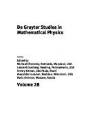
Fig. 1. The first quasar identified, 3C273, as imaged by the Hubble Space Telescope. It lies over two billion light years away and is the brightest quasar in the visible Sky. The structure to the SW (lower right) is the outer parts of its relativistic jet, which is seen from radio to X-ray wavelengths. The projected length of the jet is over 200 thousand light years, so its true length is nearly an order of magnitude larger than our galaxy. The mass of its black hole has been measured by the optical reverberation technique at almost a billion Solar masses. The X-shape is an instrumental artefact created by support structures in the telescope; it implies that the source is unresolved. 3C273 varies on week-long timescales indicating that the emission region is less than a light week across.

ject. It therefore appears that the prodigious power output of 3C273 emerges from a region of size similar to the Solar System! ¹ Kerr’s solution to the Einstein field equations was not immediately recognised as the exact solution for a spinning black hole. We now know the geometry described is the unique and complete description of the external gravitational field of an uncharged stationary black hole. It is now thought that the power of 3C273 and other quasars is due to accretion onto a Kerr black hole, which we now give some preliminary details of.

1 3C273 is not just a pointlike object but has an associated linear structure which we now know to be a relativistic jet, but the above argument is good for the main central source.

Astrophysical black holes

| 13

3.1 Rotating black holes It is now known that the totality of black holes can be described using just three parameters. Whatever makes them up, and however they were formed, in the end only three parameters matter – their mass M, charge Q, and angular momentum J. Due to the high conductivity of interstellar matter, black holes are not likely to have a net charge for long, so the only relevant parameter in addition to mass is spin.² A metric applicable to a black hole with angular momentum was found by Kerr in 1962 [31]. This metric, in the form later developed by Boyer & Lindquist [6], is ds2 = (1 −

2GMr 1 −4GMra sin 2 θ ρ 2 ) dt − [ dtdϕ + dr2 2 2 ρc Δ ρc c + ρdθ2 + (r2 + a2 +

2GMra2 sin2 θ ) sin2 θdϕ2 ] , ρc2

(18)

where a = (J/Mc) is the angular momentum of the black hole per unit mass (and has the dimensions of distance), Δ = r2 − (2GMr/c2 ) + a2 and ρ = r2 + a2 cos2 θ. Substituting this metric into equation (6) for the connection coefficients and calculating the Riemann (4) from these, the Ricci tensor R μν = R λ μνλ will be found to vanish, and therefore satisfy the vacuum field equations (3). This is a formidable calculation, however, and techniques which derive the metric in the context of more general azimuthally symmetric spacetimes (e.g. [14]) are in fact easier to carry out. Note if the black hole is non-rotating, then J = a = 0 and the Kerr metric reduces to the standard Schwarzschild metric (1). Almost certainly, all real black holes in the universe will be of the Kerr type. The idea is that just as infalling matter will have angular momentum, so will the material from which the black hole formed, leaving it both with a mass and net angular momentum.

3.2 Black holes as energy sources The enormous luminosity of 3C273 and other quasars was soon linked to black holes by Edwin Salpeter [60] and (separately) Yakov Zeldovich [78]. The energy is due to the deep gravitational potential well of the black hole which can be liberated by collisions outside the event horizon as gas falls in. If two gas clouds with small amounts of equal but opposite angular momenta fall into a Schwarzschild black hole colliding at 4rg (note rg is defined as GM/c2 ) and momentarily coming to rest with their kinetic energy emitted as radiation, then about 29% of the rest mass energy of the clouds is released. More generally the angular momentum will be much larger and the radiative

2 Newman et al [48] found the solutions to the Einstein–Maxwell field equations in 1965 and the resulting Kerr–Newman geometry describes spinning charged black holes.

14 | Andrew C. Fabian and Anthony N. Lasenby efficiency of accretion smaller. A specific model involving an accretion disc was proposed by Donald Lynden-Bell [36] in 1969. Due to the small size of a black hole, it is most unlikely that gas falling into a black hole does so radially, but will have some angular momentum which will cause it to orbit the hole. Viscosity in the swirling gas will cause matter at smaller radii, which is moving faster, to transfer its angular momentum outward to material at larger radii, which is moving slower. The gas then spreads in radius forming an accretion disc in which angular momentum is transferred outward as matter flows inward. The accretion disc model of Lynden-Bell was then studied in a detail in the early 1970s by Pringle & Rees [58], Shakura & Sunyaev [65] and, for the Kerr metric, by Novikov & Thorne [49]. The gravitational energy liberated by the inflow heats the disc which radiates locally as a quasi-blackbody. The disc is thin but may extend outward for a considerable distance. This basic picture probably accounts for much of the energy liberated by accreting black holes. There are important modifications due to the magnetic nature of the ionized infalling plasma which will be discussed later. Accretion onto a black hole is the most mass-to-energy efficient process known, apart from direct matter-antimatter annihilation which, due to the rarity of antimatter in our universe, is highly uncommon. Such accretion may account for 20–30% of the energy released in the Universe since the recombination era. To understand the details of how this can happen, we now examine particle motion in GR, first generally, and then applied specifically to the question of efficiency of gravitational energy release around a Schwarzschild black hole. (The more complicated issue of energy release around a Kerr black hole is treated in Section 7.1.)

3.3 Motion in the Schwarzschild metric The key to most astrophysical applications of the Schwarzschild metric is how point particles and photons move in it. In General Relativity, particles move on geodesics of the metric, i.e. the paths with an extremal lapse of proper time (for a massive particle) or ‘affine parameter’ (for a massless particle), along the worldline. If we let ds be the differential interval along a path, and s AB the total interval between two points A and B on a given path, then with ẋ μ ≡ dx μ /ds we have B

s AB

B

B

1

dx μ dx ν 2 = ∫ ds = ∫ [g μν dx dx ] = ∫ [g μν ] ds ds ds μ

A

ν

1 2

A

A

B

= ∫ G(x μ , ẋ μ ) ds

where

1

G(x μ , ẋ μ ) = [g μν ẋ μ ẋ ν ] 2

(19)

A

and finding the path which extremises s AB then leads to the Euler–Lagrange equations (one for each μ) d ∂G ∂G (20) )− μ =0 ( ds ∂ ẋ μ ∂x

Astrophysical black holes

| 15

Note using the result (6) is is easy to demonstrate the equivalence of (20) with the alternative, and perhaps more familiar form dx ν dx σ dx μ + Γ μ νσ =0 2 ds ds ds

(21)

The advantage of the former, (20), comes from the fact that it does not need knowledge of the connection coefficients to compute it, and also conservation laws for variables of which the metric is not an explicit function, are easy to read off. Note from its definition (compare the second and fifth quantities in the chain of equalities (19)), that as a numerical quantity G(x μ , ẋ μ ) evaluates to 1 (at least for a massive particle), which we can use to simplify formulae once its functional dependence has already been used. So we now apply these results to the metric in the general static form given by (7). (The advantage of carrying this out for the general form, rather than just Schwarzschild, is that it enables us to consider results for other types of black hole, such as Reissner– Nordstrom, and Schwarzschild–de Sitter – see below.) We can assume w.l.o.g. that the particle motion is confined to the θ = π/2 plane, and then the equations we find are A t2̇ − B r2̇ − r2 ϕ̇ 2 = 1

(22)

coming from G(x μ , ẋ μ ) = 1, and Aṫ = k ,

and

r2 ϕ̇ = h

(23)

coming from the Euler–Lagrange equations in t and ϕ respectively, and where k and h are constants. These last two equations result from the constancy of the metric coefficients in t and ϕ and correspond to the conservation of energy and angular momentum. For a particle of mass m, kmc2 can be identified as the particle energy, and h is the specific angular momentum per unit mass. There is no point forming the Euler–Lagrange equation in r, since we already have a simple expression for r ̇ available from the combination of (22) and (23), yielding r2̇ =

1 k2 h2 ( − 2 − 1) B A r

(24)

We return to this general form later, but now wish to obtain results specific to the Schwarzschild case. With A = B−1 = (1 − 2GM/r), and reinstating c for the remainder of this section, we obtain r2̇ = c2 (k 2 − 1) −

h2 2GM 2GM (1 − 2 ) + . r r2 c r

(25)

Using the usual Newtonian substitution u ≡ 1/r, and changing the independent variable to azimuthal angle ϕ rather than the interval s, so that it is easier to discuss the shape of the orbit, we differentiate (25) to obtain d2 u GM 3GM + u = 2 + 2 u2 . 2 dϕ h c

(26)

16 | Andrew C. Fabian and Anthony N. Lasenby In Newtonian gravity, the equation for planetary orbits, in the same notation, is d2 u GM +u= 2 , 2 dϕ h

(27)

so we have almost got the Newtonian answer, except for the extra term 3GMu 2 /c2 . This is what gives all the relativistic effects, and we note it correctly goes to zero as c → ∞.

3.4 Circular orbits An important application of the orbit formula in the context of high energy astrophysics, is what it tells us about circular orbits in Schwarzschild geometry. These will be approximately the orbits of material accreting onto black holes, since infalling material nearly always has angular momentum, and we would not generally expect direct radial infall. If r is constant, then our equation for u (26) yields GMr2 . r − 3GM/c2

(28)

h2 k2 r = −1 2 2 c r r − 2GM c2

(29)

h2 = Putting r ̇ = 0 in equation (25) gives us

and then putting both these last two results together yields an equation for k in terms of r alone. We derive: 1 − 2GM rc 2 k= . (30) √1 − 3GM rc 2 Remembering k = E/mc2 , where E is the particle energy, we have found that the energy of a particle in a circular orbit is Ecirc = mc2

1−

2GM rc 2

√1 −

.

(31)

3GM rc 2

An obvious check on this equation, is whether it can reproduce the Newtonian expression for the total energy of a circular orbit in the limit of large r. Using the binomial theorem we see that indeed the first two terms in an asymptotic expansion in r are Ecirc ∼ mc2 −

GMm +... , 2r

(32)

Thus we get agreement at large r with the usual Newtonian expression (derived via Etot = K.E. + P.E. =

1 2 GMm −GMm mv − = 2 r 2r

if

mv2 GMm ) = r r2

(33)

provided we realise that it enters as a correction to the rest mass energy mc2 , which is the dominant term.

Astrophysical black holes

| 17

The equation we have just found for the energy of a circular orbit, provides us with a remarkable amount of information about the nature of such orbits. First we see that in the limit m → 0, the orbit r → 3GM/c2 is of interest, since the singularity in the denominator can cancel the zero at the top. In fact this is the circular photon orbit at r = 3GM/c2 , which we will derive below in a treatment of photon motion. Secondly, we can see which orbits (for particles of non-zero rest mass) are bound. This will occur if Ecirc < mc2 , since then we have less energy than the value for a stationary particle at inifinity. The condition for Ecirc = mc2 is that (1 −

2GM 2 3GM ) = 1− rc2 rc2

(34)

This happens for r = 4GM/c2 or r = ∞. Thus over the range 4 < r < ∞ the circular orbits are bound. This appears to show we can get as close as 2 Schwarzschild radii to a black hole for particles in a circular orbit, suggesting that this is where the inner edge of any accretion disc would be. But is such an orbit stable? We discuss this first in the specific context of the Schwarzschild metric, and then later look at stability in the context of more general metrics of the form (7).

3.5 Stability of circular orbits In Newtonian dynamics the equation of motion of a particle in a central potential is 1 dr 2 ( ) + V(r) = E , 2 dt

(35)

where V(r) is an “effective potential”. For an orbit around a point mass, the effective potential is h2 GM V(r) = 2 − , (36) r 2r where h is the specific angular momentum of the particle. Since the 1/r2 term will eventually always exceed the 1/r term as r → 0, we can see that in Newtonian dynamics a non-zero angular momentum provides an angular momentum barrier preventing a particle reaching r = 0 — see Figure 2. In this effective potential, bound orbits have two turning points and a circular orbit corresponds to the special case where the particle sits at the minimum of the effective potential. However, as we have already partially seen in equation (48), the same is not true in General Relativity. Starting with equation (25) we can rewrite this as 1 2 h2 2GM GM 1 2 2 r ̇ + 2 (1 − 2 ) − = c (k − 1) 2 r 2 2r c r where we recall k = Epart /mc2 and r2 ϕ̇ = h.

(37)

18 | Andrew C. Fabian and Anthony N. Lasenby

V(r) effective potential

unbound orbit

r

elliptical orbit

circular orbit –GM r Fig. 2. The Newtonian effective potential showing how an angular momentum barrier prevents particles reaching r = 0.

Thus, although the r.h.s. is not the particle energy here, the fact that it is constant tells us that 2GM h2 GM U(r) = 2 (1 − 2 ) − (38) r 2r c r is an “effective potential” for the problem, which we can use to study stability in the same way as in the Newtonian case. Note that the relativistic term (1 − 2GM/c2 r) weakens the centrifugal effect of angular momentum at small r. Differentiating this expression, dU h2 3h2 GM GM =− 3 + + 2 , dr r c 2 r4 r

(39)

and so the extrema of the effective potential are located at the solutions of the quadratic equation 3h2 GM = 0, (40) GMr2 − h2 r + c2 i.e. at GM 2 } h2 { r= (41) 1 ± √1 − 12 ( ) }. { 2GM hc } { If h = √12 GM c there is only one extremum, and there are no turning points in the orbit for lower values of h. At this point r = 6GM/c2 = 3Rs . Figure 3 shows the effective potential for several values of h. The dots show the locations of stable circular orbits. The maxima in the potential are the locations of unstable circular orbits.

Astrophysical black holes

| 19

0,10 U(r) 0,05

0,00

5

10

20

15 h = 4,5

r

25

h=4 –0,05

h = 3,75 h = 2√3

–0,10

h=0

–0,15

Fig. 3. The effective potential U(r) plotted for several values of the angular momentum parameter h (units here have GM/c2 = 1).

What is the physical significance of this result? The smallest stable circular orbit has rmin =

6GM . c2

(42)

Gas in an accretion disc settles into circular orbits around the compact object. However, the gas slowly loses angular momentum because of turbulent viscosity (the turbulence is thought to be generated by magnetohydrodynamic instabilities). As the gas loses angular momentum it moves slowly towards the black hole, gaining gravitational potential energy and heating up. Eventually it loses enough angular momentum that it can no longer follow a stable circular orbit and so it falls into the black hole. On this basis, we can estimate the efficiency of energy radiation in an accretion disc via looking at a plot of the ‘fractional binding energy’ E/(mc2 ) − 1 = k − 1 versus r (see Figure 4). The maximum efficiency is of order the gravitational binding energy at the smallest stable circular orbit divided by the rest mass energy of the gas. From the plot we can see that this will be about 6%. More accurately, from equation (31) we see that at r = 6GM/c2 k = E/(mc2 ) is 2√2/3, hence we obtain for this efficiency ϵ acc ≈ 1 − 2√2/3 ≈ 5.7%

(43)

The equivalent Newtonian value, is not far away at ϵacc ≈

1 GMm 1 1 ∼ 8% . ≃ 2 rmin mc2 12

(44)

20 | Andrew C. Fabian and Anthony N. Lasenby Bound energy for circular Schwarzschild orbit

(E/(mc2) − 1)%

10

5

0

−5 3

4

5

6

7

8

9

10

r/μ Fig. 4. A plot of E/(mc2 ) − 1 in percent versus r (the latter measured in units of μ = GM/c2 ) where E is the energy of a particle of mass m in a circular orbit at radius r about a Schwarzschild black hole.

As we will see, this value can be even larger for a black hole with spin, and an accretion disc can convert 5–20 percent of the rest mass energy of the gas into radiation, depending on spin. This can be compared with the efficiency of nuclear burning of hydrogen to helium (26 MeV per He nucleus), ϵnuclear ∼ 0.7%

(45)

Accretion discs are capable of converting rest mass energy into radiation with an efficiency that is about 10 times greater than the efficiency of nuclear burning of hydrogen. The ‘accretion power’ of black holes causes the most energetic phenomena known in the Universe.

4 Evidence from X-rays, quasars and AGN The early 1960s also saw the birth of X-ray astronomy, when in June 1962 Riccardo Giacconi and colleagues [25] launched a sounding rocket with Geiger counters sensitive to X-rays. As the detectors scanned across the Sky during their 10 minutes above the Earth’s atmosphere, a broad peak of emission was discovered from the general direction of the Scorpius constellation and a steady background of cosmic X-rays were seen. Sco X-1 and the cosmic X-ray Background had been discovered. The rapidly variable X-ray source Sco X-1 is a neutron star accreting matter from an orbiting compan-

Astrophysical black holes

| 21

Fig. 5. The XMM COSMOS field is about 30 arcmin across and shows the X-ray Background resolved into pointlike and extended X-ray sources. The pointlike sources are mostly accreting black holes (distant AGN) and the extended sources are due to hot gas pooled in the gravitational potential wells of clusters and groups of galaxies.

ion star and the X-ray Background is now known to be the integrated emission from accreting supermassive black holes at the centres of distant galaxies (see Figure 5). The first clear association of X-ray astronomy and black holes was made after Giacconi and colleagues studied the brightest X-ray source in the constellation of Cygnus, Cyg X-1, using the first X-ray astronomy satellite, Uhuru, which continuously scanned the Sky. Cyg X-1 showed chaotic variability on timescales down to a fraction of a second. It has two relatively long-lived states, one when the spectrum is soft and the other hard. A radio source was found to appear when it switched into the hard state and accurate measurement of the position of that source enabled it to be identified with a 7th magnitude B star, HDE 226868. Separate teams of optical astronomers, Webster & Murdin [76] and Bolton [5], then found that this massive star was being swung around at 70 km s−1 by an unseen object on a 5.6 day period. This enabled mass estimates to be made (which relied on understanding the mass of the companion B star) yielding at least 3.5M⊙ which is above the likely upper mass limit for a neutron star of about 3M⊙ . The small size implied by the rapid variability combined with the lower mass limit pointed to a black hole in Cyg X-1.

22 | Andrew C. Fabian and Anthony N. Lasenby

Fig. 6. Centaurus A is one the nearest radio-loud AGN. The image on the left is a combination of infrared through X-ray images, its jets are seen going from the NE to SW. On the right is a larger scale image of low frequency radio emission showing the large diffuse lobes of radio-emitting plasma ejected by the accreting black hole out to intergalactic space.

Many other black hole X-ray binary systems are now known, some of which have much clearer mass estimates. M33 X-1, for example, in the nearby galaxy M33 has a precise distance and stellar mass estimate and also shows eclipses which enable the orbital inclination to be deduced, leading to a mass for the X-ray source of 15.64 ± 1.45M⊙ [51]. By the 1980s, many quasars and X-ray binary systems were known, showing that black holes are common. Quasars were seen to be an extreme part of the more general phenomenon of Active Galactic Nuclei (AGN). The centres of a few percent of all galaxies appear to have some non-stellar activity in the form of bright broad emission lines, a nonthermal radio source or an X-ray source. Quasars occur when the AGN outshines the host galaxy in the optical band. AGN of lesser power are known as Seyfert galaxies or just low luminosity AGN as the power drops. Jets of highly-collimated relativistically outflowing plasma are found in about 10% of AGN. An example outflow in one of the nearest AGN is shown in Figure 6. Unusual emission spectra at the centres of some galaxies had been known as a phenomenon since about 1908, and the first jet was reported in M87 by Heber Curtis in 1918 [12]. Little follow-up work was done before the 1960s, apart from Carl Seyfert’s PhD thesis in the 1940s [64]. By the end of the 1980s most astronomers considered that AGN were powered by accretion onto black holes, but a minority still favoured some

Astrophysical black holes

|

23

other explanation, such as multiple supernova outbursts. The arguments for black holes were strong but circumstantial. A major observational problem was that black holes are by definition difficult to observe directly. Quasars appear to be associated with a past phase in the evolution of the Universe, when it was 1–5 billion years old (mostly at redshifts of 2–4). They are now relatively uncommon compared with that era. (3C273 is a rare quasar at low redshift: low is relative here as it was moderately high when discovered in the early 1960s.) The enormous powers involved mean that the accretion rates were high and the mass doubling time of the black holes could have been a few 100 million years. Radiation pressure would have restricted the inflow to below a limit first deduced for stars by Eddington, known as the Eddington limit. The limit is obtained by comparing the force of radiation acting on an electron (through Thomson scattering of cross-section σ T ) at the surface of the object, with the force of gravity on a proton there. The electron and proton, although assumed free, are bound together by electrostatic attraction. Fgrav =

GMmp hν L = Frad = , σT c R2 4πR2 hν

(46)

where the radiative force term is the flux of photons (of typical energy hν) times the cross-section times the momentum of a photon. This gives LEdd =

4πGMmp c , σT

(47)

which is about 1031 W per Solar mass. Since the Eddington limit is proportional to the mass of the black hole the black hole mass can grow exponentially, if sufficient fuel is available. If growth is at the Eddington limit, the e-folding time of the black hole mass is about 4 × 107 yr. This timescale is sufficient for the typical massive black hole to have grown from stellar mass (say 30M⊙ ) but it does become challenging for the most distant billion Solar mass quasars found above redshift 6.

5 The black hole at the centre of the Milky Way 5.1 Sgr A* The evidence for the existence black holes changed though the 1990s owing to careful observations of the motion of stars moving around the centre of our own Milky Way galaxy, first starting in 1991 by Reinhard Genzel and colleagues [23] using ESO telescopes and later joined by Andre Ghez and colleagues [24] using the Keck telescopes. An interesting picture of the technique used to achieve the required image stability for this work is shown in Figure 7.

24 | Andrew C. Fabian and Anthony N. Lasenby

Fig. 7. The central stellar bulge of our Galaxy. A laser beam from one of the ESO Very Large Telescopes points at the very centre where Sgr A* resides. This creates an artificial star in the Earth’s upper atmosphere which is used to stabilise images made of the stars orbiting the central black hole.

Most stars, like the Sun, orbit the centre of the Galaxy at about 230 km s−1 , but within the innermost light year they move faster until at a distance of 2000rg from the dynamical centre a star orbits at up to 3000 km s−1 . The inferred mass within that orbit is 4 million M⊙ and the dynamical centre coincides with a strange radio source in the constellation of Sagitarius long known as Sgr A*. It is also a flickering infrared and X-ray source. No stellar emission which can be attributed to say a massive cluster of normal stars is seen. The stellar orbits of dozens of stars there are known in 3D, both from their apparent motions mapped in the plane of the Sky and from line-of-sight Doppler shifts. The orbit of one of the closest stars, S2, is shown in Figure 8 [26]. The mass density within the innermost orbits exceeds 1018 M⊙ pc−3 and there is nothing known to Physics which can lie there other than a black hole. Clusters of stars, even neutron stars, would interact and collide. The above lower limit on the mass density of the central object is increased by a further 5 orders of magnitude when constraints on the maximum size of Sgr A* obtained from millimetre band Very Long Baseline Interferometry (VLBI) are included. The origin of the young, massive stars which are bright enough to be tracked around the Galactic Centre is not yet fully understood. The underlying stellar density there is so high that it should inhibit further star formation.

Astrophysical black holes

|

25

The orbit of S2 (1992–2013)

0.175

MPE-VLT UCLA-Keck

4000

1993 2013

0.15

3000

0.125

vrad (km/s)

2000

Dec (ʺ)

0.1

0.075

0.005

1000

0

0.025

SgrA* 2001

–1000

0

2002 –2000 0.05

0.025

0

–0.025 –0.05 –0.075

R.A.(ʺ)

2000 2002 20042006 2008 2010 2012

t(yr)

Fig. 8. The path of star S2 about Sgr A*. The elliptical orbit has a period of 15.2 years, a major axis of 5.5 light days and is inclined at 46 degree to the plane of the Sky. It requires that a mass of 4 × 106 M⊙ lies within a radius of 17 light hours. The only long-lived object which is physically consistent is a massive black hole.

As well as the issues of mass within a given radius, there is also hope that general relativistic effects on the orbits of stars and possibly gas clouds near Sgr A* will be observed in the near future, so we discuss now the details of these effects, including the important aspect of ‘capture’ by a black hole.

5.2 GR effects on orbits We derived above the ‘shape’ equation for orbits around a Schwarzschild black hole, (26). For the Newtonian case, then due to the harmonic kernel at the left, and the constant at the right, it is obvious that solutions of the form u = a + b cos ϕ will work, i.e. ellipses, so if the extra term in the relativistic version (26) is small we expect the orbits to be modified ellipses. In the Solar System, in which a Schwarzschild metric due to the Sun applies, these modifications are very small (e.g. the largest effect is the 42 seconds per century precession of Mecury’s orbit), but in the Schwarzschild metric around a black hole, we can expect much larger effects. For example, in Figure 9 we show the motion for an object starting about 10 Schwarzschild radii out in an almost circular orbit. The

26 | Andrew C. Fabian and Anthony N. Lasenby

10

5

–15

–10

–5

5

10

15

20

–5

–10

–15

–20

Fig. 9. Advance of perihelion in a Schwarzschild metric. The units of distance are GM/c2 , where M is the mass of the central body. The particle is launched tangentially and given a specific angular momentum h of 3.75 where the circular orbit h would be 4.85. The circle marks the Schwarzschild radius of the central black hole.

gaps between the markers on the orbit are laid down at equal intervals of time, and so indicate how fast the object is moving. We can see that strongly precessing ellipses are obtained, but with a motion that looks as though it will continue indefinitely (which it does). However, in Figure 10, we show what happens when starting from the same point, and also moving tangentially, but now with a smaller specific angular momentum. This time, the object is clearly ‘captured’ by the black hole, and ends up crossing the black hole horizon. We can gain some insight into how the ‘capturing’ comes about, by considering the orbit equation in a different form. For a massive particle, the interval s we have been using is just the proper time of the particle, which we label τ. If we start with equation (25), differentiate with respect to interval τ and then remove first derivatives, dr/dτ using the original equation again, one arrives at the following: d2 r GM h2 3h2 GM = − + 3 − . (48) dτ2 r2 r c 2 r4 The first two terms are very Newtonian-like, and correspond to an inward gravitational force and a repulsive term, proportional to angular momentum squared, which is ba-

Astrophysical black holes

|

27

12 10 8 6 4 2

–5

0

5

10

15

20

–2 –4

Fig. 10. As for preceding figure but now for a particle projected with h = 3.5 (in units with GM/c2 = 1).

sically the ‘centrifugal force’. What is new is the third term, also proportional to angular momentum squared, but this time acting inwards. This shows that close to the hole, specifically within the radius r = 3GM/c2 , centrifugal force ‘changes sign’, and is directed inwards, thus hastening the demise of any particle that strays too close to the hole, as in the example of Figure 10.

5.2.1 Orbital precession The equation we wish to solve is d2 u GM 3GM + u = 2 + 2 u2 2 dϕ h c

(u ≡

1 ) r

(49)

in the limit that the departure from Newtonian motion is small. This would apply to the motion of the planets in our solar system for example. The Newtonian solution to this equation is u=

GM (1 + e cos ϕ) , h2

(50)

and so we can use this as a first approximation, and then iterate to get a better one. Substituting into the r.h.s. of (49), we obtain the new equation d2 u GM 3(GM)3 + u = 2 + 2 4 (1 + e cos ϕ)2 . 2 dϕ h c h This will be solved by u =

GM (1 + e cos ϕ) + the particular integral h2

d2 u + u = A(1 + 2e cos ϕ + e2 cos2 ϕ) dϕ2

(51) (P.I.) of the equation: (52)

28 | Andrew C. Fabian and Anthony N. Lasenby where A = 3(GM)3 /c2 h4 is very small. The P.I. can be found to be: A (1 + eϕ sin ϕ + e2 (

1 1 − cos 2ϕ)) . 2 6

(53)

Now, in this expression, the first and third terms are tiny, since A is. However, the second term, Aeϕ sin ϕ, might be tiny at first, but will gradually grow with time, since the ϕ part (without a cos or sin enclosing it) means it is cumulative. We must therefore retain it, and our second approximation is u=

GM (1 + e cos ϕ + δeϕ sin ϕ) h2

(54)

3(GM)2 ≪ 1. h2 c2

(55)

where δ= Using

cos (ϕ(1 − δ)) = cos ϕ cos δϕ + sin ϕ sin δϕ ≈ cos ϕ + sin ϕ δϕ

for

δ ≪ 1 , (56)

we can therefore write u≈

GM (1 + e cos[ϕ(1 − δ)]) . h2

u is therefore periodic, but with period slightly larger than 2π, and we find Δϕ =

2π . The 1−δ

(57)

r values thus repeat on a cycle which is

6π(GM)2 2π . − 2π ≈ 2πδ = 1−δ h2 c2

(58)

But from the geometry of the ellipse, and the Newtonian solution, where we know l = h2 /GM and l = a(1 − e2 ), we can get the final result: Δϕ =

6π(GM)2 6πGM . = c2 l(GM) a(1 − e2 )c2

(59)

For example, Mercury’s orbit has a = 5.8 × 1010 m, eccentricity e = 0.2 and we know M⊙ = 2 × 1030 kg. Therefore our prediction for the precession is Δϕ = 5 × 10−7

radians per orbit

󸀠󸀠

= 0 .1 per orbit. Since Mercury’s orbital period is 88 days, we would thus expect to accumulate a precession of 43󸀠󸀠 per century. This is what is observed after correction for the perturbations due to the other planets, which cause a total precession of more like 5000󸀠󸀠 per century. Turning now to the Galactic Centre, the star S2, whose orbit was shown in Figure 8, has an eccentricity of 0.876 and semi-major axis of 980 AU [16]. Taking the mass of the Galactic Centre black hole as 4 × 106 M⊙ , then our formula yields a precession of 11 arcmin per orbit, which takes about 15 years. This sounds large, but projected on the sky

Astrophysical black holes

| 29

at perihelion amounts to only about 0.5 milliarcsec. By the use of near-infra red interferometry, this may be observable in the relatively near future (see Section 10), but as for the solar system it is competing effects from other nearby masses, and the general matter distribution near the centre, that will be key to determining whether it is the GR effect itself which is being seen [44].

6 Galaxies and black holes 6.1 AGN feedback It was earlier unclear whether galaxies with central black holes were special in some way or not. Quasars could be long lived in just a few galaxies or short lived and occur in every galaxy. Then careful imaging of the centres of nearby galaxies with HST and other telescopes revealed through the 1990s that most galaxies host a massive black hole. The mass of the black hole is correlated with the mass of the galaxy bulge³ that it is embedded in (the Magorrian relation [37]). Current results indicate that the host bulge has a mass 500 times that of the black hole. Some argue that the correlation is better if the velocity dispersion of the surroundings stars (beyond the radius where the black hole’s mass dominates) is used (the M BH − σ relation – an example of this is shown in Figure 11). Both correlations show considerable scatter but hold over several orders of magnitude. The M−σ relation poses the question of how the black hole at the centre of a galaxy knows the total mass of the host galaxy? The ratio of the physical size of the black hole event horizon to the galaxy can be 100 million or more (a similar scaled comparison is the Earth and a football). Some astronomers argue that larger galaxies just have larger black holes, but the correlations look better then that. An exciting possibility is that the question should be turned round and it is the black hole which controls the mass of the host galaxy. In 1998 Silk & Rees [66] proposed that it was the phenomenal energy output in the quasar phase, as the black hole grew in mass by accretion, which was responsible. Both grow from gas in the galaxy – the galaxy forming stars from the gas, the black hole accreting the gas. Eventually the black hole is so big and powerful that it blasts all the gas from the galaxy so both stop growing and we are left with the observed relation. There is clear evidence that massive black holes have grown by accretion from the Soltan relation [67]: η Eacc (1 + z) = ρ BH c2 , (60) (1 − η)

3 This means that the mass of any galactic disc is ignored.

30 | Andrew C. Fabian and Anthony N. Lasenby 10 10

M(Mʘ)

10 9

Stellar dynamics Gas dynamics Masers Excluded Elliptical S0 Spiral

10 8

10 7

106

60

80

100

200

300

400

σ (km s –1) Fig. 11. The black holes mass – stellar velocity dispersion relation M bh − σ [27].

where z is the mean redshift at which the accretion occurs. It is a recasting of the famous equation, E = mc2 , in terms of densities. The factor of 1 + z is due to the redshifting of the energy of the radiation; there is no such factor for mass. η is the radiative ̇ 2 . The energy density of radiation from efficiency of the accretion process L = η Mc accreting black holes, Eacc can be measured from the summed spectra of AGN (and the X-ray Background) and ρ BH can be estimated from the mass function of galaxies together with the MBH − Mgal relation. Results show agreement if η is about 0.1 which, as discussed later, is typical for luminous accretion. It is straightforward to show that the growth of the central black hole by accretion can have a profound effect on its host galaxy. If the velocity dispersion of the galaxy is σ then the binding energy of the galaxy bulge, mass Mgal , is Egal ≈ Mgal σ 2 . The mass of the black hole is on average observed to be MBH ≈ 2 × 10−3 Mgal . If the radiative efficiency of the accretion process of 10%, then the energy released by the growth of the black hole is given by EBH = 0.1MBH c2 . Therefore EBH /Egal ≈ 2 × 10−4 (c/σ)2 . Very few galaxies have σ < 350 km s−1 , so EBH /Egal > 100. The energy produced by the growth of the black hole therefore exceeds the binding energy of the host galaxy by about two orders of magnitude!

Astrophysical black holes

| 31

If even a small fraction of the accretion energy can be transferred to the gas, then an AGN can have a profound effect on the evolution of its host galaxy. In practice, radiation from the accreting black hole will not have any significant influence on existing stars in the galaxy, It can however strongly influence gas clouds from which new stars can potentially form. By ejecting those clouds from the galaxy, AGN feedback can effectively stop further stellar growth of a galaxy. The original mechanism of Silk & Rees is actually a little too effective and although it predicts a slope to the relation which is acceptable, the normalization is too low. Gas is blasted out too easily. However, energy is likely to be radiated away in the process which is likely to be controlled by conservation of momentum [18, 32, 45]. (Rocket science would be much easier if only energy conservation were at stake.) It has since been shown that this leads to the correct normalization and a slightly flatter slope. The details now centre [19] on the precise mechanisms responsible for the ejection (e.g. radiation pressure or accretion disc winds). Energetic winds are seen from some AGN and UV radiation interacts strongly with dusty gas in all quasars exerting an outward force through radiation pressure. It is interesting to note that the effective Eddington limit for dusty gas exposed to the ultraviolet radiation of a quasar is about 500 times that of ionized gas such as expected close to the quasar. The M − σ relation means that when the quasar is at its Eddington limit locally, the host galaxy is also at its effective Eddington limit globally. Dramatic evidence of AGN feedback occurs in the cores of many clusters of galaxies. The intergalactic medium in clusters has been squeezed and heated by gravity to create an intracluster medium which is 10 million K or hotter. The baryons in the hot gas exceed all baryons in the galaxy members of the cluster by a factor of more than ten. The most massive galaxies known lie at the dense centres of clusters where accretion onto their massive black holes feeds energy into the intracluster medium, preventing it from cooling down due to the emission of X-rays. The total mass of gas in a cluster and the depth of the gravitational well is so large that the gas cannot be expelled. Energy instead flows from the black hole accretion process into the gas to maintain a themodynamic status quo. The energy flows from the near vicinity of the black hole in the form of relativistic jets which push the hot gas back, forming giant galaxy-sized bubbles of relativistic plasma (cosmic rays and magnetic field) – an example is shown in Figure 12. The bubbles are buoyant and when large detach and float upward in the cluster potential, while new bubbles form and grow. The power in the bubbling process can be estimated from the energy content of a bubble (4PV where P is the pressure of the surrounding gas and V is the volume of the bubble, the factor 4 being appropriate for relativistic plasma) divided by the bubble growth time. This power matches the radiative energy loss of the inner cluster core, indicating that close feedback has been maintained for billions of years [11]. AGN feedback implies that black holes play a central role in the final growth and evolution of all massive galaxies. If black holes did not exist then massive galaxies would be much larger and brighter than we now see.

32 | Andrew C. Fabian and Anthony N. Lasenby

Fig. 12. X-ray image of the core of the Perseus cluster centred on the giant galaxy NGC1275. The image is about 100 kpc or 300 thousand light years across. The AGN at the centre has blown 10 kpc diameter bubbles of relativistic plasma into the surrounding cluster gas. Detached buoyant bubbles are seen to the NW and S. Concentric ripples are seen in the hot gas due to the bubbling activity created by the AGN. It is clear that a black hole can have dramatic effects on gas structures both in and beyond the host galaxy.

6.2 Jets, Gamma-Ray Bursts and the birth of black holes Relativistic jets occur in about 10% of AGN and in low-state BHB. They are thus a marker of the presence of a black hole. The details of how the material is accelerated and collimated are still unclear, with possibilities discussed later in this Chapter. Apparent superluminal motion indicates that the bulk Lorentz factor in many jets Γ ∼ 10. Polarization indicates that the radio and much other emission are due to synchrotron radiation. The jets therefore contain electrons and a component with positive charge is expected, unless the jets represent enormous currents. Whether the positive particles are positrons or protons is not known. If they are protons (or even heavier nuclei), then the power in the jets can be huge, exceeding the radiative power in some objects. Jets are presumably accelerated magnetically by the accretion disc. Fields emerging from the disc are continuously wound up around and along the central axis. The details are not yet fully understood. Jets are seen from all classes of object exhibiting accretion discs, including young stars and accreting white dwarfs. A long discussed

Astrophysical black holes

| 33

possibility from quasar jets is that in some cases the spin energy of the black hole is being tapped by the Blandford–Znajek mechanism, which is a variant of the Penrose process (see Sections 12.5 and 12.7 below). There has been recent progress in successfully modelling jets using numerical simulations of this mechanism. The most relativistic jets occur in Gamma-Ray Bursts (GRB). These were discovered in the late 1960s by the Vela spacecraft which had a gamma-ray detector to monitor the Cold War Test Ban Treaty (but not made public by Ray Klebesadel and colleagues from Los Alamos until 1973 [33]). They are intense flashes of gamma-rays which have a flux which would make them readily visible to the naked eye if in the optical band. Many theories of their origin were proposed, mostly based on neutron stars. It was not until the late 1990s that a GRB was localized and identified with a distant galaxy, by the BeppoSax satellite, that made it clear that GRB are the most luminous events in the Universe, representing about a Solar rest mass of energy radiated within a few 10s of seconds. Luminosity and causality point to enormous concentrations of gamma-rays in a very small region which would instantly lead to electron-positron pair creation creating a electron scattering dense fog, preventing any radiation emerging. It is difficult to see how gamma-rays can be seen unless strong relativistic beaming, Γ ∼ 100, is involved. Many aspects of GRB, including the radio through X-ray afterglow all support this highly relativistic interpretation [57]. The source of GRB must also be clean of any other matter, which could prevent the radiation emerging. It may then be surprising then that the source of GRB is now believed to be the very centre of dying massive stars as a black hole is formed. The swirling matter powers intense jets which burrow through and out of the star, to produce the GRB display. The birth of a black hole is therefore marked by one of the most amazing displays in the Universe. Stars which give birth to black holes are estimated to start life at masses exceeding 25M⊙ . Such stars have luminosities which are a million times greater than the Sun and live for just a few million years.

7 Current observations of accreting black holes Apart from the nearest examples, we know of the presence of most black holes from the power emitted as radiation and jets produced as a result of accretion. Matter falling into a black hole is accelerated by gravity up to the speed of light and if collisions occur then the matter can become very hot and radiate. The efficiency of the process depends on the rate of collisions and on whether the matter has time to radiate before falling into the event horizon. If the flow is a thin dense accretion disc then collisions are plentiful and the efficiency depends on the ISCO (innermost stable circular orbit). ̇ 2 , then η ranges from 5.7% to 42% Defining the radiative efficiency η through L = η Mc as the spin a/M increases from 0 to 1. In practice it is impossible to spin a black hole up

34 | Andrew C. Fabian and Anthony N. Lasenby to exactly 1, and high spins mean η ∼ 20–30%. Note that η for complete nuclear fusion (hydrogen to iron) is 0.7%, so black hole accretion is about an order of magnitude or more higher in efficiency. We now give some details of where these numbers come from, by looking at the orbits of massive particles around a Kerr black hole.

7.1 Particle motion in the Kerr metric Before discussing the details of particle motion, we need to consider the general structure of the Kerr solution, since this determines the character of the regions in which the particles are able to move. The most important regions for astrophysical purposes are shown in Figure 13. We have drawn an outer surface, called the ‘Stationary limit surface’, and the one lying inside this is called the ‘Outer event horizon’. Both of these are complemented by further surfaces (not drawn) lying closer to the black hole centre (the ‘Inner Stationary limit’ and ‘Inner horizon’ surfaces), but these are shielded by the outer horizon, and so do not have an immediate astrophysical role. The stationary limit surface marks the point where it is no longer possible for an observer to remain stationary in the (r, θ, ϕ) coordinate system. Try as he or she might, it is inevitable that they will be swept around by the rotation of the hole. Mathematically, this corresponds to the point where the g t Killing vector corresponding to invariance of the metric under time translations, changes from timelike to spacelike, i.e. to where the g tt component of the metric (18) passes through zero. This requires (setting c = G = 1 for clarity in the expressions) r2 − 2Mr + a2 cos2 θ = 0,

i.e.

r = M ± √M 2 − a2 cos2 θ

and the outer of these surfaces is shown. θ =0 Ergosphere

Outer event horizon r = M + √M2 − a2

Stationary limit surface r = M + √M2 − a2 cos2θ

Fig. 13. The stationary limit and outer horizon surfaces for the Kerr solution.

(61)

Astrophysical black holes

| 35

The other surface drawn corresponds to the point where the g rr component of the metric (18) becomes infinite, and marks the position of the event horizon. This is the position from beyond which a particle can never escape, whatever its mass or state of motion. It is different from the stationary limit, since particles in the inbetween region, although they cannot remain stationary, can in principle escape to infinity. This inbetween region is known as the ‘ergosphere’, since it is possible to arrange particle motions so that work can be extracted from it (see Section 12.5 below). The position of the horizon itself can be found by requiring Δ = r2 − 2Mr + a2 = 0 ,

i.e.

r = M ± √ M 2 − a2

(62)

and again the outer of these two surfaces is shown. Given that this radius, unlike the stationary limit surface, does not depend on θ, it might be wondered why the surface is drawn oblate in the diagram. This is because that Boyer–Lindquist coordinates do not correspond to spherical polars even in the case where the mass vanishes, and an embedding of the 2d surfaces we are working with into Euclidean space (for the purposes of visualisation) results in ellipsoids even for r = const. – see Section 13.6 of [30] for details. The Lagrangian methods used above in the Schwarzschild case also work here, and one finds quickly the following results for the t ̇ and ϕ̇ of a particle moving in the equatorial plane in terms of its conserved specific energy and specific angular momentum, k and h: k ((r + 2M)a2 + r3 ) − 2haM ṫ = rΔ (63) h − 2M) + 2kaM (r ϕ̇ = rΔ As before, for the r ̇ equation it is simpler to use the fact that evaluated numerically the interval function G(x μ , ẋ μ ) is 1 for a massive particle, and 0 for a photon. We start with discussing a massive particle, since our initial emphasis is on the energy liberated from accretion disc orbits. Here we find r2̇ = k 2 − 1 +

2M 1 2 2M − 2 (h − a2 (k 2 − 1)) + 3 (h − ak)2 r r r

(64)

We now have three equations we can integrate to find the motion. A key quantity for the energy and stability is the effective potential in r. We define this similarly to before via 1 2 (65) r ̇ + Ukerr (r) = const. 2 resulting in Ukerr (r) = −

1 M M + 2 (h2 − a2 (k 2 − 1)) − 3 (h − ak)2 , r 2r r

where an irrelevant overall constant has been ignored.

(66)

36 | Andrew C. Fabian and Anthony N. Lasenby If we compare with the equivalent in the Schwarzschild case, equation (38), we can see that despite the increased complexity of the Kerr metric, the effective potential has terms in just 1/r, 1/r2 and 1/r3 as before, resulting in overall similar behaviour (at least for small a). A difference, however, is that now the coefficients of the second and third terms depend on the particle energy as well as the angular momentum. For a circular orbit, we can use the fact that r ̇ and r ̈ are zero to find expressions for the specific energy and angular momentum. For the prograde orbits we are currently considering, these turn out to be k=

1−

2M r

+ a√ M r3

√1 −

3M r

+ 2a√ M r3

,

h=

√Mr − √1 −

2aM r 3M r

+ a2 √ M r3

(67)

+ 2a√ M r3

An important quantity for us to find is the radius of the innermost stable circular orbit, expected to be the inner edge of an accretion disc around a Kerr black hole, and the value the energy function takes there. As in the Schwarzschild case, we can use the effective potential to do this, asking that its second derivative is positive where the first derivative vanishes. Calculating this for the U(r) in (66) leads to the relatively simple criterion for stability r2 − 6Mr + 8a√Mr − 3a2 > 0

(68)

This is soluble analytically for r, but perhaps more illuminating to is to look at a plot of rISCO (the r corresponding to the innermost stable circular orbit) versus spin, as shown in Figure 14. If a = M, an ‘extremal’ black hole, then the solutions are r = M and r = 9M. If a = 0, we get the single solution r = 6M corresponding to the Schwarzschild case. The former of these shows that stable circular orbits (in the prograde direction) persist right up to the event horizon for a black hole spinning at the maximum mathematically allowed rate, i.e. a = M. We note, however, that various effects are likely to intervene before this maximum spin rate can be achieved (mainly the counteracting torque felt by the hole in absorbing radiation from the accretion disc [70]), and a = 0.998M is considered the most likely maximum attainable value, leading to a minimum attainable rISCO of 1.24M. More generally, by eliminating r between (68) and the expression for k in (67) we can get a useful relation between the black hole spin and the efficiency of energy release for a particle which has reached the ISCO. For prograde orbits this relation is 2 (2√2√1 − k 2 − k) a = M 3√3(1 − k 2 )

(69)

This provides the plot of efficiency versus spin shown in Figure 15. Again taking the maximum attainable value of a/M as 0.998, this leads to a maximum attainable efficiency of 32%.

Astrophysical black holes

| 37

Radius of inner most stable or bit vs. spin 10 r = 9M 8

rISCO /M

6

4

2 r=M 0

−1

−0.8 −0.6 −0.4 −0.2

0 α/M

0.2

0.4

0.6

0.8

1

Fig. 14. Plot of radius of innermost stable orbit vs. spin.

7.2 Current observations of accreting black holes continued The accreted matter can be supplied by a companion star, in the case of a BHB, or from surrounding gas in AGN. How much is captured by the black hole in the AGN case will depend on the density, temperature, magnetic field and angular momentum of the gas. The case when there is no angular momentum and magnetic fields can be ignored is known as Bondi accretion, which assumes that the gas can be treated as a fluid. Basically gas within the Bondi radius, defined as the radius beyond which the gas particles have the escape velocity, will be captured and this can be many orders of magnitude larger then would occur if the particles were free particles with no interactions or collisions. Zero angular momentum is a rather extreme assumption and may not apply to any real system, but it presents an easily calculated order of magnitude estimate of the accretion rate. Angular momentum is likely to reduce any inflow rate and could even choke off the flow. Indeed accretion flows can be unstable when heating by radiation from the central accreting mass is considered. Magnetic fields and turbulence also contribute to complexity and accretion flows are commonly observed to show chaotic variability. The accretion disc will be thin, with the ratio of thickness to radius, h/r < 0.1, when the luminosity is above about 1% LEdd . At lower accretion rates the disc thickens as the collision rates drop which can then cause the efficiency to drop with further decreases in M.̇ (The black hole swallows both the matter and energy released.) The properties of such radiatively inefficient flows (RIAFS) depend on whether the electrons (which radiate) and the protons (which have much of the energy) remain cou-

38 | Andrew C. Fabian and Anthony N. Lasenby Efficiency of energy release vs. spin

Efficiency (units of mc2)

0.4

0.3

0.2

0.1

0

0

0.1

0.2

0.3

0.4

0.5

0.6

0.7

0.8

0.9

1

1.1

α/M Fig. 15. Plot of efficiency of energy release vs. spin (prograde orbits).

pled, i.e. have the same temperature. There are still theoretical issues remaining as to whether this happens in such a highly magnetized plasma, but observations do indicate changes in behaviour in objects with low accretion rates. Not least is a tendency for jets to become common. The low luminosity of Sgr A* suggests it is in an extreme RIAF state. The luminous accretion flows, however, are usually above 1% LEdd and so are thin and dense and optically thick resulting in much radiation being emitted as a black body. The spectrum of the disc is then produced by the sum of blackbodies from different radii which gives a ν−1/3 spectrum at low energies up to the highest energies, which come from the smallest radii, where it turns over into a Wien tail. The peak ̇ −1/4 temperature scales as Mr . This means that the most massive luminous black hole g systems have spectral peaks in the UV, while stellar mass black holes peak in the X-ray band. Significant power can also emerge as a results of magnetic fields wound up in the accretion flow. They can emerge from the disc, become twisted and create a mess of reconnecting field lines powering a hot corona, with a temperature which can easily be 100 times hotter then the disc itself. The million degree Solar corona with associated flares and outflows is a nearby example but even low luminosity AGN have a power 1012 times larger than the Sun, so the analogy should not be taken too literally. The corona is the source of most of the X-rays seen from AGN. Evidence discussed later indicates that the corona in bright objects is located above and close to the black hole (∼ 10rg ). The magnetic field structure also appears to power jets in some objects, and

Astrophysical black holes

|

39

outflows in others. The degree to which the spin of the black hole is important (and maybe also a small ISCO) are still debated. BHB have stellar-mass black holes and accrete from their companion star. Disc formation is implicit due to the orbital angular momentum. A few sources such as Cyg X-1 are persistent, with their long-term luminosity varying by less than an order magnitude, but sometimes switching states from hard (coronal dominated) to soft (thermal disc dominated). Many of the BHB are however transient, having outbursts every few years or decades, during which the luminosity can rise from 1033 to 1039 erg s−1 . Outbursts follow a similar pattern in the luminosity-colour (hardness) plane, starting hard as the luminosity builds up towards LEdd , then switching to being soft as the thermal disc emission dominates over the corona, before subsiding back to the hard state as they decline to quiesence [59]. At the peak of an outburst the nearest of these sources (eg A0620-00 at 2.5 kpc) can become the brightest in the sky, outshining Sco X-1 and even the Sun (except when it is flaring) by a large factor. There are also many similar X-ray binaries in our Galaxy which host a neutron star instead of a black hole. We know about the neutron star by observation of rapid pulsations due to the spin of the highly magnetic field, or from X-ray bursts which are thermonuclear flashes taking place very near the neutron star surface. Many of these are also transient and behave in a similar way to BHB. The depth of quiesence has been proposed as evidence of an event horizon in BHB by Ramesh Narayan and colleagues [47]. Black holes have no hard surface and can accrete matter and radiation whereas neutron stars must emit the gravitational energy released. BHB generally have lower quiesent luminosities than neutron star binaries which fits in with this picture. Whether these systems have similar enough accretion rates in quiescence for this to be a proof has yet to be determined. Both BHB and some neutron star systems also show quasi-periodic oscillations, discovered by Michiel van der Klis in 1986 [74]. This phenomenon is complex and may be a rich source of information about the accretion flow and geometry, but it has yet to be fully understood and interpreted. To understand at least one of the frequencies we would expect to be seen, we now calculate the expected orbital frequency seen by a distant observer for material in the innermost orbit.

7.3 Velocities and frequencies For astrophysical black holes, further important quantities for circular orbits are the velocity in the orbit, and the orbital period. For the former, the velocity determines (essentially via special relativistic effects) an important component of the shift in frequency which occurs for line radiation coming from the accretion disc, and for the latter, we can in some cases see directly the modulation of radiation associated with an orbital period. These are thought to provide one of the frequencies within the ‘quasi-periodic oscilla-

40 | Andrew C. Fabian and Anthony N. Lasenby tions’ which are occasionally observed from accreting stellar mass black holes and can have frequencies in the several hundred Hz region [74]. Working with a Schwarzschild black hole, then if we let v be the ‘ordinary’ velocity in a circular orbit, and α be the corresponding ‘rapidity’, then (temporarily dropping factors of c since this makes the formulae clearer), we have v = tanh α

r ϕ̇ = γv = sinh α

and

(70)

We can thus use (28) for h and the definition r2 ϕ̇ = h, to calculate v as a function of r, obtaining the simple result GM v2 = (71) r − 2GM For an object rotating in the innermost stable circular orbit (ISCO), at r = 6GM, we therefore find that its velocity is half the speed of light. (Note that, perhaps surprisingly, exactly the same velocity is obtained for the ISCO about a spinning black hole with any magnitude for its spin.) As regards orbital frequency, then since the t coordinate is the time as measured by a stationary observer at spatial infinity, if we can form dϕ/dt then setting this equal to 2πνorb will immediately give us the orbital frequency, in Hz, as measured by an external observer. Thus using dϕ dϕ dτ ϕ̇ = = , dt dτ dt ṫ and ṫ =

GM 1 h ϕ̇ = 2 = √ 3 r r (1 − 3GM r )

k 1−

2GM r

=

1 √1 −

,

(72)

(73)

3GM r

we find ϕ̇ √ GM dϕ , = = 2πνorb = dt r3 ṫ which despite being derived in full GR is exactly the Newtonian (Keplerian) result. As an example, evaluating at the innermost stable circular orbit, r = 6GM/c2 , for a 10 solar mass black hole, yields the impressively high result of νorb = 218 Hz. Thus an emitting blob orbiting at this radius could potentially produce this frequency in the frequency spectrum of the source.

7.4 Further AGN properties AGN range in luminosity from below 1010 to 1014 L⊙ and are situated at the centre of the host galaxy. They appear to respect the Eddington limit and show strong evolution in luminosity with redshift (and thus cosmic time). The quasar and therefore

Astrophysical black holes

| 41

mass-building phase peaked at about redshift 2.5 with quasars being observed back to redshift 7.1. An important issue with AGN is that a plentiful supply of fuel leads to obscuration of the source itself. If the absorbing column density is Thomson thick (i.e. most photons are scattered by electrons on passing out of the source), then only heavily reprocessed emission is all that remains, emerging predominantly in the infrared. Type I AGN are largely unobscured and Type II obscured. The difference may be geometrical and due to our line of sight. In a broad class of source the obscuring medium is in the form of a thick torus at a radius of about a parsec. If viewed in the plane of the torus we see a Type II obscured object and if we view it face-on then it is Type I. If at the same time there is a jet, then face-on down the jet the object appears highly beamed as a blazar [72].

8 Measurements of the masses of black holes The mass of a compact object can be measured from the motions of stars or gas in its vicinity using Newton’s Law of Gravitation. If a star makes a circular orbit around a massive black hole with velocity v at radius r then the mass of the black hole M = v2 r/G. Multiplying factors emerge for different shaped orbits but the essence of measuring velocity and radius remains the same. For the black hole at the centre of our Galaxy, Sgr A*, the 3D motion of many nearby stars has been mapped to give the best estimate of 4 × 106 M⊙ . With stellar mass black holes orbiting a normal star, then constraints on the mass are obtained by measuring periodic doppler shifts of spectral lines of that star to yield its radial velocity curve of semi-amplitude K and period P. These are combined to give the mass function (Mbh sin i)3 PK 3 f = = (74) (Ms + Mbh )2 2πG Further progress requires estimates of the mass of the normal star, perhaps from its spectral type, and of the inclination of the orbit i. If the system is eclipsing then i must be high, but if not then other means must be used such as observation of periodic ellipsoidal variations in the lightcurve of the star due to tidal distortions. These can be modelled to yield the inclination. There are now several dozen black holes with masses estimated to about 10% in this manner. The mass of supermassive black holes (SMBH) is obtained from the motions of nearby stars and gas if they lie in relatively nearby galaxies where the region of influence of the black hole can be resolved. This is roughly the radius within which the black hole-induced motions are faster than the general motions in the galaxy. The masses of more distant active SMBH can be determined using the reverberation technique. Delayed variations in the ionizing UV radiation from the nucleus are seen in orbiting broad-line clouds – the whole system appears to reverberate with delays rang-

42 | Andrew C. Fabian and Anthony N. Lasenby ing from days to weeks. (The clouds show doppler-broadened emission lines due to orbiting close to the SMBH.) The light travel-time delay then gives the radius and the line width of the clouds gives the velocity required to determine the central mass. Assumptions need to made about the geometry but careful work of the past two decades has established the success of the method [55]. It has enabled correlations to be built between the width of selected emission lines, optical luminosity and black hole mass. Current results indicate a maximum mass for observed neutron stars at just over 2M⊙ , while stellar mass black holes have masses from ∼ 4−20M⊙ , with an average of about 7M⊙ . Observed supermassive black holes have masses ranging from just below 106 to 2 × 1010 M⊙ . It is possible that some UltraLuminous X-ray sources (ULXs), which have luminosities greater than the Eddington limit for a 10M⊙ black hole, are Intermediate Mass Black Holes (IMBHs) with masses of 102 −105 M⊙ .

9 Measurements of black hole spin Whilst mass measurements can be made at a large distance from an object, spin requires a probe which is close in, within 10rg ⁴. The standard approach is to identify the inner edge of the accretion disc with the ISCO and then convert that radius to spin. This means that the inner disc must be luminous and detectable. Bright Galactic X-ray binaries in the soft state generally have a quasi-blackbody X-ray spectrum which can be used to measure the emitting area using the Stefan– Boltzmann law in an analogous way to that by which stellar radii are determined (blackbody luminosity L = 4πR2 σT 4 ) [39]. Unlike the surface of a star, an accretion disc is not all at the same temperature, so the emission profile of the disc must be assumed and the black hole mass and distance determined in order to measure the ISCO and thus spin. Light bending effects are very significant for the accretion disc near a black hole [43], so we now give some details of light bending effects in GR, first in the Schwarzschild metric, and then for Kerr black holes. An impression of what we would actually see for the accretion disc around a Schwarzschild black hole, if sufficient resolution was available, is shown in Figure 16. This can be compared with the more distorted and asymmetric image we would see from a black hole rotating at the expected maximum rate of a = 0.998M, in Figure 17.

4 If the mass accretion rate can be measured (from observations of the outer disc, say) and the total luminosity is known, then in principle spin can be deduced from the radiative efficiency using the relation in Figure 15.

Astrophysical black holes

| 43

Fig. 16. Pseudoimage of a luminous thin accretion disc around a black hole with doppler and gravitational redshift effects included. Light bending causes the distant side of the disc to appear as an arch above the hole. The smaller loop near the centre is due to scattering of photons from the (unstable) photon orbit at r = 3GM/c2 . The colour scale indicates flux received.

Fig. 17. As for Figure 16, but for a Kerr black hole rotating at the maximum attainable value of a = 0.998M (see Section 7.1). The unstable photon orbit is now near r = GM/c2 .

9.1 Equations for photon motion and redshift The other results we need for understanding astrophysical aspect of black holes, are the equations of motion for photons, and results for how their energy changes during propagation. For the equations of motion, we can use the above analysis, but with the interval function G(x μ , ẋ μ ) set equal to 0 rather than 1, once its functional variation has been taken. Tracking through the changes this causes, we find equation (25) is replaced by r2̇ = k 2 c2 −

h2 2GM (1 − ) r2 rc2

(75)

and for the ‘shape’ equation, (26), one finds that it is now the ‘Newtonian’ term that disappears on the r.h.s., and we just get 3GM d2 u + u = 2 u2 . 2 dϕ c

(76)

44 | Andrew C. Fabian and Anthony N. Lasenby Effective potential for photon motion 1.5

Veff/(1/(27μ2))

1

r = 2μ

0.5

r = 3μ

0

−0.5

1

1.5

2

2.5

3

3.5 r/μ

4

4.5

5

5.5

6

Fig. 18. Plot of the effective potential for photon motion in the Schwarzschild geometry. (Units of Veff are 1/(27μ 2 ) where μ = GM/c2 .)

One can immediately confirm from this equation that there is a circular photon orbit at r = 3GM/c2 , as mentioned above, but is it stable? To do the stability analysis, we rewrite the energy equation as r2̇ 1 + Veff (r) = 2 , 2 h b

(77)

where b = h/ck, μ = GM/c2 and the effective potential Veff (r) =

1 2μ (1 − ). 2 r r

(78)

Let us look at a plot of this function, Figure 18. We can see Veff (r) has a single maximum at r = 3μ where the value of the potential is 1/(27μ 2 ). This shows that the circular orbit at r = 3μ is unstable and in fact no stable circular photon orbit is possible in the Schwarzschild geometry. Another immediate use of equation (76) is in connection with light bending. Referring to Figure 19, we can see that a suitable first solution in which the term 3GMu 2 /c2 is completely ignored, is sin ϕ , (79) u= R where R is the radius of the body the gravitational deflection due to which we wish to work out. We iterate this equation by putting sin2 ϕ/R2 for u 2 on the r.h.s. of (76), i.e. d2 u 3GM + u = 2 2 sin2 ϕ . 2 dϕ c R

(80)

Astrophysical black holes

Δϕ/2

r

R

| 45

Δϕ/2

ϕ

Fig. 19. Gravitational deflection of light

This is satisfied by the particular integral u1 =

3GM 1 (1 + cos 2ϕ) , 3 2c2 R2

(81)

and adding this into the original solution yields u=

1 sin ϕ 3GM + 2 2 (1 + cos 2ϕ) . R 3 2c R

(82)

Now consider the limit r → ∞, i.e. u → 0. Clearly we can take sin ϕ ≈ ϕ, cos 2ϕ ≈ 1 there, and we obtain ϕ = −2GM/(c2 R) so that the total deflection (see figure) is Δϕ =

4GM . c2 R

(83)

This is the famous gravitational deflection formula. For the Sun it yields 1.77 seconds of arc, and was first verified in the 1919 eclipse expedition. More recent high precision tests use radio sources, since these can be observed near the Sun, even when there is no eclipse, and there is now no doubt that the GR prediction (which incidentally is twice what had previously been worked out using a Newtonian approach) is accurate to a fraction of a percent. In the black hole context, much stronger bending can occur, for which this first approximation is insufficient, and the full equations of motion need to be integrated. This can lead to some interesting effects, illustrated below in the context of a Kerr black hole. The other important aspect to discuss is gravitational redshift. Quite generally, for a metric with a Killing vector field g t , the redshift due to gravitational time dilation will be given by the ratio of p ⋅ g t at emission and reception, where p is the photon 4-momentum. g t becoming null, i.e. g tt going to zero, marks the point where infinite redshift is possible since p can then be in the direction of g t , e.g. for counter-rotating photons at the Kerr Stationary limit. This redshift from p ⋅ g t acts multiplicatively on any further redshifts which are occurring at a point due to special relativistic effects. E.g. for a point in an accretion disc, there will be a doppler redshift due to its motion relative to the initial path of an emitted photon, and then this will be multiplied by the gravitational redshift the photon experiences between that point and infinity. The combined effects of the redshifts can be seen in pattern of received flux seen in Figures 16 and 17, which are for the case where the accretion disc itself has constant emissivity.

46 | Andrew C. Fabian and Anthony N. Lasenby

9.2 Light bending around a Kerr black hole The treatment of photon orbits for the Kerr case can proceed in the same way as in Section 7.1, which dealt with massive particles, except that now the interval function G(x μ , ẋ μ ) evaluates to 0 instead of 1. Several textbooks, e.g. [30] and [22], deal with the details of the resulting orbits, and in particular show that as in the Schwarzschild case, there are still no stable circular photon orbits. The possible orbits for non-equatorial photons can be quite exotic. As an example, we show in Figure 20 the path of a photon emitted from an accretion disc in the equatorial plane, moving towards the black hole but with an initial upward component to its velocity. This moves round behind the black hole and is eventually able to escape to infinity, moving in a roughly opposite direction to its initial motion. This example is for a Kerr black hole with the maximum expected value for a of 0.998M — the ISCO and horizon radii are also shown.

3 2 10

8

6

4

2

1 –2 –1 –2

Fig. 20. Path of a photon emitted from an accretion disk that eventually escapes from the black hole in a direction about 180° from its initial direction.

9.3 Iron line emission The method discussed above for Galactic X-ray binaries does not work for AGN since the much higher black hole mass means that the blackbody disc emission emerges in the far UV band which is unobservable because of absorption by Galactic hydrogen clouds. Observations are made instead of broad iron-line emission produced by X-ray reflection. This is the fluorescent and back-scattered emission produced by irradiation of the disc by the coronal X-ray continuum – see Figure 21. X-rays absorbed in the disc lead to line emission, particularly iron K emission at 6.4 to 6.95 keV, depending on the ionization state of the emitter. At higher energies the X-rays are more likely to be Compton-scattered back out of the disc rather than absorbed, producing what is called the Compton hump in the reflection spectrum.

Astrophysical black holes

to observer

| 47

Direct Power-law

“Reflection spectrum”

Fig. 21. Schematic cross-section of an accretion disc around a black hole with a central corona providing irradiation. The production of the reflection spectrum is illustrated.

The spectral features are produced in the innermost parts of the accretion disc where gravitational effects are strong and lead to large doppler shifts and gravitational redshifts which skew and broaden emission lines [20, 21] – an example is shown in Figure 22. Detailed modelling of the line shape, and generally the shape of the whole observed reflection spectrum, leads to an estimate of the inner radius of the disc and thus the spin. Radii are determined in this method directly in gravitational units so the distance and mass of the black hole are not required. The broad iron line method can also be used in certain states of BHB [42] and has been found to give consistent results with the blackbody method. Confirmation that the reflection modelling is correct has recently been obtained from X-ray reverberation [73]. This involves the small (tens of seconds to tens of minutes) time delays or lags whch occur between the detection of an intrinsic change in luminosity of the corona and the corresponding change in the reflection. The energy spectrum of the high frequency time lags shows a broad iron line indicative of reflection (lower panel of Figure 22). The results for a number of objects imply that high spin is common for the brightest observed sources and the corona in those objects is compact and at a height of 5−10rg . In this regime, strong light bending occurs such that much of the coronal emission is bent down to the disc making the reflection strong. Month-long temporary episodes have been seen in a few sources in which the continuum drops to being almost unobservable, with only slight changes to the reflected spectrum. It appears that the corona has dropped below 5rg in these cases and that light bending is preventing much of the continuum being observed at all. Most of the reflection spectrum is then emerging from within 2−3rg , which is the closest emission easily seen from around any black hole [53]. Further evidence of a compact corona is obtained from microlensing studies of distant quasars which are lensed by intervening galaxies. This produces several images of the quasar which follow different light paths through the galaxy. Stars in the galaxy crossing one of those paths amplify the image by lensing to a degree depending on how the angular sizes of the emission region of the quasar and the Einstein ring of the star match one another. For typical values this means that higher amplitude

48 | Andrew C. Fabian and Anthony N. Lasenby 2.25 Mrk 335

Blurred

2

Unblurred

Relative Flux

1.75

1.5

1.25

1

0.75 5

10

20

50

20

50

Energy (keV) 1000 SWIFT J2127.4+5654 800

Time Lag (s)

600

400

200

0

−200

5

10 Energy (keV)

Fig. 22. Upper: The unblurred reflection spectrum including the iron-K emission line and Compton hump (solid line) appears relativistically blurred to the observer as shown in the line fitted to the data points. The obvious dominant redshift is gravitational due to the proximity to the black hole. The source is the Seyfert galaxy Mkn335, observed by NuSTAR during a low state. Modelling of the data shows that the black hole in Mkn335 has a spin a/M > 0.97. Most of the emission seen in the spectrum emerges from within 2r g of the event horizon [53]. Lower: Time lags measured by NuSTAR from the AGN SWIFTJ2127 showing both iron K and Compton peaks.

Astrophysical black holes

|

49

variability is expected from smaller emission regions. Both optical and X-ray observations have been made of several lensed quasars which show that the X-ray emission region is much smaller than the optical one, and in several cases is less than 10rg in size [3].

10 Future observations of astrophysical black holes Many exciting developments are expected over the next decade or so in observational studies of black holes. One important step will be the networking together of several millimetre-wavelength telescopes to form the Event Horizon Telescope which will resolve the “shadow” of the black hole in Sgr A* [13]. Extreme light bending of the emission from the accretion flow onto the black hole should reveal a dark patch, the shadow, at the position of the black hole. The diameter of the shadow is determined by the paths of light rays emitted from just above the event horizon to the observer and corresponds to about 10rg almost independent of the black hole spin.

Calculation of the shadow radius: We use the results above for the photon effective potential in the Schwarzschild case. Putting together equations (77) and (78), we find r2̇ 1 2μ 1 + (1 − )= 2 r h 2 r2 b

(84)

where μ = GM/c2 and b has been defined as h/kc. Note the dot here is not derivative w.r.t. proper time, which is zero for a photon, but w.r.t. an affine parameter along the path. We do not need to identify this parameter explicitly, since we are going to work with the shape of the orbit. Specifically, noting r2 ϕ̇ = h, we have (

r2̇ r4 ϕ̇ 2

1/2

)

=

1 dr 1 2μ 1/2 1 = ( 2 − 2 (1 − )) 2 r r dϕ b r

(85)

Solving (85) for μ = 0, which is the limit where the only role of the central mass is to define the origin of the (r, ϕ) system), we get r = b/ sin ϕ. This is the equation of a straight line, which if it continued all the way past the central object, would pass it with perpendicular distance b, so we can identify this b as the impact parameter. This generalises what we did above, where we considered the case of a light ray just grazing the surface of an object of radius R, for which the unperturbed solution was given by (79), i.e. r = R/ sin ϕ.

50 | Andrew C. Fabian and Anthony N. Lasenby Now we consider the exact equation again, and relate to a black hole. We know from the plot of photon effective potential in Figure 18, that photons straying inside r = 3GM/c2 are not free to escape to infinity. We therefore want to use this distance as the radius of an ‘object’ which the incoming photon just grazes. Using R for this object radius, we have dr 󵄨󵄨󵄨󵄨 =0 󵄨 dϕ 󵄨󵄨󵄨r=R This tells us that 1 2μ 1 = (1 − ) R b 2 R2

i.e.

b = R(

1/2 R ) R − 2μ

This expression is valid generally, and e.g. tells us that the Sun’s effective shadow is about 3 km bigger than its coordinate radius, but applied with R = 3GM/c2 for a black hole, we find b = 3√3GM/c2 , which is therefore the radius of the geometric shadow cast. Interestingly, the main effect of including black hole spin in the calculation is to cause a shift in the centroid of the shadow rather than its size – see e.g. [22] for details. For Sgr A* this distance we have just worked out corresponds to an angular diameter of 52 microarcsec. This is 2.5 × 10−10 radians, and is very small indeed. Nevertheless, the angular resolution, approximately equal to the ratio of observing wavelength to telescope diameter, is about 20 microarcsec for intercontinental mm VLBI where the effective telescope diameter is 10 000 km. Interestingly, the 6 billion M⊙ black hole in M87 is 1500 times more massive than Sgr A* and 2000 times further away which makes its event horizon appear only slightly smaller, at 40 microarcsec. Plans are also underway to resolve the M87 black hole shadow, together with the base of its jet which should help us understand how it is accelerated. All other black holes subtend smaller angular sizes. 3C273, for example, is 34 times more distant than M87, so its shadow will be about 1 microarcsec in size. Near infrared interferometry at ESO’s Very Large Telescope in Chile will use wavelengths around 2 microns and effective diameters of a 100 m to give a resolution of 4 milliarcsec. This will not resolve the black hole shadow but will resolve the motion of the orbiting stars much more precisely, particularly as the positional accuracy can be more than an order of magnitude better than the resolution. General relativistic effects on the orbits will be seen and fainter, possibly closer, stars resolved. Of great interest would be a pulsar orbiting Sgr A*, which if a millisecond pulsar could prove to be a very stable and reliable orbiting clock. None have been found yet and the ionized plasma that bathes the inner region is a problem for sensitive radio searches. A type of pulsar called a magnetar was found in 2013 within 3 arsec of Sgr A*, but this magnetar unfortunately appears to be rather unreliable as a clock [10]. A gas cloud, G2, was discovered on a highly eccentric orbit close to Sgr A* in 2012 [56]. At pericentre in 2014, about 3 Earth masses of material passes within about 2000r S . Ram pressure from the accretion flow should cause it to spiral inward over the

Astrophysical black holes

| 51

following few years leading to an increased accretion rate and associated display. It is in a similar path to an earlier discovered cloud G1 and other clouds. Their apocentre and orbital plane lie close to the orbits of some of the surrounding luminous stars. The winds of the stars may be the origin of the inspiralling gas clouds. Further past activity of Sgr A* has been revealed by X-ray fluorescent emission lines seen from molecular clouds many tens to hundreds of light years out from the Galactic Centre. One interpretation suggests that the luminosity of Sgr A* may have been almost a million times higher about 100 yr ago [7]. Sufficient numbers of black hole spin measurements are expected from X-ray studies of AGN that the spin history can begin to be understood. Present work indicates many high spin objects in the mass range from 106 −5 × 107 M⊙ . The accretion flow within 10rg and particularly within 3rg will be mapped and the corona understood. Indeed the whole power output of accreting black holes in terms of radiation, winds and jets will be explored. Tidal disruption events due to stars straying close to a massive black hole are beginning to be observed. Black holes with masses above 108 M⊙ can swallow stars whole in the sense that they are not tidally disrupted until within the event horizon. The tidal forces of the more common lower-mass black holes can however destroy stars at greater distances leading to the production of a short lived, very luminous, accretion disc which decays with a timescale of about a year. Studies of AGN feedback will accelerate with use of telescopes such as the Atacama Large Millimtre Array ALMA, the James Webb Space Telescope JWST, the Large Synoptic Survey Telescope LSST and the Advanced Telescope for High Energy Astronomy Athena. The growth of massive black holes through accretion and mergers will become understood. Actually testing GR with black holes is difficult. The astrophysical phenomena observed so far are explained within the Kerr metric. Some precision tests may occur if a pulsar is serendipitously found in a close orbit around a stellar mass black hole in our Galaxy or around Sgr A*. The discovery of gravitational waves from merging black holes will of course transform this aspect of the study of black holes. More generally, the detection of gravitational waves emitted in events involving black holes has great potential for tying down aspects of astrophysical black holes that are poorly understood at present. These include the numbers of intermediate mass holes in the range between stellar mass black holes and SMBHs in galactic centres, and the evolution of the number density of black holes with cosmic epoch. Both these aspects are key targets for a future space-borne gravitational wave detector mission, such as eLISA or a future variant, and form a key component of its science mission [17]. There are many further aspects to the importance of gravitational waves in black hole astrophysics, but we defer coverage of these to other chapters of this book.

52 | Andrew C. Fabian and Anthony N. Lasenby

11 More general spherically symmetric black holes Real black holes are embedded in a universe in which we know there are effects matching those of a cosmological constant, accounting for about 0.7 of the total energy density. Thus it is of interest to embed a black hole in a de Sitter universe. Additionally, black holes in anti-de Sitter universes are very interesting objects theoretically, since via the AdS/CFT correspondence (see e.g. [38]), the strong gravity effects of black holes can be replaced by weak perturbative effects in a conformal field theory living on the boundary of an anti-de Sitter space (though we note that the dimensionality involved does not necessarily match that of 4d spacetime). Returning to the derivations of Section 2.2, we find that to satisfy the new field equation G μν + Λg μν = −8πT μν (86) arising from introducing a cosmological constant Λ, the new equations the Ricci tensor has to satisfy are (87) R μν = Λg μν Using the components already given for the Ricci in (10) and above, one finds that this leads to a simple modification to the Schwarzschild values of A and B. We find that B is still equal to the inverse of A, and that now A = 1−

2GM Λ 2 − r 3 rc2

(88)

These are therefore the metric coefficients for a black hole of mass M embedded in a de Sitter universe, if Λ is positive, and anti-de Sitter, if Λ is negative. Horizons occur (for our current form of the metric) when B → ∞, hence here where A = 0. If Λ > 0, this now leads to an additional horizon being present, beyond the Schwarzschild one near the black hole centre, at a position close to r = √3/Λ (we are adopting a convention here in which Λ has dimensions length-2 ). This is a version of the ‘de Sitter horizon’ – its exact position is modified slightly by the presence of the mass. A further generalisation we can make, is to the case where the black hole is charged. As mentioned earlier, this is less compelling physically, since we do not expect significant charge separation to have occurred in the formation of a black hole, but the solution for this type of black hole, called the Reissner–Nordstrom solution (see e.g. [75] for references), is still of great interest theoretically. This also falls into our general scheme, and in fact the most general spherically symmetric black hole, which we can dub RNdS, for Reissner–Nordstrom–de Sitter, is given by B = A−1 ,

A = 1−

2GM Λ 2 q2 − r + 2 3 rc2 r

(89)

where q is the black hole charge. Note there are now (in general) three horizons. The Reissner–Nordstrom solution on its own introduces two horizons – one like the normal

Astrophysical black holes

| 53

Schwarzschild one, and another usually much smaller one associated with the charge – and then for Λ > 0 there is an additional de Sitter horizon. An advantage of dealing with all these cases via the A, B form of the metric, is that we can give a unified treatment of energies and angular momenta in orbits. Repeating the analysis of Section 3 for this new case, we already have r ̇ from (25) and can get r ̈ from d 2 dτ 2r ̈r ̇ d 2 = 2r ̈ (ṙ ) = (r ̇ ) = ṙ dr dτ dr For a circular orbit, both r ̇ and r ̈ have to vanish and this combination of expressions therefore says that k2 2h2 − 2 A󸀠 + 3 = 0 A r where A󸀠 ≡ dA/dr. Combining again with the expression for r ̇ = 0 we can solve for k 2 and h2 , obtaining 2A2 r3 A 󸀠 2 , and h = k2 = 2A − rA󸀠 2A − rA󸀠 So we now have the energy and angular momentum for a particle in a circular orbit for quite a wide range of metrics. To calculate criteria for stability, one can show that it is useful to work in terms of the quantity (see Lasenby (2014) in preparation) v 2 (90) T(r) = ( ) = tanh2 u c where v is the velocity in a circular orbit at radius r and u is the corresponding rapidity parameter. From what we have already derived, one can show rA󸀠 and r ϕ̇ = γv = sinh u 2A and then the criterion for stability turns out to be that T=

2T 2 − rT 󸀠 − 2T

(91)

(92)

should be negative. This simple criterion applies across all the spherically symmetric black hole cases. For example, inserting the A appropriate for a Schwarzschild–de Sitter metric, (88), we find the stability criterion 18M 2 − 15MΛr3 − 3Mr + 4Λr4 < 0

(93)

for stable circular orbits (in units with c = G = 1). For appropriate astrophysical values of M and Λ, and restoring units, the outer solution to this is well approximated by rstab ≈ (

3GM 1/3 ) 4Λc2

(94)

We can apply this formula for any central mass, not just a black hole, and one can show that e.g. for a cluster of galaxies with M = 1015 M⊙ , and for the measured value of the cosmological constant, then rstab ≈ 7.2 Mpc. This is interestingly close to the maximum cluster sizes observed, though of course circular orbit stability is not likely to be the direct criterion one would apply in this case, where effects on velocity dispersion would be more appropriate (see [46] for further details).

54 | Andrew C. Fabian and Anthony N. Lasenby

12 Primordial black holes Primordial black holes could have formed as a result of the high densities present soon after the Big Bang [8]. Their masses would be comparable to the particle horizon mass at their formation so it can range from the Planck mass (10−8 kg) at the Planck time (10−43 s), to 105 M⊙ at a time of 1 s. Primordial black holes of mass 1012 kg would have formed at 10−23 s and would be evaporating now due to the emission of Hawking radiation (see below), which would peak at 100 s of MeV. Observations provide a limit on the background intensity of 100 MeV gamma-rays such that evaporating primordial black holes cannot account for more than 10−8 of the critical density of the Universe [52]. The frequency, energies and timescales of the final explosions do not match typical observed gamma-ray bursts. It is therefore unlikely that they are an important constituent of the Universe.

12.1 Hawking radiation An initially very surprising result about black holes was proved by Hawking in 1974 [28]. This is that despite their name, the horizon radiates energy, as though it was a blackbody at the temperature of ℏc3 T= (95) 8πk B GM where k B is the Boltzmann constant and M is the black hole’s mass. The types of black hole we have mainly considered have a minimum mass of several M⊙ , and so their temperatures are less than ∼ 6 × 10−8 K, and therefore negligibly tiny. However, a 1012 kg primordial black hole of the type mentioned above, would have a temperature of ∼ 1.2 × 1011 K, and would therefore produce highly energetic radiation. The emission process as calculated originally by Hawking was explained in terms of particle production in a second quantised treatment of a massless scalar field surrounding the black hole, but the principles extend to all kinds of field, massive or massless, which will be radiated with ‘statistics’ (i.e. Bose–Einstein or Fermi–Dirac) as appropriate to their spin, and with a thermal distribution with the temperature (95). A heuristic way of demonstrating this effect is to consider vacuum fluctuations in the space just outside the horizon, which will lead to the production of virtual particle/antiparticle pairs there. Sufficiently close to the horizon, one of the pair will be able to ‘tunnel’ through the horizon and inside can become a real particle with negative energy. (The possibility of negative energy arises since as we saw above (Section 7.1), the timelike vector in the t-direction tips over to become spacelike inside the horizon, which coincides with the Stationary Limit surface in the Schwarzschild case, and so the projection of the particle momentum onto the local t-vector may be negative.) The particle remaining outside, which has positive energy, can therefore be emitted off to infinity,

Astrophysical black holes

| 55

whilst the absorption of a negative energy particle by the black hole, decreases the mass M, thus providing the overall energy for the emission. This type of derivation can be used to calculate the energy of the emitted particle, which turns out to be independent of exactly where (though assumed to be close to the horizon) the virtual pair is produced, and yields an energy E = k B T which is only a factor of 2π higher than the correct result from (95) – see Chapter 11 of [30] for details. A further possibility for a calculation avoiding the full rigours of quantum field theory (QFT), is to work with a first-quantised field surrounding the black hole. For example, a detailed derivation for a massive Dirac field is given in Section 8 of [35]. This yields precisely the result (95) together with the correct Fermi–Dirac statistics for a spin-1/2 particle, and the calculation can be extended to electromagnetic and scalar particles, with the same results that would be obtained from QFT in each case (Lasenby et al unpublished). However, it is only in a QFT context that one can be properly certain of the physics involved, and of how to go about making unique choices for the branches of analytic functions that are involved, and so a QFT approach is still necessary to be fully confident of the results.

12.2 Link with surface gravity What a full QFT approach leads to is a very general result that singles out the ‘surface gravity’ of a black hole (of any type) as the important quantity. The surface gravity would appear to be infinite at the horizon, since no particle can escape the black hole’s pull there. However, the definition of surface gravity intended here is that appropriate to the force felt at the horizon, but which would be evaluated by an observer at infinity. In e.g. [75], Exercise 6.4, this force is shown to differ from that at the horizon by the redshift factor from the horizon to infinity, which is also infinite. Specifically, one finds for a Schwarzschild black hole that the local force necessary to keep an observer of mass m stationary at radial distance r is (see e.g. Section 7 of [35]) F=

GMm 2GM −1/2 (1 − ) 2 r rc2

(96)

)1/2 , hence The gravitational redshift factor between the horizon and infinity is (1 − 2GM rc 2 2 multiplying by this, we obtain the simple expression GMm/r as the force that the observer at infinity would ascribe as being necessary to keep the observer at radius r at rest. (In the exercise in Wald ([75]), this difference is explained in terms of the different tensions necessary at the ends of a (massless) rope that extends from the observer at infinity to the one at radius r.) This may seem a mundane and wholly Newtonian result, and exactly what we would expect ‘at ininity’. However, we are now entitled to put r = 2GM/c2 , i.e. the value of r at the horizon, into this expression, in order to evaluate the ‘surface gravity’ of the black hole. This is defined as acceleration per unit mass, and customarily denoted κ, so we

56 | Andrew C. Fabian and Anthony N. Lasenby have found c4 (97) 4GM The contribution of QFT at this point, is to tell us that a horizon with surface gravity κ radiates particles with a thermal temperature κ=

T=

ℏκ 2πk B c

(98)

Unruh in 1976 [71] showed that this is the temperature of a thermal heat bath that develops around an observer accelerating at rate κ in Minkowski space. We can now understand the link with surface gravity in black holes, at least heuristically. By the equivalence principle and working close to the horizon so that global curvature effects are not important, we can expect that the heat bath seen by a stationary observer feeling the effects of the black hole surface gravity κ, should be the same as the heat bath seen by an observer in Minkowski space accelerating at the same rate, and we can see indeed that equations (97) and (98) agree with (95) for this Schwarzschild case. The advantage of this route, however, is that if we work out the surface gravity in more complicated cases, such as for Kerr or Kerr–Newman or even de Sitter spacetimes (which as we have seen, also possess a horizon), then we can make the same transition to temperature as via (98). For example, for our general spherically symmetric metric (7), it is easy to show that the surface gravity is 󵄨 A󸀠 󵄨󵄨󵄨 󵄨󵄨 κ= (99) 2√AB 󵄨󵄨󵄨B−1 =0 (The point where 1/B = 0 is picked out as being the position of the event horizon.) Evaluating this for the Reissner–Nordstrom metric discussed above, and for clarity temporarily putting G = c = 1 etc., so 1/B = A = 1 − 2M/r + q2 /r2 , we find that the surface gravity at the outer horizon is √ M 2 − q2 κ RN = (100) 2 (M + √M 2 − q2 ) and the Hawking temperature of the radiation emitted in this case is given by inserting this κ into (98).

12.3 Astrophysical aspects of black hole evaporation We can compute the rate at which a Schwarzschild black hole loses mass via the formula for the luminosity of a blackbody at temperature T, i.e. σT 4 where σ = π 2 k 4B /(60ℏ3 c2 ) is the Stefan–Boltzmann constant, together with the area of the horizon, which is 4π(2GM/c2 )2 . This yields ̇ 2 = −power radiated = − Mc

c6 ℏ 15 360 πG2 M 2

(101)

Astrophysical black holes

| 57

Solving this differential equation, we find that the cube of the mass declines linearly with time: c4 ℏ t (102) M 3 (t) = M03 − 5120 πG2 where M0 is the initial mass and t is measured from formation. This gives an evaporation time in terms of M0 of tevap = 2.66 × 10−24 M03 yrs (103) If the current age of the universe is 13.8 billion years, this means only black holes with a mass less than 1.7 × 1011 kg will have had a chance to decay by now. Due to the M −2 dependence in the expression for radiated power, (101), nearly all the energy emitted is confined to the very last moments of the black hole’s life.

12.4 Black hole entropy The fact that black holes radiate like black bodies, suggest that they should have an entropy. If we identify Mc 2 as the hole’s energy, then the thermodynamic relation dU = TdS

(104)

along with our identification of the BH temperature in (95), yields (first working in units with G = ℏ = c = kB = 1 for clarity) dM × 8πM = dS,

so that

S = 4πM 2 =

A 4

(105)

where A = 16πM 2 is the black hole area. Putting back the units, we find that the black hole entropy in units of k B , is S A = (106) k B 4ℓ2p where ℓP = √ℏG/c3 is the Planck length and A = 4π(2GM/c2 )2 is the BH area. For an astrophysical black hole, this entropy is large, and as we have seen scales like M 2 . The result of this is that it is thought that supermassive black holes in the centres of galaxies dominate the entropy budget of the observable universe. Estimates of this are given in [15], with the result that SMBH may contribute up to 7 orders of magnitude more entropy than stellar mass BHs, and approximately 15 orders of magnitude more than the next largest component, due to photons. This identification of entropy with 1/4 of the event horizon area expressed in units of ℓ2p , is the starting point for a great deal of work connected with whether a microphysics approach to black hole entropy is possible. In this approach we would seek to obtain the same result by counting states, and then assigning S = k B ln N, where N is the number of available microstates. A related question is what happens to the information about the matter and radiation from which the hole was originally formed. This information is

58 | Andrew C. Fabian and Anthony N. Lasenby screened beyond the horizon, and our lack of knowledge of the internal arrangements and compositions of this original material provides a satisfactory understanding of why the black hole should have an entropy at all, as already proposed by Beckenstein [2], before Hawking’s discovery of black hole radiation. However, at the end stage of evaporation of the black hole, we no longer have a screen, and unless the information is somehow encoded in the phases of the emitted particles and fields composing the Hawking radiation, so that this is not random after all, then the information has been irretrievably lost. This would seem to violate the basic principles of quantum mechanics, which demand unitarity of transformations between beginning and end states, and would not allow the disappearance of information in this way, given that there is no longer a casual horizon beyond which the information is hidden. These are deep and fundamental questions, which we do not venture further with, but are discussed elsewhere in this volume. We note that our discussion so far has been just in terms of a Schwarzschild black hole, but equivalences of the same nature work for all types of black hole, and are encoded in the ‘Laws of black hole thermodynamics’. We now briefly discuss these concentrating on their astrophysical implications, and in particular the possibility of extracting energy from rotating black holes.

12.5 Laws of black hole thermodynamics and the Penrose process The generalisation of (104) to an uncharged rotating black hole reads (in natural units again, for clarity): dU = TdS + Ω H dJ (107) κ i.e. dM = dA + Ω H dJ 8π where Ω H is the black hole angular velocity at the horizon, and we have again made the identification of temperature with surface gravity/2π and of entropy with one quarter of the horizon area. The new feature here is that work can be done to change the angular momentum J of the black hole. (Recall that this is related to the mass and spin parameters via J = aM.) Equation (107) is known as the ‘First law of black hole thermodynamics’. There are equivalent versions for black holes of the other three laws of thermodynamics as well – see e.g. Section 9.9 of [22] for a discussion of these. For astrophysical processes, the other law of immediate interest is the equivalent of the Second law, which states that in any classical process, the area of a black hole horizon, which we know measures the black hole’s entropy, does not decrease. The restriction to classical processes is necessary, since as we have seen, Hawking radiation succeeds in reducing both mass and surface area.

Astrophysical black holes

|

59

The most interesting immediate application of these laws is to (classical) processes in which we attempt to remove energy from the hole. This cannot be done for a nonrotating hole, but the Ω H dJ term in the First law provides a route through to this for rotating holes. The first process of this kind to be discussed, was the Penrose process [54]. In this process, an incoming particle enters the ergosphere of the black hole. It then decays into two particles. Particles can escape from the ergosphere (which lies outside the horizon), and we arrange the initial trajectory and decay such that one of the decay products escapes, and the other falls into the black hole. The key observation is now that inside the ergosphere the g t Killing vector corresponding to invariance of the metric under time displacements, becomes spacelike, (remember the definition of the ergosphere is where g2t changes sign), and it is possible for a particle to have negative energy when its 4-momentum is projected onto it. If this happens, then from conservation of energy, the energy of the emitted particle will be greater than that of the original particle, and we will have succeeded in extracting energy from the black hole. This energy has come via the BH’s absorption of the infalling negative energy particle. One can also analyse what happens to angular momentum in this process, by considering the projections onto the other Killing vector (corresponding to ϕ invariance of the metric) g ϕ . This reveals (see [77] or [22] for details) that the hole absorbs negative angular momentum as well as negative energy (meaning the emitted particle enjoys a boost to its angular momentum as well as energy, relative to the incoming one) and that the black hole parameter changes obey the inequality δM ≥ Ω H δJ

(108)

Now, the expressions in the Kerr case for the quantities appearing in the First law (107) are Horizon area A = 8π (M 2 + √M 4 − J 2 ) Horizon angular velocity

Surface gravity

ΩH = κ=

2M (M 2

J + √M 4 − J 2 )

(109)

√M 4 − J 2 2M (M 2 + √M 4 − J 2 )

(again see [77] or [22] for details). We thus have that the response of the horizon area to a general change in M and J is δA =

∂A 8πJ ∂A δM + δJ = (δM − Ω H δJ) ∂M ∂J Ω H √M 4 − J 2

(110)

From (108), we see that despite the fact that both M and J decrease, the r.h.s. here is always positive in the Penrose process. This is an example of the Second law of black hole thermodynamics in action – for a classical process, the BH entropy, as measured by the horizon area, must always increase.

60 | Andrew C. Fabian and Anthony N. Lasenby

12.6 Adiabatic (reversible) changes An interesting case to consider astrophysically, is the limit of gradual changes in mass and angular momentum, which satisfy the thermodynamic notion of adiabaticity, in particular the changes are reversible. This is possible, for example, for particular versions of the Penrose process. In the black hole context, since horizon area equates to entropy, an adiabatic process will have δA = 0. Solving (110) for δA = 0, immediately yields the following differential equation for M(J): dM J = ΩH = (111) 2 dJ 2M (M + √M 4 − J 2 ) for which the following (implicit) solution works: 2M02 = M 2 (J) + √M 4 (J) − J 2

(112)

where M0 is a constant. As an example, suppose we start with a Schwarzschild black hole with mass M 0 , and gradually feed in material with positive angular momentum. We will be able to do this until an extremal black hole with J = M 2 is reached, at which point the mass is √2M0 . An interesting point is what happens to the horizon radius router in this process. We know the general expression for it (in terms of M and J = aM) is router = M +

1 (M 2 + √M 4 − J 2 ) √M

(113)

and naively we might expect this to increase as the hole gains mass. But in fact we can see for the adiabatic process just discussed, router =

16πM02 2M02 A = = 8πM 8πM M

(114)

The horizon radius therefore goes down, reaching a minimum of √2M0 at the end of the process (corresponding to the router = M value for an extremal black hole), having started at 2M0 .

12.7 Other processes for extracting energy from a spinning black hole As well as the Penrose process, there are other ways of extracting energy from a rotating black hole. One of these is ‘superradiance’, which is the analogue for waves of what happens for particles in the Penrose process. The possibility of such a process was first drawn attention to specifically in the context of the Kerr solution by Starobinski in 1973 [68]. It involves an incoming radiation field of the form ϕ ∼ ϕ0 (r, θ)e−iωt e mϕ

(115)

Astrophysical black holes

|

61

for which part of the wave (the ‘transmitted’ wave) is absorbed by the black hole, and the other part (the ‘reflected’ wave) reaches infinity again. In the same way as for the Penrose process, due to the spacelike nature of the g t Killing vector inside the ergosphere, the transmitted wave can have negative energy, so that the reflected wave carries increased energy to infinity (specifically it will have greater amplitude at the same frequency as compared to the incident wave). We can derive the condition for this to occur (at least in a heuristic way), as follows (see e.g. Section 8.8 of [22]). We can think of the wave as composed of quanta with energy ℏω and angular momentum ℏm. When these are absorbed by the black hole, the change in the black hole’s parameters will satisfy δJ ℏm = (116) δM ℏω But we also know that δM − Ω H δJ ≥ 0 from the fact the horizon area must not decrease. Putting these together leads to δM (ω − Ω H m) ≥ 0 ω

(117)

and so the condition for superradiance (δM < 0) is 0 < ω < mΩ H

(118)

Further details of this process, which only works for bosonic fields, can be found in Section 12.4 of [75]. Our final example, concerns what may be an important way in which spinning black holes return energy to the environment, and which was referred to briefly above in Section 6.2, namely the Blandford–Znajek effect [4]. Here, one considers a Kerr black hole immersed in an ambient magnetic field, typically associated with an accretion disc around the black hole. A possible picture of the process (see e.g. [22], Section 8.9) represents the black hole horizon as a moving conductor within the magnetic field. Indeed the Kerr black hole horizon, in common with all stationary event horizons, can be modelled as having a resistance of 4π in geometrical units (377 Ohms in ordinary units). This rotating conductor coupled to the magnetic field, generates a current which flows between the poles and equator – it is in this sense like a dynamo. The main analytic field configuration chosen by Blandford & Znajek was a ‘split monopole’ – i.e. a different sign magnetic monopole solution in each hemisphere, with magnetic field lines pointing radially outwards or inwards. This needs a current sheet on the join between them in the equitorial plane, which is presumed to be supplied at least outside the hole by currents in the accretion disc. The radiated power can be calculated from the Poynting vector, and gives similar results as for a rotating magnetic dipole pulsar model evaluated on the light cylinder.

62 | Andrew C. Fabian and Anthony N. Lasenby Specifically we find (see e.g. [40], Section 14.3) PEM =

B2E r4E Ω2f

=

c

47

∼ 4.1 × 10

B2H r4H Ω2f c −1

erg s

2 BH 2 a 2 M ( 5 ) ( ) ( 9 ) M 10 G 10 M⊙

(119)

Here B E and B H are the magnetic field values at the ergosphere and horizon respectively, r E and r H the corresponding r values, and Ω f the magnetic field rotation rate, which is typically ∼ 12 Ω H . This EM power will presumably be manifested in a magnetised particle wind and jet, removing angular momentum and energy from the black hole in the process. Subsequent work (see e.g. Komissarov [34]) has shown that the Blandford– Znajek (BZ) mechanism is stable, and clarified that important components of it take place within the ergosphere itself, emphasising its links with the Penrose process and superradiance. The BZ mechanism is now thought to be an important component in generating at least some of the high energy jets we see in astrophysics [69].

13 Conclusions Black holes are now an integral features of our cosmic landscape. Many millions of stellar mass black holes reside in our Galaxy. A supermassive black hole lies at the centre of all massive galaxies. We know little about most of them, unless they are massive and nearby or accreting gas from a stellar companion or the surrounding interstellar medium. The inner part of the accretion flow can be extremely luminous. making the immediate surroundings of the blackest parts of the Universe into the brightest. The behaviour of observed black holes can so far be explained well by General Relativity and the Kerr metric. The physics of accretion onto black holes, and of the outflows and jets that often accompany inflows, is complex and leads to complicated observational phenomena which lie at the forefront of astrophysics. Understanding how quasars work remains a significant astrophysical challenge. The consequences for a galaxy hosting a supermassive black hole are profound. It is likely that the energy released by the growth of the black hole plays a decisive factor in its final stellar mass and possibly its physical size. Black holes are intrinsically relativistic objects which have stimulated and tested physical understanding to the extreme. The internal structure of the black hole, within the event horizon, is beyond direct observation and we have not discussed it here, although it is clearly of great theoretical interest. In this Chapter we have looked at black holes as observable physical objects and considered how they work as engines of gravitational energy release. The future of research into astrophysical black holes is very bright, as more telescopes probe ever deeper into more wavebands to uncover new objects, features and

Bibliography

| 63

phenomena. Serendipitous discovery plays a key role in the history of astronomy and we look forward to the discoveries of a millisecond pulsar orbiting close to a massive black hole, a rogues gallery of black hole shadows, a range of quasars above redshift 10, a complete X-ray spectral-timing deconstruction of the innermost accretion flow around a rapidly spinning black hole and, most of all, some new phenomena of black holes that we have not yet anticipated. Acknowledgment: We thank Dan Wilkins for provision of Figures 16 and 17, Michael Parker and Erin Kara for Fig. 22 and Reinhard Genzel for Fig. 8. Fig. 7 is due to ESO/Yuri Beletsky. ANL thanks Michael Hobson and George Efstathiou as co-authors of the book [30], referred to at several points in the text above.

Bibliography [1]

[2] [3] [4] [5] [6] [7]

[8] [9] [10] [11] [12] [13]

[14]

S. Antoci and D.-E. Liebscher, Editor’s Note: On the Gravitational Field of a Mass Point According to Einstein’s Theory by K. Schwarzschild, General Relativity and Gravitation 35 (2003), 945–950. J. D. Bekenstein, Black holes and the second law, Lett. Nuovo Cim. 4 (1972), 737–740. J. A. Blackburne, C. S. Kochanek, B. Chen, X. Dai and G. Chartas, The Optical, Ultraviolet, and X-Ray Structure of the Quasar HE 0435-1223, ApJ 789 (2014), 125. R. D. Blandford and R. L. Znajek, Electromagnetic extraction of energy from Kerr black holes, Mon. Not. Roy. Astron. Soc. 179 (1977), 433–456. C. T. Bolton, Identification of Cygnus X-1 with HDE 226868, Nature 235 (1972), 271–273. R. H. Boyer and R. W. Lindquist, Maximal analytic extension of the Kerr metric, J. Math. Phys. 8 (1967), 265. R. Capelli, R. S. Warwick, D. Porquet, S. Gillessen and P. Predehl, The X-ray lightcurve of Sagittarius A* over the past 150 years inferred from Fe-Kα line reverberation in Galactic centre molecular clouds, A&A 545 (2012), A35. B. J. Carr, K. Kohri, Y. Sendouda and J. Yokoyama, New cosmological constraints on primordial black holes, Phys. Rev. D 81 (2010), 104019. S. Chandrasekhar, The Maximum Mass of Ideal White Dwarfs, ApJ 74 (1931), 81. J. Chennamangalam and D. R. Lorimer, The Galactic Centre pulsar population, MNRAS 440 (2014), L86–L90. E. Churazov, R. Sunyaev, W. Forman and H. Böhringer, Cooling flows as a calorimeter of active galactic nucleus mechanical power, MNRAS 332 (2002), 729–734. H. D. Curtis, Descriptions of 762 Nebulae and Clusters Photographed with the Crossley Reflector, Publications of Lick Observatory 13 (1918), 9–42. S. Doeleman, E. Agol, D. Backer, F. Baganoff, G. C. Bower, A. Broderick, A. C. Fabian, V. Fish, C. Gammie, P. Ho, M. Honman, T. Krichbaum, A. Loeb, D. Marrone, M. Reid, A. Rogers, I. Shapiro, P. Strittmatter, R. Tilanus, J. Weintroub, A. Whitney, M. Wright and L. Ziurys, Imaging an Event Horizon: submm-VLBI of a Super Massive Black Hole, in: astro2010: The Astronomy and Astrophysics Decadal Survey, Astronomy 2010, p. 68, 2009. C. Doran and A. N. Lasenby, New techniques for analyzing axisymmetric gravitational systems. 1. Vacuum fields, Class. Quant. Grav. 20 (2003), 1077–1102.

64 | Andrew C. Fabian and Anthony N. Lasenby [15] C. A. Egan and C. H. Lineweaver, A Larger Estimate of the Entropy of the Universe, ApJ 710 (2010), 1825–1834. [16] F. Eisenhauer, R. Genzel, T. Alexander, R. Abuter, T. Paumard, T. Ott, A. Gilbert, S. Gillessen, M. Horrobin, S. Trippe, H. Bonnet, C. Dumas, N. Hubin, A. Kaufer, M. Kissler-Patig, G. Monnet, S. Ströbele, T. Szeifert, A. Eckart, R. Schödel and S. Zucker, SINFONI in the Galactic Center: Young Stars and Infrared Flares in the Central Light-Month, ApJ 628 (2005), 246–259. [17] The eLISA Consortium, The Gravitational Universe, ArXiv e-prints 1305.5720 (2013). [18] A. C. Fabian, The obscured growth of massive black holes, MNRAS 308 (1999), L39–L43. [19] A. C. Fabian, Observational Evidence of Active Galactic Nuclei Feedback, ARA&A 50 (2012), 455–489. [20] A. C. Fabian, E. Kara and M. L. Parker, Relativistic Disc lines, ArXiv e-prints (2014). [21] A. C. Fabian, M. J. Rees, L. Stella and N. E. White, X-ray fluorescence from the inner disc in Cygnus X-1, MNRAS 238 (1989), 729–736. [22] V. P. Frolov and A. Zelnikov, Introduction to black hole physics, Oxford University Press, 2011. [23] R. Genzel, F. Eisenhauer and S. Gillessen, The Galactic Center massive black hole and nuclear star cluster, Reviews of Modern Physics 82 (2010), 3121–3195. [24] A. M. Ghez, M. Morris, E. E. Becklin, A. Tanner and T. Kremenek, The accelerations of stars orbiting the Milky Way’s central black hole, Nature 407 (2000), 349–351. [25] R. Giacconi, H. Gursky, F. R. Paolini and B. B. Rossi, Evidence for x Rays From Sources Outside the Solar System, Physical Review Letters 9 (1962), 439–443. [26] S. Gillessen, F. Eisenhauer, T. K. Fritz, H. Bartko, K. Dodds-Eden, O. Pfuhl, T. Ott and R. Genzel, The Orbit of the Star S2 Around SGR A* from Very Large Telescope and Keck Data, ApJ 707 (2009), L114–L117. [27] K. Gültekin, D. O. Richstone, K. Gebhardt, T. R. Lauer, S. Tremaine, M. C. Aller, R. Bender, A. Dressler, S. M. Faber, A. V. Filippenko, R. Green, L. C. Ho, J. Kormendy, J. Magorrian, J. Pinkney and C. Siopis, The M-σ and M-L Relations in Galactic Bulges, and Determinations of Their Intrinsic Scatter, ApJ 698 (2009), 198–221. [28] S. W. Hawking, Black hole explosions, Nature 248 (1974), 30–31. [29] C. Hazard, M. B. Mackey and A. J. Shimmins, Investigation of the Radio Source 3C 273 By The Method of Lunar Occultations, Nature 197 (1963), 1037–1039. [30] M. P. Hobson, G. P. Efstathiou and A. N. Lasenby, General Relativity: An Introduction for Physicists, Cambridge University Press, 2006. [31] R. P. Kerr, Gravitational field of a spinning mass as an example of algebraically special metrics, Phys. Rev. Lett. 11 (1963), 237–238. [32] A. King, The AGN-Starburst Connection, Galactic Superwinds, and MBH -σ, ApJ 635 (2005), L121–L123. [33] R. W. Klebesadel, I. B. Strong and R. A. Olson, Observations of Gamma-Ray Bursts of Cosmic Origin, ApJ 182 (1973), L85. [34] S. S. Komissarov, Electrodynamics of black hole magnetospheres, MNRAS 350 (2004), 427–448. [35] A. Lasenby, C. Doran and S. Gull, Gravity, gauge theories and geometric algebra, Royal Society of London Philosophical Transactions Series A 356 (1998), 487. [36] D. Lynden-Bell, Galactic Nuclei as Collapsed Old Quasars, Nature 223 (1969), 690–694. [37] J. Magorrian, S. Tremaine, D. Richstone, R. Bender, G. Bower, A. Dressler, S. M. Faber, K. Gebhardt, R. Green, C. Grillmair, J. Kormendy and T. Lauer, The Demography of Massive Dark Objects in Galaxy Centers, AJ 115 (1998), 2285–2305. [38] J. M. Maldacena, The Large N limit of superconformal field theories and supergravity, Int. J. Theor. Phys. 38 (1999), 1113–1133.

Bibliography

| 65

[39] J. E. McClintock, R. Narayan, S. W. Davis, L. Gou, A. Kulkarni, J. A. Orosz, R. F. Penna, R. A. Remillard and J. F. Steiner, Measuring the spins of accreting black holes, Classical and Quantum Gravity 28 (2011), 114009. [40] D. L. Meier, Black Hole Astrophysics: The Engine Paradigm, Springer, 2009. [41] J. Michell, On the Means of Discovering the Distance, Magnitude, &c. of the Fixed Stars, in Consequence of the Diminution of the Velocity of Their Light, in Case Such a Diminution Should be Found to Take Place in any of Them, and Such Other Data Should be Procured from Observations, as Would be Farther Necessary for That Purpose. By the Rev. John Michell, B. D. F. R. S. In a Letter to Henry Cavendish, Esq. F. R. S. and A. S., Royal Society of London Philosophical Transactions Series I 74 (1784), 35–57. [42] J. M. Miller, Relativistic X-Ray Lines from the Inner Accretion Disks Around Black Holes, ARA&A 45 (2007), 441–479. [43] G. Miniutti, A. C. Fabian, R. Goyder and A. N. Lasenby, The lack of variability of the iron line in MCG-6-30-15: general relativistic effects, MNRAS 344 (2003), L22–L26. [44] M. R. Morris, L. Meyer and A. M. Ghez, Galactic center research: manifestations of the central black hole, Research in Astronomy and Astrophysics 12 (2012), 995–1020. [45] N. Murray, E. Quataert and T. A. Thompson, On the Maximum Luminosity of Galaxies and Their Central Black Holes: Feedback from Momentum-driven Winds, ApJ 618 (2005), 569–585. [46] R. Nandra, A. N. Lasenby and M. P. Hobson, The effect of an expanding universe on massive objects, MNRAS 422 (2012), 2945–2959. [47] R. Narayan and J. E. McClintock, Advection-dominated accretion and the black hole event horizon, New. Astron. Rev. 51 (2008), 733–751. [48] E T. Newman, R. Couch, K. Chinnapared, A. Exton, A. Prakash and R. Torrence, Metric of a Rotating, Charged Mass, J. Math. Phys. 6 (1965), 918–919. [49] I. D. Novikov and K. S. Thorne, Astrophysics of black holes., in: Black Holes (Les Astres Occlus) (C. Dewitt and B. S. Dewitt, eds.), pp. 343–450, 1973. [50] J. R. Oppenheimer and H. Snyder, On Continued Gravitational Contraction, Physical Review 56 (1939), 455–459. [51] J. A. Orosz, J. E. McClintock, R. Narayan, C. D. Bailyn, J. D. Hartman, L. Macri, J. Liu, W. Pietsch, R. A. Remillard, A. Shporer and T. Mazeh, A 15.65-solar-mass black hole in an eclipsing binary in the nearby spiral galaxy M 33, Nature 449 (2007), 872–875. [52] D. N. Page and S. W. Hawking, Gamma rays from primordial black holes, ApJ 206 (1976), 1–7. [53] M. L. Parker, D. R. Wilkins, A. C. Fabian, D. Grupe, T. Dauser, G. Matt, F. A. Harrison, L. Brenneman, S. E. Boggs, F. E. Christensen, W. W. Craig, L. C. Gallo, C. J. Hailey, E. Kara, S. Komossa, A. Marinucci, J. M. Miller, G. Risaliti, D. Stern, D. J. Walton and W. W. Zhang, The NuSTAR spectrum of Mrk 335: extreme relativistic effects within two gravitational radii of the event horizon?, MNRAS 443 (2014), 1723–1732. [54] R. Penrose, Gravitational Collapse: the Role of General Relativity, Nuovo Cimento Rivista Serie 1 (1969), 252. [55] B. M. Peterson, Measuring the Masses of Supermassive Black Holes, Space Sci. Rev. (2013). [56] O. Pfuhl, S. Gillessen, F. Eisenhauer, R. Genzel, P. M. Plewa, T. Ott, A. Ballone, M. Schartmann, A. Burkert, T. K. Fritz, R. Sari, E. Steinberg and A.-M. Madigan, The Galactic Center cloud G2 and its gas streamer, ArXiv e-prints 1407.4354 (2014). [57] T. Piran, The physics of gamma-ray bursts, Reviews of Modern Physics 76 (2004), 1143–1210. [58] J. E. Pringle, M. J. Rees and A. G. Pacholczyk, Accretion onto Massive Black Holes, A&A 29 (1973), 179. [59] R. A. Remillard and J. E. McClintock, X-Ray Properties of Black-Hole Binaries, ARA&A 44 (2006), 49–92. [60] E. E. Salpeter, Accretion of Interstellar Matter by Massive Objects., ApJ 140 (1964), 796–800.

66 | Andrew C. Fabian and Anthony N. Lasenby [61] M. Schmidt, 3C 273: A Star-Like Object with Large Red-Shift, Nature 197 (1963), 1040. [62] E. L. Schucking, The first Texas symposium on relativistic astrophysics, Physics Today 42 (1989), 46–52. [63] K. Schwarzschild, On the Gravitational Field of a Mass Point According to Einstein’s Theory, General Relativity and Gravitation 35 (2003), 951–959. [64] C. K. Seyfert, Nuclear Emission in Spiral Nebulae., ApJ 97 (1943), 28. [65] N. I. Shakura and R. A. Sunyaev, Black holes in binary systems. Observational appearance., A&A 24 (1973), 337–355. [66] J. Silk and M. J. Rees, Quasars and galaxy formation, A&A 331 (1998), L1–L4. [67] A. Soltan, Masses of quasars, MNRAS 200 (1982), 115–122. [68] A. A. Starobinski˘ı, Amplification of waves during reflection from a rotating ”black hole”, Soviet Journal of Experimental and Theoretical Physics 37 (1973), 28. [69] A. Tchekhovskoy, R. Narayan and J. C. McKinney, Efficient generation of jets from magnetically arrested accretion on a rapidly spinning black hole, MNRAS 418 (2011), L79–L83. [70] K. S. Thorne, Disk-Accretion onto a Black Hole. II. Evolution of the Hole, ApJ 191 (1974), 507–520. [71] W. G. Unruh, Notes on black hole evaporation, Phys. Rev. D 14 (1976), 870. [72] C. M. Urry and P. Padovani, Unified Schemes for Radio-Loud Active Galactic Nuclei, PASP 107 (1995), 803. [73] P. Uttley, E. M. Cackett, A. C. Fabian, E. Kara and D. R. Wilkins, X-ray reverberation around accreting black holes, ArXiv e-prints (2014). [74] M. van der Klis, Millisecond Oscillations in X-ray Binaries, ARA&A 38 (2000), 717–760. [75] R. M. Wald, General Relativity, University of Chicago Press, 1984. [76] B. L. Webster and P. Murdin, Cygnus X-1-a Spectroscopic Binary with a Heavy Companion?, Nature 235 (1972), 37–38. [77] A. Zee, Einstein gravity in a nutshell, Princeton University Press, 2013. [78] Y. B. Zel’dovich, The Fate of a Star and the Evolution of Gravitational Energy Upon Accretion, Soviet Physics Doklady 9 (1964), 195.

Gene G. Byrd, Arthur Chernin, Pekka Teerikorpi, and Mauri Valtonen

Observations of General Relativity at strong and weak limits Abstract: Einstein’s General Relativity theory has been tested in many ways during the last hundred years as reviewed in this chapter. Two tests are discussed in detail in this article: the concept of a zero gravity surface, the roots of which go back to Järnefelt, Einstein and Straus, and the no-hair theorem of black holes, first proposed by Israel, Carter and Hawking. The former tests the necessity of the cosmological constant Λ, the latter the concept of a spinning black hole. The zero gravity surface is manifested most prominently in the motions of dwarf galaxies around the Local Group of galaxies. The no-hair theorem is testable for the first time in the binary black hole system OJ287. These represent stringent tests at the limit of weak and strong gravitational fields, respectively. In this article we discuss the current observational situation and future possibilities.

1 Introduction In his theory of General Relativity, Einstein concluded that matter causes curvature in the surrounding spacetime, and bodies react to this curvature in such a way that there appears to be a gravitational attraction which causes acceleration [1]. From the geometry of spacetime, it is possible to calculate the orbits of bodies which are influenced by gravity. In flat spacetime the force-free motion happens on a straight line, but in a spacetime curved by mass/energy the force free motion can create practically closed orbits as seen in the elliptical motion of a planet around the Sun. The above relationship is described mathematically by the Einstein equations [2]: 1 8πG Rg μν + Λg μν = − 4 T μν . (1) 2 c The Ricci tensor R μν and the Ricci scalar R are functions of the metric tensor g μν . The metric tensor describes the geometry of the spacetime while the Ricci tensor and the Ricci scalar measure its curvature. Two dimensional examples are the abovementioned flat space surface with infinite radius of curvature corresponding to R, the surface of a sphere with finite positive curvature and a hyperboloid “saddle” surface R μν −

Gene G. Byrd: University of Alabama, Tuscaloosa, AL, 35487-0324, USA Arthur Chernin: Sternberg Astronomical Institute, Moscow University, 119899, Moscow, Russia Pekka Teerikorpi: Tuorla Observatory, Department of Physics and Astronomy, University of Turku, FI-21500, Piikkiö, Finland Mauri Valtonen: FINCA, University of Turku, FI-21500 Piikkiö, Finland

68 | Gene G. Byrd, Arthur Chernin, Pekka Teerikorpi, and Mauri Valtonen with finite negative curvature. The energy momentum tensor T μν has the dominant component T00 = ρ M c2 where ρ M is the matter density. G is the gravitational constant and c is the speed of light. The Einstein equations contain Λ, the so-called cosmological constant which we will discuss in more detail later. Here it suffices to say that the cosmological constant acts opposite matter’s gravitation. See e.g. [3, 4] for background details. In the presence of the cosmological constant Λ the metric of a spherically symmetric object of mass M was calculated by Lemaître and McVittie: ds2 = − (1 −

2GM Λr2 2GM Λr2 2 − + (1 − − ) dt ) 3 3 rc2 rc2

−1

dr2 + r2 (dθ2 + sin2 θdϕ2 ) (2)

where ds is the line element in the 4-dimensional spacetime, and t, r, θ, ϕ are the spherical polar coordinates, centered on the body ([5, 6] and [7]). For a simple unchanging flat space in spherical coordinates with no interior matter or no cosmological constant, ds2 = dr2 + r2 (dθ2 + sin2 θdϕ2 ) . (3) For the metric with the cosmological constant above, the deviation from the Minkowski “flat” metric is minimal when r = RV = (

3GM 1/3 . ) Λc2

(4)

The surface defined by this radial distance from the center is called the zero gravity surface. Inside this radius, matter gravitation dominates while outside the cosmological constant’s antigravity repulsion dominates. It is the weak field limit of General Relativity in the presence of the cosmological constant. It becomes significant in the smallest scales of cosmological expansion, such as in the Hubble flow around the Local Group of galaxies. Järnefelt was the first to derive Equation (4) [8]. The zero gravity surface is now understood to appear within the “vacuole” introduced by Einstein and Straus [9, 10] to describe the environments of bound mass concentrations in expanding space. This weak field limit is the domain of our first tests of General Relativity. We will later describe this weak field limit’s application to the Local Group and other nearby systems in detail as the closest study in space and time of the cosmological constant (or dark energy). The weak field is often also defined by [11] v/c ≪ 1 ,

r s /r ≪ 1

(5)

r s /r ∼ 1 .

(6)

while in case of a strong field we have v/c ∼ 1 ,

Observations of General Relativity at strong and weak limits

|

69

Here v is the orbital speed or other characteristic velocity, r is the orbital radius or other characteristic length scale in the system and r s is the Schwarzschild radius of the primary body of mass M 2GM (7) rs = 2 . c We will first review briefly a number of tests in the first weak field category. Historically important is the precession of Mercury’s orbit which served as a stimulus to Einstein. Also important is the observation of the predicted amount of bending of light near the Sun which served to substantiate General Relativity. More recent weak field tests are the gravitational red shift, the precession of a binary pulsar orbit, gravitational radiation from a binary pulsar, relativistic geodetic precession and the precession due to the relativistic Lense–Thirring effect. In these tests, the cosmological constant (dark energy) plays no role. We review the observational discovery at cosmological distances and times of dark energy’s effects on the observed redshift-distance relation. Since they reflect the closest cosmological distance and present-day effects, we review in detail motions of satellite galaxies around the Local Group (and other nearby systems) near the zero gravity surface. In contrast to the weak field tests, for the strong field category we have at present only the binary black hole system OJ287, and hopefully in future other merging black hole binaries. OJ287 is thus also discussed in detail since it represents the best case for testing General Relativity in the stong field case.

2 Tests in the solar system and binary systems 2.1 Orbit precession Before the detailed discussions, to provide background, we give a review of tests historically important as an impetus for or in the acceptance of General Relativity. The first test case (which served as an impetus for General Relativity) is the non-Newtonian precession of the major axis of the planet Mercury. In Newtonian theory, a small object orbiting a concentrated spherically symmetric central body should retrace the same elliptical path repeatedly. In case of Mercury, the major axis of its elliptical orbit precesses slowly. The precession is mostly due to gravitation of other planets. However, in 1859, the mathematician Urbain Le Verrier of Paris Observatory concluded, after the influence of other planets have been deducted, that there was a remaining observed 󸀠󸀠 shift of 38 /century in the perihelion of Mercury [12]. He ascribed this to an unknown planet inside Mercury’s orbit. This presumed planet was never found despite extensive searches. In 1895, the United States Naval Observatory’s Simon Newcomb [13] re󸀠󸀠 󸀠󸀠 calculated the observed perihelion shift and obtained 41 ± 2 /century (also see [14] and [15]).

70 | Gene G. Byrd, Arthur Chernin, Pekka Teerikorpi, and Mauri Valtonen With General Relativity Einstein [16] derived an additional precession term to be added to the Newtonian precession. Einstein’s calculation gave a “post Newtonian” (PN) force law which is almost but not quite the inverse square law proposed by Newton. For the post-Newtonian case, in one orbit, the ellipses traced by the two bodies orbiting each other precess through an angle given by Δϕ =

6πGM rs = 3π , 2 −e ) a(1 − e2 )

c2 a(1

(8)

where M is the total mass of the two bodies, a is the semi-major axis of the relative motion and e is the eccentricity. When one of the bodies is much greater than the other, as in the Sun–Mercury system, the latter equality is useful since it scales the result to the Schwarzschild radius of the primary body. To calculate a numerical value for the relativistic perihelion shift Δϕ for Mercury, substitute the Schwarzschild radius for the Sun, r s = 2.96 km, the semi-major axis of Mercury’s orbit a = 57.91 × 106 km, and its e = 0.2056 into the Equation above. Multiply the result by 206,265 to go from radians to arcsec and by 415, the number of revolutions per 100 years to obtain 󸀠󸀠

Δϕ = 43

(9)

per century. The agreement found in this early test of General Relativity gave great confidence in the theory. Today’s accuracy of testing General Relativity in the Solar System is at a level of 0.01%. Here the characteristic velocity is v/c ∼ 10−4 , and we are dealing with weak fields. Another more extreme and recent test of General Relativity is the radio pulsar PSR 1913+16 , a smaller member of a binary system of two neutron stars about 1/60 as far from one another as Mercury is from the Sun. Using the semi-major axis of the binary a ∼ 1.95 × 106 km, the total mass M ∼ 2.83M⊙ and eccentricity e ∼ 0.617, we find that in one year (1131 orbital revolutions) the periastron advances Δϕ ∼ 4.2∘ .

(10)

2.2 Gravitational waves Einstein [278, 279] proposed that the elasticity of space can create gravitational waves, small changes in the curvature of space which propagate in space with speed of light. For more description see [3]. Observations show that the binary system does lose energy which cannot be explained in other ways beside gravitational wave emission. The orbital parameters of PSR 1913+16 result in a prediction for the rate of loss of the orbital energy by gravitational radiation which matches observations with the accuracy of 0.2% ([17–19], and [20]). This coincidence is usually taken as proof that gravitational waves do exist, even though the radiation from PSR 1913+16 is not presently directly

Observations of General Relativity at strong and weak limits

|

71

measurable by gravitational wave antennas. In binary pulsars, a most interesting object is the double pulsar PRS J0737-3039 with the perihelion advance of 16.9∘ per year ([21] and [22]), we have v/c ∼ 2 × 10−3 . Here we are also testing General Relativity in weak fields, but including gravitational radiation.

2.3 Lense–Thirring effect and relativistic spin-orbit coupling In 1918, the dragging of space around rotating bodies in General Relativity was proposed by Austrian physicists Joseph Lense and Hans Thirring [23]. By 2004 the Lense– Thirring effect was measured in space surrounding the rotating Earth. Following the motions of two Earth satellites LAGEOS I and II , a team led by Ignazio Ciufolini of University of Lecce, Italy, and Erricos Pavlis of University of Maryland, found that the planes of the orbits of the satellites have shifted by about two meters per year in the direction of the Earth’s rotation due to dragging of space around the Earth [24] (see the next chapter in this book). The result is in agreement with the prediction of Lense and Thirring within the 10% accuracy of the experiment. The satellite Gravity Probe B, designed for the measurement of space dragging confirmed these results in 󸀠󸀠 2007 [25]. The Gravity Probe B Lense–Thirring value is 0.04 /yr in contrast to the much 󸀠󸀠 larger 6.6 /yr for the geodetic precession of its 7,027 km, 97.65 minute orbit around the Earth. In the 1970s theoretical calculations for relativistic spin-orbit coupling were made. This coupling may cause the PSR 1913+16 pulsar’s spin axis to precess ([26–29], and [30]). This precession can result in changes in pulse shape as the pulsar-observer geometry changes. Under the assumption that relativisic precession is occurring, these changes have been used to model the two-dimensional structure of the pulsar beam.

2.4 Bending of light rays and gravitational redshift An early convincing test of the General Theory of Relativity proposed by Einstein is the bending of light rays which pass close to the Sun. Consider a photon passing by a mass M with b as the minimum distance between the photon and the mass M. The total deflection from a straight line path is [31] Δϕ =

4GM rs =2 b c2 b

(11)

radians. For a light ray passing the surface of the Sun, r s = 2.96 km and b = 6.96 × 105 km. General Relativity gives 󸀠󸀠

Δϕ = 1.75 ,

(12)

in good agreement with observations a few years later by Eddington and Dyson [32, 33]. Today better measurements using radio sources agree with Einstein’s theory within

72 | Gene G. Byrd, Arthur Chernin, Pekka Teerikorpi, and Mauri Valtonen 1% accuracy. A classical Newtonian calculation only gives half the relativistic value. Bending of light provided the second early convincing test of the General Relativity theory. Via the deflection, stars close to the edge of the Sun appear to shift radially outward from the center of the Sun during a solar eclipse compared to a photograph of the same area six months earlier. In a remarkable extension of the classical test of relativity beyond using the Sun, deflection of light from background sources has been seen around massive objects resulting in gravitational lensing, multiple images or strong distortions of the sources. The apparent source flux may also change. Multiple images of the quasar Q0957+561 were detected in 1979 by a team led by Dennis Walsh of the University of Manchester [34] using the 2.1 meter telescope of Kitt Peak National Observatory. Nowadays gravitational lenses are detected frequently, and are used in astrophysical studies, in particular in estimating the relative amounts of dark matter in clusters of galaxies and matter’s importance relative to dark energy in the universe. Another test proposed by Einstein is gravitational redshift [25] in which the frequency an emitted photon is fractionally decreased by an amount (1 −

2GM 1/2 ) rc2

(13)

where r is the radius of emission and M is the mass of the body and the observer is at a large distance. After attempts to observe it in spectra of white dwarf stars, in 1959 this was definitely verified by Pound and Rebka [36] on the Earth using nuclear resonance.

2.5 Massive spinning black hole test A promising case for the study of relativistic spin-orbit coupling (as well as instrumental observation of gravitational radiation) is the binary black hole system of quasar OJ287 to be discussed later [37]. Here one of the members is more massive than a star by a factor of 1010 . Thus gravitational wave emission from this source should be very much more powerful than from the neutron stars of PSR 1913+16. The next generation of gravitational wave antennas should be able to directly confirm the emission of gravitational waves ([38, 39]). The curvature of spacetime around a rotating black hole was first calculated in 1963 by the New Zealand mathematician Roy Kerr [40]. By conservation of angular momentum, a black hole arising from a rotating body must also rotate. The rotation of the black hole influences the surrounding spacetime even well beyond the black hole’s Schwarzschild radius. The quadrupole moment of the spinning primary black hole in OJ287 has a measurable effect on the orbit of the secondary. In OJ287, v/c ∼ 0.25. Thus here we are carrying out strong field tests of General Relativity. For example, it has been shown by Valtonen and collaborators that the loss of orbital energy from the system agrees with

Observations of General Relativity at strong and weak limits

|

73

General Relativity with the accuracy of 2% [41]. More importantly, we may test the no hair theorems of black holes for the first time ([42–46], and also [47]). These theorems relate the spin and the mass of a black hole to its quadrupole moment in a unique way (see Section 9).

3 Observational discovery of a non-zero cosmological constant (dark energy) We will describe the details of a cosmologically nearby test of General Relativity including the cosmological constant. But first, we will briefly review how the constant’s non-zero value was discovered to be important by observations at cosmological distances and times. Based on General Relativity, in 1917, Einstein proposed a model for a curved finite (but still boundless) universe [2]. The cosmological constant, Λ, was specified so as to produce a static universe with no origin in time. The evolving models of the universe, standard today, were derived in the 1920s by the Russian Alexander Friedmann [48, 49]. These papers, a turning point in the study of cosmology, remained almost unnoticed. In 1927 Belgian astronomer Georges Lemaître [50] rediscovered these models, now known as Friedmann universes. Friedmann found a solution of the General Relativity equations which is more general than Einstein’s solution. The Friedmann solution includes the Einstein static solution as a special case, where the cosmological constant is non-zero and related to the matter density so as to attain the gravity-antigravity balance. However, generally, the solution puts no restrictions on the cosmological constant. It might be zero or nonzero, positive or negative, related or unrelated to the matter density. The solution depends explicitly on time. The universe is not static: it expands or contracts as a whole. Friedmann preferred expansion over contraction citing observational evidence supporting his choice in Slipher’s data of galaxies that are moving away from us. Friedmann died in 1925 at the age of 37 before the Hubble’s 1929 discovery of the redshift distance relation [51]. We can thus regard the discovery of the Hubble expansion as a predictive verification of General Relativity. After the discovery of the expansion of the universe, and other evidence for an origin in time, the so called Big Bang, it became obvious that Λ could not be as big as Einstein had calculated for his static universe model. It became common to assume that Λ = 0. The ideas changed in the late 1990s when it became possible to use extremely luminous standard candles, supernovae of type Ia, to estimate distances of galaxies whose redshifts z are comparable to unity. In 1998–99 two groups headed by Riess and Perlmutter discovered the non-zero Λ, usually interpreted as an indication of cosmic vacuum or dark energy [52, 53].

74 | Gene G. Byrd, Arthur Chernin, Pekka Teerikorpi, and Mauri Valtonen

4 Weak limit test near zero gravity surface 4.1 Dark energy antigravity as a test of General Relativity In recent years it has become customary to move the Λ term from the left hand side of Equation (1) to the right hand side. Then it may be viewed as a contribution to the energy momentum tensor. The corresponding density is called the vacuum density ρ V , with the equation of state ρ V = −P/c2 , (14) where P is the vacuum pressure. The value of the vacuum density is related to Λ by Λ=

8πG ρV . c2

(15)

Instead of Λ it is common to state its normalized value ΩΛ =

c2 Λ 3H02

(16)

which is a dimensionless number of the order of unity. H0 is the Hubble constant. From the cosmological recession of distant galaxies using Ia supernovae, the analysis of the microwave background radiation (CMB) and by many other ways (see Section 5), we find ρ V ≈ 7 × 10−30 gcm−3 , Ω Λ ≈ 0.73 . (17) According to General Relativity, gravity depends on pressure as well as density: the effective gravitating density ρ eff = ρ + 3P/c2 .

(18)

It is negative for a vacuum: ρ eff = −2ρ V , and this leads to repulsion (“antigravity”). Hence the study of the antigravity in our neighbourhood, and on short scales in general, is an important test of General Relativity and its concept of Einstein’s Λ-term in weak gravity conditions.

4.2 Local dark energy test via outflow One recently proposed way to study the local dark energy is via an outflow model ([54, 55] and [4]) which describes expansion flows around local masses. It was motivated by the observed picture of the Local Group with outflowing dwarf galaxies around it ([56] and [57]). The model treats the dwarfs as “test particles” moving in the force field produced by the gravitating mass of the group and the possible dark energy background. A static and spherically symmetric gravitational potential is a rather good approximation despite of the binary structure of the Local Group [58].

Observations of General Relativity at strong and weak limits

|

75

Soon after the discovery of the universal acceleration from observations of distant supernovae, researchers returned to the old theoretical question of Järnefelt, Einstein and Straus about what happens to the spacetime around a mass concentration in an expanding universe and asked: at what distance from the Local Group do the gravity of its mass and the antigravity of the dark energy balance each other ([54] and [59])? Treating a mass concentration as a point mass M on the background of the antigraviting dark energy, its gravity produces the radial force −GM/r2 , where r is the distance from the group barycenter. The antigravity of the vacuum produces the radial force G2ρ V (4π/3)r3 /r2 = (8π/3)ρ V r. Here −2ρ V is the effective gravitating density of a vacuum. Then the radial component of motion in this gravity/antigravity force field obeys the Newtonian equation r ̈ = −GM/r2 + r/A2 ,

(19)

where r is the distance of a particle to the barycenter of the mass concentration. The constant −1/2 A = [(8πG/3)ρ V ] (20) is the characteristic vacuum time and has the value = 5 × 1017 s (or 16 Gyr) for ρ V = 7 × 10−30 g cm−3 . Equation (19) shows that the gravity force (∝ 1/r2 ) dominates the antigravity force (∝ r) at short distances. At the “zero-gravity distance” R V = (GMA2 )

1/3

= [(3/8π)(M/ρ V )]

1/3

(21)

the gravity and antigravity balance each other, and the acceleration is zero. At larger distances, r > R V , antigravity dominates, and the acceleration is positive. For the Local Group mass M ≈ 4×1012 M⊙ and the global dark energy density, the zero-gravity distance is R V ≈ 1.6 Mpc. Equation (4) shows that we arrive at the same concept also in full General Relativity. The zero-gravity sphere for a point mass M has special significance in an expanding universe. A light test particle at r > R V experiences an acceleration outwards relative to the point mass. If it has even a small recession velocity away from M, it participates in an accelerated expansion. For an isolated system of two identical point masses M, the zero-gravity distance, where the two masses have zero-acceleration relative to their center-of-mass, is about 1.26R V [60]. If separated by a larger distance, the masses will experience outward acceleration. These examples illustrate the general result that in vacuum-dominated expanding regions perturbations do not grow. They also lead one to consider the Einstein– Straus [9] solution where any local region may be described as a spherical expanding “vacuole” embedded within the uniform distribution of matter [55]. The metric inside the vacuole is static and the zero-gravity radius and the (present-time) Einstein–Straus vacuole radius are simply related: R ES (t0 ) = (2ρ V /ρ M )1/3 R V .

(22)

76 | Gene G. Byrd, Arthur Chernin, Pekka Teerikorpi, and Mauri Valtonen

N4736

4

M81 2

M83

SGY (Mpc)

CenA IC342 MW

0

M31 M31

–2

N253

–4 –4

–2

0

2

4

SGX (Mpc) Fig. 1. Approximate zero-gravity spheres around the Local Group (at the center) and two nearby galaxy groups. The radii have been calculated using the masses 2 × 1012 M⊙ for the LG and the M81/M82 Group and 7 × 1012 M⊙ for the CenA/M83 Group (the underlying map presents the local environment up to about 5 Mpc as projected onto the supergalactic plane; it is from [59] and http://arxiv.org/pdf/astroph/0211011v1.pdf).

For instance, for the ratio ρ V /ρ M = 0.7/0.3 one obtains R ES (t0 ) = 1.67R V . The Einstein–Straus vacuole can be seen as the volume from which gravitation has gathered the matter to form the central mass concentration. Figure 1 shows the map of our local extragalactic environment up to about 5 Mpc, together with the approximate zero-gravity spheres drawn around the Local Group and two nearby galaxy groups. The spheres do not intersect. This suggests that the groups are presently receding from each other with acceleration. Using Equation (21) one may calculate typical zero-gravity radii for different astronomical systems, for the standard value of ρ V . For stars, star clusters, galaxies and tight binary galaxies the zero-gravity radius is much larger than the size of the system which is located deep in the gravity-dominated region. For galaxy groups and clusters, R V is near or within the region where the outflow of galaxies begins to be observed (about 1.6 Mpc for the Local Group). It is especially on such scales where the system and its close neighborhood could shed light on the local density of dark energy. We thus will discuss this in detail.

Observations of General Relativity at strong and weak limits

|

77

4.3 Dynamical structure of a gravitating system within dark energy The particles move radially as predicted by the Newtonian equation of motion (Equation (19)), but where the forces are the gravity of the central mass and the antigravity of the dark energy. The first integral of this equation expresses the mechanical energy conservation: 1 2 r ̇ = E − U(r) , (23) 2 where E is the total mechanical energy of a particle (per unit mass) and U(r) is the potential energy GM 1 r 2 − ( ) . (24) U(r) = − r 2 A Because of the vacuum, the trajectories with E < 0 are not necessarily finite. Such behavior of the potential has a clear analogue in General Relativity applied to the same problem. The total energy of a particle that has escaped from the gravity potential well of the system must exceed the maximal value of the potential: E > Umax = −

3 GM . 2 RV

(25)

It is convenient to normalize the equations to the zero-gravity distance RV and consider the Hubble diagram with normalized distance and velocity: x = r/RV and y = (V/HV )RV where V is the radial velocity and HV is a constant to be discussed below [62]. Then radially moving test particles will move along curves which depend only on the constant total mechanical energy E of the particle: y = x(1 + 2x−3 − 2αx−2 )1/2 .

(26)

Here α parameterizes the energy, so that E = −αGM/RV . Each curve has a velocity minimum at x = 1, i.e. at r = RV . The energy with α = 3/2 is the minimum energy which still allows a particle initially below x = 1 to reach this zero-gravity border (and if the energy is slightly larger) to continue to the vacuum-dominated region x > 1, where it starts accelerating. In the ideal case one does not expect particles with x > 1 below this minimum velocity curve. Figure 2 (first panel) shows different regions in the normalized Hubble diagram. Below r = R V , we have indicated the positive minimum velocity curve and its negative symmetric counterpart. This region defines the bound group: a galaxy will not escape beyond R V unless it obtains sufficient energy from an interaction.

78 | Gene G. Byrd, Arthur Chernin, Pekka Teerikorpi, and Mauri Valtonen 3

E=0

1.5

2

minimum energy

region of bound orbits

0

V = HVr

1

receding

0.5

–0.5

E=0

vacuum flow x = y

1

(R0)

RV

y = V/VV

normalized velocity y = V/Vv

2

RES

approaching

Emin

0

–1

LGenv LGm M81env M81m

–1 –1.5

–2

–2

–3

ΩV = 0.77

0

0.5 1 1.5 normalized distance x = r/RV

0.5

2

1

1.5 x = r/RV

2

2.5

Fig. 2. First panel: Different regions in the normalized Hubble diagram around a point mass in the vacuum. The quantities x and y are defined in the text. In the region of bound orbits a dwarf galaxy cannot move into the vacuum flow region unless it receives extra energy as a result of an interaction with other galaxies. Second panel: The normalized Hubble diagram for the observed smaller galaxies in the environments of the Local and M 81 groups, for the near standard vacuum density. The velocity-distance relation for the vacuum flow is shown. The curve for the lower limit velocity is given below and above x = 1; below x = 1 its negative counterpart is shown. The members of the groups are found within these curves. (Adapted from [62].)

The diagonal line x = y gives the “vacuum” flow with the Hubble constant H V , when dark energy is fully dominating. It is asymptotically approached by the outflying particles beyond x = 1. This limit is described by de Sitter’s static solution which has the metric of Equation (2) with M = 0. The spacetime of de Sitter’s solution is determined by the vacuum alone, which is always static. It leads to the linear velocity– distance law, V = r/A = H V r, with the constant expansion rate H V = (8πGρ V /3)1/2 : H V = 61 × (

ρV

1/2

) 7 × 10−30 g/cm3

km/s/Mpc .

(27)

The normalized vacuum energy density depends on HV : Ω Λ = HV2 /H02 . The vacuum Hubble time T V = 1/HV exceeds the global Hubble time (= 1/H0 ) by the factor (1 + ρ M /ρ V )1/2 = (Ω Λ )−1/2 for a flat universe. In the standard model T V = 16 × 109 yr and the age of the universe (13.7 × 109 yr) is about 0.85T V . Figure 2 (second panel) shows a combined normalized Hubble diagram for the Local Group, the nearby M81 group, and their environments. The M81 group is at a distance of about 4 Mpc. We have used in this diagram the mass 2 × 1012 M⊙ for both groups. The energy condition to overcome the potential well (E > −3/2GM/RV ) is not violated in the relevant range x = r/RV > 1.

Observations of General Relativity at strong and weak limits

|

79

5 Estimating cosmologically nearby dark energy: the Local Group One expects inward acceleration at distances r < R V and outward acceleration at distances r > R V within the region where the point-mass model is adequate. However, such accelerations in the nearby velocity field around the Local Goup are very small (of the order of 0.001 cm/s/yr) and impossible to measure directly. We also cannot follow a dwarf galaxy in its trajectory for millions of years in order to see the location of the minimum velocity which defines the zero-gravity distance. The objects were likely expelled in the distant past within a rather narrow time interval (e.g. [63]). What we see now is a locus of points at different distances from the center and lying on different energy curves; they make the observed velocity-distance relation. The prediction for the present-day outflow of dwarf galaxies near the Local Group (or other galaxy systems) depends on the mass of the group, the flight time (< the age of the universe), and the local dark energy density. The existence of and the value for the local dark energy density is a local test of this aspect of General Relativity. However, to study dark energy density, one must include known values for the other quantities listed above. Peirani & de Freitas Pacheco derived the velocity-distance relation using the Lemaître–Tolman model containing the cosmological constant, and compared this with the model for Λ = 0, using the central mass and the Hubble constant as free parameters [64]. Chernin and collaborators considered the total energy for different outflow velocities at a fixed distance, and then calculated the required time for the test particle to fly from near the group’s center up to this distance [56]. The locus of the points corresponding to a constant age (≈ the age of the Universe) gave the expected relation. Here we show some results from a modification of the above methods which easily allows one to vary the values of the relevant parameters and to generalize the model in various ways [65]. One generates particles close to the center of mass of the group and gives them a distribution of speeds. Then they are allowed to fly along the radial direction for a time T, and their distances from the center and velocities are noted. The flight time T, during which the integration of the equations of motion is performed, is at most the age of the standard Universe, 13.7 Gyr. We will compare two extreme “universes” local outflows compared to the observations around the Local Group to show how the “local” cosmological constant can be studied. When comparing the standard ΛCDM model, with its constant dark energy density on all scales, it is relevant to consider the “Swiss cheese model”, where the Universe has the same age as the standard model, but where the dark energy density is zero on small scales in systems of galaxies. This model could correspond to the case where dark energy (or analogous effects) operates on large scales only. Karachentsev

80 | Gene G. Byrd, Arthur Chernin, Pekka Teerikorpi, and Mauri Valtonen 300

300 ACDM

250 200

200 150 v(km/s)

v(km/s)

150 100 M = 1012

50 0

100 M = 1012

50 0

M = 2 · 1012

–50 –100 –150

no local DE

250

–100

M = 4 · 1012 0

0.5

M = 2 · 1012

–50

M = 4 · 1012

Karachentsev 2009 1

1.5 R(Mpc)

2

2.5

3

3.5

–150

0

0.5

1

1.5

2

2.5

3

3.5

R(Mpc)

Fig. 3. First panel: The location of test particles as injected from the mass centre (curves) after the flight time T 0 = 13.7 Gyr, for different masses (1 × 1012 M⊙ , 2 × 1012 M⊙ , 4 × 1012 M⊙ ). Here the standard model is used (local dark energy = global dark energy). Second panel: The location of test particles after the flight time T 0 = 13.7 Gyr, for different masses. Here the Swiss cheese model is used (no local dark energy). The data points are for the Local Group. (Credit. J. Saarinen)

and collaborators have obtained accurate outflow distances and speeds of galaxies in and outside the Local Group to 3 Mpc [57] which can be compared to the model predictions. Figure 3 shows the predicted distance–velocity curves for different masses in the standard model (which has dark energy in the plot volume) (first panel) and for the Swiss cheese model (which has no dark energy in the plot volume) (second panel). It is seen that the location of the curve depends rather strongly on the adopted mass. For instance, the Swiss cheese curve with M = 2 × 1012 M⊙ approximates the LG data along the distance range. The ΛCDM model which has non-zero dark energy with M ≈ 4× 1012 M⊙ has a good fit beyond 1.5 Mpc. A general conclusion from the outflow data is that a low-mass Local Group (M ≤ 2×1012 M⊙ ) is associated with the case of no local dark energy, while a local density near the global dark energy density requires a higher mass, M ≈ 4 × 1012 M⊙ . Figure 3 shows the cases when the particles were ejected just after the Big Bang. This case would correspond to a classical situation where the outflow around the central group is “primordial”. In practice, the age of the group and the outflowing dwarf galaxies must be less than the age of the Universe, and the origin of the outflow may be due to early interactions within the system, making galaxies escape from it (e.g., [66, 67], and [63]). The dark energy antigravity enhances the escape probability because it makes the particle potential energy barrier lower than in the presence of gravity only. The calculations show clear differences between the two cases in the sense expected: the ΛCDM curves are above the no-local-dark-energy curves and steeper, making the zero-velocity distance longer in the latter case, as already noted by Peirani & de Freitas Pacheco [64] and Chernin et al. [58]. However, in practice, the difference

Observations of General Relativity at strong and weak limits

|

81

may be difficult to detect because: First, the observed distance–velocity data points are rather scattered. Second, the independently known mass of the Local Group is uncertain. Thirdly, the model of the galaxy group has uncertainty in the exact ejection time. As is diagramed in Figure 2 and mentioned in the following section, another way to obtain the local Ω Λ , is to take the measured values of H V from the sloping line beyond the zero gravity radius in the above figures and H0 from observations of distances and Doppler shifts of other cosmologically local clusters. From the equations in the first part of Section 4, HV 2 ΩΛ = ( ) . (28) H0 Using H V = 59 km/s/Mpc and H0 = 70 km/s/Mpc, Ω Λ = 0.71, again with ±10% (the second line of Table 1).

6 Mass, dark energy density and the lost gravity effect A mutual dependence between the system mass and the derived dark energy density is typical for various local dynamical tests. A proper determination of the Local Group mass is thus needed in this test of General Relativity. Mass determination in systems of galaxies (including dark energy) is discussed in detail in the Appended Section, “Mass, dark energy density and the lost gravity effect” placed after the Conclusions section. For those who wish to skip the details, we briefly summarize the Local Group mass estimate below. The virial theorem is the “classical” method of estimating cluster or group mass using the group size and velocity dispersion. Another, powerful method is the Kahn–Woltjer method which uses the Milky Way Galaxy and the Andromeda Galaxy as members of a binary which have moved apart radially since the Big Bang and are now approaching for first time. The pair separation, mutual radial velocity and the age of the universe are used in this second method. Cosmological simulations can also be used to model the Local Group. Dark energy should be included in all these estimates which modifies the estimated mass somewhat, with a range of 3 to 5 ×1012 solar masses. On the basis of the analysis in the detailed discussion, a Local Group mass of M = 4 × 1012 solar masses, appears to be acceptable for fits to the outflow data, like that in Figure 3. With this value we get Ω Λ = 0.75, the value given on the first line of Table 1 (Section 8). The one standard deviation uncertainty may be estimated as ±10%.

82 | Gene G. Byrd, Arthur Chernin, Pekka Teerikorpi, and Mauri Valtonen

7 Dark energy in the Coma Cluster of galaxies More details are in the Appended Section “Dark energy in the Coma Cluster of galaxies”, given after the conclusions. Dark energy is less important in virial theorem mass estimates of rich clusters than in groups which will be helpful in local dark energy estimates. More and better distance estimates are needed to extend the process used for the Local Group to the Coma Cluster.

8 Testing the constancy of Λ The concept of dark energy (or more specifically Einstein’s cosmological constant) has become a routine factor in global cosmology on Gpc scales. We have shown above that it is also relevant in the local extragalactic universe. In the local weak gravity conditions the antigravity effect of dark energy becomes measurable and has to be included in dynamical studies performed in galaxy group and cluster scales of a few Mpc. In general, extragalactic mass determinations should include a correction term due to the ‘lost gravity’ effect caused by dark energy. Here we briefly mention a few other applications. Valtonen and Byrd noted how the Hubble outflow is one factor in explaining the well-known redshift anomaly in local galaxy group data via a selection effect ([108, 109] and [110]). This asymmetry between redshifts and blueshifts of group members can be seen as a signature of local dark energy. See [4] for an updated review. The zero-gravity radius is an important quantity, which has existed (with roughly the same value) since the formation of a mass concentration in the expanding universe. It defines a natural upper limit to the size of a gravitationally bound system, allowing one to give an upper limit to the cosmic gravitating matter density in the form of galaxy systems. For the local universe this was discussed in [101]. The measurement of the local value of the density of dark energy is naturally very important for our understanding of the nature of dark energy. Is it really constant on all scales and at all times, as suggested by the original concept of Einstein’s cosmological constant? After the initial period of rediscovery of the cosmological constant Λ in 1998–1999, there has been a large amount of activity in trying to determine the exact value of the constant, and to study its possible dependence on redshift ([111, 112], and [113]). As we stated before, in General Relativity Λ is an absolute constant. Tables 1–3 list a sample of Ω Λ found in the literature from year 2005 onwards together with the one standard deviation error limits. The values cluster around Ω Λ = 0.73 with a standard deviation of 0.044. This is somewhat smaller than the typical error in individual measurements. Only the cosmic microwave background (CMB) models give a significantly better accuracy, but in this case one may suspect hidden systematic errors due to foreground corrections (Whitbo [114]). Within the error bounds,

Observations of General Relativity at strong and weak limits

Table 1. Ω Λ determinations at different redshifts. Redshift 0 0 0 0.005 0.01 0.01 0.01 0.05 0.06 0.07 0.1 0.1 0.1 0.1 0.1 0.16 0.2 0.2 0.2 0.22 0.23 0.275 0.3 0.3 0.3 0.3 0.3 0.3 0.3 0.3 0.3 0.35 0.35 0.35 0.35 0.35 0.35 0.36 0.4 0.4 0.4 0.4 0.4 0.4 0.41 0.43

ΩΛ

Uncertainty

0.75 0.71 0.76 0.78 0.70 0.76 0.71 0.71 0.68 0.75 0.71 0.71 0.72 0.76 0.78 0.72 0.72 0.78 0.72 0.72 0.73 0.71 0.75 0.75 0.80 0.75 0.78 0.75 0.76 0.75 0.73 0.64 0.72 0.74 0.72 0.76 0.73 0.77 0.85 0.72 0.73 0.82 0.71 0.76 0.71 0.73

0.07 0.07 0.07 0.08 0.14 0.13 0.10 0.05 0.10 0.02 0.03 0.03 0.03 0.02 0.02 0.08 0.07 0.08 0.02 0.05 0.03 0.02 0.05 0.07 0.15 0.10 0.06 0.08 0.06 0.06 0.02 0.12 0.04 0.02 0.02 0.04 0.04 0.05 0.08 0.06 0.04 0.03 0.09 0.20 0.07 0.04

Reference this work Chernin [115] Karachentsev et al. [57] Mohayaee and Tully [116] Ma and Scott [117] Nusser and Davis [118] Park and Park [119] Kowalski et al. [120] Henry et al. [121] Beutler et al. [122] Tinker et al. [123] Simha and Cole [124] Cacciato et al. [125] Cole et al. [126] Sanchez et al. [127] Hicken et al. [128] Rozo et al. [129] Lampeitl et al. [130] Hajian et al. [131] Blake et al. [132] Kessler et al. [133] Percival et al. [134] Cabre and Caztañaga [135] Cao et al. [136] Rest et al. [137] Suyu et al. [138] Mantz et al. [139] Vikhlinin et al. [140] Campbell et al. [141] Ho et al. [142] Del Popolo et al. [143] Zhang and Wu [144] Reid et al. [145] Sanchez et al. [146] Mehta et al. [147] Tegmark et al. [148] Eisenstein et al. [149] Okumura et al. [150] Taylor et al. [151] Allen et al. [152] Mandelbaum et al. [153] Cabre et al. [154] Blake et al. [155] Freedman et al. [156] Blake et al. [155] Wood-Vasey et al. [157]

|

83

84 | Gene G. Byrd, Arthur Chernin, Pekka Teerikorpi, and Mauri Valtonen Table 2. Ω Λ table continued. Redshift 0.45 0.48 0.5 0.5 0.5 0.5 0.5 0.5 0.5 0.52 0.55 0.55 0.55 0.5 0.55 0.57 0.57 0.57 0.57 0.57 0.59 0.6 0.6 0.6 0.6 0.6 0.6 0.6 0.6 0.65 0.66 0.7 0.7 0.7 0.75 0.75 0.78 0.78 0.80 0.80 0.88 0.9 0.95 1.0 1.0 1.0

ΩΛ

Uncertainty

0.85 0.73 0.79 0.72 0.85 0.74 0.71 0.71 0.72 0.75 0.75 0.70 0.73 0.70 0.73 0.74 0.74 0.72 0.71 0.72 0.70 0.69 0.79 0.61 0.75 0.70 0.64 0.76 0.68 0.73 0.71 0.84 0.72 0.75 0.75 0.73 0.78 0.76 0.65 0.73 0.72 0.68 0.75 0.73 0.73 0.76

0.15 0.15 0.12 0.03 0.15 0.04 0.06 0.02 0.02 0.10 0.10 0.15 0.04 0.10 0.04 0.05 0.04 0.03 0.02 0.04 0.20 0.13 0.10 0.05 0.10 0.04 0.12 0.05 0.05 0.04 0.02 0.10 0.02 0.02 0.07 0.02 0.09 0.15 0.10 0.10 0.08 0.08 0.05 0.05 0.03 0.06

Reference Sullivan et al. [158] Wilson et al. [159] Oguri et al. [160] Hinshaw et al. [161] Cao and Zhu [162] Ferramacho et al. [163] Clocchiatti et al. [164] Parkinson et al. [165] Samushia et al. [166] Huff et al. [167] Del Popolo [168] Ross et al. [169] Blake et al. [170] Gaztañaga [171] Astier et al. [172] Reid et al. [173] Chuang et al. [174] Zhao et al. [175] Anderson et al. [176] Chen et al. [177] Farooq and Ratra [178] Blake et al. [132] Guy et al. [179] Feoli et al. [180] Conley et al. [181] Addison et al. [182] Ganeshalingam et al. [183] Lin et al. [184] Carneiro et al. [185] Davis et al. [186] Sereno and Paraficz [187] Heymans et al. [188] Seljak et al. [189] Freedman et al. [190] Benson et al. [191] March et al. [192] Blake et al. [132] Benjamin et al. 193] Ettori et al. [194] Giannantonio et al. [195] Chen and Ratra [196] Semboloni et al. [197] Fu et al. [198] Jassal et al. [199] Firmani et al. [200] Basilakos and Plionis [201]

Observations of General Relativity at strong and weak limits

|

85

Table 3. Ω Λ table continued. Redshift 1.02 1.3 1.3 1.3 1.4 1.5 1.6 1.6 2.3 2.5 3 3 3 3 3 3 3 3 3 3 3 3 3 3 3 3

ΩΛ

Uncertainty

0.73 0.75 0.76 0.73 0.65 0.75 0.63 0.64 0.75 0.73 0.65 0.75 0.69 0.72 0.76 0.74 0.73 0.73 0.75 0.75 0.73 0.61 0.65 0.70 0.65 0.74

0.02 0.06 0.09 0.02 0.15 0.08 0.13 0.10 0.10 0.06 0.20 0.03 0.02 0.03 0.02 0.03 0.02 0.02 0.12 0.05 0.12 0.14 0.15 0.02 0.10 0.02

Reference Suzuki et al. [202] Wei et al. [203] Lopez-Corredoira [204] Suzuki et al. [205] da Angela et al. [206] da Angela et al. [207] Kodama et al. [208] Tsutsui et al. [209] Busca et al. [210] Busti et al. [211] Da Angela et al. [212] Dunkley et al. [213] The Planck Collaboration: Ade et al. [214] Bennett et al. [215] Spergel et al. [216] Reichardt et al. [217] Komatsu et al. [218] Komatsu et al. [219] Wang [220] Liang et al. [221] Schaefer [222] Sherwin et al. [223] Pietrobon et al. [224] Spergel et al. [225] Sievers et al. [226] Larson et al. [227]

Ω Λ is constant over the redshift range that can be studied. Note that the CMB model values have been placed at redshift z = 3 since the higher redshift universe does not affect the derived Ω Λ significantly. The Ω Λ values obtained at the weak limit are the same as the cosmological determinations within errors. Thus there does not appear to be any variation in Ω Λ with time or distance. The Λ appears to be a constant just as specified in the Einstein equations.

9 Strong limit: Spinning black holes and no-hair theorem Up to now we have described weak limit tests of General Relativity. Strong limit tests involve black holes. There is plenty of evidence in support of the existence of black holes having masses in the range from a few M⊙ to a few 1010 M⊙ (see the preceding chapter in this book). However, to be sure that these objects are indeed the singulari-

86 | Gene G. Byrd, Arthur Chernin, Pekka Teerikorpi, and Mauri Valtonen ties predicted by General Relativity, we have to ascertain that at least in one case the spacetime around the suspected black hole satisfies the no-hair theorems. The black hole no-hair theorems state that an electrically neutral rotating black hole in GR is completely described by its mass M and its angular momentum S. This implies that the multipole moments, required to specify the external metric of a black hole, are fully expressible in terms of M and S. It is important to note that the no-hair theorems apply only in General Relativity, and thus they are a powerful discriminator between General Relativity and various alternative theories of gravitation that have been suggested ([228, 231], and [230]). A practical test was suggested by Thorne and collaborators ([231] and [232]). In this test the quadrupole moment Q of the spinning body is measured. If the spin of the body is S and its mass is M, we determine the value of q in Q = −q

S2 . Mc2

(29)

For true black holes q = 1, and for neutron stars and other possible bosonic structures q > 2 ([233] and [234]). In terms of the Kerr parameter χ and the dimensionless quadrupole parameter q2 the same equation reads q2 = −qχ2 ,

(30)

where q2 = c4 Q/G2 M 3 and χ = c S/G M 2 . An ideal test of the no-hair theorem is to have a test particle in orbit around a spinning black hole, and to follow its orbit. Fortunately, there exists such a system in nature. The BL Lacertae object OJ287 is a binary black hole of very large mass ratio, and it gives well defined signals during its orbit. These signals can be used to extract detailed information on the nature of the orbit, and in particular, to find the value of the parameter q in this system. Valtonen, Sillanpää and collaborators found that the optical light curve of the quasar OJ287 displays periodicities of 11.8 and 55 years ([235] and [236]), as well as a ∼ 50-day period of outbursts [237]. A model which explains these cycles, as well as a wealth of other information on OJ287 is discussed in the next section. One of the pieces of information that we are able to find out is the spin of the primary black hole, χ 1 = 0.25 ± 0.04. The timing of the next outburst at the beginning of 2016 should help to improve the accuracy of χ to about ±5%. The mass of the primary is already determined with the accuracy of ±1% which means that at least in principle we could reach the accuracy of ±10% in measuring q [238]. There exist a number of other proposals to test the black hole no-hair theorems. The scenarios include the radio timing of eccentric millisecond binary pulsars which orbit an extreme Kerr black hole [233]. Such systems are yet to be discovered. Also one may use several stars orbiting the massive Galactic center (Sgr A*) black hole at milliarcsec distances, if such stars are discovered and they are followed by infrared telescopes of the future, capable of doing astrometry at ∼ 10 μ arcseconds level [234].

Observations of General Relativity at strong and weak limits

|

87

Observations of gravitational waves from mergers of supermassive black holes, when they become possible some decades from now, may also be used to test the theorems [239]. The imaging of accretion flow around Sgr A*, when it becomes possible, may allow the testing of no-hair theorems. The test relies on the argument that a bright emission ring characterizing the flow image will be elliptical and asymmetric if the theorems are violated [240]. Finally, quasiperiodic oscillations, relativistically broadened iron lines, continuum spectrum and X-ray polarization in the accretion disk surrounding a spinning black hole may also be used as a probe of the no-hair theorems ([241–250] and [251]). It is expected that some of these other tests should be possible during the next decade. Generally, there may be some difficulty due to the potential degeneracy between accretion physics close to the last stable orbit, which itself is not fully understood, and deviations from General Relativity [238]. In contrast, the test in OJ287 has already been done, and there are good prospects of improving the accuracy to ±10% later in this decade. It does not depend on the accretion physics so close to the black hole.

10 OJ287 binary system 10.1 The binary model In what follows, we describe current knowledge of the one current strong limit test of General Relativity, the OJ287 system, and the present constraints on the value of q. The identification of the OJ287 system as a likely binary was made already in 1980s, but since the mean period of the system is as long as 12 yr, it has taken a quarter of century to find convincing proof that we are indeed dealing with a binary system ([252, 253], and [254]). The primary evidence for a binary system comes from the optical light curve. By good fortune, the quasar OJ287 was photographed accidentally since 1890s, well before its discovery in 1968 as an extragalactic object. The pre-1968 observations are generally referred to as “historical” light curve points. The light curve of over one hundred years (Figure 4) shows a pair of outbursts at ∼ 12 yr intervals. The two brightness peaks in a pair are separated by 1–2 yrs. The system is not strictly periodic, but there is a simple mathematical rule which gives all major outbursts of the optical light curve record. To define the rule, take a Keplerian orbit and demand that an outburst is produced at a constant phase angle and also at the opposite phase angle. Due to the nature of Keplerian orbits, this rule cannot be written in a closed mathematical form, but the outburst times are easily calculated from it. According to this rule two outburst peaks arise per period. By choosing an optimal value of eccentricity (which turns out to be e ∼ 0.7) and by allowing the

88 | Gene G. Byrd, Arthur Chernin, Pekka Teerikorpi, and Mauri Valtonen 11 12

V-band magnitude

13

14 15 16 17 18 1880

1900

1920

1940 1960 1980 Julian Year (J2000.0)

2000

2020

Fig. 4. Observations (+) of the brightness of OJ287 from late 1800s until today. Model predictions (−). http://arxiv.org/pdf/1111.3484.pdf.

semimajor axis of the orbital ellipse to precess in forward direction at an optimal rate (which turns out to be Δϕ ∼ 39° per period), the whole historical and modern outburst record of OJ287 is well reproduced. The type of model that follows from this rule is immediately obvious. It consists of a small black hole in orbit around a massive black hole. The secondary impacts the accretion disk of the primary twice during each full orbit (Figure 5). The two impacts produce the two flares that are observed 1–2 years apart, and the flares are repeated in every orbital cycle. However, because of relativistic precession, the pattern of flares is not exactly periodic. It is this fact that allows the determination of the precession rate, and from there the mass of the primary in a straightforward way. Note that it is not necessary to know the inclination of the secondary black hole orbit nor the orientation of the system relative to the observer in order to carry out these calculations.

10.2 OJ287 flares and jet The orbit that follows from the observed mathematical rule can be solved as soon as 5 flares are observed. Five flares have four intervals of time as input parameters, and the solution gives four parameters of the orbit uniquely: primary mass m1 , orbit eccentrity e, precession rate Δϕ, and the phase angle ϕ0 at a given moment of time. There does not need to be any solution at all if the basic model is not correct. However, Lehto and Valtonen found a solution from five flares which already proved the case in the first approximation [255].

Observations of General Relativity at strong and weak limits

|

89

flare

12 year orbit

accretion disk

100 million solar mass black hole

18 billion solar mass black hole

flare

10 light-weeks

Fig. 5. An illustration of the OJ287 binary system. The jets are not shown, but they may be taken to lie along the rotation axis of the accretion disk. The two black holes are not resolved in current observations; the required resolution is ∼ 10 μarcsec. However, the model explains all observations from radio to X-rays and the time variability of these data.

At a deeper level one has to consider the astrophysical processes that generate the flares. The flares start very suddenly, with the rise time of only about one day (Figure 6). This fact alone excludes many possibilities that one might be otherwise tempted to consider: Doppler boosting variation from a turning jet or increased accretion rate due to varying tidal force. The time scales associated with these processes are months to years quite independent of a detailed model. It turns out that the base level of emission of OJ287, which is synchrotron radiation from the jet, is affected by both of these mechanisms. The Doppler boosting variation accounts for the 55 year cycle [256] while the varying tides change the base level in a 11.8 year cycle [257]. Also the ∼ 50 day cyclic component is due to tides (Figure 7), but via a density wave at the innermost stable orbit of the primary accretion disk [237]. Figure 8 illustrates the light curve “hump” arising from increased accretion during the 2007 close approach of the two black holes. This feature is well modeled by simulations, and its time scale is about one year. In the same timescale the impact flare is a sharp “spike” on top the hump. The correct astrophysical explanation of the flares is that the impact on the accretion disk releases hot bubbles of gas from the disk [258]. These bubbles expand until they become optically thin, and the radiation from the whole volume is seen. The calculated light curve profiles agree with this model (Figure 6). The radiation is thermal bremsstrahlung at the temperature of about 3 × 105 K [259]. The addition of an unpolarised component to the emission lowers the degree of polarization [254] which is another piece of evidence pointing to bremsstrahlung radiation. In contrast, the radiation from the “hump” is clearly synchrothron radiation with a raised number

90 | Gene G. Byrd, Arthur Chernin, Pekka Teerikorpi, and Mauri Valtonen 7 OJdaily_flux 05theory

6

flux – 5.8 mJy

5 4 3 2 1 0 -1 10

12

14

16 18 20 22 24 day in 2007 September (UT)

26

28

30

Fig. 6. The optical light curve of OJ287 during the 2007 September outburst. Only low polarization (less than 10%) data points are shown. The dashed line is the theoretical fit. The arrow points to September 13.0, the predicted time of origin of the rapid flux rise. 7 OJ287 2004–2006

6

amplitude 1.14 mJy period 51.5 d rms error 0.57 mJy

mJy

5 4 3 2 1 300

400

500

600 Day

700

800

900

Fig. 7. The optical light curve of OJ287 during 2004–2006, using 10 day averages (squares). The 2005 impact flare is excluded. The three stars are points which are not used in the periodicity fit. The best fit for the remaing data is a 51.5 day period. If interpreted as the half-period of the innermost stable orbit, this implies χ 1 = 0.25.

density of radiating particles [261]. OJ287 is the only quasar which is known to have bremsstrahlung flares, and as such these flares give a unique set of signals to be used in orbit determination.

Observations of General Relativity at strong and weak limits

|

91

12 10

low polarization flux in OJ287

V-flux, mJy

8 6 4 2 0 2006

2006.5

2007 2007.5 time, yr

2008

2008.5

Fig. 8. The optical light curve of OJ287 during 2006–2008. Only low polarization (less than 10%) data points are shown.

–80 OJ287 Savolainen: Jet PA Model: Minimum viewing angle 1.1 deg

–90

JPA (deg)

–100 –110 –120 –130 –140 1980

1985

1990

1995 2000 Time (yr)

2005

2010

2015

Fig. 9. Observations of the jet position angle in OJ287 at cm wavelengths. The line represents a model where the orientation change propagates outward in the jet with speed 0.85 c. In observer’s time, it takes over 200 years to propagate the change from the optical core to the cm-wave jet. Due to the small viewing angle of ∼ 2∘ of the jet, the small changes in its direction are magnified.

What is more important, the model is able to predict future outbursts. The prediction for the latest outburst was 2007 September 13 ([261]and [252]), accurate to one day, leaving little doubt about the capability of the model (see Figure 6; the predicted time refers in this case to the start of the rapid flux rise.) The 2007 September 13 outburst was an observational challenge, as the source was visible only for a short period

92 | Gene G. Byrd, Arthur Chernin, Pekka Teerikorpi, and Mauri Valtonen of time in the morning sky just before the sunrise. Therefore a coordinated effort was made starting with observations in Japan, then moving to China, and finally to central and western Europe. The campaign was a success and finally proved the case for the binary model [254]. We see from Figure 7 that the observed flux rise coincides within 6 hours with the expected time. The accuracy is about the same with which we were able to predict the return of Halley’s comet in 1986! The astrophysical model introduces a new unknown parameter, the thickness of the accretion disk. For a given accretion rate which is determined from the brightness of the quasar (considering the likely Doppler boosting factor), the thickness is a function of viscosity in the standard α disk theory of Shakura and Sunyaev [262] and in its extension to magnetic disks by Sakimoto and Corotini [263]. The value of the viscosity coefficient α ∼ 0.3 is rather typical for other accreting systems (King et al. 2007) [264]. Different values of α lead to different delay times between the disk impact and the optical flare. The delay can be calculated exactly except for a constant factor; this factor is an extra parameter in the model. The problem remains mathematically well defined. In fact, using only 6 outbursts as fixed points in the orbit, it is possible to solve the four orbital parameters plus the time delay parameter (in effect α) in the first approximation [261]. The success of this model in predicting the 2007 outburst was encouraging. The future optical light curve of OJ287 was predicted from 1996 to 2030 [257] for every two-week interval between 1900 and 2030. During the first fifteen years OJ287 has followed the prediction with amazing accuracy, producing five outbursts at expected times, of expected light curve profile and size. It is extremely unlikely that such a coincidence should have happened by chance: these optical flux variations alone have excluded alternative models such as quasiperiodic oscillations in an accretion disk at the 5σ confidence level [265]. OJ287 is unresolved in optical, but in radio and X-ray wavelengths we observe a long jet. The radio jet has been observed since early 1980s and its orientation shows interesting, but in no way simple 12 year cycles. In Figure 9 we show the position angle (PA) observations of the jet as a function of time [266]. The line follows a model where the binary shakes the accretion disk gravitationally. This shaking is transmitted to the jet. With suitably chosen parameters the binary action explains not only the cm-wave observations of Figure 9, but also quite different mm-wave jet wobble, in addition to the changes in the optical polarization angle [256]. All these phenomena occur in the jet, far from the primary sites of action, and thus they cannot be used for high precision determination of the orbit.

10.3 OJ287 orbit parameters (without using outburst times) The orbital parameters may be determined from the basic binary model without further knowledge of the orbit solution. The precession rate may be estimated by taking

Observations of General Relativity at strong and weak limits

|

93

the ratio of the two dominant variability frequencies in the optical light curve, averaged over one month to minimize the effects of the impact flares on the analysis. If one of the frequencies (11.8 yr) relates to the orbital period while the other frequency (55 yr) arises from precession [234], then their ratio will tell what fraction of the angle π the major axis of the orbit precesses per period. Due to the symmetry of the accretion disk relative to its midplane, the precessional effects should repeat themselves after rotation by 180∘ . Therefore the precession rate per orbital period should be 11.8 × 180/55 = 38.∘ 6. Once the precession rate is known, we get a good first estimate for the mass of the primary m1 ∼ 1.8 ⋅ 1010 M⊙ . Lehto and Valtonen determined the secondary mass [255], m2 = 1.44 ⋅ 108 M⊙ , when adjusted to the ‘current’ Hubble constant of 70 km/s/Mpc and to the 5.6 mJy outburst strength, as observed in 2007. The mass value is based on the astrophysics of the impact and the strength of the maximum signal [258] and [259]. A large mass ratio is necessary for the stability of the accretion disk. The primary black hole needs to be at least ∼ 130 times more massive than the secondary [259]. The values of m1 and m2 satisfy this requirement. The moderately high eccentricity e ∼ 0.7 is expected at a certain stage of inspiral of binary black holes of large mass ratio ([267, 268], and [269]). Dynamical interaction with the stars of the galactic nucleus drives the eccentricity to e ∼ 0.99 before the gravitational radiation takes over in the evolution of the binary major axis. When the binary is at the evolutionary stage where OJ287 is now, the eccentricity has dropped to e ∼ 0.7. The value of χ1 may be determined from the period of the innermost stable orbit. The best determination for this period is 103±4 days which corresponds to χ 1 = 0.25± 0.04. The first two columns of Table 4 summarize the parameters determined by astrophysics of the binary black hole system. No information on the outburst timing has been used in the astrophysical model. Table 4. Solution parameters. Parameter Δϕ m1 m2 χ1 ϕ0 e α q

Astrophysics

Orbit

38.°6 ± 1.°0 (1.8 ± 0.1) ⋅ 1010 M ⊙ (1.4 ± 0.4) ⋅ 108 M ⊙ 0.25 ± 0.04 56.°0 ± 4.°0 0.7 ± 0.03 0.3 ± 0.2 –

39.°1 ± 0.°1 (1.84 ± 0.01) ⋅ 1010 M ⊙ (1.46 ± 0.1) ⋅ 108 M ⊙ 0.28 ± 0.03 56.°3 ± 1.°0 0.70 ± 0.001 0.3 ± 0.1 1.0 ± 0.3

94 | Gene G. Byrd, Arthur Chernin, Pekka Teerikorpi, and Mauri Valtonen

11 Modeling binaries with Post Newtonian methods (with outburst times) Post Newtonian methods and results are described in detail in the appended version of this section after the conclusion of this chapter. For readers who may wish to skip the details, here is a brief summary of this material. The OJ287 binary black hole is modeled to contain a spinning primary black hole with an accretion disk and a much lower mass secondary black hole whose spin is less important. Summarizing, the Post Newtonian approximation to General Relativity provides corrections to the Newtonian equations of motion of a compact binary in powers of (v/c)2 ∼ GM/(c2 r), where the variables are the characteristic orbital velocity, the total mass, and typical orbital separation of the binary, respectively. The correction may be to different orders. The 2PN refers to corrections to Newtonian dynamics in powers of (v/c)4 . The 2.5 PN and 3 PN include general relativistic, classical spin-orbit and radiation reaction effects for describing the evolution of a binary black hole. Differential equations describe the relative acceleration of the binary and the precessional motion for the spin of the primary black hole. The leading order spin-orbit interactions in a binary black hole force the orbital plane to precess. The orbital angular momentum vector, characterizing the orbital plane, precesses around the spin of the primary so that the angle between the orbital plane and the primary’s spin vector is nearly constant. The spin-vector precesses tracing a narrow cone. Binary parameter solutions can be uniquely obtained from the first nine accurate times of outbursts as listed in Table 4, column 3. Using the tenth outburst as a test gives for the spin χ 1 ∼ 0.23, only somewhat below that given in Table 4.

12 OJ287 results at the strong field limit As shown in Table 4, using PN-accurate dynamics, we infer that the primary black hole should spin approximately at one quarter of the maximum spin rate allowed in general relativity. In addition, the ‘no-hair theorems’ of black holes [47] are supported by the model, although the testing is possible only to a limited precision. The solutions concentrate around q = 1.0 with one standard deviation of 0.3 units. These results are achieved with the help of new data on historical outbursts as well as using the most recent outburst light curves together with the timing model for OJ287 outbursts [259]. Further, a polar orbit is assumed. Any other high inclination model would give us the same timing results. Sundelius and collaborators carried out simulations with a number of different inclinations between the disk and the orbit, and found that the inclination makes no difference [255]. This is not surprising since the impacts occur along the line of nodes, and the timing of the impacts is not a function of the impact angle.

Observations of General Relativity at strong and weak limits

|

95

We have tried varying the spin angle relative to the disk, and found that within reasonable limits (we considered inclinations up to 10°) the results do not change. Again this is what is expected since the line of nodes circulates slowly in comparison with the orbital angular motion. The reason why we would expect at least approximate alignment between the black hole spin and the disk spin is the Bardeen–Petterson effect which tends to align the two spins. However, the alignment time scale is much slower (about 107 yr, [274]) than the spin precession time, and thus the disk does not follow the black hole spin exactly but only on average. In this scenario, we have a unique solution and also a unique prediction for the next OJ287 outburst, expected in 2016. We should then be able to judge the correctness of the present solution. Note that an outburst is not expected in 2016 in any simple extrapolation from past observations, as it is well before the average 12 yr cycle is due, and thus it is a sensitive test of the general model as well as a test for the spin of the primary black hole. The observations of the 2019 outburst will then improve the accuracy of the ‘no-hair’ theorem test by a factor of two, to the level of 15%. There are at least 5 additional outbursts in the historical record which have not yet been been accurately observed. If new data of these outbursts are found it will open up the possibility of improving the model and improving that accuracy of the no-hair theorem test to the level of 10%. Searches of plate archives are recommended for this purpose.

13 Conclusions The weak field tests of General Relativity correspond to speeds much less than that of light or distances much larger than the Schwarzschild radius of the primary body of an orbiting pair. In the weak field, we briefly reviewed the precession of Mercury’s orbit, bending of light near the Sun, precession of a binary pulsar orbit, gravitational radiation from the binary pulsar, relativistic geodetic precession and the precession due to the relativistic Lense–Thirring effect. In all these cases General Relativity accounts for the observations but, as expected for these distance scales, the cosmological constant (manifested as dark energy) is not significant. However, the existence of dark energy in General Relativity can be tested in the weak field limit at large scales. Einstein proposed a cosmological constant to produce a static universe. Evolving models of the universe were derived by Friedmann and Lemaitre. The Einstein static solution is a special case, where the cosmological constant is related to the matter density so as to give gravity-antigravity balance. There are no theoretical restrictions on the cosmological constant. The universe expands or contracts as a whole. Hubble’s discovery of the redshift distance relation can be regarded as a predictive verification of General Relativity.

96 | Gene G. Byrd, Arthur Chernin, Pekka Teerikorpi, and Mauri Valtonen After the discovery of the Big Bang expansion, it seemed that the cosmological constant could not be as big as required for a static universe. It was subsequently commonly assumed to be zero. Surprisingly, when supernovae of type Ia were used to estimate distances of galaxies whose redshifts z ∼ 1, a positive cosmological constant was indicated. We describe in detail how to test the existence of dark energy at the weak field limit of General Relativity via outflow in groups and clusters of galaxies. The Local Group was found to have outflowing dwarf galaxies around it whose motion indicates not only the gravitational mass of the group but also the effect of dark energy background. Studies of the Virgo and Fornax clusters and even rich clusters like Coma show similar structure. We review the large amount of effort to determine the value of the cosmological constant, and its possible dependence on redshift or, equivalently, time. In the literature from year 2005 onwards, values cluster around Ω Λ = 0.73 with a standard deviation of 0.044, the typical error in individual measurements. Only the cosmic microwave background (CMB) models give a significantly better accuracy, but one may suspect hidden systematic errors due to foreground corrections. In our analysis of the literature including nearby groups and clusters, within the error limits, Λ appears to be a constant over the redshift range from cosmological to Local Group outflows, an impressive validation. The other extreme, strong field tests, corresponds to speeds comparable to that of light or distances comparable to the Schwarzschild radius of the primary body of a pair. An important strong field test is to be sure that black holes are indeed the singularities predicted in General Relativity. We have to ascertain that at least in one case the spacetime around a suspected black hole satisfies the no-hair theorems which state that an electrically neutral rotating black hole in General Relativity is completely described by its mass, M, and its angular momentum, S, implying that the multipole moments, required to specify the external metric are fully expressible in terms of M and S. No-hair theorems apply only in General Relativity, and thus are a powerful eliminator of various alternative theories of gravitation. An ideal test of the no-hair theorem is to have a test particle in orbit around a spinning black hole. We described results for one such system, the BL Lacertae object OJ287, a binary black hole of very large mass ratio. OJ287 gives outbursts during the secondary’s periodic orbital disk crossings of an accretion disk around the more massive member. The timing of the repeating outbursts gives the orbit and the primary’s quadrupole parameter. Post-Newtonian dynamics, necessary for such a system, implies that the primary black hole should spin at about one quarter of the maximum spin rate allowed in General Relativity. The ‘no-hair theorems’ of black holes are supported by the model but with a limited precision at present. Observations of predicted 2016 and 2019 outbursts and collection of data on more past outbursts should improve the accuracy of the ‘no-hair’ theorem test. This extreme test at the strong field limit supports General Relativity. Calculating the approximate orbit speed for OJ287,

Observations of General Relativity at strong and weak limits

|

97

we obtain a significant fraction of the speed of light, 0.4 the speed of light at close approach compared to less than 2/10 000 for the planet Mercury. We find an amazing range of validity of General Relativity in tests from the weak to strong field limits.

14 Appended section; mass, dark energy density and the “lost gravity” effect We may estimate conservative limits of local dark energy density ρ loc as follows. If the value of RV were known from the velocity-distance diagram and the mass M of the group is independently measured, the dark energy density may be estimated in the outflow region: ρ loc 1.3 Mpc 3 M =( (31) )( ) . 12 ρV RV 1.3 × 10 M⊙ In fact, attempts to probe dark energy with nearby outflows were first made (e.g. [55, 69], and [62]) by using the Equation above. Also here the derived dark energy density depends directly on the assumed mass in addition to the strong inverse dependence on the used zero gravity distance. The size of the group is a strict lower limit to R V , giving an upper limit to the local dark energy density ρ loc , for a fixed group mass. Hence, for the Local Group R V > 1 Mpc leads to ρ loc < 2.2ρ V , for the mass M = 2 × 1012 M⊙ . An upper limit for R V would give the interesting lower limit to ρ loc . One way to study R V would be to find the distance R ES , the Einstein–Straus radius where the local outflow reaches the global Hubble rate, see Equation (22) [70]. If there is no local dark energy, the outflow reaches the global expansion rate only asymptotically in this idealized point mass model. However, assuming that ρ loc = ρ V , one may expect the local flow to intersect the global Hubble relation at a distance R ES = 1.7R V . For instance, with the Local Group mass of (2 − 4) × 1012 M⊙ and using the global dark energy density, one calculates R ES = 1.7R V = 2.2 − 2.6 Mpc. This range is indeed near the distance where the local expansion reaches the global rate (Figure 3; see also [55]). Starting with the illustrative value R ES ≈ 2.6 Mpc, one may estimate that R V ≈ 1.5 Mpc [67] and a lower limit for the dark energy density around the Local Group would be ρ loc /ρ V ≥ 0.4 for the mass of 2 × 1012 M⊙ . The limit is directly proportional to the adopted mass value. In view of the uncertainties in using the outflow kinematics only, one should use it in concert with other independent methods for putting limits on the value of the local dark energy density. Such include the Kahn–Woltjer [68] method and the virial theorem, both of which can be modified to take into account the “lost gravity” effect of dark energy [58].

98 | Gene G. Byrd, Arthur Chernin, Pekka Teerikorpi, and Mauri Valtonen In 1959 Kahn and Woltjer used a simple one-dimensional two body problem to describe the relative motion of the Milky Way and M31 galaxies [71]. The motion of the galaxies was described as a bound system. The (currently) observed values r = 0.7 Mpc and V = −120 km/s lead to a limit for the estimated binary mass: M > 1 × 1012 M⊙ . The mass is M ≈ 4.5×1012 M⊙ , if the maximum separation was about 4.4 Gyr ago, corresponding to 13.2 Gyr as the time since the two galaxies started to separate from each other. With a minimal modification of the original method, the first integral of the equation of motion (equation (19)), in the presence of dark energy background, becomes: 1 2 GM G4π V = +( ) ρ V r2 + E . 2 r 3

(32)

Now the total energy for a bound system embedded in the dark energy background must be smaller than an upper limit which depends on the mass and the dark energy density: 1/3 8π 3 . (33) E < − GM 3/2 [( ) ρ V ] 2 3 The limiting value corresponds to the case where the distance between the component galaxies could just reach the zero-gravity distance. Now the lower mass limit increases to M > 3.2 × 1012 M⊙ . Also the timing argument leads to an increased mass, M ≈ 5.3 × 1012 M⊙ ([58] and [72]). On the other hand, dynamical activity during the formation and settling down of the Local Group tends to reduce “timing” mass by a large factor [66]. Though the uncertainty due to the various imperfectly known factors is rather large, the method suggests M ∼ 4 × 1012 M⊙

(34)

for the Local Group. A local volume cosmological simulation with this mass value agrees nicely with observations [73]. The classical virial theorem is a well-known way to determine the mass of a quasistationary gravitationally bound many-particle system. For a system within dark energy, the virial theorem needs an extra term due to the contribution of the particle-dark energy interaction to the total potential energy ([74] and [75]). When positive, the cosmological constant leads to a correction upwards for the mass estimates [58] and one can show that the modified virial theorem should be written, in terms of the total mass M, a characteristic velocity V and a characteristic sizes R, as: M = V2

R 8π + ρ V R3 , G 3

(35)

where the second term on the right hand side is the correction due to the dark energy. It is interestingly equal to the value of the effective (anti)gravitating mass of dark energy within the sphere of radius R. It is a measure of the lost-gravity effect, which can be significant in galaxy groups. In the Local Group the correction term contributes about 30 percent of the total mass.

Observations of General Relativity at strong and weak limits

10

99

from upper limit to R V (flow pattern)

9

from the KW method from lower limit to R V (= R H(max/1.5))

8 7 LG mass

|

from the virial theorem

6 M/L = 100

5 4 3 from lower limit to R V (flow pattern)

2 from lower limit to R V (= R H(min/1.7))

1 0

0

0.5

1

1.5

2

2.5

3

3.5

4

4.5

5

global to local dark energy ratio Fig. 10. Results on the very local density of dark energy from the Local Group and its near environment (adapted from [56]).

Chernin and collaborators [58] used the modified Kahn–Woltjer method together with the outflow data to derive the mass of the Local Group and the local dark energy density, resulting in M = (3–6) × 1012 M⊙ and ρ loc /ρ V = 0.8–3.8. The virial estimator which uses the mass and the velocity dispersion within the Local Group [68] gave ρ loc /ρ V = 0.7–2.8. We present various Local Group results in Figure 10 where the horizontal axis gives the assumed local-to-global dark energy density and the vertical axis is the mass of the Local Group. A simpler version of this diagram appeared in [58], where the admissible range from the modified Kahn–Woltjer –method was shown, together with the limiting straight lines corresponding to the upper and lower limit of R V as estimated from the appearance of the outflow pattern. These defined the darkened area as the possible range of the mass and the local dark energy density. The present Figure 10 includes additional constraints: 1. The range of the virial mass based on van den Bergh’s [56] result MLG = 2.3 ± 0.6M⊙ and using the correction term in the appendix to [58]. 2. The location of the mass-to-luminosity ratio M/L = 100 (an upper limit for small groups) as the horizontal line, based on the result that MLG = 2.3 × 1012 M⊙ [54] corresponds to M/L = 44, and 3. The lines corresponding to upper and lower limits to R V as inferred from the distance range 2.2–3 Mpc where the local flow reaches the global Hubble rate and using the calculations in [70]. These limits may be less subjective than the original thick lines which were based on visual inspection of the flow pattern.

100 | Gene G. Byrd, Arthur Chernin, Pekka Teerikorpi, and Mauri Valtonen We see that the different constraints from the Local Group put the local dark energy density into the range ρ loc /ρ V = 0.5–2.5. The preceding discussion did not make any use of the prior knowledge of the dwarf galaxy outflow. Dwarf galaxies are thrown out of the Local Group during its early assembly and later evolution. In cosmological N-body simulations where this process is seen, it is sometimes called a “back splash”. The “back splash” follows the normal rules of dynamical ejection in a potential well [76]. The dwarf ejection times have a wide distribution, with a higher rate in the beginning. However, since the Local Group is dynamically young, as the two major galaxies have not yet completed even one full orbit, the dwarf ejection rate has not yet declined significantly. The distribution of the ejection speeds P(V) is a steeply declining function of V. The probability that the escape velocity is in the interval V, V + dV is PdV ∼ V −4.5 dV

(36)

(from [76], Equation (11.33)). What it means that in practice all dwarfs cross the zero gravity surface with a speed which is very close to zero (∼ 40 km/s). It has two consequences: the flow speed of dwarfs beyond the surface is very smooth, and the time spent by the dwarfs at the zero gravity sphere is long and consequently we find an accumulation of the flow at this boundary. This makes the identification of the zero gravity radius simple. For the Local group R V = 1.6 ± 0.1 Mpc .

(37)

The two main galaxies lose orbital energy from their relative motion every time a galaxy is ejected from the group. Therefore the classic Local Group timing argument [71], when applied to the isolated pair, gives necessarily an overestimate of their combined mass. The ejections shorten the major axis of the relative orbit, and thus less mass is required to close the orbit. The importance of this effect depends on the total mass of the ejected galaxies. In the scenarios calculated in [66] the effect is 5% in the universe of 14 billion yr in age. A greater reduction in the “timing mass”, up to 25%, comes from the possibility that the rotation speed of the Galaxy is greater than the standard 220 km/s. On the other hand, the lost gravity effect would tend to increase the “timing mass” by about 30%. Therefore, all in all, the full N-body simulation model of Garrison-Kimmel et al. [73], with Local Group mass of M = 4 × 1012 solar mass, appears to be an acceptable model of the Local Group and the surrounding flows. With these values we get Ω Λ = 0.75, the value given on the first line of Table 1 (Section 8). The one standard deviation uncertainty may be estimated as ±10%. Another way to obtain the local Ω Λ , is to take the measured values of H V and H0 from observations, and calculate ΩΛ = (

HV 2 ) . H0

(38)

Observations of General Relativity at strong and weak limits

|

101

Even though both quantities on the right hand side have associated uncertainties, we get using HV = 59 km/s/Mpc and H0 = 70 km/s/Mpc, an estimate Ω Λ = 0.71 [77], again with the estimated one standard deviation uncertainty of ±10%. This value is given on the second line of Table 1.

15 Appended section: dark energy in the Coma cluster of galaxies In this Section, we extend our studies of the local dark energy effects from groups of galaxies to clusters of galaxies and address the Coma cluster considering it as the largest regular, nearly spherically-symmetrical, quasi-stationary gravitationally bound aggregation of dark matter and baryons embedded in the uniform background of dark energy. Is antigravity produced by dark energy significant in the volume of the cluster? Does it affect the structure of the cluster? Can antigravity put limits on the major gross parameters of the system? In a search for answers to these questions, we will use and develop the general considerations on the local dark energy given in the sections above.

15.1 Three mass estimates of the cluster The mass of the Coma cluster was first measured by Zwicky in the 1930s ([78] and [79]). Using the virial theorem he found that it was 3 × 1014 M⊙ when normalized to the presently adopted value of the Hubble constant H0 = 70 km/s/Mpc which is used here. Later The & White [80] found an order of magnitude larger value, 2 × 1015 M⊙ , with a modified version of the virial theorem. Hughes ([81] and [82]) obtained a similar value (1−2) × 1015 M⊙ with X-ray data under the assumption that the hot intergalactic gas in the cluster is in hydrostatic equilibrium. With a similar assumption, 4.4 × 1014 M⊙ inside the radius of 1.4 Mpc is obtained [83]. A weak-lensing analysis gave the mass of 2.6 × 1015 M⊙ [84] within 4.8 Mpc radius. Valtonen and Byrd proposed that the action of the central binary in the Coma cluster has the effect of ejecting galaxies from the cluster. It leads to an overestimate of the cluster mass if the virial theorem is used ([85, 86], and [87]). An examination of the outskirts of the cluster with the use of the caustic technique ([88] and [89]) gave the mass 2.4 × 1015 M⊙ within the 14 Mpc radius. Taken at face value, it appears that the mass within 14 Mpc is smaller than the mass within 4.8 Mpc. Most probably, this is due to uncertainties in mass determination. Indeed, the 2σ error is 1.2 × 1015 M⊙ in Geller’s et al. ([90] and [91]) data, and within this uncertainty, the result does not contradict the small-radius data.

102 | Gene G. Byrd, Arthur Chernin, Pekka Teerikorpi, and Mauri Valtonen In each of the works mentioned here, the measured mass is treated as the matter (dark matter and baryons) mass of the cluster at various clustercentric distances. However, the presence of dark energy in the volume of the cluster modifies this treatment, since dark energy makes its specific contribution to the mass of the system. This contribution is naturally measured by effective gravitating mass of dark energy in the volume of the cluster at various clustercentric distances R (Equation (35)): M V (R) =

3 4π 8π R ρ Veff R3 = − ρ V R3 = −0.85 × 1012 [ ] M⊙ . 3 3 1 Mpc

(39)

For the largest radius R = 14 Mpc we have: M V = −2.3 × 1015 M⊙ ,

R = 14 Mpc .

(40)

The total gravitating mass within the radius R is the sum M G (R) = M M (R) + M V (R) ,

(41)

where M M (R) is the matter (dark matter and baryons) mass of the cluster inside the same radius R. It is this mass M G (R) that is only available for astronomical measurements via gravity (with virial, lensing, caustic, etc. methods). Because of this, we identify the gravitating mass M G (R) with the observational masses quoted above for various clustercentric radii. In particular, the gravitating mass for the largest radius R = 14 Mpc in the Coma cluster is this: M G (R) = M V (R) + M M (R) = 2.4 × 1015 M⊙ .

(42)

Then the matter mass M M at the same radius M M (R) = M G (R) − M V (R) = 4.7 × 1015 M⊙ .

(43)

We see that the value of the matter mass M M at R = 14 Mpc obtained with the presence of dark energy is a factor of (almost) two larger than that in the traditional treatment. This implies that the antigravity effects of dark energy are strong at large radii of the Coma cluster.

15.2 Matter mass profile In the spherically symmetric approximation, the cluster matter mass M M (R) may be given in the form: M M (R) = 4π ∫ ρ(R)R2 dR ,

(44)

where ρ(R) is the matter density at the radius R. According to the widely used NFW density profile [92] 4ρ s , (45) ρ= R R 2 R s (1 + R s )

Observations of General Relativity at strong and weak limits

|

103

where ρ s = ρ(R s ) and R s are constant parameters. At small radii, R ≪ R s , the matter density goes to infinity, ρ ∝ 1/R as R goes to zero. At large distances, R ≫ R s , the density slope is ρ ∝ 1/R3 . With this profile, the matter mass profile is M M (R) = 16πρ s R3s [ln(1 + R/R s ) −

R/R s ] . 1 + R/R s

(46)

To find the parameters ρ s and R s , we may use the small-radii data (as quoted above): M1 = 4.4 × 1014 M⊙ at R1 = 1.4 Mpc, M2 = 2.6 × 1015 M⊙ at R2 = 4.8 Mpc. At these radii, the gravitating masses are practically equal to the matter masses there. The values of M1 , R1 and M2 , R2 lead to two logarithmic equations for the two parameters of the profile, which can easily be solved: R s = 4.7 Mpc, ρ s = 1.8 × 10−28 g/cm3 . Then we find the matter mass within R = 14 Mpc, M M ≃ 8.7 × 1015 M⊙ ,

(47)

to be considerably larger (over 70%) than given by our estimation above. The Hernquist density profile [93] is also popular, ρ(R) ∝

1 . R(R + α)3

(48)

Its small-radius behavior is the same as in the NFW profile: ρ → ∞, as R goes to zero. The slope at large radii is different: ρ ∝ 1/R4 . The corresponding mass profile is M M (R) = M0 [

2 R ] . R+α

(49)

The parameters M0 and α can be found from the same data as above on M1 , R1 and M2 , R2 : M0 = 1.4 × 1016 M⊙ , α = 6.4 Mpc, giving another value for the mass within 14 Mpc: M M = 6.6 × 1015 M⊙ , R = 14 Mpc . (50) Now the difference from our estimated figure is about 40%. In a search for a most suitable mass profile for the Coma cluster, we may try the following simple new relation: M M (R) = M∗ [

3 R ] . R + R∗

(51)

This mass profile comes from the density profile: ρ(R) =

3 M∗ R∗ (R + R∗ )−4 . 4π

(52)

The density goes to a constant as R goes to zero; at large radii, ρ ∝ 1/R4 , as in Hernquist’s [91] profile. The parameters M∗ and R∗ are found again from the data for the radii of 1.4 and 4.8 Mpc: M∗ = 8.7 × 1015 M⊙ , R∗ = 2.4 Mpc. The new profile leads to a lower matter mass at 14 Mpc: M M = 5.4 × 1015 M⊙ , R = 14 Mpc , (53) which is equal to our estimate above within 15% accuracy.

104 | Gene G. Byrd, Arthur Chernin, Pekka Teerikorpi, and Mauri Valtonen

15.3 Upper limits and beyond It is obvious that a system of galaxies can be gravitationally bound only if gravity dominates over antigravity in its volume. In terms of the characteristic masses introduced above, this condition may be given in the form: M M (R) ≥ |MV (R)| .

(54)

The condition is naturally met in the interior of the system. But the dark energy mass |MV (R)| increases with the radius as R3 , while the matter mass increases slower in all the three versions of the matter mass profile M M (R) discussed above. As a result, an absolute upper limit arises from this condition to the total size and the total matter mass of the cluster. For the new matter mass profile introduced above one has: Rmax = 20 Mpc ,

Mmax = 6.2 × 1015 M⊙ .

(55)

These upper limits are consistent with the theory of large-scale structure formation that claims the range 2 × 1015 < M < 1016 M⊙ for the most massive bound objects in the Universe ([94] and [95]). For comparison, the two traditional matter profiles mentioned above lead to somewhat larger values of the size and mass: Rmax = 25 Mpc , Rmax = 22 Mpc ,

Mmax = 1.5 × 1016 M⊙ 15

Mmax = 9.1 × 10 M⊙

(NFW) ,

(56)

(Hernquist) .

(57)

Generally, the limit condition M G (Rmax ) = |M V (Rmax )| leads to the relation between the upper mass limit and the upper size limit: Rmax = (

3Mmax 1/3 ) . 8πρ V

(58)

The relation shows that the upper size limit is identical to the zero-gravity radius introduced in Section 1: Rmax = RV . Studies of nearby systems like the Local Group and the Virgo and Fornax clusters ([69, 77, 96–103]) show that their sizes are indeed near the corresponding zero-gravity radii, so that each of the systems occupies practically all the volume of its gravitydomination region (R ≤ RV ). These examples suggest that the Coma cluster may have the maximal possible size and its total matter mass may be near the maximal possible value. If this is the case, the mean matter density in the system is expressed in terms of the dark energy density and does not depend on the density profile ([10]; [105] and [106]): MM ⟨ρ M ⟩ = 4π 3 = 2ρ V . (59) 3 RV Another theoretical prediction may be made about the environment of the Coma cluster at the dark energy domination area R > R V . Earlier studies have shown that

Observations of General Relativity at strong and weak limits

|

105

outflows of galaxies exist around the Local group and some other groups and clusters of galaxies. We may assume that such an outflow may be observed around the Coma cluster as well at the distance R > R V ≃ 20 Mpc from its center. The outflow is expected to have quasi-regular kinematical structure with the nearly linear velocity-distance relation. The galaxies in the outflow have been ejected by dynamical interactions in the cluster center ([107] and [3]). These theoretical predictions may be tested in current and future astronomical observations of the Coma cluster and its environment. The next generation of ground based and space telescopes should be able to resolve individual stars in the galaxies of the Coma cluster, and allow us to construct a three-dimensional map of the cluster together with the radial velocities of each galaxy. We may then be able to separate the “warm” inflow of galaxies in the outskirts of the cluster from the “cool” outflow, and to determine the position of the zero-gravity radius experimentally.

16 Appended section: modeling binaries with Post Newtonian methods The Post Newtonian approximation to General Relativity provides the equations of motion of a compact binary as corrections to the Newtonian equations of motion in powers of (v/c)2 ∼ GM/(c2 r), where v, M, and r are the characteristic orbital velocity, the total mass, and the typical orbital separation of the binary, respectively. The approximation may be extended to different orders. The terminology 2PN, for example, refers to corrections to Newtonian dynamics in powers of (v/c)4 . Valtonen and collaborators use the 2.5 PN [270] and 3PN-accurate [238] orbital dynamics that includes the leading order general relativistic, classical spin-orbit and radiation reaction effects for describing the evolution of a binary black hole [271]. The following differential equations describe the relative acceleration of the binary and the precessional motion for the spin of the primary black hole at 2.5PN order: ẍ ≡

d2 x = ẍ 0 + ẍ 1PN + ẍ SO + ẍ Q + ẍ 2PN + ẍ 2.5PN , dt2

ds1 = Ω SO × s1 , dt

(60) (61)

where x = x1 − x2 stands for the center-of-mass relative separation vector between the black holes with masses m1 and m2 and ẍ 0 represents the Newtonian acceleration given by Gm (62) ẍ 0 = − 3 x , r m = m1 + m2 and r = |x|. Kerr parameter χ 1 and the unit vector s1 define the spin of the primary black hole by the relation S1 = G m21 χ 1 s1 /c and χ1 is allowed to take values

106 | Gene G. Byrd, Arthur Chernin, Pekka Teerikorpi, and Mauri Valtonen between 0 and 1 in general relativity. Ω SO provides the spin precessional frequency due to spin-orbit coupling. The PN contributions occurring at the conservative 1PN, 2PN and the reactive 2.5PN orders, denoted by ẍ 1PN , ẍ 2PN and ẍ 2.5PN , respectively, are non-spin by nature. The explicit expressions for these contributions, suitable for describing the binary black hole dynamics [272], are

ẍ 1PN = −

Gm Gm 3 ̇ {n̂ [−2(2 + η) , + (1 + 3η)v2 − η r2̇ ] − 2(2 − η)rv} 2 2 r 2 c r

(63)

Gm 3 15 Gm 2 ̂ { n [ (12 + 29η) ( ) + η(3 − 4η)v4 + η(1 − 3η)r4̇ 4 2 4 r 8 c r 3 1 Gm − η(3 − 4η)v2 r2̇ − η(13 − 4η) ( ) v2 2 2 r Gm −(2 + 25η + 2η2 ) ( ) r2̇ ] r Gm 1 ̇ [η(15 + 4η)v2 − (4 + 41η + 8η 2 ) ( − rv ) − 3η(3 + 2η)r2̇ ]} , (64) 2 r

ẍ 2PN = −

ẍ 2.5PN =

8 G2 m 2 η Gm Gm ̇ ̂ − [3v2 + 9 {[9v2 + 17 ] rn ] v} , 15 c5 r3 r r

(65)

where the vectors n̂ and v are defined to be n̂ ≡ x/r and v ≡ dx/dt, respectively, while r ̇ ≡ dr/dt = n̂ ⋅ v, v ≡ |v| and the symmetric mass ratio η = m1 m2 /m2 . Going to the next level, Barker and O’Connell calculated the leading order spinorbit contributions to x,̈ appearing at 1.5PN order [27], ẍ SO =

1 + √1 − 4η Gm Gm ) ( 3 )( 2 4 r c r

χ 1 {[12 [s1 ⋅ (n̂ × v)]] n̂ + [(9 + 3√1 − 4η) r]̇ (n̂ × s1 ) − [7 + √1 − 4η] (v × s1 )} , (66) while Ω SO = (

7 + √1 − 4 η Gmη )( ) (n̂ × v)̂ 2c2 r2 1 + √1 − 4 η

(67)

Finally, Barker and O’Connell calculated the quadrupole-monopole interaction term ẍ Q , entering at the 2PN order [27], ẍ Q = −q χ21

3 G3 m21 m {[5(n̂ ⋅ s1 )2 − 1] n̂ − 2(n̂ ⋅ s1 )s1 } , 2 c 4 r4

(68)

where the parameter q, whose value is 1 in general relativity, is introduced to test the black hole ‘no-hair’ theorems [232]. It turns out that adding the 3PN contributions to d2 x/dt2 , are not necessary; their influence falls within error limits of the OJ287 problem. It has been important to verify

Observations of General Relativity at strong and weak limits

|

107

6 4 2

Ω/100

degrees

0

Sx

–2 –4 –6 Sy

–8 –10

0

200

400

600 years

800

1000

1200

Fig. 11. The circulation of the ascending node (Ω) of the orbit (straight line) in the coordinate system in which the initial spin vector s1 points to the direction of the z-axis. The quantities plotted are Ω/100 in degrees and the symbols s x and s y correspond to the x and y components of the spindirection vector s1 in degrees.

that the PN series converges rapidly enough to ingore the terms of order higher than 2.5PN. Similarly, the terms related to the spin of the secondary turn out be negligle in the OJ287 problem [238]. The precessional motion for the spin of the primary black hole is 2PN accurate in our calculations. The main consequence of including the leading order spin-orbit interactions to the dynamics of a binary black hole is that it forces the orbital plane to precess. The orbital angular momentum vector, characterising the orbital plane, precesses around the spin of the primary in such a way that the angle between the orbital plane and the spin vector s1 remains almost constant (roughly within ±0.°5 in the model). The spin-vector itself precesses drawing a cone with an opening angle of about 8 degrees (see Figure 11). The precessional period for both the orbital plane and the spin of the binary, provided by |Ω SO |, is about 1300 years for the orbital parameters of OJ287. The precession cone axis coincides with the mean accretion disk axis. It is reasonable to expect such a situation due to the Bardeen–Petterson effect [273]. Because the time scale of the Bardeen–Petterson effect is much longer than the black hole spin precession time scale [274], the disk axis is not able to follow the rapid precession of the primary spin axis. The orbit solutions currently involve nine accurately timed outbursts as listed in Table 5. The orbit solutions provide a unique set of parameters (Table 4, column 3). Recently also the tenth outburst from 1906 has been added [275]. In this case there are

108 | Gene G. Byrd, Arthur Chernin, Pekka Teerikorpi, and Mauri Valtonen Table 5. Outburst times with estimated uncertainties. These are starting times of the outbursts. Time 1912.970 1947.282 1957.080 1972.94 1982.964 1984.130 1995.843 2005.745 2007.692

uncertainty ±0.010 ±0.0005 ±0.020 ±0.005 ±0.0005 ±0.002 ±0.0005 ±0.005 ±0.0005

only limits for the timing; the main influence of including the 1906 data is to bring χ1 to ∼ 0.23, somewhat below the range given in Table 4. Note that the eccenticity e is defined as ra 1 + e = , (69) rp 1 − e where r a and r p are the apocenter and pericenter distances in the orbit, respectively. The instantaneous eccentricity varies during a relativistic binary orbit; in this way we get a definite number that resembles the eccentricity of a Keplerian orbit. Because we are using 8 time intervals to fit 8 parameters, the fit has no degrees of freedom. The tolerance limits of Table 4 are a consequence of having a tolerance in the fixed points of the outburst times (Table 5). The no-hair parameter q is the eigth parameter which of course should be q = 1 if General Relativity is correct. As part of the solution we obtain the list of all past and future outburst times with their uncertainties. For example, the well recognized outbursts in 1959, 1971 and 1994 are timed at 1959.213 ± 0.002, 1971.1265 ± 0.002 and 1994.6085 ± 0.005, respectively. In all these cases data are missing at the crucial time of expected rapid flux rise, and thus these predictions cannot be verified at present. It is remarkable that the two sets of parameters in second and third columns of Table 4 agree so closely. If the basic model were not correct, there would be no reason for this agreement. Also, the mere fact that an orbit solution exists at all is a strong argument for the model. Let us now turn our attention to the expected future outbursts in OJ287. We expect three more outbursts during the next two decades, occuring in 2016, 2019 and 2022. The 2016 outburst should be an easy one to detect, as it comes in January of that year. Its timing is spin-sensitive; the exact date will give us a good spin value from the following formula: χ 1 = 0.25 − 0.5 × (t − 2016.0) . (70)

Observations of General Relativity at strong and weak limits

|

109

2 Beginning of the 1995 outburst at 1995.843

Vflux - 2.18

1.5

1

0.5

0

–0.5 –1

–0.5

0 0.5 1 Day - Julian Day 2450026.65

1.5

2

Fig. 12. The observations of OJ287 during 4–7 November 1995, transformed to optical V-band. Overlaid is the theoretical light curve profile, corresponding to q = 1. The zero point of the time axis is at 3:36 UT of 1995, November 5. The peak flux of 5.1 mJy above the base level was predicted for November 8 [255], but there were no observations to confirm it. The data on November 9 and later suggest that the outburst maximum was probably missed.

Here t is the time of the beginning of the outburst in years. The expected accuracy is 0.005 units in χ 1 . The dependence on q is secondary, and thus the 2016 outburst timing is of no use by itself for the testing of the no-hair theorem. The value of q is currently best determined by the 1995 outburst. There was an intensive monitoring campaign of OJ287 (called OJ94) during this outburst season, but unfortunately there exists a gap in these observations just at the crucial time ([274], Figure 12). It may still be possible that there are measurements somewhere which are not recorded in the OJ94 campaign light curve, and which would be valuable in narrowing down q even from these data. The line in Figure 12 is drawn using the well observed 2007 outburst as a template to compare with 1995. It is should be noted that even a few more measurements of 1995 could narrow down the range of q. The 2019 outburst timing is also sensitive to the q: q = 1.0 − 1.2 × (t − t0 ) ,

(71)

where t is time of the beginning of the outburst (in days) and t0 is 2019 July 14, 11:19 UT. The expected accuracy for the q determination is 0.15 units, i.e. optimally the accuracy of the no-hair theorem test is doubled in comparison with the present uncertainty. Observing OJ287 during the rising flux of the 2019 outburst, from July 14 to July 17, is a challenge for ground based observers. This is because the angular distance between the Sun and OJ287 is only about 19 degrees at the beginning of the event, and goes

110 | Gene G. Byrd, Arthur Chernin, Pekka Teerikorpi, and Mauri Valtonen down to about 16 degrees by the time of the peak flux on July 17. T. Pursimo has measured OJ287 at the Nordic Optical telescope on 2007 July 12 [277] which demonstrates that the July measurements should also be feasible in 2019. Space observations would also be useful in order to study the outburst over a wider spectral range. The 2022 outburst is scheduled practically at the same time of year as the 2019 outburst. Obviously it would also be of interest to observe this event as it would tie down the parameters of the general model more narrowly. However, it will not give any further information on q. Acknowledgment: This work has been supported by The Finnish Society of Sciences and Letters and The Finnish Academy of Science and Letters. We note that Bruce Barker (who died in 1988 at the age of 54) was a co-author of two important theoretical papers testing General Relativity in extreme binary systems like those discussed here. He was a friend and colleague of M. V. and G. B. at the University of Alabama.

Bibliography [1] [2] [3] [4] [5] [6] [7] [8] [9] [10]

[11] [12]

A. Einstein, Die Grundlage der allgemeinen Relativitätstheorie, Annalen der Physik, 354 (1916a), 769–822. A. Einstein, Kosmologische Betrachtungen zur allgemeinen Relativitätstheorie, Sitzungsberichte der Königlich Preussischen Akademie der Wissenschaften, Berlin (1917), 142–152. G. G. Byrd, A. D. Chernin and M. J. Valtonen, Cosmology: Foundations and Frontiers, Moscow, URSS (2007). G. Byrd, A. D. Chernin, P. Teerikorpi and M. Valtonen, Paths to Dark Energy, De Gruyter, (2012). G. Lemaître, The expanding universe, Monthly Notices of the Royal Astronomical Society, 91 (1931), 490–501. G. C. McVittie, Condensations in an expanding universe, Monthly Notices of the Royal Astronomical Society, 92 (1932), 500–518. G. C. McVittie, The mass-particle in an expanding universe, Monthly Notices of the Royal Astronomical Society, 93 (1933), 325–339. G. Järnefelt, Über die Bewegung eines Massenpunktes in einem Raum mit zentralsymmetrischer Massen- und Druckverteilung, Zeitschrift für Astrophysik, 7 (1933), 326–327. A. Einstein and E. G. Straus, The Influence of the Expansion of Space on the Gravitation Fields Surrounding the Individual Stars, Reviews of Modern Physics, 17 (1945), 120–124. A. Einstein and E. G. Straus, Corrections and Additional Remarks to our Paper: The Influence of the Expansion of Space on the Gravitation Fields Surrounding the Individual Stars, Reviews of Modern Physics, 18 (1946), 148–149. D. Psaltis, Probes and Tests of Strong-Field Gravity with Observations in the Electromagnetic Spectrum, Living Reviews in Relativity, 11 (2008), 9:1–9:61. U. Le Verrier, Lettre de M. Le Verrier à M. Faye sur la theorie de Mercure et sur le mouvement du perihelie de cette planete Comptes rendus hebdomadaires des seances de l’Academie des sciences (Paris), 49 (1859), 379–383.

Bibliography

[13] [14] [15] [16] [17] [18] [19] [20] [21] [22] [23]

[24] [25] [26]

[27] [28] [29]

[30] [31] [32] [33]

[34] [35]

| 111

S. Newcomb, The elements of the four inner planets and the fundamental constants, (Washington, DC, US Govt. Office, 1895). A. Hall, A suggestion in the theory of Mercury, Astron. J., 14 (1894), 49–51. I. I. Shapiro, C. C. Counselman III and R. W. King, Verification of the principle of equivalence for massive bodies, Phys. Rev. Lett., 36 (1976), 555–558. A. Einstein, Erklärung der Perihelbewegung des Merkur aus der allgemeinen Relativitätstheorie Sitz. Preuss. Akad. Wiss., 11 (1915), 831–839. R. A. Hulse and J. H. Taylor, Discovery of a pulsar in a binary system, Astrophys. J., 195 (1975), L51–L53. J. H. Taylor and J. M. Weisberg, Further experimental tests of relativistic gravity using the binary pulsar PSR 1913 + 16, Astrophys. J., 345 (1989), 434–450. T. Damour and J. H. Taylor, On the orbital period change of the binary pulsar PSR1913+16, Astrophys. J., 366 (1991), 501–511. R. A. Hulse, The discovery of the binary pulsar, Rev. Mod. Phys., 66 (1994), 699–710. A. G. Lyne et al., A Double–Pulsar System: A Rare Laboratory for Relativistic Gravity and Plasma Physics, Science, 303 (2004), 1153–1157. M. Kramer et al., Tests of General Relativity from Timing the Double Pulsar, Science, 314 (2006), 97–102. J. Lense and H. Thirring, Über den Einfluss der Eigenrotation der Zentralkörper auf die Bewegung der Planeten und Monde nach der Einsteinschen Gravitationstheorie. Physikalische Zeitschrift, 19 (1918), 156–163. I. Ciufolini and E. C. Pavlis, A confirmation of the general relativistic prediction of the Lense– Thirring effect, Nature, 431 (2004), 958–960. C. W. F. Everitt et al., Gravity Probe B: Final Results of a Space Experiment to Test General Relativity, Physical Review Letters, 106 (2011), 221101-1–221101-5 T. Damour and R. Ruffini, Certain new verifications of general relativity made possible by the discovery of a pulsar belonging to a binary system, Acad. Sci. Paris Comptes Rendus Ser. Sci. Math., 279 (1974), 971–973. B. M. Barker and R. F. O’Connell, Gravitational two-body problem with arbitrary masses, spins, and quadrupole moments, Physical Review D, 12 (1975a), 329–335. B. M. Barker and R. F. O’Connell, Relativistic effects in the binary pulsar PSR 1913+16, Astrophys. J. Lett., 199 (1975b), L25–L26. J. M. Weisberg and J. H. Taylor, 2005, The Relativistic Binary Pulsar B1913+16: Thirty Years of Observations and Analysis, Binary Radio Pulsar, ASP Conference Series, Eds: F. A. Rasio and I. H. Stairs, 328 (2005), 25–31. J. M. Weisberg, D. J. Nice and J. H. Taylor, 2010, “Timing Measurements of the Relativistic Binary Pulsar B1913+16” Astrophys. J., 722 (2010), 1030–1034. A. Einstein, Über den Einfluss der Schwerkraft auf die Ausbreitung des Lichtes Annalen der Physik, 340 (1911), 898–908. A. S. Eddington, The total eclipse of May 29 and the influence of gravitation on light, Observatory, 42 (1919), 119–122. F. W. Dyson, A. S. Eddington and C. R. Davidson, C., A Determination of the Deflection of Light by the Sun’s Gravitational Field, from Observations Made at the Total Eclipse of May 29, 1919, Philosophical Transactions of the Royal Society of London. Series A, Containing Papers of a Mathematical or Physical Character, 220 (1920), 291–333. A. Einstein,“Über das Relativitätsprinzip und die aus demselben gezogenen Folgerungen” Jahrb. Radioakt. Elekt. 4 (1907), 411. R. V. Pound and G. A. Rebka, “Gravitational redshift in nuclear resonance”, Phys. Rev. Lett. 3 (1959), 439.

112 | Gene G. Byrd, Arthur Chernin, Pekka Teerikorpi, and Mauri Valtonen [36] [37] [38] [39]

[40] [41] [42] [43] [44] [45] [46] [47] [48] [49] [50]

[51]

[52] [53] [54] [55]

[56] [57] [58] [59]

D. Walsh, R. F. Carswell and R. J. Weymann, 0957 + 561 A, B – twin quasistellar objects or gravitational lens, Nature, 279 (1979), 381–384. M. J. Valtonen and H. J. Lehto, Outbursts in OJ 287: A New Test for the General Theory of Relativity, Astrophysical Journal Letters, 481 (1997), L5–L7. Y.-T. Sun, J.-Y. Liu, J.-Z. Liu, Y.-L. Ai, M. Zhou and E.-L. Qiao, A Research on the Gravitational Wave Radiation of OJ 287, Chinese Astronomy and Astrophysics, 35 (2011), 123–132. J. Liu, Y. Zhang, H. Zhang, Y. Sun and N. Wang, Determining gravitational wave radiation from close galaxy pairs using a binary population synthesis approach, Astronomy and Astrophysics, 540 (2012), A67:1–A67:6. R. P. Kerr, Gravitational Field of a Spinning Mass as an Example of Algebraically Special Metrics, Physical Review Letters, 11 (1963), 237–238. M. J. Valtonen et al., Measuring black hole spin in OJ287, Celestial Mech. and Dynamical Astr., 106 (2010b), 235–243. W. Israel, Event horizons in static vacuum spacetimes, Phys. Rev. 164 (1967), 1776–1779. W. Israel, Event horizons in static electrovac spacetimes, Commun. Math. Phys. 8 (1968), 245–260. B. Carter, An axisymmetric black hole has only two degrees of freedom, Phys. Rev. Lett. 26 (1970), 331–333. S. W. Hawking, Gravitational radiation from colliding black holes, Phys. Rev. Lett. 26 (1971), 1344–1346. S. W. Hawking, Black holes in general relativity, Commun. Math. Phys. 25 (1972), 152–166. C. W. Misner, K. S. Thorne and J. A. Wheeler, Gravitation (W. H. Freeman & Sons, San Francisco, p. 876, 1973). A. A. Friedmann, Über die Krümmung des Raumes, Zeitschrift für Physik, 10 (1922), 377–386. A. A. Friedmann, Über die Möglichkeit einer Welt mit konstanter negativer Krümmung des Raumes, Zeitschrift für Physik, 21, 326–332. G. Lemaitre, Un Univers homogene de masse constante et de rayon croissant rendant compte de la vitesse radiale des nebuleuses extra-galactiques, Annales de la Societe Scientifique de Bruxelles, A47 (1927), 49–59. E. Hubble, A Relation between Distance and Radial Velocity among Extra-Galactic Nebulae, Proceedings of the National Academy of Sciences of the United States of America, 15 (1929), 168–173. A. G. Riess et al., Observational evidence from supernovae for an accelerating universe and a cosmological constant, Astron. J., 116 (1998) 1009–1038. S. Perlmutter et al., Measurements of Omega and Lambda from 42 High-Redshift Supernovae, Astrophys. J., 517 (1999), 565–586. A. D. Chernin, Reviews of topical problems: Cosmic vacuum, Physics Uspekhi, 44 (2001), 1099–1118. A. D. Chernin, P. Teerikorpi and Yu. V. Baryshev, Non-Friedmann cosmology for the Local Universe, significance of the universal Hubble constant, and short-distance indicators of dark energy, Astronomy and Astrophysics, 456 (2006), 13–21. S. van den Bergh, The local group of galaxies, Astronomy and Astrophysics Review, 9 (1999), 273–318. I. D. Karachentsev, O. G. Kashibadze, D. I. Makarov and R. B. Tully, The Hubble flow around the Local Group, Monthly Notices of the Royal Astronomical Society, 393 (2009), 1265–1274. A. D. Chernin et al., Local dark matter and dark energy as estimated on a scale of 1 Mpc in a self-consistent way, Astronomy and Astrophysics, 507 (2009), 1271–1276. Yu. V. Baryshev, A. D. Chernin and P. Teerikorpi, The cold local Hubble flow as a signature of dark energy, Astronomy and Astrophysics, 378 (2001), 729–734.

Bibliography

[60]

[61] [62]

[63] [64] [65]

[66] [67] [68] [69]

[70] [71] [72] [73] [74]

[75] [76] [77] [78] [79] [80] [81]

| 113

P. Teerikorpi, A. D. Chernin and Yu. V. Baryshev, The quiescent Hubble flow, local dark energy tests, and pairwise velocity dispersion in a Ω = 1 universe, Astronomy and Astrophysics, 440 (2005), 791–797. I. D. Karachentsev et al., Local galaxy flows within 5 Mpc, Astronomy and Astrophysics, 398 (2003), 479–491. P. Teerikorpi, A. D. Chernin, I. D. Karachentsev and M. J. Valtonen, Dark energy in the environments of the Local Group, the M 81 group, and the CenA group: the normalized Hubble diagram, Astronomy and Astrophysics, 483 (2008), 383–387. A. D. Chernin et al., The very local Hubble flow: Computer simulations of dynamical history, Astronomy and Astrophysics, 415 (2004), 19–25. S. Peirani and J. A. de Freitas Pacheco, Dynamics of nearby groups of galaxies: the role of the cosmological constant, Astronomy and Astrophysics, 488 (2008), 845–851. J. Saarinen and P. Teerikorpi,The Hubble diagram for a system within dark energy: influence of some relevant quantities. Astronomy and Astrophysics, 568 (2014), A33. arXiv: 1402.0950 (2013). M. J. Valtonen, G. G. Byrd, M. L. McCall and K. A. Innanen, A revised history of the Local Group and a generalized method of timing, Astronomical Journal, 105 (1993), 886–893. G. Byrd, M. Valtonen, M. McCall and K. Innanen, Orbits of the Magellanic Clouds and Leo I in local group history, Astronomical Journal, 107 (1994), 2055–2059. A. D. Chernin et al., Local dark energy: HST evidence from the vicinity of the M81/M82 galaxy group, Astrophysics, 50 (2007), 405–415. P. Teerikorpi and A. D. Chernin, The Hubble diagram for a system within dark energy: the location of the zero-gravity radius and the global Hubble rate, Astronomy and Astrophysics, 516 (2010), A93:1–A93:4. F. D. Kahn and L. Woltjer, Intergalactic Matter and the Galaxy, Astrophysical Journal, 130 (1959), 705–717. J. Binney and S. Tremaine, Galactic Dynamics: Second Edition, Princeton University Press, Princeton, NJ USA, (2008). S. Garrison-Kimmel, M. Boylan-Kolchin, J. Bullock and K. Lee, ELVIS: Exploring the Local Volume in Simulations, arXiv: 1310.6746 (2013). W. R. Forman, A Reduction of the Mass Deficit in Clusters of Galaxies by Means of a Negative Cosmological Constant, Astrophysical Journal, 159 (1970), p.719–722. J. C. Jackson, The dynamics of clusters of galaxies in universes with non-zero cosmological constant, and the virial theorem mass discrepancy, Monthly Notices of the Royal Astronomical Society, 148 (1970), 249–260. A. D. Chernin et al., Virial estimator for dark energy, Gravitation and Cosmology, 18 (2012), 1–5. M. Valtonen and H. Karttunen, The Three-Body Problem, Cambridge University Press, Cambridge (2006). A. D. Chernin, Dark energy in the nearby Universe: HST data, nonlinear theory, and computer simulations, Physics-Uspekhi, 56 (2013), 704. F. Zwicky, Die Rotverschiebung von extragalaktischen Nebeln, Helvetica Physica Acta, 6 (1933), 110–127. F. Zwicky, On the Masses of Nebulae and of Clusters of Nebulae, Astrophysical Journal, 86 (1937), p.217–246. L. S. The and S. D. M. White, The mass of the Coma cluster, Astronomical Journal, 92 (1986), 1248–1253. J. P. Hughes, The mass of the Coma Cluster – Combined X-ray and optical results, Astrophysical Journal, 337 (1989), 21–33.

114 | Gene G. Byrd, Arthur Chernin, Pekka Teerikorpi, and Mauri Valtonen [82]

[83] [84] [85] [86] [87] [88] [89] [90] [91] [92] [93] [94] [95] [96]

[97] [98] [99] [100] [101] [102]

[103]

J. P. Hughes, Untangling Coma Berenices: A New Vision of an Old Cluster, Proceedings of the meeting held in Marseilles, June 17–20, 1997, Eds.: A. Mazure, F. Casoli, F. Durret, D. Gerbal, Word Scientific, p 175 (1998). M. Colless, The 2dF Galaxy Redshift Survey, in Encyclopedia of Astronomy and Astrophysics, P. Murdin, ed., Bristol: Institute of Physics Publishing, UK, article 5485 (2002). J. M. Kubo et al., The Mass of the Coma Cluster from Weak Lensing in the Sloan Digital Sky Survey, The Astrophysical Journal, 671 (2007), 1466–1470. M. J. Valtonen and G. G. Byrd, A binary model for the Coma cluster of galaxies, Astrophysical Journal, 230 (1979), 655–666. M. J. Valtonen, K. A. Innanen, T.-Y. Huang and S. Saarinen, No missing mass in clusters of galaxies?, Astronomy and Astrophysics, 143 (1985), 182–187. S. Laine, J.-Q. Zheng and M. J. Valtonen, Improved Models for the Evolution of the Coma Cluster of Galaxies, Astronomical Journal, 127 (2004), 765–770. A. Diaferio and M. J. Geller, Infall Regions of Galaxy Clusters, Astrophysical Journal, 481,(1997) 633–643. A. Diaferio, Mass estimation in the outer regions of galaxy clusters, Monthly Notices of Royal Astronomical Society, 309 (1999), 610–622. M. J. Geller, A. Diaferio and M. J. Kurtz, The Mass Profile of the Coma Galaxy Cluster, The Astrophysical Journal, 517 (1999), L23–L26. M. J. Geller, A. Diaferio and M. J. Kurtz, Mapping the Universe: The 2010 Russell Lecture, The Astronomical Journal, 142 (2011), 133:1–133:7. J. F. Navarro, C. S. Frenk and S. D. M. White, A Universal Density Profile from Hierarchical Clustering, Astrophysical Journal, 490 (1997), 493–508. L. Hernquist, An analytical model for spherical galaxies and bulges, Astrophysical Journal, 356 (1990), 359–364. D. E. Holz and S. Perlmutter, The Most Massive Objects in the Universe, The Astrophysical Journal Letters, 755 (2012), L36:1–L36:4. M. T. Busha, A. E. Evrard, F. C. Adams and R. H. Wechsler, The ultimate halo mass in a ΛCDM universe, Monthly Notices of the Royal Astronomical Society: Letters, 363 (2005), L11–L15. I. D. Karachentsev, A. D. Chernin and P. Teerikorpi, The Hubble Flow: Why Does the Cosmological Expansion Preserve Its Kinematical Identity from a Few Mpc Distance to the Observation Horizon?, Astrophysics (English translation of Astrofizika), 46 (2003), 399–414. A. D. Chernin, Physics of our days: Dark energy and universal antigravitation, Physics Uspekhi, 51 (2008), 253–282. A. D. Chernin, P. Teerikorpi and Yu. V. Baryshev, Why is the Hubble flow so quiet? Advances in Space Research, 31 (2003), 459–467. A. D. Chernin et al., Dark energy domination in the Virgocentric flow, Astronomy and Astrophysics, 520 (2010), A104:1–A104:7. A. D. Chernin et al., Dark energy in six nearby galaxy flows: Synthetic phase diagrams and self-similarity, Astronomy Reports, 56 (2012a), 653–663. A. D. Chernin et al., Dark energy and extended dark matter halos, Astronomy and Astrophysics, 539 (2012b), A4:1–A4:6. A. D. Chernin, G. S. Bisnovatyi-Kogan, P. Teerikorpi, M. J. Valtonen, G. G. Byrd and M. Merafina, Dark energy and the structure of the Coma cluster of galaxies, Astronomy and Astrophysics, 553 (2013), A101:1–A101:4. F. D. A. Hartwick, The Velocity Field around Groups of Galaxies, The Astronomical Journal, 141 (2011), 198:1–198:5.

Bibliography

| 115

[104] M. Merafina, G. S. Bisnovatyi-Kogan and S. O. Tarasov, A brief analysis of self-gravitating polytropic models with a non-zero cosmological constant, Astronomy and Astrophysics, 541 (2012), A84:1–A84:5. [105] G. S. Bisnovatyi-Kogan and A. D. Chernin, Dark energy and key physical parameters of clusters of galaxies, Astrophysics and Space Science, 338 (2012), 337–343. [106] G. S. Bisnovatyi-Kogan and M. Merafina, Galactic cluster winds in presence of a dark energy, Monthly Notices of the Royal Astronomical Society, 434 (2013), 3628–3632. [107] S. Saarinen and M. J. Valtonen, Simulations of clusters of galaxies with massive cores, Astronomy and Astrophysics, 153 (1985), 130–138. [108] G. G. Byrd and M. J. Valtonen, Origin of redshift differentials in galaxy groups, Astrophysical Journal, 289 (1985), 535–539. [109] M. J. Valtonen and G. G. Byrd, Redshift asymmetries in systems of galaxies and the missing mass, Astrophysical Journal, 303 (1986), 523–534. [110] S.-M. Niemi and M. Valtonen, The origin of redshift asymmetries: how ΛCDM explains anomalous redshift, Astronomy and Astrophysics, 494 (2009), 857–865. [111] J. A. Frieman, M. S. Turner and D. Huterer, Dark Energy and the Accelerating Universe, Annual Review of Astronomy and Astrophysics, 46 (2008), 385–432. [112] A. Blanchard, Evidence for the fifth element. Astrophysical status of dark energy, Astronomy and Astrophysics Review, 18 (2010), 595–645. [113] D. H. Weinberg et al., Observational probes of cosmic acceleration, Physics Reports, 530 (2013), 87–255. [114] J. R. Whitbourn, T. Shanks and U. Sawangwit, Testing WMAP data via Planck radio and SZ catalogues, Monthly Notices of the Royal Astronomical Society, 437 (2014), 622–640. [115] A. D. Chernin, Dark Energy in Systems of Galaxies, JETP Letters, 98 (2013), 394–407. [116] R. Mohayaee and R. B. Tully, The Cosmological Mean Density and Its Local Variations Probed by Peculiar Velocities, Astrophys. J., 635 (2005), L113–L116. [117] Y.-Z. Ma and D. Scott, Cosmic bulk flows on 50 h−1 Mpc scales: a Bayesian hyper-parameter method and multishell likelihood analysis, Monthly Notices of the Royal Astronomical Society, 428 (2013), 2017–2028. [118] A. Nusser and M. Davis, The Cosmological Bulk Flow: Consistency with ΛCDM and z ∼ 0 Constraints on σ 8 and γ, The Astrophysical Journal, 736 (2011), 93:1–93:9. [119] C.-G. Park and C. Park, Power Spectrum of Cosmic Momentum Field Measured from the SFI Galaxy Sample, Astrophys. J., 637 (2006), 1–11. [120] M. Kowalski et al., Improved Cosmological Constraints from New, Old, and Combined Supernova Data Sets, Astrophys. J., 686 (2008), 749–778. [121] J. P. Henry, A. E. Evrard, H. Hoekstra, A. Babul and A. Mahdavi, The X-Ray Cluster Normalization of the Matter Power Spectrum, Astrophysica. J., 691 (2009), 1307–1321. [122] F. Beutler et al., The 6dF Galaxy Survey: z ≈ 0 measurements of the growth rate and σ 8 , Monthly Notices of the Royal Astronomical Society, 423 (2012), 3430–3444. [123] J. L. Tinker et al., The Cosmological Constraints from Galaxy Clustering and the Mass-tonumber Ratio of Galaxy Clusters, Astrophys. J., 745 (2012), 16:1–16:22. [124] V. Simha and S. Cole, Cosmological constraints from applying SHAM to rescaled cosmological simulations, Monthly Notices of the Royal Astronomical Society, 436 (2013), 1142–1151. [125] M. Cacciato, F. C. van den Bosch, S. More, H. Mo and X. Yang, Cosmological constraints from a combination of galaxy clustering and lensing – III. Application to SDSS data, Monthly Notices of the Royal Astronomical Society, 430 (2013), 767–786. [126] S. Cole et al., The 2dF Galaxy Redshift Survey: power-spectrum analysis of the final data set and cosmological implications, Monthly Notices of the Royal Astronomical Society, 362 (2005), 505–534.

116 | Gene G. Byrd, Arthur Chernin, Pekka Teerikorpi, and Mauri Valtonen [127] A. G. Sanchez et al., Cosmological parameters from cosmic microwave background measurements and the final 2dF Galaxy Redshift Survey power spectrum, Monthly Notices of the Royal Astronomical Society, 366 (2006), 189–207. [128] M. Hicken et al., Improved Dark Energy Constraints from ∼ 100 New CfA Supernova Type Ia Light Curves, The Astrophysical Journal, 700 (2009), 1097–1140. [129] E. Rozo et al., Cosmological Constraints from the Sloan Digital Sky Survey maxBCG Cluster Catalog, Astrophysica. J., 708 (2010), 645–660. [130] H. Lampeitl et al., First-year Sloan Digital Sky Survey-II supernova results: consistency and constraints with other intermediate-redshift data sets, Monthly Notices of the Royal Astronomical Society, 401 (2010), 2331–2342. [131] A. Hajian et al., Measuring the thermal Sunyaev–Zel’dovich effect through the cross correlation of Planck and WMAP maps with ROSAT galaxy cluster catalogs, Journal of Cosmology and Astroparticle Physics, 11 (2013), 064:1–064:30. [132] C. Blake et al., The WiggleZ Dark Energy Survey: measuring the cosmic expansion history using the Alcock–Paczynski test and distant supernovae, Monthly Notices of the Royal Astronomical Society, 418 (2011a), 1725–1735. [133] R. Kessler et al., First-Year Sloan Digital Sky Survey-II Supernova Results: Hubble Diagram and Cosmological Parameters, Astrophysical J. Supplement, 185 (2009), 32–84. [134] W. L. Percival et al., Baryon acoustic oscillations in the Sloan Digital Sky Survey Data Release 7 galaxy sample, Monthly Notices of the Royal Astronomical Society, 401 (2010), 2148–2168. [135] A. Cabre and E. Gaztañaga, Clustering of luminous red galaxies – II. Small-scale redshiftspace distortions, Monthly Notices of the Royal Astronomical Society, 396 (2009), 1119–1131. [136] S. Cao, G. Covone, and Z.-H. Zhu, Testing the Dark Energy with Gravitational Lensing Statistics, Astrophys. J., 755 (2012), 31:1–31:13. [137] A. Rest et al., Cosmological Constraints from Measurements of Type Ia Supernovae discovered during the first 1.5 years of the Pan-STARRS1 Survey, arXiv:, 1310.3828 (2013). [138] S. H. Suyu et al., Two Accurate Time-delay Distances from Strong Lensing: Implications for Cosmology, Astrophys. J., 766 (2013), 70:1–70:19. [139] A. Mantz, S. W. Allen, D. Rapetti and H. Ebeling, The observed growth of massive galaxy clusters – I. Statistical methods and cosmological constraints, Monthly Notices of the Royal Astronomical Society, 406, (2010), 1759–1772. [140] A. Vikhlinin et al., Chandra Cluster Cosmology Project III: Cosmological Parameter Constraints, Astrophys. J., 692 (2009), 1060–1074. [141] H. Campbell et al., Cosmology with Photometrically Classified Type Ia Supernovae from the SDSS-II Supernova Survey, Astrophys. J., 763 (2013), 88:1–88:28. [142] S. Ho, C. Hirata, N. Padmanabhan, U. Seljak and N. Bahcall, Correlation of CMB with largescale structure. I. Integrated Sachs–Wolfe tomography and cosmological implications, Physical Review D, 78 (2008), 043519:1–043519:35. [143] A. Del Popolo, V. Costa and G. Lanzafame, Improvements in the X-ray luminosity function and constraints on the cosmological parameters from X-ray luminous clusters, Astronomy and Astrophysics, 514 (2010), A80:1–A80:8. [144] Q.-J. Zhang and Y.-L. Wu, Dark Energy and Hubble Constant From the Latest SNe Ia, BAO and SGL, arXiv: 0905.1234 (2009). [145] B. A. Reid et al., Cosmological constraints from the clustering of the Sloan Digital Sky Survey DR7 luminous red galaxies, Monthly Notices of the Royal Astronomical Society, 404 (2010), 60–85. [146] A. G. Sanchez, M. Crocce, A. Cabre, C. M. Baugh and E. Gaztañaga, Cosmological parameter constraints from SDSS luminous red galaxies: a new treatment of large-scale clustering, Monthly Notices of the Royal Astronomical Society, 400 (2009), 1643–1664.

Bibliography

| 117

[147] K. T. Mehta, A. J. Cuesta, X. Xu, D. J. Eisenstein and N. Padmanabhan, A 2 per cent distance to z = 0.35 by reconstructing baryon acoustic oscillations – III. Cosmological measurements and interpretation, Monthly Notices of the Royal Astronomical Society, 427 (2012), 2168–2179. [148] M. Tegmark et al., Cosmological constraints from the SDSS luminous red galaxies, Physical Review D, 74 (2006), 123507:1–123507:36. [149] D. J. Eisenstein et al., Detection of the Baryon Acoustic Peak in the Large-Scale Correlation Function of SDSS Luminous Red Galaxies, Astrophysical Journal, 633 (2005), 560–574. [150] T. Okumura et al., Large-Scale Anisotropic Correlation Function of SDSS Luminous Red Galaxies, Astrophys. J., 676 (2008), 889–898. [151] J. E. Taylor et al., Measuring the Geometry of the Universe from Weak Gravitational Lensing behind Galaxy Groups in the HST COSMOS Survey, Astrophys. J., 749 (2012), 127:1–127:12. [152] S. W. Allen et al., Improved constraints on dark energy from Chandra X-ray observations of the largest relaxed galaxy clusters, Monthly Notices of the Royal Astronomical Society, 383 (2008), 879–896. [153] R. Mandelbaum et al., Cosmological parameter constraints from galaxy-galaxy lensing and galaxy clustering with the SDSS DR7, Monthly Notices of the Royal Astronomical Society, 432 (2013), 1544–1575. [154] A. Cabre, E. Gaztañaga, M. Manera, P. Fosalba and F. Castander, Cross-correlation of Wilkinson Microwave Anisotropy Probe third-year data and the Sloan Digital Sky Survey DR4 galaxy survey: new evidence for dark energy, Monthly Notices of the Royal Astronomical Society: Letters, 372 (2006), L23–L27. [155] C. Blake et al., The WiggleZ Dark Energy Survey: mapping the distance-redshift relation with baryon acoustic oscillations, Monthly Notices of the Royal Astronomical Society, 418 (2011b), 1707–1724. [156] W. L. Freedman et al., The Carnegie Supernova Project: First Near-Infrared Hubble Diagram to z ∼ 0.7, Astrophysical Journal, 704 (2009), 1036–1058. [157] W. M. Wood-Vasey et al., Observational Constraints on the Nature of Dark Energy: First Cosmological Results from the ESSENCE Supernova Survey, Astrophysical Journal, 666 (2007), 694–715. [158] M. Sullivan et al., SNLS3: Constraints on Dark Energy Combining the Supernova Legacy Survey Three-year Data with Other Probes, Astrophys. J., 737 (2011), 102:1–102:19. [159] K. M. Wilson, G. Chen and B. Ratra, Supernova Ia and Galaxy Cluster Gas Mass Fraction Constraints on Dark Energy, Modern Physics Letters A, 21 (2006), 219–2204. [160] M. Oguri et al., The Sloan Digital Sky Survey Quasar Lens Search. VI. Constraints on Dark Energy and the Evolution of Massive Galaxies, Astron. J., 143 (2012), 120:1–120:14. [161] G. Hinshaw et al., Nine-year Wilkinson Microwave Anisotropy Probe (WMAP) Observations: Cosmological Parameter Results, Astrophys. J. Suppl., 208 (2013), 19:1–19:25. [162] S. Cao, and Z.-H. Zhu, Constraints on cosmological models from lens redshift data, Astronomy and Astrophysics, 538 (2012), A43:1–A43:7. [163] L. D. Ferramacho, A. Blanchard and Y. Zolnierowski, Constraints on CDM cosmology from galaxy power spectrum, CMB and SNIa evolution, Astronomy and Astrophysics, 499 (2009), 21–29. [164] A. Clocchiatti et al., Hubble Space Telescope and Ground-based Observations of Type Ia Supernovae at Redshift 0.5: Cosmological Implications, Astrophysical Journal, 642 (2006), 1–21. [165] D. Parkinson et al., The WiggleZ Dark Energy Survey: Final data release and cosmological results, Physical Review D, 86 (2012), 103518:1–103518:23. [166] L. Samushia et al., The clustering of galaxies in the SDSS-III DR9 Baryon Oscillation Spectroscopic Survey: testing deviations from Lambda and general relativity using anisotropic clustering of galaxies, Monthly Notices of the Royal Astronomical Society, 429 (2013), 1514– 1528.

118 | Gene G. Byrd, Arthur Chernin, Pekka Teerikorpi, and Mauri Valtonen [167] E. M. Huff et al., Seeing in the dark – II. Cosmic shear in the Sloan Digital Sky Survey, arXiv: 1112.3143 (2011), 1–23. [168] A. Del Popolo, Constraints on the cosmological parameters by means of the clusters mass function, Memorie della Societa Astronomica Italiana, 81 (2010), 157–162. [169] N. P. Ross et al., The 2dF-SDSS LRG and QSO Survey: the LRG 2-point correlation function and redshift-space distortions, Monthly Notices of the Royal Astronomical Society, 381 (2007), 573–588. [170] C. Blake et al., The WiggleZ Dark Energy Survey: small-scale clustering of Lyman-break galaxies at z < 1, Monthly Notices of the Royal Astronomical Society, 395 (2009), 240–254. [171] E. Gaztañaga, Dark Energy from the milimeter sky, Revista Mexicana de Astronomia y Astrofisica (Serie de Conferencias), 24 (2005), 40–44. [172] P. Astier et al., The Supernova Legacy Survey: measurement of Ω M , Ω Λ and w from the first year data set, Astronomy and Astrophysics, 447 (2006), 31–48. [173] B. A. Reid et al., The clustering of galaxies in the SDSS-III Baryon Oscillation Spectroscopic Survey: measurements of the growth of structure and expansion rate at z = 0.57 from anisotropic clustering, Monthly Notices of the Royal Astronomical Society, 426 (2012), 2719–2737. [174] C.-H. Chuang et al., The clustering of galaxies in the SDSS-III Baryon Oscillation Spectroscopic Survey: single-probe measurements and the strong power of f(z)σ 8 (z) on constraining dark energy, Monthly Notices of the Royal Astronomical Society, 433 (2013), 3559–3571. [175] G.-B. Zhao et al., The clustering of galaxies in the SDSS-III Baryon Oscillation Spectroscopic Survey: weighing the neutrino mass using the galaxy power spectrum of the CMASS sample, Monthly Notices of the Royal Astronomical Society, 436 (2013), 2038–2053. [176] L. Anderson et al., The clustering of galaxies in the SDSS-III Baryon Oscillation Spectroscopic Survey: baryon acoustic oscillations in the Data Release 9 spectroscopic galaxy sample, Monthly Notices of the Royal Astronomical Society, 427 (2012), 3435–3467. [177] Y. Chen, C.-Q. Geng, S. Cao, Y.-M. Huang and Z.-H. Zhu, Constraints on the inverse power-law scalar field dark energy model from strong gravitational lensing data and updated Hubble parameter measurements, arXiv: 1312.1443 (2013). [178] O. Farooq and B. Ratra, Hubble Parameter Measurement Constraints on the Cosmological Deceleration-Acceleration Transition Redshift, Astrophys. J. Lett., 766 (2013), L7:1–L7:4. [179] J. Guy et al., The Supernova Legacy Survey 3-year sample: Type Ia supernovae photometric distances and cosmological constraints, Astronomy and Astrophysics, 523 (2010), A7:1– A7:34. [180] A. Feoli, L. Mancini, V. Rillo and M. Grasso, Cosmological constraints from supernova data set with corrected redshift, Journal of Physics: Conference Series, 354 (2012), 012005:1– 012005:10. [181] A. Conley et al., Supernova Constraints and Systematic Uncertainties from the First Three Years of the Supernova Legacy Survey, Astrophys. J. Supplement, 192 (2011), 1:1–1:29. [182] G. E. Addison, G. Hinshaw and M. Halpern, Cosmological constraints from baryon acoustic oscillations and clustering of large-scale structure, Monthly Notices of the Royal Astronomical Society, 436 (2013), 1674–1683. [183] M. Ganeshalingam, W. Li and A. V. Filippenko, Constraints on dark energy with the LOSS SN Ia sample, Monthly Notices of the Royal Astronomical Society, 433 (2013), 2240–2258. [184] H. Lin et al., The SDSS Co-add: Cosmic Shear Measurement, Astrophys. J., 761 (2012), 15:1–15:15. [185] S. Carneiro, C. Pigozzo, H. A. Borges and J. S. Alcaniz, Supernova constraints on decaying vacuum cosmology, Physical Review D, 74 (2006), 023532:1–023532:7. [186] T. M. Davis et al., Scrutinizing Exotic Cosmological Models Using ESSENCE Supernova Data Combined with Other Cosmological Probes, Astrophys. J., 666 (2007), 716–725.

Bibliography

|

119

[187] M. Sereno and D. Paraficz, Hubble constant and dark energy inferred from free-form determined time delay distances, Monthly Notices of the Royal Astronomical Society, 437 (2014), 600–605. [188] C. Heymans et al., CFHTLenS tomographic weak lensing cosmological parameter constraints: Mitigating the impact of intrinsic galaxy alignments, Monthly Notices of the Royal Astronomical Society, 432 (2013), 2433–2453. [189] U. Seljak et al., Cosmological parameter analysis including SDSS Ly alpha forest and galaxy bias: Constraints on the primordial spectrum of fluctuations, neutrino mass, and dark energy, Physical Review D, 71 (2005), 103515:1–103515:21. [190] W. L. Freedman et al., Carnegie Hubble Program: A Mid-infrared Calibration of the Hubble Constant, Astrophysical Journal, 758 (2012), 24:1–24:10. [191] B. A. Benson et al., Cosmological Constraints from Sunyaev–Zel’dovich-selected Clusters with X-Ray Observations in the First 178 deg2 of the South Pole Telescope Survey, Astrophysica. J., 763 (2013), 147:1–147:21. [192] M. C. March, R. Trotta, P. Berkes, G. D. Starkman and P. M. Vaudrevange, Improved constraints on cosmological parameters from Type Ia supernova data, Monthly Notices of the Royal Astronomical Society, 418 (2011), 2308–2329. [193] J. Benjamin et al., Cosmological constraints from the 100-deg2 weak-lensing survey, Monthly Notices of the Royal Astronomical Society, 381 (2007), 702–712. [194] S. Ettori et al., The cluster gas mass fraction as a cosmological probe: a revised study, Astronomy and Astrophysics, 501 (2009), 61–73. [195] T. Giannantonio et al., Combined analysis of the integrated Sachs–Wolfe effect and cosmological implications, Physical Review D, 77 (2008), 123520:1–123520:24. [196] Y. Chen and B. Ratra, Hubble parameter data constraints on dark energy, Physics Letters B, 703 (2011), 406–411. [197] E. Semboloni et al., Cosmic shear analysis with CFHTLS deep data, Astronomy and Astrophysics, 452 (2006), 51–61. [198] L. Fu et al., Very weak lensing in the CFHTLS wide: cosmology from cosmic shear in the linear regime, Astronomy and Astrophysics, 479 (2008), 9–25. [199] H. K. Jassal, J. S. Bagla and T. Padmanabhan, Understanding the origin of CMB constraints on dark energy, Monthly Notices of the Royal Astronomical Society, 405 (2010), 2639–2650. [200] C. Firmani, V. Avila-Reese, G. Ghisellini and G. Ghirlanda, The Hubble diagram extended to z ≫ 1: the gamma-ray properties of gamma-ray bursts confirm the Lambda cold dark matter model, Monthly Notices of the Royal Astronomical Society: Letters, 372 (2006), L28–L32. [201] S. Basilakos and M. Plionis, Breaking the σ 8 − Ω m Degeneracy Using the Clustering of High-z X-ray Active Galactic Nuclei, Astrophys. J. Lett., 714 (2010), L185–L189. [202] N. Suzuki et al., The Hubble Space Telescope Cluster Supernova Survey. V. Improving the Dark-energy Constraints above z > 1 and Building an Early-type-hosted Supernova Sample, Astrophys. J., 746 (2012), 85:1–85:24. [203] J.-J. Wei, X.-F Wu, and F. Melia, The Gamma-Ray Burst Hubble Diagram and Its Implications for Cosmology, Astrophysica. J., 772 (2013), 43:1–43:11. [204] M. Lopez-Corredoira, Alcock–Paczynski cosmological test, arXiv: 1312.0003 (2013). [205] N. Suzuki et al., The Hubble Space Telescope Cluster Supernova Survey. V. Improving the Dark-energy Constraints above z > 1 and Building an Early-type-hosted Supernova Sample, Astrophys. J., 746 (2012), 85:1–85:24. [206] J. da Angela et al., The 2dF QSO Redshift Survey- XV. Correlation analysis of redshift-space distortions, Monthly Notices of the Royal Astronomical Society, 360 (2005a), 1040–1054. [207] J. da Angela et al., The 2dF-SDSS LRG and QSO survey: QSO clustering and the L-z degeneracy, Monthly Notices of the Royal Astronomical Society, 383 (2008), 565–580.

120 | Gene G. Byrd, Arthur Chernin, Pekka Teerikorpi, and Mauri Valtonen [208] Y. Kodama et al., Gamma-ray bursts in 1.8 < z < 5.6 suggest that the time variation of the dark energy is small, Monthly Notices of the Royal Astronomical Society: Letters, 391 (2008), L1–L4. [209] R. Tsutsui et al., Constraints on w 0 and w a of dark energy from high-redshift gamma-ray bursts, Monthly Notices of the Royal Astronomical Society: Letters, 394 (2009), L31–L35. [210] N. G. Busca et al., Baryon acoustic oscillations in the Lyα forest of BOSS quasars, Astronomy and Astrophysics, 552 (2013, A96:1–A96:18. [211] V. C. Busti, R. C. Santos and J. A. S. Lima, Constraining the dark energy and smoothness parameter with type Ia supernovae and gamma-ray bursts, Physical Review D, 85 (2012), 103503:1–103503:7. [212] J. da Angela, P. J. Outram and T. Shanks, Constraining beta(z) and Ω 0m from redshift-space distortions in z ∼ 3 galaxy surveys, Monthly Notices of the Royal Astronomical Society, 361 (2005b), 879–886. [213] J. Dunkley et al., Five-Year Wilkinson Microwave Anisotropy Probe Observations: Likelihoods and Parameters from the WMAP Data, Astrophysical J. Supplement, 180 (2009), 306–329. [214] Planck Collaboration; P. A. R. Ade et al., Planck 2013 results. XVI. Cosmological parameters, arXiv: 1303.5076 (2013). [215] C. L. Bennett et al., Nine-year Wilkinson Microwave Anisotropy Probe (WMAP) Observations: Final Maps and Results, Astrophysical Journal Supplement, 208 (2013), 20:1–20:54. [216] D. N. Spergel et al., Three-Year Wilkinson Microwave Anisotropy Probe (WMAP) Observations: Implications for Cosmology, Astrophysical Journal Supplement Series, 170 (2007), 377–408. [217] C. L. Reichardt et al., High-Resolution CMB Power Spectrum from the Complete ACBAR Data Set, Astrophys. J., 694 (2009), 1200–1219. [218] E. Komatsu et al., Five-Year Wilkinson Microwave Anisotropy Probe Observations: Cosmological Interpretation, Astrophys. J. Suppl., 180 (2009), 330–376. [219] E. Komatsu et al., Seven-year Wilkinson Microwave Anisotropy Probe (WMAP) Observations: Cosmological Interpretation, Astrophysical J. Suppl., 192 (2011), 18:1–18:47. [220] Y. Wang, Model-independent distance measurements from gamma-ray bursts and constraints on dark energy, Physical Review D, 78 (2008), 123532:1–123532:8. [221] N. Liang, W. K. Xiao, Y. Liu and S. N. Zhang, A Cosmology-Independent Calibration of GammaRay Burst Luminosity Relations and the Hubble Diagram, Astrophys. J., 685 (2008), 354–360. [222] B. E. Schaefer, The Hubble Diagram to Redshift > 6 from 69 Gamma-Ray Bursts, Astrophys. J., 660 (2007), 16–46. [223] B. D. Sherwin et al., Evidence for Dark Energy from the Cosmic Microwave Background Alone Using the Atacama Cosmology Telescope Lensing Measurements, Physical Review Letters, 107 (2011), 021302:1–021302:5. [224] D. Pietrobon, A. Balbi and D. Marinucci, Integrated Sachs–Wolfe effect from the cross correlation of WMAP 3year and the NRAO VLA sky survey data: New results and constraints on dark energy, Physical Review D, 74 (2006), 043524:1–043524:9. [225] D. Spergel, R. Flauger and R. Hlozek, Planck Data Reconsidered,arXiv: 1312.3313 (2013), 1–15. [226] J. L. Sievers et al., The Atacama Cosmology Telescope: cosmological parameters from three seasons of data, Journal of Cosmology and Astroparticle Physics, 10 (2013), 060:1–060:26. [227] D. Larson et al., Seven-year Wilkinson Microwave Anisotropy Probe (WMAP) Observations: Power Spectra and WMAP-derived Parameters, Astrophysical Journal Supplement, 192 (2011), 16:1–16:19. [228] C. M. Will, The Confrontation between General Relativity and Experiment, Living Reviews in Relativity, 9 (2006), 3:1–3:100. [229] N. Yunes and X. Siemens, Gravitational-Wave Tests of General Relativity with Ground-Based Detectors and Pulsar-Timing Arrays, Living Reviews in Relativity, 16 (2013), 9:1–9:124.

Bibliography

|

121

[230] J. R. Gair, M. Vallisneri, S. L. Larson and J. G. Baker, Testing General Relativity with LowFrequency, Space-Based Gravitational-Wave Detectors, Living Reviews in Relativity, 16 (2013) 7:1–7:109. [231] K. S. Thorne and J. B. Hartle, Laws of motion and precession for black holes and other bodies, Rev. Mod. Phys. D, 31 (1985), 1815–1837. [232] K. S. Thorne, R. M. Price and D. A. Macdonald, Black Holes: The Membrane Paradigm, (Yale Univ. Press, New Haven, 1986). [233] N. Wex and S. M. Kopeikin, Frame dragging and other precessional effects in black hole pulsar binaries, Astrophys. J., 514 (1999), 388–401 [234] C. M. Will, Testing the general relativistic “no-hair” theorems using the Galactic Center black hole Sagittarius A*, Astrophys. J., 674 (2008), L25–L28. [235] A. Sillanpää, S. Haarala, M. J. Valtonen, B. Sundelius and G. G. Byrd, OJ287 – Binary pair of supermassive black holes, Astrophys. J., 325 (1988), 628–634. [236] M. J. Valtonen et al., Predicting the next outbursts of OJ287 in 2006–2010, Astrophys. J., 646 (2006), 36–48. [237] P. Pihajoki, M. Valtonen and S. Ciprini, Short time-scale periodicity in OJ287, Mon. Not. RAS, 434 (2013), 3122–3129. [238] M. J. Valtonen, S. Mikkola, H. J. Lehto, A. Gopakumar, R. Hudec and J. Polednikova, Testing the Black Hole No-hair Theorem with OJ287, Astrophys. J., 742 (2011a), 22–33. [239] L. Barack and C. Cutler, Using LISA extreme-mass-ratio inspiral sources to test off-Kerr deviations in the geometry of massive black holes, Physical Review D, 75 (2007), 042003:1– 042003:11. [240] A. E. Broderick, T. Johannsen, A. Loeb and D. Psaltis, Testing the No-Hair Theorem with Event Horizon Telescope Observations of Sagittarius A*, arXiv: 1311.5564 (2013) [241] T. Johannsen and D. Psaltis, Testing the No-hair Theorem with Observations in the Electromagnetic Spectrum. I. Properties of a Quasi-Kerr Spacetime, Astrophys. J., 716 (2010a), 187–197. [242] T. Johannsen and D. Psaltis, Testing the No-hair Theorem with Observations in the Electromagnetic Spectrum. II. Black Hole Images, Astrophys. J., 718 (2010b), 446–454. [243] T. Johannsen and D. Psaltis, Testing the No-hair Theorem with Observations in the Electromagnetic Spectrum. III. Quasi-periodic Variability, Astrophys. J., 726 (2011), 11–20. [244] T. Johannsen and D. Psaltis, Testing the No-hair Theorem with Observations in the Electromagnetic Spectrum. IV. Relativistically Broadened Iron Lines, Astrophys. J., 773 (2013), 57–65. [245] C. Bambi and E. Barausse, Final stages of accretion onto non-Kerr compact objects, Physical Review D, 84 (2011), 084034:1–084034:13. [246] C. Bambi and E. Barausse, Constraining the Quadrupole Moment of Stellar-mass Black Hole Candidates with the Continuum Fitting Method, The Astrophysical Journal, 731 (2011b), 121:1– 121:12. [247] C. Bambi, Towards the use of the most massive black hole candidates in active galactic nuclei to test the Kerr paradigm, Physical Review D, 85 (2012a), 043001:1–043001:11. [248] C. Bambi, A Code to Compute the Emission of Thin Accretion Disks in Non-Kerr Spacetimes and Test the Nature of Black Hole Candidates, The Astrophysical Journal, 761 (2012b), 174:1– 174:9. [249] C. Bambi, Probing the space-time geometry around black hole candidates with the resonance models for high-frequency QPOs and comparison with the continuum-fitting method, Journal of Cosmology and Astroparticle Physics, 09 (2012c), 014:1–014:17. [250] C. Bambi, Testing the space-time geometry around black hole candidates with the analysis of the broad Kα iron line, Physical Review D, 87 (2013), 023007:1–023007:12.

122 | Gene G. Byrd, Arthur Chernin, Pekka Teerikorpi, and Mauri Valtonen [251] H. Krawczynski, Tests of General Relativity in the Strong-gravity Regime Based on X-Ray Spectropolarimetric Observations of Black Holes in X-Ray Binaries, The Astrophysical Journal, 754 (2012), 133:1–133:12. [252] M. J. Valtonen, M. Kidger, H. Lehto and G. Poyner, The structure of the October/November 2005 outburst in OJ287 and the precessing binary black hole model, Astronomy and Astrophysics, 477 (2008a), 407–412. [253] M. J. Valtonen, OJ287: a binary black hole system, Rev. Mex. Astron. y Astrofis. (Ser. Conf., The Nuclear Region, Host Galaxy and Environment of Active Galaxies, Huatulco, Mexico, April 18–20, 2007), 32 (2008), 22–24. [254] M. J. Valtonen et al., A massive binary black-hole system in OJ287 and a test of general relativity, Nature, 452 (2008b), 851–853. [255] H. J. Lehto and M. J. Valtonen, OJ287 outburst structure and a binary black hole model, Astrophys. J., 460 (1996), 207–213. [256] M. J. Valtonen and P. Pihajoki, A helical jet model for OJ287, Astronomy and Astrophysics, 557 (2013), A28:1–A38:5. [257] B. Sundelius, M. Wahde, H. J. Lehto and M. J. Valtonen, A numerical simulation of the brightness variations of OJ287, Astrophys. J., 484 (1997), 180–185. [258] P. B. Ivanov, I. V. Igumenshchev and I. D. Novikov, Hydrodynamics of Black Hole-Accretion Disk Collision, Astrophys. J., 507 (1998), 131–144. [259] M. J. Valtonen, S. Ciprini and H. J. Lehto, On the masses of OJ287 black holes, Mon. Not. RAS, 427 (2012), 77–83. [260] H. Seta, et al., Multi-Wavelength Observations of OJ 287 during the Periodic Optical Outburst in 2007, Pub. Ast. Soc. Japan, 61 (2009), 1011–1022. [261] M. J. Valtonen, New orbit solutions for the precessing binary black hole model of OJ287, Astrophys. J., 659 (2007), 1074–1081. [262] N. I. Shakura and R. A. Sunyaev, Black holes in binary systems. Observational appearance, Astronomy and Astrophysics, 24 (1973), 337–355. [263] P. J. Sakimoto and F. V. Corotini, Accretion disk models for QSOs and active galactic nuclei – The role of magnetic viscosity, Astrophys. J., 247 (1981), 19–31. [264] A. R. King, J. E. Pringle and M. Livio, Accretion disc viscosity: how big is alpha?, Mon. Not. RAS, 376 (2007), 1740–1746. [265] M. J. Valtonen, H. J. Lehto, L. O. Takalo and A. Sillanpää, Testing the 1995 Binary Black Hole Model of OJ287, Astrophys. J., 729 (2011b), 33–38. [266] M. J. Valtonen and K. Wiik, Optical polarization angle and VLBI jet direction in the binary black hole model of OJ287, Mon. Not. RAS, 421 (2012), 1861–1867. [267] H. Baumgardt, A. Gualandris and S. Portegies Zwart, Ejection of hypervelocity stars from the Galactic Centre by intermediate-mass black holes, Mon. Not. RAS, 372 (2006), 174–182. [268] T. Matsubayashi, J. Makino and T. Ebisuzaki, Orbital evolution of an IMBH in the Galactic Nucleus with a Massive Central Black Hole, Astrophys. J., 656 (2007), 879–896. [269] M. Iwasawa, S. An, T. Matsubayashi, Y. Funato and J. Makino, Eccentric Evolution of Supermassive Black Hole Binaries, Astrophys. J. Lett.), 731 (2011), L9–L13. [270] M. J. Valtonen et al., Measuring the Spin of the Primary Black Hole in OJ287, Astrophys. J., 709 (2010a), 725–732. [271] L. E. Kidder, Coalescing binary systems of compact objects to (post)5/2-Newtonian order. V. Spin effects, Physical Review D, 52 (1995), 821–847. [272] T. Mora and C. M. Will, Post-Newtonian diagnostic of quasiequilibrium binary configurations of compact objects, Physical Review D, 69 (2004), 104021:1–104021:25. [273] S. Kumar and J. E. Pringle, Twisted accretion discs – The Bardeen–Petterson effect, Mon. Not. RAS, 213 (1985), 435–442.

Bibliography

| 123

[274] G. Lodato and J. E. Pringle, The evolution of misaligned accretion discs and spinning black holes, Mon. Not. RAS, 368 (2006), 1196–1208. [275] R. Hudec, M. Basta, P. Pihajoki and M. Valtonen, The historical 1900 and 1913 outbursts of the binary blazar candidate OJ287, Astronomy and Astrophysics, 559 (2013), A20:1–A20:9. [276] M. J. Valtonen, The OJ287 binary model and the expected outburst in November 1995, Tuorla Obs. Rep. (Workshop on Two Years of Intensive Monitoring of OJ287 and 3C66A, Oxford, England, September 11–14, 1995), 176 (1996), 64–72. [277] M. J. Valtonen et al., Tidally Induced Outbursts in OJ 287 during 2005–2008, Astrophys. J., 698 (2009), 781–785. [278] A. Einstein, Näherungsweise Integration der Feldgleichungen der Gravitation, Sitzungsberichte der Königlich Preussischen Akademie der Wissenschaften, Berlin (1916), 688–696. [279] A. Einstein, Über Gravitationswellen, Sitzungsberichte der Königlich Preussischen Akademie der Wissenschaften, Berlin (1918), 154–167.

Ignazio Ciufolini

General Relativity and dragging of inertial frames Abstract: Dragging of inertial frames, or frame-dragging, is an intriguing and fascinating phenomenon predicted by Einstein’s theory of General Relativity with relevant astrophysical effects in the vicinities of rotating black holes. The first part of this paper is devoted to the theory of this phenomenon and the second part is devoted to its experimental confirmations. We first discuss the relation of frame-dragging to the riddle of the origin of inertia and inertial forces (Section 1.1). Frame-dragging can be described, in a weak gravitational field with slow motions, by a useful formal analogy with electrodynamics and is for this reason often called gravitomagnetism (Sections 1.2 and 1.3). To shed light on the riddle of the origin of inertia, it is interesting to study the behaviour of test particles, gyroscopes, and light and clocks inside a rotating sphere (Section 1.4). The phenomena caused by a rotating body or by a current of mass on the flow of time and clocks are especially fascinating (Section 1.5). Time-delay in the propagation of photons inside a rotating sphere might, in principle, be observed by gravitational lensing and by the rotation of an external cluster of galaxies (Sections 1.6 and 1.6.1). In principle, if measured, that effect might give information about the nature of dark matter and dark energy. In a strong gravitational field, frame-dragging may be defined with the use of curvature invariants (Section 1.7). Then, after briefly describing the past experimental triumph of General Relativity (Section 2.1), we describe the need to further test General Relativity, alternative theories and unified theories, including gravitational interaction, and the enigma of dark energy (Sections 2.2 and 2.3). We finally present the limits set on string theories, of Chern–Simons type, by using the current measurements of frame-dragging with the LAGEOS and LAGEOS 2 satellites, and the future improvement of these limits with the LARES satellite (Section 2.4). In the second part we review the previous experimental tests of frame-dragging which were obtained using the LAGEOS satellites and with the dedicated Gravity Probe B space mission which reported an accuracy of about 10% and 19% in their measurements in 2004–2011 and 2011, respectively (Section 3). To confirm the robustness of the results obtained with the LAGEOS satellites, we report similar results for the measurement of frame-dragging which were obtained independently by three different groups: the Universities of Salento, Maryland and Rome “Sapienza”; the University of Texas at Austin; and GFZ Potsdam. The three groups used in their analyses the three independent orbital programs GEODYN, UTOPIA and EPOS-OC, respectively. Finally, we present the LARES space experiment, which together with LAGEOS, LAGEOS 2, and the determinations of the Earth’s gravitational field by GRACE will improve the accuIgnazio Ciufolini: Dip. Ingegneria dell’Innovazione, Università del Salento, Lecce, and Centro Fermi, Rome, Italy

126 | Ignazio Ciufolini racy of the test of frame-dragging by approximately an order of magnitude and the limits on the string theories of Chern–Simons type using laser-ranged satellites (Section 4). We describe the space mission with the LARES satellite designed to minimise the orbital effects of non-gravitational perturbations (Section 4.1). The first few months of LARES observations and orbital analyses confirmed that, due to its special design, the orbit of LARES is closer to the theoretical motion of a test particle predicted by General Relativity, i.e. geodesic motion, than that of any other artificial satellite (Sections 4.2 and 4.3). Finally, we briefly report the results of extensive error analyses and of one hundred Monte Carlo simulations confirming an error budget of approximately 1% in the test of frame-dragging with the LARES space experiment (Section 4.4). The section headings in square brackets cover technical topics in General Relativity, whereas the other sections are more general.

1 Frame-dragging: the theory 1.1 Dragging of inertial frames and the origin of inertia Frame-dragging is a fascinating and intriguing phenomenon predicted by Einstein’s theory of General Relativity [1–3]. Inertial frames are systems in which any isolated body, not subject to any interaction, is at rest or moving with constant velocity. Inertial and centrifugal forces, such as the pull and push which we feel when our vehicle accelerates, brakes and turns, arise because of changes in velocity relative to uniformly moving inertial frames. However, what determines an inertial frame? And, in general, what is the origin of inertia? In the mechanics of Galileo Galilei and Isaac Newton, an inertial frame has an absolute existence, uninfluenced by the matter in the Universe. Therefore, the inertial forces arise because of acceleration relative to some absolute frame independent of the cosmological matter. An opposite view related inertial forces to acceleration relative to the cosmological masses; this is known as Mach’s principle [3, 4]: Mach thought that centrifugal and inertial forces are due to rotations and accelerations with respect to all the masses and “fixed stars” in the Universe. An echo and partial realisation of the latter idea can be found in Einstein’s theory of General Relativity [1–3], which predicts that a spinning mass will ‘drag’ inertial frames along with it. In Einstein’s gravitational theory, the inertial and centrifugal forces are due to our accelerations and rotations with respect to the so-called local inertial frames which, in turn, are determined, influenced and dragged by the distribution and flow of mass-energy in the Universe. In particular, they are dragged by the motion and rotation of nearby matter; this general relativistic phenomenon is called frame-dragging ([7], and see page 544 of [1] for example) and represents in Einstein’s gravitational theory the remnant of the ideas of Ernst Mach on the origin of inertia [8].

General Relativity and dragging of inertial frames |

127

1.2 Dragging of inertial frames and the gravitomagnetic analogy Frame-dragging phenomena, which are due to mass currents and mass rotation, have been called gravitomagnetism [3, 9] because of a formal analogy of electrodynamics and General Relativity in the weak gravitational field and slow motion approximation. In General Relativity, freely falling test-gyroscopes, i.e. sufficiently small and accurate spinning tops, determine the axes of the local, non-rotating, inertial frames [1–3],

μ ω·

B

m

(a) Ω· S

H

J

(b)

Fig. 1. Magnetism and gravitomagnetism. (a) – The magnetic field B generated by a central electric current distribution with magnetic moment m and its effect on a magnetic needle (magnetic dipole) μ. (b) – The gravitomagnetic field H generated by the angular momentum J of a central body and its effect on a test gyroscope S.

128 | Ignazio Ciufolini where the equivalence principle holds – i.e. where the gravitational field is locally ‘unobservable’ and all the laws of physics are the laws of Special Relativity theory [2]. Therefore, if we rotate with respect to these gyroscopes, we feel centrifugal forces, even though we may not rotate at all with respect to “distant stars”, contrary to our everyday intuition. Indeed, a gyroscope is dragged by spinning masses, i.e. its orientation changes with respect to “distant stars”. Whereas an electric charge generates an electric field and a current of electric charge generates a magnetic field, in Newtonian gravitational theory the mass of a body generates a gravitational field but a current of mass, for example the rotation of a body, would not generate any additional gravitational field. On the other hand, Einstein’s gravitational theory predicts that a current of mass would generate a gravitomagnetic field which would exert an additional force on surrounding bodies and would change the structure of spacetime by generating additional curvature [3, 10]. A gravitomagnetic field generates the frame-dragging of a gyroscope in a similar way to a magnetic field producing the change of the orientation of a magnetic dipole (magnetic needle). Indeed, in General Relativity, a current of mass in a loop (i.e. a gyroscope) behaves in a formally similar way to that of a magnetic dipole, which is made of an electric current in a loop (Figure 1), in electrodynamics. Figure 1 (a) shows the magnetic field B generated by a magnetic dipole m and a test magnetic dipole μ, i.e. a magnetic needle, and its precession. Figure 1 (b) shows the gravitomagnetic field H [9] generated by the spin J of a central body and the framedragging Ω̇ of a test gyroscope S.

1.3 The gravitomagnetic formal analogy of General Relativity with electrodynamics In electrodynamics, the Maxwell–Ampère equation for a stationary current distribui tion can be written: ΔA = − 4π c j, in the Coulomb gauge: ∇ ⋅ A ≡ A ,i = 0, where A is the vector potential and j the electric current density. For a localised, stationary electric current distribution j, far from the current, the lowest non-vanishing term of A is then: A(x) ≅ m×x , where m is the magnetic moment of the current distribution. Therefore, |x|3 for a localised current distribution, the lowest non-vanishing term of B is the field of a magnetic dipole with dipole moment m: B= ∇×A≅

3x(̂ x̂ ⋅ m) − m , |x|3

where m is the magnetic dipole moment of the current distribution. Then, from the Lorentz force equation, given a current distribution with current density j, the force on the current distribution due to B is: F = 1c ∫ j(x) × B(x)d3 x. The torque on it due to B is: τ = 1c ∫ x × (j × B)d3 x and the lowest non-vanishing term of the torque on a localised, stationary current distribution is then the torque on a magnetic dipole with dipole moment μ: τ = μ × B(0). For a classical electric current loop of particles of

General Relativity and dragging of inertial frames |

129

qB ; whereas charge q and mass m, the dipole moment has then a precession: ω̇ = − 2mc a different relation holds in quantum mechanics. In the mechanics of Galilei and Newton, the external field of a rotating, uncharged spherical body is only given by its mass; in General Relativity the external field of such a body is instead given by its mass M and by its angular momentum J. In the weak gravitational field and slow motion approximation of the Kerr metric, the spacetime geometry is then given in Boyer–Lindquist coordinates by [1, 3, 11]:

ds2 ≅ − (1 −

2M 2M −1 2 2 4J ) dt2 + (1 − ) dr + r (dθ2 + sin2 θdϕ2 ) − sin2 θdϕdt , (1) r r r

where in General Relativity we use geometrized units, i.e. G = c = 1. The g ϕt component of the metric is called the gravitomagnetic [3, 9] potential. In General Relativity [3], in the weak gravitational field and slow motion approximation, for a stationary, localised mass-energy distribution, the (0i) components of the Einstein field equation can be written in the Lorentz gauge: Δh0i ≅ 16πρv i

(2)

i (where in electrodynamics was: ΔA i = − 4π c ρ e v ). With solution:

h0i (x) ≅ −4 ∫

ρ(x󸀠 )v i (x󸀠 ) 3 󸀠 d x |x − x󸀠 |

(3)

Then, far from the source [16, 17], h ≡ (h01 , h02 , h03 ), can be rewritten: h(x) ≅ −2

J×x |x|3

(4)

For a slowly rotating sphere with angular momentum: J ≡ (0, 0, J), we have in spherical coordinates: 2J h0ϕ ≅ − sin2 θ (5) r i.e. the g0ϕ component of the Kerr metric, in the weak field and slow motion approximation. h is the gravitomagnetic potential. One can then define a gravitomagnetic field (Figure 1) [3, 9]: H = ∇ × h: H = ∇ × h ≅ 2[

ˆ)x̂ J − 3(J ⋅ x ] |x|3

(6)

From these equations we see that, in General Relativity, in the weak field and slow motion limit, the angular momentum J of a stationary, localised mass-energy current has a role formally similar to the magnetic dipole moment m of a stationary, localised charge current in electrodynamics (the difference between electromagnetism and weak field General Relativity is an extra −4 factor in the equations of General Relα ativity). Then, by using the geodesic equation Du ds = 0, in the weak field and slow motion limit one has: d2 x dx m 2 ≅ m (G + × H) (7) dt dt

130 | Ignazio Ciufolini M ̂ where G ≅ − |x| 2 x is the standard Newtonian acceleration and H is the gravitomagnetic field. Furthermore, as for electromagnetism, and so for General Relativity [3, 9], the torque acting on a gyroscope with angular momentum S, in the weak field and slow motion approximation is:

dS 1 S×H= ≡ Ω̇ × S (8) 2 dt Therefore, the gyroscope precesses with respect to an asymptotic inertial frame ̇ with angular velocity Ω: 1 −J + 3(J ⋅ x)̂ x̂ Ω̇ = − H = (9) 2 |x|3 where J is the angular momentum of the central object. This is the dragging of gyroscopes or dragging of inertial frames, of which the gyroscopes define the axes. As for electromagnetism, the force exerted on the gyroscope by the gravitomagnetic field H is: 1 F = ( S ⋅ ∇) H (10) 2 Finally, a central object with angular momentum J, due to the second term in the force, drags the orbital plane (and the orbital angular momentum) of a test particle (which can be thought of as an enormous gyroscope) in the sense of rotation of the central body. This dragging of the whole orbital plane is described by the formula for the rate of change of the longitude of the nodal line (the intersection between the orbital plane of the test particle and the equatorial plane of the central object) which was published by Lense and Thirring in 1918 [12]: τ≅

Lense–Thirring Ω̇ =

2J a3 (1 − e2 )3/2

(11)

where a is the semimajor axis of the test particle, e its orbital eccentricity and J the angular momentum of the central body. Similarly, by integrating the equation of motion of the test particle, we find the formulas derived by Lense–Thirring [12] for the secular rates of change of the longitude of the pericentre ω, ˜̇ (determined by the Runge–Lenz ̇ vector) and of the mean orbital longitude L0 : Lense–Thirring = ω̇̃

2J 3

a3 (1 − e2 ) 2

(J ̂ − 3 cos I l)̂

(12)

where cos I ≡ J ̂ ⋅ l ̂ and I is the orbital inclination (angle between the orbital plane and the equatorial plane of the central object). Therefore, the term containing cos I drags the pericentre in the same sense as l ̂ when J ̂ = −l,̂ and in the opposite sense when J ̂ = l,̂ and: 2J Lense–Thirring = (1 − 3 cos I) (13) L̇ 0 3 3 a (1 − e2 ) 2 Despite the beautiful and illuminating analogies between General Relativity and classical electrodynamics, the two theories are, of course, fundamentally different. Their fundamental difference is valid even for weak field, linearised gravitation, as it is unambiguously displayed by the equivalence principle.

General Relativity and dragging of inertial frames |

131

1.4 Dragging of inertial frames inside a hollow sphere According to the Mach principle, inertial and centrifugal forces arise because we accelerate and rotate with respect to all the masses in the universe and vice versa we should feel inertial and centrifugal forces if all the masses of the universe were rotating with respect to our local gyroscopes. So an interesting related question is what happens in General Relativity inside a rotating shell. In General Relativity, inside a hollow, static, spherically symmetric distribution of matter, in a vacuum, we have the flat metric η αβ . Therefore, in the weak field and slow motion approximation the metric inside a slowly rotating massive shell may be written: g αβ ≅ η αβ + h αβ , and we may then apply the results (2) and (3). Inside a thin shell of total mass M and radius R, rotating with angular velocity ω = (0, 0, ω), we thus have the field (3); furthermore, by integrating (3) inside a thin rotating shell with M 󸀠 mass density: ρ(x󸀠 ) = 4πR 2 δ(R − r ), we have inside the shell: h ≡ (h0x , h0y , h0z ) = −

4M 4M 4M ω×x= ( ωy, − ωx, 0) 3R 3R 3R

(14)

By substituting the components of h αβ inside the slowly rotating shell in the geodesic equation we then find the 1917 Thirring result [3, 13] for the acceleration of a test particle inside a rotating shell due to the rotation of the shell: 8M 4 M 2 ω ẏ + ω x 3R 15 R 4 M 2 8M ω ẋ + ω y ÿ = 3R 15 R 8 M 2 ω z z̈ = − 15 R ẍ = −

(15)

where the ω2 terms are due to the other components of h αβ and may be thought of as a change in the inertial, and gravitational, mass of the shell due to the velocity ωR. Therefore, due to the rotation of the shell, a test particle is affected by forces formally similar to the Coriolis and the centrifugal forces. Furthermore, from Eqs. (6) and (9), we have that the axes of the local inertial frames, i.e. the gyroscopes, are dragged by the rotating shell, according to: 1 1 4M Ω̇ ≅ − H = − ∇ × h = ω 2 2 3R

(16)

The 1966 Brill–Cohen solution [14] describes the metric inside a shell with arbitrary mass at the lowest order in the angular velocity. It is a lowest order series expansion in the angular velocity ω of the shell on the Schwarzschild background of a spherical mass shell of arbitrary mass M, valid both inside and outside the shell. The Brill–Cohen metric is: ds2 = −H(r)dt2 + J(r)[dr2 + r2 dθ2 + r2 sin2 θ(dϕ − ω(r)dt)2 ]

(17)

132 | Ignazio Ciufolini where H(r) = [(r − α)/(r + α)]2 for r > R; H(r) = [(R − α)/(R + α)]2 for r ≤ R; J(r) = (1 + α/r)4 for r > R; J(r) = (1 + α/R)4 for r ≤ R; and where α = 2M, and R, ω, and M are respectively the radius, angular velocity and mass of the shell. For further details on this solution, see [5] and related papers in [4]. For other solutions inside a rotating shell to higher order in the angular velocity ω and for detailed discussions on the interpretation of the forces inside a rotating shell, see [2, 4–6, 14, 15].

1.5 Frame-dragging phenomena on clocks and photons In Sections 1.2 and 1.3 we have seen that General Relativity predicts the occurrence of peculiar phenomena on gyroscopes and test-particles in the vicinities of a spinning body, caused by its rotation. However, Einstein’s gravitational theory also predicts intriguing phenomena on clocks and photons around a spinning body.

T3

A

C

B

C

A

T2

B

T1

A

B

C

Time flow

Fig. 2. Flow of time and frame-dragging. Frame-dragging effects on clocks by a rotating mass. If two twins A and C fly around a spinning body, even very slowly, and a third twin, B, awaits them at the starting point, fixed relative to the “distant stars” (a “fixed star” is shown in blue, and T1, T2 and T3 are three consecutive instants of time), when they meet again, A, travelling in the direction opposite to the rotation of the central body, is younger relative to B. On the other hand, C, travelling in the direction of rotation of the body, is older with respect to B and to A [8, 16, 17] (Earth image: IBCAO and Landsat).

General Relativity and dragging of inertial frames |

133

Frame-dragging indeed has an intriguing influence on the flow of time around a spinning body (Figure 2). The synchronisation of clocks around a closed path near a spinning body is not possible [16, 17] in any rigid frame which is not rotating relative to the “fixed stars”, because light co-rotating around a spinning body would take less time to return to a starting point (fixed relative to the “distant stars”) than light rotating in the opposite direction [8, 16, 17]. On the one hand, the orbital period of a test particle orbiting around a spinning body in the same direction as the rotation of the body, i.e. “co-rotating” with the central object, is longer than the orbital period of a particle orbiting at the same distance but in the opposite direction, i.e. “counter-rotating” with respect to the spin of the central object. The difference between co-rotating and counter-rotating orbital periods is: Δτ = 4π

J M

(18)

Nevertheless, a photon co-rotating around a spinning body takes less time to return to a “fixed point” (with respect to “distant stars”) than a photon rotating in the opposite direction; in the Kerr metric [11], characterised by the mass and angular momentum of the central object, a fixed point can be determined by constant Boyer– Lindquist spatial coordinates, i.e. by constant spatial coordinates of the weak field and slow motion metric (1) of Section 1.3; operationally a fixed point can be realised with a small telescope always pointing toward the same distant star, always oriented toward the centre of the spinning body and at the same distance from it, by using gradiometers and rockets attached to the telescope. For example, around the spinning Earth the difference between the travel-time of two pulses of electromagnetic radiation counter-propagating in the same circuit would be ∼ 10−16 seconds [18]. Since light rays are used to synchronise clocks, the different travel-time of co-rotating and counter-rotating photons implies the impossibility of the synchronisation of clocks around a closed path around a spinning body; the behaviour of light rays and the behaviour of clocks around a spinning body are intimately connected. Let us then briefly analyse the behaviour of clocks around a spinning object. In Figure 2 we show the frame-dragging effects on clocks by a rotating mass. For this time dilation, which is due to the spin of the central body, to occur, the clocks, or twins, would not need to move near the speed of light (as in the case of the well-known ‘twin-paradox’ of Special Relativity). For example, when two such twins meet again after a full revolution, having flown arbitrarily slowly around the whole Earth in opposite directions on the equatorial plane and exactly at the same altitude, the difference in their ages due to the Earth’s spin would be approximately 10−16 seconds – for an altitude of about 6000 km (see the formula here below) – which would in principle be detectable if not for the other, much larger, relativistic clock effects. Nevertheless, frame-dragging does produce relevant effects on light and matter around a rotating black hole [9].

134 | Ignazio Ciufolini In several papers the “frame-dragging clock effect” around a spinning body has been estimated and space experiments have been proposed to test it [18–21]. To synchronise clocks around a path in a stationary field, we can use light rays or even very slowly moving clocks (so that the special relativistic time-dilation is a higher order effect) which are always at the same distance from the central spherically symmetric spinning body (so that the mass time-dilation is the same for both clocks). Thus, when a clock, co-rotating very slowly (using rockets) around a spinning body and at a constant distance from it, returns to its starting point, it finds itself advanced relative to a clock kept there at “rest” (with respect to “distant stars”). Similarly, a clock, counter-rotating arbitrarily slowly and at a constant distance around the spinning body, finds itself retarded relative to the clock at rest at its starting point. For example, when a clock which co-rotates very slowly around the spinning Earth at an altitude of ∼ 6000 km returns to its starting point, it finds itself advanced relative to a clock 0i kept there at “rest” (with respect to “distant stars”) by ∮ gg00 dx i ∼ 4πJr ⊕ ∼5×10−17 seconds, where g0i ∼ 2Jr2⊕ is the Earth gravitomagnetic field and J ⊕ ≅ 145 cm2 is the Earth angular momentum in geometrised units, i.e. with the gravitational constant, G, and the speed of light, c, equal to one: G ≡ c ≡ 1. Similarly, a clock, which counter-rotates very slowly around the spinning Earth, finds itself retarded relative to a clock kept there at “rest” by the same amount. Nevertheless, a larger clock effect, of the order of 10−7 seconds, has been estimated in [19]; let us explain this apparent disagreement. The orbital period of a particle, or clock, freely co-orbiting (along a geodesic) around a spinning body is longer than the orbital period of a particle, or clock, freely counterorbiting on the same path [19], see formula (18). The difference between the two orbital periods, i.e. the difference between the two times read by a clock at a fixed point (with respect to “distant stars”, see above) when the two counter-rotating particles come back at this point after one revolution, is ∼ 4πJ/M, i.e. around the spinning Earth, is ∼ 1.4 × 10−7 s [19, 20]; this is basically the effect derived in [19]. Nevertheless, the difference between the time read by the two clocks when they meet again after a whole revolution is still ∼ 10−16 [18, 20]. In Einstein’s general theory of relativity, all these phenomena, on test particles, gyroscopes, photons, and clocks, are the result of the rotation of the central mass.

1.6 Frame-dragging, time-delay and gravitational lensing The time-delay in the propagation of photons gravitationally lensed by a central spinning body was treated in [18, 22]. Null geodesics in the Kerr metric, also in regard to gravitational lensing and the image’s position, polarisation and intensification, distortion, and optical caustic, have been studied in several papers (see: [23, 24] and references therein). By assuming that the source of electromagnetic radiation and the observer are very far from the deflecting body, so that their distance from the central body is much

General Relativity and dragging of inertial frames |

135

higher than the impact parameter, b, i.e. of the distance of closest approach of the photons to the spinning deflecting body, the relative time-delay by frame-dragging, Δt J , in the arrival time of photons gravitationally lensed by a central body with angular momentum J is then [18]: 4J Δt J ∼ (19) b where the precise amount of this time-delay depends on the geometry of the paths followed by the photons with respect to the orientation of the spin of the central deflecting body (see: [18]). Whereas, the deflection of the photons’ path due to the spin of the deflecting body is: 4J δJ ∼ 2 (20) b where the precise amount of deflection also depends on the geometry of the system (see: [18]). The time-delay of photons by frame-dragging of a deflecting spinning body could in principle be measured if other biasing effects could be taken into account. For example, in the case of an impact parameter b nearly equal to the Sun equatorial radius, the time-delay due to the Sun’s angular momentum could amount to ∼ 10−11 sec. The time-delay due to the Sun’s angular momentum could then, in principle, be detected using a laser-interferometer around the Sun; this would consist of a source and a detector on opposite sides of the Sun. The source, a laser, would emit, at the same time, photons toward the Sun but with slightly different angles so that they would travel on opposite sides of the Sun (i.e. photons co-rotating and counter-rotating with respect to the Sun’s rotation). Then, there would be a relative time-delay in the arrival time of the photons due to the Sun’s rotation. Of course all the other travel time-delays should be modelled and removed from the observed delays, in particular the time-delay due to the dispersion of electromagnetic waves by the solar plasma. The time-delay due the lensing galaxy of the Einstein cross Q2237+031, [25, 26], by assuming a simple model for the rotation and shape of the central body, might amount to a few minutes. In the case of a system with a tiny angular separation between the images such as B0218+357, it is measured a tiny relative time-delay between the images of about 10.5 days with an uncertainty of less than 10 hours. At least in principle, for such a system, one could measure the time-delay due to the angular momentum of the lensing galaxy. Of course, from the observed delays between the images one should be able to accurately enough model and remove all the other time-delays due to other physical effects, including the geometrical time-delay and that due to the quadrupole moment of the central deflecting body (see: [18]). As a third example, the relative time-delay of photons due to the spin of a typical cluster of galaxies, depending on the geometry of the system and on the path followed by the photons, has been calculated to range from a few minutes to several days [18].

136 | Ignazio Ciufolini 1.6.1 Time-delay inside a slowly rotating massive shell In Section 1.4 we have described the frame-dragging effects on gyroscopes inside a rotating shell. However there is also a spin-time-delay, and an additional deflection, due to the rotation of the external mass [27]. Inside a thin shell of mass M and radius R, rotating with slow angular velocity ω = (0, 0, ω), the g0i ≅ h0i components of the metric tensor are given by Eq. (14). Therefore, inside a rotating shell it is not possible to synchronise clocks around a closed path. Indeed, if we consider a clock co-rotating very slowly along a circular path with radius r (r < R), when it comes back to its starting point it is advanced with respect to a clock kept there at rest (with respect to “distant stars”). The difference between the time read by the co-rotating clock and the clock at rest is given in [18]. Indicating with ˆr1 and ˆr2 the unit vectors from the centre of a spherical shell to the two points on the shell where a light ray respectively enters and leaves the sphere, we have the spin-time-delay due to the rotation of the shell [18]: Δ GM = −

4MR ω ⋅ (ˆr1 × ˆr2 ) , 3

(21)

A general expression of the relative spin-time-delay due the rotation of an external mass between two photons travelling inside the mass (a) with different impact parameters, b 1 and b 2 , and (b) for any finite thickness of the external shell, is given in [18]. For a lensing galaxy of the type of the lens of the “Einstein cross” [25], the relative time-delay, due to the rotation of the external mass, between two photons travelling at a distance of b 1 ≃ 650 pc and b 2 ≃ −650 pc from the centre has been estimated to be of the order of several minutes [18]. If we consider two light rays deflected by a lensing galaxy which is inside a rotating cluster, or super-cluster of galaxies, we can also estimate the amount of timedelay due to the spin of the mass rotating around the deflecting galaxy. To get an order of magnitude of the time-delay, we can use typical super-cluster parameters [28]. By considering a lensing galaxy in the centre of the cluster and light rays with impact parameters b 1 ≃ 15kpc and b 2 ≃ −15kpc (of the order of the Milky Way radius) and by assuming for simplicity a constant mass density the spin time-delay has been estimated to be of the order of a few days. In general, it has been estimated [18] that if the lensing galaxy is not at the centre of the cluster, the relative spin-time-delay between two photons deflected by the galaxy, which are propagating inside a rotating cluster or super-cluster of galaxies, may, under special conditions, be as large as several years. In conclusion, the “spin-time-delay” due to the angular momentum of a body and experienced by the photons of two or more images of a source observed at a far point by gravitational lensing, is caused by the propagation of the photons in opposite direc-

General Relativity and dragging of inertial frames

|

137

Fig. 3. Time-delay and gravitational lensing. The path of photons propagating inside a rotating mass–energy distribution, such as a cluster of galaxies. The red and blue lines represent photons which, observed by a far detector by gravitational lensing, may have a relative delay in the arrival time at the observer due to frame-dragging by the external rotating mass.

tions with respect to the direction of the spin of the rotating body. The spin-time-delay can be caused by a central rotating mass or by the external mass of a rotating shell. In summary: The spin-time-delay may need to be taken into account in the modelling of the relative time-delays between images observed by gravitational lensing, in addition to other time-delays such as the geometrical time-delay and the delay due to the quadrupole moment of the lensing body. If other smaller time-delays could be modelled accurately enough and removed from the observations, the large relative delay due to the quadrupole moment of the lensing body could be removed for some configurations of the images by using special combinations of observables [18, 27, 29]. With this method, one could measure the spin-time-delay due to the rotation of a mass. The measurement of the spin-time-delay might, in principle, be a new observable for the determination of the total mass of a rotating body, i.e. of the dark matter content of objects such as galaxies, and clusters and super-clusters of galaxies [18]. It might, in principle, also be useful to get some insight on dark energy. Depending on the geometry of the system, the relative spin-time-delay can be quite a large effect and may then be detected on Earth, in particular in systems with a tiny angular separation and a tiny relative time-delay between the images, such as B0218+357. Indeed, this system has a time-delay between the images of about 10.5 days with an estimated uncertainty of less than 10 hours [18, 30, 31].

138 | Ignazio Ciufolini

1.7 [An invariant characterisation of frame-dragging] In electromagnetism, in a frame where a test-particle with an electric charge is at rest we only observe an electric field E k but no magnetic field, however, in a frame which is moving relative to the charge we also measure a magnetic field B k . In General Relativity, in a similar way, in a suitable frame where a non-rotating mass is at rest, the components of the gravitomagnetic vector potential h k are zero. Nevertheless, if we consider an observer moving relative to the mass, in a local frame moving with the observer, the components of the gravitomagnetic vector potential h k can be non-zero. Indeed, in a frame where a non-rotating mass M is at rest, the only components of the Schwarzschild metric g αβ different from zero (written in standard Schwarzschild 2GM 2 2 2 coordinates) are: g00 = −g−1 rr = −(1 − c 2 r ), g θθ = r and g ϕϕ = r sin θ and the three non-diagonal components of the metric g0k , i.e. the components of the “gravitomagnetic vector potential"h k , are zero. Nevertheless, if we perform a local Lorentz transformation with velocity v k relative to the mass M, the components of the gravitomagnetic vector potential g0k are in general non-zero in the new frame. The orbital effects of this gravitomagnetic vector potential, arising from the motion of the Earth–Moon system relative to the Sun’s mass, have been observed by Lunar Laser Ranging (LLR) since the first measurements of the geodetic precession of the Moon orbit, i.e. of the Earth–Moon “gyroscope” moving around the Sun [32]; we have proposed that these be called: “frame-dependent gravitomagnetic effects” [10]. On the other hand, the angular momentum J of a body generates a gravitomagnetic field and produces spacetime curvature which cannot be eliminated by a simple change of frame of reference or by a coordinate transformation. This gravitomagnetic field generates the Lense–Thirring effect on the orbit of the LAGEOS satellites; we have proposed that this be called: “intrinsic gravitomagnetic effect” [10, 33]. In order to distinguish between “intrinsic” gravitomagnetic effects (such as the Lense–Thirring effect) and “frame-dependent” ones (such as the geodetic precession), we have proposed that spacetime curvature invariants be used [3, 33]. In general, one cannot derive intrinsic gravitomagnetic effects from frame-dependent ones unless making additional theoretical hypotheses, such as the linear superposition of the frame-dependent gravitomagnetic effects; for example, the magnetic field generated by the intrinsic magnetic moment (Bohr magneton) is an intrinsic phenomenon due to the intrinsic spin of a particle which cannot be explained and derived as a framedependent effect by any Lorentz and frame transformation. In electromagnetism, in order to characterise the electromagnetic field, using the electromagnetic field Lorentz-tensor F αβ we can build the scalar Lorentz-invariant ∗ F ⋅ F ≡ 1 F ∗ F αβ = E ⋅ B, where ∗ F αβ is the dual of F αβ , defined as: ∗ F αβ = 1 ε αβμν F μν 4 αβ 2 and ε αβμν is the Levi–Civita pseudotensor (that is equal to +√−g, i.e. plus the square root of minus the determinant, g, of the metric, if the indices are even permutations of (0,1,2,3), −√−g for odd permutations of (0,1,2,3) and 0 if any indices are repeated). ∗ F ⋅ F is an invariant for Lorentz transformations (precisely a pseudo-invariant under

General Relativity and dragging of inertial frames |

139

coordinate reflections), i.e. it is either null or not in every inertial frame. For example, in the rest frame of a test-particle with charge q we have an electric field only and no magnetic field, and this invariant is zero–therefore even in a frame moving relative to q, where both B ≠ 0 and E ≠ 0, this invariant is zero. However, in a frame where a charge q and a magnetic dipole m are at rest, we have in general ∗ F ⋅ F ≠ 0 and therefore this invariant is non-zero in any other inertial frame. In General Relativity, the gravitomagnetic “vector” potential h k can be zero or not depending on the frame where it is calculated. Nevertheless, the spacetime curvature of a manifold is a coordinate-independent quantity [1–3]. Therefore, in order to test for intrinsic gravitomagnetic effects, i.e. independent of the coordinate system (and not eliminable with a coordinate transformation) we have to use the Riemann curvature tensor R αβμν . The Riemann tensor can be split in a magnetic-like part and an electriclike part, however, the magnetic part of the Riemann tensor is “frame-dependent”, for example in empty space one can find observers for which the magnetic part of the Riemann tensor (i.e. of the Weyl tensor in a vacuum) is null and observers for which it is different from zero–see, e.g. the treatment of gravitomagnetism in [34]. Therefore, since the magnetic components of the Riemann tensor are frame-dependent, we have proposed the use of curvature invariants built out of the Riemann tensor [3, 33]. Given a metric g αβ in a coordinate system (with or without the so-called “magnetic” components g0k ), in a way similar to electromagnetism, using the Riemann curvature tensor R αβμν we can build the spacetime curvature invariant ∗ R ⋅ R ≡ ∗ R αβμν R ∗ αβμν ≡ 1 ε αβσρ R μν is the αβμν , called the Pontryagin invariant, where R σρ 2 dual of R αβμν [3]. The Pontryagin invariant plays an key role in the Chern–Simons gravitational theory and in String theories of Chern–Simons type. The Chern–Simons theory is not described by the standard Post-Newtonian Parametrized parameters and predicts framedragging effects additional to General Relativity. See below, Section 2.4, for some limits put on the String theories of Chern–Simons type using LAGEOS, Gravity Probe B and LARES. In [3] the exact explicit expression of the Riemann curvature invariant ∗ R ⋅ R is given for some spacetime solutions of the Einstein field equation, i.e. in the case of the Kerr metric generated by the angular momentum J and mass M of a rotating body and in the case of the Schwarzschild metric generated by the mass only of a non-rotating body with J = 0. It turns out that ∗ R ⋅ R is in general different from zero if and only if J ≠ 0, e.g. it is different from zero in the case of the Kerr metric with J ≠ 0 but it is zero in the case of the Schwarzschild metric, with J = 0. In the case of Earth with 2 ⊕ angular momentum J ⊕ , the invariant ∗ R ⋅ R is at the lowest order: ∗ R ⋅ R ∼ G cJ5⊕rM 7 , thus the Lense–Thirring effect on the LAGEOS satellites is an intrinsic gravitomagnetic effect [3, 33] which cannot be eliminated by a change of frame of reference–indeed, as measured in any frame, the invariant ∗ R ⋅ R is different from zero.

140 | Ignazio Ciufolini

2 The need to further test General Relativity 2.1 The universe and the triumph General Relativity The current study of the universe and nature has on the one hand allowed us to understand some of the basic laws governing the infinitely small, down to spatial distances of the order of 10−16 cm or less corresponding to quarks, and on the other hand to observe and in part understand the evolution of the universe up to spatial distances of the order of 1028 cm corresponding to the position of some quasars and near the so-called big-bang. With regard to the time scale, the current study of the universe ranges from a few instants after the big-bang up to the present time, approximately 14 billion years later. General Relativity has a key role in the study of the universe. The gravitational interaction and the evolution of the universe are indeed successfully described, both theoretically and experimentally, by General Relativity [1]. Gravitation is described in Einstein’s theory as dynamical curvature of spacetime and the motion of any test-particle is just a spacetime geodesic. All test-particles with the same initial conditions follow the same spacetime geodesic as it is implied by the Equivalence Principle, which states that locally, in a freely falling frame, it is possible to eliminate the observable effects of gravitation. During the past one hundred years General Relativity has achieved an experimental triumph [3, 35, 36]. On the one hand, a number of key predictions of Einstein’s gravitational theory have been experimentally confirmed with impressive accuracy. The current experimental tests of Einstein’s gravitational theory include solar system measurements, among which are redshift and clock measurements, light deflection, pericentre advance, time-delay of electromagnetic waves, Lunar Laser Ranging (LLR), geodetic precession and frame-dragging measurements by Satellite Laser Ranging and dedicated spacecraft. However, current observational tests also include binary pulsars and cosmological observations [101] (see the preceding chapter in this book). General Relativity is indeed a basic ingredient for the understanding of the dynamics of binary systems of neutron stars and of the expanding universe. Einstein’s theory predicts and describes the observed expansion of the universe and the Hubble law, i.e. the relation between the distance of a galaxy and its velocity away from us measured by the observed red-shift of its electromagnetic radiation. On the other hand, General Relativity today has practical applications in space research, geodesy, astronomy and navigation in the Solar System, from the Global Navigation Satellite Systems (GNSS) [102] (see the next chapter in this book) to the techniques of Very Long Baseline Interferometry (VLBI) and Satellite Laser Ranging (SLR).

General Relativity and dragging of inertial frames |

141

2.2 The riddle of dark energy and dark matter One of the greatest enigmas and riddles of all time in science is the composition of most of the universe in which we live, i.e. the nature of dark energy and dark matter. The study of distant supernovae in 1998 led to the discovery that they accelerate in their expansion away from us. The discovery of the accelerated universe [37, 38] is one of the outstanding events n science today. Dark energy, or ‘quintessence’, is regarded as a new exotic physical substance which is accelerating the expansion of the universe. Dark energy and dark matter together are thought to constitute approximately 95% of the mass–energy of the universe in an unexplained form [39–41].

2.3 Unified theories, alternative gravitational theories and some limits of General Relativity In spite of its experimental and theoretical triumph, General Relativity has its limits. Einstein’s gravitational theory is a classical theory which does not include Quantum Mechanics. Attempts to come to a quantised version of General Relativity include Loop Quantum Gravity [103] and String Theory. Among its theoretical problems, General Relativity predicts the occurrence of spacetime singularities [42], events in which every known physical theory ceases to be valid, the spacetime curvature diverges and time ends. Furthermore, in observational cosmology, as explained in the previous section (2.2), the accelerated expansion of the universe is an unexplained mystery. Theories, not yet experimentally verified, such as String and Brane–World theories, try to unify gravitation with the other three interactions and to unify the two physical theories of General Relativity and Quantum Mechanics. The goal is the unification of the four interactions of nature in a theory which can be experimentally tested. Combining gravity with quantum field theory might help to solve one of the biggest mysteries of science, the composition of most of the universe in which we live, i.e. the nature of dark energy and dark matter, the riddle of the value of dark energy and whether it might be related to dark matter. However, even though a breakdown of General Relativity should occur at the quantum level, some viable modifications of Einstein‘s theory already give different predictions at the classical level and might explain the riddle of dark energy. The current observations support its interpretation as the cosmological constant introduced by Einstein. However, modifications of Einstein’s theory on cosmological scales, for instance the so called f(R) theories, with higher order curvature terms in the action, see the next section (2.4), have been proposed to explain the acceleration of the universe without dark energy [43]. General Relativity is a particular case of metric theory, i.e. a theory based on a spacetime with a dynamical geometry described by a metric tensor field which determines the spacetime distances. To distinguish the theoretical predictions of General

142 | Ignazio Ciufolini Relativity from those of some other metric theories of gravitation, one generally uses ten parameters, testing the so-called Parametrized Post-Newtonian (PPN) approximation. Non-metric theories of gravitation (those whose spacetime has, in addition to the metric tensor field, other structures, such as a non-degenerate differential 2-form or a connection 2-form, i.e. torsion) have also been proposed to describe the gravitational interaction and also to explain the accelerated expansion of the universe. These theories are not described by the standard ten PPN parameters. Some variants of Strings and Brane-World theories, possibly related to dark energy, predict deviations from General Relativity in the value of some PPN parameters, while others predict different results for the effect of frame-dragging and gravitomagnetism [44] (see the next Section 2.4). Others predict deviations from the principle of equivalence at the foundations of General Relativity and other metric theories of gravitation. Brane-World theories may have observable effects on the pericentre of the Moon and the orbit of bodies in the solar system (see, e.g. [45]). Then, new effects are being sought on very small length scales, on very large scales and even in the Solar System for what they might reveal about theories such as quantum gravity, and String and Brane-World models of the universe. Measurable effects on the orbital elements of Earth’s satellites are predicted by String theories of the type of Chern–Simons gravity (see next section and [44]). Today, in experimental gravitation, among some of its main challenges, we have the direct detection of gravitational waves, the improved measurement of the PPN parameters testing General Relativity versus alternative gravitational theories, the accurate measurement of gravitomagnetism and frame-dragging generated by mass–energy currents, e.g. by the angular momentum of a body, and the possible experimental test of non-metric theories of gravitation. Gravitational radiation can be observed using space telescopes which would allow the study of the universe via new phenomena, such as those in the very strong gravitational field near black holes. Dragging of inertial frames, or frame-dragging, was measured by Satellite Laser Ranging with approximately 10% accuracy [46, 47]. The Gravity Probe team reported a test of frame-dragging with approximately 19% accuracy through an analysis of the data of the Gravity Probe B spacecraft. A measurement of frame-dragging with much improved accuracy is expected from the analyses of the LARES satellite (see Sections 4.1–4.4).

2.4 [Frame-dragging, Chern–Simons gravity and String theory] String and Brane-World theories unify gravitation with the other three forces of nature and unify the two great physical theories of General Relativity and Quantum Mechanics. However, String and Brane-World theories have so far no experimental verification.

General Relativity and dragging of inertial frames |

143

Chern–Simons gravity is a modification of General Relativity. It is used in the interpretation of a number of cosmological and astrophysical phenomena, such as dark energy and ‘quintessence’, the dynamics of binary pulsars, gravitational wave emission by binary back holes, the properties of the jets observed in active galactic nuclei and other properties of the accretion into massive black holes; see [44, 48–52]. Chern–Simons gravity is defined by adding to the standard action of General Relativity second order terms in the curvature, i.e. adding terms containing the Riemann tensor “squared”, which may represent high energy quantum gravity corrections. One such term is the Pontryagin pseudo-invariant introduced in Section 1.7 to characterise the frame-dragging effect, i.e: ∗ R ⋅ R ≡ ∗ R αβμν R αβμν , where ∗ R αβμν ≡ 12 ε αβσρ R σρ μν is the dual of R αβμν [3]. The modified action of Chern–Simons theory is then: S CS = ∫ d4 x√−g[

1 1 l ∗ R− θ R ⋅ R − (∂θ)2 − V(θ) + L mat ] 16π 12 2

(22)

where geometrical units c = G = 1 are used, g ≡ detg αβ is the determinant of the metric, L mat is the Lagrangian density for matter, R is the Ricci scalar, θ is a dynamical scalar field and l is a new length scale parameter of the theory. Here both the Riemann tensor and the Pontryagin pseudo-invariant are defined with opposite sign with respect to ref. [44]. The dynamical equation for the scalar field θ is: ◻θ =

dV 1 ∗ + l R⋅R. dθ 12

(23)

where ◻ is the d’Alembertian operator. The modified gravitational field equations are then: 16π G αβ − lC αβ = 8πT αβ , (24) 3 where G αβ is the Einstein tensor, T αβ is the stress–energy tensor for the scalar field and matter Lagrangian, and C αβ is the Cotton–York tensor: C αβ =

1 β [(∂ σ θ) (ϵ σαμν ∇μ R ν + ϵ σβμν ∇μ R αν ) + ∇ρ (∂ σ θ) (∗ R ρασβ + ∗ R ρβσα )] 2

(25)

Then, in the weak field and slow motion approximation of Section 1.3, for a stationary mass distribution, we get the modified Maxwell–Ampère equation: Δh0i +

1 ◻H i ≅ 16πρv i m cs

(26)

Which, with respect to the analogous equation (2) of General Relativity, contains the term m1cs ◻H i , where H i = ϵ0ijk h jk , that is: H = ∇ × h. From this modified Maxwell– Ampère equation, the gravitomagnetic field, H i , for a homogeneous sphere with mass density ρ of radius R rotating with angular velocity ω i , can be derived, including the Chern–Simons contribution [44].

144 | Ignazio Ciufolini Outside the sphere the gravitomagnetic field H is then [44]: H = HGR + HCS

(27)

where HGR and HCS are the contributions of General Relativity, Equation (6), and Chern–Simons theory, respectively: HGR =

−16πρR5 [2ω + 3r̂ × (r̂ × ω)] 15r3

(28)

and: HCS = −16πρR2 {D1 (r)ω + D2 (r)ˆr × ω + D3 (r)ˆr × (r̂ × ω)}

(29)

where: 2R j2 (m cs R) y1 (m cs r) , r D2 (r) = m cs Rj2 (m cs R) y1 (m cs r) ,

D1 (r) =

D3 (r) = m cs Rj2 (m cs R) y2 (m cs r) ,

(30) (31) (32)

̇ is a Chern–Simons parameter, called the Chern–Simons and where m CS = −3/(8πl θ), mass [44], and jℓ (x) and yℓ (x) are respectively the first- and the second-kind spherical Bessel functions. Finally, by integrating the gravitomagnetic Lorentz force equation 2 i i i for a test-particle, Eq. (7), m ddtx2 ≅ m(G i + dx dt × H ), the ratio of the nodal drag of Chern–Simons gravity to that predicted by General Relativity is [44]: Ω̇ CS a2 = 15 2 j2 (mCS R) y1 (mCS a) , R Ω̇ GR

(33)

where a is the semimajor axis of the orbit of the test-particle. Then, by using the measurement of the nodal drag obtained from the LAGEOS satellites, which agrees with General Relativity with an uncertainty of about 10% (see Section 3 below), Smith et al. [44] have set the lower limit of 0.001 km−1 [44] for the Chern–Simons mass m CS . In [44] it is shown that Chern–Simons gravity is equivalent to a heterotic and type II String theory. Then the limit on the Chern–Simons mass is also a weak limit on String theories of that type. Since the LARES space experiment (described below in Sections 4.1–4.4) would improve the accuracy of the frame-dragging measurement, it would also improve the constraint on the Chern–Simons mass and on heterotic and type II String theories using laser-ranged satellites.

General Relativity and dragging of inertial frames |

145

3 The holy grail of experimental General Relativity and its observation with the LAGEOS satellites and Gravity Probe-B The search for frame-dragging has been the holy grail of experimental General Relativity since before this theory was conceived. Frame-dragging was indeed hypothesised in 1896. Researchers, influenced by the ideas of Ernst Mach, attempted to measure frame-dragging effects generated by the rotation of Earth on torsion balances [53] and ground gyroscopes [54]. The idea was right but the experimental accuracy reached with the gyroscopes should have been at least a factor 108 better. The first quantitative derivation was obtained by de Sitter in 1916 [55], on the basis of Einstein’s General Relativity, which calculated the precession of the perihelion of Mercury due to the angular momentum of the Sun. In 1918, Lense and Thirring [12] derived the formula describing, in the case of weak field and slow motion, the frame-dragging orbital effects on a test particle orbiting a rotating body, which is now known as the Lense–Thirring effect (see Section 1.3), and they estimated its effect on the satellites of Jupiter. Many other experiments were then proposed to measure frame-dragging – for a description of some of these suggested experiments and attempts to detect frame-dragging, see [3]. In 1959 and 1960, a space experiment (Gravity Probe B) was proposed to test the frame-dragging of orbiting gyroscopes [56, 57]. General Relativity predicts that, at the altitude of the Gravity Probe spacecraft, the frame-dragging secular precession of the four gyroscopes, owing to the rotation of the Earth, is approximately 39 milliarcsec per year (i.e. about 0.000 011 degrees per year) around an axis contained in the polar orbital plane of Gravity Probe B. On 20 April 2004, after more than 40 years of preparation, the experiment was launched into a polar orbit at an altitude of about 642 km. Gravity Probe B [58] (see http://einstein.stanford.edu/) consisted of a spacecraft carrying four gyroscopes and a telescope pointing towards the guide star IM Pegasi (HR8703). It was designed to measure the drifts of the gyroscopes predicted by General Relativity (frame-dragging and geodetic precession) with respect to the very distant “fixed stars”: frame-dragging should have been measured with an accuracy of less than 1%. On 14 April 2007, after approximately 18 months of data analysis the first results of Gravity Probe B were presented: the Gravity Probe B experiment was suffering from unexpectedly large drifts of the rotation axes of the gyroscopes produced by unexpected classical torques. The Gravity Probe B team [59] (see also [60]) ascribed these large drifts to electrostatic patches on the surface of the sphere of the gyroscopes and supports, and estimated the non-modelled systematic errors to be of the order of 100 milliarcsec per year, corresponding to an uncertainty of more than 250% of the frame-dragging induced by the Earth’s rotation. In 2011, after approximately four years of data analysis, the Gravity Probe B team claimed that, by including in the estimation the modelling of the systematic errors due to the effect of the charge

146 | Ignazio Ciufolini patches, the uncertainty in the measurement of frame-dragging had been reduced to about 19% [58]. An alternative approach to the measurement of the dragging of inertial frames is the use of laser-ranged satellites. The use of laser-ranged satellites to measure the Lense–Thirring effect was proposed in [61] (however, the calculated value of the Lense–Thirring effect for the LAGEOS satellite was in [61] at variance with the prediction of General Relativity). In 1984, the use of two LAGEOS-type satellites was proposed to measure the Lense–Thirring effect; two LAGEOS-type satellites were proposed to eliminate the large errors due to the non-sphericity of the Earth’s gravitational field [62, 63]. Since frame-dragging is extremely small for solar system bodies and Earth’s satellites, it is necessary to measure the position of a spacecraft with high accuracy. This is possible thanks to the technique of laser-ranging, which is the most accurate technique for measuring distances to the Moon and to artificial satellites such as LAGEOS (LAser GEOdynamics Satellite) and LAGEOS 2 [64]. Short laser pulses emitted by ground stations and reflected back from retro-reflectors placed on the Moon or on artificial satellites allow, through the measurement of their time of flight, an extremely precise determination of the distance of the retro-reflectors from the ground station. The positioning of the LAGEOS type satellites can reach an accuracy of a few millimetres [65]. The combined use of ranging measurements from a number of stations around the globe, allows the accurate reconstruction of the orbit of these satellites and in particular of the nodal longitude of LAGEOS and LAGEOS 2, which can be determined with an accuracy of a fraction of a milliarcsec per year [66–68]. The LAGEOS satellites are heavy brass and aluminium satellites, about 406 kg in weight, completely passive and covered with retro-reflectors, orbiting at an altitude of almost 6000 km above the surface of Earth. LAGEOS, launched in 1976 by NASA, and LAGEOS 2, launched by NASA and ASI (the Italian Space Agency) in 1992, have an essentially identical structure but they have different orbits. The semimajor axis of LAGEOS is a ≅ 12 270 km, the period P ≅ 3.758 hr, the eccentricity e ≅ 0.004 and the inclination I ≅ 109.9∘ . The semimajor axis of LAGEOS 2 is aII ≅ 12 163 km, the period P ≅ 3.708 hr, the eccentricity eII ≅ 0.014 and the inclination III ≅ 52.65∘ . The frame-dragging effect on the nodal longitude of the LAGEOS satellites, called the Lense–Thirring effect (see Section 1.3), is about 31 milliarcsec/yr for LAGEOS and about 31.5 milliarcsec/yr for LAGEOS 2. Since using laser-ranging makes it possible to determine the overall orbits of the LAGEOS satellites with an accuracy of within a few centimetres [66–68] and their nodal rate within an accuracy of a fraction of milliarcsec per year, provided that all their orbital perturbations are modelled well enough [63, 66, 69], it would then be possible to measure the Lense–Thirring effect and frame-dragging [63]. The LAGEOS satellites are indeed solid metal spheres with low surface-to-mass ratios, so that atmospheric particles and photons can only slightly perturb their orbits and in particular can only very slightly change the orientation of their orbital planes [66, 69–71].

General Relativity and dragging of inertial frames

|

147

Nevertheless, the main secular displacement of their orbital planes is by far that from the Earth’s deviations from spherical symmetry and in particular that from the Earth’s even zonal spherical harmonics, which are the main source of error in the measurement of frame-dragging [62, 63, 72]. The gravitational field of the Earth and its gravitational potential can be expanded in spherical harmonics and the even zonal harmonics are those of even degree and zero order, i.e. they are those deviations from spherical symmetry of the gravitational potential of Earth which are axially symmetric and which are also symmetric with respect to its equatorial plane. They produce large secular drifts of the nodes of the LAGEOS satellites. The coefficients which measure the size of the even zonal harmonics are denoted by J 2n , where 2n is their degree. In particular, the flattening of the gravitational potential of the Earth, corresponding to the second degree zonal harmonic, J 2 , describes the quadrupole moment of the Earth and is by far the largest source of error in the measurement of frame-dragging since it produces the highest secular perturbation of the nodes of the LAGEOS [63, 73] and LARES satellites (for the LARES satellite see Sections 4.1–4.4 below). However, thanks to the observations of the geodetic satellites, the Earth’s gravitational field is extremely well known. For example, the flattening of the gravitational potential of Earth is currently measured [74] with an uncertainty of only about one part in 107 , which is, however, still not sufficient for testing frame-dragging. To eliminate the orbital uncertainties due to the errors in the models of the Earth’s gravitational field, the use of both the LAGEOS and LAGEOS 2 satellites was proposed in [69] (see also [73]): “a solution would be to orbit several high-altitude, laser-ranged satellites, similar to LAGEOS, to measure J 2 , J 4 , J 6 etc, and one satellite to measure Ω̇ Lense−Thirring ". Nevertheless, it was not easy to evaluate the accuracy of some previous measurements [75] of the Lense–Thirring effect with the LAGEOS satellites, given the limitations in the knowledge of the real uncertainty of the Earth’s gravitational models available in 1998. In March 2002, the problem of the uncertainties in the Earth’s gravitational field was overcome with the launch of two twin GRACE (Gravity Recovery and Climate Experiment) satellites [76, 77] of NASA and DLR, 200–250 km apart, into a polar orbit at an altitude of about 400 km. The spacecraft range to each other by radar and they also track the Global Positioning System (GPS) satellites. The GRACE satellites have greatly improved our knowledge of the Earth’s gravitational field. The method which we proposed [69, 73] to measure the Lense–Thirring effect was to use the two observables provided by the two nodes of the LAGEOS satellites for the two unknowns: the Lense–Thirring effect and uncertainty in the Earth’s quadrupole moment J 2 . Then, by combining the Earth’s gravitational determinations obtained through GRACE with the observations of the two LAGEOS satellites, it would be possible to measure the Lense–Thirring effect. In 2004, using that method, nearly eleven years of laser ranging data were analysed and this analysis allowed the measurement of the Lense–Thirring effect with an accuracy [8, 46, 47, 78] of about 10%. The largest uncertainty in the gravitational field of the Earth, owing to its quadrupole moment J2 , was in fact eliminated with the use of

148 | Ignazio Ciufolini

Fig. 4. Maps of the anomalies of the Earth’s gravity field of the recent EIGEN-6C3stat model [100]. The Earth’s gravity field anomalies show the differences between the Earth’s actual gravity field and the gravity field of a simplified model with a smooth and featureless Earth. The anomalies display the variations in the strength of the gravitational acceleration over the surface of the Earth. The areas in yellow, orange, red and violet are those where the actual Earth’s gravity field is larger than the one of the smooth Earth’s model. The areas in green and blue are those where the actual Earth’s gravity is smaller. The units are milligal (mg), i.e. 10−6 cm/s2 (courtesy of Rolf Koenig and GFZ-Potsdam).

the two LAGEOS satellites, see Figures 5 and 6. However, that measurement was still affected by the uncertainties of the Earth’s even zonal harmonics of degree greater than two, and especially of the zonal harmonic of degree four, i.e. J4 . After 2004, more accurate determinations of the Earth’s gravitational field by GRACE were then published. The analyses of the LAGEOS orbital data were repeated independently using the new gravitational field determinations for a longer period of observation and by using three different orbital programs: GEODYN, developed by NASA Goddard, UTOPIA by the University of Texas at Austin [79, 80], and EPOS-OC by the GFZ, German Research Centre for Geosciences of Potsdam [81]; see Figure 6, which displays the measurements of frame-dragging by the three groups. The recent measurements of framedragging [47, 78–81] carried out by a team of universities (in Lecce, Rome, Maryland, and Texas) and research centres (NASA Goddard and GFZ Potsdam) have confirmed the previous determination of the Lense–Thirring effect which were obtained in 2004

milliarcsec

General Relativity and dragging of inertial frames |

149

δΩ 600 400 200 0

milliarcsec

(a) 600 400 200 0

milliarcsec

(b) 600 400 200 0 (c)

0

2

4

6 years

8

10

12

Cumulative residual of the nodal longitude of the LAGEOS satellites Fig. 5. The 2004 measurement of frame-dragging with the LAGEOS satellites. This measurement was obtained in 2004 using the LAGEOS and LAGEOS 2 satellites, the Earth’s gravitational field by GRACE [46, 82] and GEODYN. The figure shows the cumulative residual of the nodal longitudes, δΩ, of the LAGEOS satellites combined in such a way as to eliminate the uncertainty due to the quadrupole moment of Earth. In black (a) is the raw, observed, cumulative residual of the combined nodal longitudes of the LAGEOS satellites without removal of any signal, whereas in blue (b) is the observed cumulative residual of the combined nodal longitudes of the LAGEOS satellites after removal of six known periodic signals. The best fit line through this observed residual nodal longitude has a slope of 47.9 milliarcsec per year. The theoretical prediction of frame-dragging for the combined nodal longitudes of the LAGEOS satellites is plotted in red (c): its slope is 48.2 milliarcsec per year (from [46]).

with an uncertainty of approximately 10%. Error analyses of the measurements of frame-dragging with the LAGEOS satellites were carried out in a large numer of papers [47, 63, 66–69, 71, 73, 78–83, 86, 87]. The predictions of General Relativity were consistent with these measurements of frame-dragging carried out with the two LAGEOS satellites.

Measured value of frame-dragging normalized to its general relativistic value

150 | Ignazio Ciufolini

1

Error bar

0 Measurement of frame-dragging with the LAGEOS satellites: 1 is the prediction of GR

Fig. 6. The 2004–2012 independent measurements of frame-dragging with the LAGEOS satellites. These measurement of frame-dragging were obtained independently in 2004–2012 using the LAGEOS and LAGEOS 2 satellites by three international teams using three independent orbital estimators and a number of different determinations of the Earth’s gravitational field using the GRACE space mission. The red triangles show the 2008 results by the CSR team of the University of Texas at Austin using UTOPIA and a number of different GRACE models. The average value of framedragging measured by Ries et al. using these models is 0.99, where 1 is the value predicted by General Relativity. The total error budget of the CSR-UT team is about 12% of the frame-dragging effect (adapted from [79, 80]). The black squares show the measurement of frame-dragging with the LAGEOS and LAGEOS 2 satellites obtained independently in 2012 by the German GFZ team of Potsdam–Munich using EPOS-OC and a number of different GRACE models. The average value of frame-dragging measured by Koenig et al. using these models is 0.95 (adapted from [81]). The green circles show some of the measurements obtained by the team from the University of Salento, University of Rome and Maryland University using the orbital estimator GEODYN II and a number of different GRACE models. The average value of frame-dragging measured by Ciufolini et al. using these models is 0.97 (adapted from [78]).

Fig. 7. The LARES satellite on the separation mechanism before launch.

General Relativity and dragging of inertial frames |

151

4 The LARES space experiment With the launch of the LAser RElativity Satellite, LARES, by the Italian Space Agency (ASI), see Figure 7, a new orbital observable is available which will improve the accuracy of the measurement of frame-dragging according to the technique [69, 73] outlined in the previous Section 3. LARES was successfully launched on 13 February 2012 by the maiden flight of the VEGA launcher of the European Space Agency (ESA), which was developed by ELV (Avio-ASI) [83, 84]. LARES is well observed by the global network of laser stations of the ILRS [85]. The LARES orbital elements are: semi-major axis ≅ 7820 km, orbital eccentricity ≅ 0.0008, and orbital inclination ≅ 69.5∘ . The availability of this new, additional observable, along with those provided by LAGEOS and LAGEOS 2, will enable the elimination of the error source due to the Earth’s even zonal harmonic of degree four, J 4 , which introduces an uncertainty which can be as large as 10% in the measurement of frame-dragging when only the LAGEOS and LAGEOS 2 satellites are used [86]. Thus, the uncertainty in the measurement of frame-dragging using LARES, plus LAGEOS and LAGEOS 2, and the determination of the Earth’s gravitational field by the GRACE space mission, can be as low as approximately one percent [47, 86, 87]; see Section 4.4. Indeed, the GRACE space mission [76, 77] provides very accurate determinations of the Earth’s gravitational field, which are required to be able to test frame-dragging due to the Earth’s rotation with an uncertainty of a few percent. The Lense–Thirring drag of the orbital plane of LARES, theoretically predicted by General Relativity, is approximately 118 milliarcsec per year, corresponding, at the altitude of LARES, to about 4.5 m/year. The combination of the three satellites will also allow other tests of fundamental physics [47, 86, 87], see Section 2.4. Figure 8 shows an artistic representation of the LARES space experiment.

4.1 The LARES satellite, its structure and its orbit LARES is spherical and covered with 92 retro-reflectors. It has a radius of 182 mm and a total mass of 386.8 kg. It has the highest average density of any single known object in orbit in the solar system [88]. The LAGEOS satellites, which have a high sensitivity in order to detect framedragging, have an altitude of about 5900 km. Nevertheless, the qualification launch of VEGA could not inject the LARES satellite at an altitude higher than 1500 km. Therefore, the satellite was designed to minimise the orbital perturbations due to the denser atmosphere at that altitude. The ratio of cross-sectional area to mass was designed for LARES to be about 2.6 times smaller than that of the LAGEOS satellites. Before LARES, the LAGEOS satellites had the lowest cross-sectional to mass ratio of any other artificial satellite. This ratio is a key parameter because the orbital effects due to the non-gravitational per-

152 | Ignazio Ciufolini

Fig. 8. Concept of the LARES space experiment. Shown in the figure are the LARES, LAGEOS, LAGEOS 2 and GRACE satellites which play a key role in the experiment. The spacetime distortion owed to frame-dragging induced by the Earth’s rotation is represented by the distortion of the radial curves. The Earth’s colours represent the EIGEN-GRACE02S anomalies (see caption of Figure 4) of the Earth’s gravitational field obtained with GRACE.

turbations, which have to be minimised to accurately measure frame-dragging, are proportional to it. Consequently, not only the atmospheric drag but also all the other non-gravitatioanl orbital perturbations of the LARES satellite were minimised, including radiation pressure and thermal thrust. The thermal thrust, or Yarkovsky effect, on a spinning satellite is a thermal acceleration resulting from the anisotropic flux of radiation from the satellite due to the anisotropic temperature distribution on its surface by solar heating. A variation of this effect, due to the infrared radiation of the Earth absorbed by the retro-reflectors of a satellite, is the Earth–Yarkovsky effect or Yarkovsky–Rubincam effect [89, 90]. Therefore, the satellite was designed to be a single spherical piece of a very dense tungsten alloy with a density equal to about 18 000 kg/m3 . The details of the satellite construction are given in [88]. Thanks to the extremely low value of the crosssectional to mass ratio for LARES, equal to only about 0.00027 m2 /kg, and to its particular structure, a single spherical piece with high thermal conductivity, and despite the lower altitude of LARES compared to that of LAGEOS, the non-gravitational orbital perturbations, which are unmodelled or not modelled at all, are extremely small. Indeed, the non-gravitational perturbations which were observed during a few months of laser ranging observations [83] are smaller than those of any other satellite.

General Relativity and dragging of inertial frames |

153

4.2 The LARES satellite, General Relativity and geodesic motion In General Relativity, spacetime curvature, which describes the gravitational interaction, is generated by the distribution and the currents of mass–energy via the Einstein field equations [1, 3, 91]. A test particle then moves along a spacetime geodesic [92]. A time-like geodesic path in spacetime’s Lorentzian geometry (i.e. with a metric which can locally be reduced to the Minkowski metric) is one which locally maximises proper time, in analogy with the length-minimising property of Euclidean straight lines. In General Relativity a test particle is defined to be electrically neutral, to have negligible gravitational binding energy compared to its rest mass, to have negligible angular momentum and to be small enough that inhomogeneities of the gravitational field within its volume have negligible effect on its motion. A star, a planet, or a satellite can approach the behaviour of a small test particle. For example, the gravitational pull of the Earth on its Moon or on artificial satellites is explained by General Relativity through the spacetime curvature generated by the mass of the Earth. These Earth satellites can be considered as test particles whose orbits describe spacetime geodesics with deviations from ideal geodesic paths due to their finite size and to the non-gravitational forces acting on them. Geodesic motion is also used to calculate the advance of the perihelion of a planet’s orbit, such as Mercury, and the dynamics of a binary pulsar system. Since geodesic motion is at the foundations of General Relativity and of other theories in which the gravitational interaction is described by spacetime curvature dynamically generated by mass–energy, the realisation of the best possible approximation of the free motion of a test particle, a spacetime geodesic, is an outstanding result for the experiments dedicated to analysing the spacetime geometry in the vicinities of a body. Such experiments would provide high-precision tests of General Relativity and constraints on alternative gravitational theories. Given the extreme weakness of the gravitational interaction compared to the other interactions of nature, the space environment is the ideal laboratory to test gravitational and fundamental physics. However, in order to test gravitational physics, a satellite must behave as nearly as possible as a test particle and must be as little as possible affected by non-gravitational perturbations, such as radiation pressure and atmospheric drag, which shift the orbit of the satellite away from an ideal spacetime geodesic. There are basically two ways to minimise the effects of these perturbations: a dragfree satellite or a small satellite with a high density and an extremely small surfaceto-mass ratio. In the case of the Gravity Probe B drag-free satellite, an average residual acceleration of approximately 40 × 10−12 m/s2 was achieved [58]. For a passive satellite (with no drag-free system), the key feature which determines the level of attenuation of the non-gravitational perturbations is the ratio of its cross-sectional area to its mass. In addition, it is necessary to determine the position of the satellite with extreme precision: on bodies of extended dimensions, one must follow the trajectory of a precise point of the orbiting object, for example, the geometric centre or the cen-

154 | Ignazio Ciufolini tre of mass. All these considerations have influenced the design of most laser-ranged satellites and in particular that of LARES, which, at present, appears to be the best realisation around Earth of an orbiting test particle. Moreover, the retro-reflectors on its surface allow the measurement of the instantaneous distance to the satellite within an accuracy of a few millimetres by measuring the round-trip time of a laser pulse. In [83] we discuss the approximation of the motion of a satellite to the geodesic motion followed by a test particle in General Relativity and in the next section we show that LARES provides the best available test particle in the solar system with which to test General Relativity and gravitational physics, e.g. to accurately measure frame-dragging, and after modelling its known non-gravitational perturbations its orbit shows the best agreement, among those of all other satellites, with the geodesic motion predicted by General Relativity.

4.3 The LARES satellite and its preliminary orbital results The laser return signals from the LARES satellite have been observed since the 17th of February 2012. Since then, we have performed preliminary data analyses and studied the behaviour of LARES. The orbital analysis and data reduction was performed using UTOPIA of UT/CSR (Center for Space Research at the University of Texas at Austin), GEODYN II of NASA Goddard, and EPOS-OC of GFZ (Helmholtz Centre Potsdam GFZ German Research Centre for Geosciences) [93]. These orbital programs included the state-of-the-art orbital dynamical models. In particular, they included the models of the Earth’s gravitational field based on GRACE data [76, 77], the best updated models for oceans and solid Earth tides, as well as solar radiation pressure, Earth’s albedo, and atmospheric drag [70, 94, 95] with the post-Newtonian corrections of General Relativity. However, in our preliminary analyses, no model of thermal thrust was used [89, 90]. The laser data of LARES were processed in arcs of 15 days. For the 105 days analysed, GEODYN, UTOPIA and EPOS-OC independently determined that the residual along-track accelerations for LARES were only about 0.4 × 10−12 m/s2 , whereas for the two LAGEOS satellites, the acceleration residuals were in the range of 1–2 × 10−12 m/s2 . This is an outstanding result since LARES is in an orbit lower by far than that of LAGEOS. As a comparison, the residual along-track acceleration of the laser-ranged STARLETTE satellite is at a level of about 40 × 10−12 m/s2 . The residual acceleration along the orbit of a satellite is a measure of the level of minimization of its non-gravitational perturbations: atmospheric drag, solar and terrestrial radiation pressure and the effects of thermal thrust. The atmospheric drag acts mainly along the velocity vector of the satellite, while the solar radiation pressure, the pressure of terrestrial radiation (visible and infrared radiation from the Earth), and the effects of thermal thrust will have both along-track and non along-track contributions. It has to be be pointed out that assuming an out-of-plane residual acceleration, constant in direction, of the same order of magnitude as the non-modelled along-track

General Relativity and dragging of inertial frames |

155

acceleration observed in the orbit of LARES, this acceleration will produce a very small secular variation of the longitude of the LARES node, i.e. of its orbital angular momentum. For example, by assuming an out-of-plane acceleration with an amplitude of 0.4 × 10−12 m/s2 , constant in direction, its effects on the node of LARES would be many orders of magnitude smaller than the tiny secular drift of the node of LARES due to frame-dragging [47] of about 118 milliarcsec/year. Therefore, LARES, along with the LAGEOS satellites, and with the determination of the Earth’s gravitational field obtained by the GRACE mission, can be used to accurately measure the frame-dragging effect predicted by General Relativity, allowing an improvement of about one order of magnitude over the accuracy of previous measurements of frame-dragging through the use of only the two LAGEOS satellites [46, 47, 78].

4.4 [LARES error analyses] The major uncertainties in the measurement of frame-dragging using a test satellite of the Earth are due to the Earth’s lowest degree even zonal harmonics. However, the largest n − 1 uncertainties, due to the lowest degree even zonal harmonics, can be eliminated by using n test satellites ([69, 73]), thus allowing a measurement of framedragging not affected by these n − 1 uncertainties (see Section 3). In particular, using three observables, namely the three nodes of LARES, LAGEOS and LAGEOS 2, one can eliminate the two largest uncertainties due to the two lowest degree even zonal harmonics, J 2 and J 4 , and measure frame-dragging with an uncertainty of only a few percent (see below). The inclination of the orbit of LARES (set at 69.5∘ ) was chosen for the minimisation of the uncertainties from the even zonal harmonics of degree strictly larger than four, i.e. from δJ 2n with 2n > 4, compatibly with the allowed orbits of the VEGA launcher. The final chosen inclination was anyway close to the optimal one (which should have been 70∘ ) for the measurement of frame-dragging. In [47, 86] the errors induced by each even zonal harmonic up to degree 70 are analysed. As to the other gravitational perturbations, due to temporal variations of the Earth’s gravitational field, and especially due to terrestrial tides, we stress that the major tidal effects on the node of LARES are due to the zonal tides with l = 2 and m = 0 induced by the Moon’s node, and to the K1 tide with l = 2 and m = 1 (tesseral tide). However, the error caused by the medium and long period zonal tides with l = 2 and m = 0 will be eliminated, along with the static errors due to J 2 (and J 4 ), using the combination of the three nodes. Also, the uncertainties in the time-dependent secular variations J 2̇ , J 4̇ will be cancelled using this combination of three observables. Furthermore, the tesseral tide K1 produces a periodical nodal perturbation of LARES with the period of its node, therefore this tide will be fitted over a period which is a multiple of the LARES nodal period (see [66] and Chapter 5 of [68]) and will then introduce only a small uncertainty in our combination.

156 | Ignazio Ciufolini For what concerns the effects of the non-gravitational perturbations, such as solar radiation pressure, albedo, thermal thrust and atmospheric drag we refer to [66, 69, 78, 82, 86]. Here we only stress that the secular nodal shift of LARES due to atmospheric drag is negligible. This is due to the almost circular orbit of LARES, which has an orbital eccentricity e ≅ 0.0008, and to the special structure of LARES with an extremely small ratio of its cross-sectional area to its mass. In fact, even assuming that the exosphere were co-rotating with the Earth at the altitude of a satellite, in the case of zero orbital eccentricity, e = 0, the total nodal shift of the satellite would be zero, as calculated in [69]. In the case of a very small orbital eccentricity, the total nodal shift is proportional to the orbital eccentricity and thus for LARES it is a negligible effect [69] owing to its almost zero orbital eccentricity, in addition to the very small ratio of its cross-sectional area to its mass. Detailed examinations of all the error sources, both gravitational and non-gravitational, in the measurement of frame-dragging using the LAGEOS and LARES satellites have been published in a large number of papers including [47, 66–69, 73, 78, 82, 86, 87, 96, 97]. These studies have shown that the uncertainties in the knowledge of the even zonal harmonics of degree strictly higher than four are the main source of error in the LARES experiment and that this error due to the even zonal harmonics is approximately 1% of frame-dragging. An additional error analysis was recently carried out using a number of Monte Carlo simulations [87]. In [47, 86], we analysed the error due to each even zonal harmonic up to degree 70 in the measurement of frame-dragging using LARES, LAGEOS, LAGEOS 2 and the Earth’s gravitational field determined by GRACE. We concluded that the error due to each even zonal harmonic with degree greater than 4 is much less than 1% and, in particular, that the error is practically zero for even zonal harmonics of degree higher than or equal to 26. We also concluded that, using the older GRACE model EIGENGRACE02S, the total error in the LARES measurement of frame-dragging due to the even zonal harmonics is 1.4%, while, to evaluate an upper bound for this error, using as uncertainty the difference between the same even zonal coefficient in the two different GRACE models EIGEN-GRACE02S and GGM02S (today both outdated), the total error is 3.4%. The evaluation of the upper bound of the error in each harmonic coefficient by using the difference between the values for that coefficient in two different models is routinely used in space geodesy to estimate the reliability of the published errors of the harmonic coefficients of a model – however, one can apply this technique to estimate the real errors in the harmonic coefficients of two models only if these two models are comparable, i.e. if they have comparable accuracies. Then, the upper bound of the error in the measurement of frame-dragging with EIGEN-GRACE02S, i.e. 3.4%, is about two or three times larger than the error obtained using its published uncertainties, i.e. 1.4%. However, one has to consider that EIGEN-GRACE02S was just a preliminary 2004 GRACE determination of the Earth’s gravitational field based on less than 365 days of observations after the 2002 launch of GRACE. Today’s (2014) determinations of the Earth’s gravitational field are much more accurate than EIGEN-GRACE02S, especially thanks to the much longer period of observations of GRACE. Therefore, there will

General Relativity and dragging of inertial frames

|

157

be a substantial improvement in the accuracy of the frame-dragging measurements obtained using the new GRACE gravitational models available now and in the next few years, i.e. during the period of the first LARES data analyses to measure framedragging. In addition, other space missions, such as GOCE [98, 99], have further improved the knowledge of the Earth’s gravitational field over the models from 2004. In conclusion, the error in the determination of frame-dragging owing to the uncertainties in the Earth’s gravitational field is greatly minimised by the use of three satellites and by the GRACE determinations of the Earth’s gravitational field. On the other hand, a minimisation of the non-gravitational orbital perturbations was possible by optimising the design of the three satellites; the LARES and LAGEOS satellites are indeed spherical and very dense, designed with a very small surface-to-mass ratio to minimise the non-gravitational perturbations [69]. In particular, thanks to the LARES design, the orbital effects of the non-modelled perturbations are smaller for LARES, in spite of its lower orbit, than for the LAGEOS satellites, as confirmed by the preliminary orbital analyses shown above in Section 4.3 and in ref. [83]. Finally, as mentioned above, in order to obtain an extremely solid error estimate of the forthcoming LARES test of frame-dragging and to eventually confirm its previous error analyses, we used a completely independent method of analysis, i.e. a number of Monte Carlo simulations of the LARES experiment. In [87] the detailed results of these simulations are reported, and they are summarised below. One hundred simulations were designed and performed to take into account the uncertainties in the physical parameters of the LARES experiment and to quantitatively evaluate the effect of these uncertainties on the final measurement of framedragging. We first selected the main physical parameters whose uncertainties have a critical impact on the accuracy of the measurement of frame-dragging using LARES, LAGEOS and LAGEOS 2, i.e. the main parameters describing the Earth’s gravitational field and the parameters related to the orbital perturbations due to radiation pressure. These parameters are: GM, i.e. the gravitational constant times the mass of Earth, the five largest even zonal harmonics, J 2 , J 4 , J 6 , J 8 and J 10 , the secular rate of change of the two largest even zonal harmonics J 2̇ and J 4̇ and the radiation pressure coefficients of the LARES, LAGEOS and LAGEOS 2 satellites. Then, using the orbital estimator EPOS-OC, we simulated the orbits of LARES, LAGEOS and LAGEOS 2 one hundred times by generating by chance the values of GM, J 2 , J 4 , J 6 , J 8 , J 10 , of J2̇ and J 4̇ , and of the radiation pressure coefficients of the LARES, LAGEOS and LAGEOS 2 satellites. Frame-dragging was always kept equal to its value predicted by the theory of General Relativity. Finally, we performed an analysis of their simulated laser-ranging observations. The results of the 100 simulations of the LARES space experiment confirmed the previous extensive analyses. In fact, the standard deviation of the 100 simulated measurements of frame-dragging, obtained corresponding to each of the 100 Monte Carlo simulations, was equal to 1.4% of the frame-dragging effect predicted by General Relativity. The mean value of the 100 simulated measurements of frame-dragging was

158 | Ignazio Ciufolini 300

Milliarcsec

200 100 0 –100 –200 –300

0

200 400 600 800 1000 1200 Time (days)

Fig. 9. Monte Carlo simulations of the LARES experiment. This figure shows the spread of the one hundred Monte Carlo simulations and the corresponding estimated error (standard deviation) of 1.4% in the measurement of framedragging with LARES, LAGEOS and LAGEOS 2 and the GRACE Earth’s gravitational field. The red line is the theoretical prediction of General Relativity.

equal to 100.24% of its relativistic value (see Figure 9). Thus, the Monte Carlo simulations have confirmed an error budget of approximately 1% in the forthcoming measurement of frame-dragging using LARES, LAGEOS and LAGEOS 2, and the Earth’s gravitational field determined by GRACE.

5 Conclusions We have described the main theoretical and experimental aspects of the intriguing phenomenon of dragging of inertial frames, or frame-dragging, predicted by General Relativity; the effect of frame-dragging on time and clocks is especially fascinating and intriguing. We have shown that the measurement of frame-dragging may shed light on some of the biggest open problems of physics today: dark energy and dark matter, and unified theories of the fundamental interactions, such as String theories. We have then presented the measurements of frame-dragging obtained with the LAGEOS satellites and with the Gravity Probe B spacecraft, with reported accuracies of about 10% and 19%, respectively. The LARES satellite was launched in 2012 to improve these measurements of frame-dragging. Extensive error analyses and Monte Carlo simulations have shown that the LARES experiment will be able to test frame-dragging with an accuracy of approximately 1%. Acknowledgment: I gratefully acknowledge the support of the Italian Space Agency, grants I/043/08/0, I/016/07/0, I/043/08/1 and I/034/12/0 and the International Laser Ranging Service for providing high-quality laser ranging tracking of the LARES satellites.

Bibliography

| 159

Bibliography [1] [2] [3] [4] [5] [6] [7] [8] [9] [10] [11] [12]

[13]

[14] [15] [16] [17] [18] [19] [20] [21] [22]

[23]

C. W. Misner, K. S. Thorne and J. A. Wheeler, Gravitation, Freeman, San Francisco, (1973). S. Weinberg, Gravitation and Cosmology: Principles and Applications of the General Theory of Relativity, Wiley, New York, (1972). I. Ciufolini and J. A. Wheeler, Gravitation and Inertia, Princeton Univ. Press, (1995). H. Pfister, in: Mach’s Principle. From Newton’s Bucket to Quantum Gravity, eds. J. Barbour and H. Pfister, Birkhäuser, Boston, (1995), 315–331. H. Pfister and K. Braun, A mass shell with flat interior cannot rotate rigidly. Class. Quantum Grav. 3, 335–345 (1986). H. Pfister, Rotating mass shells with flat interiors. Class. Quantum Grav. 6, 487–503 (1989). A. Einstein, Letter to Ernst Mach. Zurich, 25 June 1913, in ref. [3], p. 544. I. Ciufolini, Dragging of Inertial Frames. Nature 449, 41–47 (2007). K. S. Thorne, R. H. Price and D. A. Macdonald, The Membrane Paradigm, Yale Univ. Press, New Haven, (1986). I. Ciufolini, Frame-Dragging, Gravitomagnetism and Lunar Laser Ranging. New Astronomy 15, 332–337 (2010). R. P. Kerr, Gravitational field of a spinning mass as an example of algebraically special metrics. Phys. Rev. Lett. 11, 237–238 (1963). J. Lense and H. Thirring, Über den Einfluss der Eigenrotation der Zentralkörper auf die Bewegung der Planeten und Monde nach der Einsteinschen Gravitationstheorie. Phys. Z. 19, 156–163 (1918). See also English translation by B. Mashhoon, F. W. Hehl, D. S. Theiss, Gen. Relativ. Gravit. 16, 711–750 (1984). H. Thirring, Über die Wirkung rotierender ferner Massen in der Einsteinschen Gravitationstheorie. Z. Phys. 19, 33–39 (1918). English translation by B. Mashhoon, F. W. Hehl, D. S. Theiss, Gen. Relativ. Gravit. 16, 711–750 (1984). D. R. Brill and J. M. Cohen, Rotating Masses and their Effect on Inertial Frames. Phys. Rev. 143, 1011–1015 (1966). L. Bass and F. A. E. Pirani, On the Gravitational Effects of Distant Ro- tating Masses. Phil. Mag. 46, 850–856 (1955). Ya. B. Zeldovich and I. D. Novikov, Relativistic Astrophysics, Vol. I Stars and Relativity, Univ. Chicago Press, Chicago, (1971). L. D. Landau and E. M. Lifshitz, The Classical Theory of Fields, 3rd rev. English edn., Pergamon, London, (1971). I. Ciufolini and F. Ricci, Time delay due to spin and gravitational lensing. Class. and Quantum Grav. 19, 3863–3874 (2002). J. M. Cohen and B. Mashhoon, Standard clocks, interferometry, and gravitomagnetism. Phys. Lett. A 181, 353–358 (1993). A. Tartaglia, Detection of the gravitomagnetic clock effect. Class. Quantum Grav. 17, 783–792 (2000). A. Tartaglia, Gravitomagnetism, clocks and geometry. Eur. J. Phys. 22, 105–111 (2001). I. G. Dymnikova, Gravitational time delay of signals in the Kerr metric in Relativity, in: Celestial mechanics and astrometry: High precision dynamical theories and observational verifications, Proc. of the Symposium, Leningrad, USSR, May 28–31, 1985; D. Reidel Publishing Co, Dordrecht, (1986), 411–416. S. Pineault and R. C. Roeder, Applications of Geometrical Optics to the Kerr Metric. 11. Numerical Results. Astron. J. 213, 548–557 (1977).

160 | Ignazio Ciufolini [24] [25] [26] [27] [28] [29] [30]

[31] [32] [33] [34] [35] [36] [37] [38] [39] [40] [41] [42] [43] [44] [45]

[46] [47]

K. P. Rauch and R. D. Blandford, Optical Caustics in a Kerr Spacetime and the Origin of Rapid X-ray Variability in AGN. Astron. J. 421, 46–68 (1994). J. Huchra, M. Gorenstein, S. Kent, I. Shapiro, G. Smith, E. Horine and R. Perley, 2237 + 0305: A new and unusual gravitational lens. Astron. J. 90, 691–696 (1985). R. Racine, Fifth image and photometric variability in 2237 + 0305 (‘Einstein Cross’). Astron. J. 102, 454–460 (1991). I. Ciufolini and F. Ricci, Time delay due to spin inside a rotating shell. Class. and Quantum Grav. 19, 3875–3881 (2002). G. O. Abell, in: Stars and Stellar Systems, IX Galaxies and the Universe, eds. A. Sandage, M. Sandage and J. Kristian, Univ. of Chicago Press, Chicago, (1975) p. 601. I. Ciufolini, F. Ricci, S. Kopekin and B. Mashhoon, On the Gravitomagnetic Time Delay. Phys. Lett. A 308, 101–109 (2003). A. D. Biggs, I. W. A. Browne, P. Helbig, L. V. E. Koopmans, P. N. Wilkinson, R. A. Perley, Time delay for the gravitational lens system B0218+357. Mon. Not. R. Astron. Soc. 304, 349–358 (1999). I. Ciufolini and F. Ricci, Gravitational lensing and gravitomagnetic time delay. To be published (2014). N. Ashby and B. Shahid-Saless, Geodetic Precession or Dragging of Inertial Frames? Phys. Rev. D 42, 1118–1122 (1990). I. Ciufolini, Gravitomagnetism and status of the LAGEOS III experiment. Class. Quantum Grav. 11, A73–A81 (1994). L. F. Costa and C. A. R. Herdeiro, A gravitoelectromagnetic analogy based on tidal tensors. Phys. Rev. D 78, 024021 (2008). S. Turyshev, Experimental Tests of General Relativity: Recent Progress and Future Directions. Physics-Uspekhi 52, 1–27 (2009). C. M. Will, Theory and Experiment in Gravitational Physics, 2nd edn., Cambridge Univ. Press, Cambridge, UK, (1993). A. Riess et al., Observational evidence from supernovae for an accelerating universe and a cosmological constant. Astron. J. 116, 1009–1038 (1998). S. Perlmutter et al., Measurements of Ω and Λ from 42 High-Redshift Supernovae. Astrophys. J. 517, 565–586 (1999). S. Perlmutter, Supernovae, Dark Energy, and the Accelerating Universe. Phys. Today 56, 53– 60 (2003). R. Caldwell, Dark Energy. Physics World 17, 37–42 (2004). Planck Collaboration, Planck 2013 results, to appear in Astronomy and Astrophysics (2014). R. Penrose, Gravitational Collapse and Space–Time Singularities. Phys. Rev. Lett. 14, 57–59 (1965). A. De Felice and S. Tsujikawa, f(R) Theories. Living Rev. Relativ. 13 (2010). T. L. Smith, A. Erickcek, R. Caldwell and M. Kamionkowski, Effects of Chern–Simons gravity on bodies orbiting the Earth. Phys. Rev.D 77, 024015 (2008). G. Dvali, Filtering Gravity: Modification at Large Distances? Infrared Modification of Gravity, in: Nobel Symp. on Cosmology and String Theory and Cosmology, Proc. of Nobel Symposium 127, Sigtuna, Sweden, August 2003; eds. U. Danielsson, A. Goobar and B. Nilsson World Scientific, Singapore, (2005). I. Ciufolini and E. C. Pavlis, A confirmation of the general relativistic prediction of the Lense– Thirring effect. Nature 431, 958–960, (2004). I. Ciufolini, A. Paolozzi, E. C. Pavlis, J. Ries, R. Koenig, R. Matzner, G. Sindoni and H. Neumayer, Testing Gravitational Physics with Satellite Laser Ranging. The European Physical Journal Plus 126, 72 (2011).

Bibliography

[48] [49] [50] [51] [52] [53] [54]

[55] [56]

[57]

[58] [59]

[60] [61] [62] [63] [64] [65]

[66]

[67] [68]

| 161

B. A. Campbell, M. J. Duncan, N. Kaloper and K. A. Olive, Gravitational dynamics with Lorentz Chern–Simons terms. Nuclear Physics B 351, 778–792 (1991). K. Yagi, N. Yunes and T. Tanaka, Slowly Rotating Black Holes in Dynamical Chern–Simons Gravity: Deformation Quadratic in the Spin. Phys. Rev.D 86, 044037 (2012). S. Alexander, A. Marciano and D. Spergel, Chern–Simons Inflation and Baryogenesis. JCAP 1304, 046 (2013). T. Harko, Z. Kovács, F. S. N. Lobo, Thin accretion disk signatures in dynamical Chern–Simons modified gravity. Class. Quant. Grav. 27, 105010 (2010). K. Yagi, N. Yunes and T. Tanaka, Gravitational Waves from Quasicircular Black-Hole Binaries in Dynamical Chern–Simons Gravity. Phys. Rev. Lett. 109, 251105 (2012). B. and I. Friedländer Absolute und Relative Bewegung?, Simion-Verlag, Berlin, (1896). A. Föppl, Über einen Kreiselversuch zur Messung der Umdrehungsgeschwindigkeit der Erde. Sitzb. Bayer. Akad. Wiss. 34, 5–28 (1904), Phys. Z. 5, 416; see also A. Föppl, Über Absolute und Relative Bewegung. Sitzb. Bayer. Akad. Wiss. 34, 383–395 (1904). W. de Sitter, On Einstein’s Theory of Gravitation and its Astronomical Consequences. Mon. Not. Roy. Astron. Soc. 76, 699–728 (1916). G. E. Pugh, Proposal for a Satellite Test of the Coriolis Prediction of General Relativity. Weapons Systems Evaluation Group Research Memorandum N. 11. The Pentagon, Washington, (1959). L. I. Schiff, Motion of a Gyroscope According to Einstein’s Theory of Gravitation. Proc. Nat. Acad. Sci. 46, 871–882 (1960); Possible New Test of General Relativity Theory. Phys. Rev. Lett. 4, 215–217 (1960). C. W. Everitt et al., 2011 Gravity Probe B: Final Results of a Space Experiment to Test General Relativity. Phys. Rev. Lett. 106, 22110 (2011). D. K. Gill and S. Buchman, Evidence for Patch Effect Forces On the Gravity Probe B Gyroscopes, Stanford Univ., Stanford, (April 2007); poster at http://einstein.stanford.edu/ content/aps_posters/EvidenceForPatchEffectForces.pdf. B. M. Barker and R. F. O’Connel, The gyroscope test of General Relativity. Nature 312, 314 (1984). L. Cugusi and E. E. Proverbio, Relativistic Effects on the Motion of Earth’s Artificial Satellites. Astronomy and Astrophysics 69, 321–325 (1978). I. Ciufolini, Theory and Experiments in General Relativity and other Metric Theories, PhD Dissertation, Univ. of Texas, Austin, Pub. Ann Arbor, Michigan, (1984). I. Ciufolini, Measurement of the Lense–Thirring drag on high-altitude laser-ranged artificial satellites. Phys. Rev. Lett. 56, 278–281 (1986). S. C. Cohen and P. J. Dunn (eds.), LAGEOS Scientific Results, J. Geophys. Res. 90 (B11), 9215 (1985). 13th International Workshop on Laser Ranging, Proceedings From the Science Session and Full Proceedings CD-ROM; eds. R. Noomen, S. Klosko, C. Noll and M. Pearlman, NASA CP 2003–212248, NASA Goddard, Greenbelt, MD, (2003). B. Tapley, J. C. Ries, R. J. Eanes and M. M. Watkins, NASA-ASI Study on LAGEOS III, CSR-UT publication n. CSR-89-3, Austin, Texas (1989); I. Ciufolini et al., ASI-NASA Study on LAGEOS III, CNR, Rome, Italy (1989). See also: I. Ciufolini et al., INFN study on LARES/WEBER-SAT (2004). J. C. Ries, Simulation of an experiment to measure the Lense–Thirring precession using a second LAGEOS satellite, PhD Dissertation Univ. of Texas, Austin, (1989). G. E. Peterson, Estimation of the Lense–Thirring Precession Using Laser-Ranged Satellites, PhD Dissertation Univ. of Texas, Austin, (1997).

162 | Ignazio Ciufolini [69]

[70] [71]

[72] [73] [74] [75]

[76]

[77] [78]

[79]

[80]

[81]

[82] [83]

[84] [85] [86]

I. Ciufolini, A comprehensive introduction to the Lageos gravitomagnetic experiment: from the importance of the gravitomagnetic field in physics to preliminary error analysis and error budget. Int. J. Mod. Phys. A 4, 3083–3145 (1989). D. P. Rubincam, On the secular decrease in the semimajor axis of Lageos’s orbit. Celest. Mech. 26, 361–382 (1982). D. M. Lucchesi, Reassessment of the error modelling of non–gravitational perturbations on LAGEOS 2 and their impact in the Lense–Thirring determination. Part I. Planet. Space Sci. 49, 447–463 (2001). W. M. Kaula, Theory of Satellite Geodesy, Blaisdell, Waltham, (1966). I. Ciufolini, On a new method to measure the gravitomagnetic field using two orbiting satellites. Nuovo Cimento A 109, 1709–1720 (1996). G. G Petit and B. Luzum (eds.), 2010 IERS Conventions, Verlag des Bundesamts für Kartographie und Geodaesie, Frankfurt am Main, 179 pp., ISBN 3-89888-989-6. I. Ciufolini, E. C. Pavlis, F. Chieppa, E. Fernandes-Vieira and J. Perez-Mercader, Test of general relativity and measurement of the Lense–Thirring effect with two Earth satellites. Science 279, 2100–2103 (1998). Ch. Reigber, F. Flechtner, R. Koenig, U. Meyer, K. Neumayer, R. Schmidt, P. Schwintzer and S. Zhu, GRACE Orbit and Gravity Field Recovery at GFZ Potsdam – First Experiences and Perspectives. Eos. Trans. AGU 83(47), Fall Meet. Suppl., Abstract G12B-03 (2002). B. D. Tapley, The GRACE Mission: Status and Performance Assessment, Eos. Trans. AGU 83(47), Fall Meet. Suppl., Abstract G12B-01 (2002). I. Ciufolini, E. C. Pavlis, J. Ries, R. Koenig, G. Sindoni, A. Paolozzi and H. Newmayer, Gravitomagnetism and its Measurement with Laser Ranging to the LAGEOS satellites and GRACE Earth Gravity Models, in: John Archibald Wheleer and General Relativity, eds. I. Ciufolini and R. Matzner, Springer Verlag, (2010), 371–434. J. C. Ries, R. J. Eanes and M. M. Watkins, Confirming the Frame-Dragging Effect with Satellite Laser Ranging, 16th International Workshop on Laser Ranging, 13–17 October 2008, Poznan, Poland. J. C. Ries, Relativity in Satellite Laser Ranging, American Astronomical Society, IAU Symposium 261. Relativity in Fundamental Astronomy: Dynamics, Reference Frames, and Data Analysis, 27 April – 1 May 2009, Virginia Beach, VA, USA. R. Koenig, B. Moreno Monge and G. Michalak, Some aspects and perspectives of measuring Lense–Thirring with GNSS and geodetic satellites, Second International LARES Science Workshop, September 2012, Accademia dei Lincei, Rome, Italy. I. Ciufolini, E. C. Pavlis and R. Peron, Determination of frame-dragging using Earth gravity models from CHAMP and GRACE. New Astronomy 11, 527–550 (2006). I. Ciufolini, A. Paolozzi, E. C. Pavlis, J. Ries, V. Gurzadyan, R. Koenig, R. Matzner, R. Penrose and G. Sindoni, Testing General Relativity and gravitational physics using the LARES satellite. The European Physical Journal Plus 127, 1–7 (2012). A. Paolozzi and I. Ciufolini, LARES successfully launched in orbit: Satellite and mission description. Acta Astronautica 91, 313–321 (2013). M. R. Pearlman, J. J. Degnan and J. M. Bosworth, The International Laser Ranging Service. Advances in Space Research 30, 135–143 (2002). I. Ciufolini, A. Paolozzi, E. C. Pavlis, J. Ries, R. Koenig, R. Matzner and G. Sindoni, The LARES Space Experiment: LARES Orbit, Error Analysis and Satellite Structure, in: John Archibald Wheleer and General Relativity, eds. I. Ciufolini and R. Matzner, Springer Verlag, (2010), 371– 434.

Bibliography

[87]

[88] [89] [90] [91] [92] [93] [94] [95] [96]

[97]

[98]

[99] [100]

[101]

[102] [103]

| 163

I. Ciufolini, B. Moreno Monge, A. Paolozzi, R. Koenig, G. Sindoni and G. Michalak, Monte Carlo Simulations of the LARES space experiment to test General Relativity and fundamental physics. Class. Quantum Grav. 30, 235009 (2013). A. Paolozzi, I. Ciufolini, C. Vendittozzi, Engineering and scientific aspects of LARES satellite. Acta Astronautica 69, 127–134 (2011). D. P. Rubincam, Yarkovsky Thermal Drag on LAGEOS. J. Geophys. Res. B 93, 13 805–13 810 (1988). D. P. Rubincam, Drag on the LAGEOS satellite. J. Geophys. Res. 95 (B11), 4881–4886 (1990). S. W. Hawking and G. F. R. Ellis, The Large Scale Structure of Space–Time, Cambridge University Press, (1975). I. Ciufolini, Generalized geodesic deviation equation. Physical Review D 34, 1014–1017 (1986). S. Zhu, Ch. Reigber and R. Koenig, Integrated Adjustment of CHAMP, GRACE, and GPS Data. Journal of Geodesy 78, 103–108 (2004). D. E. Pavlis et al., GEODYN operations manuals, Contractor Report, Raytheon, ITSS, Landover, MD, (1998). C. F. Martin and D. P. Rubincam, Effects of Earth albedo on the LAGEOS I satellite. J. Geophys. Res. B 101, 3215–3226 (1996). J. Ries, I. Ciufolini, E. Pavlis, A. Paolozzi, R. Koenig, R. Matzner, G. Sindoni and H. Neumayer, The Earth’s frame-dragging via laser-ranged satellites: a response to “some considerations on the present-day results for the detection of frame-dragging after the final outcome of GPB” by L. Iorio. EPL 96, 30002 (2011). V. G. Gurzadyan, I. Ciufolini, S. Sargsyan, G. Yegorian, S. Mirzoyan and A. Paolozzi, Satellite probing General Relativity and its extensions and Kolmogorov Analysis. EPL 102, 60002 (2013). M. R. Drinkwater, R. Floberghagen, R. Haagmans, D. Muzi and A. Popescu, GOCE: ESA’s first Earth Explorer Core mission, in Earth Gravity Field From Space – From Sensors to Earth Science. Space Sci. Ser. ISSI 18, eds. G. Beutler et al., Kluwer Acad., Dordrecht, Netherlands, (2003), 419–432. R. Pail et al., Combined satellite gravity field model GOCO01S derived from GOCE and GRACE. Geophys. Res. Lett. 37, L20314 (2010). C. Foerste, S. Bruinsma, J.-C. Marty, F. Flechtner, O. Abrikosov, C. Dahle, J.-M. Lemoine, K.H. Neumayer, R. Biancale, F. Barthelmes and R. Koenig: EIGEN-6C3stat – the newest High Resolution Global Combined Gravity Field Model based on the 4th Release of the GOCE Direct Approach, http://icgem.gfz-potsdam.de/ICGEM/documents/Foerste-et-al-EIGEN6C3stat.pdf, 20 October 2014. G. G. Byrd, A. Chernin, P. Teerikorpi and M. Valtonen, Observations of General Relativity at strong and weak limits, in this volume: General Relativity: The most Beautiful of Theories, ed. C. Rovelli, De Gruyter, Berlin, (2015). N. Ashby, GNSS and other applications of General Relativity, in this volume: General Relativity: The most Beautiful of Theories, ed. C. Rovelli, De Gruyter, Berlin, (2015). C. Rovelli, Quantum Gravity, Cambridge Univ. Press, Cambridge, UK, (2004).

Neil Ashby

GNSS and other applications of General Relativity Abstract: Global Navigation Satellite Systems (GNSS) rely on networks of synchronized orbiting and ground-based clocks, to provide navigation information to users. Accounting for many relativistic effects in GNSS systems is necessary in order that these systems function. Relativistic concepts and effects include the principle of equivalence, constancy of the speed of light, relativity of simultaneity, Sagnac effect, proper time, coordinate time, time dilation, gravitational frequency shifts, relations between non-rotating and rotating reference frames, and relations between time scales based on clocks at different locations and in different states of motion. This article discusses applications of General Relativity (GR) in GNSS and in internationally defined time synchronization systems.

1 Introduction “. . . no doubt many a relativist looks forward to the day when governments will seek his opinion on important questions.” –J. L. Synge [1]

The United States’ Global Positioning System (GPS) was the first GNSS system to be fully deployed. It was conceived as a military navigation system, but has had such success in numerous civilian and scientific applications, that the US has committed to providing free, world-wide navigation service through GPS in the foreseeable future, except perhaps in theaters of conflict. Other governments and international organizations, not entirely trusting US control of such a valuable asset, are creating and deploying their own systems; these include GLONASS (Russia), GALILEO (European Union), BEIDOU (China). There are also a number of augmentation systems that use geosynchronous satellites to transmit or transpond GPS-like signals. Nationalities deploying augmentation systems include Europe (EGNOS), Japan (QZSS), the US (WAAS), and India (GAGAN). Global Navigation Satellite Systems (GNSS) are essentially time distribution systems, which rely on networks of coordinated, synchronized atomic clocks that transmit their position and time to millions of receivers. To users interested in navigation (position and velocity), time that is accurate to better than 100 nanoseconds (ns) is of minor interest so many significant digits of the time data are first used to solve navNeil Ashby: National Institute of Standards and Technology, Boulder, CO 80305, USA

166 | Neil Ashby igation equations, but are then dropped. Most GNSS receivers only display time to 1 second accuracy. Concepts of time and its measurement with clocks have evolved over millennia and are still changing; a recapitulation of this history is appropriate. A clock (by definition) is an object that exhibits a repeated periodic phenomenon, together with a count of the number of repetitions (cycles) or some number that is simply related to the number of cycles. The apparently uniform rotation of the earth, as seen for example by observing motions of the stars at night, and the alternation of day and night, provide one such phenomenon that was important to ancient peoples. Other obvious periodic natural phenomena include the cycle of the seasons and the phases of the moon, although their periods are incommensurable and this leads to additional scales of time. The Egyptians divided a day into 12 hours of daytime and 12 hours of night-time; hours did not have fixed length until after Hipparchus proposed dividing the day equally into 24 hours, but many people continued to use seasonally varying hours until mechanical clocks were invented in the 14th century CE. Astronomical observatories such as Stonehenge (3000–2000 BCE), or Chankillo in Peru [2], permit the prediction of equinoxes and solstices; however such objects were probably not clocks because if cycle counting existed when these observatories were actually in use, no evidence for such tallies has survived. Counting was invented by the Sumerians about 4000 BCE. Their base-60 number system is with us today when we tell time with 60 minutes per hour and 60 seconds per minute. Counting days, seasons and years leads to the development of calendars; one of the oldest known calendars is the lunisolar calendar of Shulgi of Umma (ca. 21st century BCE), but calendars take various forms depending on whether they are based on lunar or solar cycles or on a combination of the two. The following descriptions of time scales and reference frames used for calculation in GNSS are approximate because accurate calculations, based now on many technologically advanced theories and observations, are very complicated. Two calendars are of particular current relevance. These are the Julian calendar, introduced by Julius Caesar in 46 BCE, which began its day count at noon, January 1, 4713 BCE and assigns extra “leap” days to February every four years. A Julian date is a day number that may have many significant digits after the decimal point representing divisions of the day into smaller parts; this is used in many astronomical calculations. For example, an important Julian date for GNSS calculations is denoted by “J2000,” the Julian date JD 2451545.0 = noon January 1, 2000 CE. The Julian calendar was based on the tropical year, which is determined by the position of the sun on the celestial sphere as seen from earth. However a slight lack of agreement between the Julian calendar year and the true value of the tropical year led to the Gregorian reform of 1582 CE, which reduced the number of leap years to those currently used worldwide, and eliminated ten calendar days, restoring the date of the vernal equinox to March 21. To work with smaller numbers than the current values of JD, it is common to use the Modified Julian Date (MJD), defined by MJD = JD − 2400000.5. The MJD for J2000 is then 51544.5.

GNSS and other applications of General Relativity

| 167

Earth’s rotation is currently measured by the “Universal Time” scale UT1, measured in principle by observation of distant stars crossing the Greenwich meridian every day. UT1 is proportional to the rotation angle of the earth with respect to the International Celestial Reference Frame (ICRF), which is a reference frame determined by VLBI observations of extragalactic sources. The origin of the ICRF is at the solar system barycenter, and the x, y axes lie close to the mean equator of the earth at J2000, with the x-axis pointing to the vernal equinox. UT1 neglects many small variations in earth’s rotation due for example to tides, or changes correlated with the seasons. UT1 and the earth rotation angle (ERA) are related by ERA = 2π(0.7790572732640 + 1.00273781191135448T u ) radians ,

(1)

where T u = (Julian UT1 date − 2451545.0). There are several other versions of Universal Time that incorporate or neglect small effects on earth’s rotation. For precise navigation on earth’s surface, it is important to refer positions to a welldefined reference frame fixed in the earth. The International Astronomical Union (IAU) has defined such a frame (the ITRF or International Terrestrial Reference Frame) [3], but the definition is continually being updated because the earth is constantly changing shape (due to crustal motions, post-glacial rebound, etc). The ITRF is constructed as though the geometry near earth were Euclidean, with coordinates of a number of fiducial station points precisely specified in a particular coordinate system. Up to 29 years of observations with VLBI, satellite laser ranging (SLR), Doppler Orbitography and Radio Positioning Integrated by Satellite (DORIS), and GPS observations involving over 900 observing stations have been processed to provide these coordinates. Different GNSS systems may realize an earth-fixed reference frame using surveys that are relevant for their own regions. The reference system for GPS is denoted as WGS84(G1150), which specifies the coordinates of the GPS monitor stations. Updates to these coordinates have been less than about 30 cm but further refinements can be expected. For many practical purposes this coordinate system is equivalent to the ITRF. The origin is at the center of mass of the earth, including oceans and atmosphere. It is a right-handed Cartesian coordinate system with z-axis in the direction of the International Earth Rotation Service (IERS) reference pole and the x-axis passing through the IERS reference meridian; these are at epoch 1984.0 CE and have uncertainties of about 5 milliarcseconds. (On earth’s surface .001 arcsec ≈ 30 cm.) An ellipsoidal reference surface is determined by adopting values for the equatorial radius, flattening, angular rotation rate, and a value of the product GM where G is the Newtonian gravitational constant and M is earth’s total mass. The adopted values for GPS are listed in Table 1. [5–7] An important additional parameter is the quadrupole moment coefficient of the earth, J 2 = 1.082629 821 × 10−3 . The polar radius is b = a(1 − f) and the reference surface is an ellipsoid of revolution that approximates the actual figure of the earth. GPS receivers then determine altitudes as distances measured from the reference el-

168 | Neil Ashby Table 1. WGS84 values for earth parameters used to define the GPS reference surface. Parameter

Description

Value

GM ae f ω

M is total earth mass Equatorial radius Flattening Angular velocity

3.986004418 × 1014 m3 /s2 6378 137.0 m 1/298.257223 563 7.292 115 × 10−5 radian/s

lipsoid in the direction normal to it. In the GALILEO system, the angular rotation rate of the earth is specified with additional digits; in GLONASS, a slightly different value for the flattening is specified, entailing a slightly different reference ellipsoid; these differences are negligible except for the most precise work. For navigation with satellite systems, there are four important earth rotation effects to be considered. It is simplest to describe these effects from the point of view of the International Celestial Reference Frame (ICRF). The first of these is precession, discovered by Hipparchus (ca. 190–129 BCE). Precession is the slow rotation of the pole of earth’s rotation axis on the celestial sphere, having a period of 26 000 years. Second is nutation, rocking motions of the pole that were discovered in 1728 by Bradley. Dynamical theories of nutation are based on tidal forces due to other solar system bodies and internal motions of the earth, and give rise to large numbers of contributions. The largest is due to the moon and has a period of 18.6 years. Third is earth’s rotation angle. Fourth is polar motion, a small deviation in earth’s rotation axis relative to the solid earth that is apparently due to non-rigidity of earth’s mass. The angular amplitude of this motion (including the Chandler wobble) is a few tenths of an arcsecond and is quite variable. Fluctuations in earth’s rotation rate were not observed until after atomic clocks could provide a reference more stable than that of earth’s rotation itself. For GNSS the net effect is a rotation matrix that transforms to the “EarthCentered-Earth-Fixed” (ECEF) reference frame from the ECI frame at the epoch J2000. The rotation of the earth is monitored by the IERS, which provides products (available at http://www.iers.org) from which the net rotation can be calculated. Until recently within the GPS community the rotation was specified by an “ABCD” rotation matrix where “A” represents polar motion, “B” represents earth rotation, “C” represents nutation and “D” represents precession [5]. Since 2012, the GPS [8] specifies that these rotations be calculated by the SOFA (Standards of Fundamental Astronomy) library of routines that is published and maintained by the IAU [9]. To discuss the impact of relativistic concepts, we need to consider a simple rotation matrix relating ECEF and ECI reference frames for a short period of time. Accurate time measurement has advanced over the centuries to become a highly sophisticated science. Efforts to achieve measures that realize a uniform flow of time, in the absolute sense of Newton, have resulted in different non-relativistic time scales. For example, mean solar time is a reckoning of time based on the Sun’s position in the

GNSS and other applications of General Relativity |

169

sky. Sidereal time is a similar time scale based on apparent motions of the stars; both of these have difficulties due to the earth’s orbital eccentricity and the obliquity of its rotation axis with respect to the plane of the orbit (ecliptic plane). Ephemeris time (ca. 1952–1970) used Newtonian theory to compensate for variations in earth’s orbital motion. After the Cs atomic beam clock was invented, an atomic time scale was developed that was more uniform than ephemeris time; this has evolved into terrestrial time (TT) or International Atomic Time (TAI). Several relativistic effects enter into the realization of TAI; these will be discussed in the next sections. Universal Coordinated Time (UTC) differs from TAI by an integral number of leap seconds. Ensembles of atomic clocks such as those in the GPS constellation, or the GLONASS constellation, can be appropriately averaged and weighted to create independent time scales. For example, GPS time (except for leap seconds) is steered to UTC to within about 10 ns.

2 Relativity principles To discuss relativistic relations between time scales, we summarize here the basic principles and results needed from the theory of relativity. The speed of light, c = 299 792 458 m/s, is a universal constant, relative to any source of radiation in an inertial frame. Second, solutions of the field equations of General Relativity (GR) are represented by metric tensor functions g μν (X α ), where the four coordinates that the metric depends on are denoted by a Greek superscript taking on values (0, 1, 2, 3); X 0 = cT. Latin indices take on the values (1, 2, 3). (We use Einstein’s summation convention.) The fundamental scalar invariant of the theory is − ds2 = g μν dX μ dX ν .

(2)

The negative sign on the left side of equation (2) is chosen to correspond to positive proper time; we employ the metric signature (−1, 1, 1, 1). We use capital letters to denote coordinates in a reference frame unattached to the geocenter. The proper time elapsed on an ideal clock moving along an arbitrary path from endpoint A to endpoint B is B

Δτ =

B

1 1 ∫ ds = ∫ √−g μν dX μ dX ν . c c A

(3)

A

The universality of free fall is expressed by stating that the trajectory of an arbitrary freely falling test particle passing through endpoints A and B is a geodesic, which is an extremum of the integral in equation (3). In addition, the geodesic trajectory of a light ray satisfies dτ = ds/c = 0 at each point. Excepting precise orbit determination and frame-dragging studies, most relativistic effects in the solar system can be described by keeping only the leading postNewtonian terms in the solutions of the field equations. To order c−2 , the solutions in

170 | Neil Ashby isotropic coordinates in vacuo are g00 = − (1 +

2Φ ); c2

g0i = 0 ;

g ij = δ ij (1 −

2Φ ) , c2

(4)

where Φ is the Newtonian gravitational potential and δ ik is Kronecker’s delta-function, zero unless the indices are equal. Inserting these solutions into equation (3), B

1/2

2Φ 2Φ dX 2 + dX 2 + dZ 2 1 ] Δτ = ∫ [1 + 2 − (1 − 2 ) c c c c2 dT 2

d(cT) ,

(5)

A

where we have extracted the common coordinate time factor d(cT). The last terms can be more simply written in terms of the velocity of the clock since V 2 = (dX 2 + dY 2 + dZ 2 )/dT 2 . For a slowly moving object, the product ΦV 2 /c4 is negligible. Then expanding the square root in equation (5) to leading order, B

Δτ = ∫ (1 +

Φ 1 V2 − ) dT . c2 2 c2

(6)

A

Thus an atomic clock at rest at an infinite distance away from any sources of potential would beat at the same proper rate as coordinate time T.

3 Astronomical and geocentric time scales Equations presented in the previous section permit discussion of new time scales, and relationships between them, including relativistic effects. The definition of Geocentric Coordinate Time (TCG) depends heavily on the universality of free fall and the Principle of Equivalence. Let us separate the total gravitational potential into a part ϕ due to the earth itself, and Φext due to external mass sources–other solar system bodies. Write the fundamental scalar invariant as ds2 = (1 +

2ϕ 2Φext 2ϕ 2Φext 0 2 + ) (dX ) − (1 − − ) (dX 2 + dY 2 + dZ 2 ) . c2 c2 c2 c2

(7)

Let us transform this expression into the locally inertial, freely-falling frame with origin attached to earth’s geocenter. Imagine a reference clock at the geocenter that experiences the external potential but is not subject to the potential well of the earth itself. (In GR, arbitrary coordinate transformations are allowed as long as reasonable physical conditions are satisfied.) Appropriate transformations have been published to O(c−4 ); [10]; here we shall need only terms of O(c−2 ). The reference clock at the geocenter will be subject to time dilation due to its motion, and its rate will be affected by the external potential evaluated at the geocenter,

GNSS and other applications of General Relativity

| 171

which we denote by Φ0 . The proper time on the reference clock is x0 /c; the clock position is denoted by X0k (X 0 ) and its velocity is V0k . We take the time transformation to be V i x j δ ij Φ0 1 V02 X 0 = ∫ dx0 (1 − 2 + )+ 0 . (8) 2 2c c c path

Lower case letters are used for coordinates in the freely-falling frame. The last term comes from the breakdown of simultaneity and expresses resynchronization of local clocks displaced by x k from the geocenter, due to motion of the earth. The spatial part of the transformation we take to be [10] X k = X0k + x k (1 +

Φ0 A i x j δ ij 1 x i x j δ ij A k 1 V0k V0i x j δ ij − )+ + . 2 2 2 2 c c c2 c2

(9)

The last term in equation (9) is included to account for Lorentz contraction. The additional terms allow for a change of length scale due to the external potential, and some subtle acceleration terms for enforcement of the equivalence principle. We then differentiate to obtain dX 0 = (1 −

A i x j δ ij 0 V0i dx j δ ij Φ0 1 V02 0 dx + + dX + ) 2 c2 c c2 c2

dX k = (1 +

V0i Φ0 1 A i x j δ ij 1 V0k V i dx j δ ij k 0 − ) dx + + ; dX 2 c2 c 2 c2 c2

(10)

x k A i dx j δ ij A k x i x j δ ij + . (11) c2 c2 Time dependences of acceleration and velocity have been neglected where they would contribute in higher order. Also, to the order of the calculation on the right sides, dX 0 can be replaced by dx0 . Transformation coefficients can be identified from these two expressions. Substituting into Equation (7), after many cancellations the result is −

ds2 = (1 +

2ϕ 2(Φext − Φ0 + A i x j δ ij ) + ) (dx0 )2 c2 c2

− (1 −

2ϕ 2(Φext − Φ0 + A i x j δ ij ) − ) (dx2 + dy2 + dz2 ) . c2 c2

(12)

Further cancellations in the external contributions can occur; we have not yet imposed the condition that the reference clock at the geocenter is in free fall. Developing a Taylor expansion for the external potential about the geocenter, 1 ext i (13) Φ, (X − X i (X 0 ))(X j − X j (X 0 )) . 2 ij The coefficients are evaluated at the geocenter; also, from equation (9), since the contributions already have a factor c−2 , the coordinate differences in this expansion may be replaced by local coordinate differences: i i 0 Φext = Φ0 + Φ, ext i (X − X (X )) +

i Φext = Φ0 + Φ, ext i x +

1 ext i j Φ, x x . 2 ij

(14)

172 | Neil Ashby The quadratic terms are tidal terms. If these terms are neglected then there remain terms of the form i j (Φ, ext (15) i +A )x δ ij . However if the earth is in free fall, A i = −Φ, ext i and only tidal terms remain as contributions from the external potentials. In a locally inertial, freely-falling frame, the gravitational field strength at the origin is cancelled by the acceleration of the origin due to the external potentials. This enforces Einstein’s Principle of Equivalence. The net metric is ext i j 2ϕ Φ, ij x x ds = (1 + 2 + ) (dx0 )2 c c2 2

− (1 −

ext i j 2ϕ Φ, ij x x − ) (dx2 + dy2 + dz2 ) . c2 c2

(16)

This discussion of the Principle of Equivalence is well-known, and perhaps obvious, to most students of relativity. It is included here to address one of the most common recurring incorrect criticisms of relativity in GPS, namely the argument: “The sun’s potential on the day side of the earth is lower than it is on the night side, so satellite clocks on the day side should beat more slowly and this has not been accounted for in GPS.” The argument overlooks the cancellation of the real solar gravitational field by the effective gravitational field induced by acceleration of the freely-falling earth. Also incorrect, is the claim that position calculations performed by the receiver must be performed in the receiver’s own rest frame. The Principle of General Covariance permits analysis in any admissible coordinate system. The time coordinate defined by equation (16) is Geocentric Coordinate Time (TCG – Temps-Coordonnée Géocentrique). The unit of time is the SI second. TCG is intended to be used as the independent variable of time for calculations pertaining to precession, nutation, the Moon, and artificial satellites of the earth. It was defined in 1991 by the IAU, in Recommendation III of the XXIst General Assembly. [3, 4]. TCG is defined in the context of general relativity. The relationships between TCG and other relativistic time scales are defined with fully general relativistic metrics. For example, the relationship between TCG and Barycentric Coordinate Time (TCB) is defined by a relation similar to equation (8): t

V e2 1 TCB = TGC + 2 (∫ [ − Φext + ]dt + V e ⋅ (x − xe )) , e 2 c

(17)

t0

where the subscript ‘e’ refers to the geocenter. The difference between these two times at JD 2443144.5 is −6.55 × 10−5 s [3]. The velocity and external potential at the geocenter are complicated by the many perturbations of earth’s orbit from other solar system bodies. In the resynchronization term, to the order of present calculations it is immaterial whether TCG or TCB spatial coordinates are used. To obtain better than 100 ns

GNSS and other applications of General Relativity

| 173

accuracy from equation (17), more than 100 terms of many different frequencies must be included in the integral. The leading terms in equation (17) can be calculated by modeling earth’s motion as an unperturbed Keplerian orbit with the sun the only external mass. In such an orbit, energy is conserved and V e2 GM⊙ + Φext , e =− 2 2a

(18)

where a = 1.49597870 700 × 1011 m is the orbit semi-major axis and the sun’s mass −3 is M⊙ = 1.32712442 099 × 1020 m3 s . The heliocentric radius is r = a(1 − e cos E) ,

(19)

where e is the orbit eccentricity and E is the eccentric anomaly, defined by solving the transcendental equation E − e sin E = √

GM⊙ (t − t p ) , a3

(20)

where t p is the time of perihelion passage. The integral in equation (17) is performed by changing the independent variable from t to E. Differentiating equation (20), we have dE(1 − e cos E) = √GM⊙ /a3 dt. Then integration gives t

V2 1 3GM⊙ 2√GM⊙ ae ∫ ( e + Φext (sin E − sin E0 ) . (t − t0 ) + e ) dt = 2 2 2 c 2c a c2

(21)

t0

The value of the coefficient in the first term is LC ≈

3GM⊙ = 1.48 059 × 10−8 , 2c2 a

(22)

whereas the more accurate value recommended by the IAU is L C = 1.48082686 741 × 10−8 . [3] Equation (21) will arise later in connection with similar relativistic corrections in GNSS. Barycentric time scales are important for astronomical timing studies since the specific frequency and time variations due to motions of the earth and its nearby satellites can be accounted for by reducing observations to the solar system barycenter. For example, measurements of the arrival time of photons from pulsars by x-ray observatories such as FERMI or CHANDRA have to be reduced to the barycenter. Some software systems that perform such reductions use the TDB time scale, which is related to TCG by TCG − TDB = L B (MJD − 43144) × 86 400 s , (23) where L B is a relativistic correction having the approximate value L B = 1.55051 976 × 10−8 .

(24)

174 | Neil Ashby The introduction of TDB was an attempt to introduce an average uniform time scale for ephemerides with respect to the solar system barycenter. However the solar system is not periodic, so no well-defined average exists. One can find different values of L B incorporated into different barycentric reduction programs. TDB applies to the solar-system-barycentric reference frame, and was first defined in 1976 as a successor to the (non-relativistic) former standard of ephemeris time. In 2006, after a history of multiple time-scale redefinitions, a new definition of TDB was approved by the IAU. TDB according to the 2006 redefinition can now be treated as equivalent, for practical astronomical purposes, to the long-established JPL ephemeris time argument Teph as implemented in JPL Development Ephemeris DE405 [11] (in use as the official basis for planetary and lunar ephemerides in the Astronomical Almanac, editions for 2003 and succeeding years). [12]

4 Earth-based time scales TT, TAI, UTC If it were not for dynamical processes such as those arising from solar and lunar tides, crustal motions, etc., then in the earth-fixed rotating frame the surface of the ocean would assume a smooth, nearly ellipsoidal shape. This shape (approximating mean sea level) is a surface of effectively constant gravitational potential in the rotating frame, for if there were a (this already assumes equivalence) potential gradient component directed within the surface, fluid would have to flow. Starting in the ICRF (inertial frame of reference attached to earth’s geocenter), consider a transformation to a reference frame fixed in the earth (ECEF). Denote the new spatial coordinates by (x󸀠 , y󸀠 , z󸀠 ). We consider a model in which the entire potential is that due to the earth, denoted by ϕ and assumed axially symmetric, and we transform to a rotating frame with axis instantaneously pointing in the direction of earth’s symmetry axis. The transformation is a rigid non-relativistic rotation with constant angular velocity: x = x󸀠 cos ωt − y󸀠 sin ωt ; y = x󸀠 sin ωt + y󸀠 cos ωt ; 󸀠

z=z;

(25)

󸀠

t =t.

No change in the time coordinate is made. The time t = x0 /c in the rotating frame is the same as the time in the underlying inertial frame, and so is not a “proper” time. Neglect tidal terms for the moment. In the rotating frame the metric equation (16) becomes ds2 = (1 +

2ϕ ω2 (x󸀠2 + y󸀠2 2ϕ − ) (dx0 )2 − (1 − 2 ) (dx󸀠2 + dy󸀠2 + dz󸀠2 ) c2 c2 c

2ω 󸀠 󸀠 (26) (x dy − y󸀠 dx󸀠 )dx0 . c An approximate expression for earth’s potential can now be inserted. For the GNSS, it is usually sufficient to consider only the monopole and quadrupole contributions to −

GNSS and other applications of General Relativity

| 175

the potential, which are time-independent: ϕ=−

J 2 a2 3z󸀠2 − r󸀠2 GM (1 − 󸀠2e ) 󸀠 r r 2r󸀠2

(27)

where r󸀠2 = x󸀠2 + y󸀠2 . For a fluid element at rest in the rotating frame, ds2 = (1 −

J 2 a2 3z󸀠2 − r󸀠2 2GM ω2 r󸀠2 (1 − 󸀠2e )− ) (dx0 )2 󸀠 2 󸀠2 rc r 2r c2

(28)

The effective gravitational potential, divided by c2 , in the rotating frame is then given at the equator by ω2 a2e 2ϕeff 2GM J2 =− (1 + ) − 2 2 2 c ae c c2 ϕeff = −6.969 283 × 10−10 . c2

(29) (30)

This is the numerical value of a model surface that is an effective gravitational equipotential in the rotating frame; this surface is not exactly an ellipsoid of revolution but it is conventional in GNSS to define an ellipsoidal reference surface that has a numerical value very close to that given in equation (30). In the GPS the ellipsoidal reference surface is defined in such a way that the potential on the surface is ϕGPS /c2 = −6.969289 657 × 10−10 .

(31)

Clocks at rest on this surface beat more slowly than clocks at rest at infinity. The constant estimated in equation (30) is, to within the limitations of the potential model, the same as the constant L G defined by the IAU as the value on earth’s geoid: L G = |W0 |/c2 ≡ 6.969290 134 × 10−10 ,

(32)

where W0 is earth’s gravitational potential on the geoid, including the centripetal term [3]. The constant L G takes account of higher multipolar contributions to earth’s potential. The differences among these values are almost insensible at the current time; however optical clocks with stabilities of order 10−18 are currently under development; such clocks when flown in space will require that close attention be paid to small geophysical effects that contribute to these differences. International Atomic Time (TAI) is defined by averaging the readings of many clocks in time standards laboratories on the geoid of the rotating earth. The relationship between the rates of TAI (t󸀠 ) and TCG (x0 /c) is defined by: d(TAI) = (1 − L G )d(TCG) .

(33)

176 | Neil Ashby

5 Gravitational frequency shifts We perform an additional transformation on the metric in the ECEF frame, equation (26), by transforming to TAI (now represented by t󸀠 ) by means of dx0 = cdt󸀠 (1 + L G ) ;

(34)

then to order c−2 , ds2 = (1 + −

2ϕ ω2 (x󸀠2 + y󸀠2 2ϕ + 2L G − ) (cdt󸀠 )2 − (1 − 2 ) (dx󸀠2 + dy󸀠2 + dz󸀠2 ) 2 c c2 c

2ω 󸀠 󸀠 (x dy − y󸀠 dx󸀠 )cdt󸀠 . c

(35)

Here the symbols (t󸀠 , x󸀠 , y󸀠 , z󸀠 ) refer to coordinates fixed in the earth. When the time variable changes, the unit of length changes since c is a defined constant. For fluid elements at rest on earth, equation (35) becomes ds2 = (1 +

2ϕ ω2 (x󸀠2 + y󸀠2 + 2L G − ) (cdt󸀠 )2 , 2 c c2

(36)

and earth’s geoid is the surface ϕeff = ϕ + c2 L G −

1 2 󸀠2 ω (x + y󸀠2 ) = 0 . 2

(37)

At atom at rest on the rotating geoid will satisfy the equation ds = cdt󸀠 , so TAI is a time determined by averaging the proper time readings of several hundred clocks at rest on earth’s rotating geoid. For a clock at a fixed geographic location, at a geographically vertical distance z above the geoid, the net effective gravitational potential can be obtained by a firstorder Taylor expansion of the effective potential, yielding ds2 = (1 +

2gz ) (cdt󸀠 )2 , c2

(38)

where g is the local vertical value of the acceleration of gravity. The direction of the acceleration of gravity will lie at an angle from the equatorial plane equal to the geographic latitude. Taking a square root, the proper time elapsed during coordinate time interval dt󸀠 is gz dτ = ds/c = (1 + 2 ) (dt󸀠 ) , (39) c When z is above the geoid, the proper time will elapse more rapidly than that on a reference clock on the geoid. This can be interpreted as an increased frequency of the cyclic phenomenon that is counted by the clock. The fractional frequency increase is Δf gz = 2 . f c

(40)

GNSS and other applications of General Relativity

| 177

Time standards laboratories that maintain an atomic clock at a height z above the geoid must reduce their frequency measurements to the geoid by applying a correction −gz/c2 before transmitting their frequency to the BIPM for averaging to determine TAI. For example, NIST (National Institute of Standards and Technology) in Boulder, CO, USA, is at an altitude of approximately 1650 m. The correction amounts to about −15.5 ns per day. Consider a laboratory with a cesium fountain clock at a fixed geographic location. Atoms in an atomic fountain are launched upwards through a cavity that prepares their state; they then rise upward to some height h above the starting point, and then fall back down through the cavity and are detected. While in flight their gravitational potentials and velocities change, so they suffer variations in gravitational frequency shift and second-order Doppler shift. By a series of translations and rotations, a coordinate system can be introduced with origin at the launch point of the fountain (this point is not necessarily on the geoid) and z-direction locally vertical, and negligible motion of the atoms in the horizontal direction. The second line of equation (35) is negligible, and the potential term multiplying the spatial part of the metric in equation (35) can also be neglected since atom velocities are slow. The scalar invariant takes the form 2gz v󸀠2 ds2 = (1 + 2 − 2 ) (cdt󸀠 )2 . (41) c c The proper time elapsed on an atom is then dτ = (1 +

gz 1 v2 − ) dt󸀠 . c2 2 c2

(42)

The trajectory of an atom with launch velocity v0 is given by z = v0 t −

1 2 gt ; 2

v = v0 − gt .

(43)

For an atom that rises to height h, the launch velocity is v0 = √2gh and the total time of flight is t f = √8h/g. Substituting into equation (42) and performing the integration, the proper time on the launched atom is found to be τ=√

8h gh (1 + 2 ) . g 3c

(44)

The proper time elapsed on a reference atom that remains at rest at the launch point is just τ ref = √8h/g. Therefore the fractional change in the elapsed proper time of the atom, which can be interpreted as an average fractional frequency shift, is τ − τ ref δf 1 gh = . = τ ref f 3 c2

(45)

If h ≈ 1 m, this is a fractional frequency shift of a few parts in 10−17, and is a significant systematic effect that must be accounted for in the error budgets of modern cesium fountains. Thus the best atomic clocks in the world require a relativistic correction due to their size.

178 | Neil Ashby

6 Sagnac effect; realizing coordinate time It is already well-known that the Sagnac effect prevents self-consistent synchronization of clocks on the surface of the rotating earth by ordinary synchronization processes including transport of portable clocks or transmission of electromagnetic signals. [14] This effect arises from the last term in equation (35). Suppose an atomic clock is transported from one point to another on the rotating geoid, so slowly that the spatial quadratic terms in equation (35) can be neglected. This is equivalent to neglecting second-order Doppler terms such as those calculated in the previous section. Then we obtain the special case ds2 = (1 −

󸀠 2ω 󸀠 dy󸀠 󸀠 dx (x − y )) (cdt󸀠 )2 . 󸀠 󸀠 dt dt c2

(46)

Taking a square root the proper time elapsed on the slowly moving clock is ω dy󸀠 dx󸀠 (x󸀠 󸀠 − y󸀠 󸀠 )) dt󸀠 2 dt dt c ω 󸀠 󸀠 󸀠 󸀠 = dt − 2 (x dy − y dx󸀠 ) . c

dτ = (1 −

(47)

The second term in equation (47) depends on the path of the transported clock, and can contribute a finite amount even if the clock moves extremely slowly. Imagine a vector from earth’s rotation axis to the clock that when projected on a plane parallel to the equatorial plane sweeps out an area dA󸀠 , where dA󸀠 is positive if the path is eastward and negative if the path is westward. Since dA󸀠 =

1 󸀠 󸀠 (x dy − y󸀠 dx󸀠 ) , 2

(48)

the additional effect when integrated along the path is −

2ω ω ∫ (x󸀠 dy − y󸀠 dx) = − 2 A󸀠 . 2 c c

(49)

path

For example carrying a clock eastward once around the equator, the proper time is less than that on an atomic clock that remains at rest by about 204 ns. This is basically because the transported clock has to move faster than the clock that remains at rest on the earth so suffers more time dilation, while if the transported clock moves westward the effect has the other sign. The effect vanishes if the clock is transported along a meridian as the projected area is zero. Clocks distributed on the rotating earth that beat at the rate of the SI second can be synchronized by means of transporting clocks by recognizing that TAI is a realization of the coordinate time variable t󸀠 . Solving equation (47) for the coordinate time increment, ω 2ω 2 󸀠 dA . (50) dt󸀠 = dτ + 2 ∫ (x󸀠 dy − y󸀠 dx) = dτ + c c path

GNSS and other applications of General Relativity |

179

thus one corrects the measured proper time increment for the Sagnac effect. Equation (50) can be integrated along the path followed by the clock. Such corrections are applied in the ECEF; they do not exist in the ECI reference frame. Einstein synchronization is based on constancy of the speed of electromagnetic signals. In GNSS, right circularly polarized electromagnetic signals carry the timing information; timing pulses can be thought of as places in the transmitted wave trains where there is a particular phase reversal of the circularly polarized electromagnetic signals. At such places the electromagnetic field tensor passes through zero and therefore provides relatively moving observers with sequences of events that they can agree on in principle. For such signals, the scalar invariant ds is zero at every point along the path. Then equation (35) can be approximately written as (cdt󸀠 )2 = (1 −

2(ϕ + ϕeff ) 4ω 󸀠 dA cdt󸀠 , ) dℓ󸀠2 + 2 c c

(51)

where dℓ󸀠2 = dx󸀠2 + dy󸀠2 + dz󸀠2 . To a very good approximation, dt󸀠 = dℓ󸀠 /c. Then taking a square root and keeping only correction terms of order c−2 , (ϕ + ϕeff ) 2ωdA󸀠 cdt󸀠 ) dℓ󸀠 + 2 c dℓ󸀠 c (ϕ + ϕeff ) 1 2ω dt󸀠 = (1 − ) dℓ󸀠 + 2 dA󸀠 . 2 c c c

cdt󸀠 = (1 −

(52)

Once again imagining a vector from earth’s rotation axis to the position of the electromagnetic pulse, the coordinate time required for the light to traverse a synchronization path must be corrected by an amount that can be described by the same words used to describe synchronization by transporting an atomic clock. After such corrections are applied the coordinate clocks will be self-consistently synchronized in the ECEF. A coordinate clock will read the same time as a hypothetical clock at rest at the same instantaneous position in the underlying inertial frame, which has been synchronized using relativistic principles applied in the inertial frame. The potential terms in equation (52) give very small corrections due to coordinate slowing of the electromagnetic synchronization pulses, and can be neglected for most uses of electromagnetic signals near earth. International Committees have recognized the need to apply such corrections. The International Radio Consultative Committee (CCIR) and the Committee for the Definition of the Second have recommended adoption of such procedures and indeed they have been adopted world-wide. [15, 16] Remotely situated time standards are routinely compared by methods utilizing GNSS satellites. A single satellite transmits a coded train of pulses, which are received concurrently by two distant receivers whose time bases are supplied by clocks in their respective standards laboratories. This is called a “common-view” clock comparison. The signals basically transmit the satellite’s clock time to the earth-based clocks. After

180 | Neil Ashby accounting for propagation delays and then applying the Sagnac corrections, which can be hundreds of nanoseconds, the earth-based clocks can be compared since the satellite clock time drops out of the comparison. Another comparison method called “two-way” involves a transponder in a geosynchronous satellite. Coded signals are transmitted concurrently from two ground-based laboratories, and relayed through the transponder to the other laboratory. Many common error sources are cancelled during the comparison process but the Sagnac corrections can be even larger because a geosynchronous satellite is further from the earth, consequently the projected area can be larger than in common-view.

7 Relativistic effects on orbiting clocks Operating GPS satellites each contain an atomic clock that is synchronized in coordinate time. The synchronization is “on paper;” the navigation message specifies the corrections that must be applied to the transmitted time. It is most convenient to view these clocks from the ECI frame since then there are no Sagnac corrections and the orbits are Keplerian to a very good first approximation. Also, the speeds of these clocks are small (less than 7 km/s) so terms of order v2 ϕ/c4 can be neglected. We also neglect tidal perturbations due to external solar system bodies. The appropriate time scale is TAI, so the metric used to model the motion of the satellites is ds2 = (1 +

2ϕ + 2L G ) (cdt󸀠 )2 − dx2 − dy2 − dz2 . c2

(53)

For a slowly moving clock in a satellite, this equation can be solved for dt󸀠 by factoring out (cdt󸀠 )2 , taking a square root, and writing dt󸀠 on the left side of the equation: dt󸀠 = (1 −

ϕ 1 v2 − L + ) dτ . G 2 c2 c2

(54)

This can be integrated along the path of the orbiting clock to obtain the elapsed coordinate time, using the actual proper time on the clock as the independent variable. Since the relativistic term already has a factor c−2 , the increment dτ can be replaced by dt without appreciable error. Then we can write Δt = Δτ + ∫ (−

ϕ 1 v2 − L + ) dt . G 2 c2 c2

(55)

path

For satellites sufficiently far from earth that the quadrupole and higher multipole moments of earth’s gravitational potential can be neglected, ϕ = −GM/r and energy (per unit mass) is conserved in the Keplerian orbit: 1 2 GM GM v − =− . 2 r 2a

(56)

GNSS and other applications of General Relativity |

181

Number of occurrences

140 120 100 80 60 40 20 0 –100

–50

0

100

50 Δf 10 × ―― f 12

Fig. 1. Histogram of factory frequency offsets of GPS satellite clocks. Values extracted from broadcast ephemerides for noon, January 1, for all years 1992 through 2014; 595 samples are plotted. Bins are of width 10−12 .

Eliminating the velocity term from equation (55), the elapsed time on the coordinate clock can be expressed as Δt = Δτ + ∫ (

3GM 2GM 1 1 − L G + 2 ( − )) dt . r a 2ac2 c

(57)

path

The form of the first term in this expression has already been seen: it is of the same form as the leading term in equation (21). In the GPS the first two constant rate correction terms have the values 3GM − L G = +2.5046 × 10−10 − 6.9693 × 10−10 = −4.4647 × 10−10 . 2ac2

(58)

The resulting negative sign means that the orbiting atomic clock is beating too fast, since the gravitational blueshift from the high altitude is larger in magnitude than the redshift due to time dilation. The best GPS clocks have stabilities of order a few parts in 1015 after averaging for one day. The effect calculated in equation (58) is four orders of magnitude greater than this. The GPS system is designed so that signals reaching the ground have frequency 10.23 MHz exactly, so the atomic clocks are adjusted before launch so their frequencies are 10.23 × (1 − 4.4647 × 10−10 ) = 10.229 999 995 43 MHz .

(59)

Knowing the orbital period allows one to compute the offset required so that transmitted signals have the desired frequencies when they reach the ground. This design minimizes the relativistic corrections that must be applied by the receiver. For example,

182 | Neil Ashby GLONASS satellites go around the earth 17 times during the time taken by GPS satellites to go around 16 times; GALILEO satellite ground tracks repeat every ten days, so the frequency offset corrections differ. Whereas these frequency offsets are specified explicitly in the ICD-200 Signal-in-Space documents for both GPS and GLONASS, no information is publicly available about such offsets for GALILEO or BEIDOU. The available documentation for GALILEO and BEIDOU does not mention relativity at all. Nevertheless the specified navigation messages are interoperable with GPS and GLONASS and allow for transmission of coefficients a0 , a1 , a2 in the navigation messages, just as in GPS and GLONASS. These coefficients represent corrections to the transmitted satellite clock time, clock frequency, and clock frequency drift, respectively. Frequency offsets for clocks in several satellite systems are estimated in Table 2. In GPS it would be ideal to have the clock frequency correction exactly equal to zero; this would mean that the calculated frequency offset is correctly realized. Figure 1 shows a histogram of the so-called “factory frequency offset corrections” (the a1 coefficients) of GPS clocks, taken from the GPS broadcast ephemerides for all the satellites at noon on January 1 each year for the years 1992 through 2014. Note that the units of Δf/f in Table 2 are parts in 1012 , while the bin sizes of the histogram in Figure 1 are 10−12 so that if the frequency offsets had not been applied, the histogram peak would be several hundred units off to the side. A correction whose purpose is to compensate for a relativistic effect necessarily has a sign opposite to that of the effect; the relativistic fractional frequency shift effect corresponding to the correction discussed in equation (58) is δf 3GM . = LG − f 2ac2

(60)

If the orbit were adjusted by applying thrusts that change a to a + Δa, L G does not change but the change in the frequency shift would be Δ(

δf 3GMΔa . )=+ f 2a2 c2

(61)

For a typical increase in height Δa = 20 km of a GPS satellite, the fractional frequency shift is +1.89 × 10−13 . Such frequency shifts were observed for years but were not understood until explained as a relativistic effect [19, 20]. Table 2. Estimated values of SV fractional frequency clock offsets. GNSS System

a (km)

1012 × Δf/f

GLONASS GPS BEIDOU(MEO) GALILEO Geosynchronous

25 509.64 26 562.76 27 910.20 29 601.31 42 164.17

−436.144 −446.473 −458.538 −472.191 −539.151

GNSS and other applications of General Relativity | 183

8 The eccentricity effect Due to earth’s orbital eccentricity in its revolution about the sun, there is a contribution proportional to the eccentricity in the relation between TCG and TDB, equation (21). An analogous phenomenon arises from the last two terms in equation (57). For a Keplerian orbit about the earth, equation (20) gives in terms of the satellite’s eccentric anomaly E, dt = √

a3 r dE , GM a

(62)

so the last two terms in equation (57) give ∫

2GM(a − r) √ a3 r dE GM a c2 ar

path

=

2√GMae 2√GMae ∫ cos EdE = (sin E − sin E0 ) . c2 c2

(63)

The constant term is lumped with other constant clock error corrections, while the first term, proportional to e sin E, is corrected in the receiver. In the GPS, satellite eccentricity is specified to be less than 0.030; for this eccentricity value the correction has an amplitude of 69 ns. The navigation message passes quantities such as e and √a to the receiver so that it can make this correction. This procedure was designed in the early days of GPS, but is a legacy that other GNSS systems adopt in order to be interoperable with GPS. Nowadays such an effect could be compensated by onboard software. Some GNSS augmentation systems have satellites with large eccentricities and orbits designed to spend a considerable amount of time over some locality. For example, Japan’s QZSS (Quasi-Zenith Satellite System) is designed to have four or more geosynchronous satellites with eccentricities 0.075 ± .015. Due to conservation of angular momentum, at apogee the satellites travel more slowly and the orbits can be designed so that more time is spent over a specific location. For an eccentricity of 0.08, the QZSS time correction has an amplitude of 231 ns. (100 ns error would lead to a navigation error of about 30 m.)

9 Navigation on the rotating earth Consider the trajectory of an electromagnetic pulse as it travels from a GNSS transmitter at event t󸀠j , r󸀠j to the receiver at event t, r. It is simplest to view this process in the ECI reference frame, since complications such as the Sagnac effect can then be omitted. However, terms in the metric of order v2 ϕ/c2 can no longer be neglected, as they could when discussing slow motion of satellites. The appropriate metric is obtained

184 | Neil Ashby from equation (16) where the time variable t󸀠 corresponds to TT or TAI, and ω is set equal to zero. The scalar interval is null along the path so ds2 = 0 = (1 +

2ϕ 2ϕ + 2L G ) (cdt󸀠 )2 − (1 − 2 ) (dx2 + dy2 + dz2 ) . c2 c

(64)

Solving for the coordinate time increment dt󸀠 , dt󸀠 =

1 2ϕ (1 − 2 − L G ) √dx2 + dy2 + dz2 . c c

(65)

The coordinate distance increment along the path is dℓ = √dx2 + dy2 + dz2 .

(66)

We work entirely with coordinate distances and coordinate times, even though the proper time on a clock at rest on the geoid is the same as coordinate time. Using only the monopole contribution to earth’s gravitational potential, the coordinate time elapsed along the trajectory is Δt = (1 − L G )

dℓ Δℓ 2GM + 3 ∫ . c r c

(67)

path

To a very good approximation, the integral in equation (67) can be taken along a straight line between the endpoints where it leads to a well-known expression for the Shapiro delay: [22] Δt − (1 − L G )

Δℓ 2GM |r| + |r󸀠 | + |r󸀠 − r| = ln ) . ( c |r| + |r󸀠 | − |r󸀠 − r| c3

(68)

For the earth, 2GM/c3 = 29 ps, while the logarithm is of general order unity. For the ≈ 100 ms propagation time in the GNSS, the L G correction in the above equation would be less than about 0.1 ps. Such corrections are of minor importance except in the most demanding of time comparison measurements. In the future a detailed consideration of coordinate distance scaling may be required. The proper distance corresponding to dℓ is dσ = √1 − 2ϕ/c2 dℓ. The difference between the proper distance around earth’s equator, and the coordinate distance, is less than 3 cm. Consider now signals from several satellites to a single receiver. In the ECI frame, we may assume that light travels with speed c and neglect coordinate slowing. The equations to be solved are: c(t − t j ) = |r − rj | ,

j = 1, 2, 3. . .

(69)

where the minimum number of signals is four but there will be more in general since many satellites may be in view. We use unprimed symbols to denote ECI quantities. The information about the satellite position at transmission time t j is contained in

GNSS and other applications of General Relativity | 185

the navigation message. However, the transmitter position at this instant is specified by a set of parameters that provides positions r󸀠j in the ECEF frame rather than in the ECI frame. Further, the distances between the satellites and the receivers are generally unequal, so the transmitter positions are specified at different times in the ECEF frame. This can create confusion, for it is incorrect to solve equations (69) in the ECEF frame. One way to deal with this might be to apply Sagnac corrections to the arrival time but this deepens the possibility of confusion because even though the receiver presents the signals at a particular time, the corrections would all be different. If this issue is not dealt with correctly, errors of many meters in the estimate of receiver position can result. It is clearer to recognize that the positions of the satellites in the underlying ECI frame may be rotated by different amounts into their respective ECEF frames, because their transmission times differ. Imagine then an ECI frame fixed at some arbitrary time t0 . It would be desirable if this time is not too different from the transmission times from the various satellites. Let the rotation matrix that takes the vector r󸀠j at time t j to rj be R[t j − t0 ]. The position of the transmission event in the chosen ECI frame is r j = R[t j − t0 ]r󸀠j .

(70)

The navigation equations are then expressed in the chosen ECI frame as in equation (69). Such a system of nonlinear equations may be solved by iteration: a first approximation is guessed, the equations are linearized about the assumed solution, and a set of corrections is estimated. The guess is corrected and the process is repeated until the solution converges. For example, suppose the first guess is t = t(0) + δt ,

r = r(0) + δr .

(71)

The linearized navigation equations can be put in the form cδt − ej ⋅ δr = |r(0) − r j | − c(t(0) − t j ) ,

(72)

where ej is a unit vector from the satellite position to the assumed received position: ej =

r(0) − r j . |r(0) − r j |

(73)

Equations (72) then form a system of linear equations for the corrections to the guesses. Iteration will yield a solution when the right sides of equations (72) vanish. If there are more than four signals available, there will be more than four equations determining the position and time and the receiver; there are matrix methods available to accomplish this. For example, if there are n > 4 equations and 4 unknowns represented by a column matrix X, then the linearized equations can be put in the form GX = M. Multiplying by the transpose of G, G T GX = G T M and this will be a system of four equations for four unknowns, following as a necessary condition from the

186 | Neil Ashby navigation equations provided the geometry of the transmitter configuration permits the existence of the inverse (G T G)−1 . Once a solution is found, the position of the receiver in the ECEF frame will be simply R[t − t0 ]−1 r. There is no need to distinguish between a time t in the ECEF and the corresponding time t󸀠 in the ECI since the coordinate time used is identically the same in both frames.

10 Emission coordinates In this article we described how GNSS works at the current time. GPS and GLONASS rely on a set of relativistic corrections, of order c−2 , in order to function. Dividing these corrections between the orbiting clocks and the receiver was intended to minimize the task of orbiting computers, which in the 1970’s had very limited capability. The result is a legacy of conventions for the format of transmitted navigation messages, built into the hardware and software of GPS transmitters and receivers. Navigation messages in the GPS include the transmission time t󸀠 , the clock correction coefficients, and a host of parameters enabling a receiver to compute the satellite position at t󸀠 in the ECEF. Published specifications of the navigation messages for GALILEO and BEIDOU specify similar message formats. Interoperability of the different navigation systems is a significant international issue: improved safety, reliability, and accuracy of the systems as they work together is a highly desirable outcome. A piecemeal approach to relativistic corrections is rather ungraceful; more elegant, completely relativistic, navigation systems based on “emission coordinates” have been proposed and studied within the last fifteen years by a number of researchers. [23–26, 28] An event in space-time can be described by the reception of quantities (τ 1 , τ2 , τ3 , τ4 , τ5 . . .), where τ j is the proper time of transmission of an electromagnetic pulse from the jth freely-falling clock. The pulses from one such clock generate a set of labeled surfaces that can be visualized at one instant as providing one of the coordinates of space-time. Four such sets of labelled surfaces could coordinatize an entire region of space and time, and be used for navigation. Algorithms for navigation with such coordinates in Minkowskian [27] and Schwarzschild [28] spacetimes have been developed and there have been studies of emission coordinates for rotating systems. In this picture there would be no frequency offsets of the orbiting clocks. A receiver uses solutions for the null geodesics of the signals in the given spacetime to find its position and time. An adequate discussion of emission coordinates is beyond the scope of this article. However Figure 1 illustrates the hurdles to be faced if emission coordinates are ever to be implemented in GNSS. Receivers expect signals to arrive within the narrow frequency band allocated to the system. If no factory frequency offset were applied, the histogram peak would lie several hundred units off to the side, in fact it would lie

Bibliography

|

187

near the limit of the numerical range currently allocated within the navigation message for the measured signal frequency correction. At the very least this would entail redesign of the navigation message and the signal in space, and complicate interoperability issues among systems.

11 JUNO and other missions The JUNO mission will place a probe in polar orbit about Jupiter with high eccentricity. The angular momentum of Jupiter will cause significant frame-dragging, causing among other things a secular precession of the line of nodes. The main effect amounts to a precession rate of about 9.8 × 10−10 radians/s. Using an eccentricity e = 0.947, this can be visualized in terms of a rotation of the semi-minor axis. The ends of the semiminor axis would move an estimated 85 meters during 32 polar orbits due only to this effect. The precession depends on the internal structure of Jupiter and is a rare example of a relativistic effect whose measurement can give significant geophysical information about Jupiter. Plans are under way to place an ensemble of atomic clocks with exceptional stability and accuracy on the International Space Station [29]. Position and velocity determination with on-board GPS receivers will be important in testing relativity, world-wide time synchronization, and possible additional improvements in GNSS.

12 Summary General Relativity is embedded in the conceptual design of GNSS and hence in their many applications. Demands are increasing for accurate world-wide synchronization and timing for faster communications, financial transaction time-stamping, smart roads, search and rescue, and scientific studies of all sorts. Applications in astronomy to black holes, degenerate stars, and many other topics are not discussed in this article. Without GR we would be at a loss to make sense out of recent measurements that show our universe is flat but expanding. [30] GNSS is but one of many topics that has been deeply permeated by GR.

Bibliography [1] [2] [3]

J. L. Synge, Relativity, The General Theory, North-Holland, Amsterdam, 1960, vii. I. Ghezzi and C. Ruggles, Chankillo: a 2300 year-old solar observatory in coastal Peru, Science 315, (2007), 1239–1243. IERS Conventions (2010), International Earth Rotation Service, Technical Note No. 36, (ISSN: 1019-4568), Ch. 5, pp 43–78.

188 | Neil Ashby [4]

[5] [6] [7] [8] [9] [10] [11] [12] [13] [14] [15] [16]

[17] [18] [19]

[20]

[21] [22] [23] [24] [25] [26] [27] [28] [29] [30]

Standardization of the units and origins of coordinate times used in astronomy; Geocentric Coordinate Time (TCG) and Barycentric Coordinate Time (TCB), Proc. XXIst General Assembly of the IAU, Buenos Aires, Argentina, July 23-Aug 1 (1991) available from http://www.iau.org/ science/meetings/past/general_assemblies/ Interface specification IS-GPS-200D, Navstar GPS Space Segment/Navigation User Interfaces, www.gps.gov/technical/icwg/IS-GPS-200D.pdf, Dec. 7, (2004), 175. World Geodetic System 1984, NIMA TR8350.2, 3rd edn., January 3 (2000), p. 2.2. Addendum to National Imagery and mapping Agency Technical Report 8350.2, World Geodetic System 1984, Reference Frame G1150 (National Geospatial-Intelligence Agency YEAR). Interface specification IS-GPS-705, Global Positioning Systems Directorate, www.gps.gov/ technical/icwg/IS-GPS-705C.pdf, Sept. 5, (2012), 81. The SOFA software collection may be found at the website http://iau-sofa.hmnao.com. N. Ashby and B. Bertotti, Phys. Rev. D 34 (8), (1986), pp 2246–2259. E. M. Standish, JPL Planetary and Lunar Ephemerides, DE405/LE405, JPL IOM 312.F-98-048 (1998). Astronomical Almanac for the year 2013, US Government Printing Office, PO Box 979050, St. Louis, MO 63197-9000, 2013, iii. N. Ashby and M. Weiss, Global Positioning Receivers and Relativity, NIST Technical Note Vol. 1385, US Government Printing Office, Washington D. C., 1999. E. J. Post, Revs. Mod. Phys. 39, (1967), 475–493. Recommendations and Reports of the CCIR, 1982, XVth Plenary Assembly of the ITU, Geneva, Volume VII (1982), Report 439-3, pp 112–116. La Définition de la Seconde, Consultative Committee for the Definition of the Second of the International Committee for Weights and Measures, 9e Session, 23–25 September 1980, pp 16–17. Interface Specification for QZSS (IS-QZSS), V1.5 Japan Aerospace Exploration Agency, March 27 (2013). http://www.isp.justthe80.com/space-applications/gagan. M. Epstein, E. Stoll and J. Fine, Study of SVN43 clock from 6/18/00 to 12/30/00, in Proc. 33rd Annual Precise Time and Time Interval Systems and Applications Meeting, Long Beach, Nov. 2001, L. Breakiron, ed., US Naval Observatory, Washington, DC N. Ashby, Using Lagrange perturbation theory to predict relativistic frequency changes in SV clocks due to earth’s oblateness, and due to orbit changes, in Proc. 33rd Annual Precise Time and Time Interval Systems and Applications Meeting, Long Beach, Nov. 2001, L. Breakiron, ed., US Naval Observatory, Washington, DC N. Ashby and T. Allison, Celestial Mechanics and Dynamical Astronomy 57, (1993), 537–585. I. I. Shapiro, M. E. Ash, D. B. Campbell, R. B. Dyce, R. P. Ingalls, R. F. Jurgens and G. H. Pettengill, Phys. Rev. Lett. 26, (1971), 27–30. B. Coll, Proc. 23rd Spanish Relativity Meeting, ERE-2000 on Reference Frames and Gravitomagnetism, Singapore, World Scientific, 2001, 53–65. B. Coll and J. M. Pozo, Class. Quantum Grav. 23, (2006), 7395. D. Bunandar, S. A. Caveny and R. A. Matzner, Phys. Rev. D 84, (2011), 104005. P. Delva, A. Cadez, U. Kostic and S. Carloni, A relativistic and autonomous navigation satellite system, http://arXiv.org 1106.3168v2 [gr-qc] (2011). C. Rovelli, Phys. Rev. D 65, (2002), 044017 D. Bini, A. Geralico, M. L. Ruggiero and A. Tartaglia, Class. Quant. Grav. 25, (2008), 205011. C. Salomon, L. Cacciapuoti and N. Dimarcq, Atomic Clock Ensemble in Space: Fundamental Physics and Applications, Int. Jour. Mod. Phys. D 16, (2007), 2511. D. N. Spergel, R. Bean, O. Doré, et al., Three-Year Wilkinson Microwave Anisotropy Probe (WMAP) Observations: Implications for Cosmology, ApJS 170, (2007), 377–408.

Carlo Rovelli

The strange world of quantum spacetime Abstract: Hundred years after the discovery of general relativity, consensus on a theory describing the quantum properties of gravity has not crystallized yet. But the progress has been substantial. Good tentative theories exist. Reasonable solutions of longstanding conceptual difficulties have been found. Furthermore, observations are increasingly closer to the Planck regime and have already ruled out alternatives. I describe the state of the art in the field, as I see it.

1 A world with no space The central feature of quantum gravity is that it introduces a fundamental length scale into physics. This is the Planck length LP = √

ℏG . c3

(1)

This length sets the scale of the quantum gravitational phenomena, but plays also a role similar to the speed of light in special relativity, or the Planck constant in quantum theory: it determines a physical limit. The speed of light limits the velocity of propagation of interactions. The Planck constant determines the minimal phase space volume that a single state can take: it limits the amount of information we can obtain about a system. The Planck length sets a lower limit to the divisibility of space. The existence of this limit is the core physical feature of quantum gravity, in the same sense in which maximal velocity is a core feature of special relativity. This fact was realised early by Bronstein [9, 10] and is supported today by a number of converging theoretical results. It is realised in the best developed theories that try to realise or incorporate quantum gravity, such as loop gravity or string theory. In my opinion, this is the most plausible result of quantum gravity to date. Bronstein original argument can be recast as follows. To measure the properties of a small region, we must determine this region, for instance by putting something in it. If we take a particle and confine it in a small region, its momentum is large because of the Heisenberg relations. Therefore its energy is high. Therefore its gravitational mass is high. But a large mass in a small region gives rise to a black hole, and if a black hole forms, there is no way of marking a smaller region. Quantitatively, if we fold-in the Heisenberg uncertainty relations and the Schwarzshild radius, we find easily that the minimal region we can mark is of the order of the Planck length above. Carlo Rovelli: CPT-CNRS, Case 907, Luminy, 13288 Marseille, France

190 | Carlo Rovelli This argument is just a semiclassical hint. But today the same result can be obtained by much stronger arguments. I sketch here (leaving a few details aside) the full derivation of this result from classical GR and quantum theory, as obtained in loop gravity. Our current information about gravity is encoded in the Einstein equations. Because of the existence of fermions, which can couple to tetrads but not the metric, these should be expressed, at the fundamental level, in terms of a tetrad field e I , I = 0, 1, 2, 3, a one-form with values in Minkowski space. An action that gives the Einstein equations, in first order form, is S[e, ω] = =

1 1 ∫ [(e I ∧ e J )ϵ IJKL + (e K ∧ e L )] ∧ F KL [ω] 8πG γ 1 1 ∫ [(e ∧ e)∗ + (e ∧ e)] ∧ F[ω] , 8πG γ

(2)

where ω is an SO(3, 1) connection, F[ω] its curvature and the second line is a compact writing of the first. The equations for ω gives the vanishing of the torsion T I ≡ de I + ω I J ∧ e J = 0 .

(3)

The second term of the action does not contribute to the equations of motion because when integrating by parts its bulk term is proportional to the torsion. But the boundary term remains and contains a term of the form 1 1 ∫ d(e ∧ de) ∼ ∫ e ∧ de γ8πG γ8πG

(4)

∂M

If a spacelike boundary crosses the initial time surface on a two-dimensional surface S, this term generates an e ∧ e surface term in the symplectic two form, which in turns implies that the symplectic structure contains a term purely in e. Going to the time gauge and to the triad variable e i , i = 1, 2, 3, which is a one form with values in R3 on the boundary, a brief calculation gives Poisson brackets k {E ai , E bj } = 8πγGδ ab ϵ ik k E .

(5)

for the components of the two form Ei ≡

1 i j 1 ϵ jk e ∧ e k ≡ E ai ϵ abc dx b ∧ dx c . 2 2

(6)

This implies that in the quantum theory the corresponding quantities do not commute, and satisfy the local commutation relations [E ai , E bj ] = 8πiγℏGδ ab ϵ ij k E k .

(7)

The strange world of quantum spacetime |

191

This in turn implies that these operators are generators of unitary representations of SU(2). This formal derivation is confirmed by two observations: first, these commutation relations are the standard ones among electric field components in lattice gauge theory. Second, the E fields is conjugate to the connection and generates the group action; therefore for geometrical consistency these operators must realise the gauge group algebra, which on the boundary in the time gauge is the algebra of the SU(2) group. But now observe the area of a generic surface S is given, by standard geometry, by the surface integral of the norm of the 2-form E i A[S] = ∫ √2 q d2 σ = ∫ √det q q ab n a n b d2 σ = ∫ |E| . S

S

(8)

S

where q is the 3-metric. In the quantum theory this is precisely 8πγℏG times the Casimir of SU(2). As the SU(2) Casimir’s eigenvalues are √j(j + 1) with 2j a nonnegative natural number, it follows that a straightforward application of quantum theory to general relativity implies that the area of any surface is quantized, and the eigenvalues are (sums of) elementary areas of size A = 8πγℏG√ j(j + 1) .

(9)

Similar results can be obtained for the spectra of other geometrical operator, such as volumes and angles. The importance of this result is that it shows that there is a minimal non-vanishing area in nature (in the same sense in which there is a minimal non vanishing angular momentum.) Quantum gravity is therefore the realisation that space is not continuum. There is no infinite tower of field modes all the way to infinite frequency. Space has a finite discrete granular structure. There is limit to the divisibility of space, like there is a limit to the divisibility of matter.

2 A world without time Given the immense success of quantum theory and the complete lack of empirical hints of its limitations, it is reasonable to search a quantum theory of gravity within the general formalism of quantum theory. But there is at least one aspect of the conventional formulation that has to be generalised, in order to adapt it to gravitational physics: the way time is treated. In non-relativistic physics, we describe change in terms of evolution with respect to an external time variable t, ideally measured by a clock dynamically independent from the system under consideration. This clock defines the independent variable t in terms of which the dynamics of the dependent variables q n (t) that describe the system is given. The time variable t appears in the Schrödinger equation and the evolution in

192 | Carlo Rovelli t is generated by the Hamiltonian. The same happens in conventional quantum field theory, where the Hamiltonian is incorporated as one of the generators of the Poincaré group, which acts unitarily on the state space of the theory. In general relativistic physics, this formal structure does not work anymore. Instead, we must include the independent evolution parameter among the other variables of the system, and treat it on the same footing as them.¹ Accordingly, physics does not anymore describe the evolution of the variables “in time”, but rather the relative evolution of the variables, namely the evolution of the variables with respect to one another.² The conceptual step is analogous to the step taken by describing a curve in the (x, y) plane in terms of a relation f(x, y) = 0 rather than in the form y = y(x). The first option is clearly more general than the second. In the canonical language, this means that we must work with an N + 1 dimensional extended configuration space E, if N is the number of degrees of freedom, and the dynamics is not determined by a Hamiltonian, but by a hamiltonian constraint C on the corresponding phase space. The dynamics of a finite dimensional system is compactly captured by the Hamilton function, which is a function on E×E defined as the value of the action on a solution of the equation of motion interpolating between two given points in E. For instance, the free particle dynamics is captured by the Hamilton function S(x, t; x󸀠 , t) =

(x − x󸀠 )2 . 2m(t − t󸀠 )

(10)

The derivatives of S with respect to the two variables x and t (treated on equal footing) give the two momenta p x and p t and these satisfy the hamiltonian constraint C(x, t, p x , p t ) = p t +

p2x =0. 2m

(11)

In other words, the Hamilton function satisfies the Hamilton–Jacobi equation ∂S ∂S , )=0. ∂x ∂t

(12)

∂ ∂ , ) Ψ(x, t) = 0 ∂x ∂t

(13)

C (x, t, The quantum version of this equation C (x, t,

1 No clock can be decoupled from the gravitational field. 2 The general relativistic time coordinate does not perform the same role as the Schrödinger equation time, because the corresponding generator is a constraint, and vanishes. The notion of a physical time measured by a clock reappears in general relativity under other forms, such as the proper length of a timelike worldline.

The strange world of quantum spacetime | 193

is called the Wheeler–deWitt equation. It reduces to the time-dependent Schrödingier equation in non relativistic systems, when we single out one coordinate on E as the time variable. But its validity is more general. A quantum theory is also defined by its transition amplitudes, which determine the relative probability of different processes. If spectra are continuous, transition amplitudes are functions on E × E, like the Hamilton function. In fact, in the approximation where the Planck constant ℏ can be considered small, the transition amplitude satisfy i W ∼ eℏS . (14) When everything is well defined, the transition amplitudes are the matrix elements of an operator P ∼ δ(C) that “projects” on the solutions of the Wheeler–deWitt equation W(x, t; x󸀠 , t) = ⟨x, t|P|x󸀠 , t󸀠 ⟩ .

(15)

The transition amplitudes can also be defined à la Feynman, by a functional integral over paths going from the first to the second point in E, weighted by the exponential of ℏi times the classical action of the path. In this representation it is immediately to see why (14) holds: it is just the saddle point approximation of the path integral. The dynamics of a quantum theory is defined by giving the Wheeler–deWitt equation, or by giving the path-integral representation of the transition amplitudes, or by directly giving the transition amplitudes, perhaps in terms of a perturbative expansion. The last option is that of the Feynman-rules definition of QED and is also the option used below for quantum gravity. This option circumvents the mathematical complications of the Wheeler–deWitt equation or the full path integral. The quantum dynamics determines the probability of the state |x, t⟩, given the state |x󸀠 , t󸀠 ⟩. Notice that the quantum states of the theory live on the boundary of the process considered. This formal structure can be generalized to a field theory as follows. Consider a closed compact region in spacetime and let Σ be its boundary. The states of the theory live on Σ and describe the possible outcomes of any interaction at the boundary.³ The quantum amplitudes are functions of boundary data and determine the probability of a process defined by a given boundary state. The boundary states define a Hilbert space H and the transition amplitudes can be thought, à la Feynman, as the path integral of the field in the bulk.⁴

3 Or “measurement”, in standard parlance. “Measurement” has a misleading connotation: it sounds as to refer to the presence of a human being, or a recording device. Nothing of this is required to make sense of quantum theory [31]. 4 The boundary does not need to be considered split a priori into past and future. If we do consider this split, then the boundary Hilbert space splits into the tensor product of an “in” and an “out” Hilbert spaces. Tensor product states correspond to pure states, while generic states include statistical states.[7]

194 | Carlo Rovelli In quantum gravity, the transition amplitudes describe the full process in the bulk including the gravitational phenomena, therefore there is no Riemannian manifold inside, as there is no trajectory of a quantum particle. The boundary data include the gravitational boundary data, and these amount to a specification of boundary metric quantities. Therefore information such as “the time lapsed” during the process or “the physical distance” between two boundary points are not specified externally: they are already contained in the boundary data about the boundary value of the gravitational field, that is, the metric. This is the beautiful and subtle manner in which time and space are reinterpreted in quantum gravity: as gravitational properties of the boundary data for physical processes. Notice that in equation (15) the arguments of the transition amplitudes are coordinates on E only if the quantum spectrum of these is continuous. If it is discrete, the arguments of the transition amplitudes are the quantum numbers labeling the discrete spectrum. This is what will happen below. Summarizing, to construct a quantum theory of gravity we need two ingredients: a boundary Hilbert space capable of describing the possible outcome of interactions with (“measurements” of) the gravitational field and matter on the boundary of a process, and transition amplitudes for any given boundary states. The theory will have the appropriate classical limit if the transition amplitudes behave as (14) for small ℏ, where S is the Hamilton function of General Relativity. This structure circumvents entirely the so-called “problem of time” of quantum gravity. The problem of time is resolved by this way of defining the quantum dynamics. The theory is about probabilities assigned to alternative processes. We may avoid talking about “time” altogether, we may forget the word “time”, and still fully and consistently describe change in the world.

3 Loop gravity In loop quantum gravity (see [29] for a recent introduction), the Hilbert space HΓ that represents the gravitational field on a given boundary, at fixed truncation of the theory, can be defined as follows. Let Γ be an oriented graph (defined solely by its combinatorial structure). Intuitively, Γ is the dual graph of a cellular decomposition of Σ. See Figure 1. The graph determines the truncation. Refining the graph leads to a better approximation of the theory. Associate to each link l of the graph an SU(2) element U l . The states of the theory are given by square integrable functions ψ(U l ) invariant under the gauge transformations ψ(U l ) 󳨃→ ψ(Λ s(l) U l Λ−1 (16) t(l) ) where s(l) and t(l) are the two nodes where the link l starts and ends and Λ n ∈ SU(2) for any node n of the graph. Square-integrability is under the SU(2) Haar measure.

The strange world of quantum spacetime | 195

Fig. 1. The graph Γ is the dual of a cellular decomposition of the 3d boundary of the process.

The remarkable feature of this Hilbert space is that it describes a 3d curved metric geometry in the classical limit. In a sense, this should not be surprising: the main result of Ashtekar’s formulation of general relativity [3] is that gravity can be described using the phase space of an SU(2) Yang–Mills theory, and the Hilbert space HΓ is precisely the Hilbert space of a lattice SU(2) Yang–Mills theory . Therefore it describes precisely the gravitational field on the boundary of a process [8, 12, 17]. More precisely, at each given truncation Γ, semiclassical states describe the discrete geometry of a piecewise flat cellular decomposition of a curved metric space. The key point is that there are natural derivative operators defined on the Hilbert space HΓ : the left-invariant vector fields at the nodes, along the links. These can be shown to satisfy algebraic properties that imply that they are in 1-1 correspondence with the quantities describing the metric geometry of a discrete space. In particular, the Casimir on each link is the area of the corresponding face bounding two cells. The scalar product of two links emerging from the same node determines the angle between the normals of the corresponding faces. Thus the expectation values of these operators define a piecewise flat geometry on the cellular decomposition. See Figure 2. A complete set of commuting observables in HΓ is provided by the areas of the faces and the volume of the 3d cells. Accordingly, the Hilbert space admits a basis |Γ, j l , v n ⟩, called the spin network basis [35], labelled by three groups of quantum numbers: the graph Γ itself, which gives the connectivity of the cells, the spins j l associated to the faces, that are the quantum numbers of the areas and, at each node n, the quantum number v n of the volume of the corresponding cell. Since areas of surfaces and volume of cells do not fully determine the classical geometry, the rest of the geometry fluctuates. This is a situation analog to angular momentum theory, where only L2 and L z can be diagonalized simultaneously. An important result is that the spectrum of area and volume is discrete [4, 34]. This is the realization of the intuitive idea of the existence of a physical cut off at the Planck scale. Intuitively: the physical size of the polyhedra of Figure 2 can never

196 | Carlo Rovelli

jl

vn

| Γ, jl ,vn〉 Fig. 2. A spin network and the “quanta of space” it describes.

become “smaller than the Planck size”. This is a typical quantum phenomenon: the value of the angular momentum can never become smaller than ℏ/2. In quantum gravity, it is the reason of the ultraviolet finiteness of the transition amplitudes. The transition amplitude associated to a given boundary state is defined as follows. First, pick a two-complex C bounded by Γ. Call f its faces, e its edges and v its vertices⁵. Then WC (U l ) = ∫dh vf ∏ δ( ∏ h vf ) ∏ A v (h vf ) (17) v

f

SU(2)

v

where the vertex amplitude is A(h f ) =

∫ dg e ∏ ∑ d j Tr j [h f Y † g e g e󸀠 Y] . SL(2,C)

f

(18)

j

d j = 2j + 1 and Y maps the SU(2) representation of spin j into the spin j subspace of the SL(2, C) unitary representation determined by the discrete spin k = j and the continuous parameter p = γj. The parameter γ is a free parameter in the theory⁶. This is the full definition of a quantum theory of gravity. This is amplitude was derived in [13] building on [14, 16, 23, 26], and is sometimes denoted the EPRL amplitude. For details, full references and a derivation of these expressions from the classical action of GR see [33] and [27]. The extension of this amplitude that includes the cosmological constant using a quantum deformation of the groups is defined in [15, 20]. The key properties of these amplitudes are three 1. They define transition amplitudes for the Hilbert space HΓ , that have the correct degrees of freedom to describe the gravitational field. 5 For simplicity, I consider here only two-complexes that are dual to a 4d triangulation [5]. 6 For a recent clarifying discussion on the hamiltonian structure of the theory, see [40].

The strange world of quantum spacetime |

2.

3.

197

They yield the Hamilton function of a truncation of Lorentzian General Relativity over a cellular decomposition dual to C. More precisely, the vertex amplitude (18) yields to the exponential of the Regge action on the corresponding cell [6] and the quantum deformed amplitude yields the exponential of the Regge action with cosmological content [15, 19]. The full amplitude is a truncation of a Feynman “sum over geometries” in the bulk [11]. They are finite. This is the key result. A theorem states that the vertex amplitude with cosmological constant is finite [15, 19]. The Planck length and the cosmological constant provide physical ultraviolet and infrared cut off, respectively.⁷

Notice the following structure of the theory: General Relativity

Truncated amplitudes (WC )

j→∞

Regge calculus on C

C→∞

j→∞

C→∞

Continuous limit

Fullquantum gravity (W)

Semiclassical limit

The amplitudes on a given truncation approximate the truncated dynamics of classical general relativity on a given triangulation. These approximate continuous general relativity when the truncation is refined. As in QCD and in QED, the truncation is expected to offer already a good approximation to the full dynamics, in appropriate regimes. Although a number of important technical issues, which must not be underestimated, remain open (see a discussion in [33]) equations (17–18) give a definition of a quantum theory of gravity which is finite and yields classical general relativity in an appropriate limit. The construction provides a good ground for discussing the physical question of the nature of quantum spacetime.

7 Without cosmological constant, they are still ultraviolet finite, but there are diverging radiative corrections describing large “spikes” of the geometry . These are cut off by the cosmological constant.

198 | Carlo Rovelli

4 Quantum spacetime I can now summarize the conceptual structure that has emerged, for a quantum theory of spacetime. Measurements directly involving the gravitational field are measurements of geometrical length, areas or volumes. For instance, any measurement of a cross-section is the measurement of an area. Gravitational wave detectors measure (the variation of) a length. Outcome of these measurements are described by the spin-network Hilbert space. No measurement measures an infinite number of quantities: we always have access only to a finite number of outcomes. Hence a truncation of the degrees of freedom is sufficient to describe the outcome of any measurement. The theory predicts that measurements of some geometrical quantities yield discrete values [30, 39]. According to the theory, for instance, a physical cross section cannot be smaller that the Planck scale, it can only take values which are in the spectrum of the area operator.⁸ Dynamics is given by associating an amplitude to each process. A process is determined its boundary state, namely the outcome of a measurement (or a generic interaction) on its boundary. The relative probability of distinct processes can be computed from these amplitudes. The formalism does not require to go at infinite distance from an interaction to have well-defined physical amplitudes. Spacial and temporal specifications make sense only on the boundary of a process, in the context of an interaction. In other words, space and time themselves are reduced to quantum entities like the position of a quantum particle, which is determined only at interaction time, otherwise is fluctuating.

5 Empirical evidence For a long time the possibility of observing effects of quantum gravitational phenomena appeared completely out of our reach. We expect quantum gravity phenomena to become relevant at the Planck scale, and this scale is fifteen orders of magnitude beyond the scales probed at LHC. The smallness of the Planck length appeared to represent an absolute barrier. Things have now changed (see for instance [2]), astrophysical measurements at this scale have already been performed, and the possibility of measuring quantum gravity effects does not appear remote anymore. There are also laboratory experiments that have probed scales not far from the Planck scale. For instance, the SU(5) grand unified theory has been falsified by proton-

8 See [32] for a discussion on the “diff invariance” of these prediction.

The strange world of quantum spacetime | 199

decay experiments, which effectively probe the unification scale, only a few orders of magnitudes below the Planck scale. In astrophysics, the MAGIC observations [1] and the observations on the Crab Nebula have put quantitative limit to the possibility of Lorentz invariance violations up to scales beyond the Planck scale, already ruling out quantum-gravity theories that had been considered by theoreticians. Early MAGIC observations found hints of a nontrivial energy dependence on the time of arrival from distant events [1]. The result raised hopes for a possible direct observations of quantum gravity phenomena, because such dependence was predicted by some quantum gravity theories. These hopes have now faded for two reasons: on the one hand, the theory suggests that Lorentz invariance is not violated [36, 37]; on the other, the MAGIC data appear to have different explanations [22]. Thus there is consistency, although is the somewhat disappointing context of a null result. Still, these developments have shown that if a Lorentz-violating quantum-gravity effect existed, we would have the technology to observe it. The Planck scale is not out of reach. BICEP2 has recently claimed to have observaed of the long awaited B-modes in the CMB, likely generated by primordial gravitational waves. According to current models, these are in turn generated by primordial quantum gravitational fluctuations. If confirmed, these measurements can be interpreted also as indirect evidence for quantisation of gravity. According to current cosmological model, indeed, primordial Bmodes in the CMB are generated by gravitational waves which, in turn, are generated by quantum fluctuations of the gravitational field. If confirmed, BICEP2 result suggests that the onset of inflation is around 1016 GeV, which is just three orders of magnitude below the Planck scale (12 orders of magnitude beyond LHC). The Planck mission has presented its first set of results [28] and is expected to release more data soon. More data are expected from Polarbear and the South Pole telescope. High-precision CMB data may soon be used to test quantum gravity scenarios. When the power spectrum of gravity waves is measured, going beyond the detection itself, new perspective for testing quantum gravity will open immediately. Planck scale measurements are within reach in cosmology. Other ideas for observational windows on quantum gravity have been recently put forward. Loop quantum gravity appears to predict that a strong pressure, with its origin in quantum geometry, develops when matter reaches the Planck density. This indicates that the size of the core of the black holes where quantum effects prevent the collapse be much larger than Planckian. Taking this into account, a primordial black hole ending its life today could emit radiation in the wavelength [38] 3 λ=√

tH l Pl ∼ 10−14 cm t Pl

(19)

(t H is the Hubble time, t Pl and l Pl the Planck time and Planck length.) Note that λ is in the GeV range of cosmic rays, explored for instance by the FERMI satellite, and may be detectable. At higher energies the HESS telescope provides data up the several tens

200 | Carlo Rovelli of TeV. Such measurements have already been successfully used to derive stringent limits on possible Lorentz invariance violation and therefore on possible Planck scale effects implying a modified dispersion relation. Again, they do probe the Planck scale. Roger Penrose and collaborators has observed that events in an eventual pre-BigBang phase, which different theories including Loop quantum cosmology are currently exploring, could have left observable large-angle traces in the CMB [18, 24, 25]. The observational status of these is controversial, but the suggestion is intriguing. There are other channels for possible Planck scale observations. Neutrinos astrophysics is improving rapidly and energies up to 400 TeV have been detected for atmospheric neutrinos in experiments such as ICECube opening a new promising channel for testing Lorentz and CPT invariance at high energies. At even higher energies, the Auger observatory measures cosmic-rays beyond 1020 eV with a remarkable statistics albeit substantial uncertainties are still present on the exact nature of these ultra high energy particles. This latter fact is so far preventing conclusive statements about the available constraints. However, preliminary studies (based both on ultra high energy cosmic rays as well as on their byproducts such as cosmogenic neutrinos and ultra high energy gamma rays) have proven able to cast effective constraints on dispersion relations modified by (Energy/Planckmass)2 suppressed terms (corresponding to mass-dimension five and six operators in an effective field theory framework) [21]. Specific Planck-scale effects can now be tested, and ruled out. To be sure, no direct quantum gravitational effect has been observed so far, but quantum-gravity, long a purely theoretical effort, is now beginning to confront experiments. Acknowledgment: Parts of this article reproduce a text by the author appeared in the Springer Handbook on Spacetime.

Bibliography [1] [2] [3] [4] [5] [6] [7]

J. Albert et al., Probing Quantum Gravity using Photons from a Mkn 501 Flare Observed by MAGIC, 2007. Amelino-Camelia, Gravity in quantum mechanics, Nature-Physics 10 (2014), 254. A. Ashtekar, New Variables for Classical and Quantum Gravity, Phys. Rev. Lett. 57 (1986), 2244–2247. A. Ashtekar and J. Lewandowski, Quantum theory of geometry. I: Area operators, Class. Quant. Grav. 14 (1997), A55–A82. B. Bahr, F. Hellmann, W. Kaminski, M. Kisielowski and J. Lewandowski, Operator Spin Foam Models, Class. Quant. Grav. 28 (2011), 105 003. J. W. Barrett, R. J. Dowdall, W. J. Fairbairn, F. Hellmann and R. Pereira, Asymptotic analysis of Lorentzian spin foam models, PoS QGQGS2011 (2011), 9. E. Bianchi, Talk at the 2012 Marcel Grossmann meeting, July 2012.

Bibliography

[8] [9] [10] [11] [12] [13] [14] [15] [16] [17] [18] [19] [20] [21] [22] [23] [24] [25] [26] [27] [28] [29] [30] [31] [32] [33] [34]

| 201

E. Bianchi, P. Donà and S. Speziale, Polyhedra in loop quantum gravity, Phys. Rev. D 83 (2011), 44 035. M. P. Bronstein, Kvantovanie gravitatsionnykh voln (Quantization of Gravitational Waves), Zh. Eksp. Tear. Fiz. 6 (1936), 195. M. P. Bronstein, Quantentheorie schwacher Gravitationsfelder, Phys. Z. Sowjetunion 9 (1936), 140–157. F. Conrady and L. Freidel, Path integral representation of spin foam models of 4d gravity, Class. Quant. Grav. 25 (2008), 245 010. M. Dupuis, J. P. Ryan and S. Speziale, Discrete gravity models and Loop Quantum Gravity: a short review, (2012). J. Engle, E. Livine, R. Pereira and C. Rovelli, LQG vertex with finite Immirzi parameter, Nucl. Phys. B 799 (2008), 136–149. J. Engle, R. Pereira and C. Rovelli, The loop-quantum-gravity vertex-amplitude, Phys. Rev. Lett. 99 (2007), 161301. W. J. Fairbairn and C. Meusburger, Quantum deformation of two four-dimensional spin foam models, J. Math. Phys. 53 (2012), 22501. L. Freidel and K. Krasnov, A New Spin Foam Model for 4d Gravity, Class. Quant. Grav. 25 (2008), 125018. L. Freidel and S. Speziale, Twisted geometries: A geometric parametrisation of SU(2) phase space, Phys. Rev. D 82 (2010), 84040. V. G. Gurzadyan and R. Penrose, CCC-predicted low-variance circles in CMB sky and LCDM, (2011). M. Han, 4-dimensional Spin-foam Model with Quantum Lorentz Group, J. Math. Phys. 52 (2011), 72501. M. Han, Cosmological Constant in LQG Vertex Amplitude, Phys. Rev. D 84 (2011), 64010. S. Liberati and L. Maccione, Lorentz Violation: Motivation and new constraints, Ann. Rev. Nucl. Part. Sci. 59 (2009), 245–267. S. Liberati and L. Maccione, Quantum Gravity phenomenology: achievements and challenges, (2011). E. R. Livine and S. Speziale, A new spinfoam vertex for quantum gravity, Phys. Rev. D 76 (2007), 84028. W. Nelson and E. Wilson-Ewing, Pre-big-bang cosmology and circles in the cosmic microwave background, Physical Review D 84 (2011), 043508. R. Penrose, Before the big bang: An outrageous new perspective and its implications for particle physics, Conf. Proc. C060626 (2006), 2759–2767. R. Pereira, Lorentzian LQG vertex amplitude, Class. Quant. Grav. 25 (2008), 85013. A. Perez, The Spin Foam Approach to Quantum Gravity, Living Rev.Rel. 16 (2012), 3. Planck Collaboration, Planck 2013 results. I. Overview of products and scientific results, (2013). C. Rovelli and F. Vidotto, Introduction to covariant loop quantum gravity, Cambridge University Press, to appear., 2015. C. Rovelli, A Generally covariant quantum field theory and a prediction on quantum measurements of geometry, Nucl. Phys. B 405 (1993), 797. C. Rovelli, Relational Quantum Mechanics, Int. J. Theor. Phys. 35 (1996), 1637. C. Rovelli, Comment on ‘Are the spectra of geometrical operators in Loop Quantum Gravity really discrete?’ by B. Dittrich and T. Thiemann, 2007. C. Rovelli, Zakopane lectures on loop gravity, PoS QGQGS2011 (2011), 3. C. Rovelli and L. Smolin, Discreteness of area and volume in quantum gravity, Nucl. Phys. B 442 (1995), 593–622.

202 | Carlo Rovelli [35] C. Rovelli and L. Smolin, Spin Networks and Quantum Gravity, arXiv.org gr-qc (1995). [36] C. Rovelli and S. Speziale, Reconcile Planck-scale discreteness and the Lorentz–Fitzgerald contraction, Phys. Rev. D 67 (2003), 64019. [37] C. Rovelli and S. Speziale, Lorentz covariance of loop quantum gravity, Phys. Rev. D 83 (2011), 104029. [38] C. Rovelli and F. Vidotto, Planck stars, (2014), arXiv: 1401.6562. [39] L. Smolin, Finite diffeomorphism invariant observables in quantum gravity, Phys. Rev. D 49 (1994), 4028. [40] W. Wieland, Complex Ashtekar variables and reality conditions for Holst’s action, Annales Henri Poincaré 13 (2012), 425.

Index Ω Λ at different redshifts 82 A ABCD matrix 168 accretion 7 accretion disc 14, 19, 33, 37, 42, 47 adiabatic (reversible) change 60 AdS/CFT correspondence 52 advance of perihelion 26 AGN feedback 29, 31, 51 albedo 156 Anaximander 3 anomalies of the Earth gravity field 148 antigravity 74 Ashtekar’s formulation of general relativity 195 atmospheric drag 154, 156 B Beckenstein 58 BEIDOU 165 bending of light rays by Sun 71 black hole 7 black hole entropy 57 black hole evaporation 56 Blandford–Znajek 62 Blandford–Znajek effect 61 Blandford–Znajek mechanism 33 blazar 41 boundary data 193 boundary state 193 boundary transition amplitudes 196 Boyer & Lindquist 13 Boyer–Lindquist coordinates 35 Brill–Cohen metric 131 broad iron line method 47 bulk 194 C calendar, Gregorian 166 calendar, Julian 166 calendars 166 cellular decomposition 194 CenA/M83 group zero gravity radius 76 centrifugal force 27 Chankillo 166

Chern–Simons gravity 139, 143, 144 Chern–Simons gravity and String theories 144 circular orbit 16 circular photon orbit 44 clock 166, 191 – coordinate 179 clocks and dragging of inertial frames 132–134, 136 cluster of galaxies 53 Coma cluster – dark energy effects 102 – mass estimates 101 – predicted outflow 105 – profiles 102 Coma masses from matter profiles 104 Compton hump 46 coordinate time 170, 178 – barycentric 172 coordinate, isotropic 170 coordinates, emission 186 Copernicus 1, 3, 5 cosmological constant 68, 196 Cotton–York tensor 143 criterion for stability 53 Curtis 22 curvature invariants and gravitomagnetism 138, 139 Cyg X-1 21, 39 D dark energy 141 dark energy constancy 82 dark energy from Local Group motions 99 Darwin 4 de Sitter 78, 145 de Sitter universe 52 Dirac 2, 3, 5 discrete – area 195 – volume 195 discreteness 198 disk – thickness 92 – viscosity 92 drag-free satellite 153

204 | Index dragging of inertial frames, or frame-dragging 125–163 – and error analyses 155–158 – inside a hollow sphere 131 – on clocks and photons 132–134 – on orbital period 133 – time-delay and gravitational lensing 134–137 dynamical time, barycentric 173 Dyson 71 E Earth-centered inertial frame 168 Earth-Centered-Earth-Fixed frame (ECEF) 168 Earth’s lowest degree even zonal harmonics 155 Earth’s spherical harmonics 147–149, 155–158 Earth–Yarkovsky effect 152 eccentricity 169, 183 – correction 173, 181 Eddington 71 Eddington limit 23 edge 196 effective gravitating density 74 effective potential 17, 44 efficiency 36 Ehrenfest 4 EIGEN-6C3stat Earth gravity model 148 Einstein 67, 126 Einstein equations 67 Einstein tensor 143 Einstein–Straus vacuole 75 energy momentum tensor 68 entropy 58 Ephemeris time 169 equivalence, principle of 128, 170, 172 ergosphere 35 European Space Agency (ESA) 151 even zonal harmonics 147, 156, 157 event horizon area 57 experimental triumph of General Relativity 140 extended configuration space 192 extremal black hole 36 F f(R) gravitational theories 141 face 196 factory frequency offset 181 field equations and gravitomagnetism 129, 143 field equations in Chern–Simons gravity 143 finiteness 196

First law of black hole thermodynamics 58 flattening 167 force 55 fountain, cesium 177 frame-dragging see dragging of inertial frames free fall, universality 169 Friedmann 73 – universe 73 G Galactic Centre 28 GALILEO 165 Galileo Galilei 3, 5, 126 Gamma-Ray Bursts 33 Geocentric Coordinate Time 170 geodesic equation in gravitomagnetism 129, 153–155 geodesic equation in weak field and slow motion 129 geodesic motion 153–155 geodesic motion and the LARES satellite 153–155 geodesics 14 geoid 175 German Research Centre for Geosciences (GFZ) 148 Giacconi 20 Global Navigation Satellite Systems and General Relativity 140 Global Positioning System (GPS) 147, 165 GLONASS 165 graph 194 Gravitational lensing – and dragging of inertial frames 134–137 – time-delay and frame-dragging 134–137 gravitational lensing 72 gravitational redshift 55, 72 gravitational wave 51 gravitational waves 70 gravitomagnetic – analogy 127–130 – field 128 – field and Chern–Simons gravity 143, 144 – potential 129 gravitomagnetism and curvature invariants 138, 139 gravitomagnetism and magnetism 127, 128 gravity probe B 145

Index |

205

Gravity Recovery and Climate Experiment (GRACE) 125, 147, 151, 154 gyroscope 127 gyroscopes precession 130, 145

Killing vector 61 Killing vector field 45 King Lear 1 Kuhn 4

H Hamilton function 192 Hamilton function of General Relativity 194 hamiltonian constraint 192 Hamilton–Jacobi equation 192 Hawking radiation 54 Hawking temperature 56 Hazard 11 Hernquist cluster profile 103 high energy jet 62 horizon 11 horizon angular velocity 59 horizon area 59 Hubble diagram, local 77 Hubble redshift distance relation 73

L LAGEOS (LAser GEOdynamics Satellite) 146 LAGEOS 2 146 LAGEOS satellites 145–149 – and dragging of inertial frames 142, 145 – and limits on Chern–Simons gravity 144 – and limits on heterotic String theories 144 Lambda 74 LARES (LAser RElativity Satellite) 151, 152 – and limits on Chern–Simons gravity 144 – and limits on heterotic String theories 144 – frame-dragging and error analyses 155–158 – space experiment to test frame-dragging 151–158 LARES and geodesic motion 153 LARES, LAGEOS and LAGEOS 2 155 laser-ranged satellites 146 lattice Yang–Mills theory 195 laws of black hole thermodynamics 58 Le Verrier 69 leading order spin-orbit equations 106 Lemaître 68, 73 Lense–Thirring effect 130, 145–151 Lense–Thirring effect observation 71 light bending 44, 46, 47, 49 light bending effect 42 limits on Chern–Simons gravity by LAGEOS and LARES 144 limits on heterotic String theories by LAGEOS and LARES 144 line element 68 link 194 local dark energy – density estimate 97 – estimate methods 97 – estimating 79 – limits 97 local group zero gravity radius 76 local Hubble flows and Ω Λ 100 Loop quantum gravity 194 Lorentz contraction 171 Lorentz equation for gravitomagnetism 129 Lunar Laser Ranging and general relativity 140 Lynden-Bell 14

I inertia 126 inertial frames 126 Innermost Stable Circular Orbit (ISCO) 33 Intermediate Mass Black Hole (IMBH) 42 International Astronomic Union (IAU) 167 International Celestial Reference Frame (ICRF) 167 International Earth Rotation Service (IERS) 167 International Laser Ranging Service (ILRS) 151 International Terrestrial Reference Frame (ITRF) 167 iron-line emission 46 Italian Space Agency (ASI) 151 J J2000 166 Järnefelt 68 JUNO mission 187 K Kahn–Woltjer method with dark energy 98 Kant 4 Kepler 5 Kerr 11, 13 Kerr black hole 14, 42, 43, 46, 61 Kerr metric 13, 34, 129 Kerr parameter 86

206 | Index M M81/M82 group zero gravity radius 76 Mach 126, 145 Mach’s principle 126 magnetic field 61 Magorrian relation 29 Maxwell-Ampère equation in Chern–Simons gravity 143 McVittie 68 measurement 193 metric inside a hollow sphere 131 metric of spherically symmetric object 68 metric tensor 67, 169 metric theories of Gravitation 142 Michell 8 microlensing 47 Minkowski metric 68 Modified Julian Date (MJD) 166 Monte Carlo simulations of the LARES experiment 157, 158 motion under gravity and dark energy 77 Mozart 1 N Narayan 39 NASA 147 nature of quantum spacetime 197 navigation 183, 185 Newton 2, 3, 126 NFW cluster matter profile 102 no hair theorem 73 node 194 non-metric theories of Gravitation 142 nutation 168 O obliquity 169 Odyssey 1 OJ287 – Bardeen–Petterson effect 95 – binary black hole system 72 – flare processes 89 – flares and jet 88 – jet position angle 92 – light curve 89 – model parameter and outbursts 108 – past light curve 87 – past outburst times 108 – predicted outbursts 95

– strong field q 94 – system parameters 92, 93 – test of no-hair theorem 86 orbital determination programs 148, 153 orbital frequency 40 orbital precession 27 outbursts, OJ287 predictions 91 Outer event horizon 34 outflow in groups 74 outflows with/without dark energy 79 P Parametrized Post-Newtonian (PPN) approximation 142 particle energy 16 particle motion 34 Penrose process 33, 58, 59, 61 perihelion precession 70 perihelion precession of Mercury due to frame-dragging 145 Perlmutter 73 photon orbit 17 Planck scale 195 polar motion 168 Pontryagin pseudo-invariant 139 post Newtonian binary models 105 post Newtonian corrections of General Relativity 154 post Newtonian force law 70 post Newtonian modeling of OJ287 94 potential, quadrupole 175 potential, tidal 172 precession 25, 168 precession of black hole binary 2.5 PN 105 precession of Mercury’s orbit 69 primordial black hole 54 problem of time 194 process 193, 195 proper time 169, 176 PSR 1913+16 70 Q quadrupole moment – J2 147 – of the Earth 147, 167 – Q 86 quadrupole parameter q 2 86 quadrupole-monopole interaction 106 quasar 11, 13, 22, 23, 40

Index | 207

quasi-periodic oscillation 39, 40 Quasi-Zenith Satellite System (QZSS) 183 quintessence 141 R radiatively inefficient flows (RIAFS) 37 redshift 43 reflection spectrum 46, 47 Regge action 197 Reissner–Nordstrom 15, 52, 56 Reissner–Nordstrom–de Sitter 52 relative evolution 192 relativistic jet 32 relativistic perihelion shift 70 reverberation 41 Ricci scalar 67, 143 Ricci tensor 67 Riemann tensor 9, 139 Riess 73 rotating black hole 13 rotating black hole Kerr metric 72 S Sagnac effect 178 Salpeter 13 Satellite Laser Ranging 140, 145, 146, 154 scalar invariant 169 Schmidt 11 Schwarzschild black hole 8, 14, 42, 55 Schwarzschild metric 9 Schwarzschild radius 69 Schwarzschild–de Sitter 15, 53 second, definition of 179 Seyfert 22 Sgr A* 24, 25, 38, 41, 49–51 Sgr A* no-hair theorem test 86 shadow 49 shadow radius 49 singularities 141 Sistine Chapel 1 SOFA software 168 solar and terrestrial radiation pressure 154 solar radiation pressure 156 spacetime geodesic 153 speed of light 169, 176 spikes 197 spin 47 spin network 195, 198 spin network basis 195

spin orbit binary solutions 94 spin orbit coupling, relativistic 71 spin orbit OJ287 orbit precession 107 spin orbit OJ287 spin-vector precession 107 stability 36 stability of circular orbits 17 Starobinski 60 Stationary limit surface 34, 54 statistical states 193 Stonehenge 166 String and Brane-World theories and solar system tests 142 String theories and Chern–Simons gravity 143, 144 strong field 68 strong limit test, O287 87 sum over geometries 197 Sun’s Schwarzschild radius 70 supermassive black hole (SMBH) 41 supermassive black holes 11 superradiance 60 surface gravity 55, 56, 59 synchronization 178, 179 T TAI 169 temporal variations of the Earth’s gravitational field 155 terrestrial tides 155 tesseral tide 155 test of frame-dragging with the LAGEOS satellites 145–150 test of frame-dragging with the LARES satellites 151–158 test particle 153, 154 tests of frame-dragging 125 thermal thrust 154, 156 Thirring metric inside a hollow sphere 131 Thorne no-hair theorem test 86 tidal disruption event 51 time 194 time delay 184 time dilation 170 time, ephemeris 174 time, GPS 169 time, TAI 175 time-delay, frame-dragging and gravitational lensing 134–137 timelike geodesic 153

208 | Index transition amplitudes 193 triangulation 196 two-complex 196 U UltraLuminous X-ray source (ULX) 42 universal time 167 Unruh 56 V vacuole 68 vacuum density 74 vacuum fluctuation 54 van der Klis 39 VEGA 151 VEGA launcher 151 vertex 196 vertex amplitude 196 Very Long Baseline Interferometry and General Relativity 140 virial theorem with dark energy 98 virtual pair 55

W weak field limit 68 Weinberg 1 Weyl tensor 139 WGS84 167 Wheeler–deWitt equation 193 X X-ray astronomy 21 X-ray Background 20, 21 X-ray reverberation 47 Y Yarkovsky effect 152 Z Zeldovich 13 zero gravity – distance 75 – surface 68 zonal harmonic of degree four 148

List of contributors Prof. Dr. Andrew Fabian University of Cambridge Institute of Astronomy Madingley Road, Cambridge CB3 0HA, UK [email protected]

Prof. Dr. Mauri Valtonen University of Turku Department of Physics and Astronomy Väisäläntie 20, Piikkiö 21500, Finland [email protected]

Prof. Dr. Anthony Lasenby University of Cambridge Department of Physics, Cavendish Laboratory, JJ Thomson Avenue, Cambridge CB3 0HE, UK [email protected]

Prof. Dr. Ignazio Ciufolini University of Salento Department of Innovation Engineering Via per Monteroni, Lecce 73100, Italy and Centro Fermi Piazza del Viminale 1, Roma 00184, Italy [email protected]

Prof. Dr. Gene Gilbert Byrd University of Alabama Department of Physics and Astronomy 206 Gallalee Hall, 514 University Blvd. Tuscaloosa, AL 35487-0324, USA [email protected]

Prof. Dr. Arthur D. Chernin Moscow State University Sternberg Astronomical Institute Universitetskii pr. 13, Moscow 119992, Russia [email protected]

Dr. Pekka Teerikorpi University of Turku Department of Physics and Astronomy Väisäläntie 20, Piikkiö 21500, Finland [email protected]

Prof. Dr. Neil Ashby University of Colorado Department of Physics 390 UCB, Boulder CO 80309-0390, USA [email protected]

Prof. Dr. Carlo Rovelli Aix-Marseille University Centre de Physique Théorique de Luminy Case 907, Luminy 13288 Marseille, France [email protected]

De Gruyter Studies in Mathematical Physics

Volume 27 Ivan A. Lukovsky, Peter V. Malyshev Nonlinear Dynamics, 2015 ISBN 978-3-11-031655-1, e-ISBN (PDF) 978-3-11-031657-5, e-ISBN (EPUB) 978-3-11-038973-9, Set-ISBN 978-3-11-031658-2 Volume 26 Vincent Laude Phononic Crystals, 2015 ISBN 978-3-11-030265-3, e-ISBN (PDF) 978-3-11-030266-0, e-ISBN (EPUB) 978-3-11-038791-9, Set-ISBN 978-3-11-030267-7 Volume 25 Sergey D. Algazin, Igor A. Kijko Aeroelastic Vibrations and Stability of Plates and Shells, 2015 ISBN 978-3-11-033836-2, e-ISBN (PDF) 978-3-11-033837-9, e-ISBN (EPUB) 978-3-11-038945-6, Set-ISBN 978-3-11-040491-3 Volume 24 Igor O. Cherednikov, Tom Mertens, Frederik F. van der Veken Wilson Lines in Quantum Field Theory, 2014 ISBN 978-3-11-030910-2, e-ISBN (PDF) 978-3-11-030921-8, e-ISBN (EPUB) 978-3-11-038293-8, Set-ISBN 978-3-11-030922-5 Volume 23 Boris A. Arbuzov Non-perturbative Effective Interactions in the Standard Model, 2014 ISBN 978-3-11-030292-9, e-ISBN (PDF) 978-3-11-030521-0, e-ISBN (EPUB) 978-3-11-038805-3, Set-ISBN 978-3-11-030522-7

www.degruyter.com