Fundamentals of Power Semiconductor Devices [1st ed] 0387473130, 9780387473130, 9780387473147

Citation preview

Fundamentals of Power Semiconductor Devices

B. Jayant Baliga

Fundamentals of Power Semiconductor Devices

B. Jayant Baliga Power Semiconductor Research Center North Carolina State University 1010 Main Campus Drive Raleigh, NC 27695-7924 USA

ISBN 978-0-387-47313-0

e-ISBN 978-0-387-47314-7

Library of Congress Control Number: 2008923040 © 2008 Springer Science + Business Media, LLC All rights reserved. This work may not be translated or copied in whole or in part without the written permission of the publisher (Springer Science+Business Media, LLC, 233 Spring Street, New York, NY 10013, USA), except for brief excerpts in connection with reviews or scholarly analysis. Use in connection with any form of information storage and retrieval, electronic adaptation, computer software, or by similar or dissimilar methodology now known or hereafter developed is forbidden. The use in this publication of trade names, trademarks, service marks and similar terms, even if they are not identified as such, is not to be taken as an expression of opinion as to whether or not they are subject to proprietary rights. Printed on acid-free paper. 9 8 7 6 5 4 3 2 1 springer.com

Dedication

The author would like to dedicate this book to his wife, Pratima, for her unwavering support throughout his career devoted to the enhancement of the performance and understanding of power semiconductor devices.

v

Preface

Today the semiconductor business exceeds $200 billion with about 10% of the revenue derived from power semiconductor devices and smart power integrated circuits. Power semiconductor devices are recognized as a key component for all power electronic systems. It is estimated that at least 50% of the electricity used in the world is controlled by power devices. With the widespread use of electronics in the consumer, industrial, medical, and transportation sectors, power devices have a major impact on the economy because they determine the cost and efficiency of systems. After the initial replacement of vacuum tubes by solid-state devices in the 1950s, semiconductor power devices have taken a dominant role with silicon serving as the base material. These developments have been referred to as the Second Electronic Revolution. Bipolar power devices, such as bipolar transistors and thyristors, were first developed in the 1950s. Because of the many advantages of semiconductor devices compared with vacuum tubes, there was a constant demand for increasing the power ratings of these devices. Their power rating and switching frequency increased with advancements in the understanding of the operating physics, the availability of larger diameter, high resistivity silicon wafers, and the introduction of more advanced lithography capability. During the next 20 years, the technology for the bipolar devices reached a high degree of maturity. By the 1970s, bipolar power transistors with current handling capability of hundreds of amperes and voltage blocking capability of over 500 V became available. More remarkably, technology was developed capable of manufacturing an individual power thyristor from an entire 4-inch diameter silicon wafer with voltage rating over 5,000 V. My involvement with power semiconductor devices began in 1974 when I was hired by the General Electric Company at their corporate research and development center to start a new group to work on this technology. At that time, I had just completed my Ph.D. degree at Rensselaer Polytechnic Institute by

viii

FUNDAMENTALS OF POWER SEMICONDUCTOR DEVICES

performing research on a novel method for the growth of epitaxial layers of compound semiconductors.1–4 Although I wanted to explore this approach after joining the semiconductor industry, I was unable to secure a position at any of the major research laboratories due to a lack of interest in this unproven growth technology. Ironically, the OMCVD epitaxial growth process that I pioneered with Professor Ghandhi has now become the most commonly used method for the growth of high quality compound semiconductor layers for applications such as lasers, LEDs, and microwave transistors. My first assignment at GE was to develop improved processes for the fabrication of high voltage thyristors used in their power distribution business. Since the thyristors were used for high voltage DC transmission and electric locomotive drives, the emphasis was on increasing the voltage rating and current handling capability. The ability to use neutron transmutation doping to produce high resistivity n-type silicon with improved uniformity across large diameter wafers became of interest at this time. I was fortunate in making some of the critical contributions to annealing the damage caused to the silicon lattice during neutron irradiation making this process commercially viable.5 This enabled increasing the blocking voltage of thyristors to over 5,000 V while being able to handle over 2,000 A of current in a single device. Meanwhile, bipolar power transistors were being developed with the goal of increasing the switching frequency in medium power systems. Unfortunately, the current gain of bipolar transistors was found to be low when it was designed for high voltage operation at high current density. The popular solution to this problem, using the Darlington configuration, had the disadvantage of increasing the on-state voltage drop resulting in an increase in the power dissipation. In addition to the large control currents required for bipolar transistors, they suffered from poor safe-operating-area due to second breakdown failure modes. These issues produced a cumbersome design, with snubber networks, that raised the cost and degraded the efficiency of the power control system. In the 1970s, the power MOSFET product was first introduced by International Rectifier Corporation. Although initially hailed as a replacement for all bipolar power devices due to its high input impedance and fast switching speed, the power MOSFET has successfully cornered the market for low voltage (100 kHz) applications but failed to make serious inroads in the high voltage arena. This is because the on-state resistance of power MOSFETs increases very rapidly with increase in the breakdown voltage. The resulting high conduction losses, even when using larger more expensive die, degrade the overall system efficiency. In recognition of these issues, I proposed two new thrusts in 1979 for the power device field. The first was based upon the merging of MOS and bipolar device physics to create a new category of power devices.6 My most successful innovation among MOS-bipolar devices has been the insulated gate bipolar transistor (IGBT). Soon after commercial introduction in the early 1980s, the IGBT was adopted for all medium power electronic applications. Today, it is

Preface

ix

manufactured by more than a dozen companies around the world for consumer, industrial, medical, and other applications that benefit society. The triumph of the IGBT is associated with its huge power gain, high input impedance, wide safe operating area, and a switching speed that can be tailored for applications depending upon their operating frequency. The second approach that I suggested in 1979 for enhancing the performance of power devices was to replace silicon with wide bandgap semiconductors. The basis for this approach was an equation that I derived relating the on-resistance of the drift region in unipolar power devices to the basic properties of the semiconductor material. This equation has since been referred to as Baliga’s figure of merit (BFOM). In addition to the expected reduction in the on-state resistance with higher carrier mobility, the equation predicts a reduction in on-resistance as the inverse of the cube of the breakdown electric field strength of the semiconductor material. The first attempt to develop wide-bandgap-semiconductor-based power devices was undertaken at the General Electric Corporate Research and Development Center, Schenectady, NY, under my direction. The goal was to leverage a 13-fold reduction in specific on-resistance for the drift region predicted by the BFOM for gallium arsenide. A team of ten scientists was assembled to tackle the difficult problems of the growth of high resistivity epitaxial layers, the fabrication of low resistivity ohmic contacts, low leakage Schottky contacts, and the passivation of the GaAs surface. This led to an enhanced understanding of the breakdown strength7 for GaAs and the successful fabrication of high performance Schottky rectifiers8 and MESFETs.9 Experimental verification of the basic thesis of the analysis represented by BFOM was therefore demonstrated during this period. Commercial GaAs-based Schottky rectifier products were subsequently introduced in the market by several companies. In the later half of the 1980s, the technology for the growth of silicon carbide was developed at North Carolina State University (NCSU) with the culmination of commercial availability of wafers from CREE Research Corporation. Although data on the impact ionization coefficients of SiC were not available, early reports on the breakdown voltage of diodes enabled estimation of the breakdown electric field strength. Using these numbers in the BFOM predicted an impressive 100–200-fold reduction in the specific on-resistance of the drift region for SiC-based unipolar devices. In 1988, I joined NCSU and subsequently founded the Power Semiconductor Research Center (PSRC) – an industrial consortium – with the objective of exploring ideas to enhance power device performance. Within the first year of the inception of the program, SiC Schottky barrier rectifiers with breakdown voltage of 400 V were successfully fabricated with on-state voltage drop of about 1 V and no reverse recovery transients.10 By improving the edge termination of these diodes, the breakdown voltage was found to increase to 1,000 V. With the availability of epitaxial SiC material with lower doping concentrations, SiC Schottky rectifiers with breakdown voltages over 2.5 kV have been fabricated at PSRC.11 These results have motivated many other

x

FUNDAMENTALS OF POWER SEMICONDUCTOR DEVICES

groups around the world to develop SiC-based power rectifiers. In this regard, it has been my privilege to assist in the establishment of national programs to fund research on silicon carbide technology in the United States, Japan, and Switzerland–Sweden. Meanwhile, accurate measurements of the impact ionization coefficients for 6H-SiC and 4H-SiC in defect-free regions were performed at PSRC using an electron beam excitation method.12 Using these coefficients, a BFOM of over 1,000 is predicted for SiC, providing even greater motivation to develop power devices from this material. Although the fabrication of high performance, high voltage Schottky rectifiers has been relatively straightforward, the development of a suitable silicon carbide MOSFET structure has been problematic. The existing silicon power DMOSFET and U-MOSFET structures do not directly translate to suitable structures in silicon carbide. The interface between SiC and silicon dioxide, as a gate dielectric, needed extensive investigation due to the large density of traps that prevent the formation of high conductivity inversion layers. Even after overcoming this hurdle, the much higher electric field in the silicon dioxide when compared with silicon devices, resulting from the much larger electric field in the underlying SiC, leads to reliability problems. Fortunately, a structural innovation called the ACCUFET, to overcome both of these problems, was proposed and demonstrated at PSRC.13 In this structure, a buried P+ region is used to shield the gate region from the high electric field within the SiC drift region. This concept is applicable to devices that utilize either accumulation channels or inversion channels. Devices with low specific on-resistance have been demonstrated at PSRC using both 6HSiC and 4H-SiC with epitaxial material capable of supporting over 5,000 V.14 This device structure has been subsequently emulated by several groups around the world. The availability of power semiconductor devices with high input impedance has encouraged the development of integrated control circuits. In general, the integration of the control circuit is preferred over the discrete counterpart due to reduced manufacturing costs at high volumes and improved reliability from a reduction of the interconnects. Since the complexity of including additional circuitry to an IC is relatively small, the incorporation of protective features such as over-temperature, over-current, and over-voltage has become cost effective. In addition, the chips can contain encode/decode CMOS circuitry to interface with a central microprocessor or computer in the system for control and diagnostic purposes. This technology is commonly referred to as Smart Power Technology.15 The advent of smart power technology portends a Second Electronic Revolution. In contrast to the integrated circuits for information processing, this technology enables efficient control of power and energy. These technologies can therefore be regarded as complementary, similar to the brain and muscles in the human body. Smart power technology is having an enormous impact on society. The widespread use of power semiconductor devices in consumer, industrial, transportation, and medical applications brings greater mobility and comfort to

Preface

xi

billions of people around the world. Our ability to improve the efficiency for the control of electric power results in the conservation of fossil fuels, which in turn provides reduction of environmental pollution. Due to these developments, it is anticipated that there will be an increasing need for technologists trained in the discipline of designing and manufacturing power semiconductor devices. This textbook provides the knowledge in a tutorial format suitable for self-study or in a graduate/senior level university course. In comparison with my previous textbooks16,17 (which have gone out of print), this book provides a more detailed description of the operating physics of power devices. Analytical expressions have been rigorously derived using the fundamental semiconductor Poisson’s, continuity, and conduction equations. The electrical characteristics of all the power devices discussed in this book can be computed using these analytical solutions as shown by typical examples provided in each section. Due to increasing interest in the utilization of wide bandgap semiconductors for power devices, the book includes the analysis of silicon carbide structures. To corroborate the validity of the analytical formulations, I have included the results of two-dimensional numerical simulations using MEDICI18 in each section of the book. The simulation results are also used to elucidate further the physics and point out two-dimensional effects whenever relevant. In Chap. 1, a broad introduction to potential applications for power devices is provided. The electrical characteristics for ideal power rectifiers and transistors are then defined and compared with those for typical devices. Chapter 2 provides the transport properties of silicon and silicon carbide that have relevance to the analysis and performance of power device structures. Chapter 3 discusses breakdown voltage, which is the most unique distinguishing characteristic for power devices, together with edge termination structures. This analysis is pertinent to all the device structures discussed in subsequent chapters of the book. Chapter 4 provides a detailed analysis of the Schottky rectifier structure. On-state current flow via thermionic emission is described followed by the impact of image force barrier lowering on the reverse leakage current. These phenomena influence the selection of the barrier height to optimize the power losses as described in the chapter. The influence of the tunneling current component is also included in this chapter due to its importance for silicon carbide Schottky rectifiers. Chapter 5 describes the physics of operation of high voltage P–i–N rectifiers. The theory for both low-level and high-level injection conditions during on-state current flow is developed in detail. The impact of this on the reverse recovery phenomenon during turn-off is then analyzed. The influence of end region recombination, carrier–carrier scattering, and auger recombination are included in the analysis. In Chap. 6, an extensive discussion of the operating principles and design considerations is provided for the power metal–oxide–semiconductor field effect transistor (MOSFET) structure. The influence of the parasitic bipolar transistor on the blocking voltage is described together with methods for its suppression. The

xii

FUNDAMENTALS OF POWER SEMICONDUCTOR DEVICES

basic physics of creating channels in the MOSFET structure is then developed. The concepts of threshold voltage, transconductance, and specific on-resistance are described. Various components of the on-state resistance are analyzed and optimization procedures are provided. Both the commercially available DMOS and UMOS structures are analyzed here. The modification of the physics required to produce a superlinear transfer characteristic is included due to its relevance for RF and audio applications. A detailed analysis of the device capacitances is then provided for use in the analysis of the switching behavior. Analysis of the gate charge is included here because of its common use in comparing device designs. The switching characteristics of the power MOSFET are then related to its capacitance, including the impact of the Miller effect. This is followed by discussion of the safe-operating-area, the integral body diode, high temperature characteristics, and complementary (p-channel) devices. A brief description of the process flow for the D-MOSFET and U-MOSFET structures is given in the chapter for completeness. The last portion of the chapter focuses on silicon carbide technology with the options of the Baliga–Pair configuration, the shielded planar structure, and the shielded trench-gate structure described in detail. Chapter 7 is devoted to bipolar power transistors. The basic theory for current transport and gain in an N–P–N transistor is first developed followed by a discussion of issues relevant to power transistors. The various breakdown modes of the bipolar transistors are then explained. The physics governing the current gain of the bipolar transistor is extensively analyzed including high-level injection effects, the current-induced base, and emitter current crowding. The output characteristics for the bipolar transistor are then described with analysis of the saturation region, the quasisaturation mode, and the output resistance. This is followed by analysis of the switching characteristics. The influence of stored charge on the switching behavior of the bipolar transistor is described in detail during both the turn-on and turn-off transients. Issues dealing with second breakdown are then considered followed by ways to improve the current gain by using the Darlington configuration. The physics of operation of the power thyristor is considered in Chap. 8. The impact of the four layer structure on the forward and reverse blocking capability is first analyzed including the use of cathode shorts. The on-state characteristics for the thyristor are then shown to approach those for a P–i–N rectifier. The gate triggering and holding currents are related to the cathode short design. Under switching characteristics, the turn-on physics is discussed with description of the involute design, the amplifying gate, and light-activated gate structures. The commutated switching behavior is also analyzed together with a discussion of voltage transients. The basic principles of the gate turn-off (GTO) thyristor are then described with analytical models for the storage, voltage-rise and current-fall times. The chapter concludes with the description of triacs, which are commonly used for AC power control. The insulated gate bipolar transistor (IGBT) is discussed in depth in Chap. 9. The benefits of controlling bipolar current transport in a wide base P–N–P

Preface

xiii

transistor using a MOS channel are explained. The design of both reverse blocking (symmetric) and unidirectional blocking (asymmetric) structures is considered here. The on-state characteristics of the IGBT are then extensively analyzed including the impact of high-level injection in the wide-base region and the finite injection efficiency of the collector junction. The discussion includes not only the basic symmetric IGBT structure but also the asymmetric structure and the transparent emitter structure. The utilization of lifetime control is compared with changes to the N-buffer-layer and P+ collector doping concentrations. After developing the current saturation model for the IGBT structure, the output characteristics for the three types of IGBT structure are derived. The impact of the stored charge on the switching behavior of the device is then analyzed for the case of no-load, resistive-load, and inductive-load conditions for each of the three types of structures. The optimization of the power losses in the IGBT structure is then performed, allowing comparison of the three types of structures. The next section of the chapter describes the complementary (p-channel) IGBT structure. This is followed by an extensive discussion of methods for suppression of the parasitic thyristor in the IGBT due to its importance for designing stable devices. The next section on the safe-operating-area includes analysis of the FBSOA, RBSOA, and SCSOA. The trench-gate IGBT structure is then demonstrated to produce lower on-state voltage drop. This is followed by discussion of scaling up the voltage rating for the IGBT and its excellent characteristics for high ambient temperatures. Various methods for improving the switching speed of the IGBT structure and optimizing its cell structure are then discussed. The chapter concludes with the description of the reverse conducting IGBT structure. The final chapter (Chap. 10) provides the basis for the comparison of various power devices from an applications viewpoint. A typical motor drive case is selected to demonstrate the reduction of power losses by optimization of the onstate and switching characteristics of the devices. The importance of reducing the reverse recovery current in power rectifiers is highlighted here. Throughout the book, emphasis is placed on deriving simple analytical expressions that describe the underlying physics and enable representation of the device electrical characteristics. This treatment is invaluable for teaching a course on power devices because it allows the operating principles and concepts to be conveyed with quantitative analysis. The analytical approach used in the book based on physical insight will provide a good foundation for the reader. The results of two-dimensional numerical simulations have been included to supplement and reinforce the concepts. Due to space limitations, only the basic power device structures have been included in this book. Advanced structures will be covered in monographs to be subsequently published. I am hopeful that this book will be widely used for the teaching of courses on solid-state devices and that it will become an essential reference for the power device industry well into the future. Raleigh, NC

B. Jayant Baliga

xiv

FUNDAMENTALS OF POWER SEMICONDUCTOR DEVICES

References 1

B.J. Baliga and S.K. Ghandhi, “Heteroepitaxial InAs Grown on GaAs from Triethylindium and Arsine”, Journal of the Electrochemical Society, Vol. 121, pp 1642–1650, 1974. 2 B.J. Baliga and S.K. Ghandhi, “Growth and Properties of Heteroepitaxial GaInAs Alloys Grown on GaAs Substrates from Trimethylgallium, Triethylindium and Arsine”, Journal of the Electrochemical Society, Vol. 122, pp 683–687, 1975. 3 B.J. Baliga and S.K. Ghandhi, “The Preparation and Properties of Tin Oxide Films Formed by the Oxidation of Trimethytin”, Journal of the Electrochemical Society, Vol. 123, pp 941–944, 1976. 4 B.J. Baliga and S.K. Ghandhi, “Preparation and Properties of Zinc Oxide Films Grown by the Oxidation of Diethylzinc”, Journal of the Electrochemical Society, Vol. 128, pp 558–561, 1981. 5 B.J. Baliga et al., “Defect Levels Controlling the Behavior of Neutron Transmutation Doped Silicon during Annealing”, NTD Conference, April 1987. 6 B.J. Baliga, “Evolution of MOS-Bipolar Power Semiconductor Technology”, Proceedings IEEE, pp 409–418, 1988. 7 B.J. Baliga et al., “Breakdown Characteristics of Gallium Arsenide”, IEEE Electron Device Letters, Vol. EDL-2, pp 302–304, 1981. 8 B.J. Baliga et al., “Gallium Arsenide Schottky Power Rectifiers”, IEEE Transactions on Electron Devices, Vol. ED-32, pp 1130–1134, 1985. 9 P.M. Campbell et al., “Trapezoidal-Groove Schottky-Gate Vertical-Channel GaAs FET”, IEEE Electron Device Letters, Vol. EDL-6, pp 304–306, 1985. 10 M. Bhatnagar, P.K. McLarty, and B.J. Baliga, “Silicon-Carbide High-Voltage (400 V) Schottky Barrier Diodes”, IEEE Electron Device Letters, Vol. EDL-13, pp 501–503, 1992. 11 R.K. Chilukuri and B.J. Baliga, “High Voltage Ni/4H-SiC Schottky Rectifiers”, IEEE International Symposium on Power Semiconductor Devices and ICs, pp 161–164, 1999. 12 R. Raghunathan and B.J. Baliga, “Temperature dependence of Hole Impact Ionization Coefficients in 4H and 6H-SiC”, Solid State Electronics, Vol. 43, pp 199–211, 1999. 13 P.M. Shenoy and B.J. Baliga, “High Voltage Planar 6H-SiC ACCUFET”, International Conference on Silicon Carbide, III-Nitrides, and Related Materials, Abstract Tu3b-3, pp 158–159, 1997. 14 R.K. Chilukuri and B.J. Baliga, PSRC Technical Report TR-00-007, May 2000. 15 B.J. Baliga, “Smart Power Technology: An Elephantine Opportunity”, Invited Plenary Talk, IEEE International Electron Devices Meeting, pp 3–6, 1990. 16 B.J. Baliga, “Modern Power Devices”, Wiley, New York, 1987. 17 B.J. Baliga, “Power Semiconductor Devices”, PWS, Boston, MA, 1996. 18 MEDICI TCAD Simulator, Avanti Corporation, Fremont, CA 94538.

Contents

Preface

vii

Chapter 1 Introduction 1 1.1 Ideal and Typical Power Switching Waveforms .............................................3 1.2 Ideal and Typical Power Device Characteristics .............................................5 1.3 Unipolar Power Devices ..................................................................................8 1.4 Bipolar Power Devices.................................................................................. 10 1.5 MOS-Bipolar Power Devices........................................................................ 11 1.6 Ideal Drift Region for Unipolar Power Devices ........................................... 14 1.7 Charge-Coupled Structures: Ideal Specific On-Resistance .......................... 16 1.8 Summary ....................................................................................................... 21 Problems........................................................................................................ 21 References ..................................................................................................... 22 Chapter 2 Material Properties and Transport Physics 23 2.1 Fundamental Properties................................................................................. 23 2.1.1 Intrinsic Carrier Concentration......................................................... 25 2.1.2 Bandgap Narrowing.......................................................................... 26 2.1.3 Built-in Potential............................................................................... 30 2.1.4 Zero-Bias Depletion Width .............................................................. 32 2.1.5 Impact Ionization Coefficients ......................................................... 32 2.1.6 Carrier Mobility ................................................................................ 34 2.2 Resistivity...................................................................................................... 51 2.2.1 Intrinsic Resistivity........................................................................... 51 2.2.2 Extrinsic Resistivity.......................................................................... 51 2.2.3 Neutron Transmutation Doping........................................................ 55 2.3 Recombination Lifetime................................................................................ 59

xvi

2.4 2.5

FUNDAMENTALS OF POWER SEMICONDUCTOR DEVICES

2.3.1 Shockley–Read–Hall Recombination............................................... 60 2.3.2 Low-Level Lifetime.......................................................................... 63 2.3.3 Space-Charge Generation Lifetime .................................................. 65 2.3.4 Recombination Level Optimization.................................................. 66 2.3.5 Lifetime Control ............................................................................... 75 2.3.6 Auger Recombination....................................................................... 80 Ohmic Contacts ............................................................................................. 82 Summary ....................................................................................................... 84 Problems........................................................................................................ 84 References ..................................................................................................... 86

Chapter 3 Breakdown Voltage ........................................................................ 91 3.1 Avalanche Breakdown .................................................................................. 92 3.1.1 Power Law Approximations for the Impact Ionization Coefficients 92 3.1.2 Multiplication Coefficient ................................................................ 94 3.2 Abrupt One-Dimensional Diode ................................................................... 95 3.3 Ideal Specific On-Resistance ...................................................................... 100 3.4 Abrupt Punch-Through Diode..................................................................... 101 3.5 Linearly Graded Junction Diode ................................................................. 104 3.6 Edge Terminations ...................................................................................... 107 3.6.1 Planar Junction Termination........................................................... 108 3.6.2 Planar Junction with Floating Field Ring....................................... 120 3.6.3 Planar Junction with Multiple Floating Field Rings ...................... 130 3.6.4 Planar Junction with Field Plate ..................................................... 132 3.6.5 Planar Junction with Field Plates and Field Rings ......................... 137 3.6.6 Bevel Edge Terminations ............................................................... 137 3.6.7 Etch Terminations........................................................................... 148 3.6.8 Junction Termination Extension..................................................... 149 3.7 Open-Base Transistor Breakdown .............................................................. 155 3.7.1 Composite Bevel Termination........................................................ 159 3.7.2 Double-Positive Bevel Termination ............................................... 159 3.8 Surface Passivation ..................................................................................... 162 3.9 Summary ..................................................................................................... 162 Problems...................................................................................................... 163 References ................................................................................................... 164 Chapter 4 Schottky Rectifiers........................................................................ 167 4.1 Power Schottky Rectifier Structure............................................................. 168 4.2 Metal–Semiconductor Contact.................................................................... 169 4.3 Forward Conduction.................................................................................... 171 4.4 Reverse Blocking ........................................................................................ 179 4.4.1 Leakage Current.............................................................................. 180 4.4.2 Schottky Barrier Lowering ............................................................. 181 4.4.3 Prebreakdown Avalanche Multiplication ....................................... 184

Contents

xvii

4.4.4 Silicon Carbide Rectifiers............................................................... 185 4.5 Device Capacitance ..................................................................................... 187 4.6 Thermal Considerations .............................................................................. 188 4.7 Fundamental Tradeoff Analysis.................................................................. 192 4.8 Device Technology ..................................................................................... 194 4.9 Barrier Height Adjustment.......................................................................... 194 4.10 Edge Terminations ...................................................................................... 197 4.11 Summary ..................................................................................................... 198 Problems...................................................................................................... 199 References ................................................................................................... 200 Chapter 5 P-i-N Rectifiers.............................................................................. 203 5.1 One-Dimensional Structure......................................................................... 204 5.1.1 Recombination Current................................................................... 205 5.1.2 Low-Level Injection Current .......................................................... 206 5.1.3 High-Level Injection Current ......................................................... 208 5.1.4 Injection into the End Regions ....................................................... 217 5.1.5 Carrier–Carrier Scattering Effect.................................................... 219 5.1.6 Auger Recombination Effect .......................................................... 219 5.1.7 Forward Conduction Characteristics .............................................. 221 5.2 Silicon Carbide P-i-N Rectifiers ................................................................. 230 5.3 Reverse Blocking ........................................................................................ 232 5.4 Switching Performance ............................................................................... 236 5.4.1 Forward Recovery .......................................................................... 236 5.4.2 Reverse Recovery ........................................................................... 244 5.5 P-i-N Rectifier Structure with Buffer Layer............................................... 262 5.6 Nonpunch-Through P-i-N Rectifier Structure ............................................ 263 5.7 P-i-N Rectifier Tradeoff Curves.................................................................. 270 5.8 Summary ..................................................................................................... 274 Problems...................................................................................................... 275 References ................................................................................................... 276 Chapter 6 Power MOSFETs .......................................................................... 279 6.1 Ideal Specific On-Resistance ...................................................................... 280 6.2 Device Cell Structure and Operation .......................................................... 282 6.2.1 The V-MOSFET Structure ............................................................. 283 6.2.2 The VD-MOSFET Structure .......................................................... 284 6.2.3 The U-MOSFET Structure ............................................................. 285 6.3 Basic Device Characteristics....................................................................... 286 6.4 Blocking Voltage......................................................................................... 289 6.4.1 Impact of Edge Termination........................................................... 289 6.4.2 Impact of Graded Doping Profile ................................................... 290 6.4.3 Impact of Parasitic Bipolar Transistor............................................ 291 6.4.4 Impact of Cell Pitch ........................................................................ 293

xviii

6.5

6.6

6.7

6.8

6.9

6.10 6.11 6.12 6.13

FUNDAMENTALS OF POWER SEMICONDUCTOR DEVICES

6.4.5 Impact of Gate Shape...................................................................... 296 6.4.6 Impact of Cell Surface Topology ................................................... 298 Forward Conduction Characteristics........................................................... 300 6.5.1 MOS Interface Physics ................................................................... 301 6.5.2 MOS Surface Charge Analysis....................................................... 305 6.5.3 Maximum Depletion Width............................................................ 310 6.5.4 Threshold Voltage .......................................................................... 311 6.5.5 Channel Resistance ......................................................................... 321 Power VD-MOSFET On-Resistance .......................................................... 327 6.6.1 Source Contact Resistance.............................................................. 329 6.6.2 Source Region Resistance .............................................................. 330 6.6.3 Channel Resistance ......................................................................... 331 6.6.4 Accumulation Resistance................................................................ 332 6.6.5 JFET Resistance.............................................................................. 333 6.6.6 Drift Region Resistance.................................................................. 335 6.6.7 N+ Substrate Resistance .................................................................. 339 6.6.8 Drain Contact Resistance................................................................ 339 6.6.9 Total On-Resistance........................................................................ 340 Power VD-MOSFET Cell Optimization..................................................... 343 6.7.1 Optimization of Gate Electrode Width........................................... 343 6.7.2 Impact of Breakdown Voltage........................................................ 345 6.7.3 Impact of Design Rules .................................................................. 348 6.7.4 Impact of Cell Topology................................................................. 350 Power U-MOSFET On-Resistance ............................................................. 358 6.8.1 Source Contact Resistance.............................................................. 359 6.8.2 Source Region Resistance .............................................................. 361 6.8.3 Channel Resistance ......................................................................... 361 6.8.4 Accumulation Resistance................................................................ 362 6.8.5 Drift Region Resistance.................................................................. 363 6.8.6 N+ Substrate Resistance .................................................................. 364 6.8.7 Drain Contact Resistance................................................................ 365 6.8.8 Total On-Resistance........................................................................ 365 Power U-MOSFET Cell Optimization........................................................ 368 6.9.1 Orthogonal P-Base Contact Structure ............................................ 368 6.9.2 Impact of Breakdown Voltage........................................................ 371 6.9.3 Ruggedness Improvement .............................................................. 372 Square-Law Transfer Characteristics.......................................................... 373 Superlinear Transfer Characteristics ........................................................... 377 Output Characteristics ................................................................................. 381 Device Capacitances ................................................................................... 385 6.13.1 Basic MOS Capacitance ................................................................. 386 6.13.2 Power VD-MOSFET Structure Capacitances ................................ 389 6.13.3 Power U-MOSFET Structure Capacitances ................................... 399 6.13.4 Equivalent Circuit ........................................................................... 408

Contents

xix

6.14 Gate Charge................................................................................................. 409 6.14.1 Charge Extraction ........................................................................... 409 6.14.2 Voltage and Current Dependence................................................... 417 6.14.3 VD-MOSFET vs. U-MOSFET Structure ....................................... 421 6.14.4 Impact of VD-MOSFET and U-MOSFET Cell Pitch .................... 423 6.15 Optimization for High Frequency Operation .............................................. 426 6.15.1 Input Switching Power Loss........................................................... 427 6.15.2 Output Switching Power Loss ........................................................ 432 6.15.3 Gate Propagation Delay.................................................................. 434 6.16 Switching Characteristics............................................................................ 436 6.16.1 Turn-On Transient .......................................................................... 437 6.16.2 Turn-Off Transient.......................................................................... 440 6.16.3 Switching Power Losses ................................................................. 443 6.16.4 [dV/dt] Capability ........................................................................... 443 6.17 Safe Operating Area .................................................................................... 447 6.17.1 Bipolar Second Breakdown ............................................................ 449 6.17.2 MOS Second Breakdown ............................................................... 451 6.18 Integral Body Diode .................................................................................... 452 6.18.1 Reverse Recovery Enhancement .................................................... 453 6.18.2 Impact of Parasitic Bipolar Transistor............................................ 453 6.19 High-Temperature Characteristics .............................................................. 454 6.19.1 Threshold Voltage .......................................................................... 454 6.19.2 On-Resistance ................................................................................. 455 6.19.3 Saturation Transconductance.......................................................... 456 6.20 Complementary Devices ............................................................................. 457 6.20.1 The p-Channel Structure................................................................ 458 6.20.2 On-Resistance ................................................................................. 458 6.20.3 Deep-Trench Structure.................................................................... 459 6.21 Silicon Power MOSFET Process Technology............................................ 460 6.21.1 Planar VD-MOSFET Process......................................................... 460 6.21.2 Trench U-MOSFET Process........................................................... 462 6.22 Silicon Carbide Devices .............................................................................. 465 6.22.1 The Baliga-Pair Configuration ....................................................... 465 6.22.2 Planar Power MOSFET Structure .................................................. 476 6.22.3 Shielded Planar Power MOSFET Structures.................................. 481 6.22.4 Shielded Trench-Gate Power MOSFET Structure ......................... 489 6.23 Summary ..................................................................................................... 498 Problems...................................................................................................... 499 References ................................................................................................... 503 Chapter 7 Bipolar Junction Transistors....................................................... 507 7.1 Power Bipolar Junction Transistor Structure .............................................. 508 7.2 Basic Operating Principles.......................................................................... 510 7.3 Static Blocking Characteristics ................................................................... 513

xx

FUNDAMENTALS OF POWER SEMICONDUCTOR DEVICES

7.3.1 Open-Emitter Breakdown Voltage ................................................. 514 7.3.2 Open-Base Breakdown Voltage ..................................................... 514 7.3.3 Shorted Base–Emitter Operation .................................................... 516 7.4 Current Gain ................................................................................................ 520 7.4.1 Emitter Injection Efficiency ........................................................... 522 7.4.2 Emitter Injection Efficiency with Recombination in the Depletion Region .............................................................................. 526 7.4.3 Emitter Injection Efficiency with High-Level Injection in the Base ................................................................................................... 528 7.4.4 Base Transport Factor..................................................................... 533 7.4.5 Base Widening at High Collector Current Density ........................ 536 7.5 Emitter Current Crowding........................................................................... 550 7.5.1 Low-Level Injection in the Base .................................................... 551 7.5.2 High-Level Injection in the Base.................................................... 555 7.5.3 Emitter Geometry ........................................................................... 559 7.6 Output Characteristics ................................................................................. 560 7.7 On-State Characteristics.............................................................................. 565 7.7.1 Saturation Region ........................................................................... 566 7.7.2 Quasisaturation Region................................................................... 571 7.8 Switching Characteristics............................................................................ 574 7.8.1 Turn-On Transition......................................................................... 575 7.8.2 Turn-Off Transition ........................................................................ 588 7.9 Safe Operating Area .................................................................................... 607 7.9.1 Forward-Biased Second Breakdown .............................................. 608 7.9.2 Reverse-Biased Second Breakdown............................................... 611 7.9.3 Boundary for Safe Operating Area................................................. 615 7.10 Darlington Configuration ............................................................................ 616 7.11 Summary ..................................................................................................... 619 Problems...................................................................................................... 619 References ................................................................................................... 621 Chapter 8 Thyristors ...................................................................................... 625 8.1 Power Thyristor Structure and Operation ................................................... 628 8.2 Blocking Characteristics ............................................................................. 631 8.2.1 Reverse-Blocking Capability.......................................................... 632 8.2.2 Forward-Blocking Capability ......................................................... 636 8.2.3 Cathode Shorting ............................................................................ 641 8.2.4 Cathode Shorting Geometry ........................................................... 644 8.3 On-State Characteristics.............................................................................. 651 8.3.1 On-State Operation ......................................................................... 652 8.3.2 Gate-Triggering Current ................................................................. 654 8.3.3 Holding Current .............................................................................. 657 8.4 Switching Characteristics............................................................................ 662 8.4.1 Turn-On Time ................................................................................. 663

Contents

8.5

8.6

8.7

8.8

8.9

xxi

8.4.2 Gate Design..................................................................................... 671 8.4.3 Amplifying Gate Design................................................................. 672 8.4.4 [dV/dt] Capability ........................................................................... 675 8.4.5 Turn-Off Process ............................................................................ 683 Light-Activated Thyristors.......................................................................... 685 8.5.1 [dI/dt] Capability ............................................................................ 686 8.5.2 Gate Region Design........................................................................ 687 8.5.3 Optically Generated Current Density ............................................. 688 8.5.4 Amplifying Gate Design................................................................. 690 Self-Protected Thyristors ............................................................................ 691 8.6.1 Forward Breakdown Protection...................................................... 691 8.6.2 [dV/dt] Turn-On Protection ............................................................ 694 The Gate Turn-Off Thyristor Structure....................................................... 698 8.7.1 Basic Structure and Operation........................................................ 698 8.7.2 One-Dimensional Turn-Off Criterion............................................. 701 8.7.3 One-Dimensional Storage Time Analysis ...................................... 703 8.7.4 Two-Dimensional Storage Time Model ......................................... 704 8.7.5 One-Dimensional Voltage Rise Time Model ................................. 706 8.7.6 One-Dimensional Current Fall Time Model .................................. 709 8.7.7 Switching Energy Loss ................................................................... 721 8.7.8 Maximum Turn-Off Current........................................................... 722 8.7.9 Cell Design and Layout .................................................................. 725 The Triac Structure...................................................................................... 726 8.8.1 Basic Structure and Operation........................................................ 728 8.8.2 Gate-Triggering Mode 1 ................................................................. 729 8.8.3 Gate-Triggering Mode 2 ................................................................. 730 8.8.4 [dV/dt] Capability ........................................................................... 731 Summary ..................................................................................................... 733 Problems...................................................................................................... 733 References ................................................................................................... 735

Chapter 9 Insulated Gate Bipolar Transistors ............................................ 737 9.1 Basic Device Structures .............................................................................. 741 9.2 Device Operation and Output Characteristics............................................. 745 9.3 Device Equivalent Circuit ........................................................................... 748 9.4 Blocking Characteristics ............................................................................. 748 9.4.1 Symmetric Structure Forward-Blocking Capability....................... 748 9.4.2 Symmetric Structure Reverse-Blocking Capability ....................... 753 9.4.3 Symmetric Structure Leakage Current ........................................... 754 9.4.4 Asymmetric Structure Forward-Blocking Capability .................... 760 9.4.5 Asymmetric Structure Reverse-Blocking Capability ..................... 767 9.4.6 Asymmetric Structure Leakage Current ......................................... 769 9.5 On-State Characteristics.............................................................................. 776 9.5.1 On-State Model............................................................................... 776

xxii

FUNDAMENTALS OF POWER SEMICONDUCTOR DEVICES

9.5.2 On-State Carrier Distribution: Symmetric Structure...................... 783 9.5.3 On-State Voltage Drop: Symmetric Structure................................ 791 9.5.4 On-State Carrier Distribution: Asymmetric Structure.................... 796 9.5.5 On-State Voltage Drop: Asymmetric Structure ............................. 803 9.5.6 On-State Carrier Distribution: Transparent Emitter Structure ....... 808 9.5.7 On-State Voltage Drop: Transparent Emitter Structure ................. 813 9.6 Current Saturation Model............................................................................ 815 9.6.1 Carrier Distribution: Symmetric Structure ..................................... 820 9.6.2 Output Characteristics: Symmetric Structure................................. 828 9.6.3 Output Resistance: Symmetric Structure........................................ 833 9.6.4 Carrier Distribution: Asymmetric Structure................................... 834 9.6.5 Output Characteristics: Asymmetric Structure............................... 844 9.6.6 Output Resistance: Asymmetric Structure ..................................... 848 9.6.7 Carrier Distribution: Transparent Emitter Structure ...................... 849 9.6.8 Output Characteristics: Transparent Emitter Structure .................. 853 9.6.9 Output Resistance: Transparent Emitter Structure......................... 855 9.7 Switching Characteristics............................................................................ 856 9.7.1 Turn-On Physics: Forward Recovery ............................................. 857 9.7.2 Turn-Off Physics: No-Load Conditions ......................................... 865 9.7.3 Turn-Off Physics: Resistive Load .................................................. 867 9.7.4 Turn-Off Physics: Inductive Load.................................................. 876 9.7.5 Energy Loss per Cycle.................................................................... 904 9.8 Power Loss Optimization ............................................................................ 907 9.8.1 Symmetric Structure ....................................................................... 907 9.8.2 Asymmetric Structure..................................................................... 909 9.8.3 Transparent Emitter Structure ........................................................ 911 9.8.4 Comparison of Tradeoff Curves ..................................................... 912 9.9 Complementary (P-Channel) Structure....................................................... 913 9.9.1 On-State Characteristics ................................................................. 915 9.9.2 Switching Characteristics ............................................................... 919 9.9.3 Power Loss Optimization ............................................................... 919 9.10 Latch-Up Suppression ................................................................................. 920 9.10.1 Deep P+ Diffusion ........................................................................... 922 9.10.2 Shallow P+ Layer ............................................................................ 928 9.10.3 Reduced Gate Oxide Thickness...................................................... 931 9.10.4 Bipolar Current Bypass................................................................... 936 9.10.5 Diverter Structure ........................................................................... 939 9.10.6 Cell Topology ................................................................................. 943 9.10.7 Latch-Up Proof Structure ............................................................... 948 9.11 Safe Operating Area .................................................................................... 951 9.11.1 Forward-Biased Safe Operating Area ............................................ 952 9.11.2 Reverse-Biased Safe Operating Area ............................................. 956 9.11.3 Short-Circuit Safe Operating Area ................................................. 960

Contents

xxiii

9.12 Trench-Gate Structure ................................................................................. 966 9.12.1 Blocking Mode ............................................................................... 967 9.12.2 On-State Carrier Distribution ......................................................... 969 9.12.3 On-State Voltage Drop ................................................................... 971 9.12.4 Switching Characteristics ............................................................... 973 9.12.5 Safe Operating Area ....................................................................... 974 9.12.6 Modified Structures ........................................................................ 978 9.13 Blocking Voltage Scaling ........................................................................... 980 9.13.1 N-Base Design ................................................................................ 981 9.13.2 Power MOSFET Baseline .............................................................. 982 9.13.3 On-State Characteristics ................................................................. 982 9.13.4 Tradeoff Curve................................................................................ 985 9.14 High Temperature Operation ...................................................................... 986 9.14.1 On-State Characteristics ................................................................. 986 9.14.2 Latch-Up Characteristics ................................................................ 989 9.15 Lifetime Control Techniques ...................................................................... 991 9.15.1 Electron Irradiation ......................................................................... 991 9.15.2 Neutron Irradiation ......................................................................... 993 9.15.3 Helium Irradiation .......................................................................... 993 9.16 Cell Optimization ........................................................................................ 994 9.16.1 Planar-Gate Structure...................................................................... 995 9.16.2 Trench-Gate Structure .................................................................... 999 9.17 Reverse Conducting Structure................................................................... 1006 9.18 Summary ................................................................................................... 1014 Problems.................................................................................................... 1015 References ................................................................................................. 1020 Chapter 10 Synopsis........................................................................................ 1027 10.1 Typical H-Bridge Topology...................................................................... 1027 10.2 Power Loss Analysis ................................................................................. 1029 10.3 Low DC Bus Voltage Applications .......................................................... 1032 10.4 Medium DC Bus Voltage Applications .................................................... 1037 10.5 High DC Bus Voltage Applications.......................................................... 1041 10.6 Summary ................................................................................................... 1045 Problems.................................................................................................... 1045 References ................................................................................................. 1047 Author’s Biography ............................................................................................. 1049 Index .................................................................................................................... 1053

Chapter 1

Introduction

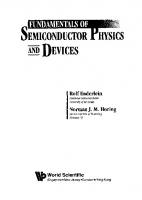
Modern society is increasingly dependent upon electrical appliances for comfort, transportation, and healthcare, motivating great advances in power generation, power distribution and power management technologies. These advancements owe their allegiance to enhancements in the performance of power devices that regulate the flow of electricity. After the displacement of vacuum tubes by solid state devices in the 1950s, the industry relied upon silicon bipolar devices, such as bipolar power transistors and thyristors. Although the ratings of these devices grew rapidly to serve an ever broader system need, their fundamental limitations in terms of the cumbersome control and protection circuitry led to bulky and costly solutions. The advent of MOS technology for digital electronics enabled the creation of a new class of devices in the 1970s for power switching applications as well. These silicon power MOSFETs have found extensive use in high frequency applications with relatively low operating voltages (below 100 V). The merger of MOS and bipolar physics enabled the creation of yet another class of devices in the 1980s. The most successful innovation in this class of devices has been the insulated gate bipolar transistor (IGBT). The high power density, simple interface, and ruggedness of the IGBT have made it the technology of choice for all medium and high power applications, with perhaps the exception of high voltage DC transmission systems. Even the last remaining bastion for the conventional power thyristors is threatened by the incorporation of MOS-gated structures. Power devices are required for systems that operate over a broad spectrum of power levels and frequencies. In Fig. 1.1, the applications for power devices are shown as a function of operating frequency. High power systems, such as HVDC power distribution and locomotive drives, requiring the control of megawatts of power operate at relatively low frequencies. As the operating frequency increases, the power ratings decrease for the devices, with typical microwave devices handling about 100 W. All these applications are served by silicon devices. Thyristors are B.J. Baliga, Fundamentals of Power Semiconductor Devices, doi: 10.1007/978-0-387-47314-7_1, © Springer Science + Business Media, LLC 2008

2

FUNDAMENTALS OF POWER SEMICONDUCTOR DEVICES

favored for the low frequency, high power applications, IGBTs for the medium frequency and power applications, and power MOSFETs for the high frequency applications. HVDC POWER DISTRIBUTION

System Power Rating (Volt-Amperes)

108 107

ELECTRIC TRAINS

106 UNINTERRUPTIBLE POWER SUPPLY

105

HYBRID-ELECTRIC CARS

104 INDUCTION HEATING

103 102

AUDIO AMPLIFIERS FLUORESCENT LAMPS TELEVISION SWEEP CELLULAR COMMUNICATION

101 100 101

MICROWAVE OVEN

102

103

104

105

106

107

108

109

System Operating Frequency (Hz) Fig. 1.1 Applications for power devices

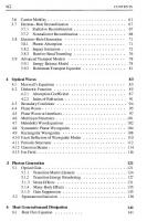
Another approach to classification of applications for power devices is in terms of their current and voltage handling requirements, as shown in Fig. 1.2. On the high power end of the chart, thyristors are available that can individually handle over 6,000 V and 2,000 A, enabling the control of over 10 MW of power by a single monolithic device. These devices are suitable for the HVDC power transmission and locomotive drive (traction) applications. For the broad range of systems that require operating voltages between 300 and 3,000 V with significant current handling capability, the IGBT has been found to be the optimum solution. When the current requirements fall below 1 A, it is feasible to integrate multiple devices on a single monolithic chip to provide greater functionality for systems such as telecommunications and display drives. However, when the current exceeds a few amperes, it is more cost effective to use discrete power MOSFETs with appropriate control ICs to serve applications such as automotive electronics and switch mode power supplies. Consequently, no single device structure exists at this time that is suitable for serving all the applications, leaving plenty of room for further innovations.

Introduction

3

HVDC TRANSMISSION ELECTRIC TRAINS

103

101

MOTOR DRIVES

AUTOMOTIVE ELECTRONICS

102

POWER SUPPLIES

Current Rating (Amperes)

104

ROBOTICS LAMP BALLAST

100 TELECOM.

10-1 10-2 101

DISPLAY DRIVES

102

103

104

Voltage Rating (Volts) Fig. 1.2 System ratings for power devices

1.1 Ideal and Typical Power Switching Waveforms An ideal power device must be capable of controlling the flow of power to loads with zero power dissipation. The loads encountered in systems may be inductive in nature (such as motors and solenoids), resistive in nature (such as heaters and lamp filaments), or capacitive in nature (such as transducers and LCD displays). Most often, the power delivered to a load is controlled by turning-on a power device on a periodic basis to generate pulses of current that can be regulated by a control circuit. The ideal waveforms for the power delivered through a power switch are shown in Fig. 1.3. During each switching cycle, the switch remains on for a time upto tON and maintains an off-state for the remainder of the period T. For an ideal power switch, the voltage drop during the on-state is zero, resulting in no power dissipation. Similarly, during the off-state, the (leakage) current in the ideal power switch is zero, resulting in no power dissipation. In addition, it is assumed that the power switch makes the transition between the on-state and off-state instantaneously, resulting in no power loss as well. The waveforms observed with typical power switches produce power dissipation during the on-state, off-state, as well as during the switching transients. As shown in Fig. 1.4, typical power devices exhibit a voltage drop (VF ) in the onstate, which results in a power dissipation in the on-state given by:

FUNDAMENTALS OF POWER SEMICONDUCTOR DEVICES

Current

4

ON STATE

OFF STATE

Voltage

t

0

tON

T

t

Current

Fig. 1.3 Ideal switching waveforms for power delivery

IF ON STATE

OFF STATE

Voltage

IL

t

VR

VF 0

t1 t2 t3

t4 t5 t6

t

Fig. 1.4 Typical switching waveforms for power delivery

PL (on) = δ I FVF

(1.1)

δ = t1 / T

(1.2)

where IF is the on-state current. In this expression, δ is referred to as the duty cycle given by:

where T is the time period (the reciprocal of the operating frequency).

Introduction

PL (off ) = (1 − δ ) I LVR

5

Power dissipation also occurs in the off-state given by (1.3)

where IL is the leakage current exhibited by the device in its off-state due to supporting a reverse bias (VR). This expression holds true if the switching times are small compared with the time period. If this assumption is not valid, the power dissipation can be obtained by using:

PL (off ) = ( t4 − t3 ) I LVR / T

(1.4)

Most often, the power dissipation in the off-state is small when compared with the other components and can be neglected. However, this does not hold true at elevated temperatures and when Schottky contacts are supporting the reverse voltage. The power dissipation that occurs during switching must be treated separately for the turn-off transient and the turn-on transient. During the turn-off transient for typical loads that are inductive in nature, the voltage across the switch increases rapidly to the DC-supply voltage, followed by a decrease in the current flowing through the switch. For the linearized waveforms shown in Fig. 1.4, the power loss during the turn-off transient can be calculated using:

PL (turnoff ) = 0.5 ( t3 − t1 ) I FVR f

(1.5)

where f is the operating frequency. In a similar manner, the power loss during the turn-on transient can be calculated using:

PL (turnon) = 0.5 ( t6 − t4 ) I FVR f

(1.6)

The total power dissipation incurred in the switch is obtained by combining these terms:

PL (total) = PL (on) + PL (off ) + PL (turnoff ) + PL (turnon)

(1.7)

At low operating frequencies, the on-state power loss is usually dominant, making it desirable to develop power switches with low on-state voltage drops. At high operating frequencies, the switching power losses are usually dominant, making it desirable to develop power switches with fast switching speeds or small transition times. Unfortunately, it is usually necessary to perform a trade off between minimizing the on-state and switching power losses in most designs. As power switch technology advances, the total power loss for the optimized design continues to reduce, providing enhancements to the efficiency of power systems.

1.2 Ideal and Typical Power Device Characteristics As discussed in the previous section, silicon power devices have served the industry for well over five decades but cannot be considered to have ideal device

6

FUNDAMENTALS OF POWER SEMICONDUCTOR DEVICES

characteristics. In general, power electronic circuits require both rectifiers to control the direction of current flow and power switches to regulate the duration of current flow. Neither of these components exhibits the ideal characteristics that are required in power circuits to prevent power dissipation. IF

ON-STATE

VF VR OFF-STATE

IR

Fig. 1.5 Characteristics of an ideal power rectifier

An ideal power rectifier should exhibit the current–voltage (i–v) characteristics shown in Fig. 1.5. In the forward conduction mode, the first quadrant of operation in the figure, it should be able to carry any amount of current with zero on-state voltage drop. In the reverse blocking mode, the third quadrant of operation in the figure, it should be able to hold off any value of voltage with zero leakage current. Further, the ideal rectifier should be able to switch between the on-state and the off-state, with zero switching time. IF

ION

VF

VOFF VON IOFF

VR

BV

IR Fig. 1.6 Characteristics of a typical power rectifier

Introduction

7

Actual silicon power rectifiers exhibit the i–v characteristics illustrated in Fig. 1.6. They have a finite voltage drop (VON) when carrying current on the onstate, leading to “conduction” power loss. They also have a finite leakage current (IOFF) when blocking voltage in the off-state, creating off-state power loss. In addition, the doping concentration and thickness of the drift region of the silicon device must be carefully chosen with a design target for the breakdown voltage (BV). Moreover, the power dissipation in power devices increases when their voltage rating is increased because of an increase in the on-state voltage drop. IF

ON-STATE

ACTIVE REGION

Increasing VG OFF-STATE

VF

Fig. 1.7 Characteristics of an ideal transistor

The i–v characteristics of an ideal power switch are illustrated in Fig. 1.7. As in the case of the ideal rectifier, the ideal transistor conducts current in the onstate with zero voltage drop and blocks voltage in the off-state with zero leakage current. In addition, the ideal device can operate with a high current and voltage in the active region, with the saturated forward current in this mode controlled by the applied gate bias. The spacing between the characteristics in the active region is uniform for an ideal transistor indicating a gain that is independent of the forward current and voltage. The i–v characteristics of a typical power switch are illustrated in Fig. 1.8. This device exhibits a finite resistance when carrying current in the on-state as well as a finite leakage current while operating in the off-state (not shown in the figure because its value is much lower than the on-state current levels). The breakdown voltage of a typical transistor is also finite as indicated in the figure with “BV”. The typical transistor can operate with a high current and voltage in the active region. This current is controlled by the base current for a bipolar transistor while it is determined by a gate voltage for a MOSFET or IGBT (as indicated in the figure). It is preferable to have gate voltage controlled characteristics because the drive circuit can be integrated to reduce its cost. The spacing between the

8

FUNDAMENTALS OF POWER SEMICONDUCTOR DEVICES

characteristics in the active region is nonuniform for a typical transistor with a square-law behavior for devices operating with channel pinch-off in the current saturation mode. Recently, devices operating under a new super-linear mode have been proposed and demonstrated for wireless base-station applications.1 These devices exhibit an equal spacing between the saturated drain current characteristics as the gate voltage is increased. This is an ideal behavior when the transistor is used for the amplification of audio, video, or cellular signals because it eliminates signal distortion that occurs with the characteristics shown in Fig. 1.8. IF

ON-RESISTANCE

ACTIVE REGION

Increasing VG

OFF-STATE

VF BV

Fig. 1.8 Characteristics of a typical transistor

1.3 Unipolar Power Devices Bipolar power devices operate with the injection of minority carriers during onstate current flow. These carriers must be removed when switching the device from the on-state to the off-state. This is accomplished by either charge removal via the gate drive current or via the electron-hole recombination process. These processes introduce significant power losses that degrade the power management efficiency. It is therefore preferable to utilize unipolar current conduction in a power device. The commonly used unipolar power diode structure is the Schottky rectifier that utilizes a metal-semiconductor barrier to produce current rectification. The high voltage Schottky rectifier structure also contains a drift region, as shown in Fig. 1.9, which is designed to support the reverse blocking voltage. The resistance of the drift region increases rapidly with increasing blocking voltage capability, as discussed later in this chapter. Silicon Schottky rectifiers are commercially available with blocking voltages of up to 100 V. Beyond this value, the on-state voltage drop of silicon Schottky rectifiers becomes too large for practical applications. Silicon P–i–N rectifiers are favored for designs with larger BVs due to their low on-state

Introduction

9

voltage drop despite slower switching properties. Silicon carbide Schottky rectifiers have much lower drift region resistance, enabling design of very high voltage devices with low on-state voltage drop and excellent switching characteristics. SCHOTTKY CONTACT METAL (ANODE)

DRIFT REGION

RS

SUBSTRATE

OHMIC CONTACT METAL (CATHODE)

Fig. 1.9 The power Schottky rectifier structure and its equivalent circuit D-MOSFET SOURCE

U-MOSFET SOURCE

GATE N+ P

N+ P

N-DRIFT REGION

N-DRIFT REGION

N+ SUBSTRATE

N+ SUBSTRATE

DRAIN

DRAIN

GATE

Fig. 1.10 Silicon power MOSFET structures

The most commonly used unipolar power transistor is the silicon power metal-oxide-semiconductor field-effect-transistor or MOSFET. Although other structures such as JFETs or SITs have been explored,2 they have not been popular for power electronic applications because of their normally-on behavior. The commercially available silicon power MOSFETs are based upon the structures shown in Fig. 1.10. The D-MOSFET was first commercially introduced in the

10

FUNDAMENTALS OF POWER SEMICONDUCTOR DEVICES

1970s and contains a “planar-gate” structure. The P-base and the N+ source regions are self-aligned to the edge of the polysilicon gate electrode by using ionimplantation of boron and phosphorus, followed by their respective drive-in thermal cycles. The n-type channel is defined by the difference in the lateral extension of the junctions under the gate electrode. The device supports positive voltage applied to the drain across the P-base/N-drift region junction. The voltage blocking capability is determined by the doping and thickness of the N-drift region. Although low voltage (300 V) device for power switching applications is the IGBT, which was developed in the 1980s by combining the physics of operation of bipolar transistors and MOSFETs.3 The structure of the IGBT is deceptively similar to that for the power MOSFET as shown in Fig. 1.12 if viewed as a mere replacement of the N+ substrate with a P+ substrate. However, this substitution creates a four-layer parasitic thyristor, which was initially considered a show-stopper because its latch-up results in destructive failure due to loss of gate control. Fortunately the parasitic thyristor can be suppressed by the addition of the P+ region within the cell while retaining the benefits of the P+ substrate for the injection of minority carriers into the N-drift region, resulting in greatly reducing its resistance. This has enabled the development of high voltage IGBT products with high current carrying capability. D-MOS IGBT

U-MOS IGBT EMITTER

EMITTER GATE N+ P+

P

N+ P+

P

N-DRIFT REGION

N-DRIFT REGION

P+ SUBSTRATE

P+ SUBSTRATE

COLLECTOR

COLLECTOR

Fig. 1.12 IGBT device structures

GATE

12

FUNDAMENTALS OF POWER SEMICONDUCTOR DEVICES

The on-state voltage drop for the IGBT increases with increasing voltage blocking capability due to the necessity to widen the N-drift region. To improve upon the on-state voltage drop while maintaining the advantages of small control currents, many MOS-gated thyristor structures have been explored. The first structure to garner attention was the MOS-controlled thyristor (MCT),4,5 which is illustrated in Fig. 1.13 with an N-type drift region. A reduced on-state voltage drop when compared with the IGBT is obtained by allowing the four-layer thyristor structure to latch-up. The thyristor is switched off by the application of a negative gate bias to form a current path that shunts the N+ emitter/P-base junction such that the gain of the upper N–P–N transistor is sufficiently diminished to prevent the regenerative action within the thyristor. One disadvantage of the structure shown in Fig. 1.13 is the complexity of forming the P-channel MOSFET within the P-base region. Another issue that has hindered its application is the lack of current saturation capability. Without gate controlled current saturation, it becomes necessary to incorporate snubbers with the device adding cost, complexity, and power losses to the system. DMOS-MCT CATHODE GATE P+ N+

N P

N-DRIFT REGION

P+ SUBSTRATE

ANODE

Fig. 1.13 MOS-controlled thyristor (MCT) structure

One solution to the above issues is the base resistance controlled thyristor (BRT)6 structure shown in Fig. 1.14. In this structure, a diverter region is integrated adjacent to the four-layer thyristor. The application of a positive bias to the gate allows turning on the thyristor, while the application of a negative bias turns off the thyristor by raising its holding current above the operating current level. The process for fabrication of this structure is compatible with that used for manufacturing IGBTs while its on-state voltage drop is similar to that for the MCT structure.

Introduction

13

DMOS-BRT CATHODE

DIVERTER GATE

N+

P+

P

N-DRIFT REGION

P+ SUBSTRATE

ANODE

Fig. 1.14 Base resistance controlled thyristor (BRT) structure

D-MOS EST CATHODE GATE

GATE N+ P+

P

N+ Cathode P

N-DRIFT REGION

P+ SUBSTRATE

ANODE

Fig. 1.15 Emitter switched thyristor (EST) structure

The MCT and BRT structure do not allow for saturated current flow under gate control, a key feature of IGBTs that is extensively utilized in power electronic circuits. This capability has been successfully incorporated in the emitter switched thyristor (EST)7 structure shown in Fig. 1.15. The EST structure contains a fourlayer thyristor without direct contact to the N+ cathode region. The current flowing into the N+ cathode region is constrained to flow via an n-channel MOSFET to the cathode contact. This provides complete gate controlled current saturation

14

FUNDAMENTALS OF POWER SEMICONDUCTOR DEVICES

capability. However, the on-state voltage drop is slightly larger than that for the MCT or BRT due to the additional voltage drop in the channel of the MOSFET.

1.6 Ideal Drift Region for Unipolar Power Devices The unipolar power devices discussed above contain a drift region, which is designed to support the blocking voltage. The properties (doping concentration and thickness) of the ideal drift region can be analyzed by assuming an abrupt junction profile with high doping concentration on one side and a low uniform doping concentration on the other side, while neglecting any junction curvature effects by assuming a parallel-plane configuration. The resistance of the ideal drift region can then be related to the basic properties of the semiconductor material.8

ANODE ELECTRIC FIELD

Em

RD

DRIFT REGION

WD SUBSTRATE

CATHODE

Fig. 1.16 The ideal drift region and its electric field distribution

The solution of Poisson’s equation leads to a triangular electric field distribution, as shown in Fig. 1.16, within a uniformly doped drift region with the slope of the field profile being determined by the doping concentration. The maximum voltage that can be supported by the drift region is determined by the maximum electric field (Em) reaching the critical electric field (Ec) for breakdown for the semiconductor material. The critical electric field for breakdown and the doping concentration then determine the maximum depletion width (WD). The specific resistance (resistance per unit area) of the ideal drift region is given by:

⎛ WD ⎞ Ron.sp = ⎜ ⎟ ⎝ qµn N D ⎠

(1.8)

Introduction

15

Since this resistance was initially considered to be the lowest value achievable with silicon devices, it has historically been referred to as the ideal specific onresistance of the drift region. More recent introduction of the charge-coupling concept, described later in this chapter, has enabled reducing the drift region resistance of silicon devices to below the values predicted by this equation. The depletion width under breakdown conditions is given by:

WD =

2BV EC

(1.9)

where BV is the desired breakdown voltage. The doping concentration in the drift region required to obtain this BV is given by:

ND =

ε S EC2

2qBV

(1.10)

Combining these relationships, the specific resistance of the ideal drift region is obtained:

Ron-ideal =

4BV 2 ε S µn EC3

(1.11)

The denominator of this equation ( ε S µ n EC3 ) is commonly referred to as Baliga’s figure of merit for power devices. It is an indicator of the impact of the semiconductor material properties on the resistance of the drift region. The dependence of the drift region resistance on the mobility (assumed to be for electrons here because in general they have higher mobility values than for holes) of the carriers favors semiconductors such as gallium arsenide and indium arsenide. However, the much stronger (cubic) dependence of the on-resistance on the critical electric field for breakdown favors wide band gap semiconductors such as silicon carbide.9 The critical electric field for breakdown is determined by the impact ionization coefficients for holes and electrons in semiconductors as discussed in the next chapter. As an example, the change in the specific on-resistance for the drift region with critical electric field and mobility is shown in Fig. 1.17 for the case of a BV of 1,000 V. The location of the properties for silicon, gallium arsenide, and silicon carbide are shown in the figure by the points. The improvement in drift region resistance for GaAs in comparison with silicon is largely due to its much greater mobility for electrons. The improvement in drift region resistance for SiC in comparison with silicon is largely due to its much larger critical electric field for breakdown. On the basis of these considerations, excellent high voltage Schottky rectifiers were developed from GaAs in the 1980s10 and from silicon carbide in the 1990s.11 Interest in the development of power devices from wide-band-gap semiconductors, including gallium nitride, continues to grow.

16

FUNDAMENTALS OF POWER SEMICONDUCTOR DEVICES

Specific On-Resistance (Ohm-cm2) Specific On-Resistance (ohm-cm2)

1.E+01 1 10

Breakdown Voltage = 1000 V

0 1.E+00 10

Si Mobility = 1000 cm2/Vs

1.E-01 -1 10

GaAs

-2 1.E-02 10

Mobility = 2000 cm2/Vs

-3 1.E-03 10

SiC 1.E-04 -4 10

Mobility = 4000 cm2/Vs

-5 1.E-05 10

Mobility = 8000 cm2/Vs

-6 10 1.E-06

1.E+05 5

10

1.E+06 6

10

1.E+07 7

10

Critical Electric Field (V/cm)

Critical Electric Field for Breakdown (V/cm)

Fig. 1.17 Specific on-resistance of the ideal drift region

1.7 Charge-Coupled Structures: Ideal Specific On-Resistance The depletion region extends in one-dimension from a junction or Schottky contact during the blocking mode for the conventional structure discussed in the previous section. In the charge-coupled structure, the voltage blocking capability is enhanced by the extension of depletion layers in two-dimensions. This effect is created by the formation of a horizontal Schottky contact on the top surface as illustrated in Fig. 1.18, which promotes the extension of a depletion region along the vertical or y-direction. Concurrently, the presence of the vertical P–N junction created by the alternate N- and P-type regions promotes the extension of a depletion region along the horizontal or x-direction. These depletion regions conspire to produce a twodimensional charge coupling in the N-drift region, which alters the electric field profile. The optimization of the charge-coupled structure requires proper choice of the doping concentration and thickness of the N- and P-type regions. It has been found that the highest BV occurs when the charge in these regions is given by: Qoptimum = 2qN DWN = ε S EC

(1.12)

where q is the charge of an electron (1.6 × 10−19 C), ND is the doping concentration of the N-type drift region, WN is half the width of the N-type drift region as shown in Fig. 1.18, εS is the dielectric constant of the semiconductor, and EC is the critical electric field for breakdown in the semiconductor. For silicon, the optimum charge

Introduction SCHOTTKY CONTACT

17

OHMIC CONTACT

WN

WP

N-DRIFT REGION

P-TYPE CHARGE COUPLING REGION

t

p N+ SUBSTRATE

CATHODE

Fig. 1.18 Basic charge coupled Schottky diode structure using P-N junctions

is found to be 3.11 × 10−7 C cm−2 based upon a critical electric field of 3 × 105 V cm−1. The optimum charge is often represented as a dopant density per unit area, in which case it takes a value of about 2 × 1012 cm−2 for silicon. A slightly lower value for the doping concentration in the drift region may be warranted as discussed later in this section of the chapter. The specific on-resistance for the drift region in the charge-coupled structures is given by: ⎛ p RD,sp = ρ D ⎜ ⎝ WN

⎞ ⎟t ⎠

(1.13)

tp q µ N N DWN

(1.14)

where ρD is the resistivity of the N-type drift region, t is the trench depth, and p is the cell pitch. Here, the uniform electric field is assumed to be produced only along the trench where the charge coupling occurs and the resistance of the remaining portion of the N-drift region is neglected. Using the relationship between the resistivity and the doping concentration, this equation can be written as:

RD,sp =

Combining this expression with (1.12): RD,sp =

2tp µ N Qoptimum

(1.15)

18

FUNDAMENTALS OF POWER SEMICONDUCTOR DEVICES

If the electric field along the trench, at the on-set of breakdown in the chargecoupled device structure, is assumed to be uniform at a value equal to the critical electric field of the semiconductor:

t=

BV EC

(1.16)

Using this expression, as well as the second part of (1.12), in (1.15) yields:

RD,sp =

2BVp µ Nε S EC2

(1.17)

This is a fundamental expression for the ideal specific on-resistance of vertical charge-coupled devices. By comparison of this expression with that for the onedimensional case (see (1.11), it can be observed that the specific on-resistance for the charge-coupled devices increases linearly with the BV unlike the more rapid quadratic rate for the conventional drift region. In addition, it is worth pointing out that the specific on-resistance for the drift region in the charge-coupled structure can be reduced by decreasing the pitch. This occurs because the doping concentration in the drift region increases when the pitch is reduced so as to maintain the same optimum charge. The larger doping concentration reduces the resistivity and hence the specific on-resistance. However, the analysis of the specific on-resistance for the drift region in charge-coupled device structures must be tempered by several considerations. First, it must be recognized that the mobility will become smaller when the doping concentration becomes larger. Second, the critical electric field for breakdown becomes smaller for the charge-coupled structures because the high electric field in the drift region extends over a larger distance, producing enhanced impact ionization. If a critical electric field for breakdown in the drift region for charge-coupled structures is reduced to 2 × 105 V cm−1, an optimum charge of 2.07 × 10−7 C cm−2, with a corresponding dopant density of about 1.3 × 1012 cm−2, is more appropriate for silicon. In designing the drift region for charge-coupled structures, it is important to recognize that, unlike in the conventional one-dimensional case, the doping concentration of the drift region is dictated by the cell pitch and not the BV. The BV in the charge-coupled structure is determined solely by the depth of the trench used to provide the charge coupling effect and is independent of the doping concentration of the N-drift region. In the case of silicon charge-coupled devices, the doping concentration for the N-type drift region is provided in Fig. 1.19 for the case of equal widths for the N-type and P-type charge coupling regions. For a typical cell pitch of 1 µm, the doping concentration in the N-type drift region is about 1.3 × 1016 cm−3 when a critical electric field of 2 × 105 V cm−1 is assumed. It is interesting to compare the ideal specific on-resistance for the drift region in the silicon charge-coupled structures to that for the one-dimensional parallel-plane case. This comparison is done in Fig. 1.20 using three values for the

Introduction

19

Doping Concentration (cm-3)

Doping Concentration (cm-3)

17 1.E+17 10

1.E+16 16 10

Silicon Charge Coupled Structure 1.E+15 15 10 0.1 0.1

1

10

1.0

10

Cell Pitch (m icrons)

Cell Pitch (microns) Fig. 1.19 Drift region doping concentration for the charge coupled structure -1 1.E-01 10

-2 1.E-02 10 Specific On-Resistance (Ohm-cm2)

Specific On-Resistance (Ω-cm2)

Silicon Charge Coupled Structure One-Dimensional case Cell Pitch = 5 µm 1.E-03 -3

10

1.E-04 -4 10

1.E-05 -5 10

1.E-06 -6 10 1.E+01 10

Cell Pitch = 1 µm Cell Pitch = 0.2 µm

1.E+02

100

Breakdow n Voltage (V)

1.E+03 1000

Breakdown Voltage (Volts) Fig. 1.20 Ideal specific on-resistance for the charge coupled structure (solid lines: charge coupled structures; dashed line: one dimensional case)

cell pitch in the case of the charge-coupled structures. The doping concentration in the N-drift region increases when the cell pitch is reduced from 5 µm to 0.2 µm, as already shown in Fig. 1.19, leading to a decrease in the specific on-resistance. The resulting reduction of the mobility with increasing doping concentration was

20

FUNDAMENTALS OF POWER SEMICONDUCTOR DEVICES

included during the calculation of the specific on-resistance in Fig. 1.20. There is a cross-over in the specific on-resistance for the two types of structures. For the cell pitch of 1 µm, the cross-over occurs at a BV of about 70 V. The cross-over moves to a BV of about 200 V when the cell pitch is increased to 5 µm, and to about 30 V if a smaller cell pitch of 0.2 µm is used. Consequently, the charge-coupled structure is more attractive for reducing the specific on-resistance when the cell pitch is smaller. This entails a more complex process technology with higher attendant costs. As a particular example, consider the case of silicon devices designed to support 200 V. In the case of the conventional structure with a one-dimensional junction, the specific on-resistance of the drift region is found to be 3.4 mΩ cm2 if a critical electric field for breakdown of 3 × 105 V cm−1 is used. In contrast, the specific on-resistance for the drift region of the charge-coupled structure with a cell pitch of 1 µm is found to be only 0.86 mΩ-cm2 if a critical electric field for breakdown of 2 × 105 V cm−1 is used. In this calculation, a bulk mobility of 1,220 cm2 V−1 s−1 was used corresponding to a doping concentration of 1.3 × 1016 cm−3 in the N-type portion of the drift region. In this example, the drift region for the charge-coupled structure would have a thickness of 10 µm when compared with 12.5 µm needed in the conventional structure. SCHOTTKY CONTACT

WN

t

CHARGE COUPLING ELECTRODE

N-DRIFT REGION

WT N+ SUBSTRATE

CATHODE Fig. 1.21 Basic charge coupled Schottky diode structure using MOS structure

An alternate method for creating a charge-coupled structure, which is simpler from a fabrication viewpoint, is illustrated in Fig. 1.21. A uniform electric field in the drift region can be created with this structure by using a graded doping profile.12 These devices have been demonstrated to provide significant reduction of

Introduction

21

the on-state voltage drop for Schottky rectifiers designed to block 30–200 V with low leakage currents.13 A detailed discussion of charge-coupled devices is beyond the scope of this book.

1.8 Summary The desired characteristics for power semiconductor rectifiers and transistors have been reviewed in this chapter. The characteristics of typical silicon power devices have been compared with those for the ideal case. Various unipolar and bipolar power device structures have been briefly introduced here. Only the basic power device structures are discussed in this book because of space constraints.

Problems 1.1

Define the current and voltage ratings of power devices for typical automotive applications.

1.2

Define the current and voltage ratings of power devices for typical computer power supply applications.

1.3

Define the current and voltage ratings of power devices for typical motor control applications.

1.4

Define the current and voltage ratings of power devices for typical electric locomotive applications.

1.5

What are the characteristics of an ideal power device?

1.6

Describe the characteristics of an ideal power rectifier.

1.7

How do the characteristics of actual power rectifiers defer from those for the ideal device?

1.8

Describe the characteristics of an ideal power transistor.

1.9

How do the characteristics of actual power transistors defer from those for the ideal device?

1.10

Why are unipolar power device structures more attractive for applications than bipolar power devices?

22

FUNDAMENTALS OF POWER SEMICONDUCTOR DEVICES

1.11

Calculate Baliga’s figure-of-merit for a semiconductor with an electron mobility of 2,000 cm2 V−1 s−1 and critical breakdown electric field strength of 5 × 105 V cm−1.

1.12

Determine Baliga’s figure-of-merit for gallium nitride assuming it has an electron mobility of 900 cm2 V−1 s−1 and critical breakdown electric field strength of 3.3 × 106 V cm−1.

References 1

B.J. Baliga, “Silicon RF Power Devices,” World Scientific, Singapore, 2005. B.J. Baliga, “Modern Power Devices,” Wiley, New York, 1987. 3 B.J. Baliga, “Evolution of MOS-Bipolar Power Semiconductor Technology,” Proceedings of the IEEE, pp. 409–418, 1988. 4 V.A.K. Temple, “MOS Controlled Thyristors (MCTs),” IEEE International Electron Devices Meeting, Abstract 10.7, pp. 282–285, 1984. 5 M. Stoisiek and H. Strack, “MOS-GTO – A Turn-off Thyristor with MOS Controlled Emitter Shorts,” IEEE International Electron Devices Meeting, Abstract 6.5, pp. 158–161, 1985. 6 M. Nandakumar, et al., “A New MOS-Gated Power Thyristor Structure with Turn-off achieved by Controlling the Base Resistance,” IEEE Electron Device Letters, Vol. EDL-12, pp. 227–229, 1991. 7 B.J. Baliga, “The MOS-Gated Emitter Switched Thyristor,” IEEE Electron Device Letters, Vol. EDL-11, pp. 75–77, 1990. 8 B.J. Baliga, “Semiconductors for High Voltage Vertical Channel Field Effect Transistors,” Journal of Applied Physics, Vol. 53, pp. 1759–1764, 1982. 9 B.J. Baliga, “Silicon Carbide Power Devices,” World Scientific, Singapore, 2006. 10 B.J. Baliga, et al., “Gallium Arsenide Schottky Power Rectifiers,” IEEE Transactions on Electron Devices, Vol. ED-32, pp. 1130–1134, 1985. 11 M. Bhatnagar, P.M. McLarty, and B.J. Baliga, “Silicon Carbide High Voltage (400V) Schottky Barrier Diodes,” IEEE Electron Device Letters, Vol. EDL-13, pp. 501–503, 1992. 12 B.J. Baliga, “Schottky Barrier Rectifiers and Method of Forming Same,” U.S. Patent 5,612,567, Issued 18 March 1997. 13 S. Mahalingam and B.J. Baliga, “The Graded Doped Trench MOS Barrier Schottky Rectifier,” Solid State Electronics, Vol. 43, pp. 1–9, 1999. 2

Chapter 2

Material Properties and Transport Physics

At present, most power semiconductor devices are manufactured using silicon as the base material. Both unipolar and bipolar devices have been successfully developed from silicon to serve a very broad range of applications. As shown in the previous chapter, the resistance of the drift region in power devices can be drastically reduced by replacing silicon with wide band gap semiconductors. Although some effort was undertaken in the 1980s to develop power devices from gallium arsenide, interest in this technology has dwindled because it is much more promising to make the power devices from silicon carbide. For this reason, the relevant properties of silicon carbide are included with those of silicon in this chapter for the purposes of comparison and design. Analytical expressions that can model these properties are provided to facilitate the analysis of power device structures. Although the fundamental material properties of the semiconductor govern the operating characteristics of power devices, processing techniques used to control these properties impose technological constraints that are equally important for obtaining the desired device characteristics. For this reason, the chapter includes a discussion of current technology, such a neutron transmutation doping (NTD) for controlling the resistivity and electron irradiation for controlling the minority carrier lifetime. These technologies have been specifically developed for manufacturing power devices and are almost exclusively used for these types of structures.

2.1 Fundamental Properties The fundamental properties of silicon1 and silicon carbide2–4 are summarized and compared in this section. Only the properties for the 4H poly-type of silicon carbide have been included here because its properties are superior to those of the

B.J. Baliga, Fundamentals of Power Semiconductor Devices, doi: 10.1007/978-0-387-47314-7_2, © Springer Science + Business Media, LLC 2008

24

FUNDAMENTALS OF POWER SEMICONDUCTOR DEVICES

other poly-types of silicon carbide. The basic properties of relevance to power devices are the energy band gap, the impact ionization coefficients, the dielectric constant, the thermal conductivity, the electron affinity, and the carrier mobility. Since the intrinsic carrier concentration and the built-in potential can be extracted by using this information, their values have also been provided for silicon and silicon carbide in this section. Properties

Silicon

4H-SiC

1.11

3.26

11.7

9.7

1.5

3.7

4.05

3.7

2.80 x 1019

1.23 x 1019

1.04 x 1019

4.58 x 1018

Energy Band Gap (eV) Relative Dielectric Constant Thermal Conductivity (W/cm-K) Electron Affinity (eV) Density of States Conduction Band (cm-3) Density of States Valence Band (cm-3) Fig. 2.1 Fundamental material properties

The fundamental material parameters for silicon and 4H-SiC are summarized in Fig. 2.1 for comparison purposes. It is worth noting that the energy band gap for 4H-SiC is three times larger than that for silicon. This results in a much lower intrinsic carrier concentration at any given temperature, as well as much smaller impact ionization coefficients at any given electric field, for this semiconductor when compared with silicon, as discussed in more detail in the next section. The dielectric constant and the density of states are comparable for both these semiconductors. The thermal conductivity for 4H silicon carbide is two to three times that for silicon, enabling superior heat extraction from devices. The difference in the electron affinity between the semiconductors appears small but is quite significant when determining the characteristics of Schottky barrier contacts.

Material Properties and Transport Physics

25

2.1.1 Intrinsic Carrier Concentration The intrinsic carrier concentration is determined by the thermal generation of electron-hole pairs across the energy band gap of a semiconductor. Its value can be calculated by using the energy band gap (EG) and the density of states in the conduction (NC) and valence (NV) bands: ni = np = N C N V e − EG / 2 kT

(2.1)

where k is Boltzmann’s constant (1.38 × 10−23 J K−1) and T is the absolute temperature. For silicon, the intrinsic carrier concentration is given by: ni = 3.87 × 1016 T 3/ 2 e − (7.02×10

3

) /T

(2.2)

)/T

(2.3)

while that for 4H-SiC is given by:

ni = 1.70 × 1016 T 3/ 2 e − (2.08×10

4

-3 Intrinsic Carrier Intrinsic CarrierConcentration Concentration (cm-3) (cm )

Using these equations, the intrinsic carrier concentration can be calculated as a function of temperature. The intrinsic carrier concentrations for silicon and 4H-SiC are plotted in Figs. 2.2 and 2.3. 1.E+17 1.E+15

Si

13 1.E+13

10

1.E+11 1.E+09

7 1.E+07

10

1.E+05 1.E+03

101

1.E+01 1.E-01

4H-SiC

1.E-03

-5 1.E-05

10

1.E-07 1.E-09 1.E-11 -11

10

1 1.0

1.5 1.5

2 2.0

2.5 2.5

3 3.0

3.5 3.5

4.04

1000/Temperature (1/K) 1000/Temperature (1/K)

Fig. 2.2 Intrinsic carrier concentration

The traditional method for making this plot is shown in Fig. 2.2 by using an inverse temperature scale for the x-axis. The additional figure (Fig. 2.3) is provided here because it is easier to relate the value of the intrinsic carrier concentration to the temperature, with its values directly plotted on the x-axis. It is obvious that the intrinsic carrier concentration for silicon carbide is far smaller

26

FUNDAMENTALS OF POWER SEMICONDUCTOR DEVICES

Intrinsic Carrier Concentration (cm-3) Intrinsic Carrier Concentration (cm-3)

than that for silicon due to the large difference in band gap energy. At room temperature (300 K), the intrinsic carrier concentration for silicon is 1.4 × 1010 cm−3 while that for 4H-SiC is only 6.7 × 10−11 cm−3. This indicates that the bulk generation current is negligible for the determination of the leakage current in silicon carbide devices but not for silicon structures. Surface generation currents may become dominant in 4H-SiC devices because of the presence of states within the band gap. 1.E+17 1.E+15

13 1.E+13 10

Si

1.E+11 1.E+09

7 1.E+07 10 1.E+05 1.E+03

1 1.E+01 10

4H-SiC

1.E-01 1.E-03

-5 1.E-05 10 1.E-07 1.E-09 1.E-11 -11 10 300 300

350

350

400

400

450

450

500

500

Temperature (K)

550

550

600

600

650

650

700

700

Temperature (K) Fig. 2.3 Intrinsic carrier concentration

For silicon, the intrinsic carrier concentration becomes equal to a typical doping concentration of 1 × 1015 cm−3 at a relatively low temperature of 540 K or 267°C. In contrast, the intrinsic carrier concentration for 4H-SiC is only 3.9 × 107 cm−3 even at 700 K or 427°C. The development of mesoplasmas has been associated with the intrinsic carrier concentration becoming comparable to the doping concentration.5 Mesoplasmas create current filaments that have very high current density, leading to destructive failure in semiconductors. This is obviously much less likely in silicon carbide. 2.1.2 Band Gap Narrowing The energy band diagram for silicon at low doping concentrations takes the form illustrated in Fig. 2.4(a), with the density of states varying as the square root of energy away from the band edges. The donor and acceptor levels are located at discrete positions within the band gap and are clearly separated from the conduction and valence band edges. The well-defined separation between the conduction and

Material Properties and Transport Physics

27

Energy

Energy

valence band edges is called the energy band gap (EG). The energy band gap for silicon and 4H silicon carbide is provided in Fig. 2.1.

EC

EC

ED

Donor Band

EG EV

EA

Density of States (a) Low Doping Case

EV

Acceptor Band

Density of States (b) High Doping Case

Fig. 2.4 Energy band diagrams at (a) low and (b) high doping concentrations

At high doping levels in the semiconductor, the band structure is altered by three effects. First, as the impurity density becomes large, the spacing between the individual impurity atoms becomes small. The interaction between adjacent impurity atoms leads to a splitting of the impurity levels into an impurity band as illustrated in Fig. 2.4(b). This phenomenon is observed when the doping concentration exceeds 1018 cm−3. Second, the conduction and valence band edges no longer exhibit a parabolic shape. The statistical distribution of the dopant atoms in the lattice introduces point-by-point differences in local doping concentration and lattice potential, leading to disorder. This results in the formation of band tails as illustrated in Fig. 2.4(b) by the dashed lines. This phenomenon is observed when the doping concentration approaches 1021 cm−3. Third, the interaction between the free carriers and more than one impurity atom leads to a modification of the density of states at the band edges. This phenomenon is called rigid band gap narrowing. The formation of the impurity bands, the band tails, and the rigid band gap narrowing are majority carrier effects related to the reduced dopant atom spacing within the semiconductor lattice. In addition to this, the electrostatic interaction of the minority carriers and the high concentration of majority carriers lead to a reduction in the thermal energy required to create an electron–hole pair. This phenomenon is also a rigid band gap reduction that does not distort the energy dependence of the density of states. The rigid band gap reduction arising from the screening of the minority carriers by the high concentration of majority carriers can be derived by using Poisson’s equation6:

28

FUNDAMENTALS OF POWER SEMICONDUCTOR DEVICES

1 d ⎛ 2 dV ⎞ q ⎜r ⎟ = − ∆n 2 εS r dr ⎝ dr ⎠

(2.4)

where V is the electrostatic potential of the screened carriers at a radial distance r. The excess electron concentration ∆n is given by Boltzmann’s equation:

∆n = n0 (e qV / kT − 1)

(2.5)

For the case of low excess electron concentrations: ⎛ qn V ⎞ ∆n = ⎜ 0 ⎟ ⎝ kT ⎠

(2.6)

Solution of (2.4) using the excess electron concentration given by (2.6) yields: V (r ) =

q ⎛ e − r / rS ⎞ ⎜ ⎟ 4πε S ⎝ r ⎠

(2.7)

where the screening radius rS is given by:

ε S kT

rS =

q 2 n0

(2.8)

The electric field distribution for the screened Coulombic potential can be obtained by the integration of (2.7): E (r ) =

q ⎛ 1 1 ⎞ − r / rS ⎜ − ⎟e 4πε S r ⎝ r rS ⎠

(2.9)

In comparison, the unscreened electric field distribution at low doping concentrations is given by: E (r ) =

q 4πε S r 2

(2.10)

The reduction of the band gap is given by the difference in the electrostatic energy between the screened and unscreened cases: ∆EG =

εS

2∫

∞

0

⎡⎣ E02 (r ) − E 2 (r ) ⎤⎦dr

(2.11)

The solution of this integral yields: ∆EG =

3q 2 16πε S

q 2 n0 ε S kT

(2.12)

In the case of low injection levels and under the assumption that all the dopant atoms are ionized:

Material Properties and Transport Physics

29

n0 = N D+ = N D

(2.13)

where ND is the doping concentration. Consequently, ∆EG =

3q 2 16πε S

q2 ND ε S kT

(2.14)

This expression, valid for small changes in the band gap, indicates that the band gap narrowing is proportional to the square root of the doping concentration. Using the appropriate parameters for silicon: ∆EG = 22.5 × 10−3

NI 1018

(2.15)

where NI is the impurity (donor or acceptor) concentration responsible for the reduction in the band gap. The decrease of the energy gap for silicon at room temperature due to high doping concentrations as predicted by the above theory is shown in Fig. 2.5. This theoretical curve has been found to provide a good fit with the measured data up to a doping concentration of 1019 cm−3, indicating that the screening of minority carriers by the majority carriers is a dominant effect responsible for band gap narrowing in silicon.7–10 1.15

1.05

Energy Band Gap (eV)

Energy Band Gap (eV)

1.10 1.1

1.00 1.0

0.95

0.90 0.9

300 oK 0.85

0.80 0.8 1.00E+15 1015

1.00E+16

1016

1.00E+17

1017

1.00E+18

1018

Doping Concentration (cm -3)

Doping Concentration

1.00E+19

1019

1.00E+20

1020

(cm-3)

Fig. 2.5 Band gap narrowing in silicon at high doping concentrations

The band gap narrowing phenomenon has a strong impact upon the product of the equilibrium concentrations of electrons and holes in the heavily doped semiconductor material. The p–n product can be represented by an effective intrinsic carrier concentration in a manner similar to that for lightly doped semiconductors:

30

FUNDAMENTALS OF POWER SEMICONDUCTOR DEVICES

(np ) = nie2

(2.16)

The larger values for the p–n product arising from band gap narrowing are related to the smaller energy band gap by: nie2 = ni2 e q∆EG / kT

(2.17)

where ∆EG is the reduction of the band gap due to the combined effects of impurity band formation, band tailing, and screening of minority carriers. By using (2.15), the effective intrinsic carrier concentration at room temperature for silicon is given by: ⎛ NI ⎞ nie = 1.4 × 1010 exp ⎜⎜ 0.433 ⎟ 1018 ⎟⎠ ⎝

(2.18)

12 1.E+12 10

300 oK Effective Intrinsic Carrier Concentration (cm-3)

Effective Intrinsic Carrier Concentration (cm-3)

where NI is the doping concentration in cm−3. The intrinsic carrier concentration predicted by this equation increases by more than one order of magnitude when the doping concentration exceeds 3 × 1019 cm−3, as shown in Fig. 2.6. These high doping concentrations are commonly encountered in the diffused end regions of power devices. The performance of bipolar power devices is affected by the band gap narrowing phenomenon because the injection of minority carriers into the end regions is enhanced by the larger intrinsic carrier concentration.

1.E+11 11 10

1.E+10 10 10 1.00E+15 1015

1.00E+16 16

10

1.00E+17 17

10

1.00E+18 18

10

1.00E+19 19

10

1.00E+20 20 10

Doping Concentration (cm -3)

Doping Concentration (cm-3) Fig. 2.6 Effective intrinsic carrier concentration in silicon at high doping levels

2.1.3 Built-in Potential

The built-in potential of P–N junctions can play an important role in determining the operation and design of power semiconductor devices. As an example, the

Material Properties and Transport Physics

31

built-in potential determines the zero-bias depletion width, which is important for the calculation of the on-resistance in power D-MOSFETs. The built-in voltage is given by: Vbi =

kT ⎛ N A− N D+ ⎞ ln ⎜ ⎟ q ⎝ ni2 ⎠

(2.19)

where NA− and ND+ are the ionized impurity concentrations on the two sides of an abrupt P–N junction. For silicon, their values are equal to the doping concentration because of the small dopant ionization energy levels.

3.00 3.0

4H-SiC 2.50

Built-in Potential (V)

Built-in Potential of P-N Junction (V)

3.50

2.00 2.0

1.50

Si

1.01.00 0.50

0.00 250

0

250

300

300

350

350

400

400

450

450

Tem perature (K)

500

500

550

550

600

600

650

650

Temperature (K) Fig. 2.7 Built-in potential for a P-N junction in Si and 4H-SiC

The calculated built-in potential for silicon and 4H-SiC is shown in Fig. 2.7 as a function of temperature for the typical operating range of power devices. In making the plots, the product (NA−ND+) was assumed to be 1035 cm−6. This would be applicable for a typical doping concentration of 1 × 1019 cm−3 on the heavily doped side of the junction and 1 × 1016 cm−3 on the lightly doped side of the junction. The built-in potential for silicon carbide is much larger than that for silicon because of the far smaller values for the intrinsic carrier concentration. This can be a disadvantage because of the larger zero bias depletion width for silicon carbide. As an example, the larger zero bias depletion width consumes space within the D-MOSFET cell structure, increasing the on-resistance by constricting the area through which current can flow. In contrast, the larger built-in potential for SiC and its associated larger zero bias depletion width can be taken advantage of in making innovative device structures, such as the ACCUFET (see Chap. 6), that are tailored to the unique properties of SiC.

32

2.1.4

FUNDAMENTALS OF POWER SEMICONDUCTOR DEVICES

Zero-Bias Depletion Width

The calculated zero bias depletion widths for silicon and 4H-SiC are shown in Fig. 2.8 as a function of the doping concentration on the lightly doped side of an abrupt P–N junction. For both silicon and silicon carbide, it can be seen that the zero bias depletion width can be substantial in size at low doping concentrations, making it important to take this into account during device design and analysis. The zero bias depletion width for SiC is much (about 2×) larger than that for silicon for the same doping concentration. However, it is worth noting that the doping concentration in SiC is much (about 100×) greater for a given breakdown voltage than for silicon as discussed later in the book. Consequently, the zero-bias depletion width for 4H-SiC devices is smaller than that for silicon devices with the same breakdown voltage. 1.E+01 1

Zero-Bias Depletion Width (microns)

Zero-Bias Depletion Width (microns)

10

4H-SiC 0 1.E+00

10

-1 1.E-01 10 1.00E+13 1013

Si

1.00E+14

1014

1.00E+15

1015

Doping Concentration (cm -3)

1.00E+16

1016

1.00E+17

1017

Doping Concentration (cm-3) Fig. 2.8 Zero-bias depletion width in Si and 4H-SiC

2.1.5 Impact Ionization Coefficients

The impact ionization coefficient for holes (αp) is defined as the number of electron–hole pairs created by a hole traversing 1 cm through the depletion layer along the direction of the electric field. Similarly, the impact ionization coefficient for electrons (αn) is defined as the number of electron–hole pairs created by an electron traversing 1 cm through the depletion layer along the direction of the electric field. The impact ionization coefficients for semiconductors are dictated by Chynoweth’s Law11,12:

α = a e−b / E

(2.20)

Material Properties and Transport Physics

33

where E is the electric field component in the direction of current flow. The parameters a and b are constants that depend upon the semiconductor material and the temperature. For silicon, the impact ionization rates have been measured as a function of electric field and temperature.13,14 Based upon these extensive measurements, the parameters for silicon have been found to be an = 7 × 105 cm−1 and bn = 1.23 × 106 V cm−1 for electrons; ap = 1.6 × 106 cm−1 and bp = 2 × 106 V cm−1 for holes for electric fields ranging between 1.75 × 105 and 6 × 105 V cm−1. The impact ionization coefficients for silicon carbide have been recently measured as a function of temperature by using an electron beam excitation method.15 This method allowed the extraction of impact ionization rates in defectfree regions of the material by isolating diodes containing defects with an EBIC (electron beam induced current) image. This was important because substantially enhanced impact ionization rates were discovered when the measurements were conducted at defect sites.16 For defect-free material, the extracted values for the impact ionization coefficient parameters for holes in 4H-SiC were found to be:

a(4H-SiC) = 6.46 ×106 − 1.07 ×104 T

(2.21)

b(4H-SiC) = 1.75 × 107

(2.22)

with

1.E+04 4

Impact Ionization Coefficient (/cm) Impact Ionization Coefficeint (/cm)

10

αn Si 1.E+03 3

10

αp

αp 2 1.E+02

10

Si

4H-SiC

1 1.E+01 10 1.E-07 10-7

1.E-06 -6

10

1.E-05 -5 10

1/Electric Field (cm /V)

1/(Electric Field) (cm/V) Fig. 2.9 Impact ionization coefficients for silicon and 4H-SiC

The impact ionization coefficients for 4H-SiC can be compared with those for silicon in Figs. 2.9 and 2.10. It is traditional to graph the ionization coefficients as the reciprocal of the electric field as shown in Fig. 2.9. However, it is more convenient to use the graph shown in Fig. 2.10 for extracting the ionization

34

FUNDAMENTALS OF POWER SEMICONDUCTOR DEVICES

coefficients at known values for the electric field. In both semiconductors, there is a very strong dependence of the ionization coefficients upon the electric field. Consequently, the breakdown voltage of power devices can be severely reduced by the presence of a high localized electric field within the structure. 1.E+04 4

αn Si 1.E+03 3

10

Alpha (/cm)

Impact Ionization Coefficient (/cm)

10

αp

αp 2 1.E+02

10

4H-SiC

Si

1 1.E+01 1.E+05 5

10

1.E+06

106

10

Electric Field (V/cm )

1.E+07

107

Electric Field (V/cm) Fig. 2.10 Impact ionization coefficients for silicon and 4H-SiC

From the above figures, it can be seen that the onset of significant generation of carriers by impact ionization occurs at much larger electric fields in 4H-SiC when compared with silicon. As a consequence, breakdown in 4H-SiC devices occurs when the electric fields are in the range of 2–3 × 106 V cm−1 – an order of magnitude larger than that for silicon. This implies a much larger critical electric field Ec for breakdown for 4H-SiC, resulting in a big increase in the Baliga’s figure of merit (see Chap. 1). The critical electric field for breakdown is discussed in more detail in the next chapter. It is worth pointing out that the impact ionization coefficient for electrons is much larger than that for holes in silicon while the opposite holds true for 4H-SiC. 2.1.6 Carrier Mobility

The resistivity (ρ) of a semiconductor region is given by:

ρ=

1 qµN

(2.23)

where µ by the mobility, which is a function of the carrier type (electrons or holes), the doping concentration (N), and the lattice temperature (T). A good understanding

Material Properties and Transport Physics

35

of the mobility for the carriers is therefore necessary to model current transport in the semiconductor regions within devices. In semiconductors, carriers are accelerated by the presence of an electric field and achieve an average velocity determined by the carrier scattering processes. Silicon is an indirect band gap semiconductor in which electron transport, under the influence of an applied electric field, occurs in six equivalent conduction band minima while the transport of holes occurs at two degenerate subbands. The inequality between the mobility of electrons and holes in silicon arises because of differences between the shapes of the conduction and valence band minima. As the free carriers are transported along the direction of the electric field, their velocity increases until they undergo scattering. In the bulk, the scattering can occur either by interaction with the lattice or at ionized donor and acceptor atoms. Consequently, the mobility is dependent upon the lattice temperature and the ionized impurity concentration. When the free carriers are transported near the semiconductor surface, additional scattering is observed, which decreases the mobility to below the bulk values. In bipolar power devices, a high concentration of holes and electrons can be simultaneously injected into the base region during on-state current flow. The probability for mutual scattering between electrons and holes increases under these conditions, reducing the effective mobility. The mobility (µ) is defined as the proportionality constant relating the average carrier velocity (vD) to the electric field (E):

vD = µ E

(2.24)

This expression is valid at low electric fields. However, when the electric field exceeds 104 V cm−1, as commonly encountered in power devices, the velocity is no longer found to increase in proportion to the electric field. In fact, the velocity approaches a constant value known as the saturated drift velocity. The dependence of the mobility upon the electric field strength must be accounted for during the analysis of the electrical characteristics of power devices. Temperature Dependence

At low doping concentrations in the semiconductor region, the scattering of free carriers occurs predominantly by interaction with the lattice vibrations. This lattice scattering phenomenon can occur by means of either acoustical phonons or optical phonons. Optical phonon scattering is important at high temperatures and electric fields while acoustical phonon scattering is dominant at low electric fields. In addition, at around room temperature, intervalley scattering mechanisms become important. For high purity, lightly doped, silicon, it has been experimentally determined that acoustical phonon scattering is dominant at temperatures below 50 K and the mobility varies as T−3/2, where T is the absolute temperature. At around room temperature, intervalley scattering comes into effect and the mobility for silicon is given by:

36

FUNDAMENTALS OF POWER SEMICONDUCTOR DEVICES

⎛ T ⎞ µn = 1360 ⎜ ⎟ ⎝ 300 ⎠ for electrons17 and:

⎛ T ⎞ µp = 495 ⎜ ⎟ ⎝ 300 ⎠

−2.42

(2.25)

−2.20

(2.26)

for holes.18 This variation of the mobility for electrons and holes in silicon is shown in Fig. 2.11 for the case of low doping concentrations (below 1015 cm−3) in the semiconductor. There is a rapid reduction of the mobility with increasing temperature, with a reduction by a factor of 2 when the temperature reaches 400 K. Since the doping concentration in the drift region of high voltage silicon devices is below 1015 cm−3, it is important to include the impact of the decrease in the mobility with temperature when analyzing the device characteristics because power devices operate at above room temperature due to power dissipation within the structure. 1600 1600

1200 1200

µn

1000 1000

Si

Mobility (cm2/Vs)

Mobility (cm2/V.s)

1400 1400

800800 600600

µn 4H-SiC

400400

µp

200200

Si

0

0 300

300

320

340

360

380

400

420

400

440

460

480

500

500

Tem perature (K)

Temperature

(oK)

Fig. 2.11 Temperature dependence of the mobility for electrons and holes in silicon and 4H-SiC

For 4H-SiC, the temperature dependence of the mobility at low doping concentrations can be modeled by4:

⎛ T ⎞ ⎟ ⎝ 300 ⎠

µn (4H-SiC) = 1140 ⎜

−2.70

(2.27)

This variation is also shown in Fig. 2.11 by the dashed line. Only the mobility for electrons in 4H-SiC is discussed here because it is preferable to make unipolar devices from silicon carbide with n-type drift regions.

Material Properties and Transport Physics

37

Doping Dependence

The presence of ionized donor or acceptor atoms in the semiconductor lattice contributes to a reduction in the mobility due to the additional Coulombic scattering of the free carriers. The impact of ionized impurity scattering is the largest at low temperatures because of the diminishing influence of lattice scattering. As the doping concentration is increased, the impact of ionized impurity scattering becomes larger, resulting in a reduction of the mobility. For silicon, the ionized impurity scattering effects are small at room temperature for doping concentrations below 1016 cm−3. Under these conditions, the mobility for electrons and holes can be considered to be independent of the doping concentration, with a magnitude of 1,360 and 495 cm2 V−1 s−1, respectively. At larger doping levels, the measured data19 for the mobility of electrons in silicon at room temperature as a function of the doping concentration can be modeled by:

µn (Si) =

5.10 ×1018 + 92 N D0.91 3.75 ×1015 + N D0.91

(2.28)

where ND is the donor concentration per cubic centimeter. When the doping concentration becomes greater than 1019 cm−3, the mobility for electrons in silicon approaches a constant value of about 90 cm2 V−1 s−1. This behavior is graphed in Fig. 2.12. 1600 1600

1400 1400

µn Si µn

1000 1000

Mobility (cm2/Vs)

Mobility (cm2/V.s)

1200 1200

800 800

4H-SiC

600 600

µp

400 400

Si

200 200

0

0 1.E+14 14

10

1.E+15 15

10

1.E+16 16

10

1.E+17 17

10

Doping Concentration (cm -3)

1.E+18 18

10

1.E+19

1019

Doping Concentration (cm-3) Fig. 2.12 Bulk mobility for electrons and holes in silicon and 4H-SiC

In the same manner, the measured data for the mobility of holes in silicon at room temperature as a function of the doping concentration can be modeled by:

38

FUNDAMENTALS OF POWER SEMICONDUCTOR DEVICES

µp (Si) =

2.90 × 1015 + 47.7 N A0.76 5.86 ×1012 + N A0.76

(2.29)

where NA is the acceptor concentration per cubic centimeter. When the doping concentration becomes greater than 1019 cm−3, the mobility for the holes in silicon approaches a constant value of about 50 cm2 V−1 s−1. This behavior is also graphed in Fig. 2.12. For silicon carbide, the mobility of electrons at room temperature as a function of the doping concentration can be modeled by3:

4.05 ×1013 + 20 N D0.61 µn (4H-SiC) = 3.55 × 1010 + N D0.61

(2.30)

This behavior of the electron mobility in 4H-SiC at room temperature is also plotted in Fig. 2.12 as a function of doping concentration. The dependence of the electron mobility on doping concentration in silicon carbide has been theoretically modeled by taking into account acoustic and polar optical phonon scattering as well as intervalley scattering.20 Electric Field Dependence

The mobility for electrons and holes in silicon is independent of the magnitude of the electric field only when the electric field is below 103 V cm−1. In this regime of operation, the velocity for the free carriers can be assumed to increase linearly with increasing electric field. At electric fields above 103 V cm−1, the velocity for electrons and holes in silicon has been found to increase sub-linearly with increasing electric field, as shown in Fig. 2.13, until it reaches a saturated value. The time of flight technique21 has been used to measure the velocity of electrons and holes in silicon at various values for the electric field and at various ambient temperatures. Based upon this empirical data, analytical expressions can be derived relating the drift velocity to the electric field. For the analysis of power devices, it is convenient to define an average mobility as the ratio of the drift velocity to the electric field in the semiconductor. At low doping concentrations in silicon, the average mobility for electrons can be related to the electric field using:

µnav =

9.85 ×106

(1.04 ×105 + E1.3 )

0.77

(2.31)

Similarly, at low doping concentrations in silicon, the average mobility for holes can be related to the electric field using:

Material Properties and Transport Physics

µpav =

39

8.91×106

(1.41×10

5

+ E1.2 )

(2.32)

0.83

At electric fields below 103 V cm−1, the mobility for electrons and holes has a constant value and becomes inversely proportional to the electric field when it exceeds 105 V cm−1.

Carrier Velocity (cm/s) Vecocity (cm/s)

7 1.E+07 10

Electrons 1.E+06 6 10

Holes

5 10 1.E+05 1.E+02 2 10

1.E+03 3 10

1.E+04 4

10

1.E+05 5 10

1.E+06 6

10

Electric Field (V/cm )

Electric Field (V/cm)

Fig. 2.13 Velocity for electrons and holes in silicon

When the electric field becomes high, the second term in the denominator for the above expressions becomes dominant and the average mobility becomes inversely proportional to the electric field strength. This implies that the velocity for the free carriers has become constant at a value given by the numerator in the expressions. This phenomenon is called drift velocity saturation. Just as the mobility is dependent upon the ambient temperature, the saturated drift velocity has also been found to be temperature dependent. For the case of electrons transported along the 〈111〉 axis in silicon:

vsat,n = 1.434 ×109 T −0.87

(2.33)

where T is the absolute temperature in Kelvin. Similarly, for the case of holes transported along the axis in silicon:

vsat,p = 1.624 ×108 T −0.52

(2.34)

where T is the absolute temperature in Kelvin. Since power devices are usually rated to operate between −25°C and 150°C, the decrease in the saturated drift

40

FUNDAMENTALS OF POWER SEMICONDUCTOR DEVICES

velocity with increasing temperature predicted by these equations is plotted in Fig. 2.14 over a slightly broader range of temperatures.

1.4

Saturated Drift Velocity (107 cm/s)

14000000

1.2

Saturated Drift Velocity (cm/s)

12000000

Electrons

10000000

1.0

8000000

0.8

Holes 0.6

6000000

0.4

4000000

2000000

0.2

00 2.E+02 200

3.E+02

250

3.E+02

300

4.E+02

350

Electric Field (V/cm )

4.E+02

400

5.E+02

450

5.E+02

500

Temperature (oK) Fig. 2.14 Saturated drift velocity for electrons and holes in silicon

It is worth pointing out that the saturated drift velocity for electrons is slightly larger than that for holes in silicon. However, the difference becomes smaller as the temperature increases. These results are applicable for lightly doped silicon. Monte Carlo calculations of the effect of ionized impurity atoms upon high field transport in silicon indicate that, in addition to the decrease in the mobility, the saturated drift velocity for electrons and holes also decreases when the doping concentration exceeds 1018 cm−3. Since the drift regions in power devices, where the high electric fields are prevalent, are doped well below this level, the use of the saturated drift velocity as described earlier is adequate for the analysis of their characteristics. The earlier discussion relates to the transport of free carriers along the direction in the silicon lattice. The mobility of electrons and holes in silicon at low electric fields is independent of the orientation of the electric field with respect to the crystal lattice. However, anisotropic transport of the free carriers is observed at high electric fields.22 This anisotropy is caused by the ellipsoidal shape of the six conduction band valleys and the warped nature of the valence sub-bands. This anisotropic behavior for transport of carriers in silicon has generally been ignored during the analysis of silicon power devices. At low doping concentrations in silicon carbide, the average mobility for electrons can be related to the electric field using4:

µnav =

µ0

⎡⎣1 + ( µ0 E / vsat,n ) 2 ⎤⎦

0.5

(2.35)

Material Properties and Transport Physics

41

where µ0 is the mobility for electrons in 4H-SiC at low electric fields (1,140 cm2 V−1 s−1) and vsat,n is the saturated drift velocity for electrons in 4H-SiC, which has a value of 2 × 107 cm s−1. This behavior of the average mobility for electrons in 4H-SiC is plotted in Fig. 2.15. As expected, at electric fields below 103 V cm−1, the mobility for electrons has a constant value and becomes inversely proportional to the electric field when it exceeds 105 V cm−1. As in the case of silicon, when the electric field becomes high, the second term in the denominator for the above expression becomes dominant and the average mobility becomes inversely proportional to the electric field strength. 100004

AverageAverage Mobility (cm2/V.s) Mobility (cm2/Vs)

10

10003 10

1002 10

10101 1.E+02 102

1.E+03

103

1.E+04

104

Electric Field (V/cm )

1.E+05

105

1.E+06

106

Electric Field (V/cm) Fig. 2.15 Average mobility for electrons in 4H-SiC

Injection Level Dependence

In highly doped regions of semiconductors, majority carrier transport by drift is dominant because of the low minority carrier density. However, in lightly doped regions of semiconductor devices, current transport occurs by a combination of drift due to the presence of an electric field and diffusion due to the presence of concentration gradients for the free carriers. Within the drift region of bipolar power devices, the transport of both electrons and holes (i.e. both majority and minority carriers) contributes to the current flow. If a low electric field is assumed to be present, the continuity equation that governs the transport of minority carriers in an n-type semiconductor can be expressed as:

∂p ' p' ∂2 p' = − + Da ∂t τa ∂x 2

(2.36)

42

FUNDAMENTALS OF POWER SEMICONDUCTOR DEVICES

where p′ is the excess hole concentration, and Da and τa are defined as the ambipolar diffusion coefficient and the ambipolar lifetime, respectively. The ambipolar diffusion coefficient is a function of the free carrier concentration:

Da =

( n + p ) Dn Dp

( nD

n

+ pDp )

(2.37)

where n and p are the electron and hole concentrations, and Dn and Dp are the electron and hole diffusion constants, respectively. These diffusion constants can be obtained from the respective mobility values by using the Einstein relationship for nondegenerate semiconductors:

D=

kT µ q

(2.38)

where k is Boltzmann’s constant and T is the absolute temperature. At low injection levels and for doping levels of several orders of magnitude above the intrinsic carrier concentration, the ambipolar diffusion coefficient is equal to the minority carrier diffusion constant. This does not hold true at high injection levels that occur in bipolar power devices during current transport with high on-state current density. At low injection levels, when the density of minority carriers is far smaller than the majority carrier concentration, the mobility responsible for carrier transport is controlled by either phonon or ionized impurity scattering, as already discussed. However, at high injection levels in the lightly doped base regions of bipolar power devices during on-state current flow, the density of both electrons and holes becomes approximately equal in order to preserve charge neutrality. Since the density of both carriers is simultaneously large, the probability for the mutual Coulombic interaction of the free carriers about a common center of mass becomes significant, resulting in a decrease in the mobility of both carriers. The diffusion coefficient and the mobility decrease as the injected carrier concentration increases because of this carrier–carrier scattering phenomenon. If the carrier– carrier scattering phenomenon is treated like ionized impurity scattering, the mobility can be shown to vary inversely with the injected carrier concentration when the injection level exceeds 1017 cm−3. Using Matthiessen’s rule:

µ 1

=

µ0 1

+

n ln (1 + 4.54 ×1011 n −0.667 ) 1.428 ×1020

(2.39)

where µ is the mobility at a carrier density of “n” per cubic centimeter, and µ0 is the majority carrier mobility (i.e. either µn or µp). In deriving this expression, it has been assumed that high-level injection conditions prevail so that the concentration of electrons (n) is equal to the concentration of holes (p). The decrease in the mobility for electrons and holes in silicon with increasing injected carrier

Material Properties and Transport Physics

43

concentration is plotted in Fig. 2.16. This decrease in the mobility has to be accounted for during the modeling of the forward voltage drop and surge current handling capability of bipolar power devices at high current densities. 1600 1600 1400 1400 Electrons

1000 1000 Mobility (cm2/Vs)

Mobility (cm2/V.s)

1200 1200

800 800

600 600

400 400

Holes

200 200

0

0 1.E+14

1014

1.E+15

1.E+16

1015

1.E+17

16 10 1017 Carrier Concentration (cm -3)

1.E+18

1018

1.E+19

1019

Carrier Concentration (cm-3) Fig. 2.16 Carrier–carrier scattering limited mobility for electrons and holes in silicon

Surface Scattering Dependence

Current flow in power MOSFETs and IGBTs occurs by the transport of carriers close to the oxide–semiconductor interface. In the case of an n-channel MOSFET, on-state current flow is induced by the formation of an inversion layer on the Pbase region by the application of a gate voltage to create a strong electric field normal to the semiconductor region. The conductivity of the inversion layer depends upon the number of free carriers induced by the gate bias in the inversion layer and their mobility along the surface. Current transport through the channel is achieved by the application of a transverse electric field with the current limited by the transport properties close to the semiconductor surface. At the high electric fields required across the gate oxide to create the inversion layer, the free carriers in the channel are confined to a thin layer located close to the surface. At low temperatures, the motion of the carriers within the inversion layer is quantized in a direction perpendicular to the surface. At room temperature, the kinetic energy of the electrons spreads their wave-function among the quantum levels and the electron transport can be treated using classical statistics. A pictorial representation of the oxide-semiconductor interface is shown in Fig. 2.17 with a rough interface between the layers. In power MOSFETs and IGBTs, an inversion layer consisting of electrons is created near the semiconductor

44

FUNDAMENTALS OF POWER SEMICONDUCTOR DEVICES

surface because of the applied electric field (EN) normal to the semiconductor surface. The electrons in the inversion layer have a Gaussian distribution as illustrated on the right hand side of the figure, and are located close to the surface, typically in the range of 100 Å. In addition to Coulombic scattering due to ionized acceptors, the electrons in the inversion layer undergo several other scattering processes: (a) surface phonon scattering due to lattice vibrations, (b) additional Coulombic scattering due to the interface state charge and the fixed oxide charge, and (c) surface roughness scattering due to the deviation of the surface from a specular interface. As in the case of carrier transport in the bulk, phonon scattering is important at high temperatures when the thermal energy in the lattice becomes large. The influence of Coulombic scattering due to the interface state charge and the fixed oxide charge is important in the case of lightly inverted surfaces and when the processing conditions produce high interface state and fixed oxide charge densities. The surface roughness scattering is predominant under strong inversion conditions because the electric field normal to the surface must be increased in order to produce a high inversion layer concentration. The high normal electric field increases the velocity of the carriers towards the surface and brings the inversion layer charge distribution closer to the surface. Both these factors enhance carrier scattering at the rough interface with the oxide as illustrated in the figure. The surface roughness scattering is sensitive to processes that influence the smoothness of the surface. A quantitative understanding of the carrier mobility in inversion and accumulation layers is of importance for the proper modeling and design of power MOS-gated devices. Fixed Oxide Charge

Free Electrons

-

Ionized Acceptors

Interface State Charge

+ +

Metal Oxide

EN

+

+

+

+

+

+ +

+

xi

ET

-

-

Semiconductor

-

-

-

-

0

-

Carrier Concentration Inversion Layer

Depletion Layer

P Fig. 2.17 Current transport at the interface between the oxide and the semiconductor in a MOSFET structure

The dependence of the surface mobility upon various parameters is discussed below. To facilitate this discussion, it is useful to define an effective mobility (µe) for carriers in the inversion or accumulation layers:

Material Properties and Transport Physics

µe

∫ =

xi

0

µ ( x)n( x)dx

∫

xi

0

45

(2.40)

n( x)dx

where µ(x) and n(x) are the local mobility and free carrier concentration in the inversion layer at a depth x from the oxide-semiconductor interface and xi is the thickness of the inversion layer. Defined in this manner, the effective mobility is a measure of the conductance of the inversion layer and is, therefore, eminently suitable for the calculation of the channel resistance in MOS-gated devices. In fact, determination of the effective mobility is usually performed by using lateral MOSFETs specifically designed to extract this parameter. In doing these measurements, special attention must be given to the surface orientation, the direction of the current flow vector, and the surface charge density because they influence the magnitude of the effective mobility. In addition, charge trapping has been found to have a strong impact on the inversion layer mobility is silicon carbide. Special Hall mobility structures have been used to extract the effective mobility in this case. The surface mobility has been found to be a strong function of the electric field (EN) normal to the surface rather than the inversion layer concentration, which is dependent upon the background doping level and the applied gate bias. As illustrated in Fig. 2.17, the inversion layer charge is distributed near the surface with a Gaussian profile. The electric field experienced by the free carriers in the inversion layer varies from the peak electric field at the oxide-semiconductor interface to that at the depletion layer interface. For the same peak surface electric field, the average electric field in the inversion layer will vary with background doping level. To describe the effect of the electric field strength normal to the surface upon the effective mobility, it is appropriate to use the average electric field rather than the peak surface electric field. This effective electric field (Eeff) is given by:

Eeff =

1 ⎛1 ⎞ ⎜ Qinv + QB ⎟ εS ⎝ 2 ⎠

(2.41)

where Qinv is the inversion layer charge density per square centimeter and QB is the bulk depletion layer charge density per square centimeter. For the same peak surface electric field, the effective electric field will become smaller as the background doping level decreases. The effective mobility in an inversion layer decreases with increasing electric field as discussed earlier. A typical variation of the effective mobility with increasing electric field normal to the surface is shown in Fig. 2.18. In general, it has been found that the effective mobility increases very rapidly with increasing inversion layer concentration under weak inversion conditions as indicated by the dashed line in the figure. As the inversion layer concentration increases, the effective mobility has a peak value and then decreases. The increase in the effective mobility at low inversion layer concentrations has been related to Coulombic scattering at

46

FUNDAMENTALS OF POWER SEMICONDUCTOR DEVICES

charged interface states. If the surface state density is adequately reduced by suitable process conditions, the effective mobility remains independent of the inversion layer concentration in the weak inversion regime.23 When the electric field normal to the surface exceeds 104 V cm−1, the effective mobility begins to decrease with increasing inversion layer charge. The enhancement of the surface scattering by the larger normal electric field is responsible for this degradation.

Effective Surface Mobility

Maximum Mobility (µe,max)

Electric Field Normal to Surface

Fig. 2.18 Effective inversion layer mobility

For electrons in silicon inversion layers, the effective mobility can be described as a function of the effective electric field by:

⎛ E ⎞ µe = µe,max ⎜ C ⎟ ⎝ Eeff ⎠

β

(2.42)

where µe,max is the maximum effective mobility for a given background doping level and fixed oxide charge density. The parameters Ec and β are empirical constants that are dependent upon the fixed oxide charge density and the background doping level. These constants have been measured for the commonly used oxidation techniques for silicon device fabrication employing steam or dry oxygen.24 The parameter β is a measure of the rate of degradation of the effective mobility with increasing electric field normal to the surface. It has a strong influence on the on-resistance and transconductance of power MOS-gated devices. Based upon empirical extraction:

β wet = 0.341 − 5.44 ×10−3 log( N A )

for wet oxidation conditions and

(2.43)

Material Properties and Transport Physics

47

β dry = 0.313 − 6.05 ×10−3 log( N A )

(2.44)

for dry oxidation conditions. The difference between the wet and dry oxidation conditions is believed to be related to the slower growth rate of dry oxide resulting in a smoother interface between the oxide and the semiconductor. Since the surface roughness scattering becomes dominant at high electric fields, dry oxidation produces superior effective mobility under strong inversion conditions. Under typical power device processing conditions, β = 0.25, i.e. the effective mobility decreases inversely as the fourth power of the effective electric field. The constant E c is dependent upon the fixed charge density and the background doping level. Based upon empirical extraction:

Ec = 2 ×10−4 N A0.25 A e BQf

(2.45)

where NA is the background doping concentration and Qf is the fixed charge density. The parameters A and B are dependent upon the oxide growth process conditions. For wet oxidation conditions, A = 2.79 × 104 V cm−1 and B = 8.96 × 10−2 cm2, while for dry oxidation conditions A = 2.61 × 104 V cm−1 and B = 1.3 × 10−1 cm2. The fixed charge density Qf is in units of 1011 cm−2 in this expression. The influence of the substrate doping concentration is small, whereas the fixed charge density has a strong influence on the effective mobility over a broad range of electric field strength.

Bulk µn

1400 1400 1200 1200

Inversion

1000 1000 Mobility (cm2/Vs)

Maximum Effective Mobility (cm2/V.s)

1600 1600

Qf = 1 x 1011 cm-2

800

800

600 600

Inversion 400 400

Qf = 3 x 1011 cm-2

200

200

0

0 1.E+14

1014

1.E+15

1015

1.E+16

1016

Doping Concentration (cm -3)

1.E+17

1017

Doping Concentration (cm-3) Fig. 2.19 Effective inversion layer mobility for electrons in silicon

1.E+18

1018

48

FUNDAMENTALS OF POWER SEMICONDUCTOR DEVICES

The maximum effective inversion layer mobility for electrons in silicon has been measured as a function of the substrate doping concentration.24 The observed behavior is plotted in Fig. 2.19 for two cases of fixed oxide charge together with the bulk mobility for comparison. It can be seen that the effective mobility decreases logarithmically with increasing doping concentration in the substrate. This decrease is not due to enhanced ionized impurity scattering. Since the inversion layer thickness is on the order of 100 Å in thickness, the number of ionized impurities is less than 1010 per square centimeter for doping levels up to 1016 cm−3. This is an order of magnitude smaller than the typical fixed oxide charge density, making ionized impurity scattering ineffective. The observed decrease in the effective mobility with increasing doping concentration arises primarily from the higher electric fields, which must be applied normal to the surface to produce surface inversion. The measured data indicates that the maximum inversion layer mobility is 75–85% of the bulk value for substrate doping ranging from 1014 to 1017 cm−3 if the fixed oxide charge is small. If the processing conditions produce a large fixed oxide charge, the maximum effective mobility can be severely degraded. This behavior of the maximum inversion layer mobility can be empirically modeled by:

µe,max =

µ0 1+ α Qf

(2.46)

where the parameters µ0 and α are dependent upon the background doping concentration (NA) per inverse cubic centimeters as given by:

and

µ0 = 3490 − 164 log( N A )

(2.47)

α = −0.104 + 0.0193log( N A )

(2.48)

The plots in Fig. 2.19 take into account this dependence of the inversion layer mobility on background doping concentration. If the interface charge density is significant, it should be added to the fixed charge (Qf) when computing the inversion layer mobility using (2.46). The effective mobility for holes in inversion layers25,26 has also been measured in silicon but in less detail than for electrons. The observed decrease in the effective mobility for holes upon the inversion layer charge is shown in Fig. 2.20. This variation can be described by (2.42) when the inversion layer concentration exceeds 5 × 1011 cm−2 by using Ec = 3 × 104 V cm−1 and β = 0.28. The dependence of these parameters on the doping concentration and fixed charge has not been studied in detail.

Material Properties and Transport Physics

49

250 250

200 200 Mobility (cm2/Vs)

Effective Hole Mobility (cm2/V.s)

300 300

150 150

100 100

5050

0 0 1.E+10 1010

1.E+11

1011 Inversion Layer Charge

(cm -2)

1.E+12

1.E+13

1012

1013

Inversion Layer Concentration (cm-2) Fig. 2.20 Effective inversion layer mobility for holes in silicon

The effective mobility in inversion layers in silicon has also been found to be anisotropic. Its value depends not only upon the orientation of the plane of the surface on which the inversion layer is formed but also upon the direction of the current flow vector within this surface. Measurements27,28 of the effective mobility for electrons on many surface orientations of silicon have demonstrated that:

µe (100) > µe (111) > µe (110)

(2.49)

while for holes on silicon surfaces

µp (110) > µp (111) > µp (100)

(2.50)

This variation of the effective mobility upon the crystal orientation has been correlated with the anisotropy of the conductivity effective mass in silicon. Based upon these observations, it is typical to manufacture n-channel power MOSFETs and IGBTs using (100) oriented silicon as the starting material. Intraplanar anisotropy24,27 of the effective mobility for electrons in inversion layers has also been reported for silicon. For the same substrate doping concentration and fixed oxide charge density, the effective mobility along the [100] direction has been found to be 30% larger than that along the [110] direction. The ratio of the effective mobility remains constant with increasing effective electric field normal to the surface, indicating that surface roughness is isotropic and that the difference between the mobilities arises from the anisotropy of the conductivity effective mass in silicon. Similar studies have been undertaken for

50

FUNDAMENTALS OF POWER SEMICONDUCTOR DEVICES

silicon carbide.29 The results show only a weak dependence on the orientation because the high interface state density tends to mask the orientation dependence. The above results are applicable for surfaces prepared by chemi-mechanical polishing processes that are standard practice in the industry. They are relevant to the design and analysis of planar gate power MOSFET and IGBT structures. In recent years, a larger channel density has been achieved for these devices by locating the MOS-gate electrode within trenches etched into the silicon surface. The effective mobility for electrons in inversion layers formed along the trench sidewalls is usually lower than that on the polished planar surface because of enhanced surface roughness. The roughness of the surface depends upon the etch chemistry and can be reduced by decreasing the etch rate. The results of measurements30 of the effective mobility on trench sidewalls have demonstrated that mobilities comparable to those on the planar surface can be obtained if proper precautions are taken to ensure smoothness of the trench sidewalls followed by sacrificial oxidation steps to remove the surface damage created by the reactive-ion-etch process used to fabricate the trenches. An accumulation layer is also utilized to improve current transport in power MOSFET and IGBT structures. The accumulation layer is formed when the electric field normal to the semiconductor surface attracts majority carriers to the surface. The carriers located in the accumulation layer are distributed further from the surface than in the case of inversion layers, reducing the impact of surface roughness scattering. The effective mobility can therefore be expected to be larger in accumulation layers than that for the same type of carriers in an inversion layer. The measured effective mobility for electrons in silicon accumulation layers24 has been reported to be about 80% of the bulk mobility. The accumulation mobility also decreases with increasing electric field normal to the surface as observed for inversion layers and exhibits anisotropy as well. The anisotropy of the effective mobility for electrons in silicon has been ascribed to the anisotropy of the effective mass for electrons in silicon. As in the case of current transport in the bulk, the velocity for the carriers within inversion layers can also undergo saturation when the transverse electric field becomes large. The saturated drift velocity in a silicon inversion layer is a function of the surface orientation and has been found to be lower than that observed in the bulk. In the case for holes, the largest saturated drift velocity is observed for the (100) orientation.31 In the case of electrons, the saturated drift velocity has been measured as a function of temperature for various surface orientations.32 The measured data can be fitted by using: i vsat,n = v0 − δ T

(2.51)

where v0 is the saturated drift velocity at 0 K and T is the absolute temperature in Kelvin. The values for v0 for the different orientations are as follows: 8.9 × 106 cm s−1 for the (100) orientation, 7.4 × 106 cm s−1 for the (111) orientation, and 6.2 × 106 cm s−1 for the (110) orientation. A value of 7 × 103 cm s−1 K−1 for the constant δ provides a good fit to the measured data for all the three orientations.

Material Properties and Transport Physics

51

2.2 Resistivity

In the absence of the dopants, the intrinsic resistivity is determined by the electrons and holes created by the thermal generation process. The resistivity of a semiconductor region can be controlled by the addition of dopants to the crystal lattice. In the case of the starting material, the resistivity of n-type silicon is usually controlled by the addition of phosphorus and the resistivity of p-type silicon is usually controlled by the addition of boron during the growth of the crystal. 2.2.1 Intrinsic Resistivity

An intrinsic semiconductor region contains an equal concentration of electrons and holes produced by the thermal generation process. The intrinsic resistivity (ρι) of the semiconductor region is then governed by the transport of both carriers as given by:

ρi =

qni ( µn + µp ) 1

(2.52)

where µn and µp are the mobility for electrons and holes, and ni is the intrinsic carrier concentration. At room temperature, the intrinsic resistivity for silicon is 2.5 × 105 Ω cm. At elevated temperatures, the intrinsic resistivity is rapidly reduced by the increase in the intrinsic carrier concentration. By using (2.2) for the intrinsic carrier concentration:

ρi = 1.75 ×10−7 T 0.8 e7020 / T

(2.53)

where T is the absolute temperature in Kelvin. 2.2.2 Extrinsic Resistivity

The resistivity of a semiconductor region can be altered by the addition of controlled amounts of impurities. The addition of impurity elements from the fifth column of the periodic table to the silicon lattice produces n-type material with a preponderance of electrons, and the addition of impurity elements from the third column of the periodic table to the silicon lattice produces p-type material with a preponderance of holes. The most commonly used n-type dopants during the fabrication of power devices are phosphorus and arsenic as in the case of integrated circuits for signal processing. The most commonly used p-type dopant for integrated circuits is boron. Although boron is also used for the fabrication of power devices, such as power MOSFETs and IGBTs, aluminum and gallium are commonly used for the fabrication of power thyristors and GTOs due to their larger diffusion coefficients.

52

FUNDAMENTALS OF POWER SEMICONDUCTOR DEVICES

The diffusion coefficients for gallium and aluminum are compared with that for boron in Fig. 2.21 for the temperature range used for the fabrication of power device structures. In modern power MOSFETs and IGBTs, the dopants are not driven by large distances after ion-implantation of the dopants. This favors the use of boron for the formation of the P-base regions within these structures. However, in the case of power thyristors designed to support very high voltages, it is advantageous to form deep p-type regions with a graded doping profile to enable supporting some of the voltage in the diffused side of the junction. Such deep, graded junctions are also favorable for the formation of beveled edge terminations with breakdown voltages approaching the ideal parallel-plane breakdown voltage. Consequently, it is commonplace to use gallium and aluminum as p-type dopants for the P-base regions within thyristors and GTOs. The diffusion coefficient for aluminum in silicon is a factor of 5 times larger than that for boron at typical temperatures. Thus, a deep junction with depth of 100 µm can be achieved using aluminum diffusion at 1,200°C in 98 h (4 days). In contrast, it would require 556 h (23 days) to obtain the same junction depth by using boron diffusion at the same temperature. A considerable savings in the processing time is obviously feasible by using aluminum instead of boron in this case. Another advantage of using aluminum in place of boron is that its ionic radius is comparable to that for silicon, resulting in minimizing misfit strain in the lattice. Superior junctions can be formed using sealed-tube diffusion of aluminum to obtain a low surface concentration with a highly graded doping profile.

Diffusion Coefficient (cm2/s) Diffusion Coefficient (cm2/s)

-10 1.0E-10 10

-11 1.0E-11 10

Aluminum Gallium

1.0E-12 -12 10

Boron 1.0E-13 -13

10

-14 1.0E-14 10 0.60 0.60

0.65

0.70 0.70

0.75

0.80 0.80

0.85

0.90 0.90

1000/[Tem perature (K)]

1000/[Temperature (oK)] Fig. 2.21 Dopant diffusion coefficients in silicon

The extrinsic resistivity of silicon doped with phosphorus has been measured33 over a broad range of doping concentrations. Similar measurements34

Material Properties and Transport Physics

53

have also been conducted for P-type silicon doped with boron. This resistivity data is shown in Fig. 2.22 as a function of the doping concentration. The resistivity of P-type silicon is larger than that for N-type silicon at any given doping concentration due to the smaller mobility for holes in silicon. 1.0E+03 3

10

2 1.0E+02 Resistivity (Ohm-cm) Resistivity (Ohm-cm)

10

1 1.0E+01

10

P-type 0 1.0E+00

10

N-type

1.0E-01 -1

10

1.0E-02 -2

10

-3 1.0E-03

10

-4 1.0E-04 1.E+13 13

10

10

1.E+14 14 10

1.E+15 15 10

1.E+16 16 10

1.E+17 17 10

1.E+18 18 10

1.E+19 19 10

1.E+20 20 10

Doping Concentration (cm -3)

Doping Concentration

(cm-3)

Fig. 2.22 Resistivity of N-type and P-type silicon

Using the relationship between doping concentration and mobility for electrons in silicon given by (2.28), the resistivity for N-type silicon can be related to the doping concentration:

3.75 ×1015 + N D0.91 ρ n (Si) = 1.47 × 10−17 N D1.91 + 8.15 × 10−1 N D

(2.54)

where ND is the donor concentration per cubic centimeter When the doping concentration becomes less than 1015 cm−3, the mobility for electrons in silicon approaches a constant value of about 1,360 cm2 V−1 s−1. The resistivity then becomes inversely proportional to the doping concentration:

ρ n (Si) =

4.6 ×1015 ND

(2.55)

This expression is suitable for computing the values for high resistivity silicon with low doping concentrations, such as the N-base regions of high voltage thyristors and GTOs. When the doping concentration becomes greater than 1019 cm−3, the mobility for electrons in silicon again approaches a constant value of about

54

FUNDAMENTALS OF POWER SEMICONDUCTOR DEVICES

90 cm2 V−1 s−1. The resistivity then also becomes inversely proportional to the doping concentration:

ρ n (Si) =

6.94 ×1016 ND

(2.56)

In a similar manner, by using the relationship between doping concentration and mobility for holes in silicon given by (2.29), the resistivity for P-type silicon can be related to the doping concentration:

ρ p (Si) =

5.86 ×1012 + N A0.76 7.63 ×10−18 N A1.76 + 4.64 ×10−4 N A

(2.57)

where NA is the acceptor concentration per cubic centimeter. When the doping concentration becomes less than 1015 cm−3, the mobility for holes in silicon approaches a constant value of about 495 cm2 V−1 s−1. The resistivity then becomes inversely proportional to the doping concentration:

ρ p (Si) =

1.26 × 1016 NA

(2.58)

This expression is suitable for computing the values for high resistivity silicon with low doping concentrations, such as the drift regions of high voltage p-channel power MOSFETs. When the doping concentration becomes greater than 1019 cm−3, the mobility for holes in silicon again approaches a constant value of about 50 cm2 V−1 s−1. The resistivity then also becomes inversely proportional to the doping concentration:

ρ p (Si) =

1.25 × 1017 NA

(2.59)

The resistivity for the starting material required for the fabrication of power devices with breakdown voltages above 100 V exceeds 1 Ω cm for N-type silicon and 3 Ω cm for P-type silicon. The starting material used for the fabrication of power devices is preferably bulk material because of its lower defect density when compared with epitaxial material. When the breakdown voltage exceeds 2,000 V, the thickness of the drift region is sufficient to allow utilization of bulk material with diffusion performed on the both sides of the wafer to form the semiconductor regions in thyristors, GTOs and IGBTs. When the breakdown voltage is below 1,500 V, the thickness of the drift region becomes too small to allow handling the thin wafers through the manufacturing process without breakage problems. Epitaxial starting material is therefore preferred for power MOSFETs and IGBTs rated at lower voltages.

Material Properties and Transport Physics

55

2.2.3 Neutron Transmutation Doping

In the case of thyristors with blocking voltage capability exceeding 2,000 V, bulk N-type material is used as the starting material. Since a low concentration of oxygen is required to avoid the formation of precipitates that can adversely impact the breakdown characteristics, float zone (FZ) silicon is preferred over Czochralski (CZ) silicon. These high voltage devices must also be capable of handling very high currents as indicated for the applications discussed in Chap. 1. It is typical to fabricate thyristors and GTOs out of an entire 3- or 4-inch-diameter silicon wafer. Variations in the resistivity across the wafer can have a strong impact on the breakdown voltage distribution. In devices that contain back-to-back junctions, such as thyristors, the breakdown voltage is limited by open-base transistor breakdown. The device breakdown voltage can then become limited by reachthrough effects at the higher resistivity regions and avalanche breakdown effects at the lower resistivity regions. Large variations in the resistivity require making design compromises, which enlarge the thickness of the drift region, leading to an increase in the on-state voltage drop and power losses. The inhomogeneous resistivity in silicon wafers grown using the floatzone process occurs in the form of striations that are attributed to local fluctuations in the growth rate caused by temperature variations. These changes in the growth rate induce variations in the dopant incorporation in the crystal because the effective segregation coefficient is determined by the growth rate. Advanced crystal growth methods have enabled reducing the resistivity variation to the range of +15% to −15%. Even superior staring material can be obtained by using the NTD process. The NTD process35 is based upon the conversion of the Si30 isotope into phosphorus atoms by the absorption of thermal neutrons. Naturally occurring silicon consists of three isotopes: the Si28 isotope has an abundance of 92.27% in the lattice; the Si29 isotope has an abundance of 4.68% in the lattice; and the Si30 isotope has an abundance of 3.05% in the lattice. These isotopes are uniformly distributed within the silicon lattice. The NTD process takes place in a nuclear reactor by the absorption of thermal neutrons. The capture of thermal neutrons by all three of the naturally occurring isotopes occurs in proportion to their abundance in the lattice and their capture cross-sections. The absorption of a neutron by the isotopes leads to the following nuclear reactions:

Si 28 (n, γ )

Si 29 (n, γ )

Si30 (n, γ )

Si 29

(2.60)

Si30

(2.61)

Si31 → P 31 + β

(2.62)

The cross-sections for the absorption of thermal neutrons for these reactions are 0.08, 0.28, and 0.13 barns (one barn equals 10−24 cm2), respectively. The first two reactions merely alter the isotope ratios within the silicon crystal. Since the doping

56

FUNDAMENTALS OF POWER SEMICONDUCTOR DEVICES

induced by the NTD process is small when compared with the density of silicon atoms, this alteration can be neglected. The third reaction creates the phosphorus atoms that can be utilized to produce n-type doping in the silicon crystal. Neutron Flux

Silicon Ingot

Reactor Core

Neutron Flux Density

d

Φ0

0

Distance x

Fig. 2.23 Neutron transmutation doping of a silicon Ingot

The phosphorus donor concentration created by the NTD process is given by:

Cdonor = 2.06 × 10−4Φ t

(2.63)

Φ = Φ 0 e− x / b

(2.64)

where Φ is the thermal neutron flux density and t is the irradiation time. Based upon the homogeneous distribution of the Si30 isotope in the silicon crystal, a homogeneous distribution of phosphorus can be created if a uniform flux of neutrons is ensured within all portions of the silicon crystal during the irradiation. However, the uniformity of the resistivity within the silicon crystal after irradiation is compromised by the abruption of the neutrons as they pass through the crystal and the presence of any inhomogeneously distributed dopants in the starting material. During the neutron transmutation process, the silicon ingot is placed inside a nuclear reactor at a location containing a uniform flux of thermal neutrons emanating from the core of the reactor as illustrated in Fig. 2.23. If the silicon ingot is assumed to be surrounded by a medium with the same thermal neutron absorption properties as silicon, the influence of the absorption of the thermal neutrons by the silicon can be modeled by

Material Properties and Transport Physics

57

where Φ is the thermal neutron flux density at a position x in the ingot as indicated in Fig. 2.23 and Φ0 is the thermal neutron flux density at x = 0 (at the edge of the ingot). The constant b is the decay length (19 cm) for the absorption of thermal neutrons in silicon. For an ingot of diameter d, a phosphorus concentration proportional to Φ0 is created at one edge of the ingot while a lower concentration (proportional to Φ0 e−d/b) is created at its opposite edge. This produces an inhomogeneous distribution of phosphorus by the NTD process, leading to a resistivity variation given by ±tanh (d/2b).

18.0 18

Without Ingot Rotation

16.0 16

Resistivity Variation (+/- Percent)

Resistivity Variation (+/- Percent)

20.0 20

14.0 14 12.0 12 10.0 10

88.0 66.0 44.0 With Ingot Rotation

22.0 00.0

0

0

1

2

20

3

4

5

6

7

40 60 Silicon Wafer Diam ter (cm )

8

80

9

10

100

Silicon Ingot Diameter (mm) Fig. 2.24 Resistivity variation produced by the NTD process in a silicon Ingot

The variation of the resistivity across the diameter of the silicon ingot due to the absorption of the thermal neutrons is shown in Fig. 2.24. It can be seen that the absorption of the thermal neutrons can lead to a significant variation in the resistivity when the ingot diameter exceeds 20 mm. Modern high current thyristors are manufactured using wafers with diameters of upto 4 in. (100 mm). A resistivity variation of over ±20% in these wafers with the NTD process would exceed that achievable with the FZ process, making this technology unacceptable. This problem can be overcome by the rotation of the silicon ingots during the neutron irradiation. If it is assumed that the ingot undergoes many complete rotations during the irradiation time in the reactor, the maximum resistivity will occur at the axis of the ingot, with the lowest resistivity at the periphery. The ratio of the neutron dose at the periphery to the dose at the axis of the cylindrical ingot is given by36:

Φ (periphery) 1 ⎛d ⎞ = 1+ ⎜ ⎟ Φ (center) 16 ⎝ b ⎠

2

(2.65)

58

FUNDAMENTALS OF POWER SEMICONDUCTOR DEVICES

This produces a maximum resistivity variation of ±[32(b/d)2 – 1]−1 across the crystal. This variation is also shown in Fig. 2.24 for comparison with the case of irradiation without rotation of the ingot. A significant improvement in the homogeneity of the doping within the crystal is produced with ingot rotation, leading to a resistivity variation of less than 2% even for wafers with diameters of 4 in. In actual practice, the silicon ingot is surrounded by heavy water or graphite in the reactor during the neutron irradiation. This tends to increase the decay length, which results in even superior uniformity of the doping than predicted by the above expressions. As mentioned earlier, the presence of inhomogeneously distributed dopants in the starting material can have a strong impact on the resistivity variation in the silicon wafer after the NTD process. Because of the high segregation coefficient for boron in silicon, a more homogeneous doping can be achieved in P-type starting material than in N-type starting material. However, it is worth pointing out that for the same initial resistivity, the background doping concentration for P-type material is larger than that in N-type starting material because of the lower mobility for holes in silicon. This becomes a consideration during the choice of the starting material because a lower initial dopant concentration is preferable. Both P-type and N-type wafers have been used for the manufacturing of the neutron transmutation doped silicon. In both cases, the concentration of the phosphorus atoms created by the NTD process should be much larger than the initial doping concentration in order to take full advantage of the improved resistivity variation inherent to the NTD process. If the initial starting material has a resistivity variation of ±α%, then the resistivity variation after the NTD process will be given by ±α(ρf/ρi) for N-type starting material and by ±α( µn/µp)(ρf/ρi) for P-type starting material. Here, ρf and ρi are the final (or post) irradiation and initial (or pre) irradiation resistivity, respectively. Typical values of the preirradiation resistivity variation are ±15%. In this case, if the resistivity variation after the NTD process must be less than ±3%, N-type starting material must have a resistivity of more than 5 times the postirradiation value, and P-type starting material must have a resistivity of more than 15 times the postirradiation value. P-type silicon can be grown with resistivity over 5,000 Ω cm, enabling the production of very homogeneously doped silicon with resistivity as high as 200 Ω cm by using the NTD process. When first proposed, the acceptance of the NTD process for the manufacturing of very homogeneously doped material for power device applications was delayed by the relatively low lifetime in this material when compared with the FZ starting material because the neutron transmutation process is accompanied by severe lattice damage. The lattice damage arises from the displacement of silicon atoms because of (a) Gamma-recoil during the transmutation reaction, (b) crystal irradiation by the energetic electrons (β particles) produced by the nuclear reaction (see (2.62)), and (c) bombardment by the fast neutrons produced in the nuclear reactors. These processes introduce deep levels in the silicon band gap, which act as recombination centers. The influence of fast neutron damage, which is more difficult

Material Properties and Transport Physics

59

to remove by annealing, can be mitigated by locating the ingot in portions of the nuclear reactor where the fast neutron flux is low. It is also common practice to clad the ingot in cadmium, which can selectively absorb the fast neutrons. In addition, the absorption of thermal neutrons by the phosphorus atoms generated by the NTD process can produce sulfur, and the absorption of fast neutrons by the silicon can produce magnesium resulting in additional deep levels in the band gap. Fortunately, the deep levels produced by the crystal damage could be eliminated by annealing the silicon ingot at appropriate temperatures.37 The concentrations of sulfur and magnesium produced during the manufacturing of high resistivity silicon were also found to have a negligible impact on the minority carrier lifetime. Because of the crystal damage produced by the above mechanisms, the resistivity of the silicon after irradiation is over 105 Ω cm. Annealing the silicon ingot at between 750 and 800°C has been found to be sufficient for the removal of the damage so that the resistivity is determined by the phosphorus concentration produced by the NTD process.37 The minority carrier lifetime is increased to the range of 1 ms, which is sufficient for the manufacturing of high voltage thyristors. These postirradiation processes have enabled improving the quality of the silicon wafers to a level where the NTD process has become widely accepted as the starting material for manufacturing power thyristors.

2.3 Recombination Lifetime

A continuous balance between the generation and recombination of electron–hole pairs occurs in semiconductors operating under thermal equilibrium conditions. The creation of excess carriers by an external stimulus disturbs this equilibrium. When the external stimulus is removed, the excess carrier density decays and the carrier concentrations are eventually returned to the equilibrium values. The rate of recovery is governed by the minority carrier lifetime. The recovery to equilibrium conditions occurs because of several simultaneous processes: (a) recombination occurring because of an electron dropping directly from the conduction band into the valence band; (b) recombination occurring because of an electron dropping from the conduction band and a hole dropping from the valence band into a recombination level located within the energy band gap; and (c) recombination occurring because of electrons from the conduction band and holes from the valence band dropping into surface traps. The transitions that occur during the recombination processes are schematically illustrated in Fig. 2.25. During recombination, the energy of the carriers is dissipated by one of several mechanisms: (1) the emission of a photon (referred to as radiative recombination); (2) the distribution of the energy into the lattice in the form of phonons (referred to as multi-phonon recombination); and (3) the transmission of the energy to a third particle, which can be either an electron or a hole (referred to as Auger recombination). All these processes simultaneously assist in the recovery of the carrier density to its equilibrium value.

60

FUNDAMENTALS OF POWER SEMICONDUCTOR DEVICES

Electron

Electron

Electron

Electrons

Recombination Center

Photon or Phonon

+

+

Hole

Hole

Band-to-Band Recombination

Deep-Level Recombination

+

+ Holes

+ Hole

Auger Recombination

Fig. 2.25 Recombination processes in a semiconductor

In a semiconductor such as silicon with an indirect band gap structure, the probability for direct transitions from the conduction band to the valence band is small. Consequently, the radiative recombination lifetime for silicon is on the order of 1 s. In comparison, the density of recombination centers is sufficiently high, even in high purity silicon used to fabricate power devices, so as to reduce the lifetime associated with recombination via the deep levels to less than 100 µs. This recombination process, therefore, proceeds much more rapidly and is predominant under most device operating conditions. The Auger recombination process becomes important in the determination of the minority carrier lifetime in very heavily doped regions and during very high injection levels in the drift regions of bipolar power devices. 2.3.1 Shockley–Read–Hall Recombination

The statistics for the recombination of electrons and holes in semiconductors was first treated independently by Shockley and Read38 and by Hall.39 Their analysis shows that the rate of recombination (U) in the steady state via a single deep level recombination center is given by:

U=

δn p0 + δpn0 + δnδp τ p0 (n0 + δn + n1 ) + τ n0 ( p0 + δp + p1 )

(2.66)

where δn and δp are the excess electron and hole concentrations, respectively, created by the external stimulus; n0 and p0 are the equilibrium concentrations for the electrons and holes, respectively; τp0 and τp0 are the minority carrier lifetimes

Material Properties and Transport Physics

61

in heavily doped N-type and P-type silicon, respectively; and n1 and p 1 are the equilibrium electron and hole density, respectively, when the Fermi level position coincides with the recombination level position in the band gap. These concentrations are given by:

and

n1 = N C e( Er − EC ) / kT = ni e( Er − Ei ) / kT

(2.67)

p1 = N V e( EV − Er ) / kT = ni e( Ei − Er ) / kT

(2.68)

where NC and NV are the density of states in the conduction and valence bands, respectively; EC, Er, and EV are the conduction band, recombination level, and the valence band energy levels, respectively; k is Boltzmann’s constant; and T is the absolute temperature. The recombination lifetime is defined as:

τ=

⎛ n + n + δn ⎞ ⎛ p0 + p1 + δ n ⎞ δn = τ p0 ⎜ 0 1 ⎟ + τ n0 ⎜ ⎟ U ⎝ n0 + p0 + δn ⎠ ⎝ n0 + p0 + δ n ⎠

(2.69)

In deriving this relationship from (2.66), the excess electron (δn) and hole (δp) concentrations are assumed to be equal in order for space charge neutrality to prevail. Since silicon power devices are usually made from N-type starting material, the rest of the treatment in this section will be confined to N-type silicon. Analogous equations can be derived for P-type silicon. In the case of N-type silicon, the electron density (n0) is much larger than the hole density (p0). Taking this into account together with the expressions in (2.67) and (2.68) and assuming that the density of states in the conduction and valence bands are equal, it can be shown that:

⎡ τ 1 E −E = ⎢1 + e( τ p0 ⎣ (1 + h ) r

F

) / kT ⎤

⎡ h 1 2 E − E − E / kT ⎤ + e( i r F ) ⎥ ⎥ +ζ ⎢ ⎦ ⎣ (1 + h ) (1 + h ) ⎦

(2.70)

where Ei and EF are the intrinsic and Fermi energy level positions, respectively. In this equation, ζ is the ratio of the minority carrier lifetime in heavily doped P-type to that in heavily doped N-type silicon:

τn0

ζ =τ p0

(2.71)

and h is the normalized injection level given by:

h=

δn n0

(2.72)

62

FUNDAMENTALS OF POWER SEMICONDUCTOR DEVICES

The minority carrier lifetime in heavily doped N-type and P-type material is dependent upon the capture cross-sections for holes (Cp) and electrons (Cn) at the recombination center:

τn0 =

1 1 = Cn N r vTnσ cn N r

(2.73)

τp0 =

1 1 = Cp N r vTpσ cp N r

(2.74)

and

where vTn and vTp are the thermal velocities for electrons and holes, respectively; σcn and σcp are the capture cross-sections for electrons and holes, respectively, at the recombination center; and Nr is the density of the recombination centers. Using these expressions:

ζ =

τn0

τp0

=

vTpσ cp

vTnσ cn

= 0.827

σ cp σ cn

(2.75)

it can be seen that the parameter ζ is independent of the recombination center concentration and is a weak function of temperature because the capture crosssections do not vary significantly with temperature. 1.0E+03 3

Normalized Lifetime Normalized Lifetime (τ/τp0)

10

Er=0.555 eV; ζ=1000

Er=0.3 eV; ζ=100

1.0E+02 2

10

Er=0.3 eV; ζ=10 Er=0.555 eV; ζ=100

1 1.0E+01

10

Er=0.8 eV; ζ=10 Er=0.555 eV; ζ=10

0 1.0E+00 1.E-03 -3

10 10

1.E-02 -2

10

1.E-01 -1 10

1.E+00 0

10

1.E+01 1 10

1.E+02 2 10

Norm alized Injection Level

Normalized Injection Level (h=δn/n0) Fig. 2.26 Minority carrier lifetime in silicon

Well-developed techniques, such as deep-level transient spectroscopy, are available for the extraction of the recombination center density, the capture

Material Properties and Transport Physics

63

cross-sections, and the position of the deep level in the energy band gap. Using this data, it is possible to compute the minority carrier lifetime pertinent to any operating conditions in the semiconductor regions. As an example, the variation of the minority carrier lifetime with injection level is shown in Fig. 2.26 for N-type silicon with a doping concentration of 5 × 1013 cm−3 at room temperature. In this figure, a range of values for the recombination center location (Er) and the parameter ζ have been considered. At low injection levels (h > 1), the lifetime asymptotically approaches a constant value referred to as the high-level lifetime (τHL). Using this condition in (2.70), the normalized high-level lifetime is given by:

τ HL

τp0 = 1 + ζ

(2.77)

From this expression, it can be seen that the high-level lifetime is not dependent on the position of the recombination center resulting in the lifetime approaching the same value at high injection levels in Fig. 2.26 for the cases with the same value for the parameter ζ. It is worth pointing out the lifetime can either increase or decrease with increasing injection level. As discussed later in this section, it is preferable to have an increase in the lifetime with increasing injection level, together with a large value for the parameter ζ, for bipolar power devices. 2.3.2 Low-Level Lifetime

The low-level lifetime depends upon the position of the recombination center in the energy gap and the relative capture cross-sections for holes and electrons as described by (2.76). To elucidate this dependence, an example of the variation of

64

FUNDAMENTALS OF POWER SEMICONDUCTOR DEVICES

the low-level lifetime with recombination level position is provided in Fig. 2.27 for the case of N-type silicon with doping concentration of 5 × 1013 cm−3. The lowlevel lifetime has its smallest value when the recombination center lies close to the mid-gap position. As the recombination center position is shifted towards the conduction band edge, the probability for capturing holes decreases, resulting in a larger value for the low-level lifetime. Similarly, the probability for capturing electrons decreases when the recombination center position is shifted towards the valence band edge, resulting in a larger value for the low-level lifetime. 1.E+05 5

Normalized Lifetime (τ /τp0) Normalized Low-Level Lifetime LL

10

ζ=1000

1.E+04 4

10

ζ=100 ζ=10

1.E+03 3

10

EF = 0.77 eV

ζ=1

1.E+02 2

10

1.E+01 1

10

1.E+00 0

10

-1 1.E-01 10

0.0

0

0.1 0.1

0.2 0.2

0.3 0.3

0.4 0.4

0.5 0.5

0.6 0.6

0.7 0.7

0.8 0.8

0.9 0.9

1.0 1.0

1.1 1.1

Recom bination Level Position (eV)

Recombination Level Position (eV) Fig. 2.27 Low-level lifetime in silicon

When the position of the recombination center is above the mid-gap location, the second term in the square brackets in (2.76) becomes small and the low-level lifetime becomes independent of the parameter ζ. In this case, the lowlevel lifetime increases rapidly when the recombination level position exceeds the Fermi level position. If the recombination center is located below the mid-gap position, the second term in square brackets in (2.76) becomes dominant and the low-level lifetime becomes dependent of the parameter ζ. To achieve high switching speed in bipolar power devices, it is necessary to have a rapid removal of the excess injected carriers within their drift regions by the recombination process. This requires a small value for the low-level lifetime. It can be seen from Fig. 2.27 that this is achievable by locating the recombination center near the midgap position. These results also indicate that in the presence of multiple recombination centers, the one located close to mid-gap will have the strongest influence on the recombination process.

Material Properties and Transport Physics

65

2.3.3 Space-Charge Generation Lifetime

Power devices must be designed to support high voltages with small current flow in order to minimize the power dissipation in the blocking mode of operation. Although an ideal device should exhibit zero current flow in this mode of operation, in practice a finite current, referred to as the leakage current, is always observed. The leakage current arises either from the diffusion of free carriers, which are generated within a minority carrier diffusion length from the edge of the depletion region (referred to as the diffusion current) or from carriers generated within the depletion layer (referred to as the space charge generation current). In the case of silicon, the generation current is much larger in magnitude than the diffusion current at room temperature. At high temperatures, the diffusion current can become comparable to the generation current. The leakage current associated with the generation of carriers within the depletion region, called the space-charge generation current (ISC), can be derived under the assumption of a uniform generation rate within the depletion region with all the generated carriers swept out of the depletion region by the strong prevailing electric field40:

I SC = qAWDU G

(2.78)

where q is the charge of an electron, A is the area of the P–N junction, WD is the width of the depletion region, and UG is the generation rate for carriers in the depletion region. The generation rate for carriers is given by:

UG =

ni

⎛ n1 p1 ⎞ ⎜τ p0 + τ n0 ⎟ ni ni ⎠ ⎝

(2.79)

The denominator of this expression is referred to as the space-charge generation lifetime (τSC). By using (2.67) and (2.68), it can be shown that:

τ SC = τ p0 ⎡⎣e( E − E ) / kT + ζ e( E − E ) / kT ⎤⎦ r

i

i

r

(2.80)

The space-charge generation current can then be obtained as:

I SC = qAWD

τ SC ni

(2.81)

A large value for the space-charge generation lifetime is desirable in order to reduce the space-charge generation leakage current. As in the case of the low-level lifetime, the space-charge generation lifetime is a function of the position of the recombination center in the band gap and the parameter ζ. An example of the variation of the space-charge generation lifetime with the position of the recombination center is shown in Fig. 2.28 for the case of a doping concentration of 5 × 1013 cm−3 in silicon. The lowest value for the

66

FUNDAMENTALS OF POWER SEMICONDUCTOR DEVICES

space-charge generation lifetime, and consequently the highest leakage currents, occur when the recombination center is located close to the mid-gap position. From this viewpoint, it is desirable for the recombination center to be located away from mid-gap towards one of the band edges. These results also indicate that in the presence of multiple recombination centers, the one located close to mid-gap will have the strongest influence on the leakage current because of the generation of carriers within depletion regions. 1.E+06 6

ζ=1000

Normalized Normalized SpaceLifetime Charge Generation(τ Lifetime SC/τp0)

10

ζ=100

1.E+05 5

10

ζ=10

1.E+04 4

10

ζ=1

1.E+03 3

10

1.E+02 2

10

1.E+01 1

10

1.E+00 0 0.0

10

0

0.1

0.1

0.2

0.2

0.3

0.3

0.4 0.4

0.5 0.5

0.6 0.6

0.7

0.7

0.8

0.8

0.9

0.9

1.0

1.0

1.1 1.1

Recom bination Level Position (eV)

Recombination Level Position (eV) Fig. 2.28 Space-charge generation lifetime in silicon

The above analysis assumes that the leakage current is proportional to the width of the depletion layer because the generation of carriers occurs uniformly through the region. Experimental measurements on silicon devices indicate that the uniform generation of carriers occurs over only a fraction of the width of the depletion region.41 The deviation is strongest when the applied reverse bias is small across the P–N junction and becomes small at larger reverse bias voltages. This phenomenon is usually neglected during the analysis of power devices. 2.3.4 Recombination Level Optimization

In the case of unipolar power devices, it is unnecessary to reduce the lifetime because of the absence of minority carrier injection during current conduction. Consequently, it is common practice to maintain a clean process to maximize the lifetime in order to reduce the leakage current. However, in the case of bipolar power devices that are dependent upon the substantial injection of minority carriers to reduce the resistance to on-state current flow, it becomes necessary to reduce the lifetime to achieve a fast switching speed because the injected carriers must be rapidly removed to reinstate the blocking mode.

Material Properties and Transport Physics

67

In the previous sections, it was demonstrated that the low-level and spacecharge generation lifetimes are dependent upon the position of the recombination center in the band gap as well as the parameter ζ, which is determined by the capture cross-sections for holes and electrons at the center. Empirical studies performed with the introduction of various elements into silicon, as well as its irradiation with high energy particles, have revealed a plethora of deep levels within the band gap. In principle, any of these deep levels could be utilized to reduce the lifetime to the desired value by controlling their concentration. However, some deep level impurities have been observed to provide superior power device performance.42 This motivated the theoretical optimization of the deep level properties to obtain the best performance in bipolar power devices.43 Low-Level Injection Devices

In the case of bipolar power devices that operate with low-level injection conditions during current conduction, the injected minority carrier concentration is well below the doping concentration of the drift region. Here, it is desirable to obtain a small low-level lifetime in order to speed up the removal of the excess minority carriers during the process of switching the device from the on-state to the off-state. At the same time, it is desirable to maintain a large space-charge generation lifetime in order to minimize the leakage current. As demonstrated by the plots in Fig. 2.27, it is necessary to locate the recombination center close to mid-gap to achieve a small low-level lifetime. Unfortunately, as shown in Fig. 2.28, it is necessary to locate the recombination center away from mid-gap to achieve a large space-charge generation lifetime. To resolve this conflict, an optimum location for the recombination center can be derived by taking the ratio of the space-charge generation lifetime to the low-level lifetime. By using (2.76) and (2.80):

τ SC e( E − E ) / kT + ζ e( E − E ) / kT = τ LL 1 + e( E − E ) / kT + ζ e(2 E − E − E ) / kT r

r

i

F

i

r

i

F

r

(2.82)

To maximize the performance of bipolar power devices operating in the on-state with low injection levels, it is necessary to choose the recombination center properties so that the above relationship is maximized. To illustrate the optimization procedure, an example of the variation of the (τSC/τLL) ratio with recombination center location is shown in Fig. 2.29 for the case of silicon with doping concentration of 5 × 1013 cm−3. The capture crosssection parameter ζ was assumed to have a value of 100 when making these plots. It is apparent that the ratio has its highest value when the recombination center is located near the conduction or valence band edges. When the temperature is increased from 300 to 400 K, the same trend is observed. However, the value of the ratio becomes smaller by nearly an order to magnitude, indicating that it is more difficult to minimize the leakage current at elevated temperatures when performing the optimization.

68

FUNDAMENTALS OF POWER SEMICONDUCTOR DEVICES

It can be observed in Fig. 2.29 that the (τSC/τLL) ratio remains high over a range of values for the recombination center location as long as it is located close to the band edges. This range is a function of the doping concentration in the silicon and the capture cross-section parameter ζ. If the range is defined to extend to 10% below the maximum value for the lifetime ratio, as indicated by the arrows in Fig. 2.29, a relationship between the optimum position of the recombination center and the doping concentration can be established. 1.E+04 4

10

Lifetime RatioLifetime/Low-Level (τSC/τLL)Lifetime Space Charge Generation

T=300 oK

1.E+03 3

10

T=400 oK

1.E+02 2

10

ζ = 100 ND = 5 x 1013 cm-3 1.E+01 1 0.0

10

0

0.1 0.1

0.2 0.2

0.3 0.3

0.4 0.4

0.5 0.5

0.6 0.6

0.7 0.7

0.8 0.8

0.9 0.9

1.0 1.0

1.1 1.1

Recom bination Level Position (eV)

Recombination Level Position (eV)

Fig. 2.29 Optimization of recombination center for silicon devices operating under low-level injection conditions in the on-state

Recombination Level Position (eV)

EC 1.0 ζ=0.01, 0.1, 1, 10, 100

0.8

0.6

ζ=100

ζ=10

0.4

ζ=1

Ei ζ=0.1

ζ=0.01

0.2

EV

0 1013

1014

1015

1016

Doping Concentration (cm-3)

Fig. 2.30 Preferred locations for the recombination center for silicon devices operating under low-level injection conditions in the on-state

Material Properties and Transport Physics

69

For the case of N-type silicon, the preferred locations of the recombination center within the band gap are indicated in Fig. 2.30 by the shaded regions. The shaded area in the figure located above mid-gap applies to all values of the capture cross-section parameter ζ. When the recombination center is located below midgap, a broader range of positions is indicated for larger values of the capture crosssection parameter ζ. For example, for a doping concentration of 1 × 1014 cm−3, the recombination center must be located within 0.15 eV from the valence band edge if ζ = 0.01 but can be located at upto 0.4 eV from the valence band edge if ζ = 100. Further, it is worth pointing out that a broader range of positions for the recombination center is available for lightly doped silicon, providing more latitude during the selection of the lifetime controlling impurity for devices with larger breakdown voltages. From Fig. 2.29, it can be seen that the maximum value for the (τSC/τLL) ratio occurs when the recombination center is located close to either the conduction or valence band edges. In both cases, the maximum value is a function of the doping concentration, but does not depend upon the capture cross-section parameter ζ. From (2.82) it can be shown that the maximum value for the (τSC/τLL) ratio is given by:

τ SC = e( E τ LL

F − Ei ) / kT

=

n0 ni

(2.83)

1.E+06 6

Lifetime Ratio (τSC/τLL)Lifetime Space Charge Generation Lifetime/Low-Level

10

1.E+05 5

10

T=300 oK

1.E+04 4

10

1.E+03 3

10

2 1.E+02

10

T=400 oK

1 1.E+01

10

0 1.E+00 1.E+13 13

10 10

1.E+14 14 10

15 101.E+15

1.E+16 16 10

Doping Concentration (cm -3)

Doping Concentration

(cm-3)

Fig. 2.31 Maximum achievable (τSC/τLL) ratio for silicon devices operating under low-level injection conditions in the on-state

The variation of the maximum achievable value for the (τSC/τLL) ratio with doping concentration is shown in Fig. 2.31 at 300 and 400 K. It is apparent that the

70

FUNDAMENTALS OF POWER SEMICONDUCTOR DEVICES

(τSC/τLL) ratio becomes smaller with decreasing doping concentration and increasing temperature. Consequently, it becomes more difficult to achieve a reduction of the low-level lifetime in high resistivity silicon, without a substantial increase in the leakage current, when compared with low resistivity silicon. This problem becomes aggravated as the temperature increases, a common problem due to self-heating in power devices. High-Level Injection Devices

Most bipolar power devices are designed to operate with high-level injection conditions during current conduction so that the injected minority carrier concentration is well above the doping concentration of the drift region. This reduces the resistance of the drift region, resulting in a smaller on-state voltage drop and power loss. Here, it is desirable to obtain a large value for the high-level lifetime in order to maximize the concentration of the injected minority carriers and hence the conductivity of the drift region during current flow. At the same time, it is desirable to minimize the low-level lifetime to facilitate the rapid removal of the excess minority carriers, resulting in turning off the current in a short time to reduce power dissipation during the switching transients. The optimization of the recombination center properties for power devices operating under high injection conditions during on-state current flow can be performed by taking the ratio of the high-level lifetime to the low-level lifetime.43 By using (2.76) and (2.77):

τ HL = τ LL 1 + e( E − E r

1+ ζ + ζ e(2 Ei − EF − Er ) / kT

F ) / kT

(2.84)

This (τHL/τLL) ratio can be maximized with respect to the recombination level position (Er) by setting:

d ⎛ τ HL ⎞ ⎜ ⎟=0 dEr ⎝ τ LL ⎠

(2.85)

and solving for Er. This produces the first optimization criterion for power devices operating with high-level injection:

Er = Ei +

kT ln (ζ ) 2

(2.86)

The optimum recombination center position is found to be independent of the doping concentration in the drift region and purely a function of the capture cross-section parameter ζ and the temperature. The optimum location for the recombination center lies above mid-gap when the cross-section parameter ζ is greater than 1 and below mid-gap when its value is less than 1, as shown by the plots in Fig. 2.32. There is a slight shift in the optimum position with temperature.

Material Properties and Transport Physics

71

T=400 oK

0.65 Optimum Recombination Center Poistion (eV)

Recombination Center Position (eV)

0.70 0.7

T=500 oK 0.60 0.6

T=300 oK 0.55

T=300 oK

0.50 0.5

T=500 oK T=400 oK

0.45

0.40 0.4 1.E-02 10-2

1.E-01 -1

1.E+00 0

10

1.E+01 1 10

10

1.E+02 2 10

Param eter Zeta

Capture Cross-Section Parameter (ζ) Fig. 2.32 Optimum location for the recombination center in silicon devices operating under high-level injection conditions in the on-state 1.E+02 2

Lifetime Ratio (τHLLifetime /τLL) High-Level Lifetime/Low-Level

10

ζ=100 T=300 oK T=400 oK ζ=10

1.E+01 1

10

ζ=1

0 1.E+00 1.E+13 13

10 10

1.E+14 14 10

1.E+15 15 10

1.E+16 16

10

Doping Concentration (cm -3)

Doping Concentration (cm-3) Fig. 2.33 Optimization of the recombination center in silicon devices operating under high-level injection conditions in the on-state

To achieve the highest degree of conductivity modulation of the drift region in power devices operating under high injection levels while maintaining a fast switching speed, it is necessary to obtain a large absolute value for the (τHL/τLL) ratio. For N-type silicon, this occurs when the capture cross-section parameter ζ is large. It becomes more difficult to achieve large values for the (τHL/τLL) ratio at

72

FUNDAMENTALS OF POWER SEMICONDUCTOR DEVICES

lower doping concentrations for the drift region and at higher temperatures. This can be illustrated by plotting the (τHL/τLL) ratio as a function of doping concentration as shown in Fig. 2.33 for several values for the capture cross-section parameter ζ at 300 and 400 K for the case of a recombination center located at 0.45 eV above the valence band edge. The temperature dependence of the (τHL/τLL) ratio arises from the variation of the low-level lifetime with temperature. For power devices operating under high injection levels during current conduction, it is desirable to achieve a rapid transition in the lifetime from lowlevel to high-level injection conditions. This maximizes the range of injection levels over which the high-level lifetime remains large so that the on-state voltage drop is low and simultaneously provides a small lifetime at low injection levels to speed up the turn-off process during the switching transient. The rate of change in the lifetime from low to high injection levels can be maximized by choosing a recombination center position such that:

d dEr

⎛ dτ ⎞ ⎜ ⎟=0 ⎝ dh ⎠

(2.87)

where τ is the lifetime described by (2.70) and h is the normalized injection level. The solution to this equation happens to be identical to that given in (2.86). The optimum recombination center positions are therefore found to lie close to the center of the energy band gap as shown in Fig. 2.32. Unfortunately, such recombination centers also enhance the space-charge generation current. Consequently, the optimum recombination center location for the high-level injection case conflicts with the need to maintain low leakage currents in power devices. ζ=100

1.E+02 2 10

Lifetime Ratio (τHLLifetime /τLL) High-Level Lifetime/Low-Level

1.E+01 1 10

ζ=10 ζ=1

1.E+00 0 10

-1 1.E-01 10

Doping = 1 x 1013 cm-3 T=300 oK

1.E-02 -2 10

T=500 oK 1.E-03 -3 10 0.0 0

0.1 0.1

0.2 0.2

0.3 0.3

0.4 0.4

0.5 0.5

0.6 0.6

0.7 0.7

0.8

0.8

0.9

0.9

1.0

1.0

1.1 1.1

Recom bination Level Position (eV)

Recombination Level Position (eV) Fig. 2.34 Optimization of the recombination center in silicon devices operating under high-level injection conditions in the on-state

Material Properties and Transport Physics

ζ=100

1.E+02 2 10

ζ=10

1.E+01 1 10

Lifetime Ratio (τHLLifetime /τLL) High-Level Lifetime/Low-Level

73

ζ=1

1.E+00 0 10

-1 1.E-01 10

Doping = 1 x 1015 cm-3 T=300 oK

1.E-02 -2 10

T=500 oK 1.E-03 -3 10 0.0 0

0.1 0.1

0.2 0.2

0.3 0.3

0.4 0.4

0.5 0.5

0.6 0.6

0.7 0.7

0.8

0.8

0.9

0.9

1.0

1.0

1.1 1.1

Recom bination Level Position (eV)

Recombination Level Position (eV) Fig. 2.35 Optimization of the recombination center in silicon devices operating under high-level injection conditions in the on-state

It is possible to resolve this conflict by a more detailed examination of the variation of the (τHL/τLL) ratio with the position of the recombination center. The variation of the (τHL/τLL) ratio with the position of the recombination center is shown in Figs. 2.34 and 2.35 for two examples of drift region doping concentrations of 1 × 1013 cm−3 and 1 × 1015 cm−3 for the case of three values for the capture cross-section parameter ζ. In the case of the higher doping level in the drift region, the (τHL/τLL) ratio exhibits a broad maxima for all three values of the capture cross-section parameter ζ. Consequently, the recombination center can be located away from the mid-gap position without suffering a significant reduction in the value for the (τHL/τLL) ratio. The leakage current can be reduced by this approach without significant impact on the on-state voltage drop. This behavior is also observed for the case of the low doping concentration at 300 K but a broad maximum is not observed at 500 K for the larger values for the capture crosssection parameter ζ. An optimum recombination center position that will provide a large value for (τHL/τLL) ratio while minimizing the leakage current can be chosen by selecting a location where the ratio is 10% below its maximum value for those instances when a broad maxima is observed and at the peak for the ratio in those instances when a sharp maxima is observed. The optimum recombination center position obtained with this approach is shown in Fig. 2.36 as a function of the doping concentration in the drift region. It is worth pointing out that although two optimum locations for the recombination center can be defined on either side of the maxima in the above figures, only the position above the mid-gap position has been chosen because this produces the desired increase in the lifetime with

74

FUNDAMENTALS OF POWER SEMICONDUCTOR DEVICES

Optimum Recombination Level Position (eV)

injection level. The flat lines at 500 K observed at lower doping concentrations are associated with cases where there is a sharp peak in the variation of the (τHL/τLL) ratio. It can be observed that the optimum location for the recombination center moves closer to the mid-gap position as the doping concentration in the drift region is reduced. This indicates that it is more difficult to achieve a low leakage current in devices designed to support higher voltages. 0.8 300 oK 400 oK 0.7

ζ=100

500 oK

ζ=10

0.6 ζ=1

0.5 1013

1014

1015

1016

Doping Concentration (cm-3)

Fig. 2.36 Optimum location for the recombination center in silicon devices operating under high-level injection conditions in the on-state

Technological Constraints

The introduction of deep levels in the energy gap due to the presence of recombination centers can result in changes in the resistivity of the drift region. When the recombination center concentration approaches the doping concentration, electrons are transferred from the donor into the deep level instead of into the conduction band. The decrease in the net free electron concentration produces an increase in the resistivity, a phenomenon referred to as compensation. Changes in the resistivity of the drift region can produce a reduction in the breakdown voltage of power devices. It is therefore desirable to minimize the compensation effect by using the lowest concentration of recombination centers that can produce the desired reduction in the minority carrier lifetime. The minority carrier lifetime is related to the concentration of the recombination centers via the relationships in (2.73) and (2.74). The same value for the minority carrier lifetime can be achieved with a smaller value for the recombination center concentration if its capture crosssection for holes and electrons is larger.

Material Properties and Transport Physics

75

From a practical manufacturing standpoint, it is also desirable that the same process for the introduction of the recombination centers be utilized for silicon drift regions over a broad range of resistivity. This enables the manufacturing of a variety of power products with a single lifetime control process. From this viewpoint, the recombination center properties should be chosen so that the (τHL/τLL) ratio remains high over a broad range of doping concentration levels. 1.E+02 2

10

Lifetime Ratio (τHLLifetime /τLL) High-Level Lifetime/Low-Level

Er = 0.7 eV Er = 0.555 eV

101

Er = 0.4 eV

0 1.E+01 1.E+00 0

10 10

1.E+01 1

1.E+02 2

10

10

1.E+03 3 10

Doping Concentration (cm -3)

Resistivity (Ohm-cm)

Fig. 2.37 Technological considerations for the recombination center in silicon devices operating under high-level injection conditions in the on-state

The change in the (τHL/τLL) ratio with variation of the resistivity for an Ntype silicon region is shown in Fig. 2.37 for the case of a cross-section parameter ζ value of 100. In this plot, three cases for the position of the recombination center have been shown for comparison. It is obvious that there is a large reduction in the (τHL/τLL) ratio when the recombination center is located below the mid-gap position. The least reduction of the (τHL/τLL) ratio is observed when the recombination center is located at the mid-gap position. However, this is detrimental to achieving low space-charge generation currents in the blocking mode. It is therefore preferable to locate the recombination center slightly above mid-gap (as shown by the case with energy level of 0.7 eV), consistent with the optimum recombination center position discussed in the previous sections. 2.3.5 Lifetime Control

The manufacturing of power semiconductor devices is performed using pristine processing conditions to minimize the introduction of recombination centers. The as-fabricated devices have slow turn-off speed because of the long time required for the removal of the minority carriers by the recombination process. To satisfy the performance requirements of various power electronic systems, the turn-off

76

FUNDAMENTALS OF POWER SEMICONDUCTOR DEVICES

speed of the devices is enhanced by the introduction of recombination centers into the lattice in a controlled manner. A larger quantity of recombination centers must be introduced into devices used for applications operating at higher frequencies to reduce switching losses. Two fundamental approaches have been developed for the control of lifetime in power devices. The first method is based upon the thermal diffusion of an impurity that exhibits deep levels in the silicon band gap. The second method entails the creation of lattice damage in the form of vacancies and interstitial atoms in the silicon crystal by bombardment with high energy particles. Historically, the diffusion based process was developed well before the particle irradiation process. A large number of impurities have been found to produce deep levels in the silicon band gap.44 Although many of these impurities are potential candidates for reducing the lifetime in silicon power devices, only gold and platinum have been extensively used for commercial devices. Similarly, although the lattice damage could be achieved 60 by using any energetic particle, only electron and C o -Gamma beam radiation have been utilized for commercial devices because of their optimal range for absorption in silicon leading to a uniform lifetime reduction with depth. The diffusion of gold and platinum in silicon occurs much more rapidly than dopant atoms, such as boron and phosphorus. Consequently, the introduction of the deep level impurities is performed after fabrication of the device structure but just prior to the application of the metallization. To ensure a homogeneous distribution of the deep level impurity within the wafer, it is customary to perform the diffusion at a temperature between 800 and 900°C. The concentration of the deep level impurity in the silicon lattice is adjusted by choosing the exact diffusion temperature because the solid solubility of the impurity depends upon it. A higher diffusion temperature produces a larger concentration of the deep level impurity, resulting in a lower lifetime. The wafer temperature must be rapidly reduced by quenching after the diffusion time to lock in the impurities within the lattice. The diffusion temperature for deep level impurities exceeds the eutectic point between silicon and the aluminum metallization used for power devices. Consequently, the metal can be applied only after the introduction of the deep level impurity in the diffusion method. This implies that the devices cannot be tested prior to performing the lifetime control process. Further, small variations in the diffusion temperature can produce a large variation in the device characteristics, resulting in a poor distribution of device parameters during manufacturing. These problems can be overcome by utilizing the high energy particle radiation process. The bombardment of silicon with high energy particles produces damage by the displacement of silicon atoms from their lattice sites. The displacement of silicon atoms from the lattice sites creates a vacancy as well as a silicon atom in the interstitial position. It has been found that the vacancy in the silicon lattice is highly mobile at room temperature. Consequently, the defects that remain after irradiation are composed of complexes of the vacancy with impurity atoms and two adjacent vacancy sites in the lattice (called a divacancy). In the high resistivity regions of silicon bipolar power devices, where the minority carrier recombination

Material Properties and Transport Physics

77

processes determine the switching speed, the divacancy defect has been identified to be the dominant recombination site for both p-type and n-type regions.45,46 For controlling the lifetime in bipolar power devices, both MeV electron irradiation42 and Co60 -Gamma irradiation47 have been shown to be practical processing techniques. There are many advantages to using these irradiation techniques: (a) the irradiation can be performed at room temperature after complete device fabrication (including metallization), allowing the initial testing of the device characteristics as well as the characteristics immediately following the irradiation; (b) the lifetime can be precisely controlled by accurately monitoring the radiation dose; (c) a tighter distribution in the device characteristics can be achieved because of improved control over the density of the recombination centers; (d) the device characteristics can be trimmed by performing the irradiation in steps with electrical testing after each step; (e) the irradiation damage can be removed by annealing the devices at 400°C, allowing the recovery of devices that may have received an overdose during the irradiation; and (f) the irradiation process is cleaner when compared with the diffusion of impurities at high temperatures, avoiding common problems with the contamination of equipment with deep level impurities such as gold. The concentration of the recombination centers created by electron irradiation is proportional to the total flux of the high energy electrons that bombard the silicon wafer per unit area. The minority carrier lifetime is dependent on the recombination centers produced by the irradiation as well as the presence of any recombination centers prior to the radiation. The minority carrier lifetime after electron irradiation is given by:

τf

1

=

τi

1

+ Kφ

(2.88)

where τi is the initial lifetime prior to electron irradiation and φ is the total fluence of electrons per square centimeter. The constant K depends upon the energy of the electrons used to create the lattice damage. For the case of 3 MeV electrons, the constant K has a value of 10−8 cm2 s−1. The electron irradiation dose can be accurately monitored by the measurement of the beam current. If the initial minority carrier lifetime is large, the postirradiation lifetime can be precisely controlled. In addition, the final lifetime becomes uniform across the area of even large devices, such as thyristors and GTOs manufactured using an entire 100-mm wafer. During the fabrication of these devices, special gettering methods are employed to achieve a high lifetime in the as-fabricated devices to obtain better control and uniformity of the lifetime after electron irradiation. Although the electron irradiation technique offers many benefits, lifetime control using gold diffusion is still used because superior on-state current conduction characteristics are observed for this method. In addition, the defects produced by electron irradiation have been found to dissociate at elevated temperatures, producing concerns regarding the long-term stability of the power device products. However, annealing studies45 have demonstrated that, although the divacancy

78

FUNDAMENTALS OF POWER SEMICONDUCTOR DEVICES

defect does dissociate at 300°C, the lifetime does not change appreciably because of the creation of a new recombination center. Thus, electron irradiation does not result in long-term instability under typical operating conditions for power devices. The introduction of recombination centers by doping silicon with gold or platinum and by the electron irradiation process produces multiple deep levels in the energy band gap. The position of the deep levels is provided in Fig. 2.38 for these three cases. The diffusion of gold into silicon produces one acceptor and one donor level in the energy gap.48 In the case of platinum, four deep levels have been identified in the energy gap, 49 while three deep levels have been observed in N-type silicon45 in the case of electron irradiation. As explained in the previous section, the deep level closest to the mid-gap position has the strongest impact upon the minority carrier recombination process. To calculate the lifetime, it is necessary to know the capture cross-section for holes and electrons at these dominant deep levels. This data is provided in Fig. 2.39 for the three cases. Gold EC

Platinum 0.91 eV 0.78 eV

Electron Irradiation 0.87 eV

0.71 eV

0.56 eV Ei 0.42 eV 0.35 eV 0.26 eV

0.27 eV

EV Fig. 2.38 Deep-levels produced by recombination centers in silicon

Using the data provided in the table, the (τHL/τLL) ratio can be calculated for each of the dominant levels for the three cases. The variation of the (τHL/τLL) ratio is plotted in Fig. 2.40 as a function of the resistivity for N-type silicon. It can be observed that the variation is much smaller for the case of gold and electron irradiation when compared with platinum, making these techniques more attractive for lifetime control in products with a wide range of breakdown voltages. It can also be seen that the ratio is much larger for gold when compared with electron irradiation, indicating that the use of gold will provide superior on-state characteristics in bipolar power devices. This has been experimentally confirmed for silicon P-i-N rectifiers.42

Material Properties and Transport Physics

Impurity Gold Platinum Electron Irradiation

79

Capture Capture Capture Dominant Energy Level Cross-Section Cross-Section Cross-Section for Holes for Electrons Parameter Position (cm2) (cm2) (eV) (ζ) 0.56 0.42

6.08 x 10-15 2.70 x 10-12

7.21 x 10-17 3.20 x 10-14

69.7 69.8

0.71

8.66 x 10-16

1.61 x 10-16

4.42

Fig. 2.39 Properties of the dominant deep-levels produced by recombination centers in silicon

102

1.E+02

Lifetime Ratio (τHL /τLL) High-Level Lifetime/Low-Level Lifetime

Gold Platinum

1 1.E+01

10

Electron Irradiation

0 1.E+00 0 1.E+00

10 10

1 1.E+01

2 1.E+02

10

10

3 1.E+03 10

Resistivity (Ohm -cm )

Resistivity (Ohm-cm)

Fig. 2.40 High-level to low-level lifetime ratio for recombination centers in silicon

It is also important to consider the impact of lifetime control performed using the above three cases on the leakage current produced by space-charge generation. The (τSC/τLL) ratio is plotted in Fig. 2.41 for the three cases as a function of temperature. At room temperature, the lowest ratio is observed for gold because the recombination center lies close to the mid-gap position. The larger values for the (τSC/τLL) ratio for the case of platinum and electron irradiation indicate that devices fabricated with these methods for lifetime control will exhibit lower leakage currents. This has indeed been observed in power rectifiers fabricated using the three lifetime control processes.42 Based upon these theoretical considerations, electron irradiation is superior to gold for lifetime control while maintaining a low leakage current. Further, the previously mentioned advantages of electron irradiations from a practical manufacturing stand point make it an attractive technology. .

80

FUNDAMENTALS OF POWER SEMICONDUCTOR DEVICES

Lifetime Ratio (τSC/τLLLifetime ) Normalized Space Charge Generation

1.E+04 4 10

1.E+03 3 10

Platinum Electron Irradiation

1.E+02 2 10

Gold

1.E+01 1 10 300.0 300

350.0

350

400.0 400

450.0 450

500.0

500

Tem perature (K)

Temperature (oK)

Fig. 2.41 Space-charge generation to low-level lifetime ratio for recombination centers in silicon

2.3.6 Auger Recombination

In the heavily doped N-type and P-type regions within power devices, another mechanism facilitates the recombination of the injected minority carriers. This process, called Auger recombination, occurs by the transfer of the energy and momentum released by the recombination of an electron–hole pair to a third mobile particle – electrons in the case of heavily doped N-type material and holes in the case of heavily doped P-type material. This recombination mechanism can also become important in the lightly doped drift regions within power devices when the injection level becomes very high, such as during on-state current flow under surge conditions. The simultaneous presence of a high density of both electrons and holes increases the probability for the transfer of energy to a third mobile particle in this case. Theoretical analyses50,51 of the Auger recombination phenomenon in indirect gap semiconductors, such as silicon, indicate that the process can occur with or without phonon assistance, and may involve either direct band-to-band transitions or transitions via deep levels. The Auger recombination process has been experimentally characterized by observing the decay of excess minority carriers at low injection levels in heavily doped N-type and P-type silicon,52 as well as by observing the decay of excess free carriers at high injection levels in lightly doped silicon.53 In the case of heavily doped N-type silicon, since the Auger process transfers the energy and momentum due to recombination to an electron in the conduction band, Auger recombination lifetime is given by:

Material Properties and Transport Physics

τ AN =

=

1 CAN n

2

1 2.8 ×10−31 n 2

81

(2.89)

where n is the concentration of electrons. In the case of heavily doped P-type silicon, since the Auger process transfers the energy and momentum because of recombination to a hole in the valence band, Auger recombination lifetime is given by:

τ AP =

1 CAP p

2

=

1 1.0 ×10−31 p 2

(2.90)

where p is the concentration of holes. In the case of Auger recombination occurring at high injection levels with a large density of holes and electrons, the Auger recombination lifetime is given by:

τ A∆n =

CA∆n ∆n 1

2

=

1 3.4 ×10−31 ∆n 2

(2.91)

where ∆n is the excess carrier concentration. The Auger coefficients (CA) are not the same for the three cases because of the difference in the structure of the conduction and valence bands in the energy-momentum space. The Auger recombination lifetime calculated using the above expressions is plotted in Fig. 2.42. The plots are shown for doping levels upto 1 × 1020 cm−3 for the case of heavily doped regions because this is common practice while fabricating power devices. The extremely low Auger lifetime values for doping levels above 1 × 1019 cm−3 have an impact on the diffusion length given by:

L = Dτ

(2.92)

where D is the diffusion coefficient given by the Einstein relationship:

D=

kT µ q

(2.93)

where µ is the mobility for the minority carriers. A reduction in the lifetime produces enhanced recombination currents in the end regions of power devices that can degrade performance as discussed later in the book. The Auger lifetime for the case of high-level injection in lightly doped regions is even lower than that in heavily doped regions because the Auger processes requiring two electrons and a hole and two holes and an electron can occur simultaneously because of the large density for both carriers. This plot of the Auger lifetime is shown for carrier densities of upto 5 × 1018 cm−3, which can occur at very high on-state current densities in power rectifiers operating at surge current conditions.

82

FUNDAMENTALS OF POWER SEMICONDUCTOR DEVICES

1.E-04 -4 10

Auger Lifetime (sec) Auger Lifetime (Sec)

1.E-05 -5 10

1.E-06 -6 10

High Level Injection

P+ Silicon

-7 1.E-07 10

-8 1.E-08 10

N+ Silicon -9 1.E-09 10

-10 1.E-10 10 1.E+17 1017

1.E+18 18 10

1.E+19 19

10

1.E+20 20 10

Carrier Cocentration (cm -3)

Majority or Injected Carrier Concentration (cm-3) Fig. 2.42 Auger lifetime in silicon

The Auger recombination process occurs simultaneously with the Shockley– Read–Hall recombination process discussed in the previous section. The effective recombination lifetime is then given by:

τ eff 1

=

τ SRH 1

+

τA 1

(2.94)

where τ SRH and τ A are the lifetimes due to the Shockley–Read–Hall and the Auger recombination processes, respectively. In the case of high voltage rectifiers and thyristors, the devices are manufactured with low defect densities to reduce the onstate voltage drop. The impact of the Auger recombination process can be substantial in this case because of the large value for the Shockley–Read–Hall lifetime. This tends to increase the on-state voltage drop for power rectifiers and thyristors under surge current conditions as discussed later in the book.

2.4 Ohmic Contacts

Contacts to power devices are made by using metal films deposited on the surface of its semiconductor layers. A common requirement is to make ohmic contacts to N-type and P-type regions. The resistance of the contacts must be made as small as possible in order to minimize the on-state voltage drop and power dissipation during current conduction. This can be achieved by using a metal-semiconductor contact with low barrier height and a high doping concentration in the semiconductor

Material Properties and Transport Physics

83

to promote tunneling current across the contact. For metal–semiconductor contacts with high doping level in the semiconductor, the contact resistance determined by the tunneling process54 is dependent upon the barrier height (φbn) and the doping concentration (ND) as given by:

⎡ 2 ε m* S Rc = exp ⎢ h ⎢⎣

⎛ φ ⎜ bn ⎜ N D ⎝

⎞⎤ ⎟⎥ ⎟⎥ ⎠⎦

(2.95)

1.E+01 1 10

1.E+00

0.8 eV

1.E-01 -1

10

Specific Contact Resistance (Ohm-cm2)

Specific Contact Resistance (Ohm-cm2)

where εS is the dielectric constant of the semiconductor, m* is the effective mass for electrons, and h is Plank’s constant. Typically, specific contact resistances of less than 1 × 10−5 Ω cm2 must be achieved in power device structures. The specific contact resistance calculated using the above formula is plotted in Fig. 2.43 as a function of the doping concentration using the barrier height as a parameter. The barrier heights of metal contacts to silicon are in the range of 0.5–0.7 eV. From the figure, it can be concluded that a specific contact resistance of 1 × 10−5 Ω cm2 can be obtained for a doping concentration of 5 × 1019 cm−3 if the barrier height is 0.6 eV. Such high surface doping concentrations can be achieved for N-type silicon by using ion-implantation of phosphorus. Similar values are achievable for contacts to P-type silicon by using aluminum as the metal and raising the surface doping concentration to about 5 × 1019 cm−3 by ion-implantation of boron.

1.E-02

-3 101.E-03

0.6 eV

1.E-04

0.4 eV

-5 101.E-05

1.E-06

-7 101.E-07 1.E+19 1019

1.E+20

Surface Doping Concentration (cm -3)

Surface Doping Concentration (cm-3) Fig. 2.43 Specific resistance at metal-semiconductor contacts

1020

84

FUNDAMENTALS OF POWER SEMICONDUCTOR DEVICES

2.5 Summary . The properties of silicon and silicon carbide relevant to power devices have been reviewed in this chapter. Among semiconductor properties that are particularly important to the analysis and operation of power devices are the impact ionization coefficients, which determine the breakdown voltage capability. The carrier mobility, in the bulk and at inversion layers formed at the oxide interface, is another important parameter that is required for the analysis of unipolar and MOSbipolar structures. For bipolar power devices, the minority carrier lifetime is a critical parameter that determines the switching speed as well as the on-state voltage drop. Since most commercially available power devices are manufactured using silicon as the base material, these properties have been treated in detail in this chapter. The basic properties required for the analysis of unipolar silicon carbide power device structures has also been provided in this chapter. For a more detailed description of the properties for silicon carbide relevant to the analysis of power devices, the reader is referred to information available in the literature.55 The basic properties of silicon and silicon carbide that have been described in this chapter will be extensively utilized for the analysis of the electrical characteristics of the power rectifiers and transistors in subsequent sections of the book. A thorough knowledge of these properties, including the impact of high doping concentrations and elevated temperatures, is essential to predicting the device electrical characteristics in an accurate manner.

Problems

2.1

Determine the intrinsic carrier concentration for silicon at 300, 400, and 500 K.

2.2

Determine the intrinsic carrier concentration for 4H-SiC at 300, 400, and 500 K.

2.3

Calculate the band-gap narrowing in silicon at a doping concentration of 1 × 1019 cm−3.

2.4

Calculate the intrinsic carrier concentration in silicon at 300 K for a region with doping concentration of 1 × 1019 cm−3.

2.5

Calculate the built-in potential for silicon at 300, 400, and 500 K using a doping concentration of 1 × 1019 cm−3 on the P-side and 1 × 1016 cm−3 on the N-side of the junction.

Material Properties and Transport Physics

85

2.6

Calculate the built-in potential for 4H-SiC at 300, 400, and 500 K using a doping concentration of 1 × 1019 cm−3 on the P-side and 1 × 1016 cm−3 on the N-side of the junction.

2.7

Determine the impact ionization coefficients for electrons and holes in silicon at an electric field of 2 × 105 V cm−1. What is the ratio of the values?

2.8

Determine the impact ionization coefficients for holes in 4H-SiC at an electric field of 2 × 106 V cm−1.

2.9

Determine the mobility for electrons and holes in silicon at 300, 400, and 500 K for a doping concentration of 1 × 1014 cm−3. What is the ratio of the values at each temperature?

2.10

Determine the mobility for electrons in 4H-SiC at 300, 400, and 500 K for a doping concentration of 1 × 1014 cm−3.

2.11

Determine the mobility for electrons and holes in silicon at 300 K for doping concentrations of 1 × 1015, 1 × 1016, 1 × 1017, 1 × 1018, and 1 × 1019 cm−3.

2.12

Determine the mobility for electrons in 4H-SiC at 300 K for doping concentrations of 1 × 1015, 1 × 1016, 1 × 1017, 1 × 1018, and 1 × 1019 cm−3.

2.13

Calculate the velocity and average mobility for electrons in silicon at 300 K for electric field values of 1 × 102, 1 × 103, 1 × 104, and 1 × 105 V cm−1.

2.14

Calculate the velocity and average mobility for electrons in 4H-SiC at 300 K for electric field values of 1 × 102, 1 × 103, 1 × 104, 1 × 105, and 1 × 106 V cm−1.

2.15

Determine the mobility for electrons and holes in silicon at 300 K for injected concentrations of 1 × 1015, 1 × 1016, 1 × 1017, 1 × 1018, and 1 × 1019 cm−3. Assume that high-level injection conditions prevail in the material.

2.16

Determine the intrinsic resistivity for silicon and 4H-SiC at 300 K.

86

FUNDAMENTALS OF POWER SEMICONDUCTOR DEVICES

2.17

Determine the resistivity for N- and P-type silicon at 300 K for doping concentrations of 1 × 1013, 1 × 1014, 1 × 1015, 1 × 1016, 1 × 1017, 1 × 1018, and 1 × 1019 cm−3.

2.18

Determine the resistivity for N-type 4H-SiC at 300 K for doping concentrations of 1 × 1013, 1 × 1014, 1 × 1015, 1 × 1016, 1 × 1017, 1 × 1018, and 1 × 1019 cm−3.

2.19

Determine the low-level lifetime at 300 K in N-type silicon with doping concentration of 1 × 1014 cm−3 for the cases of recombination centers located at an energy of 0.3, 0.5, 0.7, and 0.9 eV from the valence band. Assume a value of 1 µs for τp0 and 10 for the ζ parameter.

2.20

Determine the space-charge-generation lifetime at 300 K in N-type silicon with doping concentration of 1 × 1014 cm−3 for the cases of recombination centers located at an energy of 0.3, 0.5, 0.7, and 0.9 eV from the valence band. Assume a value of 1 µs for τp0 and 10 for the ζ parameter.

2.21

Determine the high-level lifetime at 300 K in N-type silicon with doping concentration of 1 × 1014 cm−3 for the cases of recombination centers located at an energy of 0.3, 0.5, 0.7, and 0.9 eV from the valence band. Assume a value of 1 µs for τp0 and 10 for the ζ parameter.

2.22

Determine the Auger recombination lifetime at 300 K in N- and P-type silicon with doping concentration of 1 × 1019 cm−3.

References 1

S.M. Sze, “Physics of Semiconductor Devices,” Wiley, New York, 1981. G.L. Harris, “Properties of Silicon Carbide,” IEE Inspec, 1995. 3 M. Ruff, H. Mitlehner, and R. Helbig, “SiC Devices: Physics and Numerical Simulations,” IEEE Transactions on Electron Devices, Vol. ED-41, pp. 1040– 1954, 1994. 4 N.G. Wright, et al., “Electrothermal Simulation of 4H-SiC Power Devices,” Silicon Carbide, III-Nitrides, and Related Materials – 1997, Material Science Forum, Vol. 264, pp. 917–920, 1998. 5 S.K. Ghandhi, “Semiconductor Power Devices,” Wiley, New York, 1977. 6 H.P.D. Lanyon and R.A. Turf, “Bandgap Narrowing in Heavily Doped Silicon,” IEEE International Electron Devices Meeting, Abstract 13.3, pp. 316–319, 1978. 7 J.W. Slotboom and H.C. DeGraf, “Measurements of Bandgap Narrowing in Silicon Bipolar Transistors,” Solid State Electronics, Vol. 19, pp. 857–862, 1976. 2

Material Properties and Transport Physics

8

87

A.W. Wieder, “Arsenic Emitter Effects,” IEEE International Electron Devices Meeting, Abstract 18.7, pp. 460–462, 1978. 9 R. Mertens and R.J. Van Overstraeten, “Measurement of the Minority Carrier Transport Parameters in Heavily Doped Silicon,” IEEE International Electron Devices Meeting, Abstract 13.4, pp. 320–323, 1978. 10 G.E. Possin, M.S. Adler, and B.J. Baliga, “Measurements of the p–n Product in Heavily Doped Epitaxial Emitters,” IEEE Transactions on Electron Devices, Vol. ED-31, pp. 3–17, 1984. 11 A.G. Chynoweth, “Ionization Rates for Electrons and Holes in Silicon,” Physical Review, Vol. 109, pp.1537–1545, 1958. 12 A.G. Chynoweth, “Uniform Silicon P–N Junctions II: Ionization rates for Electrons,” Journal of Applied Physics, Vol. 31, pp 1161–1165, 1960. 13 C.R. Crowell and S.M. Sze, “Temperature Dependence of Avalanche Multiplication in Semiconductors,” Applied Physics Letters, Vol. 9, pp 242–244, 1966. 14 R. Van Overstraeten and H. De Man, “Measurement of the Ionization Rates in Diffused Silicon P–N Junctions,” Solid State Electronics, Vol. 13, pp. 583–590, 1970. 15 R. Raghunathan and B.J. Baliga, “Temperature Dependence of Hole Impact Ionization Coefficients in 4H and 6H SiC,” Solid State Electronics, Vol. 43, pp. 199–211, 1999. 16 R. Raghunathan and B.J. Baliga, “Role of Defects in Producing Negative Temperature Dependence of Breakdown Voltage in SiC,” Applied Physics Letters, Vol. 72, pp. 3196–3198, 1998. 17 C. Canali, et al., “Electron Drift Velocity in Silicon,” Physical Review, Vol. B12, pp. 2265–2284, 1975. 18 G. Ottaviani, et al., “Hole Drift Velocity in Silicon,” Physical Review, Vol. B12, pp. 3318–3329, 1975. 19 C. Jacobini, et al., “A Review of Some Charge Transport Properties of Silicon,” Solid State Electronics, Vol. 20, pp. 77–89, 1977. 20 H. Iwata and K.M. Itoh, “Theoretical Calculation of the Electron Hall Mobility in n-type 4H- and 6H-SiC,” Silicon Carbide and Related Materials – 1999, Materials Science Forum, Vol. 338–342, pp. 879–884, 2000. 21 C. Canali, et al., “Electron and Hole Drift Velocity Measurements in Silicon,” IEEE Transactions on Electron Devices, Vol. ED-22, pp. 1045–1047, 1975. 22 C. Jacobini, et al., “A Review of Some Charge Transport Properties of Silicon,” Solid State Electronics, Vol. 20, pp. 77–89, 1977. 23 A.A. Guzev, G.L. Kurishev, and S.P. Sinista, “Scattering Mechanisms in Inversion Channels of MIS Structures in Silicon,” Physica Status Solidi, Vol. A14, pp. 41–50, 1972. 24 S.C. Sun and J.D. Plummer, “Electron Mobility in Inversion and Accumulation Layers on Thermally Oxidized Silicon Surfaces,” IEEE Transactions on Electron Devices, Vol. ED-27, pp. 1497–1508, 1980.

88

25

FUNDAMENTALS OF POWER SEMICONDUCTOR DEVICES

N.J. Murphy, et al., “Carrier Mobility in Silicon MOST’s,” Solid State Electronics, Vol. 12, pp. 775–786, 1969. 26 O. Leistiko, et al., “Electron and Hole Mobilities in Inversion Layers on Thermally Oxidized Silicon Surfaces,” IEEE Transactions on Electron Devices, Vol. ED-12, pp. 248–254, 1965. 27 T. Sato, et al., “Mobility Anisotropy of Electrons in Inversion Layers on Oxidized Silicon Surfaces,” Physical Review, Vol. B-4, pp. 1950–1960, 1971. 28 A. Ohwada, et al., “Effect of Crystal Orientation upon Electron Mobility at the Si/SiO 2 Interface,” Japanese Journal of Applied Physics, Vol. 8, pp. 629–630, 1969. 29 S. Sridevan and B.J. Baliga, “Phonon Scattering Limited Mobility in SiC Inversion Layers,” PSRC Technical Report, TR-98-03. 30 T. Syau and B.J. Baliga, “Mobility Study on RIE Etched Silicon Surfaces Using SF6 /O 2 Gas Etchants,” IEEE Transactions on Electron Devices, Vol. 40, pp. 1997–2005, 1993. 31 T. Sato, et al., “Drift Velocity Saturation of Holes in Silicon Inversion Layers,” Journal of Physical Society of Japan, Vol. 31, pp. 1846–1847, 1971. 32 F.F. Fang and A.B. Fowler, “Hot Electron Effects and Saturation Velocities in Silicon Inversion Layers,” Journal of Applied Physics, Vol. 41, pp. 1825–1831, 1970. 33 F. Mousty, P. Osoja, and L. Passari, “Relationship between Resistivity and Phosphorus Concentration in Silicon,” Journal of Applied Physics, Vol. 45, pp. 4576–4580, 1974. 34 D.M. Caughey and R.F. Thomas, “Carrier Mobilities in Silicon Empirically Related to Doping and Field,” Proceedings of the IEEE, Vol. 55, pp. 2192–2193, 1967. 35 M. Tanenbaum and A.D. Mills, “Preparation of Uniform Resistivity N-type Silicon by Nuclear Transmutation,” Journal of the Electrochemical Society, Vol. 108, pp. 171–176, 1961. 36 H.M. Janus and O. Malmos, “Application of Thermal Neutron Irradiation for Large Scale Production of Homogeneous Phosphorus Doping of Float Zone Silicon,” IEEE Transactions on Electron Devices, Vol. ED-23, pp. 797–802, 1976. 37 B.J. Baliga and A.O. Evwaraye, “Defect Levels Controlling the Behavior of Neutron Transmutation Doped Silicon during Annealing,” in ‘Neutron Transmutation Doping in Semiconductors’, Plenum Press, New York, 1979. 38 W. Shockley and W.T. Read, “Statistics of the Recombination of Holes and Electrons,” Physical Review, Vol. 87, pp. 835–842, 1952. 39 R.N. Hall, “Electron-Hole Recombination in Germanium,” Physical Review, Vol. 87, pp. 387–388, 1952. 40 C.T. Sah, R.N. Noyce, and W. Shockley, “Carrier Generation and Recombination in P–N Junctions and P–N Junction Characteristics,” Proceedings of the IRE, Vol. 45, pp. 1228–1243, 1957.

Material Properties and Transport Physics

41

89

P.U. Calzolari and S. Graffi, “A Theoretical Investigation of the Generation Current in Silicon P–N Junctions under Reverse Bias,” Solid State Electronics, Vol. 15, pp. 1003–1011, 1972. 42 B.J. Baliga and E. Sun, “Comparison of Gold, Platinum, and Electron Irradiation for Controlling Lifetime in Power Rectifiers,” IEEE Transactions on Electron Devices, Vol. ED-24, pp. 1103–1108, 1977. 43 B.J. Baliga and S. Krishna, “Optimization of Recombination Levels and Their Capture Cross-sections in Power Rectfiers and Thyristors,” Solid State Electronics, Vol. 20, pp. 225–232, 1977. 44 A.G. Milnes, “Deep Impurities in Semiconductors,” Wiley, New York, 1973. 45 A.O. Evwaraye and B.J. Baliga, “The Dominant Recombination Centers in Electron Irradiated Semiconductor Devices,” Journal of the Electrochemical Society, Vol. 124, pp. 913–916, 1977. 46 B.J. Baliga and A.O. Evwaraye, “Correlation of Lifetime with Recombination Centers in Electron Irradiated P-type Silicon,” Journal of the Electrochemical Society, Vol. 130, pp. 1916–1918, 1983. 47 R.O. Carlson, Y.S. Sun, and H.B. Assalit, “Lifetime Control in Silicon Power Devices by Electron and Gamma Irradiation,” IEEE Transactions on Electron Devices, Vol. ED-24, pp. 1103–1108, 1977. 48 J.M. Fairfield and B.V. Gokhale, “Gold as a Recombination Center in Silicon,” Solid State Electronics, Vol. 8, pp. 685–691, 1965. 49 K.P. Lisiak and A.G. Milnes, “Platinum as a Lifetime Control Deep Impurity in Silicon,” Journal of Applied Physics, Vol. 46, pp. 5229–5235, 1975. 50 L. Huldt, “Band-to-Band Auger Recombination in Indirect Gap Semiconductors,” Physica Status Solidi, Vol. A8, pp. 173–187, 1971. 51 A. Huag, “Carrier Density Dependence of Auger Recombination,” Solid State Electronics, Vol. 21, pp. 1281–1284, 1978. 52 J. Dziewior and W. Schmid, “Auger Coefficients for Highly Doped and Highly Excited Silicon,” Applied Physics Letters, Vol. 31, pp. 346–348, 1977. 53 K.G. Svantesson and N.G. Nilson, “Measurement of Auger Recombination in Silicon by Laser Excitation,” Solid State Electronics, Vol. 31, pp. 1603–1608, 1978. 54 S.M. Sze, “Physics of Semiconductor Devices,” Wiley, New York, p. 304, 1981. 55 B.J. Baliga, “Silicon Carbide Power Devices,” World Scientific, Singapore, 2006.

Chapter 3

Breakdown Voltage

The most unique feature of power semiconductor devices is their ability to withstand high voltages. In transistors designed for microprocessors and semiconductor memories, the pressure to reduce their size to integrate more devices on a monolithic chip has resulted in a reduction in their operating voltage. In contrast, the desire to control larger power levels in motor drive and power distribution systems has encouraged the development of power devices with larger breakdown voltages. Typical applications for power devices were illustrated in Fig. 1.2. Depending upon the application, the breakdown voltage of devices can range from 20 to 30 V for voltage regulator modules (power supplies) used to deliver power to microprocessors in personal computers and servers to over 5,000 V for devices used in power transmission networks. In a semiconductor, the ability to support high voltages without the onset of significant current flow is limited by the avalanche breakdown phenomenon, which is dependent on the electric field distribution within the structure. High electric fields can be created within the interior of power devices as well as at their edges. The design optimization of power devices must be performed to meet the breakdown voltage requirements for the application while minimizing the on-state voltage drop, so that the power dissipation is reduced. Power devices are designed to support high voltages within a depletion layer formed across either a P–N junction, a metal–semiconductor (Schottky barrier) contact, or a metal–oxide–semiconductor (MOS) interface. Any electrons or holes – that enter the depletion layer either due to the space-charge generation phenomenon or by diffusion from adjacent quasineutral regions – are swept out by the electric field produced in the region by the applied voltage. As the applied voltage is increased, the electric field in the depletion region increases, resulting in acceleration of the mobile carriers to higher velocities. In the case of silicon, the mobile carriers attain a saturated drift velocity of 1 × 107 cm s−1 when the electric

B.J. Baliga, Fundamentals of Power Semiconductor Devices, doi: 10.1007/978-0-387-47314-7_3, © Springer Science + Business Media, LLC 2008

92

FUNDAMENTALS OF POWER SEMICONDUCTOR DEVICES

field exceeds 1 × 105 V cm−1 as discussed in Chap. 2. With further increase in the electric field, the mobile carriers gain sufficient kinetic energy from the electric field, so that their interaction with the lattice atoms produces the excitation of electrons from the valence band into the conduction band. The generation of electron–hole pairs due to energy acquired from the electric field in the semiconductor is referred to as the impact ionization. Since the electron–hole pairs created by impact ionization also undergo acceleration by the electric field in the depletion region, they participate in the creation of further pairs of electrons and holes. Consequently, impact ionization is a multiplicative phenomenon, which produces a cascade of mobile carriers being transported through the depletion region leading to a significant current flow through it. Since the device is unable to sustain the application of higher voltages due to a rapid increase in the current, it is considered to undergo avalanche breakdown. Thus, avalanche breakdown limits the maximum operating voltage for power devices. In this chapter, the physics of avalanche breakdown is analyzed in relation to the properties of the semiconductor region that is supporting the voltage. After treating the one-dimensional junction, the edge terminations for power devices are described. Power devices require special edge terminations due to their finite area. The electric field at the edges usually becomes larger than in the middle of the device leading to a reduction of the breakdown voltage. Significant effort has been undertaken to develop a good understanding of the electric field enhancement at the edges, and methods have been proposed to mitigate the increase in the electric field. Various edge termination approaches are discussed in detail in this chapter because of their importance to maximizing the performance of power devices.

3.1 Avalanche Breakdown The maximum voltage that can be supported by a power device before the onset of significant current flow is limited by the avalanche breakdown phenomenon. In power devices, the voltage is supported across depletion regions. As discussed in Chap. 2, mobile carriers are accelerated in the presence of a high electric field until they gain sufficient energy to create hole–electron pairs upon collision with the lattice atoms. This impact ionization process determines the current flowing through the depletion region in the presence of a large electric field. An impact ionization coefficient was defined in Chap. 2 as the number of electron–hole pairs created by a mobile carrier traversing 1 cm through the depletion region along the direction of the electric field. The impact ionization coefficients for electrons and holes are a strong function of the magnitude of the electric field as shown in Fig. 2.10. 3.1.1 Power Law Approximations for the Impact Ionization Coefficients It is convenient to use a power law, referred to as the Fulop’s approximation1:

α F (Si) = 1.8 ×10−35 E 7

(3.1)

Breakdown Voltage

93

for the impact ionization coefficients even though they actually increase exponentially with increasing electric field, when performing analytical derivations pertinent to the performance of silicon power devices. The impact ionization coefficient obtained by using this approximation is shown in Fig. 3.1 by the dashed line together with the impact ionization coefficient for electrons in silicon as governed by the Chynoweth’s law (shown by the solid line). In the same manner, it is convenient to use the Baliga’s power law approximation2 for the impact ionization coefficients for 4H-SiC for analytical derivations:

α B (4H-SiC) = 3.9 ×10−42 E 7 .

(3.2)

The impact ionization coefficient obtained by using this approximation is also shown in Fig. 3.1 by the dashed line together with the impact ionization coefficient for holes in 4H-SiC as governed by the Chynoweth’s law (shown by a solid line).

Si

4H-SiC

1.E+03 3 10 Alpha (/cm)

Impact Ionization Coefficient (cm-1)

1.E+04 4 10

2 1.E+02 10

Fulop’s Power Law for Silicon Baliga’s Power Law for 4H-SiC

1 1.E+01 10 1.E+05 105

1.E+06

106

Electric Field (V/cm )

1.E+07

107

Electric Field (V/cm) Fig. 3.1 Power law approximations for the impact ionization coefficients in silicon and 4H-SiC

During numerical simulations of power device structures, it is customary to use the Chynoweth’s formula for the impact ionization coefficients. However, the power law approximations are valuable for obtaining analytical solutions for the breakdown voltage of planar one-dimensional junctions and the influence of various edge terminations on the breakdown voltage. These analytical solutions provide insight into the physics determining the breakdown phenomenon, enabling the design of improved device structures.

94

FUNDAMENTALS OF POWER SEMICONDUCTOR DEVICES

3.1.2 Multiplication Coefficient The avalanche breakdown condition is defined by the impact ionization rate becoming infinite. To analyze this, consider a one-dimensional reverse-biased N+/P junction with a depletion region extending primarily in the P-region. If an electron–hole pair is generated at a distance x from the junction, the hole will be swept toward the contact to the P-region, while the electron is simultaneously swept toward the junction with the N+ region. If the electric field in the depletion region is large, these carriers will be accelerated until they gain sufficient energy to create electron–hole pairs during collisions with the lattice atoms. Based upon the definitions for the impact ionization coefficients, the hole will create [αp dx] electron–hole pairs when traversing a distance dx through the depletion region. Simultaneously, the electron will create [αn dx] electron–hole pairs when traversing a distance dx through the depletion region. The total number of electron–hole pairs created in the depletion region due to a single electron–hole pair initially generated at a distance x from the junction is given by3,4

M ( x) = 1 + ∫ α n M ( x)dx + ∫ α p M ( x)dx, x

0

W

x

(3.3)

where W is the width of the depletion layer. A solution for this equation is given by x M ( x) = M (0) exp ⎡ ∫ (α n − α p )dx ⎤ , ⎢⎣ 0 ⎥⎦

{

(3.4)

}.

where M(0) is the total number of electron–hole pairs at the edge of the depletion region. Using this expression in (3.3) with x = 0 provides a solution for M(0): W x M (0) = 1 − ∫ α p exp ⎡ ∫ (α n − α p )dx ⎤ dx ⎢⎣ 0 ⎥⎦ 0

−1

(3.5)

Using this expression in (3.4) gives

x exp ⎡ ∫ (α n − α p )dx ⎤ ⎣⎢ 0 ⎦⎥ M ( x) = . W x 1 − ∫ α p exp ⎡ ∫ (α n − α p )dx ⎤ dx ⎢⎣ 0 ⎥⎦ 0

(3.6)

This expression for M(x), referred to as the multiplication coefficient, allows calculation of the total number of electron–holes pairs created as a result of the generation of a single electron–hole pair at a distance x from the junction if the electric field distribution along the impact ionization path is known. The avalanche breakdown condition, defined to occur when the total number of electron–hole pairs generated within the depletion region approaches infinity, corresponds to M becoming equal to infinity. This condition is attained by setting the denominator of (3.6) to zero:

{∫

Breakdown Voltage W

0

}

α p exp ⎡ ∫ (α n − α p )dx ⎤ dx = 1. ⎢⎣

⎥⎦

x

0

95

(3.7)

The expression on the left-hand side of (3.7) is known as the ionization integral. During the analysis of avalanche breakdown in power devices, it is common practice to find the voltage at which the ionization integral becomes equal to unity. If the impact ionization coefficients for electrons and holes are assumed to be equal, the avalanche breakdown condition can be written as

∫

α dx = 1.

W

0

(3.8)

This approach to the determination of the breakdown voltage is valid for power rectifiers and MOSFETs where the current flowing through the depletion region is not amplified. In devices, such as thyristors and IGBTs, the current flowing through the depletion region becomes amplified by the gain of the internal transistors. In these cases, it becomes necessary to solve for the multiplication coefficient instead of using the ionization integral. The multiplication coefficient for a high-voltage P+/N diode is given by5

Mp =

1 , 1 − (V / BV)6

(3.9)

where V is the applied reverse bias voltage and BV is the breakdown voltage, while that for an N+/P diode is given by

Mn =

1 . 1 − (V / BV) 4

(3.10)

Thus, the reverse current for a P+/N diode approaches infinity at a faster rate with increasing voltage than for an N+/P diode. This has been related to the diffusion current due to holes from the N-region in the P+/N diode.

3.2 Abrupt One-Dimensional Diode Power devices are designed to support high voltages across a depletion layer formed at either a P–N junction, a metal–semiconductor (Schottky barrier) contact, or a metal–oxide–semiconductor (MOS) interface. The onset of the avalanche breakdown condition can be analyzed for all these cases, by assuming that the voltage is supported across only one side of the structure. This holds true for an abrupt P–N junction with a very high doping concentration on one side when compared with the other side. In junctions formed with a shallow depth and a high surface concentration with a lightly doped underlying region of opposite conductivity type, the depletion region extends primarily in the lightly doped region allowing their treatment as abrupt junctions.

96

FUNDAMENTALS OF POWER SEMICONDUCTOR DEVICES

The analysis of a one-dimensional abrupt junction can be used to understand the design of the drift region within power devices. The case of a P+/N junction is illustrated in Fig. 3.2 where the P+ side is assumed to be very highly doped, so that the electric field supported within it can be neglected. When this junction is reverse biased by the application of a positive bias to the N-region, a depletion region is formed in the N-region together with the generation of a strong electric field within it that supports the voltage. The Poisson’s equation for the N-region is then given by

Q( x) qN d 2V dE =− =− =− D, 2 dx dx εS εS

(3.11)

where Q(x) is the charge within the depletion region due to the presence of ionized donors, εS is the dielectric constant for the semiconductor, q is the electron charge, and ND is the donor concentration in the uniformly doped N-region.

P+

Depletion Region WD

N x

E(x) Em

Va V(x)

x Fig. 3.2 Electric field and potential distribution for an abrupt parallel-plane P+/N junction

Integration of (3.11) with the boundary condition that the electric field must go to zero at the edge of the depletion region (i.e., at x = WD) provides the electric field distribution:

E ( x) = −

εS

qN D

(WD − x).

(3.12)

Breakdown Voltage

97

The electric field has a maximum value of Em at the P+/N junction (x = 0) and decreases linearly to zero at x = WD. Integration of the electric field distribution through the depletion region provides the potential distribution:

qN D ⎛ x2 ⎞ − W x ⎜ ⎟. εS ⎝ D 2⎠

V ( x) =

(3.13)

This equation is obtained by using the boundary condition that the potential is zero at x = 0 within the P+ region. The potential varies quadratically as illustrated in the figure. The thickness of the depletion region (WD) can be related to the applied reverse bias (Va) by using the boundary condition:

V (WD ) = Va ,

WD =

(3.14)

2ε SVa . qN D

(3.15)

Using these equations, the maximum electric field at the junction can be obtained:

Em =

εS

2qN DVa

.

(3.16)

When the applied bias increases, the maximum electric field approaches values at which significant impact ionization begins to occur. The breakdown voltage is determined by the ionization integral becoming equal to unity:

∫

W

0

α dx = 1,

(3.17)

where α is the impact ionization coefficient discussed in Chap. 2. To obtain a closed-form solution for the breakdown voltage, it is convenient to use the power law for the impact ionization coefficient in place of Chynoweth’s law. Substituting the Fulop’s power law into (3.17) with the electric field distribution given by (3.12), analytical solutions for the breakdown voltage and the corresponding maximum depletion layer width can be derived for silicon:

and

BVPP (Si) = 5.34 × 1013 N D−3/ 4

(3.18)

WPP (Si) = 2.67 × 1010 N D−7 / 8 .

(3.19)

In a similar manner, substituting the Baliga’s power law into (3.17) with the electric field distribution given by (3.12), analytical solutions for the breakdown voltage and the corresponding maximum depletion layer width can be derived for 4H-SiC:

98

FUNDAMENTALS OF POWER SEMICONDUCTOR DEVICES

and

BVPP (4H-SiC) = 3.0 ×1015 N D−3/ 4

(3.20)

WPP (4H-SiC) = 1.82 × 1011 N D−7 / 8 .

(3.21)

4H-SiC

1.E+04 4 10

Breakdown Voltage (V)

Breakdown Voltage (V)

1.E+05 5 10

1.E+03 3 10

2 1.E+02 10

11 1.E+01 10 1.E+13 1013

Si

1.E+14

1014

1.E+15

1015

Doping Concentration (cm -3)

1.E+16

1016

1.E+17

1017

Doping Concentration (cm-3) Fig. 3.3 Breakdown voltage for abrupt parallel-plane junctions in Si and 4H-SiC

The breakdown voltage is plotted in Fig. 3.3 as a function of the doping concentration on the lightly doped side of the junction. It can be seen that the breakdown voltage decreases with increasing doping concentration. It is worth pointing out that it is possible to support a much larger voltage in 4H-SiC when compared with silicon for any given doping concentration. The ratio of the breakdown voltage in 4H-SiC to that in silicon for the same doping concentration is found to be 56.2. It is also obvious from this figure that for a given breakdown voltage, it is possible to use a much higher doping concentration in the drift region for 4H-SiC devices when compared with silicon devices. The ratio of the doping concentration in the drift region for a 4H-SiC device to that for a silicon device with the same breakdown voltage is found to be 200. The maximum depletion width reached at the onset of breakdown is shown in Fig. 3.4 for silicon and 4H-SiC. It can be seen that the thickness of the lightly doped side of the junction must be increased to support larger voltages. For the same doping concentration, the maximum depletion width in 4H-SiC is 6.8 times larger than that in silicon because it can sustain a much larger electric field. However, for a given breakdown voltage, the depletion width in 4H-SiC is smaller than for a silicon device because of the much larger doping concentration in the drift region. This smaller depletion width, in conjunction with the far larger doping

Breakdown Voltage

99

4 101.E+04

3 101.E+03

Maximum Depletion Width (microns)

Maximum Depletion Width (microns)

concentration, results in an enormous reduction in the specific on-resistance of the drift region in 4H-SiC when compared with silicon. The onset of the avalanche breakdown for an abrupt parallel-plane junction, as defined by the above equations, is accompanied by a maximum electric field at the junction referred to as the critical electric field for breakdown.

4H-SiC

2 101.E+02

Si

1 101.E+01

10 101.E+00 1.E+13 1013

1.E+14

1014

1.E+15

1015

Doping Concentration (cm -3)

1.E+16

1016

1.E+17

1017

Doping Concentration (cm-3)

7 101.E+07

4H-SiC Critical Electric Field for Breakdown (V/cm)

Critical Electric Field for Breakdown (V/cm)

Fig. 3.4 Maximum depletion width at breakdown in Si and 4H-SiC

6 101.E+06

Si

15 101.E+05 1.E+13 1013

1.E+14

1014

1.E+15

1015

Doping Concentration (cm -3)

1.E+16

1016

Doping Concentration (cm-3) Fig. 3.5 Critical electric field for breakdown in Si and 4H-SiC

1.E+17

1017

100

FUNDAMENTALS OF POWER SEMICONDUCTOR DEVICES

Combining (3.16) and (3.18), the critical electric field for breakdown in silicon is given by

EC (Si) = 4010 N D1/ 8 ,

(3.22)

while that for 4H-SiC is given by

EC (4H-SiC) = 3.3 × 104 N D1/ 8 .

(3.23)

The critical electric field for 4H-SiC can be compared with that for silicon in Fig. 3.5. In both cases, the critical electric field is a weak function of the doping concentration. For the same doping concentration, the critical electric field in 4HSiC is 8.2 times larger than in silicon. The larger critical electric field in 4H-SiC results in a much larger Baliga’s Figure of Merit (see Chap. 1). The critical electric field is a useful parameter for identifying the onset of avalanche breakdown in power device structures. Due to the very strong dependence of the impact ionization coefficients on the electric field strength, avalanche breakdown can be usually assumed to occur when the electric field within any local region of a power device approaches the critical electric field. However, it is important to note that this provides only an indication of the onset of breakdown and the exact breakdown voltage must be determined by extracting the ionization integral. This is particularly true for devices where the electric field deviates from the triangular shape pertinent to an abrupt parallel-plane junction.

3.3 Ideal Specific On-Resistance The specific on-resistance of the drift region is related to the breakdown voltage by (1.11) which is repeated here for discussion:

Ron,sp =

4BV 2 . ε S µn EC3

(3.24)

An accurate modeling of the specific on-resistance requires taking into account the dependence of the critical electric field and mobility on the doping concentration, which varies as the breakdown voltage is changed. It is possible to do this by computing the doping concentration for achieving a given breakdown voltage and then using the equations for the depletion width and mobility as a function of doping concentration to obtain the specific on-resistance:

Ron,sp =

WPP . qµn N D

(3.25)

The specific on-resistance projected for the drift region in 4H-SiC devices by using the above method is compared with that for silicon devices in Fig. 3.6. The values for 4H-SiC are about 2,000 times smaller than for silicon devices for the same

Breakdown Voltage

101

breakdown voltage. This has encouraged the development of unipolar power devices,2 such as Schottky rectifiers and MOSFETs, from 4H-SiC.

1.E+01

Si

1.E+00 Specific On-Resistance (Ohm-cm2)

Specific On-Resistance (Ohm-cm2)

1.E+02 2 10

1.E-01 -1

10

1.E-02

4H-SiC

1.E-03

1.E-04 -4

10

1.E-05

1.E-06

-7 10 1.E-07 1.E+02

1.E+03

102

1.E+04

103

104

Breakdow n Voltage (V)

Breakdown Voltage (Volts) Fig. 3.6 Specific on-resistance of drift regions in 4H-SiC and silicon

3.4 Abrupt Punch-Through Diode In the case of some power devices, such as P-i-N rectifiers, the resistance of the drift region is greatly reduced during on-state current flow by the injection of a large concentration of minority carriers. In these cases, the doping concentration of the drift region does not determine the resistance to the on-state current flow. Consequently, it is preferable to use a thinner depletion region with a reduced

P+

N-type Depletion Region

N+

WP

x

E(x) Em

E1

Fig. 3.7 The punch-through design for a P-i-N rectifier

102

FUNDAMENTALS OF POWER SEMICONDUCTOR DEVICES

doping concentration to support the voltage. This configuration for the drift region is called the punch-through design. The electric field distribution for the punch-through design is shown in Fig. 3.7. In comparison with the triangular electric field distribution shown in Fig. 3.2, the electric field for the punch-through design takes a trapezoidal shape. The electric field varies more gradually through the drift region due to its lower doping concentration and then very rapidly with distance within the N+ end region due to its very high doping concentration. The electric field at the interface between the drift region and the N+ end region is given by

E1 = Em −

εS

qN DP

WP ,

(3.26)

where Em is the maximum electric field at the junction, NDP is the doping concentration in the N-type drift region, and WP is the width of the N-type drift region. The voltage supported by the punch-through diode is given by

⎛ E + E1 ⎞ VPT = ⎜ m ⎟WP ⎝ 2 ⎠

(3.27)

if the small voltage supported within the N+ end region is neglected. The punchthrough diode undergoes avalanche breakdown when the maximum electric field (Em) becomes equal to the critical electric field (EC) for breakdown. Using this condition in (3.27) together with the field distribution in (3.26), the breakdown voltage for the punch-through diode is given by

BVPT = ECWP −

qN DPWP2 . 2ε S

(3.28)

The breakdown voltages calculated using this relationship are shown in Fig. 3.8 for silicon punch-through diodes with various thicknesses for the drift region. In performing these calculations, the change in the critical electric field with doping concentration was taken into account. For any doping concentration for the drift region, the breakdown voltage for the punch-through diode is reduced due to the truncation of the electric field at the N+ end region. The breakdown voltage becomes smaller as the thickness of the drift region is reduced. From the point of view of designing the drift region for a P-i-N rectifier, it is possible to obtain a breakdown voltage of 1,000 V with a drift region thickness of about 50 µm. In contrast, a drift region thickness of 80 µm would be required in the nonpunch-through case. This reduced drift region thickness with the punchthrough design is beneficial not only for reducing the on-state voltage drop but also for reducing the stored charge and consequently the reverse recovery power loss as discussed later in the book.

Breakdown Voltage

103

1.E+04 4

10

Breakdown Voltage (V) Breakdown Voltage (V)

Silicon 100 1.E+03 3

10

Pa ra lle l-P

50 20

lan e

Ju nc tio n

10 2 1.E+02

10

5 WP (microns)

1.E+01 10 1011 1.E+13 1013

1.E+14

1014

1.E+15

1.E+16

1015

Doping Concentration (cm -3)

Doping Concentration

1016

1.E+17

1017

(cm-3)

Fig. 3.8 Breakdown voltages for the silicon P-i-N diodes with punch-through design 1.E+05 5

Breakdown Voltage (V) Breakdown Voltage (V)

10

Pa ra lle l-P

100 1.E+04 4

10

50

4H-SiC lan e

Ju nc tio n

20 10 3 1.E+03

10

5 WP (microns)

1.E+02 10 1012 1.E+13 1013

1.E+14

1014

1.E+15

1015

Doping Concentration (cm -3)

Doping Concentration

1.E+16

1016

1.E+17

1017

(cm-3)

Fig. 3.9 Breakdown voltages for the 4H-SiC P-i-N diodes with punch-through design

A similar analysis for the breakdown voltages can be performed for punchthrough diodes fabricated from 4H-SiC with various thicknesses for the drift region (Fig. 3.9). In performing these calculations, the change in the critical electric field with doping concentration, as described by (3.23), must be taken into account. In comparison with silicon punch-through diodes, a much higher (∼10 times) doping concentration can be used in the drift region for 4H-SiC to achieve

104

FUNDAMENTALS OF POWER SEMICONDUCTOR DEVICES

the punch-through design with a given thickness for the drift region. From the point of view of designing the drift region for a P-i-N rectifier, it is possible to obtain a breakdown voltage of 10,000 V with a drift region thickness of about 50 µm in 4H-SiC. In contrast, a drift region thickness of 80 µm would be required in the nonpunch-through case. This reduced drift region thickness with the punchthrough design is beneficial for reducing the on-state voltage drop. However, the minority carrier lifetime in 4H-SiC has been found to be low resulting in poor conductivity modulation of the drift region. It is therefore advisable to maintain a high doping concentration in the drift region for P-i-N rectifiers fabricated from 4H-SiC.

3.5 Linearly Graded Junction Diode Power devices fabricated using junctions with high surface doping concentration and shallow thickness tend to behave like the abrupt junction diodes that were discussed in the previous sections. Power devices, such as thyristors, that are designed to support very high voltages (above 2,000 V) rely upon junctions with low surface concentration and large depth to enhance the blocking voltage capability. In addition, power devices with low ( 0 EFM QM

Charge per unit area

WD

x QD

QI EOX

Electric Field ES x

VM

Potential VOX

ψS

x

Fig. 6.22 Charge, electric field, and potential distributions within the MOS structure

The charge, electric field, and potential distributions under inversion conditions are illustrated in Fig. 6.22. The inversion layer charge (QI) is confined to a very small distance from the surface with the depletion layer charge extending much further into the semiconductor. The bias voltage applied to the metal electrode in the MOS structure is shared between the oxide and the semiconductor. The electric field varies linearly with distance in the semiconductor due to its uniform doping concentration. Once the MOS structure enters the strong inversion regime of operation, all the incremental gate bias is supported across the gate oxide due to the increase in inversion layer charge at the oxide–semiconductor interface.

310

FUNDAMENTALS OF POWER SEMICONDUCTOR DEVICES

Consequently, the depletion width in the semiconductor remains constant after the on-set of strong inversion. 6.5.3 Maximum Depletion Width As discussed in Sect. 6.5.2, a depletion region forms in the semiconductor due to the band bending under the application of a positive bias to the metal electrode of an MOS structure with a P-type semiconductor region. The depletion region width increases with increasing positive bias applied to the metal electrode until the onset of strong inversion conditions. Any further increase in the voltage applied to the metal electrode produces an increase in the charge within the inversion region once strong inversion conditions are reached. Consequently, the depletion region for an MOS structure has a maximum value defined by the on-set of strong inversion conditions. 2 1.E+02

Maximum Depletion Width (microns) Maximum Depletion Width (microns)

10

P-N Junctions 1.E+01 1

10

1.E+00 0

10

1.E-01 -1

10

MOS Structures

-2 1.E-02 1.E+14 14

10

10

1.E+15 15

1.E+16 16

10

10

Doping Concentration (cm -3)

Doping Concentration

1.E+17 17

10

1.E+18 18

10

(cm-3)

Fig. 6.23 Maximum depletion layer width for silicon MOS structures

The strong inversion condition occurs when the band bending is sufficient to make the surface potential (ψS) equal to twice the magnitude of the bulk potential (ψB). This potential can therefore be used to compute the maximum depletion layer width for the MOS structure:

WM =

2ε S (2ψ B ). qN A

(6.28)

Power MOSFETs

311

Using (6.10) for the bulk potential in this equation, with the concentration for holes in equilibrium set equal to the doping concentration of the P-type semiconductor region, yields

WM =

4ε SkT ⎛ N A ⎞ ln ⎜ ⎟. q 2 N A ⎝ ni ⎠

(6.29)

The maximum depletion width for silicon MOS structures is provided in Fig. 6.23 for a broad range of doping concentrations in the semiconductor. The maximum depletion width for P–N junctions as limited by avalanche breakdown is also shown in the figure for comparison. The maximum depletion width for MOS structures is much smaller than for the P–N junction due to the formation of the inversion layer. For typical doping concentrations in the range of 1–5 × 1017 cm−3 for the base regions of power MOSFET structures, the maximum depletion width for the MOS region is less than 0.1 µm. This value is much smaller than the thickness of the P-base region, allowing the MOS depletion phenomenon to be neglected during the design of the power MOSFET channel. 6.5.4 Threshold Voltage In the previous sections, it was demonstrated that the application of a positive bias to the metal electrode in the MOS structure with a P-type semiconductor substrate first produces a depletion region. The formation of an inversion layer occurs only after exceeding a positive bias voltage sufficient to bend the bands, so that the surface potential (ψS) becomes equal to the bulk potential (ψB). Even at this bias voltage, the MOS structure operates in the weak inversion domain with a relatively low concentration of carriers in the inversion layer as shown in Fig. 6.21. The concentration of carriers is too low in the weak inversion domain of operation to allow significant current flow through the channel in a power MOSFET structure. Once the MOS structure enters the strong inversion domain of operation, the carrier density in the inversion layer becomes sufficient to allow the conduction of current through the channel in power MOSFET structures. The voltage applied to the metal electrode of the MOS structure is shared between the oxide and the semiconductor as illustrated in Fig. 6.22. Using the potential at the semiconductor surface (ψS),

VM = VOX +ψ S ,

(6.30)

where VOX is the voltage supported across the oxide. The voltage supported by the oxide can be related to the total charge in the semiconductor (QS) by

VOX = EOXtOX =

ε OX QS

tOX =

QS , COX

(6.31)

312

FUNDAMENTALS OF POWER SEMICONDUCTOR DEVICES

where COX is the specific capacitance of the oxide. The threshold voltage (VTH) is defined as the voltage applied to the metal electrode to enter the strong inversion domain of operation. When the semiconductor surface enters the strong inversion mode of operation, the surface potential (ψS) is equal to twice the bulk potential (ψB) as shown in Fig. 6.21. Using this value for ψS in (6.30) together with (6.31) for the voltage supported by the oxide,

VTH =

QS + 2ψ B . COX

(6.32)

Applying (6.27) for the total semiconductor charge per unit area under strong inversion conditions with the surface potential equal to twice the bulk potential,

VTH =

2ε SnP0 qψ B / kT e + 2ψ B . COX

(6.33)

The bulk potential (ψB) can be related to the doping concentration in the semiconductor by using (6.10), leading to

VTH =

4ε SkTN A ln( N A / ni ) 2kT ⎛ N A ⎞ + ln ⎜ ⎟. COX q ⎝ ni ⎠

(6.34)

The first term is usually dominant in this equation for the threshold voltage of power MOSFET structures. After substituting for the specific oxide capacitance, the threshold voltage is then given by

VTH =

ε OX tOX

⎛N ⎞ 4ε SkTN A ln ⎜ A ⎟ . ⎝ ni ⎠

(6.35)

Based upon this equation, the threshold voltage increases linearly with increasing oxide thickness and approximately as the square root of the doping concentration in the semiconductor. This knowledge can be used to improve the design of power MOSFET and IGBT structures as discussed later. The threshold voltage calculated by using (6.34) for silicon MOS structures with P-type substrates is shown in Fig. 6.24 for gate oxide thicknesses ranging from 100 to 10,000 Å. The doping concentration in the semiconductor substrate is used as a parametric variable to allow application of the results to a wide variety of devices. At low doping concentrations (e.g., 1 × 1015 cm−3), the first term in (6.34) becomes small resulting in a weak dependence of the threshold voltage on the oxide thickness. At large doping concentrations (e.g., 1 × 1018 cm−3) and oxide thicknesses, the first term in (6.34) becomes dominant resulting in a strong dependence of the threshold voltage on the oxide thickness as described by (6.35). From the figure, it can be concluded that a threshold voltage of about 2 V will be obtained at a doping concentration of 1 × 1017 cm−3 for n-channel power MOSFET

Power MOSFETs

313

structures with typical gate oxide thickness in the range of 500–1,000 Å. The threshold voltage for p-channel, MOSFET structures is also represented by the plots in Fig. 6.24 but the threshold voltages have a negative value. 1010 Doping Concentration

88

1e18 cm-3

7 Threshold Voltage (Volts)

Threshold Voltage (Volts)

9

1e17 cm-3

66 5

1e16 cm-3 44 3

22 1

1e15 cm-3

00 100 102

1000

103

Gate Oxide Thickness (Angstrom s)

10000

104

Oxide Thickness (Angstroms) Fig. 6.24 Threshold voltage for silicon MOS structures

The plots for the threshold voltage in Fig. 6.24 are based upon the assumption of a uniform doping concentration in the semiconductor both along the channel and perpendicular to the semiconductor surface. The actual doping profile in the channel of power MOSFET structures varies as illustrated in Fig. 6.8. In this situation, the threshold voltage is determined by the largest compensated doping concentration along the channel, which occurs in the P-base region near its junction with the N+ source region. Due to the small depth of the depletion region at this doping concentration in the P-base region, the one-dimensional analysis for the threshold voltage developed in this section can be applied to determine the threshold voltage for power MOSFET structures. The threshold voltage for actual power MOSFET structures is altered due to (a) the unequal work function for the gate electrode and the semiconductor and (b) the presence of charge in the oxide. The impact of these phenomena on n- and p-channel power MOSFET structures is discussed below. Work Function Difference If the metal and semiconductor do not have equal work functions, transfer of charge occurs between them to establish equilibrium conditions. An example for the case of a P-type semiconductor is shown in Fig. 6.25 when the work function

314

FUNDAMENTALS OF POWER SEMICONDUCTOR DEVICES

of the metal is smaller than that for the semiconductor, namely, for the case of a negative work function difference (φMS) between the metal and the semiconductor. The transfer of charge from the semiconductor produces a depletion region in the semiconductor at the oxide interface.

-

-

-

EC

Ei EFM

EFS EV

Metal

Oxide

Semiconductor

Fig. 6.25 Band diagram for an MOS structure with negative work function difference N-Type Oxide Polysilicon

P-type Silicon

P-Type Oxide Polysilicon

P-type Silicon

EC Ei EFS EV

EFP

P-Type Oxide Polysilicon

N-type Silicon

EC

N-Type Oxide Polysilicon

EFP

EFP

EC EFS Ei

Ei EFS EV

EFP

N-type Silicon EC EFS Ei EV

EV

Fig. 6.26 Band diagrams for silicon MOS structures with heavily doped polysilicon gate regions

Power MOSFETs

315

The difference in work function between the metal and the semiconductor is given by (see Fig. 6.16)

qφMS = qφB + q χ O − (q χS + Ei + qψ B ).

(6.36)

It is common practice to fabricate the silicon power MOSFET structures using a polysilicon gate electrode. The VD-MOSFET structure is fabricated by ion implantation of the P-base and N+ source regions with the gate edge acting as the masking material. The utilization of polysilicon provides a refractory gate material that can withstand the high temperatures required during driving the dopants into the silicon in the vertical and lateral directions after the ion implantation. This process allows formation of submicron channels without high-resolution lithography. The polysilicon gate can be doped with either N-type (usually phosphorus) or P-type (usually boron) impurities. The choice of the dopant type alters the work function for the gate material. The energy band diagrams for the case of silicon MOS structures with heavily doped polysilicon gate electrodes are illustrated in Fig. 6.26. For the case of an N-type polysilicon gate electrode and P-type silicon substrate, the work function difference (φ MS) is negative resulting in the formation of a depletion region in the semiconductor. This reduces the threshold voltage for the corresponding n-channel power MOSFET structure. The reduction of threshold voltage can be compensated by increasing the doping concentration in the P-base region, which is desirable to suppress reach-through breakdown and shorten the channel length. In contrast, an accumulation layer forms in the P-type silicon substrate when heavily doped P-type polysilicon is used as the gate electrode. Consequently, n-channel power MOSFET structures are fabricated using heavily doped N-type polysilicon as the gate electrode. In the case of p-channel power MOSFET structures, it is customary to use heavily doped P-type polysilicon as the gate electrode for the same reasons as illustrated by the energy band diagrams in the lower portion of Fig. 6.26. The work function difference calculated for the four possible MOS structures is provided in Fig. 6.27. For a typical doping concentration of between 1 and 5 × 1017 cm−3 for the base region in power MOSFET structures, a work function difference of about 1 V is obtained by using N+ polysilicon for n-channel devices and P+ polysilicon for p-channel devices. This potential difference can be utilized to enhance the performance of power MOSFET structures. The impact of changing the gate electrode from N+ polysilicon to P+ polysilicon on the threshold voltage is shown in Fig. 6.28 for the case of n-channel power MOSFET structures with P-type base regions. The case with no work function difference between the gate electrode and the semiconductor is indicated by the dashed line for reference. There is shift in the threshold voltage by about 1 V in the negative direction if N+ polysilicon is used instead of P+ polysilicon for the gate electrode material. A threshold voltage of 2 V can be achieved with a doping concentration of 8 × 1016 cm−3 for the case of N+ polysilicon as the gate electrode when compared with a doping concentration of 2 × 1016 cm−3 for the case

316

FUNDAMENTALS OF POWER SEMICONDUCTOR DEVICES

of P+ polysilicon. This increase in doping concentration enables reduction of the channel length and suppression of the parasitic bipolar transistor in the power MOSFET structure. It is worth pointing out that the plot shown in Fig. 6.28 can also be utilized for the analysis of p-channel power MOSFET structures if the voltage polarity for the threshold voltage is reversed. In this case, a higher doping concentration for the N-base region is obtained by using P+ polysilicon as the gate electrode material to achieve the same magnitude for the threshold voltage.

1.0 1.0 0.8 0.8

P+ Poly/N-Silicon

0.6 0.6

P+ Poly/P-Silicon

0.4 0.4 WF Difference (Volts)

Work Function Difference (Volts)

1.2 1.2

0.2 0.2 0.0 0.0

-0.2 -0.2

N+ Poly/N-Silicon

-0.4 -0.4 -0.6 -0.6

N+ Poly/P-Silicon

-0.8 -0.8 -1.0 -1.0 -1.2 -1.2 1.00E+14 1014

1.00E+15 15

1.00E+16 16

10

1.00E+17 17

10

10

Doping (cm -3)

1.00E+18 18

10

Doping Concentration (cm-3)

Fig. 6.27 Work function difference for silicon MOS structures with heavily doped polysilicon gate regions

88

Threshold Voltage (Volts)

Threshold Voltage (Volts)

1010

Gate Oxide = 500 Angstroms

66

44

P+ Polysilicon

22 N+ Polysilicon

00

-2-2 1.E+15 1015

1.E+16

1016

1.E+17 17 Doping Concentration (cm -3)

10

1.E+18

1018

Doping Concentration (cm-3) Fig. 6.28 Threshold voltage for silicon n-channel power MOSFET structures with heavily doped polysilicon gate regions

Power MOSFETs

317

Oxide Charge The growth of silicon dioxide on the surface of silicon by thermal oxidation is a widely used method for producing the gate oxide for CMOS and power devices. It has been observed that the thermally grown oxide contains a variety of positive charges that can be classified as (a) mobile ion charge, (b) fixed oxide charge, (c) trapped oxide charge, and (d) interface state charge. The location of these charges within the MOS sandwich is schematically illustrated in Fig. 6.29. Metal Na

T

Oxide

T Na F

F I

F

T F

F I

I

F I

QT (Trapped Charge)

T

QNa (Mobile Charge)

Na

QF (Fixed Charge)

F

QI (Interface Charge)

I

Silicon

Fig. 6.29 Charge in the oxide grown on silicon surfaces

The presence of mobile ion charge (labeled as QNa in the figure) was discovered during the early stages of the development of MOS technology. These charges were found to drift through the oxide layer under the presence of an electric field at relatively low temperatures (150–200°C).12 The mobile ions were found to be associated with the incorporation of either sodium or potassium atoms and identified to have positive charge. One of the reasons for the failure of the V-groove technology for power MOSFET structures was the utilization of a potassium hydroxide-based etchant solution for preparing the V-groove. The residual potassium in the gate oxide introduced a large concentration of mobile potassium ions in the gate oxide. Even in the case of the planar CMOS and power MOSFET structures, sodium contamination was found to be introduced from the solvents used to clean the wafers. The mobile ions have a stronger influence on the semiconductor when located closer to the oxide interface. As the mobile ions migrate through the oxide during device operation, they produce an undesirable shift in the threshold voltage with time. Improvements in the quality of the cleaning solutions and clean-room practices have eliminated this problem. The oxide grown on silicon surfaces also contains a trapped oxide charge (labeled as QT in the figure) due to imperfections. In addition, there are fixed oxide charges (labeled as QF in the figure) located close to the silicon surface produced by the incomplete oxidation of the silicon. Although located close to the silicon surface, the fixed oxide charges are not in communication with the silicon and cannot be charged and discharged during normal device operating conditions. The

318

FUNDAMENTALS OF POWER SEMICONDUCTOR DEVICES

density of the fixed oxide charge depends upon the surface orientation of the silicon and the oxidation conditions. Since a smaller density of fixed oxide charge can be obtained by using the {100} surface of silicon, this is the preferred orientation for wafers used to manufacture the planar VD-MOSFET structure. In addition, the sudden termination of the semiconductor lattice at the oxide–silicon interface introduces positively charged interface state charges (labeled as QI in the figure). These charges are in communication with the silicon and can be charged and discharged during normal device operation. Their density also depends upon the surface orientation of the silicon and the oxidation conditions. Since a smaller density of interface state oxide charge can be obtained by using the {100} surface of silicon, this is the preferred orientation for wafers used to manufacture the planar VD-MOSFET structure. Under carefully controlled process conditions, it is possible to reduce the density of the fixed and interface state charges to below 2 × 1010 cm−2. However, in practical power MOSFET structures, the charge density can be much greater with values ranging up to 5 × 1011 cm−2. This occurs due to the high-temperature drivein processes that are required to achieve the desired junction depths subsequent to the growth of the gate oxide. It is therefore necessary to account for the presence of the positive charge in the gate oxide when determining the threshold voltage. A convenient approach for taking the oxide charge into account is to assume that there is an effective total positive charge in the oxide (QOX) located at the metal– oxide interface as illustrated in Fig. 6.30. The presence of the positive charge produces band bending at the semiconductor surface even without the application of a bias to the metal electrode. The band bending for the case of a P-type semiconductor creates a depletion region as shown in the figure. This reduces the threshold voltage for the MOS structure.

QOX +

QD -

-

-

EC

+

Ei +

EFM

EFS EV

+

Metal

Oxide

Semiconductor

Fig. 6.30 Energy band diagram for an MOS structure in the presence of positive charge in the oxide

Power MOSFETs

319

The impact of the positive charge in the oxide on the threshold voltage for power MOSFET structures can be conveniently performed by assuming that all the charge is located at the metal–oxide interface. Under this assumption, the threshold voltage is given by

VTH =

4ε SkTN A ln( N A / ni ) 2kT ⎛ N A ⎞ QOX + ln ⎜ , ⎟− COX q ⎝ ni ⎠ COX

(6.37)

where the total effective charge in the oxide (QOX) includes the mobile ion charge (QNa), the trapped oxide charge (QT), the fixed oxide charge (QF), and the interface state charge (QI) after taking into account the fact that these charges are distributed throughout the oxide. 88

66 Oxide Charge (cm-2) Threshold Voltage (Volts)

Threshold Voltage (Volts)

Gate Oxide = 500 Angstroms; N+ Polysilicon 1 x 1012

44 5 x 1011 2x

22 Zero

1011

1 x 1011

00

-2-2

-4-4 1.E+15 1015

1.E+16 16

10

1.E+17 17 Doping Concentration (cm-3)

Doping Concentration

10

1.E+18

1018

(cm-3)

Fig. 6.31 Threshold voltage shift for silicon n-channel power MOSFET structures due to oxide charge

The threshold voltages calculated for a typical case of a gate oxide thickness of 500 Å are provided in Fig. 6.31 for various values of the oxide charge. It can be observed that the threshold voltage is shifted in the negative direction by about 1 V due to the presence of an oxide charge of 5 × 1011 cm−2 in magnitude. This is desirable from the point of view of increasing the doping concentration for the P-base region. For instance, the doping concentration for the P-base region, required to obtain a threshold voltage of 2 V, is increased from 8 × 1016 to 1.8 × 1017 cm−3 with an oxide charge of 5 × 1011 cm−2. However, it is necessary to ensure a uniform concentration for the oxide charge across the wafer and from wafer to wafer during manufacturing to take advantage of the positive oxide charge.

320

FUNDAMENTALS OF POWER SEMICONDUCTOR DEVICES

-2-2 Threshold Voltage (Volts)

Threshold Voltage (Volts)

00

Zero -4

-4

1 x 1011 2 x 1011 5 x 1011

-6-6 1 x 1012 -8-8

Oxide Charge

(cm-2)

Gate Oxide = 500 Angstroms; P+ Polysilicon -10 10

-10 1.E+15 15

1.E+16 16

10

1.E+17 17 Doping Concentration (cm -3)

Doping Concentration

10

1.E+18

1018

(cm-3)

Fig. 6.32 Threshold voltage shift for silicon p-channel power MOSFET structures due to oxide charge

In the case of p-channel power MOSFET structures, the positive oxide charge shifts the threshold voltage in the negative direction as shown in Fig. 6.32. This undesirable increase in the threshold voltage must be compensated by reducing the doping concentration for the N-base region. For instance, the doping concentration for the N-base region, required to obtain a threshold voltage of −2 V, is decreased from 8 × 1016 to 2 × 1016 cm−3 with an oxide charge of 5 × 1011 cm−2. The low N-base doping concentration will make the MOSFET structure prone to reach-through breakdown problems unless the thickness of the N-base region is made very large. The long channel length for such structures, in conjunction with the lower mobility for holes in silicon, makes the on-resistance for the p-channel MOSFET structure very high. Consequently, in the case of p-channel power MOSFET structures, it is imperative to reduce the oxide charge as much as possible during device fabrication. Field Oxide The power MOSFET structure must be constructed with a large number of cells that are interconnected by the source and gate electrodes on the upper surface. The source electrode is typically fabricated using a thick layer of aluminum because it covers a large area of the top surface while interconnecting the device cells. In contrast, the gate electrode is located below the source electrode as illustrated in the cross sections for the power MOSFET structures (see Fig. 6.3). The polysilicon layer used as the gate electrode has a substantial resistance (typically 30 Ω sq−1). It

Power MOSFETs

321

is necessary to periodically make a metal contact to the polysilicon to form a gate bus that is brought to a gate contact pad on one location on the chip surface. During the design of the gate bus architecture, it is necessary to ensure that an inversion layer is not formed below this region when the gate bias is applied to the power MOSFET structure to switch it on. This can be accomplished by employing a thick field oxide layer below the gate bus to increase the threshold voltage. From Fig. 6.24, it can be concluded that a field oxide thickness greater than 6,000 Å is sufficient to raise the threshold voltage above 10 V. The same thick field oxide layer is usually also utilized for the formation of the edge termination for the power MOSFET structure. 6.5.5 Channel Resistance In the power MOSFET structure, the on-state current flow is established by the formation of an n-channel region that connects the N + source region with the Ndrift region. The electrical properties of the channel determine the on-state resistance and the output characteristics of the device. The electrical characteristics of the channel can be analyzed by considering the basic lateral n-channel MOSFET structure shown in Fig. 6.33. This structure consists of N+ source and drain regions formed in a P-base region. The contact to the P-base region (or substrate for the lateral MOSFET structure) is achieved by overlapping the source contact metal with the junction J2 between the N+ source and P-base regions. VD (VG – VTH)

Source

Drain Gate N+

N+

P-Base Region

Fig. 6.36 Lateral MOSFET structure representing the channel region for drain bias voltages well above channel pinch-off conditions

If the drain voltage is increased beyond the value required to achieve channel pinch-off conditions, the drain current remains constant. The additional drain voltage is supported along the channel with a depletion region formed

324

FUNDAMENTALS OF POWER SEMICONDUCTOR DEVICES

between the edge of the inversion layer and the N+ drain region as illustrated in Fig. 6.36. Although the inversion layer no longer extends along the entire length of the channel, drain current flow can still occur because electrons are transported from the edge of the inversion layer through the depletion region by the prevailing longitudinal electrical field. Under these operating conditions, the effective channel length is reduced resulting in a finite output resistance for the MOSFET as discussed later in this chapter. The resistance of the inversion layer that forms the channel for the lateral MOSFET structure is a function of the gate and drain bias voltages. An analytical treatment of the channel resistance can be performed under the following assumptions (a) an ideal gate MOS structure with no charge transport through the gate dielectric, (b) a free carrier mobility in the inversion layer that is independent of the transverse and longitudinal electric fields, (c) a uniformly doped base region, (d) current transport through the channel exclusively by the drift phenomenon, (e) negligible leakage current in the substrate, and (f) a longitudinal electric field along the surface much smaller when compared with the transverse electric field created by the gate bias. The last assumption is referred to as the gradual channel approximation. Consider an elemental segment of the channel of width dx located at a distance x from the N+ source region as illustrated in Fig. 6.34. The resistance of the elemental segment is determined by the local inversion layer charge density [Qn(x)]:

dR =

dx , Z µniQn ( x)

(6.40)

where µni is the inversion layer mobility. The charge in the inversion layer at this location is determined by the gate bias voltage and the local potential V(x) in the channel:

Qn ( x) = COX [VG − VTH − V ( x)].

(6.41)

The voltage drop across the elemental segment due to the channel current flow is given by

dV = I DdR,

(6.42)

because the same drain current (ID) must prevail through the entire channel. Combining these expressions and integrating along the channel,

∫

LCH

0

I Ddx = Z µniCOX ∫ (VG − VTH − V )dV , VD

0

leading to

ID =

Z µniCOX [2(VG − VTH )VD − VD2 ]. 2 LCH

(6.43)

(6.44)

Power MOSFETs

325

This equation describes the i–v characteristics for the channel in the lateral MOSFET structure until the drain voltage reaches the pinch-off voltage for the MOSFET, which is given by

VP = VG − VTH .

(6.45)

When the drain bias voltage is very small when compared with the gate voltage, the second term in (6.44) becomes negligible and the drain current increases linearly with increasing drain bias voltage:

ID =

Z µ niCOX [(VG − VTH )VD ]. LCH

(6.46)

In the linear regime of operation, a channel resistance can be defined:

RCH =

VD LCH . = I D Z µniCOX (VG − VTH )

(6.47)

The same expression was derived previously by assuming a uniform inversion layer charge for the entire channel. From this expression, it can be concluded that the channel resistance can be decreased by increasing the gate bias voltage. Although this behavior is observed in MOSFET structures, the reduction of the resistance becomes limited by a reduction of the mobility with increasing gate bias due to the concomitant increase in the electric field normal to the semiconductor surface. In addition, the resistance for power MOSFET structures becomes limited by other components that are discussed later in this chapter. The transconductance for the MOSFET structure in the linear regime of operation is given by

g mL =

dI D Z µniCOX = VD . dVG LCH

(6.48)

It can be concluded from this expression that the transconductance is independent of the gate bias voltage and proportional to the drain bias voltage. This behavior is illustrated in Fig. 6.5 for a typical MOSFET structure. When the drain bias voltage is made comparable with the gate bias voltage, the drain current increases sublinearly, as predicted by (6.44), due to a reduction of the inversion layer charge at the drain end of the channel. Eventually, the drain voltage becomes equal to the pinch-off voltage leading to the saturation of the drain current. Substituting the pinch-off voltage as given by (6.45) into (6.44) provides an expression for the saturated drain current:

I D,sat =

Z µniCOX (VG − VTH ) 2 . 2 LCH

(6.49)

326

FUNDAMENTALS OF POWER SEMICONDUCTOR DEVICES

Based upon this equation, the saturated drain current increases as the square of the gate bias voltage. This is commonly referred to as the square-law characteristic for MOSFET structures. In this expression, the drain current is independent of the drain bias voltage, indicating that the output impedance for the MOSFET structure is infinite in magnitude. The transconductance for the MOSFET structure in the saturated current regime of operation is given by

g mS =

dI D Z µniCOX (VG − VTH ). = LCH dVG

(6.50)

It can be concluded from this expression that the transconductance is proportional to the gate bias voltage and independent of the drain bias voltage. The dependence of the transconductance on the gate bias voltage is a fundamental nonlinearity inherent in MOSFET structures that operated with current saturation due to channel pinch-off. Recently, a new mode of operation, discussed in Sect. 6.11, that produces a transconductance that is independent of the gate bias voltage has been discovered for power MOSFET structures.13 These superlinear MOSFET structures are ideal for amplification of analog signals in audio and cellular applications. 2.52.5 VG

VTH = 2 V

10 V

Current Saturation Boundary

1.51.5 Drain Current (A)

Drain Current (A)

2.02.0 9V

8V

1.0

1.0

7V 6V

0.50.5

5V 4V 3V

00.0 0.0

0

1.0

1

2.0

2

3.0

3

4.0

4

5.0

5

Drain Voltage (V)

6.0

6

7.0

7

8.0

8

9.0

9

10.0

10

Drain Voltage (Volts) Fig. 6.37 Output characteristics for a MOSFET structure operating under channel pinch-off conditions

The i–v characteristics for an MOSFET structure operating under channel pinch-off controlled conditions are provided in Fig. 6.37. In this structure, a channel width (Z) of 1 cm and channel length (LCH) of 1 µm were assumed with a gate oxide thickness of 500 Å and an inversion layer mobility of 200 cm2 V−1 s−1.

Power MOSFETs

327

The structure has a threshold voltage of 2 V. The linear regime of operation can be observed at drain bias voltages below 1 V. The drain current reaches its saturated value at the boundary defined by the dashed line. For each gate bias voltage, the drain current becomes constant when the drain current exceeds the pinch-off voltage. In the saturated current regime of operation, the drain current increases in a nonlinear manner as defined by the square-law relationship between the drain current and gate bias voltage.

6.6 Power VD-MOSFET On-Resistance The on-resistance (RON) for a power MOSFET structure is defined as the total resistance to current flow between the drain and source electrodes when a gate bias is applied to turn on the device. The on-resistance limits the maximum currenthandling capability of the power MOSFET structure. The power dissipated in the power MOSFET structure during on-state operation is given by

PD = I DVD = I D2 RON ,

(6.51)

which can also be expressed on a unit area basis:

PD = PDA = J D2 RON,SP , A

(6.52)

where A is the active area of the device, JD is the on-state drain current density, and RON,SP is the specific on-resistance of the power MOSFET structure. The power dissipation per unit area is limited by the allowable maximum junction temperature (TJM) based upon reliability considerations. The increase in temperature above the ambient value (TA) is determined by the thermal impedance of the package (Rθ). Combining these relationships, the maximum current density as limited by continuous on-state operation is given by

J DM =

TJM − TA . RON,SP Rθ

(6.53)

From this expression, it can be concluded that the current-handling capability for the power MOSFET structure can be increased by reducing its specific onresistance. This has been one of the main objectives of the power semiconductor development community by using a combination of structural innovations and improvements to the process technology. The power VD-MOSFET structure is shown in Fig. 6.38 with its internal resistance components. In addition to the channel resistance (RCH) that was discussed in Sect. 6.5.5, there are seven resistances that must be analyzed to obtain the total

328

FUNDAMENTALS OF POWER SEMICONDUCTOR DEVICES

Source

RCS

Gate RN+

RCH R A

RJFET

N+ P-Base

RD N-Drift Region RSUB

N+ Substrate

RCD

Drain

Fig. 6.38 Power VD-MOSFET structure with its internal resistances

on-resistance between the source and drain electrodes when the device is turned on. It is customary to analyze not only the resistance for a particular cell design but also the specific resistance for each of the components by multiplying the cell resistance with the cell area. The total on-resistance for the power MOSFET structure is obtained by the addition of all the resistances because they are considered to be in series in the current path between the source and drain electrodes:

RON = RCS + RN+ + RCH + RA + RJFET + RD + RSUB + RCD .

(6.54)

Each of the resistances within the power VD-MOSFET structure is analyzed below. A cross section of the power VD-MOSFET structure is illustrated in Fig. 6.39 with various dimensions that can be used for the analysis of the onresistance components. Here, WCell is the pitch for the linear cell geometry analyzed in this section, WG is the width of the gate electrode, WPW is the width of the polysilicon window, WC is the width of the contact window to the N+ source and Pbase regions, and WS is the width of the photoresist mask used during the N+ source ion implantation. In addition, the current flow pattern in this device structure is indicated by the shaded area. In this illustration, it is assumed that the current spreads at a 45° angle in the drift region and then becomes uniformly distributed when it enters the N+ substrate.

Power MOSFETs

329

WCell WC/2

WG

LCH LA

WS/2 xJP

Source Gate N+ P-Base

a

LN+ W0

t

WPW/2

y dy

N-Drift Region XD

tSUB

N+ Substrate

Drain

Fig. 6.39 Power VD-MOSFET structure with current flow (model A) used for analysis of its internal resistances

6.6.1 Source Contact Resistance The contact to the N+ source region is made over a relatively small area in the VDMOSFET structure because the size of the window in the polysilicon must be minimized to obtain the lowest possible specific on-resistance as demonstrated later in this section. Further, the area for the contact is limited by the need to simultaneously contact the P-base region with the source electrode to suppress the parasitic N–P–N bipolar transistor. During device fabrication, the P-base region is defined by the polysilicon edges within the VD-MOSFET cell structure. One edge of the N+ source region is also defined by the same polysilicon edge to control the channel length by the relative diffusion depth of the N+ source and P-base regions under the gate electrode. The other end of the N+ source region is defined by using a photoresist boundary. The contact between the source metal electrode and the N+ source region occurs only from this boundary to the edge of the contact window, which is defined by another photolithographic masking step. For computation of the contact resistance between the N+ source region and its electrode, it is necessary to determine the contact area for the source region. The contact area for the N+ source region is determined by the difference in width of the contact window (WC) and the N+ source ion implant window (WS). The contact resistance to each of the N+ source regions within the power VD-MOSFET cell structure can be obtained by dividing the specific contact resistance (ρC), which is determined by the work function of the contact metal and the doping concentration at the surface of the N+ region as discussed in Chap. 2, with the contact area:

330

FUNDAMENTALS OF POWER SEMICONDUCTOR DEVICES

RCS =

2 ρC , Z (WC − WS )

(6.55)

where Z is the length of the cell in the orthogonal direction to the cross section shown in the figure. The specific contact resistance for the source regions within the power VD-MOSFET structure can then be obtained by multiplying the source contact resistance with the cell area (WCellZ), while recognizing that there are two source regions within each cross section shown in the figure:

RCS,SP = ρC

WCell . WC − WS

(6.56)

This expression indicates that the contact resistance to the N+ source regions can be significantly enhanced when the design rules are reduced to shrink the size of the polysilicon window. The cell width is related to the polysilicon gate width (WG) and the polysilicon window width (WPW):

WCell = WG + WPW .

(6.57)

To illustrate the amplification of the contact resistance to the source region, consider a conservative power VD-MOSFET structural design with a polysilicon gate width (WG) of 10 µm, a polysilicon window width (WPW) of 10 µm, a source contact window width (WC) of 8 µm, and a source boundary width (WS) of 4 µm. In this design, the width of the contact to the N+ source region is only 2 µm while the cell width (WCell) is 20 µm. Consequently, the contact resistance to the source gets amplified by a factor of 5 times. If the design rules are altered to reduce the polysilicon window (WPW) to 5 µm by reducing the source contact window width (WC) to 4 µm and a source boundary width (WS) to 3 µm, the width of the contact to the N+ source region is only 1 µm while the cell width (WCell) is 15 µm. Consequently, the contact resistance to the source gets amplified by a factor of 7.5 times. It is necessary to ensure that the specific contact resistance (ρC) is less than 1 × 10−5 Ω cm2, by increasing the surface doping concentration of the N+ region above 5 × 1019 cm−3, to avoid a strong impact on the total on-resistance for the power MOSFET structure. It is also common practice to use a low barrier height contact metal such as titanium or titanium silicide to reduce the specific contact resistance. 6.6.2 Source Region Resistance Upon entering the N+ source region from the contact, the current must flow along the source region until it reaches the channel. The resistance contributed by the source region is determined by the sheet resistance of the N+ diffusion (ρSQN+) and its length (LN+):

Power MOSFETs

RSN+ = ρSQN+

331

LN+ . Z

(6.58)

The length of the N+ source region is determined by the windows, shown in Fig. 6.39, used during the fabrication of the cell:

LN+ =

WPW − WS + 2 xJN+ , 2

(6.59)

where xJN+ is the depth of the source region. The specific resistance contributed by the current flow through the N+ source region is obtained by multiplying its resistance with the cell area and taking into account the presence of two source regions within each cell:

RSN + ,SP =

ρSQN+ LN+WCell 2

.

(6.60)

The specific resistance of the N+ source region is usually negligible in the power VD-MOSFET structure. In the case of the conservative power VD-MOSFET design with cell pitch of 20 µm, the length of the N+ source region is 5 µm if the junction depth of the source region is 1 µm. For a typical sheet resistance for the N+ source region of 10 Ω sq−1, the specific resistance contributed by current flow through the source region is only 0.01 mΩ cm2. 6.6.3 Channel Resistance In Sect. 6.5.5, a lateral MOSFET structure was analyzed to obtain an expression for the channel resistance:

RCH =

LCH , Z µniCOX (VG − VTH )

(6.61)

where LCH is the channel length, µni is the inversion layer mobility, COX is the specific capacitance of the gate oxide, VG is the gate bias voltage, and VTH is the threshold voltage. In the case of the power VD-MOSFET structure, the channel length is defined by the difference in the depth of the P-base and N+ source junctions below the gate as indicated in Fig. 6.39:

LCH = xJP − xN+ ,

(6.62)

where xJP is the junction depth of the P-base region and xN+ is the junction depth of the N+ source region. These junction depths are usually defined for doping profiles taken orthogonal to the upper surface of the semiconductor. In the power VDMOSFET structure, the pertinent junction depths are along the surface of the semiconductor below the gate oxide. These depths can be smaller than the vertical junction depth by a factor of 80%.14 In addition, it is common practice to enhance

332

FUNDAMENTALS OF POWER SEMICONDUCTOR DEVICES

the doping concentration in the JFET region located between the P-base regions to reduce its resistance as discussed later in this section. The enhanced doping usually has its largest value at the surface of the semiconductor. This tends to reduce the junction depth (xJP) of the P-base region, making the channel length shorter than that given by (6.62). The specific on-resistance contributed by the channel in the power VDMOSFET structure can be obtained from (6.61) by multiplying the cell resistance with the cell area after accounting for the fact that there are two channels within each cross section of the structure that feed the current from the source into the JFET region:

RCH,SP =

LCHWCell . 2 µniCOX (VG − VTH )

(6.63)

For the conservative power MOSFET design with a cell width of 20 µm, the specific resistance contributed by the channel at a gate bias of 10 V is 0.92 mΩ cm2 if the channel length is 1 µm and the gate oxide thickness is 500 Å. When the cell pitch is reduced to 15 µm with the more aggressive design rules, the specific resistance contributed by the channel at a gate bias of 10 V is reduced to 0.69 mΩ cm2. The reduction in the specific on-resistance contributed by the channel is due to the increase in the channel density, which is defined as the channel width per unit area. The channel resistance can be reduced by decreasing the gate oxide thickness but this is accompanied by a proportionate increase in the input capacitance, which can slow down the switching speed of the power MOSFET structure. 6.6.4 Accumulation Resistance In the power MOSFET structure, the current flowing through the inversion channel enters the drift region at the edge of the P-base junction. The current then spreads from the edge of the P-base junction into the JFET region. The current spreading phenomenon is aided by the formation of an accumulation layer in the semiconductor below the gate oxide due to the positive gate bias applied to turn on the device. For an analytical treatment, it is convenient to first calculate the resistance for current flow via the accumulation layer from the edge of the P-base region to the center of the gate. This distance LA, shown in Fig. 6.39, is given by

⎛W ⎞ LA = ⎜ G − xJP ⎟ . ⎝ 2 ⎠

(6.64)

The resistance of the accumulation layer between the edge of the P-base junction and the center of the gate electrode is then given by

RA =

LA . Z µnACOX (VG − VTH )

(6.65)

Power MOSFETs

333

The specific on-resistance contributed by the accumulation layer in the power VD-MOSFET structure can be obtained from (6.65) by multiplying the above resistance with the cell area after accounting for the fact that there are two accumulation layer paths within each cross section of the structure that feed the current from the two source regions into the JFET region:

RA,SP = K A

(WG − 2 xJP )WCell . 4 µnACOX (VG − VTH )

(6.66)

In writing this expression, a coefficient KA has been introduced to account for the current spreading from the accumulation layer into the JFET region. A typical value for this coefficient is 0.6 based upon the current flow observed from numerical simulations of power VD-MOSFET structures. The threshold voltage in this expression is for the on-set of formation of the accumulation layer. Although this has a lower value than the threshold voltage previously derived for the formation of the inversion layer, it is convenient to use the same threshold voltage when performing the analytical computations. For the conservative power MOSFET design with a cell width of 20 µm, the specific resistance contributed by the accumulation layer at a gate bias of 10 V is 0.66 mΩ cm2 if the P-base junction depth (xJP) is 2 µm and the gate oxide thickness is 500 Å. When the cell pitch is reduced to 15 µm with the more aggressive design rules, the specific resistance contributed by the accumulation layer at a gate bias of 10 V is reduced to 0.50 mΩ cm2. The accumulation layer resistance can be reduced by decreasing the gate width (WG). However, this increases the JFET and drift region resistances as discussed below. 6.6.5 JFET Resistance The electrons entering from the channel into the drift region are distributed into the JFET region via the accumulation layer formed under the gate electrode. The spreading of current in this region was accounted for by using a constant KA of 0.6 for the accumulation layer resistance. Consequently, the current flow through the JFET region can be treated with a uniform current density. In the power VDMOSFET structure, the cross-sectional area for the JFET region increases with distance below the semiconductor surface due to the planar shape of the P-base junction. However, to simplify the analysis, a uniform cross section for the current flow with a width a will be assumed for the JFET region as illustrated by the shaded area in Fig. 6.39. The width of the current flow is related to the device structural parameters:

a = WG − 2 xJP − 2W0 ,

(6.67)

where W0 is the zero-bias depletion width for the JFET region. The depletion region boundary is indicated in Fig. 6.39 with the dashed lines. In the model, it is assumed that no current can flow through the depleted region because all the free

334

FUNDAMENTALS OF POWER SEMICONDUCTOR DEVICES

carriers have been swept out by the prevailing electric field across the junction. The zero-bias depletion width (W0) in the JFET region can be computed by using the doping concentrations on both sides of the junction:

W0 =

2ε S N AVbi , qN DJ ( N A + N DJ )

(6.68)

where NA is the doping concentration in the P-base region and NDJ is the doping concentration in the JFET region. In (6.68), the built-in potential is also related to the doping concentrations on both sides of the junction:

Vbi =

kT ⎛ N A N DJ ⎞ ln ⎜ ⎟. q ⎝ ni2 ⎠

(6.69)

In practical devices, the P-base region is diffused into the N-drift region producing a graded doping profile as shown in Fig. 6.8. However, these expressions based upon assuming a uniform doping concentration for the P-base region are adequate for analytical computations. Further, it is common practice to enhance the doping concentration for the JFET region above that for the drift region. It is then appropriate to use the enhanced doping concentration (NDJ) of the JFET region in the above expressions. If the JFET region is assumed to extend to the bottom the P-base junction, the resistance of the JFET region can be obtained by using

RJFET =

ρ JFET xJP Za

=

ρ JFET xJP

Z (WG − 2 xP − 2W0 )

,

(6.70)

where ρJFET is the resistivity of the JFET region given by

ρ JFET =

1 , qµn N DJ

(6.71)

where µn is the bulk mobility appropriate to the doping level of the JFET region. The specific on-resistance contributed by the JFET region in the power VD-MOSFET structure can be obtained by multiplying the above resistance with the cell area:

RJFET,SP =

ρ JFET xJPWCell

WG − 2 xP − 2W0

.

(6.72)

For the conservative power MOSFET design with a cell width of 20 µm, the specific resistance contributed by the JFET region is 0.192 mΩ cm2 if the P-base junction depth (xJP) is 2 µm and resistivity of the JFET region is 0.267 Ω cm based upon a JFET doping concentration of 2 × 1016 cm−3. When the cell pitch is reduced to 15 µm with the more aggressive design rules, the specific resistance contributed

Power MOSFETs

335

by the JFET region is reduced to 0.144 mΩ cm2. The JFET region resistance can be reduced by increasing the gate width (WG). However, this increases the channel and accumulation layer resistances. 6.6.6 Drift Region Resistance The resistance contributed by the drift region in the power VD-MOSFET structure is enhanced well above that for the ideal drift region discussed earlier in this chapter due to current spreading from the JFET region. The cross-sectional area for the current flow in the drift region increases from the width a of the JFET region as illustrated in Fig. 6.39 by the shaded area. Several models for this current spreading have been proposed in the literature.7,15 The first model (model A) for the resistance of the drift region developed in this section is based upon the current flow pattern shown in Fig. 6.39. In this pattern, it is assumed that the cross-section width (XD) for current flow increases at a 45° angle from the JFET region. It is also assumed that the width of the polysilicon window (WPW) in conjunction with the depth of the P-base region (xJP) does not allow the current flow paths to merge when the current reaches the N+ substrate. Under these conditions, the width of the cross-sectional area for current flow at a depth y below the JFET region, as indicated in the figure, is given by

X D = a + 2 y.

(6.73)

The resistance of an elemental segment of thickness dy at this depth below the JFET region is then given by

dRD =

ρ D dy ZX D

=

ρ Ddy

Z (a + 2 y )

.

(6.74)

The resistance contributed by the drift region can be obtained by integration of the above elemental resistance from y = 0 to y = t:

RD =

ρD

⎡ a + 2t ⎤ ln ⎢ . 2 Z ⎣ a ⎥⎦

(6.75)

The specific on-resistance contributed by the drift region in the power VDMOSFET structure can be obtained by multiplying the above resistance with the cell area:

RD,SP =

ρ DWCell 2

⎡ a + 2t ⎤ ln ⎢ . ⎣ a ⎥⎦

(6.76)

For the conservative power MOSFET design with a cell width of 20 µm, the specific resistance contributed by the drift region is 0.337 mΩ cm2 if the P-base junction depth (xJP) is 2 µm and resistivity of the drift region is 0.50 Ω cm based upon a doping concentration of 1 × 1016 cm−3. When the cell pitch is reduced to

336

FUNDAMENTALS OF POWER SEMICONDUCTOR DEVICES

15 µm with the more aggressive design rules, the specific resistance contributed by the drift region is reduced to 0.255 mΩ cm2. The drift region resistance can be reduced by increasing the gate width (WG). However, this increases the channel and accumulation layer resistances. In these designs, the current spreads to a width of 10.4 µm before reaching the N+ substrate, so that there is no overlap of the current flow paths within cell width of either 20 or 15 µm. An alternate model (model B) for the current distribution in the drift region is illustrated in Fig. 6.40 with the shaded area. In this model, the current is assumed to spread from the JFET region to the entire cell width when it reaches the N+ substrate. Under these conditions, the width of the cross-sectional area for current flow at a depth y below the JFET region, as indicated in the figure, is given by

XD = a +

WCell − a y. t

(6.77)

WCell WC

WG

WPW/2

LCH

Source Gate

xJP

W0 t

N+ P-Base

a

LN+

y

N-Drift Region

dy XD

tSUB

N+ Substrate

Drain

Fig. 6.40 Power VD-MOSFET structure with current distribution (model B) in the drift region

The resistance of an elemental segment of thickness dy at this depth below the JFET region is then given by

dRD =

ρ D dy ZX D

=

ρ Dt dy

Z [at + (WCell − a) y ]

.

(6.78)

The resistance contributed by the drift region can be obtained by integration of the above elemental resistance from y = 0 and y = t:

RD =

ρ Dt

⎡W ⎤ ln ⎢ Cell ⎥ . Z (WCell − a ) ⎣ a ⎦

(6.79)

Power MOSFETs

337

The specific on-resistance contributed by the drift region in the power VDMOSFET structure can be obtained by multiplying the above resistance with the cell area:

RD,SP =

ρ DtWCell

⎡W ⎤ ln ⎢ Cell ⎥ . WCell − a ⎣ a ⎦

(6.80)

In the special case where (WCell − a ) / 2 becomes equal to t, the current spreads at a 45° angle in this model resulting in the same expression for the specific onresistance for the drift region given by (6.76). For the conservative power MOSFET design with a cell width of 20 µm, the specific resistance contributed by the drift region calculated by using this model is 0.237 mΩ cm2 if the P-base junction depth (xJP) is 2 µm and resistivity of the drift region is 0.50 Ω cm based upon a doping concentration of 1 × 1016 cm−3. When the cell pitch is reduced to 15 µm with the more aggressive design rules, the specific resistance contributed by the drift region is reduced to 0.211 mΩ cm2. Model B predicts a smaller value for the drift region resistance when compared with model A with the 45° distribution angle due to greater current spreading in the drift region. To increase the blocking voltage capability of the power VD-MOSFET structure, it is necessary to reduce the doping concentration and increase the thickness of the N-drift region to support the voltage. The analytical model for the drift region resistance with the 45° spreading angle can be extended to this situation by taking into account the overlap of the current flow paths as illustrated in Fig. 6.41. The resistance of the drift region is now determined by two portions: a first portion with a cross-sectional area that increases with the depth and a second portion with a uniform cross-sectional area for the current flow. Under these conditions, the width of the cross-sectional area for the first portion of the current path at a depth y below the JFET region is given by

X D = a + 2 y.

(6.81)

The resistance of an elemental segment of thickness dy at this depth below the JFET region is then given by

dRD =

ρ D dy ZX D

=

ρ D dy

Z (a + 2 y )

.

(6.82)

The resistance contributed by the first portion of the drift region can be obtained by integration of the above elemental resistance for the segment over the limits y = 0 and y = (WCell − a ) / 2 :

RD1 =

ρD

⎡W ⎤ ln ⎢ Cell ⎥ . 2Z ⎣ a ⎦

(6.83)

338

FUNDAMENTALS OF POWER SEMICONDUCTOR DEVICES

WCell WC

WG

WPW/2

LCH

Source Gate

xJP

N+ P-Base

a

LN+ W0

y dy

t XD N-Drift Region

LD2 tSUB

N+ Substrate

Drain

Fig. 6.41 Power VD-MOSFET structure with overlapping current distribution paths (model C) in the drift region

The resistance contributed by the second portion of the drift region is determined by current flowing through a uniform cross-sectional width (WCell). The distance (LD2, shown in Fig. 6.41) over which the cross-sectional area is uniform is given by

LD2 = t +

a WCell . − 2 2

(6.84)

The resistance of this portion of the drift region is then given by

RD2 =

ρD ⎛

a WCell ⎞ ⎜t + − ⎟. ZWCell ⎝ 2 2 ⎠

(6.85)

The specific on-resistance contributed by the drift region in the high-voltage power VD-MOSFET structure (using model C) can be obtained by multiplying the above two resistances with the cell area:

RD,SP =

ρ DWCell 2

⎡W ⎤ ⎛ a W ⎞ ln ⎢ Cell ⎥ + ρ D ⎜ t + − Cell ⎟ . 2 ⎠ ⎣ a ⎦ ⎝ 2

(6.86)

Power MOSFETs

339

Consider a power VD-MOSFET structure constructed using a drift region with doping concentration of 1 × 1015 cm−3. This structure is capable of supporting a parallel-plane breakdown voltage of 300 V with a depletion width of 20 µm. For the conservative power MOSFET design with a cell width of 20 µm, the specific resistance contributed by the drift region calculated by using the above model is 11.9 mΩ cm2 if the P-base junction depth (xJP) is 2 µm and resistivity of the drift region is 4.65 Ω cm based upon the above doping concentration. When the cell pitch is reduced to 15 µm with the more aggressive design rules, the specific resistance contributed by the drift region is reduced to 10.57 mΩ cm2. The improvement in the specific on-resistance obtained with the smaller design rules is not as large as in the case of the device with lower breakdown voltage. 6.6.7 N+ Substrate Resistance When the current reaches the bottom of the N-drift region, it is very quickly distributed throughout the heavily doped N+ substrate. The current flow through the substrate can therefore be assumed to occur with a uniform cross-sectional area. Under this assumption, the specific resistance contributed by the N+ substrate is given by

RSUB,SP = ρSUBtSUB ,

(6.87)

where ρSUB and tSUB are the resistivity and thickness of the N+ substrate, respectively. When processing the wafers used to manufacture power MOSFET structures, it is necessary to use a substrate with a thickness of 500 µm on which the thin (2–50 µm) epitaxial drift region is grown to avoid breakage during handling of the wafers in the processing equipment. The lowest available resistivity for a typical phosphorus-doped silicon wafer is 0.003 Ω cm. The specific resistance contributed by this wafer is 0.15 mΩ cm2. Although this value is acceptable for power MOSFET structures designed to support high (>200 V) voltages, it makes a large contribution to power MOSFET structures designed to support low ( (rSM − rKM ).

(8.109)

The desired [dV/dt] at which the thyristor is triggered into the on-state with self-protection can be achieved by using the above equations for selecting the radius of N + cathode region under the gate electrode. From Sect. 8.4.3 for the amplifying gate structure design, the inner and outer radii for the N+ cathode region of the amplifying gate thyristor were found to be 0.5 and 0.55 cm, respectively, with a gate electrode radius of 0.25 cm. By using a radius of 0.24 cm for the N+ cathode region under the gate contact, a self-protected [dV/dt] capability of about 100 V µs−1

698

FUNDAMENTALS OF POWER SEMICONDUCTOR DEVICES

can be obtained while ensuring that the criterion defined by (8.109) is met by the design. Inner and outer radii for the N+ cathode region for the main thyristor of 0.6 and 0.7 cm, respectively, will also satisfy the criterion defined by (8.109). 8.7 The Gate Turn-Off Thyristor Structure As discussed in the previous sections, the thyristor structure contains a set of coupled transistors that provide a regenerative action during the conduction of current in the on-state. These devices are designed for operation in AC circuits where the anode voltage cycles between positive and negative values. The regenerative action is disrupted whenever the anode voltage reverses from positive to negative. The turn-off of the device then occurs with a reverse recovery process to establish blocking voltage capability. Such device structures are not suitable for applications in DC circuits unless expensive commutation circuits16 are added to reverse the anode voltage polarity. Until the development of the IGBT, power bipolar transistors were the device of choice for DC circuits. As discussed in Chap. 7, the current gain and onstate characteristics of bipolar power transistors degrade rapidly with increasing voltage rating. This has precluded the development of devices with voltage ratings above 2,000 V that are suitable for traction (electric locomotive) applications. The development of a thyristor structure that can be designed to turn on and turn off the current flow under control by a gate signal in a DC circuit was motivated by this need. Such thyristors have been named gate turn-off (GTO) thyristors. The GTO is turned on in the same manner as the thyristor structures described in the previous sections. The turn-off for the GTO is accomplished by the application of a large reverse gate current. The gate current must be sufficient to remove the stored charge from the P-base region and disrupt the regenerative action of the internal coupled transistors. In this section, the basic operation for the GTO is first discussed. A simple one-dimensional analysis for turning off the GTO is then developed. A twodimensional analysis for the removal of the stored charge is included to provide a more accurate computation of the storage time. This analysis allows analytical description of the turn-off waveforms for the anode current and voltage. The maximum controllable current for the GTO is then shown to be limited by the breakdown voltage of the N+ cathode/P-base junction. It is demonstrated that the GTO structure exhibits a long tail in the anode current that can lead to high power losses during turn-off. An anode-shorted structure is described that can reduce this switching power loss. 8.7.1 Basic Structure and Operation The basic structure for the GTO thyristor is illustrated in Fig. 8.60. Although similar to the conventional thyristor structure, it is important to note that the GTO structure does not contain cathode shorts. In addition, the width (WKS) of the cathode

Thyristors

699

region for the GTO structure is made much shorter than for the conventional thyristor to facilitate turning off the anode current. The electric field profile for this structure is shown on the right-hand side of the figure during the forward-blocking mode of operation. The voltage is supported across the P-base/N-base junction (J2). The forward-blocking capability is determined by the open-base breakdown voltage of the N–P–N transistor as described earlier for the conventional thyristor. The above structure has approximately the same reverse-blocking voltage capability when the voltage is supported by the P+ anode/N-base junction (J1). WKS/2 GATE

CATHODE ELECTRIC FIELD N+ P-BASE REGION

J3 J2

DEPLETION REGION

N-BASE REGION

J1 P+ ANODE

y

ANODE

Fig. 8.60 Symmetric gate turn-off thyristor structure

WKS/2 GATE

CATHODE ELECTRIC FIELD N+ P-BASE REGION

J3 J2

DEPLETION REGION N-BASE REGION N-BUFFER LAYER P+ ANODE

ANODE

J1

y

Fig. 8.61 Asymmetric gate turn-off thyristor structure

700

FUNDAMENTALS OF POWER SEMICONDUCTOR DEVICES

Since the GTO structure is intended for use in DC circuits, its reverseblocking capability does not have to match its forward-blocking capability. An asymmetric GTO structure that takes advantage of this is illustrated in Fig. 8.61. Here, an N-buffer layer is added in the N-base region adjacent to the P+ anode region. The N-buffer layer has a much larger doping concentration than the lightly doped portion of the N-base region. These changes result in a trapezoidal shape for the electric field profile as illustrated on the right-hand side of the figure. The same forward-blocking capability can be achieved for the asymmetric GTO structure with a smaller net thickness for the N-base region than necessary for the symmetric structure. This enables reduction of the on-state voltage drop. The presence of the N-buffer layer also reduces the current gain of the P–N–P transistor, which will be shown to improve the turn-off gain of the GTO. The N-buffer layer is often used in conjunction with an anode short to reduce the turn-off time as discussed later in this section. IA On-state

Gate Triggered Turn-Off

Gate Triggered Turn-On

BVR,S

BVR,AS Reverse Blocking State

Forward Blocking State

BVF

VA

Fig. 8.62 Output characteristics of the GTO structure

The output characteristics for the GTO structure are illustrated in Fig. 8.62. The symmetric structure has a high reverse-blocking capability (BVR,S) while the asymmetric structure can support only a relatively small voltage (BVR,AS) in the reverse-blocking mode. The GTO can be triggered into the on-state while operating in the forward-blocking mode by the application of a small gate current. Once the device enters its regenerative mode of operation, it can sustain the onstate current flow without any gate drive signal. The device can be turned off without reversing the anode voltage by the application of a large reverse gate current. The i–v trajectory during the turn-off transient is shown by the dashed lines for an inductive load. The GTO structure can be turned off by the application of either a constant reverse gate current (step drive) or a gate current that increases with time in the

Thyristors

701

reverse direction (ramp drive) as shown in the upper part of Fig. 8.63. In both cases, the regenerative action within the thyristor does not cease until a time interval called the storage time (t S) has elapsed. The storage time can be reduced by increasing the reverse gate current for the step drive or the ramp rate for the ramp drive. After the storage time interval, the anode voltage increases to the DC supply voltage. The anode current then exhibits an abrupt decrease followed by a long slow decay of the current. This slow decay of the anode current is referred to as the current tail. Due to high anode voltage during the time duration of the current tail, a large switching power loss occurs that limits the frequency of operation of the GTO structure. In addition, considerable power loss is associated with the voltage rise time interval (tV) during which the anode voltage increases to the supply voltage while the anode current remains at the on-state value for an inductive load. 0

t Step Drive

IGR

iG(t) t

0 Ramp Drive

IGR

iG(t) iA(t) IA,ON tS IA,D 0.1 IA,ON 0

0

Current Tail t

ti

vA(t) VA,S Inductive Load VON 0 0

tV

t

Fig. 8.63 Switching characteristics of the GTO structure

8.7.2 One-Dimensional Turn-Off Criterion A one-dimensional analysis of the gate current required to turn off the thyristor structure can be developed by taking into consideration the currents flowing at the

702

FUNDAMENTALS OF POWER SEMICONDUCTOR DEVICES

P-base/N-base junction (J2). During on-state operation, the regenerative coupling between the inherent N–P–N and P–N–P transistors within the thyristor structure produces the currents indicated in Fig. 8.64 at the P-base/N-base junction (J2). The collector current for the N–P–N transistor provides the base drive current for the P–N–P transistor while the collector current for the P–N–P transistor provides the base drive current for the N–P–N transistor. The regenerative action can be disrupted by the application of a reverse gate current that deprives the N–P–N transistor of its base drive current. If sufficient gate drive current is applied, the regenerative action will be interrupted leading to the turn-off of the thyristor structure. IGR J3 G

J2

J1 αPNP IA

K

A

αNPN IK

IK

N+

P

N-

P+

IA

Fig. 8.64 Current components during turn-off for the GTO structure

The base drive current required to maintain current flow in the N–P–N transistor is [(1 − αNPN)IK]. The base drive current for the N–P–N transistor supplied by the P–N–P transistor is (αPNPIA) while the base drive current for the N–P–N transistor removed during turn-off is the reverse gate drive current (IGR). To make the net base drive current supplied to the N–P–N transistor less than the base drive current required to maintain current flow, it is necessary to satisfy the condition

[(α PNP I A ) − I GR ] < [(1 − α NPN ) I K ].

(8.110)

Applying Kirchhoff’s current law to the GTO structure,

I A = I K + I GR .

(8.111)

The criterion developed for turning off the GTO by combining these relationships is

⎛α + α PNP − 1 ⎞ I GR > ⎜ NPN ⎟ IA. α NPN ⎝ ⎠

(8.112)

Using a typical value of 0.9 for the common-base current gain for the N–P–N transistor, the gate current must exceed 0.2 times the anode current according to this equation to achieve interruption of the regenerative action within the thyristor, if the common-base current gain for the P–N–P transistor is reduced to 0.28. The above criterion for turn-off of the GTO structure under gate control can also be expressed by defining a turn-off gain (β):

Thyristors

β=

IA . I GR

703

(8.113)

Based upon (8.112), the maximum turn-off gain is given by

⎞ α NPN ⎟. ⎝ α NPN + α PNP − 1 ⎠

⎛

βM = ⎜

(8.114)

A maximum turn-off current gain of 5 can be obtained according to this equation by using a typical value of 0.9 for the common-base current gain for the N–P–N transistor and reducing the current gain of the P–N–P transistor to 0.28. Nonetheless, a large reverse gate current is required to turn off the GTO structure. This increases the complexity and cost of the gate drive circuit for the GTO. From the above relationships, it can be concluded that a larger turn-off current gain can be achieved by making the current gain of the N–P–N transistor close to unity while reducing the current gain for the P–N–P transistor. Based upon the need to maintain a high-current gain for the N–P–N transistor, cathode shorts are not utilized during the design of the GTO structure. Instead, the width of the cathode between the gate electrodes is made much smaller than for conventional thyristors, and the gate electrode is distributed across the entire wafer. A high [dV/dt] capability and good high temperature forward-blocking capability are ensured by shorting the gate electrode to the cathode electrode by the external gate drive circuit except when triggering the device between the on- and off-states. The turn-off current gain can be increased by reducing the current gain for the P–N–P transistor by several methods. In the case of the asymmetric GTO structure, the addition of the highly doped N-type buffer layer reduces the emitter injection efficiency of the P–N–P transistor. A further reduction of the emitter injection efficiency of the P–N–P transistor can be obtained by adding anode shorts as discussed later in this section. Another approach to reducing the current gain for the P–N–P transistor is by reducing the lifetime in the N-base region to decrease the base transport factor. A reduction of the lifetime in the N-base region also facilitates reduction of the switching losses because of a faster decay of the tail current. However, a reduction of the lifetime in the N-base region produces an increase in the on-state voltage drop. It is customary to make a tradeoff between the on-state and switching power losses for the GTO structure as in the case of all bipolar devices. 8.7.3 One-Dimensional Storage Time Analysis The storage time for the GTO structure can limit its operating frequency. During the storage time interval, the applied reverse gate current extracts the stored charge within the P-base region. Prior to the application of the reverse gate current, the GTO structure is operating in its on-state like a P-i-N rectifier. In the P-i-N rectifier model for the thyristor in its on-state, a large density of free carriers is stored within

704

FUNDAMENTALS OF POWER SEMICONDUCTOR DEVICES

the P-base and N-base regions (see Sect. 8.3.1). The stored charge can be represented by an average free carrier density (see Sect. 5.1.3) given by

na =

J A,ONτ HL . q (WP + WN )

(8.115)

In the simple one-dimensional analysis, the storage time is determined by the reverse gate current removing all the stored charge (QS,PB) within the P-base region. Consequently, for the step drive case,

J GR tS = QS,PB = qnaWP .

(8.116)

Combining the above relationships yields

⎛ Wτ ⎞⎛ J ⎞ ⎛ Wτ ⎞ tS = ⎜ P HL ⎟⎜ A,ON ⎟ = ⎜ P HL ⎟ β T , ⎝ WP + WN ⎠⎝ J GR ⎠ ⎝ WP + WN ⎠

(8.117)

where βT is the turn-off gain. From the above equation developed with the one-dimensional analysis, it can be concluded that the storage time can be reduced by decreasing the high-level time and increasing the gate drive current, i.e., by operating with a lower turn-off current gain. A reduction of the high-level lifetime increases the on-state voltage drop producing greater power dissipation while a larger gate current increases the complexity and cost of the gate drive circuit as well as the gate drive power losses. For a typical GTO structure with P-base and N-base widths of 40 and 300 µm, respectively, with a high-level lifetime of 20 µs, the storage time calculated by using the above equation is 4.7 µs when the device is turned off at a current gain of 2. In the case of the ramp drive case, the storage time becomes twice as large for the same value of the peak reverse gate current (compare shaded areas in Fig. 8.63).

8.7.4 Two-Dimensional Storage Time Model A simple two-dimensional analysis for the storage time during the turn-off of the GTO structure can be performed by assuming that the reverse gate current is used to remove the charge stored within the P-base region. The stored charge in the P-base region due to the on-state current flow is indicated by the shaded region in Fig. 8.65. If a linear GTO structure topology is assumed with a depth Z orthogonal to the cross section, the total stored charge in the P-base region is given by

QS,PB = qWP

WK Zna , 2

(8.118)

where the average carrier concentration within the P-base region due to the on-state current flow is given by

Thyristors

na =

705

τ HL

⎛ 2 I A,ON ⎞ ⎜ ⎟. q (WP + WN ) ⎝ WK Z ⎠

(8.119)

Combining these relationships,

⎛ WP ⎞ QS,PB = ⎜ ⎟ I A,ONτ HL . ⎝ WP + WN ⎠

IGR

(8.120)

WKS/2 GATE

P-BASE

CATHODE N+ Stored Charge

WP

N-BASE

P+ ANODE

ANODE

IA,ON

Fig. 8.65 Stored charge in the P-base region of the two-dimensional GTO structure

In the case of a step drive with constant reverse gate current during the turn-off transient, the charge removed by the gate current (as illustrated by the shaded area in Fig. 8.63) is given by

QR = I GR tS,STEP .

(8.121)

Equating this to the stored charge in the P-base region provides the storage time:

⎛ WP ⎞⎛ I A,ON ⎞ ⎛ WP ⎞ tS,STEP = ⎜ ⎟⎜ ⎟τ HL = ⎜ ⎟ β Tτ HL . ⎝ WP + WN ⎠⎝ I GR ⎠ ⎝ WP + WNB ⎠

(8.122)

In the case of a ramp drive with a ramp rate a during the turn-off transient, the charge removed by the gate current (as illustrated by the shaded area in Fig. 8.63) is given by

706

FUNDAMENTALS OF POWER SEMICONDUCTOR DEVICES

QR =

1 1 2 I GR tS,RAMP = atS,RAMP . 2 2

(8.123)

Equating this to the stored charge in the P-base region provides the storage time:

⎛ WP ⎞ ⎛ I A,ON ⎞ tS,RAMP = 2 ⎜ ⎟⎜ ⎟τ HL . ⎝ WP + WN ⎠ ⎝ a ⎠

(8.124)

For a GTO structure with a P-base width of 40 µm and an N-base width of 300 µm with a high-level lifetime of 20 µs, the storage time obtained by using the above equation is 9.7 µs if the ramp rate for the gate is 50 A cm−2 µs−1 and the on-state current density is 100 A cm−2.

8.7.5 One-Dimensional Voltage Rise Time Model Once the stored charge in the P-base region has been removed by the reverse gate drive current, the P-base/N-base junction (J2) begins to support voltage across a space-charge region as illustrated in Fig. 8.66. Unlike the depletion region formed across this junction under the steady-state forward-blocking mode, the spacecharge region formed during the turn-off of the GTO contains a large concentration of holes due to the transport of these carriers from the stored charge remaining within the N-base region. Since the electric field in the space-charge region is large, it can be assumed that the holes are transported at their saturated drift velocity (vsat,p) in this region. The hole concentration (pSC) within the space-charge IGR J3 G

N+

IK

J2

P

J1 SpaceCharge Region

WP

N-

StoredCharge

P+

IA

WN

Em

E(y)

y ySC

pa

p(y)

pSC

y

Fig. 8.66 Electric field and free carrier distributions during turn-off for the GTO structure

Thyristors

707

region is therefore related to the on-state anode current density that continues to flow during the voltage rise time interval:

pSC =

J A,ON . qvsat,p

(8.125)

As an example, the hole concentration within the space-charge region is 6.25 × 1013 cm−3 at an anode current density of 100 A cm−2. Since this is comparable with the doping concentration in the N-base region (typically 5 × 1013 cm−3), the presence of the holes must be accounted for when deriving the width of the spacecharge region. The width of the space-charge region (ySC) at any point in time is determined by the solution of Poisson’s equation with a net charge given by the sum of the positive charge from the ionized donors and the positive charge from the holes being transported through the region. The anode voltage at any time during the voltage rise time interval is then related to the space-charge region width by

ySC (t ) =

2ε SVA (t ) . q ( N D + pSC )

(8.126)

Taking the time derivative of this expression yields

dySC (t ) dVA εS = . dt 2q ( N D + pSC )VA (t ) dt

(8.127)

As the space-charge region expands, it extracts some of the remaining stored charge at its boundary. The anode current density is also related to this extraction of the stored charge:

J A,ON = qpa

dySC (t ) , dt

(8.128)

where pa is the concentration of the holes in the stored charge region as shown in the figure. Using (8.127),

J A,ON = qpa

εS

dVA . 2q ( N D + pSC )VA (t ) dt

(8.129)

This equation can be rewritten in the form

2 2( N D + pSC ) J A,ON dVA dt = . 2 qε S pa VA (t )

Integration of this expression yields

(8.130)

708

FUNDAMENTALS OF POWER SEMICONDUCTOR DEVICES 2 2( N D + pSC ) J A,ON t = 2 VA (t ). qε S pa2

(8.131)

The voltage transient during the rise time interval is then obtained:

VA (t ) =

2 ( N D + pSC ) J A,ON t 2. 2qε S pa2

(8.132)

The average hole concentration (pa) in the stored charge region is determined by the free carrier distribution within the GTO during the on-state:

pa =

J A,ONτ HL . q(WP + WN )

(8.133)

Substituting this into (8.132) yields

VA (t ) =

q( N D + pSC )(WP + WN ) 2 2 t . 2 2ε Sτ HL

(8.134)

According to this solution for the voltage transient, the anode voltage will rise as the square of time. 1200 1200

P-Base Width = 40 µm

N-Base Width = 300 µm

800800 A n o d e V o lt a g e ( V )

Anode Voltage (Volts)

1000 1000

600600

400400

200200

0 00.00 0

11.00

2.00

2

3.00

3

4.00

4

5.00

5

Time (microsec)

6.00

6

7.00

7

8.00

8

9.00

9

Time (microseconds)

Fig. 8.67 Anode voltage transient during turn-off for the GTO structure

The voltage transient obtained by using the above one-dimensional analysis is illustrated in Fig. 8.67 for the case of a GTO structure with a P-base width of 40 µm and an N-base width of 300 µm. The doping concentration of the N-base region was assumed to be 5 × 1013 cm−3 with a high-level lifetime of 20 µs.

Thyristors

709

The device was assumed to be turned off from an initial on-state current density of 100 A cm−2 leading to a hole concentration within the space-charge region of 6.25 × 1013 cm−3. It can be observed that the anode voltage reaches 500 and 1,000 V in 4.5 and 6.3 µs, respectively. This waveform is applicable after the end of the storage time interval. The time taken for the anode voltage to reach a supply voltage (VS), defined as the voltage rise time (tV), can be derived from (8.134):

tV =

2ε SVS τ HL . q( N D + pSC )(WP + WN ) 2

(8.135)

The values for the voltage rise times given in the previous paragraph can be computed by using this expression. Based upon this expression, it can be concluded that the voltage rise time will be larger when the high-level lifetime is increased, which in turn will lead to larger power dissipation during this phase of operation.

8.7.6 One-Dimensional Current Fall Time Model In the case of switching an inductive load with a clamping diode, the anode voltage becomes constant at the supply voltage after the voltage rise time interval. The anode current then decreases as illustrated in Fig. 8.63 with a sharp drop in value followed by a current tail. The sudden drop in the anode current is associated with the cessation of cathode current flow at the end of the voltage rise time interval. Just prior to the turn-off of the thyristor, the base drive current for the P–N–P transistor (IB,PNP) due to the electrons supplied by the N–P–N transistor is given by (αNPNIK) as indicated in Fig. 8.64. This base drive current for the P–N–P transistor produces an anode current given by

⎛ α ⎞ I AT = β PNP I B,PNP = ⎜ PNP ⎟ α NPN I K . ⎝ 1 − α PNP ⎠

(8.136)

When the cathode current is interrupted by the cessation of regenerative action during the turn-off of the GTO structure, the anode current is abruptly reduced by the above amount leading to the sudden fall in the anode current. The anode current at the start of the current tail is therefore given by

⎛ α ⎞ I A,D = I A,ON − I AT = I A,ON − ⎜ PNP ⎟ α NPN I K , ⎝ 1 − α PNP ⎠

(8.137)

with the cathode current related to the anode current by (8.111). For a typical common-base current gain of 0.9 for the N–P–N transistor and 0.65 for the P–N–P transistor, an 80% fall in the anode current is predicted by this equation, resulting in an initial tail current of 20% of the initial on-state anode current.

710

FUNDAMENTALS OF POWER SEMICONDUCTOR DEVICES

The decay of the anode current after the initial abrupt reduction is governed by the recombination of the excess holes and electrons that are trapped within the N-base region. These stored charges are shown by the shaded area in Fig. 8.66. In the absence of diffusion, the continuity equation for holes in the N-base region is given by

dδ p N δp =− N, dt τ HL

(8.138)

where δpN is the excess hole concentration in the N-base region. The solution for this equation is

δ pN (t ) ≈ pN (t ) = pa e −t /τ , HL

(8.139)

because high-level injection conditions prevail in the N-base region with the initial concentration of holes in the stored charge region being equal to the average hole concentration due to the injection of carriers in the on-state. Since this concentration (pa) is given by (8.133) because of high-level injection conditions in the N-base region,

pN (t ) =

J A,ONτ HL −t /τ HL e . q (WP + WN )

(8.140)

The anode current flow that supports the recombination of carriers within the stored charge region can be analyzed by examination of the carrier distribution on both sides of the P+ anode/N-base junction (J1). The free carrier concentration in the N-base region in the vicinity of junction J1 can be assumed to be independent of distance but a function of time as given by (8.140). The high concentration of electrons in the N-base region produces the injection of electrons into the P+ anode region as indicated in Fig. 8.68. These injected electrons diffuse away from the junction producing an exponential decay in concentration as shown in the figure. The free carrier concentrations on the two sides of the junction are related by

pA n (t ) = N = e qVA / kT , pN (t ) nA (0, t )

(8.141)

where pN(t) and nN(t) are the hole and electron concentrations in the N-base region at junction J1 given by (8.140), pA is the hole concentration in the P+ anode region, and nA(0, t) is the electron concentration at junction J1 in the P+ anode region. The hole concentration in the P+ anode region can be assumed to be equal to its acceptor doping concentration (NAA). Using this in (8.141) yields

nA (0, t ) =

nN (t ) pN (t ) pN2 (t ) = . N AA N AA

(8.142)

Thyristors

711

The electrons diffuse into the P+ anode region with an exponential distribution due to low-level injection conditions:

nA ( y, t ) = nA (0, t )e − y / LnP+ ,

(8.143)

where LnP+ is the diffusion length for electrons in the P+ anode region.

N-

Depletion Region

StoredCharge

P+

IA

J1

pA=NAA

Carrier Density (Log Scale)

nN(t)=pN(t)

t nA(0,t)

t

nA(y,t)

y

0

Fig. 8.68 Free carrier distribution at the P+ anode/N-base junction during turn-off

The anode current is produced by the diffusion of the injected electrons in the P+ anode side of the junction:

J A (t ) = − qDn

∂nA ( y, t ) ∂y

y =0

=

qDn nA (0, t ) LnP+

(8.144)

by using (8.143). Making use of (8.140) and (8.142) yields

J A (t ) =

2 2 τ HL Dn J A,ON qDn pN2 (t ) e −2t /τ HL = J A,D e −2t /τ HL . (8.145) = 2 LnP+ N AA qLnP+ N AA (WP + WN )

This equation indicates that the anode current varies as the square of the carrier density in the stored charge region during the anode current tail. Consequently, the anode current decreases exponentially with time with a time constant of one half of the high-level lifetime even though the free carrier density in the stored charge region is decreasing exponentially with time with a time constant equal to the highlevel lifetime. Consider the case of a GTO structure with P-base and N-base widths of 40 and 300 µm, respectively, a high-level lifetime of 20 µs in the N-base region, and an anode doping concentration of 1 × 1019 cm−3. The diffusion coefficient for electrons (Dn) in the anode region for this doping concentration is 3 cm2 V−1 s−1. The diffusion length for electrons (Ln) in the anode region is then 2.74 µm if the low-level recombination lifetime in this region is 25 ns. Using these values in

712

FUNDAMENTALS OF POWER SEMICONDUCTOR DEVICES

(8.145) with an on-state anode current density of 100 A cm−2 yields an anode current density (JA,D) of 24 A cm−2 at the beginning of the anode current tail. The anode current waveform predicted by the above equation is shown in Fig. 8.69. In this figure, a small portion with constant anode current is included prior to the anode current transient for clarity. It is common practice to define a current turn-off time (ti) as the duration for the anode current to decrease to one tenth of its on-state value. This time can be derived from (8.145):

ti =

2 ⎡10 J A,D ⎤ τ HL ⎡ 10 Dn J A,ONτ HL ⎤ ln ⎢ ln ⎢ . ⎥= 2⎥ 2 2 ⎣ qLnP+ N AA (WP + WN ) ⎦ ⎣⎢ J A,ON ⎦⎥

τ HL

(8.146)

Using the values given in the previous paragraph, the current turn-off time is found to be 8.6 µs. This is a relatively long time interval during which there is a substantial anode current density flowing through the GTO structure while its anode voltage is high. Consequently, the high power dissipation associated with the current tail limits the frequency of operation for the GTO structure. P-Base Width = 40 µm; N-Base Width = 300 µm

100100

JA,ON

A n o d e C u rre n t D e n s it y ( A /c m 2 )

Anode Current Density (A/cm2)

120120

8080

6060

4040

JA,D

2020

0.1JA,ON 0 00.00 0

ti 5.00

5

10.00 10

15.00 15

20.00 20

Time (microsec)

25.00 25

30.00 30

35.00 35

40.00

40

Time (microseconds) Fig. 8.69 Anode current transient during turn-off for the GTO structure

Simulation Example To gain insight into the operation of the GTO structure during its turn-off, the results of two-dimensional numerical simulations for a typical structure are discussed here for the case of a ramp gate drive. The device structure used has the cross section shown in Fig. 8.60 with a width of 200 µm. No cathode short was used in the structure. The width of the cathode in the structure was 190 µm with a gate contact electrode of 5 µm in width.

Thyristors

713

The doping profile for the GTO structure used in the simulations is provided in Fig. 8.70. The widths of the P-base and N-base regions are 40 and 300 µm, + + respectively, as indicated in the figure. The N cathode and P anode regions have a thickness of 10 and 50 µm, respectively. GTO Structure 1020

N+

Doping Concentration (cm-3)

1019

WP = 40 µm

1018

P+

1017 1016

P

1015

WN = 300 µm

1014

N 1013 0

100

200 300 Distance (microns)

400

Fig. 8.70 Doping profile for the GTO structure

The waveforms for the anode voltage and current, as well as the gate current, are shown in Fig. 8.71. The simulations were performed with a gate ramp rate of 1 2 −5 A cm− µs− . Two cases for the anode supply voltage were used to examine the impact on the anode voltage rise time and anode current fall time. The storage time extracted from the simulations is 7.5 µs. The simple two-dimensional analysis for the storage time provides a good estimate for this time interval. After the storage time, the anode current increases as the square of the time as predicted by the analytical model. The anode voltage rise time for the case of supply voltages of 500 and 1,000 V obtained in the simulations is 4 and 5.1 µs, respectively. The one-dimensional analysis for the voltage rise time provides a good prediction for this time interval. The anode current waveform exhibits a sharp drop at the end of the voltage rise time interval and then decays slowly over a period of about 30 µs. After the abrupt drop in the anode current, the cathode current ceases making the anode and gate currents equal in magnitude. The one-dimensional model for the anode current waveform (see Fig. 8.69) is also consistent with these results. To gain further insight into the turn-off process within the GTO structure, it is instructive to look at the free carrier distribution at various points of time. The electron concentration is shown in Fig. 8.72 when the GTO structure is operating in its initial on-state with an anode current density of 100 A cm−2. The electron concentration is almost uniform throughout the P-base and N-base regions in both the

714

FUNDAMENTALS OF POWER SEMICONDUCTOR DEVICES

x- and y-directions. This provides justification for using the average carrier concentration (na) as given by (8.115) during the turn-off analysis.

Fig. 8.71 GTO turn-off waveforms Baseline GTO Structure: t = 0 µs

Electron Concentration (cm-3)

Gate Contact

Cathode Finger P-Base Region N-Base Region

1018 1016 1014

Fig. 8.72 Initial electron charge distribution within the GTO structure

Thyristors

715

Baseline GTO Structure: t = 3.3 µs

Electron Concentration (cm-3)

Gate Contact

Cathode Finger P-Base Region N-Base Region

1018 1016 1014

Fig. 8.73 Three-dimensional view of the electron charge distribution within the GTO structure during the turn-off transient

Baseline GTO Structure: t = 6.6 µs

Electron Concentration (cm-3)

Gate Contact

Cathode Finger P-Base Region N-Base Region

1018 1016 1014

Fig. 8.74 Three-dimensional view of the electron charge distribution within the GTO structure during the turn-off transient

FUNDAMENTALS OF POWER SEMICONDUCTOR DEVICES

Baseline GTO Structure: t = 7.7 µs

Electron Concentration (cm-3)

Gate Contact

Cathode Finger P-Base Region N-Base Region

1018 1016 1014

Fig. 8.75 Three-dimensional view of the electron charge distribution within the GTO structure during the turn-off transient

Baseline GTO Structure: t = 9.2 µs

Gate Contact Hole Concentration (cm-3)

716

Cathode Finger P-Base Region N-Base Region

1018 1016 1014

Space Charge Region

Fig. 8.76 Three-dimensional view of the hole charge distribution within the GTO structure during the turn-off transient

Thyristors

717

Baseline GTO Structure: t = 11.7 µs

Hole Concentration (cm-3)

Gate Contact

Cathode Finger P-Base Region N-Base Region

1018 1016 1014

Space Charge Region

Fig. 8.77 Three-dimensional view of the hole charge distribution within the GTO structure during the turn-off transient

Baseline GTO Structure: t = 14.6 µs

Hole Concentration (cm-3)

Gate Contact

Cathode Finger P-Base Region N-Base Region

1018 1016 1014

Space Charge Region

Fig. 8.78 Three-dimensional view of the hole charge distribution within the GTO structure during the turn-off transient

718

FUNDAMENTALS OF POWER SEMICONDUCTOR DEVICES

Baseline GTO Structure: t = 26.1 µs

Hole Concentration (cm-3)

Gate Contact

Cathode Finger P-Base Region N-Base Region

1018 1016 1014

Space Charge Region

Fig. 8.79 Three-dimensional view of the hole charge distribution within the GTO structure during the turn-off transient

Three-dimensional views of the carrier distribution within the GTO structure reveal the physics of operation during the turn-off process. These distributions are shown at various points in time during the storage phase, the anode voltage rise time phase, and the anode current reduction phase as indicated by the dots on the waveforms in Fig. 8.71. It is instructive to examine the minority carrier concentration in the P-base region during the storage phase. The electron carrier distribution is therefore provided in Fig. 8.73 during the storage time interval at 3.3 µs. It can be observed that the reverse gate current has removed some stored charge from the P-base region in the vicinity of the gate contact. The electron concentration in the N-base region remains close to the initial on-state distribution. The electron carrier distribution is shown in Fig. 8.74 during the storage time interval at 6.6 µs. It can be observed that the reverse gate current has now removed more charge from the P-base region while the electron concentration in the N-base region still remains close to the initial on-state distribution. The electron carrier distribution is shown in Fig. 8.75 at the end of the storage time interval (at 7.7 µs). It can be observed that the reverse gate current has removed almost all the stored charge from the P-base region while the electron concentration in the N-base region still remains close to the initial on-state distribution, justifying the model used for the storage time. At the end of the storage time, the device begins to support voltage – anode voltage was found to increase to 2 V from the on-state voltage drop of 1.2 V. It is instructive to examine the minority carrier distribution within the N-base region after the storage phase. The hole carrier distribution is therefore provided in Fig. 8.76 during the voltage rise time interval at 9.2 µs. It can be observed that some of the stored charge has been removed from the N-base region in the vicinity of the P-base/N-base junction. A space-charge region is visible at this junction with

Thyristors

719

a small hole concentration due to the anode current flow. The presence of these holes was accounted for by the term pSC in (8.126). The hole distribution within the structure can be observed to be still remarkably one-dimensional in nature. This provides justification for using a one-dimensional analysis for the voltage rise time. The anode voltage has risen to 100 V at this point in time. The hole carrier distribution is provided in Fig. 8.77 at the end of the voltage rise time interval at 11.7 µs when the anode voltage has reached a supply voltage of 1,000 V. It can be observed that more of the stored charge has been removed from the N-base region in the vicinity of the P-base/N-base junction. The space-charge region at this junction has widened to support the larger anode voltage. After the voltage rise time, the anode current decreases abruptly followed by a long current tail. The hole carrier distribution is provided in Fig. 8.78 during the anode current tail interval at 14.6 µs when the anode current density has decayed to 19 A cm−2. It can be observed that the hole concentration in the space-charge region is smaller because of this reduced current density. The space-charge region at the junction has widened slightly to support the same anode voltage with a smaller space-charge density. Finally, the hole carrier distribution is provided in Fig. 8.79 during the anode current tail interval at 26.1 µs when the anode current density has decayed to 7 A cm−2. It can be observed that the hole concentration in the space-charge region has fallen below 1013 cm−3 because of the reduced current density. The space-charge region at the junction has widened slightly to support the same anode voltage with the smaller space-charge density. Eventually, all the stored charge in the N-base region is removed by the recombination process. GTO Structure

Hole Carrier Concentration (cm-3)

1017

0 (SS) 6.6 7.7

1016

9.2 1015 10.6 11.7

1014

Time (microseconds) SpaceCharge Region

1013

1012

0

100

200

300

400

Distance (microns)

Fig. 8.80 Hole carrier distribution at the center of the cathode finger during the turn-off transient

720

FUNDAMENTALS OF POWER SEMICONDUCTOR DEVICES

The three-dimensional views of the carrier distributions shown in the above figures demonstrate that the hole carrier distribution is remarkably one dimensional in nature even though the turn-off process is two dimensional in nature. This observation justifies creating one-dimensional analytical models for the turn-off waveforms that provide a good description of the GTO switching behavior. Further insight into the turn-off process, especially during the anode current tail, can be obtained by examination of the carrier density at the center of the N+ cathode. A one-dimensional view of the minority carrier distribution in the GTO structure at the center of the cathode is shown in Fig. 8.80 from the initial steady-state operating point (t = 0 µs) to the end of the voltage rise time (t = 11.7 µs). The initial carrier distribution has a catenary form within the P-base and N-base regions because the GTO operates like a P-i-N rectifier in the on-state. The carrier concentration is almost constant through these regions. This carrier distribution does not change significantly until the end of the storage phase (t = 7.7 µs). After this time, a spacecharge region begins to form as indicated in the figure. The hole concentration in 3 13 the space-charge region is about 7 × 10 cm− , which is consistent with the value for pSC obtained by using the analytical model with the carriers moving at the saturated drift velocity. The width of the space-charge region can be observed to be about 110 µm, which is consistent with the predictions of the analytical model (see (8.126)). GTO Structure 1017

Time (microseconds)

Hole Carrier Concentration (cm-3)

20.7 26.1

1016

34.9 SpaceCharge Region

1015

11.7

1014

11.9 12.1

1013

SS 1012

0

100

200

300

400

Distance (microns)

Fig. 8.81 Hole carrier distribution at the center of the cathode finger during the turn-off transient

A one-dimensional view of the minority carrier distribution in the GTO structure at the center of the cathode is shown in Fig. 8.81 from the end of the storage phase (t = 11.7 µs) to the completion of the turn-off process. When the anode current reduces abruptly between t = 11.7 µs and t = 12.1 µs, the hole

Thyristors

721

concentration decreases in the space-charge region but is not altered within the rest of the N-base region. This is consistent with the assumption used in the analytical model that the hole concentration within the stored charge in the N-base region at the beginning of the anode current decay phase is equal to the initial on-state carrier concentration (see (8.139)). Subsequently, the hole concentration in the stored charge region decreases due to the recombination process. This results in a smaller anode current and a smaller hole concentration within the space-charge region as well. The slight expansion of the space-charge region during the anode current tail can also be observed in Fig. 8.81.

8.7.7 Switching Energy Loss The power loss incurred during the switching transient limits the maximum operating frequency for the GTO structure. During the storage time interval, the voltage across the device is equal to its on-state voltage drop. Consequently, although the storage time for the GTO structure is very long, it can be accounted for as a part of the on-time interval. From the point of view of limiting the maximum frequency of operation, consider the case of a device operating at a 50% duty cycle with the on-time being determined by the storage time. In this case, since half the period (T) is equal to the storage time (tS), the maximum operating frequency is given by

f max =

1 1 = . T 2tS

(8.147)

A storage time of 10 µs would correspond to a maximum operating frequency of 50 kHz. In practice, the maximum operating frequency for the GTO structure is limited by the turn-off losses. The turn-off losses are associated with the voltage rise time interval and the current fall time interval. The energy loss for each event can be computed by integration of the power loss, as given by the product of the instantaneous current and voltage. During the voltage rise time interval, the anode current is constant while the voltage increases as the square of the time. The energy loss during the voltage rise time interval is therefore given by

EOFF,V = ∫ J A,ONVA (t )dt. tV

0

(8.148)

Using (8.134) for the anode voltage waveform,

EOFF,V =

qJ A,ON ( N D + pSC )(WP + WN ) 2 tV 2 2 ∫0 t dt 2ε Sτ HL

( N + pSC )(WP + WN ) 2 3 qJ = A,ON D tV . 2 6ε Sτ HL

(8.149)

722

FUNDAMENTALS OF POWER SEMICONDUCTOR DEVICES

For the example shown in Fig. 8.67 with an anode supply voltage of 1,000 V, the energy loss per unit area during the voltage rise time is found to be 0.22 J cm−2 if the on-state current density is 100 A cm−2. During the anode current tail, the anode voltage is constant while the current decreases exponentially with time. The energy loss during the current tail is therefore given by

EOFF,I = ∫ J A (t )VSdt. ∞

0

(8.150)

Using (8.145) for the anode current waveform,

EOFF,I = ∫ VS J A,De −2t /τ HL dt ∞

=

J A,DVSτ HL . 2 0

(8.151)

For the example shown in Fig. 8.69 with an anode supply voltage of 1,000 V and an on-state current density of 100 A cm−2, the energy loss per unit area during the current tail is found to be 0.24 J cm−2. Thus, the total energy loss per unit area (EOFF,V + EOFF,I) during the turn-off process for the GTO structure is found to be 0.46 J cm−2. For operation of the GTO structure at a 50% duty cycle with an on-state current density of 100 A cm−2, the power dissipation per unit area is 60 W cm−2 due to an on-state voltage drop of 1.2 V. When operated at a frequency of 150 Hz, the turn-off power loss per unit area is found to be 69 W cm−2 by using the energy loss per unit area given above. Thus, the total power loss per unit area for the GTO structure is 129 W cm−2 when operated at 150 Hz, which is a reasonable power density for typical power device packaging technology. This analysis indicates that the maximum operating frequency for the GTO structure is limited to relatively low frequencies due to the high turnoff energy losses. The turn-off energy loss can be reduced by decreasing the highlevel lifetime but this is accompanied by an increase in the on-state voltage drop, which increases the on-state power dissipation and negates the overall improvement in performance.

8.7.8 Maximum Turn-Off Current The largest anode current that can be turned off under gate control is referred to as the maximum turn-off current or the maximum controllable current. The maximum turn-off current has been found to be limited by the on-set of breakdown of the N+ cathode/P-base junction during the turn-off process. This limitation can be understood by examination of the gate current flow at the end of the storage phase as illustrated in Fig. 8.82. At this point in time, the stored charge in the P-base region has been confined to the middle of the cathode finger as shown in the figure by the

Thyristors

723

shaded area. The reverse gate drive current must traverse the entire P-base region under the N+ cathode to remove the remaining stored charge. The reverse gate current flows through the P-base region producing a voltage drop at point A due to the resistance RBM. If this voltage drop becomes equal to the breakdown voltage of the N+ cathode/P-base junction, impact ionization-induced current begins to flow at point A which sustains the gate current preventing further removal of the stored charge. Consequently, the GTO structure will be unable to turn off. IK IGR

WKS/2 GATE

A IGR

CATHODE N+

RPB

Stored Charge

P-BASE N-BASE

P+ ANODE

ANODE

IA

Fig. 8.82 Gate current flow at the end of the storage phase during the turn-off for the GTO structure

The maximum reverse gate current that can flow before the on-set of breakdown of the N+ cathode/P-base junction is given by

I GR ,M =

BVGK 2BVGK Z , = ρSBWKS RPB

(8.152)

where BVGK is the breakdown voltage of the N+ cathode/P-base junction and ρSB is the sheet resistance of the P-base region under the N+ cathode. The maximum anode current that can be turned off by this reverse gate current is given by

I A,M = β M I GR ,M =

2 β M BVGK Z . ρSBWKS

(8.153)

Using the maximum turn-off gain obtained from the one-dimensional analysis (8.114),

724

FUNDAMENTALS OF POWER SEMICONDUCTOR DEVICES

I A,M =

⎞ 2BVGK Z ⎛ α NPN ⎜ ⎟. ρSBWKS ⎝ α NPN + α PNP − 1 ⎠

(8.154)

The maximum turn-off current density can then be obtained by dividing the above current by the device area:

J A,M =

⎞ 4BVGK ⎛ α NPN ⎟. 2 ⎜ ρSBWKS ⎝ α NPN + α PNP − 1 ⎠

(8.155)

The typical GTO structure has a maximum turn-off gain of about 5, a typical P-base region sheet resistance of 350 Ω sq−1 and a breakdown voltage for the N + cathode/P-base junction of 30 V. For the case of an N+ cathode width of 400 µm, the maximum turn-off current density for this GTO structure by using the above equation is 1,000 A cm−2.

PASSIVATION

MOLYBDENUM PLATE CATHODE N+

GATE P-BASE N-BASE

P+ ANODE

ANODE

Fig. 8.83 Recessed gate architecture for the GTO structure

The maximum turn-off current density can be improved by increasing the breakdown voltage of the N+ cathode/P-base junction. An improvement in the breakdown voltage of the junction at point A can be achieved by eliminating the cylindrical junction curvature of the planar junction. The etching of a mesa at the gate region allows removal of the junction curvature and simultaneously recesses the gate contact, so that a large molybdenum plate can be placed on top of the wafer to contact the cathode electrode. This commonly used GTO architecture is illustrated in Fig. 8.83.

Thyristors

725

8.7.9 Cell Design and Layout

(a)

Cathode Finger

Gate Finger

Gate Finger

Cathode Finger

Cathode Finger

Gate Finger

Cathode Finger

Gate Finger

Cathode Finger

Cylindrical Junction

Cathode Finger

QuasiCylindrical Junction

Spherical Junction

Cylindrical Junction

(b)

Fig. 8.84 Cathode cell designs for the GTO structure

The simplest cathode finger design from a layout standpoint utilizes rectangular cathode fingers as illustrated in Fig. 8.84a. In this case, a cylindrical junction is formed at the edges of the fingers and a spherical junction is formed at the corners of the fingers as indicated in the figure. The breakdown voltage of the N+ cathode/P-base junction is then limited by spherical junction curvature as discussed in Chap. 3. An increase in the breakdown voltage for the N+ cathode/P-base junction can be achieved by using the modified layout with rounded fingers as illustrated in Fig. 8.84b. A typical width for the cathode finger in the GTO structure of 400 µm results in a radius of 200 µm for the rounding of the fingers. Since this radius is far greater than the typical depth of 10 µm for the N+ cathode/P-base junction, a quasicylindrical junction is formed at the ends of the fingers which increase the breakdown voltage to that for cylindrical curvature. Consequently, the commonly used design for the cathode finger contains rounded ends as shown in Fig. 8.84b. A typical layout for the GTO structure across a circular wafer is illustrated in Fig. 8.85. The gate contact electrode is shown in the center of the wafer as in the case of the conventional thyristor structure. However, due to the high-current required to turn off the GTO structure, it is common to also place a gate contact to the GTO structure on the periphery of the wafer. All the cathode fingers are usually made with the same width and length to achieve uniform and simultaneous turn-off over the entire device area. Unless this is accomplished, the cathode current can constrict to only a few fingers during the turn-off process, producing a very high local power dissipation that leads to destructive failure of the GTO structure.17

726

FUNDAMENTALS OF POWER SEMICONDUCTOR DEVICES

K

K

G

G

Fig. 8.85 Typical layout for the GTO structure

8.8 The Triac Structure 18

180 180

Anode Voltage

10

100 Current and Voltage (A,V)

Anode Voltage (Volts)

Anode Current

60

60

6

20

2

-20

-2

20

-20

-60 -60

-6

Gate Triggering

-100 -100

t (A)

14

100

Anode Cu

140 140

-10 -14

-140 -140

-180 -180

-18 00

22

44

66

88

Tim e (m sec)

10 10

12 12

14 14

16 16

Time (milli-seconds)

Fig. 8.86 Phase control power delivery during both half-cycles of an AC voltage source

Power is most commonly delivered to applications using AC sinusoidal sources as in the case of residences. The operation of household appliances such as mixers and food processors are some typical examples of these applications. The power

Thyristors

727

delivery in these applications is done by using phase control circuits. This was previously discussed with the aid of Fig. 8.6 for the case of a thyristor as the power switch. The thyristor can conduct current during the positive half-cycle of the AC voltage source after it is triggered at an appropriate time during the half-cycle. It supports the AC voltage during the negative half-cycle preventing power delivery to the load. More efficient operation is achieved by delivering power to loads during both half-cycles of the AC voltage source, with the current conduction time during both half-cycles controlled by the power circuit as illustrated in Fig. 8.86. T1 G1

K1

A2

N+

P+

P N

ION,F

ION,R Thyristor 1

Thyristor 2 N P

P+

N+ K2

A1

G2

T2

Fig. 8.87 Back-to-back thyristor configuration

This capability can be achieved by connecting two thyristors in a back-toback configuration as shown in Fig. 8.87. In this configuration, one of the terminals is used as the reference or ground terminal as indicated for terminal T1 in the figure. The anode and gate voltages must be applied in reference to this terminal. During the first half-cycle, when the voltage applied to terminal T2 is positive, thyristor 1 operates in the forward-blocking mode while thyristor 2 operates in the reverseblocking mode. Thyristor 1 can be triggered into its on-state during any time in the first half-cycle of operation allowing current to flow in the load. Similarly, during the second half-cycle, when the voltage applied to terminal T2 is negative, thyristor 2 operates in the forward-blocking mode while thyristor 1 operates in the reverseblocking mode. Consequently, thyristor 2 can be triggered into its on-state during any time in the second half-cycle of operation allowing current to flow in the load. Thus, phase control operation can be achieved with the back-to-back thyristor configuration with power flow to the load during both half-cycles. However, this solution has several disadvantages. Firstly, two thyristors are required to achieve

728

FUNDAMENTALS OF POWER SEMICONDUCTOR DEVICES

the function. Secondly, the voltage at gate terminal (G2) for thyristor 2 is close to its cathode voltage, which is operating at a high (and variable) voltage because it is connected to terminal T2. This complicates the gate drive circuitry. For obtaining phase control operation in both half-cycles of the AC voltage supply, it is preferable to use a device with the output characteristics shown in Fig. 8.88. This device has symmetrical forward- and reverse-blocking capability, and can be triggered into the on-state in both the first and third quadrants. In addition, it is desirable that the gate triggering is achievable by using a single gate terminal. A thyristor-based device structure that has been developed18 with these features is referred to as the triode AC switch or triac. IA On-state

Gate Triggered Turn-On

Reverse Blocking State

BVR Forward Blocking State

BVF

VA

Gate Triggered Turn-On

On-state

Fig. 8.88 Output characteristics for the triac

8.8.1 Basic Structure and Operation The triac structure illustrated in Fig. 8.89 can be considered to be the monolithic combination of two thyristors in a back-to-back configuration. However, to create this structure, it is necessary to form two P-base regions on opposite surfaces of the structure. This introduces a lightly doped portion to the anode region for both the thyristors. The gate region is formed on only one side of the device. The gate electrode makes contact to the P-base region as in the case of conventional thyristor structures. Cathode shorts are incorporated for both thyristors within the triac to obtain a good blocking voltage and [dV/dt] capability. When a positive bias is applied to terminal T2 of the triac structure, the voltage is supported across junction J2 with the blocking voltage capability determined by the open-base P–N–P transistor. The device can be triggered into its on-state

Thyristors

729

with thyristor 1 carrying the current in the first quadrant. When a negative bias is applied to terminal T2 of the triac structure, the voltage is supported across junction J1 with the blocking voltage capability again determined by the open-base P–N–P transistor. The device can be triggered into its on-state with thyristor 2 carrying the current in the third quadrant. In both cases, most of the voltage is supported within the N-base region resulting in a symmetric blocking voltage capability. Since different portions of the triac structure carry current in the first and third quadrants of operation, its area is twice that for the thyristor structure. The main advantage of the triac structure is that it can be triggered into the on-state using a single gate terminal referenced to one of the high-current carrying terminals. The gate-triggering mechanisms are discussed in the subsequent sections.

T1

G N

+

P+

J3 J2

P N

Thyristor 1

Thyristor 2 N

J1 P P+

J4

N+

T2

Fig. 8.89 Monolithic triac structure

8.8.2 Gate-Triggering Mode 1 When the triac is operated in the first quadrant with a positive bias applied to terminal T2, thyristor 1 is operating in its forward-blocking mode. A positive bias applied to the gate terminal will induce a gate current flow to the cathode short as shown by the dashed line in Fig. 8.90. This produces a voltage drop in the P-base resistance under the N+ cathode region which forward biases junction J3. The largest forward bias occurs at location A near the gate contact. If the voltage drop at point A becomes close to the built-in potential, injection of electrons is initiated from junction J3, which promotes the injection of holes from junction J1, ultimately triggering thyristor 1 into its on-state. This triggering mode is similar to that for conventional thyristor structures.

730

FUNDAMENTALS OF POWER SEMICONDUCTOR DEVICES

T1

J3 N+

IG

G P+

A

RPB

P

J2

N

Electron Injection

Thyristor 1 Thyristor 2

Hole Injection

N

J1 P P+

J4

N+

T2

Fig. 8.90 Gate-triggering mode 1 for the triac structure

8.8.3 Gate-Triggering Mode 2

T1

J3 N+

IG

G P+

A

RPB

P

J2 Hole Injection

Electron Injection

Thyristor 1

N

Thyristor 2 Hole Injection

Electron Injection

N

J1 P +

J4

N+

P

T2

Fig. 8.91 Gate-triggering mode 2 for the triac structure

When the triac is operated in the third quadrant with a negative bias applied to terminal T2, thyristor 2 is operating in its forward-blocking mode. A positive bias applied to the gate terminal will induce a gate current flow to the cathode short as shown by the dashed line in Fig. 8.91. This produces a voltage drop in the P-base resistance under the N+ cathode region which forward biases junction J3. The

Thyristors

731

largest forward bias occurs at location A near the gate contact. If the voltage drop at point A becomes close to the built-in potential, injection of electrons is initiated from junction J3. Although junction J2 is forward biased, it collects the injected electrons and transfers them to the N-base region as indicated in the figure. These electrons act as the base drive current for the P–N–P transistor within thyristor 2, promoting the injection of holes from junction J2. These holes diffuse through the N-base region and are collected by junction J1. They then provide the base drive current for the N–P–N transistor for thyristor 2. This initiates the injection of electrons from junction J4. These electrons diffuse through the P-base region and are collected at junction J1. They then serve as the base drive current for the P–N–P transistor. This creates the regenerative action within thyristor 2 triggering it into its on-state. Since the electrons that are responsible for turning on thyristor 2 are derived from N+ cathode region located within thyristor 1, this mechanism is referred to as the remote gate triggering. The triac structure can therefore be turned on using the same gate terminal when the voltage at terminal T2 is either positive or negative. 8.8.4 [dV/dt] Capability One of the problems observed with the triac structure is inadvertent turn-on under the application of a rapid change in the voltage applied to terminal T2. This problem occurs because the device is usually conducting current just before the voltage across it is reversed at the end of each half-cycle as can be observed in Fig. 8.86. For an AC sinusoidal voltage waveform, the highest [dV/dt] occurs when the voltage crosses zero. The combination of the high [dV/dt] and the presence of the stored charge can lead to the undesirable turn-on of the triac without application of the gate control signal.

T1

G N

+

P+ J3 P

J2

N Stored Charge Hole Diffusion

Thyristor 1 J1 P

Depletion Region

Thyristor 2

N

Hole Current

P+

RPB N+

T2

Fig. 8.92 Impact of stored charge on the triac structure

J4

732

FUNDAMENTALS OF POWER SEMICONDUCTOR DEVICES

Consider the case of thyristor 1 operating in its on-state during the first halfcycle of the voltage waveform. A large amount of stored charge is then produced within the N-base region as indicated by the shaded region in Fig. 8.92. When the voltage at terminal T2 changes from positive to negative, the junction J1 becomes reverse biased. The depletion region at this junction expands as the anode voltage increases removing the stored holes. Due to the diffusion of the stored charge from the thyristor 1 region toward the thyristor 2 region, some of the holes produce a current within thyristor 2 as shown in the figure. This current produces a voltage drop across resistor RPB, which forward biases junction J4 at the middle of the N+ cathode of thyristor 2. It has been found that the stored charge within the triac structure is sufficient to forward bias the N+ cathode of thyristor 2 to produce the injection of electrons leading to its turn-on. Thyristor 2 will then conduct current for the entire second half-cycle without a gate-triggering signal. This disrupts the phase control operation.19 The problems with [dV/dt] turn-on during commutation have restricted the triac structure to operation at below 1,200 V and 100 A.20 However, they have been extensively used for home appliance controls. In these applications, the electromagnetic interference (EMI) created by the uncontrolled rate of rise of the device current in the triac during their turn-on has been found to produce flicker in television reception. These devices have consequently been displaced by IGBTs in modern household applications.

T1

J3 N

G

+

P+ P

J2

N

Thyristor 1

Low Lifetime Zone

Thyristor 2

N J1 P

J4

P+

N+

T2

Fig. 8.93 Improving the [dV/dt] performance of the triac structure

One option for improving the [dV/dt] capability is to isolate the two thyristors and suppress the migration of the stored charge between the two segments. This can be accomplished by creating a low lifetime zone between the two thyristors as illustrated in Fig. 8.93. At the same time, a high lifetime is maintained in the thyristor regions to produce devices with low on-state voltage drop. The low lifetime zone

Thyristors

733

can be produced by using electron irradiation with a tungsten mask to protect the thyristor regions within the triac structure.

8.9 Summary The physics of operation of the thyristor structure has been described in this chapter. The thyristor structure contains two coupled transistors that create a regenerative action within the device that can sustain on-state current flow with no external stimulus. Very high-voltage devices can be synthesized with low on-state voltage drop and high-current handling capability. Thyristors are extensively used in HVDC transmission systems with special gate structures that allow optically induced triggering. They are also employed for driving very high power motors. A thyristor structure (GTO) capable of turning off current in DC power circuits has been developed for motor drives used in traction (electric locomotives) applications. These devices found extensive use in high speed rail transport systems until recently. The development of the IGBT21 in the early 1980s followed by scaling its voltage- and current-handling capability in 1990s has resulted in the displacement of the GTO in traction applications. However, the physics of operation for the thyristor continues to have relevance because a four-layer (parasitic thyristor) device is formed within the IGBT structure. The design of the IGBT requires a good understanding of thyristor physics to prevent its destructive failure under certain circuit operating conditions.

Problems 8.1

Consider an N+PN–P+ power thyristor structure with uniformly doped N+ cathode, P-base, N-drift, and P+ anode regions. The N+ cathode region has a doping concentration of 2 × 1019 cm−3 and thickness of 10 µm. The P-base region has a doping concentration of 2 × 1017 cm−3 and thickness of 20 µm. The N-drift region has a doping concentration of 5 × 1013 cm−3 and thickness of 300 µm. The P+ anode region has a doping concentration of 2 × 1019 cm−3 and thickness of 50 µm. The Shockley–Read–Hall (lowlevel, high-level, and space-charge generation) lifetime is 10 ns in the N+ cathode and P+ anode regions, 10 µs in the P-base and N-drift regions. Ignore band-gap narrowing and Auger recombination. Use an ambipolar diffusion constant Da of 15 cm2 s−1 for the on-state calculations. The structure has a linear cell geometry with an emitter width of 0.5 cm and length of 1 cm. What is the blocking voltage capability for the device?

8.2

Determine the cathode short distance (D) for a square shorting array to prevent turn-on of the above thyristor structure. Use a maximum forward

734

FUNDAMENTALS OF POWER SEMICONDUCTOR DEVICES

bias for the cathode/base junction of 0.5 V at a leakage current density of 1 A cm−2. Assume a cathode short size (d) of 25 µm. 8.3

Determine the on-state current for the thyristor structure described in Problem 8.1 at a forward bias of 1.0 V.

8.4

Calculate the gate-triggering current for the thyristor structure described in Problem 8.1. Use the cathode shorting distance from Problem 8.2.

8.5

What is the holding current for the thyristor structure described in Problem 8.1? Use the cathode shorting distance from Problem 8.2 and a current gain of 0.5 for the N–P–N transistor in the on-state.

8.6

Determine the [dV/dt] capability for the thyristor structure described in Problem 8.1 when the device is blocking 100 V. What is the maximum operating frequency for the thyristor if the sinusoidal anode voltage has a maximum value of 1,000 V?

8.7

Calculate the current rise time when turning on the thyristor structure described in Problem 8.1 with an anode supply voltage of 10 V. What is the current rise time if the anode supply voltage is increased to 100 V? Use a gate current density of 1 A cm−2.

8.8

Using the typical current spreading velocity in a thyristor, determine the current spreading time for the thyristor structure described in Problem 8.1.

8.9

Design an amplifying gate thyristor structure using a gate electrode pad with radius of 0.25 cm to achieve a gate-triggering current of 200 mA. Use the parameters given in Problem 8.1 for the semiconductor regions.

8.10

Design a light-triggered thyristor using an optically generated current density of 0.1 A cm−2 in the semiconductor. The central gate region has a radius of 0.25 cm.

8.11

A gate turn-off thyristor structure has uniformly doped N+ cathode, P-base, N-drift, and P+ anode regions with the following parameters. The N+ cathode region has a doping concentration of 2 × 1019 cm−3 and thickness of 10 µm. The P-base region has a doping concentration of 2 × 1017 cm−3 and thickness of 40 µm. The N-drift region has a doping concentration of 5 × 1013 cm−3 and thickness of 300 µm. The P+ anode region has a doping concentration of 2 × 1019 cm−3 and thickness of 50 µm. The Shockley– Read–Hall (low-level, high-level, and space-charge generation) lifetime is 10 ns in the N+ cathode and P+ anode regions, 10 µs in the P-base and N-drift regions. Ignore band-gap narrowing and Auger recombination.

Thyristors

735

Use an ambipolar diffusion constant Da of 15 cm2 s−1 for the on-state calculations. The structure has a linear cell geometry with an emitter width of 200 µm and length of 1 cm. Determine the on-state current at an onstate voltage drop of 1.0 V. 8.12

Determine the storage time if the gate turn-off thyristor structure described in Problem 8.11 is turned off at a current gain of 2 with a constant gate drive current.

8.13

The gate turn-off thyristor structure described in Problem 8.11 is turned off using a DC supply voltage of 1,000 V. Determine the voltage rise time.

8.14

Determine the current waveform during turn-off for the gate turn-off thyristor structure described in Problem 8.13. Provide the magnitude of the sudden drop in the anode current. What is the time constant for the exponential decay in the anode current? Determine the current turn-off time.

8.15

Determine the energy loss during the turn-off of the gate turn-off thyristor structure described in Problems 8.13 and 8.14. Provide the energy loss values associated with the voltage rise time and the current fall time.

8.16

What is the maximum controllable anode current for the gate turn-off thyristor structure described in Problem 8.11. Assume one-dimensional parallel-plane breakdown voltage for the cathode/base junction.

References 1

I.M. Mackintosh, “The Electrical Characteristics of Silicon p–n–p–n Triodes”, Proceeding of the IRE, Vol. 46, p. 1229, 1958. 2 R.W. Aldrich and N. Holonyak, “Multiterminal p–n–p–n Switches”, Proceeding of the IRE, Vol. 46, p. 1236, 1958. 3 A. Herlet, “The Maximum Blocking Capability of Silicon Thyristors”, Solid-State Electronics, Vol. 8, pp. 655–671, 1965. 4 P.S. Raderecht, “A Review of the Shorted Emitter Principle as Applied to p–n–p–n Silicon Controlled Rectifiers”, International Journal of Electronics, Vol. 31, pp. 541–564, 1971. 5 A. Munoz-Yague and P. Leturcq, “Optimum Design of Thyristor Gate–Emitter Geometry”, IEEE Transactions on Electron Devices, Vol. ED-23, pp. 917–924, 1976. 6 S.K. Ghandhi, “Power Semiconductor Devices”, pp. 210–214, Wiley, New York, 1977.

736

7

FUNDAMENTALS OF POWER SEMICONDUCTOR DEVICES

R.L. Longini and J. Melngailis, “Gated Turn-On of Four Layer Switch”, IEEE Transactions on Electron Devices, Vol. ED-10, pp. 178–185, 1963. 8 W.H. Dodson and R.L. Longini, “Probed Determination of Turn-On Spread of Large Area Thyristors”, IEEE Transactions on Electron Devices, Vol. ED-13, pp. 478–484, 1966. 9 H.J. Ruhl, “Spreading Velocity of the Active Area Boundary in a Thyristor”, IEEE Transactions on Electron Devices, Vol. ED-17, pp. 672–680, 1970. 10 Y. Yamasaki, “Experimental Observation of the Lateral Plasma Propagation in a Thyristor”, IEEE Transactions on Electron Devices, Vol. ED-22, pp. 65–68, 1975. 11 V.A.K. Temple and A.P. Ferro, “High-Power Dual Amplifying Gate Light Triggered Thyristors”, IEEE Transactions on Electron Devices, Vol. ED-23, pp. 893–898, 1976. 12 T. Horigome et al., “A 100 kV Thyristor Converter for High Voltage DC Transmission”, IEEE Transactions on Electron Devices, Vol. ED-17, pp. 809–815, 1976. 13 D. Silber, W. Winter, and M. Fullmann, “Progress in Light Activated Power Thyristors”, IEEE Transactions on Electron Devices, Vol. ED-23, pp. 899–904, 1984. 14 S.M. Sze, “Physics of Semiconductor Devices”, 2nd Edition, pp. 754–756, Wiley, New York, 1981. 15 F.J. Niedernostheide et al., “Light Triggered Thyristors with Integrated Protection Functions”, IEEE International Symposium on Power Semiconductor Devices and ICs, pp. 267–270, 2000. 16 F.F. Mazda, “Power Electronics Handbook”, Chapter 11, pp. 227–245, Butterworths, Boston, 1993. 17 A.A. Jaecklin, “Performance Limitations of a GTO with Near-Perfect Technology”, IEEE Transactions on Electron Devices, Vol. ED-39, pp. 1507–1513, 1992. 18 F.E. Gentry, R.I. Scace, and J.K. Flowers, “Bidirectional Triode P–N–P–N Switches”, Proceedings of the IEEE, Vol. 53, pp. 355–369, 1965. 19 G.D. Bergman, “Gate Isolation and Commutation in Bi-Directional Thyristors”, International Journal of Electronics, Vol. 21, pp. 17–35, 1966. 20 P.D. Taylor, “Thyristor Design and Realization”, pp. 147–151, Wiley, New York, 1987. 21 B.J. Baliga et al., “The Insulated Gate Transistor”, IEEE Transactions on Electron Devices, Vol. ED-31, pp. 821–828, 1984.

Chapter 9

Insulated Gate Bipolar Transistors

The insulated gate bipolar transistor (IGBT) concept was discovered1 and developed in the early 1980s to provide an improved alternate power device to bipolar power transistors.2 As discussed in Chap. 7, one of the major shortcomings of the bipolar power transistor is its low-current gain when designed to operate at high voltages. This increases the size, weight, and cost of its discrete gate drive circuit. In addition, the bipolar power transistor needs snubber circuits to compensate for its poor safe operating area (SOA). The resulting system solution obtained with bipolar power transistors is cumbersome in design, difficult to manufacture, and expensive for implementation in consumer and industrial applications. MOSFET GATE

E IB S

N+

IE

EMITTER

IB

IE

N+

P-BASE REGION

N-P-N Transistor

B

N-P-N Transistor

SOURCE

G MOSFET

ID

D

C

IC

N-DRIFT REGION

ID

N+ SUBSTRATE

DRAIN

IC

COLLECTOR

Fig. 9.1 Hybrid MOS–bipolar power devices

B.J. Baliga, Fundamentals of Power Semiconductor Devices, doi: 10.1007/978-0-387-47314-7_9, © Springer Science + Business Media, LLC 2008

738

FUNDAMENTALS OF POWER SEMICONDUCTOR DEVICES

One of the approaches taken to create an improved high-voltage switch is to use a hybrid solution with a power MOSFET structure providing the gate drive current to a bipolar power transistor.3 The equivalent circuit for this hybrid MOS– bipolar configuration is shown in Fig. 9.1 together with its monolithic implementation. Note that the MOSFET and bipolar transistor are located in different portions of the silicon chip in this concept. The gate drive signal for this hybrid configuration is applied to the power MOSFET, providing the advantages of compact, low cost, integrated gate drive circuits made possible by the high input impedance, voltagecontrolled operation. The source current for the power MOSFET is used to provide the base drive current for the bipolar power transistor. The bipolar power transistor is designed to carry most of the device current because of its superior on-state characteristics. Both the transistors can be simultaneously fabricated by forming a single P-region as the base of the bipolar power transistor and the base of the power MOSFET, and a single N+ diffusion to create the emitter of the bipolar power transistor and the source of the power MOSFET. Unfortunately, the hybrid MOS–bipolar configuration has many disadvantages. Firstly, the power MOSFET must have the same high-voltage blocking capability as the bipolar power transistor. The high specific on-resistance for highvoltage power MOSFET structures, together with the low-current gain for the bipolar power transistor, results in a large area occupied by the power MOSFET in spite of typically carrying a tenth of the total device current. This reduces the average on-state current density making the die size and cost large. Secondly, a reverse base drive current cannot be applied in this circuit to the bipolar power transistor resulting in a very long turn-off time. Attempts made to improve upon this circuit by using an additional MOSFET in series with the emitter of the bipolar transistor have not found widespread applications.4 The IGBT represents the true MOS–bipolar integration in the sense of intermingling the physics of operation of the MOSFET structure with the physics of operation of bipolar transistors.5 In this concept, the MOSFET structure is used to provide the base drive current for the bipolar transistor with the bipolar transistor used to modulate the conductivity of the drift region for the MOSFET structure. The reduced resistance of the power MOSFET structure allows providing much greater base drive current to the bipolar transistor in this configuration. Consequently, the bipolar power transistor structure can be altered from the traditional narrowbase N–P–N transistor structure to the wide-base P–N–P transistor structure. Although this change reduces the current gain of the bipolar transistor, it greatly enhances the SOA for the composite structure. Moreover, the IGBT structure has inherent forward- and reverse-blocking capability enabling its utilization in both DC and AC circuit applications. The first observation of the IGBT mode of operation in a four-layer vertical device structure was reported in 1979.1 In this work, the ability to increase and reduce the current flow in a four-layer structure under the control of a gate voltage without latch-up of the thyristor was experimentally demonstrated over a limited current range for the first time. The first IGBT devices with substantial

Insulated Gate Bipolar Transistors

739

current ratings were reported in the literature in 1982 with a symmetric (equal forward and reverse) blocking voltage capability of 600 V in recognition of their prospective applications in DC and AC circuits.6 It was soon apparent that the asymmetrical IGBT structure, with only forward-blocking capability, could be optimized with superior on-state and switching speed capability.7,8 The ability to scale the voltage rating of the IGBT structure with modest increase in the on-state voltage drop was also recognized immediately after its invention.5 This provided a strong impetus to scale up the voltage rating of IGBT structures as shown in Fig. 9.2. This chart has been created using data published on IGBT devices at the IEEE International Electron Devices Meeting until 1990 and the IEEE International Symposium on Power Semiconductor Devices and ICs beyond this time frame. Within a short span of 10 years, devices capable of supporting over 3,000 V were developed. Continued interest in using the IGBT for traction (electric locomotive drives) applications led to the scaling up of the voltage ratings to 6,500 V for these devices by work done in Europe and Japan. 77 Trench Gate Symmetric Blocking 55 Voltage rating (KV)

IGBT Voltage Rating (kV)

66

44 Planar Gate, Asymmetric Blocking

33 22 11 00 80 1980

85 1985

90 1990

95 1995 Year

100 2000

105 2005

110 2010

Year

Fig. 9.2 Growth in voltage ratings for IGBTs

Interest in reducing the on-state voltage drop for IGBTs motivated the utilization of a trench-gate architecture in place of the planar-gate configuration in 1987.9 Subsequently, the observation of an enhanced carrier concentration in the vicinity of the trench-gate region, named the injection enhancement effect,10 has stimulated the development of devices that have the same high-voltage and currenthandling capability as planar devices. In addition, although IGBT structures with reverse-blocking capability were first reported in 1982,6 these structures lay dormant for many years due to higher degree of interest in DC circuit applications as well as the difficulties for formation of passivated reverse-blocking junctions. There has been a recent resurgence of interest in these structures for applications in matrix (AC-to-AC) converters.11–14

740

FUNDAMENTALS OF POWER SEMICONDUCTOR DEVICES

4 10000

10

IGBT Current (A) Current rating Rating (A)

Trench Gate 3 1000 10

Symmetric Blocking

100 2 10

Planar Gate, Asymmetric Blocking

10101

1001 80 1980

85 1985

90 1990

95 1995 Year

100 2000

105 2005

110 2010

Year Fig. 9.3 Growth in current-handling capability for IGBTs 4 10000

10

IGBT Power Rating (kVA) Power rating (kVA)

Trench Gate 3 1000 10

Symmetric Blocking

Planar Gate, Asymmetric Blocking

100 2 10

10101

1001 80 1980

85 1985

90 1990

95 1995 Year

100 2000

105 2005

110 2010

Year Fig. 9.4 Growth in power-handling capability for IGBTs

The growth in the current-handling capability for the IGBT devices is charted in Fig. 9.3 using the same reference sources used for the voltage ratings. The first IGBTs reported in 1982 had a modest current rating of 10 A, which quickly scaled to 25 A for use in adjustable speed motor drives for air-conditioning applications. Since then, interest in Europe and Japan in using the IGBT for traction applications has motivated a steady growth in the current-handling

Insulated Gate Bipolar Transistors

741

capability. This has been accomplished by scaling the die size as well as improving the packaging. Press pack IGBTs have now become available with the capability of switching 2,000 A. These devices have utilized the planar-gate structure due its larger die yield and ruggedness. The current-handling capability of trench-gate IGBT devices has generally lagged behind in time when compared with planargate devices. However, trench-gate IGBTs have now been developed capable of handling 1,300 A. The extraordinarily rapid growth in the power-handling capability of IGBT devices is charted in Fig. 9.4. The chart has been developed by using the previously cited reference sources augmented by review papers that have reported these trends.5,15 The first IGBTs reported in 1982 were capable of delivering 6 kW of power to a load. Since then, a rapid growth in power-handling capability has been achieved by scaling both the voltage and the current ratings. A single IGBT module is now available with the ability to control 9 MW of power. Consequently, the IGBT structure has not only completely displaced the bipolar power transistor in medium power applications but is now displacing the gate turn-off thyristor (GTO) in high power applications. In this chapter, the basic structure and operating characteristics of the IGBT are first described. The analysis of forward- and reverse-blocking capability is then performed followed by discussion of the on-state characteristics of IGBTs with various collector structures. The IGBT structure is shown to behave like a P–i–N rectifier in the on-state, producing a low on-state voltage drop even for structures designed to support large voltages. The switching behavior of the IGBT is then analyzed including discussion of lifetime control processes for optimization of the tradeoff between on-state and switching losses. Various methods to suppress the parasitic thyristor within the IGBT structure are discussed in detail because this is essential to the design of functional devices. The analysis and design of trenchgate IGBT structures are also provided in this chapter.

9.1 Basic Device Structures The basic structure for an n-channel symmetric blocking IGBT structure is illustrated in Fig. 9.5. The current-carrying terminals for the IGBT structure have been labeled the emitter and collector terminals because this made the device structure pin compatible with existing bipolar transistor circuits when the IGBT was initially developed. Unfortunately, this is contradictory to the physics of operation of the internal bipolar transistor within the IGBT structure. The control terminal for the IGBT is labeled as a gate terminal because it has an MOS structure similar to that in a power MOSFET device. The IGBT structure is formed by using four (N–P–N–P) alternating semiconductor layers. This creates a basic thyristor structure. However, the thyristor structure is made inoperative by including a deep P+ diffusion and short circuiting the P-base region to the N+ emitter region using the emitter electrode as shown in

742

FUNDAMENTALS OF POWER SEMICONDUCTOR DEVICES

the figure. When thyristor operation is suppressed, the IGBT structure operates as a transistor as discussed in more detail below. The symmetric blocking IGBT structure is often referred to as the nonpunch-through (NPT) IGBT structure because the electric field does not extend through the entire width of the lightly doped portion of the N-drift region. Lateral Doping Profile

Emitter WG Gate

P+

N+

N+ P

P

J3

P+ J2

Vertical Doping Profile

Channel

JFET Region

N-Drift Region J1 P+ Region

WCELL Collector

Fig. 9.5 Symmetric IGBT device structure Lateral Doping Profile

Emitter WG Gate

P+

N+

N+ P

P

J3

P+ J2

Vertical Doping Profile

Channel

JFET Region

N- Drift Region N-Buffer Layer P+ Region WCELL Collector

Fig. 9.6 Asymmetric IGBT device structure

J1

Insulated Gate Bipolar Transistors

743

The cross section for the asymmetric IGBT structure is shown in Fig. 9.6. This IGBT structure is optimized for DC circuit applications where no reverse bias is applied to the device because it operates exclusively in the first quadrant of the i–v characteristics. The main distinguishing feature of the asymmetric IGBT structure is the introduction of an N-buffer layer within the N-drift region. This layer is sometimes referred to as the field-stop layer. In the asymmetric IGBT structure, the forward-blocking voltage can be supported by a thinner N-drift region resulting in reducing the on-state voltage drop. This structure is often referred to as the punch-through (PT) IGBT structure because the electric field “punches through” the entire lightly doped portion of the N-drift region. Doping Concentration (Log Scale)

Doping Concentration (Log Scale)

NP+

P+ J2

xJP+

Deep P+ Diffusion

ND

N-

NP+

P+ J2

xJP+

Deep P+ Diffusion

ND

N-

NB N

xJC

J1

xJC

J1

P+

P+ y (a) Symmetric Structure

NCS

y

NC

(b) Asymmetric Structure

Fig. 9.7 Vertical doping profiles for the IGBT device structures

The symmetric IGBT structure is usually fabricated by starting with a lightly doped N-type silicon wafer whose resistivity is chosen based upon the blocking voltage rating for the device. The collector P+ region is formed by the diffusion of dopants from the backside of the wafer to a junction depth xJC. The asymmetric IGBT structure is usually fabricated by the growth of the N-type drift region on top of a P+ substrate. The initial growth of the N-type drift region is performed with a larger doping concentration to create the N-buffer layer. The rest of the N-type drift region is then grown with a low doping concentration to the thickness necessary to support the forward-blocking voltage. In both IGBT structures, a deep P+ region is formed at the center of the window in the polysilicon gate electrode to suppress the latch-up of the parasitic thyristor. Its depth (xJP+) is chosen such that the P-type dopant does not penetrate into the semiconductor below the gate electrode

744

FUNDAMENTALS OF POWER SEMICONDUCTOR DEVICES

Doping Concentration (Log Scale)

due to lateral diffusion. The doping profiles taken in the vertical direction along the dashed lines shown in the device cross sections are illustrated in Fig. 9.7. NES

N+ Diffusion (Emitter)

NBS P Diffusion (Base)

ND,JFET xJE

x

xJB

Emitter Gate x

N+ J3 P P+

Channel

JFET Region

J2 N-Drift Region

Fig. 9.8 Lateral doping profile for the IGBT device structure

The gate oxide is grown after the formation of the deep P+ region, immediately followed by the deposition of the polysilicon gate electrode. The Pbase is then created in both IGBT structures by the ion implantation of boron as the P-type dopant using the polysilicon as the mask. The P-type dopant is diffused to a depth of xJB to form the P-base region. Next, a mask is used in the center of the polysilicon window during the ion implantation of the N+ emitter to allow the short circuiting of the junction J3 between the N+ emitter and the P-base regions. The N-type dopant is diffused to a depth of xJE to form the N+ emitter region. The N+ emitter and P-base regions are consequently self-aligned to the edge of the polysilicon gate electrode, enabling control of the channel length by their relative diffusion depths. Electrodes are formed on the front side of the wafer to contact the emitter and gate regions, and on the backside of the wafer to contact the collector region. No contact electrode is usually attached to the N-drift (N-base) region. The doping profile taken in the lateral direction, just under the gate oxide along the dashed lines shown in the device cross sections, is illustrated in Fig. 9.8. The N+ emitter and P-base regions have Gaussian doping profiles with surface concentrations of NES and NBS, respectively. The doping concentration of the JFET

Insulated Gate Bipolar Transistors

745

region is sometimes enhanced to ND,JFET by an additional diffusion of N-type dopants prior to the formation of the P+ region on the top surface of the wafer. The larger doping concentration in the JFET region reduces the lateral diffusion depth xJB of the P-base region. This must be accounted for when designing the process to obtain an adequate channel length. The maximum P-type doping concentration of the P-base region, after accounting for compensation by the N-type emitter dopant, determines the threshold voltage for the IGBT structure. This concentration is usually controlled by adjusting the dose of the P-type ion implantation, which determines the surface concentration NBS of the P-base region. IC On-state

VGE

Gate Voltage Controlled Active Region

BVR,S

BVR,AS

VGE = 0 BVF

Reverse Blocking State

VCE

Forward Blocking State

Fig. 9.9 Output characteristics of the IGBT device structures

9.2 Device Operation and Output Characteristics The IGBT structure is capable of supporting high voltages when the gate electrode is short circuited to the emitter electrode by the external gate control circuit. When a positive bias is applied to the collector of either the symmetric or asymmetric IGBT structure, junction J1 is forward biased while junction J2 becomes reverse biased. The applied voltage is supported across the reverse-biased deep P+/N-base (or N-drift) region junction J2 with the depletion region extending in the N-base region toward junction J1. The maximum forward-blocking voltage capability of the symmetric IGBT structure is determined by the open-base breakdown voltage of the P–N–P transistor. The thickness of the N-base region and the minority carrier lifetime in this region determine the breakdown voltage. In the case of the asymmetric IGBT structure, the lightly doped portion of the N-base (N-drift) region becomes completely depleted at a relatively low voltage. The electric field stops at the interface between the N-drift region and the N-buffer layer because of the

746

FUNDAMENTALS OF POWER SEMICONDUCTOR DEVICES

relatively high doping concentration (1016–1017 cm−3) of the N-buffer layer. The N-buffer layer thickness and doping concentration must be sufficient to suppress reach-through and keep the gain of the P–N–P transistor as low as possible. In this case, the forward-blocking capability of the asymmetric IGBT structure will be determined by the thickness of the lightly doped portion of the N-base region. When a negative bias is applied to the collector of the IGBT structure, junction J1 is reverse biased while junction J2 becomes forward biased. The applied voltage is supported across the reverse-biased junction J1 with the depletion region extending in the N-base region toward junction J2. The maximum reverse-blocking voltage capability of the symmetric IGBT structure is determined by the open-base breakdown voltage of the P–N–P transistor. The thickness of the N-base region and the minority carrier lifetime in this region determine the breakdown voltage. The reverse-blocking voltage capability is consequently equal to the forwardblocking voltage capability. In the case of the asymmetric IGBT structure, the junction J1 cannot support a high voltage because of the high doping concentration (1016–1017 cm−3) of the N-buffer layer and the P+ collector region (1019 cm−3). This is acceptable for utilization of the asymmetric IGBT structure in DC circuits, especially for motor control where an antiparallel diode is connected across the IGBT device. The application of a positive bias to the gate of the IGBT structures creates an inversion layer channel under the gate electrode, which connects the N+ emitter region to the N-base region. This allows the transport of electron current from the N+ emitter region to the N-base region when a positive voltage is applied to the collector terminal. The electron current serves as the base drive current for the P– N–P transistor, promoting the injection of holes from the P+ collector/N-base junction J1. The injected holes produce the emitter current of the P–N–P bipolar transistor. Consequently, current flow occurs from the collector terminal to the emitter terminal with a bipolar component associated with the wide-base P–N–P transistor and a unipolar component via the channel of the MOSFET region. The N-base (N-drift) region of the IGBT structures operates with high-level injection conditions during current flow. This reduces the resistance of the N-base region allowing high-current flow with low on-state voltage drop. With sufficiently large gate bias to ensure operation of the MOSFET region in its linear (triode) mode, the on-state characteristics of the IGBT structure look like those of a P–i–N rectifier as illustrated in Fig. 9.9. When the gate bias voltage is made only slightly above the threshold voltage of the MOSFET region, the channel enters pinch-off conditions resulting in limiting the electron current delivered to the N-base region. Since this limits the base drive current for the P–N–P bipolar transistor, its current also becomes saturated. The IGBT structure is therefore capable of exhibiting an active region with the collector current saturated at a value determined by the applied gate bias as illustrated in Fig. 9.9. These characteristics are valuable for providing shortcircuit protection features in applications. The SOA for the IGBT has been found

Insulated Gate Bipolar Transistors

747

to be excellent eliminating the need for snubbers that were essential when bipolar power transistors were used in applications. The switching of the IGBT device in power circuits can be performed by toggling the gate bias between zero and a positive bias VGS above its threshold voltage. When the gate bias is abruptly increased from zero to VGS, the collector current of the IGBT increases rapidly with an on-state voltage drop that is determined by the modulation of the conductivity of the N-base region. The rate of rise in collector current can be controlled by tailoring the rate of rise of the gate bias voltage. When the gate bias is rapidly decreased from VGS to zero, the collector current is turned off with a current tail associated with the removal of the stored charge in the N-base region. The turn-off switching losses can be reduced by decreasing the lifetime in the N-base region but this is accompanied by an increase in the on-state voltage drop. It is therefore customary to perform a tradeoff between the on-state voltage drop and the switching losses when designing IGBT devices. As mentioned earlier, the IGBT structure consists of four alternating semiconductor layers that also constitute a thyristor structure as indicated in Fig. 9.10. It is necessary to completely suppress the operation of this thyristor structure to preserve the IGBT mode of operation over a broad range of currents and voltages. The suppression of the triggering and latch-up of the parasitic thyristor can be accomplished by numerous techniques that are discussed in detail later in this chapter. The successful implementation of these methods for suppressing the parasitic thyristor has been crucial to the success of the IGBT device as a product for power electronic applications. Emitter

MOSFET

Gate N+ P+

Bipolar Transistor

N+ P

P

Parasitic Thyristor

N-Drift Region P+ Region

Collector Fig. 9.10 Parasitic thyristor within the IGBT device structure

P+

748

FUNDAMENTALS OF POWER SEMICONDUCTOR DEVICES

E

E

IE

IE

IG

RS N-P-N Transistor

IG

G

G

MOSFET P-N-P Transistor

IC

MOSFET P-N-P Transistor

IC

C (a)

C (b)

Fig. 9.11 Equivalent circuits for the IGBT device structure

9.3 Device Equivalent Circuit The equivalent circuit representation of the IGBT structure is provided in Fig. 9.11a. The circuit contains the coupled P–N–P and N–P–N transistors that form the parasitic thyristor as well as the MOSFET which provides the base drive current for the P–N–P transistor. Although the N+ emitter and P-base regions in the IGBT structure are short circuited by the emitter electrode, there is a finite resistance for bipolar current flow to the emitter electrode indicated by the resistor RS. If this resistance is made extremely small, the N–P–N transistor within the IGBT structure cannot be activated. In this case, the equivalent circuit for the IGBT becomes a bipolar transistor driven by a MOSFET transistor as illustrated in Fig. 9.11b.

9.4 Blocking Characteristics As discussed in the previous section, the symmetric IGBT structure provides both forward-blocking capability in the first quadrant of operation and reverse-blocking capability in the third quadrant of operation. The voltage-blocking capability in both quadrants is approximately equal making the IGBT well suited for AC power circuits. In the case of the asymmetric IGBT structure, the operating characteristics for the device are optimized for operation in the first quadrant while sacrificing the reverse-blocking capability. 9.4.1 Symmetric Structure Forward-Blocking Capability When a positive bias is applied to the collector terminal of the IGBT structure, the deep P+ region/N-base junction (J2) becomes reverse biased while the junction (J1) between the P+ collector region and the N-base region becomes forward biased. The collector voltage is supported across the P+ region/N-base junction (J2) with

Insulated Gate Bipolar Transistors

749

a depletion layer extending mostly within the N-base region as illustrated in Fig. 9.12. Here, a one-dimensional view of only the portion under the deep P+ region is illustrated because this governs the blocking voltage capability for the IGBT structure. The maximum electric field occurs at the P+ region/N-base junction (J2). On the one hand, if the width of the N-base region is very large when compared with the depletion layer width, the blocking voltage capability is limited by avalanche breakdown when the maximum electric field (Em) becomes equal to the critical electric field. This corresponds to the multiplication coefficient (M) becoming equal to infinity. The avalanche breakdown voltage is given by

BVPP = 5.34 ×1013 N D−3/ 4 .

(9.1)

However, a very large width for the N-base region is unacceptable because it increases the on-state voltage drop of the IGBT structure. J2

J1

αPNP IC IL

IE

P+

Depletion Region

N-

P+

IC

WN E(y)

Em

y WDN E(y)

Em

l N-Base Reach Through y

Fig. 9.12 Electric field distribution during the forward-blocking mode in the symmetric IGBT structure

On the other hand, if the width of the N-base region is made small when compared with the depletion layer width, the depletion region can extend through the entire N-base region as illustrated at the bottom of Fig. 9.12 while the maximum electric field at the junction is well below the critical electric field for breakdown. This phenomenon is referred to as the reach-through condition. When the depletion region from the reverse-biased junction J2 reaches the forward-biased junction J1, holes are injected from junction J1 producing an abrupt increase in the anode current. This phenomenon limits the maximum blocking capability of the IGBT structure at the reach-through breakdown voltage given by

750

FUNDAMENTALS OF POWER SEMICONDUCTOR DEVICES

BVRT =

qN D 2 WN , 2ε S

(9.2)

where ND is the doping concentration of the N-base region and WN is its width. The actual breakdown voltage for the IGBT structure in the forwardblocking mode falls between the above limits, and is governed by the open-base transistor breakdown phenomenon. To analyze this phenomenon for the IGBT structure, consider the currents flowing at the boundary of the depletion region as illustrated in Fig. 9.12. The current consists of the leakage current due to the generation process within the depletion region and the collector current amplified by the current gain of the P–N–P transistor. Based upon the application of Kirchhoff’s current law to the IGBT structure in the absence of a gate current,

I C = α PNP I C + I L = I E ,

(9.3)

leading to the relationship

IC =

1 − α PNP IL

.

(9.4)

From this expression, it can be concluded that the collector current will increase very rapidly when the common-base current gain of the P–N–P bipolar transistor within the IGBT structure approaches unity. As the positive collector bias is increased, the width of the undepleted portion of the N-base region becomes smaller producing an increase in the base transport factor (αT). Concurrently, the maximum electric field at junction J2 becomes larger leading to an increase in the multiplication coefficient. Both phenomena produce an increase in the commonbase current gain with increasing collector bias until it becomes equal to unity resulting in open-base transistor breakdown. Based upon the above analysis, the open-base transistor breakdown condition for the IGBT structure is given by

α PNP = (γ Eα T ) PNP M = 1.

(9.5)

The injection efficiency (γE) of the P+ collector/N-base junction (J1) is close to unity because of the relatively high doping concentration in the P+ collector region and the low doping concentration of the N-base region. The magnitude of the other two terms in the above equation is a function of the collector bias. The base transport factor is determined by the width (l) of the undepleted portion of the N-drift region (see Fig. 9.12):

αT =

with

1 cosh(l / Lp )

(9.6)

Insulated Gate Bipolar Transistors

l = WN −

751

2ε SVC , qN D

(9.7)

where VC is the applied positive bias to the collector electrode and Lp is the diffusion length for holes in the N-base region. As the collector bias increases, the width of the undepleted portion of the N-base region shrinks resulting in an increase in the base transport factor. The multiplication factor is determined by the collector bias relative to the avalanche breakdown voltage of the deep P+ region/N-base junction (BVPP):

M=

1 , 1 − (VC / BVPP ) n

(9.8)

where n = 6 for the case of a P+/N diode. The multiplication coefficient also increases with increasing collector bias. The open-base transistor breakdown voltage (and the forward-blocking capability of the IGBT structure) is determined by the collector voltage at which the multiplication factor becomes equal to the reciprocal of the base transport factor.

ND = 7.5 x 1013 cm-3 1400 1400

ND = 1.0 x 1014 cm-3 1200 1200

ND = 1.25 x 1014 cm-3

1000 1000 B re a k d o w n V o lt a g e ( V )

Open-Base Breakdown Voltage (Volts)

1600 1600

800800 600600

ND = 5.0 x 1013 cm-3

400400

ND = 2.5 x 1013 cm-3

200200 0 100

0 100

Symmetric IGBT: Forward Blocking 125 125

150 150

175 175

Drift Width (microns)

200 200

225 225

250 250

Drift Region Width (microns)

Fig. 9.13 Open-base breakdown voltage for the symmetric IGBT structure in the forward-blocking mode

As an example of the design procedure for optimization of the drift region doping concentration and width, consider the case of an IGBT structure that must have a forward-blocking voltage of 1,200 V. In the case of avalanche breakdown, there is a unique value of 1.6 × 1014 cm−3 for the doping concentration of the drift region to obtain this blocking voltage. However, in the case of open-base transistor breakdown, many combinations of the drift region doping concentration and width

752

FUNDAMENTALS OF POWER SEMICONDUCTOR DEVICES

can be used to obtain this blocking voltage capability. This is illustrated in Fig. 9.13 where the open-base breakdown voltage is plotted as a function of the drift region width for five cases of the drift region doping concentration. A lifetime of 10 µs was used in the N-drift region for this analysis.

Optimum Doping Concentration and Width

250250

200200 O p t im u m W id t h ( m ic ro n s )

Drift Region Width (microns)

300300

150150

100100

Symmetric IGBT Forward Blocking Capability = 1200 Volts

5050

0 02.00E+13 2

4.00E+13

4

6.00E+13

6

8.00E+13

8

Doping (cm-3)

1.00E+14

10

1.20E+14

12

Drift Region Doping Concentration (1013 cm-3) Fig. 9.14 Optimum width and doping concentration of the drift region for the symmetric IGBT structure to obtain a forward-blocking capability of 1,200 V

It can be observed from Fig. 9.13 that the open-base breakdown voltage becomes equal to 1,300 V (10% greater than a design target of 1,200 V) at a drift region width greater than 250 µm for a drift region doping concentration of 2.5 × 1013 cm−3. In this case, the base transport factor becomes close to unity under breakdown conditions. When the doping concentration of drift region is increased to 5 × 1013 cm−3, the drift region thickness is reduced to 200 µm to achieve the same open-base breakdown voltage of 1,300 V. If the doping concentration of drift region is increased to 1.25 × 1014 cm−3, the drift region thickness increases to 300 µm to achieve the same open-base breakdown voltage of 1,300 V. In this case, the multiplication coefficient becomes large under open-base breakdown conditions. These examples demonstrate that there is an optimum drift region doping concentration to obtain a minimum drift region width to achieve an open-base breakdown voltage of 1,300 V. The location of the optimum design with a width of 190 µm and a doping concentration of 6 × 1013 cm−3 is illustrated for this case in Fig. 9.14. The forward-blocking voltage capability for the symmetric IGBT structure is also dependent upon the ambient temperature. As temperature increases, the impact ionization coefficients are reduced leading to a decrease in the multiplication coefficient. Concurrently, the base transport factor increases due to an increase in

Insulated Gate Bipolar Transistors

753

the minority carrier lifetime. In general, the reduction of the impact ionization is dominant as temperature goes up. Consequently, the forward-blocking voltage capability for the symmetric IGBT structure increases with increasing temperature. 9.4.2 Symmetric Structure Reverse-Blocking Capability When a negative bias is applied to the collector terminal of the IGBT structure, the P+ collector/N-base junction (J1) becomes reverse biased while the junction (J2) between the deep P+ region and the N-base region becomes forward biased. The reverse-blocking voltage is supported across the P+ region/N-base junction (J1) with a depletion layer extending mostly within the N-base region as illustrated in Fig. 9.15. Here, a one-dimensional view of only the portion under the deep P+ region is illustrated because this governs the blocking voltage capability for the IGBT structure. The maximum electric field occurs at the P+ collector/N-base junction (J1). On the one hand, if the width of the N-base region is very large when compared with the depletion layer width, the blocking voltage capability is limited by avalanche breakdown when the maximum electric field (Em) becomes equal to the critical electric field. This corresponds to the multiplication coefficient (M) becoming equal to infinity. The avalanche breakdown voltage is given by (9.1). However, a very large width for the N-base region is unacceptable because it increases the on-state voltage drop of the IGBT structure. J2

J1

αPNP IE IL

IE

P+

Depletion Region

N-

P+

IC

WN

Em

E(y)

y l E(y)

WDN

Em N-Base

Reach Through y

Fig. 9.15 Electric field distribution during the reverse-blocking mode in the symmetric IGBT structure

754

FUNDAMENTALS OF POWER SEMICONDUCTOR DEVICES

On the other hand, if the width of the N-base region is made small when compared with the depletion layer width, the depletion region can extend through the entire N-base region as illustrated at the bottom of Fig. 9.15 while the maximum electric field at the junction is well below the critical electric field for breakdown. This phenomenon is referred to as the reach-through condition. When the depletion region from the reverse-biased junction J1 reaches the forward-biased junction J2, holes are injected from junction J2 producing an abrupt increase in the collector current. This phenomenon limits the maximum blocking capability for the symmetric IGBT structure at the reach-through breakdown voltage given by (9.2). The actual breakdown voltage for the symmetric IGBT structure in the reverse-blocking mode falls between the above limits, and is governed by the open-base transistor breakdown phenomenon. Since the depletion layer extends in the symmetric IGBT structure in the same N-base region as during the forwardblocking mode, the open-base breakdown voltage in the reverse-blocking mode is the same as for the forward-blocking mode. The forward-blocking analysis is therefore pertinent to determination of the reverse-blocking voltage as well. The equations derived in Sect. 9.4.1 can therefore be used for determination of the reverse-blocking capability. 9.4.3 Symmetric Structure Leakage Current The leakage current in reverse-blocking junctions is produced by space-charge generation within the depletion region as discussed in Chap. 5. In the case of the symmetric IGBT structure in the forward-blocking mode, the space-charge generation current at the reverse-biased deep P+/N-base junction J2 is amplified by the gain of the internal P–N–P transistor:

JL =

J SCG , 1 − α PNP

(9.9)

where the space-charge generation current density is given by

J SCG =

τ SC

qWD ni

=

τ SC ni

2qε SVC . ND

(9.10)

The space-charge generation current increases with increasing collector bias. Concurrently, the current gain (αPNP) of the P–N–P transistor is also a function of the collector bias voltage. The base transport factor and the multiplication factor increase when the collector bias increases. At collector bias voltages less than 80% of the open-base breakdown voltage, the multiplication factor remains close to unity. It is therefore sufficient to account for the increase in the base transport factor with collector bias as given by (9.6) and (9.7). As an example, consider the case of a symmetric IGBT structure that is designed with a forward-blocking capability of 1,200 V. This would be satisfied by

Insulated Gate Bipolar Transistors

755

using an N-base region with a doping concentration of 5 × 1013 cm−3 and a width of 200 µm. The leakage current computed by using the above analysis is shown in Fig. 9.16 for the case of a space-charge generation lifetime (τSC) of 20 µs. The leakage current density (JSC) at 300 K due to just space-charge generation, without amplification by the gain of the P–N–P transistor, is also shown in the figure. It can be seen that this current increases with collector bias voltage due to the expansion of the width of the depletion region. However, an increase in the leakage current by an order of magnitude occurs at a collector bias of 800 V when the gain of the P–N–P transistor is included in the analysis. In this figure, the leakage current at elevated temperatures is also plotted as a function of the collector bias. Due to the significant increase in the intrinsic carrier concentration with temperature, the leakage current increases by a factor of 500 times when the temperature increases from 300 to 400 K.

-1 101.E-01

JL(450 oK) -2 101.E-02

L e a k a g e C u rre n t D e n s it y ( A /c m 2 )

Leakage Current Density (A/cm2)

0 101.E+00

-3 101.E-03

JL(400 oK)

-4 101.E-04

JL(300 oK)

JL(350 oK)

-5 101.E-05

-6 101.E-06

JSC(300 oK) -7 101.E-07 00

100

200 200

300

400 400

500

600 600

Collector Voltage (Volts)

700

800 800

900

1000 1000

Collector Bias (Volts) Fig. 9.16 Leakage current for the symmetric IGBT structure

The changes in the leakage current due to variations of the lifetime can also be modeled by using the equations derived in this section. When the spacecharge generation lifetime is reduced, the space-charge generation current increases as described by (9.10). At the same time, the current gain of the P–N–P transistor is reduced due to the concomitant decrease in the minority carrier low-level lifetime and diffusion length. This behavior can be observed in Fig. 9.17 where the leakage current density is plotted for the above structure for three values of the low-level lifetime. The space-charge generation lifetime was assumed to be equal to twice the low-level lifetime. When the low-level lifetime is increased from 10 to 100 µs, the leakage current density at low collector bias voltages becomes smaller. However, the leakage current increases more rapidly with collector voltage due to

756

FUNDAMENTALS OF POWER SEMICONDUCTOR DEVICES

the larger minority carrier diffusion length leading to a crossover of the current at 900 V. When the low-level lifetime is reduced from 10 to 1 µs, the leakage current density at low collector bias voltages increases but the current does not increase as rapidly with increasing collector bias due to the smaller minority carrier diffusion length.

JL(τLL = 1 µs) -5 101.E-05

L e a k a g e C u rre n t D e n s it y ( A /c m 2 )

Leakage Current Density (A/cm2)

-4 101.E-04

JL(τLL = 10 µs)

-6 101.E-06

JL(τLL = 100 µs)

-7 101.E-07

00

100

200 200

300

400 400

500

600 600

Collector Voltage (Volts)

700

800 800

900

1000 1000

Collector Bias (Volts) Fig. 9.17 Leakage current for the symmetric IGBT structure

Simulation Example To gain further insight into the physics of operation for the symmetric IGBT structure under voltage-blocking conditions, the results of two-dimensional numerical simulations for a typical structure are described here. The simulations were performed by using a cell with half the width of the structure shown in Fig. 9.5, i.e., extending from the center of the diffusion window to the center of the polysilicon gate electrode. −7 −2 This cell has a width of 15 µm (area = 1.5 × 10 cm ) with an opening of 7 µm in the polysilicon gate electrode. The symmetric IGBT structure used for the simulations was formed by starting with a uniformly doped N-drift region with concentration of 13 −3 5 × 10 cm and thickness of 220 µm. The P-base region has a Gaussian doping 17 −3 profile with a surface concentration of 4 × 10 cm and a vertical depth of 3 µm. + The N emitter region has a Gaussian doping profile with a surface concentration of 1 × 1020 cm−3 and a vertical depth of 1 µm. The deep P+ region has a Gaussian 19 3 doping profile with a surface concentration of 1 × 10 cm− and a vertical depth of 5 µm. The doping concentration in the JFET region was enhanced by using a 16 3 Gaussian doping profile with a surface concentration of 1 × 10 cm− and a vertical + depth of 5 µm. The P collector region was formed at the bottom of the device using a 19 −3 Gaussian doping profile with a surface concentration of 1 × 10 cm and a depth of + 20 µm. The doping profile in the vertical direction through the deep P region is

Insulated Gate Bipolar Transistors

757

shown in Fig. 9.18, indicating that the net width of the N-base region is 195 µm after accounting for the diffusions. Symmetric IGBT Structure 1019

Doping Concentration (cm-3)

1018

1017

P+

P+

1016

1015

WN = 195 µ

1014

N 1013 0

50

100 150 Distance (microns)

200

Fig. 9.18 Vertical doping profile for the simulated symmetric IGBT structure

Symmetric IGBT Structure 1020

Doping Concentration (cm-3)

N+ 1019

1018

LCH

1017

P

N

1016

1015 6

8

10

12

14

Distance (microns)

Fig. 9.19 Lateral doping profile for the simulated symmetric IGBT structure

758

FUNDAMENTALS OF POWER SEMICONDUCTOR DEVICES

The lateral doping profile for the simulated symmetric IGBT structure is provided in Fig. 9.19. The channel for the MOSFET region in the IGBT structure is + formed by the relative diffusion of the P-base and N emitter regions with a common polysilicon boundary located at x = 7 µm. Note that the JFET doping enhances the − concentration of the N-base region to 1 × 1016 cm 3. The peak concentration in the −3 17 P-base region is 1.5 × 10 cm which results in a reasonable threshold voltage while preventing reach-through problems. The channel length can be observed to be 1.5 µm. Symmetric IGBT Structure 10-7

Collector Current (A/micron)

10-8

450 oK

10-9 400 oK 10

-10

350 oK 10-11 10-12 10-13 10-14 0

300 oK Temperature Lifetime τp0 = 10 µs 1000 500 Collector Bias Voltage (Volts)

1500

Fig. 9.20 Forward-blocking characteristics for the symmetric IGBT structure

The forward-blocking capability was obtained by increasing the collector bias while maintaining the gate electrode at 0 V. The characteristics obtained at various temperatures are provided in Fig. 9.20 for the case of a minority carrier lifetime (τp0) of 10 µs. In all cases, the leakage current increases rapidly with increasing collector voltage. This occurs due to the increase in the space-charge generation volume and the increase in the current gain (αPNP) of the open-base P–N–P transistor. The simple analytical theory (see Fig. 9.16) provides a very good qualitative and quantitative description of the leakage current behavior as a function of both the collector voltage and the temperature. The leakage currents obtained at 300 K using the numerical simulations are provided in Fig. 9.21 as a function of the lifetime in the N-base region. It can be observed that the leakage current decreases at low collector voltages when the lifetime is increased from 10 to 100 µs. However, the blocking voltage capability is compromised and falls below 1,200 V due to the increase in the current gain of the P–N–P transistor. When the lifetime is reduced to 1 µs, the leakage current at low collector voltages increases but the rate of increase with voltage becomes smaller.

Insulated Gate Bipolar Transistors

759

The behavior obtained by using the simple analytical model for the leakage current (see Fig. 9.17) is in remarkably good qualitative and quantitative agreement with these simulation results. Symmetric IGBT Structure 10-9 Temperature = 300 oK

Collector Current (A/micron)

10-10 Lifetime τp0 = 1 µs

10-11

10-12 τp0 = 100 µs

τp0 = 10 µs

10-13

10-14 0

1000 500 Collector Bias Voltage (Volts)

1500

Fig. 9.21 Forward-blocking characteristics for the symmetric IGBT structure

Symmetric IGBT Structure 2.0

Electric Field (105 V/cm)

Junction J2

1.0

+1200V +800V

Junction J1

-1200V -800V

+400V +200V

-400V -200V

+100V

-100 V

0 0

50 100 150 Distance (microns)

200

Fig. 9.22 Electric field profiles in the forward- and reverse-blocking mode for the symmetric IGBT structure

760

FUNDAMENTALS OF POWER SEMICONDUCTOR DEVICES

The voltage is primarily supported within the N-base region in the symmetric IGBT structure. This is illustrated in Fig. 9.22 where the electric field profiles are shown during operation in the reverse- and forward-blocking modes at five voltages. It can be observed that the P+ collector/N-base junction (J1) becomes reverse biased during the reverse-blocking mode with the depletion region extending toward the left-hand side with increasing (negative) collector bias. In contrast, the deep P+/N-base junction (J2) becomes reverse biased during the forward-blocking mode with the depletion region extending toward the right-hand side with increasing (positive) collector bias. The electric field profiles used in Figs. 9.12 and 9.15 to develop the analytical models for the blocking voltage are consistent with those observed with the simulations.

9.4.4 Asymmetric Structure Forward-Blocking Capability When a positive bias is applied to the collector terminal of the asymmetric IGBT structure, the deep P+ region/N-base junction (J2) becomes reverse biased while the junction (J1) between the P+ collector region and the N-base region becomes forward biased. The forward-blocking voltage is supported across the deep P+ region/Nbase junction (J2) with a depletion layer extending mostly within the N-base region J2

J1

αPNP IC IL

IE

P+

Depletion Region

N-

NNB

WN E(y)

WNB

Em

P+

IC

Before N-Base Reach Through

y WDN E(y)

l

Em

N-Base Reach Through

y E(y)

Em

WDNB

E1

After NBase Reach Through

y Fig. 9.23 Electric field distribution during the forward-blocking mode in the asymmetric IGBT structure

Insulated Gate Bipolar Transistors

761

as illustrated in Fig. 9.23. Here, a one-dimensional view of only the portion under the deep P+ region is illustrated because this governs the blocking voltage capability for the IGBT structure. The maximum electric field occurs at the P+ region/N-base junction (J2). On the one hand, if the width of the N-base region is very large when compared with the depletion layer width, the blocking voltage capability is limited by avalanche breakdown when the maximum electric field (Em) becomes equal to the critical electric field. This corresponds to the multiplication coefficient (M) becoming equal to infinity. The avalanche breakdown voltage is given by

BVPP = 5.34 ×1013 N D−3/ 4 ,

(9.11)

where ND is the doping concentration in the lightly doped portion of the N-base region. However, a very large width for the N-base region is unacceptable because it increases the on-state voltage drop of the thyristor. On the other hand, if the width of the N-base region is made small when compared with the depletion layer width, the depletion region can extend through the entire lightly doped portion of the N-base region as illustrated in the middle of Fig. 9.23 while the maximum electric field at the junction is well below the critical electric field for breakdown. The depletion region reaches through the lightly doped portion of the N-base region at a collector bias given by

VRT =

qN D 2 WN , 2ε S

(9.12)

where WN is the width of the lightly doped portion of the N-base region. Due to the presence of the N-buffer layer in the asymmetric IGBT structure, the device can continue to support voltages after the depletion region reaches through the lightly doped portion of the N-base region. The electric field distribution for this case is illustrated at the bottom of Fig. 9.23. (The vertical axes for the three electric field plots in the figure have different scales to allow displaying the field distributions. The slope of the electric field with distance within the lightly doped portion of the N-base region is the same for all three cases as determined by the doping concentration in the region.) The electric field has a trapezoidal shape typical of punch-through structures. As discussed in Chap. 3, the avalanche breakdown voltage for the punch-through structure is given by

BVPT = ECWN −

qN D 2 WN , 2ε S

(9.13)

where EC is the critical electric field for breakdown corresponding to the doping concentration ND in the lightly doped portion of the N-base region. The actual breakdown voltage for the asymmetric IGBT structure in the forward-blocking mode falls below the punch-through breakdown voltage because it is governed by the open-base transistor breakdown phenomenon. To analyze this phenomenon for the IGBT structure, consider the currents flowing at the boundary of the depletion region as illustrated in Fig. 9.23. The current consists of the

762

FUNDAMENTALS OF POWER SEMICONDUCTOR DEVICES

leakage current due to the generation process within the depletion region and the collector current amplified by the current gain of the P–N–P transistor. Based upon the application of Kirchhoff’s current law to the IGBT structure in the absence of a gate current,

I C = α PNP I C + I L = I E ,

(9.14)

leading to the relationship

IC =

1 − α PNP IL

.

(9.15)

From this expression, it can be concluded that the collector current will increase very rapidly when the common-base current gain of the P–N–P bipolar transistor within the asymmetric IGBT structure approaches unity. As discussed earlier for the symmetric IGBT structure, when the positive collector bias is increased, the width of the undepleted portion of the N-base region becomes smaller producing an increase in the base transport factor (αT). Concurrently, the maximum electric field at junction J2 becomes larger leading to an increase in the multiplication coefficient. Both phenomena produce an increase in the common-base current gain with increasing collector bias. However, for the asymmetric IGBT structure, the emitter injection efficiency becomes smaller than unity due to the high doping concentration of the N-buffer layer. The emitter injection efficiency for the P+ collector/N-buffer junction (J1) can be obtained by using an analysis similar to that described for the bipolar power transistor in Chap. 7 (see (7.39)):

γE =

Dp,NB LnE N AE

Dp,NB LnE N AE + DnEWNB N DNB

,

(9.16)

where Dp,NB and DnE are the diffusion coefficients for minority carriers in the Nbuffer and P+ collector regions, NAE and LnE are the doping concentration and diffusion length for minority carriers in the P+ collector region, and NDNB and WNB are the doping concentration and width of the N-buffer layer. In determining the diffusion coefficients and the diffusion length, it is necessary to account for the high doping concentrations in the P+ collector region and N-buffer layer. In addition, the lifetime within the highly doped P+ collector region is reduced due to heavy doping effects, which shortens the diffusion length. Based upon the above analysis, the open-base transistor breakdown condition for the asymmetric IGBT structure is given by

α PNP = (γ Eα T ) PNP M = 1.

(9.17)

Before the advent of reach-through of the lightly doped portion of the N-base region, the base transport factor (αT) is determined by the width (l) of the undepleted portion of the N-drift region (see Fig. 9.23):

Insulated Gate Bipolar Transistors

αT =

763

1 cosh(l / Lp )

with

l = WN −

(9.18)

2ε SVC , qN D

(9.19)

where VC is the applied forward bias to the collector electrode. As the forward bias increases, the width of the undepleted portion of the N-base region shrinks resulting in an increase in the base transport factor. However, when the collector bias exceeds the reach-through voltage (VRT), the electric field is truncated by the high doping concentration of the N-buffer layer making the undepleted width equal to the width of the N-buffer layer. The base transport factor is then given by

αT =

1 cosh(WNB / Lp,NB )

,

(9.20)

which is independent of the collector bias. Here, Lp,NB is the diffusion length for holes in the N-buffer layer. This analysis neglects the depletion region extension (shown as WDNB in Fig. 9.23) within the N-buffer layer. The diffusion length for holes (Lp,NB) in the N-buffer layer depends upon the diffusion coefficient and the minority carrier lifetime in the N-buffer layer. The diffusion coefficient varies with the doping concentration in the N-buffer layer based upon the concentration dependence of the mobility. In addition, the minority carrier lifetime has been found to be dependent upon the doping concentration.16 The variation of the minority carrier lifetime with doping concentration is inherent in the lifetime analysis provided in Chap. 2 (see (2.76)) because the Fermi level position varies with doping concentration:

n0 = N D = nie( EF − Ei ) / kT .

(9.21)

Combining this relationship with (2.76) yields

⎤ τ LL ⎡ n n = ⎢1 + i e( E − E ) / kT ⎥ + ζ i e − ( E − E ) / kT , τ p0 ⎣ N D ND ⎦ r

i

r

i

(9.22)

where Er is the recombination center position within the band gap. The variation of the low-level lifetime computed by using the above expression is plotted in Fig. 9.24 for two cases of the recombination level position and the ζ parameter. A reduction of the low-level lifetime with increasing doping concentration is observed when the recombination center is located well below midgap and has a large ζ parameter. However, recombination centers located close to midgap have been found to dominate in the recombination process. In this case,

764

FUNDAMENTALS OF POWER SEMICONDUCTOR DEVICES

there is no significant variation of the low-level lifetime with doping concentration when the concentration of the recombination center is kept constant as shown in the figure.

Analytical Model (Er=0.3eV, ζ=1000)

1 101.E+01

N o r m a liz e d L if e t im e

Normalized Low-Level Lifetime

2 101.E+02

0 101.E+00

Analytical Model (Er=0.55eV, ζ=1)

-1 101.E-01

Simulation Model

-2 101.E-02

-3 101.E-03 1.E+1616 10

1.E+17 17 10

Doping (cm-3)

1.E+18 18 10

19 101.E+19

Doping Concentration (cm-3) Fig. 9.24 Low-level lifetime variation with doping concentration

However, it has been empirically observed that the low-level lifetime decreases with increasing doping concentration.16,17 This is usually modeled by using the relationship

1 τ LL = , τ p0 1 + ( N D / N REF )

(9.23)

where NREF is a reference doping concentration18 whose value will be assumed to be 5 × 1016 cm−3. This behavior is also plotted in Fig. 9.24 as the simulation model. The reduction of the low-level lifetime indicated by this model must be taken into account for computing the diffusion length of minority carriers when the doping concentration in the N-buffer layer is increased. The multiplication factor given by (9.8) is determined by the collector bias relative to the avalanche breakdown voltage of the deep P+ region/N-base junction (BVPP) without the punch-through phenomenon. To apply this formulation to the punch-through case relevant to the asymmetric IGBT structure, it is necessary to relate the maximum electric field at the junction for the two cases. The electric field at the interface between the lightly doped portion of the N-base region and the N-buffer layer is given by

Insulated Gate Bipolar Transistors

E1 = Em −

εS

qN DWN

765

.

(9.24)

The voltage supported by the device is given by

qN D 2 ⎛ E + E1 ⎞ VC = ⎜ m WN . ⎟WN = EmWN − 2ε S ⎝ 2 ⎠

(9.25)

From this expression, the maximum electric field is given by

Em =

VC qN DWN . + WN 2ε S

(9.26)

The corresponding equation for the nonpunch-through case is

Em =

εS

2qN DVNPT

.

(9.27)

Consequently, the nonpunch-through voltage that determines the multiplication coefficient M corresponding to the applied collector bias VC for the punch-through case is given by

VNPT

ε S Em2

ε S ⎛ VC

qN W ⎞ = = + D N⎟ . ⎜ 2qN D 2qN D ⎝ WN 2ε S ⎠ 2

(9.28)

The multiplication coefficient can be computed by using this nonpunch-through voltage:

M=

1 , 1 − (VNPT / BVPP ) n

(9.29)

where n = 6 for the case of a P+/N diode. The multiplication coefficient increases with increasing collector bias. The open-base transistor breakdown voltage (and the forward-blocking capability of the asymmetric IGBT structure) is determined by the collector voltage at which the multiplication factor becomes equal to the reciprocal of the product of the base transport factor and the emitter injection efficiency. As an example of the design procedure for optimization of the drift region doping concentration and width, consider the case of an IGBT structure that must have a forward-blocking voltage of 1,200 V. In the case of avalanche breakdown, there is a unique value of 1.6 × 1014 cm−3 for the doping concentration of the drift region to obtain this blocking voltage. However, in the case of the asymmetric IGBT structure, it is advantageous to use a much lower doping concentration for the lightly doped portion of the N-base region to reduce its width. The strong conductivity modulation of the N-base region during on-state operation favors a

766

FUNDAMENTALS OF POWER SEMICONDUCTOR DEVICES

smaller thickness for the N-base region independent of its original doping concentration. The doping concentration of the N-buffer layer must be sufficiently large to prevent reach-through of the electric field to the P+ collector region. Doping concentrations above 1 × 1016 cm−3 are sufficient to accomplish this goal. A larger doping concentration in the N-buffer layer produces a reduction of the emitter injection efficiency which results in an increase in the blocking voltage. This is illustrated in Fig. 9.25 where the open-base breakdown voltage is plotted as a function of the N-buffer region doping concentration. A lifetime of 1 µs was used in the N-drift region for this analysis with the lifetime in the N-buffer layer scaled in accordance with (9.23). It can be observed that the base transport factor decreases with increasing doping concentration in the N-buffer layer due to a reduction of the lifetime in accordance with (9.20). The emitter injection efficiency is also reduced with increasing doping concentration in the N-buffer layer in accordance with (9.16). The reduction of the product of the base transport factor and the emitter injection efficiency produces the observed increase in the openbase breakdown voltage.

1600 1600

Forward Blocking Voltage

1400 1400

1200 1200 B re a k d o w n V o lt a g e ( V )

Open-Base Breakdown Voltage (Volts)

1800 1800

Base Transport Factor (αT)

1000 1000

1.0

800800 600600

0.8 Emitter Injection Efficiency (γE)

0.4

400400 200200 00 1.00E+16 16 10

0.6

Asymmetric IGBT: Forward Blocking 1.00E+17 17 10

Buffer Doping (cm-3)

0.2 0 1.00E+18 18 10

Buffer Layer Doping Concentration (cm-3) Fig. 9.25 Open-base breakdown voltage for the asymmetric IGBT structure in the forward-blocking mode

The forward-blocking voltage capability for the asymmetric IGBT structure is also dependent upon the ambient temperature. As temperature increases, the impact ionization coefficients are reduced leading to a decrease in the multiplication coefficient. Concurrently, the base transport factor increases due to an increase in the minority carrier lifetime. In general, the reduction of the impact ionization is dominant as temperature goes up. Consequently, the forward-blocking voltage capability for the asymmetric IGBT structure increases with increasing temperature.

Insulated Gate Bipolar Transistors

767

9.4.5 Asymmetric Structure Reverse-Blocking Capability When a negative bias is applied to the collector terminal of the IGBT structure, the P+ collector/N-base junction (J1) becomes reverse biased while the junction (J2) between the deep P+ region and the N-base region becomes forward biased. The reverse-blocking voltage is supported across the P+ collector/N-buffer layer junction (J1) with a depletion layer extending mostly within the N-buffer layer as illustrated in Fig. 9.26. The maximum electric field occurs at the P+ collector/Nbuffer layer junction (J1). The base transport factor for the P–N–P transistor is small under these conditions because of the large undepleted width of the lightly doped portion of the N-base region. Consequently, the blocking voltage capability is limited by avalanche breakdown when the maximum electric field (Em) becomes equal to the critical electric field at the P+ collector/N-buffer layer junction (J1). Based upon the analysis of avalanche breakdown voltage in Chap. 3, the reverseblocking voltage can be obtained from the doping concentration of the N-buffer layer: −3/ 4 BVRB = 5.34 ×1013 N NB

(9.30)

and the depletion layer extension in the N-buffer layer at breakdown can be obtained by using −7 / 8 WD,NB = 2.67 ×1010 N NB .

(9.31)

The magnitudes of the breakdown voltage and depletion layer width at breakdown are provided in Fig. 9.27 for the typical range of doping concentrations in the N-buffer layer. The breakdown voltage ranges from 53 to 3.4 V as the doping in the N-buffer layer is increased from 1 × 1016 to 4 × 1017 cm−3. In this doping range, the maximum depletion region extension in the N-buffer layer is only 2.6 µm. It is therefore sufficient to use an N-buffer layer thickness of 10 µm J2

J1 Depletion Region

NNB

IE

E(y)

P+

P+

N-

IC

Em y

Fig. 9.26 Electric field distribution during the reverse-blocking mode in the asymmetric IGBT structure

768

FUNDAMENTALS OF POWER SEMICONDUCTOR DEVICES

to ensure absence of reach-through of the N-base region during forward- and reverse-blocking operation. 3 1.E+03 10

101

2 1.E+02 10

100 Depletion Width

1 1.E+01 10

10-1 Breakdown Voltage

0 10 1.E+00 1.E+16 16 10

1.E+17 17 10

Doping Concentration (cm -3)

Depletion Width (microns)

Breakdown Voltage (V)

Breakdown Voltage (Volts)

Asymmetric IGBT Structure

10-2 1.E+18 18 10

Doping Concentration (cm-3) Fig. 9.27 Reverse breakdown voltage for the asymmetric IGBT structure and the corresponding depletion layer width

HIGH VOLTAGE DC POWER BUS

FLY-BACK DIODE IGBT

MOTOR WINDING

FLY-BACK DIODE IGBT

FLY-BACK DIODE IGBT

FLY-BACK DIODE IGBT

Fig. 9.28 Typical totem pole configuration used in PWM motor drives

The asymmetric IGBT structure is commonly used in H-bridge circuits for motor control applications, such as variable speed drives. In this topology, a reverse conducting or fly-back diode is connected across the IGBT, as shown in Fig. 9.28, to carry current during some circuit operating conditions.19 When a power MOSFET is used in this totem pole configuration, its internal body diode can complete for the reverse current flow with the fly-back diode. This problem

Insulated Gate Bipolar Transistors

769

does not occur for the asymmetric IGBT structure if its reverse-blocking capability exceeds 4 V. Even without special termination of the P+ collector/N-buffer layer junction (J1) at the edges of the chip, the asymmetric IGBT structure can support this voltage if the N-buffer layer doping does not exceed 4 × 1017 cm−3. 9.4.6 Asymmetric Structure Leakage Current The leakage current in reverse-blocking junctions is produced by space-charge generation within the depletion region as discussed in Chap. 5. In the case of the asymmetric IGBT structure in the forward-blocking mode, the space-charge generation current at the reverse-biased deep P+/N-base junction J2 is amplified by the gain of the internal P–N–P transistor:

JL =

J SCG . 1 − α PNP

(9.32)

The space-charge generation current density is given by

J SCG =

τ SC

qWD ni

=

τ SC ni

2qε SVC ND

(9.33)

at low collector bias voltages before the depletion region in the lightly doped portion of the N-base region reaches through to the interface between the lightly doped portion of the N-base region and the N-buffer layer. The space-charge generation current increases with increasing collector bias in this regime of operation for the asymmetric IGBT structure. Concurrently, the current gain (αPNP) of the P–N–P transistor is also a function of the collector bias voltage because the base transport factor increases when the collector bias increases. Prior to the complete depletion of the lightly doped portion of the N-base region, the multiplication factor remains close to unity. It is therefore sufficient to account for the increase in the base transport factor with collector bias as given by (9.18) and (9.19). Once the lightly doped portion of the N-base region becomes completely depleted, the electric field becomes truncated at the interface between the lightly doped portion of the N-base region and the N-buffer layer as illustrated at the bottom of Fig. 9.23. The space-charge generation width then becomes independent of the collector bias because the depletion width in the N-buffer layer is small. Under these bias conditions, the base transport factor also becomes independent of the collector bias as given by (9.20). Consequently, the leakage current becomes independent of the collector bias until the on-set of avalanche multiplication. The transport of minority carriers through the N-base region of the P–N–P transistor occurs through the N-buffer layer and the lightly doped portion of the Nbase region that has not been depleted by the applied collector bias. The base transport factor is therefore given by

770

FUNDAMENTALS OF POWER SEMICONDUCTOR DEVICES

α T = α T,N-Bufferα T,N-Base .

(9.34)

The base transport factor associated with the N-buffer layer can be obtained from the decay of the hole current within the N-buffer layer as given by low-level injection theory:

α T,N-Buffer =

J p (WNB −) J p ( yN )

=

γ E J Ce γ E JC

−WNB / Lp ,NB

=e

−WNB / Lp ,NB

,

(9.35)

where Jp(yN) is the hole current density at the P+ collector/N-buffer layer junction (J1), Jp(WNB−) is the hole current density at the interface between the lightly doped portion of the N-base region and the N-buffer layer, WNB is the width of the Nbuffer layer, and Lp,NB is the minority carrier diffusion length in the N-buffer layer. The base transport factor for the lightly doped portion of the N-base region is similar to that previously derived for the bipolar power transistor in Sect. 7.4.4 under low-level injection conditions appropriate for computation of the leakage current:

α T,N-Base =

1 , cosh[(WN − WDN ) / Lp,N ]

(9.36)

where WN is the width of the lightly doped portion of the N-base region and Lp,N is the minority carrier diffusion length in the lightly doped portion of the N-base region. In this expression, the depletion width WDN prior to punch-through is given by

WDN =

2ε SVC . qN D

(9.37)

As the collector bias voltage increases, the base transport factor for the P–N–P transistor increases until it becomes equal to that for the N-buffer layer. As an example, consider the case of an asymmetric IGBT structure that is designed with a forward-blocking capability of 1,200 V. This would be satisfied by using an N-base region with a lightly doped portion having a doping concentration of 5 × 1013 cm−3 and a width of 100 µm, and an N-buffer layer with a thickness of 10 µm. The leakage current computed by using the above analysis is shown in Fig. 9.29 for the case of a space-charge generation lifetime (τSC) of 1 µs in the lightly doped portion of the N-base region for two cases of doping concentration in the N-buffer layer. In performing this analysis, the reduction of the lifetime with increasing doping concentration in the N-buffer layer (see (9.23)) was taken into account. The space-charge generation current is also included in the figure for comparison purposes. It can be seen that the space-charge generation leakage

Insulated Gate Bipolar Transistors

771

current increases with collector bias voltage (to 2.2 × 10−5 A cm−2) due to the expansion of the width of the depletion region until about 400 V. This corresponds to a reach-through voltage of 386 V obtained by using (9.12). The space-charge generation leakage current then becomes independent of the collector bias. The leakage current for the asymmetric IGBT structure is larger than the space-charge generation current due to the current gain of the P–N–P transistor. For the case of an N-buffer layer doping of 1 × 1017 cm−3, the current gain of the P–N–P transistor is 0.44 after the lightly doped portion of the N-base region becomes completely depleted. The leakage current density for this case is 3.9 × 10−5 A cm−2. When the − doping concentration of the N-buffer layer is reduced to 1 × 1016 cm 3, the current gain of the P–N–P transistor increases to 0.70 after the lightly doped portion of the N-base region becomes completely depleted. Consequently, the leakage current density for this case increases to 7 × 10−5 A cm−2.

JL(Ν DB = 1 x 1016 cm-3) JL(Ν DB = 1 x 1017 cm-3) L e a k a g e C u rre n t D e n s it y ( A /c m 2 )

Leakage Current Density (A/cm2)

-4 101.E-04

JSC(300 oK)

-5 101.E-05

-6 101.E-06

00

100

200 200

300

400 400

500 Collector Bias (Volts)

600 600

700

800 800

900

1000 1000

Collector Bias (Volts) Fig. 9.29 Leakage current for the asymmetric IGBT structure

The leakage current for the asymmetrical IGBT structure at elevated temperatures can also be obtained by using the above analytical model. As an example, consider the case of an N-buffer layer doping concentration of 1 × 1016 cm−3. The leakage current density at various temperatures calculated by using the analytical model is provided in Fig. 9.30 together with the space-charge generation current at 300 K. When the temperature increases from 300 to 400 K, the leakage current increases by a factor of 500 times because of the rapid increase in the intrinsic carrier concentration.

772

FUNDAMENTALS OF POWER SEMICONDUCTOR DEVICES

JL(Τ = 450 oK)

-1 101.E-01

JL(Τ = 400 oK)

L e a k a g e C u rre n t D e n s it y ( A /c m 2 )

Leakage Current Density (A/cm2)

0 101.E+00

-2 101.E-02

JL(Τ = 350 oK)

-3 101.E-03

JL(Τ = 300 oK)

-4 101.E-04

-5 101.E-05

-6 101.E-06 00

JSC(300 oK)

100

200 200

300

400 400

500 Collector Bias (Volts)

600 600

700

800 800

900

1000 1000

Collector Bias (Volts) Fig. 9.30 Leakage current for the asymmetric IGBT structure

Simulation Example To gain further insight into the physics of operation for the asymmetric IGBT structure under voltage-blocking conditions, the results of two-dimensional numerical simulations for a typical structure are described here. The simulations were performed by using a cell with half the width of the structure shown in Fig. 9.6, i.e., extending from the center of the diffusion window to the center of the polysilicon −7 −2 gate electrode. This cell has a width of 15 µm (area = 1.5 × 10 cm ) with an opening of 7 µm in the polysilicon gate electrode. The asymmetric IGBT structure + used for the simulations was formed by using a uniformly doped P substrate with 19 −3 a doping concentration of 1 × 10 cm with an epitaxial N-base region consisting 13 −3 of a lightly doped portion with concentration of 5 × 10 cm and thickness of 100 µm and an N-buffer layer with thickness of 10 µm. The doping concentration in the N-buffer layer was varied to examine its impact on the forward-blocking capability and leakage current. The P-base region has a Gaussian doping profile with a surface concentration of 4 × 1017 cm−3 and a vertical depth of 3 µm. The N+ emitter region has a 20 −3 Gaussian doping profile with a surface concentration of 1 × 10 cm and a vertical + depth of 1 µm. The deep P region has a Gaussian doping profile with a surface 19 −3 concentration of 1 × 10 cm and a vertical depth of 5 µm. The doping concentration in the JFET region was enhanced by using a Gaussian doping profile with a surface concentration of 1 × 1016 cm−3 and a depth of 5 µm. The doping profile in + the vertical direction through the deep P region is shown in Fig. 9.31, indicating + that the net width of the N-base region is 95 µm after accounting for the deep P region. The lateral doping profile for the simulated asymmetric IGBT structure is the same as that used for the symmetric IGBT structure (see Fig. 9.19).

Insulated Gate Bipolar Transistors

773

Asymmetric IGBT Structure 1019

Doping Concentration (cm-3)

P+ 10

18

1017

N-Buffer

P+

1016

1015

10

WNB = 10 µ

14

N WN = 95 µ

1013 0

20

40 60 80 Distance (microns)

100

120

Fig. 9.31 Doping profile for the simulated asymmetric IGBT structure

Asymmetric IGBT Structure 10-6

Collector Current (A/micron)

10-7

450 oK

10-8 400 oK 10-9 350 oK 10-10 10-11 10-12 10-13 0

300 oK Temperature Lifetime τp0 = 1 µs 500

1000

1500

Collector Bias Voltage (Volts)

Fig. 9.32 Forward-blocking characteristics for the asymmetric IGBT structure

774

FUNDAMENTALS OF POWER SEMICONDUCTOR DEVICES

The forward-blocking capability was obtained by increasing the collector bias while maintaining the gate electrode at 0 V. The characteristics obtained at various temperatures are provided in Fig. 9.32 for the case of a minority carrier lifetime (τp0) of 1 µs. In all cases, the leakage current increases rapidly with increasing collector voltage until about 400 V. This occurs due to the increase in the spacecharge generation volume and the increase in the current gain (αPNP) of the openbase P–N–P transistor until the collector bias becomes equal to the reach-through voltage obtained by using the analytical solution given by (9.12). The leakage current then becomes independent of the collector voltage until close to the breakdown voltage. This behavior is well described by the analytical model (see Fig. 9.30). The leakage current density obtained by using the analytical model is within a factor of 2 of the values derived from the numerical simulations at all the temperatures. Thus, the simple analytical theory provides a very good qualitative and quantitative description of the leakage current behavior as a function of both the collector voltage and the temperature. Asymmetric IGBT Structure 10-9

Collector Current (A/micron)

Temperature = 300 oK

10-10

N-Buffer Doping NDB = 1 x 1016 cm-3

10-11

10-12

10-13 0

NDB = 1 x 1017 cm-3

1000 500 Collector Bias Voltage (Volts)

1500

Fig. 9.33 Forward-blocking characteristics for the asymmetric IGBT structure

The leakage currents obtained by using the numerical simulations are provided in Fig. 9.33 for two doping concentrations in the N-buffer layer. A lifetime of 1 µs (τp0) was used in the lightly doped portion of the N-base region for both cases. It can be observed that the leakage current decreases when the N-buffer layer doping concentration is increased due to the reduction of the emitter injection efficiency and the base transport factor of the P–N–P transistor. The reduced current gain of the P–N–P transistor also results in an increase in the open-base breakdown voltage. The behavior obtained by using the simple analytical model for

Insulated Gate Bipolar Transistors

775

the leakage current (see Fig. 9.29) is in good qualitative and quantitative agreement with these simulation results. Asymmetric IGBT Structure 2.50

Electric Field (105 V/cm)

Junction J2

Junction J1

NDB = 1 x 1016 cm-3 -50V

+1200V

1.25

+800V -20V

+400V +200V

-10 V

+100V 0 0

20

80 40 60 Distance (microns)

100

120

Fig. 9.34 Electric field profiles in the forward- and reverse-blocking mode for the asymmetric IGBT structure

The voltage is primarily supported within the lightly doped portion of the Nbase region in the asymmetric IGBT structure during operation in the forwardblocking mode. This is illustrated in Fig. 9.34 where the electric field profiles are shown during operation in the reverse- and forward-blocking modes at several collector voltages. It can be observed that the deep P+/N-base junction (J2) becomes reverse biased during the forward-blocking mode with the depletion region extending toward the right-hand side with increasing (positive) collector bias. The electric field has a triangular shape until the entire lightly doped portion of the N-base region becomes completely depleted. This occurs at a collector bias of 400 V in precise agreement with the value obtained by using the analytical solution (see (9.12)). The electric field profile then takes a trapezoidal shape due to the high doping concentration in the N-buffer layer. The electric field profiles used in Fig. 9.23 to develop the analytical models for the blocking voltage are consistent with those observed with the simulations. The P+ collector/N-base junction (J1) becomes reverse biased during the reverse-blocking mode with the depletion region confined to the N-buffer layer for the asymmetric IGBT structure. This can be observed in Fig. 9.34 for the electric field profiles shown with the dashed lines. A very high electric field occurs when the collector voltage reaches −50 V. The reverse breakdown voltage obtained with the simulations for this case was found to be 54 V. The analytical model for the reverse breakdown voltage (see (9.30) and Fig. 9.27) is able to predict this accurately.

776

FUNDAMENTALS OF POWER SEMICONDUCTOR DEVICES

9.5 On-State Characteristics As already discussed in Sect. 9.2, the IGBT structure is designed to support a large voltage when the gate bias is below the threshold voltage. However, if a gate bias is applied with a value much larger than the threshold voltage, the MOSFET within the IGBT structure operates in its linear region. Electrons supplied into the N-base region from the channel of the MOSFET promote the injection of holes from the P+ collector/N-base junction. Due to the low doping concentration used in the N-base region to achieve the high blocking voltage capability, the concentration of the injected holes exceeds the doping concentration in the N-base region even at moderate collector current densities. Consequently, the N-base region operates under high-level injection conditions with strong modulation of its conductivity. This reduces the resistance within the IGBT structure during on-state operation allowing it to carry high-current densities with a low on-state voltage drop. The output characteristics of the IGBT structure then resemble those for a P–i–N rectifier when the IGBT is operated with a large gate bias as illustrated in the Fig. 9.35. However, if the gate bias is made only slightly above the threshold voltage, the MOSFET region will enter its saturation mode and the IGBT collector current will also saturate as shown in the figure. In this mode, it is appropriate to treat the IGBT structure as a MOSFET providing the base drive current for a P–N– P transistor. iC

On-State (Large VG)

IF

VG > VTH

ISat VG < VTH

VF

vC

Fig. 9.35 Forward conduction characteristics for the IGBT structure

9.5.1 On-State Model A simple model that can be used to analyze the on-state characteristics of the IGBT structure consists of a P–i–N rectifier connected in series with a MOSFET operating in its linear region. This equivalent circuit for the IGBT structure is shown in Fig. 9.36 together with the cross section of the device, indicating the corresponding regions in the device that constitute the MOSFET and P–i–N

Insulated Gate Bipolar Transistors

777

rectifier. The current flow path pertinent to the MOSFET/P–i–N rectifier model is indicated by the shaded area in the figure. For most of the current flow in the Nbase region, the current density remains uniform allowing simplification of the model for the P–i–N rectifier to a one-dimensional structure. The collector current then transfers to the MOSFET at location A in the figure. The MOSFET current flow is governed by operation of the MOSFET in its linear region. MOSFET

IE Emitter

Gate

E IE

P+

N+

A

P

MOSFET

G VG A P-i-N Rectifier

IC

P-i-N Rectifier p

N-Drift Region

C

P+ Region Collector

(a)

IC

(b)

Fig. 9.36 On-state MOSFET/P–i–N equivalent circuit for the IGBT structure

The application of a large positive gate bias to induce operation of the IGBT structure in the on-state leads to the formation of an accumulation layer under the gate electrode where it overlaps the N-base region. During on-state current flow, the electrons arriving in the accumulation layer via the channel of the MOSFET can be viewed as being injected into the N-base region. The corresponding injection of holes from the P+ collector region produces high-level injection conditions within the N-base region. The electron and hole concentrations within the N-base region take a catenary distribution under the gate electrode as illustrated in Fig. 9.37. In accordance with the analysis for the P–i–N rectifier in Sect. 5.1.3,

n( y ) = p ( y ) =

τ HL J C ⎡ cosh( y / La )

sinh( y / La ) ⎤ − ⎢ ⎥, 2qLa ⎣ sinh(d / La ) 2cosh(d / La ) ⎦

(9.38)

where the distance d is half the width (WN) of the N-base region as indicated in the figure.

778

FUNDAMENTALS OF POWER SEMICONDUCTOR DEVICES

Oxide

Accumulation Layer

G

J1 C

P+

N-

WN

p Carrier Density

n=p ND

(Log Scale) n

y

n0P+

2d Fig. 9.37 Carrier distribution within the P–i–N rectifier portion of the IGBT structure in the on-state

The voltage drop across the P–i–N rectifier portion in the IGBT structure can be obtained (see Chap. 5) by using

VF,PiN =

⎤ J CWN 2kT ⎡ ln ⎢ ⎥. q ⎣ 4qDa ni F (WN / 2 La ) ⎦

(9.39)

As in the case of the P–i–N rectifier, a minimum on-state voltage drop occurs when the ambipolar diffusion length (La) is equal to the distance d or one half the width (WN) of the N-base region. The typical contribution to the on-state voltage drop for the IGBT structure from the P–i–N rectifier portion is approximately 1 V at a collector current density of 100 A cm−2. The voltage drop in the P–i–N portion produces a “knee” in the on-state characteristics when it is plotted on a linear scale because the current increases exponentially with the on-state voltage drop as given by

JC =

4qDa ni ⎛ WN F⎜ WN ⎝ 2 La

⎞ qVPiN / 2 kT . ⎟e ⎠

(9.40)

In the MOSFET/P–i–N rectifier model, all of the collector current in the IGBT structure flows through the MOSFET before leaving through the emitter terminal. The voltage drop across the MOSFET portion must be added to the voltage drop across the P–i–N portion to determine the total on-state voltage drop for the IGBT structure. The voltage drop across the channel of the MOSFET when operated in its linear regime (see Sect. 6.6.3 for the channel resistance RCH) is given by

Insulated Gate Bipolar Transistors

VF,MOSFET = I C RCH =

779

I C LCH , Z µniCOX (VG − VTH )

(9.41)

where Z is the length of the IGBT structure orthogonal to the cross section shown in Fig. 9.36. The collector current is related to the collector current density by

I C = J C pZ ,

(9.42)

where p is the cell pitch indicated in Fig. 9.36. Applying this relationship,

VF,MOSFET =

pLCH J C . µniCOX (VG − VTH )

(9.43)

The on-state voltage drop for the IGBT structure is then given by the addition of the voltage drops across the P–i–N and MOSFET portions of the device:

VF,IGBT =

⎤ 2kT ⎡ J CWN pLCH J CH ln ⎢ . ⎥+ − µ 4 ( / 2 ) ( ) q qD n F W L C V V a i N a ni OX G TH ⎣ ⎦

(9.44)

At low on-state collector current densities with a large gate bias voltage, the first term in the above equation becomes dominant. In this regime of operation, the collector current in the IGBT structure increases exponentially with increasing onstate voltage drop similar to that observed for the P–i–N rectifier. At larger collector current densities, the second term in the above equation becomes significant, adding a resistance in series with the diode voltage drop.

Threshold Voltage = 5V

900

800800 O n - S t a t e C u rr e n t D e n s it y ( A /c m 2 )

Collector Current Density (A/cm2)

1000 1000

Gate Bias

700

600600

15 V

500

10 V

400400 300

8V

200200

6V VKnee

100

00 00

11

22

Collector Bias (Volts)

33

44

55

Collector Bias Voltage (Volts)

Fig. 9.38 On-state characteristics for the symmetric IGBT structure using linear region model for MOSFET portion

780

FUNDAMENTALS OF POWER SEMICONDUCTOR DEVICES

As an example, the on-state i–v characteristics are provided in Fig. 9.38 for the symmetric IGBT structure with an N-base width of 200 µm. The lifetime (τ p0, τn0) was assumed to be 10 µs in the N-base region. The structure has a cell pitch of 15 µm and a channel length of 1.5 µm. A channel mobility of 200 cm2 V−1 s−1 was used with a gate oxide thickness of 500 Å. It can be seen that very little current flow occurs until the collector bias exceeds a knee voltage of about 0.8 V as in the case of a P–i–N rectifier. The current then increases with a differential resistance which becomes smaller with increasing gate bias. 3 101.E+03

15 V

10 V

10

6V

O n - S t a t e C u rre n t D e n s it y ( A /c m 2 )

Collector Current Density (A/cm2)

8V 2 1.E+02

Gate Bias

1 101.E+01

Power MOSFET

0 101.E+00

-1 101.E-01

Power Density = 100 W/cm2

Blocking Voltage = 1200V Threshold Voltage = 5V

-2 101.E-02

00

11

22 33 Collector Bias (Volts) Collector Bias (Volts)

44

55

Fig. 9.39 On-state characteristics for the symmetric IGBT structure

The exponential increase in the collector current with collector bias for the above symmetric IGBT structure can be observed in Fig. 9.39. From this figure, it can also be seen that the characteristics are similar to those of the P–i–N rectifier at large gate bias voltages. At a gate bias of 5 V above the threshold voltage (VG of 10 V in the figure), the on-state voltage drop is found to be 1.26 V at an on-state current density of 100 A cm−2. Since the specific on-resistance for a power MOSFET capable of supporting 1,200 V is 0.3 Ω cm2, the forward voltage drop for the power MOSFET at this current density would be 30 V. In practice, the onstate operating point is dictated by maintaining the power dissipation at a value required to keep the junction temperature below 125°C from reliability considerations. Based upon typical thermal impedances, the power dissipation for power devices is about 100 W cm−2. The locus of the power dissipation is indicated in Fig. 9.39 by the dotted line. The intersection of this line with the on-state characteristics defines the operating point for the device. In the case of the 1,200-V

Insulated Gate Bipolar Transistors

781

symmetric IGBT structure, the operating point is at a current density of 85 A cm−2 with an on-state voltage drop of 1.18 V. In contrast, for a silicon power MOSFET that is designed to support 1,200 V, the operating point is at a current density of 18 A cm−2 with an on-state voltage drop of 5.44 V. Consequently, the chip area for the IGBT structure is nearly five times smaller than that of the power MOSFET structure. This not only reduces the cost of the power device but also reduces the gate drive current because of the smaller input capacitance. Threshold Voltage = 5V

900

Gate Bias

800800 O n - S t a t e C u rre n t D e n s it y ( A /c m 2 )

Collector Current Density (A/cm2)

1000 1000

15 V

700

10 V

600600 500

400400 8V

300

200200 VKnee

100

6V

00 00

11

22

Collector Bias (Volts)

33

44

55

Collector Bias Voltage (Volts)

Fig. 9.40 On-state characteristics for the symmetric IGBT structure including channel pinch-off model for MOSFET portion

The on-state characteristics for the IGBT structure obtained by using the MOSFET/P–i–N model can be analyzed to include the saturation of the collector current at large collector current levels when the gate bias is close to the threshold voltage. In this case, the voltage drop across the MOSFET channel is no longer assumed to be small when compared with the gate bias voltage. When the channel pinch-off phenomenon is included in the analysis of the channel resistance, the voltage drop across the MOSFET channel is related to the collector current by (see Sect. 6.5.5)

I C = J C pZ =

µniCOX Z 2 LCH

2 [2(VG − VTH )VF,MOSFET − VF,MOSFET ].

(9.45)

Solving for the voltage drop across the MOSFET channel yields

⎡ ⎤ 2 pLCH J C VF,MOSFET = (VG − VTH ) ⎢1 − 1 − . 2 ⎥ µ C V V ( ) − ni OX G TH ⎣ ⎦

(9.46)

782

FUNDAMENTALS OF POWER SEMICONDUCTOR DEVICES

The voltage drop across the IGBT structure can be obtained by adding the voltage drop across the P–i–N portion (given by (9.39)) to this voltage drop across the MOSFET portion. The results are shown in Fig. 9.40 for the same structure that was used to obtain Fig. 9.38. The saturation of the collector current is now evident when the gate bias becomes close to the threshold voltage. Simulation Example To gain further insight into the physics of operation for the IGBT structure in the on-state, the results of two-dimensional numerical simulations for the typical symmetric structure (described in the previous section) are discussed here. The simulations were performed by using a cell with half the width of the structure shown in Fig. 9.6, i.e., extending from the center of the diffusion window to the center of the polysilicon gate electrode. This cell has a width of 15 µm (area = 1.5 × 10−7 cm−2) with an opening of 7 µm in the polysilicon gate electrode. To operate the IGBT structure in its on-state, various gate voltages were applied while sweeping the collector voltage. Symmetric IGBT Structure 1.0

Collector Current (10-4 A/micron)

Gate Bias 0.8

15 V

10 V 8V

0.6 6V 0.4

0.2

JON = 100 A/cm2 5V

0 0

1.0 2.0 3.0 4.0 Collector Bias Voltage (Volts)

5.0

Fig. 9.41 Typical forward conduction characteristics for the IGBT structure

The forward conduction characteristics are shown in Fig. 9.41 for the case of a lifetime (τp0, τn0) of 10 µs. It can be observed that the collector current increases only after the collector bias exceeds a “knee voltage” of about 0.8 V. The on-state voltage drop decreases when the gate bias is increased. At a gate bias of 5 and 6 V (close to the threshold voltage of 4.7 V), the current becomes saturated. The MOSFET/P–i–N model provides an accurate depiction of these phenomena (see

Insulated Gate Bipolar Transistors

783

Fig. 9.40). The on-state voltage drop is 1.26 V at a collector current density of 100 A cm−2 for a gate bias of 10 V. The MOSFET/P–i–N model provides an accurate quantitative assessment of this value. The forward conduction characteristics for the symmetric IGBT structure are shown in Fig. 9.42 using a logarithmic scale for the collector current. The collector current can be observed to increase exponentially with collector bias voltage for −2 current densities below 10 A cm when a gate bias of 15 V is applied to maintain the MOSFET channel in its linear mode of operation. This behavior is accurately modeled by the P–i–N portion of the equivalent circuit for the IGBT structure. When the gate bias is reduced, the resistance contributed by the channel increases producing a nonexponential rise in the collector current with the applied collector bias. At the smallest gate bias of 5 V, a strong saturation of the collector current becomes evident. Thus, the on-state i–v characteristics predicted by the MOSFET/ P–i–N model (see Fig. 9.39) provide an accurate description of the IGBT structure.

Symmetric IGBT Structure

Collector Current (A/micron)

10-4

15 V

10-5

10 V

8V 6V

JON = 100 A/cm2 5V Gate Bias

10-6

10-7

10-8

10-9 0

1.0

2.0

3.0

4.0

5.0

Collector Bias Voltage (Volts)

Fig. 9.42 Typical forward conduction characteristics for the symmetric IGBT structure

9.5.2 On-State Carrier Distribution: Symmetric Structure According symmetric exhibits a reasonable

to the MOSFET/P–i–N model for the on-state characteristics of the IGBT structure, the free carrier distribution within the N-base region catenary distribution in accordance with (9.38). Although this is a approximation at the middle of the gate electrode, a low free carrier

784

FUNDAMENTALS OF POWER SEMICONDUCTOR DEVICES

concentration occurs under the deep P+ region because this junction is reverse biased when the IGBT structure is operating in its on-state. Consequently, the boundary conditions for the IGBT structure are different from those for the P–i–N rectifier.20 The reduced free carrier concentration in the portion of the device away from the middle of the gate electrode tends to increase the on-state voltage drop. A one-dimensional analysis of the free carrier distribution can be performed for the portion of the IGBT structure under the deep P+ region by solving the continuity equation for minority carriers (holes in the N-base region) under steady-state high-level injection conditions (see (5.23)):

d2 p p − = 0, dy 2 L2a

(9.47)

where La is the ambipolar diffusion length in the N-base region given by

La = Daτ HL .

(9.48)

The general solution for the carrier distribution is given by

⎛ y p ( y ) = A cosh ⎜ ⎝ La

⎞ ⎛ y ⎟ + B sinh ⎜ ⎠ ⎝ La

⎞ ⎟, ⎠

(9.49)

where A and B are parameters determined by the boundary conditions. If the distance y is defined as starting from the P+ collector/N-base junction (J1) and ending at the deep P+/N-base junction (J2) (i.e., at y = WN), these boundary conditions are

p (0) = p0

(9.50)

due to the injection of holes from the P+ collector/N-base junction (J1) and

p (WN ) = 0

(9.51)

due to the reverse-biased deep P+/N-base junction (J2). Using these boundary conditions yields

A = p0

(9.52)

and

B=−

p0 . tanh(WN / La )

(9.53)

Substituting into (9.49) and performing simplification of the terms yields

p ( y ) = p0

sinh[(WN − y ) / La ] . sinh(WN / La )

(9.54)

Insulated Gate Bipolar Transistors

785

The hole concentration (p0) at the P+ collector/N-base junction (J1) can be related to collector current (JC) by using

⎛ dp ⎞ 2qDp ⎜ ⎟ = J p (0) = γ E,ON J C , ⎝ dy ⎠ y = 0

(9.55)

where γE,ON is the injection efficiency of the P+ collector/N-base junction (J1) in the on-state and Jp(0) is the portion of the total collector current due to holes at the junction. Under low-level injection conditions, the injection efficiency for the P+ collector/N-base junction (J1) is close to unity due to the low doping concentration within the N-base region for the symmetric IGBT structure. However, during onstate operation with high collector current density, the electron concentration within the N-base region at the P+ collector/N-base junction (J1) becomes large due to high-level injection conditions. This promotes increased injection of electrons into the P+ collector region reducing the injection efficiency. yN J1 yP P+

N-Base

n=p

C

p = NAE

p0

Carrier Density

n0N n0

p0N

(Log Scale) n0P+

y JC Jp Jn y

Current Density 0

Fig. 9.43 Impact of high-level injection at the P+ collector/N-base junction in the symmetric IGBT structure

The free carrier concentrations are illustrated in the vicinity of the P+ collector/N-base junction (J1) in Fig. 9.43 for the IGBT structure in the on-state. The electron and hole concentrations are much larger than the minority and majority carrier concentrations in equillibrium on the N-base side. The electron and hole current densities in the N-base region do not vary rapidly with distance. The injected electron concentration in the P+ collector region (which is behaving as an emitter within the IGBT structure) is enhanced by the high concentration of electrons on

786

FUNDAMENTALS OF POWER SEMICONDUCTOR DEVICES

the N-side of the junction. These electrons decay at the characteristic diffusion length (LnE) for the P+ collector region. The electron and hole components of the collector current are illustrated at the bottom of the figure. The electron current in the P+ collector region decreases within the P+ collector region. The electron and hole currents are considered to be continuous through the depletion region.21 Using the Boltzmann quasiequilibrium boundary condition for the P–N junction,

p(yN ) n(yP ) = = e − ( q∆ψ / kT ) , p ( yP ) n( yN )

(9.56)

where p(yN) and p(yP) are the hole concentrations on the two sides of the junction, n(yN) and n(yP) are the electron concentrations on the two sides of the junction, and ∆ψ is the potential barrier across the junction under forward bias operation. Due to low-level injection conditions in the P+ collector region, the hole concentration is equal to the acceptor doping concentration (NAE):

p( yP ) = p0E = N AE .

(9.57)

The electron and hole concentrations at the junction on the N-base side are equal due to high-level injection conditions:

n( yN ) = p( yN ) = p0 .

(9.58)

Using these relationships in (9.56) yields

n( yP ) = n0 =

p02 . N AE

(9.59)

The diffusion current due to electrons in the P+ collector region under low-level injection conditions is given by

qDnE n0 qDnE p02 J n ( yP ) = = . LnE LnE N AE

(9.60)

Since the electron current is continuous through the depletion region,

J n (yN ) = J n (yP ) =

qDnE p02 . LnE N AE

(9.61)

The injection efficiency for holes at the P+ collector/N-base junction (J1) is then determined by

γ E,ON =

J p ( yN ) JC

= 1−

J n ( yN ) . JC

(9.62)

Insulated Gate Bipolar Transistors

787

A diffused P+ collector region with a surface concentration of 1 × 1019 cm−3 has an effective doping concentration of 1 × 1018 cm−3 due to the graded doping profile. Using an injected hole carrier concentration (p0) of 1 × 1017 cm−3 in the N-base region at a collector current density of 100 A cm−2, the hole and electron currents at the junction are found to be 25 and 75 A cm−2, respectively. Thus, the injection efficiency is typically reduced to about 0.25 due to the high-level injection conditions in the N-base region. The electron current density in the N-base region at the P+ collector/N-base junction (y = 0) is given by

⎛ dn ⎞ J n (0) = qµn n(0) E (0) + qDn ⎜ ⎟ = (1 − γ E,ON ) J C . ⎝ dy ⎠ y = 0

(9.63)

From this equation, an expression for the electric field in the N-base region at the junction (y = 0) is obtained:

E (0) =

(1 − γ E,ON ) J C kT ⎛ dp ⎞ − ⎜ ⎟ qµn p0 qp0 ⎝ dy ⎠ y =0

(9.64)

based upon making the electron concentration n(0) at the junction equal to the hole concentration (p0) due to high-level injection conditions in the N-base region. The hole current density at the P+ collector/N-base region (y = 0) is given by

⎛ dp ⎞ J p (0) = qµp p (0) E (0) − qDp ⎜ ⎟ . ⎝ dy ⎠ y = 0

(9.65)

Using (9.64) in (9.65) yields

⎛µ ⎞ ⎛ dp ⎞ J p (0) = ⎜ p ⎟ (1 − γ E,ON ) J C − 2qDp ⎜ ⎟ . ⎝ dy ⎠ y = 0 ⎝ µn ⎠

(9.66)

However, the hole current density is also given by

J p (0) = γ E,ON J C .

(9.67)

Combining these relationships,

⎤ ⎛ µn ⎞ ⎛ µp ⎞ ⎛ J C ⎞ ⎡ ⎛ dp ⎞ = − − 1 . γ γ ⎢ ⎜ ⎟ ⎜ ⎟ ⎜ ⎟ E,ON ⎜ ⎟ ⎜ ⎟ E,ON ⎥⎥ ⎝ dy ⎠ y =0 ⎝ µn ⎠ ⎝⎜ 2qDp ⎠⎟ ⎢⎣ ⎝ µp ⎠ ⎦

Based upon (9.54),

⎛ dp ⎞ p0 . ⎜ ⎟ = ⎝ dy ⎠ y =0 La tanh(Wn / La )

(9.68)

(9.69)

788

FUNDAMENTALS OF POWER SEMICONDUCTOR DEVICES

Using (9.69) in (9.66) together with (9.67) provides a solution for the hole concentration at the P+ collector/N-base junction:

p0 =

⎡ ⎤ ⎛ µn ⎞ J C La ⎛ µp ⎞ ⎜ ⎟ tanh(WN / La ) ⎢1 − γ E,ON − ⎜⎜ ⎟⎟ γ E,ON ⎥ . 2qDp ⎝ µn ⎠ ⎢⎣ ⎥⎦ ⎝ µp ⎠

(9.70)

Combining this expression with (9.61) and (9.62) yields a quadratic solution for the hole concentration (p0) at the P+ collector/N-base junction:

ap02 + bp0 + c = 0

with coefficients

a=

b=−

qDnE ⎛ µn ⎞ ⎜1 − ⎟ , LnE N AE J C ⎜⎝ µp ⎟⎠

⎛ µp ⎞ ⎜ ⎟, La J C tanh(WN / La ) ⎝ µn ⎠ 2qDp

⎛µ ⎞ c = − ⎜ n ⎟. ⎜µ ⎟ ⎝ p⎠

(9.71)

(9.72)

(9.73)

(9.74)

The value of the hole concentration (p0) at the P+ collector/N-base junction can then be computed by using

p0 = −

b ⎡ ⎛ 4ac ⎞ ⎤ ⎢1 + 1 − ⎜ 2 ⎟ ⎥ . 2a ⎢⎣ ⎝ b ⎠ ⎥⎦

(9.75)

As an example, the hole carrier densities calculated by using (9.54) with the above analytical solution for the hole concentration (p0) at the P+ collector/Nbase junction are provided in Fig. 9.44 for the symmetric IGBT structure with an N-base width of 200 µm at an on-state collector current density of 100 A cm−2. The high-level lifetime was varied from 200 to 0.2 µs in the N-base region. In this analysis, a diffusion length for electrons (LnE) of 0.5 µm was obtained in the P+ collector region for a high-level lifetime of 20 µs in the N-base region after scaling the lifetime in the P+ collector region in proportion to the lifetime in the N-base region. A doping concentration of 1 × 1018 cm−3 was used for the P+ collector region as being representative of a diffused region with surface concentration of 1 × 1019 cm−3. It can be seen that there is a high concentration of holes (indicated by p0 in the figure) at the P+ collector/N-base junction (J1) which reduces to zero at the deep P+/N-base junction (J2) at y = 200 µm. The injected hole concentration (p0) at the P+ collector/N-base junction (J1) becomes smaller when the lifetime is reduced. In the case of the smallest lifetime of 0.2 µs, high-level injection conditions

Insulated Gate Bipolar Transistors

789

do not prevail throughout the N-base region because the hole concentration falls below the doping concentration indicated by the dashed line. The analytical model derived above is not applicable for the upper half of the N-base region in this case.

17 1.E+17

10

J1 τHL = 20 µs

O n - S t a t e H o le C a rrie r D e n s it y ( c m - 3 )

Hole Carrier Density (cm-3)

J2 18 101.E+18

τHL = 200 µs p0

16 101.E+16

τHL = 2 µs

15 101.E+15

1014

1.E+14

τHL = 0.2 µs ND

Symmetric IGBT Structure 13 101.E+13 0 200

50

150

100 100

Distance y (microns)

150 50

200

0

Distance (microns) Fig. 9.44 On-state hole distribution within the symmetric IGBT structure under the deep P+ region

Simulation Example To gain further insight into the physics of operation for the IGBT structure in the on-state, the results of two-dimensional numerical simulations for the typical symmetric structure (described in the previous section) are discussed here. The 2 hole concentration was obtained in the on-state at a current density of 100 A cm− for various values for the high-level lifetime. A three-dimensional view of the free carrier distribution is shown in Fig. 9.45 for the case of a high-level lifetime of 20 µs. It can be observed that the hole concentration reduces to zero at the deep + P /N-base junction. There is a slight increase in the hole concentration under the gate electrode but even in this portion, the carrier profile is closer to that described by (9.54) rather than a catenary distribution applicable to P–i–N rectifiers. A one-dimensional view of the hole distribution under the deep P+ region obtained from simulations performed with the various high-level lifetime values is provided in Fig. 9.46. It can be observed that the hole concentration at the P+ collector/N-base junction (J1) is much larger than the background doping concen+ tration and goes to zero at the deep P /N-base junction (J2). The hole concentration + at the P collector/N-base junction (J1) becomes smaller when the lifetime is reduced. The predictions of the analytical model (see Fig. 9.44) are in very good qualitative and quantitative agreement with the results of the simulations for practical lifetime values (>1 µs) for the symmetric IGBT structure, providing validation for the utility of the analytical model.

FUNDAMENTALS OF POWER SEMICONDUCTOR DEVICES

Symmetric IGBT Structure: τHL = 20 µs

Hole Concentration (cm-3)

Emitter Contact

Gate Electrode

N-Base Region 1018

1016 1014

Fig. 9.45 Hole distribution in the on-state for the symmetric IGBT structure

1018

J2

Symmetric IGBT Structure

J1

JC = 100 A/cm2 200 µs Carrier Concentration (cm-3)

790

10

20 µs

17

p0

1016

2 µs 0.2 µs

1015

Lifetime (τHL) 1014 0

50

100

150

200

Distance (microns)

Fig. 9.46 Hole distribution in the on-state for the IGBT structure

Insulated Gate Bipolar Transistors

791

9.5.3 On-State Voltage Drop: Symmetric Structure In Sect. 9.5.2, it was established that the free carrier distribution within the N-base region of the IGBT structure deviates from that for the P–i–N rectifier. The lower carrier concentration in the upper portion of the IGBT structure tends to increase the voltage drop in the N-base region when compared with the P–i–N rectifier. It is therefore necessary to derive the voltage drop in the N-base region for the IGBT structure using the carrier distribution given by (9.54). In addition, a more accurate prediction for the on-state voltage drop for the IGBT structure can be obtained by addition of the accumulation and JFET region contributions to the channel contribution from the MOSFET portion. The on-state voltage drop for the IGBT structure can be obtained by using

VON = VP+ N + VNB + VMOSFET ,

(9.76)

where VP+N is the voltage drop across the P+ collector/N-base junction (J1), VNB is the voltage drop across the N-base region after accounting for conductivity modulation due to high-level injection conditions, and VMOSFET is the voltage drop across the MOSFET portion. The voltage drop across the P+ collector/N-base junction (J1) can be obtained from the increase in the minority carrier concentration at the junction boundary:

VP+ N =

kT ⎛ p0 ⎞ kT ⎛ p0 N D ⎞ ln ⎜ ln ⎜ ⎟= ⎟, q ⎝ p0N ⎠ q ⎝ ni2 ⎠

(9.77)

where the minority carrier density in equilibrium (p0N) has been related to the doping concentration in the N-base region. The increase in the hole concentration at the junction (p0) can be obtained from the analysis provided in Sect. 9.5.2. The voltage drop across the N-base region (VNB) can be obtained by integration of the electric field within the N-base region. The electric field can be derived by analysis of the hole and electron current density in the N-base region:

⎡ kT dp ⎤ J p ( y ) = qµp ⎢ p ( y ) E ( y ) − , q dy ⎥⎦ ⎣ ⎡ kT dn ⎤ J n ( y ) = qµ n ⎢ n( y ) E ( y ) + . q dy ⎥⎦ ⎣

(9.78)

(9.79)

The increase in y along the left direction (see Figs. 9.37 and 9.43) has been accounted for when writing these expressions. Continuity of collector current flow requires

J n ( y) + J p ( y) = J C.

(9.80)

792

FUNDAMENTALS OF POWER SEMICONDUCTOR DEVICES

Due to high-level injection conditions in the N-base region, the electron and hole concentrations, as well as their derivatives, can be assumed to be equal. Combining these expressions with this knowledge and solving for the electric field yields

E ( y) =

JC kT ⎛ µn − µp ⎞ 1 dp − . ⎜ ⎟ qp ( y )( µn + µp ) q ⎜⎝ µn + µp ⎟⎠ p ( y ) dy

(9.81)

Using the free carrier distribution given by (9.54),

E ( y) =

J C sinh(WN / La ) qp0 ( µn + µp )sinh[(WN − y ) / La ]

kT ⎛ µ − µp ⎞ 1 . − ⎜ n ⎟ q ⎜⎝ µn + µp ⎟⎠ La tanh[(WN − y ) / La ]

(9.82)

The voltage drop across the N-base region can be obtained by integrating the above electric field from y = 0 at the P+ collector/N-base junction (J1) to the edge of depletion region of the deep P+/N-base junction (J2), namely at y = (WN − WON), where WON is the depletion width at the deep P+/N-base junction (J2) in the on-state. The voltage drop associated with the first part of the above electric field expression is

VNB1 =

2 La J C sinh(WN / La ) {tanh −1[e − (WON / La ) ] − tanh −1[e − (WN / La ) ]}. qp0 ( µn + µp )

(9.83)

The depletion width (WON) across the deep P+/N-base junction (J2) in the on-state depends on the on-state voltage drop. The voltage drop associated with the second part of the above electric field expression is

VNB2 =

kT ⎛ µn − µp ⎞ ⎡ tanh(WON / La ) cosh(WON / La ) ⎤ ⎜ ⎟ ln ⎢ ⎥. q ⎜⎝ µn + µp ⎟⎠ ⎣ tanh(WN / La ) cosh(WN / La ) ⎦

(9.84)

The voltage drop across the MOSFET portion includes contributions from the JFET region, the accumulation layer, and the channel. As discussed in Sect. 9.5.2, the free carrier concentration becomes small in the vicinity of the deep P+/N-base junction (J2). Consequently, it is appropriate to compute the resistance of the JFET region based upon its doping concentration. Since IGBT structures have low doping concentrations in the N-base region to obtain high blocking voltage ratings, the JFET region can become completely depleted by the built-in potential of the deep P+/N-base junction (J2). For instance, the zero bias depletion width is 5 µm for a typical doping concentration of 5 × 1013 cm−3 in the N-base region. For a typical gate electrode width (WG) of 16 µm and a P-base depth of 3 µm, the available space for current flow in the JFET region is then reduced to

Insulated Gate Bipolar Transistors

793

zero. This can not only lead to a high on-state voltage drop for the IGBT structure but also produce a negative resistance (snapback) in the forward i–v characteristics that is detrimental to circuit operation. This problem can be overcome by enhancing the doping concentration in the JFET region by the ion implantation and diffusion of phosphorus. For the purposes of formulating an analytical model, the JFET region will be assumed to have an effective doping concentration of 5 × 1015 cm−3 based upon a Gaussian profile with a surface concentration of 1 × 1016 cm−3. The resistivity (ρJFET) for the JFET region is then about 1.25 Ω cm. Based upon the analysis for the power MOSFET structure (see (6.72)),

VJFET = J C RJFET,SP =

J C ρ JFET ( xJP + W0 )WCELL , WG − 2 xJP − 2W0

(9.85)

where xJP is the junction depth of the deep P+ region. The voltage drop across the accumulation layer in the IGBT structure can also be derived based upon the analysis for the power MOSFET structure (see (6.66)):

VACC = J C RA,SP =

J C K A (WG − 2 xJP )WCELL . 4 µnACOX (VG − VTH )

(9.86)

The accumulation layer coefficient (KA) for the IGBT structure can be assumed to have the same value (0.6) as for power MOSFET structures. The voltage drop across the channel of the MOSFET portion can also be obtained by using the analysis for the power MOSFET structure (see (6.63)):

VCH = J C RCH,SP =

J C LCHWCELL . 2µ niCOX (VG − VTH )

(9.87)

As an example, the components of the on-state voltage drop determined by using the above analytical model are provided in Fig. 9.47 for the case of the symmetric IGBT structure with blocking voltage capability of 1,200 V. The device has an N-base width of 200 µm with a depth of 5 µm for the deep P+ region. All the parameters used for the structure are the same as those used to compute the free carrier concentration in Fig. 9.44. The MOSFET portion has an effective JFET region doping concentration of 5 × 1015 cm−3 corresponding to a diffused region with surface concentration of 1 × 1016 cm−3 and depth of 5 µm, a gate oxide thickness of 500 Å, and a channel length of 1.5 µm. The mobility for electrons in the inversion and accumulation layers was assumed to be 450 and 1,000 cm2 V−1 s−1, respectively (the same as those used for analysis of power MOSFET structures in Chap. 7). The IGBT structure had a cell pitch (WCELL) of 30 µm with a gate electrode width (WG) of 16 µm. The gate bias and threshold voltages used were 15 and 5 V, respectively. From the figure, it can be concluded that the voltage drop across the P+ collector/N-base junction and the MOSFET portion is dominant when

794

FUNDAMENTALS OF POWER SEMICONDUCTOR DEVICES

the high-level lifetime is large (>20 µs). When the high-level lifetime is reduced, the voltage drop across the N-base region increases and becomes dominant for lifetime value below 2 µs. A very rapid increase in the on-state voltage drop is observed when the high-level lifetime is reduced below 1 µs. This limits the maximum switching speed for the symmetric IGBT structure. 66.0

Symmetric IGBT Structure 55.0

44.0 O n - S t a t e V o lt a g e ( V )

Voltage Drop (Volts)

Blocking Voltage = 1200 V

33.0

22.0 VON

VNB 11.0

00.0 1.E-01 0.1

VP+N VMOSFET 1.E+00

1.0

1.E+01

10

HL Lifetime (microseconds)

1.E+02

100

1.E+03 1000

High-Level Lifetime (microseconds) Fig. 9.47 On-state voltage drop for the symmetric IGBT structure

Simulation Example To corroborate the analytical model for the on-state voltage drop, the results of two-dimensional numerical simulations for the typical symmetric structure (described in the previous section) are discussed here. A three-dimensional view of the doping distribution at the upper portion of the device structure is provided in Fig. 9.48. The N+ emitter and deep P+ diffusions are located on the upper left-hand side while the MOSFET portion is located on the upper right-hand side. The enhanced doping of the JFET region can be observed at the upper right-hand side with a surface concen16 −3 tration of 1 × 10 cm and a depth of 5 µm. From the profile, an effective doping 15 −3 concentration of 5 × 10 cm is appropriate in the analytical model. −2 The on-state voltage drop was obtained at a current density of 100 A cm at a gate bias of 15 V for various values for the high-level lifetime. It was found that the on-state voltage drop increases rapidly when the high-level lifetime is reduced below 2 µs. The on-state voltage drop obtained from the numerical simulations is compared with those obtained by using the analytical model in Fig. 9.49. The analytical model provides an accurate prediction of the on-state voltage drop until the high-level lifetime becomes smaller than 1 µs. When the lifetime becomes smaller than 1 µs, the assumptions of high-level injection conditions within the N-base region used for the analytical model are not satisfied in the upper portion of the structure.

Insulated Gate Bipolar Transistors

795

In spite of this, the analytical model is adequate for the analysis of the on-state voltage drop for the symmetric IGBT structure over a broad range of parameters.

Symmetric IGBT Structure N+

MOSFET Channel

Emitter

Doping Concentration (cm-3)

Deep P+ Region

P-Base Region

1019 1017

JFET Region

1015 1013 N-Base Region

Fig. 9.48 Doping distribution within the IGBT structure at the upper portion

66.0

Blocking Voltage = 1200 V Simulation VON:

44.0 O n - S t a t e V o lt a g e ( V )

On-State Voltage Drop (Volts)

Symmetric IGBT Structure 55.0

Analytical VON

33.0

22.0

11.0

00.0 1.E-01 0.1

1.E+00 1.0

1.E+01 10

HL Lifetime (microseconds)

1.E+02 100

High-Level Lifetime (microseconds) Fig. 9.49 On-state voltage drop for the symmetric IGBT structure

1.E+03 1000

796

FUNDAMENTALS OF POWER SEMICONDUCTOR DEVICES

9.5.4 On-State Carrier Distribution: Asymmetric Structure Based upon the analysis in Sect. 9.5.3, the on-state voltage drop for the symmetric IGBT structure was observed to increase rapidly when the recombination lifetime in the N-base region is reduced. This limits the maximum switching frequency for the symmetric IGBT structure as discussed later in this chapter. An improvement in the switching speed, while maintaining a low on-state voltage drop, can be derived by using the asymmetric IGBT structure due to its smaller N-base width for the same forward-blocking voltage capability. As an example, it was demonstrated in Sect. 9.4 that an N-base width of 110 µm can be utilized for the asymmetric IGBT structure when compared with 200 µm for the symmetric IGBT structure to achieve the same forward-blocking capability of 1,200 V. If the buffer layer concentration in the asymmetric IGBT is relatively low (0.2 µs) for the asymmetric IGBT structure, providing validation for the model for the case of relatively low buffer layer doping levels.

798

FUNDAMENTALS OF POWER SEMICONDUCTOR DEVICES

1018

J2

J1

Asymmetric IGBT Structure

200 µs

20 µs

1017

p0

1016

2 µs

1015

0.2 µs Lifetime (τHL)

10

Buffer Layer

Carrier Concentration (cm-3)

JC = 100 A/cm2

P+

14

0

20

40

60

80

100

120

Distance (microns)

Fig. 9.51 Hole distribution in the on-state for the asymmetric IGBT structure with N-buffer layer doping concentration of 1 × 1016 cm−3

An alternate approach (to changing the lifetime in the N-base region) for controlling the on-state and switching characteristics for the asymmetric IGBT structure is by adjusting the doping concentration in the N-buffer layer.6,22 When the doping level in the N-buffer layer is increased, the injection efficiency at the P+ collector/N-buffer junction (J1) is reduced producing a smaller injected hole concentration in the N-base region. This increases the on-state voltage drop for the asymmetric IGBT structure and simultaneously reduces the turn-off time during switching. This provides an approach to trading off the on-state and switching power losses in a manner similar to that obtained with lifetime control. When the doping concentration in the N-buffer layer is made greater than 1 × 1017 cm−3, high-level injection conditions do not prevail within the N-buffer layer and are confined to the lightly doped portion of the N-base region. It is therefore necessary to use low-level injection analysis at junction J1 and high-level injection analysis within the lightly doped portion of the N-base region. The carrier distributions and currents are illustrated in Fig. 9.52 under these conditions on both sides of the P–N junction (J 1). The component of the current due to the injection of holes into the N-side of the junction is given by21

Insulated Gate Bipolar Transistors

J p (yN ) =

799

Dp,NB p0,NB Ln,P+

Dp,NB p0,NB Ln,P+ + Dn,P+ n0,P+ Lp,NB

JC ,

(9.89)

where Dp,NB and Dn,P+ are the diffusion coefficients for holes in the N-buffer layer and electrons in the P+ collector region, p0,NB and n0,P+ are the minority carrier concentrations in the N-buffer layer and the P + collector region in equilibrium, and Lp,NB and Ln,P+ are the minority carrier diffusion coefficients in the N-buffer layer and the P+ collector region. yN J1 yP N-Base

C

P+

N-Buffer

p = NAE n0,NB

Carrier Density

p( p(y yN)

p(WNB+)

n=p p(WNB-) p0,NB

n0,N p0,N

n( n(y yP)

y

(Log Scale) n0,P+

JC Jn

Current Density

Jp y

Fig. 9.52 On-state carrier and current distributions at the P+ collector/N-buffer junction within the asymmetric IGBT structure under low-level injection in the N-buffer layer

The concentration of the injected minority carriers on both sides of the junction is given by

p ( yN ) = n( yP ) =

p0,NB Lp,NB Ln,P+

J C + p0,NB ,

(9.90)

n0,P+ Lp,NB Ln,P+

J C + n0,P+ .

(9.91)

qDp,NB p0,NB Ln,P+ + qDn,P+ n0,P+ Lp,NB qDp,NB p0,NB Ln,P+ + qDn,P+ n0,P+ Lp,NB

The minority carriers diffuse away from the junction at their respective characteristic diffusion lengths leading to an exponential decay in their concentrations.

800

FUNDAMENTALS OF POWER SEMICONDUCTOR DEVICES

This is shown in Fig. 9.52 as a straight line due to the logarithmic scale for the free carrier densities. Within the P+ collector region, the minority carrier density decreases to its equilibrium concentration. Within the N-buffer layer, the minority carrier density decreases to

p (WNB −) =

p0,NB Lp,NB Ln,P+

qDp,NB p0,NB Ln,P+ + qDn,P+ n0,P+ Lp,NB

JC e

− (WNB / Lp ,NB )

(9.92)

if the minority carrier concentration in equilibrium is neglected. This equation provides the hole concentration on the right-hand side of the boundary between the lightly doped portion of the N-base region and the N-buffer layer as indicated in Fig. 9.52. In accordance with low-level injection theory for a P–N junction, the hole current density on the N-side decreases exponentially away from the junction. Consequently, the hole current density at the interface between the lightly doped portion of the N-base region and the N-buffer layer is given by

J p (WNB −) =

Dp,NB p0,NB Ln,P+

Dp,NB p0,NB Ln,P+ + Dn,P+ n0,P+ Lp,NB

JC e

− (WNB / Lp ,NB )

.

(9.93)

The free carrier distribution in the lightly doped portion of the N-base region can be obtained by solving the continuity equation for minority carriers (holes in the N-base region) under steady-state high-level injection conditions. This solution has the same form as previously derived for the asymmetric structure, namely (see (9.88))

p ( y ) = p (WNB +)

sinh[(WN + WNB − y ) / La ] sinh[(WN + WNB ) / La ]

(9.94)

which is valid for y > WNB. The hole concentration (p(WNB+)) at the left-hand side of the interface between the lightly doped portion of the N-base region and the Nbuffer layer can be obtained by recognizing that the hole current density at the interface must be continuous:

J p (WNB +) = J p (WNB −).

(9.95)

The hole current density at the left-hand side of the interface between the lightly doped portion of the N-base region and the N-buffer layer is given by

2qDp p (WNB +) ⎛ dp ⎞ = J p (WNB +) = 2qDp ⎜ ⎟ ⎝ dy ⎠ y =WNB+ La tanh[(WN + WNB ) / La ]

by using (9.94). Combining (9.95) with (9.96) yields

(9.96)

Insulated Gate Bipolar Transistors

p (WNB +) =

801

La tanh[(WN + WNB ) / La ] J p (WNB −). 2qDp

(9.97)

In conjunction with (9.93), this expression provides a solution for the hole concentration at the left-hand side of the interface between the lightly doped portion of the N-base region and the N-buffer layer. The hole and electron concentration profiles in the lightly doped portion of the N-base region can then be calculated by using (9.94). The discontinuity in the hole concentration at the interface between the lightly doped portion of the N-base region and the N-buffer layer is illustrated in Fig. 9.52. J1

J2 17 101.E+17 N-Buffer Doping (1017 cm-3)

p( p(yN)

NNB = 1x

O n - S t a t e H o le C a rrie r D e n s it y ( c m - 3 )

16 101.E+16

NNB = 2x

NNB = 10x

15 101.E+15

N-Buffer Layer

Hole Carrier Density (cm-3)

NNB = 0.5x

ND

Asymmetric IGBT Structure 14 101.E+14 0

10

100

20

30 80

40

50 60

60

Distance y (microns)

70 40

80

90 20

100

110

0

Distance (microns) Fig. 9.53 On-state hole distribution within the asymmetric IGBT structure under the deep P+ region for high buffer layer doping concentrations

As an example, the hole carrier densities calculated by using the above analytical solutions for the hole concentrations are provided in Fig. 9.53 for the asymmetric IGBT structure at an on-state collector current density of 100 A cm−2. The lightly doped portion of the N-base region has a width of 100 µm and the Nbuffer layer has a thickness of 10 µm. The high-level lifetime in the N-base region is 1 µs while the lifetime in the N-buffer layer is scaled with its doping concentration. In this analysis, a doping concentration of 1 × 1019 cm−3 was used for the P+ collector region as being representative of a heavily doped substrate region on which the N-base region was formed using epitaxial growth. The Nbuffer layer doping concentration was varied from 5 × 1016 to 1 × 1018 cm−3. It can be seen that the injected concentration of holes (indicated by p(yN) in the figure) at the P+ collector/N-buffer junction (J1) is below the doping concentration in the

802

FUNDAMENTALS OF POWER SEMICONDUCTOR DEVICES

N-buffer layer. The injected hole concentration decays exponentially from the P+ collector/N-buffer junction (J1) within the N-buffer layer. The concentration of holes on the left-hand side of the interface between the lightly doped portion of the N-base region and the N-buffer layer is larger than on its right-hand side. The hole profile within the lightly doped portion of the N-base region decreases with increasing distance in a manner similar to that for the symmetric IGBT structure. The hole concentration becomes smaller when the doping concentration in the Nbuffer layer is increased. For the largest doping concentration of 1 × 1018 cm−3 in the N-buffer layer, no conductivity modulation of the lightly doped portion of the N-base region is observed. Simulation Example To gain further insight into the physics of operation for the asymmetric IGBT structure in the on-state, the results of two-dimensional numerical simulations for the asymmetric structure with high doping concentrations in the N-buffer layer are discussed here. This structure had an N-base region consisting of a lightly doped (5 × 1013 cm−3) portion with a width of 100 µm and an N-buffer layer with a width of 10 µm. The hole concentration was obtained in the on-state at a current density of −2 100 A cm for various values for the doping concentration in the N-buffer layer. J2

Asymmetric IGBT Structure J1

1017

pWNB+

p(YN)

0.5x 1016 1.0x 2.0x 1015

10x

N-Buffer Doping (1017 cm-3) 1014 0

20

40

60

80

Buffer Layer

Carrier Concentration (cm-3)

JC = 100 A/cm2

100

P+

120

Distance (microns)

Fig. 9.54 Hole distribution in the on-state for the asymmetric IGBT structure with high N-buffer doping concentrations

A one-dimensional view of the hole distribution under the deep P+ region obtained from simulations performed with the various N-buffer layer doping values

Insulated Gate Bipolar Transistors

803 +

is provided in Fig. 9.54. It can be observed that the hole concentration at the P collector/N-base junction (J1) is smaller than the background doping concentration + within the N-buffer layer and goes to zero at the deep P /N-base junction (J2). The + hole concentration at the P collector/N-base junction (J1) becomes smaller when the N-buffer layer doping concentration is increased. The predictions of the analytical model for high N-buffer layer doping concentrations (see Fig. 9.53) are in very good qualitative and quantitative agreement, including the discontinuity at the interface between the lightly doped portion of the N-base region and the N-buffer layer, with the results of the simulations for the asymmetric IGBT structure, providing validation for the analytical model for the case of relatively high buffer layer doping levels.

9.5.5 On-State Voltage Drop: Asymmetric Structure In Sect. 9.5.4, it was established that the free carrier distribution within the N-base region of the asymmetric IGBT structure is identical to that for the symmetric IGBT structure when the doping concentration in the N-buffer layer is low (2 µs). When the high-level lifetime is reduced, the voltage drop across the N-base region increases and becomes dominant for lifetime value below 0.5 µs. A very rapid increase in the on-state voltage drop is observed when the high-level lifetime is reduced below 0.3 µs. In comparison with the symmetric IGBT structure with the same voltage-blocking capability (discussed in Sect. 9.5.3), a much lower on-state voltage drop is obtained with the asymmetric IGBT structure for small values for the high-level lifetime. For example, at a high-level lifetime of 0.8 µs, the on-state voltage drop for the symmetric IGBT structure is 5 V while that for the asymmetric IGBT structure is only 1.6 V. The asymmetric IGBT structure is therefore preferred for power circuits operated from a DC power bus (as in the case of variable speed motor control).

Insulated Gate Bipolar Transistors

805

Simulation Example To corroborate the analytical model for the on-state voltage drop for the asymmetric 17 IGBT structure with N-buffer layer doping concentration below 1 × 10 cm−3, the results of two-dimensional numerical simulations for the typical asymmetric structure (described in the previous section) are discussed here. The on-state voltage drop was obtained at a current density of 100 A cm−2 at a gate bias of 15 V for various values for the high-level lifetime. It was found that the on-state voltage drop increases rapidly when the high-level lifetime is reduced below 0.3 µs. The on-state voltage drop obtained from the numerical simulations is compared with those obtained by using the analytical model in Fig. 9.56. It can be concluded that the analytical model provides an accurate prediction of the on-state voltage drop over a broad range of high-level lifetime values. 44.0

Blocking Voltage = 1200 V

33.0

Simulation VON: O n - S t a t e V o lt a g e ( V )

On-State Voltage Drop (Volts)

Asymmetric IGBT Structure

22.0

Analytical VON

11.0

00.0 1.E-01 0.1

1.E+00 1.0

1.E+01 10

HL Lifetime (microseconds)

1.E+02 100

1.E+03 1000

High-Level Lifetime (microseconds) Fig. 9.56 On-state voltage drop for the asymmetric IGBT structure with Nbuffer layer doping concentration of 1 × 1016 cm−3

When the doping concentration in the N-buffer layer is increased beyond 5 × 1016 cm−3, the model for the voltage drop contributed by the N-base region must be modified to account for low-level injection conditions within the N-buffer layer. The total voltage drop across the asymmetric IGBT structure is still given by

VON = VP+ N + VNB + VMOSFET ,

(9.100)

where VP+N is the voltage drop across the P+ collector/N-base junction (J1), VNB is the voltage drop across the N-base region (both portions) after accounting for conductivity modulation due to high-level injection conditions, and VMOSFET is the voltage drop across the MOSFET portion. In the asymmetric IGBT structure with large N-buffer layer doping concentrations, the junction (J1) between the

806

FUNDAMENTALS OF POWER SEMICONDUCTOR DEVICES

P+ collector region and the N-base region operates at low injection levels. Consequently, the voltage drop across the junction (J1) must be modified to

VP+ N =

kT ⎛ p( yN ) ⎞ kT ⎛ p ( yN ) N D,NB ⎞ ln ⎜ ln ⎜ ⎟= ⎟, q ⎜⎝ p0,NB ⎟⎠ q ⎝ ni2 ⎠

(9.101)

where p(yN) is the injected hole concentration at the junction in the N-buffer layer (see Fig. 9.52) and ND,NB is the doping concentration in the N-buffer layer. The voltage drop across the N-base region consists of the voltage drop across the N-buffer layer and the lightly doped portion of the N-base region. Since the N-buffer layer operates under low injection levels, there is only a small ohmic voltage drop (20 µs). When the high-level lifetime is reduced, the voltage drop across the N-base region increases and becomes dominant for lifetime value below 5 µs. A very rapid increase in the on-state voltage drop is observed when the high-level lifetime is reduced below 2 µs. Simulation Example To corroborate the analytical model for the on-state voltage drop for the p-channel IGBT structure, the results of two-dimensional numerical simulations for the typical symmetric structure are discussed here. The doping profiles for this structure are similar to those for the n-channel device with all the N-type layers replaced by Ptype layers, and vice versa. The on-state voltage drop was obtained at a current 2 density of 100 A cm− at a gate bias of 15 V for various values for the high-level lifetime. It was found that the on-state voltage drop increases rapidly when the high-level lifetime is reduced below 2 µs. The on-state voltage drop obtained from the numerical simulations is compared with those obtained by using the analytical model in Fig. 9.136. The analytical model provides an accurate prediction of the on-state voltage drop. 66.0

Blocking Voltage = 1200 V Simulation VON:

44.0 O n - S t a t e V o lt a g e ( V )

On-State Voltage Drop (Volts)

Symmetric p-channel IGBT Structure 55.0

33.0

22.0

Analytical VON

11.0

00.0 1.E-01 0.1

1.E+00 1.0

1.E+01 10

HL Lifetime (microseconds)

1.E+02 100

1.E+03 1000

High-Level Lifetime (microseconds) Fig. 9.136 On-state voltage drop for the symmetric p-channel IGBT structure

The electron distribution within the P-base region of the p-channel IGBT structure is shown in Fig. 9.137. It can be observed that the electron concentration is much larger than the background doping concentration in the P-base region confirming its conductivity modulation. This strong conductivity modulation is

Insulated Gate Bipolar Transistors

919

responsible for the excellent on-state characteristics of the p-channel IGBT structure. The carrier profiles are very similar to those in Fig. 9.46 for the symmetrical nchannel IGBT structure. This justifies using the same model for determination on the on-state characteristics for both structures.

1018

J2 Symmetric p-Channel IGBT Structure J1

Carrier Concentration (cm-3)

JC = 100 A/cm2 200 µs

1017

n0

20 µs 1016

2 µs

1015

Lifetime (τHL) 10

14

0

50

100 150 Distance (microns)

200

Fig. 9.137 On-state carrier distribution in the symmetric p-channel IGBT structure

9.9.2 Switching Characteristics The p-channel IGBT structure can be turned off by removal of the gate bias. As in the case of the n-channel structure, this eliminates the channel in the MOSFET portion cutting off the base drive current for the wide-base N–P–N transistor. The turn-off of the symmetric p-channel IGBT occurs by the removal of the stored electrons in the P-base region by recombination at high injection levels. Since this process is identical to that discussed previously for the symmetric n-channel IGBT structure in Sect. 9.7.4, the turn-off energy loss per cycle for the symmetric pchannel IGBT structure is identical to the n-channel structure for the same lifetime in the wide-base region. The equations developed in Sect. 9.7.4 can therefore be used for the symmetric P-channel IGBT structure as well. 9.9.3 Power Loss Optimization As in the case of the symmetric n-channel IGBT structure, the power loss incurred in the symmetric p-channel IGBT structure can be optimized from an application’s perspective by performing a tradeoff between the on-state voltage drop and the turn-off energy loss per cycle. The tradeoff curve obtained by using the analytical

920

FUNDAMENTALS OF POWER SEMICONDUCTOR DEVICES

200200

Symmetric IGBT Structures 150150

E ( o f f ) ( m J /c m 2 )

Turn-Off Energy Loss per Cycle (mJ/cm2)

models for the on-state voltage drop and the turn-off energy loss per cycle for the symmetric p-channel IGBT structure is provided in Fig. 9.138. From this figure, it can be concluded that the on-state voltage drop increases rapidly if the energy loss per cycle is reduced below 70 mJ cm−2. For comparison, the tradeoff curve for the symmetric n-channel IGBT structure is also shown in Fig. 9.138. It can be observed that the tradeoff curve for the symmetric p-channel IGBT is worse than that for the n-channel structure.33 For this reason, most of the IGBT products have been developed by using the nchannel structure. The p-channel IGBT structure is utilized in applications only when there is a need for complementary devices in the power circuit.

100100 p-Channel

5050 n-Channel

00 00

1

2

2.0

3

4

4.0

5 V(on) (Volts)

6

6.0

7

8

8.0

9

10 10.0

On-State Voltage Drop (Volts)

Fig. 9.138 Tradeoff curve for the symmetric p-channel IGBT structure

9.10 Latch-Up Suppression The IGBT structure normally operates as a wide-base bipolar transistor being driven by a MOSFET structure to provide its base current. However, the construction of the IGBT structure produces four alternating layers of N-type and P-type regions, which constitute a parasitic thyristor. The parasitic P+–N–P–N+ thyristor formed within an n-channel IGBT structure is indicated in Fig. 9.10. If the parasitic thyristor is triggered during operation in the first quadrant, it can latch up resulting in current flow that bypasses the MOSFET channel in the IGBT structure. Consequently, once the parasitic thyristor latches up, it is no longer possible to control the device operation with the gate signal. The IGBT structure can undergo destructive failure when the latch-up occurs because of a sudden upsurge in the current flow. When the IGBT structure was first proposed, skeptics considered the sufficient suppression of the parasitic thyristor to be impossible making the device not viable from a commercial standpoint. Fortunately, the

Insulated Gate Bipolar Transistors

921

latch-up phenomenon was successfully suppressed by a concerted research effort undertaken in the 1980s. When invented, n-channel IGBT structures were proposed without the N + region to eliminate the parasitic thyristor.34 This approach has not yet been found to be practical. At that time, it was also recognized that the parasitic thyristor can be suppressed by short circuiting the N+ region to the P-base region as illustrated in Fig. 9.10. Unfortunately, this short circuit occurs only at one end of the N+ region. During on-state operation, the bipolar current must flow from the N-base region into the P-base region, which acts as the collector of the wide-base N–P–N transistor. The bipolar current collected by the P-base region flows out of the device at the center of the window in the polysilicon gate electrode where the emitter electrode is in contact with the P-base region. The bipolar current collected at the edge of the P-base region near the center of the gate electrode must flow below the N+ emitter region before being removed by the emitter electrode. The resistance of the P-base region under the N+ emitter region produces a voltage drop that forward biases the junction J3 between these regions. When the forward bias becomes sufficient to promote the injection of electrons from the N+ emitter region, the parasitic thyristor gets triggered resulting in latch-up.

JC Thyristor On-state Thyristor

JC,L

Latch-up

IGBT

JC,ON

On-state

VON

VC

Fig. 9.139 Latch-up characteristics for the IGBT structure

The i–v characteristic of the IGBT with the portion after latch-up is shown in Fig. 9.139. It can be observed that there is distinct snapback of the characteristic when latch-up occurs. This is a signature used to define the on-set of latch-up in these devices. To obtain a broad range of operating current levels, the latch-up current density (JC,L) is usually made at least ten times larger than the on-state current density (JC,ON). The abrupt reduction of the voltage drop across the IGBT

922

FUNDAMENTALS OF POWER SEMICONDUCTOR DEVICES

structure at the on-set of latch-up can produce a surge in the current flow during circuit operation which can result in destructive failure of the device. A thorough effort was undertaken during the early years of development of the IGBT structure to find methods to suppress the activation of the parasitic thyristor. The widespread commercial success of the device has resulted from the application of these ideas. In this section, the various approaches that have been explored to suppress the activation of the parasitic thyristor are analyzed. The approaches that have been shown to have a strong impact on latch-up suppression are highlighted. Using these methods, the IGBT structure can be operated up to a high-current density sufficient for various applications. In the ideal case, the device can be designed to undergo current saturation prior to the on-set of latch-up of the parasitic thyristor eliminating this problem. In order for triggering the parasitic thyristor into its regenerative mode, the current gain of the two coupled bipolar transistors within the IGBT structure must exceed unity as discussed in Chap. 8. At the fundamental level, the suppression of latch-up of the parasitic thyristor can be achieved by reducing the current gain of either the N–P–N transistor or the P–N–P transistor or both. Since the wide-base P–N–P transistor within the n-channel IGBT structure participates in conducting the on-state current, suppressing the gain of the P–N–P transistor has an adverse impact on the on-state voltage drop. It is therefore preferable to reduce the current gain of the N–P–N transistor within the n-channel IGBT structure. Consequently, most of the effort on latch-up suppression has been directed toward reducing the gain of the N–P–N transistor within the n-channel IGBT structure. 9.10.1 Deep P+ Diffusion The most effective technique developed to suppress the latch-up of the parasitic thyristor in the IGBT structure is by reducing the resistance for the hole current path. This cannot be accomplished by increasing the doping level of the P-base region because this would increase the channel doping concentration and hence the threshold voltage. The inclusion of a deep P+ diffusion in the middle of the polysilicon window can be used to reduce the sheet resistance of the P-base region under the N+ region without changing the doping in the channel of the MOSFET portion.35 The IGBT structure with the deep P+ region is compared with the IGBT structure without the P+ region in Fig. 9.140. The location and depth of the P+ region must be carefully chosen to ensure that the lateral extension of its diffused profile does not approach the peak doping concentration (approximately 1 × 1017 cm−3) of the channel. A simple analysis of the latch-up current density for the IGBT structure can be performed by analysis of the forward bias across the junction (J3) between the N+ emitter region and the P-base region. In the n-channel IGBT structure, the hole current component is responsible for producing the forward bias across this junction as it flows through the P-base region. The hole current component is given by

Insulated Gate Bipolar Transistors

923

J p = α PNP,ON J C = γ Eα T,ON J C .

(9.346)

During on-state operation, the injection efficiency is reduced due to high-level injection in the N-base region as discussed in Sect. 9.5.2. The base transport factor in the on-state is given by

α T,ON =

1 . cosh(WN / La )

(9.347)

The common-base current gain (αPNP) for the P–N–P transistor in the IGBT structure is typically 0.4 under on-state operating current levels. Emitter

Emitter

Gate

Gate

N+ P

In

RB LN+

N+ RB2

Ip

LP+

P

In

RB1 LP

p = WCELL/2

p = WCELL/2

N-Drift Region

N-Drift Region

P+

IC

P+

Ip

P+ Region

Region

Collector

IC

(a)

Collector (b)

Fig. 9.140 IGBT structures with and without the deep P+ region

For the IGBT structure shown in Fig. 9.140a without the deep P+ region, latch-up of the parasitic thyristor will occur when the voltage drop in the P-base region produced by the hole current becomes equal to the built-in potential of the P–N junction:

I p RB = Vbi .

(9.348)

The hole current is equal to the product of the hole current density and the cell area (WCELLZ), where Z is the length of the IGBT cell orthogonal to the cross section in the figure. The resistance of the P-base region is given by

924

FUNDAMENTALS OF POWER SEMICONDUCTOR DEVICES

RB =

ρSP LN+ Z

=

ρ P LN+

( xJ,P − xJ,N+ ) Z

=

LN+ , qµPB N AP ( xJ,P − xJ,N + ) Z

(9.349)

where ρSP is the pinch sheet resistance of the P-base region below the N+ emitter region. The resistivity (ρP) and the doping concentration (NAP) of the P-base region that are appropriate for this expression are determined by only the portion of the Ptype diffusion located below the N+ region. Combining these relationships provides an expression for the latch-up current density:

J C,L (NoP + ) =

α PNP,ON ρSP LN+ p Vbi

.

(9.350)

For a typical P-base surface concentration of about 2 × 1017 cm−3, required to obtain a peak channel doping concentration of 1 × 1017 cm−3, the average doping concentration (NAP) in the P-base region is 5 × 1016 cm−3. Typical values for the vertical junction depths of the P-base (xJ,P) and N+ (xJ,N+) regions are 3 and 1 µm, respectively. For these parameters, the pinch sheet resistance for the P-base region is found to be 2,150 Ω sq−1. For a 16-µm cell pitch (p) with a polysilicon window of 8 µm and a diffusion of the N+ emitter region up to a 2-µm wide window in the middle of the polysilicon window, the length of the N+ region (LN+) including its lateral extensions is 8 µm. Using these values, the latch-up current density obtained by using the analytical model is 725 A cm−2 for a built-in potential of 0.8 V and a current gain of 0.4. Although this may seem to be adequately above the typical onstate current density of 100 A cm−2, the degradation of the latch-up current density with increasing temperature must be taken into account.36 When the temperature of the IGBT structure increases due to power dissipation during circuit operation, the latch-up current density is reduced by (1) a reduction of the mobility for holes in the P-base region, (2) a reduction of the built-in potential for the injection at the P– N junction, and (3) an increase in the current gain due to an increase in the lifetime. As an example, when the temperature is increased by 100°C, the mobility for holes is reduced by a factor of 2 times and the built-in potential is reduced to 84%. The net impact of these changes is a reduction of the latch-up current density to only 300 A cm−2 at 100°C. This is inadequate because the IGBT structure must be able to handle the large reverse recovery current of the fly-back diode during circuit operation as illustrated in Fig. 9.89. The improvement in the latch-up current density for the IGBT structure by the addition of the deep P+ region can be analyzed by using the structure shown in Fig. 9.140b. In this case, the hole current component flows through a portion of the P-base region with a high doping concentration associated with the deep P+ region and a portion of the P-base region with smaller doping concentration near the edge of the gate electrode. The resistance of the P-base region is then given by

RB = RB1 + RB2 ,

(9.351)

Insulated Gate Bipolar Transistors

925

where the resistance of the portion of the P-base region with smaller doping concentration near the edge of the gate electrode is given by

RB1 = and

RB2 =

ρSP+ LP+ Z

=

ρ P LP

( xJ,P − xJ,N+ ) Z

ρ P+ LP+

( xJ,P+ − xJ,N+ ) Z

=

ρSP LP

=

(9.352)

Z

LP+ . qµpP+ N AP+ ( xJ,P+ − xJ,N+ ) Z

(9.353)

The resistivity (ρP+) and the doping concentration (NAP+) of the P+ region that are appropriate for this expression are determined by only the portion of the P-type diffusion located below the N+ region. Combining these relationships provides an expression for the latch-up current density:

J C,L (with P + ) =

Vbi . α PNP,ON ( ρSP LP + ρSP+ LP+ ) p

(9.354)

Symmetric IGBT Structure 4000

4000 Latch-up Current Density (A/cm2)

Latch-up Current Density (A/cm2)

5000 5000

Gate

3000 3000

N+ P+

2000 2000

P

WP+

LP+

LP

1000 1000

00 00

1

2

2.0

3

4

4.0

5

6

6.0

Length (Lp) (m icrons)

7

8

8.0

9

10 10.0

Length Lp (microns)

Fig. 9.141 Latch-up current density for the n-channel IGBT structure with the deep P+ region

For a typical deep P+ region with surface concentration of 1 × 1019 cm−3, the average doping concentration (NAP+) in the P+ region is 5 × 1018 cm−3. A typical value for the junction depth of the P+ region (xJ,P+) is 5 µm. For these parameters, the pinch sheet resistance for the P+ region is found to be 50 Ω sq−1. The latch-up current density depends on width of the window (WP+) through which the deep P+ diffusion is performed as shown in Fig. 9.141. For the case of a length of the N+ region (LP) extending beyond the deep P+ region of 1 µm, the latch-up current

926

FUNDAMENTALS OF POWER SEMICONDUCTOR DEVICES

density obtained by using the analytical model is 5,000 A cm−2 for a built-in potential of 0.8 V. This value provides a sufficiently large margin that takes into account high temperature operation. The values obtained by using the analytical model are in good agreement with those reported for experimental devices in the literature.35 Simulation Example To corroborate the analytical model for the latch-up current density for the IGBT structure, the results of two-dimensional numerical simulations for the typical symmetric n-channel structure are discussed here. A three-dimensional view of + the doping profile for a structure with a deep P region with width (WP+) of 2 µm is + + shown in Fig. 9.142. The length of the N region beyond the deep P region is approximately 3 µm for this case. Symmetric IGBT Structure

N+ P+

Doping Concentration (cm-3)

P N 1020 1019 1018 1017 1016 1015 1014 1013

Fig. 9.142 Three-dimensional view of the doping distribution in the symmetric N-channel IGBT structure

The latch-up current density was obtained by using a gate bias of 15 V by sweeping the collector voltage until the collector current exhibited the snapback signature, indicating latch-up of the parasitic thyristor. To examine the impact of the position of the P+ diffusion window, structures with various values for the + diffusion window (WP+) for the deep P region, as well as the case without the deep + P region, were analyzed. The lifetime in the N-base region was 10 µs for all the structures. The on-state i–v characteristic for the IGBT structure with a deep P+ window of 2 µm is shown in Fig. 9.143 with the electron and hole components. It can be observed from this figure that the common-base current gain is decreasing with increasing collector current density. This phenomenon is due to the reduction

Insulated Gate Bipolar Transistors

927

of the injection efficiency as the device enters into high-level injection conditions in the N-base region. At the on-state current density of 100 A cm−2, the commonbase current gain (αPNP,ON) is found to be 0.4. Symmetric IGBT Structure 10-4 JC

Collector Current (A/micron)

JON = 100 A/cm2 10-5

Jn Jp

10-6

10-7 0

1.0 2.0 Collector Bias Voltage (Volts)

3.0

Fig. 9.143 On-state current components for the symmetric IGBT structure Symmetric IGBT Structure

Collector Current Density (103 A/cm2)

4.0

WP+=4µm

2.0 WP+=2µm

No Deep P+

0 0

2.0 4.0 6.0 Collector Bias Voltage (Volts)

8.0

Fig. 9.144 Latch-up characteristics of symmetric IGBT structures

928

FUNDAMENTALS OF POWER SEMICONDUCTOR DEVICES

The latch-up characteristics for the symmetric n-channel IGBT structures + at 300 K with two values of the deep P diffusion window are compared with the + device structure without a deep P region in Fig. 9.144. The latch-up current + 2 density for the structure without the deep P region is 700 A cm− as predicted by the analytical model. The latch-up current densities for the structure with the deep + P regions are 1,670 and 3,330 A cm−2 corresponding to LP values of 1.5 and 3.0 µm extracted from the doping distributions. The analytical model provides an accurate estimation of the latch-up current density in spite of the complex nonuniform dopant distributions in the actual structures. Symmetric IGBT Structure 4.0

Collector Current Density (103 A/cm2)

WP+ = 2µm

2.0 300 oK 350 oK 400 oK

0 0

2.0 4.0 Collector Bias Voltage (Volts)

6.0

Fig. 9.145 Latch-up characteristics of a symmetric IGBT structure at various temperatures

The latch-up characteristics for the symmetric n-channel IGBT structure with a deep P+ region formed by using a diffusion window of 2 µm are shown in Fig. 9.145 at various ambient temperatures. The latch-up current density is 1,670, 2 1,330, and 930 A cm− at 300, 350, and 400 K, respectively. The latch-up current density decreases by about a factor of 2 from 300 to 400 K as predicted by the analytical model.

9.10.2 Shallow P+ Layer An alternate method for reducing the resistance in the P-base region to suppress latch-up of the parasitic thyristor in the IGBT structure utilizes a shallow P+ region instead of the deep P+ region described in Sect. 9.10.1. A cross section of the structure is shown in Fig. 9.146 together with the doping profile. For the most effective improvement in the latch-up current level, it is preferable to align the P+

Insulated Gate Bipolar Transistors

929

ion implantation to the polysilicon gate electrode, so that the sheet resistance of the P-base region is reduced along its entire length. However, this limits the maximum depth of the P+ region below the semiconductor surface because the ion implant energy cannot be increased beyond the point of penetration through the gate electrode. By ion implantation of boron (chosen due to its low mass and higher range in silicon) with an energy of 120 keV, the shallow P+ region can be placed about 1 µm below the surface. The dose of the shallow P+ region is constrained to 1 × 1014 cm−2 (corresponding to a peak concentration of about 1 × 1018 cm−3) by the compensation of the N+ emitter region. Emitter

Doping Concentration

Gate

N+

P+

N+

P

P Shallow P+ Region

LN+

p = WCELL/2

N-Drift Region P+ Region Collector +

Fig. 9.146 IGBT structure with the shallow P region and its doping profile

The latch-up current density for the IGBT structure with the shallow P+ layer can be derived by using the approach used in Sect. 9.10.1. Since the shallow P+ layer extends under the entire N+ region, the resistance of the P-base region is given by

RB =

ρSPB LN+ Z

,

(9.355)

where ρSPB is the pinch sheet resistance of the P-base region below the N+ region, including the shallow P+ layer. This sheet resistance can be obtained as the parallel combination of the sheet resistance of the original P-base diffusion and the sheet resistance of the shallow P+ layer:

ρSPB =

ρSP ρSSP . ρSP + ρSSP

(9.356)

The sheet resistance (ρSP) of the original P-base region is given by (9.349). The sheet resistance (ρSSP) of the shallow P+ layer is given by

930

FUNDAMENTALS OF POWER SEMICONDUCTOR DEVICES

ρSSP =

1 , qµpP+ N AE,P+tSP

(9.357)

where NAE,P+ is the effective doping concentration of the shallow P+ region and tSP is its thickness. The latch-up current density can then be computed by using

J C,L (shallow P + ) =

α PNP,ON ρSPB LN+ p Vbi

.

(9.358)

For the shallow P+ layer described previously, the effective doping concentration is about 5 × 1017 cm−3 with a thickness of about 1 µm. For these parameters, the sheet resistance (ρSSP) for the shallow P+ layer is found to be 680 Ω sq−1 when compared with 2,150 Ω sq−1 for the original P-base region. Consequently, the latch-up current density is enhanced by about three times from 725 to 2,290 A cm−2 for the device structure with dimensions provided in the previous section. This improved performance has been experimentally confirmed by using high energy boron ion implantation self-aligned to the gate electrode.37 One of the problems encountered with this approach is the compensation of the N+ region by the dopants from the shallow P+ layer. This can increase the resistance of the N+ region, which can lead to a larger on-state voltage drop. Simulation Example To corroborate the analytical model for the latch-up current density for the IGBT + structure with the shallow P layer, the results of two-dimensional numerical simulations for the typical n-channel structure are discussed here. The vertical + doping profile for the structure with the shallow P region is provided in Fig. 9.147. IGBT Structure with Shallow P+ Layer 1020

N+ Doping Concentration (cm-3)

1019

Shallow P+ Layer

1018 1017 1016

P-Base

1µm

1015 1014

N 1013 0

2

4 6 Distance (microns)

8

10

Fig. 9.147 Vertical doping profile in the IGBT structure with shallow P+ layer

Insulated Gate Bipolar Transistors

931 +

The latch-up current density for the IGBT structure with the shallow P layer was obtained by using a gate bias of 15 V by sweeping the collector voltage until the collector current exhibited the snapback signature, indicating latch-up of the parasitic thyristor. The latch-up characteristic for this structure is compared with the symmetric n-channel IGBT structure with just the P-base region in Fig. 9.148. + The latch-up current density for the structure with the shallow P region is −2 2,000 A cm , an improvement by a factor of about 3 times as predicted by the analytical model. No change in the on-state voltage drop is observed.

IGBT Structure with Shallow P+ Layer

Collector Current Density (103 A/cm2)

4.0

2.0

With P+ Layer

No P+ Layer 0 0

2.0 4.0 Collector Bias Voltage (Volts)

6.0

Fig. 9.148 Improvement in the latch-up characteristics of symmetric IGBT structure by addition of the shallow P+ layer

9.10.3 Reduced Gate Oxide Thickness To increase the latching current density of the IGBT structure, it is desirable to reduce the sheet resistance of the P-base region by increasing its doping concentration. This can be accomplished without an undesirable increase in the threshold voltage by simultaneously reducing the gate oxide thickness. This has the added benefit of reducing the channel resistance which improves the on-state voltage drop of the IGBT structure. The threshold voltage for the IGBT structure can be derived by using the same methodology used for the power MOSFET structure (see Sect. 6.5.4):

932

FUNDAMENTALS OF POWER SEMICONDUCTOR DEVICES

VTH =

tOX 4ε SkTN A ln( N A / ni )

ε OX

+

2kT ⎛ N A ⎞ ln ⎜ ⎟. q ⎝ ni ⎠

(9.359)

In writing this equation, the impact of the work function of the gate electrode and oxide charge is not included for simplicity. 1010

P-Base Doping Concentration

88

1 x 1018 cm-3

7 Threshold Voltage (Volts)

Threshold Voltage (Volts)

9

66 5

1 x 1017 cm-3

44 3

1 x 1016 cm-3 22 1

00

0

0

100

200

200

300

400

400

500

600

600

700

Gate Oxide Thickness (Angstrom s)

800

800

900

1000

1000

Gate Oxide Thickness tOX (Angstroms) Fig. 9.149 Dependence of threshold voltage on gate oxide thickness 1010

Gate Oxide Thickness

88

1000 A

7 Threshold Voltage (Volts)

Threshold Voltage (Volts)

9

66

500 A

5

44 3

250 A

22 1

00

0.E+00

0

1.E+08

2.E+08

0.2

3.E+08

4.E+08

0.4

5.E+08 SQRT(Doping)

6.E+08

0.6

7.E+08

8.E+08

0.8

9.E+08

[P-Base Doping Concentration (NAP)]1/2 [1018 cm-3]1/2 Fig. 9.150 Dependence of threshold voltage on P-base doping concentration

1.E+09

1.0

Insulated Gate Bipolar Transistors

933

The threshold voltage computed by using (9.359) is plotted in Fig. 9.149 as a function of the gate oxide thickness. It is apparent that the threshold voltage increases linearly with gate oxide thickness in accordance with the first term in the equation. The threshold voltage obtained by using this equation is plotted in Fig. 9.150 as a function of the square root of the P-base doping concentration. It is apparent that there is a linear variation of the threshold voltage in this plot in accordance with the first term in the equation. From these plots, it can be concluded that the first term in the equation is dominant allowing computation of the threshold voltage by using

VTH =

ε OX tOX

⎛N ⎞ 4ε SkTN A ln ⎜ A ⎟ . ⎝ ni ⎠

(9.360)

Based upon this equation, the threshold voltage increases linearly with increasing oxide thickness and approximately as the square root of the doping concentration in the semiconductor. Consequently, a reduction of the gate oxide thickness by a factor 2 times allows increasing the doping concentration of the P-base region by a factor of 4 times while maintaining the same threshold voltage. This should produce an increase in the latch-up current density by a factor of 4 times as well. In practice, the improvement in latch-up current density is smaller due to a reduction of the mobility with increasing doping level. 4 10000

Latch-upLatch-up Current Density (A/cm2) Current Density (A/cm2)

10

Symmetric IGBT Structure

Gate N+ P

LN+=8 µm

1000 3 10

101002 00

100

200 200

300

400 400

500

600 600

Gate Oxide Thickness (tOX) (A)

700

800 800

900

1000 1000

Gate Oxide Thickness (Angstroms) Fig. 9.151 Latch-up current density for IGBT structures with different gate oxide thickness

The improvement in the latch-up current density that can be achieved by scaling down the gate oxide thickness while maintaining a fixed threshold voltage is demonstrated in Fig. 9.151 for the case of the symmetric IGBT structure. This

934

FUNDAMENTALS OF POWER SEMICONDUCTOR DEVICES

structure has no deep P+ region as illustrated in the inset in the figure. This structure has an N-base region with width of 200 µm and high-level lifetime of 20 µs resulting in a common-base current gain of 0.4. The P-base doping concentration used for the computation is based upon using (9.359) to obtain the maximum P-base doping concentration in the P-base region and dividing this by a factor of 2 to obtain the effective doping concentration in the P-base region. It can be observed from this figure that the latch-up current density can be increased from about 300 to 1,500 A cm−2 by scaling the gate oxide down from 1,000 to 250 Å. The improvements projected by the analytical model were experimentally confirmed during the early stages of IGBT development, providing strong impetus to scale the gate oxide down in products.

Threshold Voltage = 5V 250

O n - S t a t e C u rre n t D e n s it y ( A /c m 2 )

Collector Current Density (A/cm2)

300300

Gate Bias = 15 V

200200

Gate Oxide Thickness 1000 A

250 A

150

100100 500 A 50

00 00.0

0.5 0.5

1.0 1.0

Collector Bias (Volts)

1.5 1.5

2.0 2.0

Collector Bias Voltage (Volts) Fig. 9.152 On-state characteristics of IGBT structures with different gate oxide thickness

A reduction of the gate oxide thickness produces a reduction of the channel resistance in the MOSFET portion of the IGBT structure. The resulting improvement in the on-state characteristics can be predicted by using the P–i– N/MOSFET model. As an example, the on-state characteristics for the symmetric IGBT structure are shown in Fig. 9.152 for three cases of the gate oxide thickness. This structure has an N-base region with width of 200 µm and high-level lifetime of 20 µs. The channel length is 1.5 µm. From this figure, it can be concluded that the on-state voltage drop improves from 1.26 to 1.00 V when the gate oxide thickness is reduced from 1,000 to 250 Å. In actual devices, the improvement becomes greater when the lifetime in the N-base region is reduced because a larger proportion of the collector current flows through the channel in these cases.

Insulated Gate Bipolar Transistors

935

Simulation Example To corroborate the analytical model for the improvement in the latch-up current density for the IGBT structure with scaled gate oxide thickness, the results of twodimensional numerical simulations for the typical symmetric n-channel structure + without a deep P region are discussed here. The surface doping concentration of the P-base diffusion was adjusted as the gate oxide thickness was changed to maintain a constant threshold voltage. Symmetric IGBT Structure 600

Collector Current Density (A/cm2)

VC = 2 V 250 A 400

500 A

1000 A

200

Gate Oxide Thickness VTH 0 0

5 10 Gate Bias Voltage (Volts)

15

Fig. 9.153 Transfer characteristics for the IGBT structures with different gate oxide thicknesses

The transfer characteristics for the IGBT structures obtained at a collector bias of 2 V are shown in Fig. 9.153 for the case of three gate oxide thicknesses. The threshold voltages for all three cases are identical. The collector current density at a gate bias of 15 V increases when the gate oxide thickness is reduced as expected from the improvement in the on-state characteristics predicted by the analytical model. The latch-up current densities for the IGBT structures with the different gate oxide thicknesses were obtained by using a gate bias of 15 V by sweeping the collector voltage until the collector current exhibited the snapback signature, indicating latch-up of the parasitic thyristor. The latch-up characteristics for the structures with three gate oxide thicknesses can be compared in Fig. 9.154. The latch-up current density improves by a factor of about 3.5 times, which is a little less than the 5 times improvement predicted by the analytical model (see Fig. 9.151), when the gate oxide thickness is reduced from 1,000 to 250 Å.

936

FUNDAMENTALS OF POWER SEMICONDUCTOR DEVICES Symmetric IGBT Structure

Collector Current Density (103 A/cm2)

3.0

2.0

Gate Oxide Thickness 250 A

1.0 500 A 1000 A 0 0

2.0

4.0

6.0

Collector Bias Voltage (Volts)

Fig. 9.154 Latch-up characteristics of symmetric IGBT structure with different gate oxide thicknesses

9.10.4 Bipolar Current Bypass The latch-up of the IGBT structure is produced by the forward biasing of the N+ emitter/P-base junction by the flow of the bipolar current in the P-base region under the N+ emitter region. The forward biasing of the junction can be mitigated by providing an alternate path (called the bypass) for the bipolar current. A cross section of the structure with the bipolar current bypass is shown in Fig. 9.155. This structure is created by eliminating the N+ emitter region on one side of the device cell structure.38 The latch-up current density for the IGBT structure with the bipolar bypass path can be derived by using the approach used in the previous sections. A simple view of the structure is that half of the bipolar current (IP2) flows via the bypass path while the rest of the bipolar current (IP1) flows under the N+ emitter region. The latch-up current density is then given by

J C,L (bypass) =

2Vbi . α PNP,ON ρSP LN+WCELL

(9.361)

Unfortunately, this much improvement is not observed in the IGBT structure because the bipolar current does not flow uniformly as assumed in the above analysis. To preserve charge neutrality, the holes in the N-base region tend to flow

Insulated Gate Bipolar Transistors

937

Emitter

Gate

Gate N+ P

P

Ip2

LN+

In Ip1

WCELL N-Drift Region P+ Region Collector

Fig. 9.155 IGBT structure with the bipolar current bypass path

toward the supply of electrons via the channel of the MOSFET portion in the IGBT structure. Consequently, the bipolar current component (IP1) that flows under the N+ emitter region is almost equal to the total bipolar current. The IGBT structure with the bipolar current bypass path has a larger onstate voltage drop because of the reduction in the channel density. The reduced channel density also produces a reduction in the saturated current level. This can be taken advantage of to produce current saturation prior to the on-set of latchup.38 Simulation Example To clarify the operation of the IGBT structure with the bipolar bypass path, the results of two-dimensional numerical simulations for the typical symmetric Nchannel structure are discussed here. This structure had an N-base region with thickness of 200 µm. The gate oxide thickness for the MOSFET portion was 500 Å with a channel length of 1.5 µm. The P-base region was formed by using a surface 17 concentration of 4 × 10 cm−3 and a vertical depth of 3 µm. A doping concentration in the JFET region was enhanced by using N-type doping with a surface concen16 + tration of 1 × 10 cm−3 and depth of 5 µm. No deep P region was utilized to highlight the impact of the bipolar bypass path. The latch-up current density for the IGBT structure was obtained by using a gate bias of 15 V by sweeping the collector voltage until the collector current exhibited the snapback signature, indicating latch-up of the parasitic thyristor. The latch-up characteristic for this structure is compared with the symmetric n-channel IGBT structure with just the P-base region in Fig. 9.156. The latch-up current 2 density for the structure with the bipolar bypass is 470 A cm− when compared with −2 730 A cm for the structure without the bipolar bypass path.

FUNDAMENTALS OF POWER SEMICONDUCTOR DEVICES IGBT Structure with Bipolar Bypass 1.5

3.0

With Bipolar Bypass

1.0

2.0

Without Bipolar Bypass 1.0

0.5

0

Collector Current Density (103 A/cm2)

Collector Current Density (103 A/cm2)

0 2.0 4.0 Collector Bias Voltage (Volts)

0

6.0

Fig. 9.156 Latch-up characteristics of symmetric IGBT structure with and without the bipolar bypass path 2 Emitter JC = 100 A/cm ;VG = 15 Volts

-1

Gate 0

N+

2

P-Base Distance (microns)

938

4

6

8

N-Drift Region 10 0

2

4

6

8

10

12

14

Distance (microns)

Fig. 9.157 Current distribution (flow lines) in the symmetric IGBT structure without the bipolar bypass path

Insulated Gate Bipolar Transistors

939

To understand the reason for the lack of improvement in latch-up current density with the bipolar bypass path, it is necessary to examine the current distribution within the IGBT structures during on-state operation. The current distributions for the structures with and without the bipolar bypass path are provided in Figs. 9.157 and 9.158. From these figures, it can be observed that the current tends to congregate in the vicinity of the MOSFET channel. This produces a symmetric current distribution around the polysilicon window for the structure without the bipolar current bypass path. In contrast, the current distribution for the IGBT structure with the bipolar bypass path is asymmetric around the polysilicon + window. Since most of the bipolar current flows under the N emitter region in the structure with the bipolar current bypass path, latch-up occurs at nearly the same absolute collector current level as the structure without the bipolar current bypass path. Since the area of the structure with the bipolar current bypass path is twice as large as for the structure without the bipolar current bypass path, the latch-up current density for the structure with the bipolar current bypass path is smaller than for the structure without the bipolar current bypass path. JC = 100 A/cm2;VG = 15 Volts -1

Emitter

Gate

Gate

0

N+ 2

Distance (microns)

P-Base 4

6

8

N-Drift Region 10 0

5

10

15

20

25

30

Distance (microns)

Fig. 9.158 Current distribution (flow lines) in the symmetric IGBT structure with the bipolar bypass path

9.10.5 Diverter Structure The latch-up of the IGBT structure is produced by the forward biasing of the N+ emitter/P-base junction (J3) by the flow of the bipolar current in the P-base region under the N+ emitter region. In the previous section, it was demonstrated that the bipolar current tends to congregate close to the channel of the MOSFET portion in the IGBT structure. The forward biasing of the N+ emitter/P-base junction (J3) can

940

FUNDAMENTALS OF POWER SEMICONDUCTOR DEVICES

be mitigated by diverting the bipolar current flowing in the vicinity of the channel with the incorporation of a diverter region39 near the channel. A cross section of the structure with the P+ diverter region is shown in Fig. 9.159. WG

Emitter

Gate N+

P+

P

Ip1

Diverter

In Ip2 WDIV

WCELL

N-Drift Region P+ Region

IC

Collector

Fig. 9.159 IGBT structure with the diverter region

The latch-up current density for the IGBT structure with the diverter can be derived by analysis of the fraction of the bipolar current that flows into the diverter region. A simple approach for this analysis is to assume that the fraction of the bipolar current (IP2) that flows into the diverter is proportional to the area in the cell on the right-hand side of the middle of the gate electrode. The width of this region is (WDIV + (WG/2)). The bipolar current flowing into the P-base region is then given by

I P1 =

WCELL − WDIV − (WG / 2) I Cα PNP,ON . WCELL

(9.362)

Using this current as the basis for creating the forward bias across the N+ emitter/P-base junction yields the following latch-up current density:

⎡ ⎤ WCELL Vbi J C,L (div) = ⎢ . ⎥ ⎣WCELL − WDIV − (WG / 2) ⎦ α PNP,ON ρSP LN+WCELL

(9.363)

As an example, if a 1-µm deep P+ diverter region is formed by using a 2-µm wide diverter window (WDIV) in the IGBT structure with a cell width (WCELL) of 16 µm, the latch-up current density increases by about 50%. The introduction of the diverter into the IGBT structure produces an increase in the on-state voltage drop because of the constriction of the channel

Insulated Gate Bipolar Transistors

941

current flow. The presence of the P+ diverter region reduces the area for spreading the current from the channel. For this reason, it is important to maintain a shallow junction depth for the P+ diverter region. Since the diverter is connected to the emitter electrode, the same metal layer can be used to simultaneously make contact to the N+ emitter, P-base, and P+ diverter regions. This allows using a single large area metal electrode at the top of the device (as in the case of the basic IGBT structure) eliminating any fine line patterning of the thick contact metal for the emitter. Simulation Example To clarify the operation of the IGBT structure with the diverter region, the results of two-dimensional numerical simulations for the typical symmetric n-channel structure are discussed here. The latch-up current density for the IGBT structure was obtained by using a gate bias of 15 V by sweeping the collector voltage until the collector current exhibited the snapback signature, indicating latch-up of the parasitic thyristor. The on-state current components for this structure are provided in Fig. 9.160. It can be observed that the bipolar current extracted via the diverter (IDIV) is about one third of the current (IPB) flowing through the contact to the P-base region.

Symmetric IGBT Structure with Diverter 10-4 IC

Collector Current (A/micron)

JON = 100 A/cm2 10-5

IPB 10-6

IDIV

10-7 0

1.0 2.0 Collector Bias Voltage (Volts)

3.0

Fig. 9.160 Current components in the symmetric IGBT structure with the diverter region

FUNDAMENTALS OF POWER SEMICONDUCTOR DEVICES IGBT Structure with Diverter

Collector Current Density (103 A/cm2)

3.0

2.0

Without Diverter

1.0

With Diverter

0 0

2.0

1.0

3.0

4.0

Collector Bias Voltage (Volts)

Fig. 9.161 Latch-up characteristics of symmetric IGBT structure with and without the diverter region 2 Emitter JC = 100 A/cm ;VG = 15 Volts

-1

Emitter

Gate 0

N+

P+

2

P-Base Distance (microns)

942

4

6

8

N-Drift Region 10 0

2

4

6

8

10

12

14

Distance (microns)

Fig. 9.162 Current distribution (flow lines) in the symmetric IGBT structure with the diverter region

Insulated Gate Bipolar Transistors

943

The latch-up characteristic for the symmetric IGBT structure with the diverter is compared with the symmetric n-channel IGBT structure with just the Pbase region in Fig. 9.161. The point of latch-up is indicated by the horizontal arrows. The latch-up current density for the structure with the diverter is 1,130 A cm−2 when compared with 730 A cm−2 for the structure without the diverter. The improvement in latch-up current density is consistent with the simple analytical model based upon partitioning of the current. To understand the reason for the improvement in latch-up current density obtained with the diverter, it is necessary to examine the current distribution within the IGBT structures during onstate operation. The current distribution for this structure is provided in Fig. 9.162. It can be observed that some of the current in the vicinity of the MOSFET channel flows out of the P+ diverter. The current distribution in the structure with the diverter remains symmetric around the polysilicon window. Since the bipolar current flow + under the N emitter region in the structure with the diverter is reduced, latch-up occurs at a larger collector current density than for the structure without the diverter.

9.10.6 Cell Topology The layout of the polysilicon gate structure on the surface of the IGBT structure has an impact on the latch-up current density. Many cell topologies can be utilized for the IGBT structure as illustrated in Fig. 9.163. The topology shown in Fig. 9.163a with a linear window in a linear array was used for the analyses described in all the previous sections. The other topologies have been described in the literature for the optimization of the performance of the IGBT structures. The impact of these alternate topologies on the latch-up current density is analyzed in this section.

(a) Linear Window Linear Array

(d) Circular Window Hexagonal Array

(b) Square Window Square Array

(e) Hexagonal Window Hexagonal Array

(c) Circular Window Square Array

(f) Atomic Lattice Layout

Fig. 9.163 Cell topologies for the IGBT structure

944

FUNDAMENTALS OF POWER SEMICONDUCTOR DEVICES

Square Window in a Square Array The use of a square-shaped polysilicon window in a square array provides a simple design of the IGBT structure from the point of view of the layout tools. However, this layout can significantly degrade the latch-up current density. This occurs due to two reasons. Firstly, the bipolar current that is responsible for promoting latchup is collected from a greater area at the corners of the polysilicon window as illustrated in Fig. 9.164. To make matters worse, the length (LP) of the P-base region under the N+ emitter (see inset cross section in Fig. 9.141) beyond the edge of the deep P+ region is larger at the corners because the deep P+ region is also formed by using a smaller square window inside the polysilicon window as illustrated in Fig. 9.164. In this figure, the dashed lines represent the edges of the diffusion windows (polysilicon for the N+ emitter and P-base region, and a photoresist mask for the deep P+ diffusion). The degradation of the latch-up current density in comparison with the linear cell in a linear array can be analyzed by computing the impact of the larger current collected at the corners of the square cell and the larger size for the length (LPC) of the P-base region (under the N+ emitter beyond the edge of the deep P+ region) at the corner vs. the length (LPE) of the P-base region (under the N+ emitter beyond the edge of the deep P+ region) at the straight edges:

J C,L (SquareCell,SquareArray) = f LP f A . J C,L (LinearCell, LinearArray)

(9.364)

WCELL

Hole Current

Cell Boundary

WG

LPE P-Base Boundary

LPC WPOLY WP+ Deep P+ Diffusion Boundary

N+ Boundary

Deep P+ Boundary Polysilicon Boundary

Fig. 9.164 Bipolar current distribution in the IGBT structure with square polysilicon window in a square array

Insulated Gate Bipolar Transistors

945

In the above equation, the length factor obtained by using geometrical analysis is given by

f LP =

LPE (WPOLY − WP+ ) − ( xJP+ − xJN+ ) . = LPC 2(WPOLY − WP+ ) − ( xJP+ − xJN+ )

(9.365)

The area factor (fA) can be obtained by assuming that the hole current from the corner of the cell flows into a sector with radius equal to the average of the junction depths of the N+ and deep P+ regions:

fA =

π ( xJP+ + xJN+ )WPOLY 4WG2

.

(9.366)

For typical cell dimensions of 8 µm for the polysilicon window (WPOLY), 8 µm for the polysilicon width (WG), and junction depths of 1 and 5 µm for the N+ and deep P+ diffusions, the length factor is 0.45 while the area factor is 0.59. This leads to net reduction of the latch-up current density by a factor of 3.8 times. Based upon this analysis, it can be concluded that the topology with a square cell in a square array is highly detrimental to the performance of the IGBT structure. This has been experimentally confirmed in the literature.40 Circular Window in a Hexagonal Array The use of a circular-shaped polysilicon window in a circular array (see Fig. 9.163d) is difficult to replicate from the point of view of the layout tools because the mask edges must be defined by straight boundaries. However, this layout has been approximated by using the hexagonal-shaped polysilicon window in a hexagonal array (see Fig. 9.163e). Both of these topologies can be analyzed by Hole Current Deep P+ Boundary Deep P+ Diffusion Boundary

Cell Boundary

Polysilicon Boundary

P-Base Boundary N+ Boundary

Fig. 9.165 Bipolar current distribution in the IGBT structure with circular polysilicon window in a circular array

946

FUNDAMENTALS OF POWER SEMICONDUCTOR DEVICES

using the hole current distribution shown in Fig. 9.165. In this figure, the dashed lines represent the edges of the diffusion windows (polysilicon for the N+ emitter and P-base region, and a photoresist mask for the deep P+ diffusion). As illustrated in the figure, the current distribution is uniform for this topology. In addition, the length (LP) of the P-base region under the N+ emitter (see inset cross section in Fig. 9.141) beyond the edge of the deep P+ region is also uniform around the polysilicon window. In spite of this symmetry, the latch-up current density for this topology is worse than that for the linear cell because the resistance of the bipolar current path is greater due to the circular geometry. For the IGBT structure, latch-up of the parasitic thyristor will occur when the voltage drop in the P-base region produced by the hole current becomes equal to the built-in potential of the P–N junction:

I p RB = Vbi .

(9.367)

The hole current for the circular cell arrangement is given by 2 I p = π WCELL J Cα PNP,ON .

(9.368)

The resistance of the P-base region is dominated by the portion of the P-base region that extends beyond the edge of the deep P+ diffusion. Using cylindrical coordinates appropriate for the circular cell geometry,

RB = ∫

WPOLY + xJN+

WP+ + xJP+

⎛W ρSB ρ +x ⎞ dr = SB ln ⎜ POLY JN+ ⎟ . 2π r 2π ⎝ WP+ + xJP+ ⎠

(9.369)

In this expression, WPOLY and WP+ are the radii of the polysilicon window and the deep P+ diffusion window, respectively. Combining these relationships provides an expression for the latch-up current density:

J C,L (CC,CA) =

α PNP,ON ρSPW

2 CELL

2Vbi . ln[(WPOLY + xJN + ) /(WP+ + xJP+ )]

(9.370)

For comparison with the linear cell topology, it is appropriate to use the same device physical parameters: junction depths of the deep P+ region (xJ,P+) and N+ region (xJ,N+) of 5 and 1 µm, respectively; a pinch sheet resistance for the P-base region of 2,150 Ω sq−1; a 16-µm cell radius (WCELL) with a polysilicon window radius of 8 µm; and a diffusion of the deep P+ region from a 2-µm radius window (WP+) in the middle of the polysilicon window. Using these values, the latch-up current density obtained by using the above analytical model is 2,890 A cm−2 for a built-in potential of 0.8 V. This value is a factor of 1.8 times smaller than that computed for the linear cell topology. Consequently, the circular and hexagonal topologies degrade the latch-up performance of the IGBT structure in comparison with the linear cell geometry.

Insulated Gate Bipolar Transistors

947

Atomic Lattice Layout In the previous sections, it was demonstrated that the current crowding in the square cell and the enhanced P-base resistance in the circular cell degrade the latch-up current density for the IGBT structure. Both of these problems can be overcome by utilizing the atomic lattice layout (ALL) topology illustrated in Fig. 9.163f. The basic concept behind the ALL topology is to use circular polysilicon islands with the diffusions being performed from outside its boundaries. This is the inverse of the circular cell topology. The polysilicon islands must be interconnected using the thin polysilicon bars to allow application of the gate bias. The moniker “atomic lattice layout” is derived from the resemblance of this topology to atoms in a crystal lattice with bonds between them.41 The ALL topology can be analyzed by using the hole current distribution shown in Fig. 9.166. In this figure, the dashed lines represent the edges of the diffusion windows (polysilicon for the N+ emitter and P-base region, and a photoresist mask for the deep P+ diffusion). As illustrated in the figure, the current distribution is uniform around the polysilicon window for this topology. In addition, the length (LP) of the P-base region under the N+ emitter (see inset cross section in Fig. 9.141) beyond the edge of the deep P+ region is also uniform around the polysilicon window. However, the latch-up current density for this topology is superior to that for the linear cell because the resistance of the bipolar current path is reduced due to the current radiating outward. WCELL Deep P+ Boundary Deep P+ Diffusion Boundary

Polysilicon Boundary

Cell Boundary Hole Current

P-Base Boundary N+ Boundary

Fig. 9.166 Bipolar current distribution in the IGBT structure with atomic lattice layout

For the IGBT structure, latch-up of the parasitic thyristor will occur when the voltage drop in the P-base region produced by the hole current becomes equal to the built-in potential of the P–N junction:

948

FUNDAMENTALS OF POWER SEMICONDUCTOR DEVICES

I p RB = Vbi .

(9.371)

The hole current for the ALL cell arrangement is given by

I p = π WG2 J Cα PNP,ON .

(9.372)

The resistance of the P-base region is dominated by the portion of the P-base region that extends beyond the edge of the deep P+ diffusion. Using cylindrical coordinates appropriate for the ALL cell geometry,

RB = ∫

WP+ − xJP+

WPOLY − xJN +

⎛ W −x ⎞ ρSB ρ dr = SB ln ⎜ P+ JP+ ⎟ . 2π r 2π ⎝ WPOLY − xJN+ ⎠

(9.373)

In this expression, WPOLY and WP+ are the radii of the polysilicon window and the deep P+ diffusion window, respectively. Combining these relationships provides an expression for the latch-up current density:

J C,L (ALL) =

2Vbi . α PNP,ON ρSPW ln[(WP+ − xJP+ ) /(WPOLY − xJN+ )] 2 G

(9.374)

For comparison with the linear cell topology, it is appropriate to use the same device physical parameters: junction depths of the deep P+ region (xJ,P+) and N+ region (xJ,N+) of 5 and 1 µm, respectively; a pinch sheet resistance for the P-base region of 2,150 Ω sq−1; a polysilicon window radius of 8 µm; and a diffusion of the deep P+ region from a 14-µm diameter window (WP+). Using these values, the latch-up current density obtained by using the above analytical model is 11,570 A cm−2 for a built-in potential of 0.8 V. This value is a factor of 2.2 times larger than that computed for the linear cell topology. Consequently, the ALL topology provides an enhancement of the latch-up performance of the IGBT structure in comparison with the linear cell geometry. This improvement was first experimentally confirmed for p-channel IGBT structures. 41 Subsequently, the ALL cell topology has been shown to produce n-channel IGBT structures that exhibit current saturation without latch-up even at 200°C.42 9.10.7 Latch-Up Proof Structure In the previous sections, improvements in the latch-up current density for the IGBT structure that can be achieved by using a variety of techniques were individually evaluated. In practice, it is prudent to apply a combination of several of these methods to suppress the latch-up phenomenon. When this design approach is taken, an IGBT structure can be created that undergoes current saturation at the gate bias used for on-state operation prior to on-set of latch-up. Such a highly desired device design is referred to as the latch-up proof IGBT structure. A criterion for creating the latch-up proof IGBT structure can be defined by comparison of the saturation current density with the latch-up current density.

Insulated Gate Bipolar Transistors

949

The saturated current density for the IGBT structure at a gate bias (VG) is given by (see Sect. 9.6)

J C,SAT =

µniCOX

2 LCHWCELL (1 − α PNP )

(VG − VTH ) 2 .

(9.375)

The latch-up current density for the linear structure with a deep P+ region is given by

J C,L =

Vbi α PNP ρSP LPWCELL

(9.376)

if the resistance contributed from the deep P+ region is neglected in comparison with the much larger resistance of the P-base region. The latch-up criterion requires

J C,L > J C,SAT .

(9.377)

This leads to the latch-up proof operating condition:

(VG − VTH )