First International workshop on metacomputation in Russia: proceedings, Pereslavl-Zalessky, Russia, July 2-5, 2008 9785901795125

Citation preview

Russian Academy of Sciences Program Systems Institute

First International Workshop on Metacomputation in Russia

Proceedings Pereslavl-Zalessky, Russia, July 2–5, 2008

Pereslavl-Zalessky

УДК 004.42(063) ББК 32.97 П26

First International Workshop on Metacomputation in Russia // Proceedings of the first International Workshop on Metacomputation in Russia. Pereslavl-Zalessky, Russia, July 2–5, 2008 / Edited by A. P. Nemytykh. — Pereslavl Zalessky : Ailamazyan University of Pereslavl, 2008, 180 p. — ISBN 978-5-901795-12-5

Первый международный семинар по метавычислениям в России // Сборник трудов Первого международного семинара по метавычислениям в России, г. Переславль-Залесский, 2–5 июля 2008 г. / Под редакцией А. П. Немытых. — Переславль-Залесский : «Университет города Переславля», 2008, 180 с. (англ). — ISBN 978-5-901795-12-5

c Program Systems Institute of RAS ⃝ Институт программных систем РАН

2008

c Ailamazyan University of Pereslavl ⃝ 2008 НОУ «Институт программных систем — Университет города Переславля“ им. А.К. Айламазяна» ”

ISBN 978-5-901795-12-5

Foreword

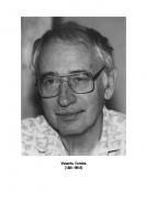
Metacomputation is a research area related to deep program transformation. The main problems addressed are program specialization (making use of partially known input data and other information about a program), program fusion (composing functions or program components of other kind), program inversion (constructing a program that computes input data from known or desired output results), program slicing (building a program that computes a subset of the source program’s results). Despite the fact that, initially, metacomputation was mainly considered as a technique for improving the efficiency of programs, later it has been found to be applicable to other areas, such as theorem proving, program verification, as well as various kinds of program analyses. The origins of metacomputation can be traced back to work by Lionello Lombardi on incremental computation in the 60s. The most known methods created in the 70s and 80s are supercompilation by Valentin Turchin, mixed computation by Andrei Ershov, partial evaluation by Neil Jones, (generalized ) partial computation by Yoshihiko Futamura, deforestation by Phil Wadler, partial deduction by Jan Komorowski, narrowing by Maria Alpuente et al. We mention just the initiators and research leaders in the field of metacomputation. Certainly, there are many other people who have contributed to the developments in this area and are doing active research related to metacomputation. While students, we were fortunate to witness the dawn of metacomputation. In Winter 1971/72 Valentin Turchin demonstrated at the Refal seminar in Keldysh Institute that applying a kind of partial evaluation to a simple interpreter produced the effect that could be seen as “compilation”. Two years later, in Fall 1974, he gave detailed lectures on supercompilation to a group of students who perceived the ideas with great enthusiasm. In 1976 V. F. Turchin met A. P. Ershov, who had come to Moscow from Novosibirsk in order to present the computer science community his ideas on mixed computation. Valentin Turchin and Andrei Ershov were pleased to discover they independently worked on close topics. V. F. Turchin showed A. P. Ershov three metasystem transition formulas describing the way of producing a compiled program, a compiler and a compiler compiler by supercompiling an interpreter and the supercompiler itself. A. P. Ershov demonstrated how his notion of generating extension is applicable to solving various system programming tasks including generation of a compiler. As a result of their contact the connection between the generating extension and the second Turchin’s formula had

been established (which was later referred to by A. P. Ershov as “the double run-through1 theorem by V. F. Turchin”2 ). At that time A. P. Ershov had found a reference to “a rather interesting, judging by the title, Y. Futamura’s paper”3 published in 1971 in a Japanese journal with limited availability. When the paper was finally obtained, a concise and elegant formulation of what was later called “the first and second Futamura projections” was found in it. Afterwards Andrei Ershov “infected” Neil Jones with the ideas, and soon his team in Copenhagen University had introduced a new idea of a preliminary “binding time analysis”, which radically simplified the machinery of partial evaluation and led to the first successful self-application of a specializer. This, in turn, gave an opportunity to make experiments with the Futamura projections demonstrating that they do work in practice and even produce results looking as “natural” from the human viewpoint. Thus, the area of metacomputation (although the term was not used yet) got its second wind and attracted the attention of the computer science community. Since then metacomputation has become a mature scientific discipline, many problems have been solved, a lot of new problems have been discovered, and first applications have been made. Nevertheless, metacomputation methods are not used by rank-and-file programmers yet, and a lot of work is to be done. The First International Workshop on Metacomputation in Russia will bring together researchers working in the areas of program analysis and program manipulation based on metacomputation. These pre-proceedings contain 13 papers accepted by the Program Committee. They represent the current state of research of Moscow and Pereslavl scientists belonging to the Turchin’s school of metacomputation as well as the achievements of our colleagues from Europe. The workshop is planned to have enough time for seriously discussing the papers and for panels on the wide topics of common interest. We are sure it will give new insights into the understanding of new methods and open problems. The papers are also available online at the workshop web site.4 It is our pleasure to extend our warm greetings and best wishes to our teacher Valentin Turchin, who, unfortunately, has no possibility to attend the workshop, but whose presence we always feel. June, 2008

1

2 3 4

Sergei Abramov Andrei Klimov Andrei Nemytykh Sergei Romanenko

“Run-through” is a literal translation for the Russian term “прогонка”, which is now usually rendered in English as “driving” and denotes one of the techniques used in supercompilation. A. P. Ershov, however, used the term “run-through” to refer to the supercompilation process as a whole. http://ershov.iis.nsk.su/archive/eaimage.asp?lang=2&did=27518&fileid=166648 http://ershov.iis.nsk.su/archive/eaimage.asp?did=27518&fileid=166664 http://meta2008.pereslavl.ru

Workshop Organization

Honorary Chairman Valentin Turchin, Professor Emeritus of The City University of New York, USA

Workshop Chair Sergei Abramov, Program Systems Institute of RAS, Russia

Program Committee Chair Andrei Nemytykh, Program Systems Institute of RAS, Russia

Program Committee Robert Gl¨ uck, University of Copenhagen, Denmark Geoff Hamilton, Dublin City University, Republic of Ireland Andrei Klimov, Keldysh Institute of Applied Mathematics of RAS, Russia Alexei Lisitsa, Liverpool University, Great Britain Sergei Romanenko, Keldysh Institute of Applied Mathematics of RAS, Russia

Sponsoring Institutions The Russian Academy of Sciences Russian Federal Agency of Science and Innovation (№ 2007-4-1.4-18-02-064) Russian Foundation for Basic Research (№ 08-07-06031-г)

Table of Contents

Constructing Programs From Metasystem Transition Proofs . . . . . . . . . . . . G. W. Hamilton, M. H. Kabir Interpretive Overhead and Optimal Specialisation. Or: Life without the Pending List . . . . . . . . . . . . . . . . . . . . . . . . . . . . . . . . . . . . . . . . . . . . . . . . . . Lars Hartmann, Neil D. Jones, Jakob Grue Simonsen The Language FLAC: Computational Model and Modularity . . . . . . . . . . . Victor L. Kistlerov

9

27 39

An Approach to Supercompilation for Object-oriented Languages: the Java Supercompiler Case Study . . . . . . . . . . . . . . . . . . . . . . . . . . . . . . . . . Andrei V. Klimov

43

A Program Specialization Relation Based on Supercompilation and its Properties . . . . . . . . . . . . . . . . . . . . . . . . . . . . . . . . . . . . . . . . . . . . . . . . . . . . . . . . Andrei V. Klimov

54

An Approach to Polyvariant Binding Time Analysis for a Stack-Based Language . . . . . . . . . . . . . . . . . . . . . . . . . . . . . . . . . . . . . . . . . . . . . . . . . . . . . . . . Yuri A. Klimov

78

XSG: Fair Language with Built-in Equality . . . . . . . . . . . . . . . . . . . . . . . . . . . Yuri A. Klimov, Anton Yu. Orlov

85

Verification as Specialization of Interpreters with Respect to Data . . . . . . . Alexei P. Lisitsa, Andrei P. Nemytykh

94

Supercompilation for Equivalence Testing in Metamorphic Computer Viruses Detection . . . . . . . . . . . . . . . . . . . . . . . . . . . . . . . . . . . . . . . . . . . . . . . . . 113 Alexei P. Lisitsa, Matt Webster An Experience with Term Rewriting for Program Verification . . . . . . . . . . . 119 Sergei D. Mechveliani On the Place of Supercompilation inside Program Specialization . . . . . . . . 131 Andrei P. Nemytykh Higher-Order Functions as a Substitute for Partial Evaluation (A Tutorial 145 Sergei A. Romanenko Data Abstraction in a Language of Multilevel Computations Based on Pattern Matching . . . . . . . . . . . . . . . . . . . . . . . . . . . . . . . . . . . . . . . . . . . . . . 163 Igor B. Shchenkov

Constructing Programs From Metasystem Transition Proofs G.W. Hamilton and M.H. Kabir School of Computing Dublin City University Dublin 9 IRELAND

Abstract. It has previously been shown by Turchin in the context of supercompilation how metasystem transitions can be used in the proof of universally and existentially quantified conjectures. Positive supercompilation is a variant of Turchin’s supercompilation which was introduced in an attempt to study and explain the essentials of Turchin’s supercompiler. In our own previous work, we have proposed a program transformation algorithm called distillation, which is more powerful than positive supercompilation, and have shown how this can be used to prove a wider range of universally and existentially quantified conjectures in our theorem prover Poit´ın. In this paper we show how a wide range of programs can be constructed fully automatically from first-order specifications through the use of metasystem transitions, and we prove that the constructed programs are totally correct with respect to their specifications. To our knowledge, this is the first technique which has been developed for the automatic construction of programs from their specifications using metasystem transitions.

1

Introduction

The construction of programs from their specifications is a difficult process which cannot always be performed fully automatically. In this paper, we show that if specifications are encoded in a specialised form, which we call distilled form, then we can construct programs meeting these specifications fully automatically. Distilled form is distinguished by creating no intermediate data structures; this means that existence proofs for specifications in distilled form will require no intermediate lemmas, and can therefore be performed fully automatically. Distilled form corresponds to the ‘read-only’ primitive recursive programs as defined by Jones [11], within which data can be higher-order. As shown in [11], this class of programs can be used to encode all problems which belong to the fairly wide class of elementary sets. In previous work [8], we proposed the distillation program transformation algorithm, which was originally devised with the goal of eliminating intermediate data structures from functional programs. The distillation algorithm was largely influenced by positive supercompilation [7] (a variant of Turchin’s supercompiler

10

G.W. Hamilton and M.H. Kabir

[25]), but improves greatly upon it. For example, positive supercompilation can only produce a linear speedup in programs with a call-by-name semantics, while distillation can produce a superlinear speedup. The form of programs generated by the distillation algorithm is precisely our distilled form. This suggests a twostep process for the construction of programs from their specifications: firstly, the specifications are transformed using distillation, then the distilled specifications are provided as input to a theorem prover which can automatically construct programs meeting these specifications. The step from a program to the application of a metaprogram to this program is a kind of metasystem transition [26,7]. Turchin has shown how metasystem transitions can be used in conjunction with supercompilation to prove explicitly quantified conjectures [24] by defining metaprograms for proving both universally and existentially quantified conjectures. However, he has not shown how programs can be constructed from these proofs. We have previously shown how techniques similar to those of Turchin can be used in conjunction with the distillation algorithm to prove a wider range of universally and existentially quantified conjectures using metasystem transitions in our theorem prover Poit´ın [12,14]. In this paper we show how programs can be constructed fully automatically from first-order specifications which are in distilled form through the use of metasystem transitions, and prove that the constructed programs are totally correct with respect to their specifications. To our knowledge, this is the first technique which has been developed for the automatic construction of programs from their specifications using metasystem transitions. The remainder of this paper is organised as follows. In Section 2, we describe the language which will be used throughout this paper. We give a brief overview of the distillation algorithm, and define the distilled form of expressions which is generated by the algorithm. In Section 3, we show how the Poit´ın theorem prover proves universally and existentially quantified conjectures through the use of metasystem transitions. We give an example proof and we show that the theorem prover is sound and complete for programs which are in distilled form. In Section 4, we show how programs can be constructed fully automatically from specifications which are in distilled form through the use of metasystem transitions. We give an example of this program construction and prove that the constructed programs are totally correct with respect to their specifications. Section 5 considers related work and concludes.

2

Distillation

In this section, we define the language used throughout this paper and we give a brief overview of the distillation algorithm. 2.1

Language

Definition 1 (Language). The language used throughout this paper is a simple higher-order functional language as shown in Fig. 1. □

Constructing Programs From Metasystem Transition Proofs

11

prog ::= e0 where f1 = e1 ; . . . ; fn = en ; program e ::= v variable | c e1 ... en constructor application | λv.e lambda abstraction |f function variable | e0 e1 application | case e0 of p1 ⇒ e1 | ... | pk ⇒ ek case expression | let v = e0 in e1 let expression | letrec f = e0 in e1 letrec expression p ::= c v1 . . . vn

pattern

Fig. 1. Language

Programs in the language consist of an expression to evaluate and a set of function definitions. It is assumed that the language is typed using the HindleyMilner polymorphic typing system (so erroneous terms such as (c e1 . . . en ) e and case (λv.e) of p1 ⇒ e1 | · · · | pk ⇒ ek cannot occur). The variables in the patterns of case expressions and the arguments of λ-abstractions are bound; all other variables are free. We use F V (e) to denote the free variables in the expression e. We require that each function has exactly one definition and that all variables within a definition are bound. The propositional operators (and , or , i mplies, etc.) are implemented as functions in this language. Each constructor has a fixed arity; for example Nil has arity 0 and Cons has arity 2. Within the expression case e0 of p1 ⇒ e1 | · · · | pk ⇒ ek , e0 is called the selector, and e1 . . . ek are called the branches. The patterns in case expressions may not be nested. Methods to transform case expressions with nested patterns to ones without nested patterns are described in [1,27]. No variables may appear more than once within a pattern. We assume that the patterns in a case expression are non-overlapping and exhaustive. An example program in the language is shown in Fig. 2. 2.2

Distillation

Distillation [8] is a powerful program transformation technique to remove intermediate data structures from higher-order functional programs and represents a significant advance over the positive supercompilation algorithm [7]. Using the positive supercompilation algorithm, it is only possible to obtain a linear improvement in the run-time performance of programs with a call-by-name semantics; with distillation it is possible to produce a superlinear improvement. This extra power is obtained by performing more than one transformation pass over terms, as opposed to the single pass performed by positive supercompilation. We do not give a full description of the distillation algorithm here; details can be found in [8]. These details are not required to understand the remainder

12

G.W. Hamilton and M.H. Kabir

implies (and (member y xs) (member z xs)) (leq y z ) where implies = λx .λy. case x of True ⇒ y | False ⇒ True and = λx .λy. case x of True ⇒ y | False ⇒ False member = λy.λxs. case xs of Nil ⇒ False | Cons x xs ⇒ case (eq x y) of True ⇒ True | False ⇒ member y xs leq = λx .λy. case x of Zero ⇒ True | Succ x ⇒ case y of Zero ⇒ False | Succ y ⇒ leq x y eq = λx .λy. case x of Zero ⇒ case y of Zero ⇒ True | Succ y ⇒ False | Succ x ⇒ case y of Zero ⇒ False | Succ y ⇒ eq x y

Fig. 2. Example Program

of this paper; it is sufficient to know that the expressions resulting from distillation are in a specialised form which we call distilled form. The logical rules presented in this paper are defined over this distilled form without the need to know how expressions are converted into this form. The transformation rules in distillation essentially perform normal-order reduction. Folding is performed when an expression is encountered which is an instance of a previously encountered expression, and generalization is performed to ensure termination of the transformation process. The terms which are compared before folding or generalizing in distillation are terms which have already been transformed; in positive supercompilation these will be untransformed terms. Generalization is performed when an expression is encountered within which a previously encountered expression is embedded. The form of embedding which we use to guide this generalization is the homeomorphic embedding relation which was derived from results by Higman [9] and Kruskal [18] and was defined within term rewriting systems [6] for detecting the possible divergence of the term rewriting process.

Constructing Programs From Metasystem Transition Proofs

2.3

13

Distilled Form

Definition 2 (Distilled Form). The expressions resulting from distillation are in distilled form dt{} , where within an expression of the form dtρ , ρ denotes the set of all variables which have been introduced using let expressions, and cannot therefore appear in the selectors of case expressions. Distilled form dtρ is defined as shown in Fig. 3. □

dt ρ ::= | | | | | |

v0 v 1 . . . vn c dt1ρ . . . dtnρ λv .dt ρ case v of p1 ⇒ dt1ρ | · · · | pk ⇒ dtkρ , where v ∈ /ρ (ρ∪{v }) let v = dt0ρ in dt1 letrec f = λv1 . . . vn .dt ρ in f v1 . . . vn f v 1 . . . vn

Fig. 3. Distilled Form

In addition, at least one of the parameters in every function definition must be decreasing; all functions which do not have this property are replaced by ⊥ during distillation, where ⊥ is treated as a constructor in our language. Variables which are introduced using let expressions cannot appear in the selectors of case expressions. Expressions in distilled form therefore create no intermediate structures. This means that proofs over expressions which are in distilled form will require no intermediate lemmas, and can therefore be performed fully automatically. Programs in distilled form correspond to the ‘read-only’ primitive recursive programs as defined in [11]. The program defined in Fig. 2 is transformed by distillation into the program shown in Fig. 4. Note that the variables xs, y and z are also free within this program. We can see that all the intermediate structures have been eliminated from this program.

3

Theorem Proving Using Metasystem Transitions

In this section, we show how the theorem prover Poit´ın handles explicit quantification using metasystem transitions. To facilitate this, we add quantifiers of the form ALL v.e and EX v.e to our language, where the quantified variable v must be first-order. These quantifiers are defined over the three-valued logic with values T rue, F alse and ⊥. The universally quantified expression ALL v.e has the value T rue if the expression e has the value T rue for all possible values of the quantified variable v, F alse if e has the value F alse for at least one value of v, and ⊥ if e has the value ⊥. The existentially quantified expression EX v.e has the value T rue if the expression e has the value T rue for at least one value of the

14

G.W. Hamilton and M.H. Kabir

case xs of Nil ⇒ True Cons x xs ⇒ letrec f = λx .λxs. case xs of Nil ⇒ letrec g = λx .λy.λz . case x of Zero ⇒ case y of Zero ⇒ True | Succ y ʹ ⇒ case z of Zero ⇒ False | Succ z ʹ ⇒ True Succ x ʹ ⇒ case y of Zero ⇒ False | Succ y ʹ ⇒ case z of Zero ⇒ True | Succ z ʹ ⇒ g x ʹ y ʹ z ʹ in g x y z Cons x ʹ xs ʹ ⇒ letrec h = λy.λz . case y of Zero ⇒ f x xs ʹ | Succ y ⇒ case z of Zero ⇒ f x ʹ xs ʹ | Succ z ⇒ h y z in h x x ʹ in f x xs

Fig. 4. Example Program Distilled

quantified variable v, F alse if e has the value F alse for all values of v, and ⊥ if e has the value ⊥. These quantifiers can be arbitrarily nested within an expression, provided that the expression is well-typed. The addition of these quantifiers into our language means that programs are no longer executable; however, the rules defined in this section show how these quantifiers can be eliminated to produce an executable program. We give the definitions of the sets of rules A for eliminating universal quantifiers and E for eliminating existential quantifiers which have been implemented in Poit´ın. More details of these rules, including examples of their application and a proof of their soundness, can be found in [15,12]. When a quantified expression is encountered by Poit´ın, the expression is first of all transformed by distillation. A metasystem transition is then used to apply inductive proof rules to the resulting distilled expression. If there are a number of nested quantifiers within the conjecture to be proved, then the proof rules are applied to the innermost quantified expression first. These inner

Constructing Programs From Metasystem Transition Proofs

15

quantified expressions may contain free variables, which will be bound by another quantifier in some outer scope. The expression resulting from the application of the proof rules may therefore also contain free variables if these were present in the original expression. We therefore construct a hierarchy of metasystems in which the construction of each subsequent level is achieved by a metasystem transition. All quantifiers will be eliminated in the final resulting expression. 3.1

Rules for Universal Quantification

The rules for proving a universally quantified conjecture e are of the form A[[e]] ρ ϕ σ as shown in Fig. 5, where the parameter ρ is an environment mapping local variables to their values, ϕ is the set of previously encountered function calls and σ is the set of universally quantified variables. Note that these rules will only be applied to expressions which are in distilled form. Using these rules, the local variables contained within the domain of ρ and the universally quantified variables contained within σ are eliminated, and a simplified expression defined over the remaining free variables is obtained. If there are no free variables, then the input conjecture is reduced to a value in our three-valued logic. In rule (A1), if a local variable is encountered, then the value of this variable in the environment ρ is substituted for it and the resulting expression is further simplified using the proof rules. If a universally quantified variable is encountered, then since it must have a value in our three-valued logic, the value F alse is returned as the variable cannot always have the value T rue. If a free variable is encountered, then it remains unchanged. In rule (A2), if a constructor is encountered, then the value of this constructor is returned; this must be a value in our three-valued logic, since the input term is also of this type and contains no intermediate structures. In rule (A3), if a λ-abstraction is encountered, then the body of the abstraction is further simplified. In rule (A4), if we encounter a case expression then, since this expression must be in distilled form, the redex must be a non-local variable. If this variable is universally quantified, then a case split is performed in which we prove the current term separately for each of the possible values of the selector, and then return the conjunction of the resulting values. The different possible values of the selector are simply the patterns within the case expression. If the redex variable is not universally quantified, then it must be free, so it remains in the resulting term, and the proof rules are further applied to the branches of the case expression. In rule (A5), if we encounter a let expression and none of the variables in the extracted expression are free, then the proof rules are applied to the extracted expression and the resulting value for the let variable is added to the environment ρ before applying the proof rules to the generalized expression. If the extracted expression contains free variables, then the proof rules are applied to each of the sub-expressions within the let. In rule (A6), if we encounter a letrec function definition and none of the parameters in the initial application of this function are free, then this function application is a potential inductive hypothesis. Since at least one of these parameters must be decreasing, this parameter can be used as the induction variable. If we subsequently encounter a recursive call of this

16

G.W. Hamilton and M.H. Kabir

A[[v0 v1 . . . vn ]] ρ ϕ σ = A[[e[v1 /v1ʹ . . . vn /vnʹ ]]] ρ ϕ σ, if ρ(v0 ) = λv1ʹ . . . vnʹ .e = F alse, if v0 ∈ σ = v0 v1 . . . v n , otherwise

(A1)

A[[c]] ρ ϕ σ = c

(A2)

A[[λv.e]] ρ ϕ σ = λv.A[[e]] ρ ϕ σ

(A3)

A[[case v of p1 : eʹ1 | . . . | pk : eʹk ]] ρ ϕ σ (A4) = (A[[eʹ1 ]] ρ ϕ σ1 ) ∧ . . . ∧ (A[[eʹk ]] ρ ϕ σk ), if v ∈ σ = case v of p1 : (A[[eʹ1 ]] ρ ϕ σ) | . . . | pk : (A[[eʹk ]] ρ ϕ σ), otherwise where σi = σ ∪ F V (pi ) A[[let v = e0 in e1 ]] ρ ϕ σ (A5) = A[[e1 ]] ρ[(A[[e0 ]] ρ ϕ σ)/v] ϕ σ, if F V (e0 ) ⊆ (dom(ρ) ∪ σ) = let v = (A[[e0 ]] ρ ϕ σ) in (A[[e1 ]] ρ ϕ σ), otherwise A[[letrec f = λv1 . . . vn .e0 in f v1ʹ . . . vnʹ ]] ρ ϕ σ (A6) = eʹ0 , if {v1ʹ . . . vnʹ } ⊆ (dom(ρ) ∪ σ) = letrec f = λv1ʹʹ . . . vkʹʹ .eʹ0 in f v1ʹʹ . . . vkʹʹ , otherwise where eʹ0 = A[[e0 ]] ρ (ϕ ∪ {f v1ʹ . . . vnʹ }) σ {v1ʹʹ . . . vkʹʹ } = {v1ʹ . . . vnʹ } \ (dom(ρ) ∪ σ) A[[f v1 . . . vn ]] ρ ϕ σ = T rue, if {v1ʹ . . . vnʹ } ⊆ (dom(ρ) ∪ σ) = (f v1ʹʹ . . . vkʹʹ )[v1 /v1ʹ . . . vn /vnʹ ], otherwise where (f v1ʹ . . . vnʹ ) ∈ ϕ {v1ʹʹ . . . vkʹʹ } = {v1ʹ . . . vnʹ } \ (dom(ρ) ∪ σ)

(A7)

Fig. 5. Proof Rules for Universal Quantification

function in rule (A7), then we have re-encountered this inductive hypothesis, so the value True is returned. If a function definition contains free variables, then the function is re-defined over these free variables. As an example of the application of these rules, consider the expression ALL z.e where e is the program defined in Fig. 2. We first of all apply distillation to the expression e, yielding the distilled expression eʹ as shown in Fig. 4. We then apply the universal proof rules A[[eʹ ]] {} {} {z} for the universal variable z giving the program shown in Fig. 6. We can see that the variable z has been eliminated, and the variables xs and y are still free within the resulting program.

Constructing Programs From Metasystem Transition Proofs

case xs of Nil ⇒ True Cons x xs ⇒ letrec f = λx .λxs. case xs of Nil

17

⇒ letrec g = λx .λy. case x of Zero

⇒ case y of Zero | Succ y ʹ | Succ x ʹ ⇒ case y of Zero | Succ y ʹ

⇒ True ⇒ False ⇒ False ⇒ g x ʹ yʹ

in g x y | Cons x ʹ xs ʹ ⇒ letrec h = λy.λz . case y of Zero ⇒ f x xs ʹ | Succ y ⇒ case z of Zero ⇒ f x ʹ xs ʹ | Succ z ⇒ h y z in h x x ʹ in f x xs

Fig. 6. Program Resulting From Application of Universal Proof Rules

3.2

Rules for Existential Quantification

The rules for proving an existentially quantified conjecture e are of the form E[[e]] ρ ϕ σ as shown in Fig. 7, where the parameter ρ is an environment mapping local variables to their values, ϕ is the set of previously encountered function calls and σ is the set of existentially quantified variables. Using these rules, the local variables contained within the domain of ρ and the existentially quantified variables contained within σ are eliminated, and a simplified expression over the remaining free variables is obtained. The rules are similar to those for universal quantification, with the only major differences being in rules (E1), (E4), (E6) and (E7). In rule (E1), if an existentially quantified variable is encountered, then since it must have a value in our three-valued logic, the value True is returned as the value of the variable can be T rue. In rule (E4), if the redex in a case expression is an existentially quantified variable, then we also perform a case split and prove the current term separately for each of the possible values of the selector, but in this instance we return the disjunction of the resulting values. In rules (E6) and (E7), function applications are no longer possible inductive hypotheses as they contain existential variables. However, if none of the parameters in a function application are

18

G.W. Hamilton and M.H. Kabir

E[[v0 v1 . . . vn ]] ρ ϕ σ = E[[e[v1 /v1ʹ . . . vn /vnʹ ]]] ρ ϕ σ, if ρ(v0 ) = λv1ʹ . . . vnʹ .e = T rue, if v0 ∈ σ = v0 v1 . . . v n , otherwise

(E1)

E[[c]] ρ ϕ σ = c

(E2)

E[[λv.e]] ρ ϕ σ = λv.E[[e]] ρ ϕ σ

(E3)

E[[case v of p1 : eʹ1 | . . . | pk : eʹk ]] ρ ϕ σ (E4) = (E[[eʹ1 ]] ρ ϕ σ1 ) ∨ . . . ∨ (E[[eʹk ]] ρ ϕ σk ), if v ∈ σ = case v of p1 : (E[[eʹ1 ]] ρ ϕ σ) | . . . | pk : (E[[eʹk ]] ρ ϕ σ), otherwise where σi = σ ∪ F V (pi ) E[[let v = e0 in e1 ]] ρ ϕ σ (E5) = E[[e1 ]] ρ[(E[[e0 ]] ρ ϕ σ)/v] ϕ σ, if F V (e0 ) ⊆ (dom(ρ) ∪ σ) = let v = (E[[e0 ]] ρ ϕ σ) in (E[[e1 ]] ρ ϕ σ), otherwise E[[letrec f = λv1 . . . vn .e0 in f v1ʹ . . . vnʹ ]] ρ ϕ σ (E6) = eʹ0 , if {v1ʹ . . . vnʹ } ⊆ (dom(ρ) ∪ σ) = letrec f = λv1ʹʹ . . . vkʹʹ .eʹ0 in f v1ʹʹ . . . vkʹʹ , otherwise where eʹ0 = E[[e0 ]] ρ (ϕ ∪ {f v1ʹ . . . vnʹ }) σ {v1ʹʹ . . . vkʹʹ } = {v1ʹ . . . vnʹ } \ (dom(ρ) ∪ σ) E[[f v1 . . . vn ]] ρ ϕ σ = F alse, if {v1ʹ . . . vnʹ } ⊆ (dom(ρ) ∪ σ) = (f v1ʹʹ . . . vkʹʹ )[v1 /v1ʹ . . . vn /vnʹ ], otherwise where (f v1ʹ . . . vnʹ ) ∈ ϕ {v1ʹʹ . . . vkʹʹ } = {v1ʹ . . . vnʹ } \ (dom(ρ) ∪ σ)

(E7)

Fig. 7. Proof Rules for Existential Quantification

free then the value False is returned as we know that the search space of the existential variables has been exhausted. As an example of the application of these rules, consider the proof of the conjecture ALL xs.EX y.ALL z.e where e is the program defined in Fig. 2. We first of all apply distillation to the expression e, yielding the distilled expression eʹ as shown in Fig. 4. We then apply the universal proof rules as shown above to the expression ALL z.eʹ , giving the expression eʹʹ shown in Fig. 6. The existential proof rules E[[eʹʹ ]] {} {} {y} are then applied for the existential variable y giving the program shown in Fig. 8.

Constructing Programs From Metasystem Transition Proofs

19

case xs of Nil ⇒ True Cons x xs ⇒ letrec f = λx .λxs. case xs of Nil

⇒ letrec g = λv . case v of Zero ⇒ | Succ v ⇒ in g x | Cons x ʹ xs ʹ ⇒ letrec h = λy.λz . case y of Zero | Succ y

True g v

⇒ f x xs ʹ ⇒ case z of Zero ⇒ f x ʹ xs ʹ | Succ z ⇒ h y z

in h x x ʹ in f x xs

Fig. 8. Program Resulting From Application of Existential Proof Rules We can see that the variable y has been eliminated and that the variable xs is still free. We then apply the universal proof rules A[[eʹʹʹ ]] {} {} {xs} where eʹʹʹ is the expression shown in Fig. 8 and xs is the universally quantified variable, giving the value True as required. 3.3

Soundness and Relative Completeness

In this section, we consider the soundness and relative completeness of our theorem prover. Full details of the proofs of these properties can be found in [15,12]; we do not include these here. To facilitate these proofs, sequent calculus rules are defined for the distilled form of conjecture which is input to our theorem prover. Note that there is no need for a cut rule as all the intermediate structures in the input conjecture will have been eliminated. Our proof rules are proved to be sound by showing that all conjectures in distilled form which are found to have the value T rue using our proof rules can also be proved using the sequent calculus rules. Theorem 1 (Soundness of Universal Proof Rules). A[[e]] {} ϕ {v1 . . . vn } = T rue ∧ e ∈ dt{} ⇒ ϕ ⊢ ALL v1 . . . vn .e

□

Theorem 2 (Soundness of Existential Proof Rules). E[[e]] {} ϕ {v1 . . . vn } = T rue ∧ e ∈ dt{} ⇒ ϕ ⊢ EX v1 . . . vn .e

□

Our proof rules are proved to be complete for all conjectures which are in distilled form by showing that all conjectures in distilled form which can be proved using the sequent calculus rules also have the value T rue using our proof rules.

20

G.W. Hamilton and M.H. Kabir

Theorem 3 (Relative Completeness of Universal Proof Rules). ϕ ⊢ ALL v1 . . . vn .e ∧ e ∈ dt{} ⇒ A[[e]] {} ϕ {v1 . . . vn } = T rue

□

Theorem 4 (Relative Completeness of Existential Proof Rules). ϕ ⊢ EX v1 . . . vn .e ∧ e ∈ dt{} ⇒ E[[e]] {} ϕ {v1 . . . vn } = T rue

□

The proofs of each of these theorems are by recursion induction on the rules A and E. Details of the proofs can be found in [15,12].

4

Program Construction Using Metasystem Transitions

In this section, we present our novel technique for the construction of programs from specifications. The constructed programs essentially compute the existential witness of the proof of their corresponding specification. To facilitate this, we add specifications of the form ANY v.e to our language, where the quantified variable v must be first-order. The specification ANY v.e can have any value of the quantified variable v for which the expression e has the value T rue; if no such value exists, then it has the undefined value ⊥. The variable v is therefore implicitly existentially quantified within e, but the ANY quantifier differs from the existential quantifier EX in that it has the same type as the variable v, rather than being a vlaue in our three-valued logic. When a specification ANY v.e is encountered by Poit´ın, the quantified expression e is first of all transformed using distillation. A metasystem transition is then used to apply the rules for program construction to the resulting distilled expression, thus constructing an executable program form a non-executable specification. 4.1

Rules for Program Construction

The program construction rules are defined by C[[e]] [[eʹ ]] ϕ σ as shown in Fig. 9, where the expression e is the distilled specification, eʹ is the existential witness, ϕ is the set of the previously encountered function calls and σ is the set of universally quantified variables. For a specification ANY v.e, the quantified variable v is passed as the initial existential witness and the free variables in the specification are passed as the initial set of universally quantified variables. In rule (C1), if a universally quantified variable is encountered, then since it must be a value in our three-valued logic, the value ⊥ is returned as the variable cannot have the value T rue. Otherwise, the value of the variable is returned unchanged. In rule (C2), if we encounter a constructor, then if this constructor is True and the existential witness is fully instantiated, the value of the existential witness is returned. Otherwise, the value ⊥ is returned. In rule (C3), if a λ-abstraction is encountered, then the program construction rules are applied to the body of the abstraction. In rule (C4), if we encounter a case expression then, since this expression must be in distilled form, the redex must be a non-local variable. If this variable is universally quantified, then it remains within the expression and the program construction rules are further applied to the branches

Constructing Programs From Metasystem Transition Proofs

21

C[[v0 v1 . . . vn ]][[e]] ϕ σ = ⊥, if v0 ∈ σ = v0 v1 . . . vn , otherwise

(C1)

C[[c]][[e]] ϕ σ = e, if c = T rue ∧ F V (e) = {} = ⊥,otherwise

(C2)

C[[λv .e]][[e ʹ ]] ϕ σ = λv .C[[e]][[e ʹ ]] ϕ σ

(C3)

C[[case v of p1 ⇒ e1 | · · · | pn ⇒ en ]][[e]] ϕ σ = case v of p1 ⇒ (C[[e1 ]][[e]] ϕ σ1 ) | · · · | pn ⇒ (C[[en ]][[e]] ϕ σn ), if v ∈ σ = (C[[e1 ]][[e[p1 /v ]]] ϕ σ) ⊔ . . . ⊔ (C[[en ]][[e[pn /v ]]] ϕ σ), otherwise where σi = σ ∪ F V (pi )

(C4)

C[[let v = e0 in e1 ]][[e]] ϕ σ = let v = (C[[e0 ]][[e]] ϕ σ) in (C[[e1 ]][[e]] ϕ σ)

(C5)

C[[letrec f = λv1 . . . vn .e0 in f v1ʹ . . . vnʹ ]][[v ]] ϕ σ = eʹ0 , if {v1ʹ . . . vnʹ } ∩ σ = {} ʹʹ ʹʹ ʹ ʹʹ ʹʹ = letrec f = λv1 . . . vk .e0 in f v1 . . . vk , otherwise where eʹ0 = C[[e0 ]][[v ]] (ϕ ∪ {f v1ʹ . . . vnʹ }) σ {v1ʹʹ . . . vkʹʹ } = {v1ʹ . . . vnʹ } ∩ σ

(C6)

C[[letrec f = λv1 . . . vn .e0 in f v1ʹ . . . vnʹ ]][[c e1 . . . ek ]] ϕ σ (C7) = C[[e0 ]][[c e1 . . . ek ]] (ϕ ∪ {f v1ʹ . . . vnʹ }) σ, if {v1ʹ . . . vnʹ } ∩ σ = {} = c (C[[letrec f = λv1 . . . vn .e0 in f v1ʹ . . . vnʹ ]][[e1 ]] ϕ σ) otherwise . . . (C[[letrec f = λv1 . . . vn .e0 in f v1ʹ . . . vnʹ ]][[ek ]] ϕ σ), C[[f v1 . . . vn ]][[v ]] ϕ σ = ⊥, if {v1ʹ . . . vnʹ } ∩ σ = {} ʹʹ ʹʹ ʹ ʹ = f v1 . . . vk [v1 /v1 . . . vn /vn ], otherwise where (f v1ʹ . . . vnʹ ) ∈ ϕ {v1ʹʹ . . . vkʹʹ } = {v1ʹ . . . vnʹ } ∩ σ

(C8)

C[[f v1 . . . vn ]][[c e1 . . . ek ]] ϕ σ = ⊥, if {v1ʹ . . . vnʹ } ∩ σ = {} = c (C[[f v1 . . . vn ]][[e1 ]] ϕ σ) . . . (C[[f v1 . . . vn ]][[ek ]] ϕ σ), otherwise

(C9)

Fig. 9. Rules for Program Construction

of the case expression. Before transforming each branch, the corresponding pattern variables are added to σ as they are also implicitly universally quantified. If the selector is existentially quantified, existential witnesses are constructed for each of the branches separately. These witnesses will be constructed using the corresponding patterns which give the value of the selector within the branch.

22

G.W. Hamilton and M.H. Kabir

The existential witness for the overall expression is then given by the least upper bound of these existential witnesses for each branch (the least upper bound operator ⊔ is defined separately for each of the data types in our language). In rule (C5), if we encounter a let expression, then the program construction rules are applied to each of the sub-expressions contained within it. In rules (C6)-(C9), if we encounter a recursive function call, then this is simplified to be defined over only the universal variables of this call. If the recursive call does not contain any universally quantified variables, then the value ⊥ is returned as the search space of the existential variables has been exhausted.

4.2

Example

In this section, we give an example of the application of our program construction rules. Consider the construction of a program from the specification ANY y. ALL z.e where e is the program defined in Fig. 2. We first of all apply distillation to the expression e, yielding the distilled expression eʹ as shown in Figure 4. We then apply the universal proof rules as shown previously to the expression ALL z.eʹ , giving the expression eʹʹ as shown in Fig. 6. We then apply the program construction rules C[[eʹʹ ]][[y]] {} {xs} where y is the existential witness and xs is the only free variable in eʹʹ , giving the program shown in Fig. 10.

case xs of Nil ⇒⊥ Cons x xs ⇒ letrec f = λx .λxs. case xs of Nil

⇒ letrec g = λv . case v of Zero ⇒ | Succ v ⇒ in g x | Cons x ʹ xs ʹ ⇒ letrec h = λy.λz . case y of Zero | Succ y

Zero Succ (g v )

⇒ f x xs ʹ ⇒ case z of Zero ⇒ f x ʹ xs ʹ | Succ z ⇒ h y z

in h x x ʹ in f x xs

Fig. 10. Program Resulting From Application of Program Construction Rules

Constructing Programs From Metasystem Transition Proofs

23

From this, we can see that we have generated a program for finding the smallest element in the list xs fully automatically from the specification, and that this program creates no intermediate data structures. 4.3

Correctness of Constructed Programs

In order to prove that the programs constructed by our program construction rules are correct with respect to the original specification ANY v.e we need to show that when the constructed existential witnesses are substituted for the existential variables in the specification, then the specification statement has the value T rue. Theorem 5 (Correctness of Constructed Programs). C[[e]][[e ʹ ]] ϕ σ = eʹ [e1 /v1 . . . en /vn ] ⇒ A[[e[e1 /v1 . . . en /vn ]]] {} ϕ σ = T rue where {v1 . . . vn } = F V (eʹ )

□

The proof is by recursion induction on the rules C. Full details of the proof can be found in [13,12].

5

Conclusion and Related Work

In this paper, we have shown how metasystem transitions can be used in conjunction with the distillation transformation algorithm to prove a wide range of theorems in first-order logic fully automatically. The programs generated by distillation are in distilled form; they create no intermediate structures, and correspond to the ‘read-only’ primitive recursive programs [11], within which data can be higher-order. As shown in [11], this form can be used to encode all problems which belong to the fairly wide class of elementary sets. We have shown that our theorem prover is sound and complete for theorems which are in this form. We then showed how programs can be constructed fully automatically from specifications which are in this form through the use of metasystem transitions. We have given an example of the application of our approach, and proved that the constructed programs are totally correct with respect to their specifications. The most closely related work to that presented here is Turchin’s work on supercompilation [25]. Turchin has shown how metasystem transitions can be used in conjunction with supercompilation to prove explicitly quantified conjectures [26], but has not shown how programs can be constructed from their specifications using metasystem transitions. To our knowledge, the techniques described in this paper are the first which have been developed for the automatic construction of programs from their specifications using metasystem transitions. Distillation is more powerful than positive supercompilation [7], removing more intermediate structures. The presence of more intermediate structures implies the need for more intermediate lemmas when theorem proving. The set of theorems which can be proved fully automatically using positive supercompilation is therefore a subset of those which can be proved fully automatically using distillation.

24

G.W. Hamilton and M.H. Kabir

The transformation of logic programs can be regarded as the construction of programs from specifications which contain implicit existential quantification. There has been a considerable amount of work on the use of logic program transformation for inductive theorem proving (for example, [22,23,19]). Many of these techniques are not fully automatic, and their fully automated components are of similar power to supercompilation, so they will not be able to prove as many theorems fully automatically as the technique described in this paper. A wide range of inductive theorem proving systems have been developed (for example, NQTHM [4], CLAM [5], INKA [3], RRL [16]), but these tend to concentrate mainly on universal quantification, and therefore cannot be used for program synthesis. The inclusion of existential quantification is very problematic and greatly complicates the theorem proving process. Some techniques which have been developed for program synthesis from non-executable specifications include constructive synthesis, deductive synthesis and middle-out reasoning. Constructive synthesis (e.g. [2]) is based on the Curry-Howard isomorphism [10] and uses the proof-as-programs principle. In this approach, a proof is constructed in a constructive type theory such as that of Martin-L¨ of [21]. There is a one-to-one relationship between this constructive proof and the corresponding program, which can be easily extracted from the proof. Deductive synthesis (e.g. [20]) attempts to derive an executable program from a high level specification by applying rules of inference. For example, the approach of Manna and Waldinger [20] incorporates ideas from resolution and inductive theorem proving as rules of inference. Middle-out reasoning (e.g. [17]) represents undefined functions in the synthesis conjecture as meta-variables. These meta-variables are instantiated gradually as the subsequent proof takes place. When the proof is complete, the meta-variables should be instantiated to the correct corresponding program. The programs constructed using the above techniques can often be quite inefficient. The programs constructed using our technique will construct no intermediate structures and should therefore be more efficient. Also, none of the above techniques for program construction are fully automatic and may therefore require user guidance. Although it may be argued that the additional lemmas which are required using these techniques can themselves be automated, the techniques can never be fully automatic as it will never be possible to encode all possible lemmas within them. However, it will of course be possible to construct some programs using these techniques which cannot be constructed using the technique described in this paper. Research is still continuing on determining the class of specifications which can be transformed by distillation into distilled form to allow programs to be constructed automatically from them using our technique.

References 1. L. Augustsson. Compiling Pattern Matching. In Functional Programming Languages and Computer Architecture, volume 201 of Lecture Notes in Computer Science, pages 368–381. Springer-Verlag, 1985.

Constructing Programs From Metasystem Transition Proofs

25

2. J.L. Bates and R.L. Constable. Proofs as Programs. ACM Transactions on Programming Languages and Systems, 7(1):113–136, January 1985. 3. S. Biundo, B. Hummel, D. Hutter, and C. Walther. The Karlrsruhe Induction Theorem Proving System. Lecture Notes in Computer Science, 230:672–674, 1987. 4. R.S. Boyer and J.S. Moore. A Computational Logic. Academic Press, 1979. 5. Alan Bundy, Frank Van Harmelen, Christian Horn, and Alan Smaill. The OysterCLAM System. In Proceedings of the 10th International Conference on Automated Deduction, pages 647–648, 1990. 6. N. Dershowitz and J.-P. Jouannaud. Rewrite Systems. In J. van Leeuwen, editor, Handbook of Theoretical Computer Science, pages 243–320. Elsevier, MIT Press, 1990. 7. Robert Gl¨ uck and Morten Heine Sørensen. A Roadmap to Metacomputation by Supercompilation. In Partial Evaluation, volume 1110 of Lecture Notes in Computer Science, pages 137–160. Springer-Verlag, 1996. 8. G.W. Hamilton. Distillation: Extracting the Essence of Programs. In Proceedings of the ACM SIGPLAN Symposium on Partial Evaluation and Semantics-Based Program Manipulation, pages 61–70, 2007. 9. G. Higman. Ordering by Divisibility in Abstract Algebras. Proceedings of the London Mathemtical Society, 2:326–336, 1952. 10. W.A. Howard. The Formulae-as-Types Notion of Construction. In To H.B. Curry: Essays on Combinatory Logic, Lambda Calculus and Formalism, pages 479–490. Academic Press, 1980. 11. N.D. Jones. The Expressive Power of Higher-Order Types or, Life Without CONS. Journal of Functional Programming, 11(1):55–94, January 2001. 12. M.H. Kabir. Automatic Inductive Theorem Proving and Program Construction Methods Using Program Transformation. PhD thesis, School of Computing, Dublin City University, October 2007. 13. M.H. Kabir and G.W. Hamilton. Constructing Programs From Metasystem Transition Proofs. Working Paper CA07-02, School of Computing, Dublin City University, 2007. 14. M.H. Kabir and G.W. Hamilton. Extending Poit´ın to Handle Explicit Quantification. In Proceedings of the Sixth International Workshop on First-Order Theorem Proving, pages 20–34, 2007. 15. M.H. Kabir and G.W. Hamilton. Extending Poit´ın to Handle Explicit Quantification. Working Paper CA07-01, School of Computing, Dublin City University, 2007. 16. Deepak Kapur, G. Sivakumar, and Hantao Zhang. RRL: A Rewrite Rule Laboratory. Lecture Notes in Computer Science, 230:691–692, 1986. 17. I. Kraan, D. Basin, and A. Bundy. Middle-Out Reasoning For Synthesis and Induction. Journal of Automated Reasoning, 16(1–2):113–145, 1996. 18. J.B. Kruskal. Well-Quasi Ordering, the Tree Theorem, and Vazsonyi’s Conjecture. Transactions of the American Mathematical Society, 95:210–225, 1960. 19. Helko Lehmann and Michael Leuschel. Inductive Theorem Proving by Program Specialisation: Generating Proofs for Isabelle Using Ecce. In 13th International Symposium on Logic Based Program Synthesis and Transformation, pages 1–19, 2003. 20. Z. Manna and R. Waldinger. A Deductive Approach to Program Synthesis. ACM Transactions on Programming Languages and Systems, 2(1):90–121, January 1980. 21. P. Martin-L¨ of. Constructive Mathematics and Computer Programming. Logic, Methodology and Philosophy of Science, VI:153–175, 1980.

26

G.W. Hamilton and M.H. Kabir

22. Alberto Pettorossi and Maurizio Proietti. Synthesis and Transformation of Logic Programs Using Unfold/Fold Proofs. Journal of Logic Programming, 41(2–3):197– 230, 1999. 23. Abhik Roychoudhury, K. Narayan Kumar, C. R. Ramakrishnan, and I. V. Ramakrishnan. Proofs by Program Transformation. In International Symposium on Logic Based Program Synthesis and Transformation, 1999. 24. V.F. Turchin. The Use of Metasystem Transition in Theorem Proving and Program Optimization. Lecture Notes in Computer Science, 85:645 – 657, 1980. 25. V.F. Turchin. The Concept of a Supercompiler. ACM Transactions on Programming Languages and Systems, 8(3):90–121, July 1986. 26. V.F. Turchin. Metacomputation: Metasystem Transitions plus Supercompilation. Lecture Notes in Computer Science, 1110:481–509, 1996. 27. P. Wadler. Efficient Compilation of Pattern Matching. In S.L. Peyton Jones, editor, The Implementation of Functional Programming Languages, pages 78–103. Prentice Hall, 1987.

Interpretive Overhead and Optimal Specialisation. Or: Life without the Pending List (Workshop Version) Lars Hartmann, Neil D. Jones, Jakob Grue Simonsen DIKU (Computer Science Dept., University of Copenhagen, Denmark)

Abstract. A self-interpreter and a program specialiser with the following characteristics are developed for a simple imperative language: 1) The self-interpreter runs with program-independent interpretive overhead; 2) the specialiser achieves optimal specialisation, that is, it eliminates all interpretation overhead; 3) the specialiser has been run on a variety of small and large programs, including specialising the selfinterpreter to itself; 4) all specialiser parts except for loop unfolding have been proven to terminate. We achieve the above by using a structured language with separated control and data flow, containing loops but without while. The specialiser uses two-level binding-time annotations in a new way: source annotations are used to ensure correctness of specialised programs. A novelty: the specialiser has no need for a pending list, and does no call graph analysis of the residual program. A source-to-source normalisation phase does program transformations to avoid situations where the specialiser would need to specialise code based on an unknown state. A pruning phase efficiently achieves the effect of Romanenko’s arity raising.

Two interesting lines of work concern self-interpreters for programming languages. One line is to develop a self-interpreter with program-independent interpretation overhead; this was the basis for the linear-time complexity hierarchy of [27,25,14,16,24,4]. Another line is to develop a program specialiser1 and a self-interpreter that allow optimal program specialisation, a measure of the strength/quality of a program specialiser, discussed in [18] Sections 6.4 and 8.5.1, and in [9,8,10,19,28]2 . The technical breakthrough for each line was to construct a self-interpreter with a certain property. We know of no prior self interpreter sint that simultaneously possesses both properties: – sint runs programs with program-independent overhead; and – sint can be specialised optimally. 1 2

Also known as a partial evaluator. As known from many fields, “optimality” is a very slippery concept. The formulation for the strength/quality of a specialiser in [18] turned out to be practically useful, and has since been dubbed Jones-optimality.

28

Lars Hartmann, Neil D. Jones, Jakob Grue Simonsen

The above was our initial goal. Bottom line: the goal was achieved (see [11] for details) and, along the way, new insights were gained into the control structure of specialised programs; relations between binding-time annotations, conditionals and loop unfolding rules; the use of program transformation to allow more liberal unfolding; and how to specialise programs with tree-structured values.

1

Programming languages, interpretation overhead and optimality

Basics. Program specialisation, or partial evaluation, is a well-established automatic program transformation [18,6]. Its purpose is to speed up programs by exploiting partial, compile-time, knowledge of the subject program’s run-time input. Standard jargon is to use the term static for that part of the program’s input known at specialisation time, and dynamic for that part of the input only known at run-time. We briefly recapitulate central notions concerning interpreters and specialisers; for an in-depth coverage, the reader is referred to [18,16]. A programming language L consists of a set of programs Prog, a set of data D, and a semantic function [[ ]] : Prog → (D ⇀ D) that assigns to each p ∈ Prog a partial input-output function [[p]] : D ⇀ D. A timed programming language has in addition a function time p (d) assigning a running time (a positive integer) to each input, such that [[p]](d) is defined if and only if time p (d) is defined. We further assume that the data set is closed under pairing, meaning D×D ⊆ . D; and that the language has concrete syntax, meaning Prog ⊆ D. Write d1 = d2 to indicate partial equality: that both sides are undefined, or both sides are defined and equal. Interpretation and its overhead. A self-interpreter is a program sint that satisfies . ∀p∀d([[sint]](p, d) = [[p]](d)) The interpretation overhead can be measured by the ratio overhead sint (p, d) = time sint (p, d)/time p (d) In general practice, a self-interpreter will satisfy ∀p∃c∀d( overhead sint (p, d) ≤ c ) that is, interpreting a program incurs (at most) a slowdown of a factor of c in relation to running the program natively. Factor c can depend on p, so the overhead is program-dependent in general. Typical causes of program-dependent overhead can be the need for the interpreter to look up variables in a run-time store, or to find the target of a function call or a goto command.

Interpretive Overhead and Optimal Specialisation

29

We say that the self-interpreter has program-independent interpretation overhead if the overhead does not depend on the program p, that is, the following holds (note the changed order of the quantifiers): ∃c∀p∀d( overhead sint (p, d) ≤ c ) Such an interpreter is called “efficient” (see e.g. [16, Def. 19.1.1]). There exist efficient self-interpreters, e.g., for structured programs with only one variable. This has been proven in [14,16,2,24] where it is shown to lead to a complexity-theoretic linear hierarchy theorem: that even within linear time, for such a language, increasing an allowed running time bound properly increases the class of decision problems that can be solved within the given bound. Specialisation and optimality. A program specialiser is a program spec that satisfies . ∀p∀s∀d([[[[spec]](p, s)]](d) = [[p]](s, d)) We call [[spec]](p, s) the specialised program, and denote it for short by ps . In general practice, the result of program specialisation will satisfy : ∀p∃cʹ ∀s∀d( speedup p (s, d) ≥ cʹ ) where speedup p (s, d) =

time p (s, d) time ps (d)

The point of specialisation is speedup: ps may be substantially faster than p. The optimality criterion arose as a precise criterion for being able to state that a partial evaluator is “good enough”, that is, able to remove as much static overhead as can reasonably be expected. This criterion is rather vague, but as specialisers have been much applied to program interpreters as well-known examples of programs with significantly large static overheads, the following more precise—and ambitious—criterion can be stated: Given a self-interpreter sint, the specialiser should ideally be able to remove all interpretation overhead. Technically, this can be formulated as follows: given a program p, construct program pʹ = [[spec]](sint, p) by specialisation. It is straightforward to see that this transformed program is semantically equivalent to p, i.e., that [[pʹ ]] = [[p]]. The specialiser is called optimal (Definition 6.4 of [18]) if pʹ is always at least as fast as p, that is, for all input data d we have timep (d) ≥ time pʹ (d) Another way to say this is: speedup sint (p, d) ≥ overhead sint (p, d) In words: pʹ suffers from none of the overhead that was introduced by use of the interpreter sint. This goal, while often stated, is not often achieved. Remark: optimality is more a property of the strength of the specialiser than of the self-interpreter.

30

2

Lars Hartmann, Neil D. Jones, Jakob Grue Simonsen

Designing LOOP

Our two goals: program-independent interpretation overhead and optimal specialisation. The program-independent requirement on interpretation overhead is quite stringent: It rules out the use of an unbounded number of program variables as it would take program-dependent time to search the store or value environment; and it also rules out the use of unstructured control such as goto or calls to named functions, as these would also need program-dependent searches in the program symbol table. One step to circumventing these difficulties is to use an imperative language with structured control. Another step is to follow the LISP/Scheme/ML tradition of tree-structured data, and to limit programs to have at most a single variable with only one leaf value N (nil). Perhaps surprisingly this does not cause any loss of expressiveness in the sense that all Turing-computable function may still be computed; in addition, the restriction to one variable does not have violent effects on asymptotic program running times [14,2,24]. We follow this principle in our design of our language LOOP , admitting at most a single variable, X, to be accessed by any program. Specialisation and loop unfolding Specialisation has two dimensions: data and control. The data aspect is classically handled using a division: a classification of the store (the program’s run-time data) into static parts and dynamic parts. In the present context where the store contains only one variable, the division identifies each data operation on a part of the current value of X as either static: to be computed at specialisation time; or dynamic: to be used to generate residual code. The main specialisation technique for data amounts to large-scale constant propagation. We use an analogous technique, adapted to tree-structured data. The control aspect is more tricky. In most of the specialisers in [18] (the exception being lambda-mix) a program point in the residual program is a pair (pp, vs) where pp is a program point in the subject program, and vs is a tuple of static data values. Any control transfer from a program point pp is specialised into residual form: goto (pp, vs), i.e., an unstructured goto statement.3 Alas, such a solution is incompatible with our goal of efficient interpretation, as it requires considerable program-dependent overhead to interpret a goto statement. Hence we restrict the LOOP language to structured loops. A tricky point about specialisation: write subject,... ⇒ residual to mean that a subject command, in the presence of specialisation-time information ... about static values, is transformed into a residual command. Then the following is a plausible but incorrect transformation rule: E, ... ⇒ Eʹ C, ... ⇒ Cʹ while E do C, ... ⇒ while Eʹ do Cʹ Interestingly, this familiar-looking context rule is incorrect for specialisation. When execution reaches the end of the loop body C, static data may not have 3

The specialised program points (pp, vs) are kept track of during specialisation time by means of the “pending list”, implementing the set poly ([18], e.g., Section 4.5).

Interpretive Overhead and Optimal Specialisation

31

the same values as they had at the entry to the loop. Thus in the residual (specialised) program the loop does not return to the same point as in the subject program (!) To see the need for care, consider a simple imperative language with a whileloop and the following example where variable s is static and d is dynamic. s := 1; while( d 0 ) do { if( s = 1 ) then C1; s := 2 else if( s = 2 ) then C2; s = 0 else C3 }

Since s is statically determined all the ifs can be handled at specialisation time. Following the inference rule above the code would be specialised to while( d 0 ) do C1

This is clearly wrong as no account is taken of the changing value of s. A solution: apply the context rule yielding while Eʹ do Cʹ only if we are certain that static values are the same at entry to and exit from Cʹ . Technically this may be done by annotating each “repeat point” (a program point in the loop where control is returned to the beginning of the loop) as residual (not to be unfolded) only when this property holds. An added benefit of an explicit representation (and annotation) of repeat points is that we may allow unfolding of loops for which static data get smaller (see also [26]), and[18] Section 5.5.1) and that we may avoid both general gotos and the “pending list” as a specialiser can be guided by the now-explicit control flow. The imperative language LOOP and its self-interpreter. Guided by the remarks above, our subject programming language has programs with a single variable X; separated control and data flow; and explicit loop returns. The result is computationally and efficiency-wise equivalent (up to small constant factors) to the usual WHILE language of [16], but easier to manage and analyse. LOOP syntax is as follows (C = command, E = expression, V = value). Values are binary trees with only a single atom N (pronounced “nil”), for example, v = (N,(N,N)). Operators: cons builds a tree, hd and tl deconstruct, =? tests for equality, and value N is read as falsity in if and (the result of) =?. The single program variable is called X. C ::= X := E | C1 ; C2 | loop{C} | if(E) then{C1 } else{C2 } | repeat E ::= X | V | hd E | tl E | cons E1 E2 | =? E1 E2 V ::= N | (V1 , V2 ) Semantics: command repeat transfers control to the nearest enclosing loop; all else is as expected.

32

Lars Hartmann, Neil D. Jones, Jakob Grue Simonsen

The familiar while construction can be paraphrased by: while E do C ≡ loop{if(E)then{C; repeat}else{X:=X}} Self-interpretation of LOOP . Self-interpretation is straightforward and details are thus omitted from this short abstract. Constant-overhead interpretation of the loop{C} construction is done by pushing C on a separate “loop stack”, using the stack top when interpreting repeat, and popping the stack if control reaches the end of C without a repeat command. Experiments using an implementation in ML showed that an interpreted program runs around 200 times slower than direct execution when compared using unit cost timing. Symbolically, time sint (p, d) ≥ 200 · time p (d). But the specialiser will be seen to be optimal, so time p (d) ≥ time sintp (d), i.e., all interpretation overhead is removed by specialisation. This implies that specialisation gives very high speedup. Indeed, by the definition of Section 1: speedup p (d) =

3

time sint (p, d) ≥ 200 time sintp (d)

Specialisation of LOOP

An important insight: since the language uses only one variable, the entire store can be represented by a single expression. We can then at specialisation time maintain all static store changes occurring between dynamic store updates efficiently in an “accumulator” expression. As seen earlier, specialisation of loops is tricky and engenders a need for explicit annotation of “repeat” statements. To cope with this we add to the source program annotations that carry information to direct the specialisation. Two-level annotated LOOP programs We give a very brief account of the 2-level annotation [18, Section 5.3] used, details can be found in [11]. The annotations add a static (s ) or dynamic (d ) tag to each assignment (:=) and conditional (if). Tagging a command as dynamic will make the command appear in the residual code. An assignment := is marked static if the the right-hand side of the assignment only involves lookups in parts of X known to be static. The dynamic, hence unknown, parts of X may be freely copied by giving a reference to their top node in the tree. For example, if the left subtree is dynamic we may statically compute hd( X ) but not hd( hd( X ) ). Conditional commands if (E) then {C1 } else {C2 } are marked as static if E can be computed at specialisation time. Expressions may be extended with tag lift or static. The tag lift marks an expression part whose value is static, and will be transferred into the residual program. Tag static marks an expression part that does not depend on the

Interpretive Overhead and Optimal Specialisation

33

dynamic input. C ::= C1 ;C2 | loop{C} | X :=s E | X :=d E| ifs (E)then{C1 }else{C2 } | ifd (E)then{C1 }else{C2 } | repeat | unfold | duplicate E ::= X | V | cons E1 E2 | =? E1 E2 | hd E | tl E | static E | lift E V ::= N | (V1 ,V2 ) The crux of specialisation of LOOP is the repeat command; this command may be annotated in one of three ways: 1. Dynamic: generate a residual repeat. Annotated form: repeat. (As remarked above, this is only semantics preserving if static data are unchanged in the loop; otherwise, incorrect residual code will be produced.) 2. Static duplicate: generate a copy of the entire enclosing loop (not just its body). Annotated form: duplicate. This is necessary to handle the interpretation of a loop command, which should result in a residual loop. In general this is required when the size of the static data increases. 3. Static unfold: replace repeat by the body of the loop. Annotated form: unfold. (This is generally semantics-preserving, and terminates if static data has properly decreased in size since the beginning of the loop.) To enable aggressive specialisation, we perform a number of program transformations to turn the source program into a semantically equivalent program better suited for specialization. Consider the following case and two transformations: Loop with successor ;

; C

loop

Transformation I ⇒ if

if E C1 C2

.. . repeat

C1

C2

.. .

C3

E

;

Transformation II ; ⇒ loop ;

C1 C3 C2 C 3

loop C2 C1

; C1 C2

repeat

The tricky point is how to specialise the code marked C after specialisation of the loop. A simple program transformation can be performed to turn the source program into an equivalent program where the loop does not have a successor. Concretely, we use a suite of various transformations to alleviate this problem, essentially by moving the code following certain commands like loop or if inside the loop or if command. Note that while Transformation I is always applicable, Transformation II may not be performed when execution of C2 could end in a repeat: moving a repeat inside a loop may clearly change the semantics of the program, hence should be disallowed.

34

Lars Hartmann, Neil D. Jones, Jakob Grue Simonsen

We denote the process of applying the transformations outlined above (plus numerous terminating small optimisations such as hd(cons E Eʹ ) = E, etc.) by normalisation. The normalisation process has been formally proven to terminate; we refer the reader to [11] for details. The various phases of the specialisation of program p to static data s are: p

normalize

annotate

normalize

s

specialize

prune

After the specialiser generates code by a second application of normalisation, further improvements are done. The final phase is pruning. Its purpose: straightforward specialisation may generate “dead” parts of the store that are never referenced by the residual program. Worse, as the store consists of a single variable, these dead parts may cause a slowdown in the residual program, since unnecessary store operations may be needed to get to the live parts. To keep the specialisation conceptually simple, we have chosen to perform the removal of dead parts in a separate phase called pruning; we again refer the reader to [11] for details. The pruning serves a purpose similar to Romanenko’s arity raising [23,22]. Our specialiser performs two tasks while scanning its subject program: – Generate residual code for dynamic parts of the subject program – Between points where code is generated, maintain an accumulator expression that sums up the effect of the static program computations since the last point where residual code was generated. Example To illustrate how the accumulator expression is used to keep track of the static changes to the program, the simple example in the left column of the table below is used. The left branch of X is assumed to be static and the right branch is dynamic. The example uses integers, +, and - as shorthand for easily defined encodings of integers and the successor and predecessor functions. Annotated subject code X:=s X:=s X:=d X:=s X:=d

accumulator Residual code X cons(3,X); cons(3,X) cons(hd(X)+2,tl(X)); cons(5,tl(X)) cons(hd(X),tl(X)-1); X X:=cons(5,tl(X)-1) cons(hd(X)-1,tl(X)) cons(4,tl(X)) cons(hd(X),tl(X)-2) X X:=cons(4,tl(X)-2)

Interpretive Overhead and Optimal Specialisation

4

35

Experimental results

Experiments were performed, divided into a number of runs, each representing different configurations of specialisation, with or without involvement of the selfinterpreter: Computer runs I, II, III, IV, V, VI I: out := [[p]](s,d) II: out := [[sint]](p,(s,d)) III: out := [[sint]]((sint,p),(s,d)) IV: out := [[[[spec]](p,s)]](d) V: out := [[[[spec]](sint,p)]](s,d) VI: out := [[[[spec]](sint,sint)]](p,(s,d)) For each run, a suite of different input programs p were considered, in particular, two versions of the append function, a program for lexicographic ordering, and four instances of the string matching problem using a naive string matcher.4 The timing results for all experiments are given below. Timing figures count 1 for each primitive operation. Times for runs IV, V, VI are for the outermost [[ ]], i.e., they do not include the time to do specialisation. Run→ I II III IV V VI Ohead Ohead Speedup Optim II III I I Program↓ I II IV V append 103 19526 4182587 6 103 19526 190 214.2 17.17 1.0 append2 107 20385 4366607 105 107 20385 191 214.2 1.02 1.0 lex 131 24723 5301189 33 131 24723 189 214.4 3.97 1.0 string 1 637 131922 28287715 291 637 131922 207 214.4 2.19 1.0 string 2 21 4121 882810 2 21 4121 196 214.2 10.5 1.0 string 3 115 23682 5077711 55 115 23682 206 214.4 2.09 1.0 string 4 478 98310 21078960 189 478 98310 206 214.4 2.53 1.0 The experimental runs back our claim of optimal specialisation on substantial programs. Specialising programs to static data yields speedups as seen in the Speedup column showing the ratio of the execution times of columns I and IV. The column Optim shows the relation between the time for direct program execution (I) and the speed of the result of specialising the self-interpreter (V). For the final run (VI) we expect the specialisation of the interpreter with itself to yield an interpreter. Again for optimality this interpreter must run as fast as the original interpreter. The unshown comparison of VI/II shows this to be true. If the specialiser is optimal the execution time of the specialised interpreter should be at least as fast as direct execution. This is the case for our specialiser. Even though the the specialised interpreter’s execution time turned out to be 4

Ideally the specialisation of the string matcher should produce code equivalent to the Knuth-Morris-Pratt algorithm for string matching. This is not the case here, but the specialisation still provides a substantial speedup.

36

Lars Hartmann, Neil D. Jones, Jakob Grue Simonsen

the same as the time for direct execution, examination of the code produced by the specialiser reveals a program that is not identical to the one the interpreter is specialised to. Further evidence that we succeeded in our overhead goal is that the interpretive overhead (ratios of columns II/I and III/II) are nearly constant over a wide range of program sizes, even over double self-interpretation (run III).

5

Future work

The semantic basis for specialisation needs to be better formulated, and its correctness proven. Ideally, optimality could be proven (beyond the fairly extensive pragmatic results of the previous section). Further, it would be good to re-express the ideas using a more general store; the constructions we used don’t seem to have a fundamental connection with the restriction to one-variable programs. Another issue concerns program annotation: a binding-time analysis has yet to be devised and implemented. The current status is that all test programs were hand annotated (including the self-interpreter, a tricky job). This establishes that the two-level language is expressive enough for nontrivial specialisation. However, a better formal understanding of annotated programs is needed before the process of annotating a program can be completely automated. We aim to do so, once the two-level semantic issues are better understood.

References 1. M. S. Ager, O. Danvy, and H. K. Rohde. Fast partial evaluation of pattern matching in strings. In Proceedings of the 2003 ACM SIGPLAN workshop on Partial evaluation and semantics-based program manipulation, pages 3–9. ACM Press, 2003. 2. A. Ben-Amram and N. Jones. Computational complexity via programming languages: Constant factors do matter. Acta Informatica, 37:83–120, 2000. 3. D. Bjørner, A. P. Ershov, and N. D. Jones, editors. Partial Evaluation and Mixed Computation, North-Holland, 1988. Elsevier Science Publishers B.V. 4. A. Blass and Y. Gurevich. The linear time hierarchy theorems for abstract state machines and rams. Journal of Universal Computer Science, 3(4):247–278, apr 1997. 5. C. Consel and O. Danvy. Partial evaluation of pattern matching in strings. Information Processing Letters, 30(2):79–86, 1989. 6. C. Consel and O. Danvy. Tutorial notes on partial evaluation. In Proceedings of the 20th ACM SIGPLAN-SIGACT symposium on Principles of programming languages, pages 493–501. ACM Press, 1993. 7. O. Danvy, R. Gl¨ uck, and P. Thiemann. Partial Evaluation. Dagstuhl castle, Germany, volume 1110 of Lecture Notes in Computer Science. Springer-Verlag, 1996. 8. B. Feigin and A. Mycroft. Jones optimality and hardware virtualization: a report on work in progress. In Hatcliff et al. [12], pages 169–175. 9. J. Gade and R. Gl¨ uck. On Jones-optimal specializers: A case study using Unmix. In N. Kobayashi, editor, Programming Languages and Systems. Proceedings, volume 4279 of Lecture Notes in Computer Science, pages 406–422. Springer-Verlag, 2006.

Interpretive Overhead and Optimal Specialisation

37

10. R. Gl¨ uck. Jones optimality, binding-time improvements, and the strength of program specializers. In Proceedings of the Symposium on Partial Evaluation and Semantics-Based Program Manipulation, pages 9–19. ACM Press, 2002. 11. L. Hartmann. LOOP, a language with Jones optimal interpretation and program independent interpretation overhead. Technical report, DIKU, University of Copenhagen, URL=ftp://ftp.diku.dk/diku/semantics/papers/D-589.pdf, 2008. 12. J. Hatcliff, R. Gl¨ uck, and O. de Moor, editors. Proceedings of the 2008 ACM SIGPLAN Symposium on Partial Evaluation and Semantics-based Program Manipulation, PEPM 2008, San Francisco, California, USA, January 7-8, 2008. ACM, 2008. 13. J. Hatcliff, T. Mogensen, and P. Thiemann. Partial Evaluation - Practice and Theory, DIKU 1998 International Summer School, volume 1706 of Lecture Notes in Computer Science. Springer-Verlag, 1999. 14. N. D. Jones. Constant time factors do matter. In S. Homer, editor, STOC ’93. Symposium on Theory of Computing, pages 602–611. ACM Press, 1993. 15. N. D. Jones. The essence of program transformation by partial evaluation and driving. In M. S. Neil D. Jones, Masami Hagiya, editor, Logic, Language and Computation, a Festschrift in honor of Satoru Takasu, pages 206–224. SpringerVerlag, Apr. 1994. 16. N. D. Jones. Computability and Complexity from a Programming Perspective. Foundations of Computing. MIT Press, Boston, London, 1 edition, 1997. 17. N. D. Jones. Transformation by interpreter specialisation. Sci. Comput. Program., 52(1-3):307–339, 2004. 18. N. D. Jones, C. K. Gomard, and P. Sestoft. Partial evaluation and automatic program generation. Prentice-Hall, Inc., 1993. 19. H. Makholm. On Jones-optimal specialization for strongly typed languages. In W. Taha, editor, Semantics, Applications and Implementation of Program Generation, volume 1924 of Lecture Notes In Computer Science, pages 129–148, Montreal, Canada, 20 Sept. 2000. Springer-Verlag. 20. T. Mogensen. Inherited limits. In J. Hatcliff, T. Mogensen, and P. Thiemann, editors, Partial Evaluation: Practice and Theory. Proceedings of the 1998 DIKU International Summerschool, volume 1706 of Lecture Notes in Computer Science, pages 189–202. Springer-Verlag, 1999. 21. J. C. Reynolds. Definitional interpreters for higher-order programming languages. Higher-Order and Symbolic Computation, 11(4):363–397, 1998. 22. S. A. Romanenko. Arity raiser and its use in program specialization. In ESOP 1990, pages 341–360, 1990. 23. S. A. Romanenko. The specializer UNMIX (for scm scheme). Technical report, Keldysh Institute of Applied Mathematics, Russian Academy of Sciences, 1993. 24. E. Rose. Linear time hierachies for a functional language machine model. In H. R. Nielson, editor, Programming Languages and Systems – ESOP‘96, volume 1058 of LNCS, pages 311–325, Link¨ oping, Sweden, Apr 1996. Link¨ oping University, Springer-Verlag. 25. A. Sch¨ onhage. Storage modification machines. SIAM Journal of Computing, 9:490– 508, 1980. 26. P. Sestoft. Automatic call unfolding in a partial evaluator. In D. Bjørner, A. Ershov, and N. Jones, editors, Partial Evaluation and Mixed Computation, pages 485–506. North-Holland, 1988. 27. I. H. Sudborough and A. Zalcberg. On families of languages defined by timebounded random access machines. SIAM J. Comput., 5(2):217–230, 1976.

38

Lars Hartmann, Neil D. Jones, Jakob Grue Simonsen

28. W. Taha, H. Makholm, and J. Hughes. Tag elimination and Jones-optimality. In O. Danvy and A. Filinski, editors, Programs as Data Objects, volume 2053 of LNCS, pages 257–275, Heidelberg, Germany, 21–23 May 2001. Springer-Verlag. 29. P. Thiemann. Aspects of the PGG system: Specialization for standard scheme. In Partial Evaluation - Practice and Theory, DIKU 1998 International Summer School, pages 412–432. Springer-Verlag, 1999. 30. V. F. Turchin. The concept of a supercompiler. ACM Transactions on Programming Languages and Systems (TOPLAS), 8(3):292–325, 1986.

The Language FLAC: Computational Model and Modularity Victor L. Kistlerov Institute of Information Transmission Problems Russian Academy of Sciences [email protected]

Abstract. The development of a language for algebraic computation actually needs a specific computation model that supports typical behavior of formula manipulation. For this purpose an “intentional” model with suspended computations was developed, and language FLAC with specific modularity is an implementation of the model.

The development of a language for algebraic computation actually needs a specific computational model that supports typical essential features of algebraic computation. The base of the model is the concept of suspended computations, that regards all functions as partial ones, and result of computation of f (x0 ), that is a call of function f at point x0 , specifically depends on the domain of f . It is fundamentally, that if x0 ∈ / Dom(f ) then the function call f (x0 ), in spite of conventional approach, is suspended, i.e. function f is extended at the point x0 by so called “intensional”, that is a ground term f (x0 ).The intensional is appended to the set of values, and the computation continues on the extended set of values. A reason for the model is substantiated by examples of regular means for imitation of constructors for numbers and algebraic expressions. For example, number −1 is regarded as an intesional, arisen as a suspension of function subtract for naturals in expression subtract(0,1). Similarly 1/2 is the same for natural function divide: divide(1,2); the imaginary number I is intensinal, arisen for real function sqrt at the point −1. And finaly, the polynomial x + 1 is the intensional of the function add. The FLAC language [1] (is an abbreviation for Functional Language for Algebraic Computation) is a functional language much similar to Refal [2] with conventional elements of the languages like terms, variables, pattern matching, alternation and recursion. Any function defined in a program is regarded as partial one, and programming in FLAC is extending the functions.

40

Victor L. Kistlerov

Here is a syntax of a simple version of the language. Program

=

Sentence = Term

"="

|

{Sentence";"}

Snt:

Sentence

Expression

T: St: SGt:

Term = Simple-Term | Compound-Term Simple-Term = Simple-Ground-Term | Variable Simple-Ground-Term = Identifier | Number | Literal

Ct: Compound-Term = Head "(" List ")" H: Head = Name | Term-Variable Name: Name = Identifier L: List = Term | Term {"," List} Gt: Ground-Term = Simple-Ground-Term | Compound-Ground-Term CGt: Compound-Ground-Term = Name "(" Ground-Term-List ")" Gl: Ground-Term-List = Ground-Term {"," Ground-Term-List}

V: Vt: Vl:

Variable = Term-Variable | List-Variable Term-Variable = "&" Identifier List-Variable = "#" Identifier

Id: Num: Liter:

Identifier Number Literal

The following is the famous factorial function written in FLAC: fac(0) = 1; fac(&n) = &n * fac(&n-1); The most specific feature of the language is to support suspended computations. Any ground term is regarded as functional call and is trying to be converted. If a ground term t calls a function f outside its domain then the term t is suspended and converted to a ground term tʹ which denotes the result of suspension of the term t. For the sake of usability the tʹ is represented literally by the ground term t itself. As a result of the suspension the term tʹ is appending to the set of values for further computations. Actually, we have to consider every resulted ground term as an intensional of suspended computation. Program is a sequence of definitions. The sentences of a function description give alternative patterns, that are tried one by one. To convert a term f(a) pattern matching process starts with the first sentence of description of the function f. Each Term-Variable can take only one Ground-Term, and List-Variable can take Ground-Term-List, when matching from left to right. If it is impossible to

The Language FLAC: Computational Model and Modularity

41

match the current sentence, the process restarts from the beginning of the next sentence. For example, let function apply applies first argument to each element of the list of the second argument, that is the compound ground term with the name Terms: apply(&f,Terms(&x,#l)) apply(&f,Terms(#l))

= =

&f(&x), apply(&f,Terms(#l)); #l;

Compound ground terms are also used for data type representation: the name of a compound term is used as the name of type. For example, matrix ( A=

cos(φ) −sin(φ) sin(φ) cos(φ)

)

may be represented as: A = Mat(2,2, Row(cos(fi), -sin(fi)), Row(sin(fi), cos(fi))); Each sentence of description of function f defines also the domain Dif , and ⋃ so the function has the domain Df = dfi . i

Usually, programming systems have modularity. Conventional tradition allows make definition of one function only in one of composed modules. However, it is not convenient for algebraic computations, because mathematical tradition dictates necessity of extension of earlier defined operations for new mathematical objects. FLAC has modularity that allows a once defined function to be extended in other modules. So, if function f has definitions in modules m1 , . . . , mn that are composed ⋃ f into a single-module M , then the domain of the function f is f Dm = Dm . k k

For instance, if functions + and * were before only numeric ones, and we have made new module with defined matrix operations named addmat and mulmat, then we can just add extra definitions: Mat(#l1) + Mat(#l2) Mat(#l1) * Mat(#l2)

= =

addmat(Mat(#l1), Mat(#l2)); mulmat(Mat(#l1), Mat(#l2));

and now use it in algebraic manner: B = A ∗ A + M; Moreover, on modules m1 , . . . , mn may be defined a partial order with corresponding semantics of the function f on each branch of the tree. Though resulted domain of f does not depend on order of modules in M , but result of computation may essentially depend on it.

42

Victor L. Kistlerov

References 1. V. Kistlerov. The principals of development of the Computer Algebra Language. Preprint of Institute of Control Sciences, Moscow, 1987. (In Russian). 2. V. Turchin Refal-5: Programming Guide and Reference Manual, New England Publishing Co. Holyoke MA, 1989. 3. Victor Kistlerov. An operational semantics of suspended computations. In Complex Systems: Control And Modeling Problems, Samara, June 1999.

An Approach to Supercompilation for Object-oriented Languages: the Java Supercompiler Case Study Andrei V. Klimov⋆ Keldysh Institute of Applied Mathematics Russian Academy of Sciences 4 Miusskaya sq., Moscow, 125047, Russia [email protected]

Abstract. An extension of Turchin’s supercompilation from functional to object-oriented languages as it is implemented in the current version of a Java supercompiler (JScp) is reviewed. There are two novelties: first, the construction of the specialized code of operations on objects is separated into two stages—residualization of all operations on objects during supercompilation proper and elimination of redundant code in post-processing; and second, limited configuration analysis, which processes each Java control statement one by one using width-first unfolding of a process graph, is used. The construction of JScp is based on the principle of user control of the process of supercompilation rather than building a black-box automatic supercompiler. The rationale for this decision is discussed. Keywords: specialization, supercompilation, object-oriented languages.

1

Introduction

Turchin’s supercompilation [15] and related metacomputation technologies— partial evaluation, deforestation, mixed computation, etc.—for program specialization, fusion, slicing, inversion, etc., although being under development for more than three decades, are still in a state of infancy from the practical viewpoint. One may ask, why is it taking so long? One evident reason is that time is always needed for a method to become mature enough to be embedded in tools and systems and used by rank-and-file programmers. However, from our viewpoint, there are essential reasons that have not allowed things to go this way quickly. Supercompilation belongs to a new kind of program transformation technology which oversteps the limits of black-box program optimization used in widespread optimizing compilers. When a method is built in a subsystem that is almost invisible from outside, users accept it and it is put into practice easily. ⋆

Supported by Russian Foundation for Basic Research projects No. 06-01-00574-a and No. 08-07-00280-a and Russian Federal Agency of Science and Innovation project No. 2007-4-1.4-18-02-064.

44

Andrei V. Klimov

To be “invisible”, a method must work quickly—preferably in linear time on the size of code. The commercial compiler developers consider this requirement essential. However, such limitation does not allow for unbounded evolution of the intelligence of program transformers. In the early years of supercompilation development there was a dream of fully automatic supercompilers that could kind of “solve all problems” (note this is similar to the dream and belief in strong artificial intelligence in the same decades). But now, despite the evident progress in supercompilation and other metacomputation methods, we should adopt another viewpoint, another paradigm. Unbounded evolution is possible only in human-machine systems, the human performing the role of a metasystem [14]. Often the human control is considered as an interim measure with the goal to fully automate the control later and to commit it to the machine. It is indeed a good approach. In particular, it simplifies the first steps of system development by avoiding complex and possibly unsolvable problems in early stages. The only difference we argue for is that full automation should not be the ultimate goal. The goal must be careful division of labor between machine and human, putting at the machine level what it can do better, and on the human level what he can do better, and permanent movement of activities from human to machine, preserving the (meta) role of the human. Such an approach requires development of new specific human-machine interfaces, and redevelopment of program transformation methods in such a way that they are comprehensible and controllable by the user. Based on these considerations, from the very beginning, the Java supercompiler (JScp) [4,6] has been developing as a user-controlled system rather than an automatic supercompiler. We have not yet constructed JScp as a convenient system for a user with an appropriate graphical user interface (GUI). At the current stage, this principle influenced the development in such a way that we were not afraid of introducing options in all places of supercompilation algorithms where there are degrees of freedom. Now the options are typed in a separate advice file which is an additional input to JScp. It is not easy to use JScp now. This is the main reason why we cannot suggest it to ordinary users. In future, a special GUI will have to be developed. This work has been just initiated and it is too early to discuss this topic in this paper in more detail. Concluding the introductory part, I would like to share a strong impression based on experiments with the Java supercompiler that from the beginning of the Millennium we have practically no limitations from the hardware side for performing research and experiments in the area of metacomputation. The situation is quite opposite to what we had in the previous decades. Now we see that this was an objective reason for the slowness of the development of the methods. The few megabytes of memory that were not available in the 70s and were enough in the mid to late 80s to achieve self-application of specializers based on the method of partial evaluation [5,11], were totally insufficient to do what we do now. On the other hand, the modern gigahertzes and gigabytes give us an

An Approach to Supercompilation for Object-oriented Languages

45

impressive freedom of experimenting, and in the nearest future we will observe the burst of results in our area.

2

Design Decisions of Java Supercompilation

2.1

User Control

As it was mentioned above, the Java supercompiler (JScp) has been developing as a user-controlled system rather than an automatic supercompiler. Let us turn to more tangible reasons for the decision: – The project was initiated more than a decade ago, when research supercompilers had not yet shown themselves to be practical tools, while our goal was ambitious: to attack a practical language Java. There was not enough confidence in the possibility of automatic supercompilation at all, since experimental supercompilers (first of all, the V.F. Turchin’s one [17,18]) were still weak. – The main foreseeable problem was, is, and will be, scalability of the methods to large industrial code. Supercompilation as well as other relative methods have exponential (and perhaps even more) complexity. The user control is an effective (and perhaps, the only practicable) method to beat the exponential complexity down. – The JScp project was a venture into supercompilation of the new objectoriented world, and a lot of experimenting to test and tune the methods was required. Since then A.P. Nemytykh continued and has completed the development of the V.F. Turchin’s supercompiler for the functional language Refal [10] and its practical usage has begun [9]. To a large extent, it may be considered as an automatic supercompiler. It solves a reasonable class of problems in almost automatic mode.1 Nevertheless the mentioned uncertainties and risks remain, and we continue considering user-controlled rather than black-box supercompilers the high road of their development. 2.2

First Milestone

Construction of a supercompiler for such a cumbersome language as Java should be a stepwise process. Our first goal was to find such a subset of the supercompilation method “wheels” that is sufficient to implement the first supercompiler that has practical sense, kind of first “milestone”. After it is achieved, we can get feedback from experiments with realistic code, and start the development of 1

The combination of particular features implemented in it—negative information propagation at the level of driving and combination of V.F. Turchin’s stack “whistle” [16] and the “whistle” [13,17] based on Kruskal’s homeomorphism embedding [8]—have proven themselves to be highly successful.

46

Andrei V. Klimov

convenient means to control the supercompiler by the user (which is a new area of research). We consider the JScp project being just at this stage. In general outline, the current version of JScp (downloadable from the project site [6]) implements the following features: – quite complete driving, which is, in particular, capable of rigorous specialization of operations on mutable objects. We observed that underdevelopments in driving noticeably reduce the depth of specialization. Nevertheless, some well-studied features of driving are not implemented yet: there is no negative information propagation and contractions after a test for equality are performed only for primitive data (and this feature is switched off by default). We observed these features are not as important than plain positive information propagation; – limited configuration analysis. We gave up implementing the traditional configuration analysis that traversed all processes by driving and performed the operations on configurations to compare them, to loop-back, to generalize, to split, and thus constructed the residual graph. The main reason for this decision is that it is too monolithic: nearly a dozen of Java control statements must be fused into the algorithm of unfolding and folding the graph of configurations. For the first version of JScp we have made another decision where each control statement is driven, analyzed and residualized separately. This entailed the change from depth-first traversal of processes and configurations to width-first: for each control statement, its graph of configurations until the end of the statement is recursively built from the graphs of nested statements. This allowed us to elaborate the subtleties of each control statement one by one. Otherwise we did not manage the qualitative complexity of Java notions in the first version of JScp. Thus there are two main differences in the method of supercompilation of Java implemented in the current version of JScp from the traditional supercompilation of functional languages: – driving of operations on mutable objects (discussed in more detail in the next section). This is applicable to all object-oriented languages; and – new method of configuration analysis of Java control statements by widthfirst unfolding of the graph of configurations and recursive constriction of residual code from the residual code of nested statements. (This is not further discussed in this paper.) This method is applicable not only to objectoriented languages, but to all imperative languages with a sophisticated set of control statements.

3

Driving of Operations on Objects

The most notable distinction of supercompilation in JScp is driving of objects. An important feature of functional languages which is not preserved in objectoriented ones, and on which supercompilers and partial evaluators rely, is that

An Approach to Supercompilation for Object-oriented Languages

47

values partially known at specialization time are easily residualized (“lifted”): a representation of a value (possibly with configuration variables) in a configuration can always be compiled into code producing the value at run-time, each execution of the code or its copies producing equal values. Objects do not possess this property. It is no problem to represent the result of construction of an object as a result of driving of an instance creation expression new C (arguments), where C is a class name, and to store it in the heap part of a configuration. It is not a problem to perform all operations on the representation of the object at supercompilation time. But it is impossible to generate the code that reconstructs the object at run-time. One of the reasons is that this code would generate different instances each time it is executed. In “off-line” partial evaluators for object-oriented languages the preliminary binding time analysis supplies each instance creation expression with an annotation telling what to do: either to residualize the new expression, or not to residualize it and instead possibly residualize some of its fields as local variables. The necessity to take this decision in advance, when the values are completely unknown, restricts the depth of specialization. The preliminary analysis gives approximate information about the future of the objects. 3.1

Residualization of Operations on Objects

In “on-line” supercompilation, when driving meets an instance creation expression new C (...) it does not know whether the new object will be needed at run-time, or only some information from its fields. Hence, it is forced to always residualize it. The representation of the object is kept in configurations in order to perform operations on it at supercompilation time. If all information about the object is known then all operations will be performed by the supercompiler. Simultaneously all operations are residualized (except reading known values or configurations variables from fields) in order to create an object with the equivalent state at run-time. In such a way, correct residual code is built but it contains a lot of redundant operations (see example in Fig. 3 below). Even local variables, which keep references to unused objects, may be unneeded. Often objects can be transformed to local variables that keep the values of part of fields needed at run-time. Such transformation is performed in JScp by post-processing, which propagates information backwards from the points of use of objects to the points of their creation, from the future to the past. 3.2

Redundant Code Elimination by Post-processing

To eliminate redundant variables and code, the well-known methods from optimization compilers could be used. One might expect that an optimizing Java compiler can do this work and there is no need to implement this feature in JScp. However, all methods of redundant code elimination are approximate and address specific kinds of redundancy. The mainstream optimizing compilers are tuned for code written by humans or generated by preprocessors. It is unjustified

48

Andrei V. Klimov

to expect that they can find the redundant code produced by a supercompiler and perform expected transformations such as conversion of objects to local variables representing their fields. Another reason why we have implemented a special-purpose post-processing analysis for redundant code elimination in JScp is that it is important to produce readable residual code—in particular, to support the user control that we argue for. (Compare the code in Fig. 3 and Fig. 4.) The current version of post-processing analysis in JScp is a first approximation. It can be improved in future versions, but perhaps at the expense of time spent for analysis. The analysis is monovariant with respect to code, that is, all operations on reference variables are considered as an unordered set. One decision is made for each residual instance creation expression: whether to residualize it or not. If the instance is residualized, no fields are moved to local variables, although this may be beneficial in some branches of code. Our experiments with supercompilation of realistic code show that such approximate analysis and transformation behaves rather well. The majority of redundant code is eliminated.

4

Example

Consider the famous A.P. Ershov’s example of program specialization of a power function with respect to a known exponent. The only difference is that we use complex numbers represented by objects of class Complex (Fig. 1) instead of real numbers, in order to demonstrate how the two-stage residualization of objects works. The program to be supercompiled is shown in Fig. 2. It consists of a general method toPower, which raises a complex number x to the power of an arbitrary nonnegative integer n, and a special method toPower3, which invokes the method toPower with n = 3. The task for JScp is to supercompile method toPower3. In this case the JScp command line looks as follows: jscp ComplexPower.java Complex.java -m toPower3 -aggr -invoke where – arguments ComplexPower.java and Complex.java are the source Java file names; – option -m toPower3 tells JScp to supercompile method toPower3 from the first .java file; – options -aggr and -invoke control supercompilation: the first one means using the standard set of “aggressive” options and the second one means unconditionally invoking (inlining) all method invocations at supercompilation time. In Fig. 3 and Fig. 4 the actual output from the current version (0.1.99) of the Java supercompiler, which can be downloaded from the project site [6], is shown.

An Approach to Supercompilation for Object-oriented Languages

49

public final class Complex { public final double re; public final double im; public Complex(double real, double imag) { re = real; im = imag; } ... public Complex times(Complex b) { Complex a = this; double real = a.re * b.re - a.im * b.im; double imag = a.re * b.im + a.im * b.re; return new Complex(real, imag); } ... }

Fig. 1. A fragment of class Complex

public class ComplexPower { public static Complex toPower(Complex x, int n) { Complex res = new Complex(1, 0); while (n != 0) { if (n % 2 == 1) { n=n-1; res = res.times(x); } else { n=n/2; x = x.times(x); } } return res; } public static Complex toPower3(Complex x) { return toPower(x, 3); } }

Fig. 2. Source class ComplexPower and method toPower3 to be supercompiled

50

Andrei V. Klimov

public static power.Complex toPower3(final power.Complex x_1) { //{ 1 power.ComplexPower.toPower(power.Complex x_1, int 3) power.Complex res 2 = new power.Complex(1D, 0D); //{ 2 power.Complex res_2.times(power.Complex x_1) double re_5 = x_1.re; double im_6 = x_1.im; power.Complex res 7 = new power.Complex(re_5, im_6); //} 2 power.Complex res_2.times(power.Complex x_1) //{ 2 power.Complex x_1.times(power.Complex x_1) double double_12 = re_5 * re_5; double double_13 = im_6 * im_6; double real_14 = double_12 - double_13; double double_15 = re_5 * im_6; double double_16 = im_6 * re_5; double imag_17 = double_15 + double_16; power.Complex res 18 = new power.Complex(real_14, imag_17); //} 2 power.Complex x_1.times(power.Complex x_1) //{ 2 power.Complex res_7.times(power.Complex x_18) double double_23 = re_5 * real_14; double double_24 = im_6 * imag_17; double real_25 = double_23 - double_24; double double_26 = re_5 * imag_17; double double_27 = im_6 * real_14; double imag_28 = double_26 + double_27; power.Complex res_29 = new power.Complex(real_25, imag_28); //} 2 power.Complex res_7.times(power.Complex x_18) //} 1 power.ComplexPower.toPower(power.Complex x_1, int 3) return res_29; }

Fig. 3. Residual method toPower3 before post-processing (underlined variables are redundant)

public static power.Complex toPower3(final power.Complex x_1) { final double re_5 = x_1.re; final double im_6 = x_1.im; final double real_14 = re_5 * re_5 - im_6 * im_6; final double imag_17 = re_5 * im_6 + im_6 * re_5; return new power.Complex(re_5 * real_14 - im_6 * imag_17, re_5 * imag_17 + im_6 * real_14); }

Fig. 4. Residual method toPower3 after post-processing

An Approach to Supercompilation for Object-oriented Languages

51

Figure 3 contains the residual code before post-processing (which is output by option -raw). Notice the residual instance creation expressions, whose values are assigned to local variables with underlined names. The new expressions are redundant, since the underlined variables do not occur elsewhere. In this simple case the redundant variables are found even by the algorithm implemented in the Eclipse development platform. Its GUI shows this by similar underlining. Figure 4 shows the final residual code. Post-processing also performs various equivalent transformations of code to make it more readable.

5

Conclusion and Related Work

The main contributions of our work on supercompilation of object-oriented languages are as follows: – the method of supercompilation of code with mutable objects based on separation of the process into two stages: first, during driving and supercompilation proper, (almost) all operations on objects are residualized; second, thus obtained redundant code is eliminated by a specially developed postprocessing; – practical demonstration that a certain post-processing analysis is sufficient to eliminate the overwhelming majority of the redundant code; – user-controlled configuration analysis based on width-first unfolding of a configuration graph rather than depth-first one used in existing supercompilers for functional languages. To the best of our knowledge, this work is the first attempt to apply supercompilation-like methods to object-oriented languages. It goes without saying that it is based on previous works of various authors on supercompilation of functional languages, first of all on the works by V.F. Turchin. Before we have undertaken a venture of supercompilation of Java, it was very important for us to extract its essence from the gory details. The works [3] and [1] on simplification and clarification of basic notions of supercompilation were the most important for us to become optimistic. The closest line of research is specialization of programs in object-oriented languages by partial evaluation. The main problem to be addressed is the same— evaluation of mutable objects at specialization time. However, the early work avoided this problem by restricting to immutable objects. Then, the method was extended to cover more and more parts of object-oriented notions. The most valuable works are that by U.P. Schultz et al. for Java [12] and a later one by Yu.A. Klimov et al. for the Common Intermediate Language (CIL) of the Microsoft.NET platform [2,7], which have extended the “polyvariance” of binding time analysis almost to the limit and allowed for all computations to be performed at specialization time when enough data is known. As usual, supercompilation for object-oriented languages as an “on-line” technique is capable of performing deeper specialization than “off-line” partial evaluation. Experiments with partial evaluators and supercompilers show that ap-

52

Andrei V. Klimov

plication code and libraries often require to be refactored, but the amount of changes in the case of supercompilation are rather small and reasonable. Concluding, we would like to say that the results of our development of the experimental Java supercompiler, the quality and even readability of the residual code, have exceeded our expectations, and hidden rocks turned out to be smaller than we were afraid of in advance.

6

Acknowledgments

The development of the Java supercompiler would not be possible without the whole of the team. The project was started together with Larry Witte and Valentin Turchin. The author is greatly indebted to the main developers of various parts of the JScp system Arkady Klimov and Artem Shvorin. We are very grateful to our partners Ben Goertzel and Yuri Mostovoy: without their help and support such a complex project could not be accomplished. The ideas and results of Java supercompilation were discussed at the seminar on Refal and metacomputation at Keldysh Institute. Special thanks to its most active participants: Sergei Abramov, Arkady Klimov, Yuri Klimov, Ilya Klyuchnikov, Andrei Nemytykh, Leonid Provorov, Igor Shchenkov, Sergei Romanenko, Anton Orlov, and others. Comments by Geoff Hamilton on the draft of this paper were invaluable.

References 1. Sergei M. Abramov. Metavychislenija i ikh prilozhenija (Metacomputation and its applications). Nauka, Moscow, 1995. (In Russian). 2. Andrei M. Chepovsky, Andrei V. Klimov, Arkady V. Klimov, Yuri A. Klimov, Andrei S. Mishchenko, Sergei A. Romanenko, and Sergei Yu. Skorobogatov. Partial evaluation for common intermediate language. In Manfred Broy and Alexandre V. Zamulin, editors, Perspectives of Systems Informatics, 5th International Andrei Ershov Memorial Conference, PSI 2003, Akademgorodok, Novosibirsk, Russia, July 9-12, 2003, Revised Papers, volume 2890 of Lecture Notes in Computer Science, pages 171–177. Springer, 2003. 3. Robert Gl¨ uck and Andrei V. Klimov. Occam’s razor in metacomputation: the notion of a perfect process tree. In P. Cousot, M. Falaschi, G. Fil`e, and G. Rauzy, editors, Static Analysis Symposium. Proceedings, volume 724 of Lecture Notes in Computer Science, pages 112–123. Springer-Verlag, 1993. 4. Ben Goertzel, Andrei V. Klimov, and Arkady V. Klimov. Supercompiling Java Programs, white paper, 2002. http://www.supercompilers.com/white paper.shtml. 5. Neil D. Jones, Carsten K. Gomard, and Peter Sestoft. Partial Evaluation and Automatic Program Generation. Prentice-Hall, 1993. 6. Andrei V. Klimov, Arkady V. Klimov, and Artem B. Shvorin. The Java Supercompiler Project. http://www.supercompilers.ru. 7. Yuri A. Klimov. Program specialization for object-oriented languages by partial evaluation: approaches and problems. Preprint 28, Keldysh Institute of Applied Mathematics, Russian Academy of Sciences, 2008. (In Russian).

An Approach to Supercompilation for Object-oriented Languages

53

8. Joseph B. Kruskal. Well-quasi-ordering, the tree theorem, and Vazsonyi’s conjecture. Transactions of the American Mathematical Society, 95(2):210–225, 1960. 9. Alexei Lisitsa and Andrei P. Nemytykh. Verification as a parameterized testing (experiments with the SCP4 supercompiler). Programming and Computer Software, 33(1):14–23, 2007. 10. Andrei P. Nemytykh. Superkompilyator SCP4: Obschaya struktura (The Supercompiler SCP4: General Structure). URSS, Moscow, 2007. (In Russian). 11. Sergei A. Romanenko. A compiler generator produced by a self-applicable specializer can have a surprisingly natural and understandable structure. In Dines Bjørner, Andrei P. Ershov, and Neil D. Jones, editors, Partial Evaluation and Mixed Computation, pages 445–463. North-Holland, 1988. 12. Ulrik P. Schultz, Julia L. Lawall, and Charles Consel. Automatic program specialization for Java. ACM Trans. Program. Lang. Syst., 25(4):452–499, 2003. 13. Morten Heine Sørensen and Robert Gl¨ uck. An algorithm of generalization in positive supercompilation. In J. W. Lloyd, editor, International Logic Programming Symposium, Portland, Oregon. MIT Press, 1995. (To appear). 14. Valentin F. Turchin. The Phenomenon of Science. Columbia University Press, New York, 1977. 15. Valentin F. Turchin. The concept of a supercompiler. Transactions on Programming Languages and Systems, 8(3):292–325, 1986. 16. Valentin F. Turchin. The algorithm of generalization in the supercompiler. In Dines Bjørner, Andrei P. Ershov, and Neil D. Jones, editors, Partial Evaluation and Mixed Computation, pages 531–549. North-Holland, 1988. 17. Valentin F. Turchin. Metacomputation: Metasystem transitions plus supercompilation. In Olivier Danvy, Robert Gl¨ uck, and Peter Thiemann, editors, Dagstuhl Seminar on Partial Evaluation, volume 1110 of Lecture Notes in Computer Science, pages 481–509. Springer, 1996. 18. Valentin F. Turchin. Supercompilation: techniques and results. In Dines Bjørner, Manfred Broy, and Igor V. Pottosin, editors, Perspectives of System Informatics, Second International Andrei Ershov Memorial Conference, Akademgorodok, Novosibirsk, Russia, June 25-28, 1996, Proceedings, volume 1181 of Lecture Notes in Computer Science, pages 227–248. Springer, 1996.

A Program Specialization Relation Based on Supercompilation and its Properties Andrei V. Klimov⋆ Keldysh Institute of Applied Mathematics Russian Academy of Sciences 4 Miusskaya sq., Moscow, 125047, Russia [email protected]

Abstract. An input-output relation for a wide class of program specializers for a simple functional language in the form of Natural Semantics inference rules is presented. It covers polygenetic specialization, which includes deforestation and supercompilation, and generalizes the author’s previous paper on specification of monogenetic specialization like partial evaluation and restricted supercompilation. The specialization relation expresses the idea of what is to be a specialized program, avoiding as much as possible the details of how a specializer builds it. The relation specification follows the principles of Turchin’s supercompilation and captures its main notions: configuration, driving, generalization of a configuration, splitting a configuration, as well as collapsed-jungle driving. It is virtually a formal definition of supercompilation abstracting away the most sophisticated parts of supercompilers— strategies of configuration analysis. Main properties of the program specialization relation—idempotency, transitivity, soundness, completeness, correctness—are formulated and discussed. Keywords: specialization, input-output relation, partial evaluation, supercompilation, correctness.

1

Introduction

Program specialization is an equivalence transformation. A specializer spec maps a source program p to a residual program q , which is equivalent to p on a given subset D of the domain of the program p : q = spec(p, D) . The equivalence of the source and residual programs is understood extensionally, that is, nonconstructively: p ≈D q if for all d ∈ D : p(d) = q(d) or both p(d) and q(d) do not terminate. The correctness of specializers is usually proven by reducing it to the extensional equivalence [4,2,11]: q = spec(p, D) ⇒ p ≈D q. ⋆

Supported by Russian Foundation for Basic Research projects No. 06-01-00574-a and No. 08-07-00280-a and Russian Federal Agency of Science and Innovation project No. 2007-4-1.4-18-02-064.

A Program Specialization Relation

55

In this paper we define a constructive, intensional relation of specialization, that is, a relation of equivalence of source and residual programs, which many specialization methods satisfy, including partial evaluation [5], deforestation [18], supercompilation [16,17]. Let p ≃D q denote such intensional equivalence of a source program p and a residual one q on a set D of input data values. To be correct, it must be a subset of the extensional relation, (≃) ⊂ (≈) , that is, p ≃D q ⇒ p ≈D q . The intensional relation provides a shorter way for proving the correctness of specializers than the extensional equivalence does: q = spec(p, D) ⇒ p ≃D q ⇒ p ≈D q. The specialization relation is defined in this paper by inference rules in the style of Natural Semantics [6]. The rules serve as formal specification of a wide class of specializers. By the nature of Natural Semantics, the specification allows for automated derivation of specializers as well as checkers of the correctness of residual programs, which can help in debugging practical specializers. Some notions (e.g. driving) are defined precisely enough to unambiguously derive the corresponding algorithm by the well-known methods. Other notions (e.g. generalization and splitting configurations) are defined with certain degrees of freedom to allow for various decision-taking algorithms and strategies. The specialization relation is based on the ideas of supercompilation, but agrees with partial evaluation and deforestation as well. The inference rules model at abstract level the operational behavior of supercompilers. All essential notions of supercompilation are captured: configuration, driving, generalization of a configuration, splitting a configuration, as well as collapsed-jungle driving [12,13], while abstracting from the problems of algorithmic decisions of when, what and how to generalize and when to terminate. In paper [8] a similar specialization relation was presented for the simpler case of monogenetic specialization [10] where any program point in the residual program is produced from a single program point of the source program. In this paper the relation definition is developed further to polygenetic specialization [10] where a residual program point is produced from one or several source program points. Monogenetic specialization includes partial evaluation but excludes deforestation and supercompilation. Polygenetic specialization covers all of them. For completeness sake, the basic notions and the definition of driving from [8] are repeated in Section 2, Figs. 6, 7. The main contributions of the paper are as follows: – a complete formal definition of what supercompilation is, in form of an inputoutput specialization relation, is given; – several interesting properties that the presented specialization relation obeys are formulated and related to each other: idempotency, transitivity, soundness, completeness, correctness. The paper is organized as follows. A simple object language, which is both the source and target language of specializers, is presented in Section 2.1 together with semantic domains for interpretation and supercompilation. In Section 2.2

56

Andrei V. Klimov

k x z a d s r v u

∈ ∈ ∈ ∈ ∈ ∈ ∈ ∈ ∈

Atom Data CData Arg Prim Term Term Var Var

l f p q b c ∆ d, s z|∆ m

∈ ∈ ∈ ∈ ∈ ∈ ∈ ∈ ∈ ∈

LVar FName Prog Prog Args Contr Expl MConf PConf CMap

atomic data ground data configuration data source arguments source primitives source program terms residual program terms source program variables residual program variables and configuration variables liaison variables function names source programs residual programs argument bindings contractions explications monogenetic configurations polygenetic configurations mapping of residual function names to configurations

k x z a d

::= ::= ::= ::= ::= | s ::= | | |

True | False | Nil | . . . k | Cons x x k | Cons z z | u | l z | Cons a a | v a | fst v | snd v cons? v | equ? v a d if v then s1 else s2 let v = s1 in s2 call f b

Prog Args Contr Expl MConf PConf CMap

= = = = = = =

FName → Term Var → Arg Var → CData LVar → MConf Term CData × Expl FName → PConf

Fig. 1. Object language syntax and semantic domains

the notion of configuration is introduced. In Section 2.3 the operation of substitution as it is used in this paper is defined. Section 2.4 discusses the supercompilation notion of contraction. Sections from 3 to 5 present the definition of the specialization relation: in Section 3 the specifics of our definition of the language semantics and specialization is explained; in Section 4 the semantics and driving of the language primitives and in Section 5 the semantics and specialization of control program terms are specified. In Section 6 the most interesting properties of the specialization relation are formulated and discussed, and in Section 7 we conclude.

2 2.1

Basic Notions Object Language and Semantic Domains

Figure 1 contains the definition of the abstract syntax of the object language together with semantic domains for interpretation and specialization. It is a simple first-order functional language. It has conventional control constructs ifthen-else, let-in, call, adjusted a bit to make the specialization inference rules simpler. Figure 2 shows an example of a program and an initial configuration for specialization.

A Program Specialization Relation

rev v1 = loop v1 [] loop [] v2 = v2 loop (v4 : v5 ) v2 = loop v5 (v4 : v2 )

— a program in Haskell

p = { rev → ⊦ call loop {v1 ⊦→ v1 , v2 ⊦→ Nil}, — loop → ⊦ let v3 = cons? v1 in if v3 then let v4 = fst v1 in let v5 = snd v1 in call loop {v1 ⊦→ v5 , v2 ⊦→ Cons v4 v2 } else v2 } s0 = call rev {v1 ⊦→ Cons A (Cons u1 (Cons B u2 ))} z | ∆ = l0 | {l0 ⊦→ s0 }

57

the same program in the object language

— an initial term — an initial configuration

Fig. 2. An example of a program p and an initial configuration Data. A data domain Data is a constructor-based domain recursively defined from a set of atoms Atom by applying a binary constructor Cons. The set Atom contains at least True, False, and Nil. Any constructor-based domain has the nice property that it can be easily extended to meta-data without the need for encoding. In particular, a constant in program code coincides with the value it represents. That is, Data ⊂ Term , where Term is the domain of program terms. Configuration Data. Another extension of Data originates from the need to constructively represent sets of data values and sets of program states. The basic method to represent sets is to embed free variables into the representation of data. In the theory of supercompilation such variables are referred to as configuration variables. The general principle is that a configuration variable, u ∈ Var , can occur in any position where a ground value is allowed. A characteristic feature of supercompilation, which is preserved in our specialization relation definition, is that configuration variables become residual program variables. To specify polygenetic specialization, we use a representation of configurations in form of directed acyclic graphs [12,13], which we define in the next section and refer to as polygenetic configurations or polyconfigurations for short. It requires one more extension of the data domain by so called liaison1 variables, l ∈ LVar , bound variables that link positions in terms to subterms. 1

The term is due to V. Turchin, who suggested the use of such a representation of configurations in supercompilers in 1970s.

58

Andrei V. Klimov

The data and configuration data domains, Data and CData, and the Term domain are embedded in each other: Data ⊂ CData ⊂ Term . Primitives. Data values are analyzed by primitive predicates equ? v a (are two values equal?) and cons? v (is the value of a variable v a term of the form Cons z1 z2 ?), which return atoms True or False, and selectors fst v and snd v , which require the value of v to be a Cons term and return its first and second argument respectively. To avoid dealing with exceptions, we impose a context restriction on selectors fst v and snd v : they can occur only on the positive branch of an if-term with the conditional cons? v . Control. Control terms if-then-else and let-in are the usual conditional term and let binding respectively. The following restriction is imposed for the simplicity of the specialization definition: the conditional must be a variable v that is bound to a conditional primitive, equ? or cons?, by an enclosing let term, e.g. let v = cons? v1 in . . . if v then s1 else s2 . . . A program is a finite mapping of function names to program terms. A function call, which usually looks like f (a1 , . . . , an ) , is written in our language as call f {v1 ⊦→ a1 , . . . , vn ⊦→ an } where v1 , . . . , vn are the free variable names of the term that the name f is bound to in the program. For simplicity, terms are in the so called administrative normal form, that is, the arguments of all terms except the let-in term and the then and else branches of the if term, has trivial form: v ∈ Var or a ∈ Arg . Notation. – FVars(t) denotes the set of free variables occurring in term t . – LVars(t) denotes the set of liaison variables in a term or in a configuration. – Dom(m) and Rng(m) denote the domain and range of mapping m respectively. 2.2

Configuration

While an interpreter runs a program on a ground data, a specializer runs a source program on a set of data. A representation of a program state in interpretation and that of a set of states in specialization is referred to as a configuration. We follow the general rule of construction of the notion of the configuration in a supercompiler from that of the program state in an interpreter that reads as follows: add configuration variables to the data domain, and allow the variables to occur anywhere where an ordinary ground value can occur. A configuration

A Program Specialization Relation

59

represents the set that is obtained by replacing all configuration variables with all possible values. There are two kinds of configurations, which we refer to as monogenetic configurations and polygenetic configurations, or monoconfigurations and polyconfigurations for short. In our previous work [8] monoconfigurations were actual configurations. In this work monoconfigurations are used as configurations in the rules for primitives, and polyconfigurations are configurations in the rules for control terms. Polyconfigurations comprise monoconfigurations. Syntactically, a monoconfiguration is a source program term, in which program variables are replaced with their values.2 A polyconfigurations is a representation of a program state as directed acyclic graphs (as in [12,13]). A polyconfiguration can be thought of as obtained from a monoconfiguration in these steps: 1) decompose a monoconfiguration into a topmost term and some subterms; 2) bind the subterms to fresh liaison variables; 3) put the liaison variables into the topmost term instead of respective subterms; 4) decompose some subterms analogously. A polyconfiguration is denoted by z | ∆, where z is the topmost subterm, and ∆ the binding of liaison variables to terms (monoconfigurations), referred to as an explication.3 Topmost terms are restricted to z ∈ CData, that is, primitives and control terms must be picked out (explicated ) and put into the binding. As an example, see the initial configuration in Fig. 2: z | ∆ = l0 | {l0 ⊦→ call rev {v1 ⊦→ Cons A (. . .)}}. While initial configurations are usually trees, during specialization polyconfigurations form directed acyclic graphs in general. In the case of the applicative evaluation order, the polyconfiguration is a call stack. However, the inference rules do not fix the order of evaluation, and we consider the explication as an unordered set of bindings. Each time we write {l ⊦→ s} ∆, we imply ∆1 {l ⊦→ s} ∆2 for some ∆1 and ∆2 such that ∆ = ∆1 ∆2 . When it is clear from the context what kind of configuration is meant, we say just a configuration. It is a monogenetic configuration when the rules of driving of primitives are considered, and a polygenetic configuration in other cases. 2.3

Substitution

To avoid the ambiguity of traditional postfix notation for substitution tθ when it is used in inference rules (either juxtaposition, or application of substitution), we lift up the substitution symbol θ and use a kind of power notation tθ . 2

3

An alternative is to keep program terms untouched and to represent the monoconfiguration as a pair consisting of a program term and an environment that binds program variables to their values. Although this representation is more common in implementations of interpreters and specializers, we prefer to substitute the environment into the term for conciseness of inference rules. The term is due to V. Turchin.

60

Andrei V. Klimov

−

: FName × Prog → Term f {..., f ⊦→s, ...} = s

−

: Term × (Contr ∪ Args ∪ Expl) → Term zθ v

= z if z ∈ Atom ∪ Var ∪ LVar and z ̸∈ Dom(θ)

{..., v⊦→z, ...}

Cons a1 a2 fst v

=z

θ

= Cons aθ1 aθ2

θ

snd v

= fst v θ θ

= snd v θ

cons? v

θ

= cons? v θ θ

= equ? v θ aθ

equ? v a

θ

if v then s1 else s2 = if v θ then sθ1 else sθ2 let v = s1 in s2 call f b −

θ

θ

= let v = sθ1 in sθ2 = call f bθ

: Args × (Contr ∪ Args ∪ Expl) → Args {v1 ⊦→ a1 , . . . , vn ⊦→ an }θ = {v1 ⊦→ aθ1 , . . . , vn ⊦→ aθn }

−

: Expl × (Contr ∪ Expl) → Expl {l1 ⊦→ s1 , . . . , ln ⊦→ sn }θ = {l1 ⊦→ sθ1 , . . . , ln ⊦→ sθn }

−

: PConf × (Contr ∪ Expl) → PConf θ

z | ∆ = z θ | ∆θ

Fig. 3. The definition of substitution tθ for those domains which it is applied to in the specialization relation definition Thus tθ denotes the replacement of all occurrences of variables v ∈ Dom(θ) in t with their values from a binding θ . Notation tηθ means sequential application of substitutions η and θ to t in that order. When the argument of a θ

substitution is unclear, it is over-lined, e.g. a b c d . The bindings listed in Fig. 1 are used as substitutions as follows: – f p gets the term bound to a function name f in a program p ; – f pb builds a monoconfiguration from a program term f b and the argument binding b from a monoconfiguration call f b;

A Program Specialization Relation

61

{l⊦→z ʹ }

– z|∆ substitutes a value z ʹ for a liaison variable l in a polyconfiguration z | ∆ ; c

– sc and z | ∆ contracts a monoconfiguration s and a polyconfiguration z | ∆ respectively by replacing a configuration variable u with the configuration value z ʹ bound to u by a contraction c = {u ⊦→ z ʹ }. See Fig. 3 for the formal definition of the substitution operation. 2.4

Contraction

After evaluation of a conditional, the current configuration divides into two subconfigurations, the initial configurations of the positive and negative branches. In our definition the subconfigurations represent the subsets precisely, that is, they are disjoint. There are two Boolean primitives, equ? v a and cons? v , in the object language. After substitution of configuration values into the arguments of the primitives, they ultimately reduce (by rules in Fig. 7 below) to the following checks on configuration variables that produce branching in residual code: equ? u k , equ? u uʹ , and cons? u , where k is an atom, u and uʹ configuration variables. For each of the primitives, the set of the values of a configuration variable u that go to the positive branch can be represented by a substitution {u ⊦→ k} , {u ⊦→ uʹ } , or {u ⊦→ Cons u1 u2 }, where k ∈ Atom , u1 and u2 are new configuration variables. Such a substitution is referred to as a contraction. Being applied to a configuration, it produces a configuration representing a subset of the original one. For uniformity’s sake, the opposite case of “negative” information—the set of the values that go to the negative branch—is represented by a substitution as well. To achieve this, we assume the representation of a configuration variable contains a negative set: a set of “negative entities” the variable must be unequal to. The negative entities are atoms, configuration variables, and the word Cons, which represents inequality to all terms of the form Cons z1 z2 . We denote the operation to add an entity n to the negative set of a configuration variable u by u−n . Thus the following substitutions are negative conʹ tractions: {u ⊦→ u−k } , {u ⊦→ u−u } , and {u ⊦→ u−Cons }. 2.5

Definition of Relations by Inference Rules

In the next sections the input-output interpretation and specialization relations are defined in the style of Natural Semantics. The relations are formalized by judgments listed and commented in Fig. 4. A relation holds for some terms if the corresponding judgment is deducible. The axioms, from which, and the inference rules, by which the judgments are deduced, are presented in Figs. 5–11. When we say just “deducible”, it means “deducible from all axioms and by all inference rules presented in this paper”. When only part of axioms or rules is used (e.g. for defining interpretation), it is mentioned explicitly.

62

Andrei V. Klimov

d↝z

Interpretation and transient driving of a primitive d produces a value z. (The term d is a monoconfiguration.)

d ≺ T (c1 , c2 )

Driving with branching: Driving of a primitive d produces a branching represented by a residual conditional term T ( , ) with two free positions for positive and negative branches. In the right-hand side T (c1 , c2 ) these positions are occupied by contractions c1 and c2 . The contractions being substituted to the configuration before the branching produce the initial configurations for the positive and negative branches respectively.

p:s⇒q:r

Specialization: A residual program q with an initial term r is a specialization of a source program p with an initial term s. (The term s is a monoconfiguration. The initial polyconfiguration is l | {l ⊦→ s}.)

p :z | ∆ ⇝ m : r

Specialization to a term: A residual term r is a specialization of a source program p with an initial polyconfiguration z | ∆ with respect to a mapping m of residual function names to polyconfigurations.

p : z | ∆ ⇝ ∅ : zʹ

Interpretation as a subset of specialization: In the case where the residual program is empty, and hence m = ∅, and the residual term z ʹ is a configuration value, z ʹ ∈ CData, the previous judgment means interpretation or transient driving.

p:s→z

◦

p:s→z

Interpretation as a subset of specialization: This is a shortcut notation for the particular case of the above judgment of the form p : l | {l ⊦→ s} ⇝ ∅ : z. Interpretation (semantics): This judgement is equivalent to p : s → z with the requirement that it be deduced using only the interpretation and transient driving rules marked with ◦ . This is proper interpretation when FVars(s) = ∅ and hence z is a ground value, z ∈ Data.

Fig. 4. Judgments

3

Interpretation as a Subset of Specialization

A specialization relation is an extension of the semantics of a language, which is usually a function (for deterministic languages). We could give the language semantics, develop separately the specialization relation, and then prove the statement that the specialization relation includes the semantics. However, to save space and mental effort we follow another line. We define the specialization relation by inference rules in such a way that a subset of the rules

A Program Specialization Relation

p : l | {l ⊦→ s} ⇝ ∅ : z tr-drv

p:s → z p:s → z

int

◦

p:s → z

63

z ∈ CData

if inferred with ◦ -rules only z ∈ CData

Fig. 5. Transient driving and interpretation as a subset of specialization defines the semantics, interpretation. The interpretation rules have labels marked with ◦ . The rules with unmarked labels extend interpretation to specialization. The specialization judgments p : s ⇒ q : r and p : z | ∆ ⇝ m : r contain a residual program q and an auxiliary mapping m (explained in Section 5.1 below), which has the same domain, Dom(q) = Dom(m) ⊂ FName , the set of residual function names. When there are no residual functions, that is, p = q = ∅ , the residual code is merely a tree represented by the term r that cannot contain call terms. The particular case where the residual term r is a value virtually defines the semantics of the language. It can be proven that judgments of this form are deducible by means of the interpretation rules only. We define a shortcut notation p : s → z for this case by rule tr-drv, and denote by a circle over the arrow the fact that it is inferred by the interpretation ◦ rules only: p : s → z (see rule int in Fig. 5). The interpretation rules also define transient driving, which is the basic case of driving where the configuration and liaison variables do not prevent a specializer from unambiguously performing a step. The case of proper interpretation can be distinguished from the case of transient driving by the restriction that the initial configuration does not contain configuration variables, FVars(s) = ∅ . Definition 1 (Interpretation, semantics). A source program p with an initial term s (in which arguments have been substituted) without configuration variables, FVars(s) = ∅ , evaluates to a term x ∈ Data if the following judgment is deducible: ◦ p:s→x

4 4.1

Interpretation and Specialization of Primitives Interpretation and Transient Driving of Primitives

A judgment of the form d ↝ z means interpretation or transient driving of a primitive monoconfiguration d (i.e., a source program primitive term, in which program variables have been replaced with their values) produces a value z . In the rules we distinguish between the case where configuration values can occur and the case where only ground values occur by the names of free variables: k ∈ Atom ⊂ Data, x ∈ Data, z ∈ CData, that is, k and x range over ground

64

Andrei V. Klimov

i-value◦

z ↝ z

i-fst◦

fst (Cons z1 z2 ) ↝ z1

i-snd◦

snd (Cons z1 z2 ) ↝ z2

i-cons-t◦

cons? (Cons z1 z2 ) ↝ True

i-cons-f◦

cons? k ↝ False

i-eq-t◦

equ? z z ↝ True

i-eq-f◦

equ? x1 x2 ↝ False

x1 ̸= x2 x1 , x2 ∈ Data

d-eq-ck

equ? (Cons z1 z2 ) k ↝ False

k ∈ Atom

z ∈ CData

k ∈ Atom

equ? z1i z2i ↝ False d-eq-cc

equ? (Cons z11 z12 ) (Cons z21 z22 ) ↝ False

i ∈ {1, 2}

Fig. 6. Interpretation and transient driving of primitives

values and z ranges over configuration values that may contain configuration and liaison variables. Note that only rules i-cons-f ◦ and i-eq-f ◦ , which defines inequality, require values to be ground. The last two rules in Fig. 6, d-eq-ck and d-eq-cc, and the rules in Fig. 7 that infer judgments of the form d ↝ z define the cases of transient driving that are not covered by the interpretation rules. The rules in Fig. 7 mean: – d-cons-f and d-eq-ucf — returning False in the case where a configuration variable u contains in its negative set the symbol Cons and hence is unequal to any Cons term; – d-eq-com — commutativity of equ?; – d-eq-ukf — returning False in the case where a configuration variable u contains in its negative set the atom k it is compared to; – d-eq-uuf — returning False in the case where a configuration variable u1 contains in its negative set the configuration variable u2 it is compared to.

A Program Specialization Relation

4.2

65

Driving with Branching

A judgment of the form d ≺ T (c1 , c2 ) means driving 4 of a primitive monoconfiguration d produces a branching in residual code represented by a conditional term T ( , ) with two free positions for positive and negative branches and two contractions c1 and c2 . The contractions c1 and c2 , being applied as substitutions to the configuration d , divide it into two subconfigurations, which are initial configurations for positive and negative branches respectively. For the sake of notation brevity, the contractions c1 and c2 occupy in T ( , ) the positions where the residual terms for the positive and negative branches will occur in the final residual code. Figure 7 contains the rules that infer branching in residual code for the source primitives cons? and equ?. The branching happens when a configuration variable u (or two variables u1 and u2 in the case of the equ? term) prohibits from performing an evaluation step. Notice the branching rules perform no evaluation step of the source program, but just produce a residual if term and contractions. The proper evaluation step is performed by transient driving rules for the same primitive after contractions c1 and c2 has been substituted into the current configuration by rule ps-branch, which produces initial configurations for branches, and transient driving of the primitive has been “invoked” by rule ps-prim ◦ in Fig. 9. The correctness of this deduction is based on the perfectness [3] of contractions c1 and c2 and on the fact that after substitution of ci into d some transient driving rule for the judgment dci ↝ z is applicable. In each of the three use cases of the term T ( , ) in Fig. 7 it meets the following property: the value of T (x1 , x2 ) is either x1 for the configuration obtained by contraction c1 , or x2 for the configuration obtained by contraction c2 . The correctness of rule ps-branch relies on this property. In Fig. 7, the rules of driving of equ? and cons? terms that infer judgments of the form d ≺ T (c1 , c2 ) mean: – Rule d-cons defines the branching in a residual program that corresponds to a monoconfiguration of the form cons? u . The right-hand side consists of the residual if term that tests the value of the variable u , the assignments of the parts of the u value to fresh variables u1 and u2 on the positive branch, and two complementary contractions {u ⊦→ Cons u1 u2 } and {u ⊦→ u−Cons } occupying in the term T ( , ) the positions of the positive and negative branches respectively. – Rules d-eq-uk and d-eq-uu analogously define the branchings corresponding to monoconfigurations equ? u k and equ? u1 u2 in the case where there is no information in negative sets of configuration variables about the equalities under the respective tests. 4

What is usually called driving in the theory of supercompilation is unfolding an infinite process tree [17,3,1]. This sense could be captured by the ◦ -rules together with rule ps-branch if we consider infinite residual terms r . However, it would be another theory.

66

Andrei V. Klimov

d-cons-f

cons? u ↝ False

d-cons

cons? u ≺ let u0 = cons? u in if u0 then let u1 = fst u in let u2 = snd u in {u ⊦→ Cons u1 u2 } else {u ⊦→ u−Cons } equ? u z ↝ T

d-eq-com

equ? z u ↝ T

u = u−Cons u ∈ Var u ̸= u−Cons u0 , u1 , u2 new u, ui ∈ Var

u ∈ Var

d-eq-ukf

equ? u k ↝ False

u = u−k u ∈ Var k ∈ Atom

d-eq-uk

equ? u k ≺ let u0 = equ? u k in if u0 then {u ⊦→ k} else {u ⊦→ u−k }

u ̸= u−k u0 new u, u0 ∈ Var k ∈ Atom

d-eq-uuf

equ? u1 u2 ↝ False

2 u1 = u−u 1 u ∈ Var

d-eq-uu

equ? u1 u2 ≺ let u0 = equ? u1 u2 in if u0 then {u1 ⊦→ u2 } 2 else {u1 ⊦→ u−u , u2 ⊦→ u2−u1 } 1

d-eq-ucf

equ? u (Cons z1 z2 ) ↝ False

cons? u ≺ T d-eq-uc

equ? u (Cons z1 z2 ) ≺ T

Fig. 7. Driving of primitives

2 u1 ̸= u−u 1 u0 new ui ∈ Var

u = u−Cons u ∈ Var or u ∈ FVars(z1 ) or u ∈ FVars(z2 ) u ̸= u−Cons u ∈ Var u ̸∈ FVars(z1 ) u ̸∈ FVars(z2 )

A Program Specialization Relation

67

– Rule d-eq-uc reduces the test of equality of a variable u and a Cons term, equ? u (Cons z1 z2 ), to the test of whether u is a Cons term or not, cons? u . Recall the judgment d ≺ T (c1 , c2 ) defines no evaluation step, only a branching. So, the rule reads as follows: to advance driving of the configuration equ? u (Cons z1 z2 ) residualize the same branching as for the configuration cons? u . After that, the evaluation step will be performed by the driving rules for the equ? term.

5

Interpretation and Specialization of Control Terms

A judgment of the form p : z | ∆ ⇝ m : r inferred by the rules in Fig. 9 asserts that a residual term r is a specialization of a source program p with an initial polyconfiguration z | ∆ with respect to a mapping m of residual function names to polyconfigurations. 5.1

Correspondence between Residual Functions and Configurations

The mapping m : Dom(q) → PConf assigns meaning to the residual call terms occurring in r . This can be explained in terms of the language semantics as follows. For all values of the configuration variables of the configuration z | ∆ and the residual term r ,5 evaluation of the configuration z | ∆ with the source program p gives the same result as evaluation of the term r in the following two steps: 1) for each subterm of the form call fi bi occurring in r , evaluate the configbi

uration fimbi = zi | ∆i with the source program p , where zi | ∆i is the configuration bound to the function name fi by the mapping m; 2) evaluate the term r using the thus obtained values of the call terms. In other words, each residual function body in q is equivalent to the corresponding configuration in m. In its turn, the equivalence can be stated by the specialization relation. Notice the sense of the mapping m is inherently recursive: on the one hand, m is used in the definition of the specialization relation; on the other hand, its sense is based on the semantics of the language, which is a subset of the specialization relation. To escape from the vicious circle, we define a relation between m and source and residual programs p , q . We refer to it as consistency of m with p and q . Definition 2 (Consistency). A mapping m : Dom(q) → PConf of residual function names to configurations is consistent with source and residual programs p and q if for every residual function name f ∈ Dom(q) the following judgment is deducible: p : fm ⇝ m : fq provided the judgment is not inferred immediately from axiom ps-gen. 5

Note FVars(z | ∆) = FVars(r) .

68

Andrei V. Klimov

p : l | {l ⊦→ s} ⇝ m : r spec

p:s ⇒ q:r

if m is consistent with p and q

Fig. 8. Specialization relation

The equivalence of configurations and residual terms represented by the mapping m is virtually an inductive hypotheses, the deduction of the judgments in the definition being an induction step. When proving by induction, care must be taken to avoid premature use of the inductive hypothesis. This is the role of the provision in the definition. Otherwise, the residual program may contain a loop that is absent in the source program, and the residual program may not terminate when the source program terminates. 5.2

Specialization Relation

Now we are ready to define the specialization relation, a relation between pairs consisting of a program and an initial term. We denote the pairs by p : s and q : r for a source program pair and a residual program pair respectively, p, q ∈ Prog , s, r ∈ CData. Only such terms s and r that have the same configuration variables can relate by the specialization relation, FVars(s) = FVars(r) . For the sake of uniformity of input and output, we consider the specialization relation over plain terms (monoconfigurations) rather polygenetic configurations. An initial term s corresponds to the initial polyconfiguration l | {l ⊦→ s} . Definition 3 (Specialization). A pair q : r of a residual program q and an initial term r is a specialization of a pair p : s of a source program p and an initial term s if there exist a mapping m of residual function names to configurations, consistent with p and q , such that the following judgment is deducible: p : l | {l ⊦→ s} ⇝ m : r. We denote the fact that pairs p : s and q : r satisfy the specialization relation by judgment p : s ⇒ q : r . Formally it is defined by rule spec in Fig. 8. 5.3

Rules for Control Terms

Figure 9 contains the main part of the specialization relation definition for the control terms. Interpretation of Control Terms. Axiom ps-base ◦ asserts the evident fact that a constructor term z ∈ CData is equivalent to itself considered as either a configuration, or a residual term.

A Program Specialization Relation

ps-base◦

p : z | {} ⇝ m : z

z ∈ CData

d ↝ zʹ {l⊦→z ʹ }

ps-prim◦

p:z|∆ ⇝ m:r

d ∈ Prim z ʹ ∈ CData

p : z | {l ⊦→ d} ∆ ⇝ m : r

d ≺ T (c1 , c2 ) c1

p : z | {l ⊦→ d} ∆ ⇝ m : r1 c2

p : z | {l ⊦→ d} ∆ ⇝ m : r2 ps-branch

ps-if-t◦

ps-if-f◦

p : z | {l ⊦→ d} ∆ ⇝ m : T (r1 , r2 )

p : z | {l ⊦→ s1 } ∆ ⇝ m : r p : z | {l ⊦→ if True then s1 else s2 } ∆ ⇝ m : r

p : z | {l ⊦→ s2 } ∆ ⇝ m : r p : z | {l ⊦→ if False then s1 else s2 } ∆ ⇝ m : r

{v⊦→lʹ }

◦

ps-let

ps-call◦

ps-gen

FVars(d) ⊆ Dom(ρ) d ∈ Prim

p : z | {lʹ ⊦→ s1 , l ⊦→ s2

}∆ ⇝ m:r

p : z | {l ⊦→ let v = s1 in s2 } ∆ ⇝ m : r

p : z | {l ⊦→ f pb } ∆ ⇝ m : r p : z | {l ⊦→ call f b} ∆ ⇝ m : r

p : f mb ⇝ m : call f b

Fig. 9. Polygenetic specialization

lʹ new lʹ ∈ LVar

FVars(f p ) ⊆ Dom(b) f ∈ Dom(p) f ∈ FName b ∈ Var → Arg FVars(f m ) ⊆ Dom(b) f ∈ Dom(m) f ∈ FName b ∈ Var → Arg

69

70

Andrei V. Klimov

Rule ps-prim ◦ describes the case where a monoconfiguration d taken from a polyconfiguration z | {l ⊦→ d} ∆ can be evaluated to a value z ʹ , that is, d ↝ z ʹ . Rules ps-if-t ◦ and ps-if-f ◦ define the semantics of the if term. Rule ps-let ◦ defines the let term by decomposing it into two parts and reducing to a configuration where the parts s1 and s2 are bound to separate liaison variables lʹ and l respectively. Rule ps-call ◦ defines the term call f b by picking up the body f p of a function f from a program p and applying the argument substitution to it. Other rules specify specialization proper. Residualization of Conditional Term. Rule ps-branch uses the result of driving of a Boolean primitive to build a branching in residual code. It was commented in Section 4.2 above. Notice the case where a value of a conditional a is a configuration variable, is absent. It is useless due to the syntactic restriction on the term a (see Section 2.1). Generalization. The most interesting rule is axiom ps-gen that defines the notion of generalization of a configuration together with folding into a residual call term. Reading the judgment p : f mb ⇝ m : call f b from left to right in terms of production of residual code rather than its specification, we say that some configuration f mb = z | ∆ is generalized to configuration b

f m = z ʹ | ∆ʹ with the substitution b such that z | ∆ = z ʹ | ∆ʹ . The term call f b is residualized, where the function f has such a body r = f q that satisfies the specialization relation p : z ʹ | ∆ʹ ⇝ m : r which is implied by the consistency requirement to the mapping m of residual function names to configurations. Splitting a Configuration. The definition of polygenetic specialization is incomplete without a rule that allows for composition of configurations if inference rules are read forwards, or splitting a configuration into two ones if inference rules are read backwards. Such rule ps-split is presented in Fig. 10. Rules ps-gen and ps-split are the only rules that do not allow for unambiguously constructing the specialization algorithm from the inference rules. They reveal the place in construction of supercompilers where decision-taking strategies when and how to generalize and when and how to split configurations are to be developed. This is the most sophisticated part of supercompilers. The quality of residual programs depends mainly on them, while the correctness is guaranteed by the mere fact the result matches these inference rules.

A Program Specialization Relation

71

ps-split {l⊦→u}

p : z | ∆1 ⇝ m : r1 p : l | {l ⊦→ s} ∆2 ⇝ m : r2

V1 ∩ V2 = {l} u new u ∈ Var

p : z | ∆1 {l ⊦→ s} ∆2 ⇝ m : let u = r2 in r1

where V1 = LVars(z | ∆1 ) V2 = LVars({l ⊦→ s} ∆2 )

Fig. 10. Splitting a Configuration

{lʹ ⊦→l}

p : z | {l ⊦→ s} ∆ ⇝ m : r ps-collapse

ps-nonstrict◦

p : z | {l ⊦→ s, lʹ ⊦→ s} ∆ ⇝ m : r p:z|∆ ⇝ m:r p : z | {l ⊦→ s} ∆ ⇝ m : r

l∈ ̸ LVars(z | ∆) l ∈ LVar

Fig. 11. Extensions of interpretation and specialization

5.4

Extensions

The specialization relation can be infinitely extended by adding more and more rules that describe additional equivalences between source and residual programs. Figure 11 demonstrates two of them. The first extension is collapsed-jungle driving [12,13] defined by rule pscollapse. It avoids multiple evaluation of equal terms by deleting one of two liaison variable bindings of the form {l ⊦→ s, lʹ ⊦→ s} and replacing all occurrences of the deleted variable lʹ by the variable l . The classic example of application of this rule is transformation of the naive recursive definition of the Fibonacci function with exponential complexity to the definition with linear complexity. The second rule ps-nonstrict ◦ extends the relation to non-strict semantics, which means the possibility of evaluation of a function call without evaluation of its arguments. The specialization rules allow for arbitrary order of evaluation. All of the other rules preserve unevaluated terms even if their results are unneeded. With rule ps-nonstrict ◦ , which removes a binding of an unused liaison variable, the relation allows for both non-strict semantics and lazy evaluation in an interpreter as well as in a specializer. Notice rule ps-collapse is considered a specialization relation rule (having no ◦ mark), while ps-nonstrict ◦ is marked with ◦ as an interpretation rule. The reason for the difference is that the former rule does not change the language denotational semantics, while the latter does. The collapsed-jungle driving allows

72

Andrei V. Klimov

Idempotency

Transitivity

p:s ⇒ q:r

p:s ⇒ q:r q : rc ⇒ qʹ : rʹ

q:r ⇒ q:r

c

ʹ

p:s ⇒ q :r

Completeness

Soundness

p:s ⇒ q:r p : sc → x

p:s ⇒ q:r q : rc → x

q : rc → x

p : sc → x

ʹ

Preservation of semantics by specialization ◦

(p : s → x) ⇔ (p : s → x)

Correctness p:s⇒q:r c ◦

◦

(p : s → x) ⇔ (q : rc → x)

Fig. 12. Properties of the specialization relation for merely achieving additional speed-up by specialization, while the non-strict extension changes the termination behavior of a program. If rule ps-nonstrict ◦ were applied only to specialization then a residual program might have a larger domain than the source program. This is often the case of practical supercompilers for strict languages (e.g. for Refal [9]), since supercompilers use lazy evaluation for achieving better results. This is the reason for the widespread myth that supercompilation in essence violates the termination behavior. However, if both source and residual programs as well as a specializer use the same semantics—either strict, or non-strict—the semantics is preserved (provided some other rules do not violate it).

6

Properties of Specialization Relation

As it is common in mathematics, relations obey more interesting properties than functions. In Fig. 12 the most important properties of the specialization relation are summed up. For readability, the statements are written out in form of inference rules. Their validity can be proven from the specialization rules. The properties are rather natural for such a relation. Some of the properties are mandatory: preservation of semantics, soundness, completeness, and their corollary—correctness. Others—idempotency and transitivity—are additional nice properties that allow for simpler and more natural reasoning about specialization in form of a relation. 6.1

Idempotency

Intuitively, we consider returning an unchanged program to be a trivial case of specialization. One may expect that p : s ⇒ p : s is true, that is, the specialization relation is reflexive. However, our rules require some specialization of function bodies always be performed, and hence many programs cannot occur in the right-hand sides of deducible judgments. In principle, it is easy to add

A Program Specialization Relation

73

several rules that would allow for “doing nothing”, but we prefer the present version, which guide us in construction of non-trivial specializers. Nevertheless, any residual program is allowed to be its own specialization by our relation. Such property is referred to as idempotency. Proposition 1 (Idempotency). For all p , s, q , r such that p:s⇒q:r the following judgment is deducible: q:r⇒q:r 6.2

Transitivity

Specialization can be performed stepwise: specialization of a source program p : s with respect to a part of arguments (let them be already substituted into s) followed by specialization of the residual program q : r with respect to a part of the rest arguments (let them be represented by a substitution c) produces the second residual program q ʹ : rʹ , which may be expected to be a specialization of the source program with respect to all information known so far. This property (referred to as transitivity) is not generally true when specializer functions are concerned, but it may hold for a specialization relation. This is indeed our case. Proposition 2 (Transitivity). For all p , s, c, q , r , q ʹ , rʹ such that p:s ⇒q:r q : rc ⇒ qʹ : rʹ the following judgment is deducible: p : sc ⇒ q ʹ : rʹ 6.3

Soundness

Consider the special case of transitivity where the second specialization is interpretation, that is, the residual program is empty, q ʹ = ∅ , and the residual term x is a configuration value, x ∈ CData. In this case transitivity means: if a residual program q : r when run with arguments given by a contraction c produces some result x, the source program p : s run with the same arguments also terminates and gives the same result. This property is soundness of specialization. Proposition 3 (Soundness). For all p , s, c, q , r , x such that p:s ⇒q:r q : rc → x the following judgment is deducible: p : sc → x Soundness is an immediate corollary of transitivity and a necessary condition for correctness.

74

6.4

Andrei V. Klimov

Completeness

The converse property to soundness is completeness: if a source program p : s when run with arguments c produces some result x, a residual program q : r run with the same arguments also terminates and gives the same result. Proposition 4 (Completeness). For all p , s, q , r , c, x such that p:s ⇒q:r p : sc → x the following judgment is deducible: q : rc → x Completeness is one more necessary condition for correctness. 6.5

Preservation of Semantics

Recall we use a subset of the specialization rules as the definition of the language semantics. Hence, the fact that specialization includes interpretation is trivial. However, we must ensure that the specialization rules do not occasionally extend the semantics. Formally speaking, the following proposition must hold and it holds for our specialization relation indeed. Proposition 5 (Preservation of semantics). For all p , s, x such that p:s→x the following judgment is deducible: ◦

p:s→x 6.6

Correctness

Since the semantics of the object language is represented by a part of the inference rules, the correctness of the specialization relation is its internal property that can be expressed as follows. Proposition 6 (Correctness). For all p , s, q , r such that p:s⇒q:r it holds that for all c and x the following judgments are deducible or not deducible simultaneously: ◦ p : sc → x ◦ q : rc → x The last two judgments mean interpretation of source and residual programs p : s and q : r with values supplied by a contraction c produces equal results x. The correctness is an immediate corollary of soundness, completeness and preservation of semantics.

A Program Specialization Relation

7

75

Conclusion and Related Work

This paper presents a formal specification of a class of specializers by inference rules in the style of Natural Semantics [6]. The rules define a relation between source and residual programs, which partial evaluation and supercompilation obey. The proposed intensional relation lies between algorithmic definitions of specializers and the extensional equivalence of programs. The specialization relation definition declaratively captures the essential notions of supercompilation: configuration, driving, generalization of a configuration, splitting a configuration, as well as advanced notions like collapsed-jungle driving and variations of strictness and laziness of semantics, while abstracting from algorithmic problems of when, what and how to generalize and split, and when to terminate. It provides a basis for correctness proofs of supercompilers and for construction of an alternative proof of the correctness of partial evaluators [4,2]. To prove the correctness of a particular specializer we just need to prove that its inputs and outputs satisfy the specialization relation. By nature of Natural Semantics, the definition in form of inference rules allows for automated derivation of specializers that satisfy it as well as checkers of the correctness of residual programs. An earlier version of specialization relation definition was presented at the Dagstuhl Seminar on Partial Evaluation, where only abstract [7] was published. It continues the work started in [3] and aimed at clarifying and formalizing the ideas of supercompilation. This paper gives a generalization of the definition presented in [8] from monogenetic to polygenetic case. In Turchin’s original papers [16,17] and others, the essential ideas of supercompilation and technical details of algorithms were not separated enough to give their short formal definition. Later on, several works have been done to fill this gap, e.g. [3,13,14,15]. All of them formalize the function of the supercompiler, while our work is, to our knowledge, the first attempt to define an input-output relation, which specializers based on both supercompilation and partial evaluation satisfy. The closest related work is [13,14] where the notion of the graph of configurations is formalized by inference rules that deduce the arcs of the graph. The specialization relation obeys a number of nice properties: idempotency, transitivity and its corollary soundness, completeness, correctness, and others. Future work will include development of specialization relation definitions for more sophisticated languages, including object-oriented ones, further investigation into their properties, and construction of supercompilers that satisfy the specialization relation and hence are provably correct.

8

Acknowledgments

The material of this paper is a refinement of Valentin Turchin’s ideas of supercompilation. I would like to express my sincere gratitude to him for introducing me into this exciting field more than three decades ago and deeply influencing my life and work during all years.

76

Andrei V. Klimov

I am very grateful to Sergei Romanenko and Yuri Klimov for their invaluable comments and suggestions to make the formalism simpler and more readable, and to Alexei Lisitsa for helpful advices to improve the quality of the paper.

References 1. S. M. Abramov. Metavychislenija i ikh prilozhenija (Metacomputation and its applications). Nauka, Moscow, 1995. (In Russian). 2. C. Consel and S. C. Khoo. On-line and off-line partial evaluation: semantic specifications and correctness proofs. Journal of Functional Programming, 5(4):461–500, Oct. 1995. 3. R. Gl¨ uck and A. V. Klimov. Occam’s razor in metacomputation: the notion of a perfect process tree. In P. Cousot, M. Falaschi, G. Fil`e, and G. Rauzy, editors, Static Analysis Symposium. Proceedings, volume 724 of Lecture Notes in Computer Science, pages 112–123. Springer-Verlag, 1993. 4. C. K. Gomard. A self-applicable partial evaluator for the lambda calculus: correctness and pragmatics. ACM TOPLAS, 14(2):147–172, 1992. 5. N. D. Jones, C. K. Gomard, and P. Sestoft. Partial Evaluation and Automatic Program Generation. Prentice-Hall, 1993. 6. G. Kahn. Natural Semantics. In F. G. Brandenburg, G. Vidal-Naquet, and W. Wirsing, editors, STACS87. 4th Annual Symposium on Theoretical Aspects of Computer Science, Passau, Germany, volume 247 of Lecture Notes in Computer Science, pages 22–39. Springer-Verlag, 1987. 7. A. V. Klimov. A specification of a class of supercompilers. In O. Danvy, R. Gl¨ uck, and P. Thiemann, editors, Draft Proceedings of the Dagstuhl Seminar on Partial Evaluation, page 232. Technical Report WSI-96-6, Universit¨ at T¨ ubingen, Germany, 1996. 8. A. V. Klimov. Specifying monogenetic specializers by means of a relation between source and residual programs. In Perspectives of Systems Informatics (Proc. 6th International Andrei Ershov Memorial Conference, PSI 2006, Novosibirsk, Russia, June 27-30, 2006), volume 4378 of Lecture Notes in Computer Science, pages 248– 259. Springer-Verlag, 2007. 9. A. P. Nemytykh. Superkompilyator SCP4: Obschaya struktura (Supercompiler SCP4: general structure). Editorial URSS, Moscow, 2007. (In Russian). 10. S. A. Romanenko. Arity raiser and its use in program specialization. In N. D. Jones, editor, ESOP’90, Copenhagen, Denmark, volume 432 of Lecture Notes in Computer Science, pages 341–360. Springer-Verlag, May 1990. 11. D. Sands. Proving the correctness of recursion-based automatic program transformations. Theoretical Computer Science, 167(10), October 1996. 12. J. P. Secher. Driving in the jungle. In O. Danvy and A. Filinski, editors, Programs as Data Objects, volume 2053 of Lecture Notes in Computer Science, pages 198– 217, Aarhus, Denmark, May 2001. Springer-Verlag. 13. J. P. Secher and M. H. B. Sørensen. On perfect supercompilation. In D. Bjørner, M. Broy, and A. Zamulin, editors, Proceedings of Perspectives of System Informatics, volume 1755 of Lecture Notes in Computer Science, pages 113–127. SpringerVerlag, 2000. 14. M. H. Sørensen and R. Gl¨ uck. Introduction to supercompilation. In J. Hatcliff, T. Mogensen, and P. Thiemann, editors, Partial Evaluation: Practice and Theory, volume 1706 of Lecture Notes in Computer Science, pages 246–270. SpringerVerlag, 1999.

A Program Specialization Relation

77

15. M. H. Sørensen, R. Gl¨ uck, and N. D. Jones. A positive supercompiler. Journal of Functional Programming, 6(6):811–838, 1996. 16. V. F. Turchin. The language Refal, the theory of compilation and metasystem analysis. Courant Computer Science Report 20, Courant Institute of Mathematical Sciences, New York University, 1980. 17. V. F. Turchin. The concept of a supercompiler. Transactions on Programming Languages and Systems, 8(3):292–325, 1986. 18. P. Wadler. Deforestation: transforming programs to eliminate trees. Theoretical Computer Science, 73:231–248, 1990.

An Approach to Polyvariant Binding Time Analysis for a Stack-Based Language Yuri A. Klimov⋆ Keldysh Institute of Applied Mathematics, Russian Academy of Sciences RU-125047 Moscow, Russia, [email protected]

Abstract. Binding time analysis (BTA) is used in specialization by means of partial evaluation method. Usual BTA only annotates a source program. Polyvariant BTA transforms a source program to an annotated one. Polyvariant BTA is known technique for functional languages. In this paper polyvariant BTA for a model imperative stack-based language is presented. It is described by means of building annotated control-flow graph for a source program.

1

Introduction

Partial evaluation is well known program specialization method [9]. Given values of static (known) arguments of a program, partial evaluation constructs a residual program — a specialized version of the source program, which on application to values of remaining dynamic arguments produces the same result as the source program applied to values of all arguments. Offline partial evaluation stages the specialization in two phases: binding time analysis (BT-analysis, BTA) and residual program generating. BTA starts with a source program and a binding time values (BT-values) of all arguments and produces an annotated program. There are two kinds of BT-analysis: monovariant and polyvariant. A monovariant BTA annotates the source program, does not transform it, whereas a polyvariant BTA generates a new annotated program. Monovariant BTAs are simple and efficient to implement [1,2,9,15,16]. Polyvariant BTAs [3,5,7,17] are more complex, but performs better result in many situations, when the same methods or variables are used in different contexts. This paper consists of two part. First syntax and operational semantics of model imperative stack-based languages (SIL) are described. Then the polyvariant BTA for this language is presented by means of building annotated controlflow graph for a source program. ⋆

Supported by Russian Foundation for Basic Research project No. 06-01-00574-a and No. 08-07-00280-a, and Russian Federal Agency of Science and Innovation project No. 2007-4-1.4-18-02-064.

An Approach to Polyvariant Binding Time Analysis

79

Grammar p ∈ Program ::= instr∗ instr ∈ Instruction ::= Pop | Dup | Swap | Const(c) | Goto(n) | IfGoto(n) Unary(op) | Binary(op) | LoadVar(n) | StoreVar(n)

Fig. 1. Abstract syntax of SIL-programs

2

Imperative Stack-Based Language

For describing the polyvariant BTA the imperative stack-based language (SIL) is used. SIL is a very simple stack language (fig. 1). A program at this language is just sequence of instructions (no methods and invoke instructions) with conditional and unconditional goto instructions (IfGoto(m) and Goto(m)). Other instructions are load (LoadVar(n)) and store (StoreVar(n)) data from stack to local variables, operations with data on stack (Unary(op) and Binary(op)) and simple stack operations (Pop, Dup, Swap).

Instructions Pop ⊢int (x : st, σ) → (st, σ) Dup ⊢int (x : st, σ) → (x : x : st, σ) Swap ⊢int (x1 : x2 : st, σ) → (x2 : x1 : st, σ) Const(c) ⊢int (st, σ) → (c : st, σ) Unary(op) ⊢int (x : st, σ) → (op(x) : st, σ) Binary(op) ⊢int (x1 : x2 : st, σ) → (op(x1 , x2 ) : st, σ) LoadVar(n) ⊢int (st, σ) → (σ(n) : st, σ) StoreVar(n) ⊢int (x : st, σ) → (st, σ[n ⊦→ x]) Instructions with control point Goto(n) ⊢int (m, (st, σ)) → (n, (st, σ)) IfGoto(n) ⊢int (m, (0 : st, σ)) → (m + 1, (st, σ)) IfGoto(n) ⊢int (m, (1 : st, σ)) → (n, (st, σ)) instr ⊢int (st, σ) → (stʹ , σ ʹ ) instr ⊢int (m, (st, σ)) → (m + 1, (stʹ , σ ʹ )) Program p(m) ⊢int (m, (st, σ)) → (mʹ , (stʹ , σ ʹ )) p ⊢int (m, (st, σ)) → (mʹ , (stʹ , σ ʹ )) p ⊢int (0, (st, σinit )) →∗ (length(p), (stʹ , σ)) p ⊢int st ⇒ stʹ

Fig. 2. Operational semantics of SIL-programs

80

Yuri A. Klimov

The data in SIL is integer numbers. Nevertheless it is easy to extend data by other data (double numbers or boolean values). Operation op in Unary(op) and Binary(op) can be any operation with integer numbers, including, but not limited to, addition (+), subtraction (−), multiplication (×), compare (, ≥), negate and etc. The semantic of SIL is straightforward and it is described at fig. 2. A SILprogram is evaluated by steps. Each step changes a state. Each state (m, (st, σ)) has three parts: m — number of current instruction (control point), st — stack of values, σ — mapping from local variables to their values. A computation of a program begins from initial state (0, (st, σinit )), where st — program arguments, and σinit — mapping from local variables to initial value 0. At each step state is changed in according to the rules. When number of current instruction becomes equal to length of the program then evaluation of this program is finished. Values at a stack are results of this program. If number of current instruction becomes more than length of the program or no rules can be applied then evaluation of this program is terminated with error. The SIL is similar to stack-based languages described in [2] or [15]. It contains same instruction set except array instructions and method invoke instructions.

3

Binding Time Analysis

The goal of BTA is to divide all instructions in two classes: static (S) and dynamic (D). Static instructions will be evaluated during residual program generating, dynamic instructions will be put to residual program. The presented method of building annotated program is close to the Supercompilation [18]. It uses driving and whistling for building possibly infinity binding time tree (BT-tree) and for reducing it to finite binding time graph (BT-graph) respectively. 3.1

Driving

BT-tree is a tree with annotated instructions at nodes and with binding time states (BT-states) at ridges (fig. 4). BT-tree is similar to control-flow graph without ridge to previous nodes, each ridge is going to a new node. This BT-tree can be applied to arguments values like usual program. The BT-tree is fully equivalent to the source program: on application to values it produces the same result as the source program applied to same values. BT-state is a state with binding time values (BT-values) S and D instead of usual values. Bold style for binding time values and variables are used below: S and D are BT-values, x is a binding time variable (BT-variable) that rages over BT-values S and D. Building of BTA tree begins with a initial BT-state (0, (st, σinit )), where st — BT-values of arguments (S corresponds to known arguments and D corresponds to unknown during specialization arguments) and σinit — mapping from local variables to initial BT-value S.

An Approach to Polyvariant Binding Time Analysis

81

Lifting instruction Lifting(n) ⊢int (st, σ) → (st, σ) Instructions Pop ⊢bta (x : st, σ) → ⟨Popx ; (st, σ)⟩ Dup ⊢bta (x : st, σ) → ⟨Dupx ; (x : x : st, σ)⟩ Swap ⊢bta (x : x : st, σ) → ⟨Swapx ; (x : x : st, σ)⟩ Swap ⊢bta (S : D : st, σ) → ⟨SwapS ; (D : S : st, σ)⟩ Swap ⊢bta (D : S : st, σ) → ⟨SwapS ; (S : D : st, σ)⟩ Const(c) ⊢bta (st, σ) → ⟨Const(c)S ; (S : st, σ)⟩ Unary(op) ⊢bta (x : st, σ) → ⟨Unary(op)x ; (x : st, σ)⟩ Binary(op) ⊢bta (x : x : st, σ) → ⟨Binary(op)x ; (x : st, σ)⟩ Binary(op) ⊢bta (S : D : st, σ) → ⟨Lifting(0)D , Binary(op)D ; (D : st, σ)⟩ Binary(op) ⊢bta (D : S : st, σ) → ⟨Lifting(1)D , Binary(op)D ; (D : st, σ)⟩ LoadVar(n) ⊢bta (st, σ) → ⟨LoadVar(n)σ(n) ; (σ(n) : st, σ)⟩ StoreVar(n) ⊢bta (x : st, σ) → ⟨StoreVar(n)x ; (st, σ[n ⊦→ x])⟩ Instructions with control point Goto(n) ⊢bta (m, (st, σ)) → ⟨Goto(n)S ; (n, (st, σ))⟩ IfGoto(n) ⊢bta (m, (x : st, σ)) → ⟨IfGoto(n)x ; (n, (st, σ)), (m + 1, (st, σ))⟩ instr ⊢bta (st, σ) → ⟨instrs; (stʹ , σ ʹ )⟩ instr ⊢bta (m, (st, σ)) → ⟨instrs; (m + 1, (stʹ , σ ʹ ))⟩ Program p(m) ⊢bta (m, (st, σ)) → ⟨instrs; brs⟩ p ⊢bta (m, (st, σ)) → ⟨instrs; brs⟩

Fig. 3. Trace semantics for binding time trees

For each BT-state one of rules (fig. 3) is applied. The rule shows an annotated instruction at new node and one or two new BT-states at ridges in subject to current BT-state and instruction. For example, if there are BT-state (m, (x : st, σ)) and current instruction IfGoto(n), then it is needed to add new node with two new ridges to BT-tree. The node must contain annotated instruction IfGoto(n)x and the ridges must contain BT-states (n, (st, σ)) and (m + 1, (st, σ)). In come cases new instruction Lifting(n) is added to a BT-tree. This instruction tells residual program generator that static (known) value in stack at depth n must be residualized be means of generating Const(c) instruction and some stack instructions. For interpretation Lifting(n) instruction means no operation.

82

Yuri A. Klimov

Source program p = [IfGoto(2), Swap, Dup, Binary(×), Binary(+)] Annotated program

(1, ([S, D], σinit )) (2, ([D, S], σinit )) (3, ([D, D, S], σinit )) (4, ([D, S], σinit ))

(5, ([D], σinit ))

[S, S, D] ↓ (0, ([S, S, D], IfGoto(2)S ↙ ↘ (2, SwapS DupS ↓ ↓ (3, DupD Binary(×)S ↓ ↓ (4, Binary(×)D Lifting(0)D ↓ Binary(+)D Lifting(1)D ↓ (5, Binary(+)D [D] ↓ [D]

σinit )) ([S, D], σinit )) ([S, S, D], σinit )) ([S, D], σinit ))

([D], σinit ))

Fig. 4. BT-tree for the program p(x, y, z) = if x then y 2 + z else z 2 + y; x and y are static (known), z is dynamic (unknown).

3.2

Whistling

During BT-tree building all BT-states are checked for conjunction. If two BTstates (may be at different branches) are equal (whistling) when nodes at the end of this ridges are be merged into the new node. It is permitted because BT-tree constructed from some BT-state depends on this BT-state only. Building of BT-graph is ending because there are only finite numbers of all possible BT-states for a SIL-program. Residual BT-graph is graph representation of annotated program. Residual Program Generating for such annotated program is identical to [2]. 3.3

Example

Let’s consider a small program p (fig. 4). The polyvariant BTA produces a BTgraph represented at fig. 4. This BT-graph contains two instructions Binary(×) with different BT-annotations according to different BT-annotations of stack at the same program point. At the left hand size instruction Binary(×) annotated as dynamic (D), while at the right hand size instruction Binary(×) annotated as static (S). This means that if first argument of p is false during specialization then instruction Binary(×) will be residualized. In other case instruction Binary(×) will be evaluated during residual program generating.

An Approach to Polyvariant Binding Time Analysis

4

83

Related Work

In many prior works monovariant BTAs [9] for functional languages are described. In [3,7,17] polyvariant BTAs for functional languages are presented. In minority works [1,2,15,16] monovariant or polyvariant BTAs for imperative languages are considered [13]. L. O. Andersen [1] uses C language. P. Bertelsen [2] and H. Masuhara and A. Yonezawa [15] describe monovariant BTA for various subsets of stack-based Java Byte Code [8]. In both papers simple stack-based language like SIL (which is described in this paper) is uses: in [2] SIL is extended with array instruction and in [15] SIL is extended with method invocation instruction. U. P. Schultz [16] introduces monovariant BTA some subset of Java language [8]: object-oriented but not stack-based language. Also he suggests some polyvariant (class polyvariant and method polyvariant) extensions of BTA. N. H. Christensen and R. Gl¨ uck [5] present polyvariant BTA for flowchart imperative language. Presented BTA extends prior monovariant BTAs for stack-based language by introducing control-point polyvariant, stack polyvariant and environment polyvariant annotation method. It uses infinite control-flow tree for building finite annotated graph. This new method bases on ideas of Supercompilation [18]. It is possible to enhance this method for a object-oriented stack-based language [10,11,12].

5

Conclusion

In this paper polyvariant BTA for simple stack-based language is introduced. This method is fully automatic and it is used in specializer CILPE [4,14]. In some cases polyvariant BTA can produce a huge residual program. I would like to investigate extensions of polyvariant BTA for producing a program of reasonable size. Another direction of research is to enhance this method for object-oriented stack-based languages such as Java Byte Code (Java platform) [8] and Common Intermediate Language (Microsoft .NET platform) [6] which are used in popular virtual machines.

References 1. L. O. Andersen. Program Analysis and Specialization for the C Programming Language. PhD thesis, Computer Science Department, University of Copenhagen, 1994. DIKU Technical Report 94/19. 2. P. Bertelsen. Binding-time analysis for a JVM core language. Unpublished note; available from http://www.dina.kvl.dk/$\sim$pmb. 1999. 3. M. A. Bulyonkov. Extracting polyvariant binding time analysis from polyvariant specializer. Partial evaluation and semantics-based program manipulation. Proceedings, 59–65. ACM Press, 1993.

84

Yuri A. Klimov

4. A. M. Chepovsky, An. V. Klimov, Ar. V. Klimov, Yu. A. Klimov, A. S. Mishchenko, S. A. Romanenko, S. Yu. Skorobogatov. Partial Evaluation for Common Intermediate Language. M. Broy and A. V. Zamulin (eds.), Perspectives of Systems Informatics. Proceedings, LNCS 2890, 171–177. Springer-Verlag, 2003. 5. N. H. Christensen, R. Gl¨ uck Offline partial evaluation can be as accurate as online partial evaluation. ACM Transactions on Programming Languages and Systems, vol. 26(1), 191-2004. ACM Press, 2004. 6. Common Language Infrastructure. http://msdn2.microsoft.com/en-us/ netframework/aa569283.aspx. 7. C. Consel. Polyvariant binding-time analysis for applicative languages. Partial evaluation and semantics-based program manipulation. Proceedings, 66–77. ACM Press, 1993. 8. Java Virtual Machine. http://java.sun.com/docs/books/jvms/. 9. N. D. Jones, C. K. Gomard, P. Sestoft. Partial Evaluation and Automatic Compiler Generation. C.A.R. Hoare Series, Prentice-Hall, 1993. 10. Yu. A. Klimov. Polyvariant binding time analysis in specializer CILPE for Common Intermediate Language of Microsoft .NET planform. Microsoft technologies in theory and practice of programming. Proceedings, 128. 2005. (In Russian) 11. Yu. A. Klimov. About polyvariant binding time analysis for specializer for objectoriented language. Scientific service in the Internet: technology of distributed computations. Proceedings, 89–91. 2005. (In Russian) 12. Yu. A. Klimov. Residual program generator and correctness of specializer for object-oriented language. Scientific service in the Internet: technology of parallel programming. Proceedings, 137-140. 2006. (In Russian) 13. Yu. A. Klimov. Program specialization for object-oriented languages by partial evaluation: approaches and problems. Preprint No. 12, Keldysh Institute of Applied Mathematics, Russian Academy of Sciences, 2008. (In Russian) 14. Yu. A. Klimov. Specializer CILPE: examples of object-oriented program specialization. Preprint No. 30, Keldysh Institute of Applied Mathematics, Russian Academy of Sciences, 2008. (In Russian) 15. H. Masuhara, A. Yonezawa. Run-time Program Specialization in Java Bytecode. Workshop on Systems for Programming and Applications. Proceedings. 1999. 16. U. P. Schultz. Object-Oriented Software Engineering Using Partial Evaluation. PhD thesis, University of Rennes I, Rennes, France, December 2000. 17. P. Thiemann, M. Sperber. Polyvariant expansion and compiler generators. D. Bjørner, M. Broy, I. V. Pottosin (eds.), Perspectives of Systems Informatics. Proceedings, LNCS 1181, 285–296. Springer-Verlag, 1996. 18. V. F. Turchin. The concept of a supercompiler. ACM Transactions on Programming Languages and Systems, 8(3):292–325. ACM Press, 1986.

XSG: Fair Language with Built-in Equality Yuri A. Klimov1 and Anton Yu. Orlov2 1

⋆

Keldysh Institute of Applied Mathematics, Russian Academy of Sciences RU-125047 Moscow, Russia, [email protected] 2 Program Systems Institute, Russian Academy of Sciences RU-152140 Pereslavl-Zalessky, Russia, [email protected]

Abstract. We describe the XSG programming language and define a formal semantics for it.

1

Introduction

XSG is a functional-logic untyped first-order language. Like a functional language it has functions which return results (not predicates only as classic logic languages). And like a logic language it allows implicit definition of variables’ values. XSG is developed as a model language for metacomputations. It is a successor of the TSG and NTSG languages used by S. M. Abramov and R. Gl¨ uck for formal description of basic metacomputation tools such as driving, PPT and URA [1,2,3,4,5,6,7]. In XSG the concept of pattern matching is generalized by introducing equations. Both free and bound variables in equations can go both at the left and at the right sides. Also a variable can occur in an equation several times. Thus there is a notion of equality inherent in the language. Every variable in XSG is a logic variable: it designates a set of possible values. The equations are global constraints on the variables. Thus there is an embedded nondeterminism in the language as the program result is an unordered set of possible answers. Free variables may also occur in function arguments. In order to find values for such variables universal resolving algorithm (URA) [2,3,4,5,6,7] is used. URA guaranties to find every solution for an equation system with such implicitly defined variables in finite time (though, of course, URA itself does not always terminate). In that sense the language is fair : every solution will be found eventually.

2

Key Features of XSG

XSG has several particular features that can not be found in the majority of programming languages. ⋆

Supported by Russian Foundation for Basic Research projects No. 06-01-00574-a, and No. 07-07-92100-GFEN a, and No. 08-07-00280-a, and Russian Federal Agency of Science and Innovation project No. 2007-4-1.4-18-02-064.

86

Yuri A. Klimov and Anton Yu. Orlov

A function in XSG can have several arguments and several results (nontrivial coarity). As XSG is first-order untyped language, coarity is essential for avoiding dynamic checks of function results. In the majority of existing programming languages equality is not built-in construction: for every user-defined data structure the user should provide an equality test. The user should be aware of the evaluation order while specifying equality so that it does terminate. For example in Haskell language library function (==) is defined to work in the left to right order for tuples. Consequently, the following expression in Haskell does not terminate: (undef, ‘A’) == (undef, ‘B’) where undef = undef Some languages (see Curry [14]) provide built-in strict equality which is satisfied if both sides are reducible to a same ground data. The problem with strict equality is that it forces evaluation of the ground data even if it can be proven that there is not any possible one. Consider, for example, the following code in Curry: undef = undef f x = x =:= 0 & x =:= 1 Main1 = f x where x free Main2 = f undef Equational constraint (=:=) is evaluated as strict equality in Curry. The result of the evaluation of Main1 function is an empty set of answers. That is, the system have proven there is no any possible values for x. But the evaluation of Main2 function does not terminate. XSG provides built-in equality which is not strict. Contrary to other programming languages, in XSG, condition x = y is always immediately true if x is textually identical to y up to free variables renaming (note that x and y can contain variables bounded to function calls but not the calls themselves). Moreover, in XSG the order of evaluation guaranties that all reachable to the moment equations will be considered in finite time, so Main2 from the Curry example above would terminate as well as Main1.

3 3.1

Formal Semantics of XSG Syntax

Data domain for an XSG program is built by user-defined constructors. Each constructor has a fixed arity. Atoms are presented as nullary constructors. XSG has a rather simple grammar (see figure 1). A program consists of a number of function definitions. Each function has a fixed number of arguments and a fixed number of results.

XSG: Fair Language with Built-in Equality

87

Function definition contains a number of sentences. A sentence consists of left hand side and right hand side parts. Before with all the function results are constructed. After with there goes a set of conditions and terms. The order of terms and conditions is not important: they are considered as a whole. A condition is an equality test of two expressions. As both expressions can contain free variables it is more general then the equality test and the pattern matching in traditional programming languages and corresponds to the mathematical notion of an equation. Note that function calls are presented in equations not directly but by liaison variables introduced in terms. A term is just a function call assigned to fresh liaison variables. Free, liaison, and argument variables can repeat in one or several equations as well as in function arguments in terms. A particular expression is a result of a function if it can be obtained from the left hand side of some sentence by applying a substitution which turns all the equations into identities. That is, all sentences are considered independently. In each term the number of liaison variables is equal to the number of results of the corresponding function. The number of arguments in a call is equal to the number of arguments of the corresponding function. See section 5 for examples of simple XSG programs.

Grammar p q s f c

∈ Program ::= q + ∈ Definition ::= (define f x ¯ s∗ ) ∗ ∗ ∈ Sentence ::= (¯ e with k t ) ∈ Function name ∈ Constructor name

a∗ − set of items of type a a+ − nonempty set of items of type a

k t e x

∈ ∈ ∈ ∈

Condition ::= (eq? e e) Term ::= (¯ x := (call f e¯)) Expression ::= (cons c e¯) | x Variable

a ¯ − ordered sequence of items of type a

Fig. 1. Abstract syntax of XSG

3.2

Natural Semantics

Natural semantics of XSG is presented in figure 2. First two rules are usual for logical programming languages such as Prolog. The first rule says that each sentence result can be obtained by applying a substitution to the left hand side of the sentence. The substitution assigns extended values to some free variables. The extended values can contain indefinite constructors, see “Indefinite Call” rule. The substitution must be correct: after applying it to the right hand side of the sentence all the equations must become true.

88

Yuri A. Klimov and Anton Yu. Orlov

The second rule just says that one can obtain a result of a function call from any sentence from the function definition. The third rule is the one that differentiate XSG from other logical programming languages. In essence it introduces a possibility for laziness in equality. It allows one to proceed without computing the actual value of the called function. The results of the function call are assumed to be some unique indefinite data — new indefinite constructors. Each indefinite constructor is equal to itself only.

Sentence ∃θ

∀k ∈ k∗ k = (eq? e1 e2 ) e1 /θ = e2 /θ ∀t ∈ t∗ t = (¯ x := (call f e¯arg )) ⊢Γ (call f e¯arg /θ) ⇒ x ¯/θ ⊢Γ (¯ e with k∗ t∗ ) ⇒ e¯/θ

Call

Indefinite Call ∗

Γ (f ) = (define f x ¯par s ) ∃s ∈ s∗ ⊢Γ s/[¯ xpar ⊦→ e¯arg ] ⇒ e¯res ⊢Γ (call f e¯arg ) ⇒ e¯res

u ¯ − new indefinite constructors ⊢Γ (call f e¯arg ) ⇒ u ¯

Fig. 2. Natural semantics of XSG-programs

3.3

Trace Semantics

Now let us consider the semantics of XSG from the interpreter point of view (see figure 3). Conditions are simplified (step-by-step) by means of the most general unification algorithm (MGU). For a system of equations MGU returns a substitution for some variables or fails if the system is inconsistent. MGU also changes the system of equations by removing identities, so we denote the resulting system as ∗ knew . Another way to proceed with a sentence is to fulfil a function call. That is done by substituting the results from one of the called function sentences for liaisons. Note that a term to be reduced as well as a sentence from that term’s function can be chosen arbitrarily. This is nondeterministic step and an interpreter should try all possible choices. The “Main” rule says that a given function call can produce a particular result if there exists such a sequence of MGU- and Call-steps that leads to it.

4

Discussion

We have shown big-step and small-step semantics for the language. In order to present the possibility of comparing expressions without actually evaluating them to a ground data we have introduced indefinite constructors.

XSG: Fair Language with Built-in Equality MGU

89

∗ mgu(k∗ ) = (knew , θ) ∗ ∗ ∗ ⊢Γ (¯ e with k t ) → (¯ e/θ with knew t∗ /θ)

Call for some t ∈ t∗ t = (¯ x := (call f e¯arg )) Γ (f ) = (define f x ¯par s∗ ) ∗ ∗ ∗ for some s ∈ s s/[¯ xpar ⊦→ e¯arg ] = (¯ eres with k1 t1 ) θ = [¯ x ⊦→ e¯res ] ⊢Γ (¯ e with k∗ t∗ ) → (¯ e/θ with k∗ /θ k1∗ (t∗ \t)/θ t∗1 ) Main ⊢Γ (¯ x with (¯ x := (call f e¯arg ))) →∗ (¯ eres with t∗ ) e¯res does not contain variables from t∗ ⊢Γ (call f e¯arg ) ⇝ e¯res

Fig. 3. Trace semantics of XSG-programs

Indefinite constructors obviously can not be presented in a program answer as they are abandoned function calls. Apart from that the result for a given program evaluation by either of the presented semantics is the same. So we can formulate the following theorem. Theorem 1. ⊢Γ (call f e¯arg ) ⇒ e¯res and e¯res does not contain indefinite constructors iff ⊢Γ (call f e¯arg ) ⇝ e¯res . Now we have fixed the language semantics, so we can build a perfect process tree (PPT) for a given program [11]. The amazing fact is that the trace semantics for an XSG program coincides with the trace semantics for its perfect process tree. In other words, PPT can be considered as the language interpreter. This proves that there exists an interpreter for the XSG language with the following remarkable property. Theorem 2 (Fairness). Any result for any function call that can be obtained by applying any evaluation strategy will be eventually computed by the interpreter.

5

Examples

Due to the embedded URA it is possible to specify a function by its inverse in XSG. For example, if we have defined addition, then subtraction definition is trivial. See figure 4 for addition and subtraction for unary numbers. The definition of Sub can be read as following: x1 − x2 is such number x3 that x2 + x3 is equal to x1 . As can be seen it is precisely the algebraic definition of subtraction. Another interesting example is shown in figure 5. Similarly to subtraction in figure 4 we define list splitting as an inverse for concatenation. Note that Split is different from Sub in two ways: 1) it returns two expressions — two parts of the

90

Yuri A. Klimov and Anton Yu. Orlov

Definitions for Add and Sub (define Add x1 x2 ( x2 with (eq? x1 (cons O )) ) ( (cons I x3 ) with (eq? x1 (cons I xʹ1 )) (x3 := (call Add xʹ1 x2 )) ) ) (define Sub x1 x2 ( x3 with (eq? x1 xʹ1 ) (xʹ1 := (call Add x2 x3 )) ) )

Fig. 4. XSG-functions for unary addition and subtraction

given list; 2) there is a lot of ways to split the list in two parts, so the function is nondeterministic. Function P erm uses nondeterminism of the function Split to (nondeterministically) compute all permutations of the numbers from zero to its argument. It returns each permutation as a list of that unary numbers. Its definition can be read as following: 1) if the argument (x1 ) is zero, then return the only possible permutation as a list of length one; 2) else find all permutations for x1 − 1, split each in two parts (in all possible ways), and insert x1 between the parts.

6

Conclusion and Future Work

We have defined formal semantics for the XSG language and have shown that it has some interesting properties which differentiate it from other programming languages. The main obstacle for practical programming in XSG is the absence of negative restrictions. A programmer can specify positive tests (equality) only, and fails in those tests are not propagated anywhere but silently discarded. Programming without “else” is not very convenient for a lot of tasks, so adding negative restrictions to the language would be a major achievement. XSG is developed as a model language for metacomputations simultaneously with the development of metacomputation tools for it. Another stage of development would be a supercompiler for XSG. Here arises the (hopefully, solvable) problem of splitting a configuration without changing the semantics of a program. The matter is identity equation in the original configuration can require (possibly, infinite) computation in the split one. Further issues for the supercompilation are raised by the rational XSG data (infinite periodic trees) which are not discussed in the present paper. XSG interpreter is implemented in Haskell. All sources for the system and sample XSG programs are freely available from the web [33]. Authors would like to thank S. M. Abramov and A. S. Mishchenko who participated a lot in the development of the language.

XSG: Fair Language with Built-in Equality

91

Definitions for Concat, Split, and Perm (define Concat x1 x2 ( x2 with (eq? x1 (cons N il )) ) ( (cons Cons xʹ1 x3 ) with (eq? x1 (cons Cons xʹ1 xʹʹ1 )) (x3 := (call Concat xʹʹ1 x2 )) ) ) (define Split x1 ( x2 x3 with (eq? x1 xʹ1 ) (xʹ1 := (call Concat x2 x3 )) ) ) (define P erm x1 ( x2 with (eq? x1 (cons O )) (eq? x2 (cons Cons (cons O ) (cons N il ))) ) ( x5 with (eq? x1 (cons I xʹ1 )) (x2 := (call P erm xʹ1 )) (x3 x4 := (call Split x2 )) (x5 := (call Concat x3 (cons Cons x1 x4 ))) ) )

Fig. 5. XSG-functions for list concatenation, splitting, and permutations generation

References 1. S. M. Abramov. Metavychislenija i logicheskoe programmirovanie (Metacomputation and logic programming). Programmirovanie, 3:31–44, 1991. (In Russian). 2. S. M. Abramov, R. Gl¨ uck. The universal resolving algorithm: inverse computation in a functional language. In R. Backhouse, J. N. Oliveira (eds.), Mathematics of Program Construction. Proceedings, LNCS 1837, 187–212. Springer-Verlag, 2000. 3. S. M. Abramov, R. Gl¨ uck. Inverse Computation and the Universal Resolving Algorithm. Wuhan University Journal of Natural Sciences, 6(1-2):31–45, 2001. 4. S. M. Abramov, R. Gl¨ uck. The universal resolving algorithm and its correctness: inverse computation in a functional language. Science of Computer Programming, 43(2-3):193–229, 2002. 5. S. M. Abramov, R. Gl¨ uck. Principles of inverse computation and the universal resolving algorithm. In T. Mogensen, D. Schmidt, I. H. Sudborough (eds.) The Essence of Computation: Complexity, Analysis, Transformation. Essays Dedicated to Neil D. Jones, LNCS 2566, 269–295. Springer-Verlag, 2002. 6. S. M. Abramov, R. Gl¨ uck, Yu. A. Klimov An improved universal resolving algorithm for inverse computation of non-flat languages. In A. K. Ailamazyana (ed.), Matematika, informatika: teoriya i praktika. Sbornik trudov, posvyashennyi 10-letiyu Universiteta goroda Pereslavlya, 11–23. Pereslavl’-Zalesskii: Izdatel’stvo “Universitet goroda Pereslavlya”, 2003. 7. S. M. Abramov, R. Gl¨ uck, Yu. A. Klimov An universal resolving algorithm for inverse computation of lazy languages. In I. Virbitskaite, A. Voronkov (eds.), Perspectives of System Informatics. Proceedings, LNCS 4378, 27–40. Springer-Verlag, 2007.

92

Yuri A. Klimov and Anton Yu. Orlov

8. E. Albert, G. Vidal. The narrowing-driven approach to functional logic program specialization. New Generation Computing, 20(1):3–26, 2002. 9. A. P. Ershov. On the essence of compilation. In E. Neuhold (ed.), Formal Description of Programming Concepts, 391–420. North-Holland, 1978. 10. R. Bird, O. d. Moor. Algebra of Programming. Prentice Hall International Series in Computer Science. Prentice Hall, 1997. 11. R. Gl¨ uck, A. V. Klimov. Occam’s razor in metacomputation: the notion of a perfect process tree. In P. Cousot, M. Falaschi, G. Fil´e, A. Rauzy (eds.), Static Analysis. Proceedings, LNCS 724, 112–123. Springer-Verlag, 1993. 12. R. Gl¨ uck, M. H. Sørensen. Partial deduction and driving are equivalent. In M. Hermenegildo, J. Penjam (eds.), Programming Language Implementation and Logic Programming. Proceedings, LNCS 844, 165–181. Springer-Verlag, 1994. 13. M. Hanus. The integration of functions into logic programming: from theory to practice. Journal of Logic Programming, 19&20:583–628, 1994. 14. M. Hanus. Curry: an integrated functional logic language (version 0.8). Report, University of Kiel, 2003. 15. J. Hatcliff. An introduction to online and offline partial evaluation using a simple flowchart language. In J. Hatcliff, T. Mogensen, P. Thiemann (eds.), Partial Evaluation. Practice and Theory, LNCS 1706, 20–82. Springer-Verlag, 1999. 16. B. Hoffmann, D. Plump. Implementing term rewriting by jungle evaluation. Informatique Theorique et Applications/Theoretical Informatics and Applications, 25(5):445–472, 1991. 17. N. D. Jones. The essence of program transformation by partial evaluation and driving. In N. D. Jones, M. Hagiya, M. Sato (eds.), Logic, Language and Computation, LNCS 792, 206–224. Springer-Verlag, 1994. 18. S. Katsumata, A. Ohori. Proof-directed de-compilation of Java bytecode. In D. Sands (ed.), Programming Languages and Systems. Proceedings, LNCS 2028, 352–366. Springer-Verlag, 2001. 19. R. Kowalski. Predicate logic as programming language. In J. L. Rosenfeld (ed.), Information Processing 74, 569–574. North-Holland, 1974. 20. J. W. Lloyd. Foundations of Logic Programming. Second, extended edition. Springer-Verlag, 1987. 21. J. McCarthy. Recursive functions of symbolic expressions. Communications of the ACM, 3(4):184–195, 1960. 22. T. Æ. Mogensen, A. Bondorf. Logimix: a self-applicable partial evaluator for Prolog. In K.-K. Lau, T. Clement (eds.), Logic Program Synthesis and Transformation, Workshops in Computing. Springer-Verlag, 1993. 23. J. J. Moreno-Navarro, M. Rodriguez-Artalejo. Logic programming with functions and predicates: the language Babel. Journal of Logic Programming, 12(3):191–223, 1992. 24. S.-C. Mu, R. Bird. Inverting functions as folds. In E. A. Boiten, B. M¨ oller (eds.), Mathematics of Program Construction. Proceedings, LNCS 2386, 209–232. Springer-Verlag, 2002. 25. A. Y. Romanenko. The generation of inverse functions in Refal. In D. Bjørner, A. P. Ershov, N. D. Jones (eds.), Partial Evaluation and Mixed Computation, 427–444. North-Holland, 1988. 26. J. P. Secher. Perfect Supercompilation. M. Sc. thesis, Department of Computer Science, University of Copenhagen, 1998. 27. J. P. Secher. Driving in the jungle. In O. Danvy, A. Filinsky (eds.), Programs as Data Objects. Proceedings, LNCS 2053, 198–217. Springer-Verlag, 2001.

XSG: Fair Language with Built-in Equality

93

28. J. P. Secher, M. H. Sørensen. On perfect supercompilation. In D. Bjørner, M. Broy, A. Zamulin (eds.), Perspectives of System Informatics. Proceedings, LNCS 1755, 113–127. Springer-Verlag, 2000. 29. J. P. Secher, M. H. Sørensen. From checking to inference via driving and DAG grammars. In ACM SIGPLAN Workshop on Partial Evaluation and SemanticsBased Program Manipulation, 41–51. ACM Press, 2002. 30. M. H. Sørensen, R. Gl¨ uck, N. D. Jones. A positive supercompiler. Journal of Functional Programming, 6(6):811–838, 1996. 31. V. F. Turchin. The use of metasystem transition in theorem proving and program optimization. In J. W. de Bakker, J. van Leeuwen (eds.), Automata, Languages and Programming, LNCS 85, 645–657. Springer-Verlag, 1980. 32. V. F. Turchin. The concept of a supercompiler. ACM Transactions on Programming Languages and Systems, 8(3):292–325, 1986. 33. XSG web resources. http://botik.ru/˜xsg/

Verification as Specialization of Interpreters with Respect to Data Alexei P. Lisitsa1 and Andrei P. Nemytykh2⋆ 1

Department of Computer Science, The University of Liverpool [email protected] 2 Program Systems Institute of Russian Academy of Sciences [email protected]

Abstract. In the paper we explain the technique of verification via supercompliation taking as an example verification of the parameterised Load Balancing Monitor system. We demonstrate detailed executable specification of the Load Balancing Monitor protocol in a functional programming language REFAL and discuss the result of its supercompilation by the supercompiler SCP4. This case study is interesting both from the point of view of verification and program specialization. From the point of view of verification, a new type of non-determinism is involved in the protocol, which has not been covered yet in previous applications of the technique. With regard to program specialization, we argued earlier that our approach to program verification may be seen as specialization of interpreters with respect to data [25]. We showed that by supercompilation of an interpreter of a simplest purely imperative programming language. The language corresponding to the Load Balancing Monitor protocol that we consider here has some features both of imperative and functional languages. Keywords: Program specialization, supercompilation, program verification, broadcast protocols.

1

Introduction

Valentin Turchin in his classical paper on supercompilation [41] has suggested the following scheme of using this program transformation technique for proving properties of the (functional) programs: . . . if we want to check that the output of a function F (x) always has the property P (x), we can try to transform the function P (F (x)) into an identical T . ⋆

The second author is supported by Russian Foundation for Basic Research (grants 07-07-92100-GFEN a, 08-07-00280-a), Program for Basic Research of Presidium of Russian Academy of Sciences (as a part of “Development of the basis of scientific distributed informational-computing environment on the base of GRID technologies”) and Russian Federal Agency of Science and Innovation project No. 2007-4-1.4-1802-064.

Verification as Specialization of Interpreters with Respect to Data

95

The scheme albeit being very natural has not attracted much attention and has not been used until recently for proving properties of programs. In [19,21,22,20] we revitalized the idea and proposed the particular scheme of parameterized testing + supercompilation based on Turchin’s proposal, suitable for verification of parameterized protocols. Various protocols have been verified using the scheme [19,21,22,23,24,25]. In this paper we explain the technique by presenting the verification of yet another protocol that is a Load Balancing Monitor [2]. This case study is interesting both from the point of view of verification and program specialization. From the point of view of verification, a new type of non-determinism is involved in the protocol, which has not been covered yet in previous applications of the technique. With regard to program specialization we argued in [25] that our approach to program verification may be seen as specialization of interpreters with respect to data; we gave an example of the task (successfully resolved by the supercompiler SCP4), where the language to be interpreted was a purely imperative programming language L. Here under the language we mean a simplest programming language L corresponding to a parameterized cache coherence protocol. A prorgam in the language L is a finite sequence of instructions corresponding to the actions of the protocol. Any instruction when executed updates the global state of the computing system controlled by the protocol. The LBM protocol provides an example of a simplest language with functional features: the programs not only transform the global memory, but also the data passed through the arguments. Taking into account our choice of a program model of the protocol, the “brute force” algorithm involved in supercompilation and traversing all programs together with their arguments makes possible the analysis of non-deterministic choices of a next action (and/or a values of an argument). Despite simplicity of the languages generated by the protocols (and, what is more, due to their algorithmic incompleteness), automatic specialization of their interpreters opens very interesting and important problems leading to more fundamental understanding the nature of program specialization. Indeed, algorithmic completeness of any language to be interpreted makes any interesting specialization task (per se) of its interpreter algorithmic undecidable, while algorithmic incompleteness of a language provides reasonable hope that statements on properties of the tools specializing such interpreters3 may be formulated and proved. For example, the classical specialization task considered in the following section (specialization of an interpreter int with respect to a given program) aims to eliminate the whole interpretive overhead. But such a task (per se) is undecidable, when the language to be interpreted is algorithmically complete; just because in such a case the int has to be written itself in an algorithmically complete programming language. An incomplete programming language L to 3

The properties concerning the specialization task to be solved.

96

Alexei P. Lisitsa and Andrei P. Nemytykh

be interpreted provides a hope that an interpreter int simulating the programs written in L may be implemented itself in another incomplete programming language. The last in its turn gives a hope that the problem to eliminate the whole overhead may be decidable (not only per se but by means of a concrete specializer). Especially that is very interesting when such an incomplete language L (to be interpreted) originates from practice. That is our case. In practical implementation of the technique we use the functional programming language REFAL [43] and the most advanced REFAL supercompiler SCP4 [31,34]

2

Verification as Specialization of Interpreters

Given two programming languages L, M and the semantics of L described by an interpreter int(p,d) written in M, where the first argument stands for the source L-programs and the second ranges over the data of the L language. There is a famous task for automated specialization of the interpreter with respect to the first argument int(p0 ,d), i.e. the program p0 is known while the data d is unknown. Specialization has to generate a residual program q such that q(d) = int(p0 ,d), where the equality holds whenever the pair (p0 ,d) belongs to the domain of the interpreter. Certainly the q is written in M: consequently q can be seen as a result of compilation of p0 from L to M. The goal is to construct an optimal q. The formulated problem is both undecidable (of course) and interesting. A lot of work was devoted to approximation of the problem (see [5,6,8,9,29,35] for examples). In the paper [25] we showed that specialization of interpreters with respect to data may be reasonable and leads to interesting applications in verification. We considered the following specialization problem int(p,d,d0 ), where the known part of the data is separated from the unknown part. Firstly, for the sake of simplicity, let us think of the languages L,M as relational languages, i.e. the languages defining only (partial) predicates rather than arbitrary recursive functions. Another assumption is that the interpreter int terminates for all possible values of its arguments, but for some values it may terminate with abnormal stop. The abnormal stop indicates that the input values of the arguments are outside of the domain. Let us have a robust specializer generating a residual program q defining an extension of the partial predicate defined by the problem int(p,d,d0 ). Assume that q is a partial constant function TRUE or FALSE and this property is expressed explicitly in syntax of q. For example, q does not contain any syntactic construction with the semantics return FALSE (in the case of the TRUE partial constant). Thus, we assume that specializer was weak enough not to be able to optimize the predicate int as q(p,d) { return TRUE; } but was strong enough to eliminate all syntactic constructors of the form return FALSE;. In such a case, the result of specialization can be considered as a proof of the (partial) constant property. The termination property of int mentioned

Verification as Specialization of Interpreters with Respect to Data

97

above guarantees that the domain of the original partial predicate is not empty. Notice that we assume that the specializer is allowed to extend the domain of the original partial predicate. This provides additional important possibilities for specialization (see [30]) and distinguishes supercompilation, the technology of specialization we use (see Section 5), from other well known specialization technologies (e.g. partial evaluation [8]). Consider now a more complicated interpreter. Let int be a composition φ ◦ fint of a functional language interpreter fint (i.e. not only predicative) and a predicate-postcondition φ testing the result of fint-interpretation. Now the TRUE-constant property of the residual program q means all source programs p satisfy the post-condition φ (in the given context of specialization). In such a case we conclude that the specializer solved a verification problem. The composition φ ◦ fint can be encoded in various ways. The following sections are devoted to a non-trivial application of the idea.

3

Parameterized Testing and Verification

In this section we describe our general technique for the verification of parameterized systems. The technique is based on the translation of the statements about safety properties of a system to be verified into the statements about properties of the program that simulates and tests the system. The reader is called to trace parallels with the previous Section 2. The scheme works as follows. Let S be a parameterized system (a protocol) and we would like to establish some safety property Q of S. We write a program fintS simulating execution of S for n steps, where n is an input parameter. If the system is non-deterministic, an additional parameter p¯ is provided, whose value is assumed to be a sequence of choices at the branching points of execution, e.g. it may be a string of characters labeling the choices. Thus, we assume that given the values of input parameters n and p¯, the program fintS returns the state of the system S after the execution of n steps of the system, following the choices provided by the value of p¯. Let TQ ( ) be a testing program, which given a state s of S returns the result of testing the property Q on s (TRUE or FALSE). Consider a composition TQ (fintS (n, p¯)). This program first simulates the execution of the system and then tests the property required. Now the statement “the safety property Q holds in any possible state reachable by the execution of the system S” is equivalent to the statement “the program T (fintQ (n, x ¯)) never returns the value FALSE, no matter what values are given to the input parameters”. Here we assume additionally that both programs fintQ and T terminate for all possible inputs, but for some values they may terminate with abnormal stop.

98

Alexei P. Lisitsa and Andrei P. Nemytykh

In practical implementation of the scheme we use functional programming language REFAL-5 to implement a program TQ (fintS (n, p¯)) and the supercompiler SCP4 to transform a program to a form, from which one can easily establish the required property. In present paper we extend this basic technique to tackle protocols with new type of non-determinism. To this end choices at the branching points of execution of protocols are labeled not by characters but rather by terms. Further, there is not need for two separate parameters n and p¯ – the length of (the value of) p¯ will play the role of n.

4

REFAL Programming Language

The REFAL programming language [43] (Recursive Functions Algorithmic Language) is a first-order strict functional language. Unlike LISP the language is based on the model of computation known as Markov’s algorithms [28]. Here we restrict ourselves with a fragment of REFAL and everywhere we will mean the fragment. program ::= $ENTRY definition+ definition ::= function-name { sentence;+ } sentence ::= left-side = expression left-side ::= pattern expression ::= empty | term expression | function-call expression function-call ::= arg ::= expression pattern ::= empty | term pattern term ::= SYMBOL | variable | (expression) variable ::= e.variable-name | s.variable-name | t.variable-name empty ::= /* nihil */ REFAL data are defined by the grammar: d ::= d1 d2 | (d1 ) | SYMBOL | empty Roughly speaking, a program in REFAL is a term rewriting system. The semantics of the language is based on pattern matching. As usual, the rewriting rules are ordered to match from the top to the bottom. The terms are generated using two constructors. The first is concatenation. It is binary, associative and is used in infix notation, which allows us to drop its parentheses. The blank is used to denote concatenation. The second constructor is unary. It is syntactically denoted by its parentheses only (that is without a name). The unary constructor is used for constructing tree structures. Formally, every function is unary. The empty sequence is a special basic ground term. This term is denoted with nothing and called “empty expression”. It is the neutral element (both left and right) of concatenation. All other basic ground terms are named as “symbols”. That is

Verification as Specialization of Interpreters with Respect to Data

99

unlike the LISP data set including only binary trees (i.e. not arbitrary trees and not sequences of trees). There exist three types of variables – e.name, s.name and t.name. An evariable can take any expression as its value, an s-variable can take any symbol as its value and t-variable can take any term as its value (a term is either a symbol or an expression in structure brackets). For every sentence its set of variables from the left side includes its set of variables from the right side; there are no other restrictions on the variables. Associativity of the concatenation may cause abstract pattern matching to be ambiguous on some patterns4 . In the context of this paper, it is not important how the ambiguousness is actually resolved. It is sufficient to assume that the pattern matching is done deterministically. Let a current active function call be given. A step of the REFAL machine is the following sequence of actions: pattern matching, replacement of the right side variables with their values – with the result of the pattern matching, replacement of the active function call (in the function stack) with the updated right side and labeling of a new function call on the top of the changed stack as active. Example: The following program replaces every occurrence of the identifier LISP with the identifier REFAL in an arbitrary REFAL datum. $ENTRY Go Repl { (s.x e.v) (s.x e.v) (s.x e.v) (s.x e.v)

{ e.inp = ; } = ; s.x e.inp = e.v ; s.y e.inp = s.y ; (e.y) e.inp = () ;

} On the right side of the first sentence of Repl we see the empty expression. The left sides of the last three sentences and the right side of the second sentence of Repl show associativity of the concatenation. Consider a trace of a REFAL computation for the program given above. Let the computation start with the call . The REFAL datum (A LISP) represents a binary tree with the leaves A, LISP. The computation proceeds with the following steps: 2: 3: () 4: (A ) 4

For example, the following equation e.1 e.2 = A B has three solutions: 1) e.1 = [], e.2 = A B; 2) e.1 = A, e.2 = B; 3) e.1 = A B, e.2 = []; Here [] stands for the empty expression. In such cases the real REFAL pattern matching takes the solution with minimal length of the datum taken by the first e-variable (from the left to the right) and so on by induction (see [43] for the details). In our case the first solution e.1 = [], e.2 = A B will be chosen.

100

Alexei P. Lisitsa and Andrei P. Nemytykh

5: (A REFAL ) 6: (A REFAL) 7: (A REFAL) Another example is the function append, which can be defined in REFAL in one line: append { (e.xs) (e.ys) = e.xs e.ys; } The LISP style append-function is defined as follows: LispAppend { () (e.ys) = e.ys; (t.x e.xs) (e.ys) = t.x ; } A detailed description of the language is available in an electronic format [43] (see also [30]).

5

Supercompiler SCP4

In this section we present a short introduction to supercompilation process, as it is implemented in the supercompiler SCP4. More details can be found in [31,34,32,33]. Consider a program written in some programming language together with a parameterized input entry of the program. Such a pair defines a partial inputoutput mapping f: D ⊦→ D, where D is the data set of the language. By definition, a supercompiler is a transformer of such pairs. The supercompiler SCP4 iterates an extension of the interpretation of REFAL steps (see Section 4), called driving [41], on parameterized sets of the input entries. Driving constructs a directed tree of all possible computations for the given parameterized input entry and a given REFAL step. The edges of this tree are labeled with predicates over values of the parameters. The predicates specify concrete computation branches and describe the narrowing of the parameters (unknown data) along the chosen branches5 . Iteration of the driving unfolds a potentially infinite tree of all possible computations. The computations can depend on the values of the parameters that can be unknown during transformation. The supercompiler reduces in the process the redundancy that could be present in the original program. It folds the tree into a finite graph of states and transformations between possible configurations of the computing system. To make a folding possible a generalization procedure is used. Sometimes it may lead to the loss of some information on the structure of arguments of configurations. 5

In this sense the driving works similarly to a PROLOG interpreter. Both tools accept parameters (free variables) as their input data and narrow the parameters.

Verification as Specialization of Interpreters with Respect to Data

101

If it is not possible to reduce a current configuration (to be developed in the meta-tree) to a previous configuration (on the path from the tree root to the latter) then generalization looks for a previous configuration, which is similar to the current. A homeomorphic embedding pre-order specifies the similarity relation on the configurations [16,38,31]. Only similar configurations are generalized. We say the term Current is not less complex compared to the Previous iff the Previous can be homeomorphically embedded to the Current. If the set of the basic terms is reasonable enough (see [11,15,16] for the details), then any infinite term sequence tn has a pair ti , tk such that k > i and tk is not less complex compared to ti . The property is crucial to ensure termination of SCP4, if all configurations appearing in the meta-tree are analyzed by generalization (in a weak strategy of supercompilation). The aim of specialization is to perform as many actions of the input program at supercompile-time as possible. The parameterized configurations corresponding to the meta-tree nodes originating single branches can be one-step-developed uniformly on values of the parameters. Thus, we emphasize that the output of the supercompiler is defined in terms of the parameters (semantic objects). The resulting definition is constructed solely based on the meta-interpretation of the source program rather than by a step-by-step transformation of the program. The crucial property of the supercompilation procedure, that we rely upon in our verification methodology, is Property 1. The output pair (the residual program and its input entry) defines an extension of the partial mapping defined by the corresponding input pair.

6

Load Balancing Monitor Protocol

As a case study we consider in this section verification of a multiprocess system with a load balancing monitor. The Figure 1 (from [2]) shows an abstraction of such a system, two different finite automata, one is for the monitor another for a process. In general, we are interested in parameterized systems, consisting of an arbitrary number m of processes (here m is a parameter) and a single monitor. In the initial configuration of the system the processes are in state req, and the monitor is in state the idle. When the monitor broadcasts the message swapout (and moves to busy) all processes in the CPU are suspended. Two different priorities, high and low are assigned non-deterministically to the suspended processes. When the CPU is released by the monitor (through the broadcast release), it is assigned to processes with high priority. Processes with low-priority go back to the request state. We use a specification of such a parameterized system given in [2] in terms of Extended Finite State Machines (EFSM)[1]:

102

Alexei P. Lisitsa and Andrei P. Nemytykh

use ≥ 0, idle ≥ 0, busy ≥ 0, high ≥ 0, low ≥ 0 → . idle ≥ 1 → req’ = req - 1, use’ = use + 1. idle ≥ 1 → req’ = req + 1, use’ = use - 1. → idle’ = idle - 1, busy’ = busy + 1, high’ + low’ = high + low + use, high’ ≥ high, use’ = 0. (4) busy ≥ 1 → busy’ = busy - 1, idle’ = idle + 1, high’ = 0, low’ = 0, use’ = use + high, req’ = req + low.

(0) (1) (2) (3)

req ≥ 0, req ≥ 1, use ≥ 1, idle ≥ 1

swap_out, swap_in

req, release

swap_in

req

use

req

idle swap_out

release swap_out swap_in swap_in

swap_in

high

low

busy swap_out

swap_out

Process P

Monitor

Fig. 1. Load balancing monitor Here req,use,idle,busy,high,low are non-negative integer variables of the EFSM model, which represent counting abstraction of the original parameterized automata model: the names denote various states of the automaton and the values of the variables keep track of the number of automata in corresponding states. The rules (0)-(4) define the dynamics of the EFSM model. Starting with some initial evaluation of the variables, the system may apply non-deterministically any of the rules. In the case the guard of a rule (its left-hand part) is satisfied in a current state (evaluation of all variables, i.e. the integer vector), the update expressed by the right-hand side of the rule is executed. Primed variable names are used in updates to denote updated values. Updates may be deterministic, like use’ = use + 1, or non-deterministic, like high’ + low’ = high + low + use. In the latter case execution of an update assigns the values to the variables nondeterministically, provided they satisfy all constraints of the right-hand side of the rule. For example in the rule (3) an additional constraint is high’ ≥ high.

Verification as Specialization of Interpreters with Respect to Data

103

Correctness of the Load Balancing Monitor Protocol specified by the above EFSM is formulated as follows: the system if started in the initial configuration where all processes are in state req and the monitor is in a state idle never reaches a configuration where there coexists processes in states busy and use.

7

Load Balancing Monitor Specification in REFAL

In this section we apply the parameterized testing + supercompilation approach described above to the verification of the Load Balancing Monitor. To do so we need to write down a REFAL program, which first simulates the execution of the protocol (in fact, it may be considered to be an executable specification) and then tests the correctness condition. The following fragment of the program defines the function int which is the entry point of the program: $ENTRY int { e.p (e.d) = ; } It has two input parameters e.p and e.d which according to the REFAL conventions may take arbitrary REFAL expressions as the values. The function int is defined though only for the inputs of special form. For e.p the only values in the range of int are of the form (ti1 ) . . . (tik ), where tij are expressions labeling different rules of the above EFSM model. With the exception of the rule (3) these are just names, whilst for the rule (3) this is a name with an additional parameter (see definition of the RandomAction function below). The value of the variable e.d is assumed to be a string of characters each representing a process in the model. So the length of a string (value of) e.d is a number of processes in the modeled system. In general, we use the following representation of the global state of the system by REFAL data: (e.p) (idle e.1)(busy e.2)(req e.3)(use e.4)(high e.5)(low e.6) where e.p represents the sequence of remaining rules to be executed, and the length of the value of each string e.i represents the value of the corresponding variable (e.g. the length of the value of e.4 is a value of use at any given moment). Returning to the definition of the function int, it takes two input parameters and calls the function fint (reminder: angular brackets denote a function call in REFAL). The syntactical form of arguments for this call of fint reflects constraints on the initial configuration of EFSM – the (single) monitor is in idle state, some processes are in the state req and no processes are in any other state. The definition of the function fint contains two sentences: one for quitting the loop and passing to the correctness testing (first sentence)6 and another for 6

Such a kind of the encoding of the composition is crucial for successful automatic verification of the protocol.

104

Alexei P. Lisitsa and Andrei P. Nemytykh

making a recursive call of fint with the decremented first argument value and the current state updated depending on the term t.t. Update is done by the call to the RandomAction function. fint { () (idle e.1)(busy e.2)(req e.3)(use e.4)(high e.5)(low e.6) = ; (t.t e.p) (idle e.1)(busy e.2)(req e.3) (use e.4)(high e.5)(low e.6) = ; } The sentences in the definition of the RandomAction function7 correspond to the rules of the EFSM model. Since the rule (0) does not do anything (the system is waiting with no changes in its global state) and we are going to verify a safety property, we can safely omit this rule from the REFAL specification8 RandomAction { * r1 (r1) (idle I e.1)(busy e.2)(req I e.3)(use e.4)(high e.5)(low e.6) = (idle I e.1)(busy e.2)(req e.3)(use I e.4) (high e.5)(low e.6); * r2 (r2) (idle I e.1)(busy e.2)(req e.3)(use I e.4)(high e.5)(low e.6) = (idle I e.1)(busy e.2)(req I e.3)(use e.4) (high e.5)(low e.6); * r3 (r3 e.r3) (idle I e.1)(busy e.2)(req e.3)(use e.4) (high e.5)(low e.6) = (idle e.1)(busy I e.2) ; * r4 (r4) (idle e.1)(busy I e.2)(req e.3)(use e.4)(high e.5)(low e.6) = (idle I e.1)(busy e.2)(req e.3 e.6)(use e.4 e.5) (high )(low ); } As an example consider the case when RandomAction is called with arguments matching the left-hand side of the first rule. Then the call will return the (representation of) global state expected after application of the rule (1). 7 8

Here the asterisk sign stands for one line comment. Leaving this rule in place and providing suitable REFAL translation would not do any difference in the verification.

Verification as Specialization of Interpreters with Respect to Data

105

Further, it is straightforward to check that the left-hand sides (resp. right-hand sides) of sentences commented as *r1, *r2, *r4 implement guards (resp. deterministic updates) of the corresponding EFSM rules (1), (2), (4). The rule (3) is more involved because of its non-deterministic update. Its implementation by the sentence *r3 of RandomAction definition uses an additional call to function RandomDistribution, the definition of which is as follows: RandomDistribution { (r3 (low_use I e.lu) (high_low I e.hl)) (req e.3)(use e.4)(high e.5)(low e.6) = ; (r3

(low_use e.lu) (high_low )) (req e.3)(use e.4)(high e.5)(low e.6) = (req e.3)(use e.4)(high e.5)(low e.lu e.6);

(r3

(low_use ) (high_low e.hl)) (req e.3)(use e.4)(high e.5)(low e.6) = (req e.3)(use e.4)(high e.5)(low e.6);

} The function RandomDisribution implements the non-deterministic update high’+low’ = high+low+use with the constraint high’ ≥ high. The latter condition may be reformulated as high’ = high + delta for some non-negative integer value delta. Then we have low’ = low + use - delta. The last two conditions can be considered as almost deterministic updates, where the only non-determinism remaining is concerning the value of delta. Consider the definition of RandomDistribution. Following the same convention for representing integer variables by REFAL data it introduces two auxiliary integer variables9 low use and high low. When RandomDistribution is called within the *r3 sentence of RandomAction the variable low use gets the value use+low (in REFAL terms on the left-hand side of the *r3 we have (use e.4) and (low e.6) and on the right-hand side (low_use e.4 e.6)). As to the high low variable its value represents the above delta. Where does it come from? Inspection of definitions of all functions defined so far shows that the value of high low is passed via parameters e.r3 of RandomAction, t.t of fint and e.p of int. Consider now computation of RandomDistribution in terms of integer variables. It starts10 with low use = use + low. If low use ≥ 1 and high low ≥ 1, both low use and high low are decremented by 1, high is incremented by 1 and RandomDistribution is recursively called (the first sentence of definition). If high low hits 0 then the call returns with low’ = use + low - high low and high’ = high + high low as required (the second sentence). 9

10

Here we mean integer variables in a sense of the EFSM model, not REFAL variables. Integer variables low use and high low are presented by REFAL terms (low use . . .) and (high low . . .). When called from the *r3.

106

Alexei P. Lisitsa and Andrei P. Nemytykh

If, however, low use hits 0 first (the third sentence) that indicates the value of high low is incorrect (high low > low+use), but the call returns the still correct update: low’ = 0 and high’ = high+low+use. Correctness condition. Finally, the definition of the function Test embodies the correctness conditions of the protocol (compare with the definition of safety properties in Section 6). Test { (idle e.1)(busy I e.2)(req e.3)(use I e.4) (high e.5)(low e.6) = FALSE; (idle e.1)(busy e.2)(req e.3)(use e.4) (high e.5)(low e.6) = TRUE; } The function Test returns FALSE if called on a configuration with busy ≥ 1 and idle ≥ 1, in all other cases it returns TRUE. Taking all above definitions together we get a REFAL program int(e.p, e.d) which simulates execution of the Load Balancing Monitor system with one monitor and k (= the length of the value of e.d) processes for n steps (= the length of sequence (ti1 ) . . . (tin ), the value of e.p) and then tests the correctness condition.

8

Verification via Supercompilation

Now we apply the supercompiler SCP4 to the program int(e.p, e.d) (with the parameterized entry point). That is to say, we specialize the interpreter fint with respect to partial known data, while the program e.p is unknown:

Here we treat the fint-interpreter as an interpreter of the programming language L defined by the protocol rules: each program is a finite sequence of the actions evaluating the protocol. Notice that not all actions are applicable to all protocol states; an attempt of execution of a non-applicable action leads to an abnormal stop of the program. The simplest language L has a functional aspect: calls for the action r3 have arguments e.r3. I.e. this action may be considered as a function transforming both the global (the global protocol state) and local (the value of the e.r3) memory. The residual program is given in the Appendix A. At first glance the resulting program does not look much simpler than the original one and definitely it is much less comprehensible. However, it is now simple to check the entire resulting program unlike the original one does not contain the operator return FALSE.

Verification as Specialization of Interpreters with Respect to Data

107

That means whatever values input parameters are given, the program will never return FALSE. Since the resulting program is equivalent to the original one on the domain of the original program and the original program is never looping forever, we conclude that original program will also never return FALSE. That implies the correctness of the encoded parameterized protocol. 8.1

On Associativity of the Concatenation

An interesting question arises here: how does the associative property of the REFAL concatenation matter in the successful verification of the LBM protocol? And a more general question is: how does the associative property influence the transformation power of the supercompiler SCP4? In fact the questions are questions on language dependence of results of verification. The answer is as follows. On the one hand associativity of the concatenation simplifies the structure of the programs encoding the models of the protocols. There exist no loops just adding stepwise the terms forming the expressions (i.e. the loops modify in no way the terms). As a consequence the analysis of such a potentional loop is shifted to purely syntactic structures of the corresponding configurations representing such concatenation and may be done much more precisely compared to the concatenation loops, which (of course) are in no way marked out by specific syntax and hence, in general, are algorithmically unrecognizable as loops encoding concatenation. On the other hand the algorithm generalizing the configurations during supercompilation becomes ambiguous: the non-trivial relation imposed on the object terms has to be taken into account. We may imitate the LISP style concatenation by means of the LispAppend function defined in Section 4. The LISP style program encoding the LBM protocol is as follows: RandomAction { ......... * r3 (r3 e.r3) (idle I e.1)(busy e.2)(req e.3)(use e.4) (high e.5)(low e.6) = (idle e.1)(busy I e.2) ; * r4 (r4) (idle e.1)(busy I e.2)(req e.3)(use e.4)(high e.5)(low e.6) = (idle I e.1)(busy e.2)(req ) (use )(high )(low ); }

108

Alexei P. Lisitsa and Andrei P. Nemytykh

RandomDistribution { ......... (r3 (low_use e.lu) (high_low )) (req e.3)(use e.4)(high e.5)(low e.6) = (req e.3)(use e.4)(high e.5)(low ); ......... } Where we omitted sentences and functions coinciding with the REFAL style encoding. The result of specialization by the supecompiler SCP4 once again does not contain the operators return FALSE;, which in REFAL terms have to be represented just as the symbolic constant FALSE. Thus the SCP4 succeeds in verification of the LISP style encoding the LBM protocol.

9

Discussion and Further Directions

The correctness of the method is heavily based on the crucial Property 1 of supercompilers. It has been shown, in particular in [38,40,37] that (variants of) supercompilation is a correct transformation, in a sense it always returns (if any) the program equivalent to the input program (on the domain of the latter). So the answer for the above question is positive if the SCP4 indeed implements correctly the supercompilation process as it is described in the above papers. This however is not a trivial question, especially because of the specific semantic assumptions of REFAL, like built-in associativity of concatenation as a term forming construct. We incorporated a call for the Test into the body of fint (in its first sentence) to organize the composition TQ (fintS (n, p¯)) (Section 7). Such a kind of encoding of the composition is crucial for successful automatic verification of the LBM protocol. Another important point allowing us to successfully verify the protocol is the following property of the testing function Test: the number of its REFAL steps is uniformly bounded on the size of the input data of the function. In fact in our case there is just a single step. That would be very interesting to bring a protocol with a safety property not satisfying such a uniform condition to successful verification via supercompilation. The simple protocols given in the survey [14] in terms of counter machines seem to be good candidates to try. With the point of view of strengthening the supercompilation algorithm based on associative concatenation, it is very important to implement Makanin’s algorithm solving string equations [26]. In our opinion, implementation of Khmelevski˘i’s algorithm [12] (working only with such equations with three variables) and using this algorithm for handling of restrictions (see [41,44,32,33]) could lead to solution (by supercompilation technology) of new very interesting tasks. We would like to say again that despite simplicity of the languages generated by the protocols (and, what is more, due to their algorithmic incompleteness), automatic specialization of their interpreters opens very interesting and important

Verification as Specialization of Interpreters with Respect to Data

109

problems leading to more fundamental understanding of the nature of program specialization (Section 1). An extension of the class of the protocols and their properties to be successfully verified is a very attractive task. Here we mean both automatic verification per se and specialization of the interpreters of the algorithmic incomplete programming languages generated by the protocols. We have to point to a class of elementary algorithms [13,27], which (as far as we know) was still never studied in the context of specialization of its interpreters. An interesting direction for future work would be to modify supercompiler so that during supercompilation process within the parameterized testing scenario it would produce an inductive proof of safety properties. For any particular successfull verification then one can check the produced inductive proof by a simple proof checker. Another important direction is to establish completeness results for classes of verification problems and particular strategies of the supercompiler and to compare the method with other verification methods based on program transformations [7,17,18,36]. Acknowledgements. The authors thank anonymous referees for several insightful comments that led to a substantial improvement of the paper.

References 1. Cheng, K.-T., Krishnakumar A.S.: Automatic Generation of Functional Vectors Using the Extended Finite State Machine Model. ACM Transactions on Design Automation of Electronic Systems 1(1):57–79, 1996. 2. Delzanno, G.: Load Balancing Monitor, at the web page Automatic Verification of Parameterized Synchronous Systems. http://www.disi.unige.it/person/DelzannoG/parameterized.html 3. Delzanno, G.: Verification of Consistency Protocols via Infinite-state Symbolic Model Checking, A Case Study. In Proc. of FORTE/PSTV, pp 171–188, 2000. 4. Delzanno, G.: Contsraint-based Verification of Paremeterized Cache Coherence Protocols. Formal Methods in System Design 23(3):257-301, 2003. 5. Futamura, Y.: Partial Evaluation of Computation Process – An Approach to a Compiler-Compiler. In: Systems. Computers. Controls. 2(5) (1971) 45–50 6. Futamura, Y., Nogi, K., Takano, A.: Essence of generalized partial computation. Theoretical Computer Science. 90 (1991) 61–79. Amsterdam. North-Holland Publishing Co. 7. Gl¨ uck, R., Leuschel, M.: Abstraction-based partial deduction for solving inverse problems – a transformational approach to software verification. In Proc. of the PSI’99, LNCS, Vol. 1755 (1999) 93–100, Springer-Verlag 8. Jones, N.D., Gomard, C.K., Sestoft, P.: Partial Evaluation and Automatic Program Generation. (1993) Prentice Hall International 9. Jones, N.D.: What not to do when writing an interpreter for specialization. In Proc. of the PEPM’96, LNCS, Vol. 1110 (1996) 216–237, Springer-Verlag 10. Handy, J.: The Cache Memory Book. Academic Press, 1993. 11. Higman, G.: Ordering by divisibility in abstract algebras. Proc. London Math. Soc. 2(7) (1952) 326–336

110

Alexei P. Lisitsa and Andrei P. Nemytykh

12. Khmelevski˘i, Yu.I.: Equations in Free Semigroups. (in Russian) In I.G. Petrovski˘i (Ed.), Trudy Math. Inst. Steklov, Vol. 107 (1971). English translation in: Proc. of Steklov Inst. Math., 107, Amer. Math. Soc., 1976. 13. Kossovski, N.K.: Foundation of the theory of elementary algorithms. (Book in Russian), Leningrad University Press, Leningrad, 1987. 14. Ibarra, O.H., Dang, Zh., Yang, L.: On counter machines, Diophantine equations, and reachability problems. In Proc. of the Workshop on Reachability Problems, TUCS General Publication, No. 45, Part 2, June 2007, pp 8–24. 15. Kruskal, J.B.: Well-quasi-ordering, the tree theorem, and vazsonyi’s conjecture. Trans. Amer. Math. Society, 95 (1960) 210–225 16. Leuschel, M.: On the Power of Homeomorphic Embedding for Online Termination. In Proc. of the SAS’98, LNCS, 1503 (1998), Springer-Verlag. 17. Leuschel, M., Lehmann, H.: Solving coverability problems of Petri nets by partial deduction. In Proc. of the 2nd Int. ACM SIGPLAN Conf. on Principles and Practice of Declarative Programming (PPDP’2000), Montreal, Canada, pp 268-279, 2000. 18. Leuschel, M., Massart, T.: Infinite state model checking by abstract interpretation and program specialisation. In A. Bossi (Ed.), Logic-Based Program Synthesis and Transformation. Proc. of LOPSTR’99, LNCS, 1817 (2000) 63–82, Springer-Verlag. 19. Lisitsa, A.P., Nemytykh, A.P.: Verification via Supercompilation. http://www.csc.liv.ac.uk/~alexei/VeriSuper/ 20. Lisitsa, A.P., Nemytykh, A.P.: Experiments on verification via supercompilation. http://refal.botik.ru/protocols/, 2007. 21. Lisitsa, A.P., Nemytykh, A.P.: Towards Verification via Supercompilation. In Proc. of COMPSAC 05, the 29th Annual International Computer Software and Applications Conference, Workshop Papers and Fast Abstracts, pages 9-10, IEEE, 2005. 22. Lisitsa, A.P., Nemytykh, A.P.: Verification of parameterized systems using supercompilation. A case study, in Proc. of the Third Workshop on Applied Semantics (APPSEM05), M. Hofmann, H.W. Loidl (Eds.) , Fraunchiemsee, Germany. Ludwig Maximillians Universitat Munchen. (2005), Accessible via: ftp://www.botik.ru/pub/local/scp/refal5/appsem\_verification2005.ps 23. Lisitsa, A.P., Nemytykh, A.P.: Verification as a Parameterized Testing (Experiments with the SCP4 Supercompiler). Programmirovanie. No.1 (2007) (In Russian). English translation in J. Programming and Computer Software, Vol. 33, No.1 (2007) 14–23. 24. Lisitsa, A.P., Nemytykh, A.P.: Reachability Analysis in Verification via Supercompilation. In Proc. of the Workshop on Reachability Problems, TUCS General Publication, No. 45, Part 2, June 2007, pp 53–67. 25. Lisitsa, A.P., Nemytykh, A.P., A Note on Specialization of Interpreters. In Proc. of the 2nd International Computer Science Symposium in CSR 2007, LNCS, 4649 (2007) 237–248, Springer-Verlag. 26. Makanin, A.S.: The problem of solvability of equations in a free semigroup. (in Russian) Matematicheskii Sbornik, 103(2), 147–236, 1977. English translation in: Math. USSR-Sb., 32, 129–198, 1977. 27. Marchenkov, S.S.: Elementary recursive functions. (Book in Russian), Moscow, MCCME, 112 pages, 2003. 28. Markov, A.A.: The Theory of Algorithms (in Russian), Trudy V.A. Steklov Math. Inst., Vol. 42 (1954) 3–374. 29. Mogensen, T.: Evolution of Partial Evaluators: Removing Inherited Limits. In Proc. of the PEPM’96, LNCS, Vol. 1110 (1996) 303–321, Springer-Verlag

Verification as Specialization of Interpreters with Respect to Data

111

30. Nemytykh, A.P.: A Note on Elimination of Simplest Recursions.. In Proc. of the ACM SIGPLAN Asian Symposium on Partial Evaluation and Semantics-Based Program Manipulation, (2002) 138–146, ACM Press 31. Nemytykh, A.P.: The Supercompiler SCP4: General Structure (extended abstract). In Proc. of the Perspectives of System Informatics, LNCS, 2890 (2003) 162–170, Springer-Verlag 32. Nemytykh, A.P.: The Supercompiler SCP4: General Structure Program systems: theory and applications, vol. 1, pp. 448-485. (in English) Moscow, Fizmatlit. 2004. ( ftp://ftp.botik.ru/pub/local/scp/refal5/GenStruct.ps.gz ) 33. Nemytykh, A.P.: The Supercompiler SCP4: General Structure. (Book in Russian), URSS, Moscow, 152 pages, 2007. 34. Nemytykh, A.P., Turchin, V.F.: The Supercompiler SCP4: sources, on-line demonstration, http://www.botik.ru/pub/local/scp/refal5/, (2000). 35. Pettorossi, A., Proietti, M.: Transformation of logic programs: Foundations and techniques. In J. of Logic Programming. 19,20 (1994) 261–320 36. Roychoudhury, A., Ramakrishnan, I.V.: Inductively Verifying Invariant Properties of Parameterized Systems. In. J. Automated Software Engineering. 11 (2004) 101–139 37. Sands, D.: Proving the correctness of recursion-based automatic program transformation. In Theory and Practice of Software Development, LNCS, 915 (1995) 681–695, Springer-Verlag 38. Sørensen, M.H., Gl¨ uck, R.: An algorithm of generalization in positive supercompilation. In Logic Programming: Proceedings of the 1995 International Symposium, pp 486–479. MIT Press, 1995. 39. Sørensen, M.H., Gl¨ uck, R.: Introduction to Supercompilation. Partial Evaluation - Practice and Theory, DIKU 1998 International Summer School. June 1998. http://repository.readscheme.org/ftp/papers/pe98-school/D-364.pdf 40. Sørensen, M.H., Gl¨ uck, R., Jones, N.D.: A positive supercompiler. In Journal of Functional Programming, 6(6) (1996) 811–838 41. Turchin, V.F.: The concept of a supercompiler. ACM Transactions on Programming Languages and Systems. 8 (1986) 292–325, ACM Press 42. Turchin, V.F.: The algorithm of generalization in the supercompiler. In Proceedings of the IFIP TC2 Workshop, Partial Evaluation and Mixed Computation, pages 531– 549. Amsterdam: North-Holland Publishing Co., 1988. 43. Turchin, V.F.: Refal-5, Programming Guide and Reference Manual. Holyoke, Massachusetts. (1989) New England Publishing Co. (electronic version: http://www.botik.ru/pub/local/scp/refal5/ ,2000) 44. Turchin, V.F.: Supercompilation: Techniques and results. In Proc. of PSI’96, LNCS, 1181 (1996) 227–248, Springer-Verlag

Appendix: Residual Program * InputFormat: $ENTRY int { e.41 (e.101) = ; }

112

Alexei P. Lisitsa and Andrei P. Nemytykh

* InputFormat: F115 { (e.146) (I e.147) (I e.148) (e.149) e.150 = ; () (e.147 ) () (e.149 ) e.150 = TRUE; ((r4 ) e.146) (e.147) () (e.149) e.150 = ; () () (e.148) (e.149) e.150 = TRUE; ((r4 ) e.146) () (e.148) (e.149) e.150 = ; } * InputFormat: F35 { () (e.110) e.111 = TRUE ; ((r1 ) e.109) (e.110) e.111 = ; ((r2 ) e.109) (e.110) I e.111 = ; ((r3 (high_low I e.121)) e.109) (e.110) I e.111 = ; ((r3 (high_low ))) (e.110) e.111 = TRUE ; ((r3 (high_low )) (r4 ) e.109) (e.110) e.111 = ; ((r3 (high_low e.121 ))) (e.110) = TRUE; ((r3 (high_low e.121 )) (r4 ) e.109) (e.110) = ; } * InputFormat: F24 { () (e.110) e.111 = TRUE; ((r1 ) e.109) (I e.110) e.111 = ; ((r2 ) e.109) (e.110) e.111 = ; ((r3 (high_low I e.144)) e.109) (e.110) e.111 = ; ((r3 (high_low ))) (e.110) e.111 = TRUE; ((r3 (high_low )) (r4 ) e.109) (e.110) e.111 = ; } * InputFormat: F5 { () e.101 = TRUE; ((r1 ) e.41) I e.101 = ; ((r3 (high_low ))) e.101 = TRUE; ((r3 (high_low )) (r4 ) e.41) e.101 = ; ((r3 (high_low e.163))) e.101 = TRUE; ((r3 (high_low e.163)) (r4 ) e.41) e.101 = ; }

Supercompilation for Equivalence Testing in Metamorphic Computer Viruses Detection Alexei P. Lisitsa and Matt Webster⋆ Department of Computer Science, The University of Liverpool {A.Lisitsa,M.P.Webster}@csc.liv.ac.uk

1

Introduction

In this paper we present a novel approach to detection of metamorphic computer viruses by using proving program equivalence based on program transformation technique known as supercompilation [7]. Proving program equivalence is an undecidable problem in the general case; however, in specific cases we may find decidable or semi-decidable procedures that can prove that a sub-class of programs are equivalent. This is of relevance for detecting metamorphic computer viruses, which use a variety of semantics-preserving, syntax-mutating methods for code obfuscation. The main purpose of this obfuscation is to avoid detection by signature scanning. An important factor here is that semantics is preserved; therefore, if we can prove using some procedure that two different programs are equivalent, then in principle we can detect metamorphic computer viruses using this procedure. The supercompilation1 is a semantic based program transformation technique [7] for functional programming languages proposed by V. Turchin in the early 1970s. A variant of symbolic execution is used for the transformation: the program is executed with a partially defined input and that leads to the unfolding a potentially infinite tree of all possible computations of the parameterized program. In the process the tree of configurations is analysed and folded into the finite graph of parameterized configurations and posible transitions between them. To make folding possible a generalization procedure can be used. Finally, the supercompiler analyses the graph and builds the definition of output program based on that. Thus, a supercompiler implements the mapping ⟨P, e⟩ ⊦→ ⟨P ʹ , eʹ ⟩, where P, P ʹ are programs and e, eʹ are their corresponding parameterized entry points. The result of supercompilation, in general, implements an extension of the (partial) function implemented by the original program, i.e. P ʹ produces the same outputs on the inputs for which P terminates, but may terminate on some inputs for which P does not. The primary purpose of supercompilation is for specialization and optimization of the programs. In Lisitsa & Nemytykh [3] it has been shown that it can be used for verification as well. ⋆

1

A version of this paper has been presented at the Workshop on the Theory of Computer Viruses, 2008, Nancy, 15.05.2008 from super vised compilation

114

Alexei P. Lisitsa and Matt Webster

Here we notice that due to the fact that resulting program is produced from a behavioural graph of possible computations (without referring to the original syntax) supercompilation can be seen also as, behavior-based normalization procedure 2 , potentially applicable for the equivalence testing. Development of supercompilation have been done mainly in the context of functional programming language Refal of Turchin [8] and SCP4 of Nemytykh & Turchin [5,6] is the most advanced supercompiler for Refal. There are many methods of detecting metamorphic computer viruses in the literature. Our approach bears some similarity to the work of Webster & Malcolm [10,9] on detection of metamorphic computer viruses using algebraic specification, in which a specification of Intel 64 was given using Maude. The two approaches are similar in that the specification of Webster & Malcolm and the interpreter here use a notion of stores in the definitions of the semantics of the Intel 64 language. The approaches differ, however, in that the algebraic specification of Webster & Malcolm is based on a formal syntax and semantics of Intel 64, and the values of various variables are queried using rewriting, whereas the semantics of Intel 64 is specified informally in our work, and the supercompiler is used to optimise the evaluation function parameterised by a specific program. Our approach is also similar to the program rewriting/normalisation approach of Bruschi et al [1,2], as supercompilation essentially rewrites a function corresponding to the execution of a program. Although the supercompilation is not strictly a normalisation procedure, as we cannot guarantee that in all cases two equivalent programs will have the same normal form, the process resembles normalisation as two functions representing different equivalent programs may be rewritten to the same form.

2

Supercompilation for Detection

Supercompilation is a program transformation process that traces possible generalized histories of a program in an attempt to reduce redundancy. As we will show, we can use the supercompilation process to produce supercompiled versions of metamorphic code fragments that are identical. This is useful for the detection of metamorphic computer viruses, which can be acheived by proving equivalence of a metamorphic computer virus signature to some suspect code fragment. We understand equivalence for two programs as equality of partial fucntions (mapping inputs to outputs, or inital states to the final states) implemented by programs. Our technique uses a supercompiler for Refal called Scp4 [5]. We define the semantics of Intel 64 instructions operationally using Refal. Essentially, the result is a general-purpose interpreter for the Intel 64 instructions3 we have defined. 2

3

At the moment we suggest this reading as semi-formal. Determining precise conditions under which supercompilation would be a normalization procedure is an interesting problem for future investigations. At the moment only a small subset of instructions is covered.

Supercompilation for Equivalence Testing

115

Our interpreter can be found in the Appendix. If we pass a program as a parameter to the interpreter, the result is an emulation of that Intel 64 program in Refal. We can therefore apply Scp4 to the emulation in order to eliminate redundancy in the program. If two syntactically-different programs are supercompiled to the same form, we can conclude that the programs must be equivalent (under additional assumption that both programs terminate on all inputs). If programs may not terminate on some inputs then equality of residual programs provides only partial evidence for equivalence on a subset of inputs. Example 1. The following two programs have the overall effect of assigning the value 5 to the variable eax, 6 to the variable ebx and 1 (or “true”) to the zero flag of the EFLAGS register: p1 = mov eax,5; move ebx,5; cmp eax,ebx; move ebx,6 p2 = mov ecx,4; move eax,1; mov ebx,0; label 2: cmp eax,ebx; je 1; mov eax,5; label 1: move ebx,6; loop 2

We can imagine p1 as part of the zeroth generation of a metamorphic computer virus, and p2 as some obfuscated form. Applying the supercompiler to the interpreter twice, once for each program, results in the same supercompiled Refal program: $ENTRY Go { (e.101 )(e.102 ) (e.103 ) (e.104 ) = (eax 5 ) (ebx 6 ) (ecx ) (Zflag 1); } In each case, the supercompiler has optimised the interpreter, parameterised with programs p1 and p2 to the same Refal program, which simply assigns the values 5, 6 and 1 to the variables eax, ebx and Zflag 4 . Essentially, we have translated p1 and p2 into Refal, and the supercompiler has then shown the translated forms to be equivalent. If one of these programs was our signature, and the other was the suspect code, then this technique could be used to detect a metamorphic computer virus. More examples can be found in [4].

3

Conclusion

In a practical setting, e.g., within an anti-virus software package, we assume that code fragments for equivalence analysis will be extracted and presented before 4

For simplicity of presentation, as it is the only place where arithmetic involved at the moment, we treat the values of counter register ecx differently from other registers. In the interpreter the values of ecx are modelled by unary strings and decrement operation is defined accordingly. Under such a convention the residual program assigns the value 0 to ecx register (as expected).

116

Alexei P. Lisitsa and Matt Webster

supercompilation. The supercompiler will then run with the two fragments as input, and the output of the supercompiler will be analysed in order to determine whether the two fragments are equivalent. This analysis, in the ideal case, is trivial: for example, the supercompiler could simply return the value “true” iff the two fragments are found to be equivalent. In the case where one fragment is a signature of a metamorphic computer virus, and the other fragment is some suspect code, then the positive identification of equivalence will indicate infection of the suspect code by that virus. Of course, this procedure is prone to false negatives in the case where the supercompilation process has not identified equivalence. Future work will include an expansion of the Intel 64 instruction subset used, and an application to the detection of real-life metamorphic computer viruses. In addition, we intend to establish the theoretical constraints on our approach.

References 1. Danilo Bruschi, Lorenzo Martignoni, and Mattia Monga. Using code normalization for fighting self-mutating malware. In Proceedings of the International Symposium on Secure Software Engineering, 2006. 2. Danilo Bruschi, Lorenzo Martignoni, and Mattia Monga. Code normalization for self-mutating malware. IEEE Security & Privacy, 5(2):46–54, 2007. 3. Lisitsa, A.P., Nemytykh, A.P.: Verification as a Parameterized Testing (Experiments with the SCP4 Supercompiler). Programmirovanie. No.1 (2007) (In Russian). English translation in J. Programming and Computer Software, Vol. 33, No.1 (2007) 14–23 4. A. Lisitsa, M. Webster: Detecting Metamorphic Computer Viruses using Supercompilation. In Proceedings of Workshop on Theory of Computer Viruses, 2008 (to appear), 5p 5. A. P. Nemytykh. The Supercompiler Scp4: General Structure. (Extended abstract). Proceeding of the PSI’03,, LNCS, vol. 2890, pp: 162-170, 2003 6. A. P. Nemytykh and V. F. Turchin. The Supercompiler Scp4: sources, on-line demonstration. http://www.botik.ru/pub/local/scp/refal5/, 2000. 7. V.F. Turchin. The concept of a supercompiler. ACM Transactions on Programming Languages and Systems, 8:292–325, 1986. 8. V. F. Turchin. Refal-5, Programming Guide and Reference Manual. New England Publishing Co., Holyoke, Massachusetts, 1989. (electronic version: http://www.botik.ru/pub/local/scp/refal5/ ,2000.). 9. Matt Webster and Grant Malcolm. Detection of metamorphic and virtualizationbased malware using algebraic specification. In Proceedings of the 17th Annual European Institute for Computer Antivirus Research (EICAR) Conference. To appear. 10. Matt Webster and Grant Malcolm. Detection of metamorphic computer viruses using algebraic specification. Journal in Computer Virology, 2(3):149–161, December 2006. DOI: 10.1007/s11416-006-0023-z.

Supercompilation for Equivalence Testing

4

Appendix. An interpreter of a subset of Intel 64 instruction set in Refal

*$MST_FROM_ENTRY; *$STRATEGY Applicative; *$LENGTH 3; *$MATCING ForReapeatedSpecialization;

* A STORE is a list of variable-value pairs, e.g. * (eax 0) (ebx 1) (ecx 2)

* entry point for the interpreter executing program p_2 from Example 1 $ENTRY Go {(e.1) (e.2)(e.3)(e.4) = ; } * execute statement list Exec { * Execute jmp * jump forward (e.1 (control)(jmp e.label) e.2 (label e.label) e.3) e.store = ; * jump backward (e.1 (label e.label) e.2 (control)(jmp e.label) e.3 ) e.store = ; *Execute mov (e.1 (control)(mov e.2 e.3) e.4) e.store = ; *Execute cmp and set Zflag (e.1 (control)(cmp (e.2) (e.3)) e.4) e.store = ; *Execute je *If Zflag is 1, jump forward (e.1 (control)(je e.label) e.2 (label e.label) e.3) e.4 (Zflag 1) = ; *If Zflag is 1, jump backward (e.1 (label e.label) e.2 (control)(je e.label) e.3) e.4 (Zflag 1) = ; *If Zflag is 0 Skip (e.1 (control)(je e.label) e.2) e.3 (Zflag 0) = ; *Skip the label (e.1 (control)(label e.label) e.2) e.store = ;

* Execute "loop label1": decrement counter register ecx, * check if counter register is 0, if * yes go to the next instruction, if not * go to label1.

117

118

Alexei P. Lisitsa and Matt Webster

* The integer value of the counter ecx is presented in the unary form II...III. * Only positive values are correctly dealt with * Exit the loop (e.1 (control)(loop e.label) e.2) e.3 (ecx I)(Zflag e.5) = ; * Go to the label backward (e.1 (label e.label) e.2 (control)(loop e.label) e.3) e.4 (ecx I I e.ecx)(Zflag e.5) = ; * Go to the label forward (e.1 (control)(loop e.label) e.2 (label e.label) e.3) e.4 (ecx I I e.ecx)(Zflag e.5) = ;

*End of the statements list, nothing to execute (e.1 (control))e.store = e.store; } * Effects of mov execution mov { (eax (const e.1))(eax e.2)(ebx e.3)(ecx e.4)(Zflag e.5) (eax (reg eax))(eax e.1)(ebx e.2)(ecx e.3)(Zflag e.4) = (eax (reg ebx))(eax e.1)(ebx e.2)(ecx e.3)(Zflag e.4) = (ebx (reg eax))(eax e.1)(ebx e.2)(ecx e.3)(Zflag e.4) = (ebx (const e.1))(eax e.2)(ebx e.3)(ecx e.4)(Zflag e.5) (ecx (const e.1))(eax e.2)(ebx e.3)(ecx e.4)(Zflag e.5) }

= (eax e.1)(ebx e.3)(ecx e.4)(Zflag e.5); (eax e.1)(ebx e.2)(ecx e.3)(Zflag e.4); (eax e.2)(ebx e.2)(ecx e.3)(Zflag e.4); (eax e.1)(ebx e.1)(ecx e.3)(Zflag e.4); = (eax e.2)(ebx e.1)(ecx e.4)(Zflag e.5); = (eax e.2)(ebx e.3)(ecx e.1)(Zflag e.5);

* Effects of cmp execution cmp { ((reg ((reg ((reg ((reg }

eax)(reg ebx))(eax e.1)(ebx e.1)(ecx e.2)(Zflag e.3) = eax)(reg ebx))(eax e.1)(ebx e.2)(ecx e.3)(Zflag e.4) = eax)(const e.1))(eax e.1)(ebx e.2)(ecx e.3)(Zflag e.4) eax)(const e.1))(eax e.2)(ebx e.3)(ecx e.4)(Zflag e.5)

(eax e.1)(ebx e.1)(ecx e.2)(Zflag 1); (eax e.1)(ebx e.2)(ecx e.3)(Zflag 0); = (eax e.1)(ebx e.2)(ecx e.3)(Zflag 1); = (eax e.2)(ebx e.3)(ecx e.4)(Zflag 0);

An Experience with Term Rewriting for Program Verification Sergei D. Mechveliani

⋆

Program Systems Institute, Pereslavl-Zalessky, Russia, [email protected]

Abstract. We have developed a proof assistant based on many-sorted term rewriting, unfailing completion, and inductive reasoning. We are going to interface it to our computer algebra library. Its application also includes automated program and digital device analysis. It also can be used for generating certificates for proofs and programs, with automatic certificate check. The system and the CA library are implemented in the Haskell language. Key words: automatic equational prover, term rewriting, inductive reasoning, proof certificate.

1

Introduction

Having designed a computer algebra library DoCon [Me1], we try to extend this system with the ability of automatic reasoning. In this paper we shortly describe the aims and the design principles of our program system for this project. 1.1

The Aim of the Project

The aim is to develop an efficient proof assistant for providing proof certificates for the areas of (1) mathematics, (2) functional programming, (3) digital device analysis. We need to keep in mind that the general problem of the proof search is algorithmically undecidable. So far, we presume that a human researcher does the main parts of the proof search, the ones which need more ingenuity, and orders the program assistant to fill the “technical” parts with detailed proof. This process is iterated. This approach should lead to the two benefits: (1) human effort economy in solving problems, (2) proof certificate. It is known from mathematical logic that each mathematical proof can be unwind to a sequence of elementary steps. Each elementary step is similar to the following: to superpose two formulae (equations) by substituting appropriate ⋆

This work is supported by the Program of Fundamental Research of the Russian Academy of Sciences Presidium (“Razrabotka fundamentalnykh osnov sozdaniya nauchnoj raspredelennoj informatcionno-vychislitelnoj sredy na osnove tekhnologij GRID”).

120

Sergei D. Mechveliani

expressions for universally quantified variables, and to derive by this another formula (Robinson’s resolution in mechanized reasoning). A proof certificate is a symbolic code consisting of elementary steps of this kind. This is a matter of a program assistant: to obtain the details of certificate and also to check automatically a certificate of a proof or program provided with such by any other system — if this system supports the certificate standard. A certificate guarantees the truth of the statement and that there is no error in the proof. But to be really usable, such a proof assistant needs – to “understand” a high-level object language which is close to the human mathematical language, – to be able to incorporate and use an algorithm and knowledge library for each domain of application, – to have a powerful proof search strategy, in order to make the automatic proof search part possibly greater (for we think, in the practice of modern assistants, more than 99 % of the effort is by human). 1.2

About our Approach in General

The object language of our system is of the many-sorted term rewriting and also of the predicate calculus. An object program (subjected to verification) is represented as a set of rewrite rules. We represent a knowledge about a computation domain in the form of equations and apply the technique of many-sorted term rewriting. The predicate calculus statements also convert to equations (in the proof by contradiction) represented as Boolean terms. This enables refutational proofs via completion. The inductive inference is applied for the proofs in the initial model, and it cooperates with completion in a natural way. As to application to programming: inductive proofs for programs correspond to establishing truth in the initial model for a set of equations [Hu:Op]. Introductory reading [K:B], [Hu:Op], [Hsi:Ru], and [Lo:Hi] introduce to term rewriting (TRW) and its completion method. [Sti] explains unification modulo associativity and commutativity, which leads to AC-completion (implemented in our prover). [Hsi] describes how TRW (with extension to Boolean terms) is applied to refutational proof in predicate calculus. [Bu:Al] and [Bu2] present explanations about language and a program system Theorema for proof assistant which looks as the most advanced modern project of this kind. Another two assistant examples: Coq, Isabelle. Our prover and the DoCon library are implemented in the Haskell language. Our prover is called Dumatel. This joke Russian word is taken from the novel “Skazka o troike” by the brothers Strugatsky, and it can be translated as “thinker”. Dumatel is a library of Haskell functions and structures. About other projects There exist many prover systems. We pay attention to theoretic principles, preferring to implement them in our own system — due to desired interface to our computer algebra library, and due to other reasons. The main particular points of our prover design are the following.

Term Rewriting for Program Verification

121

– The intention to express, as possible, all knowledge via equations and TRW. – Extension of “unfailing” completion to Boolean terms, with a particular treatment of order on monomials. – Proof by cases, combined in a special way with completion. – A particular procedure for the search of a useful lemma for inductive proof. – The resource distribution approach in the proof search. – Symbolic representation of a proof search state by an explicit tree data. We use the following abbreviations and denotations: AC — associativity and commutativity, BT — Boolean term (with &, xor); CA — computer algebra, ground term — a term free of variables; IL, OL — (respectively) implementation language and object language; TRW — term rewriting, ukb(b) — unfailing Knuth-Bendix completion; &, |, xor, ==> — Boolean connectives “and”, “or”, exclusive “or”, implication; ‘‘==’’ is the syntactic equality on terms; =E= is the equivalence relation on terms defined by the set E of equations contained in a calculus. “Proof (of a statement) in initial” means (as standard) a proof of this statement for the initial model of the considered calculus (theory).

2

The Prover Principles and Design

Programming system and languages So far, we choose Haskell as implementation language. Here we shall call it IL, for generality. The prover is a program written in IL which processes specification data. A specification represents a calculus in the object language (OL) of many-sorted equational specification. Representation of a proof goal This is a data g :: Goal of IL containing 1) a calculus calc = goalCalculus g, 2) the statement f = goalFormula g (in the predicate calculus language) which needs to be proved in calc, 3) the kind mode = goalMode g of the truth and proof: InVariety or InInitial. Proof search state, representation of proof search The prover has a set StepKinds of a few search step kinds (attempt kinds), each one presenting a particular method for an attempt to find a proof from the current search state (Dumatel-1.06 has 5 main search step kinds). Each attempt is restricted by the resource rcPerStep measured in a certain conventional unit. When this resource is exhausted, the attempt stops, returning the current state. The search state is represented by the IL data ProofSearchState. This is a tree which has sub-goals as nodes, and as edges it has search steps, where each attempt stores its current state. When the sub-goal is proved, it is replaced with the true node, and all the tree simplifies according to the meaning of each edge. The proof success is expressed by the tree of a single node containing the formula true. The current (large) action loop of the proof search is: choosing of an appropriate leaf in the search state tree and either continuing the attempt stored in this leaf or adding another (appropriate) attempts (with new edges) to this leaf. The new state is appended to the list of search states. So, the

122

Sergei D. Mechveliani

intelligence of the proof search strategy depends only on how wisely it selects the current leaf, search step kind, and parameters for this step. Each node in the search tree has the kind: All or Any. ‘‘All’’ means that the truth of the statement in this node is conjunction of the statement truth of each of the “sons” of this node. ‘‘Any’’ means disjunction of their truth. When a node is proved, the tree simplifies according to the kind of each node. Prover This is the IL function prove which takes an initial search state and appends to it the list of the search states built according to the strategy. The default strategy for the proof search is: develop the state tree by search in breadth. The result list can be printed out. The printing formats allow the user to see the search progress with skipping details or in a more detail. The time being taken by each such an attempt is restricted by the given resource rcPerStep. If the search fails, the result state list may unwind infinitely. Concerning this, we keep in mind that evaluation in Haskell is “lazy”. Also it is always possible for a client function to apply the function prove and take first n states from its result. The resource distribution approach Each method in a search step has the resource limit rcPerStep. Such a method calls for various sub-functions: completion procedure, trying substitutions with constants, recursive calls of the prover, and so on. Many of these sub-functions take an additional argument rc — a resource bound to be spent. Such a function also returns the remainder rc’ of the resource. If this value occurs non-zero, the prover adds it when calls other sub-functions. The idea of this approach is to prevent the strategy from running into infinity in an unlucky search step. For example, the search step by completion may loop infinitely for some data, and it is impossible to uniformly predict when it will occur infinite. Trace data for proof certificate Most of the prover functions take the trace data among the arguments and accumulate it in the result. For example, the function reduce returns the result term and also the trace sequence of the reduction: which current term is reduced to which term by applying which equation, etc. This is a provision for the proof certificate. Because an automaton can check the proof by applying one by one the elementary steps returned in the trace. Again, the “laziness” of Haskell is very useful here. Because if the client function does not use the trace, then the trace part of the result does not spend memory nor time. Parts of a calculus A calculus consists of description of several sorts, operators, variables, rules, equations, BT (converted skolemized formulae), description of a term ordering ‘‘>>’’ and its operator precedence. We use here a “sugar” operator declaration which is not yet implemented. For example, _+_ : Natural Natural -> Natural ...

means a binary infix operator on the sort Natural.

Term Rewriting for Program Verification

2.1

123

Rules, Equations, Term Ordering, Reduction

The list rules is an OL program. The interpreter evaluate calc t evaluates this program, contained in the rules part of the calculus calc, at the data term t as usual in rewriting programming, and with treating variables in t as constants. This evaluation is required to terminate. A partial term ordering ‘‘>>’’ is an IL function to compare terms. It depends on the operator precedence table. It must satisfy the restrictions formulated in [Hsi:Ru]. The equation set in a calculus is often not Church-Rosser, and the prover does not rely on any particular order of applying equations. Instead, it exploits that unfailing completion is directed to a ground Church-Rosser equation set. Equations and rules must define the same equivalence relation =E= on terms. Often the initial equations appear as converted from the rules by re-orienting the rule sides according to the TRW ordering. The reduction by equations and equation superposition are subdued to the TRW ordering [Hsi:Ru]. The function reduce calculus t, reduces a term t to the normal form by equations under the given term comparison. With equations, it is possible to do program computation as well as reasoning. Also the program evaluation can be modeled (at a cost overhead) by setting appropriate ordering and applying the function completeAndReduce. This method intermingles unfailing completion and “ordered” reduction.

2.2

Boolean Terms

BT represent skolemized predicate calculus formulae in the form of Zhegalkin polynomials f. They have the meaning of the Boolean equation f = 0 (= false). We prefer to use BT, with special unification and superposition methods for BT, because the connectives & and xor have more properties than just being AC operators, and we like to use these properties in forming superpositions. For example, the cancellation law for xor holds. In our system, BTs appear in the calculus as in the following example (in the Section 3). The formula forall [X,Y] (X > Y ==> not (Y > X)) specified for the calculus list is converted to the equation (not (X > Y) | not (Y > X)) + 1 = 0, and then, to the BT (X > Y)&(Y > X) (a monomial). This conversion is based on the correspondence 0 false, 1 true, & multiplication, + xor, (+1) not. A BT is a (commutative) sum of several different monomials. Each monomial is a (commutative) product of several different atoms. A monomial has an integer modulo 2 as its coefficient. The law A & A = A holds here. In the refutational proof, the prover applies the formula negation, skolemization, bringing to a conjunctive normal form. The disjuncts are converted further to BTs. The obtained BTs are added to the calculus, and there applies completion, with the aim to derive a BT true, which stands for the equation true = false.

124

2.3

Sergei D. Mechveliani

Completion

Its function ukbb rc calc goals is designed after the principles by [Hsi:Ru] and also applies various optimizations. It is also extended to process Boolean equations in the form of BT. The method’s ideology for the BT part is of the RN+ strategy by [Hsi]. The procedure also applies intermediate reduction of goals. Completion stops when the resource is zero, or all the goal facts are reduced to trivial or the current set of the facts is complete. In returns a set of facts and the resource remainder rc’. We also apply certain optimizations: with a special ordering on b-monomials, a stronger reduction relation on BT, and others. 2.4

The Search Step Kinds

They are (pCp) positive goal completion and reduction (always pre-applied), (cnf) bringing to conjunctive normal form (always pre-applied), (arC) proof by substituting arbitrary constants for variables, (ec) proof by parting equational conditions from implication, (nCp) negation (, skolemization) and refutation by completion and cases, (ind) induction by an expression value — for a universally quantified formula and the goal mode InInitial. (lsi) proof by searching lemmata (LSI abbreviates “Lemma Search for Initial model”). (pCp) performs a limited number of completion steps, together with reduction of the formula. If the formula simplifies to true, then the goal is proved and deleted. Induction by an expression value (ind): when in a given calculus a sort S is attributed with the annotation GeneratedBy , (for constructing ground terms of this sort), the prover recognizes the correctness of proving a statement for S by induction by the sort construction with the given operators. The prover tries various expressions for induction by their value. In the current version, an expression for induction can be only a variable from the list under the ‘‘forall’’ construct in the goal formula. We skip here explanation for the inference rules arC, ec. Let us describe shortly the remaining rules of nCp and lsi. Refutation by completion and cases The functions refuteByCompletion, proveByNegationAndCompletion implement the inference rule (nCp). A calculus specification may contain a construct for finite enumeration of a sort with constants. And the above two refutation procedures rely on such construct. For example, the library calculus bool provides the enumeration [true, false] for the domain Bool. For expressing such enumeration, the prover has the construct FiniteEnumeration S [c_1,...,c_n].

Term Rewriting for Program Verification

125

Its meaning is: only those models are taken in account for the proof, in which each value of the sort S coincides with some value listed in the enumeration. Respectively, the refutation applies completion together with equating the enumeration constants to the selected terms. Half of the resource is spent on the attempt by completion only. If this fails, the remainder is spent on completion with finding and applying the relevant cases. In each “case”, completion applies to the calculus extended with the equations gi = ci , where ci is one of the enumeration constants for the domain of a ground term gi . To make the procedure more feasible, the part of refuteByCompletion applies certain heuristics for selection of appropriate terms gi . Lemma search This is a procedure of looking through the candidate formulae for lemma, with a certain fast check for rejection, and with the attempt of inductive proof (under a certain mean resource) for the candidates which have passed the check. The prover adds the proved lemmata to the calculi of all appropriate nodes in the current search state. This approach of LSI increases greatly the set of practically provable statements.

3

Proof Search Example.

Let us define in OL the calculus list for ordering lists. The first line of the below IL program builds the library calculus boolCalc, and the further lines add declarations to extend it with the needed sorts, operators, and equations. By all this, it imports the sort Bool together with the Boolean connectives and their laws (equations). This forms the calculus list. It has the sort Elt for list elements and sort List for lists over the domain Elt. The empty list operator nil and the operator ":" : Elt List -> List for prepending an element are the constructors for the list data. The declaration SortGen List [[nil, ":"]] helps the prover to recognize that induction by these constructors for List is a correct way to prove statements for the initial model of the calculus list with respect to the domain List. The operator ‘‘>’’ is for an order relation on Elt. The library function addFormulae adds to the calculus the formula expressing a couple of usual axioms for the properties of ‘‘>’’. This predicate calculus formula is converted to BT and takes part in completion during the proof search. The predicate eq_Elt is for equality on the domain Elt. The predicate isOrdered is for expressing that a list is ordered with by the relation ‘‘>’’. The Rules part of this calculus actually contains the program to evaluate the ground terms constructed via the above operators. This is evaluation by rewriting, each rule applying “from left to right”. For example, the library function call evaluate list (insert b (a: c: nil)) results in the term a: b: c: nil. 3.1

A Digression: the Idea of Equational Reasoning for Programs

In order to reason about this program, the prover adds equations made from these rules — see in the sequel the call of the library function

126

Sergei D. Mechveliani

rulesFromCalculusToEquations. The term ordering cp is set as a certain rpos library function (currently, the default one), which details we skip here. The library function ‘‘prove’’ does reasoning about the “program” of list in terms of the above equations, by applying them, maybe in both directions, by superposing them, and also comparing terms by cp to find which expression is “simpler”. The equation set is considered rather as a calculus than a program for evaluation. For example, concerning the above program insert, the prover uses that the “input” term insert b (a: c: nil) equals to the “result” term (a: b: c: nil) modulo the equations obtained in the calculus list, and also that the latter term is conceptually “simpler” (by the TRW ordering cp) than the former. Of course, this approach is applied to all programs. Also this approach is for reasoning about algebraic objects, in mathematics. Concerning application to the program analysis, we stress that TRW and equational reasoning methods (as completion) really use all the information contained in a set of equations (the completeness property of the method). 3.2

Continuing with Example

The predicate isOrdered is defined in the rules via ‘‘>’’ and the auxiliary operator isOrd. The operator insert for inserting an element to a list according to the order ‘‘>’’, and its auxiliary operator ins, are bound in mutual recursion. boolCalc = bool_default rpos list = addFormulae preList (forall [X,Y] (X eq_Elt Y xor X > Y xor Y > X)) where preList = (\calc -> addEquations calc $ rulesFromCalculusToEquations calc) $ addDeclarations_default boolCalc $ Calculus {Sorts [Elt, List], SortGen List [[nil, ":"]], Operators {nil : List _:_ : Elt List -> Bool (ParsePreceds 5 5), _>_ : Elt Elt -> Bool ..., eq_Elt: Elt Elt -> Bool (...Commutative), --equality predicate on Elt insert : Elt List -> List ..., ins : Elt Elt List Bool -> List ..., isOrdered : List -> Bool ..., isOrd : Bool Bool -> Bool ..., a, b, c : Elt -- constants for constructing list examples } opPrecedDecls = [... [insert, ins, isOrdered, isOrd, :, nil, >, eq_Elt, a, b, c, false]], ... TermComparison = rpos Variables = [X Y Z : Elt, Xs Ys Zs : List, bo : Bool], Rules =

Term Rewriting for Program Verification [X a X a b c

eq_Elt eq_Elt > X -> > b -> > a -> > a ->

X -> true, b -> false, false , false, a true, b true, c

127

-- laws for equality on Elt a eq_Elt c -> false, b eq_Elt c -> false, -- laws for order on Elt > c -> false, > c -> false, > b -> true,

isOrdered nil -> true, isOrdered (X:nil) -> true, isOrdered (X:Y:Ys) -> isOrd (X > Y) (isOrdered (Y:Ys)), isOrd true bo -> false, isOrd false bo -> bo, insert X nil -> X : insert X (Y : Xs) -> ins ins X Y Xs true -> Y ins X Y Xs false -> X

nil, X Y Xs (X > Y) : (insert X Xs), : Y : Xs ]

The above declaration opPrecedDecls = ...insert, ins, >, ... defines the operator precedence relation preced. By setting the precedence the user gives the prover a notion of which “program” (operator) is simpler, and gives a certain direction of reasoning. Together with the library function rpos, it defines the term comparison related to this calculus. In particular, due to this precedence, the prover will consider the term (insert a (b:Xs)) as more complex than (ins a b Xs (a > b)), so that the former will be replaced with the latter, and not the reverse. Goal setting. Example Prove that if a list Xs is ordered, then the list (insert X Xs) is ordered. This is actually an important part for verification of the program ‘‘insert’’. In our system, this means to prove the above statement in the initial model of the calculus list. The user IL program ‘‘main’’ is short. It parses the goal formula forall [Xs, X] (isOrdered Xs ==> isOrdered (insert X Xs))

to fF :: Formula and builds the Goal expressing the problem of derivation list

|-InInitial-

fF.

It makes the initial search state initState from this goal, and applies prove rcPerStep initState (for this example, it is sufficient to set rcPerStep = 2*10^6). It also prints out the result list of the proof search states. Here we skip the definition of the function ‘‘main’’. Let us describe how the prover forms the successive search states (trees). First, the strategy applies all the following fitting search step kinds to the initial state: pCp, nCp, arC, ind. For this example, we skip a particular search step LSI, in order to demonstrate the main and regular part of the strategy. This stage produces the search tree of four leaves. The kind of the tree root is Any, because by the meaning of the prover standard search steps, the prover needs

128

Sergei D. Mechveliani

to prove at least one of these leaves. In the next pass-through, the prover tries, in succession, to apply the corresponding proof methods in these leaves, trying to prove the current leaf under the resource rcPerStep. For the evident reason, this attempt fails for the leaves of pCp, nCp, arC, and the prover spends some resource for this. The leaf of ind Xs means induction by the value of Xs. Further, this leaf branches to the base of induction (substitute Xs = nil) and inductive step. The goal formula of the “step” has new variable z0. The node of induction has the kind All, because by its meaning, both the base and “step” goals need to be proved. The prover continues this search in breadth by visiting the current set of leaves, except the ones, which are skipped by various optimizations in the strategy and also by the user marks (hints) ‘‘closed’’. After several steps, the prover forms the state tree shown schematically below. In this picture, the mark “-” near a node means that this node is not proved, so far, and “+” means that it is proved. -------------------- goal /pCp /nCp /arC | ind Xs ... ... ... &1/ \ &2 pCp / \ + ------------------| ind z0 \ nCp- \ arC&1/ \ &2 + nCp | | nCp +

The symbols &1 and &2 denote the branches of the induction base and step respectively. The induction by Xs proves its base trivially. And the step formula is forall [Y] ( (forall [z0,X] (isOrdered z0 ==> isOrdered (insert X z0))) ==> (forall [z0,X] (isOrdered (Y:z0) ==> isOrdered (insert X (Y:z0)))) )

In the further induction by z0, the “base” formula (substitute z0 := nil) is reduced by the list calculus to forall [Y,X] (isOrdered (ins X Y nil (X > Y))).

The attempt with nCp builds negation for this formula and produces the calculus list

U

[isOrdered (ins A B nil (A > B)) = false],

with the indefinite Skolem constants A, B : Elt, aiming to derive a contradiction. It tries completion for this — under the resource rcPerStep/2. But this occurs not sufficient. Then, it extracts a useful information from the failed proof attempt. To do this, it searches for appropriate ground subterms in this completion result which domains are provided (in the calculus specification) with a finite enumeration.

Term Rewriting for Program Verification

129

The calculus includes bool, and the latter specifies an enumeration for the sort Bool. The “case” procedure finds a ground subterm A > B, which value cases may simplify the search. The first case A > B = true is added to the calculus, and the formula is reduced to isOrdered (B : (insert A nil)) = false, and then, to isOrd (B > A) true = false. The BT part of the calculus contains a representation of the law (X > Y & Y > X) = false. It superposes with the “case” equation producing B > A = false. This derives the equation isOrd false true = false,

and then,

true = false, finishing the refutation for the case. The case of A > B = false is refuted in a similar way.

Nested selection of subterms for “cases” Further, there are applied several search steps, and among them — induction by z0. Its “step” formula is forall [y01,z01] (forall [y0] ((forall [X] (isOrdered z01 ==> isOrdered insert X z01)) ==> (forall [X] (isOrdered (y0:z01) ==> (isOrdered ins X y0 z01 (X > y0))))) ==> forall [y0] ( (forall[X]...)==> (forall[X] ( isOrd (y0 > y01) (isOrdered (y01:z01)) ==> (isOrdered ins X y0 (y01:z01) (X > y0)) ) ) ) )

This formula is negated and skolemized, several equations are added to the calculus. Here refutation deals with the ground equations like isOrdered (ins A y0 (y01:z01) (A > y0)) = false.

It considers the cases for the term A > y0. It fails to refute this set of two cases. Then, it searches among the facts produced by completion for new ground terms suitable to consider their cases. It finds a new subterm A > y01. Refutation by completion considers the sub-cases for this term: the procedure makes recursion. This continues until either the resource is out or the complete set of the cases is refuted. In our example, it finishes with the report of kind Proof by negation and completion for the goal ...There were considered 6 cases for appropriate ground subterms ... The branch is proved.

By this, the lower two leaves of the current tree (on the picture) become proved, the whole tree simplifies according to the kind in each node, and the tree is converted to the trivially true one. So, this goal is proved by combining the above standard proof attempts. The successful branch contains two induction edges, and also the final attempt nCp of the proof by negation and completion together with considering “cases”. The whole search process is similar to human reasoning, when a human searches for the proof of the above statement for the program ‘‘insert’’.

4

Possible Development Directions

There are many ways in which the current prover should progress. Let us name the three of them.

130

Sergei D. Mechveliani

1. Similarly as with human reasoning in solving problems, really efficient methods are feasible only for a specialized subject domain. For example, sorting methods, finite groups, polynomials, and so on. This leads to specialized knowledge bases, and needs an interface to a CA library. 2. Various improvements and extensions are needed for the existing strategy. Many optimizations are possible for the BT processing and AC-Id completion. 3. It is useful to extend the object language with conditional rewriting, highorder operators, functoriality.

References [Bu:Al] Buchberger, B., Dupr´e, C., Jebelean, T., Kriftner, F., Nakagawa, K., V˘ asaru, D., Windsteiger, W. The THEOREMA Project: A Progress Report. In: Symbolic Computation and Automated Reasoning (Proceedings of CALCULEMUS 2000, Symposium on the Integration of Symbolic Computation and Mechanized Reasoning), (98–113) August 6-7, 2000, St. Andrews, Scotland, A.K. http://www.risc.uni-linz.ac.at/people/buchberg/main publications.html [Bu2] Buchberger, B. Algorithm-Supported Mathematical Theory Explanation: A Personal View and Strategy. In Proceedings of AISC 2004 7th International Conference on Artificial Intelligence and Symbolic Computation, September, 2004, RISC Institute, Linz, Austria. Lecture Notes in Artificial Intelligence, Volume 3249, 2004, pages 236 – 250. [Hsi] Hsiang, J. Refutational theorem proving using term-rewriting systems. Artificial Intelligence, 1985, Volume 25, pages 255-300. [Hsi:Ru] Hsiang, J., Rusinowitch, M. On word problems in equational theories. In Th. Ottman (ed.), Proceedings of the Fourteenth International Conference on Automata, Languages and Programming, Karlsruhe, West Germany, July 1987, Springer Verlag, Lecture Notes in Computer Science 267, pages 54 – 71, 1987. [Hu:Op] Huet, G., Oppen, D. Equations and rewrite rules. A Survey. In “Formal languages: perspectives an open problems”, pages 349 – 405. New York, Pergamon Press, 1980. [K:B] Knuth, D., Bendix, P. Simple word problems in universal algebras. In John Leech, editor, “Computational Problems in Abstract Algebra”, (263–297), Pergamos Press, 1970. [Lo:Hi] L¨ ochner, B., Hillenbrand T. A Phytography of Waldmeister. AC Communications (15) (2,3) (2002) (127–133). [Me1] Mechveliani, S. Computer algebra with Haskell: applying functional – categorial – “lazy” programming. In Proceedings of International Workshop CAAP-2001, pages 203–211, Dubna, Russia. http://ca-d.jinr.ru/confs/CAAP/Final/proceedings/proceed.ps [Me2] Mechveliani, S. The Dumatel program system and book (manuscript). A preliminary version of 1.06-pre3 (half of the manual need update). http://www.botik.ru/pub/local/Mechveliani/dumatel/1.06-pre3/ [Sti] Stickel, M.E. A Unification Algorithm for Associative-Commutative Functions, Journal of the Association for Computer Machinery, Volume 28, No 3, (1981), pages 423–434.

On the Place of Supercompilation inside Program Specialization Andrei P. Nemytykh⋆ Program Systems Institute of Russian Academy of Sciences [email protected]

Abstract. Research in the field of creating systematical methods for specialization of programs with respect to fixed properties of their arguments, compositional structure and given invariants were started by Russian scientists A. P. Ershov (“mixed computation”), V. F. Turchin (“supercompilation”) and Japanese scientist Y. Futamura (“generalized partial computation”) in the 1970-ths. To the current moment a huge amount of facts mainly related to the object domain of functional programming languages was accumulated in the literature. Ideas of supercompilation were mainly being studied on the base of a functional programming language REFAL, although a series of the results were polished on the LISP’s experimental base. At present time, along with a number of primitive supercompilers constructed for simplest purely theoretical languages, there exists the only experimental supercompiler SCP4 for a real programming language (REFAL-5). The name SCP4 was suggested by V. F. Turchin as reflecting the history of the supercompilation ideas. In this paper we consider various approaches to formulation of the specialization task per se. We give a short survey of the main achievements derived (to the given moment) in the field of specialization of functional programs, analyze principal distinctions between supercompilation and other existing methods. We survey the attempts of constructing of supercompilers. Keywords: Program transformation, program specialization, supercompilation, partial evaluation, REFAL.

1

Preliminaries

Definition 1. An implementation of a functional programming language ℜ is a quadruple ⟨P,D,U,T⟩, where sets P, D are called as a ℜ-program set and a ℜ-data set correspondingly; partial recursive functions U: P×D ⊦→ D and T : P × D ⊦→ ℕ are named correspondingly as a universal function (or semantics) and a time ⋆

The author is supported by Russian Foundation for Basic Research (grants 07-0792100-GFEN a, 08-07-00280-a), Program for Basic Research of Presidium of Russian Academy of Sciences (as a part of “Development of the basis of scientific distributed informational-computing environment on the base of GRID technologies”) and Russian Federal Agency of Science and Innovation project No. 2007-4-1.4-18-02-064.

132

Andrei P. Nemytykh

measure function of the ℜ language. Here ℕ stands for the set of the natural numbers. Below we use the shorthand notation p(x) for U(p,x).

2

On Two Task Statements of Program Specialization

Two different statements of the specialization task per se are considered in the scientific literature. We will formulate them in natural precision terms. The difference between the concepts of a total recursive function and a partial recursive function is essential in the following statements of the tasks. Let an implementation of a functional programming language ℜ = ⟨P,D,U,T⟩ ⋃ be given, where D = n∈ℕ M n for a nonempty set M . The task 1. Let a program p(x,y) from P define a partial recursive function F (x, y) : D × D ⊦→ D. Given a value of the first argument x0 ∈ D of the function F , the specialization task requires to construct another program q(y) ∈ P such that ∀y ∈ D.(q(y) = p(x0 , y)) ∧ (T(q,y) ≤ T(p,x0 , y)), where the value q(y) determined if and only if the value p(x0 ,y) determined. Otherwise their non-determination types (abnormal stop or infinite evaluation time) must coincide. That is to say, in this task the programs q(y) and p(x0 ,y) define the same parial recursive function, namely F (x0 , y). The task 2. Let a program p(x,y) from P define a total recursive function F (x, y) : X × Y ⊦→ D, where X ⊂ D, Y ⊂ D. Given a value of the first argument x0 ∈ D of the function F , the specialization task requires to construct another program q(y) ∈ P such that ∀y ∈ Y.(q(y) = p(x0 , y)) ∧ (T(q,y) ≤ T(p,x0 , y)). In the other words, in the second task the program q defines an extension of the total recursive function F (x0 , y) : Y ⊦→ D onto the second argument. The program q(y) is said to be a residual program. The substantial part of the tasks is to construct an optimal q (with respect to the running time). Various specifications of the concept of optimality (the time measure function T) define concrete approximations of the specialization task per se. Roughly speaking, the first task demands that the residual program q has to preserve the operational semantics of the source program p. The second task is more natural from the point of view of applications: usually, operational behavior of the residual program does not matter for users, if the input data do not belong

On the Place of Supercompilation inside Program Specialization

133

to the users’ subject domain. On the other hand, the conditions of the second task provide more freedom for concrete specialization methods. That frequently allows construct more optimal residual programs as compared with the methods restricted with the constraints imposed by the first task. Supercompilation methods are oriented to solve the second task.

3

A Survey of the Results in the Field of Program Specialization

Great difficulties arose on the way of development and implementation of the basic ideas formulated by A. P. Ershov, V. F. Turchin and Y. Futamura. Later N. D. Jones (Denmark) suggested to weaken the originally set goals at the expense of the specialization methods [16,14]. This simplified technique known as partial evaluation is the most developed one to the given moment. It solves the first specialization task. Trying to solve the tasks of self-application of a specializer, also independently formulated by the three above mentioned researchers in the 70-ths, N. D. Jones together with his colleagues made still another principal step towards simplification of the specialization methods. In the 1985-th N. D. Jones, P. Sestoft and H. Søndergaard (University of Copenhagen) succeed in solving an approximation task of self-application of a Copenhagen partial evaluator mix [15]. Here we have to note that there exists always a time measure function T allowing to construct the following residual program: q(y) { = p(x0 ,y); } i.e. simply copying the source program p and fixing the given value of the first argument in the entry point of the p. The first results of self-application of mix, substantially, just slightly differed from the trivial residual program given above. In the 1995-th [11] N. D. Jones wrote that the length of the residual program obtained as a result of a simplest task of self-application mix(mix(p0 ,x,y))1 of mix with respect to a given three-line program p0 (x,y) was five hundred pages. Here values of y are unknown to both copies of mix; the value of the x argument is known to the mix being specialized, while it is unknown to the mix specializing the program p0 . Analyzing the residual program the Copenhagen group suggested the concepts of “online” and “offline” specialization methods [14]. Below we consider these concepts. The choice of the simpler “offline” methods allowed in the 1986-th to solve more reasonable tasks of self-application of the partial evaluator mix [14,35]. By means of introduction of tools rising the arities of the programs being specialized (as well as their subprograms) in the frames of the “offline” approach, in the 1987-th [31,33,34], S. A. Romanenko succeeded in substantial improvement of the structural and running time properties of the 1

Here the underline denotes an encoding.

134

Andrei P. Nemytykh

residual programs resulted in several tasks of self-application of the Moscow partial evaluator unmix. The following name of his paper describing unmix is self explanatory: “A compiler generator produced by a self-applicable specializer can have a surprisingly natural and understandable structure” [31,33]. Offline specialization parts analyzing the source program p and metainterpretation of the local p’s steps (evaluation of which can be done without knowledge of the concrete values of the unknown part of the steps’ arguments) in separate processing stages. The input for the first stage named as biding time analysis (BTA) is the p and information indicating the part of the p’s arguments, which will be known to the second stage of transformation (metainterpretation) rather than concrete values of the arguments, and the other part of the arguments, which will be unknown to the second stage. The first kind of the arguments is named as static, while the second kind is named as dynamic. The BTA’s output is an annotated program pann , in which each elementary action is annotated as static whenever it can be unambiguously interpreted without knowledge of the concrete values of the dynamic part of the input of these actions-steps. The arguments of every such a step are annotated as static or dynamic as well. The BTA analyses the static information flow (“movement”) along the program p. Obviously, the task (per se) formulated for the BTA is algorithmically undecidable. Everywhere here, by default, we mean some approximation of the task formulated for the BTA. The input for the second stage (which, in fact, is named just as “specialization” in such an approach) is the pann together with the values of its static arguments. “Specialization” (the second stage) is logically simple and decidable; all substantial problems were moved to the BTA. The Jones’ group, as well as S. A. Romanenko, solved the following task 2 mix(mixann (pann 0 ,x,y))

rather than the original classical self-application task. The solved task is substantially simpler as compared with the classical one: both copies of mix perform only the second stage of transformation and do nothing concerning the biding time analysis. Later the Jones-Romanenko’s offline self-application experiments were reproduced and made more accurate by a number of authors. Here is substantially that the input data (both static and dynamic, represented by the parameters) for every p’s step are being scanned the only time (by the single processing) during the “specialization” (the second) stage. Online specialization performs metacompucation of the steps of the program p being transformed “on the fly” of analyzing various properties of the program; generally speaking, in no way a priori restricting itself both in any means and in the number of processing along the program p (or along segments (parts) of the program; for example, – along the input data of each program’s step). Each such 2

Here, in the task solved by S.A. Romanenko both mix must be replaced with unmix.

On the Place of Supercompilation inside Program Specialization

135

a processing gives a loop, which, in general case, can not be automatically recognized even if it works without any consequences, not doing transformations, but only looking for a property such that the program p does not satisfy the property. Hence, in general case, this loop will be presented in the residual program and will increasing the time complexity of the residual program. In any attempt of such self-application the data processings trying to separate (recognize) the static data from the dynamic ones will be observed by the transforming copy of the specializer. That essentially complicates its logic (as compared with the offline approach). Algorithmically undecidable and decidable parts of the logic are not separated at all. Resume: development of the methods of online specialization is much more complicated as compared with the methods of offline specialization. By definition, online specialization is lesser restricted in the methods being used than offline specialization and, as a consequence, is potentially considerably stronger. The most important point here is as follows: offline specialization is able to transform only the source program p, while online specialization is able to transform (and it really performs such transformations in the case of supercompilation) also subprograms constructed by a specializer itself (and, hence, simple inefficient structures may be presented in such subprograms), but not only the p’s subprograms written by an human. Supercompilation and “generalized partial computation” as collections of the online specialization methods provide much more stronger mechanisms for automatic program analyzing and transformation as compared with the partial evaluation technology. As a consequence, they set much more difficult problems: pure cognitive, algorithmic and technological (implementation of concrete specializers). The methods of supercompilation and generalized partial computation, unlike the partial evaluation methods, sometimes allows decrease the time complexity order of the programs being specialized. The residual programs are entirely constructed on the base of metainterpretation of the program being specialized, rather than on stepwise cleaning of the program. The section 4 is devoted to a survey of the supercompilation ideas. Apparently, at the current moment, the ideas of generalized partial computation must be considered as the least developed. Unlike partial evaluation and supercompilation, the generalized partial computation approach to program specialization is not closed under itself. For example, an experimental semiautomatic specializer WSDFU announced in the 2002-nd [6] turns to an external theorem prover TPU [2] and to an external knowledge base for proving some properties of the programs being specialized. We have to note very interesting examples of specialization of programs with numerical arguments, generalized partial computation of which results in decreasing the time complexity of the programs [4,6]. Both the partial evaluation and supercompilation methods can do almost nothing with numerical data; here the main attention is attended to the programs transforming the binary trees (partial evaluation) and the finite sequences of arbitrary trees (supercompilation).

136

Andrei P. Nemytykh

The partial evaluation methods as the simplest ones have been developed most thoroughly. Here the main contribution was made by N. D. Jones and his students. As we already mentioned above, the substantial part of the methods is the BTA-analysis approximating the algorithmically undecidable part of the specialization task per se. The task to be solved by the BTA is to most accurately recognize the control operators of the program being specialized, which can be evaluated without any information of the dynamic part of their input data, and at the same time the BTA has to terminate most frequently3 . The most success in development of the BTA was achieved by means of analysis of a size change of a program being specialized (C. S. Lee, N. D. Jones, A. M. Ben-Amram [22]). The algorithms generalizing of parameterized configurations in supercompilation and generalized partial computation are analogues of the BTA; any preliminary annotation of the source program p, which is able to help in improving the generalization algorithms, can be very useful in the technologies. As far as we know there exist no attempts of using the BTA’s methods in the supercompilation context. On the other hand, separation of the BTA and properly specialization, as well as the orientation on stepwise cleaning of the source program p, lead to direct (often undesirable) inheritance of the p’s properties by the residual program (see, for example, the Mogensen’s paper [24]). Such an inheritance was the subject to be bypassed by S. A. Romanenko, when he was developing the arity rising algorithm (see above). The original restriction imposed on partial evaluation to construct the residual programs satisfying the properties formulated in the Task 1 (see above) puts irresistible difficulties on the way of very desirable optimizations. For example, the type specialization problem posed by N. D. Jones in [11] can be decided only in the frame of the Task 2. That was pointed by J. Hughes in the paper [10] describing some type specialization methods. Speaking on partial evaluation the author have to mention the excellent N. D. Jones’ book “Computability and Complexity from a Programming Perspective” (1997, [13]), in which N. D. Jones, with a purely theoretical viewpoint, tried to understand and generalize the experience accumulated in the partial evaluation filed.

4

An Historical Survey of Development of the Supercompilation Methods

In 1970-th years V. F. Turchin proposed a number of ideas on automatic program transformation. He called the idea as “supercompilation”4 . 3

4

The requirement obligating a specializer to terminate on any its input data, usually, immediately confines the time measure function T to a simplest one; any interesting transformations cannot be expected. In our point of view the chosen name is poor. Supercompilation is not a kind of compilation; likewise a multivalued function is not a function and a vector field is not a field.

On the Place of Supercompilation inside Program Specialization

137

He posed a task to create tools for supervision over the operational semantics of a program, when the function F being calculated by the program is fixed. Such supervision must result in a new algorithmic definition of an extension of the function F . The new algorithm is constructed with the aim of quicker calculation of the F on fixed arguments (as compared with the original program). Supercompilation was considered by V. F. Turchin with a point of view an application of his “metasystem transition philosophy”. In the given paper we are not interested in the Turchin’s philosophical constructions. Below we name main stages of the history of development of the supercompilation ideas according to a Turchin’s terminology given in the papers [43,44]. The supercompiler SCP4 was named by V. F. Turchin as well. The first Turchin’s publication “Ekvivalentnye preobrazovaniya rekursivnykh funktcij, opredelennykh na yazyke REFAL” (in Russian, “Equivalent transformations of recursive functions defined in REFAL”) is dated with the 1972-nd [38]. The language REFAL was originally projected by V. F. Turchin as a metalanguage aiming to transform programs (in particularly, the programs written in the programming language REFAL). In this paper V. F. Turchin describes a fragment of REFAL called as strict REFAL, in which the time taken by matching of input data of a function with a pattern is uniformly bounded on size of the input data. To define the language fragment, a restriction was imposed on syntax of the patterns. The corresponding strict patterns were called as L-expressions. All models of the supercompilers5 developed early than the supercompiler SCP4 used subject programming languages including only the strict patterns (or subsets of the strict pattern set). V. F. Turchin introduces (absolutely natural for any metacomputation) a concept of driving of the L-expressions, although he does not name the concept. He formulates an equivalent transformation calculus for the strict REFAL programs. The ideas of the calculus laid the basis for the supercompilation methods. The Courant Computer Science report #20 stating many ideas on program transformation became the second important Turchin’s work (1980, [40]), where many of the ideas are given very vaguely and, frequently, unconvincing. The work bristles with examples of non-algorithmic transformations and problem statements, most of which are not solved up to now. The examples substantially use the associative property of the REFAL’s concatenation constructor. The report does put questions but does not answer the questions. SCP1. The first simplest model of a supercompiler was implemented by V. F. Turchin, B. Nirenberg and D. V. Turchin in New York, in the 1981-st [48]. The supercompiler SCP1 was written in a REFAL’s dialect. It worked in a dialog mode asking a human how to generalize the encountered configurations. Thus the main problem of approximation of the algorithmically undecidable part of the supercompilation logic was taken out of the consideration at all. The SCP1 represented an important step in polishing the driving algorithm, which performed metacomputation of calls by need (during the supercompilation stage). 5

Including the supercompilers for LISP’s toy-dialects.

138

Andrei P. Nemytykh

The authors of the SCP1 succeeded in specialization of a number of simple examples. One of the examples became classical: a two-processing program replacing the symbol ’a’ with ’b’ in a given string and, after that, – the symbol ’b’ with ’c’ was specialized to an one-processing program (with respect to the call context of the two processings, which was directly represented by the syntactic composition f (g(x))). Thus the SCP1 was aimed to solve the second specialization task (see Section 2). Later such semantics was named as “lazy” semantics. In the 1990-th P. Wadler called a program transformation algorithm based on such driving as “deforestation” [50] and described an algorithmically incomplete language allowing only finitely many of parameterized configurations for a given program in iterative repetition of the lazy driving’s steps.

SCP2 was developed by V. F. Turchin in the 1984-th. The Turchin’s paper “The concept of a supercompiler” published in the 1986-th [42] and describing some ideas of the SCP2 implementation became the main classical work on supercompilation. The logical negation connective was introduced in the SCP2’s language describing parameterized configurations. That allowed solve the following classical program transformation task by the supercompilation methods. An naive algorithm p(s,x) searching a substring s in a string x was transformed in an algorithm known as KMP [18]: by means of specialization of the source program with respect to the first argument p(s0 ,x). It was shown that the supercompiler can be used for automatic proofs of simple existence theorems. The generalization algorithm implemented in the SCP2 works ad hoc and, as a consequence, a human help is needed for the algorithm, if one wants to obtain more or less interesting transformations. In the 1980-ths, at a Moscow REFAL workshop, A. Vedenov annotated a speedy completion (by himself) of a release of a REFAL supercompiler. Any publications or reports on such an actual implementation were not followed. Two preprints written by Turchin’s students were published by M. V. Keldysh Institute of Applied Mathematics of the Russian Academy of Sciences in the 1987-th. The works considered several supercompilation problems were “REFAL4 – rasshirenie REFALa-2, obespechvajuschee vyrazimost’ progonki” (S. A. Romanenko, in Russian, “REFAL-4 is an extension of REFAL-2, which supports expressibility of the driving”, [32]) and “Metavychislitel’ dlya yazyka REFAL, osnovnye ponyatiya i primery” (And. V. Klimov and S. A. Romanenko, in Russian, “A metaevaluator for the language REFAL, basic concepts and examples”, [17]). The work “The algorithm of generalization in the supercompiler” (1988, [41]) became the second impotent Turchin’s paper. The paper describes an algorithm of generalization of function call’s stacks and proves termination of the algorithm. The algorithm was called as the Obninsk algorithm cutting the stack; after a Russian city where Turchin presented the algorithm for the first time. The Obninsk algorithm is one of most important supercompilation algorithms. The supercompiler SCP2 was improved by the algorithm (see [46]).

On the Place of Supercompilation inside Program Specialization

139

The first actual attempt of self-application of a supercompiler was done in the 1989-th. A set of parameterized configurations of a program p being specialized is said to be a basic configurations’ set if the p can be described in terms of the parameterized configurations. Finite sets of the basics configurations for a number of concrete simple tasks of self-application were manually constructed as a result of studying the trace of looping SCP2 self-application. These basic configurations’ sets guaranteed termination of the supercompiler SCP2 running on the given tasks and not using any generalization algorithm. The generalization algorithm was withdrawn from the SCP2 with the goal to achieve self-application. The basic configurations’ sets corresponding to the chosen simple self-application tasks were given as inputs to the SCP2. As a consequence, the SCP2 succeed in the self-application tasks. A paper describing these experiments saw light in the 1990-th [8]. Thus, the algorithmic decidable part (i.e. without the approximating generalization algorithm) of the simple specialization tasks per se was solved. In the 1990-th N. V. Kondratiev [19], who is a Turchin’s student, made an attempt of implementation of a supercompiler for REFAL. The attempt remains unfinished. A REFAL-graph language was used as an internal language for transformations. The REFAL-graph language is used in the supercompiler SCP4 (see below). In the 1992-nd S. M. Abramov and R. F. Gurin (other Turchin’s students) made a similar unfinished attempt for a simple model programming language working with the LISP data. The main hindrance, which they were not able to overcome, was development of an algorithm constructing output formats of the intermediate functions being constructed during supercompilation. In the 1992-nd And. V. Klimov and R. Gl¨ uck published a paper “Occam’s razor in metacomputation: the notion of a perfect process tree” [7], where the driving algorithm described in the LISP terms (by means of binary trees). The main goal of the work was familiarization of western researchers with several simple ideas of supercompilation. The authors demonstrate the ideas on the simpler data as compared with the REFAL data. (For various reasons, importance of the associative property of the REFAL concatenation is not appreciated out of Russia until now.) The paper refined several concepts of the driving algorithm. A supercompiler for a simplest model LISP-like language was represented as well. This simple supercompiler also a priory assumes termination of the supercompilation process and does not use the principal generalization algorithm approximating the algorithmic undecidability of the specialization task per se. SCP3. The experience of manual constructing the basic configuration’s set in the experiments on self-application of the SCP2 made it clear that on the way of completely automatic self-application of supercompilers we are facing with many difficult problems. In the 1993-rd, V. F. Turchin decided to restrict the subject language of his supercompiler to a “flat” algorithmic complete fragment of REFAL-5. The fragment forbids the explicit syntactical constructions of the function call’s compositions. The main goal in developing such a supercompiler transforming “flat” programs was achievement of its completely automatic

140

Andrei P. Nemytykh

self-application. Here the SCP3 itself was developed in the terms of the whole REFAL. It was supposed that before self-application the SCP3’s sources have to be translated in the flat REFAL. A crucial step in development of the supercompiler SCP3 was an extension of the parameter language describing the configurations of the program being transformed: adding new types of the parameters. The additional typing allows be more accurate in description of the self-application tasks (see details in [47,28]). In the 1994-th, it became possible to achieve completely automatic SCP3 self-application on a number of simple self-application tasks. Thus the long standing open question on the principal possibility of self-application of a specializer constructed on the base of the supercompilation methods was positively closed. In the 1996-th, V. F. Turchin, A. P. Nemytykh and V. A. Pinchuk published a paper (“A Self-Applicable Supercompiler”, [29]) stating the basic ideas allowing to make these successful experiments and describing the experiments themselves. The algorithm generalizing the flat configurations still did not have a firm theoretical basis, although it did work completely automatically. In the 1995-th, M. H. Sørensen (Denmark) [36] suggested to use an HigmanKruskal relation [9,21] to make an important approximating decision by the generalization algorithm: “Given two configurations, have we to generalize them? Have not?”. This suggestion put the algorithm generalizing the “positive” part of the configurations (that is to say, a part described without the negation connectivity) on a firm theoretical base. In the 1996-th, M. H. Sørensen, R. Gl¨ uck and N. D. Jones published a paper [37] describing a model supercompiler for a simplest subset of the language LISP. In the supercompiler the language describing the parameterized configurations does not use the negation connective. In the 1995-th, S. M. Abramov published a book “Metavychisleniya i ikh primenenie” (in Russian, “Metacomputation and their applications”, [1]), in which the author describes an algorithm generalizing a negative part of the configurations. The negative part is given only in the unit-size terms (in the terms of “symbols/atoms”). SCP4. A long-continued research (under supervision by V. F. Turchin) of the author (of this paper) resulted in development and implementation of an experimental supercompiler SCP4 (1999-2003) for a real programming language REFAL-5. In other words, without any restriction imposed on the language. Landmark program transformation algorithms were developed and implemented during this work. The very key algorithm from the series of the global analysis algorithms is an online algorithm constructing an output format of a function F . I.e. the output format is being constructed on the fly of the supercompilation process. That allows immediately use the constructed format for specialization (with respect the format) both other functions calling the F and the function F itself. The SCP4 is the first experimental free distributed supercompiler. An internet online version of the supercompiler is available as well. In the 2007-th, the author published a book “Superkompilyator SCP4: obschaya struktura” (in Russian, “The supercompiler SCP4: general structure”) [28].

On the Place of Supercompilation inside Program Specialization

141

The supercompilation task is in essence a difficult task and, in its nature, an approximating task. Practically almost any interesting optimization problem is undecidable. The problem is, on one hand, in step-by-step movement to extension of the existing methods and algorithms and development of new ones; on the other hand, in compact description of the algorithms, which allows control the source code of the supercompiler itself. The existing collection of the basic methods used by the supercompiler SCP4 allows obtain enough interesting transformations thanks to diversity of composition of the methods. It is appropriate comparison here the situation with the classical Turing Machine, which possessing a collection of its trivial basic actions, nevertheless, allows define arbitrary algorithm by means of diversity of the elementary actions.

5

Supercompilation vs. Partial Evaluation

The Turing Machine (TM) gives another cause for returning to comparison supercompilation with partial evaluation. What is the essence of the Jones’ idea simplifying the online program transformation ideas and leading to partial evaluation? The answer is as follows. Given a finite collection of elementary program transformations {q1 , q2 , . . . , qn } (i.e. a calculus) a supercompiler has to manipulate by the trivial transformations like a juggler with the goal of optimization of a given input program. One part of these trivial transformations (let it be {q1 , q2 , . . . , qm }) are responsible for generalization of the program configurations, while another part is directly used for metainterpretation (for specialization itself). As mentioned above (see Section 3) the BTA algorithm is an analogue of the generalization algorithm. The essence of the Jones’s idea is to manipulate by the transformations {q1 , q2 , . . . , qm } by means of the BTA only; and the result of such manipulation must be given as an input to the second transformation stage manipulating only the second part of the elementary transformations. Such a partition immediately leads to disastrous effects. To feel deeply what the effects are let us once again consider the TM example. Let us apply the Jones’ idea to the basic TM’s operators6 {t1 , . . . , moveto left , moveto right , . . . , tk } and part this collection in two ones: {t1 , . . . , moveto left } and {moveto right , . . . , tk }. Now according to partial evaluation we have to separately manipulate by the operators {t1 , . . . , moveto left } and just after that we are allowed to use the second part of the operators. Manipulation of the whole collection of the TM’s operators provides possibility for generating any algorithm. But what can be programmed if we will follow the Jones’ idea? The answer is trivial! 6

Here moveto left and moveto right stand for the operators moving the TM’s head.

142

Andrei P. Nemytykh

References 1. Abramov, S. M.: Metacomputation and their applications (in Russian). 1995, Nauka-Fizmatlit, Moscow. 2. Chang, C., Lee, R. C.: Symbolic Logic and Mechanical Theorem Proving, 1973, Academic Press. 3. Futamura, Y.: Partial Evaluation of Computation Process – An Approach to a Compiler-Compiler. In: Systems. Computers. Controls. 2(5) (1971) 45–50. 4. Futamura, Y., Nogi, K.: Generalized partial computation In the Proc. of the IFIP TC2 Workshop, (1988) 133–151. Amsterdam: North-Holland Publishing Co. 5. Futamura, Y., Nogi, K., Takano, A.: Essence of generalized partial computation. Theoretical Computer Science. 90 (1991) 61–79. Amsterdam. North-Holland Publishing Co. 6. Futamura, Y., Konishi, Z., Gl¨ uck, R.: Program Transformation System Based on Generalized Partial Computation. New Generation Computing. Vol. 90 (2002) 75– 99. Ohmsha Ltd. and Springer-Verlag. 7. Gl¨ uck, R., Klimov, And. V.: Occam’s razor in metacomputation: the notion of a perfect process tree. In Proc. of the Static Analysis Symposium, LNCS, Vol. 724 (1993) 112–123, Springer-Verlag. 8. Gl¨ uck, R., Turchin, V. F.: Application of metasystem transition to function inversion and transformation. In the Proc. of the ISSAC’90 (1990), 286–287. ACM Press. 9. Higman, G.: Ordering by divisibility in abstract algebras. Proc. London Math. Soc. 2(7) (1952) 326–336. 10. Hughes, J.: Type Specialization for the Lambda-Calculus; or a new Paradigm for Partial Evaluation Based on Type Inference. In Proc. the PEPM’96, LNCS, Vol. 1110 (1996) 183–215, Springer-Verlag. 11. Jones, N.D.: MIX ten years later. In the Proc. of the ACM SIGPLAN PEPM’95, (1995) 24–38, ACM Press. 12. Jones, N.D.: What not to do when writing an interpreter for specialization. In Proc. the PEPM’96, LNCS, Vol. 1110 (1996) 216–237, Springer-Verlag. 13. Jones, N. D.: Computability and Complexity from a Programming Perspective. (1997) The MIT Press. 14. Jones, N.D., Gomard, C.K., Sestoft, P.: Partial Evaluation and Automatic Program Generation. (1993) Prentice Hall International. 15. Jones, N.D., Sestoft, P., Søndergaard, H.: An experiment in partial evaluation: the generation of a compiler generator. In Proc. of Conf. on Rewriting Techniques and Applications, LNCS, 202 (1985), 125–140. Springer-Verlag. 16. Jones, N.D., Sestoft, P., Søndergaard, H.: Mix: A Self-Applicable Partial Evaluator for Experiments in Compiler Generation. Lisp and Symbolic Computation, 2(1) (1989) 9–50. 17. Klimov, And. V., Romanenko, S. A.: A metaevaluator for the language REFAL, basic concepts and examples. (in Russian), Preprint Num. 71 (1987), M.V.Keldysh Institute of Applied Mathematics of Russian Academy of Sciences, Moscow. 18. Knuth, D. E., Morris, J. H., Pratt, V. R.: Fast Pattern Matching in strings. SIAM J. Comput., Vol. 6(2) (1977) 323–350. 19. Kondratiev, N. V.: Approaches to construction of a supercompiler. (1990), (unpublished, private communication). 20. Korlyukov, A.V. User manual on the Supercompiler SCP4. (in Russian) (1999) http://www.refal.net/supercom.htm

On the Place of Supercompilation inside Program Specialization

143

21. Kruskal, J.B.: Well-quasi-ordering, the tree theorem, and vazsonyi’s conjecture. Trans. Amer. Math. Society, 95 (1960) 210–225. 22. Lee, C. S., Jones, N. D., Ben-Amram, A. M.: The Size-Change Principle for Program Termination. ACM Symposium on Principles of Programming Languages. 28 (2001) 81–92, ACM press. 23. Leuschel, M.: Homeomorphic Embedding for Online Termination. In Proc. of the 8th Int. Workshop on Logic Program Synthesis and Transformation (LOPSTR), LNCS, Vol. 1559, 199–218. Springer-Verlag. 24. Mogensen, T.: Evolution of Partial Evaluators: Removing Inherited Limits. In Proc. the PEPM’96 LNCS, Vol. 1110 (1996) 303–321, Springer-Verlag. 25. Nemytykh, A.P.: A Note on Elimination of Simplest Recursions.. In Proc. of the ACM SIGPLAN Asian Symposium on Partial Evaluation and Semantics-Based Program Manipulation, (2002) 138–146, ACM Press. 26. Nemytykh, A.P.: The Supercompiler SCP4: General Structure (extended abstract). In Proc. of the Perspectives of System Informatics, LNCS, 2890 (2003) 162–170, Springer-Verlag. 27. Nemytykh, A.P.: Playing on REFAL. In Proc. of the International Workshop on Program Understanding, (2003) 29–39, A.P. Ershov Institute of Informatics Systems, Syberian Branch of Russian Academy of Sciences. Accessible via: ftp://www.botik.ru/pub/local/scp/refal5/nemytykh PU03.ps.gz 28. Nemytykh, A.P.: The Supercompiler SCP4: General Structure. Moscow, URSS. (A book in Russian, to appear) 29. Nemytykh, A. P., Pinchuk, V. A., Turchin, V. F.: A Self-Applicable Supercompiler. In Proc. the PEPM’96 LNCS, Vol. 1110 (1996) 322–337, Springer-Verlag. (ftp://ftp.botik.ru/pub/local/APP/self-appl.ps.gz). 30. Nemytykh, A.P., Turchin, V.F.: The Supercompiler SCP4: sources, on-line demonstration, http://www.botik.ru/pub/local/scp/refal5/, (2000). 31. Romanenko, S. A.: A compiler generator produced by a self-applicable specializer can have a surprisingly natural and understandable structure (in Russian), Preprint Num. 20 (1987), M.V.Keldysh Institute of Applied Mathematics of Russian Academy of Sciences, Moscow. 32. Romanenko, S. A.: REFAL-4 is an extension of REFAL-2, which supports expressibility of the driving (in Russian), Preprint Num. 147 (1987), M.V.Keldysh Institute of Applied Mathematics of Russian Academy of Sciences, Moscow. 33. Romanenko, S. A.: A compiler generator produced by a self-applicable specializer can have a surprisingly natural and understandable structure. In The Proc. of the IFIP TC2 Workshop, Partial Evaluation and Mixed Computation, (1988) 445–463, North-Holland Publishing Co. 34. Romanenko, S. A.: Arity raiser and its use in program specialization In the Proc. of the ESOP’90, LNCS, Vol. 432 (1990) 341–360, Springer-Verlag. 35. Sestoft, P.: The structure of a self-applicable partial evaluator. In the Proc. of the Programs as Data Objects, LNCS, Vol. 217 (1986) 236–256, Springer-Verlag. 36. Sørensen, M. H., Gl¨ uck, R.: An algorithm of generalization in positive supercompilation. Logic Programming: Proceedings of the 1995 International Symposium (1995) 486–479, MIT Press. 37. Sørensen, M. H., Gl¨ uck, R., Jones, N. D.: A positive supercompiler. Journal of Functional Programming, Vol. 6(6) (1996) 811–838, MIT Press. 38. Turchin, V.F.: Equivalent transformations of recursive functions defined in REFAL. (in Russian), In the Proc. of the symposium on Theory of Languages and Methods of Constructing of Programming Systems, (1972) 31–42.

144

Andrei P. Nemytykh

39. Turchin, V.F.: The use of metasystem transition in theorem proving and program optimization. In Proc. the 7th Colloquium on Automata, Languages and Programming, LNCS, Vol. 85 (1980) 645–657, Springer-Verlag. 40. Turchin, V.F.: The language Refal – The Theory of Compilation and Metasystem Analysis. Courant Computer Science Report, Num. 20 (February 1980), New York University. 41. Turchin, V.F.: The algorithm of generalization in the supercompiler. In the Proc. of the IFIP TC2 Workshop, (1988) 531–549. 42. Turchin, V.F.: The concept of a supercompiler. ACM Transactions on Programming Languages and Systems. 8 (1986) 292–325, ACM Press. 43. Turchin, V.F.: Metacomputation: Metasystem transition plus supercompilation. In Proc. the PEPM’96, LNCS, Vol. 1110 (1996) 481–509, Springer-Verlag. 44. Turchin, V.F.: Supercompilation: Techniques and results. In the Proc. of PSI’96, LNCS, Vol. 1181 (1996) 227–248, Springer-Verlag. 45. Turchin, V.F.: Refal-5, Programming Guide and Reference Manual. Holyoke, Massachusetts. (1989) New England Publishing Co. (electronic version: http://www.botik.ru/pub/local/scp/refal5/ ,2000) 46. Turchin, V.F.: Metacomputation in the language Refal (1990). (unpublished, private communication) 47. Turchin, V. F., Nemytykh, A. P.: Metavariables: Their implementation and use in Program Transformation, Technical Report CSc. TR 95-012 (1995), City College of the City University of New York. 48. Turchin, V. F., Nireberg, R., Turchin, D. V.: Experiments with a supercompiler Conference Record of the ACM Symposium on LISP and Functional Programming, (1982) 47–55, ACM Press. 49. Turchin, V.F., Turchin, D.V., Konyshev, A.P., Nemytykh, A.P.: Refal-5: sources, executable modules. http://www.botik.ru/pub/local/scp/refal5/, (2000) 50. Wadler, P.: Deforestation: Transforming programs to eliminate tree. Theoretical Computer Science, Vol. 73 (1990) 231–238.

Higher-Order Functions as a Substitute for Partial Evaluation (A Tutorial)⋆ Sergei A. Romanenko Keldysh Institute of Applied Mathematics Russian Academy of Sciences 4 Miusskaya sq., Moscow, 125047, Russia [email protected]

Abstract. This tutorial shows how to rewrite an interpreter written in a higher-order functional language, so that it will become more similar to a compiler, thereby eliminating the overhead due to interpretation.

1

Defining a language by means of an interpreter

When writing programs in a functional language, it is fairly easy to “extend” the language by defining an interpreter run, which will take a program prog, and some input data d, and return the result of applying prog to d: run prog d Hence, in this way the programmer can include in his program pieces written in the language implemented by run. run is usually said to give an operational semantics for the language thus defined. Unfortunately, an interpreter written in a straightforward way is likely to introduce a considerable overhead. However, the overhead can be reduced by refactoring a na¨ıve interpreter in such a way that it becomes more similar to a compiler. The refactoring is based on replacing some first-order functions with higher-order ones.

2

An example interpreter

For the user to feel comfortable, run should accept programs written in humanoriented form, which can be achieved with the aid of quotation/antiquotation mechanism as usually implemented by Standard ML implementations. The techniques of translating programs from the “concrete” syntax into the abstract syntax are well known, and will not be considered in this paper. Hence, for the sake ⋆

Supported by Russian Foundation for Basic Research projects No. 06-01-00574-a and No. 08-07-00280-a and Russian Federal Agency of Science and Innovation project No. 2007-4-1.4-18-02-064.

146

Sergei A. Romanenko

datatype exp = INT of int | VAR of string | BIN of string * exp * exp | IF of exp * exp * exp | CALL of string * exp list type prog = (string * (string list * exp)) list;

Fig. 1. Abstract syntax of programs.

val fact_prog = [ ("fact", (["x"], IF( BIN("=", VAR "x", INT 0), INT 1, BIN("*", VAR "x", CALL("fact", [BIN("-", VAR "x", INT 1)]))) )) ];

Fig. 2. A program in abstract syntax.

of simplicity, run is supposed to accept programs represented by abstract syntax trees. As an example, we shall consider a function run having type val run : prog -> int list -> int A program will be a list of mutually recursive first-order function definitions, each function accepting a fixed number of integer arguments, and returning an integer. The abstract syntax of programs is shown in Figure 1. For example, the well-known factorial function fun fact x = if x = 0 then 1 else x * fact (x-1) when written in abstract syntax, takes the form shown in Figure 2. Combining the interpreter run and the program fact_prog, we can define the function fact computing factorials of integers:

Higher-Order Functions as a Substitute for Partial Evaluation (A Tutorial)

147

fun eval prog ns exp vs = case exp of INT i => i | VAR n => getVal (findPos ns n) vs | BIN(name, e1, e2) => (evalB name) (eval prog ns e1 vs, eval prog ns e2 vs) | IF(e0, e1, e2) => if eval prog ns e0 vs 0 then eval prog ns e1 vs else eval prog ns e2 vs | CALL(fname, es) => let val (ns0, body0) = lookup prog fname val vs0 = evalArgs prog ns es vs in eval prog ns0 body0 vs0 end and evalArgs prog ns es vs = map (fn e => eval prog ns e vs) es fun run (prog : prog) vals = let val (_, (ns0, body0)) = hd prog in eval prog ns0 body0 vals end

Fig. 3. First-order interpreter.

fun fact x = run fact_prog [x]; fact 4; The interpreter run can be defined in a straightforward way (see Figure 3). Some auxiliary declarations used in this interpreter (and further examples) can be found in Figures 4 and 5.

3

Denotational definition

If the program being executed contains a loop, the interpreter may analyze the same fragments of the source program again and again, which slows down the execution. Let us try to eliminate this overhead by rewriting our interpreter in denotational style.

148

Sergei A. Romanenko

fun findPos ns let fun loop | loop if

n = [] i = raise Fail "findPos" (n0::ns) i = n = n0 then i else loop ns (i+1) in loop ns 0 end

fun getVal 0 vs = hd vs | getVal n vs = getVal (n-1) (tl vs) fun lookup [] n = raise Fail "lookup" | lookup ((k,v) :: rest) n = if k=n then v else lookup rest n

Fig. 4. Look-up functions.

fun | | |

evalB "+" = op + evalB "-" = op evalB "*" = op * evalB "=" = (fn(x, y) => if x = y then 1 else 0) | evalB _ : int * int -> int = (raise Fail "evalB")

Fig. 5. Meaning of primitive operators.

3.1

What is a denotational definition?

A denotational definition is essentially a compiler that maps the source program prog into its “meaning” [[prog]], a function that, given the input data, will produce the result of running prog with that input. There is an additional requirement any denotational definition must satisfy: namely, the meaning of each program fragment must be formulated in terms of the meanings of its constituent parts. The interpreter in Figure 3 violates this requirement, because the function eval takes as arguments both an expression and the whole program. Hence the meaning of an expression is defined via the meaning of the whole program. This subtle point can be illustrated by contrasting two definitions of the Pascal construct while exp do st . The semantics of statements can be given via a function evalS, which takes as arguments a statement st and a store s, and returns a new store evalS st s . Figure 6 shows a version of evalS that is not denotational, because evalS recursively calls itself passing as argument the same fragment of the source

Higher-Order Functions as a Substitute for Partial Evaluation (A Tutorial)

149

fun evalS (WHILE(exp, st)) s = if evalE exp s then evalS(WHILE(exp, st)) (evalS st s) else s | evalS (ASSIGN(id, exp)) s = ... ...

Fig. 6. An operational definition of the while loop.

fun evalS (WHILE(exp, st)) s = let fun loop s = if evalE exp s then loop(evalS st s) else s in loop s end | evalS (ASSIGN(id, exp)) s = ... ...

Fig. 7. A denotational definition of the while loop.

program: the whole construct while. This definition, however, can be “rectified” by introducing an auxiliary function loop (see Figure 7). Now the meaning of WHILE(exp,st) is expressed in terms of the meanings of exp and st ! 3.2

Turning the interpreter into a denotational definition

We may turn our interpreter into a denotational definition by replacing the parameter containing the text of the program with a function environment ϕ, mapping function names onto their meanings (see Figure 8). Hence, the meaning of an expression depends only upon the meanings of its constituent subexpressions (and is defined with respect to some function environment). The only problem is how to find the function environment ϕ corresponding to the whole program. If the denotational definition is written in a lazy programming language, ϕ can be given a circular definition val rec phi = ... phi ... in which case phi will be found as the “least fixed point” of the above equation. But, if the denotational definition is to be written in a strict language (like SML), the right hand side of a recursive equation must be a λ-abstraction. This restriction will be satisfied, if we rewrite the equation as

150

Sergei A. Romanenko

fun eval phi ns exp vs = case exp of INT i => i | VAR n => getVal(findPos ns n) vs | BIN(name, e1, e2) => (evalB name) (eval phi ns e1 vs, eval phi ns e2 vs) | IF(e0, e1, e2) => if eval phi ns e0 vs 0 then eval phi ns e1 vs else eval phi ns e2 vs | CALL(fname, es) => phi fname (evalArgs phi ns es vs) and evalArgs phi ns es vs = map (fn e => eval phi ns e vs) es fun run (prog : prog) = let fun phi fname = let val (ns, e) = lookup prog fname in eval phi ns e end val (_, (ns0, e0)) = hd prog in eval phi ns0 e0 end

Fig. 8. Denotational definition.

fun phi fname = ... phi ... See the declaration of run in Figure 8 for technical details. 3.3

Representing loops by cyclic data structures

The drawback of the denotational definition in Figure 8 is that, instead of representing the loops appearing in the source program by a cyclic data structure, we, first, replace it with a non-cyclic—but infinite—tree, and then unroll that tree incrementally. However, we can represent the function environment as a finite graph by making use of some “imperative features” of Standard ML (see Figure 9). The constructor ref creates “memory locations”. When applied to a value v, it creates a new location, v being the initial contents of the location, and returns a reference to the location. The function ! , when applied to a reference, returns a copy of the contents of the corresponding location. The assignment E1 :=E2 evaluates E1 , which must return a reference to a location, and E2 . Then the contents of the location is replaced with the value returned by E2 .

Higher-Order Functions as a Substitute for Partial Evaluation (A Tutorial)

151

fun eval phi ns exp vs = case exp of INT i => i | VAR n => getVal (findPos ns n) vs | BIN(name, e1, e2) => (evalB name) (eval phi ns e1 vs, eval phi ns e2 vs) | IF(e0, e1, e2) => if eval phi ns e0 vs 0 then eval phi ns e1 vs else eval phi ns e2 vs | CALL(fname, es) => let val r = lookup phi fname in (!r) (evalArgs phi ns es vs) end and evalArgs phi ns es vs = map (fn e => eval phi ns e vs) es fun dummyEval (vs : int list) : int = raise Fail "dummyEval" fun app f [] = () | app f (x :: xs) = (f x : unit; app f xs) fun run (prog : prog) = let val phi = map (fn (n,_) => (n, ref dummyEval)) prog val (_, r0) = hd phi in app (fn (n, (ns, e)) => (lookup phi n) := eval phi ns e) prog; !r0 end

Fig. 9. Using references to represent cycles in the call graph.

The function run builds the environment phi by creating a separate location for each function definition and associating the function’s name with the location. Then the location is assigned the meaning of the function definition.

152

4

Sergei A. Romanenko

Separating binding times

4.1

Being denotational is not enough

Theoretically, the denotational definition in Figure 9 transforms a function into its meaning. But, if we examine it more closely, we can easily find out that it can hardly be called a “compiler”: the function eval does not compute anything, before it has been given parameter vs, the values of variables. One of the consequences is that, if the source program contains loops, the same subexpressions may be analyzed and “compiled” again and again. We may however improve the definition, by applying a few techniques developed in the framework of lazy programming languages. 4.2

Binding times

When an expression like (fn x => fn y => fn z => e) is applied, x is bound before y, which again is bound before z. According to [Hol90], we call the variables that are bound first early and the ones that are bound later late. The early variables will be said to be more static than the late ones, whereas the late variables will be said to be more dynamic than the earlier ones. 4.3

Lifting static subexpressions

Consider the declarations val h = fn x => fn y => sin x * cos y val h’ = h 0.1 val v = h’ 1.0 + h’ 2.0 When h’ is declared, no real evaluation takes place, because the value of y is not known yet. Hence, sin 0.1 will be evaluated twice, when evaluating the declaration of v. This can be avoided if we rewrite the declaration of h in the following way: val h = fn x => let val sin_x = sin x in fn y => sin_x * cos y end The transformation of that kind (see [Hol90]), when applied to a program in a lazy language is known as transforming the program to a “fully lazy form”1 . Now by lifting static subexpressions in the denotational definition of the while loop (shown in Figure 7), we can obtain an improved definition shown in Figure 10. 1

Needless to say that in the case of a strict language such transformation may be unsafe, because it may change termination properties of the program. For example, if we replace sin x with monster x, where monster is an ill-behaved function, the evaluation of monster 0.1 may never terminate!

Higher-Order Functions as a Substitute for Partial Evaluation (A Tutorial)

153

fun evalS (WHILE(exp, st)) s = let val c1 = evalE exp val c2 = evalS st fun loop s = if c1 s then loop(c2 s) else s in loop s end | evalS (ASSIGN(id, exp)) s = ... ...

Fig. 10. The result of lifting static subexpressions in the definition of the while loop.

4.4

Liberating control

Consider the expression fn x => fn y => if (p x) then (f x y) else (g x y) If we apply the transformation described above, we can avoid reevaluating (p x): fn x => let val p_x = p x in fn y => if p_x then (f x y) else (g x y) end The question is whether f x and g x should be lifted too. If we lift both f x and g x, this will result in unnecessary computation, because either the value of f x or g x will be thrown away. If e do not lift them, either f x or g x will be repeatedly reevaluated. Another deficiency of the above solution is that the conditional remains inside the inner λ-abstraction. Hence, the choice between the two branches of the conditional is not made, until the value of y becomes known. (Despite the fact that the value of the test p x is evaluated as soon as the value of x has been supplied.) Fortunately, this difficulty can be overcome by means of another trick: instead of lifting the test from within fn y => ..., we can push fn y => over if p x into the branches of the conditional! Thus the expression can be rewritten as: fn x => if p x then fn y => (f x y)

154

Sergei A. Romanenko

else fn y => (g x y) and then as fn x => if p x then let val f_x in (fn y => else let val g_x in (fn y =>

= f x f_x y) end = g x g_x y) end

which enables us to avoid unnecessary as well as repeated evaluation2 . Similarly, fn y => can be pushed into other control constructs, containing conditional branches. For example, fn x => fn case f x A => | B =>

y => of g x y h x y

can be rewritten as fn x => case f x of A => fn y => g x y | B => fn y => h x y and then as fn x => case f x of A => let val g_x = in fn y => g_x | B => let val h_x = in fn y => h_x

g y h y

x end x end

The above transformation is usually applied to programs written in a lazy language to achieve “improved full laziness” [Hol89,Hol90], but can also be applied to programs in a strict language. In the latter case, however, it may not preserve termination properties of the program (which is also true of the transformations performed by some automatic program specializers). 2

See, however, the previous footnote.

Higher-Order Functions as a Substitute for Partial Evaluation (A Tutorial)

4.5

155

Separating binding times in the interpreter

Now let’s return to the version of the interpreter in Figure 9, and try to separate the static computations, which depend only on the text of the source program, from the dynamic ones, which may also depend on the input data. The function run is good enough already, and need not be revised. So let’s consider the definition of the function eval. It has the form fun eval phi ns exp vs = case exp of INT i => i ... First of all, let’s move vs to the right hand side: fun eval phi ns exp = fn vs => case exp of INT i => i ... Now we can push fn vs => into the case construct: fun eval phi ns exp = case exp of INT i => (fn vs => i) ... so that the right hand side of each match rule begins with fn vs =>, and can be transformed further, independently from the other right hand sides. The final result of the transformations is shown in Figure 11. In the case of the rules corresponding to INT, BIN, and IF, the transformation is straightforward: we just lift static subexpressions. In the case of VAR, the right hand side takes the form fn vs => getVal (findPos ns n) vs and we can perform η-reduction getVal (findPos ns n) Then we have to improve the definition of getVal. Again, this can be done by moving vs to the right hand sides, and by applying η-reductions and lifting static subexpressions. The revised version of getVal is shown in Figure 11 under the name getVal’. By the way, we could also circumvent the explicit lifting of static subexpressions, by formulating the definition of getVal in terms of the infix operation o, the composition of functions: fun getVal’ 0 = hd | getVal’ n = getVal’ (n-1) o tl

156

Sergei A. Romanenko

fun getVal’ 0 = hd | getVal’ n = let val sel = getVal’ (n-1) in fn vs => sel (tl vs) end fun eval phi ns exp = case exp of INT i => (fn vs => i) | VAR n => getVal’(findPos ns n) | BIN(name, e1, e2) => let val b = evalB name val c1 = eval phi ns e1 val c2 = eval phi ns e2 in (fn vs => b (c1 vs, c2 vs)) end | IF(e0, e1, e2) => let val c0 = eval phi ns e0 val c1 = eval phi ns e1 val c2 = eval phi ns e2 in fn vs => if c0 vs 0 then c1 vs else c2 vs end | CALL(fname, es) => let val r = lookup phi fname val c = evalArgs phi ns es in fn vs => (!r) (c vs) end and evalArgs phi ns [] = (fn vs => []) | evalArgs phi ns (e :: es) = let val c’ = eval phi ns e val c’’ = evalArgs phi ns es in fn vs => c’ vs :: c’’ vs end

Fig. 11. The result of lifting static subexpressions.

This solution appears to be more elegant, but finding it requires more “insight”. (Besides, it is less efficient.) Now let’s consider the right hand side of the rule corresponding to CALL. fn vs => let val r = lookup phi fname in (!r) (evalArgs phi ns es vs) end Here the subexpressions lookup phi fname and evalArgs phi ns es are static, and we just lift them out of the λ-abstraction.

Higher-Order Functions as a Substitute for Partial Evaluation (A Tutorial)

157

Finally, we have to transform the definition of evalArgs, which can be done in two steps. First, we can replace the call to the higher-order function map with explicit recursion: and evalArgs phi ns [] vs = [] | evalArgs phi ns (e :: es) vs = eval phi ns e vs :: evalArgs phi ns es vs After that the techniques described above become applicable. In the end, we come to the definition of run in Figure 11, which “compiles” the source program into a composition of λ-abstractions, representing the meaning of the source program. Since the revised run examines a fragment of the source program no more than once, it is much closer to a compiler, than to an interpreter.

5

Higher-order functions with separated binding times

When separating binding times in our example interpreter, we had to replace a call to the “general-puprose” functional map with explicit recursion. This is evidently against the spirit of the “high-order” programming, for the possibility to use functionals is one of its main attractive features. 5.1

Separating for free!

Holst and Hughes [HH90] suggest that binding times should be separated by applying commutative-like laws, which can be derived from the types of polymorphic functions using the “free-theorem” approach [Wad89]. In our case a suitable law is map (d o s) xs = map d (map s xs) because, if s and xs are static subexpressions, and d a dynamic one, then map s xs is a static subexpresion, which can be subsequently lifted out of the dynamic context. In the interpreter in Figure 9, the expression map (fn e => eval phi ns e vs) es can be transformed into map ((fn c => c vs) o (eval phi ns)) es and then into map (fn c => c vs) (map (eval phi ns) es) Now the subexpression

158

Sergei A. Romanenko

(map (eval phi ns) es) is purely static, and can be lifted out. A drawback of the above solution is that an intermediate list of pre-computed functions has to be generated. Then this list will be repeatedly interpreted by the outer call to map. Note that the length of the intermediate list is statically determined by the list es, but the outer map makes no use of that fact. 5.2

Specialized general-purpose functionals

It seems that the weakness of the “free-theorem” approach is that the solution has to be expressed in terms of the functionals that are already present in the program being transformed. But, as shown by Holst and Gomard [HG91], it is possible to eat the cake and have it too: namely, to let functionals express recursion in the transformed program without introducing intermediate data structures. This can be achieved by introducing transformed versions of functionals. Let’s return to the expression map d (map s xs) The difficulty here is that we can’t combine two occurrences of map into a single static expression. To achieve that, we need to swap the arguments of the outer map. So, let’s introduce a new function fun map’ xs f = map f xs Now we can rewrite map d (map s xs) as map’ (map s xs) d, and the subexpression map’ (map s xs) becomes purely static! Unfortunately, our joy is somewhat premature, because map’ as defined above will not do anything, before it has been given both arguments. We can however develop a better definition for map’, that will start to work as soon as it is given only the first argument. First, let’s write down an explicit recursive definition of map’: fun map’ xs f = [] | map’ (x :: xs) f = f x :: map’ xs f Now we can apply the standard techniques described in Section 4: f should be rearranged to the right hand sides, and the static subexpressions lifted. The result is fun map’ xs = (fn f => []) | map’ (x :: xs) = let val c = map’ xs in fn f => f x :: c f end Now the expression

Higher-Order Functions as a Substitute for Partial Evaluation (A Tutorial)

159

map (fn c => c vs) (map (eval phi ns) es) can be transformed into map’ (map (eval phi ns) es) (fn c => c vs) where map’ (map (eval phi ns) es) is static. This solution is not perfect, however: the intermediate list of functions will still be generated by the inner map and immediately consumed by the outer map’3 . This is due to the generality of map’, which is excessive in our particular case. After all, our goal was to separate binding times in map (d o s) xs, and the decision to reduce this expression to map d (map s xs) seems to be justified by nothing, except for our “insight” and voluntarism. A more straightforward approach is to introduce a specialized functional fun map_dos s xs d = map (d o s) xs whose direct definition is fun map_dos s [] d = [] | map_dos s (x :: xs) d = d (s x) :: map_dos s xs d which, upon separating binding times, takes the form fun map_dos s | map_dos s let val val in fn d

[] (x x1 x2 =>

= (fn d => []) :: xs) = = s x = map_dos s xs d x1 :: x2 d end

Now the expression map ((fn c => c vs) o (eval phi ns)) es can be rewritten as map_dos (eval phi ns) es (fn c => c vs) A minor deficiency of that definition is that a strange auxiliary function fn c => c vs has had to be introduced. This can be rectified, if we return to the initial expression map (fn e => eval phi ns e vs) es which is a special case of 3

Unlike the previous solution, this list will be consumed only once, at “compile-time”, rather than each time the value of vs is supplied.

160

Sergei A. Romanenko

map (fn x => s x d) xs Thus let’s introduce the functional fun map_sxd s xs d = map (fn x => s x d) xs Defining it in terms of explicit recursion fun map_sxd s [] d = [] | map_sxd s (x :: xs) d = s x d :: map_sxd s xs d and separating binding times, we obtain fun map_sxd s | map_sxd s let val val in fn d

[] (x c1 c2 =>

= (fn d => []) :: xs) = = s x = map_sxd s xs c1 d :: c2 d end

Now the expression map (fn e => eval phi ns e vs) es can be rewritten as map_sxd (eval phi ns) es vs 5.3

Static values under dynamic control

Consider the expression fn s => fn d => s (if d then 1 else 2) in which the test in the conditional is dynamic, whereas both its branches are static. Hence, the choice between the two branches cannot be made until the value of d becomes known, for which reason the application of s gets delayed too. Nevertheless, if we push s into the conditional fn s => fn d => if d then s 1 else s 2 the applications of s become static, so that they can be lifted out of fn d => : fn s => let val x1 = s 1 and x2 = s 2 in fn d => if d then x1 else x2 end

Higher-Order Functions as a Substitute for Partial Evaluation (A Tutorial)

161

This works fine, if a static function s is immediately applied to a dynamic conditional, but s may be applied to a function call s (f d) , where the body of the definition of f is known to contain dynamic conditionals with static branches. In this case we need a trick to propagate the application of s to the static values. This trick may consist in rewriting the function f in continuation-passing style, or CPS [HG91]. Namely, f is replaced with f’, its version in CPS, such that s(f d) = f’ s d . For example, let’s consider the function lookup in Figure 4, and the expression s (lookup kvs d) where s and kvs are static, and d dynamic. Since the definition of lookup contains a conditional with a dynamic test if k=n then v else lookup rest n the result of the function is dynamic too. However, if we rewrite the definition of lookup in CPS fun lookup’ c [] n = c (raise Fail "lookup") | lookup’ c ((k,v) :: rest) n = if k=n then c v else lookup’ c rest n and separate binding times fun lookup’ c [] = fn n => c (raise Fail "lookup") | lookup’ c ((k,v) :: rest) = let val x1 = c v val x2 = lookup’ c rest in fn n => if k=n then x1 else x2 n end the expression s (lookup kvs d) can be rewritten as where the subexpression lookup’ s kvs is purely static.

6

lookup’ s kvs d ,

Conclusions

If we write language definitions in a first-order language, we badly need a partial evaluator in order to remove the overhead introduced by the interpretation. But, if our language provides functions as first-class values, an interpreter can be relatively easily rewritten in such a way that it becomes more similar to a compiler, rather than to an interpreter. The language in which the interpreters are written need not be a lazy one, but, if the language is strict, some attention should be paid by the programmer to preserving termination properties of the program being transformed.

162

Sergei A. Romanenko

References [Hol89] Carsten Kehler Holst. Syntactic currying: yet another approach to partial evaluation. Student report 89-7-6, DIKU, University of Copenhagen, Denmark, July 1989. [Hol90] Carsten Kehler Holst. Improving full laziness. In Simon L. Peyton Jones, Graham Hutton, and Carsten Kehler Holst, editors, Functional programming, Ullapool, Scotland, 1990, Springer-Verlag. [HH90] Carsten Kehler Holst and John Hughes. Towards improving binding times for free! In Simon L. Peyton Jones, Graham Hutton, and Carsten Kehler Holst, editors, Functional programming, Ullapool, Scotland, 1990, Springer-Verlag. [HG91] Carsten Kehler Holst and Carsten Krogh Gomard. Partial evaluation is fuller laziness. In Partial Evaluation and Semantics-Based Program Manipulation, New Haven, Connecticut. (Sigplan Notices, vol. 26, no.9, September 1991), pages 223–233, ACM, 1991. [Wad89] Philip Wadler. Theorems for free! In Functional Programming Languages and Computer Architectures, pages 347–359, London, September 1989. ACM.

Data Abstraction in a Language of Multilevel Computations Based on Pattern Matching⋆ Igor B. Shchenkov Keldysh Institute of Applied Mathematics Russian Academy of Sciences 4 Miusskaya sq., Moscow, 125047, Russia

Abstract. It is well-known that data abstraction badly coexists with pattern matching. Pattern matching is applicable in the domain with “transparent” structure of symbolical data while the traditional data abstraction supposes hiding data from the user. In this paper, it is shown how it is possible to provide data abstraction at reception of all completeness of convenience of it by simple means within the framework of the system of symbolic manipulations based on pattern matching. However, the problem is not put to hide abstract data from the programmer completely. In our case data abstraction is based on possibility of obtaining of values of functions being inversed to functions-constructors that in turn is based on possibility of dynamic computation of patterns. Used way of pattern matching is based on multilevel computations. The examples of data abstraction given in this paper are based on the subsystem of algebraic computations that has been built in the system of symbolic manipulations. Keywords: Refal, multilevel computations, pattern matching, data abstraction, algebraic computations.

1

Introduction

The purpose of our project is such principle of computations when by means (by a set of operators) G of a programming language some operator H can be constructed: = G (M), where M — some material for making of operator H; this operator will be used then in the program for transformation generally intermediate data D in intermediate result R: R = H (D). Such process of computations combines as making of operator H, and application of this operator to some data as a result for the purpose of obtaining a new data R which can be both intermediate, and final. The combination of program code construction and its execution is the subject of multilevel computations. Generally operator H can contain a set of arbitrary operators of the source language. In particular case operator H can contain the limited set of own operators of language, such case just represents a subject of consideration of this paper. ⋆

Supported by Russian Foundation for Basic Research projects No. 06-01-00574-a.

164

Igor B. Shchenkov

Proceeding from the object in view, symbolic manipulations language should be the language potentially providing both making of operators, and their application. The opportunity of application of the constructed operators during initial program execution also is a subject of the present development. Some examples are given below. Refal was taken [24,25,1,27,2,5], as a prototype of the programming language for our purposes as the language with the developed mechanism of symbolic manipulations. At the same time the language is compact enough and laconic in its expressive possibilities, this feature is of great importance for programmer. Multilevelness of computations, widely used in our approach and described below, is based on the construction of a program code (program fragments) and its execution in single process of program execution. It means, that the program is changing itself during its execution, i.e. it is not static. At the same time all existing implementations of Refal are based on the compilation which demands static character and invariance of a program code. Therefore, an interpreting way of program execution has been chosen for the implementation of the given project. It assumes separate implementation. It is expedient, besides, to build functional language as functionality is important property for the further works on automatic updating, optimization and supercompilation [26] of programs written in such language. All the more so, as the chosen prototype of building language, — Refal, — possesses functionality. Let’s add that language of multilevel computations can be easily expanded by the means providing convenient performance of algebraic computations likely it takes place at Refal using. In papers [9,10,6] such expansion of Refal is reached by various ways: as simple addition of library of the corresponding functions, allowing to carry out those or other transformations of algebraic objects, including the convenient form of input/output, and additional to library the special source language of algebraic computations, programs in which are translated into Refal by preprocessing. Created language of multilevel computations is named Santra 3 (SANTRA — Symbol-ANalytic TRAnsformations; digit 3 means following generation in relation to language and system Santra 2 [15,16,17,18,19,20]). In comparison with the system Santra 2 — Santra 3 is represented completely altered implementation constructed on the basis of last dialects of Refal (Refal-5 [27], Refal-6 [2], Refal Plus [5]) in comparison with Refal 2 [25,1] which is used as base of Santra 2 language. It is supposed also that, besides altering language means of actually symbolic manipulations, new language means of algebraic computations should be anew implemented. In implementation aspect the library of algebraic functions should be altered also. The sketch of language Santra 3 is given in paper [8]. In this paper additional properties of language will be considered. It would be desirable to note one feature of the given approach which is the tendency in programming in general. In our case at first from the Refal a language of multilevel computations was build actually, means of such computations were entered into Refal by insignificant expansion and updating of its syntax and semantics. Then the constructed language has been expanded by ad-

Data Abstraction and Pattern Matching

165

ditional means of algebraic computations so the language Santra 3 was built in result. So we obtained conceptual hierarchy of languages in a direction of expansion of their possibilities. The similar hierarchy is well looked through in Refal family which has at least 4 versions, not considering the language Flac [6] and the present language Santra 3. It has been supposing further use of the language Santra 3 as the base for the creation of hierarchy of languages of the algebraic computations having or universal character, but more simple on syntax and semantics in respect of habitualness of the mathematician using it, or having this or that problem-oriented character in various areas of applied mathematics. The problem-oriented language Dislan intended for difference schemes construction [11,12] can serve as an example. It was built on over language Santra [13,14] which was the predecessor of language Santra 2. It is possible to say, that the environment of family of languages of Refal type, including language Flac and family of languages Santra, is the environment for building domain-specific languages (DSL).

2

Related Work on Multilevel and Multistage Languages

Works on multilevel languages and multistage programming can be classified into two ways: for languages without static typing and languages with static typing. (The represented project concerns the first class of languages). In works for not typed languages, i.e. languages without static typing, substantial programming problems of building of metalanguages for the description of specialized constructions and languages are solved basically. And researches for the typed languages are devoted basically to a problem as, overcoming typing restriction, to build multilevel languages with safe system of typing. From our point of view, at the given stage of development of these methods typing too much complicates and blocks up the metalanguage building though in distant prospect it can really lead to occurrence of reliable and convenient means of programming. 2.1

Typed Languages

Historically the earliest line of works on languages with means of dynamic generation of programs goes back to the language Lisp and its “descendant” - to the language Scheme [21]. Occurrence of the language Scheme was in the late seventies connected with many “unneatnesses” of the language Lisp, preventing generation of programs. The language Scheme is nice for the “hygienic” macrosystem in which there is no mess in levels of the local variables, taking place in the language Lisp. However, a macrosystem in Scheme as all macrosystems, “tuned” for definition only one level over the programming language. Therefore and syntax of “hygienic” macrodefinitions in Scheme is adjusted for such narrow application. Though among users of Lisp and Scheme style of programming with dynamic generation of programs, on the basis of these languages, was always popular, as far as we know, except two-level “hygienic” macro means, means of multilevel programming have not been developed. From our point of view, it is connected

166

Igor B. Shchenkov

with too “low level” languages Lisp and Scheme. Our experience of working out of multilevel language shows that use of language of higher level of Refal type [27] is required. Among the modern languages without static typing “languages of scenarios” (scripting languages), such as Tcl, Phyton, Ruby, etc are popular. As a rule, they allow to generate and execute dynamically programs, but — using for programs code forming simple operations over lines and not offering means for multilevel programming. Thus, among the not typed languages till now there are still no languages supporting means of fully-featured multilevel programming though, from our point of view, such languages are just convenient for the decision of the given problem. In the present project the step on filling of this gap is made. 2.2

Untyped Languages

A more formalized stage in the development of ideas of multilevel languages has begun with the end of 80th years [7] on the basis of the ideas of partial computations and the automatic analysis of the program for its division into execution stages which have appeared by then. The concept of only two-level languages [7] was first studied and the problem of development of multilevel programming was not put. The following stage in the development of multilevel languages has been summed up in the late nineties by publications [22,23]. Authors have developed the typed language MetaML in the frameworks of which the programmer can write down multilevel programs. The basic problem which was solved by the authors of MetaML — the making of an adequate system of types. From the recent publications on multilevel languages the language ReFLect [4] is of interest. It is the universal functional typed language, but first of all intended for special practical application in systems of modeling of integrated schemes logic (in the Intel Company). Multilevel language is used for the generation of schemes from compact descriptions. In these works the basic difficulties of language’s building are connected with their typing. These problems are not present in our approach. In logic programming the idea of multilevelness for support of self-application of logic theories and programs also was investigated. For example, in the paper [3] the expansion of the Prologue language for the processing of mathematical theories by multilevel means is offered. However, the metalogic programming language Alloy defined in this paper was not developed further, probably because of its high complexity and narrow orientation on the processing of logic systems. It sharply differs from our purposes of working out the universal multilevel functional language of symbolic manipulation.

3

Multilevel Expression

Language Santra 3 differs from Refal mainly in the aspect that in Refal computations are determined by functions calls only while in language Santra 3

Data Abstraction and Pattern Matching

167

concept of computations is expanded by construction and execution of program fragments in addition to functions calls. For this aim the concept of structural expression is entered, such expressions syntactically are embraced by parentheses. Basic elements of structural expressions in the language Santra 3 are, besides traditional for Refal calls of functions, — names of functions preceded by sign #, numbers, structural expressions in parentheses and variables. Functions calls are expanded by arithmetic expressions also. Computation of structural expressions in parentheses is initiated by angular brackets: . As an example of the of concrete structural expression computation divining can serve the following: . Here 55 and Alfa — number and the name of function translated in internal representation of the computer, e1 — a variable instead of which its value must be substituted, and ‘123’ — the literally given text. This text is not subject for computation that is pointed out by means of inverted commas, however, in the course of computation of structural expression inverted commas are evacuated, and the number 123 becomes a set of digits already without inverted commas. Thus, inverted commas are means of a delay of computations while angular brackets are means of computations initiation. Besides, calculated values of self-defined elements, such as 55 and Alfa from an example above, are not subject to the further computation. However, they can be a part of structural expression so that to participate in the further computations. For example, Alfa can be a name of calling function. The values of structural expressions are new structural expressions, in particular case these values represent new fragments of the program or computed values in essence. On this in addition to Refal 6 [2] all computations are based in language Santra 3. Traditional compilation imposes a condition of static character of program fragments, operators and functions owing to what it is inapplicable for multilevel computations. Therefore in this case just interpretation is chosen which is that in essence.

4

Multilevel Computations

Structural expressions are the basis of multilevel computations and represent the special form of coding (giving) of the program. The coding essence consists in a marking, what parts of the program need to be left invariable and what need to be transformed. The invariance of parts of fragments is provided by a delay of their transformation (computation) up to a certain stage while other parts of the program should be transformed by the general rules. Thus, for multilevel computations the way of marking is necessary, first, computation of what program parts needs to be delayed and, secondly, at what stage of the program execution these parts should be computed, as there can be some stages of program forming. Such marking is provided by means of a so-called metacode. Metacode using is known in the supercompiler [26], however, there it is used for a marking of the program for the purpose of differentiation of the status of variables for further program transformation. In our case the metacode is used,

168

Igor B. Shchenkov

the main thing, for a marking, what fragments need to be calculated, and what computation needs to be delayed. Such regular use of a special metacode for traditional program executions is of interest for programming. Thus, structural expressions are the program fragments given in a metacode.

5

Metacode

Main principle of a metacode as means for supporting of multilevel computations is the way of program making at which parts of the program where computation demands a delay, are given in the literal form. The degree of a delay is determined by the level of a nesting of literals. As a result at the program execution at each stage of literal use there is a text of a corresponding level of a nesting that allows to use it as a fragment of the program at a corresponding step of it performance. The concept of multilevelness also includes the performance of partial computations the results of which can be used in further computations. The examples are transformation of numbers and functions names to their internal computer representation. Besides, rather complex computations can be executed and values can be obtained, and these values can be included in building program. Repeated use of such values can essentially raise the efficiency of computations as a whole. At the program execution including its dynamic construction, the transformed fragments can be transferred further for the subsequent transformation or execution by means of variables or arguments of functions; also the generated fragments can be executed in place for what angular brackets are used, it has been mentioned above. Angular brackets are used as well for the invocation of the transferred fragments and also in other places of the program. Difference from a traditional way of use of the calculated values by means of variables consists in an opportunity of building of the program fragments including just variables values with absence of variables themselves. For the giving of the literal structures the essential nesting of which is typical for the mapping of multilevel computations, a pair of inverted commas is used. It is demonstrable, convenient and besides the length of the text at a nesting grows as 2*n where n is the depth of a nesting. In connection with a special role of “literals” for the considered way of programming of multilevel computations and importance of their essential nesting, the special term — ’multitext’ is entered for them. This term is entered also for the reflection of potentially consecutive, multistage stile of transformation of structural expressions and “literals” entrances into them. We will give a multitext example. The text, its multitext, the multitext from the multitext: ABC‘123 --> ‘ABC\‘123’ --> ‘‘ABC\‘123’’ Let’s give an example of dynamic generation of fragments of the program and their execution. Let, for example, it is necessary to calculate value of some expression and to increase it by 1. And let this expression, for example, -1+3*5 be

Data Abstraction and Pattern Matching

169

assigned in a symbolical kind as a value to the variable eX. Then for execution of the given actions in the language Santra 3 it is necessary to write down: ‘-1+3*5’: eX, As a result number 15 will be obtained as the value of the given expression. The main difference from Refal 6 [2] in this example is the use of multitexts instead of literals and the use of angular brackets for arithmetic expression giving and performance of actions over expressions in brackets. In this example at first the multitext ‘-1+3*5’ will be transformed into the text -1+3*5 which will be assigned as a value to the variable eX. Then the program fragment will be generated and the text -1+3*5 will be its value. Further this text taking into account a sign - at its beginning will be inserted in resulting expression instead of dots. It will lead to that the new fragment of the program will be built which will be already finally executed. The given example does not represent essentially anything new in comparison with Refal, it is demonstrated with the purpose to make it easier to accept syntax of the language Santra 3.

6

Functions-constructors in Patterns

It is interesting to use in patterns functions-constructors which arguments contain variables. In this case the value of function-constructor, containing variables of the pattern without change, will enter in the pattern. Therefore, the set of the objects defined by the pattern as a whole will depend on the set of the objects defined by the values of function-constructor also. This function when used entirely as the pattern will define in this case not a concrete matrix, but a set of matrixes of the given dimension if a number of elements of these matrixes is fixed, and if variables stand instead of other elements. Let’s look at an example. Let function FORMMA be a function forming a matrix of the given dimension. It is a function-constructor in relation to the arguments that give matrix elements. Its arguments are the dimension of a matrix given by the numbers of rows and columns, and the elements listed in rows. For example, for forming of a matrix 2*2 1 2 3 4 it is necessary to write down

170

Igor B. Shchenkov

This function can be used also for giving the set of matrixes of the given dimension on which main diagonal arbitrary elements stand, as follows: : = Here instead of the elements standing on the main diagonal, variables e11 and e22 are used. The sign = in the end of text is one of the separators of the operators of language, it is similar to how it takes place in language Refal 6 [2]. If now these two examples will be concatenated as a program fragment, at its execution, the concrete matrix will be compared with the pattern of a matrix of the same dimension, so the value number 1 will be assigned to variable e11, and the value number 4 will be assigned to variable e22. Furthermore, numbers and , which stand not on the main diagonal of an initial matrix and a matrix-pattern, should coincide, and that, naturally, takes place. Thus, the values of a function to be inverted to function-constructor FORMMA in relation to elements of the main diagonal of a matrix will be obtained.

7

Functions

Let’s give an example of the function calculating a factorial of the integer nonnegative number and described in the mathematics by a recurrent relations FACT (1) = 1 FACT (N) = N * FACT (N-1) In language Santra 3 this function is described by means of special function FDEF as follows: = Here function FDEF is the system metafunction intended for defining of new functions. Its call, as well as a call of any function, is pointed by prefix sign #, and its arguments are the name of defining function FACT and the text of the program corresponding to mathematical definition, given by the multitext. Without going into other syntactic and semantic details, we would like to notice that giving this program text as the multitext allows in the process of the execution of the initial

Data Abstraction and Pattern Matching

171

program to prepare it for the execution and to delay the generated function till the moment of its call. Thus one program is generating dynamically in the process of execution of another program. The moment of execution of the given program is defined by the call of the function representing this program, by its name, for example:

The calculated value, naturally, should be a part of the expression in which it is used, properly.

8

Abstract Data Types

Another function-constructor is the function of assigning type to the object. It is named CLASS as the word “class” covers a wide sphere of subjects and phenomena. Its first parameter is the classname, and the second is classified (typified) expression. For example, for the classification of structure of the matrix which is the value of a variable eM as an abstract type “matrix”, it is necessary to write: or , which is the same. Here letter M is using as a class name. Function CLASS is the function-constructor in relation to the second parameter. This function is used, for example, in the description of the function FORMMU forming a matrix of an abstract type and having a format of the function FORMMA, in the following way: = Here the function FORMMA — mentioned above function directly forming matrix structure. By a call of the function FORMMU the function FORMMA is called first then the type “matrix” is assigned to the generated by the function FORMMA structure what is carried out by the function CLASS call. All parameters of the function FORMMU are passed to the function FORMMA entirely by means of the only variable eA. (By the way, in the example of finding the elements of a matrix given above instead of the function FORMMA it would be possible to use the function FORMMU). Syntax of a call of the function FORMMA has also some specifics that we will not mention here. Now for actions with typified matrixes it is necessary to describe operations so that it would be possible to call corresponding functions for actions with matrixes in its pure content, i.e. without attributes of typing. For example, arithmetic operation + occurrence in arithmetic expression causes the function ADDU, intended for addition of objects of various types of data, call accordingly. This function should distinguish the types of data and call the corresponding function which is carrying out the addition of objects in the pure content.

172

Igor B. Shchenkov

The example of the description of the function ADDU in special case for recognition only objects of matrix type and a call of corresponding function performing addition of matrixes in its pure content is the following: = Let’s look at this in more details. The definition of the function ADDU is given by the function FDEF, and the function CLASS serves for giving the “matrix” data type. The sign , is used for the separation of the two added parameters, and the sign = is used for the separation of matrixes recognition and their assigning as values to variables eM1 and eM2 from the following action: actually addition of matrixes in its pure content by the function ADDM and result classification as matrixes of abstract type by the function CLASS. Here the delay of computations is actively used; it is possible to illustrate it by displaying a delay of computations by a lower level on a vertical instead of the use of inverted commas as follows:

M (eM1)>, < M (eM2)>)=< M (< (eM1, eM2)>)>;}

Here at the bottom level the elements which should be passed to the functions FDEF without change are located, i.e. their computations concerning preparation of parameters should be delayed, for what they have been presented by multitexts. Furthermore, type of matrix M is simply a letter which then is used by the function CLASS as a classname. Similarly, the name of the defined function ADDU is also a set of letters similar. These elements essentially are the literals given by the means of a of pair inverted commas. Elements, the computation of which should be delayed in essence, are also entered by the means of multitexts. Two aspects of a delay of computations in this case take place with the aim of providing of: 1) abstract data type recognition and extraction of matrixes structures in the pure content 2) actual addition of matrixes and typing the result as a matrix. Abstract data types providing consists of 1.1) pattern variables forming and 1.2) call of the function CLASS with these variables as arguments. Each of these stages would be more logically represented by the separate level of the multitext the depth of which would point out the order of it fulfilling. Accordingly, the number of levels should be 3, including the external level of the call of the function FDEF and the transformation of the names of the functions CLASS and ADDM into references to functions. The second aspect does not demand splitting on sublevels and can be left, as shown above. Let’s list the contents of these levels integrally: 0. the function FDEF call, names of the functions FDEF, CLASS and ADDM which must be transformed in references to the functions, plus corresponding parenthesis;

Data Abstraction and Pattern Matching

173

1. the classname of matrixes, the variables which must be formed with corresponding parenthesis, the syntactic signs of statements and functions, which form result, calls with the corresponding parenthesis and the angle brackets; 2. the syntactic signs of the function CLASS call for the purpose of pattern forming, including the necessary parenthesis, and just a call, indicated by angle brackets. It is possible to illustrate it as follows:

M (eM2) = < M (< (eM1, eM2)>)>;} >, < >)

In essence, at the top zero level of the multitexts the names of the functions FDEF, CLASS and ADDM are transformed into the references to functions and the call of the function FDEF is being executed. Transition to the following levels is caused by the necessity to pass the parameters of the function FDEF in its original invariable kind already for the substantial transformation. Furthermore, actually just the function FDEF forms the statement into which calls of the functions CLASS and ADDM, brackets, a semicolon and variables must be entered properly. The sequence of actions for the correct forming of a name of defined function and actually the statement representing its body is set by corresponding levels of multitexts. Furthermore, at second level there are only the angular brackets which provide the function CLASS calls and parenthesis, containing them (the comma relates to the parenthesis structure), for the purpose of data abstraction providing. However, it turned out to be that the step of the data abstraction providing, caused by the act of the function-constructor CLASS call, does not depend on the step caused by the act of pattern variables forming. In this connection it appeared possible to join together two bottom levels of providing of abstract data types due to their independence which takes place in essence and to avoid the occurrence of the second level by that as it was shown in the example given in the beginning.

9

Pattern Matching and Data Abstraction

In this paper it is shown how it is possible to provide data abstraction by the means of only one function intended for data types setting within the framework of the system of symbolic manipulations based on the pattern matching. Such opportunity follows from a special way of building of patterns which is so taken that to provide a possibility to obtain values of the inversed functions. As a result we get the opportunity of obtaining a value of function being inversed to function which set the types of data. Obtaining of such value allows both to distinguish data by their types, and to take this data itself for the performance of operations above them, that is a necessary condition of supporting the data abstraction. The necessary way of building the patterns is provided on the basis of multilevel computations. The noted opportunity of data abstraction appears entirely within the framework of the mechanism of symbolic manipulations based

174

Igor B. Shchenkov

on the pattern matching principle at providing of multilevel computations in a special manner. The paper by Philip Wadler [28] also is devoted to a problem of interrelation of pattern matching and abstract data types; Wadler offers a way of reconciling pattern matching with data abstraction for the purpose of possibility of their fitting together, while both the mechanism of pattern matching and the mechanism of data abstraction are self-defined and independent mechanisms. In his paper possibility of valuable qualities of a combination of two these mechanisms is shown. Thus, the approach offered by us and Wadler’s approach seem to be absolutely different. First, Wadler considers two mechanisms and, secondly, these mechanisms are independent, while in our case only one mechanism of symbolic manipulations on the basis of pattern matching takes place. Nevertheless, the doubtless conceptual likeness of the two approaches takes place, despite the essential distinction of objects considered. We will look at it in more details. According to Wadler, the mechanism of reconciling pattern matching with data abstraction offered by him could allow to use all possibilities of pattern matching during the use of data abstraction. Initial Wadler’s position consists in that the pattern matching is the convenient and effective mechanism of the data transformation for such purposes as the proof of correctness of programs or their transformation; however, the presence of abstract data brings these valuable qualities to nothing. The problem of reconciling pattern matching with data abstraction is caused by especially various ways of data representation and their processing: for the systems based on pattern matching the representation providing the convenient review of objects structure is used and for data abstraction systems the representation is approached to machine one for the purpose of peak efficiency reaching and compactness. As a result data of abstract types appear to be hidden from direct visualization by means of pattern matching. For the purpose of such visualization Wadler suggests to enter special functions, separately for each concrete data type. Besides such functions entering it is necessary to enter inversed functions so for transformation of the obtained results by pattern matching means into abstract type. The term “visualization” is used just as a reflection of such qualities as clearness, obviousness, transparency and convenience taking place in pattern matching systems. Here two things are looking through at once: 1) at us all actions are carried out exclusively within the framework of system of symbolic manipulations, and Wadler connects absolutely various two mechanisms: the mechanism of symbolic manipulations and the data abstraction mechanism and 2) at us it is entered the only one function, at Wadler — two mutually inversed functions. It is interesting that at visible distinction there is one similarity: Wadler in addition to the abstract data visualization function suggests to enter inversed to it function while at us unique function of data type setting is entered, and computation of value of inversed to it function is carried out automatically on the basis of certain manner of performance of symbolic manipulations. Thus, at us two functions, direct and inversed take place also. However, inversed function is virtual, and

Data Abstraction and Pattern Matching

175

it does not need to be defined unlike Wadler. Thus, despite formal distinction of two approaches, they conceptually have much in common in view of a generality of properties both symbolic manipulations, and data abstraction without dependence from their implementations. It is necessary to notice also, that Wadler offers not a concrete implementation, but only the interesting idea which is subject to the further development. We offer the concrete implementation, automatically giving the possibility to use the data abstraction during the performance of symbolic manipulations, in particular, for algebraic computations. Despite all that, undoubtedly, the ideas of Wadler deserve attention.

10

Conclusion

In this paper a number of properties is shown which were received in the particular case of multilevel computations with the use of the symbolic manipulations language on the basis of the pattern matching of Refal type during the inclusion of a possibility to compute the patterns in the language. These properties are the following: – the possibility to find value of functions being inversed to the functionsconstructors at their use as a part of the patterns and – on this basis — directly following possibility of data abstraction. Let’s notice that the specified possibilities automatically become the possibilities as well of the subsystems of algebraic computations in full at its implementation into the system of the symbolic manipulations constructed on the basis of the provided ideas. Implementation itself conceptually does not concern the mechanism of symbolic manipulations, and changes syntax of the constructed language a bit. These changes consist, mainly, in the insignificant expansion of the language of symbolic manipulations with new possibilities. The expansion of Refal by possibility to compute patterns leads to interesting and valuable qualities. It is necessary to note the naturalness of inclusion in the language of this possibility which practically does not change the syntax of the source language, but only expands it possibilities, due to new semantic properties. Additional inclusion in the language of the means of algebraic computations appeared to have little effect on the syntax of the language which shows the expediency of expansion. The possibilities of algebraic computations were automatically added with the means of data abstraction and, besides, were essentially expanded by the full volume of symbolic manipulations in the widest sense, including symbolical making of new program fragments and their execution that can appear important for algebraic computations in essence.

11

Acknowledgments

I would like to express my sincere gratitude to Andrei V. Klimov for permanent attention to my work and help without which the present work would be hardly

176

Igor B. Shchenkov

accomplished. I am deeply grateful to Georgy B. Efimov for his interest to my work and moral support from the beginning of my scientific activity. I would also like to express gratitude to Gleb V.Fomin for his support and assistance.

References 1. And.V. Klimov, Ark.V. Klimov, A.G. Krasovsky, S.A. Romanenko, E.V. Travkina, V.F. Turchin, V.F. Khoroshevsky, I.B. Shchenkov. Basic REFAL and Its Implementation on Computers. CNIPIASS, V-40, Moscow, 1977. (In Russian). 2. Ark.V. Klimov. Refal-6. http://refal.ru/~arklimov/refal6 3. J. Barklund, K. Boberg, and P. Dell’Acqua. A Basis for a Multilevel Metalogic Programming Language. In L. Fribourg and F. Turini (eds.), Logic Program Synthesis and Transformation — Meta Programming in Logic, LNCS 883, Springer, 1994, pages 262–275. 4. Jim Grundy, Tom Melham, and John O’Leary. A Reflective Functional Language for Hardware Design and Theorem Proving. Journal of Functional Programming, 16 (2):157–196, March 2006. 5. R.F. Gurin, S.A. Romanenko. The Programming Language Refal Plus. Intertekh, Moscow, 1991. (In Russian). 6. V.L. Kistlerov. Principles of Building of Language of Algebraic Computations FLAC. Preprint In. Prob. Contr., Moscow, 1987. (In Russian). 7. F. Nielson, and H.R. Nielson. Two-level Semantics and Code Generation. Theoretical Computer Science 56, 1 (Jan. 1988): 59–133. 8. A.W. Niukkanen, I.B. Shchenkov, G.B. Efimov. A Project of a Globally Universal Interactive Program of Formula Derivation Based on Operator Factorization Method. Keldysh Inst. of Appl. Math. RAS, preprint No 82, 2003. 9. L.V. Provorov, V.S. Shtarkman. ALKOR: System of Analytical Manipulations. Release 1. The Source Language Description. Keldysh Inst. of Appl. Math. RAS, preprint No 61. Moscow, 1982. (In Russian). 10. L.V. Provorov, V.S. Shtarkman. ALKOR: System of Analytical Manipulations. Release 2. Operations on Power Series, New Possibilities of System. Keldysh Inst. of Appl. Math. RAS, preprint No 166. Moscow, 1982. (In Russian). 11. M.J. Shashkov, I.B. Shchenkov. Use of Symbolic Manipulations for Construction and Research Differences Schemes. Proceedings of All-Union Conference of System for Analytical Transformations to the Mechanic, GSU, Gorkiy, 1984. (In Russian). 12. M.J. Shashkov, I.B. Shchenkov. System DISLAN. Keldysh Inst. of Appl. Math. RAS, preprint No 23, 1985. (In Russian). 13. I.B. Shchenkov. System SANTRA. In Works of the International Meeting on Analytical Manipulations on the COMPUTER and to their Application in the Theoretical Physics, JINR, Dubna, 1985, pages 39–44. (In Russian). 14. I.B. Shchenkov. System for Symbol-Analytical Transformations SANTRA. The Source Language (the Informal Description). Keldysh Inst. of Appl. Math. RAS, preprint No 19, 1987. (In Russian). 15. I.B. Shchenkov. System for Symbol-Analytical Transformations SANTRA-2. The Description of a Formal Part of the Source Language. Keldysh Inst. of Appl. Math. RAS, preprint No 1, 1989. (In Russian). 16. I.B. Shchenkov. System for Symbol-Analytical Transformations SANTRA-2. The Description of Dynamic Functions. Keldysh Inst. of Appl. Math. RAS, preprint No 7, 1989. (In Russian).

Data Abstraction and Pattern Matching

177

17. I.B. Shchenkov. System for Symbol-Analytical Transformations SANTRA-2. The Description of the Functions Providing Nonalgebraic Operations. Keldysh Inst. of Appl. Math. RAS, preprint No 21, 1989. (In Russian). 18. I.B. Shchenkov. System for Symbol-Analytical Transformations SANTRA-2. Operations over Expressions of the Basic Classes. Keldysh Inst. of Appl. Math. RAS, preprint No 14, 1991. (In Russian). 19. I.B. Shchenkov. System for Symbol-Analytical Transformations SANTRA-2. Operations over Matrixes. Keldysh Inst. of Appl. Math. RAS, preprint No 15, 1991. 20. I.B. Shchenkov. System for Symbol-Analytical Transformations SANTRA-2. Preparation of Programs and a Debugging Facility. Keldysh Inst. of Appl. Math. RAS, preprint No 1, 1993. 21. Guy Lewis Steele, Jr. and Gerald Jay Sussman. The Revised Report on Scheme, a Dialect of Lisp. Massachusetts Institute of Technology. MIT AI Memo 452. January 1978. 22. Walid Taha. Multi-stage Programming: Its Theory and Applications. PhD dissertation. Oregon Graduate Institute of Science and Technology, USA. 1999. 23. Walid Taha, Tim Sheard. MetaML and Multi-stage Programming with Explicit Annotations. Theor. Comput. Sci. 248 (1–2: 211–242) (2000). 24. V.F. Turchin. The Algorithmic Language of Recursive Functions (Refal). Keldysh Inst. of Appl. Math. AS USSR, 1968. (In Russian). 25. V.F. Turchin. Programming in Language Refal. Keldysh Inst. of Appl. Math. AS USSR, 1971, preprints N 41, N 43, N 44, N 48, N 49. (In Russian). 26. Valentin F. Turchin. The Concept of a Supercompiler. ACM Transactions on Programming Languages and Systems (TOPLAS), Volume 8, Issue 3. MIT Press, 1986. Pages: 292–325. 27. V.F. Turchin. Refal-5, Programming Guide and Reference Manual. New England Publishing Co., Holyoke, 1989. 28. Philip Wadler. Views. A Way for Pattern Matching to Cohabit with Data Abstraction. In Conference Record of the Fourteenth Annual ACM Symposium on Principles of Programming Languages (POPL 1987), Munich, Germany, January 1987, pages: 307–313.

Author Index

Hamilton, G. W. 9 Hartmann, Lars 27

Mechveliani, Sergei D. Nemytykh, Andrei P.

Jones, Neil D.

27

Orlov, Anton Yu.

94, 131

85

Kabir, M. H. 9 Kistlerov, Victor L. 39 Klimov, Andrei V. 43, 54 Klimov, Yuri A. 78, 85

Romanenko, Sergei A.

Lisitsa, Alexei P.

Webster, Matt

94, 113

119

145

Shchenkov, Igor B. 163 Simonsen, Jakob Grue 27 113

Научное издание Труды конференции

Сборник трудов Первого международного семинара по метавычислениям в России, Переславль-Залесский, 2–5 июля 2008 г. Под редакцией А. П. Немытых.

Для научных работников, аспирантов и студентов.

Издательство «Университет города Переславля» им. А. К. Айламазяна, 152020 г. Переславль-Залесский, ул. Советсткая 2. Гарнитура Computer Modern. Формат 60×84/16. Дизайн обложки: Н. А. Федотова. Уч. изд. л. 14.21. Усл. печ. л. 11.25. Подписано к печати 22.06.2008. Ответственные за выпуск: С. В. Знаменский, В. Н. Юмагужина.

Отпечатано в ООО «ИПК Индиго“», г. Ярославль, ул, Своболы 97. ” Печать Riso. Бумага офсетная. Тираж 150 экз. Заказ .