Disturbing Geomorphology by Transportation Infrastructure: Problem, Prospect, and Solution (Earth and Environmental Sciences Library) 3031378962, 9783031378966

Citation preview

Earth and Environmental Sciences Library

Suvendu Roy

Disturbing Geomorphology by Transportation Infrastructure Problem, Prospect, and Solution

Earth and Environmental Sciences Library Series Editors Abdelazim M. Negm, Faculty of Engineering, Zagazig University, Zagazig, Egypt Tatiana Chaplina, Antalya, Türkiye

Earth and Environmental Sciences Library (EESL) is a multidisciplinary book series focusing on innovative approaches and solid reviews to strengthen the role of the Earth and Environmental Sciences communities, while also providing sound guidance for stakeholders, decision-makers, policymakers, international organizations, and NGOs. Topics of interest include oceanography, the marine environment, atmospheric sciences, hydrology and soil sciences, geophysics and geology, agriculture, environmental pollution, remote sensing, climate change, water resources, and natural resources management. In pursuit of these topics, the Earth Sciences and Environmental Sciences communities are invited to share their knowledge and expertise in the form of edited books, monographs, and conference proceedings.

Suvendu Roy

Disturbing Geomorphology by Transportation Infrastructure Problem, Prospect, and Solution

Suvendu Roy Department of Geography Khalisani Mahavidyalaya Khalisani, Chandannagar, Hooghly West Bengal, India

ISSN 2730-6674 ISSN 2730-6682 (electronic) Earth and Environmental Sciences Library ISBN 978-3-031-37896-6 ISBN 978-3-031-37897-3 (eBook) https://doi.org/10.1007/978-3-031-37897-3 © The Editor(s) (if applicable) and The Author(s), under exclusive license to Springer Nature Switzerland AG 2023 This work is subject to copyright. All rights are solely and exclusively licensed by the Publisher, whether the whole or part of the material is concerned, specifically the rights of translation, reprinting, reuse of illustrations, recitation, broadcasting, reproduction on microfilms or in any other physical way, and transmission or information storage and retrieval, electronic adaptation, computer software, or by similar or dissimilar methodology now known or hereafter developed. The use of general descriptive names, registered names, trademarks, service marks, etc. in this publication does not imply, even in the absence of a specific statement, that such names are exempt from the relevant protective laws and regulations and therefore free for general use. The publisher, the authors, and the editors are safe to assume that the advice and information in this book are believed to be true and accurate at the date of publication. Neither the publisher nor the authors or the editors give a warranty, expressed or implied, with respect to the material contained herein or for any errors or omissions that may have been made. The publisher remains neutral with regard to jurisdictional claims in published maps and institutional affiliations. This Springer imprint is published by the registered company Springer Nature Switzerland AG The registered company address is: Gewerbestrasse 11, 6330 Cham, Switzerland

Foreword

Professor Andrew Goudie

The global transport sector is huge and growing and it is therefore scarcely surprising that it has a considerable range of impacts on the geomorphological environment. On the one hand, transportation created a series of anthropogenic landforms—cuttings, canals, embankments, straitened rivers, etc. On the other, transportation has a series of less direct or intentional human impacts. One only has to look down from space, for example, to see the ways in which desert surfaces have been transformed by off-road vehicular activity, to see how permafrost in tundra regions can be disturbed by the movement of tracked vehicles or the construction of hydrocarbon pipelines, or how slopes in mountainous regions have been scarred by landslides associated with road construction. If one considers rivers, valleys are often transport routes and so are frequently followed by roads and railways. This creates what have been termed ‘transport disconnections’. These can impede the natural tendencies for meandering and migration of channels across floodplains. Truncated meanders and reduced channel sinuosity

v

vi

Foreword

develop. This in turn disrupts the erosion and cut-and-fill alluviation that creates habitat and biological diversity across active channels and floodplains. Within the channel, confining structures such as bridges often concentrate energy, which leads to higher shear stress and stream power that can wash out riffles and degrade lowvelocity habitats such as pools and alcoves. There may be less channel complexity because of the presence of fewer bars and islands. Ponds, oxbow lakes, and palaeochannels with water-loving vegetation can lose their water supply as they become disconnected from the channel and therefore can shrink or disappear. This disconnected floodplain can contain a proportionally reduced proportion of stream banks with gallery forest. Likewise, if one considers slopes, roads and trails associated with forestry operations decrease slope stability by overloading them with embankment fill, oversteepening both cut-and-fill slopes, removing support of the cut slope, and re-routing and concentrating drainage water. The undercutting and removal of the trees of slopes for the construction of roads and paths has also led to landsliding in the Himalayas. This is also the case in mountainous Nepal, where the number of fatal landslides shot up during the 1990s. This seemed to be correlated with the rapid development of the road network after about 1990. Similarly, landslides that were triggered by a great earthquake in Kashmir in 2005 occurred preferentially in areas where road construction had taken place. Unpaved forest roads and skid trails change soil properties and the water behaviour on hillslopes. Roads increase the sediment yield, especially in tropical areas with intense rainfall, as a result of mass movements on steep embankments or as a consequence of the direct impact of raindrops and turbulent runoff. Among the causes of increased erosion and runoff are: (i) the alteration of hillside profiles, with consequent disruption of surface and subsurface flows, (ii) the construction of cuttings and embankments with steep gradients, (iii) the lack of vegetation to protect the soil, and (iv) the highly compacted surface of the road surface itself and the low infiltration capacities of unpaved road surfaces. The connection of ditches and culverts with stream networks facilitates the movement of runoff that quickly reaches channels. Consequently, there may be faster flow peaks and higher total discharges that can lead to gully formation and contribute substantially to stream sedimentation. However, not all accelerated erosion associated with roads and paths is related to forestry. In southern England, especially in areas with sandy lithologies, sunken lanes (also called ‘hollow ways’) have developed as a consequence of long-term use by humans and their animals some of which are developed in loess. They are erosional, mostly linear depressions. Broadly, similar features occur in the Middle East around Bronze Age and Chalcolithic mounds (tells). Footpaths and trails used for recreation in mountainous areas are another source of erosion and can scar hillsides.

Foreword

vii

These examples give a flavour of the importance that transport infrastructure has for the development of landscapes and the modification of land-forming processes. This new work by Dr. Roy therefore provides an important new perspective in anthropogeomorphology. May 2023

Andrew Goudie University of Oxford Oxford, UK

Preface

The development of technology enables human society to interact with almost all geomorphological processes and modify them as necessary. One of the anthropogenic legacies that have a considerable impact on geomorphological processes, hydrology, and ecology of the earth’s surface is the improvement of transportation infrastructure. Numerous anthropogeomorphic studies have been conducted over the past century (1917–2020) with a focus on the construction of dams and reservoirs, channelisation, changes to land use and land cover (LULC), urbanisation, mining (in-stream and out-stream), and water lifting as some of the major anthropogenic activities. Less attention has been paid, nevertheless, to how transport system infrastructure impacts the hydro-geomorphic alternation of the earth’s surface and how that affects socioeconomic status, property, and human life. The main goal of this effort is to produce systematic insights into the multifaceted effects of transportation systems and infrastructure on geomorphological and hydrological forms and processes, spatially and temporally. With an emphasis on the interactions between transportation systems and geomorphological processes and landforms, the endeavour seeks to introduce a new subfield of anthropogeomorphology called ‘Transportation Geomorphology.’ It investigates how various major and minor transport infrastructures affect geomorphological processes and offers guidance for protecting transport infrastructure from geomorphic dangers by using geomorphological research with engineering strategies. As it is crucial to consider its effects on the environment during planning, this book could assist in understanding how to maintain a peaceful harmony between the transport network and its surrounding geomorphology. Along with the economy and traffic flow benefits, other important factors including the geomorphic landscape, soil erosion, aesthetic degradation, and ecological concerns are also carefully taken into account. Chandannagar, India April 2023

Suvendu Roy

ix

Contents

Part I 1

2

Introduction

General Introduction: Transportation System and Geomorphic Landscape . . . . . . . . . . . . . . . . . . . . . . . . . . . . . . . . . . . . 1.1 The Context . . . . . . . . . . . . . . . . . . . . . . . . . . . . . . . . . . . . . . . . . . . . . 1.2 Transportation Infrastructures (TIs) in the Phase of Great Acceleration . . . . . . . . . . . . . . . . . . . . . . . . . . . . . . . . . . . . . . . . . . . . . 1.3 Prospect to Study the Role of TIs on Geomorphological Alteration . . . . . . . . . . . . . . . . . . . . . . . . . . . . . . . . . . . . . . . . . . . . . . . 1.4 Structure and Approach of the Book . . . . . . . . . . . . . . . . . . . . . . . . 1.5 Conclusion . . . . . . . . . . . . . . . . . . . . . . . . . . . . . . . . . . . . . . . . . . . . . . References . . . . . . . . . . . . . . . . . . . . . . . . . . . . . . . . . . . . . . . . . . . . . . . . . . . .

9 14 15 16

Types and Development of Transportation Infrastructure . . . . . . . . . 2.1 History of Transportation . . . . . . . . . . . . . . . . . . . . . . . . . . . . . . . . . . 2.2 Types of Major Transportation Infrastructures (TIs) . . . . . . . . . . . 2.2.1 Footpath or Trails . . . . . . . . . . . . . . . . . . . . . . . . . . . . . . . . . 2.2.2 Roadways . . . . . . . . . . . . . . . . . . . . . . . . . . . . . . . . . . . . . . . 2.2.3 Railways . . . . . . . . . . . . . . . . . . . . . . . . . . . . . . . . . . . . . . . . 2.2.4 River Crossings (Culvert and Bridges) . . . . . . . . . . . . . . . 2.2.5 Tunnels . . . . . . . . . . . . . . . . . . . . . . . . . . . . . . . . . . . . . . . . . 2.2.6 Airports . . . . . . . . . . . . . . . . . . . . . . . . . . . . . . . . . . . . . . . . . 2.2.7 Ports/Harbour . . . . . . . . . . . . . . . . . . . . . . . . . . . . . . . . . . . . 2.2.8 Causeways . . . . . . . . . . . . . . . . . . . . . . . . . . . . . . . . . . . . . . . 2.3 Development of Transport Network . . . . . . . . . . . . . . . . . . . . . . . . . 2.4 Conclusion . . . . . . . . . . . . . . . . . . . . . . . . . . . . . . . . . . . . . . . . . . . . . . References . . . . . . . . . . . . . . . . . . . . . . . . . . . . . . . . . . . . . . . . . . . . . . . . . . . .

19 19 21 25 25 29 30 33 36 37 38 38 44 44

3 3 6

xi

xii

Contents

Part II 3

4

Mode of Geomorphic Alteration

Transportation Infrastructure and Geomorphic Connectivity . . . . . 3.1 Concept of Geomorphic Connectivity . . . . . . . . . . . . . . . . . . . . . . . 3.2 Importance of Geomorphic Connectivity . . . . . . . . . . . . . . . . . . . . . 3.3 Human Interventions in Geomorphic Connectivity . . . . . . . . . . . . 3.3.1 Dam, Barrages, and Weirs . . . . . . . . . . . . . . . . . . . . . . . . . . 3.3.2 Embankment, Artificial Levees and Dikes . . . . . . . . . . . . 3.3.3 Land Use Land Cover Change . . . . . . . . . . . . . . . . . . . . . . 3.3.4 River Straightening and Channelization . . . . . . . . . . . . . . 3.4 Forms of Geomorphic Connectivity and Their Interaction with Transportation Infrastructures . . . . . . . . . . . . . . . . . . . . . . . . . . 3.4.1 Fluvial Connectivity and Transport Infrastructure . . . . . . 3.4.2 Hillslope Connectivity and Transport Infrastructure . . . . . . . . . . . . . . . . . . . . . . . . . . . . . . . . . . . . 3.5 Case Study Based Estimating of Transportation Infrastructure (TIs) Induced Geomorphic Disconnectivity . . . . . . 3.5.1 Lateral Disconnectivity of Floodplain Across the Catchments of West Bengal (India), an Assessment Using Geographical Information System (GIS) . . . . . . . . . . . . . . . . . . . . . . . . . . . . . . . . . . . . 3.5.2 Longitudinal Disconnectivity of Ephemeral Streams at Selected Crossing Sites of Eastern India, an Assessment Using Field Based Geomorphic Survey . . . . . . . . . . . . . . . . . . . . . . . . . . . . . . . 3.6 Conclusion . . . . . . . . . . . . . . . . . . . . . . . . . . . . . . . . . . . . . . . . . . . . . . References . . . . . . . . . . . . . . . . . . . . . . . . . . . . . . . . . . . . . . . . . . . . . . . . . . . . Transportation Infrastructure, Slope Instability, and Soil Erosion . . . . . . . . . . . . . . . . . . . . . . . . . . . . . . . . . . . . . . . . . . . . . . . . . . . . . . . 4.1 Interface Between Transportation Infrastructures (TIs), Slope Instability and Soil Erosion . . . . . . . . . . . . . . . . . . . . . . . . . . . 4.2 Proximity on Road Networks and Slope Instability (Landslide) . . . . . . . . . . . . . . . . . . . . . . . . . . . . . . . . . . . . . . . . . . . . . . 4.3 Variation in the Nature of Slope Failure Around the Road Network . . . . . . . . . . . . . . . . . . . . . . . . . . . . . . . . . . . . . . . . . . . . . . . . 4.4 Formation of Rills and Gullies Around the Transport Network . . . . . . . . . . . . . . . . . . . . . . . . . . . . . . . . . . . . . . . . . . . . . . . . 4.4.1 Case Study on the Role of Culvert Dimension in Gully Initiation . . . . . . . . . . . . . . . . . . . . . . . . . . . . . . . . . 4.5 Conclusion . . . . . . . . . . . . . . . . . . . . . . . . . . . . . . . . . . . . . . . . . . . . . . References . . . . . . . . . . . . . . . . . . . . . . . . . . . . . . . . . . . . . . . . . . . . . . . . . . . .

49 49 50 57 57 59 61 64 66 66 75 76

76

82 98 98 109 109 114 116 119 122 131 131

Contents

5

6

7

Transportation Infrastructure and Road Surface Hydrology . . . . . . 5.1 Interaction Between Stream Flow and Road Networks . . . . . . . . . 5.2 Effect of Road Surface Runoff on Altering Hydro-Geomorphology . . . . . . . . . . . . . . . . . . . . . . . . . . . . . . . . . . . 5.2.1 Role of Road Cut Slope on Road Hydrology . . . . . . . . . . 5.2.2 Role of Ditches on Road Hydrology . . . . . . . . . . . . . . . . . 5.2.3 Methods to Estimate Road Surface Runoff . . . . . . . . . . . . 5.3 Conclusion . . . . . . . . . . . . . . . . . . . . . . . . . . . . . . . . . . . . . . . . . . . . . . References . . . . . . . . . . . . . . . . . . . . . . . . . . . . . . . . . . . . . . . . . . . . . . . . . . . . Geomorphological Alteration by Trails and Off-Roading Activities . . . . . . . . . . . . . . . . . . . . . . . . . . . . . . . . . . . . . . . . . . . . . . . . . . . . . 6.1 Trails/Footpaths and Geomorphological Alteration . . . . . . . . . . . . 6.1.1 Formation of Trails and Path Erosion . . . . . . . . . . . . . . . . 6.1.2 Research and Development in Trails and Path Erosion Study . . . . . . . . . . . . . . . . . . . . . . . . . . . . . . . . . . . . 6.1.3 Maintenance and Management of Trail Erosion . . . . . . . 6.2 Off-Roading Activities and Geomorphological Alteration . . . . . . 6.2.1 Understanding of Off-Roading Activity, Types and Its Purpose . . . . . . . . . . . . . . . . . . . . . . . . . . . . . . . . . . . 6.2.2 Involvement in Off-Roading Activities . . . . . . . . . . . . . . . 6.2.3 Major Geomorphological Changes by Off-Roading Activity . . . . . . . . . . . . . . . . . . . . . . . . . . . 6.3 Conclusion . . . . . . . . . . . . . . . . . . . . . . . . . . . . . . . . . . . . . . . . . . . . . . References . . . . . . . . . . . . . . . . . . . . . . . . . . . . . . . . . . . . . . . . . . . . . . . . . . . . Construction of Airports and Geomorphological Changes . . . . . . . . . 7.1 Introduction . . . . . . . . . . . . . . . . . . . . . . . . . . . . . . . . . . . . . . . . . . . . . 7.2 Major Forms of Geomorphological Alteration . . . . . . . . . . . . . . . . 7.2.1 Obsolete Airfield as Initiating Gully Formation . . . . . . . 7.2.2 Airport Construction as Altering Drainage System . . . . . 7.2.3 Reclamation of Land for Airport Development . . . . . . . . 7.3 Conclusion . . . . . . . . . . . . . . . . . . . . . . . . . . . . . . . . . . . . . . . . . . . . . . References . . . . . . . . . . . . . . . . . . . . . . . . . . . . . . . . . . . . . . . . . . . . . . . . . . . .

xiii

135 135 136 138 139 143 144 144 147 147 147 150 151 158 158 158 163 171 171 175 175 177 177 179 181 184 184

Part III Ecological Alteration, Vulnerability and Management 8

Ecological Disturbances by Transportation Infrastructure . . . . . . . . 8.1 Interaction Between Road and Landscape Ecology . . . . . . . . . . . . 8.1.1 Fragmentation of Habitat . . . . . . . . . . . . . . . . . . . . . . . . . . 8.1.2 Primary Ecological Effects . . . . . . . . . . . . . . . . . . . . . . . . . 8.1.3 Secondary Ecological Effects . . . . . . . . . . . . . . . . . . . . . . . 8.2 Effect on Riverine Ecology . . . . . . . . . . . . . . . . . . . . . . . . . . . . . . . . 8.3 Role of Transportation Sector on Level of Emission . . . . . . . . . . . 8.4 Conclusion . . . . . . . . . . . . . . . . . . . . . . . . . . . . . . . . . . . . . . . . . . . . . . References . . . . . . . . . . . . . . . . . . . . . . . . . . . . . . . . . . . . . . . . . . . . . . . . . . . .

189 189 190 191 196 196 198 199 201

xiv

9

Contents

Vulnerability of Transportation Infrastructures by Changing Climate and Geomorphic Hazards . . . . . . . . . . . . . . . . . . . . . . . . . . . . . . 9.1 Effect of Climate Change on Transportation Sector . . . . . . . . . . . . 9.1.1 Effect on Land-Based Transportations . . . . . . . . . . . . . . . 9.1.2 Effect on Air Transportations . . . . . . . . . . . . . . . . . . . . . . . 9.1.3 Effect on Water Transportations . . . . . . . . . . . . . . . . . . . . . 9.2 Effects of Natural Hazards on Transportation Infrastructures . . . . 9.2.1 Effect of Flooding on Transportation Infrastructures . . . . . . . . . . . . . . . . . . . . . . . . . . . . . . . . . . . . 9.2.2 Effect of Landslide on Transportation Infrastructures . . . . . . . . . . . . . . . . . . . . . . . . . . . . . . . . . . . . 9.2.3 Effect of Earthquake on Transportation Infrastructures . . . . . . . . . . . . . . . . . . . . . . . . . . . . . . . . . . . . 9.3 Conclusion . . . . . . . . . . . . . . . . . . . . . . . . . . . . . . . . . . . . . . . . . . . . . . References . . . . . . . . . . . . . . . . . . . . . . . . . . . . . . . . . . . . . . . . . . . . . . . . . . . .

10 Modernization, Sustainability, and Environmental Management of Transportation Infrastructures . . . . . . . . . . . . . . . . . . 10.1 Major Technological Advancement in Transportation Sector . . . . . . . . . . . . . . . . . . . . . . . . . . . . . . . . . . . . . . . . . . . . . . . . . . 10.2 Major Sustainable Ways of Transportation Infrastructure Development . . . . . . . . . . . . . . . . . . . . . . . . . . . . . . . . . . . . . . . . . . . . 10.2.1 To Reduce the Geomorphic Disconnectivity of River Valley . . . . . . . . . . . . . . . . . . . . . . . . . . . . . . . . . . . 10.2.2 To Reduce Slope Instability and Soil Erosion Around the TIs . . . . . . . . . . . . . . . . . . . . . . . . . . . . . . . . . . . 10.2.3 To Reduce Effect of Road Runoff on Hydro-Geomorphology Around the TIs . . . . . . . . . . . 10.2.4 To Avoid the Effect of Changing Climate on TIs . . . . . . . 10.2.5 To Avoid Ecological Disturbance by TI . . . . . . . . . . . . . . 10.3 Environmental Management of Transportation Sector . . . . . . . . . . 10.4 Conclusion . . . . . . . . . . . . . . . . . . . . . . . . . . . . . . . . . . . . . . . . . . . . . . References . . . . . . . . . . . . . . . . . . . . . . . . . . . . . . . . . . . . . . . . . . . . . . . . . . . .

205 205 207 211 212 213 213 219 221 225 225 229 229 230 231 232 236 237 238 240 242 243

About the Author

Dr. Suvendu Roy, Ph.D., is an Assistant Professor in the Department of Geography, Khalisani Mahavidyalaya, Chandannagar, Hooghly, West Bengal, India. His primary research interest is on the interface between anthropogenic activities and changing channel geomorphology, especially on the impact of transportation system on fluvial system. Since 2013, he is deeply involved in this research area—human-induced changes in river systems. This includes field-based studies to identify micro-geomorphological alternation in processes and landforms. Additionally, he is fascinated by the use of remote sensing and GIS to identify the effects of human activity on landscapes. He earned a B.A. degree in Geography at Burdwan Raj College, the University of Burdwan, and an M.A. degree in Geography (specialised in advanced geomorphology) at the University of Burdwan (India). He earned a Ph.D. in Geography (anthropogeomorphology) at the University of Kalyani (India). In addition to more than 25 research publications in a variety of journals of international and national reputation, he has published two books with the titles Anthropogeomorphology of Bhagirathi-Hooghly River System in India and Floods in the Ganga-Brahmaputra-Meghna Delta. He is the life member of International Association of Hydrological Sciences (IAHS); Foundation of Practicing Geographer (Kolkata, India); Indian Institute of Geomorphologists (Allahabad, India). He is an invited reviewer of different

xv

xvi

About the Author

Scopus and SCI indexed journals of Springer, Elsevier, Taylor & Francis, Willy, Science Domain groups of publication. His main areas of innovative research include forest river geomorphology, anthropogeomorphology, and archaeogeomorphology.

Part I

Introduction

Chapter 1

General Introduction: Transportation System and Geomorphic Landscape

Abstract The current book advances knowledge of anthropogeomorphology from the viewpoint of “transportation geomorphology,” which primarily concentrates on the interaction between transportation systems and their infrastructures (TIs) on the alternation of geomorphology, hydrology, and ecology with a variety of perspectives, simulation, geo-environmental modelling, case studies, and examples from various geomorphological regions of the world. The bibliometric survey on available literature on this aspect shows in comparison to other anthropogeomorphic drivers, the systematic study of the impact of TIs on the modification of geomorphological shapes and processes has received less attention. The current book demonstrates through ten chapters how major TIs, including trails, roads, railways, tunnels, causeways, waterways, airports, and off-roading activity, can have a significant impact on ecology and various geomorphological processes, such as the movement of earth material, geomorphic connectivity, slope instability, sediment production, gully initiation, and surface runoff. Keywords Transportation geomorphology · Transportation infrastructures · Anthropogeomorphology · Anthropocene · Slope instability · Ecology

1.1 The Context The Anthropocene is a term used to describe a proposed new geological epoch, one that is defined by the significant impact that humans have had on every sphere of the Earth. The term Anthropocene is derived from the Greek word “anthropos,” which means “human,” and “cene,” which refers to a geological epoch. Paul Jozef Crutzen, a Nobel Laureate Dutch meteorologist and atmospheric chemist, introduced the term and concept in 2000 during a scientific meeting of the IGBP (International GeosphereBiosphere Programme) in Cuernavaca, Mexico (Crutzen and Stoermer 2000). The contention of the Anthropocene is that human activity has become a significant driver of global environmental change (Crutzen 2002; Zalasiewicz et al. 2008, 2010, 2011). This includes changes in atmospheric chemistry, biodiversity loss, and alteration of © The Author(s), under exclusive license to Springer Nature Switzerland AG 2023 S. Roy, Disturbing Geomorphology by Transportation Infrastructure, Earth and Environmental Sciences Library, https://doi.org/10.1007/978-3-031-37897-3_1

3

4

1 General Introduction: Transportation System and Geomorphic Landscape

the Earth’s land surface, oceans, and water cycles (Bhaduri et al. 2014; Schwägerl 2014; Whitehead 2014; Waters et al. 2016). The Anthropocene is characterized by a rapid increase in the rate and scale of human activities, including industrialization, urbanization, and agriculture, which have transformed the planet’s geomorphology and ecosystems (Goudie and Viles 2016). The idea of the Anthropocene is not without controversy, as it is debated among scientists and scholars as to when it began and whether it is a useful concept. Some argue that the Anthropocene began with the Industrial Revolution in the eighteenth century, while others suggest it began earlier with the advent of agriculture, or even as far back as the early Holocene period around 11,700 years ago. Others contend that the Anthropocene is not a useful concept because it fails to capture the complexity and heterogeneity of human-environmental interactions. Despite the debate, the idea of the Anthropocene has gained traction in scientific and public discourse, as it highlights the need for humanity to take responsibility for its environmental impacts and to work towards a more sustainable and equitable future. The Geological Society of America has entitled its 2011 annual meeting ‘Archean to Anthropocene: The past is the key to the future’ (GSA 2011); at present number of academic journals use the word in their titles e.g. Anthropocene, Elementa— Science of the Anthropocene, The Anthropocene Review (Meadows 2016), the world’s leading journals (e.g. Nature, Nature Geoscience, Science, GSA Today) are published a number of articles on this topic (Crutzen 2002; Zalasiewicz et al. 2008; Certini and Scalenghe 2015; Darimont et al. 2015; Lewin and Macklin 2014; Waters et al. 2016), and also a number of books have been published with the term in their title (Ehlers and Krafft 2006; Bhaduri et al. 2014; Schwägerl 2014; Whitehead 2014; Goudie and Viles 2016). However, a major concern of scientists has been observed over the anthropogenic changes to the Earth’s landscape in particular. Hooke (1994, 2000) defined the profound impact of human activities on geology, where geomorphology is an integral part of geological alteration which defines by ‘human as geomorphic agent’. For example, where the worldwide annual flux of continental sediment to the oceans through rivers is ~24 Gt and in glaciers annually about 10 Gt of erosional materials have been deposited as till in moraines and outwash fans; the annual amount of Earth materials moved by human activities (intentionally and unintentionally) is significantly greater (~40–45 Gt/yr) than that of any other single geomorphic agent (Hooke 1994). Grill et al. (2019) have investigated about 12 million kilometres of rivers channel worldwide and revealed that only 23% of flows are only uninterrupted along the entire length before meeting the oceans. In the context of such illustrations ‘anthropogenic geomorphology’ (Szabo 2010) or ‘anthropogeomorphology’ (Cuff 2008) emerges as a new sub-field in the geomorphological study (Haff 2003), which primarily deals with the landforms produced by human activities (directly and/or indirectly) and also about the modification of geomorphological processes such as weathering, erosion, transport, and deposition (Loczy 2010; Szabo 2010; Szabo et al. 2010; Goudie and Viles 2016). The term ‘anthropogeomorphology’ proposed by Golomb and Eder (1964), although the investigation on this issue was initiated by G.P. Marsh (1864) in the ‘Man and Nature’, a milestone work on human-induced modification of the physical world. Figure 1.1

1.1 The Context

5

demonstrates the timeline to develop the anthropogeomorphic approach since the mid-ninetieth century.

Fig. 1.1 Timeline of the development in anthropogenic thought on the interface between human and environment. Source After Roy (2018)

6

1 General Introduction: Transportation System and Geomorphic Landscape

Goudie and Viles (2016) have mentioned multiple drivers of anthropogeomorphological changes. The drivers of anthropogeomorphology are the various factors that contribute to human impact on the landscape. Some of the key drivers of anthropogeomorphology include: a. Population growth: As the global population continues to grow, the demand for resources and the need for land use changes also increase. b. Urbanization: The growth of cities and urban areas leads to the conversion of natural landscapes into built environments, as well as increased demand for resources such as water and energy. c. Agriculture: Agriculture is a major driver of land use changes, as forests and other natural landscapes are converted into farmland to support the growing demand for food. d. Industrialization: The development of industry and manufacturing has led to increased demand for natural resources and energy, as well as increased pollution and waste. e. Transportation: The growth of transportation infrastructure, including roads, highways, railways, and airports, has led to significant changes in the natural landscape, as well as increased greenhouse gas emissions and air pollution. f. Climate change: Climate change is also a major driver of anthropogeomorphology, as it is altering ecosystems and landscapes, and changing the way humans interact with the natural environment. These drivers are all interconnected and have complex interactions with each other. Understanding how these drivers impact the natural landscape is crucial for developing sustainable land use practices that can help to mitigate the negative impacts of human activities on the environment. The present book intensively focuses only on the role of transportation systems and related infrastructures in the alteration of geomorphological forms and processes. Transportation infrastructure (TI) is essential for economic growth and development, as it provides the physical connections necessary for people, goods, and services to move within and between regions. However, the infrastructure for transportation systems often negatively interacts with the earth’s surface processes and landforms as they share common space.

1.2 Transportation Infrastructures (TIs) in the Phase of Great Acceleration The term “Great Acceleration” (GA) is used to describe the period of rapid and unprecedented global changes in human activity, technology, and environmental impacts that began in the mid-twentieth century and continue to the present day (Fig. 1.2). During the last 60 years, a significant transformation in the relationship between human and environment has been denoted through the term (IGBP 2015). The Great Acceleration is often divided into three phases:

1.2 Transportation Infrastructures (TIs) in the Phase of Great Acceleration

7

Fig. 1.2 The phase of Great Acceleration (GA) denoted by the significant growth of different indicators related to human activities which are directly or indirectly negatively influence the nature and/or environment since 1950s. Source Adopted from Steffen et al. (2004)

8

1 General Introduction: Transportation System and Geomorphic Landscape

Fig. 1.2 (continued)

1. The first phase, from around 1950 to the early 1970s, was characterized by rapid economic growth, population expansion, and increasing consumption of natural resources, particularly fossil fuels. 2. The second phase, from the early 1970s to the early 2000s, saw the continued acceleration of these trends, as well as the emergence of new environmental challenges such as climate change and biodiversity loss. 3. The third phase, which began in the early 2000s and is ongoing, has been marked by increasing global awareness of environmental issues and the urgent need for action to address them, as well as rapid technological innovation and globalization. During this third phase, there has been a growing recognition that our current trajectory is not sustainable, and that we need to transition to a more sustainable and equitable future. The development of TIs could be a reflective example in this regard, in particular, the expansion of the aviation industry especially from a single paved runway in 1916 to more than 74,000 airports within a span of 106 years only, is a profound example of great acceleration by the construction of enormous TIs. In the bottom left corner of Fig. 1.2, the diagram on the temporal growth of transport through motor vehicles

1.3 Prospect to Study the Role of TIs on Geomorphological Alteration

9

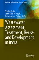
Fig. 1.3 Expansion of Indian Road Network since 1951. Data Source MoRTH (2022)

also indicates the importance of the GA phase in terms of TIs development. Since 1950, a significant change and expansion of transport network has been observed in every country. For example, in India since 1950 the length of the road network has increased by almost 16 times from 3.99 lakh km in 1951 to 63.32 lakh km in 2019 (MoRTH 2022). Figure 1.3 also reveals the profound development since 1951 as per the types of roads and maximum expansion has been observed for the rural road as it holds about 71.40% of the total road network of India. In case of USA, significant expansions of airport number, length of highways, gas pipelines, interstate motor carriers are also observed during the phase of GA (Fig. 1.4). However, David et al. (2011) have identified that the initial progress and maximum transport network expansion occurred since the industrial revolution and after World War II, respectively. Currently, the world is featured with ~21 million km of the road among 222 countries with significant spatial variation of road density and the study has also predicted addition 3.0–4.7 million km of road by 2050 (Fig. 1.5; Meijer et al. 2018).

1.3 Prospect to Study the Role of TIs on Geomorphological Alteration An adequate number of studies have been done to monitor the impact of different anthropogenic drivers e.g., dams, deforestation, channelization, mining, urbanization, water extraction etc. on the deformation of geomorphological forms and processes, whereas, limited work has focused on the influence of transportation infrastructure as another important anthropogeomorphic driver to do the same (Roy 2022). Previously Knighton (1984) had also excluded transportation as an anthropogenic factor that can affect fluvial geomorphology directly or indirectly (Table 1.1),

10

1 General Introduction: Transportation System and Geomorphic Landscape

Fig. 1.4 Development of transportation infrastructures in the USA during the phase of GA. Data Source National Transportation Statistics, Bureau of Transportation Statistic, US Dept. of Transportation

Fig. 1.5 Spatial distribution of road density across the globe. Source Adopted from Meijer et al. (2018)

1.3 Prospect to Study the Role of TIs on Geomorphological Alteration Table 1.1 Different man-induced changes in channel morphology

11

Direct or channel-phase changes

Indirect or land-phase changes

River regulationWater storage by reservoirs Diversion of water Channel changesBank stabilization Channel straightening Stream gravel extraction

Land use changesRemoval of vegetation, especially deforestation Afforestation Changes in agricultural practices Urbanization Mining activity Land drainageAgricultural drains Storm-water sewerage systems

Source After Knighton (1984, p. 198)

similar trend has been followed by Rhoads (2020) by skipping the effect of TS on river dynamics. Although, the noticeable alteration of the earth’s surface for the construction of roadway was started by Roman civilization during the 4th–5th Century B.C. (David et al. 2011). In this process of construction to make the road more durable, after clearing the forest cover up to 60 m alongside the road, a deep excavation (>1 m) had been done to prepare a five-layer paved surface for the roadway (David et al. 2011). Such type of excavation of the earth’s surface up to 1–10 m below the ground level for the construction of TIs like tunnels, subways, and underground metros could be termed as ‘shallow anthroturbation’ (Zalasiewicz et al. 2014). For example, from the Gotthard Base Tunnel in Switzerland with a length of 57 km, about 28.20 million tons of earth material has been excavated from below the Swiss Alps (Amberg Engineering 2018). Out of this concern, Fig. 1.6 is the result of an in-depth understanding of the interface between human actions to developed different modes of TIs and related alteration of geomorphological processes and possible geomorphic outcomes. A bibliometric analysis based on the review of 120 literature collected and shortlisted from different sources (Fig. 1.7) shows the initial insights on the interaction between TIs and geomorphological alternation came from a group of engineers during 1970s (Bradley 1970; Shen 1971; Neill 1973; Klingeman 1973; Task Committee 1978 Jansen et al. 1979) (Fig. 1.8a). In this phase, several works by river engineers have been highlighted the impact of in-stream TIs like bridge, culvert on the problem of scouring, backwater effect, instability of channel, river bed degradation, risk assessment of flooding etc. (see table 1 in Gregory and Brookes 1983, pp. 148–149). Other impacts of TI installation have come through doubling of downstream channel width, carrying capacity and width–depth ratio in comparison with the upstream morphology (Gregory and Brookes 1983; Douglas 1985), disturbance in floodplain geomorphic connectivity (Snyder et al. 2002; Blanton and Marcus 2009;

12

1 General Introduction: Transportation System and Geomorphic Landscape

Fig. 1.6 Schematic model to represent the effect of human actions related to the TIs development on the altering geomorphological processes and possible outcomes

Roy 2021). The reviewed literature covers the period of 1972–2022 and a significant focus on the respective aspect comes after the 2000s with an average of four publications every year which was only one up to 2000 (Fig. 1.8b).

Fig. 1.7 Procedure for shortlisting the relevant literatures to study the effect of TIs on geomorphological forms and processes

1.3 Prospect to Study the Role of TIs on Geomorphological Alteration

13

Fig. 1.8 a Timeline of the important milestones in the process of transportation geomorphology development; b annual frequency of published literature since 1972

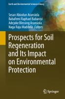
The country-level origin of reviewed works shows that the maximum number of publications have been published from the USA only (~34%) and the area of investigation is concentrated in the mountain region of the Pacific Northwest and/or Western United States (e.g., Oregon, Idaho, Colorado) (Fig. 1.9a). About 25% contribution comes from the Southeast Asia, followed by the Europe (~18%), Globally (~12.5%). India and China are individually contributing ~10% and ~5.8% articles, respectively. However, in respectively of the particular sub-theme of geomorphology, Fig. 1.9b shows that about 48% of works are dealing with the role of TIs on the generation of sediment and/or soil erosion, followed by the role of changing channel morphology (~27%), slope instability (~25%), alteration of surface hydrology (~20%), hydrological connectivity (~16%) and so on. With a limited study on the impact of TIs on hillslope geomorphology and fluvial geomorphology in particular, a noticeable research gap has been observed for the other field of geomorphology, whereas, a significant influence of TIs on the desert environment, peri-glacial regions are also noticeable nowadays. The present book has tried to fill such gaps with more insights from different parts of the world. In particular, this book not only focuses on the impact of TIs on the different sub-theme of geomorphology but also included the impact of different types of TIs which are less focused on in the published literature.

14

1 General Introduction: Transportation System and Geomorphic Landscape

Fig. 1.9 a Country-level distribution of reviewed literature source, the yellow-coloured countries have contributed one article each and grey colour indicates no literature; b Work tendency on the effect of transport infrastructure on different sub-fields of geomorphology

1.4 Structure and Approach of the Book The present book is designed to provide a basic understanding of the interaction between the transportation systems and geomorphological systems over the earth’s surface, which is a very common phenomenon although neglected in the research community. The book contains a total of ten chapters which are categorized into three parts: Part I is composed of two chapters related to a general introduction to the topic and the history of the transportation system, whereas Part II, and Part III are composed of five and three chapters respectively. This chapter starts with the context of the present book in the phase of Anthropocene as an important anthropogeomorphic driver to alter geomorphological forms and processes. This chapter is also highlighting the development of transportation infrastructures in the phase of Great Acceleration since the 1950s and the prospect to study the impact TIs on geomorphology with a bibliometric literature survey to find the progress of knowledge in this particular issue. Chapter 2 deals with the history and/or evolution of transportation around the world, which extends from the development of trails through the initial human footprint to the recent development of the hyperloop using different models and maps. This chapter has also explained the major types of transportation infrastructures e.g., roads, railways, bridges, culverts, airports, etc. which are having a significant role in the disturbance of geomorphology. The chapter also includes the continental scale as well as country-level development of such infrastructures. Part II deals with different modes of geomorphic alteration by different types of TIs. In particular, Chapter 3 has illustrated on the disturbances created in geomorphic connectivity by TIs starting with a basic concept on the importance of connectivity in geomorphology. This chapter has discussed on different types of human intervention on geomorphic connectivity with a special focus on the TIs and their effect on lateral, longitudinal, and vertical dimensions of connectivity. To give more emphasis on the effect of TIs on geomorphic connectivity, two catchment-level case studies have been included to show the effect of TIs on lateral and longitudinal connectivity at different watersheds of West Bengal (India) and selected sites of road-stream

1.5 Conclusion

15

crossing, respectively. Chapter 4 has been prepared to investigate the impact of road construction on slope instability in the hilly region and their possible consequences as soil erosion and landslides. A case study on the influence of undersized crossing to form gully has been also included. Chapter 5 has explained the potentiality of the road surface to generate runoff and their role in the alteration of surface hydrogeomorphology. This chapter also is including the potentiality of the road surface to generate water resources by harvesting rainwater. Chapter 6 has investigated the effect of different human recreational activities in form of adventure tourism, offroading activity, hiking, and adventure games on the modification of geomorphology, which is a neglected section of anthropogenic alteration of earth surface forms and processes. This chapter has separately discussed the effect of off-roading activity on aeolian geomorphology, coastal geomorphology, fluvial geomorphology, hillslope and forest geomorphology. Chapter 7 is another section of this book, which is also dealing with limited knowledge on this anthropogeomorphic factor i.e., construction airports and/or obsoleted airfields as a reason to modify channel geomorphology, gully erosion, and coastal geomorphology. The Chapters in Part III imply the environmental perspectives to deal with the effect of TIs on ecology, the environment, interaction with different geo-hazards and their vulnerability, and sustainable management to protect the environment as well as the transportation system. In particular, Chapter 8 deals with the major ecological disturbance done by different TIs in their phase of construction as well as the continuous effect on habitat, river ecology, carbon emission etc. Chapter 9 explores the vulnerability of TIs to changing climate and different geo-hazards like landslides, floods, and earthquakes across the world. A national-level case study from India has also been included to show the effect of flooding on transportation infrastructures. Chapter 10 concludes the book with recent advancements in the transportation sector to cope with future climate change, geomorphic hazards, carbon emission, to avoid human casualty etc., in addition to the ways of sustainable management of the environment.

1.5 Conclusion Anthropogeomorphological investigation became an essential field of study in the context of ‘Anthropocene’. Among the anthropogenic drivers, the effect of TIs on the geomorphological alteration is less studied and the initial insights on this issue came from a group of engineers during 1970s. However, notable progress in this field of inquiry has been seen globally since the turn of the twenty-first century, with a focus on sediment production and disturbance on hillslopes. The level of human interference in natural systems of the earth has significantly increased since the 1960s including the number of dams on river systems, the number of vehicles and length of transport routes, number of ports for air and water transport, the level of carbon emission, and the phase is designated as GA. Where the effect of such anthropogenic activity has been studied at an expectable level, the effect of transportation section on

16

1 General Introduction: Transportation System and Geomorphic Landscape

earth’s surface has been profoundly neglected. Therefore, the goal of the current book is to give readers a fundamental grasp of how transportation and geomorphological systems interact on the surface of the earth which comprised ten chapters divided into three parts.

References Amberg Engineering (2018) Gotthard Base Tunnel. Retrieved from http://www.ambergengineering. com/references/projects/gotthard-base-tunnel/. Accessed on 9 August 2021 Bhaduri A, Bogardi J, Leentvaar J, Marx S (eds) (2014) The global water system in the anthropocene: challenges for science and governance. Springer, New York Blanton P, Marcus WA (2009) Railroads, roads and lateral disconnection in the river landscapes of the continental United State. Geomorphology 112(3–4):212–227 Bradley JN (1970) Hydraulics of bridge waterways. Report of Hydraulic Branch Division, Hydraulic Design Series No. 1, Bureau of Public Roads Office of Engineering and Operations, Washington, DC Certini G, Scalenghe R (2015) Holocene as Anthropocene. Science 349:246. https://doi.org/10. 1126/science.349.6245.246a Crutzen PJ (2002) Geology of mankind. Nature 415:23. https://doi.org/10.1038/415023a Crutzen PJ, Stoermer EF (2000) The “Anthropocene”. IGBP Newsl 41:17–18 Cuff D (2008) Anthropogeomorphology. In: Cuff D, Goudie A (eds) Oxford companion to global change. Oxford University Press, Oxford, pp 31–35 Darimont CT, Fox CH, Bryan HM, Reimchen TE (2015) The unique ecology of human predators. Science 349(6250):858–860. https://doi.org/10.1126/science.aac4249 David L, Ilyes Z, Baros Z (2011) Geological and geomorphological problems caused by transportation and industry. Cent Eur J Geosci 3(3):271–286 Douglas I (1985) Hydrogeomorphology downstream of bridges: one mechanism of channel widening. Appl Geogr 9:167–170 Ehlers E, Krafft T (2006) Earth system science in the Anthropocene: emerging issues and problems. Springer, New York Golomb B, Eder HM (1964) Landforms made by man. Landscape 14:4–7 Goudie AS, Viles HA (2016) Geomorphology in the Anthropocene. Cambridge University Press, London Gregory KJ, Brookes A (1983) Hydrogeomorphology downstream from bridges. Appl Geogr 3:145– 159 Grill G et al (2019) Mapping the world’s free-flowing rivers. Nature 579:215–236 GSA (Geological Society of America) (2011) 2011 GSA annual meeting on Archean to Anthropocene: the past is the key to the future. Retrieved from http://www.geosociety.org/meetings/ 2011/ Haff PK (2003) Neogeomorphology, prediction, and the anthropic landscapes. In: Wilcock PR, Iverson RM (eds) Prediction in geomorpholog, geophys. Monograph Series. 135. AGU, Washington, DC, pp 15–26 Hooke RL (1994). On the efficacy of humans as geomorphic agents. GSA Today 4(9):217, 224–225 Hooke RL (2000) On the history of humans as geomorphic agents. Geology 28(9):843–846 IGBP (2015) Planetary dashboard shows “Great Acceleration” in human activity since 1950. Retrieved from http://www.igbp.net/news/pressreleases/pressreleases/planetarydashboardsho wsgreataccelerationinhumanactivitysince1950.5.950c2fa1495db7081eb42.html. Accessed on 23 March 2023 Jansen PP, Van Bendegom L, Den Berg V et al (1979) Principles of river engineering. Pitman, London

References

17

Klingeman PC (1973) Hydrologic evaluations in bridge pier scour design. Proceedings American Society of Civil Engineers. J Hydraul Div 99(2):175–184 Knighton AD (1984) Fluvial forms and processes. Edward Arnold, London Lewin J, Macklin MG (2014) Marking time in geomorphology: should we try to formalise an Anthropocene definition? Earth Surf Proc Land 39:133–137. https://doi.org/10.1002/esp.3484 Loczy D (2010) Anthropogenic geomorphology in environmental management. In: Szabo J, David L, Loczy D (eds) Anthropogenic geomorphology: a guide to man-made landforms. Springer, Dordrecht, pp 25–38 Marsh GP (1864) Man and nature, or physical geography as modified by human action. S. Low, Son and Marston, London Meadows ME (2016) Geomorphology in the Anthropocene: perspectives from the past, pointers for the future? In: Meadows ME, Lin J-C (eds) Geomorphology and society. Springer, Tokyo, pp 7–22 Meijer JR, Huijbregts MAJ, Schotten KCGJ, Schipper AM (2018) Global patterns of current and future road infrastructure. Environ Res Lett 13(6):064006. https://doi.org/10.1088/1748-9326/ aabd42 MoRTH: Ministry of Road Transport and Highways (2022) Basic road statistics of India (2018– 2019). Transport Research Wing, Govt. of India, New Delhi Neill CR (1973) Guide to bridge hydraulics. University of Toronto Press, Toronto Rhoads BL (2020) River dynamics: Geomorphology to support management. Cambridge University Press, Cambridge Roy S (2018) Human interference in changing river morphology a study in the Kunur river basin Barddhaman District West Bengal. PhD Thesis, University of Kalyani, India. Retrieved from http://hdl.handle.net/10603/312121 Roy S (2021) Impact of linear transport infrastructure on fluvial connectivity across the catchments of West Bengal, India. Geocarto Int 37(17):5041–5066. https://doi.org/10.1080/10106049.2021. 1903576 Roy S (2022) Role of transportation infrastructures on the alteration of hillslope and fluvial geomorphology. Anthropocene Rev 9(3):344–378. https://doi.org/10.1177/20530196221128371 Schwägerl C (2014) The Anthropocene: the human era and how it shapes our planet. Synergetic Press, London Shen HW (1971) River mechanics. Colorado State University, Fort Collins Snyder EB, Arango CP, Eitemiller DJ et al (2002) Floodplain hydrologic connectivity and fisheries restoration in the Yakima River, U.S.A. Internationale Vereinigung für Theoretische und Angewandte Limnologie: Verhandlungen 28(4):1653–1657 Steffen W, Sanderson A, Tyson PD, Jäger J, Matson PA, Moore B III, Oldfield F, Richardson K, Schellnhuber HJ, Turner BL, Wasson RJ (2004) Global change and the earth system: a planet under pressure. Springer-Verlag, Berlin, Heidelberg, and New York Szabo J (2010) Anthropogenic geomorphology: subject and system. In: Szabo J, David L, Loczy D (eds) Anthropogenic geomorphology: a guide to man-made landforms. Springer, Dordrecht, pp 3–10 Szabo J, David L, Loczy D (eds) (2010) Anthropogenic geomorphology: a guide to man-made landforms. Springer, Dordrecht Task Committee (1978) Environmental effects of hydraulic structures. Proceedings American Society of Civil Engineers. J Hydraul Div 104:203–221 Waters CN, Zalasiewicz J, Summerhayes C, Barnosky AD, Poirier C, Gałuszka A, Cearreta A, Edgeworth M, Ellis EC (2016) The Anthropocene is functionally and stratigraphically distinct from the Holocene. Science 351(6269):1–10. https://doi.org/10.1126/science.aad2622 Whitehead M (2014) Environmental transformation: a geography of the Anthropocene. Routledge, New York Zalasiewicz J, Williams M, Smith A, Barry TL, Coe AL, Bown PR, Brenchley P, Cantrill D, Gale A, Gibbard PL, Gregory FJ, Hounslow MW, Kerr AC, Pearson P, Knox R, Powell J, Waters C,

18

1 General Introduction: Transportation System and Geomorphic Landscape

Marshall J, Oates M, Rawson P, Stone P (2008) Are we now living in the Anthropocene? GSA Today 18:4–8 Zalasiewicz J, Williams M, Steffen W, Crutzen P (2010) The new world of the Anthropocene. Environ Sci Technol 44:2228–2231 Zalasiewicz J, Williams M, Haywood A, Ellis M (2011) The Anthropocene: a new epoch of geological time? Philos Trans R Soc 369:835–841. https://doi.org/10.1098/rsta.2010.0339 Zalasiewicz J, Waters CN, Williams M (2014) Human bioturbation, and the subterranean landscape of the Anthropocene. Anthropocene 6:3–9

Chapter 2

Types and Development of Transportation Infrastructure

Abstract The current chapter gave a complete overview of the transport system’s development and the foundational elements of its architecture since 10000 B.C. Throughout the history of human civilisation, transportation infrastructure (TI) development has ranged from the human footprint to the hyperloop. Roman Empire is a significant era in the development of TI in terms of improvements in road engineering and network growth. The invention of the steam engine in 1712 significantly helped the expansion of the transport network across all modes of transport. The development of TIs in major countries has been also explained here. Physical infrastructures such as trails, roads, railroads, tunnels, airports, culvert-bridges, causeways, and seaports have been examined here for their substantial role on the modifications of the earth’s surface as well as the ecology. Keywords Transportation infrastructure · Human footprint · Hyperloop · Steam engine · Roman Empire

2.1 History of Transportation Transportation means the movement of people and goods/freights from one location to another in different ways, which begins with the arrival of humans and has been significantly changed over time (Fig. 2.1). Initially human used their foot for roaming around the landscapes and the routes developed by their walked popularly known as trails or footpaths. During the early Mesolithic (8040–7510 BC), human was learned to use waterways by hollowed tree bodies, which is known as dugout canoe and name of the world’s oldest boat is ‘Pesse Canoe’, which has been excavated from a wetland peat in The Netherlands in 1955 (Roorda 2020). Although animal domestication had been started about 12,000 years ago (Zeder 2008), while in particular from the perspective of transportation, horses were started to domesticate for riding and load-bearing during 3600 BC in the Western Steppe (Taylor and Barrón-Ortiz 2021). As per Australian archaeologist V. Gordon Childe (1935), the Neolithic period (10000–4500 BC) is the radical and important period of beginning in context of the © The Author(s), under exclusive license to Springer Nature Switzerland AG 2023 S. Roy, Disturbing Geomorphology by Transportation Infrastructure, Earth and Environmental Sciences Library, https://doi.org/10.1007/978-3-031-37897-3_2

19

20

2 Types and Development of Transportation Infrastructure

anthropogenic activities when humans had started to shift from hunting-gathering to the cultivation of plants, breeding of animals for food and construction of permanent settlements. Mesopotamia is the earliest site of Neolithic revolution through the innovation of agricultural practice around the Fertile Crescent region of the Middle East, the use of irrigation, the wheel and stone-paved roads (Lay 1992). ‘Ur’, an important Sumerian city-state in ancient Mesopotamia, is the cultural hearth of the stone-paved road in about 4000 BC, at the same time Corduroy Road (log road) was an alternative of stone-paved found in Glastonbury, England (Lay 1992). On the Somerset Levels of the Brue River valley in England, the oldest timber-based engineering road causeways or trackways have been discovered, which are named as ‘Post Track’ and ‘Sweet Track’ and built in 3838 BC and 3807 BC, respectively as retrieved from the dendrochronology (Brunning et al. 2000). The Neolithic ‘Sweet’ trackway was developed across the wetlands for about two km to explore the wetland resources and as a route of communication (Coles and Coles 1986). Meanwhile, in 3000 BC archaeologists have also traced the first brick-paved road in the Indus Valley Civilization of the Indian subcontinent (Lay 1992). In the process of transportation infrastructure development, innovation of wheel is the most crucial milestone achieved by the Mesopotamian civilization around 4200–4000 BC, which was a true potter’s wheel and easy for spinning by wheeland-axel mechanism (Potts 2012). During the 4th millennium BC different pieces of evidences of wheel movement has been traced in and around the Black Sea and throughout Europe, however, the prominent evidence of wheeled wagons on ‘clay tablet pictographs’ (3500–3350 BC) has been found in the Sumerian civilization (Bakker et al. 2006). The first spoked wheel and the chariot (i.e., two or four wheels enable house-drawn ancient vehicles) were invented during middle of the Bronze Age (2200–1550 BC) and with the passage of time it has been improved with lighter

Fig. 2.1 Schematic illustration of the history of transportation infrastructure development since the early arrival of humans

2.2 Types of Major Transportation Infrastructures (TIs)

21

design and moving with higher speed. By the fourteenth century BC, it was introduced in Chinese steppes and has been seen to use in Peking municipality by 300 BC. The major structural development and expansion in road network have been observed during the period of Roman Empire since 400–300 BC (David et al. 2011). The nature of roman transportation is largely controlled by regional geomorphology in particular by the Mediterranean basin (Fig. 2.2). Therefore, significant progress in maritime and little fluvial transportation have been observed to support the trading between major coastal cities like Salona, Carthage, Alexandria, Constantinople, etc. (Rodrigue 2020). The Appian Way is an earliest important strategic hard-surfaced highway of Rome, primarily used for military purpose and extended for about 560 km. At the height of Roman empire (around 200 BC) about 80,000 km of first-class roads have been constructed across the provinces. The world’s first dual carriageway was also constructed by Romans to connect its port city Ostia at the confluence of Tiber via Portuensis (Rodrigue 2020). The idea of railways was also initially coming from the ‘rutways’ and ‘Diolkos Wagonways’ used in Roman and Greece transportation, which were functioning through the determined path (grooved roads) to the exact spacing between the wheels of wagon’s axel prepared by the cutting on paved road (Lee 1997). Although, an improved form of railway track came into the existence during mid of the sixteenth century in surrounding the modern-day Germany and later in the England. It was the wooden-railed and men and/or horse-drawn tramroad used mainly in the mining sector to carry coal for a short distance from a pit. By 1600, the funicular railway was developed at Broseley in Shropshire to transfer coal from highland to river by a railway track on steep slope. The first large scale (5 miles) double wooden railway track with the capacity of 2.5-ton waggon was constructed by 1725, part of which is still operational under Tanfield Railway (England). Around 1799, the wooden-rails were started to replace with iron edge railway tracks with the capacity of changing gauge. The discovery of steam engine in 1712 by Thomas Newcomen and a critical improvement by James Watt in 1764 was significantly powered the development of transportation system in all mode of transit. The initial use of steam power on rail transport developed by Richard Trevithick in 1804, Penydarren or Pen Darren locomotive, which was first carried about 10 tons of iron. The first commercial use of steam locomotive Salamanca was used on the Middleton Railways, Leeds in 1812. In different phase of eighteenth and nineteenth century, the development of steamed railway has been taken place across the world with a major expansion in England (Table 2.1). Similarly Fig. 2.3 is also showing the evolution of roadway vehicles since the development of self-powered road vehicle in 1769.

2.2 Types of Major Transportation Infrastructures (TIs) Infrastructures for transportation systems are generally containing fixed installation of essential structures, equipment, technologies which are varying with the changing mode of transportation e.g., air, land (road and railway), water, pipeline and space,

22

2 Types and Development of Transportation Infrastructure

Fig. 2.2 Expansion of road networks and maritime routes in the period of Roman Empire. Source Adopted from Rodrigue (2020)

in addition with, different auxiliary arrangements like, terminals, ports, warehouses, stations for rails and buses, etc. TIs are essential elements of the society for wellfunctioning of the regional economic activities, to facilitate the social well-being, ensuring every day’s mobility of the population, distribution of goods and production, heath facility, security, etc. Besides playing a significant role in the development of cultural landscape, TIs are also prominently altering the physical landscape by disturbing the hydro-geomorphological forms and processes across the globe (Montgomery 1994; Wemple et al. 1996; Sidle and Ziegler 2012; Tarolli 2014). Here, the physical infrastructures (e.g., trails, roads railways, tunnels, airports, culvertsbridges, causeways, seaports) have been considered only, which are have a significant role in the alteration of hydro-geomorphology condition of the earth surface as well as the environmental ecology. The primary consideration in transportation system (TS) is the transport network (TN), which is an integrated part of different components like node, link, flow, gateway, hub, corridor and works as a graph on geographical space to connect different nodes and hubs by links or edges distributed over the earth surface (Rodrigue 2020) (Fig. 2.4). A node could be an airport, seaport, major city, where different kinds of transport routes or links are assembled and bifurcated to connect other locations. A link may represent any trails, roadways, railway lines (in land transport), sea routes, canals, rivers (in water transport), airline routes, the trajectory of spacecraft (in air transport). The flow in TS indicates by the number and weight of passengers, vehicles and freights transport from one node to another, respectively. Another important aspect of TS is the topology of transport networks, which defines by the comprehensive arrangement of different nodes and their level of connectivity through

2.2 Types of Major Transportation Infrastructures (TIs)

23

Table 2.1 Major milestones in the development of engine powered locomotive across the globe Year

City, country

Name of the railway/ locomotive

Distance cover Purpose

1804

Wales, UK

Penydarren (First Steam Locomotive)

15.69 km

To carry iron

1812

Leeds, England

Middleton Railway (First commercial use of locomotive)

1.6 km

To carry passengers

1825

England

Stockton and Darlington Railway (S&DR)

1827

USA

Baltimore & Ohio Railroad

1829

Paris, France

Saint-Étienne–Andrézieux railway

1831

Source(s)

World’s first public railway to use steam locomotives

Kirby (2002)

20.91 km

First U.S. Railway Chartered to Transport Freight and Passengers

The Library of Congress

18 km

To transport coal

Manchester, The Bolton and Leigh England Railway

12.1 km

Enable to carry 150 passengers at a time

1837

Saint Petersburg, Russia

27 km

First Russian passenger train with 8 carriages

1837

First electric locomotive discovered by Robert Davidson (Scotland)

1839

Italy

Tsarskoye Selo Railway

The Naples–Portici railway

7.25 km

For passengers and goods traffic

1840s United Kingdom

About 10,010 km of railway lines have been constructed across the Mitchell UK. A significant development has been observed among countries (1975) of Europe also with installation of railway lines

1842

Belgium to France

First international railway route in Europe to connected Belgium and France

1848

British Guyana, South America

From Georgetown to Rosignol and between Vreeden Hoop and Parika

1850

Europe

Expansion of railway lines like Great Britain: 9,797 km (plus Ireland: 865 km); Germany: 5,856 km; France: 2,915 km; Austria: 1,357 km; Belgium: 854 km; Russia: 501 km; The Netherlands: 176 km

1851

Chile

Caldera to Copiapó

1852

Alexandria, Egypt

First railway line in Africa

129 km standard-gauge and several narrow-gauge

80 km

To serve the people and industrial product transfer Mitchell (1975)

For passengers and goods traffic

(continued)

24

2 Types and Development of Transportation Infrastructure

Table 2.1 (continued) Year

City, country

Name of the railway/ locomotive

1853

Mumbai, India

Railways introduced to India; 34 km train ran from Bombay (now Mumbai) to Thane

Moving with 400 passengers in 14 carriages

1854

Melbourne, Australia

First Australian steam railway line by Melbourne and Hobson’s Bay Railway Company

For moving people and goods

1879

Berlin, Germany

World’s first electric railway has been demonstrated

1881

Berlin, Germany

Gross Lochtefeld Tramway

2.4 km

First electric passenger train

1890

London

The City and South London Railway (C&SLR)

5.1 km

Introduction of World’s first deep-underground tube railway system, passing under the River Thames

1891

Russia

Construction began for the Trans-Siberian Railway for about 9313 km, and completed on 1904

1912

Switzerland Winterthur–Romanshorn railway

1960

End of the era of steam engine locomotive, last steam engine (evening star) is made in Britain

1964

Shinkansen or Bullet Train service has been introduced in Japan, between Tokyo and Osaka with a top speed of 210 km/h

1984

Kolkata, India

2007

High speed trains introduced in different countries with a maximum speed of 574.8 km/h in France

Distance cover Purpose

4.02 km

World’s first diesel locomotive

India’s first underground train service ‘Kolkata Metro’ has been started

2018

Introduce of driverless trains

2020

Latest data shows about 1.37 million km total railways has been constructed in the world

Fig. 2.3 Evolution of powered vehicle on roads

Source(s)

2.2 Types of Major Transportation Infrastructures (TIs)

25

Fig. 2.4 A typical framework of transport network by numbers of nodes and links (edges)

links, geometry of network, direction of flow (unidirectional or bi-directional), locations, specific pattern or structure of the networks (centrifugal, centripetal, linear, distributed, etc.) and every network is characterised by a unique topology (Zhang et al. 2015; Rodrigue 2020).

2.2.1 Footpath or Trails Footpaths or trails are the most primitive transportation medium on land since the arrival of human beings, which are now popularly shown through the countryside, in the forest, on the slope of mountains and rangelands for a special purpose. A footpath or trail could be treated as an unpaved road, which is constructed by substantially altered vegetation and topsoil structure caused by human movement on the grasslands, forests, scrublands, hill slopes primarily for recreational purposes e.g., outdoor sports like, hiking, off-road biking and cycling, horseback riding, etc. and the popularity of which was increasing very fast since the 1970s (Callahan 2008; Salesa and Cerda 2020).

2.2.2 Roadways Roads are mild to hard engineered routes on the land surface in a predefined direction to connect different nodes or places. Although there is long history of roadways development since 4000 BC, however, well constructive road building was started since the Roman civilization (David et al. 2011). The romans were very aware about

26

2 Types and Development of Transportation Infrastructure

the importance of good road on military, economy, and administrative activities. Romans are collected the different skills of road construction like cement technology, street paving, pavement structure construction, surveying from the well-established civilizations in past to build their enduring roads (Lay and Benson 2016). They were the first who had invented the layered road system with drainage ditches alongside the routes in 400 BC (Fig. 2.5). In this process of construction, at first the bare surface was excavated for about one metre to prepared a thick base layer with tamped clay collected from the earth work for ditches and from clean ground closest to the road, onto which sequentially another four layers were prepared: (i) first 25–60 cm thick the Statumen layer was constructed with high quarry-stone of at least 5 cm in size; (ii) followed by the Rudus layer, a 20–25 cm cemented layer made from stones under 5 cm sized; (iii), the Nucleus, a layer placed with about 30 cm thick using concrete from walnut-sized crushed rocks, gravel, coarse sand and carbonate debris, mostly used on very important roads; (iv) the final layer Summum dorsum was the road surface consist with large stone slabs (mostly volcanic flagstones) of almost 25 cm thick (David et al. 2011; Lay and Benson 2016). Therefore, the total thickness of these roads was between 1 m and 1.8 m and significantly raised above the ground with a width of about 35 m for single lane (the Appian Way) and/or 15 m for double lane roads and such a standard practice of road construction has been continued for next 2000 years (Lay and Benson 2016). Roadways are primary the medium of transportation for any country for their multi-dimensional importance like the capability to reach every nook and corner of the country, providing door to door service, less changes of delay and damage, comparatively easy and cheap to construct and maintenance, significant role in defence sector etc. Roads are also characterised by multiple types based on different criteria (Table 2.2). Table 2.2 represents such diversity in brief.

Fig. 2.5 Cross-section of the Roman Roads to show the first employed layered structure technology with roadside ditches. Source After Lay and Benson (2016)

2.2 Types of Major Transportation Infrastructures (TIs)

27

Table 2.2 Categorically short descriptions of different types of roads Criteria

Types

Short description

Carriageway

Paved road

Constructed with hard pavement course using Cement concrete, Bituminous, Water Bound Macadam (WBM)

Unpaved road

Road surface are usually made with Earthen, Kankar, Murram

Earthen road

Used the available soil close to the construction sites; Cheapest Road and designed for very low traffic

Gravel road

Slightly better than earthen road for mixing significant amounts of gravels with soil during construction

Murram

Roads built with the quarried gravely lateritic material, provides better surface than above two types for its higher compactness

Kankar road

Name in India, when road constructed with the impure parts of limestone

Water Bound Macadam road [WBM]

Primarily used clean and crushed stone (aggregate) in the base course, which is mechanically interlocked by rolling operation. Such materials are bound with filler material (which are also called screenings) and water

Bituminous road

During the distillation of petrol, a black viscous and adhesive material are produced, which are known as Bituminous. The primary material for the paved road all over the world for its smooth and strong surface finish

Concrete road

Use of cementing technology for the preparation of road surface, which very hard and long-lasting pavement. Most costly and time-consuming technology among all roads. Mostly recommended at the places of the high volume of traffic

Materials used in the construction

Speed and accessibility Freeways

Expressways

Designed for very first moving vehicles for long-distance with very high speed, four lanes (two in each side). There is no intersection with other roads and railways, no direct entry in the main lanes, only access through ramps Designed for a quick and comfortable journey without no sharp curve/turn, no intersection with other modes of way. High acceleration enables vehicles are only permitted here, no parking is allowed beside the road (continued)

28

2 Types and Development of Transportation Infrastructure

Table 2.2 (continued) Criteria

Volume of traffic

Types of traffic

Usage

Rigidity

Types

Short description

Highways

Such roads connect villages to cities, cities to other cities, with capitals, state to state. Try to cover the length and breadth of the country, generally two lanes without any divider. Further classified as National Highways, State Highways, Urban Highways, and Rural Highways

Arterials

Laid inside the city to connect CBD with suburban regions and always carry a high volume of traffic, which is controlled by a signalling system. Pedestrians are allowed to cross the roads at specific places, no parking is allowed on road

Local streets

A road for lower traffic volume, mainly constructed to reach individuals’ property, marketing places within the urban area. Pedestrians are allowed to cross the roads at any place, parking is allowed on road

Collector roads

Roads connecting local street to arterials with speed limit of 35–55 km/h

Low traffic road

Roads are carrying less than 400 vehicles per day

Medium traffic road

Roads are carrying average 400–1000 vehicles per day

High traffic road

Roads are carrying more than 1000 vehicles per day

Cycle tracks

Especially used for bicycles and provided on both sides of the pavement

Pedestrian ways

A route built specifically for pedestrians where any vehicles are strictly restricted

Motorways

All types of roads where different types of vehicles are permitted for free flow

All-weather roads

Such roads are accessible throughout the year

Fair-weather roads

Such roads are accessible only during the fair atmospheric condition. Higher snowfall, rainfall and other conditions may restrict the traffic seasonally

Flexible road

A four-layered flexible road topped with bituminous material (wearing course) and underlying by three different layers of sub-base, base and subgrade courses. Periodic maintenance is required

Rigid road

A three-layered (Surface course, Base and Subgrade course) non-flexible road, usually Cement concrete road falls under this category (continued)

2.2 Types of Major Transportation Infrastructures (TIs)

29

Table 2.2 (continued) Criteria

Types

Short description

Topography

Hilly road

The roads are constructed in hilly areas with frequent steep bends, ups and downs. In comparison with plain roads, required more capital for construction and take a large time to travel

Plain area road

Roads on the plain region with fewer bends and ups–downs. Speedy travel is possible

Low-cost road

Required less capital for construction, using local materials like soil, gravel etc. Preferred for only low traffic volume

Medium-cost road

Required higher fund than the low-cost roads, as it is prepared by bituminous, and for connecting villages to cities with medium o high volume of traffic

High-cost road

Primary roads for connecting major cities, capitals, and states with higher quality materials, therefore, required maximum funds for these roads to support higher traffic volume with higher longevity

Cost of construction

2.2.3 Railways Railway lines are basically metallic or steel made parallel tracks upon which the trains or locomotives are run, which is an important medium of land transportation. Although, there is a substantive history of railway tracks and locomotive development as mentioned in Table 2.1. A huge investment is required to developed railway network for purchasing land, installation of metallic tracks, bridges, construction of platforms and stations, upgraded signalling system, regular maintenance etc., which are not possible by individual person, that why this transportation system is normally belongs to the government in all countries. This system is very useful for long distance travel with heavy load. Based on the minimum vertical distance between the inner sides of two parallel railway tracts (i.e., the Gauge distance), globally four type railway gauge has been used e.g., (i) Broad gauge: the inner distance of the track is 1676 mm, although, any gauge wider than (ii) Standard gauge or 1435 mm is known as broad gauge. About 60% of the world’s railway tracts are standard gauge. (iii) Metre gauge: when the distance between two tracks is only 1000 mm; (iv) Narrow gauge: any railway tracks with less than metre gauge is generally called narrow gauge, most common narrow gauges are 762 mm and 610 mm. The Darjeeling Himalayan Railway is a world-famous example of narrow gauge, which is also comes under UNESCO World Heritage on 24 July 2008.

30

2 Types and Development of Transportation Infrastructure

2.2.4 River Crossings (Culvert and Bridges) A stream crossing (SC) is any bridge or culvert passing over a creek, river, stream or formed channel (Melbourne Water 2011). Culverts and bridges all provide for the management and conveyance of storm water runoff throughout a roadway system (FHWA 2012). Frequency of culverts and bridges varies depending upon the region and terrain (IRC 2004; Blanton and Marcus 2009). SC is classified into two broad types (i) bridges and (ii) culverts. Bridges are defined legally as structures with a centerline span of 6 m or more (IRC 2004; NBIS 2006; FHWA 2012). IRC (2004) have also mentioned two types of bridges e.g., (a) Minor Bridges, which are having a total length of up to 60 m and individual span is more than 10 m; (b) Small Bridges, where the overall length of the bridge is up to 30 m and where individual span is not more than 10 m. According to FHWA (2012), culverts may define as a structure, which is distinguished from bridges and usually covered with embankment and is composed of structural material around the entire perimeter, although some are supported on spread footings with the streambed serving as the bottom of the culvert. Geometrically it is 6 m or less in centerline span width between extreme ends of openings for multiple boxes (IRC 2004; NBIS 2006). There are several shapes of culverts (Fig. 2.6), which are usually designed to operate with the inlet submerged.

Fig. 2.6 Commonly used culverts (closed conduit and open-bottom) shapes. Source After VANR (2009)

2.2 Types of Major Transportation Infrastructures (TIs)

2.2.4.1

31

Selection of Crossing Structure for a Site

Comparing culverts to bridges the designer must determine which type of structure is preferred hydraulically, aesthetically and economically (FHWA 2012). Hydraulically, culverts are used—where bridges are not hydraulically required, and debris and ice potential are tolerable. Whereas, bridges are used—where culverts are impractical; to satisfy land use and access requirements; to mitigate environmental concerns those are not satisfied by a culvert; to avoid floodway encroachments and to accommodate ice and large debris (FHWA 2012). Economic considerations are also primary importance in deciding the type of SC. The initial cost for a culvert is usually less than a bridge but the frequency of maintenance activities is high for culverts, however bridges maintenance is typically more costly. Maintenance for a culvert includes channel erosion at the inlet and outlet, sedimentation, erosion and deterioration of culvert invert, ice and debris buildup and embankment repair (FHWA 2012). Maintenance aspects related to a bridge are bridge deck and superstructure, erosion around piers and abutments, and possible sediment and debris accumulation. Safety and aesthetic consideration are also involved in the choice of a bridge or culvert. A bridge may be considered more aesthetically pleasing in traversing a scenic valley or canyon (FHWA 2012). Safety measures for culverts include the use of guardrails or safety grates. Long span (>6 m) culverts and old bridges are subject to routine inspection according to NBIS requirements and especially, during the rainy season or flooding time.

2.2.4.2

Shapes and Materials of Culverts

Selection of culvert’s shape and used materials are based on the cost of construction, the limitation on upstream water surface elevation, roadway embankment height, hydraulic performance, and estimate of service life (FHWA 2012). Numerous crosssectional shapes are available for both closed conduit and open-bottom culverts. The most common closed conduit shapes are circular, box (rectangular), elliptical and pipe-arch (Fig. 2.6). These shapes may be constructed with embedment, which is a depression below the streambed of both inlet and outlet inverts (IRC 2004; FHWA 2012). Typical open-bottomed culverts are mainly dominated in box and arch shapes. Usually concrete (both reinforced and non-reinforced), corrugated metal (aluminum or steel), and plastic (high-density polyethylene or polyvinyl chloride) are used as culvert materials and less commonly used materials are clay, stone, and wood, as might be found in historic culvert structure (FHWA 2012).

2.2.4.3

Components of a Bridge and Culvert (see Fig. 2.7a, b)

Length of the Structure: This structural dimension has been measured across the roadway and in most cases, length is same as the road width.

32

2 Types and Development of Transportation Infrastructure

Fig. 2.7 Diagrams show the structure components and common channel features adjacent to the bridge (a) and culvert (b). Source After VANR (2009)

Structure Width or Span: A total length between the inner faces of the dirt walls. Width (span) of the crossing has been measured along the roadway. Structure Clearance (height): Distance from the channel bed (sometimes water surface) to the underside of the saturate top. Abutment and Wing-walls: Structures in the both end of crossings to support stand is abutment and wing-walls are concrete, wooden, or metal walls that flare out from the side of the opening of the bridge, arch, or culvert. Inlet and Outlet: Channel flow where inter the crossing is called inlet and outlet is where flow leave it. The hydraulic capacity of a culvert depends upon the appropriate inlet selection. Undersize culvert inlet may cause for the problem in channel geomorphology as well as river biota. Embedded and open-bottom

2.2 Types of Major Transportation Infrastructures (TIs)

33

culverts provide a natural inlet. Outlet of structure should also capable to pass water that inter in the inlet. Drop of the structure: It is very importance parameter to know the outlet condition of a crossing. The height difference between structure outlet and bottom of the stream bed in the immediate upstream of the crossing is called drop of the structure. Higher value is not suitable for stream health and morphology. Pier(s): It is an upright support for a bridge. The common cross-section of a pier is square, or rectangular. Single-span Bridge does not have piers but the multi-span bridges require piers to support the ends of spans between the abutments. Scour: Removal of material from around piers, abutments, spure, and embankments caused by an acceleration of flow and resulting vortices induced by obstructions to the flow.

2.2.5 Tunnels To reduce the obstacles (e.g., ridges in the hilly area, water bodies, large snow cover) across the route of transport network development, horizontally an underground or underwater passage is constructed by applying advanced technology of civil engineering, which is known as transportation tunnels. However, tunnels are also used for other purposes like pipeline, mining ores, canals for water and sewage. The construction of tunnels had a history since ancient civilization, for example, the Babylonians have used tunnels for irrigation, Egyptians have drilled on rock cliffs to construct hollow rooms for temples, Greeks and Romans were also used tunnels for their urban drainage system; similar construction have been also found in the Indus civilization. Initially, gunpowder was used to blast for tunnelling on the rock in France in 1681, thereafter, dynamites were started to use by the mid-nineteenth century and also started to develop drilling technology. To construct a tunnel beneath the Thames River in London between 1820 and 1865, shield technology was used. Now a day all tunnels for public utility and/or transportation are constructed through self-contained tunnel boring machines. With the rapid urbanization, the need for tunnels has been increasingly significant to contain different infrastructures (e.g., sewages, metro, stormwater management, communication lines etc.) within a limited space. The world’s longest tunnel (137 km) ‘Delaware Aqueduct’ in New York City (USA) is also constructed for water supply for half of the city with the capacity of 1.3 billion gallons per day. Tables 2.3 and 2.4 representing the world’s longest tunnels (in descending order) for transportation purposes only. Based on the available data on used and under-constructed major transportation tunnels of the world (where minimum length is considered more than 13 km), Wikipedia (https://en.wikipedia.org/wiki/List_of_longest_tunnels) has prepared a list of 200 tunnels from across the world, of which about 55% tunnels have been constructed for metro network only with an average length of 26 km, followed by the railway (35%) and road tunnels (10%), whereas, in 13% cases twin tunnels system

34

2 Types and Development of Transportation Infrastructure

Table 2.3 List of first twenty longest tunnels for transportation across the globe Tunnel types

Name of the tunnel

Location

Length (m)

Metro

Paris Métro Line 15

Paris Petite Couronne, France

75,000 m Under construction

Metro

Bolshaya Koltsevaya line

Moscow Metro, Russia

69,000 m Under construction

Metro

Guangzhou Metro Line 3

Guangzhou, China

57,930 m Completed

Railway Mont d’Ambin Base Tunnel twin tube

Cottian Alps, France—Italy

57,500 m Under construction

Railway Gotthard Base Tunnel twin tube

Central Swiss Alps, Switzerland

57,104 m Completed

Beijing, China

57,100 m Completed

Railway Brenner Base Tunnel twin tube

Stubai Alps, Austria—Italy

55,000 m Under construction

Railway Seikan Tunnel single tube

Tsugaru Strait, Japan

53,850 m Completed

Railway Channel Tunnel twin tube

English Channel, United 50,450 m Completed Kingdom/France

Railway Yulhyeon Tunnel single tube

Seoul Capital Area, South Korea

Metro

Beijing Subway Line 10

Present status

50,300 m Completed

Metro

Seoul Subway: Line 5

Seoul, South Korea

47,600 m Completed

Metro

Downtown line

Singapore, Singapore

43,700 m Completed

Metro

Thomson-East Coast Line

Singapore, Singapore

43,000 m Under construction

Railway Yigong tunnel

China—Tibet

42,500 m Under construction

Metro

Nanjing Metro Line 3

Nanjing, China

41,567 m Completed

Metro

Serpukhovsko-Timiryazevskaya Moscow Metro, Russia Line

41,500 m Completed

Metro

Madrid Metro: Line 12

40,900 m Completed

Madrid, Spain

Metro

Toei Oedo Line

Tokyo, Japan

40,700 m Completed

Metro

Shanghai Subway: Line 7

Shanghai, China

40,200 m Completed

Metro

Chengdu Metro Line 2

Chengdu, China

38,643 m Completed

Source https://en.wikipedia.org/wiki/List_of_longest_tunnels. Accessed on 30 November 2021

Sichuan, China

Jingpingshan

Gotthard Road Tunnel

Road

Road

16,918 m

17,500 m

24,510 m

19,000 m

22,035 m

26,700 m

23,844 m

34,577 m

35,391 m

34,586 m

37,900 m

42,500 m

47,600 m

57,100 m

57,930 m

43,000 m

69,000 m

75,000 m

Length (m)

Source https://en.wikipedia.org/wiki/List_of_longest_tunnels. Accessed on 30 November 2021

Lepontine Alps, Switzerland

Sydney, Australia Lærdal—Aurland, Norway

WestConnex

Lærdal Tunnel

Road

China

Randaberg-Kvitsøy-Bokn, Norway

Road

Sengli Daban Tunnel

Road

west of Vienna, Austria

Lainzer/Wienerwaldtunnel

Rogfast tunnel

Railway

Road

Bernese Alps, Switzerland

Lötschberg Base Tunnel

Railway

Yunnan, China Dongguan, China

Gaoligongshan Tunnel

Songshan Lake Tunnel

Railway

China—Tibet

China—Tibet

Railway

Sejila tunnel

Railway

Seoul, South Korea

Seoul Subway: Line 5

Yigong tunnel

Metro

Railway

Beijing, China

Beijing Subway Line 10

Metro

Singapore, Singapore Guangzhou, China

Thomson-East Coast Line

Guangzhou Metro Line 3

Metro

Metro

Paris Petite Couronne, France Moscow Metro, Russia

Paris Métro Line 15

Bolshaya Koltsevaya line

Metro

Metro

Location

Name of tunnel

Tunnel type

1980

2008

2000

2023

2024

2031

2012

2007

2016

2022

2030

2030

1995

2012

2018

2024

2023

2030

Year of completed (to be)

Table 2.4 Categorically longest completed and under-constructed tunnels for metro, railways and road transportation of the world

Completed

Completed

Completed

Under construction

Under construction

Under construction

Completed

Completed

Completed

Under construction

Under construction

Under construction

Completed

Completed

Completed

Under construction

Under construction

Under construction

Status

2.2 Types of Major Transportation Infrastructures (TIs) 35

36

2 Types and Development of Transportation Infrastructure

Fig. 2.8 Country level distribution of major tunnels (>13 km) with cumulative length

is used. The longest metro tunnel ‘Paris Métro Line 15’ (75 km) is currently under construction and expected to complete by 2030, whereas the longest used metro tunnel (57.93 km) is in Guangzhou, China. The longest railway (42.50 km) and road tunnels (26.70 km) are also under construction in China and Norway, respectively (Table 2.4). Among the major 200 tunnels (>13 km) of the world, China in alone holds 58 (29%) of the major tunnels followed by the South Korea (27), Japan (17), Spain (14), Russia (8) and Switzerland (Fig. 2.8). In terms of total length carried by such tunnels, first three countries (China—30%; South Korea—14%, Japan—8%) hold more than half length of all 200 major tunnels (4751.13 km).

2.2.6 Airports Since the beginning of the twentieth century, the importance of airways and the construction of airports (also called airfields or aerodromes) were increased with the development of aircraft after the Wright brothers’ first aeroplane in 1903. Runways are the essential component of any airport for continuous landing and take-off of aircraft on and from a defined rectangle flat ground respectively. Until the introduction of heavy monoplanes such as the Douglas DC-3 during the late 1930s, the length of the runways was limited to 600 m and rarely paved (Ashford 2019). The first paved runway was constructed during the first World War in Clermont Ferrand in France (1916). Nowadays, the dimension of a runway varies from 245 m long and 8 m wide for small general aviation to 5500 m long and 80 m wide runways at the International Airports to accommodate the large jets and space shuttles. Apart from the runways, numerous infrastructures are also important for an airport like terminals, air traffic control towers, taxi stands, apron areas for the smooth and

2.2 Types of Major Transportation Infrastructures (TIs)

37

Fig. 2.9 Worldwide distribution of airports (in blue dots; n ≥ 55,000) and seaports (in yellow dots, n = 3630). Date Source Airports: https://ourairports.com/data/; Seaports: World Port Index: 2019, NGA

safe function of the entire aviation system. Therefore, a wide area is required for the development of a new airport after qualifying in different site-selection factors. As per the recent updates by the OurAirports (https://ourairports.com/data/), a total 69,197 airfields have been detected worldwide, among them there are 36 balloon ports, 16,870 heliports, 447 large airports, 4746 medium airports, 37,703 small airports, 1096 seaplane bases, including 8299 closed airfields with a major concentration in the United States (~40%), followed by Brazil (8.7%), Canada (4.1%), Japan (4.1%) (Fig. 2.9).

2.2.7 Ports/Harbour Harbours or ports are mostly natural or sometimes artificial water bodies along the sea shore or any large river or canal which are connected with sea with enough deep for anchoring ships and proving shelter and safety to them from winds, waves and current. The primary functions of a port are loading and unloading of ships and dropping off and picking up passengers. Site selection for a harbour depends on numerous crucial factors like the calm marine condition, stabilized coastline, pollution-free seawater, industrial belt adjoining to the port, well-connected transport network, easy availability of construction materials, enough port area to accommodate numbers of large ships etc. Harbours could be classified into different types based on (a) nature of safety or protection (natural, semi-natural, and artificial harbours), (b) based on location (sea, river, and canal harbours), (c) based on primary purpose of a port (commercial, fishery, military, marine, and harbours of refuge). The National Geospatial-Intelligence Agency (NGA) (Virginia, USA) has reported the details of

38

2 Types and Development of Transportation Infrastructure

a total of 3630 ports around the world in their recent edition of ‘World Port Index— 2019’ (Fig. 2.9). As per the details of 3630 ports, only 160 ports are classified as large harbour, 362 as medium harbour, 977 as small harbours and 2125 as very small harbours. Based on the types those ports are also categorized as river natural (18.4%), coastal natural (34.8%), and coaster breakwater or artificial ports (21.8%), open roadstead (18.4%), lake or canal (2%) etc. Depth of the ports also varies from 1.5 m to over 25 m, in particulate about 9% of ports are having a depth of over 25 m. Country level distribution shows that only United States holds 666 (18.3%) of total ports followed by Canada (239), United Kingdom (184), Japan (163), Norway (135, Indonesia (123).

2.2.8 Causeways Construction of causeways, “a raised path, especially across a wet area” as per the Dictionary of Cambridge University, in the coastal region is a typical transport network to connect the coastal and barrier islands with the mainland. Such causeways usually consist with a number of bridges and elevated embankments or sometimes fill-type also. Davis (2019) has designated causeways as an indirect human impact on the modification of coastal geomorphology, with the active involvement of dredging and filling processes using heavy machinery. Such structures are significantly altering the tidal prism of the tidal inlet(s) and related changes in the inlet stability (Davis 2019). An example from Dunedin Pass of the Florida Gulf Coast showed a profound reduction in its cross-section area immediate after the construction of Clear-water Causeway in 1922 and Dunedin Causeway in 1964, and overall reduction in coastal stability (Lynch-Blosse and Davis 1977). The process of active dredging and filling are reducing the area of back-barriers and consequently impacted the tidal prism (Davis and Barnard 2000). Reimer et al. (2015) show how a 4.75 km Kaichu-Doro causeway construction has divided the large tidal flat in Okinawa, Japan and reduced the free movement of water exchange which significantly influenced the biota of the region. A geospatial spatial based study by Adnan et al. (2021) to investigate the changes in the coastline along the Pulau Tuba, Langkawi shows the maximum erosion has been observed along a causeway (Pulau Dayang Bunting- Pulau Tuba causeway) and the section classified as critical erosion prone coastal zone.

2.3 Development of Transport Network Since the early development of stone-paved road around 4000 BCE, the maximum expansion of paved road network (~80,000 km) has been traced during the Roman empire (~400–300 BCE) over the ancient Mediterranean region and also it was extended up to southwestern Asia, Spain, Northern Africa (Britannica 2018). Some of the ancient roads still remain in different parts of the world, while due to

2.3 Development of Transport Network

39

modernization parts of the such ancient routes might be changed and renamed. For example, The Grand Trunk (GT) Road, formally known as ‘Uttarapath’, ‘Sarak-eAzam’, ‘Badshahi Sarak’, ‘Sarak-e-Sher Shah’, one of the oldest and longest routes in Asia (Elisseeff 2000). The initial construction of GT Road was started by the Chandragupta Maurya of the Mauryan Empire in ancient India during third century BCE in the name of Uttarapath, extended from the mouth of the Ganga to north-western part of his empire. Later time to time, it was replanned and rebuilt by Ashoka, Sher Shah Suri, the Mughals and the British (Thapar 2004). The rough length of this ancient route is about 2500 km from Teknaf, Bangladesh on the border with Myanmar west to Kabul, Afghanistan passing through the famous Khyber Pass (1070 m amsl), and in its way of extension, it connects three major cities e.g., Dhaka, Delhi, and Lahore, which are now lie in three different countries like Bangladesh, India, and Pakistan, respectively (Fig. 2.10). Another famous ancient route, the Silk Road was a network of trade routes that connected the East and West, stretching from China to the Mediterranean Sea (Fig. 2.11). The name “Silk Road” comes from the lucrative Chinese silk trade, which was one of the main commodities exchanged along the route (Hartel 1982). The length of the Silk Road varied depending on the specific routes taken, but it is estimated to have spanned over 11,000 km (7,000 miles) (McLaughlin 2016; UNESCO 2023). The main route started in the ancient Chinese capital of Xi’an, and then went through Central Asia, Iran, and Turkey before reaching the Mediterranean Sea. From there, trade goods were shipped to Europe and Africa. There were also several branch

Fig. 2.10 Extension of Grand Trunk (G.T.) Road and evidence of a section of heritage path exit near Islamabad. Source Adopted from “Grand Trunk Road.” Wikipedia, Wikimedia Foundation, 14 March 2023, en.wikipedia.org/wiki/Grand_Trunk_Road. Accessed on 17 March 2023

40

2 Types and Development of Transportation Infrastructure

routes that extended from the main Silk Road, such as the Southern Silk Road that went through Tibet and the Himalayas, and the Maritime Silk Road that involved sea routes between China, Southeast Asia, and India. The Silk Road was not a single, fixed route, but rather a network of trade routes that evolved over time and shifted based on political and economic changes. Along these routes, merchants traded goods such as silk, spices, tea, porcelain, precious metals, and gems (McLaughlin 2016). The Silk Road played a significant role in the development of civilizations in the regions it connected. It facilitated the exchange of ideas, religions, and cultures, as well as goods. Buddhism, for example, was spread from India to China along the Silk Road. The road also served as a channel for the dissemination of technologies such as papermaking, gunpowder, and printing. The Silk Road declined in importance after the fifteenth century due to the opening of sea routes, the decline of the Mongol Empire, and the emergence of new trade routes. However, its legacy lives on in the cultural and economic ties that it created between East and West (McLaughlin 2016; UNESCO 2023). To get an idea about the present status of TIs distribution in different countries, Table 2.5 shows country-level ranking based on the number of respective infrastructures like the length of roadways, length of railway networks, number of airport and sea ports, based on available data as of 2021. The USA leads in the sectors of land and air transportation except in the case of the number of sea ports. However, the initial development of transportation sector in the USA comes through the canal system during the first half of nineteenth century, which is also known as “age of canals” (Grubler and Nakicenovic 1991). In the USA, the first canal was constructed in 1780s and reached to its maximum extension of 6,400 km (4000 miles) by 1870; similarly, the first railway line was built in 1830s and reached its saturation in the 1920s with a total length of 4,80,000 km (3,00,000 miles) in 1929 (Grubler and Nakicenovic

Fig. 2.11 The network of Silk Road and other maritime and land-based trade routes. Source Adopted from UNESCO 2023. https://en.unesco.org/silkroad/about-silk-roads. Accessed on 31 March 2023

2.3 Development of Transport Network

41

1991). Figure 2.12 shows the growth pattern of major transportation systems in the USA. China has also a long history of developing its transport network, dating back to ancient times. The earliest known examples of transport infrastructure in China were the Grand Canal, which was constructed over 2,000 years ago during the Sui Dynasty, and the Silk Road, which connected China to the West. Over the centuries, China continued to develop its transport network, building roads, bridges, and canals to connect different regions of the country. In modern times, China has made significant investments in its transport infrastructure, particularly in the areas of rail and air transport (Jin et al. 2012). China now has the world’s largest high-speed rail network, with over 22,000 miles (35,000 km) of track, and has invested heavily in new airports and aviation technology. The Chinese government has also launched several initiatives to improve the country’s transport infrastructure, including the “One Belt, One Road” initiative, which aims to promote connectivity and economic development across Asia, Europe, and Africa through infrastructure investment and development. Table 2.5 Country-level ranking based on major transportation infrastructures like length of railways and roads, number of airports and seaports as of 2021 Name of country with rank 1. United States 2. China

Length of railway network (km)

Name of country with rank

2,50,000 1. United States 1,39,000 2. India

Length of road network (km)

Name of country with rank

65,86,610 1. United States

Number Name of of Active country Airports with rank

Number of active sea ports

14,926

34,000

1. China

59,03,293 2. Brazil

4,093

2. Japan

2,786

3. Russia

85,500

3. China

50,00,000 3. Mexico

1,714

3. United States

2,722

4. India

68,000

4. Brazil

17,51,868 4. Canada

1,467

4. Indonesia

1,580 1,212

5. Russia

13,81,200 5. Russia

1,218

5. India

6. Germany

5. Canada 46,000 41,000

6. Japan

12,65,456 6. China

1,195

6. Philippines

941

7. Australia

36,000

7. Canada 10,42,300 7. Australia

537

7. Brazil

715

8. 36,000 Argentina

8. Indonesia

5,44,446 8. India

449

8. Russia

601

9. Brazil

9. Mexico

4,12,532 9. Argentina

444

9. Canada

580

10,28,446 10. Indonesia

442

10. Malaysia

501

29,000

10. France 29,000

10. France

Data Source Respective data has been collected from different secondary sources like the World Bank, the Our World in Data, the CIA World Factbook, and different governmental websites of respective country, all data are as of 2021

42

2 Types and Development of Transportation Infrastructure

Fig. 2.12 Temporal development trends of canals, railways, roadways, and airways in the USA in 1000 miles. Source After Grubler and Nakicenovic (1991)

Table 2.6 show the significant development of TIs in China during the last 70 years (1949–2018) since the development of People’s Republic of China (PRC). The road network in India is extensive, covering over 5.9 million km of roads. The government has invested heavily in the road network, including the construction of new highways and expressways, such as the Golden Quadrilateral and the North– South and East–West Corridors. These projects have improved connectivity between major cities and regions of the country and reduced travel times. The railway system in India is also well developed, with over 67,000 km of track. Indian Railways is one of the largest railway networks in the world and is used for the transportation of goods and passengers. The government has made significant investments in the railway system in recent years, including the construction of new high-speed rail lines and the modernization of existing infrastructure. India has several major ports that handle a significant amount of the country’s trade. The Port of Jawaharlal Nehru in Mumbai is the largest port in the country, followed by the Port of Chennai and the Port of Visakhapatnam. The government has implemented several initiatives to Table 2.6 Development of TIs in China since the development of PRC Year 1949

Total railway length (km) 21,800

Total highway length (km) 81,000

Expressways (km) 0

Inland waterway length (km) 74,000

Civil aviation flights routes 12

1978

52,000

890,000

18

–

–

2018

132,000

4,847,000

143,000

127,000

4945

Source http://www.china.org.cn/china/70-years-of-chinas-transport-development/index.html. Accessed on 31 March 2023

2.3 Development of Transport Network

43

improve the efficiency of the ports, including the introduction of digital technologies and the construction of new facilities. Air transport is an important mode of transport in India, with several major international airports in cities such as Delhi, Mumbai, and Bangalore. The government has also initiated several initiatives to promote regional air connectivity, including the UDAN scheme (Ude Desh ka Aam Naagrik), which aims to connect underserved areas of the country by air. In addition, the government has recently invested in the development of inland waterways, with several new waterway projects currently under construction. These projects aim to improve the transportation of goods and reduce the cost of logistics. The European Union (EU) has a highly developed transport network, which has been crucial to the economic and social development of the region. The EU has made significant investments in transport infrastructure over the years, with a focus on improving connectivity, reducing travel times, and increasing safety and efficiency. One of the key components of the EU’s transport network is its extensive road network, which includes over 5 million km of paved roads. The EU has also invested heavily in rail infrastructure, with high-speed rail lines connecting many major cities across the region. In addition, the EU has a comprehensive air transport network, with thousands of airports and airlines serving millions of passengers each year. The EU has also made significant investments in maritime transport, given the importance of shipping for trade within the region and with other parts of the world. The EU has several major ports that handle a significant amount of freight traffic, and the region is also home to several of the world’s largest shipping companies. To ensure that the transport network operates efficiently and safely, the EU has implemented a range of regulations and standards. For example, the EU has implemented measures to reduce greenhouse gas emissions from transport, promote road safety, and improve the quality of air transport services. The road network in Australia is extensive, covering over 900,000 km of roads. The majority of roads are paved, and there are several major highways that connect different parts of the country. The government has made significant investments in the road network in recent years, with a focus on improving safety and reducing congestion in urban areas. The rail network in Australia is also well developed, with over 33,000 km of track. The rail system is used primarily for the transportation of goods, including minerals, agricultural products, and manufactured goods. There are also passenger trains that operate between major cities, including high-speed rail services in some areas. Australia has several major ports that handle a significant amount of the country’s trade. The Port of Melbourne is the largest port in the country, followed by the Port of Sydney and the Port of Brisbane. These ports handle a wide range of goods, including minerals, agricultural products, and manufactured goods. Air transport is an important mode of transport in Australia, given the country’s vast size and the distances between major cities. There are over 600 airports in Australia, including several major international airports in cities such as Sydney, Melbourne, and Brisbane.

44

2 Types and Development of Transportation Infrastructure

2.4 Conclusion The history of transportation infrastructure development is very enriched since 10000 BC and their interaction with the earth’s surface started with the development of trails by the regional movement for the purpose of hunting and gathering. In terms of regional expansion, structural development, and the modification of surface geomorphology caused by massive earthwork and deforestation, the Roman Empire is the most notable period in the history of TIs development. By connecting the world via all-weather routes, the Silk Route and GT Road are carrying the legacy of the advancement of human civilization. There are many different types of TIs, such as roads, bridges, tunnels, causeways, airports, harbours, and auxiliary structures, which are impacting the geomorphology and hydrology of the earth’s surface gradually. Despite this, every nation continues to experience rapid growth in its transportation infrastructure, which promotes their socioeconomic development.

References Adnan NA, Fadilah FQS et al (2021) Geospatial analysis of coastline erosion along Pulau Tuba, Langkawi. IOP Conf. Series: Earth and Environmental Science 620. https://doi.org/10.1088/ 1755-1315/620/1/012017 Ashford NJ (2019) Airport. Encyclopedia Britannica, 18 July. Retrived from https://www.britan nica.com/technology/airport. Accessed on 8 December 2021 Bakker JA, Kruk J, Lanting AE, Milisauskas S (2006) Bronocice, Flintbek, Uruk, Jebel Aruda and Arslantepe: The earliest evidence of wheeled vehicles in Europe and the Near East. In Attema PAJ, Los-Weijns MA, Pers, ND M-V d (eds) Palaeohistoria 47/48. Barkhuis, Eelde Blanton P and Marcus WA (2009) Railroads, roads and lateral disconnection in the river landscapes of the continental United States. Geomorphology 112(3-4):212–227 Britannica, T. Editors of Encyclopaedia (2018) Roman road system. Encyclopedia Britannica, April 3. Retrived from https://www.britannica.com/technology/Roman-road-system Brunning R, Hogan D, Jones J, Jones M, Maltby Ed, Robinson M, Straker V (2000) Saving the sweet track: the in-situ preservation of a Neolithic wooden trackway, Somerset, UK. Conserv Manag Archaeol Sites 4(1):3–20. https://doi.org/10.1179/135050300793138417 Callahan J (2008) Erosion and trail building: a case study of the East Tennessee State University Trail System. MS Theses, East Tennessee State University, USA Childe VG (1935) The prehistory of Scotland. Kegan Paul, London Coles BJ, Coles JM (1986) Sweet Track to Glastonbury: The Somerset Levels in prehistory. Thames and Hudson, London Davis RA (2019) Human impact on coasts. In: Finkl CW, Makowski C (eds) Encyclopedia of coastal science. Encyclopedia of Earth Sciences Series. Springer, Cham. https://doi.org/10.1007/9783-319-93806-6_175 Davis RA, Barnard PL (2000) How anthropogenic factors in the back-barrier area influence tidal inlet stability: examples from the Gulf Coast of Florida, USA. In: Pye K, Allen JRL (eds) Coastal and estuarian environments: sedimentology, geomorphology, and geoarchaeology, Special Publication 175. Geological Society, London, pp 293–303 David L, Ilyes Z, Baros Z (2011) Geological and geomorphological problems caused by transportation and industry. Central European Journal of Geosciences 3(3):271–286 Elisseeff V (2000) The Silk Roads: highways of culture and commerce. Berghahn Books, New York

References

45

FHWA (Federal Highway Administration) (2012) HDS 5, Hydraulic Design of Highway Culverts. Retrieved from https://www.fhwa.dot.gov\bridges\hydpub.htm Grubler A, Nakicenovic N 1991 Evolution of transport systems: past and future. International Institute for Applied Systems Analysis, Laxenburg Hartel H (1982) Along the ancient Silk Routes: Central Asian art from the West Berlin state museums. The Metropolitan Museum of Art, New York IRC (Indian Roads Congress) (2004) Guidelines for the Design of Small Bridges and Culverts. IRC: SP: 13-2004, Govt. of India, New Delhi Jin F, Ding J, Wang J, Dong L, Chengjin W (2012) Transportation development transition in China. Chin Geogr Sci 22:319–333. https://doi.org/10.1007/s11769-012-0538-9 Kirby MW (2002) The origins of railway enterprise: the Stockton and Darlington Railway 1821– 1863. Cambridge University Press Lay MG (1992) Ways of the world: A history of the world’s roads and of the vehicles that used them. Rutgers University Press, New Brunswick Lay MG, Benson FJ (2016) Roads and highways. Encyclopedia Britannica, 6 June. Retrived from https://www.britannica.com/technology/road. Accessed on 28 November 2021 Lee CE (1997) Some railway facts and fallacies. In: Chrimes M (ed) The civil engineering of canals and railways before 1850. Routledge, New York Lynch-Blosse MA, Davis RA (1977) Stability of Dunedin and Hurricane passes, Pinellas Country, Florida, Coastal Sediments ’77. ASCE, New York, pp 774–789 McLaughlin R (2016) The Roman Empire and the Silk Routes: the ancient world economy and the empires of Parthia, Central Asia and Han China. Pen and Sword History, Barnsley, South Yorkshire Melbourne Water (2011) Constructing Waterway Crossings: a guide on building road (Bridge/ Culvert) crossings across Melbourne water’s waterways and drains. Available at: https://www. melbournewater.com.au. Accessed on 21 July 2021 Mitchell BR (1975) European historical statistics 1750–1970. The Macmillan Press, London Montgomery DR (1994) Road surface drainage, channel initiation, and slope instability. Water Resources Research 30(6):1925–1932 NBIS (National Bridge Inspection Standards (2006) Regulation of National Bridge Inspection Standards. Department of Transportation, Federal Highway Administration. Retrieved from https://www.fhwa.dot.gov\bridges\hydpub.htm Potts DT (2012) A companion to the archaeology of the ancient Near East. Wiley, Chichester Reimer JD, Yang S-Y, White KN et al (2015) Effects of causeway construction on environment and biota of subtropical tidal flats in Okinawa, Japan. Mar Pollut Bull 94(1–2):153–167. https://doi. org/10.1016/j.marpolbul.2015.02.037 Rodrigue JP (2020) The geography of transport system, 5th edn. Routledge, New York Roorda EP (2020) Canoes: The world’s first—and simplest, and most graceful—boats. In: Roorda EP (ed) The ocean reader: history, culture, politics. Duke University Press, New York, pp 58–59. https://doi.org/10.1515/9781478007456-018 Salesa D and Cerda A (2020) Soil erosion on mountain trails as a consequence of recreational activities. A comprehensive review of the scientific literature. Journal of Environmental Management 271: 110990 Sidle RC and Ziegler AD (2012) The dilemma of mountain roads. Nature Geoscience 5:437–438 Tarolli P (2014) High-resolution topography for understanding Earth surface processes: Opportunities and challenges. Geomorphology 216: 295–312 Taylor WTT, Barrón-Ortiz CI (2021) Rethinking the evidence for early horse domestication at Botai. Sci Rep 11:7440. https://doi.org/10.1038/s41598-021-86832-9 Thapar R (2004) Early India: From the origins to AD 1300. University of California Press, Los Angles UNESCO (2023) About the Silk Route, Silk Road Programme, UNESCO Youth Eyes on the Silk Roads. Retrived from https://en.unesco.org/silkroad/about-silk-roads. Accessed on 31 March 2023

46

2 Types and Development of Transportation Infrastructure

VANR (Vermont Agency of Natural Resources) (2009) Appendix G: Bridge and Culvert Assessment. Vermont Stream Geomorphic Assessment, Stream Geomorphic Assessment Handbooks Wemple BC, Jones JA, Grant GE (1996) Channel network extension by logging roads in two basins, Western Cascades, Oregon. Water Resources Bulletin 32(6):1195–1207 World Port Index: 2019, NGA Zeder MA (2008) Domestication and early agriculture in the Mediterranean Basin: origins, diffusion, and impact. Proc Natl Acad Sci 105(33):11597–11604 Zhang X, Miller-Hooks E, Denny K (2015) Assessing the role of network topology in transportation network resilience. J Transp Geogr 46:35–45. https://doi.org/10.1016/j.jtrangeo.2015.05.006

Part II

Mode of Geomorphic Alteration

Chapter 3

Transportation Infrastructure and Geomorphic Connectivity

Abstract Connectivity is an inherent property of geomorphology and works in different forms, dimensions. Anthropogenic interference such as dams, barrages, embankments, changes in land use and land cover, river engineering, and transportation systems, all of which are discussed in the current chapter with a particular emphasis on the effect of transportation infrastructures (TIs) on disconnecting geomorphic continuity laterally, longitudinally, and vertically. Case-study based investigation has been performed here to understand the potential interaction between TIs and geomorphic connectivity. According to a study of the catchments in West Bengal, India, ~21% of the floodplain land is laterally detached from rivers and might increase by ~260% with the addition of artificial embankments along the rivers. Approximately 40% of the state’s land is within one km of a river and a transportation network, and ~13% of those networks have a chance of becoming inundated during floods. Another study reveals a significant impact of stream crossings (culverts and bridges) on the modification of channel geomorphology, particularly longitudinal disconnectivity, by creating artificial knick points, boosting flow velocity, and altering channel planform. The primary cause of these changes in channel geomorphology is structural inefficiency of stream crossing. Keywords Geomorphic connectivity · Anthropogenic interference · River engineering · Dams · Stream crossings · Floodplain

3.1 Concept of Geomorphic Connectivity Connectivity refers to the linkages between different components within a system. The concept of connectivity in ecology is popularly practising since the past; however, it gains its popularity in the field of geomorphology since the beginning of the twentyfirst century (Hooke and Souza 2021). The geomorphic connectivity explicitly deals with pathways or routes through which material (water, sediment, nutrients), energy and biota move among the different patches of landscape (Wohl 2017). From the perspective of geomorphic system, if two different components in a landscape can © The Author(s), under exclusive license to Springer Nature Switzerland AG 2023 S. Roy, Disturbing Geomorphology by Transportation Infrastructure, Earth and Environmental Sciences Library, https://doi.org/10.1007/978-3-031-37897-3_3

49

50

3 Transportation Infrastructure and Geomorphic Connectivity

exchange matters each other in a hierarchical way, then it is a connected system otherwise, it will treat as disconnected. This notion of movement is also described as ‘gradational’ (Wohl 2017), for example, the fluxes of sediment and water between floodplain and trunk channel substantially increase from a single rainstorm to a major flood. The degree of connectivity significantly depends on the spatial and temporal scale and its definition also varies with the field of interest e.g., types of connectivity, components of connectivity and dimension of connectivity (Table 3.1; Fig. 3.1). Although all such connectivity directly or indirectly depends on each other. For example, the degree of sediment connectivity on a hillslope directly depends on the arrangements of surface features like vegetation cover, presence of rills and gullies, terraces, from the perspective of structural connectivity. As per the investigation of Moreno-de-las-Heras et al. (2020), the presence of a rill network (structural connectivity) is significantly increased the overland flow and corresponding sediment delivery (functional connection) on the hillslopes in the Mediterranean region, whereas, the patches of vegetation also significantly reduce the movement of such matters due to lack of landscape connectivity. The approach of geomorphic connectivity has been treated as a paradigm for catchment level investigation of sediment and runoff distribution and their interaction with the surface processes and landforms (Wohl 2017; Hooke and Souza 2021). The critical understanding of connectivity in geomorphology could improve the dimension of environmental management by the identification of disconnected part within a system (Brierley et al. 2006).

3.2 Importance of Geomorphic Connectivity The concept of connectivity is not new in geomorphology, even it has been rooted since very past (~5000 BCE) when Sumerians and Egyptians were controlled the movement of river water for irrigation and flood mitigation (Newson 1997, Wohl et al. 2019). On this regard, Bracken et al. (2015) mentioned about the weakness of geomorphology in a special issue on connectivity by Earth Surface Processes and Landforms (Vol. 40, 2015), where geomorphologists started to follow “Old wine in new bottle”, specially to discussion about the hydrological and sediment connectivity in a catchment. Marsh (1864) used earlier the concept of landscape linkage to account the effect of hillslope deforestation on the propagation of flood in the channel by increasing river sedimentation. The term connectivity initially used in geomorphology by Chorley and Kennedy (1971) to integrate the process-response approach and transfer of matter and energy among the landforms with in a system (Wohl et al. 2019). The term ‘coupling’ (Brunsden and Thornes 1979) also used interchangeably with connectivity to represent the mechanism of linkages between different components within a geomorphic system, e.g., “within-hillslope coupling, hillslope-to-channel coupling, and within-channels, tributary junction and reach-toreach coupling” (Harvey 2002). Brunsden and Thornes (1979) also mentioned that the rate of landscape change depends on the degree of connectivity, in terms of the capacity to transfer matter and energy among the components of a system. The classic

3.2 Importance of Geomorphic Connectivity

51

Table 3.1 Definitions of different mode of connectivity applied in geomorphology Connectivity

Definitions

References

A. Based on the types of connectivity Landscape connectivity

It refers to the coupling between different elements Brierley et al. (2006) of landscape, which are physically connected to each and Wohl et al. (2019) other for easy transfer of matters, energy, and biota

Hydrological connectivity

It refers to the “water-mediated transfer of matters, energy, and/or organism within or among the components of landscapes”, e.g., the channel, floodplain, alluvial aquifer, etc. for riverine landscape and/or ecosystem

Pringle (2003), Kondolf (2006), and Wohl (2017)

Sediment connectivity

It refers to the “the degree of linkage that controls sediment fluxes throughout landscape and in particular between sediment sources and downstream areas”, where water plays as a driving medium to transfer among the components

Cavalli et al. (2013), Fryirs (2013), and Wohl (2017)

B. Based on the components of connectivity Structural connectivity

It describes the physical links and spatial patterns of the landscape units, which are important elements of hydrology to allow for easy transfer of matters, energy and biota

Turnbull et al. (2008) and Moreno-de-las-Heras et al. (2020)

Functional connectivity

It refers to the processes of active connection among the landscape units by which the fluxes of water and sediment take place after any particular hydrological events e.g., rainstorm, flood etc.

Turnbull et al. (2008), Bracken and Croke (2007), Wohl (2017), and Moreno-de-las-Heras et al. (2020)

C. Based on the dimensions of connectivity Lateral connectivity

It refers to the lateral links between the components Ward (1989), Junk et al. (1989), and Stanford of any system like, connection between the channel–floodplain, hillslope–channel, though and Ward (1992, 1993) which the matters, energy, and organism move lateral

Longitudinal connectivity

It refers the hierarchical links or longitudinal continuity within a system such as the connection between upstream–downstream of rivers, tributary–main channel connection to deliver sediment, water, and biota

Vannote et al. (1980) and Montgomery (1994)

Vertical connectivity

It refers to the link between surface and sub-surface to exchange hydrological and biological components; also applicable in surface and atmospheric exchange

Ward (1989), Junk et al. (1989), and Hancock (2002)

Temporal connectivity

It deals with the changing magnitude and pattern of others connectivity over time

Ward (1989)

52

3 Transportation Infrastructure and Geomorphic Connectivity

Fig. 3.1 The conceptual models of geomorphic connectivity

ideas of Horton (1945) and Strahler (1954) as overland flow and stream ordering, respectively, are also carried the flavour of connectivity concept. In context of spatial linkages within a drainage basin, Schumm (1977) have also classified a watershed into production, transfer and depositional zones of sediment and the magnitude of connectivity also varies significantly into these zones (Boulton et al. 2017; Fig. 3.2). The dynamics of sediment from its source to sink and sediment yield (Walling 1983) are also the inherent part of geomorphic connectivity. The amount of sediment and water discharge at the confluence of a river basin is the reflective signature of hydrogeomorphic events happening in the upstream watershed (Chorley 1962), however, the event-based yield capacity is directly depending on the structural and functional connectivity within the watershed (Masselink et al. 2016). Although, the theme of connectivity is an implicit part of geomorphological exploration, but the major focus has been given to the conceptual dimension of connectivity up to the end of twentieth century (Wohl et al. 2017). However, since the last two decades, ecologist and geoscientists are continuously trying to develop specific methodology and techniques to quantify the concept of connectivity and to add specific attributes in this regard. Wohl et al. (2017) have also pointed some major research gaps on geomorphic connectivity: a. Major focus has been given on the connectivity on the fluvial landscape only, and also less study on the vertical connectivity in comparison with the research on longitudinal and lateral connectivity, b. Need to filter the most effective research and management questions which are explicitly comes under the framework of connectivity,

3.2 Importance of Geomorphic Connectivity

53

Fig. 3.2 Catchment level spatial variation in three-dimensional connectivity (lateral, longitudinal, and vertical); the width of the arrow indicates the magnitude of connectivity. Source Adopted from Boulton et al. (2017)

c. Need to focus on the quantitative investigation on different facets of connectivity like magnitudes, duration, frequency, timing, spatial extend of fluxes, transfer within a natural system like river, d. Need to determine the threshold of connectivity, and if crossed, identifying the changes take place in the specific system, e. Have to understand the level of interaction among the facets of connectivity, and f. Have to monitor the feedback mechanism corresponding to the specific changes in connectivity. On the landscape and catchment scale geomorphology, four major forms of connectivity e.g., sediment, hydrological, landscape, and geochemical are continuously interacting with each other to determine the forms and processes of earth surface through the movement of water, sediment, nutrients, solutes, and organisms. The understanding of ‘sediment connectivity’ helps to interpret the role of network structure (also channel morphology) and allocation of tributary—trunk river confluences on the in-stream sedimentation pattern and the behaviours of sediment pulse at catchment scale (Hooke 2003; Rice 2016; Gran and Czuba 2016). In this regard, Kondolf (1997) has introduced the concept of ‘hungry water’ to highlight the problem of sediment discontinuity in the river system due to anthropogenic interventions (dam and gravel mining) and its effect on channel morphology. Similarly, the understanding of linkages between weathering regime/hillslope (source point) and channel (sink point) could help to reveal the pattern of sediment size distribution along the trunk channel (Sklar et al. 2016). In addition, the critical knowledges of link between different point (e.g., mass movement) and non-point (e.g., agricultural land, mining sites, urban area) sources of sediment with the channels are also facilitated to sustainable watershed management through soil and water conservation, sedimentation in

54

3 Transportation Infrastructure and Geomorphic Connectivity

Fig. 3.3 Photos illustrated the point and non-point sources of sediment input to the river system (Teesta) by mass wasting on the hillslope and earthwork for the construction road, respectively

reservoir, restoration of rivers, planning of land use land cover change etc. (Gao and Puckett 2012; Fig. 3.3). In the connected landscape, a well-developed sediment archive helps to interpret the palaeoclimate, palaeohydrology and palaeogeology by holding the pieces of evidence coming from the upland regions (Leng and Marshall 2004; Affouri et al. 2016). The concept of ‘hydrological connectivity’ enhances the understanding about the response of geomorphic system with changing magnitude and frequency of hydrological events e.g., extreme storm, peak flood, lag time and helps in corresponding management strategies development (Harvey 2002). Explicitly hydrological connectivity is the primary medium to sustain the entire fluvial system by connecting components structurally as well as functionally through fluid mechanics. For example, the exchange of sediment, nutrients, organisms, water between channel and floodplain is profoundly dependent on the degree of hydrological connectivity. Such interaction between the river and its adjustment land is popularly known as ‘riverine connectivity’ or fluvial connectivity (Ward 1989). As per Kondolf (2006), fluvial connectivity refers to the “water-mediated transfer of material, energy, and organism within and among the components like channel, floodplain, alluvial aquifer, etc. of riverine ecosystem”. Junk et al. (1989) initially revealed the importance of the ‘Flood Pulse’ concept to sustain the lateral continuity of floodplain and channel by periodic inundation and drought, in addition with the importance of longitudinal continuity represented in the ‘River Continuum Concept’ by Vannote et al. (1980) and ‘Serial Discontinuity Concept’ of Ward and Stanford (1983). In contrast of it, Wohl and Beckman (2014) represent the ‘Leaky River’ concept to show the positive features of natural stream disconnectivity by logjams. According to them, logjam induces backwater effect along the headwater streams decreased the flow velocity and transport capacity and creating in-stream temporary storages of organic matter and fine sediments and enhancing the ecological stability of the stream (Fig. 3.4). Clearances of forest cover over the catchment area have obstructed the involvement of logs within the river system and reduced the complexity in the channel by increasing longitudinal connectivity. The investigation over the streams of

3.2 Importance of Geomorphic Connectivity

55

Fig. 3.4 Typical examples of logjam on the Quinault River, Washington, United States. Source https://www.wikiwand.com/en/Log_jam. Accessed on 28 April 2023

Colorado Front Range examines that at the individual logjam could be accumulated ~11 m3 of fine sediment containing about 21% of organic matter (Wohl and Beckman 2014). In the same time, the less forest cover on the catchment hillslope enhances the hydrological and sediment connectivity between hillslope—channel by the feedback mechanism. In addition, the logjam and beaver dams assist enhanced sedimentation reduces the channel carrying capacity and encourages for higher lateral connectivity by overbank flooding (John and Klein 2004; Westbrook et al. 2011). Hydrological connectivity is also playing primary role in the vertical exchange/ connectivity of water, nutrients and organism through a surface–subsurface interface (Brierley et al. 2006). In case of vertical connectivity, ‘Hyporheic Zone (HZ)’ within a channel is essential part of river ecosystem and hydrology (Merril and Gregory, 2007; Hancock 2002). It plays an importance interlinking role as a combined parameter for hydrology and ecosystem (Fig. 3.5). The importance and influence of HZ are regulated by water movement, permeability, substrate particle size, resident biota and physiochemical features (Boulton et al. 1998; Olsen and Townsend 2003). The HZ is a dynamic ecotone between streams and groundwater (Marmonier et al. 1993) and composed of the shallow, saturated sediment below and to the sides of the stream bottom (Schindler and Krabbenhoft 1998). The HZ is a key hydrological and biological component of most sand bed and gravel streams. Impacts on the hyporheic zone potentially jeopardize the water quality of streams and groundwater (Merril and

56

3 Transportation Infrastructure and Geomorphic Connectivity

Fig. 3.5 Role of Hyporheic Zone as a modulator for linkages between the stream, groundwater, riparian, and alluvial aquifer systems. Source Adopted from Boulton et al. (1998)

Gregory, 2007). It acts as a biological filter that is a refuge from the shear stress of the surface for macro and micro invertebrate fauna (Boulton et al. 1998; Hancock 2002). HZ below the stream-sediment interface has unique hydrologic, hydrogeological, biological, and geochemistry characteristics (Chen 2011). Hydrologically, the zone helps to increase lag-time of a stream flow and/or river basin. Water that enters the hyporheic zone moves at a much slower rate than water in the stream channel. Thus, hyporheic exchange increases the residence time of water within a stream system (Water Encyclopaedia 2014). By identifying of disconnectivity, it is possible to demarketing the sensitive zone in a landscape. The sensitivity and responsiveness of any landscape to the different geomorphological agents depends on the physical connection between various components on the earth surface or simply on the ‘landscape connectivity’, through unobstructed transfer of matter and energy. Brunsden (2001) introduces such concept through the landscape sensitivity model in geomorphology. In case of degree of connectivity, the individual units of any landscape play a different role in enhancing or reducing the flux of matter, energy, and organisms within a system. Fryirs et al. (2007) have classified the components of fluvial landscape into different impediment for catchment scale sediment disconnectivity such as (Fig. 3.6): a. Buffer: the landforms restricting the movement of sediment to the channels and alter the lateral and longitudinal linkages through different pockets of sediment

Fig. 3.6 Typical example of natural buffer to restrict sediment to entre river system (Teesta) by stable floodplain (a) and by the development of micro alluvial fan (b)

3.3 Human Interventions in Geomorphic Connectivity

57

retention, such as the alluvial fan, floodplain pockets, piedmont zones, flood-outs, terraces, trapped tributary fills etc. b. Barriers: the features disrupting the longitudinal flow of sediments along the channels by changing base level and channel bed profile, e.g., dams, woody debris, bedrock steps, valley constriction, sediment slugs etc. c. Blankets: the features disrupting the new sediment generation through geomorphic processes by reducing the vertical linkages or surface—subsurface interaction, generally developed on the river bed, floodplain e.g., sand sheets over floodplain, channel bed armouring, infills of the gravel bed rivers etc. The production of sediment is also largely controlled by the area of ‘effective catchment’ presence within the catchment, which is also dictated by the distribution of impediments (Fryirs et al. 2007; Nicoll and Brierley 2017). Lastly, the ‘geochemical connectivity’ mainly explores the distribution or exchange of different nutrients solute with the water and sediment across the basin. The ecological status of any river significantly depends on the exchange of nutrients and organism longitudinally, laterally and vertically by hydrogeochemical connectivity (Ward 1989). The hydrology and quality of river water are also profoundly controlled by the exchange of water and solutes between groundwater and surface water (Biehler et al. 2020).

3.3 Human Interventions in Geomorphic Connectivity As documented in numerous research works, the spatial and temporal patterns of geomorphic connectivity are significantly depending on the sediment and water fluxes between different components over the landscape. However, numerous human activities are continuously disturbing the concerned processes in direct or indirect manners. In most cases, different anthropogenic infrastructures and related activities to develop such structures are interacting with the earth surface and processes in form of deforestation, embankment, earthwork, rerouting, ground levelling etc. to alter the natural form of geomorphic connectivity. Following listed infrastructures are the major interventions in geomorphic connectivity.

3.3.1 Dam, Barrages, and Weirs A ‘dam’ is the oldest form of human intervention to the river system and was constructed in Egypt ~5000 years ago for the purpose of irrigation and water management by creating strong impervious barriers across the channel (Goudie and Viles 2016). As per the latest update (April 2020) by the International Commission on Large Dams (ICOLD) (www.icold-cigb.org), there are 58,713 numbers of ‘large dams’ across the globe (Fig. 3.7), which are defined as—“A dam with a height of 15 m or greater from lowest foundation to crest or a dam between 5 and 15 m

58

3 Transportation Infrastructure and Geomorphic Connectivity

Fig. 3.7 Worldwide distribution of large dams (n = 58,713, April 2020) as per enlisted by International Commission on Large Dams (www.icold-cigb.org), the grey filled polygon indicates no large dam

impounding more than 3 million cubic metres” (ICOLD 2011). Among the large dams, China holds the leading position with the largest number of 23,841 followed by the US (9263), India (4407), Japan (3130), Brazil (1365). Nevertheless, there are countless number of others form of dams including barrages and wires in different countries with relevant inventory in few countries. For example, as per the National Inventory of Dams of the United States governments (www.nid.sec.usace.army.mi), there are total 92,071 numbers of dam in the USA as on January 2022, and the average age of such dams is ~60 years (Fig. 3.8). In terms of the dis(connectivity) by the dam construction, the longitudinal connectivity is directly disturbed by the impoundment of water and sediment in the upstream of the dam and also significantly reduced the hydrological and sediment connectivity by altering the water and sediment regime of the global river system (Table 3.2; Fig. 3.9). As per Walling (2012), currently about 50% of the world’ rivers water is obstructed by the dams and the immediate consequent has been shown through the reduction of annual land—ocean sediment flux by ~2 to 5 Gt year−1 and impounded about 25–60 Gt year−1 of sediment behind the dams and related reservoirs with typically ~85% of trap efficiency (Vörösmarty et al. 2003). On the other hand, dams are also regulating the global water flow by impounding of about 7,000–10,000 km3 of total water with the help of about 2.8 million dams worldwide in different scales (Grill et al. 2019), the amount of such a huge impounded water is equivalent with the about one-sixth of the total continental discharge to the ocean annually (Oki and Kanae 2006; Chao et al. 2008; Abbott et al. 2019). The immediate effects of such hydrological and sediment disconnectivity could be assessed downstream of this anthropogenic barrier (Dam); by depriving of the essential water flow and sediments to sustain the channel geomorphology as well as the riverine ecosystem (Kondolf et al. 2014); by changing the pattern of annual flooding

3.3 Human Interventions in Geomorphic Connectivity

59

Fig. 3.8 Height wise distribution of all dams (n = 92,071) across the USA as on January 2022 as per the National Inventory of Dams of the United States governments. Source www.nid.sec.usace. army.mi. Accessed on 11 January 2022

events with altering frequency, duration and timing of water regime (Voeroesmarty et al. 1997). On this regard, Graf (2005, 2006) mentioned that “the hydrology and geomorphology of large rivers in America reflect the pervasive influence of an extensive water control infrastructure including more than 75,000 dams”. Kondolf (1997) also introduces the concept of ‘hungry water’ effects on downstream river hydrogeomorphology due to the trapping of sediment by dam. The upstream section of the dam is also severely affected by the changing local base level and corresponding hydro-geomorphological problems like reducing the sediment transporting capacity and development of sediment slugs, deltas and bars etc. (Graf 2006).

3.3.2 Embankment, Artificial Levees and Dikes Embankment is “a raised structure (as of earth or gravel) used especially to hold back water or to carry a roadway” as per the Dictionary of Webster (https://www. merriam-webster.com/dictionary/embankment). The artificial levees and dikes are also functionally similar to the embankment by preventing or blocking water from the rivers or oceans or any form of waterbody to the adjacent land. However, typically such structures are constructed along the rivers and shoreline to restrict water within the waterbodies only. Although, these structures are working as flood defence systems in the floodplain and coastal regions, while this mechanism of preventing water is also pushing the sediment back to the river and sea and significantly disturbed the entire system by lateral disconnectivity. The impact of lateral disconnectivity due

60

3 Transportation Infrastructure and Geomorphic Connectivity

Table 3.2 Dam and reservoirs induced reduction in sediment load of selected river basins across the world as complied by the Milliman and Farnsworth (2011) Sl. No.

River

Country

Reduction in sediment load (%)

Load reduction (MT year−1 )

1

Colorado

Mexico

100

120

2

Nile

Egypt

100

120

3

Cauvery

India

99

32

4

Krishna

India

98

63

5

Asi

Turkey

98

19

6

Kizil Irmak

Turkey

97

17

7

Rio Grande

USA

97

19 240

8

Indus

Pakistan

96

9

Sebou

Morocco

95

35

10

Sao Francisco

Brazil

95

14

11

Moulaya

Morocco

93

11

12

Ebro

Spain

93

16

13

Volta

Ghana

92

17

14

Mahi

India

91

20

15

Chao Phraya

Thailand

90

27

16

Drini

Albania

87

14

17

Limpopo

Mozambique

82

27

18

Zambezi

Mozambique

81

39

19

Orange

South Africa

81

72

20

Namada

India

79

55

21

Mahanadi

India

74

45

22

Godavari

India

72

123

23

Red River

Vietnam

60

60

24

Mississippi

USA

48

190

Total

1395

Source Adopted from Walling (2012, table 1)

to the construction of embankment have been revealed through the altering channel hydro-geomorphology. For example, Roy (2020) noticed it in reducing channel width towards downstream and temporally increasing the flood height due to sedimentation on the channel bed of Ajay River (Eastern India), which are preventing the natural process of channel widening processes. A similar trend of downstream channel constriction and river bed lifting induced by embankment have been also represented for the Mayurakshi River Basin, another river system of the same region (Islam et al. 2020). Being a riverine state of eastern India, West Bengal faces very frequent and severe flooding across the twenty major catchments of the state (Roy 2021). To prevent

3.3 Human Interventions in Geomorphic Connectivity

61

Fig. 3.9 Graphical representation on effect of reservoirs on sediment trapping in global rivers (n = 217) by comparative study between pre-Anthropocene and Anthropocene condition. Source Adopted from Syvitski et al. (2005)

the negative effect of such flood events, the Government of West Bengal has been constructed about 10,400 kms of embankment along the flood-prone river reaches in this region (IDW-GoWB 2019). In this regard, an eminent scholar and engineer Majumdar (1941) was stated that “construction of embankment as flood controlling measure would be like mortgaging the future generation” with concern about the long-term effect of this linear structure. As noticed by Roy (2020) and Islam et al. (2020), Malik and Pal (2020) have also been pointed the downstream decreasing trend in all the low-lying rivers of West Bengal, most of these rivers are prone to flood and protected by the embankment. Adnan et al. (2019) have demonstrated that the project of polder land creation through embankment in the south-western coastal part of Bangladesh has increased (~6.5%) the ‘pluvial flooding’ by restricting drain of rainwater to entre in the river system. This scenario will be more devastative with the effect of land subsidence across the region (2–3 mm y−1 ) due to the lateral disconnectivity and associated problems like sedimentation, compaction of sediment and increasing anthropogenic activities within the embanked region (Auerbach et al. 2015; Brown and Nicholls 2015).

3.3.3 Land Use Land Cover Change The pattern of land use land cover (LULC) is an important element over the earth surface to control the degree of connectivity positively as well as negatively. For example, the presence of forest cover helps water and sediment retain long on the hillslope by reducing the effect of raindrop and overland flow on soil erosion and

62

3 Transportation Infrastructure and Geomorphic Connectivity

also increasing the capacity of infiltration. Cienciala (2021) present an effective review article on the role of vegetation in controlling geomorphic connectivity. The study highlights the role of vegetation as a biophysical control on geomorphological processes especially on the fluxes of water and sediment by the effect of stabilizing and/or destabilizing the surface and contributing as a nonlinear response to the geomorphic processes e.g., bank erosion, landslides, avulsion, logjams etc. However, the catchment-level anthropogenic disturbances specially the LULC change have been significantly disturbed the geomorphic connectivity. In this regard, the wellrecognised diagram by Wolman (1967) on the cyclic nature of sedimentation and erosion in the river system has been indirectly synchronised the degree of geomorphic connectivity with the changing mode of LULC and linked with the capacity of sediment yield in a catchment and channel condition (Fig. 3.10). As forest cover helps to retain sediment on the surface by reducing the sediment and hydrological connectivity, the sediment yield curve is very low, whereas the impervious lands of the urban areas are increasing the hydrological connectivity with the higher overland flow and carrying all the artificially created loose materials in urban as sediment to the channels which are inducing to rise the curve of sediment yield. Syvitski et al. (2005) demonstrated the effect of human activities on increasing the sediment delivery by the global rivers by ~2.3 ± 0.6 billion metric tons y−1 in comparison with the prehuman sediment flux, however only ~1.4 ± 0.3 billion metric tons y−1 of sediments are able to reach the coasts due to dam induced retention within the reservoirs (Table 3.3). Through this process since past 50 years, ~100 billion metric tons of sediments including 1–3 billion metric tons of carbon are now stored behind the reservoirs due to the lack of longitudinal disconnectivity along the global rivers.

Fig. 3.10 Graph represents the condition of sediment yield from different land use and associated changes in channel condition. Source Adopted from Wolman (1967)

3.3 Human Interventions in Geomorphic Connectivity

63

Table 3.3 Landmass, ocean basin, climatic zone, and elevation class wise composition in changing scenario of sediment supply during pre-human phase and human-induced phase in the world Area (Mkm2 )

Discharge [Q] (km3 y−1 )

Pre-human Sediment Load [Qs] (MT y−1 )

Human Induced Sediment Load [Qs] (MT y−1 )

Load Stored in Reservoirs (%)

Landmass Africa

20

3,800

1,310 ± 250

800 ± 100

25

Asia

31

9,810

5,450 ± 1,300

4,740 ± 800

31

Australasia Europe Indonesia North America Ocean islands South America

4

610

420 ± 100

390 ± 40

8

10

2,680

920 ± 210

680 ± 90

12

3

4,260

900 ± 340

1,630 ± 300

1

21

5,820

2,350 ± 610

1,910 ± 250

13

4±1

8±3

2,680 ± 690

2,450 ± 310

580 ± 120

420 ± 60

3,850 ± 800

3,410 ± 420

14

0.01 17

20 11,540

0 13

Ocean basin Arctic Ocean

17

3,570

Atlantic Ocean

42

18,480

Indian Ocean

5

15

5,060

3,810 ± 1,020

3,290 ± 410

15

Inland seas (endorheic)

5

400

470 ± 180

140 ± 30

30

Mediterranean and Black Seas

8

710

890 ± 280

480 ± 60

30

Pacific Ocean

18

10,320

4,430 ± 1,100

4,870 ± 910

26

Tropical (>25 °C)

17

7,110

1,690 ± 480

2,220 ± 360

16

Warm temperate (10–25 °C)

47

21,110

9,070 ± 2,600

8,030 ± 1,250

15

Cold temperate (0–10 °C)

17

4,760

1,940 ± 250

1,460 ± 160

47

Polar (15°) into green lands to prevent the problems like severe soil erosion, desertification, scarcity of water resource, degradation of vegetation (Zhou et al. 2012; Zhao et al. 2013). As per Wang et al. (2012), the project has successfully increased the vegetation of the Loess Plateau from 6.5% in 1970s to 51% in 2010. However, the weighty change of vegetation has also significantly decreased the water yield capacity by reducing the surface runoff and rising evapotranspiration (Yang and Lu 2014; Qiu et al. 2017).

3.3.4 River Straightening and Channelization The determination of threshold in geomorphic connectivity is a concerning research gap as mentioned by Wohl (2016) because when the construction of dam, barrages, embankment, and LULC change are creating problems in geomorphological processes by limiting the connectivity; at the same time, actions for the artificial enhancement of geomorphic connectivity e.g., river straightening and channelization are also influencing in alteration of geomorphological processes. Channelization of a stream is a process of river engineering which includes the artificial widening and deepening of channel reaches and increasing the carrying capacity and gradients of channel towards downstream with shortening the stream length through river straightening (Pierce and King 2013). As per National Research Council (1992), there are no official figures regarding the number of streams that have been channelized, however, it has been confirmed that its effect is more extensive than damming, which could be observed in most of the world’s largest river (Nilsson et al. 2005). Thies (2017) beautifully represents through schematic diagram the effect of channelization on in-stream configuration and changing extension of floodplain (Fig. 3.11a). Instability of channel is a common outcome of channelization mainly through the formation of head-cuts of headwater streams and incision, widening through bank erosion with the increasing stream gradient and velocity (Simon and Rinaldi 2006).

3.3 Human Interventions in Geomorphic Connectivity

65

Fig. 3.11 a Schematic representation of the effect of channelization of channel configuration and changing nature of floodplain extension. Source Adopted from Thies (2017); b formation of valley plug and typical condition of sediment aggradation in a channelized steam. Source Adopted from Pierce and King (2013)

Upstream erosional processes like head-cut, incision, bank erosion is increasing the sediment load towards downstream and create problem of sediment aggradation and resulting reduced channel carrying capacity, valley-plug condition, swamp area over floodplain, formation of anastomosing channel etc. (Fig. 3.11b; Pierce and King 2013). Although, channelization can typically reduce the flooding condition of the concerned reaches in short-term basis, however, it has significant long-term negative effect on the downstream channel geomorphology as well as on ecology by increasing peak flood condition with quick supply of upstream runoff and sediments (Shankman and Pugh 1992), channel incision and makes channel disconnected from the adjacent floodplain and preventing the functional connectivity like decreasing the sediment depositional rate by little or no sediment retention on the floodplain (Kroes and Hupp 2010). Tucci and Hileman (1992) have also reported the effect of channelization along with the regular dredging on the lowering of groundwater level by one metre near Sidonia, Tennessee. A profound effect on land use change has been also monitored in the western Tennessee by Barstow (1971), in particular the clearance of forest cover for agricultural land use after improvement in the irrigation facility through channelized streams. The floodplain forest cover has been significantly reduced after this project of channelization, and the estimated figure shows the it has reduced from 404,000 ha in 1940 to 291,000 ha in 1970 (Turner et al. 1981).

66

3 Transportation Infrastructure and Geomorphic Connectivity

3.4 Forms of Geomorphic Connectivity and Their Interaction with Transportation Infrastructures 3.4.1 Fluvial Connectivity and Transport Infrastructure Rivers are now being disconnected from their riverine environment in multiple ways, which is now an alarming challenge for a sustainable world. Therefore, catchment specific understanding of geomorphic connectivity is an essential task for the effective management of our fluvial environment (Poeppl et al. 2020). Construction of transportation infrastructures (TIs) within the catchment area is also becoming an effecting anthropogenic signature to alter the catchment scale geomorphic connectivity, although the aspect is less focused with limited researches considering the effect of transport network on the three prominent dimensions of connectivity e.g., lateral, longitudinal, and vertical. In this regards, Blanton and Marcus (2009) have conceptualized the topography level variation in the interaction between of transport and river networks and modelled on lateral and longitudinal disconnectivity (Fig. 3.12). In particular, over the plain region in the downstream extended alluvial valley the degree of topography relief index (TRI) is low but presence of complex interaction between rivers and roads as TIs could be developed in any direction with any number of road stream crossings (e.g., bridges, culverts), whereas, in the upstream narrow valley region with higher TRI the transport networks have to follow the trunk channels due to lack valley space to constructed transport lines, therefore effects of lateral disconnectivity are more prominent than plain regions. The effective way of investigation on the catchment-scale assessment of TIs induced changes in geomorphic connectivity is by focusing on the estimation of ‘three-dimensional’ disconnectivity. The term ‘three-dimensional’ refers to the structural and functional alternation of stream geomorphology and ecology laterally (along

Fig. 3.12 Catchment scale variation in topography relief index (TRI) from plain region to upstream narrow valley and corresponding variation in the lateral and longitudinal (crossing) disconnectivity. Source Adopted from Blanton and Marcus (2009)

3.4 Forms of Geomorphic Connectivity and Their Interaction …

67

the river), longitudinally (across the river), and vertically (surface and sub-surface part of river system).

3.4.1.1

Lateral (Dis)Connectivity

Transport lines along the stream can laterally disconnect the channel from its floodplain working as a barrier to restrict the natural fluxes of sediment, nutrients, floodwater, biotic elements and also the free movement of animals (Junk et al. 1989; James and Marcus 2006). Lateral disconnection could cause significant ecological damage, including loss of riparian forest, channel and floodplain habitat loss and/ or simplification, and loss of richness and diversity for both terrestrial and aquatic species (Bravard et al. 1986; Ward and Stanford 1995; Blanton and Marcus 2009). Blanton and Marcus (2009) noticed that the interaction between transport and stream networks is significantly controlled by physiographic condition over the regions. In the high relative relief area transport network is depending on the relief condition, but in the low relief area, the geographical pattern of transportation infrastructure is largely independent and sometime follows the existing drainage pattern. Blanton and Marcus (2009) have also analysed the potential impact of roads and railroads network on lateral connectivity of alluvial floodplain and their changing functions and forms for throughout the continent of United States with the help of GIS techniques. Blanton and Marcus (2014) also prepared a new technique to map and quantify the area of disconnected from the floodplain due to the transport infrastructure. The study has obtained that over the three studied basins (e.g., Upper and Lower Yakima, and Upper Chehalis) about 44–58% of the total floodplain area is disconnected by roads and railroads, which is a significant limitation for stream and floodplain restoration. The study also motivated to further research on the magnitude and spatial extent of transportation-driven lateral disconnection. Previously, Snyder et al. (2002) have also noticed about 44–69% of floodplain in Yakima River basin in Washington State is laterally disconnected due to the construction of roads, railroads, and levees. Cong et al. (2014) also worked on the impact of road on lateral disconnection and stream crossing on river landscape of the Lancang River Valley in the Yunnan province, China. According to Cong et al. (2014), constructions of lateral roads (trunk and town road) have also destroyed the forests nearby river because the zones close to roads were relatively easy to access. On contrary, wide alluvial valleys are having a high potential for sediment storage landforms with maximum sharing of sediment trapping area (Fryirs 2013), and reducing flow connectivity (Mekonnen et al. 2015). However, in recent decades, the enormous growth of transport networks over the alluvial valleys has increased the interaction between stream and road networks (Pechenick et al. 2014; Tarolli and Sofia 2016). The interaction works as a pathway to alter hydro-geomorphic processes and increase the natural rate of erosion as well as increase the hydrologic connectivity and efficiency of sediment delivery from hillslopes or roadsides to fluvial networks (Fransen et al. 2001; Luce 2002; Ziegler et al. 2004; Fu et al. 2010; Thomaz et al. 2014; Thomaz and Peretto 2016). The best possible mechanisms for these events

68

3 Transportation Infrastructure and Geomorphic Connectivity

are changes in the routing of water from hillslopes to streams (Montgomery 1994; Wemple et al. 1996; Jones and Grants 1996; Thoms 2003) and road surface may limit infiltration and increase the runoff, accumulated with fine-grained sediment production in the watershed (Dunne 1979; Fahey and Coker 1989; Wemple et al. 2001). Road Curvature Index (RCI) and Nearest-distance Analysis (NdA) or Proximity mapping techniques are effective GIS based techniques to know the spatial distribution of road and river networks and their spatial correlation. The road curvature index (RCI) has been proposed by Blanton and Marcus (2009), which is applied to differentiate the straight road lines from the curved lines as follows: RCI =

Ls Ls f

(3.1)

where, L s is the curvilinear length of a section of road line, and L sf is the linear distance between the start and finish points for each line segment. Blanton and Marcus (2009) suggested that curvature values ≥1.1 represented the locations where road lines followed the pattern of river valleys, while the values lower than 1.1 are associated with radial patterns in low relief areas. In addition, road lines with curvature values ≥1.1 as portions of the road network are indicating a high potentiality for lateral disconnection along their lengths. Near-distance Analysis (NdA) or proximity mapping and buffer analysis are commonly used techniques to quantify spatially the distance between transport network and streams lines and their relative impact on river system (Watts et al. 2007; Blanton and Marcus 2009, 2014; Roy and Sahu 2017). Transport line close to stream seems to have maximum potentiality to alter the river system (physically and biologically).

3.4.1.2

Longitudinal (Dis)Connectivity

The in-stream installed transport infrastructures especially those are constructed across the channel e.g., bridges, culverts, causeways, low water crossings, create problems of longitudinal disconnectivity. Since 3000 BC, dam plays as a barrier or structure across the stream to disconnect the upstream–downstream continuity of channel morphology, riverine ecology, sediment supply and natural flow regime (Smith 1971; Gregroy 2006). A host of scholars and careful thinkers have described the substantial effects of dam on river geomorphology, hydrology and riverine ecology across the world, however, the effect of crossing structures as another important barrier for river’s longitudinal continuity has been less focused. Stream crossings are necessary for the land transport system to cross waterways. But improperly designed crossing structure may cause for the alteration of stream geomorphology and may create environmental harm for stream habitat (Resh 2005; Wheeler et al. 2005; Merril and Gregory 2007; Bouska et al. 2010). The fish communities are more vulnerable to road-stream crossing (RSC) as physical blockage of migration

3.4 Forms of Geomorphic Connectivity and Their Interaction …

69

(Jackson 2003). These crossings also can have negative effects on the hydrology and ecology at the regional level (Gregory and Brookes 1983; Wellman et al. 2000; Hancock 2002; Blanton and Marcus 2009). Culverts and bridges may affect fluvial system by increased stream flow velocity, shear stress, turbulence of flow, degradation and aggradation, development of deep scours, channel braiding and downstream bank erosion (Singh 1983; Garde and Kothyari 1998; Richardson and Richardson 1999; Kothyari and Ranga Raju 2001; Roy and Sahu 2018). Therefore, works in river engineering are frequently criticized for causing river instability (Rankin 1982; Erskine 1990). Brookes (1985, 1988) summarized a large number of published works from different disciplines to highlight the potential range of environmental impacts produced by various types of river engineering works. Those impacts include both physical and biological effects and the majority of works mentioned the variation of effects in upstream and downstream reaches using a comparative study. Since 1950s, scientists who are working on the interaction between stream crossing and river system, mainly concentrated on the mechanism of scour in the downstream or around the bridge piers and culvert outlets, and are less focused on the changing channel morphology. For example, Smith (1957) examined the drop of kinetic energy at outlet of circular culverts and its impact upon the removal of bed materials. Opie (1967), Stevens (1969), Chen (1970), all have worked on the scour phenomena at different types of culvert shapes. Blodgett (1986) examined 224 bridge sites in the U.S. and Canada and developed a guideline to assist in selecting measure that could be used to reduce bridge losses attributable to scour and bank erosion. Southard (1992) also formulated equation to predict scour around the bridge piers based on data obtained on scour from different bridge sites in Arkansas. Some other studies also show bridge piers are modify the channel morphology by increasing water velocity with turbulent flows (McKenney et al. 1995; Robert 2003; Wang et al. 2010) and also play as obstruction for boulders and woody debris which are directly influence the channel anabranching, planform geometry, floodplain topography (Abbe and Montgomery 2003). Richardson and Richardson (1999) recorded that during the high flows bed can degradation up to six metres and as a result deep scour has been formed there. Scour can have a long-term impact on bed degradation and affect entire channel reaches (Simon and Johnson 1999). Pagliara and Kurdistani (2013) predicted the maximum scour depth due to construction of Cross-Vanes; a hydraulic structure used to stabilize the riverbed and control the Garde for river restoration and classify the scour morphology. In India, Garde and Kothyari (1998) have described the major factors of scour development and mathematical mechanism of different shape of bridge piers and their role on scour making. Kothyari and Ranga Raju (2001) also investigated the mechanism of scour around spur dikes and bridge abutments. Deviating from bridge pier and associate scouring problem, few studies have also documented the effect of road-stream crossing (RSC) on the dynamics of channel hydro-geomorphology and related effects on stream morphology and ecology. Hydro-geomorphic changes in stream geomorphology due to RSC have been well studied by Gregory and Brookes (1983), Douglas (1985) over the New Forest area of England and Jalan Damansara Bridge in the Kuala Lumpur, respectively. According

70

3 Transportation Infrastructure and Geomorphic Connectivity

to Gregory and Brookes (1983), width-depth ratio and channel carrying capacity have nearly doubled in the downstream of bridge sites in comparison with the upstream channel morphology due to deep incision and scouring. In particular, the average downstream width is 1.99 times wider than upstream width and the effect continue in the downstream up to the ten times of channel width from bridge structure. However, Douglas (1985) has noticed channel enlargement takes place immediate downstream of the bridge only because constricted channel under the bridge induced to raised water level and increased flow velocity. FHWA (1990) has reported the significant general and local effects of highway and bridge construction on the geomorphology and hydraulics of river systems and categorized into two types: (i) immediate, and (ii) delay (Table 3.4). Wellman et al. (2000) stated about the long-term effect of bridges or culverts construction or re-construction on river sedimentation. Depth of sediment and percentage of silt–clay are significantly greater at the streams with culvert than at stream with bridge. However, no significant differences have been observed between structure and downstream reach either stream with culvert or bridge, whereas depth is greater at structure than upstream at the stream with culvert only. Merril and Gregory (2007) examined 14 RSC (six bridges and eight culverts) at North Carolina and reported channel cross-section area has been increased in the downstream of crossing structure and also decreased the riffle habitat area in downstream. According to Bouska et al. (2010), RSC are acting as partial or check dam within the channel and affects the fish passage. Bouska et al. (2010) have also studied the comparative effects of three different types of RSC (low-water crossing, box and pipe culverts) on stream geomorphology, particularly riffle spacing, bankfull width, mean depth, width-depth ratio and channel material between upstream and downstream. Study shows mean riffle spacing in the upstream of low-water crossing (8.65 m) are nearly double followed by downstream reach (4.4 m), although there is no significant difference between upstream and downstream of box and pipe culverts. However, the fundamental principle on spacing between pools or riffles i.e., five to seven times of bankfull width (Rosgen 1996) has not followed. Table 3.4 Short-term and long-term effects of in-stream highway, bridge and/or culverts construction on river geomorphology and hydraulics Immediate effects

Delay effects

Increased flow velocity; Contraction; Local scour development; Sediment remove from upstream and deposition in the immediate downstream; Backwater effect; Increase sediment yield in river water

Become straight planform of the channel in the downstream; River incision or low entrenchment ratio; Increase of the stream gradient; Lowering of water level in the main channel, and negative change in the local base level of erosion of the tributary streams, increased channel bed gradient and erosional activities in the tributaries and start to degradation of local area; Instability of river bank and bridge/culvert

Source After FHWA (1990)

3.4 Forms of Geomorphic Connectivity and Their Interaction …

71

From hydrological aspect, Conesa-Garcia and Garcia-Lorenzo (2011) prepared flood hazard indices for RSC in ephemeral streams based on stream hydrological, hydraulic and morphological parameters and evaluate the risk factors to collapse RSC. Conesa-Garcia and Garcia-Lorenzo (2013) also evaluated the effectiveness of RSC in ephemeral stream to pass discharge at different return periods i.e., at bankfull, flood-prone and 100-year stages using HY-8 program of FHWA and HEC-RAS model of Crop of Engineer, USA. Application of these indices over the Mediterranean coast of the Murcia Region (Spain) shows about 63% of bridges have sufficient capacity to drain catchment water with the return period up to 500 years, whereas 16% bridges are inefficient to pass discharge and significantly affected the bridge stability with high net erosion rates and deep local scouring (Conesa-Garcia and Garcia-Lorenzo 2011). Kalantari et al. (2014) applied hydrological and hydraulic modelling to predict the capacity and potentiality of present RSC to stand still with changing water level and peak discharge due to climate change and land cover transformation in near future. In India, Bhattacharya (1958) has criticized about the construction of bridge over the Rupnarayan River in Bengal for the Kolkata-Mumbai national highway with number of piers. According to Bhattacharya (1958), wrong design has been followed to construct the bridge. As a result, the river is still facing problems like: heavy sedimentation, frequent flooding and reduction of river navigability with the losses of water passing capacity. Singh (1983) examined the construction of bridge across the river modifies the direction of channel flow and increase flow velocity which encourages the erosion of downstream. For example, construction of road-bridge across the Gomti River, particularly 500 m downstream from the old rail-bridge on Gomti River near Kaithi village (Varanasi District, India) has straightened the course of river Gomti which resulted into the shifting of confluence because of accelerated erosion through meander loop. Roy (2013) has mentioned that in the downstream reach of a bridge, river has been incised and characterized with low entrenchment ratio ( yc ) to critical (yn = yc ) and mild (M) to critical (C) respectively. Simulated WS and EG profiles for the discharge of at 100-year return period are also showing a significant difference between them, where EG is much higher than WS and creates a subcritical condition. However, during bankfull stage both profiles are run together and somewhere EG is located below the WS and makes supercritical condition adjacent to the crossing structures. • The morphological diversity and complexity presence in the channel form could be assessed through the determination of areal asymmetry of channel relative to its centreline (Knighton 1981; Milne 1983; Rauburg and Neave 2008). As per the thump-rule of fluvial geomorphology, the natural streams are typically

92

3 Transportation Infrastructure and Geomorphic Connectivity

Fig. 3.27 Longitudinal profiles are showing the variation of channel thalweg, bankfull water surface, 100-year flow height, and channel energy at ten different crossing sites using 1-D HEC-RAS modelling

3.5 Case Study Based Estimating of Transportation Infrastructure (TIs) …

93

Fig. 3.27 (continued)

exhibiting asymmetrical cross-sectional form over much of their length (Leopold et al. 1964; Schumm et al. 1987), whereas human influenced streams are highly symmetric in form (Rauburg and Neave 2008). Calculated asymmetry values of all 100 cross-sections from ten different crossing sites have been represented in Table 3.9 and Fig. 3.28. Asymmetry values and bar heights are indicating that close to the crossing structure channels are highly modified with symmetric shape and lower asymmetry index (< ±0.1) and the major modifications have been observed up to 10 m in the upstream and downstream directions from the crossing structure with lower bar height (< ±0.2). However, respectively above and below of the U5 and D5 reaches bar heights are increasing and channel shape becomes asymmetry. Type of crossing structure also plays a significant role in the channel shape modification. In case of pipe culvert, channels are more symmetric than others and box culvert has less influenced on the channel shape alteration followed by the bridge (Table 3.9; Fig. 3.28). Table 3.9 Calculated values of ‘Asymmetry Index’ (Knighton 1981) for all 100 cross-sections collected from ten different road-stream crossings Crossings U50 P-1

U20

−0.41 −0.22

BI-2

0.05

U10 0.42

U5 0.37

U1

D1

D5

D10

0.03 −0.05 −0.12 −0.3

0.12 −0.06

0.02 −0.04 0.22

BI-3

−0.14

0.13

0.31

BI-4

0.19

0.12

0.04 −0.07 −0.03

B-5

0.12

0.16

0.08

0.08

0.14 −0.03

0.06 −0.04

0.02

0.12

0.02 −0.3

0.15 −0.08

0.03 −0.08

0.11

0.2

0.15 −0.26 −0.17 −0.09 −0.04 −0.1

0.13

0.04

0.21

0.15

0.03

0.06

0.02

0.1

BI-8

0.11

0.14

0.16

0.21

0.12

0.08

0.02

0.05

−0.08 −0.06 0.03

0.03 −0.16 −0.1

0.06 −0.32 −0.26

0.04

0.15 −0.21

0.45 −0.32

0.04 −0.15 −0.02

P-6

P-9

D50

0.07

B-7

P-10

D20

0.1 0.26

−0.03 −0.05 0.21

−0.41 −0.35 −0.32 −0.12 −0.33 0.12

0.03

0.06 −0.12 −0.22

0.13

0.07

0.04

0.05 −0.11

94

3 Transportation Infrastructure and Geomorphic Connectivity

Fig. 3.28 Bar height (towards positive or negative) represents the variation of channel shape based on the distance from crossing structure and types. Red dashed line indicates the location RSC

• In order to estimate the efficiency of existing crossing structure as per the methodology provided by the Corps of the Engineers (2013), IRC (2004), NBIS (2006), FHWA (2012), VANR (2009), the computed culvert diameter (for pipe) and width (for bridge and box) are showing that structurally all crossing sites are undersized (Table 3.10; Fig. 3.29a). The maximum difference between existed culvert width and required width has been observed at BI-2 (5.12 m). Besides this, the result of culvert’s (pipe and box) hydraulic potentiality also shows that all crossings are able to pass the generated discharge at bankfull stage while they are inadequate to pass peak discharge of 100-year flood flow (Fig. 3.29b). All bridges are capable to pass water easily except BI-2, where the transformed land use after the installation of this bridge, especially from forest to agriculture, might increase channel discharge by generating higher surface runoff. P-1 can clearly drain flood water due to the installation of three pipes in a row, whereas P-9, P-10 creates the problem for single undersized pipe installation. Rectangular barrel (2.25 × 1.95) of B-7 is also undersized ~2.79 m but the square shape barrel (2.5 × 2.5) in B-5 is capable of passing water sufficiently (0.1 m). • The major geomorphic problem arising from such inefficiency of river engineering are severe bank erosion in the downstream of the crossing structures, developing drop height in the downstream, removing underneath support of the crossing structure and consequently generating deep scouring and bridge failure (Figs. 3.30 and 3.31).

2.60

1.25

1.67

B-5

7.24

5.04

0.96

1.00

3.70

2.73

2.77

BI-8

P-9

P-10

0.60

1.00

3.50

2.25

1.00

2.50

4.00

5.00

3.00

1.00

d p or wc (m)

10

5

4.8

10

12

5.3

5

6

14

10

L (m)

N.A.

N.A.

2.5

1.95

N.A.

2.5

1.5

4

5

N.A.

h (m)

1

1

1

1

3

1

1

1

1

3

Np

0.60

0.30

0.20

0.65

1.05

1.00

1.30

0.80

0.25

0.95

H (m)

0.15

0.21

0.35

0.65

0.28

0.34

0.47

0.74

0.48

0.67

R (m)

3.50

2.48

0.92

1.14

3.80

0.94

0.93

0.98

1.26

3.50

Ke

0.37

0.13

0.06

0.06

0.22

0.07

0.05

0.03

0.12

0.06

Kf

0.86

1.65

6.22

2.96

1.40

4.40

4.27

14.10

9.71

1.47

λ 9.8

g (m s−1 )

2.94

3.99

12.32

10.54

19.02

19.45

21.52

55.84

21.46

19.05

Qc (m3 /s)

10.17

3.11

6.48

10.11

21.99

12.90

13.99

29.51

23.62

6.91

Q − 100 (m3 /s)

0.18

0.12

0.72

0.65

0.59

0.59

0.96

4.36

2.27

2.36

Qm (m3 /s)

Note w = width of channel; C d = computed diameter for pipe; C w = computed width of bridge or box culvert; d p = diameter of pipe in field; wc = width box and bridge in field; L = length of the crossing; h = height of the crossing from stream bed; N p = no. of installed pipe or barrel; H = head loss between culvert inlet to outlet; R = hydraulic radius of pipe or box or barrel; K e = entry loss co-efficient; K f = friction loss-co-efficient; λ = Conveyance Factor; g = gravitational acceleration (9.8 ms−1 ); Qc = Computed discharge of installed culverts and bridges; Q − 100 = channel discharge in 100-year return period; and Qm = channel discharge at bankfull stage

5.04

6.06

3.70

P-6

B-7

6.16

5.53

4.63

BI-3

BI-4

8.12

1.48

6.07

6.27

P-1

C d or C w (m)

w (m)

BI-2

Crossing ID

Table 3.10 Variables of hydraulic geometry, computed minimum diameter of pipe and width of bridge and box culverts require for sufficient discharge, and discharge estimated for the road-stream crossing with pipes and culverts at bankfull stage and in 100-year floods

3.5 Case Study Based Estimating of Transportation Infrastructure (TIs) … 95

96

3 Transportation Infrastructure and Geomorphic Connectivity

Fig. 3.29 a Structural efficiency of studied crossings for sufficient flow condition and aquatic migration; b degree of hydraulic efficiency of the culverts in the road-stream crossings in compare to bankfull and 100-year discharge amounts

3.5 Case Study Based Estimating of Transportation Infrastructure (TIs) …

97

Fig. 3.30 a Sinuous channel thalweg in the upstream of a crossing, b which is become straight in the downstream; c–e notable drop height at the outlet of some crossings; f high flow removing the bank materials and basement support of a bridge pier, which may a serious problem of bridge failure; g–i severe bank erosion in the immediate as well as at 30 m downstream from crossing structure. Source Field survey

98

3 Transportation Infrastructure and Geomorphic Connectivity

Fig. 3.31 a–d Examples of bridge failures during high flow due to lack of engineering efficiency and unstable reaches with deep incision; e–f lack of hydraulic efficiency made flooding situation around the road-stream crossings. Source Field survey

3.6 Conclusion Geomorphic connectivity is facing an obvious problem of discontinuity by various forms of anthropogenic activity like damming the rivers, construction of weirs and barrages across the rivers, embankments, dikes, changing land use and land cover, straightening and channelizing the streams. Construction of TIs is one of these anthropogenic features which profoundly affects the geomorphic connectivity, especially on the landscape of fluvial and hillslope in different dimensions. The alignment of transportation networks and installation of stream crossings along and across the waterways significantly disconnected the continuity in the riverscape by obstructing the free exchange of matters and energy between floodplain and channels, and between upstream and downstream, respectively. The alteration of geomorphic connectivity and fluvial hydro-geomorphology by acting as artificial barriers along the channel and knick points at the crossing sites, respectively, is primarily caused by the close proximity of roads and rivers, engineering inefficiency in the selection of types and sizes of in-stream crossings, and lack of maintenance.

References Abbe TB, Montgomery DR (2003) Patterns and processes of wood debris accumulation in the Queets River basin, Washington. Geomorphology 51:81–107 Abbott BW et al (2019) Human domination of the global water cycle absent from depictions and perceptions. Nat Geosci 12:533–540

References

99

Adnan MSG, Haque A, Hall JW (2019) Have coastal embankments reduced flooding in Bangladesh? Sci Total Environ 682:405–416. https://doi.org/10.1016/j.scitotenv.2019.05.048 Affouri A, Dezileau L, Kallel N (2016) Extreme flood events reconstruction during the last century in the El Bibane lagoon (Southeast of Tunisia): a multi-proxy approach. Clim Past 13(6):711–727. https://doi.org/10.5194/cp-2016-40 Auerbach LW, Goodbred SL Jr, Mondal DR, Wilson CA, Ahmed KR, Roy K et al (2015) Flood risk of natural and embanked landscapes on the Ganges-Brahmaputra tidal delta plain. Nat Clim Chang 5:153–157 Bandyopadhyay S, Kar NS, Das S, Sen J (2014) River systems and water resources of West Bengal: a review. Geol Soc India Spec Publ 3:63–84 Barstow CJ (1971) Impact of channelization on wetland habitat in the Obion-Forked Deer Basin, Tennessee. In: Trefethen JB (ed) Transactions of the Thirty-Sixth North American Wildlife and Natural Resources Conference. Wildlife Management Institute, Washington, DC, pp 362–376 Bhattacharya K (1958) Bangladesher Nad-Nadi o Parikalpana (in Bengali), 1st edn. Bidyadoya Library Ltd., Calcutta Biehler A, Chaillou G, Buffin-Bélanger T, Baudron P (2020) Hydrological connectivity in the aquifer–river continuum: impact of river stages on the geochemistry of groundwater floodplains. J Hydrol 590:125379. https://doi.org/10.1016/j.jhydrol.2020.125379 Blanton P, Marcus WA (2009) Railroads, roads and lateral disconnection in the river landscapes of the continental United State. Geomorphology 122:212–227 Blanton P, Marcus WA (2014) Roads, railroads, and floodplain fragmentation due to transportation infrastructure along rivers. Ann Assoc Am Geogr 104(3):413–431. https://doi.org/10.1080/000 45608.2014.892319 Blodgett JC (1986) Rock riprap design for protection of stream channels near highway structure, Vol. 1 Hydraulic characteristics of open channels. USDI, U.S. Geological Survey Water Resource Investigations Report 86-4127. Sacramento, CA, p 60 Boulton AJ, Findley S, Marmonier P, Stanely EH, Valett HM (1998) The functional significance of the Hyporheic Zone in streams. Annu Rev Ecol Syst 29:59–81 Boulton AJ, Rolls RJ, Jaeger KL, Datry T (2017) Hydrological connectivity in intermittent rivers and ephemeral streams. In: Datry T, Bonada N, Boulton A (eds) Intermittent rivers and ephemeral streams. Elsevier, pp 79–108. https://doi.org/10.1016/B978-0-12-803835-2.00004-8 Bouska WW, Keane T, Paukert CP (2010) The Effects of road crossings on prairie stream habitat and function. J Freshw Ecol 25(4):499–506 Bracken LJ, Croke J (2007) The concept of hydrological connectivity and its contribution to understanding runoff-dominated geomorphic systems. Hydrol Process 21(13):1749–1763 Bracken LJ, Turnbull L, Wainwright J, Bogaart P (2015) Sediment connectivity: a framework for understanding sediment transfer at multiple scales. Earth Surf Proc Land 40(2):177–188. https:/ /doi.org/10.1002/esp.3635 Bravard JP, Amoros C, Pautou G (1986) Impact of civil engineering works on the successions of communities in a fluvial system: a methodological and predictive approach applied to a section of the Upper Rhône River, France. Oikos 47(1):92–111. https://doi.org/10.2307/3565924 Brierley G, Fryirs K, Jain V (2006) Landscape connectivity: the geographic basis of geomorphic applications. Area 38:165–174. https://doi.org/10.1111/j.1475-4762.2006.00671.x Brookes A (1985) River channelization: traditional engineering methods, physical consequences and alternative practices. Progr Phys Geogr 9:44–73 Brookes A (1988) Channelized rivers: perspectives for environmental management. Wiley, Chichester Brown S, Nicholls RJ (2015) Subsidence and human influences in mega deltas: The case of the Ganges–Brahmaputra–Meghna. Sci Total Environ 527–528:362–374 Brunsden D (2001) A critical assessment of the sensitivity concept in geomorphology. Catena 42:99–123 Brunsden D, Thornes JB (1979) Landscape sensitivity and change. Trans Inst Br Geogr NS 4:463– 484

100

3 Transportation Infrastructure and Geomorphic Connectivity

Castro J (2003) Geomorphic impacts of culvert replacement and removal: avoiding channel incision. United States Fish and Wildlife Service—Oregon Fish and Wildlife Office, Portland Cavalli M, Trevisani S, Comiti F, Marchi L (2013) Geomorphometric assessment of spatial sediment connectivity in small Alpine catchments. Geomorphology 188:31–41 CDF (California Department of Forestry) (2004) Designing watercourse crossings for passage of 100-year flood flows, wood, and sediment. Report No. 1, Sacramento, CA Chao BF, Wu YH, Li YS (2008) Impact of artificial reservoir water impoundment on global sea level. Science 320:212 Chen YH (1970) Scour at outlets of box culverts. M.S. Thesis. Colorado State University, Fort Collins, CO Chen X (2011) Fluctuation of Hyporheic Zone thickness due to inflow and outflow across the water-sediment. International Symposium on Water Resource and Environmental Protection (ISWREP), Papers in Natural Resources. Paper 355, pp 388–391. Retrieved from http://digita lcommons.unl.edu/natrespapers/355 Chorley RJ (1962) Geomorphology and general systems theory. U.S. Geological Survey Professional Paper 500-B Chorley RJ, Kennedy BA (1971) Physical geography: a systems approach. Prentice Hall, London Chow VT (1964) Handbook of applied hydrology. McGraw-Hill, New York Cienciala P (2021) Vegetation and geomorphic connectivity in mountain fluvial systems. Water 13:593. https://doi.org/10.3390/w13050593 Conesa-Garcia C, Garcia-Lorenzo R (2011) Flood hazard factors and indexes for road stream crossings in ephemeral channels: study applied to the coastal southern area of the Murcia region. Boletin De La Asociacion De Geografos Espanoles 57:433–438 Conesa-Garcia C, Garcia-Lorenzo R (2013) Evaluating the effectiveness of road-crossing drainage culverts in ephemeral streams. Hydrol Process 27:1781–1796. https://doi.org/10.1002/hyp.9335 Cong W, Shiliang L, Li D, Qi L, Juejie Y (2014) Road lateral disconnection and crossing impacts in river landscape of Lancang River Valley in Yunnan Province, China. Chin Geogr Sci 24(1):28– 38. https://doi.org/10.1007/s11769-014-0653-x Corps of Engineers (2013) Stream crossings: guidelines and best management practices. U.S. Army, Adirondack Park Agency. Retrieved from http://www.dec.ny.gov/permits/49066.html Douglas I (1985) Hydrogeomorphology downstream of bridges: one mechanism of channel widening. Appl Geogr 9:167–170 Dunne T (1979) Sediment yield and land use in tropical catchments. J Hydrol 42:281–300 Dunne T, Leopold LB (1978) Water in environmental planning. Freeman, San Francisco, p 818 Erskine WD (1990) Hydrogeomorphic effects of river training works: the case of the Allyn River, NSW. Auslr Geogr Stud 28:62–76 Fahey BD, Coker RJ (1989) Forest road erosion in the granite terrain of southwest Nelson, New Zealand. J Hydrol NZ 28:123–141 FHWA (Federal Highway Administration) (1990) Manual for river environment conservation. Highways in the river environment (HIRE), Report No. FHWA-HI-90-016 FHWA (Federal Highway Administration) (2012) HDS 5, hydraulic design of highway culverts. Retrieved from www.fhwa.dot.gov/bridges/hydpub.htm FHWA (Federal Highway Administration) (2014) Design for fish passage at roadway—stream crossings: synthesis report. Available from: http://www.fhwa.dot.gov/engineering/hydraulics/ pubs/07033/7.cfm Fransen PJB, Phillips CJ, Fahey BD (2001) Forest road erosion in New Zealand: overview. Earth Surf Proc Land 26(2):165–174 Fritz KM, Johnson BR, Walters DM (2008) Physical indicators of hydrologic permanence in forested headwater streams. J N Am Benthol Soc 27(3):690–704. https://doi.org/10.1899/07-117.1 Fryirs KA (2013) (Dis)connectivity in catchment sediment cascades: a fresh look at the sediment delivery problem. Earth Surf Process Landf 38(1):30–46 Fryirs KA, Brierley GJ, Preston NJ, Kasai M (2007) Buffers, barriers and blankets: the (dis)connectivity of catchment-scale sediment cascades. CATENA 70(1):49–67

References

101

Fu B, Newham LTH, Ramos-Scharrón CE (2010) A review of surface erosion and sediment delivery models for unsealed roads. Environ Modell Softw 25(1):1–14 Gao P, Puckett J (2012) A new approach for linking event-based upland sediment sources to downstream suspended sediment transport. Earth Surf Process Landforms 37:169–179 Garde RJ, Kothyari UC (1998) Scour around bridge piers. PINSA 64A(4):569–580 Goudie AS, Viles HA (2016) Geomorphology in the Anthropocene. Cambridge University Press, Cambridge Graf WL (2005) Geomorphology and American dams: the scientific, social, and economic context. Geomorphology 71:3–26 Graf WL (2006) Downstream hydrologic and geomorphic effects of large dams on American rivers. Geomorphology 79:336–360 Gran KB, Czuba JA (2016) Sediment pulse evolution and the role of network structure. Geomorphology. https://doi.org/10.1016/j.geomorph.2015.12.015 Gregory KJ, Brookes A (1983) Hydrogeomorphology downstream from bridges. Appl Geogr 3:145– 159 Gregroy KJ (2006) The human role in changing river channels. Geomorphology 79:172–191. https:/ /doi.org/10.1016/j.geomorph.2006.06.018 Grill G et al (2019) Mapping the world’s free-flowing rivers. Nature 569:215–221 Hadley RF, Emmett WW (1998) Channel changes downstream from a dam. J Am Water Resour Assoc 34(3):629–636 Hancock PJ (2002) Human impacts on the stream-groundwater exchange zone. Environ Manage 29(6):763–781 Harvey AM (2002) Effective timescales of coupling within fluvial systems. Geomorphology 44:175–201 Hooke J (2003) Coarse sediment connectivity in river channel systems: a conceptual framework and methodology. Geomorphology 56:79–94 Hooke J, Souza J (2021) Challenges of mapping, modelling and quantifying sediment connectivity. Earth Sci Rev 223:103847 Horton RE (1945) Erosional development of streams and their drainage basins: hydrophysical approach to quantitative morphology. Bull Geol Soc Am 56:275–370 ICOLD (International Commission on Large Dams) (2011) Constitution status. ICOLD/CIGB, Paris IRC (Indian Roads Congress) (2004) Guidelines for the design of small bridges and culverts. IRC: SP: 13-2004, Govt. of India, New Delhi Islam A, Barman SD, Islam M, Ghosh S (2020) Role of human interventions in the evolution of forms and processes in the Mayurakshi River Basin. In Das BC et al (eds) Anthropogeomorphology of Bhagirathi-Hooghly river system in India. CRC Press, Boca Raton, pp 135–188 IWB-GoWB (Irrigation and Waterway Directorate-Govt. of West Bengal) (2019) Annual flood report for the year 2019. Advance Planning, Project Evaluation, and Monitoring Cell, Jalsampad Bhavan, Salt Lake, Kolkata Jackson SD (2003) Design and construction of aquatic organism passage at road-stream crossings: ecological considerations in the design of river and stream crossings. In: Irwin CL, Garrett P, McDermott KP (eds) Proceedings of the International Conference on Ecology and Transportation. Centre for Transportation and the Environment, North Carolina State University, Raleigh, NC, pp 20–29 James LA, Marcus WA (2006) The human role in changing fluvial systems: retrospect, inventory and prospect. Geomorphology 79(3–4):152–171. https://doi.org/10.1016/j.geomorph.2006.06.017 John S, Klein A (2004) Hydrogeomorphic effects of beaver dams on floodplain morphology: avulsion processes and sediment fluxes in upland valley floors (Spessart, Germany). Quaternaire 15:219–231 Jones JA, Grant GE (1996) Peak flow responses to clear cutting and roads in small and large basins, western Cascades, Oregon. Water Resour Res 32:959–974 Junk WJ, Bayley PB, Sparks RE (1989) The flood pulse concept in river-floodplain systems. Can Spec Publ Fish Aquat Sci 106:110–127

102

3 Transportation Infrastructure and Geomorphic Connectivity

Kalantari Z, Briel A, Lyon SW, Olofsson B, Folkeson L (2014) On the utilization of hydrological modelling for road drainage design under climate and land use change. Sci Total Environ 475:97– 103. https://doi.org/10.1016/j.scitotenv.2013.12.114 Kellerer-Pirklbauer VA (2002) The influence of landuse on the stability of slopes with examples from the European Alps. Mitt Naturwiss Ver Steiermark 132:43–62 Knighton AD (1981) Asymmetry of river channel cross-section: part 1, quantitative indices. Earth Surf Proc Land 6:581–588 Kondolf GM (1997) Hungry water: effects of dams and gravel mining on river channels. Environ Manage 21(4):533–551 Kondolf GM et al (2014) Sustainable sediment management in reservoirs and regulated rivers: experiences from five continents. Earth’s Futur 2:256–280 Kondolf GM (2006) River restoration and meanders. Ecol Soc 11(2):42. Retrieved from http://www. ecologyandsociety.org/vol11/iss2/art42/ Kothyari UC, Ranga Raju KG (2001) Scour around spur dikes and bridge abutments. J Hydraul Res 39(4):367–374 Kroes DE, Hupp CR (2010) The effect of channelization on floodplain sediment deposition and subsidence along the Pocomoke River, Maryland. J Am Water Resour Assoc 46:686–699 Kumar R, Jain V, Babu GP, Sinha R (2014) Connectivity structure of the Kosi megafan and role of rail-road transport network. Geomorphology 227:73–86. https://doi.org/10.1016/j.geomorph. 2014.04.031 Leng MJ, Marshall JD (2004) Palaeoclimate interpretation of stable isotope data from lake sediment archives. Quatern Sci Rev 23(7–8):811–831 Leopold LB, Wolman MG, Miller JP (1964) Fluvial processes in geomorphology. Dover, New York Luce CH (2002) Hydrological processes and pathways affected by forest roads: what do we still need to learn? Hydrol Process 16(14):2901–2904 Macfarlane MJ (1976) Laterite and landscape. Academic Press, London Maignien R (1966) A review of research on laterite. UNESCO, Natural Resources Research, 4 Majumdar SC (1941) Rivers of Bengal Delta. Department of Irrigation and Waterways, Govt. of West Bengal Malik S, Pal SC (2020) Decreasing downstream channel capacity of a low-lying ephemeral river of Bengal Basin, Eastern India. J Indian Soc Remote Sens 48:1057–1081. https://doi.org/10.1007/ s12524-020-01138-z Marmonier P, Vervier P, Gibert J, Dole-Olivier MJ (1993) Biodiversity in ground waters. Trends Ecol Evol 8:392–394 Marsh GP (1864) Man and nature; or, physical geography as modified by human action. S. Low, Son and Marston, London Masselink RJ, Keesstra SD, Temme AJ, Seeger M, Giménez R, Casalí J (2016) Modelling discharge and sediment yield at catchment scale using connectivity components. Land Degrad Dev 27(4):933–945 McKenney R, Jacobson RB, Wetheimer RC (1995) Woody vegetation and channel morphogenesis in low gradient gravel-bed streams in the Ozark Plateaus, Missouri and Arkansas. Geomorphology 13:175–198 Mekonnen M, Keesstra SD, Stroosnjider L, Baartman JEM, Maroulis H (2015) Soil conservation through sediment trapping: a review. Land Degrad Dev 26(6):544–556. https://doi.org/10.1002/ ldr.2308 Merril MA, Gregory J (2007) The effects of culverts and bridges on stream geomorphology. In: Levine JF et al (eds) A comparison of the impacts of culverts versus bridges on stream habitat and aquatic fauna. Technical Report (FHWA/NC/2006-15). NC State University and NC Museum of Natural Sciences, Raleigh, pp 15–45 Meyer JL, Wallace JB (2001) Lost linkages and lotic ecology: rediscovering small streams. In: Press MC, Huntly NJ, Levin S (eds) Ecology: achievement and challenge. Blackwell Science, Oxford, pp 295–317

References

103

Milliman JD, Farnsworth KL (2011) River discharge to the coastal ocean: a global synthesis. Cambridge University Press, Cambridge, 384 pp Milne JA (1983) Variation in cross-sectional asymmetry of coarse bedload river channels. Earth Surf Proc Land 8:503–511 Montgomery DR (1994) Road surface drainage, channel initiation, and slope instability. Water Resour Res 30(6):1925–1932 Moreno-De-Las-Heras M, Merino-Martín L, Saco PM, Espigares T, Gallart F, Nicolau JM (2020) Structural and functional control of surface-patch to hillslope runoff and sediment connectivity in Mediterranean dry reclaimed slope systems. Hydrol Earth Syst Sci 24(5). https://doi.org/10. 5194/hess-24-2855-2020 MoRTH: Ministry of Road Transport and Highways (2019) Basic road statistics of India (2016– 2017). Transport Research Wing, Govt. of India, New Delhi Nadeau TL, Rains MC (2007) Hydrological connectivity between headwater streams and downstream waters: how science can inform policy. J Am Water Resour Assoc 43:118–133 National Research Council (1992) Restoration of aquatic ecosystems. National Academy Press, Washington, DC NBIS (National Bridge Inspection Standards) (2006) Regulation of national bridge inspection standards. Department Of Transportation, Federal Highway Administration. Retrieved from www. fhwa.dot.gov/bridges/hydpub.htm Newson MD (1997) Land, water and development, sustainable management of river basin systems, 2nd edn. Routledge, London Nicoll T, Brierley G (2017) Within-catchment variability in landscape connectivity measures in the Garang Catchment, Upper Yellow River. Geomorphology 277:197–209. https://doi.org/10. 1016/j.geomorph.2016.03.014 Nilsson C, Reidy CA, Dynesius M, Revenga C (2005) Fragmentation and flow regulation of the world’s large river systems. Science 308:405–408 Oki T, Kanae S (2006) Global hydrological cycles and world water resources. Science 313:1068 Olsen DA, Townsend CR (2003) Hyporheic community composition in a gravel-bed stream: influence of vertical hydrological exchange, sediment structure and physic chemistry. Freshw Biol 48:1363–1378 Opie TR (1967) Scour at Culvert Outlets. M.S. Thesis, Colorado State University, Fort Collins, CO Pagliara S, Kurdistani SM (2013) Scour downstream of cross-vane structures. J Hydro-Environ Res 7:236–242. https://doi.org/10.1016/j.jher.2013.02.002 Pechenick AM, Rizzo DM, Morrissey LA, Garvey KM, Underwood KL, Wemple BC (2014) A multi-scale statistical approach to assess the effects of connectivity of road and stream networks on geomorphic channel condition. Earth Surf Process Landf 39:1538–1549. https://doi.org/10. 1002/esp.3611 Pierce AR, King SL (2013) Valley plugs, land use, and phytogeomorphic response. In: Shroder J. (Editor in chief), Butler DR, Hupp CR (eds) Treatise on geomorphology, vol 12. Ecogeomorphology. Academic Press, San Diego, CA, pp 221–235 Poeppl RE, Fryirs KA, Tunnicliffe J, Brierley GJ (2020) Managing sediment (dis)connectivity in fluvial systems. Sci Total Environ 736:13962. https://doi.org/10.1016/j.scitotenv.2020.139627 Pringle C (2003) What is hydrological connectivity and why is it ecologically important? Hydrol Process 17:2685–2689 Qiu L, Wu Y, Wang L, Lei X, Liao W, Hui Y, Meng X (2017) Spatiotemporal response of the water cycle to land use conversions in a typical hilly–gully basin on the Loess Plateau, China. Hydrol Earth Syst Sci 21(12):6485–6499. https://doi.org/10.5194/hess-21-6485-2017 Rankin D (1982) Stabilising stream channels by river training and interaction with the environment. Civ Eng Trans Inst Engin Austr CE24:135–142 Rauburg SC, Neave M (2008) Assessing morphological complexity and diversity in river systems using three-dimensional asymmetry indices for bed elements, bedforms and bar units. River Res Appl 24:1343–1361. https://doi.org/10.1002/rra.1096

104

3 Transportation Infrastructure and Geomorphic Connectivity

Resh VH (2005) Stream crossings and the conservation of diadromous invertebrates in South Pacific Island streams. Aquat Conserv Mar Freshwat Ecosyst 15:313–317 Rice SP (2016) Tributary connectivity, confluence aggradation and network biodiversity. Geomorphology. https://doi.org/10.1016/j.geomorph.2016.03.027 Richardson EV, Richardson JR (1999) Determining contraction scour. In: Richardson EV, Lagasse PF (eds) Stream stability and scour at highway bridges. American Society of Engineers, Reston, VA, pp 483–490 Robert A (2003) River processes. Arnold, London Rosgen DL (1996) Applied river morphology. Wildland Hydrology. Pagosa Springs, CO Roy S (2013) The effect of road crossing on river morphology and riverine aquatic life: a case study in Kunur River Basin, West Bengal. Ethiop J Environ Stud Manag 6(Suppl.):435–445. https:// doi.org/10.4314/ejesm.v6i6.14S Roy S (2021) Impact of linear transport infrastructure on fluvial connectivity across the catchments of West Bengal, India. Geocarto Int. https://doi.org/10.1080/10106049.2021.1903576 Roy S, Sahu AS (2017) Potential interaction between transport and stream networks over the lowland rivers in Eastern India. J Environ Manage 197:316–330. https://doi.org/10.1016/j.jen vman.2017.04.012 Roy S, Sahu AS (2018) Road-stream crossing an instream intervention to alter channel morphology of headwater streams: case study. Int J River Basin Manag 16(1):1–19. https://doi.org/10.1080/ 15715124.2017.1365721 Roy S (2020) Anthropogeomorphological signatures over the Ajay River Basin. In: Das BC et al (eds) Anthropogeomorphology of Bhagirathi-Hooghly river system in India. CRC Press. Boca Raton, pp 189–213 Rudra K (2016) State of India’s rivers: West Bengal. India River Week 2016. Retrieved from https:/ /sandrp.files.wordpress.com/2017/03/west-bengal.pdf/. Accessed on 11 May 2020 Sangra R, Singh Y, Bhat GM, Pandita SK, Hussain G (2017) Geotechnical investigation on slopes failures along the Mughal Road from Bafliaz to Shopian, Jammu and Kashmir, India. J Geol Soc India 90(5):616–622 Schindler JE, Krabbenhoft DP (1998) The Hyporheic Zone as a source of dissolved organic carbon and carbon gases to a temperate forested stream. J Biochem 43:157–174 Schumm SA (1977) The fluvial system. Wiley-Interscience, New York Schumm SA, Mosley MP, Weaver WE (1987) Experimental fluvial geomorphology. Wiley, Chichester, New York Shankman D, Pugh TB (1992) Discharge response to channelization for a Coastal Plain stream. Wetlands 12(3):157–162 Shepherd SL, Dixon JC, Davis RK, Feinstein R (2011) The effect of land use on channel geometry and sediment distribution in gravel mantled bedrock stream, Illinois River Watershed, Arkansas. River Res Appl 27:857–866. https://doi.org/10.1002/rra.1401 Siddique T, Mondal MEA, Pradhan SP, Salman M, Sohel M (2020) Geotechnical assessment of cut slopes in the landslide-prone Himalayas: rock mass characterization and simulation approach. Nat Hazards 104:413–435. https://doi.org/10.1007/s11069-020-04175-6 Simon A, Johnson PA (1999) Relative roles of long-term channel adjustments processes and scour on the reliability of bridge foundations. In: Richardson EV, Lagasse PF (eds) Stream stability and scour at highway bridges. American Society of Civil Engineers, Reston, VA, pp 151–165 Simon A, Rinaldi M (2006,) Disturbance, stream incision, and channel evolution: the roles of excess transport capacity and boundary materials in controlling channel response. Geomorphology 79:361–383 Singh S (1983) Flood hazards and environmental degradation: a case study of the Gomti River. In: Singh LR (ed) Environmental management. Allahabad Geographical Society. Department of Geography, Allahabad University, Allahabad, pp 301–306 Sinha R, Gaurav K, Chandra S, Tandon SK (2013) Exploring the channel connectivity structure of the August 2008 avulsion belt of the Kosi River, India: application to flood risk assessment. Geology 41:1099–1102

References

105

Skilodimou HD, Bathrellos GD, Koskeridou E, Soukis K, Rozos D (2018) Physical and anthropogenic factors related to landslide activity in the Northern Peloponnese, Greece. Land 7:85. https://doi.org/10.3390/land7030085 Sklar LS, Riebe CS, Marshall JA, Genetti J, Leclere S, Lukens CL, Merces V (2016) The problem of predicting the size distribution of sediment supplied by hillslopes to rivers. Geomorphology. https://doi.org/10.1016/j.geomorph.2016.05.005 Smith N (1971) A history of dams. Peter Davies, London Smith GL (1957) An analysis of scour below culvert outlets. M.S. Thesis. Colorado State University, Fort Collins, CO Snyder EB, Arango CP, Eitemiller DJ, Stanford JA, Uebelacker ML (2002) Floodplain hydrologic connectivity and fisheries restoration in the Yakima River, U.S.A. Verh Internat Verein Limnol 28:1653–1657 Southard RE (1992) Scour around bridge piers on streams in Arkansas. U.S. Geological Survey Water Resource Investigations Report 92-4126, p 29 Stanford JA, Ward JV (1992) Management of aquatic resources in large catchments: recognizing interactions between ecosystem connectivity and environmental disturbance. In: Naiman RJ (ed) Watershed management. Springer-Verlag, New York, pp 91–124 Stanford JA, Ward JV (1993) An ecosystem perspective of alluvial rivers: connectivity and the hyporheic corridor. J N Am Benthol Soc 12:48–60 Stevens MA (1969) Scour in riprap at culvert outlets. M.S. Thesis. Colorado State University, Fort Collins, CO Strahler AN (1954) Dimensional analysis in quantitative terrain descriptions. Ann Assoc Am Geogr 44:282 Syvitski JP, Vörösmarty CJ, Kettner AJ, Green P (2005) Impact of humans on the flux of terrestrial sediment to the global coastal ocean. Science 308(5720):376–80. https://doi.org/10.1126/sci ence.1109454. PMID: 15831750 Tarolli P, Sofia G (2016) Human topographic signatures and derived geomorphic processes across landscapes. Geomorphology 255:140–161. https://doi.org/10.1016/j.geomorph.2015.12.007 Tarolli P, Calligaro S, Cazorzi F, Fontana GD (2013) Recognition of surface flow processes influenced by roads and trails in mountain areas using high-resolution topography. Eur J Remote Sens 46(1):176–197. https://doi.org/10.5721/EuJRS20134610 Thies MS (2017) Geomorphic characteristics and sediment transport in natural and channelized reaches of Big Barren Creek, Southeast Missouri. MSU Graduate Theses. 3067. Retrieved from https://bearworks.missouristate.edu/theses/3067 Thomaz EL, Peretto GT (2016) Hydrogeomorphic connectivity on roads crossing in rural headwaters and its effect on stream dynamics. Sci Total Environ 550:547–555. https://doi.org/10.1016/ j.scitotenv.2016.01.100 Thomaz EL, Vestena LR, Scharron RCE (2014) The effects of unpaved roads on suspended sediment concentration at varying spatial scales—a case study from Southern Brazil. Water Environ J 28:547–555 Thoms MC (2003) Floodplain-river ecosystem: lateral connections and the implication of human interference. Geomorphology 56:335–349 Tucci P, Hileman GE (1992) Potential effects of dredging the South Fork Obion River on groundwater levels near Sidonia, Weakley County, Tennessee. US Geological Survey, Water-Resources Investigations Report 90-4041 Turnbull L, Wainwright J, Brazier RE (2008) A conceptual framework for understanding semiarid land degradation: ecohydrological interactions across multiple-space and time scales. Ecohydrology 1:23–34 Turner RE, Forsythe SW, Craig NJ (1981) Bottomland hardwood forest land resources of the southeastern US. In: Clark JR, Benforado J (eds) Wetlands of bottomland hardwood forests. Proceedings of a Workshop on Bottomland Hardwood Forest Wetlands of the Southeastern US. Elsevier, New York, NY, pp 13–43

106

3 Transportation Infrastructure and Geomorphic Connectivity

Vannote RL, Minshall GW, Cummins KW, Sedell JR, Cushing CE (1980) The river continuum concept. Can J Fish Aquat Sci 37:130–137 VANR (Vermont Agency of Natural Resources) (2009) Appendix G: bridge and culvert assessment. Vermont Stream Geomorphic Assessment, Stream Geomorphic Assessment Handbooks VAT (Vermont Department of Transportation) (2001) Hydraulics manual. Vermont Agency of Transportation, Montpelier, VT VDFW (Vermont Department of Fish and Wildlife) (2009) Guidelines for the design of stream/road crossings for passage of aquatic organisms in Vermont. Montpelier, VT Voeroesmarty CJ et al (1997) The storage and aging of continental runoff in large reservoir systems of the world. Ambio 26:210–219 Vörösmarty C, Meybeck M, Fekete B, Sharma K, Green P, Syvitski JPM (2003) Anthropogenic sediment retention: major global-scale impact from the population of registered impoundments. Glob Planet Chang 39:169–190. https://doi.org/10.1016/S0921-8181(03)00023-7 Walling DE (1983) The sediment delivery problem. J Hydrol 65:209–237 Walling DE (2012) The role of dams in the global sediment budget. Erosion Sediment Yields Chang Environ 356:3–11 Wang S, Fu BJ, Gao GY, Yao XL, Zhou J (2012) Soil moisture and evapotranspiration of different land cover types in the Loess Plateau, China. Hydrol Earth Syst Sci 16:2883–2892. https://doi. org/10.5194/hess-16-2883-2012 Wang J, Edwards PJ, Goff WA (2010) Assessing changes to in-stream turbidity following construction of a forest road in West Virginia. TMDL 2010 Watershed Management to Improve Water Quality CD-ROM Proceedings, ASABE Publication Number 711P0710cd Ward JV (1989) The four-dimensional nature of the lotic ecosystem. J N Am Benthol Soc 8:2–8 Ward JV, Stanford JA (1983) The serial discontinuity concept of lotic ecosystems. In: Fontaine TD, Bartell SM (eds) Dynamics of lotic ecosystems. Ann Arbor Science, Ann Arbor, MI, pp 29–42 Ward JV, Stanford JA (1995) Ecological connectivity in alluvial river ecosystems and its disruption by flow regulation. Regul Rivers: Res Manage 11(1):105–119. https://doi.org/10.1002/rrr.345 0110109 Water Encyclopaedia (2014) Stream, Hyporheic Zone of a forum. Retrieved from http://www.wat erencyclopedia.com/St-Ts/Stream-Hyporheic-Zone-of-a.html Watts RD, Compton RW, McCammon JH, Rich CL, Wright SM, Owens T, Ouren DS (2007) Road less space of the conterminous United States. Science 316(5825):736–738 Weaver WE, Hagans DK (1994) Handbook for forest and ranch roads. Final report prepared for the Mendocino County Resource Conservation District, Ukiah, CA, p. 161 Wellman JC, Combs DL, Bradford CS (2000) Long-term impacts of bridge and culvert construction or replacement on fish communities and sediment characteristics of streams. J Freshw Ecol 15(3):317–328. https://doi.org/10.1080/02705060.2000.9663750 Wemple BC, Jones JA (2003) Runoff production on forest roads in a steep, mountain catchment. Water Resour Res 39(8):1220. https://doi.org/10.1029/2002WR001744 Wemple BC, Jones JA, Grant GE (1996) Channel network extension by logging roads in two basins, western Cascades, Oregon. Water Resour Bull 32:1195–1207 Wemple BC, Swanson FJ, Jones JA (2001) Forest roads and geomorphic process interactions, Cascade Range, Oregon. Earth Surf Proc Land 26:191–204 Westbrook CJ, Cooper DJ, Baker BW (2011) Beaver assisted river valley formation. River Res Appl 27(2):247–256 Wheeler PA, Angermeier PL, Rosenberger AE (2005) Impact of new highways and subsequent landscape urbanization on stream habitat and biota. Rev Fish Sci 13(3):141–164 Winter TC, Harvey JW, Franke OL, Alley WM (1998) Groundwater and surface water: a single resource. U.S. Geological Survey Circular 1139. USGS, CO Wohl E (2016) Spatial heterogeneity as a component of river geomorphic complexity. Prog Phys Geogr 40:598–615 Wohl E (2017) Connectivity in rivers. Prog Phys Geogr 41(3):345–362

References

107

Wohl E, Beckman ND (2014) Leaky rivers: implications of the loss of longitudinal fluvial disconnectivity in headwater streams. Geomorphology 205:27–35 Wohl E, Magilligan FJ, Rathburn SL (2017) Introduction to the special issue: connectivity in geomorphology. Geomorphology 277:1–5. https://doi.org/10.1016/j.geomorph.2016.11.005 Wohl E, Brierley G, Cadol D, Coulthard TJ, Covino T, Fryirs KA, Grant G, Hilton RG, Lane SN, Magilligan FJ, Meitzen KM, Passalacqua P, Poeppl RE, Rathburn SL, Sklar LS (2019) Connectivity as an emergent property of geomorphic systems. Earth Surf Process Landf 44:4–26. https://doi.org/10.1002/esp.4434 Wolman MG (1967) A cycle of sedimentation and erosion in urban river channels. Geografiska Annaler 49:385–395 Yang X, Lu X (2014) Drastic change in China’s lakes and reservoirs over the past decades. Sci Rep 4:6041. https://doi.org/10.1038/srep06041 Yarid DL, Nagler FA, Woodward SM (1926) Flow of water through culvert. University of Iowa Studies, Bulletin No. 1. University of Iowa, Iowa City Zhao G, Mu X, Wen Z, Wang F, Gao P (2013) Soil erosion, conservation, and eco-environment changes in the Loess Plateau of China. Land Degrad Dev 24:499–510. https://doi.org/10.1002/ ldr.2246 Zhou D, Zhao S, Zhu C (2012) The grain for Green Project induced land cover change in the Loess Plateau: a case study with Ansai County, Shanxi Province, China. Ecol Indic 23:88–94. https:// doi.org/10.1016/j.ecolind.2012.03.021 Ziegler AD, Giambelluca TW, Sutherland RA, Nullet MA, Yarnasarn S, Pinthong J, Preechapanya P, Jaiaree S (2004) Toward understanding the cumulative impacts of roads in upland agricultural watersheds of Northern Thailand. Agric Ecosyst Environ 104:145–158

Chapter 4

Transportation Infrastructure, Slope Instability, and Soil Erosion

Abstract Role of transportation network on the instability of hillslope has been assessed through the proximity analysis between road networks and landslide inventory. In spite of various seismic factors, the result shows that at the global and regional levels, respectively, about 40 and 65% of landslides occurred within a 500 m radius of highways. The cut-and-fill method of building roads has a substantial impact on slope instability, flow modification, and related sediment delivery to the neighbouring river systems. The chapter has also evaluated various slope instability mechanisms that occur on and near roads as well as their impact on the development of rills and gullies. In the eastern Himalayan foothills, the impact of an inadequately sized culvert on gully formation has been also studied with detail field investigation and geomorphic survey. Keywords Hillslope · Slope instability · Landslide · Earthwork · Cut-and-fill · Soil erosion

4.1 Interface Between Transportation Infrastructures (TIs), Slope Instability and Soil Erosion Instability of hillslope is the function of geology, geomorphology and hydrological condition of the concern region, which are primarily depending on the different natural (e.g., geodynamics, precipitation, groundwater, vegetation, seismicity) and anthropogenic factors (e.g., land-use practices, engineering works, range of other human activities) (Soeters and van Western 1993). The most common event of slope instability originates in the name of mass movement or commonly called as landslide, which is immensely widespread across the globe with a predominant clustering in the hilly regions. Landslide is a process of mass wasting (rock, debris, or earth) happening on the natural and artificial ground towards downslope under the influence of gravity, and often identified in different forms of movement like sliding, flowing, falling, toppling, spreading or in a combined way (Cruden and Varnes

© The Author(s), under exclusive license to Springer Nature Switzerland AG 2023 S. Roy, Disturbing Geomorphology by Transportation Infrastructure, Earth and Environmental Sciences Library, https://doi.org/10.1007/978-3-031-37897-3_4

109

110

4 Transportation Infrastructure, Slope Instability, and Soil Erosion

Fig. 4.1 Modelled result showing the climate change induced increasing potentiality of landslide events by the years 2061–2100 across the Himalayan region. Source Adopted from NASA’s Earth Observatory/Joshua Stevens (2020) Retrieved on 29 January 2021

1996; Hungr et al. 2013). A common contradiction is present among the scientific community regarding the interface between the transport network and slope instability, whether the construction activities for TIs are altering hillslope stability or damages in the transport network are happening for slope instability. However, the propensity of researches on this issue is high towards the first condition by the works of geoscientists, while the works from engineering background are focusing on the second one. Therefore, the interdisciplinary works will be more effective and essential in the present scenario, when the occurrence of landslide events are significantly increasing with the higher number of climatic extremes by changing climate (Gariano and Guzzetti 2016). As per a modelled base analysis by NASA’s Earth Observatory/Joshua Stevens (2020) under the Landslide Hazard Assessment for Situational Awareness (LHASA) programme, the increasing frequency and intensity of rainfall events due to climate change could significantly increase 30–70 per cent of landslide events in near future along the high mountain region of the China, Tibet and Nepal (Fig. 4.1). Among the anthropogenic factors for slope instability, extensive rate of TIs construction and related deforestation are profoundly disturbing the landscape and generating huge loose soil by slope failure and enhanced surface runoff. To ensure the effective mobility of human beings and transport their required commodities, the worldwide expansion of the transport network is at exponential mode. McAdoo et al. (2018) have noticed that the landslides either triggered by earthquakes or rainfall are closely associated with the construction of informal roads across the Nepal Himalaya, while the major concentration of landslides has been observed where the landscape is relatively developed through agricultural and transport connectivity. Being the most attractive tourist destination, the Himalayan region of India is also facing a similar problem of landslides along the major transportation routes from east to west (Siddique et al. 2020; Batar and Watanabe 2021). The recent expansion of railway network in the eastern India to connect Sikkim, has also tiggered multiple landslides along 52.70 km the routes with 14 tunnels and 17 bridges (Singh 2019). In Arhavi, Turkey also out of 570 about 90% of landslides has been occurred during

4.1 Interface Between Transportation Infrastructures (TIs), Slope Instability …

111

and after the period of road construction, the result of proximity shows about 88% of slope instability happened within 100 m road buffer only (Tanya¸s et al. 2022). In Vietnam also due to the torrential rainfall during October 2020 multiple landslides occurred along the NH 12A and became a cause of $15 million in financial loss for the government (Petley 2020). During the cut and fill work for hillside road construction, the discontinuing of underlying rock from their parent material is the main cause of slope instability (Sangra et al. 2017; Siddique et al. 2020). Such a method of road construction is also increasing the steepness of the side slope and correspondingly enhances the chance of slope failure (Hack 2016). According to Arbanas and Dugonji´c (2010), hills with more than 15 per cent slope value with up to 10 m thick soil layer are categorized as a high-risk zone of landslide, therefore any form of construction for TIs in this zone might trigger the probability of slope failure. Figure 4.2 is illustrating the different integrated processes with cut and fill methods for road construction which is inducing to increasing slope instability and soil erosion. During the surface excavation by cutslope, the process of subsurface flow on hillslope is intensely disturbed and increased the road surface runoff through interception of subsurface stormflow (SSF) by upward cutslope (Fig. 4.2a). In addition, the support wall for the cutslope is also increased the weight of upslope soil layer with higher water content by the obstruction of SSF and increasing the vulnerability of landslide. Correspondingly, the fill method is also causing for slip of the surface by overloading the head of slump with fill materials (Fig. 4.2b). The amount of earth work, amount of sediment and steepness of the cutslope are also depending on the method followed during hillslope excavation. In particular, for cut-and-fill road the expected width of the road is achieved through filling of the downslope by materials of the upslope cutting, whereas, for full benched road no filling method is followed road width increased with deep cut of hillslope, which also enhances the steepness of the cutslope with higher amount of unused earth material than the cut-and-fill method (Fig. 4.2c). The chances of rill and gully formation and related soil erosion in the downslope direction is also enhanced by the ditch outlet of concentred road surface flow onto the unconsolidated fill material (Fig. 4.2b). Sometimes the unpaved road is also caused for the severe soil erosion by developing long narrow rills on any outsloped road pathway (LT ) by increasing potential length of overland flow (LF ) which can cross the threshold limit of soil erodibility (Fig. 4.2d). Montgomery (1994) has also mentioned about the profound role of road surface on the alteration of surface runoff patterns and the formation of gullies at the outlet of those concentrated surface flows. The direct results of such roadside slope failure in combination with the surface flow alteration are soil erosion and corresponding sediment supply to the adjoining river systems. Hooke (1994) has also considered road-building as a major human activity for significant earth movement across the world. The study shows that due to the excavation and related anthropogenic activities for road and corresponding infrastructure construction about 3.8 billion tons of earth materials have been moved annually in the USA only (Hooke 1994). An experimental study by Sthapit and Mori (1994) in Nepal Himalaya shows for the construction of a five-metre-wide and ten-kilometre-long road about 345,644 m3 of earthwork volume is required. In

112

4 Transportation Infrastructure, Slope Instability, and Soil Erosion

Fig. 4.2 Schematic diagrams are showing the different role of cut-and-fill method of road construction on slope instability and flow alteration. Source Adopted from MacDonald and Coe (2008)

Georgia, the process of road cutting has been increased the sediment yields up to 20,000–50,000 t km2 y–1 (Wolman and Schick 1967). MacDonald and Coe (2008) have tabulated the varying rate of sediment production from the surface of road or travelway, cutslope, and fillslope as studied by the different researchers across the world in megagrams (106 g) per hectare of road per year (Mg h−1 yr−1 ) (Table 4.1). The tabulated values show a profound variation from location to location, whereas, a consistently high value of soil erosion has been observed from the cutslope. In some areas, a significantly higher rate of soil erosion has been estimated from the road surface or travelway due to poor sealing or unpaved conditions. Construction of roads within the forest is also a common practice for harvesting forest resources, tourism activity, and conservation works. However, the inappropriate way of construction might cause the degradation of land, river and forest ecosystem in the form of soil erosion and sediment production, formation of rills and gullies, channelizing surface flow, removing canopy cover, increasing accessibility to the core forest etc. (Black and Luce 2013; Parsakhoo et al. 2014; Al-Chokhachy et al. 2016; Zhou et al. 2020). Megahan and Kidd (1972) have estimated that due to the construction of unsealed logging road the downstream sediment yield has been increasing by 45-times in Idaho region of USA (from 8.8 to 396 metric t km–2 y–1 ). In the western USA, rivers within the forest land are facing the problem of excessive sedimentation immediate after the significant development of forest roads (Luce and Black 1999; Madej 2001), due to the enormous amount of sediment mobilization from unpaved roads to the nearest channels (Anderson and Macdonald 1998).

4.1 Interface Between Transportation Infrastructures (TIs), Slope Instability … Table 4.1 Rate of sediment production from different prism of road (travelway, cutslope and fillslope) in different country of the world

Geographic location

Portion of road prism

113

Sediment production rate (Mg ha−1 yr−1 )

North Carolina, USA Travelway

1143

North Carolina, USA Travelway

7110

Idaho Batholith, USA Travelway

73

Idaho Batholith, USA Travelway

20

Washington, USA

Travelway

4.8–66

Southeast, USA

Travelway

8–120

North Carolina, USA Travelway

37

Northeast Oregon, USA

Travelway

0–7

Northwest Washington, USA

Travelway

1–1010

North Carolina, USA Travelway

0.3–52.4

Western Washington, Travelway USA

52

Idaho Batholith, USA Travelway

23–76

New Zealand

Travelway

0–113

Poland

Travelway

98

Australia

Travelway

50–90

Oregon Coast Range, Travelway USA

1.8–37

U.S. Virgin Islands

Travelway

0.46–74

U.S. Virgin Islands

Travelway

74

Sierra Nevada CA, USA

Travelway

0.002–40

North Coast CA, USA

Travelway

0.5–46

Georgia, USA

Cutslopes

26–108

Oregon, USA

Cutslopes

153–370

Oregon, USA

Cutslopes

75–105

Idaho Batholith, USA Cutslopes

150–165

New Guinea

Cutslopes

1050

New South Wales, Australia

Cutslopes

36–58

South Island, New Zealand

Cutslopes

52–152

Idaho Batholith, USA Cutslopes

0.1–248

Idaho Batholith, USA Fillslopes

107

Idaho Batholith, USA Fillslopes

12 (continued)

114 Table 4.1 (continued)

4 Transportation Infrastructure, Slope Instability, and Soil Erosion

Geographic location

Portion of road prism

Sediment production rate (Mg ha−1 yr−1 )

South Island, New Zealand

Fillslopes

1–12.0

Source AfterMacDonald and Coe (2008)

4.2 Proximity on Road Networks and Slope Instability (Landslide) In the global context, the landslide inventory of NASA’s Open Data Portal has marked a total of 6788 points of major mass movements across the world and among these movements, landslides are dominated by −70% of the total points followed by mudslide −22% (Fig. 4.3). The result from spatial analysis through proximity tools is showing a distinctive distribution in the location of slope instability in terms of landslides corresponding to the major roads of the world (Table 4.2). Half of these landslides were generated within a kilometre of any major road and in particular − 40% of landslide occurred within the 500 m proximity of any road only. On the regional scale, the detailed inventories of landslide events over the Western Himalaya of Northern India and Western Ghat of South India, prepared by the Geological Society of India (Bhukosh), have been also used to understand the proximity with road network (up to tertiary level i.e., State Highway: SH roads in the open street map) of this region (Fig. 4.4). Tectonically, the Western Himalaya is located in the high to very high seismic zone (i.e., IV–V), whereas, the Western Ghat of India locates in the lower seismic zone (i.e., II–III). However, the trend shows that irrespective of different seismic influences almost 65% of landslides happened within the

Fig. 4.3 Distribution of the global landslide inventory and alignments of major roads across the world. Data Source Global landslide inventory form NASA’s open data portal; Global roads open access data set from NASA’s SEDAC

2764

3784

892

250.001–500

5906

6472

6788

–

855

566

316

6788

2500.001–5000

5000.001–10,000

> 10,000 ∑ –

100

95.34

87.01

74.41

55.75

40.72

656

13,742

199

574

953

1903

1430

1191

1189

–

13,742

13,543

12,969

12,016

10,113

8683

7492

6303

5647

–

100.00

98.55

94.37

87.44

73.59

63.19

54.52

45.87

41.09

5341

3

67

333

818

636

600

668

310

1906

No. of landslide events

–

5341

5338

5271

4938

4120

3484

2884

2216

1906

Cumulative

Western Ghat (Seismic zone II–III)

–

100.00

99.94

98.69

92.45

77.14

65.23

54.00

41.49

35.69

%

Data Source Global landslide inventory form NASA’s open data portal; Global roads open access data set from NASA’s SEDAC; Landslide inventory of geological society of India for Western Himalaya and Western Ghat

5051

1020

1267

500.001–1000

1000.001–2500

15.7 27.58

5647

1066

1872

420

806

50.001–100

9.52

646

%

646

Cumulative

No. of landslide events

Cumulative

No. of landslide events

%

Western Himalaya (Seismic zone IV–V)

World

100.001–250

0–50.00

Distance from road (m)

Table 4.2 Proximity analysis between the location of landslide points and major road networks in different spatial scale and in different seismic zone

4.2 Proximity on Road Networks and Slope Instability (Landslide) 115

116

4 Transportation Infrastructure, Slope Instability, and Soil Erosion

Fig. 4.4 Proximity of road networks and landslide over the Western Himalaya and Western Ghat of India

500 m of proximal distance with roads in both regions (Table 4.2), which portraits the profound connection between slope failure and road construction. Figure 4.5 shows overall trends of proximity values between three spatial units (i.e., the world, western ghat and western Himalaya) almost similar, except at 50 m zone because at global scale only the national highways have been considered, whereas for regional level up to state highways have been taken under consideration. A case study from the Western Himalaya (i.e., Bhagirathi River valley) by Das et al. (2012) have also confirmed that about 63% landslides were located within the 50 m buffer of a major road network.

4.3 Variation in the Nature of Slope Failure Around the Road Network The process of slope failure around the road infrastructure has been observed mainly in five different modes as pointed out by McAdoo et al. (2018) across the Nepal Himalayas. Similar conditions have been also noticed in the Darjeeling Himalaya (Fig. 4.6). Mode I: Debris flow occurs on the excavated materials deposited on the fillslope, which will not directly affect the road condition. However, due to intense rainfall and road surface-induced runoff, rills and gullies on such hillslope spots may be developed, as seen in Fig. 4.6-stage 1. Due to this process, the hilly road networks are losing the roadside and underlying support strength given by fillslope to resist

4.3 Variation in the Nature of Slope Failure Around the Road Network

117

Fig. 4.5 Statistical illustration of proximity between road networks and landslide events at the global level and regional level

Fig. 4.6 Five principal mode of slope failure around the road network captured from the Darjeeling Himalaya

118

4 Transportation Infrastructure, Slope Instability, and Soil Erosion

Fig. 4.7 Sinking of road surface due to losing roadside and underlying strength to resist the lateral pressure of soil by debris flow from the fillslope materials and down valley slope

the lateral pressure of soil. As a result, the road surface is started to sink downward and will initiate landslides in the coming days as noticed in Fig. 4.7. Mode II: Deep-seated failure or landslide of the fillslope and/or fillslope including the regolith or bedrock due to the poor condition of road drainage and seepage of water inducing instability of slope below the road. In this condition, the road network is partly or severely damaged. Mode III: Generally shallow failure occurs from the immediate cutslope for its steepness, which may block the roadside drain or ditch and that might be mitigated by the bio-engineering treatment of the slope. Mode IV: Circular failure occurs from the cutslope (above the wall of protection) by oversteepening and removing of vegetation roots. It may partly or completely block the road. Mode V: Deep failure from cutslope as well as from the above hillslope including the bedrock and generate enormous debris which completely block or destroy the path connectivity. In the same context, Hunt et al. (2008) have been prepared a detailed manual on roadside slope maintenance and classified such slope instability into two primary categories, (a) Instability of slope above the road, and (b) Instability of slope below the road, with a detail descriptive diagram (Fig. 4.8 and Table 4.3).

4.4 Formation of Rills and Gullies Around the Transport Network

119

Fig. 4.8 Schematic representation of slope instability on hillslope from above and below the road network. Source After Hunt et al. (2008)

4.4 Formation of Rills and Gullies Around the Transport Network Generally, soil loss is maximum during and immediate after the road construction before initiating any type of measures to control it e.g., planation of grasses, different retaining walls, and/or bio-engineering practices. Construction of roads on hillslope opens three distinct faces of soil erosion i.e., cut slope, road surface and fill slope by altering their erodibility (Llyod 1984). Formation of rills and gullies are the primary way to commencement of soil erosion from such faces as a result of artificial encouragement on the higher concentration of runoff water from a higher area of drainage through road pathways (Montgomery 1994; Wemple et al. 1996). Megahan et al. (2001) have evaluated the effect of slope characteristic on soil erosion from the road cut in Idaho, USA, while the statistical analysis has proved that soil gradient is the primary determinant on the degree of soil loss. Xu et al. (2009) referred the role of rainfall intensity and slope length on the variation in soil loss, and the study over the Qinghai–Tibet highway side slopes in China finds soil loss positively correlates with rainfall intensity while negatively correlate with length of the slope. Seutloali and Beckedahl (2015) have also investigate the role vegetation cover on hillslope, its

120

4 Transportation Infrastructure, Slope Instability, and Soil Erosion

Table 4.3 Different mode of slope instability from above and below the road with common indicators and possible consequences Mode of slope instability

Indications

Consequences

Above the road Erosion of the cut • Debris present in roadside drains slope surface • Gullies have formed in the cut slope • Signs of damage to the vegetation

• Debris will block drains and adjacent carriageway and may damage the road surface • Loss of mass on the cut slope may undermine the hill slope above and cause a failure

Failure in cut slope only

• A cone of debris blocking the drain and extending on to the carriageway • A landslide scar on the cut slope

• Debris will block drains and may damage the road surface • Water from the blocked drains may flow across the road and cause erosion down slope • Traffic will be disrupted on at least one side of the road • Loss of mass on the cut slope may undermine the hill slope above and cause a larger failure

Failure in hill slope but above the cut slope

• Debris on or above the cut slope, possibly extending down as far as the side drain and road • A landslide scar on the hill slope above the cut slope

• Debris may block the side drain or cause damage and disruption to the road • The cut slope will be surcharged by the additional weight of debris from above, and may fail as a result

Failure in cut slope and hillslope

• Debris on the cut slope, probably extending into the side drain and road • A landslide with the upper part of its scar on the hill slope and the lower part on the cut slope • Entire failure of the slope above the road

• Debris will block drains and may damage the road surface • Water from the blocked drains may flow across the road and cause erosion on the lower side • Traffic will be disrupted on at least one side of the road • The failure may block the road entirely

Erosion of the fill slope surface

• Gullies have formed in the fill slope • Signs of damage to the vegetation

• If untreated, the erosion may cause a failure of the fill slope

Failure in fill slope only

• Tension cracks on the valley side of the road • A landslide scar in the fill slope

• The road may be partly or wholly cut off • Traffic may be disrupted on at least one side of the road (continued)

Below the road

4.4 Formation of Rills and Gullies Around the Transport Network

121

Table 4.3 (continued) Mode of slope instability

Indications

Consequences

Failure in fill • Tension cracks on the valley side • Loss of mass on the slope will slope and original of the road undermine the fill slope above and • A landslide scar in the fill slope valley slope may cause a larger failure extending into the original ground beneath • Evidence that the slope below and either side of the fill slope is moving (e.g., scars, tension cracks) Failure in original • A landslide scar in the original valley slope but hillside beneath the fill slope not in fill slope

• Loss of mass on the slope may undermine the hill slope above and cause a larger failure

Deep failure in the • Indication that the entire road and original ground possibly the slope above is failing underneath the Road

• The road will be damaged and may be partly or wholly cut • Traffic will be disrupted

Loss of support from below by river erosion

• Loss of mass on the slope may undermine the hill slope above and cause a larger failure

• Obvious active or periodic river scour

Source After Hunt et al. (2008)

length and gradient on the degradation of roadcut slope in form of rill formation and their geometry. The study finds that the geometric dimension of rills is significantly increased with higher roadcut gradients and decreased with dense vegetation cover. The presence of vegetation on the hillslope generally helps to reduce the runoff and sediment generation by expanding the interception of rainfall, infiltration capacity and flow resistance (Woo et al. 1997). Therefore, factor of vegetation cover is significantly influenced the dimension of rills on roadcut slopes. The study also reveals that the dimension of the slope also significantly varies from upslope to downslope, in particular, the width and depth of the rills have reduced toward downslope. The result implies that a higher rate of soil detachment from the newly cleared upslope and a corresponding higher rate of sedimentation in the lower slope have significantly influenced the unusual geometry of studied rills. Initiation of rills and gullies is a function of the critical threshold level, which is determined by the critical value of drainage area and slope amount (Schumm 1979; Montgomery and Dietrich 1988, 1994; Katz et al. 2014). A well-accepted power function used to show this relationship is Scr =a Db , where Scr is the critical slope value, D is drainage area and a and b are respectively coefficient and exponent, which are determined from a large number of empirical estimations. The result of numerous studies (e.g., Montgomery and Dietrich 1994; Desmet et al. 1999; Croke and Mockler 2001; Nyssen et al. 2002; Moeyersons 2003) shows that any watershed with road network significantly reduced the critical slope value to initiate rills and gullies in comparison with the watershed without transport networks with all other constant factors. The presence of road networks and their elongated road surface

122

4 Transportation Infrastructure, Slope Instability, and Soil Erosion

Fig. 4.9 a Road surface induced concentration of runoff and formation of gully beside the pathways; b Formation of gully at the outlet of a ditch

with ditches are altering the surface drainage arrangement and increasing the surface runoff with a higher degree of flow concentration through road surfaces and ditches (Montgomery 1994; Wemple et al. 1996). The outlet of such concentrated flow often through any culverts are playing crucial role to initiated the gully on downhill slope at the point of its release (Katz et al. 2014). Figure 4.9a and b re exhibiting the role of the road surface as well as the ditch outlet on the formation of gullies and related soil erosion by concentrated surface runoff. Therefore, the formation of rills and gullies around the travelways becomes a major research concern for road planners to manage the failure of transport networks.

4.4.1 Case Study on the Role of Culvert Dimension in Gully Initiation The dimension of any outlet (mostly known as a culvert) is an important factor in the process of downstream rill and/or gully formation. A case study on the comparative assessment between three box culverts (denoted as A, B, and C; Table 4.4) with different dimensions on a single road (NH 31) at the foothill region of Darjeeling Himalaya shows significant variation in their role in gully formation (Fig. 4.10). The average elevation of this area is about 130 m with an average slope of 1.25° and physiographicaly the region developed by the coalesced alluvial fans dominated by the Tista Megafan (Bandyopadhyay et al. 2014). The older alluvium of middle to upper Pleistocene period governs the geology of the region and soil texture varies from gravelly in the north sandy in the south, whereas, the lithological characteristics suggest the nature of the deposition is unconsolidated and the product of periglacial, fluviatile and product of sub-areal erosion (Bhattacharya 1993; Bandyopadhyay et al.

4.4 Formation of Rills and Gullies Around the Transport Network

123

2014; Roy 2020). The upstream land use of the studied catchments is dominated by the tea plantation. The surveyed streams are joined with the Buribalason river in their downstream, a tributary of the Mahananda River. To estimate the morphometry of the streams and gully and also the dimension of culverts field based geomorphic survey has been conducted with the help of surveying instruments e.g., auto-level, staff, tape, GPS etc. During the survey, two cross-sections from each site, in particular, one in the upstream and one in the downstream at a 20 m distance from the crossing structure along with a long profile from all sites were carried out. Such data has been graphically plotted using HEC-RAS 5.0.1 software. The engineering compatibility of studied culverts to transfer upstream stormflow has been estimated based on the method mentioned in Chapter 3. The result shows a significant variation in drainage density among the catchments and the density value is negatively correlated (r = –0.91; p = 0.01) with drainage area due to the artificial drainage pattern by upstream tea gardens. However, the presence of gully is also noticed in the small catchments i.e., B and C with higher drainage density. Figure 4.11 and Table 4.5 are also revealed that although types of culverts are same but the dimension of crossing structures are varying from site A to C. At the same time, it has been also estimated that as per the international protocol on culvert construction all three culverts are under-width by 22, 31 and 33% in site A, B, and C, respectively. In terms of required cross-section area of crossing structure, site A is over sized by 110%, whereas, site B, and C are under-sized by 8% and 69%, respectively (Table 4.5 and Fig. 4.12). As a result, due to constrict flow from the respective outlet, which is a about 69% undersized crossing structure as per the upstream hydro-geomorphic requirement, an enormous gully has been formed below the site C (Fig. 4.13). The morphometry of this gully shows that the average depth is −12 m and top edge width varies 14 m in headward section to 49 m in the middle section with a covering area of −5.49 hectares. A primary level initiation of gully has been also observed below the culvert of site B due to only 8% of undersized crossing, whereas, no gully has been initiated below the site A culvert for its oversized structure as per requirement. Culvert-level effect on the modification of channel geomorphology could be assessed from the drawn cross-sections and longitudinal profiles of all three sites in Figs. 4.14 and 4.15. The cross-sections from the upstream and downstream of the site A are showing that the channel form still denotes its limited alteration with higher width-depth ratio (>10), asymmetric shape, and relatively less change in the downstream in comparison with the upstream values of width (14%), mean depth (25%), and cross-section area (42%) (Table 4.6). Effect of undersized crossing structure is profoundly assessed from the site C, where, the massive change in downstream channel depth (560%), width (480%) and cross-section area (3728%) in comparison with the upstream channel signifies the severity of land degradation in form of gully erosion induced by a transport infrastructure. In addition, the comparative assessment of longitudinal profile of all three site also reveals the outlet induced abrupt fall (28%) in the channel gradient at site C compare to the gradual change (4.2%) in site A. Therefore, such findings could assure that structural inefficiency on the installation of crossing structure is one of the main reason channel modification

*

Box Culvert

Box Culvert

Box Culvert

26°39' 52.70"N; 88°18' 48.04"E

26°38' 55.46"N; 88°18' 37.81"E

Crossing type

26°40' 15.27"N; 88°18' 59.07"E

Location

1.36

2.07

2.33

Catchment area* (km2 )

Catchment area measures up to the crossing sites

C

B

A

Site code

Artificial

Artificial

Natural + Artificial

Drainage system

9.71

8.50

6.27

Drainage density (km/km2 )

Table 4.4 Characteristics of the surveyed catchments and crossing type

Tea Garden

Tea Garden

Tea Garden with limited natural forest

Upstream land use

0.65

0.66

0.25

0.55

0.49

0.41

Circularity ratio (Cr) (Miller 1953)

Basin shape analysis Form ratio (Fr) (Horton 1932)

A large extended gully has been developed and still expanding through its tributaries

The initial phase of gully development

No gully has been observed still now

Problem of gully initiation

124 4 Transportation Infrastructure, Slope Instability, and Soil Erosion

4.4 Formation of Rills and Gullies Around the Transport Network

125

Fig. 4.10 Location of the selected site for case study at the foot-hill of Darjeeling Himalaya

and associated gully erosion at the downstream of outlet. In particular, the underestimation of runoff generation capacity of anthropogenically modified upstream might be a cause of undersized culvert construction and corresponding geomorphic changes.

126

4 Transportation Infrastructure, Slope Instability, and Soil Erosion

Fig. 4.11 Ground level view of all three box culverts and condition of channel form in their upstream and downstream; Man (1.62 m) standing in front of culvert and channel can use used as scale of reference to understand the magnitude of gully. Source Field Survey (2019)

Table 4.5 Upstream channel geometry and differences between existing and required culvert width and cross-section area at sample sites in reference to the international protocols Site ID

Upstream channel geometry

Dimensions of box culverts

Required width of culvert inlet (FHWA 2014)

Required area of culvert inlet (CDF 2004)

w (m)

d (m)

a (m2 )

w (m)

h (m) a (m2 )

A

7.1

0.65

4.62

7.3

4.0

9.12 m

13.46 m2

B

2.4

1.20

2.88

2.0

4.0

8.00

3.48 m

8.64 m2

C

2.0

1.20

2.40

1.5

1.5

2.25

3.00 m

7.20 m2

29.2

w: width of channel and culvert; d: mean depth of channel; a: cross-section area of channel and culvert; h: height of the culvert Source Filed Survey and Author’s Calculation (2019)

4.4 Formation of Rills and Gullies Around the Transport Network

127

Fig. 4.12 Level of the efficiency of crossing structures based on culvert width (left) and crosssection area (right); Values at the top of actual’s bar indicate the level of undersized () than required dimensions

Fig. 4.13 Areal view of the gully area in the downstream of Site C and the real picture of gully inside at the triangle located in satellite image; height of the man (1.62 m) can use to access the inside configuration of the formed gully. Source Google Earth Pro and Field Survey (2019)

128

4 Transportation Infrastructure, Slope Instability, and Soil Erosion

Fig. 4.14 Diagrammatic comparison of channel form of three sites from their upstream to downstream. Source Filed Survey (2019)

4.4 Formation of Rills and Gullies Around the Transport Network

129

Fig. 4.15 Longitudinal profiles of the study sites from upstream to downstream of the crossing sites. Source Filed Survey (2019)

Channel mean depth (m)

Channel cross-section area (m2 )

Width-depth ratio (w/d)

2.8

2.4

2.0

B

C

11.6

8.1

7.1

A

480

17

14 1.20

1.20

0.65 7.92

1.91

0.81 560

59

25 2.40

2.88

4.62 91.87

5.35

6.56

3728

86

42

1.67

2.00

10.92

1.46

1.46

10.00

Upstream Downstream Change (%) Upstream Downstream Change (%) Upstream Downstream Change (%) Upstream Downstream

Site ID Channel width (m)

Table 4.6 Variation in channel geometry from upstream to downstream of crossing sites

130 4 Transportation Infrastructure, Slope Instability, and Soil Erosion

References

131

4.5 Conclusion The stability of hillslopes is being seriously jeopardised by the ongoing increase of the human population and associated infrastructure development across the hilly region, which leads to the construction of new roads or expanding the existing ones. Such initiative became a threat to the hillslope stability and significantly influencing in landslide occurrence around the transportation networks. Study finds that the global level proximity analysis shows −40% of landslides happen within the 500 m of any major roads only, while at the regional scale it becomes −65% irrespective of the degree of seismicity. Cut-and-fill method is a widely used technique to construct roads on the hills, while such a process of slope alteration is the main reason for triggering landslides, sediment generation by discontinuing the attachment of surface materials (soil, rock) from their underneath parent materials, by altering surface and subsurface flow pattern, by initiating rills and gullies on cut and fill slopes. The mode of slope instability also varies with its allocation in respect to the road alinement and installation of undersized culverts are also influencing to generate gully in the downward hills. The mode of slope instability also varies with its location with respect to the road alinement and installation of undersized culverts are also influencing the development of gullies in the downward hills.

References Al-Chokhachy R, Black TA, Thomas C et al (2016) Linkages between unpaved forest roads and streambed sediment: why context matters in directing road restoration. Restor Ecol 24(5):589– 598 Anderson DM, Macdonald LH (1998) Modelling road surface sediment production using a vector geographic information system. Earth Surf Proc Land 23:95–107 Arbanas Ž, Dugonji´c S (2010) Landslide risk increasing caused by highway construction. In: SuChin Chen (ed) Interpraevent 2010: international symposium in Pacific Rim. Taiwan, 26–30 April, 2010. International Research Society Interpraevent, Taipei, pp 333–343 Bandyopadhyay S, Kar NS, Das S, Sen J (2014) River systems and water resources of West Bengal: a review. Geological Society of India Special Publication 3:63–84 Batar AK, Watanabe T (2021) Landslide susceptibility mapping and assessment using geospatial platforms and weights of evidence (WoE) method in the Indian Himalayan Region: recent developments, gaps, and future directions. ISPRS Int J Geo Inf 10(3):114 Bhattacharya SK (1993) A comprehensive study of the problems of management of the Rakti Basin in the Darjeeling Himalaya. Ph.D. Thesis, Department of Geography, North Bengal University Black TA, Luce CH (2013) Measuring water and sediment discharge from a road plot with a settling basin and tipping bucket. Gen Tech Rep RMRS-GTR-287. U.S. Department of Agriculture, Forest Service, Rocky Mountain Research Station, Fort Collins, CO. p 38 CDF (California Department of Forestry) (2004) Designing watercourse crossings for passage of 100-year flood flows, wood, and sediment. Report No. 1, Sacramento, CA Croke J, Mockler S (2001) Gully initiation and road-to-stream linkage in a forested catchment, Southeastern Australia. Earth Surf Process Land 26:205–217

132

4 Transportation Infrastructure, Slope Instability, and Soil Erosion

Cruden DM, Varnes DJ (1996) Landslide types and processes. In: Turner AK, Schuster RL (eds) Landslides, investigation and mitigation, special report 247. Transportation Research Board, Washington DC, pp 36–75. ISSN: 0360–859X, ISBN: 030906208X Das I, Stein A, Kerle N, Dadhwal VK (2012) Landslide susceptibility mapping along road corridors in the Indian Himalayas using Bayesian logistic regression models. Geomorphology 179:116– 125 Desmet PJJ, Poesen J, Govers G, Vandaele K (1999) Importance of slope gradient and contributing area for optimal prediction of the initiation and trajectory of ephemeral gullies. Catena 37(3–4): 377–392 FHWA (Federal Highway Administration) (2014) Design For fish passage at roadway—stream crossings: synthesis report. Available from: http://www.fhwa.dot.gov/engineering/hydraulics/ pubs/07033/7.cfm Gariano SL, Guzzetti F (2016) Landslides in a changing climate. Earth Sci Rev 162:227–252. https:/ /doi.org/10.1016/j.earscirev.2016.08.011 Hack R (2016) Roads in landslide areas. In: Caribbean Disaster emergency management agency. Available at: https://www.cdema.org/virtuallibrary/index.php/charim-hbook/use-case-book/3acritical-infrastructure/3-2-design-guidelines/3-2-3-roads-in-landslide-areas. Accessed on 4July 2021 Hooke R LeB (1994) On the efficacy of humans as geomorphic agents. GSA Today 4(9):217, 224–225 Hungr O, Leroueil S, Picarelli L (2013) The Varnes classification of landslide types, an update. Landslides 11(2):167–194. https://doi.org/10.1007/s10346-013-0436-y Hunt T, Hearn G, Chonephetsarath X, Howell J (2008) Slope maintenance manual. Ministry of public works and transport, Lao PDR—Scott Wilson Ltd in association with Lao Consulting Group, Vientiane. www.gov.uk/dfid-research-outputs/seacap-21-slope-maintenance-manual Katz HA, Daniels JM, Ryan S (2014) Slope-area threshold of road-induced gully erosion and consequent hillslopechannel interaction. Earth Surf Process Land 39:285–295 Llyod WS Jr (1984) Soil losses from roadbeds and cut and Fill slopes in the Southern Appalachian Mountain. South J Appl for 8(4):209–216. https://doi.org/10.1093/sjaf/8.4.209 Luce CH, Black TA (1999) Sediment production from forest roads in western Oregon. Water Resour Res 35(8):2561–2570 MacDonald LH, Coe DBR (2008) Road sediment production and delivery: processes and management. In: Proceedings of the first world landslide forum, International programme on landslides and International strategy for disaster reduction. United Nations University, Tokyo, Japan, pp 381–384 Madej MA (2001) Erosion and sediment delivery following removal of forest roads. Earth Surf Proc Land 26:175–190 McAdoo BG, Quak M, Gnyawali KR, Adhikari BR, Devkota S, Rajbhandari PL, Sudmeier-Rieux K (2018) Roads and landslides in Nepal: how development affects environmental risk. Nat Hazards Earth Syst Sci 18:3203–3210. https://doi.org/10.5194/nhess-18-3203-2018 Megahan WF, Kidd WJ (1972) Effects of logging and logging roads on erosion and sediment deposition from steep Terrain. J Forest 70(3):136–141 Megahan WF, Wilson M, Monsen SB (2001) Sediment production from granitic cutslopes on forest roads in Idaho, USA. Earth Surf Proc Land 26:153–163 Moeyersons J (2003) The topographic thresholds of hillslope incisions in southwestern Rwanda. Catena 50(2–4):381–400 Montgomery DR (1994) Road surface drainage, channel initiation, and slope instability. Water Resour Res 30(6):1925–1932 Montgomery DR, Dietrich WE (1988) Where do channels begins? Nat 336:232–234 Montgomery DR, Dietrich WE (1994) Landscape dissection and drainage area-slope thresholds. In: Kirkby KJ (ed) Theory in geomorphology, John Wiley, New York, pp. 221–246 Nyssen J, Poesen J, Moeyersons J et al. (2002) Impact of road building on gully erosion risk: a case study from The Northern Ethiopian Highlands. Earth Surf Process Land 27:1267–1283

References

133

Parsakhoo A, Lotfalian M, Kavian A, Hosseini SA (2014) Prediction of the soil erosion in a forest and sediment yield from road network through GIS and SEDMODL. Int J Sedim Res 29:118–125 Petley D (2020) Landslides and roads—recent examples. In: The landslide blog, American Geophysical Union: Advancing Earth and Space Science. Available at: https://blogs.agu.org/landslide blog/2020/10/26/landslides-and-roads-recent-examples/. Accessed on 5 July 2021 Roy S (2020) Influence of road-stream crossing on the initiation of gully: case study from the terai region of Eastern India. In Gully Erosion Studies from India and Surrounding Regions; Springer Nature: Cham, Switzerland, pp. 251–263 Sangra R, Singh Y, Bhat GM et al (2017) Geotechnical investigation on slopes failures along the Mughal Road from Bafliaz to Shopian, Jammu and Kashmir. J Geol Soc India 90(5):616–622 Schumm SA (1979) Geomorphic thresholds: the concept and its applications. Trans Inst Br Geogr 4(4):485–515. https://doi.org/10.2307/622211 Seutloali KE, Beckedahl HR (2015) Understanding the factors influencing rill erosion on roadcuts in the south eastern region of South Africa. Solid Earth 6:633–641. https://doi.org/10.5194/se6-633-2015 Siddique T, Mondal MEA, Pradhan SP et al (2020) Geotechnical assessment of cut slopes in the landslide-prone Himalayas: rock mass characterization and simulation approach. Nat Hazards 104:413–435 Singh G (2019) Sikkim rail project: is it development or disaster waiting to happen? In: Mongabay. Available at https://india.mongabay.com/2019/09/sikkim-rail-project-is-it-development-or-dis aster-waiting-to-happen/. Accessed on 3 July 2021 Soeters R, van Western CJ (1993) Slope instability, recognition, analysis, and zonation. In: Turner AK, Schuster RL (eds) Landslides, investigation and mitigation, special report 247. Transportation Research Board, Washington DC, pp 129–177 Stevens J (2020) Climate change could trigger more landslides in high mountain Asia. NASA’s Earth Observatory. Retrieved from https://climate.nasa.gov/news/2951. (Accessed on 29 January 2021) Sthapit N, Mori H (1994) Model to estimate highway earthwork cost in Nepal. J Transp Eng 120(3):498–504 Tanya¸s H, Görüm T, Kirschbaum D et al (2022) Could Road constructions be more hazardous than an earthquake in terms of mass movement? Nat Hazards. https://doi.org/10.1007/s11069-02105199-2 Xu XL, Liu W, Kong YP, Zhang KL, Yu B, Chen JD (2009) Runoff and water erosion on road sideslopes: effects of rainfall characteristics and slope length. Transp Res D 14:497–501. https:// doi.org/10.1016/j.trd.2009.05.006 Wemple BC, Jones JA, Grant GE (1996) Channel network extension by logging roads in two basins, Western Cascades Oregon. Water Res Bullet 32(6):1195–1207 Wolman MG, Schick AP (1967) Effects of construction on fluvial sediment, urban and suburban areas of Maryland. Water Resour Res 3(2):451–464 Woo M, Fang G, di Cenzo PD (1997) The role of vegetation in the retardation of rill erosion. CATENA 29:145–159 Zhou T, Luo X, Hou Y et al (2020) Quantifying the effects of road width on roadside vegetation and soil conditions in forests. Landscape Ecol 35:69–81. https://doi.org/10.1007/s10980-01900930-8

Chapter 5

Transportation Infrastructure and Road Surface Hydrology

Abstract The interplay between stream networks and roads in mountainous areas, specifically on hillslopes, is the focus of the current chapter, concentrating especially on the road surface hydrology. Less interaction occurs along the ridge, while more happens down the middle and lower slope. Road surface acts as a pathway to transfer the generated and accumulated runoff to the nearest waterbodies and significantly alter the surface hydrogeomorphology by reducing infiltration, surface and subsurface flow interception, changing frequency and magnitude of peak discharge, supplying sediments, increasing structural connectivity, reduction of runoff travel time by roadside ditches, abrupt changes in flow direction. Estimating road surface runoff and managing it well could aid in restoring the geomorphology of hillslopes, and accumulated water can be used for a variety of things. Keywords Road surface hydrology · Hydrogeomorphology · Flow interception · Hillslope

5.1 Interaction Between Stream Flow and Road Networks Certain models can aid in the comprehension of road surface hydrology and its accompanying control of hillslope geomorphology. For example, Jones et al. (2000) have proposed several conceptual models to understand the varying level of interaction between stream networks and roadways over the mountain regions or in particular on the hillslope (Fig. 5.1). Figure 5.1a illustrated the landscape-level interaction between patches, physical networks of rivers, and artificial networks of roadways. The patches are usually containing various types of vegetation, soil, and different historical disturbances by natural or management practices (Jones et al. 2000). Figure 5.1b shows that roadways also interact with the flow in four different ways, in particular, roadways work as corridor or pathways to transfer runoff, it can work as barriers to interrupt flow direction, it can sink water, and also knows as a major source of water. Figure 5.1c shows the interaction between roadways and stream networks also depends on their position on the hillslope, in particular, there © The Author(s), under exclusive license to Springer Nature Switzerland AG 2023 S. Roy, Disturbing Geomorphology by Transportation Infrastructure, Earth and Environmental Sciences Library, https://doi.org/10.1007/978-3-031-37897-3_5

135

136

5 Transportation Infrastructure and Road Surface Hydrology

Fig. 5.1 a Three types of possible interaction between patches (gray polygons) to roadways (dashed lines) (1), between roadways to patches (2), and roadways to river networks (solid lines) (3); b Different ways of flow interaction by roadways; c Hillslope scale degree of interaction between streams (solid bold lines) and roads (double line); d Interaction of flow and roads art midslope. Source Adopted from Jones et al. (2000)

is less interaction in the upper slope or in the ridge area, whereas, higher interaction is observed in the middle and lower slope, where both networks cross each other at a perpendicular angle, and in the valley floor roads run parallel to the streams. Figure 5.1d is highlighted the five types of interaction between roads and streams on the midslope. In midslope, roads are usually constructed parallel to the contours using the cut-and-fill method, this process can make subsurface flow interception (A), generate flow on the road surface (B), routing of flow by ditches (C), coupling flow with streams quickly (D), and transfer flow into the gullies (F).

5.2 Effect of Road Surface Runoff on Altering Hydro-Geomorphology Every country portrays a genuine tendency to improve transportation infrastructures (TIs) through the construction of paved roads or by the transformation of unpaved roads into paved ones. In India also, a significant (r = 0.93) growth and/or transformation has been observed to make paved or surface roads since 1951, in particular

5.2 Effect of Road Surface Runoff on Altering Hydro-Geomorphology

137

70.0 60.0 y = 0.9143x + 40.992 R² = 0.8646, r = 0.93

50.0 40.0 30.0 20.0

1951 1961 1971 1981 1991 2001 2002 2003 2004 2005 2006 2007 2008 2009 2010 2011 2012 2013 2014 2015 2016 2017 2018 2019

Percent of Surfaced/Paved Road

about 64% of the total road network (−6.3 million km) are paved as of 2019 (MoRTH 2022) (Fig. 5.2). Such a figure indicates an enormous potentiality to generate surface runoff from road surfaces because the paved or surfaced road acts as an impervious surface and led to generate quick runoff after every rain by restricting the infiltration (Frazer 2005; Yu et al. 2021). The unpaved roads can also aid to generate potential surface runoff to initiate rills and gullies (Ziegler et al. 2000; Ramos-Scharrón and LaFevor 2016). A study by the Center for Watershed Protection (https://cwp.org/) believes that about 65% impervious surface of the American landscape comes under the streets, parking lots, and driveways, which are collectively refer as “habitat for cars” (Frazer 2005). The management of this runoff may produce plenty of water resources to use for multiple purposes, however, such a huge runoff from artificial surface has also significant potentiality to change the surface hydro-geomorphology of any region (Jones et al. 2000). Catchment level multiple studies have also examined that the presences of road network within the catchment significantly increased the frequency and magnitude of peak discharge, possibly by altering the routing system of surface runoff from hillslope to streams (Montgomery 1994; Wemple et al. 1996; Jones and Grant 1996; Mauri et al. 2022). Hydrological behaviour of road surface and its adjoining ditches is a key understanding to know its effect on river dynamics as well as for watershed management. Although, a small portion of catchment is covered by road network but its effect is very intensive by direct flow routing and by provoking in different indirect hydro-geomorphological alteration (Bryan and Jones 1997; Wemple et al. 2001; Cunha and Thomaz 2017). By enhancing the speed and volume of surface runoff, roads are also helping to form new channels below the road drainage by reducing the required area to initiate channels as per the Horton Overland Flow (Montgomery 1994). In addition, such conditions often are also facilitating to developed gully immediately below the outlet of any structure helping in road drainages such as ditches, relief culverts, and water bars (Wemple et al. 1996; Croke and Mockler 2001; Nyssen et al. 2002). In

% of surfaced road

Linear (% of surfaced road)

Fig. 5.2 Growth of paved or surfaced road share in India in respect of total road network of the country. Data Source MoRTH (2022)

138

5 Transportation Infrastructure and Road Surface Hydrology

this process, the local drainage density can also be increased up to 6–39% by the extension of rills and gullies (Wemple et al. 1996; Croke and Mockler 2001). A comparative study on six small watersheds in the Oregon Coast Range by Harr et al. (1975) shows that the presence of road can significantly increase the peak flow only when the road surface occupied at least 12% of the catchment area, however, no significant effect of roads has been observed on the downstream flooding. King and Tennyson (1984) studied two watersheds in north central Idaho and showed that a non-treated watershed with the road has increased peak discharge by 31% at 25-year peak flow, whereas, in another treated watershed peak flow has decreased by 19–29% due to routing the road surface runoff to the outside of the respective watershed. The major reason behind such a result is increasing structural connectivity, as roadways are acting as pathways of runoff to the river networks. However, Thomas and Megahan (1998) and Beschta et al. (2000) have raised questions on such findings related to increasing peak flow by road with limited field study and lack of calibration. In contrast to this, the Distributed Hydrologic Vegetation Simulation Model (DHVSM), a physical based model has been started to apply to explain the coupling effect of roads in the catchment and for predicting the changes in peak flow due to forest road (Coe 2004). Studies based on this model find that roads can increase the road runoff by intercepting subsurface stormflow (SSSF) (Wemple et al. 1996; Croke and Mockler 2001), in particular, it can increase the mean flood flow by 2–12%, and can decrease the lag-time by 2–20 h (LaMarche and Lettenmaier 2001; Bowling et al. 2001). Another experimental study (e.g., RamosScharrón et al. 2022) shows that road surface helps to generate runoff by significantly reducing the rate of infiltration, in particular, in the northeastern Caribbean capacity of infiltration for undisturbed soil in dry and wet condition are around 45–60 mm hr–1 and 30–240 mm hr–1 , respectively, which becomes only 6–20 mm hr–1 on the roads constructed over there.

5.2.1 Role of Road Cut Slope on Road Hydrology Wemple and Jones (2003) addressed that hydrologic alteration by road network depends on the individual road segments because each segment of such roads can be considered as a sub-catchment of the basin. In this process, the characteristic of road cut-slope and alignment of ditches play a crucial role in altering horological regime by intercepting the subsurface flow from the steep upslope section and converting them into surface flow after capturing and routed through the ditches installed along road cut (King and Tennyson 1984; Jones and Grant 1996). Engineers are often following the alignment of hillslope contours to construct roads on steep terrains and the cut-and-fill method is the primary way to complete it. Cut slopes are the artificial slope built by cutting the original hillslope along the inside edge of the road, therefore which is also known as back slopes or cut banks (Fig. 5.3) (FHWA 2017). Whereas, fill slope means the inclined slope extending from the outer edge of the road shoulder to the toe or bottom of the fill, which is mainly filled with the excavated materials

5.2 Effect of Road Surface Runoff on Altering Hydro-Geomorphology

139

Fig. 5.3 Cross-sectional view of a hillslope for the construction of road. Source Adopted from FHWA (2017)

from the cut slope and tries to maintain a balance between excavation and filling of the hillslope (FHWA 2017). Cut slope is essential to provide the placement of roadways on the hillslope, however, sometimes the water table has intersected with it during the vertical cutting of hills and bringing groundwater to the surface and consequently increasing the surface runoff (WSDOT 2019). The subsurface flow is also intercepted frequently by the cut slopes along the hillsides (Wemple et al. 1996; Croke and Mockler 2001). The position of the road on the hillslope section is also playing an important role to control the level of interception because the fundamental rules of hillslope hydrology show that due to the higher rate of infiltration in the mid-slope region (the slopedeposit region in particular), subsurface flow or throughflow in high than any other slope sections (Fig. 5.4) (Caballero et al. 2002). Therefore, the construction of a road on this section by the cut-and-fill method profoundly affects the subsurface as well as the surface hydrology of the hillslope (Fig. 5.4). In such a situation, subsurface flow generally comes out onto the road through the number of pipes developed in the subsurface zone, which are released from the section of cut slope (Cunha and Thomaz 2017) (Fig. 5.5b). Three types of interception, e.g., saturated throughflow, pipe flow, and return flow, are often noticed on hillslopes due to the coupling of subsurface hydrology and road constriction, as noticed and conceptualised by Cunha and Thomaz (2017) using a schematic model integrated with field photographs (Table 5.1; Fig. 5.5).

5.2.2 Role of Ditches on Road Hydrology According to FHWA (2017), a ditch can be defined as “a channel or shallow canal along the road intended to collect water from the road and adjacent land for transport

140

5 Transportation Infrastructure and Road Surface Hydrology

Fig. 5.4 Schematic representation to show the process of subsurface and surface interception by cut slope for road construction. Source Modified after Dougherty et al. (2004)

Fig. 5.5 Types of subsurface flow or throughflow interception by road construction on different section of a hillslope, and the inserted photos a, b, and c are showing the field evidence of saturated throughflow, flows through pipes, and return flow, respectively. Source Modified after Cunha and Thomaz (2017)

5.2 Effect of Road Surface Runoff on Altering Hydro-Geomorphology

141

Table 5.1 Details on the types of subsurface flow interception by road construction on different position of a hillslope Types of interception

Position on the hillslope

Process of interaction between subsurface flow and road segment

Saturated throughflow

Convex section of Upper Slope

In the upper slope region throughflow Figure 5.5a comes out parallel to the cut slope, terrain is divergent-convex, due to higher slope angle takes less time to generate it after rain

Pipe flow

Nearly Straight section Pipes, the cavities in the ground, of Midslope acting as pathways to bring out the subsurface flow in the midslope region where through flow is more than upper slope due to higher infiltration

Figure 5.5b

return flow

Convergent-concave part of Toeslope

Figure 5.5c

Mostly seen in the downslope near the river floodplain or on fluvial terrace with very gentle slope, groundwater table very close to surface and saturated zone, combine action of water exfiltration and subsurface flow

Reference photograph

Source Modified afterCunha and Thomaz (2017)

to a suitable point of disposal. It is commonly along the inside edge of the road. It also can be along the outside edge or along both sides of the road” (Fig. 5.3). Ditches are typically designed to capture and channel stormwater runoff away from the road and into nearby bodies of water, such as rivers or streams. This helps to prevent flooding and erosion, and also helps to protect water quality by filtering out pollutants and sediment (Cucchiaro et al. 2021). Ditches play an important role in road hydrology by helping in the accumulation of surface and subsurface runoff from the road surface and cut slope of the uphill region, respectively, and channelized or routing the collected runoff to an outlet, which is primarily a culvert or roadstream crossing. In this process, the major consequences on hydro-geomorphology are coming as follows: • Unvegetated ditches are altering Horton’s law of overland flow by reducing the rate of infiltration and length of overland flow (Ziegler and Giambelluca 1997; Wemple and Jones 2003). Therefore, the quickly concentred water onto a natural slope will initiate a new channel and consequently evolve into a large gully and becomes a hotspot for soil erosion and non-point source of sediment for the nearby streams (Buchanan et al. 2012). A study on an agricultural watershed by Buchanan et al. (2012) shows that about 94% of ditches around the roads discharge runoff to any natural streams and consequently doubling the drainage density and increased the peak discharge and total event flow of those streams by 78% and 58%, respectively. The effect of ditches on surface hydrology by

142

5 Transportation Infrastructure and Road Surface Hydrology

significant reduction in the travel time across the catchment has been illustrated by a model-based investigation of Buchanan et al. (2013) (Fig. 5.6). • Construction of roads along with the ditches also change the direction of flow abruptly coming from uphill section (Fig. 5.7). Effects of such flow diversion are visualised by enlargement of unbanked ditch lines due to scouring by higher accumulated flows, failures of road fills, formation of beak of slope by abrupt change in ditch slope and initiation of head cut erosion (Furniss et al. 1997). • Helps to concentrate more runoff and enhance the peak of hydrograph by increasing the land water link or hydrological connectivity between road and

Fig. 5.6 Effect of ditches on reduction of runoff travel time on a sample catchment. Source Adopted from Buchanan et al. (2013)

Fig. 5.7 Abrupt change in flow direction due to road and formation of gully and abandoned channel downhill region of the road. Source Adopted from Furniss et al. (1997)

5.2 Effect of Road Surface Runoff on Altering Hydro-Geomorphology

143

streams (Kastridis 2020). In particular, ditch-enabled roads are sometimes responsible for increasing or decreasing the discharge of a catchment by diversion of flow to the adjacent watershed. This usually happens in hills due to the construction or cutting of roadways across the water divider or ridgeline. With respect to the alignment of the roadways, the precipitated water or runoff from the upper catchment will divert to the catchment in the down-road section by ditches and road surface (Furniss et al. 1997). • Although some vegetated ditches are helping in filtering the water quality by clogging sediments and pollutants, the concretized ditches can easily accumulate and transfer pollutants and sediment from runoff, which can lead to water quality problems.

5.2.3 Methods to Estimate Road Surface Runoff The estimation of runoff from the road surface depends upon the factors like, characteristic of precipitation (depth and intensity of rain), type of road (paved or unpaved), dimension of road surface (width, length), road drainage system (ditch type), which are collectively control the amount of runoff can be generated. Rational Method, a commonly used simple formula to estimate road runoff is (Nissen-Petersen 2006): QR =(AR ×RC ×RD )/100 where, QR defines the discharge of road in cubic metre (m3 ), AR is area of road surface, which can calculate by multiplying the width and length of the studied road, RC is the runoff coefficient based on the table value provided by hydrologists in varying condition of soil and land cover, and RD is the depth of the rainfall. The calculation can be done for a single event or for an annual average. A basic estimation can be revealed by this equation, however, a number of factors like road slope, additional intercepted runoff from the surface and subsurface flow by cut slope are not considered here, which are also playing important role in road runoff. Therefore, it is essential to incorporate the rate of subsurface flow interception on road as predicted by Wemple and Jones (2003). The Storm Water Management Model (SWMM) is a hydrologic simulation opensource public software used to model the quantity and quality of stormwater runoff within urban areas or from the impervious surface like roadways (Rossman and Simon 2022). SWMM uses a combination of mathematical models to simulate the movement of rainfall through various components of a stormwater system, including pipes, channels, storage facilities, and treatment devices. It was developed by the United States Environmental Protection Agency (EPA) in 1971 and is widely used by engineers and planners to design and analyse stormwater management systems. SWMM is a powerful tool that can help engineers and planners design and evaluate stormwater management systems that meet water quality standards, reduce flood risk, and protect public health and the environment.

144

5 Transportation Infrastructure and Road Surface Hydrology

5.3 Conclusion Studies on the hills find that the interaction between the transportation network and streamlines is higher on the midslope and lower sections of the hillslope. Due to this interplay, the hydrology of the hillslope is significantly affected by the interception of subsurface flow, rerouting of surface flow with higher runoff volume, increasing discharge of the streams, and the formation of rills and gullies. In particular, the cut-slope and construction of ditches are key factors in such alternation of hillslope hydrology by subsurface flow interception (saturated throughflow, flows through pipes, and return flow) and by redirecting and reducing the flow time of surface runoff, respectively.

References Beschta RL, Pyles MR, Skaugset AE, Surfleet CG (2000) Peak flow responses to forest practices in the western cascades of Oregon, USA. J Hydrol 233:102–120 Bowling LC, Storck P, Lettenmaier DP (2000) Hydrologic effects of logging in western Washington, United States. Water Res Res 36(11):3223–3240 Bryan RB, Jones JAA (1997) The significance of soil piping processes: inventory and prospect. Geomorphology 20(4):209–218 Buchanan BP, Falbo K, Schneider RL, Easton ZM, Walter MT (2012) Hydrological impact of roadside ditches in an agricultural watershed in Central New York: implications for non-point source pollutant transport. Hydrol Process 27(17):2422–2437. https://doi.org/10.1002/hyp.9305 Buchanan B, Easton ZM, Schneider RL, Walter MT (2013) Modeling the hydrologic effects of roadside ditch networks on receiving waters. J Hydrol 486:293–305 Caballero Y, Jomelli V, Chevallier P, Ribstein P (2002) Hydrological characteristics of slope deposits in high tropical mountains (Cordillere Rea, Bolivia). Catena 47:101–116 Coe H (2004) The hydrologic impacts of roads at varying spatial and temporal scales: a review of published literature as of April 2004. CMER #04–410, Washington State Department of Natural Resources Croke J, Mockler S (2001) Gully initiation and road-to-stream linkage in a forested catchment, Southeastern Australia. Earth Surf Proc Land 26:205–217 Cucchiaro S, Straffelini E, Chang K, Tarolli P (2021) Mapping vegetation-induced obstruction in agricultural ditches: a low-cost and flexible approach by UAV-SfM. Agric Water Manag 256:107083. https://doi.org/10.1016/j.agwat.2021.107083 da Cunha MC, Thomaz EL (2017) Subsurface flow intercepted by rural roads: characteristics and distribution on the landscape. Bol Goia Geogr 37(3):429–446 Dougherty WJ, Fleming NK, Cox JW, Chittleborough DJ (2004) Phosphorus transfer in surface runoff from intensive pasture systems at various scales: a review. J Environ Qual 33:1973–1988 FHWA: Federal Highway Administration (2017) Roadside revegetation: an integrated approach to establishing native plants and pollinator habitat. Technical Report by FHWA, U.S. Department of Transportation, Washington DC Frazer L (2005) Paving paradise: the peril of impervious surfaces. Environ Health Perspect 113(7):A456–A462. https://doi.org/10.1289/ehp.113-a456 Furniss MJ, Love M, Flanagan SA (1997) Diversion potential at road stream crossings. USDA Forest Service Technology and Development Program 9777–1814-SDTDC, p 12 Harr DH, Harper WC, Krieger JT (1975) Changes in storm hydrographs after road building and clear-cutting in the Oregon coast range. Water Resour Res 11(3):436–444

References

145

Jones JA, Grant GE (1996) Peak flow responses to clear-cutting and roads in small and large basins, western Cascades Oregon. Water Res Res 32(4):959–974 Jones JA, Swanson FJ, Wemple BC, Snyder KU (2000) Effect of roads on hydrology, geomorphology, and disturbance patches in stream networks. Conserv Biol 14(1):76–85 Kastridis A (2020) Impact of forest roads on hydrological processes. Forests 11(11):1201. https:// doi.org/10.3390/f11111201 King JG, Tennyson LC (1984) Alteration of streamflow characteristics following road construction in North Central Idaho. Water Resour Res 20(8):1159–1163 LaMarche JL, Lettenmaier DP (2001) Effects of forest roads on flood flows in the Deschutes River Washington. Earth Surf Process Landf 26:115–134 Mauri L, Straffelini E, Tarolli P (2022) Multi-temporal modeling of road-induced overland flow alterations in a terraced landscape characterized by shallow landslides. Int Soil Water Conserv Res 10(2):240–253. https://doi.org/10.1016/j.iswcr.2021.07.004 Montgomery DR (1994) Road surface drainage, channel initiation, and slope instability. Water Resour Res 30(6):1925–1932 MoRTH: Ministry of Road Transport and Highways (2022) Basic road statistics of India (2018– 2019). Transport Research Wing, Govt. of India, New Delhi Nissen–Petersen E (2006) Water from roads: a handbook for technicians and farmers on harvesting rainwater from roads. ASAL consultants Ltd, Nairobi. Available at https://www.samsamwater. com/library/Book6_Water_from_roads.pdf. Accessed on 14 April 2023 Nyssen J, Poesen J, Moeyersons J et al (2002) Impact of road building on gully erosion risk: a case study from The Northern Ethiopian Highlands. Earth Surf Proc Land 27:1267–1283 Ramos-Scharrón CE, LaFevor MC (2016) The role of unpaved roads as active source areas of precipitation excess in small watersheds drained by ephemeral streams in the Northeastern Caribbean. J Hydrol 533:168–179 Ramos-Scharrón CE, Alicea EE, Sanchez YF et al (2022) Three decades of road and trail runoff and erosion work in the Northeastern Caribbean—a research program perspective. J Asabe 66(1):35–45. https://doi.org/10.13031/ja.15078 Rossman LA, Simon MA (2022). Storm water management model user’s manual version 5.2. Center for Environmental Solutions and Emergency Response, U.S. Environmental Protection Agency, EPA- 600/R-22/030, Washington DC Thomas RB, Megahan WF (1998) Peak flow responses to clear-cutting and roads in small and large basins, western Cascades, Oregon: a second opinion. Water Resour Res 34(12):3393–3403 Wemple BC, Jones JA (2003) Runoff production on forest roads in a steep, mountain catchment. Water Resour Res 39(8):1220 Wemple BC, Jones JA, Grant GE (1996) Channel network extension by logging roads in two basins, Western Cascades Oregon. Water Resour Bull 32(6):1195–1207 Wemple BC, Swanson FJ, Jones AA (2001) Forest roads and geomorphic process interactions, Cascade Range Oregon. Earth Surf Process Landf 26(2):191–204 WSDOT: Washington State Department of Transportation (2019) WSDOT guidance—cut slope wetlands. Available at https://wsdot.wa.gov/sites/default/files/2021-10/Env-Wet-DelinGuideCu tSlopes.pdf. Accessed on 6 April 2023 Yu W, Zhao L, Fang Q, Hou R (2021) Contributions of runoff from paved farm roads to soil erosion in karst uplands under simulated rainfall conditions. Catena 196:104887. https://doi.org/10.1016/ j.catena.2020.104887 Ziegler AD, Sutherland RA, Giambelluca TW (2000) Runoff generation and sediment production on unpaved roads, footpaths and agricultural land surfaces in Northern Thailand. Earth Surf Proc Land 25(5):519–534 Ziegler AD, Giambelluca TW (1997) Importance of rural roads as source areas for runoff in mountainous areas of Northern Thailand. J Hydrol 196:204–229

Chapter 6

Geomorphological Alteration by Trails and Off-Roading Activities

Abstract Hiking is a popular way for people to experience the outdoors, which is getting popular and leading to an increase in the number of trails on the natural terrain and the resulting soil erosion. A thorough overview of various trail erosion investigation techniques and their associated environmental effects is given in the current chapter. This chapter also describes the five essential elements required to build sustainable trails. Off-road vehicles (ORVs) are increasingly being used for recreational purposes, which poses a severe risk to the geomorphology of deserts, coasts, hillslopes, and fluvial landscapes by modifying surface hydrology, soil erosion, sediment input, eliminating vegetation, etc. Keywords Hiking · Trails · Footpath · Path erosion · Off-roading activity · Recreational activity

6.1 Trails/Footpaths and Geomorphological Alteration 6.1.1 Formation of Trails and Path Erosion To escape from the monotonous urban and/or job life, recently a significant number of people have started to spend time alone in the forest, highlands, hills, rangeland etc., which is popularized since 1970s. In this process, hiking is an often curriculum in their activity to live with nature, as a result, trails are developing in those areas. Trails are generally a designated pathway reserved for individuals. Length of the trails are generally increasing significantly in the remote upland regions and mostly at high altitude, where problem of path erosion is clearly noticeable with time as recovery of vegetation cover takes much longer time than low lands. ‘Waymarked Trail’, (https:/ /hiking.waymarkedtrails.org/) a web-based platform to show major hiking routes across the world based on crowdsourcing data integrated with Open Street Map (OSM), reveals that hiking is a leading recreational activity in the European countries in comparison with the rest of the world (Fig. 6.1). The detail map for North America developed by National Trail System, USA shows relatively more hiking routes than © The Author(s), under exclusive license to Springer Nature Switzerland AG 2023 S. Roy, Disturbing Geomorphology by Transportation Infrastructure, Earth and Environmental Sciences Library, https://doi.org/10.1007/978-3-031-37897-3_6

147

148

6 Geomorphological Alteration by Trails and Off-Roading Activities

provide by Waymarked Trail service (Fig. 6.2). The longest hiking trail in the world is ‘The Great Trail’ or ‘The Trans Canada Trail’ located in Canada connecting the Pacific, Atlantic, and Arctic Oceans through its stretch of about 24,000 km. The American Discovery Trail and The Great Western Loop are the longest hiking trails in the US. The popularity of hiking could be assessed by the annually almost 12 million visitors attracted by the Lake District in the UK, of which about 87% visitors predominantly use footpath (LDNPA 2007). As a result, the region faces severe problem of path erosion as mentioned by Coleman (1977, 1979, 1981), LDNPA: Lake District National Park Authority (2007, 2017). Coleman (1981) has described and modelled the footpath morphology and the factors behind their development (Fig. 6.3). Environmental site conditions, the pressure of recreation, and the fluctuation of seasonal weather are the significant groups of factors behind the dimension of a path, extent of the path, the amount of bare ground, and the formation of rills and gully into the regolith and soil (Coleman 1981). Path or footpath erosion is a result of continue walking or hiking on popular trails for many years, which resulting serious trampling of vegetation and soil (Coleman 1977). Soil erosion from such path takes place due to lack of vegetation and higher soil compaction on and around the trails, which significantly increased the surface runoff concentration along the trail and initiate sheet erosion by overcoming the soil resistivity (Wallin and Harden 1996; Gyasi-Agyei et al. 2001). There are several physical and human factors behind the degree of path erosion as physical factors like, the angle, altitude, and aspect of slope, depth and type of soil, drainage pattern, compaction, climate, vegetation type, length of growing season; and human factors like, visitor pressure, type of activity carried out, proximity to the car parking, popularity of the route, winter use etc. (LDNPA 2007). Lake District National Park Authority (2007, 2017) has prepared a well-researched model on four stages of footpath erosion as shown in Fig. 6.4a. The model effectively shows how the surface configuration

Fig. 6.1 Continent level concentration of major hiking routes across the world as provided by (https://hiking.waymarkedtrails.org/)

6.1 Trails/Footpaths and Geomorphological Alteration

149

Fig. 6.2 Major hiking routes in the North America as per National Trail System of USA. Source https://www.nps.gov/subjects/nationaltrailssystem/maps.htm

Fig. 6.3 Model on the controlling factors of footpath morphology. Source After Coleman (1981)

150

6 Geomorphological Alteration by Trails and Off-Roading Activities

Fig. 6.4 a Four stages model of footpath erosion prepared by Lake District National Park Authority, UK; b Chart on the processes of change with changing level of use, vegetation cover, and soil structure; c & d Formation of rills and valley side slope failure on footpath, respectively. Source After LDNPA (2007, 2017)

changes over time from good vegetation cover to a severe form of gully. The same authority has also provided a chart to show how the process varies with site-wise level of land use, changing condition of vegetation and soil structure (Fig. 6.4b).

6.1.2 Research and Development in Trails and Path Erosion Study Although there is a widespread impact of footpaths on soil erosion, less consideration has been delivered in this field in comparison to the other form of soil erosion problems. A comprehensive review on published literature (n = 126; 1970 to 2020) by Salesa and Cerda (2020) shows the range of soil erosion by trails varies from 6.1 Mg ha−1 y−1 to 2090 Mg ha−1 y−1 and among these pieces of literature −55% works published just after 2010 although initial work was started since the 1970s and

6.1 Trails/Footpaths and Geomorphological Alteration

151

mostly (−45%) done in USA (Salesa and Cerda 2020). Due to the extra attention of tourists on the National Parks and other protected areas of different countries, the spatial extent of trail networks is significantly increased over time (Arp and Simmons 2012). For example, Goeft and Alder (2001) noticed about a 25–30% yearly increase in hiking and mountain biking in the natural area of Australia (eastern) since 1997. In the Spanish Pyrenees, a national park, the number of annual visitors is more the 6,00,000 (Bodoque et al. 2017), more than 500 people as daily visitors come to Aconcagua Provincial Park (Barros et al. 2013), and annually 3.5 million tourists ´ akała et al. 2017). Salesa and Cerda visit the Tatra National Park in Poland (Cwi˛ (2020) have also found a positive relationship between the ratio between GDP and the population of a country with the number of works done on this topic. For this, the USA holds the maximum number of research on this field followed by Australia, Poland, and Spain. Therefore, the recreational trails are significantly increasing the mountains of the developed countries in comparison with the underdeveloped and developing countries, as people in developing countries have more money and time to spend on such activities. However, knowledge of the negative impact of such trails on soil sustainability is relatively less, which should be investigated very utmost care. A wide of range of methodologies have been applied by researchers in the qualification of soil erosion from the trails (Salesa and Cerda 2020). The spectrum of such methods is started from very common but effective cross-sectional area and volumetric measurement for soil loss estimation (Webb et al. 1978; Fish et al. 1981; Cao et al. 2014; Esque et al. 2016) to very expensive but high precision and resolution based LiDAR (Tarolli et al. 2013; Rodway-Dyer and Ellis 2018) or the optically stimulated luminescence (OSL) method (Munoz-Salinas and Castillo 2018) or the application of artificial radionuclides to investigate soil particle transport (LopezVicente and Navas 2009; Rodway-Dyer and Walling 2010). Table 6.1 shows the details of different methods used in the investigation of path and/or trail erosion and related environmental consequences.

6.1.3 Maintenance and Management of Trail Erosion Although, the practice of trail-based tourism is significantly increasing since the last half of the 20th Century and also helps to generate a profound amount of revenue from such activity (Goda Lukoseviciute et al. 2022). Therefore, it is an essential task for researchers and policymakers to support such recreational activity with sustainable trail planning and routine maintenance. Often, it has been observed that poorly designed and lack of maintenance are the prime reason for trail erosion and significant stress on the environment (Bodoquo et al. 2017). Alignment of trails perpendicular to the contour lines and/or slope angle of trails exceeding 10% are major causes of trail degradation (Leung and Marion 1996; Farrell and Marion 2002; Nepal 2008). On this issue State of Western Australia (2019) has suggested eight stages of trail development process after intensive research by the Department of Biodiversity, Conservation and Attractions and the Department of Local Government, Sport and

Advantages

Details of the technique

To get the two-dimensional shape of the eroded trail path, • Commonly used a cross-section survey is conducted across the trail based technique for its on a section line after installing two reference points on the simple way of unaltered ground at two different ends of the section line measurement; and connecting by measuring tape for taking the readings • Cost effective; of depth using scale at specific intervals • Required very common instruments like, measuring tape, scale; • Real time experience of the path and can revisit same site; • Helps to get volumetric estimation of soil loss after multiplying with soil bulk density; • The accuracy of this method is positively acceptable because of the accurate measurement of width and depth, which are the important parameters for volume measurement

Major techniques

Cross-Sectional Area by Transect Survey

Table 6.1 Different techniques to study the impact of trails and path erosion Disadvantages • Time consuming for minor level detail field measurement and chance of human error during data collection; • Showing the variation of surface along the section line only, may affected by site selection error

Used by

(continued)

Webb et al. (1978), Fish et al. (1981), Cao et al. (2014), Esque et al. (2016)

152 6 Geomorphological Alteration by Trails and Off-Roading Activities

• Extensive field work and laboratory-based analysis increase the cost of research very high as well as time consuming

A highly sophisticated technology to detect the changes on • Helps to get data earth surface and transport soil particle using optically on site, which stimulated luminescence (OSL) dating and application of may not possible artificial radionuclides (fallout of 137 Cs) to detect temporal through remote sensing and any change in erosion and deposition of sediment physical and chemical data analysis;

Dating Technique

Disadvantages

Satellite data and GIS technology is a widely used • Such geospatial • Very expansive technology to study the spatial expansion of trail networks technology helps • Required experienced and to detect changes on the surface on a temporal scale. In to get very high and expert to run of particular, ground-based geospatial technology like precision and instruments • Time consuming to Terrestrial Laser Scanning (TLS) or also called terrestrial higher spatial collect and process LiDAR (light detection and ranging) integrated with resolution DEM the raw data Unmanned Aerial Vehicles (UAV) or Drone are started to data to estimate use by emitting laser pulses to generate XYZ coordinates the microof numerous point cloud and to prepared digital elevation topographic model (DEM) changes after respective event • Provide best visualization of changes and easy estimation of three-dimensional geometric data

Geospatial Technology

Advantages

Details of the technique

Major techniques

Table 6.1 (continued)

(continued)

Munoz-Salinas and Castillo (2018), Lopez-Vicente and Navas (2009), Rodway-Dyer and Walling (2010)

Tomczyk and Ewertowski (2013), Bodoque et al. (2017), Ancin–Murguzur et al. (2019), Cao et al. (2014), Tarolli et al. (2013), Rodway-Dyer and Ellis (2018)

Used by

6.1 Trails/Footpaths and Geomorphological Alteration 153

Details of the technique

Advantages

Disadvantages

Mathematical Model based Survey

Application of different models are also widely use to estimate the erosion from trails and path erosion. Like relative path impact index based on morphometric methods, Universal Soil Loss Equation (USLE) and its modified version

• After collection • Accuracy is a directly of required data, depends on the data it’s easy to run the quality model(s) based on software and to get multiple result with changing input; • Helps to assess the risk in future also

• Higher precision • Importance of soil Dendro-geomorphological A sophisticated method to study the past geomorphological processes based on the growth of tree of erosion rate microtopography Survey rings and roots. By analysing the tree root characteristic estimation; generally ignored to and exposure within the slope, the rate of erosion could be • Having get reliable erosion reasonable spatial determined for a larger area in a specific frame of space rate; and temporal • Time consuming and and time. “The standard dendrogeomorphic method used resolution of soil relatively costly field to estimate sheet erosion rates is based on the erosion; experiment determination of the height of the exposed part of the root measured in situ (Ex), and is then contrasted with the time • Allow to obtain erosion rate for a elapsed (in yr) since the first exposure to the present day” larger area than (LaMarche, 1961; Bodoque et al., 2005, 2017) the conventional methods • Macroscopic (root-base) and microscopic (tissue or cell based) analysis possible

Major techniques

Table 6.1 (continued)

(continued)

Tarolli et al. (2013), Johnson and Smith (1983), Tomczyk (2011)

Pelfini and Santilli (2006), Bodoque et al. (2005, 2017)

Used by

154 6 Geomorphological Alteration by Trails and Off-Roading Activities

Details of the technique

Trail Problem-Assessment The condition of trails is assessed based on multiple Method (TPAM) pre-defined indicators, may be divided into multiple categories, collected from the intensive field survey to develop such inventory

Major techniques

Table 6.1 (continued) Disadvantages

• Categorical • Time taking for model and easy to collecting data of carry out; multiple indicator; • Easily repeatable; • Required huge fund for intensive survey • Give a wholistic approach to study the problem

Advantages

Leung and Marion (1999), Farrell and Marion (2001), Nepal (2008), Randall and Newsome (2008)

Used by

6.1 Trails/Footpaths and Geomorphological Alteration 155

156

6 Geomorphological Alteration by Trails and Off-Roading Activities

Fig. 6.5 Trail development processes as prescribed by the Department of Biodiversity, Conservation and Attractions and the Department of Local Government, Sport and Cultural Industries, Govt. of Western Australia. Source After State of Western Australia (2019)

Cultural Industries of the Govt. of Western Australia (Fig. 6.5). The study has also cited about the environmental, social, and economic values of the trail development, after adopted from Middle et al. (2017), which are site specific and treated as pillars of sustainability. The environmental values include biodiversity, international relation, landscape and visual amenity, wilderness, and waterways or wetlands. Major social values are coming like recreation, education, aboriginal heritage, health and wellbeing, nature interaction, wildness interaction, and local sense of place. The economic values are like tourism, local employment, liability, initial costs, pay per use, mining, public water resource etc. International Mountain Bicycle Association (IMBA) (2009) have suggested sustainable trail development and National Park Service (1991) define a sustainable trail as a trail which supports current and future use with less impact on the natural system around the trail routes; the trail must be not severely influenced on soil loss as well as the movement of soil and allowing the plant systems to inhabit within the corridor; for maintenance of trail carefully pruning or removal of certain plants is also essential; should not adversely affect the fauna around the trail; with appropriate use sustainable trail will accommodate existing and future use; and such trails should make simple modification in their routes and required minimum maintenance in future. To developed sustainable trails five essential elements have been suggested by IMBA (2009) (Fig. 6.6). For sustainable trail design, the concept of grade is essential to know, which defines by the ratio between the rise and run of topography as illustrated in the first diagram in the upper left corner using red arrows. Here, the percentage of grade (10%) comes after dividing the vertical elevation (rise) of 10 feet by the linear distance (run) of 100 feet and multiplying by 100. Amount of grade plays significant role in the stability as well as to control soil erosion (IMBA 2009). The following elements of trail design are also directly depending on the grade value.

6.1 Trails/Footpaths and Geomorphological Alteration

157

Fig. 6.6 Major elements like, the half rule, ten percent grade average, grade reversal, outslope for the sustainable trail development. Source Adopted from International Mountain Bicycle Association (2009)

A. The Half Rule: As per this rule, the grade value of the respective trail should be half of the grade value on the sideslope of the trail. In such conditions when the trail grade is more than sideslope grade it will be considered a fall-line trail. Then, the runoff will immediately follow fall-line and makes the path less resistant and not flow across the trail. As illustrated in the top three diagrams (Fig. 6.6), when the trail grade is 15%, which is higher than half of the sideslope grade (20%) water follows the fall-line trail but when the trail grade is 8%, water can flow across the trail. B. The Ten Percent Grade Average: As per this rule, the average grade of the trail should not exceed 10%. The term average is used here with a valid reason, the value of grade could be higher than 10% even 15% also in some sections of the trail route as per the respective value of sideslope, mostly when it developed over the undulation plain. As illustrated in the diagram, the average grade value is 8% but section wise it varies like 9, 7, 5, 15, and 4% (Fig. 6.6).

158

6 Geomorphological Alteration by Trails and Off-Roading Activities

C. Maximum Sustainable Trail Grades: The value of maximum grade is significantly depending on the site-specific factors, such as soil type, basement geology or rock type, annual rainfall, types and numbers of user, level of trail difficulty sideslope amount, which could help to build trail with higher grade values. D. Grade Reversal: An important element to control the drainage pattern on the trail by breaking the grade with a section of level ground for about 10–50 feet before rising again. The section helps to exit water from trail tread as low point. From hiking or cycling point of view it makes hiking enjoyable by proving space to take rest as well as by reducing speed of the cycle. For better result, frequent grade reversal is essential for sustainable train design. E. Outslope: As illustrated in the diagram, a trail contour across the hillside, the outer edge of the trail should be slightly lower than hillside or in-side edge by 5%. Such condition could help the sheet flow across the trail rather than following the trail path and inducing soil erosion from the trails.

6.2 Off-Roading Activities and Geomorphological Alteration 6.2.1 Understanding of Off-Roading Activity, Types and Its Purpose Off-roading activity (ORA) means driving any vehicles on the bare surface or an undesignated path for any movement. The primary intention of ORA is recreational driving on hills, desert, beach, within the forest etc. as well as other purposes like roadside parking of heavy vehicles, taking a short-cut path to avoid detours and/or curvature of the road and to avoid speed-brakers of road. Such activities are profoundly altering the surface configuration by reducing vegetation cover and stability of soil and slope, therefore, study on these issues became a prime concern by geoscientists and environmentalist. Table 6.2 and Figs. 6.7 and 6.8 shows different types of recreational ORA and their possible impact on geomorphology.

6.2.2 Involvement in Off-Roading Activities According to Global Market Insight (https://www.gminsights.com/industry-ana lysis/off-road-vehicles-market), a USA-based global market research and consulting agency, the global market size of off-road vehicles (ATV, UTV, SSV, Off-road motorcycle, snowmobiles) will be raised by 8% within a decade, in particular from 20 billion USD in 2022 to 45 billion USD by the end of 2032. Regionally, a profound boom in this market will be seen in Europe with the presence of numerous hilly and

6.2 Off-Roading Activities and Geomorphological Alteration

159

rocky terrain and the rapid electrification of ATVs. The other major supportive observations by this agency are rapid inclination towards off-road recreational activity by the population of Asia Pacific, and Latin America; more investment in tourism and off-roading sports. The popularity of ATVs had increased in the USA since the 1970s when commercial popularity began (Villegas et al. 2016). A report by Cordell et al. (2005) shows rapid growth in the purchase of Off-highway vehicles (OHVs), in particular ATVs and Off-highways motorcycles (OHM), during the 1990s. In the USA, the number of OHVs was around 2.9 million in 1993, which became almost 5.9 million in 1998 only. Figure 6.9 also indicates the rapid growth in retail sales of ATVs and OHMs during the 1990s and which minorly declined during the 2000s. Cordell et al. (2005) also revealed that these are the figure for only new purchases, whereas, including the figure still operable OHVs it would be more than 9.8 million as on January 2008 and also across the globe, more than 70% OHVs are operated in the USA only. Participant level statistic shows one in every five person of 16 years and older in the USA participate in one or more off-roading recreational activity, Table 6.2 Detailed description of major off-road recessional sports and driving activity with supporting photographs and their possible impact on geomorphology Type of recreational off-roading

Description of the activity

Possible effects on geomorphology

Dirt Bike—Hill Riding/Climbing

A famous off-road sport with a motorcycle (dirt bike) on an extremely steep hill surface, where riders go straight to the hilltop through the course of sandy, muddy, rocky. The same route or course is followed by every rider. The game was initially played in the USA and is now popular in other countries also

Such type of off-road activity initially de-vegetated the hill surface and formed trails, where over time rills and gullies are formed and degraded the landscape by potential soil erosion. Figure 6.7a are 6.7b are showing how hill climbing by bike profoundly removed the grass cover and made a fragile hill surface for soil loss and slope instability, also causing deep gully erosion from the hillside, respectively

Rock Crawling

Rock Crawling is an advanced level of ORA with highly modified four-wheelers like trucks, jeeps etc. over very rough terrains, especially climbing across the mountain’s rocky trails, large obstacles of boulders and rock, rocky escarpment etc. The process requires a high level of driving skill with a low-speed operator, and major vehicles modification like—a lift kit, robust bumper, large tyres, rock sliders, and special hardy covers of engine parts

Disintegration of rock layers by highly griped powerful wheels, and their speedy rotation with huge vehicle weight; Altering landscape by manually modification of rocky trails; Making vulnerable to hillslope for water erosion by disintegrated surface and generated loose materials. Induce to de-vegetate the landscape and its rapid degradation with rills and gullies as seen in Fig. 6.8 (continued)

160

6 Geomorphological Alteration by Trails and Off-Roading Activities

Table 6.2 (continued) Type of recreational off-roading

Description of the activity

Possible effects on geomorphology

Dune Bashing

This ORA involves the desert surface for recreational sports for getting a combined feeling of driving on mud as well as on hills. In particular, dune bashing is driving on the soft sand dunes, mostly popular in desert area like Saudi Arabia and the United Arab Emirates, with moderate to light weight sport-utility vehicles (SUVs). Special attention has to give to the tyre pressure to increase the wheels’ footprint on the sand. Ground pressure should reduce to increase the higher surface area, as wider tyres are working better

It becomes a serious threat to the sand dunes and the government of many countries are starting to strictly prohibit it. Geomorphologically, such activities are destroying the natural shape of the dunes and altering the natural aeolian processes and landforms. From the environmental perspective, it also damages the local ecosystem by destroying native vegetation and wildlife and also enhancing the chance of desertification and also generates huge amount of fugitive dust

Mudding and Mud-plugging

Such types of ORA operate through an area or tract of very wet mud or clay using highly powerful engines enable by especially recommended tyres like balloon tyres, mud-terrain tyres, paddles tyre etc. The primary goal of this game is to cross the given muddy distance as early as possible, which is very popular in the USA

By drive over the wet and soft muddy ground, heavy vehicle’s wheels are developed deep track which are act as pathways for enormous volume of sediments and runoff to the nearest streams and/or water bodies; becoming a hotspot of soil erosion by corresponding development of gullies

Off-road Trailing

A low-speed ORA by following long trails across a variety of unexplored landscapes like creeks/ streams, canyons, hills, mountain ranges, forests and grasslands lands to explore nature and off-road adventures. Road Taxed Vehicle (RTV) trailing and Cross-Country Vehicle (CCV) trailing are common form of off-road trailing with standard and highly modified vehicles, respectively

With continue trailing on the same tracks, makes compaction and channelizing flow and causing more erosion by deepening process; trailing through streams and creeks significantly modify the channel geomorphology and disturbed the flow pattern. Off-road activity across the streams also increases the lateral connectivity between the floodplain and channel and increases the lateral connectivity to enter more sediments and water easily through wheel tracks

6.2 Off-Roading Activities and Geomorphological Alteration

161

Fig. 6.7 a Effect of dirt biking on the hillslope through removing the vegetation cover and making ground surface fragile to soil erosion; b The initiation of gully from hillside as an effect of bike riding on hillslope; c Formation of multiple ruts by vehicles tyre; d Example or mudding; e Typical example of sand bashing in desert area; f Alteration of channel geomorphology by off-road activity; g Development of trails in forest by vehicles

based on survey during the period of 2005–2007 (Cordell et al. 2005). While, the total number of participants has been significantly increased from 37.6 million to 51.6 million people in between 1999 and 2003. However, four-wheel-vehicle automobiles for off-roading activity like sports utility vehicles (SUVs) are not registered or listed properly, which would be much higher than OHVs, and their impact might more effective on the ground than ATVs and OHMs. A statistical insight by Carlier (2022) shows the worldwide popularity of SUVs since the late 1990s of the past Century with the top-selling model of Toyota RAV4 in 2020. Globally, a total of 200 million units of SUVs are operational as of 2019 and in addition, about 30.7 million more SUVs have been sold in 2020 including 1.1 million units of electric SUVs. China, USA and Germany have emerged as the largest SUV markets in the world, and in 2019 a third of passenger vehicles were sold as SUV variants; in particular in the Germany only about 9,30,000 units of SUVs and off-road vehicles have been sold in 2020 (Carlier 2022). Although such figures do not indicate all these vehicles are used for off-roading activity and alter the surface hydro-geomorphology, however, all these vehicles are having equal potential to do so.

162

6 Geomorphological Alteration by Trails and Off-Roading Activities

Fig. 6.8 a–d A typical example of deforestation for recreational game with ATV and generated issues like rill and gully formation in Rock Crawling at Blue Holler Off-Road Park (Kentucky, USA); e Formation deep gullies on hillside; f Artificial changes in hillslope for off-roading activity; g Development of deep gully cum lanes by off-roading

Fig. 6.9 Sale size of the ATVs and OHMs in USA during 1995 to 2006. Date Source Cordell et al. (2005)

6.2 Off-Roading Activities and Geomorphological Alteration

163

6.2.3 Major Geomorphological Changes by Off-Roading Activity Being an attractive and/or exciting recreational activity around the world, off-roading is often criticized by environmentalists and earth scientists for its severe effect on the disturbance of different geomorphic landscapes. The Bureau of Land Management (BLM), an agency of the United State Department of the Interior has listed detailed effect of ORA, especially by the off-highway vehicles (OHV), on the structural and functional soil/site stability including overall function within a watershed like a water flow pattern and runoff volume, infiltration etc., the effect of vegetation, effect on the wildlife and habitats, effects on the water and air quality, and also listed the effect on socioeconomic condition of local stakeholders (Ouren et al. 2007). Figure 6.10 shows that the agency has listed potential indicators to evaluate and monitor the effect of OHV, and also suggested the urgent need for effective research in this field. According to Pellant et al (2005), among these indicators 11 parameters could be used for better assessment of soil/site stability and hydrological/watershed functions, qualitatively as well as quantitatively using the presence, extent, number, depth, height of (1) rills, (2) flow pattern of water, (3) bare ground, (4) pedestals/terracettes erosion, (5) gullies and gully erosion, (6) blowouts by wind-scoured and/or deposition, (7) movement of litter, (8) level of soil surface resistance to erosion, (9) structure of soil surface and organic content within the soil, (10) level of infiltration and runoff by surface plant community and their spatial distribution, and (11) compaction of layers. With changing geomorphic landscapes such indicators react differently and altering the landscape based on the level of ORA. The spatial and temporal scales are crucial factors to study the effect of ORAs on any landscape. For example, a single route of any ATVs or SUVs are affected the soil compaction along the line only and the effect will be very limited like reduced infiltration capacity and remove of plant cover along the route. Whereas, if such routes are stated to use very often by a number of off-road vehicles of different sizes, those single routes might be transformed into rills and consecutively in a gully. Brooks and Lair (2005) have also stated the effectiveness of the cumulative impact of OHV on the landscape with an example of animal movement; if the single routes of OHVs are converted into crisscross routes, the routes which helped once in habitat connectivity might be disrupted such movement now (Forman et al. 2003). Ouren et al. (2007) have also noted that any direct effect of off-roading activity may influence to happened many more indirect effects. Like, removing vegetation by the wheels (direct effect) may be the cause of intensive soil erosion in and around tracts and correspondingly increased the sediment supply and turbidity of downstream wetlands and/or streams. a. Effect on Aeolian Geomorphology: Off-roading activities on the arid and semiarid regions popularly for recreational purpose e.g., dune bashing, sand dunning, trail riding, rock crawling, rock racing are budding causes of land degradation by intensive soil erosion, removal of vegetation, increasing soil bulk density, reducing porosity, redirecting the rainwater (Belnap 1995; Assaeed et al. 2019). Joanne (1992) has done an experimental study over the gravel plains of the

164

6 Geomorphological Alteration by Trails and Off-Roading Activities

Fig. 6.10 Major indicators for the effective evaluation and monitoring of the effect of off-highway vehicles (OHV) on different aspects of the environment as listed by the Bureau of Land Management (BLM), an agency of the United State Department of the Interior. Source After Ouren et al. (2007)

central Namib Desert, Namibia to know the impact of vehicle track with varying width and pressure of tyres, speed of travel, number of passes, carrying-load of vehicles, on the desert surface. Using visual comparison from the ground and aerial photography, the study finds the track made at high speed affects less than the track at a lower speed. In concern of the profound disturbance of soil structure by multiple-pass and narrow tyre pass, the study shows the maximum extent of soil layer disturbance is up to 80 mm and mostly confined within 0–50 mm only. It has been also shown that significant effect observed on the lichens, about 80% cover has reduced by the impact of vehicles, whereas, less impact has been shown on the calcrete plain. Another experimental study by Webb (1982) on the California Desert (Mojave Desert in particular) shows the impact of motorcycle passes on soil density, penetration resistance, and infiltration properties (Table 6.3). Webb (1982) has done the experiment using a motorcycle with the specific tyre weights of the front (68 kg) and back (93 kg) over an alluvial fan surface consisting of loamy sand and at a specific level of moisture content. To make a comparative assessment four tracks have been investigated with 1, 10, 100, and 200 passes at a fixed speed of the run. The study finds width and depth of trails have been profoundly increased with the number of passes and most of the annual vegetation has been destroyed after 10 passes only. No definite berms or lateral ledges have been observed at 1 and 10 passes, whereas, the presence of such effects has been noticed at trails developed after 100 and 200 passes, in particular about 10–30 mm of trail depth develop along the track of motorcycle.

6.2 Off-Roading Activities and Geomorphological Alteration

165

Table 6.3 Comparative statistics from the experiment by Webb (1982) on the effect of off-road motorcycle passing tracks with undisturbed track on soil bulk density, pore volume, and moisture content at different depths of soil No. of motorcycle passes

0–30 mm depth

30–60 mm depth

Bulk Pore Volume Weight Bulk density volume- percentage percentage density (t/m3 ) mean moisture moisture (t/m3 ) sample density (t/m3 )

Pore Volume Weight volume- percentage percentage mean moisture moisture sample density (t/m3 )

Undisturbed 1.5

1.5

6.1

4.1

1.6

1.6

9.7

6.2

1.6

1.6

5.9

3.8

1.6

1.6

9.7

6.0

1 10

1.7

1.7

8.3

4.9

1.7

1.7

10.9

6.5

100

1.8

1.7

8.7

4.9

1.8

1.8

11.1

6.3

200

1.8

1.7

9.2

5.2

1.8

1.8

11.8

6.6

Data Source Webb (1982)

Fig. 6.11 a Change in the soil penetration resistivity at different depth with different number of passes. Source After Webb (1982); b The effect of ORV also shows through the relationship between distance from road verges and height of the vegetation (down) and percentage of canopy cover (up). Source After Assaeed et al. (2019)

166

6 Geomorphological Alteration by Trails and Off-Roading Activities

The study shows average density of soil significantly increased (r = 0.79) with more off-road passes, in particular, up to the soil depth of 0–60 mm the average soil density increased from 1.53 t/m3 to 1.77 t/m3 after 200 times of passes (Webb 1982). The soil infiltration capacity after 2 hours has also significantly decreased from 98 mm/hr in undisturbed soil to 29 mm/hr after 200 off-roading passing (Webb 1982). Assaeed et al. (2019) have also noticed about a 38% decrease in soil bulk density under the track by ORV in comparison with the undisturbed field. The study has also cited ORV as are a major cause of land degradation in the arid region through an intensive study on a desert rangeland of Saudi Arabia with major findings like, the canopy cover and height of vegetation significantly are influenced by the proximity of the road network. In particular, the canopy cover of grasses and fobs are negatively associated with road verges, whereas, woody vegetation acts oppositely (Figure 6.11). Effect of ORV on the soil electrical conductivity shows that the value is significantly higher under the tracks (5.45 mS cm–1 ) than undisturbed soil field (1.32 mS cm–1 ) (Assaeed et al. 2019). The major impact of such vehicular routes comes through alternation of hydrological pattern by redirecting pathways developed after rainfall in and around the road networks (Belnap 1995), and most significant consequences comes through impact on the b. Effect on Coastal Geomorphology: Vogt (1979) has mentioned about the significant effect of off-roading vehicles (ORV) on sand dunes along the coastlines. A study by Schlacher and Thompson (2008) along the coast of Fraser Island, Australia has shown the effect of ORV tracks in destroying the sand dunes and associated problems of accelerated erosion and retreat of the shoreline. Another experimental study by Anders and Leatherman (1987) using a microtopography profiler (MTP) to monitor and quantify the displacement of sand on the south shore of Long Island, New York by the effect of ORV shows passes of vehicles on the beach significantly control the rate of beach erosion and sand displacement. In particular, about 119,300 m3 yr–1 of sand has been delivered to the swash zone from the beach by ORV. The major factors behind the ORV-induced erosion in the coastal region are the number of vehicles actively engaged, their weight, frequency and speed of passes on beaches, slope characteristics of the beach and orientation of vehicles to the slope, sand composition, sand moisture (Niedoroda 1975; Anders and Leatherman 1987). The study by Anders and Leatherman (1987) shows that slope of the beach is a primary factor behind the downslope sand displacement, in particular, a higher rate of displacement has been observed in the portion of the steep slope region e.g., the dune region. Other important independent controlling factors are the number of vehicles passes, vertical compaction of sand, tire pressure, and speed. The vertical compaction of sand is negatively correlated with the sand displacement, while, the number of passes is positively correlated with the displacement of beach sand and associated erosion. However, sand’s moisture and vertical compaction are also strongly correlated (positively) to each other, indicating that wet sand helps reduce sand displacement. The movement of vehicles is generally helping seaward migration of sand and the rate of such migration is profoundly affected by slope amount. For this, the

6.2 Off-Roading Activities and Geomorphological Alteration

167

Fig. 6.12 Beach topography level variation in the impact of vehicles pass on sand disruption. Source Modified after Anders and Leatherman (1987)

dune zone is a most sensitive segment in terms of beach erosion as well as overall environmental degradation, therefore, traffic movement should be banned in this area. Anders and Leatherman (1987) have been also made a comparative assessment to show topography level sand disruption by vehicles passes over the beach between dune, back-dune, back-berm, and foreshore (Figure 6.12). The study finds sand disruption is significantly high at dune followed by back-dune, back-berm, and foreshore. c. Effect on Fluvial Geomorphology: Recreational stream-crossing is a major nonpoint source of sediment to the river system, which is gradually increasing with the rising trend of trial-based recreation across the world (Kidd et al. 2014). The intersection of such trails with the stream networks occurs when their routes are approaching the stream. Such approaching points may be designated by any permanent culverts and low-level ford stream crossing, which are acting as a pathway and becomes the potential zone of sediment input to the river and water quality degradation with the input of more surface runoff (Kidd et al. 2014). For example, an experimental study by Thomaz and Peretto (2016) shows about 413% and 50% increase in suspended sediment and discharge respectively at road-stream crossing of a headwater stream in comparison with an unaffected area. Brown (1994) have also investigated the problem of river-bed sedimentation by ORV at river fords in the Victorian Highland, Australia. The study has pointed out five major processes of such sedimentation: i. “Creation of wheel ruts and concentration of surface runoff, ii. the existence of tracks and exposed surfaces,

168

6 Geomorphological Alteration by Trails and Off-Roading Activities

iii. the compaction and subsequent reduction in the infiltration rate of soils leading to increased surface runoff, iv. backwash from the vehicle, and v. undercutting of banks by bow wave action”. ORV that passes through the floodplain create wheel ruts, which are playing a significant role as a pathway to enter sediments and run off straightly into the streams (Figure 6.13). Such wheel ruts are easily channelized rain water into the streams with higher velocity in comparison with the unaltered floodplain. Therefore, in these processes, the potentiality of sediment detachment has been increased with higher chance of bank erosion (Figure 6.13). As measured by Brown (1994) during wet season the dimension of wheel ruts were about 20–30 cm deep and −20 cm wide, and extended several metres from the water’s edge. The frequency of vehicle passes could influence the length of such wheel ruts because as consecutive vehicles pass through the same ford crossing the extent of surface saturation from the water’s edge will increase. As a result, such saturation conditions may create problems for griping of the wheels for heavy vehicles and require heavy breaking and acceleration to cross the stream, and further rutting of the road increased sediment input to the stream (Brown 1994). The investigation by Brown (1994) shows that passes of recreational vehicles and/or ORV across the river directly or indirectly increased the sedimentation on the river bed, in particular, about 970 g m-2 30-d sediment has been measured as mean sediment deposition rate at the selected study sites. The primary sources of these deposited sediments are approach roads and banks on either side of the ford crossing; however, the amount of the deposition also depends on the velocity of the stream, distance from the bank and frequency of the crossing use (Brown 1994). A field-based study along a recreational trail (Poverty Creek Trail System) of Montgomery Country, Virginia by Kidd et al. (2014) have been also revealed the direct role of recreational stream crossing on soil erosion and sediment input into the stream. However, there is a significant difference in the rate of soil erosion and sediment generation with the type of stream crossings e.g., culverts and fords. Kidd et al. (2014) have run two different models to estimate soil erosion i.e., the Universal Soil Loss Equation for forestry (USLE-Forest) and Water Erosion Prediction Project (WEPP), where both models are showing a higher rate of soil erosion and sediment yield at the ford crossing than culvert crossing, based on six sample culvert crossing sites and five ford crossing sites (Figure 6.14). In particular, as USLE-Forest model the rate of soil erosion at culvert and ford are 1.2–8.8 t ha-1 y-1 and 2.0–9.7 t ha-1 y-1 , respectively, however, as per WEPP model the same rate are like 2.5–10.0 t ha-1 y-1 at culvert crossing and 10.7–20.5 t ha-1 y-1 at ford crossing. In terms of predicted sediment yield, as per the USLE-Forest model the value is again significantly higher at ford crossing (1.8–50.8 kg y-1 ) than culvert crossing (4.0–20.3 kg y-1 ) and as per WEPP model the values are like 7.7–30.4 kg y-1 at the approach of culvert crossing and 12.0–137.5 kg y-1 at the approach of ford crossing. Based on WEPP model on the Kentuck Trail system in the Talladega Country, Alabama, Ayala et al. (2005) have also estimated that average annual sediment

6.2 Off-Roading Activities and Geomorphological Alteration

169

Fig. 6.13 Off-roading activity developed prominent wheel ruts on the floodplain of the mountain river (up) and the approach road at a ford crossing act as a major source point of sediment and bank erosion (down)

Fig. 6.14 Differences in the rate of soil erosion (at right) and sediment yield (at left) between culverts and ford based on USLE-Forest and WEPP model. Source After Kidd et al. (2014)

delivery from an ORV trail crossing is about 126.8 t ha-1 , which is much higher than admissible by USDA-Forest Service from a temporary road. Another study (Arp and Simons 2012) over the boreal lowland (Wrangell-St. Elias National Park and Preserve, Alaska) shows the impact of ORV trails on the watershed processes specially in the evolution of stream based on a temporal study since 1957. The study finds irrespective of soil characteristics due to the ORV trails the points of channel

170

6 Geomorphological Alteration by Trails and Off-Roading Activities

initiation have been shifted towards upslope and noticed an headward expansion of the drainage network over time. The ORV trails of this region also influence the runoff pattern by increasing flow accumulation of rain water below the trail crossing (Arp and Simmons 2012). d. Effect on Hillslope and Forest Geomorphology: The major effects of ORAs on hillslope and forest land are shown by soil compaction, diminishing water infiltration capacity, diminishing soil stability, and accelerating soil erosion in the form of rills and gullies (Liddle 1997; Webb 1982; Ouren et al. 2007). Removal of vegetation, the most obvious effect comes through the ORV on hillslopes and forest land and also by altering the soil properties future vegetation growth is also significantly disturbed by ORV (Ouren et al. 2007). The major consequence of such surface alteration is acceleration of sediment yield to the nearest streams and the extent of such deformation depends on the soil types, vegetation cover, topography and intensity of use (Brown 1994). However, an experimental study by Wilson and Seney (1994) suggested that sediment yield is limited by the detachment of soil rather than its transport, therefore, wet trails generate more sediment than dry and off-roading through horses produced more sediment than hiking, off-road bicycles and motorcycles. Deluca et al. (1998) have also confirmed about the consistently higher sediment generation by horse riding on trails with lower bulk density and higher surface roughness of soil. Higher rates of soil erosion by the use of ORV are generally observed on the steep hillslope as documented that ORV use could increase soil bulk density by 1.1–2.7 times, reduction of infiltration capacity by 32–97%, and 2–103 times increase rate of soil erosion in comparison with undisturbed soil surface (Meadows et al. 2008; Ramos-Scharron 2021). As per Ramos-Scharron (2021), the ORV routes on hillslope are also enhancing the landscape connectivity for transporting sediment and water and the predicted sediment yield is about 2.7 Mg ha−1 y−1 from an area with road density of 11.9 km km–2 . To control the effect of ORV use on hillslope soil erosion, the U.S. Department of Agriculture has issued a guideline (National Soils Handbook Notice #42, April 19, 1979) on the slope level potentiality of soil erosion by off-roading. In particular, slopes greater than 40% have a severe potentiality of soil erosion, moderate potentiality in between 25–40% of the slope and less potentiality when the slope amount to less than 25% (Griggs and Walsh 1981). However, in the case of Hungry Valley of Southern California, severe soil erosion has been observed only on greater than 20% slope due to erosive surface materials and overuse of ORV and hills with slopes between 10–20% considered as moderate erosion potential zone (Griggs and Walsh 1981). The profound effect of ORV on the hillslope of Hungry Valley is monitored through the loss of vegetation, severe soil loss through the formation of gullies along the tributary and main valleys and the development of alluvial fans by generated sediment discharge from the hillslope. The effect of ORV trail on the dynamics of sediment flux and soil compaction has been studied by Sack and Luz (2003) on a forest land of Wayne National Forest of the Appalachian Highlands. Precise measurement of surface profile within a season of ORV activity from September 1998 to March

References

171

1999 shows a maximum degradation of –37.0 cm at an ORV trail point and maximum aggradation of 27.5 cm at an ORV forest trail point. The combined data from all sites shows that a mean aggradation of sediment has been dominated on the forest land adjacent to the ORV trails and a mean degradation has taken place within the ORV trails path. Data obtained from penetrometer has also revealed the trail path make more compaction of soil than forest land. Sack and Luz (2003) have also noticed about the climatic zone wise variation in the trail erosion, for example, rate of trail erosion in humid climate is much higher than the semi-arid climate.

6.3 Conclusion The chapter notices that trails and off-roading activities (ORAs) are increasingly contributing to the degradation of land, particularly in areas that have been less impacted by human activity such as rangeland, forest, grasslands, hills etc. The major alternation of the landscape by trails and ORAs comes through the significant tampering of surface vegetation, soil compaction, sheet erosion, changing surface and subsurface runoff pattern by reducing infiltration, initiating rills and gullies, and enormous soil erosion. This field of research has been popularized very recently and worked on the development of different techniques to estimate soil erosion as well as for their management with sustainable ways of trail development. The effect of ORAs has been profoundly observed and studied in different fields of geomorphology, which would be more effective in the coming years as the tendency to use off-roading vehicles (ORVs) is growing very fast.

References Ancin-Murguzur FJ, Munoz L, Monz C, Hausner VH (2019) Drones as a tool to monitor human impacts and vegetation changes in parks and protected areas. Remote Sens Ecol Conserv 6(1):105–113 Anders FJ, Leatherman SP (1987) Disturbance of beach sediment by off-road vehicles. Environ Geo Water Sci. 9(3):183–189 Arp CD, Simmons T (2012) Analyzing the impacts of off-road vehicle (ORV) trails on watershed processes in Wrangell-St. Elias National Park and Preserve, Alaska. Environ Manage 49:751– 766. https://doi.org/10.1007/s00267-012-9811-z Assaeed AM, Al-Rowaily SL, El-Bana MI, Abood AAA, Dar BAM, Hegazy AK (2019) Impact of off-road vehicles on soil and vegetation in a desert rangeland in Saudi Arabia. Saudi J Biol Sci 26(6):1187–1193. https://doi.org/10.1016/j.sjbs.2018.05.001 Ayala RD, Srivastava P, Brodbeck CJ, Carter EA, McDonald TP (2005) Modeling sediment transport from an off-road vehicle trail system crossing using WEPP model. American Society of Agricultural and Biological Engineers (ASAE) Meeting Presentation, Paper No. 052017, Tampa Convention Centre, Florida Barros A, Gonnet J, Pickering C (2013) Impacts of informal trails on vegetation and soils in the highest protected area in the Southern Hemisphere. J Environ Manag 127:50–60

172

6 Geomorphological Alteration by Trails and Off-Roading Activities

Belnap J (1995) Surface disturbances: their role in accelerating desertification. Environ Monit Assess 37(1):39–57 Bodoque JM, Ballesteros-Cánovas JA, Rubiales JM, Perucha MÁ, Nadal-Romero E, Stoffel M (2017) Quantifying soil erosion from hiking trail in a protected natural area in the Spanish Pyrenees. Land Degrad Dev 28(7):2255–2267 Bodoque JM, Díez-Herrero A, Martín-Duque JF, Rubiales JM, Godfrey A, Pedraza J, Carrasco RM, Sanz MA (2005) Sheet erosion rates determined by using dendrogeomorphological analysis of exposed tree roots: two examples from Central Spain. Catena 64(1):81–102 Brooks ML, Lair B (2005) Ecological effects of vehicular routes in a desert ecosystem. US Department of the Interior, Geological survey, Western Ecological Research Center, Las Vegas, NV, USA Brown KJ (1994) River-bed sedimentation caused by off-road vehicles at river fords in the Victorian highlands, Australia. Water Resour Bull 30(2):239–250 Cao L, Zhang K, Liang Y (2014) Factors affecting rill erosion of unpaved loess roads in China. Earth Surf Process Landf 39(13):1812–1821 Carlier M (2022) Sports utility vehicles worldwide—statistics and facts. Statista: Transport and Logistics. Retrieved from https://www.statista.com/topics/6185/suv-market-worldwide/# topicOverview. Accessed on 5 February 2023 Coleman RA (1977) Simple techniques for monitoring footpath erosion in mountain areas of NorthWest England. Environ Conserv 4(2):145–148 Coleman RA (1979) Effect of recreation and environment upon the erosion of mountain footpaths in the Lake District National Park. Unpublished PhD thesis. University of Sheffield Coleman RA (1981) Footpath erosion in the English Lake District. Appl Geogr 1:121–131 Cordell HK, Betz CJ, Green G, Owens M (2005) Off-highway vehicle recreation in the United States, regions, and states: a national report from the national survey on recreation and the environment (NSRE). http://www.fs.fed.us/recreation/programs/ohv/OHV_final_report.pdf. Accessed on 5 February 2023 ´ akała P, Kocierz R, Puniach E, N˛edzka M, Mamczarz K, Niewiem W, Wi˛acek P (2017) AssessCwi˛ ment of the possibility of using unmanned aerial vehicles (UAVs) for the documentation of hiking trails in alpine areas. Sensors 18(1):81 Deluca TH, Patterson WA IV, Freimund WA, Cole DN (1998) Influence of Llamas, Horses, and Hikers on soil erosion from established recreation trails in Western Montana, USA. Environ Manage 22(2):255–262 Esque TC, Inman R, Nussear KE, Webb RH, Girard MM, DeGayner J (2016) Comparison of methods to monitor the distribution and impacts of unauthorized travel routes in a border park. Nat Area J 36(3):248–258 Farrell TA, Marion JL (2002) Trail impacts and trail impact management related to ecotourism visitation at Torres del Paine National Park, Chile. Leisure/Loisir: J Canadian Association for Leisure Stud 26:31–59. https://doi.org/10.1080/14927713.2001.9649928 Farrell TA, Marion JL (2001) Trail impacts and trail impact management related to visitation at Torres del Paine National Park, Chile. Leisure/loisir 26(1–2):31–59 Fish EB, Brothers GL, Lewis RB (1981) Erosional impacts of trails in Guadalupe mountains national park, Texas. Landsc Plann 8(4):387–398 Forman RTT, Sperling D, Clevenger AP, Bissonette JA, Cutshall CD, Dale VH, Fahrig L, France R, Goldman CR, Heanue K, Jones JA, Swanson FJ, Turrentine T, Winter TC (2003) Road ecology: science and solutions. Island Press, Washington, DC Goda Lukoseviciute G, Pereira LN, Panagopoulos T (2022) The economic impact of recreational trails: a systematic literature review. J Ecotour 21(4):366–393. https://doi.org/10.1080/147 24049.2022.2030745 Goeft U, Alder J (2001) Sustainable mountain biking: a case study from the southwest of Western Australia. J Sustain Tour 9(3):193–211 Griggs GB, Walsh BL (1981) The impact, control, and mitigation of off-road vehicle activity in Hungry Valley, California. Environ Geol 3:229–243

References

173

Gyasi-Agyei Y, Sibley J, Ashwath N (2001) Quantitative evaluation of strategies for erosion control on a railway embankment batter. Hydrol Process 15(17):3249–3268 International Mountain Bicycle Association (IMBA) (2009) Sustainable trail development: a guide to designing and constructing native-surface trails. International mountain bicycle association, Town of Castle Rock, Colorado. Retrieved from https://www.crgov.com/DocumentCenter/View/ 1430/Sustainable-Trail-Development-Guidelines-PDF. Accessed on 4 March 2023 Joanne LD (1992) The impact of off-road vehicle traffic on the gravel plains of the central Namib Desert. M.sc Thesis, University of Natal Namibia Johnson CW, Smith JP (1983) Soil loss caused by off-road vehicle use on steep slopes. Transactions of the ASAE 26(2):402–0405 Kidd KR, Aust WM, Copenheaver CA (2014) Recreational stream crossing effects on sediment delivery and macroinvertebrates in Southwestern Virginia, USA. Environ Manage 54:505–516. https://doi.org/10.1007/s00267-014-0328-5 LaMarche V (1961) Rate of slope erosion in the White Mountains, California. Geol Soc Am Bull 72(10):1579–1579 LDNPA: Lake District National Park Authority (2007) Footpath erosion factsheet education service, Brockhole, Windermere, Cumbria LA23 1LJ. Retrieved from https://geographista.files.wordpr ess.com/2007/02/factsheets_erosion.pdf. Accessed on 23 February 2023 LDNPA: Lake District National Park Authority (2017) Path erosion and management education service, Brockhole, Windermere, Cumbria LA23 1LJ. Retrieved from https://www.fixthefells. co.uk/wp-content/uploads/2017/12/path_erosion_factsheet.pdf. Accessed on 23 February 2023 Leung Y-F, Marion JL (1996) Trail degradation as influenced by environmental factors: A state-ofknowledge review. J Soil Water Conserv 51(2):130–136 Leung YF, Marion JL (1999) Assessing trail conditions in protected areas: application of a problemassessment method in great smoky mountains national park USA. Environ Conserv 26(4):270– 279 Liddle MJ (1997) Recreation ecology—The ecological impact of outdoor recreation and ecotourism. Chapman and Hall, London, p 666 Lopez-Vicente M, Navas A (2009) Predicting soil erosion with RUSLE in Mediterranean agricultural systems at catchment scale. Soil Sci 174(5):272–282 McCaffery C, Yang J, Karavalakis G, Yoon S, Johnson KC, Miller JW, Durbin TD (2022) Evaluation of small off-road diesel engine emissions and aftertreatment systems. Energy 251:123903. https:/ /doi.org/10.1016/j.energy.2022.123903 Meadows D, Foltz R, Geehan N (2008) Effects of all-terrain vehicles on forested lands and grasslands. US Forest Service, National Technology & Development Program, Recreation Management No. 0823–1811-SDTDC, p 110 Middle I, Hughes M, Middle G, Ty M (2017) Application of multi-criteria decision analysis for recreational trails decision making in Western Australia: Final technical report. Curtin University, Perth, Centre for Sport and Recreation Research Munoz-Salinas E, Castillo M (2018) Assessing conservation practices in amalacaxco gorge (IztaPopo national park, Central Mexico) using fallout 137 CS and optically stimulated luminescence (OSL). J Mt Sci 15(3):447–460 National Park Service (1991) Developing sustainable mountain trail corridors: an overview. Rocky Mountain Region, Sustainable Mountain Trail Corridors Colorado Trails Forum. Retrieved from https://cdn2.assets-servd.host/materialcivet/production/images/documents/DevelopingSu stainableMountainTrails_1991_AF.pdf. Accessed on 4 March 2023 Nepal SK (2008) Trail impacts in Sagarmatha (Mt. Everest) National Park, Nepal: a logistic regression analysis. Environ Manag 32(2):312–321. https://doi.org/10.1007/s00267-003–0049–7 Niedoroda A (1975) Geomorphological effects of ORVs on coastal systems of Cape Cod. University of Massachusette, National Park Service, Massachusette. Research Unit, Amherst, Report No. 17, p 100 Ouren DS, Haas C, Melcher CP, Stewart SC, Ponds PD, Sexton NR, Burris L, Fancher T, Bowen ZH (2007) Environmental effects of off-highway vehicles on Bureau of land management lands: a

174

6 Geomorphological Alteration by Trails and Off-Roading Activities

literature synthesis, annotated bibliographies, extensive bibliographies, and internet resources: U.S. Geological Survey, Open-File Report 2007–1353, p 225 Pelfini M, Santilli M (2006) Dendrogeomorphological analyses on exposed roots along two mountain hiking trails in the Central Italian Alps. Geogr Ann Phys Geogr 88(3):223–236 Pellant M, Shaver P, Pyke DA, Herrick JE (2005) Interpreting indicators of rangeland health, version 4—Technical Reference 1734–6: Denver, Colorado, U.S. Bureau of Land Management, National Science and Technology Center, Report no. BLM/WO/ST-00/001+1734/REV05, p 122 Ramos-Scharron CE (2021) Impacts of off-road vehicle tracks on runoff, erosion and sediment delivery—a combined field and modeling approach. Environ Model Softw 136:104957. https:/ /doi.org/10.1016/j.envsoft.2020.104957 Randall M, Newsome D (2008) Assessment, evaluation and a comparison of planned and unplanned walk trails in coastal south-western Australia. Conserv Sci West Aust 7(1):19–34 Rodway-Dyer S, Ellis N (2018) Combining remote sensing and on-site monitoring methods to investigate footpath erosion within a popular recreational heathland environment. J Environ Manag 215:68–78 Rodway-Dyer SJ, Walling DE (2010) The use of 137Cs to establish longer-term soil erosion rates on footpaths in the UK. J Environ Manag 91(10):1952–1962 Sack D, da Luz S (2003) Sediment flux and compaction trends on off-road vehicle (ORV) and other trails in an Appalachian Forest setting. Phys Geogr 24(6):536–554 Salesa D, Cerda A (2020) Soil erosion on mountain trails as a consequence of recreational activities. a comprehensive review of the scientific literature. J Environ Manage 271:110990. https://doi. org/10.1016/j.jenvman.2020.110990 Schlacher TA, Thompson LMC (2008) Physical damage to coastal dunes and ecological impacts caused by vehicle tracks associated with beach camping on sandy shores: a case Study from Fraser Island Australis. J Coast Conserv 12(2):67–82 State of Western Australia (2019) Trails development series part A: a guide to the trail development process. Department of Local Government, Sport and Cultural Industries, Govt. of Western Australia. Retrieved from https://pws.dbca.wa.gov.au/management/trails. Accessed on 3 March 2023 Tarolli P, Calligaro S, Cazorzi F, Fontana GD (2013) Recognition of surface flow processes influenced by roads and trails in mountain areas using high-resolution topography. Eur J Remote Sens 46(1):176–197 Thomaz EL, Peretto GT (2016). Hydrogeomorphic connectivity on roads crossing in rural headwaters and its effect on stream dynamics. Sci Total Environ 550:547e555. https://doi.org/10.1016/ j.scitotenv.2016.01.100 Tomczyk AM (2011) A GIS assessment and modelling of environmental sensitivity of recreational trails: the case of Gorce National Park, Poland. Appl Geogr 31(1):339–351 Tomczyk AM, Ewertowski M (2013) Quantifying short-term surface changes on recreational trails: the use of topographic surveys and ‘digital elevation models of differences (DODs). Geomorphology 183:58–72 Villegas CV, Bowman SM, Zogg CK et al (2016) The hazards of off-road motor sports: are four wheels better than two? Injury 47:178–183. https://doi.org/10.1016/j.injury.2015.08.001 Vogt G (1979) Adverse effects of recreation on sand dunes: a problem for coastal zone management. J Coast Zone Manage 6(1):37–68 Wallin TR, Harden CP (1996) Estimating trail-related soil erosion in the humid tropics: Jatun Sacha, Ecuador, and La Selva, Costa Rica. Ambio:517–522 Webb RH (1982) Off-road motorcycle effects on desert soil. Environ Conserv 9(3):197–208 Webb RH, Ragland HC, Godwin WH, Jenkins O (1978) Environmental effects of soil property changes with off-road vehicle use. Environ Manag 2(3):219–233 Wilson JP, Seney JP (1994) Erosional impact of hikers, horses, motorcycles, and off-road bicycles on mountain trails in Montana. Mt Res Dev 14(1):77–88

Chapter 7

Construction of Airports and Geomorphological Changes

Abstract Building additional airports is an expanding trend for every nation as it works to connect every area via air travel. Significant interaction with surface geomorphology is a frequent occurrence. The geomorphic changes that occurred before, during, and after the building of airports or airfields are listed in the present current chapter. The growing number of decommissioned airfields around the world and their enormous impervious surfaces are major contributors to land degradation by creating permanent ephemeral gullies, generating sediment for the nearby river system, altering surface hydrology by preventing infiltration and related hydrogeomorphic processes. Present chapter shows the alteration of surface drainage system include stream rerouting and channelization due to the major anthropogenic changes for airport construction. The natural processes of erosion and sedimentation that shape the coast are altered by seaward land reclamation for an airport or any other structure, which also has a substantial effect on the coastal geomorphology. Keywords Airports · Gully · Infiltration · Channelization · Land reclamation · Coastal geomorphology

7.1 Introduction The aviation industry is now at its global heights. Every country is trying to connect it’s all major and minor cities by air transport for quick and comfortable journeys and/or movement of goods and services. As a result, a number of new airports or aerodromes are being constructed every year in each country by altering their physical landscape. Table 7.1 shows the significant growth trend of the aviation industry in different continents and reveals a profound increase across the globe. Worldwide a total 74,786 airfields have been listed and mapped by OurAirports as on March 2023 (https://ourairports.com/data/) in six major categories included 10,096 abandoned or closed airfield (Table 7.2). Major concentration of airfields has been observed in North America (48.40%) followed by Asia (14.40%), South America (13.60%),

© The Author(s), under exclusive license to Springer Nature Switzerland AG 2023 S. Roy, Disturbing Geomorphology by Transportation Infrastructure, Earth and Environmental Sciences Library, https://doi.org/10.1007/978-3-031-37897-3_7

175

176

7 Construction of Airports and Geomorphological Changes

Europe (13.20%), Africa (5.30%). Maximum number of airfields comes under the category of small airport (52.50%), and there are only 463 large airports in the world. The primary anthropogeomorphic change for airport construction comes through the alteration of natural topography by ground engineering for the essentially flat ground by removing major to minor topographic highs and by filling the depressions (Pijet-Migo´n and Migo´n 2018). Douglas and Lawson (2003) have initially recognized with the help of several case studies on airports like Hong Kong, Osaka Table 7.1 Continent level share of aviation industry as on 2021 and respective growth then previous year (2020) Continents Total scheduled revenue passenger-kilometres performed (RPKs) of World Traffic (%) Share (%)

International scheduled passenger traffic

Growth (%) Share (%)

Domestic scheduled passenger traffic

Growth Share (%) (%)

International freight traffic

Growth Share (%) (%)

Growth (%)

Europe

25.40

31.30

50.00

26.60

10.90

46.10

26.70

29.20

Africa

2.00

21.10

4.20

18.30

0.70

32.20

2.50

30.00

Middle East

7.20

11.60

17.30

11.00

1.20

16.80

17.30

22.20

Asia and Pacific

27.10

13.60

6.90

70.60

38.90

8.50

36.00

17.20

North America

32.00

72.60

16.00

31.30

41.40

85.80

15.00

14.30

6.30

43.70

5.60

22.00

6.90

57.30

2.50

9.90

Latin America and Caribbean

Data Source ICAO: International Civil Aviation Organization (2023)

Table 7.2 Distribution of total airfields in different continents and type of airfields as on April, 2023 Continent

Frequency

Percent

Type of airfield

Frequency

Percent

Africa

3964

5.3

Balloon port

45

Antarctica

43

0.1

Closed

10,096

13.5

0.1

Asia

10,760

14.4

Heliport

19,023

25.4

Europe

9845

13.2

Large Airport

463

0.6

North America

36,179

48.4

Medium Airport

4756

6.4

Oceania

3817

Seaplane Base

1133

1.5

5.1

South America

10,178

13.6

Total

74,786

100.0

Small Airport

39,270

52.5

Total

74,786

100.0

Data Source OurAirports (https://ourairports.com/data/)

7.2 Major Forms of Geomorphological Alteration

177

Table 7.3 Major and minor changes in geomorphology during airport construction Transportation Primary infrastructures alterations

Minor alterations Second-order changes

Sources

Construction of Airport/ Airfield/ Aerodrome

• Channelisation • Drainage ditch, ponds, tunnels • Causeway to connect artificial island with mainland • Artificial hills as observation points • Earth embankment

Pijet-Migo´n and Migo´n (2018), Dávid et al. (2010), and Douglas and Lawson (2003)

• Large volume of earth excavation and filling • Removing of Topographical Highs • Land Reclamation/ Artificial Island based Airport • Coastline Alteration • Seabed Dredging for Hydroplanes

• Enhancing erosion and deposition • Subsidence of land • Exposure to weathering and mass movement of Rock slope • Rill erosion on unconsolidated dumping ground

Kansai, Singapore, Incheon-Seoul that airport construction could be a geomorphological issue by altering landforms, channel morphology, artificial land creation, expansion of mainland towards the sea etc. Table 7.3 shows a multi-dimensional effect of airport construction in form of major, minor and second-order changes of geomorphology. Douglas and Lawson (2003) also listed the required quantity of materials that have been moved for different airport construction in the forms of rock excavation, sand excavation, marine mud removal, runway pavement etc. A maximum volume of 430 million cubic metres has been moved for the construction of Kansai International Airport. To reduce the acquisition of new natural land for cultural development, Favargiotti (2018) has proposed and designed the way of transformation of obsolete and abandoned airports into a new cultural landscape with hi-tech plans of architecture.

7.2 Major Forms of Geomorphological Alteration 7.2.1 Obsolete Airfield as Initiating Gully Formation Gully erosion is a profound cause of soil erosion and land degradation for the in-situ and downstream regions, and significantly increases the sediment yield of a watershed and becomes a cause for the corresponding issues in a river basin like water quality degradation, siltation, reducing carrying capacity, negatively affect the riverine biota

178

7 Construction of Airports and Geomorphological Changes

etc. (Karydas and Panagos 2020; Rahmati et al. 2022). Anthropogenic factors are significantly influencing to generate new gullies or enhancing the ongoing geomorphic processes to form larger form of gullies across the world (Poesen et al. 2003; Rahmati et al. 2022). The type of land use plays a significant role in the process of gully initiation, where natural landscapes with grassland and forest cover resist gully formation, there the artificial landscape/landcover such as canals, or roads positively influence to initiate of the gully (Poesen et al. 2003). In particular, the presence of a road network significantly influences to form or accelerates the formation of the gully, as observed by Nyssen et al. (2002) in the Ethiopian Highlands, where after the construction of a road, gullies evolved from 33 to 55% due to inappropriate runoff and drainage pattern. The profound role of paved road surface on the alternation of surface runoff and formation of gully at the outlet is also mentioned by Montgomery (1994). Therefore, if a single road surface has a significant role in the surface hydrology and soil erosion through the formation of rills and gullies, an airfield with long runways, terminals, outside taxi stands and related paved area might also profoundly affect the surface hydrology and corresponding hydro-geomorphic processes too. An active airfield or airport surely follows the management practices to control this issue, however, an obsoleted airfield may not able to manage the surface runoff and leading to gully formation and become a cause for the degradation of the surrounding landscape. The increasing number of obsoleted airfields across the world, at present around 10,000 as listed by OurAirports (Table 7.2; Fig. 7.1), should be an important concern for land managers and policymakers because the huge impervious surfaces, such as concrete or asphalt, might be a hotspot of land degradation by developing permanent ephemeral gullies, sediment generation for the surrounding river system, altering surface hydrology by interrupting infiltration and related hydro-geomorphic processes, and also by altering vegetation growth. In particular, the formation of a gully occurs when water flows across the surface and erode the soil after concentrating in an adequate amount to overcome surface

Fig. 7.1 Distribution of obsoleted airfields across the world

7.2 Major Forms of Geomorphological Alteration

179

Fig. 7.2 Surface flow concentration over the impervious surface of an abandoned airfield/runway in West Bengal (India) (Right), and initiation of rills and gully at the outlet of concentrated surface runoff (Left)

resistivity and creating channel which will be known as rills or gullies as per their dimension over time. For example, Fig. 7.2 shows a field illustration of gully formation due to a higher concentration of surface runoff in a single direction at an abandoned airport i.e., Surichua Air Base (24°11' 17.59'' N; 87°42' 5.82'' E) in West Bengal, India.

7.2.2 Airport Construction as Altering Drainage System Airport construction can indeed alter the natural drainage system of an area, particularly if the airport is built on a site that was previously wetlands or other types of natural ecosystems. The construction process typically involves significant earthworks, including excavation, grading, and compaction of soils, which can alter the natural topography of the site and lead to changes in surface water flow patterns and can affect the local drainage system. One of the most significant impacts of airport construction on surface hydrology is the increase in impervious surfaces. These surfaces, such as runways, taxiways, and parking lots, do not allow water to infiltrate into the ground as easily as natural surfaces do. As a result, more rainwater runs off the site and into nearby streams, rivers, or stormwater systems, increasing the risk of flooding and erosion downstream. In this regard, an ideal example comes from the construction of Kazi Nazrul Islam Airport (23°37' 3.92'' N; 87°14' 26.06'' E), West Bengal, India, where a natural river network of Tamla Nala Basin, a small tributary of Damodar River, has been completely modified for the airport construction and transformed into a long straight artificial channel in the airport premises and

180

7 Construction of Airports and Geomorphological Changes

also channelized the downstream section to sustain the stormwater runoff from the impervious surface as well as wastewater of airport (Figs. 7.3 and 7.4). The profound effect of channel redesign and channelization of Talma Nala has been illustrated in Fig. 7.4, downstream of the airport the natural healthy riverine ecosystem with adequate vegetation has been transformed into an artificial channel with stable concretized non-vegetated bank sides. In addition, the long-term effect

Fig. 7.3 Alteration of surface drainage network after started the construction of airport (Kazi Nazrul Islam, West Bengal, India) on 2010; yellow network lines are showing the new channelized route of Tamal Nala within the airport premises to install new drainage system whereas previous one has been eliminated

7.2 Major Forms of Geomorphological Alteration

181

Fig. 7.4 Transformation of the natural channel reach of Talma Nala into a channelized section as a consequence of airport construction in the upstream to hold the additional water pressure generated from the huge impervious surface and waste water

of river channelization along with regular dredging has been reported by lowering groundwater level (Tucci and Hileman 1992), channel incision and functional disconnectivity from floodplain (Kroes and Hupp 2010), significant change in the flow regime in particularly by increasing peak discharge with reducing lag-time (Shankman and Pugh 1992), and land use land cover change (Turner et al. 1981).

7.2.3 Reclamation of Land for Airport Development Reclamation of land from the surface of the sea or ocean or lake is now a rising trend in the developed country located along the coast where there is limited land availability to construct artificial islands, airports, and any other commercial or recreational activities. The major processes of reclamation involve dredging or pumping sand, gravel, or other materials from the seabed or nearby land and using it to create new land. The Flevopolder of the Netherlands is the best example of an artificial island as it is the largest in the world with an area of about 970 km2 . The other profound examples of arterial islands are ‘The Palm Islands’, ‘The World Islands’ and hotel Burj al-Arab off Dubai in the United Arab Emirates. To cope with the rising need for transportation infrastructure development, the construction of new airports on such types of reclaimed land or artificial island is also now a technological marvel across

182

7 Construction of Airports and Geomorphological Changes

Fig. 7.5 Aerial view of some major airports constructed on reclaimed land from sea surface

the world, as for example, Kansai International Airport (in Osaka) and Hong Kong International Airport. Here are some examples of airports on artificial islands with their area and year of construction (Fig. 7.5): 1. Kansai International Airport, Japan: This airport was completed in 1994 on a man-made island in Osaka Bay, and covers an area of 4.97 km2 . 2. Hong Kong International Airport, China: The airport was built on the island of Chek Lap Kok and was completed in 1998. It covers an area of 12.48 km2 . 3. Incheon International Airport, South Korea: This airport was completed in 2001 on an artificial island off the coast of Incheon, and covers an area of 10.5 km2 . 4. Abu Dhabi International Airport, United Arab Emirates: The airport was completed in 2005 on a man-made island near the city of Abu Dhabi, and covers an area of 8.5 km2 . 5. New Doha International Airport, Qatar: This airport was completed in 2014 on a reclaimed land in the Persian Gulf, and covers an area of 22 km2 . 6. Istanbul New Airport, Turkey: This airport was completed in 2018 on a manmade island in the Black Sea and covers an area of 76.5 km2 .

7.2 Major Forms of Geomorphological Alteration

183

7. Narita International Airport, Japan: This airport was built on reclaimed land from the sea in the 1960s to serve the Tokyo metropolitan area. It covers an area of 1165 hectares. 8. Amsterdam Airport Schiphol, Netherlands: The airport was built on reclaimed land from the sea in the 1910s and covers an area of 2787 hectares. 9. Suvarnabhumi Airport, Thailand: This airport was built on reclaimed land from the sea in the early 2000s to serve the Bangkok metropolitan area. It covers an area of 3240 hectares. 10. Dubai International Airport, United Arab Emirates: The airport was built on reclaimed land from the sea in the 1950s and has since expanded through further reclamation projects. It covers an area of 7200 hectares. 11. Taoyuan International Airport, Taiwan: This airport was built on reclaimed land from the sea in the 1970s to serve the Taipei metropolitan area. It covers an area of 1460 hectares. 12. Beijing Daxing International Airport, China: This airport was built on reclaimed land from the sea in the early 2010s and covers an area of 47 km2 . Some possible reasons of land reclamation for airport development are like: a. Land scarcity: In some areas, there is limited land availability for airport development, so reclamation is necessary to create more land. b. Strategic location: Reclamation allows airports to be built in strategic locations, such as near urban centers or major shipping routes. c. Environmental protection: By building on reclaimed land, airports can avoid impacting sensitive environmental areas or ecosystems. d. Future expansion: Reclaimed land can provide space for future airport expansion, allowing for more runways, terminals, and other facilities as needed. A crucial challenge for such land reclamation during airport building is the movement of a significant quantity of material. Douglas and Lawson (2003) have listed the qualities of materials involved in different airport construction in form of sand excavation, earthworks, pavement construction, and sand used for land reclamation (Table 7.4). Seaward land reclamation for airport or any other construction can have significant impact on the coastal geomorphology by altering the natural processes of erosion and sedimentation that shape the coast. According to Zhu et al. (2016), land reclamation plays a prominent role to alter the shape and position of the shoreline, which can in turn affect the patterns of wave energy and sediment transport. Xue Hong et al. (2016) have mentioned coastal geomorphological disturbances like subsidence of coastal land, coastal erosion, longshore sediment dynamics, and altering hydrology by different anthropogenic structures in the sea including airports. An et al. (2007) have estimated that about 51% coastal wetland of China has been lost due to land reclamation. Construction of artificial islands are also affecting the evolution of coastal geomorphology by alternating the rate of sediment deposit within the river which are entering sea and rate of erosion in the wave shadow zone (An et al. 2013). A model-based study on Rach-Gia Bay, Vietnam shows the significant effect of land

184 Table 7.4 Volume of material used for the construction of airports on reclaimed land

7 Construction of Airports and Geomorphological Changes

Name of the project

Volume of material moved (m3 )

Hong Kong International Airport

1. Rock excavation: 122,000,000 2. Sand excavation: 76,000,000 3. Marine mud and overburden removed: 109,000,000

Kansai International Airport Total: 430,000,000 Singapore Changi Airport

Sand used in land reclamation: 210,000,000

Central Japan International Airport

Total: 7,800,000

Source After Douglas and Lawson (2003)

reclamation on coastal processes through the changes in the actions of tidal current, impact of wave action with changing direction and increasing height, changes in suspended sediment concentration (SSC) (Pham et al. 2022). However, land reclamation can also have environmental and social impacts, including loss of marine ecosystems, soil microbial communities, alteration of other coastal processes, and displacement of communities. Therefore, it is important to carefully consider the potential impacts and involve stakeholders in the decision-making process when planning and implementing land reclamation for airport development.

7.3 Conclusion Construction activities related to the airfield and/or airports could be a substantial cause of geomorphological alternation, which is one of the less focused aspects in the field of anthropogeomorphology. The present chapter shows the significant role of airport construction on the changing geomorphology by rills and gully formation through the uncontrolled concentered flow of surface runoff from the vast impervious surface, by alteration of the surface drainage pattern, channelization, changing coastal geomorphology by the development of artificial land for airports through the reclamation of land from the surface of the sea or ocean or lake.

References An S, Li H, Guan B, Zhou C, Wang Z, Deng Z, Zhi Y, Liu Y, Xu C, Fang S, Jiang J, Li H (2007) China’s natural wetlands: past problems, current status, and future challenges. Ambio 4:335–342 An Y, Yang K, Wang Y, Li J (2013) Effect on trend of coastal geomorphological evolution after construction of artificial islands in Longkou Bay. Adv Mater Res 726–731:3308–3312. https:// doi.org/10.4028/www.scientific.net/amr.726-731.3308

References

185

Dávid L, Ilyés Z, Baros Z (2010) Transportation and industry. In: Szabó J, Dávid L, Lóczy D (eds) Anthropogenic geomorphology: a guide to man-made landforms. Springer, Dordrecht, pp 189–215 Douglas I, Lawson N (2003) Airport construction: materials use and geomorphic change. J Air Transp Manag 9:177–185 Favargiotti S (2018) Renewed landscapes: obsolete airfields as landscape reserves for adaptive reuse. J Landsc Arch 13(3):90–100 ICAO (2023) The world of air transport 2021. Annual report of the council. Available at https://www.icao.int/sustainability/WorldofAirTransport/Pages/the-world-of-air-transp ort-in-2021.aspx. Accessed on 17 March 2023 Karydas C, Panagos P (2020) Towards an assessment of the ephemeral gully erosion potential in Greece using google earth. Water 12(2):603. https://doi.org/10.3390/w12020603 Kroes DE, Hupp CR (2010) The effect of channelization on floodplain sediment deposition and subsidence along the Pocomoke River, Maryland. J Am Water Resour Assoc 46:686–699 Montgomery DR (1994) Road surface drainage, channel initiation, and slope instability. Water Resour Res 30(6):1925–1932 Nyssen J, Poesen J, Moeyersons J et al (2002) Impact of road building on gully erosion risk: a case study from the northern Ethiopian highlands. Earth Surf Proc Land 27:1267–1283 Pham V, To H, Vo T, Nguyen T, Huynh T, Bui T, Le T, Vo L, Lin T, Dang N (2022) Analyzing effects of land reclamation on coastal geomorphology: case study in Rach Gia Bay, Vietnam. XAYDUNG 1:110–115 Pijet-Migon E, Migon P (2018) Landform change due to airport building. In: Thornbush MJ, Allen CD (eds) Urban geomorphology: landforms and processes in cities. Elsevier, Netherlands, pp 101–111 Poesen J, Nachtergaele J, Verstraeten G, Valentin C (2003) Gully erosion and environmental change: importance and research needs. CATENA 50:91–133 Rahmati O, Kalantari Z, Ferreira CS, Chen W, Soleimanpour SM, Kapovi´c-Solomun M, SeifollahiAghmiuni S, Ghajarnia N, Kazemabady NK (2022) Contribution of physical and anthropogenic factors to gully erosion initiation. CATENA 210:105925. https://doi.org/10.1016/j.catena.2021. 105925 Shankman D, Pugh TB (1992) Discharge response to channelization for a coastal plain stream. Wetlands 12(3):157–162 Tucci P, Hileman GE (1992) Potential effects of dredging the South Fork Obion River on groundwater levels near Sidonia, Weakley County, Tennessee. US Geological Survey, Water-Resources Investigations Report 90-4041 Turner RE, Forsythe SW, Craig NJ (1981) Bottomland hardwood forest land resources of the southeastern US. In: Clark JR, Benforado J (eds) Wetlands of bottomland hardwood forests. Proceedings of a workshop on bottomland hardwood forest wetlands of the Southeastern US. Elsevier, New York, NY, pp 13–43 Xue Hong C, Xin C, Ping L, Li Jun C, Shu P, Miao L (2016) Science China special topic: global mapping of artificial surfaces at 30-m resolution. Sci China Earth Sci 59:2295–2306 Zhu MS, Sun T, Shao DD (2016) Impact of land reclamation on the evolution of shoreline change and nearshore vegetation distribution in Yangtze River Estuary. Wetlands 36(Suppl):11–17. https:// doi.org/10.1007/s13157-014-0610-6

Part III

Ecological Alteration, Vulnerability and Management

Chapter 8

Ecological Disturbances by Transportation Infrastructure

Abstract The profound impact of transportation infrastructure (TI) on affecting the ecology of the planet has been covered in this chapter. According to estimates, between 15 and 22% of the land in the continental United States (US) is defined as a road-impact zone, which is an effective approach that scientists have presented to examine the interaction between TIs and ecology. The alignment of transportation networks is fragmenting the ecosystem, which has effects such as habitat loss, obstructions to the migration of wildlife, ecological casualties, and edge effects. As seen in the Amazon Rainforest, the road network acts a significant role in enhancing habitat loss, which is mostly caused by deforestation around the roadways. Installation of stream crossings also significantly disturbed the riverine ecology by affecting the longitudinal continuity of the stream habitat, acting as barriers for the movement of river biota, altering the hyporheic zone (HZ), reducing the diversity of macroinvertebrates etc. The input of fine to coarse sediment to the streams from roadways is also a major problem of riverine ecology. The transportation sector is also significantly influencing in climate change by enhancing the emission of greenhouse gases into the atmosphere. Keywords Ecology · Habitat fragmentation · Deforestation · Wildlife · Hyporheic zone · Emissions · Climate change

8.1 Interaction Between Road and Landscape Ecology The cultural landscape includes the transport infrastructures (TIs), which interacts with the natural environment in direct and/or indirect ways on dimensions spanning from hydro-geomorphology to ecology. Apart from the profound effect of TIs on the hydro-geomorphological alteration in different regions as discussed in the earlier chapters, the significant impact on ecological characteristics of the earth’s surface is also an essential aspect to discuss. With the exponential need of TI and corresponding traffic flow, the conflict between TI and natural environment is inevitable. To define such interaction ‘road-effect zone’ is a useful concept proposed by Forman © The Author(s), under exclusive license to Springer Nature Switzerland AG 2023 S. Roy, Disturbing Geomorphology by Transportation Infrastructure, Earth and Environmental Sciences Library, https://doi.org/10.1007/978-3-031-37897-3_8

189

190

8 Ecological Disturbances by Transportation Infrastructure

and Deblinger (2000) to quantify the negative impact of road ways and their traffic on ecology and environment. The extend of the road-effect zone is determined by multiple factors (Ree et al. 2015) like, i. characteristics of the road like, width, surface type, grade value and pattern; ii. volume and speed of the traffic on the respective road; iii. characteristics of the adjacent landscape like, topography, hydrology, type of vegetation, habitat type; iv. flow direction of wind and water; and v. sensitiveness of the ecological niche adjacent to the road. As per previous studies, the general tendency shows there is an adverse relationship between the distance from road and degree of impact (Eigenbrod et al. 2009). According to the Forman (2000), about 15–22% of land of the continental United Sates (US) categorized as road-impact zone, as ~83% land of the US comes under the proximity of one kilometre only with any road network (Ree et al. 2015). There are several ways to monitor the ecological disturbance created by the transport infrastructure, which are discussed as follows.

8.1.1 Fragmentation of Habitat One of the direct impacts comes through the fragmentation of natural habitats by the alignment of transport networks across the habitat. In this process, the natural habitat is split into small and isolated patches and acts as barriers between surrounding patches (Damarad and Bekker 2003). The significant impact of habitat fragmentation (HF) on the decreasing biodiversity in Europe is reported by Seiler and Folkeson (2006). The primary effect of HF comes through the reduction of habitat size and then the isolation of species from each other within the small patches and the corresponding chance of local and regional vulnerability and extinction of some species (IENE 2003). Degree of fragmentation works as an important indicator to monitor quality of biodiversity and related problem by unplanned TI development and rapid urbanization (Jaeger et al. 2008). Many countries including Switzerland has been applied a specific index i.e., effective mesh density (seff ) using geoinformatics to monitor such problems. In particular, the result finds that the degree of landscape fragmentation is higher in the lowland region in comparison with the higher altitudes (Fig. 8.1a). The reason may be as the plain and lowland regions are attributed to the higher expansion of the transport network, as observed in Fig. 8.2, where a dense natural forest of North Bengal (India), a foothill region of Eastern Himalaya, has been fragmented by wide roadways and railway lines. Figure 8.1b illustrated the process of effective mesh density estimation, which shows the two random points are connected (A) or separated by a barrier (B). With a higher number of barriers, the connectivity may be lost between points and effective mesh density will be low. This index is basically an expression of probability to find how many hypothetical points are connected across the space and the value of index increases with higher

8.1 Interaction Between Road and Landscape Ecology

191

Fig. 8.1 a Degree of landscape fragmentation in different elevation zones since 1885; b Illustration of effective mesh size matric. Source Adopted from FSO and FOEN (2007) and Ree et al. (2015)

fragmentation (Jaeger et al. 2008). As per Barber et al. (2014), within the world’s greatest rainforest, Amazon, about 260,000 km of road network has been constructed so far, which reveals the possible effect of TL on the fragmentation of this crucial habitat of the earth.

8.1.2 Primary Ecological Effects IENE (2003) illustrated the five primary ecological effect by roadways as like, (1) loss of habitat for wildlife; (2) barrier or filter to movement; (3) casualty of fauna as a result of collision between transport and animal; (4) disturbance to the wildlife and environmental pollution; (5) edge effect of TI (Fig. 8.3a). Another study by Forman et al. (2003) shows with a model that the effect of fragmentation on wildlife population is time-dependent and it may take decades to place significant imprints on the entire ecosystem (Fig. 8.3b). In the pre-road period, there is a low risk of wildlife and during the time lag period, the immediate impact comes through significant habitat loss in the beginning phase of road construction followed by a reduction in habitat quality, wildlife mortality and connectivity reduction comes in the last phase

192

8 Ecological Disturbances by Transportation Infrastructure

Fig. 8.2 Roadway and railway lines are fragmentating a dense natural forest of North Bengal (India) and also acting as barriers for the movement of wildlife

of time lag. At the end of the time lag, when population are also reduced, they faced high risk of extinction (Ree et al. 2015). 1. Habitat Loss: The immediate consequence comes in the form of habitat loss for the wildlife due to the development of TI. In process of road construction, a significant amount of vegetation cover is destroyed in and around the network. After construction of road, it will attract secondary development and again be a cause of deforestation as well as degradation of the forest quality. The study by Barber et al. (2014) has also suggested the role of transport network on accelerating the process of deforestation within the Amazon Rainforest. In particular, the world’s richest biodiversity region is also experiencing world’s highest deforestation too at a rate of 18,857 km2 y−1 since last two decades (INPE 2009). Figure 8.4 shows a significant reduction in the rate of deforestation in the Amazon, in particular, a ~84% reduction has been noticed in 2020 in comparison to the highest deforestation in 2004 (~27.77 thousand km2 ) (Silva Junior et al. 2020). However, the rate is also alarming in comparison with the deforestation rate since the beginning of

8.1 Interaction Between Road and Landscape Ecology

193

Fig. 8.3 a Primary level five major ecological effects by transport network. Source Adopted from IENE (2003); b Model on the ecological effect by road and traffic on animal population and role of time lag for cumulative effect. Source Adopted from Forman et al. (2003)

the twenty-first century. The role of transport networks in forest clearance could be revealed by the proximity statistics, which show that 95% of deforestation has happened within 5.5 km of any road and 1 km of any river (Barber et al. 2014). Figure 8.5 also reveals the influence of road networks on the pattern of deforestation, as it is showing that around the primary and secondary roads, most of the deforestation has taken place.

Fig. 8.4 Yearly deforestation of Amazon Rainforest since 2000. Source https://www.statista.com/ statistics/940696/brazil-amazon-deforestation-rate-area/#:

194

8 Ecological Disturbances by Transportation Infrastructure

Fig. 8.5 Pattern of deforestation around the primary and secondary denoting positive influence of road development on loss of forest in Brazilian Amazon

2. Barrier or Filter to Movement: The construction of railways or roadways across natural habitats is generating gaps and preventing or restricting the free movement of wildlife as a barrier. The severity of such gaps or barriers depends on the width and types of the transport network, the volume and speed of traffic, the richness of biodiversity etc. (Riley et al. 2006). The negative impact of road barriers comes through restricting the dispersal ability of organisms, which is a key factor in their survival (IENE 2003). The movement of organisms on the landscape involves in search for food, shelter, and mate, which are negatively affected by such barriers. A study by IENE (2003) shows the relationship between traffic density and nature of mammal’s permeability (Table 8.1). Table 8.1 Relationship between road traffic and mammal’s permeability Density of road traffic

Permeability of mammals

10,000 vehicles/ Impermeable to most species day Source Adopted from IENE (2003)

8.1 Interaction Between Road and Landscape Ecology

195

3. Casualty of Fauna: Roads and railway lines located in and around any habitat region are experiencing significant wildlife mortality due to the collisions of wildlife and traffic when wild animals take attempts to cross the transport lines. A large number of on-road fauna casualty may not to be the threat to the population of respective species but study shows about 1–4% population of common species like, rabbits, foxes, rodents, sparrows, blackbirds, etc. are killed by traffic movement only (IENE 2003). There is various factor affecting the severity of wildlife casualties such as climatic condition (rainfall, temperature, humidity), seasonal variability (time of breeding, dispersal, migration pattern), time of day, land use land cover and traffic flow pattern (Pagany 2020). Alignment of the road on any specific landscape also significantly influences casualty, for example, a road conducted along the transition zone between forest and grassland or any two different types of habitats is more vulnerable than a road run within the forest or grassland only (IENE 2003). The impact of wildlife-vehicle collision (WVC) is a widely concern issue with the enhancement of transport network world wise. Pagany (2020) has done an exclusive review work on WVC with 645 literature and shows that since 2000 a significant concern on this topic has been shown by the publishing of an average of 31 articles each year by researchers and policymakers. While a total of 31 publication was only dedicated to this topic during the period of 1970–1999. In this review work, based on 464,000 sample cases of WVC along the road length of 20,000 km, the average casualty is 24 cases per km. The collision of trains and elephants is a major issue in India, as the massive railway network of the country crosses different elephant habitats in several states of India, and about 200 elephant death has been encountered during the period 1987 to 2015 (Roy and Sukumar 2017). 4. Disturbance to Wildlife and Environmental Pollution: Since the beginning of construction work for transport infrastructure, including the immediate loss of habitat, natural activities in wildlife are also significantly disturbed by different attributes of the transportation system like noise and vibration of vehicles, heavy lighting and visual disturbances, roadside parking, chemical pollutions, air pollution and emission, water and soil pollution (Lucas et al. 2017). 5. Edge Effect: The verges of TI are often used by many species as their habitat, although it leads to higher mortality of such species, which is also known as edge effect for TI. Verges are generally enhancing the longitudinal connectivity among the ecological patches and functioning as corridors to make the movement of organisms. In the non-forest area such as agricultural landscapes, roadside verges are playing an important role by developing new habitats zone for different species. However, verges are also responsible for introducing non-native species and bringing related competition among them to survive. Road verges are also sometimes becoming major source points for forest fires (IENE 2003).

196

8 Ecological Disturbances by Transportation Infrastructure

8.1.3 Secondary Ecological Effects The secondary effects include changes in land use and land cover and the development of human settlements or commercial places with the development of TI. Along the new road network, significant changes in regional ecology come through the construction of new housing estates, deforestation, alteration of the landscape, pollution etc. Major threats come with increasing human accessibility to new places and related disturbances.

8.2 Effect on Riverine Ecology The negative impact of TI development, specially by the installation of instream culvert and bridges, on river ecosystem comes through disturbing the longitudinal continuity along the channels (Leopold and Maddock 1953; Vannote et al. 1980; Montgomery 1999), obstruction in fish movement (Warren Jr. and Pardew 1998; Jackson 2003; Bouska et al. 2010), alteration of hyporheic zone (HZ) (Boulton et al. 1998; Hancock 2002; Merril and Gregory 2007), impact on the diversity macroinvertebrates (Barton 1977), reducing stream habitat and biota (Wheeler et al. 2005), fragmentation of riparian landscape and lateral discontinuity between floodplain and channels (Fischer and Lindenmayer 2007; Ward and Stanford 1995; Blanton and Marcus 2009). As illustrated in the Fig. 8.6, how the installation of pipe culvert can affect the free movement of fish by increasing downstream flow velocity, inadequate depth of water, last of pool area, and higher drop height at outlets. The importance of systematic change in downstream channel slope for river biota has been successfully represented by Camana et al. (2016). Federal Highway Administration (FHWA) (1990) have listed some major encroachments in form of occupancy of riverine land for highway use. The major forms of encroachment are like, construction of earth-fill embankment on floodplain or within the main channel, reducing the required width and depth of the river crossing structures, installation of bridge piers, abutments, wingwalls etc. Angermeier et al. (2004) have conceptualized the effect of highway development on river ecosystem in three stages: (a) the initial phase of highway construction: when the effect is at the local level for temporary mode on physical characteristics only; (b) the presence of highways: when the effect extends from local to regional in chronic mode on physical as well as chemical characteristics; (c) eventual urbanized landscape: the effect will significantly increase at regional level for the long run and modify physical and chemical nature of river ecosystem. Wheeler et al. (2005) also suggested that new highway construction is a principal threat to the stream ecosystem by short-term as well as long-term changes in river physical, chemical, and biological characteristics. Highway construction is directly responsible for increasing fine to coarse sediment to the nearest river system due to huge earthwork. The TI-induced fine sediment pollution input is becoming the cause of various problems for river biota like

8.2 Effect on Riverine Ecology

197

Fig. 8.6 Diagram to show the effect of pipe culvert as barrier for fish movement due higher flow velocity (A), insufficient depth of water (B), lack of downstream pool (C) and higher outlet drop height (D). Source Adopted from Keller and Sherar (2003)

direct mortality, reduction in the food supply, and threat to reproduction capacity (Waters 1995). A study by Barton (1977) founds that during highway construction the suspended solids load has been increased from an average of 2.8 mg/l to 352.0 mg/l during the initial “clearing phase” and peaked at 1390 mg/l of an Ontario stream. Another study in Pennsylvania shows even with the presence of sediment control measures the stream impacted by highway construction carried 5 to 12 times more sediment than the unaffected stream (Weber and Reed 1976). The input of such a large amount of sediment also significantly impacts the river biotic community through the deposition of sediment in the downstream pools and riffles, and impoundments (Duck 1985; Brookes 1986). According to Bruton (1985), fine sediment may also affect by clogging the gills of fish and reducing the quality of habitat for feeding by poor visibility and significantly reducing the abundance of the fish community by up to 50%. However, after reducing the effect of fine sediment, the affected biotic community started to recover again. Other forms of river ecosystem degradation related to TI development are caused by the use of heavy machinery for road construction, removal of riparian vegetation, and channelization of the roadside stream for bank stabilization, which all lead to more soil erosion and sedimentation in the river system (Wheeler et al. 2005). A comparative study between channelized and unchannelized streams in California has found that the biomass of fish and invertebrates in the channelized streams has been reduced by one-third than that of unchannelized streams (Moyle 1976). Warren Jr. and Pardew (1998) have noticed the profound effect of river crossing on small-stream fishes with an intensive study on 26 species in the Ouachita National

198

8 Ecological Disturbances by Transportation Infrastructure

Forest (Ouachita River drainage), Montgomery County, Arkansas. The study finds river crossings negatively control the fish passage but such activity is also significantly altered with crossing types. Open-box and ford crossings are making less influence than culverts and slab crossings. The reason behind such variation could be assessed through the work by Roy and Sahu (2018), which shows how the flow velocity, backwater effects, and drop height significantly change with crossing type. The study has also noticed pipe culverts are more effective in changing channel hydrogeomorphology than small bridges and box culverts. The culverts are negatively affected stream habitat by lowering the channel bottom complexity with uniformly higher flow velocity (Slawski and Ehlinger 1998). A comprehensive study on over 2500 stream crossings by the New South Wales (NSW) Department of Primary Industries (2006) over the rivers of northern rivers catchments shows important findings on the role of crossing type on fish migration or movement. The study finds that none of the investigated bridges (1500) is acting as barriers for fish movement, whereas, out of 524 crossings with a profound role in obstructing, pipe culverts (51%) are a more common barrier for fish passage followed by causeways (28%) and box culverts (18%). The study also finds that excessive headloss (>100 mm) is the most dominant cause for creating barriers at ~64% of crossing sites with a mean headloss of 500 mm. In addition, higher flow velocity at 51% of crossing sites and shallow depth of flow at 38% of sites are also responsible for barrier creation. The hyporheic zone (HZ), an important layer of interface between surface water and groundwater within the riverine and/or riparian zone with significant importance for ecohydrology and biogeochemical cycling (Krause et al. 2011), is also affected by the stream crossing at different sites and negatively affected river ecosystem (Boulton et al. 1998; Hancock 2002). Bridge and culverts have drastically affected the stability of the stream bottom and altered the HZ, which act as a habitat for many biotic communities including mussels (Merril and Gregory 2007). A higher depth of HZ supports good health for river biota and vice-versa. However, the study finds that at the site of stream crossing artificial river beds are developed with very thin or no HZ, and the higher flow velocity also significantly reduced the depth of HZ in the downstream section (Merril and Gregory 2007).

8.3 Role of Transportation Sector on Level of Emission The transportation sector plays a significant role in the level of emissions, particularly of greenhouse gases (GHGs), that are released into the atmosphere. The primary sources of emissions from transportation sector are the combustion of fossil fuels, such as gasoline and diesel, in vehicles’ engines, which release carbon dioxide (CO2 ), nitrogen oxides (NOx), and also a source for other harmful pollutants into the air like particulate matters (PM), volatile organic compounds (VOCs). The level of emissions from transportation is influenced by several factors, including the number of vehicles on the road, the fuel efficiency of those vehicles, and the distance and frequency of trips taken (Paladugula et al. 2018). For example, a higher number of

8.4 Conclusion

199

vehicles on the road will generally lead to higher emissions, as will vehicles with lower fuel efficiency or those that are driven over longer distances or more frequently. For example, as per US EPA (2023) of the United States Environmental Protection Agency, in the USA the transportation sector only contributes about 55% of total NOx emissions, ~10% of total VOCs and ~10% of PM2.5 and PM10. Towards the contribution of GHGs in the USA in 2020, the maximum share comes from the transportation sector with ~27% followed by electric power (25%), industry (24%) (US EPA 2022), which is consistently increase since 1990, although a 13% decrease has been observed after 2019 due to the effect of COVID-19 pandemic (Fig. 8.7a). The global-level emission of CO2 from transportation sector also shows significant increase from less the 3 billion metric tonnes in 1970 to over 8 billion metric tonnes in 2018 (Fig. 8.7b). Out of these 8 billion metric tonnes of CO2 in 2018, 74.5% comes from road transport only (passenger: 45.1%; freight: 29.4%), whereas, other mode of transportation like aviation, shipping, rail, and others contributing by 11.6%, 10.6%, 1%, 2.2%, respectively (Our World in Data 2020).

8.4 Conclusion Significant impacts of transportation systems on ecology have been identified through habitat loss and fragmentation, obstruction of wildlife’s free movement and their death when crossing roads and railway lines, edge effects, and environmental pollution by the emission of about 27% GHGs, pollution of water, air, noise, soil. Study finds rapid extension of transportation routes within the forest region are inducing significant deforestation as observed in the Amazon rainforest and higher casualty of wildlife. The construction of undersized and less efficient stream crossings is responsible for disturbance of longitudinal continuity in river ecology by restricting free movement of biotic elements like fish along the waterways.

200

8 Ecological Disturbances by Transportation Infrastructure

Fig. 8.7 a Greenhouse Gas (CO2 ) emission from transportation sector in USA during 1990–2020. Data Source Inventory of U.S. Greenhouse Gas Emissions and Sinks, US EPA (2022); b Global level CO2 emission from transportation sector since 1970. Source Statista (2023)

References

201

References Angermeier PL, Wheeler AP, Rosenberger AE (2004) A conceptual framework for assessing impacts of roads on aquatic biota. Fisheries 29:19–29 Barber CP, Cochrane MA, Souza CM Jr, Laurance WF (2014) Roads, deforestation, and the mitigating effect of protected areas in the Amazon. Biol Conserv 177:203–209 Barton BA (1977) Short-term effects of highway construction on the limnology of a small stream in southern Ontario. Freshw Biol 7:99–108 Blanton P, Marcus WA (2009) Railroads, roads and lateral disconnection in the river landscapes of the continental United State. Geomorphology 112:212–227 Boulton AJ, Findley S, Marmonier P, Stanely EH, Valett HM (1998) The functional significance of the hyporheic zone in streams. Annu Rev Ecol Syst 29:59–81 Bouska WW, Keane T, Paukert CP (2010) The effects of road crossings on prairie stream habitat and function. J Freshw Ecol 25(4):499–506 Brookes A (1986) Response of aquatic vegetation to sedimentation downstream from river channelisation works in England and Wales. Biol Conserv 38:351–367 Bruton MN (1985) The effects of suspensoids on fish. Hydrobiologia 125:221–241 Camana M, Dala-Cort RB, Becker FG (2016) Relation between species richness and stream slope in riffle fish assemblages is dependent on spatial scale. Environ Biol Fishes 99(6–7):1–10. https:// doi.org/10.1007/s10641-016-0502-0 Damarad T, Bekker GJ (2003) COST 341-habitat fragmentation due to transportation infrastructure: findings of the COST action 341. Office for Official Publications of the European Communities, Luxembourg Duck RW (1985) The effect of road construction on sediment deposition in Loch Earn, Scotland. Earth Surf Process Land 10:401–406 Eigenbrod F, Hecnar S, Fahrig L (2009) Quantifying the road-effect zone: threshold effects of a motorway on anuran populations in Ontario, Canada. Ecol Soc 14:24 FHWA (Federal Highway Administration) (1990) Manual for river environment conservation. Highways in the river environment (HIRE), Report No. FHWA-HI-90-016 Fischer J, Lindenmayer DB (2007) Landscape modification and habitat fragmentation: a synthesis. Glob Ecol Biogeogr 16:265–280 Forman RTT (2000) Estimate of the area affected ecologically by the road system in the United States. Conserv Biol 14:31–35 Forman RTT, Deblinger RD (2000) The ecological road-effect zone of a Massachusetts (USA) suburban highway. Conserv Biol 14:36–46 Forman RTT, Sperling D, Bissonette JA, Clevenger AP, Cutshall CD, Dale VH, Fahrig L, France R, Goldman CR, Heanue K, Jones JA, Swanson FJ, Turrentine T, Winter TC (2003) Road ecology. Science and solutions. Island Press, Washington, DC Hancock PJ (2002) Human impacts on the stream-groundwater exchange zone. Environ Manag 29(6):763–781 IENE: Infrastructure and Ecology Network Europe (2003) Wildlife and traffic: a European handbook for identifying conflicts and designing solutions. Retrieved from https://handbookwildlifetraffic. info/ch-3-effects-of-infrastructure-on-nature/3-1-defining-habitat-fragmentation/ on 4 March 2023 INPE, Instituto Nacional de Pesquisas Espaciais (2009) Monitoramento da Floresta Amazônica Brasileira por Satélite – Projeto Prodes. Instituto Nacional de Pesquisas Espaciais, São José dos Campos, Brazil. http://www.obt.inpe.br/prodes/ Jackson SD (2003) Design and construction of aquatic organism passage at road-stream crossings: ecological considerations in the design of river and stream crossings, In: Irwin CL, Garrett P, McDermott KP (eds) 2003 Proceedings of the international conference on ecology and transportation. Center for Transportation and the Environment, North Carolina State University, Raleigh, NC, pp 20–29

202

8 Ecological Disturbances by Transportation Infrastructure

Jaeger JAG, Bertiller R, Schwick C, Müller K, Steinmeier C, Ewald KC, Ghazoul J (2008) Implementing landscape fragmentation as an indicator in the Swiss Monitoring System of Sustainable Development (MONET). J Environ Manag 88:737–751 Keller G, Sherar J (2003) Low volume roads engineering: best management practices field guide. USDA forest service. National Transportation Library Web Site, ntl.bts.gov Krause S, Hannah DM, Fleckenstein JH, Heppell CM, Kaeser D, Pickup R, Pinay G, Robertson AL, Wood PJ (2011) Inter-disciplinary perspectives on processes in the hyporheic zone. Ecohydrology 4:481–499 Leopold LB, Maddock T Jr (1953) The hydraulic geometry of stream channels and some physiographic implication. U.S. Geol Surv Prof Pap 252, 57 Lucas PS, de Carvalho RG, Grilo C (2017) Railway disturbances on wildlife: types, effects, and mitigation measures. In: Borda-de-Água L et al (eds) Railway ecology. Springer Nature, Cham, Switzerland, pp 81–99 Merril MA, Gregory J (2007) The effects of culverts and bridges on stream geomorphology. In: Levine JF et al (eds) A comparison of the impacts of culverts versus bridges on stream habitat and aquatic fauna. Technical Report (FHWA/NC/2006–15), NC State University and NC Museum of Natural Sciences, Raleigh, pp 15–45 Montgomery DR (1999) Process domains and the river continuum. J Am Water Resour Assoc 35:397–410 Moyle PB (1976) Some effects of channelization on the fishes and invertebrates of Rush Creek, Modoc County, California. Calif Fish Game 62:179–186 NSW Department of Primary Industries (2006) Reducing the impact of road crossings on aquatic habitat in coastal waterways—Northern Rivers, NSW. Report to the New South Wales Environmental Trust. NSW Department of Primary Industries, Wollongbar, NSW Our World in Data (2020) Cars, planes, trains: where do CO2 emissions from transport come from? Accessed from https://ourworldindata.org/co2-emissions-from-transport on 30 March 2023 Pagany R (2020) Wildlife-vehicle collisions—influencing factors, data collection and research methods. Biol Conserv 251:108758. https://doi.org/10.1016/j.biocon.2020.108758 Paladugula AL, Kholod N, Chaturvedi V, Ghosh PP, Pal S, Clarke L, Evans M et al (2018) A multi-model assessment of energy and emissions for India’s transportation sector through 2050. Energy Policy 116:10–18 Ree R van der, Smith DJ, Grilo C (2015) The ecological effects of linear infrastructure and traffic: challenges and opportunities of rapid global growth. In: Ree R van der, Smith DJ, Grilo C (eds) Handbook of road ecology. Wiley Blackwell, UK, pp 1–9 Riley SPD, Pollinger JP, Sauvajot RM, York EC, Bromley C, Fuller TK, Wayne RK (2006) A southern California freeway is a physical and social barrier to gene flow in carnivores. Mol Ecol 15:1733–1741 Roy S, Sahu AS (2018) Road-stream crossing an instream intervention to alter channel morphology of headwater streams: case study. International Journal of River Basin Management 16(1):1–19 Roy M, Sukumar R (2017) Railways and wildlife: a case study of train-elephant collisions in northern West Bengal, India. In: Borda-de-Água L et al (eds) Railway ecology. Springer Nature, Cham, Switzerland, pp 157–176 Seiler A, Folkeson L (2006) Habitat fragmentation due to transportation infrastructure. COST 341 national state-of-the-art report Sweden. VTI rapport 530A, 50157, Linköping, Sweden Silva Junior CHL, Pessôa ACM, Carvalho NS et al (2021) The Brazilian Amazon deforestation rate in 2020 is the greatest of the decade. Nat Ecol Evol 5:144–145. https://doi.org/10.1038/s41559020-01368-x Slawski TM, Ehlinger TJ (1998) Fish habitat in box culverts: management in the dark. N Am J Fish Manag 18:676–685 Statista (2023) Carbon dioxide emissions of the transportation sector worldwide from 1970 to 2021(in billion metric tons). Accessed from https://www.statista.com/statistics/1291615/car bon-dioxide-emissions-transport-sector-worldwide/ on 30 March 2023

References

203

Swiss Federal Statistical Office and the Swiss Federal Office for the Environment (FSO & FOEN) (2007) Swiss environmental statistics: a brief guide 2007. Swiss Confederation, Neuchatel/ Berne, 34 pp US EPA (2022) Sources of greenhouse gas emissions, U.S. Environmental Protection Agency. Accessed from https://www.epa.gov/ghgemissions/sources-greenhouse-gas-emissions on 30 March 2023 US EPA (2023) Smog, soot, and other air pollution from transportation. U.S. Environmental Protection Agency. Accessed from https://www.epa.gov/transportation-air-pollution-and-climate-cha nge/smog-soot-and-other-air-pollution-transportation on 30 March 2023 Vannote RL et al (1980) The river continuum concept. Can J Fish Aquat Sci 37:130–137 Ward JV, Stanford JA (1995) Ecological connectivity in alluvial river ecosystems and its disruption by flow regulation. Regul Rivers: Res Manage 11(1):105–119. https://doi.org/10.1002/rrr.345 0110109 Warren ML Jr, Pardew MG (1998) Road crossings as barriers to small-stream fish movement. Trans Am Fish Soc 127(4):637–644. https://doi.org/10.1577/1548-8659(1998)127%3c0637: RCABTS%3e2.0.CO;2 Waters TF (1995) Sediment in streams: sources, biological effects, and control. American Fisheries Society, Bethesda, MD, Monograph 7 Weber WG Jr, Reed LA (1976) Sediment runoff during highway construction. Civil Eng ASCE, 46:76–79 Wheeler AP, Angermeier PL, Rosenberger AE (2005) Impacts of new highways and subsequent landscape urbanization on stream habitat and biota. Rev Fish Sci 13(3):141–164

Chapter 9

Vulnerability of Transportation Infrastructures by Changing Climate and Geomorphic Hazards

Abstract Transportation systems and its infrastructures on land, water, and air are significantly affected by climate change in form of deformation of road pavement and railway tracks, failure of culverts and bridges for land transportation; reducing the navigability on waterbodies by lowering the water level, problem in visibility by dense fog, floating large icebergs; disturbance in air transportation by unwanted changes in wind speed, behaviours of the jet stream, clear-air turbulence. The frequency and intensity of different natural hazards like landslides, flooding, cyclones are also increasing over time as a result of climate change. The direct result of such a scenario has come through a huge financial loss globally every year and has also been projected for an exponential increase of the loss in the near future. River and surface flooding plays main role for damaging the TIs by generating maximum (~73%) global Expected Annual Damage (EAD). According to the case study on India, the country’s flooding area has decreased by about 40% in recent decades compared to the severe phase of the Indian Flood (1970s–1980s), but damage to public utilities, particularly the loss of transport infrastructure, has increased significantly by about 240% as a result of unplanned TI growth in the flood-prone area. Keywords Climate change · Natural hazards · Flood · Landslide · Vulnerability · Expected annual damage (EAD)

9.1 Effect of Climate Change on Transportation Sector Since the release of the Intergovernmental Panel on Climate Change’s Fifth Assessment Report (IPCC 2022), the apparent scenario that has been substantially revealed is climate change and its associated effects in all sectors of the physical and cultural environment of the world. With a high degree of certainty, this report illustrates the increasing risk of global infrastructure vulnerability due to climate change. Transportation Infrastructures (TIs), as an extensively distributed open-air infrastructure of the world, are experiencing the effect of extreme weather and climatic phenomena

© The Author(s), under exclusive license to Springer Nature Switzerland AG 2023 S. Roy, Disturbing Geomorphology by Transportation Infrastructure, Earth and Environmental Sciences Library, https://doi.org/10.1007/978-3-031-37897-3_9

205

206

9 Vulnerability of Transportation Infrastructures by Changing Climate …

more than any other infrastructure in the world (NRC 2008). Nevertheless, the transportation system is also significantly responsible for changing climate through the emission of greenhouse gasses, in particular, ~26% of the total global carbon dioxide emission comes from this sector only (International Energy Agency: IEA 2008; Tokuslu 2021), which could be increased as much as 60% by 2050 with the growing need of mobility (World Bank 2022). Table 9.1 shows the major effects of changing climatic parameters on TIs. In this context, a global-level investigation on climate change-induced multi-hazard exposure and generated risk on TIs by Koks et al. (2019) shows about 27% of all global rail and road networks are exposed to at least one hazard and globally expected annual damage amount is around 3.1 to 22 billion US dollars, most of which (~73%) is caused by surface and river flooding only (Fig. 9.1c). The study has also produced global-level maps on the regional variation of multi-hazard exposure of TIs and region-level dominance of hazard type on TIs (Fig. 9.1a, b). China, Japan and Indonesia hold the top three places in the list of country-wide variations of expected annual damage of TIs (Fig. 9.1d). The study on such issue is essential as United Nations (2022) already predicted that the severity of medium to large-scale disasters will be increased by 40% from 2015 to 2050. With respect to North America, the report of IPCC (2007) stated that the Gulf of Mexico and Atlantic coasts will face the problem of coastal flooding due to sea level rise and storm surges frequently be a serious threat to the critical infrastructures (Field et al. 2007) and along the coast the TIs might be permanently inundated by the next century (Gornitz 2001; Dingerson 2005). According to Jacob et al. (2007), “a meter global sea level rise would increase the frequency of coastal storm surges and flooding incidences by a factor 2 to 10, with an average of 3”. Using a digital elevation model and futuristic model simulation at predicted height of sea level, ICF (2008) reported a detailed knowledge of the impact of sea level rise on different TIs along the East Coast of the United States. Kafalenos and Leonard (2008) have also performed a similar exercise along the Gulf Coast region in addition to the potential Table 9.1 Multiple ways of impact by climate change Aspect of climate changes

Effects on transport sector

Changing temperature

• Melting road surfaces and buckling railway lines • Damage to roads due to melting of seasonal ground frost or permafrost • Changing demand for ports as sea routes open due to melting of arctic ice

Sea level rise

• Inundation of coastal infrastructure, such as ports, roads or railways

Changing pattern of precipitation

• Disruption of transport due to flooding • Changing water levels disrupt transport on inland waterways

Changing pattern of storms

• Damage to assets, such as bridges • Disruption to ports and airports

Source After OECD (2018)

9.1 Effect of Climate Change on Transportation Sector

207

Fig. 9.1 a Global level spatial variation of multi-hazard exposure on TIs and b region level dominance of particular hazard type on TIs damage; c, d hazard and country wise expected annual damage, respectively. Source Adopted from Koks et al. (2019)

impact of hurricanes under climate change in 2100. The study finds about 64% of port facilities will severely be affected by sea level rise (122 cm) with little impact on roads and railways in 2100. Whereas, the effect of hurricanes will be significant, in particular, “50–60% of the roads, 30–40% of the railway lines, and 22–29 of the airports are vulnerable to surges of 5.5–7 m” (Koetse and Rietveld 2009). However, a small portion of the road and railways disturbance could affect the entire transport system profoundly by disconnection important nodes and critical links for freight and people movement (Taylor 2017). Based on the ‘Special Report 290’ of Transportation Research Board (2008), Li et al. (2011) has tabulated the potential impact of climate change in the process of plan, design, construction, operation and maintenance of the TIs in the United States (Table 9.2).

9.1.1 Effect on Land-Based Transportations Roadways and railway lines are the key components of land-based transportation, in particular, ~70% of goods transportation in the world is done by roadways only (Gelete and Gokcekus 2018). However, the issues of climate change adversely influence their physical strength, performance and serviceability in different parts of the world. Rising temperature is a prime established concern in climate change issues, which significantly compromises the performance of road infrastructure by affecting the service life of pavement roads (Almeida and Picado-Santos 2022). Bitumen is the

208

9 Vulnerability of Transportation Infrastructures by Changing Climate …

Table 9.2 Potential impact of climate change on the operation and TIs in respect to the United State Potential climate change

Examples of impacts on operations

Examples of impacts on infrastructure

Increases in very hot days and heat waves

Impact on lift-off load limits at Thermal expansion of bridge high-altitude or hot-weather expansion joints; rail-track airports with insufficient runway deformities lengths; limits on construction activity due to health and safety concerns

Increases in Arctic temperatures

Longer ocean transport season and more ice-free ports in northern regions; possible availability of a northern sea route or a northwest passage

Thawing of permafrost, causing subsidence of rail beds, bridge supports, pipelines and runway foundations

Rising sea levels, combined with storm surges

More frequent interruptions to coastal and low-lying roadway travel and rail service due to storm surges; more severe storm surges requiring evacuation or changes in development plans; potential for closure of airports in coastal zones

Inundation of rail lines and airport runways in coastal areas, more frequent or severe flooding of underground tunnels and low- lying infrastructure; erosion of bridge supports; reduced clearance under bridges; changes in harbor and port facilities to cope with tides

Increases in intense precipitation events

Increases in weather-related delays and traffic disruptions; increased flooding of evacuation routes; increases in airline delays

Increases in flooding of rail lines, subterranean tunnels and runways; damages to rail bed support structures; damages to pipes

More frequent strong hurricanes (Category 4–5)

More frequent interruptions to air service; more frequent and potentially more extensive emergency evacuations; more debris on roads and rail lines, interrupting travel

Greater probability of infrastructure failures; increased threat to stability of bridge decks; adverse impacts on harbor infrastructure from waves and storm surges

Source After Transportation Research Board (2008); Adopted from Li et al. (2011)

main ingredient used to prepare the upper layer’s asphalt pavement, and its behaviour significantly depends on the temperature as it becomes solid in low temperatures and viscous fluid at high temperatures (Speight 2016). The major deformations in asphalt pavement are coming through the combined actions of higher temperatures, moisture, water infiltration and traffic in form of cracking, pot-holes, depression, rutting, corrugation and shoving, and ravelling (Table 9.3; Fig. 9.2). The rising temperature due to climate change creates breaks inside a brief on the asphalt pavement shortly after the construction and high-temperature in combination with solar radiation energy shorter the service life of paved roads, heavy precipitation induces to create pot holes, edge cracking, and problem of flooding (Taylor and Philp 2010; Gelete and Gokcekus 2018). A recent report by Adshead et al. (2022) on the impact of climate change on transport sector of the Ghana has estimated that by

9.1 Effect of Climate Change on Transportation Sector

209

2050 risk of climate change related damage could rise by up to $3.9 billion, which is much higher than the recent investment by Ghana for the development of this sector of $1.3 billion in 2019. An event specific report on weather extremes during 2007 in Ghana by EPA (2010) shows that “about 1016 km of feeder streets destroyed, 13 bridges were collapsed and 442 culverts were destroyed in the northern district of the country”. Another study by Chinowsky et al. (2013) has estimated by 2050 Table 9.3 Major deformation on road pavement and their link with climate variability Major pavement deformation

Nature of deformation

Cracking

A very common pavement failure due to use • The higher range of daily of improper materials, settling of subgrade or temperature and an base of road, traffic load etc., and visible in inability of asphalt binder different form like, alligator cracking, block to expand and contract cracking, slippage cracks, edge cracking, accordingly, for block linear cracking carking and slippage cracking in particular • Edge cracking is a result of poor drainage and lack of edge support. The higher rainfall and related flooding may help to create this problem • Variabilities in normal freezing and thawing cycles of clod climate are also influencing in such cracking and related deformation

Pot-holes

A small blow-shape depression on road surface with sharp edge extended up to the base of the road. Alligator cracking with water content helps to developed it

• Not significantly linked by climatic variability, mostly developed after cracking of road which helps to infiltrate more water and adding moisture to the pavement

Depression

A portion of the paved roads when slightly lower elevated than the surroundings and easily visible after rain are known as depression

• The high-temperature makes the asphalt layer softer and then heavily loaded traffic on such pavement may create depression

Rutting

A channelized depressions on asphalt • High-temperature may pavement along the wheel tracks, caused by soften the asphalt consolidation and/or lateral movement of any pavement and thereafter, pavement layers due to different reason heavy vehicle tracks possibly create such ruts • Infiltration of water

Role of climate variability on the deformation

(continued)

210

9 Vulnerability of Transportation Infrastructures by Changing Climate …

Table 9.3 (continued) Major pavement deformation

Nature of deformation

Role of climate variability on the deformation

Corrugation and shoving

The deformation on the surface of the pavement that occurs at regular intervals in the form of ridges and valleys, when such a form of pavement is developed along the direction road run, it is called corrugation; and shoving is denoted by their run perpendicular to the road direction

• Excessive soft asphalt pavement due to very high-temperature

Ravelling

Degradation of the surface of asphalt due to continuous ingress of water, and correspondingly separated aggregate particles from the surface of the road, which looks like patches of erosion

• Excessive rainfall and water supply

Upheaval

It is a form of deformation developed due to • Excessive fall in the upward movement of the pavement due temperature and freezing to swelling of the subgrade. Higher moisture and thawing action on the content and frost action (under the pavement) infiltration water content could be the cause of this condition below the surface of the road

Fig. 9.2 Various types of deformation on asphalt pavement road surface

the maintaining and repairing cost of road infrastructure could be reached $596 million for three South African countries (Malawi, Mozambique, and Zambia) as the potential effect of climate change in form of changes in temperature and precipitation characteristics. In other continents too, countries are experiencing more financial loss for the higher cost of TIs repairing damaged by climate change. For example,

9.1 Effect of Climate Change on Transportation Sector

211

Australia spends more than $50 million per year, the USA spends an additional 20% more on aviation and highway infrastructure which nearly equal to $47 million, and European Union is also spending yearly 1.8 billion euros for weather-induced damages in TIs (Gelete and Gokcekus 2018). Apart from road transport, the railway network is also adversely affected by climate change by rising water level above the tracks during flood, faults on rail tracks for extrema temperature, lighting, storm like extrema events (Posey 2012). Due to the adverse weather condition in 2003 multiple failures of rail transportation has been observed in Netherland (Duinmeijer and Bouwknegt 2004).

9.1.2 Effect on Air Transportations Worldwide expecting to grow aviation industry by 5% every year, therefore, it is an essential task to study on the effect of climate change on this process of development (Bernabeo et al. 2018). The aviation industry is highly weather depended phenomena. Therefore, little changes in normal mode of weather condition can significantly affect the regular flight plan and invites problem of delays, cancellation, capacity reduction, increasing fuel burn. As reported several incidents of plane crash were happened due to bad weather condition across the world. A plane could be affected by the atmospheric perils like rainstorms, icing, overwhelming precipitation, lightning, hail, wind shear, and low cloud (Gelete and Gokcekus 2018). Gratton et al. (2022) noted significant effect of climate change on atmospheric layers where planes are usually fly i.e., within the troposphere and lower stratosphere, in particular the changes in wind speed, behaviours of jet stream, clear-air turbulence. International Civil Aviation Organisation (2019) have also confirmed about significant effect of climate change on air transport and plan for working on climate change adaptation. Eurocontrol (2021), a leading en-route air navigation provider in Europe, have also reported about the impact of sea level rise on 34 major airports. The review work by Gratton et al. (2022) concluded with major findings like, the effects of climate change on air transport are perceptible through: a. the length of runways is increasing (where available) or adjust with reduced payload, as effect of temperature anomaly and partly for wind effect; b. increasing the risk of bird-strike due to shifting of bird population; c. increasing the problem of extreme precipitation and related issues like flooding and contamination in airports; d. increasing en-route flight time by changing wind and temperature character; e. increasing clear-air turbulence, stronger wind shear in and jet stream.

212

9 Vulnerability of Transportation Infrastructures by Changing Climate …

9.1.3 Effect on Water Transportations The impact of climate change on water transportation includes problems in inland waterways and marine water transportation. Inland Water Transport (IWT) means the movement of watercraft like pontoons, engine boats, wooden boats, river ferries, and others on inland water bodies like rivers, lakes, and canals for carrying goods and passengers (Sriraman 2010). IWT is the most reliable and safe mode of transportation with least cost and low environmental impact in comparison with road transport (Hendrickx and Breemersch 2012). Therefore, it could be the best alternative to reduce the pressure on road transport and to reduce environmental problems. However, even having adequate potential, IWT is somehow neglected in different countries. For example, a country like the USA is using IWT for transporting about 21% of its total cargo movement, whereas, in India, this figure is just 0.1%, even though the country holds large numbers of major rivers, canals and lakes (Solomon et al. 2021). However, the development of IWT in those relatively higher used countries is also not up to mark and facing lots of difficulties and challenges (Kaushal 2018). Among them climate change is the leading problem for the IWT by lowering the water level in the many waterbodies for longer drought condition in the catchment areas, which reduced the carrying capacity of cargos, increasing the transport cost by using more trips for the same cargo and correspondingly increasing pressure on the road transportation (Hendrickx and Breemersch 2012; Schweighofer 2014; Solomon et al. 2021). An exclusive climatic model-based study by Scheepers et al. (2018) has estimated that the number of days with a water level of 5 m and more will be decreased from 74 days in 1974–2000 to 42 days in the 2080s in the Mackenzie River Basin, the largest river basin of Canada. Alternatively, sometimes extreme rainfall and because of sudden increase in temperature provoked higher runoff from melting snow can increased the severity of flood, as observed during 2019 Flood of Mississippi River (Parida 2021), which significantly influenced the inland waterways by hindrance in navigation system with higher flow velocity and strong eddies (Schweighofer 2014). Financially the Mississippi Flood became a cause for losses of around $20 billion and most of this amount related to farming, manufacturing and inland freight transportation. In other ways, a fall of temperature below zero for a longer duration can also affect the IWT by the occurrence of ice on waterways and leading to suspension of transportation (Schweighofer 2014). Due to different weather phenomena like dense fog, heavy rainfall, and snowfall suddenly reduced the visibility of the route, which also significantly affect the IWT by delaying and increasing the chance of accident between two vessels (Schweighofer 2014). From the perspective of global freight transportation, marine transportation (MT) is the only sustainable option for movement in terms of cost, environmental issues, and international relationships. About 90% cargo by volume of in the world is transported through MT (Sekimizu 2013). TIs for marine transport include ports, harbours, terminals, ships, and barges, which usually run in pre-defined sea lanes. Climate

9.2 Effects of Natural Hazards on Transportation Infrastructures

213

change can affect MT positively as well as negatively, for example, rising temperatures could open the opportunity for shippers with longer shipping season by reducing the problem of ice accumulation on waterways and other related infrastructures or by thinning the ice cover and reducing the occurrence of dense fog (Transportation Research Board 2008). However, the adverse effect comes through by affecting the functionality of important ports, harbours and related infrastructures due to sea level rise, frequent destructive storm surges, coastal flooding, high tides etc.

9.2 Effects of Natural Hazards on Transportation Infrastructures TIs are abundantly distributed over the earth’s surface with a rising need to connect every corner of the world. As a result, they are very much exposed and vulnerable to the different natural hazards that happened here and there and experience significant losses. Study finds due to such scenario by 2030 countries will need to allot about 0.5– 3.3% ($157 billion–1 trillion) of their gross domestic product (GDP) values annually in the construction of new TIs and an additional 1–2% of GDP for the maintenance of TIs (Rioja 2013). Findings from Koks et al. (2019) have estimated that the global expected annual damage (GEAD) of rail and road assets due to major hazards is about $3.1–22 billion. However, Koks et al. (2019) have done the study based on five major hazards only i.e., surface flooding, river flooding, coastal flooding, earthquake, and cyclones, whereas, the study has excluded the impact of landslide on TIs, a globally recognized geo-hazard for damaging assets including TIs. The WorldRiskReport 2022 has prepared the global disaster risk index i.e., the WorldRiskIndex map for 193 countries as a combined effect result of susceptibility, exposure, vulnerability, lack of coping capacity, and lack of adaptive capacity (Fig. 9.3). Due to a lack of consistent data available on the effect of landslides, this important factor is also excluded from this index report. The highest risk for the top five positions has been estimated for the countries like the Philippines (46.82), India (42.31), Indonesia (41.46), Colombia (38.37), and Mexico (37.55).

9.2.1 Effect of Flooding on Transportation Infrastructures Flooding is the most common geo-hazard around the world, as mentioned by Koks et al. (2019) about 73% of the GEAD on railways and roadways infrastructure comes from surface and river flooding only. The high-resolution modelled data on global climate projection clearly shows the positive correlation between atmospheric warming and global flood risk, in particular, the 4 °C of global warming can increase the flood risk by 500% for such countries which are containing ~70% of the global population and GDP with a profound indication of increasing flood prone area and

214

9 Vulnerability of Transportation Infrastructures by Changing Climate …

Fig. 9.3 WorldRiskIndex map based on the major disaster in 193 countries. Source Adopted from ‘WorldRiskReport 2022’, available at WorldRiskReport-2022_Online.pdf (weltrisikobericht.de) accessed on 10 March 2023

flood height (Alfieri et al. 2017). Therefore, the world’s TIs are going to face the more frequent problem of flooding, which will significantly damage infrastructures like roadways, railway lines, terminals, bridges and culverts, and also going to disturb their serviceability and reliability. The direct effect of such circumstances will significantly affect the regional economy and livelihood (World Bank 2016; Taylor 2017). The exposure of global resources to the river and coastal flooding is expected to increase from $46 trillion in 2010 to $158 trillion by 2050 due to the continuously unplanned socio-economic development within the flood prone areas (Jongman et al. 2012). World Resource Institute (WRI) also noticed that the population affected by global river flooding will double by 2030 from 65 to 132 million and the amount of property loss in the urban area will also experience a three-fold surge from $157 million to $535 million (Ward et al. 2020). The impact of flooding on the transportation system is classified into two categories, (a) Direct Impact: damages of TIs come due to physical contact with flood-water, and (b) Indirect Impact: problems arising through disturbing the traffic flow, interruption of business performance, increasing emission, and which are lasting for a long duration for an extended area (Pyatkova et al. 2019; Brown and Dawson 2016; Hammond et al. 2015; Walsh et al. 2012; Pregnolato et al. 2017) (Table 9.4). However, the degree of flood damage on TIs does not always depend on the temporal enhancement of flooding areas due to changing climate. The case study from India with a special emphasis on the state of Bihar and West Bengal located over the flood-prone area of Lower Gangetic Basin (LGB)

9.2 Effects of Natural Hazards on Transportation Infrastructures

215

Table 9.4 Multi-dimensional effects of flooding on transportation system Direct impacts

Indirect impacts

Physical damages of infrastructures • Bridge and culvert collapse • Road and railway washed away • Erosion of embankments for transport networks e.g., approach road for bridge • Damage of different vehicles

Problem in traffic • Delay of traffic due to congestion • Increasing transport cost for taking detour path • Larger carbon emission • Reducing reliability and network performance • Overall disturbances in regional economy and livelihood

Fig. 9.4 a Distribution of major river systems in different states of India; b Regional flood risk map of India. Source Adopted from Nanditha and Mishra (2021)

(Fig. 9.4), shows how unplanned development of TIs within the flood-prone area can significantly increase the damage amount over years, while the total flood-prone area of the country is reduced than earlier.

9.2.1.1

Case Study on the Nature of Flooding and Its Role on TI Losses in India

India is a leading country in the world in respect of its the length of transport network. As per the total length of the road network and railway lines, the country holds the position of second and fourth among the countries of the world, by holding 5.90 million km of roadways (MoRTH 2019) and 67,415 km of railways, respectively

216

9 Vulnerability of Transportation Infrastructures by Changing Climate …

(MoR 2019). On the other hand, being a riverine country, the country also faces severe problem of flooding every year and significant financial losses. For example, due to floods in 2018, property worth about |960 billion has been damaged, and the cumulative amount of this is about |4700 billion since 1953 (CWC 2019). As per the flood damage data of the country for the last 66 years (1953–2018), the average floodaffected area is ~7.14 million hectares (Mha) and affected ~33 million population every year (CWC 2019). Working Group on Flood Management under the Planning Commission during the 12th Five-Year Plan (2012–2017) has updated the old data (in 1980, Rashtriya Barh Ayog) on the total flood-prone area of the country using new technology and the result shows that it has been raised from 40 Mha to 49.815 Mha (cwc.gov.in/fm-projects). During the same period, tremendous growth in the country’s road transportation has been observed since 1951 (Fig. 9.5). As per GDP the fifth largest country in the world, India is spending about one per cent of its total GDP on the development of TIs. Therefore, the interaction between the country’s vast transport network and the extended flood-prone area is an obvious phenomenon and needs to investigate with special care. The comprehensive data on the country’s flood extent and damage shows the 1970s and 1980s was the most destructive flood period in comparison with the last two decades 2000s, 2010s. In particular, the average flooded area was 9.53 Mha and 9.66 Mha for the 1970s and 1980s, respectively, however, during the last two decades the value has decreased to 5.82 Mha and 5.52 Mha for the 2000s and 2010s, respectively. The possible causes behind such a scenario might be effective flood control measures by dams, barrages, embankments, etc. In comparison with the 1980s flood characteristic, during the 2010s flood-affected areas decreased by about 42% and populated affected by the flood also decreased by ~38% (Table 9.5). However, the scatter plot shows a negative trend but not significant (MK − 0.135, p > 0.27) in the annual flood-affected area of India for the last 58 years (Fig. 9.6). Therefore, such

Fig. 9.5 Development of Indian road network since 1951. Data Source MoRTH (2019)

9.2 Effects of Natural Hazards on Transportation Infrastructures

217

findings reveal that over the year spatial expansion of flood in India is not increased, whereas a declining trend has been noticed. To analysis the financial damage by flood since 1960, the monetary values have been normalized to adjust the effect of inflation based on the wholesale price index WPI) of India (2010 = 100). The widely used equation has been followed for this exercise: Normalized Value of Money = Past Money Value × Ending WPI ÷ Past WPI where, ‘past money value’ indicates the amount of money spend in the past years i.e., 1960 and onwards and ‘ending WPI’ is the value of price index in 2018 (132.593), ‘past WPI’ means price index of the year 1960 and onwards. Durbin–Watson test has been used on temporal data sets to remove the problem of autocorrelation and Mann–Kendall’s Test and Theil–Sen’s Slope have been used to analysis the temporal trends and magnitude of changes techniques, respectively. In respect of the annual damage amount, significant increases have been observed in human live losses, cost of house damage, damage to public utility, and total damage amount (Table 9.6; Fig. 9.7). The scatter plot also shows a significant positive trend in the temporal damage of public utility across the country (Fig. 10.6). In connection with the present chapter’s objective, the values of public utility loss are essential data to analyses the role of flooding on TIs loss in India, because this data could be used as proxy data of TIs damage during a flood. According to Webster’s Dictionary (2010), a public utility (PU) refers to “an organization supplying water, electricity, transportation, etc. to the public, operated, usually as a monopoly, by a private corporation under governmental regulation or by the government directly”. In India, the losses of public utility mostly come from the damages of TIs as they are directly coming into contact with the flood water, whereas, others are mostly located underground and aboveground public utilities like pipelines for water, gas, electricity, telecommunication, etc. Therefore, it can be concluded that though having a decreasing trend in the flood-affected area of the country, the damage to public utility (or TIs) by flood has significantly increased due to the unplanned development of the transport networks within the flood-prone area. Bridge failure is also a serious problem for the transportation system of any country. Natural hazards are playing a key role in their destruction, in India about 80% of (Garg et al. 2020) and in the USA about 60% (Cook and Barr 2017) bridge failure happened due to natural hazards only. In particular, flooding is responsible for a larger portion of these failures with a share of about 52% and 55% for India and the USA, respectively. IWB-GoWB (2019) reported a total of 38 cases of flood-induced failure of bridges and culverts in West Bengal (India) in 2018 only. Table 9.7 also tabulated major events of bridge failures in India during the monsoon season of 2020 with financial losses collected from different sources (Fig. 9.8).

−37.93

5.82

5.52

−42.91

2000s

2010s

33.37

33.71

−5.08

4.71

4.66

3.34

4.96

4.95

2.34

Damage to crops area (Mha)

−53.15

53,454.22

96,787.50

87,920.80

114,084.80

187,931.20

49,980.20

Cattle lost (Nos.)

−14.29

1689.33

1969.40

1817.00

1971.00

2475.80

887.30

Human live lost (Nos.)

−6.91

6743.55

5442.01

3780.27

7244.45

6301.87

2622.40

Normalized crops damage in crores

12.31

2812.17

3539.49

1586.01

2503.87

1329.47

427.53

Normalized house damage in crores

240.64

24,529.33

10,980.33

4373.93

7200.96

2496.49

364.91

Normalized damage to public utility in crores

101.10

34,085.06

19,961.83

9740.21

16,949.28

10,127.84

3414.89

Normalized total damages in crores

Data Source FFM Directorate, CWC (2019) [http://www.indiaenvironmentportal.org.in/files/file/water-and-related-statistics-2019.pdf, retrieved on March 13, 2023]

Change (%) [1980s – 2010s]

31.99

7.11

1990s

43.30

51.53

9.53

9.66

1970s

15.06

Population affected in million

1980s

5.53

Flood affected area (Mha)

1960s

Year

Table 9.5 Decadal pattern of flood damage in India during 1960–2018

218 9 Vulnerability of Transportation Infrastructures by Changing Climate …

9.2 Effects of Natural Hazards on Transportation Infrastructures

219

Fig. 9.6 Group scatter plots are showing the converse trend of floods affected area and damages to the public utilities in India, West Bengal and Bihar

9.2.2 Effect of Landslide on Transportation Infrastructures In Chapter 4, it has been shown that there is a close proximity between roadways and landslides on the global scale as well as regional scale. In particular, at the global scale about 41% of landslides and at the regional scale more than 60% of landslides have occurred within the 500 m distance of any road (Figs. 4.3 and 4.4; Table 4.2). Therefore, landslide as a natural hazard profoundly affects the road infrastructure across the globe. However, due to a lack of consistent data like flood hazard effect of this hazard has been excluded in the WorldRiskIndex mapping as well as from the estimation of the global level expected damage of TIs by the landslides (Koks et al. 2019). Any region attributed with steep slopes and extreme weather faces frequent disruption of transportation systems due to landslides, as Meyer et al. (2015) have observed for southern Norway and estimated additional costs for detouring the path. Dilley (2005) has shown that globally about 45,000 km of railway and roadway are directly exposed to the landslide. Freeborough et al. (2018) have revealed the impact of landslides on the railway system of Great Britain with the experience of delays in goods movement, derailments, and major damages to the railway infrastructure. In Scotland also, the national road networks are also susceptible to regional landslides and are expected to significant economic loss in the country due to the indirect cause of road closer by landslide (Postance et al. 2017). However, the construction of roads is also responsible for triggering landslides by the instability of hillslopes and consequently affecting the transportation system of the region (Roy 2022) (Fig. 9.9). For example, a study in Arhavi, Turkey shows about 90% of the landslide occurred during the period of road construction, based on the 557 sample sites, in particular, ~88% of them occurred within a 100 m road buffer zone (Tanya¸s et al. 2022). Petley

7.22

Mean

0.765

0.112

0.272

−0.038

Sig. (2-tailed)

Theil-Sen’s Slope

** Significant at 0.01 level (2-tailed)

0.053

0.021

0.138

0.133

2.34

16.94

3.50

−0.134

4.15

12.30

0.27

Damage to crops Area (Mha)

34.88

79.74

3.61

Population affected in million

Mann–Kendall (MK)

SD

1.10

17.50

Minimum

Flood affected area (Mha)

Maximum

Variable

337.551

0.494

0.082

116,877.69

99,120.90

618,248.00

4572.00

Cattle lost (Nos.)

18.538

0.005**

0.282

1545.94

1803.54

11,316.00

79.00

Human live lost (Nos.)

39.795

0.068

0.153

3629.87

5332.23

18,372.23

193.09

Normalized crops damage in crores

29.844

0.002**

0.280

2597.33

2019.89

15,703.25

6.58

Normalized house damage in crores

210.074

References

Recommend Papers
![Heavy Metal Remediation: Sustainable Nexus Approach (Earth and Environmental Sciences Library) [2024 ed.]
3031536878, 9783031536878](https://ebin.pub/img/200x200/heavy-metal-remediation-sustainable-nexus-approach-earth-and-environmental-sciences-library-2024nbsped-3031536878-9783031536878.jpg)
- Author / Uploaded
- Suvendu Roy
File loading please wait...