Deep Learning with Python MEAP [2 ed.]
1,440 146 9MB
English Pages [214]
Deep Learning with Python, Second Edition MEAP V04
Copyright
Welcome
Brief contents
Chapter 1: What is deep learning?
1.1 Artificial intelligence, machine learning, and deep learning
1.1.1 Artificial intelligence
1.1.2 Machine learning
1.1.3 Learning rules and representations from data
1.1.4 The “deep” in deep learning
1.1.5 Understanding how deep learning works, in three figures
1.1.6 What deep learning has achieved so far
1.1.7 Don’t believe the short-term hype
1.1.8 The promise of AI
1.2 Before deep learning: a brief history of machine learning
1.2.1 Probabilistic modeling
1.2.2 Early neural networks
1.2.3 Kernel methods
1.2.4 Decision trees, random forests, and gradient boosting machines
1.2.5 Back to neural networks
1.2.6 What makes deep learning different
1.2.7 The modern machine-learning landscape
1.3 Why deep learning? Why now?
1.3.1 Hardware
1.3.2 Data
1.3.3 Algorithms
1.3.4 A new wave of investment
1.3.5 The democratization of deep learning
1.3.6 Will it last?
Chapter 2: The mathematical building blocks of neural networks
2.1 A first look at a neural network
2.2 Data representations for neural networks
2.2.1 Scalars (rank-0 tensors)
2.2.2 Vectors (rank-1 tensors)
2.2.3 Matrices (rank-2 tensors)
2.2.4 Rank-3 tensors and higher-rank tensors
2.2.5 Key attributes
2.2.6 Manipulating tensors in NumPy
2.2.7 The notion of data batches
2.2.8 Real-world examples of data tensors
2.2.9 Vector data
2.2.10 Timeseries data or sequence data
2.2.11 Image data
2.2.12 Video data
2.3 The gears of neural networks: tensor operations
2.3.1 Element-wise operations
2.3.2 Broadcasting
2.3.3 Tensor product
2.3.4 Tensor reshaping
2.3.5 Geometric interpretation of tensor operations
2.3.6 A geometric interpretation of deep learning
2.4 The engine of neural networks: gradient-based optimization
2.4.1 What’s a derivative?
2.4.2 Derivative of a tensor operation: the gradient
2.4.3 Stochastic gradient descent
2.4.4 Chaining derivatives: the Backpropagation algorithm
2.5 Looking back at our first example
2.5.1 Reimplementing our first example from scratch in TensorFlow
2.5.2 Running one training step
2.5.3 The full training loop
2.5.4 Evaluating the model
2.6 Chapter summary
Chapter 3: Introduction to Keras and TensorFlow
3.1 What’s TensorFlow?
3.2 What’s Keras?
3.3 Keras and TensorFlow: a brief history
3.4 Setting up a deep-learning workspace
3.4.1 Jupyter notebooks: the preferred way to run deep-learning experiments
3.4.2 Using Colaboratory
3.5 First steps with TensorFlow
3.5.1 Constant tensors and Variables
3.5.2 Tensor operations: doing math in TensorFlow
3.5.3 A second look at the GradientTape API
3.5.4 An end-to-end example: a linear classifier in pure TensorFlow
3.6 Anatomy of a neural network: understanding core Keras APIs
3.6.1 Layers: the building blocks of deep learning
3.6.2 From layers to models
3.6.3 The "compile" step: configuring the learning process
3.6.4 Picking a loss function
3.6.5 Understanding the "fit" method
3.6.6 Monitoring loss & metrics on validation data
3.6.7 Inference: using a model after training
3.7 Chapter summary
Chapter 4: Getting started with neural networks: classification and regression
4.1 Classifying movie reviews: a binary classification example
4.1.1 The IMDB dataset
4.1.2 Preparing the data
4.1.3 Building your model
4.1.4 Validating your approach
4.1.5 Using a trained model to generate predictions on new data
4.1.6 Further experiments
4.1.7 Wrapping up
4.2 Classifying newswires: a multiclass classification example
4.2.1 The Reuters dataset
4.2.2 Preparing the data
4.2.3 Building your model
4.2.4 Validating your approach
4.2.5 Generating predictions on new data
4.2.6 A different way to handle the labels and the loss
4.2.7 The importance of having sufficiently large intermediate layers
4.2.8 Further experiments
4.2.9 Wrapping up
4.3 Predicting house prices: a regression example
4.3.1 The Boston Housing Price dataset
4.3.2 Preparing the data
4.3.3 Building your model
4.3.4 Validating your approach using K-fold validation
4.3.5 Generating predictions on new data
4.3.6 Wrapping up
4.4 Chapter summary
Chapter 5: Fundamentals of machine learning
5.1 Generalization: the goal of machine learning
5.1.1 Underfitting and overfitting
5.1.2 The nature of generalization in deep learning
5.2 Evaluating machine-learning models
5.2.1 Training, validation, and test sets
5.2.2 Beating a common-sense baseline
5.2.3 Things to keep in mind about model evaluation
5.3 Improving model fit
5.3.1 Tuning key gradient descent parameters
5.3.2 Leveraging better architecture priors
5.3.3 Increasing model capacity
5.4 Improving generalization
5.4.1 Dataset curation
5.4.2 Feature engineering
5.4.3 Using early stopping
5.4.4 Regularizing your model
5.5 Chapter summary
Chapter 6: The universal workflow of machine learning
6.1 Define the task
6.1.1 Frame the problem
6.1.2 Collect a dataset
6.1.3 Understand your data
6.1.4 Choose a measure of success
6.2 Develop a model
6.2.1 Prepare the data
6.2.2 Choose an evaluation protocol
6.2.3 Beat a baseline
6.2.4 Scale up: develop a model that overfits
6.2.5 Regularize and tune your model
6.3 Deploy your model
6.3.1 Explain your work to stakeholders and set expectations
6.3.2 Ship an inference model
6.3.3 Monitor your model in the wild
6.3.4 Maintain your model
6.4 Chapter summary
Chapter 7: Working with Keras: a deep dive
7.1 A spectrum of workflows
7.2 Different ways to build Keras models
7.2.1 The Sequential model
7.2.2 The Functional API
7.2.3 Subclassing the Model class
7.2.4 Mixing and matching different components
7.2.5 Remember: use the right tool for the job
7.3 Using built-in training and evaluation loops
7.3.1 Writing your own metrics
7.3.2 Using Callbacks
7.3.3 Writing your own callbacks
7.3.4 Monitoring and visualization with TensorBoard
7.4 Writing your own training and evaluation loops
7.4.1 Training versus inference
7.4.2 Low-level usage of metrics
7.4.3 A complete training and evaluation loop
7.4.4 Make it fast with tf.function
7.4.5 Leveraging fit() with a custom training loop
7.5 Chapter summary
Notes
Recommend Papers


![Designing Deep Learning Systems (MEAP V08). [MEAP Edition]](https://ebin.pub/img/200x200/designing-deep-learning-systems-meap-v08-meap-edition.jpg)
![Inside Deep Learning: Math, Algorithms, Models [MEAP]](https://ebin.pub/img/200x200/inside-deep-learning-math-algorithms-models-meap.jpg)
![Probabilistic Deep Learning with Python [1 ed.]
1617296074, 9781617296079](https://ebin.pub/img/200x200/probabilistic-deep-learning-with-python-1nbsped-1617296074-9781617296079.jpg)

![Deep Learning with Python: Learn Best Practices of Deep Learning Models with PyTorch [2 ed.]
1484253639, 9781484253632](https://ebin.pub/img/200x200/deep-learning-with-python-learn-best-practices-of-deep-learning-models-with-pytorch-2nbsped-1484253639-9781484253632.jpg)
![Deep Learning with Python MEAP [2 ed.]](https://ebin.pub/img/200x200/deep-learning-with-python-meap-2nbsped.jpg)
- Author / Uploaded
- Francois Chollet
File loading please wait...
Citation preview
MEAP Edition Manning Early Access Program
Deep Learning with Python Second Edition
Version 4
Copyright 2020 Manning Publications For more information on this and other Manning titles go to manning.com
©Manning Publications Co. To comment go to liveBook
welcome Thank you for purchasing the MEAP for Deep Learning with Python, second edition. If you are looking for a resource to learn about deep learning from scratch and to quickly become able to use this knowledge to solve real-world problems, you have found the right book. Deep Learning with Python is meant for engineers and students with a reasonable amount of Python experience, but no significant knowledge of machine learning and deep learning. It will take you all the way from basic theory to advanced practical applications. This is the second edition of Deep Learning with Python, updated for the state-of-the-art of deep learning in 2020, featuring a lot more content than the 2017 edition. About 50% more content, in fact. We'll cover the latest Keras and TensorFlow 2 APIs, the latest model architectures and the latest tricks of the trade. Deep learning is an immensely rich subfield of machine learning, with powerful applications ranging from machine perception to natural language processing, all the way up to creative AI. Yet, its core concepts are in fact very simple. Deep learning is often presented as shrouded in a certain mystique, with references to algorithms that “work like the brain”, that “think” or “understand”. Reality is however quite far from this sciencefiction dream, and I will do my best in these pages to dispel these illusions. I believe that there are no difficult ideas in deep learning, and that’s why I started this book, based on the premise that all of the important concepts and applications in this field could be taught to anyone, with very few prerequisites. This book is structured around a series of practical code examples, demonstrating on realworld problems every notion that gets introduced. I strongly believe in the value of teaching using concrete examples, anchoring theoretical ideas into actual results and tangible code patterns. These examples all rely on Keras, the Python deep learning library. When I released the initial version of Keras almost five years ago, little did I know that it would quickly skyrocket to become one of the most widely used deep learning frameworks. A big part of that success is that Keras has always put ease of use and accessibility front and center. This same reason is what makes Keras a great library to get started with deep learning, and thus a great fit for this book. By the time you reach the end of this book, you will have become a Keras expert. I hope that you will find this book valuable -- deep learning will definitely open up new intellectual perspectives for you, and in fact it even has the potential to transform your career, being one of the most in-demand scientific specialization these days. I am looking forward to your reviews and comments. Your feedback is essential in order to write the best possible book, that will benefit the greatest number of people. — François Chollet
©Manning Publications Co. To comment go to liveBook
brief contents 1 What is deep learning? 2 The mathematical building blocks of neural networks 3 Introduction to Keras and TensorFlow 4 Getting started with neural networks: classification and regression 5 Fundamentals of machine learning 6 The universal workflow of machine learning 7 Working with Keras: a deep dive 8 Introduction to deep learning for computer vision 9 Advanced computer vision 10 Deep learning for timeseries 11 Deep learning for text 12 Generative deep learning 13 Best practices for the real world 14 Conclusions
©Manning Publications Co. To comment go to liveBook
1
1
What is deep learning?
This chapter covers High-level definitions of fundamental concepts Timeline of the development of machine learning Key factors behind deep learning’s rising popularity and future potential
In the past few years, artificial intelligence (AI) has been a subject of intense media hype. Machine learning, deep learning, and AI come up in countless articles, often outside of technology-minded publications. We’re promised a future of intelligent chatbots, self-driving cars, and virtual assistants — a future sometimes painted in a grim light and other times as utopian, where human jobs will be scarce and most economic activity will be handled by robots or AI agents. For a future or current practitioner of machine learning, it’s important to be able to recognize the signal in the noise so that you can tell world-changing developments from overhyped press releases. Our future is at stake, and it’s a future in which you have an active role to play: after reading this book, you’ll be one of those who develop the AI agents. So let’s tackle these questions: What has deep learning achieved so far? How significant is it? Where are we headed next? Should you believe the hype? This chapter provides essential context around artificial intelligence, machine learning, and deep learning.
1.1 Artificial intelligence, machine learning, and deep learning First, we need to define clearly what we’re talking about when we mention AI. What are artificial intelligence, machine learning, and deep learning? How do they relate to each other?
©Manning Publications Co. To comment go to liveBook https://livebook.manning.com/#!/book/deep-learning-with-python-second-edition/discussion
2
Figure 1.1 Artificial intelligence, machine learning, and deep learning
1.1.1 Artificial intelligence Artificial intelligence was born in the 1950s, when a handful of pioneers from the nascent field of computer science started asking whether computers could be made to “think” — a question whose ramifications we’re still exploring today. While many of the underlying ideas had been brewing in the years and even decades prior, “artificial intelligence” finally crystallized as a field of research in 1956, when John McCarthy, then a young Assistant Professor of Mathematics at Dartmouth College, organized a summer workshop under the following proposal: The study is to proceed on the basis of the conjecture that every aspect of learning or any other feature of intelligence can in principle be so precisely described that a machine can be made to simulate it. An attempt will be made to find how to make machines use language, form abstractions and concepts, solve kinds of problems now reserved for humans, and improve themselves. We think that a significant advance can be made in one or more of these problems if a carefully selected group of scientists work on it together for a summer. At the end of the summer, the workshop concluded without having fully solved the riddle it set out to investigate. Nevertheless, it was attended by many people who would move on to become pioneers in the field, and it set in motion an intellectual revolution that is still ongoing to this day. Concisely, AI can be described as the effort to automate intellectual tasks normally performed by humans. As such, AI is a general field that encompasses machine learning and deep learning, but that also includes many more approaches that may not involve any learning. Consider that until the 1980s, most AI textbooks didn’t mention “learning” at all! Early chess programs, for instance, only involved hardcoded rules crafted by programmers, and didn’t qualify as machine ©Manning Publications Co. To comment go to liveBook https://livebook.manning.com/#!/book/deep-learning-with-python-second-edition/discussion
3
learning. In fact, for a fairly long time, most experts believed that human-level artificial intelligence could be achieved by having programmers handcraft a sufficiently large set of explicit rules for manipulating knowledge stored in explicit databases. This approach is known as symbolic AI. It was the dominant paradigm in AI from the 1950s to the late 1980s. It reached its peak popularity during the expert systems boom of the 1980s. Although symbolic AI proved suitable to solve well-defined, logical problems, such as playing chess, it turned out to be intractable to figure out explicit rules for solving more complex, fuzzy problems, such as image classification, speech recognition, or natural language translation. A new approach arose to take symbolic AI’s place: machine learning.
1.1.2 Machine learning In Victorian England, Lady Ada Lovelace was a friend and collaborator of Charles Babbage, the inventor of the Analytical Engine: the first-known general-purpose mechanical computer. Although visionary and far ahead of its time, the Analytical Engine wasn’t meant as a general-purpose computer when it was designed in the 1830s and 1840s, because the concept of general-purpose computation was yet to be invented. It was merely meant as a way to use mechanical operations to automate certain computations from the field of mathematical analysis — hence, the name Analytical Engine. As such, it was the intellectual descendant of earlier attempts at encoding mathematical operations in gear form, such as the Pascaline, or Leibniz’s step reckoner, a refined version of the Pascaline. Designed by Blaise Pascal in 1642 (at age 19!), the Pascaline was the world’s first mechanical calculator — it could add, subtract, multiply, or even divide digits. In 1843, Ada Lovelace remarked on the invention of the Analytical Engine: The Analytical Engine has no pretensions whatever to originate anything. It can do whatever we know how to order it to perform… Its province is to assist us in making available what we’re already acquainted with. Even with 177 years of historical perspective, Lady Lovelace’s observation remains arresting. Could a general-purpose computer “originate” anything, or would it always be bound to dully execute processes we humans fully understand? Could it ever be capable of any original thought? Could it learn from experience? Could it show creativity? Her remark was later quoted by AI pioneer Alan Turing as “Lady Lovelace’s objection” in his landmark 1950 paper “Computing Machinery and Intelligence,” 1 which introduced the Turing test 2 as well as key concepts that would come to shape AI. Turing was of the opinion — highly provocative at the time — that computers could in principle be made emulate all aspects of human intelligence.
©Manning Publications Co. To comment go to liveBook https://livebook.manning.com/#!/book/deep-learning-with-python-second-edition/discussion
4
Figure 1.2 Machine learning: a new programming paradigm
A machine-learning system is trained rather than explicitly programmed. It’s presented with many examples relevant to a task, and it finds statistical structure in these examples that eventually allows the system to come up with rules for automating the task. For instance, if you wished to automate the task of tagging your vacation pictures, you could present a machine-learning system with many examples of pictures already tagged by humans, and the system would learn statistical rules for associating specific pictures to specific tags. Although machine learning only started to flourish in the 1990s, it has quickly become the most popular and most successful subfield of AI, a trend driven by the availability of faster hardware and larger datasets. Machine learning is tightly related to mathematical statistics, but it differs from statistics in several important ways. Unlike statistics, machine learning tends to deal with large, complex datasets (such as a dataset of millions of images, each consisting of tens of thousands of pixels) for which classical statistical analysis such as Bayesian analysis would be impractical. As a result, machine learning, and especially deep learning, exhibits comparatively little mathematical theory — maybe too little — and is fundamentally an engineering discipline. Unlike theoretical physics or mathematics, machine learning is a very hands-on field driven by empirical findings and deeply reliant on advances in software and hardware.
1.1.3 Learning rules and representations from data To define deep learning and understand the difference between deep learning and other machine-learning approaches, first we need some idea of what machine-learning algorithms do. We just stated that machine learning discovers rules to execute a data-processing task, given examples of what’s expected. So, to do machine learning, we need three things: Input data points — For instance, if the task is speech recognition, these data points could be sound files of people speaking. If the task is image tagging, they could be pictures. Examples of the expected output — In a speech-recognition task, these could be human-generated transcripts of sound files. In an image task, expected outputs could be tags such as “dog,” “cat,” and so on. A way to measure whether the algorithm is doing a good job — This is necessary in order to determine the distance between the algorithm’s current output and its expected output. The measurement is used as a feedback signal to adjust the way the algorithm works. ©Manning Publications Co. To comment go to liveBook https://livebook.manning.com/#!/book/deep-learning-with-python-second-edition/discussion
5
This adjustment step is what we call learning. A machine-learning model transforms its input data into meaningful outputs, a process that is “learned” from exposure to known examples of inputs and outputs. Therefore, the central problem in machine learning and deep learning is to meaningfully transform data: in other words, to learn useful representations of the input data at hand — representations that get us closer to the expected output. Before we go any further: what’s a representation? At its core, it’s a different way to look at data — to represent or encode data. For instance, a color image can be encoded in the RGB format (red-green-blue) or in the HSV format (hue-saturation-value): these are two different representations of the same data. Some tasks that may be difficult with one representation can become easy with another. For example, the task “select all red pixels in the image” is simpler in the RGB format, whereas “make the image less saturated” is simpler in the HSV format. Machine-learning models are all about finding appropriate representations for their input data — transformations of the data that make it more amenable to the task at hand. Let’s make this concrete. Consider an x-axis, a y-axis, and some points represented by their coordinates in the (x, y) system, as shown in figure 1.3.
Figure 1.3 Some sample data
As you can see, we have a few white points and a few black points. Let’s say we want to develop an algorithm that can take the coordinates (x, y) of a point and output whether that point is likely to be black or to be white. In this case, The inputs are the coordinates of our points. The expected outputs are the colors of our points. A way to measure whether our algorithm is doing a good job could be, for instance, the percentage of points that are being correctly classified. What we need here is a new representation of our data that cleanly separates the white points from the black points. One transformation we could use, among many other possibilities, would be a coordinate change, illustrated in figure 1.4. ©Manning Publications Co. To comment go to liveBook https://livebook.manning.com/#!/book/deep-learning-with-python-second-edition/discussion
6
Figure 1.4 Coordinate change
In this new coordinate system, the coordinates of our points can be said to be a new representation of our data. And it’s a good one! With this representation, the black/white classification problem can be expressed as a simple rule: “Black points are such that x > 0,” or “White points are such that x < 0.” This new representation, combined with this simple rule, neatly solves the classification problem. In this case, we defined the coordinate change by hand: we used our human intelligence to come up with our own appropriate representation of the data. This is fine for such an extremely simple problem, but could you do the same if the task were to classify images of handwritten digits? Could you write down explicit, computer-executable image transformations that would illuminate the difference between a 6 and a 8, between a 1 and a 7, across all kinds of different handwritings? This is possible to an extent. Rules based on representations of digits such as “number of closed loops”, or vertical and horizontal pixel histograms (yet another representation) can do a decent job at telling apart handwritten digits. But finding such useful representations by hand is hard work, and as you can imagine the resulting rule-based system would be brittle — a nightmare to maintain. Every time you would come across a new example of handwriting that would break your carefully thought-out rules, you would have to add new data transformations and new rules, while taking into account their interaction with every previous rule. You’re probably thinking, if this process is so painful, could we automate it? What if we tried systematically searching for different sets of automatically-generated representations of the data and rules based on them, identifying good ones by using as feedback the percentage of digits being correctly classified in some development dataset? We would then be doing machine learning. Learning, in the context of machine learning, describes an automatic search process for data transformations that produce useful representations of some data, guided by some feedback signal — representations that are amenable to simpler rules solving the task at hand. These transformations can be coordinate changes (like in our 2D coordinates classification ©Manning Publications Co. To comment go to liveBook https://livebook.manning.com/#!/book/deep-learning-with-python-second-edition/discussion
7
example), or taking a histogram of pixels and counting loops (like in our digits classification example), but they could also be linear projections, translations, nonlinear operations (such as “select all points such that x > 0”), and so on. Machine-learning algorithms aren’t usually creative in finding these transformations; they’re merely searching through a predefined set of operations, called a hypothesis space. For instance, the space of all possible coordinate changes would be our hypothesis space in the 2D coordinates classification example. So that’s what machine learning is, concisely: searching for useful representations and rules over some input data, within a predefined space of possibilities, using guidance from a feedback signal. This simple idea allows for solving a remarkably broad range of intellectual tasks, from speech recognition to autonomous driving. Now that you understand what we mean by learning, let’s take a look at what makes deep learning special.
1.1.4 The “deep” in deep learning Deep learning is a specific subfield of machine learning: a new take on learning representations from data that puts an emphasis on learning successive layers of increasingly meaningful representations. The deep in deep learning isn’t a reference to any kind of deeper understanding achieved by the approach; rather, it stands for this idea of successive layers of representations. How many layers contribute to a model of the data is called the depth of the model. Other appropriate names for the field could have been layered representations learning and hierarchical representations learning . Modern deep learning often involves tens or even hundreds of successive layers of representations — and they’re all learned automatically from exposure to training data. Meanwhile, other approaches to machine learning tend to focus on learning only one or two layers of representations of the data (say, taking a pixel histogram and then applying a classification rule); hence, they’re sometimes called shallow learning. In deep learning, these layered representations are (almost always) learned via models called neural networks, structured in literal layers stacked on top of each other. The term neural network is a reference to neurobiology, but although some of the central concepts in deep learning were developed in part by drawing inspiration from our understanding of the brain (in particular the visual cortex), deep-learning models are not models of the brain. There’s no evidence that the brain implements anything like the learning mechanisms used in modern deep-learning models. You may come across pop-science articles proclaiming that deep learning works like the brain or was modeled after the brain, but that isn’t the case. It would be confusing and counterproductive for newcomers to the field to think of deep learning as being in any way related to neurobiology; you don’t need that shroud of “just like our minds” mystique and mystery, and you may as well forget anything you may have read about hypothetical links between deep learning and biology. For our purposes, deep learning is a mathematical framework for learning representations from data. ©Manning Publications Co. To comment go to liveBook https://livebook.manning.com/#!/book/deep-learning-with-python-second-edition/discussion
8
What do the representations learned by a deep-learning algorithm look like? Let’s examine how a network several layers deep (see figure 1.5) transforms an image of a digit in order to recognize what digit it is.
Figure 1.5 A deep neural network for digit classification
As you can see in figure 1.6, the network transforms the digit image into representations that are increasingly different from the original image and increasingly informative about the final result. You can think of a deep network as a multistage information-distillation operation, where information goes through successive filters and comes out increasingly purified (that is, useful with regard to some task).
Figure 1.6 Deep representations learned by a digit-classification model
©Manning Publications Co. To comment go to liveBook https://livebook.manning.com/#!/book/deep-learning-with-python-second-edition/discussion
9
So that’s what deep learning is, technically: a multistage way to learn data representations. It’s a simple idea — but, as it turns out, very simple mechanisms, sufficiently scaled, can end up looking like magic.
1.1.5 Understanding how deep learning works, in three figures At this point, you know that machine learning is about mapping inputs (such as images) to targets (such as the label “cat”), which is done by observing many examples of input and targets. You also know that deep neural networks do this input-to-target mapping via a deep sequence of simple data transformations (layers) and that these data transformations are learned by exposure to examples. Now let’s look at how this learning happens, concretely. The specification of what a layer does to its input data is stored in the layer’s weights, which in essence are a bunch of numbers. In technical terms, we’d say that the transformation implemented by a layer is parameterized by its weights (see figure 1.7). (Weights are also sometimes called the parameters of a layer.) In this context, learning means finding a set of values for the weights of all layers in a network, such that the network will correctly map example inputs to their associated targets. But here’s the thing: a deep neural network can contain tens of millions of parameters. Finding the correct value for all of them may seem like a daunting task, especially given that modifying the value of one parameter will affect the behavior of all the others!
Figure 1.7 A neural network is parameterized by its weights.
To control something, first you need to be able to observe it. To control the output of a neural network, you need to be able to measure how far this output is from what you expected. This is the job of the loss function of the network, also sometimes called the objective function or cost function. The loss function takes the predictions of the network and the true target (what you wanted the network to output) and computes a distance score, capturing how well the network has done on this specific example (see figure 1.8).
©Manning Publications Co. To comment go to liveBook https://livebook.manning.com/#!/book/deep-learning-with-python-second-edition/discussion
10
Figure 1.8 A loss function measures the quality of the network’s output.
The fundamental trick in deep learning is to use this score as a feedback signal to adjust the value of the weights a little, in a direction that will lower the loss score for the current example (see figure 1.9). This adjustment is the job of the optimizer, which implements what’s called the Backpropagation algorithm: the central algorithm in deep learning. The next chapter explains in more detail how backpropagation works.
Figure 1.9 The loss score is used as a feedback signal to adjust the weights. ©Manning Publications Co. To comment go to liveBook https://livebook.manning.com/#!/book/deep-learning-with-python-second-edition/discussion
11
Initially, the weights of the network are assigned random values, so the network merely implements a series of random transformations. Naturally, its output is far from what it should ideally be, and the loss score is accordingly very high. But with every example the network processes, the weights are adjusted a little in the correct direction, and the loss score decreases. This is the training loop, which, repeated a sufficient number of times (typically tens of iterations over thousands of examples), yields weight values that minimize the loss function. A network with a minimal loss is one for which the outputs are as close as they can be to the targets: a trained network. Once again, it’s a simple mechanism that, once scaled, ends up looking like magic.
1.1.6 What deep learning has achieved so far Although deep learning is a fairly old subfield of machine learning, it only rose to prominence in the early 2010s. In the few years since, it has achieved nothing short of a revolution in the field, with remarkable results on perceptual tasks and even natural language processing tasks — problems involving skills that seem natural and intuitive to humans but have long been elusive for machines. In particular, deep learning has enabled the following breakthroughs, all in historically difficult areas of machine learning: Near-human-level image classification Near-human-level speech transcription Near-human-level handwriting transcription Dramatically improved machine translation Dramatically improved text-to-speech conversion Digital assistants such as Google Now and Amazon Alexa Near-human-level autonomous driving Improved ad targeting, as used by Google, Baidu, or Bing Improved search results on the web Ability to answer natural-language questions Superhuman Go playing We’re still exploring the full extent of what deep learning can do. We’ve started applying it with great success to a wide variety of problems that were thought to be impossible to solve just a few years ago — automatically transcribing the tens of thousands of ancient manuscripts held in the Vatican’s Secret Archive, detecting and classifying plant diseases in fields using a simple smartphone, assisting oncologists or radiologists with interpreting medical imaging data, predicting natural disasters such as floods, hurricanes or even earthquakes… With every milestone, we’re getting closer to an age where deep learning assists us in every activity and every field of human endeavor — science, medicine, manufacturing, energy, transportation, software development, agriculture, and even artistic creation. ©Manning Publications Co. To comment go to liveBook https://livebook.manning.com/#!/book/deep-learning-with-python-second-edition/discussion
12
1.1.7 Don’t believe the short-term hype Although deep learning has led to remarkable achievements in recent years, expectations for what the field will be able to achieve in the next decade tend to run much higher than what will likely be possible. Although some world-changing applications like autonomous cars are already within reach, many more are likely to remain elusive for a long time, such as believable dialogue systems, human-level machine translation across arbitrary languages, and human-level natural-language understanding. In particular, talk of human-level general intelligence shouldn’t be taken too seriously. The risk with high expectations for the short term is that, as technology fails to deliver, research investment will dry up, slowing progress for a long time. This has happened before. Twice in the past, AI went through a cycle of intense optimism followed by disappointment and skepticism, with a dearth of funding as a result. It started with symbolic AI in the 1960s. In those early days, projections about AI were flying high. One of the best-known pioneers and proponents of the symbolic AI approach was Marvin Minsky, who claimed in 1967, “Within a generation … the problem of creating ‘artificial intelligence' will substantially be solved.” Three years later, in 1970, he made a more precisely quantified prediction: “In from three to eight years we will have a machine with the general intelligence of an average human being.” In 2020, such an achievement still appears to be far in the future — so far that we have no way to predict how long it will take — but in the 1960s and early 1970s, several experts believed it to be right around the corner (as do many people today). A few years later, as these high expectations failed to materialize, researchers and government funds turned away from the field, marking the start of the first AI winter (a reference to a nuclear winter, because this was shortly after the height of the Cold War). It wouldn’t be the last one. In the 1980s, a new take on symbolic AI, expert systems, started gathering steam among large companies. A few initial success stories triggered a wave of investment, with corporations around the world starting their own in-house AI departments to develop expert systems. Around 1985, companies were spending over $1 billion each year on the technology; but by the early 1990s, these systems had proven expensive to maintain, difficult to scale, and limited in scope, and interest died down. Thus began the second AI winter. We may be currently witnessing the third cycle of AI hype and disappointment — and we’re still in the phase of intense optimism. It’s best to moderate our expectations for the short term and make sure people less familiar with the technical side of the field have a clear idea of what deep learning can and can’t deliver.
©Manning Publications Co. To comment go to liveBook https://livebook.manning.com/#!/book/deep-learning-with-python-second-edition/discussion
13
1.1.8 The promise of AI Although we may have unrealistic short-term expectations for AI, the long-term picture is looking bright. We’re only getting started in applying deep learning to many important problems for which it could prove transformative, from medical diagnoses to digital assistants. AI research has been moving forward amazingly quickly in the past ten years, in large part due to a level of funding never before seen in the short history of AI, but so far relatively little of this progress has made its way into the products and processes that form our world. Most of the research findings of deep learning aren’t yet applied, or at least not applied to the full range of problems they can solve across all industries. Your doctor doesn’t yet use AI, and neither does your accountant. You probably don’t use AI technologies very often in your day-to-day life. Of course, you can ask your smartphone simple questions and get reasonable answers, you can get fairly useful product recommendations on Amazon.com, and you can search for “birthday” on Google Photos and instantly find those pictures of your daughter’s birthday party from last month. That’s a far cry from where such technologies used to stand. But such tools are still only accessories to our daily lives. AI has yet to transition to being central to the way we work, think, and live. Right now, it may seem hard to believe that AI could have a large impact on our world, because it isn’t yet widely deployed — much as, back in 1995, it would have been difficult to believe in the future impact of the internet. Back then, most people didn’t see how the internet was relevant to them and how it was going to change their lives. The same is true for deep learning and AI today. But make no mistake: AI is coming. In a not-so-distant future, AI will be your assistant, even your friend; it will answer your questions, help educate your kids, and watch over your health. It will deliver your groceries to your door and drive you from point A to point B. It will be your interface to an increasingly complex and information-intensive world. And, even more important, AI will help humanity as a whole move forward, by assisting human scientists in new breakthrough discoveries across all scientific fields, from genomics to mathematics. On the way, we may face a few setbacks and maybe even a new AI winter — in much the same way the internet industry was overhyped in 1998–1999 and suffered from a crash that dried up investment throughout the early 2000s. But we’ll get there eventually. AI will end up being applied to nearly every process that makes up our society and our daily lives, much like the internet is today. Don’t believe the short-term hype, but do believe in the long-term vision. It may take a while for AI to be deployed to its true potential — a potential the full extent of which no one has yet dared to dream — but AI is coming, and it will transform our world in a fantastic way.
©Manning Publications Co. To comment go to liveBook https://livebook.manning.com/#!/book/deep-learning-with-python-second-edition/discussion
14
1.2 Before deep learning: a brief history of machine learning Deep learning has reached a level of public attention and industry investment never before seen in the history of AI, but it isn’t the first successful form of machine learning. It’s safe to say that most of the machine-learning algorithms used in the industry today aren’t deep-learning algorithms. Deep learning isn’t always the right tool for the job — sometimes there isn’t enough data for deep learning to be applicable, and sometimes the problem is better solved by a different algorithm. If deep learning is your first contact with machine learning, then you may find yourself in a situation where all you have is the deep-learning hammer, and every machine-learning problem starts to look like a nail. The only way not to fall into this trap is to be familiar with other approaches and practice them when appropriate. A detailed discussion of classical machine-learning approaches is outside of the scope of this book, but we’ll briefly go over them and describe the historical context in which they were developed. This will allow us to place deep learning in the broader context of machine learning and better understand where deep learning comes from and why it matters.
1.2.1 Probabilistic modeling Probabilistic modeling is the application of the principles of statistics to data analysis. It was one of the earliest forms of machine learning, and it’s still widely used to this day. One of the best-known algorithms in this category is the Naive Bayes algorithm. Naive Bayes is a type of machine-learning classifier based on applying Bayes' theorem while assuming that the features in the input data are all independent (a strong, or “naive” assumption, which is where the name comes from). This form of data analysis predates computers and was applied by hand decades before its first computer implementation (most likely dating back to the 1950s). Bayes' theorem and the foundations of statistics date back to the eighteenth century, and these are all you need to start using Naive Bayes classifiers. A closely related model is the logistic regression (logreg for short), which is sometimes considered to be the “hello world” of modern machine learning. Don’t be misled by its name — logreg is a classification algorithm rather than a regression algorithm. Much like Naive Bayes, logreg predates computing by a long time, yet it’s still useful to this day, thanks to its simple and versatile nature. It’s often the first thing a data scientist will try on a dataset to get a feel for the classification task at hand.
©Manning Publications Co. To comment go to liveBook https://livebook.manning.com/#!/book/deep-learning-with-python-second-edition/discussion
15
1.2.2 Early neural networks Early iterations of neural networks have been completely supplanted by the modern variants covered in these pages, but it’s helpful to be aware of how deep learning originated. Although the core ideas of neural networks were investigated in toy forms as early as the 1950s, the approach took decades to get started. For a long time, the missing piece was an efficient way to train large neural networks. This changed in the mid-1980s, when multiple people independently rediscovered the Backpropagation algorithm — a way to train chains of parametric operations using gradient-descent optimization (later in the book, we’ll precisely define these concepts) — and started applying it to neural networks. The first successful practical application of neural nets came in 1989 from Bell Labs, when Yann LeCun combined the earlier ideas of convolutional neural networks and backpropagation, and applied them to the problem of classifying handwritten digits. The resulting network, dubbed LeNet, was used by the United States Postal Service in the 1990s to automate the reading of ZIP codes on mail envelopes.
1.2.3 Kernel methods As neural networks started to gain some respect among researchers in the 1990s, thanks to this first success, a new approach to machine learning rose to fame and quickly sent neural nets back to oblivion: kernel methods. Kernel methods are a group of classification algorithms, the best known of which is the Support Vector Machine (SVM). The modern formulation of an SVM was developed by Vladimir Vapnik and Corinna Cortes in the early 1990s at Bell Labs and published in 1995, 3 although an older linear formulation was published by Vapnik and Alexey Chervonenkis as early as 1963. 4
Figure 1.10 A decision boundary
SVMs proceed to find these boundaries in two steps: 1. The data is mapped to a new high-dimensional representation where the decision boundary can be expressed as a hyperplane (if the data was two-dimensional, as in figure ©Manning Publications Co. To comment go to liveBook https://livebook.manning.com/#!/book/deep-learning-with-python-second-edition/discussion
1.
16
1.10, a hyperplane would be a straight line). 2. A good decision boundary (a separation hyperplane) is computed by trying to maximize the distance between the hyperplane and the closest data points from each class, a step called maximizing the margin. This allows the boundary to generalize well to new samples outside of the training dataset. The technique of mapping data to a high-dimensional representation where a classification problem becomes simpler may look good on paper, but in practice it’s often computationally intractable. That’s where the kernel trick comes in (the key idea that kernel methods are named after). Here’s the gist of it: to find good decision hyperplanes in the new representation space, you don’t have to explicitly compute the coordinates of your points in the new space; you just need to compute the distance between pairs of points in that space, which can be done efficiently using a kernel function. A kernel function is a computationally tractable operation that maps any two points in your initial space to the distance between these points in your target representation space, completely bypassing the explicit computation of the new representation. Kernel functions are typically crafted by hand rather than learned from data — in the case of an SVM, only the separation hyperplane is learned. At the time they were developed, SVMs exhibited state-of-the-art performance on simple classification problems and were one of the few machine-learning methods backed by extensive theory and amenable to serious mathematical analysis, making them well understood and easily interpretable. Because of these useful properties, SVMs became extremely popular in the field for a long time. But SVMs proved hard to scale to large datasets and didn’t provide good results for perceptual problems such as image classification. Because an SVM is a shallow method, applying an SVM to perceptual problems requires first extracting useful representations manually (a step called feature engineering), which is difficult and brittle. For instance, if you want to use a SVM to classify handwritten digits, you can’t start from the raw pixels, you should first find by hand useful representations that make the problem more tractable — like the pixel histograms we mentioned earlier.
1.2.4 Decision trees, random forests, and gradient boosting machines Decision trees are flowchart-like structures that let you classify input data points or predict output values given inputs (see figure 1.11). They’re easy to visualize and interpret. Decisions trees learned from data began to receive significant research interest in the 2000s, and by 2010 they were often preferred to kernel methods.
©Manning Publications Co. To comment go to liveBook https://livebook.manning.com/#!/book/deep-learning-with-python-second-edition/discussion
17
Figure 1.11 A decision tree: the parameters that are learned are the questions about the data. A question could be, for instance, “Is coefficient 2 in the data greater than 3.5?”
In particular, the Random Forest algorithm introduced a robust, practical take on decision-tree learning that involves building a large number of specialized decision trees and then ensembling their outputs. Random forests are applicable to a wide range of problems — you could say that they’re almost always the second-best algorithm for any shallow machine-learning task. When the popular machine-learning competition website Kaggle (kaggle.com) got started in 2010, random forests quickly became a favorite on the platform — until 2014, when gradient boosting machines took over. A gradient boosting machine, much like a random forest, is a machine-learning technique based on ensembling weak prediction models, generally decision trees. It uses gradient boosting, a way to improve any machine-learning model by iteratively training new models that specialize in addressing the weak points of the previous models. Applied to decision trees, the use of the gradient boosting technique results in models that strictly outperform random forests most of the time, while having similar properties. It may be one of the best, if not the best, algorithm for dealing with nonperceptual data today. Alongside deep learning, it’s one of the most commonly used techniques in Kaggle competitions.
1.2.5 Back to neural networks Around 2010, although neural networks were almost completely shunned by the scientific community at large, a number of people still working on neural networks started to make important breakthroughs: the groups of Geoffrey Hinton at the University of Toronto, Yoshua Bengio at the University of Montreal, Yann LeCun at New York University, and IDSIA in Switzerland. In 2011, Dan Ciresan from IDSIA began to win academic image-classification competitions with GPU-trained deep neural networks — the first practical success of modern deep learning. But the watershed moment came in 2012, with the entry of Hinton’s group in the yearly large-scale image-classification challenge ImageNet (ImageNet Large Scale Visual Recognition Challenge or ILSVRC for short). The ImageNet challenge was notoriously difficult at the time, consisting of classifying high-resolution color images into 1,000 different categories after training on 1.4 ©Manning Publications Co. To comment go to liveBook https://livebook.manning.com/#!/book/deep-learning-with-python-second-edition/discussion
18
million images. In 2011, the top-five accuracy of the winning model, based on classical approaches to computer vision, was only 74.3%. Then, in 2012, a team led by Alex Krizhevsky and advised by Geoffrey Hinton was able to achieve a top-five accuracy of 83.6% — a significant breakthrough. The competition has been dominated by deep convolutional neural networks every year since. By 2015, the winner reached an accuracy of 96.4%, and the classification task on ImageNet was considered to be a completely solved problem. Since 2012, deep convolutional neural networks (convnets) have become the go-to algorithm for all computer vision tasks; more generally, they work on all perceptual tasks. At any major computer vision conference after 2015, it was nearly impossible to find presentations that didn’t involve convnets in some form. At the same time, deep learning has also found applications in many other types of problems, such as natural-language processing. It has completely replaced SVMs and decision trees in a wide range of applications. For instance, for several years, the European Organization for Nuclear Research, CERN, used decision tree–based methods for analysis of particle data from the ATLAS detector at the Large Hadron Collider (LHC); but CERN eventually switched to Keras-based deep neural networks due to their higher performance and ease of training on large datasets.
1.2.6 What makes deep learning different The primary reason deep learning took off so quickly is that it offered better performance on many problems. But that’s not the only reason. Deep learning also makes problem-solving much easier, because it completely automates what used to be the most crucial step in a machine-learning workflow: feature engineering. Previous machine-learning techniques — shallow learning — only involved transforming the input data into one or two successive representation spaces, usually via simple transformations such as high-dimensional non-linear projections (SVMs) or decision trees. But the refined representations required by complex problems generally can’t be attained by such techniques. As such, humans had to go to great lengths to make the initial input data more amenable to processing by these methods: they had to manually engineer good layers of representations for their data. This is called feature engineering. Deep learning, on the other hand, completely automates this step: with deep learning, you learn all features in one pass rather than having to engineer them yourself. This has greatly simplified machine-learning workflows, often replacing sophisticated multistage pipelines with a single, simple, end-to-end deep-learning model. You may ask, if the crux of the issue is to have multiple successive layers of representations, could shallow methods be applied repeatedly to emulate the effects of deep learning? In practice, there are fast-diminishing returns to successive applications of shallow-learning methods, because the optimal first representation layer in a three-layer model isn’t the optimal first layer in a one-layer or two-layer model. What is transformative about deep learning is that it allows a model to learn all layers of representation jointly, at the same time, rather than in succession ( ©Manning Publications Co. To comment go to liveBook https://livebook.manning.com/#!/book/deep-learning-with-python-second-edition/discussion
19
greedily, as it’s called). With joint feature learning, whenever the model adjusts one of its internal features, all other features that depend on it automatically adapt to the change, without requiring human intervention. Everything is supervised by a single feedback signal: every change in the model serves the end goal. This is much more powerful than greedily stacking shallow models, because it allows for complex, abstract representations to be learned by breaking them down into long series of intermediate spaces (layers); each space is only a simple transformation away from the previous one. These are the two essential characteristics of how deep learning learns from data: the incremental , layer-by-layer way in which increasingly complex representations are developed , and the fact that these intermediate incremental representations are learned jointly, each layer being updated to follow both the representational needs of the layer above and the needs of the layer below. Together, these two properties have made deep learning vastly more successful than previous approaches to machine learning.
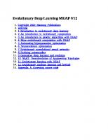
1.2.7 The modern machine-learning landscape A great way to get a sense of the current landscape of machine-learning algorithms and tools is to look at machine-learning competitions on Kaggle. Due to its highly competitive environment (some contests have thousands of entrants and million-dollar prizes) and to the wide variety of machine-learning problems covered, Kaggle offers a realistic way to assess what works and what doesn’t. So, what kind of algorithm is reliably winning competitions? What tools do top entrants use? In early 2019, Kaggle ran a survey asking teams that ended in the top five of any competition since 2017 which primary software tool they had used in the competition (see figure [TODO]). It turns out that top teams tend to use either deep learning methods (most often via the Keras library) or gradient boosted trees (most often via the LightGBM or XGBoost libraries).
©Manning Publications Co. To comment go to liveBook https://livebook.manning.com/#!/book/deep-learning-with-python-second-edition/discussion
20
Figure 1.12 ML tools used by top teams on Kaggle
It’s not just competition champions, either. Kaggle also runs a yearly survey among machine learning and data science professionals worldwide. With thousands of respondents, this survey is one of our most reliable sources about the state of the industry. Figure [TODO] shows the percentage of usage of different machine learning software frameworks.
©Manning Publications Co. To comment go to liveBook https://livebook.manning.com/#!/book/deep-learning-with-python-second-edition/discussion
21
Figure 1.13 Tool usage across the machine learning and data science industry (source: www.kaggle.com/kaggle-survey-2019)
From 2016 to 2020, the entire machine learning and data science industry has been dominated by these two approaches: deep learning and gradient boosted trees. Specifically, gradient boosted trees is used for problems where structured data is available, whereas deep learning is used for perceptual problems such as image classification. Users of gradient boosted trees tend to use Scikit-Learn, XGBoost or LightGBM. Meanwhile, most practitioners of deep learning use Keras, often in combination with its parent framework TensorFlow. The common point of these tools is they’re all Python libraries: Python is by far the most widely-used language for machine learning and data science. These are the two techniques you should be the most familiar with in order to be successful in applied machine learning today: gradient boosted trees, for shallow-learning problems; and deep
©Manning Publications Co. To comment go to liveBook https://livebook.manning.com/#!/book/deep-learning-with-python-second-edition/discussion
22
learning, for perceptual problems. In technical terms, this means you’ll need to be familiar with Scikit-Learn, XGBoost, and Keras — the three libraries that currently dominate Kaggle competitions. With this book in hand, you’re already one big step closer.
1.3 Why deep learning? Why now? The two key ideas of deep learning for computer vision — convolutional neural networks and backpropagation — were already well understood by 1990. The Long Short-Term Memory (LSTM) algorithm, which is fundamental to deep learning for timeseries, was developed in 1997 and has barely changed since. So why did deep learning only take off after 2012? What changed in these two decades? In general, three technical forces are driving advances in machine learning: Hardware Datasets and benchmarks Algorithmic advances Because the field is guided by experimental findings rather than by theory, algorithmic advances only become possible when appropriate data and hardware are available to try new ideas (or scale up old ideas, as is often the case). Machine learning isn’t mathematics or physics, where major advances can be done with a pen and a piece of paper. It’s an engineering science. The real bottlenecks throughout the 1990s and 2000s were data and hardware. But here’s what happened during that time: the internet took off, and high-performance graphics chips were developed for the needs of the gaming market.
1.3.1 Hardware Between 1990 and 2010, off-the-shelf CPUs became faster by a factor of approximately 5,000. As a result, nowadays it’s possible to run small deep-learning models on your laptop, whereas this would have been intractable 25 years ago. But typical deep-learning models used in computer vision or speech recognition require orders of magnitude more computational power than what your laptop can deliver. Throughout the 2000s, companies like NVIDIA and AMD invested billions of dollars in developing fast, massively parallel chips (Graphical Processing Units, or GPUs) to power the graphics of increasingly photorealistic video games — cheap, single-purpose supercomputers designed to render complex 3D scenes on your screen in real time. This investment came to benefit the scientific community when, in 2007, NVIDIA launched CUDA (developer.nvidia.com/about-cuda), a programming interface for its line of GPUs. A small number of GPUs started replacing massive clusters of CPUs in various highly parallelizable applications, beginning with physics modeling. Deep neural networks, consisting mostly of many small matrix multiplications, are also highly ©Manning Publications Co. To comment go to liveBook https://livebook.manning.com/#!/book/deep-learning-with-python-second-edition/discussion
23
parallelizable; and around 2011, some researchers began to write CUDA implementations of neural nets — Dan Ciresan 5 and Alex Krizhevsky 6 were among the first. What happened is that the gaming market subsidized supercomputing for the next generation of artificial intelligence applications. Sometimes, big things begin as games. Today, the NVIDIA Titan RTX, a GPU that cost $2,500 at the end of 2019, can deliver a peak of 16 TeraFLOPs in single precision (16 trillion float32 operations per second). That’s about 500 times more computing power than the world’s fastest supercomputer from 1990, the Intel Touchstone Delta. On a Titan RTX, it takes only a few hours to train an ImageNet model of the sort that would have won the ILSVRC competition around 2012 or 2013. Meanwhile, large companies train deep-learning models on clusters of hundreds of GPUs. What’s more, the deep-learning industry has been moving beyond GPUs and is investing in increasingly specialized, efficient chips for deep learning. In 2016, at its annual I/O convention, Google revealed its Tensor Processing Unit (TPU) project: a new chip design developed from the ground up to run deep neural networks, significantly faster and far more energy efficient than top-of-the-line GPUs. Today, in 2020, the 3rd iteration of the TPU card represents 420 TeraFLOPs of computing power. That’s 10,000 times more than the Intel Touchstone Delta from 1990. These TPU cards are designed to be assembled into large-scaled configurations, called “pods”. One pod (1024 TPU cards) peaks at 100 PetaFLOPs. For scale, that’s about 10% of the peak computing power of the current largest supercomputer, the IBM Summit at Oak Ridge National Lab, which consists of 27,000 NVIDIA GPUs and peaks at around 1.1 ExaFLOP.
1.3.2 Data AI is sometimes heralded as the new industrial revolution. If deep learning is the steam engine of this revolution, then data is its coal: the raw material that powers our intelligent machines, without which nothing would be possible. When it comes to data, in addition to the exponential progress in storage hardware over the past 20 years (following Moore’s law), the game changer has been the rise of the internet, making it feasible to collect and distribute very large datasets for machine learning. Today, large companies work with image datasets, video datasets, and natural-language datasets that couldn’t have been collected without the internet. User-generated image tags on Flickr, for instance, have been a treasure trove of data for computer vision. So are YouTube videos. And Wikipedia is a key dataset for natural-language processing. If there’s one dataset that has been a catalyst for the rise of deep learning, it’s the ImageNet dataset, consisting of 1.4 million images that have been hand annotated with 1,000 image categories (one category per image). But what makes ImageNet special isn’t just its large size, but also the yearly competition associated with it. 7 ©Manning Publications Co. To comment go to liveBook https://livebook.manning.com/#!/book/deep-learning-with-python-second-edition/discussion
24
As Kaggle has been demonstrating since 2010, public competitions are an excellent way to motivate researchers and engineers to push the envelope. Having common benchmarks that researchers compete to beat has greatly helped the rise of deep learning, by highlighting its success against classical machine learning approaches.
1.3.3 Algorithms In addition to hardware and data, until the late 2000s, we were missing a reliable way to train very deep neural networks. As a result, neural networks were still fairly shallow, using only one or two layers of representations; thus, they weren’t able to shine against more-refined shallow methods such as SVMs and random forests. The key issue was that of gradient propagation through deep stacks of layers. The feedback signal used to train neural networks would fade away as the number of layers increased. This changed around 2009–2010 with the advent of several simple but important algorithmic improvements that allowed for better gradient propagation: Better activation functions for neural layers Better weight-initialization schemes, starting with layer-wise pretraining, which was then quickly abandoned Better optimization schemes, such as RMSProp and Adam Only when these improvements began to allow for training models with 10 or more layers did deep learning start to shine. Finally, in 2014, 2015, and 2016, even more advanced ways to help gradient propagation were discovered, such as batch normalization, residual connections, and depthwise separable convolutions. Today, we can train from scratch models that are arbitrarily deep. This has unlocked the use of extremely large models, which hold considerable representational power — that is to say, which encode very rich hypothesis spaces. This extreme scalability is one of the defining characteristic of modern deep learning. Large-scale model architectures, which feature tens of layers and tens of millions of parameters, have brought about critical advances both in computer vision (for instance, architectures such as ResNet, Inception, or Xception) and natural language processing (for instance, large Transformer-based architectures such as BERT, GPT-2, or XLNet).
1.3.4 A new wave of investment As deep learning became the new state of the art for computer vision in 2012–2013, and eventually for all perceptual tasks, industry leaders took note. What followed was a gradual wave of industry investment far beyond anything previously seen in the history of AI.
©Manning Publications Co. To comment go to liveBook https://livebook.manning.com/#!/book/deep-learning-with-python-second-edition/discussion
25
Figure 1.14 OECD estimate of total investments in AI startups (source: www.oecd-ilibrary.org/sites/3abc27f1-en/index.html?itemId=/content/component/3abc27f1-en&mimeType=t
EDITION NOTE: we should re-render the chart to avoid copyright issues, and also shorten the URL of the source. In 2011, right before deep learning took the spotlight, the total venture capital investment in AI worldwide was less than a billion dollars, which went almost entirely to practical applications of shallow machine-learning approaches. In 2015, it had risen to over $5 billion, and in 2017, to a staggering $16 billion. Hundreds of startups launched in these few years, trying to capitalize on the deep-learning hype. Meanwhile, large tech companies such as Google, Facebook, Amazon, and Microsoft have invested in internal research departments in amounts that would most likely dwarf the flow of venture-capital money. Machine learning — in particular, deep learning — has become central to the product strategy of these tech giants. In late 2015, Google CEO Sundar Pichai stated, “Machine learning is a core, transformative way by which we’re rethinking how we’re doing everything. We’re thoughtfully applying it across all our products, be it search, ads, YouTube, or Play. And we’re in early days, but you’ll see us — in a systematic way — apply machine learning in all these areas.” 8 ©Manning Publications Co. To comment go to liveBook https://livebook.manning.com/#!/book/deep-learning-with-python-second-edition/discussion
26
As a result of this wave of investment, the number of people working on deep learning went in less than ten years from a few hundred to tens of thousands, and research progress has reached a frenetic pace.
1.3.5 The democratization of deep learning One of the key factors driving this inflow of new faces in deep learning has been the democratization of the toolsets used in the field. In the early days, doing deep learning required significant C++ and CUDA expertise, which few people possessed. Nowadays, basic Python scripting skills suffice to do advanced deep-learning research. This has been driven most notably by the development of the now-defunct Theano and then TensorFlow — two symbolic tensor-manipulation frameworks for Python that support autodifferentiation, greatly simplifying the implementation of new models — and by the rise of user-friendly libraries such as Keras, which makes deep learning as easy as manipulating LEGO bricks. After its release in early 2015, Keras quickly became the go-to deep-learning solution for large numbers of new startups, graduate students, and researchers pivoting into the field.
1.3.6 Will it last? Is there anything special about deep neural networks that makes them the “right” approach for companies to be investing in and for researchers to flock to? Or is deep learning just a fad that may not last? Will we still be using deep neural networks in 20 years? Deep learning has several properties that justify its status as an AI revolution, and it’s here to stay. We may not be using neural networks two decades from now, but whatever we use will directly inherit from modern deep learning and its core concepts. These important properties can be broadly sorted into three categories: Simplicity — Deep learning removes the need for feature engineering, replacing complex, brittle, engineering-heavy pipelines with simple, end-to-end trainable models that are typically built using only five or six different tensor operations. Scalability — Deep learning is highly amenable to parallelization on GPUs or TPUs, so it can take full advantage of Moore’s law. In addition, deep-learning models are trained by iterating over small batches of data, allowing them to be trained on datasets of arbitrary size. (The only bottleneck is the amount of parallel computational power available, which, thanks to Moore’s law, is a fast-moving barrier.) Versatility and reusability — Unlike many prior machine-learning approaches, deep-learning models can be trained on additional data without restarting from scratch, making them viable for continuous online learning — an important property for very large production models. Furthermore, trained deep-learning models are repurposable and thus reusable: for instance, it’s possible to take a deep-learning model trained for image classification and drop it into a video-processing pipeline. This allows us to reinvest previous work into increasingly complex and powerful models. This also makes deep learning applicable to fairly small datasets. ©Manning Publications Co. To comment go to liveBook https://livebook.manning.com/#!/book/deep-learning-with-python-second-edition/discussion
27
Deep learning has only been in the spotlight for a few years, and we may not have yet established the full scope of what it can do. With every passing year, we learn about new use cases and engineering improvements that lift previous limitations. Following a scientific revolution, progress generally follows a sigmoid curve: it starts with a period of fast progress, which gradually stabilizes as researchers hit hard limitations, and then further improvements become incremental. When I was writing the first edition of this book, in 2016, I predicted that deep learning was still in the first half of that sigmoid, with much more transformative progress to come in the following few years. This has proven true in practice, as 2017 and 2018 have seen the rise of Transformer-based deep learning models for natural language processing, which have been a revolution in the field, while deep learning also kept delivering steady progress in computer vision and speech recognition. Today, in 2020, deep learning seems to have entered the second half of that sigmoid. We should still expect significant progress in the years to come, but we’re probably out of the initial phase of explosive progress. An area that I am extremely excited about today is the deployment of deep learning technology to every problem it can solve — the list is endless. Deep learning is still a revolution in the making, and it will take many years to realize its full potential.
©Manning Publications Co. To comment go to liveBook https://livebook.manning.com/#!/book/deep-learning-with-python-second-edition/discussion
28
2
The mathematical building blocks of neural networks
This chapter covers A first example of a neural network Tensors and tensor operations How neural networks learn via backpropagation and gradient descent
Understanding deep learning requires familiarity with many simple mathematical concepts: tensors, tensor operations, differentiation, gradient descent, and so on. Our goal in this chapter will be to build your intuition about these notions without getting overly technical. In particular, we’ll steer away from mathematical notation, which can be off-putting for those without any mathematics background and isn’t necessary to explain things well. The most precise, unambiguous description of a mathematical operation is its executable code. To add some context for tensors and gradient descent, we’ll begin the chapter with a practical example of a neural network. Then we’ll go over every new concept that’s been introduced, point by point. Keep in mind that these concepts will be essential for you to understand the practical examples that will come in the following chapters! After reading this chapter, you’ll have an intuitive understanding of the mathematical theory behind deep learning, and you’ll be ready to start diving into Keras and TensorFlow, in chapter 3.
©Manning Publications Co. To comment go to liveBook https://livebook.manning.com/#!/book/deep-learning-with-python-second-edition/discussion
29
2.1 A first look at a neural network Let’s look at a concrete example of a neural network that uses the Python library Keras to learn to classify handwritten digits. Unless you already have experience with Keras or similar libraries, you won’t understand everything about this first example right away. You probably haven’t even installed Keras yet; that’s fine. In the next chapter, we’ll review each element in the example and explain them in detail. So don’t worry if some steps seem arbitrary or look like magic to you! We’ve got to start somewhere. The problem we’re trying to solve here is to classify grayscale images of handwritten digits (28 × 28 pixels) into their 10 categories (0 through 9). We’ll use the MNIST dataset, a classic in the machine-learning community, which has been around almost as long as the field itself and has been intensively studied. It’s a set of 60,000 training images, plus 10,000 test images, assembled by the National Institute of Standards and Technology (the NIST in MNIST) in the 1980s. You can think of “solving” MNIST as the “Hello World” of deep learning — it’s what you do to verify that your algorithms are working as expected. As you become a machine-learning practitioner, you’ll see MNIST come up over and over again, in scientific papers, blog posts, and so on. You can see some MNIST samples in figure 2.1. SIDEBAR
Note on classes and labels In machine learning, a category in a classification problem is called a class. Data points are called samples. The class associated with a specific sample is called a label.
Figure 2.1 MNIST sample digits
You don’t need to try to reproduce this example on your machine just now. If you wish to, you’ll first need to set up a deep learning workspace, which is covered in chapter 3. The MNIST dataset comes preloaded in Keras, in the form of a set of four NumPy arrays. Listing 2.1 Loading the MNIST dataset in Keras from keras.datasets import mnist (train_images, train_labels), (test_images, test_labels) = mnist.load_data()
train_images and train_labels form the training set, the data that the model will learn from.
The model will then be tested on the test set, test_images and test_labels. The images are encoded as NumPy arrays, and the labels are an array of digits, ranging from 0 to 9. The images and labels have a one-to-one correspondence. ©Manning Publications Co. To comment go to liveBook https://livebook.manning.com/#!/book/deep-learning-with-python-second-edition/discussion
30
Let’s look at the training data: >>> train_images.shape (60000, 28, 28) >>> len(train_labels) 60000 >>> train_labels array([5, 0, 4, ..., 5, 6, 8], dtype=uint8)
And here’s the test data: >>> test_images.shape (10000, 28, 28) >>> len(test_labels) 10000 >>> test_labels array([7, 2, 1, ..., 4, 5, 6], dtype=uint8)
The workflow will be as follows: First, we’ll feed the neural network the training data, train_images and train_labels. The network will then learn to associate images and labels. Finally, we’ll ask the network to produce predictions for test_images, and we’ll verify whether these predictions match the labels from test_labels. Let’s build the network — again, remember that you aren’t expected to understand everything about this example yet. Listing 2.2 The network architecture from tensorflow.keras import models from tensorflow.keras import layers model = models.Sequential([ layers.Dense(512, activation='relu'), layers.Dense(10, activation='softmax') ])
The core building block of neural networks is the layer, a data-processing module that you can think of as a filter for data. Some data goes in, and it comes out in a more useful form. Specifically, layers extract representations out of the data fed into them — hopefully, representations that are more meaningful for the problem at hand. Most of deep learning consists of chaining together simple layers that will implement a form of progressive data distillation. A deep-learning model is like a sieve for data processing, made of a succession of increasingly refined data filters — the layers. Here, our model consists of a sequence of two Dense layers, which are densely connected (also called fully connected) neural layers. The second (and last) layer is a 10-way softmax classification layer, which means it will return an array of 10 probability scores (summing to 1). Each score will be the probability that the current digit image belongs to one of our 10 digit classes. To make the model ready for training, we need to pick three more things, as part of the ©Manning Publications Co. To comment go to liveBook https://livebook.manning.com/#!/book/deep-learning-with-python-second-edition/discussion
31
compilation step: An optimizer — The mechanism through which the model will update itself based on the training data it sees, so as to improve its performance. A loss function — How the model will be able to measure its performance on the training data, and thus how it will be able to steer itself in the right direction. Metrics to monitor during training and testing — Here, we’ll only care about accuracy (the fraction of the images that were correctly classified). The exact purpose of the loss function and the optimizer will be made clear throughout the next two chapters. Listing 2.3 The compilation step model.compile(optimizer='rmsprop', loss='sparse_categorical_crossentropy', metrics=['accuracy'])
Before training, we’ll preprocess the data by reshaping it into the shape the model expects and scaling it so that all values are in the [0, 1] interval. Previously, our training images, for instance, were stored in an array of shape (60000, 28, 28) of type uint8 with values in the [0, 255] interval. We transform it into a float32 array of shape (60000, 28 * 28) with values between 0 and 1. Listing 2.4 Preparing the image data train_images = train_images.reshape((60000, 28 * 28)) train_images = train_images.astype('float32') / 255 test_images = test_images.reshape((10000, 28 * 28)) test_images = test_images.astype('float32') / 255
We’re now ready to train the model, which in Keras is done via a call to the model’s fit method — we fit the model to its training data: Listing 2.5 "Fitting" the model >>> model.fit(train_images, train_labels, epochs=5, batch_size=128) Epoch 1/5 60000/60000 [==============================] - 5s - loss: 0.2524 - acc: 0.9273 Epoch 2/5 51328/60000 [========================>.....] - ETA: 1s - loss: 0.1035 - acc: 0.9692
Two quantities are displayed during training: the loss of the model over the training data, and the accuracy of the model over the training data. We quickly reach an accuracy of 0.989 (98.9%) on the training data. Now that we have a trained model, you can use it to predict class probabilities for new digits — images that weren’t part of the training data, like those from the test set:
©Manning Publications Co. To comment go to liveBook https://livebook.manning.com/#!/book/deep-learning-with-python-second-edition/discussion
32
Listing 2.6 Using the model to make predictions >>> test_digits = test_images[0:10] >>> predictions = model.predict(test_digits) >>> predictions[0] array([1.0726176e-10, 1.6918376e-10, 6.1314843e-08, 8.4106023e-06, 2.9967067e-11, 3.0331331e-09, 8.3651971e-14, 9.9999106e-01, 2.6657624e-08, 3.8127661e-07], dtype=float32)
Each number of index i in that array corresponds to the probability that digit image test_digits[0] belong to class i. This first test digit has the highest probability score (0.99999106, almost 1) at index 7, so according to our model, it must be a 7: >>> predictions[0].argmax() 7 >>> predictions[0][7] 0.99999106
We can check that the test label agrees: >>> test_labels[0] 7
On average, how good is our model at classifying such never-seen-before digits? Let’s check by computing average accuracy over the entire test set. Listing 2.7 Evaluating the model on new data >>> test_loss, test_acc = model.evaluate(test_images, test_labels) >>> print('test_acc:', test_acc) test_acc: 0.9785
The test-set accuracy turns out to be 97.8% — that’s quite a bit lower than the training set accuracy (98.9%). This gap between training accuracy and test accuracy is an example of overfitting: the fact that machine-learning models tend to perform worse on new data than on their training data. Overfitting is a central topic in chapter 3. This concludes our first example — you just saw how you can build and train a neural network to classify handwritten digits in less than 15 lines of Python code. In this chapter and the next, we’ll go into detail about every moving piece we just previewed and clarify what’s going on behind the scenes. You’ll learn about tensors, the data-storing objects going into the model; tensor operations, which layers are made of; and gradient descent, which allows your model to learn from its training examples.
©Manning Publications Co. To comment go to liveBook https://livebook.manning.com/#!/book/deep-learning-with-python-second-edition/discussion
33
2.2 Data representations for neural networks In the previous example, we started from data stored in multidimensional NumPy arrays, also called tensors. In general, all current machine-learning systems use tensors as their basic data structure. Tensors are fundamental to the field — so fundamental that TensorFlow was named after them. So what’s a tensor? At its core, a tensor is a container for data — usually numerical data. So, it’s a container for numbers. You may be already familiar with matrices, which are rank-2 tensors: tensors are a generalization of matrices to an arbitrary number of dimensions (note that in the context of tensors, a dimension is often called an axis).
2.2.1 Scalars (rank-0 tensors) A tensor that contains only one number is called a scalar (or scalar tensor, or rank-0 tensor, or 0D tensor). In NumPy, a float32 or float64 number is a scalar tensor (or scalar array). You can display the number of axes of a NumPy tensor via the ndim attribute; a scalar tensor has 0 axes (ndim == 0). The number of axes of a tensor is also called its rank. Here’s a NumPy scalar: >>> import numpy as np >>> x = np.array(12) >>> x array(12) >>> x.ndim 0
2.2.2 Vectors (rank-1 tensors) An array of numbers is called a vector, or rank-1 tensor, or 1D tensor. A rank-1 tensor is said to have exactly one axis. Following is a NumPy vector: >>> x = np.array([12, 3, 6, 14, 7]) >>> x array([12, 3, 6, 14, 7]) >>> x.ndim 1
This vector has five entries and so is called a 5-dimensional vector. Don’t confuse a 5D vector with a 5D tensor! A 5D vector has only one axis and has five dimensions along its axis, whereas a 5D tensor has five axes (and may have any number of dimensions along each axis). Dimensionality can denote either the number of entries along a specific axis (as in the case of our 5D vector) or the number of axes in a tensor (such as a 5D tensor), which can be confusing at times. In the latter case, it’s technically more correct to talk about a tensor of rank 5 (the rank of a tensor being the number of axes), but the ambiguous notation 5D tensor is common regardless.
©Manning Publications Co. To comment go to liveBook https://livebook.manning.com/#!/book/deep-learning-with-python-second-edition/discussion
34
2.2.3 Matrices (rank-2 tensors) An array of vectors is a matrix, or rank-2 tensor, or 2D tensor. A matrix has two axes (often referred to rows and columns). You can visually interpret a matrix as a rectangular grid of numbers. This is a NumPy matrix: >>> x = np.array([[5, 78, 2, 34, 0], [6, 79, 3, 35, 1], [7, 80, 4, 36, 2]]) >>> x.ndim 2
The entries from the first axis are called the rows, and the entries from the second axis are called the columns. In the previous example, [5, 78, 2, 34, 0] is the first row of x, and [5, 6, 7] is the first column.
2.2.4 Rank-3 tensors and higher-rank tensors If you pack such matrices in a new array, you obtain a rank-3 tensor (or 3D tensor), which you can visually interpret as a cube of numbers. Following is a NumPy rank-3 tensor: >>> x = np.array([[[5, [6, [7, [[5, [6, [7, [[5, [6, [7, >>> x.ndim 3
78, 79, 80, 78, 79, 80, 78, 79, 80,
2, 3, 4, 2, 3, 4, 2, 3, 4,
34, 35, 36, 34, 35, 36, 34, 35, 36,
0], 1], 2]], 0], 1], 2]], 0], 1], 2]]])
By packing rank-3 tensors in an array, you can create a rank-4 tensor, and so on. In deep learning, you’ll generally manipulate tensors with ranks 0 to 4, although you may go up to 5 if you process video data.
2.2.5 Key attributes A tensor is defined by three key attributes: Number of axes (rank) — For instance, a rank-3 tensor has three axes, and a matrix has two axes. This is also called the tensor’s ndim in Python libraries such as NumPy or TensorFlow. Shape — This is a tuple of integers that describes how many dimensions the tensor has along each axis. For instance, the previous matrix example has shape (3, 5), and the rank-3 tensor example has shape (3, 3, 5). A vector has a shape with a single element, such as (5,), whereas a scalar has an empty shape, (). Data type (usually called dtype in Python libraries) — This is the type of the data contained in the tensor; for instance, a tensor’s type could be float16, float32, float64, uint8, and so on. In TensorFlow, you are also likely to come across string tensors. ©Manning Publications Co. To comment go to liveBook https://livebook.manning.com/#!/book/deep-learning-with-python-second-edition/discussion
35
To make this more concrete, let’s look back at the data we processed in the MNIST example. First, we load the MNIST dataset: from keras.datasets import mnist (train_images, train_labels), (test_images, test_labels) = mnist.load_data()
Next, we display the number of axes of the tensor train_images, the ndim attribute: >>> print(train_images.ndim) 3
Here’s its shape: >>> print(train_images.shape) (60000, 28, 28)
And this is its data type, the dtype attribute: >>> print(train_images.dtype) uint8
So what we have here is a rank-3 tensor of 8-bit integers. More precisely, it’s an array of 60,000 matrices of 28 × 28 integers. Each such matrix is a grayscale image, with coefficients between 0 and 255. Let’s display the fourth digit in this rank-3 tensor, using the library Matplotlib (part of the standard scientific Python suite); see figure 2.2. Listing 2.8 Displaying the fourth digit digit = train_images[4] import matplotlib.pyplot as plt plt.imshow(digit, cmap=plt.cm.binary) plt.show()
Figure 2.2 The fourth sample in our dataset ©Manning Publications Co. To comment go to liveBook https://livebook.manning.com/#!/book/deep-learning-with-python-second-edition/discussion
36
Naturally, the corresponding label is just the integer 9: >>> train_labels[4] 9
2.2.6 Manipulating tensors in NumPy In the previous example, we selected a specific digit alongside the first axis using the syntax train_images[i]. Selecting specific elements in a tensor is called tensor slicing. Let’s look at the tensor-slicing operations you can do on NumPy arrays. The following example selects digits #10 to #100 (#100 isn’t included) and puts them in an array of shape (90, 28, 28): >>> my_slice = train_images[10:100] >>> print(my_slice.shape) (90, 28, 28)
It’s equivalent to this more detailed notation, which specifies a start index and stop index for the slice along each tensor axis. Note that : is equivalent to selecting the entire axis: >>> my_slice = train_images[10:100, :, :] >>> my_slice.shape (90, 28, 28) >>> my_slice = train_images[10:100, 0:28, 0:28] >>> my_slice.shape (90, 28, 28)
Equivalent to the previous example Also equivalent to the previous example In general, you may select between any two indices along each tensor axis. For instance, in order to select 14 × 14 pixels in the bottom-right corner of all images, you do this: my_slice = train_images[:, 14:, 14:]
It’s also possible to use negative indices. Much like negative indices in Python lists, they indicate a position relative to the end of the current axis. In order to crop the images to patches of 14 × 14 pixels centered in the middle, you do this: my_slice = train_images[:, 7:-7, 7:-7]
2.2.7 The notion of data batches In general, the first axis (axis 0, because indexing starts at 0) in all data tensors you’ll come across in deep learning will be the samples axis (sometimes called the samples dimension). In the MNIST example, samples are images of digits. In addition, deep-learning models don’t process an entire dataset at once; rather, they break the ©Manning Publications Co. To comment go to liveBook https://livebook.manning.com/#!/book/deep-learning-with-python-second-edition/discussion
37
data into small batches. Concretely, here’s one batch of our MNIST digits, with batch size of 128: batch = train_images[:128]
And here’s the next batch: batch = train_images[128:256]
And the nth batch: n = 3 batch = train_images[128 * n:128 * (n + 1)]
When considering such a batch tensor, the first axis (axis 0) is called the batch axis or batch dimension. This is a term you’ll frequently encounter when using Keras and other deep-learning libraries.
2.2.8 Real-world examples of data tensors Let’s make data tensors more concrete with a few examples similar to what you’ll encounter later. The data you’ll manipulate will almost always fall into one of the following categories: Vector data — rank-2 tensors of shape (samples, features) Timeseries data or sequence data — rank-3 tensors of shape (samples, timesteps, features)
Images — rank-4 tensors of shape (samples, height, width, channels) or (samples, channels, height, width)
Video — rank-5 tensors of shape (samples, frames, height, width, channels) or (samples, frames, channels, height, width)
2.2.9 Vector data This is one of the most common cases. In such a dataset, each single data point can be encoded as a vector, and thus a batch of data will be encoded as a rank-2 tensor (that is, an array of vectors), where the first axis is the samples axis and the second axis is the features axis. Let’s take a look at two examples: An actuarial dataset of people, where we consider each person’s age, ZIP code, and income. Each person can be characterized as a vector of 3 values, and thus an entire dataset of 100,000 people can be stored in a rank-2 tensor of shape (100000, 3). A dataset of text documents, where we represent each document by the counts of how many times each word appears in it (out of a dictionary of 20,000 common words). Each document can be encoded as a vector of 20,000 values (one count per word in the dictionary), and thus an entire dataset of 500 documents can be stored in a tensor of shape (500, 20000). ©Manning Publications Co. To comment go to liveBook https://livebook.manning.com/#!/book/deep-learning-with-python-second-edition/discussion
38
2.2.10 Timeseries data or sequence data Whenever time matters in your data (or the notion of sequence order), it makes sense to store it in a rank-3 tensor with an explicit time axis. Each sample can be encoded as a sequence of vectors (a rank-2 tensor), and thus a batch of data will be encoded as a rank-3 tensor (see figure 2.3).
Figure 2.3 A rank-3 timeseries data tensor
The time axis is always the second axis (axis of index 1), by convention. Let’s look at a few examples: A dataset of stock prices. Every minute, we store the current price of the stock, the highest price in the past minute, and the lowest price in the past minute. Thus every minute is encoded as a 3D vector, an entire day of trading is encoded as a matrix of shape (390, 3) (there are 390 minutes in a trading day), and 250 days' worth of data can be stored in a rank-3 tensor of shape (250, 390, 3). Here, each sample would be one day’s worth of data. A dataset of tweets, where we encode each tweet as a sequence of 280 characters out of an alphabet of 128 unique characters. In this setting, each character can be encoded as a binary vector of size 128 (an all-zeros vector except for a 1 entry at the index corresponding to the character). Then each tweet can be encoded as a rank-2 tensor of shape (280, 128), and a dataset of 1 million tweets can be stored in a tensor of shape (1000000, 280, 128).
2.2.11 Image data Images typically have three dimensions: height, width, and color depth. Although grayscale images (like our MNIST digits) have only a single color channel and could thus be stored in rank-2 tensors, by convention image tensors are always rank-3, with a one-dimensional color channel for grayscale images. A batch of 128 grayscale images of size 256 × 256 could thus be stored in a tensor of shape (128, 256, 256, 1), and a batch of 128 color images could be stored in a tensor of shape (128, 256, 256, 3) (see figure 2.4).
©Manning Publications Co. To comment go to liveBook https://livebook.manning.com/#!/book/deep-learning-with-python-second-edition/discussion
39
Figure 2.4 A rank-4 image data tensor (channels-first convention)
There are two conventions for shapes of images tensors: the channels-last convention (which is standard in TensorFlow) and the channels-first convention. The channels-last convention places the color-depth axis at the end: (samples, height, width, color_depth). Meanwhile, the channels-first convention places the color depth axis right after the batch axis: (samples, color_depth, height, width). With the channels-last convention, the previous examples would become (128, 1, 256, 256) and (128, 3, 256, 256). The Keras API provides support for both formats.
2.2.12 Video data Video data is one of the few types of real-world data for which you’ll need rank-5 tensors. A video can be understood as a sequence of frames, each frame being a color image. Because each frame can be stored in a rank-3 tensor (height, width, color_depth), a sequence of frames can be stored in a rank-4 tensor (frames, height, width, color_depth), and thus a batch of different videos can be stored in a rank-5 tensor of shape (samples, frames, height, width, color_depth). For instance, a 60-second, 144 × 256 YouTube video clip sampled at 4 frames per second would have 240 frames. A batch of four such video clips would be stored in a tensor of shape (4, 240, 144, 256, 3). That’s a total of 106,168,320 values! If the dtype of the tensor was float32 , then each value would be stored in 32 bits, so the tensor would represent 405 MB. Heavy! Videos you encounter in real life are much lighter, because they aren’t stored in float32, and they’re typically compressed by a large factor (such as in the MPEG format).
©Manning Publications Co. To comment go to liveBook https://livebook.manning.com/#!/book/deep-learning-with-python-second-edition/discussion
40
2.3 The gears of neural networks: tensor operations Much as any computer program can be ultimately reduced to a small set of binary operations on binary inputs (AND, OR, NOR, and so on), all transformations learned by deep neural networks can be reduced to a handful of tensor operations applied to tensors of numeric data. For instance, it’s possible to add tensors, multiply tensors, and so on. In our initial example, we were building our model by stacking Dense layers on top of each other. A Keras layer instance looks like this: keras.layers.Dense(512, activation='relu')
This layer can be interpreted as a function, which takes as input a matrix and returns another matrix — a new representation for the input tensor. Specifically, the function is as follows (where W is a matrix and b is a vector, both attributes of the layer): output = relu(dot(W, input) + b)
Let’s unpack this. We have three tensor operations here: a dot product (dot) between the input tensor and a tensor named W; an addition (+) between the resulting matrix and a vector b; and, finally, a relu operation. relu(x) is max(x, 0). NOTE
Although this section deals entirely with linear algebra expressions, you won’t find any mathematical notation here. I’ve found that mathematical concepts can be more readily mastered by programmers with no mathematical background if they’re expressed as short Python snippets instead of mathematical equations. So we’ll use NumPy and TensorFlow code throughout.
2.3.1 Element-wise operations The relu operation and addition are element-wise operations: operations that are applied independently to each entry in the tensors being considered. This means these operations are highly amenable to massively parallel implementations ( vectorized implementations, a term that comes from the vector processor supercomputer architecture from the 1970–1990 period). If you want to write a naive Python implementation of an element-wise operation, you use a for loop, as in this naive implementation of an element-wise relu operation: def naive_relu(x): assert len(x.shape) == 2 x = x.copy() for i in range(x.shape[0]): for j in range(x.shape[1]): x[i, j] = max(x[i, j], 0) return x
©Manning Publications Co. To comment go to liveBook https://livebook.manning.com/#!/book/deep-learning-with-python-second-edition/discussion
41
x is a rank-2 NumPy tensor. Avoid overwriting the input tensor. You could do the same for addition: def naive_add(x, y): assert len(x.shape) == 2 assert x.shape == y.shape x = x.copy() for i in range(x.shape[0]): for j in range(x.shape[1]): x[i, j] += y[i, j] return x
x and y are rank-2 NumPy tensors. Avoid overwriting the input tensor. On the same principle, you can do element-wise multiplication, subtraction, and so on. In practice, when dealing with NumPy arrays, these operations are available as well-optimized built-in NumPy functions, which themselves delegate the heavy lifting to a Basic Linear Algebra Subprograms (BLAS) implementation if you have one installed (which you should). BLAS are low-level, highly parallel, efficient tensor-manipulation routines that are typically implemented in Fortran or C. So, in NumPy, you can do the following element-wise operation, and it will be blazing fast: import numpy as np z = x + y z = np.maximum(z, 0.)
Element-wise addition Element-wise relu Let’s actually time the difference: import time x = np.random.random((20, 100)) y = np.random.random((20, 100)) t0 = time.time() for _ in range(1000): z = x + y z = np.maximum(z, 0.) print('Took: %.2f s' % (time.time() - t0))
This takes 0.02s. Meanwhile, the naive version takes a stunning 2.45s: t0 = time.time() for _ in range(1000):
©Manning Publications Co. To comment go to liveBook https://livebook.manning.com/#!/book/deep-learning-with-python-second-edition/discussion
42 z = naive_add(x, y) z = naive_relu(z) print('Took: %.2f s' % (time.time() - t0))
Likewise, when running TensorFlow code on a GPU, elementwise operations are executed via fully-vectorized CUDA implementations that can best utilize the highly-parallel GPU chip architecture.
2.3.2 Broadcasting Our earlier naive implementation of naive_add only supports the addition of rank-2 tensors with identical shapes. But in the Dense layer introduced earlier, we added a rank-2 tensor with a vector. What happens with addition when the shapes of the two tensors being added differ? When possible, and if there’s no ambiguity, the smaller tensor will be broadcasted to match the shape of the larger tensor. Broadcasting consists of two steps: 1. Axes (called broadcast axes) are added to the smaller tensor to match the ndim of the larger tensor. 2. The smaller tensor is repeated alongside these new axes to match the full shape of the larger tensor. Let’s look at a concrete example. Consider X with shape (32, 10) and y with shape (10,). First, we add an empty first axis to y, whose shape becomes (1, 10). Then, we repeat y 32 times alongside this new axis, so that we end up with a tensor Y with shape (32, 10), where Y[i, :] == y for i in range(0, 32). At this point, we can proceed to add X and Y, because they have the same shape. In terms of implementation, no new rank-2 tensor is created, because that would be terribly inefficient. The repetition operation is entirely virtual: it happens at the algorithmic level rather than at the memory level. But thinking of the vector being repeated 10 times alongside a new axis is a helpful mental model. Here’s what a naive implementation would look like: def naive_add_matrix_and_vector(x, y): assert len(x.shape) == 2 assert len(y.shape) == 1 assert x.shape[1] == y.shape[0] x = x.copy() for i in range(x.shape[0]): for j in range(x.shape[1]): x[i, j] += y[j] return x
x is a rank-2 NumPy tensor. y is a NumPy vector. Avoid overwriting the input tensor. With broadcasting, you can generally apply two-tensor element-wise operations if one tensor has ©Manning Publications Co. To comment go to liveBook https://livebook.manning.com/#!/book/deep-learning-with-python-second-edition/discussion
43
shape (a, b, … n, n + 1, … m) and the other has shape (n, n + 1, … m). The broadcasting will then automatically happen for axes a through n - 1. The following example applies the element-wise maximum operation to two tensors of different shapes via broadcasting: import numpy as np x = np.random.random((64, 3, 32, 10)) y = np.random.random((32, 10)) z = np.maximum(x, y)
x is a random tensor with shape (64, 3, 32, 10). y is a random tensor with shape (32, 10). The output z has shape (64, 3, 32, 10) like x.
2.3.3 Tensor product The tensor product, or dot product (not to be confused with an element-wise product, the * operator) is one of the most common, most useful tensor operations. In NumPy, a tensor product is done using the np.dot function (because the mathematical notation for tensor product is usually a dot). x = np.random.random((32,)) y = np.random.random((32,)) z = np.dot(x, y)
In mathematical notation, you’d note the operation with a dot (•): z = x • y
Mathematically, what does the dot operation do? Let’s start with the dot product of two vectors x and y. It’s computed as follows: def naive_vector_dot(x, y): assert len(x.shape) == 1 assert len(y.shape) == 1 assert x.shape[0] == y.shape[0] z = 0. for i in range(x.shape[0]): z += x[i] * y[i] return z
x and y are NumPy vectors. You’ll have noticed that the dot product between two vectors is a scalar and that only vectors with the same number of elements are compatible for a dot product. You can also take the dot product between a matrix x and a vector y , which returns a vector ©Manning Publications Co. To comment go to liveBook https://livebook.manning.com/#!/book/deep-learning-with-python-second-edition/discussion
44
where the coefficients are the dot products between y and the rows of x. You implement it as follows: def naive_matrix_vector_dot(x, y): assert len(x.shape) == 2 assert len(y.shape) == 1 assert x.shape[1] == y.shape[0] z = np.zeros(x.shape[0]) for i in range(x.shape[0]): for j in range(x.shape[1]): z[i] += x[i, j] * y[j] return z
x is a NumPy matrix. y is a NumPy vector. The first dimension of x must be the same as the 0th dimension of y! This operation returns a vector of 0s with the same shape as y. You could also reuse the code we wrote previously, which highlights the relationship between a matrix-vector product and a vector product: def naive_matrix_vector_dot(x, y): z = np.zeros(x.shape[0]) for i in range(x.shape[0]): z[i] = naive_vector_dot(x[i, :], y) return z
Note that as soon as one of the two tensors has an ndim greater than 1, dot is no longer symmetric, which is to say that dot(x, y) isn’t the same as dot(y, x). Of course, a dot product generalizes to tensors with an arbitrary number of axes. The most common applications may be the dot product between two matrices. You can take the dot product of two matrices x and y (dot(x, y)) if and only if x.shape[1] == y.shape[0]. The result is a matrix with shape (x.shape[0], y.shape[1]), where the coefficients are the vector products between the rows of x and the columns of y. Here’s the naive implementation: def naive_matrix_dot(x, y): assert len(x.shape) == 2 assert len(y.shape) == 2 assert x.shape[1] == y.shape[0] z = np.zeros((x.shape[0], y.shape[1])) for i in range(x.shape[0]): for j in range(y.shape[1]): row_x = x[i, :] column_y = y[:, j] z[i, j] = naive_vector_dot(row_x, column_y) return z
x and y are NumPy matrices. The first dimension of x must be the same as the 0th dimension of y! This operation returns a matrix of 0s with a specific shape. ©Manning Publications Co. To comment go to liveBook https://livebook.manning.com/#!/book/deep-learning-with-python-second-edition/discussion
45
Iterates over the rows of x … … and over the columns of y. To understand dot-product shape compatibility, it helps to visualize the input and output tensors by aligning them as shown in figure 2.5.
Figure 2.5 Matrix dot-product box diagram x, y, and z are pictured as rectangles (literal boxes of coefficients). Because the rows of x and the
columns of y must have the same size, it follows that the width of x must match the height of y. If you go on to develop new machine-learning algorithms, you’ll likely be drawing such diagrams often. More generally, you can take the dot product between higher-dimensional tensors, following the same rules for shape compatibility as outlined earlier for the 2D case: (a, b, c, d) • (d,) -> (a, b, c) (a, b, c, d) • (d, e) -> (a, b, c, e)
And so on.
2.3.4 Tensor reshaping A third type of tensor operation that’s essential to understand is tensor reshaping. Although it wasn’t used in the Dense layers in our first neural network example, we used it when we preprocessed the digits data before feeding it into our model: train_images = train_images.reshape((60000, 28 * 28))
©Manning Publications Co. To comment go to liveBook https://livebook.manning.com/#!/book/deep-learning-with-python-second-edition/discussion
46
Reshaping a tensor means rearranging its rows and columns to match a target shape. Naturally, the reshaped tensor has the same total number of coefficients as the initial tensor. Reshaping is best understood via simple examples: >>> x = np.array([[0., 1.], [2., 3.], [4., 5.]]) >>> print(x.shape) (3, 2) >>> x = x.reshape((6, 1)) >>> x array([[ 0.], [ 1.], [ 2.], [ 3.], [ 4.], [ 5.]]) >>> x = x.reshape((2, 3)) >>> x array([[ 0., 1., 2.], [ 3., 4., 5.]])
A special case of reshaping that’s commonly encountered is transposition. Transposing a matrix means exchanging its rows and its columns, so that x[i, :] becomes x[:, i]: >>> x = np.zeros((300, 20)) >>> x = np.transpose(x) >>> print(x.shape) (20, 300)
Creates an all-zeros matrix of shape (300, 20)
2.3.5 Geometric interpretation of tensor operations Because the contents of the tensors manipulated by tensor operations can be interpreted as coordinates of points in some geometric space, all tensor operations have a geometric interpretation. For instance, let’s consider addition. We’ll start with the following vector: A = [0.5, 1]
It’s a point in a 2D space (see figure 2.6). It’s common to picture a vector as an arrow linking the origin to the point, as shown in figure 2.7.
©Manning Publications Co. To comment go to liveBook https://livebook.manning.com/#!/book/deep-learning-with-python-second-edition/discussion
47
Figure 2.6 A point in a 2D space
Figure 2.7 A point in a 2D space pictured as an arrow
Let’s consider a new point, B = [1, 0.25], which we’ll add to the previous one. This is done geometrically by chaining together the vector arrows, with the resulting location being the vector representing the sum of the previous two vectors (see figure 2.8).
©Manning Publications Co. To comment go to liveBook https://livebook.manning.com/#!/book/deep-learning-with-python-second-edition/discussion
48
Figure 2.8 Geometric interpretation of the sum of two vectors
In general, elementary geometric operations such as translation, rotation, scaling, skewing, and so on can be expressed as tensor operations. Here are a few examples. Translation: As you just saw, adding a vector to a point will move this points by a fixed amount in a fixed direction. Applied to a set of points (such as a 2D object), this is called a “translation” (see figure TODO).
Figure 2.9 2D translation as a vector addition
Rotation: A rotation of a 2D vector by an angle theta (see figure TODO) can be achieved via a dot product with a 2 × 2 matrix R = [[cos(theta), sin(theta)], [-sin(theta), cos(theta)]].
©Manning Publications Co. To comment go to liveBook https://livebook.manning.com/#!/book/deep-learning-with-python-second-edition/discussion
49
Figure 2.10 2D rotation as a dot product
EDITION NOTE: the angle theta in the figure should be represented via a arc of circle. Scaling: A vertical and horizontal scaling of the image (see figure TODO) can be achieved via a dot product with a 2 x 2 matrix S = (note that such a matrix is called a “diagonal matrix”, because it only has non-zero coefficients in its “diagonal”, going from the top left to the bottom right).
Figure 2.11 2D scaling as a dot product
Linear transform: A dot product with an arbitrary matrix implements a linear transform. Note that scaling and rotation, seen above, are by definition linear transforms. Affine transform: An affine transform (see figure TODO) is the combination of a linear transform (achieved via a dot product some matrix) and a translation (achieved via a vector addition). As you have probably recognized, that’s exactly the y = W • x + b computation implemented by the Dense layer! A Dense layer without an activation function is an affine layer.
©Manning Publications Co. To comment go to liveBook https://livebook.manning.com/#!/book/deep-learning-with-python-second-edition/discussion
50
Figure 2.12 Affine transform in the plane Dense layer with relu activation: An important observation about affine transforms is
that if you apply many of them repeatedly, you still end up with an affine transform (so you could just have applied that one affine transform in the first place). Let’s try it with two: affine2(affine1(x)) = W2 • (W1 • x + b1) + b2 = (W2 • Wa) • x + (W2 • b1 + b2). That’s an affine transform where the linear part is the matrix W2 • W1 and the translation part is the vector W2 • b1 + b2. As a consequence, a multi-layer neural network made entirely of Dense layers without activations would be equivalent to a single Dense layer. This “deep” neural network would just be a linear model in disguise! This is why we need activation functions, like relu (seen in action in figure TODO). Thanks to activation functions, a chain of Dense layer can be made to implement very complex, non-linear geometric transformation, resulting in very rich hypothesis spaces for your deep neural networks. We cover this idea in more detail in the next chapter.
Figure 2.13 Affine transform followed by relu activation
2.3.6 A geometric interpretation of deep learning You just learned that neural networks consist entirely of chains of tensor operations, and that all of these tensor operations are just simple geometric transformations of the input data. It follows that you can interpret a neural network as a very complex geometric transformation in a high-dimensional space, implemented via a series of simple steps. ©Manning Publications Co. To comment go to liveBook https://livebook.manning.com/#!/book/deep-learning-with-python-second-edition/discussion
51
In 3D, the following mental image may prove useful. Imagine two sheets of colored paper: one red and one blue. Put one on top of the other. Now crumple them together into a small ball. That crumpled paper ball is your input data, and each sheet of paper is a class of data in a classification problem. What a neural network (or any other machine-learning model) is meant to do is figure out a transformation of the paper ball that would uncrumple it, so as to make the two classes cleanly separable again. With deep learning, this would be implemented as a series of simple transformations of the 3D space, such as those you could apply on the paper ball with your fingers, one movement at a time.
Figure 2.14 Uncrumpling a complicated manifold of data
Uncrumpling paper balls is what machine learning is about: finding neat representations for complex, highly folded data manifolds. At this point, you should have a pretty good intuition as to why deep learning excels at this: it takes the approach of incrementally decomposing a complicated geometric transformation into a long chain of elementary ones, which is pretty much the strategy a human would follow to uncrumple a paper ball. Each layer in a deep network applies a transformation that disentangles the data a little — and a deep stack of layers makes tractable an extremely complicated disentanglement process.
2.4 The engine of neural networks: gradient-based optimization As you saw in the previous section, each neural layer from our first model example transforms its input data as follows: output = relu(dot(W, input) + b)
In this expression, W and b are tensors that are attributes of the layer. They’re called the weights or trainable parameters of the layer (the kernel and bias attributes, respectively). These weights contain the information learned by the model from exposure to training data. Initially, these weight matrices are filled with small random values (a step called random initialization). Of course, there’s no reason to expect that relu(dot(W, input) + b), when W and b are random, will yield any useful representations. The resulting representations are meaningless — but they’re a starting point. What comes next is to gradually adjust these weights, based on a feedback signal. This gradual adjustment, also called training, is basically the learning that machine learning is all about. This happens within what’s called a training loop, which works as follows. Repeat these steps in ©Manning Publications Co. To comment go to liveBook https://livebook.manning.com/#!/book/deep-learning-with-python-second-edition/discussion
52
a loop, until the loss seems sufficiently low: 1. Draw a batch of training samples x and corresponding targets y_true. 2. Run the model on x (a step called the forward pass) to obtain predictions y_pred. 3. Compute the loss of the model on the batch, a measure of the mismatch between y_pred and y_true. 4. Update all weights of the model in a way that slightly reduces the loss on this batch. You’ll eventually end up with a model that has a very low loss on its training data: a low mismatch between predictions y_pred and expected targets y_true. The model has “learned” to map its inputs to correct targets. From afar, it may look like magic, but when you reduce it to elementary steps, it turns out to be simple. Step 1 sounds easy enough — just I/O code. Steps 2 and 3 are merely the application of a handful of tensor operations, so you could implement these steps purely from what you learned in the previous section. The difficult part is step 4: updating the model’s weights. Given an individual weight coefficient in the model, how can you compute whether the coefficient should be increased or decreased, and by how much? One naive solution would be to freeze all weights in the model except the one scalar coefficient being considered, and try different values for this coefficient. Let’s say the initial value of the coefficient is 0.3. After the forward pass on a batch of data, the loss of the model on the batch is 0.5. If you change the coefficient’s value to 0.35 and rerun the forward pass, the loss increases to 0.6. But if you lower the coefficient to 0.25, the loss falls to 0.4. In this case, it seems that updating the coefficient by -0.05 would contribute to minimizing the loss. This would have to be repeated for all coefficients in the model. But such an approach would be horribly inefficient, because you’d need to compute two forward passes (which are expensive) for every individual coefficient (of which there are many, usually thousands and sometimes up to millions). A much better approach is to take advantage of the fact that all operations used in the model are differentiable, and compute the gradient of the loss with regard to the model’s coefficients. You can then move the coefficients (all at once in a single update, rather than one at a time) in the opposite direction from the gradient, thus decreasing the loss. If you already know what differentiable means and what a gradient is, you can skip to section TODO. Otherwise, the following two sections will help you understand these concepts.
©Manning Publications Co. To comment go to liveBook https://livebook.manning.com/#!/book/deep-learning-with-python-second-edition/discussion
53
2.4.1 What’s a derivative? Consider a continuous, smooth function f(x) = y, mapping a number x to a new number y. Because the function is continuous, a small change in x can only result in a small change in y — that’s the intuition behind continuity. Let’s say you increase x by a small factor epsilon_x: this results in a small epsilon_y change to y: f(x + epsilon_x) = y + epsilon_y
In addition, because the function is smooth (its curve doesn’t have any abrupt angles), when epsilon_x is small enough, around a certain point p, it’s possible to approximate f as a linear function of slope a, so that epsilon_y becomes a * epsilon_x: f(x + epsilon_x) = y + a * epsilon_x
Obviously, this linear approximation is valid only when x is close enough to p. The slope a is called the derivative of f in p. If a is negative, it means a small change of x around p will result in a decrease of f(x) (as shown in figure 2.10); and if a is positive, a small change in x will result in an increase of f(x). Further, the absolute value of a (the magnitude of the derivative) tells you how quickly this increase or decrease will happen.
Figure 2.15 Derivative of f in p
For every differentiable function f(x) (differentiable means “can be derived”: for example, smooth, continuous functions can be derived), there exists a derivative function f'(x) that maps values of x to the slope of the local linear approximation of f in those points. For instance, the derivative of cos(x) is -sin(x), the derivative of f(x) = a * x is f'(x) = a, and so on. If you’re trying to update x by a factor epsilon_x in order to minimize f(x), and you know the derivative of f, then your job is done: the derivative completely describes how f(x) evolves as you change x. If you want to reduce the value of f(x), you just need to move x a little in the opposite direction from the derivative.
©Manning Publications Co. To comment go to liveBook https://livebook.manning.com/#!/book/deep-learning-with-python-second-edition/discussion
54
2.4.2 Derivative of a tensor operation: the gradient A gradient is the derivative of a tensor operation. It’s the generalization of the concept of derivatives to functions of multidimensional inputs: that is, to functions that take tensors as inputs. Consider an input vector x, a matrix W, a target y_true, and a loss function loss. You can use W to compute a target candidate y_pred, and compute the loss, or mismatch, between the target candidate y_pred and the target y_true: y_pred = dot(W, x) loss_value = loss(y_pred, y_true)
If the data inputs x and y_true are frozen, then this can be interpreted as a function mapping values of W to loss values: loss_value = f(W)
Let’s say the current value of W is W0. Then the derivative of f in the point W0 is a tensor grad(loss_value, W0) with the same shape as W, where each coefficient grad(loss_value, W0)[i, j] indicates the direction and magnitude of the change in loss_value you observe when modifying W0[i, j]. That tensor grad(loss_value, W0) is the gradient of the function f(W) = loss_value in W0, also called “gradient of loss_value with respect to W around W0”. Note that the tensor function grad(f(W), W) (which takes as input a matrix W) can be expressed as a combination of scalar functions grad_ij(f(W), w_ij), each of which would return the derivative of loss_value = f(W) with respect to the coefficient W[i, j] of W, assuming all other coefficients are constant. grad_ij is called the partial derivative of f with respect to W[i, j]. Concretely, what does grad(loss_value, W0) represent? You saw earlier that the derivative of a function f(x) of a single coefficient can be interpreted as the slope of the curve of f. Likewise, grad(loss_value, W0) can be interpreted as the tensor describing the curvature of loss_value = f(W) around W0. For this reason, in much the same way that, for a function f(x), you can reduce the value of f(x) by moving x a little in the opposite direction from the derivative, with a function f(W) of a tensor, you can reduce loss_value = f(W) by moving W in the opposite direction from the gradient: for example, W1 = W0 - step * grad(f(W0), W0) (where step is a small scaling factor). That means going against the curvature, which intuitively should put you lower on the curve. Note that the scaling factor step is needed because grad(loss_value, W0) only approximates the curvature when you’re close to W0, so you don’t want to get too far from W0.
©Manning Publications Co. To comment go to liveBook https://livebook.manning.com/#!/book/deep-learning-with-python-second-edition/discussion
55
2.4.3 Stochastic gradient descent Given a differentiable function, it’s theoretically possible to find its minimum analytically: it’s known that a function’s minimum is a point where the derivative is 0, so all you have to do is find all the points where the derivative goes to 0 and check for which of these points the function has the lowest value. Applied to a neural network, that means finding analytically the combination of weight values that yields the smallest possible loss function. This can be done by solving the equation grad(f(W), W) = 0 for W. This is a polynomial equation of N variables, where N is the number of coefficients in the model. Although it would be possible to solve such an equation for N = 2 or N = 3, doing so is intractable for real neural networks, where the number of parameters is never less than a few thousand and can often be several tens of millions. Instead, you can use the four-step algorithm outlined at the beginning of this section: modify the parameters little by little based on the current loss value on a random batch of data. Because you’re dealing with a differentiable function, you can compute its gradient, which gives you an efficient way to implement step 4. If you update the weights in the opposite direction from the gradient, the loss will be a little less every time: 1. Draw a batch of training samples x and corresponding targets y_true. 2. Run the model on x to obtain predictions y_pred (this is called the forward pass). 3. Compute the loss of the model on the batch, a measure of the mismatch between y_pred and y_true. 4. Compute the gradient of the loss with regard to the model’s parameters (this is called the backward pass). 5. Move the parameters a little in the opposite direction from the gradient — for example W -= learning_rate * gradient — thus reducing the loss on the batch a bit. The learning rate (learning_rate here) would be a scalar factor modulating the “speed” of the gradient descent process. Easy enough! What we just described is called mini-batch stochastic gradient descent (mini-batch SGD). The term stochastic refers to the fact that each batch of data is drawn at random (stochastic is a scientific synonym of random). Figure TODO illustrates what happens in 1D, when the model has only one parameter and you have only one training sample.
©Manning Publications Co. To comment go to liveBook https://livebook.manning.com/#!/book/deep-learning-with-python-second-edition/discussion
56
Figure 2.16 SGD down a 1D loss curve (one learnable parameter)
As you can see, intuitively it’s important to pick a reasonable value for the learning_rate factor. If it’s too small, the descent down the curve will take many iterations, and it could get stuck in a local minimum. If learning_rate is too large, your updates may end up taking you to completely random locations on the curve. Note that a variant of the mini-batch SGD algorithm would be to draw a single sample and target at each iteration, rather than drawing a batch of data. This would be true SGD (as opposed to mini-batch SGD). Alternatively, going to the opposite extreme, you could run every step on all data available, which is called batch SGD. Each update would then be more accurate, but far more expensive. The efficient compromise between these two extremes is to use mini-batches of reasonable size. Although figure TODO illustrates gradient descent in a 1D parameter space, in practice you’ll use gradient descent in highly dimensional spaces: every weight coefficient in a neural network is a free dimension in the space, and there may be tens of thousands or even millions of them. To help you build intuition about loss surfaces, you can also visualize gradient descent along a 2D loss surface, as shown in figure TODO. But you can’t possibly visualize what the actual process of training a neural network looks like — you can’t represent a 1,000,000-dimensional space in a way that makes sense to humans. As such, it’s good to keep in mind that the intuitions you develop through these low-dimensional representations may not always be accurate in practice. This has historically been a source of issues in the world of deep-learning research.
©Manning Publications Co. To comment go to liveBook https://livebook.manning.com/#!/book/deep-learning-with-python-second-edition/discussion
57
Figure 2.17 Gradient descent down a 2D loss surface (two learnable parameters)
Additionally, there exist multiple variants of SGD that differ by taking into account previous weight updates when computing the next weight update, rather than just looking at the current value of the gradients. There is, for instance, SGD with momentum, as well as Adagrad, RMSProp, and several others. Such variants are known as optimization methods or optimizers. In particular, the concept of momentum, which is used in many of these variants, deserves your attention. Momentum addresses two issues with SGD: convergence speed and local minima. Consider figure 2.13, which shows the curve of a loss as a function of a model parameter.
Figure 2.18 A local minimum and a global minimum
As you can see, around a certain parameter value, there is a local minimum: around that point, moving left would result in the loss increasing, but so would moving right. If the parameter
©Manning Publications Co. To comment go to liveBook https://livebook.manning.com/#!/book/deep-learning-with-python-second-edition/discussion
58
under consideration were being optimized via SGD with a small learning rate, then the optimization process would get stuck at the local minimum instead of making its way to the global minimum. You can avoid such issues by using momentum, which draws inspiration from physics. A useful mental image here is to think of the optimization process as a small ball rolling down the loss curve. If it has enough momentum, the ball won’t get stuck in a ravine and will end up at the global minimum. Momentum is implemented by moving the ball at each step based not only on the current slope value (current acceleration) but also on the current velocity (resulting from past acceleration). In practice, this means updating the parameter w based not only on the current gradient value but also on the previous parameter update, such as in this naive implementation: past_velocity = 0. momentum = 0.1 while loss > 0.01: w, loss, gradient = get_current_parameters() velocity = past_velocity * momentum - learning_rate * gradient w = w + momentum * velocity - learning_rate * gradient past_velocity = velocity update_parameter(w)
Constant momentum factor Optimization loop
2.4.4 Chaining derivatives: the Backpropagation algorithm In the algorithm above, we casually assumed that because a function is differentiable, we can easily compute its gradient. But is that true? How can we compute the gradient of complex expressions in practice? In our two-layer network example, how can we get the gradient of the loss with regard to the weights? That’s where the Backpropagation algorithm comes in. THE CHAIN RULE Backpropagation is a way to use the derivative of simple operations (such as addition, relu, or tensor product) to easily compute the gradient of arbitrarily complex combinations of these atomic operations. Crucially, a neural network consists of many tensor operations chained together, each of which has a simple, known derivative. For instance, the model from our first example can be expressed as a function parameterized by the variables W1, b1, W2, and b2 (belonging top the first and second Dense layers respectively), involving the atomic operations dot, relu, softmax, and +, as well as our loss function loss, which are all easily differentiable: loss_value = loss(y_true, softmax(dot(W2, relu(dot(W1, inputs) + b1)) + b2))
Calculus tells us that such a chain of functions can be derived using the following identity, called the chain rule: Consider two functions f and g, as well as the composed function fg such that y = fg(x) == ©Manning Publications Co. To comment go to liveBook https://livebook.manning.com/#!/book/deep-learning-with-python-second-edition/discussion
59
f(g(x)): def fg(x): x1 = g(x) y = f(x1) return y
Then the chain rule states that grad(y, x) == grad(y, x1) * grad(x1, x). This enables you to compute the derivative of fg as long as you know the derivatives of f and g. The chain rule is named like this because when you add more intermediate functions, it starts looking like a chain: def fghj(x): x1 = j(x) x2 = h(x1) x3 = g(x2) y = f(x3) return y grad(y, x) == grad(y, x3) * grad(x3, x2) * grad(x2, x1) * grad(x1, x)
Applying the chain rule to the computation of the gradient values of a neural network gives rise to an algorithm called Backpropagation. Let’s see how that works, concretely. AUTOMATIC DIFFERENTIATION WITH COMPUTATION GRAPHS A useful way to think about backpropagation is in terms of computation graphs. A computation graph is the data structure at the heart of TensorFlow and the deep learning revolution in general. It’s a directed acyclic graph of operations — in our case, tensor operations. For instance, this is the graph representation of our first model:
©Manning Publications Co. To comment go to liveBook https://livebook.manning.com/#!/book/deep-learning-with-python-second-edition/discussion
60
Figure 2.19 The computation graph representation of our two-layer model
Computation graphs have been an extremely successful abstraction in computer science because they enable us to treat computation as data: a computable expression is encoded as a machine-readable data structure that can be used as the input or output of another program. For instance, you could imagine a program that receives a computation graph and returns a new computation graph that implements a large-scale distributed version of the same computation — this would mean that you could distribute any computation without having to write the distribution logic yourself. Or imagine… a program that receives a computation graph and can automatically generate the derivative of the expression it represents. It’s much easier to do these things if your computation is expressed as an explicit graph data structure rather than, say, lines of ASCII characters in a .py file. To explain backpropagation clearly, let’s look at a really basic example of a computation graph. We’ll consider a simplified version of the graph above, where we only have one linear layer and where all variables are scalar. We’ll take two scalar variables w, b, a scalar input x, and apply some operations to them to combine into an output y. Finally, we’ll apply an absolute value error
©Manning Publications Co. To comment go to liveBook https://livebook.manning.com/#!/book/deep-learning-with-python-second-edition/discussion
61
loss function: loss_val = abs(y_true - y). Since we want to update w and b in a way that would minimize loss_val, we are interested in computing grad(loss_val, b) and grad(loss_val, w).
Figure 2.20 A basic example of a computation graph
Let’s set at concrete values for the “input nodes” in the graph x, that is to say the input x, the target y_true, w and b. We propagate these values to all nodes in the graph, from top to bottom, until we reach loss_val. This is the forward pass.
©Manning Publications Co. To comment go to liveBook https://livebook.manning.com/#!/book/deep-learning-with-python-second-edition/discussion
62
Figure 2.21 Running a forward pass
Now let’s “reverse” the graph: for each edge in the graph going from a to b, we will create an opposite edge from b to a, and ask “how much does b vary when a vary”? That is to say, what is grad(b, a)? We’ll annotate each inverted edge with this value. This backward graph represents the backward pass.
©Manning Publications Co. To comment go to liveBook https://livebook.manning.com/#!/book/deep-learning-with-python-second-edition/discussion
63
Figure 2.22 Running a backward pass
We have: grad(loss_val, x2) = 1, because as x2 varies by an amount epsilon, loss_val = abs(4 - x2) varies by the same amount. grad(x2, x1) = 1, because as x1 varies by an amount epsilon, x2 = x1 + b = x1 + 1 varies by the same amount. grad(x2, b) = 1, because as b varies by an amount epsilon, x2 = x1 + b = 6 + b
varies by the same amount. grad(x1, w) = 2, because as w varies by an amount epsilon, x1 = x * w = 2 * w varies by 2 * epsilon. What the chain rule says about this backward graph is that you can obtain the derivative of a node with respect to another node by multiplying the derivatives for each edge along the path linking the two nodes. For instance, grad(loss_val, w) = grad(loss_val, x2) * grad(x2, x1) * grad(x1, w). (see figure TODO).
©Manning Publications Co. To comment go to liveBook https://livebook.manning.com/#!/book/deep-learning-with-python-second-edition/discussion
64
Figure 2.23 Path from loss_val to w in the backward graph
By applying the chain rule to our graph, we obtain what we were looking for: grad(loss_val, w) = 1 * 1 * 2 = 2 grad(loss_val, b) = 1 * 1 = 1
NOTE
If there are multiple paths linking the two nodes of interest a, b in the backward graph, we would obtain grad(b, a) by summing the contributions of all the paths.
And with that, you just saw backpropagation in action! Backpropagation is simply the application of the chain rule to a computation graph. There’s nothing more to it. Backpropagation starts with the final loss value and works backward from the top layers to the bottom layers, computing the contribution that each parameter had in the loss value. That’s where the name “backpropagation” comes from: we “back propagate” the loss contributions of different nodes in a computation graph. Nowadays, and for years to come, people implement neural networks in modern frameworks that are capable of automatic differentiation, such as TensorFlow. Automatic differentiation is implemented with the kind of computation graph presented above. Automatic differentiation makes it possible to retrieve the gradients of arbitrary compositions of differentiable tensor operations without doing any extra work besides writing down the forward pass. When I wrote
©Manning Publications Co. To comment go to liveBook https://livebook.manning.com/#!/book/deep-learning-with-python-second-edition/discussion
65
my first neural networks in C in the 2000s, I had to write my gradients by hand. Now, thanks to modern automatic differentiation tools, you’ll never have to implement backpropagation yourself. Consider yourself lucky! THE GRADIENT TAPE IN TENSORFLOW The API through which you can leverage TensorFlow’s powerful automatic differentiation capabilities is the GradientTape. It’s a Python scope that will “record” the tensor operations that run inside it, in the form of a computation graph (sometimes called a “tape”). This graph can then be used to retrieve the gradient of any output with respect to any variable or set of variables (instances of the tf.Variable class). A tf.Variable is a specific kind of tensor mean to hold mutable state — for instance, the weights of a neural network are always tf.Variable instances. import tensorflow as tf x = tf.Variable(0.) with tf.GradientTape() as tape: y = 2 * x + 3 grad_of_y_wrt_x = tape.gradient(y, x)
Instantiate a scalar Variable, with initial value 0 Open a GradientTape scope Inside the scope, apply some tensor operations to our variable Use the tape to retrieve the gradient of the output y with respect to our variable x The GradientTape works with tensor operations: x = tf.Variable(tf.random.uniform((2, 2))) with tf.GradientTape() as tape: y = 2 * x + 3 grad_of_y_wrt_x = tape.gradient(y, x)
Instantiate a Variable with shape (2, 2) and initial value all-zeros grad_of_y_wrt_x is a tensor of shape (2, 2) (like x) describing the curvature of y = 2 * a + 3 around x = [[0, 0], [0, 0]]
It also works with lists of variables: W = tf.Variable(tf.random.uniform((2, 2))) b = tf.Variable(tf.zeros((2,))) x = tf.random.uniform((2, 2)) with tf.GradientTape() as tape: y = tf.matmul(W, x) + b grad_of_y_wrt_W_and_b = tape.gradient(y, [W, b])
grad_of_y_wrt_W_and_b is a list of two tensors, with the same shapes as W and b
respectively ©Manning Publications Co. To comment go to liveBook https://livebook.manning.com/#!/book/deep-learning-with-python-second-edition/discussion
66
You will learn about the gradient tape in the next chapter.
2.5 Looking back at our first example You’re nearing the end of this chapter, and you should now have a general understanding of what’s going on behind the scenes in a neural network. What was a magical black box at the start of the chapter has turned into a clearer picture, as illustrated in figure TODO: the model, composed of layers that are chained together, maps the input data to predictions. The loss function then compares these predictions to the targets, producing a loss value: a measure of how well the model’s predictions match what was expected. The optimizer uses this loss value to update the model’s weights.
Figure 2.24 Relationship between the network, layers, loss function, and optimizer
Let’s go back to the first example and review each piece of it in the light of what you’ve learned in the previous sections. This was the input data: (train_images, train_labels), (test_images, test_labels) = mnist.load_data() train_images = train_images.reshape((60000, 28 * 28)) train_images = train_images.astype('float32') / 255 test_images = test_images.reshape((10000, 28 * 28)) test_images = test_images.astype('float32') / 255
Now you understand that the input images are stored in NumPy tensors, which are here formatted as float32 tensors of shape (60000, 784) (training data) and (10000, 784) (test data), respectively. This was our model: ©Manning Publications Co. To comment go to liveBook https://livebook.manning.com/#!/book/deep-learning-with-python-second-edition/discussion
67 model = models.Sequential([ layers.Dense(512, activation='relu'), layers.Dense(10, activation='softmax') ])
Now you understand that this model consists of a chain of two Dense layers, that each layer applies a few simple tensor operations to the input data, and that these operations involve weight tensors. Weight tensors, which are attributes of the layers, are where the knowledge of the model persists. This was the model-compilation step: model.compile(optimizer='rmsprop', loss='sparse_categorical_crossentropy', metrics=['accuracy'])
Now you understand that sparse_categorical_crossentropy is the loss function that’s used as a feedback signal for learning the weight tensors, and which the training phase will attempt to minimize. You also know that this reduction of the loss happens via mini-batch stochastic gradient descent. The exact rules governing a specific use of gradient descent are defined by the rmsprop optimizer passed as the first argument. Finally, this was the training loop: model.fit(train_images, train_labels, epochs=5, batch_size=128)
Now you understand what happens when you call fit: the model will start to iterate on the training data in mini-batches of 128 samples, 5 times over (each iteration over all the training data is called an epoch). For each batch, the model will compute the gradient of the loss with regard to the weights (using the backpropagation algorithm, which derives from the chain rule in calculus), and move the weights in the direction that will reduce the value of the loss for this batch. After these 5 epochs, the model will have performed 2,345 gradient updates (469 per epoch), and the loss of the model will be sufficiently low that the model will be capable of classifying handwritten digits with high accuracy. At this point, you already know most of what there is to know about neural networks. Let’s prove it by reimplementing a simplified version of that first example “from scratch” in TensorFlow, step by step.
©Manning Publications Co. To comment go to liveBook https://livebook.manning.com/#!/book/deep-learning-with-python-second-edition/discussion
68
2.5.1 Reimplementing our first example from scratch in TensorFlow What’s better to demonstrate full, unambiguous understanding than to implement everything from scratch? Of course, what “from scratch” means here is relative: we won’t reimplement basic tensor operations, and we won’t implement backpropagation. But we’ll go to such a low level that we will barely use any Keras functionality at all. Don’t worry if you don’t understand every little detail in this example just yet. The next chapter will dive in more detail into the TensorFlow API. For now, just try to follow the gist of what’s going on — the intent of this example is to help crystalize your understanding of the mathematics of deep learning using a concrete implementation. Let’s go! A SIMPLE DENSE CLASS You’ve learned earlier that the Dense layer implements the following input transformation, where W and b are model parameters, and activation is an elementwise function (usually relu, but it would be softmax for the last layer): output = activation(dot(W, input) + b)
Let’s implement a simple Python class NaiveDense that creates two TensorFlow variables W and b, and exposes a call method that applies the above transformation. import tensorflow as tf class NaiveDense: def __init__(self, input_size, output_size, activation): self.activation = activation w_shape = (input_size, output_size) w_initial_value = tf.random.uniform(w_shape, minval=0, maxval=1e-1) self.W = tf.Variable(w_initial_value) b_shape = (output_size,) b_initial_value = tf.zeros(b_shape) self.b = tf.Variable(b_initial_value) def __call__(self, inputs): return self.activation(tf.matmul(inputs, self.W) + self.b) @property def weights(self): return [self.W, self.b]
Create a matrix W of shape “(input_size, output_size)“, initialized with random values. Create a vector b of shape (output_size,), initialized with zeros. Apply the forward pass. Convenience method for retrieving the layer’s weights. ©Manning Publications Co. To comment go to liveBook https://livebook.manning.com/#!/book/deep-learning-with-python-second-edition/discussion
69
A SIMPLE SEQUENTIAL CLASS Now, let’s create a NaiveSequential class to chain these layers. It wraps a list of layers, and exposes a call methods that simply call the underlying layers on the inputs, in order. It also features a weights property to easily keep track of the layers' parameters. class NaiveSequential: def __init__(self, layers): self.layers = layers def __call__(self, inputs): x = inputs for layer in self.layers: x = layer(x) return x @property def weights(self): weights = [] for layer in self.layers: weights += layer.weights return weights
Using this NaiveDense class and this NaiveSequential class, we can create a mock Keras model: model = NaiveSequential([ NaiveDense(input_size=28 * 28, output_size=512, activation=tf.nn.relu), NaiveDense(input_size=512, output_size=10, activation=tf.nn.softmax) ]) assert len(model.weights) == 4
A BATCH GENERATOR Next, we need a way to iterate over the MNIST data in mini-batches. This is easy: class BatchGenerator: def __init__(self, images, labels, batch_size=128): self.index = 0 self.images = images self.labels = labels self.batch_size = batch_size def next(self): images = self.images[self.index : self.index + self.batch_size] labels = self.labels[self.index : self.index + self.batch_size] self.index += self.batch_size return images, labels
2.5.2 Running one training step The most difficult part of the process is the “training step”: updating the weights of the model after running it on one batch of data. We need to: 1. Compute the predictions of the model for the images in the batch 2. Compute the loss value for these predictions given the actual labels 3.
©Manning Publications Co. To comment go to liveBook https://livebook.manning.com/#!/book/deep-learning-with-python-second-edition/discussion
70
3. Compute the gradient of the loss with regard to the model’s weights 4. Move the weights by a small amount in the direction opposite to the gradient To compute the gradient, we will use the TensorFlow GradientTape object we introduced in section TODO. Like this: def one_training_step(model, images_batch, labels_batch): with tf.GradientTape() as tape: predictions = model(images_batch) per_sample_losses = tf.keras.losses.sparse_categorical_crossentropy( labels_batch, predictions) average_loss = tf.reduce_mean(per_sample_losses) gradients = tape.gradient(average_loss, model.weights) update_weights(gradients, model.weights) return average_loss
Run the “forward pass” (compute the model’s predictions under a GradienTape scope) Compute the gradient of the loss with regard to the weights. The output gradients is a list where each entry corresponds to a weight from the model.weights list. Update the weights using the gradients (we will define this function below) As you already know, the purpose of the “weight update” step (represented above by the update_weights function) is to move the weights by “a bit” in a direction that will reduce the loss on this batch. The magnitude of the move is determined by the “learning rate”, typically a small quantity. The simplest way to implement this update_weights function is to subtract gradient * learning_rate from each weight: learning_rate = 1e-3 def update_weights(gradients, weights): for g, w in zip(gradients, model.weights): w.assign_sub(w * learning_rate)
assign_sub is the equivalent of -= for TensorFlow variables.
In practice, you will almost never implement a weight update step like this by hand. Instead, you would use an Optimizer instance from Keras. Like this: from tensorflow.keras import optimizers optimizer = optimizers.SGD(learning_rate=1e-3) def update_weights(gradients, weights): optimizer.apply_gradients(zip(gradients, weights))
Now that our per-batch training step is ready, we can move one to implementing an entire epoch of training.
©Manning Publications Co. To comment go to liveBook https://livebook.manning.com/#!/book/deep-learning-with-python-second-edition/discussion
71
2.5.3 The full training loop An epoch of training simply consists of the repetition of the training step for each batch in the training data, and the full training loop is simply the repetition of one epoch: def fit(model, images, labels, epochs, batch_size=128): for epoch_counter in range(epochs): print('Epoch %d' % epoch_counter) batch_generator = BatchGenerator(images, labels) for batch_counter in range(len(images) // batch_size): images_batch, labels_batch = batch_generator.next() loss = one_training_step(model, images_batch, labels_batch) if batch_counter % 100 == 0: print('loss at batch %d: %.2f' % (batch_counter, loss))
Let’s test-drive it: from tensorflow.keras.datasets import mnist (train_images, train_labels), (test_images, test_labels) = mnist.load_data() train_images = train_images.reshape((60000, 28 * 28)) train_images = train_images.astype('float32') / 255 test_images = test_images.reshape((10000, 28 * 28)) test_images = test_images.astype('float32') / 255 fit(model, train_images, train_labels, epochs=10, batch_size=128)
2.5.4 Evaluating the model We can evaluate the model by taking the argmax of its predictions over the test images, and comparing it to the expected labels: predictions = model(test_images) predictions = predictions.numpy() predicted_labels = np.argmax(predictions, axis=1) matches = predicted_labels == test_labels print('accuracy: %.2f' % matches.average())
Calling .numpy() on a TensorFlow tensor converts it to a NumPy tensor. All done! As you can see, it’s quite a bit of work to do “by hand” what you can do in a few lines of Keras code. But because you’ve gone through these steps, you should now have a crystal clear understanding of what goes on inside a neural network when you call fit(). Having this low-level mental model of what your code is doing behind the scenes will make you better able to leverage the high-level features of the Keras API.
©Manning Publications Co. To comment go to liveBook https://livebook.manning.com/#!/book/deep-learning-with-python-second-edition/discussion
72
2.6 Chapter summary Tensors form the foundation of modern machine learning systems. They come in various flavors of dtype, rank, and shape. You can manipulate numerical tensors via tensor operations (such as addition, tensor product, or elementwise multiplication), which can be interpreted as encoding geometric transformations. In general, everything in deep learning is amenable to a geometric interpretation. Deep learning models consist of chains of simple tensor operations, parameterized by weights, which are themselves tensors. The weights of a model are where its “knowledge” is stored. Learning means finding a set of values for the model’s weights that minimizes a loss function for a given set of training data samples and their corresponding targets. Learning happens by drawing random batches of data samples and their targets, and computing the gradient of the model parameters with respect to the loss on the batch. The model parameters are then moved a bit (the magnitude of the move is defined by the learning rate) in the opposite direction from the gradient. This is called mini-batch gradient descent. The entire learning process is made possible by the fact that all tensor operations in neural networks are differentiable, and thus it’s possible to apply the chain rule of derivation to find the gradient function mapping the current parameters and current batch of data to a gradient value. This is called backpropagation. Two key concepts you’ll see frequently in future chapters are loss and optimizers. These are the two things you need to define before you begin feeding data into a model. The loss is the quantity you’ll attempt to minimize during training, so it should represent a measure of success for the task you’re trying to solve. The optimizer specifies the exact way in which the gradient of the loss will be used to update parameters: for instance, it could be the RMSProp optimizer, SGD with momentum, and so on.
©Manning Publications Co. To comment go to liveBook https://livebook.manning.com/#!/book/deep-learning-with-python-second-edition/discussion
73
3
Introduction to Keras and TensorFlow
This chapter covers: A closer look at TensorFlow, Keras, and their relationship Setting up a deep-learning workspace An overview of how core deep learning concepts translate to Keras and TensorFlow
This chapter is meant to give you everything you need to start doing deep learning in practice. We’ll give you a quick presentation of Keras (keras.io) and TensorFlow (tensorflow.org), the Python-based deep-learning tools that we’ll use throughout the book. You’ll find out how to set up a deep-learning workspace, with TensorFlow, Keras, and GPU support. Finally, building on top of the first contact you’ve had with Keras and TensorFlow in chapter 2, we’ll review the core components of neural networks and how they translate to the Keras and TensorFlow APIs. By the end of this chapter, you’ll be ready to move on to practical, real-world applications — which will start with chapter 4.
3.1 What’s TensorFlow? TensorFlow is a Python-based, free, open-source machine learning platform, developed primarily by Google. Much like NumPy, the primary purpose of TensorFlow is to enable engineers and researchers to manipulate mathematical expressions over numerical tensors. But TensorFlow goes far beyond the scope of NumPy in the following ways: It can automatically compute the gradient of any differentiable expression (as you saw in chapter 2), making it highly suitable for machine learning. It can run not only on CPU, but also on GPUs and TPUs, highly-parallel hardware accelerators. Computation defined in TensorFlow can be easily distributed across many machines. ©Manning Publications Co. To comment go to liveBook https://livebook.manning.com/#!/book/deep-learning-with-python-second-edition/discussion
74
TensorFlow programs can be exported to other runtimes, such as C++, JavaScript (for browser-based applications), or TFLite (for applications running on mobile devices or embedded devices), etc. This makes TensorFlow applications easy to deploy in practical settings. It’s important to keep in mind that TensorFlow is much more than a single library. It’s really a platform, home to a vast ecosystem of components, some developed by Google, some developed by third-parties. For instance, there’s TF-Agents for reinforcement learning research, TFX for industry-strength machine learning workflow management, TF-Serving for production deployment, there’s the TF-Hub repository of pretrained models… Together, these components cover a very wide range of use cases, from cutting-edge research to large-scale production applications. TensorFlow scales fairly well: for instance, scientists from Oak Ridge National Lab have used it to train a 1.1 ExaFLOP extreme weather forecasting model on the 27,000 GPUs of the IBM Summit supercomputer. Likewise, Google has used TensorFlow to develop very compute-intensive deep learning applications, such as the chess-playing and Go-playing agent AlphaZero. For your own models, if you have the budget, you can realistically hope to scale to around 10 PetaFLOPs on a small TPU Pod or a large cluster of GPUs rented on Google Cloud or AWS. That would still be around 1% of the peak compute power of the top supercomputer in 2019!
3.2 What’s Keras? Keras is a deep-learning API for Python, built on top of TensorFlow, that provides a convenient way to define and train any kind of deep-learning model. Keras was initially developed for research, with the aim of enabling fast deep learning experimentation. Through TensorFlow, Keras can run on top different types of hardware (see figure 1) — GPU, TPU, or plain CPU — and can be seamlessly scaled to thousands of machines.
Figure 3.1 Keras and TensorFlow: TensorFlow is a low-level tensor computing platform, Keras is a high-level deep learning API
Keras is known for prioritizing developer experience. It’s an API for human beings, not ©Manning Publications Co. To comment go to liveBook https://livebook.manning.com/#!/book/deep-learning-with-python-second-edition/discussion
75
machines. It follows best practices for reducing cognitive load: it offers consistent and simple workflows, it minimizes the number of actions required for common use cases, and it provides clear and actionable feedback upon user error. This makes Keras easy to learn as a beginner, and highly productive to use as an expert. Keras has well over 370,000 users as of late 2019, ranging from academic researchers, engineers, and data scientists at both startups and large companies, to graduate students and hobbyists. Keras is used at Google, Netflix, Uber, CERN, NASA, Yelp, Instacart, Square, and hundreds of startups working on a wide range of problems across every industry. Keras is also a popular framework on Kaggle, the machine-learning competition website, where most deep-learning competitions have been won using Keras models. Because Keras has a large and diverse user base, it doesn’t force you to follow a single “true” way of building and training models. Rather, it enables a wide range of different workflows, from the very high-level to the very low-level, corresponding to different user profiles. For instance, you have an array of ways to build models and an array of ways to train them, each representing a certain trade-off between usability and flexibility. In chapter 5, we’ll review in detail a good fraction of this spectrum of workflows. You could be using Keras like you would use Scikit-Learn — just calling fit() and letting the framework do its thing — or you could be using it like NumPy — taking full control of every little detail. This means that everything you’re learning now as you’re getting started will still be relevant once you’ve become an expert. You can get started easily and then gradually dive into workflows where you’re writing more and more logic from scratch. You won’t have to switch to an entire different framework as you go from student to researcher, or from data scientist to deep learning engineer. This philosophy is not unlike that of Python itself! Some languages only offer one way to write programs — for instance, object-oriented programming, or functional programming. Meanwhile, Python is a multi-paradigm language: it offers an array of possible usage patterns, which all work nicely together. This makes Python suitable to a wide range of very different use cases: system administration, data science, machine learning engineering, web development… or just learning how to program. Likewise, you can think of Keras as the Python of deep learning: a user-friendly deep learning language that offers a variety of workflows to different user profiles.
©Manning Publications Co. To comment go to liveBook https://livebook.manning.com/#!/book/deep-learning-with-python-second-edition/discussion
76
3.3 Keras and TensorFlow: a brief history Keras predates TensorFlow by eight months. It was released in March 2015, while TensorFlow was released in November 2015. You may ask, if Keras is built on top of TensorFlow, how it could exist before TensorFlow was released? Keras was originally built on top of Theano, another tensor manipulation library that provided automatic differentiation and GPU support — the earliest of its kind. Theano, developed at the Montréal Institute for Learning Algorithms (MILA) at the Université de Montréal, was in many ways a precursor of TensorFlow. It pioneered the idea of using static computation graphs for automatic differentiation and for compiling code to both CPU and GPU. In late 2015, after the release of TensorFlow, Keras was refactored to a multi-backend architecture: it became possible to use Keras with either Theano or TensorFlow, and switching between the two was as easy as changing an environment variable. By September 2016, TensorFlow had reached a level of technical maturity where it became possible to make it the default backend option for Keras. In 2017, two new additional backend options were added to Keras: CNTK (developed by Microsoft) and MXNet (developed by Amazon). Nowadays, both Theano and CNTK are out of development, and MXNet is not widely used outside of Amazon. Keras is back to being a single-backend API — on top of TensorFlow. Keras and TensorFlow have had a symbiotic relationship for many years. Throughout 2016 and 2017, Keras became well known as the user-friendly way to develop TensorFlow applications, funneling new users into the TensorFlow ecosystem. By late 2017, a majority of TensorFlow users were using it through Keras or in combination with Keras. In 2018, the TensorFlow leadership picked Keras as TensorFlow’s official high-level API. As a result, the Keras API is front and center in TensorFlow 2.0, released in September 2019 — an extensive redesign of TensorFlow and Keras that takes into account over four years of user feedback and technical progress. By this point, you must be eager to start running Keras and TensorFlow code in practice. Let’s get you started.
3.4 Setting up a deep-learning workspace Before you can get started developing deep-learning applications, you need to set up your development environment. It’s highly recommended, although not strictly necessary, that you run deep-learning code on a modern NVIDIA GPU rather than your computer’s CPU. Some applications — in particular, image processing with convolutional networks — will be excruciatingly slow on CPU, even a fast multicore CPU. And even for applications that can realistically be run on CPU, you’ll generally see speed increase by a factor or 5 or 10 by using a recent GPU. ©Manning Publications Co. To comment go to liveBook https://livebook.manning.com/#!/book/deep-learning-with-python-second-edition/discussion
77
To do deep learning on a GPU, you have three options: Buy and install a physical NVIDIA GPU on your workstation. Use GPU instances on Google Cloud Platform or AWS EC2. Use the free GPU runtime from Colaboratory, a hosted notebook service offered by Google (for details about what a “notebook” is, see the next section). Colaboratory is the easiest way to get started, as it requires no hardware purchase and no software installation — just open a tab in your browser and start coding. It’s the option we recommend for running the code examples in this book. However, the free version of Colaboratory is only suitable for small workloads. If you want to scale up, you’ll have to use the first or second option. If you don’t already have a GPU that you can use for deep learning (a recent, high-end NVIDIA GPU), then running deep-learning experiments in the cloud is a simple, low-cost way for you to move to larger workloads without having to buy any additional hardware. If you’re developing using Jupyter notebooks, the experience of running in the cloud is no different from running locally. But if you’re a heavy user of deep learning, this setup isn’t sustainable in the long term — or even for more than a few months. Cloud instances aren’t cheap: you’d pay $1.46 per hour for a P100 GPU on Google Cloud at the end of 2019. Meanwhile, a solid consumer-class GPU will cost you somewhere between $1,500 and $2,500—a price that has been fairly stable over time, even as the specs of these GPUs keep improving. If you’re a heavy user of deep learning, consider setting up a local workstation with one or more GPUs. Additionally, whether you’re running locally or in the cloud, it’s better to be using a Unix workstation. Although it’s technically possible to use Keras on Windows, we don’t recommend it. If you’re a Windows user and you want to do deep learning on your own workstation, the simplest solution to get everything running is to set up an Ubuntu dual boot on your machine. It may seem like a hassle, but using Ubuntu will save you a lot of time and trouble in the long run.
3.4.1 Jupyter notebooks: the preferred way to run deep-learning experiments Jupyter notebooks are a great way to run deep-learning experiments — in particular, the many code examples in this book. They’re widely used in the data-science and machine-learning communities. A notebook is a file generated by the Jupyter Notebook app ( jupyter.org), which you can edit in your browser. It mixes the ability to execute Python code with rich text-editing capabilities for annotating what you’re doing. A notebook also allows you to break up long experiments into smaller pieces that can be executed independently, which makes development interactive and means you don’t have to rerun all of your previous code if something goes wrong late in an experiment. We recommend using Jupyter notebooks to get started with Keras, although that isn’t a ©Manning Publications Co. To comment go to liveBook https://livebook.manning.com/#!/book/deep-learning-with-python-second-edition/discussion
78
requirement: you can also run standalone Python scripts or run code from within an IDE such as PyCharm. All the code examples in this book are available as open source notebooks; you can download them from the book’s website at www.manning.com/books/deep-learning-with-python.
3.4.2 Using Colaboratory Colaboratory (or Colab for short) is a free Jupyter notebook service that requires no installation, and runs entirely in the cloud. Effectively, it’s a webpage that lets you write and execute Keras scripts right away. It gives you access to a free (but limited) GPU runtime and even a TPU runtime — so you don’t have to buy your own GPU. Colaboratory is what we recommend for running the code examples in this book. We offer Colab notebook versions of all book chapters at TODO. FIRST STEPS WITH COLABORATORY To get started with Colab, go to colab.research.google.com/ and click the "New Python 3 Notebook" button. You’ll get to the standard Notebook interface:
Figure 3.2 A Colab notebook
You’ll notice two buttons in the toolbar: "+ Code" and "+ Text". They’re for creating executable Python code cells, and annotation text cells respectively. After entering code in a code cell, hitting shift + enter will execute it. Like this:
©Manning Publications Co. To comment go to liveBook https://livebook.manning.com/#!/book/deep-learning-with-python-second-edition/discussion
79
Figure 3.3 Creating a code cell
In a text cell, you can use Markdown syntax (see figure TODO). Hitting shift + enter on a text cell will render it.:
Figure 3.4 Creating a text cell
Text cells are useful to give a readable structure to your notebooks: use them to annotate your code with section titles, long explanation paragraphs, or to embed figures. Notebooks are meant to be a multi-media experience!
©Manning Publications Co. To comment go to liveBook https://livebook.manning.com/#!/book/deep-learning-with-python-second-edition/discussion
80
INSTALLING PACKAGES WITH PIP The default Colab environment already comes with TensorFlow and Keras installed, so you can start using right away without any installation steps required. But if you ever need to install something using pip, you can do so by using the following syntax in a code cell (note that the line starts with !, to indicate that it is a shell command rather than Python code): !pip install package_name
USING THE GPU RUNTIME The use the GPU runtime with Colab, go to "runtime" → "change runtime type", and select "GPU" (see figure TODO).
Figure 3.5 Using the GPU runtime with Colab
TensorFlow and Keras will automatically execute on GPU if a GPU is available, so there’s nothing more you need to do after you’ve selected the GPU runtime. You’ll notice that there’s also a TPU runtime option in that "hardware accelerator" dropdown menu. Unlike the GPU runtime, using the TPU runtime with TensorFlow and Keras does require a bit of manual setup in your code. We cover this in chapter TODO. For the time being, we recommend that you stick to the GPU runtime to follow along the code examples in the book. You now have a way to start running Keras code in practice. Next, let’s see how the key ideas you learned about in chapter 2 translate to Keras and TensorFlow code.
©Manning Publications Co. To comment go to liveBook https://livebook.manning.com/#!/book/deep-learning-with-python-second-edition/discussion
81
3.5 First steps with TensorFlow As you saw in the previous chapters, training a neural network revolves around the following concepts: First, low-level tensor manipulation — the infrastructure that underlies all modern machine learning. This translates to TensorFlow APIs: Tensors, including special tensors that store the network’s state (variables) Tensor operations such as addition, relu, matmul Backpropagation, a way to compute the gradient of mathematical expressions (handled in TensorFlow via the GradientTape object) Second, high-level deep learning concepts. This translates to Keras APIs: Layers, which are combined into a model A loss function, which defines the feedback signal used for learning An optimizer, which determines how learning proceeds Metrics to evaluate model performance, such as accuracy A training loop that performs mini-batch stochastic gradient descent In the previous chapter, you’ve already had a first light contact with some of the corresponding TensorFlow and Keras APIs: you’ve briefly used TensorFlow’s Variable class, the matmul operation, and the GradientTape. You’ve instantiated Keras Dense layers, packed them into a Sequential model, and trained that model with the fit method. Now, let’s take a deeper dive into how all of the different concepts above can be approached in practice using TensorFlow and Keras.
3.5.1 Constant tensors and Variables To do anything in TensorFlow, we’re going to need some tensors. Tensors need to be created with some initial value, so common ways to create tensors are: Listing 3.1 All-ones or all-zeros tensors >>> import tensorflow as tf >>> x = tf.ones(shape=(2, 1)) >>> print(x) tf.Tensor( [[1.] [1.]], shape=(2, 1), dtype=float32) >>> x = tf.zeros(shape=(2, 1)) >>> print(x) tf.Tensor( [[0.] [0.]], shape=(2, 1), dtype=float32)
Equivalent to np.ones(shape=(2, 1)) ©Manning Publications Co. To comment go to liveBook https://livebook.manning.com/#!/book/deep-learning-with-python-second-edition/discussion
82
Equivalent to np.zeros(shape=(2, 1)) Listing 3.2 Random tensors >>> x = tf.random.normal(shape=(3, 1), mean=0., stddev=1.) >>> print(x) tf.Tensor( [[-0.14208166] [-0.95319825] [ 1.1096532 ]], shape=(3, 1), dtype=float32) >>> x = tf.random.uniform(shape=(3, 1), minval=0., maxval=1.) >>> print(x) tf.Tensor( [[0.33779848] [0.06692922] [0.7749394 ]], shape=(3, 1), dtype=float32)
Tensor of random values drawn from a normal distribution with mean 0 and standard deviation 1. Equivalent to np.random.normal(size=(3, 1), loc=0., scale=1.). Tensor of random values drawn from a uniform distribution between 0 and 1. Equivalent to np.random.uniform(size=(3, 1), low=0., high=1.). A significant difference between NumPy arrays and TensorFlow tensors is that TensorFlow tensors aren’t assignable: they’re constant. For instance, in NumPy, you can do: Listing 3.3 NumPy arrays are assignable import numpy as np x = np.ones(shape=(2, 2)) x[0, 0] = 0.
Try to do the same thing in TensorFlow: you will get an error, "EagerTensor object does not support item assignment". Listing 3.4 TensorFlow tensors are not assignable x = tf.ones(shape=(2, 2)) x[0, 0] = 0.
This will fail, as a tensor isn’t assignable. To train a model, we’ll need to update its state, which is a set of tensors. If tensors aren’t assignable, how do we do it, then? That’s where variables come in. tf.Variable is the class meant to manage modifiable state in TensorFlow. You’ve already briefly seen it in action in the training loop implementation at the end of chapter 2. To create a variable, you need to provide some initial value, such as a random tensor:
©Manning Publications Co. To comment go to liveBook https://livebook.manning.com/#!/book/deep-learning-with-python-second-edition/discussion
83
Listing 3.5 Creating a Variable >>> v = tf.Variable(initial_value=tf.random.normal(shape=(3, 1))) >>> print(v) array([[-0.75133973], [-0.4872893 ], [ 1.6626885 ]], dtype=float32)>
The state of a variable can be modified via its assign method: Listing 3.6 Assigning a value to a Variable >>> v.assign(tf.ones((3, 1))) array([[1.], [1.], [1.]], dtype=float32)>
It also works for a subset of the coefficients: Listing 3.7 Assigning a value to a subset of a Variable >>> v[0, 0].assign(3.) array([[3.], [1.], [1.]], dtype=float32)>
Similarly, assign_add and assign_sub are efficient equivalents of += and -=: Listing 3.8 Using assign_add >>> v.assign_add(tf.ones((3, 1))) array([[2.], [2.], [2.]], dtype=float32)>
3.5.2 Tensor operations: doing math in TensorFlow Just like NumPy, TensorFlow offers a large collection of tensor operations to express mathematical formulas. Here are a few examples: Listing 3.9 A few basic math operations a b c d e e
= tf.ones((2, 2)) = tf.square(a) = tf.sqrt(a) = b + c = tf.matmul(a, b) *= d
Take the square. Take the square root. Add two tensors (element-wise). ©Manning Publications Co. To comment go to liveBook https://livebook.manning.com/#!/book/deep-learning-with-python-second-edition/discussion
84
Take the product of two tensors (see chapter 2). Multiply two tensors (element-wise). Importantly, each operation we just wrote gets executed on the fly: at any point, you can print what the current result is, just like in NumPy. We call this eager execution.
3.5.3 A second look at the GradientTape API So far, TensorFlow seems to look a lot like NumPy. But here’s something NumPy can’t do: retrieve the gradient of any differentiable expression with respect to any of its inputs. Just open a GradientTape scope, apply some computation to one or several input tensors, and retrieve the gradient of the result with respect to the inputs. Listing 3.10 Using the GradientTape input_var = tf.Variable(initial_value=3.) with tf.GradientTape() as tape: result = tf.square(input_var) gradient = tape.gradient(result, input_var)
This is most commonly used to retrieve the gradients of the weights of a model with respect to its loss: gradients = tape.gradient(loss, weights). In chapter 2, you’ve seen how the GradientTape works on either a single input or a list of inputs, and how inputs could be either scalars or high-dimensional tensors. So far, you’ve only seen the case where the input tensors in tape.gradient() were TensorFlow variables. It’s actually possible for these inputs to be any arbitrary tensor. However, only trainable variables are being tracked by default. With a constant tensor, you’d have to manually mark it as being tracked, by calling tape.watch() on it: Listing 3.11 Using the GradientTape with constant tensor inputs input_const = tf.constant(3.) with tf.GradientTape() as tape: tape.watch(input_const) result = tf.square(input_const) gradient = tape.gradient(result, input_const)
Why? Because it would be too expensive to preemptively store the information required to compute the gradient of anything with respect to anything. To avoid wasting resources, the tape needs to know what to watch. Trainable variables are watched by default because computing the gradient of a loss with regard to a list of trainable variables is the most common use case of the gradient tape. The gradient tape is a powerful utility, even capable of computing second-order gradients, that is ©Manning Publications Co. To comment go to liveBook https://livebook.manning.com/#!/book/deep-learning-with-python-second-edition/discussion
85
to say, the gradient of a gradient. For instance, the gradient of the position of an object with regard to time is the speed of that object, and the second-order gradient is its acceleration. If you measure the position of a falling apple along a vertical axis over time, and find that it verifies position(time) = 4.9 * time ** 2, what is its acceleration? Let’s use two nested gradient tapes to find out. Listing 3.12 Using nested gradient tapes to compute second-order gradients time = tf.Variable(0.) with tf.GradientTape() as outer_tape: with tf.GradientTape() as inner_tape: position = 4.9 * time ** 2 speed = inner_tape.gradient(position, time) acceleration = outer_tape.gradient(speed, time)
We use the outer tape to compute the gradient of the gradient from the inner tape. Naturally, the answer is 4.9 * 2 = 9.8.
3.5.4 An end-to-end example: a linear classifier in pure TensorFlow You know about tensors, variables, tensor operations, and you know how to compute gradients. That’s enough to build any machine learning model based on gradient descent. And you’re only at chapter 3! In a machine learning job interview, you may be asked to implement a linear classifier from scratch in TensorFlow: a very simple task that serves as a filter between candidates who have some minimal machine learning background, and those who don’t. Let’s get you past that filter, and use your newfound knowledge of TensorFlow to implement such a linear classifier. First, let’s come up with some nicely linearly-separable synthetic data to work with: two classes of points in a 2D plane. Listing 3.13 Generating two classes of random points in a 2D plane num_samples_per_class = 1000 negative_samples = np.random.multivariate_normal( mean=[0, 3], cov=[[1, 0.5],[0.5, 1]], size=num_samples_per_class) positive_samples = np.random.multivariate_normal( mean=[3, 0], cov=[[1, 0.5],[0.5, 1]], size=num_samples_per_class)
Generate the first class of points: 1000 random 2D points with specified "mean" and "covariance matrix". Intuitively, the "covariance matrix" describes the shape of the point cloud pictured in the figure below, and the "mean" describes its position in the plane. cov=[[1, 0.5],[0.5, 1]] corresponds to "an oval-like point cloud oriented from bottom left to top right". Generate the other class of points with a difference mean and the same covariance matrix (point cloud with a different position and the same shape). ©Manning Publications Co. To comment go to liveBook https://livebook.manning.com/#!/book/deep-learning-with-python-second-edition/discussion
86
negative_samples and positive_samples are both arrays with shape (1000, 2). Let’s stack
them into a single array with shape (2000, 2): Listing 3.14 Stacking the two classes into an array with shape (2000, 2) inputs = np.vstack((negative_samples, positive_samples)).astype(np.float32)
Let’s generate the corresponding target labels, an array of zeros and ones of shape (2000, 1), where targets[i, 0] is 0 if inputs[i] belongs to class 0 (and inversely): Listing 3.15 Generating the corresponding targets (0 and 1) targets = np.vstack((np.zeros((num_samples_per_class, 1), dtype='float32'), np.ones((num_samples_per_class, 1), dtype='float32')))
Let’s plot our data with Matplotlib, a well-known Python data visualization library (it comes preinstalled in Colab, so no need for you to install it yourself): Listing 3.16 Plotting the two point classes import matplotlib.pyplot as plt plt.scatter(inputs[:, 0], inputs[:, 1], c=targets[:, 0]) plt.show()
Figure 3.6 Our synthetic data: two classes of random points in the 2D plane
Now, let’s create a linear classifier that can learn to separate these two blobs. A linear classifier is an affine transformation (prediction = W • input + b) trained to minimize the square of the difference between predictions and the targets. As you’ll see, it’s actually a much simpler example than the end-to-end example of a toy two-layer neural network from the end of chapter 2. However, this time, you should be able to ©Manning Publications Co. To comment go to liveBook https://livebook.manning.com/#!/book/deep-learning-with-python-second-edition/discussion
87
understand everything about the code, line by line. Let’s create our variables W and b, initialized with random values and with zeros respectively: Listing 3.17 Creating the linear classifier variables input_dim = 2 output_dim = 1 W = tf.Variable(initial_value=tf.random.uniform(shape=(input_dim, output_dim))) b = tf.Variable(initial_value=tf.zeros(shape=(output_dim,)))
The inputs will be 2D points. The output predictions will be a single score per sample (close to 0 if the sample is predicted to be in class 0, and close to 1 if the sample is predicted to be in class 1). Here’s our forward pass function: Listing 3.18 The forward pass function def model(inputs): return tf.matmul(inputs, W) + b
Because our linear classifier operates on 2D inputs, W is really just two scalar coefficients, w1 and w2: W = [[w1], [w2]]. Meanwhile, b is a single scalar coefficient. As such, for given input point [x, y], its prediction value is: prediction = [[w1], [w2]] • [x, y] + b = w1 * x + w2 * y + b. Here’s our loss function: Listing 3.19 The mean squared error loss function def square_loss(targets, predictions): per_sample_losses = tf.square(targets - predictions) return tf.reduce_mean(per_sample_losses)
per_sample_losses will be a tensor of with the same shape as targets and predictions, containing per-sample loss scores
We need to average these per-sample loss scores into a single scalar loss value: this is what reduce_mean does. Now, the training step, which receives some training data and updates the weights W and b so as to minimize the loss on the data:
©Manning Publications Co. To comment go to liveBook https://livebook.manning.com/#!/book/deep-learning-with-python-second-edition/discussion
88
Listing 3.20 The training step function learning_rate = 0.1 def training_step(inputs, targets): with tf.GradientTape() as tape: predictions = model(inputs) loss = square_loss(predictions, targets) grad_loss_wrt_W, grad_loss_wrt_b = tape.gradient(loss, [W, b]) W.assign_sub(grad_loss_wrt_W * learning_rate) b.assign_sub(grad_loss_wrt_b * learning_rate) return loss
Forward pass, inside of a gradient tape scope Retrieve the gradient of the loss with regard to weights Update the weights For simplicity, we’ll do batch training instead of mini-batch training: we’ll run each training step (gradient computation and weight update) on the entire data, rather than iterate over the data in small batches. On one hand, this means that each training step will take much longer to run, since we compute the forward pass and the gradients for 2,000 samples at once. One the other hand, each gradient update will be much more effective at reducing the loss on the training data, since it will encompass information from all training samples instead of, say, only 128 random samples. As a result, we will need much fewer steps of training, and we should use a larger learning rate than what we would typically use for mini-batch training (we’ll use learning_rate = 0.1, defined above). Listing 3.21 The batch training loop for step in range(20): loss = training_step(inputs, targets) print('Loss at step %d: %.4f' % (step, loss))
After 30 steps, the training loss seems to have stabilized around 0.025. Let’s plot how our linear model classifies the training data points. Because our targets are zeros and ones, a given input point will be classified as "0" if its prediction value is below 0.5, and as "1" if it is above 0.5: predictions = model(inputs) plt.scatter(inputs[:, 0], inputs[:, 1], c=predictions[:, 0] > 0.5) plt.show()
©Manning Publications Co. To comment go to liveBook https://livebook.manning.com/#!/book/deep-learning-with-python-second-edition/discussion
89
Figure 3.7 Our model’s predictions on the training inputs: pretty similar to the training targets
Recall that the prediction value for a given point [x, y] is simply prediction == [[w1], [w2]] • [x, y] + b == w1 * x + w2 * y + b. Thus, class "0" is defined as: w1 * x + w2 * y + b < 0.5 and class "1" is defined as: w1 * x + w2 * y + b > 0.5 . You’ll notice that what you’re looking at is really the equation of a line in the 2D plane: w1 * x + w2 * y + b = 0.5. Above the line, class 1, below the line, class 0. You may be used to seeing line equations in the format y = a * x + b; in the same format, our line becomes: y = - w1 / w2 * x + (0.5 - b) / w2. Let’s plot this line: x = np.linspace(-1, 4, 100) y = - W[0] / W[1] * x + (0.5 - b) / W[1] plt.plot(x, y, '-r') plt.scatter(inputs[:, 0], inputs[:, 1], c=predictions[:, 0] > 0.5)
Generate 100 regularly spaced numbers between -1 and 4, which we will use to plot our line This is our line’s equation Plot our line ('-r' means "plot it as a red line") Plot our model’s predictions on the same plot
©Manning Publications Co. To comment go to liveBook https://livebook.manning.com/#!/book/deep-learning-with-python-second-edition/discussion
90
Figure 3.8 Our model, visualized as a line
This is really what a linear classifier is all about: finding the parameters of a line (or, in higher-dimensional spaces, a hyperplane) neatly separating two classes of data.
3.6 Anatomy of a neural network: understanding core Keras APIs At this point, you know the basics of TensorFlow, and you can use it to implement a toy model from scratch, such as the batch linear classifier above, or the toy neural network from the end chapter 2. That’s a solid foundation to build upon. It’s now time to move on to a more productive, more robust path to deep learning: the Keras API.
3.6.1 Layers: the building blocks of deep learning The fundamental data structure in neural networks is the layer, to which you were introduced in chapter 2. A layer is a data-processing module that takes as input one or more tensors and that outputs one or more tensors. Some layers are stateless, but more frequently layers have a state: the layer’s weights, one or several tensors learned with stochastic gradient descent, which together contain the network’s knowledge. Different types of layers are appropriate for different tensor formats and different types of data processing. For instance, simple vector data, stored in 2D tensors of shape (samples, features), is often processed by densely connected layers, also called fully connected or dense layers (the Dense class in Keras). Sequence data, stored in 3D tensors of shape (samples, timesteps, features), is typically processed by recurrent layers, such as an LSTM layer, or 1D convolution layers (Conv1D). Image data, stored in 4D tensors, is usually processed by 2D convolution layers (Conv2D). You can think of layers as the LEGO bricks of deep learning, a metaphor that is made explicit by Keras. Building deep-learning models in Keras is done by clipping together compatible layers to ©Manning Publications Co. To comment go to liveBook https://livebook.manning.com/#!/book/deep-learning-with-python-second-edition/discussion
91
form useful data-transformation pipelines. THE BASE LAYER CLASS IN KERAS A simple API should have a single abstraction around which everything is centered. In Keras, that’s the Layer class. Everything in Keras is either a Layer or something that closely interacts with a Layer. A Layer is an object that encapsulates some state (weights) and some computation (a forward pass). The weights are typically defined in a build() (although they could also be created in the constructor init()), and the computation is defined in the call() method. In the previous chapter, we implemented a NaiveDense class that contained two weights W and b and applied the computation output = activation(dot(W, input) + b). This is what the same layer would look like in Keras: from tensorflow import keras class SimpleDense(keras.layers.Layer): def __init__(self, units, activation=None): super(SimpleDense, self).__init__() self.units = units self.activation = activation def build(self, input_shape): input_dim = input_shape[-1] self.W = self.add_weight(shape=(input_dim, self.units), initializer='random_normal') self.b = self.add_weight(shape=(self.units,), initializer='zeros') def call(self, inputs): y = tf.matmul(inputs, self.W) + self.b if self.activation is not None: y = self.activation(y) return y
All Keras layers inherit from the base Layer class. Weight creation takes place in the build() method. add_weight is a shortcut method for creating weights. It is also possible to create standalone variables and assign them as layer attributes, like: self.W = tf.Variable(tf.random.uniform(w_shape)).
We define the forward pass computation in the call() method. In the next section, we’ll cover in detail the purpose of these build() and call() methods. Don’t worry if you don’t understand everything just yet! Once instantiated, a layer like this can be used just like a function, taking as input a TensorFlow tensor: >>> my_dense = SimpleDense(units=32, activation=tf.nn.relu) ©Manning Publications Co. To comment go to liveBook
https://livebook.manning.com/#!/book/deep-learning-with-python-second-edition/discussion
92 >>> >>> >>> >>> (2,
my_dense = SimpleDense(units=32, activation=tf.nn.relu) input_tensor = tf.ones(shape=(2, 784)) output_tensor = my_dense(input_tensor) print(output_tensor.shape) 32)
Instantiate our layer, defined above Create some test inputs Call the layer on the inputs, just like a function Now, you’re probably wondering, why did we had to implement call() and build(), since we ended up using our layer by plainly calling it, that is to say, by using its call method? It’s because we want to be able to create the state just in time. Let’s see how that works. AUTOMATIC SHAPE INFERENCE: BUILDING LAYERS ON THE FLY Just like with LEGO bricks, you can only “clip” together layers that are compatible. The notion of layer compatibility here refers specifically to the fact that every layer will only accept input tensors of a certain shape and will return output tensors of a certain shape. Consider the following example: from tensorflow.keras import layers layer = layers.Dense(32, activation='relu')
A dense layer with 32 output units This layer will return a tensor where the first dimension has been transformed to be 32. It can only be connected to a downstream layer that expects 32-dimensional vectors as its input. When using Keras, you don’t have to worry about size compatibility most of the time, because the layers you add to your models are dynamically built to match the shape of the incoming layer. For instance, suppose you write the following: from tensorflow.keras import models from tensorflow.keras import layers model = models.Sequential([ layers.Dense(32, activation='relu'), layers.Dense(32) ])
The layers didn’t receive any information about the shape of their inputs — instead, they automatically inferred their input shape as being the shape of the first inputs they see. In the toy version of a Dense layer that we’ve implemented in chapter 2 (which we named NaiveDense), we had to pass the layer’s input size explicitly to the constructor in order to be able to create its weights. That’s not ideal, because it would lead to models that looks like this, where each new layer needs to be made aware of the shape of the layer before it: ©Manning Publications Co. To comment go to liveBook https://livebook.manning.com/#!/book/deep-learning-with-python-second-edition/discussion
93 model = NaiveSequential([ NaiveDense(input_size=784, output_size=32, activation='relu'), NaiveDense(input_size=32, output_size=64, activation='relu'), NaiveDense(input_size=64, output_size=32, activation='relu'), NaiveDense(input_size=32, output_size=10, activation='softmax') ])
It would be even worse when the rules used by a layer to produce its output shape are complex. For instance, what if our layer returned outputs of shape (batch, input_size * 2 if input_size % 2 == 0 else input_size * 3)? If we were to reimplement our NaiveDense layer as a Keras layer capable of automatic shape inference, it would simpler look like the SimpleDense layer above (see code block TODO), with its build() and call() methods. In SimpleDense, we no longer create weights in the constructor like in the NaiveDense example, instead, we create them in a dedicated state-creation method build(), which receives as argument the first input shape seen by the layer. The build() method is called automatically the first time the layer is called (via its call method). In fact, that’s why we defined the computation in a call method rather than in call! The call method of the base layer schematically looks like this: def __call__(self, inputs): if not self.built: self.build(inputs.shape) self.built = True return self.call(inputs)
With automatic shape inference, our previous example becomes simple and neat: model = keras.Sequential([ SimpleDense(32, activation='relu'), SimpleDense(64, activation='relu'), SimpleDense(32, activation='relu'), SimpleDense(10, activation='softmax') ])
Note that automatic shape inference is not the only thing that the Layer class' call method handles. It takes care of many more things, in particular routing between eager and graph execution (a concept you’ll learn about in chapter 6), and input masking (which we cover in chapter TODO). For now, just remember: when implementing your own layers, put the forward pass in the call method.
3.6.2 From layers to models A deep-learning model is a graph of layers. In Keras, that’s the Model class. For now, you’ve only seen Sequential models (a subclass of Model), which are simple stack of layers, mapping a single input to a single output. But as you move forward, you’ll be exposed to a much broader variety of network topologies. Some common ones are: ©Manning Publications Co. To comment go to liveBook https://livebook.manning.com/#!/book/deep-learning-with-python-second-edition/discussion
94
Two-branch networks Multihead networks Residual connections Network topology can get quite involved. For instance, this is the topology of the graph of layers of a Transformer, a common architecture designed to process text data:
Figure 3.9 A Transformer architecture
There are generally two ways of building such models in Keras: you could directly subclass the Model class, or you could use the Functional API, which lets you do more with less code. We’ll cover both approaches in chapter 7. The topology of a model defines a hypothesis space. You may remember that in chapter 1, we described machine learning as “searching for useful representations of some input data, within a predefined space of possibilities, using guidance from a feedback signal.” By choosing a network topology, you constrain your space of possibilities (hypothesis space) to a specific series of tensor operations, mapping input data to output data. What you’ll then be searching for is a good set of values for the weight tensors involved in these tensor operations. To learn from data, you have to make assumptions about it. These assumptions define what can be learned. As such, the structure of your hypothesis space — the architecture of your model — ©Manning Publications Co. To comment go to liveBook https://livebook.manning.com/#!/book/deep-learning-with-python-second-edition/discussion
95
is extremely important. It encodes the assumptions you make about your problem, the prior knowledge that the model starts with. For instance, if you’re working on a two-class classification problem with a model made of a single Dense layer with no activation (a pure affine transformation), you are assuming that your two classes are linearly separable. Picking the right network architecture is more an art than a science; and although there are some best practices and principles you can rely on, only practice can help you become a proper neural-network architect. The next few chapters will both teach you explicit principles for building neural networks and help you develop intuition as to what works or doesn’t work for specific problems. You’ll build a solid intuition about what type of model architectures work for different kinds of problems, how to build these networks in practice, how to pick the right learning configuration, and how to tweak a model until it yields the results you want to see.
3.6.3 The "compile" step: configuring the learning process Once the model architecture is defined, you still have to choose three more things: Loss function (objective function) — The quantity that will be minimized during training. It represents a measure of success for the task at hand. Optimizer — Determines how the network will be updated based on the loss function. It implements a specific variant of stochastic gradient descent (SGD). Metrics — The measures of success you want to monitor during training and validation, such as classification accuracy. Unlike the loss, training will not optimize directly for these metrics. As such, metrics don’t need to be differentiable. Once you’ve picked your loss, optimizer, and metrics, you can use the built-in compile() and fit() methods to start training your model. Alternatively, you could also write your own custom training loops — we cover how to do this in chapter 6. It’s a lot more work! For now, let’s take a look at compile() and fit(). The compile() method configures the training process — you’ve already been introduced to it in your very first neural network example in chapter 2. It takes the argument optimizer, `loss , and metrics (a list): model = keras.Sequential([keras.layers.Dense(1)]) model.compile(optimizer='rmsprop', loss='mean_squared_error', metrics=['accuracy'])
Define a linear classifier Specify the optimizer by name: RMSprop (it’s case-insensitve) Specify the loss by name: mean squared error Specify a list of metrics: in this case, only accuracy In the above call to compile(), we passed the optimizer, loss, and metrics as strings (such as ©Manning Publications Co. To comment go to liveBook https://livebook.manning.com/#!/book/deep-learning-with-python-second-edition/discussion
96
'rmsprop'). These strings are actually shortcuts that get converted to Python objects. For
instance, 'rmsprop' becomes keras.optimizers.RMSprop(). Importantly, it’s also possible to specify these arguments as object instances, like this: model.compile(optimizer=keras.optimizers.RMSprop(), loss=keras.losses.MeanSquaredError(), metrics=[keras.metrics.BinaryAccuracy()])
This is useful if you want to pass your own custom losses or metrics, or if you want to further configure the objects you’re using — for instance, by passing a learning_rate argument to the optimizer: model.compile(optimizer=keras.optimizers.RMSprop(learning_rate=1e-4), loss=my_custom_loss, metrics=[my_custom_metric_1, my_custom_metric_2])
In chapter 6, we cover how to create custom losses and metrics. In general, you won’t have to create your own losses, metrics, or optimizers from scratch, because Keras offers a wide range of built-in options that is likely to include what you need: Optimizers: SGD() (with or without momentum) RMSprop() Adam() Adagrad()
Etc. Losses: CategoricalCrossentropy() SparseCategoricalCrossentropy() BinaryCrossentropy() MeanSquaredError() KLDivergence() CosineSimilarity()
Etc. Metrics: CategoricalAccuracy() SparseCategoricalAccuracy() BinaryAccuracy() AUC() Precision() Recall()
Etc. ©Manning Publications Co. To comment go to liveBook https://livebook.manning.com/#!/book/deep-learning-with-python-second-edition/discussion
97
Throughout this book, you’ll see concrete applications of many of these options.
3.6.4 Picking a loss function Choosing the right loss function for the right problem is extremely important: your network will take any shortcut it can to minimize the loss; so if the objective doesn’t fully correlate with success for the task at hand, your network will end up doing things you may not have wanted. Imagine a stupid, omnipotent AI trained via SGD, with this poorly chosen objective function: “maximizing the average well-being of all humans alive.” To make its job easier, this AI might choose to kill all humans except a few and focus on the well-being of the remaining ones — because average well-being isn’t affected by how many humans are left. That might not be what you intended! Just remember that all neural networks you build will be just as ruthless in lowering their loss function — so choose the objective wisely, or you’ll have to face unintended side effects. Fortunately, when it comes to common problems such as classification, regression, and sequence prediction, there are simple guidelines you can follow to choose the correct loss. For instance, you’ll use binary crossentropy for a two-class classification problem, categorical crossentropy for a many-class classification problem, and so on. Only when you’re working on truly new research problems will you have to develop your own objective functions. In the next few chapters, we’ll detail explicitly which loss functions to choose for a wide range of common tasks.
3.6.5 Understanding the "fit" method After compile() comes fit(). The fit method implements the training loop itself. Its key arguments are: The data (inputs and targets) to train on. It will typically be passed either in the form of NumPy arrays, of a TensorFlow Dataset object. You’ll learn more about the Dataset API in the next chapters. The number of epochs to train for: how many times the training loop should iterate over the data passed. The batch size to use within each epoch of mini-batch gradient descent: the number of training examples considered to compute the gradients for one weight update step. Listing 3.22 Calling fit with NumPy data history = model.fit( inputs, targets, epochs=5, batch_size=128 )
The input examples, as a NumPy array ©Manning Publications Co. To comment go to liveBook https://livebook.manning.com/#!/book/deep-learning-with-python-second-edition/discussion
98
The corresponding training targets, as a NumPy array The training loop will iterate over the data 5 times. The training loop will iterate over the data in batches of 128 examples. The call to fit returns a History object. This object contains a history field which is a dict mapping keys such as "loss" or specific metric names to the list of their per-epoch values. >>> history.history {'binary_accuracy': [0.855, 0.9565, 0.9555, 0.95, 0.951], 'loss': [0.6573270302042366, 0.07434618508815766, 0.07687718723714351, 0.07412414988875389, 0.07617757616937161]}
3.6.6 Monitoring loss & metrics on validation data The goal of machine learning is not to obtain models that perform well on the training data — which is easy, all you have to do is follow the gradient. The goal is to obtain models that perform well in general, in particular on data points that the model has never encountered before. Just because a model performs well on its training data doesn’t mean it will perform well on data it has never seen! For instance, it’s possible that your model could end up merely memorizing a mapping between your training samples and their targets, which would be useless for the task of predicting targets for data the model has never seen before. We’ll go over this point in much more detail in the chapter 5. To keep an eye on how the model does on new data, it’s standard practice to reserve a subset of the training data as “validation data”: you won’t be training the model on this data, but you will use it to compute a loss value and metrics value. You do this use the validation_data argument in fit(). Like the training data, the validation data could be passed as NumPy arrays or as a TensorFlow Dataset object.
©Manning Publications Co. To comment go to liveBook https://livebook.manning.com/#!/book/deep-learning-with-python-second-edition/discussion
99
Listing 3.23 Using the validation data argument model = keras.Sequential([keras.layers.Dense(1)]) model.compile(optimizer=keras.optimizers.RMSprop(learning_rate=0.1), loss=keras.losses.MeanSquaredError(), metrics=[keras.metrics.BinaryAccuracy()]) indices_permutation = np.random.permutation(len(inputs)) shuffled_inputs = inputs[indices_permutation] shuffled_targets = targets[indices_permutation] num_validation_samples = int(0.3 * len(inputs)) val_inputs = shuffled_inputs[-num_validation_samples:] val_targets = shuffled_targets[-num_validation_samples:] training_inputs = shuffled_inputs[:num_validation_samples] training_targets = shuffled_targets[:num_validation_samples] model.fit( training_inputs, training_targets, epochs=5, batch_size=16, validation_data=(val_inputs, val_targets) )
To avoid having samples from only one class in the validation data, shuffle the inputs and targets using a random indices permutation Reserve 20% of the training inputs and targets for “validation” (we’ll exclude these samples from training and reserve them to compute the “validation loss” and metrics) Training data, used to update the weights of the model Validation data, used only to monitor the “validation loss” and metrics The value of the loss on the validation data is called the “validation loss”, to distinguish it from the “training loss”. Note that it’s essential to keep the training data and validation data strictly separate: the purpose of validation is to monitor whether what the model is learning is actually useful on new data. If any of the validation data has been seen by the model during training, your validation loss and metrics will be flawed. Note that if you want to compute the validation loss and metrics after training is complete, you can call the evaluate method: loss_and_metrics = model.evaluate(val_inputs, val_targets, batch_size=128) evaluate() will iterate in batches (of size batch_size) over the data passed, and return a list of
scalars, where the first entry is the validation loss and the following entries are the validation metrics. If the model has no metrics, only the validation loss is returned (rather than a list).
©Manning Publications Co. To comment go to liveBook https://livebook.manning.com/#!/book/deep-learning-with-python-second-edition/discussion
100
3.6.7 Inference: using a model after training Once you’ve trained your model, you’re going to want to use it to make predictions on new data. This is called "inference". To do this, a naive approach would simply be to call the model: predictions = model(new_inputs)
Takes a NumPy array or TensorFlow tensor and returns a TensorFlow tensor However, this will process all inputs in new_inputs at once, which may not be feasible if you’re looking at a lot of data (in particular, it may require more memory than your GPU has). A better way to do inference is to use the predict() method. It will iterate over the data in small batches, and return a NumPy array of predictions. And unlike call, it can also process TensorFlow Dataset objects. predictions = model.predict(new_inputs, batch_size=128)
Takes a NumPy array or a Dataset and returns a NumPy array For instance, if we use predict() on some of our validation data with the linear model we trained earlier, we get scalar scores between 0 and 1 — below 0.5 indicates that the model considers the corresponding point to belong to class 0, and above 0.5 indicates that the model considers the corresponding point to belong to class 1. >>> predictions = model.predict(val_inputs, batch_size=128) >>> print(predictions[:10]) [[0.3590725 ] [0.82706255] [0.74428225] [0.682058 ] [0.7312616 ] [0.6059811 ] [0.78046083] [0.025846 ] [0.16594526] [0.72068727]]
For now, this is all your need to know about Keras models. At this point, you are ready to move on to solving real-world machine problems with Keras, in the next chapter.
©Manning Publications Co. To comment go to liveBook https://livebook.manning.com/#!/book/deep-learning-with-python-second-edition/discussion
101
3.7 Chapter summary TensorFlow is am industry-strength numerical computing framework that can run on CPU, GPU, or TPU. It can automatically compute the gradient of any differentiable expression, it can be distributed to many devices, and it can export programs to various external runtimes — even Javascript. Keras is the standard API to do deep learning on top of TensorFlow. It’s what we’ll use throughout this book. Key TensorFlow objects include tensors, variables, tensor operations, and the gradient tape. The central class of Keras is the Layer. A layer encapsulate some weights and some computation. Layers are assembled into models. Before you start training a model, you need to pick an optimizer, a loss, and some metrics, which you specify via the model.compile() method. To train a model, you can use the fit() method, which runs mini-batch gradient descent for you. You can also use it to monitor your loss and metrics on “validation data”, a set of inputs that the model doesn’t see during training. Once your model is trained, use the model.predict() method to generate predictions on new inputs.
©Manning Publications Co. To comment go to liveBook https://livebook.manning.com/#!/book/deep-learning-with-python-second-edition/discussion
102
4
Getting started with neural networks: classification and regression
This chapter covers: Your first examples of real-world machine learning workflows Handling classification problems over vector data Handling continuous regression problems over vector data
This chapter is designed to get you started with using neural networks to solve real problems. You’ll consolidate the knowledge you gained from chapters 2 and 3, and you’ll apply what you’ve learned to three new tasks covering the three most common use cases of neural networks — binary classification, multiclass classification, and scalar regression: Classifying movie reviews as positive or negative (binary classification) Classifying news wires by topic (multiclass classification) Estimating the price of a house, given real-estate data (scalar regression) These examples will be your first contact with end-to-end machine learning workflows: you’ll get introduced to data preprocessing, basic model architecture principles, and model evaluation. By the end of this chapter, you’ll be able to use neural networks to handle simple classification and regression tasks over vector data. You’ll then be ready to start building a more principled, theory-driven understanding of machine learning in chapter 5. SIDEBAR
Classification and regression glossary Classification and regression involve many specialized terms. You’ve come across some of them in earlier examples, and you’ll see more of them in future chapters. They have precise, machine-learning-specific definitions, and you should be familiar with them: ©Manning Publications Co. To comment go to liveBook https://livebook.manning.com/#!/book/deep-learning-with-python-second-edition/discussion
103
SIDEBAR
Sample or input — One data point that goes into your model. Prediction or output — What comes out of your model. Target — The truth. What your model should ideally have predicted, according to an external source of data. Prediction error or loss value — A measure of the distance between your model’s prediction and the target. Classes — A set of possible labels to choose from in a classification problem. For example, when classifying cat and dog pictures, dog'' and cat'' are the two classes. Label — A specific instance of a class annotation in a classification problem. For instance, if picture #1234 is annotated as containing the class dog,'' then dog'' is a label of picture #1234. Ground-truth or annotations — All targets for a dataset, typically collected by humans. Binary classification — A classification task where each input sample should be categorized into two exclusive categories. Multiclass classification — A classification task where each input sample should be categorized into more than two categories: for instance, classifying handwritten digits. Multilabel classification — A classification task where each input sample can be assigned multiple labels. For instance, a given image may contain both a cat and a dog and should be annotated both with the cat'' label and the dog'' label. The number of labels per image is usually variable. Scalar regression — A task where the target is a continuous scalar value. Predicting house prices is a good example: the different target prices form a continuous space. Vector regression — A task where the target is a set of continuous values: for example, a continuous vector. If you’re doing regression against multiple values (such as the coordinates of a bounding box in an image), then you’re doing vector regression. Mini-batch or batch — A small set of samples (typically between 8 and 128) that are processed simultaneously by the model. The number of samples is often a power of 2, to facilitate memory allocation on GPU. When training, a mini-batch is used to compute a single gradient-descent update applied to the weights of the model.
©Manning Publications Co. To comment go to liveBook https://livebook.manning.com/#!/book/deep-learning-with-python-second-edition/discussion
104
4.1 Classifying movie reviews: a binary classification example Two-class classification, or binary classification, is one of the most common kinds of machine-learning problem. In this example, you’ll learn to classify movie reviews as positive or negative, based on the text content of the reviews.
4.1.1 The IMDB dataset You’ll work with the IMDB dataset: a set of 50,000 highly polarized reviews from the Internet Movie Database. They’re split into 25,000 reviews for training and 25,000 reviews for testing, each set consisting of 50% negative and 50% positive reviews. Just like the MNIST dataset, the IMDB dataset comes packaged with Keras. It has already been preprocessed: the reviews (sequences of words) have been turned into sequences of integers, where each integer stands for a specific word in a dictionary. This enables us to focus on model building, training, and evaluation. In chapter TODO, you’ll learn how to process raw text input from scratch. The following code will load the dataset (when you run it the first time, about 80 MB of data will be downloaded to your machine). Listing 4.1 Loading the IMDB dataset from tensorflow.keras.datasets import imdb (train_data, train_labels), (test_data, test_labels) = imdb.load_data( num_words=10000)
The argument num_words=10000 means you’ll only keep the top 10,000 most frequently occurring words in the training data. Rare words will be discarded. This allows you to work with vector data of manageable size. If we didn’t set this limit, we’d be working with 88,585 unique words in the training data, which is unnecessarily large. Many of these words only occur in a single sample, and thus can’t be meaningfully used for classification. The variables train_data and test_data are lists of reviews; each review is a list of word indices (encoding a sequence of words). train_labels and test_labels are lists of 0s and 1s, where 0 stands for negative and 1 stands for positive: >>> train_data[0] [1, 14, 22, 16, ... 178, 32] >>> train_labels[0] 1
Because you’re restricting yourself to the top 10,000 most frequent words, no word index will exceed 10,000: >>> max([max(sequence) for sequence in train_data]) 9999
©Manning Publications Co. To comment go to liveBook https://livebook.manning.com/#!/book/deep-learning-with-python-second-edition/discussion
105
For kicks, here’s how you can quickly decode one of these reviews back to English words: Listing 4.2 Decoding reviews back to text word_index = imdb.get_word_index() reverse_word_index = dict( [(value, key) for (key, value) in word_index.items()]) decoded_review = ' '.join( [reverse_word_index.get(i - 3, '?') for i in train_data[0]])
word_index is a dictionary mapping words to an integer index. Reverses it, mapping integer indices to words Decodes the review. Note that the indices are offset by 3 because 0, 1, and 2 are reserved indices for “padding,” “start of sequence,” and “unknown.”.
4.1.2 Preparing the data You can’t directly feed lists of integers into a neural network. They have all different lengths, but a neural network expects to process contiguous batches of data. You have to turn your lists into tensors. There are two ways to do that: Pad your lists so that they all have the same length, turn them into an integer tensor of shape (samples, 1), and then use it as the first layer in your model a layer capable of handling such integer tensors (the Embedding layer, which we’ll cover in detail later in the book). One-hot encode your lists to turn them into vectors of 0s and 1s. This would mean, for instance, turning the sequence [8, 5] into a 10,000-dimensional vector that would be all 0s except for indices 8 and 5, which would be 1s. Then you could use as the first layer in your model a Dense layer, capable of handling floating-point vector data. Let’s go with the latter solution to vectorize the data, which you’ll do manually for maximum clarity. Listing 4.3 Encoding the integer sequences via one-hot encoding import numpy as np def vectorize_sequences(sequences, dimension=10000): results = np.zeros((len(sequences), dimension)) for i, sequence in enumerate(sequences): results[i, sequence] = 1. return results x_train = vectorize_sequences(train_data) x_test = vectorize_sequences(test_data)
Creates an all-zero matrix of shape (len(sequences), dimension) Sets specific indices of results[i] to 1s Vectorized training data Vectorized test data ©Manning Publications Co. To comment go to liveBook https://livebook.manning.com/#!/book/deep-learning-with-python-second-edition/discussion
106
Here’s what the samples look like now: >>> x_train[0] array([ 0., 1.,
1., ...,
0.,
0.,
0.])
You should also vectorize your labels, which is straightforward: y_train = np.asarray(train_labels).astype('float32') y_test = np.asarray(test_labels).astype('float32')
Now the data is ready to be fed into a neural network.
4.1.3 Building your model The input data is vectors, and the labels are scalars (1s and 0s): this is one of the simplest problem setups you’ll ever encounter. A type of model that performs well on such a problem is a plain stack of densely-connected (Dense) layers with relu activations. There are two key architecture decisions to be made about such a stack of Dense layers: How many layers to use How many units to choose for each layer In chapter 5, you’ll learn formal principles to guide you in making these choices. For the time being, you’ll have to trust me with the following architecture choice: Two intermediate layers with 16 units each A third layer that will output the scalar prediction regarding the sentiment of the current review Figure 3.6 shows what the model looks like. And here’s the Keras implementation, similar to the MNIST example you saw previously.
©Manning Publications Co. To comment go to liveBook https://livebook.manning.com/#!/book/deep-learning-with-python-second-edition/discussion
107
Figure 4.1 The three-layer model
Listing 4.4 Model definition from tensorflow import keras model = keras.Sequential([ layers.Dense(16, activation='relu'), layers.Dense(16, activation='relu'), layers.Dense(1, activation='sigmoid') ])
The first argument being passed to each Dense layer is the number of units in the layer: the dimensionality of representation space of the layer. You remember from chapter 2 and 3 that each such Dense layer with a relu activation implements the following chain of tensor operations: output = relu(dot(W, input) + b)
Having 16 units means the weight matrix W will have shape (input_dimension, 16): the dot product with W will project the input data onto a 16-dimensional representation space (and then you’ll add the bias vector b and apply the relu operation). You can intuitively understand the dimensionality of your representation space as “how much freedom you’re allowing the model to have when learning internal representations.” Having more units (a higher-dimensional representation space) allows your model to learn more-complex representations, but it makes the model more computationally expensive and may lead to learning unwanted patterns (patterns that will improve performance on the training data but not on the test data). The intermediate layers use relu as their activation function, and the final layer uses a sigmoid activation so as to output a probability (a score between 0 and 1, indicating how likely the sample is to have the target “1”: how likely the review is to be positive). A relu (rectified linear unit) is a function meant to zero out negative values (see figure 3.4), whereas a sigmoid ©Manning Publications Co. To comment go to liveBook https://livebook.manning.com/#!/book/deep-learning-with-python-second-edition/discussion
108
“squashes” arbitrary values into the [0, 1] interval (see figure 3.5), outputting something that can be interpreted as a probability.
Figure 4.2 The rectified linear unit function
Figure 4.3 The sigmoid function
©Manning Publications Co. To comment go to liveBook https://livebook.manning.com/#!/book/deep-learning-with-python-second-edition/discussion
109
SIDEBAR
What are activation functions, and why are they necessary? Without an activation function like relu (also called a non-linearity), the Dense layer would consist of two linear operations — a dot product and an addition: output = dot(W, input) + b
So the layer could only learn linear transformations (affine transformations) of the input data: the hypothesis space of the layer would be the set of all possible linear transformations of the input data into a 16-dimensional space. Such a hypothesis space is too restricted and wouldn’t benefit from multiple layers of representations, because a deep stack of linear layers would still implement a linear operation: adding more layers wouldn’t extend the hypothesis space (as you saw in chapter 2). In order to get access to a much richer hypothesis space that would benefit from deep representations, you need a non-linearity, or activation function. relu is the most popular activation function in deep learning, but there are many other candidates, which all come with similarly strange names: prelu, elu, and so on.
Finally, you need to choose a loss function and an optimizer. Because you’re facing a binary classification problem and the output of your model is a probability (you end your model with a single-unit layer with a sigmoid activation), it’s best to use the binary_crossentropy loss. It isn’t the only viable choice: you could use, for instance, mean_squared_error. But crossentropy is usually the best choice when you’re dealing with models that output probabilities. Crossentropy is a quantity from the field of Information Theory that measures the distance between probability distributions or, in this case, between the ground-truth distribution and your predictions. As for the choice of the optimizer, we’ll go with rmsprop, which is a usually a good default choice for virtually any problem. Here’s the step where you configure the model with the rmsprop optimizer and the binary_crossentropy loss function. Note that you’ll also monitor accuracy during training. Listing 4.5 Compiling the model model.compile(optimizer='rmsprop', loss='binary_crossentropy', metrics=['accuracy'])
©Manning Publications Co. To comment go to liveBook https://livebook.manning.com/#!/book/deep-learning-with-python-second-edition/discussion
110
4.1.4 Validating your approach As you learned in chapter 3, a deep learning model should never be evaluated on its training data — it’s standard practice to use a “validation set” to monitor the accuracy of the model during training. Here, you’ll create a validation set by setting apart 10,000 samples from the original training data. Listing 4.6 Setting aside a validation set x_val = x_train[:10000] partial_x_train = x_train[10000:] y_val = y_train[:10000] partial_y_train = y_train[10000:]
You’ll now train the model for 20 epochs (20 iterations over all samples in the x_train and y_train tensors), in mini-batches of 512 samples. At the same time, you’ll monitor loss and accuracy on the 10,000 samples that you set apart. You do so by passing the validation data as the validation_data argument. Listing 4.7 Training your model model.compile(optimizer='rmsprop', loss='binary_crossentropy', metrics=['acc']) history = model.fit(partial_x_train, partial_y_train, epochs=20, batch_size=512, validation_data=(x_val, y_val))
On CPU, this will take less than 2 seconds per epoch — training is over in 20 seconds. At the end of every epoch, there is a slight pause as the model computes its loss and accuracy on the 10,000 samples of the validation data. Note that the call to model.fit() returns a History object, as you’ve seen in chapter 3. This object has a member history, which is a dictionary containing data about everything that happened during training. Let’s look at it: >>> history_dict = history.history >>> history_dict.keys() [u'acc', u'loss', u'val_acc', u'val_loss']
The dictionary contains four entries: one per metric that was being monitored during training and during validation. In the following two listing, let’s use Matplotlib to plot the training and validation loss side by side (see figure 3.7), as well as the training and validation accuracy (see figure 3.8). Note that your own results may vary slightly due to a different random initialization of your model.
©Manning Publications Co. To comment go to liveBook https://livebook.manning.com/#!/book/deep-learning-with-python-second-edition/discussion
111
Listing 4.8 Plotting the training and validation loss import matplotlib.pyplot as plt history_dict = history.history loss_values = history_dict['loss'] val_loss_values = history_dict['val_loss'] epochs = range(1, len(loss_values) + 1) plt.plot(epochs, loss_values, 'bo', label='Training loss') plt.plot(epochs, val_loss_values, 'b', label='Validation loss') plt.title('Training and validation loss') plt.xlabel('Epochs') plt.ylabel('Loss') plt.legend() plt.show()
“bo” is for “blue dot.” “b” is for “solid blue line.”
Figure 4.4 Training and validation loss
Listing 4.9 Plotting the training and validation accuracy plt.clf() acc = history_dict['acc'] val_acc = history_dict['val_acc'] plt.plot(epochs, acc, 'bo', label='Training acc') plt.plot(epochs, val_acc, 'b', label='Validation acc') plt.title('Training and validation accuracy') plt.xlabel('Epochs') plt.ylabel('Accuracy') plt.legend() plt.show()
Clears the figure
©Manning Publications Co. To comment go to liveBook https://livebook.manning.com/#!/book/deep-learning-with-python-second-edition/discussion
112
Figure 4.5 Training and validation accuracy
As you can see, the training loss decreases with every epoch, and the training accuracy increases with every epoch. That’s what you would expect when running gradient-descent optimization — the quantity you’re trying to minimize should be less with every iteration. But that isn’t the case for the validation loss and accuracy: they seem to peak at the fourth epoch. This is an example of what we warned against earlier: a model that performs better on the training data isn’t necessarily a model that will do better on data it has never seen before. In precise terms, what you’re seeing is overfitting: after the fourth epoch, you’re over-optimizing on the training data, and you end up learning representations that are specific to the training data and don’t generalize to data outside of the training set. In this case, to prevent overfitting, you could stop training after three epochs. In general, you can use a range of techniques to mitigate overfitting, which we’ll cover in chapter 4. Let’s train a new model from scratch for four epochs and then evaluate it on the test data. Listing 4.10 Retraining a model from scratch model = keras.Sequential([ layers.Dense(16, activation='relu'), layers.Dense(16, activation='relu'), layers.Dense(1, activation='sigmoid') ]) model.compile(optimizer='rmsprop', loss='binary_crossentropy', metrics=['accuracy']) model.fit(x_train, y_train, epochs=4, batch_size=512) results = model.evaluate(x_test, y_test)
The final results are as follows: >>> results [0.2929924130630493, 0.88327999999999995]
©Manning Publications Co. To comment go to liveBook https://livebook.manning.com/#!/book/deep-learning-with-python-second-edition/discussion
113
This fairly naive approach achieves an accuracy of 88%. With state-of-the-art approaches, you should be able to get close to 95%.
4.1.5 Using a trained model to generate predictions on new data After having trained a model, you’ll want to use it in a practical setting. You can generate the likelihood of reviews being positive by using the predict method, as you’ve learned in chapter 3: >>> model.predict(x_test) array([[ 0.98006207] [ 0.99758697] [ 0.99975556] ..., [ 0.82167041] [ 0.02885115] [ 0.65371346]], dtype=float32)
As you can see, the model is confident for some samples (0.99 or more, or 0.01 or less) but less confident for others (0.6, 0.4).
4.1.6 Further experiments The following experiments will help convince you that the architecture choices you’ve made are all fairly reasonable, although there’s still room for improvement: You used two representation layers before the final classification layer. Try using one or three representation layers, and see how doing so affects validation and test accuracy. Try using layers with more units or fewer units: 32 units, 64 units, and so on. Try using the mse loss function instead of binary_crossentropy. Try using the tanh activation (an activation that was popular in the early days of neural networks) instead of relu.
4.1.7 Wrapping up Here’s what you should take away from this example: You usually need to do quite a bit of preprocessing on your raw data in order to be able to feed it — as tensors — into a neural network. Sequences of words can be encoded as binary vectors, but there are other encoding options, too. Stacks of Dense layers with relu activations can solve a wide range of problems (including sentiment classification), and you’ll likely use them frequently. In a binary classification problem (two output classes), your model should end with a Dense layer with one unit and a sigmoid activation: the output of your model should be a scalar between 0 and 1, encoding a probability. With such a scalar sigmoid output on a binary classification problem, the loss function you should use is binary_crossentropy. The rmsprop optimizer is generally a good enough choice, whatever your problem. That’s one less thing for you to worry about. ©Manning Publications Co. To comment go to liveBook https://livebook.manning.com/#!/book/deep-learning-with-python-second-edition/discussion
114
As they get better on their training data, neural networks eventually start overfitting and end up obtaining increasingly worse results on data they’ve never seen before. Be sure to always monitor performance on data that is outside of the training set.
4.2 Classifying newswires: a multiclass classification example In the previous section, you saw how to classify vector inputs into two mutually exclusive classes using a densely-connected neural network. But what happens when you have more than two classes? In this section, you’ll build a model to classify Reuters newswires into 46 mutually exclusive topics. Because you have many classes, this problem is an instance of multiclass classification; and because each data point should be classified into only one category, the problem is more specifically an instance of single-label, multiclass classification. If each data point could belong to multiple categories (in this case, topics), you’d be facing a multilabel, multiclass classification problem.
4.2.1 The Reuters dataset You’ll work with the Reuters dataset, a set of short newswires and their topics, published by Reuters in 1986. It’s a simple, widely used toy dataset for text classification. There are 46 different topics; some topics are more represented than others, but each topic has at least 10 examples in the training set. Like IMDB and MNIST, the Reuters dataset comes packaged as part of Keras. Let’s take a look. Listing 4.11 Loading the Reuters dataset from tensorflow.keras.datasets import reuters (train_data, train_labels), (test_data, test_labels) = reuters.load_data( num_words=10000)
As with the IMDB dataset, the argument num_words=10000 restricts the data to the 10,000 most frequently occurring words found in the data. You have 8,982 training examples and 2,246 test examples: >>> len(train_data) 8982 >>> len(test_data) 2246
As with the IMDB reviews, each example is a list of integers (word indices): >>> train_data[10] [1, 245, 273, 207, 156, 53, 74, 160, 26, 14, 46, 296, 26, 39, 74, 2979, 3554, 14, 46, 4689, 4329, 86, 61, 3499, 4795, 14, 61, 451, 4329, 17, 12]
©Manning Publications Co. To comment go to liveBook https://livebook.manning.com/#!/book/deep-learning-with-python-second-edition/discussion
115
Here’s how you can decode it back to words, in case you’re curious. Listing 4.12 Decoding newswires back to text word_index = reuters.get_word_index() reverse_word_index = dict([(value, key) for (key, value) in word_index.items()]) decoded_newswire = ' '.join([reverse_word_index.get(i - 3, '?') for i in train_data[0]])
Note that the indices are offset by 3 because 0, 1, and 2 are reserved indices for “padding,” “start of sequence,” and “unknown.” The label associated with an example is an integer between 0 and 45 — a topic index: >>> train_labels[10] 3
4.2.2 Preparing the data You can vectorize the data with the exact same code as in the previous example. Listing 4.13 Encoding the input data def vectorize_sequences(sequences, dimension=10000): results = np.zeros((len(sequences), dimension)) for i, sequence in enumerate(sequences): results[i, sequence] = 1. return results x_train = vectorize_sequences(train_data) x_test = vectorize_sequences(test_data)
Vectorized training data Vectorized test data To vectorize the labels, there are two possibilities: you can cast the label list as an integer tensor, or you can use one-hot encoding. One-hot encoding is a widely used format for categorical data, also called categorical encoding. For a more detailed explanation of one-hot encoding, see section TODO. In this case, one-hot encoding of the labels consists of embedding each label as an all-zero vector with a 1 in the place of the label index. Here’s an example: Listing 4.14 Encoding the labels def to_one_hot(labels, dimension=46): results = np.zeros((len(labels), dimension)) for i, label in enumerate(labels): results[i, label] = 1. return results one_hot_train_labels = to_one_hot(train_labels) one_hot_test_labels = to_one_hot(test_labels)
Vectorized training labels Vectorized test labels ©Manning Publications Co. To comment go to liveBook https://livebook.manning.com/#!/book/deep-learning-with-python-second-edition/discussion
116
Note that there is a built-in way to do this in Keras: from tensorflow.keras.utils import to_categorical one_hot_train_labels = to_categorical(train_labels) one_hot_test_labels = to_categorical(test_labels)
4.2.3 Building your model This topic-classification problem looks similar to the previous movie-review classification problem: in both cases, you’re trying to classify short snippets of text. But there is a new constraint here: the number of output classes has gone from 2 to 46. The dimensionality of the output space is much larger. In a stack of Dense layers like that you’ve been using, each layer can only access information present in the output of the previous layer. If one layer drops some information relevant to the classification problem, this information can never be recovered by later layers: each layer can potentially become an information bottleneck. In the previous example, you used 16-dimensional intermediate layers, but a 16-dimensional space may be too limited to learn to separate 46 different classes: such small layers may act as information bottlenecks, permanently dropping relevant information. For this reason you’ll use larger layers. Let’s go with 64 units. Listing 4.15 Model definition model = keras.Sequential([ layers.Dense(64, activation='relu'), layers.Dense(64, activation='relu'), layers.Dense(46, activation='softmax') ])
There are two other things you should note about this architecture: You end the model with a Dense layer of size 46. This means for each input sample, the network will output a 46-dimensional vector. Each entry in this vector (each dimension) will encode a different output class. The last layer uses a softmax activation. You saw this pattern in the MNIST example. It means the model will output a probability distribution over the 46 different output classes — for every input sample, the model will produce a 46-dimensional output vector, where output[i] is the probability that the sample belongs to class i. The 46 scores will sum to 1. The best loss function to use in this case is categorical_crossentropy. It measures the distance between two probability distributions: here, between the probability distribution output by the model and the true distribution of the labels. By minimizing the distance between these two distributions, you train the model to output something as close as possible to the true labels. ©Manning Publications Co. To comment go to liveBook https://livebook.manning.com/#!/book/deep-learning-with-python-second-edition/discussion
117
Listing 4.16 Compiling the model model.compile(optimizer='rmsprop', loss='categorical_crossentropy', metrics=['accuracy'])
4.2.4 Validating your approach Let’s set apart 1,000 samples in the training data to use as a validation set. Listing 4.17 Setting aside a validation set x_val = x_train[:1000] partial_x_train = x_train[1000:] y_val = one_hot_train_labels[:1000] partial_y_train = one_hot_train_labels[1000:]
Now, let’s train the model for 20 epochs. Listing 4.18 Training the model history = model.fit(partial_x_train, partial_y_train, epochs=20, batch_size=512, validation_data=(x_val, y_val))
And finally, let’s display its loss and accuracy curves (see figures 3.9 and 3.10). Listing 4.19 Plotting the training and validation loss loss = history.history['loss'] val_loss = history.history['val_loss'] epochs = range(1, len(loss) + 1) plt.plot(epochs, loss, 'bo', label='Training loss') plt.plot(epochs, val_loss, 'b', label='Validation loss') plt.title('Training and validation loss') plt.xlabel('Epochs') plt.ylabel('Loss') plt.legend() plt.show()
Listing 4.20 Plotting the training and validation accuracy plt.clf() acc = history.history['accuracy'] val_acc = history.history['val_accuracy'] plt.plot(epochs, acc, 'bo', label='Training accuracy') plt.plot(epochs, val_acc, 'b', label='Validation accuracy') plt.title('Training and validation accuracy') plt.xlabel('Epochs') plt.ylabel('Accuracy') plt.legend() plt.show()
Clears the figure ©Manning Publications Co. To comment go to liveBook https://livebook.manning.com/#!/book/deep-learning-with-python-second-edition/discussion
118
Figure 4.6 Training and validation loss
Figure 4.7 Training and validation accuracy
The model begins to overfit after nine epochs. Let’s train a new model from scratch for nine epochs and then evaluate it on the test set.
©Manning Publications Co. To comment go to liveBook https://livebook.manning.com/#!/book/deep-learning-with-python-second-edition/discussion
119
Listing 4.21 Retraining a model from scratch model = keras.Sequential([ layers.Dense(64, activation='relu'), layers.Dense(64, activation='relu'), layers.Dense(46, activation='softmax') ]) model.compile(optimizer='rmsprop', loss='categorical_crossentropy', metrics=['accuracy']) model.fit(partial_x_train, partial_y_train, epochs=9, batch_size=512, validation_data=(x_val, y_val)) results = model.evaluate(x_test, one_hot_test_labels)
Here are the final results: >>> results [0.9565213431445807, 0.79697239536954589]
This approach reaches an accuracy of ~80%. With a balanced binary classification problem, the accuracy reached by a purely random classifier would be 50%. But in this case, we have 46 classes, and they may not be equally represented. What would be the accuracy of a random baseline? We could try quickly implementing one to check this empirically: >>> import copy >>> test_labels_copy = copy.copy(test_labels) >>> np.random.shuffle(test_labels_copy) >>> hits_array = np.array(test_labels) == np.array(test_labels_copy) >>> float(np.sum(hits_array)) / len(test_labels) 0.18655387355298308
As you can see, a random classifier would score around 19% classification accuracy, so the results of our model seem pretty good in that light.
4.2.5 Generating predictions on new data Calling the model’s predict method on new samples returns a class probability distribution over all 46 topics for each sample. Let’s generate topic predictions for all of the test data. predictions = model.predict(x_test)
Each entry in “predictions` is a vector of length 46: >>> predictions[0].shape (46,)
The coefficients in this vector sum to 1, as they form a probability distribution: >>> np.sum(predictions[0]) 1.0
©Manning Publications Co. To comment go to liveBook https://livebook.manning.com/#!/book/deep-learning-with-python-second-edition/discussion
120
The largest entry is the predicted class — the class with the highest probability: >>> np.argmax(predictions[0]) 4
4.2.6 A different way to handle the labels and the loss We mentioned earlier that another way to encode the labels would be to cast them as an integer tensor, like this: y_train = np.array(train_labels) y_test = np.array(test_labels)
The only thing this approach would change is the choice of the loss function. The loss function used in listing 3.21, categorical_crossentropy, expects the labels to follow a categorical encoding. With integer labels, you should use sparse_categorical_crossentropy: model.compile(optimizer='rmsprop', loss='sparse_categorical_crossentropy', metrics=['accuracy'])
This new loss function is still mathematically the same as categorical_crossentropy; it just has a different interface.
4.2.7 The importance of having sufficiently large intermediate layers We mentioned earlier that because the final outputs are 46-dimensional, you should avoid intermediate layers with many fewer than 46 units. Now let’s see what happens when you introduce an information bottleneck by having intermediate layers that are significantly less than 46-dimensional: for example, 4-dimensional. Listing 4.22 A model with an information bottleneck model = keras.Sequential([ layers.Dense(64, activation='relu'), layers.Dense(4, activation='relu'), layers.Dense(46, activation='softmax') ]) model.compile(optimizer='rmsprop', loss='categorical_crossentropy', metrics=['accuracy']) model.fit(partial_x_train, partial_y_train, epochs=20, batch_size=128, validation_data=(x_val, y_val))
The model now peaks at ~71% validation accuracy, an 8% absolute drop. This drop is mostly due to the fact that you’re trying to compress a lot of information (enough information to recover the separation hyperplanes of 46 classes) into an intermediate space that is too low-dimensional. The model is able to cram most of the necessary information into these four-dimensional representations, but not all of it. ©Manning Publications Co. To comment go to liveBook https://livebook.manning.com/#!/book/deep-learning-with-python-second-edition/discussion
121
4.2.8 Further experiments Try using larger or smaller layers: 32 units, 128 units, and so on. You used two intermediate layers before the final softmax classification layer. Now try using a single intermediate layer, or three intermediate layers.
4.2.9 Wrapping up Here’s what you should take away from this example: If you’re trying to classify data points among N classes, your model should end with a Dense layer of size N. In a single-label, multiclass classification problem, your model should end with a softmax activation so that it will output a probability distribution over the N output classes. Categorical crossentropy is almost always the loss function you should use for such problems. It minimizes the distance between the probability distributions output by the model and the true distribution of the targets. There are two ways to handle labels in multiclass classification: Encoding the labels via categorical encoding (also known as one-hot encoding) and using categorical_crossentropy as a loss function Encoding the labels as integers and using the sparse_categorical_-crossentropy loss function If you need to classify data into a large number of categories, you should avoid creating information bottlenecks in your model due to intermediate layers that are too small.
4.3 Predicting house prices: a regression example The two previous examples were considered classification problems, where the goal was to predict a single discrete label of an input data point. Another common type of machine-learning problem is regression, which consists of predicting a continuous value instead of a discrete label: for instance, predicting the temperature tomorrow, given meteorological data; or predicting the time that a software project will take to complete, given its specifications. NOTE
Don’t confuse regression and the algorithm logistic regression. Confusingly, logistic regression isn’t a regression algorithm — it’s a classification algorithm.
©Manning Publications Co. To comment go to liveBook https://livebook.manning.com/#!/book/deep-learning-with-python-second-edition/discussion
122
4.3.1 The Boston Housing Price dataset You’ll attempt to predict the median price of homes in a given Boston suburb in the mid-1970s, given data points about the suburb at the time, such as the crime rate, the local property tax rate, and so on. The dataset you’ll use has an interesting difference from the two previous examples. It has relatively few data points: only 506, split between 404 training samples and 102 test samples. And each feature in the input data (for example, the crime rate) has a different scale. For instance, some values are proportions, which take values between 0 and 1; others take values between 1 and 12, others between 0 and 100, and so on. Listing 4.23 Loading the Boston housing dataset from tensorflow.keras.datasets import boston_housing (train_data, train_targets), (test_data, test_targets) = boston_housing.load_data()
Let’s look at the data: >>> train_data.shape (404, 13) >>> test_data.shape (102, 13)
As you can see, you have 404 training samples and 102 test samples, each with 13 numerical features, such as per capita crime rate, average number of rooms per dwelling, accessibility to highways, and so on. The targets are the median values of owner-occupied homes, in thousands of dollars: >>> train_targets [ 15.2, 42.3, 50. ...
19.4,
19.4,
29.1]
The prices are typically between $10,000 and $50,000. If that sounds cheap, remember that this was the mid-1970s, and these prices aren’t adjusted for inflation.
4.3.2 Preparing the data It would be problematic to feed into a neural network values that all take wildly different ranges. The model might be able to automatically adapt to such heterogeneous data, but it would definitely make learning more difficult. A widespread best practice to deal with such data is to do feature-wise normalization: for each feature in the input data (a column in the input data matrix), you subtract the mean of the feature and divide by the standard deviation, so that the feature is centered around 0 and has a unit standard deviation. This is easily done in NumPy.
©Manning Publications Co. To comment go to liveBook https://livebook.manning.com/#!/book/deep-learning-with-python-second-edition/discussion
123
Listing 4.24 Normalizing the data mean = train_data.mean(axis=0) train_data -= mean std = train_data.std(axis=0) train_data /= std test_data -= mean test_data /= std
Note that the quantities used for normalizing the test data are computed using the training data. You should never use in your workflow any quantity computed on the test data, even for something as simple as data normalization.
4.3.3 Building your model Because so few samples are available, you’ll use a very small model with two intermediate layers, each with 64 units. In general, the less training data you have, the worse overfitting will be, and using a small model is one way to mitigate overfitting. Listing 4.25 Model definition def build_model(): model = keras.Sequential([ layers.Dense(64, activation='relu'), layers.Dense(64, activation='relu'), layers.Dense(1) ]) model.compile(optimizer='rmsprop', loss='mse', metrics=['mae']) return model
Because you’ll need to instantiate the same model multiple times, you use a function to construct it. The model ends with a single unit and no activation (it will be a linear layer). This is a typical setup for scalar regression (a regression where you’re trying to predict a single continuous value). Applying an activation function would constrain the range the output can take; for instance, if you applied a sigmoid activation function to the last layer, the model could only learn to predict values between 0 and 1. Here, because the last layer is purely linear, the model is free to learn to predict values in any range. Note that you compile the model with the mse loss function — mean squared error, the square of the difference between the predictions and the targets. This is a widely used loss function for regression problems. You’re also monitoring a new metric during training: mean absolute error (MAE). It’s the absolute value of the difference between the predictions and the targets. For instance, an MAE of 0.5 on this problem would mean your predictions are off by $500 on average.
©Manning Publications Co. To comment go to liveBook https://livebook.manning.com/#!/book/deep-learning-with-python-second-edition/discussion
124
4.3.4 Validating your approach using K-fold validation To evaluate your model while you keep adjusting its parameters (such as the number of epochs used for training), you could split the data into a training set and a validation set, as you did in the previous examples. But because you have so few data points, the validation set would end up being very small (for instance, about 100 examples). As a consequence, the validation scores might change a lot depending on which data points you chose to use for validation and which you chose for training: the validation scores might have a high variance with regard to the validation split. This would prevent you from reliably evaluating your model. The best practice in such situations is to use K-fold cross-validation (see figure 3.11). It consists of splitting the available data into K partitions (typically K = 4 or 5), instantiating K identical models, and training each one on K – 1 partitions while evaluating on the remaining partition. The validation score for the model used is then the average of the K validation scores obtained. In terms of code, this is straightforward.
Figure 4.8 3-fold cross-validation
©Manning Publications Co. To comment go to liveBook https://livebook.manning.com/#!/book/deep-learning-with-python-second-edition/discussion
125
Listing 4.26 K-fold validation k = 4 num_val_samples = len(train_data) // k num_epochs = 100 all_scores = [] for i in range(k): print('processing fold #%d' % i) val_data = train_data[i * num_val_samples: (i + 1) * num_val_samples] val_targets = train_targets[i * num_val_samples: (i + 1) * num_val_samples] partial_train_data = np.concatenate( [train_data[:i * num_val_samples], train_data[(i + 1) * num_val_samples:]], axis=0) partial_train_targets = np.concatenate( [train_targets[:i * num_val_samples], train_targets[(i + 1) * num_val_samples:]], axis=0) model = build_model() model.fit(partial_train_data, partial_train_targets, epochs=num_epochs, batch_size=1, verbose=0) val_mse, val_mae = model.evaluate(val_data, val_targets, verbose=0) all_scores.append(val_mae)
Prepares the validation data: data from partition #k Prepares the training data: data from all other partitions Builds the Keras model (already compiled) Trains the model (in silent mode, verbose = 0) Evaluates the model on the validation data Running this with num_epochs = 100 yields the following results: >>> all_scores [2.112449, 3.0801501, 2.6483836, 2.4275346] >>> np.mean(all_scores) 2.5671294
The different runs do indeed show rather different validation scores, from 2.1 to 3.1. The average (2.6) is a much more reliable metric than any single score — that’s the entire point of K-fold cross-validation. In this case, you’re off by $2,600 on average, which is significant considering that the prices range from $10,000 to $50,000. Let’s try training the model a bit longer: 500 epochs. To keep a record of how well the model does at each epoch, you’ll modify the training loop to save the per-epoch validation score log.
©Manning Publications Co. To comment go to liveBook https://livebook.manning.com/#!/book/deep-learning-with-python-second-edition/discussion
126
Listing 4.27 Saving the validation logs at each fold num_epochs = 500 all_mae_histories = [] for i in range(k): print('processing fold #%d' % i) val_data = train_data[i * num_val_samples: (i + 1) * num_val_samples] val_targets = train_targets[i * num_val_samples: (i + 1) * num_val_samples] partial_train_data = np.concatenate( [train_data[:i * num_val_samples], train_data[(i + 1) * num_val_samples:]], axis=0) partial_train_targets = np.concatenate( [train_targets[:i * num_val_samples], train_targets[(i + 1) * num_val_samples:]], axis=0) model = build_model() history = model.fit(partial_train_data, partial_train_targets, validation_data=(val_data, val_targets), epochs=num_epochs, batch_size=1, verbose=0) mae_history = history.history['val_mae'] all_mae_histories.append(mae_history)
Prepares the validation data: data from partition #k Prepares the training data: data from all other partitions Builds the Keras model (already compiled) Trains the model (in silent mode, verbose=0) You can then compute the average of the per-epoch MAE scores for all folds. Listing 4.28 Building the history of successive mean K-fold validation scores average_mae_history = [ np.mean([x[i] for x in all_mae_histories]) for i in range(num_epochs)]
Let’s plot this; see figure 3.12. Listing 4.29 Plotting validation scores plt.plot(range(1, len(average_mae_history) + 1), average_mae_history) plt.xlabel('Epochs') plt.ylabel('Validation MAE') plt.show()
©Manning Publications Co. To comment go to liveBook https://livebook.manning.com/#!/book/deep-learning-with-python-second-edition/discussion
127
Figure 4.9 Validation MAE by epoch
It may be a little difficult to see the plot, due to scaling issues and relatively high variance. Let’s do the following: Omit the first 10 data points, which are on a different scale than the rest of the curve. Replace each point with an exponential moving average of the previous points, to obtain a smooth curve. The result is shown in figure 3.13. Listing 4.30 Plotting smoothed validation scores, excluding the first 10 data points def smooth_curve(points, factor=0.9): smoothed_points = [] for point in points: if smoothed_points: previous = smoothed_points[-1] smoothed_points.append(previous * factor + point * (1 - factor)) else: smoothed_points.append(point) return smoothed_points smooth_mae_history = smooth_curve(average_mae_history[10:]) plt.plot(range(1, len(smooth_mae_history) + 1), smooth_mae_history) plt.xlabel('Epochs') plt.ylabel('Validation MAE') plt.show()
©Manning Publications Co. To comment go to liveBook https://livebook.manning.com/#!/book/deep-learning-with-python-second-edition/discussion
128
Figure 4.10 Validation MAE by epoch, excluding the first 10 data points
According to this plot, validation MAE stops improving significantly after 80 epochs. Past that point, you start overfitting. Once you’re finished tuning other parameters of the model (in addition to the number of epochs, you could also adjust the size of the intermediate layers), you can train a final production model on all of the training data, with the best parameters, and then look at its performance on the test data. Listing 4.31 Training the final model model = build_model() model.fit(train_data, train_targets, epochs=80, batch_size=16, verbose=0) test_mse_score, test_mae_score = model.evaluate(test_data, test_targets)
Gets a fresh, compiled model Trains it on the entirety of the data Here’s the final result: >>> test_mae_score 2.5532484335057877
You’re still off by about $2,550.
4.3.5 Generating predictions on new data When calling predict() on our binary classification model, we retrieved a scalar score between 0 and 1 for each input sample. With our multi-class classification model, we retrieved a probability distribution over all classes for each sample. Now, with this scalar regression model, predict() returns the model’s guess for the sample’s price in thousands dollars: ©Manning Publications Co. To comment go to liveBook https://livebook.manning.com/#!/book/deep-learning-with-python-second-edition/discussion
129 >>> predictions = model.predict(test_data) >>> predictions[0] array([9.990133], dtype=float32)
The first house in the test set is predicted to have a price of about $10,000.
4.3.6 Wrapping up Here’s what you should take away from this example: Regression is done using different loss functions than what we used for classification. Mean squared error (MSE) is a loss function commonly used for regression. Similarly, evaluation metrics to be used for regression differ from those used for classification; naturally, the concept of accuracy doesn’t apply for regression. A common regression metric is mean absolute error (MAE). When features in the input data have values in different ranges, each feature should be scaled independently as a preprocessing step. When there is little data available, using K-fold validation is a great way to reliably evaluate a model. When little training data is available, it’s preferable to use a small model with few intermediate layers (typically only one or two), in order to avoid severe overfitting.
4.4 Chapter summary You’re now able to handle the most common kinds of machine-learning tasks on vector data: binary classification, multiclass classification, and scalar regression. The “Wrapping up” sections earlier in the chapter summarize the important points you’ve learned regarding these types of tasks. You’ll usually need to preprocess raw data before feeding it into a neural network. When your data has features with different ranges, scale each feature independently as part of preprocessing. As training progresses, neural networks eventually begin to overfit and obtain worse results on never-before-seen data. If you don’t have much training data, use a small model with only one or two intermediate layers, to avoid severe overfitting. If your data is divided into many categories, you may cause information bottlenecks if you make the intermediate layers too small. Regression uses different loss functions and different evaluation metrics than classification. When you’re working with little data, K-fold validation can help reliably evaluate your model.
©Manning Publications Co. To comment go to liveBook https://livebook.manning.com/#!/book/deep-learning-with-python-second-edition/discussion
130
5
Fundamentals of machine learning
This chapter covers: Understanding the tension between generalization and optimization, the fundamental issue in machine learning Evaluation methods for machine learning models Best practices to improve model fitting Best practices to achieve better generalization
After the three practical examples in chapter 4, you should be starting to feel familiar with how to approach classification and regression problems using neural networks, and you’ve witnessed the central problem of machine learning: overfitting. This chapter will formalize some of your new intuition about machine learning into a solid conceptual framework, highlighting the importance of accurate model evaluation and the balance between training and generalization.
5.1 Generalization: the goal of machine learning In the three examples presented in chapter 3 — predicting movie reviews, topic classification, and house-price regression — we split the data into a training set, a validation set, and a test set. The reason not to evaluate the models on the same data they were trained on quickly became evident: after just a few epochs, performance on never-before-seen data started diverging from performance on the training data — which always improves as training progresses. The models started to overfit. Overfitting happens in every machine-learning problem. The fundamental issue in machine learning is the tension between optimization and generalization. Optimization refers to the process of adjusting a model to get the best performance possible on the training data (the learning in machine learning), whereas generalization refers to how well the trained model performs on data it has never seen before. The goal of the game is to get good generalization, of course, but you don’t control ©Manning Publications Co. To comment go to liveBook https://livebook.manning.com/#!/book/deep-learning-with-python-second-edition/discussion
131
generalization; you can only fit the model to its training data. If you do that too well, overfitting kicks in and generalization suffers. But what causes overfitting? How to achieve good generalization?
5.1.1 Underfitting and overfitting For all models you’ve seen in the previous chapter, performance on the held-out validation data started by improving as training went on, then inevitably peaked after a while. This pattern (illustrated in figure TODO) is universal. You’ll see it with any model type and any dataset.
Figure 5.1 Canonical overfitting behavior
At the beginning of training, optimization and generalization are correlated: the lower the loss on training data, the lower the loss on test data. While this is happening, your model is said to be underfit: there is still progress to be made; the network hasn’t yet modeled all relevant patterns in the training data. But after a certain number of iterations on the training data, generalization stops improving, validation metrics stall and then begin to degrade: the model is starting to overfit. That is, it’s beginning to learn patterns that are specific to the training data but that are misleading or irrelevant when it comes to new data. Overfitting is particularly likely to occur when your data is noisy, if it involves uncertainty, or if it includes rare features. Let’s look at concrete examples. NOISY TRAINING DATA In real-world datasets, it’s fairly common for some inputs to be invalid. Perhaps a MNIST digit could be an all-black image, for instance. Or something like this:
©Manning Publications Co. To comment go to liveBook https://livebook.manning.com/#!/book/deep-learning-with-python-second-edition/discussion
132
Figure 5.2 Some pretty weird MNIST training samples
What are these? I don’t know either. But they’re all part of the MNIST training set. What’s even worse, however, is having perfectly valid inputs that end up mislabeled. Like these:
Figure 5.3 Mislabeled MNIST training samples
If a model goes out of its way to incorporate such outliers, its generalization performance will degrade, as shown in figure TODO. For instance, a 5 that looks very close to the mislabeled 5 above may end up getting classified as a 7.
Figure 5.4 Dealing with outliers: robust fit vs. overfitting
©Manning Publications Co. To comment go to liveBook https://livebook.manning.com/#!/book/deep-learning-with-python-second-edition/discussion
133
AMBIGUOUS FEATURES Not all data noise comes from inaccuracies — even perfectly clean and neatly labeled data can be noisy, when the problem involves uncertainty and ambiguity. In classification tasks, it is often the case that some regions of the input feature space are associated with multiple classes at the same time. Let’s say you’re developing a model that takes an image of a banana and predicts whether the banana is unripened, ripe, or rotten. These categories have no objective boundaries, so the same picture might be classified as either unripened or ripe by different human labelers. Similarly, many problems involve randomness. You could use atmospheric pressure data to predict whether it will rain tomorrow, but the exact same measurements may be followed sometimes by rain, sometimes by a clear sky — with some probability.
Figure 5.5 Robust fit vs. overfitting giving an ambiguous area of the feature space
A model could overfit to such probabilistic data by being too confident about ambiguous regions of the feature space, like in figure TODO. A more robust fit would ignore individual data points and look at the bigger picture. RARE FEATURES AND SPURIOUS CORRELATIONS If you’ve only ever seen two orange tabby cats in your life, and they both happened to be terribly antisocial, you might infer that orange tabby cats are generally likely to be antisocial. That’s overfitting: if you had been exposed to a wider variety of cats, including more orange ones, you’d have learned that cat color is not well correlated with character. Likewise, machine learning models trained on datasets that include rare feature values are highly susceptible to overfitting. In a sentiment classification task, if the word "cherimoya" (a fruit native to the Andes) only appears in one text in the training data, and this text happens to be negative in sentiment, a poorly-regularized model might put a very high weight on this word and always classify new texts that mention cherimoyas as negative. Whereas, objectively, there’s nothing negative about the cherimoya. 9 Importantly, a feature value doesn’t need to occur only a couple of times to lead to spurious ©Manning Publications Co. To comment go to liveBook https://livebook.manning.com/#!/book/deep-learning-with-python-second-edition/discussion
134
correlations. Consider a word that occurs in 100 samples in your training data, and that’s associated with a positive sentiment 54% of the time and with a negative sentiment 46% of the time. That difference may well be a complete statistical fluke, yet, your model is likely to learn to leverage that feature for its classification task. This is one the most common sources of overfitting. Here’s a striking example. Take MNIST. Create a new training set by concatenating 784 white-noise dimensions to the existing 784 dimensions of the data — so half of the data is now noise. For comparison, also create an equivalent dataset by concatenating 784 all-zeros dimensions. Our concatenation of meaningless features does not at all affect the information content of the data: we’re only adding something. Human classification accuracy wouldn’t be affected by these transformations at all. Listing 5.1 Adding white-noise channels or all-zeros channels to MNIST from tensorflow.keras.datasets import mnist import numpy as np (train_images, train_labels), _ = mnist.load_data() train_images = train_images.reshape((60000, 28 * 28)) train_images = train_images.astype('float32') / 255 train_images_with_noise_channels = np.concatenate( [train_images, np.random.random((len(train_images), 784))], axis=1) train_images_with_zeros_channels = np.concatenate( [train_images, np.zeros((len(train_images), 784))], axis=1)
Now, let’s train the model from chapter 2 on both of these training sets.
©Manning Publications Co. To comment go to liveBook https://livebook.manning.com/#!/book/deep-learning-with-python-second-edition/discussion
135
Listing 5.2 Training the same model on MNIST data with noise channels or all-zero channels from tensorflow import keras from tensorflow.keras import layers def get_model(): model = keras.Sequential([ layers.Dense(512, activation='relu'), layers.Dense(10, activation='softmax') ]) model.compile(optimizer='rmsprop', loss='sparse_categorical_crossentropy', metrics=['accuracy']) return model model = get_model() hist_noise = model.fit( train_images_with_noise_channels, train_labels, epochs=10, batch_size=128, validation_split=0.2) model = get_model() hist_zeros = model.fit( train_images_with_zeros_channels, train_labels, epochs=10, batch_size=128, validation_split=0.2)
Listing 5.3 Plotting a validation accuracy comparison import matplotlib.pyplot as plt val_acc_noise = hist_noise.history['val_accuracy'] val_acc_zeros = hist_zeros.history['val_accuracy'] epochs = range(1, 11) plt.plot(epochs, val_acc_noise, 'b-', label='Validation accuracy with noise channels') plt.plot(epochs, val_acc_zeros, 'b--', label='Validation accuracy with zeros channels') plt.title('Effect of noise channels on validation accuracy') plt.xlabel('Epochs') plt.ylabel('Accuracy') plt.legend()
Despite the data holding the same information in both cases, the validation accuracy of the model trained with noise channels ends up about one percentage point lower — purely through the influence of spurious correlations. The more noise channels you would add, the further accuracy would degrade.
©Manning Publications Co. To comment go to liveBook https://livebook.manning.com/#!/book/deep-learning-with-python-second-edition/discussion
136
Figure 5.6 Effect of noise channels on validation accuracy
Noisy features inevitably lead to overfitting. As such, in cases where you aren’t sure whether the features you have are informative or distracting, it’s common to do feature selection before training. Restricting the IMDB data to the top 10,000 most common words was a crude form of feature selection, for instance. The typical way to do feature selection is to compute some usefulness score for each feature available — a measure of how informative the feature is with respect to the task, such as the mutual information between the feature and the labels — and only keep features that are above some threshold. Doing this would filter our the white-noise channels in the example above. We’ll cover feature selection best practices in-depth in chapter TODO.
5.1.2 The nature of generalization in deep learning A remarkable fact about deep learning models is that they can be trained to fit anything, as long as they have enough representational power. Don’t believe me? Try shuffling the MNIST labels and train a model on that. Even though there is no relationship whatsoever between the inputs and the shuffled labels, the training loss goes down just fine, even with a relatively small model. Naturally, the validation loss does not improve at all over time, since there is no possibility of generalization in this setting.
©Manning Publications Co. To comment go to liveBook https://livebook.manning.com/#!/book/deep-learning-with-python-second-edition/discussion
137
Listing 5.4 Fitting a MNIST model with randomly shuffled labels (train_images, train_labels), _ = mnist.load_data() train_images = train_images.reshape((60000, 28 * 28)) train_images = train_images.astype('float32') / 255 random_train_labels = train_labels[:] np.random.shuffle(random_train_labels) model = keras.Sequential([ layers.Dense(512, activation='relu'), layers.Dense(10, activation='softmax') ]) model.compile(optimizer='rmsprop', loss='sparse_categorical_crossentropy', metrics=['accuracy']) model.fit(train_images, random_train_labels, epochs=100, batch_size=128, validation_split=0.2)
In fact, you don’t even need to do this with MNIST data — you could just generate white-noise inputs and random labels. You could fit a model on that, too, as long as it has enough parameters. It would just end up memorizing specific inputs, much like a Python dictionary. If this is the case, then how comes deep learning models generalize at all? Shouldn’t they just learn an ad-hoc mapping between training inputs and targets, like a fancy dict? What expectation can we have that this mapping will work for new inputs? As it turns out, the nature of generalization in deep learning has rather little to do with deep learning models themselves, and much to do with the structure of information in the real world. Let’s take a look at what’s really going on here. THE MANIFOLD HYPOTHESIS The input to a MNIST classifier (before preprocessing) is a 28x28 array of integers between 0 and 255. The total number of possible input values is thus 784 to the power of 256 — much greater than the number of atoms in the universe. However, very few of these inputs would look like valid MNIST samples: actual handwritten digits only occupy a tiny subspace of the parent space of all possible 28x28 uint8 arrays. What’s more, this subspace isn’t just a set of points sprinkled at random in the parent space: it is highly structured. First, the subspace of valid handwritten digits is continuous: if you take a sample and modify it a little, it will still be recognizable as the same handwritten digit. Further, all samples in the valid subspace are connected by smooth paths that run through the subspace. This means that if you take two random MNIST digits A and B, there exists a sequence of "intermediate" images that morph A into B, such that two consecutive digits are very close to each other (figure TODO). Perhaps there will be a few ambiguous shapes close to the boundary between two classes, but even these shapes would still look very digit-like. ©Manning Publications Co. To comment go to liveBook https://livebook.manning.com/#!/book/deep-learning-with-python-second-edition/discussion
138
TODO: fig: sequence of digits morphing into another (will insert figure after chapter on generative DL is completed, please be patient!) In technical terms, you would say that handwritten digits form a manifold within the space of possible 28x28 uint8 arrays. That’s a big word, but the concept is pretty intuitive. A "manifold" is a lower-dimensional subspace of some parent space, that is locally similar to a linear (Euclidian) space. For instance, a smooth curve in the plane is a 1D manifold within a 2D space, because for every point of the curve, you can draw a tangent (the curve can be approximated by a line in every point). A smooth surface within a 3D space is a 2D manifold. And so on. More generally, the manifold hypothesis posits that all natural data lies on a low-dimensional manifold within the high-dimensional space where it is encoded. That’s a pretty strong statement about the structure of information in the universe. As far as we know, it’s accurate, and it’s the reason why deep learning works. It’s true for MNIST digits, but also for human faces, tree morphology, the sounds of the human voice, and even natural language. TODO: fig: a small area of the manifold of human faces (will insert figure after chapter on generative DL is completed, please be patient!) The manifold hypothesis implies that: Machine learning models only have to fit relatively simple, low-dimensional, highly-structured subspaces within their potential input (latent manifolds). Within one of these manifolds, it’s always possible to interpolate between two inputs, that is to say, morph one into another via a continuous path along which all points fall on the manifold. The ability to interpolate between samples is the key to understanding generalization in deep learning. INTERPOLATION AS A SOURCE OF GENERALIZATION If you work with data points that can be interpolated, you can start making sense of points you’ve never seen before, by relating them to other points that lie close on the manifold. In other words, you can make sense of the totality of the space using only a sample of the space. You can use interpolation to fill in the blanks, as illustrated in figure TODO. TODO: fig: illustration of interpolation between two samples on a latent manifold, and demonstration of how this differs from linear interpolation. (this figure will be added later, please be patient!) Note that interpolation on the latent manifold is different from linear interpolation in the parent space. For instance, the average of pixels between two MNIST digits is usually not a valid digit. Crucially, while deep learning achieves generalization via interpolation on a learned ©Manning Publications Co. To comment go to liveBook https://livebook.manning.com/#!/book/deep-learning-with-python-second-edition/discussion
139
approximation of the data manifold, it would be a mistake to assume that interpolation is all there is to generalization. It’s the tip of the iceberg. Interpolation can only help you make sense of things that are very close to what you’ve seen before: it enables local generalization. But remarkably, humans deal with extreme novelty all the time, and they do just fine. You don’t need to be trained in advance on countless examples of every situation you’ll ever have to encounter. Every single of your days is different from any day you’ve experienced before, and different from any day experienced by anyone in since the dawn of humanity. You can switch between spending a week in NYC, a week in Shanghai, and a week in Bangalore without requiring thousands of lifetimes of learning and rehearsal for each city. Humans are capable of extreme generalization, which is enabled by cognitive mechanisms other than interpolation — abstraction, symbolic models of the world, reasoning, logic, common sense, innate priors about the world. What we generally call reason, as opposed to intuition and pattern recognition. The latter are largely interpolative in nature, but the former isn’t. Both are essential to intelligence. We’ll talk more about this in chapter TODO. WHY DEEP LEARNING WORKS Remember the crumpled paper ball metaphor from chapter 2? A sheet of paper represents a 2D manifold within 3D space. A deep learning model is a tool for uncrumpling paper balls, that is, for disentangling latent manifolds.
Figure 5.7 Uncrumpling a complicated manifold of data
A deep-learning model is basically a very high-dimensional curve (with constraints on its structure, originating from model architecture priors) fitted with gradient descent. It has enough parameters that it could fit anything — indeed, if you let your model train for long enough, it will effectively end up purely memorizing its training data and won’t generalize at all. However, because the data you’re fitting to forms a highly-structured, low-dimensional manifold within the input space, and because the fit happens gradually and smoothly over time, as gradient descent progresses, there will be an intermediate point during training at which the model roughly approximates the natural manifold of the data, as you can see in figure TODO.
©Manning Publications Co. To comment go to liveBook https://livebook.manning.com/#!/book/deep-learning-with-python-second-edition/discussion
140
Figure 5.8 Going from a random model to an overfit model, and achieving a robust fit as an intermediate state
Moving along the curve learned by the model at that point will come close to moving along the actual latent manifold of the data — as such, the model will be capable of making sense of never-seen-before inputs via interpolation between training inputs. Besides the trivial fact that they have sufficient representational power, there are a few properties of deep learning models that make them particularly well-suited to learning latent manifolds: ©Manning Publications Co. To comment go to liveBook https://livebook.manning.com/#!/book/deep-learning-with-python-second-edition/discussion
141
1) Deep learning models implement a smooth, continuous mapping from their inputs to their outputs. It has to be smooth and continuous because it must be differentiable, by necessity (you couldn’t do gradient descent otherwise). This smoothness helps approximate latent manifolds, which follow the same properties. 2) Deep learning models tend to be structured in a way that mirrors the "shape" of the information in their training data (via architecture priors). This is the case in particular for image-processing models (see chapter TODO) and sequence-processing models (see chapter TODO). More generally, deep neural networks structure their learned representations in a hierarchical and modular way, which echoes the way natural data is organized. TRAINING DATA IS PARAMOUNT While deep learning is indeed well-suited to manifold learning, the power to generalize is more a consequence of the natural structure of your data than a consequence of any property of your model. You’ll only be able to generalize if your data forms a manifold where points can be interpolated. The more informative and the less noisy your features are, the better you will be able to generalize, since your input space will be simpler and better-structured. Data curation and feature engineering are essential to generalization. Further, because deep learning is curve-fitting, for a model to perform well, it needs to be trained on a dense sampling of its input space. A "dense sampling" in this context means that the training data should densely cover the entirety of the input data manifold (see figure TODO). This is especially true near decision boundaries. With a sufficiently dense sampling, it becomes possible to make sense of new inputs by interpolating between past training inputs, without having to use common-sense, abstract reasoning, or external knowledge about the world — all things that machine learning models have no access to. TODO: figure: dense sampling, how it helps learning a manifold As such, you should always keep in mind that the best way to improve a deep learning model is to train it on more data or better data (of course, adding overly noisy or inaccurate data will harm generalization). A denser coverage of the input data manifold will yield a model that generalizes better. You should never expect a deep learning model to perform anything more that crude interpolation between its training samples, and thus, you should do everything you can to make interpolation as easy as possible. The only thing you will find in a deep learning model is what you put into it: the priors encoded in its architecture, and the data it was trained on. When getting more data isn’t possible, the next-best solution is to modulate the quantity of information that your model is allowed to store, or to add constraints on the smoothness of the model curve. If a network can only afford to memorize a small number of patterns, or very regular patterns, the optimization process will force it to focus on the most prominent patterns, which have a better chance of generalizing well. The processing of fighting overfitting this way is called regularization. We’ll review regularization techniques in-depth in section TODO. ©Manning Publications Co. To comment go to liveBook https://livebook.manning.com/#!/book/deep-learning-with-python-second-edition/discussion
142
Before you can start tweaking your model to help it generalize better, you need a way to assess how your model is currently doing. In the following section, you’ll learn about how you can monitor generalization during model development: model evaluation.
5.2 Evaluating machine-learning models You can only control what you can observe. Since your goal is to develop models that can successfully generalize to new data, it’s essential to be able to reliably measure the generalization power of your model. In this section, we’ll formally introduce the different ways you can evaluate machine-learning models. You’ve already seen most of them in action in the previous chapter.
5.2.1 Training, validation, and test sets Evaluating a model always boils down to splitting the available data into three sets: training, validation, and test. You train on the training data and evaluate your model on the validation data. Once your model is ready for prime time, you test it one final time on the test data, which is meant to be as similar as possible to production data. Then you can deploy the model in production. You may ask, why not have two sets: a training set and a test set? You’d train on the training data and evaluate on the test data. Much simpler! The reason is that developing a model always involves tuning its configuration: for example, choosing the number of layers or the size of the layers (called the hyperparameters of the model, to distinguish them from the parameters, which are the network’s weights). You do this tuning by using as a feedback signal the performance of the model on the validation data. In essence, this tuning is a form of learning : a search for a good configuration in some parameter space. As a result, tuning the configuration of the model based on its performance on the validation set can quickly result in overfitting to the validation set, even though your model is never directly trained on it. Central to this phenomenon is the notion of information leaks. Every time you tune a hyperparameter of your model based on the model’s performance on the validation set, some information about the validation data leaks into the model. If you do this only once, for one parameter, then very few bits of information will leak, and your validation set will remain reliable to evaluate the model. But if you repeat this many times — running one experiment, evaluating on the validation set, and modifying your model as a result — then you’ll leak an increasingly significant amount of information about the validation set into the model. At the end of the day, you’ll end up with a model that performs artificially well on the validation data, because that’s what you optimized it for. You care about performance on completely new data, not the validation data, so you need to use a completely different, never-before-seen dataset ©Manning Publications Co. To comment go to liveBook https://livebook.manning.com/#!/book/deep-learning-with-python-second-edition/discussion
143
to evaluate the model: the test dataset. Your model shouldn’t have had access to any information about the test set, even indirectly. If anything about the model has been tuned based on test set performance, then your measure of generalization will be flawed. Splitting your data into training, validation, and test sets may seem straightforward, but there are a few advanced ways to do it that can come in handy when little data is available. Let’s review three classic evaluation recipes: simple hold-out validation, K-fold validation, and iterated K-fold validation with shuffling. We’ll also talk about the use of common-sense baseline to check that your training is going somewhere. SIMPLE HOLD-OUT VALIDATION Set apart some fraction of your data as your test set. Train on the remaining data, and evaluate on the test set. As you saw in the previous sections, in order to prevent information leaks, you shouldn’t tune your model based on the test set, and therefore you should also reserve a validation set. Schematically, hold-out validation looks like figure TODO. The following listing shows a simple implementation.
Figure 5.9 Simple hold-out validation split
Listing 5.5 Hold-out validation num_validation_samples = 10000 np.random.shuffle(data) validation_data = data[:num_validation_samples] data = data[num_validation_samples:] training_data = data[:] model = get_model() model.train(training_data) validation_score = model.evaluate(validation_data) # At this point you can tune your model, # retrain it, evaluate it, tune it again... model = get_model() model.train(np.concatenate([training_data, validation_data])) test_score = model.evaluate(test_data)
Shuffling the data is usually appropriate. ©Manning Publications Co. To comment go to liveBook https://livebook.manning.com/#!/book/deep-learning-with-python-second-edition/discussion
144
Defines the validation set Defines the training set Trains a model on the training data, and evaluates it on the validation data Once you’ve tuned your hyperparameters, it’s common to train your final model from scratch on all non-test data available. This is the simplest evaluation protocol, and it suffers from one flaw: if little data is available, then your validation and test sets may contain too few samples to be statistically representative of the data at hand. This is easy to recognize: if different random shuffling rounds of the data before splitting end up yielding very different measures of model performance, then you’re having this issue. K-fold validation and iterated Kfold validation are two ways to address this, as discussed next. K-FOLD VALIDATION With this approach, you split your data into K partitions of equal size. For each partition i, train a model on the remaining K – 1 partitions, and evaluate it on partition i. Your final score is then the averages of the K scores obtained. This method is helpful when the performance of your model shows significant variance based on your train-test split. Like hold-out validation, this method doesn’t exempt you from using a distinct validation set for model calibration. Schematically, K-fold cross-validation looks like figure TODO. Listing TODO shows a simple implementation.
Figure 5.10 Four-fold validation
©Manning Publications Co. To comment go to liveBook https://livebook.manning.com/#!/book/deep-learning-with-python-second-edition/discussion
145
Listing 5.6 K-fold cross-validation k = 4 num_validation_samples = len(data) // k np.random.shuffle(data) validation_scores = [] for fold in range(k): validation_data = data[num_validation_samples * fold: num_validation_samples * (fold + 1)] training_data = data[:num_validation_samples * fold] + data[num_validation_samples * (fold + 1):] model = get_model() model.train(training_data) validation_score = model.evaluate(validation_data) validation_scores.append(validation_score) validation_score = np.average(validation_scores) model = get_model() model.train(data) test_score = model.evaluate(test_data)
Selects the validation-data partition Uses the remainder of the data as training data. Note that the + operator represents list concatenation, not summation. Creates a brand-new instance of the model (untrained) Validation score: average of the validation scores of the k folds Trains the final model on all non-test data available ITERATED K-FOLD VALIDATION WITH SHUFFLING This one is for situations in which you have relatively little data available and you need to evaluate your model as precisely as possible. I’ve found it to be extremely helpful in Kaggle competitions. It consists of applying K-fold validation multiple times, shuffling the data every time before splitting it K ways. The final score is the average of the scores obtained at each run of K-fold validation. Note that you end up training and evaluating P × K models (where P is the number of iterations you use), which can be very expensive.
5.2.2 Beating a common-sense baseline Besides the different evaluation protocols you have available, one last thing you should know about is the use of common-sense baselines. Training a deep learning model is a bit like pressing a button that launches a rocket in a parallel world. You can’t hear it or see it. You can’t observe the manifold learning process — it’s happening in a space with thousands of dimensions, and even if you projected it to 3D, you couldn’t interpret it. The only feedback you have is your validation metrics — like an altitude meter on your invisible rocket. A particularly important point is to be able to tell whether you’re getting off the ground at all. What was the altitude you started at? Your model seems to have an accuracy of 15%, is that any ©Manning Publications Co. To comment go to liveBook https://livebook.manning.com/#!/book/deep-learning-with-python-second-edition/discussion
146
good? Before you start working with a dataset, you should always pick a trivial baseline that you’ll try to beat. If you cross that threshold, you’ll know you’re doing something right: your model is actually using the information in the input data to make predictions that generalize — you can keep going. This baseline could be performance of a random classifier, or the performance of the simplest non-machine learning technique you can imagine. For instance, in the MNIST digit-classification example, a simple baseline would be a validation accuracy greater than 0.1 (random classifier); in the IMDB example, it would be a validation accuracy greater than 0.5. In the Reuters example, it would be around 0.18-0.19, due to class imbalance. If you have a binary classification problem where 90% of samples belong to class A and 10% belong to class B, then a classifier that always predicts A already achieves 0.9 in validation accuracy, and you’ll need to do better than that. Having a common sense baseline you can refer to is essential when you’re getting started on a problem no one has solved before. If you can’t beat a trivial solution, your model is worthless — perhaps you’re using the wrong model, or perhaps the problem you’re tackling can’t even be approached with machine learning in the first place. Time to go back to the drawing board.
5.2.3 Things to keep in mind about model evaluation Keep an eye out for the following when you’re choosing an evaluation protocol: Data representativeness — You want both your training set and test set to be representative of the data at hand. For instance, if you’re trying to classify images of digits, and you’re starting from an array of samples where the samples are ordered by their class, taking the first 80% of the array as your training set and the remaining 20% as your test set will result in your training set containing only classes 0–7, whereas your test set contains only classes 8–9. This seems like a ridiculous mistake, but it’s surprisingly common. For this reason, you usually should randomly shuffle your data before splitting it into training and test sets. The arrow of time — If you’re trying to predict the future given the past (for example, tomorrow’s weather, stock movements, and so on), you should not randomly shuffle your data before splitting it, because doing so will create a temporal leak: your model will effectively be trained on data from the future. In such situations, you should always make sure all data in your test set is posterior to the data in the training set. Redundancy in your data — If some data points in your data appear twice (fairly common with real-world data), then shuffling the data and splitting it into a training set and a validation set will result in redundancy between the training and validation sets. In effect, you’ll be testing on part of your training data, which is the worst thing you can do! Make sure your training set and validation set are disjoint. Having a reliable way to evaluate the performance of your model is how you’ll be able to monitor the tension at the heart of machine learning — between optimization and generalization, underfitting and overfitting.
©Manning Publications Co. To comment go to liveBook https://livebook.manning.com/#!/book/deep-learning-with-python-second-edition/discussion
147
5.3 Improving model fit To achieve the perfect fit, you must first overfit. Since you don’t know in advance where the boundary lies, you must cross it to find it. Thus, your initial goal as you start working on a problem is to achieve a model that shows some generalization power, and that is able to overfit. Once you have such a model, you’ll focus on refining generalization by fighting overfitting. There are three common problems you’ll encounter at this stage: Training doesn’t get started: your training loss doesn’t go down over time. Training gets started just fine, but your model doesn’t meaningfully generalize: you can’t beat the common-sense baseline you set. Training and validation loss both go down over time and you can beat your baseline, but you don’t seem to be able to overfit — which indicates you’re still underfitting. Let’s see how you can address these issues to achieve the first big milestone of a machine learning project: getting a model that has some generalization power (it can beat a trivial baseline) and that is able to overfit.
5.3.1 Tuning key gradient descent parameters Sometimes, training doesn’t get started, or stalls too early. Your loss is stuck. This is always something you can overcome: remember that you can fit a model to random data. Even if nothing about your problem makes sense, you should still be able to train something — if only by memorizing the training data. When this happens, it’s always a problem with the configuration of the gradient descent process: your choice of optimizer, the distribution of initial values in the weights of your model, your learning rate, or your batch size. All these parameters are interdependent, and as such, it is usually sufficient to tune the learning rate and the batch size while maintaining the rest of the parameters constant. Let’s look at a concrete example: let’s train the MNIST model from chapter 2 with an inappropriately large learning rate, of value 1.
©Manning Publications Co. To comment go to liveBook https://livebook.manning.com/#!/book/deep-learning-with-python-second-edition/discussion
148
Listing 5.7 Training a MNIST model with an incorrectly high learning rate (train_images, train_labels), _ = mnist.load_data() train_images = train_images.reshape((60000, 28 * 28)) train_images = train_images.astype('float32') / 255 model = keras.Sequential([ layers.Dense(512, activation='relu'), layers.Dense(10, activation='softmax') ]) model.compile(optimizer=keras.optimizers.RMSprop(1.), loss='sparse_categorical_crossentropy', metrics=['accuracy']) model.fit(train_images, train_labels, epochs=10, batch_size=128, validation_split=0.2)
The model quickly reaches a training and validation accuracy in the 30%-40% range, but cannot get past that. Let’s try to lower the learning rate to a more reasonable value of 1e-2: Listing 5.8 The same model with a more appropriate learning rate model = keras.Sequential([ layers.Dense(512, activation='relu'), layers.Dense(10, activation='softmax') ]) model.compile(optimizer=keras.optimizers.RMSprop(1e-2), loss='sparse_categorical_crossentropy', metrics=['accuracy']) model.fit(train_images, train_labels, epochs=10, batch_size=128, validation_split=0.2)
The model is now able to train. If you find yourself in a similar situation, try: - Lowering or increasing the learning rate. A learning rate that is to high may lead to updates that vastly overshoot a proper fit, like in the example above, and a learning rate that is too low may make training so slow that it appears to stall. - Increasing the batch size. A batch with more samples with lead to gradients that are more informative and less noisy (lower variance). You will, eventually, find a configuration that gets training started.
5.3.2 Leveraging better architecture priors You have a model that fits, but for some reason your validation metrics aren’t improving at all. They remain no better than what a random classifier would achieve: your model trains, but doesn’t generalize. What’s going on? This is perhaps the worst machine learning situation you can find yourself in. It indicates that something is fundamentally wrong with your approach, and it may not be easy to tell what. Here ©Manning Publications Co. To comment go to liveBook https://livebook.manning.com/#!/book/deep-learning-with-python-second-edition/discussion
149
are some tips. First, it may be that the input data you’re using simply doesn’t contain sufficient information to predict your targets: the problem as formulated is not solvable. This is what happened earlier when we tried to fit a MNIST model where the labels were shuffled: the model would train just fine, but validation accuracy would stay stuck at 10%, because it was plainly impossible to generalize with such a dataset. It may also be that the kind of model you’re using is not suited for the problem at hand. For instance, in chapter TODO, you’ll see an example of a timeseries prediction problem where a densely-connected architecture isn’t able to beat a trivial baseline, wheras a more appropriate recurrent architecture does manage to generalize well. Using a model that makes the right assumptions about the problem is essential to achieve generalization: you should leverage the right architecture priors. In the following chapters, you’ll learn about the best architectures to use for a variety of data modalities — images, text, timeseries, and so on. In general, you should always make sure to always read up on architecture best practices for the kind of task you’re attacking — chances are you’re not the first person to attempt it.
5.3.3 Increasing model capacity If you manage to get to a model that fits, where validation metrics are going down, and that seems to achieve at least some level of generalization power, congratulations: you’re almost there. Next, you need to get your model to start overfitting. Consider the following small model — a simple logistic regression — trained on MNIST pixels. Listing 5.9 A simple logistic regression on MNIST model = keras.Sequential([layers.Dense(10, activation='softmax')]) model.compile(optimizer='rmsprop', loss='sparse_categorical_crossentropy', metrics=['accuracy']) history_small_model = model.fit( train_images, train_labels, epochs=50, batch_size=128, validation_split=0.2)
You get loss curves that look like this: import matplotlib.pyplot as plt val_loss = history_small_model.history['val_loss'] epochs = range(1, 21) plt.plot(epochs, val_loss, 'b--', label='Validation loss') plt.title('Effect of insufficient model capacity on validation loss') plt.xlabel('Epochs') plt.ylabel('Loss') plt.legend()
©Manning Publications Co. To comment go to liveBook https://livebook.manning.com/#!/book/deep-learning-with-python-second-edition/discussion
150
Figure 5.11 Effect of insufficient model capacity on loss curves
Validation metrics seems to stall, or to improve very slowly, instead of peaking and reversing course. The validation loss goes to 0.26 and just stays there. You can fit, but you can’t clearly overfit, even after many iterations over the training data. You’re likely to encounter similar curves often in your career. Remember that it should always be possible to overfit. Much like the problem "the training loss doesn’t go down", this is an issue that can always be solved. If you can’t seem to be able to overfit, it’s likely a problem with the representational power of your model: you’re going to need a bigger model. One with more capacity, that is to say, able to store more information. You can increase representational power by adding more layers, using bigger layers (layers with more parameters), or using kinds of layers that are more appropriate for the problem at hand (better architecture priors). Let’s try training a bigger model, one with two intermediate layers with 96 units each: model = keras.Sequential([ layers.Dense(96, activation='relu'), layers.Dense(96, activation='relu'), layers.Dense(10, activation='softmax'), ]) model.compile(optimizer='rmsprop', loss='sparse_categorical_crossentropy', metrics=['accuracy']) history_large_model = model.fit( train_images, train_labels, epochs=20, batch_size=128, validation_split=0.2)
The training curves now look exactly like they should: the model fits fast, and starts overfitting after 8 epochs.
©Manning Publications Co. To comment go to liveBook https://livebook.manning.com/#!/book/deep-learning-with-python-second-edition/discussion
151
Figure 5.12 Validation loss for a model with appropriate capacity
5.4 Improving generalization Once your model has shown to have some generalization power and to be able to overfit, it’s time to switch your focus towards maximizing generalization.
5.4.1 Dataset curation You’ve already learned that generalization in deep learning originates from the latent structure of your data. If your data makes it possible to smoothly interpolate between samples, then you will be able to train a deep learning models that generalizes. If your problem is overly noisy or fundamentally discrete, like, say, list sorting, deep learning will not help you. Deep learning is curve-fitting, not magic. As such, it is essential that you make sure that you’re working with an appropriate dataset. Spending more effort and money on data collection almost always yields a much greater return on investment than spending the same on developing a better model. Make sure you have enough data. Remember that you need a dense sampling of the input-cross-output space. More data will yield a better model. Sometimes, problems that seem impossible at first become solvable with a larger dataset. Minimize labeling errors — visualize your inputs to check for anomalies, and proof-read your labels. Clean your data and deal with missing values (we will cover this in chapter TODO). If you have many features and you aren’t sure which ones are actually useful, do feature selection (we will cover this in chapter TODO). A particularly important way you can improve the generalization potential of your data is feature engineering. For most machine learning problems, feature engineering is key ingredient for success. Let’s take a look. ©Manning Publications Co. To comment go to liveBook https://livebook.manning.com/#!/book/deep-learning-with-python-second-edition/discussion
152
5.4.2 Feature engineering Feature engineering is the process of using your own knowledge about the data and about the machine-learning algorithm at hand (in this case, a neural network) to make the algorithm work better by applying hardcoded (non-learned) transformations to the data before it goes into the model. In many cases, it isn’t reasonable to expect a machine-learning model to be able to learn from completely arbitrary data. The data needs to be presented to the model in a way that will make the model’s job easier. Let’s look at an intuitive example. Suppose you’re trying to develop a model that can take as input an image of a clock and can output the time of day (see figure TODO).
Figure 5.13 Feature engineering for reading the time on a clock
If you choose to use the raw pixels of the image as input data, then you have a difficult machine-learning problem on your hands. You’ll need a convolutional neural network to solve it, and you’ll have to expend quite a bit of computational resources to train the network. But if you already understand the problem at a high level (you understand how humans read time on a clock face), then you can come up with much better input features for a machine-learning algorithm: for instance, it’s easy to write a five-line Python script to follow the black pixels of the clock hands and output the (x, y) coordinates of the tip of each hand. Then a simple machine-learning algorithm can learn to associate these coordinates with the appropriate time of day. You can go even further: do a coordinate change, and express the (x, y) coordinates as polar coordinates with regard to the center of the image. Your input will become the angle theta of ©Manning Publications Co. To comment go to liveBook https://livebook.manning.com/#!/book/deep-learning-with-python-second-edition/discussion
153
each clock hand. At this point, your features are making the problem so easy that no machine learning is required; a simple rounding operation and dictionary lookup are enough to recover the approximate time of day. That’s the essence of feature engineering: making a problem easier by expressing it in a simpler way. Make the latent manifold smoother, simpler, better-organized. It usually requires understanding the problem in depth. Before deep learning, feature engineering used to be the most important part of the machine learning workflow, because classical shallow algorithms didn’t have hypothesis spaces rich enough to learn useful features by themselves. The way you presented the data to the algorithm was absolutely critical to its success. For instance, before convolutional neural networks became successful on the MNIST digit-classification problem, solutions were typically based on hardcoded features such as the number of loops in a digit image, the height of each digit in an image, a histogram of pixel values, and so on. Fortunately, modern deep learning removes the need for most feature engineering, because neural networks are capable of automatically extracting useful features from raw data. Does this mean you don’t have to worry about feature engineering as long as you’re using deep neural networks? No, for two reasons: Good features still allow you to solve problems more elegantly while using fewer resources. For instance, it would be ridiculous to solve the problem of reading a clock face using a convolutional neural network. Good features let you solve a problem with far less data. The ability of deep-learning models to learn features on their own relies on having lots of training data available; if you have only a few samples, then the information value in their features becomes critical.
5.4.3 Using early stopping In deep learning, we always use models that are vastly over-parameterized: they have way more degrees of freedom that the minimum necessary to fit to the latent manifold of the data. This over-parameterization is not an issue, because you never fully fit a deep learning model. Such a fit wouldn’t generalize at all. You will always interrupt training much, much before you’ve reached the minimum possible training loss. Finding the exact point during training where you’ve reached the most generalizable fit — the exact boundary between an underfit curve and an overfit curve — is one of the most effective things you can do to improve generalization. In the examples from the previous chapter, we would start by training our models for longer than needed to figure out the number of epochs that yielded the best validation metrics, then we would re-train a new model for exactly that number of epochs. This is a pretty standard. ©Manning Publications Co. To comment go to liveBook https://livebook.manning.com/#!/book/deep-learning-with-python-second-edition/discussion
154
However, it requires you to do redundant work, which can sometimes be expensive. Naturally, you could just save your model at the end of each epoch, then once you’ve found the best epoch, reuse the closest saved model you have. In Keras, it’s typical to do this with an EarlyStopping callback, which will interrupt training as soon as validation metrics have stopped improving, while remembering the best known model state. You’ll learn to use callbacks in chapter 7.
5.4.4 Regularizing your model Regularization techniques are a set of best practices that actively impede the model’s ability to fit perfectly to the training data, with the goal of making the model perform better during validation. This is called "regularizing" the model, because it tends to make the model simpler, more "regular", its curve smoother, more "generic" — thus less specific to the training set and better able to generalize by more closely approximating the latent manifold of the data. Keep in mind that "regularizing" a model is a process that should always be guided by an accurate evaluation procedure. You will only achieve generalization if you can measure it. Let’s review some of the most common regularization techniques and apply them in practice to improve the movie-classification model from chapter 4. REDUCING THE NETWORK’S SIZE You’ve already learned that a model that is too small will not overfit. The simplest way to mitigate overfitting is to reduce the size of the model (the number of learnable parameters in the model, determined by the number of layers and the number of units per layer). If the model has limited memorization resources, it won’t be able to simply memorize its training data; thus, in order to minimize its loss, it will have to resort to learning compressed representations that have predictive power regarding the targets — precisely the type of representations we’re interested in. At the same time, keep in mind that you should use models that have enough parameters that they don’t underfit: your model shouldn’t be starved for memorization resources. There is a compromise to be found between too much capacity and not enough capacity. Unfortunately, there is no magical formula to determine the right number of layers or the right size for each layer. You must evaluate an array of different architectures (on your validation set, not on your test set, of course) in order to find the correct model size for your data. The general workflow to find an appropriate model size is to start with relatively few layers and parameters, and increase the size of the layers or add new layers until you see diminishing returns with regard to validation loss. Let’s try this on the movie-review classification model. This was our original model:
©Manning Publications Co. To comment go to liveBook https://livebook.manning.com/#!/book/deep-learning-with-python-second-edition/discussion
155
Listing 5.10 Original model from tensorflow.keras.datasets import imdb (train_data, train_labels), _ = imdb.load_data(num_words=10000) def vectorize_sequences(sequences, dimension=10000): results = np.zeros((len(sequences), dimension)) for i, sequence in enumerate(sequences): results[i, sequence] = 1. return results train_data = vectorize_sequences(train_data) model = keras.Sequential([ layers.Dense(16, activation='relu'), layers.Dense(16, activation='relu'), layers.Dense(1, activation='sigmoid') ]) model.compile(optimizer='rmsprop', loss='binary_crossentropy', metrics=['accuracy']) hist_original = model.fit(train_data, train_labels, epochs=20, batch_size=512, validation_split=0.4)
Now let’s try to replace it with this smaller model. Listing 5.11 Version of the model with lower capacity model = keras.Sequential([ layers.Dense(4, activation='relu'), layers.Dense(4, activation='relu'), layers.Dense(1, activation='sigmoid') ]) model.compile(optimizer='rmsprop', loss='binary_crossentropy', metrics=['accuracy']) hist_smaller_model = model.fit( train_data, train_labels, epochs=20, batch_size=512, validation_split=0.4)
Figure TODO shows a comparison of the validation losses of the original model and the smaller model.
©Manning Publications Co. To comment go to liveBook https://livebook.manning.com/#!/book/deep-learning-with-python-second-edition/discussion
156
Figure 5.14 Original model vs. smaller model on IMDB review classification
As you can see, the smaller model starts overfitting later than the reference model (after six epochs rather than four), and its performance degrades more slowly once it starts overfitting. Now, let’s add to our benchmark a model that has much more capacity — far more than the problem warrants. While it is standard to work with models that are significantly over-parameterized for what they’re trying to learn, there can definitely be definitely such a thing as too much memorization capacity. You’ll know your model is too large if it starts overfitting right away and if its validation loss curve looks choppy, high-variance (although choppy validation metrics could also be a symptom of using an unreliable validation process, such as a validation split that’s too small). Listing 5.12 Version of the model with higher capacity model = keras.Sequential([ layers.Dense(512, activation='relu'), layers.Dense(512, activation='relu'), layers.Dense(1, activation='sigmoid') ]) model.compile(optimizer='rmsprop', loss='binary_crossentropy', metrics=['accuracy']) hist_larger_model = model.fit( train_data, train_labels, epochs=20, batch_size=512, validation_split=0.4)
Figure TODO shows how the bigger model fares compared to the reference model.
©Manning Publications Co. To comment go to liveBook https://livebook.manning.com/#!/book/deep-learning-with-python-second-edition/discussion
157
Figure 5.15 Original model vs. much larger model on IMDB review classification
The bigger model starts overfitting almost immediately, after just one epoch, and it overfits much more severely. Its validation loss is also noisier. It gets training loss near zero very quickly. The more capacity the model has, the more quickly it can model the training data (resulting in a low training loss), but the more susceptible it is to overfitting (resulting in a large difference between the training and validation loss). ADDING WEIGHT REGULARIZATION You may be familiar with the principle of Occam’s razor: given two explanations for something, the explanation most likely to be correct is the simplest one — the one that makes fewer assumptions. This idea also applies to the models learned by neural networks: given some training data and a network architecture, multiple sets of weight values (multiple models) could explain the data. Simpler models are less likely to overfit than complex ones. A simple model in this context is a model where the distribution of parameter values has less entropy (or a model with fewer parameters, as you saw in the previous section). Thus a common way to mitigate overfitting is to put constraints on the complexity of a model by forcing its weights to take only small values, which makes the distribution of weight values more regular. This is called weight regularization, and it’s done by adding to the loss function of the model a cost associated with having large weights. This cost comes in two flavors: L1 regularization — The cost added is proportional to the absolute value of the weight coefficients (the L1 norm of the weights). L2 regularization — The cost added is proportional to the square of the value of the weight coefficients (the L2 norm of the weights). L2 regularization is also called weight decay in the context of neural networks. Don’t let the different name confuse you: weight decay is mathematically the same as L2 regularization. In Keras, weight regularization is added by passing weight regularizer instances to layers as ©Manning Publications Co. To comment go to liveBook https://livebook.manning.com/#!/book/deep-learning-with-python-second-edition/discussion
158
keyword arguments. Let’s add L2 weight regularization to the movie-review classification model. Listing 5.13 Adding L2 weight regularization to the model from tensorflow.keras import regularizers model = keras.Sequential([ layers.Dense(16, kernel_regularizer=regularizers.l2(0.002), activation='relu'), layers.Dense(16, kernel_regularizer=regularizers.l2(0.002), activation='relu'), layers.Dense(1, activation='sigmoid') ]) model.compile(optimizer='rmsprop', loss='binary_crossentropy', metrics=['accuracy']) hist_l2_reg = model.fit( train_data, train_labels, epochs=20, batch_size=512, validation_split=0.4)
l2(0.002) means every coefficient in the weight matrix of the layer will add 0.002 * weight_coefficient_value to the total loss of the model. Note that because this penalty is
only added at training time, the loss for this model will be much higher at training than at test time. Figure TODO shows the impact of the L2 regularization penalty. As you can see, the model with L2 regularization has become much more resistant to overfitting than the reference model, even though both models have the same number of parameters.
Figure 5.16 Effect of L2 weight regularization on validation loss
As an alternative to L2 regularization, you can use one of the following Keras weight regularizers.
©Manning Publications Co. To comment go to liveBook https://livebook.manning.com/#!/book/deep-learning-with-python-second-edition/discussion
159
Listing 5.14 Different weight regularizers available in Keras from keras import regularizers regularizers.l1(0.001) regularizers.l1_l2(l1=0.001, l2=0.001)
L1 regularization Simultaneous L1 and L2 regularization Note that weight regularization is more typically used for smaller deep learning models. Large deep learning models tend to be so over-parameterized that imposing constraints on weight values hasn’t much impact on model capacity and generalization. In these cases, a different regularization technique is preferred: dropout. ADDING DROPOUT Dropout is one of the most effective and most commonly used regularization techniques for neural networks, developed by Geoff Hinton and his students at the University of Toronto. Dropout, applied to a layer, consists of randomly dropping out (setting to zero) a number of output features of the layer during training. Let’s say a given layer would normally return a vector [0.2, 0.5, 1.3, 0.8, 1.1] for a given input sample during training. After applying dropout, this vector will have a few zero entries distributed at random: for example, [0, 0.5, 1.3, 0, 1.1]. The dropout rate is the fraction of the features that are zeroed out; it’s usually set between 0.2 and 0.5. At test time, no units are dropped out; instead, the layer’s output values are scaled down by a factor equal to the dropout rate, to balance for the fact that more units are active than at training time. Consider a Numpy matrix containing the output of a layer, layer_output, of shape (batch_size, features). At training time, we zero out at random a fraction of the values in the matrix: layer_output *= np.random.randint(0, high=2, size=layer_output.shape)
At training time, drops out 50% of the units in the output At test time, we scale down the output by the dropout rate. Here, we scale by 0.5 (because we previously dropped half the units): layer_output *= 0.5
At test time Note that this process can be implemented by doing both operations at training time and leaving the output unchanged at test time, which is often the way it’s implemented in practice (see figure ©Manning Publications Co. To comment go to liveBook https://livebook.manning.com/#!/book/deep-learning-with-python-second-edition/discussion
160
TODO): layer_output *= np.random.randint(0, high=2, size=layer_output.shape) layer_output /= 0.5
At training time Note that we’re scaling up rather scaling down in this case. Listing 5.15 Dropout applied to an activation matrix at training time, with rescaling This technique may seem strange and arbitrary. Why would this help reduce overfitting? Hinton says he was inspired by, among other things, a fraud-prevention mechanism used by banks. In his own words, ``I went to my bank. The tellers kept changing and I asked one of them why. He said he didn’t know but they got moved around a lot. I figured it must be because it would require cooperation between employees to successfully defraud the bank. This made me realize that randomly removing a different subset of neurons on each example would prevent conspiracies and thus reduce overfitting.'' The core idea is that introducing noise in the output values of a layer can break up happenstance patterns that aren’t significant (what Hinton refers to as conspiracies), which the model will start memorizing if no noise is present. In Keras, you can introduce dropout in a model via the Dropout layer, which is applied to the output of the layer right before it. Let’s add two Dropout layers in the IMDB model to see how well they do at reducing overfitting. Listing 5.16 Adding dropout to the IMDB model model = keras.Sequential([ layers.Dense(16, activation='relu'), layers.Dropout(0.5), layers.Dense(16, activation='relu'), layers.Dropout(0.5), layers.Dense(1, activation='sigmoid') ]) model.compile(optimizer='rmsprop', loss='binary_crossentropy', metrics=['accuracy']) hist_dropout = model.fit( train_data, train_labels, epochs=20, batch_size=512, validation_split=0.4)
Figure TODO shows a plot of the results. This is a clear improvement over the reference model — it also seems to be working much better than L2 regularization, since the lowest validation loss reached has improved.
©Manning Publications Co. To comment go to liveBook https://livebook.manning.com/#!/book/deep-learning-with-python-second-edition/discussion
161
Figure 5.17 Effect of dropout on validation loss
To recap, these are the most common ways to maximize generalization and prevent overfitting in neural networks: Get more training data, or better training data. Develop better features. Reduce the capacity of the model. Add weight regularization (for smaller models). Add dropout.
©Manning Publications Co. To comment go to liveBook https://livebook.manning.com/#!/book/deep-learning-with-python-second-edition/discussion
162
5.5 Chapter summary The purpose of a machine learning model is to generalize: to perform accurately on never-seen-before inputs. It’s harder than it seems. A deep neural network achieves generalization by learning a parametric model that can successfully interpolate between training samples — such a model can be said to have learned the "latent manifold" of the training data. This is why deep learning models can only make sense of inputs that are very close to what they’ve seen during training. The fundamental problem in machine learning is the tension between optimization and generalization: to attain generalization, you must first achieve a good fit to the training data, but improving your model’s fit to the training data will inevitably start hurting generalization after a while. Every single deep learning best practice deals with managing this tension. The ability of deep learning models to generalize comes from the fact that they manage to learn to approximate the latent manifold of their data, and can thus make sense of new inputs via interpolation. It’s essential to be able to accurately evaluate the generalization power of your model while you’re developing it. You have at your disposable an array of evaluation methods, from simple hold-out validation, to K-fold cross-validation and iterated K-fold cross-validation with shuffling. Remember to always keep a completely separate test set for final model evaluation, since information leaks from your validation data to your model may have occurred. When you start working on a model, your goal is first to achieve a model that has some generalization power and that can overfit. Best practices to do this include tuning your learning rate and batch size, leveraging better architecture priors, increasing model capacity, or simply training longer. As your model starts overfitting, your goal switches to improving generalization through model regularization. You can reduce your model’s capacity, add dropout or weight regularization, and use early stopping. And naturally, a larger or better dataset is always the number one way to help a model generalize.
©Manning Publications Co. To comment go to liveBook https://livebook.manning.com/#!/book/deep-learning-with-python-second-edition/discussion
163
6
The universal workflow of machine learning
This chapter covers Steps for framing a machine learning problem Steps for developing a working model Steps for deploying your model in production and maintaining it
Our previous examples have assumed that we already had a labeled dataset to start from, and that we could immediately start training a model. In the real world, this is often not the case. You don’t start from a dataset, you start from a problem. Imagine that you’re starting your own machine learning consulting shop. You incorporate, you put up a fancy website, you notify your network. The projects start rolling in. A personalized photo search engine for the users a picture-sharing social network — type in "wedding", and retrieve all the pictures you took at weddings, without any manual tagging needed. Flagging spam and offensive text content among the posts of a budding chat app. Building a music recommendation system for users of an online radio. Detecting credit card fraud for an e-commerce website. Predicting display ad click-through-rate to make the decision of which ad to serve to a given user at a given time. Flagging anomalous cookies on the conveyor belt of a cookie-manufacturing line. Using satellite images to predict the location of as-of-yet unknown archeological sites.
©Manning Publications Co. To comment go to liveBook https://livebook.manning.com/#!/book/deep-learning-with-python-second-edition/discussion
164
SIDEBAR
Note on ethics You may sometimes be offered ethically dubious projects, such as "building a AI that rates the trustworthiness of someone from a picture of their face". First of all, the validity of the project is in doubt: it isn’t clear why trustworthiness would be reflected on someone’s face. Second, such a task opens the door to all kinds of ethical problems. Collecting a dataset for this task would amount to recording the biases and prejudices of the people who label the pictures. The models you would train on such data would be merely encoding these same biases — into a blackbox algorithm which would give them a thin veneer of legitimacy. In a largely tech-illiterate society like ours, "the AI algorithm said this person cannot be trusted" strangely appears to carry more weight and objectivity than "John Smith said this person cannot be trusted" — despite the former being a learned approximation of the latter. Your model would be whitewashing and operationalizing at scale the worst aspects of human judgement, with negative effects on the lives of real people. Technology is never neutral. If your work has any impact on the world, then this impact has a moral direction: technical choices are also ethical choices. Always be deliberate about the values you want your work to support.
It would be very convenient if you could import the correct dataset from keras.datasets and start fitting some deep learning models. Unfortunately, in the real world, you’ll have to start from scratch. In this chapter, you’ll learn about the universal step-by-step blueprint that you can use to approach and solve any machine-learning problem, like those listed above. This template will bring together and consolidate everything you’ve learned in chapters 4 and 5, and will give you the wider context that should anchor what you will learn in the next chapters. The universal workflow of machine learning is broadly structured in three parts: Define the task: understand the problem domain and the business logic underlying what the customer asked. Collect a dataset, understand what the data represents, and choose how you will measure success on the task. Develop a model: prepare your data so that it can be processed by a machine learning model, select a model evaluation protocol and a simple baseline to beat, train a first model that has generalization power that can overfit, then regularize and tune your model until you achieve the best possible generalization performance. Deploy the model: present your work to stakeholders, ship the model to a web server, a mobile app, a web page, or an embedded device, monitor the model’s performance in the wild, and start collecting the data you’ll need to build the next model generation. Let’s dive in. ©Manning Publications Co. To comment go to liveBook https://livebook.manning.com/#!/book/deep-learning-with-python-second-edition/discussion
165
6.1 Define the task You can’t do good work without a deep understanding of the context of what you’re doing. Why is your customer trying to solve this particular problem? What value will they derive from the solution — how will your model be used, how will it fit into your customer’s business processes? What kind of data is available, or could be collected? What kind of machine learning task can be mapped to the business problem?
6.1.1 Frame the problem Framing a machine learning problem usually involves many detailed discussions with stakeholders. Here are the questions that should be on top of your mind. What will your input data be? What are you trying to predict? You can only learn to predict something if you have available training data: for example, you can only learn to classify the sentiment of movie reviews if you have both movie reviews and sentiment annotations available. As such, data availability is usually the limiting factor at this stage. In many cases, you will have to resort to collecting and annotating new datasets yourself (which we cover in the next section). What type of machine learning task are you facing? Is it binary classification? Multiclass classification? Scalar regression? Vector regression? Multiclass, multilabel classification? Image segmentation? Ranking? Something else, like clustering, generation, or reinforcement learning? In some cases, it may be that machine learning isn’t even the best way sense of your data, and you should use something else, such as plain old-school statistical analysis. The photo search engine project is a multiclass, multilabel classification task. The spam detection project is a binary classification task. If you set "offensive content" as a separate class, it’s a three-way classification task. The music recommendation engine turns out to be better handled not via deep learning, but via matrix factorization (collaborative filtering). The credit card fraud detection project is a binary classification task. The CTR prediction project is a scalar regression task. Anomalous cookie detection is a binary classification task, but it will also require an object detection model as a first stage in order to correctly crop out the cookies in raw images. Note that the set of machine learning techniques known as "anomaly detection" would not be a good fit in this setting! The project about finding new archeological sites from satellite images is an image-similarity ranking task: you need to retrieve new images that look the most like known archeological sites. What do existing solutions look like? Perhaps your customer already has a hand-crafted algorithm that handles spam filtering or credit card fraud detection — with lots of nested if statements. Perhaps a human is currently in charge of manually handling the process considered — monitoring the conveyor belt at the cookie plant and manually removing the bad cookies, or crafting playlists of song recommendations to be sent out to users who liked a specific artist. You should make sure to understand what systems are already in place, and how they work. Are there particular constraints you will need to deal with? For example, you could find ©Manning Publications Co. To comment go to liveBook https://livebook.manning.com/#!/book/deep-learning-with-python-second-edition/discussion
166
out that the app for which you’re building a spam-detection system is strictly end-to-end encrypted, so that the spam detection model will have to live on the end-user’s phone, and must be trained on an external dataset. Perhaps the cookie filtering model has such latency constraints that it will need to run on an embedded device at the factory rather than on a remote server. You should understand the full context in which your work will fit. Once you’ve done your research, you should know what your inputs will be, what your targets will be, and what broad type of machine learning task the problem maps to. Be aware of the hypotheses you’re making at this stage: You hypothesize that your targets can be predicted given your inputs. You hypothesize that the data that’s available (or that you will soon collect) is sufficiently informative to learn the relationship between inputs and targets. Until you have a working model, these are merely hypotheses, waiting to be validated or invalidated. Not all problems can be solved with machine learning; just because you’ve assembled examples of inputs X and targets Y doesn’t mean X contains enough information to predict Y. For instance, if you’re trying to predict the movements of a stock on the stock market given its recent price history, you’re unlikely to succeed, because price history doesn’t contain much predictive information.
6.1.2 Collect a dataset Once you understand the nature of the task and you know what your inputs and targets are going to be, it’s time for data collection — the most arduous, time-consuming, and costly part of most machine learning projects. The photo search engine project requires you to first select the set of labels you want to classify — you settle on 10,000 common image categories. Then, you need to manually tag hundreds of thousands of your past user-uploaded images with labels from this set. For the chat app spam detection project, because user chats are end-to-end encrypted, you cannot use their contents for training a model. You need to gain access to a separate dataset of tens of thousands of public social media posts, and manually tag them are spam, offensive, or acceptable. For the music recommendation engine, you can just use the "likes" of your users. No new data needs to be collected. Likewise for the click-through-rate prediction project: you have an extensive record of CTR for your past ads, going back years. For the cookie-flagging model, you will need to install cameras above the conveyor belts to collect tens of thousands of images, and then someone will need to manually label these images. The people who know how to do this currently work at the cookie factory — but it doesn’t seem too difficult, you should be able to train people to do it. The satellite imagery project will require a team of archeologists to collect a database of existing sites of interest, and for each site, you will need to find existing satellite images taken in different weather conditions. To get a good model, you’re going to need thousands of different sites. ©Manning Publications Co. To comment go to liveBook https://livebook.manning.com/#!/book/deep-learning-with-python-second-edition/discussion
167
You’ve learned in chapter 5 that a model’s ability to generalize comes almost entirely from the properties of the data it is trained on — the number of data points you have, the reliability of your labels, the quality of your features. A good dataset is an asset worthy of care and investment. If you get an extra 50 hours to spend on a project, chances are that the most effective way to allocate them is to collect more data, rather than search for incremental modeling improvements. The point that data matters more than algorithms was most famously made in a 2009 paper by Google researchers titled "The Unreasonable Effectiveness of Data" (the title is a riff on the well-known 1960 book "The Unreasonable Effectiveness of Mathematics in the Natural Sciences" by Eugene Wigner). This was before deep learning was popular, but remarkably, the rise of deep learning has only made the importance of data greater. If you’re doing supervised learning, then once you’ve collected inputs (such as images) you’re going to need annotations for them (such as tags for those images): the targets you will train your model to predict. Sometimes, annotations can be retrieved automatically — for instance, in the case of our music recommendation task or our click-through-rate prediction task. But often, you have to annotate your data by hand. This is a labor-heavy process. INVESTING IN DATA-ANNOTATION INFRASTRUCTURE Your data annotation process will determine the quality of your targets, which in turn determine the quality of your model. Carefully consider the options you have available: Should you annotate the data yourself? Should you a crowdsourcing platform like Mechanical Turk to collect labels? Should you use the services of a specialized data-labeling company? Outsourcing can potentially save you time and money, but takes away control. Using something like Mechanical Turk is likely to be inexpensive and to scale well, but your annotations may end up being quite noisy. To pick the best option, consider the constraints you’re working with: Do the data labelers need to be subject matter experts, or could anyone annotate the data? The labels for a cat-versus-dog image classification problem can be selected by anyone, but those for a dog breed classification task require specialized knowledge. Meanwhile, annotating CT scans of bone fractures pretty much requires a medical degree. If annotating the data requires specialized knowledge, can you train people to do it? If not, how can you get access to relevant experts? Do you, yourself, understand the way experts come up with the annotations? If you don’t, you will have to treat your dataset as a black box, and you won’t be able to perform manual feature engineering — this isn’t critical, but it can be limiting. ©Manning Publications Co. To comment go to liveBook https://livebook.manning.com/#!/book/deep-learning-with-python-second-edition/discussion
168
If you decide to label your data in-house, ask yourself what software you will use to record annotations. You may well need to develop that software yourself. Productive data-annotation software will save you a lot of time, so it’s something worth investing in early in a project. BEWARE OF NON-REPRESENTATIVE DATA Machine learning models can only sense of inputs that are similar to what they’ve seen before. As such, it’s critical that the data used for training should be representative of the production data. This concern should the foundation of all of your data collection work. Suppose you’re developing an app where users can take pictures of a dish to find out its name. You train a model using pictures from an image-sharing social network that’s popular with foodies. Come deployment time, and feedback from users angry users starts rolling in: your app gets the answer wrong 8 times out of 10. What’s going on? Your accuracy on the test set was well over 90%! A quick look at user-uploaded data reveals that mobile picture uploads of random dishes from random restaurants taken with random smartphones look nothing like the professional-quality, well-lit, appetizing pictures you trained the model on: your training data wasn’t representative of the production data. That’s a cardinal sin — welcome to machine learning hell. If possible, collect data directly from the environment where your model will be used. A movie review sentiment classification model should be used on new IMDB reviews, not on Yelp restaurant reviews, nor on Twitter status updates. If you want to rate the sentiment of a tweet, start by collecting and annotating actual tweets — from a similar set of users as those you’re expecting in production. If it’s not possible to train on production data, then make sure you fully understand how your training and production data differ, and that you are actively correcting these differences. A related phenomenon you should be aware of is concept drift. You’ll encounter concept drift in almost all real-world problems, especially those that deal with user-generated data. Concept drift occurs when the properties of the production data change over time, causing model accuracy to gradually decay. A music recommendation engine trained in the year 2013 may not be very effective today. Likewise, the IMDB dataset you worked with was collected in 2011, and a model trained on it would likely not perform as well on reviews from 2020 compared to reviews from 2012, as vocabulary, expressions, and movie genres evolve over time. Concept drift is particular acute in adversarial contexts like credit card fraud detection, where fraud patterns change practically every day. Dealing with fast concept drift requires constant data collection, annotation, and model retraining. Keep in mind that machine learning can only be used to memorize patterns that are present in your training data. You can only recognize what you’ve seen before. Using machine learning trained on past data to predict the future is making the assumption that the future will behave like the past. That often isn’t the case. ©Manning Publications Co. To comment go to liveBook https://livebook.manning.com/#!/book/deep-learning-with-python-second-edition/discussion
169
SIDEBAR
Note: the problem of sampling bias A particularly insidious and common case of non-representative data is sampling bias. Sampling bias occurs when your data collection process interacts with what you are trying to predict, resulting in biased measurements. A famous historical example occurred in the 1948 US presidential election. On election night, the Chicago Tribune printed the headline "DEWEY DEFEATS TRUMAN". The next morning, Truman emerged as the winner. The editor of the Tribune had trusted the results of a phone survey — but phone users in 1948 were not a random, representative sample of the voting population. They were more likely to be richer, conservative, and to vote for Dewey, the Republican candidate. Nowadays, every phone survey takes sampling bias into account. That doesn’t mean that sampling bias is a thing of the past in political polling — far from it. But unlike in 1948, pollsters are aware of it and take steps to correct it.
TODO: image of Truman with DEWEY DEFEATS TRUMAN paper
6.1.3 Understand your data It’s pretty bad practice to treat a dataset as a blackbox. Before you start training models, you should explore and visualize your data to gain insights about what makes it predictive — which will inform feature engineering — and screen for potential issues. If your data includes images or natural-language text, take a look at a few samples (and their labels) directly. If your data contains numerical features, it’s a good idea to plot the histogram of feature values to get a feel for the range of values taken and the frequency of different values. If your data includes location information, plot it on a map. Do any clear patterns emerge? Are some samples missing values for some features? If so, you’ll need to deal with this when you prepare the data (we cover how to do this in the next section). If your task is a classification problem, print the number of instances of each class in your data. Are the classes roughly equally represented? If not, you will need to account for this imbalance (we introduce techniques to do this in chapter TODO). Check for target leaking: the presence of features in your data that provide information about the targets which may not be available in production. If you’re training a model on medical records to predict whether someone will be treated for cancer in the future, and the records include the feature "this person has been diagnosed with cancer", then your targets are being artificially leaked into your data. Always ask yourself, is every feature in your data something that will be available in the same form in production?
©Manning Publications Co. To comment go to liveBook https://livebook.manning.com/#!/book/deep-learning-with-python-second-edition/discussion
170
6.1.4 Choose a measure of success To control something, you need to be able to observe it. To achieve success on a project, you must first define what you mean by success — accuracy? Precision and recall? Customer-retention rate? Your metric for success will guide all of the technical choices you will make throughout the project. It should directly align with your higher-level goals, such as the business success of your customer. For balanced classification problems, where every class is equally likely, accuracy and area under the receiver operating characteristic curve (ROC AUC) are common metrics. For class-imbalanced problems, ranking problems or multilabel classification, you can use precision and recall, as well as a weighted form of accuracy or ROC AUC. And it isn’t uncommon to have to define your own custom metric by which to measure success. To get a sense of the diversity of machine-learning success metrics and how they relate to different problem domains, it’s helpful to browse the data science competitions on Kaggle (kaggle.com); they showcase a wide range of problems and evaluation metrics.
6.2 Develop a model Once you know how you will measure your progress, you can get started with model development. Most tutorials and research projects assume that this is the only step — skipping problem definition and dataset collection, which are assumed already done, and skipping model deployment and maintenance, which is assumed to be handled by someone else. In fact, model development is only one step in the machine learning workflow, and if you ask me, it’s not the most difficult one. The hardest things in machine learning are framing problems, and collecting, annotating, and cleaning data. So cheer up, what comes next will be easy in comparison!
6.2.1 Prepare the data As you’ve learned before, deep learning models typically don’t ingest raw data. Data preprocessing aims at making the raw data at hand more amenable to neural networks. This includes vectorization, normalization, or handling missing values. Many preprocessing techniques are domain specific (for example, specific to text data or image data); we’ll cover those in the following chapters as we encounter them in practical examples. For now, we’ll review the basics that are common to all data domains.
©Manning Publications Co. To comment go to liveBook https://livebook.manning.com/#!/book/deep-learning-with-python-second-edition/discussion
171
VECTORIZATION All inputs and targets in a neural network must be typically tensors of floating-point data (or, in specific cases, tensors of integers or strings). Whatever data you need to process — sound, images, text — you must first turn into tensors, a step called data vectorization. For instance, in the two previous text-classification examples from chapter 4, we started from text represented as lists of integers (standing for sequences of words), and we used one-hot encoding to turn them into a tensor of float32 data. In the examples of classifying digits and predicting house prices, the data already came in vectorized form, so you were able to skip this step. VALUE NORMALIZATION In the MNIST digit-classification example from chapter 2, you started from image data encoded as integers in the 0–255 range, encoding grayscale values. Before you fed this data into your network, you had to cast it to float32 and divide by 255 so you’d end up with floating-point values in the 0–1 range. Similarly, when predicting house prices, you started from features that took a variety of ranges — some features had small floating-point values, others had fairly large integer values. Before you fed this data into your network, you had to normalize each feature independently so that it had a standard deviation of 1 and a mean of 0. In general, it isn’t safe to feed into a neural network data that takes relatively large values (for example, multi-digit integers, which are much larger than the initial values taken by the weights of a network) or data that is heterogeneous (for example, data where one feature is in the range 0–1 and another is in the range 100–200). Doing so can trigger large gradient updates that will prevent the network from converging. To make learning easier for your network, your data should have the following characteristics: Take small values — Typically, most values should be in the 0–1 range. Be homogenous — That is, all features should take values in roughly the same range. Additionally, the following stricter normalization practice is common and can help, although it isn’t always necessary (for example, you didn’t do this in the digit-classification example): Normalize each feature independently to have a mean of 0. Normalize each feature independently to have a standard deviation of 1. This is easy to do with Numpy arrays: x -= x.mean(axis=0) x /= x.std(axis=0)
Assuming x is a 2D data matrix of shape (samples, features)
©Manning Publications Co. To comment go to liveBook https://livebook.manning.com/#!/book/deep-learning-with-python-second-edition/discussion
172
HANDLING MISSING VALUES You may sometimes have missing values in your data. For instance, in the house-price example, the first feature (the column of index 0 in the data) was the per capita crime rate. What if this feature wasn’t available for all samples? You’d then have missing values in the training or test data. You could just discard the feature entirely, but you don’t necessarily have to. If the feature is categorical, it’s safe to create a new category that means "the value is missing". The model will automatically learns what this implies with respect to the targets. If the feature is numerical, avoid inputting an arbitrary value like "0", because it may create a discontinuity in the latent space formed by your features, making it harder for a model trained on it to generalize. Instead, consider replacing the missing value with the average or median value for the feature in the dataset. You could also train a model to predict the feature value given the values of other features. You will see examples of these techniques in practice in chapter TODO. Note that if you’re expecting missing categorial features in the test data, but the network was trained on data without any missing values, the network won’t have learned to ignore missing values! In this situation, you should artificially generate training samples with missing entries: copy some training samples several times, and drop some of the categorical features that you expect are likely to be missing in the test data.
6.2.2 Choose an evaluation protocol As you’ve learned in the previous chapter, the purpose of a model is to achieve generalization, and every modeling decision you will make throughout the model development process will be guided by validation metrics that seek to measure generalization performance. The goal of your validation protocol is to accurately estimate of what your success metric of choice (such as accuracy) will be on actual production data. The reliability of that process is critical to building a useful model. In chapter 5, we’ve reviewed three common evaluation protocols: Maintaining a hold-out validation set — The way to go when you have plenty of data Doing K-fold cross-validation — The right choice when you have too few samples for hold-out validation to be reliable Doing iterated K-fold validation — For performing highly accurate model evaluation when little data is available Just pick one of these. In most cases, the first will work well enough. As you’ve learned before, always be mindful of the representativity of your validation set(s), and be careful not to have redundant samples between your training set and your validation set(s). ©Manning Publications Co. To comment go to liveBook https://livebook.manning.com/#!/book/deep-learning-with-python-second-edition/discussion
173
6.2.3 Beat a baseline As you start working on an the model itself, your initial goal is to achieve statistical power, as you saw in chapter 5: that is, to develop a small model that is capable of beating a simple baseline. At this stage, these are the three most important things you should focus on: Feature engineering — filter out uninformative features (feature selection) and use your knowledge of the problem to develop new features that are likely to be useful. Selecting the correct architecture priors: what type of model architecture will you use? A densely-connected network, a convnet, a recurrent neural network, a Transformer? Is deep learning even a good approach for the task, or should you use something else? Selecting a good enough training configuration — what loss function should you use? What batch size and learning rate? SIDEBAR
Note: picking the right loss function It’s often not possible to directly optimize for the metric that measures success on a problem. Sometimes there is no easy way to turn a metric into a loss function; loss functions, after all, need to be computable given only a mini-batch of data (ideally, a loss function should be computable for as little as a single data point) and must be differentiable (otherwise, you can’t use backpropagation to train your network). For instance, the widely used classification metric ROC AUC can’t be directly optimized. Hence, in classification tasks, it’s common to optimize for a proxy metric of ROC AUC, such as crossentropy. In general, you can hope that the lower the crossentropy gets, the higher the ROC AUC will be. Table 1 can help you choose a last-layer activation and a loss function for a few common problem types. Table 6.1mChoosing the right last-layer activation and loss function for your model Problem type
Last-layer activation
Loss function
Binary classification
sigmoid
binary_crossentropy
Multiclass, single-label
softmax
categorical_crossentropy
sigmoid
binary_crossentropy
classification Multiclass, multilabel classification Regression to arbitrary values None
mse
For most problems, there are existing templates you can start from. You’re not the first person to try to build a spam detector, a music recommendation engine, or an image classifier. Make sure to research prior art to identify the feature engineering techniques and model architectures that ©Manning Publications Co. To comment go to liveBook https://livebook.manning.com/#!/book/deep-learning-with-python-second-edition/discussion
174
are most likely to perform well on your task. Note that it’s not always possible to achieve statistical power. If you can’t beat a simple baseline after trying multiple reasonable architectures, it may be that the answer to the question you’re asking isn’t present in the input data. Remember that you’re making two hypotheses: You hypothesize that your outputs can be predicted given your inputs. You hypothesize that the available data is sufficiently informative to learn the relationship between inputs and outputs. It may well be that these hypotheses are false, in which case you must go back to the drawing board.
6.2.4 Scale up: develop a model that overfits Once you’ve obtained a model that has statistical power, the question becomes, is your model sufficiently powerful? Does it have enough layers and parameters to properly model the problem at hand? For instance, a logistic regression model has statistical power on MNIST but wouldn’t be sufficient to solve the problem well. Remember that the universal tension in machine learning is between optimization and generalization; the ideal model is one that stands right at the border between underfitting and overfitting; between undercapacity and overcapacity. To figure out where this border lies, first you must cross it. To figure out how big a model you’ll need, you must develop a model that overfits. This is fairly easy, as you learned in chapter 5: 1. Add layers. 2. Make the layers bigger. 3. Train for more epochs. Always monitor the training loss and validation loss, as well as the training and validation values for any metrics you care about. When you see that the model’s performance on the validation data begins to degrade, you’ve achieved overfitting.
6.2.5 Regularize and tune your model Once you’ve achieved statistical power and you’re able to overfit, you know you’re on the right path. At this point, your goal becomes to maximize generalization performance. This phase will take the most time: you’ll repeatedly modify your model, train it, evaluate on your validation data (not the test data, at this point), modify it again, and repeat, until the model is as good as it can get. Here are some things you should try: Try different architectures; add or remove layers. Add dropout. ©Manning Publications Co. To comment go to liveBook https://livebook.manning.com/#!/book/deep-learning-with-python-second-edition/discussion
175
If your model is small, add L1 or L2 regularization. Try different hyperparameters (such as the number of units per layer or the learning rate of the optimizer) to find the optimal configuration. Optionally, iterate on data curation or feature engineering: collect and annotate more data, develop better features, or remove features that don’t seem to be informative. It’s possible to automate a large chunk of this work by using automated hyperparameter tuning software, such as Keras Tuner. We’ll cover this in chapter TODO. Be mindful of the following: every time you use feedback from your validation process to tune your model, you leak information about the validation process into the model. Repeated just a few times, this is innocuous; but done systematically over many iterations, it will eventually cause your model to overfit to the validation process (even though no model is directly trained on any of the validation data). This makes the evaluation process less reliable. Once you’ve developed a satisfactory model configuration, you can train your final production model on all the available data (training and validation) and evaluate it one last time on the test set. If it turns out that performance on the test set is significantly worse than the performance measured on the validation data, this may mean either that your validation procedure wasn’t reliable after all, or that you began overfitting to the validation data while tuning the parameters of the model. In this case, you may want to switch to a more reliable evaluation protocol (such as iterated Kfold validation).
6.3 Deploy your model Your model has successfully cleared its final evaluation on the test set — it’s ready to be deployed and to begin its productive life.
6.3.1 Explain your work to stakeholders and set expectations Success and customer trust are about consistently meeting or exceeding people’s expectations; the actual system you deliver is only half of that picture. The other half is setting appropriate expectations before launch. The expectations of non-specialists towards AI systems are often unrealistic. For example, they might expect that the system "understands" its task and is capable of exercising human-like common sense in the context of the task. To address this, you should consider showing some examples of the failure modes of your model (for instance, show what incorrectly-classified samples look like, especially those for which the misclassification seems surprising). They might also expect human-level performance, especially for processes that were previously handled by people. Most machine learning models, because they are (imperfectly) trained to approximate human-generated labels, do not nearly get there. You should clearly convey model performance expectations. Avoid using abstract statements like "the model has 98% accuracy" ©Manning Publications Co. To comment go to liveBook https://livebook.manning.com/#!/book/deep-learning-with-python-second-edition/discussion
176
(which most people mentally round up to 100%), and prefer talking, for instance, about false negative rates and false positive rates. You could say, "with these settings, the fraud detection model would have a 5% false negative rate and a 2.5% false positive rate. Every day, an average of 200 valid transactions would be flagged as fraudulent and sent for manual review, and an average of 14 fraudulent transactions would be missed. An average of 266 fraudulent transactions would be correctly caught". Clearly relate the model’s performance metrics to business goals. You should also make sure to discuss with stakeholders the choice of key launch parameters — for instance, the probability threshold at which a transaction should be flagged (different thresholds will produce different false negative and false positive rates). Such decisions involves tradeoffs that can only be handled with a deep understanding of the business context.
6.3.2 Ship an inference model A machine learning project doesn’t end when you arrive at a Colab notebook that can save a trained model. You rarely put in production the exact same Python model object that you manipulated during training. First, you may want to export your model to something else than Python: Your production environment may not support Python at all — for instance, if it’s a mobile app or an embedded system. If the rest of the app isn’t in Python (it could be in JavaScript, C++, etc.), the use of Python to serve a model may induce significant overhead. Second, since your production model will only be used to output predictions (a phase called inference), rather than for training, you have room to perform various optimizations that can make the model faster and reduce its memory footprint. The topic of model deployment is covered much more in-depth in chapter TODO; what follows is only a quick overview of the different options that you have available. DEPLOYING A MODEL AS A REST API This is perhaps the common way to turn a model into a product: install TensorFlow on a server or cloud instance, and query the model’s predictions via a REST API. You could build your own serving app using something like Flask (or any other Python web development library), or use TensorFlow’s own library for shipping models as APIs, called TensorFlow Serving. You can use TensorFlow Serving (www.tensorflow.org/tfx/guide/serving) to deploy a Keras model in minutes. You should use this deployment setup when: The application that will consume the model’s prediction will have reliable access to the ©Manning Publications Co. To comment go to liveBook https://livebook.manning.com/#!/book/deep-learning-with-python-second-edition/discussion
177
Internet (obviously). For instance, if your application is a mobile app, serving predictions from a remote API means that the application won’t be usable in airplane mode or in a low-connectivity environment. The application does not have strict latency requirements: the request, inference, and answer roundtrip will typically take around 500ms. The input data sent for inference is not highly sensitive: the data will need to be available on the server in a decrypted form, since it will need to be seen by the model (but note that you should use SSL encryption for the HTTP request and answer). For instance, the image search engine project, the music recommender system, the credit card fraud detection project, and the satellite imagery project are all good fit for serving via a REST API. An important question when deploying a model as a REST API is whether you want to host the code on your own, or whether you want to use a fully-managed third-party cloud service. For instance, Cloud AI Platform, a Google product, lets you simply upload your TensorFlow model to Google Cloud Storage (GCS) and gives you an API endpoint to query it. It takes care of many practical details such as batching predictions, load balancing, and scaling. DEPLOYING A MODEL ON DEVICE Sometimes, you may need your model to live on the same device that runs the application that uses it — maybe a smartphone, an embedded ARM CPU on a robot, or a microcontroller on an tiny device. For instance, perhaps you’ve already seen a camera capable of automatically detecting people and faces in the scenes you pointed it at: that was probably a small deep-learning model running directly on the camera. You should use this setup when: Your model has strict latency constraints or needs to run in a low-connectivity environment. If you’re building an immersive augmented-reality application, querying a remote server is not a viable option. Your model can be made sufficiently small that it can run under the memory and power constraints of the target device. In section TODO, we’ll review how you can optimize models to this effect. Getting the highest possible accuracy isn’t mission-critical for your task: there is always a trade-off between runtime effiency and accuracy, so memory and power constraints often require you to ship a model that isn’t quite as good as the best model you could run on a large GPU. The input data is strictly sensitive and thus shouldn’t be decryptable on a remote server. For instance, our spam detection model will need to run on the end user’s smartphone as part of the chat app, because messages are end-to-end encrypted and thus cannot be read by a remotely-hosted model at all. Likewise, the bad cookie detection model has strict latency constraints and will need to run at the factory. Thankfully, in this case, we don’t have any power or space constraints, so we can actually run the model on a GPU. ©Manning Publications Co. To comment go to liveBook https://livebook.manning.com/#!/book/deep-learning-with-python-second-edition/discussion
178
To deploy a Keras model on a smartphone or embedded device, your go-to solution is TensorFlow Lite (www.tensorflow.org/lite). It’s a framework for efficient on-device deep learning inference that runs on Android and iOS smartphones, as well as ARM64-based computers, Raspberry Pi, or certain microcontrollers. It includes a converter that can straightforwardly turn your Keras model into the TensorFlow Lite format. DEPLOYING A MODEL IN THE BROWSER Deep learning is often used in browser-based or desktop-based JavaScript applications. While it is usually possible to have the application query a remote model via a REST API, there can be key advantages in having instead the model run directly in the browser, on the user’s computer (utilizing GPU resources if available). Use this setup when: You want to offload compute to the end-user, which can dramatically reduce server costs. The input data needs to stay on end-user’s computer or phone. For instance, in our spam detection project, the web and version and desktop version of the chat app (implemented as a cross-platform app written in JavaScript) should use a locally-run model. Your application has strict latency constraints: while a model running on the end-user’s laptop or smartphone is likely to be slower than one running on a large GPU on your own server, you don’t have the extra 100ms of network roundtrip. You need your app to keep working without connectivity, after the model has been downloaded and cached. Of course, you should only go with this option if your model is small enough that it won’t hog the CPU, GPU, or RAM of your user’s laptop or smartphone. In addition, since the entire model will be downloaded to the user’s device, you should make sure that nothing about the model needs to stay confidential. Be mindful of the fact that, given a trained deep learning model, it is usually possible to recover some information about the training data: better not to make your trained model public if it was trained on sensitive data. To deploy a model in JavaScript, the TensorFlow ecosystem includes TensorFlow.js ( www.tensorflow.org/js), a JavaScript library for deep learning that implements almost all of the Keras API (it was originally developed under the working name WebKeras) as well as many lower-level TensorFlow APIs. You can easily import a saved Keras model into TensorFlow.js to query it as part of your browser-based JavaScript app or your desktop Electron app. INFERENCE MODEL OPTIMIZATION Optimizing your model for inference is especially important when deploying in an environment with strict constraints on available power and memory (smartphones and embedded devices) or for applications with low latency requirements. You should always seek to optimize your model before importing in TensorFlow.js or exporting it to TensorFlow Lite. ©Manning Publications Co. To comment go to liveBook https://livebook.manning.com/#!/book/deep-learning-with-python-second-edition/discussion
179
There are two popular optimization techniques you can apply: Weight pruning: not every coefficient in a weight tensor contributes equally to the predictions. It’s possible to considerably lower the number of parameters in the layers of your model, by only keeping the most significant ones. This reduces the memory and compute footprint of your model, at a small cost in performance metrics. By tuning how much pruning you want to apply, you are in control of the trade-off between size and accuracy. Weight quantization: deep learning models are trained with single-precision floating point (float32) weights. However, it’s possible to quantize weights to 8-bit signed integers (int8) to get an inference-only model that’s four times smaller but remains near the accuracy of the original model. The TensorFlow ecosystem include a weight pruning and quantization toolkit ( www.tensorflow.org/model_optimization) that is deeply integrated with the Keras API.
6.3.3 Monitor your model in the wild You’ve exported an inference model, you’ve integrated it into your application, and you’ve done a dry run on production data — the model behaved exactly as you expected. You’ve written unit tests as well as logging and status monitoring code — perfect. Now, it’s time to press the big red button and deploy to production. Even this is not the end. Once you’ve deployed a model, you need to keep monitoring its behavior, its performance on new data, its interaction with the rest of the application, and its eventual impact on business metrics. Is user engagement in your online radio up or down after deploying the new music recommender system? Has average ad CTR increased after switching to the new CTR prediction model? Consider using randomized A/B testing to isolate the impact of the model itself from other changes: a subset of cases should go through the new model, while another control subset should stick to the old process. Once sufficiently many cases have been processed, the difference in outcomes between the two is likely attributable to the model. If possible, do a regular manual audit of the model’s predictions on production data. It’s generally possible to reuse the same infrastructure as for data annotation: send some fraction of the production data to be manually annotated, and compare the model’s predictions to the new annotations. For instance, you should definitely do this for the image search engine and the bad cookie flagging system. When manual audits are impossible, consider alternative evaluation avenues such as user surveys (for example, in the case of the spam and offensive content flagging system).
©Manning Publications Co. To comment go to liveBook https://livebook.manning.com/#!/book/deep-learning-with-python-second-edition/discussion
180
6.3.4 Maintain your model Lastly, no model lasts forever. You’ve already learned about concept drift: over time, the characteristics of your production data will change, gradually degrading the performance and relevance of your model. The lifespan of your music recommender system will be counted in weeks. For the credit card fraud detection systems, it would be days. A couple of years in the best case for the image search engine. As soon as your model has launched, you should be getting ready to train the next generation that will replace it. As such: Watch out for changes in the production data. Are new features becoming available? Should you expand or otherwise edit the label set? Keep collecting and annotating data, and keep improving your annotation pipeline over time. In particular, you should pay special attention to collecting samples that seem to be difficult to classify for your current model — such samples are the most likely to help improve performance. This concludes the universal workflow of machine learning — that’s a lot of things to keep in mind. It takes time and experience to become an expert, but don’t worry, you’re already a lot wiser than you were a few chapters ago.
6.4 Chapter summary You are now familiar with the big picture — the entire spectrum of what machine learning projects entail. You have learned about the step-by-step template you can use to approach a new problem: First, define the problem at hand: Understand the broader context of what you’re setting out to do — what’s the end goal and what are the constraints? Collect and annotate a dataset; make sure you understand your data in depth. Choose how you’ll measure success on your problem — what metrics will you monitor on your validation data? Once you understand the problem and you have an appropriate dataset, develop a model: Prepare your data. Pick your evaluation protocol: hold-out validation? K-fold validation? Which portion of the data should you use for validation? Achieve statistical power: beat a simple baseline. Scale up: develop a model that can overfit. Regularize your model and tune its hyperparameters, based on performance on the validation data. A lot of machine-learning research tends to focus only on this step — but keep the big picture in mind. When your model is ready and yields good performance on the test data, it’s time for deployment: ©Manning Publications Co. To comment go to liveBook https://livebook.manning.com/#!/book/deep-learning-with-python-second-edition/discussion
181
First, make sure to set appropriate expectations with stakeholders. Optimize a final model for inference, and ship a model to the deployment environment of choice — web server, mobile, browser, embedded device… Monitor your model’s performance in production and keep collecting data so you can develop the next generation of model. While most of this book will focus on the model development part, you’re now aware that it’s only one part of the entire workflow. Always keep in mind the big picture!
©Manning Publications Co. To comment go to liveBook https://livebook.manning.com/#!/book/deep-learning-with-python-second-edition/discussion
182
7
Working with Keras: a deep dive
This chapter covers The different ways to create Keras models: the Sequential class, the Functional API, and Model subclassing How to use the built-in Keras training & evaluation loops — including how to use custom metrics and custom losses Using Keras callbacks to further customize how training proceeds Using TensorBoard for monitoring your training & evaluation metrics over time How to write your own training & evaluation loops from scratch
You’re starting to have some amount of experience with Keras — you’re familiar with the Sequential model, Dense layers, and built-in APIs for training, evaluation, and inference — compile(), fit(), evaluate(), and predict(). You’ve even learned in chapter 3 how to inherit from the Layer class to create custom layers, and how to use the TensorFlow GradientTape to implement a step-by-step training loop. In the coming chapters, we’ll dig into computer vision, timeseries forecasting, natural language processing, and generative deep learning. These complex applications will require much more than a Sequential architecture and the default fit() loop. So let’s first turn you into a Keras expert! In this chapter, you’ll get a complete overview of the key ways to work with Keras APIs: everything you’re going to need to handle the advanced deep learning use cases you’ll encounter next.
©Manning Publications Co. To comment go to liveBook https://livebook.manning.com/#!/book/deep-learning-with-python-second-edition/discussion
183
7.1 A spectrum of workflows The design of the Keras API is guided by the principle of progressive disclosure of complexity: make it easy to get started, yet make it possible to handle high-complexity use cases, only requiring incremental learning at each step. Simple use cases should be easy and approachable, and arbitrarily advanced workflows should be possible: no matter how niche and complex the thing you want to do, there should be a clear path to it. A path that builds upon the various thing you’ve learned from simpler workflows. This means that you can grow from beginner to expert and still use the same tools — only in different ways. As such, there’s not a single "true" way of using Keras. Rather, Keras offers a spectrum of workflows, from the very simple to the very flexible. There are different ways to build Keras models, and different ways to train them, answering different needs. Because all these workflows are based on shared APIs, such as Layer and Model, components from any workflow can be used in any other workflow: they can all talk to each other.
7.2 Different ways to build Keras models There are three APIs for building models in Keras: The Sequential model, the most approachable API — it’s basically a Python list. As such, it’s limited to simple stacks of layers. The Functional API, which focuses on graph-like model architectures. It represents a nice mid-point between usability and flexibility, and as such, it’s the most commonly-used model-building API. Model subclassing, a low-level option where you write everything yourself from scratch. This is ideal if you want full control over every little thing. However, you won’t get access to many built-in Keras features, and you will be more at risk of making mistakes.
Figure 7.1 Progressive disclosure of complexity for model building
7.2.1 The Sequential model The simplest way to build a Keras model is the Sequential model, which you already know about:
©Manning Publications Co. To comment go to liveBook https://livebook.manning.com/#!/book/deep-learning-with-python-second-edition/discussion
184
Listing 7.1 The Sequential class from tensorflow import keras from tensorflow.keras import layers model = keras.Sequential([ layers.Dense(64, activation='relu'), layers.Dense(10, activation='softmax') ])
Note that it’s possible to build the same model incrementally, via the add() method, similar to the append() method of a Python list: Listing 7.2 Incrementally building a Sequential model model = keras.Sequential() model.add(layers.Dense(64, activation='relu')) model.add(layers.Dense(10, activation='softmax'))
You’ve seen in chapter 4 that layers only get built (which is to say, create their weights) when they are called for the first time. That’s because the shape of the layers' weights depend on the shape of their input: until the input shape is known, they can’t be created. As such, the Sequential model above does not have any weights until you actually call it on some data, or call its build() method with an input shape: Listing 7.3 Calling a model for the first time to build it >>> model.weights ValueError: Weights for model sequential_1 have not yet been created. >>> model.build(input_shape=(None, 3)) >>> model.weights [,
, ]
At that point, the model isn’t built yet. Builds the model — now the model will expect samples of shape (3,). The None in the input shape signals that the batch size could be anything. Now you can retrieve the model’s weights. After the model is built, you can display its contents via the summary() method, which comes handy for debugging:
©Manning Publications Co. To comment go to liveBook https://livebook.manning.com/#!/book/deep-learning-with-python-second-edition/discussion
185
Listing 7.4 The summary method >>> model.summary() Model: "sequential_1" _________________________________________________________________ Layer (type) Output Shape Param # ================================================================= dense_2 (Dense) (None, 64) 256 _________________________________________________________________ dense_3 (Dense) (None, 10) 650 ================================================================= Total params: 906 Trainable params: 906 Non-trainable params: 0 _________________________________________________________________
As you can see your model happens to be named "sequential_1". You can actually give names to everything in Keras — every model, every layer. Like this: Listing 7.5 Naming models and layers with the name argument >>> model = keras.Sequential(name='my_example_model') >>> model.add(layers.Dense(64, activation='relu', name='my_first_layer')) >>> model.add(layers.Dense(10, activation='softmax', name='my_last_layer')) >>> model.build((None, 3)) >>> model.summary() Model: "my_example_model" _________________________________________________________________ Layer (type) Output Shape Param # ================================================================= my_first_layer (Dense) (None, 64) 256 _________________________________________________________________ my_last_layer (Dense) (None, 10) 650 ================================================================= Total params: 906 Trainable params: 906 Non-trainable params: 0 _________________________________________________________________
When building a Sequential model incrementally, it’s useful to be able to print a summary of what the current model looks like after you add each layer. But you can’t print a summary until the model is built! There’s actually a way to have your Sequential get built on the fly: just declare the shape of the model’s inputs in advance. You can do this via the Input class: Listing 7.6 Specifying the input shape of your model in advance model = keras.Sequential() model.add(keras.Input(shape=(3,))) model.add(layers.Dense(64, activation='relu'))
Use an Input to declare the shape of the inputs. Note that the shape argument must be the shape of each sample, not the shape of one batch. Now you use summary() to follow how the output shape of your model changes as you add more layers: >>> model.summary()
©Manning Publications Co. To comment go to liveBook https://livebook.manning.com/#!/book/deep-learning-with-python-second-edition/discussion
186 Model: "sequential_2" _________________________________________________________________ Layer (type) Output Shape Param # ================================================================= dense_4 (Dense) (None, 64) 256 ================================================================= Total params: 256 Trainable params: 256 Non-trainable params: 0 _________________________________________________________________ >>> model.add(layers.Dense(10, activation='softmax')) >>> model.summary() Model: "sequential_2" _________________________________________________________________ Layer (type) Output Shape Param # ================================================================= dense_4 (Dense) (None, 64) 256 _________________________________________________________________ dense_5 (Dense) (None, 10) 650 ================================================================= Total params: 906 Trainable params: 906 Non-trainable params: 0 _________________________________________________________________
This is a pretty common debugging workflow when dealing with layers that transform their inputs in complex ways, such as the convolutional layers you’ll learn about in chapter 8.
7.2.2 The Functional API The Sequential model is easy to use, but its applicability is extremely limited: it can only express models with a single input and a single output, applying one layer after the other in a sequential fashion. In practice, it’s pretty common to encounter models with multiple inputs (say, an image and its metadata), multiple outputs (different things you want to predict about the data), or non-linear topologies. In such cases, you’d build your model using the Functional API. This is what most Keras models you’ll encounter in the wild use. It’s fun and powerful — it feels like playing with LEGO bricks. A SIMPLE EXAMPLE Let’s start with something simple: the two-layer stack of layers we used in the section above. Its Functional API version looks like this: inputs = keras.Input(shape=(3,), name='my_input') features = layers.Dense(64, activation='relu')(inputs) outputs = layers.Dense(10, activation='softmax')(features) model = keras.Model(inputs=inputs, outputs=outputs)
Let’s go over this step by step. We started by declaring an Input (note that you can also give names to these input objects, like everything else): inputs = keras.Input(shape=(3,), name='my_input')
©Manning Publications Co. To comment go to liveBook https://livebook.manning.com/#!/book/deep-learning-with-python-second-edition/discussion
187
This inputs object holds information about the shape and dtype of the data that the model will process: >>> inputs.shape (None, 3) >>> inputs.dtype float32
The model will process batches where each sample has shape (3,). The number of sample per batch is variable (indicated by the None batch size). These batches will have dtype float32. We call such an object a "symbolic tensor". It doesn’t contain any actual data, but it encodes the specifications of the actual tensors of data that the model will see when you use it. It stands for future tensors of data. Next, we created a layer and called it on the input: features = layers.Dense(64, activation='relu')(inputs)
All Keras layers can be called both on real tensors of data, or on these symbolic tensors. In the latter case, they return a new symbolic tensor, with updated shape and dtype information: >>> inputs.shape (None, 64)
After obtaining the final outputs, we instantiated the model by specifying its inputs and outputs in the Model constructor: outputs = layers.Dense(10, activation='softmax')(features) model = keras.Model(inputs=inputs, outputs=outputs)
Here’s the summary of our model: >>> model.summary() Model: "functional_1" _________________________________________________________________ Layer (type) Output Shape Param # ================================================================= my_input (InputLayer) [(None, 3)] 0 _________________________________________________________________ dense_6 (Dense) (None, 64) 256 _________________________________________________________________ dense_7 (Dense) (None, 10) 650 ================================================================= Total params: 906 Trainable params: 906 Non-trainable params: 0 _________________________________________________________________
©Manning Publications Co. To comment go to liveBook https://livebook.manning.com/#!/book/deep-learning-with-python-second-edition/discussion
188
MULTI-INPUT, MULTI-OUTPUT MODELS Unlike this toy model, most deep learning models don’t look like lists — they look like graphs. They may, for instance, have multiple inputs or multiple outputs. It’s for this kind of model that the Functional API really shines. Let’s say you’re building a system for ranking customer support tickets by priority and routing them to their appropriate department. Your model has three inputs: The title of the ticket (text input) The text body of the ticket (text input) Any tags added by the user (categorical input, assumed here to be one-hot encoded) We can encode the text inputs as an arrays of ones and zeros of size vocabulary_size (see chapter 11 for detailed informations about text encoding techniques). Your model also has two outputs: The priority score of the ticket, a scalar between 0 and 1 (sigmoid output) The department that should handle the ticket (softmax output over the set of departments) You can build this model in a few lines with the functional API: vocabulary_size = 10000 num_tags = 100 num_departments = 4 title = keras.Input(shape=(vocabulary_size,), name='title') text_body = keras.Input(shape=(vocabulary_size,), name='text_body') tags = keras.Input(shape=(num_tags,), name='tags') features = layers.Concatenate()([title, text_body, tags]) features = layers.Dense(64, activation='relu')(features) priority = layers.Dense(1, activation='sigmoid', name='priority')(features) department = layers.Dense( num_departments, activation='softmax', name='department')(features) model = keras.Model(inputs=[title, text_body, tags], outputs=[priority, department])
Define model inputs Combine input features into a single tensor, features, by concatenating them Apply intermediate layer to recombine input features into richer representations Define model outputs Create the model by specifying its inputs and outputs The Functional API is a simple, LEGO-like, yet very flexible way to define arbitrary graphs of layers like these.
©Manning Publications Co. To comment go to liveBook https://livebook.manning.com/#!/book/deep-learning-with-python-second-edition/discussion
189
TRAINING A MULTI-INPUT, MULTI-OUTPUT MODEL You can train your model in much the same way as you would train a Sequential model, by calling fit() with lists of input and output data following the same structure as what you passed to the Model() constructor. import numpy as np num_samples = 1280 # Dummy input data. title_data = np.random.randint(0, 2, size=(num_samples, vocabulary_size)) text_body_data = np.random.randint(0, 2, size=(num_samples, vocabulary_size)) tags_data = np.random.randint(0, 2, size=(num_samples, num_tags)) # Dummy target data. priority_data = np.random.random(size=(num_samples, 1)) department_data = np.random.randint(0, 2, size=(num_samples, num_departments)) model.compile(optimizer='adam', loss=['mean_squared_error', 'categorical_crossentropy'], metrics=[['mean_absolute_error'], ['accuracy']]) model.fit([title_data, text_body_data, tags_data], [priority_data, department_data], epochs=1) model.evaluate([title_data, text_body_data, tags_data], [priority_data, department_data]) priority_preds, department_preds = model.predict([title_data, text_body_data, tags_data])
If you don’t want to rely on input order (for instance because you have many inputs or outputs), you can also leverage the names you gave to the Input objects and to the output layers, and pass data via dictionaries: model.compile(optimizer='adam', loss={'priority': 'mean_squared_error', 'department': 'categorical_crossentropy'}, metrics={'priority': ['mean_absolute_error'], 'department': ['accuracy']}) model.fit({'title': title_data, 'text_body': text_body_data, 'tags': tags_data}, {'priority': priority_data, 'department': department_data}, epochs=1) model.evaluate({'title': title_data, 'text_body': text_body_data, 'tags': tags_data}, {'priority': priority_data, 'department': department_data}) priority_preds, department_preds = model.predict( {'title': title_data, 'text_body': text_body_data, 'tags': tags_data})
THE POWER OF THE FUNCTIONAL API: ACCESS TO LAYER CONNECTIVITY A Functional model is an explicit graph data structure. This make it possible to inspect how layers are connected and reuse previous graph nodes (which are layer outputs) as part of new models. It also nicely fits the "mental model" that most researchers use when thinking about a deep neural network: a graph of layers. This enables two important use cases: model visualization, and feature extraction. Let’s take a look.
©Manning Publications Co. To comment go to liveBook https://livebook.manning.com/#!/book/deep-learning-with-python-second-edition/discussion
190
PLOTTING LAYER CONNECTIVITY
Let’s visualize the connectivity of the model we just defined (the topology of the model). You can plot a Functional model as a graph with the plot_model() utility: keras.utils.plot_model(model, "ticket_classifier.png")
You can add to this plot the input and output shapes of each layer in the model, which can be helpful during debugging: keras.utils.plot_model(model, "ticket_classifier_with_shape_info.png", show_shapes=True)
FEATURE EXTRACTION WITH A FUNCTIONAL MODEL
Access to layer connectivity also means that you can inspect and reuse individual nodes (layer calls) in the graph. The model property model.layers provides the list of layers that make up the model, and for each layer you can query layer.input and layer.output: >>> model.layers [, , , , , , ]
©Manning Publications Co. To comment go to liveBook https://livebook.manning.com/#!/book/deep-learning-with-python-second-edition/discussion
191 >>> model.layers[3].input [, , ] >>> model.layers[3].output
This enables you to do feature extraction: creating models that reuse intermediate features from another model. Let’s say you want to add another output to the model we defined above — you want to also predict an estimate of how long a given issue ticket will take to resolve, a kind of difficulty rating. You could do this via a classification layer over 3 categories — "quick", "medium", "difficult". You don’t need to recreate and retrain a model from scratch! You can just start from the intermediate features of your previous model, since you have access to them. Like this: features = model.layers[4].output difficulty = layers.Dense(3, activation='softmax', name='difficulty')(features) new_model = keras.Model( inputs=[title, text_body, tags], outputs=[priority, department, difficulty])
Let’s plot our new model: keras.utils.plot_model(model, "updated_ticket_classifier.png", show_shapes=True)
7.2.3 Subclassing the Model class The last model building pattern you should know about is the most advanced one: Model subclassing. You’ve already learned in chapter 3 how to subclass the Layer class to create custom layers. Subclassing Model is pretty similar: In the init method, define the layers the model will use. In the call method, define the forward pass of the model, reusing the layers previously created. Instantiate your subclass and call it on data to create its weights. ©Manning Publications Co. To comment go to liveBook https://livebook.manning.com/#!/book/deep-learning-with-python-second-edition/discussion
192
REWRITING OUR PREVIOUS EXAMPLE AS A SUBCLASSED MODEL Let’s take a look at a simple example: we will reimplement the customer support ticket management model using a Model subclass. class CustomerTicketModel(keras.Model): def __init__(self, num_departments): super(CustomerTicketModel, self).__init__() self.concat_layer = layers.Concatenate() self.mixing_layer = layers.Dense(64, activation='relu') self.priority_scorer = layers.Dense(1, activation='sigmoid') self.department_classifier = layers.Dense( num_departments, activation='softmax') def call(self, inputs): title = inputs['title'] text_body = inputs['text_body'] tags = inputs['tags'] features = self.concat_layer([title, text_body, tags]) features = self.mixing_layer(features) priority = self.priority_scorer(features) department = self.department_classifier(features) return priority, department
Don’t forget to call the super constructor! Define sublayers in the constructor. Define the forward pass in the call() method. Once you’ve defined the model, you can instantiate it. Note it will only create its weights the first time you call it on some data — much like Layer subclasses. model = CustomerTicketModel(num_departments=4) priority, department = model( {'title': title_data, 'text_body': text_body_data, 'tags': tags_data})
So far, everything looks very similar to Layer subclassing, a workflow you’ve already encounter in chapter 3. What, then, is the difference between a Layer subclass and a Model subclass? It’s simple: a "layer" is a building block you use to create models, and a "model" is the top-level object that you will actually train, export for inference, etc. In short, a Model has a fit(), evaluate(), and predict() method. Layers don’t. Other than that, the two classes virtually identical (another difference is that you can save a model to a file on disk — which we will cover in a few sections). You can compile and train a Model subclass just like a Sequential or Functional model: model.compile(optimizer='adam', loss=['mean_squared_error', 'categorical_crossentropy'], metrics=[['mean_absolute_error'], ['accuracy']]) model.fit({'title': title_data, 'text_body': text_body_data, 'tags': tags_data}, [priority_data, department_data], epochs=1) model.evaluate({'title': title_data, 'text_body': text_body_data, 'tags': tags_data},
©Manning Publications Co. To comment go to liveBook https://livebook.manning.com/#!/book/deep-learning-with-python-second-edition/discussion
193 [priority_data, department_data]) priority_preds, department_preds = model.predict( {'title': title_data, 'text_body': text_body_data, 'tags': tags_data})
The structure of what you pass as the loss and metrics must match exactly what gets returned by call() — since we returned a list of two elements, so should loss and metrics be lists of two elements. The structure of the input data must match exactly what is expected by the call() method, and the structure of the target data must match exactly what gets returned by the call() method. Here, the input data must be a dict with 3 keys ('title', 'text_body', and 'tags') and the target data must be a list of two elements. The Model subclassing workflow is the most flexible way to build a model: it enables you to build models that cannot be expressed as directed acyclic graphs of layer — imagine, for instance, a model where the call() method uses layers inside a for loop, or even calls them recursively. Anything is possible — you’re in charge. BEWARE: WHAT SUBCLASSED MODELS DON’T SUPPORT This freedom comes at a cost: with subclassed models, you are responsible for more of the model logic, which means your potential error surface is much larger. As a result, you will have more debugging work to do. You are developing a new Python object, not just snapping together LEGO bricks. Functional and subclassed models are also substantially different in nature: a Functional model is an explicit data structure — a graph of layers, which you can view, inspect, and modify. Meanwhile, a subclassed model is a piece of byte code — a Python class with a call() method that contains raw code. This is the source of the subclassing workflow’s flexibility — you can just code up whatever functionality you like — but it introduces new limitations. For instance, because the way layers are connected to each other is hidden inside the body of the call() method, you cannot access that information. Calling summary() will not display layer connectivity, and you cannot plot the model topology via plot_model(). Likewise, if you have a subclassed model, you cannot access the nodes of the graph of layers to do feature extraction — because there is simply no graph. Once the model is instantiated, its forward pass becomes a complete blackbox.
7.2.4 Mixing and matching different components Crucially, choosing one of these patterns — the Sequential model, the Functional API, Model subclassing — does not lock you out of the others. All models in the Keras API can smoothly interoperate with each other, whether they’re Sequential models, Functional models, or subclassed models written from scratch. They’re all part of the same spectrum of workflows. For instance, you can use a subclassed Layer or Model in a Functional model: ©Manning Publications Co. To comment go to liveBook https://livebook.manning.com/#!/book/deep-learning-with-python-second-edition/discussion
194 class Classifier(keras.Model): def __init__(self, num_classes=2): if num_classes == 2: num_units = 1 activation = 'sigmoid' else: num_units = num_classes activation = 'softmax' self.dense = layers.Dense(num_units, activation=activation) def call(self, inputs): return self.dense(inputs) inputs = keras.Input(shape=(3,)) features = layers.Dense(64, activation='relu')(inputs) outputs = Classifier(num_classes=10)(features) model = keras.Model(inputs=inputs, outputs=outputs)
Inversely, you can use a Functional model as part of a subclassed Layer or Model: inputs = keras.Input(shape=(64,)) outputs = layers.Dense(1, activation='sigmoid')(inputs) binary_classifier = keras.Model(inputs=inputs, outputs=outputs) class MyModel(keras.Model): def __init__(self, num_classes=2): self.dense = layers.Dense(64, activation='relu') self.classifier = binary_classifier def call(self, inputs): features = self.dense(inputs) return self.classifier(features) model = MyModel()
7.2.5 Remember: use the right tool for the job You’ve learned about the spectrum of workflows for building Keras models, from the simplest workflow — the Sequential model — to the most advanced one, Model subclassing. When should you use one over the other? The Functional API and model subclassing each have their pros and cons — pick the one most suitable for job at hand. In general, the Functional API provides you with a pretty good trade-off between easy-of-use and flexibility. It also gives you direct access to layer connectivity, which is very powerful for use cases such as model plotting or feature extraction. If you can use the Functional API — that is, if your model can be expressed as a directed acyclic graph of layers — I recommend using it over Model subclassing. Going forward, all examples in this book will use the Functional API — simply because all of the models we will work with are expressible as graphs of layers. We will, however, make
©Manning Publications Co. To comment go to liveBook https://livebook.manning.com/#!/book/deep-learning-with-python-second-edition/discussion
195
frequent use of subclassed layers. In general, using Functional models that include subclassed layers provides the best of both world: high development flexibility while retaining the advantages of the Functional API.
7.3 Using built-in training and evaluation loops The principle of progressive disclosure of complexity — access to a spectrum of workflows that go from dead easy to arbitrarily flexible, one step at a time — also applies to model training. Keras provides you with different workflows for training models — it can be as simple as calling fit() on your data, or as advanced as writing a new training algorithm from scratch. You are already familiar with the compile(), fit(), evaluate(), predict() workflow. As a reminder, it looks like this: from tensorflow.keras.datasets import mnist def get_mnist_model(): inputs = keras.Input(shape=(28 * 28,)) features = layers.Dense(512, activation='relu')(inputs) features = layers.Dropout(0.5)(features) outputs = layers.Dense(10, activation='softmax')(features) model = keras.Model(inputs, outputs) return model (images, labels), (test_images, test_labels) = mnist.load_data() images = images.reshape((60000, 28 * 28)).astype('float32') / 255 test_images = test_images.reshape((10000, 28 * 28)).astype('float32') / 255 train_images, val_images = images[10000:], images[:10000] train_labels, val_labels = labels[10000:], labels[:10000] model = get_mnist_model() model.compile(optimizer='rmsprop', loss='sparse_categorical_crossentropy', metrics=['accuracy']) model.fit(train_images, train_labels, epochs=3, validation_data=(val_images, val_labels)) test_metrics = model.evaluate(test_images, test_labels) predictions = model.predict(test_images)
Create a model (we factor this into a separate function so as to reuse it later). Load your data, reserving some for validation. Compile the model by specifying its optimizer, the loss function to minimize, and metrics to monitor. Use fit() to train the model, optionally providing validation data to monitor performance on unseen data. Use evaluate() to compute the loss and metrics on new data. Use predict() to compute classification probabilities on new data. There are a few ways you can customize this simple workflow: Providing your own custom metrics ©Manning Publications Co. To comment go to liveBook https://livebook.manning.com/#!/book/deep-learning-with-python-second-edition/discussion
196
Passing callbacks to the fit() method to schedule actions to be taken at specific points during training Let’s take a look at these.
7.3.1 Writing your own metrics Metrics are key to measure the performance of your model — in particular, to measure the difference between its performance on the training data and its performance on the test data. Commonly used metrics for classification and regression are already part of the built-in keras.metrics module — most of the time, that’s what you will use. But if you’re doing anything out of the ordinary, you will need to be able to write your own metrics. It’s simple! A Keras metric is a subclass of the keras.metrics.Metric class. Similarly to layers, a metric has an internal state stored in TensorFlow variables. Unlike layers, these variables aren’t updated via backpropagation, so you have to write the state update logic yourself — which happens in the update_state() method. For example, here’s a simple custom metric that measures the Root Mean Squared Error (RMSE). import tensorflow as tf class RootMeanSquaredError(keras.metrics.Metric): def __init__(self, name='rmse', **kwargs): super(RootMeanSquaredError, self).__init__(name=name, **kwargs) self.mse_sum = self.add_weight( name='mse_sum', initializer='zeros') self.total_samples = self.add_weight( name='total_samples', initializer='zeros', dtype='int32') def update_state(self, y_true, y_pred, sample_weight=None): y_true = tf.one_hot(y_true, depth=tf.shape(y_pred)[1]) mse = tf.reduce_sum(tf.square(y_true - y_pred)) self.mse_sum.assign_add(mse) num_samples = tf.shape(y_pred)[0] self.total_samples.assign_add(num_samples)
Subclass the Metric class. Define the state variables in the constructor. Like for layers, you have access to the add_weight() method. Implement the state update logic in update_state(). The y_true argument is the targets (or labels) for one batch, while y_pred represents the corresponding predictions from the model. To match our MNIST model, we expect categorical predictions and integer labels. You an ignore the sample_weight argument, we won’t use it here. You use the result() method to return the current value of the metric: def result(self): return tf.sqrt(self.mse_sum / tf.cast(self.total_samples, tf.float32))
©Manning Publications Co. To comment go to liveBook https://livebook.manning.com/#!/book/deep-learning-with-python-second-edition/discussion
197
Meanwhile, you also need to expose a way to reset the metric state without having to re-instantiate it — this enables the same metric objects to be used across different epochs of training or across both training and evaluation. You do this is the reset_states() method: def reset_states(self): self.mse_sum.assign(0.) self.total_samples.assign(0)
Custom metrics can be used just like built-in ones. Let’s test-drive our own metric: model = get_mnist_model() model.compile(optimizer='rmsprop', loss='sparse_categorical_crossentropy', metrics=['accuracy', RootMeanSquaredError()]) model.fit(train_images, train_labels, epochs=3, validation_data=(val_images, val_labels)) test_metrics = model.evaluate(test_images, test_labels)
You can now see the fit() progress bar display the RMSE of your model.
7.3.2 Using Callbacks Launching a training run on a large dataset for tens of epochs using model.fit() can be a bit like launching a paper airplane: past the initial impulse, you dont have any control over its trajectory or its landing spot. If you want to avoid bad outcomes (and thus wasted paper airplanes), it’s smarter to use not a paper plane, but a drone that can sense its environment, send data back to its operator, and automatically make steering decisions based on its current state. The Keras callbacks API will help you transform your call to model.fit() from a paper airplane into a smart, autonomous drone that can self-introspect and dynamically take action. A callback is an object (a class instance implementing specific methods) that is passed to the model in the call to fit() and that is called by the model at various points during training. It has access to all the available data about the state of the model and its performance, and it can take action: interrupt training, save a model, load a different weight set, or otherwise alter the state of the model. Here are some examples of ways you can use callbacks: Model checkpointing— Saving the current state of the model at different points during training. Early stopping— Interrupting training when the validation loss is no longer improving (and of course, saving the best model obtained during training). Dynamically adjusting the value of certain parameters during training— Such as the learning rate of the optimizer. Logging training and validation metrics during training, or visualizing the representations learned by the model as they’re updated— The fit() progress bar that you’re familiar with is in fact a callback! ©Manning Publications Co. To comment go to liveBook https://livebook.manning.com/#!/book/deep-learning-with-python-second-edition/discussion
198
The keras.callbacks module includes a number of built-in callbacks (this is not an exhaustive list): keras.callbacks.ModelCheckpoint keras.callbacks.EarlyStopping keras.callbacks.LearningRateScheduler keras.callbacks.ReduceLROnPlateau keras.callbacks.CSVLogger
Let’s review a two of them to give you an idea of how to use them: EarlyStopping and ModelCheckpoint. THE EARLYSTOPPING AND MODELCHECKPOINT CALLBACKS When you’re training a model, there are many things you can’t predict from the start. In particular, you can’t tell how many epochs will be needed to get to an optimal validation loss. Our examples so far have adopted the strategy of training or enough epochs that you begin overfitting, using the first run to figure out the proper number of epochs to train for, and then finally launching a new training run from scratch using this optimal number. Of course, this approach is wasteful. A much better way to handle this is to stop training when you measure that the validation loss is no longer improving. This can be achieved using the EarlyStopping callback. The EarlyStopping callback interrupts training once a target metric being monitored has stopped improving for a fixed number of epochs. For instance, this callback allows you to interrupt training as soon as you start overfitting, thus avoiding having to retrain your model for a smaller number of epochs. This callback is typically used in combination with ModelCheckpoint, which lets you continually save the model during training (and, optionally, save only the current best model so far: the version of the model that achieved the best performance at the end of an epoch): callbacks_list = [ keras.callbacks.EarlyStopping( monitor='accuracy', patience=1, ), keras.callbacks.ModelCheckpoint( filepath='my_checkpoint_path', monitor='val_loss', save_best_only=True, ) ] model = get_mnist_model() model.compile(optimizer='rmsprop', loss='sparse_categorical_crossentropy', metrics=['accuracy']) model.fit(train_images, train_labels, epochs=10, callbacks=callbacks_list, validation_data=(val_images, val_labels))
©Manning Publications Co. To comment go to liveBook https://livebook.manning.com/#!/book/deep-learning-with-python-second-edition/discussion
199
Callbacks are passed to the model via the callbacks argument in fit(), which takes a list of callbacks. You can pass any number of callbacks. Interrupts training when improvement stops Monitors the model’s validation accuracy Interrupts training when accuracy has stopped improving for more than one epoch (that is, two epochs) Saves the current weights after every epoch Path to the destination model file These two arguments mean you won’t overwrite the model file unless val_loss has improved, which allows you to keep the best model seen during training. You monitor accuracy, so it should be part of the model’s metrics. Note that because the callback will monitor validation loss and validation accuracy, you need to pass validation_data to the call to fit(). Note that you can always save models manually after training as well — just call model.save('my_checkpoint_path'). To reload the model you’ve saved, just use: model = keras.models.load_model('my_checkpoint_path')
7.3.3 Writing your own callbacks If you need to take a specific action during training that isn’t covered by one of the built-in callbacks, you can write your own callback. Callbacks are implemented by subclassing the class keras.callbacks.Callback. You can then implement any number of the following transparently-named methods, which are called at various points during training: on_epoch_begin(epoch, logs) on_epoch_end(epoch, logs) on_batch_begin(batch, logs) on_batch_end(batch, logs) on_train_begin(logs) on_train_end(logs)
Called at the start of every epoch Called at the end of every epoch Called right before processing each batch Called right after processing each batch Called at the start of training Called at the end of training These methods all are called with a logs argument, which is a dictionary containing information about the previous batch, epoch, or training run: training and validation metrics, and so on. The on_epoch_* and on_batch_* methods also take the epoch or batch index as first argument (an ©Manning Publications Co. To comment go to liveBook https://livebook.manning.com/#!/book/deep-learning-with-python-second-edition/discussion
200
integer). Here’s a simple example saving a list of per-batch loss values during training, and saves a graph of these values at the end of each epoch: from matplotlib import pyplot as plt class LossHistory(keras.callbacks.Callback): def on_train_begin(self, logs): self.per_batch_losses = [] def on_batch_end(self, batch, logs): self.per_batch_losses.append(logs.get("loss")) def on_epoch_end(self, epoch, logs): plt.clf() plt.plot(range(len(self.per_batch_losses)), self.per_batch_losses, label='Training loss for each batch') plt.xlabel('Batch (epoch %d)' % (epoch,)) plt.ylabel('Loss') plt.legend() plt.savefig('plot_at_epoch_%d' % (epoch,)) self.per_batch_losses = []
Let’s test-drive it: model = get_mnist_model() model.compile(optimizer='rmsprop', loss='sparse_categorical_crossentropy', metrics=['accuracy']) model.fit(train_images, train_labels, epochs=10, callbacks=[LossHistory()], validation_data=(val_images, val_labels))
We get plots that look like this:
©Manning Publications Co. To comment go to liveBook https://livebook.manning.com/#!/book/deep-learning-with-python-second-edition/discussion
201
7.3.4 Monitoring and visualization with TensorBoard To do good research or develop good models, you need rich, frequent feedback about what’s going on inside your models during your experiments. That’s the point of running experiments: to get information about how well a model performs—as much information as possible. Making progress is an iterative process, or loop: you start with an idea and express it as an experiment, attempting to validate or invalidate your idea. You run this experiment and process the information it generates. This inspires your next idea. The more iterations of this loop you’re able to run, the more refined and powerful your ideas become. Keras helps you go from idea to experiment in the least possible time, and fast GPUs can help you get from experiment to result as quickly as possible. But what about processing the experiment results? That’s where TensorBoard comes in.
Figure 7.2 The loop of progress
TensorBoard is a browser-based application that you can run locally. It’s the best way to monitor everything that goes on inside your model during training. With TensorBoard, you can: Visually monitor metrics during training Visualize your model architecture Visualize histograms of activations and gradients Explore embeddings in 3D If you’re monitoring more information than just the model’s final loss, you can develop a clearer vision of what the model does and doesn’t do, and you can make progress more quickly. The easiest way to use TensorBoard with a Keras model and the fit method is the keras.callbacks.TensorBoard callback. In the simplest case, just specify where you want the callback to write logs, and you’re good to go: model = get_mnist_model() model.compile(optimizer='rmsprop', loss='sparse_categorical_crossentropy', metrics=['accuracy'])
©Manning Publications Co. To comment go to liveBook https://livebook.manning.com/#!/book/deep-learning-with-python-second-edition/discussion
202
tensorboard = keras.callbacks.TensorBoard( log_dir='/full_path_to_your_logs', ) model.fit(x_train, y_train, epochs=10, validation_data=(x_val, y_val), callbacks=[tensorboard])
Once the model starts running, it will write logs at the target location. If you are running you Python script on a local machine, you can then launch the local TensorBoard server using the following command (note that the tensorboard executable should be already available if you have installed TensorFlow via pip; if not, you can install TensorBoard manually via pip install tensorboard). tensorboard --logdir /full_path_to_your_logs
You can then navigate to the URL that the command returns to access the TensorBoard interface. If you are running your script in a Colab notebook, you can run an embedded TensorBoard instance as part of your notebook, using the following commands: %load_ext tensorboard %tensorboard --logdir /full_path_to_your_logs
In the TensorBoard interface, you will be able to monitor live graphs of your training and evaluation metrics: TODO: TB screenshot
7.4 Writing your own training and evaluation loops The fit() workflow strikes a nice balance between ease of use and flexibility. It’s what you will use most of the time. However, it isn’t meant to support everything a deep learning researcher may want to do — even with custom metrics, custom losses, and custom callbacks. After all, the built-in fit() workflow is solely focused on supervised learning: a setup where there are known targets (also called labels or annotations) associated with your input data, and where you compute your loss as a function of these targets and the model’s predictions. However, not every form of machine learning falls into this category. There are other setups where no explicit targets are present, such as generative learning (which we will introduce in chapter 12), self-supervised learning (where targets are obtained from the inputs), or reinforcement learning (where learning is driven by occasional "rewards" — much like training a dog). And even if you’re doing regular supervised learning, as a researcher, you may want to add some novel bells and whistles that require low-level flexibility. Whenever you find yourself in a situation where the built-in fit() is not enough, you will need to write your own custom training logic. You’ve already seen simple examples of low-level training loops in chapters 2 and 3. As a reminder, the contents of a typical training loop look like ©Manning Publications Co. To comment go to liveBook https://livebook.manning.com/#!/book/deep-learning-with-python-second-edition/discussion
203
this: 1. Run the "forward pass" (compute the model’s output) inside a "gradient tape" to obtain a loss value for the current batch of data 2. Retrieve the gradients of the loss with regard to the model’s weights 3. Update the model’s weights so as to lower the loss value on the current batch of data These steps are repeated for as many batches as necessary. This is essentially what fit() does under the hood. In this section, you will learn to reimplement fit() from scratch, which will give you all the knowledge you need to write any training algorithm you may come up with. Let’s go over the details.
7.4.1 Training versus inference In the low-level training loop examples you’ve seen so far, step 1 (the forward pass) was done via predictions = model(inputs), and step 2 (retrieving the gradients computed by the gradient tape) was done via gradients = tape.gradient(loss, model.weights). In the general case, there are actually two subtleties you need to take into account. Some Keras layers, such as the Dropout layer, have different behaviors during training and during inference (when you use them to generate predictions). Such layers expose a training boolean argument in their call() method. Calling dropout(inputs, training=True) will drop some activation entries, while calling dropout(inputs, training=False) does nothing. By extension, Functional models and Sequential models also expose this training argument in their call() methods. Remember to pass training=True when you call a Keras model during the forward pass! Our forward pass thus becomes predictions = model(inputs, training=True). In addition, note that when you retrieve the gradients of the weights of your model, you should not use tape.gradients(loss, model.weights), but rather tape.gradients(loss, model.trainable_weights). Indeed, layers and models own two kinds of weights: "trainable weights", meant to be updated via backpropagation to minimize the loss of the model, such as the kernel and bias of a Dense layer. "non-trainable weights", which are meant to be updated during the forward pass by the layers that own them. For instance, if you wanted a custom layer to keep a counter of how many batches it has processed so far, that information would be stored in a non-trainable weight, and at each batch, your layer would increment the counter by one. Among Keras built-in layers, the only layer that features non-trainable weights is the BatchNormalization layer, which we will introduce in chapter 9. The BatchNormalization
©Manning Publications Co. To comment go to liveBook https://livebook.manning.com/#!/book/deep-learning-with-python-second-edition/discussion
204
layer needs non-trainable weights in order to track information about the mean and standard deviation of the data that passes through it, so as to perform an online approximation of feature normalization (a concept you’ve learned about in chapter 6). Taking into account these two details, a supervised learning training step ends up looking like this: def train_step(inputs, targets): with tf.GradientTape() as tape: predictions = model(inputs, training=True) loss = loss_fn(targets, predictions) gradients = tape.gradients(loss, model.trainable_weights) optimizer.apply_gradients(zip(model.trainable_weights, gradients))
7.4.2 Low-level usage of metrics In a low-level training loop, you will probably want to leverage Keras metrics (whether custom ones of the built-in ones). You’ve already learned about the metrics API: simply call update_state(y_true, y_pred) for each batch of targets and predictions, then use result() to query the current metric value. metric = keras.metrics.SparseCategoricalAccuracy() targets = [0, 1, 2] predictions = [[1, 0, 0], [0, 1, 0], [0, 0, 1]] metric.update_state(targets, predictions) current_result = metric.result() print('result: %.2f' % (current_result,))
You may also need to track the average of a scalar value, such as the model’s loss. You can do this via the keras.metrics.Mean metric: values = [0, 1, 2, 3, 4] mean_tracker = keras.metrics.Mean() for value in values: mean_tracker.update_state(value) print('Mean of values: %.2f' % (mean_tracker.result()))
Remember to use metric.reset_state() when you want to reset the current results (at the start of a training epoch or at the start of evaluation).
7.4.3 A complete training and evaluation loop Let’s combine the forward pass, backwards pass, and metrics tracking into a fit()-like training step function that takes a batch of data and targets, and returns the logs that would get displayed by the fit() progress bar: model = get_mnist_model() loss_fn = keras.losses.SparseCategoricalCrossentropy() optimizer = keras.optimizers.RMSprop() metrics = [keras.metrics.SparseCategoricalAccuracy()] loss_tracking_metric = keras.metrics.Mean() def train_step(inputs, targets): with tf.GradientTape()©Manning as tape: Publications Co. To comment go to liveBook
https://livebook.manning.com/#!/book/deep-learning-with-python-second-edition/discussion
205 with tf.GradientTape() as tape: predictions = model(inputs, training=True) loss = loss_fn(targets, predictions) gradients = tape.gradient(loss, model.trainable_weights) optimizer.apply_gradients(zip(gradients, model.trainable_weights)) logs = {} for metric in metrics: metric.update_state(targets, predictions) logs[metric.name] = metric.result() loss_tracking_metric.update_state(loss) logs['loss'] = loss_tracking_metric.result() return logs
Prepare the loss function. Prepare the optimizer. Prepare the list of metrics to monitor. Prepare a Mean metric tracker to keep track of the loss average. Run the forward pass. Note that we pass training=True. Run the backwards pass. Note that we use model.trainable_weights. Keep track of metrics. Keep track of the loss average. Return the current values of the metrics and the loss. We will need to reset the state of our metrics at the start of each epoch and before running evaluation. Here’s a utility function to do it: def reset_metrics(): for metric in metrics: metric.reset_states() loss_tracking_metric.reset_states()
We can now lay out our complete training loop. Note that we use a tf.data.Dataset object to turn our NumPy data into an iterator that goes iterates the data in batches of size 32. training_dataset = tf.data.Dataset.from_tensor_slices((train_images, train_labels)) training_dataset = training_dataset.batch(32) epochs = 3 for epoch in range(epochs): reset_metrics() for inputs_batch, targets_batch in training_dataset: logs = train_step(inputs_batch, targets_batch) print('Results at the end of epoch %d:' % (epoch,)) for key, value in logs.items(): print('...%s: %.4f' % (key, value))
And here’s the evaluation loop: a simple for loop that repeatedly calls a test_step function, which processes a single batch of data. The test_step function is just a subset of the logic of train_step. It omits the code that deal with updating the weights of the model, that is to say, everything involving the GradientTape and the optimizer. ©Manning Publications Co. To comment go to liveBook https://livebook.manning.com/#!/book/deep-learning-with-python-second-edition/discussion
206 def test_step(inputs, targets): predictions = model(inputs, training=False) loss = loss_fn(targets, predictions) logs = {} for metric in metrics: metric.update_state(targets, predictions) logs['val_' + metric.name] = metric.result() loss_tracking_metric.update_state(loss) logs['val_loss'] = loss_tracking_metric.result() return logs val_dataset = tf.data.Dataset.from_tensor_slices((val_images, val_labels)) val_dataset = val_dataset.batch(32) reset_metrics() for inputs_batch, targets_batch in val_dataset: logs = test_step(inputs_batch, targets_batch) print('Evaluation results:') for key, value in logs.items(): print('...%s: %.4f' % (key, value))
Note that we pass training=False Congrats — you’ve just reimplemented fit() & evaluate()! Or almost: fit()& evaluate() support many more features, including large-scale distributed computation, which requires a bit more work. It also includes several key performance optimizations. Let’s take a look a key optimization: TensorFlow function compilation.
7.4.4 Make it fast with tf.function You may have noticed that your custom loops are running significantly slower than the built-in fit() and evaluate(), despite implementing essentially the same logic. That’s because by default, TensorFlow code is executed line-by-line, "eargerly", much like NumPy code or regular Python code. Eager execution makes it easier to debug your code, but from a performance standpoint, it is far from optimal. It’s more performant to compile your TensorFlow code into a computation graph, which can be globally optimized in a way that code interpreted line-by-line cannot. The syntax to do this is very simple: just add a @tf.function to any function you want to compile before executing. Like this: @tf.function def test_step(inputs, targets): predictions = model(inputs, training=False) loss = loss_fn(targets, predictions)
# Note the training=False
logs = {} for metric in metrics: metric.update_state(targets, predictions) logs['val_' + metric.name] = metric.result() loss_tracking_metric.update_state(loss) logs['val_loss'] = loss_tracking_metric.result() return logs val_dataset = tf.data.Dataset.from_tensor_slices((val_images, val_labels))
©Manning Publications Co. To comment go to liveBook https://livebook.manning.com/#!/book/deep-learning-with-python-second-edition/discussion
207 val_dataset = val_dataset.batch(32) reset_metrics() for inputs_batch, targets_batch in val_dataset: logs = test_step(inputs_batch, targets_batch) print('Evaluation results:') for key, value in logs.items(): print('...%s: %.4f' % (key, value))
This is the only line that changed. On the Colab CPU, we go from taking 1.80s to run the evaluation loop, to only 0.8s. Much faster! Remember: while you are debugging your code, prefer running it eagerly, without any @tf.function decorator. It’s easier to track bugs this way. Once your code is working and you want to make it fast, add a @tf.function decorator to your training step and your evaluation step — or any other performance-critical function.
7.4.5 Leveraging fit() with a custom training loop In the sections above, we were writing our own training loop entirely from scratch. Doing so provides you with the most flexibility, but you end up writing a lot of code, while simultaneously missing out on many convenient features of fit(), such as callbacks, or built-in support for distributed training. What if you need a custom training algorithm, but you still want to leverage the power of the built-in Keras training logic? There’s actually a middle ground between fit() and a training loop written from scratch: you can provide a custom training step function and let the framework do the rest. You can do this by overridding the train_step method of the Model class. This is the function that is called by fit() for every batch of data. You will then be able to call fit() as usual — and it will be running your own learning algorithm under the hood. Here’s a simple example: We create a new class that subclasses keras.Model. We override the method train_step(self, data). Its contents are nearly identical to what we used in the section above. We return a dictionary mapping metric names (including the loss) to their current value. loss_fn = keras.losses.SparseCategoricalCrossentropy() loss_tracker = keras.metrics.Mean(name="loss") class CustomModel(keras.Model): def train_step(self, data): inputs, targets = data with tf.GradientTape() as tape: predictions = self(inputs, training=True) loss = loss_fn(targets, predictions) gradients = tape.gradient(loss, model.trainable_weights) optimizer.apply_gradients(zip(gradients, model.trainable_weights))
©Manning Publications Co. To comment go to liveBook https://livebook.manning.com/#!/book/deep-learning-with-python-second-edition/discussion
208
loss_tracker.update_state(loss) return {'loss': loss_tracker.result()} @property def metrics(self): # We list our `Metric` objects here so that `reset_states()` can be # called automatically at the start of each epoch # or at the start of `evaluate()`. # If you don't implement this property, you have to call # `reset_states()` yourself at the time of your choosing. return [loss_tracker]
This metric object will be used to track the average of per-batch losses during training and evaluation. We override the train_step method. Note that we use self(inputs, training=True) instead of model(inputs, training=True), since our model is the class itself. We update the loss tracker metric that tracks the average of the loss. We return the average loss so far by querying the loss tracker metric. Listing the loss tracker metric in the model.metrics property enables the model to automatically call reset_states() on it at the start of each epoch and at the start of a call to evaluate() — so you don’t have to do it by hand. Any metric you would like to reset across epochs should be listed here. We can now instantiate our custom model, compile it (we only pass the optimizer, since the loss is already defined outside of the model), and train it using fit() as usual. inputs = keras.Input(shape=(28 * 28,)) features = layers.Dense(512, activation='relu')(inputs) features = layers.Dropout(0.5)(features) outputs = layers.Dense(10, activation='softmax')(features) model = CustomModel(inputs, outputs) model.compile(optimizer=keras.optimizers.RMSprop()) model.fit(train_images, train_labels, epochs=3)
Note: This pattern does not prevent you from building models with the Functional API. You can do this whether you’re building Sequential models, Functional API models, or subclassed models. You don’t need to use a @tf.function decorator when you override train_step — the framework does it for you. Now, what about metrics, and what about configuring the loss via compile()? After you’ve called compile(), you get access to: self.compiled_loss — the loss function you passed to compile(). self.compiled_metrics — a wrapper for the list of metrics you passed, which allows you to call self.compiled_metrics.update_state() to update all of your metrics at
once. ©Manning Publications Co. To comment go to liveBook https://livebook.manning.com/#!/book/deep-learning-with-python-second-edition/discussion
209
self.metrics — the actual list of metrics you passed to compile(). Note that it also
includes a metric that tracks the loss, similarly to what we did manually with our loss_tracking_metric earlier. We can thus write: class CustomModel(keras.Model): def train_step(self, data): inputs, targets = data with tf.GradientTape() as tape: predictions = self(inputs, training=True) loss = self.compiled_loss(targets, predictions) gradients = tape.gradient(loss, model.trainable_weights) optimizer.apply_gradients(zip(gradients, model.trainable_weights)) self.compiled_metrics.update_state(targets, predictions) return {m.name: m.result() for m in self.metrics}
Compute the loss via self.compiled_loss Update the model’s metrics via self.compiled_metrics Return a dict mapping metric names to their current value Let’s try it: inputs = keras.Input(shape=(28 * 28,)) features = layers.Dense(512, activation='relu')(inputs) features = layers.Dropout(0.5)(features) outputs = layers.Dense(10, activation='softmax')(features) model = CustomModel(inputs, outputs) model.compile(optimizer=keras.optimizers.RMSprop(), loss=keras.losses.SparseCategoricalCrossentropy(), metrics=[keras.metrics.SparseCategoricalAccuracy()]) model.fit(train_images, train_labels, epochs=3)
That was a lot of information, but by now you know enough to use Keras to do almost anything.
7.5 Chapter summary Keras offers a spectrum of different workflows, based on the principle of progressive disclosure of complexity. They all smoothly interoperate together. You can build models via the Sequential class, via the Functional API, or by subclassing the Model class. Most of the time, you’ll be using the Functional API. The simplest way to train & evaluate a model in via the default fit() & evaluate() methods. Keras callbacks provide a simple way to monitor models during your call to fit() and automatically take action based on the state of the model. You can also fully take control of what fit() does by overriding the train_step method. Beyond fit(), you can also write your own training loops entirely from scratch. This is useful for researchers implementing brand new training algorithms.
©Manning Publications Co. To comment go to liveBook https://livebook.manning.com/#!/book/deep-learning-with-python-second-edition/discussion
163 210
Notes 1.mA. M. Turing, “Computing Machinery and Intelligence,” Mind 59, no. 236 (1950): 433-460. Although the Turing test has something been interpreted as a literal test — a goal the field of AI should set 2.mout to reach — Turing merely meant it as a conceptual device in a philosophical discussion. Vladimir Vapnik and Corinna Cortes, “Support-Vector Networks,” Machine Learning 20, no. 3 (1995): 3.m273–297. Vladimir Vapnik and Alexey Chervonenkis, “A Note on One Class of Perceptrons,” Automation and Remote 4.mControl 25 (1964). See “Flexible, High Performance Convolutional Neural Networks for Image Classification,” Proceedings of the 22nd International Joint Conference on Artificial Intelligence (2011), 5.mwww.ijcai.org/Proceedings/11/Papers/ 210.pdf. See “ImageNet Classification with Deep Convolutional Neural Networks,” Advances in Neural Information 6.mProcessing Systems 25 (2012), mng.bz/2286. The ImageNet Large Scale 7.mwww.image-net.org/challenges/LSVRC.
Visual
Recognition
Challenge
8.mSundar Pichai, Alphabet earnings call, Oct. 22, 2015. 9.mMark Twain even called it "the most delicious fruit known to men".
©Manning Publications Co. To comment go to liveBook https://livebook.manning.com/#!/book/deep-learning-with-python-second-edition/discussion
(ILSVRC),