Complex Algebraic Curves 9780511623929

Citation preview

London Mathematical Society Student Texts 23

Complex Algebraic Curves Frances Kirwan Mathematical Institute, University of Oxford

The right nf ihe University of Cambridge lo print ami seli all manner of boof:s was granted by Henry VIII in 1534­ The University has printed and published continuously since 1584.

CAMBRIDGE UNIVERSITY PRESS Cambridge

New York Port Chester

Melbourne Sydney

Published by the Press Syndicate of the University of Cambridge The Pitt Building, Trumpington Street, Cambridge CB2 IRP 40 West 20th Street, New York, NY 10011^211, USA 10 Stamford Road, Oakleigh, Victoria 3166, Australia © Cambridge University Press 1992 First published 1992

Printed in Great Britain at the University Press, Cambridge

Library of Congress cataloguing in publication data available A catalogue record for this book is available from the British Library

ISBN 0 521 41251 X hardback ISBN 0 521 42353 8 paperback

Contents Introduction and background 1

1.1 A brief history of algebraic curves 2

1.2.1 Number theory 9

1.2 Relationship with other parts of mathematics 9

1.2.2 Singularities and the theory of knots 10

1.2.3 Complex analysis 17 15 1.2.4 Abelian integrals 1.31.3.1 Real Algebraic Curves 20 Hilbert's NuUstellensatz 21 1.3.2 Techniques for drawing real algebraic curves 22

Foundations 29

1.3.3 Real algebraic curves inside complex algebraic curves . 24

1.3.4 Important examples of real algebraic curves 24

2.1 Complex algebraic curves in C^ 29 2.2 Complex projective spaces 34 2.3 Complex projective curves in P2 40

2.5 Exercises 46 Algebraic properties 3.1 Bezout's theorem 51 51 3.3 Exercises 78 2.4 Affine and projective curves 42 3.2 Points of inflection and cubic curves 70

Topological properties 85 4.1 The degree-genus formula 87

4.1.1 The first method of proof 87

The second method of proof 90 4.24.1.2 Branched covers of Pi 94 4.3 Proof of the degree-genus formula 98

4.4 Exercises 110

VI CONTENTS

55.1 Riemann surfaces 111 The Weierstrciss p-function Ill

5.2 surfaces138 124 5.3Riemann Exercises

6 Differentials on Riemann surfaces 143

6.1 differentials152 143 6.2Holomorphic Abel's theorem

6.3 The Exercises Riemann-Roch theorem 159 6.4 177

77.1Singular curves 185 Resolution of singularities 185

7.4 Exercises 222 A Algebra 227

7.2 Newton polygons and Puiseux expansions 203

7.3 The topology of singular curves 213

B Complex analysis 229

CC.lTopology 235 Covering projections 235 C.2 The genus is a topological invariant 240

C.3 Spheres with handles 249

Preface This book on complex algebraic curves is intended to be accessible to any third year mathematics undergraduate who hcis attended courses on algebra, topology and complex analysis. It is an expanded version of notes written to accompany a lecture course given to third year undergraduates at Oxford. It hcis usually been the case that a number of graduate students have also attended the course, and the lecture notes have been extended somewhat for the sake of others in their position. However this new material is not intended to daunt undergraduates, who can safely ignore it. The original lecture course consisted of Chapters 1 to 5 (except for some of §3.1 including the definition of intersection multiplicities) and part of Chapter 6, although some of the contents of these chapters (particularly the introductory material in Chapter 1) was covered rather briefly.

Each section of each chapter has been arranged as far as possible so that the important ideas and results appear near the start and the more difficult and technical proofs are left to the end. Thus there is no need to finish each section before beginning the next; when the going gets tough the reader can afford to skip to the start of the next section.

The main aim of the course was to show undergraduates in their final year how the bcisic idecis of pure mathematics they had studied in previous years could be brought together in one of the showpieces of mathematics. In particular it was intended to provide those students not intending to continue mathematics beyond a first degree with a final year course which could be regarded cis a culmination of their studies, rather than one consisting of the

development of more machinery which they would never have the opportunity to use. As well as being one of the most beautiful arecis of mathematics,

the study of complex algebraic curves is one in which it is not necessary to develop new machinery before starting - the tools are already available from bcisic algebra, topology and complex analysis. It was also hoped that the

course would give those students who might be tempted to continue mathematics an idea of the flavour, or rather the very varied and exciting array of flavours, of algebraic geometry, illustrating the way it draws on all parts of mathematics while avoiding as much as possible the elaborate and highly developed technical foundations of the subject.

The contents of the book are as follows. Chapter 1 "can be omitted for examination purposes" as the original lecture notes said. This chapter is simply intended to provide some motivation and historical background for the

study of complex algebraic curves, and to indicate a few of the numerous reasons why they are of interest to mathematicians working in very different arecis. Chapter 2 lays the foundations with the technical definitions and basic

viii PREFACE results needed to start the subject. Chapter 3 studies algebraic questions about complex algebraic curves, in particular the question of how two curves meet each other. Chapter 4 investigates what complex algebraic curves look

like topologically. In Chapters 5 and 6 complex analysis is used to investigate complex algebraic curves from a third point of view. Finally Chapter 7

looks at singular complex algebraic curves which are much more complicated

objects than nonsingular ones and are mostly ignored in the first six chapters. The three appendices contain results from algebra, complex analysis

and topology which are included to make the book as seK- contained cis possible: they are not intended to be easily readable but simply to be available for those who feel the need to consult them.

There are many excellent books available for those who wish to study the subject further: see for example the books by Arbarello & al, Beardon, Brieskorn and Knorrer, Chern, Clemens, Coolidge, Farkas and Kra, Fulton, Griffiths, Griffiths and Harris, Gunning, Hartshorne, Jones, Kendig, Morrow and Kodaira, Mumford, Reid, Semple and Roth, Shafarevich, Springer, and Walker listed in the bibliography. Many of these references I have used to prepare the lecture course and accompanying notes on which this book was bcised, as well as the book itself. Indeed, the only reason I had for writing lecture notes and then this book was that each of the books listed either cissumes a good deal more background knowledge than undergraduates are likely to have or else takes a very different approach to the subject. Finally I would like to record my grateful thanks to Graeme Segal, for first suggesting that an undergraduate lecture course on this subject would be worthwhile, to all those students who attended the lecture course and the graduate students who helped run the accompanying classes for their useful comments, to David Tranah of the Cambridge University Press and Elmer Rees for their encouragement and advice on turning the lecture notes into a book, and to Mark Lenssen and Amit Badiani for their great help in producing the final version. Frances Kirwan Balliol College, Oxford August 1991

Chapter 1

Introduction and background A complex algebraic curve in C^ is a subset C of C^ = C x C of the form

C={{x,y)eC':P{x,y) = 0} (1.1) where P{x, y) is a polynomial in two variables with complex coefficients. (See §2.1 for the precise definition). Such objects are called curves by analogy with real algebraic curves or "curved lines" which are subsets of R^ of the form

{{x,y)GR':P{x,y) = 0} (1.2) where P[x,y) is now a polynomial with real coefficients.

Of course to each real algebraic curve there is associated a complex algebraic curve defined by the same polynomial. Real algebraic curves were

studied long before complex numbers were recognised as acceptable mathematical objects, but once complex algebraic curves appeared on the scene

it quickly became clear that they have at once simpler and more interesting properties than real algebraic curves. To get some idea why this should be,

consider the study of polynomial equations in one variable with real coefficients: it is easier to work with complex numbers, so that the polynomial factorises completely, and then decide which roots are real than not to allow the use of complex numbers at all.

In this book we shall study complex algebraic curves from three different points of view: algebra, topology and complex analysis. An example of the kind of algebraic question we shall ask is "Do the polynomial equations and

P{x,y) = 0 Q{x,y) = 0

defining two complex algebraic curves have any common solutions (x, J/) € C^, and if so, how many are there?" 1

2 CHAPTER 1. INTRODUCTION AND BACKGROUND An answer to this question will be given in Chapter 3.

The relationship of the study of complex algebraic curves with complex analysis arises when one attempts to make sense of "multi-valued holomorphic functions" such cis and

zi-> (z^ + z^ + 1)

One ends up looking at the corresponding complex algebraic curves, in these cases

23

y = x' and

y^ ^x^ + x^ + l. Complex analysis will be important in Chapter 5 and Chapter 6 of this book.

We shall also investigate the topology (that is, roughly speaking, the shape) of complex algebraic curves in Chapter 4 and §7.3. It is of course not possible to sketch a complex algebraic curve in C^ in the same way that

we can sketch real algebraic curves in R^, because C^ has four real dimensions. None the less, we can draw sketches of complex algebraic curves (with

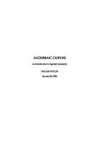
some extra points added "at infinity"), which are accurate iopo/o^ica/pictures of the curves but which do not reflect the way they sit inside C^. For some examples, see figure 1.1. It is important to stress the fact that these pictures can only represent the complex curves cis topological spaces, and not the way

they lie in C^. For example, the complex curve defined by xj/ = 0 is the union of the two "complex lines" defined by x = 0 and j/ = 0 in C^, which meet at the origin (0,0). Topologically when we add a point at infinity to each complex line it becomes a sphere, and the complex curve becomes the union of two spheres meeting at a point as in figure 1.2. This picture, though topologically correct, represents the two complex lines as tangential to each other at the point of intersection, and this is not the ccise in C^. We cannot avoid this problem without making the complex lines look "singular" at the origin as in figure 1.3, which again is not really the Ccise.

1.1 A brief history of algebraic curves. Real algebraic curves have been studied for more than two thousand years, although it was not until the introduction of the systematic use of coordinates into geometry in the seventeenth century that they could be described in the form (1.2).

1.1. A BRIEF HISTORY OF ALGEBRAIC CURVES.

Equation Real algebraic curve

Complex algebraic curve

(with points "at infinity")

a2 b2 ^

y^ = x'' + x^ + 1

y2 = x^ -X

y2 = x^ + x^

y2 = x3

X* + y* = 1

Figure 1.1: Some algebraic curves

CHAPTER 1. INTRODUCTION AND BACKGROUND

Figure 1.2: The complex curve xy = 0

Figure 1.3: Another view of the complex curve xy = 0

J.J. A BRIEF HISTORY OF ALGEBRAIC CURVES. 5 The story starts with the Greeks, who had very sophisticated geometrical methods but a relatively primitive understanding of algebra. To them a circle was not defined by an equation

{x - af + {y- bf = r' but was instead the locus of all points having equal distance r from a fixed point P = (a, 6). Similarly a parabola to the Greeks was the locus of all points having equal distance from a given point P and a given line L, while an ellipse (hyperbola) was the locus of all points for which the sum (difference) of the distances from two given points P and Q had a fixed value.

Lines and circles can of course be drawn with a ruler and compasses, and the Greeks devised more complicated mechanisms to construct parabolas, ellipses and hyperbolas. With these they were able to solve some famous problems such as "duplicating the cube"; in other words constructing a cube whose volume is twice the volume of a given cube (this Wcis called the Delian problem. This comes down to constructing a line segment of length 2'^^ times

the length of a given unit segment. The Greeks realised that this could be done by constructing the points of intersection of the parabolas

y^=2x and x^ = y.

They tried very hard to do this and other constructions (such as trisecting an arbitrary angle and drawing regular polygons) using ruler and compasses alone. They failed, and in fact it can be shown using Galois theory (see for example [Stewart 73] pp.57-67) that these constructions are impossible with ruler and compasses.

Besides lines and circles, ellipses, parabolas and hyperbolas the Greeks knew constructions for many other curves, for example the epicyclic curves used to describe the paths of planets before the discovery of Kepler's laws.

(An epicyclic curve is the path of a point on a circle which rolls without slipping on the exterior of a fixed circle: see figure 1.4). Greek mathematics Wcis almost forgotten in Western Europe for many centuries after the end of the Roman Empire, but in the late Middle Ages and Renaissance period it was gradually rediscovered through contact with Arab mathematicians. It was during the Renaissance that new algebraic curves were discovered by artists such cis Leonardo da Vinci who were interested in drawing outlines of three-dimensional shapes in perspective.

As well cis reintroducing Greek mathematics the Arabs introduced to Europe a much more sophisticated understanding of algebra and a good algebraic

CHAPTER 1. INTRODUCTION AND BACKGROUND

Figure 1.4: An epicyclic curve

notation. It can be difficult for us to realise how important good notation is in the solution of a mathematical problem. For example the simple argument

x^ + 3 = 5x^{x- 5/2)' = 13/4 ^ x = (5 ± yi3)/2 becomes much harder to express and to follow using words alone.

By the end of the seventeenth century mathematicians were familiar with the idea pioneered by Descartes and Fermat of describing a locus of points in the plane by one or more equations in two variables x and y. The methods of the differential calculus were gradually being understood and applied to curves. It was known that many real algebraic curves turned up in problems

in applied mathematics (one example being the nephroid or kidney curve which is seen when light is reflected from a mirror whose cross-section is part of a circle). Around 1700 Newton made a detailed study of cubic curves (that is, curves defined by polynomials of degree three) and described seventy two different cases. He investigated the singularities of a curve C defined by a polynomial P{x,y), i.e. the points {x,y) € C satisfying

—(.,y) = 0 = —(x,y). These are points where the curve does not look "smooth", such as the origin in the cubic curves defined by y^ = x^ + x^ and y^ = x^ (cf. figure 1.1). We shall investigate the singularities of curves in greater detail in Chapter 7.

Once the use of complex numbers was understood in the nineteenth century it was realised that very often it is easier and more profitable to study

the complex solutions to a polynomial equation P[x,y) = 0 instead of just

1.1. A BRIEF HISTORY OF ALGEBRAIC CURVES. 7 the real solutions. For example, if we allow complex projective changes of coordinates f ax + by + c dx + ey + f^ hx + jy + k' hx + jy + k where

is a nonsingular matrix (see Chapter 2 for more details), then many of Newton's seventy two different cubics become equivalent to one another. In fact any complex curve defined by an irreducible cubic polynomial can be put into one of the forms

y' — x{x — l){x ­- A) with A ^ 0,1 (nonsingular cubic) y' = x^x + l) (nodal cubic) y' = x^ (cuspidal cubic) (see corollary 3.34 and exercise 3.9).

Another example of the "better" behaviour of complex curves than real ones is the fact that a real algebraic curve can be so degenerate it doesn't look like a curve at all. For example, the subset

{{x,y)eB?:x^ + y^=0} of R^ is the single point (0, 0) and

{{x,y)eB?:x^ + y^ = -l} is the empty set. But if P[x,y) is any nonconstant polynomial with complex coefficients then the subset of the complex space C^ given by

{{x,y)eC':P{x,y)=0} is nonempty and "hcis complex dimension one" in a reasonable sense.

In the nineteenth century it was realised that if suitable "points at infinity" are added to a complex algebraic curve it becomes a compact topological

space, just cis the Riemann sphere is made by adding an extra point oo to C. Moreover one can make sense of the concepts of holomorphic and meromor­ phic functions on this topological space, and much of the theory of complex analysis on C can be applied. This leads to the theory of Riemann surfaces'. ^ There is an unfortunate inconsistency of terminology in the theory of complex algebraic

curves and Riemann surfaces. A complex algebraic curve is called a curve because its complex dimension is one, but its real dimension is two so it can also be called a surface.

8 CHAPTER 1. INTRODUCTION AND BACKGROUND called after Bernhard Riemann (1826-1866). Riemann wcis extremely influential in developing the idea that geometry should deal not only with ordinary

Euclidean space but also with much more general and abstract spaces. At the same time as Riemann and his followers were investigating complex algebraic curves using complex analysis and topology, other mathematicians began to use purely algebraic methods to obtain the same results. In 1882 Dedekind and Weber showed that much of the theory of algebraic curves remained valid when the field of complex numbers wcis replaced by another

(preferably algebraically closed) field K. Instead of studying the curve C defined by an irreducible polynomial P{x,y) directly, they studied the "field of rational functions on C" which consists of all functions f : C —>■ K U {oo} of the form

f{x,y) =Q{x,y)/R{x,y) where Q{x,y) and R{x,y) are polynomials with coefficients in K such that

R{x,y) is not divisible by P{x,y) (i.e. such that R[x,y) does not vanish identically on C).

It is often useful to study curves defined over fields other than the fields of real and complex numbers. For example number theorists interested in the integer solutions to a diophantine equation

P{x,y) = 0, where P[x,y) is a polynomial with integer coefficients, often first regard the equation as a congruence modulo a prime number p. Such a congruence can be thought of as defining an algebraic curve over the finite field

F, = Z/pZ consisting of the integers modulo p, or over its algebraic closure.

By the end of the nineteenth century mathematicians had begun to make progress in studying the solutions of systems of more than one polynomial equation in more than two variables. During the twentieth century many more ideas and results have been developed in this area of mathematics (known as algebraic geometry). Algebraic curves and surfaces axe now reasonably well understood, but the theory of algebraic varieties of dimension greater than two remains very incomplete. (An algebraic variety is, roughly speaking, the set of solutions to finitely many polynomial equations in finitely many variables over a field K). The study of algebraic curves and Riemann surfaces, involving cis it does a

rich interplay between algebra, analysis, topology and geometry, with applications in many different areas of mathematics, has been the subject of active

1.2. RELATIONSHIP WITH OTHER PARTS OF MATHEMATICS 9 research right up to the present day. Just one example of its importance in

modern research is a theory of the structure of elementary physical particles which received much attention in the 1980s. In this theory particles are

represented by "strings" or loops, and the surfaces in space-time swept out by these strings as they develop from creation to annihilation are Riemann surfaces which are closely related to complex algebraic curves in the complex plane C^ with some points added at infinity.

1.2 Relationship with other parts of mathematics

Nowadays complex algebraic curves turn up and are useful in all sorts of arecis of mathematics ranging from theoretical physics to number theory. This section gives a brief explanation of their importance in a few of these arecis.

1.2.1 Number theory In the rest of this book the links between the study of complex algebraic curves and number theory will not be stressed, but they are important. Number theorists are interested in the integer solutions to equations such as

x^ + y^-z". (1.3) For example, does this equation have any solutions with x, y, and z nonzero integers when n > 2? This comes down to the question of whether there exist nonzero rational solutions

s = x/z,t = y/z, to the equation

5'' + r = i, (1.4)

which defines a complex algebraic curve called the Fermat curve of degree n. This curve is called after the French mathematician Pierre Fermat (1601­ 1665) because Fermat wrote in the margin of one of his books that he had found a "truly marvellous proof [demonstrationem mirabilem sane) that the equation (1.3) has no nonzero integer solutions when n > 2. For more than three hundred years mathematicians have been trying to prove or disprove this statement, without success although it hcis been proved that there are no nonzero integer solutions for many particular values of n. In 1983 the German mathematician Faltings proved that a complex algebraic curve of

10 CHAPTER 1. INTRODUCTION AND BACKGROUND genus at least two has only finitely many points with rational coefficients (see

Chapter 4 for the definition of genus). The Fermat curve of degree n has genus

i(n-l)(n-2) (see §4.3) so when n > 4 it follows that there are only a finite number of rational solutions to (1.4). Whether that finite number is ever nonzero, nobody knows.

1.2.2 Singularities and the theory of knots Another important area which will just be touched on in this book is the study of singularities (see Chapter 7). For more details and lots of pictures see [Brieskorn & Knorrer 86].

A singularity of an algebraic curve C defined by a polynomial equation

P{x,y)=0 is a point (a, 6) € C satisfying

-(a, 6)^0=-(a, 6). For example the curve

y^=x^ + x' + l has no singularities, whereas the curves y'^ = x^ + x^

i=x' have singularities at the origin. Figure 1.1 showed the real points on these curves.

We have already observed that drawing the real points on a complex algebraic curve is not always helpful in studying the complex curve (e.g. for the curve x^ + j/^ + 1 = 0! ) though it can give some idea of what is going on near a singularity with real coordinates. A better way to study what the curve looks like near a singularity (a, 6) is to look at its intersection with a small three-dimensional sphere

{{x,y)eC':\x-a\' + \y-b\'=e'}

1.2. RELATIONSHIP WITH OTHER PARTS OF MATHEMATICS 11 in C^ = R** with centre at (a, 6). This intersection will be a "knot" or "link" in the three-dimensional sphere. We can identify this three-dimensional sphere

topologically with Euclidean space R^ together with an extra point at infinity by using stereographic projection. Let us assume for simplicity that the centre (a, 6) of the sphere is the origin (0,0) in C^. Then stereographic projection of the sphere from the point (0,£) maps each point {x,y) of the sphere other

than (0,£) to the point of intersection of the (real) line joining (x,3/) and (0,£) with the three-dimensional real space

{{p,q)eC':Re{q)=0}, where Re[q) and Im[q) are the real and imaginary parts of q. The point (0,£) is mapped to oo. Explicitly

C / cRe(x) clm(x} clm(y} \ -r p ( \ I ^ [x,y)^\ U-Re(y)' =-Re(y)' c-B^(y)) " ""^Vi'i 7= e

' [ oo if Rt(\j) = £

with inverse

OO l-> (0,£). Example 1.1 Let C be the complex algebraic curve defined by xy = y'^

which is the union of the complex lines defined by j/ = 0 and x = y. Under stereographic projection, as above, the intersections of these complex lines with the sphere

S={{x,y)eC' ■.\x\' + \y\'=e'} are mapped to the circle

{{u,v,w) eR^ : w = 0,u^ +v^ =£'^} and the ellipse

{(u,u,iy) eR^ : v = w,{u-ef+ 2v^ =2e'^} in R^U {oo}. This circle and ellipse are linked in the sense that neither can be continuously shrunk to a point without pcissing through the other (see figure 1.5).

12 CHAPTER 1. INTRODUCTION AND BACKGROUND

Figure 1.5: A link

Example 1.2 Now let C be the cubic curve defined by

y' = x\ Any point (x,3/) € C can be written as

for a unique s £ C, and then (x,3/) belongs to the sphere

5-{(x,y)eC^ :|x|^ + |yp=£^} if and only if

\s\=8

where 8 is the unique positive solution to the equation

8''+ 8^ = £^ Therefore

Cn5={((5'e'",(5V'') : ie[0,27r)} which is contained in the subset

{(x,y)eC^ ■.\x\^8\\y\=8^} of S. Under stereographic projection this subset is mapped onto the subset of R^ consisting of all those [u, v,w) € R^ satisfying

2£V«2 + v^ = (5'(«' + v^ + «;H £') or equivalently

1.2. RELATIONSHIP WITH OTHER PARTS OF MATHEMATICS 13

Figure 1.6: A torus

This is the surface T in R^ swept out by rotating the circle with equation 2;:2 (v-eH-'Y+w' e'S (1.5)

about the ly-axis. Topologically T is a torus— that is, the surface of a ring (see figure 1.6). The image of C PI S under stereographic projection is a knot in R^ which lies on the torus T. As we travel along the points

of C n 5 with the parameter t varying from 0 to 27r, the angle of rotation about the ly-axis of the corresponding points in T is given by tan

- © ­ tan _j j Im[x) Re{x)

= arg(x) = 2i (mod 27r)

which varies from 0 to 27r twice. Thus the knot on T winds twice around the ly-axis. On the other hand the standard angular coordinate on the circle defined by equation (1.5) rotated through some fixed angle about the to-axis is

tan"

Vu'^+w^-c^S-^ /

= tan '

Im{y)

= tan 1 / sin(3t)

Wl+42cos(3t)-4

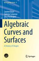
and it is not difficult to see that when S is small enough this varies from 0 to 27r three times as t varies from 0 to 27r. This means that the image oi C f] S under stereographic projection is a ire/oi/knot on the torus T (see figure 1.7). Only two points on this knot can be seen in the real picture (figure 1.8).

Algebraic singularities are important in many parts of mathematics besides knot theory (e.g. catcistrophe theory, which hcis been applied to areas as diverse as physics, ecology and economics. For a layman's introduction see V. Arnol'd's book [Arnol'd 86] or [Brieskorn & Knorrer 86] p.52).

14 CHAPTER 1. INTRODUCTION AND BACKGROUND

Figure 1.7: A trefoil knot in the plane and a trefoil knot on a torus

Figure 1.8: The real points on the curve j/^ = x^ and a small sphere about the origin

1.2. RELATIONSHIP WITH OTHER PARTS OF MATHEMATICS 15

Figure 1.9: Two copies of the cut plane glued along [0, cxd)

1.2.3 Complex analysis There is no holomorphic single-valued function x/z defined on the whole complex plane C. However if we cut C along the non-negative real axis [0,cx)) we can define two holomorphic functions ±x/z on C — [0, cxd) by

±V^=±v/Fe'f if z = re''',O C is a continuous path in C, R{x, y) is a rational function of two variables and w[z) is a continuous function of z defined on the image of the path 7 such that w[z) and z satisfy a polynom.ial relation

P{z,w{z)) = 0. Integrals of this form were extensively studied in the last century, in part icular

by the Norwegian mathematician Niels Hendrik Abel, after whom they are named. They occur in many problems in applied mathematics.

Example 1.4 li w[z) satisfies

w{zY = (z-ai)...(z-ai) where ai,..., a^ are distinct complex numbers then

I R{z,w{z)) dz is called an elliptic integral if fc is 3 or 4 and a hyperelliptic integral if k is at least 5.

20 CHAPTER 1. INTRODUCTION AND BACKGROUND Example 1.5 The arc-length of an ellipse

between points with ^-coordinates c and d is

1 l-i a" + {}? - a?)x^ 1 /•y'^=^y = 0 or a;^ > 1 and the only point of the curve satisfying y = 0 is the origin.

For another example consider the cubic curve defined by y^ = x^ (see figure 1.1). Again the curve has a singular point at the origin and the lowest order term is y^. In this case a;^ = j/2 => a; > 0

CHAPTER 1. INTRODUCTION AND BACKGROUND

24

0 be a fixed constant. Then the locus of all points p 6 R^ such that the line in R^

1.3. REAL ALGEBRAIC CURVES 25 through p and q meets C at a point of distance a from p is called a conchoid of C with respect to q and with parameter a. There are many classical examples of conchoids.

The conchoid of Nicomedes (c. 225 B.C.) is the conchoid of a line with respect to a point not on the line. If the line is defined by X=b

and the point is the origin (0,0) then the conchoid has equation

{x^ + y^){x - by = a^x\ One can see from their definition that conchoids of Nicomedes can be drawn with the aid of a simple apparatus. This apparatus was used by the Greeks to trisect angles (this was a famous problem: cf. §1.1). They showed that it is possible to trisect an arbitrary angle a, given as the angle between two lines meeting at a point q, as follows. First one draws the perpendicular L to one line from a point r on the other line. Then one draws the conchoid of L with respect to q and with parameter a = 21

where / is the distance of r from q. The parallel to the first line through r meets the conchoid on the side away from 5 at a point p, and the line through p and q trisects the angle a (see figure 1.15).

The limacon of Pascal (named after the seventeenth century French mathematician Pascal) is the conchoid of a circle of radius 6 with respect to a point

q on its circumference which we may take to be the origin. If we take the centre of the circle to lie on the i-axis, then the equation is

{x' + y'- 2bxf = a\x-' + y'). The limacon is the path traced by a point rigidly attached to a circle rolling on an equal fixed circle. More generally if the circles are allowed to have different radii 6 and c one obtains a curve called a epitrochoid or hypotro­ choid, depending on whether the rolling circle is outside or inside the fixed circle. When the attached point actually lies on the rolling circle one has an epicycloid or hypocycloid. Epicycloids and hypocycloids were used (probably as early as the seventeenth century) to design the so-called cycloidal gear. Important special cases of epicycloids and hypocycloids are the cardioid

(an epicycloid with 6 = c), so called because of its heartlike shape, the

26

CHAPTER 1. INTRODUCTION AND BACKGROUND

Figure 1.15: Trisecting an angle

Figure 1.16: Cardioid

nephroid or kidney curve (an epicycloid with c = 26), the deltoid (a hypocy­

cloid with 36 = c) and the astroid (a hypocycloid with 46 = c). Their equations in suitable coordinate systems are

2bxf {x' + y' - iby

Ab'{x' + y') Cardioid 1086*2/2 276*

x' + yy - Sbx{x^ - 3j/2) + 1862(a;2 + y2) = ,2^2„2 _ 0. + y'- b^ + 27b'x'y

Nephroid Deltoid Astroid

Examples are sketched in figures 1.16-1.19. The degenerate case of an epicycloid which occurs when the fixed circle is replaced by a line is called a cycloid (see figure 1.20). It was discovered by Bernoulli and others (around 1700) that given two points in a vertical plane, the curve along which a particle

takes the least time to slide from one point to the other under gravity is a cycloid. This discovery led to the development of the theory of variations.

1.3. REAL ALGEBRAIC CURVES

Figure 1.17: Nephroid

Figure 1.18: Deltoid

Figure 1.19: Astroid

Figure 1.20: Cycloid

27

28 CHAPTER 1. INTRODUCTION AND BACKGROUND Another curve discovered by the Greeks is the cissoid of Diodes. A cissoid

is associated to the choice of two curves C and D and a fixed point q. The cissoid of C and D with respect to q is the locus of all points p such that the line through p and q meets C and D in two points whose distance apart is the same as the distance between p and q. The cissoid of Diodes is the cissoid of a circle and a tangent line with respect to the point on the circumference of the circle opposite the point of tangency. If we take this point to be the origin and the tangent line to be defined by a; = a then the equation of the cissoid is y^{a — x) = x^.

This cissoid can be drawn using, for example, an apparatus due to Newton. A right angle with two arms of length a is moved in the plane in such a way that the endpoint of one arm moves on the line defined by a; = |a and the other arm always passes through the point (—|a,0). Then the midpoint of the first arm describes the cissoid. Diodes was able to use his cissoid to solve the Delian problem of doubling the cube (that is, constructing a line segment of length 2 J times a given unit length). The intersection of the dssoid

y'{l-x) = x' with the line defined by

x + 2y = l

is the point (237,7) where 7 = 2 + 23. Using this and standard ruler and compass constructions a line segment of length 23 units can be drawn.

Real algebraic curves important in mechanics are the caustic curves investigated by Tschirnhausen and Huygens at the end of the seventeenth century.

A catacaustic (respectively diacaustic) of a given curve C is a curve which is tangent to all the light rays from a given source after reflection (respectively

refraction) in C. If the light source is at infinity the incoming rays are parallel. For example the catacaustic of a circle C with source 5 is a cardioid if g 6 C, a nephroid ii q = 00 and a limacon of Pascal otherwise.

Chapter 2 Foundations This chapter contains the basic definitions and material we shall need to study complex algebraic curves. We shall first define complex algebraic curves in C^ and then add "points at infinity" to obtain complex projective curves.

2.1 Complex algebraic curves in C^ Let P{x,y) be a non-constant polynomial in two variables with complex coefficients. We say that P{x,y) has no repeated factors if we cannot write

Pix,y) = iQ{x,y)YRix,y) where Q[x,y) and R[x,y) are polynomials and Q{x,y) is nonconstant. Definition 2.1 Let P{x, y) be a nonconstant polynomial in two variables with complex coefficients and no repeated factors. Then the com.plex algebraic curve in C^ defined by P[x,y) is

C={{x,y) EC' : P{x,y) = 0}. The reason for the assumption in this definition that P{x,y) has no repeated factors is the theorem called Hilbert's Nullstellensatz already quoted in §1.3.

Theorem (Hilbert's Nullstellensatz) If P{x,y) and Q{x,y) are polynomials with complex coefficients then

{{x,y)EC' : P{x,y)=0} = {{x,y)EC' : Q{x,y) = 0} if and only if there exist positive integers m and n such that P divides Q" and Q divides P"*; or equivalently if and only if P and Q have the same irreducible factors, possibly occuring with different m.ultiplicities. 29

30 CHAPTER 2. FOUNDATIONS Corollary 2.2 If P{x,y) and Q{x,y) have no repeated factors then they define the same complex algebraic curve in C if and only if they are scalar m.ultiples of each other, i.e.

P{x,y) = XQ{x,y) for some A 6 C — {0}.

Proof. This is an immediate consequence of Hilbert's Nullstellensatz. D Remark 2.3 A more general way of defining a complex algebraic curve in C^ is as an equivalence class of nonconstant polynomials in two variables, where two polynomials are equivalent if and only if they are scalar multiples of each

other. A polynomial with repeated factors is then thought of as defining a curve with multiplicities attached; for example {y — x^Y defines the same curve a,s y — x^ but with multiplicity three. Through most of this book the definition 2.1 will be sufficient; occasionally however (e.g. in §3.1) we shall need to allow the use of curves defined by polynomials with repeated factors.

Definition 2.4 The degree d of the curve C defined by P{x,y) is the degree of the polynom.ial P, i.e. d = max {r + s : Cr.j y^ 0} where

A point [a, b) E C is called a singular point (or singularity^ of C if

9P, r,= „0=-ia,b). dP, ,, -ia,b) The set of singular points of C is denoted Sing(C). C is called nonsingular if Sing (C) = .

Examples 2.5 The curve defined hy x^ -\- y^ — \ is nonsingular. The curve defined by y^ = x^ has one singular point (0,0).

Definition 2.6 A curve defined by a linear equation ax + I3y + -/ = 0,

where 0,^,7 are com.plex num.bers and a and ^ are not both zero, is called a line.

At this point we must recall an important definition and lemma.

2.1. COMPLEX ALGEBRAIC CURVES IN C" 31 Definition 2.7 A nonzero polynomial P(a;i,... ,Xn) in n variables is homogeneous of degree d if

P{Xx,,...,\Xr.) = \'P{x,,...,Xr.) for all X E C. Equivalently P has the form

P{xu...,Xr,)= Yl ar,...r„xY . . . Xl" ri + ...+r„=d

for som.e com.plex num.bers ari...r„­

Note that every polynomial factor Q{xi,... ,a;„) of a homogeneous polynomial P{xi,..., Xn) is also homogeneous (see Appendix A).

Lemma 2.8 If P{x,y) is a nonzero homogeneous polynomial of degree d in two variables with complex coefficients then it factors as a product of linear polynomials

P{x,y) = '[[{aix + I3,y)

d d r=0 r=0 y

for some ai,j3i 6 C. Proof. We can write

^r.,d-r .,d '

,X ^

where Oq, ..., a^ 6 C are not all zero. Let e be the largest element of {0,. .., d)

such that a^ ^ 0. Then

r=o y is a polynomial with complex coefficients of degree e in one variable - and so can be factorised as

r=o y ti\y J for some 71,... ,7^ 6 C. Then

Pix,y) = a,y'UU(l-li) = ie2/^-=nLi(^-7.2/)­ The result follows. D

Note that since P{x, y) is a polynomial it has a finite Taylor expansion

S^+^P (x-aYiy-by about any point (a, 6) (see exercise 2.3).

32 CHAPTER 2. FOUNDATIONS Definition 2.9 The multiplicity of the curve C defined by P[x,y) at a point (a, 6) £ C is the smallest positive integer m such that gmp

for some t > 0, j > 0 such that i + j = m. The polynomial

^ d'-p ix-ay{y-by t+j=m ^ •^ is then homogeneous of degree m and so by lemma 2.8 can then be factored as the product of m linear polynomials of the form.

a{x - a) + I3{y - b) where {a,P) 6 C^ — {(0,0)}. The lines defined by these linear polynomials are called the tangent lines to C at (a, 6). The point (a, 6) is singular if and only if its m.ultiplicity m is 1; in this case C has just one tangent line at (a, 6) defined by

dP dP

^{a,b){x-a) + ^{a,b){y-b) = 0. A point (a, 6) 6 C is called a double point (respectively triple point, etc.) if its multiplicity is two (respectively three, etc.). A singular point (a, 6) is called ordinary if the polynomial (2.1) has no repeated factors, i.e. if C has m distinct tangent lines at {o.,b). Example 2.10 The cubic curves defined by y^ = x^ + x^ and

23

y=X

have double points at the origin; the first is an ordinary double point but the second is not (see figure 2.1). The curve defined by

{x' + yy = x'y' has a singular point of multiplicity four at the origin which is not ordinary; the curve defined by

{x* + y*-x'- yy = 9x'y' has an ordinary singular point of multiplicity four (see figure 2.2).

2.1. COMPLEX ALGEBRAIC CURVES IN C^

33

Figure 2.1: The curves y = a; + a;^ and y = x

Figure 2.2: The curves (a;* + y^ = x^y^ and [x* + y* - x^ - y'^f = 9x^y^

34 CHAPTER 2. FOUNDATIONS Definition 2.11 A curve C defined by a polynomial P{x,y) is called irreducible if the polynomial is irreducible; that is, if P{x,y) has no factors other than constants and scalar multiples of itself.

If the irreducible factors of P{x,y) are

Pi{x,y),...,Pk{x,y) then the curves defined by

Pi{x,y),...,Pk{x,y) are called the (irreducible) components of C ■

2.2 Complex projective spaces A complex algebraic curve C in C^ is never compact (see exercise 2.7). Recall some of the important properties of the topological condition of compactness (cf. e.g. Chapter 5 of [Sutherland 75]).

Properties 2.12 (i) A subset of R" or C" is compact if and only if it is closed and bounded (Heine-Borel theorem).

(ii) If f : X —> Y is a continuous map between topological spaces and X is compact, then f{X) is compact. (Hi) It follows from (i) and (ii) that if X is a compact topological space and f : X —> ^ is a continuous function then f is bounded and attains its bounds. (iv) A closed subset of a compact space is compact. (v) A compact subset of a Hausdorff space is closed. (vi) A finite union of compact spaces is compact. For many purposes it is useful to compactify complex algebraic curves in C^ by adding "points at infinity". For example, suppose we wish to study the intersection points of two curves, such as

221

t/ = X — 1, y = ex where c is a complex number. If c ^ ±1 these curves meet in two points. When c = ±1 they do not intersect, but they are asymptotic as x and y tend to infinity (cf. figure 2.3). We want to add points at infinity to C^ in such a way that the curves y^ = x^ + 1 and y = ex intersect "at infinity" when c = ±1. Similarly parallel lines should "meet at infinity". More generally we would like any curves which are aisymptotic to "meet at infinity". To make this precise we use the concept of a projective space. The idea is to identify each {x,y) £ C^ with the one-dimensional complex linear subspace

2.2. COMPLEX PROJECTP/E SPACES

Figure 2.3: The curve j/^ = x^ — 1 and the lines y — ±x

35

36 CHAPTER 2. FOUNDATIONS of C^ spanned by (x, J/, 1). Every one-dimensional linear subspace of C^ which

does not lie in the plane {[x,y,z) £ C^ : 2 = 0} contains a unique point of the form (x,t/,l). The one-dimensional subspaces of {[x,y,z) £ C^ : 2 = 0} can be thought of as "points at infinity". Definition 2.13 Complex projective space P^ of dimension n is the set of complex one-dimensional subspaces of the complex vector space C""*"^. When

n — 1 we have the complex projective line Pi and when n — 2 we have the complex projective plane P2.

Remark 2.14 If V is any vector space over any field K then the associated projective space P(V) is the set of one-dimensional subspaces of V. We shall work only with the case K ~ C and V — C""*"^ so to simplify the notation we write P„ for P(C"+i). A one-dimensional linear subspace [/ of C""*"^ is spanned by any nonzero u £ U. Therefore we can identify Pn with the set of equivalence classes for the equivalence relation ~ on C""*"^ — {0} such that a ~ 6 if there is some A e C - {0} such that a = \b.

Definition 2.15 Any nonzero vector ■ [Xq, . . . , Xn)

in C""*"^ represents an element x ofF^-' we call [xo,...,x,i) homogeneous coordinates for x and write X — [xo,. ■ ■ ,Xn\­

Then

{[xo,...,xJ : (xo,...,x„)eC"+i-{0}} and

[xo,...,Xn] = [yo,----,yn] if and only if there is some A £ C — {0} such that Xj — \yj for all j. Now we can make P^ into a topological space (we shall show that unlike C" it is compact). We define H : C"+i - {0} -^ P„ by

n(xo,...,Xn) = [xo,...,Xn] and give Pn the quotient iopo/o^t/induced from the usual topology on C""*"^ —

{0} (cf. [Sutherland 75] p.68). That is, a subset A of P^ is open if and only if n-i(>l) is an open subset of C"+^ - {0}.

2.2. COMPLEX PROJECTIVE SPACES 37 Remark 2.16 Note that (i) a subset B of P^ is closed if and only if 11"^ (5) is a closed subset of C"+i - {0}; (ii) n : C"+^ - {0} -y P„ is continuous; (iii) if X is any topological space a function f : Pn —> X is continuous if and only if

/ o n: c"+^ -{o]-^x

is continuous; more generally if A is any subset of P^ then a function f : A -^ X is continuous if and only if

fon:Tl-\A)->X is continuous. We define subsets [/q, .. ■, L'n of P^ by

[/, = {[xo,...,xJeP„ : x,-7^0}. Notice that the condition Xj ^ 0 is independent of the choice of homogeneous coordinates, and that

n-i([/,) = {(xo,...,x„)eC"+^ : x,-^0} is an open subset of C""*"^ — {0}, so Uj is an open subset of P„ . Define C^ by

->■ [^,yi,---,yn]

by definition 2.15. The coordinates (t/i,... ,!/„) are called inhomogeneous coordinates on Uq.

It is easy to check using remark 2.16 that (po : Uq —> C" is continuous (we just have to show that its composition with IT : n~^(L'o) —> Uq is continuous) and its inverse is the composition of IT with the continuous map from C" to

C"+i - {0} given by {yi,---,yn) >->■ (i,yi,---,yn). Thus (po is a homeomorphism.

Similarly there are homeomorphisms (pj : Uj —> C" for each j between 1 and n given by Xo

(pjixo, . . . , Xn]

x/ ■ ■

^j-1 ^j+1

Xj Xj

Xji

'' Xj

38 CHAPTER 2. FOUNDATIONS Remark 2.17 The complement of [/„ in P^ is the hyperplane

{[xo,...,X„] £Pn ■■ Xn =0}. This can be identified with Pn-i in the obvious way. Thus we can build up the projective spaces P^ inductively. Po is a single point. Pi can be thought of as C together with a single point oo (i.e. a copy of Pq) and thus can be identified with the Riemann sphere

CU{oo}. P2 is C^ together with a "line at infinity" (i.e. a copy of Pj), and in general Pn is C" with a copy of Pn-i at infinity.

Since {Uj : 0 < j < n} is an open cover of P^ and , : U, -^ C"

is a homeomorphism for each j, a function / from P^ to a topological space X is continuous if and only if / o 0 so

[Xo, . . . ,XnJ = [A 2Xq,...,A 2XnJ.

2.2. COMPLEX PROJECTIVE SPACES 39 But so

[xo,...,xjen(s^"+^). Thus n : 5^""*"^ —> Pn is surjective, and the result follows. D

Definition 2.19 A projective transformation o/Pn is a bijection

/ . Pn -^ Pn such that for some linear isomorphism a : C""*"^ —> C""*"^ we have

/[xo,...,x„] = [t/o,...,t/n] where

(yo, ■■■,J/n) = a{xo,...,Xn), i.e.

foTl = Tloa where H : C""*"^ — {0} —> Pn is defined as before by

n(xo,... ,Xn) = [xq, ... ,Xn]. Lemma 2.20 A projective transformation f -.P^ —> Pn ^s continuous.

Proof. We have for some linear isomorphism a : C""*"^ -+ C""*"^. Since IT is continuous (by 2.16(ii)) and a is continuous it follows that /o 11 is continuous, and therefore

by 2.16(iii) that / is continuous. □ Definition 2.21 A hyperplane in P^ is the image under H : C""*"^ — {0} —> ^n of V — {0} where V is a subspace o/C"+^ of dimension n.

Lemma 2.22 Given n + 2 distinct points po,...,Pn o^nd q of P^, no n-\-\ of which lie on a hyperplane, there is a unique projective transformation taking Pi to [0,... ,0,1,0,... ,0] where 1 is in the ith place, and taking q to [1,. .. ,1]. Proof. Let Uq, ... ,Un and i; be elements of C""*"^ — {0} whose images under

n are po,...,Pn and q. Then Mo,---,Wn form a basis of C""*"^ so there is a unique linear transformation a of C""*"^ taking Uq, ..., Un to the standard baisis (1,0,.. .,0),.. .,(0,.. .,0,1). Moreover the condition on po,---,Pn and q implies that

"{v) = (Ai,...,A„)

40 CHAPTER 2. FOUNDATIONS where Ai,..., A^ are all nonzero complex numbers. Thus the composition of a with the linear transformation defined by the diagonal matrix

a 0 ■■■ 0 \

0 ■■. 0

V 0 ... 0 iy defines a projective transformation taking p; to

[0,...,o,-,o,.:.,o] = [o,...,0,1,0,...,0] and q to [1,1,... ,1]. Uniqueness is eaisy to check. □

Proposition 2.23 The projective space P^ is Hausdorff.

Proof. We need to show that if p and q are distinct points of P„ then they have disjoint open neighbourhoods in Pn. We have shown that there is a homeomorphism (po '■ Uq —> C" where Uo is an open set of P^ . If p and q lie in Uo then (fio{p) and (j)o{q) have disjoint open neighbourhoods V and W in C" (since C" is Hausdorff) and o^{W) are disjoint open neighbourhoods of p and q in Pn. In particular this applies when p — [1,0,..., 0] and q — [1,1,... ,1]. In general we can find points po, ■ ■ ■ iPn of P^ such that Po = p and no n + 1 of the n + 2 points po,... ,Pn and q lie in a hyperplane. Then by lemma 2.22 there is a projective transformation / : P^ -^- P^ taking p to [1,0,... ,0]

and q to [1,1,... ,1]. We have already shown that [1,0,... ,0] and [1,1,... ,1] have disjoint open neighbourhoods (/i^ (V) and (/lo^(W^) in Pn- Since / is continuous (by lemma 2.20) and a bijection, the subsets /~^((/io^^(V')) and /~^((/i^^(VK)) are disjoint open neighbourhoods of p and q in Pn, as required.

n

2.3 Complex projective curves in P2 Recall from §2.2 that the complex projective plane P2 is the set of one­ dimensional complex subspaces of C^. We denote by [x, t/, z\ the subspace spanned by (x,t/,2) £ C^ — {0}, and thus

P2 = {[x,t/,2] : (x,t/,2)eC3-{0}} and

2.3. COMPLEX PROJECTIVE CURVES IN P2 41 if and only if there exists some A £ C — {0} such that

X ~ Au, y — Au, z = \w.

dii

Recall also that a polynomial P{x,y,z) is called homogeneous of degree

P{Xx,Xy,Xz) = \'P{x,y,z) for all A £ C. Note that the first partial derivatives of P are homogeneous polynomials of degree d — 1.

Definition 2.24 Let P{x,y,z) be a nonconstant homogeneous polynomial in three variables x,y,z with complex coefficients. Assume that P(i,t/, z) has no repeated factors. Then the projective curve C defined by P[x,y,z) is

C={[x,y,z]£P2 ■■ P{x,y,z)==0]. Note that the condition P[x,y,z) — 0 is independent of the choice of homogeneous coordinates (x,t/,2) because P is a homogeneous polynomial and hence

P(\x,\y,\z) = 0 0. 2.9. For which values of A £ C are the following projective curves in P2 nonsingular? Describe the singularities when they exist.

(a), i^ + t/^ + 2^ + 3Axt/2 = 0.

(b). x^'^y'^z^'Wi^x^y^zf^^. 2.10. Suppose nine distinct points in P2 are given, and that they do not all lie on any line in P2. Suppose that any straight line which parses through two

of these points also passes through a third. Show that there is a projective transformation taking these points to the points

[0,1,-1] [-1,0,1] [1,-1,0] [0,1, a] [a, 0,1] [l,a,0]

[0,a,l] [l,0,a] [a,l,0]

for some a £ C. Show that a^ — a+ 1 =0. Show also that a projective curve of degree 3 passes through these nine points if and only if it is defined by a polynomial of the form x^ +1/^ + 2^ + 3Axt/2

for some A £ C U {00}, and it is singular precisely when

A £ {00,—l,a,a}, in which case it is the union of three lines in P2.

2.11. Show that the complex line in P2 through the points [0,1,1] and [i,0,l] meets the projective curve C defined by

2,2 2

X -Vy = z

in the two points [0,1,1] and [2i,i^ — l,i^ + 1]. Show that there is abijection from the complex line defined by t/ = 0 to C given by

[i,0,l]H^[2i,i'-l,i' + l] and [1,0,0] H^ [0,1,1].

Deduce that the complex solutions to Pythagoras' equation

2122

48 CHAPTER 2. FOUNDATIONS are

with A,/i £ C. Show that the real solutions are

x = 2A/i, y==\''-fi\ 2 = ±(A' + /i') with A, /i £ R, and the integer solutions are

x = 2A/ii/, 3/= (A^-/i^)i/, 2 = (A^+/i^)i/ where A and fi are coprime integers, not both odd, and f £ Z, or

where A and fi are coprime odd integers and f £ Z. 2.12. Let C be a nonsingular projective curve of degree two in P2 defined by a polynomial with rational coefficients. Use the following steps to obtain an algorithm which decides whether or not C hais any rational points, i.e. whether

there is a point of C which can be represented by rational homogeneous coordinates (or equivalently by integral homogeneous coordinates).

(a). Use the theory of the diagonalisation of quadratic forms to show that

there is a projective transformation defined by a matrix with rational coefficients taking C to the curve defined by

2,T22

ax + by — z for some a, 6 £ Q — {0}.

(b). Show that by making an additional diagonal transformation we can aissume that a and h are integers with no square factors, i.e. each is a product of distinct primes. Show that we may also aissume that | a |>| 6 |.

(c). Show that if C hais a rational point then 6 is a square modulo p for every prime p dividing a. Deduce from the Chinese remainder theorem that 6 is a square modulo a, so there are integers m,ai such that | m |mp(C)mp(D) where mp(C) and mj,{D) are the multiplicities of C and D a.t p as defined in exercise 2.8, and that equahty holds if and only if C and D have no tangent lines in common.

In order to prove proposition 3.22 we first need to prove the following lemma.

Lemma 3.24 If p £ C Ci D is a singular point of C then Ij,{C,D) > 1.

64 CHAPTERS. ALGEBRAIC PROPERTIES Proof. We may assume that C and D have no common component, and hence we may choose coordinates such that p = [0,0,1] and the conditions (a)-(c) of theorem 3.18 hold. We wish to show that y^ divides the resultant T^P,Q[yj^) of the polynomials P[x,y,z) and Q[x,y,z) defining C and D. Since p £ Sing{C) we have

1^(0,0,1) = 1^(0,0,1) = P(0,0,1) = 0. Hence P{x, y, z) is a sum of monomials all of degree at least two in x and y; i.e.

P{^,y,z) = ao(y,z) + ai(y,z)x + ... + a„(y,z)x'' where y^ divides 00(3/, z) and y divides 01(3/, z). Also (5(0,0,1) = 0 so

Q{3:,y,z) = bo{y,z) + b^{y,z)x + ... + 6„(y,z)x"' where y divides bo[y,z). Thus we can write

bo[y,z) = ioiyz"""' +y%(y,z), and

6i(y,z) = 6ioz"'-'+yci(y,z) for some homogeneous polynomials 00(3/,z) and Ci{y,z). If 601 = 0 then the first column of the determinant defining TZp^Q[y,z) is divisible by y^ and hence y^ divides 'Rp^Q{y,z) as required. If 601 7^ 0 then the first column is divisible by y; if we take out this factor y and subtract bio/boi times the first column from the second column then the second column becomes divisible by y. Hence again y^ divides TZp^Q{y,z). D

Proof of proposition 3.22. We may assume that p belongs to C Pi D and that C and D have no common component. Thus we may choose coordinates such that the conditions (a)-(c) of theorem 3.18 are satisfied and p — [0, 0,1]. By corollary 3.10 we may also assume that p is a nonsingular point of C and

of D. Let P[x,y,z) and Q[x,y,z) be the polynomials defining C and D. We wish to show that the tangent Hnes to C and D ai p coincide if and only if y^ divides the resultant TZp^Q[y,z), or equivalently if and only if

since 'Rp^Q[y,z) is homogeneous and divisible by y. By (c) of theorem 3.18, the point [1,0,0] does not lie on the tangent Hne

X—(0,0,1) + y^(o,o,i) + ^^(0,0,1) = 0

3.1. BEZOUTS THEOREM 65 to Cat p= [0,0,1], so

1^(0,0,1)^0. (3.1)

Therefore by the imphcit function theorem for complex polynomials (see Appendix B) applied to the polynomial P{x,y,\) in x and y, there is a holo­ morphic function Xi : U —>■ V where U and V are open neighbourhoods of 0

in C such that Ai(0) = 0

and li X £ V and y £ U then

P(x,y,l) = 0 if and only if

x = Ai(y). Moreover

P{x,y,\) = {x-\,{y))l{x,y) where /(x, y) is a polynomial in x whose coefficients are holomorphic functions of y. If we assume as we may that the coefficient P(l, 0, 0) of x" in P[ x, y, z) is one then

/(x,y) = n(x-A.(y)) i=2

where \i[y),..., \n[y) are the roots of P[x,y,\) regarded as a polynomial in X with y fixed. Similarly if U and V are chosen small enough there is a holomorphic function fi^ : U ^> V such that

/.,(0) = 0 and we can write

Q{x,yA) = {x - li\{y))m{x,y) where Tn

i=2

is a polynomial in x whose coefficients are holomorphic functions of y. Then the tangent lines to C and D at p = [0,0,1] are defined by the equations X = A;(0)y

and X = /^i(0)2/­

li y £ U then by lemma 3.6

7^p,Q(y,l) = (/^i(y)-Ai(y))5(y) (3.2)

66 CHAPTERS. ALGEBRAIC PROPERTIES where

S[y)= n (My) - A,(y)). Note that S{y) is the product of the resultants of the pairs of polynomials l{x, y) and m(x, y), l{x, y) and x — /ii(3/), and m(x, y) and x — Ai(3/). Hence S{y) is a holomorphic function oi y £ U. Since Ai(0) = 0 = /ii(0) we obtain on differentiating equation 3.2 that

dy

(o,i) = (/.;(o)-AUo))5(o).

It follows from the inequality 3.1 that the polynomial P{x, 0,1) does not have repeated roots at 0 so if f > 1 then

A.(0)^0 = /.i(0) and similarly

;,.(0)^0 = Ai(0). Moreover if Ai(0) = /ij(0) for some i,j > 1 then [0,0,1] and

[A.(0),0,l] = [/.,(0),0,1] are distinct points oi C Pi D both lying on the line y = 0, which contradicts condition (b) of theorem 3.18. Hence

5(0)^0. Thus

If («.')­ if and only if

A'i(O) = ii'M,

i.e. /p(C, D) > 1 if and only if the tangents to C and D sX p coincide. □

Corollary 3.25 Let C and D he projective curves in P2 of degrees n andm. Suppose that every p £ CCiD is a nonsingular point of C and of D, and that the tangent lines to C and D at p are distinct. Then the intersection C Cl D consists of exactly nm points. Proof. This follows directly from theorem 3.1 and proposition 3.22. □

3.1. BEZOUTS THEOREM 67 Remark 3.26 Even if we allow curves to be defined by polynomials with repeated factors, the conditions of this corollary are never satisfied if either of the polynomials P{x,y,z) and Q[x,y,z) defining C and D have repeated factors. For suppose P[x,y,z) = A(x,3/, z)^S(x,3/,z) where A(x,3/, z) is a nonconstant irreducible polynomial. Then the curve defined by A(x,3/, z) meets D in at least one point p. It is easy to check that p £ C D D and all the partial derivatives of P vanish at p. We shall finish this section by proving lemmas 3.3-3.7.

Proof of lemma 3.3. Let P(x) = ao + Ojx + ... + a^x" and Q{x) = bo + biX + ... + brr,x"'

be polynomials of degrees n and m in x. Then P{x) and Q{x) have a non­ constant common factor R{x) if and only if there exist polynomials (j>{x) and

^{x) such that P(x) = R[x)[x),Q{x) ^ R{x)i,{x).

This happens if and only if there exist nonzero polynomials

(l>[x) = ao + ct\x + ... + an-ix""' and i^{x) = l3o + I3,x + ... + Pm-ix""-^

of degrees at most n — 1 and m — 1, such that

P(x)V'(x) = Q{x)^{x).

Equating the coefficients of x' in this equation for 0 < j < mn — 1, we find

aoPo = Poao aoPi + aiPo = Piao + Poa-^

The existence of a nonzero solution (ao,---,an-i,/^o, •••,/^m-i)

to these equations is equivalent to the vanishing of the determinant which defines 'R-p^q. D

68 CHAPTERS. ALGEBRAIC PROPERTIES Proof of lemma 3.4. Let P[x,y,z) and Q{x,y,z) be nonconstant homogeneous polynomials in x, y, z of degrees n and m such that

p(i,o,o)^o^g(i,o,o). We may assume that P(1,0,0) = 1 = (5(1,0,0). Then we can regard P and Q as monic polynomials of degrees n and m in x with coefficients in the ring C[3/,z] of polynomials in y and z with complex coefficients. This ring C[3/,z] is contained in the field C{y,z) of rational functions of y and z, i.e. functions of the form 9{y,z)

where f{y,z) and g{y,z) are polynomials and g{y,z) is not identically zero.

Since C{y,z) is a field the proof of lemma 3.3 shows that the resultant TZp^Q{y,z) vanishes identically if and only if P{x,y,z) and Q{x,y,z) have

a nonconstant common factor when regarded as polynomials in x with coefficients in C(j/,z). It follows from the Gauss lemma (see Appendix A) that

this happens if and only if P[x,y,z) and Q{x,y,z) have a nonconstant common factor when regarded as polynomials in x with coefficients in C[3/,z], or

equivalently as polynomials in x,y,z with coefficients in C. Since any polynomial factor of a homogeneous polynomial is homogeneous (see Appendix

A) the result follows. D

Proof of lemma 3.6. If we regard

P(x) = (x-Ai)...(x-A„) and

Q[x) = (x-/ii)...(x-/i„) as homogeneous polynomials in x, Aj, ..., A„ and /ij, ..., /i„ then the proof of lemma 3.7 shows that the resultant Tip^q is a homogeneous polynomial of degree nm in the variables Al, . ■ . , A„, fli, . . . , firn­

Moreover by lemma 3.3 this polynomial vanishes if A; = iij for any \ < i < n and 1 < j < m, so it is divisible by

n (/^. - ^.)­

l 2 this means not identically zero) it defines a projective curve in P2 in the generalised sense of remarks 2.3 and 2.25. Since the whole of §3.1 applies to curves in this generalised sense the result follows fromtheforms 3.8 and 3.9 of Bezout's theorem once we have shown that P and Tip have no nonconstant common factor ii d > 1. Since a nonsingular curve is irreducible (by corollary 3.10(i)) if P and Tip have a nonconstant common factor then P divides Tip, so every point of C is a point of inflection. The result is now a consequence of lemma 3.32. D

Corollary 3.34 Let C be a nonsingular cubic curve in P2. Then C is equivalent under a projective transformation to the curve defined by y^z = x{x — z){x — Xz)

for some A £ C — {0,1}.

Proof. By proposition 3.33 C has a point of inflection. By applying a suitable projective transformation we may assume that [0,1,0] is a point of inflection of C and the tangent line to C at [0,1, 0] is the line z = 0. Then C is defined by a homogeneous polynomial P{x, y, z) of degree three such that

P(0,1,0) = 0 = 1^(0,1,0) = 1^(0,1,0) =Wp(0,1,0). Also

f(o,i,o)^o because C is nonsingular. Applying lemma 3.30 with the roles of y and z reversed, we get

p

p. p. p. Ip p. 2 p.. p^ p.

■*■ XX

y^'Hp{x,y,z) = 4det

0

p.^ \

=­ 0 = Wp(0,l,0) = 4det 0 00 P,p. I =-4(P,)2P,,,

\ P.. P. P.:

74 CHAPTERS. ALGEBRAIC PROPERTIES where the partial derivatives are evaluated at (0,1,0). Thus

P,,(0,1,0)=0 and hence P{x, y, z) = yz{ax + fiy + fz) + {x, z)

where (j>{x, z) is homogeneous of degree three in x and z and

^=1^(0,1,0)^0. After the projective transformation given by

[x, y, z\ i->[x,y + ———, z\,

the curve C is defined by the equation

I3yh + ^{x,z) = 0

where ip{x,z) is homogeneous of degree three in x and z, and hence is a product of three linear factors. Since C is nonsingular it is irreducible (by corollary 3.10(i)), and hence 4'{x,z) is not divisible by z so the coefficient of x^ in rp[x,z) is not zero. Therefore after a suitable diagonal projective transformation C is defined by the equation y^z — (i — az){x — bz){x — cz)

for some a, t, c 6 C. Since a, b, c are distinct (otherwise C would be singular) we can apply the projective transformation

f[x,y,z\ 1 f^~"^ 1 H^ [- ,TO,z] 0—a

where t; 6 C satisfies

„2 /l(6-a)­ „\-3

to put C into the form y z = x{x — z){x — \z)

for some A 6 C-{0,1}. □ Remark 3.35 Note that the proof of corollary 3.34 actually shows that if p is any point of inflection on a nonsingular cubic curve C then there is a projective transformation taking p to [0,1,0] and taking C to a curve defined by y^z = x{x — z){x — \z)

for some A 6 C - {0,1}.

3.2. POINTS OF INFLECTION AND CUBIC CURVES. 75 Example 3.36 As an application of this last result and the corollary 3.25 to Bezout's theorem we can show that a nonsingular cubic curve C in P2 hcis exactly nine points of inflection. (Thus the bound given in proposition 3.33(i) is always attained in the case of a nonsingular cubic.) To prove this we suppose that C is defined by P[x,y,z) and we let D be the projective curve in P2 defined by the Hessian Hp{x,y,z). We know from remark 3.28 that T-lp{x,y,z) is homogeneous of degree 3; however it may have repeated factors so as in the proof of proposition 3.33 D must be regarded as a curve in the generalised sense of remarks 2.3 and 2.25. Since the whole of §3.1 a.pplies to curves in this generalised sense, it suffices to show that the conditions of

corollary 3.25 are satisfied. That is, we have to show that if p 6 C H D, or equivalently if p is a point of inflection of C, then p is a nonsingular point of C and of D and the tangent lines to C and D aX p are distinct. We know from the last remark that by applying a suitable projective transformation we can assume that

p= [0,1,0] and P{x, y, z) = y^z — x{x — z){x — \z)

dP dP

for some A 6 C - {0,1}. We find that

-(0,1,0) = 0=^(0,1,0), dP

dz (0,1,0) = 1,

dHp dx

dHp dy

(0,1,0) = 24,

(0,1,0) = 0,

and

dHp

^^ (0,1,0) = 8(A-1). Thus the conditions of corollary 3.25 are satisfied.

As another useful result about points of inflection on cubics we prove

Lemma 3.37 A line L in P2 meets a nonsingular cubic C either (a) in three distinct points p,q,r each with intersection multiplicity one (i.e. L is not the tangent line to C at p,q or r); or

76 CHAPTERS. ALGEBRAIC PROPERTIES (b) in two points, p with intersection multiplicity one and q with intersection multiplicity two (i.e. L is the tangent line to C at q but not at p and q is not a point of inflection on C); or (c) in one point p with intersection multiplicity three (i.e. L is the tangent line to C at p and p is a point of inflection on C).

Proof. This can be deduced from the strong form 3.1 of Bezout's theorem by checking that the definition of intersection multiplicities given in the

statement of the lemma coincides with the definition given in theorem 3.18. However it is hardly longer and perhaps more illuminating to give a direct proof, so that is what will be done here. Since C is irreducible (by corollary 3.10(i)) it does not contain L, so we may cissume that L is the line defined by j/ = 0

and the point [1,0,0] does not belong to C. Let

C={[x,y,z]eP2 : P{x,y,z) = 0}. Then by lemma 2.8 we can factorise P(i,0,z) as P{x,0,z) = n{x — \\z){x — \iz){x — Xgz) for some Ai, A2, A3 6 C and /i 6 C — {0}, so

cm = {[x,Q,z]eP2 : P{x,Q,z) = 0] = {[A.,0,1] : l 0 such that if s 6 [0,1] and I i — s |< e([x,y,z\ = [x,z\

is well-defined (i.e. [0,1,0] ^ C) and the ramification index i/^[a,6, c] of 4> at every [a,h.^c\ £ C satisfies i/^[a, 6, c] < 2.

Then by lemma 4.7 (j> has exactly d{d — 1) ramification points, i.e. j^R =

d{d-\). By lemma 4.21 if r > 3 and r > d{d—\) then we can choose a triangulation

(V, E, F) of Pi such that V D {R)

and #y = r, #£ = 3r - 6 and #F = 2r - 4. Therefore by proposition 4.22 there is a triangulation [V, E, F) of C with

#^ = i#£ = 3(r-2)i, #F = i#F = 2(r-2)i

106 CHAPTER 4. TOPOLOGICAL PROPERTIES

Figure 4.16: A subdivision of C

and

Since #/? = d{d — 1) and i'^(p) = 2 for a.\\ p G R we have

#y = ri-i(d-l) as required. □ Proof of lemma 4.21. We can prove this for example by induction on r > 3.

When r = 3 lemma 2.22 tells us that there is a projective transformation taking pi to 1, pj to eT~ and ps to e^~. (Here as usual we identify Pi with C U {oo}.) We can join these three points by segments of the unit circle in C (see figure 4.16).

The exterior of the unit circle together with the point at infinity is mapped by the projective transformation z i-> i to the interior of the unit circle. Since there is a homeomorphism

A-> {zgC :|z|< 1} which takes the vertices of the triangle A to l,e"5~ and e"5~ and takes the edges of A to the appropriate segments of the unit circle, we get a triajigula­ tion of Pi with three edges and two faces when r = 3. Now suppose r > 3 and we have a triangulation with vertices pi,... ,Pr-i and 3r — 9 edges and 2r — 6 faces. If Pr lies in the interior of a face / (more precisely, if p^ € /(A")) we can add three edges joining pr to the vertices of

the face / (see figure 4.17) and obtain a new triangulation with one extra vertex, p^, three extra edges and one old face subdivided into three new ones.

If Pr does not lie in the interior of a face then it lies on an edge e (more precisely pr = e(f) for some t £ (0,1)). We can then replace e by two edges joining p^ to e(0) and e(l), and add two edges joining Pr to the remaining vertices of the faces f* and /" (see figure 4.18). This gives a triangulation with one new vertex, pr, two extra edges and one old edge replaced by two new

4.3. PROOF OF THE DEGREE-GENUS FORMULA

Figure 4.17: A subdivision of a triangle

Pr

Figure 4.18: A subdivision of two adjacent triangles

107

108 CHAPTER 4. TOPOLOGICAL PROPERTIES ones, and two old faces each replaced by two new ones. The result follows. □

Proof of proposition 4.22. We must show that V,E and F satisfy the conditions (i)-(v) in the definition 4.9 of a triangulation, and that the formulas for ^V,^E and #F are correct. This uses some topological results proved in Appendix C. By C.8 and C.9 of Appendix C, if / € F and p € C and

hp) = m for some f G A not equal to any of the vertices (0,0), (1,0) or (0,1), then there is a unique continuous map

/ : A -> C such that 0 where g{z) is holomorphic in an open neighbourhood of a and g{a) ^ 0. Equivalently we can express /(z) as a Laurent series n'^—m

where

g{z) = J2c^_rr.{z-ar n>Q

is the Taylor expansion of g{z) and

c_,n ~ g{a) ^ 0.

Then m is called the order or muUipUcity of the pole. The coefficient c_i is called the residue of f{z) at a and is denoted by

res{f{z);a} Remark 5.1 It is easy to check that in this situation

m_ has a simple pole (that is, a pole of order one) at a with residue —m. Similarly if / has a zero of multiplicity (or order) m at a, that is, if near a we can write

f{z) = {z-arg{z) where g{z) is holomorphic in an open neighbourhood of a and g{a) ^ 0, then

f{z) has a simple pole at a with residue m.

5.1. THE WEIERSTRASS p-FUNCTION 113 Residues of meromorphic functions at poles are closely related to integrals of the functions along paths in C. Recall that a piecewise-smooth path in an open subset H^ of C is a continuous map 7 : [c, d] —+ W, defined on a closed interval [c, d\ of the real line, which is the join of finitely many smooth paths 71,..., 7t in W. By this we mean that there exist real numbers

c = co by —u>, to get

p{-z) = p(z) Vzec. In particular c(C) = p(|C) ~ P(~K) ~ ^' ''■"'^ *'^^^

p(z + C) = p(z) VzeC. This completes the proof. □

Definition 5.14 Functions f on C with the property that

f{z + 0 = f{z) Vzec.vceA, or equivalently

f{z + Lj,) = f{z) = f{z + u;^) VzeC, are called doubly periodic with period lattice A (or with periods Wi and u>i)­ Thus the Weierstrass p-function is a doubly periodic meromorphic function on C.

118 CHAPTERS. RIEMANN SURFACES Lemma 5.15 A doubly periodic holomorphic function f on C is constant.

Proof. Since / is holomorphic it is continuous, and hence by proposition 2.18 is bounded on any closed bounded subset of C such as the parallelogram

P^{siJi + tu;2 : s,te [0,1]}. But given z G C we can find C € A such that z + ( £ P, and since / is doubly periodic,

Thus / is bounded on C, so the result follows from

Theorem 5.16 (Liouville's theorem). Any bounded holomorphic function on C is constant. Proof. [Priestley 85] 5.2. D

Using lemma 5.15 we can prove an extremely important identity concerning the Weierstrass p-function.

Lemma 5.17 p'{zf = Apizf - g2p{z) - . The transition functions are then either the identity or compositions of the form X i-> {x,g{x)) ^ g{x) or

where g and h are holomorphic. Therefore this atlas is holomorphic. O The argument for projective curves is very similar.

Proposition 5.28 If C is a projective curve in Pj defined by a homogeneoxis polynomial P{x,y,z) then C — Sing{C) has a holomorphic atlas.

Proof. Suppose that [o,6,c] € C, i.e. P{a,b,c) = 0, and that

idP/dy)ia,b,c)ytO.

128 CHAPTERS. RIEMANN SURFACES By Euler's relation (see lemma 2.32)

so

o = c = 0 =>• a = b — c = 0 which is impossible by the definition of Pj. Hence o ,1^ 0 or c ,1^ 0. Assume that c ^ 0. Then by the homogeneity of P

where d is the degree of P. The implicit function theorem (see Appendix B) applied to the polynomial P(x,y,l) in x and y now tells us that there are open neighbourhoods V and W of a/c and b/c in C and a holomorphic function g :V ^ W such that if x G V and y £W then

P(x,y,l) = 0 «^=^ y = : U —y V defined by (f>[x,y,z] = x/z is a homeomorphism with inverse w i-> [w,g{w),l].

Similarly if [o, b,c]eC and {dP/dy){a, b,c)^O^a, or if {dP/dx){a, b,c)^0 or {dP/dz){a, b,c) ^ 0, then we can find a homeomorphism (f> : U —* V from an open neighbourhood U of [o,6, c] in C — Sing[C) onto an open subset V of C such that (f>[x,y,z] is one of the following:

z/x,y/z,z/y,x/y,y/x and the inverse of has the form

u; h-> [l,(/(u;),u;],[(/(u;),u;,l],[(/(u;),l,u;],[u;,l,(/(u;)] or [l,w,g{w)] where g :V —y C is holomorphic. Thus we get an atlas on C — Sing{C) each of whose transition functions is of one of the following forms

w i-> w,l/w,g{w),l/g{w),w/g{w) or (/(u;)/u;

such that g is holomorphic and the denominator does not vanish on the set where the transition function is defined. Thus this atlas is holomorphic. □

5.2. RIEMANN SURFACES 129 Remark 5.29 It is easy to show that the complement of a finite set of points in a surface is dense. Thus the claim in the proof of proposition 4.22 that the complement of a finite set of points in a nonsingular projective curve is dense is substantiated by proposition 5.28.

The point of having a holomorphic atlas on a surface is that it makes it possible to talk about holomorphic functions on the surface. Definition 5.30 Let # = {(f>c, : Ua —* Va : a E A} be a holomorphic atlas on a surface S. A continuous map / : 5 —» C is called holomorphic with respect to ^ at X £ S if there is a chart cf>c, ■ Uc, —* Va in # such that x £ Uc, and

focf>-':V^^C is holomorphic at (f>aix) in the usual sense as a function from the open subset

Va of C to C. The map f is called holomorphic with respect to # if it is holomorphic at every x £ S.

Remark 5.31 Because # is a holomorphic atlas the choice of chart (f>c, : Ua —* Va such that X G t/a in this definition makes no difference. If x G Ua n Up and a '■ Ua ^> Va,(f>/3 : U/3 ^f V/3

are charts in # then a{Ua n Up) is an open subset of V^ containing 4a{x) and / ° a^ UciUcnU^)- if ° p^) ° il3 ° K^) UciUcnU^) ■

Since cf>i3 0 (f>~^ and its inverse (f>c, o (f)^^ are both holomorphic and the composition of holomorphic functions is always holomorphic, it follows that / o (f>~^ is holomorphic at (f>a{x) if and only if / o (f>Z^ is holomorphic at p(x).

This remark proves

Lemma 5.32 A continuous function / ; S —» C is holomorphic with respect to a holomorphic atlas ^ on S if and only if

focf>-':Va^C is holomorphic for every chart a '• Ua —* Va in $.

Definition 5.33 Let S andT be surfaces with holomorphic atlases # and $. A continuous map f : S —y T is called holomorphic with respect to # and $ if i^l3°f° a'' \MUa '-Ua —* Va in # and every chart ipp : Wp —*

Yn in *.

130 CHAPTERS. RIEMANN SURFACES Note that /~^(W^) is an open subset of S because / is continuous, and thus (j>a{Ua n f'^{}Vfi)) is an open subset of C. We can replace the condition that / should be continuous by the weaker condition that f'^{Wp) should be an open subset of S for all j3, or equivalently that a{Uc, fl /'^{Wp)) should

be an open subset of C for all a and /?. Lemma 5.34 If f : S —* T and g : T —* R are holomorphic with respect to given holomorphic atlases #, $, 0 on the surfaces S,T, R then g o f : S —* R is holomorphic with respect to the holomorphic atlases #,0 on S and R.

Proof. Suppose x G 5; we need to show that g o f is holomorphic at x. Let us choose holomorphic charts cf>c : Uc ^ Vc C C

on S,

on T and

on R such that

X e t/„, /(x) e Wp, g{fix)) e y^. It is enough to show that 0^ o g o f o ^~^ is holomorphic at ^ai^) € Va- But in the open neighbourhood

Mu.nf-'{Wp)nf-'g-\Y^)) of (f>c,{x) we can write

e^ogofO(f)-^ = {e^ogo ^-l) o (^^ o / o (f)^^ (see figure 5.4) and this is the composition of two holomorphic functions in the usual sense of complex analysis, so it is holomorphic. □

Definition 5.35 Two holomorphic atlases # and '^ on a surface S are called compatible if the identity map Is : S —* S is holomorphic both as a map from

S with atlas ^ to S with atlas $ and as a map from S with atlas '^ to S with atlas #. It is easy to check that compatibility is an equivalence relation on the set of holomorphic atlases on a surface S.

5.2. RIEMANN SURFACES

131

iliiilh, I ?0O,(X)|I

V/. ^t,(f{x))//>

/ .9^(g(f(x)))

'J I I I I M I I I I

Figure 5.4: Composition of holomorphic functions

1?

132 CHAPTERS. RIEMANN SURFACES Example 5.36 The holomorphic atlases

{I5 -.S^S} and

{h : U —yV : U,V open in C, /i holomorphic with holomorphic inverse } on C are compatible. These atlases are not compatible with the holomorphic atlas on C consisting of the single chart : C —y C defined by {z) = z.

Remark 5.37 It follows from lemma 5.43 by considering the composition It-o/oIs with appropriate atlases that if # and $ are compatible holomorphic atlases on a surface S and # and ^ are compatible holomorphic atlases on a surface T then a continuous function

f:S^T is holomorphic with respect to # and # if and only if it is holomorphic with

respect to $ and ^.

Definition 5.38 A Riemann surface is a surface S together with an equivalence class Ti of holomorphic atlases on S. In other words a Riemann surface

is given by a surface S with a holomorphic atlas on S, and two holom,or­ phic atlases on S define the sam,e Riemann surface if and only if they are compatible with each other.

If {S,7{) and {T,T) are Riemann surfaces and f : S —y T is continuous then by remark 5.37 we can say that / is a holomorphic map between the Riemann surfaces {S,7{) and (T, .F) if it is holomorphic with respect to any (or equivalently all) of the holomorphic atlases ^ £ Ti on S and $ G .F on T.

We often denote a Riemann surface (S, H) by the same symbol S as the underlying surface, unless confusion is likely to arise. Definition 5.39 Two Riemann surfaces S and T are co//e4U^ nW) : aeA) makes W into a Riemann surface. Note in particular that it is easy to prove from definition 5.25 that every connected component of a Riemann surface S is an open subset of S and hence is a Riemann surface.

(c). Proposition 5.27 tells us that every nonsingular complex curve C in C^ can be regarded as a Riemann surface in a natural way. The restrictions to C of the X and y-coordinates on C^ are then holomorphic functions on C, as are all polynomial functions of x and y. Similarly it follows from propositions 5.27 and 5.28 that if C is an affine or projective complex curve then C — Sing(C) is a Riemann surface.

(d). The Riemann sphere is Pj = C U {oo} (sometimes written C) where z e C is identified with [z, 1] £ Pj and oo is [1,0].

Let [/ = Pi - {oo} and let y = Pj - {0}. Define .^ : t/ -» C and V-: V ^ C by (j>[x,y\ =x/y, ■tp[x,y] =y/x.

Then (^ : [/ —» C and tp : V ^ C form a holomorphic atlas on Pi with transition functions o rp-^ = iP o (f,-^ : C - {0} ^ C - {0}

both given by z i-> 1/z.

Recall that if U is an open subset of C then a meromorphic function on U is a function / : t/ —» C U {oo} such that if a £ U there exists e > 0 such that in the punctured disc

{zG C :00

is holomorphic and h{a) ^ 0. Thus f{z) is meromorphic in a neighbourhood of a with a pole at a if and only if

l/fiz) ^{z- ar/hiz) is holomorphic near a with value 0 at a. This means that a meromorphic function on U is holomorphic in the sense of Riemann surfaces as a mapping from f/ to Pi = C U {oo}. Conversely any holomorphic function f : U —* V\ which does not take the constant value oo on any connected component of U defines a meromorphic function on U. If

p{z) = ao + aiz + ... + a^z""

and q{z) = feo + fel2 + - + fem^"

are polynomials of degrees n and m with no common factor then there is a holomorphic map / : Pi —» Pi whose restriction to C is the rational function P(2)/9(2)

and whose value at oo is

(0 if m > n, a„/fe„ if m = n oo if m < n. Note that unless / is constant it must take the value oo at some point. In fact every nonconstant holomorphic function / : Pi —» Pi is of this form.

5.2. RIEMANN SURFACES 135 Lemma 5.41 Any nonconstant holomorphic map / : Pi —» Pi is rational (and hence takes the value oo at least once).

Proof. The restriction of / to C is a meromorphic function on C, as is the function

where we interpret j as oo. If a meromorphic function has a pole at a point a £ C then it is holomorphic on some punctured disc

{zee : Q—rrij

is the Laurent expansion of / about a^, and let

j=l n——mj

Then ^ is a rational, and hence meromorphic function on C which extends to a holomorphic function / : Pi —» Pi such that g{oo) = 0. Moreover f — g has no poles in C, so it has a Taylor expansion

/(z)-ff(z) = ^c„z" n>0

valid for all 2 £ C. Therefore the Laurent expansion oi f — g about oo with respect to the local chart given by lu = - is n>0

This expression only defines a meromorphic function if c^ = 0 for all sufficiently large n (otherwise there is an essential singularity: see e.g. [Priestley 85

6.6). Thus f — g is a, polynomial on C. Hence / is the sum of two rational functions and so it is itself rational. O We have one last important example of Riemann surfaces.

Example 5.42 Complex tori. As in §5.1 let ui and U2 be complex numbers which are linearly independent over R. Then the lattice

A = {nui + mu}2 : n,m £ Z}

136 CHAPTERS. RIEMANN SURFACES in C is an additive subgroup of C. We have already noted in remark 5.21 that the quotient group C/A has a natural topology, the quotient topology induced by the map tt ; C —» C/A which maps 2 I-+ A + 2.

It follows immediately from lemma 5.11 that there exists 6 > 0 such that I nui + mu}2 |> 6

for all pairs of integers n, m not both zero. Hence if a £ C the restriction of IT to the open disc

Ua = {zeC -.{z-alK^-S} in C is a homeomorphism onto the open subset ir{Ua) of C/A. If ir{Ua) PI Tr{Ub) ^ 0 then there is a unique nui + mu}2 £ A

such that I nu!i + m,u!2 + a — 6 |< -S,

and then (tt Ic/J"' o tt |c7,nff-iMC7^)).- t/a n Tr-\Tr{Ub)) -^ Ub

is given by translation by nui + muj2. Therefore the charts

^a = (tt Ic/J-' : 7r(f/i) = g{z) = g{z + wj)

for all 2 £ C. Functions with this property are called doubly periodic with periods ui and u;2. Finally we can prove as promised that the homeomorphism u : C/A —» C^ and its inverse are holomorphic.

5.2. RIEMANN SURFACES 137 Proposition 5.43 The homeomorphism u : C/A —» C\ defined by

u(A + z)-i [pW'P'W'1] if^^^

"^^ + ^^-\ [0,1,0] iizeA is holomorphic. So is its inverse u~^ : C\ —> C/A.

Proof. To show that u is holomorphic we must check that if A + lu £ C/A then

i^pouo :' : UU. n u-\W0)) ^ Yff is holomorphic in the usual sense of complex analysis for some holomorphic charts ^„ : f/„ —» Va on C/A and rjjp : Wjg —» V^ on Ca such that A + u; £ £/„

and u(A + tu) £ W^. As in example 5.42 we may take ^^ to be the inverse of

TT : K ^ f/„ = 7r(K) where y„ is a sufficiently small open disc in C and tt : C —» C/A maps z to its coset A + 2. Thus ^~' = tt : 14 —» £/„. If u! ^ A then u(A + ui) = [p{z), p'{z), 1] so by the proof of proposition 5.28 we can take ^/j to be either [x,y,z] 1-+ z­ or

[x,y,z\ 1-+ -.

Thus rjjp o u o (j)~^ is the restriction of either p or p', both of which are holomorphic near w. If u! £ A so that u(A -\- w) = [0,1,0] the proof of proposition 5.28 shows

that we can take ^^ to be the map [x,y,z\ 1-+ ­ y

since

^(0,1,0)^0 (see definition 5.19). Thus

This function is holomorphic near 0 (and hence near every point of A by double periodicity) since near 0 we can write

138 CHAPTERS. RIEMANN SURFACES and

where g and h are holomorphic near 0 and ^(0) and h{0) are nonzero (cf. the proof of proposition 5.23).

This completes the proof that u is holomorphic. To show that u~^ is holomorphic we must check that ^„ o u-^ o t/;-^ = {t/jpouo (t>~^)'^

is holomorphic for every holomorphic chart ^„ :£/„—» 14 on C/A and tj;p : W^/3 —^YgonC\. This can be proved directly as was done for u, but it also follows immediately from the inverse function theorem of complex analysis ([Priestley 85] 10.25) which tells us that \i f : U —^ V is a, holomorphic bijection between open subsets of C then /"' : V —^ U is also holomorphic. D

5.3 Exercises 5.1. The identity theorem (or principle of analytic continuation) of complex analysis tells us that ii f : U —^ C and g : U —* C are holomorphic functions

from a connected open subset f/ of C to C, and if f{z) = g{z) for all z in some nonempty open subset W oi U then f{z) = g{z) for all 2 E f/ (cf.

[Priestley 85] 5.16). Use this to show that ii f : R ^ S a.nd g : R ^ S are holomorphic functions between Riemann surfaces R and S and if R is connected and f{z) = g{z) for all z in some nonempty open subset W oi R then f{z) = g(^z) for all z E R. [Hint: show that the union of all the open subsets of R on which / and g agree is nonempty and is both open and closed in R, so it must be R itself]. 5.2. The open mapping theorem of complex analysis (see [Priestley 85] 10.24)

says that if / : f/ —» C is a nonconstant holomorphic function from a connected open subset f/ of C to C then f{U) is open in C. Use this to show that

a f : R —t S is a, nonconstant holomorphic map between Riemann surfaces and R is connected then f{R) is an open subset of S.

5.3. Show that a nonconstant holomorphic function f : R —* S between connected Riemann surfaces R and S such that R is compact is surjective. [Hint: use exercise 5.2 and the fact that the image of a compact space under a continuous map to a Hausdorff space is compact and hence closed]. Deduce

that S is compact. 5.4. Show that if i? is a compact connected Riemann surface then there are no nonconstant holomorphic functions f : R —* C.

5.3. EXERCISES 139 [Hint: Use exercise 5.3]

5.5. Use the theorem of isolated zeros from complex analysis (see [Priestley 85 5.14) to show that if / : i? —» 5 is a nonconstant holomorphic map between connected Riemann surfaces then every x £ R has an open neighbourhood U in R such that f{y) ^ f{x) for a.11 y £ U - {x}.

5.6. The inverse function theorem of complex analysis (see [Priestley 85] 10.25) says that \i f : U —^ V is a, holomorphic bijection between open subsets

of C then f'{z) ^ 0 for all 2 E f/ and /"' : V —» f/ is holomorphic. Deduce that if / : i? —» 5 is a holomorphic bijection between Riemann surfaces then /~^ : 5 —» i? is holomorphic.

5.7. (a). Show that the union of two compatible holomorphic atlases on a surface 5 is a holomorphic atlas. (b). A holomorphic atlas on a surface S is called complete if it contains every holomorphic atlas which is compatible with it. Show that in every equivalence class "H of compatible holomorphic atlases on S there is a unique complete holomorphic atlas. 5.8. Let 5 be a surface with open subsets Y and W such that s = V K^ W.

Suppose that V and W have holomorphic atlases $ and ^ such that the holomorphic atlases $ \vr\'W and ^ \vriw on V fl VF are compatible. Show that $ U ^ is a holomorphic atlas on S. 5.9. Use exercise 5.4 and example 5.42 to show that there are no nonconstant holomorphic doubly periodic functions / : C —» C.

5.10. Let p(2) be the Weierstrass p-function associated with the lattice A in C. Explain why the function

p : C/A -> Pi = C U {oo} defined by p(A + 2) = p(2) is holomorphic in the sense of Riemann surfaces. Given that p'(2) has a simple zero at each point in |A — A and no other zeros in C, show that if A is generated by ui\ and uii then

(P(2) - P(2'^1))(P(2) - P(2'^2))(p(2) - p(-Wl + 2'^2))/p'(2)' is a holomorphic doubly periodic function on C. Deduce using exercise 5.9 that there is a cubic polynomial Q[x) such that

p'(2)^ = Q(p(2)) for all z.

5.11. Let / be a nonconstant meromorphic function on C which is even (i.e. /(—2) — f{z) for all 2 £ C) and doubly periodic with period lattice A (i.e.

140 CHAPTERS. RIEMANN SURFACES f{z + A) = f{z) for all 2 E C and A E A). Let p{z) be the Weierstrass p-function associated to A. Using Cauchy's residue theorem applied to the boundary of a suitable parallelogram (as in the proof of proposition 5.18) or otherwise, show that the number n(/) of cosets A + a consisting of zeros of f{z) is even and positive and is the same as the number of cosets consisting of poles (allowing for multiplicities of zeros and poles). Show that if a is a zero and 6 is a pole then

f /(^)(P(^) - P(fe))/(PW - P(a)) a^A, fe^A

g{z)=\ fiz)ipiz)--p{a) pib))a aEA, i /(2)/p(2) ^A, 66E^A A is an even doubly periodic meromorphic function and either g{z) is constant or n{g) = n{f) — 2. Deduce that there is a rational function R{z) such that

fiz) = Ripiz)). Show that p'{zY is an even doubly periodic meromorphic function and deduce that

p'izY = i{p{z) - p{a)){p{z) - p{b)){p{z) - p(c)) for some a, 6, c E C — A.

5.12. Let A be a lattice in C. Show that ff2(A)^ - 27ff3(A)^ ^ 0.

5.13. Let A and A be lattices in C and let

F : C/A -> C/A be a holomorphic map. Show that there exist a, 6 E C such that aA C A and

F(A + z) = K + az + h

for all 2 E C. [Hint: define maps tt and f from C to C/A and C/A by ■k{z) = a + 2, Tt[z) = A + 2. If ^ is a holomorphic local inverse for tt show that the composition ^ o F o tt is holomorphic and depends on the choice of iji only up to the addition of a constant. Deduce that its derivative extends to a doubly periodic holomorphic function on C, and hence is constant].

5.14. Let C and C be nonsingular projective cubic curves in P2 defined by the equations

y^z = 4i^ - g^xz'^ - gsz^, y^z = 4i^ - ^212^ - g^z^.

5.3. EXERCISES 141 Show that there is a projective transformation of P2 given by a diagonal matrix taking C to C if and only if J{C) = J{C) where

5.15. Let A and A be lattices in C. Use exercises 5.13 and 5.14 to show that the following statements are equivalent.

(i). C/A is biholomorphic to C/A. (ii). A = aA for some a E C — {0}. (iii). J(A) = J(A) where J(A) ^ g.iAf/ig^iAf - 27ff3(A)^). [Hint: show (i)=>(ii)=»(iii)=>(i)].

5.16. Let f : R —^ S he a, holomorphic map between Riemann surfaces with p E. R and f{p) = q E S. Show that there are holomorphic charts a '■ Ua —^ Va On R near p and rp/} : Wp —^ Xp on S near q such that

Mp) = 0 = ^pii) and Tp0 o f o ^~^ is either identically zero or is given by

for some positive integer u. Show also that u is independent of the choice of charts ^^ and ^^; it is called the ramification index of / at p. Show that this definition agrees with the definition given in §4.2. We also say that / takes the value q aX p with multiplicity v.

5.17. Let / : i? —» 5 be a nonconstant holomorphic map between connected

compact Riemann surfaces. Show that / takes each value in S the same number of times, counting multiplicities. [Hint: use e.g. [Priestley 85] 10.22

to show that if 5 £ 5 and f~^{q) = {pi,... ,pi] where the multiplicity of / at Pi is Vi then there are disjoint open neighbourhoods U\,... ,Ui oipi,... ,pi in R and V of 5 in 5 such that the restriction of / to f/, takes each value in V exactly i/, times, counting multiplicities. Since

i? - (f/i U ... U f/„) is compact, deduce that

w = v n{s - f{R- {u,u ...uUr.))) is an open neighbourhood of 5 in 5 such that / takes each value in W exactly

142 CHAPTERS. RIEMANN SURFACES times. Now use the connectedness of S to obtain the required result]. 5.18. Let

C = {[x,y,z]eP2 ■■ P(x,2/,z) = 0} be a nonsingular projective curve. The mapping

, ,dP dP dP, from P2 to P2 is called the polar mapping associated with C, and the image of C is called the dual curve C of C.

(i). Use Euler's relation (lemma 2.32) and the fact that C is nonsingular to show that the polar mapping is well-defined.

(ii). Show that if C is a conic then the polar mapping is a projective transformation and hence the dual curve C is also a nonsingular conic,

(iii). Show that the polar mapping from C to C is holomorphic, but that it does not have a holomorphic inverse if the degree of C is at least three. [Hint; you may wish to consider the inflection points of C\.

Chapter 6 Differentials on Riemann surfaces 6.1 Holomorphic differentials We have associated to a lattice A in C a nonsingular cubic curve C\ in P2 defined by 2/^2 = 4i^ - ff2(A)x2^ - ff3(A)2^

Conversely given the curve C\ can we recover the lattice A? For this we need the concept of the integral of a holomorphic differential along a piecewise­ smooth path in a Riemann surface.

The definition of a piecewise-smooth path in a Riemann surface is the obvious generalisation of the definition of a piecewise-smooth path in C.

Definition 6.1 A piecewise-smooth path in a Riemann surface S is a continuous map 7 from a closed inteT-val [a, b] in Jl to S such that if ^ : U —* V

is a holomorphic chart on an open subset U of S and [c,d] C 'y~^(f/) then o f : [c, d\ ^> V

is a piecewise-smooth path in the open subset VofC. (See the definition after remark 5.1). The path 7 is closed iff{a) = 7(6).

The definitions of holomorphic and meromorphic differentials on a Riemann surface are not quite so immediate and need some motivation. First we need to say what we mean by meromorphic functions on a Riemann surface.

Recall from example 5.40(d) that a meromorphic function on an open subset W oi C can be interpreted as a function W —* Pi which is holomorphic in the sense of Riemann surfaces (and is not identically 00 on any connected

component of W). Here as usual we identify Pi with C U {00}. Thus it is reasonable to make the following definition. 143

144 CHAPTER 6. DIFFERENTIALS ON RIEMANN SURFACES Definition 6.2 A meromorphic function on a Riemann surface S is a function / : 5 —» Pi which is holomorphic in the sense of Riemann surfaces and is not identically oo on any connected component of S.

Remark 6.3 If we are considering compact Riemann surfaces S (such as non­ singular projective curves) then meromorphic functions on S are much more

interesting than holomorphic functions / ; 5 —» C. This is because every holomorphic function / : 5 —» C on a compact Riemann surface is constant

(see exercise 5.4 and lemma 6.26) but there are lots of meromorphic functions / ; 5 —» Pi. This is very hard to prove in general (see e.g. [Jones 71], Chapter VI) but we can give examples such as the Weierstrass p-function on a complex torus, and rational functions on nonsingular projective curves. By a rational function on C — Sing[C) where

C = {[x,y,z\eV^ : P{x,y,z) = Q} is an irreducible projective curve in P2, we mean a meromorphic function on C — Sing(C) of the form

S{x,y,z) T{x,y,z)

where S{x,y,z) and T{x,y,z) are homogeneous polynomials of the same degree and T{x,y,z) does not vanish identically on C (i.e. T{x,y,z) is not divisible by P{x,y,z)). Note that if S{x,y,z) and T{x,y,z) have degree k then

S{Xx,Xy,Xz) _ X''S{x,y,z)

T{Xx,Xy,Xz) X''T{x,y,z) so the function is independent of the choice of homogeneous coordinates.

Definition 6.4 Let f and g be m,erom,orphic functions on a Riemann surface S. Then we say that

fdg is a meromorphic differential on S, and if f and g are also meromorphic functions on S, we say that

fdg = fdg if and only if for every holomorphic chart : U ^> V on an open subset U of S we have

ifor')igor'y = ifor')i9or'Y­

Note that the com,positions of f,g,f and g with (j>~^ are m,eromorphic functions on the open subset V ofC, so we can differentiate them and multiply them, together pointwise in the usual way.

6.1. HOLOMORPHIC DIFFERENTIALS 145 Remarks 6.5 (i) Formally a meromorphic differential on S is an equivalence class of pairs (/, g) of meromorphic functions on S such that two pairs (/, g) and (/, g) are equivalent if and only if for every holomorphic chart (j): U —* V on S and for every z eV we have

/ o r\^)i9 o r'n^) = fo-\z){g o r'n^)­ (ii) To get some idea of why this definition might be useful, consider the following question.

"Does it make sense to differentiate a meromorphic function on a Riemann surface 5?"

Note that if p'nM^)){h°:')'iM^))­ Therefore {go 4>a^)'° a and {go^^^)'o (f)p differ by a factor of (^/j o cj>~^)'o^„

where cjtp o (j)~^ are the transition functions of the atlas.

This means that if we "differentiate" the meromorphic function ^ on 5 by differentiating all the meromorphic functions g o ^~^ : 14 —» C which are defined on open subsets of C and then transferring back to get merom^orphic functions (g o ^~^)' o ^^ on the open subsets f/„ which cover S, we do not get

a function on S. Instead, we get an abstract object called a (meromorphic)

146 CHAPTER 6. DIFFERENTIALS ON RIEMANN SURFACES differential, written dg. We multiply differentials by meromorphic functions / on 5 to get new differentials written / dg. Two meromorphic differentials

/ dg and f dg on S will then be the same if the meromorphic functions if ° ^a^){9 ° ^a^Y ^^^ if ° ^a^)i9 ° ^a^Y which represent them on Ua via the chart ^a —* Va are equal for all a £ >1. These ideas lead to the following alternative definition of a meromorphic differential.

Definition 6.6 Let {^^ :£/„—» 14 • a E A] be a holomorphic atlas on a Riemann surface S. Then a meromorphic differential r} on S is given by a collection

{tic-.Vc^CU {oo} : aeA} of meromorphic functions on the open subsets Va of C such that if a, P E. A and u E Uar\ Up then

TiaiM^)) = r,0iM^))i0°:'YiU^)Y Given two meromorphic functions / and ^ on 5 we can define a meromorphic differential f dg on S in this sense \>y f dg ~ r} where

r}.=ifoZ')i9oK'Y­ Remark 6.7 If r] and C, are meromorphic differentials according to this definition and C is not identically zero on any connected component of S then the ratios r]alC,a define meromorphic functions on the open subsets Va of C satisfying

'?a(^a(«))/Ca(^a(")) = MM^)) / CffiM^))

for all u £ £/„; or equivalently t; = f(. Therefore to show that every meromorphic differential t; in the sense of definition 6.6 is a meromorphic differential

of the form / dg it is enough to show that there is at least one noncon­ stant meromorphic function g on every Riemann surface. We have already remarked at 6.3 that it is beyond the scope of this book to prove that this is true for any Riemann surface but we have already seen examples of noncon­ stant meromorphic functions on the Riemann surfaces we are interested in, namely nonsingular curves and complex tori.

Remark 6.8 Note that when S is the complex plane C any meromorphic differential f dg on S can be expressed uniquely in the form hdz where h = fg' is meromorphic and z denotes the identity function on C. Thus meromorphic differentials on C can be identified naturally with meromorphic functions on C.

6.1. HOLOMORPHIC DIFFERENTIALS 147 Remark 6.9 The most important thing to remember about a meromorphic differential / dg is that it is represented on the range of a holomorphic chart 4a '■ Ua —^ Va by the meromorphic function (f ° 4a^)i9 ° a^)'•

Definition 6.10 We say that the meromorphic differential f dg has a pole at a point p in S if the meromorphic function (/ o 4~^){g o (j)~^)' has a pole at {p) when (j> : U ^> V is a holom,orphic chart on an open neighbourhood U

of p in S. We call f dg a holomorphic differential if it has no poles.

Our reason for introducing holomorphic differentials is that they are the natural objects to integrate on a Riemann surface S.

Definition 6.11 If f dg is a holomorphic differential on S then the integral of f dg along a piecewise-smooth path 7 : [a,fe] —» 5 is

j fdg = jjo^{t){go^)'{t)dt. Remark 6.12 To know that this definition makes sense we must check that

\i f dg = f dg then

/ f°l{t){gof)'{t)dt= I fo^{t){go^y{t)dt. We know that

for every holomorphic chart ^^ :£/„—» 14. Since the open subsets Ua cover S we can find a = Oq < O] < ... < Op = 6

and ai,..., Op £ A such that 7([a,_i,a,]) C f/„.

if 1 < ! < p. Then by the chain rule

f fdg = j:r fo^{t){go^)'{t)dt = E /"■ (/ ° :i) ° iK o 7)(0(ff ° O' ° {.. ° im{a, o int)dt and this last expression is unaltered if we replace / by / and g by g.

148 CHAPTER 6. DIFFERENTIALS ON RIEMANN SURFACES Remark 6.13 If ^ : [c,d\ —» [a,b] is a piecewise-smooth map between the intervals [c, d\ and [a, b] then 7 o ^ : [c, C/A is defined by ■k{z) = A + 2 then

■k't] = ir'u'^y'^dx) = {u o it)'{y~^dx)

= {p'Vdp = {p'Vp'd^ = dz where 2 : C —» C denotes the identity function. Since tt is locally a holomor­ phic bijection with holomorphic inverse and dz is a holomorphic differential

on C it follows that t} has no poles, i.e. 7; is a holomorphic differential on C/A. Since u is a holomorphic bijection with holomorphic inverse it also follows that y~^dx is a holomorphic differential on C\. Choose any A £ A and define 7 : [0,1] —» C by ^{t) = t\. If 7 = tt o 7 : [0,1] -> C/A then 7(0 = A + iA and hence 7(0) = A + 0 = A + A = 7(1), so 7 is a piecewise-smooth closed path in C/A. By definition 6.15 and example 6.14(2) we have

[n= [r'ri= / C\ is defined as at (5.22) by

"^^^"^-\ [0,1,0] ifz€A, then u is a holomorphic bijection and its inverse is given by rp

u"^(p) = A + / y'^dx -'[0,1,0]

where the integral is over any piecewise-smooth path in C\ from [0,1,0] to p.

Theorem 6.23 Abel's theorem for tori.

6.2. ABEL'S THEOREM

155

Figure 6.3: The lines joining the points of inflection on C\

Ift,v,w 6 C then t + v + w e A.

if and only if there is a line L in P2 whose intersection with C\ consists of the points u(A + t),u{A. + v) and u(A + w) (allowing for multiplicities). Equivalently if p,q,r 6 C\ then

A +-'[0,1,0] r y~'^dx -'[0,1,0] + r y~'^dx + / y~^ dx = A + 0 -'[0,1,0] if and only ifp,q,r are the points of intersection of C\ with a line in Pj.

Remark 6.24 We can interpret Abel's theorem as an addition formula modulo A for elliptic integrals of the form

dx -'[0,1,0]

on C\.

Proof of Abel's theorem. First let us show that if L is a line in P2 which intersects Ca in the points p, 5, r (allowing for multiplicities) then

A+-'[0,1,0] / y~^dx+-'[0,1,0] r y~'^dx+ [ y~'^dx = \ + Q. -'[0,1,0] We consider three cases, each more general than the last.

156 CHAPTER 6. DIFFERENTIALS ON RIEMANN SURFACES

Case 1. Suppose that L is the tangent line z ~ 0 io C\ si the point of inflection [0,1,0]. Then

P = 9 = r= [0,1,0] so the equality we want to prove is trivial.

Cast 2. Suppose that L is a line of the form cy = bz. Then L meets C^ in the three points

Pi{b,c) ^ [ai,h,c] Pii^c) = [a2,b,c] P3{b,c) = [a3,&,c] where Oj, Oj, 03 are the roots of the polynomial

Q/,{x, b, c) = b'^c - 4x3 + g2{S)xc^ + g^i^^

in X. Define a map

// : Pi -^ C/A by

//[6,c] =-'[0,1,0] A+/ y-^dx+ -'[0,1,0]y-'^dx+ -'[0,1,0]y'Ux where the integrals are over any paths in C from [0,1,0] to Pi(&,c),P2(&, c) and ^3(6, c). This map fi is well-defined by remark 6.20. We need two lemmas.

Lemma 6.25 // : Pj —> C/A is holomorphic.

Lemma 6.26 Any holomorphic map from Pj to C is constant. Given these lemmas (whose proofs are at the end of this section) we deduce from lemma C.3 of Appendix C that there is a continuous map /5 : Pi —> C such that // = TT o /i, where as before it from C to C/A is defined by Tr{z) = A + z. Since the inverse of the restriction of tt to a suitable open neighborhood of any a 6 C defines a holomorphic chart on a neighbourhood of A + a in C/A and fi is holomorphic it follows that ji is holomorphic, and hence by lemma 6.26 fi is constant. Thus // is a constant map. Since //[1,0] — A + 0 by Case 1 it follows that //[6, c] = A + 0 for all [6, c] 6 Pj, i.e. that the equality we want to prove holds when L is of the form cy — bz.

Case 3. Suppose now that L is any line in P2. Then the equation for L can be written in the form sx + t{cy — bz) = 0

for some s, t not both zero and 6, c not both zero. Fix 6, c and define 1/ : Pj —>

C/A by

rqii'.t) rqi(',t) rq^i'.t)y'Ux iy[s,t] =-'[0,1,0] \+ y-^dx+ y~Ux+ -'[0,1,0] -'[0,1,0]

6.2. ABEL'S THEOREM 157 where ^j (s, t), q2{s,t) and 93(3, 0 for all p 6 C we write £) > 0 and say that D is effective (or positive). We write D > D'\i D - D' >Q. Note that \i D > D' then

dtg D > dtg D'.

160 CHAPTER 6. DIFFERENTIALS ON RIEMANN SURFACES Let / be a meromorphic function on C which is not identically zero. If p E C v/e can choose a holomorphic chart a '■ Ua —^ Va on C such that p E Ua- Then / o (f>~^ is a meromorphic function on the open subset Va of C. If m is a positive integer we say that / has a pole or a zero of multiplicity m at p if / o (f>~^ has a pole or a zero of multiplicity m at (f>a{p), i-e. near a{p)

we can write

fo deg{mH) + l-g when m is large enough. The Riemann-Roch theorem says that we have equality here, or equivalently that every meromorphic function f on C satisfying

(/) +mH >0 is of the form

Q{x,y,z) R{x,y,z)"' for some Q{x,y,z) E Cm[x,y,z], and in particular it is rational. The same argument shows that if Lj,..., !/„, are hnes in P2 and pec

for I < j < m, then if m is large enough every meromorphic function f on C satisfying

(/) + i7i + • • • + i7^ > 0 is rational. But it is easy to see that every meromorphic function f on C satisfies

U) + H, + --- + H^>Q for some such i/j,... ,Hm- Thus we have proved that the following special case of Chow's theorem is a consequence of the Riemann-Roch theorem.

166 CHAPTER 6. DIFFERENTIALS ON RIEMANN SURFACES Theorem 6.41 All meromorphic functions on a nonsingular projective curve in P2 are rational. In order to prove the Riemann-Roch theorem we need two lemmas whose proofs will be left to the end of this section.

Lemma 6.42 Given any divisor D on C and any positive integer mg there exists m > mg and points pi,... ,pk of C (not necessarily distinct) such that D + pi + ■ ■ ■ + pk ~ rnH

where H is defined as in example 6.4O.

Lemma 6.43 If D is any divisor on C, k is a canonical divisor and p is any point of C then

0 deg{mH) - g + l-k

= degD-g + l as required. □

From this we can prove the Riemann-Roch theorem, which says that in fact equality holds in 6.44.

Proof of theorem 6.37 (Riemann-Roch). Let D be any divisor on C and let k be a canonical divisor. By proposition 6.31 deg K = 2g — 2.

By corollary 6.44 applied first to D and then to k — i? we have

1{D)~1{k-D)> degD-g + l and

1{k-D)-1{D) > deg{K-D)-g + l

= 2g-2-degD-g + l

= -deg D + g-1.

We deduce that equality holds, i.e. that the Riemann-Roch theorem is true. D

It remains to prove propositions 6.29 and 6.31 and lemmas 6.42 and 6.43. The proof of lemma 6.42 is straightforward.

Proof of lemma 6.42. Let

be any divisor on C and let mg be any positive integer. We wish to show that there exist points Pi,... ,Pk E C and m > rriQ such that

D +pi + (- Pi ~ mH. By adding points pto D v/e may assume without loss of generality that n^ > 0 for all p 6 C and that deg D > mg. For each of the finitely many p E C such that Tip > 0 we can choose a line in P2 through p whose points of intersection with C (allowing for multiplicities) are

Jp) _ _ Jp) Jp)

I1 — P^li 1- ■ ■ i^ld •

168 CHAPTER 6. DIFFERENTIALS ON RIEMANN SURFACES Note that the ratio of two linear homogeneous polynomials in x, y, z defines a meromorphic function on C so ii qi,... ,qd are the points of intersection of any line in P2 with C (allowing for multiplicities) then qi + ■■■ + qd~ H.

Thus setting m = deg D we have m > mg and

np>0 l-* y, z >-* ax + z

we can assume that if [a, b,c] E C and

f(a,M)=0 then c ^ Q. Now let u) be the differential d{x/z) of the meromorphic function x/z on C. Near points [a, b,c] E C with c^ 0 and

dP we can take x/z as a local holomorphic chart on C (see the proof of proposition 5.28) and hence w has no zeros or poles at such points.

At any point [a, h,c] E C such that c = 0 we have a ^ 0 and

dP

^(a,6,c)^0

6.3. THE RIEMANN-ROCH THEOREM 169 by our choice of coordinates, so z V=— X

is a local holomorphic chart on C and w = (f ( — I = —v~^dv

has a pole of multiplicity two. Moreover the assumption that

dP whenever [a, 6, c] 6 C and c = 0 tells us that the line

z=0

is nowhere tangent to C, so by the corollary 3.25 to Bezout's theorem it meets C in precisely d points. These points contribute —2d to the degree of the divisor (w). Finally consider the points [a, 6, c] 6 C such that

These points are precisely the ramification points of the mapping 5 in a Riemann surface S are called homotopic if there is a piecewise-smooth map

C?:[0,l]x[0,l]->S with G(0, C is holomorphic then

/ f{z)dz= [ f{z)dz. Deduce that if 70 and 71 are homotopic closed piecewise-smooth paths in a Riemann surface S and 7/ is a holomorphic differential on S then

/' = /

178 CHAPTER 6. DIFFERENTIALS ON RIEMANN SURFACES [Hint: show that if G : [0,1] X [0,1] —> 5 is continuous then there is a positive integer N such that if 1 < i, A; < A'^ then there is a holomorphic chart 4>jk '■ Ujk —> Vjk on an open subset Ujk of S with the ^ by ^ square

Dik = [(;• - 1)/^,;/^] X p - l)/N,k/N] c G-\Ui,). Use the deformation theorem from complex analysis to show that the integral of 7/ around the path in S given by restricting G to the boundary of the square Djk is zero. Add up all these integrals to obtain the result.]

6.3. The holomorphic differential dz on C extends to a meromorphic differential oo. Deduce that there are no holomorphic differentials on Pi. 6.4. Complete the proof of lemma 6.25 by showing that the map fj, from Pi to C/A is continuous at any [b,c] S Pi. [Hint: this should be obvious. To prove it rigorously it is enough to show that every sequence [6„,c„] in Pj converging to [b,c] has a subsequence [6nr>Cnr]

such that the points p,(6nr>Cnr) i^i C'a converge to p,(6, c) for i = 1,2,3, where Pi{b,c),p2{b,c) and ^3(6, c) can be reordered if necessary. To prove this, note that since C\ is compact there is a subsequence [6n,,c„,] such that p{bnr,Cr,r),