Compiler Construction 978-1-4612-9731-4, 978-1-4612-5192-7

Citation preview

Texts and Monographs in Computer Science

Editor

David Gries Advisory Board F. L. Bauer K.S.Fu

J. J. Horning R.Reddy D. C. Tsichritzis W. M. Waite

Compiler Construction William M. Waite Gerhard Goos

With 196 Figures

I Springer-Verlag New York Berlin Heidelberg Tokyo

William M. Waite

Gerhard Goos

Department of Electrical Engineering University of Colorado Boulder, CO 80309 U.S.A.

Institut fur Informatik II Universitat Karlsruhe 7500 Karlsruhe I Postfach 6380 West Germany

Series Editor David Gries Department of Computer Science Cornell University Upson Hall Ithaca, NY 14853 U.S.A.

AMS Subject Classification 68B99 (C.R.) Computer Classification: D2

Library of Congress Cataloging in Publication Data Waite, W. M. (William McCastiine) Compiler construction. (Texts and monographs in computer science) I. Compiling (Electronic computers) I. Goos, Gerhard, 1937II. Title. III. Series. 001.64'25 83-14714 QA76.6.W3195 1983 © 1984 by Springer-Verlag New York Inc.

Softcover reprint of the hardcover 1st edition 1984

All rights reserved. No part of this book may be translated or reproduced in any form without written permission from Springer-Verlag, 175 Fifth Avenue, New York, New York 10010, U.S.A. Media conversion by House of Equations Inc., Newton, New Jersey. 9 8 7 6 543 2 I

ISBN-13: 978-1-4612-9731-4 DOl: 10. 1007/ 978-1-4612-5192-7

e-ISBN-13: 978-1-4612-5192-7

To all who know more than one language

Preface

Compilers and operating systems constitute the basic interfaces between a programmer and the machine for which he is developing software. In this book we are concerned with the construction of the former. Our intent is to provide the reader with a firm theoretical basis for compiler construction and sound engineering principles for selecting alternate methods, implementing them, and integrating them into a reliable, economically viable product. The emphasis is upon a clean decomposition employing modules that can be re-used for many compilers, separation of concerns to facilitate team programming, and flexibility to accommodate hardware and system constraints. A reader should be able to understand the questions he must ask when designing a compiler for language X on machine Y, what tradeoffs are possible, and what performance might be obtained. He should not feel that any part of the design rests on whim; each decision must be based upon specific, identifiable characteristics of the source and target languages or upon design goals of the compiler. The vast majority of computer professionals will never write a compiler. Nevertheless, study of compiler technology provides important benefits for almost everyone in the field . • It focuses attention on the basic relationships between languages and machines. Understanding of these relationships eases the inevitable transitions to new hardware and programming languages and improves a person's ability to make appropriate tradeoft's in design and implementation . • It illustrates application of software engineering techniques to the solution of a significant problem. The problem is understandable to most users of computers, and involves both combinatorial and data processing aspects.

viii

Preface

• Many of the techniques used to construct a compiler are useful in a wide variety of applications involving symbolic data. In particular, every man-machine interface constitutes a form of programming language and the handling of input involves these techniques. We believe that software tools will be used increasingly to support many aspects of compiler construction. Much of Chapters 7 and 8 is therefore devoted to parser generators and analyzers for attribute grammars. The details of this discussion are only interesting to those who must construct such tools; the general outlines must be known to all who use them. We also realize that construction of compilers by hand will remain an important alternative, and thus we have presented manual methods even for those situations where tool use is recommended. Virtually every problem in compiler construction has a vast number of possible solutions. We have restricted our discussion to the methods that are most useful today, and make no attempt to give a comprehensive survey. Thus, for example, we treat only the LL and LR parsing techniques and provide references to the literature for other approaches. Because we do not constantly remind the reader that alternative solutions are available, we may sometimes appear overly dogmatic although that is not our intent. Chapters 5 and 8, and Appendix B, state most theoretical results without proof. Although this makes the book unsuitable for those whose primary interest is the theory underlying a compiler, we felt that emphasis on proofs would be misplaced. Many excellent theoretical texts already exist; our concern is reduction to practice. A compiler design is carried out in the context of a particular language/machine pair. Although the principles of compiler construction are largely independent of this context, the detailed design decisions are not. In order to maintain a consistent context for our major examples, we therefore need to choose a particular source language and target machine. The source language that we shall use is defined in Appendix A. We chose not to use an existing language for several reasons, the most important being that a new language enabled us to control complexity: Features illustrating significant questions in compiler design could be included while avoiding features that led to burdensome but obvious detail. It also allows us to illustrate how a compiler writer derives information about a language, and provides an example of an informal but relatively precise language definition. We chose the machine language of the IBM 370 and its imitators as our target. This architecture is widely used, and in many respects it is a difficult one to deal with. The problems are representative of many computers, the important exceptions being those (such as the Intel 8086) without a set of general registers. As we discuss code generation and assembly strategies we shall point out simplifications for more uniform architectures like those of the DEC PDPII and Motorola 68000. We assume that the reader has a minimum of one year of experience with a block-structured language, and some familiarity with computer organiza-

Preface

ix

tion. Chapters 5 and 8 use notation from logic and set theory, but the material itself is straightforward. Several important algorithms are based upon results from graph theory summarized in Appendix B. This book is based upon many compiler projects and upon the lectures given by the authors at the U niversitat Karlsruhe and the University of Colorado. For self-study, we recommend that a reader with very little background begin with Section 1.1, Chapters 2 and 3, Section 12.1 and Appendix A. His objective should be to thoroughly understand the relationships between typical programming languages and typical machines, relationships that define the task of the compiler. It is useful to examine the machine code produced by existing compilers while studying this material. The remainder of Chapter 1 and all of Chapter 4 give an overview of the organization of a compiler and the properties of its major data structures, while Chapter 14 shows how three production compilers have been structured. From this material the reader should gain an appreciation for how the various subtasks relate to one another, and the important characteristics of the interfaces between them. Chapters 5, 6 and 7 deal with the task of determining the structure of the source program. This is perhaps the best-understood of all compiler tasks, and the one for which the most theoretical background is available. The theory is summarized in Chapter 5, and applied in Chapters 6 and 7. Readers who are not theoretically inclined, and who are not concerned with constructing parser generators, should skim Chapter 5. Their objectives should be to understand the notation for describing grammars, to be able to deal with finite automata, and to understand the concept of using a stack to resolve parenthesis nesting. These readers should then concentrate on Chapter 6, Section 7.1 and the recursive descent parse algorithm of Section 7.2.2. The relationship between Chapter 8 and Chapter 9 is similar to that between Chapter 5 and Chapter 7, but the theory is less extensive and less formal. This theory also underlies parts of Chapters 10 and 11. We suggest that the reader who is actually engaged in compiler construction devote more effort to Chapters 8-11 than to Chapters 5-7. The reason is that parser generators can be obtained "off the shelf' and used to construct the lexical and syntactic analysis modules quickly and reliably. A compiler designer must typically devote most of his effort to specifying and implementing the remainder of the compiler, and hence familiarity with Chapters 8-11 will have a greater effect on his productivity. The lecturer in a one-semester, three-hour course that includes exercises is compelled to restrict himself to the fundamental concepts. Details of programming languages (Chapter 2), machines (Chapter 3) and formal languages and automata theory (Chapter 5) can only be covered in a cursory fashion or must be assumed as background. The specific techniques for parser development and attribute grammar analysis, as well as the whole of Chapter 13, must be reserved for a separate course. It seems best to present

x

Preface

theoretical concepts from Chapter 5 in close conjunction with the specific methods of Chapters 6 and 7, rather than as a single topic. A typical outline is: 4 hours I. The Nature of the Problem l.l. Overview of compilation (Chapter 1) l.2. Languages and machines (Chapters 2 and 3) 4 hours 2. Compiler Data Structures (Chapter 4) 10 hours 3. Structural Analysis 3.1. Formal Systems (Chapter 5) 3.2. Lexical analysis (Chapter 6) 3.3. Parsing (Chapter 7) 2 hours Review and Examination 10 hours 4. Consistency Checking 4.1. Attribute grammars (Chapter 8) 4.2. Semantic analysis (Chapter 9) 5. Code Generation (Chapter 10) 8 hours 6. Assembly (Chapter II) 2 hours 7. Error Recovery (Chapter 12) 3 hours Review 2 hours The students do not write a compiler during this course. For several years it has been run concurrently with a practicum in which the students implement the essential parts of a LAX compiler. They are given the entire compiler, with stubs replacing the parts they are to write. In contrast to project courses in which the students must write a complete compiler, this approach has the advantage that they need not be concerned with unimportant organizational tasks. Since only the t:entral problems need be solved, one can deal with complex language properties. At the same time, students are forced to read the environment programs and to adhere to interface specifications. Finally, if a student cannot solve a particular problem it does not cause his entire project to fail since he can take the solution given by the instructor and proceed.

Acknowledgments This book is the result of many years of collaboration. The necessary research projects and travel were generously supported by our respective universities, the Deutsche Forschungsgemeinschaft and the National Science Foundation. It is impossible to list all of the colleagues and students who have influenced our work. We WOUld, however, like to specially thank four of our doctoral students, Lynn Carter, Bruce Haddon, Uwe Kastens and Johannes Rohrich, for both their technical contributions and their willingness to read the innumerable manuscripts generated during the book's gestation. Mae Jean Ruehlman and Gabriele Sahr also have our gratitude for learning more than they ever wanted to know about computers and word processing as they produced and edited those manuscripts.

Contents

CHAPTER 1

Introduction and Overview 1.1 1.2

1.3 1.4 I.S

Translation and Interpretation The Tasks of a Compiler Data Management in a Compiler Compiler Structure Notes and References

4 7

8 12

CHAPTER 2

Properties of Programming Languages

IS

2.1 2.2 2.3 2.4

IS 19

2.S 2.6

Overview Data Objects and Operations Expressions Control Structures Program Environments and Abstract Machine States Notes and References

28 30 32

43

CHAPTER 3

Properties of Real and Abstract Machines

46

3.1 3.2 3.3 3.4 3.S

47

Basic Characteristics Representation of Language Elements Storage Management Mapping Specifications Notes and References

S3

69 78 81

xii

Contents

CHAPTER 4

Abstract Program Representations 4.1 4.2 4.3

Intermediate Languages Global Tables Notes and References

85 85 94 100

CHAPTER 5

Elements of Formal Systems

102

5.1 5.2 5.3 5.4

102 112 119

Descriptive Tools Regular Grammars and Finite Automata Context-Free Grammars and Pushdown Automata Notes and References

133

CHAPTER 6

lexical Analysis

135

6.1 6.2 6.3

135 138

Modules and Interfaces Construction Notes and References

146

CHAPTER 7

Parsing

149

7.1 Design 7.2 LL (1) Parsers 7.3 LR Parsers 7.4 Notes and References

149 155 166 180

CHAPTER 8

Attribute Grammars

183

8.1 Basic Concepts of Attribute Grammars 8.2 Traversal Strategies 8.3 Implementation Considerations 8.4 Notes and References

189 206 214

183

CHAPTER 9

Semantic Analysis

220

9.1 Description of Language Properites via Attribute Grammars 9.2 Implementation of Semantic Analysis 9.3 Notes and References

220 242 249

xiii

Contents

CHAPTER 10 Code Generation

253

10.1 10.2 10.3 10.4

254 257 271 279

Memory Mapping Target Attribution Code Selection Notes and References

CHAPTER 11 Assembly

282

11.1 11.2 11.3 11.4

283 288 292 298

Internal Address Resolution External Address Resolution Instruction Encoding Notes and References

CHAPTER 12 Error Handling

302

12.1 12.2 12.3 12.4

303 308 318 322

General Principles Compiler Error Recovery Run-Time Errors Notes and References

CHAPTER 13 Optimization

326

13.1 14.2 13.3 13.4

327 332

The Computation Graph Local Optimization Global Optimization Efficacy and Cost

342

353

CHAPTER 14 Implementing the Compiler

358

14.1 Implementation Decisions 14.2 Case Studies 14.3 Notes and References

358 364 381

Appendix A:

383

A.I A.2 A.3 A.4

Sample Programming Language LAX

Basic Symbols Program Structure Declarations Expressions

384 385 387 390

xiv Appendix B:

Contents

Useful Algorithms for Directed Graphs

395 395

B.l Terminology B.2 Directed Graphs as Data Structures BJ Partitioning Algorithms B.4 Notes and References

400 404

Bibliography

415

Index

435

412

CHAPTER 1

Introd uction and Overview

The term compilation denotes the conversion of an algorithm expressed in a human-oriented source language to an equivalent algorithm expressed in a hardware-oriented target language. We shall be concerned with the engineering of compilers - their organization, algorithms, data structures and user interfaces.

1.1. Translation and Interpretation Programming languages are tools used to construct formal descriptions of finite computations (algorithms). Each computation consists of operations that transform a given initial state into some final state. A programming language provides essentially three components for describing such computations: • Data types, objects and values with operations defined upon them. • Rules fixing the chronological relationships among specified operations. • Rules fixing the (static) structure of a program. These components together constitute the level of abstraction on which we can formulate algorithms in the language. We shall discuss abstractions for programming languages in detail in Chapter 2. The collection of objects existing at a given point in time during the computation constitutes the state, s, of the computation at that time. The set, S, of all states that could occur during computations expressed in the language is called the state space of the language. The meaning of an algorithm is the (partially-defined) function f: S -+S by which it transforms initial states to final states.

1

2

Chapter 1. Introduction and Overview

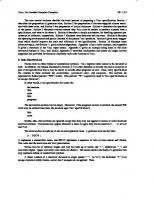
Figure 1.1 illustrates the concept of a state. Figure 1.1 a is a fragment of a program written in Pascal. Since this fragment does not declare the identifiers i and j, we add the fact that both are integer variables. The values of i and j before the given fragment begins to execute constitute the initial state; their values after execution ceases constitute the final state. Figure 1.1 b illustrates the state transformations carried out by the fragment, starting from a particular initial state. Let I be the function defined by the state transformation of some particular algorithm A. If we are to preserve the meaning of A when compiling it

*

while i j do ifi>j theni:=i-j elsej:=j-i; a) An algorithm

=

36 j = 24 i i = 12 j = 24 Final: i = 12 j = 12 b) A particular sequence of states Initial:

Figure 1.1 Algorithms and States

to a new language then the state transformation function I f of the translated algorithm A f must, in some sense, 'agree' with I. Since the state space, Sf, of the target language may differ from that of the source language, we must first decide upon a function, M, to map each state s E S to a subset M (s) of Sf. The function!, then preserves the meaning ofl if!,(M(s)) is a subset of M(J (s)) for all allowable initial states s ES. For example, consider the language of a simple computer with a single accumulator and two data locations called I and J respectively (Exercise 1.3). Suppose that M maps a particular state of the algorithm given in Figure l.la to a set of machine states in which I contains the value of the variable i, J contains the value of the variable j, and the accumulator contains any arbitrary value. Figure 1.2a shows a translation of Figure 1.1 a for this machine; a partial state sequence is given in Figure 1.2b. In determining the state sequence of Figure 1.1 b, we used only the concepts of Pascal as specified by the language definition. For every programming language, PL, we can define an abstract machine: The operations, data structures and control structures of PL become the memory elements and instructions of the machine. A 'Pascal machine' is therefore an imaginary computer with Pascal operations as its machine instructions and the data objects possible in Pascal as its memory elements. Execution of an algorithm written in PL on such a machine is called interpretation; the abstract machine is an interpreter. A pure interpreter analyzes the character form of each source language instruction every time that instruction is executed. If the given instruction is

3

1.1. Translation and Interpretation

only to be executed once, pure interpretation is the least expensive method of all. Hence it is often used for job control languages and the 'immediate commands' of interactive languages. When instructions are to be executed LOOP

SUBI

LOAD SUB JZERO JNEG STORE JUMP LOAD SUB STORE JUMP

I J EXIT SUBI I LOOP J

I J

LOOP

EXIT a) An algorithm Initial:

1=36 1=36 1=36

J = 24

J = 24 J = 24

ACC =? ACC = 36 ACC = 12

ACC = 0 Final: J = 12 1= 12 b) A sequence of states corresponding to Figure l.l b Figure 1.2 A Translation of Figure 1.1

repeatedly, a better approach is to analyze the character form of the source program only once, replacing it with a sequence of symbols more amenable to interpretation. This analysis is simply a translation of the source language into some target language, which is then interpreted. The translation from the source language to the target language can take place as each instruction of the program is executed for the first time (intepretation with substitution). Thus only that part of the program actually executed will be translated; during testing this may be only a fraction of the entire program. Also, the character form of the source program can often be stored more compactly than the equivalent target program. The disadvantage of interpretation with substitution is that both the compiler and interpreter must be available during execution. In practice, however, a system of this kind should not be significantly larger than a pure interpreter for the same language. Examples may be found of virtually all levels of interpretation. Atone extreme are the systems in which the compiler merely converts constants to internal form, fixes the meaning of identifiers and perhaps transforms infix

4

Chapter 1. Introduction and Overview

notation to postfix (APL and SNOBOL4 are commonly implemented this way); at the other are the systems in which the hardware, assisted by a small run-time system, forms the interpreter (FORTRAN and Pascal implementations usually follow this strategy).

1.2. The Tasks of a Compiler A compilation is usually implemented as a sequence of transformations (SL, L 1), (Lb L 2), ... , (Lk> TL), where SL is the source language and TL is the target language. Each language Li is called an intermediate language. Intermediate languages are conceptual tools used in decomposing the task of compiling from the source language to the target language. The design of a particular compiler determines which (if any) intermediate language programs actually appear as concrete text or data structures during compilation. Any compilation can be broken down into two major tasks: • Analysis: Discover the structure and primitives of the source program, determining its meaning . • Synthesis: Create a target program equivalent to the source program. This breakdown is useful because it separates our concerns about the source and target languages. The analysis concerns itself solely with the properties of the source language. It converts the program text submitted by the programmer into an abstract representation embodying the essential properties of the algorithm. This abstract representation may be implemented in many ways, but it is usually conceptualized as a tree. The structure of the tree represents the control and data flow aspects of the program, and additional information is attached to the nodes to describe other aspects vital to the compilation. In Chapter 2 we review the general characteristics of source languages, pointing out the properties relevant for the compiler writer. Figure 1.3 illustrates the general idea with an abstraction of the algorithm of Figure l.la. Figure l.3a describes the control and data flow of the algorithm by means of the 'e h descendant of' relation. For example, to carry out the algorithm described by a subtree rooted in a while node we first evaluate the expression described by the subtree that is the first descendant of the while node. If this expression yields true then we carry out the algorithm described by the subtree that is the second descendant. Similarly, to evaluate the expression described by an expression subtree, we evaluate the first and third descendants and then apply the operator described by the second descendant to the results. The algorithm of Figure l.la is not completely characterized by Figure l.3a. Information must be added (Figure 1.3b) to complete the description. Note that some of this information (the actual identifier for each idn) is taken directly form the source text. The remainder is obtained by process-

5

1.2. The Tasks of a Compiler

a) Control and data flow Node

idn name exp

Additional Information identifier corresponding declaration type of the variable type of the expression value

b) Additional information about the source program Node

name if

while

Additional Information corresponding data location address of code to carry out the else part address of the expression evaluation code

c) Additional information about the target program Figure 1.3 An Abstract Program Fragment

ing the tree. For example, the type of the expression value depends upon the operator and the types of the operands. Synthesis proceeds from the abstraction developed during analysis. It augments the tree by attaching additional information (Figure l.3c) that reflects the source-to-target mapping discussed in the previous section. For example, the access function for the variable i in Figure 1.1a would become the address of data location I according to the mapping M assumed by Figure 1.2. Similarly, the address of the else part of the conditional was represented by the label SUBI. Chapter 3 discusses the general characteristics of machines, highlighting properties that are important in the development of source-to-target mappings.

6

Chapter 1. Introduction and Overview

Formal definitions of the source language and the source-to-target mapping determine the structure of the tree and the computation of the additional information. The compiler simply implements the indicated transformations, and hence the abstraction illustrated in Figure 1.3 forms the basis for the entire compiler design. In Chapter 4 we discuss this abstraction in detail, considering possible intermediate languages and the auxiliary data structures used in transforming between them. Analysis is the more formalized of the two major compiler tasks. It is generally broken down into two parts, the structural analysis to determine the static structure of the source program, and the semantic analysiS to fix the additional information and check its consistency. Chapter 5 summarizes some results from the theory of formal languages and shows how they are used in the structural analysis of a program. Two subtasks of the structural analysis are identified on the basis of the particular formalisms employed: Lexical analysis (Chapter 6) deals with the basic symbols of the source program, and is described in terms of finite-state automata; syntactic analysis, or parsing, (Chapter 7) deals with the static structure of the program, and is described in terms of pushdown automata. Chapter 8 extends the theoretical treatment of Chapter 5 to cover the additional information attached to the components of the structure, and Chapter 9 applies the resulting formalism (attribute grammars) to semantic analysis. There is little in the way of formal models for the entire synthesis process, are known. We view synthesis as although algorithms for various ｳｵ｢ｴ｡ｾｫ＠ consisting of two distinct subtasks, code generation and assembly. Code generation (Chapter 10) transforms the abstract source program appearing at the analysis/synthesis interface into an equivalent target machine program. This transformation is carried out in two steps: First we map the algorithm from source concepts to target concepts, and then we select a specific sequence of target machine instructions to implement that algorithm. Assembly (Chapter 11) resolves all target addressing and converts the target machine instructions into an appropriate output format. We should stress that by using the term 'assembly' we do not imply that the code generator will produce symbolic assembly code for input to the assembly task. Instead, it delivers an internal representation of target instructions in which most addresses remain unresolved. This representation is similar to that resulting from analysis of symbolic instructions during the first pass of a normal symbolic assembler. The output of the assembly task should be in the format accepted by the standard link editor or loader on the target machine. Errors may appear at any time during the compilation process. In order to detect as many errors as possible in a single run, repairs must be made such that the program is consistent, even though it may not reflect the programmer's intent. Violations of the rules of the source language should be detected and reported during analysis. If the source algorithm uses concepts of the source language for which no target equivalent has been defined in a particular implementation, or if the target algorithm exceeds limitations

1.3. Data Management in a Compiler

7

of a specific target language interpreter (e.g. requires more memory than a specific computer provides), this should be reported during synthesis. Finally, errors must be reported if any storage limits of the compiler itself are violated. In addition to the actual error handling, it is useful for the compiler to provide extra information for run-time error detection and debugging. This task is closely related to error handling, and both are discussed in Chapter

12. A number of strategies may be followed in an attempt to improve the target program relative to some specified measure of cost. (Code size and execution speed are typical cost measures.) These strategies may involve deeper analysis of the source program, more complex mapping functions, and transformations of the target program. We shall treat the first two in our discussions of analysis and code generation respectively; the third is the subject of Chapter 13.

1.3. Data Management in a Compiler As with other large programs, data management and access account for many of the problems to be solved by the design of a compiler. In order to control complexity, we separate the functional aspects of a data object from the implementation aspects by regarding it as an instance of an abstract data type. (An abstract data type is defined by a set of creation, assignment and access operators and their interaction; no mention is made of the concrete implementation technique.) This enables us to concentrate upon the relationships between tasks and data objects without becoming enmeshed in details of resource allocation that reflect the machine upon which the compiler is running (the compiler host) rather than the problem of compilation. A particular implementation is chosen for a data object on the basis of the relationship between its pattern of usage and the resources provided by the compiler host. Most of the basic issues involved become apparent if we distinguish three classes of data:

• Local data of compiler tasks • Program text in various intermediate representations • Tables containing information that represents context-dependence in the program text Storage for local data can be allocated statically or managed via the normal stacking mechanisms of a block-structured language. Such strategies are not useful for the program text, however, or for the tables containing contextual information. Because of memory limitations, we can often hold only a small segment of the program text in directly-accessible storage. This constrains us to process the program sequentially, and prevents us from representing it directly as a linked data structure. Instead, a linear notation that represents a specific traversal of the data structure (e.g. prefix or postfix) is often

8

Chapter 1. Introduction and Overview

employed. Information to be used beyond the immediate vicinity of the place where it was obtained is stored in tables. Conceptually, this information is a component of the program text; in practice it often occupies different data structures because it has different access patterns. For example, tables must often be accessed randomly. In some cases it is necessary to search them, a process that may require a considerable fraction of the total compilation time. For this reason we do not usually consider the possibility of spilling tables to a file. The size of the program text and that of most tables grows linearly with the length of the original source program. Some data structures (e.g. the parse stack) only grow with the complexity of the source program. (Complexity is generally related to nesting of constructs such as procedures and loops. Thus long, straight-line programs are not particularly complex.) Specification of bounds on the size of any of these data structures leads automatically to restrictions on the class of translatable programs. These restrictions may not be onerous to a human programmer but may seriously limit programs generated by pre-processors.

1.4. Compiler Structure A decomposition of any problem identifies both tasks and data structures. For example, in Section 1.2 we discussed the analysis and synthesis tasks. We mentioned that the analyzer converted the source program into an abstract representation and that the synthesizer obtained information from this abstract representation to guide its construction of the target algorithm. Thus we are led to recognize a major data object, which we call the structure tree, in addition to the analysis and synthesis tasks. We define one module for each task and each data structure identified during the decomposition. A module is specified by an interface that defines the objects and actions it makes available, and the global data and operations it uses. It is implemented (in general) by a collection of procedures accessing a common data structure that embodies the state of the module. Modules fall into a spectrum with single procedures at one end and simple data objects at the other. Four points on this spectrum are important for our purposes: • Procedure: An abstraction of a single 'memoryless' action (i.e. an action with no internal state). It may be invoked with parameters, and its effect depends only upon the parameter values. (Example - A procedure to calculate the square root of a real value.) • Package: An abstraction of a collection of actions related by a common internal state. The declaration of a package is also its instantiation, and hence only one instance is possible. (Example - The analysis or structure tree module of a compiler.)

9

1.4. Compiler Structure

OUTPUT Target Code Error Reports

INPUT Source text

Compilation \

LOCAL Structure Tree Figure 1.4 Decomposition of the Compiler

OUTPUT Error Reports Structure Tree

INPUT Source text

Analysis

Structural Analysis

Semantic Analysis

LOCAL Connection Sequence Figure 1.5 Decomposition of the Analysis Task

• Abstract data type: An abstraction of a data object on which a number of actions can be performed. Declaration is separate from instantiation, and hence many instances may exist. (Example - A stack abstraction providing the operations push, pop, top, etc.) • Variable: An abstraction of a data object on which exactly two operations,fetch and store, can be performed. (Example - An integer variable in most programming languages.) Abstract data types can be implemented via packages: The package defines a data type to represent the desired object, and procedures for all operations on the object. Objects are then instantiated separately. When an operation

10

Chapter 1. Introduction and Overview

OUTPUT Error Reports Connection Sequence

INPUT Source text

Structural Analysis

Lexical Analysis

LOCAL Token Sequence Figure 1.6 Decomposition of the Structural Analysis Task

INPUT Structure Tree

OUTPUT Error Reports Target Code

Code

I Generation LOCAL Target Tree Figure 1.7 Decomposition of the Synthesis Task

is invoked, the particular object to which it should be applied is passed as a parameter to the operation procedure. The overall compiler structure that we shall use in this book is outlined in Figures 1.4 through 1.8. Each of these figures describes a single step in the decomposition. The central block of the figure specifies the problem being decomposed at this step. To the left are the data structures from which information is obtained, and to the right are those to which information is delivered. Below is the decomposition of the problem, with boxes represent-

11

1.4. Compiler Structure

OUTPUT Error Reports Target Tree

INPUT Structure Tree

Code Generation

Target Mapping

Code Selection

LOCAL Computation Graph Figure 1.8 Decomposition of the Code Generation Task

ing subtasks. Data structures used for communication among these subtasks are listed at the bottom of the figure. Each box and each entry in any of the three data lists corresponds to a module of the compiler. It is important to note that Figures 1.4 through 1.8 reflect only the overall structure of the compiler; they are not flowcharts and they do not specify module interfaces. Our decomposition is based upon our understanding of the compilation problem and our perception of the best techniques currently available for its solution. The choice of precise boundaries is driven by control and data flow considerations, primarily minimization of flow at interfaces. Specific criteria that influenced our decisions will be discussed throughout the text. The decomposition is virtually independent of the underlying implementation, and of the specific characteristics of the source language and target machine. Clearly these factors influence the complexity of the modules that we have identified, in some cases reducing them to trivial stubs, but the overall structure remains unchanged. Independence of the modules from the concrete implementation is obtained by assuming that each module is implemented on its own abstract machine, which provides the precise operations needed by the module. The local data structures of Figures 1.4-1.8 are thus components of the abstract machine on which the given subproblem is solved. One can see the degree of freedom remaining in the implementation by noting that our diagrams never prescribe the time sequence of the subproblem solutions. Thus, for example, analysis and synthesis might run sequentially. In this case the structure tree must be completely built as a linked data structure during analysis, written to a file if necessary, and then processed during synthesis. Analysis and synthesis might, however, run con-

12

Chapter 1. Introduction and Overview

currently and interact as coroutines: As soon as the analyzer has extracted an element of the structure tree, the synthesizer is activated to process this element further. In this case the structure tree will never be built as a concrete object, but is simply an abstract data structure; only the element being processed exists in concrete form. In particular, our decomposition has nothing to do with the possible division of a compiler into passes. (We consider a pass to be a single, sequential scan of the entire text in either direction. A pass either transforms the program from one internal representation to another or performs specified changes while holding the representation constant.) The pass structure commonly arises from storage constraints in main memory and from input/output considerations, rather than from any logical necessity to divide the compiler into several sequential steps. One module is often split across several passes, and/or tasks belonging to several modules are carried out in the same pass. Possible criteria will be illustrated by concrete examples in Chapter 14. Proven programming methodologies indicate that it is best to regard pass structure as an implementation question. This permits development of program families with the same modular decomposition but different pass organization. The above consideration of coroutines and other implementation models illustrates such a family.

l.5. Notes and References Compiler construction is one of the areas of computer science that early workers tried to consider systematically. Knuth [1962] reports some of those efforts. Important sources from the first half of the 60's are an issue of the Communications of the ACM [1961], the report of a conference sponsored by the International Computing Centre [ICC 1962] and the collection of papers edited by Rosen [1967]. Finally, Annual Review in Automatic Programming contains a large number of fundamental papers in compiler construction. The idea of an algorithmic conversion of expressions to a machineoriented form originated in the work of Rutishauser [1952]. Although most of our current methods bear only a distant resemblance to those of the 50's and early 60's, we have inherited a view of the description of programming languages that provides the foundation of compiler construction today: Intermediate languages were first proposed as interfaces in the compilation process by a SHARE committee [Mock 1958]; the extensive theory of formal languages, first developed by the linguist Noam Chomsky [1956], was employed in the definition of ALGOL 60 [Naur 1963]; the use of pushdown automata as models for syntax analysis appears in the work of Samelson and Bauer [1960]. The book by Randell and Russell [1964] remains a useful guide for a quick implementation of ALGOL 60 that does not depend upon extensive tools. Grau, Hill and Langmaack [1967] describe an ALGOL 60 implemen-

1.5. Notes and References

13

tation in an extended version of ALGOL 60. The books by Gries [1971], Aho and Ullman [1972, 1977a] and Bauer and Eickel [1976] represent the state of the art in the mid 1970's. Recognition that parsing can be understood via models from the theory of formal languages led to a plethora of work in this area and provided the strongest motivation for the further development of that theory. From time to time the impression arises that parsing is the only relevant component of compiler construction. Parsing unquestionably represents one of the most important control mechanisms of a compiler. However, while just under one third of the papers collected in Pollack's 1972 bibliography are devoted to parsing, there was not one reference to the equally important topic of code generation. Measurements [Lalonde 1972] have shown that parsing represents approximately 9% of a compiler's code and II % of the total compilation time. On the other hand, code generation and optimization account for 50-70% of the compiler. Certainly this discrepancy is due, in part, to the great advances made in the theory of parsing; the value of this work should not be underestimated. We must stress, however, that a more balanced viewpoint is necessary if progress is to be maintained. Modular decomposition [Parnas 1972, Parnas 1976] is a design technique in which intermediate stages are represented by specifications of the external behavior (interfaces) of program modules. The technique of data-driven decomposition was discussed by Liskov and Zilles [1974], and a summary of program module characteristics was given by Goos and Kastens [1978]. This latter paper shows how the various kinds of program modules are constructed in several programming languages. Our diagrams depicting single decompositions are loosely based upon some ideas of Stevens, Myers and Constantine [1974]. EXERCISES

1.1. Consider the Pascal algorithm of Figure l.la. a. What are the elementary objects and operations? b. What are the rules for chronological relations? c. What composition rules are used to construct the static program?

1.2. Determine the state transformation function, f, for the algorithm of Figure l.la. What initial states guarantee termination? How do you characterize the corresponding final states? 1.3. Consider a simple computer with an accumulator and two data locations. The instruction set is: LOAD STORE

d: d:

Copy the contents of data location d to the accumulator. Copy the contents of the accumulator to data location d.

SUB

d:

JUMP

i:

Subtract the contents of data location d from the accumulator, leaving the result in the accumulator. (Ignore any possibility of overflow.) Execute instruction i next.

14

Chapter 1. Introduction and Overview

JZERO

i:

JNEG

i:

a. b. c. d.

Execute instruction i next if the accumulator contents are zero. Execute instruction i next if the accumulator contents are less than zero.

What are the elementary objects? What are the elementary actions? What composition rules are used? Complete the state sequence of Figure 1.2b.

CHAPTER 2

Properties of Programming Languages

Programming languages are often described by stating the meaning of the constructs (expressions, statements, clauses, etc.) interpretively. This description implicitly defines an interpreter for an abstract machine whose machine language is the programming language. The output of the analysis task is a representation of the program to be compiled in terms of the operations and data structures of this abstract machine. By means of code generation and the run-time system, these elements are modeled by operation sequences and data structures of the computer and its basic software (operating system, etc.) In this chapter we explore the properties of programming languages that

determine the construction and possible forms of the associated abstract machines, and demonstrate the correspondence between the elements of the programming language and the abstract machine. On the basis of this discussion, we select the features of our example source language, LAX. A complete definition of LAX is given in Appendix A.

2.1. Overview The basis of every language implementation is a language definition. (See the Bibliography for a list of the language definitions that we shall refer to in this book.) Users of the language read the definition as a user manual: What is the practical meaning of the primitive elements? How can they be meaningfully used? How can they be combined in a meaningful way? The compiler writer, on the other hand, is interested in the question of which constructions are permitted. Even if he cannot at the moment see any useful application of a construct, or if the construct leads to serious implementation

15

16

Chapter 2. Properties of Programming Languages

difficulties, he must implement it exactly as specified by the language definition. Descriptions such as programming textbooks, which are oriented towards the meaningful applications of the language elements, do not clearly define the boundaries between what is permitted and what is prohibited. Thus it is difficult to make use of such descriptions as bases for the construction of a compiler. (Programming textbooks are also informal, and often cover only a part of the language.)

2.1.1. Syntax, Semantics and Pragmatics

The syntax of a language determines which character strings constitute well-formed programs in the language and which do not. The semantics of a language describe the meaning of a program in terms of the basic concepts of the language. Pragmatics relate the basic concepts of the language to concepts outside the language (to concepts of mathematics or to the objects and operations of a computer, for example). Semantics include properties that can be deduced without executing the program as well as those only recognizable during execution. Following Griffiths [1973], we denote these properties static and dynamic semantics respectively. The assignment of a particular property to one or the other of these classes is partially a design decision by the compiler writer. For example, some implementations of ALGOL 60 assign the distinction between integer and real to the dynamic semantics, although this distinction can normally be made at compile time and thus could belong to the static semantics. Pragmatic considerations appear in language definitions as unelaborated statements of existence, as references to other areas of knowledge, as appeals to intuition, or as explicit statements. Examples are the statements '[Boolean] values are the truth values denoted by the identifiers true and false' (Pascal Report, Section 6.1.2), 'their results are obtained in the sense of numerical analysis' (ALGOL 68 Revised Report, Section 2.l.3.l.e) or 'decimal numbers have their conventional meaning' (ALGOL 60 Report, Section 2.5.3). Most pragmatic properties are hinted at through a suggestive choice of words that are not further explained. Statements that certain constructs only have a defined meaning under specified conditions also belong to the pragmatics of a language. In such cases the compiler writer is usually free to fix the meaning of the construct under other conditions. The richer the pragmatics of a language, the more latitude a compiler writer has for efficient implementation and the heavier the burden on the user to write his program to give the same answers regardless of the implementation. We shall set the following goals for our analysis of a language definition: • Stipulation of the syntactic rules specifying construction of programs . • Stipulation of the static semantic rules. These, in conjunction with the syntactic rules, determine the form into which the analysis portion of the compiler transforms the source program.

17

2.1. Overview

• Stipulation of the dynamic semantic rules and differentiation from pragmatics. These determine the objects and operations of the languageoriented abstract machine, which can be used to describe the interface between the analysis and synthesis portions of the compiler: The analyzer translates the source program into an abstract target program that could run on the abstract machine . • Stipulation of the mapping of the objects and operations of the abstract machine onto the objects and operations of the hardware and operating system, taking the pragmatic meanings of these primitives into account. This mapping will be carried out partly by the code generator and partly by the run-time system; its specification is the basis for the decisions regarding the partitioning of tasks between these two phases.

2.1.2. Syntactic Properties

The syntactic rules of a language belong to distinct levels according to their meaning. The lowest level contains the 'spelling rules' for basic symbols, which describe the construction of keywords, identifiers and special symbols. These rules determine, for example, whether keywords have the form of identifiers (begin) or are written with special delimiters ('BEGIN', .BEGIN), whether lower case letters are permitted in addition to upper case, and which spellings « =, .LE., 'NOT' that cannot be repro'GREATER') are permitted for symbols such as duced on all I/O devices. A common property of these rules is that they do not affect the meaning of the program being represented. (In this book we have distinguished keywords by using boldface type. This convention is used only to enhance readability, and does not imply anything about the actual representation of keywords in program text.) The second level consists of the rules governing representation and interpretation of constants, for example rules about the specification of exponents in floating point numbers or the allowed forms of integers (decimal, hexadecimal, etc.) These rules affect the meanings of programs insofar as they specify the possibilities for direct representation of constant values. The treatment of both of these syntactic classes is the task of lexical analysis, discussed in Chapter 6. The third level of syntactic rules is termed the concrete syntax. Concrete syntax rules describe the composition of language contructs such as expressions and statements from basic symbols. Figure 2.la shows the parse tree (a graphical representation of the application of concrete syntax rules) of the Pascal statement 'if a or band c then ... else .. , '. Because the goal of the compiler's analysis task is to determine the meaning of the source program, semantically irrelevant complications such as operator precedence and certain keywordS can be suppressed. The language constructs are described by an abstract syntax that specifies the compositional structure of a program while leaving open some aspects of its concrete representation as a string of basic symbols. Application of the abstract syntax rules can be illustrated by a structure tree (Figure 2.1 b).


5.2. Regular Grammars and Finite Automata

113

1. If X -'>t (X EN, t E T) is a production of P then let Xt -'>f be a production of R. 2. If X -'>tY (X, YEN, t E T) is a production of P then let Xt -'> Y be a production of R .

Further, F = {f} U {X I X -'>( EP}. Figure 5.9 is an automaton constructed by this process from the grammar of Figure 5.4a. T = {n,.,+,-,E} Q

= {C,F,I,X,S,U,q}

R = { Cn -'>q, Cn -'>F, C. -'>1, F. -,>1, FE -'>S, In -'>q, In -'>X, XE -'>S, Sn -'>q, S + -'> U, S - -'> U, Un -'>q } qo = C F = {q} Figure 5.9. An Automaton Corresponding to Figure 5.4a

One can show by induction that the automaton constructed in this manner has the following characteristic: For any derivation Z'TX =? *X X=?* q ('T, X E T*, X EN, 'TX EL (A ), q EF), the state X specifies the nonterminal symbol of G that must have been used to derive the string X. Clearly this statement is true for the initial state Z if'TX belongs to L (G). It remains true until the final state q, which does not generate any further

symbols, is reached. With the help of this interpretation it is easy to prove that each sentence of L ( G) also belongs to L (A ) and vice-versa. Figure 5.9 is an unsatisfactory automaton in practice because at certain steps - for example in state I with input symbol n - several transitions are possible. This is not a theoretical problem since the automaton is capable of producing a derivation for any string in the language. When implementing this automaton in a compiler, however, we must make some arbitrary decision at each step where more than one production might apply. An incorrect decision requires backtracking in order to seek another possibility. There are three reasons why backtracking should be avoided if possible: • The time required to parse a string with backtracking may increase exponentially with the length of the string . • If the automaton does not accept the string then it will be recognized as incorrect. A parse with backtrack makes pinpointing the error almost impossible. (This is illustrated by attempting to parse the string

114

Chapter 5. Elements of Formal Systems

n.nE + +n with the automaton of Figure 5.9 trying the rules in the sequence in which they are written.) • Other compiler actions are often associated with state transitions. Backtracking then requires unraveling of actions already completed, generally a very difficult task. In order to avoid backtracking, additional constraints must be placed upon the automata that we are prepared to accept as models for our recognition algorithms. Definition 5.14. An automaton is deterministic if every derivation can be continued by at most one move. A finite automaton is therefore deterministic if the left-hand sides of all rules are distinct. It can be completely described by a state table that has one row for each element of Q and one column for each element of T. Entry (q,t) contains q' if and only if the production qt -+q' is an element of R. The rows corresponding to qo and to the elements of F are suitably marked. Backtracking can always be avoided when recognizing strings in a regular language:

Theorem 5.15. For every regular grammar, G, there exists a deterministic finite automaton, A, such that L (A ) =L (G). Following construction 5.13, we can derive an automaton from a regular grammar G =(T,N,P,Z) such that, during acceptance of a sentence in L (G), the state at each point specifies the element of N used to derive the remainder of the string. Suppose that the productions X -+tU and X -+tV belong to P. When t is the next input symbol, the remainder of the string could have been derived either from U or from V. If A is to be deterministic, however, R must contain exactly one production of the form Xt -+q'. Thus the state q' must specify a set of nonterminals, anyone of which could have been used to derive the remainder of the string. This interpretation of the states leads to the following inductive algorithm for determining Q, R and F of a deterministic automaton A =(T,Q,R.qo,F). (In this algorithm, q represents a subset Nq of N U {f },f fiN): l. Initially let Q = {qo} and R

= 0, with Nqo = {Z}.

2. Let q be an element of Q that has not yet been considered. Perform steps (3)-(5) for each t ET.

3. Letnext(q,t)

= {U 1:3

XENq such that X -+tUEP}.

4. If there is an X ENq such that X -+t EP or X -+f.EP then add next (q, t) if it is not already present.

f

to

5. If next(q,t)=F0 then let q' be the state representing Nq,=next(q,t).

115

5.2. Regular Grammars and Finite Automata

Add q' to Q and qt -+q' to R if they are not already present. 6. If all states of Q have been considered then let F = {q stop. Otherwise return to step (2).

If

ENq } and

You can easily convince yourself that this construction leads to a deterministic finite automaton A such that L (A ) =L (G). In particular, the algorithm terminates: All states represent subsets of N u {f}, of which there are only a finite number. To illustrate this procedure, consider the construction of a deterministic finite automaton that recognizes strings generated by the grammar of Figure 5.4a. The state table for this grammar, showing the correspondence between states and sets of nonterminals, is given in Figure 5.lOa. You should derive

+

n q]

E

{C}

q2 q3

q2

{f,F}

{I}

q4 qs

q6

{S}

q6 q3

{f,X}

{f}

{U}

qs

a) The state table T = {n,.,+,-,E}

p

= { qon -+q], qo· -+q2, q]. -+q2, q]E -+q3, q2n -+q4, q3n -+qs, q3 + -+q6, q3 - -+q6, q4E -+q3, q6n -+qs }

F = {q].q4,qS}

b) The complete automaton Figure 5.10. A Deterministic Automaton Corresponding to Figure 5.4a

116

Chapter 5. Elements of Formal Systems

this state table for yourself, following the steps of the algorithm. Begin with a single empty row for qo and work across it, filling in each entry that corresponds to a valid transition. Each time a distinct set of nonterminal symbols is generated, add an empty row to the table. The algorithm terminates when all rows have been processed. Theorem 5.16. For every finite automaton, A, there exists a regular grammar, G, such that L (G)=L (A).

Theorems 5.l5 and 5.16 together establish the fact that finite automata and regular grammars are equivalent. To prove Theorem 5.16 we construct the production set P of the grammar G = (T,Q,P,qo) from the automaton (T,Q,R,qo,F) as follows: P = {q -+tq'

I qt -+q'ER}

u {q

-+£

I q EF}

5.2.2. State Diagrams and Regular Expressions

The phrase structure of the basic symbols of the language is usually not interesting, and in fact may simply make the description harder to understand. Two additional formalisms, both of which avoid the need for irrelevant structuring, are available for regular languages. The first is the representation of a finite automaton by a directed graph:

Definition 5.17.: Let A =(T,Q,R,qo,F) be a finite automaton, D = {(q,q') I 3 t ,qt-+q'ER}, andJ:(q,q')-+{t I qt-+q'ER} be a mapping from D into the powerset of T. The directed graph (Q,D) with edge labels J «q,q'» is called the state diagram of the automaton A . Figure 5.lla is the state diagram of the automaton described in Figure 5. lOb. The nodes corresponding to elements of F have been represented as squares, while the remaining nodes are represented as circles. Only the state numbers appear in the nodes: 0 stands for qo, 1 for qb and so forth.

a) State diagram n nEn n.nEn

.n nE + n n.nE + n b) Paths

n.n nE-n n.nE-n

Figure 5.11. Another Description of Figure 5.1 Db

117

5.2. Regular Grammars and Finite Automata

In a state diagram, the sequence of edge labels along a path beginning at qo and ending at a state in F is a sentence of L (A). Figure 5.lla has exactly 12 such paths. The corresponding sentences are given in Figure 5.11 b. A state diagram specifies a regular language. Another characterization is the regular expression: Definition 5.1S. Given a vocabulary V, and the symbols E, t:, +, *, ( and) not in V. A string p over V U {E ,t:, +, *,(,)} is a regular expression over V if I. p is a single symbol of V or one of the symbols E or t:, or if 2. p has the form (X + Y), (XY) or (X) * where X and Yare regular expressions. Every regular expression results from a finite number of applications of rules (1) and (2). It describes a language over V: The symbol E describes the empty language, t: describes the language consisting only of the empty string, v E V describes the language {v}, (X + Y) = {w I wEX or wE Y}, (XY) = {Xy I X EX,yE Y}. The closure operator (*) is defined by the following infinite sum: X* =t:+X +XX + XXX +

...

As illustrated in this definition, we shall usually omit parentheses. Star is unary, and takes priority over either binary operator; plus has a lower priority than concatenation. Thus W +XY* is equivalent to the fullyparenthesized expression (W +(X(Y*))). Figure 5.12 summarizes the algebraic properties of regular expressions. The distinct representations for X· show that several regular expressions can be given for one language. The main advantage in using a regular expression to describe a set of strings is that it gives a precise specification, closely related to the 'natural language' description, which can be written in text form suitable for input to a computer. For example, let I denote any single letter and d any single digit. The expression I (I +d) * is then a direct representation of the natural language description 'a letter followed by any sequence ofletters and digits'. The equivalence of regular expressions and finite automata follows from: Theorem 5.19. Let R be a regular expression that describes a subset, S, of T*. There exists a deterministic finite automaton, A =(T,Q,P,qo,F) such that L(A )=S. The automaton is constructed in much the same way as that of Theorem 5.15: We create a new expression R' by replacing the elements of T occurring in R by distinct symbols (multiple occurrences of the same element will receive distinct symbols). Further, we prefix another distinct symbol to the altered expression; if R =E, then R' consists only of this starting symbol. (As symbols we could use, for example, natural numbers with 0 as the starting symbol.) The states of our automaton correspond to subsets of the sym-

Chapter 5. Elements of Formal Systems

118

X+Y

= Y+X

(commutative)

(X + Y)+Z = X +(Y +Z) (XY)Z = X(YZ) X(Y +Z) (X + Y)Z

= XY +XZ = XZ + yz

X +E = E +X Xf.=£X=X XE

(distributive)

=X

(identity)

= EX = E

X +X

(associative)

(zero)

=X

(idempotent)

(X·>* =X· X· = f.+XX· X· = X+X· f.

•

E'

=f.

= f.

Figure 5.12. Algebraic Properties of Regular Expressions

R = 1(l + d) * R' = 0 1 (2 + 3)* a) Modifying the Regular Expression

d

{O}

ql

q2

q3

{l}

(final)

q2

q3

{2}

(final)

q2

q3

{3}

(final)

b) The resulting state table Figure 5.13. Regular Expressions to State Tables

bol set. The set corresponding to the initial state qo consists solely of the starting symbol. We inspect the states of Q one after another and add new states as required. For each q EQ and each t ET, let q' correspond to the set of symbols in R' that replace t and follow any of the symbols of the set corresponding to q. If the set corresponding to q' is not empty, then we add

119

5.3. Context-Free Grammars and Pushdown Automata

qt -"q' to P and add {q'} to Q if it is not already present. The set F of final states consists of all states that include a possible final symbol of R'. Figure 5.13 gives an example of this process. Starting with qo= {O}, we obtain the state table of Figure 5.13b, with states qlo ql and q3 as final states. Obviously this is not the simplest automaton which we could create for the given language; we shall return to this problem in Section 6.2.2.

5.3. Context-Free Grammars and Pushdown Automata Regular grammars are not sufficiently powerful to describe languages such as algebraic expressions, which have nested structure. Since most programming languages contain such structures, we must change to a sufficiently powerful descriptive method such as context-free grammars. Because regular grammars are a subclass of context-free grammars, one might ask why we bother with regular languages at all. As we shall see in this section, the analysis of phrase structure by means of context-free grammars is so much more costly that one falls back upon the simpler methods for regular grammars whenever possible. Here, and also in Chapter 7, we assume that all context-free grammars (T,N,P,Z) contain a production Z --S. This is the only production in which the axiom Z appears. (Any grammar can be put in this form by addition of such a production.) We assume further that the terminator # follows each sentence. This symbol identifies the condition 'input text completely consumed' and does not belong to the vocabulary. Section 5.3.3 assumes further that the productions are consecutively numbered. The above production has the number 1, n is the total number of productions and the ith production has the form X; -"Xi, Xi =Xi, l ' .. Xi,m' The length, m, of the right-hand side is also called the length of the production. We shall denote a leftmost derivation X :::;/ Y by X =;;, L Y and a rightmost derivation by X =;;,R Y. We find the following notation convenient for describing the properties of strings: The k-head k:w of w gives the first min(k, I w I + 1) symbols of w#. FIRSTk(w) is the set of all terminal k-heads of strings derivable from w. The set EFFk (w) ('t:-free first') contains all strings from FIRSTk (w) for which no t:-production A -"t: was applied at the last step in the rightmost (w) comprises all terminal k -heads that could derivation. The set ｆｏｌｾ＠ followw. By definition FOLLOWdZ) = {# } foranyk. Formally: k .w _ {w# .

-

a

FIRSTk(w) = {'T EFFk(W) = {'TEFIRSTk(w)

I :3

when I w I < k when w = ay and

Ia I = k

vET' such that w=;;,'v, 'T=k:v}

I :3 A EN, vET'

such that w =;;,R A 'TV ｾ＠

'Tv}

120

ｆｏｌｾＨｷＩ＠

Chapter 5. Elements of Formal Systems

= {T 1:3

JlEV' such that Z ｾＮ＠

p.6JJI,

T=k:JI}

We omit the index k when it is 1. These functions may be.applied to sets of strings, in which case the result is the union of the results of applying the function to the elements of its argument. Finally, if a is a string and 0 is a set of strings, we shall define aO = {aw I wEO}. 5.3.1. Pushdown Automata For finite automata, we saw that the state specifies the set of nonterminal symbols of G that could have been used to derive the remainder of the input string. Suppose that a finite automaton has reached the first right parenthesis of the following expression (which can be derived using a context-free grammar):

(al +(a2+(··· +(am )'"

»

It must then be in a state specifying some set of nonterminal symbols that can derive exactly m right parentheses. Clearly there must be a distinct state for each m. But if m is larger than the number of states of the automaton (and this could be arranged for any given number of states) then there cannot be a distinct state for each m. Thus we need a more powerful automaton, which can be obtained by providing a finite automaton with a stack as an additional storage structure.

Definition 5.20. A pushdown automaton is a septuple A =(T.Q,R,qo,F,S,so), where (T U Q U S ,R) is a general rewriting system, q0 is an element of Q, F is a subset of Q, and So is an element of S or SO=f. The sets T and Q are disjoint. Each element of R has the form aqaT-+a'q'T, where a and a' are elements of ｓｾ＠ q and q' are elements of Q, a is an element of T or a =f, and T is an element of r*. Q, qo and F have the same meaning as the corresponding components of a finite automaton. S is the set of stack symbols, and So is the initial content of the stack. The pushdown automaton accepts a string TET' ifsoqoT ｾＪｱ＠ for some q in F. If each sentence is followed by #, the pushdown automaton A defines the language L(A) = {T I ｳｯｱｔＣｾＪＬｅｆｲｽＮ＠ (In the literature one often finds the requirement that a be an element of S rather than S*; our automaton would then be termed a generalized pushdown automaton. Further, the definition of 'accept' could be based upon either the *aq, aES',q EF, or the relation ｳｯｱｔｾ＠ *q, q arbitrary. relation ｓｯｱｔｾ＠ Under the given assumptions these definitions prove to be equivalent in power.) We can picture the automaton as a machine with a finite set Q ofintemal states and a stack of arbitrary length. If we have reached the configuration s I ... Sn q T in a derivation, then the automaton is in state q, T is the unread part of the input text being analyzed, and s I ... Sn is the content of the stack (s I is the bottom item and Sn the top). The transitions of the automaton either read the next symbol of the input text (symbol-controlled) or are spon-

121

5.3. Context-Free Grammars and Pushdown Automata

taneous and do not shorten the input text. Further, each transition may alter the topmost item of the stack; it is termed a stacking, unstacking or replacing

transition, respectively, if it only adds items, deletes items, or changes them without altering their total number. The pushdown automaton can easily handle the problem of nested parentheses: When it reads a left parenthesis from the input text, it pushes a corresponding symbol onto the stack; when it reads the matching right parenthesis, that symbol is deleted from the stack. The number of states of the automaton plays no role in this process, and is independent of the parenthesis nesting depth.

Theorem 5.21. For every context free grammar, G, there exists a pushdown automaton, A, such that L (A ) = L (G).

As with finite automata, one proves this theorem by construction of A . There are two construction procedures, which lead to distinct automata; we shall go into the details of these procedures in Sections 5.3.2 and 5.3.3 respectively. The automata constructed by the two procedures serve as the basic models for two fundamentally different parsing algorithms. A pushdown automaton is not necessarily deterministic even if the left sides of all productions are distinct. For example, suppose that a\q'T-Hlq''T' are two distinct productions and a2 is a proper tail of al' and ｡ＲｱＧｔｾＢ＠ Thus al = aa2 and both productions are applicable to the configuration aa2q'TX. If we wish to test formally whether the productions unambiguously specify the next transition, we must make the left-hand sides the same length. Determinism can then be tested, as in the case of finite automata, by checking that the left-hand sides of the productions are distinct. We shall only consider cases in which the state q and k lookahead symbols of the input string are used to determine the applicable production. Unfortunately, it is not possible to sharpen Theorem 5.21 so that the pushdown automaton is always deterministic; Theorem 5.15 for regular grammars cannot be generalized to context-free grammars. Only by additional restrictions to the grammar can one guarantee a deterministic automaton. Most programming languages can be analyzed deterministically, since they have grammars that satisfy these restrictions. (This has an obvious psychological basis: Humans also find it easier to read a deterministically-analyzable program.) The restrictions imposed upon a grammar to obtain a deterministic automaton depend upon the construction procedure. We shall discuss the details at the appropriate place.

5.3.2. Top-Down Analysis and LL(k) Grammars Let G=(T,N,P,Z) be a context-free grammar, and consider the pushdown automaton A = (T, {q},R,q, {q}, V,Z) with V=T u Nand R defined as follows: R = {tqt ｾｱ＠ B

ｾ｢ｬＧＢ＠

I t ET}

u {Bq

ｾ｢ｮ＠

... blq

bn EP, n? 0, BEN, bi EV}

122

Chapter 5. Elements of Formal Systems

This automaton accepts a string in L (G) by constructing a leftmost derivation of that string and comparing the symbols generated (from left to right) with the symbols actually appearing in the string. Figure 5.14 is a pushdown automaton constructed in this manner from the grammar of Figure 5.3a. In the left-hand column of Figure 5.15 we show the derivation by which this automaton accepts the string i +i*i. The right-hand column is the leftmost derivation of this string, copied from Figure 5.5. Note that the automaton's derivation has more steps due to the rules that compare a terminal symbol on the stack with the head of the input T = { +, * ,(,),i)

Q = {q} R = { Eq ｾ＠ Tq, Eq ｾ＠ T + Eq, Tq ｾｆｱＬ＠ Tq ｾｆＪｔｱＬ＠ Fq ｾｩｱＬ＠ Fq ｾＩｅＨｱＬ＠ ＫｱｾＬＪＨ＠

ＩｱｾＬｩｽ＠

qo = q F = {q}

s

= {+,*,(,),i,E, T,F}

So

= E

Figure 5.14. A Pushdown Automaton Constructed from Figure 5.3a

Stack

Input

Leftmost derivation

E q T+E q T+T q T+F q T+i q T+ q Tq F*T q F*F q F*i q F* q Fq q q

i +i*i i +i*i i +i*i i +i *i i +i *i +i*i i *i i *i i *i i *i *i

E E+T T+T F+T i+T

i

i+T*F i+F*F i +i*F

i +i *i

Figure 5.15. Top-Down Analysis

5.3. Context-Free Grammars and Pushdown Automata

123

string and delete both. Figure 5.16 shows a reduced set of productions combining some of these steps with those that precede them. R' = { Eq -+ Tq , Eq -+ T + Eq , Tq -+Fq, Tq -+F*Tq, Fqi-+q, Fq( -+ )Eq, +q + -+q, *q*-+q, )q)-+q } Figure 5.16. Reduced Productions for Figure 5.14

The analysis performed by this automaton is called a top-down (or predictive) analysis because it traces the derivation from the axiom (top) to the sentence (bottom), predicting the symbols that should be present. For each configuration of the automaton, the stack specifies a string from v* used to derive the remainder of the input string. This corresponds to construction 5.13 for finite automata, with the stack content playing the role of the state and the state merely serving to mark the point reached in the input scan. We now specify the construction of deterministic, top-down pushdown automata by means of the LL(k) grammars introduced by Lewis and Steams [1969]: Definition 5.22. A context-free grammar G = (T,N,P,Z) is LL (k) for given k ;> 0 if, for arbitrary derivations

Z ｾｌ＠

/LA X ｾＯｌｷｘ＠

ｾ＠

'/LY'

y'ET', wE V'

(k :y=k :y') implies p=w. Theorem 5.23. For every LL(k) grammar, G, there exists a deterministic pushdown automaton, A, such that L (A ) =L (G). A reads each sentence of the language L (G) from left to right, tracing a left-

most derivation and examining no more than k input symbols at each step. (Hence the term 'LL(k) prime .) In our discussion of Theorem 5.13, we noted that each state of the finite automaton corresponding to a given grammar specified the nonterminal of the grammar that must have been used to derive the string being analyzed. Thus the state of the automaton characterized a step in the grammar's derivation of a sentence. We can provide an analogous characterization of a step in a context-free derivation by giving information about the production being applied and the possible right context: Each state of a pushdown automaton could specify a triple (p,j,O), where ｏｾ＠ j ｾ＠ np gives the number of symbols from the right-hand side of production Xp -+Xp, 1 ••• xp , np already analyzed and 0 is the set of k -heads of strings

124

Chapter 5. Elements of Formal Systems

that could follow the string derived from Xp. This triple is called a situation, and is written in the following descriptive form:

[XJ, ｾｰＺｊｉ［ｏ｝＠

JL=Xp,I'" Xp,j, JI=xp,j+I'" xp,np

The dot (which is assumed to be outside of the vocabulary) marks the position of the analysis within the right-hand side. (In most cases 0 contains a single string. We shall then write it without set brackets.) Given a grammar (T,N,P,Z), we specify the states Q and transitions R of the automaton inductively as follows: 1. Initially let Q = {qo} and R = 0, with qo=[Z ｾﾷｓ［Ｃ｝Ｎ＠ (Note that ｆｏｌｾＨｚＩ］＠ {# }.) The initial state is qo, which is also the initial stack content of A. (We could have chosen an arbitrary state as the initial stack content.) The automaton halts if this state is reached again, the stack is empty, and the next input symbol is the terminator # . 2. Let q = [X ｾ＠ JL' JI; 0] be an element of Q that has not yet been considered. 3. If JI=f. then add ｱｦＮｾ＠ to R if it is not already present. (The notation ｱＧｔｾ＠ is shorthand for the set of spontaneous unstacking transitions ｱＧｔｾ＠ with arbitrary q'.) 4. IfJl=ty for some t ET and yE V', let q'=[X ｾｊｌｴﾷｹ［ｏ｝Ｎ＠ Add q' to Q and qt ｾｱＧ＠ to R if they are not already present. 5. If JI=By for some BEN and yEV: let ｱＧ］｛ｘｾｊｌｂｹ［ｏ｝＠ and H = HB ｾＧｐ［＠ ;FIRSTk(yO)] I B ｾｐ［＠ EP}. Set Q : = Q u {q'} u Hand R := R U {q'T; ｾｱＧｨ［ｔ＠ I h; EH, 'T; EFIRSTk(P;yO)}. 6. If all states in Q have been examined, stop. Otherwise, return to step (2). The construction terminates in all cases, since the set of situations is finite. One can show that the resulting automaton is deterministic if and only if G is an LL(k) grammar, and therefore the construction provides a test for the LL(k) property. Consider the grammar of Figure 5.l7a. We can apply Construction 5.23 with k = 3 to show that this grammar is LL(3), obtaining the states of Figure 5.l7b and the transitions of Figure 5.l7c. With k =2 the construction leads to identical states. In state q7, however, we obtain the following transitions:

q7ca ｾｱｬｏ｣｡Ｌ＠

q7ca ｾｱｬｏｉＲ｣｡＠

The automaton is therefore nondeterministic and hence the grammar is LL(3), but not LL(2). The example also shows that the lookahead symbols are examined only at spontaneous, stacking transitions that correspond to entry into a new production. As soon as such a transition is executed, the reading of terminal symbols and the decision to terminate the production with an unstacking transition proceeds without further lookahead. There exist grammars that do not have the LL(k) property for any k. Among the possible reasons is the occurrence of left recursive nonterminals - nonterminals A for which a derivation A ｾ＠ A w, w-=l= f., is possible. In a

125

5.3. Context-Free Grammars and Pushdown Automata

P = { Z -->X, X --> Y, X -->b Ya, Y -->c, Y -->ca }

a) An LL(3) grammar qo=[Z -->'X;# 1 ql =[Z -->X';# 1 q2=[X -->. Y;# 1 q3=[X -->·bYa;# 1 q4=[X --> y.;# 1 q5=[Y -->'c;# 1 q6=[Y -->'ca;# 1 q7=[X -->b'Ya;# 1 q8=[Y -->c·;# 1

q9=[Y -->c'a;# 1 qlO=[X -->bY'a;# 1 qll =[Y -->·c ;a# 1 ql2=[Y -->'ca;a# 1 q13=[Y -->ca';# 1 qI4=[X -->bYa';# 1 qI5=[Y -->c';a# 1 qI6=[Y -->c'a;a# 1 q17=[Y -->ca';a# 1

b) States of the automaton, with the situations they represent R = {

qoc # -->qlq2c #, qoca # -->qlq2ca #, qolx:a -->qIq3lx:a, q I -->(, q2c # -->q4q5c #, q2ca # -->Q4q6ca #, q3b -->Q7, Q4 -->(, Q5 c -->Q8, Q6 c -->Q9,

q7ca # -->qlOqllca #, q7caa -->q IOq l2 caa , q8 -->(, q9a -->qI3, q lOa -->q 14, QII C -->q 15, Q12C -->Q 16, Q13 -->(, Q14 -->(, Q15 -->(, Q16a -->Q 17, Q17-->( }

c) Production set of the Automaton Figure 5.17. Constructing a Deterministic Top-Down Automaton

predictive automaton, left recursive nonterminals lead to cycles that can be broken only by examining a right context of arbitrary length. They can, however, be eliminated through a transformation of the grammar.

Theorem 5.24. An LL(k) grammar can have no left recursive nonterminal symbols.

Theorem 5.25. For every contextfree grammar G = (T,N,P,Z) with left recursive nonterminals, there exists an equivalent grammar G' = (T,N ｾｐ＠ left recursive nonterminals.

ｾｚＩ＠

with no

Let the elements of N be numbered consecutively: N = {XI, ... , Xn }. If we choose the indices such that the condition i J0 w then G has no left recursive nonterminals. If such a numbering is

126

Chapter 5. Elements of Formal Systems

not possible for G, we can guarantee it for G' through the following construction:

1. Let N'=N, P'=P. Perform steps (2) and (3) for i = I, ... , n. 2. For j = I, ... , i - I replace all productions X; ..... Xj wEP' by {Xi ..... Xj w J0 . . . Xj EP'}. (After this step, X;:::;:, + J0 Yimplies i R p.'B w' =>p.'yw' p.' E V*, w' E T*, B --+yEP

( I p.x I +k):p.x w = (I p.'y I +k):p.'yw'implies p.=p.', A =B and X =y.

130

Chapter 5. Elements of Formal Systems

The automaton given at the beginning of this section scans the input text from left to right, tracing the reverse of a rightmost derivation and examining no more than k input symbols at each step. (Hence the term "LR(k )".) Theorem 5.31. A context free grammar is LR(k)

if and

only

if its

k -stack

classes are pairwise-disjoint. On the basis of this theorem, we can test the LR(k) property by determining the intersection of the k-stack classes. Unfortunately the k-stack classes can contain infinitely many pairs (p, '1'): The length restriction permits only a finite number of strings '1', but the lengths of the stack contents are unrestricted. However, we can give a regular grammar Gj for each k -stack class Rj,k such that L(Gj )= {(p&'T) I (p,'T)ERj,d. Since algorithms exist for determining whether two regular languages are disjoint, this construction leads to a procedure for testing the LR(k) property.

>

Theorem 5.32. Let G = (T,N,P,Z) be a contextftee grammar, and let k O. Assume that & is not an element of the vocabulary V = TuN. There exists a set ofregular grammars Gj,j =0, ... , n such that L (Gj )= {p&'T I (p,'T) ERj,k}'

The regular grammars that generate the k -stack classes are based upon the situations introduced in connection with Theorem 5.23:

I X ｾｬｌｰｅｐＬ＠

W = ([X ｾｉｌＧｐ［ｗＩ＠

wEFOLLOWdX)}

These situations are the nonterminal symbols of the regular grammars. To define the grammars themselves, we first specify a set of grammars that generate the k -stack classes, but are not regular:

G 'j

= (Vu {&,#}, W,plu P"u Pj ,[Z ｾﾷｳ＠

;#])

The productions in P' U P" build the p components of the k-stack class. They provide the finite description of the infinite strings. Productions in Pj attach the 'I' component, terminating the k -stack class:

P' = ([X ｾｬｌＧｶｙ［ｷＩ＠

ｾｶ｛ｘ＠

ｾｬｌｶＢｹ［ｷＩ＠

P" = ([X ｾｉｌＧｂｹ［ｷ｝｛＠ Po = ([X ｾｉｌＧｐ［ｗ｝Ｆ＠

ｾＧＬＸ［ｔ｝＠

Pp = {[xp

ｾｘｰＧ［ｷ｝Ｆ＠

'I'

I P=/= t:,

I v E V} I B ｾＬＸｅｐ＠

'TEEFFk(yw)}

'TEEFFk(pw)}

w} P = I, ... , n

Remember that the lengths of 'I' and ware limited to k symbols, so the number of possible strings & 'I' and & w is finite. If we regard these strings as single terminal symbols, productions in P I and Pj , j = 0, ... , n, are allowable in a regular grammar. Productions in P" are not allowable, however, since they are of the form A ｾ＠ B , A, B EN. Thus G j is not regular. It is always possible to rewrite a grammar so that it contains no produc-

5.3. Context-Free Grammars and Pushdown Automata

131

tions such as those in pIt. The key is the closure of a nonterminal:

H(A)

= {A}

u {B

I C -+B EP,C EH(A)}

The procedure for rewriting the grammar is: 1. Select anA EN forwhichH(A)#: {A}.

2. SetP 3. Set P

= P - {A -+B I BEN}. = P u {A -+/3 I B -+/3EP, B EH(A), /3f!.N}.

The algorithm terminates when no selection can be made in step (1). We obtain Gj from Gj by applying this algorithm. The strings /3 are all of the form v[ ... ], & T or & w, and therefore all introduced productions satisfy the conditions for a regular grammar.

Theorem 5.33. For every LR(k) grammar G there exists a deterministic pushdown automaton A such that L (A ) = L (G). Let G =(T,N,P,Z). We base construction of the automaton on the grammars Gj , effectively building a machine that simultaneously generates the k -stack classes and checks them against the reverse of a rightmost derivation of the string. Depending upon the particular k -stack class, the automaton pushes the input symbol onto the stack or reduces some number of stacked symbols to a nonterminal. The construction algorithm generates the necessary situations as it goes, and uses the closure operation discussed above 'on the fly' to avoid considering productions from P". As in the construction associated with Theorem 5.15, a state of the automaton must specify a set of situations, anyone of which might have been used in deriving the current k -stack class. It is convenient to restate the definition of a closure directly in terms of a set of situations M:

H(M)=MU

HB ....·/3;T] I :3

[X .... p.-By;w]EH(M),

B -+/3EP, TEFIRSTk(yw)} The elements of Q and R are determined inductively as follows: 1. Initially let Q

={qo} and R = 0, with qo=H({[Z -+·S;#]}).

2. Let q be an element of Q that has not yet been considered. Perform steps (3)-(5) for each v E V. 3. Let basis (q,v)

= {[X -+p.v--y;w] I [X -+p;vy;w]Eq}.

4. If basis(q,v) #: 0, then let next(q,v)=H(basis(q,v». Add q'=next(q, v) to Q if it is not already present.

5. Ifbasis(q,v)#: 0 and v ET then set R := R

U

{

1 {qv-+qq'} ｦｫｾ＠ｩ {qvT-+qq'T I [X -+1.&"Vy;w]Eq, TEFlRSTk_1(yW)} otherwise

Chapter 5. Elements of Formal Systems

132

[2 -+'X;#] [X -+. Y;#] [X -+·bYa;# ] [Y -+·c;# ] [Y-+·ca;#] [2 -+K;#] [X -+ y.;#] [X -+b· Ya;# ] [Y -+·c ;a#] [Y -+·ca ;a# ]

q4:

[Y -+C·;#] [Y-+c'a;#]

q5: q6:

[X -+bY·a;#] [Y -+c·;a#] [Y-+c·a;a#] [Y -+ca·;#] [X -+bYa·;#] [Y -+ca·;a# ]

q7:

qg: q9:

a) States R

= { qobc -+qOq3c, qoc # -+qOq4#' q3ca -+q3q6a, q4 a # -+q4q7#' q5a # -+q5qg#, q6aa -+q6q9a, qoq2 # -+qoq 1#, qOq4 # -+qOq2 #, q3q6a # -+q3q5a #, qOq4q7# -+qOq2#, QOQ3Q5Qg# -+QoQI #, Q3Q6Q9a # -+Q3Q5 a # }

b) Transitions Figure 5.22. A Deterministic Bottom-Up Automaton for Figure 5.17a

6. If all elements of Q have been considered, perform step (7) for each Q E Q and then stop. Otherwise return to step (2). 7. For each [X-+X·;w]EQ, where X=XI···X n , set R := R u {Ql ... qnqW-+qlq'w I [X -+·x ;w] Eqhqi +1 = next (qi, Xi)(i = I, ... , n -I), q =next(qn, x n ), q'= next(ql,X)}

The construction terminates in all cases, since only a finite number of situations [X -+X·y;w] exist. Figure 5.22 illustrates the algorithm by applying it to the grammar of Figure 5.17a with k =2. In this example k = I would yield the same set of states. (For k =0, q4 and q7 would be coalesced, as would q7 and q9.) Nevertheless, a single look ahead symbol is not sufficient to distinguish between the shift and reduce transitions in state 6. The grammar is thus LR(2), but not LR(l). We shall conclude this section by quoting the following theoretical results:

5.4. Notes and References

133

Theorem 5.34. For every LR(k) grammar with k> I there exists an equivalent LR (I) grammar. Theorem 535. Every LL (k) grammar is also an LR (k ) grammar. Theorem 536. There exist LR (k) grammars that are not LL (k ') for any k '. Theorem 537. There exists an algorithm that, when given an LR(k) grammar G, will decide in a finite number of steps whether there exists a k' such that G is LL (k'). As a result of Theorem 5.34 we see that it might possibly be sufficient to concern ourselves only with LR(l) grammars. (As a matter of fact, the transformation underlying the proof of this theorem is unsuitable for practical purposes.) The remaining theorems support our intuitive thoughts at the end of Section 5.3.2.

5.4. Notes and References The basic symbols of a programming language are often described by arbitrary context-free productions, as illustrated by the LAX definition of Appendix A.I. This description does not provide a suitable starting point for mechanical construction of a lexical analyzer, and must therefore be recast by hand in terms of a regular set or regular grammar. Our interpretation of finite automata and pushdown automata as special cases of general rewriting systems follows Salomaa [1973]. By this means we avoid a special definition of concepts such as configurations or transitions of an automaton. BNF notation was first used to describe ALGOL 60 [Naur 1963]. Many authors have proposed extensions similar to our EBNF, using quoted terminals rather than bracketed nonterminals and having a regular expression capability. EBNF definitions are usually shorter than their BNF equivalents, but the important point is that they are textual representations of syntax charts [Jensen 1974, ANSI 1978]. This means that the context-free grammar can actually be developed and described to the user by means of pictures. Pushdown automata were first examined by Samelson and Bauer [1960] and applied to the compilation of a forerunner of ALGOL 60. Theoretical mastery of the concepts and the proofs of equivalence to general contextfree grammars followed later. Our introduction of LR(k) grammars via reduction classes follows the work of Langmaack [1971]. Aho and Ullman [1972] (and many other books dealing with formal languages) cover essentially the same material as this chapter, but in much greater detail. The proofs that are either outlined here or omitted entirely can be found in those texts.

134

Chapter 5. Elements of Formal Systems

EXERCISES

5.1. Prove that there is no loss of generality by prohibiting formal systems in which a derivation 'TT=i;> + 'TT of a string from itself is possible. 5.2. Choose some useless nonterminal from the LAX definition and briefly justify its inclusion in Appendix A. 5.3. Give an intuitive justification of Theorem 5.lD. 5.4. Write a program to examine a finite automaton A and return the accepted language L (A) in closed form as a regular expression. 5.5. Regular expressions X I, ... , X. can also be defined implicitly via systems of regular equations of the form:

Here the ajj are known regular expressions. State the conditions under which such a system has a unique solution, and give an algorithm to compute this the equation X =aX +b has the solution b 'a.) solution. (Hint: For b

* (,

5.6. Give an explanation of the need for

'-;;?RI'

in Definition 5.28.

5.7. Prove that the algorithm for rewriting G to remove productions of the form A ->B,A,B EN results in a grammar G such that L(G)=L(G).

CHAPTER 6

Lexical Analysis

Lexical analysis converts the source program from a character string to a sequence of semantically-relevant symbols. The symbols and their encoding form the intermediate language output from the lexical analyzer. In principle, lexical analysis is a subtask of parsing that could be carried out by the normal parser mechanisms. To separate these functions, the source language grammar G must be partitioned into subgrammars Go, GJ, G2 , ... such that GJ, G2 , .•. describe the structure of the basic symbols and Go describes the structure of the language in terms of the basic symbols. L(G) is then obtained by replacing the terminal symbols of Go by strings from L (G I ), L (G 2 ) , ... The separation of lexical analysis from parsing gives rise to higher organizational costs that can be justified only by realizing greater savings in other areas. Such savings are possible in table-driven parsers through reduction in table size. Further, basic symbols usually have such a simple structure that faster procedures can be used for the lexical analysis than for the general parsing. We shall first discuss the partitioning of the grammar and the desired results oflexical analysis, and then consider implementation with the help of finite automata.

6.1. Modules and Interfaces In this section we devote ourselves to the 'black box' aspects of lexical analysis: Decomposition of the grammar and with it the definition of the tasks of lexical analysis, arriving at the interface between the lexical analyzer and the remainder of the compiler.

135

136

Chapter 6. Lexical Analysis

6.1.1. Decomposition of the Grammar

Delimiters (keywords, meaningful special characters and combinations of special characters), identifiers and constants together are termed basic symbols. In sharp contrast to other language elements, their structure and representation may be arbitrarily changed (say by introducing French or German keywords or by representby '.LT.') without altering the power of the language. Further, the ing structure of the basic symbols can generally be described with regular grammars or regular expressions. The productions of Section A.l describe the basic symbols of LAX. (Conversion to a regular grammar is left to the reader.) The productions A. 1.0.1 , A.1.0.9-12 are superfluous because only the nonterminals identifier and constant, single keywords, special characters and special character combinations (other than '(*') occur in the remainder of the grammar. In many languages the grammar for basic symbols (symbol grammar) is not so easily determined from the language definition, or it results in additional difficulties. For example, the ALGOL 60 Report defines keywords, letters, digits, special characters and special character combinations as basic symbols; it does not include identifiers, numbers and strings in this category. This description must be transformed to meet the requirements of compiler construction. In PL/l, as in other languages in which keywords are lexically indistinguishable from identifiers, context determines whether an identifier (e.g. IF) is to be treated as a keyword or a freely-chosen identifier. Two symbol grammars must therefore be distinguished on the basis of context; one accepts identifiers and not keywords, the other does the converse. An example of similar context-dependence in FORTRAN is the first identifier of a statement: In an assignment it is interpreted as the identifier of a data object, while in most other cases it is interpreted as a keyword. (Statement classification in FORTRAN is not an easy task - see the discussion by Sale [1971] for details.) Even if it is necessary to consult context in order to determine which symbols are possible at the given point in the input text, a finite automaton often suffices. The automaton in this case has several starting states corresponding to the distinct symbol grammars. We shall not pursue this point further.

'[q1

I qt-->q'tiR}

qo' = [qo] F' = {[q]

I q EF}

As an example, consider the automaton of Figure 5.13, which recognized the regular expression I (I +d)*. The initial partition consists of two blocks

{qo} and {q" q2, q3} and is not refined, leading to the automaton of Figure 6.2. We would have achieved the same result if we had begun with the regular expression (A +B + ... +Z)(A +B + ... +Z +0+· .. +9)*.

Figure 6.2. Reduced Automaton Accepting /(l +d)*

141

6.2. Construction

In order to apply the algorithm of Section B.3.2 to this example we must complete the original automaton, which permits only I as an input character in state qo. To do this we introduce an 'error state', qe, and transitions qt ｾｱ･＠ for all pairs (q, t 1 q E Q, t E T, not corresponding to transitions of the given suffices.) In practice, however, it is automaton. (In the example, qod ｾｱ･＠ easier to modify the algorithm so that it does not require explicit error transitions. If c denotes any character other than the quote, then the regular expression "" + "(c + "")(c + "")*" describes the characters and strings of Pascal. Figure 6.3a shows the automaton constructed from this expression according to the procedure of Theorem 5.19, and the reduced automaton is shown in Figure 6.3b.

a) Unreduced ｯｾＭ＠

b) Reduced Figure 6.3. Finite Automata Accepting ",,,

+

"(c

+ ")(c + ")*'

In our application we must modify the equivalence relation still further, and only treat final states as equivalent when they lead to identical subsequent processing. For an automaton recognizing the symbol grammar of LAX, we divide the final states into the following classes: • Identifiers or keywords • Special characters • Combinations of special characters • Integers • Floating point numbers • Floating point numbers with exponents

142

Chapter 6. Lexical Analysis

This results in the reduced automaton of Figure 6.4. Letters denote the following character classes:

• a

= all characters other than '.'

• a' = all characters other than '.' or ')' • c

= all characters other than quote

• d

= digits

• I

= letters

• s =

'+' '.' '*' '' , i ' ';' ',' ')' '[' ']'

Figure 6.4 illustrates several methods of obtaining the code corresponding to a basic symbol. States, I, 6, 7, 9, and 12-18 all provide the code directly. IdentifyJymbol must be used in state 4 to distinguish identifiers from keywords. In state 19 we might also use identifyJymbol, or we might use some other direct computation based on the character codes.

Figure 6.4. Finite Automaton Accepting LAX Basic Symbols

143

6.2. Construction

The state reduction in these examples could be performed by hand with no display of theory, but the theory is required if we wish to mechanically implement a lexical analyzer based upon regular expressions.

6.2.3. Programming the Lexical Analyzer

In order to extract the basic symbol that follows a given position p in the input stream we must recognize and delete irrelevant characters such as spaces and newlines, use the automaton to read the symbol, and fix the terminal position p'. Superfluous spaces can be deleted by adding transitions q" ..... q to all states q in which such spaces are permitted. Since newlines (card boundaries or carriage returns) are input characters if they are significant, we can handle them in the same way as superfluous spaces in many languages. There are two possibilities from which to choose when programming the automaton: • Representing the transition table as a matrix, so that the program for the automaton has the general form: while bask...symboLnoLyeLcomplete do

state: = table [state,nexLcharacter]; • Programming the transition table as a case clause for each state. The first method is generally expensive in terms of memory. For LAX we need a 20 X 57 matrix, even without considering characters that may occur only in comments. We can reduce the size of this matrix by grouping together all characters that are treated uniformly by the lexical analyzer and provide one column for each such character class. The class to which a character belongs is then obtained from an array indexed by the character. This array makes the remainder of the compiler relatively independent of changing character sets and their encoding, thus increasing its machineindependence. For LAX the classes are: {letters other than E}, {E}, {digits}, L}, {O' OJ, {*}, {+ -}, {;}, {=}, {I}, {"}, {.}, {:}, {< j, [ ]}, {space tab newline}, {terminator (#)}, {characters allowed only in comments}; the matrix size is then 20 X 18. The storage requirements can often be reduced still further, possibly by means of techniques introduced in the next chapter. In contrast to the matrix representation, mechanical implementation of the transition table by case clauses can be carried out only at great cost. Hand coding is rather simple, however, and one usually obtains a much smaller lexical analyzer. Steps can also be taken to speed up execution of the most-frequently performed transitions. The simplest way to provide output from the automaton is to add the input character to a string - empty at the start of the basic symbol - during each state transition. This strategy is generally inadequate. For example, the quotes bounding a Pascal character or string denotation should be omitted and any doubled internal quote should be replaced by a single quote.

>

Chapter 6. Lexical Analysis

144

Thus more general actions may need to be taken at each state transition. It usually suffices, however, to provide the following four options: • Add (some mapping of) the input character to the output string. • Add a given character to the output string. • Set a pointer or index to the output string. • Do nothing. Figure 6.5 illustrates three of these actions applied to produce output from the automaton of Figure 6.3b. A slash separates the output action from the input character; the absence of a slash indicates the 'do nothing' action. In order to produce the standard representation of floating point numbers (see Section 4.2.2), we require three indices to the characters of the significand: beg: Initially indexes the first character of the significand, finally indexes the first nonzero digit. pnt: Indexes the first position to the right of the decimal point. lim: Initially indexes the first position to the right of the significand, finally indexes the first position to the right of the last nonzero digit.

By moving the indices beg and lim, the leading and trailing zeros are removed so that the significand is left over in standard form. If e is the value of the explicit exponent, then the adjusted exponent e' is given by: e':=e +(beg -pnt) e': =e +(pnt -lim)

significand interpreted as a fraction significand interpreted as an integer

The standard representation of a floating point zero is the pair ('0',0). This representation is obtained by taking a special exit from the standardization algorithm if beg becomes equal to lim during the zero-removal process. Many authors suggest that the next...character operation be implemented by a procedure. We have already pointed out that the implementation of next-character strongly influences the overall speed of the compiler; in many cases simple use of a procedure leads to significant inefficiency. For ｏｲＭｾ＠

Figure 6.5. Finite Transducer for Pascal Strings

6.2. Construction

145

Table 6.6. Lexical Analysis on a Control Data 6400 [Dunn 1974] Lexical Analysis Time Microseconds Fraction of Translator Program per character total compile time 3.56 14% Page Formatter without comments 3.44 9% Flowchart Generator 3.3 11.5% 5.1 21 % COMPASS 2.0 I/O Package Pascal Compiler 35.6 39.6% Pascal 3.4

example, Table 6.6 shows the results of measuring lexical analysis times for three translators running on a Control Data 6400 under KRONOS 2.0. RUN 2.3 is a FORTRAN compiler that reads one line at a time, storing it in an array; the next-.character operation is implemented as a fetch and index increment in-line. The COMPASS 2.0 assembler implements some instances of next-character by procedure calls and others by in-line references, while the Pascal compiler uses a procedure call to fetch each character. The two test programs for the FORTRAN compiler had similar characteristics: Each was about 5000 lines long, composed of 30-40 heavilycommented subprograms. The test program for COMPASS contained 900 lines, about one-third of which were comments, and that for Pascal (the compiler itself) had 5000 lines with very few comments. Further measurements on existing compilers for a number of languages indicate that the major subtasks of lexical analysis can be rank-ordered by amount of time spent as follows: 1. 2. 3. 4.

Skipping spaces and comments. Collecting identifiers and keywords. Collecting digits. All other tasks.

In many cases there are large (factor of at least 2) differences in the amount of time spent between adjacent elements in this hierarchy. Of course the precise breakdown depends upon the language, compiler, operating system and coding technique of the user. For example, skipping a comment is trivial in FORTRAN; on the other hand, an average non-comment card in FORTRAN has 48 blank columns out of the 66 allocated to code [Knuth 1971 ]. Taken together, the measurements discussed in the two paragraphs above lead to the conclusion that the lexical analyzer should be partitioned further: Tasks 1-3 should be incorporated into a scanner module that implements the next _character operation, and the finite automaton and its underlying regular grammar (or regular expression) should be defined in terms of the characters digit -string, identifier, keyword, etc. This decomposition drastically

146

Chapter 6. Lexical Analysis

reduces the number of invocations of next _character, and also the influence of the automaton implementation upon the speed of the lexical analyzer. Tasks 1-3 are trivial, and can be implemented 'by hand' using all of the coding tricks and special instructions available on the target computer. They can be carefully integrated with the 110 facilities provided by the operating system to minimize overhead. In this way, serious inefficiencies in the lexical analyzer can be avoided while retaining systematic construction techniques for most of the implementation.

6.3. Notes and References The fact that the basic symbols are regular was first exploited to generate a lexical analyzer mechanically in the RWORD System [Johnson 1968, Gries 1971]. More recently, DeRemer [1974] has proposed the use of a modified LR technique (Section 5.3.3) for this generation. Lesk [1975] describes how such a system can be linked to the remainder of a compiler. Lexical analyzer generators are still the exception rather than the rule. The analyzers used in practice are simple, and hand coding is not prohibitively expensive. There are also many indications that the hand-coded product provides significant savings in execution time over the products of existing generators. Many of the coding details (table formats, output actions, limited backtrack and character class tradeoffs) are discussed by Waite [1973a] in his treatment of string-directed pattern matching. Two additional features, macros and compiler control commands (compiler options, compile-time facilities) complicate the lexical analyzer and its interface to the parser. Macro processing can usually be done in a separate pre-pass. If, however, it is integrated into the language (as in PL/M or Burroughs Extended ALGOL) then it is a task of the lexical analyzer. This requires additional information from the parser regarding the scope of macro definitions. We recommend that control commands always be written on a separate line, and be easily recognizable by the lexical analyzer. They should also be syntactically valid, so that the parser can process them if they are not relevant to lexical analysis. Finally, it is important that there be only one form of control command, since the user should not be forced to learn several conventions because the compiler writer decides to process commands in several places.

EXERCISES

6.1. Derive a regular grammar from the LAX symbol grammar of Appendix A.1. Derive a regular expression.

6.3. Notes and References

147

6.2. [Sale 1971, McIlroy 1974] Consider the definition of FORTRAN 66. a. Partition the grammar as discussed in Section 6.1.1. Explain why you distinguished each of the symbol subgrammars Gi . b. Carefully specify the lexical analyzer interface. How do you invoke different symbol subgrammars? 6.3. Consider the following set of tokens, which are possible in a FORTRAN assignment statement [McIlroy 1974] (identifier is constructed as usual, d denotes a nonempty sequence of digits, and s denotes either' +' or ,-,):

+-*/**(),= .TRUE. .F ALSE . .AND. .OR. .NOT. .L T. .LE. .EQ. .NE. .GE. .GT. identifier d d. d.d .d dEd d.Ed d.dEd .dEd dEsd d .Esd d .dEsd .dEsd Assume that any token sequence is permissible, and that the ambiguity of ,***, may be resolved in any convenient manner. a. Derive an analysis automaton using the methods of Section 5.2, and minimize the number of states by the method of Section B.3.3. b. Derive an analysis automaton using the methods given by Aho and Corasick [1975], and minimize the number of states. c. Describe in detail the interaction between the parser and the automaton derived in (b). What information must be retained? What form should that information take? d. Can you generalize the construction algorithms of Aho and Cora sick to arbitrary regular expression inputs? 6.4. Write a line-imaging routine to accept an arbitrary sequence of printable characters, spaces and backspace characters and create an image of the input line. You should recognize an extended character set which includes arbitrary underlining, plus the following overstruck characters: c overstruck by / interpreted as 'cents' = overstruck by / interpreted as 'not equal' (Note: Overstrikes may occur in any order.) Your image should be an integer array, with one element per character position. This integer should encode the character (e.g. 'cents') resulting in that position from the arbitrary input sequence. 6.5. Write a program to implement the automaton of Figure 6.4 as a collection of case clauses. Compile the program and compare its size to the requirements for the transition table. 6.6. Attach output specifications to the transitions of Figure 6.4. How will the inclusion of these specifications affect the program you wrote for Exercise 6.5? Will their inclusion change the relationship between the program size and transition table size significantly? 6.7. Consider the partition of a lexical analyzer for LAX into scanner and an automaton.

148

Chapter 6. Lexical Analysis

a. Restate the symbol grammar in terms of identifier, digitJtring, etc. to reflect the partition. Show how this change affects Figure 6.4. b. Carefully specify the interface between scanner and automaton. c. Rewrite the routine of Exercise 6.5, using the interface defined in (b). Has the overall size of the lexical analyzer changed? (Don't forget to include the scanner size!) Has the relationship between the two possible implementations of the automaton (case clauses or transition tables) changed? d. Measure the time required for lexical analysis, comparing the implementation of (c) with that of Exercise 6.5. If they differ, can you attribute the difference to any specific feature of your environment (e.g. an expensive procedure mechanism)? If they do not differ, can you explain why? 6.8. Suppose that LAX is being implemented on a machine that supports both upper and lower case letters. How would your lexical analyzer change under each of the following assumptions: a. Upper and lower case letters are indistinguishable. b. Upper and lower case may be mixed arbitrarily in identifiers, but all occurrences of a given identifier must use the same characters. (In other words, if an identifier is introduced as ArraySize then no identifier such as arraysize can be introduced in the same range.) Keywords must always be lower case. c. As (b), except that upper and lower case may be mixed arbitrarily in keywords, and need not always be the same. d. Choose one of the schemes (a)-(c) and argue in favor of it on grounds of program portability, ease of use, documentation value, etc.

CHAPTER 7

Parsing

The parsing of a source program determines the semantically-relevant phrases and, at the same time, verifies syntactic correctness. As a result we obtain the parse tree of the program, at first represented implicitly by the sequence of productions employed during the derivation from (or reduction to) the axiom according to the underlying grammar. In this chapter we concern ourselves with the practical implementation of parsers. We begin with the parser interface and the appropriate choice of parsing technique, and then go into the construction of deterministic parsers from a given grammar. We shall consider both the top-down and bottomup parsing techniques introduced in Section 5.3.2 and 5.3.3. Methods for coding parsers by hand and for generating them mechanically will be discussed.

7.1. Design To design a parser we must define the grammar to be processed, augment it with connection points (points at which information will be extracted) and choose the parsing algorithm. Finally, the augmented grammar must be converted into a form suited to the chosen parsing technique. After this preparation the actual construction of the parser can be carried out mechanically. Thus the process of parser design is really one of grammar design, in which we derive a grammar satisfying the restrictions of a particular parsing algorithm and containing the connection points necessary to determine the semantics of the source program. Even if we are given a grammar for the language, modifications may be necessary to obtain a useful parser. We must, of course, guarantee that the modified grammar actually describes the same language as the original, and 149

150

Chapter 7. Parsing

that the semantic structure is unchanged. Structural syntactic ambiguity leading to different semantic interpretations can only be corrected by altering the language. Other ambiguities can frequently be removed by deleting productions or restricting their applicability depending upon the parser state.

7.1.1. The Parser Interface

A parser accepts a sequence of basic symbols, recognizes the extant syntactic structure, and outputs that structure along with the identity of the relevant symbols. If the syntactic structure is not error-free, the parser invokes the error handler to report errors and to aid in recovery so that processing can continue. (The details of the recovery mechanism will be discussed in Section 12.2.2.) Figure 7.1 shows the information flow involved in the parsing process. Three possible interface specifications are suggested by Figure 7.1, depending upon the overall organization of the compiler. The most common is for the parser module to provide the operation parse _program. It invokes the lexical analyzer's next -symbol operation for each basic symbol, and reports each connection point by invoking an appropriate operation of some other module. (We term this invocation a parser action.) Control of the entire transduction process resides within the parser in this design. By moving the control out of the parser module, we obtain the two alternative designs: The parser module provides either an operation parse -symbol that is invoked with a token as an argument, or an operation next _connection that is invoked to obtain a connection point specification. It is also possible to divide the parsing over more than one pass. Properties of the language and demands of the parsing algorithm can lead to a situation where we need to know the semantics of certain symbols before we can parse the context of the definitions of these symbols. ALGOL 68, for example, permits constructs whose syntactic structure can be recognized by deterministic left-to-right analysis only if the complete set of type identifiers

Lexical analyzer

Tokens

Connection points

Parser

Error reports

Synthesized tokens

Error handler

Figure 7.1. Parser Information Flow

Semantic analyzer

7.1. Design

151

is known beforehand. When the parsing is carried out in several passes, the sequence of symbols produced by the lexical analyzer will be augmented by other information collected by parser actions during previous passes. The details depend upon the source language. We have already considered the interface between the parser and the lexical analyzer, and the representation of symbols. The parser looks ahead some number of symbols in order to control the parsing. As soon as it has accepted one of the lookahead symbols as a component of the sentence being analyzed, it reads the next symbol to maintain the supply of lookahead symbols. Through the use of LL or LR techniques, we can be certain that the program is syntactically correct up to and including the accepted symbol. The parser thus need not retain accepted symbols. If the code for these symbols, or their values, must be passed on to other compiler modules via parser actions, these actions must be connected directly to the acceptance of the symbol. We shall term connection points serving this purpose symbol connections. We can distinguish a second class of connection point, the structure connection. It is used to connect parser actions to the attainment of certain sets of situations (in the sense of Section 5.3.2) and permits us to trace the phrases recognized by the parser in the source program. Note carefully that symbol and structure connections provide the only information that a compiler extracts from the input text. In order to produce the parse tree as an explicit data structure, it suffices to provide one structure connection at each reduction of a simple phrase and one symbol connection at acceptance of each symbol having a symbol value; at the structure connections we must know which production was applied. We can fix the connection points for this process mechanically from the grammar. This process has proved useful, particularly with bottom-up parsing. Parser actions that enter declarations into tables or generate code directly cannot be fixed mechanically, but must be introduced by the programmer. Moreover, we often know which production is to be applied well before the reduction actually takes place, and we can make good use of this knowledge. In these cases we must explicitly mark the connection points and parser actions in the grammar from which the parser is produced. We add the symbol encoding (code and value) taken from the lexical analyzer as a parameter to the symbol connections, whereas parser actions at structure connections extract all of their information from the state of the parser. Figure 7.2a illustrates a grammar with connection points. The character % marks structure connections, the character & symbol connections. Following these characters, the parser action at that point is specified. Definitions of the parser actions are given in Figure 7.2b. The result of these specifications is a translation of arithmetic expressions from infix to postfix form.

152

Chapter 7. Parsing

Expression :: = Term (' +' Term %Addop) * . Term :: = Factor ('*' Factor %Mulop)* . Factor :: = 'Identifier' &Ident I '(' Expression ')'.

a) A grammar for expressions Addop: Mulop: Ident:

Output "+" Output "*" Output the identifier returned by the lexical analyzer b) Parser actions to produce postfix Figure 7.2. Connection Points

The processes for parser generation to be described in Sections 7.2 and 7.3 can interpret symbol and structure connections introduced explicitly into the grammar as additional nonterminals generating the null string. Thus the connection points do not require special treatment; only the generated parsing algorithm must distinguish them from symbols of the grammar. In addition, none of the transformations used during the generation process alters the invocation sequence of the associated parser actions. The introduction of connection points can alter the properties of the grammar. For example, the grammar whose productions are {Z --S, S --abc, S --ahd} is LR(O). The modified grammar {Z --S, S --a&Abc, S --a&Bbd} no longer possesses this property: After reading a it is not yet clear which of the parser actions should be carried out. If a grammar does not have a desired property before connection points are introduced, then their inclusion will not provide that property. This does not, however, prohibit a parser action from altering the state of the parser and thus simulating some desirable property. For example, one can occasionally distinguish among several possible state transitions through the use of semantic information and in this manner establish an LL property not previously present. More problems are generally created than avoided by such ad hoc measures, however.

7.1.2. Selection ofthe Parsing Algorithm The choice of which parsing technique to use in a compiler depends more upon the economic and implementation viewpoint than upon the source language and its technical properties. Experience with a particular technique and availability of a program to construct the parser (or the cost of developing such a program) are usually stronger criteria than the suitability of the technique for the given source language. The reason is that, in many cases, the grammar for a language can be modified to satisfy the restrictions of several parsing techniques. As we have previously stressed, the parser should work deterministically under all circumstances. Only in this way can we parse correct programs in

7.1. Design

153

a time linearly dependent upon program length, avoiding backtrack and the need to unravel parser actions. We have already pointed out the LL and LR algorithms as special cases of deterministic techniques that recognize a syntactic error at the first symbol, t, that cannot be the continuation of a correct program; other algorithms may not discover the error until attempting to reduce the simple phrase in which t occurs. Moreover, LR(k) grammars comprise the largest class whose sentences can be parsed using deterministic pushdown automata. In view of these properties we restrict ourselves to the discussion of LL and LR parsing algorithms. Other techniques can be found in the literature cited in Section 7.4. Usually the availability of a parser generator is the strongest motive for the choice between LL and LR algorithms: If one has such a generator at one's disposal, then the technique it implements is given preference. If no parser generator is available, then an LL algorithm should be selected because the LL conditions are substantially easier to verify by hand. Also a transparent method for obtaining the parser from the grammar exists for LL but not for LR algorithms. By using this approach, recognizers for large grammars can be programmed relatively easily by hand. LR algorithms apply to a larger class of grammafs than LL algorithms, because they postpone the decision about the applicable production pntil the reduction takes place. The main advantage of LR algorithms is that they permit more latitude in the representation of the grammar. As the example at the end of Section 7.1.1 shows, however, this advantage may be neutralized if distinct structure connections that frustrate deferment of a parsing decision must be introduced. (Note that LL and LR algorithms behave identically for all language constructs that begin with a special keyword.) We restrict our discussion to parsers with only one-symbol lookahead, and thus to LL(l) and LR(l) grammars. Experience shows that this is not a substantial restriction; programming languages are usually so simply constructed that it is easy to satisfy the necessary conditions. In fact, to a large extent one can manage with no lookahead at all. The main reason for the restriction is the considerable increase in cost (both time and space) that must be invested to obtain more lookahead symbols in the parser generator and in the generated parser. When dealing with LR grammars, not even the restriction to the LR(l) case is sufficient to obtain practical tables. Thus we use an LR(l) parse algorithm, but control it with tables obtained through a modification of the LR(O) analyzer. 7.1.3. Parser Construction LL and LR parsers are pushdown automata. Given a grammar G =(T,N,P,Z), we can use either construction 5.23 (LL) or construction 5.33 (LR) to derive a parsing automaton A =(T,Q,R.qo,{qo},Q,qo). To implement this automaton, we must represent the transitions of R in a convenient form so that we can determine the next

154

Chapter 7. Parsing

transition quickly and at the same time keep the total storage requirement reasonable. For this purpose we derive a transition function,f (q, v), from the production set R. It specifies which of the possible actions (e.g. read a symbol, reduce according to a production from P, report an error) should be taken in state q when the input string begins with the element vET. In the LR case we also define f (q, v) for v EN; it then specifies the action to be taken in state q after a reduction to v. The transition function may be represented by a (transition) matrix. Some of the entries off (q, v) may be unreachable, regardless of the terminal string input to the parser. (We shall give examples in Section 7.3.1.) Because these entries can never be reached, the actions they specify are irrelevant. In the terminology of sequential machines, these entries are don't-cares and the transition function is incompletely specified. The presence of don't-cares leads to possible reduction in table size by combining rows or columns that differ only in those elements. The transition function may be stored as program fragments rather than as a matrix. This is especially useful in an LL parser, where there are simple rules relating the program fragments to the original grammar. Parser generation is actually compilation: The source program is a grammar with embedded connection points, and the target program is some representation of the transition function. Like all compilers, the parser generator must first analyze its input text. This analysis phase tests the grammar to ensure that it satisfies the conditions (LL(l), LR(l), etc.) assumed by the parser. Some generators, like 'error correcting' compilers, will attempt to transform a grammar that does not meet the required conditions. Other transformations designed to optimize the generated parser may also be undertaken. In Sections 7.2 and 7.3 we shall consider some aspects of the 'semantic analysis' (condition testing) and optimization phases of parser generators. Table 7.3 summarizes the computational complexity of the parser generation algorithms presented in the remainder of this chapter. (The parameter n is the sum of the lengths of the right-hand sides of all productions.) It should be emphasized that the expressions of Table 7.3 represent asymptotic Table 7.3. Computational Complexity of Parser Generation [Hunt 1975] Grammar Type LL(l) Strong LL(k) LL(k) SLR(l) SLR(k) LR(k)

Test

Parser generation

n2

nk + 1 2nk +(k + I) log n 2n +Iogn 2n +k logn 2nk+1+k logn

155

7.2. LL(1)Parsers

bounds on execution time. All of the bounds given are sharp, since in every case grammars exist whose parsers require an amount of table space proportional to the time bound specified for parser construction.

7.2. LL(l) Parsers LL(l) parsers are top-down pushdown automata that can be obtained by construction 5.23. We shall first sharpen the definition of an LL grammar and thereby simplify the construction of the automaton. Next we explain the relationship between a given LL(l) grammar and the implementation of the pushdown automaton. Finally we develop the algorithms for an LL(I) parser generator. We defer the problem of error handling until Section 12.2.2.

7.2.1. Strong LL(k) Grammars

Consider an LL(k) grammar G =

(T,N,P,Z) and a left derivation: Z =,,;>L J-tA v=";> J-ty

J-t,yET*,A EN,vE v*

According to Definition 5.22, we can predict the next applicable production A ..... x if p. and k :y are given. The dependence upon p. is responsible for the fact that, in construction 5.23, we must carry along the right context w in the situation [A ..... a· fl;w]. Without this dependence we could use the following in place of step 5 of the construction algorithm: 5' If v=By for some BEN and yEV*, let q'=[X ..... p.B·y;n] and H = {[B ..... ·Pi ;FOLLOWk (B)] I B ..... Pi EP}. Set Q : = Q u {q'} u H, andR := R U {q'T ..... q'hi'T I hi ｅｈＬＧｔｆｉｒｓ､ｐ［ｏｌｾＨｂﾻｽＮ＠ In this way, situations distinct only in the right context always belong to the same state. This simplification is made possible by the strong LL(k) grammars introduced by Rosenkrantz and Steams [1970]: Definition 7.1. A context free grammar G = (T,N,P,Z) is called a strong LL (k) grammar for given k 0 if, for arbitrary derivations

>

p.,yET: v,x E V:A EN Z :::;::,L p.'AX':::;::, p.'wx'=,,;> * p.'y' p.',y'ET: w,X'EV* (k :y=k :y') implies v=w.

The grammar with P = {Z ..... aAab, Z ..... bAbb, A ..... a, A ..... (} is LL(2), as can be seen by writing down all derivations. On the other hand, the derivations Z =,,;>aAab =,,;>aab and Z =,,;>bAbb =,,;>babb violate the conditions for strong LL(2) grammars. The dependence upon J-t, the stack contents of the automaton, is reflected

156

Chapter 7. Parsing

in the fact that two distinct states q =[X ｾｗｰ［ｷ｝＠ and q' =[X ｾｗｰ［ｷＧ｝Ｌ＠ identical except for the right context, can occur in construction 5.23 and lead to distinct sequences of transitions. Without this dependence the further course of the parse is determined solely by X ｾｗｐＬ＠ and FOLLOWdX) cannot distinguish the right contexts w,w'.

Theorem 7.2. (LL (I) condition) A context free grammar G is LL ( I) iffor two productiOns X ｾｘＬ＠ X ｾｘＧＬ＠ X =1= X' implies that FIRST(X FOLLOW(X» and FIRST(X' FOLLOW(X» are disjoint. To prove Theorem 7.2 we assume atE T that is an element of both FIRST(X FOLLOW(X» and FIRST(X' FOLLOW(X».

Then one of the following cases must hold:

1. t EFIRST(X), t EFIRST(X') 2. f.EFIRST(X), t EFIRST(X'), t EFOLLOW(X) 3. f.EFIRST(X'), t EFIRST(X), t EFOLLOW(X) 4. f.EFIRST(X), f.EFIRST(X'), t EFOLLOW(X) With the aid of the definition of FOLLOW we can easily see that each of these cases contradicts Definition 5.22 for k = 1. Thus G is not an LL(l) grammar; in fact, in case (4) the grammar is ambiguous. If, on the other hand, the grammar does not fulfill the specifications of Definition 5.22, then one of the above cases holds and the grammar does not satisfy the LL( I) condition. (Note that Theorem 5.24 may be derived directly from the LL( I) condition.) If the grammar is f.-free, the LL( 1) condition can be simplified by omitting FOLLOW(X). Obviously it is fulfilled if and only if G is a strong LL(k) grammar. Thus Theorem 7.3 follows from Theorem 7.2:

Theorem 7.3. Every LL(1) grammar is a strong LL(1) grammar.

k>

Theorem 7.3 cannot be generalized to I, as illustrated by the LL(2) Z ｾ｢ａＬ＠ A ｾ｡Ｌ＠ A ｾｦＮｽ＠ cited above. The grammar with P = {Z ｾ｡ａ｢Ｌ＠ simplification of pushdown automata mentioned at the beginning of the section thus applies only to the LL(l) case; it is not applicable to LL(k) grammars with k > I.

7.2.2. The Parse Algorithm

A matrix representation of the transition function for the LL(l) case does not provide as much insight into the parsing process as does the conversion of the productions of the grammar to recursive procedures. We shall thus begin our treatment by discussing the technique known as recursive descent. In a recursive descent parser we use a position in the parser to reflect the state of the automaton. The stack therefore contains locations at which exe-

157

7.2. LL(1 )Parsers

Transition set q ->f ql ->q'

Program schema q:end q: if symbol = I then next -..symbol else error; q': q:X;q': ., .

...

.. .

qII->q'qI/I

...

qlm ->q'qm 1m

procX: begin case symbol of II: begin qI: ... end;

...

1m : begin qm: '" otherwise error end end;

end

Figure 7.4. Program Schemata for an LL(l) Parser

cution of the parser may resume. When a state represents a situation [X ->WBv;w), B EN, we must enter information into the stack about the following state [X ->p.B·v;w) before proceeding to the consideration of the production B -> /1 If we are using a programming language that permits recursive procedures, we may associate a procedure with each nonterminal Band use the standard recursion mechanism of the language to implement the automaton's stack. With this approach, the individual steps in construction 5.23 lead to the program schemata shown in Figure 7.4. These schemata assume the existence of a global variable symbol containing the value of the last symbol returned by the lexical analyzer, which is reset by a call to next -..symbol. Consider the grammar of Figure 7.5a, which, like the grammar of Figure 5.3b, satisfies the LL(l) condition. By construction 5.23, with the simplification discussed in Section 7.2.1, we obtain the pushdown automaton whose states are shown in Figure 7.5b and whose transitions appear in Figure 7.5c. Figure 7.6 shows a parser for this grammar implemented by recursive descent. As suggested, the procedures correspond to the nonterminals of the grammar. We have placed the code to parse the axiom on the end as the main program. The test of the lookahead symbol in state qI guarantees that the input has been completely processed. This systematically-constructed program can be simplified, also systematically, as shown in Figure 7.7a. The correspondence between the productions of Figure 7.5a and the code of Figure 7.7a results from the following transformation rules:

1. Every nonterminal X corresponds to a procedure X; the axiom of the grammar cOITesponds to the main program.

158

Chapter 7. Parsing

Z -+E E-+FEI E 1 -+£ I +FEI F -+i I (E)

a) The grammar qo: [Z -+·E] ql: [Z -+£0] q2: [E -+·FEd q3: [E -+F-Ed q4: [F -+·i] q5: [F -+·(E)] q6: [E -+FEd q7: [E 1 -+·e]

qs: q9: qlO: qll: q12: q13: q14:

[E 1 -+· +FEd [F -+i·] [F -+(·E)] [E 1 -+ +·FEd [F -+(E·)] [E 1 -+ +F·Ed [F -+(Er] qls: [E 1 -+ +FEd

b) The states of the parsing automaton qoi -+qlq2 i ,qO-+qlq2(' ql-+£,

q2i -+q3q4i ,q2 -+q3q5(, q3 # -+q6q7 #,q3 -+q6q7,q3 + -+q6qg +, q4i -+q9, q5 -+qlO, q6-+£, q7-+£, qg+-+qll, q9-+£, qlOi -+Q12Q2i ,QIO-+Q12q2(, Qlli -+QI3Q4i ,Qll( -+Q13Qs(, Ql2 -+QI4,

Q13# -+QISQ7#,Q13) -+QISQ7),Q 13 + -+QlsQg +, QI4-+£, qls -+£

c) The transitions of the parsing automaton Figure 7.5. A Sample Grammar and its Parsing Automaton

2. The body of procedure X consists of a case clause that distinguishes the productions with X as left-hand side. Every nonterminal on the righthand side of a production is converted to a call of the corresponding procedure. Every terminal leads to a call of next -symbol, after the presence of the terminal has been verified.

159

procedure parser; procedure E ;forward; procedure F; begin (* F *) case symbol of 'j ':

begin (* q4: *) if symbol (* q9: *) end;

= 'i 'then next-symbol else error;

begin q 5: *) if symbol = '( ,then next -symbol else error; qlO: *) E; q 12: *) if symbol = ')' then next -symbol else error; q14: *) end otherwise error end; end; (* F *) (* (* (* (*

procedure E 1; begin (* E 1 *) case symbol of '#', ')':

'+': begin (* q8:*) if symbol = (*qll:*)F; (* q13:*) E 1; (* qI5:*) end

'+ 'then next-symbol else error;

otherwise error end; end; (* E 1 *) procedure E; begin (* E *) (* q2: *) F; (* q3: *) El; (* q6: *) end; (* E *) begin (* parser *) (* qo: *) E; (* ql: *) if symbol < > '# 'then error; end; (* parser *) Figure 7.6. A Recursive Descent Parser for the Grammar of Figure 7.5

160

Chapter 7. Parsing

procedure parser; procedure E ; forward; procedure F; begin (* F *) case symbol of 'j ':

next -symbol; '(': begin

next -symbol; E;

if symbol = ｾＧ＠ then next -symbol else error; end otherwise error end; end; (* F *) procedure E 1; begin (* E 1 *) case symbol of '#', ')':

'+': begin next -symbol; F; E 1 end otherwise error end; end; (* EI *) procedure E; begin F; E 1 end; begin (* parser *) E;

if symbol

< > '# ' then error;

end; (* parser *)

a) Errors detected within E 1 procedure E 1; begin (* E 1 *) if symbol = '+ ' then begin next -symbol; F; E end; end; (* El *) b) Errors detected after exit from E 1 Figure 7.7. Figure 7.6 Simplified

161

7.2. LL(1 )Parsers

3. In case none of the expected terminals is present, the error handler is invoked. If an empty production occurs for a nonterminal, this alternative can, in principle, be deleted. Thus the procedure corresponding to E I could also be written as shown in Figure 7.7b. Any errors would then be detected only after return to the calling procedure. In Section 12.2.2 we shall see that the quality of error recovery is degraded by this strategy. If we already know that a grammar satisfies the LL( 1) condition, we can easily use these transformations to write a parser (either by mechanical means or by hand). With additional transformation rules we can generalize the technique sufficiently to convert our extended BNF (Section 5.1.3) and connection points. Some of the additional rules appear in Figure 7.S. Figure 7.9 illustrates the use of these rules.

Element Option

Program schema

[x]

if symbol in FIRST(x ) then x ;

x+

repeat x until not(symbol in FIRST(x»

x*

while symbol in FIRST(x) do x;

Closure

List

x

IId

x; while symbol in FIRST(d) do begin d; x end;

t&Y

if Symbol = t then begin Y; next Jymbol end else error;

%Z

Z

Connection

Figure 7.8. Extension of Figure 7.4

Recursive descent parsers are easy to construct, but are not usually very efficient in either time or storage. Most grammars have many nonterminals, and each of these leads to the dynamic cost associated with the call of and return from a recursive procedure. The procedures that recognize nonterminals could be implemented substantially more efficiently than arbitrary recursive procedures because they have no parameters or local variables, and there is only a single global variable. Thus the alteration of the environment pointer on procedure entry and exit can be omitted. An interpretive implementation of a recursive descent parser is also possible: The control program interprets tables generated from the grammar.

162

Chapter 7. Parsing

expression :: = term ('+' term %addop )*. term :: = 'i' &ident I '(' expression ｾ＠ '. a) Grammar (compare Figure 7.2a) procedure parser; procedure term ;forward; procedure expression; begin (* expression *)

term; while symbol = '+ 'do begin next-symbol; term; addop end; end; (* expression *) procedure term ; begin (* term *) case symbol of '; ': begin ident; next -symbol end; '(': begin

next -symbol; expression; if symbol = ｾＧｴｨ･ｮ＠

next-symbol else error;

end otherwise error end; end; (* term *) begin (* parser *) expression; if symbol < > '# 'then error; end (* parser *) b) Parser Figure 7.9. Parser for an Extended BNF Grammar

Every table entry specifies a basic operation of the parser and the associated data. For example, a table entry might be described as follows:

= record operation: integer; lookahead : set of symbol_code; next: integer

type parse _table _entry

end;

(* Transition *) (* Input or lookahead symbol *) (* Parse table index *)

163

7.2. LL(1 )Parsers

States corresponding to situations that follow one another in a single production follow one another in the table. Figure 7.10 specifies a recursive

procedure parser; var current: integer; stack: array [l..max -.Stack] of integer; stack _pointer: 0.. max Jtack ; begin (* parser *) current: = I; stack _pointer: = 0; repeat with parse _table [current] do case operation of I: (* X ...... p:tv*) if symbol in lookahead then begin next Jymbol; current: =current + I end else error; 2: (* X ...... X·*) begin current: = stack [stack_pointer ]; stack _pointer: = stack _pointer - I; end; 3: (* X ...... p:Bv *) begin if stack -pointer = max -.Stack then abort; stack _pointer: = stack _pointer + I; stack [stack _pointer]: = current + I; current: = next; end; 4: (* X ...... ·Xi (not the last alternative) *) if symbol in lookahead then current: = current + I else current: = next; 5: (* X ...... ·Xm (last alternative) *) if symbol in lookahead then current: = current + I else error; 6: (* X ...... ·tVi (not the last alternative) *) if symbol in lookahead then begin next Jymbol; current: = current + I end else current: = next end; until current = I; if symbol < > '# 'then error; end; (* Parser *) Figure 7.10. An Interpretive LL(l) Parser

164 descent

Chapter 7. Parsing

interpreter

assuming

that

parse _table

is

an

array

of

parse _table _entry .

Alternatives (1)-(5) of the case clause in Figure 7.10 supply the program schemata for qt -+q', q -+£ and qtj -+q'qjtj introduced in Figure 7.4. As before, the transition qt; -+q'q;ti is accomplished in two steps (alternative 3 followed by either 4 or 5). The situations represented by the alternatives are given as comments. Alternative 6 shows one of the possible optimizations, namely the combination of selecting a production X -+Xi (alternative 4) with acceptance of the first symbol of Xi (alternative I). Further optimization is possible (Exercise 7.6).

7.2.3. Computation of FIRST and FOLLOW Sets

The first step in the generation of an LL( I) parser is to ensure that the grammar G =(T,N,P'Z) satisfies the LL(l) condition. To do this we compute the FIRST and FOLLOW sets for all X EN. For each production X -+X EP we can then determine the director set W =FIRST(X FOLLOW(X». The director sets are used to verify the LL(l) condition, and also become the 100kahead sets used by the parser. With the computation of these sets, the task of generating the parser is essentially complete. If the grammar does not satisfy the LL(l) condition, the generator may attempt transformations automatically (for example, left recursion removal and simple left factoring) or it may report the cause of failure to the user for correction. The following algorithm can be used to compute FIRST(X) and initial values for the director set W of each production X -+ X. 1. Set FIRST(X) empty and repeat steps (2)-(5) for each production X -+X. 2. Let X =x I ... X n , i =0 and W = {# }. If n =0, go to step 5. 3. Set i: =i + 1 and W: = WU FIRST(Xi). (If Xi is an element of T, FIRST(Xj) = {Xi}; if FIRST(x;) is not available, invoke this algorithm recursively to compute it.) Repeat step 3 until either i =n or # is not an element of FIRST(Xi ). 4. If # is not an element of FIRST(Xi), set W: = W - {#}. 5. Set FIRST(X): =FIRST(X) u W. Note that if the grammar is left recursive, step (3) will lead to an endless recursion and the algorithm will fail. This failure can be avoided by marking each X when the computation of FIRST(X) begins, and clearing the mark when that computation is complete. If step (3) attempts to invoke the algorithm with a marked nonterminal, then a left recursion has been detected. This algorithm is executed exactly once for each X EN. If # is not in W at the beginning of step 5 then W is the complete director set for the production X -+X. Otherwise the complete director set for X -+X is (W -{#})UFOLLOW(X).

Efficient computation of FOLLOW(X) is somewhat trickier. The problem is that some elements can be deduced from single rules, while others reflect interactions among rules. For example, consider the grammar of Fig-

165

7.2. LL(1 )Parsers

ure 7.5a. We can immediately deduce that FOLLOW(F) includes FIRST(E I), because of the production E 1 --+ +FE 1 Since E I::;> *£, FOLLOW(F) also contains FOLLOW(E 1), which includes FOLLOW(E) because of the production E --+ FE I. Interaction among the rules can be represented by the relation LAST: Definition 7.4. Given a context free grammar G = (T,N,P,Z). For any two nonterminals A, B, A LAST B if B --+/LA pEP and v=? \.

This relation can be described by a directed graph F = (N, D), with D {(A, B) I A LAST B}. If there is a path from node A to node B in F, then FOLLOW(A) is a subset of FOLLOW(B); all nodes in a strongly connected region of F have identical follow sets. The general strategy for computing follow sets is thus to compute provisional sets FOL (X) = {t I A --+ /LX v EP , t EFIRST(v)} - {#} based only upon the relationships among symbols within productions, and then use F to combine these sets. We can easily compute the graph F and the set FOL (X) by scanning the production backward and recalling that A=?* £ if # is in FIRST(A). Since F is sparse ( I D I IN XN I ), it must be represented by an edge list rather than an adjacency matrix if the efficiency of the remaining computation is to be maintained.

X HALT ERROR

if basis (q, v)=f= 0 if[X ->X';Q]Eq, v EQ ifv=# and [Z->S·;{# }]Eq otherwise

Figure 7.l5c shows the LALR(l) automaton derived from Figure 7.l5a. Note that we can only recognize a B by reducing production 6, and this can be done only with b or c as the look ahead symbol (see rows 5 and 7 of Figure 7.15c). States 4 and 6 are entered only after recognizing a B, and hence the current symbol must be b or c in these states. Thus Figure 7.15c has don't-care entries for all symbols other than band c in states 4 and 6.

174

Chapter 7. Parsing

(

0 1

-6

6

7 8 9

+

*

#

7

* +3

6

+3 -6 -6 -6

E

5

2 5

)

+3

5 5 5

8

T

F

2

-5

2

-5 -5 -4

9

-7

6

+2

+2

7

+2

Figure 7.16. The Automaton of Figure 7.12 Recast for Shift-Reduce Transitions

7.3.3. Shift-Reduce Transitions

For most programming languages 3050% of the states of an LR parser are LR(O) reduce states, in which reduction by a specific production is determined without examining the context. In Figure 7.13 these states are 3, 4, 10 and 11. We can combine these reductions with the stacking of the previous symbol to obtain a new kind of trans ition - the shift-reduce transition - specifying both the stacking of the last symbol of the right-hand side and the production by which the next reduction symbol is to be made. Formally: If j(q: v)=X ..... X (or j(q', v)=HALT) is the only possible action (other than ERROR) in state q' then redefine j (q, v) to be 'shift reduce X ..... X' for all states q withj(q, v )=q' and for all v E V. Then delete state q'.

With this simplification the transition function of Figure 7.12 can be written as shown in Figure 7.16. (The notation remains the same, with the addition of - p to indicate a shift-reduce transition that reduces according to the i h production.) Introduction of shift-reduce transitions into a parsing automaton for LAX reduces the number of states from 131 to 70.

7.3.4. Chain Production Elimination

A chain production A ..... B is a

semantically meaningless element of P with a right-hand side of length 1. In this section we shall denote chain productions by A ..... C B and derivations using only chain productions by A =>c B (instead of A=> *B). Any productions not explicitly marked are not chain productions. Chain productions are most often introduced through the description of expressions by rules like sum :: = term I sum addop term. They also frequently arise from the collection of single concepts into some all-embracing concept (as in A.3.0.1, for example). Reductions according to chain productions are completely irrelevant, and simply waste time. Thus elimination of all chain productions may speed up the parsing considerably. During the parse of the statement A: =B in LAX, for example, we must reduce 11 times by productions of length 1 before reaching the form name ': = ' expression, which can be recognized as an

175

7.3. LR Parsers

assignment. Of these reductions, only the identification of an identifier as a name (A.4.0.l6) has relevant semantics. All other reductions are semantically meaningless and should not appear in the structure tree. We could remove chain productions by substitution, a process used in conjunction with Theorem 5.25. The resulting definition of the LR parser would lead to far too many states, which we must then laboriously reduce to a manageable number by further processing. A more satisfactory approach is to try to eliminate the reductions by chain productions from the parser during construction. In many cases this technique will also lower the number of states in the final parser. The central idea is to simultaneously consider all chain productions that could be introduced in a given parser state. Suppose that a state q contains a situation [X ..... WAv;t I and A ｾ＠ + B. We must first reduce to B, then to A . If however, the derivation A ｾ＠ + B consists solely of chain productions then upon a reduction to B we can immediately reduce to A without going through any intermediate steps. Construction 7.7, when applied to Figure 7.17a (a simplified version of Figure 7.12a), yields a parser with the state diagram given in Figure 7.17b. If we reach state 2, we can reduce to E given the lookahead symbol #, but we could also reduce to Z immediately. We may therefore take either the (1) Z ..... E (2)E ..... E+T (3)£ ..... T (4) T ..... T*i (5) T ..... i a) The grammar +3 on #,+

+5 on #, +,

on# +4

on #, +, *

* b) The transition diagram HALT on#

* +4

on #, +,

*

7 I..---=----( ｾＭＪｲＶ＠

on#

+2

on#.+

c) After elimination of the chain production (3) E ..... T Figure 7.17. A Simple Case of Chain Production Elimination

*

176

Chapter 7. Parsing

actions of state 1 or those of state 2. Figure 7.17c shows the parser that results from merging these two states. Note that in Figure 7.17b the actions for states I and 2 do not conflict (with the exception of the reduction E ..... T being eliminated). This property is crucial to the reduction; fortunately it follows automatically from the LR(I) property of the grammar: Suppose that for A of=. B, A =>c C and B =>C C. Suppose further that some state q contains situations [X ""'/L"A y;f] and [Y ＢＧＨｊﾷｂ｣Ｕ［ｾＩＮ＠ The follower condition 'FIRST(YT) and FIRST(M) disjoint' must then hold, since otherwise it would be impossible to decide whether to reduce C to A or B in state f (q, C). Consideration of state 0 in Figure 7.l7b with A = E, B = C = T illustrates that the follower condition is identical to the absence of conflict required above. Situations involving chain productions are always introduced by a closure operation. Instead of using these chain production situations when establishing a new state, we use the situations that introduced them. This is equivalent to saying that reduction to the right-hand side of the chain production should be interpreted as reduction to the left-hand side. Thus the only change in construction 7.7 comes in computation of basis (q, v):

3'. Letbasis(q,v) = - {[A ..... B· ;Q]

I ｛ｸＢＧＯｌｶｹ［ｲ｝ＬＨｔ｡｣Ｕｾｅｱ＠

ｻ｛ｹＢＧＨｊ｡ﾷ｣Ｕ［ｾ｝＠

I A .....

C

a=>cv}

B}.

As an example of the process, assume that the productions E ..... T and T ..... F in the grammar of Figure 7.l2a are chain productions. Figure 7.18 shows the derivation of an LALR(l) automaton that does not reduce by these productions. (Compare this derivation with that of Figure 7.13.)

7.3.5. Implementation

In order to carry out the parsing practically, a table of the left sides and lengths of the right sides of all productions (other than chain productions), as well as parser actions to be invoked at connection points, must be known to the transition function. The transition function is partitioned in this way to ease the storage management problems. Because of cost we store the transition function as a packed data structure and employ an access routine that locates the value f (q, v) given (q, v). Some systems work with a list representation of the (sparse) transition matrix; the access may be time consuming if such a scheme is used, because lists must be searched. The access time is reduced if the matrix form of the transition function is retained, and the storage requirements are comparable to those of the list method if as many rows and columns as possible are combined. In performing this combination we take advantage of the fact that two rows can be combined not only when they agree, but also when they are compatible according to the following definition:

Definition 7.8. Consider a transition matrix f (q, v). Two rows q, q' E Q are compatible if, for each column v, either f (q, v) = f (q', v) or one of the two entries is a don't-care entry.

177

7.3. LR Parsers

State 0

2

3 4

5

•

• • • • • • •

•

6

•

7

• •

8

9

10 11

• •

• • • • •

Situation [Z .... ·E;{# }] [E ....·E +T;{# +}] [E .... ·T;{# +}] [T .... -r·F;{# +.}] [T .... ·F;{# +.}] [F ....·i ;{# +.}] [F .... ·(E);{# +.}] [Z .... E·;{# }] [E .... E-+T;{# +}] [Z .... E·;{# }] [E .... E· +T;{# +}] [T .... T··F;{# +.}] [F .... i·;{# +.)}] [F .... (·E);{# +.)}] [E .... ·E +T;{)+}] [E .... ·T;{)+}] [T .... -r·F;{)+·}] [T .... ·F;{)+·}] [F .... ·i ;{)+.}] [F ....·(E);{)+·}] [E .... E +·T;{# +)}] [T .... -r·F;{# +.)}] [T .... ·F;{# +.)}] [F .... ·i ;{# +.)}] [F .... ·(E);{# +.)}] [T .... T··F;{# +.)}] [F ....·i;{# +.)}] [F ....·(E);{# +.)}] [F .... (E·);{# +.)}] [E .... E-+T;{)+}] [F .... (E·); {# +.)}] [E .... E· +T;{)+}] [T .... T··F;{)+·}] [E .... E +T·;{# +)}] [T .... T··F;{# +.)}] [T .... T·P.;{# +.)}] [F .... (E};{# +.)}]

v E

f(q, v)

T

2

F

2 3 4 HALT

(

# + # +

•

1

5 HALT

5

E

6 reduce 6 7

T

8

F i ( T

8 3 4

F

9 3 4 10 3

( F ( )

+ )

+

•

#)+

•

9

4

11 5 11 5 6 reduce 2 6 reduce 4 reduce 7

Figure 7.18. Chain Production Elimination Applied to Figure 7.12

178

Chapter 7. Parsing

Compatibility is defined analogously for two columns v, v'E V. We shall only discuss the combination of rows here. We inspect the terminal transition matrix, the submatrix of f (q, v) with vET, separately from the nonterminal transition matrix. Often different combinations are possible for the two submatrices, and by exploiting them separately we can achieve a greater storage reduction. This can be seen in the case of Figure 7.l9a, which is an implementation of the transition matrix of Figure 7.18. In the terminal transition matrix rows 0, 4, 5 and 6 are compatible, but none of these rows are compatible in the nonterminal transition matrix. In order to increase the number of compatible rows, we introduce a Boolean failure matrix, F[ q, t], q E Q, t E T. This matrix is used to filter the access to the terminal transition matrix: f(q, t)= if F[q, t] then error else entry_in_the_transition_matrix;

For this purpose we define F[q, t] as follows: F[q,t]

=

{true ｩｦＨｱＬｾＩ＠ = ERROR false otherwise

Figure 7.19b shows the failure matrix derived from the terminal transition matrix of Figure 7.19a. Note that the failure matrix may also contain don't-care entries, derived as discussed at the end of Section 7.3.2. Rowand column combinations applied to Figure 7.l9b reduce it from 9 X 6 to 4 X 4. With the introduction of the failure matrix, all previous error entries become don't-care entries. Figure 7.l9c shows the resulting compression of the terminal transition matrix. The nonterminal transition matrix is not affected by this process; in our example it can be compressed by combining both rows and columns as shown in Figure 7.19d. Each matrix requires an access map consisting of two additional arrays specifying the row (column) of the matrix to be used for a given state (symbol). For grammars of the size of the LAX grammar, the total storage requirements are generally reduced to 5-10% of their original values. We have a certain freedom in combining the rows of the transition matrix. For example, in the terminal matrix of Figure 7.19a we could also have chosen the grouping {(0,4,5,6,9),(l,2,7,8)}. In general these groupings differ in the final state count; we must therefore examine a number of possible choices. The task of determining the minimum number of rows reduces to a problem in graph theory: We construct the (undirected) incompatibility graph I =(Q, D) for our state set Q, in which two nodes q and q' are connected if the rows are incompatible. Minimization of the number of rows is then equivalent to the task of coloring the nodes with a minimum number of colors such that any pair of nodes connected by a branch are of different colors. (Graph coloring is discussed in Section B.3.3.) Further compression may be possible as indicated in Exercises 7.12 and 7.13.

179

7.3. LR Parsers

*

+

-6

0

5 5

-6 -6 -6

6

E

4

1

2 4 5

#

7

-7 -7 +2

5 5 +2

F

2

2

8 9

8 9 -4

* *

6

4 4 4

7 8 9

T

6 6

+2

a) Transition matrix for Figure 7.18 with shift-reduce transitions (

)

+

*

#

false

false

6

true false false false

7 8 9

true true

true true

true false false true true true false false false

true

true false false false

true true true true true true false false false

true false false true true true true true false

0 I 2 4 5

false true true true false false

b) Uncompressed failure matrix for (a)

0,1,2,4, 5,6,7,8 9

-6

(

)

4

-7

+2

*

#

5

6

*

+2

6

+2

+

c) Compressed terminal transition matrix

0,1,2 4 5 6,7,8,9

E

TF

7

8 9 -4

if-l

d) Compressed nonterminal transition matrix Figure 7.19. Table Compression

180

Chapter 7. Parsing

7.4. Notes and References LL(l) parsing in the form of recursive descent was, according to McClure

[1972], the most frequently-used technique in practice. Certainly its flexibility and the fact that it can be hand-coded contribute to this popularity. LR languages form the largest class of languages that can be processed with deterministic pushdown automata. Other techniques (precedence grammars, (m, n )-bounded context grammars or Floyd-Evans Productions, for example) either apply to smaller language classes or do not attain the same computational efficiency or error recovery properties as the techniques treated here. Operator precedence grammars have also achieved significant usage because one can easily construct parsers by hand for expressions with infix operators. Aho and Ullman [1972] give quite a complete overview of the available parsing techniques and their optimal implementation. Instead of obtaining the LALR(l) parser from the LR(I) parser by merging states, one could begin with the SLR(l) parser and determine the exact right context only for those states in which the transition function is ambiguous. This technique reduces the computation time, but unfortunately does not generalize to an algorithm that eliminates all chain productions. Construction 7.7 requires a redundant effort that can be avoided in practice. For example, the closure of a situation [X ..... p:By;O] depends only upon the nonterminal B if the look ahead set is ignored. The closure can thus be computed ahead of time for each B EN, and only the lookahead sets must be supplied during parser construction. Also, the repeated construction of the follower state of an LALR( I) state that develops from the combination of two LR(l) states with distinct lookahead sets can be simplified. This repetition, which results from the marking of states as not yet examined, leaves the follower state (specified as a set of situations) unaltered. It can at most add lookahead symbols to single situations. This addition can also be accomplished without computing the entire state anew. Our technique for chain production elimination is based upon an idea of Pager [1974]. Use of the failure matrix to increase the number of don't-care entries in the transition matrix was first proposed by 10liat [1973,1974]. EXERCISES

7.1. Consider a grammar with embedded connection points. Explain why transformations of the grammar can be guaranteed to leave the invocation sequence of the associated parser actions invariant. 7.2. State the LL(I) condition in terms of the extended BNF notation of Section 5.1.3. Prove that your statement is equivalent to Theorem 7.2. 7.3. Give an example of a grammar in which the graph of LAST contains a cycle. Prove that FOLLOW(A ) = FOLLOW(B) for arbitrary nodes A and B in the same strongly connected subgraph.

7.4. Notes and References

181

7.4. Design a suitable internal representation of a grammar and program the generation algorithm of Section 7.2.3 in terms of it. 7.5. Devise an LL(l) parser generation algorithm that accepts the extended BNF notation of Section 5.1.3. Will you be able to achieve a more efficient parser by operating upon this form directly, or by converting it to productions? Explain. 7.6. Consider the interpretive parser of Figure 7.10. a. Define additional operation codes to implement connection points, and add the appropriate alternatives to the case statement. Carefully explain the interface conventions for the parser actions. Would you prefer a different kind of parse table entry? Explain. b. Some authors provide special operations for the situations [X --'p:B] and [X --'p:tB]. Explain how some recursion can be avoided in this manner, and write appropriate alternatives for the case statement. c. Once the special cases of (b) are recognized, it may be advantageous to provide extra operations identical to 4 and 5 of Figure 7.10, except that the conditions are reversed. Why? Explain. d. Recognize the situation [X --.p:t] and alter the code of case 4 to absorb the processing of the 2 operation following it. e. What is your opinion of the value of these optimizations? Test your predictions on some language with which you are familiar. 7.7. Show that the following grammar is LR(l) but not LALR(I): Z --.A , A --.aBcB, A --.B, A --.D, B --.b, B --.Ff, D --.dE, E --.FcA, E --.FcE,

F --.b 7.8. Repeat Exercise 7.5 for the LR case. Use the algorithm of Section 7.3.4. 7.9. Show that FIRST(A) can be computed by any marking algorithm for directed graphs that obtains a 'spanning tree', B, for the graph. B has the same node set as the original graph, G, and its branch set is a subset of that of G. 7.10. Consider the grammar with the following productions: Z --.AXd, Z --.BX, Z --.C, A --.B,A --.C,

B--.CXb, C --.c, X

--.£

a. Derive an LALR(l) parser for this grammar. b. Delete the reductions by the chain productions A --. B and A --. C . 7.11. Use the techniques discussed in Section 7.3.5 to compress the transition matrix produced for Exercise 7.8. 7.12. [Anderson 1972] Consider a transition matrix for an LR parser constructed by one of the algorithms of Section 7.3.2.

Chapter 7. Parsing

182

a. Show that for every state q there is exactly one symbol z (q) such that I(q', a) implies a =z (q). b. Show that, in the case of shift-reduce transitions introduced by the algoexists rithms of Sections 7.3.3 and 7.3.4, an unambiguous symbol z (A ｾｘＩ＠ such that I (q, a) = 'shift and reduce A ｾ＠ X' implies a =z (A ｾ＠ X). c. The states (and shift-reduce transitions) can be numbered in such a way that all states in column c have sequential numbers co+i, i =0,1, ... Thus it suffices to store only the relative number i in the transition matrix; the base Co is only given once for each column. In exactly the same manner, a list of the reductions in a row can be assigned to this row and retain only the appropriate index to this list in the transition matrix. d. Make these alterations in the transition matrix produced for Exercise 7.8 before beginning the compression of Exercise 7.11, and compare the result with that obtained previously. 7.13. [Bell 1971] Consider an m Xn transition matrix, t, in which all unspecified entries are don't-cares. Show that the matrix can be compressed into a p X q matrix c, two length-m arrays I and u, and two length-n arrays g and v by the following algorithm: Initially Ij =gj = 00, I';;; i';;; m, I';;; j';;; n, and k = I. If all occupied columns of the j Ih row of t uniformly contain the value r, then set/j:=k, k:=k+l, Uj:=r and delete the jlh row oft. Ifthe/h column is uniformly occupied, delete it also and set g/ =k, k: =k + I, v/ =r. Repeat this process until no uniformly-occupied row or column remains. The remaining matrix is the matrix c. We then enter the row (column) number in c of the former jlh row (jlh column) into Uj (Vj)' The following relation then holds: tj,j

=

if Ij

(Hint: Show that the size of c is independent of the sequence in which the rows and columns are deleted.)

CHAPTER 8

Attribute Grammars

Semantic analysis and code generation are based upon the structure tree. Each node of the tree is 'decorated' with attributes describing properties of that node, and hence the tree is often called an attributed structure tree for emphasis. The information collected in the attributes of a node is derived from the environment of that node; it is the task of semantic analysis to compute these attributes and check their consistency. Optimization and code generation can be also described in similar terms, using attributes to guide the transformation of the tree and ultimately the selection of machine instructions. Attribute grammars have proven to be a useful aid in representing the attribution of the structure tree because they constitute a formal definition of all context-free and context-sensitive language properties on the one hand, and a formal specification of the semantic analysis on the other. When deriving the specification, we need not be overly concerned with the sequence in which the attributes are computed because this can (with some restrictions) be derived mechanically. Storage for the attribute values is also not reflected in the specification. We begin by assuming that all attributes belonging to a node are stored within that node in the structure tree; optimization of the attribute storage is considered later. Most examples in this chapter are included to show constraints and pathological cases; practical examples can be found in Chapter 9.

8.1. Basic Concepts of Attribute Grammars An attribute grammar is based upon a context-free grammar G = (N,T,P,Z). It associates a set A (X) of attributes with each symbol, X, in the vocabulary of G. Each attribute represents a specific (context-sensitive) property of the

183

184

Chapter 8. Attribute Grammars

symbol X, and can take on any of a specified set of values. We write Xa to indicate that attribute a is an element of A (X). Each node in the structure tree of a sentence in L (G) is associated with a particular set of values for the attributes of some symbol X in the vocabulary of G. These values are established by attribution rules R (p) = ｻｾＮ｡＠ +-f(J0.b, ... , Xk·c)} for the productions P:XO-->Xl··· Xn used to in terms of attributes construct the tree. Each rule defines an attribute ｾＮ｡＠ J0.b, ... , Xk·c of symbols in the same production. (Note that in this chapter we use upper-case letters to denote vocabulary symbols, rather than using case to distinguish terminals from nonterminals. The reason for this is that any symbol of the vocabulary may have attributes, and the distinction between terminals and nonterminals is generally irrelevant for attribute computation. )

rule assignment:: = name ': =' expression. attribution name. environment +- assignment. environment ; expression.environment +- assignment. environment ; name.postmode +- name.primode ; expression.postmode +if name.primode =ref _int _type then int _type else real_type 6; rule expression :: = name addop name . attribution name [I ].environment +- expression.environment ; name[2].environment +- expression.environment; expression.primode +if coercible (name [1 ].primode, int _type) and coercible (name [2].primode, int _type) then int _type else real_type 6; addop.mode +- expression.primode; name [ I ].postmode +- expression.primode ; name [2 ].postmode X I ... Xn E P the set of defining occurrences of attributes isAF(p) = {Xi.a I Xi·a x and Xa , in AF(p); it is called inherited if there exists a production q: Y ->/LX v ana x'a EAF(q).

Synthesized attributes of a symbol represent properties resulting from consideration of the subtree derived from the symbol in the structure tree. Inherited attributes result from consideration of the environment. In Figure 8.1, the name.primode and addop.operation attributes were synthesized; name. environment and addop.mode were inherited. Attributes such as the value of a constant or the symbol of an identifier, which arise in conjunction with structure tree construction, are called intrinsic. Intrinsic attributes reflect our division of the original context-free grammar into a parsing grammar and a symbol grammar. If we were to use the entire grammar of Appendix A as the parsing grammar, we could easily compute the symbol attribute of an identifier node from the subtree rooted in that node. No intrinsic attributes would be needed because constant values could be assigned to left-hand side attributes in rules such as letter:: = 'a '. Thus our omission of intrinsic attributes in Definition 8.2 results in no loss of generality.

Theorem 8.3. The following sets are disjOint for all X in the vocabulary of G : AS (X) = {Xa A/(X) = {X.a

I 3p:X ->x EP and Xa EAF(p)} I 3q:Y ->/LXV EP andXa EAF(q)}

188

Chapter 8. Attribute Grammars

Further, there exists at most one rule Xa ....f a EA(X).

( ... ) in R (p ) for each p

EP and

Suppose that an attribute a belonged to both AS(X) and A/(X). Some derivation Z =>* aYT => ap,XPT => ap,XPT =>* w (wEL(G» would then have two different rules for computing the value of attribute a at node X. But this situation is prohibited by the last condition of Definition 8.1. It can be shown that Theorem 8.3 is equivalent to that condition. Definition 8.1 does not guarantee that a synthesized attribute a EA (X) will be computable in all cases, because it does not require that Xa be an element of AF(p) for every production p:X ->X. A similar statement holds for inherited attributes. Definition 8.4. An attribute grammar is complete if the following statements hold for all X in the vocabulary of G : For all p:X ->X EP, AS(X) C.AF(p) For all q: Y ->p,Xv EP, A/(X) C.AF(q) AS(X)uA/(X)= A (X)

Further, if Z is the axiom of G then A/(Z) is empty.

ii\ As compiler writers, we are only interested in attribute grammars that ailow us to compute all of the attribute values in any structure tree. Definition 8.5. An attribute grammar is well. .defined if, for each structure tree corresponding to a sentence of L (G), all attributes are effectively comput. . able. A sentence of L (G) is correctly attributed if, in addition, all conditions yield true. It is clear that a well . .defined attribute grammar must be complete. A complete attribute grammar is well . .defined, however, only if no attribute can depend upon itself in any structure tree. We therefore need to formalize the dependency graph introduced in Figure 8.3.

Definition 8.6. For each p:Xo->X,··· Xn EP the set of direct attribute dependencies is given by DDP(p) = {(Xi·a,xj.b)

I Xj.b ｾｦＨＧＢ＠

Xi·a··· )ER(p)}

The grammar is locally acyclic if the graph of DDP(p) is acyclic for each pEP.

We often write Ｈｘ［Ｎ｡Ｌｾ｢Ｉ＠ EDDP(p) as X;.a Ｍ＾ｾＮ｢＠ EDDP(p), and follow the same convention for the relations defined below. If no misunderstand . . ing can occur, we omit the specification of the relation. In Figure 8.3 the arrows lying inside each large box are the edges of DDP(p) for a particular p.

8.2. Traversal Stategies

189

We obtain the complete dependency graph for a structure tree by 'pasting together' the direct dependencies according to the syntactic structure of the tree. Definition 8.7. Let S be the attributed structure tree corresponding to a sentence in L (G), and let Ko' .. Kn be the nodes corresponding to application ofp:Xo->X\'" X n . We write Kj.a ->Kj.b ifX;.a Ｍ＾ｾＮ｢＠ EDDP(p). The set DT(S) = {K;.a ->Kj.b}, where we consider all applications of productions in S, is called the dependency relation over the tree S.

Theorem 8.8. An attribute grammar is well-defined if and only if it is complete and the graph of DT(S) is acyclic for each structure tree S corresponding to a sentence of L (G).

If AG is a well-defined attribute grammar (WAG) then a nondeterministic algorithm can be used to compute all attribute values in the attributed structure tree for a sentence in L (G): We provide a separate process to compute each attribute value, which is started after all operands of the attribution rule defining that value have been computed. Upon completion of this process, the value will be available and hence other processes may be started. Computation begins with intrinsic attributes, which become available as soon as the structure tree has been built. The number of processes depends not upon the grammar, but upon the number of nodes in the structure tree. Well-definedness guarantees that all attributes will be computed by this system without deadlock, independent of the precise construction of the attribute rules. Before building a compiler along these lines, we should verify that the grammar on which it is based is actually WAG. Unfortunately, exponential time is required to verify the conditions of Theorem 8.8. Thus we must investigate subclasses of WAG for which this cost is reduced. It is important to note that the choice of subclass is made solely upon practical considerations; all well-defined attribute grammars have the same formal descriptive power. The proof of this assertion involves a 'hoisting' transformation that is sometimes useful in molding a grammar to a prespecified tree traversal: An inherited attribute of a symbol is removed,. along with all synthesized attributes depending upon it, and replaced by a computation in the parent node. We shall see an example of this transformation in Section 8.2.3.

8.2. Traversal Strategies A straightforward implementation of any attribute evaluation scheme will fail in practice because of gigantic storage requirements for attribute values and correspondingly long computation times. Only by selecting an evalua-

190

Chapter 8. Attribute Grammars

tion scheme that permits us to optimize memory usage can the attribute grammar technique be made practical for compiler construction. Section 8.3.2 will discuss optimizations based upon the assumption that we can determine the sequence of visits to a particular node solely from the symbol corresponding to that node. We shall require that each production ｐＺｘｏｾｬＧＢ＠ Xn EP be associated with a fixed attribution algorithm made up of the following basic operations: • Evaluate an element of R(p). • Move to child node i (i = I, ... , n). • Move to parent node. Conceptually, a copy of the algorithm for p is attached to each node corresponding to an application of p. Evaluation begins by moving to the root and ends when the algorithm for the root executes 'move to parent'. We first discuss algorithms based upon these operations - what they look like and how they interact - and characterize the subclass of WAG for which they can be constructed. We then examine two different construction strategies. The first uses the attribute dependencies to define the tree traversal, while the second specifies a traversal a priori. We only discuss the general properties of each strategy in this section; implementation details will be deferred to Section 8.3.

8.2.1. Partitioned Attribute Grammars

Because of the properties of inherited and synthesized attributes, the algorithms for two productions p :X"",X and q: Y ..... p.X p must cooperate to evaluate the attributes of an interior node of the structure tree. Inherited attributes would be computed by rules in R (q), synthesized attributes by rules in R (p). The attribution of X represents the interface between the algorithms for p and q. In Figure 8.3, for example, the algorithms for expression :: = name addop name and assignment :: = name ': =' expression are both involved in computation of attributes for the expression node. Because all computation begins and ends at the root, the general pattern of the (coroutine) interaction would be the following: The algorithm for q computes values for some subset of AI (X) using a sequence of evaluation instructions. It then passes control to the algorithm for p by executing 'move to child i'. After using a sequence of evaluation operations to compute some subset of AS (X), the algorithm for p returns by executing 'move to parent'. (Of course both algorithms could have other attribute evaluations and moves interspersed with these; here we are considering only computation of X's attributes.) This process continues, alternating computation of subsets of AI(X) and AS(X) until all attribute values are available. The last action of each algorithm is 'move to parent'. Figure 8.4 gives possible algorithms for the grammar of Figure 8.1. Because a symbol like expression can appear in several productions on the left or right sides, we always identify the production for the child node by giving only the left-hand-side symbol. We do not answer the question of

8.2. Traversal Stategies

191

Evaluate name. environment Move to name Evaluate expression.environment Move to expression Evaluate name.postmode Move to name Evaluate expression.postmode Move to expression Move to parent a) Procedure for assignment :: = name ' =' expression Evaluate name [I J.environment Move to name [I J Evaluate name[2J.environment Move to name [2J Evaluate expression.primode Move to parent Evaluate name [IJ.postmode Move to name [I J Evaluate addop.mode Move to addop Evaluate name[2J.postmode Move to name[2J Evaluate condition Move to parent b) Procedure for expression :: = name addop name Evaluate name.primode Move to parent Evaluate condition Move to parent c) Procedure for name :: = identifier Figure 8.4. Attribution Algorithms for Figure 8.1

which production is really used because in general we cannot know. For the same reason we do not specify the parent production more exactly. The attributes of X constitute the only interface between the algorithms for p and q. When the algorithm for q passes control to the algorithm for p by executing 'move to child i', it expects that a particular subset of AS(X) will be evaluated before control returns. Since the algorithms must work for all structure trees, this subset must be evaluated by every algorithm corresponding to a production of the form X -+x. The same reasoning holds for subsets of AI (X) evaluated by algorithms corresponding to productions of the form Y -+"x". Definition 8.9. Given a partition of A (X) into disjoint subsets Ai (X),

192

Chapter 8. Attribute Grammars

i = 1, ... , m (X) for each X in the vocabulary of G, the resulting partition of the entire attribute set A is admissible if, for all X, Ai (X) is a subset of AS(X) for i = m, m -2, ... and Ai (X) is a subset of AI(X) for

i =m -1, m -3, ... Ai (X) may be empty for any i.

Definition 8.10. An attribute grammar is partitionable if it is locally acyclic and an admissible partition exists such that for each X in the vocabulary of G the attributes of X can be evaluated in the order A I (X), ... , Am (X). An attribute grammar together with such a partition is termed partitioned. Since all attributes can be evaluated, a partitionable grammar must be welldefined. A set of attribution algorithms satisfying our constraints can be constructed if and only if the grammar is partitioned. The admissible partition defines a partial ordering on A (X) that must be observed by every algorithm. Attributes belonging to a subset Ai (X) may be evaluated in any order permitted by DDP(p), and this order may vary from one production to another. No context switch across the X interface occurs while these attributes are being evaluated, although context switches may occur at other interfaces. A move instruction crossing the X interface follows evaluation of each subset. The grammar of Figure 8.1 is partitioned, and the admissible partition used to construct Figure 8.4 was:

A I (expression) = {environment} A 2( expression) = {prim ode } A 3(expression ) = {postmode} A 4{ expression) = {}

A I (name) A2(name) A 3(name) Ainame)

= {environment} = {primode} = {postmode} = {}

A I (addop ) = {mode} A z(addop) = {operation} A4 is empty in the cases of both expression and name because the last nonempty subset in the partition consists of inherited attributes, while Definition 8.9 requires synthesized attributes. At this point the algorithm actually contains a test of the condition, which we have already noted can be regarded as a synthesized attribute of the left-hand-side symbol. With this interpretation, it would constitute the single element of A4 for each symbol.

8.2.2. Derived Traversals

Let us now tum to the questions of how to partition an attribute grammar and how to derive algorithms from an admissible partition that satisfies Definition 8.10, assuming no a priori constraints upon the tree traversal. For this purpose we examine dependency graphs, with which the partitions and algorithms must be compatible. Suppose that Xa is an element of Ai (X) and Xb is an element of Aj (X)

193

8.2. Traversal Stategies

p

q

Figure 8.5. A Cycle Involving More Than One Production

in an admissible partition, and i > j. Clearly Kx.a ｾｋｸＮ｢＠ cannot be an element of DT(S) for any structure tree S, because then Xb could not be calculated before Xa as required by the fact that i > j. DDP(p) gives direct dependencies for all attributes, but the graph of DT(S) includes indirect dependencies resulting from the interaction of direct dependencies. These indirect dependencies may lead to a cycle in the graph of DT(S) as shown in Figure 8.5. We need a way of characterizing these dependencies that is independent of the structure tree. In a locally acyclic grammar, dependencies between attributes belonging to AF(p) can be removed by rewriting the attribution rules:

X;.a ｾｦＨｯＮＬｸｪ｢Ｉ＠

ｾＮ｢ｧＨＢﾷＩ＠

becomes

X;.a ｾ＠ f(oo.,g(· .. ),00') Xj.b ｾｧＨＢ＠ .)

In Figure 8.3 this transformation would, among other things, replace the by name [I ].primode ｾ＠ dependency expression.primode ｾ｡､ｯｰＮｭ･＠ addop.mode and name [2].primode ｾ＠ addop.mode. Dependencies that can be removed in this way may require that the attributes within a partition element Ai (X) be computed in different orders for different productions, but they have no effect on the usability of the partition itself (Exercise 8.3). Definition 8.11. For each p :Xo ｾｘｬ＠ sure of DDP (p ) is

... Xn EP, the normalized transitive clo-

NDDP(p) = DDP(p)+ - {(X;.a,Xj.b)

I Xi.a,Xj.b EAF(p)}

The dependencies arising from interaction of nodes in the structure tree

194

Chapter 8. Attribute Grammars

are summarized by two collections of sets, IDP and IDS. IDP(p) shows all of the essential dependencies between attributes appearing in production p, while IDS (X) shows those between attributes of symbol X. Definition 8.12. The induced attribute dependencies of an attribute grammar (G,A,R,B) are defined as follows: l. Forallp EP,IDP(p):=NDDP(p). 2. For all X in the vocabulary of G,

IDS(X):={(Xa,Xb)

I

3q such that (Xa,Xb)EIDP(q)+}

3. Forallp:Xo ...... X(··· Xn EP, IDP(p):=IDP(p)uIDS(Xo)u", uIDS(Xn )

4. Repeat (2) and (3) until there is no change in any lOP or IDS. IDP(p) and IDS (X) are pessimistic approximations to the desired dependency relations. Any essential dependency that could be present in any structure tree is included in IDP(p) and IDS (X), and all are assumed to be present simultaneously. The importance of this point is illustrated by the grammar of Figure 8.6, which is well-defined but not partitioned. Both c ...... e and d ......f are included in IDS(y) even though it is clear from Figure 8.7 that only one of these dependencies could occur in any structure tree. A similar situation occurs for e ...... d and f ...... c. The result is that IDS(Y) indicates a cycle that will never be present in any DT. The pessimism of the indirect dependencies is crucial for the existence of a partitioned grammar. Remember that it must always be possible to evaluate the attributes of X in the order specified by the admissible partition. Thus the order must satisfy all dependency relations simultaneously.

Theorem 8.13. If an attribute grammar is partitionable then the graph of IDP(p) is acyclic for every pEP and the graph of IDS (X) is acyclic for every X in the vocabulary of G. Further, if a ...... b is in IDS (X) then a EA; (X) and b EAj (X) implies i j.


E# (3) E--->F (2) E --->E +F, (4) F --->i, (5) F --->(E) a) The grammar

0:

I:

Z--->.E; # E--->.F;# + E--->.E+F; # F--->.i; # + F--->.(E); # + Z--->E.;# E--->E.+F; #

2:

E --->F. ; # +)

3:

F --->i. ; # +)

4:

F--->(.E); # +) E--->.F ;)+ E--->.E+F;)+ F--->.i;)+ F --->.(E);)+

5:

E--->E+.F; # +) F --->.i ; # +) F--->.(E); # +)

6:

F--->(E.); # +) E--->E.+F;)+

7:

E--->E+F.; # +)

+

+

8: F--->(E).; # +) b) States of the Automaton (

o

-4'

)

-4' -4'

#

5

* I'

E

4

F

-3

I

4 5 6

+

4 4

6

-5'

-3 -2

5

c) The transition function for the parser Figure 12.7. Error Recovery in an LR(O) Parser

317

12.2. Compiler Error Recovery

qoi + )i# qoql +)i# qoqlqs)i#

a) Parse to the point of error detection D={i () D = {i ( + # } b) Continuation to the final state the normal parse may now continue c) Continuation to the resume point Figure 12.8. LR Error Recovery

format as Figure 12.6. The erroneous sentence is i + )i#. In this case, ) does not appear in the set of anchors and is therefore deleted. One obvious question raised by use of automatic syntactic error recovery is that of providing meaningful error reports for the user. Fortunately, the answer is also obvious: Describe the repair that was made! This description requires one error number per token class (Section 4.1.1) to report insertions, plus a single error number to report deletions. Since token classes are usually denoted by a finite type, the obvious choice is to use the ordinal of the token class as the error number to indicate that a token of that class has been inserted. Missing or superfluous closing brackets always present the danger that avalanches will occur because brackets are inserted in (globally) unsuitable places. For this reason we must take cognizance of error recovery when designing the grammar. In particular, we wish to make bracketed constructs 'visible' as such to the error recovery process. Thus the grammar should be written to ensure that closing brackets appear in the anchor sets for any errors that could cause them to be deleted from the input string. This condition guarantees that an opening bracket will not be deleted by mistake and lead to an avalanche error at the matching closing bracket. It is easy to see that the grammar of Figure 12.5a satisfies the condition, but that it would not if F were defined as follows: F

F ｾｩＬ＠

ｾＨｆＧＬ＠

ｆＧｾｅＩ＠

12.2.3. Lexical Errors The lexical analyzer recognizes two classes of lexical error: Violations of the regular grammar for the basic symbols and illegal characters not belonging to the terminal vocabulary of the language or, in languages with stropping conventions, misspelled keywords. Violations of the regular grammar for the basic symbols (,structural' errors), such as the illegal LAX floating point number .E2, are recovered in

318

Chapter 12. Error Handling

essentially the same way as syntax errors. Characters are not usually deleted from the input string, but insertions are made as required to force the lexical analyzer to either a final state or a state accepting the next input character. If a character can neither form part of the current token, nor appear as the first character of any token, then it must be discarded. A premature transition to a final state can make two symbols out of one, usually resulting in syntactic avalanche errors. A third possibility is to skip to a symbol terminator like 'space' and then return a suitable symbol determined in an ad hoc manner. This is interesting because in most languages lexical errors occur primarily in numbers, where the kind of symbol is known. Invalid characters are usually deleted without replacement. Occasionally these characters are returned to the parser so it can give a more informative report. This behavior violates the important basic principle that each analysis task should cope with its own errors. When keywords are distinguished by means of underlines or bracketed by apostrophes, the compiler has sufficient information available to attempt a more complete recovery by checking for certain common misspellings. If we restrict ourselves to errors consisting of single-character substitutions, insertions, omissions or transpositions then the length of the basic symbol cannot change by more than one character. For each erroneous symbol there exists a (relatively small) set of correct keywords that are identical to it if one of these errors occurred. If a spelling-correction algorithm is used, it should form a distinct module that tests a pair of strings to determine whether they are equivalent under one of the four transformations listed in the previous paragraph. The two strings should be in a standard form, chosen to speed the test for equivalence. This module can be used in other cases also, such as to check whether an undefined identifier is misspelled. The spelling-correction algorithm should not be required to scan a list of candidate strings, since different callers will generate candidates in different ways. The decision to provide spelling correction usually has far-reaching effects on the compiler data structures: Searches for additional candidates to test against a misspelled word often have a pattern different from the normal accesses. This entails additional linkage, as well as the additional information to facilitate 'quick checks'. Such increases in data storage violate our previously-stated principle that an error-free program should not be required to pay for error recovery.

12.3. Run-Time Errors During execution of a program, the values of the data objects obey certain restrictions and relationships, so that the operations of the program can be carried out. Most relationships result either implicitly or explicitly from the language definition or implementation restrictions. When the validity of

319

12.3. Run-Time Errors

these relationships cannot be determined from the context during compilation, they can be tested at run time with the help of the hardware or by code generated by the compiler. If such a test fails, then a symptom of a run-time error has been detected. Examples of such relationships are given in Figure 12.9. Since c** 2 cannot be less than 0, the compiler could prove that both the first and the third assertions in Figure 12.9b hold; in the case of I +c** 2 =1= 0, however, this would be costly. Frequently the first assertion will be tested again at run time (and consequently the test could be omitted at compile time), because the computation and test of the storage mapping function is done by a standard library routine. A run-time error report should give the symptom and location in the source program. The compiler must therefore provide at least the information needed by the run-time system to locate the symptom of the error. If a more exact description or a diagnosis of the cause of the error is required, the compiler must prepare additional information about the neighborhood of the error and its dynamic environment. Debugging aids (like traces and snapshots) require similar information from the compiler's symbol and definition tables. In this section we shall not consider run-time error handling in detail. Our concern will be with the information that the compiler must provide to the run-time system to make competent error handling possible.

a: array [l:4, 1:4] of real;

b:=a[3,i]/(l+c**2) a) A LAX fragment Ｑｾ＠

Ｓｾ＠

4

1 ｾ＠ i ｾ＠ 4 1+c**2=1=

°

b) Relationships implied by the LAX definition and (a) J = K *L c) A FORTRAN statement

I K 12. We wish to find the partition R = {R I> ••• , Rr } with smallest r such that: • Each ｾ＠ is a subset of some Pj ('R is a refinement of P') • If a and b are elements of Rk then, for each (a,x) ED and (b,y) ED, x ('R is compatible with D'). and yare elements of some one ｾ＠ The state minimization problem discussed in Section 6.2.2 and the determination of structural equivalence of types from Section 9.1.2 can both be cast in this form. The obvious strategy for making a refinement is to check the successors of all nodes in a single element of the current partition. This element must be split if two nodes have successors in different elements of the partition. To obtain the refinement, split the element so that these two nodes lie in different elements. The refined partition is guaranteed to satisfy condition (I). The process terminates when no element must be split. Since a partition in which each element contains exactly one node must satisfy condition (2), the process of successive refinement must eventually terminate. It can be shown that this algorithm is quadratic in the number of nodes. By checking predecessors rather than successors of the nodes in an element, it is possible to reduce the asymptotic behavior of the algorithm to O(n log n), where n is the number of nodes. This reduction is achieved at the cost of a more complex algorithm, however, and may not be worthwhile for small problems. In the remainder of this section we shall discuss the O(n log n) algorithm, leaving the simpler approach to the reader (Exercise B.6). The refinement procedure of Figure B.9 accepts a graph G = (K,D) and a partition {P I, ... , Pm } of K with m 2. The elements of D correspond to a mapping f:K -+K for which (k,k') is an element of D if f(k)=k'. Refine inspects the inverse mappings f-I(Pj ). A set Pk must be split into two subsets if and only if Pk n f-I(Pj ) is nonempty for some j, and yet Pk is not a subset of f-I(Pj ). The two subsets are then P'k = (Pk nf-I(Pj )) and P"k = Pk -P'k' This split must be carried out once for every Pj . If Pj

>

408

Appendix B. Useful Algorithms for Directed Graphs

contributes to the splitting of Pk and is itself split later, both subsets must again be used to split other partitions. The first step in each execution of the split procedure is to construct the inverse of block Pj . Next the blocks Pk for which Pk n f-'(Pj ) is nonempty but Pk is not a subset of f-'(Pj ) are split and the smaller of the two components is returned to the stack of blocks yet to be considered. Figure B.IO defines an abstract data type that can be used to represent f-'(Pj ). When inverse is instantiated, it represents an empty set. Nodes are added to the set by invoking inv_node. After all nodes belonging to inverse(j) have been added to the set, we wish to consider exactly those

procedure refine(p : partition; f : graph); (* Make p be the coarsest partition compatible with p and f *) var

pending: fixed-depth _stack (f n ); i: integer; procedure split (block: integer); var inv: inverse (j,block,p ); (* Construct the inverse of block *) b,k,n : integer; begin ( * split *) k: =inv.nexLblock; while k =1= 0 do (block) *) begin (* Pk U f- ' (block) =1= 0 but not Pk ｾｦＭＧ＠ b : = p. new _block; while (n: =inv.common_node) =1= 0 do p.add_node(n,b); if pending. member (k ) or (p.element _count( k) >p.elemenLcount( b» then pending.push (b) else pending.push (k) k : = inv. next _block; end end; (* split *) begin ( * refine *) for i : = I to p. block _count do pending.push (i); repeat pending.pop (i); split (i) until pending. empty end; (* refine *)

Figure B.9. Refinement Algorithm.

B.3. Partitioning Algorithms

409

module inverse (f : graph; b : integer; p : partition); (* Representation off-1(b) with respect to partition p *)

var node: array [1..f n ] of integer; block: array [l..p.block _count] of record first.....node,link,count:integer end; i ,j,block _list,node _list: integer; public procedure inv.....node(n:integer); var b: integer; begin ( * inv _node *) b: =p.block_containing(n); with block [b ] do begin if count = 0 then begin link: = block _list; block _list: = bend;

node [n ]: =firsLnode ; firsLnode : =n ; count: =count + I

end end; (* inv _node *) public function nexL.hlock:integer; begin ( * next _block *) while block _list =1= 0 and

block [block _list ].count = p.node _count (block _list) do block _list: =block [block _list ].link ; if block _list =0 then next _block: =0 else begin

next -1Jlock : = block _list with block [block _list] do begin node _list: =firsLnode ; block _list: =link end; end end; (* next-block *) public function common.....node:integer); begin ( * common _node *) if node _list = 0 then common _node: = 0 else begin common _node: =node _list; node _list: =node [node _list] end end; (* common _node *) begin ( * inverse *) for i: = I to p.block_count do with block[i] dofirsLnode: = count : =0;

block _list: =0; i : =p.firsLnode (b) ;

while i =1= 0 do begin

j: =ffirsLpredecessor (i); whilej =1= Odo begin inv_node(j);j: =fnext_predecessor(j) end; i: =p.nexLnode;

end end; (* inverse *) Figure B.IO. Abstract Data Type for an Inverse.

410

Appendix B. Useful Algorithms for Directed Graphs

blocks that contain elements of inverse (j) but are not themselves subsets of inverse(j). The module allows us to obtain a block satisfying these constraints by invoking next-block. (If next-block returns 0, no more such blocks exist.) Once a block has been obtained, successive invocations of common-node yield the elements common to that block and inverse (j). Note that each of the operations provided by the abstract data type requires constant time.

B.3.3. Coloring The problem of minimizing the number of rows in a parse table can be cast as a problem in graph theory as follows: Let each row correspond to a node. Two nodes k and k' are adjacent (connected by edges (k,k ') and (k:k) ) if the corresponding rows are incompatible and therefore cannot be combined. We seek a partition of the graph such that no two adjacent nodes belong to the same block of the partition. The rows corresponding to the nodes in a single block of the partition then have no incompatibilities, and can be merged. Clearly we would like to find such a partition having the smallest number of blocks, since this will result in maximum compression of the table. This problem is known in graph theory as the coloring problem, and the minimum number of partitions is the chromatic number of the graph. It has been shown that the coloring problem is NP-complete, lind hence we seek algorithms that efficiently approximate the optimum partition. Most approximation algorithms are derived from backtracking algorithms that decide whether a given number of colors is sufficient for the specified graph. If such an algorithm is given a number of colors equal to the number of nodes in the graph then it will never need to backtrack, and hence all of the mechanism for backtracking can be removed. A good backtracking algorithm contains heuristics designed to prune large portions of the search tree, which, in this case, implies using as few colors as possible for trial colorings. But it is just these heuristics that lead to good approximations when there is no backtracking! A general approach is to make the most constrained decisions first. This can be done by sorting the nodes in order of decreasing incident edge count. The first node colored has the maximum number of adjacent nodes and hence rules out the use of its color for as many nodes as possible. We then choose the node with the most restrictive constraint on its color next, resolving ties by taking the one with most adjacent nodes. At each step we color the chosen node with the lowest possible color. Figure B.ll gives the complete coloring algorithm. We assume that g contains no cycles of length 1. (A graph with cycles of length 1 cannot be colored because some node is adjacent to itself and thus, by definition, must have a different color than itself.) First we partition the nodes according to number of adjacencies, coloring any isolated nodes immediately. Because

procedure coloring (g: graph; p : partition); ( * Make p define a coloring of g *) var sort: partition (g. n ) ; choice: array [l..g.n) of integer; available: array [l..g.n,l..g.n) of boolean; i,},k,uncolored,min _choice,node,color: integer; begin ( * coloring *) for i : = 1 to g. n do begin }: = sort. new_block ; choice[ i): =g. n; for}: = 1 to g.n do available[i,}): = true ; end;

uncolored: = 0; for i : = 1 to g. n do if g..ftrsLsuccessor (i) =0 then p.add _node (i, I) else

begin } : = I; while g. next -successor =1= 0 do} : =} + 1; sort. add _block (i,}) end;

for i : = 1 to uncolored do begin min_choice:=g.n +1; for}: =g.n downto 1 do begin k : =sort..ftrsLnode (j ); while k =1= 0 do begin if choice [k ) min _choice then begin node: =k ; min _choice: = choice [k ) end; k: =sort.nexLnode; end




B.7. Consider the problem of structural equivalence of types discussed in Section 9.1.2. We can solve this problem as follows: a. Define a graph. each of whose nodes represents a single type. There is an edge from node k I to node k 2 if type k I 'depends upon' type k 2. One type 'depends upon' another if its definition uses that type. For example, if k I is declared to be of type ref k 2 then k I 'depends upon' k 2') b. Define a partition that groups all of the 'similarly defined' types. (Two types are 'similarly defined' if their type definitions have the same structure, ignoring any type specifications appearing in them. For example, ref k I and ref k2 are 'similarly defined'.)

414

Appendix B. Useful Algorithms for Directed Graphs

c. Apply the refinement algorithm of Section B.3 .2. Assume that array types are 'similarly defined' if they have the same dimensions, and record types are 'similarly defined' if they have the same field identifiers in the same order. Apply the procedure outlined above to the structural equivalence problem of Exercise 2.2. B.B. Consider the problem of state minimization discussed in Section 6.2.2. The state diagram is a directed graph with node and edge labels. It defines a function l(i,s), where i is an input symbol selected from the set of edge labels and s is a state selected from the set of node labels. a. Assume that the state diagram has been completed by adding an error state, so that there is an edge for every input symbol leaving every node. Define a three-block partition on the graph, with the error state in one block, all final states in the second and all other states in the third. Consider the edges of the state diagram to define a set of functions, Ih one per input symbol. Show that the states of the minimum automaton correspond to the nodes of the reduction (Definition 3.3) of the state diagram with respect to the refinement of the three block partition compatible with all Ii. b. Show that Definition B. I permits only a single edge directed from one specific node to another. Is this limitation enforced by Figure B.4? If so, modify Figure B.4 to remove it. c. Modify Figure B.4 to allow attachment of integer edge labels. d. Modify Figure B.9 to carry out the refinement of a graph with edge labels, treating each edge label as a distinct function. e. Modify the result of (d) to make completion of the state diagram unnecessary: When a particular edge label is missing, assume that its destination is the error state.

Bibliography

We have repeatedly stressed the need to derive information about a language from the definition of that language rather than from particular implementation manuals or textbooks describing the language. In this book, we have used the languages listed below as sources of examples. For each language we give a reference that we consider to be the 'language definition'. Any statement that we make regarding the language is based upon the cited reference, and does not necessarily hold for particular implementations or descriptions of the language found elsewhere in the literature. Ada-The definition of Ada was still under discussion when this book went to press. We have based our examples upon the version described by Ichbiah [Ichbiah 1980]. ALGOL 60-[Naur 1963] ALGOL 68-[Wijngaarden 1975] BASIC-Almost every equipment manufacturer provides a version of this language, and the strongest similarity among them is the name. We have followed the standard for 'minimal BASIC' [ANSI 1978a]. COBOL-[ANSI 1968] Euclid-[Lampson 1977] FORTRAN-We have drawn examples from both the 1966 [ANSI 1966] and 1978 [ANSI 1978b] standards. When we refer simply to 'FORTRAN', we assume the 1978 standard. If we are pointing out differences, or if the particular version is quite important, then we use 'FORTRAN 66' and 'FORTRAN 77' respectively. (Note that the version described by the 1978 standard is named 'FORTRAN 77', due to an unforeseen delay in publication of the standard.) 415

416

Bibliography

LIS-[Ichbiah 1974] LISP-The examples for which we use LISP depend upon its applicative nature, and hence we rely upon the original description [McCarthy 1960] rather than more modern versions. MODULA2-[Wirth 1980] Pascal-Pascal was in the process of being standardized when this book went to press. We have relied for most of our examples on the User Manual and Report [Jensen 1974], but we have also drawn upon the draft standard [Addyman 1980]. The examples from the latter have been explicitly noted as such. SIMULA-[Dahl1970] SNOBOL4-[Griswold 1971] ACM 1961 ACM Compiler Symposium 1960. Communications of the ACM 4(1), 3-84 (1961). ANSI 1966 FORTRAN. American National Standards Institute, New York, X3.9-1966,1966. ANSI 1968 COBOL. American National Standards Institute, New York, X3.231968, 1968. ANSI 1978a Minimal BASIC. American National Standards Institute, New York, X3.60-1978,1978. ANSI 1978b FORTRAN. American National Standards Institute, New York, X3.9-1978,1978. Addyman 1980 Addyman, A. M. A Draft Proposal for Pascal. SIGPLAN Notices 15(4), 1-66 (1980). Aho 1972 Aho, A. V. and J. D. Ullman. The Theory of Parsing, Translation and Compiling. Prentice-Hall, Englewood Cliffs, NJ, 1972. Aho 1974 Aho, A. V., J. E. Hopcroft, and J. D. Ullman. The Design and Analysis of Computer Algorithms. Addison-Wesley, Reading, Ma, 1974. Aho 1975 Abo, A. V. and M. J. Corasick. Efficient String Matching: An Aid to Bibliographic Search. Communications of the ACM 18(6), 333-340 ( 1975). Aho 1976 Aho, A. V. and S. C. Johnson. Optimal Code Generation for Expression Trees. Journal of the ACM23(3), 488-501 (1976).

Bibliography

417

Aho 1977a Aho, A. V. and J. D. Ullman. Principles of Compiler Design. AddisonWesley, Reading, Ma, 1977. Aho 1977b Aho, A. V., S. C. Johnson, and J. D. Ullman. Code Generation for Machines with Multiregister Operations. Journal of the ACM, 21-28 ( 1977). Allen 1981 Allen, F. E., J. Cocke, and K. Kennedy. Reduction of Operator Strength. In Muchnick, S. S. and N. D. Jones (Eds.) Program Flow Analysis: Theory and Applications. Prentice-Hall, Englewood Cliffs, NJ, 1981, pp. 79-101. Ammann 1974 Ammann, U. The Method of Structured Programming Applied to the Development of a Compiler. In Proceedings of the International Computing Symposium 1973. North-Holland, Amsterdam, 1974, pp. 94-99. Ammann 1975 Ammann, U. Die Entwicklung eines PASCAL-Compilers nach der Methode des Strukturierten Programmierens. Eidgenossische Technische Hochschule Ziirich, Ziirich, Ph.D. Thesis, 1975. Ammann 1977 Ammann, U. On Code Generation in a PASCAL Compiler. SoftwarePractice and Experience 7,391-423 (1977). Anderson 1973 Anderson, T., J. Eve, and J. J. Horning. Efficient LR(1) Parsers. Acta Informatica 2, 12-39 (1973). Asbrock 1979 Asbrock, B. Attribut-Implementierung und - Optimierung fiir Attributierte Grammatiken. Fakultat fur Informatik, Universitat Karlsruhe, Karlsruhe, FRG, Diplomarbeit, 1979. Baker 1982 Baker, T. P. A One-Pass Algorithm for Overload Resolution in Ada. ACM Transactions on Programming Languages and Systems 4(4),615-649 (1982). Balzer 1969 Balzer, R. M. EXDAMS - Extendable Debugging and Monitoring System. AFIPS Conference Proceedings 34,567-580 (1969). Banatre 1979 Banatre, J. P., J. P. Routeau, and L. Trilling. An Event-Driven Compiling Technique. Communications of the ACM22(1), 34-42 (1979). Barron 1963 Barron, D. W. and D. F. Hartley. Techniques for Program Error Diagnosis on EDSAC2. Computer Journal 6, 44-49 (1963). Barth 1977 Barth, J. M. Shifting Garbage Collection Overhead to Compile Time.

418

Bibliography

Communications of the ACM20(7), 513-518 (1977). Bauer 1976 Bauer, F. L. and J. Eickel (Eds.) Compiler Construction - An Advanced Course. (Lecture Notes in Computer Science 21) Springer-Verlag, Heidelberg, FRG, 1976. Bayer 1967 Bayer, R., D. Gries, M. Paul, and H. Wiehle. The ALCOR ILLINOIS 709017094 Post Mortem Dump. Communications of the ACM 10(12), 804-808 (1967). Beatty 1974 Beatty, J. C. Register Assignment Algorithm for Generation of Highly Optimized Object Code. IBM Journal of Research and Development 18(1),20-39 (1974). Belady 1966 Belady, L. A. A Study of Replacement Algorithms for a Virtual Storage Computer. IBM Systems Journal 5(2), 613-640 (1966). Bell 1974 Bell, J. R. A Compression Method for Compiler Precedence Tables. In Rosenfeld, J. L. (Ed.) Information Processing 74. North-Holland, Amsterdam, 1974, pp. 359-362. Berge 1962 Berge, C. The Theory of Graphs and Its Applications. Wiley, New York. 1962. Bochmann 1976 Bochmann, G. V. Semantic Evaluation from Left to Right. Communications of the ACM 19(2), 55-62 (1976). Borowiec 1977 Borowiec, J. Pragmatics in a Compiler Production System. (Lecture Notes in Computer Science 47) Springer-Verlag, Heidelberg, FRG, 1977. Brelaz 1979 Brelaz, D. New Methods to Color the Vertices of a Graph. Communications of the ACM22(4), 251-256 (1979). Brinch-Hansen 1975a Brinch-Hansen, P. and A. C. Hartmann. Sequential Pascal Report. California Institute of Technology, Pasadena, Ca, 1975. Brown 1977 Brown, W. S. A Realistic Model of Floating-Point Computation. In Rice, J. R. (Ed.) Mathematical Software III. Academic Press, New York, 1977, pp. 343-360. Brown 1981 Brown, W. S. A Simple But Realistic Model of Floating-Point Computation. Bell Telephone Laboratories, Murray Hill, NJ, Computing Science Technical Report 83,1981.

Bibliography

419

Bruno 1975 Bruno, J. L. and T. Lassagne. The Generation of Optimal Code for Stack Machines. Journal of the ACM22(3), 382-396 (1975). Bruno 1976 Bruno, J. L. and R. Sethi. Code Generation for a One-Register Machine. Journal of the ACM 23(3),382-396 (1976). Busam 1971 Busam, V. A. On the Structure of Dictionaries for Compilers. SIGPLAN Notices 6(2),287-305 (1971). Carter 1982 Carter, L. R. An Analysis of Pascal Programs. UMI Research Press, Ann Arbor, Mi, 1982. Cercone 1982 Cercone, N., M. Kraus, and J. Boates. Lexicon Design Using Perfect Hash Functions. SIGSOC Bulletin 13(2),69-78 (1982). Chaitin 1981 Chaitin, G. J., M. A. Auslander, A. K. Chandra, J. Cocke, M. E. Hopkins, and P. W. Markstein. Register Allocation via Coloring. Computer Languages 6, 47-57 (1981). Chaitin 1982 Chaitin, G. J. Register Allocation & Spilling via Coloring. SIGPLAN Notices 17(6),98-105 (1982). Chomsky 1956 Chomsky, N. Three Models for the Description of Language. IRE Transactions on Information Theory IT -2, 113-124 (1956). Cichelli 1980 Cichelli, R. J. Minimal Perfect Hash Functions Made Simple. Communications of the ACM 23( I), 17-19 (1980). Clark 1977 Clark, D. W. and C. C. Green. An Empirical Study of List Structure in LISP. Communications of the ACM20(2), 78-87 (1977). Cocke 1977 Cocke, J. and K. Kennedy. An Algorithm for Reduction of Operator Strength. Communications of the ACM 20( 11),850-856 (1977). Cocke 1980 Cocke, J. and P. W. Markstein. Measurement of Code Improvement Algorithms. In Lavington, S. H. (Ed.) Information Processing 80. North-Holland, Amsterdam, 1980, pp. 221-228. Cody 1980 Cody, W. J. and W. M. Waite. Software Manual for the Elementary Functions. Prentice-Hall, Englewood Cliffs, NJ, 1980. Conway 1973 Conway, R. and T. R. Wilcox. Design and Implementation of a Diagnostic Compiler for PLil. Communications of the ACM 16(3), 169-179 (1973).

420

Bibliography

DIN 1980 Programmiersprache PEARL. Beuth-Verlag, DIN 66253, 1980. Dahl 1970 Dahl, 0., B. Myrhaug, and K. Nygaard. SIMULA 67 Common Base Language. Norwegian Computing Center, Oslo, S-22, 1970. Dakin 1973 Dakin, R. J. and P. C. Poole. A Mixed Code Approach. Computer Journal 16(3), 219-222 (1973). Damerau 1964 Damerau, F. A Technique for Computer Detection and Correction of Spelling Errors. Communications o/the ACM 7(3), 171-176 (1964). Davidson 1980 Davidson, J. W. and C. W. Fraser. The Design and Application of a Retargetable Peephole Optimizer. ACM Transactions on Programming Languages and Systems 2(2), 191-202 (1980). Day 1970 Day, W. H. E. Compiler Assignment of Data Items to Registers. IBM Systems Journal 9(4), 281-317 (1970). DeRemer 1969 DeRemer, F. L. Practical Translators for LR(k) Languages. Massachusetts Institute of Technology, Cambridge, Ma, MAC-TR-65, 1969. DeRemer 1971 DeRemer, F. L. Simple LR(k) Grammars. Communications o/the ACM 14(7),453-460 (1971). DeRemer 1974 DeRemer, F. L. Lexical Analysis. In Bauer, F. L. and J. Eickel (Eds.) Compiler Construction - An Advanced Course. (Lecture Notes in Computer Science 21) Springer-Verlag, Heidelberg, FRG, 1974, pp. 109120.

Dencker 1977 Dencker, P. Ein Neues LALR-System. Institut fUr Informatik, Universitat Karlsruhe, Karlsruhe, FRG, Diplomarbeit, 1977. Deutsch 1976 Deutsch, L. P. and D. G. Bobrow. An Efficient, Incremental, Automatic Garbage Collector. Communications o/the ACM 19, 522-526 (1976). Dijkstra 1960 Dijkstra, E. W. Recursive Programming. Numerische Mathematik 2, 312-318 (1960). Dijkstra 1963 Dijkstra, E. W. An ALGOL 60 Translator for the Xl. Annual Review in Automatic Programming 3,329-345 (1963). Durre 1973 Durre, K. An Algorithm for Coloring the Vertices of an Arbitrary Graph. In Deussen, P. (Ed.) 2. Jahrestagung der Gesellschaft for Infor-

Bibliography

421

matik Karlsruhe, 1972. (Lecture Notes in Economics and Mathematical Systems 78) Springer-Verlag, Heidelberg, FRG, 1973, pp. 82-89. Dunn 1974 Dunn, R. C. Design of a Higher-Level Language Transput System. University of Colorado, Boulder, Co, Ph.D. Thesis, 1974. Dunn 1981 Dunn, R. C. and W. M. Waite. SYNPUT. Department of Electrical Engineering, University of Colorado, Boulder, Co, 1981. Elson 1970 Elson, M. and S. T. Rake. Code-Generation Technique for Large Language Compilers. IBM Systems Journal 9(3), 166-188 (1970). Fang 1972 Fang, I. FOLDS, a Declarative Formal Language Definition System. Stanford University, Stanford, Ca, Ph.D. Thesis, 1972. GE 1965 GE-625/635 General Loader Reference Manual. General Electric Company, Phoenix, Az, CPB-l008B, 1965. Gaines 1969 Gaines, R. S. The Debugging of Computer Programs. Princeton University, Princeton, NJ, Ph.D. Thesis, 1969. Galler 1964 Galler, B. A. and M. J. Fischer. An Improved Equivalence Algorithm. Communications of the ACM7(5), 301-303 (1964). Gallucci 1981 Gallucci, M. A. SAM/SAL. An Experiment Using an Attributed Grammar. University of Colorado, Boulder, Co, Ph.D. Thesis, 1981. Ganzinger 1978 Ganzinger, H. Optimierende Erzeugung von Ubersetzerteilen aus implementierungsorientierten Sprachbeschreibungen. Technische Universitiit Munchen, Munchen, FRG, Ph.D. Thesis, 1978. Garey 1976 Garey, M. S. and D. S. Johnson. The Complexity of Near-Optimal Graph Coloring. Journal of the ACM23(1), 43-49 (1976). Giegerich 1979 Giegerich, R. Introduction to the Compiler Generating System MUG2. Institut flir Mathematik und Informatik, Technische Universitiit Munchen, Munchen, FRG, TUM-INFO 7913,1979. Glanville 1978 Glanville, R. S. and S. L. Graham. A New Method for Compiler Code Generation. In Conference Record of the Fifth ACM Symposium on Principles of Programming Languages. Association for Computing Machinery, New York, 1978, pp. 231-240. Goos 1978 Goos, G. and U. Kastens. Programming Languages and the Design of Modular Programs. In Hibbard, P. and S. Schuman (Eds.) Constructing

422

Bibliography

Quality Software. North-Holland, Amsterdam, 1978, pp. 153-186. Gordon 1979 Gordon, M. J. C. The Denotational Definition of Programming Languages. An Introduction. Springer-Verlag, Heidelberg, FRG, 1979. Graham 1965 Graham, M. L. and P. Z. Ingerman. An Assembly Language for Reprogramming. Communications ofthe A CM 8(12), 769-773 (1965). Grau 1967 Grau, A. A., U. Hill, and H. Langmaack. Translation of ALGOL 60. Springer-Verlag, Heidelberg, FRG, 1967. Gries 1971 Gries, D. Compiler Construction for Digital Computers. Wiley, New York,1971. Griffiths 1973 Griffiths, M. Relationship Between Definition and Implementation of a Language. In Bauer, F. L. (Ed.) Advanced Course on Software Engineering. (Lecture Notes in Economics and Mathematical Systems 81) Springer-Verlag, Heidelberg, FRG, 1973, pp. 76-110. Griswold 1971 Griswold, R. E., J. F. Poage, and I. P. Polonsky. The SNOBOL4 Programming Language. Prentice-Hall, Englewood Cliffs, NJ, 1971. Griswold 1972 Griswold, R. E. The Macro Implementation of SNOBOL4. w. C. Freeman and Co., San Francisco, 1972. Guttag 1975 Guttag, J. The Specification and Application to Programming of Abstract Data Types. Computer Systems Research Group, University of Toronto, Toronto, CSRG-59, 1975. Guttag 1977 Guttag, J. Abstract Data Types and the Development of Data Structures. Communications ofthe ACM20(6), 396-404 (1977). Habermann 1973 Habermann, A. N. Critical Comments on the Programming Language Pascal. Acta Informatica 3,47-58 (1973). Hall 1975 Hall, A. D. FDS. A FORTRAN Debugging System Overview and Installers Guide. Bell Telephone Laboratories, Murray Hill, NJ, Computing Science Technical Report 29, 1975. Hangelberger 1977 Hangelberger, P. Ein Algorithmus zur Losung des Problems der kurzen Spriinge. Elektronische Rechenanlagen 19,68-71 (1977). Harary 1969 Harary, F. Graph Theory. Addison-Wesley, Reading, Ma, 1969. Hartmann 1977 Hartmann, A. C. A Concurrent Pascal Compiler for Minicomputers.

Bibliography

423

(Lecture Notes in Computer Science 50) Springer-Verlag, Heidelberg, FRG,1977. Hecht 1977 Hecht, M. S. Flow Analysis of Computer Programs. Elsevier NorthHolland, New York, 1977. Hedberg 1963 Hedberg, R. Design of an Integrated Programming and Operating System Part III. The Expanded Function of the Loader. IBM Systems Journal 2, 298-310 (1963). Hill 1976 Hill, U. Special Run-Time Organization Techniques for ALGOL 68. In Bauer, F. L. and J. Eickel (Eds.) Compiler Construction - An Advanced Course. (Lecture Notes in Computer Science 21) SpringerVerlag, Heidelberg, FRG, 1976, pp. 222-252. Hoare 1973 Hoare, C. A. R. and N. Wirth. An Axiomatic Definition of the Programming Language PASCAL. Acta Informatica 3, 335-355 (1973). Holt 1977 Holt, R. c., D. B. Wortman, D. T. Barnard, and J. R. Cordy. SP Ik: A System for Teaching Computer Programming. Communications of the ACM20(5), 301-309 (1977). Housden 1975 Housden, R. J. W. On string Concepts and their Implementation. ComputerJournaI18(2), 150-156 (1975). Hunt 1975 H. B. Hunt, T. G. Szymanski, and J. D. Ullman. On the Complexity of LR(k) Testing. In Conference Record of the Second ACM Symposium on Principles of Programming Languages. Association for Computing Machinery, 1975, pp. 137-148. IBM 1968 IBM System/360 Operating System FORTRAN IV (H) Compiler Program Logic Manual. IBM Corporation, Y28-6642-3, 1968. ICC 1962 Symbolic Languages in Data Processing. Gordon and Breach, New York, 1962. Ichbiah 1974 Ichbiah, J. D., J. P. Rissen, J. C. Heliard, and P. Cousot. The System Implementation Language LIS, Reference Manual. CII HoneywellBull, Louveciennes, France, Technical Report 4549 E/EN, 1974. Ichbiah 1980 Ichbiah, J. D. Ada Reference Manual. (Lecture Notes in Computer Science 106) Springer-Verlag, Heidelberg, FRG, 1980. Irons 1961 Irons, E. T. A Syntax-Directed Compiler For ALGOL 60. Communications of the ACM 4(1),51-55 (1961).

424

Bibliography

Irons 1963a Irons, E. T. Towards More Versatile Mechanical Translators. In Experimental Arithmetic, High Speed Computing and Mathematics. (Proceedings of Symposia in Applied Mathematics 15) American Mathematical Society, Providence, RI, 1963, pp. 41-50. Irons 1963b Irons, E. T. An Error Correcting Parse Algorithm. Communications of theACM6(1l), 669-673 (1963). Jazayeri 1975a Jazayeri, M., W. F. Ogden, and W. C. Rounds. On the Complexity of the Circularity Test for Attribute Grammars. In Conference Record of

the Second ACM Symposium on Principles of Programming Languages. Association for Computing Machinery, New York, 1975, pp. 119-129. Jazayeri 1975b Jazayeri, M. and K. G. Walter. Alternating Semantic Evaluator. In Proceedings of the ACM National Conference. Association for Computing Machinery, New York, 1975, pp. 230-234. Jazayeri 1977 Jazayeri, M. and D. P. Pozefsky. Algorithms for Efficient Evaluation of Multi-pass Attribute Grammars Without a Parse Tree. Department of Computer Science, University of North Carolina, Chapel Hill, NC, TP77 -001, 1977. J azayeri 1981 Jazayeri, M. A Simpler Construction Showing the Intrinsically Exponential Complexity of the Circularity Problem for Attribute Grammars. Journal of the A CM 28( 4), 715-720 (1981). Jensen 1974 Jensen, K. and N. Wirth. PASCAL User Manual and Report. (Lecture Notes in Computer Science 18) Springer-Verlag, Heidelberg, FRG, 1974. Johnson 1974 Johnson, D. S. Worst Case Behavior of Graph Coloring Algorithms. In

Proceedings of the Fifth Southeastern Conference on Combinatorics, Graph Theory and Computing. Utilitas Mathematica Publishing, Winnipeg, Canada, 1974, pp. 513-523. Johnson 1968 Johnson, W. L., J. H. Porter, S. I. Ackley, and D. T. Ross. Automatic Generation of Efficient Lexical Processors Using Finite State Techniques. Communications of the ACM 11( 12),805-813 (1968). Johnston 1971 Johnston, J. B. Contour Model of Block Structured Processes. SJGPLAN Notices 6(2),55-82 (1971). Joliat 1973 Joliat, M. L. On the Reduced Matrix Representation of LR(k) Parser Tables. University of Toronto, Toronto, Ph.D. Thesis, 1973.

Bibliography

425

Joliat 1974 Joliat, M. L. Practical Minimization of LR(k) Parser Tables. In Rosenfeld, J. L. (Ed.) Information Processing 74. North-Holland, Amsterdam, 1974, pp. 376-380. Jones 1971 Jones, C. B. and P. Lucas. Proving Correctness of Implementation Techniques. In Enge1er, E. (Ed.) Symposium on Semantics of Algorithmic Languages. (Lecture Notes in Mathematics 188) SpringerVerlag, Berlin, 1971, pp. 178-211. Karp 1972 Karp, R. M. Reducibility Among Combinatorial Problems. In Miller, R. E. and J. W. Thatcher (Eds.) Complexity of Computer Computations. Plenum Press, New York, 1972, pp. 85-104. Kastens 1976 Kastens, U. Systematische Analyse semantischer Abhiinigkeiten. In Programmiersprachen. (Informatik Fachberichte 1) Springer-Verlag, Heidelberg, FRG, 1976, pp. 19-32. Kastens 1980 Kastens, U. Ordered Attribute Grammars. Acta Informatica 13(3), 229-256 (1980). Kastens 1982 Kastens, U., B. Hutt, and E. Zimmermann. GAG: A Practical Compiler Generator. (Lecture Notes in Computer Science 141) Springer-Verlag, Heidelberg, FRG, 1982. Kennedy 1976 Kennedy, K. and S. K. Warren. Automatic Generation of Efficient Evaluators for Attribute Grammars. In Conference Record of the Third ACM Symposium on Principles of Programming Languages. Association for Computing Machinery, New York, 1976, pp. 32-49. Kennedy 1979 Kennedy, K. and J. Ramanathan. A Deterministic Attribute Grammar Evaluator Based on Dynamic Sequencing. A CM Transactions on Programming Languages and Systems I, 142-160 (1979). Kennedy 1981 Kennedy. K. A Survey of Data Flow Analysis Techniques. In Muchnick, S. S. and N. D. Jones (Eds.) Program Flow Analysis: Theory and Applications. Prentice-Hall, Englewood Cliffs, NJ, 1981, pp. 5-54. Klint 1979 Klint, P. Line Numbers Made Cheap. Communications of the ACM 22( 10), 557-559 (1979). Knuth 1962 Knuth, D. E. History of Writing Compilers. Computers and Automation II, 8-14 (1962). Knuth 1965 Knuth, D. E. On the Translation of Languages from Left to Right.

426

Bibliography

Information and Control 8(6), 607-639 (1965). Knuth 1968a Knuth, D. E. Semantics of Context-Free Languages. Mathematical Systems Theory 2(2), 127-146 (1968). Knuth 1968b Knuth, D. E. Fundamental Algorithms. (The Art of Computer Programming 1) Addison-Wesley, Reading, Ma, 1968. Knuth 1969 Knuth, D. E. Seminumerical Algorithms. (The Art of Computer Programming 2) Addison-Wesley, Reading, Ma, 1969. Knuth 1971a Knuth, D. E. Semantics of Context-free Languages: Correction. Mathematical Systems Theory 5, 95-96 (1971). Knuth 1971b Knuth, D. E. An Empirical Study of FORTRAN Programs. SoftwarePractice and Experience 1, 105-133 (1971). Knuth 1973 Knuth, D. E. Sorting and Searching. (The Art of Computer Programming 3) Addison-Wesley, Reading, Ma, 1973. Koster 1969 Koster, C. H. A. On Infinite Modes. SIGPLAN Notices 4(3), 109-112 (1969). Koster 1971 Koster, C. H. A. Affix Grammars. In Peck, J. E. L. (Ed.) ALGOL 68 Implementation. North-Holland, Amsterdam, 1971, pp. 95-109. Koster 1973 Koster, C. H. A. Error Reporting, Error Treatment and Error Correction in ALGOL Translation. Part 1. In Deussen, P. (Ed.) 2. Jahrestagung der Gesellschaft fur Informatik Karlsruhe, 1972. (Lecture Notes in Economics and Mathematical Systems 78) Springer-Verlag, Heidelberg, FRG, 1973. Koster 1974 Koster, C. H. A. Using the CDL Compiler-Compiler. In Bauer, F. L. and J. Eickel (Eds.) Compiler Construction - An Advanced Course. (Lecture Notes in Computer Science 21 ) Springer-Verlag, Berlin, 1974, pp. 366-426. Kruseman-Aretz 1971 Kruseman-Aretz, F. E. J. On the Bookkeeping of Source-Text Line Numbers During the Execution Phase of ALGOL 60 Programs. In MC-25 Informatica Symposium. (Mathematical Centre Tracts 37) Mathematisch Centrum, Amsterdam, 1971, pp. 6.1-6.12. Lalonde 1972 Lalonde, W. R., E. S. Lee, and J. J. Horning. An LALR(k) Parser Generator. In Freiman, C. V. (Ed.) Information Processing 71. NorthHolland, Amsterdam, 1972, pp. 513-518.

Bibliography

427

Lampson 1977 Lampson, B. W., J. J. Horning, R. L. London, J. G. Mitchell, and G. L. Popek. Report on the Programming Language Euclid. SIGPLAN Notices 12(2), 1-79 (1977). Landin 1964 Landin, P. J. The Mechanical Evaluation of Expressions. Computer Journal 6(4), 308-320 (1964). Landwehr 1982 Landwehr, R., H. Jansohn, and G. Goos. Experience With an Automatic Code Generator Generator. SIGPLAN Notices 17(6),56-66 (1982). Langmaack 1971 Langmaack, H. Application of Regular Canonical Systems to Grammars Translatable from Left to Right. Acta Informatica 1, 111-114 (1971 ). Language Resources 1981

Language Resources Pascal System BLIM-86 Binding Language Specification. Language Resources Inc., Boulder, Co, 1981. Lecarme 1974 Lecarme, O. and G. V. Bochmann. A (Truly) Usable and Portable Compiler Writing System. In Rosenfeld, J. L. (Ed.) Information Processing 74. North-Holland, Amsterdam, 1974, pp. 218-22l. Lesk 1975 Lesk, M. E. Lex - A Lexical Analyzer Generator. Bell Telephone Laboratories, Murray Hill, NJ, Computing Science Technical Report 39, 1975. Levy 1975 Levy, J. Automatic Correction of Syntax-Errors in Programming Languages. Acta Informatica 4,271-292 (1975). Lewis 1969 Lewis, P. M. and R. E. Stearns. Property Grammars and Table Machines. Information and Control 14(6), 524-549 (1969). Lewis 1974 Lewis, P. M., D. J. Rosenkrantz, and R. E. Stearns. Attributed Translations. Journal of Computer and System Sciences 9(3), 279-307 (1974). Liskov 1974 Liskov, B. and S. ZiUes. Programming with Abstract Data Types. SIGPLAN Notices 9( 4), 50-59 (1974). Lowry 1969 Lowry, E. S. and C. W. Medlock. Object Code Optimization. Communications of the ACM 12(1), 13-22 (1969). Lucas 1969 Lucas, P. and K. Walk. On the Formal Description of PLiI. Annual Review in Automatic Programming 6(3), 105-181 (1969).

428

Bibliography

Lyon 1974 Lyon, G. Syntax-Directed Least-Error Analysis for Context-Free Languages: A Practical Approach. Communications of the ACM 17(1), 3-14 (1974). McCarthy 1960 McCarthy, J. Recursive Functions of Symbolic Expressions and their Computation by Machine, Part 1. Communications of the ACM 3(4), 184-195 (1960). McClure 1972 McClure, R. M. An Appraisal of Compiler Technology. AFIPS Conference Proceedings 40, 1-9 (1972). McIlroy 1974 McIlroy, M. D. ANS FORTRAN Charts. Bell Telephone Laboratories, Murray Hill, NJ, Computing Science Technical Report 13, 1974. McKeeman 1965 McKeeman, W. M. Peephole Optimization. Communications of the ACM8(7), 443-444 (1965). McLaren 1970 McLaren, M. D. Data Matching, Data Alignment and Structure Mapping in PLiI. SIGPLAN Notices 5(12), 30-43 (1970). Mealy 1963 Mealy, G. H. A Generalized Assembly System. Rand Corporation, Santa Monica, Ca, RM-3646-PR, 1963. Miller 1972 Miller, R. E. and J. W. Thatcher (Eds.) Complexity of Computer Computations. Plenum Press, New York, 1972. Mock 1958 Mock, 0., 1. Olsztyn, 1. Strong, T. B. Steel, A. Tritter, and J. Wegstein. The Problem of Programming Communications with Changing Machines: A Proposed Solution. Communications of the ACM 1(2), 1218 (1958). Morel 1979 Morel, E. and C. Renvoise. Global Optimization by Suppression of Partial Redundancies. Communications of the ACM 22(11), 96-103 (1979). Morgan 1970 Morgan, D. L. Spelling Correction in System Programs. Communications of the ACM 13, 90-94 (1970). Morris 1978 Morris, F. L. A Time- and Space-Efficient Garbage Compaction Algorithm. Communications of the ACM21(8), 662-665 (1978). Morrison 1982 Morrison, R. The String as a Simple Data Type. SIGPLAN Notices 17(3),46-52 (1982).

Bibliography

429

Moses 1970 Moses, J. The Function of function in LISP. SIGSAM Bulletin, 13-27 (1970). Naur 1963 Naur, P. Revised Report on the Algorithmic Language ALGOL 60. Communications of the ACM6(1), 1-17 (1963). Naur 1964 Naur, P. The Design of the GIER ALGOL Compiler. Annual Review in Automatic Programming 4,49-85 (1964). Pager 1974 Pager, D. On Eliminating Unit Productions from LR(k) Parsers. In Loeckx, J. (Ed.) Automata, Languages and Programming. (Lecture Notes in Computer Science 14) Springer-Verlag, Heidelberg, FRG, 1974, pp. 242-254. Palmer 1974 Palmer, E. M., M. A. Rahimi, and R. W. Robinson. Efficiency of a Binary Comparison Storage Technique. Journal of the ACM 21(3), 376-384 (1974). Parnas 1972 Parnas, D. L. On the Criteria to be Used in Decomposing Systems Into Modules. Communications of the ACM 15(12),1053-1058 (1972). Parnas 1976 Parnas, D. L. On the Design and Development of Program Families. IEEE Transactions on Software Engineering SE-2(1), 1-9 (1976). Peck 1971 Peck, J. E. L. (Ed.) ALGOL 68 Implementation. North-Holland, Amsterdam, 1971. Persch 1980 Persch, G., G. Winterstein, M. Dausmann, and S. Drossopoulou. Overloading in Preliminary Ada. SIGPLAN Notices 15(11),47-56 (1980). Peterson 1972 Peterson, T. G. Syntax Error Detection, Correction and Recovery in Parsers. Stevens Institute of Technology, Hoboken, NJ, Ph.D. Thesis, 1972. Pierce 1974 Pierce, R. H. Source Language Debugging on a Small Computer. Computer Journal 17(4), 3l3-317 (1974). Pozefsky 1979 Pozefsky, D. P. Building Efficient Pass-Oriented Attribute Grammar Evaluators. University of North Carolina, Chapel Hill, NC, Ph.D. Thesis, 1979. Quine 1960 Quine, W. V. O. Word and Object. Wiley, New York, 1960. Riiihii 1977 Rliihli, K. and M. Saarinen. An Optimization of the Alternating

430

Bibliography

Semantic Evaluator. Information Processing Letters 6(3),97-100 (1977). Riiihii 1978 Riiihii, K., M. Saarinen, E. Soisalon-Soininen, and M. Tienari. The Compiler Writing System HLP (Helsinki Language Processor). Department of Computer Science, University of Helsinki, Helsinki, Finland, Report A-1978-2, 1978. Riiihii 1980 Riiiha, K. Bibliography on Attribute Grammars. SIGPLAN Notices 15(3),35-44 (1980). Ramamoorthy 1976 Ramamoorthy, C. V. and P. Jahanian. Formalizing the Specification of Target Machines for Compiler Adaptability Enhancement. In Proceedings of the Symposium on Computer Software Engineering. Polytechnic Institute of New York, New York, 1976, pp. 353-366. Randell 1964 Randell, B. and L. J. Russell. ALGOL 60 Implementation. Academic Press, London, 1964. Richards 1971 Richards, M. The Portability of the BCPL Compiler. Software - Practice and Experience 1,135-146 (1971). Ripken 1977 Ripken, K. Formale Beschreibung von Maschinen, Implementierungen und Optimierender Machinecoderzeugung Aus Attributierten Programmgraphen. Technische Universitat Miinchen, Miinchen, FRG, Ph.D. Thesis, 1977. Rohrich 1978 Rohrich, J. Automatic Construction of Error Correcting Parsers. Universitat Karlsruhe, Karlsruhe, FRG, Interner Bericht 8, 1978. Rohrich 1980 Rohrich, J. Methods for the Automatic Construction of Error Correcting Parsers. Acta Informatica 13(2), 115-139 (1980). Robertson 1979 Robertson, E. L. Code Generation and Storage Allocation for Machines with Span-Dependent Instructions. ACM Transactions on Programming Languages and Systems 1(1),71-83 (1979). Rosen 1967 Rosen, S. Programming Systems and Languages. McGraw-Hill, New York,1967. Rosenkrantz 1970 Rosenkrantz, D. J. and R. E. Stearns. Properties of Deterministic TopDown Grammars. Information and Control 17, 226-256 (1970). Ross 1967 Ross, D. T. The AED Free Storage Package. Communications of the ACM 10(8), 481-492 (1967).

Bibliography

431

Rutishauser 1952 Rutishauser, H. Automatische Rechenplanfertigung bei Programmgesteuerten Rechenmaschinen. (Mitteilungen aus dem Institut fUr Angewandte Mathematik der ETH-Ziirich 3) Birkhauser, Basel, 1952. Sale 1971 Sale, A. H. J. The Classification of FORTRAN Statements. Computer Journal 14, 10-12 (1971). Sale 1977 Sale, A. H. J. Comments on 'Report on the Programming Language Euclid'. SIGPLAN Notices 12(4), 10 (1977). Sale 1979 Sale, A. H. J. A Note on Scope, One-Pass Compilers, and Pascal. Pas-

cal News (15), 62-63 (1979). Salomaa 1973 Salomaa, A. Formal Languages. Academic Press, New York, 1973. Samelson 1960 Samelson, K. and F. L. Bauer. Sequential Formula Translation. Com-

munications ofthe A CM 3(2}, 76-83 (1960). Satterthwaite 1972 Satterthwaite, E. Debugging Tools for High Level Languages. Software

- Practice and Experience 2, 197-217 (1972). Scarborough 1980 Scarborough, R. G. and H. G. Kolsky. Improved Optimization of FORTRAN Object Programs. IBM Journal of Research and Develop-

ment 24(6}, 660-676 (1980). Schulz 1976 Schulz, W. A. Semantic Analysis and Target Language Synthesis in a Translator. University of Colorado, Boulder, Co, Ph.D. Thesis, 1976. SeegmiiIler 1963 SeegmiiIler, G. Some remarks on the Computer as a Source Language Machine. In Popplewell, C. M. (Ed.) Information Processing 1962. North-Holland, Amsterdam, 1963, pp. 524-525. Sethi 1970 Sethi, R. and J. D. Ullman. The Generation of Optimal Code for Arithmetic Expressions. Journal of the ACM 17(4}, 715-728 (1970). Steele 1977 Steele, G. L. Arithmetic Shifting Considered Harmful. SIGPLAN

Notices 12(11}, 61-69 (1977). Stephens 1974 Stephens, P. D. The IMP Language and Compiler. Computer Journal 17,216-223 (1974). Stevens 1974

Stevens, W. P., G. J. Myers, and L. L. Constantine. Structured Design. IBM Systems Journal 2, llS-139 (1974).

432

Bibliography

Stevenson 1981 Stevenson, D. A Proposed Standard for Binary Floating-Point Arithmetic. Computer 14(3),51-62 (1981). Szymanski 1978 Szymanski, T. G. Assembling Code for Machines with SpanDependent Instructions. Communications of the ACM 21(4), 300-308 (1978). Talmadge 1963 Talmadge, R. B. Design of an Integrated Programming and Operating System Part II. The Assembly Program and its Language. IBM Systems Journal 2, 162-179 (1963). Tanenbaum 1976 Tanenbaum, A. S. Structured Computer Organization. Prentice-Hall, Englewood Cliffs, NJ, 1976. Tanenbaum 1978 Tanenbaum, A. S. Implications of Structured Programming for Machine Architecture. Communications of the ACM 21(3), 237-246 (1978). Tanenbaum 1982 Tanenbaum, A. S., H. v. Staveren, and J. W. Stevenson. Using Peephole Optimization on Intermediate Code. ACM Transactions on Programming Languages and Systems 4(1),21-36 (1982). Tennent 1981 Tennent, R. D. Principles of Programming Languages. Prentice-Hall International, London, 1981. Tienari 1980 Tienari, M. On the Definition of an Attribute Grammar. In SemanticsDirected Compiler Generation. (Lecture Notes in Computer Science 94) Springer-Verlag, Heidelberg, FRG, 1980, pp. 408-414. Uh11982 Uhl, J., S. Drossopoulou, G. Persch, G. Goos, M. Dausmann, G. Winterstein, and W. Kirchgassner. An Attribute Grammar for the Semantic Analysis of Ada. (Lecture Notes in Computer Science 139) Springer-Verlag, Heidelberg, FRG, 1982. Waite 1973a Waite, W. M. Implementing Software for Non-Numerical Applications. Prentice-Hall, Englewood Cliffs, NJ, 1973. Waite 1973b Waite, W. M. A Sampling Monitor for Applications Programs. Software - Practice and Experience 3( 1), 75-79 (1973). Waite 1974 Waite, W. M. Code Generation. In Bauer, F. L. and J. Eickel (Eds.) Compiler Construction - An Advanced Course. (Lecture Notes in Computer Science 21) Springer-Verlag, Berlin, 1974, pp. 302-332.

Bibliography

433

Waite 1977 Waite, W. M. Janus. In Brown, P. J. (Ed.) Software Portability. Cambridge University Press, Cambridge, 1977, pp. 277-290. Wegbreit 1972 Wegbreit, B. A Generalised Compactifying Garbage Collector. Computer Journal 15, 204-208 (1972). Wegner 1972 Wegner, P. The Vienna Definition Language. Computing Surveys 4(1), 5-63 (1972). Wells 1971 Wells, M. B. Elements of Combinatorial Computing. Pergamon Press, Oxford, 1971. Wijngaarden 1975 Wijngaarden, A v., B. J. Mailloux, J. E. L. Peck, C. H. A Koster, M. Sintzoff, C. H. Lindsey, L. G. L. T. Meertens, and R. G. Fisker. Revised Report on the Algorithmic Language ALGOL 68. Acta Informatica 5, 1-236 (1975). Wilcox 1971 Wilcox, T. R. Generating Machine Code for High-Level Programming Languages. Computer Science Department, Cornell University, Ithaca, NY, Ph.D. Thesis, 1971. Wilhelm 1977 Wilhelm, R. Baum Transformatoren: Ein Vergleich mit BaumTransduktoren und Aspekte der Implementierung. Technische Universitat Miinchen, Miinchen, FRG, Ph.D. Thesis, 1977. Wirth 1980 Wirth, N. Modula-2. Eidgenossische Technische Hochschule, Ziirich, Bericht 36, 1980. Wulf 1975 Wulf, W. A, R. K. Johnsson, C. B. Weinstock, and S. O. Hobbs. The Design of an Optimizing Compiler. American Elsevier, New York, 1975.

Index

AAG,204 Abnormal termination, 346 Absolute_text, 292, 294 Abstract data type, 7-9, 401-408 Abstract machine, 2, 17, 79--81 Abstract syntax, 17, 86-88 Abstract_token, 86 Accepting a symbol, 139 Access path, 47-53, 59, 61-{i3, 79,82,273275 Activation record, 70-78, 254--255, 273275, 377-379 Activation record base, 70-71, 73, 258 Ada, 19-20,22-23,25,27,40-41,43-44, 60,75,95,218,228,241,249,251, 257,291,331 Addressable, 61, 273-275 Add_possession, 247 Admissible partition, 192 AF(p) , 187 Aggregate, 49 Aho, Ao Vo, 13,81, 100, 133, 147, 180, 250,259,279--280,340,412 Al(X) , 187 ALADIN, 215, 221 Algebraic identities, 265-266 ALGOL 60,12,16,19--20,22-23,25,30-

31,33-35,38,40-41,43-44,57,67, 69, 81-82, 133, 136, 138-139, 222, 227-228, 249-251, 304--305, 310312, 320, 323, 325, 364, 366, 375 ALGOL 68,16,19-27,30-31,33-35,41, 44--45,60, 68-{i9, 76-77, 81-82, 100, 137,150,232,237,241,249--251,331 Aliasing problem, 34, 329 Alignment, 59, 254--255 Allen, Fo Eo, 348, 350 Allocatable object, 254, 273 Alphabet, 102 Ammann, Uo, 368, 371, 382 Analysis, 4-{i Analytic system, 104 Ancestor, 397 Anchor, 313 Anderson, To, 181 Anticipated computation, 346 APL, 4, 24, 28, 36 Applied occurrence of an identifier, 384 Area, 255 Array descriptor, 58, 255 construction, 68 Asbrock, Bo, 216 Assembly, 6, 372, 375 AS(X) , 187

435

436

Attribute, 87-89, 183, 296 collateral computation, 186 defining occurrence, 187 dependency, 188 distribution, 363 lifetime, 212 transmission by reference, 213 Attribute grammar, 183 alternating evaluable (AAG), 204 development, 221 left-to-right evaluable (LAG), 201 ordered (OAG), 198 well defined (WAG), 188 Attribute storage, 212-213 Attribution algorithm, 190 Attribution rule, 184, 187 Automatic extent, 35 Available computation, 346 Avalanche, 306 Axiom, 104

Back edge, 399 Backtracking, 113-114 limited, 139 Backward pass, 361 Bad_symbol, 228 Bad_type, 227 Baker, T. P., 249 Balance, 236 Balancing, 237-238, 394 Balzer, R. M., 323 Banatre, J. P., 215, 217 Barron, D. W., 321 Barth, J. M., 81 Base address, 254, 273 Base register, 47--48, 288, 296, 377 Base type, 237 BASIC, 69,83, 101,251 Basic block, 329 Basic symbol, 17, 142 in LAX, 384 recognition, 142-143 representation, 85-86, 139, 362 Basis, 173, 176 Bauer, F. L., 12-13, 100, 133,250 Bayer, R., 323, 325 Beatty, J. C., 352 Belady, L. A., 341

Index

Bell, 1. R., 182 Berge, C., 412 Bliss-ll, 332, 355-356 Block, 255 BNF,133 Bochmann, G. V., 216 Borowiec, J., 215 Bottom-up parse, 128-129 Brelaz, D., 412 Brinch-Hansen, P., 323 Brown, W. S., 44, 81 Bruno, J. L., 279-280 Burroughs 5000, 47, 52 Burroughs 670017700, 48, 52, 58, 73, 324 Burroughs Extended ALGOL, 146 Busam, V. A., 250

C ij , 199-200 Call hierarchy, 321 Callbegin, 67 Callend,67 Carter, L. R., 354 Cercone, N., 100 Chain production, 174 Chaitin, G. J., 352-353, 355 Character class, 143 Child, 397 Chomsky hierarchy, 105 Chomsky, N., 12 Chromatic number, 410 Cichelli, R. 1., 100 Clark, D. W., 81 Clause, 393 Closure of a nonterminal, 131 of a procedure, 73, 81 COBOL, 19-20,24,31-36,43, 139,215, 245, 251 Cocke, J., 348, 354 Code basing, 379 Code generation, 6 Code motion, 346-348 Code quality predictor, 355 Code size improvement, 356 Cody, W. J., 81 Coercible, 232 Coercion, 23 in LAX, 391

437

Index

Collateral computation, 30, 32 in LAX, 390 Collision resolution, 100 COMMON, 81, 222, 290-291 Common subexpression, 334-335 COMPASS, 145 Compatibility relation in a transition matrix, 176 Compatible types, 230 Compile-time facility, 146 Complete attribute grammar, 188 Completely specified finite automaton, 140

Complete_env, 235 Component, 20 Composite object, 20, 57 as function result, 69 storage mapping, 254 Computation graph, 90, 327 Concatenation, 103 Concrete syntax, 17, 87-88 Condensation graph, 396-397 Condition, 185, 187 Condition code, 47-48, 338 Configuration, 120 Congruent operands, 328 Connection point, 149-152, 161, 243 Consistent renaming, 44 in LAX, 366 Constant folding, 33, 336 propagation, 343 Constant table, 97, 137, 332, 363 Constantine, L. L., 13 Constraints, implementation-imposed, 305 Context-free grammar, 105-106 Context-sensitive grammar, 105-106 Contour, 69-70 Contour model, 36 Control Data 3000, 52 Control Data 6400, 145 Control Data Cyber, 52, 359, 367, 372 Control dictionary, 290 Controlled extent, 35 Controlled variable, 66, 258 Conway, R., 323 Coordinate system for the listing, 320

Coordinates, 86 Copy rule, 393 Corasick, M. J., 147,340

Correctness, 302

Cost, 266, 269 Cross edge, 399 Cross-jumping, 355 Cross-referencing, 289, 321

Current_definition, 247 Cut, 108, 398 Cycle, 395

Dakin, R. J., 354 Damerau, F., 323 Data flow analysis, 343 Data General Nova, 300 Data management, 7 Data object, 18-19 Davidson, 1. W., 279, 336, 338-339, 356 Day, W. H. E., 351 DDP(p), 188, 199 normalized transitive closure NDDP(p), 193 Dead code elimination, 355 Deadly error, 306-307 Debugging aids, 319 DEC PDPll, 50, 52, 101, 338-339 Decision, 266, 268 Decision table, 80, 277-278, 331 Declaration, 8-9 Declaration_list, 225, 266 Defining occurrence of an identifier, 384-386

Definition, 222-223 Definition table, 99, 243-245, 366, 375-376

Definition_class, 223 Definition_in_range, 247 Definition_table, 223 Delay of store instructions, 275 Delimiter, 136 Dencker, P., 412 Denotation, 97, 384 Dependency graph, 186 Deproceduring coercion, 237-238, 392 Depth-first numbering, 398 Depth-first search, 398 Dereferencing coercion, 237-238, 392 DeRemer, F. L., 146, 169 Derivable, 103 Derivation, 104

438

Index

Entity, 244 Entry point, 289-291

Derivative relation, 103 Derived attribute, 187 Descendant, 397 Descriptor, 271-272

Entry_point, 292 Environment, 222

Desire, 262-263 Determine_traversals, 204

ep, 36,72

Deterministic bottom-up automaton, 132 finite automaton, 114-115 parsing techniques, 153 pushdown automaton, 121 Deutsch, L. P., 81 Diagnosis, 303 Dictionary, 100 Dijkstra, E. W., 44 Directed graph, 395 acyclic, 165, 397 Directly derivable, 103 Directly reducible, 104 Director set, 164 Displacement, 70, 273 Display, 73-75 Don't-care, 178 Doubly-linked list, 404 DP(p), 195,199 DT(S), 189

Dunn, R. C., 324 DUrre, K., 412 Dynamic array, 24 Dynamic composition, 18 Dynamic constant, 33 Dynamic semantics, 16-17

EBNF, 109,383 Edge, 395 EDSAC 2,321 EFF.. 119 Effective address, 48, 254 Eickel, 1., 13 Elementary action, 14 Elementary object, 13-14,20 Elementary variable, 33 Elson, M., 279, 281 EMAS, 298 Empty language, 117 Empty string, 103 Enter _constant, 137

Enter _range, 247

Environment pointer, 36 Epilogue, 346 E-free grammar, 106 E-production, 106 Equivalence relation, 141 EQUIVALENCE statement, 81 Equivalent grammars, 105 Equivalent types, 230 ERe, 172-173

Error, 303, 307 context, 308 density, 308 lexical, 317 message, 307-309 number, 307 recovery, 313-317 run-time, 318

Error, 308 Error handling, 7 in FORTRAN H, 375 in ZUrich Pascal, 370 Error state, 141 Euclid, 27, 29, 34, 323-324 Evaluating constant expressions, 355 Exact right context, 172-173 Execution order, 257, 259, 261, 264, 271, 327,331,377 Expression, 28 Extended Backus-Naur form (EBNF), 109, 383 Extended basic block, 329 Extent, 34-35, 76, 388 External address resolution, 288-291

External_reference, 293

Failure matrix, 178-179 Fall-back position, 139 Fang, I., 215 Fatal error, 306-307 Fictitious base address, 57-58, 275 Final attribute, 212 Final state, 112 Finite automaton, 112

Index

Finite-state acceptor, 112 Finite-state transducer, 138

FIRST,l64 FIRST., 119 First order storage, 70, 72 Fixed-depth stack, 405 Flexible array, 24-25 Flow graph, 329 propagating information over, 343

FOUOW, l64 FOUOW., 119-120 Follower condition, 176

Forbegin, 66-67 Forend,66 Fonnal system, 103 Fonnula,28 FORTRAN, 20, 23, 31, 33, 35, 39-40, 43-44,57,68-69,81-82, 101, 136, 138-139, 145, 147, 222, 225, 228, 250-251, 255, 290-292, 299, 304, 312, 319, 332, 354-356, 359, 374377,380 FORTRAN 66,34-35,41 FORTRAN 77,25,29-30 FORTRAN H, 355, 374 Forward edge, 399 Forward pass, 361 Fraser, C. W., 339, 356

GAG,215 Gaines, R. S., 323 Galler, B. A., 299 Gallucci, M. A., 215 Ganzinger, H., 216 Garey, M. S., 412 GE,301 General register, 47-49 General rewriting system, 103 Generalized pushdown automaton, 120 Generative system, 104 Gennum, 224 Giegerich, R., 216 GIER ALGOL, 364

Give_operand_identifier, 329 Give_string, 95 Give_symbol,95 Give_tuple, 329 Glanville, R. S., 280

439 Global optimization, 356 Global register allocation, 355 Goos, G., 13 Gordon, M. J. C., 43 Graham, M. L., 299 Graham, S. L., 280 Grammar, 104-106 left recursive, 164 Graph coloring, 178,352-354,410 Grau, A. A., 12, 250 Green, C. C., 81 Gries, D., 13, 100, 146,250,280, 323-324 Griffiths, M., 16 Griswold, R. E., 44 Growth point, 255 Guttag, J., 250-251

Habennann, A. N., 44 Hall, A. D., 328 Hangelberger, P., 299 Harary, F., 412 Hartmann, A. C., 100,250,382 Hash technique, 95-96 Head of a string, 103 Hecht, M. S., 343 Hedberg, R., 301 Hill, U., 12,81 Hoare, C. A. R., 43 Hoisting transfonnation, 189 Holt, R. C., 323 Hopcroft, J. E., 412 Host, 7 Housden, R. J. W., 44

IBM FORTRAN H, 280

IBM 1400, 49, 52 IBM 704017090,52

mM 1620, 52 ＶＲｾＬ＠ 67, 70, 258-259, 262-263, 271-275, 277, 281, 287, 291, 294-295, 298, 331, 336-339,341-342,348,352,372,374 mM 360,374,377,380-381 msys, 298 ICL 2900,52 Identified_type, 228

IBM 370, 47-54, 56,

440

Identifier, 136 applied occurrence, 384 defining occurrence, 384-385 implicit type, 250 maximum length, 95 undeclared, 310 Identifier _use, 223 Identify_symbol, 137 Identify_type, 235 Identity declaration, 33, 233 in LAX, 389 IDP(p) , 194, 199 IDS(X) , 194 Implicit declarations in FORTRAN, 226 Inadequate state, 169 Incompatibility graph, 178 Index register, 47--48, 273 Indexing, 24-25, 273-275 Induced attribute dependencies, 194 Induction variable, 348 derived, 351 Ingerman, P. Z., 299 Inherited attribute, 187 Initial state, 112 Initialize _lexical_analysis, 136 Instantiation, 8-9, 39 Instruction format, 278 Instruction pointer, 36 Intel 8080, 52 Intel 8086, 50 Interface, 8 Interference graph, 352 Intermediate attribute, 212 Intermediate language, 4, 85, 361 Internal_reference, 293 Interpreter, 2-3 Interpretive LL(1) parser, 163 Intrinsic attribute, 187 calculation, 209 Ip, 36,72 Irons, E. T., 214, 323

Jahanian, P., 340 Jansohn, H.-St., 280 Jazayeri, M., 215-216, 218 Jensen, K., 133 Johnson, D. S., 412 Johnson, S. C., 279

Index

Johnson, W. L., 146 Johnston,1. B., 44 Joliat, M. L., 180 Jones, C. B., 44 Jump cascade, 56, 64, 263-264 Jump history, 321

Karp, R. M., 412 Kastens, U., 13, 215, 221, 249 Kennedy, K., 215, 343 Kernel of an LR state, 172-173 Keyword, 17, 100, 136,318,384 representation, 139-140 k-head, 119 Klint, P., 323 Knuth, D. E., 12, 44, 81, 98, 100, 129, 145, 214, 354 Kolsky, H. G., 351 Koster, C. H. A., 214, 249, 322 rule, 185 Kruseman-Aretz, F. E. J., 323, 325 k-stack class, 129-131, 172

Label, 395 Label function, 395 Label_definition, 224 LAG, 201, 218 LALR(l) automaton, 176 LALR(1) construction algorithm, 173 Landin, P. J., 81 Landwehr, R., 280 Langmaack, H., 12, 133 Language Resources, 299 Lassagne, T., 279 LAST, 165 LAX, 15,23,25,27,30,34-35,41,84, 86-87, 97-98, 106, 109, 133-134, 136, 141-143, 147-148, 172, 174, 178, 186, 213-214, 216-217, 221-224, 227-228, 231-233, 236237, 240-241, 245, 249, 251, 259, 271-274, 280-281, 295, 303-304, 309, 317, 319, 321, 323, 331, 356, 383 Leaf,397 Leave_range, 247 Lecarme, 0., 216

441

Index

Left factoring, 127 Left recursion removal, 126 Leftmost derivation, 107, 122 Left-recursive nonterminal, 124-125

LR(I) grammar, 181 LR(k) grammar, 129 Lucas, P., 43-44 Lyon, G., 323

Lengthen, 287 Lesk, M. E., 146 Level array, 273-275 Level of abstraction, 1 Levy, J., 323 Lewis, P. M., 214, 216 LEX, 146 Lexical analysis, 6 in FORTRAN H, 375 in GIER ALGOL, 363-364 in Zurich Pascal, 368 timings, 145 Lexical error, 308, 317 Lexicographic order, 398 Library, 291-292 Lifetime, 34 Line boundaries, 143 Line numbers, 320 Line-imaging routine, 140 Link editor, 6 LIS, 222 Liskov, B., 13 LISP, 35-36, 38,44,77,81-82 Listing coordinates, 306-307 Listing editor, 307 Literal pooling, 367 Live variables, 343 Live/dead analysis, 378 LL(l) condition, 156 LL(l) parser, 155 LL(k) grammar, 123 LL(K) grammar, 123 Load map, 320 Loader, 6 Load/store motion, 352 Locally acyclic attribute grammar, 188 Location counter, 372 Lookahead in a lexical analyzer, 138 Lookahead symbol, 121 Lookup mechanism, 95-96 Loop optimization, 348 Lowry, E. S., 280, 382 LR parsers, 166 LR(O) grammar, 167 LR(O) reduce state, 174

Machine simulation, 271 in FORTRAN H, 377 in Zurich Pascal, 372 Machine state, 275-277 Macro, 294-298 Maintainability, 359 Mapping function, 2 Mapping specification, 78-80 McCarthy, J., 81 McClure, R. M., 180 McIlroy, M. D., 101, 147 McKeeman, W. M., 279 McLaren, M. D., 81 Mealy, G. H., 299 Membership relation, 404 Memory access, 379 Memory dump, 321 Memory mapping, 57-58, 79-80, 254-255 in FORTRAN H, 377 in Zurich Pascal, 371

Merge, 173 Miller, R. E., 279 Minimum-distance correction 312 Mixed code, 354 ' Mock, 0.,12 Mode, 20 Mode, 228 MODULA 2, 218, 251 Module, 8

Module_name, 292 Module_size, 292 Mod_list, 286-287 Morel, E., 348 Morgan, D. L., 323-324 Morris, F. L., 81 Morrison, R., 44 Moses, J., 81 Motorola 68000, 48, 51-52, 62, 80, 262 273 ' MUlti-pass attribute grammar, 201 Myers, G. J., 13 Name, 393

442 Name analysis, 222 in Ziirich Pascal, 370 Name equivalence, 27-28 verification, 231 Naur, P., 12, 100, 133, 250, 364, 382 NDDP(p), 193 Newline as a separator, 139 New_range, 247 Next_character, 137, 145 Next_connection, 150 Next_symbol, 150 Next_token, 136 Nil_type, 228 Node, 395 Non-LR(O) grammar, 168 Nonterminal, 104 Nonterminal transition matrix, 178-179 Normal form, 259 Number, 136

OAG,215 Object, 388 One_ref, 238 Open hashing, 96 Operand, 5 Operand_sequence, 257, 260-261 Operation, 18 specification, 241 Operation, 184 Operational specification, 18 Operator, 5 Operator identification, 202 Operator indication, 87 in LAX, 390 Operator/operand pair, 375-376 Optimization factors, 355 Optimization in FORTRAN H, 377-379 Ordered attribute grammar (OAG), 198 Ordered tree, 397-398 Origin, 283-285 Origin, 94 OS/360,298 Oscillation, 260-261

Package, 8-9 Packing, 59, 254-255 PAG,192

Index

Pager, D., 180 Palmer, E. M., 100 Parameter transmission, 40 Parent, 397 Parnas, D. L., 13 Parse, 112 extracting information from, 151 information flow in, 150 programming by hand, 153 selection of an algorithm, 152 Parse table size, reduction in, 154 Parse tree, 17, 108 Parser generator, 153-154 Parser-defined error, 312-313 Parse_program, 150 Parse_symbol, 150 Parse_table_entry, 162 Parsing, 6 Parsing algorithm, 121 Partial qualification, 36, 245-248 Partition, 140, 401-404 Partitionable attribute grammar, 192 Partitioned attribute grammar (pAG), 192 Pascal, 2, 4, 13, 16-17, 19-21, 23, 25-27,30-31,33,35-36,40,43-44, ＵＬＷＹｾＰＶＭ＠ 73, 76, 78,80, 82-84,97, 100, 141, 143, 145,215, 222, 227-228, 232, 243, 245, 249252, 254-255, 308, 323, 328, 330331, 346-347, 354, 359, 361-362, 367-368, 370-372, 375, 382 Pascal-6000, 367 Pascal-P, 367 Pass structure, 12, 359-361 Path, 395,405 PDPll, 53, 98, 260-262, 273, 280, 285, 291 PEARL, 249 Peck, J. E. L., 100,249-250 Peephole optimization, 338 Performance, 359 measurement, 381 Persch, G., 249 Peterson, T. G., 323 Phrase, 107-108 Phrase structure, 108 Pierce, R. H., 323 PL/l, 24-26, 35-36,43,69, 76,136,139, 245-246, 281, 354-355

Index

PUlL, 354-356 PL360, 28 PUC, 323 PUM, 146 Pointer, 25-26 Poole, P. C., 354 Portability, 359 Possession, 244 Postmode, 236 Pozefsky, D. P., 216 Pragmatics, 16--17 Precedence grammar, 180 Predictive analysis, 123 Primade, 235 Procedure, 8 Procedure-oriented storage allocation, 38,273 Production, 103-106 Profitability, 348 Program counter, 47-48, 273 Program point, 328 Prologue, 346 Pushdown automaton, 120-122

Quadruple, 92, 376--378 Quine, W. V. 0., 29

RAG, 203, 208, 218 Riiihii, K., 214, 216 Ramamoorthy, C. V., 340 Ramanathan, J., 215 Randell, B., 12,81,250,310 Range, 35-36, 244 in LAX, 385 Recognizer, 112 Recovery, 305-306 Recursive descent, 156--161 Reduce transition, 129 Reduced automaton, 140-142 Reducible, 104 Reduction class, 128-129 Reduction of a graph, 396 Referential transparency, 29-30 Refinement, 140, 407 Register allocation, 257, 271, 341, 351 in FORTRAN H, 378 in Zi.irich Pascal, 372

443

Register descriptor, 275-277 Register estimate, 265, 275, 331 Register management, 276 Register pair, 48-50, 62, 262 Register state, 341 Register transfer notation, 336 Register _class, 263 Register _count, 261 Regular expression, 117-118 Regular grammar, 105-106, 112, 130 Regular language, 105 Rehostability, 359-360 Relative address, 51, 254 Reliability, 302 Relocatable binary representation, 372, 380 Relocation bits, 291 Relocation table, 286--287 Renvoise, c., 348 Repair, 305-306 Report, 305 Report_lexical_error, 137 Reserved word, 139 Resource allocation, 7 Retargetability, 359-360 Richards, M., 81 Right sibling, 398 Rightmost derivation, 107, 128 Ripken, K., 216 Robertson, E. L., 300 Rohrich, J., 323-324 Root, 404 Rosen, S., 12 Rosenkrantz, D. J., 155,214,216 Ross, D. T., 81 Run-time error, 318-319 Run-time system, 4 Russell, L. J., 12, 81 Rutishauser, H., 12 RWORD,146

Safety, 346 Sale, A. H. J., 101, 136, 147,250,324 Salomaa, A., 133 Samelson, K., 12, 133 Satterthwaite, E., 323 Scanner, 145 Scarborough, R. G., 351, 382 Scatter loading, 293

444

Schulz, W. A., 214 Scope, 35-36 Scope analysis, 222 Second order storage, 70, 72 SeegmUller, G., 323 Semantic analysis, 6, 87 in FORTRAN H, 376 in ZUrich Pascal, 370 Semantic error, 309 Semantic transfer, 221 Semantics, 16 Sentence, 103 correctly attributed, 188 Separate compilation, 288 Sequence numbers, 320 Sethi, R., 279 Set_location, 292 Severity level of error messages, 307 Shift transition, 129 Shift-reduce transition, 174 Short-circuit evaluation, 30, 64, 263 Side effect, 18, 328 Siemens 7000, 321 Simple phrase, 108 SIMULA, 36, 38--41,44-45,70,75,207, 218, 305 Simulator blocking, 276 Size, 254 SLR(l) grammar, 170 SLR(1) parser, 280 Snapshot, 319, 321 SNOBOL4, 4, 20, 24-25, 44 Source language, 1 Space as a separator, 139 Span-dependent instruction, 285-288 Spanning forest, 398-399 Spanning tree of a directed graph, 181 Special character, 136 Spelling checks, 318 Spelling rule, 17 Spill, 332, 341, 353 SPIk,323 Spontaneous transition, 121, 124 Stack, 47, 73-74, 262 Stack symbol, 120 Stacking transition, 121, 124 Start symbol, 104 State, 1-2, 18 sequence, 14

Index

State minimization, 140-142,407 State table, 115 State transition, 112 Statement, 224 Statement classification in FORTRAN, 136 Statement_list, 224 Static analysis, 354 Static array, 24 Static extent, 35 Static semantics, 16 Stearns, R. E., 155, 214, 216 Steele, G. L., 82 Stephens, P. D., 298 Stepwise refinement, 367 Stevens, W. P., 13 Storage class, 47, 79, 273 Storage constraint, 12 Store, 257,260-261 Straight-line segment, 329 Strength reduction, 348-351 in FORTRAN H, 378 String, 25, 136 String table, 95-97, 363 Strong LL(k) grammar, 155 Strongly connected component, 396, 404-406 Strongly contiguous, 259 Strongly-typed language, 20 Stropping convention, 140 Structural equivalence, 27-28, 232, 407 Structure connection, 151-152 Structure tree, 8, 17-18, 85-87, 327 attributed, 87, 183 deleting declarations from, 230 linearizati on, 90 traversal, 88-90 Substr, 96 Summary report, 307 Suppressing error message, 307 Symbol, 184 Symbol connection, 151-152 Symbol dictionary, external, 363 Symbol grammar, 136 Symbol table, 95-96, 137, 243-245 in FORTRAN H, 376 in GIER ALGOL, 365 in ZUrich Pascal, 368-370 Symbol-controlled transition, 120 Symbolic constant, 33

Index

Symbolic execution, 332 Symptom, 303 Syntactic analysis, 6 in FORTRAN H, 375-376 in GIER ALGOL, 366 in ZUrich Pascal, 368 Syntactic class, 86 Syntactic error recovery, 311 in ZUrich Pascal, 369 Syntactic rule, 17 Syntactic variable, 104 Syntax, 16 Synthesis, 4-6 Synthesized attribute, 187 Szymanski, T. G., 299-300

Table compression, 179 Table representation, 362 Table storage, freeing of, 363 Tail of a string, 103 Talmadge, R. B., 298-299 Tanenbaum, A. S., 81, 338-340 Target attribution, 257, 331 Target label, 286 Target language, 1 Target path, 337 Target tree, 92-94, 284 Targeting, 262-264 Target_labels, 257 Tennent, R. D., 43 Tenninal, 104 Tenninal transition matrix, 178-179 Tenninator, 137 Texas Instruments 990, 53 Textual equivalence, 27 Tienari, M., 214 Token sequence, 85-86 Too_short, 287 Top-down analysis, 121 Trace, 319 Transfer, 221 Transfer vector, 289-290 Transfonnation, 4 Transition, 120-121 Transition function, 154 implementation, 176 Transition matrix, 176-179 Translatable, 185

445

Translation, 2-3 Tree, 397,401-402 Tree edge, 399 Tree transfonnation, 90 Triple, 92 Tuple sequence, 328 Type, 20, 388 Type compatibility, 227, 232 Type declaration, 234, 389 Type equivalence, 26-27, 230-231, 413 in LAX, 388-389 Type identification, 235 Type template, 77, 254-255, 321 Type transfonnation, 240 Typed language, 20 Typeless language, 20 Type_class, 228 Type_equivalent, 231

Uhl, J., 249 Ullman, J. D., 13,81,133,180,279,412 Unambiguous, 224 Unambiguous grammar, 107 Unary complement costing, 269 Unary complement elimination, 265-267 Undefinition of a variable, 33-34, 329-330 Union, 251 Univac 1100, 47, 52 Univac 1108, 262, 305 Unknown_definition, 222 Unreachable state, 140 Unrestricted extent, 35 Unstacking transition, 121, 124 USECOUNT, 335 Useless symbol, 106, 383

Value, 388 Value descriptor, 273-278 Value numbering, 332-335 Variable, 9 Variable declaration, 233 Virtual storage, 95 Visibility, 34, 385 Vocabulary, 102-104 Void,392 Voiding coercion, 237

446

WAG, 189-190 Waite, W. M., 61, 146,279,381 Walter, K. G., 216 Warning, 307 Warren, S. K., 215 Weakly-typed language, 20 Wegbreit, B., 81 Wegner, P., 43

Index

Well-defined attribute grammar (WAG), 188 Wells, M. B., 412 Whetstone ALGOL compiler, 310 Widening coercion, 392 Wilcox, T. R., 279 Wilhelm, R., 216

Wrapup_lexical_analysis, 136 Wulf, W. A., 279, 332, 337, 348, 355

Texts and Monographs in Computer Science Suad Alagic and Michael A. Arbib The Design of Well-Structured and Correct Programs 1978. x, 292pp. 14 illus. cloth Michael A. Arbib, A.J. Kfoury, and Robert N. Moll A Basis for Theoretical Computer Science 1981. vii, 220pp. 49 illus. cloth

F. L. Bauer and H. Wossner Algorithmic Language and Program Development 1982. xvi, 497pp. 109 illus. cloth Edsger W. Dijkstra Selected Writings on Computing: A Personal Perspective 1982. xvii, 362pp. I illus. cloth Peter W. Frey, Ed. Chess Skill in Man and Machine, 2nd Edition 1983. xiv, 329pp. 104 illus. cloth David Gries, Ed. Programming Methodology: A Collection of Articles by Members of IFIP WG2.3 1978. xiv, 437 pp. 68 illus. cloth David Gries The Science of Programming 1981. xvi, 366pp. cloth A. J. Kfoury, Robert N. Moll, and Michael A. Arbib A Programming Approach to Computability 1982. viii, 251pp. 36 iIlus. cloth Brian Randell, Ed. The Origins of Digital Computers: Selected Papers 3rd Edition. 1982. xvi, 580pp. 126 illus. cloth Arto Salomaa and Matti Soittola Automata-Theoretic Aspects of Formal Power Series 1978. x, 171pp. cloth Jeffrey R. Sampson Adaptive Information Processing: An Introductory Survey 1976. x, 214pp. 83 illus. cloth William M. Waite and Gerhard Goos Compiler Construction 1984. xiv, 446pp. 196 illus. cloth Niklaus Wirth Programming in Modula-2 2nd Corr. Edition. 1983. iv, 176 pp. cloth