Colour Measurement: Principles, Advances and Industrial Applications (Woodhead Publishing Series in Textiles) 9781845695590, 9780857090195, 1845695593
The measurement of color is important in many commercial operations and professions, such as bleaching and coloration of
681 84 3MB
English Pages 433 Year 2010
Recommend Papers
![Polyolefin Fibres: Industrial and Medical Applications (Woodhead Publishing in Textiles) [1 ed.]
142009985X, 9781420099850](https://ebin.pub/img/200x200/polyolefin-fibres-industrial-and-medical-applications-woodhead-publishing-in-textiles-1nbsped-142009985x-9781420099850.jpg)


![Modelling and Predicting Textile Behaviour (Woodhead Publishing in Textiles) [1 ed.]
143980107X, 9781439801079](https://ebin.pub/img/200x200/modelling-and-predicting-textile-behaviour-woodhead-publishing-in-textiles-1nbsped-143980107x-9781439801079.jpg)
![Textile Advances in the Automotive Industry (Woodhead Publishing in Textiles: Number 79) [1 ed.]
1420090003, 9781420090000](https://ebin.pub/img/200x200/textile-advances-in-the-automotive-industry-woodhead-publishing-in-textiles-number-79-1nbsped-1420090003-9781420090000.jpg)


File loading please wait...
Citation preview
1 2 3 4 5 6 7 8 9 10 1 2 3 4 5 6 7 8 9 20 1 2 3 4 5 6 7 8 9 30 1 2 3 4 5 6 7 8 9 40 1 2 43X
Colour measurement
i © Woodhead Publishing Limited, 2010
1 2 3 4 5 6 7 8 9 10 1 2 3 4 5 6 7 8 9 20 1 2 3 4 5 6 7 8 9 30 1 2 3 4 5 6 7 8 9 40 1 2 43X
The Textile Institute and Woodhead Publishing The Textile Institute is a unique organisation in textiles, clothing and footwear. Incorporated in England by a Royal Charter granted in 1925, the Institute has individual and corporate members in over 90 countries. The aim of the Institute is to facilitate learning, recognise achievement, reward excellence and disseminate information within the global textiles, clothing and footwear industries. Historically, The Textile Institute has published books of interest to its members and the textile industry. To maintain this policy, the Institute has entered into partnership with Woodhead Publishing Limited to ensure that Institute members and the textile industry continue to have access to high calibre titles on textile science and technology. Most Woodhead titles on textiles are now published in collaboration with The Textile Institute. Through this arrangement, the Institute provides an Editorial Board which advises Woodhead on appropriate titles for future publication and suggests possible editors and authors for these books. Each book published under this arrangement carries the Institute’s logo. Woodhead books published in collaboration with The Textile Institute are offered to Textile Institute members at a substantial discount. These books, together with those published by The Textile Institute that are still in print, are offered on the Woodhead website at: www.woodheadpublishing.com. Textile Institute books still in print are also available directly from the Institute’s website at: www.textileinstitutebooks.com A list of Woodhead books on textile science and technology, most of which have been published in collaboration with The Textile Institute, can be found on pages xv–xxi.
ii © Woodhead Publishing Limited, 2010
Woodhead Publishing Series in Textiles: Number 103
1 2 3 4 5 6 7 8 9 10 1 2 3 4 5 6 7 8 9 20 1 2 3 4 5 6 7 8 9 30 1 2 3 4 5 6 7 8 9 40 1 2 43X
Colour measurement Principles, advances and industrial applications Edited by M. L. Gulrajani
Oxford
Cambridge
Philadelphia
New Delhi iii
© Woodhead Publishing Limited, 2010
1 2 3 4 5 6 7 8 9 10 1 2 3 4 5 6 7 8 9 20 1 2 3 4 5 6 7 8 9 30 1 2 3 4 5 6 7 8 9 40 1 2 43X
Published by Woodhead Publishing Limited in association with The Textile Institute Woodhead Publishing Limited, Abington Hall, Granta Park, Great Abington Cambridge CB21 6AH, UK www.woodheadpublishing.com Woodhead Publishing, 525 South 4th Street #241, Philadelphia, PA 19147, USA Woodhead Publishing India Private Limited, G-2, Vardaan House, 7/28 Ansari Road, Daryaganj, New Delhi-110002, India www.woodheadpublishingindia.com First published 2010, Woodhead Publishing Limited © Woodhead Publishing Limited, 2010 The authors have asserted their moral rights. This book contains information obtained from authentic and highly regarded sources. Reprinted material is quoted with permission, and sources are indicated. Reasonable efforts have been made to publish reliable data and information, but the authors and the publisher cannot assume responsibility for the validity of all materials. Neither the authors nor the publisher, nor anyone else associated with this publication, shall be liable for any loss, damage or liability directly or indirectly caused or alleged to be caused by this book. Neither this book nor any part may be reproduced or transmitted in any form or by any means, electronic or mechanical, including photocopying, microfilming and recording, or by any information storage or retrieval system, without permission in writing from Woodhead Publishing Limited. The consent of Woodhead Publishing Limited does not extend to copying for general distribution, for promotion, for creating new works, or for resale. Specific permission must be obtained in writing from Woodhead Publishing Limited for such copying. Trademark notice: Product or corporate names may be trademarks or registered trademarks, and are used only for identification and explanation, without intent to infringe. British Library Cataloguing in Publication Data A catalogue record for this book is available from the British Library. ISBN 978-1-84569-559-0 (print) ISBN 978-0-85709-019-5 (online) ISSN 2042-0803 Woodhead Publishing Series in Textiles (print) ISSN 2042-0811 Woodhead Publishing Series in Textiles (online) The publisher’s policy is to use permanent paper from mills that operate a sustainable forestry policy, and which has been manufactured from pulp which is processed using acid-free and elemental chlorine-free practices. Furthermore, the publisher ensures that the text paper and cover board used have met acceptable environmental accreditation standards. Typeset by RefineCatch Limited, Bungay, Suffolk, UK Printed by TJI Digital, Padstow, Cornwall, UK
iv © Woodhead Publishing Limited, 2010
Contents
Contributor contact details Woodhead Publishing Series in Textiles
xi xv
Part I Theories, principles and methods of measuring colour
1
1
3
Colour vision: theories and principles V. V. PÉREZ, D. DE FEZ SAIZ and F. MARTINEZ VERDÚ, University of Alicante, Spain
1.1 1.2 1.3 1.4 1.5 1.6 2
Introduction Human colour vision Chromatic perception Defective colour vision Colour constancy Bibliography
3 6 10 12 15 17
Scales for communicating colours
19
A. K. ROY CHOUDHURY, Government College of Engineering and Textile Technology, India
2.1 2.2 2.3 2.4 2.5 2.6 2.7 2.8 2.9 2.10
Introduction Systematic arrangements of colours Colour order systems Various colour order systems Comparison and interrelation of various systems Accuracy of colour order systems Computer-based systems Universal colour language (UCL) Future trends References
19 22 23 31 51 54 54 61 63 65
v © Woodhead Publishing Limited, 2010
11 2 3 4 5 6 7 8 9 10 1 2 3 4 5 6 7 8 9 20 1 2 3 4 5 6 7 8 9 30 1 2 3 4 5 6 7 8 9 40 1 2 43X
vi 1 2 3 4 5 6 7 8 9 10 1 2 3 4 5 6 7 8 9 20 1 2 3 4 5 6 7 8 9 30 1 2 3 4 5 6 7 8 9 40 1 2 43X
3
Contents
Expressing colours numerically
70
V. C. GUPTE, Advanced Graphic Systems, India
3.1 3.2 3.3 3.4 3.5 3.6 3.7 3.8 3.9 3.10 3.11 3.12 3.13
Introduction Colour specifications The Commission Internationale de l’Eclairage (CIE) system The CIE standard light sources/illuminants The CIE Standard Observer and unreal primaries Computation of tristimulus values Reflectance measurement Chromaticity coordinates and chromaticity diagram Usefulness of the CIE XYZ system Limitations of the CIE system Transformation and improvement of the CIE system Future trends References
70 70 72 72 74 77 79 80 81 82 82 86 86
4
Visual and instrumental evaluation of whiteness and yellowness
88
R. HIRSCHLER, SENAI/CETIQT Colour Institute, Brazil
4.1 4.2 4.3 4.4 4.5 4.6 4.7 4.8
Introduction: whiteness and yellowness Visual assessment of whiteness Measuring techniques and instruments Indices for whiteness and yellowness Applications in industry, cosmetics and dentistry Future trends Sources of further information and advice References
88 90 95 100 111 115 117 119
5
Use of artificial neural networks (ANNs) in colour measurement
125
M. SENTHILKUMAR, PSG College of Technology, India
5.1 5.2 5.3 5.4 5.5 5.6 5.7 5.8 5.9 5.10
Introduction Artificial neural networks (ANNs): basic principles Architecture of an artificial neural network Learning process Feed-forward neural network Training of an artificial neural network using back propagation algorithm Application of artificial neural networks to colour measurement Recipe prediction Evaluation of the ANN method Case studies
© Woodhead Publishing Limited, 2010
125 126 127 129 130 130 132 135 140 140
Contents
vii
5.11 5.12 5.13
Future trends Sources of further information and advice References
141 144 144
6
Camera-based colour measurement
147
F. MARTÍNEZ-VERDÚ, E. CHORRO and E. PERALES, University of Alicante, Spain, M. VILASECA and J. PUJOL, Technical University of Catalonia, Spain
6.1 6.2 6.3 6.4 6.5 6.6 6.7 6.8 6.9 7
Introduction Principles of camera-based colour measurement Procedures of camera-based colour measurement Strengths and weaknesses Case studies Future trends Conclusions Sources of further information and advice References
147 149 151 154 158 162 163 163 163
Colour shade sorting
167
M. L. GULRAJANI, India Institute of Technology, India
7.1 7.2 7.3 7.4 7.5 7.6 7.7
Introduction (555) Fixed-grid shade sorting system Clemson Colour Clustering K-means clustering Modified CCC shade sorting method Shade sequencing and clustering References
167 168 174 178 180 180 182
8
Determining uncertainty and improving the accuracy of color measurement
184
J. A. LADSON, Color Science Consultancy, USA
8.1 8.2 8.3 8.4 8.5 8.6 8.7 8.8 8.9 8.10 8.11
Introduction to determining uncertainty Uncertainty Definitions Tables of results Conclusions: determining uncertainty Improving accuracy: the absolute correction of instrumentally generated spectrometer values Introduction to improving accuracy Experimental modeling Applications Conclusions: improving accuracy References
© Woodhead Publishing Limited, 2010
184 185 186 187 189 190 190 191 193 194 195
1 2 3 4 5 6 7 8 9 10 1 2 3 4 5 6 7 8 9 20 1 2 3 4 5 6 7 8 9 30 1 2 3 4 5 6 7 8 9 40 1 2 43X
viii 1 2 3 4 5 6 7 8 9 10 1 2 3 4 5 6 7 8 9 20 1 2 3 4 5 6 7 8 9 30 1 2 3 4 5 6 7 8 9 40 1 2 43X
9
Contents
Colour measurement and fastness assessment
196
M. BIDE, Department of Textiles, Fashion Merchandising and Design, University of Rhode Island, USA
9.1 9.2 9.3 9.4 9.5 9.6 9.7 9.8 9.9
Introduction: colour and colourfastness The use and usefulness of colourfastness testing Colourfastness test method development Colourfastness test standard setting organizations Standard colourfastness test format Testing for colourfastness: specific tests Colourfastness testing: assessment of results (colour measurement) Conclusions References
196 197 199 200 201 203 207 216 216
Part II Colour measurement and its applications
219
10
221
Colour measurement methods for textiles N. S. GANGAKHEDKAR, Compute Spectra Color Pvt. Ltd., India
10.1 10.2 10.3 10.4 10.5 10.6 10.7 10.8 10.9 10.10 10.11 10.12 10.13 10.14
Introduction Colour as numbers Colour specification Metamerism Reasons why colours do not match Visual versus numerical pass/fail Colour measurement techniques for textiles On-line colour measurement Colour of dry and wet fabrics Inspection of colour of finished fabrics: a case study Future trends Conclusions Sources of further information and advice References
221 222 224 226 231 232 236 242 247 248 250 250 251 251
11
Grading of cotton by color measurement
253
B. XU, The University of Texas, USA
11.1 11.2 11.3 11.4 11.5 11.6 11.7 11.8 11.9
History of cotton color grading USDA cotton color grades HVI colorimeter Factors affecting cotton color grade Color measurement using color image analysis Using neural networks Using fuzzy logic Conclusions References
© Woodhead Publishing Limited, 2010
253 253 254 255 259 263 268 276 277
Contents
12
Colour measurement of paint films and coatings
ix
279
N. S. GANGAKHEDKAR, Compute Spectra Color Pvt. Ltd., India
12.1 12.2 12.3 12.4 12.5 12.6 12.7 12.8 12.9 12.10 12.11 12.12 12.13 12.14 13
Introduction Quality control of paints Sample preparation for colour measurement Pigment quality control Problems in match prediction: paint applications Computer colour matching for paints Colour control system Measuring colour properties of wet paints Instant colour matching at the paint shop Colour matching of automotive paints Future trends Conclusions Sources of further information and advice References
279 280 291 292 295 295 297 299 300 307 309 309 310 310
Colour measurement of food: principles and practice
312
D. B. MACDOUGALL, Formerly of the University of Reading, UK
13.1 13.2 13.3 13.4 13.5 13.6 13.7 13.8 13.9 13.10 13.11 13.12
Introduction Colour vision: trichromatic detection The influence of ambient light and food structure Appearance Absorption and scatter Colour description: the CIE system Colour description: uniform colour space Instrumentation Food colour appearance measurement in practice Illuminant spectra and uniform colour Conclusions and future trends References
312 313 316 317 318 319 320 325 327 336 337 339
14
Colorimetric evaluation of tooth colour
343
A. JOINER, Unilever Oral Care, UK
14.1 14.2 14.3 14.4 14.5 14.6 14.7 14.8 14.9 14.10
Introduction The human dentition and its environment Optical properties of teeth The colour of teeth Factors that impact tooth colour and its perception Tooth whiteness Measurement of tooth colour Measurement of extrinsic stain Methods to improve tooth colour Future trends
© Woodhead Publishing Limited, 2010
343 344 345 347 348 351 352 356 357 361
1 2 3 4 5 6 7 8 9 10 1 2 3 4 5 6 7 8 9 20 1 2 3 4 5 6 7 8 9 30 1 2 3 4 5 6 7 8 9 40 1 2 43X
x 1 2 3 4 5 6 7 8 9 10 1 2 3 4 5 6 7 8 9 20 1 2 3 4 5 6 7 8 9 30 1 2 3 4 5 6 7 8 9 40 1 2 43X
Contents
14.11 Sources of further information and advice 14.12 References
362 363
15
371
Hair color measurement D. J. TOBIN, University of Bradford, UK
15.1 15.2 15.3 15.4 15.5 15.6 15.7 15.8 15.9 15.10
Introduction Background Natural hair color Gray hair and age Effect of environment Artificial hair coloring shades Color measurement methods and instruments Future trends Sources of further information and advice References
371 371 373 379 382 383 386 388 388 388
Index
393
© Woodhead Publishing Limited, 2010
Contributor contact details
(* = main contact)
Chapter 1
Chapter 3
Valentín Viqueira Pérez,* Dolores de Fez Saiz and Dr Francisco Martínez-Verdú Department of Optics, Pharmacology and Anatomy Faculty of Sciences University of Alicante Alicante Spain
V. C. Gupte Advanced Graphic Systems 601/602, Trade World B Wing, Kamla City Senapati Bapat Marg, Lower Parel Mumbai-400013 India
E-mail: [email protected]
Chapter 4
Chapter 2 Professor (Dr) A. K. Roy Choudhury Govt College of Engineering and Textile Technology Serampore-712201 Hooghly (W.B.) India
E-mail: [email protected]
Dr Robert Hirschler SENAI/CETIQT Colour Institute Rua Dr. Manuel Cotrim 195 Rio de Janeiro Brazil, 20961-040 E-mail: [email protected]
E-mail: [email protected]
xi © Woodhead Publishing Limited, 2010
1 2 3 4 5 6 7 8 9 10 1 2 3 4 5 6 7 8 9 20 1 2 3 4 5 6 7 8 9 30 1 2 3 4 5 6 7 8 9 40 1 2 43X
xii 1 2 3 4 5 6 7 8 9 10 1 2 3 4 5 6 7 8 9 20 1 2 3 4 5 6 7 8 9 30 1 2 3 4 5 6 7 8 9 40 1 2 43X
Contributor contact details
Chapter 5
Chapter 8
M. Senthilkumar Department of Textile Technology PSG College of Technology Peelamedu Coimbatore-641004 Tamil Nadu, India
Jack A. Ladson Color Science Consultancy 1000 Plowshare Road Yardley, PA 19067 USA E-mail: [email protected]
E-mail: [email protected]
Chapter 9 Chapter 6 Francisco Martínez-Verdú*, Elisabet Chorro, Esther Perales Department of Optics, Pharmacology and Anatomy University of Alicante Carretera de San Vicente del Raspeig s/n, 03690 – Alicante (Spain) E-mail: [email protected]; elisabet.chorro@ ua.es; [email protected]
Meritxell Vilaseca, Jaume Pujol Center for Sensors, Instruments and Systems Development (CD6) Technical University of Catalonia Rambla de Sant Nebridi 10, 08222 – Terrassa (Spain) E-mail: [email protected]; pujol@ oo.upc.edu
Dr Martin Bide Department of Textiles, Fashion Merchandising and Design University of Rhode Island RI 02881 USA E-mail: [email protected]
Chapter 10 Dr N. S. Gangakhedkar Compute Spectra Color Pvt. Ltd., India 306, So Lucky Corner Chakala, Andheri East Mumbai-400 099 India E-mail: narendra.gangakhedkar@ gmail.com
Chapter 11
Dr M. L. Gulrajani Department of Textile Technology India Institute of Technology New Delhi-110016 India
Dr B. Xu, Professor The University of Texas School of Human Ecology University of Texas at Austin Gearing Hall 225 Austin, TX 78712 USA
E-mail: [email protected]
E-mail: [email protected]
Chapter 7
© Woodhead Publishing Limited, 2010
Contributor contact details
Chapter 12
Chapter 14
Dr N. S. Gangakhedkar Compute Spectra Color Pvt. Ltd., India 306, So Lucky Corner Chakala, Andheri East Mumbai-400 099 India
Dr Andrew Joiner Unilever Oral Care Quarry Road East, Bebington Wirral CH63 3JW UK
E-mail: narendra.gangakhedkar@ gmail.com
Chapter 15
Chapter 13 Dr D. B. MacDougall Formerly of the University of Reading Whiteknights PO Box 217 Reading RG6 6AH UK
xiii
E-mail: [email protected]
Dr D. J. Tobin Centre for Skin Sciences School of Life Sciences, University of Bradford Richmond Road, Bradford West Yorkshire BD7 1DP UK E-mail: [email protected]
E-mail: douglas.macdougall1@ btinternet.com
© Woodhead Publishing Limited, 2010
1 2 3 4 5 6 7 8 9 10 1 2 3 4 5 6 7 8 9 20 1 2 3 4 5 6 7 8 9 30 1 2 3 4 5 6 7 8 9 40 1 2 43X
xiv 1 2 3 4 5 6 7 8 9 10 1 2 3 4 5 6 7 8 9 20 1 2 3 4 5 6 7 8 9 30 1 2 3 4 5 6 7 8 9 40 1 2 43X
Woodhead Publishing Series in Textiles
1 2 3 4 5 6 7 8 9 10 11 12 13 14
Watson’s textile design and colour Seventh edition Edited by Z. Grosicki Watson’s advanced textile design Edited by Z. Grosicki Weaving Second edition P. R. Lord and M. H. Mohamed Handbook of textile fibres Vol 1: Natural fibres J. Gordon Cook Handbook of textile fibres Vol 2: Man-made fibres J. Gordon Cook Recycling textile and plastic waste Edited by A. R. Horrocks New fibers Second edition T. Hongu and G. O. Phillips Atlas of fibre fracture and damage to textiles Second edition J. W. S. Hearle, B. Lomas and W. D. Cooke Ecotextile ’98 Edited by A. R. Horrocks Physical testing of textiles B. P. Saville Geometric symmetry in patterns and tilings C. E. Horne Handbook of technical textiles Edited by A. R. Horrocks and S. C. Anand Textiles in automotive engineering W. Fung and J. M. Hardcastle Handbook of textile design J. Wilson xv © Woodhead Publishing Limited, 2010
1 2 3 4 5 6 7 8 9 10 1 2 3 4 5 6 7 8 9 20 1 2 3 4 5 6 7 8 9 30 1 2 3 4 5 6 7 8 9 40 1 2 43X
xvi 1 2 3 4 5 6 7 8 9 10 1 2 3 4 5 6 7 8 9 20 1 2 3 4 5 6 7 8 9 30 1 2 3 4 5 6 7 8 9 40 1 2 43X
15 16 17 18 19 20 21 22 23 24 25 26 27 28 29 30 31 32 33 34
Woodhead Publishing Series in Textiles
High-performance fibres Edited by J. W. S. Hearle Knitting technology Third edition D. J. Spencer Medical textiles Edited by S. C. Anand Regenerated cellulose fibres Edited by C. Woodings Silk, mohair, cashmere and other luxury fibres Edited by R. R. Franck Smart fibres, fabrics and clothing Edited by X. M. Tao Yarn texturing technology J. W. S. Hearle, L. Hollick and D. K. Wilson Encyclopedia of textile finishing H-K. Rouette Coated and laminated textiles W. Fung Fancy yarns R. H. Gong and R. M. Wright Wool: Science and technology Edited by W. S. Simpson and G. Crawshaw Dictionary of textile finishing H-K. Rouette Environmental impact of textiles K. Slater Handbook of yarn production P. R. Lord Textile processing with enzymes Edited by A. Cavaco-Paulo and G. Gübitz The China and Hong Kong denim industry Y. Li, L. Yao and K. W. Yeung The World Trade Organization and international denim trading Y. Li, Y. Shen, L. Yao and E. Newton Chemical finishing of textiles W. D. Schindler and P. J. Hauser Clothing appearance and fit J. Fan, W. Yu and L. Hunter Handbook of fibre rope technology H. A. McKenna, J. W. S. Hearle and N. O’Hear
© Woodhead Publishing Limited, 2010
Woodhead Publishing Series in Textiles
35 36 37 38 39 40 41 42
43 44 45 46 47 48
49 50 51 52 53
Structure and mechanics of woven fabrics J. Hu Synthetic fibres: Nylon, polyester, acrylic, polyolefin Edited by J. E. McIntyre Woollen and worsted woven fabric design E. G. Gilligan Analytical electrochemistry in textiles P. Westbroek, G. Priniotakis and P. Kiekens Bast and other plant fibres R. R. Franck Chemical testing of textiles Edited by Q. Fan Design and manufacture of textile composites Edited by A. C. Long Effect of mechanical and physical properties on fabric hand Edited by Hassan M. Behery New millennium fibers T. Hongu, M. Takigami and G. O. Phillips Textiles for protection Edited by R. A. Scott Textiles in sport Edited by R. Shishoo Wearable electronics and photonics Edited by X. M. Tao Biodegradable and sustainable fibres Edited by R. S. Blackburn Medical textiles and biomaterials for healthcare Edited by S. C. Anand, M. Miraftab, S. Rajendran and J. F. Kennedy Total colour management in textiles Edited by J. Xin Recycling in textiles Edited by Y. Wang Clothing biosensory engineering Y. Li and A. S. W. Wong Biomechanical engineering of textiles and clothing Edited by Y. Li and D. X-Q. Dai Digital printing of textiles Edited by H. Ujiie
© Woodhead Publishing Limited, 2010
xvii 1 2 3 4 5 6 7 8 9 10 1 2 3 4 5 6 7 8 9 20 1 2 3 4 5 6 7 8 9 30 1 2 3 4 5 6 7 8 9 40 1 2 43X
xviii 1 2 3 4 5 6 7 8 9 10 1 2 3 4 5 6 7 8 9 20 1 2 3 4 5 6 7 8 9 30 1 2 3 4 5 6 7 8 9 40 1 2 43X
54 55 56 57 58 59 60 61 62 63 64 65 66 67 68 69 70 71 72 73
Woodhead Publishing Series in Textiles
Intelligent textiles and clothing Edited by H. Mattila Innovation and technology of women’s intimate apparel W. Yu, J. Fan, S. C. Harlock and S. P. Ng Thermal and moisture transport in fibrous materials Edited by N. Pan and P. Gibson Geosynthetics in civil engineering Edited by R. W. Sarsby Handbook of nonwovens Edited by S. Russell Cotton: Science and technology Edited by S. Gordon and Y-L. Hsieh Ecotextiles Edited by M. Miraftab and A. R. Horrocks Composite forming technologies Edited by A. C. Long Plasma technology for textiles Edited by R. Shishoo Smart textiles for medicine and healthcare Edited by L. Van Langenhove Sizing in clothing Edited by S. Ashdown Shape memory polymers and textiles J. Hu Environmental aspects of textile dyeing Edited by R. Christie Nanofibers and nanotechnology in textiles Edited by P. Brown and K. Stevens Physical properties of textile fibres Fourth edition W. E. Morton and J. W. S. Hearle Advances in apparel production Edited by C. Fairhurst Advances in fire retardant materials Edited by A. R. Horrocks and D. Price Polyesters and polyamides Edited by B. L. Deopura, R. Alagirusamy, M. Joshi and B. S. Gupta Advances in wool technology Edited by N. A. G. Johnson and I. Russell Military textiles Edited by E. Wilusz
© Woodhead Publishing Limited, 2010
Woodhead Publishing Series in Textiles
74
75 76 77 78 79 80 81
82 83 84 85 86 87 88 89 90 91 92
xix
3D fibrous assemblies: Properties, applications and modelling of three-dimensional textile structures J. Hu Medical and healthcare textiles Edited by S. C. Anand, J. F. Kennedy, M. Miraftab and S. Rajendran Fabric testing Edited by J. Hu Biologically inspired textiles Edited by A. Abbott and M. Ellison Friction in textile materials Edited by B. S. Gupta Textile advances in the automotive industry Edited by R. Shishoo Structure and mechanics of textile fibre assemblies Edited by P. Schwartz Engineering textiles: Integrating the design and manufacture of textile products Edited by Y.E. El-Mogahzy Polyolefin fibres: Industrial and medical applications Edited by S. C. O. Ugbolue Smart clothes and wearable technology Edited by J. McCann and D. Bryson Identification of textile fibres Edited by M. Houck Advanced textiles for wound care Edited by S. Rajendran Fatigue failure of textile fibres Edited by M. Miraftab Advances in carpet technology Edited by K. Goswami Handbook of textile fibre structure Volume 1 and Volume 2 Edited by S. J. Eichhorn, J. W. S. Hearle, M. Jaffe and T. Kikutani Advances in knitting technology Edited by K-F. Au Smart textile coatings and laminates Edited by W. C. Smith Handbook of tensile properties of textile and technical fibres Edited by A. R. Bunsell Interior textiles: Design and developments Edited by T. Rowe
© Woodhead Publishing Limited, 2010
1 2 3 4 5 6 7 8 9 10 1 2 3 4 5 6 7 8 9 20 1 2 3 4 5 6 7 8 9 30 1 2 3 4 5 6 7 8 9 40 1 2 43X
xx 1 2 3 4 5 6 7 8 9 10 1 2 3 4 5 6 7 8 9 20 1 2 3 4 5 6 7 8 9 30 1 2 3 4 5 6 7 8 9 40 1 2 43X
93 94 95 96 97 98 99 100 101 102 103
104 105 106 107 108 109 110 111
Woodhead Publishing Series in Textiles
Textiles for cold weather apparel Edited by J. T. Williams Modelling and predicting textile behaviour Edited by X. Chen Textiles, polymers and composites for buildings Edited by G. Pohl Engineering apparel fabrics and garments J. Fan and L. Hunter Surface modification of textiles Edited by Q. Wei Sustainable textiles Edited by R. S. Blackburn Advances in textile technology Edited by C. A. Lawrence Handbook of medical textiles Edited by V. T. Bartels Technical textile yarns Edited by R. Alagirusamy and A. Das Applications of nonwovens in technical textiles Edited by R. A. Chapman Colour measurement: Principles, advances and industrial applications Edited by M. L. Gulrajani Textiles for civil engineering Edited by R. Fangueiro New product development in textiles Edited by B. Mills Improving comfort in clothing Edited by G. Song Advances in textile biotechnology Edited by V. A. Nierstrasz and A. Cavaco-Paulo Textiles for hygiene and infection control Edited by B. McCarthy Nanofunctional textiles Edited by Y. Li Joining textiles: Principles and applications Edited by I. Jones and G. Stylios Soft computing in textiles Edited by A. Majumdar
© Woodhead Publishing Limited, 2010
Woodhead Publishing Series in Textiles
112 113 114 115
Textile design Edited by A. Briggs-Goode and K. Townsend Biotextiles as medical implants Edited by M. King and B. Gupta Textile thermal bioengineering Edited by Y. Li Woven textile structure B. K. Behera and P. K. Hari
© Woodhead Publishing Limited, 2010
xxi 1 2 3 4 5 6 7 8 9 10 1 2 3 4 5 6 7 8 9 20 1 2 3 4 5 6 7 8 9 30 1 2 3 4 5 6 7 8 9 40 1 2 43X
xxii 1 2 3 4 5 6 7 8 9 10 1 2 3 4 5 6 7 8 9 20 1 2 3 4 5 6 7 8 9 30 1 2 3 4 5 6 7 8 9 40 1 2 43X
Part I Theories, principles and methods of measuring colour
1 © Woodhead Publishing Limited, 2010
1 2 3 4 5 6 7 8 9 10 1 2 3 4 5 6 7 8 9 20 1 2 3 4 5 6 7 8 9 30 1 2 3 4 5 6 7 8 9 40 1 2 43X
2
Colour measurement
1 2 3 4 5 6 7 8 9 10 1 2 3 4 5 6 7 8 9 20 1 2 3 4 5 6 7 8 9 30 1 2 3 4 5 6 7 8 9 40 1 2 43X
© Woodhead Publishing Limited, 2010
1 Colour vision: theories and principles V. VI QU E I R A P É REZ , D . D E FEZ SA IZ and F. M ARTI N E Z VE R DÚ , University of Alicante, Spain
Abstract: When viewing any scene, the human visual system is able to extract information regarding light wavelength, which is why we see in colour. This chapter discusses the mechanisms of human colour vision. The chapter first reviews the anatomy and the physiology of the visual system, and then describes the generic ATD models of colour vision. From these models, the chapter discusses the topics of colour appearance, colour constancy, and defective colour vision. Key words: ATD models, colour appearance, defective colour vision, colour constancy, mechanisms of chromatic adaptation.
1.1
Introduction
1.1.1 Advantages of colour vision When viewing any scene, the human visual system is able to extract information regarding light wavelength, which is why we see in colour. But what advantages does this ability give to human vision? In evolutionary terms, the advantages for our ancestors are clear: seeing in colour makes it easier to detect food, such as the colour of fruit against the green of a leafy background, and the ability to detect animals hidden from view, be they predators or possible prey. Today, considering the fact that people with chromatic anomalies or deficiencies are able to lead a normal life, we would tend to think that colour vision is not a relevant factor. But consider the sheer amount of information that surrounds us, and how much of it is based on colour – is it not surprising to realise that most information is actually colour-coded? Traffic signs, advertising, graphic design, the internet. … Not only will people who have difficulties seeing in colour not be qualified for certain jobs, it could also mean that they do not properly recognise information surrounding them in their normal life.
1.1.2 Anatomy and physiology of the human visual system (rods; L, M and S cones LGN and cortical areas) The visual system is the part of the brain that makes us see. It does this by interpreting information from available light to build a representation of the outside world. The process begins when light passes through the eye’s transparent elements and hits the retina. All the elements involved before the retina form the ocular optic system (optically, the eye consists of a series of refractive surfaces 3 © Woodhead Publishing Limited, 2010
1 2 3 4 5 6 7 8 9 10 1 2 3 4 5 6 7 8 9 20 1 2 3 4 5 6 7 8 9 30 1 2 3 4 5 6 7 8 9 40 1 2 43X
4 1 2 3 4 5 6 7 8 9 10 1 2 3 4 5 6 7 8 9 20 1 2 3 4 5 6 7 8 9 30 1 2 3 4 5 6 7 8 9 40 1 2 43X
Colour measurement
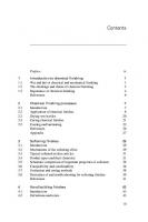
defined by transitions between air, fluid and solid tissues, the study of which is not the purpose of this book). The human eye is roughly spherical in shape (Fig. 1.1), and is made up of three distinct layers of tissue: sclerotic coat, choroid coat and retina. The sclerotic coat is the outer layer. It is white and extremely tough, except in the front where it forms the transparent cornea which contributes to the image-forming process by refracting light entering the eye. The surface of the cornea is kept moist and dustfree by the secretion from the tear glands. The intermediate layer is the choroid coat. This layer is deeply pigmented with melanin that reduces reflection of stray light within the eye. The choroid coat forms the iris, a diaphragm of variable size whose function is to adjust the size of the pupil to regulate the amount of light admitted into the eye. The pupil contraction is under the control of the autonomic nervous system: in dim light, the pupil opens wider letting more light into the eye; in bright light the pupil closes down. The retina is the inner layer of the eye. It contains the light receptors, the rods and cones. Inside the eye, the cavity between the lens and cornea – called the anterior chamber – is filled with a gel-like fluid called aqueous. The lens is located just behind the iris. The lens is a flexible unit that consists of layers of tissue enclosed in a tough capsule. It is suspended from the ciliary muscles by the zonule fibres. Behind the lens is the vitreous: a thick, transparent substance that fills the back of the eye. It is composed mainly of water and comprises about two-thirds of the eye’s volume, giving it form and shape. The next element is the retina, a neurosensory layer that initiates the neural processes of vision. An inverted image of the outside world is projected onto the retina, and the visual system then has the complex task of rebuilding a three-dimensional image
Sclera
Choroid Retina
Cornea Fovea Pupil
Lens Optic nerve
Iris Ciliary body 1.1 Human eye structure.
© Woodhead Publishing Limited, 2010
Colour vision: theories and principles
5
from this two-dimensional projection. The end result of this process is visual perception. The retina is in fact a prolongation of the brain. Anatomically, it is structured in ten layers for different types of neurones: photoreceptors (cones and rods), which are in fact modified neurones, and horizontal, bipolar, amacrine and ganglion cells. However, the photoreceptor’s mosaic is not evenly distributed along the retina. In physiological terms, it has a central zone and an outer area. The central zone includes the fovea, a small pit that ensures best visual acuity. The fovea is located in an area known as the macula lutea (Latin for yellow spot), which takes its name from the yellow pigment that covers it. The central retina includes another region, the optic disc, at the exit of the optic nerve, formed by the ganglion cell axons leaving the eyeball to form the optic nerve. This elongated pink disc is located in the nasal area and usually measures around 1.5 mm2. It has no photoreceptors, and as a result forms a blind spot in our vision, where we cannot see (since there are no cells to detect light, this part of the field of vision is not perceived). The rest, named the peripheral retina, has a low concentration of photoreceptors. The retina is inverted, in such a way that light passes through its entire structure before hitting the photosensitive layer. A photoreceptor is a specialist neurone capable of performing phototransduction, by which light is converted into electrical signals, which are then transmitted from neurone to neurone. Cones and rods are anatomically and physiologically different. Cones are much more abundant in the central retina, so the fovea contains only cones and, more importantly, the cones connect with the bipolar and ganglion cells at a proportion of 1:1:1, whereas in the peripheral retina area, several hundred or thousands of cones converge to a single bipolar cell. This explains why visual acuity is so much sharper in the fovea than at any other point on the retina. In terms of light sensitivity, rods can function in low light, whereas cones need much higher levels of light. So, rods are responsible for night vision, and cones are used for daytime vision, seeing colours and visual acuity. When light hits a photoreceptor, it sends a proportional synaptic response to a bipolar cell, which in turn sends the signal to a ganglion cell. Furthermore, there are two substrata at a synaptic level, with horizontal cells and amacrine cells (see Plate I in colour section between pages 42 and 43). These modify the initial signal to an extent that, after two or three synapses, the signal contains much more complex information than a simple point-to-point visual representation. From the ganglion cells, the signal reaches the appropriate left and right lateral geniculate nuclei (LGNs). The function of the LGNs is complex. We know that there is a three-system separation of fibres (PC cells, MC cells and KC cells), relating to Magno, Parvo and Konio systems. The LGNs have six layers, numbered from 1 (innermost layer) to 6 (outermost layer). Layers 1 and 2 contain the largest cell bodies and constitute the magnocellular system, whereas layers 3, 4, 5 and 6, which have smaller neurones, are part of the parvocellular system. Layers 2, 3
© Woodhead Publishing Limited, 2010
1 2 3 4 5 6 7 8 9 10 1 2 3 4 5 6 7 8 9 20 1 2 3 4 5 6 7 8 9 30 1 2 3 4 5 6 7 8 9 40 1 2 43X
6 1 2 3 4 5 6 7 8 9 10 1 2 3 4 5 6 7 8 9 20 1 2 3 4 5 6 7 8 9 30 1 2 3 4 5 6 7 8 9 40 1 2 43X
Colour measurement
and 5 receive fibres from the homolateral eye, and layers 1, 4 and 6 from the contralateral eye. Between each layer are the KC cells, which belong to the koniocellular system. Eighty per cent of the cells form part of the parvo system, ten per cent belong to the magno system, and ten per cent to the konio system. The LGN signals are sent to the primary visual cortex (V1), located at the back of the brain. The V1 fibres are then projected to area V2, and from V2 to V3, V4 and V5. Another important fact is that more than half of the LGN and V1 neurones process information from the fovea. A process therefore exists that gives priority to the part of the scene that is projected onto the fovea (the fixation point).
1.2
Human colour vision
1.2.1 Chromatic stimulus and perceived colour When we observe a scene, our visual system creates a perception of the outside world from the radiating energy that reaches our eyes from the objects within that scene. One of the elements of that perception is colour. But where is the colour? Is it external, or is it inside our visual system? The answer is clear: there are different chromatic stimuli in any scene that we view, and our visual system is able to capture that information, relating to the wavelength of light, which is how colour ‘emerges’. Colour, therefore, is something internal. Colour is perception. The chromatic stimulus is electromagnetic radiation from sources and objects that hits the optic system and triggers the visual process. Perceived colour, therefore, is a sensation produced by the chromatic stimulus that makes it possible to differentiate that stimulus from others with the same area, duration, shape and texture. As we shall see, chromatic stimuli have three variables, which are directly related to three perceptual variables.
1.2.2 Models of chromatic vision The trichromatic theory (Young–Helmholtz–Maxwell) In the early nineteenth century, Thomas Young (1801) suggested that the retina contained three types of nerve fibres that can be stimulated to a greater or lesser extent by the different wavelengths that correspond to red, green and violet colours. Several years later, James C. Maxwell would demonstrate that any colour in the spectrum could be matched with three monochromatic primary colours: red, green and blue. These two ideas were concurrent, and gave a clear, simple explanation of colour vision. Thus, a colour that stimulates the red and green particles in equal measure will be perceived as yellow; if it stimulates green and violet, we see blue. Chromatic vision is simply a matter of additive mixing. At around the same time, the German physicist Hermann V. Helmholtz also suggested that subjects with deficient colour vision (dichromats) had reduced
© Woodhead Publishing Limited, 2010
Colour vision: theories and principles
7
forms of normal vision, which lacked one of the three receptor types. This explains the fact that dichromats accept as equal the same kind of matchings as do subjects with normal vision. However, there were weak points in the theory in terms of colour appearance: if everything can be explained through mixes of colours, why are there no reddish greens or bluish yellow colours? Theory of chromatic opponency Ewald Hering (1872–4) was more concerned with the appearance of colours. In his reports to the Imperial Academy of Sciences in Vienna, Hering proposed the existence of three opponent processes generated at some point in the visual process: red-green, blue-yellow and black-white mechanisms. The idea of opponency is that the red-green categories (and, similarly, the blueyellow and light-shadow categories) are opposed and represent two extremes of variations in a continuum. More red necessarily implies less green. Despite having no experimental proof, Hering challenged both the established trichromatic theory and the prevailing physiological theory (Müller’s doctrine of specific nerve energies) head-on: ‘a nerve fibre is capable of conducting only one type of qualitative information’. A nerve fibre, therefore, could not transmit both red and green information, as they are qualitatively different. These two theories, which in principle seemed to take opposing views, are in fact compatible; the three retina cone types would in fact correspond to trichromacy, and the sensor responses by these cones would then be combined in the three red-green, blue-yellow and light-shadow mechanisms (although, as we shall see, dark-light is an additive rather than an opposing mechanism). It was not until 1957, a hundred years later, that D. Jameson and L. M. Hurvich would prove the existence of the opposing mechanisms. Paradoxically, Hering himself had suggested that these two theories did not have to be necessarily incompatible. Today we know that the parvo cells are responsible for the red-green mechanisms (L – M cells and M – L cells), and the konio cells are responsible for the blueyellow mechanisms S – (L + M) cells. Magno cells, on the other hand, are not opposing cells, but rather add the inputs from the L, M and S cells. Therefore it is an additive mechanism. ATD models (two-stage models) Each of these previous theories can explain a series of phenomena: the trichromatic theory reproduces many psychophysical experiments, but it does not predict appearance, which the colour opponency theory does. Combining the two theories leads to models that combine an initial trichromatic stage at the receptor level (first stage), with a stage of neural processing ruled by colour opponency mechanisms (second stage), comprising a non-opposing luminance
© Woodhead Publishing Limited, 2010
1 2 3 4 5 6 7 8 9 10 1 2 3 4 5 6 7 8 9 20 1 2 3 4 5 6 7 8 9 30 1 2 3 4 5 6 7 8 9 40 1 2 43X
8 1 2 3 4 5 6 7 8 9 10 1 2 3 4 5 6 7 8 9 20 1 2 3 4 5 6 7 8 9 30 1 2 3 4 5 6 7 8 9 40 1 2 43X
Colour measurement
mechanism (A) and the two opposing chromatic mechanisms: green-red (T) and blue-yellow (D). To a certain extent, the CIELAB values, which are very useful for industrial colorimetry, represent these concepts as Lightness (L) and can be linked to the achromatic channel (A); the chromatic coordinate a* to the greenness-redness channel (T) and the chromatic coordinate b* to the yellownessblueness channel (D). The model as a whole is summed up in an ATD matrix resulting from the combination of the L, M and S cone signals, as shown in equation 1.1. The three independent channels are listed as A (achromatic), T (tritan) and D (deutan): A T
=
D
a11
a12
a13
L
a21
a22
a23 *
M
a31
a32
a33
S
[1.1]
The Boynton model (1986) is a good representation of these two-stage models. It proposes three cone types, the spectral response curves of which are the Smith and Pokorny fundamentals. The coefficients for the resulting matrix are shown in equation 1.2, and the general functioning for this model is summarised in colour Plate II. The illustration also shows how the S cones contribute to the achromatic channel, though this value is very low and in the matrix is worth zero. A T D
=
0
L
1
1
1
−2 0 *
M
1
1
−1
S
[1.2]
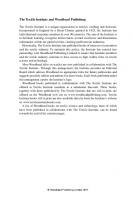
Why does the matrix have these coefficients? If we look at the single 575 nm yellow in the Smith and Pokorny fundamentals (Fig. 1.2), (L – M) would be a positive value, i.e. red would predominate over green, and we would see a reddish orange colour. However, the M cones’ response becomes balanced by applying a factor of two, so that in 575 nm they are cancelled out (T = 0) and a pure yellow colour is perceived. The red-green channel gives no signal (T = 0), and the blueyellow channel gives a response tending towards yellow. Another justification for this factor of two is in the proportion of cones in the retina: L:M = 10:5. According to this model, there is also a small intrusion of the S cones in the RG channel, though generally it is not taken into consideration. The oponnent process yellow-blue receives an amplified signal with a negative sign from relatively small values of the S cone, and a positive signal from the L and M cones: (L + M) – S. If S > L + M, the channel’s response is negative and is interpreted in upper states of the visual process as blue. But if S < L + M, the channel’s response is positive and the colour is interpreted as yellow. For lengths above 520 nm, the S cones give no signal; the channel signal will always be positive and interpreted as yellow. Finally, we can state that the L + M signal is transmitted by different nerve fibres to those that transmit the L – 2M signal.
© Woodhead Publishing Limited, 2010
Colour vision: theories and principles
9
40 S cones M cones L cones
30
Log sensitivity
20 10 0 –10 –20 –30 –40 350
400
450
500
550
600
650
700
750
Wavelength (nm)
1.2 Smith and Pokorny fundamentals.
Almost all chromatic vision models largely coincide in this general structure that we have just seen for the Boynton model: there are two opposing channels (channels T and D), and one additive channel (no opponent) for luminance (channel A). The differences are in the matrix coefficients. However, there are certain points that have not been fully clarified: Channel T: There is L – M opponency, but there are doubts over contribution from the S cones. If there is a contribution, it would be of the (L + S) – M type. Channel D: There is L – S opponency, but there are doubts over contribution from the M cones to this channel. Channel D: The achromatic channel is L + M, but there are doubts over contribution from the S cones to this channel. If there is a contribution, it would be of the L + M + S additive type. Nevertheless, most of the experimental results point to such a contribution not existing. Other more complex models, also exist, such as the De Valois-De Valois (1993) model. This considers a second opposing stage of cones (ATDinterm) that generates three colour opponent signals (rather than two) at the LGN cell level, corresponding approximately to L – M, M – L and S – (L + M). A third perceptual (linear) opposing stage would then occur, generating one achromatic and two chromatic channels. Finally, there are other non-linear models that succeed in explaining effects resulting from adaptation to a light source, and the influence of the background and the environment surrounding the stimulus, etc. In this case, non-linearities need to
© Woodhead Publishing Limited, 2010
1 2 3 4 5 6 7 8 9 10 1 2 3 4 5 6 7 8 9 20 1 2 3 4 5 6 7 8 9 30 1 2 3 4 5 6 7 8 9 40 1 2 43X
10 1 2 3 4 5 6 7 8 9 10 1 2 3 4 5 6 7 8 9 20 1 2 3 4 5 6 7 8 9 30 1 2 3 4 5 6 7 8 9 40 1 2 43X
Colour measurement
be introduced into the ATD response calculation. The 1990 Guth model, and subsequent modifications up to 1995, are a good example of these models. The general outline for these models is as follows (equation 1.3): from LMS an initial non-linearity is introduced, obtaining LMSs that are adapted to those conditions. Following this, the ATD exchange matrix and a second non-linearity are applied to obtain the adapted ATDs. L M S
L NL
M S
A M adap
T D
A NL
T
[1.3]
D adap
xn— . The non-linearities are normally of the following type: a— + xn As always, the objective with this model is to explain chromatic vision by reproducing the behaviour of the physiological A, T and D mechanisms.
1.3
Chromatic perception
1.3.1 Chromatic discrimination Colour differences are of enormous importance in industry. Understanding the human visual system’s degree of tolerance to colour differences is fundamental in knowing the maximum tolerable error in formulating a paint or printing a fabric. The most important aspect is not in fact the differences of the various components of colour (hue, colourfulness and lightness), but rather the perceptive differences of colour as a whole. In 1934, Wright evaluated colour differences with constant illumination by means of a 2° bipartite field, with 100 td retinal illumination throughout the whole spectrum and for five directions of the chromaticity diagram. In this way, he determined intervals or segments with edges that represent a constant difference in chromaticity. As a result of this experiment, it was deduced that the CIE1931xy space had very little uniformity, as two very distant points in the area of greens differ in colour just as two very close points in the area of blues and purples do. In 1942, MacAdam took these studies further. Using a bipartite field, a fixed reference stimulus was placed in one of the two fields, and colour matching was carried out in the other; the test was for 2° and was surrounded by an adaptation field of white light of the same luminance (200 td). After 50 matchings, two symmetrical points were defined in the same direction. By repeating this same operation for various directions and joining the points (within the standard deviations), an ellipse was generated. MacAdam showed the results in the CIE1931xy space for 25 reference colours. The result of joining the experimental colour discrimination points is an ellipse. These ellipses are of different sizes, orientation and shape throughout the chromaticity diagram. The ellipses are smaller in the area of blues, of medium size
© Woodhead Publishing Limited, 2010
Colour vision: theories and principles
11
Table 1.1 Physical and perceptual colour descriptors for isolated and related colours Chromatic stimuli
Isolated colour
Related colour
Wavelength (nm) Luminance (cd/m2) Colorimetric purity
Hue Brightness Colourfulness
Hue Lightness Chroma
in the reds and larger in the greens. By considering the distance from the centre of the ellipse to the edge as the unit of colour difference, it can be confirmed that this distance is not the same from one ellipse to another; it can thus be deduced that the CIE1931xy space is not uniform. In a space of uniform representation, representing colour differences would obtain circumferences of equal radius, regardless of the centre colour chosen, rather than ellipses of different sizes and orientation. As a result of these works, attempts have been made to find a more uniform colour representation space. The most commonly used are CIELAB, CIELUV, Guth’s ATD and SVF, among others.
1.3.2 Appearance of colour: chromatic effects Colour is trivariant, which means that in an isolated colour stimulus, we can distinguish three separate qualities: hue, brightness and saturation. When one studies a related colour, i.e. one that forms part of a scene, the descriptors refer to the environment, and one thus speaks of hue, lightness and colourfulness. Similarly, any colour is defined by means of three physical variables that correspond to these three perceptive variables: wavelength to hue, luminance to brightness, and colorimetric purity to saturation (see Table 1.1). However, these relationships do not display absolute independence, but rather there is interference between parameters. A variation in a single parameter (L, Pc, λ) can affect not only the perceptual attribute to which it is associated, but the other two as well. On the other hand, environmental modifications also affect colour. These effects cannot be explained by a linear model, as occurs with characterisation by three-way stimulus values or by means of opponency. We thus know that there must be some subsequent process, and that it cannot be linear. Studies of these chromatic effects are many and varied, and are beyond the scope of this work; we can merely provide a brief explanation of some of the better known and more widely considered of these chromatic effects. •
Bezold-Brücke effect: ‘A variation in luminance can alter the tone, thus changing its colour appearance.’ Bezold and Brücke (1873 and 1878) discovered this effect independently, and both indicated that at high luminance levels, reds and yellowish greens tended towards yellow, whereas greenish blues and violets became blue. However, they also confirmed that there are
© Woodhead Publishing Limited, 2010
1 2 3 4 5 6 7 8 9 10 1 2 3 4 5 6 7 8 9 20 1 2 3 4 5 6 7 8 9 30 1 2 3 4 5 6 7 8 9 40 1 2 43X
12 1 2 3 4 5 6 7 8 9 10 1 2 3 4 5 6 7 8 9 20 1 2 3 4 5 6 7 8 9 30 1 2 3 4 5 6 7 8 9 40 1 2 43X
•
•
•
•
•
Colour measurement three hues that do not vary: yellow (571 nm), green (506 nm) and blue (474 nm). This effect shows that tone and luminosity attributes are not completely independent. Aubert-Abney effect: ‘By adding white to a purple or a monochromatic colour, not only is saturation reduced, but hue changes also occur.’ This effect can be seen in Munsell’s Atlas colour samples, with equal tone and different chroma in the xy diagram. Theoretically, they should be straight lines of constant λd, but instead a curve is obtained that becomes greater the nearer the samples are to the locus. Again, there are some exceptions to this behaviour: for 572 nm yellow and for a purple (0.240,0.035) (λc = 559 nm). Helmholtz-Kohlrausch effect: ‘In heterochromatic Matching and with identical luminance, Brightness varies with the chromaticity of the stimulus.’ With identical luminance levels, achromatic colours display lower luminosity than chromatic colours. And equally, the other way round, with identical luminosity levels, achromatic colours display greater luminance than chromatic colours. In any matching of a white with any colour, then (Lwhite / Lcolour) > 1 applies. This ratio nears 1 when the colour is more desaturated, and reaches values higher than 1.6 for monochromatic colours. Simultaneous contrast: An increase in the brightness of a stimulus with the simultaneous decrease of background luminance. A dark environment makes one grey seem lighter than another with a white environment. Crispening effect: An increase in the difference between two stimuli occurs if the background is similar to the stimuli; in this case the brightness differential threshold is lower. Apparent mix: When the spatial frequency of an object is high, a chromatic mix of background and stimulus is produced. This colour quality is applied in artistic painting, with its maximum expression in the pointillist movement. George Seurat used this technique; his brushstrokes are tiny points, with no merging between them on the canvas, yet when viewed from a certain distance they create the desired combinations on the retina. The same occurs with the pixels of a television screen.
1.4
Defective colour vision
1.4.1 Anomalies and deficiencies in colour vision Most people see colour in the same way, which we can call normal chromatic vision. However, other people’s sight behaves abnormally. In most of these cases, they are able to differentiate colours, but their chromatic vision is much poorer than that of someone with normal sight. There are many colours which for a normal observer are clearly different and which the person with chromatic deficiency views as the same. The reason can be explained with any ATD model, by considering the hypothesis that chromatic deficiency is due to the lack of one of the three cone
© Woodhead Publishing Limited, 2010
Colour vision: theories and principles
13
Table 1.2 Types of colour vision depending on the cones Type of cones
Type of chromatic vision
Normal vision
LMS
Normal
Defective vision Protanopia Deuteranopia Tritanopia Monochromatism Achromatism
–MS L–S LM– ––S –––
Defective (R/G confusion) Defective (R/G confusion) Defective (B/Y confusion) No chromatic vision No chromatic vision
Anomalous vision Protanomaly Deuteranomaly Tritanomaly
L’ M S L M’ S L M S’
Irregular (R/G confusion) Irregular (R/G confusion) Irregular (B/Y confusion)
types. This lack of a cone type means a failure in either the T or the D chromatic mechanisms. Consider the Boynton model. The chromatic channels are T = L – 2M and D = (L + M) – S. If one of the two terminals is cancelled out, the channel response will always be of the same sign. What happens if the L cone is missing? Channel D would function, but in an anomalous way (reduced to D = M – S), and its response would differ to that of the normal channel, but a positive or negative response would still be possible; however, channel T (T = – 2M) would always respond in the same direction. Clearly, chromatic vision would thus be greatly reduced. In the hypothetical case of two cone types being missing (L and M), neither chromatic channel could function, and the subject would have no chromatic vision of any kind. A person lacking one cone type is known as a dichromat. Given that there are three types (L, M and S), there can be three separate categories, known as protanopia (lacking L cones), deuteranopia (lacking M cones) and tritanopia (lacking S cones). Individuals with these deficiencies have sight that differs between the three types. Table 1.2 includes all types of reduced colour vision currently reported. As well as chromatic deficiencies, another anomaly type also exists: people who have all three cone types, one of which has a slightly displaced curve response for that pigment. In this case, the person will also suffer from poor colour discrimination. These cases are known as protanomalous, deuteranomalous and tritanomalous. In people with protanomaly, maximum pigment L absorption is not at 560 nm, but instead is displaced slightly to shorter wavelengths and is thus closer to the M pigment. If we analyse the response to a red 650 nm wavelength, for example, sensitivity for this colour is reduced when compared with someone with normal sight, and as a result, in a yellow match with a sum of red and green, people with protanomaly have to add more red than a normal observer.
© Woodhead Publishing Limited, 2010
1 2 3 4 5 6 7 8 9 10 1 2 3 4 5 6 7 8 9 20 1 2 3 4 5 6 7 8 9 30 1 2 3 4 5 6 7 8 9 40 1 2 43X
14 1 2 3 4 5 6 7 8 9 10 1 2 3 4 5 6 7 8 9 20 1 2 3 4 5 6 7 8 9 30 1 2 3 4 5 6 7 8 9 40 1 2 43X
Colour measurement
People with deuteranomaly suffer a similar problem, but in their case it is the M pigment that is abnormally displaced towards red. Maximum absorption is no longer 540 nm, but rather is displaced towards a high wavelength and is thus closer to the L pigment. This hypothesis of abnormal displacement in maximum pigment absorption has been confirmed in works by Piantanida, Sperlig and Rushton, who identified the existence of abnormal pigments in people with protanomaly and deuteranomaly. Tritanomaly has been observed in a very few cases, though the cause is always pathological due to lesions in the optic nerve or retina, rather than from an abnormal pigment. Despite the fact that the vast majority of chromatic vision abnormalities are due to the absence or alteration of a visual pigment, there are other (very few) cases that are the result of pathological disorders.
1.4.2 Confusion lines and colour discrimination tests Imagine two colours, blue and yellow, with the same L and M inputs (Fig. 1.3). If we place these samples, C1 and C2, in the same scene, a subject without S cones will not notice any chromatic difference between the two. As there is no contribution from the S cones, these two colours will show the same response for the T channel and the D channel, and as such the subject will not see any chromatic difference between them. In the CIE31xy chromaticity diagram, the colours that meet this condition are spread along a straight line (there is only one degree of variation). The colours that are indistinguishable to dichromats are located along lines that converge at a single point. This point of convergence is known as the confusion point, and is characteristic for each deficiency type (identifying the chromatic co-ordinates of the missing response mechanism, although in practice there would be an influence from absorption of the pre-receptor media). Figure 1.4 shows the
L1 L2 3 3 C1 = M1 = 6 C2 = M2 = 6 S1 S2 7 2 A1 1 1 0 3 T1 = 1 –2 0 * 6 D1 1 1 –1 0 A2 1 1 0 3 T2 = 1 –2 0 * 6 D2 1 1 –1 0 TRITANOPIC
=
A1 ≡ A2 T1 ≡ T2 D1 ≡ D2
1.3 Two different colours C1 and C2d will be similar for a tritanopic subject. T and D responses are equal.
© Woodhead Publishing Limited, 2010
Colour vision: theories and principles 520
0.8
15
530 540
510 0.7
550 560
0.6 570
500 0.5
580
y
590 0.4
0.3
600 610 620
490
0.2 480 0.1 470 460 0.0 0.0
0.1
0.2
0.3
0.4 x
0.5
0.6
0.7
1.4 Protanopic confusion lines.
confusion lines for deuteranopia. As can be seen, this anomaly confuses all monochromatic colours from 540 nm to 700 nm. In protanopia, the confusion point is at the co-ordinates (0.747, 0.253), in deuteranopia it is at (1.080, – 0.080), and in tritanopia it is at (0.171, 0.000). Of all these lines, there is always one that passes through the equienergetic white, and all these colours will be confused with white, including the corresponding cut-off point in the locus, which can be called the neutral point (494 nm for protanopia, 499 nm for deuteranopia and 570 nm for tritanopia). The neutral point is important because it characterises the type of deficiency, and this fact is used to design detection tests and to categorise chromatic anomalies and deficiencies (see colour Plate III).
1.5
Colour constancy
1.5.1 Mechanisms of adaption Adaptation is the process by which the visual system changes its sensitivity, depending on luminance level in the visual field, so as to adapt to existing
© Woodhead Publishing Limited, 2010
1 2 3 4 5 6 7 8 9 10 1 2 3 4 5 6 7 8 9 20 1 2 3 4 5 6 7 8 9 30 1 2 3 4 5 6 7 8 9 40 1 2 43X
16
Low luminance response High luminance response 1,2 1,0 0,8 Sensitivity
1 2 3 4 5 6 7 8 9 10 1 2 3 4 5 6 7 8 9 20 1 2 3 4 5 6 7 8 9 30 1 2 3 4 5 6 7 8 9 40 1 2 43X
Colour measurement
0,6 0,4 0,2 0,0
400
450
500
550 600 Wavelength
650
700
1.5 Von Kries law: each photoreceptor can change its own sensitivity.
light levels. The process can be explained (at least in part) because each photoreceptor on the retina can change its own sensitivity curve depending on the amount of light it receives. It is a slow process that can take several minutes (Fig. 1.5). The visual system uses various mechanisms to adapt to high and low light levels. The iris contracts very quickly, followed by a much slower reaction from the retina’s photoreceptors as they adapt their sensitivity. The change in response from the photoreceptors is a very effective method of adaptation, whereas the contraction of the pupil is thought to be more of an initial defence mechanism to protect the retina against sudden changes in light.
1.5.2 Chromatic adaptation and gain control mechanisms The human visual system is able to adapt in such a way that the colour of an object remains unchanged, despite any changes in the light. Thus, chromatic adaptation is defined as the ability of the visual system to deduct the light spectrum so as to preserve the chromatic appearance of that object. A sheet of paper seen with daylight or under a light bulb will always seem white, even though sunlight is much more blue than the light from a tungsten bulb, and if we measure the colour of that piece of paper with a photometer in both situations, the results are very different. All colour adaptation models are based on the Von Kries coefficient law: ‘The individual components present in the eye are completely independent of one another and each is adapted exclusively according to its own function.’ According to modern interpretation, the Von Kries law means that each
© Woodhead Publishing Limited, 2010
Colour vision: theories and principles
17
photoreceptor has its own gain control mechanism, so that sensibility is adapted according to equation 1.3. La = KL * L Ma = KM * M
[1.3]
Sa = KS * S La, Ma and Sa are the post-adaptation cone signals, L, M and S are the initial cone signals, and Kn is the gain control mechanisms. Gain control mechanisms can be explained by changes in photoreceptor responses. A high luminance level will split a large number of the cones’ pigment molecules, and as such the number of molecules available to produce a visual response is much lower. This explanation of the gain control mechanisms only refers to cones and rods, and an explanation of chromatic adaptation in its entirety involves understanding other subsequent mechanisms of adaptation – probably neural gain control mechanisms at a horizontal, bipolar and ganglion cell level.
1.5.3 Illuminant discount As we have seen in the previous section, chromatic adaptation is a change in the sensitivity of the chromatic mechanisms, which makes it possible for the colour appearance to remain unchanged. Colour constancy can be seen as an extreme case of chromatic adaptation that associates a colour to an object regardless of the light in which the object is seen. Thus, many well-known objects (our car or our coat, for example) seem to be always the same colour, whether we see them in daylight or under fluorescent lighting. In colorimetric terms, the colours will be different, but the visual system interprets them as being the same. However, failures in this colour constancy also occur. These failures are explained by a marked colour variation in lighting that the visual system is unable to adapt to, or because the system produces an inappropriate adaptation response.
1.6
Bibliography
Chalupa, L.M. & Werner, J., The Visual Neurosciences, Cambridge: The MIT Press, 2003. Fairchild, M.D., Colour Appearance Models, Chichester, West Sussex (UK): John Wiley & Sons, 2000. Foster, D.H., ‘Inherited and acquired colour vision deficiencies: fundamental aspects and clinical studies’. In Vision and Visual Dysfunctions, Vol. VII, Ed. J.R. Cronly-Dillon London: Macmillan Press Ltd., 1991. Gegenfurtner, K.R. & Sharpe, L.T., Colour Vision. From Genes to Perception, Cambridge: Cambridge University Press, 1999. Kaiser, P.K. and Boynton, R.M., Human Color Vision, 2nd edition, Washington, DC: Optical Society of America, 1996.
© Woodhead Publishing Limited, 2010
1 2 3 4 5 6 7 8 9 10 1 2 3 4 5 6 7 8 9 20 1 2 3 4 5 6 7 8 9 30 1 2 3 4 5 6 7 8 9 40 1 2 43X
18 1 2 3 4 5 6 7 8 9 10 1 2 3 4 5 6 7 8 9 20 1 2 3 4 5 6 7 8 9 30 1 2 3 4 5 6 7 8 9 40 1 2 43X
Colour measurement
Marr, D., Vision, New York: W.H. Freeman and Company, 1982. Schwartz, S.H., Visual Perception: A Clinical Orientation, 3rd edition, New York: McGraw-Hill, 2004. Spillmann, L. & Werner, J.S., Visual Perception: The Neurophysiological Foundations, New York: Academic Press, 1990. Wandell, B.A., Foundations of Vision, Sunderland: Sinauer Associates, 1995.
© Woodhead Publishing Limited, 2010
Plate I Photograph of a section of vertebrate retina (cones, bipolar, ganglion and amacrine cells). Courtesy of Dr Nicolas Cuenca, Department of Physiology, Genetics and Microbiology, University of Alicante, Spain.
+
+
L
+
M
–
S
2
– +
L
M
S
Plate II Boynton’s model representation.
© Woodhead Publishing Limited, 2010
1 2 3 4 5 6 7 8 9 10 1 2 3 4 5 6 7 8 9 20 1 2 3 4 5 6 7 8 9 30 1 2 3 4 5 6 7 8 9 40 1 2 43X
Plate III Colour vision simulation for protanopic, deuteranopic and tritanopic subjects.
© Woodhead Publishing Limited, 2010
2 Scales for communicating colours A. K . R OY C HO UD HU RY, Government College of Engineering and Textile Technology, Serampore, India
Abstract: In colorant production and application industries, colour order systems or colour notations are required for effective communication, comparison, recording and formulation of colours. This chapter discusses merits-demerits and accuracy of various important colour order systems, namely Munsell, Natural colour system, Ostwald, DIN, OSA-UCS, Coloroid, etc. in the material form as well as digitised form. The comparison and interrelations between various systems are also discussed. Key words: colour order systems, colour notation, colour atlas, colour naming, Munsell system.
2.1
Introduction
While communicating or talking about colour, a language which is understandable by all parties must be followed. A logical scheme for ordering and specifying colours on the basis of some clearly defined attributes is known as the ‘colour notation system’. The attributes are generally three in number, as our vision is trichromatic, and they constitute the coordinates of the resultant ‘colour space’. Colour notation systems also encompass ‘colour order systems’ which typically comprise material standards in the form of a colour atlas. Due to constraints of the colorant gamut, the atlases may depict only a physically realisable subset of a colour order system. Colour notations can be classified into three categories (Rhodes, 2002): 1 Device dependent systems – the most common imaging devices used for reproducing colour are the computer-controlled CRT displays and the colour printers. The associated colour order system and colour spaces are hardwareoriented and they lack perceptually based attributes. 2 Mathematical systems – uniform colour spaces based on mathematical transformation of CIE tristimulus values such as CIELUV and CIELAB belong to this category. 3 Systems based on database of aim points – colour order systems existing principally in physical form, the colour samples of which can be measured to establish a database of aim points. Using interpolation techniques among limited available samples, many more colours can be defined. Humans with normal colour vision can distinguish among some two million colours when viewed against a mid-grey background and perhaps double this 19 © Woodhead Publishing Limited, 2010
1 2 3 4 5 6 7 8 9 10 1 2 3 4 5 6 7 8 9 20 1 2 3 4 5 6 7 8 9 30 1 2 3 4 5 6 7 8 9 40 1 2 43X
20 1 2 3 4 5 6 7 8 9 10 1 2 3 4 5 6 7 8 9 20 1 2 3 4 5 6 7 8 9 30 1 2 3 4 5 6 7 8 9 40 1 2 43X
Colour measurement
when the background is widely varied (Kuehni, 2005). The orderly and meaningful arrangement has been a matter of concern for the last 2000 years as a colour system which will manage to meet all requirements needs to be based on many years of physical and psychological research and experience. Until the seventeenth century, the prevailing opinion of the great Greek philosopher, Aristotle was that colour is generated from the interaction of darkness and light and that there are seven simple colours out of which all others are obtained by mixture. These seven are white (pure white), yellow, red, purple, green, blue and black (pure darkness). The history of colour order shows that the relationships between colours are rather complex and took two millennia to unravel. Originally, colour order systems consisted of lists of colours, such as those by Aristotle or Alberti. It was only at the beginning of the seventeenth century that the first graphical representation of colour order appeared in the work of Forsius. A different style of graphical representation of colour order was developed by the Belgian Jesuit and scholar François d’Aguilon (1567–1617). In his graphic representation, d’Aguilon showed tonal mixtures of the three chromatic simple colours with white and black as well as intermediates between white and black (a grey scale), with arcs above the line of the simple colours. Below the line, he represented with other arcs the hue mixtures of the three chromatic simple colours (Kuehni, 2003). The modern concept of colour was founded in 1704 by Isaac Newton. Before this, all colour order systems were one dimensional or linear but Newton recognised three colour attributes and drew an incomplete (spectral colours only) chromatic diagram in the form of spectral colours on the circumference and white in the centre. The saturation lines were drawn as radial lines from the white centre to the spectral periphery. Newton was also an alchemist believing in universal harmony. In analogy to musical tones, he chose seven hues in the spectrum: red, orange, yellow, green, blue, indigo and violet (ROYGBIV). However, the choice of seven is always controversial – repeated tests have shown about 120 discernible colours in the spectrum (Kuehni, 2005). LeBlon (1756) was first to make a clear distinction between mixing pigment colours and mixing colours of light. He stated that all visible objects can be represented by three colours, yellow, red and blue, and mixing these three colours makes black or all other colours. He named them as material colours or those used by painters. He further added that for a mixture of spectral colours those proposed by Sir Isaac Newton could not produce black, but the very contrary, white. Moreover, purple is perceivable in object colours only. The first proposal for a three-dimensional double tetrahedron system was made by the German mapmaker and astronomer Tobias Mayer in 1758. A French silk merchant, Gaspard Grégoire, first proposed a three-dimensional object colour order system based on the perceptual attributes hue, (relative) chroma and lightness and an atlas with 1350 samples was introduced before 1813 (Kuehni, 2008a). Matthias Klotz (1748–1821), a German painter, also proposed a three-dimensional
© Woodhead Publishing Limited, 2010
Scales for communicating colours
21
colour order system based on independent perceptual colour attributes. He proposed the cylindrical colour order system that consisted of a well-defined lightness scale (Kuehni, 2008b). About 100 years later Albert Munsell introduced a system based on intensive scientific studies very similar to the above systems. Four-dimensional Riemannian colour space was first proposed by Helmholtz with the help of a linear element which is difficult to define precisely and hence, the conceptualisation remained unclear. Recent studies (Leonev and Sokolov, 2008) showed that perceived colours can be represented on a spherical colour space of unit radius (hyper-sphere) in 4D Riemannian space. The model devotes a dimension to the stimulus parameter ‘darkness’ recognising the separate signals conveyed by light and dark neuronal channels. The advantage claimed is that the model defines mathematically the relation between the perception of large colour differences and the physical characteristics of luminous stimuli more consistently. However, a four-dimensional space is difficult to visualise. It is not very clear how colour names developed historically. One of the two prevailing opinions is that people of all societies became aware of different colours or colour categories and then named them in the same sequence: white and black, red, green, yellow, blue, brown, purple, pink, orange, grey (Berlin and Kay, 1969). Others think that all colour names are group cultural achievements and there is little common thread. Many colour words are related to materials, such as orange, ultramarine, olive, malachite green, bottle-green, peanut-green, sea-green, etc. These common names refer to the colour of various common objects which can be quickly recognised and memorised by most people. Some names reflect poetic invention, such as Cuban Sand, Ashes of Rose, Blue Fox and so on. But such colour names are very approximate, unreliable and temporary. Their meaning also changes with observer, time, place, style, technology, language, culture, etc. It is common practice to describe colour in terms of hues like red or yellow along with tone or secondary hue such as greenish or bluish and the amount of light reflected such as dark or pale. However when we describe a colour as ‘dark greenish blue’, the description is very inadequate as there may be many thousands of such colours. This problem was realised long ago. The accurate description of colour is essential for communication and for accurate reproduction of colour across a wide range of products. The colour of any object is commonly registered or recorded in two ways, namely: • •
preserving coloured physical samples recording in terms of common colour names.
Physical samples of dyed/printed fabrics, yarns or fibre paint panels, patches of printing inks, coloured papers, etc. are frequently used to express colours in the trade. Collections of such colour samples are very useful as examples of coloured product if the number of colours required is fairly limited. A good example of such collections is the dye-manufacturers’ ‘shade cards’. The shade cards carry
© Woodhead Publishing Limited, 2010
1 2 3 4 5 6 7 8 9 10 1 2 3 4 5 6 7 8 9 20 1 2 3 4 5 6 7 8 9 30 1 2 3 4 5 6 7 8 9 40 1 2 43X
22 1 2 3 4 5 6 7 8 9 10 1 2 3 4 5 6 7 8 9 20 1 2 3 4 5 6 7 8 9 30 1 2 3 4 5 6 7 8 9 40 1 2 43X
Colour measurement
numerous coloured objects on specific substrates (e.g. pieces of paper or various textile materials) along with procedures and names of the colorants to be used. The paint and printing ink manufacturers also publish shade cards for their products (colours) with names very specific to the concerned industry. However the exemplifications are very limited. They are restricted to the specific type of colorant or substrate and cannot be used for general reference. In the modern age, the celebrated German scientist A. G. Werner (1750–1817) was probably first to standardise colours by developing a method of describing minerals by their external characteristics like colours. In 1814 Werner’s system was bought in book form (entitled Werner’s Nomenclature of Colours, containing 110 samples of colours) by a flower painter of Edinburgh, Patrick Syme. In 1905 a French work, Répertoire de Couleurs, was published containing 365 plates consisting of 1 356 colours as in horticulture, traditional and textile use, described by colour names in various languages.
2.2
Systematic arrangements of colours
When we deal with a reasonable number of specimens, say a few thousand, to cover the whole range of possible colours (one million or more), the specimen must be selected according to a system or plan. The colour naming systems were popular for a long time, but they were not very systematic – hence the accuracy of specification was limited. It is absolutely necessary to arrange the colours in a systematic manner to tackle the enormous number of colours we can perceive. It is well known that the colours are three-dimensional. However, the dimensions of colour are expressed in various ways in different fields. For systematic arrangements, the dimensions should be independent of each other. The question is, therefore, which dimensions are to be chosen to arrange colours in a threedimensional space? The most natural and logical approach can be illustrated by Judd’s ‘desert island’ experiment (Billmeyer, 1981). A person sitting idly on a desert island may decide to arrange systematically the large number of pebbles surrounding him according to colour. First he sorts out coloured (i.e. chromatic) and colourless (i.e. achromatic) pebbles. Then he arranges colourless pebbles – black, dark grey, medium grey, light grey and white (Plate IV, step 1, in the colour section between pages 42 and 43). This classification is based on a property called ‘lightness’ or ‘value’. Then chromatic pebbles are classified according to their common colour names. All surface or object colours can be classified broadly into five principal colours namely red, yellow, green, blue and purple (Plate IV, step 2). While the former four can be seen as spectral colours, purple is perceivable in object colours only. If the variation of colour in the pebbles is great we may have reds admixed with yellow, yellow admixed with green and so on. The hues intermediate of the five principal hues can be named as red-yellow, yellow-green, green-blue, blue-purple
© Woodhead Publishing Limited, 2010
Scales for communicating colours
23
and purple-red (Plate IV, step 3). Now there can be red colours having varying degrees of yellowness, and each may be considered as a separate hue. Hence the above ten hues can be further classified into any number of intermediate hues. For assembling into a decimal system, each of the above ten hues may be classified into a further ten intermediate hues. Hence we can have 100 hues; the number is for convenience and can be changed into any other number. After classifying the coloured pebbles into separate hues, further classification may be done according to lightness or value. For example, pink, light bluish-red, medium bluish-red, dark bluish-red – all may be of the same hue, only varying in lightness (colour Plate IV, step 4). Lightness is actually a measure of the total amount of light reflected in the visible region of wavelength. After classifying the pebbles according to hue and lightness, all pebbles in a group may not be equally colourful – some are very vivid and colourful and the others are dirty and less colourful or pale. This is due to the varying degree of hue or colour content. Two objects of equal lightness means both reflect equal amounts of light. But a colour may be admixed with grey or black and a portion of the reflected light may be due to this grey component. This grey content, or conversely the colour content, is the third dimension of colour called ‘chroma’ or ‘saturation’. So the pebbles of equal hue and lightness can be further classified according to chroma or saturation (colour Plate IV, step 5). Clearly, chroma and saturation have different meanings; the former is the hue content in relation to the brightness of a reference white, while the later is the hue content in relation to its own brightness. Every colour sensation unites three distinct qualities and one quality can be varied without disturbing the other. A colour may be weakened or strengthened in chroma without changing its value or hue. Wright (1984) identified two sets of visual attributes, namely: Group A attributes are lightness, hue and chroma. Group B attributes are whiteness, blackness and chromaticness. According to Wright (1984) and Nayatani (1984), group B attributes are more useful because it is most easily understood and is more fundamental for observers to represent colour appearance. However they are less studied in psychometric (equal perception) terms. The colours of the outermost Munsell (group A) hue circle are close to full colours which is a term for group B attributes.
2.3
Colour order systems
A colour order system is a systematic and rational method of arranging all possible colours or subsets by means of material samples. Once the colours are arranged systematically they are named in some descriptive terms and/or are numbered (Graham, 1985). It is also desirable that the samples included in any colour order system are to be properly specified in terms of any standard colorimetric specification, the most common being the CIE colorimetric system.
© Woodhead Publishing Limited, 2010
1 2 3 4 5 6 7 8 9 10 1 2 3 4 5 6 7 8 9 20 1 2 3 4 5 6 7 8 9 30 1 2 3 4 5 6 7 8 9 40 1 2 43X
24 1 2 3 4 5 6 7 8 9 10 1 2 3 4 5 6 7 8 9 20 1 2 3 4 5 6 7 8 9 30 1 2 3 4 5 6 7 8 9 40 1 2 43X
Colour measurement
The colour order systems are constrained by the following facts (Fairchild, 2006): • • • •
Orderly (and continuous) arrangement of colours. A logical system of denotation. Perceptually meaningful dimensions. Embodied with stable, accurate and precise samples.
Colour specifiers or atlases are convenient physical forms of any colour order system. Colour order systems are three-dimensional, but atlases are twodimensional so that they can be presented in the form of a book or flat form (Lewis and Park, 1989). They have multiple functions such as: • • • • •
Stand-alone design tool for colour ideas. Quick communication of colour ideas over distance. The larger swatches provide master standards. Basis for specifying colours during colour formulations and colour ideas. Supporting role for instrumental response or visual perception of instrumentally measured colours.
An atlas should fulfil certain criteria such as: 1 2
3 4 5
The ideal design should be based on colours uniformly distributed throughout the colour solid. Selection of the substrate for an atlas is very important. Colours illustrated on cotton are readily matched on other substrates using the appropriate class of dyes (Park, 2008). To facilitate accurate assessments, however, some atlases have been prepared on multiple substrates. Moreover, different applications require different colour ranges. The full range of requirements for textiles, paint, plastics and ceramics are quite different. The ideal atlas should be highly stable and should have good fastness properties, particularly to light. It should be simple and easy to understand. The samples are to be reproducible and replacement pieces should be available. It should be cheap, portable and globally used.
However, no atlas is expected to represent visually millions of colours that can be detected by our eyes. There is no ideal colour order system and hence no ideal atlas.
2.3.1 The necessity of a colour order system It is a difficult task to deal with the millions of colours which our eyes can distinguish. We can feel the problem instantly if we try to describe a colour variation from memory or when we try to describe a colour to a man at a distance via communication channels (Roy Choudhury, 1996). The problem was known in
© Woodhead Publishing Limited, 2010
Scales for communicating colours
25
ancient times and several people have tried to solve it in their own way: Nobel laureate W. Ostwald, American artist A. H. Munsell and many others studied the problem in great detail. In colorant production and application industries, colours are to be communicated, compared, recorded and formulated on a regular basis. This necessitates the systematic classification of colours, which can be done in various ways. The classification may be based on visually or instrumentally assessed colour parameters as various colour order systems were developed originally on the basis of visual attributes, but later supported and modified by instrumental assessment. The main reasons for the widespread interest of colour order systems are for communication about colour over distance and time as well as for analysis and definition of the aesthetic relations among colours (Härd and Sivik, 1983–4).
2.3.2 Classification The colour order systems are of three types (Wyszecki, 1986): 1 2 3
Colorant-mixture system based on subtractive mixture of colorants. Colour-mixture system based on additive mixture of colour stimuli, for example the Ostwald system. Colour appearance system based on the principles of colour perception or colour appearance.
However, Derefeldt (1991) suggests that colour appearance systems are the only systems which are appropriate for general use because these are defined by perceptual colour coordinates with uniform or equal visual spacing of colours. Colorant-mixture systems These systems display the range of colours which can be achieved with declared quantities of colorants. The desired colours are developed by compounding a limited number of pigments or dyes in systematically varied proportions. The main purpose of these systems is to illustrate the range and other properties of a set of colorants. The principle of colorant mixing is subtractive and the colour gamut is restricted by the choice of primary colorants. This is helpful in the reproduction of shades for a particular coloration industry. However the method of application should be identical to that of the atlas. The dyes obtained from different manufacturers vary in colour considerably, but for the paint and printing ink industry the problem is less severe and the manufacturers’ recommended mixed shades are fairly reproducible. Examples of colorant-mixture systems are the colour atlases developed by different dye manufacturers. The ICI Colour Atlas (1969) was a collection of 1 379 original colours and 27,580 variations printed on papers. Similarly other
© Woodhead Publishing Limited, 2010
1 2 3 4 5 6 7 8 9 10 1 2 3 4 5 6 7 8 9 20 1 2 3 4 5 6 7 8 9 30 1 2 3 4 5 6 7 8 9 40 1 2 43X
26 1 2 3 4 5 6 7 8 9 10 1 2 3 4 5 6 7 8 9 20 1 2 3 4 5 6 7 8 9 30 1 2 3 4 5 6 7 8 9 40 1 2 43X
Colour measurement
atlases were also developed by different dye-makers such as the ‘Tootal Atlas’ (2 200 fabrics, 1970), ‘Hoechst Atlas’, ‘Ciba-Geigy Colour Atlas’ (625 fabrics, 1982) and the ‘BASF Colourthek III’ (2 580 fabrics, 1970). Examples also include ‘Piochere Colour System’ and ‘Martin-Senour Nu-Hue System’ (Wyszecki and Stiles, 1982). The Pantone colour system is basically a colour mixture system. The Pantone system (www.pantone.co.uk) began life in 1963 in the USA for defining colours for printers, but expanded into other fields later, e.g. textiles in 1984, plastics in 1993, and architecture and interiors (1 925 colours) in 2002, each of which has a six digit numerical notation (e.g. # 19-1764) and an ‘inspirational’ colour name. This is widely used in graphic art and also in the textile industry mainly because of its low cost, though the colours are not equally spaced and the shades are prepared on paper using printing inks. It is not a colour order system since it does not include a continuous scale. It is more appropriately considered a colour naming system. The Pantone system is loosely based on a three-dimensional scale using a six digit reference number, two each of which indicate colour strength, hue and tone successively, but CIE specifications are not available. Recently, a textile version of the Pantone atlas (having 1 001 reactive dyed cotton fabrics) has been introduced in the market. Colour-mixture systems The basic idea of a colour-mixture system is to show, in the form of material standards, the sequence of colours related either to manipulation of the controls of a tristimulus colorimeter or to variation in simple ways of the proportions of sector areas on a Maxwell disk. So the basic principle of generating colour is additive colour mixing. The tristimulus colorimeter aims to tie in colours with the CIE system of colorimetry, or more specifically with the chromaticity diagram. However, long before the development of the CIE system of colorimetry, the Maxwell disk was used to develop colours of constant dominant wavelength by varying the proportion of the chromatic sector and the achromatic sector (white, grey or black) on the disk. Judd and Wyszecki (1963) preferred an additive colourmixture based colour order system due to its resemblance to our everyday experience of colour perception. The most popular in this category is the Ostwald colour system. A few other examples of colour-mixture systems are as follows. The Colour Standards and Colour Nomenclature atlas of Robert Ridways, a bird curator in the United States National Museum, was published in 1912 containing 1 113 named coloured samples. Each sample is 1" by ½" rectangular matte printed paper. In a page, the lightest sample is at the top followed by seven steps of increasing grey content. Each column represents constant dominant wavelength obtained by rotary mixing of white, black and a chromatic pigment. The system represents 35 dominant wavelengths maintaining approximately uniform hue-spacing. The representation of near-whites is poor, but of near-greys
© Woodhead Publishing Limited, 2010
Scales for communicating colours
27
is excellent. The system was popular among naturalists for colour specification of plants, flowers, birds, insects, rocks etc. The Colour Harmony Manual is one of the most important colour-mixture systems, published by the Container Corporation of America during 1942–72 (Jacobson, 1972). It consists of a set of 12 hand-books, each showing a pair of complementary hues. Each colour chip is specified by the Ostwald method on a 24-step hue scale, i.e. 12 pairs of complementary hues of constant dominant wavelength. The number 24 was chosen because it is divisible into equal intervals of 2, 3, 4, 6, 8 and 12 for selecting multi-hue harmonies. Each hue-chart shows samples having varying black, white and full-colour content represented by double-letter names such as na, ga, ca, etc. The vertical series in the triangle were called ‘shadow series’ because they have the same dominant wavelength and chromaticity and differ only in reflectance. The first and fourth (last) editions of the manual contain 680 and 949 chips respectively. Light colours and near-whites were not included in the manual and the system cannot readily translate the attributes into useful textile terms. The publication of the manual was discontinued after 1972 mainly due to poor standard of reproduction (Greenville, 1994). The Dictionary of Colour, published in book form by Mearz and Paul (1950), shows a collection of over seven thousand colours (precisely 7 056 numbers) classified into seven hue groups. Considerable effort has been made to describe the colours by commonly used colour names. The names are displayed on the left-hand pages, while the corresponding colours are shown opposite. The names have been gathered from the sources mentioned above and other reliable and established sources and no name has been originated by the authors of the book. The various adjectives (e.g., light, pale, etc.), trade or commercial names have been excluded and emphasis has been solely based on the names’ colour perception. The above system is an intermediate between subtractive colorant-mixture and additive colour-mixture systems. The colours are created by variable-density overprints of inks of different colours. Wherever there is overprint, there is subtraction, while in remaining areas the colours are additively mixed. The system shows a collection of over seven thousand colours printed in the form of a book, but colour variations from copy to copy are reported as these are printed on paper. Near-blacks and light-saturated colours are not included, while the colours used are remarkably permanent. The order of seven hues in The Dictionary of Colour follows the spectrum – red to orange, orange to yellow, yellow to green, green to blue-green, blue-green to blue, blue to red, and purple to red. The plates are divided into twelve rows (A to L) and twelve columns (1 to 12). The rows start with ‘no hue’ at one end and ‘full hue’ at the other end. The columns represent hues as a mixture of two hues in varying quantities. Each of the seven hues is presented in eight successive plates with an increasing grey content. The perfect scale of reduction should be the geometric series, based on the Weber-Fechner law, having a percentage of reflection in the order of 0, 12, 22, 32, 42, 52, 62, 72, 82, 92, 102. However, some of
© Woodhead Publishing Limited, 2010
1 2 3 4 5 6 7 8 9 10 1 2 3 4 5 6 7 8 9 20 1 2 3 4 5 6 7 8 9 30 1 2 3 4 5 6 7 8 9 40 1 2 43X
28 1 2 3 4 5 6 7 8 9 10 1 2 3 4 5 6 7 8 9 20 1 2 3 4 5 6 7 8 9 30 1 2 3 4 5 6 7 8 9 40 1 2 43X
Colour measurement
the steps like 0 or 100% are impractical and, moreover, smaller intervals were given for lighter colours so that they are in sufficient numbers. In this system, effort has been made to arrange colours in some definite order, however the spacing of the samples is somewhat arbitrary and not equally spaced. The system describes a very small portion of the colours visualised by us. Intermediate colours can be interpolated, but such interpolation cannot be communicated to others because the samples are not spaced equally as per the visual colour perception. Colour appearance systems These systems are based on the perception of colours by an observer with normal colour vision and the scales are chosen to represent attributes of perceived colours. However, attributes represented in various systems are different. The spacing of colours along the scales also varies from one system to another, even when the same attribute is used in both systems. Most of the earlier atlases were in favour of inclusion of colours of long traditional usage, thereby emphasising tighter spacing of colours in some hue regions. Such systems sample the colour solid non-uniformly. In other words, there is no uniform placement of the colour samples throughout the total colour space. Some areas of colour space are over-emphasised, while some areas are poorly presented or not presented at all. A universal urge to arrange the colour chips on the basis of constant hue is strongly felt by the designer of colour order systems. However, the mixture of chromatic colour, black and white is only an approximation to constant hue. The main emphasis of appearance-based systems is the uniform visual spacing. The systems thus allow easy interpolation between the samples represented and extrapolation of colours not illustrated in a given collection. The collections of samples are generally represented in pages of constant hue. The most popular appearance-based colour order system is the Munsell system. Psychometric scales provide a way of assigning numbers to physical stimuli according to the psychological attributes that the stimuli evoke. The relationships between perceptual magnitudes and physical measures of stimulus intensity are assessed by scaling experiments. The types of scales may be as follows (Wyszecki and Stiles, 1982; Kuehni, 2003). ‘Nominal scales’ merely determine whether or not things are equal. The same name or symbol is assigned if they have the same value for the attributes. The colours, for example, can be grouped into yellows, reds, greens, blues, etc. ‘Ordinal scales’ assign numbers in such a way that the order of the numbers corresponds to the order of the magnitudes of the attribute being scaled. The stimulus with higher scale value will be perceived as having more of the attribute. An ordinal scale is subject to logical operations: equal to, greater/less than, etc. ‘Interval scales’ have all the properties of ordinal scales and, in addition, the differences (intervals) between the numbers characterise the sizes of the
© Woodhead Publishing Limited, 2010
Scales for communicating colours
29
corresponding perceived difference of the attribute (e.g. Celsius and Fahrenheit scales). Colour scales are usually interval scales. ‘Ratio scales’ are interval scales with a natural origin. Examples are length in metres, duration in seconds and temperature in degrees Kelvin. The zero point of the scale corresponds to a stimulus for which the attribute has zero magnitude. As a result, the numbers on the scale are proportional to the perceived magnitudes of the attribute being scaled. Many colour order systems consist of ratio scales. A variety of techniques have been devised for psychometric scaling (Wyszecki and Stiles, 1982; Fairchild, 2006) such as: • • • • • • •
Rank order Graphical rating Category scaling Paired comparisons Partition scaling Magnitude estimation Ratio estimation.
2.3.3 Merits–demerits The advantages of material-based colour order systems (Hunt, 1987) are listed below. 1
2 3 4
5
6
As represented by physical samples, the systems are realistic and easy to understand. It is easy for the eye to specify object colours by comparison with reference to physical samples, rather than by matching with colours in memory (Hunter and Harold, 1978: 300). The atlases are easy to use. In most cases, side-by-side comparisons are made under standard viewing conditions and, as such, no instrument is required. The systems based on perceptual scaling like Munsell and NCS can be used to evaluate mathematical colour appearance models. At present, most of the colour order systems are calibrated in terms of tristimulus values; hence reference can be made to the colour order systems for colour control or for colorant formulations by computer, even in the absence of reference samples. Visually uniform colour spaces, such as Munsell and OSA, can prove a useful way of organising the colours of a digitally controlled colour television monitor. Future uniform colour spaces will probably be defined with the aid of these monitors but with a higher flexibility and wider colour gamut than the complex pigment technology presently in use (Durrett, 1987). Colour order systems can be used as sources for test targets for imaging systems or other measurement devices. The Macbeth Colour Checker chart, commonly used as a test target for imaging systems, is partially based on the Munsell system.
© Woodhead Publishing Limited, 2010
1 2 3 4 5 6 7 8 9 10 1 2 3 4 5 6 7 8 9 20 1 2 3 4 5 6 7 8 9 30 1 2 3 4 5 6 7 8 9 40 1 2 43X
30 1 2 3 4 5 6 7 8 9 10 1 2 3 4 5 6 7 8 9 20 1 2 3 4 5 6 7 8 9 30 1 2 3 4 5 6 7 8 9 40 1 2 43X
Colour measurement
Some of their limitations are: • •
•
•
•
•
•
• • •
A number of colour order systems are used globally and they are not mutually convertible. The actual colour of the physical samples in the atlas may be quite different from the intended aim colour. The error may be of several CIELAB colour difference units and may differ from batch to batch, i.e. poor reproducibility. It is not possible to include all perceivable colours in any colour order system. The Chroma cosmos 5000 is the largest, with 5 000 uniquely dyed samples, whereas most of the atlases consist of around two thousand samples. Any colour atlas is a serious abridgement of the colour world as there are gaps between the available physical samples. Interpolation or extrapolation is, therefore, frequently necessary for colour specifications, the accuracy of which largely depends on the colour discrimination efficiency and experience of the observer. As colour order atlases are composed of a limited number of physical samples, future inclusion of newer samples may be a problem. Though most of the systems keep provision for addition of newer samples, it may occasionally be necessary to alter the spacing. The perceptual scales of colour appearance in a colour order system have been established for a specific viewing condition. No data have been provided with respect to change in viewing conditions and the visual spacing of the samples is valid only if standard illuminating and viewing conditions are maintained. The errors are not likely to be very high if typical indoor daylight is used, but viewing under other artificial lights may result in serious errors. The visual interpolation between atlas samples to determine the notation of colours not represented in the atlas is subjective and may differ between individuals. The phenomenon is known as ‘observer metamerism’ (Roy Choudhury and Chatterjee, 1992). As the system uses physical samples, there are chances of deterioration of the standards due to limited stability of the colorants, extensive use or long exposure to light. High chroma colours may require fluorescent dye or pigment, the use of which is restricted due to limited stability. The manufacturer takes proper care for good performance, but still after a certain interval of time, the genuineness of the sample may be questioned. Moreover the user will be completely unaware of such changes. Most of the colour order systems cannot be used for self-luminous colours such as light sources unless ancillary apparatus is used. Though colour order systems are used for a variety of applications in colour appearance, they are not a substitute for a colour appearance model. The relation between perceptual coordinates of the colour order systems and colorimetric coordinates are complex and cannot be expressed by accurate equations. Approximate transformation equations have been derived by statistic fitting and neural network modelling and look-up table interpolation techniques are used for transformation from the CIE colorimetry to colour order coordinates.
© Woodhead Publishing Limited, 2010
Scales for communicating colours
2.4
31
Various colour order systems
The idea of using a three-dimensional colour solid to represent all colours was developed during the eighteenth and nineteenth centuries. Several different shapes for such a solid were proposed, including a double triangular pyramid by Tobias Mayer in 1758, a single triangular pyramid by Johann Heinrich Lambert in 1772, a sphere by Philipp Otto Runge in 1810, a hemisphere by Michel Eugène Chevreul in 1839, a cone by Hermann von Helmholtz in 1860, a tilted cube by William Benson in 1868 and a slanted double cone by August Kirschmann in 1895 (Kuehni, 2002). These systems became progressively more sophisticated, with Kirschmann’s even recognising the difference between coloured lights and object colours. But all of them remained either purely theoretical or encountered practical problems in accommodating all colours. Furthermore, none was based on any rigorous scientific measurement of human vision; before Munsell, the relationship between hue, value and chroma was not understood. Munsell replaced all historical approaches with the proposal of a balanced colour sphere, later replaced by an irregular solid. Subsequently a large number of colour order systems have been developed in different parts of the globe at different times. However, there is no internationally agreed colour order system to date. Some systems are very popular, some are used occasionally while some are obsolete. Six popular colour order systems and their respective colour attributes are as follows: 1 2 3 4 5 6
Munsell – hue, value and chroma Natural colour system – hue, blackness and chromaticness Ostwald system – hue, lightness and saturation DIN system – hue, saturation degree and darkness degree OSA-UCS – no separate scaling of three attributes Coloroid system – hue, saturation and lightness.
In addition, there are a few less known and newly developed colour order systems such as: Swiss Colour Atlas 2541, Chevreul, Colourcurve, Eurocolour system, Acoat system, Pope colour system (Heila, 1988). A one-dimensional colour order system for dental shade guides has been proposed by O’Brien, Groh and Boenke (1989) by visual ranking of translucent porcelain bioform shade guide teeth of the American Dental Association.
2.4.1 Munsell colour order system Professor Munsell (1905), an artist, wanted to create a ‘rational way to describe colour’ that would use decimal notation instead of colour names (which he felt were ‘foolish’ and ‘misleading’) and so developed the oldest and by far the most popular colour order system to fill the gap between art and science. The Munsell atlas was released in 1915, commercialised in 1929 and the system has been extensively studied by Billmeyer (1987). The Association Internationale de la © Woodhead Publishing Limited, 2010
1 2 3 4 5 6 7 8 9 10 1 2 3 4 5 6 7 8 9 20 1 2 3 4 5 6 7 8 9 30 1 2 3 4 5 6 7 8 9 40 1 2 43X
32 1 2 3 4 5 6 7 8 9 10 1 2 3 4 5 6 7 8 9 20 1 2 3 4 5 6 7 8 9 30 1 2 3 4 5 6 7 8 9 40 1 2 43X
Colour measurement
Couleur (AIC) study group on colour order systems prepared a computer-based annotated bibliography containing about 400 entries out of which 115 references are on the Munsell system (Billmeyer, 1985). Prior to 1943, the Munsell system was defined by the physical samples composing the 1929 MBC colour chips and thus the basic specification of the Munsell system was the spectral reflectance function of each colour chip. The spacing of the chips was intensively studied by the Colorimetry Committee of the Optical Society of America and in 1943 the CIE tristimulus values of ideally spaced chips were published as the Munsell renotation system (Newhall et al., 1943). Obviously there are many important physical and psycho-physical differences between earlier reflectance based systems and the present tristimulus based systems (Berns and Billmeyer, 1985). The system (colour Plate V) consists of the following three independent dimensions which can be represented cylindrically in three dimensions as an irregular colour solid. 1 Hue (H), measured along circumference of the horizontal circles. 2 Chroma (C) or purity of colour, measured radially outward from the neutral (grey) vertical axis. 3 Value (V), measured vertically from 0 (black) to 10 (white). Munsell determined the spacing of colours along these dimensions by taking measurements of human visual responses. In each dimension, Munsell colours are as close to perceptually uniform as he could make them, which makes the resulting shape quite irregular. The perceptual uniformity of the system is only valid under illuminant C, a uniform middle grey (N5) background with a sufficiently high illumination level (greater than 500 lux). The Munsell system divides each horizontal hue circle into five unique or principal hues: Red (5R), Yellow (5Y), Green (5G), Blue (5B), and Purple (5P), along with five intermediate hues (5YR, 5GY, 5BG, 5PB, 5RP) halfway between adjacent principal hues. In the original Munsell book, each hue sector (H) is divided further into four finer categories, namely, 2.5H, 5H, 7.5H and 10H (0 for the next H). However, each of these ten steps may also be broken into further ten sub-steps, so that 100 hues are obtained with integer values (though Munsell originally sampled only 20 hues, later 40). The naming of these hues starts from the mid-point between major hues and numbered from 0 to 10, e.g. 5R, 6R-9R, 10R or 0YR, then 1YR, 2YR and so on. For the modern Munsell hue scale to be visually uniform, Kuehni (2005) observed that different numbers of Munsell hue steps are required between average unique hues namely: Unique hue sector → red to yellow yellow to green green to blue blue to red Munsell hue steps → 20 23 26 31 The open-ended chroma increases from 0 for a neutral colour to colours with stronger hue content. There is no maximum for the chroma. The highest chroma
© Woodhead Publishing Limited, 2010
Scales for communicating colours
33
depends on the hue and value of the samples and the colorant used to produce them. With the available colorants, chroma is generally restricted to a maximum of 16 or 18. A colour is fully specified by three numbers for hue, value and chroma, e.g. H V/C. The Munsell atlas is usually available on painted paper in glossy (1 488 chips) and matt forms (1 277 chips). As the Munsell system is based on polar coordinates, smaller perceptual differences occur in the near-neutral grey region of colour space than in the outermost saturated regions. Physical distance between neighbouring hue increases with increase in chroma, i.e. increase in distance from the neutral axis. In the Munsell system, therefore, the evaluation of near-neutral samples is problematic – hence the ‘Nearly Neutral Collection’ came onto the market in 1990. The atlas contains a range of light and near grey samples, an important colour region for various fields of design and architecture such as wall and house colour, colour of furniture and office equipment, building materials, cosmetics, etc. Each page contains a grey scale running in half steps of lightness from Munsell value 6/ to 9/ and Munsell chroma /0.5 to /4 for 20 hues, two for each of Munsell’s ten principal hues. However it is difficult to combine the two atlases during evaluation. Indow and Watanabe (1980) demonstrated that human observers can memorise the scheme of Munsell notation and, without comparing with the Munsell standard chips, they can specify colour samples in terms of (H V/C). It is not guaranteed that one step in ‘V’, one step in ‘C’ and one step in ‘H’ represent the same size of perceptual difference. The scaling perceptual differences δjk between two Munsell standard chips j and k have shown that chips are embeddable as a configuration of points (Pj) in a 3D space locally Euclidean metric. However, in order to accumulate through this approach a tremendous amount of experimentation is necessary to collect sufficient information necessary to provide the Munsell colour solid with a unified distance scale (Indow and Romney, 2008). The relations between Munsell and CIE variables are very complex. In the CIE chromaticity diagram, lines of constant Munsell hue are curved and the location changes with change of Munsell value. The Munsell value (V) scale is related to CIE luminance factor (Y) by a complex fifth degree polynomial equation called Judd’s polynomial as follows (Newhall, 1940): Y = 1.2219V – 0.23111V2 + 0.23951V3 – 0.021009V4 + 0.0008404V5
[2.1]
The equation was devised by Judd with measurements based on the use of magnesium oxide, and assigned a value of absolute reflectance of 1.026 for 45°/0° illumination and viewing. This can be inverted through iterative methods to obtain the approximation (Rhodes, 2002) as follows: V = 0.01612Y + 2.5649Y1/6 + 1.3455Y1/3 + 0.08797Y–1 – (2.685 × 10⁻⁷)Y3 – 3.116
© Woodhead Publishing Limited, 2010
[2.2]
1 2 3 4 5 6 7 8 9 10 1 2 3 4 5 6 7 8 9 20 1 2 3 4 5 6 7 8 9 30 1 2 3 4 5 6 7 8 9 40 1 2 43X
34 1 2 3 4 5 6 7 8 9 10 1 2 3 4 5 6 7 8 9 20 1 2 3 4 5 6 7 8 9 30 1 2 3 4 5 6 7 8 9 40 1 2 43X
Colour measurement
Land and Pinney (1955) proposed a simpler equation: V = 2.468Y1/3 – 1.636
[2.3]
However, no simple relation has been reported so far for Munsell hue or chroma with respective CIE parameters. The NBS computer program (Rheinboldt and Menard, 1960) utilises a look-up table followed by interpolation but a simple and faster program has been proposed by Simon and Frost (1987). Artificial intelligence computer programs such as ‘artificial neural network’ (ANN) has been utilised to convert Munsell coordinates into CIE coordinates. Neural network models to imitate some functions of the human brain are described by Tominaga (1993). If we set aside the small problem that a uniform colour space in three dimensions is impossible, then CIELAB does remarkably well. A standard basis for comparison is the distribution of Munsell target colours at Munsell values 4, 6 and 8, out to the limits of surface colour chroma. Ideally the diagram would look like radial spokes within concentric circles. However, Munsell hue loci showed (Hunt, 1978) to depart from straight radial lines having equal angular spacing and departures of the Munsell chroma loci from equally spaced concentric circles. The exaggerated spacing of Munsell chroma into the yellow and yellow-green hues, the displacement in the lines of constant hue as lightness increases (especially in the blue greens), the curving lines of constant violet and green hues and the wide gap in the hue spacing of green colours, are all primarily or partly due to irregularities in the CIELAB system although some are actually problems in the Munsell system. As a rule of thumb, ten units of CIELAB lightness exactly match one unit of Munsell value, and ten units of CIELAB chroma approximately match two units of Munsell chroma. It may be noted that all CIE systems reverse the ordering of Munsell hues. The clockwise movement along the Munsell hue circle results in the change of hue from red to yellow, while in CIELAB the same change requires anticlockwise movement. The chromaticities of the Munsell renotation data set were applied to eight colour-appearance models namely CIELAB, Hunt, Nayatani, RLAB, LLAB, CIECAM97s, ZLAB and IPT by Wyble and Fairchild (2000). In general, the models derived from the Munsell system performed well except for some deviations in hue spacing and linearity. Limitations of the Munsell system Munsell and his successors worked hard to produce colour samples that were ‘perceptually equidistant’ from neighbouring colours on the individual dimensions of value, chroma and hue. The relationship between Munsell step size and perceived colour is not constant across the three dimensions. The equality of visual spacing is such that one value step (on a scale of 10 between white and
© Woodhead Publishing Limited, 2010
Scales for communicating colours
35
black) is equal to two steps in chroma and 0.3 major hue step (3 step on a 100 step hue scale) at chroma 5 (Nickerson, 1936). In a series of articles, Indow and Aoki (1983) applied multidimensional scaling to the Munsell chips and pointed out a number of minor deviations from perfect equal spacing, both locally and globally. Despite these known minor deviations from the goal of local equality of visual spacing, the Munsell is often considered, because of extensive documentation (some 3,000,000 colour judgements by 40 observers), as the standard against which other colour order systems can be compared. Munsell realised that the natural colour space is highly irregular when it is represented without geometrical preconceptions. Thus, Munsell always conceived of his colour model as a sphere, but allowed for unequal dimensions of chroma at different levels of lightness and across different hues. The range of colours represented in a Munsell atlas is limited by the gamut of paints or inks used to create the colour samples. As a result, no simple geometrical form accurately represents perceptual colour space. All other colour models based on triangles, circles, squares, pyramids, cones, spheres, cubes or cylinders must (and do) grossly distort perceived colour relationships. The Munsell system has a few inherent problems. • • •
A variety of discrepancies were found in the perceptual spacing of colours, depending on their location in the colour space. The quantitative difference between colours could only be defined on a single colour attribute (lightness, chroma or hue) at a time. Complementary colours are not on opposite sides, so that one cannot predict the results of colour mixing very well.
As the intervals of hue, value and chroma are not perceptually equal, it is desirable to have diagonal dimensions added to the Cartesian space for assessment of perceived colour differences in all directions of the colour space using identical psychometric tasks. In plain language, it is impossible to represent uniform colour differences in a three-dimensional colour model. The human colour space is non-Euclidean.
SCOTDIC colour atlas SCOTDIC, a textile version of Munsell created by fusion of two quite different systems – Standard Colour of Textile (Japan) and Dictionnaire Internationale de la Couleur (France), is adopted by over 8 000 companies worldwide. Textile standard colours of the SCOTDIC colour system are widely used as colour tools by fashion colour professionals. The system has three versions – glossy (2 468 colours on polyester crepe fabric), matt (2 038 colours on cotton poplin fabric) and yarn (1 100 colours on wool yarns). It has incorporated many bright colours and the number on the constant hue chart has been increased to 54 (20 for wool).
© Woodhead Publishing Limited, 2010
1 2 3 4 5 6 7 8 9 10 1 2 3 4 5 6 7 8 9 20 1 2 3 4 5 6 7 8 9 30 1 2 3 4 5 6 7 8 9 40 1 2 43X
36 1 2 3 4 5 6 7 8 9 10 1 2 3 4 5 6 7 8 9 20 1 2 3 4 5 6 7 8 9 30 1 2 3 4 5 6 7 8 9 40 1 2 43X
Colour measurement
The SCOTDIC system uses a six digit code for each standard colour – the first two digits for hue, the second two digits for value and the third two digits for chroma. The prefix corresponds to the material of textile bases – P for polyester, C for cotton, W for wool. Therefore, the notation C-155010 means cotton standard sample having hue = 15, value = 50 and chroma = 10. In a recent study (Roy Choudhury, 2008) of locations of SCOTDIC cotton samples in CIELAB colour space, the following observations were made. •
•
•
For most of the Munsell hues, hue angles vary between 10° and 20°, but for a good number of Munsell hues, the hue angles vary within much broader ranges. For a few borderline Munsell hues, the hue angles vary from 0° to 360°. But if we consider that hues belonging to hue angles 0° and 360° are identical, the range of variation is quite narrow. Figure 2.1 shows constant SCOTDIC loci in CIELAB space at a constant value level of 60. As expected, constant SCOTDIC hue loci form radial lines emerging from origin and for many hues the lines are curved, especially at high chroma. The hues show unequal angular spacing and in many cases the spacing has changed at high chroma. The loci of constant chroma represent near-circles with diameter increasing with increase of chroma. Theoretically all constant chroma points should have been located at constant radial distance from the centre of an a*−b* 80 70 60 50 40 30 20 10 0 –60 –50 –40 –30 –20 –10 0 –10
10
20
30
40
–20 –30 –40
2.1 Constant SCOTDIC hue loci in CIELAB space.
© Woodhead Publishing Limited, 2010
50
60
1 3 11 14 15 17 19 25 35 37 41 43 49 55 69 73 85 87 93 95 97
Scales for communicating colours
•
37
diagram. In reality, the points are somewhat scattered and the radial distance from the centre is higher for yellow hues, i.e. the near-circles are tilted towards a+b* direction. In other words, for all levels of SCOTDIC chroma, the yellow hues have higher b* values as compared to other hues of identical chroma. The a*−b* values of identical SCOTDIC chroma but of different SCOTDIC values have not overlapped. Close observation shows at higher value levels, the near-circles tilted more towards a+b* direction as compared to near-circles of lower value. The study further showed that the actual SCOTDIC notations are quite different from Munsell notations predicted from reflectance data.
2.4.2 Practical colour coordinate system (PCCS) The Japanese Colour Research Institute (JCRI) developed two colour order systems – one of the largest collections globally, the ‘Chroma Cosmos 5000 atlas’ (1978) and a smaller collection, ‘Chromatogen 707’ (Birren, 1983). The numbers denote the number of chips in the respective atlas. The chips in Chroma Cosmos 5000 are represented in usual Munsell notation of Munsell hue, chroma and value. The chips are arranged in the planes of constant chroma, on which value (0.5 to 9.5 in steps of 0.5) is represented against hue (40 equally spaced hues for all levels of chroma except for chroma = 1, where 20 hues are considered). Later eight hues were supplemented and a few high chroma blue and green hues were dropped. Chromatogen 707 is based on the less known Japanese colour order system, PCCS. The system is a modification of the Munsell system in which chroma is replaced by PCCS saturation which is constant for the purest colour available for each hue. The chips are arranged in seven planes of constant PCCS saturation, on which Munsell value and hue are variables. Of the 5 000 chips in Chroma Cosmos 5000, only 1 325 have similar chips in the Munsell book of colour. Billmeyer and Loppnow (1988) reported that the chips are denoted by Munsell notations, but accuracy of many chips are poor, 31% of the chips had CIELAB colour difference greater than 3 units, 62% between 1 and 3 units and only 7% less than 1 unit against the corresponding Munsell chip. The maximum colour difference observed increases with increasing chroma. Of the 451 pairs having colour difference greater than 3 units, a large number of samples (60%) showed three or more cross-over of reflectance curves against respective Munsell samples. So different sets of colorants were used for JCRI and Munsell chips and some degree of metamerism is inevitable. Of the 83 chips in Chromatogen 707 having Munsell equivalence, only one had colour difference of 3 CIELAB units, 46 chips had the difference between 1 and 3 units and 36 less than 1 unit against the corresponding Munsell chip. So the latter system is more reliable.
© Woodhead Publishing Limited, 2010
1 2 3 4 5 6 7 8 9 10 1 2 3 4 5 6 7 8 9 20 1 2 3 4 5 6 7 8 9 30 1 2 3 4 5 6 7 8 9 40 1 2 43X
38 1 2 3 4 5 6 7 8 9 10 1 2 3 4 5 6 7 8 9 20 1 2 3 4 5 6 7 8 9 30 1 2 3 4 5 6 7 8 9 40 1 2 43X
Colour measurement
2.4.3 Natural colour system The natural colour system (NCS) was developed in Sweden (Härd and Sivik, 1981). It is accepted as the national standard of Sweden and many other European countries. By 1611 the scientist A. S. Forsius published the embryo of the NCS in his book Physica. The system is based on six primary colours suggested by Leonardo da Vinci (Hesselgren, 1984) and an opponent colour scale proposed by Hering (1872–4). Johansson (1937) first defined the concept of a ‘natural colour system’ and the Hesselgren (1952) colour atlas having 507 samples came onto the market in 1952. After thorough research at the Swedish Colour Centre Foundation, the first commercial atlas containing 1 412 samples was brought into the market by the Swedish National Building Research Foundation in 1979. A second revision was made to improve the accuracy of the samples and to exclude pigment containing harmful lead and cadmium in 1995 and the number of samples was raised to 1 741 with corrected notation of boundary samples and inclusion of low saturated samples. In this system six elementary colours, namely white (W), black (S), yellow (Y), red (R), blue (B) and green (G), are perceived as pure colours and cannot be described by other than themselves. All other colours can be described on the basis of their resemblance to these six elementary colours. The colour names in capital letters indicate pure or full colour and the colour names in small letters indicate the colour content. The three fundamental variables used by NCS are hue, blackness and chromaticness, i.e. the intensity of the colour sensation. Colour Plate VI (a) shows the NCS constant hue triangle with three corners, namely white (W), black (S) and pure chromatic colour (C). The distance of the location of the test colour from the corners indicate the whiteness, blackness and chromatic content respectively. The NCS colour triangle is a radial plane, normal to the hue circle, which shows samples with the same hue. NCS hue, ϕ, is defined as degree of resemblance of the test colour to the nearest two chromatic elementary colours. Y80R indicates 80% resemblance to red and 20% to yellow. The NCS hue circle, shown in colour Plate VI (b), is a horizontal plane showing samples with the same whiteness (or blackness). In the atlas, the samples are at every 20th hue step, starting at Y10R – namely Y10R, Y30R, Y50R, Y70R, Y90R, R10B, etc., ending with G90Y. The colours are placed in a polar coordinate system as in the Munsell system. While the 20 hue steps are acceptable for less chromatic colours, the perceived total difference or interval between the hues will be too large for strongly chromatic colours. Hence for chromaticness, c ≥ 40, the number of hues has doubled by adding extra hues as Y20R, Y40R, etc. In the second edition of the atlas, about a hundred more samples have been included having high whiteness and chromaticness, c ≥ 40. The acceptable tolerance is ±2 units for all NCS attributes. The sequence of NCS hues is similar to the CIELAB arrangement and opposite to the Munsell system. The hue circle sequence is Y → R → B → G → Y. It follows that Y50R is an NCS hue code, but R50Y is not.
© Woodhead Publishing Limited, 2010
Scales for communicating colours
39
The opponent colour theory suggests that we can perceive the following two chromatic attributes simultaneously: • • • •
Yellowness and redness (e.g. Y80R) Redness and blueness (e.g. R20B) Blueness and greenness (e.g. B70G) or Greenness and yellowness (e.g. G50Y).
In a single colour element, it is not possible to perceive the two chromatic attributes, yellowness and blueness or redness and greenness in combination as described by opponent colour theory. Saturation (m) is expressed with a number between 0 for the achromatic colour and 1 for colour devoid of whiteness and is symbolised by the line S-C. The natural colour system is based on unique psychological perception. The huedifference between the neighbouring colours is not the same. For example, if at constant lightness and chroma there are 10 equal hue steps between unique yellow and unique red, there may be 20 to 50 hue steps of the same size between unique red and unique blue. The colours of different hues, but having equal NCS blackness and chromaticness are described by the colour designers as having a certain equivalence called equality of nuance or weight. From the NCS notations of nuance and hue, the relationship between colours can be illustrated graphically in a three-dimensional model called the NCS colour solid, having biconical shape limited by two points, white (W) and black (S). Every imaginable colour percept of the surface mode can be defined by a point and each point in NCS space denotes only one colour. When the NCS space is seen from above, the NCS hue circle can be seen. The side projection of a half of the NCS space is the colour triangle. The NCS system is diagrammed as equilateral triangles, but the maximum purity colours (called maximal colours) are not at the end point of a triangle. In over half the hues, the full colour is sampled by two or three colours in a vertical row inside the triangle. This is known as the oversaturated area. No simple correlate of CIE lightness or Munsell value is proposed in this system, as NCS blackness is claimed to be more readily perceived. NCS chromaticness, c, is the resemblance of the test colour to the colour of the same hue having maximum possible chromatic content. It can also be defined as the sum of the chromatic elementary attributes (redness, yellowness, greenness and blueness) of a colour. c=r+y+g+b
[2.4]
The most visually intense shade of a surface colour is defined to have a chromaticness of 100 and a blackness of 0 (and a whiteness of 0). A slightly less intense shade of the same hue may have a chromaticness of 80, for example. The lightest possible shade with same intensity of colour has a whiteness value of 20 and a blackness value of 0. The darkest possible shade with the same intensity
© Woodhead Publishing Limited, 2010
1 2 3 4 5 6 7 8 9 10 1 2 3 4 5 6 7 8 9 20 1 2 3 4 5 6 7 8 9 30 1 2 3 4 5 6 7 8 9 40 1 2 43X
40 1 2 3 4 5 6 7 8 9 10 1 2 3 4 5 6 7 8 9 20 1 2 3 4 5 6 7 8 9 30 1 2 3 4 5 6 7 8 9 40 1 2 43X
Colour measurement
of colour has a whiteness value of 0 and a blackness value of 20. NCS blackness (s) or NCS whiteness (w) is the resemblance of the colour to the perfect black or white respectively. The triangle shape arises as a consequence of the rule that the combined attributes of chromaticness, whiteness and blackness add up to exactly 100. s + w + r + y + g + b = w + s + c = 100
[2.5]
Since the sum of the attributes adds to 100, it is only necessary to quote two of the attributes. The two attributes chosen were blackness and chromaticness. The third attribute, whiteness, is easily obtained by the difference of the sum of the other two from 100, w = 100 – (s + c)
[2.6]
The NCS notation starts with an S, indicating that it is the second edition. Next the nuance is described by four figures (the nuance is the combination of blackness and chromaticness). Lastly, the hue is described by two figures between the two characters for the two sounding elementary colours. The colour S 2060-Y80R (Swedish standard, sc-ϕ), for example, has blackness (s) = 20, chromaticness (c) = 60 and the hue = Y80R (red with 20% yellow). These are shown in colour Plate VI (a) and (b) respectively. The following deductions can be derived from the above notation: The whiteness, w = 100 – (20 + 60) = 20. Redness, r = c × %R = (60 × 80)/100 = 48 Yellowness, y = c × %Y = (60 × 20)/100 = 12 or as c = r + y, y = 60 – 48 = 12.
The saturation, m is the relationship between the chromaticness and whiteness. m = c/(c + w)
[2.7]
Pure grey colours have no hue and are given nuance notations followed by -N to describe neutral. The pure grey scale is a scale from white to black and the samples are provided from 0300-N which is white, to 9000-N which is black. Among strong chromatic colours of different hues, some appear lighter than others even if they are of the same nuance. Hering described that strongly chromatic yellow has an inherent lightness and strong chromatic blue has an inherent darkness. Lightness has been considered in the NCS system as a quantity of intensity determining how distinctly colours contrast to one another. Accordingly, NCS lightness value (v) of a chromatic colour is determined by comparing the test colour sample with the reference scale samples, with the colours juxtaposed and on the same plane (Härd et al., 1996). The chromatic sample is defined as having the same lightness as that grey reference sample against which its border appears to be minimally distinct (MGT) and the lightness of the grey sample is calculated from its blackness value, s, as follows:
© Woodhead Publishing Limited, 2010
Scales for communicating colours Lightness, v (for grey sample) = (100 – s)/100
41 [2.8]
Like the Munsell system, the NCS is embedded in an atlas containing samples of 40 different hues and samples in steps of ten along the blackness and chromaticness scales. The NCS can be interpreted to have a fundamental greyness-chromaticness plane, no whiteness or blackness can be perceived in them. Some non-uniformity observed in chromaticness and hue spacing while analysing the NCS system with a nonlinear colour-appearance model, probably resulted from inaccuracy in the assessing and scaling method. Based on the analysis, a method is developed to predict NCS colour notations from colorimetric values x, y, Y using a nonlinear colour-appearance model (Nayatani et al., 1989). The spacing of NCS aim points in the CIELAB system has been studied by Derefeldt and Sahlin (1986). The aim points had been interpolated to derive CIE values of 16,000 notations in Swedish Standard, SS 01 91 01 (1983), but no accurate analytical relations between the NCS and CIE systems could be derived as in the Munsell system. When the samples are specified by CIE tristimulus values based on extensive visual observations, there may be abstract or conceptual systems, which do not require use of an atlas. The NCS system claimed to reflect universal perceptual processes (Härd and Sivik 1981); hence the conceptual version may be used independent of the atlas version. It is also stated that people without the knowledge of colour assessment can understand and describe the NCS notations of object colours in the absence of an atlas, after short training of about 15 minutes. But another study (Whitfield et al., 1988) showed that the accuracy of colour identification is over-estimated and the performance of the Munsell colour order system in similar situation is not much different.
2.4.4 Ostwald system The German chemist and Nobel laureate, Ostwald, who met Albert H. Munsell in 1905 on a journey to America, attempted to devise a colour order system, similar to that of the American painter, based on perception and equalising the respective differences between individual colours. Expressed in our modern technical language, we can say that Ostwald attempted to construct a perceptual coloursystem using non-empirical methods. In place of Munsell’s three parameters, he selected an alternative group of variables: namely, colour-content, white-content and black-content. He also introduced the special term ‘full colour’, by which he meant a colour which permitted the sensation of one single colour-tone (Munsell ‘hue’) and was not tempered by white or black. To be more accurate, we could say that a full colour is an optimally pure colour – in other words, of maximum saturation and at the same time bright. Full colours are, of course, ideal colours which cannot be reproduced by actual pigments. (When Ostwald published his
© Woodhead Publishing Limited, 2010
1 2 3 4 5 6 7 8 9 10 1 2 3 4 5 6 7 8 9 20 1 2 3 4 5 6 7 8 9 30 1 2 3 4 5 6 7 8 9 40 1 2 43X
42 1 2 3 4 5 6 7 8 9 10 1 2 3 4 5 6 7 8 9 20 1 2 3 4 5 6 7 8 9 30 1 2 3 4 5 6 7 8 9 40 1 2 43X
Colour measurement
Colour Primer, his full colours contained about 5% white and slightly less black, as he himself admitted.) Ostwald described a double-cone colour solid of related colours based on additive disk mixture. Ostwald (1915, 1916) devised this colour order system and the various physical exemplifications, including the ‘Colour Harmony Manual’ (1942–72), once developed but no longer available. The system was favoured by artists and designers because of the similarity of the construction and artist’s method of preparation of colour mix and has immense historical interest (Derefeldt, 1991). Ostwald’s original system and ‘Colour Harmony’ contained 24 hues, later the number of hues was increased to 60 in the ‘Swiss Colour Atlas 2541’ (SCA-2541) and related atlases (Müller, 1962–5). Like the NCS, Ostwald’s system is also based on Hering’s opponent colour theory. The hue circle was set up with Hering’s four unique hues – red, yellow, green and blue. However, instead of perceptually opponent hues, colorimetric complementary hues (i.e. hues lying on opposite sides of a white point in the chromaticity diagram) are placed opposite to each other. The hues, particularly the last two, are different from the NCS unique hues. The opposite hues, combined in proper proportions in a rotating spinning disk, must appear neutral grey. Other hues are selected by equal visual spacing in each quadrant and are represented by constant dominant wavelengths. The Ostwald hue circle (colour Plate VII (b)) begins with yellow at the 12 o’clock position and proceeds clockwise to red, blue and green, unlike the Munsell system where it starts from red and proceeds to yellow, green, blue, etc. The opposite hues are complementary and give achromatic colour when mixed optically. Ostwald’s colour circle consists of a sequence of 24 hues divided into eight groups of three, named yellow, orange, red, purple, blue, turquoise, sea-green and leaf-green. Like the NCS, the Ostwald system defines all colours as a mixture of full colour (r), black (s) and white (w) and the constant hue is represented in tri-linear space of full-colour content, white content and black content (colour Plate VII (a)). The important difference between the two systems is that in the NCS such planes are defined according to perceptual colour scale, while in the Ostwald system the planes are defined by additive colour mixtures of the three maxima located at the corners of the triangles. The system was set-up with colour appearance in mind (using Hering’s theory), but the samples were selected from additive colour mixing. In other words, the system represents a combination of a colour appearance system and a colour mixture system (Fairchild, 2006). This is based on Hering’s colour equation: r + s + w = 1. The equation was interpreted in terms of reflectance data. However, the real colours used in the disk mixture did not have idealised reflectances. The ‘Ostwald solid’, constructed of equilateral triangles, is much simpler in structure as compared to the Munsell solid. Colour Plate VII (a) shows a vertical cross-section through the Ostwald double-cone solid with two complementary hues (hues 1 and 13) at two ends shown as full colours. The central vertical axis is a grey scale. The full colours locate on the periphery of the central plane. All
© Woodhead Publishing Limited, 2010
Scales for communicating colours
43
colours of a particular hue are placed on an equilateral triangle, i.e. half of the vertical section through the centre of the double cone shown in the figure is the constant-hue page of the Ostwald system. The runs of colour in this system are straight, symmetrically arranged and the end point colours are easily recognisable. As in Hering’s constant hue triangles, lines parallel to the line joining full colour and white represent colours of equal blackness and those parallel to the line joining full colour and black represent colours of equal whiteness. The colours of equal purity lie on lines parallel to the line joining black and white. For agreement between psychological scaling and psychophysical colour solid, Ostwald applied the Weber and Fechner law, which states that the perceived magnitude of a stimulus is proportional to the logarithmic of the physical stimulus intensity. Sixteen grades (‘a’ to ‘p’) in each direction, i.e. from black to white, black to full colour and white to full colour, resulted in 15 visual equidistant steps There are 120 chromatic samples in a triangle and a double letter system (black and white content) in addition to the hue number is used for their identification. The colour solid can be sliced in four different directions, namely equal hue, equal whiteness, equal blackness and equal purity. The three variables in the Ostwald system are hue, lightness and saturation, with saturation scaled in relation to full colours or optimal colours. The theory of optimal colour stimuli was developed by Austrian physicist, Schrödinger in 1920 and further developed by Rösch in 1928. MacAdam (1935) calculated chromaticity loci of optical colour (called MacAdam limits) as a function of luminous reflectance Y and these are different from the NCS colours of 100% chromaticness. Most saturated colours available at the time were used as ‘full colours’, whereas 100% chromatic colours are imaginary end points. No analytical relation has been proposed between the Ostwald and CIE systems. The Ostwald colour system remained popular for several decades following its introduction, but has now been very largely superseded by the American Munsell and Swedish natural colour systems. This is primarily because the original colours chosen for the system were laid out in such a way that (unlike the Munsell system) their arrangement could not be modified or extended as pigments and dyes of greater saturation were brought onto the market.
2.4.5 DIN system Work by Dr Manfred Richter on the DIN (Deusches Institut für Normund) system started in 1930 with the intention to substitute the older Ostwald system. The first physical embodiment with 600 matt samples was produced in 1960–2, a glossy edition with 1 000 samples was released in 1978–83 and then colorimetrically specified as German Standard DIN 6164 (Richter and Witt, 1986). DIN colour solid forms a modified double cone with distance from the full hue plane to white much shorter than to black. The system defines three scales – darkness degree (D), DIN hue (T) and saturation degree (S).
© Woodhead Publishing Limited, 2010
1 2 3 4 5 6 7 8 9 10 1 2 3 4 5 6 7 8 9 20 1 2 3 4 5 6 7 8 9 30 1 2 3 4 5 6 7 8 9 40 1 2 43X
44 1 2 3 4 5 6 7 8 9 10 1 2 3 4 5 6 7 8 9 20 1 2 3 4 5 6 7 8 9 30 1 2 3 4 5 6 7 8 9 40 1 2 43X
Colour measurement
Darkness degree (D) is the relative lightness scale with respect to that of an optimal colour having the same chromaticity. This is calculated as follows:
(
D = 10 – 6.1723 log 40.7 –Y– – 1 Y0
)
[2.9]
where Y0 is the maximum possible luminous reflectance of the optimal colour of the same hue defined by MacAdam (1935). For ideal black D = 0 and for ideal white D = 10. The scale is similar to NCS blackness rather than the Munsell value. DIN hue (T) has the usual meaning utilising 24 equally spaced hues of Ostwald hue circle with some simplification by defining lines of constant hue to be straight line radiating from white point in the chromaticity diagram. The hue circle starts with greenish yellow at 12 o’clock, followed by (clockwise) unique yellow (DIN colour 2), unique red (DIN colour 9), unique blue (DIN colour 17) and unique green (DIN colour 21); the missing colour numbers are intermediate hues. Saturation degree (S) is the chromatic amount measured by the perceptual distance from an achromatic sample of the same luminance factor. It is calculated as follows: S = [(u' – 0.2105)2 + (v' – 0.4737)2]1/2/r1
[2.10]
where (u', v' ) are the CIE 1976 chromaticity coordinates of the colour; (0.2105, 0.4737) are the coordinates of illuminant D65; r1 represents saturation distance and is computed from r = r6/6; r6 is obtained by interpolation from a table according to the values of T and S. Six saturation steps were visually scaled at one lightness level only and extrapolated to other levels. Colours of equal saturation degree are located on roughly elliptical contours in the chromaticity diagram. The DIN colour chart based on the DIN system includes constant hue pages with rectangular sampling of darkness and saturation. Columns on a DIN page represent constant DIN saturation (constant chromaticity) and appear as shadow series (same object seen at different levels of illumination of same illuminant). The system is useful to illustrate the difference between chroma and saturation as it shows how the saturation is related to a shadow series, i.e. an object illuminated by decreasing illuminance levels of the same spectral power distribution. The methods for conversion of CIE and DIN coordinates have been discussed by Richter and Witt (1986). A number of compromises were made to keep a simple relation between DIN and CIE coordinates. The guiding principle of the DIN system is equality of visual spacing, but the equality of visual spacing was maintained locally and not globally in all three dimensions.
© Woodhead Publishing Limited, 2010
Scales for communicating colours
45
2.4.6 OSA-UCS system If all the corners of a cube are sliced off down to the midpoint of each edge, a special form will result which mathematicians call a cubo-octahedron. Such a structure, with a centre and 12 corner points, was used in 1960 by the Optical Society of America in the design of their colour system. Intensive studies during and after the Second World War showed that it is difficult to represent hue, chroma and lightness in a Euclidean system. The committee on Uniform Colour Scales set-up by the Optical Society of America in 1947 proposed the OSA Uniform Colour Scale or OSA-UCS system which was described by MacAdam (1974, 1978). In spite of being a colour appearance system, it is quite different from the Munsell or NCS systems. It was claimed that best uniform visual spacing can be achieved on a regular rhombohedral (equalsided polygon) lattice, allowing closest uniform spacing in three dimensions. In 1953, the committee aimed to produce 500 chips. However, in 1967 the committee concluded that such an ideal space does not exist and modified its objective to the production of the best approximation to such a lattice for a neutral (/6) background. The committee also noticed the paucity of near-neutral samples and decided to add a series of such samples at half steps centred on L = 0. The near-neutral sample set consists of 134 samples range from L = –1.5 to L = 1.5. The revised atlas consisting of 558 chips (424 in regular set and 134 in pastel set) was produced in 1976. The system is not based on the separate scaling of three attributes like Munsell or NCS. In order to make each sample equally spaced from each of its neighbours, a regular rhombohedral 3-D space is required (Billmeyer, 1987) in which each colour (not lying on the boundary of the object colour solid) is surrounded by 12 neighbouring colours, all at perceptually equal distance from the given colour. If the 12 points of the nearest neighbours are connected, they form a polyhedron known as a cubo-octahedron (Fig. 2.2). The objective of equal colour differences in all directions results in a very different type of colour order system. The OSA space is designated in a three-dimensional Euclidean geometry, similar to opponent colour scale, named lightness (L), yellowness/blueness ( j, from the French term jaune) and greenness/redness (g). Figure 2.2 shows the cubooctahedron along with locations of L, j and g axes, central colour (M) and 12 neighbouring lattices. The signs of the attributes have meaning similar to the opponent colour scale: –L (light), +L (dark), +j (yellow), –j (blue), +g (green), –g (red). For the samples in the atlas j ranges from –6 (blue) to +12 (yellow), g from –10 (red) to +6 (green), L from –7 (dark) to +5 (light). The colour having L = j = g = 0 is neutral grey with 30% reflectance, similar to Munsell N/6. Hue and chromatic amount has no meaning in the OSA system. However, the ASTM subcommittee E12.07 has recently proposed the concept of OSA hue and OSA chroma. OSA hue = arctan (g/j), OSA chroma = ( j2 + g2)1/2
© Woodhead Publishing Limited, 2010
[2.11]
1 2 3 4 5 6 7 8 9 10 1 2 3 4 5 6 7 8 9 20 1 2 3 4 5 6 7 8 9 30 1 2 3 4 5 6 7 8 9 40 1 2 43X
46 1 2 3 4 5 6 7 8 9 10 1 2 3 4 5 6 7 8 9 20 1 2 3 4 5 6 7 8 9 30 1 2 3 4 5 6 7 8 9 40 1 2 43X
Colour measurement –j
+g
M –L
+L
–g
+j
2.2 OSA-UCS cubo-octahedron.
The OSA-UCS system uses a rectangular coordinate system in which unit spacing on the vertical (lightness) axis is √2 times on the horizontal chroma axis. Actual physical distance between two colours = [2(ΔL)2 + (Δj)2 + (Δg)2]1/2
[2.12]
Δ indicates the difference in respective attributes of the two colours. Each colour can be displayed as a part of a two-dimensional array by cutting at various planes – horizontal, vertical and oblique. For the horizontal plane, L = constant. OSA-UCS colour solid is proved to be visually uniform for fairly large colour dissimilarities (14–15 just-noticeable difference units, the approximate size of UCS full step), not for small colour differences (Taylor and Billmeyer, 1988). CIE tristimulus values can be converted into L, j, g coordinates by a series of mathematical equations (MacAdam, 1974; Taylor, 1984), unfortunately the equations are not invertible. The equations and sample point specifications can be found in Wyszecki and Stiles (1982). The CIE tristimulus values are converted to cone sensitivity functions (R, G, B) that are much different from those of Smith and Pokorny. R10 = 0.799X10 + 0.4194Y10 – 0.1648Z10 G10 = –0.4493X10 + 1.3265Y10 + 0.0927Z10 B10 = –0.1149X10 + 0.3394Y10 + 0.717Z10 Lightness and two chromaticness coordinates are calculated as follows:
© Woodhead Publishing Limited, 2010
[2.13]
Scales for communicating colours
Lightness, L = 5.9
[
1/3
Y0–2 3 + 0.042(Y0 – 30)1/3
]
47
[2.14]
where: Y0 = Y(4.4934x2 + 4.3034y2 – 4.276xy – 1.3744x – 2.5643y + 1.8103) yellowness/blueness, j = C(1.7R1/3 + 8G1/3 – 9.7B1/3) greenness/redness, g = C(–13.7R1/3 + 17.7G1/3 – 4B1/3)
[2.15]
where: C=
1 + 0.042(Y0 – 30)1/3 Y01/3 – 2/3
The variable C adjusts chromaticness for the lightness crispening effect and the variable Y0 adjusts lightness and chromaticness for the Helmholtz – Kohlrausch effect.
2.4.7 Coloroid system This Hungarian colour order system has been designed particularly for the use of architects and designers by Nemcsics (1987, 1993, 1994) and co-workers at the Technical University of Budapest. The system aimed at spacing colours evenly in terms of their aesthetic effects rather than in terms of colour differences as in the Munsell system or perceptual content as in the NCS system. The Coloroid system introduces the phrase ‘aesthetically uniform colour space’ for the first time. A scale is regarded as being aesthetically uniform when it appears to an observer as both complete and exhibiting gradual change. The idea behind this construction will become clear with the realisation that, when planning a coloured environment, a harmony must be created for colours with regard to hue, saturation and brightness. For the designer, aesthetic uniformity is more important than the ability to accurately register small differences in colour and then repeatedly reproduce them at the same value. For him harmonious interplay of the colours was more important than the actual differences between them. A series of experiments of great dimensions have been processed between 1962 and 1996 at the Technical University of Budapest, Hungary, and also in other countries, in order to formulate rules of colour harmony and describe aesthetic relationships. Nearly 80 000 observers performed 26 million elementary observations. The equality of spacing is considered to be ‘evenness’ of appearance in all scales of colours in the system and was done by extensive visual scaling based on harmony threshold instead of perception threshold. In harmony scaling, neighbouring colours are compared with a given group of colours and not with all hues. The colours are divided into five groups – yellow, red, purple, blue and green. The largest deviation between these two types of scales occurs in the green and purple colour ranges. These are areas where colour scales of the Munsell and DIN systems (perceptual scaling) differ most from the Coloroid system (harmony © Woodhead Publishing Limited, 2010
1 2 3 4 5 6 7 8 9 10 1 2 3 4 5 6 7 8 9 20 1 2 3 4 5 6 7 8 9 30 1 2 3 4 5 6 7 8 9 40 1 2 43X
48 1 2 3 4 5 6 7 8 9 10 1 2 3 4 5 6 7 8 9 20 1 2 3 4 5 6 7 8 9 30 1 2 3 4 5 6 7 8 9 40 1 2 43X
Colour measurement
scaling). The Coloroid system contains proportionally fewer purple and more green samples than the above two systems. Like the Munsell system, the colours are arranged inside a normal circular cylinder with achromatic colours along its axis closed by absolute white and absolute black at two ends and hues varying with the angular coordinate. The system represents colours by three numbers – hue (A), saturation (T) and lightness (V). The system is composed of 48 basic hues having constant dominant or complementary dominant wavelength, numbering 10–76 with some missing numbers. Intermediate hues are represented by decimal numbers (e.g. 12.673). The extreme reds and violets, beyond dominant wavelengths 625 and 450 nm respectively are omitted from the system. In the Munsell system as many as four hues may have the same dominant wavelength depending on saturation. Again the dominant wavelength of colours having the same Munsell hue, say 5YR, but different lightness and chroma, may vary. The Coloroid hue value, beyond the notation ‘A’, can be expressed also by the angular value φ around the D65 white point in the CIE xy system. Coloroid saturation ‘T’ is defined as the percent spectral colour (or the nonspectral purple) in an additive mixture with perfect black and perfect white to match the colour. A linear relation exists between excitation purity and Coloroid saturation. The relation between Coloroid saturation and Munsell chroma is as under: T = kAVC2/3
[2.16]
where kAV is a variable depending on hue and lightness and ‘C’ is the Munsell chroma. Coloroid lightness ‘V’ is defined as a square-root function of luminance factor claimed to produce optimum aesthetically even spacing. The lightness scale is developed from the equal harmonic interval between absolute white and absolute black. Grey scales of the Coloroid system are reported to vary visually uniformly, whereas those of the Munsell and DIN systems vary more gradually in the darker ranges. Both the Coloroid saturation and lightness are represented on a scale of 1–100. The relation between CIE Y and Coloroid lightness V is same as that of Hunter (1942): V = 10 Y1/2
[2.17]
No analytical relation has been proposed for Coloroid hue and saturation with CIE tristimulus values; however they are directly related to dominant wavelength and excitation purity, which can be linked with the CIE chromaticity diagram. Hirschler (2008) criticised the Coloroid system as follows: •
The system is full of contradictions. It was originally launched as a perceptually uniform system, but after a lot of debate it was decided to call it aesthetically uniform.
© Woodhead Publishing Limited, 2010
Scales for communicating colours •
• •
49
Nemcsics investigated unevenness in Munsell colour spacing. At several regions of colour space, the spacing in the Munsell and Coloroid systems are different. This is probably because uniform variations of colour stimuli at several regions elicit uneven variations of colour perception, or human colour perception is uncertain in these regions of colour space. The coordinates for basic hues in the original Coloroid system are specified to three decimals (e.g. 0.001 nm), which is absurd. The Coloroid system treats spectral colours as if they were surface colours and make them the ‘basic colours’ of the system. Moreover pure red and pure blue are considered as primary colours for both additive and subtractive colour mixing. Both are contradictory to generally accepted views.
2.4.8 Other less known systems There are a few less known and newly developed colour order systems such as the RAL system, Chevreul, Pope colour system, Colorcurve, Eurocolour system, Acoat system, etc. Some of these systems are defined by a set of aim points specified in the CIE system. RAL system RAL atlas (BS: 5252) is a successor to the German DIN atlas and is based on CIELAB colour space. It comprises 1 688 colours, each with a seven-digit notation describing hue, lightness and chroma, e.g. RAL 210 60 30. Hue, the horizontal angle in the colour space, runs from 010 to 360 – in 10° increments, so there are 36 hues. Lightness, the vertical axis of the colour space, runs from 0 (black) to 100 (white). Chroma corresponds to the distance from the vertical axis, with achromatic colours at zero chroma. Saturated (maximum chroma) colours vary from hue to hue and with lightness so, as in the CIELAB and Munsell colour spaces, the envelope is an irregular shape. Chevreul colour order system M. E. Chevreul (1786–1889), a French chemist and director of a famous French manufacturing company, described a three-dimensional colour space (Heila, 1991) in the form of a hemisphere in which 12 pure colours and gradations, with the adjacent colour running clockwise, formed a 72-hue chromatic circle from the base. Twenty grades of lightness of the corresponding hue are located on radial lines from the white centre, ending in black on the periphery of the circle. In this ladder the full colour of each hue is located at its appropriate level of lightness. However, Chevreul later placed all full colours on the same grade. The modification of pure colour by grey forms the upper part of the hemisphere in the form of a quadrant, the radius of which is equal to that of the circle. The Chevreul system
© Woodhead Publishing Limited, 2010
1 2 3 4 5 6 7 8 9 10 1 2 3 4 5 6 7 8 9 20 1 2 3 4 5 6 7 8 9 30 1 2 3 4 5 6 7 8 9 40 1 2 43X
50 1 2 3 4 5 6 7 8 9 10 1 2 3 4 5 6 7 8 9 20 1 2 3 4 5 6 7 8 9 30 1 2 3 4 5 6 7 8 9 40 1 2 43X
Colour measurement
was never fully illustrated. Ten 72-hue circles form the full colours with increasing amounts of black and twelve constant hue ladders represent the key colours of the base plane and were prepared by Chevreul using paper printing techniques. The Chevreul colour order system was useful for the artists desiring to paint in a naturalistic manner as well as for those who were interested to know the change of colour due to light effects. Pope colour system The rounded double cone with tilted central plane colour solid proposed by American art educator Arthur Pope (1880–1974) is based on the subtractive mixing of pigment colorants, primarily to assist the understanding of the relationships among colours produced by the artists putting less importance on colour notations and more an visual perception (Heila, 1988). The system has three attributes, namely: value, hue and intensity. Twelve pure colours (of 100% intensity) are placed at equal distances from the neutral axis. Scales of purity (i.e. the degree of blackness) and brilliance (i.e. the degree of whiteness) lie on the two clearly placed and visually evident planes. This is similar to the black or white content of the Ostwald system. Pope, however, acknowledged that his system is based on approximations rather than scientific measurement. Colorcurve colour order system This colour communication system (Stanziola, 1992) represents a combination of colour appearance and colour mixture systems. Eighteen constant lightness planes were constructed using CIELAB space and L* levels ranging from 30 to 95 in steps of 5. A few extra levels at higher L* were included for light colours which are popular for wall paint. At each lightness level, nine hue points with specified (a*, b*) values, i.e. of specific hues, were defined using principles of colour appearance space. Each quadrant of the a*b* plane was filled with a rectangular sampling of additive mixtures of grey and three chromatic (hue) starting points in that quadrant. Equal steps in the Colorcurve designations represent equal additive mixtures between the four starting points. After defining the aim points by additive mixing, the standards were formulated with real pigments. The system is represented by two atlases on nitrocellulose coated paper – the master atlas with 1 200 standards at 18 lightness levels and 956 additional standards in a grey and pastel atlas. As standards are specified by spectral reflectance characteristics, it is possible to prepare a spectral match. The samples thus prepared are universal matches and the viewing illumination is not important in these cases. This is not possible with other colour order systems. The standards in the atlas are circular and not square as in other systems. This avoids contrast illusion of dark spots at the corners between the square samples (Hermann grid illusion) (Fairchild, 2006).
© Woodhead Publishing Limited, 2010
Scales for communicating colours
51
Eurocolour system The Eurocolour system exhibits planes of constant CIELAB hue angle on which CIELAB chroma and lightness are variable. An atlas was published by Schwabenmuster in Germany (Gall, 1984), but it is no longer available. Acoat system An atlas based on the Acoat system was published by Sikkens GmbH (1978) in the Netherlands for paint industries. Using the techniques of colorimetry, the Acoat colour coding (ACC) system was intended to facilitate the uniform supply of colour-batches and colour-charts while attaining clarity through even spacing in the system and economy through the avoidance of complex conversion procedures between perceived and actual values; to offer, in other words, economically priced colour samples (Döring, 1981). The ACC system comprises a cylinder with a base circle divided into 24 colour segments arranged alphabetically. The two other parameters, brightness and saturation, can register 100 graduations numbered 00 to 99. The chromatic content does not distinguish saturation or chromaticness (Krewinkel, 1979).
2.5
Comparison and interrelation of various systems
The principal goal of colour order systems is to facilitate the specification and communication of colour information. The existing colour order systems will not be superseded by a single universal system because (Rhodes, 2002): • • •
different systems have already been adopted as either national or industry standards, many users are highly experienced with a particular system and the change in the system is time consuming, expensive and less attractive, the historical data, such as colour differences in a system, are difficult to transform into other forms.
In the absence of a universal system, the colour communication may need interrelation and conversion between existing systems. The computer software has been developed for inter-conversion, but the source code has not been published. Smith et al. (1990c) compared different colour scales, using the OSA-UCS as a benchmark for comparison. OSA-UCS atlas samples were mapped on to other colour spaces to check the perceptual spacing of the respective colours atlases. They observed that • •
the NCS system is most radically different in hue spacing from that of the OSA-UCS system, the OSA chroma, Munsell chroma and NCS chromaticness have similar but non-identical axis,
© Woodhead Publishing Limited, 2010
1 2 3 4 5 6 7 8 9 10 1 2 3 4 5 6 7 8 9 20 1 2 3 4 5 6 7 8 9 30 1 2 3 4 5 6 7 8 9 40 1 2 43X
52 1 2 3 4 5 6 7 8 9 10 1 2 3 4 5 6 7 8 9 20 1 2 3 4 5 6 7 8 9 30 1 2 3 4 5 6 7 8 9 40 1 2 43X
• • •
Colour measurement OSA chroma, DIN saturation and Coloroid saturation are distinctly different from each other, NCS, DIN and Coloroid achromatic scales are distinctly different from the OSA-UCS lightness scale, and the Munsell and OSA-UCS spaces are closer.
Judd and Nickerson (1975) derived idealised relations between the NCS and Munsell systems. Billmeyer and Bencuya (1987) found that no simple relation could be written between NCS hue, NCS chromaticness and NCS blackness against Munsell hue, Munsell chroma and Munsell value respectively. However, they were convinced that the two systems sample the same underlying colour space. No analytical relation could be formulated, possibly due to incompatibility of their respective aim points. It is suggested that some smoothening of NCS aim points may be necessary, as for Munsell renotation in the Munsell system. One reason for the difference between the two systems is reported to be the lower precision of the magnitude estimation technique used to scale the NCS system as compared to the ratio scaling technique used to scale the Munsell system. A colour notation conversion program was developed (Smith et al., 1990d) for mutual conversion between the Munsell, OSA-UCS, NCS, DIN, Coloroid and CIE systems. The conversion was based on the principle that the colour order systems are defined by their aim points defined by CIE coordinates. Conversion from one system to another, therefore, can be achieved by converting the given point in the source system onto CIE colour space and then by converting the coordinates onto the target colour space. Two problems are associated with this conversion. First, illuminant, illuminating and viewing conditions should be same in both cases. Correction is not possible for variations in the above conditions. Rhodes (1995) tried to compensate the differences in illumination conditions and media through the application of a colour appearance conversion model. Secondly, the aim points and actual samples are not necessarily the same. Smith and Billmeyer (1994) compared the attributes of different colour order systems which can be summarised as follows.
2.5.1 Representation of hue The OSA-UCS and Colorcurve systems use a grid arrangement having only four constant hue planes. Most of the other colour order systems represent constant hue along radial lines. All but the NCS colour order system have colours spaced at visually equal steps around an achromatic axis. NCS is based on four elementary colours located 90° apart on opponent axes as is the CIELAB colour scale. In the Munsell system, the hues are so arranged that equal small hue differences occupy equal angles around the entire hue circle, and hence the unique hues are located at irregular angular spacings – red to yellow 67°, yellow to green 75°, green to
© Woodhead Publishing Limited, 2010
Scales for communicating colours
53
blue 90° and blue to red 128°. This difference in hue spacing is because the NCS system is based on colour-appearance magnitude, while the Munsell system is based on colour-appearance differences. Since the Munsell system is based on polar coordinates, the samples at chroma 4 have larger hue difference than those at chroma 0.5. The samples of Colorcurve are based on cartesian coordinates, with samples at the corner of a square grid. Compared to the Munsell ‘Nearly Neutral Collection’, the ‘grey and pastel’ Colorcurve atlas furnishes samples of higher lightness, however the number of samples in both the atlases are approximately the same – 1 132 in Colorcurve and 1 100 in Munsell.
2.5.2 Representation of chroma/saturation The notations of chromatic amount are of three types – chroma, saturation and a combination of whiteness, blackness and chroma. Munsell chroma is independent of Munsell value. DIN saturation and Coloroid saturation are radically different in spite of the fact that both take into account the effect of lightness. In a perceptual uniform colour space, colours of equal Munsell chroma lie on the surface of a cylinder whereas colours of equal DIN saturation lie on the surface of a cone (Robertson, 1984). In the NCS and Ostwald-based Swiss Colour Atlas (SCA-2541) systems, the concept of chroma is tightly bound between two achromatic scales – the sum of the chroma, blackness and whiteness values is always constant. Smith and Billmeyer (1994) summarised that the three approaches to chromatic scales are not comparable. NCS and SCA-2541 chroma are more close to Munsell and OSA-UCS chroma than DIN and Coloroid saturation. Judd and Nickerson (1975) attempted to derive chroma-chromaticness conversion and postulated a simple proportionality, NCS chromaticness, c ≈ 5 × C (Munsell chroma)
[2.18]
Billmeyer and Bencuya (1987) found a still good approximation as C = Ac + B
[2.19]
where A and B vary with hue.
2.5.3 Representation of achromaticity There are two approaches producing substantial underlying scaling differences: 1
Lightness axis in Munsell, OSA-UCS, Colorcurve, Coloroid and DIN (opposite notation Darkness). 2 Blackness-whiteness-chroma combined relationship of NCS and SCA-2541. Billmeyer and Bencuya (1987) suggested the following relation for achromatic colours between Munsell Value (V) and NCS blackness (s).
© Woodhead Publishing Limited, 2010
1 2 3 4 5 6 7 8 9 10 1 2 3 4 5 6 7 8 9 20 1 2 3 4 5 6 7 8 9 30 1 2 3 4 5 6 7 8 9 40 1 2 43X
54 1 2 3 4 5 6 7 8 9 10 1 2 3 4 5 6 7 8 9 20 1 2 3 4 5 6 7 8 9 30 1 2 3 4 5 6 7 8 9 40 1 2 43X
Colour measurement V = 10.03 – 0.1248s + 1.209 × 10⁻³s2 – 8.793 × 10⁻⁶s3
[2.20]
The relation for chromatic colours in Munsell and NCS systems is considerably complicated.
2.6
Accuracy of colour order systems
The accuracies of the NCS, DIN and OSA-UCS atlases have been studied (Smith et al., 1990a). It was found that the accuracies for the DIN and OSA-UCS systems are similar. Initially it was reported that these systems are on average 3½ times more accurate than NCS colour atlas samples. However it was corrected further (Smith et al., 1990b), saying that the errors of NCS atlas samples on average are approximately one ΔECIELAB unit. The error for the DIN and OSA-UCS systems varies between 0.11 and 6.48 ΔECIELAB units, whereas that of the NCS system varies between 0.04 and 16.21 ΔECIELAB units. The major source of inaccuracy for NCS samples present on the edge of the NCS colour solid. The samples of NCS blackness = 0 or NCS whiteness = 0 are highly inaccurate (Smith et al., 1991). However Döring (1995) pointed out that the accuracy of NCS samples are independent of chromaticness. In the outside gamut of the NCS solid, all colour samples deviate from their aim points systematically towards the centre of the colour solid. For chromaticness greater than 50, the accuracy decreases slightly. A visually ordered colour atlas permits selection of not only specific colours found in the set, but also of a way to specify many intermediate colours by visual interpolation. A set of 1 000 colours may allow one to visualise and specify 100,000 colours. The accuracies of visual interpolation for various colour order systems, namely Munsell, NCS and DIN 6164, were studied by Döring (1990). The uncertainties during visual interpolation had been found to be independent of colorimetric precision of the colour samples in the atlas. Döring also observed that the mean colour difference (ΔECIELAB) between colour notation by colour measurement and by visual interpolation were 2 ± 2.7 and 4 ± 3.9 respectively for the DIN and NCS systems which reduced to 1.2 ± 2.8 and 1.7 ± 2.6 for low to medium chroma samples.
2.7
Computer-based systems
Though colour atlases are convenient, portable, easy to understand and relatively cheap, there are several reasons for the increasing popularity of computer-based colour order systems (Rhodes, 2002): •
•
The cost of colour atlases, especially those containing tight-tolerance colour samples, are ever-increasing and a set of multiple atlases are not affordable for many users. On the other hand, computers and software are becoming a costeffective alternative. The physical atlases are inherently portable. On the other hand, LCD and other low-power displays have made portable computers a viable alternative.
© Woodhead Publishing Limited, 2010
Scales for communicating colours
•
•
•
•
•
55
The latter systems can be used anywhere, depending on the availability of the software. The availability of coloured chips in an atlas is limited by the practical constraints and costs and generally restricted to around 2 000 – far below the number of perceptible colours (a few million). Computer equivalents have no such limitation and any number of colours can be interpolated. An electronic or digital atlas can represent colours outside the colour gamut, but the accuracy of display may be questionable. Computer software can instantly convert colours from one notation system to another, while for physical samples even experienced observers need substantial time for specifying colours in a colour notation system. Physical coloured samples have a limited lifespan – they fade, scratch and soil easily. These limitations are not applicable to computer monitors and they can accurately represent colours if properly characterised and periodically calibrated. To avoid metamerism, physical colour standards are recommended to be viewed under a specific illuminant, which may not be portable. Monitor colours are self-luminous and such a problem does not arise. The greatest advantage of computer-based systems is that colours can be communicated globally through electronic networks, even in the absence of physical samples.
The monitors and printers follow device-dependent specification systems. In cathode ray tube (CRT) displays, colour television, and most computer video displays, colour stimuli are generated with three different types of phosphors after activation by electron beams. The three additive primary colours generated by such activation are orange-red, leaf-green and violet. A large number of colours can be created by their mixture. The two most common additive systems used in connection with computer displays are RGB (based on mixing three additive primary colours red, green and blue, produced by the phosphors of the display unit in cubic space) and HSB (hue, saturation and brightness in cylindrical form). RGB is a device-dependent colour space. Not all monitors or other RGB devices can produce the same range of colours. The term gamut is used to describe the universe of colours a given device or other range of colours can produce or describe. A better monitor, for instance, probably has a wider gamut than a cheaper one does and older monitors will have a harder time than newer ones, since their phosphors are starting to wear out. With today’s technology, a CRT monitor has a wider gamut than an LCD one does. If we feed 255, 0, 0 (pure red in RGB) to one monitor then we might get a more saturated red than another monitor is capable of. Each is doing its best to put out pure red, and neither can do a perfect job of it, but one may do better than the other. A colour space is a particular instance of a colour model that describes the specific colours one may get for each combination
© Woodhead Publishing Limited, 2010
1 2 3 4 5 6 7 8 9 10 1 2 3 4 5 6 7 8 9 20 1 2 3 4 5 6 7 8 9 30 1 2 3 4 5 6 7 8 9 40 1 2 43X
56 1 2 3 4 5 6 7 8 9 10 1 2 3 4 5 6 7 8 9 20 1 2 3 4 5 6 7 8 9 30 1 2 3 4 5 6 7 8 9 40 1 2 43X
Colour measurement
of numbers (red, green and blue in this case). Thus, a colour space differs from a colour model in that it maps specific values to specific colours while a colour model only determines that the values will be the red, green and blue components (or whatever) without saying how much of any given component is needed to get what specific result. Every RGB device (scanner, monitor) will have its own unique colour space even though they all share the same RGB colour model. When the exact chromaticities of the red, green and blue primaries are defined, the colour model then becomes an absolute colour space, such as sRGB (s = standard) or Adobe RGB (which has a significantly larger gamut). A set of primary colours, such as the sRGB primaries, define a colour triangle inside the chromaticity diagram. Only colours within this triangle (colour gamut) can be reproduced by mixing the primary colours. The chromaticity of illuminant (D65, D50 or C) is the white point. The chromaticity coordinates of red, green, blue and white point are (0.64, 0.33), (0.30, 0.60), (0.15, 0.06) and (0.31, 0.33) respectively. As of 2007, sRGB is by far the most commonly used RGB colour space, particularly in consumer grade digital cameras, high definition video cameras, computer monitors and high definition televisions, because it is considered adequate for most consumer applications. Having all devices use the same colour space is convenient in that an image does not need to be converted from one colour space to another (colour management) before being displayed. However, sRGB’s limited gamut leaves out many highly saturated colours that can be produced by printers or in film, and thus is not ideal for some high quality applications. The wider gamut Adobe RGB is being built into more medium-grade digital cameras, and is favoured by many professional graphic artists for its larger gamut. The mixed colour stimuli are represented in the RGB colour cube. The abbreviations (R, G, B) are used to represent, loosely, the three additive colour primaries used. The cube resembles the Benson cube (Kuehni, 2003) in which white and black are placed on two opposed corners of the tilted cube with yellow, pink and sea-green on the upper three intermediate corners and red, blue and green on the lower three. The centre of the cube is occupied by a medium grey. For a colour, the standard values of the three components in the RGB system range from 0 to 255. This gives us 256 different possible values for each primary colour which works well with the way computers store numbers. It is possible to generate 16.7 million different possibilities (256 × 256). As the cube is rotated, the white and black fall on a vertical axis, a version of a polar coordinate system is imitated and termed as HSB space. In this space, hue is expressed in hue angle in degree. Saturation is expressed in percentage – 0% at achromatic point (grey) to 100% at full saturation. Brightness is expressed as a percentage from 0% at black to 100% at white. Achromatic colours have identical values for the three components, while for chromatic colours they have different values. Both the spaces are regular but not uniform. The gamut or maximum chromatic range, possible to create, is dictated by the phosphor used. These systems are based on increments of colour stimulus and have no connection to perceptual scales (Kuehni, 2005).
© Woodhead Publishing Limited, 2010
Scales for communicating colours
57
On a printer, a complete absence of any ink would leave the colour of the paper to be printed (usually white) unchanged. The RGB system does not work too well for printers since they have to combine various inks to get the desired colour and it is not possible to produce inks that are sufficiently pure in colour. Generally, black ink is added as a fourth colour to deal with the situation. Printers therefore work differently from monitors to produce colour and we most often use printer inks with colours different from the primary colours used by monitors. The CMYK colour model uses cyan, magenta, yellow and black inks (K is used to avoid confusion with blue) combined to produce various colours. A white colour has zero values for all components, while the grey scale differs in percentage of K. A chromatic colour may have percentage values in all four categories. The gamut of CMYK is usually smaller than the gamut for RGB because of the limited chroma of printing primaries. HSL and HSV are two related representations of points in an RGB colour space, which attempt to describe perceptual colour relationships more accurately than RGB, while remaining computationally simple. HSL stands for hue, saturation, lightness, while HSV stands for hue, saturation, value. The HSV model (Fig. 2.3(a)) forms a single hexacone colour space starting from black ‘K’ (S = 0, V = 0) with the grey scale run vertically and ends at white ‘W’ (S = 0, V = 1) with six corners with primary and secondary colours, namely red ‘R’ (H = 0°), yellow ‘Y’ (H = 60°), green ‘G’ (H = 120°), cyan ‘C’ (H = 180°), blue ‘B’ (H = 240°) and magenta ‘M’ (H = 300°). The HLS model (Fig. 2.3(b)) forms a double hexacone space in which the white point is stretched to form the upper hexacone at L = 1. In the former model, the white point lies in the centre of a hexagon, while in the latter it is the starting point of the upper hexacone. For three sets of RGB values, the corresponding HSL and HSV values are shown below: RGB (1, 0, 0) (0.5, 1, 0.5) (0, 0, 0.5)
HSL (0°, 1, 0.5) (120°, 1, 0.75) (240°, 1, 0.25)
HSV (0°, 1, 1) (120°, 0.5, 1) (240°, 1, 0.5)
The first device, on independent colour specification system for display users, was commercialised by Tektronix (1990). In the TekHVC system based on CIELUV, the hue (H) is offset (hUV – θ) by angle (θ) so that 0° corresponds with illuminantdependent ‘best red’ at u' = 0.7127 and v' = 0.4931. The chroma (C) is multiplied by a scaling factor, while V is identical with L*. It is a widely used, devicedependent, cross-platform colour notation system. However, like the CIELUV and CIELAB systems, physical embodiment is not available with the system. Various software packages also implement individual colour notation systems. Adobe Photoshop (www.adobe.com) displays colours in terms of RGB, HSB, CMYK and CIELAB values. In addition, the Adobe Colour Picker allows choosing custom colours from the Pantone Matching system, the Trumatch Swatching system, the Focoltone colour system, the TOYO Color Finder 1050 system, the ANPA-Colour system, HKS colour system, and the DIC Colour Guide.
© Woodhead Publishing Limited, 2010
1 2 3 4 5 6 7 8 9 10 1 2 3 4 5 6 7 8 9 20 1 2 3 4 5 6 7 8 9 30 1 2 3 4 5 6 7 8 9 40 1 2 43X
1 2 3 4 5 6 7 8 9 10 1 2 3 4 5 6 7 8 9 20 1 2 3 4 5 6 7 8 9 30 1 2 3 4 5 6 7 8 9 40 1 2 43X
V Y
G
W
C
S
R H
B
M
K (a)
W
L
Y
G
S
C
B
M
K (b)
2.3 (a) HSV and (b) HLS colour spaces.
© Woodhead Publishing Limited, 2010
R
H
Scales for communicating colours
59
The Pantone matching system includes 1 114 solid colours (premixed ink) and 3 000 process colour (colour separable, CMYK ink) combinations. The Trumatch system, represented in a swatch book containing 2 000 process colours, is slightly more perceptually based than the Pantone system and allows computer users to select CMYK colour specifications according to the appearance of printed patches instead of the approximate colour represented on CRT displays. The user chooses the desired colour from the swatch book and uses CMYK values to colour the images, ignoring the colour displayed on the monitor. A colour profile is a file that the computer uses to understand what it needs to know about any given colour space. It does this by mapping colours in an internal colour space (usually CIE LAB or CIE XYZ) used by the colour management system (CMS) embedded in the operating system or other software. This internal colour space is known as the profile connection space and serves only as a way to map colours in one space to those in another. Standard ‘ICC-profiles’ are produced according to a norm of the International Colour Consortium (ICC), in order to reproduce colour files on diverse output devices with colour fidelity. The procedure can perfectly adjust colour files via ICC-profile, e.g. for offset print, provided accurately documented high value profiles are available. The ICC process for pictures containing many colours delivers good overall results. However, our naked eye may find better matching RGB/CMYK values for individual specific colour tones than the calculation does. An ICC profile contains between 400 and 1 500 interpolation points in which the comparison colours are mathematically interpolated. This is by no means enough to filter out the best-fitting field from the approximately 20,000 CMYK colour fields within a sensible atlas. Imprecise results may occur when an ICC profile is used to convert a specific RAL colour into RGB or CMYK.
2.7.1 Digital colour atlases Most of the material based atlases are now available in digitised form. ‘Colourtalk’ software system (Rhodes et al., 1992) incorporates both an on-screen visualisation of existing colour notation systems and also the transparent inter-conversion between them. The NCS Digital Atlas (www.ncscolour.com) is a colour atlas that visualises all the 1 950 NCS original colours specified in CMYK and positioned in the NCS colour space. The NCS colours can easily be selected from the digital colour palettes by clicking on the colour sample in the colour library of the software. The RAL system is also available for various CAD packages, through RAL Digital. The Coloroid Colour Plan Designer (1994) software generates very simple and user-friendly harmonic colour sets in computer monitors, and it can be applied in architecture, computer graphics, visualisation, product design, web page planning, in the paint industry and other fields, where harmonic colour sets are required.
© Woodhead Publishing Limited, 2010
1 2 3 4 5 6 7 8 9 10 1 2 3 4 5 6 7 8 9 20 1 2 3 4 5 6 7 8 9 30 1 2 3 4 5 6 7 8 9 40 1 2 43X
60 1 2 3 4 5 6 7 8 9 10 1 2 3 4 5 6 7 8 9 20 1 2 3 4 5 6 7 8 9 30 1 2 3 4 5 6 7 8 9 40 1 2 43X
Colour measurement
The Designer supports monochromatic, dichromatic and trichromatic harmonies, based on 1, 2 and 3 basic hues, respectively. The software takes the level of ambient light in consideration, using a colour appearance model, CIECAM97. Coordinates of colours, selected interactively by mouse or by defining coordinates, will be transformed in several colour systems, like CIE XYZ, xyz, Lab, Luv, Hunter Lab, display RGB with the corrected g values, and linear rgb in [0,1] assuming the sRGB primaries, and also all of Coloroid related data, like A, T, V, φ, additive components of s, w and p, and all of the hue angles and ‘A’ hue coordinates with highest harmony. A number of colour harmony rules like ‘Equidistant colour scales are always harmonic’ have been suggested in the software (Neumann et al., 2005). The Digital Colour Atlas 3.0 (www.dtpstudio.de) enables comparing colour tones from about 150 colour systems (e.g. Munsell, Pantone, RAL, etc.). Persuasive harmonies can be calculated quickly and every colour from every system can be imported into any software. 200 colour fans and CMYK-books were measured spectral photometrically and all the calculations are based on this huge CIELAB database (about 200,000). During colour comparison, the program searches for the colour which has the minimum colour distance (ΔECIELAB) to the input colour. The advantages of the Digital Colour Atlas are: •
•
•
• •
The colour samples can be compared with reasonably high precision very quickly (maybe in a fraction of a second) as compared to hard copy comparison, which may take several minutes, e.g. CMYK values needed for RAL 3000 can be found in fractions of a second. A further advantage is the independence of such comparison from ambient light. On the other hand, paper or textile colour atlases are to be used in standardised artificial light. Many colour atlases are difficult to obtain or are no longer available. The digital colour atlas can specify colours in terms of several atlases and colour order systems in digital format even in their absence. Colour harmonies can be created on a CIELAB basis assuring accuracy to colour perception. Very fast visual communication in the trade.
In the software an approximate evaluation takes place according to the following conditions: ΔECIELAB Difference between two colours < 0.5 1 2 (6/29)3 else, f(Qi) = (841/108)Qi + 4/29 if Qi ≤ (6/29)3 where i varies as X, Y and Z. The tristimulus values Xn, Yn and Zn define the tristimulus values of the standard illuminant with Yn equal to 100. C*ab and hab are calculated as follows: C*ab = {(a*)2 + (b*)2}½ hab = tan−1 (b*/a*) If b* = 0 then hab = 90 – 90 sign(a*) else, hab = 180 – (180/π) tan−1 (b*/a*) −90 sign(b*). The CIE L*a*b* C*ab hab colour space is illustrated in Fig. 3.5. Colour can be specified in CIE L*a*b* – lightness/darkness, red/green and yellow/blue. L* varies from 100 to 0: for perfect white, L* is 100 and for black, it is zero. When L* is 70, colour is light or light grey (when a and b are zero); when L* is 50, colour is medium or medium grey; when L* is 25 or less, colour is dark or
© Woodhead Publishing Limited, 2010
1 2 3 4 5 6 7 8 9 10 1 2 3 4 5 6 7 8 9 20 1 2 3 4 5 6 7 8 9 30 1 2 3 4 5 6 7 8 9 40 1 2 43X
84 1 2 3 4 5 6 7 8 9 10 1 2 3 4 5 6 7 8 9 20 1 2 3 4 5 6 7 8 9 30 1 2 3 4 5 6 7 8 9 40 1 2 43X
Colour measurement White
Yellow +b
L* b* c* –a Green
h a
+a Red
–b Blue Black
3.5 The CIEL*a*b* 1976 Colour Space.
dark grey. There is no colour having L* = 0 under SCI measurement, which is commonly used in most colour applications. L* can be near zero under SCE measurement or using 45/0 or 0/45 geometry. When a* is positive, colour is red or in red direction; when a* is negative, colour is green or in green direction. When b* is positive, colour is yellow or in yellow direction. When b* is negative, colour is blue or in blue direction. Colour can also be specified in LCH – lightness, chroma and hue. The chroma or saturation Cab* is the distance between the achromatic point and colour. Chroma can be explained from the a*b* plot (see Fig. 3.6). The longer the distance of a colour from the achromatic point, the higher is the chroma or brighter (more saturated) will be the colour. All bright yellows, oranges, reds, greens, blues and violets have medium to higher chroma values. The shorter the distance of colour, the lower will be the chroma or duller (less saturated) is the colour. Greys, olives and coffees have low chroma values. Figure 3.7 illustrates hues in the a*b* plot. CIE hab is measured in degrees starting with hab=0 in the red direction and increasing anticlockwise. All real hues fall within definite angles expressed in degrees: Red – 350 to 360 and 0 to 35 Orange – 35 to 70 Yellow – 70 to 105 Green – 105 to 195 Blue – 195 to 285 Violet – 285 to 350
© Woodhead Publishing Limited, 2010
Expressing colours numerically b c = (a2 + b2 )½
c b
a
a
3.6 Chroma C calculation from a and b.
70º
105º
re G
35
º
e ng ra O
en
Yellow
350º
V i ol et
e lu B
195º
285º
3.7 Hue circle.
© Woodhead Publishing Limited, 2010
85 1 2 3 4 5 6 7 8 9 10 1 2 3 4 5 6 7 8 9 20 1 2 3 4 5 6 7 8 9 30 1 2 3 4 5 6 7 8 9 40 1 2 43X
86 1 2 3 4 5 6 7 8 9 10 1 2 3 4 5 6 7 8 9 20 1 2 3 4 5 6 7 8 9 30 1 2 3 4 5 6 7 8 9 40 1 2 43X
Colour measurement
L* a* b* are referred to as rectangular coordinates, L* Cab* hab are referred to as polar coordinates. In conclusion, the CIE system provides a numerical specification of colour in terms of tristimulus values X, Y, Z and chromaticity coordinates x, y, z. These are further transformed into more uniform colour space, L* a* b* Cab* hab. These numerical specifications form the basis for most colour applications.
3.12
Future trends
The CIE system is well established and despite its limitations, it enables in solving most colour applications quite satisfactorily. The CIE system is nearly eighty years old, but there have not been any major modifications to the basic system since its introduction and there is no possibility of the CIE system getting replaced by any other system in the near future. It is known that the CIE is not uniform due to which it has some limitations, so colour scientists and researchers modified basic parameters (L* a* b* Cab hab) to improve its acceptance with visual assessment. The recent colour difference equation, CIEDE2000, which is the result of such modifications, hopefully will meet most requirements of colour difference assessment. However, for visual colour assessment, one must have accurate simulation of D illuminants, particularly D65. This is still not possible to simulate very easily in a laboratory or light booths. One must have the same illuminant for visual assessment as well as for instrumental assessment. When it is available, it will overcome this major limitation. The other area which may require improvement is the standard observer, which is an average of the limited number of observers (2° and 10° observers are the averages of 17 and 67 observers respectively). The objective should be such that the standard observer truly represents the average observer.
3.13
References
1. Munsell, A.H. (1905) A Color Notation, 1st Edition, Munsell Color Company, Baltimore, MD. 2. Munsell, A.E.O., Sloan, L.L. and Godlove, I.H. (1933) Munsell Neutral Value Scale, J. Opt. Soc. Amer., 23, 394–411. 3. Munsell Book of Colors, X-Rite Inc. USA 4. Judd, D.B., MacAdam, D.L. and Wyszecki, G. (1964) Spectral distribution of typical daylight as a function of correlated color temperature, J. Opt. Soc. Amer., 54, 1031–1040. 5. Wright, W.D. (1928–1929) A re-determination of the trichromatic co-efficients of the spectral colours, Trans. Opt. Soc., 30, 141–164. 6. Guild, J. (1931) The colorimetric properties of the spectrum, Phil. Roy. Soc. (London), A 230, 149. 7. Rigg, B. (1997) The Colour Physics for Industry, Society of Dyers and Colourists, 90–93. 8. Stiles, W.S. and Burch, J.M. (1958) NPL colour-matching investigation: final report, Optica. Acta, 6, 1.
© Woodhead Publishing Limited, 2010
Expressing colours numerically
87
9. Speronskaya, N.I. (1959) Determination of spectrum color coordinates for twentyseven normal observers, Optics and Spectroscopy, 7, 424. 10. Stearns, E.I. (1975) Weights for calculation of tristimulus values, Clemson Rev. Ind. Managem. Tex. Sci., 14, 79. 11. Wright, W.D. (1941) The sensitivity of the eye to small colour differences, Proc. Phys. Soc. London, 53, 93. 12. MacAdam, D.L. (1942) Visual sensitivities to color differences in daylight, J. Opt. Soc. Amer., 32, 18–26. 13. Stiles, W.S. (1946) A modified Helmholtz line element in brightness-colour space, Proc. Phys. Soc. London, 58, 41. 14. Hunter, R.S. (1942) ‘Photoelectric tristimulus colorimetry with three filters’, NBS Circular 429, U.S. Govt. Printing Press, Washington D.C., reprinted in J. Opt. Soc. Amer., 32, 509. 15. Adams, E.Q. (1942) X–Z planes in 1931 ICI System of Colorimetry, J. Opt. Soc. Amer. 32, 168–173. 16. Nickerson, D. (1950) Tables for use in computing small color differences, Am. Dyestuff Reptr. 39, 541. 17. CIE Publication No. 15, Supplement No. 2 (1978), Colorimetry (E1.3.1)(TC1.3) Paris, Bureau Central de la CIE. 18. CIE Publication No 15 :2004, Colorimetry, Central Bureau of the CIE, Vienna, 2004.
© Woodhead Publishing Limited, 2010
1 2 3 4 5 6 7 8 9 10 1 2 3 4 5 6 7 8 9 20 1 2 3 4 5 6 7 8 9 30 1 2 3 4 5 6 7 8 9 40 1 2 43X
1 2 3 4 5 6 7 8 9 10 1 2 3 4 5 6 7 8 9 20 1 2 3 4 5 6 7 8 9 30 1 2 3 4 5 6 7 8 9 40 1 2 43X
4 Visual and instrumental evaluation of whiteness and yellowness R . H I R S CH L E R , S EN AI /C ET IQT Colour Institute, Brazil
Abstract: Whiteness and yellowness are important characteristics of many industrial products and due to the uncertainties of visual evaluation instrumental measurement is the preferred method. This chapter describes the problems involved in the visual assessment: the lack of standardized illumination and the controversies due to the definition of a ‘preferred white’. Whiteness and yellowness indices based on instrumental measurements are widely used in industry, cosmetics and dentistry, but even they do not always yield unambiguous results. Key words: whiteness, yellowness, brightness, tint, fluorescent whitening agent (FWA).
4.1
Introduction: whiteness and yellowness
White, like any other colour, is both an attribute of visual sensation and a characteristic of certain objects. We describe those objects as white which appear to be neither ‘coloured’ (i.e. their Munsell chroma is very low, usually less than a few tenths) nor ‘greyish’ (i.e. their Munsell value is very high, usually more than 9). According to the ISCC-NBS Method of Designating Colors (Judd and Kelly, 1967) white must have a Munsell chroma no higher than 0.5 for all hues, except for 4Y to 9Y where up to 0.7 is acceptable, and a Munsell value of at least 8.5. White occupies a very small area within the CIE chromaticity diagram. The limits of objects that may commercially be called ‘white’ according to the CIE (2004) definition are shown in Fig. 4.1 as compared to the limits of optimal colours (calculated from data of Wyszecki and Stiles, 2000). The optimal colour boundary shows the limits for the given luminance factor (CIE tristimulus value Y=90) within which the chromaticity of all imaginable (not necessarily real) nonfluorescent objects must fall. A significant part of the whiteness area can only be achieved using fluorescent whitening agents (FWAs). However, white is not really like any other colour. The perception of white depends not only on the spectral characteristics of the stimulus reaching the eye and the characteristics of the observer, but also on the spatial characteristics of the reflected light (diffuse or specular). Thus a mirror measured with the specular component included will show very high reflectance (see Fig. 4.2) in the specular included (SPIN) mode as if it were white, while it will show nearly zero reflectance in the specular excluded (SPEX) mode as if it were black. For comparison Fig. 4.2 also shows the reflectance curves of a glossy white tile with both measurement geometries. 88 © Woodhead Publishing Limited, 2010
Visual and instrumental evaluation of whiteness and yellowness
89
0.6
Optimal colours
y
0.5
0.4
Whiteness limits
0.3
0.2 0
0.2
0.4 x
0.6
4.1 Limits of white objects and optimal colours in the CIE 1931 chromaticity diagram for Y = 90. The X within the whiteness limits marks the position of the ideal white for illuminant D65.
100
Reflectance (%)
80 60
White tile SPIN White tile SPEX
40
Mirror SPIN Mirror SPEX
20 0 400
500
600 Wavelength (nm)
700
4.2 Spectral reflectance factor measurements of a glossy white tile and a mirror with the specular component included (SPIN) and excluded (SPEX).
Wittgenstein (1977) raises the questions: ‘Why is it that something can be transparent green but not transparent white? … Why can’t we imagine transparent-white glass, – even if there isn’t any in actuality?’ Evans (1949) discusses in much detail the definition of colour (referring to a report of the Colorimetry Committee of the Optical Society of America) according to which ‘color can be seen in any mode and has only the attributes of hue, saturation and brightness’. He then concludes, that ‘color seen in the aperture mode does not contain either white or grey. We are forced to the conclusion, therefore, that white and grey are not colors under the definition.’
© Woodhead Publishing Limited, 2010
1 2 3 4 5 6 7 8 9 10 1 2 3 4 5 6 7 8 9 20 1 2 3 4 5 6 7 8 9 30 1 2 3 4 5 6 7 8 9 40 1 2 43X
90 1 2 3 4 5 6 7 8 9 10 1 2 3 4 5 6 7 8 9 20 1 2 3 4 5 6 7 8 9 30 1 2 3 4 5 6 7 8 9 40 1 2 43X
Colour measurement
On the other hand whiteness is so much part of the colour sensation that some colour order systems, among them the very popular Swedish NCS – Natural Colour System (see Chapter 2), use ‘white content’ as one the three attributes of any colour (together with ‘black content’ and hue). We would thus be in a very difficult position indeed if we were to leave white out of the universe of colours, but we must always remember that it has a unique position in this universe. Yellow is a much simpler concept than white, being one of the five principal hues of the Munsell system and one of the four unitary hues of the NCS system (see Chapter 2). According to the ISCC-NBS Method of Designating Colors (Judd and Kelly, 1967) we may call ‘yellow’ (without a hue modifier) colours with Munsell hue 1Y to 7Y with chroma above 2 to 3 and value above 5.5. The concept and the measurement of whiteness are of great importance in a number of practical fields. We shall see in the following sections the possibilities for the visual and instrumental evaluation and the indices used for the numerical characterisation of whiteness. Yellowness as a characteristic of materials is used only in a limited way; it shall therefore be discussed only briefly.
4.2
Visual assessment of whiteness
The application of the concept of ‘whiteness’, as we could see above, is not limited to objects which are totally devoid of hue (i.e. whose Munsell chroma is zero), but also (in practice, mainly) to a wide range of slightly tinted ‘near-whites’ where the degree of whiteness is not simply a function of lightness. As soon as a combination of lightness, chroma and hue has to be evaluated, observers differ in their assessment of which sensation is to be called ‘whiter’. One of the major difficulties in visually assessing whiteness, determining which of two white objects is to be considered ‘whiter’ is the lack of a reference white. Before the advent of FWAs the idea of the ‘ideal white’ seemed to be very simple: an object diffusely reflecting 100% of the incident light throughout the visible spectrum. Even that could be questioned: for some observers a bluish (or violetish or even greenish) white would be preferred, i.e. considered whiter than a neutral white of equal or even somewhat higher luminance factor. For samples treated with FWAs there is no well-defined upper limit, and the possibility of having ‘metameric whites’, i.e. samples with different spectral power distribution (SPD) but the same degree of whiteness, is significantly greater. The decision would then have to be taken whether to prefer a white with a somewhat higher luminance factor, or one with lower chroma, or a third one with a different tint. According to Vaeck (1979): ‘At any given level of illuminance and for all normal observers, the chromaticity corresponding to the highest whiteness perception is never identical with the achromatic colour. It is always to the blue or purple side of the achromatic point (achromatic being taken here in the colorimetric sense).’ When ordering 20 white samples (all within the CIE defined range of ‘commercially white’) by 22 naïve observers, Jafari and Amirshahi (2008) found
© Woodhead Publishing Limited, 2010
Visual and instrumental evaluation of whiteness and yellowness
91
that observers can rank samples with a low whiteness index with much more consistency than those with a high whiteness index.
4.2.1 The effect of illumination In spite of the truly amazing capability of the human eye to adapt to changes in the illumination, visual evaluation of whiteness (just as that of colour) depends on the quality (and to a lesser degree, the intensity) of illumination. A white object will appear white even under extreme conditions, e.g. illuminated by monochromatic yellow sodium light (Wright, 1972). A white sheet of paper in the shade may emit less radiant power than a light grey sheet in sunlight, yet we shall perceive the former as white and the latter as grey. For the comparative evaluation of non-fluorescent objects the quality of illumination may not be critical, but, as we shall see later, the spectral radiance factor, and consequently the perceived whiteness of fluorescent objects, depends to a large extent on the SPD of the illumination. Therefore it is very surprising how little attention to the exact specification and recording of the SPD of the illumination was paid during the visual assessment and evaluation of white samples reported in the literature. Over 35 years ago Stensby (1973) complained that ‘many of the previous whiteness studies lack strict scientific meaning because experimental conditions and influencing factors were not carefully standardized and defined’. This was, in a way, understandable for the early work done on nonfluorescent samples, much less so for those involving samples treated with an FWA. MacAdam (1934) reported on the arrangement for the visual classification of 36 samples by 30 observers as follows: ‘A room was selected on the top floor of a building high enough to avoid reflection from neighboring buildings. This room had white walls and a northern exposure through large windows. The tests were carried out on completely overcast days.’ Judd (1936) was even less precise in determining the illumination conditions for his 15 observers: ‘The observations were carried out in the observer’s own laboratories under the customary illuminant, presumably daylight, and by his own method.’ Hunter (1958) reported on the work of the Inter-Society Color Council Subcommittee on Problem 19, White Surfaces, and stated that: ‘Standardized artificial light sources and inspection cabinets are popular, but natural daylight, preferably from the north sky, is still used for much if not most visual examinations.’ Since the 1970s, experimenters have become more careful in designing and defining the experimental conditions also as regards illumination, yet it should be noted how little we know of the exact conditions under which the basic experiments, leading up to the currently used whiteness formulae, were conducted. Probably the most carefully designed and best documented series of experiments in this field were those conducted by members of the CIE Subcommittee on Whiteness as reported in Die Farbe (Berger-Schunn, 1977; Berglund and Stenius, 1977; Mattiello and Lozano, 1977; Stenius, 1977) and in a series of articles by
© Woodhead Publishing Limited, 2010
1 2 3 4 5 6 7 8 9 10 1 2 3 4 5 6 7 8 9 20 1 2 3 4 5 6 7 8 9 30 1 2 3 4 5 6 7 8 9 40 1 2 43X
92 1 2 3 4 5 6 7 8 9 10 1 2 3 4 5 6 7 8 9 20 1 2 3 4 5 6 7 8 9 30 1 2 3 4 5 6 7 8 9 40 1 2 43X
Colour measurement
Ganz (1976, 1979a, 1979b), Ganz and Griesser (1981) and Ganz and Pauli (1995) in Applied Optics. From these publications we learn that indeed, the experiments were carefully designed, but, unfortunately, the technical details of the illumination are not sufficient to reproduce them if one wanted to. Berger-Schunn (1977) specified the following conditions: (a) ‘northsky light, behind glass’ and (b) ‘alternatively artificial daylight the irradiance distribution of which should be largely in accordance with D65’. Berglund and Stenius (1977) only state that the experimental conditions have to be standardized: ‘With regards to whiteness this means that the surround should be neutral with constant illuminance and constant SPD of the illuminant. The latter should moreover be of best obtainable agreement with the CIE standard illuminant D65 chosen for colorimetric analysis of the samples.’ Mattiello and Lozano (1977) illuminated their samples by ‘southern-hemisphere daylight of approximately 1000 lx’, while Stenius (1977) stated that: ‘The illumination was either natural daylight in front of a window, or the samples were placed in a viewing booth equipped with an illuminant claimed to correspond to the CIE standard illuminant D65.’ Swenholt et al. (1978) used ceiling illumination of Macbeth D65 fluorescent lamps (but gave no details of the characteristics of these). Ganz (1976) described in detail the importance of the control of sample irradiation in both visual and instrumental assessment, but also explained that: ‘For some industrial routine work such discrepancies are without consequence. Relative visual assessments and relative instrumental measurements of whiteness are sufficient for comparing the whitening effect of similar products, evaluating various application procedures, assessing fastness properties, etc.’ On the other hand, for critical work this may not be sufficient, as he himself described in an earlier work (Ganz, 1972): three whites W1, W2, W3 appear as increasing in whiteness under D65, whereas W2 appears less white than W1 under illuminant A (less UV) and whiter than W3 under unfiltered Xenon light (more UV). In their work on the assessment of tint Ganz and Griesser (1981) stated that the ‘visual assessments were carried out on a windowsill illuminated by natural north sky light through UV transmitting windows’. Recent research sheds some light on the influence of illumination on whiteness perception. Ayama et al. (2003) changed the illumination by using fluorescent lamps with correlated colour temperatures (CCT) from 2800 to 6700 K and observing the whiteness ranking of a neutral (N9.25) and eleven nearly white (Munsell value 9.25, Munsell chroma 0.5), non-fluorescent samples. They found significant changes in the ranking of different hues (some got a higher, others a lower ranking with the increase of CCT) in spite of the samples being nonfluorescent. Katayama et al. (2007) used exactly the same sample set, but only four fluorescent lamps, with CCT ranging from 3330 to 6160 K, and arrived at the conclusion that the ranking of different hues depended very little on the CCT of the illumination.
© Woodhead Publishing Limited, 2010
Visual and instrumental evaluation of whiteness and yellowness
93
While the importance of the SPD of illumination on the ranking of nonfluorescent whites may be open to discussion, for fluorescent whites this SPD is obviously all-important. What should be the reference illuminant? It depends primarily on the application in question: paper industry professionals have long argued that it must be ‘indoor daylight’, which has only recently been defined by the CIE (2009). For the textile industry it has for a long time been D65. For household appliances probably tungsten light (illuminant A) should be preferred, while for the evaluation of the whiteness of teeth any of the above might be used (from a purely practical point of view) as reference illuminant. The current most widely used whiteness and yellowness formulae (see 4.4) can only be applied to illuminant C or D65, thus these should be selected also for visual evaluation, provided they can be realized as practical sources.
4.2.2 Practical daylight simulators for visual evaluation Why is it that no ‘standard light source’ was used in any of the publications cited above? The relative SPD of the D65 CIE standard illuminant for daylight (CIE, 1986a) is based on experimental measurements of natural daylight, as reported by Judd et al. (1964). The D illuminants, recommended by the CIE (1964) as the SPDs best representing various phases of daylight, have not yet been, and probably never will be reproduced ‘exactly’, i.e. there are no physical sources having identical SPDs to D65 or any of the other daylight illuminants. Daylight simulators (i.e. practical sources with SPD similar to daylight illuminants) can be evaluated by a method published as a joint ISO/CIE Standard 23603 (2005). The basis for the assessment is the special metamerism index for change in illuminant, using eight pairs of virtual specimens: three pairs for the UV-range evaluation (consisting each of one fluorescent and one non-fluorescent specimen) and five pairs for the visible range evaluation. The colour difference between the members of the pairs is (by definition) zero for the reference illuminants (D50, D55, D65 or D75) and the average of that shown under the test light source is the UV-range metamerism index (MIuv) for the first three pairs and the visible range index (MIvis) for the set of five pairs. Based on these indices light sources (daylight simulators) are rated in five categories for the visible and five for the UV range, and the rating is given by two letters, the first for the visible and the second for the UV range, category A being the best and category E the worst. According to the Standard Practice for Visual Evaluation of Color Differences of Opaque Materials (ASTM, 2003): ‘For critical appraisal of colors and color differences, the category determined by that method shall be BC (CIELAB) or better. This rating ensures that the source provides ultraviolet and visible power in the right proportions to make both nonfluorescent and fluorescent materials look very nearly the way they would in the corresponding phase of natural daylight.’ There are currently three major technologies competing in the field: filtered incandescent (tungsten filament) lamps with an additional UV source, filtered
© Woodhead Publishing Limited, 2010
1 2 3 4 5 6 7 8 9 10 1 2 3 4 5 6 7 8 9 20 1 2 3 4 5 6 7 8 9 30 1 2 3 4 5 6 7 8 9 40 1 2 43X
94 1 2 3 4 5 6 7 8 9 10 1 2 3 4 5 6 7 8 9 20 1 2 3 4 5 6 7 8 9 30 1 2 3 4 5 6 7 8 9 40 1 2 43X
Colour measurement
xenon short arc and fluorescent lamps. According to Hirschler and Oliveira (2007) there exist Category BC sources (i.e. acceptable according to ASTM D 1729) available for each technology, but the vast majority of commercially available light booths and sources are far from being adequate. This, unfortunately, means that most of the visual evaluations of white (particularly fluorescent white) materials are not performed under conditions comparable to those of instrumental measurements, thus no close correlation may be expected between the two.
4.2.3 Sorting and ranking methods for visual whiteness determination Whiteness, as already described above, is a very complex concept. Even its dimensionality is not quite certain: according to some studies (Evans, 1964) achromatic colours are multidimensional. Lie (1969) reviewed the literature on this problem and stated that ‘as far as phenomenological descriptions are concerned, general agreement appears to exist … that the achromatic colours may be varied along two separate dimensions, from black to white and from dim to bright’. In the experiments leading up to the current CIE whiteness formula Berglund and Stenius (1977) arrived at the conclusion, that: ‘Perceptual whiteness may be regarded as unidimensional in the sense that a onedimensional solution correlates well with direct unidimensional scaling … [while a] more sophisticated analysis reveals that perceptual whiteness is to be considered multidimensional in the sense that independent perceptual components may in different combinations create the same perception of whiteness.’ The two most important forms of visual experiments leading up to the quantification of whiteness are either of the pair comparison or the ranking type. In the former the observer is shown only two samples at a time, and has to decide which of the two is ‘whiter’. In forced judgements the ‘they are equally white’ answer is not acceptable. The consistency of pair comparisons can be measured by the ratio of circular triads, where the same observer found sample A whiter than B, B whiter than C and C whiter than A. In the CIE experiments (Stenius, 1977 and Ganz, 1979a, 1979b) the individual number of circular triads ranged from 0 (for some of the professional colour matchers) to 62 out of the theoretically possible 120 triads. It is noteworthy that the average number was somewhat higher for the assessments performed under natural daylight and somewhat lower for those under artificial light. Ranking (placing a given number, in the CIE experiments 10, of samples in order according to increasing whiteness) is even more difficult, particularly if whites of different tint (i.e. not entirely neutral) are involved. Some professionals, who performed very well in the pair comparison experiments, simply refused to assess the samples by ranking, declaring ‘the task is impossible owing to the extreme differences in tint’ (Ganz, 1979b).
© Woodhead Publishing Limited, 2010
Visual and instrumental evaluation of whiteness and yellowness
4.3
95
Measuring techniques and instruments
In view of the difficulties in visual whiteness assessment, instrumental measurement and evaluation of white samples has long been the preferred method. The measurement of fluorescent samples, however, is far from being straightforward: differently from the spectrophotometric measurement of nonfluorescent specimens both the optical arrangement of the instrument and the quality of the illumination have a fundamental effect on the result. Figure 4.3 shows the total radiance factor (TRF – the sum of reflectance and fluorescence) measurements for a fluorescent white textile sample with two instruments. Even though the instrument with the ‘classical’ forward optics design (monochromatic illumination of the sample) has enough energy also in the UV range the TRF curve is completely wrong. The proper arrangement is polychromatic illumination and monochromatic viewing (‘reverse optics’), where we get the true TRF.
4.3.1 The effect of illumination In the spectrophotometry of non-fluorescent specimens the SPD of the light source has no influence on the results. The measured spectral transmittance or reflectance is a relative quantity, independent of the illumination. This, however, is not the case when measuring fluorescent specimens, where the SPD, particularly the UV/visible ratio of the illumination, is of primary importance. Figure 4.4 shows the TRF of a non-fluorescent and a fluorescent white textile sample measured with three positions of an adjustable UV filter (see 4.3.2). For the non-fluorescent specimen the UV content has no influence on the TRF, while
Total radiance factor (%)
140 120 100 80 60
Mono-poly
40
Poly-mono
20 0 400
500
600 Wavelength (nm)
700
4.3 Effect of instrument optics on the total radiance factor of fluorescent specimen measured with forward (mono-poly) and reverse (poly-mono) optics.
© Woodhead Publishing Limited, 2010
1 2 3 4 5 6 7 8 9 10 1 2 3 4 5 6 7 8 9 20 1 2 3 4 5 6 7 8 9 30 1 2 3 4 5 6 7 8 9 40 1 2 43X
96
140 120 Total radiance factor (%)
1 2 3 4 5 6 7 8 9 10 1 2 3 4 5 6 7 8 9 20 1 2 3 4 5 6 7 8 9 30 1 2 3 4 5 6 7 8 9 40 1 2 43X
Colour measurement
100 80 Fluorescent – 100% UV
60
Fluorescent – 50% UV 40
Fluorescent – No UV Non-fluorescent
20 0 400
500
600
700
Wavelength (nm)
4.4 Effect of the UV content of the illumination on the total radiance factor of fluorescent and non-fluorescent specimens.
for the fluorescent one there is a significant difference in the 420 to 530 nm region and, consequently, on the whiteness indices, which increase from WI = 66 for the UV cut-off measurement to WI = 146 for the 100% UV measurement.
4.3.2 Practical daylight simulators for the instrumental measurement We have seen before that for visual work most of the currently available practical daylight simulators are not quite acceptable according to the relevant standards. With colour-measuring spectrophotometers the situation is somewhat different. Using filtered pulsed xenon illumination it is possible to achieve excellent simulation of the D65 illuminant. Hirschler et al. (2003) reported Category AB and Category BA ratings for different commercial instruments and stated that: ‘Modern single-monochromator spectrophotometers can have fully satisfactory daylight simulators as light sources both for the UV and the visible range when applied to fluorescent whites with excitation mainly in the UV region.’ The problem with these instruments is that the light source (nearly always a pulsed xenon lamp) ages and loses energy in the UV region (300 to 400 nm) as compared to the visible region (400 to 700 nm) of the spectrum. There are currently two technologies used to overcome this problem: the Gaertner-Griesser (1975) device and numerical UV control (Imura et al., 1997). The Gaertner-Griesser (1975) UV calibrating device consists of a UV adjustment filter with a steep absorption slope at about 400 nm which is inserted partially into the light path of the source (Fig. 4.5.) UV-free and UV-rich radiation are mixed inside the integrating sphere of the instrument illuminating the sample
© Woodhead Publishing Limited, 2010
Visual and instrumental evaluation of whiteness and yellowness UVabsorbing filter (400 nm) V
97
Integrating sphere
UV-free radiation UV-rich radiation
Mixed radiation
Xenon lamp
Sample
4.5 The Gaertner-Griesser UV calibrating device (Griesser, 1994). © 1994 John Wiley & Sons, Inc. Reprinted with permission of John Wiley & Sons, Inc.
with polychromatic light. When the lamp is new (high UV content) there is an excess of UV radiation which can be filtered out by inserting the UV-absorbing filter up to the optimum point. As the lamp ages and loses some of the UV (relative to the visible, i.e. longer wavelength) radiation, the UV filter is partially moved out of the beam thus recomposing the ‘original’ illumination (which is the best fit to D65). The degree of removal is determined by a calibration process (Griesser, 1994). The ‘UV calibration’ is changing the balance between the short and the long wavelength parts of the emitted light; the illumination inside the sphere is a linear combination of I1 (UV-rich illumination) and I2 (UV-free illumination): Ic(λ) = KI1(λ) + (1-K)I2(λ)
[4.1]
where Ic(λ) is the composite illumination and K depends on the position of the filter, is λ-independent. As can be seen in Fig. 4.6 the filter only changes the shape of the spectral curve in the 300–400 nm range and can thus ‘bring back’ the original UV content, it serves to compensate for the ageing of the lamp, but cannot ‘improve’ the D65 fit, it will not turn the source into a better daylight simulator than it originally had been. This method had been developed before pulsed xenon was introduced in spectrophotometers, but has been used since in most of the advanced industrial instruments. In 1997 Imura et al. patented a method called ‘numerical UV control’ or NUVC based on making two flashes for each measurement: one with a lamp with a UV-absorbing filter in front of it (‘UV excluded’) and another without such a filter (‘UV included’). In this method both lamps make one flash each (whose intensity is checked) for the total spectral radiance factor β1(λ) by illumination I1 (UV-rich) and for β2(λ) by illumination I2 (UV-free) and then the best linear combination of β1(λ) and β2(λ) is determined by calculation:
© Woodhead Publishing Limited, 2010
1 2 3 4 5 6 7 8 9 10 1 2 3 4 5 6 7 8 9 20 1 2 3 4 5 6 7 8 9 30 1 2 3 4 5 6 7 8 9 40 1 2 43X
98
βc(λ) = Kλβ1(λ) + (1-Kλ)β2(λ)
[4.2]
where βc(λ) is the composite total spectral radiance factor and Kλ is determined by calculation for each fluorescent wavelength λ, may be λ-dependent (Imura, 2008). In this case the UV part of the illumination (and the resulting fluorescence) may be numerically calculated, in a sense ‘optimized’ between the two curves in the 300 to 400 nm region and thus the CIE rating showing the goodness of fit is normally very high. In the visible region (400 to 800 nm) the goodness of fit depends on the D65 filter, but in the case of modern instruments this is normally also very good, thus this technology ( just as the Gaertner-Griesser method) offers excellent daylight simulation in colour measuring spectrophotometers, adequate for most practical purposes.
4.3.3 Measurement of white and near-white samples The reflectance curves of some of the whitest non-fluorescent artefacts used as ‘white standards’ in spectrophotometry are illustrated in Fig. 4.7. Whiteness measurement, like colour measurement in general, is subject to measurement uncertainties and errors, and to a great extent these are due to the differences in illumination and measurement geometry of different instruments. In a detailed study conducted in the textile industry (Hardt et al., 2003), 8 non-fluorescent and 4 fluorescent textile samples were measured in 16 industrial laboratories, 5 public measuring laboratories and by 4 instrument manufacturers, and the results were disastrous. The difference between some of the non-fluorescent samples was as high as 34 Berger whiteness units; for fluorescent samples this was only somewhat worse (36 Berger units). Even within the public measuring laboratories group differences
160 Spectral power distribution (%)
1 2 3 4 5 6 7 8 9 10 1 2 3 4 5 6 7 8 9 20 1 2 3 4 5 6 7 8 9 30 1 2 3 4 5 6 7 8 9 40 1 2 43X
Colour measurement
140 120 100 80 60
UV = 0% UV = 50% UV = 100%
40 20 0 300
400
500
600
700
Wavelength (nm)
4.6 Three levels of UV radiation in an industrial reflectance spectrophotometer with UV calibration capabilities.
© Woodhead Publishing Limited, 2010
800
Visual and instrumental evaluation of whiteness and yellowness
99
Reflectance (%)
100
Spectralon
80
Barium sulfate Russian opal glass White ceramic tile 60 400
500
600
700
Wavelength (nm)
4.7 Reflectance curves of four white artefacts used for the photometric scale adjustment of reflectance spectrophotometers.
Table 4.1 CIE WI measured on four different instruments and compared to the nominal values given by the Hohensteiner Institute for the four textile samples and by BAM for the Halon standard
T1
T2
T3
T4
Halon standard
Filter
Nominal SF500 CM3720d
77.32 77.40 77.88
103.71 102.40 103.04
128.37 126.50 127.00
154.77 153.80 156.29
124.91 121.70 122.36
NUVC
Textile samples Instrument
CM3600d CM2600d
78.54 73.26
105.08 100.13
129.71 127.35
154.97 155.41
125.75 124.71
Source: Reproduced from Hirschler et al. (2003) by permission of the CIE Central Bureau, Vienna, Austria.
of 15 to 20 units were found. Willis (2002) reported differences of up to 20 CIE WI units between measurement results on the same samples on different instruments as ‘not unusual’. These differences may be reduced to a few CIE units with a proper calibration procedure. According to Hirschler et al. (2003) the differences between nominal values of a research institute’s BAM-traceable measurements and the BAM data can be as large as 9 Ganz-Griesser units, but, under carefully controlled conditions, different instruments can measure with a difference of only a few CIE WI units as shown in Table 4.1. Using proper calibration and adjustment procedures in a comparative trial involving 24 different instruments the standard deviation of the different whiteness value results was 0,7 whiteness units (ISO, 2004). It has to be emphasized here that these differences are due only to measurement uncertainties (instrument geometry, illumination, calibration procedure) and the
© Woodhead Publishing Limited, 2010
1 2 3 4 5 6 7 8 9 10 1 2 3 4 5 6 7 8 9 20 1 2 3 4 5 6 7 8 9 30 1 2 3 4 5 6 7 8 9 40 1 2 43X
100 1 2 3 4 5 6 7 8 9 10 1 2 3 4 5 6 7 8 9 20 1 2 3 4 5 6 7 8 9 30 1 2 3 4 5 6 7 8 9 40 1 2 43X
Colour measurement
situation becomes much worse when these are combined with the difficulties of translating measurement results into visually meaningful whiteness formulae.
4.4
Indices for whiteness and yellowness
Three years after the introduction of the CIE system of colour measurement MacAdam (1934) suggested a method for the numerical specification of whiteness based on brightness (‘a known factor of the value of Y’) and purity. Based on a study of 36 white textile samples, he arrived at the conclusion that for these samples, all having a dominant wavelength of 575±1 nm whiteness depends primarily on brightness when the purity was less than three percent; and on purity for samples having a purity greater than five percent. The first whiteness formula was suggested by Judd (1935) and it was followed by literally hundreds of others, which found their way into numerous fields of applications. References to most of these can be found in Sève (1977) and a brief description of some of the most popular ones in Puebla (2002).
4.4.1 Luminance factor Y Everything else (hue and chroma) being equal higher Y always means higher whiteness, but we know that for the large majority of practical samples we always have to consider the influence of all three dimensions. In some cases Y alone was used for the characterization of the whiteness of a specimen (Hunter and Harold, 1987), such as for grading raw cotton (where it is to be expected that the yellowness will be eliminated by bleaching) or in the measurement of soil removal for textiles.
4.4.2 Paper brightness For over 70 years the paper industry has been using ‘brightness’ as a useful measure to describe the optical characteristics of pulp and paper, particularly during the process of bleaching of pulp. (It is somewhat confusing that the word ‘brightness’ is used differently to the established CIE usage where it means the perceptual correlate of luminance – in this chapter we will restrict the usage to the special meaning as used in the paper industry.) Paper brightness is a weighted function of the spectral reflectance as defined by several national and international standards, but it is important to notice that the measurement conditions recommended are different, thus leading to different results. What has become known as TAPPI (or GE) brightness (TAPPI, 2008; ASTM, 2007) refers to bi-directional (45/0) measuring geometry. These standards define the SPD for a light source between CIE illuminants A and C as illustrated in Fig. 4.8. ISO brightness (TAPPI, 2006; ISO, 2009) is defined for diffuse/0 measurement geometry and illuminant C, while D65 brightness (ISO, 2008) for diffuse/0 measurement geometry and illuminant D65.
© Woodhead Publishing Limited, 2010
Visual and instrumental evaluation of whiteness and yellowness
101
Spectral power distribution (%)
120 ASTM
100
CIE A 80
CIE C
60 40 20 0 300
350
450
400
500
Wavelength (nm)
Reflectance (%)/Brightness function
4.8 SPD of the light source recommended by ASTM (2007) and TAPPI (2008) (solid curve) for the measurement of TAPPI (GE) brightness as compared to that of CIE illuminants A and C.
100 80 Bleached Bleached and blued Brightness function
60 40 20 0 400
500 Wavelength (nm)
4.9 The brightness function with maximum at 457 nm and full width at half height of 44 nm as compared to the spectral reflectance of a bleached and blued paper specimen.
Whatever the geometry and the illumination, all paper brightness measurements refer to filtering the reflected light by a filter with maximum transmittance at 457 nm and a width at half height of 44 nm (see Fig. 4.9). In modern instruments the measurements are made spectrally and the same weighing functions applied to arrive – depending on the illumination and measurement geometry – at the TAPPI, ISO or D65 brightness value. The considerations of Bristow (1994a) made for ISO brightness are thus valid for all brightness measurements: •
[ISO] brightness is essentially useful as an arbitrary but sensitive measure of the progress of bleaching in a bleaching plant.
© Woodhead Publishing Limited, 2010
1 2 3 4 5 6 7 8 9 10 1 2 3 4 5 6 7 8 9 20 1 2 3 4 5 6 7 8 9 30 1 2 3 4 5 6 7 8 9 40 1 2 43X
102 1 2 3 4 5 6 7 8 9 10 1 2 3 4 5 6 7 8 9 20 1 2 3 4 5 6 7 8 9 30 1 2 3 4 5 6 7 8 9 40 1 2 43X
•
Colour measurement
[ISO] brightness is not a direct measure of any visual property. It is not related to any system of colorimetric measurement, and it has no foundation in perceptual psychology.
Brightness measurements should thus never be used in the place of whiteness measurements. Figure 4.9 also shows the reflectance curves of two paper samples, one bleached and the other one bleached and ‘blued’ (tinted with a violet dye to achieve higher whiteness). Visually the blued sample appears to be significantly whiter and this is well reflected in the much higher whiteness index of the latter (CIE WI = 89.1) as compared to the first (CIE WI = 76.4), while the ISO brightness values are nearly the same: 88.9 vs. 87.9.
4.4.3 Traditional whiteness formulae (Berger, Hunter, Stensby, Taube) One of the best known traditional formulae was developed by Berger (1959). It is based on the Selling and Friele (1950) data with some new, FWA-treated samples added. The original formula was suggested in a form directly related to values obtainable by the then most popular tristimulus instruments: – – – WIBerger = f(Y) + (Z – X) [4.3] – – – where Y, X and Z are the measured instrumental values (with MgO=100 as white reference), from which the 2 degree CIE tristimulus values for illuminant C may be calculated by – – X = 0.783 X + 0.197 Z – Y=Y – Z = 1.181Z [4.4] – For f(Y) Berger suggested Y/3, the whiteness formula. Equation 4.3 thus became – – [4.5] WIBerger = (Y/3) + (Z – X) In various later publications this was then converted to CIE tristimulus values in the form WIBerger = Y/3 + k1Z – k2X
[4.6]
but, depending on who quoted the original publication (Berger, 1959), k1 and k2 took different values as shown in Table 4.2. Hunter (1960) suggested a very simple formula based on the difference of the Hunter lightness (L) and yellowness (b) values: WIHunter = L – 3b
© Woodhead Publishing Limited, 2010
[4.7]
Visual and instrumental evaluation of whiteness and yellowness
103
Table 4.2 Coefficients in the Berger whiteness formula (Eq. 4.6) according to different sources; all values refer to CIE illuminant C Observer
Reference
– f(Y )
k1
k2
CIE 1931 CIE 1964 CIE 1931 CIE 1931 CIE 1931
Puebla (2003) Puebla (2003) Thielert and Schliemann (1972) Smith (1997) ASTM (2005)
Y Y Y/3 Y/3 Y
3.440 3.448 1.240 1.060 3.108
3.895 3.905 1.310 1.277 3.831
which, expressed in terms of CIE tristimulus values (ASTM, 2005) takes the form: WIHunter = 10(Y – 21)1/2(Y – 0.847Z)/Y1/2
[4.8]
Stensby (1967) modified the Hunter formula by adding a redness term: WIStensby = L – 3b + 3a
[4.9]
which, expressed in terms of CIE tristimulus values (Thielert and Schliemann, 1972) takes the form: WIStensby = 20.832 – 63.50Y + 55.12X √Y
[4.10]
Taube (1958) simply took the weighted difference between the blue and green reflectance: WTaube = 4B – 3G
[4.11]
which, according to Thielert and Schliemann (1972) takes the form WTaube = 3.97Z – 3Y
[4.12]
while the ASTM standard (2005) gives it as WTaube = 3.388Z – 3Y
[4.13]
Thielert and Schliemann (1972) compared the performance of the Berger, Taube, Hunter, Stensby and Stephansen formulae and found that they are all equally well suited for describing the visual impression of whiteness, except when the samples that differed strongly in hue or neutral white had to be compared with lighter but distinctly coloured samples. They found correlation coefficients above 0.97 for not too different samples, but for ‘complicated’ sample sets it was 0.78 or even much less. Figure 4.10 compares the hue preference of the four maybe best known conventional formulae. The different whiteness indices are plotted for a set of Munsell samples of different hue at chroma 0.3 and the neutral of the same Munsell value (9) in function of the hue. The Taube and Hunter formulae show no hue preference, which means that the P, PB and B samples are rated whiter, the G to R
© Woodhead Publishing Limited, 2010
1 2 3 4 5 6 7 8 9 10 1 2 3 4 5 6 7 8 9 20 1 2 3 4 5 6 7 8 9 30 1 2 3 4 5 6 7 8 9 40 1 2 43X
100
90
90
WI Stensby
100
80 70 60
80 70 60
50
50 5R 5RP 5P 5PB 5B 5BG 5G 5GY 5Y 5YR
5R 5RP 5P 5PB 5B 5BG 5G 5GY 5Y 5YR
Munsell hue
Munsell hue
100
100
90
90
WI Berger
WI Hunter
1 2 3 4 5 6 7 8 9 10 1 2 3 4 5 6 7 8 9 20 1 2 3 4 5 6 7 8 9 30 1 2 3 4 5 6 7 8 9 40 1 2 43X
Colour measurement
WI Taube
104
80 70
80 70 60
60
50
50
5R 5RP 5P 5PB 5B 5BG 5G 5GY 5Y 5YR
5R 5RP 5P 5PB 5B 5BG 5G 5GY 5Y 5YR
Munsell hue
Munsell hue
4.10 Comparison of the hue preferences of four conventional brightness formulae.
samples are rated less white than the neutral, the RP and BG hues are judged equal to the neutral. The Stensby formula (red preference) rates the R and RP hues whiter, the B as white as and the BG to YR less white than the neutral; while the Berger formula (green preference) rates the R and RP less white and the BG whiter, the G as white as the neutral.
4.4.4 Colour difference from a reference white A very logical whiteness index was mentioned by Judd and Wyszecki (1963) based on the colour difference from the ‘preferred white of whatever material is being studied’. Today we would define it as the colour difference (in CIELAB) from the perfect diffuser: W = 100 – √(100 – L*)2 + a*2 + b*2 [4.14] This index has never been much used, because it does not take into account the preference for bluish white as opposed to yellowish whites; a sample with the same L* and a* coordinates would be rated just as white with b* = 0.5 (yellowish) as with b* = – 0.5 (bluish) which, visually, is clearly not the case. In spite of its shortcomings this index appears in the literature for some applications.
4.4.5 The Ganz linear whiteness and tint formulae; hue preferences Contrary to the ‘traditional’ whiteness formula based on some kind of combination of the three tristimulus functions, Ganz (1972) suggested a family of linear whiteness formulae with the general form
© Woodhead Publishing Limited, 2010
Visual and instrumental evaluation of whiteness and yellowness WI = f(Y) + g(x,y)
105 [4.15]
Based on systematic investigations of previously published L, a, b type (e.g. Hunter, Stensby) and B, G, A type (e.g. Berger, Taube) formulae his new, versatile, linear formula was: WIGanz = ∂W (Y + ω(px + qy)) + c ∂Y
[4.16]
in which p and q depend on the hue preference only, c serves to keep W = 100 for the ideal diffuser and with (∂W / ∂Y) = 1. The scaling of the formula may be adjusted and any combination of illuminant and observer may be selected by varying the coefficients in the formula. This formula is the basis for the Ganz-Griesser method described in 4.4.7. Based on visual assessments of the sample set prepared by Berger-Schunn (1977) for CIE TC-1.3, Ganz (1976, 1979a) later proposed a tentative formula for tint and new linear formulae for whiteness of neutral, green and red hue preference. The neutral hue preference formula for illuminant D65 and both CIE 1931 and 1964 standard colorimetric observers is: WIGanz, neutral = Y – 800(x – x0) – 1700(y – y0)
[4.17]
the supplementary formula of green hue preference: WIGanz, green = Y – 1700(x – x0) – 900(y – y0)
[4.18]
and the one of red hue preference: WIGanz, red = Y – 800(x – x0) – 3000(y – y0)
[4.19]
Figure 4.11a shows the very high correlation of the Ganz green preference formula (Eq. 4.18) with the Berger formula (Eq. 4.6), and Fig. 4.11b that of the Ganz red preference formula (Eq. 4.19) with the Stensby formula (Eq. 4.10). Two standard tint formulae were proposed for illuminant D65, one each for the CIE 1931 standard colorimetric observer: T = – 1000(x – x0) + 700(y – y0)
[4.20]
and for the CIE 1964 standard colorimetric observer: T = – 900(x – x0) + 800(y – y0)
[4.21]
Based on new visual evaluations these tint formulae were later slightly modified by Ganz and Griesser (1981), at the same time setting T = 1 for the perfect diffuser: TVGG(1931) = 1000(x0 – x) – 650(y0 – y) + 1
[4.22]
TVGG(1964) = 900(x0 – x) – 650(y0 – y) + 1
[4.23]
and
© Woodhead Publishing Limited, 2010
1 2 3 4 5 6 7 8 9 10 1 2 3 4 5 6 7 8 9 20 1 2 3 4 5 6 7 8 9 30 1 2 3 4 5 6 7 8 9 40 1 2 43X
106
90
R2 = 0.9982
Green preference Red preference
WI Ganz red/green
85 80 75 70 65 60 60
65
70 WI Berger
75
80
4.11a Correlation of the Ganz green preference formula with the Berger formula (also showing green preference).
90
Green preference
R2 = 0.9806
Red preference 85 WI Ganz red/green
1 2 3 4 5 6 7 8 9 10 1 2 3 4 5 6 7 8 9 20 1 2 3 4 5 6 7 8 9 30 1 2 3 4 5 6 7 8 9 40 1 2 43X
Colour measurement
80 75 70 65 60 75
80
85 WI Stensby
90
95
4.11b Correlation of the Ganz red preference formula with the Stensby formula (also showing red preference).
4.4.6 The CIE whiteness and tint formulae In the 1960s and early 1970s there were hundreds of whiteness formulae used in different applications, but none of them was proven to be much better than the others. A subcommittee was formed in 1969 within CIE Technical Committee
© Woodhead Publishing Limited, 2010
Visual and instrumental evaluation of whiteness and yellowness
107
TC –1.3 to start a systematic study on whiteness. Berger-Schunn (1977) prepared a set of 56 paper samples within a range of (what we now call) CIE whiteness 48 to 148 and CIE tint –10 to +5. Berglund and Stenius (1977) provided a methodological study on the evaluation of perceptual whiteness, and Mattiello and Lozano (1977) and Stenius (1977) reported on the psychophysical studies and the first results. Sève (1977) published an extensive bibliography on whiteness. In 1978 a new CIE task force was set up (Brockes, 1982) which, after much discussion, formulated a proposal for two whiteness and two tint formulae, one each for the 1931 and the 1964 standard colorimetric observer, based on the publications of the subcommittee cited above and later publications by Ganz (1976, 1979a, 1979b) and Ganz and Griesser (1981). The whiteness index adopted was the neutral (no hue preference) formula of Ganz (Eq. 4.17) and the tint formula was that of Ganz and Griesser (1981) (Eqs. 4.22 and 4.23) but without the additional term ‘+1’ at the end (thus for the perfect diffuser T = 0 again). The current form of the CIE whiteness and tint formulae for the CIE standard illuminant D65 was published in the latest edition of CIE Publication 15 (CIE, 2004) as: W = Y + 800(xn – x) + 1700(yn – y)
[4.24]
W10 = Y10 + 800(xn,10 – x10) + 1700(yn, 10 – y10)
[4.25]
Tw = 1000(xn – x) + 650(yn – y)
[4.26]
Tw, 10 = 900(xn,10 – x10) – 650(yn,10 – y10)
[4.27]
where Y is the Y-tristimulus value of the sample, x and y are the x,y chromaticity coordinates of the sample, and xn, yn are the chromaticity coordinates of the perfect diffuser, all for the CIE 1931 standard colorimetric observer. Y10, x10, y10, xn,10 and yn,10 are similar values for the CIE 1964 standard colorimetric observer. The application of the CIE formulae is restricted to samples that • • •
are called ‘white’ commercially; do not differ much in colour and fluorescence; and are measured on the same instrument at nearly the same time.
The CIE also set limits to the whiteness and tint limits. The values of W and Tw must lie within the following limits for the 1931 standard colorimetric observer: 40 < W < 5Y-280 and –4 < Tw < +2 and similarly for the 1964 standard colorimetric observer. These limits have been changed since the previous edition of CIE Publication 15 (CIE 1986b) where the tint limits were given as –3 < Tw < +3. Figure 4.12 shows the old and new tint limits for L* = 96 on the CIELAB a*–b* diagram, indicating the positions of the original whiteness samples (Berger-Schunn, 1977) used by the CIE subcommittee in the development of the formulae.
© Woodhead Publishing Limited, 2010
1 2 3 4 5 6 7 8 9 10 1 2 3 4 5 6 7 8 9 20 1 2 3 4 5 6 7 8 9 30 1 2 3 4 5 6 7 8 9 40 1 2 43X
108
20.00 Berger samples T=0 10.00
Old limits New limits
b*
1 2 3 4 5 6 7 8 9 10 1 2 3 4 5 6 7 8 9 20 1 2 3 4 5 6 7 8 9 30 1 2 3 4 5 6 7 8 9 40 1 2 43X
Colour measurement
0.00
–10.00
–20.00 –5
0
5
10
a*
4.12 Old and new tint limits in the CIELAB a* – b* diagram at Y = 90 (L* = 96) as defined by the CIE (1986b resp. 2004) whiteness and tint formulae. Also shown are the data points of the original whiteness samples (Berger-Schunn, 1977).
The restriction that the samples be measured ‘on the same instrument at nearly the same time’ limits the application of the CIE formulae to relative measurements, i.e. they are not supposed to be used when the samples have been measured in different laboratories (even of the same organization) and only differences – rather than absolute values – are supposed to be relevant. These restrictions are not always followed in an industrial environment, where whiteness and tint tolerance limits are very often set up and used in absolute terms. In the paper industry these practices are standardized with the provision that traceable reference white standards are used for the adjustment of the UV content of the measuring spectrophotometer; in the textile industry the Ganz-Griesser calibration procedure and the application of the related formulae gained popularity (see 4.4.7). AATCC (2005) permits using the CIE formulae also for the illuminant C / 1931 standard colorimetric observer combination using the appropriate values of xn and yn. ASTM (2005) gives the xn and yn values for illuminants C, D50 and D65 for both observers, but both standards carry the warning that conditions for illuminants C or D50 ‘are unofficial and should be used for in-house comparisons only’.
4.4.7 Instrument specific parameters; the Ganz-Griesser method The Ganz linear whiteness formula has been in use at the former Ciba-Geigy since 1971 (Griesser, 1981) in the general form:
© Woodhead Publishing Limited, 2010
Visual and instrumental evaluation of whiteness and yellowness W = (DY) + (Px) + (Qy) + C
109 [4.28]
where Y, x and y are the colorimetrically determined values for the Y tristimulus value and the chromaticity coordinates; D, P, Q and C are the formula parameters whose magnitude determines the ‘whiteness bias’ of the formula. These parameters may be standard values for a given illuminant/observer combination, or instrument specific values determined through the Ganz-Griesser calibration procedure. The CIE whiteness formula is a specific case with the parameters given in Eqs. 4.24 and 4.25 for D65 and the two standard colorimetric observers, respectively. The Ganz-Griesser calibration method is based on one proposed by Levene and Knoll (1978) to calculate the formula parameters so that the calculated whiteness values • •
relate to the nominal values of any existing white scale, and are adapted to the illumination of the measuring instrument used (Griesser, 1981).
The tint formula uses the adjustable parameters m, n and k: TVnom(Ganz-Griesser) = mx + ny + k
[4.29]
also calculated through the calibration procedure. The method uses a set of calibrated whiteness scales incorporating the hue preferences and scaling for the Ganz whiteness formula (Eq. 4.28) and the GanzGriesser tint formulae (Eq. 4.29). Using these scales the industrial user or the equipment manufacturer performs the following steps (Griesser, 1994): 1
Adaptation of the illumination for the best UV/visible ratio that can be achieved with the particular instrument, with the light source using the Griesser-Gärtner UV-calibration device or numerical UV-control (see 4.3.2). 2 Calculation of the instrument-specific formula parameters D, P, Q and C. 3 Determination of the illumination check samples for the working instrument. 4 Periodic checking of the illumination conditions for the working instrument. Should the measured values of the illumination check sample exceed the predetermined tolerance limits the process has to be re-started from Step 1. According to Smith (1997): The combination of the methods of adjustable filtration and modifying the coefficients of the Ganz formula thus removes the restriction that specimens to be compared must be measured on the same instrument at nearly the same time. Although neither method has been accepted as a standard, the hardware and software required for the combination has been widely used in industry for several years, generally with good results.
Gay et al. (2004) reported some improvement in the comparison of four industrial spectrophotometers using the Ganz-Griesser calibration procedure as compared
© Woodhead Publishing Limited, 2010
1 2 3 4 5 6 7 8 9 10 1 2 3 4 5 6 7 8 9 20 1 2 3 4 5 6 7 8 9 30 1 2 3 4 5 6 7 8 9 40 1 2 43X
110
to using the CIE formula, but there still seems to be not enough evidence in favour of the former to have justified standardization.
4.4.8 Yellowness indices Yellowness is defined by ASTM (2005) as ‘the attribute of color perception by which an object color is judged to depart from colorless or a preferred white toward yellow’. According to Hunter (1981): ‘Yellowness is the result of a tendency of many materials (especially organic) to absorb more light in the blue end than in the rest of the visible spectrum.’ Traditionally yellowness was defined by visual scales and in the 1970s and 1980s there were ‘as many as 25 different scales for rating the yellowness of oils, resins, chemicals, solvents, plastics, fibers and so on, by visual comparison with color standards’. A typical such scale was the Gardner Scale (ASTM, 2004) consisting of 18 glass filters from colourless (Y = 80) to very dark reddish amber (Y = 4) as illustrated in Fig. 4.13. Yellowness is defined by ASTM (2005) as YI =
100(CXX – CZ Z) Y
[4.30]
where CX and CZ are coefficients defined for different illuminant/observer combinations as shown in Table 4.3. Very often the CIELAB b* yellowness coordinate is used as a measure of yellowness (the higher the b* value the yellower the specimen), but this does not take the lightness dimension into consideration. Hunter (1981) described the results of a study of four tristimulus scales most frequently used for measuring yellowness and came to the conclusion that bL (Hunter b) or b* (CIELAB), as well 100
13
11
14
12
10
80
16
9
17
8
60
15
18
7
b*
1 2 3 4 5 6 7 8 9 10 1 2 3 4 5 6 7 8 9 20 1 2 3 4 5 6 7 8 9 30 1 2 3 4 5 6 7 8 9 40 1 2 43X
Colour measurement
6
40 5
4
20
3 2 1
0 –20
0
20 a*
40
60
4.13 Data points of the 18 Gardner filters (ASTM, 2004) in the CIELAB a* – b* diagram.
© Woodhead Publishing Limited, 2010
Visual and instrumental evaluation of whiteness and yellowness
111
Table 4.3 Coefficients of the ASTM E 313-05 YI for different illuminants and observers CIE standard illuminant and standard observer Coefficient
C, 1931
D65, 1931
C, 1964
D65, 1964
CX CZ
1.2769 1.0592
1.2985 1.1335
1.2871 1.0781
1.3013 1.1498
Source: Adapted from ASTM (2005).
0.6
Optimal colours
y
0.5
0.4
0.3
Whiteness limits
0.2
4.14 Yellowness index (ASTM, 2005) and CIELAB b* coordinate as a function of the Gardner Scale value.
as an earlier yellowness index of ASTM, were only satisfactory for the white-toyellow portion of the colour gamut, but did not work where the scales turn from yellow toward reddish amber. This is well illustrated in Fig. 4.14 showing the b* and the current ASTM (2005) Yellowness Index values for the original Gardner Scale, with the YI steadily increasing (as it should with increasing ‘yellowness’) while the b* value starts to decrease after scale point 11 (the lightness steadily decreases from scale point 1 through 18).
4.5
Applications in industry, cosmetics and dentistry
4.5.1 Textiles The textile industry was the first to use the concepts of whiteness and yellowness for product qualification. As early as 1931 Nickerson described procedures for the grading of raw cotton, by means of disk colorimetry, which provide an adequate description of the colour of the samples. Even today cotton grading is to a large extent made by an
© Woodhead Publishing Limited, 2010
1 2 3 4 5 6 7 8 9 10 1 2 3 4 5 6 7 8 9 20 1 2 3 4 5 6 7 8 9 30 1 2 3 4 5 6 7 8 9 40 1 2 43X
112 1 2 3 4 5 6 7 8 9 10 1 2 3 4 5 6 7 8 9 20 1 2 3 4 5 6 7 8 9 30 1 2 3 4 5 6 7 8 9 40 1 2 43X
Colour measurement
instrument called the High Volume Fiber Test System or HVI (Zellweger Uster, 1999) which measures the colour of cotton in +b (the yellow coordinate of the Hunter system) and Rd (reflectance), and only recently attempts have been made to convert these values into CIELAB coordinates (Thibodeaux et al., 2008). Most of the advanced colour measuring systems offered for textiles have UV-calibration capabilities for the measurement of fluorescent white specimens, using either the Gaertner-Griesser device or numerical UV control (see 4.3.2). Most of the spectrophotometers, however, have sphere geometry, only one supplier offers bi-directional (0/45) geometry with UV-calibration capabilities. Whereas the ISO-authorized laboratories use the CIE-recommended 0/45 geometry for the calibration of fluorescent standard reference material (SRM), the transfer to industry is done through research laboratories already using sphere instruments. In spite of its wide acceptance by industry the Ganz-Griesser method has not yet been standardized. The textile industry thus uses either the CIE whiteness formula (with or without some kind of UV calibration) or the Ganz-Griesser formula (based on transfer standards provided by not ISO-authorized laboratories). The number one unsolved technical problem in textile colorimetry today is probably that of the determination of the degree of whiteness of fluorescent (optically brightened) textiles, and the basic reasons for this are the following: •
•
•
Visual assessments are generally performed under non-standard illumination conditions (acceptable D65 simulators for visual inspection are extremely scarce in the textile industry), and thus the results are not reliable. Even under the best-controlled conditions, the concept of ‘white’ or ‘whiter’ is subjective, observers within the same organization show significant disagreement in ranking samples according to whiteness. There are very few colour-measuring reflectance spectrophotometers in industry which are ideal for the measurement of fluorescent samples. Those which would be adequate are very often not properly calibrated, and even in the best possible cases the calibration process is not standardized. Strictly following CIE recommendations, whiteness indices can only be used as relative values – a solution which, for many of the applications, just does not suffice.
4.5.2 Paper and pulp Instrumental methods for evaluating whiteness, brightness and fluorescence have long been used in the paper industry (Parkes, 1989). TAPPI and ISO brightness has been widely used for process control in pulp manufacturing, e.g. in the control of colour removal in paper recycling (Popson et al., 1997). Whiteness and brightness are important quality attributes of office paper, and the paper industry has long been in the forefront of research and application of whiteness evaluation. According to Smith (2008) industry standard office paper has TAPPI brightness 92, but demand has increased also for brightness 96 or even
© Woodhead Publishing Limited, 2010
Visual and instrumental evaluation of whiteness and yellowness
113
98 in North America, and a minimum of CIE whiteness of 145 was also set. The whitest paper reported so far has CIE whiteness of 175 (Tindal, 2005). Bristow (1994b) reported the methodology developed in five authorized laboratories to establish and maintain a calibration chain for reference instruments and paper samples to achieve reasonable agreement between different instruments at the user’s site. The intention was to use the CIE whiteness equation and to avoid instrument-specific constants. The paper industry has thus not embraced the GanzGriesser method of whiteness determination so widely used in the textile field. The d/0 measuring geometry implemented in the standards and consequently in the measuring instruments for brightness and whiteness measurement of paper is unique (as opposed to the d/8 geometry used in all other fields). Another speciality of the paper industry is the use of illuminant C (e.g. TAPPI, 2005a, 2005b), which is no longer a CIE standard illuminant, but its SPD has been reproduced in the latest edition of the Colorimetry publication (CIE, 2004) ‘as many practical measurement instruments and calculations still use this illuminant’. A number of publications discuss the most appropriate illuminants (and sources) to be used in the paper industry (Jordan and O’Neill, 1991; Jordan, 2003; Jordan et al., 2003) as well as that of the most appropriate geometry (Singh et al., 2008), but the choice among the many standard conditions is left for the user. Bonham (2006) came to the conclusion that ‘if a single variable is used to rank the appearance of white papers, it makes little difference for a broad data set … whether one uses brightness or whiteness or whether one uses illuminant C or D65’. He warns, however, that ‘this statement should not be interpreted as saying that the choice of illuminant is irrelevant’.
4.5.3 Leather In the leather industry they very rarely try to obtain a really white surface (it would only be possible with a strongly hiding white pigment). Very often the ‘white’ obtained is a greyish white of rather low CIELAB lightness (L* around 80–85) and very low degree of whiteness (CIE WI around 55–60) (Defoe, 1993).
4.5.4 Food In the food industry whiteness formulae are rarely applied, probably because ‘white’ foodstuff (milk, flour, etc.) is seldom really white due to its natural coloration. Rankin and Brewer (1998) used L and b values for ‘whiteness’ and ‘yellowness’ in quantifying the effect of fermentation on the colour of milk. Avena-Bustillos et al. (1993) used the colour difference from the ideal white (Eq. 4.14) to characterise a whitish, dried appearance (white blush) on the surface of peeled carrot pieces. Gobbi et al. (2006) used the same index (together with L*) to measure the effect of an anti-oxidant treatment and the influence of cultivar on the change of quality – including whiteness – of minimally processed organically grown apples during shelf-life.
© Woodhead Publishing Limited, 2010
1 2 3 4 5 6 7 8 9 10 1 2 3 4 5 6 7 8 9 20 1 2 3 4 5 6 7 8 9 30 1 2 3 4 5 6 7 8 9 40 1 2 43X
114 1 2 3 4 5 6 7 8 9 10 1 2 3 4 5 6 7 8 9 20 1 2 3 4 5 6 7 8 9 30 1 2 3 4 5 6 7 8 9 40 1 2 43X
Colour measurement
4.5.5 Cosmetics In cosmetics the main product whose whiteness is of importance is talcum powder. The whiteness of talcum powders (CIE WI of 50 to 75) as a quality index for pharmaceutical uses was described by Soriano et al. (1998). In other applications CIELAB lightness (L*) is often used for ‘whiteness’ and b* for ‘yellowness’. An interesting combination of L* and b* is used for the characterization of skin type (Choe et al., 2006): ITAo = (arctan(L* –50)/b*) × 180/π
[4.31]
The individual typology angle is believed to be a quantitative and objective value, which can be used to classify an individual’s skin colour, but not even the category of ‘very light skin’ (ITAo > 55; L* ~ 72, b* ~10) can be considered white.
4.5.6 Dentistry In clinical practice the evaluation of tooth whiteness is still mostly done by visual comparison using one of the well-known shade guides (Bayindir et al., 2007; Paravina, 2008), but the dentistry literature is rich in articles referring to some kind of instrumental measurement (Joiner et al., 2008). In addition to spectrophotometers and tristimulus colorimeters, digital cameras are often used (Luo et al., 2007); and there are already quite a few instruments developed specifically for the measurement of tooth colour, such as the Shade Vision (X-Rite), the ShadePilot (DeguDent) and the SpectroShade (MHT). There are, however, a number of problems in the colour measurement of human teeth: the reproducibility of the measurement itself is very poor due to the irregular surface of the teeth, translucency influences the measurement accuracy, and in vivo measurements are only possible with special tooth colorimeters or digital cameras (whose precision is still not as good as that of industrial spectrophotometers). The evaluation of whiteness is also rather controversial: human teeth cannot be considered ‘white’ due to its low luminance factor and yellowish coloration. Typical values for human teeth are in the order of L* = 55 to 75 and b* = 6 to 12 (Joiner et al., 2008), and only the extreme case of L* = 89.5, a* = 0.3 and b* = 5.7 signifies WICIE = 48, just above the limit which may be considered white. Typical values for some of the shade guides were given by Lee et al. (2002): the ‘whitest’ specimens would get WICIE = –13 to –16. In spite of the human tooth not being ‘white’ in the colorimetric sense there are regular references in the literature to CIE whiteness (Eq. 4.24) with absurd values of –142.29 or similar. A special ‘tooth whiteness index’ has also been suggested (Luo et al., 2005): WIO = Y + 1075.012(xn – x) + 145.516(yn – y) but this also yields large negative values.
© Woodhead Publishing Limited, 2010
[4.32]
Visual and instrumental evaluation of whiteness and yellowness
115
The use of the Judd and Wyszecki (1963) colour difference type formula (Eq. 4.14) was also reported by Luo et al. (2007). In spite of the large negative values obtained for the CIE index and for WIO, and the extreme colour difference from the perfect diffuser (average values of over 48), reasonable correlation was claimed in comparing relative measurements with visual evaluations. Details on tooth colour measurement may be found in Chapter 14.
4.6
Future trends
4.6.1 New whiteness formulae Although the CIE whiteness and tint formulae have been widely accepted and used there is a search for ‘better’ formulae (which, according to their authors, correlate better with the results of visual evaluations or correct some of its shortcomings). The first ‘improved’ formula is a result of extensive work conducted by the Color Science Association of Japan, as reported by Uchida (1998). In fact there are two formulae, one for ‘in-base point samples’ (i.e. those whose CIE whiteness indices lie within the newly defined limits 40 < WCIE < 5Y–275) and another one for ‘out-base point samples’. For the former group the formula simply deducts twice the tint value squared from the CIE whiteness index: W10 = WCIE, 10 – 2 (Tw,10)2
[4.33]
For the ‘out-base point samples’ a new formula is suggested: W10 = Pw,10 – 2 (Tw,10)2
[4.34]
where
{
}
0.82 [4.35] Pw,10 = (5Y10 – 275) – 800[0.2742 + 0.00127(100 – Y10) – x10] + 1700[0.2762 + 0.00176(100 – Y10) – y10]0.82
Uchida found much better correlation between the visual and instrumental evaluation with the new formula than with the original WICIE. Jafari and Amirshahi (2007), however, could not confirm these results. In their investigations conducted with 113 different white fabrics they arrived at the conclusion that for both inside and outside boundary samples the CIE formula performed noticeably better than the one proposed by Uchida. Aksoy et al. (2003a, 2003b) proposed two new whiteness formulae, one corresponding to maximum whiteness for the perfect reflecting diffuser, the other based on the assumption that observers prefer a more bluish white (if it is not too blue). Coppel et al. (2007) proposed a further two formulae, WNEW and WeCIE which are modifications of those proposed by Uchida (1998) and Aksoy et al. (2003a, 2003b): WNEW = W0 0.5
(
(a'−a1*) c23
2
+
(b'−b1*)2 c42
)
© Woodhead Publishing Limited, 2010
[4.36]
1 2 3 4 5 6 7 8 9 10 1 2 3 4 5 6 7 8 9 20 1 2 3 4 5 6 7 8 9 30 1 2 3 4 5 6 7 8 9 40 1 2 43X
116 1 2 3 4 5 6 7 8 9 10 1 2 3 4 5 6 7 8 9 20 1 2 3 4 5 6 7 8 9 30 1 2 3 4 5 6 7 8 9 40 1 2 43X
Colour measurement
where the a' and b' variables are the coordinates in a coordinate system aligned with the CIE whiteness, C3 is the distance in a' at which the function decays to half its maximum and C4 is the corresponding distance in b'. C3 was set as the maximum absolute a* in the whiteness region determined by the original CIE tint and whiteness limits. C4 and b*1 were determined by requiring WNEW = WCIE at maximum whiteness and at L*a*b* = {100,0,0}. An alternative (WeCIE) to the previous whiteness model is to keep the CIE whiteness within its region of validity and use a penalty function only for samples outside the limits (Coppel et al., 2007).
4.6.2 Open questions in the instrumental evaluation of whiteness There are four open questions of great practical importance in the instrumental evaluation of whiteness which need to be resolved in the future (Zwinkels, 2009): • • • •
measurement geometry, illumination, practical calibration of spectrophotometers, CIE whiteness limits.
Measurement geometry ISO standardizing laboratories use the CIE recommended 45/0 geometry for the measurement of fluorescent samples, including transfer standards, while authorized laboratories and industry use sphere geometry (typically d/0 in the paper industry and d/8 or d/t in the textile industry). A standardized procedure is needed for how to apply this geometric correction (Hirschler and Zwinkels, 2008). Illumination The currently used whiteness formulae (CIE and Ganz) have been developed and tested for illuminant D65. Out of practical necessity some standards (AATCC, ASTM) permit other illuminants (C, D50), and the paper industry is advocating, in addition to D65, C and also ‘indoor daylight’ defined only recently by the CIE. There is, however, no practical experience in using the whiteness formulae under these light sources, so further research and standardization is needed. Practical methods for the calibration of spectrophotometers For fluorescent specimens the quality (SPD) of the illumination in commercially available reflectance spectrophotometers has a strong influence on the measured
© Woodhead Publishing Limited, 2010
Visual and instrumental evaluation of whiteness and yellowness
117
total reflectance factor. When measuring white fluorescent specimens the UV content of the illumination in the instrument has to be regularly checked and adjusted (the instrument has to be ‘calibrated’). There are different methods used in the paper industry (based on paper specimens calibrated by ISO standardizing laboratories) and in the textile industry (based on the Ganz-Griesser method, which has never been accepted as an international standard). CIE whiteness limits The CIE whiteness formula establishes tint and whiteness limits (see 4.4.6) but many commercial papers and possibly also textiles perceived as white fall outside these (Coppel et al., 2007). The formula should be modified, probably by the introduction of a penalty function to handle white materials at the vicinity of the upper CIE whiteness limit.
4.7
Sources of further information and advice
Standards organizations AATCC: American Association of Textile Chemists and Colorists Research Triangle Park, NC, USA, www.aatcc.org ASTM: American Society for Testing and Materials West Conshohocken, PA, USA, www.astm.org CIE: Commission Internationale de l’Éclairage Central Bureau, Vienna, Austria, www.cie.co.at ISO: International Organization for Standardization Central Secretariat, Geneva, Switzerland, www.iso.org TAPPI: (Formerly) Technical Association of the Pulp and Paper Industry Norcross, GA, USA, www.tappi.org National standardizing/metrology institutions BAM: Bundesanstalt für Materialforschung und -prüfung Berlin, Germany, www.bam.de NIST: National Institute of Standards and Technology Gaithersburg, MD, USA, www.nist.gov NPL: National Physical Laboratory Teddington, UK, www.npl.co.uk NRC: National Research Council of Canada (ISO Standardizing Laboratory) Ottawa, Ontario, Canada, www.nrc-cnrc.gc.ca
© Woodhead Publishing Limited, 2010
1 2 3 4 5 6 7 8 9 10 1 2 3 4 5 6 7 8 9 20 1 2 3 4 5 6 7 8 9 30 1 2 3 4 5 6 7 8 9 40 1 2 43X
118 1 2 3 4 5 6 7 8 9 10 1 2 3 4 5 6 7 8 9 20 1 2 3 4 5 6 7 8 9 30 1 2 3 4 5 6 7 8 9 40 1 2 43X
Colour measurement
PTB: Physikalisch-Technische Bundesanstalt (ISO Standardizing Laboratory) Braunschweig, Germany, www.ptb.de
Instrument manufacturers Autoelrepho: d/0 spectrophotometers for the paper industry San Pedro de Alcántara, Marbella, Spain, www.autoelrepho.com Datacolor: d/0 spectrophotometers for the paper industry, d/8 spectrophotometers for other industries Lawrenceville, NJ, USA, www.datacolor.com DeguDent: dental colorimetry Hanau, Germany, www.degudent.com HunterLab: 45/0 and d/8 spectrophotometers Reston, VA, USA, www.hunterlab.com Konica-Minolta: d/0 and d/8 spectrophotometers Tokyo, Japan, www.konicaminolta.com Lorentzen & Wettre: d/0 spectrophotometers for the paper industry Kista, Sweden, www.lorentzen-wettre.com MHT S.p.A.: dental colorimetry Verona, Italy, www/mht.it Technidyne: d/0 spectrophotometers for the paper industry New Albany, IN, USA, www.technidyne.com X-Rite: industrial spectrophotometers, dental colour measurement Grand Rapids, MI, USA, www.xrite.com Industrial research and ISO authorized laboratories providing whiteness standards and/or calibration services Centre Technique du Papier: ISO authorized laboratory Grenoble, France, www.webctp.com FPInnovations – Paprican Division: ISO authorized laboratory Pointe Claire, Quebec, Canada, www.paprican.ca Hohenstein Institute Hohenstein, Germany, www.hohenstein.de KCL The Finnish Pulp & Paper Research Institute: ISO authorized laboratory Espoo, Finland, www.kcl.fi STFI-Packforsk AB Optical Calibration Laboratory: ISO authorized laboratory Stockholm, Sweden, www.stfi-packforsk.se
© Woodhead Publishing Limited, 2010
Visual and instrumental evaluation of whiteness and yellowness
119
Technidyne Corporation: ISO authorized laboratory New Albany, Indiana, USA, www.technidyne.com TITV: Textilforschungsinstitut Thüringen-Vogtland Greiz, Germany, www.titv-greiz.de
4.8
References
AATCC (2005), ‘Whiteness of Textiles’, Test method 110–2000, AATCC Technical Manual, 167–8, Research Triangle Park, NC, American Association of Textile Chemists and Colorists. Aksoy B, Fleming P D, Joyce M K and Sharma A (2003a), New measures of whiteness that correlate with perceived color appearance. Available at www.wmich.edu/pci/faculty/ publication/fleming_Pb.html, downloaded on 9 July 2009. Aksoy B, Fleming P D and Joyce M K (2003b), Whiteness evaluations on tinted and FWA added papers. Available at www.wmich.edu/pci/faculty/publication/fleming_Pb.html, downloaded on 9 July 2009. ASTM (2003), D 1729–89 Standard Practice for Visual Evaluation of Color Differences of Opaque Materials, West Conshohocken, PA, American Society for Testing and Materials. ASTM (2004) D 1544–04 Standard Test Method for Color of Transparent Liquids (Gardner Color Scale), West Conshohocken, PA, American Society for Testing and Materials. ASTM (2005), E 313–05 Standard Practice for Calculating Yellowness and Whiteness Indices from Instrumentally Measured Color Coordinates, West Conshohocken, PA, American Society for Testing and Materials. ASTM (2007), D 985–97 Standard Test Method for Brightness of Pulp, Paper, and Paperboard (Directional Reflectance at 457 nm), West Conshohocken, PA, American Society for Testing and Materials. Avena-Bustillos R J, Cisneros-Zevallos L A, Krochta J M and Saltveit M E (1993), Optimization of edible coatings on minimally processed carrots using response surface methodology, Transactions of the ASAE, 36: 801–4. Ayama M, Akatsu T, Toriumi E, Mukai K and Kanaya, S (2003), Whiteness perception under different types of fluorescent lamps, Col Res Appl, 28: 96–102, doi: 10.1002/ col.10129. Bayindir F, Kuo S, Johnston W M and Wee A G (2007), Coverage error of three conceptually different shade guide systems to vital unrestored dentition, J Prosth Dent, 98: 175–85, doi: 10.1016/S0022–3913(07)60053–5. Berger A (1959), Weissgradformeln und ihre praktische Bedeutung, Die Farbe, 8: 187–202. Berger-Schunn A (1977), Description of samples used and their colorimetric measurement, Farbe, 26: 7–16. Berglund B and Stenius Å S (1977), A methodological study on the evaluation of perceptual whiteness, Farbe, 26: 17–45. Bonham J S (2006), The appearance of ‘white’ papers, Appita Journal, 59: 446–51. Bristow A (1994a), What is ISO brightness? Tappi Journal, 77: 174–8. Bristow A (1994b), The calibration of instruments for the measurement of paper whiteness, Color Res Appl, 19: 475–83, doi: 10.1002/col.5080190607.
© Woodhead Publishing Limited, 2010
1 2 3 4 5 6 7 8 9 10 1 2 3 4 5 6 7 8 9 20 1 2 3 4 5 6 7 8 9 30 1 2 3 4 5 6 7 8 9 40 1 2 43X
120 1 2 3 4 5 6 7 8 9 10 1 2 3 4 5 6 7 8 9 20 1 2 3 4 5 6 7 8 9 30 1 2 3 4 5 6 7 8 9 40 1 2 43X
Colour measurement
Brockes A (1982) The evaluation of whiteness, CIE Journal, 1: 38–9. Choe Y B, Jang S J, Jo S J, Ahn K J and Youn J I (2006), The difference between the constitutive and facultative skin color does not reflect skin phototype in Asian skin, Skin Res Techn, 12: 68–72, doi: 10.1111/j.0909-725X.2006.00167. CIE (1964) ‘Official recommendations, Committee E-1.3.1 – Colorimetry’, in: Proceedings of the 15th Session, 1963, Vol. A, CIE Publication 11 A, Commission Internationale de l’Éclairage, Vienna. CIE (1986a), Colorimetric Illuminants, CIE S 001, Commission Internationale de l’Éclairage, Vienna. CIE (1986b), Colorimetry, CIE 15.2 – 1986, second edition, Commission Internationale de l’Éclairage, Vienna. CIE (2004), Colorimetry, CIE 15:2004, third edition, Commission Internationale de l’Éclairage, Vienna. CIE (2009), Indoor Daylight Illuminants, CIE 184:2009, Commission Internationale de l’Éclairage, Vienna. Coppel L, Lindberg S and Rydefalk S (2007), Whiteness assessment of paper samples at the vicinity of the upper CIE whiteness limit, Proceedings CIE 26th Session, Vol. 1, D1-10–14, International Commission on Illumination, Beijing. Defoe G A (1993), The psychological concept of whiteness in crust leather, Farbe, 39: 169–75. Evans R M (1949), On some aspects of white, gray, and black, J Opt Soc Am, 39: 774–9, doi:10.1364/JOSA.39.000774. Evans R M (1964), Variables of perceived color, J Opt Soc Am, 54: 1467–9, doi:10.1364/ JOSA.54.001467. Gaertner F and Griesser R (1975) A device for measuring fluorescent white samples with constant UV excitation, Farbe, 24: 199–207. Ganz E (1972), Whiteness measurement, J Col Appear, 1(5):33–41. Ganz E (1976), Whiteness: photometric specification and colorimetric evaluation, Appl Opt, 15: 2039–58, doi:10.1364/AO.15.002039. Ganz E (1979a), Whiteness formulas: a selection, Appl Opt, 18: 1073–8, doi:10.1364/ AO.18.001073. Ganz E (1979b), Whiteness perception: individual differences and common trends, Appl Opt, 18: 2963–70, doi:10.1364/AO.18.002963. Ganz E and Griesser R (1981), Whiteness: assessment of tint, Appl Opt, 20: 1395–6, doi:10.1364/AO.20.001395. Ganz E and Pauli H K A (1995), Whiteness and tint formulas of the Commission Internationale de l’Eclairage: approximations in the Lab color space, Appl Opt, 34: 2998–9, doi:10.1364/AO.34.002998. Gay J K, Melo C C and Hirschler R (2004), Instrumental Whiteness Evaluation – Practical Results Of Inter-Instrument Agreement Tests, Proceedings of the AIC 2004 Color and Paints, Interim Meeting of the International Color Association. Available at http://www. aic–colour.org/congr_archivos/aic2004proc.pdf Gobbi S, Genna A, Cerasi M, Kelderer M and Senesi E (2006), Influence of cultivar and dipping pre-treatment on quality of minimally processed organically grown apples, Paper presented at Joint Organic Congress, Odense, Denmark, 30–31 May 2006. Downloaded from http://orgprints.org/7557/ 14 March 2009. Griesser R (1981), Instrumental measurement of fluorescence and determination of whiteness: review and advances, Rev Prog Coloration, 11: 25–36.
© Woodhead Publishing Limited, 2010
Visual and instrumental evaluation of whiteness and yellowness
121
Griesser R (1994), Assessment of whiteness and tint of fluorescent substrates with good interinstrument correlation, Color Res Appl, 19: 446–60, doi: 10.1002/col.5080190605. Hardt P, Kahle V, Drenker K H, Lillotte W, Metz P, Mücke U, Müller B, Schlegel F, Schütze U, Seidl B, Tiedemann K, Mehlhorn A and Wurster P (2003), Are we being deceived by the instrumental measurement of whiteness? Melliand English, 84, E96 (534–8). Hirschler R, Gay J K, Oliveira D F and Gomes J C (2003), Practical daylight simulators for the colour measurement of fluorescent substrates, Proceedings CIE 25th Session, Vol. 1, D2-14–D2-17, International Commission on Illumination, San Diego. Hirschler R and Oliveira D F (2007), Visual colour control – are we standardized? AIC 2007 Color Science for Industry, Hangzhou, 12–14 July 2007 Proc. Guanrong YE and Haisong XU (eds.) pp. 14–17. Hirschler R and Zwinkels J (2008), ‘Use of CIE colorimetry in the pulp, paper, and textile industries’, in: Schanda J (ed.), Colorimetry: Understanding the CIE System, New York, John Wiley and Sons, 427–8. Hunter R S (1958), Description and measurement of white surfaces, J Opt Soc Am, 48; 597–605, doi:10.1364/JOSA.48.000597. Hunter R S (1960), New reflectometer and its use for whiteness measurement, J Opt Soc Am, 50: 44–8, doi: 10.1364/JOSA.50.000044. Hunter R S (1981), Conversion of visual to instrumental measurement of yellowness, JAOCS, 58: 608–12, doi:10.1007/BF02672375. Hunter R S and Harold R W (1987), The Measurement of Appearance, New York, John Wiley & Sons, 195–208. Imura K (2008), ‘Comments to TC1-44 Draft No. 3’, communicated to the CIE TC1-44 Practical daylight simulators for colorimetry (report to be published). Imura K, Imai K, Kawabata T and Makino M (1997), Measuring apparatus for measuring an optical property of a fluorescent sample, United States Patent 5,636,015, United States Patent and Trademark Office, Attlington. ISO (2004), 11475 Paper and board – Determination of CIE whiteness, D65/10 (outdoor daylight), International Organization for Standardization, Geneva. ISO (2008), 2470–2 Paper, board and pulps – Measurement of diffuse blue reflectance factor – Part 2: Outdoor daylight conditions, International Organization for Standardization, Geneva. ISO (2009), 2470–1 Paper, board and pulps – Measurement of diffuse blue reflectance factor – Part 1: Indoor daylight conditions (ISO brightness), International Organization for Standardization, Geneva. ISO/CIE (2005), 23603 Standard method of assessing the spectral quality of daylight simulators for visual appraisal and measurement of colour, Commission Internationale de l’Éclairage, Vienna. Jafari R and Amirshahi S H (2007), A comparison of the CIE and Uchida Whiteness Formulae as predictor of average visual whiteness evaluation of textiles, Textile Research Journal, 77: 756–63, doi: 10.1177/0040517507080688. Jafari R and Amirshahi S H (2008), Variation in the decisions of observers regarding the ordering of white samples, Color Technol, 124: 127–31, doi:10.1111/j.1478– 4408.2008.00132.x. Joiner A, Hopkinson I, Deng Y and Westland S (2008), A review of tooth colour and whiteness, J Dent, 36S: S2–S7, doi: 10.1016/j.jdent.2008.02.001. Jordan B D (2003), Accurate colorimetry of fluorescent paper, Proceedings CIE 25th Session, Vol. 1, International Commission on Illumination, San Diego.
© Woodhead Publishing Limited, 2010
1 2 3 4 5 6 7 8 9 10 1 2 3 4 5 6 7 8 9 20 1 2 3 4 5 6 7 8 9 30 1 2 3 4 5 6 7 8 9 40 1 2 43X
122 1 2 3 4 5 6 7 8 9 10 1 2 3 4 5 6 7 8 9 20 1 2 3 4 5 6 7 8 9 30 1 2 3 4 5 6 7 8 9 40 1 2 43X
Colour measurement
Jordan B D, Zwinkels J and McGarry P (2003), ‘The influence of the illuminant on the luminescent radiance factor spectrum of a reference fluorescent paper’, in: Proceedings of TAGA, Montreal, QC, 420–34. Jordan B D and O’Neill M A (1991), The whiteness of paper – Colorimetry and visual ranking, Tappi J, 74: 93–101. Judd D B (1935), A method for determining whiteness of paper, I, Paper Trade Journal, 100: 40–2. Judd D B (1936), A method for determining whiteness of paper, II, Paper Trade Journal, 103: 38–44. Judd D B and Kelly L K (1967), The ISCC–NBS Method of Designating Colors and a Dictionary of Color Names, NBS Circular, Washington: U.S. Department of Commerce. Judd D B, MacAdam D L and Wyszecki G (1964), Spectral distribution of typical daylight as a function of correlated color temperature, J Opt Soc Amer, 54: 1031–40, doi: 10.1364/JOSA.54.001031. Judd D B and Wyszecki G (1963), Color in Business, Science and Industry, 299, New York, John Wiley & Sons. Katayama I, Masumi K and Aoki T (2007), Quantitative evaluation of perceived whiteness under different illuminants, J Light Vis Env, 31: 24–32. Lee Y K, Yoon T H, Lim B S, Kim C W and Powers J M (2002), Effects of colour measuring mode and light source on the colour of shade guides, Journal of Oral Rehabilitation, 29: 1099–1107, doi: 10.1046/j.1365–2842.2002.00961.x. Levene R and Knoll A (1978), Determination of fluorescent whiteness: experience in using linear whiteness formulae, J Soc Dyers Col, 94: 144–9. Lie I (1969), Psychophysical invariants of achromatic colour vision: I. The multidimensionality of achromatic colour experience, Scand J Psychol, 10: 167–75, doi: 10.1111/j.1467–9450.1969.tb00024. Luo W, Westland S, Ellwood R and Pretty I (2005), Evaluation of whiteness formulae for teeth, Proc. 10th Congress of the International Colour Association, AIC 2005, 839–42. Luo W, Westland S, Brunton P, Ellwood R, Pretty I A and Naveen Mohan (2007), Comparison of the ability of different colour indices to assess changes in tooth whiteness, J Dent, 35: 109–16. MacAdam D L (1934), The specification of whiteness, J Opt Soc Am, 24, 188–91, doi: 10.1364/JOSA.24.000188. Mattiello M L F and Lozano R D (1977), A psychophysical study of whiteness, Farbe, 26: 47–61. Nickerson D (1931), A colorimeter for use with disk mixture, J Opt Soc Am, 21: 640, doi:10.1364/JOSA.21.000640. Paravina, R D (2008), New shade guide for tooth whitening monitoring: visual assessment, J Prosth Dent, 99: 178–84, doi: 10.1016/S0022-3913(08)60041–4. Parkes D (1989), Instrumental methods for evaluating whiteness, brightness, and fluorescence, Tappi Journal, 72: 95–100. Popson S J, Malthouse D D and Robertson P C (1997), Applying brightness, whiteness, and color measurements to color removal, Tappi Journal, 80: 137–47. Puebla C (2002), On whiteness formulas. Downloaded from http://mitglied.lycos.de/ whiteness/Reports/reports.html on 14 March 2009. Puebla C (2003), A whiteness primer. Downloaded from http://mitglied.lycos.de/ whiteness/Reports/reports.html on 14 March 2009.
© Woodhead Publishing Limited, 2010
Visual and instrumental evaluation of whiteness and yellowness
123
Rankin S A and Brewer J L (1998), Color of nonfat fluid milk as affected by fermentation, J Food Sci, 63: 178–80, doi: 10.1111/j.1750–3841.1998.00178.pp.x. Selling H J and Friele L F C (1950), Whiteness relations and their applications, Appl. Sci. Res. Section B, 1: 453–76. Sève R (1977), A bibliography on whiteness, Farbe, 26: 89–109. Singh J, Rowland C and Olsen E (2008), Diffuse versus directional brightness measurement comparison for paper, J ASTM Intnt, 5(2). Available online at www.astm.org, doi: 10.1520/JAI101370. Smith C (2008), Extra white, extra bright can be achieved cost-effectively, Pulp & Paper, 82(2), 34–36. Downloaded on 24 April 2008 from http://findarticles.com/p/articles/ mi_qa3636/ Smith, K J (1997), ‘Colour order systems, colour spaces, colour difference and colour scales’, in: Colour Physic for Industry, 2nd edition, edited by Roderick McDonald, Bradford: Society of Dyers and Colourists, 195–208. Soriano M, Melgosa M, Sánchez-Marañon M, Delgado G, Gámiz E and Delgado R (1998), Whiteness of talcum powders as a quality index for pharmaceutical uses, Color Res Appl, 23: 178–85. Stenius Å S (1977), Results of the visual assessment of the whiteness samples by pair comparison and ranking, Farbe, 26: 63–88. Stensby P S (1967), Optical brighteners and their evaluation, Soap and Chem Spec, 43(7): 80. Stensby P S (1973), Questions in regard to whiteness evaluation, J Col App, 2(1): 39–42. Swenholt B K, Grum F and Witzel R F (1978) Colorimetry of fluorescent materials: visual evaluation of fluorescent whites, Color Res Appl, 3: 141–5, doi: 10.1002/col.5080030312. TAPPI (2005a), CIE whiteness and tint of paper and paperboard (d/0 geometry, C/2 illuminant /observer), Test Method T 560 om–05, Norcross, GA, TAPPI. TAPPI (2005b), CIE whiteness and tint of paper and paperboard (45/0 geometry, C/2 illuminant/observer), Test Method T 562 om–05, Norcross, GA, TAPPI. TAPPI (2006), Diffuse brightness of paper, paperboard and pulp (d/0), Test Method T 525 om–06, Norcross, GA, TAPPI. TAPPI (2008), Brightness of pulp, paper, and paperboard (directional reflectance at 457 nm), Test Method T 452 om–08, Norcross, GA, TAPPI. Taube K (1958), Part of unpublished ‘Study of home-laundering methods’ (Housing and Equipment Laboratory, Institute of Home Economics, U.S.D.A., Beltsville, Maryland), referenced in Hunter (1960). Thibodeaux D, Rodgers J, Campbell J and Knowlton J (2008), Feasibility relating HVI color standards to CIELAB coordinates, AATCC Review, 8(11): 44–8. Thielert R and Schliemann G (1972), Korrelation zwischen visueller Bewertung und farbmetrischer Kennzeichnung optisch aufgehellter Proben, Die Farbe, 21: 113–30. Tindal A (2005), World’s Whitest Paper? With A Little Help From SAPPI & Clariant, 24 February 2005. Downloaded from www.pulpandpaperonline.com on 14 March 2009. Uchida H (1998), A new whiteness formula, Color Res Appl, 23: 202–9, doi: DOI: 10.1002/ (SICI)1520–6378(199808)23:43.0.CO;2–S. Vaeck S V (1979), Some new experiments on the colorimetric evaluation of whiteness, J Soc Dyers Col, 95: 262–9. Willis R F (2002), The color measurement of textiles which contain FWA’s, AATCC Proc International Conference and Exhibition, Charlotte, NC, American Association of Textile Chemists and Colorists. Wittgenstein L (1977), Remarks on Colour, Oxford: Basil Blackwell.
© Woodhead Publishing Limited, 2010
1 2 3 4 5 6 7 8 9 10 1 2 3 4 5 6 7 8 9 20 1 2 3 4 5 6 7 8 9 30 1 2 3 4 5 6 7 8 9 40 1 2 43X
124 1 2 3 4 5 6 7 8 9 10 1 2 3 4 5 6 7 8 9 20 1 2 3 4 5 6 7 8 9 30 1 2 3 4 5 6 7 8 9 40 1 2 43X
Colour measurement
Wright W D (1972), ISCC Fluorescence Conference summary, J Col Appearance, 1(5): 4–5. Wyszecki G and Stiles W S (2000) Color Science: Concepts and Methods, Quantitative Data and Formulae, 2nd edition, New York: John Wiley and Sons. Zellweger Uster (1999), Instruction Manual Uster HVI 900™ High Volume Fiber Test System, Zellweger Uster AG: Uster, Switzerland. Zwinkels J (2009), Evaluation of Whiteness, Report presented to the CIE Division 1 meeting, Budapest, Hungary, 2 June 2009.
© Woodhead Publishing Limited, 2010
5 Use of artificial neural networks (ANNs) in colour measurement M. S E NTH I L K UM AR , PSG College of Technology, India
Abstract: An artificial neural network (ANN) is an information processing paradigm that is inspired by the way biological nervous systems, such as the brain, process information. ANNs are used for modelling non-linear problems and to predict the output values for given input parameters from their training values. Most of the coloration processes and the related quality assessments are non-linear in nature and hence neural networks find application in colour science. The conventional approaches used for assessing and predicting the colour parameters are based on the approximations to the physical processes actually taking place and this leads to inaccuracy. It has been suggested that ANNs could be used to predict the colour parameters and recipe, controlling of dyeing process, classification of dyes, etc., based on the colorant concentrations and spectral reflectances. The formulation of colour parameters and assessments using ANNs is claimed to have better accuracy compared to any other models. Key words: feed forward neural networks, back propagation, recipe formulation, absorbance and reflectance value, colour difference.
5.1
Introduction
Artificial neural networks (ANNs) are used for modelling non-linear problems and to predict the output values for given input parameters from their training values. Most of the coloration processes and the related quality assessments are non-linear in nature and hence neural networks find application in colour science. Inspection of dyeing defects in the textile dyeing process, prediction of reflectance values from the concentration values of various colorants, colour matches on yarns dyed with different dyes, controlling of batch dyeing process of textiles, construction of reflectance curves of cotton fibres based on their tristimulus values, colour calibration, colour classifications in textiles, on-line colour measurements, prediction of dye absorbance from wavelength and concentration, predicting the concentration of fluorescent dyes, prediction of dyeing time and CIELAB values in textile dyeing are some of the areas where ANNs have been attempted. Since the early development of a computer colorant formulation method, computer recipe prediction has become one of the most important industrial applications of colorimetry. The determination of the amount of colorants, which are required in the application on substrate in order to produce the same colour as target, is the purpose of any colorant formulation. A relatively simple approach for 125 © Woodhead Publishing Limited, 2010
1 2 3 4 5 6 7 8 9 10 1 2 3 4 5 6 7 8 9 20 1 2 3 4 5 6 7 8 9 30 1 2 3 4 5 6 7 8 9 40 1 2 43X
126 1 2 3 4 5 6 7 8 9 10 1 2 3 4 5 6 7 8 9 20 1 2 3 4 5 6 7 8 9 30 1 2 3 4 5 6 7 8 9 40 1 2 43X
Colour measurement
relating concentration and reflectance was presented by Kubelka-Munk (Nobbs, 1985). This model, which is still commonly used in computer colorant prediction, is a source of error in colorant formulation. Some theories have been introduced for colour matching of blend of precoloured fibres, the most applicable being the Kubelka-Munk theory. This method is commonly used in colorant prediction (Amirshahi and Pailtorpe, 1994). The Kubelka-Munk theory allows the prediction of spectral reflectance for a mixture of components (colorants) that have been characterized by absorption K and scattering S coefficients. It has been shown that the Kubelka-Munk coefficients K and S are related to, but not equal to, the fundamental optical coefficients for absorption and scattering (Marjoniemi and Mantysalo, 1997a). The conventional 2-flux theory of Kubelka and Munk employed for computer colorant formulation reaches its limits in certain areas of coloration, suggesting the need to look at an alternative approach. More recently it has been suggested that ANNs may be able to provide alternative mappings between colorant concentrations and spectral reflectances (Bishop et al., 1991; Westland et al., 1991) and, more generally, are able to provide transforms between colour spaces (Kang and Anderson, 1992; Tominaga, 1993). Since most of the colour application processes quality assessments are non-linear in nature, neural networks find application. The formulation of colour parameters and assessments using ANNs is claimed to have better accuracy compared to any other models.
5.2
Artificial neural networks (ANNs): basic principles
5.2.1 History of artificial neural networks An artificial neural network is a system based on the operation of biological neural networks, in other words, is an emulation of a biological neural system (Hinton, 1992). Neural network simulations appear to be a recent development. However, this field was established before the advent of computers, and has survived at least one major setback and several eras (Anderson, 1995). McCulloch and Pitts (1943) developed models of neural networks based on their understanding of neurology. These models made several assumptions about how neurons worked, their networks being based on simple neurons which were considered to be binary devices with fixed thresholds. Progress during the late 1970s and early 1980s was important to the re-emergence of interest in the neural network field. ANNs are now recognized worldwide as the most effective and appropriate artificial intelligence technology for prediction and pattern recognition. They offer solutions to a variety of classification problems such as speech, character and signal recognition, as well as prediction and system modelling where physical processes are not well understood or are highly complex (Rao and Rao, 1996).
© Woodhead Publishing Limited, 2010
Use of artificial neural networks (ANNs) in colour measurement
127
5.2.2 Artificial neural networks An ANN is an information processing paradigm that is inspired by the way biological nervous systems, such as the brain, process information. The key element of this paradigm is the novel structure of the information processing system. It is composed of a large number of highly interconnected processing elements (neurons) working in unison to solve specific problems. ANNs, like people, learn by example. An ANN is configured for a specific application, such as pattern recognition or data classification, through a learning process. Learning in biological systems involves adjustments to the synaptic connections that exist between the neurons (Haykin, 1999). One of the main problems with recipe prediction is that the application of exact colour theory is not computationally practical and an approximation to it has to be employed. It was expected that a neural network approach to recipe prediction would offer a novel and profitable new solution to this problem, since many problems in artificial intelligence (AI) involve systems where conventional rulebased knowledge is not perfect or the application of the pure theory is too computer intensive to be used in practical systems. In the field of recipe prediction it was hoped that a suitable network system would automatically learn relationships between colorants and colour, and hence learn to predict which colorants, and at which concentrations, need to be applied to a particular substrate in order to produce a specified colour.
5.3
Architecture of an artificial neural network
ANNs are typically composed of interconnected ‘units’ which serve as model neurons. The schematic diagram of a typical ANN is shown in Fig. 5.1. Outputs
Output layer
Hidden layer
……….
Input layer
……….
Input signals
5.1 Schematic diagram of an artificial neural network.
© Woodhead Publishing Limited, 2010
Connection by weights
1 2 3 4 5 6 7 8 9 10 1 2 3 4 5 6 7 8 9 20 1 2 3 4 5 6 7 8 9 30 1 2 3 4 5 6 7 8 9 40 1 2 43X
128 1 2 3 4 5 6 7 8 9 10 1 2 3 4 5 6 7 8 9 20 1 2 3 4 5 6 7 8 9 30 1 2 3 4 5 6 7 8 9 40 1 2 43X
Colour measurement
5.3.1 Artificial neuron ANNs consist of a large number of neurons or simple processing units, also referred to as neurodes, and an artificial neuron mimics the characteristics of the biological neuron. Here, a set of inputs are applied, each representing an output of another neuron. Each input is multiplied by a corresponding weight, analogous to synaptic strengths and the weighted inputs are summed to determine the activation level of the neuron. The connection strengths or the weight represents the knowledge in the system. Information processing takes place through the interaction among these units (Fausett, 1994; Gurney, 1997).
5.3.2 Network layers The commonest type of artificial neural network consists of three groups, or layers, of units: a layer of ‘input’ units is connected to a layer of ‘hidden’ units, which is connected to a layer of ‘output’ units (Fig. 5.1). The activity of the input units represents the raw information that is fed into the network. Whereas, the activity of each hidden unit is determined by the activities of the input units and the weights on the connections between the input and hidden units. Similarly, the behaviour of the output units depends on the activity of the hidden units and the weights between the hidden and output units.
5.3.3 Types of network Feed-forward networks A general feed-forward network is illustrated in Fig. 5.1. This is a feed-forward, fully connected hierarchical network consisting of an input layer, one or more middle or hidden layers and an output layer. The internal layers are called ‘hidden’ because they only receive internal inputs and produce internal outputs. This network allows signals to travel only from input to output. There is no feedback (loops), i.e. the output of any layer does not affect that same layer. Feedforward ANNs tend to be straightforward networks that associate inputs with outputs. Feedback networks Feedback networks can have signals travelling in both directions by introducing loops in the network. Networks of this type operate by allowing neighbouring neurons to adjust other nearby neurons either in a positive or negative direction. Feedback networks are changing continuously until they reach an equilibrium point, where they remain until the input changes and a new equilibrium needs to be found. Feedback architectures are also referred to as interactive or recurrent neural networks.
© Woodhead Publishing Limited, 2010
Use of artificial neural networks (ANNs) in colour measurement
5.4
129
Learning process
True human-like learning is beyond all artificial intelligence techniques, although some learning techniques have been developed which allow machines to mimic human intelligence. These techniques that allow computers to acquire information with some degree of autonomy are collectively known as machine learning. Neural networks exhibit the ability to learn in a similar fashion to animal learning: they have a given structure (topology and learning method), they are presented with stimulus (inputs), and they adapt to that stimulus. When the neural network produces an incorrect decision the connections in the network are weakened, so it will not produce that answer again. Similarly, when the network produces a correct decision the connections in the network are strengthened, so it will become more likely to produce that answer again. Through many iterations of this process, giving the network hundreds or thousands of examples, the network will eventually learn to classify all characters it has seen. This process is called supervised learning and it is critical that the data given to the network is very carefully selected to represent the information the network is to learn. There are generally three different ways to approach neural network learning (Pham and Liu, 1995): 1 2 3
supervised learning unsupervised learning reinforcement learning.
5.4.1 Supervised learning Supervised learning requires the programme to give the network examples of inputs and correct output for each given input. In this way the network can compare what it has output against what it should output and it can correct itself (Fig. 5.2). Back propagation, is the most widely used method for neural network training because it is the easiest to implement and to understand and it works reasonably well for most linear and nonlinear problems.
5.4.2 Unsupervised learning Unsupervised learning provides input but no correct output. A network using this type of learning is only given inputs and the network must organize its connections and outputs without direct feedback.
5.4.3 Reinforcement learning Reinforcement learning is a special case of supervised learning. Instead of using a teacher to give target outputs, a reinforcement learning algorithm employs a
© Woodhead Publishing Limited, 2010
1 2 3 4 5 6 7 8 9 10 1 2 3 4 5 6 7 8 9 20 1 2 3 4 5 6 7 8 9 30 1 2 3 4 5 6 7 8 9 40 1 2 43X
130 1 2 3 4 5 6 7 8 9 10 1 2 3 4 5 6 7 8 9 20 1 2 3 4 5 6 7 8 9 30 1 2 3 4 5 6 7 8 9 40 1 2 43X
Colour measurement
Input signal
ANN
–
Weight adjustment
+
Target value
Error value
Supervised learning
5.2 Supervised learning of ANN.
critic only to evaluate the goodness of the neural network output corresponding to a given input.
5.5
Feed-forward neural network
Feed-forward neural networks are the most popular and most widely used models in many practical applications. They are known by many different names, such as ‘multilayer perceptrons’ (MLP). A feed-forward neural network is a biologically inspired classification algorithm. It consists of a number of simple neuron-like processing units, organized in layers and every unit in a layer is connected with all the units in the previous layer. These connections are not all equal, as each connection may have a different strength or weight. The weights on these connections encode the knowledge of a network. Often the units in a neural network are called nodes. Data enters at the input and passes through the network, layer by layer, until it arrives at the output as shown in Fig. 5.3. The input layer consists of just the inputs to the network. Then follows a hidden layer, which consists of any number of neurons, or hidden units placed in parallel. Each neuron performs a weighted summation of the inputs (eqn 5.1), which then passes a transfer/activation function, also called the neuron function. During normal operation there is no feedback between layers. n
vk = Σ wkjxj
[5.1]
j=1
5.6
Training of an artificial neural network using back propagation algorithm
In order to train a neural network to perform some task, the weights of each unit have to be adjusted in such a way that the error between the desired output and the actual output is reduced. This process requires that the neural network
© Woodhead Publishing Limited, 2010
Use of artificial neural networks (ANNs) in colour measurement
131
Output yk Activation function
vk
Σ
wk1
wk2
wk3
×1
×2
×3
Summing function
……….
wkn
Synaptic weights
………. ×n
Input signals
5.3 Mathematical representation of a feed-forward neural network.
compute the error derivative of the weights. The back propagation algorithm is the most widely used method for determining the error derivative (Werbos, 1974; Rumelhart et al., 1986). In most learning networks the difference between the actual output and the desired output is calculated. This raw error is then transformed by the error function to match a particular network architecture. The artificial neuron’s error is then typically propagated into the learning function of another processing element. This error term is sometimes called the current error. The current error is typically propagated backwards to a previous layer. Yet, this back-propagated value can be either the current error scaled in some manner (derivative of the transfer function), or some other desired output depending on the network type. Normally, this backpropagated value, after being scaled by the learning function, is multiplied against each of the incoming connection weights to modify them before the next learning cycle.
5.6.1 Training phases The training of a multilayered feed-forward neural network is accomplished by using a back-propagation algorithm that involves two phases (Werbos, 1974; Rumelhart et al., 1986).
© Woodhead Publishing Limited, 2010
1 2 3 4 5 6 7 8 9 10 1 2 3 4 5 6 7 8 9 20 1 2 3 4 5 6 7 8 9 30 1 2 3 4 5 6 7 8 9 40 1 2 43X
132 1 2 3 4 5 6 7 8 9 10 1 2 3 4 5 6 7 8 9 20 1 2 3 4 5 6 7 8 9 30 1 2 3 4 5 6 7 8 9 40 1 2 43X
Colour measurement
Forward phase: During this phase the free parameters of the network are fixed, and the input signal is propagated through the network layer by layer. The forward phase finishes with the computation of an error signal (Ei) Ei = di – oi
[5.2]
where di is the desired output and oi is the actual output produced by the network in response to the input xi. Backward phase: During this second phase, the error signal Ei is propagated through the network in the backward direction. It is during this phase that adjustments are applied to the free parameters of the network so as to minimize the error Ei in a statistical sense.
5.6.2 Transfer function The behaviour of an ANN depends on both the weights and the input–output function (transfer/activation function) that is specified for the units. This function typically falls into one of three categories: 1 2 3
linear threshold logistic or sigmoid.
For linear units, the output activity is proportional to the total weighted output, while for threshold units, the output is set at one of two levels, depending on whether the total input is greater than or less than some threshold value. The sigmoid (logistic) function has a rich history of application as a cumulative distribution function in demographic studies and in modelling growth function (Balakrishnan, 1992). The particular functional form that is often used for the logistic or sigmoid activation function (eqn 5.3) is 1 oi = f (neti) = ——— 1+e−neti
[5.3]
– [0,1]. This is shown in Fig. 5.4. which yields oi C The sigmoid function is so important and popular because for sigmoid units, the output varies continuously but not linearly as the input changes. Sigmoid units bear a greater resemblance to real neurons than do linear or threshold units.
5.7
Application of artificial neural networks to colour measurement
The application of ANNs to colour measurement and colour match prediction was first demonstrated by Westland et al. (1991), who concluded that this technique
© Woodhead Publishing Limited, 2010
Use of artificial neural networks (ANNs) in colour measurement
133
f (neti)
1
oi = f (neti) =
1 1+ e–neti
0
neti
5.4 The sigmoid activation function.
could be applied to colorimetric systems with complex behaviour. There are many types of ANN, one of the simplest and most successful of which has been described using colour problem solving; this is the multilayer perceptron (MLP). This network can be used to predict the reflectance values in the range of 400nm to 700nm (visible region) from the concentration values of various colorants; for example concentration values of cyan, magenta, yellow and black (CMYK) in a paper printer. Linear output functions are not used and would not lead to satisfactory results in these networks because the functional composition of several linear functions is itself a linear function. Before the networks can be used to solve a given task it must first be trained using known pairs of input and output vectors. For example, to train the system to convert a given reflectance curve to CMYK values, the output vectors would be a selection of CMYK values and the input vectors the measured reflectance curves of the samples printed with these values. Pairs of input and output vectors are presented to the input and output layers of the networks respectively. The weights between the neurons are adjusted so as to reduce the error between the calculated output of the last output layer and the desired output. Mathematical techniques such as ‘back propagation of the generalized delta rule’ are used for systematic optimization of the weights to minimize error (Bishop et al., 1991). The neural network with fuzzy logic technique was applied to control the batch dyeing operation of textiles by Smith and Lu (1993). McGregor et al. (1996) used the artificial neural network as a non-linear tool to predict colour matches on polyester yarns dyed using three different dyestuffs. Since neural networks perform a non-linear mapping, they should be able to predict more accurately the dye recipe of a three-component mixture than a linear model. In order to judge the effectiveness of the neural network, the results obtained were compared to results obtained using the traditional, linear algebra, method. The input to both methods were the K/S values obtained from the spectral reflectance data taken from each yarn sample using a spectrophotometer. The structure of the
© Woodhead Publishing Limited, 2010
1 2 3 4 5 6 7 8 9 10 1 2 3 4 5 6 7 8 9 20 1 2 3 4 5 6 7 8 9 30 1 2 3 4 5 6 7 8 9 40 1 2 43X
134 1 2 3 4 5 6 7 8 9 10 1 2 3 4 5 6 7 8 9 20 1 2 3 4 5 6 7 8 9 30 1 2 3 4 5 6 7 8 9 40 1 2 43X
Colour measurement
neural network was set up to have thirty-one input nodes for the K/S spectral values, fifteen middle-layer nodes, and three output nodes. The three output nodes yield the predicted concentrations of five each of the dyes for a particular spectral input. The neural network was set up to be trained using back propagation with momentum and an adjustable learning rate with the middle and output layers being set up to use a log-sigmoid function neuron. All of the neurons were fully connected. The traditional method uses individual, single dyeings as the input data to ‘train’ or establish the model and the dye recipe is expressed as a linear combination of the single-dyes. The problem with this method is that the dyes do not combine linearly. On the other hand, a neural network can model the non-linear interactions but requires a larger ‘training’ set to establish the model. The ‘training’ set for the neural network includes both the combination-dye data and single-dye data. In order to accurately compare the two methods of obtaining a colour match, an absolute error was calculated for each sample under each method. Fernández et al. (1995) developed a multilayer neural network in the modelling and prediction of colour of red wines. While a Hopfield network was used for colour image segmentation by Campadelli et al. (1997). Faes (1998) has shown how neural networks based on colorimetric data obtained by reflection measurement of the dyed material can be used as a reliable predictor of visual assessment. Gross et al. (1999) have used ANN to retrieve chlorophyll pigments in the near-surface of oceans from ocean colour measurements. This bio-optical inversion was established by analysing concomitant sunlight spectral reflectances over the ocean surface and pigment concentration. An artificial neural network with Bayesian regularization training technique was developed to predict colour appearance (from colorimetric attributes to colour-appearance attributes) by Xin et al. (2000). Xin et al. (2002) have developed a multilayer perceptron feedforward artificial neural network model with Bayesian regularization technique for training to predict the colour appearance from colorimetric values. Schettini (2001) has developed a method for approximating the colour appearance model CIECAM97s by means of feed-forward neural networks trained with the error back-propagation algorithm. The ANN technique was used to reconstruct the reflectance curves of cotton fibres based on their tristimulus values by Dupont (2002), while Alman and Ningfang (2002) have done an experiment with CRT colour calibration to explain the methods to avoid an over-trained condition in the ANN model development. A multilayered feed-forward neural network was developed to predict the reflectance spectra of yarn from the roving reflectance spectra using a back-propagation training algorithm by Thevenet et al. (2002). Xu (2003) has developed two models using neural networks, fuzzy clustering and fuzzy logic to colour classifications in textiles. The first application was the identification of colour patterns on a printed fabric. The self-organizing map and fuzzy clustering algorithm was used to automatically separate coloured patterns for independent evaluations. The second application was the colour classification of cotton fibres using fuzzy logic. He concluded that the fuzzy logic appears to
© Woodhead Publishing Limited, 2010
Use of artificial neural networks (ANNs) in colour measurement
135
be effective in dealing with ambiguity and uncertainty in cotton colour grading. Tandukar (2007) has developed a model to predict a recipe for reproducing the desired colour by using only three primary subtractive colours (cyan, magenta, and yellow), then be able to correct it dynamically for a reproduction close to the target. Blanco et al. (2007) have developed a multilayer feed-forward neural network with three hidden neurons to predict the colour of the final food products based on in-line measurements and they concluded that the predicted CIELAB values have an acceptable correlation with off-line colour parameters. In order to use the neural network to predict any type of value, it has to be trained with known values for the input and output parameters. The set of input and output parameters are known as the training pattern (Senthilkumar, 2007). So the colour of any material can be predicted using ANN by training the network with set of training patterns. The accuracy of the network depends on the number of training patterns used for training and the association of input parameters with the output parameters.
5.8
Recipe prediction
The conventional approaches to recipe formulation depend on equations resulting from the analytical treatment of the relationship between reflected light and colorant concentration. In general these equations are only approximations to the physical processes actually taking place and this leads to inaccuracies in recipe formulation due to a variety of reasons, for example: • • •
• •
Failure of the prediction theory to deal adequately with the non-linear relationship between dye applied from the dyebath and reflectance. Interaction between dyes, leading to dye uptake behaviour which is different from the uptake of the dyes when applied individually. Scaling-up problems, when recipes based on laboratory-scale dyeing ranges are applied in bulk machinery, and deliberate or accidental variations in the dyeing process compared with the calibration dyeings. Variations in physical structure of the substrate, compared with the calibration ranges. Mistakes in processing.
The failure to match the target may be detected either in a check dyeing carried out in the laboratory or in the dye lot processed under bulk conditions. In either case it is necessary to have some method of correcting the defective recipe to bring the colour closer to target. Similar problems arise in many sciences, and the need to tackle them has led to the application of the branch of artificial intelligence known as the artificial neural network (ANN) theory. In a conventional computer program, the computer carries out a set of specific instructions to complete a given task. Unlike a conventional computer program a neural network is designed to adapt and acquire knowledge over time in order to complete a certain task. ANN
© Woodhead Publishing Limited, 2010
1 2 3 4 5 6 7 8 9 10 1 2 3 4 5 6 7 8 9 20 1 2 3 4 5 6 7 8 9 30 1 2 3 4 5 6 7 8 9 40 1 2 43X
136 1 2 3 4 5 6 7 8 9 10 1 2 3 4 5 6 7 8 9 20 1 2 3 4 5 6 7 8 9 30 1 2 3 4 5 6 7 8 9 40 1 2 43X
Colour measurement
programs represent a different approach to problem solving which has strong parallels to the way the human brain is though to operate. Westland et al. (1991) have applied neural networks to recipe prediction with some degree of success. The network consisted of three input units (CIELAB values), 24 hidden units arranged in two layers of 8 and 16 units, and three output units (three dye concentrations). The training input consisted of a series of twodye recipe samples and single-dye recipe samples and the output vector was the measured CIELAB values of the samples. The training consisted of 55,000 epochs using 30 dyed samples, consisting of 12 single-dye and 18 binary mixtures. Predictions were then made to match these 30 samples plus another 21 samples not included in the training set. In the 54 predictions, 33 of the targets were binary mixtures and for these 78.8% gave errors less than 0.8 CMC(2:1) unit. Predictions of the remaining 21 targets dyed with single dyes were not so accurate, leading to an overall accuracy for the complete data set of 60% with errors less than one CMC(2:1) unit. They claim that the use of ANN offers several potential advantages over the conventional recipe prediction approach using absorption coefficients: • •
•
It is not necessary to prepare a special database of dyes in order to use the ANN method. The network can be trained on actual production samples. The network can continue to learn after the initial training period, since future production samples can be presented to the system and this knowledge incorporated into the network weights. This gives the network the potential to adapt to changes in factors such as water supply, change of substrate, change of dye strength and so forth. The network may be able to learn the behaviour of colorants for which the mathematical descriptions are complex. For example, fluorescent dyes and metallic paint systems are currently difficult to treat using the standard Kubelka-Munk theory.
The first paper to provide details about the application of ANN in colour parameters prediction was one by Jasper et al. (1993). They took three commercial dyes, namely Cibacron yellow G-E, Cibacron brilliant red 4G-E, and Cibacron blue TR-E, and mixed them in combinations of 0.00, 0.05, 0.10 and 0.15g/L. This gave them 62 dye solutions. Each dye mixture contained 50 g/L of NaCl, and all measurements were made at 27 °C. The full visible absorbance spectra (380–780 nm) of all the 62 dye solutions were measured. Three different methods were used to predict dye concentrations from the absorbances – Beer’s law, modified Beer’s law and a feed-forward neural network. Beer’s law proved to be very poor as a predictive tool and gave an average error of 51%. The modified Beer’s law gave good results when all the three components were present and gave an overall error of 9%. The neural network, in which the entire absorbance spectra were given as input, gave an error of only 2.6%. In a comment on this paper, Vangheluwe et al. (1994) pointed out that this error of 2.6% was the error of the training set. Indeed,
© Woodhead Publishing Limited, 2010
Use of artificial neural networks (ANNs) in colour measurement
137
the researchers had not kept any test set for validating the trained network. In a reply to the comments of Vangheluwe et al. the authors reported carrying out some cross-validation. A neuro-fuzzy technique was developed to colour recipe prediction by Mizutani et al. (1995). This relates surface spectral reflectance of a target colour to several colorant proportions. Marjoniemi and Mantysalo (1997a) have reported an experiment in which an Adaptive Neuro Fuzzy Inference System (ANFIS) was used to predict dye absorbance from wavelength and concentration. Two data sets were generated for this purpose, each of two dye mixtures. In data set 1, the concentration of yellow dye was kept at 50 mg/L, while in set 2 it was kept at 100 mg/L. The concentration of red dye was varied from 0 to 900 mg/L in both data sets 1 and 2, giving eighteen levels for each of them. Nineteen levels of wavelengths were recorded in the range 400–580 nm. The training data thus had 342 examples for each of the data sets. In later work, the same authors (Marjoniemi and Mantysalo, 1997b) have tried to predict the concentration of the red dye from wavelength and absorbance values. Bezzera and Hawkyard (2000) have reported an experiment in which they tried out four different feed forward neural networks for predicting the concentration of fluorescent dyes from the total spectral radiance factor (SRF), SRF curves (SRFC), XYZ, and L*a*b*, respectively. Some 283 samples were used for training and 28 for testing. They reported that the method used for this study is simple to apply, and requires only a representative database of fluorescent and non-fluorescent colorants, a commercial spectrophotometer adequately calibrated to measure SRF values and the software to create and train an adequate network able to learn the relationship between the colour parameters and dye concentrations. From the network types studied to predict dye concentrations, the one using SRF values as the input colour parameters proved to be the most appropriate way (an average error of 3.92%) to relate a fluorescent coloured sample with the dyes and the concentrations required to reproduce it. When the SRF-C network was used to predict dye concentrations for a sample, the only way to find out the difference in colour between that and the standard sample was to apply predicted dye concentrations to a substrate and then measure its SRF. Predicting SRF curves from concentrations also produced good results. Westland et al. (2001) have developed number of multilayer feed-forward neural networks and those networks were trained, using the back-propagation with momentum learning algorithm, to perform the mapping from colour to reflectance for a set of known paint samples (training set). Each of the networks used a single hidden layer of processing units and the number of units in that layer was varied between 3 and 15. Each network was trained using the full training set and alternative training sets (each being sub-sets of the full training set) in order that the performance of the networks could be assessed for different training set sizes. Furthermore, two types of networks were employed. The first
© Woodhead Publishing Limited, 2010
1 2 3 4 5 6 7 8 9 10 1 2 3 4 5 6 7 8 9 20 1 2 3 4 5 6 7 8 9 30 1 2 3 4 5 6 7 8 9 40 1 2 43X
138 1 2 3 4 5 6 7 8 9 10 1 2 3 4 5 6 7 8 9 20 1 2 3 4 5 6 7 8 9 30 1 2 3 4 5 6 7 8 9 40 1 2 43X
Colour measurement
type of network was a standard network that was fully connected. The second type was a hand-crafted partially connected system that was specially designed for the task of colour prediction. This second type of network was inspired by a consideration of the K-M model. The performance of all of the trained networks was assessed by computing CMC(2:1) colour differences, under D65/1964 conditions, between the predicted reflectances and the measured reflectances for the test set. Senthilkumar and Selvakumar (2006) have reported an experiment in which they predicted the dyeing time of cotton fabrics dyed with high exhaustion reactive dyes using a feed-forward neural network. For the study they selected three reactive HE dyes, namely Procion Brilliant Red HE 3B, Procion Green HE 4BD and Procion Brilliant Red HE 7B, and two different types of cotton fabric. The following training patterns were used to train the network. Input parameters • • • • • •
K/S values of the undyed fabrics %Total dye fixed on the fabric for a selected %shade Percentage shades NaCl concentrations Na2CO3 concentration K/S values of the dyed and washed samples.
Output parameters • •
Time for primary exhaustion Time for dye fixation.
The network was trained using the input and output parameters and the training process of the neural network developed was started with 10,000 preliminary cycles to optimize the ANN prediction accuracy. These cycles were carried out with different network structures and different learning parameter values and the network training errors were obtained. The best structure is the one that gives the lowest training error and it was found to be 6/9/9/9/2 in the present study (the structure used in this study is given in Fig. 5.5). The training of the network was further continued in order to reduce the training error and the average training error of 1.0% was obtained when 1,00,000 cycles were used. Senthilkumar and Selvakumar concluded that the neural network developed could be used to determine the primary exhaustion time and fixation time for producing the expected depth of shade with high exhaustion reactive dye on cotton fabric. Senthilkumar (2007) developed a model using the ANN technique to predict the CIELAB value of vinyl sulphone dyed cotton fabrics. He used three dyes and two different types of cotton fabrics to develop a model using the following training patterns.
© Woodhead Publishing Limited, 2010
Use of artificial neural networks (ANNs) in colour measurement Input layer
Hidden layers
139
Output layer
K/S values of the fabrics to be dyed Percentage total dye fixed on the fabrics Percentage shades NaCl concentrations
Primary exhaustion time Fixation time
Na2CO3 concentration K/S values of dyed samples
5.5 Schematic diagram of the ANN used for prediction of dyeing time.
Input parameters • • • • • •
Whiteness Index of the fabric to be dyed %Total dye fixed on the fabric Percentage shades Salt concentrations Alkali concentration Dyeing time.
Output parameters • • •
L* a* b*
The above training patterns were used to develop a network and the best structure that gives the lowest training error was 7/10/10/10/3. A training error of 2.0% was obtained when 85 000 cycles were used. The network was also tested with six different sets of input parameters and the error percentage was calculated (see Table 5.1). Senthilkumar also concluded that the neural network model developed could be used to optimize the dyeing parameters for producing the required depth of shade for any type of vinyl sulphone dyes. In order to formulate the dyeing recipe or optimize the process parameters, ANN can be used by selecting suitable input parameters (should be associated with output parameters) and training the network with sufficient cycles. There are limitations in the use of neural networks for colour recipe prediction. • •
An adequate number of samples must be prepared and presented for the network to learn the relationship between input and output parameters An increase in number of dyes/colours will increase the network topology.
© Woodhead Publishing Limited, 2010
1 2 3 4 5 6 7 8 9 10 1 2 3 4 5 6 7 8 9 20 1 2 3 4 5 6 7 8 9 30 1 2 3 4 5 6 7 8 9 40 1 2 43X
140 1 2 3 4 5 6 7 8 9 10 1 2 3 4 5 6 7 8 9 20 1 2 3 4 5 6 7 8 9 30 1 2 3 4 5 6 7 8 9 40 1 2 43X
Colour measurement
Table 5.1 Actual and predicted dyeing time % shade
0.25 1.00 1.75 2.50 3.25 4.00
Primary exhaustion time (min) Actual
Predicted
% error
Actual
Predicted
% error
15 15 15 15 15 15
14.90 15.21 15.05 15.33 15.34 14.96
0.67 1.40 0.33 2.20 2.27 0.27
15 15 15 15 15 15
14.91 15.20 15.06 15.32 15.33 14.95
0.60 1.33 0.40 2.13 2.22 0.33
Mean absolute error
5.9
Fixation time (min)
1.19
1.17
Evaluation of the ANN method
In order to evaluate the prediction accuracy of ANNs, a set of input parameters has to be fixed to evaluate output parameter and the error percentage has to be calculated. Senthilkumar and Selvakumar (2006) have selected a twill fabric with unknown specifications and a dye namely Procion Brilliant Red HE 7B to test the prediction accuracy of the neural network developed. The K/S value of the fabric and the %total dye uptake of the fabric to be dyed with above dye were found out. Testing samples were produced with the %shades beyond the range used for training the network and the K/S values of these samples were found out. Followed by this, the input parameters were fed in to the neural network and corresponding output parameters, namely primary exhaustion time and fixation time, were obtained. These predicted timings, along with the actual timings, are given in Table 5.1. It can be observed that the mean absolute error with respect to prediction is around 1%. Senthilkumar (2007) has tested the model developed by calculating the two input parameters, namely %total dye fixed on the fabric and the whiteness index of undyed sample, experimentally. The rest of the input parameters were fixed arbitrarily and dyeing was carried out at various %shades using unknown vinyl sulphone dye. The above-prepared samples are considered as the control and using those input parameters, the output parameters (L* a* b*) were predicted. The actual and predicted values are given in Table 5.2. The colour difference (ΔE*) also calculated between actual and predicted values (Table 5.2).
5.10
Case studies
The developed ANN model was implemented in a textile based dyeing industry to predict the dyeing time. When goods are taken for dyeing, once the recipe and the conditions of dyeing for a given machine is fixed, the only parameter which needs attention to achieve the expected depth of shade is ‘the duration of the process’.
© Woodhead Publishing Limited, 2010
Use of artificial neural networks (ANNs) in colour measurement
141
Table 5.2 Actual and predicted L* a* and b* values and ΔE* value %
L*
a*
b*
Shade Actual Predicted % Actual Predicted % Actual Predicted % ΔE* error error error 0.25 0.75 1.25 1.75 2.25 2.75
66.03 59.44 56.54 54.53 53.37 52.34
65.02 60.32 55.76 55.09 52.92 52.66
1.53 1.48 1.38 1.03 0.84 0.61
Mean absolute error
1.15
44.34 50.88 54.16 56.59 58.05 59.40
45.27 49.93 55.09 55.89 58.65 58.98
2.09 1.87 1.72 1.24 1.03 0.71
13.53 16.53 18.22 19.59 20.46 21.30
1.44
13.93 16.06 18.73 19.19 20.83 21.03
2.96 2.84 2.79 2.04 1.81 1.27
1.43 1.38 1.31 0.98 0.83 0.60
2.29
The following input parameters were fixed for known reactive HE dye, fabric and target with six different depths of colour. • • • •
K/S value of the undyed fabric and target % total dye fixed was calculated % shade NaCl and Na2CO3 concentration based on percent shade.
All the above parameters were fed into the network, the dyeing time was predicted and samples were produced. The spectral reflectance curves of the samples produced with predicted timings and the target are given in Fig. 5.6. As these curves show insignificant difference with respect to various %shades, it can be said that the network developed can be implemented to predict the dyeing time for achieving expected depth of shade. Dyed textile materials are generally accepted when the ΔE* values are between 0 and 1.5 and the ΔL* values are between –0.7 and 0.4. If the ΔE* value is above 1.5 the colour difference between sample and control is very high and it is to be rejected. If the ΔL* values are less than –0.7 the samples are darker in shade and if greater than 0.4 the samples are lighter in shade compared to that of the control sample (Shah and Gandhi, 1990). The L*, a* and b* values of the sample to be dyed were predicted before dyeing by feeding input parameters to a developed ANN. Based on the CIELAB values predicted, the input parameters were adjusted and the fabric was taken for dyeing, then compared with the target. The spectral reflectance curve of those samples is shown in Fig. 5.7 for various %shades.
5.11
Future trends
The work reported in this chapter suggests that neural network techniques can be useful for solving recipe prediction problems. It has been shown that the Kubelka-Munk model has been approximated to develop the system. There is no
© Woodhead Publishing Limited, 2010
1 2 3 4 5 6 7 8 9 10 1 2 3 4 5 6 7 8 9 20 1 2 3 4 5 6 7 8 9 30 1 2 3 4 5 6 7 8 9 40 1 2 43X
142
100 Reflectance (%)
Reflectance (%)
100 0.25% shade
75 50 25 0 400
500
600
1.0% shade
75 50 25 0 400
700
500
Actual
Predicted
Actual
100
700
Predicted
100 1.75% shade
75
Reflectance (%)
Reflectance (%)
600
Wavelength (nm)
Wavelength (nm)
50 25 0 400
500
600
2.5% shade
75 50 25 0 400
700
Wavelength (nm) Actual
500
600
700
Wavelength (nm)
Predicted
Actual
100
Predicted
100 Reflectance (%)
Reflectance (%)
1 2 3 4 5 6 7 8 9 10 1 2 3 4 5 6 7 8 9 20 1 2 3 4 5 6 7 8 9 30 1 2 3 4 5 6 7 8 9 40 1 2 43X
Colour measurement
3.25% shade
75 50 25 0 400
500
600
700
75
4.0% shade
50 25 0 400
Wavelength (nm) Actual
Predicted
500
600
700
Wavelength (nm) Actual
Predicted
5.6 Spectral reflectance curves of samples dyed with actual and predicted timings.
reason to believe that similar neural networks cannot learn the relationship between colorant concentrations and colour coordinates for real coloration systems. In order for this approach to become viable it will be necessary to extend the training data to include a greater number of colorants. It remains to be seen how many training recipes will be necessary to enable the network to make accurate predictions when a larger number of colorants are used. It will also be necessary to be able to include information regarding illuminants other than D65; it is possible that this may be accomplished by entering colorimetric data for more than one illuminant or by using reflectance values for the target data during training. The ANN can also be used in colour science, coupled with fuzzy logic so the accuracy of prediction will be enhanced. In order to develop a universal solution
© Woodhead Publishing Limited, 2010
Use of artificial neural networks (ANNs) in colour measurement
143
70
L* value
60
50
40 0.25
0.75
1.25 1.75 % shade Actual
2.25
2.75
2.25
2.75
2.25
2.75
Predicted
70
a* value
60
50
40 0.25
0.75
1.25 1.75 % shade Actual
Predicted
25
b* value
20
15
10 0.25
0.75
1.25 1.75 % shade Actual
Predicted
5.7 Actual and predicted L*, a* and b* values for various % shade dyed material.
© Woodhead Publishing Limited, 2010
1 2 3 4 5 6 7 8 9 10 1 2 3 4 5 6 7 8 9 20 1 2 3 4 5 6 7 8 9 30 1 2 3 4 5 6 7 8 9 40 1 2 43X
144 1 2 3 4 5 6 7 8 9 10 1 2 3 4 5 6 7 8 9 20 1 2 3 4 5 6 7 8 9 30 1 2 3 4 5 6 7 8 9 40 1 2 43X
Colour measurement
for recipe prediction, a network has to be developed by training the network with the training pattern generated with all combination of dyes, dye depth, dyeing conditions, dyeing additives concentration, dyeing machines, substrates, etc.
5.12
Sources of further information and advice
Bishop C M (1995), Neural Network for Pattern Recognition, Oxford University Press, New Delhi. Chattopadhyay R and Guha A (2004), Artificial Neural Networks: Applications to Textiles, The Textile Institute, Manchester. Freeman J A and Skapura D M (1999), Neural Networks Algorithms, Applications and Programming Techniques, Addison Wesley Publishing Company Inc, USA. McDonald R (1997), Colour Physics for industry, Society of Dyers and Colourists, Bradford. Nelson M M and Illingworth W T (1991), A Practical Guide to Neural nets, AddisonWesley Publishing Company Inc, USA. Nigrin A (1993), Neural Networks for Pattern Recognition, The MIT Press, Cambridge, MA. Schalkoff R J (1997), Artificial Neural Networks, The McGraw-Hill Companies, Inc, New Delhi.
5.13
References
Alman D H and Ningfang L (2002), ‘Overtraining in back-propagation neural networks: A CRT color calibration example’, Color Res Application, 27, 2, 122–125. doi: 10.1002/ col.10027 Amirshahi S H and Pailtorpe M T (1994), ‘Application of the Kubelka-Munk equation to explain the color of blends prepared from precolored fiber’, Textile Res J, 64, 357–367. doi: 10.1177/004051759406400608 Anderson J A (1995), Introduction to Neural Networks, Cambridge, MA: MIT Press. Balakrishnan N (1992), Handbook of the Logistic Distribution, New York: Marcel Dekker. Bezzera C M and Hawkyard C J (2000), ‘Computer match prediction for fluorescent dyes by neural networks’, J Society of Dyers and Colorists, 116, 163–169. Blanco R V, Virdi A I S, Balke S T and Diosady L L (2007), ‘In-line colour monitoring during food extrusion: Sensitivity and correlation with product colour’, Food Res International, 40(9), 1129–1139. doi:10.1016/j.foodres.2007.06.008 Bishop J M, Bushnell M J and Westland S (1991), ‘Application of neural networks to computer recipe prediction’, Color Res Application, 16(1), 3–9. doi: 10.1002/ col.5080160104 Campadelli P, Medici D and Schettini R (1997), ‘Color image segmentation using Hopfield networks’, Image and Vision Computing, 15(3), 161–166. doi: 10.1016/S02628856(96)01121-3 Dupont D (2002), ‘Study of the reconstruction of reflectance curves based on tristimulus values: Comparison of methods of optimization’, Color Res Application, 27(2), 88–99. doi: 10.1002/col.10031 Faes G (1998), ‘Neural Networks in Colorimetry’, Melliand Textilberichte, 79, 462–465.
© Woodhead Publishing Limited, 2010
Use of artificial neural networks (ANNs) in colour measurement
145
Fausett L (1994), Fundamentals of Neural Networks, Englewood Cliffs, NJ: Prentice-Hall. Fernández M C O, Gutiérrez A H, Pastor M S S, Sarabia L A and Crespo M I (1995), ‘The UNEQ, PLS and MLF neural network methods in the modeling and prediction of colour of the young red wines from the Demonination orgin of Rioja’, Chemometrics and Intelligent Laboratory Systems, 28(2), 273–285. doi:10.1016/0169-7439(95) 80063-F Gross L, Thiria S and Frouin R (1999), ‘Applying artificial neural network methodology to ocean color remote sensing’, Ecological Modelling, 120(2–3), 237–246. doi:10.1016/ S0304-3800(99)00105-2 Gurney K (1997), An Introduction to Neural Networks, London: UCL Press. Haykin S (1999), Neural Networks, 2nd edition, Englewood Cliffs, NJ: Prentice Hall. Hinton G E (1992), ‘How neural networks learn from experience’, Scientific American, 267, 145–151. Jasper W J, Kovacs E T and Berkstresser G A (1993), ‘Using neural networks to predict dye concentrations in multiple-dye mixtures’, Textile Res Journal 63, 545. doi: 10.1177/004051759306300907 Kang H R and Anderson P G (1992), ‘Neural network applications to the colour scanner and printer calibrations’, Journal of Electronic Imaging, 1(1), 125–134. McCulloch W S and Pitts W (1943), ‘A logical calculus of the ideas immanent in nervous activity’, Bulletin of Mathematical Biology, 52, 1–2, 99–115. doi: 10.1007/BF02459570 McGregor R, Beck K R, Lee G K F, Smith C B and Jasper W J (1996), ‘Project S95-4: Real Time Analysis and Control of Batch Dyeing Processes’, National Textile Center Annual Report: November, 203–210. Marjoniemi M and Mantysalo E (1997a), ‘Neuro-Fuzzy Modeling of Spectroscopic Data. Part A: Modeling of Dye Solutions’, J Society of Dyers and Colorists, 113, 13–17. Marjoniemi M and Mantysalo E (1997b), ‘Neuro-Fuzzy Modeling of Spectroscopic Data. Part B: Dye Concentration Prediction’, J Society of Dyers and Colorists, 113, 64–67. Mizutani E, Jang J S R, Nishio K, Takagi H and Anslander D M (1995), ‘Coactive neuro-fuzzy modelling for colour recipe prediction’, Neural Networks, 5, Nov/Dec, 2252–2257. doi: 10.1109/ICNN.1995.487712 Nobbs J H (1985), ‘Kubelka-Munk theory and the prediction of reflectance’, Review of Progress in Coloration (SDC), 15, 66–75. Pham D T and Liu X (1995), Neural Networks for Identification, Prediction and Control, Verlag, London. Rao V and Rao H (1996). C++ Neural Networks and Fuzzy Logic, BPB publications, New Delhi, India. Rumelhart D E, Hinton G E and Williams R J (1986), Chapter 8 in Learning Internal Representations by Error Propagation, vol. 1 (eds D. E. Rumelhart and J. L. McCleland), Cambridge, MA: MIT Press. Schettini R (2001), ‘Approximating the CIECAM97s color appearance model by means of neural networks’, Image and Vision Computing, 19(9–10), 691–697. doi:10.1016/ S0262-8856(01)00041-5 Senthilkumar M (2007), ‘Modelling of CIELAB values in vinyl sulphone dye application using feed-forward neural networks’, Dyes and Pigments, 75(2), 356–361. doi:10.1016/j. dyepig.2006.06.010 Senthilkumar M and Selvakumar N (2006), ‘Achieving expected depth of shade in reactive dye application using artificial neural network technique’, Dyes and Pigments, 68(2–3), 89–94. doi:10.1016/j.dyepig.2004.12.016
© Woodhead Publishing Limited, 2010
1 2 3 4 5 6 7 8 9 10 1 2 3 4 5 6 7 8 9 20 1 2 3 4 5 6 7 8 9 30 1 2 3 4 5 6 7 8 9 40 1 2 43X
146 1 2 3 4 5 6 7 8 9 10 1 2 3 4 5 6 7 8 9 20 1 2 3 4 5 6 7 8 9 30 1 2 3 4 5 6 7 8 9 40 1 2 43X
Colour measurement
Shah H S and Gandhi R S (1990), Instrumental Colour Measurements and Computer Aided Colour Matching for Textiles, Mahajan Book Distributors, Ahmadabad, India. Smith B and Lu J (1993), ‘Improving computer control of batch dyeing operations’, American Dyestuff Reporter, September, 17–36. Tandukar J (2007), ‘Generic dyeing and color correction’, Journal of Theoretical and Applied Information Technology, 3, 4, 51–60. Thevenet L, Dupont D and Desodt A M J (2002), ‘Modeling color change after spinning process using feedforward neural networks’, Color Res Application, 28(1), 50–58. doi: 10.1002/col.10114 Tominaga S (1993), ‘Color notation conversion by neural networks’, Color Res Application, 18(4), 253–259. doi: 10.1002/col.5080180408 Vangheluwe L, Sette S and Pynckels F (1994), ‘Comments on using neural networks to predict dye concentrations in multiple dye mixtures’, Textile Res J. 64, 182–183. Werbos P J (1974), Beyond regression: New tools for prediction and analysis in the behavioral sciences, Ph.D. Thesis, Harvard University, Cambridge, MA. Westland S, Bishop J M, Bushnell M J and Usher A L (1991), ‘An intelligent approach to colour recipe prediction’, J Society of Dyers and Colourists, 107, 235–237. Westland S, Iovine L and Bishop J M (2001), ‘Kubelka-Munk or Neural Networks for Computer Colorant Formulation’. Proceedings of SPIE: 9th Congress of the International Color Association, 4421, 745–748, Rochester, USA. Xin J H, Shao S and Chung K F (2000) ‘Colour-appearance modeling using feedforward networks with Bayesian regularization method. Part I: Forward model’, Color Res Application, 25(6), 424–434. doi: 10.1002/1520-6378(200012)25:6 3.0.CO;2-Q Xin J H, Sijie S and Chung K (2002) ‘Colour-appearance modeling using feedforward networks with Bayesian regularization method. Part II: Reverse model’, Color Res Application, 27(2), 116–121. doi: 10.1002/col.10030 Xu B (2003), Soft Computing in Textile Sciences, Physica-verlag GmbH Heidelberg, Germany.
© Woodhead Publishing Limited, 2010
6 Camera-based colour measurement F. M A RTÍ NE Z - VE R DÚ, E . CH O R R O and E. PER AL ES, University of Alicante, Spain, M . VIL ASEC A and J. P U J OL, Technical University of Catalonia, Spain
Abstract: For several decades, imaging sensors (CCD and CMOS) have been extensively used in many types of imaging capture devices (cameras and scanners). This first stage in any digital imaging workflow is very important in order to control the exact colour reproduction of images in subsequent applications (astronomy, television, cinema, printing, machine vision, mobiles, etc). However, there are many parameters (spectral sensitivities, white balance, dynamic range, etc) which can negatively influence accurate control of the colour reproduction of digital imaging devices. Nevertheless, if all these parameters are controlled, it is possible to transform a conventional digital imaging capture device into a versatile tele-colorimeter or even telespectrocolorimeter. In this chapter, the fundamentals and challenges of camerabased colour measurement will be explained, including several aspects of special interest, such as the control of raw RGB colour space, and the similarities and differences between spectral and colorimetric characterization and calibration. Finally, future trends with clear industrial applications will be described, including case studies focused on the spatial-chromatic dithering of texture images (textiles, ceramic tiles, natural stones, etc), and the pseudo-visualization of non-visible images from multi-spectral imaging capture. Key words: imaging sensor, digital imaging workflow, spectral sensitivity, white balance, exposure level, dynamic range, raw RGB colour space, colour gamut, calibration vs. characterization, luminance adaptation, multi-spectral imaging, spatial-chromatic dithering in texture images, pseudo-visualization of non-visible images
6.1
Introduction
With the invention in 1969 of the charge-coupled device (CCD) (Holst 1998) by Willard S. Boyle and George E. Smith – both awarded the Nobel Prize in Physics in 2009 – and its combination with photo-detection sensors, it was possible to expand many industrial applications, and even introduce new ones. In digital colour imaging, this invention was considered a significant milestone, together with the invention in 1993 of the CMOS or active pixel sensor by E. Fossum (Lee 2005; Nakamura 2006; Ohta 2008). Although both imaging sensors present similarities and differences, it is probable that the specific advantages and drawbacks of each in respect to each particular application will condition future trends in their application fields (see Fig. 6.1). In digital colour imaging these imaging sensors are essential elements for any digital imaging workflow (Jacobson et al. 2000; Saxby 2002; Sharma 2003; Peres 147 © Woodhead Publishing Limited, 2010
1 2 3 4 5 6 7 8 9 10 1 2 3 4 5 6 7 8 9 20 1 2 3 4 5 6 7 8 9 30 1 2 3 4 5 6 7 8 9 40 1 2 43X
1 2 3 4 5 6 7 8 9 10 1 2 3 4 5 6 7 8 9 20 1 2 3 4 5 6 7 8 9 30 1 2 3 4 5 6 7 8 9 40 1 2 43X
Colour measurement
Performance
148
High performance Low volume
CCDs
Low cost High volume
CMOS
Tubes
1960
1970
1980
1990
2000
Professional DSC Motion analysis Medical – Radiology – Digital endoscopy Low power space apps Automotive Computer video Consumer ESC Biometrics Optical micro Imaging phones Toys Bar code Security
2010
6.1 Evolution of CCD and CMOS application fields over the last fifty years.
2007; Trussell and Vhrel 2008; Langford and Bilissi 2008) focused on digital cinema, television, print media, telecommunications, and other applications (Lukac and Plataniotis 2007; Koschan and Abidi 2008), since they substitute the human eye position and role in any capture of a scene. Thus, for any digital imaging workflow we can define the main elements as follows: • •
•
Scene: composed of several natural and/or artificial objects and light sources, arranged in different positions and orientations towards each other. Input devices: imaging capture devices (cameras or scanners) based on CCD/ CMOS sensors, with an optical system which enables the light coming from the scene to be focused on the photodetector plane (Johnson 2003), as in the human retina. Output devices: display and printing devices, primarily used for encoding and visualizing the information registered in the input devices, for editing and transference to different application fields.
Although there are many challenges in coordinating the colour encoding languages (namely, colour spaces) associated with each colour device in a digital imaging workflow, that is, colour management (Rodney 2005; Nelson 2007; Padova and Mason 2007), this chapter will only focus on the main issues related to the extensive use of imaging sensors for colour measurement, specifically the conversion of conventional digital cameras and scanners to colour devices, with features and performance similar to commercial colour instruments: tele-spectrocolorimeters, spectrophotometers and colorimeters (see Chapter 8, and Part II of this book) (Shevell 2003; Xin 2006). Therefore, given the general scheme of a digital imaging workflow, the following sections will mainly be focused on the interaction of the features of any scene with input devices, with special emphasis on the spectral
© Woodhead Publishing Limited, 2010
Camera-based colour measurement
149
and colorimetric information that these kinds of devices can provide before and after the corresponding digital colour encoding (Holm et al. 2002; Sharma 2003; Westland and Ripamonti 2004; Ramanath et al. 2005; Trussell and Vhrel 2008).
6.2
Principles of camera-based colour measurement
Imaging capture devices basically consist of an optoelectronic sensor, or analogical photosensor, and a device which converts analogical signals into a digital code. The sensor is a matrix of small cells modelled as a spatially uniform array. Each cell is a microscopic photosensitive element which has the ability to produce electrical impulses of different intensity regarding the incident light. This device, in spite of its photosensitivity, distinguishes light intensity variations, but not colours. To distinguish between colours it is necessary to use optical filters in order to separate red, green, or blue light into selected pixel sensors. Conceptually, the scene is codified by three spectral bands (red, green and blue), as in the human visual system. To analyse colour reproduction in imaging capture devices, one should bear in mind that the RGB colour space is dependent on the device, worsening the colour control rendering of these technologies. Due to the great variety of colour spaces, it is necessary to establish transforms which enable the RGB values associated with the imaging capture device to be converted into CIE-XYZ tristimulus values. Consequently, the device metamerism should be taken into account, that is, a colour stimulus with the same tristimulus values in the CIE-XYZ colour space can be encoded differently in the RGB colour space, and vice versa. Imaging capture devices are additive colour reproduction systems and therefore, in order to obtain an exact reproduction, their spectral sensitivities, or equivalently, their colour matching functions, should be an exact linear combination of the CIE-1931 XYZ colour matching functions. However, only a small group of input devices fulfils this important condition. Thus, from an initial and general point of view, all input devices are not colorimetric devices, so it is necessary to perform a preliminary colorimetric characterization process in order to convert them into colour measuring instruments. The main components of any imaging capture colour device consist of (see Fig. 6.2): •
•
An optical filter set and an optical system. An objective lens which excludes ultraviolet radiation (τUV, UV), an additional filter which cuts infra-red radiation (τIR, IR), and finally, the RGB colour filters (τR, τG, τB) to spectrally separate the photoelectrical information into three colour channels. An optoelectronic semiconductor device (CCD or CMOS) as a photodetector plane with a specific spectral sensitivity s(λ).
Mathematically, and given that the device performance is considered linear, the device responses (R, G, B) of any scene can be expressed as:
© Woodhead Publishing Limited, 2010
1 2 3 4 5 6 7 8 9 10 1 2 3 4 5 6 7 8 9 20 1 2 3 4 5 6 7 8 9 30 1 2 3 4 5 6 7 8 9 40 1 2 43X
150 1 2 3 4 5 6 7 8 9 10 1 2 3 4 5 6 7 8 9 20 1 2 3 4 5 6 7 8 9 30 1 2 3 4 5 6 7 8 9 40 1 2 43X
Colour measurement R ∝ Σ ρ(λ)·S(λ)·sR(λ)·Δλ G ∝ Σ ρ(λ)·S(λ)·sG(λ)·Δλ
[6.1]
B ∝ Σ ρ(λ)·S(λ)·sB(λ)·Δλ where S(λ) is the spectral power distribution of the light source, ρ(λ) is the object spectral reflectance, and sR(λ) = τUV(λ)τIR(λ)·τR(λ)·s(λ), sG(λ) = τUV(λ) τIR(λ)·τG(λ)·s(λ), sB(λ) = τUV(λ)τIR(λ)·τB(λ)·s(λ) are the spectral sensitivities of the RGB channels respectively. As stated above, the colorimetric characterization of a digital colour camera implies knowing which CIE-XYZ tristimulus values are associated with the object from the RGB values encoded by the camera. This characterization enables the use of devices such as tele-colorimeters. However, a complete characterization model for cameras entails spatial, spectral and colorimetric characterization, which can be summarized as follows. •
•
•
Spatial characterization (de Lasarte et al. 2007), which involves the application of a linear correction algorithm to compensate for the spatial non-uniformity of the camera sensor response when the object plane is homogeneously illuminated. Spectral characterization (Martínez-Verdú et al. 2002; ISO 17321-1:2006), which involves obtaining the RGB pseudo-colour matching functions of the camera, that is, the responses for each camera channel depending on the wavelength of the object being analysed. Colorimetric characterization (Martínez-Verdú et al. 2003; ISO 173212WD:2009), which implies obtaining the colorimetric profile, that is, the
6.2 Process of imaging capture of a scene: lighting, object and imaging device with zoom lens, colour separation (filters) and imaging sensor.
© Woodhead Publishing Limited, 2010
Camera-based colour measurement
151
matrix which enables the CIE-XYZ tristimulus values to be calculated from the RGB digital levels. A different method for colorimetrically characterizing a digital colour camera, without the need to apply the previous spectral characterization, is to use a direct transformation, which enables either the CIE-XYZ or CIELAB values to be obtained from the RGB digital signals (Hong et al. 2001; Sharma 2003). In this type of characterization, the tristimulus values of a colour stimulus are generally computed from a polynomial combination of its RGB signals. The polynomial modelling is obtained by taking into account the previous measurement of a training set with representative colour patches, from which both groups of values (RGB signals and CIE-XYZ or CIELAB values) are a-priori known. The Color Checker charts are two of the most widely used training sets for achieving this purpose (see Colour Plate VIII between pages 42 and 43). The classic Color Checker is a colour chart with 24 patches used for calibrating and evaluating colour reproduction systems. On the other hand, the digital Color Checker Semi Gloss (SG) is specifically designed to meet the needs of digital photography. Besides colorimetric characterization, it is also quite important to know the limits of the imaging capture device in order to obtain a perfect characterization, such as: •
•
•
Dynamic range: the limits of luminance values that a camera can capture, always smaller than the human dynamic range (from 10–3 cd/m2 under night illumination to 105 cd/m2 under daylight illumination). Spectral exposure level H(λ): the total amount of monochromatic light allowed to fall on the image sensor, which mainly depends on the spectral radiance of the colour stimuli Le(λ), the exposure time t, and the f-number N. White balance: the global adjustment of colour signals (typically red, green, and blue primary colours) to correctly render neutral colours, taking into account the chromaticity (correlated colour temperature) of the illuminant. Essentially, this procedure aims to replicate the human perception property known as colour constancy, using some basic algorithms from chromatic adaptation mechanisms in the human visual system.
6.3
Procedures of camera-based colour measurement
As mentioned earlier, the main purpose of using a digital colour camera as a colorimetric instrument is to transform the RGB signals corresponding to its device-dependent colour space, known in Digital Photography as raw RGB colour space (Steinmueller and Gubbins 2005; Andrews et al. 2006), to CIE-XYZ or CIELAB values. In order to achieve this, it is essential to set the camera settings which can alter the raw RGB colour space. In general, it is sufficient to set the exposure time, f-number, white balance and other gain and offset values specified
© Woodhead Publishing Limited, 2010
1 2 3 4 5 6 7 8 9 10 1 2 3 4 5 6 7 8 9 20 1 2 3 4 5 6 7 8 9 30 1 2 3 4 5 6 7 8 9 40 1 2 43X
152 1 2 3 4 5 6 7 8 9 10 1 2 3 4 5 6 7 8 9 20 1 2 3 4 5 6 7 8 9 30 1 2 3 4 5 6 7 8 9 40 1 2 43X
Colour measurement
by the manufacturer. The selected configuration may have an influence on the performance limits of the input device, and may only be useful for certain specific scenes or input conditions (colour and intensity level of illumination, position of the input device with regard to the scene, etc). Taking these initial instructions into account, the procedures for the colorimetric characterization of cameras will now be described. As stated above, the first option in order to obtain a complete characterization model for cameras entails spatial, spectral and colorimetric characterization. The first step is spatial characterization. If a digital camera is to be used as a colour measuring instrument, it must be borne in mind that they are not perfect detectors. There are various noise sources inherent to their performance that alter the digital levels corresponding to each pixel, distort the real image acquired in an unknown manner, and diminish the radiometric accuracy, the image quality and the resolution (Janesick 2001). Due to their origin and fundamental characteristics, frame averaging removes all noise sources except the spatial non-uniformity of the digital camera’s response (Healey and Kondepudy 1994), which must be corrected if the imaging system is to be used as a measuring instrument with high spatial resolution. The most commonly used technique for this is known as flat-field correction, and is based on calibrating the RGB channels of the detector by means of two images: a dark image and a uniform field or flat-field image. The spatially corrected image is the result of the linear combination of these two images with the image to correct (de Lasarte et al. 2007; Bellia et al. 2003; Berns 2001). The second step is spectral characterization, which consists in measuring the RGB signals provided by the digital colour camera when it is irradiated with a set of monochromatic stimuli with different radiances and wavelengths. Then, with a monochromator based experimental set-up (see Fig. 6.3), it is possible to obtain the spectral sensitivities of any digital imaging capture device (Martínez-Verdú et al. 2002) without knowing the spectral functions of their optical elements (zoom lens, colour filters, imaging sensor, etc). From these known spectral data,
Spectracolorimeter Halogen lamp
CCD camera Light diffuser PC unit
Monochromator
6.3 Monochromator based experimental set-up for measuring the spectral sensitivities of a digital imaging capture device.
© Woodhead Publishing Limited, 2010
Camera-based colour measurement
153
it is very easy to find a basic colorimetric profile (3×3 matrix) connecting the raw RGB and XYZ colour spaces, and to test the linear correlation between experimental and predicted RGB digital values under different lighting conditions for any scene. The third step is colorimetric characterization. For this purpose, several options are possible, including a colorimetric profile based on spectral sensitivities (MartínezVerdú et al. 2003), or direct polynomial modelling (Hong et al. 2001; Sharma 2003). Since the second method is the fastest and easiest to implement, it will be explained in more detail. In polynomial characterization or modelling, the colorimetric tristimulus values of a colour stimulus, such as the CIELAB coordinates, are calculated from the polynomial combination of their corresponding RGB signals. For instance, if a third order polynomial is used, the functions which relate both sets of values, that is, L* = f1(R, G, B, RG, …, RGB), a* = f2(R, G, B, RG, …, RGB), b* = f3(R, G, B, RG, …, RGB), can be expressed as follows:
1
Rn
[6.2]
b*n
Gn
Bn
RnGn RnBn ...
R3n
G3n
B31 ...
G13 ...
...
R13 ...
R1G1 R1B1 ... ...
B1
...
G1
...
...
V=
R1
...
1
a*n
...
L*n
b1* ...
...
D=
a1* ...
L*1
[6.3]
B3n
D=M·V
[6.4]
M = (mij)3×20 = ((Vt · V)−1Vt · D)t
[6.5]
where M is the matrix with the transformation polynomial coefficients characterizing the camera, {Rn, Gn, Bn} are the digital levels of the training colour patches measured by the camera and {L*n, a*n, b*n} are the CIELAB values of the training set measured by a spectrophotometer or other conventional colour instrument. Finally, transformation of the RGB values is achieved using the following equation: 1 R L*
G
a*
= (mij)3×20 · B
b*
[6.6]
RG ... B3
20×1
© Woodhead Publishing Limited, 2010
1 2 3 4 5 6 7 8 9 10 1 2 3 4 5 6 7 8 9 20 1 2 3 4 5 6 7 8 9 30 1 2 3 4 5 6 7 8 9 40 1 2 43X
154 1 2 3 4 5 6 7 8 9 10 1 2 3 4 5 6 7 8 9 20 1 2 3 4 5 6 7 8 9 30 1 2 3 4 5 6 7 8 9 40 1 2 43X
Colour measurement
It should be borne in mind that the coefficients which appear in the above equations are calculated by measuring the training set, such as the colour patches from the Color Checker charts.
6.4
Strengths and weaknesses
Nowadays colour characterization of input devices is a significant scientifictechnological challenge for various reasons. For example, despite the mission of the International Standardization Organisation (ISO), and the fact that some ISO standards do exist which focus on digital photography (ISO 12232:2008; ISO 14524:2009; ISO 22028:2006; ISO 15739:2003; etc), methods for determining transforms of raw RGB values from input devices to scene-referred image data (namely, absolute CIE-XYZ tristimulus values) do not constitute an active item of ISO work. Although there has been significant progress with the publication of ISO 17321-1:2006 (Graphic technology and photography – Colour characterization of digital still cameras (DSCs) – Part 1: Stimuli, metrology and test procedures), consensus among ISO experts in the search for the best method for determining these RGB-XYZ/L*a*b* transforms remains difficult to achieve (ISO 17321-2 working draft), as it depends on camera spectral sensitivities, the spectral radiances of the colours to be analysed, and various tradeoffs (e.g. colorimetric accuracy vs. noise amplification). However, regardless of the continuing confusion concerning digital camera colour characterization, even including terms and definitions (camera colour analysis gamut, etc), the use of digital cameras to determine scene colorimetry persists. Bearing these antecedents in mind, the main purpose of the following subsections is to provide some advice and ideas, which have proven valid and effective, for successfully carrying out the conversion of any input device as a colour measuring instrument.
6.4.1 Similarities and differences among camera characterization models Before describing the main similarities and differences between the input device characterization models described above, it is important to distinguish between characterization and calibration. The characterization procedure for input devices aims to select and apply a colour modelling or algorithm (with many parameters to be calculated) for use in the experimental set-up and data collection. In contrast, the purpose of the calibration procedure is to repeat the characterization procedure for obtaining new colour modelling parameters resulting from changes to the initial configuration (illumination change, f-number, exposure time, white balance, gain, offset, etc). This issue is particularly critical for colorimetric characterization, because the colorimetric calibration parameter set should not be applied to other camera and scene conditions, due to the risk of losing all initial performance in your input device converted into a colorimeter. Therefore, our advice is very clear: one scene and camera configuration, one characterization procedure.
© Woodhead Publishing Limited, 2010
Camera-based colour measurement
155
Turning to the complete characterization model, it is important to remember here that both spatial and colorimetric characterization procedures are always necessary. However, spectral characterization enables a relationship (3×3 matrix) between RGB and XYZ values to be obtained with ease. This is the basis for any colorimetric profile, such as that necessary for colour management workflows. Nevertheless, colorimetric characterization based on polynomial modelling usually performs well with test colours, which are very different to the training set. Therefore, although this increases computational cost and complexity, we recommend using several training sets with reduced chromatic ranges for each polynomial modelling (maximum number, three) until CIE colour space is completely covered. Obviously, these problems and challenges are not recent, so in the following subsections, we will focus on current alternative approaches for solving or minimizing them.
6.4.2 Concept of luminance adaptation model for cameras covering a high dynamic range Digital colour cameras have a limited dynamic range, where their response to exposure is practically linear. Generally, a change to the camera settings, such as exposure time, gain or offset, enables their dynamic range to adapt to the actual range of radiances. Nevertheless, it is very probable that digital responses for some of the image pixels are not located within the linear response zone of the imaging system due to the large radiance differences of the different objects imaged. Information loss is observed in highly illuminated areas, where all light variations are mapped onto the same value and thus become saturated, and in dimly illuminated areas, where information is overridden by sensor-noise. One way of overcoming this limitation is to use models for increasing the dynamic range of systems (Battiato et al. 2003). These techniques are mainly based on capturing sequences of images of the same scene taken under different exposure conditions (Reinhard et al. 2006; Mantiuk et al. 2007), and then merging them into a single image of increased dynamic range. For instance, luminance adaptation models (Martínez-Verdú et al. 2003; Pujol et al. 2006) transform the digital levels for each channel at a certain exposure time to virtual digital levels at a reference exposure time common to all pixels by means of a linear transformation. This enables all imaged samples to be mapped onto the same exposure time, and therefore, they are comparable and useful for metrological purposes, such as colorimetric measurements.
6.4.3 Introduction to multi-spectral capture systems: reconstruction of spectral reflectances from multi-channel colour values On the other hand, an alternative approach to improve the low accuracy of RGB digital colour cameras when measuring colour and which avoids the metamerism present in these systems is the use of multispectral capture systems (Hardeberg
© Woodhead Publishing Limited, 2010
1 2 3 4 5 6 7 8 9 10 1 2 3 4 5 6 7 8 9 20 1 2 3 4 5 6 7 8 9 30 1 2 3 4 5 6 7 8 9 40 1 2 43X
156 1 2 3 4 5 6 7 8 9 10 1 2 3 4 5 6 7 8 9 20 1 2 3 4 5 6 7 8 9 30 1 2 3 4 5 6 7 8 9 40 1 2 43X
Colour measurement
Table 6.1 Image capturing systems classification by their number of channels Number of channels
Description
1 3 4 to 9 10 to 100 More than 100
Monochromatic RGB or trichromatic Multispectral Hyperspectral Ultraspectral
1999; Hill 2002; de Lasarte et al. 2006). A multispectral capture system also consists of a digital camera but it records the scene through various acquisition channels with different spectral transmittance (see colour Plate IX as an example). Although this overall definition includes any device capable of sampling in frequency any incoming light, the ‘multispectral’ term is mostly applied to those systems that use more than the three conventional colour channels, but with fewer spectral bands than traditional spectrophotometers. In literature, it is common to find the classification given in Table 6.1 of image capturing systems depending on the number of channels or spectral bands used (van der Meer and de Jong 2001; Imai et al. 2003). A multispectral system is capable of providing instant information on the reflectance spectrum of a colour sample, and therefore, on its colour, from the corresponding digital response level for each pixel. This is achieved by means of spectral reconstruction mathematical algorithms such as principal component analysis (PCA) (Hardeberg 1999; Hardeburg et al. 2002; Tzeng and Berns 2005), the Moore-Penrose pseudoinverse (Vhrel et al. 1994; Vilaseca et al. 2004, 2006; Hardeberg 1999) and other higher-order polynomial fittings (Herzog et al. 1999; Hong et al. 2001; Cheung et al. 2005). Furthermore, in order to use multispectral systems for spectral reconstructions, it is essential to carry out prior training of the system so that digital responses can be related to the spectra that originated them, through the use of a reference colour patch training set with known spectra (de Lasarte et al. 2008a), similar to the process carried out for colorimetric characterization with polynomial modelling. The most conventional configuration of a multispectral capture system consists of a monochrome camera and a set of narrowband filters covering the whole visible range of the spectrum, which may be interference (de Lasarte et al. 2006; Vilaseca 2008) or tunable (Hardeberg et al. 2002; Tominaga and Tanaka 2008). However, other configurations comprising a colour camera and broadband absorption filters (Imai and Berns 2000; Vilaseca 2008) or newer ones with a monochrome camera and a set of narrowband spectral emitters, such as lightemitting diodes (Wenger et al. 2003; Yamamoto and Miyake 2007) are also possible. Figure 6.4 shows examples of transmittances associated with the acquisition channels of multispectral systems with different configurations. Due to the possibility offered by multispectral imaging systems of accurately estimating the reflectance spectrum at each pixel and, from this, the corresponding
© Woodhead Publishing Limited, 2010
Camera-based colour measurement (a)
60
157
F400 F450 F500 F550 F600 F650 F700
50 40 %
30 20 10 0
F400 F450 F500 F550 F600 F650 F700 400
(b)
700
500 600 Wavelength (nm)
100
R CCD G CCD B CCD Blue filter
80
%
60 40 20 0 400
450
500
550
600
650
700
Wavelength (nm)
6.4 Relative spectral transmittances of the interference filters used in a 7-channel configuration (a) and RGB relative spectral sensitivities and transmittance of an additional blue filter used in a 3/6-channel configuration (b), of two visible multispectral systems.
CIE-XYZ tristimulus values of a colour sample, the application fields of multispectral imaging systems have increased considerably in recent years. Some of these applications include accurate colour reproduction systems (Boosman and Hill 2004), the restoration and conservation of paintings and other artworks (Schmitt et al. 2005; Tominaga and Tanaka 2008), and the acquisition of high dynamic range images (Haneishi 2005). Furthermore, multispectral technology has also been applied to reconstruct and visualize spectra outside the visible range, such as infrared (Vilaseca et al. 2005, 2006).
6.4.4 Similarities and differences between spectral and colorimetric imaging based colour measurement Both the camera-based colorimetric and multispectral systems use imaging sensors. However, while there are three channels involved in a conventional
© Woodhead Publishing Limited, 2010
1 2 3 4 5 6 7 8 9 10 1 2 3 4 5 6 7 8 9 20 1 2 3 4 5 6 7 8 9 30 1 2 3 4 5 6 7 8 9 40 1 2 43X
158 1 2 3 4 5 6 7 8 9 10 1 2 3 4 5 6 7 8 9 20 1 2 3 4 5 6 7 8 9 30 1 2 3 4 5 6 7 8 9 40 1 2 43X
Colour measurement
colorimetric imaging configuration (RGB), the number of spectral bands used in multispectral systems is higher. Thus, colour assessment accuracy is much higher with multispectral systems, and the metamerism often associated with digital trichromatic cameras is avoided (de Lasarte 2008a, 2008b). Nevertheless, some authors have studied changes in multispectral system accuracy by increasing the number of channels, and have shown that from a certain number of spectral bands onwards (often less than 10 (Vhrel et al. 1994; Hardeberg 1999)), neither the accuracy of colour measurement nor the accuracy of spectral reconstruction improves significantly, which can be explained by the spectral properties of most surfaces, which are relatively smooth. On the other hand, drawbacks of multispectral systems include their slowness in scene acquisition through the various acquisition channels, and the cost of current implementations, which basically depends on the number and type of filters used: interference or broadband absorption filters may be cheap, although liquid crystal tunable filters are expensive. Compared to standard spectrophotometers and spectroradiometers, which use diffraction gratings in order to accurately sample the spectral data on the photosensors, colorimetric and multispectral camera-based systems do not have equally good levels of colour and spectral accuracy. However, they offer high spatial resolution and are relatively low cost; therefore, they may be acceptable for many industrial applications and thus have much potential.
6.5
Case studies
Despite the foregoing, nowadays it is possible, on the international market, to find several industrial machine vision solutions which combine all the strengths of camera-based non-contact colour measurement. One example is the DigiEye™. Here we have a compact machine vision system which is mainly composed of a (fixed) lighting system which provides homogeneous cover of the target/scene, a calibrated digital camera, versatile, powerful digital image processing software for replicating the cortical performance of human visual perception, and a calibrated monitor and printer. Other industrial machine vision solutions prefer a free lighting system for adjusting to on-line processes, or free positioning of the calibrated digital camera for measuring the 3-D optical behaviour of materials (Tominaga and Tanaka 2008), both with normal or special effects. In the following pages, two interesting, open challenges will be described: the fundamentals of spatio-chromatic dithering in imaging capture, and the pseudovisualization of non-visible images from multi-spectral imaging capture.
6.5.1 Spatial-chromatic dithering in imaging capture: effects on visual appearance and measurement of textures In many cases, a trichromatic input device transforms the spectral information of a scene into three digital signals (RGB), compressing all initial spectral radiance
© Woodhead Publishing Limited, 2010
Camera-based colour measurement
159
data into three digital values. Consequently, the camera is also performing dithering when digitizing a scene. But depending on the distance between the camera and the target being digitized, relevant spatial information on colour can be dithered or not. This process is the same as when we use a tele-colorimeter or tele-spectrocolorimeter and its measuring spot (displayed in the ocular lens) covers spatially non-homogeneous samples (natural and artificial textures). Thus, both RGB pixels and measuring spots provide a spatially averaged colour signal inside the projected area in the scene. How then can we control the spatial issue before capturing any image and take into account the posterior effects on the final visual appearance? From a geometrical point of view, a digital camera’s sensor plane can be modelled as a spatially uniform array of small sensors. Camera sensor spatial resolution is determined by the sensor size p' and the distance x' between the object and sensor, according to equation 6.7: p' u = 2arctan — 2x'
[6.7]
( )
If the target/object is near enough to the camera sensor, the visual angle is smaller than the smallest detail of the object and hence the image is properly sampled. The borderline situation occurs when the visual angle subtended by the sensor exactly matches the visual angle subtended by a pixel, because this implies having identical spatial resolutions for both sensor and object. In this situation, the target will be at the appropriate distance x0 (see Fig. 6.5), and the area covered by the visual angle u is p0. Therefore, the distance x0 is fixed by the sensor size and the focal length of the optical system and x0 is the greatest distance from the image that does not cause spatial dithering in the sensor array. If the target is at a greater distance (x), which is k times the initial distance x0, the visual angle u takes k2 pixels of the original image. Given that, our aim is to simulate the appearance of an image placed at a greater viewing distance than the original one, without having to recapture the image at the new distance, averaging k2 pixels of the original image to calculate each pixel of the simulated
u
u Cell (spot, vein, etc) x0
p
x' Image distance
Far distance
x = kx0
6.5 Schema of the spatio-chromatic dithering in any imaging capture process.
© Woodhead Publishing Limited, 2010
Sensor area
Calibrated active pixel p'
1 2 3 4 5 6 7 8 9 10 1 2 3 4 5 6 7 8 9 20 1 2 3 4 5 6 7 8 9 30 1 2 3 4 5 6 7 8 9 40 1 2 43X
160 1 2 3 4 5 6 7 8 9 10 1 2 3 4 5 6 7 8 9 20 1 2 3 4 5 6 7 8 9 30 1 2 3 4 5 6 7 8 9 40 1 2 43X
Colour measurement
image. The digital level values of the image could be used directly as averaged quantities, but this would be colorimetrically unsound, because these values do not predict colour appearance. Therefore, it was proposed to average CIE-XYZ tristimulus values, because these represent psychophysical encoding in colour science, necessary for calculating forward CIE L*a*b* values. Then, if the digital level values of k2 pixels are fitted by {Xi,j Yi,j Zi,j}i=1,. .k; j=1,…k, the new tristimulus values will be: 1 X=— k2
k
Σ X(i,j), i,j=1
1 Y= — k2
k
Σ Y(i,j), i,j=1
1 Z=— k2
k
Σ Z(i,j) i,j=1
[6.8]
where all tristimulus values have the same weight, regardless of position. From this theoretical approach, combining geometrical optics and colour science (Chorro et al. 2007), it is possible to predict different grades of spatiochromatic dithering of captured images by changing the value k, i.e. the viewing distance, or the size of the minimum spatial detail of target, in order to compare their effects through contrasting colour differences between images. However, as with other alternative versions of this approach such as spatial-CIELAB (Sharma 2003) or iCAM, it is necessary to find the direct relationship with true visual judgements by planning well-managed psychophysical experiments with human observers.
6.5.2 Multispectral capture system covering VIS and NIR radiation for textile applications The colour control process is a very important issue in the textile industry. In the past, these adjustments were often carried out visually, although obtaining results was time consuming and they were only valid for each specific evaluation. For these reasons, colour measurement devices are now used extensively in this field, although some drawbacks of this technology have still not been overcome. Examples of these are the colour measurement of very small areas, needed in patterned or printed fabrics, and the slowness usually associated with conventional colorimeters, which can only measure one integrated large uniform area at a time. Therefore, the use of colour digital cameras, or even multispectral systems, with high spatial resolution and a lower cost could be very useful and would speed up the control process, enabling faster production. Some preliminary attempts at using multispectral systems in the textile industry have already been carried out. For instance, a seven channel multispectral system has been used to perform colour measurements and spectral reflectance reconstructions of textile samples in the visible range of the electromagnetic spectrum (de Lasarte 2009). Specifically, the system was used to analyse 56 textile samples grouped in 28 pairs, made specifically to test the applicability of colour difference formulae to textile samples, particularly the CIELAB colour difference formula. Hence, these samples had quite similar spectra between pairs, making it
© Woodhead Publishing Limited, 2010
Camera-based colour measurement
161
difficult to distinguish between them (see Fig. 6.6). In this study, the multispectral imaging system developed was shown to be able to detect slight differences, therefore breaking the device metamerism, both in colour and in reflectance spectra between real samples, and making it useful for applications that require colour discrimination. Another multispectral system, in this case consisting of five spectral bands located at the near-infrared range of the electromagnetic spectrum (800–1000nm), was used to develop a pseudo-colour visualization system for the visual discrimination of textile samples (Vilaseca et al. 2005). This system used different
1 18A 18B
0.9 0.8
Reflectance
0.7 0.6 0.5 0.4 0.3 0.2 0.1 0 400
450
500
550
600
650
700
Wavelength (nm) 1 27A 27B
0.9 0.8
Reflectance
0.7 0.6 0.5 0.4 0.3 0.2 0.1 0 400
450
500
550
600
650
700
Wavelength (nm)
6.6 Reflectance spectra of (a) the pair 18 with a ΔE*ab = 0.750 between them, and (b) the pair 27 with a ΔE*ab = 3.018.
© Woodhead Publishing Limited, 2010
1 2 3 4 5 6 7 8 9 10 1 2 3 4 5 6 7 8 9 20 1 2 3 4 5 6 7 8 9 30 1 2 3 4 5 6 7 8 9 40 1 2 43X
162 1 2 3 4 5 6 7 8 9 10 1 2 3 4 5 6 7 8 9 20 1 2 3 4 5 6 7 8 9 30 1 2 3 4 5 6 7 8 9 40 1 2 43X
Colour measurement
colour space representations which associated the camera responses with the colour channels of a calibrated monitor. Samples with the same colour or appearance in the visible region, which are therefore indistinguishable to the human eye, can have different reflectance spectra in other parts of the electromagnetic spectrum, specifically in the near-infrared. Therefore, these samples can be discriminated by using the extra information provided by the five additional multispectral images in this region. Colour Plate X shows some blue and garnet textile samples, the appearance of which is exactly the same since they have equal visible spectra, but which nevertheless have different spectral features in the near-infrared. Using the pseudo-colour visualization system developed, the samples could be clearly differentiated using the five multispectral images provided by the system, and also with the pseudo-coloured images obtained as a combination of them, using different colour space representations. The methodology developed could have potential applications in the control of garment counterfeiting by adding special components with specific spectral characteristics to the conventional dyes utilized in the textile industry.
6.6
Future trends
During the last decade, some advances in new imaging sensors and colour architectures (Super CCD, CMOS Foveon, HAD, etc) promise new frontiers in the applicability of camera-based non-contact colour measurement. On other hand, new challenges associated with new applications for special optic materials (luminescent, gonio, sparkle, glitter, etc) with varied measurement geometries will increase in importance and relevance. The use of camera-based systems for colour and spectral measurements is at an experimental stage, and therefore much remains to be done in order to extend their use commercially. In this context, only a few attempts have been made so far, such as the example of imaging spectrographs, which change an area scan camera to a spectral line imaging device that produces full continuous spectral information in each line pixel with high spectral resolution. Imaging colorimeters which capture complex luminance and colour distributions instantaneously constitute a further example. On the other hand, new trends and research directions in camera-based systems for spectral measurements include the use of new light sources (for instance LEDs), the development of spectral reproduction systems rather than colour matching devices, the combination of spectral and colour information, and the compression, management and visualization of multispectral data. Finally, and of no less importance, as we mentioned previously, it is to be hoped that experts will reach a consensus in order to recommend and publish new ISO standards related to versatile and complete input device characterization procedures. Given the main goal sought as regards camera-based non contact colour measurement, these new standards should not rule out certain issues related to the repeatability and
© Woodhead Publishing Limited, 2010
Camera-based colour measurement
163
reproducibility of performance tests between calibrated hyper/multi-spectral and trichromatic cameras.
6.7
Conclusions
Camera-based systems for non-contact colour measuring are less accurate than conventional colorimetric systems such as spectrophotometers and spectroradiometers. However, they have higher spatial resolution and are generally lower cost. This makes them suitable for several industrial applications where colour accuracy is not the main issue. Furthermore, these types of systems can easily be integrated into industrial production lines, or even into scientific and multimedia applications.
6.8
Sources of further information and advice
http://en.wikipedia.org/wiki/Charge-coupled_device http://en.wikipedia.org/wiki/Active_pixel_sensor http://www.123di.com/dpr.php http://www.cambridgeincolour.com/tutorials.htm http://www.color.org/info_profiles2.xalter#digitalphotography http://en.wikipedia.org/wiki/Hyperspectral_imaging http://www.specim.fi/products/spetral-imaging-products/imaging-spectrographs.html http://www.directindustry.com/prod/instrument-systems/spectroradiometer-57082377325.html
6.9
References
Andrews P, Butler Y J and Farace J (2006), RAW Workflow from Capture to Archives: A complete digital photographer’s guide to raw imaging, Focal Press, Oxford. Battiato S, Castorina A and Mancuso M (2003), ‘High dynamic range imaging for digital still camera: an overview’, J Elec Imag, 12(3), 459–469. Bellia L, Cesarano A, Minichiello F, Sibilio S and Spada G (2003), ‘Calibration procedures of a CCD camera for photometric measurements’, 20th Instrumentation and Measurement Technology Conference, 2003 (IMTC’03), Proc IEEE 1, 89–93. Berns R S (2001), ‘The Science of Digitizing Paintings for Color-Accurate Image Archives: A review’, J Imag Sci Technol, 45(14), 305–325. Boosmann T and Hill B (2004), ‘Estimation of Control Values for a 6-primary Display Considering Different Observers’, Proc IS&T Second European Conference on Colour in Graphics, Imaging and Vision (Aachen, Germany), 242. Cheung V, Westland S, Li C, Hardeberg J and Connah D (2005), ‘Characterization of trichromatic color cameras by using a new multispectral imaging technique’, J Opt Soc Am A, 22(7), 1231–1240. Chorro E, Perales E, Fez D de, Luque M J and Martínez-Verdú F M (2007) ‘Application of the S-CIELAB color model to processed and calibrated images with a colorimetric dithering method’, Opt Express, 15(12), 7810–7817. Haneishi H (2005), ‘Image acquisition technique for high dynamic range scene using multiband camera’, Proc 10th Congress of the International Colour Association (AIC Colour 05) 1, 183–187.
© Woodhead Publishing Limited, 2010
1 2 3 4 5 6 7 8 9 10 1 2 3 4 5 6 7 8 9 20 1 2 3 4 5 6 7 8 9 30 1 2 3 4 5 6 7 8 9 40 1 2 43X
164 1 2 3 4 5 6 7 8 9 10 1 2 3 4 5 6 7 8 9 20 1 2 3 4 5 6 7 8 9 30 1 2 3 4 5 6 7 8 9 40 1 2 43X
Colour measurement
Hardeberg J Y (1999), Acquisition and reproduction of color images: colorimetric and multispectral approaches, PhD Thesis, École Nationale Supérieur des Télécommunications, Paris. Hardeberg J Y, Schmitt F and Brettel H (2002), ‘Multispectral color image capture using a liquid crystal tunable filter’, Opt Eng 40(10), 2532–2548. Healey G E and Kondepudy R (1994), ‘Radiometric CCD camera calibration and noise estimation’, IEEE Trans Pattern Anal Machine Intell, 16(3), 267–276. Herzog P G, Knipp D, Stiebig H and König F (1999), ‘Colorimetric characterization of novel multiple-channel sensors for imaging and metrology’, J Elec Imaging, 8(4), 342–353. Hill B (2002), ‘Revolution of color imaging systems’, Proceedings of the IS&T First European Conference on Colour in Graphics, Imaging and Vision (Poitiers, France), 473–479. Holm J, Tastl I, Hanlon L and Hubel P (2002), ‘Color processing for digital photography,’ in Green P and MacDonald L, Colour Engineering: Achieving Device Independent Colour, Wiley, New York, 179–220. Holst G C (1998), CCD Arrays, Cameras and Displays, 2nd edn, SPIE Optical Engineering, Bellingham. Hong G, Luo M R and Rhodes P A (2001), ‘A study of digital camera colorimetric characterization based on polynomial modelling’, Color Res Appl, 26(1), 76–84. Imai F H and Berns R S (2000), ‘Comparative analysis of spectral reflectance reconstruction in various spaces using a trichromatic camera system’, J Imag Sci Technol, 44, 280–287. Imai F H, Wyble D R, Berns R S and Tzeng D (2003), ‘A feasibility study of spectral color reproduction’, J Imag Sci Technol, 47, 543–553. Jacobson R E, Ray S F, Attridge G G and Axford N R (2000), The Manual of Photography Photographic and Digital Imaging 9th edn, Focal Press, Oxford. Janesick J R (2001), Scientific Charged-Coupled Devices, SPIE Press, Bellingham WA, USA. Johnson M (2003), Photodetection and Measurement: Maximizing Performance in Optical Systems, McGraw-Hill, New York. Koschan A and Abidi M (2008), Digital Color Image Processing, Wiley-Interscience, New York. Langford M and Bilissi E (2008), Langford’s Advanced Photography, 7th edn, Focal Press, Oxford. de Lasarte M. (2009), Thorough Characterization and Analysis of a Multispectral Imaging System Developed for Colour Measurement, PhD Thesis, Technical University of Catalonia, Terrassa, Spain. de Lasarte M., Pujol J, Arjona M and Vilaseca M (2007), ‘Optimized algorithm for the spatial non-uniformity correction of an imaging system based on a CCD colour camera’, Appl Opt 46, 167–174. de Lasarte M., Pujol J, Arjona M and Vilaseca M (2008a), ‘Influence of the size of the training set on colour measurements performed using a multispectral imaging system’, Proceedings of the IS&T Fourth European Conference on Colour in Graphics, Imaging and Vision (Terrassa, Spain), 437–440. de Lasarte M., Pujol J, Arjona M and Vilaseca M (2008b), ‘Influence of colour ranges on colour measurements performed with a colorimetric and a multispectral imaging system’, Proceedings of the IS&T Fourth European Conference on Colour in Graphics, Imaging and Vision (Terrassa, Spain), 444–449. de Lasarte M., Vilaseca M, Pujol J and Arjona M (2006), ‘Color measurements with colorimetric and multispectral imaging systems,’ Proc SPIE 6062, 0F1–0F11.
© Woodhead Publishing Limited, 2010
Camera-based colour measurement
165
Lee H-C (2005), Introduction to Color Imaging Science, Cambridge University Press, Cambridge. Lukac R and Plataniotis K N (2007), Color Image Processing Methods and Applications, CRC Press, Boca Raton. Mantiuk R, Krawczyka G, Mantiuk R and Seidela H P (2007), ‘High dynamic range imaging pipeline: perception-motivated representation of visual content’, Human Vision and Electronic Imaging XII, Proc SPIE 6492, 212. Martínez-Verdú F M, Pujol J and Capilla P (2002), ‘Calculation of the color matching functions of digital cameras from their complete spectral sensitivities’, J Imag Sci Technol, 46(1), 15–25. Martínez-Verdú F, Pujol J and Capilla P (2003), ‘Characterization of a digital camera as an absolute tristimulus colorimeter’, J Imag Sci Technol, 47(4), 279–374. Meer F D van der and Jong S M de (2001), Imaging Spectrometry Basic Principles and Prospective Applications, Kluwer Academic Publishers, Dordrecht. Nakamura J (2006), Image Sensors and Signal Processing for Digital Still Cameras, CRC Press, Boca Raton. Nelson P (2007), The Photographer’s Guide to Color Management Professional Techniques for Consistent Results, Phil Nelson, Buffalo. Ohta J (2008), Smart CMOS Image Sensors and Applications, CRC Press, Boca Raton. Padova T and Mason D (2007), Color Management for Digital Photographers for Dummies, Wiley Publishing Inc, Indianapolis. Peres M R (2007), Focal Encyclopedia of Photography Digital Imaging, Theory and Applications, History, and Science, 4th edn, Elsevier, Amsterdam. Pujol J, de Lasarte M., Vilaseca M and Arjona M (2006), ‘High Dynamic Range Multispectral System for Wide Color Gamut Measurements’, Third European Conference on Color in Graphics, Imaging and Vision (CGIV’06), Proc IS&T’s, (Leeds, UK), 404–409. Ramanath R, Snyder W E, Yoo Y and Drew M S (2005), ‘Color image processing pipeline’, IEEE Signal Processing Magazine, 22, 1, 34–43. Reinhard E, Ward G, Pattanaik S and Devebec P (2006), High Dynamic Range Imaging Acquisition, Display and Image-based Lighting, Elsevier, Amsterdam. Rodney A (2005), Color Management for Photographers: Hands on Techniques for Photoshop Users, Focal Press, Oxford. Saxby G (2002), The Science of Imaging, An Introduction, IOP Publishing, Bristol. Schmitt F, Aitken G, Alquié G, Brettel H, Chouikha M B, Colantoni P, Cotte P, Cupitt J, Deyne C de, Dupraz D, Lahanier C, Liang H, Pilay R, Ribes A and Saunders D (2005), ‘CRISATEL Multispectral Imaging System’, Proc 10th Congress of the International Colour Association (AIC Colour 05) 1, 463–467. Sharma G (2003), Digital Color Imaging Handbook, CRC Press, Boca Raton. Shevell S K (2003), The Science of Color, 2nd edn, Optical Society of America and Elsevier, Oxford. Steinmueller U and Gulbins J (2005), The Art of RAW Conversion Optimal Image Quality from Photoshop CS2 and Leading RAW Converters, Steinmueller Photo. Available from http://www.outbackphoto.com/, http://www.outbackphoto.com/booklets/dop3002/ DOP3002-6_TOC.pdf Tominaga S and Tanaka N (2008), ‘Spectral image acquisition, analysis, and rendering for art paintings’, Journal of Electronic Imaging, 17(4), 043022. Available from http:// spiedl.aip.org/getabs/servlet/GetabsServlet?prog=normal&id=JEIME500001700000 4043022000001&idtype=cvips&gifs=
© Woodhead Publishing Limited, 2010
1 2 3 4 5 6 7 8 9 10 1 2 3 4 5 6 7 8 9 20 1 2 3 4 5 6 7 8 9 30 1 2 3 4 5 6 7 8 9 40 1 2 43X
166 1 2 3 4 5 6 7 8 9 10 1 2 3 4 5 6 7 8 9 20 1 2 3 4 5 6 7 8 9 30 1 2 3 4 5 6 7 8 9 40 1 2 43X
Colour measurement
Trussell H J and Vhrel M J (2008), Fundamentals of Digital Imaging, Cambridge University Press, Cambridge. Tzeng D-Y and Berns R S (2005), ‘A review of principal component analysis and its Applications to color technology’, Color Res Appl, 20 (2), 84–98. Vilaseca M, Mercadal R, Pujol J, Arjona M, de Lasarte M., Huertas R, Melgosa M and Imai F H (2008), ‘Characterization of the human iris spectral reflectance with a multispectral imaging system’, Appl Opt, 47, 5622. Vilaseca M, Pujol J and Arjona M (2004), ‘Illuminant influence on the reconstruction of near-infrared spectra’, J Imag Sci Technol, 48(2), 111–119. Vilaseca M, Pujol J, Arjona M and de Lasarte M. (2006), ‘Multispectral system for the reflectance reconstruction in the near-infrared region’, Appl Opt, 45(18), 4241–4253. Vilaseca M, Pujol J, Arjona M and Martínez-Verdú F M (2005), ‘Color visualization system for near-infrared multispectral images’, J Imag Sci Technol, 49(3), 246–255. Vrhel M J, Gershon R and Iwan L S (1994), ‘Measurement and analysis of object reflectance spectra’, Color Res and Appl, 19, 4. Wenger A, Hawkins T and Debevec P (2003), ‘Optimizing color matching in a lighting reproduction system for complex subject and illuminant spectra’, 14th Eurographics Symposium on Rendering, Leuven (Belgium), 249–250. Westland S and Ripamonti C (2004), Computational Colour Science Using MATLAB, John Wiley & Sons, Chichester. Xin J H (2006), Total Colour Management in Textiles, Woodhead Publishing and The Textile Institute, CRC Press, Abington. Yamamoto S and Miyake T Y (2007), ‘Development of a multi-spectral scanner using LED array for digital color proof’, J Imag Sci and Technol, 51(1), 61–69.
© Woodhead Publishing Limited, 2010
1 2 3 4 5 6 7 8 9 10 1 2 3 4 5 6 7 8 9 20 1 2 3 4 5 6 7 8 9 30 1 2 3 4 5 6 7 8 9 40 1 2 43X
(a)
GretagMacbeth˜ ColorChecker color rendition chart
(b)
Digital ColorChecker© SG 1 2 3 4 5 6 7 8 9 10 A
B
C
D
E
F
G
H
I
gretagmacbeth
J
K 1
Plate VIII Classic (a) and digital (b) ColorChecker charts.
© Woodhead Publishing Limited, 2010
L
M
N mm
0
2
3
4
5
6
Illuminant Spectral reflectance
1.0
Spectral reconstruction
Sample #1 0.8 0.6 0.4 0.2 0.0 800
Sample
Filters
850 900 950 1000 Wavelength (nm) Reconstructed spectral reflectance
CCD camera
Plate IX Multispectral imaging workflow.
BLUE SAMPLES
GARNET SAMPLES 1.0
B1 B2 B3 B4 B5 B6 B7 B8
0.8 0.6
Spectral reflectance
Spectral reflectance
1.0
0.4 0.2 0.0 400
500
600
700
800
Wavelength (nm)
900
1000
G1 G2 G3 G4 G5 G6 G7
0.8 0.6 0.4 0.2 0.0 400
500
600
700
800
900
1000
Wavelength (nm)
Plate X Visible and near-infrared spectral reflectances of blue and garnet textile samples with the same appearance. Since they have different spectral features in the near-infrared, they can be differentiated in the five multispectral images (Im_F1-Im_F5) provided by the system. The pseudocoloured images obtained as a combination of the five independent images using different colour space representations are also shown.
© Woodhead Publishing Limited, 2010
1 2 3 4 5 6 7 8 9 10 1 2 3 4 5 6 7 8 9 20 1 2 3 4 5 6 7 8 9 30 1 2 3 4 5 6 7 8 9 40 1 2 43X
7 Colour shade sorting M . L . GU L R AJA NI , India Institute of Technology, India
Abstract: Shade sorting of the acceptable fabric lots is necessitated because the fabric swatches from these dyed lots, when placed together for stitching, show visual colour difference. Even though one can sort coloured samples visually, it is not in practice due to poor observer-to-observer correlation and inconsistent repeatability. Instrumental shade sorting is preferred and is considered more reliable. The first instrumental shade sorting method was evolved by Simon in 1961 and over the past 40 years many sorting methods have been developed that include 555 shade sorting, Clemson Colour Clustering, K-means clustering and adaptive clustering. A brief description of these methods of shade sorting has been covered in this chapter. Key words: 555 shade sorting, Clemson Colour Clustering, K-means clustering, sequencing, tapering, adaptive clustering, hierarchical clustering.
7.1
Introduction
Shade sorting is a process of segregating acceptable groups of dyed lots of fabric into subsets where the minute colour difference between the lots is not perceivable to the naked eye. This is necessitated because the fabric swatches from these dyed lots, when placed together for stitching, show visual colour difference. In view of this, more critical colour tolerances are required and the acceptable coloured batches need to be divided into subgroups with visually acceptable colour differences. Even though one can sort coloured samples visually, it is not in practice due to poor, observer-to-observer correlation. Instrumental shade sorting is preferred and considered more reliable. According to Li et al. (1998) four equally important prerequisites for efficient instrumental shade sorting are: • • • •
Effective data gathering: this includes both the colour measurement and data treatment process. Uniform colour space generated colorimetrically for allocating the coloured textile samples in coordinated form. Proper determination of the tolerance limit for dividing colour space and population of coloured textile samples. An efficient method for the separation of the colour space and population of colorimetric textile sample.
The first instrumental shade sorting method was evolved by Simon in 1961. However, due to non-availability of proper instruments and software its use in 167 © Woodhead Publishing Limited, 2010
1 2 3 4 5 6 7 8 9 10 1 2 3 4 5 6 7 8 9 20 1 2 3 4 5 6 7 8 9 30 1 2 3 4 5 6 7 8 9 40 1 2 43X
168 1 2 3 4 5 6 7 8 9 10 1 2 3 4 5 6 7 8 9 20 1 2 3 4 5 6 7 8 9 30 1 2 3 4 5 6 7 8 9 40 1 2 43X
Colour measurement
a slightly modified form started during the mid-1960s (Aspland and Howard, 1997). During the last forty years many improved methods have been developed and are available in the form of software that can be integrated with the various other colour measurement and colour communication modules. Shade sorting methods are being mostly used by the garment industry. Even though they source the material that has been ‘passed’ by an instrumental method of ‘fail-pass’ as per the criteria set by them, still they find that some colour differences become visually perceivable on stitching of the garment from the ‘passed’ lots of the same shade. The perceptible difference in the colour of the ‘passed’ lots occurs due to various reasons, such as: • • •
The reflection of more light in one direction than in another resulting in lustre and appearance differences between two samples. Material might have been dyed with chemically different dyes that match in one source but appear different under another source of light. The ‘passed’ samples may be lying at the two opposite ends of the periphery of the pass-fail ellipsoid.
7.2
(555) Fixed-grid shade sorting system
In the 555 shade shorting system as proposed in 1961, the colours were sorted on three-dimensional grids with lightness, chroma and hue as the coordinates in the UCC colour difference system (Hirschler and Zwinkels, 2007). The CIE chromacity coordinates, x, y, along with Y were calculated for each sample and used to quantify the colours for sorting. These were later replaced by more visually uniform CIELAB coordinates, L*, a* and b* or their equivalents in CMC and CIEDE2000 colour difference equations. In this system ‘standard’ shade is assigned the number ‘5’ for all the three colour axes, i.e. L*, a* and b* or L*, C*, H*. Therefore, the ‘standard’ shade is termed as ‘555’ and located at the centre of the 555 box. It is also known as the sort code of the sample. The first digit represents lightness or darkness, the second digit is for the redness-greenness (a*) or for saturation (C*), the third digit denotes yellowness-blueness (b*) or the hue angle (h) (represented by hue, H*, a function of hue angle) as the case may be. The 555 box is created around the standard with samples having ΔL*, Δa* and Δb* or ΔL*, ΔC* and ΔH* in the pre-defined tolerance limit. However, a sample may have a negative value of ΔL*, or Δa* or Δb* or ΔC* or ΔH* that is at the periphery of the box and another sample with a plus value of ΔL*, or Δa* or Δb* or ΔC* or ΔH* at the other end of the box, so the tolerance limit in the box becomes twice the pre-defined tolerance limit (Aspland and Howard, 1997). As shown in Fig. 7.1 the two samples having maximum acceptable negative and positive values of ΔL* will lie at points A and B, the colour difference in the case
© Woodhead Publishing Limited, 2010
Colour shade sorting
h0
C*
L*
A
169
B
7.1 Tolerance ellipsoid and position of two accepted samples A and B.
919 915
911 511
111
955 855 559 525 755 558 535 7 5 5 545 655 556 555 455 565 575 355 585 255 551 595 155 515
999
199
151 191
7.2 Arrangement of ‘boxes’ of 555 shade sorting system.
of these two samples and standard at the centre will be acceptable. However, the colour difference between these two samples will be more than the limits set in the pass-fail criterion. So a garment stitched with parts from these samples will have perceptible colour difference. Having quantified the standard and having put it in the centre box, other boxes are created around it whose orientation is parallel to the three-dimensional axes of the opponent-colour scale system shown in Fig. 7.2. There is no dead space and no
© Woodhead Publishing Limited, 2010
1 2 3 4 5 6 7 8 9 10 1 2 3 4 5 6 7 8 9 20 1 2 3 4 5 6 7 8 9 30 1 2 3 4 5 6 7 8 9 40 1 2 43X
170 1 2 3 4 5 6 7 8 9 10 1 2 3 4 5 6 7 8 9 20 1 2 3 4 5 6 7 8 9 30 1 2 3 4 5 6 7 8 9 40 1 2 43X
Colour measurement
Table 7.1 Colour specification for apparel: block sizes for 555 shade sorting in Cartesian (L* a* b*) coordinate Colour
Lightness range
ΔL* allowance
Δa* allowance
Δb* allowance
Grey Grey/Black Black Blue Blue Navy Brown Brown Brown Green Orange Orange Red Red Red Violet Yellow Yellow
70–90 20–70 0–20 50 20–50 10–20 70–90 40–70 10–40 40 60 30–60 60 30–60 10–30 10–80 80 10–80
0.8 0.8 0.8 0.6 0.6 0.6 0.8 0.8 0.8 1.0 0.4 0.5 0.35 0.5 0.8 0.7 0.5 0.7
0.4 0.5 0.5 0.2 0.2 0.3 0.4 0.5 0.5 0.4 0.35 0.4 0.35 0.5 0.5 0.5 0.4 0.5
0.6 0.6 0.6 0.5 0.5 0.6 0.6 0.6 0.6 0.5 0.6 0.6 0.35 0.5 0.5 1.2 1.2 1.2
overlapping portion between the boxes. The 555 box is in the centre and other boxes have sort codes between 111 and 999. The dimensions of the three axis of the boxes are set as per the preset tolerance limits for the ΔL*, Δa*, Δb* or ΔL*, ΔC* and ΔH*. A guideline for setting up tolerance limits for individual colours in terms of ΔL*, Δa*, Δb* is shown in Table 7.1 (Li et al., 1998). These specifications have been worked out on the basis of the experience of colourists handling the shade sorting process and provide the specification for all three dimensions for the different regions of the colour space. However, one may use one’s own shade sorting criteria for adjusting the tolerance limit according to his or her experience. These specifications are applicable to the Cartesian (L*, a*, b*) coordinate. These are not entirely suitable for both the polar (L*, C*, h) coordinate and CMC microspace concept because both of these systems consider colour in terms of lightness, chroma and hue rather than lightness, redness-greenness and yellowness-blueness. In a subsequent study, Li et al. (1999) carried out regression analysis of twenty sets of coloured cotton knitted fabrics including eight main shade groups (red, orange, yellow, green, blue, violet, brown and black) dyed with reactive dyes, to determine the optimum colour tolerance level for instrumental shade sorting. On the basis of this study these investigators have concluded that although the performance of CIE94 and CMC were quite similar, the CMC equation is recommended for generation of micro-spaces for shade sorting processes since it gives a better overall performance over a whole set of batches.
© Woodhead Publishing Limited, 2010
Colour shade sorting
171
In 1986, Aspland and Jarvis introduced a graphical method for determining initial colour tolerance limits based on the CMC (l:c) formula. A tolerance limit of 0.5 CMC (2:1) or below as detailed in AATCC Test Method 173-1991 is generally used in creating boxes (Aspland and Jarvis, 1992). It also means that the maximum permissible colorimetric difference between coloured fabrics within a box will remain ≤1.0 ΔECMC units on either side (periphery) of the box. This also applies to the standard 555 box. Moreover, the coloured fabrics in a given box may ‘match’ each other but they may be several ΔE units away from the standard. Thus a dyed sample having shade number (sort code) 853 will be lighter (+L*) than the standard by 3 box units, will have the same redness-greenness (a*) as that of the standard and will be 2 box units bluer (b*) than the standard. However, in the case of the L*, C*, H* system the sample will be lighter (+L*), with the same degree of saturation as that of the standard (C*) and lower hue angle than that of the standard (h). The advantages of 555 shade sorting are its arithmetical simplicity and a welldefined relationship between the shade sorting blocks and the standard. These characteristics permit allocation of a new sample of a different production lot in the previously created relevant block. A simple method of calculating the sort code (shade number) is described by Sule (1997). According to this method, group limits (i.e. tolerance limits) have to be specified for a given set of samples to be sorted. These are the dimensions of the three axes of the boxes as per the preset tolerance limits for the ΔL*, Δa*, Δb* or ΔL*, ΔC*, ΔH* systems and they have to be lower than the limits set as the pass–fail criterion set for passing or rejecting the supplied samples. The group limits are denoted by the letter G as indicated below. GL – Group limit for lightness Ga – Group limit for redness/greenness Gb – Group limit for yellowness/blueness GC – Group limit for chroma GH – Group limit for hue. The next step is the calculation of the sort ratios (SR) by the following procedure: SR (L) = ΔL/GL, SR (a) = Δa/Ga, SR (b) = Δb/Gb SR(C) = ΔC/GC, SR (H) = ΔH/GH The sort code or the shade number of any given sample can then be calculated as illustrated by an example below. If for a given sample the colour difference as calculated by the CIELAB (1976) equation is ΔL* = 1.4; Δa* = –0.9; Δb* = 1.4 and the group limits are set as: GL* = 0.5; Ga* = 0.4; Gb* = 0.4, then the sort ratio will be,
© Woodhead Publishing Limited, 2010
1 2 3 4 5 6 7 8 9 10 1 2 3 4 5 6 7 8 9 20 1 2 3 4 5 6 7 8 9 30 1 2 3 4 5 6 7 8 9 40 1 2 43X
172 1 2 3 4 5 6 7 8 9 10 1 2 3 4 5 6 7 8 9 20 1 2 3 4 5 6 7 8 9 30 1 2 3 4 5 6 7 8 9 40 1 2 43X
Colour measurement SR (L) = ΔL*/GL* = 1.4/0.5 = 2.8 SR (a) = Δa*/Ga* = – 0.9/0.4 = – 2.25 SR (b) = Δb*/Gb* = 1.4/0.4 = 3.5
The sort code for this sample will be obtained by adding 5.5 to the Sort Ratios and considering only the integer of the sum without rounding up. SC (L) = (2.8 + 5.5) = 8.3 = 8 SC (a) = (– 2.25 + 5.5) = 3.25 = 3 SC (b) = (3.5 + 5.5) = 9.0 = 9 Thus the sort code of the given sample will be = 839. For the 555 sorting method sort codes of all the supplied samples are calculated and the samples having the same sort code are grouped together and stitched so as to avoid any perceptible shade differences in the garment or any other made-up product. The 555 shade sorting method is also referred to as the fixed-grid method that relies on the closely packed array of boxes or blocks as discussed above. The dimensions of the three axes of the box depend on the preset tolerance resulting in rectangular or cubic blocks. Initially a suggestion was made that the best overall ratio between the three dimensions of the box is 4:2:1, that of the common (American) brick (Simon, 1983), however this was found to be unsatisfactory. In a cubic block sample, the centre of the cube will be 0.5 units away from all the six sides of the cube (i.e. the acceptable limit), but 0.87 units away from the corners. The distance along the longest diagonal in this case will be 1.73 units and 1.41 across the shortest diagonal. This lack of non-uniformity can be overcome by changing the shape of the box to a spherical shape with only one colour unit such as the ΔE colour tolerance unit for diameter such as 0.5 CMC (2:1). As discussed above, in that case all the samples within the sphere would have ≤1.0 ΔECMC units colour difference and hence will be in the acceptable limit. However, the spheres cannot be closely packed as shown in Fig. 7.3 and would cover only 52.3% of the original tolerance cube; resulting in the non inclusion of many acceptable samples in the specified tolerance space (cube). Another shape of the tolerance space that has been used is the truncated octahedron (TO) with 14 faces, six square and eight hexagonal faces, with each side having the same length as shown in Fig. 7.4(a) (Aspland and Howard, 1997). Truncated octahedrons can be closely packed as shown in Fig. 7.4(b). The numbers are integers in the case of 555, but include half-integers in the case of TO sorting blocks, e.g. 5.5, 4.5, 6.5. The truncated octahedron shade sorting programme was used in all shade sorting programmes supplied by Instrumental Colour Systems in 1984 (McLaren, 1987).
© Woodhead Publishing Limited, 2010
Colour shade sorting
7.3 Packing of spheres.
(a)
7.4 (a) Truncated octahedron; (b) close packing of truncated octahedrons.
© Woodhead Publishing Limited, 2010
(b)
173 1 2 3 4 5 6 7 8 9 10 1 2 3 4 5 6 7 8 9 20 1 2 3 4 5 6 7 8 9 30 1 2 3 4 5 6 7 8 9 40 1 2 43X
174 1 2 3 4 5 6 7 8 9 10 1 2 3 4 5 6 7 8 9 20 1 2 3 4 5 6 7 8 9 30 1 2 3 4 5 6 7 8 9 40 1 2 43X
Colour measurement
Table 7.2 Indices of shade sorting effectiveness Geometry of block
Colour uniformity
Inherent efficiency (%)
Sphere Truncated octahedron Rhombic dodecahedron Cube
100 78.0 71.0 58.0
100 68.3 47.7 36.8
It is suggested that the relative colour uniformity of the samples in the chosen block may be assessed from the ratio of the minimum and maximum dimensions of the shade sorting blocks and the inherent efficiency, as a percentage relative to the volume of a sphere of the same diameter (Table 7.2) (Aspland et al., 1990). The use of shapes of blocks other than simple cubes, such as the rhombic dodecahedron and truncated octahedron shapes, improve relative uniformity but still suffer from the inherent disadvantage of the block systems. The block sorting system, even if refined, still does not optimise the sorting process to minimise the number of groups produced. They rely on allocation of samples into one of the blocks in the rigidly structured array around the standard. Block sorting systems may be satisfactory in a situation in which it is desirable to locate future production into previously established groups (Wardman et al., 1992). Another, drawback of the fixed grid is that of the closely matching samples falling on the periphery of the adjacent boxes resulting into more groups of samples adding to increased inventory, storage and handling problems.
7.3
Clemson Colour Clustering
In a pioneering effort of developing an alternate method of shade sorting, Aspland and co-workers (Aspland et al., 1987) proposed a clustering method in 1985 and named it as the Clemson Colour Clustering (CCC) method. In this method a set of dyed samples is divided into a minimum number of groups such that the colour difference in each group is within the specified tolerance limit. Each group of dyed sample is called a cluster that is located in a sphere in colour space. The main difference between the CCC method and the 555 method is that in the 555 method the colour acceptability space (i.e. tolerance limit) is defined in a specified manner and the dyed samples falling within the acceptability space are ‘put’ into the boxes (cubes or polyhedra) while in the CCC method a minimum number of spheres (clusters) of specified size are created to house all the dyed samples. This method does not take into consideration the concept of colour acceptability space while creating the cluster. Some of the salient points of the CCC method are: •
The exact number and position of the clusters exclusively depends on the sample colorimetric data.
© Woodhead Publishing Limited, 2010
Colour shade sorting •
• •
175
The spheres (clusters) that are created to ‘accommodate’ the dyed samples may not cover the entire acceptable colour space, however, all the dyed samples presented for sorting as a given lot are accommodated in one or the other sphere. The spheres created for accommodating the dyed samples may overlap each other but no dyed sample will be accommodated in more than one sphere. This method is independent of the equations used to determine the colour difference.
The clustering technique employed in the CCC method is known as the hierarchical agglomerative clustering technique or according to the authors, hierarchical complete linkage clustering technique (Aspland et al., 2000). In this technique, starting with one point (single sample) cluster the other clusters are recursively merged to the ‘parent’ cluster to create a large cluster until the termination criterion is reached. The choice as to which cluster is to be merged next is determined by the clusters of minimum colour difference. The colour difference between two clusters is quantified by the colour difference between those two points (samples), one from each cluster, that have maximum colour difference (ΔECMC). It is also referred to as the colour merge value (Aspland and Jarvis, 1992). The diameter of the sphere (cluster) is the function of the maximum colour difference between all pairs of dyed samples in that cluster. This process of recursive merger to the ‘parent’ cluster with other clusters to create a large cluster is illustrated in Fig. 7.5. In this figure four clusters have been recursively merged to produce a single cluster. The final number of clusters produced by this method determines the number and size of the shade sorting groups.
88, 1.04 265, 1.53 112, 0.79 177, 1.14
301, 2.18
65, 1.07
36, 0.99
7.5 CCC clustering process in which successive groups are being linked where blocks have shade number and colour difference. (Reproduced from Aspland et al., 1987.)
© Woodhead Publishing Limited, 2010
1 2 3 4 5 6 7 8 9 10 1 2 3 4 5 6 7 8 9 20 1 2 3 4 5 6 7 8 9 30 1 2 3 4 5 6 7 8 9 40 1 2 43X
176 1 2 3 4 5 6 7 8 9 10 1 2 3 4 5 6 7 8 9 20 1 2 3 4 5 6 7 8 9 30 1 2 3 4 5 6 7 8 9 40 1 2 43X
Colour measurement
Table 7.3 Comparing two populations sorted by the CCC and 555 methods Shade sorting geometry
Population sorted
Total number of sort groups
CCC
Blue twill
4
555
Blue twill
11
Groups
Percentage of samples in group
1 2 3 4 1 2 3 4 5–10
37 29 22 12 77 8 5 3 7*
*Percentage of all groups
On the basis of the shade sorting of the 301 navy blue twill fabric samples by visual sorting by experts and by the CCC method into 10 and 11 clusters, respectively, it has been concluded by Aspland et al. (1987) that the samples in CCC clusters were more uniform without any exception. Moreover, they later reported that the CCC method normally classifies a given set of samples into less than half the number of groups than the 555 shade sorting method, as indicated in Table 7.3 (Aspland et al., 1990). These observations establish that the CCC method sorts a given set of samples into the minimum number of groups and the samples within the group have a more even distribution of samples of acceptable colour difference. When assessed by this criterion, the CCC method has been shown to be far superior to the 555 and other block methods of shade sorting. The CCC shade sorting system is a ‘dynamic’ system, in which the supplied dyed rolls (lots) or those in the stock grouped together initially may change when a new shipment is added to the inventory. This may change the number of groups and also the position of the initially grouped rolls from one cluster to another. As previously stated, it is the colorimetric values of the rolls which determine how they are grouped, not how they fall into a grid; while in the 555 system new rolls on evaluation fall into the previously created boxes (groups) on a grid. No need to re-group all the rolls of fabric. Figure 7.6 shows how the CCC programme should be used in order to best utilise its capabilities. Note that the inventory is shade sorted after new shipments arrive and after rolls have been removed for cutting. It is to the user’s advantage to update the clusters and repeat shade sorting after each of these operations. A limitation of the CCC clustering method is that the sorting is carried out without reference to a standard. This means that the groups produced are not coded according to their position in the colour space relative to the standard.
© Woodhead Publishing Limited, 2010
Colour shade sorting
177
Inventory
Shade sort
Cut rolls
New inventory
Rolls removed
7.6 Demonstration of CCC clustering for adoption by industry.
Table 7.4 Groups produced by various sorting methods Colour
Turquoise Pink Dark blue Yellow-orange Khaki Light blue Brown Blue Green
No. of samples
40 43 47 45 30 44 30 29 45
Number of sorted groups Visual
Clustering
Scotsort
555
4 2 5 4 3 2 2 3 5
4 2 4 3 2 2 2 2 5
6 3 3 3 4 2 3 2 5
12 6 9 8 6 5 4 5 15
Thus the colour difference between the samples within a group and the standard coloured sample cannot be assessed. A method to overcome this limitation of the CCC method has been proposed by Wardman et al. (1992). These investigators have suggested that initially a ‘primary’ cluster be created around the standard sample having samples with less than half of the value of the set tolerance limit of acceptability. In this way, all of the samples in the primary cluster will be an acceptable match to each other. The normal clustering method is then applied to the remaining samples that lie outside the primary cluster. This has been termed the Scotsort method. When sets of actual production samples were sorted by the visual, clustering, Scotsort and 555 methods (Table 7.4) it was observed that the Scotsort method was less efficient than the free clustering method, but only marginally so. In fact it gave the same number of sorted groups with three of the sets, and for the dark blue set actually sorted the samples into one group less. The Scotsort method was found to be more efficient than the 555 method.
© Woodhead Publishing Limited, 2010
1 2 3 4 5 6 7 8 9 10 1 2 3 4 5 6 7 8 9 20 1 2 3 4 5 6 7 8 9 30 1 2 3 4 5 6 7 8 9 40 1 2 43X
1 2 3 4 5 6 7 8 9 10 1 2 3 4 5 6 7 8 9 20 1 2 3 4 5 6 7 8 9 30 1 2 3 4 5 6 7 8 9 40 1 2 43X
178
Colour measurement
7.4
K-means clustering
This method has been used by Venkatraj, Gulrajani and Ramanujam (1994) to shade sort 307 olive-green dyed fabrics supplied by different dyeing units and accepted by field inspectors for stitching of army uniforms. These authors measured the L*, a* and b* values of all the samples and used the K-means clustering technique module of SYSTAT statistical and graphing software. K-means (MacQueen, 1967) is one of the simplest unsupervised learning algorithms that solves clustering problems. The procedure follows a simple and easy way to classify a given data set through a certain number of clusters (assume k clusters) fixed a priori. The clustering modules operate using the following logic. Initially the (L*, a*, b*) data file is scanned by the clustering module and depending on the user defined clusters the seed points are created randomly. The samples having (L*, a* and b*) nearest to the seed point are picked up until no sample is left out. The first step is completed and initial clusters are formed. Subsequently new seed points are recalculated to create better fitting clusters. This iterative process continues until the seed points do not shift any further. Finally, this algorithm aims at minimising an objective function, in this case a squared error function. The objective function (equation 7.1) is k
x
||
||
2
J = Σ Σ x(ij)–cj , j –1 i–1
[7.1]
where ||x(j)i – cj||2 is a chosen distance measure between a data point x(ij) and the cluster centre cj, is an indicator of the distance of the n data points from their respective cluster centres. Distance between the seed point and an isolated point within the cluster is called mean distance (MD). Since the mean distance of various points in the cluster is nearly equal, an average mean distance for all the clusters has been calculated. Likewise, the overall mean distance of each cluster group of 4 to 20 clusters has been calculated and plotted against the number of clusters as shown in Fig. 7.7. The plot indicates that as the number of groups increase, the average mean distance decreases and becomes asymptotical. This indicates that grouping of data beyond some cluster groups is not the right solution. Tangents are drawn along the curve and an optimal number of clusters, 13 in the present case with an average mean distance of 0.3053, is obtained. The distribution of samples within a cluster is graphically represented in Fig. 7.8 for six major clusters. The graph has been plotted between sample numbers and their respective MD by scaling each MD by a factor of 1.00 to each successive cluster so that the isolated points within the cluster can be represented more clearly. Barring some isolated samples, all the samples lie within a very narrow range showing uniformity of the shade within a cluster. Li et al. (2001) have studied the performance of CCC and K-means shade sorting methods and observed that the performance of CCC shade sorting arithmetic is
© Woodhead Publishing Limited, 2010
Colour shade sorting 0.8
Average mean distance
0.6
0.4
0.2
0
0
4
8
12
16
20
24
28
280
320
Number of clusters
7.7 Number of clusters vs. mean distance.
6
Mean distance (MD)
5
4
3
2
1
0 0
40
80
120
160
200
240
Sample number MD + 0, MD + 1, MD + 2, MD + 3, MD + 4, MD + 5
7.8 Graphic presentation of clusters.
© Woodhead Publishing Limited, 2010
179 1 2 3 4 5 6 7 8 9 10 1 2 3 4 5 6 7 8 9 20 1 2 3 4 5 6 7 8 9 30 1 2 3 4 5 6 7 8 9 40 1 2 43X
180 1 2 3 4 5 6 7 8 9 10 1 2 3 4 5 6 7 8 9 20 1 2 3 4 5 6 7 8 9 30 1 2 3 4 5 6 7 8 9 40 1 2 43X
Colour measurement
very effective, resulting in a good utilisation of fabric. However, the K-means shade sorting could do the same job with higher compactness of the sorted groups. They have stated that it is rather difficult to distinguish which is the more suitable for shade sorting.
7.5
Modified CCC shade sorting method
Li et al. (2001), having evaluated the CCC and K-means shade sorting methods and finding these methods to be equally effective, carried out modifications of the CCC shade sorting process by combining hierarchical and non-hierarchical algorithms into a single process to improve the effectiveness of shade sorting. In the modified CCC method, cluster seeds are located for non-hierarchical clustering. Subsequently, sequential K-means sorting is used to modify the outcomes obtained from the CCC shade sorting method. A comparative study was carried out to assess the performance of the original CCC and the modified CCC with sequential K-means shade sorting in terms of: • • • • •
formation of sorted groups, variation of colour within sorted groups, utilisation of coloured fabric, distribution of the population, and compactness of individuals in a sorted group.
This study indicated that the modified CCC method, originating from CCC sorting and subjected to additional sequential K-means clustering, shows better overall performance.
7.6
Shade sequencing and clustering
Shade sequencing is a traditional process of manually arranging lots of dyed pieces so that the colour difference between the adjacent pieces is not visually perceptible before stitching a garment. The shades can be sequenced by using visual tapering method, i.e. arranging lighter to darker or vice-a-versa, which is a one-dimensional solution to the three-dimensional problem since colours are described in terms of three parameters, namely lightness, chroma and hue. It fits into the argument that, not withstanding the sophistication of instruments or the complexity of the mathematical formulae applied, there is always, at some stage of the process, someone who must look at the colour and decide whether to accept or reject it. The problem of visual sequencing becomes complex when slight variation of hue is encountered along with the shade depth variation. In a study conducted by Wills (1997) it was observed that disagreements between shade sorters as well as the repeatability of a single shade sorter increased when the variation in shade occurred due to hue, chroma and lightness-darkness of the shade (random
© Woodhead Publishing Limited, 2010
Colour shade sorting
181
variation). However, when variation occurred primarily in L* or C* (linear variation) the tapering and sequencing becomes easy with good agreement between sorters. Similarly when both L* and C* vary, tapering can be done smoothly, more so when the variation of one colour parameter is predicted by the second as in the case of dyed indigo denim, where L* and b* are taken into consideration for tapering as shown in Fig. 7.9. A solution to the linear tapering and random variations has been proposed by Wills. In the case of linear variation, the two parameters with largest variation (such as ΔL* and ΔC*) may be plotted by adding the minimum range of L*, a* and b* to each piece so that all the points lie in the first quadrant and the best-fit line can be worked out. Using the slope and intercept of this line, ΔEcmc between each point and intercept are calculated and arranged sequentially from highest to lowest along with the sample numbers to create a linear taper sequence. The samples so arranged may be divided into groups for stitching. For taper sequencing of samples with random variation of colour, Wills has developed a method called Minimum Path which mimics the type of pattern produced by human shade sorters. The acceptability of the taper sequence can be judged by the number of adjacent pieces that exceed the ΔEcmc value of 0.35–0.50.
L*
b*
7.9 Graphical representation of linear tapering of blue dyed sample from light to dark shade and the best fit line.
© Woodhead Publishing Limited, 2010
1 2 3 4 5 6 7 8 9 10 1 2 3 4 5 6 7 8 9 20 1 2 3 4 5 6 7 8 9 30 1 2 3 4 5 6 7 8 9 40 1 2 43X
182 1 2 3 4 5 6 7 8 9 10 1 2 3 4 5 6 7 8 9 20 1 2 3 4 5 6 7 8 9 30 1 2 3 4 5 6 7 8 9 40 1 2 43X
Colour measurement
Clustering of the tapered samples can be carried out by a pattern recognition technique known as the nearest neighbour technique. However, this technique cannot be applied when garment parts are cut at different times and then stitched or when multiple products must match each other. A further improvement in the combined sequencing and cluster technique has resulted in the development of the adaptive clustering technique. Adaptive clustering uses external feedback to improve cluster quality; past experience serves to speed up execution time. The algorithm carries out simultaneous n-dimensional clustering of multiple data observations. It first orders the observations by successive nearest neighbour, in the n-dimensional Euclidean sense, from a defined starting point. It performs clustering adaptively without any assumptions about the size, number, or statistical characteristics of the clusters. The adaptive clustering technique developed by SheLyn Inc for shade sorting combines clustering, sequencing and historical analysis. Initially ellipsoidal clusters are created based on user-defined ΔEcmc tolerance. The data of the pieces that do not fall into any cluster is maintained and when the new pieces arrive their data is compared with the left-out pieces. If found compatible, all these pieces are then used to create a new cluster which may be slightly shifted towards the centre of gravity of the cluster. The process is terminated when a sufficient number of pieces are added to the cluster. The pieces within each cluster are also sequenced, thus these clusters can ‘adopt’ based on evolving history. SheLyn Inc. has incorporated all these features in their Color iMatch Industrial software. This software is being used by GretagMacbeth.
7.7
References
Aspland J R and Howard R W (1997), ‘Instrumental shade sorting: Past, present and future’, in: Colour Technology in Textile Industry, 2nd edition, Committee RA36 Colour Measurement Test Methods, AATCC, 121–130. Aspland J R and Jarvis J P (1992), ‘Shade sorting re-examined’, Text. Chem. Col., 24(9), 88–91. Aspland J R, Jarvis C W and Jarvis J P (1987), ‘An Improved method for numerical shade sorting’, Text. Chem. Col., 19(5), 22–25. Aspland J R, Jarvis C W and Jarvis J P (1990), ‘A review and assessment of numerical shade sorting methods’, JSDC, 106, 315–320. Aspland J R, Balasaygun K D, Jarvis J P and Whitaker T H (2000), ‘Alternative mathematical approaches to shade sorting’, Color Research and Application, 25(5), 369–375. Hirschler R and Zwinkels J (2007), ‘Use of CIE colorimetry in the pulp, paper, and textile industries’, in: Schanda J (ed.), Colorimetry: Understanding the CIE System, New York: John Wiley and Sons, 425. Li Y S W, Yuen C W M, Yeung K W and Sin K M (1998), ‘Instrumental shade sorting in the past three decades’, JSDC, 114, 203–209. Li Y S W, Yuen C W M, Yeung K W and Sin K M (1999), ‘Regression analysis to determine the optimum colour tolerance level for instrumental shade sorting’, JSDC, 115, 95–99. Li Y S W, Yuen C W M, Yeung K W and Sin K M (2001), ‘Modifying an existing numerical shade sorting system through cluster analysis’, Textile Res. J. , 71(4), 287–294.
© Woodhead Publishing Limited, 2010
Colour shade sorting
183
MacQueen J B (1967), ‘Some methods for classification and analysis of multivariate observations’, Proceedings of 5th Berkeley Symposium on Mathematical Statistics and Probability, 1, 281–297, Berkeley: University of California Press. McLaren K (1987), ‘Colour space, colour scales and colour difference’, in: Colour Physics for Industry, ed. R McDonald, Bedford: SDC, 114. Simon F T (1983), ‘Practical applications of colour control’, AATCC/ISCC, 22. Sule A D (1997), Computer Colour Analysis: Textile Applications, New Age International (P) Ltd, New Delhi, India, 118. Venkatraj R, Gulrajani M L and Ramanujam V (1994), ‘Shade sorting using a novel technique’, in Technological Conference, Resumé of Papers, BTRA, SITRA, NITRA & ATIRA, 35, 167–177. Wardman R H, Weedall P J and Lavelle D A (1992), ‘Some observations on the colour clustering method of shade sorting’, JSDC, 108, 74–78. Wills F B (1997), ‘Automated taper shading and clustering methods’, in: Colour Technology in Textile Industry, 2nd edition, Committee RA36 Colour Measurement Test Methods, AATCC, 131–134.
© Woodhead Publishing Limited, 2010
1 2 3 4 5 6 7 8 9 10 1 2 3 4 5 6 7 8 9 20 1 2 3 4 5 6 7 8 9 30 1 2 3 4 5 6 7 8 9 40 1 2 43X
1 2 3 4 5 6 7 8 9 10 1 2 3 4 5 6 7 8 9 20 1 2 3 4 5 6 7 8 9 30 1 2 3 4 5 6 7 8 9 40 1 2 43X
8 Determining uncertainty and improving the accuracy of color measurement J. A. LAD S ON, Color Science Consultancy, USA
Abstract: We review the subject of uncertainty of measurement in spectrometric measurements of colored materials. Definitions of uncertainty components are offered, and methods of assessment and calculation of those components are revealed; this allows a user to prepare an uncertainty budget for their system. We address the practical applications of industrial measurement system uncertainty and example data sets are presented from measurements obtained from different industries. The reduction of uncertainty in color measurements can be addressed by training, the proper use of statistics, and reducing the systematic errors in spectrometers. Reducing systematic errors enables users to correlate global color values so that they will be nearly identical and can therefore be compared directly. This includes instruments manufactured by different manufacturers, and instruments manufactured by the same manufacturer. The methodology can be deployed on six different spectrometer modalities, including bi-directional geometries, that is, 45°/0°; hemispherical, either d/0° or d/8° geometries; or multi-angle geometries. Multi-angle geometries are used to characterize and assess gonioapparent colorants. Key words: colorimeter, colorimetry, diffuse reflectance, inter-instrument agreement, measurement uncertainty, spectrometer, spectrophotometer, uncertainty.
8.1
Introduction to determining uncertainty
Measurement accuracy of color is an important parameter of color measurement, especially in today’s society. Looking around our world and being sensitive we see color everywhere we look as it is an important commercial parameter of many, many products. For instance, the sales of a particular brand of digital televisions (LCDs) are significantly influenced by their color reproduction accuracy; i.e., which one has ‘better color’ when viewed and compared in the store. The same accuracy in color measurement that is required here to make the best appearing color display is also present in other industries; such as colorants, coatings, food-stuffs, inks, paints, paper, plastics and textiles. In these industries and others, color reproduction accuracy is essential to transmit not only the perception of quality to the consumer but to reduce the manufacturing expense using process control methodologies. That means reproducing the same exact color consistently from batch to batch, from day to day, and from year to year. The best way to address the issue of color reproduction is to first access the error budget and then focus on reducing the single largest source of error. Let us begin with quantifying the uncertainty of measurement. 184 © Woodhead Publishing Limited, 2010
Improving the accuracy of color measurement
8.2
185
Uncertainty
Technically, uncertainty analysis is the determination of the quality of the measurement result. It determines the range of values that can reasonably be attributed to the measured quantity and will most often be expressed as result ± uncertainty values. Previously published literature1,2,3 has generally referred to analysis of uncertainty components that would pertain at the level of a national standardizing laboratory. National laboratories promulgate the scales by which we measure reflectance and thereby color. We, the users, receive the standardized scales through the mechanism of a transfer standard(s) from the national laboratory, through the instrument manufacturer, and to our measurement system where they become a component of our uncertainty. The Guide to Measurement Uncertainty4 (GUM) is an international standard that outlines the methods by which laboratories may assess and report uncertainty. ISO 170255 requires laboratories seeking accreditation to report uncertainty with each accredited measurement. Because the teachings of the GUM do not entirely apply to the measurement of color, we offer the following as a reasonable alternative methodology for estimating the uncertainty of one’s measurements. There are several industrial applications in which an understanding of the total measurement system of uncertainty would be useful. For instance, here are a few examples. •
•
•
•
What product tolerances can we maintain in manufacturing? Certainly, no product tolerance can be maintained that is less than the uncertainty of the measurement system controlling it. Many times multiple manufacturing sites will produce the same or a similar colored product. Total measurement system uncertainty answers the question: How close in terms of total color difference, CIELAB ΔE, can we produce product standards? What contribution do differing measuring instruments in different locations, say quality control and manufacturing, make to the total measurement system uncertainty? Another frequent issue is: Color measurement varies over the surface of the specimen and from batch to batch. How many measurements on a sample do we need to make to obtain a value that is statistically representative of the product?
Quantifying the total measurement system uncertainty allows us to provide quantitative, definitive answers to these and other typical industrial questions. Answering these questions, and others not posed here, adds value to the enterprise by increasing the throughput of manufacturing, increasing product quality, and decreasing manufacturing costs. Measurement system uncertainty is, therefore, going to have a wave of future interest directed to it.
© Woodhead Publishing Limited, 2010
1 2 3 4 5 6 7 8 9 10 1 2 3 4 5 6 7 8 9 20 1 2 3 4 5 6 7 8 9 30 1 2 3 4 5 6 7 8 9 40 1 2 43X
186 1 2 3 4 5 6 7 8 9 10 1 2 3 4 5 6 7 8 9 20 1 2 3 4 5 6 7 8 9 30 1 2 3 4 5 6 7 8 9 40 1 2 43X
Color measurement
The goal of this chapter is to provide an easy-to-use methodology for the user of a spectrometer (spectrophotometer) to assess the uncertainty of his colorimetric measurement and to provide some detailed examples applicable to industries. The term spectrometer replaces spectrophotometer, and is the accepted term defined by ASTM6 E-2847.
8.3
Definitions
Let us begin by defining several terms that will be utilized in order that we may discuss these concepts, with reader and writer agreed as to the ways in which the language of uncertainty is to be used. Measurement system – the entirety of variable factors that could affect a measurement’s precision, accuracy, or uncertainty such as the instrument, the operator, the environmental conditions, the traceability scheme of the calibration, the quality of the transfer standard, the specimen aperture size, as well as other factors. Instrument uncertainty conditions, of a measurement – conditions wherein the measurements are made repetitively as rapidly as is feasible, or desired, without replacement of the specimen being measured in the specimen port of the instrument. Operator uncertainty conditions, of a measurement – conditions wherein the measurements are made repetitively as rapidly as is feasible, or desired, with replacement of the specimen being measured by the operator completely withdrawing the specimen from the specimen port and replacing the specimen in the specimen port prior to the ensuing measurement so that the specimen aperture samples the same location on the specimen to the best of the operator’s ability to accomplish. Levelness uncertainty conditions, of a measurement – conditions wherein the measurements are made repetitively as rapidly as is feasible, or desired, with replacement of the specimen being measured to an entirely new location on the face of the specimen with the intent of sampling the entire surface of the specimen, or as much of the surface as is practical, by the end of the repetitive sampling run. Instrument uncertainty – the results of uncertainty analysis of a measurement system made under instrument uncertainty conditions. Operator uncertainty – the results of uncertainty analysis of a measurement system made under operator uncertainty conditions. Levelness uncertainty – the results of uncertainty analysis of a measurement system made under levelness uncertainty conditions. Levelness – the property of a colored specimen whereby the specimen presents itself to an instrument with an identical measurement over the entire surface to be measured. Discussion: Generally high levelness (the same colorimetric value all-over) is considered a salutary property, and low levelness is considered a deleterious property.
© Woodhead Publishing Limited, 2010
Improving the accuracy of color measurement
187
When we measure levelness uncertainty, for instance, the two earlier uncertainties, instrument and operator are included as may be conceptualized by Fig. 8.1. If we measure each of the three kinds of uncertainty, we will be able to quantify each component by subtraction of the included components from the inclusive one and thereby obtain by calculation the value representing the total measurement uncertainty of the system. The measurement of uncertainty is done through the use of multiple measurements and by the determination using statistical techniques of the 95% confidence interval, which would be the equivalent to a two sigma expansion factor in a normal distribution. The range of that value when added and subtracted from the measured value gives a range in which 95% of the variation is expected.
8.4
Tables of results
In the tables, values may be found for the calculated (subtracted) uncertainties for the component values of CIE XYZ tristimulus values; X, Y, and Z, as well as the CIELAB component uncertainty values; L*, a*, and b*. These are given in columns from left to right under the following uncertainty components: calculated instrument uncertainty (CIU), calculated operator uncertainty (COU), and calculated levelness uncertainty (CLU). The total uncertainty is the vector length (the square root of the sum of the squares) of these three components. Because these components add under quadrature, the total uncertainty is the same as the largest component as in the case of Table 8.1, but this is not always the case. The units of the table are those of the value itself. That is, the uncertainty of the CIE X tristimulus value is expressed in the same un-dimensioned units as
Levelness
Operator
Instrument
8.1 Relationship of uncertainty parameters.
© Woodhead Publishing Limited, 2010
1 2 3 4 5 6 7 8 9 10 1 2 3 4 5 6 7 8 9 20 1 2 3 4 5 6 7 8 9 30 1 2 3 4 5 6 7 8 9 40 1 2 43X
188 1 2 3 4 5 6 7 8 9 10 1 2 3 4 5 6 7 8 9 20 1 2 3 4 5 6 7 8 9 30 1 2 3 4 5 6 7 8 9 40 1 2 43X
Color measurement
Table 8.1 The uncertainty values in units of the value itself for a single yellow smooth glossy plastic plaque for Instrument 100
CIE X CIE Y CIE Z CIE L* CIE a* CIE b* CIE ΔE*
CIU
COU
CLU
Total uncertainty
0.04 0.04 0.01 0.03 0.01 0.05 0.06
0.00 0.00 0.00 0.00 0.00 0.03 0.04
0.40 0.47 0.56 0.32 0.35 1.39 1.46
0.40 0.47 0.56 0.32 0.35 1.39 1.46
the value of CIE X component unit is expressed, and the uncertainty value of component value CIE b* is in CIELAB units. In Table 8.1, the uncertainty values in units of the value itself for a single yellow smooth glossy plastic plaque for Instrument 100, we find the results of an uncertainty assessment of a yellow smooth glossy plastic plaque on two instruments of the same manufacturer and geometry. Instrument 100 has a sample aperture of about 7 mm and Instrument 500 has an aperture of 25 mm. Notice that the instrument uncertainties are both small and of the order that is reported to us by the instrument manufacturers at the time of purchase as the instrument repeatability specification. In the subsequent columns of the table, we take into account the operator’s ability to replace the specimen in the exact same location for each measurement. There is added uncertainty involved with this operation. Finally, we take into account color difference that may arise by the sample’s lack of levelness over the entire surface to be measured. We cannot determine where on the specimen the aperture might be placed if a duplicate measurement were to be made by another person. Consequently, measuring all over the surface is a legitimate component of uncertainty for any measurement. All expressed uncertainties in the tables are 95% confidence intervals determined from 30 measurements. While as few as ten measurements is generally sufficient to characterize these values adequately, the uncertainty values are a little larger when a small number of replicate measurements are used due to elements of uncertainty introduced by the fewer measurements. Beyond, say, 32 measurements, a point of diminishing returns takes over and no further additional number of measurements will improve the precision of the values obtained. In Table 8.2, we find the uncertainty components of a second plastic plaque. This time the plaque is a baby blue smooth glossy plastic. Similar results pertain. In Tables 8.3 and 8.4 we find the uncertainty values for the same plaques measured by the same operator on a different instrument. In this case, the instrument is Instrument 500 with a larger aperture. Variations in the results emphasize that the uncertainty results are dependent upon all elements of the measurement system and the way in which they interact.
© Woodhead Publishing Limited, 2010
Improving the accuracy of color measurement
189
Table 8.2 The uncertainty values in units of the value itself for a single baby blue smooth glossy plastic plaque for Instrument 100
CIE X CIE Y CIE Z CIE L* CIE a* CIE b* CIE ΔE*
CIU
COU
CLU
Total uncertainty
0.00 0.01 0.01 0.00 0.01 0.01 0.02
0.07 0.15 0.19 0.11 0.20 0.02 0.23
0.23 0.15 0.34 0.10 0.29 0.47 0.43
0.24 0.21 0.39 0.15 0.35 0.47 0.49
Table 8.3 The uncertainty values in units of the value itself for the same single yellow smooth glossy plastic plaque for Instrument 500
CIE X CIE Y CIE Z CIE L* CIE a* CIE b* CIE ΔE*
CIU
COU
CLU
Total uncertainty
0.02 0.02 0.00 0.02 0.04 0.02 0.05
0.05 0.05 0.08 0.03 0.03 0.23 0.22
0.12 0.14 0.35 0.09 0.10 0.98 0.99
0.13 0.15 0.36 0.10 0.11 1.01 1.02
Table 8.4 The uncertainty values in units of the value itself for the same single baby blue smooth glossy plastic plaque for Instrument 500
CIE X CIE Y CIE Z CIE L* CIE a* CIE b* CIE ΔE*
CIU
COU
CLU
Total uncertainty
0.00 0.00 0.01 0.00 0.00 0.00 0.00
0.01 0.01 0.00 0.01 0.01 0.01 0.01
0.10 0.10 0.07 0.07 0.08 0.14 .016
0.10 0.10 0.07 0.07 0.08 0.14 0.16
One might expect that the larger aperture of Instrument 500 would average the color levelness of the baby blue plaque in the same way it appears to be doing to the yellow plastic. In both cases, this averaging appears to take place resulting in an approximate halving of the uncertainty measurement on the larger instrument.
8.5
Conclusions: determining uncertainty
In the case of these plastic plaques the major component of uncertainty of measurement is the levelness contribution. It is incumbent upon the spectroscopist,
© Woodhead Publishing Limited, 2010
1 2 3 4 5 6 7 8 9 10 1 2 3 4 5 6 7 8 9 20 1 2 3 4 5 6 7 8 9 30 1 2 3 4 5 6 7 8 9 40 1 2 43X
190 1 2 3 4 5 6 7 8 9 10 1 2 3 4 5 6 7 8 9 20 1 2 3 4 5 6 7 8 9 30 1 2 3 4 5 6 7 8 9 40 1 2 43X
Color measurement
quality control and quality assurance personnel, colorists, and laboratory managers to assess the total measurement system uncertainty under their conditions. Having obtained the measurement uncertainty values one may decide to reduce the most significant error, which is usually a difference between instruments.
8.6
Improving accuracy: the absolute correction of instrumentally generated spectrometer values
Generally, for modern instruments that are close in performance, that is less than 1 CIELAB DE unit, 1 DE*ab, different from one another, one can expect that the errors will be reduced nearly an order of magnitude to an average of less than 0.10 DE*ab unit across 14 BCRA8 tiles. This agreement or correlation between two instruments can be relative, that is one instrument to another, or absolute, that is, correlating one or more instruments to a reference instrument or reference values. ISO9 and CGATS.510 recommend methods to improve inter-instrument agreement. The software uses traceable artifact standards to do the training. Implementing this program allows conformance to in-house certification programs, ISO requirements, and CGATS. This is of particular importance to those who utilize ICC profiling. Typically, there are multiple implementation methodologies available. For instance, software can be incorporated into your existing software through a Dynamic Linked Library (DLL). It can be used externally in post processing modes with an MS Excel spreadsheet, or it is usually available as part of a fullfeatured, quality control package. These programs operate transparently to the user. One can expect that the software, the support programs, and documentation required to utilize the program are included.
8.7
Introduction to improving accuracy
The authors are professionally engaged in the instrumental measurement of color. The correlation of instrumental measurements is desired and yet has been elusive. There are at least five situations where improvement of instrumental spectrometer values would be beneficial. The first case involves customers with multiple manufacturing sites. In this case, customers want identical color values from multiple color measuring spectrometers around the globe so that data can be compared and analyzed. In many industries manufacturing facilities are off-shore while the central laboratories are located in the US, for instance. The second case involves customers who in this business climate of corporate acquisition acquire companies that have spectrometers of different modalities. For instance, there are six popular modalities: SIN11, SEX12, d/8°13, d/0°14, 45/0°15 and multi-angle16. Not included but also appropriate are a plethora of
© Woodhead Publishing Limited, 2010
Improving the accuracy of color measurement
191
non-standard modalities. It is desirable to correlate values from any instrument with any modality to those values generated by a central laboratory instrument. The third case is customers who have large product databases. In this case, the customer wants to preserve the integrity of the database. Often they are told that the database has to be ‘scrapped’ because the values obtained with the new instrumentation do not correlate with the values obtained with the old instrument. Utilizing the old database values with the new instrumentation enables them to utilize standardized methods without introducing confusion. The fourth case involves customers who utilize a single universal database. Colorant manufacturers and large manufacturers require data compatibility from around the globe as they use the colorant information for computer color matching and product colorization. The fifth case involves companies who regularly utilize computer color matching or batch correction. These colorizing methods involve the preparation of multiple calibrations (let downs) for each colorant in a formula. Typically three to six colorants will be used to create each color. In this case the K/S values are calculated from measured spectral reflectance values at each wavelength. The K in the K/S represents the absorption component of the mixture and the S represents the scattering component of the mixture. A form of Kulbeka-Munk17 equations uses these values to compute the desired pigment concentrations. Statistical studies of the customer’s databases for these cases show a weak correlation between different modalities, configurations, and different manufacturer’s instruments. A model that could provide such a vehicle is of interest to the color community and has commercial value. Today as we engage in globalization and standardization, such as ISO, correlation becomes increasing important. The ability to utilize digital color values transmitted over the internet such as Gates described in Business @ the Speed of Thought18 has enormous competitive advantage by shortening the supply chain and reducing the time to market.
8.8
Experimental modeling
The parameters for a proprietary algorithm and their coefficients were put together in a computer program that allowed us to input data (such as a database or library), process that data, and analyze the results generated by the executable program. This allowed us to validate and adjust empirically if necessary the program, thereby optimizing the results. The results of the executable program are reported in two sets of specimens. The first set consists of less than ( x0) indicates an increase in the color attribute without a spot being present. Table 11.3 summarizes the Δ in Rd, a or b of the samples. It can be seen that all the color attributes of these four samples are affected by the presence of spots, with the change in a being the maximum. The Δ(Rd) values show a positive change and Δ(a) and Δ(b) show negative changes, suggesting that the spots make the samples appear darker and more chromatic. As a result, the color grades of the samples are lowered when a spot is present inside the viewing area. Although the color change does not shift the color grade of sample 2, its sub-grade has changed from 31-4 to 31-3. Depending on the color and size of the spot, the influence on cotton color varies. Overall, the colorimeters with smaller viewing areas will be more sensitive to the existence of spots.
11.4.3 Factor three: trash particles Trash particles, such as leaf, bark and grass, are foreign matters in cotton that have substantially different colors from lint. They will affect the output of a colorimeter if they are not either physically or computationally removed from the scene as the colorimeter takes the measurement, as the color alteration depends on the type and amount of trash particles that the sample contains. Five cotton samples that have the same classifier’s color grade but different leaf grades were selected to test the influence of leaf on the color measurements made by the CR-210 colorimeter. A higher leaf grade means a higher leaf content. Table 11.4 shows the color values and grades of the samples before and after the leaves were manually removed from the samples. After the removal of leaves, the Rd of the samples increases, a decreases, and b shows only a slight increase. These tendencies are clearer when the leaf grade increases. The change in a is greater than in b. This reveals that leaves contribute more a components to the cotton chroma. For the samples whose leaf grades are not larger than 3, the color differences caused by leaves are not significant enough to alter the samples’ color grades. For the samples whose leaf grades are larger than 3, the color differences bring
© Woodhead Publishing Limited, 2010
Grading of cotton by color measurement
259
Table 11.4 Influence of leaves on color measurements with CR-210 colorimeter No
1 2 3 4 5
Leaf Classifier With leaf grade grade Rd a
b
Grade
Rd
a
b
Grade
2 3 5 6 7
7.5 7.9 8.5 7.6 7.4
41–2 41–4 31–3 41–2 51–1
72.6 71.8 74.9 73.5 71.4
0.72 1.44 0.88 1.03 0.95
7.7 8.0 8.6 8.0 7.5
41–2 41–4 31–4 41–1 41–2
41 41 41 41 41
71.7 71.6 74.5 72.2 69.6
Without leaf
0.84 1.48 1.04 1.13 1.24
Press foot Cotton sample
Window Flasher Lens
CCD camera
11.3 Schematic set-up of the imaging colorimeter.
about some changes in the color grades, especially for sample 5 whose leaf grade is 7. The leaf content of a high leaf grade sample becomes more noticeable in the viewing area of CR-210. Hence, CR-210, or any other colorimeter with a small viewing area, is not suitable for grading the color of a heavily contaminated sample. The CR-210 color grades without including leaves are closer to the classifier’s grades. This is because classifiers are trained to make color grades independent of trash particles.
11.5
Color measurement using color image analysis
Advanced imaging devices have been used to construct a new image-based colorimeter to measure both cotton trash contents and color.9 As depicted in Fig. 11.3, the imaging colorimeter uses a 3-chip color CCD camera (JVC KY-F55B) and a xenon flash light (Vivitar Electronic Flash 1900) to capture images of cotton fibers over a much larger area ((8.47 × 6.35 cm2) than traditional colorimeters. This camera has a high resolution and convenient ways to adjust white balance and other settings. The flash can uniformly illuminate the entire viewing area with high-intensity, short-duration pulses. It was found that the overall variation
© Woodhead Publishing Limited, 2010
1 2 3 4 5 6 7 8 9 10 1 2 3 4 5 6 7 8 9 20 1 2 3 4 5 6 7 8 9 30 1 2 3 4 5 6 7 8 9 40 1 2 43X
260 1 2 3 4 5 6 7 8 9 10 1 2 3 4 5 6 7 8 9 20 1 2 3 4 5 6 7 8 9 30 1 2 3 4 5 6 7 8 9 40 1 2 43X
Colour measurement
in intensity in a grabbed image of a white paper over the same viewing area is 2.3%.9 A specially designed circuit was added to the Vivitar flasher to obtain a steady flashing intensity each time the camera captures the image, and therefore the repeatability of color measurement can be ensured. The computer triggers the flasher when an image is being grabbed. The schematic set-up of this computer vision system is presented in Fig. 11.3.
11.5.1 Identification of irregular regions Chromatic areas, such as trash, spots and shadows, in the color image of a cotton sample are called irregular regions, which should be excluded from cotton color measurements (Fig. 11.4). The imaging colorimeter uses not only lightness, but also other color attributes to identify these irregular regions before taking color pixel counts for cotton fibers. Fig. 11.5 shows the typical CIE L*C*h distributions of the cotton sample shown in Fig. 11.4. The peaks of these three curves correspond to the L*C*h values of white cotton lint, which has a brightness around 90, a chroma of around 9, and a hue angle of 85° (yellow regions in a color wheel). The typical L*C*h values of trash particles, spotted and shadowed areas can be obtained by manually selecting a number of these features from various images, and the thresholds for screening these regions can then be selected. Although one threshold in either lightness or chroma is inadequate to discern these features from white lint, using thresholds in both dimensions and combining the two criteria with a logical ‘AND’ can achieve this goal more effectively. That is, if a pixel satisfies: L* < L*0; and C* > C*0 the pixel will be assigned to the irregular regions. Here, L*0 and C*0 are a set of the threshold. Image a in Fig. 11.6 shows identified trash, spots, and shadows a
Shadow
Shadow Spots
11.4 Irregular regions in cotton image.
© Woodhead Publishing Limited, 2010
Frequency
Grading of cotton by color measurement 0.5
0.5
0.5
0.25
0.25
0.25
0
0 0
20
40
60
80
100
261
0 0
L*
20
40
60
80
100
C*
0
60 120 180 240 300 360
h (degree)
11.5 L*C*h distributions of cotton sample.
(a (a) a)
(b)
(c)
(d)
11.6 Identified irregular regions; (a) all, (b) spots, (c) shadows, (d) trash particles.
in the sample (Fig. 11.4). The irregular regions can be further separated by using a multi-dimension thresholding algorithm9, 10 illustrated in Fig. 11.7. L*1, C*1, h1 and C*2 are a set of threshold levels that are determined from the averages and standard deviations of L*C*h values in these regions. Images (b), (c) and (d) in Fig. 11.6 are the maps of separated spots, shadows and trash particles.
11.5.2 Color measurement The imaging colorimeter system (IC) provides a comprehensive function for measuring cotton colors and distributions in various color coordinate systems.11 Twelve cotton samples (S1–S12) with various trash contents were used as the
© Woodhead Publishing Limited, 2010
1 2 3 4 5 6 7 8 9 10 1 2 3 4 5 6 7 8 9 20 1 2 3 4 5 6 7 8 9 30 1 2 3 4 5 6 7 8 9 40 1 2 43X
262 1 2 3 4 5 6 7 8 9 10 1 2 3 4 5 6 7 8 9 20 1 2 3 4 5 6 7 8 9 30 1 2 3 4 5 6 7 8 9 40 1 2 43X
Colour measurement Irregular regions
C* > C1*?
N
N
C* < C2*? Y
Y Spot and trash
Shadow and trash
L* > L1* and h > h1? Y
L* > L1* and h > h1? N
Spot
N Trash
Y Shadow
11.7 Multi-dimension thresholding.
80 IC
CR-210
SPL
MCI
75 70 Rd 65 60 55 S1 S8 S5 S9 S4 S11 S6 S10 S7 S12 S2 S3 11 10 9 +b
8 7 6 5 4 S7 S11 S5 S2 S9 S8 S1 S12 S10 S6 S3 S4
11.8 Rd and +b comparisons of the samples.
experimental materials. For each sample, five images were captured at different locations of the sample, and the results from the five images were combined for the final report. The samples were also tested by Spinlab HVI (SPL), and Motion Control HVI (MCI) and Minolta colorimeter CR-210 (Fig. 11.8). The results exhibit a high consistency between the systems, although the Rd and +b readings of the Minolta CR-210 are systematically lower than the corresponding readings of
© Woodhead Publishing Limited, 2010
Grading of cotton by color measurement
263
the other colorimeters. This is because any difference in light source, color sensor and set-up geometry may contribute to the differences in the results that colorimeters output. This figure indicates that the imaging system (IC) has been adjusted to generate Rd and +b values very similar to those of SPL and MCI colorimeters. The system is also able to yield the distributions of the color attributes since it measures color of every pixel in a relatively large area. Figure 11.9 shows the Rd ab distributions of S1, indicating the dispersions of the color measurements in the sample. The red-green attribute a concentrates in a range from –5 to 5 with larger distributions being in the positive range. A negative a indicates a green constituent in the sample. Usually, the average a of a cotton sample falls in the range 1–2, and the average b in the range 6–10. Because of a relatively small portion of a, only Rd and +b are taken into account in the previous cotton color measuring systems.
11.6
Using neural networks12
The disagreements of HVI and classifier color grades were examined specifically in the major and sub-categories of cotton colors. Table 11.5 shows the distributions of the disagreements among the five major categories. A substantial amount (44.3%) of the samples were graded ‘white’ by the HVI, but disputably graded ‘light spotted’ by the classifier. However, almost no ‘light spotted’ samples graded by the HVI were graded ‘white’ by the classifier. Hence, there is a biased trend in the disagreements between the white and light spotted categories. The disagreement in these two categories is a determinant (about 82%) in the total disagreement.
Frequency
0.4
0.6
0.2
0.4 0.2
0.1 0.2 0
0 0
20
40
60
80 100
–10
0
10
Rd
20
30
0
40
a
10
20
30
40
50
+b
11.9 Rdab distributions of a cotton sample. Table 11.5 Disagreement (%) in the major categories Classifier HVI White Light spotted Spotted Tinged Yellow stained
White
0 0
Light spotted
Spotted
44.3
0 0.2
Tinged
0.08
© Woodhead Publishing Limited, 2010
Yellow stained
1 2 3 4 5 6 7 8 9 10 1 2 3 4 5 6 7 8 9 20 1 2 3 4 5 6 7 8 9 30 1 2 3 4 5 6 7 8 9 40 1 2 43X
264 1 2 3 4 5 6 7 8 9 10 1 2 3 4 5 6 7 8 9 20 1 2 3 4 5 6 7 8 9 30 1 2 3 4 5 6 7 8 9 40 1 2 43X
Colour measurement
Table 11.6 Disagreement (%) in the subcategories Classifier HVI GM SM M SLM LM SGO GO
GM
SM
M
SLM
LM
SGO
GO
2.79 0
3.34 1.07
2.19 0.56
0.52 0.12
0
GM: good middling, SM: strict middling, M: middling, SLM: strict low middling, LM: low middling, SGO: strict good ordinary; GO: good ordinary.
Between the light spotted and spotted categories, the disagreements are nearly negligible and unbiased. The disagreements among other categories are not available from this sample set, but they are expected to be low. Table 11.6 shows the distributions of the disagreements among the seven subcategories. Overall, the disagreements in the subcategories are much lower, and more widely spread than in the major categories. The HVI has a slight tendency to give higher grades to the samples than the classifier in the subcategories. The possible sources attributable to HVI–classifier disagreements can be both systematic and random. Systematic disagreements mainly occur among the major color categories, particularly between ‘white’ and ‘light spotted’, and are the dominant component in the total disagreements. A neural network classification provides an effective solution for solving this disagreement problem.
11.6.1 Multilayer perceptron (MLP) A neural network (NN) is a computational system that can provide sophisticated mappings from a set of input variables to a set of output variables according to the relationships learned from the training data.13, 14 An NN usually contains massive processing units (neurons) organized in successive layers. The neurons between two adjacent layers are connected with adjustable parameters governing the form of the input–output mapping. To perform an explicit mapping, the connections of neurons must be feed-forward. One of the most common feed-forward networks is a multilayer perceptron (MLP), which normally composes one input layer, one or more hidden layers and one output layer (Fig. 11.10). To design an MLP for solving a specific classification problem, the developer needs to determine the inputs, outputs, number of hidden layers, number of neurons in each layer, and the training algorithm that is suited for the problem.
© Woodhead Publishing Limited, 2010
Grading of cotton by color measurement (n)
(1)
W ij x1 x2
265
(1) y1
(n) y1
y 2(1)
y 2(n)
(1) yM 1
(n) yM n
W ij
(n+1)
y1
(n+1)
y2
(n+1)
xM0
Input
Hidden
yM
n+1
Output
11.10 MLP topology.
11.6.2 Neural network classifier for cotton color grading To classify cotton color, the inputs of the MLP should utilize the statistic information, such as the means and standard deviations, of Rd, a and b of samples, and the imaging colorimeter is capable of measuring these data. In this research, however, we were unable to obtain enough cotton samples that had been graded by the classifier and HVI for us to use the imaging colorimeter to collect these data needed for training the NN classifier. We had to use only the Rd and b means from the HVI as the inputs. The principle and procedure established by using these two inputs are directly applicable to the one using more inputs. Normally, the MLP uses one output neuron to represent one respective category, such as a color grade. Since there are 25 official color grades and five belowgrades in the USDA universal standards, a neural network should have 30 output neurons to differentiate these grades. However, the color grades of U.S. cotton heavily concentrate in the white and light-spotted categories. The sample set randomly selected for this research cannot equally represent all the color grades. There would be a negative bias over less represented grades if all the grades were judged simultaneously. Therefore, a two-step approach was adopted in developing a neural-network-based classifier. This classifier consists of multiple neural networks that perform the classifications of the major and sub-color categories separately (Fig. 11.11). The color data of a sample are first classified by an MLP to determine the main color category, and then sent to a separate MLP to determine the sample’s subcategory within the identified main category. The classifier has one main MLP that has two inputs, two hidden layers, and five output neurons corresponding to the five main categories (1–white, 2–light spotted, …). The two hidden layers have six and twelve neurons, respectively. For each main category, there is a subMLP that may have three to eight output neurons depending on how many subcategories (1–good middling, 2–strict middling, …) are available in this main
© Woodhead Publishing Limited, 2010
1 2 3 4 5 6 7 8 9 10 1 2 3 4 5 6 7 8 9 20 1 2 3 4 5 6 7 8 9 30 1 2 3 4 5 6 7 8 9 40 1 2 43X
266 1 2 3 4 5 6 7 8 9 10 1 2 3 4 5 6 7 8 9 20 1 2 3 4 5 6 7 8 9 30 1 2 3 4 5 6 7 8 9 40 1 2 43X
Colour measurement Sub Main category category 1 2 3 4 5 12345678
Sub-MLP1 Sub-MLP2 Sub-MLP3 Sub-MLP4 Sub-MLP5 1 2 3 4 5 Main MLP Rd b
11.11 The neural network classifier.
category. A sub-MLP also uses a two hidden-layer structure, with six neurons being on the first layer and 15 neurons on the second layer. Each output of the main MLP is also used to control a switch that permits the color data to be sent to the corresponding sub-MLP when it is turned on. After two categories are identified, a color grade is generated by placing two digits together. The connecting weights Wij(n) of two adjacent layers in each MLP were determined through a supervised training procedure called the error back-propagation algorithm.13, 14
11.6.3 Cotton color grading results by NN classifier The training data used should be those obtained from the universal standards for Upland cotton. Unfortunately, the universal standards do not include the physical samples (biscuits) for all the color grades, whose colors can be measured by an instrument. We had to use the classifier’s color grades as targeted grades in the network training, since they are currently ‘official’. The same sample set (2489 color data of 1996 crops) was used as the training set. 1385 more samples from 1997 U.S. crops were used as a validation set to check the generalization performance of the classifier. It was found that the NN classifier reduced the machine–classifier disagreements from 54.08% to 16.35% for the training set. The NN–classifier disagreement seems to have reached a minimal level (around 20%), because the classifier’s reproducibility is generally 80%. Figure 11.12 presents the distributions of the
© Woodhead Publishing Limited, 2010
Grading of cotton by color measurement
267
% 100 90 80 70 60 50 40 30 20
53
10 0 11 12
21 22
23 31
32 33 41
HVI
42 43 51 52
53 61 62
63 83
11
12
21
22
23
31
32
33
41
42
43
Cl
51
as
61
62
63
83
52
sif
ier
HVI–classifier
(a)
% 100 90 80 70 60 50 40 30 20
53
10 0 11 12
21 22
23 31
32 33 41
NN (b)
42 43 51 52
53 61 62
63 83
11
12
21
22
23
31
32
33
41
42
43
51
as Cl
61
62
63
83
52
sif
ier
NN–classifier
11.12 Distributions of color grade disagreement: (a) HVI–classifier, (b) NN–classifier.
© Woodhead Publishing Limited, 2010
1 2 3 4 5 6 7 8 9 10 1 2 3 4 5 6 7 8 9 20 1 2 3 4 5 6 7 8 9 30 1 2 3 4 5 6 7 8 9 40 1 2 43X
268 1 2 3 4 5 6 7 8 9 10 1 2 3 4 5 6 7 8 9 20 1 2 3 4 5 6 7 8 9 30 1 2 3 4 5 6 7 8 9 40 1 2 43X
Colour measurement
color grade disagreements of the training samples between HVI–classifiers (a), and NN–classifiers (b). Compared with the HVI–classifier disagreements, the NN–classifier disagreements are much smaller and more evenly spread across all the grades. That means that the NN classifier can drastically reduce systematic disagreements with the classifier. The NN–classifier disagreements of the validation samples decrease from 62.09% to 22.89%, which are consistent with those of the training samples. The result from the validation set shows that the NN classifier provides a good generalization for new cotton color data.
11.7
Using fuzzy logic15
11.7.1 Boundaries of cotton color grades The partition of the color space in the Nickerson-Hunter (Rd, +b) diagram was based on the experimental data of cotton crops in the 1950s. The boundaries between color blocks may not accurately represent color differences in today’s cotton. The crisp, abrupt separations of color grades in the diagram do not reflect the clustering nature of cotton color classes, which often have blur boundaries and neighboring classes always overlap to some extent. Thus, the belongingness of a sample point in an overlapping region is inherently ambiguous. The above analysis can be further evidenced by the color data of 2489 bales of cotton selected from the 1996 crop. To facilitate the discussion, we focused on two major color classes, white and light spotted, which are also the two most disputable color grades. Fig. 11.13(a) shows the distributions of the white and light spotted classes labeled by classifiers for 2489 bales of cotton selected from the 1996 crop. Both the white and light spotted classes seem to follow a two-dimensional Gaussian distribution. Note that the real boundaries separating three major color classes, white (W), light spotted (LS) and spotted (S), were also drawn on the Rd–b plane. Although the two classes have distinct populations, they overlap extensively and their intersection does not seem to coincide with the W–LS boundary. It is evident that the W–LS boundary does not provide a realistic separation between the white and light spotted classes. This mismatch brings a systematic error into the HVI’s color grading, as shown in Fig. 11.13(b). The clear split between the white and light spotted classes arises from the crisp boundary used by the HVI. However, the W–LS separation by the HVI does not indicate the natural grouping of the cotton color data in these two classes. It is logical to consider that the two peaks of the distribution represent two separate populations in the color data as seen in Fig. 11.13(a). The HVI, however, did not allocate these two populations properly. This is the reason why the HVI tends to grade cotton colors for the white class more likely than for the light spotted class. In order to make the machine grading more realistically reflect the natural grouping of cotton colors, the Cotton Program of the USDA and the cotton community agreed to adjust the boundaries of the Nickerson-Hunter color diagram in 2000.
© Woodhead Publishing Limited, 2010
Grading of cotton by color measurement
o − White * − Light spotted
0.2 Frequency
269
0.1
0 90 80 Rd
LS
W
70
S
12 10
60 50
8 b
6 4
(a)
o − White * − Light spotted
Frequency
0.2
0.1
0 90 80
W
70 Rd
LS
S
12 10
60
8 6
b
4 (b)
11.13 Distributions of white and light spotted colors: (a) graded by classifier, (b) graded by HVI.
However, the modified color diagram still does not deal with problems associated with overlapping boundaries of color classes.
11.7.2 Fuzzy inference system (FIS) for cotton color grading Fuzzy logic uses the fuzzy set theory and approximate reasoning to deal with imprecision and ambiguity in decision-making.16–19 It provides intuitive, flexible ways to create fuzzy inference systems for solving complex control and
© Woodhead Publishing Limited, 2010
1 2 3 4 5 6 7 8 9 10 1 2 3 4 5 6 7 8 9 20 1 2 3 4 5 6 7 8 9 30 1 2 3 4 5 6 7 8 9 40 1 2 43X
270 1 2 3 4 5 6 7 8 9 10 1 2 3 4 5 6 7 8 9 20 1 2 3 4 5 6 7 8 9 30 1 2 3 4 5 6 7 8 9 40 1 2 43X
Colour measurement
classification problems. For classification applications, fuzzy logic is a process of mapping an input space into an output space using membership functions and linguistically specified rules. In this study, we take the output of the HVI colorimeter, the Rd, b data, as the input, and color grades as the output. Our discussion in this paper will be limited to the classification for five major color classes, white (W), light spotted (LS), spotted (S), tinged (T) and yellow stained (YS). Figure 11.14 presents a schematic diagram of the fuzzy inference system (FIS) for cotton color grading.
11.7.3 Fuzzy sets and membership functions Elements in ordinary or crisp sets have full membership in one set and zero membership in others. A fuzzy set contains elements only with partial membership ranging from 0 to 1 to describe uncertainty for classes that do not have sharply defined boundaries. For each input and output variable of an FIS, fuzzy sets are created by dividing its universe of discourse (entire space) into a number of sub-regions and are named in linguistic terms. Fuzzy sets’ linguistic terms are useful in establishing fuzzy rules. In designing an FIS for cotton color grading, five fuzzy sets were selected for the input variable Rd and six for b. The fuzzy sets for Rd represent five levels of brightness varying from very low (I), low (II), median (III), high (IV) to very high (V), and the fuzzy sets for b represent six levels of yellowness ranging from very low (I) to extremely high (VI). Table 11.7 lists the ranges and other distribution parameters of the input fuzzy sets. Each fuzzy set overlaps with its adjacent fuzzy sets. The reason for adding one more fuzzy set for b is that b seems more critical than Rd in determining major cotton
Input (Rd, b)
Fuzzy rules
Fuzzification
Defuzzification
Output (W, LS, S, T, YS)
11.14 Fuzzy inference system for cotton color grading.
Table 11.7 Parameters for the fuzzy sets of the input variables Fuzzy set
Very low (I) Low (II) Medium (III) High (IV) Very high (V) Extremely high (VI)
b
Rd Range
m
σ
Range
m
σ
40–52.5 45–65 54–75 60–82.5 67.5–87.5
46.5 55 64 71.5 77.5
3.5 3 3 3.5 3.5
4–7 4–11 7–12.5 9–17 11–18 14–18
4.0 7.2 9.5 12.4 15.1 18.0
1.00 1.00 0.80 1.19 1.19 1.19
© Woodhead Publishing Limited, 2010
Grading of cotton by color measurement
271
color classes (white, light-spotted, etc.). In general, the more intermediate levels are used, the higher accuracy the classification would be. However, increasing the fuzzy sets will significantly increase the number of fuzzy rules in the next step. The final selection on the number of fuzzy sets and their range may be determined by trial and error. Since this FIS was designed to classify five major color classes, the output variable was split by five fuzzy sets named as white (1), light-spotted (2), spotted (3), tinged (4) and yellow stained (5). The range of the output variable was equally divided into five sections for the five fuzzy sets. Once the fuzzy sets are chosen, a membership function for each set should be created. A membership function is a curve that maps an input element to a value between 0 and 1 showing its degree of belongingness to a fuzzy set. The curve can have different shapes, such as bell (Gaussian), sigmoid, triangle or trapezoid, for different types of fuzzy sets.16, 17 In this study, the Gaussian distribution curve was used to build the membership functions for the input fuzzy sets Rd and b: 2
µ(x) = e–(x−m)2/2σ
where m and σ are the mean and the standard variation of one fuzzy set in x (Rd or b). Finding the right parameters for the functions is a major task, which may be selected arbitrarily and then tweaked by using a known set of input– output data. The m and σ values used in this FIS are included in Table 11.7, and the membership functions are displayed in Fig. 11.15. The extent of overlap between the membership functions of two adjacent sets indicates the nature of the soft boundary between two color classes. For the simplicity of defuzzification, a triangular shape was used to construct the membership functions for the output fuzzy sets:
{
= 0, µ(x) = = (x – a)/(b – a), = (c – x)/(c – b),
x < a or x ≥ c a≤x> 100. T = 900 (Xn – X) – 650 (Yn – Y) ¾ Tint. In 1987, the CIE Whiteness formula was incorporated in ISO, Part J02 and in 1989 it was written into AATCC Test Method 110 – 1989. The CIE Whiteness index generally seems to agree well with visual assessment but different researchers reported different formulae (Ganz 1975). One can use the formula based on agreement between buyers and sellers of colour products. ASTM (E313) and ASTM 1925 are the most popular whiteness indices used in industry (Hunter 1958 & 1960). Yellowness index Yellowness is a property important in paint industry. One can always find yellowing of paint, particularly white paint. The purity of white pigments may be determined based on the amount of yellowness present. Also, some paints degrade and yellow with exposure to sunlight, temperature, or other environmental factors during use. Thus, yellowness has become an important variable to measure in the paint industry. There are different types of yellowness indices available, depending on the type of product being measured. Two of the most common are ASTM D 1925 Yellowness and ASTM Designation E313-73 (Reapproved 1993), ‘Standard Test Method for Indexes of Whiteness and Yellowness of Near-White, Opaque Materials’. ASTM D 1925 yellowness YI (1925) = {(128X – 106Z)}/ Y
[12.13]
ASTM E313 yellowness YI (ASTM-313) = 100 (Y-100Z/Z0) / Y
© Woodhead Publishing Limited, 2010
[12.14]
1 2 3 4 5 6 7 8 9 10 1 2 3 4 5 6 7 8 9 20 1 2 3 4 5 6 7 8 9 30 1 2 3 4 5 6 7 8 9 40 1 2 43X
290 1 2 3 4 5 6 7 8 9 10 1 2 3 4 5 6 7 8 9 20 1 2 3 4 5 6 7 8 9 30 1 2 3 4 5 6 7 8 9 40 1 2 43X
Colour measurement
where Y and Z are tristimulus values and Z0 is the Z value of a perfect diffuser. This is applicable to nearly white or colourless samples. (For details of whiteness and yellowness measurements see Chapter 4.)
12.2.8 Opacity/contrast ratio and hiding power Opacity The opacity of a material is an indication of how much light passes through the material. The higher the opacity, the lower the amount of light that can pass through. Generally, opacity is calculated from reflectance measurements of the material with a black backing and the material with a white backing. Opacity = [Yblack backing / Ywhite backing]
[12.15]
where Y is the CIE tristimulus value. Contrast ratio (CR) The ratio of luminous reflectance of a specimen backed with black material (RB) specified reflectance to reflectance of the same specimen backed with white material (RW) specified reflectance is CR = RB/ RW.
[12.16]
Hiding power Determination of the hiding power of non-coloured paints The hiding power (HP) of paint is understood to be its ability to eliminate the contrast between a black and a white substrate to the extent that the reflectance obtained over a black substrate is 98% of that obtained over a white substrate. The hiding power of paint measures its ability to obscure a background of contrasting colour. White pigments scatter incident visible light at all wavelengths whereas coloured pigments absorb incident visible light at characteristic wavelengths. Measurement of hiding power for white versus coloured paints We have to get HP for pastel and dark-coloured paints. It is easier to absorb light with a coloured pigment (and thus gain hiding) than it is to increase the amount of light scattered in a white paint. In fact there is little interest in measuring the HP of very dark-coloured paints because they have more than enough HP for conventional usage. Only TiO2 will produce high-hiding white paints whereas many coloured pigments will produce high-hiding, dark coloured paints. Computation of hiding power of white paint is given in detail in the Pigment Hand Book, Vol III (Paton 1973). It is based on computation of scattering
© Woodhead Publishing Limited, 2010
Colour measurement of paint films and coatings
291
coefficient (S) of TiO2. Using K-M equations, we can calculate absolute scattering (S) and absorbance (K) coefficients. We can determine the hiding power of white (TiO2) based on S which is representative of the hiding power of white. The mathematical formulae are available in the above mentioned book.
12.2.9 Pigment load For pigment load calculation (Parker 1973) we have to use the concept of absolute K and S (not relative). Contrast ratio, thickness and pigment load decide the quality of paint or plastic material and optimization is very important for determining the loading of pigment. This is taken into consideration in the pigment loading program based on calculations of absolute K and S (see Paton 1973). Table 12.3 gives the hiding power data of two white pigments taking into consideration thickness and contrast ratio. In answer to ‘How to arrive at the optimum concentrations of pigments so that the desired shade gives complete hiding or opacity?’, pigment load calculations can be used (Gangakhedkar 1992; Paton 1973).
12.3
Sample preparation for colour measurement
Tips for preparing paint samples (Gangakhedkar 2003) for colour measurement are given below. •
• •
• • • • •
The pigment must be fully developed, preferably by pre-dispersion in concentrated form. Be on the lookout for streaks, specks and other indications of incomplete dispersion. For colour measurement by instrument, an opaque sample is recommended. Side by side comparison with the standard, either by drawdown or by press-out, is preferred. This is even more important if transparent samples are being measured so that differences due to film thickness are minimized. Make certain that there are no surface blemishes, bronzing or differences in gloss. Be extremely cautious about the effects caused by temperature. Be on the lookout for indications of incompatibility such as flocculation, crazing or slight solubility of pigment. Design the test to examine one property of the pigment. Use one test to examine colour. Use another test to examine for ease of dispersion and so on.
Table 12.3 Hiding power calculation (white paint) Sample
RG
RB
RW
(A) White 7100 9000 9140 (B) White 7250 9100 9250
Tmil
CR
a
2.5630 2.0582
0.9851 0.00334 0.9770 1.00052
b
ST
S
0.08181 12.1559 4.7426 0.03413 10.6121 5.1555
© Woodhead Publishing Limited, 2010
HP (sq/lit) 775.04 735.74
1 2 3 4 5 6 7 8 9 10 1 2 3 4 5 6 7 8 9 20 1 2 3 4 5 6 7 8 9 30 1 2 3 4 5 6 7 8 9 40 1 2 43X
292 1 2 3 4 5 6 7 8 9 10 1 2 3 4 5 6 7 8 9 20 1 2 3 4 5 6 7 8 9 30 1 2 3 4 5 6 7 8 9 40 1 2 43X
• •
• • • • • • • •
•
Colour measurement
Note that coloured samples are subjected to the vagaries caused by normal sample preparation errors. Take the time to prepare duplicate samples. First check for reproducibility and repeatability. Measure the colour differences and strength of duplicate samples. While fixing the tolerances, consider the variations observed in the duplicate or reproduced sample. Even the most carefully conceived, simplest, and most carefully run test will exhibit some difference in sample preparation. Duplicate samples had an average measured colour difference of 0.2 units. In no case did the duplicate samples exactly match one another. Despite our best efforts to control variations, we will find that strength differences between duplicates are as much as two or three percent. Test sample surfaces must be the same with regard to gloss, texture and surface regularity. Surfaces must also be free from fish eyes, pinholes, bronzing, crazing, etc. Differences in surface gloss account for the colour difference. The unthinking instrument might be showing us where we have gone wrong. We must remember that instruments are intelligent machines which see only what we give them to see. In most cases, the source of the problem is an improperly prepared sample or a sample preparation procedure that has more errors in it than we realize.
12.4
Pigment quality control
Note the following tips for application techniques: •
• •
• •
Always use a film applicator to achieve uniform film thickness. Apply standard and sample side by side. Check repeatability and reproducibility of laboratory technique. Make visual observations and compare with physical (instrumental) measurements. Establish tolerance limits for each hue, i.e. red, green, blue, etc. Always remember ‘Look and Think’. The smaller the tolerance limit, the more problems in reproduction. Be reasonable and select the tolerance limit based on supplier and manufacturer information. Take maximum care before presenting samples for spectroscopic measurements. As a computer reading can be taken only after complete drying, the approval time is considerably increased. The solution to this problem is to compare sample and standard side by side during wet or semi-dry conditions. Approval time can be reduced if comparison is made under identical conditions. Use of the IR drying technique is recommended as it does not produce colour drift.
© Woodhead Publishing Limited, 2010
Colour measurement of paint films and coatings • •
•
293
Laboratory data is to be statistically analysed and correlation between laboratory and production batches is to be established by creating analytical history. For coloured pigments, determine the strength at maximum absorption (Rmin). In case of yellow and red pigments, the absorption region is a flat spectral curve. So, we may select the danger point. We cannot correct for the deviations in chromaticity of incoming pigment but can always correct for strength by adding required pigment or clear. Use strength correction factors for assembling the production batches (Gangakhedkar 2003).
In the paint development laboratory, we have to test pigments and make primaries of colorants for the database required for the match prediction. We should also remember the following points. • •
•
•
• •
•
Remember, you are not matching formulae you have already established. Your objective should be to get the least metameric and low cost formulation. Primaries for database: We have to prepare separate primaries based on the production process, i.e. separate primaries for sand mill processing and ball mill processing for the same pigment (1 pass–2 pass). We have to make new primaries if colour development (strength and chromaticity) is very much affected due to the process. Then we have to collect the data of optical properties for each pigment based on the pigment-medium-process combination. Water base paints: We can use the pastes of unknown pigmentation, but care should be taken while mixing with the black: in no case is bronzing to be observed and clear or proper pigmentation is to be prepared. The concentration of the mix with white is to be selected so that reflectance of the mix with black will not be more than that of the mix with white. This will depend upon the strength/depth of colour paste. In the case of colours where the TiO2 percentage is at 4%, a separate white base is to be prepared. Specular excluded (SCE) mode: Gloss plays a very important role. In a computer program, proper calibration values of SCE are to be stored and after getting the correct data we can use this SCE mode of operation to run a match program with SCE data. Metamerism/Non-metamerism: We will see the colour difference (ΔE) in A, D and CW F illuminants and look at Metamerism Index. Colour difference unit: Our eye is non-linear and equal colour differences in different hues are not equivalent to each other. In one of the author's case studies, we selected three paints of three different hues (red, yellow and green). Visually matches were very close between the sample and standard of these three different hues, but instrumental measurements indicated large deviations (see Table 12.4). This case study indicates why there are differences in visual and instrumental assessment of colour. Colour difference in metallics: If we measure the metallic colour at four different places and compare with the standard, considerable colour differences
© Woodhead Publishing Limited, 2010
1 2 3 4 5 6 7 8 9 10 1 2 3 4 5 6 7 8 9 20 1 2 3 4 5 6 7 8 9 30 1 2 3 4 5 6 7 8 9 40 1 2 43X
294 1 2 3 4 5 6 7 8 9 10 1 2 3 4 5 6 7 8 9 20 1 2 3 4 5 6 7 8 9 30 1 2 3 4 5 6 7 8 9 40 1 2 43X
Colour measurement
Table 12.4 Color difference in FMCII and CIELAB unit for three different hues
1 2 3
•
•
Shade
Visual observation
FMCII
CIELAB
P.O. Red G. Yellow Green
Close match Close acceptable Close match
1.6 1.8 3.1
0.8 0.6 1.4
are noticed. While fixing tolerances, we should note down these influences and deviations. If we prepare the samples the same way each time, then each sample will be the same as all previous and all subsequent ones. This is called reproducibility of making samples. We must realize that in setting colour specification, we must have good repeatability of sample making. Most carefully run tests will exhibit some differences in sample preparation. In no case did the duplicate samples exactly match one another. We may get a colour difference in the range 0.04–0.6 CMC units. The pigment manufacturers usually allow a maximum batch to batch strength variation from standard of plus or minus three percent and total colour difference ΔE = 0.5 CMC units. This is to be strictly controlled.
12.4.1 Pigment evaluations For proper evaluation of pigment, bases and white, note the following points (Gangakhedkar 2003). •
•
•
•
Quality of pigment or bases is based on pigment dispersion. The shade or mass tone of any pigment will often vary significantly, depending upon how well the pigment is dispersed. The maximum strength of pigment can be obtained with complete dispersion but the presence of streaks and specks indicate incomplete dispersion of pigment. This will result in inaccuracies in colour measurement. There is a relationship between shear viscosity and processing temperature which affects pigment colour development. For example, phthalo blue milled at 275°F and 300°F will have significantly different tone and strength. System failures: Flocculation, bleeding, spewing, crazing, mottling and migration are due to system failures. Colour measurement will be a futile exercise if system failures are observed in pigment dispersion and paint making. Sample surface differences: If there is a difference in surface appearance (e.g. gloss), then colour measurement will be inaccurate. Gloss, texture and surface irregularity will create problems in colour measurement while differences in surface gloss account for the colour differences.
© Woodhead Publishing Limited, 2010
Colour measurement of paint films and coatings
295
12.4.2 Uncertainties in sample preparation To avoid uncertainties, we must note the following. • • •
• • •
•
Prepare a standard sample along with a batch sample together to minimize small variations. In the case of paint/pigments, samples have the same drawdown and should show complete hiding. In the case of paint samples, wide variations are observed in duplicate drawdown when drawdown is made at either fast or slow speed. This is due to the different film thickness of the drawdown. We can reduce the variations to a minimum by using opaque samples. Samples made with different equipment will show large variations. Samples made by different operators will show considerable variations. In paint applications, we have to remember variations occur due to different variables such as dispersion technique, temperature effect, system failures, sample surface differences and anomalous pigment behaviour. Geometric metamerism plays an important role in metallic colour matching.
12.5
Problems in match prediction: paint applications
Variables in paint processing make the problem complicated and areas of poor control are to be considered along with the evaluation of process areas (Gangakhedkar 2003). Some of the factors affecting the prediction of matches are: • • • •
application errors in sample preparation brushing/spraying/human errors, role of dispersion and dispersibility (machine variables – resin/pigment behaviour), role of white TiO2 and extender in hiding, orientation of metallic flakes.
Variables such as changing standards, efficiency of grinding machines with respect to required dispersions, colour and strength variations in in-coming pigment batches, floating, flooding, flocculation, settling of pigments, skinning, strength of tinters (bases and whites), substrate variations on thickness developed, paint application methods such as brushing, spraying, stoving create colour matching problems.
12.6
Computer colour matching for paints
Colorant formulation or what is commonly but inaccurately termed colour matching, is the determination of colorant concentrations required in the application on a substrate so that the combined colour of these will be the same as that of the standard. Recent developments in the chemical technology of dyes and pigments have given the modern colorist an almost endless number of colorants
© Woodhead Publishing Limited, 2010
1 2 3 4 5 6 7 8 9 10 1 2 3 4 5 6 7 8 9 20 1 2 3 4 5 6 7 8 9 30 1 2 3 4 5 6 7 8 9 40 1 2 43X
296 1 2 3 4 5 6 7 8 9 10 1 2 3 4 5 6 7 8 9 20 1 2 3 4 5 6 7 8 9 30 1 2 3 4 5 6 7 8 9 40 1 2 43X
Colour measurement
with which nearly any colour that can be perceived can be reproduced on a variety of substrates. If this is to be done faster and at lower cost, then we have to replace the trial and error method by a more scientific method based on colour measuring instruments integrated with personal computers. Davidson and Hemmendinger (1966) revolutionized the concept of colour matching by introducing the analogue Colorant Mixture Computer (COMIC) in 1965. In computer colour matching, we have to first make an attempt to quantify colours by virtue of a unique reflectance pattern that each colour exhibits and then to match this unique pattern by a blend of various pigments. The blend that gives an identical reflectance pattern is an exact match for the desired colour. For this, we have to collect the spectral reflectance data for both the standard colour and the pigments. This data is then to be analysed by using the Turbid-Medium theory (Kubelka and Munk 1931). K-M equations do work well when properly applied, depending upon the type of the system. Optical properties of pigments are described by famous Kubelka-Munk equations which are used to determine the absorption coefficient (K) and scattering coefficient (S) of the colorants used. The basic relationship of the Kubelka-Munk equation can be expressed in the following equation: K/S = [{(1 – R)2/ 2 R}]
[12.17]
where R is the reflectance value of samples at a given wavelength. This equation is valid for an opaque paint film at any wavelength in the visible region. K-M equations do work well when properly applied, depending upon the type of the system. For example in a paint system, while applying the K-M theory, we have to make an assumption that the total absorption coefficient for a paint film is the sum of the absorption coefficients of each colorant weighted by its concentration and similarly for the scattering coefficients. We have to determine separate K and S values and use the two constant Kubelka-Munk theories. Using additive concept, we can write:K = C1 K1 + C2 K2 + C3 K3 + Cw Kw
[12.18]
S = C1 S1 + C2 S2 + C3 S3 + Cw Sw
[12.19]
where C1 C2 C3 are concentrations of coloured pigments K1 K2 K3 are absorption coefficients S1 S2 S3 are scattering coefficients Cw is concentration of white pigment Kw and Sw are absorbance and scattering coefficients of white. Using characteristic optical properties of colorants (K and S) we can compute the colorant concentrations in a desired colour and colour mixture theories based on different mathematical models are available (Kuehni, 1975). An enormous amount of calculations are involved in solving colour matching equations but a digital computer provides the fastest solution to this problem because it can be interfaced directly to the colour measuring instrument.
© Woodhead Publishing Limited, 2010
Colour measurement of paint films and coatings
297
The basic equations used in computer colour matching are based on the Tristimulus Match and Two Constant Theory. Match prediction mathematics is given in details by Eugene Allen (1966) and Rolf Kuehni (1975), in his book Computer Colorant Formulation, reviewed all the earlier work and presented the complete mathematical know-how for the colour matching problem. Gangakhedkar (1991, 1992), in his two books, worked out the practical problems and explained how to write the software program based on all earlier works. We have to prepare calibration samples for creating a database for match prediction and the colour computer system is a powerful tool for predicting paint formulation based on low cost and least metameric matches. The ‘right first time match’ is the dream of any paint formulator and new developments in the computer colour matching (CCM) technique offer a complete solution to colour matching problems.
12.7
Colour control system
A colour control system consists of: • • • •
spectrophotometer, computer hardware and system software, colour programs, and application technology.
The real backbone of a colour control system is the colour software and application technology required for specific colour problems. The colour software necessary for the solution of most colour problems is relatively complex and there are a number of commercial colour systems available on the market based on different spectrophotometers and colour matching software. Computer colour matching (CCM) today is quite different from what CCM was in the 1970s and ‘computer tinting’ is a reality at the point-of-sale (POS) terminal. One can make any given colour quickly by using automatic paint dispensing machines interfaced with colour matching computer systems, a most important trend in the paint industry. Portable spectrophotometers are also now available with very high accuracy and at reasonably affordable costs. ‘Do it yourself’ is a concept used in the paint industry in the USA while a ‘POS’ system equipped with a mobile computer colour matching system is now a reality and will help to expand the coating business.
12.7.1 Colour measuring instruments A spectrophotometer, colour measuring instrument can make the same kinds of judgement that human observers do. Our main objective in the use of a colourmeasuring instrument is to find a meaningful correlation with visual perception, but please note that an instrument has nowhere near the versatility of the eye.
© Woodhead Publishing Limited, 2010
1 2 3 4 5 6 7 8 9 10 1 2 3 4 5 6 7 8 9 20 1 2 3 4 5 6 7 8 9 30 1 2 3 4 5 6 7 8 9 40 1 2 43X
298 1 2 3 4 5 6 7 8 9 10 1 2 3 4 5 6 7 8 9 20 1 2 3 4 5 6 7 8 9 30 1 2 3 4 5 6 7 8 9 40 1 2 43X
Colour measurement
Design features of modern colour spectrophotometers are discussed in detail in other chapters, but we will mention some important points which will help us in the proper selection of an instrument.
12.7.2 Today’s colour measuring instruments It is to be noted that the race between competing designs seems to be over – at least for the time being. Today’s industrial instrument is most likely to have a pulsed xenon flash source and a replica grating monochromator with diode array detector. The most important characteristics of the instruments are: • • • •
precision (repeatability, reproducibility and accuracy) measurement geometry and the size of measured area UV calibration of the light source different sample holders.
Additional features desired are: • • • • •
automatic identification of aperture 45/ 0° geometry with UV calibration facility LED based instrument numerical gloss control numerical UV control.
We have to make the choice of instrument based on real needs and type of application. Most of the top of the line instruments have excellent agreement with the National Physical Laboratory and the Hemmendinger Colour Laboratory (RPI 1978; AIC 1981).
12.7.3 Instrument performance The author has experienced many difficulties as his customers were pigment suppliers and paint manufacturers with multiple production plants using colour measurement methods for quality assurance. Users were very critical for setting-up numerical tolerance limits for pass/fail (paint manufacturers as buyer and pigment manufacturers as sellers). Performance and functioning of instruments at each location was critical and we had to look into problems related to: • • • • • •
standardization instrument calibration short term repeatability long term repeatability inter-instrument agreement sample preparation procedures.
© Woodhead Publishing Limited, 2010
Colour measurement of paint films and coatings
299
12.7.4 Problems of instrument metamerism If a company with multiple plants uses different models and different makes of instrument and uses colorimetric data for quality assurance, instrument metamerism can cause serious problems. It is related to geometry, aperture size, light source, design of integrating sphere, dispersing elements, detector system, standards used in calibration and the manufacturer’s design approach. Ideally speaking, we should have the same instrumentation everywhere if colorimetric data is to be transferred and used in multiple plants. BCRA tile data will indicate the performance of instruments but cannot identify the problem of instrument metamerism. The problem is more serious if instruments are of different make or different models from the same manufacturer. It is to be noted that the role of instrument metamerism confuses the language of digital communication, but nowadays, inter-instrument agreement is fairly good and manufacturers are supplying special programs for this. There are problems when using instruments from different manufacturers for the reasons given above.
12.8
Measuring colour properties of wet paints
Wet-paint colour matching is a new trend in paint matching. A non-contact spectrophotometer is effectively used for wet-paint colour matching with suitable software for quality control and match prediction. We have to find out the correlation between wet and dry paint and there are some limitations. However, colour measurement of wet paint is not a problem. How to make a database of wet-paint and find correlations with dry-paint measurements is a major concern. Accuracy will be based on preparation of the database and storing of the wet and dry standards. We also have to make colour files for each product line, which is tedious. Wet-paint colour matching certainly saves considerable time and increases productivity but some more work is needed for industrial use. The most important component of a wet-paint colour system is the non-contact spectrophotometer for wet-paint measurement.
12.8.1 Non-contact spectrophotometer Recently on-line colour measuring instruments were made available for wet-paint colour matching. The Minolta CF-1440 is an ideal non-contact spectrophotometer widely used in the paint industry (one can get details from the manufacturer’s website). Konica Minolta recently introduced a new portable non-contact model CR-241 which measures colour without touching the sample. X-Rite offers a range of instruments, namely the TeleFlash 130, TeleFlash 445 and VERY COLOR spectrophotometers.
© Woodhead Publishing Limited, 2010
1 2 3 4 5 6 7 8 9 10 1 2 3 4 5 6 7 8 9 20 1 2 3 4 5 6 7 8 9 30 1 2 3 4 5 6 7 8 9 40 1 2 43X
300 1 2 3 4 5 6 7 8 9 10 1 2 3 4 5 6 7 8 9 20 1 2 3 4 5 6 7 8 9 30 1 2 3 4 5 6 7 8 9 40 1 2 43X
Colour measurement
12.8.2 Wet-paint colour matching A number of wet-paint colour matching systems are in operation in industry with latest new generation software for wet-paint application, quality control and formulation; the description of the wet-paint software is the same as for dry-paint matching except for the non-contact spectrophotometer (Gangakhedkar 2003). Some of the features are as follows: • •
• • •
• • •
Wet-paint software is suitable for oil based alkyd paints/water based paints and industrial paints. Wet-paint software is used for quality control, first trial matching, and correction of a batch. It is necessary to use a non-contact spectrophotometer, which measures colour from a distance of 10 cm. One has to prepare the colour file (data file) on a wet basis and standards must be measured on a wet basis. Wet matching helps save time, control paint product and increase productivity. On the contrary, with traditional methods by contact, for an oil paint to be controlled after its application on the substrate, we must wait for at least 12 hours for drying and may have to do up to two corrections. If everything is OK, still production stops for 24 hours, i.e. three working days of eight hours each. With wet-paint matching, we may match the shade in one hour. Precision and accuracy will depend on the data files and standardization, i.e. preparation accuracy. It is possible to work with all types of paint products. We make colour files by the same methods. Note that if the colour file is performed on wet then the standard must be measured in wet and all controls must be performed in wet.
12.9
Instant colour matching at the paint shop
A computer colour matching system is a must for any paint company for handling day-to-day colour problems of formulation, batch correction and perfect matching. This system is required for plant matching new colours, production correction and quality control. It is called the ‘mother’ system and has a complete database. A ‘daughter’ system with portable low cost instruments and limited colour software is installed at the paint dealer’s shop, commonly known as the Point of Sales (POS) system. Some of the features of mother/daughter colour systems are given below. • •
Any mother system software consists of a complete package for formulation, batch correction and quality control. Formulation is based on calculation of load of pigments in consideration of desired covering for the applied thickness.
© Woodhead Publishing Limited, 2010
Colour measurement of paint films and coatings • • •
•
•
301
Correction of the first imitation is expressed in addition and reformulation. Automatic saving of the formulation in the Formula Book and automatic search. Choice of spectrophotometers: One can select any low, medium or top-of-the range spectrophotometer from a leading manufacturer for the mother system and also a portable, low cost spectrophotometer for the daughter system. For example, the Tethered spectrophotometer from X-Rite is lightweight, flexible, simple to use, and allows the user to take spectral measurements. It is based on 45°/ 0° geometry and is ideal for lower-volume paint retailers (see Fig. 12.7). The PocketSpec Spectrophotometer is a colour reader used by Benevue Colour Management System. It is accurate, low cost and reliable instrument (see Fig. 12.7). Wet-paint colour matching is a new trend in paint matching. It is necessary to buy a non-contact spectrophotometer and software suitable for wet-paint colour matching. Hardware and software interface with the POS system: Mother system software should be integrated to any tinting machine. There are a number of
Tethered spectrophotometer (X-rate)
035/067/149 035/063/144 +0 – 4 –5 %diff = 3.59
Pocket spectrophotometer
12.7 Low cost spectrophotometers for POS.
© Woodhead Publishing Limited, 2010
1 2 3 4 5 6 7 8 9 10 1 2 3 4 5 6 7 8 9 20 1 2 3 4 5 6 7 8 9 30 1 2 3 4 5 6 7 8 9 40 1 2 43X
302 1 2 3 4 5 6 7 8 9 10 1 2 3 4 5 6 7 8 9 20 1 2 3 4 5 6 7 8 9 30 1 2 3 4 5 6 7 8 9 40 1 2 43X
• •
• •
•
Colour measurement
commercial paint dispensing systems on the world market. Mother system software and tinting machine hardware and software integration is a must for any good system. A POS system consists of three components: (1) base paints – whites and colorants, (2) tinting machines and (3) portable colour measuring instrument. POS tinting machines (CORAB/FLUID, etc.): Canister management and dosing management are made available by tinting machine manufacture, but one needs the ‘LINK’ package for integration and shakers for proper mixing. POS spectrophotometer: For on-spot colour measurement, select the required instrument for on-spot colour measurement of custom colour. In a POS system, the Formula Book with automatic search program is stored in the computer along with data of colour cards, individual colour chips, and fan decks. The mother system has a complete database which is transferred to the POS (daughter) system either by transferring the required database or through internet connectivity. Any given colour can be made quickly by using an automatic paint dispensing machine interfaced with POS colour matching systems.
12.9.1 Internet based colour matching at point of sale (POS) There is an innovative development in the POS colour system based on internet technology (Benevue 2009). It is not based on normally used conventional K-M theory for match prediction. In this new POS colour system, you need a colour sensor and access to the web page of the service provider. There is no need to determine optical properties (K and S coefficients) of the bases and colorants. You have just to supply the existing formulae of the fan deck colours in electronic form and the service provider’s software will take care of matching any given custom colour. There is secrecy surrounding the software package as the manufacturers do not want to disclose the mathematics of colour matching. It is mainly database driven and for every colour, there is a formula. Every colour has a unique colour specification such as X, Y, Z or L, a, b. This is correlated to the colour formula. Once you have a large number of colours covering the full colour gamut and you have the established formula bank, you can predict the tint formula for any custom colour by using database and powerful mathematics. Benevue has done a lot of work in this field and the author knows this product’s development. The main features of this system are: • •
Zap your inspiration: Take your colour reader and simply measure the desired custom color in terms of three numbers (R, G, and B). See Fig. 12.8. Log on to your internet website by entering your user name and password (see Fig. 12.9).
© Woodhead Publishing Limited, 2010
Colour measurement of paint films and coatings
303
12.8 Colour reader of Benevue Colour Management System. The user scans the custom colour and gets three numbers (R, G, B).
12.9 Benevue website: Enter user name and password for access to the service provider’s central server which has software and database.
• • • •
You will see various options available in the menu – book formula, closest colour and tint by name, etc. (Figs 12.10, 12.11 and 12.12). You enter the three colour values of custom colour (see Fig. 12.13), and select the desired option, say ‘Tint by Reading’. You will get the exact colour formula by selecting the option ‘Tint by Reading’ (see Fig. 12.14). The computer instantly gives the tinting formula which can be sent to an automatic dispenser or you can mix it manually.
© Woodhead Publishing Limited, 2010
1 2 3 4 5 6 7 8 9 10 1 2 3 4 5 6 7 8 9 20 1 2 3 4 5 6 7 8 9 30 1 2 3 4 5 6 7 8 9 40 1 2 43X
304 1 2 3 4 5 6 7 8 9 10 1 2 3 4 5 6 7 8 9 20 1 2 3 4 5 6 7 8 9 30 1 2 3 4 5 6 7 8 9 40 1 2 43X
Colour measurement
12.10 Book formula: Users select the colour ID of the fan deck and retrieve the tint formula.
12.11 Closest colour: After entering the three numbers (R, G, B) of the custom colour, users find the closest match from their own fan deck colour. In this output, three close matches are found. The user can visually compare and find the best match.
© Woodhead Publishing Limited, 2010
Colour measurement of paint films and coatings
305
12.12 Tint by name: In this option, users select the fan deck name and sample ID. The user can store a large number of fan deck colours and obtain tint formulae by using this option.
12.13 Unit ID is the ID of the colour reader. After measuring the custom colour, the user just enters the three colour numbers – Red Value (R), Green Value (G) and Blue Value (B) of the custom colour to get a tint formula. The user can also select the quantity. To find the formula, click ‘Find Formula’.
© Woodhead Publishing Limited, 2010
1 2 3 4 5 6 7 8 9 10 1 2 3 4 5 6 7 8 9 20 1 2 3 4 5 6 7 8 9 30 1 2 3 4 5 6 7 8 9 40 1 2 43X
306 1 2 3 4 5 6 7 8 9 10 1 2 3 4 5 6 7 8 9 20 1 2 3 4 5 6 7 8 9 30 1 2 3 4 5 6 7 8 9 40 1 2 43X
Colour measurement
12.14 ‘Tint by reading’ gives an instant colour match of a measured custom colour. In this option, the user just enters the three colour numbers of the measured sample to get a tinting formula.
•
Number of fan deck colours and their formulae are stored on central server along with matching software and one can get the formula by using the name of colour in fan deck or any other options.
The author has worked with the Benevue Colour Management System and introduced it to a leading paint company in India and established the technology at a number of paint dealer shops. Results are extremely good. Illustrations mentioned here are the actual data obtained by the author who has matched hundreds of pastel and saturated colours using the Benevue Colour Management System. It is a unique system offering low cost, internet based colour matching solutions.
12.9.2 Conventional CCM vs internet based point of sale •
• •
•
In a conventional CCM system, the daughter system at the dealer’s shop needs an experienced operator and the database is updated as instructed by the mother system. An internet based shop system can be updated automatically as it is on a central server. In an internet based colour management system, the centralized database of the fan deck, Formula Book, etc., is on the main server which is instantly available to any paint dealer shop on the internet. The dealer need not worry about updates. An internet based system is equipped for instant use of the Formula Book, closet formula, formula for any product line, formula for any base/any tint base.
© Woodhead Publishing Limited, 2010
Colour measurement of paint films and coatings •
307
The central server has an ‘eye’ on the paint dealer shop and one can get all the information about the usage of the dealer, number of new custom colours matched, new formulae found, competitor’s colours popularly used, regional sales, dealers sales, etc. It offers a unique data mining facility which is extremely useful for sales/marketing analysis.
12.10 Colour matching of automotive paints Computer colour matching programs for automotive paints are now addressing the needs of opaque, translucent or gonioapparent paints. Point of sale colour matching started with consumer paints but is now common also in automotive refinish and industrial finishes. The following three factors are required to be successful with instrumental colour matching. 1 2
The right measurement geometry for the specific paint. Appearance matching: commonly including factors such as gloss, haze, etc., gonioapparent colours must also match in apparent texture and sparkle. 3 A reproducible application procedure, representative of the end-use: Colour may not be the same as from brushing or roller-coating, but colour match is not very critical. In automotive OEM, robotic spraying in a controlled environment, representative of assembly line conditions is necessary (X-Rite 2009; Hunterlab 2009).
12.10.1 Measurement of metallic and pearlescent colours A portable multi-angle spectrophotometer can measure metallic, pearlescent, and special effect colours on curved surfaces with five angles of measurement: 15°, 25°, 45°, 75°, and 110°. Measurements are taken remotely and can be uploaded to a PC. The full range of angular viewing allows accurate evaluation of the changes exhibited in various colour finishes. Sample preparation, procedure for creation of database and fixing tolerance limits for pass/fail for metallic colours are important points to be noted for success of this technique. Computer colour matching programs for automotive paints are now addressing the needs of opaque, translucent or gonioapparent paints. Point of sale colour matching started with consumer paints but is now common also in automotive refinish and industrial finishes (X-Rite 2009).
12.10.2 Portable multi-angle spectrophotometer The portable multi-angle spectrophotometer is a next generation measurement tool designed for consistent, precise colour measurement of metallic, pearlescent,
© Woodhead Publishing Limited, 2010
1 2 3 4 5 6 7 8 9 10 1 2 3 4 5 6 7 8 9 20 1 2 3 4 5 6 7 8 9 30 1 2 3 4 5 6 7 8 9 40 1 2 43X
308 1 2 3 4 5 6 7 8 9 10 1 2 3 4 5 6 7 8 9 20 1 2 3 4 5 6 7 8 9 30 1 2 3 4 5 6 7 8 9 40 1 2 43X
Colour measurement
and other complex special effect finishes. The unit provides 10 measurement angles and two illumination angles to create a unique master profile of each colour that serves as a benchmark for optimizing colour communication from initial design, through formulation, processing, and quality assurance. These instruments are used in automotive paint industry with partial success. The MA98 multi-angle spectrophotometer (Fig. 12.15) features a rugged, compact, ergonomically efficient design. Colour values are obtained for the following colorimetric systems: L*a*b*, ΔL*, Δa*, Δb*, C*, h°, ΔL*, ΔC*, ΔH* Flop Index, ΔE ab, ΔECMC, ΔE 94, ΔE 2000. It meets DIN and ASTM standards. Minolta instrument The CM-512m3 is a multi-angle spectrophotometer (Fig 12.16) especially designed for metallic paints. It uses an exclusive geometry with 0° viewing and illumination at 25°, 45° and 75° angles. This special geometry is truly symmetric and therefore free of orientation errors often found in traditional multi-angle instruments. In addition, this illumination gives very accurate results even when curved surfaces are measured. Therefore difficult samples such as vehicle mirror bodies or door handles can be measured easily. The CM-512m3 is extremely rugged because it is free of any moving parts (Konikam Minolta 2009). The temperature data of the sample is taken at each measurement. This data is memorized with each sample reading, so that thermochromatic effects can be analysed. Another practical feature
CM-512m3 Spectrophotometer (spectral type, multi-angle)
Multi-angle spectrophotometer for metallic colors.
XDNA
TM
The New Technology X-Rite MA98TM Portable Multi-Angle spectrophotometer
12.15 Multi-angle instruments from Minolta and X-Rite.
© Woodhead Publishing Limited, 2010
Colour measurement of paint films and coatings
309
is the infrared data transfer to an external PC, which avoids troublesome cable connections. Measurement is not much of a problem as suitable software is required for the desired application. There are a few research groups working on these aspects but no more details are available due to confidentiality issues.
12.11 Future trends At present, colour matching software is based on the Kubelka-Munk theory or a modification of the K-M theory. Now researchers are looking beyond this and new software will be based on databases and internet technology. Low cost and cheaper spectrophotometers will be available in the market in coming years and custom colour matching will be driving the market. Colour matching problems with metallic, special effect pigments and fluorescent colours will be solved with new measurement techniques and mathematical solutions will be obtained for developing new colour software for increasing the accuracy of match prediction. Wet-paint colour matching is still a problem and new low cost instruments are to be developed. New pigments, resins and processing equipments for paints and coating will generate new colour matching problems and a colour measurement tool will be very useful for new developments. ‘Colour on demand’ will be the challenge and the paint formulator will have to use colour measurement tools intelligently. ‘Do it yourself’ is also a concept used in the market. As POS systems equipped with a mobile computer colour matching system will help to expand the coating business, colour measurement will continue to be an important tool which will have to be used effectively.
12.12 Conclusions We have discussed in detail how to fix three-dimensional tolerance limits (DL, Da, Db) or a single number tolerance limit (DE) for paint quality control. We have seen how to quantify various colour related properties such as whiteness index, yellowness index, colour strength of pigment, opacity, contrast ratio and hiding power. We have reviewed various theoretical and practical aspects such as quality control of incoming pigment, pass/fail decisions for outgoing paint products, colour formulation, production batch correction, quantifying colour related properties such as pigment load and opacity. We covered procedures for preparation of colour samples for quality control of paint and new techniques of wet-paint colour matching. We have looked at new colour matching systems for a paint shop and new developments based on internet technology for the POS system. We looked into measurement of metallic colours and special effect pigments, and measurement techniques for automotive paints. A new digital colour management system for paint dealer shops was illustrated indicating innovative trends in ‘computer tinting’.
© Woodhead Publishing Limited, 2010
1 2 3 4 5 6 7 8 9 10 1 2 3 4 5 6 7 8 9 20 1 2 3 4 5 6 7 8 9 30 1 2 3 4 5 6 7 8 9 40 1 2 43X
310 1 2 3 4 5 6 7 8 9 10 1 2 3 4 5 6 7 8 9 20 1 2 3 4 5 6 7 8 9 30 1 2 3 4 5 6 7 8 9 40 1 2 43X
Colour measurement
12.13 Sources of further information and advice Proceedings of conferences of CIE, AIC, SDC, AATCC, and ISCC. Publications of CIE: Central Bureau of CIE, Kegelgasse 27, and A-1030 Vienna, Austria (Email: [email protected]). See on internet: NEWSGOUP: Sci.eng.color – a number of issues related to colour measurement were raised and colour experts have answered them. The author extracted and compiled information and presented it in ‘Color Clinic’, J. Colour Technology and Management, Vol 1, No 9, September 2004, pp 4–28. Web sites of colour instrument manufacturers (Datacolor, X-Rite/ GretagMacbeth, Hunterlab, Orintex). http://www.datacolor.com: Latest colour matching software, portable spectrophotometers and articles on colour measurement by colour experts – Ken Butts and others. http://www.x-rite.com: Look for recently introduced on-line, non-contact and multi-angle spectrophotometers. http://www.konicaminolta.com: Look for non-contact spectrophotometers. See Hunterlab web site: http://www.hunterlab.com Look for colour education with the topic ‘Color theory’. This includes an excellent presentation ‘The Basics of Color Perception and Measurement’ and papers related to test methods, instrument theory as well as colour theory and colour scales. Also see articles and papers and the book The Measurement of Appearance, Second Edition, edited by Richard S. Hunter and Richard W. Harold, published by John Wiley & Sons, Inc., New York, 411 pp. (ISBN 0-47183006-2) 1987.
12.14 References AIC (1981), Proceedings AIC Color ’81, 21–25 September, 4th Congress of AIC Berlin. Allen E. (1966), J. Opt. Soc. Amer., 56(9), 1256. Benevue (2009), http://www.benevue.com Billmeyer F. W. Jr. and Saltzman M. (1966), Principles of Color Technology, New York, John Wiley and Sons. Billmeyer F. W. Jr and Wyszecki G. (1978), Color ’77, Adam Hilger Ltd. CIE (1931) International Commission on Illumination (1931), Proceedings of the Eighth Session, Cambridge, England. CIE (1976), CIE Recommendations Uniform Color Spaces, Color Difference Equations and Metric Color Terms, Supplement No. 2 to CIE Publication No. 15, Bureau Central de la CIE, Paris. CIE (1995), CIE Technical Report: Industrial Color Difference Evaluation, CIE Publication No. 116, Vienna, Austria, Central Bureau of the CIE. Committee on Colorimetry, Optical Society of America (1953), The Science of Color, Crowell, New York. Clark F. J. J., McDonald R. and Rigg B. (1984), ‘Modification to JPC 79 Color Difference Formula’, Jour. Soc. Dyers Col., 11, 128–132 and 281–282. Datacolor (2009), http://datacolor,com Davidson H. R. and Hemmendinger H. (1966), ‘Colour Prediction Using the Two ConstantTurbid-Media Theory’, J. Opt. Soc. Amer., 56(8), 1102. Gangakhedkar N. S. (1974), Chromatic Notes, In-house Publication, Asian Paints (India) Ltd., Mumbai, October 14.
© Woodhead Publishing Limited, 2010
Colour measurement of paint films and coatings
311
Gangakhedkar N. S. (1991), Understanding Computer Color Matching, Mumbai, Rutu Prakashan. Gangakhedkar N. S. (1992), Two Constant Theory for Paints & Plastics, Mumbai, Rutu Prakashan. Gangakhedkar N. S. (2003), Understanding Science and Technology of Color, Mumbai, Rutu Prakashan. Ganz E. (1975), ‘Whiteness Measurement’, J. Color Res. & Appl. 4/5, 33. Hunter R. S. (1958 & 1960), ‘Description and Measurement of White Surfaces’, J. Opt. Soc. Amer., 48, 597–605 and J. Opt. Soc. Amer., 50, 44. Hunter R. S. (1975), The Measurement of Appearance, New York, John Wiley and Sons, Inc. Hunterlab (2009) http://www.hunterlab.com Judd D. B. and Wyszecki G. (1952), Colour in Business, Science and Industry, New York, John Wiley and Sons, Inc. Judd D. B. and Wyszecki G. (1975), Color in Business, Science and Industry, 2nd edn, New York, John Wiley and Sons, Inc. Kubelka P. and Munk F. (1931), ‘Ein Beitrage zur Optik der Farbanstriche’, Z. Techn. Physik, 12, 593. Kuehni R. G. (1975), Computer Colorant Formulation, Lexington, Massachusetts, Lexington Books, DC Heath and Company. Konikaminolta (2009), http://www.konicaminolta.com Luo M. R. (2001), ‘The CIE 2000 Color Difference Formula.’ Color and Imaging Institute, University of Derby. Luo M. R., Cui G. and Rigg B. (2001), ‘The Development of the CIE 2000 Color Difference Formula,’ Color Res. Appl. 26, 340–350. McDonald R. (1987), Color Physics For Industry, Society of Dyers and Colorists – Dyers Company Publication Trust. Parker B. M. (1973), ‘Opacity, Hiding Power and Tinting Strength’ in Pigment Hand Book, Volume III, 289–339, New York, John Wiley & Sons. Paton T. C., ed. (1973), Pigment Handbook, Volume III, New York, John Wiley & Sons. Rensselaer Polytechnic Institute (RPI) (1978), Advances In Color Technology, Topics, Experiments, Reprints Bibliography, Rensselaer Polytechnic Institute, Troy, New York. Rensselaer Polytechnic Institute (RPI) (1978), Color Technology for Management, Reprint, Bibliography, Department of Chemistry, Rensselaer Polytechnic Institute, Troy, New York. Wyszecki G. and Stiles W. S. (1967), Color Science, Concepts and Methods, Quantitative Data and Formulas, New York, John Wiley and Sons, Inc. X-Rite (2009), http://www.x-rite.com
© Woodhead Publishing Limited, 2010
1 2 3 4 5 6 7 8 9 10 1 2 3 4 5 6 7 8 9 20 1 2 3 4 5 6 7 8 9 30 1 2 3 4 5 6 7 8 9 40 1 2 43X
1 2 3 4 5 6 7 8 9 10 1 2 3 4 5 6 7 8 9 20 1 2 3 4 5 6 7 8 9 30 1 2 3 4 5 6 7 8 9 40 1 2 43X
13 Colour measurement of food: principles and practice D . B . M ACD O U G A L L, Formerly of the University of Reading, UK Abstract: Foods have an infinite variety of appearance characteristics. Their surfaces may be diffuse, glossy, irregular, porous or flat. They may be transparent, hazy, translucent or opaque and their colours may be uniform, patchy or multilayered. The interactive role of pigment absorption with light scatter from food structure can have massive effects on colour and visual appearance. This is demonstrated in studies on coffee, orange juice and fresh meat. Colour was measured by CIELAB, a visually uniform colour space, and the relative effects of pigmentation to scatter determined by the Kubelka Munk analysis. The relationship of various food colours, in colour space, from their spectra is shown. Key words: appearance, vision, colour, CIELAB, absorption, scatter, Kubelka Munk, food variety.
13.1
Introduction
We perceive the world in which we live by our five senses, vision, hearing, touch, taste and smell, of which the sense of vision is usually the first used in detecting events and objects around us in the visual world. The process of seeing comprises many co-operating activities, first detected by our eyes and then interpreted in our brain, recognition of movement and location of object, relationships of objects to their surroundings, the intensity and quality of the light and the colour appearance of objects or events in the visual scene. From the time humans first recorded events pictorially, e.g., cave paintings and then by printing, the incorporation of colour as a medium was an integral component of the procedures. This was especially so in the development of printing and in the world of art. Artists, from earliest times, attempted to portray the colour appearance of food in their pictures as realistically as possible with the limited number and type of pigments available. Most national art galleries contain examples of both classical and modern painting where food items are part of or are central to the painting. With modern photographic techniques and computercontrolled printing, accurate and attractive pictures of food items are now expected in illustrated magazine articles. Although representational portrayal of natural objects by paint and print can appear real and visually pleasing, it was only in the last two centuries or so that a scientific understanding of the processes involved in determining colour appearance has been elucidated. Scientific studies into the mechanism of vision and human colour perception began in the seventeenth century with the recognition that the eye’s lens must 312 © Woodhead Publishing Limited, 2010
Colour measurement of food: principles and practice
313
somehow project an image of the object viewed onto the back of the eye. Newton’s classic experiments on the refraction of light led him to conclude that the rainbow did not possess colour but it was the spectrum’s rays that produced the sensation (Wright 1967). The rationality of arranging colours into orderly systems, based on Newton’s seven rainbow colours, has resulted in the construction of colour atlases which attempt to arrange their colours in such a way that equal visual distances exist between adjacent colours. Two of the most used atlases are the earlier Munsell system and the newer Swedish natural colour space system. The former, developed in the USA, is based on five hues and the latter, used mainly in Europe, is based on the six unique perceptions of black, white, red, green, yellow and blue (Hard and Sivik 1981). The experiments of Maxwell, Young and Helmholtz in the nineteenth century in mixing coloured lights (MacAdam 1970) clearly demonstrated that people with normal colour vision must have at least three retinal pigments in their eyes, detecting in the short-, mid- and long-wave regions of the visible spectrum. By the late 1920s and early 1930s, the eye’s sensitivity to light relative to wavelength was established and the so-called ‘standard observer’ defined (Wright 1980). This led to the first truly functional system for measuring colour as specified by the Commission Internationale de l’Éclairage (CIE), the so-called CIE 1931 2° visual field system of colour measurement (CIE 1986). Although colours could be defined unambiguously in this space, the space is not visually uniform. Since that time, many improvements have been incorporated into the system to make it nearly visually uniform and this research continues. With the development of the computer, complex colour measurements and calculations are now routinely used for such industrial processes as paint formulation (Best 1987), colour match prediction (Nobbs 1997) and control of the appearance of dyed textiles (McLaren 1986; McDonald 1997). Improvements in instrument specification and design have led to a considerable increase in their use in industry. In the food industry, colour measuring instruments are now routinely used in research and for studies into product functionality, for product ingredient standardisation and process control.
13.2
Colour vision: trichromatic detection
Three interacting factors are required for the measurement of the colour appearance of any object in a scene. These are an understanding of the human visual process, the effect of light on objects in their environment and the nature of the materials observed. The sensation of colour is a psychophysical phenomenon, which is only part of the overall visual perception of the information detected by the eye and interpreted by the brain. The complex visual response can be thought of as the sum of the responses recognised in the brain from the signals detected by the eye of the scene viewed. The sensation, therefore, is perceived as if it were projected out into the world from which it originated. This leads to the error of imputing to
© Woodhead Publishing Limited, 2010
1 2 3 4 5 6 7 8 9 10 1 2 3 4 5 6 7 8 9 20 1 2 3 4 5 6 7 8 9 30 1 2 3 4 5 6 7 8 9 40 1 2 43X
314 1 2 3 4 5 6 7 8 9 10 1 2 3 4 5 6 7 8 9 20 1 2 3 4 5 6 7 8 9 30 1 2 3 4 5 6 7 8 9 40 1 2 43X
Colour measurement
the scene the sensations it generated. Sensations exist in the observer’s mind and not in the external world which produces them. Human eyes have a near circular field of view and are composed of three membranes (Fig. 13.1a). The outer membrane, the sclera, is continuous posteriorly with the sheath of the optic nerve and anteriorly with the cornea. The iris and the ciliary body, which suspends the lens, arise out of the middle layer, the choroid, which contains the capillary network. The light-detecting inner membrane, the retina, lines the inside of the posterior of the eye. The first step in the visual process is the automatic control of the amount of light entering the eye through the iris. The flux is then focused by the lens on to the fovea in the central region of the retina where it is detected as colour. The signal is amplified (Normann and Werblin 1974) and then transmitted through the visual pathway (Rodieck 1979) for interpretation in specific areas of the visual cortex of the brain (Hubel 1988; Zeki 1993). The retina has two types of light-detecting receptors, the cones and rods, so named because of the shape of their structures as viewed by the microscope. The ‘photoptic’ colour-detecting cones are sensitive to three wavelength ranges in people with normal colour vision and are densely packed in mosaic pattern in the centre of the fovea. This occupies 100 times more sensitive ‘scotoptic’ colourless detecting rods increase in density to 20° from the fovea and then decrease towards the periphery of vision (Fig. 13.1b). In 1964 a supplementary standard observer with a 10° field of view was created to accommodate the changes that occur in colour perception as the visual angle increases beyond 2° where some rods are included in the detecting field. Light energy, focused on the retina, is converted into electrical signals by changes in the conformation of the photopigments in the multifolded disk-shaped structures in the outer segments of the rods and cones (Wald 1968; Hurvich 1981; Jacobs 1981; Stryer 1988). Although only the rod pigment rhodopsin has been characterised, determination of the spectral absorption of the cone pigments has been possible using retinal densitometry with colour-blind observers deficient in one pigment (Smith and Pokorny 1975). The sensitivity curves of human cones determined by Estévez (1982) are presented in Fig. 13.1c. Rhodopsin absorbs maximally at 505 nm and the so-called blue (B), green (G) and red (R) cone pigments, that is the short-, mid- and long-wave sensors, are maximally sensitive at approximately 440, 540 and 570 nm respectively. The sensitivity range of B absorption marginally overlaps G and R between 450 and 550 nm, whereas the G and R absorption functions overlap substantially, displaced from each other by only 20 to 30 nm. Thus monochromatic light at 580 nm which is near maximum for R appears yellow and not red because of the combined contributions of G and R. Increasing the wavelength to > 600 nm increases the contribution of R relative to G and the perceived colour becomes redder. The fact that the R and G cones overlap gives rise to the enormous number of colours and colour differences that are experienced by people with normal colour vision.
© Woodhead Publishing Limited, 2010
Colour measurement of food: principles and practice
315
Retina
Ciliary body
Choroid
Iris Cornea
Sclera Lens
Fovea
Optic nerve
(a)
200 000
Cones
Number (mm–2 )
Rods
(b)
100 000
0 –10
0
10
30
50
Angle from fovea (degrees)
13.1 Detection of light in the eye: (a) structure of the human eye (b) distribution of cones and rods in the temporal side of the retina (nasal side is similar except for the blind spot between 12° and 18° from the fovea).
Because cone vision is trichromatic, it means a suitable mixture of red, green and blue primary lights, as would be expected from a three-receptor system, can match any coloured light. The actual colour-matching functions depend on the wavelengths used as primaries. Although the initial detection of the stimulus is trichromatic, subsequent post-retinal processing gives rise to an achromatic lightness/darkness mechanism and coloured red/green and blue/yellow opponent mechanisms (Hurvich 1981; Hunt 2001). The lightness component consists of a
© Woodhead Publishing Limited, 2010
1 2 3 4 5 6 7 8 9 10 1 2 3 4 5 6 7 8 9 20 1 2 3 4 5 6 7 8 9 30 1 2 3 4 5 6 7 8 9 40 1 2 43X
316
200
Relative sensitivity
1 2 3 4 5 6 7 8 9 10 1 2 3 4 5 6 7 8 9 20 1 2 3 4 5 6 7 8 9 30 1 2 3 4 5 6 7 8 9 40 1 2 43X
Colour measurement
B
G
100
R
0 (c)
400
500 600 Wavelength (nm)
700
13.1 continued. (c) spectral sensitivities of blue (B), green (G) and red (R) cone pigments.
weighted summation of all three cone pigment absorptions, whereas it is the degree of differences among the B, G, R absorptions that generates the opponent colour mechanism. However, the neural linkages among the pigment cone signals are not in simple one-to-one opposition. The simplest scheme that can be constructed is that the red/green opponent response is red activated by absorption of B plus R and green activated by G; yellow is activated by G plus R in opposition to blue activated by B.
13.3
The influence of ambient light and food structure
13.3.1 Adaptation and colour constancy Adaptation is the process whereby the visual system conditions itself to the chromatic nature of the surroundings as affected by the quality, that is the wavelength distribution, and intensity of the illumination. It compensates for changes in the spectral power distribution of the light and serves to keep the eye in balance (Boynton 1979). The magnitude of this near automatic adjustment that chromatic adaptation has on visual experience is not usually recognised because of the limitations of human memory for individual colours and the phenomenon of colour constancy (Brill and West 1986). White objects appear to be white over a vast range of light conditions, e.g., from bright sunlight to the relatively dim levels of light found in room interiors, while colours appear to have similar colour appearance under most types of white or near white illumination. Studies into the phenomena
© Woodhead Publishing Limited, 2010
Colour measurement of food: principles and practice
317
of adaptation which elicit this near constancy of colour appearance have been concerned mostly with predicting the changes that occur to colour recognition when lamp type and output are altered (Bartleson 1979a). Lightness and contrast among greys are affected by luminance while colourfulness increases with an increase in the level of illumination and varies with the spectral emission of the lamp and its colour temperature (Hunt 1977). The phenomena of adaptation can be subdivided into three components, chromatic adaptation, light adaptation and colour constancy. Chromatic adaptation occurs where changes in the visual system compensate for changes in the spectral quality of the illumination. Light adaptation occurs where the visual system attempts to compensate for changes in the level of illumination and colour constancy is experienced where the colour of an object tends to remain constant although the level and colour of the illumination are changed (Berns 2000). This is further discussed in section 3.9.1 on fresh meat, where the degree of red enhancement of lamp spectra is shown to affect the perception of product attractiveness. Models of cone adaptation response have been used to predict the consequences of changing lamp spectra on object appearance (Bartleson 1979b; Nayatani et al. 1986; Hunt 1987). The concept of apparent colourfulness has been used to construct grids of constant hue from which other grids can be derived for other illuminants (Pointer 1980; 1982). Such models use logarithmic and hyperbolic functions to mimic the physiological mechanisms involved. Hunt’s (1987) model can be used to predict the changes that occur in object colours at any level of illumination for a wide range of backgrounds in the realistic situation where the eye’s fixation wanders. A considerable amount of research has been done into the subject of chromatic adaptation since the late 1980s. The most recently tested chromatic adaptation transform, CMCCAT2000, for predicting the change in colour appearance on changing illuminant has been shown to be simpler to use than previous models and has superior predictive accuracy (Li et al. 2002). These effects of light quality on colour perception illustrate the difficulties in separating the concept of vision from that of appearance. The light from the scene modulates vision, whereas the characteristics of appearance are modified by the light incident upon the object. Hence, procedures devised for observing and measuring colour must take account of the nature, quality and quantity of the light as it affects the observer’s perception. The British Standards Institute and the International Standards Organisation have recently produced general guidance and test methods for the assessment of the colour of foods (BSI 1999).
13.4
Appearance
Colour is usually considered the most important attribute of any food’s appearance (Francis and Clydesdale 1975) especially if it is associated with other aspects of food quality, for example, the ripening of fruit or the visible deterioration which occurs when a food spoils. Nearly every food product has an acceptable colour range, which depends on a wide range of factors including variability among consumers,
© Woodhead Publishing Limited, 2010
1 2 3 4 5 6 7 8 9 10 1 2 3 4 5 6 7 8 9 20 1 2 3 4 5 6 7 8 9 30 1 2 3 4 5 6 7 8 9 40 1 2 43X
318 1 2 3 4 5 6 7 8 9 10 1 2 3 4 5 6 7 8 9 20 1 2 3 4 5 6 7 8 9 30 1 2 3 4 5 6 7 8 9 40 1 2 43X
Colour measurement
their age and ethnic origin, and the physical nature of the surroundings at time of judgement (Francis 1999). However, in addition to colour specification, the nature and extent of internally scattered light and the distribution of surface reflectance are required for a more complete description of appearance. The food’s structure and pigmentation interact to affect both colour and translucency/opacity, for example, small changes in scatter may produce larger changes in colour appearance than are attributable to change in pigment concentration (MacDougall 1982). The characterisation of an object’s appearance is accomplished in two stages. The first is physical and the second is psychological. The physical characteristics are the size, shape and uniformity of the object along with the type, degree and variability of pigmentation throughout the object and the nature of the object’s structure that attenuates light. The physical information is converted to the psychological by translating the object’s reflectance or transmittance spectrum into its tristimulus values and then to a defined colour space. The concept of ‘total appearance’ (Hutchings 1999) can be applied to foods where it comprises more than just the food’s physical appearance characteristics and takes account of such social factors as the observer’s culture, memory, preferences and appreciation of the product. Foods have an infinite variety of appearance characteristics. Their surfaces may be diffuse, glossy, irregular, porous, or flat. They may be transparent, hazy, translucent or opaque and their colour may be uniform, patchy or multilayered. Hence, colour-measuring procedures for foods often have to be modified from those used in the measurement of flat opaque surfaces such as paint and paper, for which most colour-measuring instruments are designed. However this is not always recognised by those involved in food colour appearance measurement. Different instrument optical geometries will lead to difficulties in sample presentation and, coupled with the uncertainties of sample structure, are likely to give different colour values for the same material if measured on different instruments. The inclusion or exclusion of surface specular reflection in the measurement procedure depends not only on its importance as a characteristic of the food but also on the design of the detector/sensor unit in the instrument. The spreading of the light transmitted within the food depends largely on its structure as well as the level of pigmentation. Hence, lateral transmittance of light through translucent materials will affect both their reflectance and visual appearance (Atkins and Billmeyer 1966; Hunter and Harold 1988; MacDougall 1988; Hutchings 1999). The translucence effect must be allowed for in the assessment of such products as tomato paste (Brimelow 1987) because the ratio of absorption to scatter varies with aperture area and the concentration of components in the product (Best 1987; MacDougall 1987).
13.5 Absorption and scatter The reflection of light from opaque and translucent materials depends on the ratio of absorption to scatter as affected by pigmentation, refractive index and the
© Woodhead Publishing Limited, 2010
Colour measurement of food: principles and practice
319
light-scattering properties of the material. The Kubelka-Munk (KM) method for separating subsurface absorption and scatter (Kubelka 1948) is illustrated by Judd and Wyszecki (1975). Its use in the determination of pigment absorption in opaque materials is given in the latest edition of the book by Billmeyer and Saltzman (Berns 2000) and its use in opaque, translucent and layered materials is fully discussed by Nobbs (1997). The KM procedure relates reflectivity R∞, i.e., reflectance at infinite thickness, to the coefficients of absorption K and scatter S by K/S = (1 – R∞)2/2R∞ Hence K/S can be calculated directly from measurement of infinite thickness but to calculate K and S separately it is necessary to measure the reflectance of thin layers mounted on white and black backgrounds. If K and S are required for prediction purposes, the accuracy of their measurement can be improved by appropriate correction factors for surface reflection (Saunderson 1942). Colour calculated from R∞, with separate estimation of the specular component as gloss is usually sufficient information to describe opaque objects, but for translucent or layered materials K and S are also necessary.
13.6
Colour description: the CIE system
The CIE system of colour measurement (ASTM 2000; CIE 1986) transforms the reflection or transmission spectrum of the object into three-dimensional colour space using the spectral power distribution of the illuminant and the colourmatching functions of the standard observers (CIE 1986). The mathematical procedures are given in any standard text on colour, for example Wright (1980), Judd and Wyszecki (1975), Hunt (2001) and Berns (2000). The system is based on the trichromatic principle but, instead of using ‘real’ red, green and blue primaries with their necessity for negative matching, it uses ‘imaginary’ positive primaries X, Y, and Z. Primary Y, known as luminous reflectance or transmittance, contains the entire lightness stimulus. Every colour can be located uniquely in the 1931 CIE colour space by Y and its chromaticity coordinates x = X/(X + Y + Z) and y = Y/(X + Y + Z), provided the illuminant and the observer are defined. The original illuminant representative of daylight was defined by the CIE as source C, but is now superseded by D65, i.e., an illuminant which includes an ultraviolet component and has a colour temperature of 6500°K. The colour temperatures of lamps and daylight range from approximately 3000°K for tungsten filament lamps and 4000°K for warm white fluorescent to 5500°K for sunlight and 6500°K for average overcast daylight to approximately 20000°K for totally sunless blue sky. Because the original 2° colour-matching functions apply strictly only to small objects, i.e., equivalent to a 15 mm diameter circle viewed at a distance of 45 cm, the CIE has added a 10° observer (Fig. 13.2) where the object diameter is increased to 75 mm. Currently, the trend in colour measurement is to use D65 and the 10° observer except for very small objects. The
© Woodhead Publishing Limited, 2010
1 2 3 4 5 6 7 8 9 10 1 2 3 4 5 6 7 8 9 20 1 2 3 4 5 6 7 8 9 30 1 2 3 4 5 6 7 8 9 40 1 2 43X
320
z10 (λ) 2.0
Colour matching functions
1 2 3 4 5 6 7 8 9 10 1 2 3 4 5 6 7 8 9 20 1 2 3 4 5 6 7 8 9 30 1 2 3 4 5 6 7 8 9 40 1 2 43X
Colour measurement
1.5 x10 (λ) y10 (λ)
1.0
0.5
0.0 400
x10 (λ)
500 600 Wavelength (nm)
700
13.2 Colour matching functions of the CIE 10° standard observer.
1986 CIE recommended procedures for colorimetry are included in the ASTM Standards (2000) and also in Hunt (2001) along with the weighting factors for several practical illuminants (Rigg 1987). These include representative fluorescent lamps, of which F2 is a typical lamp at 4230° K but with a low colour-rendering index (Ra) of 64 (Fig. 13.3). The colour-rendering index Ra is a measure of the efficiency of a lamp at a given colour temperature to render the true appearance of Munsell colours. The broadband lamp F7 has the same colour temperature (6500°K) and chromaticity co-ordinates as D65 and, because of its flatter spectrum, it has a high Ra of 90. The triband lamp F11 (4000° K) also has a moderately high Ra of 80, but its main advantage is its much improved efficiency in energy utilisation.
13.7
Colour description: uniform colour space
The original 1931 CIE Y, x, y system of colour measurement is not visually uniform (Fig. 13.4a). Constant hue and chroma are distorted and equal visual distances increase several-fold from purple-red to green. Improved spacing has been accomplished by both linear and non-linear transformations of Y, x, y (Berns 2000). Near uniform colour spaces of practical importance are the Hunter and the CIELUV and CIELAB spaces. In the Hunter (1958) L, a, b colour space the lightness co-ordinate L is the square root of the tristimulus value Y, and a, and b are the red/green and yellow/blue opponent co-ordinates. The 1976 CIELUV and CIELAB spaces (Robertson 1977) attempted to reduce the many scales then
© Woodhead Publishing Limited, 2010
Colour measurement of food: principles and practice 40 30 F2 20 10 0
Relative spectral power distributions
50 40
F7
30 20 10 0
80 F11 60
40
20
0 300
400
500 600 700 Wavelength (nm)
800
13.3 Relative spectral power distributions of preferred CIE representative fluorescent lamps.
© Woodhead Publishing Limited, 2010
321 1 2 3 4 5 6 7 8 9 10 1 2 3 4 5 6 7 8 9 20 1 2 3 4 5 6 7 8 9 30 1 2 3 4 5 6 7 8 9 40 1 2 43X
322 1 2 3 4 5 6 7 8 9 10 1 2 3 4 5 6 7 8 9 20 1 2 3 4 5 6 7 8 9 30 1 2 3 4 5 6 7 8 9 40 1 2 43X
Colour measurement 1.0 520 530
0.8 Green 0.6 500
y
580 Yellow
0.4 630 Red
770 nm
Blue 480 380
0.2
0.0 0.0 (a)
0.2
0.4
0.8
0.6
1.0
x L* = 100 = white
+b* (yellow)
(green) –a*
C* h* +a* (red) (blue) –b*
(b)
0 = black
13.4 Colour diagrams: (a) CIE 1931 chromaticity diagram showing non-uniformity of spacing of red, yellow and blue unique hues; (b) CIELAB uniform diagram showing relationship of red/green (a*+/–) and yellow/blue (b*+/–) opponent co-ordinates to lightness L*, chroma C* and hue angle h*.
in use to two. The lightness co-ordinate L* is the same for both but the spaces use different concepts in their construction. The CIE L*, a*, b* space (Fig. 13.4b), known as CIELAB, has generally replaced the Hunter space for industrial applications although this has been somewhat slower in parts of the food industry where methods established on the Hunter system have economic reasons for its continued use. The improvements in CIELAB are due to the
© Woodhead Publishing Limited, 2010
Colour measurement of food: principles and practice
323
nonlinear cube root transformation of the 1931 tristimulus values, which more approximate the visual spacing of the coloured samples in the Munsell system. The formulae are L* = 116(Y/Yn)1/3 – 16 L* = 903.3 (Y/Yn
)1/3 –
)1/3
–
a* = 500[(X/Xn
)1/3
b* = 200[(X/Xn
for Y/Yn > 0.008856 for Y/Yn < 0.008856
(Y/Yn)1/3] (Z/Zn)1/3]
where Xn, Yn, Zn refer to the nominally white object colour stimulus. The co-ordinates of L*, a* and b* in CIELAB serve to define the location of any colour in the uniform colour space. However, in most industrial applications the object of measuring products is usually to determine how far they may be divergent from a set standard, both in colorimetric terms and in acceptability of visual match. The determination of uniform colour differences by CIELAB is not the same as the recognition of acceptability. CIELAB is based on the perception of just noticeable colour differences in the cylindrical co-ordinates of the system. However, acceptability differences are based on the perception of colour tolerance differences of real materials of industrial interest, e.g., textiles. Colour terms can be divided into the subjective and the objective (Hunt 1978). The subjective, i.e., the psychosensorial, are brightness, lightness, hue, saturation, chroma and colourfulness. Colourfulness, a more recently introduced term, is that aspect of visual sensation according to which an area appears to exhibit more or less chromatic colour. Although hue is easily understood as that attribute described by colour names red, green, purple, etc., the difference between saturation and chroma is less easily comprehended. Saturation is colourfulness judged in proportion to its brightness, whereas chroma is colourfulness relative to the brightness of its surroundings. A similar difference exists between lightness and brightness. Lightness is relative brightness. Lightness is unaffected by illumination level because it is the proportion of the light reflected, whereas the sensation of brightness increases with an increase in the level of illumination. The objective, i.e., the psychophysical are related to the stimulus and are evaluated from spectral power distributions, the reflectance or transmittance of the object and observer response. They provide the basis for the psychometric qualities which correspond more nearly to those perceived. For CIELAB space the terms are lightness L*, hue h* = tan–1 (b*/a*) and chroma C* = (a*2 + b*2)1/2. CIELAB total colour differences ΔE* can be expressed either as the co-ordinates of colour space or as the correlates of lightness, chroma and hue. Hence ΔE* = [(ΔL*)2 + (Δa*)2 + (Δb*)2]1/2 or ΔE* = [(ΔL*)2 + (ΔC*)2 + (ΔH*)2]1/2
© Woodhead Publishing Limited, 2010
1 2 3 4 5 6 7 8 9 10 1 2 3 4 5 6 7 8 9 20 1 2 3 4 5 6 7 8 9 30 1 2 3 4 5 6 7 8 9 40 1 2 43X
324 1 2 3 4 5 6 7 8 9 10 1 2 3 4 5 6 7 8 9 20 1 2 3 4 5 6 7 8 9 30 1 2 3 4 5 6 7 8 9 40 1 2 43X
Colour measurement
where ΔH* is used rather than Δh* because the latter is angular. For small colour differences away from the L* axis, if h* is expressed in degrees, then ΔH* = C* Δh* (π/180) The major colour scales with their associated terminology are given in Table 13.1.
Table 13.1 Overview of colour description systems and notation CIE system (1931) This is based on the imaginary positive primaries X, Y, Z (transformed from real red, green and blue trichromatic primaries which may contain negative values). In CIE space, colour is located by (Y, x, y), where Y x, y
luminous reflectance or transmittance (containing the entire lightness stimulus) chromaticity co-ordinates X = x/(X + Y + Z ) y = Y/(X + Y + Z )
CIE space is not visually uniform. Hunter Lab System (1958) In Lab space, colour space is more uniform than CIE and is defined by (L, a, b), where L a, b
correlate of lightness red/green and yellow/blue opponent co-ordinate correlates L = 10 Y1/2 a = [17.5(1.02Y – Y)]/Y 1/2 b = [7.0(Y – 0.847Z)]/Y 1/2
CIELAB system (1976) In CIELAB space, colour space is defined by (L*, a*, b*), where L* visually uniform lightness a*, b* visually uniform chromaticness co-ordinates L* = 116(Y/Yn)1/3 – 16 for (Y/Yn)1/3 > 0.008856 for (Y/Yn)1/3 < 0.008856 L* = 903.3(Y/Yn)1/3 1/3 a* = 500[(X/Xn) – (Y/Yn)1/3] b* = 200[–(Y/Yn)1/3 – (Z/Zn)1/3] Where Xn, Yn, Zn are the values of X, Y, Z for the reference white. Further terms used are h* = tan–1 (b*/a*) hue C* = (a*2 + b*2)1/2 chroma Note: Recent colour difference formulae CMC(1;c) and CIE94 are derivations of CIELAB with weighting functions applied to make vectors of ΔL, ΔC and H more visually acceptable. The most recent and superior formula is CIE2000. Worked example of CIE2000 is given in Luo et al. (2001) The most recent chromatic adaptation formula for describing colour appearance under different viewing conditions is given in Li et al. (2002).
© Woodhead Publishing Limited, 2010
Colour measurement of food: principles and practice
325
It has been the task of the CIE for several years to create a single number pass/ fail equation that would weight the three components that make up the total CIELAB colour difference ΔE*, that is, ΔL*, ΔC* and ΔH* the lightness, chroma and hue vector differences. Equations that are a distinct improvement in this regard have been devised by the CIELAB on a very large body of experimental evidence (Berns 2000). The Colour Measuring Committee (CMC) of the Society of Dyers and Colourists formulated a significant improvement in uniform colour difference formulae from the earlier JPC79 (J and P Coates) colour difference formula. In this CMC(1:c) formula, adjusting constants are incorporated by the user to weight the importance of lightness and chroma relative to hue (BSI 1988). Subsequently, on the basis of the work of Luo and Rigg (1986), Alman et al. (1989) and Berns et al. (1991), the CIE recommended the use of a new colour difference equation for use in industry, known as CIE94 where total colour difference is designated as ΔE94. It includes a term for the visually perceived magnitude of the colour difference. For those industries that require accurate colour difference measurement that is related to perception and acceptability, e.g., the textile industry E94 is used preferentially. A further improvement has now been recommended by the CIE on the basis of work described by Luo and his associates and is designated as the CIEDE2000 Colour-Difference Formula (Luo et al. 2001). It has now been officially adopted by the CIE (CIE 2001) and a worked example of its use is given in the Luo et al. (2001) publication. The food industry’s demand for such a level of precision of colour difference as recommended by CIEDE2000 remains to be assessed.
13.8
Instrumentation
Since colour is a psychological phenomenon, its measurement must be based on human colour perception. Hence, photoelectric instruments are corrected for both lighting and human visual response, while visual techniques must use observers with ‘normal’ colour vision under defined lighting. Examples of direct visual assessment are colour atlases for broad definition of the location of colours in colour space, collections or sets of printed or painted coloured papers specific to products or processes and visual matching instruments which use coloured filters. Typical of the former are the Munsell and Swedish NCS atlases which are structured on uniform colour space, and the Pantone collections of printer’s colours with defined ink mixtures printed from 10 to 100 per cent tinting strength. Probably the best known of the visual matching instruments is the Lovibond Tintometer in which the object, under specified illumination, is viewed and matched against a series of coloured filters interposed over a white background by the observer. Photoelectric colour measuring instruments can be divided into two classes, trichromatic colorimeters and spectrophotometers. The most successful of the early trichromatic colorimeters was developed in the 1940s by Hunter (1958). It comprised a light source and three wideband red, green and blue filters to
© Woodhead Publishing Limited, 2010
1 2 3 4 5 6 7 8 9 10 1 2 3 4 5 6 7 8 9 20 1 2 3 4 5 6 7 8 9 30 1 2 3 4 5 6 7 8 9 40 1 2 43X
326 1 2 3 4 5 6 7 8 9 10 1 2 3 4 5 6 7 8 9 20 1 2 3 4 5 6 7 8 9 30 1 2 3 4 5 6 7 8 9 40 1 2 43X
Colour measurement
approximate CIE standard illuminant C and the 2° observer. The tristimulus values obtained were transformed into Hunter L, a, b colour space. Until the advent of the computer and the photodiode such instruments were much less expensive than spectrophotometers and, although absolute accuracy may have been poor, they were extremely good at measuring the small colour differences demanded for industrial process control (Patterson 1987). The more modern tristimulus instruments are linked to computers with automatic calibration and the provision of a number of colour spaces. Such instruments may be supplied with a selection of sensor heads of different illuminating geometries to allow measurement of a wide range of product types depending on the nature and dimensions of their surfaces. Several companies now manufacture a range of hand-held lightweight colorimeters and miniature diode array spectrophotometers, with optical geometries comparable in function with the larger bench instruments. Their compactness is a direct result of the use of high-energy pulsed xenon arc lamps combined with filtered silicon detectors and microchip circuitry. Because such instruments, with their built-in memories and choice of colour scales, are comparatively inexpensive it has resulted in an increase in their use for in-line colour measurement in all branches of industry where colour control is necessary or desirable, e.g., in the printing and automotive industries. The most accurate instrument for measuring colour is the spectrophotometer. Reflectance instruments are usually fitted with an integrating sphere with the choice of including or excluding the specular component of reflectance. Care must be exercised in deciding which geometry is appropriate for particular applications. The diffuse component of reflectance from subsurface absorption and scatter is wavelength dependent, whereas the specular component is not. For materials with glossy surfaces the inclusion of the specular will increase measured reflectance which, when translated into colour space, can lead to large discrepancies in the interpretation of visual lightness, as usually viewed, and to a lesser extent of the chromaticness of the colour. For example, highly glossy black tiles used for instrument calibration have tristimulus Y values of approximately 0.3 when the specular is excluded but 4.5 when included. The consequence of this difference in Y of 4 per cent produces a specular excluded uniform lightness L* of 3 and an included L* of > 25. For medium grey and white tiles the excluded to included Y values are approximately 25 to 29 and 78 to 82 respectively, which give L* values of approximately 57 to 61 and 91 to 92 respectively. Hence the near constant effect of 4 per cent in Y from the specular reflectance produces a decreasing effect from black to white from > 20 to about 1 per cent in L*. The CIE recommends that colorimetric specifications of opaque materials should be obtained with one of the following conditions of illumination and viewing geometries which should be specified in any report: • •
45°/0° or 0°/45°, specular excluded diffuse/0° or 0°/diffuse, specular included or excluded.
© Woodhead Publishing Limited, 2010
Colour measurement of food: principles and practice
327
However, spectrophotometers most commonly used for measuring colour do not have identical geometries. Three typical instruments were compared by Patterson (1987), who points out that probably the biggest source of differences among the instruments can be traced to the specular component. Hunt (1987) suggests that if measurements are to be compared it is better to include the specular because of the considerable variation in the area of gloss traps used in different spheres. However, the more nearly correct measurements in relation to practical visual observation are with the specular excluded (Best 1987). For computer match prediction of pigmented materials, e.g., paint formulation, the total reflection (i.e., specular included) is preferred. This restriction does not usually apply to tristimulus colorimeters which normally exclude the specular component of reflectance where the illumination viewing geometry is 45°/0°, as is the case in the classic Hunter bench colorimeter. Another important source of variation among tristimulus colorimeters and spectrophotometers is the area of the viewing aperture relative to the area of the illuminating light spot, which affects both the direction and the amount of light returned from translucent materials. MacDougall (1987) demonstrated that translucent suspensions of milk exhibit a tenfold decrease in K/S for an increase in aperture area from 5 to 20mm. Best (1987) states that accurate determination of K and S by measuring thin layers on black and white backgrounds requires that the ratio of the aperture area to the thickness of the sample must be considerably greater than 10, a criterion unlikely to be met for many foods. One further source of potential error, in addition to those associated with instrument geometry and sample structure, is the wavelength interval used to calculate the tristimulus values. Although the CIE (1986) specifies the standard observer at 5 nm intervals from 380 to 780 nm, such accuracy is not required for most practical purposes. For 10 nm accuracy the intermediate 10 nm values from the 5 nm tables should be used. However, the CIE has not yet officially recommended the use of 20 nm intervals, although many modern colour spectrophotometers detect at 20 nm intervals. Tables of weighting functions at 20 nm intervals for the CIE illuminants and several fluorescent lights are published in the up-to-date colour textbooks cited in this chapter. Errors attributable to wavelength interval are likely to be less important than those from instrument geometry, except when estimating the effects of narrow-band emission lamps on materials with several absorption bands. Here the 20 nm interval may prove to be less efficient.
13.9
Food colour appearance measurement in practice
Colour fading from pigment oxidation in fresh meat, the effect of illumination on the appearance of orange juice, the effects of varying coffee and milk concentration on coffee appearance and measuring breakfast cereals by grinding to a defined particle size are given as examples of the types of problems encountered in food colour appearance measurement. The effect of the illuminant
© Woodhead Publishing Limited, 2010
1 2 3 4 5 6 7 8 9 10 1 2 3 4 5 6 7 8 9 20 1 2 3 4 5 6 7 8 9 30 1 2 3 4 5 6 7 8 9 40 1 2 43X
328
on the calculated CIELAB colour values for a variety of food spectra is also presented.
13.9.1 Fresh meat The surface of freshly cut meat oxygenates to bright red on exposure to air from the purple ferrous haem pigment myoglobin to the covalent complex oxymyoglobin. The red oxymyoglobin then oxidises to brownish green metmyoglobin (MacDougall 1982; MacDougall and Powell 1997) during refrigerated display and is affected by both the intensity of illumination and the temperature. Twenty per cent dilution of the surface oxymyoglobin with metmyoglobin causes the product to be rejected at retail because of its faded colour (Hood and Riordan 1973). The changes in the mean reflectance spectra of over 100 packages of beef overwrapped with oxygen permeable film and held in the light at < 5°C over a period of one week are shown in Fig. 13.5. As the pigment oxidises there is an increase in reflectance in the green region of the spectrum as the alpha and beta absorption bands decrease. This is accompanied with a distinct loss in reflectance in the red region with development of the metmyoglobin absorption band at 50
Hours
40 2 Reflectance (%)
1 2 3 4 5 6 7 8 9 10 1 2 3 4 5 6 7 8 9 20 1 2 3 4 5 6 7 8 9 30 1 2 3 4 5 6 7 8 9 40 1 2 43X
Colour measurement
30 48
168
20
168 10 2
0 400
500 600 Wavelength (nm)
700
13.5 Reflectance spectra of fresh beef during oxidation of oxymyoglobin to metmyoglobin obtained on a diode array spectrophotometer at 20 nm intervals: means of over 100 samples wrapped in oxygen-permeable film and stored at