CBFEM book - Component-based finite element design of steel connections 9788001068618, 9788001068625

Citation preview

[email protected] 12 Jul 2022

COMPONENT–BASED FINITE ELEMENT DESIGN OF STEEL CONNECTIONS Frantisek Wald et al.

[email protected] 12 Jul 2022

Prof Frantisek Wald Professor and Head of the Department of Steel and Timber Structures at the Czech Technical University in Prague. During his rich professional career, he has participated in ten European projects in connection design and several other projects focused on component method, column bases, steel and concrete connections, fire design and the advanced finite element analysis. He has been working in ECCS TC 10 Structural joints in WG8 and Project team for preparation of EN 1993-1-8:2025. He is also a member of CEN Working Groups for new generation of EN 1993-1-2 and EN 1993-1-14. Prof Wald received two awards for the development of Component-based Finite Element Method (CBFEM) – the CKAIT Pavel Juchelka Czech Award and the ECCS Charles Massonet European Award.

[email protected] 12 Jul 2022

Component-based finite element design of steel connections Wald F., Šabatka L., Bajer M., Kožich M., Vild M., Golubiatnikov K., Kabeláč J., Kuříková M.

[email protected] 12 Jul 2022

Component-based finite element design of steel connections © 2021 by Wald F., Šabatka L., Bajer M., Kožich M., Vild M., Golubiatnikov K., Kabeláč J., Kuříková M. Published by the Czech Technical University in Prague Prepared by Faculties of Civil Engineering of the Czech Technical University in Prague and the Brno University of Technology Second extended edition, 250 copies ISBN 978-80-01-06861-8 print ISBN 978-80-01-06862-5 online

[email protected] 12 Jul 2022

[email protected] 12 Jul 2022

LIST OF CONTENTS TERMS AND SYMBOLS .................................................................................................................................................... 6 1

INTRODUCTION .................................................................................................................................................... 10

2

CONNECTION DESIGN ........................................................................................................................................ 11

3

COMPONENT-BASED FINITE ELEMENT METHOD

4

5

3.1

Material model ................................................................................................................................. 19

3.2

Plate model and mesh convergence ........................................................................................ 21

3.3

Contacts ............................................................................................................................................... 25

3.4

Welds ................................................................................................................................................... 26

3.5

Bolts ...................................................................................................................................................... 29

3.6

Interaction of shear and tension in bolt ................................................................................ 31

3.7

Preloaded bolts ................................................................................................................................ 33

3.8

Anchor bolt ........................................................................................................................................ 34

3.9

Concrete block .................................................................................................................................. 35

3.10

Local buckling of compressed plates ...................................................................................... 38

3.11

Moment-rotation relation ........................................................................................................... 40

3.12

Bending stiffness ............................................................................................................................. 43

3.13

Deformation capacity .................................................................................................................... 46

3.14

Joints in global analyses ............................................................................................................... 48

3.15

Fatigue analysis by Nominal stress method ........................................................................ 52

WELDED CONNECTION 4.1

Fillet weld in lap joint..................................................................................................................... 54

4.2

Fillet weld in angle plate joint .................................................................................................... 59

4.3

Fillet weld in fin plate joint .......................................................................................................... 62

4.4

Fillet weld in beam to column joint .......................................................................................... 66

4.5

Connection to unstiffened flanges............................................................................................. 70

BOLTED CONNECTION 5.1

T-stub in tension .............................................................................................................................. 75

5.2

Splices in shear ................................................................................................................................. 84

5.3

End plate minor axis connection ............................................................................................... 88

5.4

Interaction of shear and tension................................................................................................ 91

5.5

Splices in shear in slip-resistant connection ........................................................................ 96

5.6

Block shear resistance ................................................................................................................... 99

5.7

End plate connection with four bolts in row ......................................................................106

[email protected] 12 Jul 2022

6

7

8

9

SLENDER PLATE IN COMPRESSION 6.1

Triangular haunch .........................................................................................................................110

6.2

Column web panel in shear........................................................................................................117

6.3

Column web stiffener ...................................................................................................................121

HOLLOW SECTION JOINTS 7.1

Circular hollow sections ..............................................................................................................125

7.2

Rectangular hollow sections .....................................................................................................137

7.3

Plate to circular hollow section................................................................................................147

7.4

Uniplanar T-joint between RHS brace and H/I chord ....................................................153

COLUMN BASE 8.1

Open section column in compression ...................................................................................160

8.2

Open section column in bending to strong axis ...............................................................165

8.3

Open section column in bending to weak axis ..................................................................171

8.4

Hollow section column ...............................................................................................................177

COLUMN WEB PANEL IN SHEAR 9.1

Welded portal frame eaves moment connection .............................................................185

9.2

Bolted portal frame eaves moment connection ...............................................................193

10 PREDICTION OF STIFFNESS 10.1

Bending stiffness of welded joint of open sections .........................................................198

10.2

Bending stiffness of bolted joint of open sections ............................................................201

10.3

Bending stiffness of column base ............................................................................................205

11 PREDICTION OF DEFORMATION CAPACITY 11.1

Deformation capacity of welded joint of open sections .................................................209

11.2

Deformation capacity of bolted joint of open sections ...................................................213

12 PREQUALIFIED JOINTS FOR SEISMIC APPLICATIONS 12.1

EQUALJOINTS project ..................................................................................................................218

12.2

End plate joints ...............................................................................................................................219

12.3

Welded reduced beam section joint .......................................................................................227

13 FATIQUE 13.1

Bolted connection ..........................................................................................................................229

13.2

Welded connection ........................................................................................................................235

REFERENCES .......................................................................................................................................................................238

[email protected] 12 Jul 2022

Terms and symbols The symbols are introduced in relevant chapters. The terminology and symbols follow the rules applied in EN1993-1-8:2006. The major general variables are described below. Terms Connection Connection is a location at which two or more elements meet. For design purposes, it represents the location where the relevant internal forces and moments are transferred. Initial stiffness The secant rotational stiffness at the initial part of the moment-rotational curve at 2/3 of the joint bending resistance. Joint Joint represents a zone where two or more members are interconnected. A beam-to-column joint consists usually of a column web panel and either one connection (single-sided joint configuration) or two connections (double-sided joint configuration). Node Node is defined as a point within which axes of two or more inter-connected members intersect. Rotational capacity The angle through which the joint can rotate for a given resistance level without failing. Rotational stiffness The moment required to produce unit rotation in a joint.

6

[email protected] 12 Jul 2022

Symbols The following symbols are used: a

is

the length of base plate;

aw

is

the effective throat thickness of fillet weld;

b

is

the width of base plate;

bb

is

the width of the beam;

bc

is

the width of the column;

bi

is

the overall out-of-plane width of RHS member i (i = 0, 1, 2 or 3);

beff

is

the effective width for a brace member to chord connection;

be,ov is

the effective width for an overlapping brace to overlapped brace connection;

be,p

is

the effective width for punching shear;

bp

is

the width of a plate;

c

is

the effective width of the flexible base plate;

d

is

the nominal bolt diameter, the diameter of the pin or the diameter of the fastener;

d0

is

the hole diameter for a bolt, a rivet or a pin;

dc

is

the clear depth of the column web;

di

is

the overall diameter of CHS member i (i = 0, 1, 2 or 3);

dm

is

the mean of the across points and across flats dimensions of the bolt head or the nut, whichever is smaller;

dw

is

the depth of the web of an I or H section chord member;

e

is

the eccentricity of a joint;

e1

is

the end distance from the center of a fastener hole to the adjacent end of any part, measured in the direction of load transfer;

e2

is

the edge distance from the center of a fastener hole to the adjacent edge of any part, measured at right angles to the direction of load transfer;

e3

is

the distance from the axis of a slotted hole to the adjacent end or edge of any part;

e4

is

the distance from the center of the end radius of a slotted hole to the adjacent end or edge of any part;

fcd

is

the design value of compressive cylinder strength of concrete fcd = fck / γc ;

fck

is

the characteristic value of concrete compressive cylinder strength;

fu

is

the material ultimate strength;

fub

is

the ultimate strength of the bolt;

fy

is

the material yield stress;

fyb

is

the yield stress of the bolt;

g

is

the gap between the brace members in a K or N joint (negative values of g represent an overlap q ); the gap g is measured along the length of the connecting face of the chord, between the toes of the adjacent brace members;

hb

is

the depth of the beam;

hc

is

the depth of the column;

hi

is

the overall in-plane depth of the cross-section of member i (i = 0, 1, 2 or 3);

7

[email protected] 12 Jul 2022

i

is

an integer subscript used to designate a member of a joint, i = 0 denoting a chord and i = 1, 2 or 3 the brace members. In joints with two brace members, i = 1 normally denotes the compression brace and i = 2 the tension brace;

keq

is

the equivalent stiffness coefficient;

ki

is

the stiffness coefficient of component i;

ℓeff

is

the effective length (of fillet weld or T stub);

n

is

the number of the friction surfaces or the number of fastener holes on the shear face;

p1

is

the spacing between centers of fasteners in a line in the direction of load transfer;

p1,0

is

the spacing between centers of fasteners in an outer line in the direction of load transfer;

p1,i

is

the spacing between centers of fasteners in an inner line in the direction of load transfer;

p2

is

the spacing measured perpendicular to the load transfer direction between adjacent lines of fasteners;

r

is

the root radius of an I or H section or the corner radius of a rectangular hollow section;

ss

is

the length of stiff bearing;

ta

is

the thickness of the angle cleat;

tf

is

the flange thickness of an I or H section;

ti

is

the wall thickness of member i (i = 0, 1, 2 or 3);

tp

is

the thickness of the end plate or base plate;

tw

is

the thickness of the web or bracket;

z

is

the lever arm;

A

is

the gross cross-section area of bolt;

Ai

is

the cross-sectional area of member i (i = 0, 1, 2 or 3);

Avc

is

the shear area of the column;

As

is

the tensile stress area of the bolt or of the anchor bolt;

Av,eff is

the effective shear area;

Bp,Rd is

the design punching shear resistance of the bolt head and the nut;

E

Young’s modulus of steel;

is

Ft,Ed is

the design tensile force per bolt for the ultimate limit state;

Ft,Rd is

the design tension resistance per bolt;

FT,Rd is

the tension resistance of an equivalent T-stub flange;

Fv,Rd is

the design shear resistance per bolt;

Fb,Rd is

the design bearing resistance per bolt;

Fv,Ed is

the design shear force per bolt for the ultimate limit state;

L

the system length of a member;

is

Mip,i,Rd is

the design value of the resistance of the joint, expressed in terms of the in-plane internal moment in member i (i = 0, 1, 2 or 3);

Mip,i,Ed is

the design value of the in-plane internal moment in member i (i = 0, 1, 2 or 3);

Mj,Rd is

the design moment resistance of a joint;

Mpl,Rd is

the design plastic moment resistance of a cross-section;

8

[email protected] 12 Jul 2022

Ni,Rd is

the design value of the resistance of the joint, expressed in terms of the internal axial force in member i (i = 0, 1, 2 or 3);

Ni,Ed is

the design value of the internal axial force in member i (i = 0, 1, 2 or 3);

Nj,Rd is

the axial design resistance of the joint;

Sj

is

the rotational stiffness of a joint;

Sj,ini

is

the initial rotational stiffness of a joint;

Vwp,Rd is

the plastic shear resistance of a column web panel;

Weℓ,i is

the elastic section modulus of member i (i = 0, 1, 2 or 3);

Wpℓ,i is

the plastic section modulus of member i (i = 0, 1, 2 or 3);

α

is

the reduction factor of bearing resistance;

αb

is

the factor for bearing resistance;

αcr

is

the critical buckling factor;

αult,k is

the load amplifier;

βLw

is

the reduction factor for long welds;

ε

is

the material yield strain;

φ

is

the rotation of a joint;

φCd

is

the design rotation capacity of a joint;

θi

is

the included angle between brace member i and the chord (i = 1, 2 or 3);

φ

is

the angle between the planes in a multiplanar joint.

n

is

the stiffness reduction factor;

λov

is

the overlap ratio, expressed as a percentage ( λov = (q/p) x 100%);

λp

is

the plate slenderness;

ρ

is

the reduction buckling factor;

σ0,Ed is

the maximum compressive stress in the chord at a joint;

σp,Ed is

the value of σ0,Ed excluding the stress due to the components parallel to the chord axis of the axial forces in the braces at that joint;

σ┴

is

the normal stress perpendicular to the throat section;

τ┴

is

the shear stress (in the plane of the throat section) perpendicular to the axis of the weld;

τ║

is

the shear stress (in the plane of the throat section) parallel to the axis of the weld.

9

[email protected] 12 Jul 2022

1 INTRODUCTION Four decades ago, Finite Element Analysis (FEA) of structural connection was treated by some researchers as a non-scientific matter. Two decades later, it was already a widely accepted addition or even necessarily an extension of experimental and theoretical work. Today computational analysis, in particular computational mechanics and fluid dynamics, is commonly used as an indispensable design tool and a catalyst for many relevant research fields. The recommendation for design by advanced modeling in structural steel is already hidden but ready to be used in Chapter 5 and Annex C of EN 1993-1-5:2006. Development of modern generalpurpose software and decreasing cost of computational resources facilitate this trend. As the computational tools become more readily available and easier to use, even to relatively inexperienced engineers, more skepticism and scrutiny should be employed when judging one’s computational analysis. The FEA of structural connection is the next, fast approaching step in structural steel design. The only way to prove the correctness of simulated results is through a methodical verification and validation (V&V) process. Without V&V the finite element analysis is meaningless and cannot be used for making any decisions. To help with this process is prepared the hierarchy of benchmark cases in presented monography. This second extended edition is completed by benchmarks for the fatique desig according to the nominal stress method in Ch. 13. The design of the hollow section joints in Ch. 7 was finalised by the circular hollow section branch plate joints . The work was developed under the R&D project MERLION III supported by Technology Agency of the Czech Republic, project No. TH02020301. The review of the text was prepared by A. Uhlíř, M. Strejček, and J. Šabatka.

In Prague, 6 May 2021 František Wald

10

[email protected] 12 Jul 2022

2 CONNECTION DESIGN 2.1 Design models The structural steel connections are designed by experimental, curve fitting, analytical and numerical models. The tests with connections are a simple and economical solution for a prediction of their behavior. Designed tables for standardized connections were prepared by interpolation and even extrapolation based on tests. In the nineties of the last century, databases of tests, see e.g. (Chen and Abdalla, 1995), were collected and published. Over three thousand tests are described, and the collection is a valuable resource for learning about the behavior of typical joints, although some necessary data is missing. Curve fitting models are known since 1930. Mathematical formulas expressing the influence of geometrical and material parameters are reproducing the behavior of similar connections well but are not appointing the significant parameters for design and, in particular, the resistance. Today, modeling is applied even for connections in seismic design. The analytical modeling of components of connections is well developed for connectors, bolts, welds, anchor bolts etc. Analytical models of connections need good engineering assumption of internal forces and proper selection of components, which affects the resistance and stiffness. The complexity of finite element analyses was deeply studied in the last twenty years. Later, the procedures to reach proper results in research-oriented finite element models were commonly accepted together with the firm limits for the application of design FE models. The behavior of well-described and published components loaded by elevated temperature, as tying forces, moment normal interaction and torsion, and of the new less described components, such as backing channel, was developed based on numerical experiments validated on experiments. The fast development of the computer-assisted design of steel and composite structures in the field of complex structures, such as plated structures in bridges, excavators and wind towers, glass structures, and cold-formed structures, clarified the design procedures of models and its application in civil engineering. 2.2 Component method The latest version of analytical models for connections of steel and steel and concrete structures predicts not only the most important design resistance but also the initial stiffness and the deformation capacity, which allows design of ductile structures. This model, prepared for selected types of configurations, is known as Component method (CM). CM builds upon standard procedures evaluating the internal forces in selected geometries of connections and their checking. Zoetemeijer (1985) was the first who equipped the model for resistance with prediction of stiffness and deformation capacity for end plate connections. The formulation and calculation

11

[email protected] 12 Jul 2022

of the elastic stiffness were improved in the work of Steenhius (1994). For most beam-to-column joint configurations, description of components behavior by Jaspart (Jaspart, 2002) and by for column bases Wald et al. (2008) were prepared under European network COST C1. Method is currently implemented in the current European structural standard for steel and composite connections; see EN 1993-1-8:2005 and EN 1994-1-1:2010 and applied in the majority of software for structural steel design used in Europe. The component model was generalized by da Silva (2008). Currently, the model is applied for the design of joints at elevated temperatures during fire, see e.g. (Block et al. 2013), for 3D modeling of connections in space structures, for joints in timber structures, for prediction of behavior under cyclic loading during earthquake etc. The procedure starts with a decomposition of a joint to components followed by their description in terms of normal/shear force deformation behavior. After that, components are grouped to examine joint moment–rotational behavior and classification/representation in a spring/shear model and application in global analyses. The advantage of the component model is an integration of current experimental and analytical knowledge of connection components behavior: bolts, welds, end plates, flanges, anchor bolts, and base plates. This provides a very accurate prediction of behavior in elastic and ultimate level of loading. Verification of the model is possible using simplified calculation. Disadvantage of component model is that experimental evaluation of internal forces distribution is done only for a limited number of joint configurations. Also, in temporary scientific papers and background materials, description of typical components is either not present or has low validity. There are no generally accepted standardized procedures for determination of rotation capacity compared to well-accepted methods for determination of initial stiffness and resistance of many types of structural joints. The criteria are selected in EN 1993-1-8:2005 to help the engineers. The estimation of the rotation capacity is important in many applications, namely in connections exposed to seismic; see (Grecea et al. 2004). The deformation capacity of components has been studied from the end of last century; see (Foley and Vinnakota, 1995). Faella et al. (2000) carried out tests on T-stubs and derived deformation capacity by analytical expressions. Kuhlmann and Kuhnemund (2000) performed tests on the column web subjected to transverse compression at different levels of axial compression force in the column. Da Silva et al. (2002) predicted deformation capacity at different levels of axial force in the connected beam. Based on the test results combined with FE analysis, deformation capacities are established for the basic components by analytical models by Beg at al. (2004), where components are represented by nonlinear springs, and appropriately combined in order to determine the rotation capacity of the joint for end-plate connections with an extended or flush end-plate and welded connections. For these connections, the most important components that may significantly contribute to the rotation capacity were recognized as the column web in compression, column web in tension, column web

12

[email protected] 12 Jul 2022

in shear, column flange in bending, and end-plate in bending. Components related to the column web are relevant only when there are no stiffeners in the column that resist compression, tension or shear forces. The presence of a stiffener eliminates the corresponding component, and therefore its contribution to the rotation capacity of the joint can be neglected. End plates and column flanges are important only for end plate connections, where the components act as a Tstub, where also the deformation capacity of the bolts in tension is included. The questions and limits of deformation capacity of connections of high strength steel were studied by Girao et al. (2004). In all works, the connector’s behavior was combined with FEA analyses of plates to check the steel limiting strain, which was first prepared by Sherbourne and Bahaari (1994) and (1996). Models of hollow section connections based on knowledge from the nineties are described in Ch. 7 of EN 1993-1-8:2005 by curve fitting procedures. The latest version brings the world standard IIW XV-1439-13 ISO/FDIS 14346 (2012). The transfer to a higher level of analytical modeling by component method was finished by mechanical transferring of reduction factors to the effective widths and the predefined lever arms; see (Jaspart and Weinand 2015). The CM is not developed for hand calculation. The analyses of all components in connection and its assembly is focused on preparation of design tables or tools. 2.3 Finite element models Finite element analyses (FEA) for connections are used from the 70s of last century as researchoriented procedures. Their ability to express real behavior of connections is making it a valid alternative to testing – standard but expensive source of knowledge of connection behavior. Material model for FEM uses true strain stress-strain diagram, which is calculated from experimental results of coupon tests taking into account the contraction of the sample during the inelastic stage of testing. Today computational analysis, in particular computational mechanics and fluid dynamics, is commonly used as an indispensable design tool and a catalyst for many relevant research fields. The recommendation for design by advanced modeling in structural steel is ready to be used in Chapter 5 and Annex C of EN 1993-1-5:2006. The design strain is recommended to be limited to 5%, see Cl. C.8(1) EN 1993-1-5:2006. Implementation of safety into advanced design models under ultimate limit state design is summarised in Cl. C.9(2) of EN 19931-5:2006. Standard procedure with partial safety factors for material/connections may be applied. More advanced and accurate solution, which takes into consideration accuracy of a model and material separately, gives more accurate and economical solution to structural connections. The complexity of FE modeling of the structural steel connections was deeply studied since the eighties; see (Krishnamurthy, 1978). Later the procedures to reach proper results in scientific oriented FE models and the strong limits for application of design FE models were commonly accepted; see (Bursi and Jaspart, 1997) and (Virdi K. S. et al. 1999).

13

[email protected] 12 Jul 2022

2.4 Validation and verification In publications dealing with computational mechanics, the authors express a need for Validation and Verification (V&V) studies, which could be used by software developers and users; see (Kwasniewski, 2010). However, there are different opinions on how such reference material should be developed, how complex problems should be considered, theoretical or with practical meaning, and if benchmark questions should refer only to analytical and numerical solutions or should also include experimental data. These inquiries are related to the differences between validation and verification. In the formal procedure called System Response Quantity (SRQ), see prEN1993-1-14:2020, validation compares the numerical solution with the experimental data, whereas verification compares computational solutions with highly accurate (analytical or numerical) benchmark solutions. According to AIAA Guide (1998), code verification can be conducted through tests of agreement between a computational solution and four types of benchmark solutions: analytical, highly accurate numerical solutions, and manufactured solutions (Oberkampf and Trucano, 2008). In contrast to numerical solutions used in the validation stage, the numerical solutions applied for verification can represent mathematical models with little physical importance. The verification on the analyst’s side is based on the test of agreement with the known correct results, if such are available. Most of commercial codes, such as ANSYS, ABAQUS (SIMULIA, 2011), and MIDAS, support lists of well-documented benchmark cases (tests). For example, ABAQUS in three manuals provides a wide variety of benchmark tests (including 93 NAFEMS benchmarks) from simple one-element tests to complex engineering problems and experiments (validation benchmarks). These example problems, containing input files, are advantageous for a user not only as material for verification but also as a great help in individual modeling, see (Wald et al. 2014). Nevertheless, there is still lack of benchmark studies for some specific research areas, such as connection design. The experimental data, which can be used for validation, should be treated separately and differently compared to benchmark solutions applied for verification. The reasons for that are unavoidable errors and uncertainties associated with the results of experimental measurements. An error of measurement (calculation) can be defined as the result of measurement (calculation) minus the value of the measured (accurate solution); see (ISO, 1993). As the accurate solution is usually unknown (eventually known for simplified cases), the user can only deal with estimates of errors. Uncertainty can be thought of as a parameter associated with the result of measurement (solution) that characterizes the dispersion of the values that could be reasonably attributed to the measured. Experimental validation in structural connection design through comparison between numerical results and experimental data obtained using the beam tests with simple connections loaded in shear and cruciform tests for moment resistant connections loaded by bending moments

14

[email protected] 12 Jul 2022

are especially tricky and have their limitations. Complex connection tests may be compared to the simplest ones, but are the comparison is limited due to inevitable uncertainties characterizing the specimen behavior. The limitations of experimental validation increase the importance of verification, which is supposed to deliver evidence that mathematical models are adequately implemented and that the numerical solution is correct with respect to the mathematical model. 2.5 Benchmark cases Even though examples of experimental studies and examples of calculations following the structural Eurocode procedures are also useful and can be helpful for other users, here the term benchmark studies refer to computer simulations (numerical analysis). A well-developed benchmark example should satisfy the following requirements. The problem considered should be relatively simple, easy to understand. In authors’ opinion, for more complex problem, less reliable solution can be provided. For complex problems, for example with actual material properties of steel or concrete, only numerical solutions can be obtained. Comparison among the numerical solutions obtained with the help of different software shows quite often unexpected discrepancy among the results as well. Even if the results are similar, this should not be considered as strong evidence of the solution’s reliability. Two different numerical solutions can only be compared based on a solution sensitivity analysis. Seeking simplicity, we should accept that a considered case may show little practical meaning. It is supposed to be used for verification of computational models not to solve an engineering problem. Critical is the material model considered. If the material models developed for actual structural materials are used, for example based on EC, with all required nonlinearities, only approximate solutions are possible and can substantially vary for different software. It is difficult to find a good balance between simplicity and a practical meaning of the chosen benchmark case. To solve this difficulty, it is recommended to use in benchmark studies a hierarchical approach where a set of problems is considered, starting from simple cases with analytical solutions. Then more complex problems, closer to the practice, are investigated numerically. Such approach gives more confidence towards obtained solutions. As a part of benchmark study, the complete input data must be provided in the way easy to follow. All assumptions, such as material properties, boundary conditions, temperature distribution, loading conditions, and large/small deformations and displacements, must be clearly identified. For experimental examples, all measurements and a detailed description of the test procedure should be provided. For numerical benchmark examples, mesh density study should also be conducted. It should be shown that the provided results are within the range of asymptotic convergence. If possible, the recommended solution should be given as the estimate of the asymptotic solution based on solutions for at least two succeeding mesh densities. For finite

15

[email protected] 12 Jul 2022

element calculations, the complete procedures such as Grid Convergence Index (GCI), based on Richardson extrapolation, are recommended (Roache, 1998). During the development of benchmark studies, it also should be considered to check alternative numerical models. e. g. using different codes or solid vs. shell finite elements (if possible). Such approach increases the validity of the solution. 2.6 Numerical experiments Parametric study is a desired element of experimental work and an indispensable element of a numerical analysis. The cost needed to perform multiple experiments related to structural connections is usually small, but a probabilistic distribution of the system response is rarely available. However, in the case of simulated benchmark problems, computational cost of running multiple instances of a simple numerical experiment with varying input parameters is competitive. The variance of a system response depends on the variance in the input parameters but also on the range at which it is tested. Nonlinearity of the response has to be considered as well when designing the benchmark tests. The numerical experiments should be performed out in the range where a reasonable variation in an input parameter causes a reasonable change in the system’s response. Designing a benchmark test producing either a non-sensitive or overly sensitive response is undesirable. The sensitivity study for a system with multiple variable input parameters and multiple responses should be performed by regression analysis or variance-based methods. Actually, selection of the System Response Quantity (SRQ), see (Kwasniewski, 2010), is important for both verification and validation. However, in both cases, it is subject to different limitations. In verification, SRQ means a quantity which describes the response of the structure and is selected for comparison with the value obtained from the benchmark solution. A user is less limited here than in the case of validation, where the experimental data is always limited by the number of gauges and other instrumentation. The selection of the SRQ should reflect the main objective of the analysis, and for structures in fires, it usually refers to quantities describing heat transfer or mechanical response. For heat transfer problems, temperatures obtained at the specific time instance at selected locations seem to be an optimal choice. For mechanical structural response, we can choose between local and global (integral) quantities. Engineers are usually interested in stresses and internal forces, which are local quantities. They are subject to larger uncertainties, especially in the case of validation. More appropriate are global quantities such as deflection, which reflects deformation of the whole, or a large part of structure and its boundary condition.

16

[email protected] 12 Jul 2022

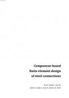
2.7 Experimental validation As the experimental data is stochastic by nature and is always subject to some variation, it should be actually defined by a probability distribution. For complete comparison, the numerical results should also be presented in an analogous probabilistic manner using a probability distribution, generated by repeated calculations with some selected input data varying following prescribed distributions, so-called probability simulations. Such extensive calculations can be conducted automatically with the help of specialized optimization packages (e.g., LS-OPT®, HyperStudy® or ModeFrontier®), which are more often included in nowadays commercial computational systems. For many authors working on principles of validation and verification (Kwasniewski, 2010), the term calibration has a negative meaning and describes a practice which should be avoided in numerical modeling. Calibration here means unjustified modification of the input data applied to a numerical model in order to shift the numerical results closer to the experimental data. An example of erroneous calibration is shown in Fig. 2.1, where at the beginning, it is assumed that the numerical model well reflects the experiment. However, due to some uncertainties associated with the experiment, the first numerical prediction differs from the first experimental result. Frequently in such cases, the discrepancy between the experiment and the numerical simulation is attributable to some by the analyst unidentified input parameter and not to a limitation of the software, and then, through hiding one error by introducing another, the calibration process itself is erroneous. Calibration, applied for example through variation of material input data, shifts the result closer to the experimental response but, at the same time, changes the whole numerical model whose probability is now moved away from the experimental one. Due to the calibration, the new numerical model may easily show poorer predictive capability. This fact is principally revealed for modified input data, e.g. loading conditions.

Fig. 2.1: Example of calibration meaning unjustified shifting the numerical results closer to the experimental data (Kwasniewski, 2010) There is a situation when the calibration process actually makes sense. If a full stochastic description of experimental data is known and probabilistic analysis was performed for the simulation, and there is a difference between means of measured and simulated responses, then

17

[email protected] 12 Jul 2022

calibration of physical models may be needed. The adjustment of the model introduces a change in the response that brings the entire spectrum of results closer to the experimental set of data. The calibration defined that way is much more complex process than just tweaking of the models and must be confirmed on different simulated events.

18

[email protected] 12 Jul 2022

3 COMPONENT-BASED FINITE ELEMENT METHOD 3.1 Material model The most common material diagrams used in finite element modeling of structural steel are the ideal plastic, elastic model with strain hardening, and the true stress-strain diagram, see Fig. 3.1.1. The true stress-strain diagram is calculated from the material properties of mild steels at ambient temperature obtained in tensile tests. The true stress and strain may be obtained as follows: σtrue = σ (1 + ε)

(3.1.1)

εtrue = ln(1 + ε)

(3.1.2)

where σtrue is true stress, εtrue true strain, σ nominal stress, and ε nominal strain. The elastoplastic material with strain hardening is modeled according to EN 1993-1-5:2006. The material behavior is based on von Mises yield criterion. It is assumed to be elastic before reaching the yield strength, fy. The ultimate limit state criteria for regions not susceptible to buckling is reaching a limiting value of the principal membrane strain. The value of 5 % is recommended.

Fig. 3.1.1 Material diagrams of steel in numerical models The limit value of plastic strain is often discussed. In fact, ultimate load has low sensitivity to the limit value of plastic strain when ideal plastic model is used. It is demonstrated in the following example of a beam-to-column joint. An open section beam IPE 180 is connected to an open section column HEB 300 and loaded by bending moment, as shown in Fig. 3.1.2. The influence of the limit value of plastic strain on the resistance of the beam is shown in Fig. 3.1.3. The limit plastic strain is changing from 2 % to 8 %, but the change in moment resistance is less than 4 %.

19

[email protected] 12 Jul 2022

a) loads

b) stresses

c) strains

Resistance [kNm]

Fig. 3.1.2 Example of prediction of ultimate limit state of a beam to column joint

42 41 40 39 38 37 36 35

39,65

39,25

40,8

40,4

CBFEM CM 0

1

2

3

4

5

6

7

8

9

Plastic strain [%]

Fig. 3.1.3 Influence of the limit value of plastic strain on the moment resistance

20

[email protected] 12 Jul 2022

3.2

Plate model and mesh convergence

3.2.1 Plate model Shell elements are recommended for modeling of plates in design FEA of structural connection. 4-node quadrangle shell elements with nodes at its corners are applied. Six degrees of freedom are considered in every node: 3 translations (ux, uy, uz) and 3 rotations (φx, φy, φz). Deformations of the element are divided into membrane and flexural components. The formulation of membrane behavior is based on the work of Ibrahimbegovic (1990). Rotations perpendicular to the plane of the element are considered. Complete 3D formulation of the element is provided. The out-of-plane shear deformations are considered in the formulation of the flexural behavior of element based on Mindlin hypothesis. The MITC4 elements are applied, see Dvorkin (1984). The shell is divided into five integration points along the height of the plate, and plastic behavior is analyzed in each point. It is called Gaus–Lobatto integration. The nonlinear elastic-plastic stage of material is analyzed in each layer based on the known strains. 3.2.2 Mesh convergence There are some criteria for the mesh generation in the connection model. The connection check should be independent of the element size. Mesh generation on a separate plate is problem-free. The attention should be paid to complex geometries such as stiffened panels, T-stubs, and base plates. The sensitivity analysis considering mesh discretization should be performed for complicated geometries. All plates of a beam cross-section have common size of elements. Size of generated finite elements is limited. Minimal element size is set to 10 mm and maximal element size to 50 mm. Meshes on flanges and webs are independent of each other. Default number of finite elements is set to 8 elements per cross-section height, as shown in Fig. 3.2.1.

Fig. 3.2.1 Mesh on beam with constrains between web and flange plate The mesh of end plates is separate and independent of other connection parts. Default finite element size is set to 16 elements per cross-section height, as shown in Fig. 3.2.2.

21

[email protected] 12 Jul 2022

Fig. 3.2.2 Mesh on end plate, with 7 elements along its width Following example of a beam-to-column joint shows the influence of mesh size on moment resistance. An open section beam IPE 220 is connected to an open section column HEA 200 and loaded by bending moment, as shown in Fig. 3.2.3. The critical component is column panel in shear. The number of finite elements along the cross-section height is changing from 4 to 40, and the results are compared; see Fig. 3.2.4. Dashed lines are representing 5%, 10%, and 15% difference. It is recommended to subdivide the cross-section height into 8 elements.

h beam height

Resistance [kNm]

Fig. 3.2.3 Beam to column joint model and plastic strains at ultimate limit state

50 49 48 47 46 45 44 43 42 41 40

15 % 10 % 5%

0

4

8

12 16 20 24 28 32 36 40

Number of elements on edge [-]

Fig. 3.2.4 Influence of number of elements on the moment resistance

22

[email protected] 12 Jul 2022

Mesh sensitivity study of a slender compressed stiffener of column web panel is presented. The geometry of the example is taken from Chapter 6.3. The number of elements along the width of the stiffener is changed from 4 to 20. The first buckling mode and the influence of a number of elements on the buckling resistance and critical load are shown in Fig. 3.2.5. The differences by 5% and 10% are displayed. It is recommended to use 8 elements along the stiffener width. 10 %

Joint resistance [kNm]

330

CBFEM - M

320

5%

CBFEM - Mcr

310 10 %

300 290

5%

280 bs stiffener width

270 4

8

12

16 20 Number of elements [-]

Fig. 3.2.5 First buckling mode and influence of number of elements along the stiffener on the moment resistance Mesh sensitivity study of T-stub in tension is presented. The geometry of the T-stub is described in Chapter 5.1. Half of the flange width is subdivided into 8 to 40 elements, and the minimal element size is set to 1 mm. The influence of the number of elements on the T-stub resistance is shown in Fig. 3.2.6. The dashed lines are representing the 5 %, 10 %, and 15 %

T-stub resistance [kN]

difference. It is recommended to use 16 elements on the half of the flange width. 200 195

15 %

190 185

10 %

180 175

5%

170 165

bf is half of flange width

160 0

4

8 12 16 20 24 28 32 36 40 Number of elements [-]

Fig. 3.2.6 Influence of number of elements on the T-stub resistance Mesh sensitivity study of uniplanar transverse plate circular hollow section T joint in compression is presented. The geometry of the T joint is described in Chapter 7.3. The number of elements along surface of the biggest circular hollow member is changed from 16 to 128. The influence of the number of elements on the joint resistance is shown in Fig. 3.2.7. The dashed lines

23

[email protected] 12 Jul 2022

are representing the 5 % and 15 % difference. It is recommended to use 64 elements along the

Joint resistance [kN]

surface of the circular hollow member. 150 140 130 120 110 100 90

15 %

80 70

5%

60 50 10

30

50

70

90

110

130

Number of elements [-]

Fig. 3.2.7 Influence of number of elements on the joint resistance of CHS member Mesh sensitivity study of uniplanar square hollow section X joint in compresion is presented in Fig. 3.2.8. The geometry of the joint is described in Chapter 7.2. The number of elements on the biggest web of hollow member is changed from 4 to 24. The influence of the number of elements on the joint resistance is shown. The dashed lines are representing the 5 % and 15 % difference.

Joint resistance [kN]

It is recommended to use 16 elements on the biggest web of rectangular hollow member. 300 280 260 240 220 200 180 160 140 120 100 80

15 % 5%

4

8

12

16

20

24

Number of elements [-]

Fig. 3.2.8 Influence of number of elements on the joint resistance of rectangular hollow member

24

[email protected] 12 Jul 2022

3.3 Contacts The standard penalty method is recommended for modeling a contact between plates. If penetration of a node into an opposite contact surface is detected, penalty stiffness is added between the node and the opposite plate. The penalty stiffness is controlled by a heuristic algorithm during nonlinear iteration to get better convergence. The solver automatically detects the point of penetration and solves the distribution of contact force between the penetrated node and nodes on the opposite plate. It allows creating the contact between different meshes, as shown in Fig. 3.3.1. The advantage of the penalty method is the automatic assembly of the model. The contact between the plates has a significant impact on the redistribution of forces in connection.

Fig. 3.3.1 Example of contact stress of bolted connections of purlins from two overlapped Z sections

25

[email protected] 12 Jul 2022

3.4 Welds Several options for treating welds in numerical models exist. Large deformations make the mechanical analysis more complex, and it is possible to use different mesh descriptions, different kinetic and kinematic variables, and constitutive models. The different types of geometric 2D and 3D models and thereby finite elements with their applicability for different accuracy levels are generally used. Most often used material model is the common rate-independent plasticity model based on von Mises yield criterion. Two approaches that are used for welds are described.

3.4.1

Direct connection of plates

The first option of weld model between plates is direct merge of meshes, as shown in Fig. 3.4.1. The load is transmitted through force-deformation constrains based on Lagrangian formulation to the opposite plate. The connection is called multi point constraint (MPC) and relates the finite element nodes of one plate edge to another plate. The finite element nodes are not connected directly. The advantage of this approach is the ability to connect meshes with different densities. The constraint allows to model midline surface of the connected plates with the offset, which respects the real plate thickness. This type of connection is used for full penetration butt welds.

3.4.2

Weld with plastic redistribution of stress

The load distribution in weld is derived from the MPC, so the stresses are calculated in the throat section. This is important for stress distribution in a plate under the weld and for modeling of T-stubs. This model does not respect the stiffness of the weld, and the stress distribution is conservative. Stress peaks, which appear at the ends of plate edges, in corners and rounding, govern the resistance along the whole length of the weld. To express the weld behavior, an improved weld model is applied. A special elastoplastic element is added between the plates. The element respects the weld throat thickness, position, and orientation. The equivalent weld solid is inserted with the corresponding weld dimensions, as shown in Fig. 3.4.2. The nonlinear material analysis is applied, and elastoplastic behavior in equivalent weld solid is considered. The stress peaks are redistributed along the weld length. The aim of design weld models is not to capture reality perfectly. Residual stresses or weld shrinkage are neglected. The design weld models are verified for their resistance according to relevant codes. An appropriate design weld model is selected for each code. The resistances of the regular welds, welds to unstiffened flange, long welds, and multi-oriented weld groups were investigated to select parameters of the design weld element. The plastic strain in steel plates is normalized to 5 % to confirm with the maximum plastic strain of plates.

26

[email protected] 12 Jul 2022

Fig. 3.4.1 Constraint between mesh nodes

3.4.3

Fig. 3.4.2 Constraint between weld element and mesh nodes

Weld deformation capacity

The weld deformation capacity is determined to comply with resistance of welds to unstiffened flange, see cl. 4.10 in EN 1993-1-8:2006 and long welds, see cl. 4.11 in EN 1993-1-8:2008 and cl. J.2.2b AISC 360-16 etc. The deformation capacity was compared to sets of experiments from literature for longitudinal welds (Kleiner, 2018) and transverse welds (Ng et al, 2002). From the following figures, it can be seen that the weld model with plastic redistribution of stress is very conservative for longitudinal

Shear stress, 𝜏II, MPa

welds and at lower boundary for transverse welds.

CBFEM

Deformation, mm

Fig. 3.4.3 Longitudinal welds, stress–deformation diagrams of real tests by Kleiner (2018) compared to model of weld with plastic stress redistribution

27

[email protected] 12 Jul 2022

Fig. 3.4.3 Transverse welds, strain at fracture, e.g. deformation divided by weld leg size, for tests of lapped splice joints in (Ng et al., 2002) compared to the model of weld with plastic stress redistribution.

28

[email protected] 12 Jul 2022

3.5 Bolts In CBFEM, the component bolt in tension and shear is modeled by a dependent nonlinear spring. The deformation stiffness of the shell element modeling the plates distributes the forces between the bolts and simulates the adequate bearing of the plate. 3.5.1

Tension

The spring of a bolt in tension is described by its initial deformation stiffness, design resistance, initialization of yielding, and deformation capacity. The initial stiffness is derived analytically as 𝑘=

𝐸𝐴𝑠 𝐿𝑏

(3.5.1)

where E is Young’s modulus, As the tensile stress area of a bolt, and Lb the bolt elongation length. The model corresponds well to experimental data, see (Gödrich et al. 2014). For the initialization of yielding and the deformation capacity, it is assumed that the plastic deformation occurs in the threaded part of the bolt shank only. The load-deformation diagram of the bolt is shown in Fig. 3.5.1 and is derived for 𝐹𝑡,𝑒𝑙 = 𝑐

𝐹𝑡,𝑅𝑑

(3.5.2)

1 ∙𝑐2 −𝑐1 +1

𝑅𝑚 −𝑅𝑒

(3.5.3)

𝑘𝑡 = 𝑐1 ∙ 𝑘; 𝑐1 = 1

∙𝐴𝐸−𝑅𝑒

4

𝑢𝑒𝑙 =

𝐹𝑡,𝑒𝑙

(3.5.4)

𝑘 𝐴∙𝐸

(3.5.5)

𝑢𝑡,𝑅𝑑 = 𝑐2 ∙ 𝑢𝑒𝑙 ; 𝑐2 = 4∙𝑅

𝑒

where k is the linear stiffness of bolt, kt the stiffness of bolt at the plastic branch, Ft,el the limit force for linear behavior, A the percentage elongation after a fracture of a bolt, Ft,Rd the limit bolt resistance, and ut,Rd the limit deformation of a bolt. The design values according to ISO 898:2009 are summarised in Tab. 3.5.1. Tension force in bolt, kN Ft,Rd k

Ft,el

t

u el

ut, Rd

Bolt deformation, mm

Fig. 3.5.1 Load–deformation diagram of a bolt in tension

29

[email protected] 12 Jul 2022

Table 3.5.1 Bolt parameters in tension, based on ISO 898:2009 Rm

Re = Rp02

A

E

c1

c2

[MPa]

[MPa]

[%]

[MPa]

[-]

[-]

4.8

420

340

14

2,1E+05

0,011

21,6

5.6

500

300

20

2,1E+05

0,020

35,0

5.8

520

420

10

2,1E+05

0,021

12,5

6.8

600

480

8

2,1E+05

0,032

8,8

8.8

830

660

12

2,1E+05

0,030

9,5

10.9

1040

940

9

2,1E+05

0,026

5,0

Grade

3.5.2

Shear

The initial stiffness and the design resistance of a bolt in shear are modeled in CBFEM according to Cl. 3.6 and 6.3.2 in EN 1993-1-8:2006. The spring representing the bolt in shear has bi-linear force deformation behavior. Deformation capacity is considered according to (Wald et al. 2002) as (3.5.6)

𝛿𝑝𝑙 = 3 𝛿𝑒𝑙 Initialization of yielding is expected, see Fig. 3.5.2, at

(3.5.7)

Fv,el = 2/3 Fv,Rd

Shear force in bolt, kN Fv,Rd k

Fv,el

s

δ el

δp l

Relative deformation, δ

Fig. 3.5.2 Force–deformation diagram of the bolt in shear

30

[email protected] 12 Jul 2022

3.6 Interaction of shear and tension in a bolt A combination of shear and tension in a bolt is expressed in EN 1993-1-8:2005, Tab. 3.4 by a bilinear relation and checked as max⁡{

𝐹𝑡,Ed 𝐹v,Ed 𝐹t,Ed , + } ⁡ ≤ 1,0 𝐹t,Rd 𝐹v,Rd 1,4⁡𝐹t,Rd

(3.6.1)

where Fv,Ed is the acting bolt shear force, Ft,Ed is the acting bolt tensile force, Fv.Rd is the bolt shear resistance, and Ft.Rd is the bolt tensile resistance. A condition limiting the bolt resistance is shown

𝐹t,Ed ⁡ ≤ 1,0 𝐹t,Rd

Bolt tensile force,

Ft,Rd

in Fig. 3.6.1.

𝐹v,Ed 𝐹t,Ed + ≤ 1,0 𝐹v,Rd 1,4⁡𝐹t,Rd

Fv,Rd Bolt shear force, Fv,Ed

Fig. 3.6.1 Limit condition of interaction of shear and tension in a bolt The tensile and shear behaviors of the bolt in a numerical model are represented by a bilinear spring model, see previous Chapter 3.5. The nonlinear spring has special behavior in the interaction of the shear and tension. The shear and tension forces are presented as nonlinear functions of shear and tension deformations composed from ruled surfaces; see Fig. 3.6.2 and 3.6.3, where δs is the bolt shear deformation, δt is the bolt deformation in tension, δel is the elastic limit of the bolt deformation, δRd is the bolt deformation at its resistance, Fel is the bolt force at the elastic limit of deformation, and FRd is the bolt resistance. The functions respect the limit condition of interaction, which is shown above. It is clear that the bolt can be in three states: a linear behavior, a plastic state in tension, and a plastic state in interaction of the tension and the shear.

31

Bolt tension force, Ft,Ed

[email protected] 12 Jul 2022

Bolt tension deformation, δt

Ft.Rd

Ft.Rd

𝑟=

Ft.el

Ft.el

1,4 − 1 1.4

δt,Rd r.δv,Rd δt,el r.δv,el δv,el

δv,Rd Bolt shear deformation, δv

Bolt shear force, Fv,Ed

Fig. 3.6.2 Bolt tension force as a function of deformation in shear and tension

r.Fv.Rd

Bolt tension deformation, δt

Fv.Rd δt,Rd

r.Fv,el

Fv,el

r.δv,Rd δt,el r.δv,el

𝑟= δv,el

1,4 − 1 1.4

δv,Rd Bolt shear deformation, δv

Fig. 3.6.3 Bolt shear force as a function of deformation in shear and tension

32

[email protected] 12 Jul 2022

3.7 Preloaded bolts In connection with preloaded bolts, the shear force is transferred by friction between both surfaces. Compared to regular bolts, the friction is controlled by the preloaded force. The final resistance is assured by bolt shearing and bolt and plate bearing after the slippage of a bolt in a hole. In EN 1993-1-8:2005, the resistances of preloaded bolts classes 8.8 and 10.9 are summarized in Chapter 3.9. The bolts are expected to be preloaded to 70 % of their strength, fub, see eq. 3.7.1 (eq. 3.6 in EN 1993-1-8:2005) and the bolt preloading force is (3.7.1)

𝐹p,C = 0,7𝑓ub 𝐴s

where fub is the bolt strength and As is the bolt area effective in tension. It is expected that the bolt deforms by 80 % and the plate by 20 %. If the external tensile force Ft.Ed is applied to joint in the direction of a bolt, the slip resistance will be reduced 𝐹s,Rd = 𝑘s 𝜇

𝐹p,C −0,8𝐹t,Ed

(3.7.2)

𝛾M3

where ks is the bolt hole size factor and µ the slip factor. Bolt spring model

Ft.Ed

Fs,Rd

Fp,C

Fp,C

Fp,C

Fp,C

Shear force to bolt, Fv,Ed

Fs.Rd Slip

Fs,Rd Ft,Ed Shear deformation, δv

Fig. 3.7.1 Shear characteristic of the preloaded bolt In numerical design model, the component preloaded bolt is simulated either as nonlinear spring using the preloading force and deformation or by restrains between surfaces, which are representing the friction, with a spring, which is including a preloading force in a bolt. For the bolt component represented by the preloading force and its slip deformation, the model is similar to a conventional, snug-tight bolt model. The shear characteristic is shown in Fig. 3.7.1. The initial linear shear stiffness is determined from the stiffness of the cylinder under the head of the bolt, and it is practically rigid. The shear force limit includes the external tensile load to the bolt in accordance with EN 1993-1-8:2005. The advantage of this simplified model is its computational stability and low demands of the FE model and the consistency of results with Cl. 3.6.2.2 in EN 1993-1-8:2005. The model does not respect the actual distribution of contact pressures between the plates and the history of preloading.

33

[email protected] 12 Jul 2022

3.8

Anchor bolt

3.8.1

Description

The anchor bolt is modeled with similar procedures as structural bolts. The bolt is fixed on one side to the concrete block. Its length Lb is taken according to EN 1993-1-8:2005 as a sum of washer thickness tw, base plate thickness tbp, grout thickness tg, and free length embedded in concrete, which is expected as 8d, where d is bolt diameter. The stiffness in tension is calculated as k = E As/Lb. The load-deformation diagram of the anchor bolt is shown in Fig. 3.8.1. The used design values according to ISO 898:2009 are summarised in Tab. 3.5.1 and in eq. (3.5.1) to (3.5.4).

Force in anchor bolt, Ft kN Ft,Rd kt

Ft,el Ft,Ed k uel

ut,Rd

Deformation of anchor bolt, mm

Fig. 3.8.1 Load–deformation diagram of the anchor bolt The stiffness of the anchor bolt in shear is taken as the stiffness of the structural bolt in shear. The anchor bolt resistance is evaluated according to EN 1992-4:2018. Steel failure mode is determined according to Cl. 6.2.6.12 in EN 1993-1-8:2005. 3.8.2

Anchor bolts with stand-off

Anchors with stand-off can be checked as a construction stage before the column base is grouted or as a permanent state. Anchor with stand-off is designed as a bar element loaded by shear force, bending moment, and compressive or tensile force. The anchor is fixed on both sides; one side is 0.5×d below the concrete level, the other side is in the middle of the thickness of the plate. The buckling length is conservatively assumed as twice the length of the bar element. Plastic section modulus is used. The forces in anchor with stand-off are determined using finite element analysis. Bending moment is dependent on the stiffness ratio of anchors and base plate.

34

[email protected] 12 Jul 2022

3.9

Concrete block

3.9.1

Design model

In component-based finite element method (CBFEM), it is convenient to simplify the concrete block as 2D contact elements. The connection between the concrete and the base plate resists in compression only. Compression is transferred via Winkler-Pasternak subsoil model, which represents deformations of the concrete block. Tension force between the base plate and concrete block is carried by anchor bolts. Shear force is transferred by friction between a base plate and a concrete block, by shear lug, or by bending of anchor bolts. The resistance of bolts in shear is assessed analytically. Friction is modeled as a full single-point constraint in the plane of the base plate-concrete contact. At the shear lug model, the shear load is assumed to act in the mid-plane of the base plate, and it is resisted by concrete bearing stress at the whole area of the shear lug embedded in concrete. The bearing strength is based on a uniform bearing stress acting over the area of the shear lug. The area of the shear lug in grout layer is assumed as ineffective. There is a lever arm between the point of shear load application (base plate mid-plane) and the center of resistance (mid-depth of the shear lug embedded in concrete). This causes additional bending moment that needs to be resisted by the bearing resistance of concrete and tension in anchors. 3.9.2

Resistance

The resistance of concrete in 3D compression is determined based on EN 1993-1-8:2005 by calculating the design bearing strength of concrete in the joint fjd under the effective area Aeff of the base plate. The design bearing strength of the joint fjd is evaluated according to Cl. 6.2.5 in EN 1993-1-8:2005 and Cl. 6.7 in EN 1992-1-1:2005. The grout quality and thickness is introduced by the joint coefficient jd. For grout quality equal or better than the quality of the concrete block is expected  jd = 1,0. The effective area ACM under the base plate is estimated to be of the shape of the column cross-section increased by additional bearing width c

c=t

fy

(3.9.1)

3 fj  M0

where t is the thickness of the base plate, fy is the base plate yield strength, c is the partial safety factor for concrete, and M0 is the partial safety factor for steel. The effective area is calculated by iteration until the difference between additional bearing widths of a current and a previous iteration |𝑐𝑖 − 𝑐𝑖−1 | is less than 1 mm. The area where the concrete is in compression is taken from the results of FEA. This area in compression AFEM allows determining the position of a neutral axis. The intersection of the area in compression AFEM and the effective area ACM creates the effective area in compression Aeff, which allows assessing the resistance for a generally loaded column base of any column shape with any

35

[email protected] 12 Jul 2022

stiffeners. The average stress σ on the effective area Aeff is determined as the compression force divided by the effective area. Check of the component is in stresses 𝜎 ≤ 𝑓𝑗𝑑 . This procedure of assessing the resistance of the concrete in compression is independent of the mesh of the base plate, as can be seen in Fig. 3.9.1 and 3.9.2. The geometry of the model used for comparison is described in detail in Chapter 8.1.3. Two cases are investigated: loading by pure compression 1 200 kN, see Fig. 3.9.1, and loading by a combination of compressive force 1 200 kN

σ/fjd

and bending moment 90 kNm; see Fig. 3.9.2. 70% 68% 66% 64% 62% 60% 0

No. of elements 4 6 8 10 15 20

Aeff [m2] 0,06 0,06 0,06 0,06 0,06 0,06

σ [MPa] 18,5 18,2 18,5 18,4 18,5 18,5

5

10

15 20 25 Number of elements [-]

fjd [MPa] 26,8 26,8 26,8 26,8 26,8 26,8

Fig. 3.9.1 Influence of number of elements on prediction of resistance of concrete in compression in case of pure compression

36

[email protected] 12 Jul 2022

105%

σ/fjd

100% 95% 90% 0

5

10 15 20 Number of elements [-]

25

No. of elements Aeff [m2] σ [MPa] fjd [MPa] 4 0,05 26,0 26,8 6 0,04 25,8 26,8 8 0,04 26,1 26,8 10 0,05 25,9 26,8 15 0,04 26,3 26,8 20 0,04 26,6 26,8

Fig. 3.9.2 Influence of number of elements on prediction of resistance of concrete in compression in case of compression and bending 3.9.3

Deformation stiffness

The stiffness of the concrete block may be predicted for the design of column bases as an elastic hemisphere. A Winkler-Pasternak subsoil model is commonly used for a simplified calculation of foundations. The stiffness of subsoil is determined using modulus of elasticity of concrete and effective height of subsoil as

k=

Ec Aeff (1 +  )  Aref

    1   + 4   h     d + 3   2 

(3.9.2)

where k is stiffness in compression, Ec is modulus of elasticity, n is Poisson coefficient of concrete foundation, Aeff is effective area, Aref is reference area, d is base plate width, h is column base height, and αi are coefficients. The following values for coefficient were used based on the results of research-oriented finite element models with concrete modeled by solid elements: Aref = 1 m2; α1 = 1,65; α2 = 0,5; α3 = 0,3; α4 =1,0.

37

[email protected] 12 Jul 2022

3.10 Local buckling of compressed plates In research FEA models, the slender plates in compression taking into account plate geometrical imperfections, residual stresses, and large deformation during analyses may be designed according to EN 1993-1-5:2006. This should be précised according to the different plate/joint configuration. The FEA procedure naturally offers the prediction of the buckling load of the joint. The design procedure for class 4 cross-sections according to reduced stress method is described in Annex B of EN 1993-1-5:2006. It allows predicting the post-buckling resistance of the joints. Critical buckling modes are determined by materially linear and geometrically nonlinear analysis. In the first step, the minimum load amplifier for the design loads to reach the characteristic value of the resistance of the most critical point coefficient αult,k is obtained. Ultimate limit state is reached at 5 % plastic strain. The critical buckling factor αcr is determined by linear buckling analysis and stands for the load amplifier to reach the elastic critical load under complex stress field. Examples of critical buckling mode in steel joints are shown in Fig. 3.10.1.

Fig. 3.10.1 Examples of first buckling mode in CBFEM models The load amplifiers are related to the non-dimensional plate slenderness, which is determined as follows

=

 ult  cr

(3.10.1)

Reduction buckling factor ρ is calculated according to EN 1993-1-5:2006 Annex B. Conservatively, the lowest value from longitudinal, transverse, and shear stress is taken. Fig. 3.10.2 shows the relation between plate slenderness and reduction buckling factor. The verification of the plate is based on von Mises yield criterion and reduced stress method. Buckling resistance is assessed as αult . 1  M1

(3.10.2)

38

[email protected] 12 Jul 2022

where γM1 is partial safety factor. Based on the distribution of strains calculated in MNA and the critical buckling factor in LBA is assessed the buckling resistance without using second order calculation and applying imperfections. It is recommended to check the buckling resistance for critical buckling factor smaller than 3.0. Otherwise is the resistance governed by reaching 5 % plastic strain for plates with smaller slenderness. The procedure is summarised in the diagram,

Buckling reduction factor, ρ

see Fig. 3.10.3. 1,2 1,0 0,8 0,6 0,4 0,2 0,0 0

1

2 3 4 Plate slenderness, λp

Fig. 3.10.2 Buckling reduction factor ρ according to EN 1993-1-5:2006 Annex B

Fig. 3.10.3 The design procedure according to EN 1993-1-5:2006 Annex B

39

[email protected] 12 Jul 2022

a)

e)

b)

f)

c)

g)

d)

h)

Fig. 3.11.2 Development of plastic zones in connection by CBFEM analyses, from first yielding under the tensile bolt a), through development of full plasticity in the column web panel loaded in shear e)–f), till reaching the 5 % strain in panel h) As is commonly known in well-designed connections, the plastification starts early, see Fig. 3.11.2a. The column web panel in shear brings the deformation capacity of a connection and guides the nonlinear part of behavior; see Fig. 3.11.2e–f. Fig. 3.11.3 demonstrates the fast development of yielding in the column web panel after reaching the 5 % strain.

41

[email protected] 12 Jul 2022

3.11 Moment-rotation relation The joint is generally three dimensional. The moment–rotation curve for connection in a joint is evaluated for each element, which is attached to the joint. The calculation of the moment–rotation relation by the FEA model is different compared to the stress/strain analysis of a joint. The moment rotation is analyzed for connection of the connected member separately in the planes where the connections are loaded. The modeling of the moment rotational curve may be documented on the behavior of a welldesigned portal frame eaves moment bolted connection developed based on US best practice and applied in good European practice represented by British and German design books. The composition of the connection geometry of the bolted connection is demonstrated in Fig. 3.11.1. The rafter of cross-section IPE 400 column is connected to column HEA 320 by the full depth end plate of thickness 25 mm by 12 bolts M24 8.8. The haunch is 700 mm long and 300 mm high with flange dimensions 15×150 mm. The stiffeners are designed from plate thickness 20 mm. The material of all plates is steel grade S355. The results of CBFEM analyses show in Fig. 3.11.2 the development of plastic zones in connection, from first yielding under the bolt in tension, through the development of full plasticity in the column web panel in shear, till reaching the 5 % strain in column web panel. After reaching this strain, the plastic zones propagate rapidly in the column web panel in shear, and for small steps in bending moment, the rotation of the joint rises significantly, see Fig. 3.11.3.

Fig. 3.11.1 Composition portal frame eaves moment bolted connection

40

[email protected] 12 Jul 2022

Fig. 3.11.3 After reaching the 5 % strain in the column web panel in shear the plastic zones propagate rapidly

42

[email protected] 12 Jul 2022

3.12 Bending stiffness The bending/deformation stiffness of structural joints has only an indirect influence on the resistance of the structure. Generally, it is expected that its underestimation is a safe assumption. The prediction models by component method (CM) show mostly higher values compared to experiments. It is given by stiffness of experimental set-ups but also by an assumption of modulus of elasticity of streel as 210 000 MPa. In reality, the experimental value is 206 000 MPa as a maximum. The calculation by the FEA model is different compared to the stress/strain analysis of a joint. The joint is three dimensional. The bending/deformation stiffness for connection of a member is influenced by the shear deformation in the joint and the connection deformation of the particular member in the selected plane of the member. For joints connecting more members, the bending stiffnesses of the connections are analyzed separately in the plains, where they are loaded. For the evaluation of the bending stiffness of a particular connection, it is assumed that members are supported at the ends, and only the analyzed member i has a free end, see Fig. 3.12.1. The analyzed member i is loaded by a bending moment in plane yz coming from the global analyses. To learn the secant rotational stiffness Sj,i,yz for rotation i,yz the bending moment Mj,Ed,i,yz is applied in a selected plane yz. The secant rotational stiffness Sj,s,i,yz is derived from the formula: Sj,s,i,yz = Mj,Ed,i,yz / i,yz

(3.12.1)

3.12.1 FEA model for analysis of stiffness of selected connected member The total rotation j,i,yz of the end section of analyzed member i in plane yz is derived on a model with one free/observed member. All the other members are fixed. The calculated value is influenced by the deformation of all members in the joint. The effects of member deformation are removed by analyzing the substitute model of the joint, which is composed of members with appropriate cross-sections, as shown in Fig. 3.12.2. By loading this substitute model by bending moment Mi,yz the rotation j,ei,yz is obtained, which represents the stiffness of the particular

43

[email protected] 12 Jul 2022

connected member only. In the substitute model, the node is expected to be rigid. The rotation caused only by the construction of the connection is derived as:

j,i,yz = j,ti,yz – j,ei,yz

(3.12.2)

Fig. 3.12.2 The substitute 1D model to eliminate the bending flexibility if the connected elements The secant stiffness of connection j,i,yz is derived during its loading. The initial stiffness j,ini is defined as elastic stiffness and is expected to be linear till 2/3 Mj,Rd, see Cl. 6.3.1 in EN 1993-18:2005. The calculation of the initial bending stiffness by the FEA model is taken as a secant stiffness loaded till 2/3 Mj,Rd from the acting bending moment till 2/3 M2/3Rd,i,yz and corresponding rotation in connection 2/3Rd,i,yz as: Sj,ini,i,zy  Sj,s,2/3Rd,i,zy = M2/3Rd,i,yz / 2/3Rd,i,yz

(3.12.3)

For the connection presented in Fig. 3.12.1, the values of the bending resistance Mj,Rd,i,yz and initial stiffness j.ini,i,yz are summarized in Fig. 3.12.3.

Fig. 3.12.3 Moment/rotation diagram of connection in joint for one connected member

44

[email protected] 12 Jul 2022

The bending resistance Mj,Rd,i,yz of connection is in CBFEM evaluated by strain 5 % in plates/sections or resistance of connectors, e.g. bolts, welds. Fig. 3.12.4 shows the strain in the joint exposed to moments in the plane of the strong axis of the connected open I section beam in Fig. 3.12.1 from My = 25 kNm to 72 kNm. The maximal reached strain εmax ranges from 0,2 % till 22,7 %.

My = 25 kNm with εmax = 0,2 %

My =40 kNm with εmax = 0,4 %

My =55 kNm with εmax = 0,7 %

My =60 kNm with εmax = 1,3 %

My = 63 kNm with εmax = 2,5 %

My =65 kNm with εmax = 4,6 %

My =68 kNm with εmax = 10,8 % My =70 kNm with εmax = 16,4 % My =72 kNm with εmax = 22,7 %

Fig. 3.12.4 The maximal strains εmax in joint during its loading by bending moment My in the plane of the strong axis of the connected open I section beam

45

[email protected] 12 Jul 2022

3.13 Deformation capacity The deformation capacity/ductility δCd belongs, together with resistance and stiffness, to the three basic parameters describing the behavior of connections. In moment resistant connections, the ductility is achieved by a sufficient rotation capacity φCd. The deformation/rotation capacity is calculated for each connection in the joint separately. The prediction of deformation capacity δCd of connections is currently studied by component method (CM) but is not offered as a standardized procedure. Compared to well-accepted methods for determination of the initial stiffness and resistance of many types of structural joints, there are no generally accepted standardized procedures for the determination of the rotation capacity. The deemed to satisfy criteria are selected to help the engineers in Cl 6.4.2 of EN 1993-1-8:2005. A beam-to-column joint in which the design moment resistance of the joint Mj,Rd is governed by the design resistance of the column web panel in shear, may be assumed to have adequate rotation capacity for global plastic analysis, provided that: d/tw ≤ 69 ε

(3.13.1)

where d the column web panel width, tw is the web thickness, and 𝜀 ≤ √235/𝑓𝑦 is the steel yield strength ratio. In Cl 6.4.2(2), the plastic distribution between the bolt rows for joints with a bolted end plate connection is limited provided that the design moment resistance of the joint is governed by the design resistance of the column flange or the beam end plate in bending or the thickness t of either the column flange or the beam end plate or tension flange cleat satisfies: (3.13.2)

𝑡 ≤ 0,36 𝑑 √𝑓𝑢𝑏 /𝑓𝑦

where d and fu.b are the diameter and ultimate strength of a bolt and fy is the yield strength of the relevant plate. The rotation capacity φCd of a welded beam-to-column connection may be assumed to be not less than the value given by the following expression provided that its column web is stiffened in compression but unstiffened in tension, and its design moment resistance is not governed by the design shear resistance of the column web panel, see 6.4.2(1): φCd = 0,025 hc / hb ...

(3.13.3)

where hb is the depth of the beam and hc is the depth of the column. An unstiffened welded beamto-column joint designed in conformity with the provisions of this section may be assumed to have a rotation capacity φCd of at least 0,015 radians. The estimation of the rotation capacity is important for connections exposed to earthquake; see (Gioncu and Mazzolani, 2002) and (Grecea 2004), and extreme loading; see (Sherbourne AN, Bahaari, 1994 and 1996). The deformation capacity of components has been studied from the end

46

[email protected] 12 Jul 2022

of the last century (Foley and Vinnakota, 1995). Faella et al. (2000) carried out tests on T-stubs and derived the analytical expressions for the deformation capacity. Kuhlmann and Kuhnemund (2000) performed tests on the column web subjected to transverse compression at different levels of axial compression force in the column. Da Silva et al. (2002) predicted deformation capacity at different levels of axial force in the connected beam. Based on the test results combined with FE analysis, deformation capacities are established for the basic components by analytical models by Beg et al. (2004). In this work, components are represented by non-linear springs, and appropriately combined in order to determine the rotation capacity of the joint for the end plate connections, with an extended or flush end plate, and welded connections. For these connections, the most important components that may significantly contribute to the rotation capacity column were recognized as the web in compression, column web in tension, column web in shear, column flange in bending, and end plate in bending. Components related to the column web are relevant only when there are no stiffeners in the column that resist compression, tension or shear forces. The presence of a stiffener eliminates the corresponding component, and its contribution to the rotation capacity of the joint can be therefore neglected. End plates and column flanges are important only for end plate connections, where the components act as a T-stub, where also the deformation capacity of the bolts in tension is included. The questions and limits of deformation capacity of connections of high strength steel were studied by Girao et al. (2004).

47

[email protected] 12 Jul 2022

3.14 Joint model in global analyses The recommendation about the joint modeling is summarized in EN 1993-1-8:2005 in Ch. 5. Ch. 5.1 helps to select a joint model for a global analysis according to its bending stiffness as nominally pinned, rigid or semi-rigid. Cl. 5.1.5 covers a global analysis of lattice girders from hollow sections. The distribution of axial forces in a lattice girder may be determined on the assumption that the members are connected by pinned joints. The eccentricity of members is discussed. Ch. 5.3 covers the modeling of beam-to-column joints. The influence of the column web panel in shear is discussed. The transfer of a web panel stiffness to a central point and a simplified model are included. Questions of the application of advanced models using FEA in global analyses are summarized in the chapter below. Joints of members are in 2D FEA used for global analyses and modeled as massless points when analyzing a steel frame or a girder structure, see Fig. 3.14.1. Equilibrium equations are assembled in joints, and after solving the whole structure, internal forces on ends of beams are determined. In fact, the joint is loaded by those forces. The resultant of the forces from all members in the joint is zero – the whole joint is in equilibrium. The real shape of the joint is not known in the structural model. For better visualization of CBFEM model, the end forces on 1D members are applied as loads on segment ends. Six components of the internal forces from the theoretical node are transferred to the outer end of segment – the values of forces are kept, but the moments are modified by the actions of the forces on corresponding arms. Inner ends of the segments are not connected.

Fig. 3.14.1 Theoretical (massless) joint and the real shape of the joint without modified member ends Each node of a 3D FEM model is in equilibrium. The equilibrium requirement is correct, but the input of data may be treated more sophisticatedly. One member of a joint is treated as bearing and the others as connected. If only a connection of the connected member is checked, it is not

48

[email protected] 12 Jul 2022

necessary to keep the equilibrium during the loading. Two modes of the load input are shown in Fig. 3.14.2.

Fig. 3.14.2 Simplified and advanced model of supports in CBFEM model of the joint End forces of the frame analysis model are transferred to the outer ends of the member segments. Eccentricities of the members caused by the joint design are respected during the transfer. The analysis model created by CBFEM corresponds to the real joint very precisely. On the other hand, the analysis of the internal forces is performed on the idealized 3D FEM model where the individual beams are modeled using centerlines, and the joints are modeled using immaterial nodes, as shown in Fig.3.14.3.

a) Real shape of joint b) Theoretical shape in 3D FEM model Fig. 3.14.3 Joint of vertical column and horizontal beam The internal forces are analyzed using 1D members in 3D model. Fig. 3.14.4 shows an example of courses of the internal forces.

a) Bending moment M b) Shear force V Fig. 3.14.4 Course of internal forces on horizontal beam. M and V are the end forces of the joint

49

[email protected] 12 Jul 2022

The effects caused by a member on a joint are important to design the joint with its connections. The effects are illustrated in Fig. 3.14.5.

a) 1D member model b ) CBFEM model – dark color Fig. 3.14.5 Load effects of member on the joint A bending moment MEd and a shear force VEd act in a theoretical joint. The point of the theoretical joint does not exist in CBFEM model; thus the load cannot be applied here. The model is loaded by actions M and V which are transferred to the end of a segment in a distance r MEd,c = MEd – VEd . r

(3.14.1)

VEd.c = VEd

(3.14.2)

In the CBFEM model, the end section of the segment is loaded by the moment MEd,c and the shear force VEd.c. When designing the joint, its real position relative to the theoretical point of the joint should be determined and respected. The internal forces in the position of the real joint are often different from the internal forces in the theoretical point of the joint. Thanks to the precise CBFEM model, the design is performed on reduced forces, see moment MEd,r in Fig. 3.14.6.

Fig. 3.14.6 Course of bending moment in CBFEM model, the arrow points to the real position of the connection

50

[email protected] 12 Jul 2022

a) 1D members model b) CBFEM model Fig. 3.14.7 Position of the hinge in theoretical 3D FEM model and in the real structure. Fig. 3.14.7 illustrates that the position of a hinge in the theoretical 1D model differs from the real position in the structure. The theoretical model does not correspond to reality. When applying the calculated internal forces, a significant bending moment is applied to the shifted joint, and the designed joint is either overloaded or cannot be designed. The solution is simple – both models must correspond. Either the hinge in the 1D member model must be defined in the proper position, or the courses of the internal forces must be shifted to get the zero moment in the real position of the hinge.

Fig. 3.14.8 Position of the hinge in theoretical 3D FEM model and in the real structure.

51

[email protected] 12 Jul 2022

3.15 Fatigue analysis by Nominal stress method The estimation of the fatigue life of a building structure is based on the main assumptions: the average stress in the element increases at the connecting elements and the dependence between the range stress and the number of cycles to failure is assumed. The basic method is the Nominal stresses method (NSM), which considers the structural parameters indirectly. The method limits the validity of fatigue classes by boundary conditions, such as weld length (Tab. 8.4 det. 1 in EN 1993-1-9:2005) or plate thickness (Tab. 8.3 det. 9-11 in EN 1993-1-9: 2005). Eq. 3.15.1 (eq. 6.1-6.3 in EN 1993-1-9:2005) allow the determination of the design value of the stress range. For the design of shear stress amplitude ∆𝜎𝐸,2 , ∆𝜎 should be replaced by ∆𝜏𝐸,2 , ∆𝜏. 𝛾𝐹1 . ∆𝜎𝐸,2 = 𝜆1 . 𝜆2 . … 𝜆𝑛 . ∆𝜎 for elements 𝛾𝐹1 . ∆𝜎𝐸,2 = 𝐾𝑡 . 𝜆1 ∗ 𝜆2 . … 𝜆𝑛 ∗ ∆𝜎 for joints

(3.15.1)

𝛾𝐹1 ∗ ∆𝜎𝐸,2 = 𝐾1 ∗ 𝜆1 . 𝜆2 . … 𝜆𝑛 ∗ ∆𝜎 for welded joints of hollow cross-sections where 𝜆1 . 𝜆2 . … 𝜆𝑛 are damage equivalent factors from different factors 𝛾𝐹1 is partial factor for equivalent constant amplitude stress ranges 𝐾𝑡 , 𝐾1 are stress concentration factors for open cross-sections/sheets and closed cross-sections 𝐾1 is described in the literature, e.g. in EN 1993-1-9:2005 are considered the values in tab. 4.1 and 4.2. The concentration factor 𝐾𝑡 is described on the basis of geometric and material properties. Note in chapter 6.3 and the coefficient 𝐾𝑡 expressed by eq. 3.15.2 enable calculation of stress by the finite element method. (3.15.2)

𝐾𝑡 = 𝜎𝑡𝑚𝑎𝑥 ⁄𝜎𝑛

The category of detail is selected, and the number of cycles of fatigue life is determined according to Eq. 3.15.3 (Chapter 7.1 in EN 1993-1-9:2005). ∆𝜎𝑅𝑚 ∗ 𝑁𝑅 = ∆𝜎𝐶𝑚 ∗ 2 × 106

(3.15.3)

∆𝜏𝑅𝑚 ∗ 𝑁𝑅 = ∆𝜏𝐶𝑚 ∗ 2 × 106

where 𝑁𝑅 is design lifetime expressed as a number of cycles related to a constant stress range

52

[email protected] 12 Jul 2022

∆𝜎𝐶 , ∆𝜏𝐶 is reference value of the fatigue strength at 2 million cycles (number 1 in Fig. 3.15.1) 𝑚 is slope of fatigue strength curve, see Fig. 3.15.1

(b)

(a)

Fig. 3.15.1. Fatigue strength curves for stress ranges: a – normal; b – shear

53

[email protected] 12 Jul 2022

4 WELDED CONNECTION 4.1 Fillet weld in lap joint 4.1.1 Description The object of this chapter is verification of component-based finite element method (CBFEM) of a fillet weld in a lap joint with component method (CM). Two plates are connected in three configurations, namely with a transverse weld, with a longitudinal weld, and a combination of transverse and longitudinal welds. The length and throat thickness of the weld are the changing parameters in the study. The study covers also long welds whose resistance is reduced due to stress concentration. The joint is loaded by a normal force. 4.1.2 Analytical model The fillet weld is the only component examined in the study. The welds are designed to be the weakest component in the joint. The weld is designed according to EN 1993-1-8:2005. The design resistance of the fillet weld is determined using the Directional method given in section 4.5.3.2 in EN 1993-1-8:2005. The available calculation methods for checking the strength of fillet welds are based upon simplifying assumption that stresses are uniformly distributed within a throat section of a fillet weld. Uniform distribution of stress is assumed in a throat section of a weld, leading to the normal stresses and shear stresses shown in Fig. 4.1.1, as follows: σ⊥ is the normal stress perpendicular to the throat section; σ∥ is the normal stress parallel to the axis of the weld in its cross-section; τ⊥ is the shear stress (in the plane of the throat section) perpendicular to the axis of the weld; τ∥ is the shear stress (in the plane of the throat section) parallel to the axis of the weld. The normal stress σ∥ parallel to the axis is not considered when verifying the design resistance of a weld.

Fig. 4.1.1 Stresses in a throat section of a fillet weld

54

[email protected] 12 Jul 2022

The design resistance of the fillet weld will be sufficient if the following are both satisfied: √𝜎⊥2 + 3(𝜏⊥2 + 𝜏∥2 ) ≤ 𝜎⊥ ≤

𝑓u 𝛽w 𝛾M2

(4.1.1)

0,9𝑓u 𝛾M2

(4.1.2)

In lap joints longer than 150 a, the reduction factor βLw1 is given by: 0,2𝐿j

𝛽Lw,1 = 1,2 − 150𝑎

but

𝛽Lw,1 ≤ 1,0

(4.1.3)

4.1.3 Numerical model The weld component in CBFEM is described in Chapter 3.4. Nonlinear elastic-plastic material is used for welds in this study. The limiting plastic strain is reached in the longer part of the weld, and stress peaks are redistributed. 4.1.4 Verification of resistance Overview of the considered examples and the material properties is given in Tab. 4.1.1. The weld configurations T is for transverse, P for parallel weld, and TP for a combination of both; see the geometry in Fig. 4.1.2. Steel grade was S235 (fy = 235 MPa, fu = 360 MPa, E = 210 GPa, βw = 0,8). Partial safety factors were γM0 = 1.0, γM0 = 1.25. The geometry of the model is shown in Fig. 4.1.2. The plates have the thickness of 20 mm. The connection is symmetrical and the plate is pulled out of the welded splice connection. The length and width of the plates is adjusted according to the length of parallel and transverse weld. The weld resistance is always governing failure mode. The weld throat thickness is 3 mm. The lengths of the transverse and parallel weld are varying in this parametric study. Design weld resistance calculated by CBFEM is compared with the results of CM. The results are presented in Tab. 4.1.1–4.1.3 and Fig. 4.1.3 and 4.1.4.

Fig. 4.1.2 Specimen geometry

55

[email protected] 12 Jul 2022

Tab. 4.1.1 Parallel welds

P50 P100 P150 P200 P250 P300 P350 P400 P450 P500 P550 P600

L [mm] 50 100 150 200 250 300 350 400 450 500 550 600

βLw 1.00 1.00 1.00 1.00 1.00 1.00 1.00 1.00 1.00 0.98 0.96 0.93

CM FRd [kN] 125 249 374 499 624 748 873 998 1122 1219 1311 1397

CBFEM FRd [kN] 117 234 363 492 609 738 855 984 1102 1230 1348 1477

CBFEM / CM 94% 94% 97% 99% 98% 99% 98% 99% 98% 101% 103% 106%

1500 1200

CBFEM [kN]

Example

900 600 300 0 0

300 600 900 1200 1500

CM [kN]

Tab. 4.1.2 Transverse welds

T40 T60 T80 T100 T120 T140 T160 T180 T200 T220 T240 T260 T280 T300 T320 T340 T360 T380 T400 T420 T440 T460 T480 T500

L [mm] 40 60 80 100 120 140 160 180 200 220 240 260 280 300 320 340 360 380 400 420 440 460 480 500

CM FRd [kN] 61 92 122 153 183 214 244 275 305 336 367 397 428 458 489 519 550 580 611 641 672 703 733 764

CBFEM CBFEM FRd / CM [kN] 63 102% 94 102% 125 102% 156 102% 188 102% 223 104% 254 104% 285 104% 316 104% 348 103% 379 103% 410 103% 441 103% 473 103% 504 103% 535 103% 566 103% 598 103% 629 103% 660 103% 691 103% 719 102% 750 102% 781 102%

1000

800

CBFEM [kN]

Example

600

400

200

0 0

200

400

600

CM [kN]

56

800

1000

1600

900

1400

800

1200

700

Weld resistance [kN]

Weld resistance [kN]

[email protected] 12 Jul 2022

1000 800

CM

600

CBFEM

400 200

600 500 CM

400

CBFEM

300 200 100

0

0 0

200

400

600

800

0

Weld length [mm]

200

400

600

Weld length [mm]

a)

b) Fig. 4.1.3 Comparison of load resistances of group of a) parallel and b) transverse welds Tab. 4.1.3 Group of transverse and parallel welds Example T100L100 T100L200 T100L300 T100L400 T100L500 T100L600 T200L100 T200L200 T200L300 T200L400 T200L500 T200L600 T300L100 T300L200 T300L300 T300L400 T300L500 T300L600 T400L100 T400L200 T400L300 T400L400 T400L500 T400L600

Transverse L FRd [mm] [kN] 100 153 100 153 100 153 100 153 100 153 100 153 200 305 200 305 200 305 200 305 200 305 200 305 300 458 300 458 300 458 300 458 300 458 300 458 400 611 400 611 400 611 400 611 400 611 400 611

Parallel L [mm] 100 200 300 400 500 600 100 200 300 400 500 600 100 200 300 400 500 600 100 200 300 400 500 600

βLw 1.00 1.00 1.00 1.00 0.98 0.93 1.00 1.00 1.00 1.00 0.98 0.93 1.00 1.00 1.00 1.00 0.98 0.93 1.00 1.00 1.00 1.00 0.98 0.93

57

FRd [kN] 249 499 748 998 1219 1397 249 499 748 998 1219 1397 249 499 748 998 1219 1397 249 499 748 998 1219 1397

CM FRd [kN] 402 652 901 1150 1372 1549 555 804 1054 1303 1525 1702 708 957 1206 1456 1678 1855 860 1110 1359 1609 1830 2008

CBFEM FRd [kN] 387 645 891 1137 1383 1629 539 797 1043 1289 1535 1781 691 949 1195 1441 1688 1922 844 1102 1348 1594 1828 2074

CBFEM / CM 96% 99% 99% 99% 101% 105% 97% 99% 99% 99% 101% 105% 98% 99% 99% 99% 101% 104% 98% 99% 99% 99% 100% 103%

[email protected] 12 Jul 2022

2500

CBFEM [kN]

2000 1500 1000 500 0 0

500

1000

1500

CM [kN]

2000

2500

Fig. 4.1.4 Comparison of load resistances of group of transverse and parallel welds The resistance of parallel welds, transverse welds and multi-oriented weld groups is nearly identical according to CM and CBFEM. The biggest difference in this study is 6% in load resistance. The parallel CBFEM results of parallel welds are slightly conservative but starts to diverge for long welds. The reduction of resistance due to long welds is not captured by CBFEM but it is not expected that welds longer than 200×throat thickness could appear in any connection and up to this length, the results are still very close. For transverse welds, CBFEM provides very consistent results with 2–4% higher resistance. 4.1.5 Benchmark example Inputs Member 1 – Iw60x500 •

Welded from plates with thickness t = 20 mm

•

Width b = 500 mm

•

Web is removed by Opening manufacturing operation

•

Steel S235

Member 2 – Plate 20x1000 •

Thickness t = 20 mm

•

Width b = 1000 mm

•

Steel S235

•

Offset ex = 90 mm

Transverse fillet weld at both sides of Member 2 •

Throat thickness ab = 3 mm

•

Weld length Lb = 400 mm

Output •

Design resistance in tension FRd = 629 kN

58

[email protected] 12 Jul 2022

4.2 Fillet weld in angle plate joint 4.2.1 Description In this chapter, the model of the fillet weld in angle plate joint calculated by component-based finite element method (CBFEM) is verified on component method (CM). An angle is welded to a plate and loaded by normal force. The angle size and the length of the weld are studied in a sensitivity study. 4.2.2 Analytical model The fillet weld is the only component examined in the study. The welds are designed according to Chapter 4 in EN 1993-1-8:2005 to be the weakest component in the joint. The design resistance of the fillet weld is described in section 4.1. Overview of considered examples and material is given in Tab. 4.2.1. The geometry of the joints with dimensions is shown in Fig. 4.2.1. Tab. 4.2.1 Examples overview Example 50×L80×10 100×L80×10 150×L80×10 200×L80×10 100×L160×16 170×L160×16 240×L160×16 310×L160×16 380×L160×16 450×L160×16

Material fy fu E γM0 [MPa] [MPa] [GPa] [-] 235 360 210 1 235 360 210 1 235 360 210 1 235 360 210 1 235 235 235 235 235 235

360 360 360 360 360 360

210 210 210 210 210 210

1 1 1 1 1 1

Weld a Weld b γM2 aa La ab Lb [-] [mm] [mm] [mm] [mm] 1,25 3 50 3 50 1,25 3 100 3 100 1,25 3 150 3 150 1,25 3 200 3 200

Angle Plate section bp tp [-] [mm] [mm] 80×10 240 10 80×10 240 10 80×10 240 10 80×10 240 10

1,25 1,25 1,25 1,25 1,25 1,25

160×16 160×16 160×16 160×16 160×16 160×16

5 5 5 5 5 5

100 170 240 310 380 450

3 3 3 3 3 3

Fig. 4.2.1 Joint geometry with dimensions

59

100 170 240 310 380 450

400 400 400 400 400 400

16 16 16 16 16 16

[email protected] 12 Jul 2022

4.2.3 Numerical model The model of the weld in CBFEM is described in section 3.4. The weld model has an elastic-plastic material diagram, and stress peaks are redistributed along the weld length. 4.2.4 Verification of resistance The weld design resistances calculated by CBFEM are compared with the results of CM; see Tab. 4.2.2. Two parameters are studied: the length of the weld and the angle section. Tab. 4.2.2 Comparison of CBFEM and CM Design resistance

Design resistance Example

CM

CBFEM

diff.

[kN]

[kN]

[%]

50×L80×10

124

112

-11

100×L80×10

249

219

150×L80×10

374

200×L80×10

498

Example

CM

CBFEM

diff.

[kN]

[kN]

[%]

100×L160×16

332

320

-4

-14

170×L160×16

565

531

-6

323

-16

240×L160×16

798

734

-9

430

-16

310×L160×16

1030

950

-8

380×L160×16

1263

1172

-8

450×L160×16

1496

1395

-7

1600 Design resistance [kN]

Design resistance [kN]

600 500 400 300 200 CM

100

CBFEM

0 0

50

100 150 200 Weld length [mm]

1200 800 400

Řada2 Řada1

0 250

a) Angle cleat 80×10

0

100 200 300 400 Weld length [mm]

500

b) Angle cleat 160×16

Fig. 4.2.2 Sensitivity study of weld length Results of CBFEM and CM are compared, and the sensitivity study is presented. The influence of weld length on the design resistance of a welded angle joint is shown in Fig. 4.2.2. The study shows good agreement for all weld configurations. To illustrate the accuracy of the CBFEM model, the results of the study are summarized in a diagram comparing design resistances by CBFEM and CM; see Fig. 4.2.3. The results show that the difference between the two calculation methods is in most cases less than 10 %.

60

CBFEM [kN]

[email protected] 12 Jul 2022

1500 1200 900 600 300 0 0

300

600

900

1200

1500

CM [kN]

Fig. 4.2.3 Verification of CBFEM to CM 4.2.5 Benchmark example Inputs Angle •

Cross-section 2×L80×10

•

Distance between angles 10 mm

Plate •

Thickness tp = 10 mm

•

Width bp = 240 mm

Weld, parallel fillet welds, see Fig. 4.2.4 •

Throat thickness aw = 3 mm

•

Weld length Lw = 50 mm

Outputs •

Design resistance in tension FRd = 112 kN

Fig. 4.2.4 Benchmark example of the welded angle plate joint with parallel fillet welds

61

[email protected] 12 Jul 2022

4.3 Fillet weld in fin plate joint 4.3.1 Description In this chapter, component-based finite element method (CBFEM) of a fillet weld in a fin plate joint is verified with component method (CM). A fin plate is welded to open section column HEB. The height of the fin plate is changed from 150 to 300 mm. The plate/weld is loaded by normal and shear force and bending moment. 4.3.2 Analytical model The fillet weld is the only component examined in the study. The welds are designed to be the weakest component in the joint according to Chapter 4 in EN 1993-1-8:2005. The design resistance of the fillet weld is described in section 4.1. Overview of considered examples and material is given in Tab. 4.3.1. Three load cases are considered: normal force N, shear force V, and bending moment M. Geometry of the joint with dimensions is shown in Fig. 4.3.1. Tab. 4.3.1 Examples overview Example

Material fu E [MPa] [GPa] 360 210 360 210 360 210 360 210 360 210 360 210 360 210

γM0 [-] 1 1 1 1 1 1 1

γM2 [-] 1,25 1,25 1,25 1,25 1,25 1,25 1,25

Weld aw [mm] 3 3 3 3 3 3 3

Fin plate hp tp e [mm] [mm] [mm] 150 10 200 175 10 200 200 10 200 225 10 200 250 10 200 275 10 200 300 10 200

Column

N150 N175 N200 N225 N250 N275 N300

fy [MPa] 235 235 235 235 235 235 235

V150 V175 V200 V225 V250 V275 V300

235 235 235 235 235 235 235

360 360 360 360 360 360 360

210 210 210 210 210 210 210

1 1 1 1 1 1 1

1,25 1,25 1,25 1,25 1,25 1,25 1,25

3 3 3 3 3 3 3

150 175 200 225 250 275 300

15 15 15 15 15 15 15

100 100 100 100 100 100 100

HEB200 HEB200 HEB200 HEB200 HEB200 HEB200 HEB200

M150 M175 M200 M225 M250 M275 M300

235 235 235 235 235 235 235

360 360 360 360 360 360 360

210 210 210 210 210 210 210

1 1 1 1 1 1 1

1,25 1,25 1,25 1,25 1,25 1,25 1,25

3 3 3 3 3 3 3

150 175 200 225 250 275 300

15 15 15 15 15 15 15

200 200 200 200 200 200 200

HEB400 HEB400 HEB400 HEB400 HEB400 HEB400 HEB400

62

Section HEB400 HEB400 HEB400 HEB400 HEB400 HEB400 HEB400

[email protected] 12 Jul 2022

Fig. 4.3.1 Joint geometry with dimensions 4.3.3 Numerical model The model of the weld in CBFEM is described in section 3.4. The weld model has an elastic-plastic material diagram, and stress peaks are redistributed along the weld length. 4.3.4 Verification of resistance Design resistance calculated by CBFEM is compared with the results of CM. The comparison is presented in Tab. 4.3.2. The study is performed for one parameter: length of the weld, i.e. height of the fin plate, and three load cases: normal and shear force and bending moment. The shear force is applied in a weld plane to neglect the effect of an additional bending. The bending moment is applied at the end of the fin plate. The influence of the weld length on the design resistance of the fin plate joints loaded by the normal and shear force are shown in Fig. 4.3.2. The relation between the weld length and the bending moment resistance of the joint is shown in Fig. 4.3.3. Tab. 4.3.2 Comparison of CBFEM and CM Design resistance

Design resistance Example

CM

CBFEM

diff.

[kN]

[kN]

[%]

N150

229

225

-2

N175

267

262

-2

N200

305

299

N225

343

N250

Example

Design resistance

CM

CBFEM

diff.

[kN]

[kN]

[%]

V150

187

185

-1

M150

V175

218

217

0

M175

-2

V200

249

248

0

M200

336

-2

V225

280

278

-1

381

371

-3

V250

310

309

N275

419

407

-3

V275

342

N300

457

442

-4

V300

374

63

Example

CM

CBFEM

diff.

[kN]

[kN]

[%]

8,5

8,4

-1

11,6

11,4

-2

15,2

15,0

-1

M225

19,3

19,1

-1

0

M250

23,8

23,4

-2

340

-1

M275

28,8

28,3

-2

371

-1

M300

34,3

33,6

-2

[email protected] 12 Jul 2022

The results of CBFEM and CM are compared, and the sensitivity study is presented. The influence of weld length on the design resistance in a fin plate joint loaded by normal force is shown in Fig. 4.3.2, by shear force in Fig. 4.3.3, and by bending moment in Fig. 4.3.4. The study

500

Design resistance [kN]

Design resistance [kN]

shows good agreement for all applied load cases.

400 300 200 CM

100

CBFEM

0 100

150 200 250 300 Weld length [mm]

350

400 350 300 250 200 150 100 50 0

CM CBFEM 100

150 200 250 300 Weld length [mm]

350

Fig. 4.3.3 Parametric study of fin plate joint

loaded by normal force

loaded by shear force

Design resistance [kNm]

Fig. 4.3.2 Parametric study of fin plate joint

40 35 30 25 20 15 10 5 0

CM CBFEM 100

150 200 250 300 Weld length [mm]

350

Fig. 4.3.4 Parametric study of fin plate joint loaded by bending moment To illustrate the accuracy of the CBFEM model, the results of the parametric studies are summarized in a diagram comparing the design resistances of CBFEM and CM; see Fig. 4.3.5. The results show that the difference between the two calculation methods is in all cases less than 10 %.

64

[email protected] 12 Jul 2022

40 CBFEM [kNm]

CBFEM [kN]

400 300 200 100

Normal f. Shear f.

0 0

100

200 300 CM [kN]

30 20 10 Bending m. 0

400

0

10

20 30 CM [kNm]

Fig. 4.3.5 Verification of CBFEM to CM 4.3.5 Benchmark example Inputs Column •

Steel S235

•

HEB 400

Fin plate •

Thickness tp = 15 mm

•

Height hp = 175 mm

Weld, double fillet weld see Fig. 4.3.6 •

Throat thickness aw = 3 mm

Outputs •

Design resistance in poor bending MRd = 11,4 kNm

Fig. 4.3.6 Benchmark example for the welded fin plate joint

65

40

[email protected] 12 Jul 2022

4.4 Fillet weld in beam to column joint 4.4.1 Description The objective of this chapter is verification of component-based finite element method (CBFEM) for a fillet weld in a stiffened beam-to-column joint with component method (CM). An open section beam IPE is connected to open section column HEB 400. The stiffeners are inside column opposite to beam flanges. The beam section is the changing parameter. Three load cases are considered: the beam is loaded in tension, shear, and bending. 4.4.2 Analytical model The fillet weld is the only component examined in the study. The welds are designed according to Chapter 4 in EN 1993-1-8:2005 to be the weakest component in the joint. The design resistance of the fillet weld is described in section 4.1. Overview of considered examples and material is given in the Tab. 4.4.1. Geometry of the joint with dimensions is shown in Fig. 4.4.1. Tab. 4.4.1 Examples overview Material Example

Weld

Beam

Column

fy

fu

E

γM0

γM2

aw

[MPa]

[MPa]

[GPa]

[-]

[-]

[mm]

IPE160

235

360

210

1

1,25

3

IPE160

200

HEB400

IPE180

235

360

210

1

1,25

3

IPE180

200

HEB400

IPE200

235

360

210

1

1,25

3

IPE200

200

HEB400

IPE220

235

360

210

1

1,25

3

IPE220

200

HEB400

IPE240

235

360

210

1

1,25

3

IPE240

200

HEB400

IPE270

235

360

210

1

1,25

3

IPE270

200

HEB400

IPE300

235

360

210

1

1,25

3

IPE300

200

HEB400

IPE330

235

360

210

1

1,25

3

IPE330

200

HEB400

IPE360

235

360

210

1

1,25

3

IPE360

200

HEB400

IPE400

235

360

210

1

1,25

3

IPE400

200

HEB400

Section

e [mm]

Section

4.4.3 Numerical model The model of weld in CBFEM is described in section 3.4. Nonlinear elastic-plastic material is used for welds in this study. The plastic branch is reached in a part of the weld, and stress peaks are redistributed along the weld length.

66

[email protected] 12 Jul 2022

Fig. 4.4.1 Joint geometry with dimensions 4.4.4 Verification of resistance Design resistance calculated by CBFEM Idea StatiCa software is compared with the results of CM. The weld design resistances are compared; see Tab. 4.4.2. The study is performed for one parameter beam section and three load cases: normal force NEd, shear force VEd, and bending moment MEd. Tab. 4.4.2 Comparison of CBFEM and CM Normal force NEd CM CBFEM Example [kN] [kN] IPE160 455 441 IPE180 511 508 IPE200 567 574 IPE220 625 641 IPE240 684 703 IPE270 774 789 IPE300 863 863 IPE330 937 922 IPE360 1008 962 IPE400 1097 1002

Diff. [%] -3 -1 1 2 3 2 0 -2 -5 -9

Example IPE160 IPE180 IPE200 IPE220 IPE240 IPE270 IPE300 IPE330 IPE360 IPE400

Shear force VEd CM CBFEM [kN] [kN] 105 111 127 133 151 156 175 181 200 208 239 248 278 297 315 344 350 401 399 473

Diff. [%] 5 4 3 3 4 4 6 8 13 16

Bending moment MEd CM CBFEM Example [kN] [kN] IPE160 26 26 IPE180 33 33 IPE200 40 41 IPE220 49 50 IPE240 59 60 IPE270 75 76 IPE300 93 94 IPE330 110 110 IPE360 129 126 IPE400 155 148

Diff. [%] 0 1 3 3 1 1 1 0 -3 -5

Results of CBFEM and CM are compared, and a sensitivity study is presented. The influence of beam cross-section on the design resistance of a welded beam-to-column joint loaded in tension is shown in Fig. 4.4.2, in shear in Fig. 4.4.3, and in bending in Fig. 4.4.4. The study shows good agreement for all applied load cases.

67

[email protected] 12 Jul 2022

CBFEM

CM

1200 1000 800 600 400 200 0 150

200

250

300

350

CBFEM

500

Design resistance [kN]

Design resistance [kN]

CM

400 300 200 100 0

400

150

200

250

Beam IPE

300

350

400

Beam IPE

Fig. 4.4.2 Sensitivity study of beam-to-

Fig. 4.4.3 Sensitivity study of beam-to-column

column joint loaded by normal force

joint loaded by shear force

Design resistance [kNm]

CM

CBFEM

200 150 100 50 0 150

200

250

300

350

400

Beam IPE

Fig. 4.4.4 Sensitivity study of beam-to-column joint loaded by bending moment To illustrate the accuracy of the CBFEM model, the results of the sensitivity study are summarized in a diagram comparing design resistances of CBFEM and CM; see Fig. 4.4.5. The results show that the difference between the two calculation methods is in all cases less than 10%.

1000

160

CBFEM [kNm]

200

CBFEM [kN]

1200

800 600 400 Normal force Shear force

200

120 80 40 Bending moment

0

0 0

200

400

600

800

1000 1200

0

40

CM [kN]

80

120

CM [kNm]

Fig. 4.4.5 Verification of CBFEM to CM

68

160

200

[email protected] 12 Jul 2022

4.4.5 Benchmark example Inputs Column •

Steel S235

•

HEB 400

Beam •

Steel S235

•

IPE 160

•

Force eccentricity to weld x = 400 mm, see Fig. 4.4.6

Weld •

Throat thickness aw = 3 mm

Outputs: •

Design resistance in shear VRd = 111 kN

V

x

Fig. 4.4.6 Benchmark example of the welded beam to column joint with force eccentricity

69

[email protected] 12 Jul 2022

4.5 Connection to unstiffened flanges 4.5.1. Description In this chapter, component-based finite element method (CBFEM) of a fillet weld connecting a plate to an unstiffened column is verified on component method (CM). The steel plate is connected to the open and box section columns and loaded in tension. 4.5.2. Analytical model The fillet weld is the only component examined in the study. The welds are designed according to Chapter 4 in EN 1993-1-8:2005 to be the weakest component in the joint. The design resistance of the fillet weld is described in section 4.1. The force applied perpendicular to a flexible plate, which is welded to an unstiffened section, is limited. The stresses are concentrated in an effective width while the weld resistance around the unstiffened parts is neglected, as shown in Fig. 4.5.1. For an unstiffened I or H section the effective width is obtained according to: (4.5.1)

𝑏eff = 𝑡w + 2𝑠 + 7𝑘𝑡f 𝑡f 𝑓y,f

𝑘=𝑡

(4.5.2)

p 𝑓y,p

The dimension s is for a rolled section s = r and for a welded section s = √2 a. For a box or channel section, the effective width should be obtained from: 𝑏eff = 2𝑡w + 5𝑡f

but

𝑏eff ≤ 2𝑡w + 5𝑘𝑡f

(4.5.3)

Fig. 4.5.1 Effective width of an unstiffened joint (Fig. 4.8 in EN 1993-1-8:2005) 4.5.3. Numerical model The model of weld in CBFEM is described in section 3.4. The plastic branch is reached in a part of the weld, and stress peaks are redistributed along the weld length.

70

[email protected] 12 Jul 2022

4.5.4. Verification of resistance Design resistance calculated by CBFEM is compared with the results of CM. The weld design resistance is compared only. Overview of considered examples and material is given in Tab. 4.5.1. Geometry of joints with dimensions is shown in Fig. 4.5.2. Tab. 4.5.1 Examples overview Column

Material

Weld

Plate

fy

fu

E

γM0

γM2

aw

bp

tp

[MPa]

[MPa]

[GPa]

[-]

[-]

[mm]

[mm]

[mm]

HEB160

235

360

210

1

1,25

3

160

15

HEB180

235

360

210

1

1,25

3

180

16

HEB200

235

360

210

1

1,25

3

200

17

HEB220

235

360

210

1

1,25

3

220

18

HEB240

235

360

210

1

1,25

3

240

19

HEB260

235

360

210

1

1,25

3

260

19

Section

Material Column

Weld

Flexible plate

Column

fy

fu

E

γM0

γM2

aw

bp

tp

bf

tf

tw

[MPa]

[MPa]

[GPa]

[-]

[-]

[mm]

[mm]

[mm]

[mm]

[mm]

[mm]

K200/5

235

360

210

1

1,25

3

190

5

200

5

5

K200/6

235

360

210

1

1,25

3

190

6

200

6

6

K200/7

235

360

210

1

1,25

3

190

7

200

7

7

K200/8

235

360

210

1

1,25

3

190

8

200

8

8

K200/10

235

360

210

1

1,25

3

190

10

200

10

10

a) Flexible plate to open section

b) Flexible plate to box section

Fig. 4.5.2 Joint geometry and dimensions The results are presented in Tab. 4.5.2. The study is performed for two parameters: flange width of the HEB section and web thickness of the box section. The flexible plate is loaded in

71

[email protected] 12 Jul 2022

tension. The influence of the flange width of HEB section on design resistance of a joint is shown in Fig. 4.5.3. The relation between the web thickness of box section on design resistance of a joint is shown in Fig. 4.5.4. Tab. 4.5.2 Comparison of CBFEM and CM Design resistance Example

Design resistance

CM

CBFEM

Diff.

[kN]

[kN]

[%]

HEB160

178

161

-11

HEB180

189

177

HEB200

210

192

HEB220

221

HEB240 HEB260

Example

CM

CBFEM

Diff.

[kN]

[kN]

[%]

K200/5

53

52

-2

-7

K200/6

64

66

2

-9

K200/7

74

72

-3

207

-7

K200/8

85

82

-4

242

223

-9

K200/10

106

103

-3

260

233

-12

Results of CBFEM and CM are compared in a sensitivity study. The influence of the flange width of HEB section on design resistance of a joint is studied in Fig. 4.5.3. The influence of the web thickness of box section on design resistance of a joint is presented in Fig. 4.5.4. The parametric

300

Design resistance [kN]

Design resistance [kN]

studies show very good agreement of the results for all weld configurations.

250 200 150 CM

100

CBFEM

50

120 100 80 60 40

CM

20

CBFEM

0

0 160

180

200

220

240

4

260

HEB section

Fig. 4.5.3 Flange width of the HEB section

5

6

7

8 9 10 11 Web thickness [mm]

Fig. 4.5.4 Web thickness of the box section

The results of the sensitivity study are summarized in a diagram comparing design resistances of CBFEM and CM; see Fig. 4.5.5 illustrating the accuracy of the CBFEM model.

72

CBFEM [kN]

[email protected] 12 Jul 2022

280 240 200 160 120 80

Flange width (HEB)

40

Web thickness (box s.)

0 0

40

80

120 160 200 240 280 CM [kN]

Fig. 4.5.5 Verification of CBFEM to CM The influence of the plate thickness on the design resistance of the weld is shown in Fig. 4.5.6. The column cross-section is HEB 180 with a flange thickness of 14 mm. A weld connecting a plate thicker than the column flange has the same resistance for CM and CBFEM. On the other hand, the weld connecting the plate to column flange of the same or smaller thickness has in numerical models design resistance smaller by 20%. The plate thickness is not taken into account in

Design resistance [kN]

numerical models with shell elements, which causes the difference.

250 200 150 100 CM 50

CBFEM

0 10 11 12 13 14 15 16 17 18 Plate thickness tp [mm]

Fig. 4.5.6 Influence of plate thickness on the resistance of joint with unstiffened column HEB 180

73

[email protected] 12 Jul 2022

4.5.5. Benchmark example Inputs Column •

Steel S235

•

RHS 200/200/5

Flexible plate •

Steel S235

•

Thickness tp = 5 mm

•

Width bp = 190 mm

Weld, double fillet welds see Fig. 4.5.7 •

Throat thickness aw = 3 mm

Outputs •

Design resistance in tension NRd = 52 kN

Fig. 4.5.7 Benchmark example for the welded connection of plate to unstiffened column

74

[email protected] 12 Jul 2022

5 BOLTED CONNECTION 5.1 T-stub in tension 5.1.1. Description The objective of this chapter is verification of component-based finite element method (CBFEM) of T-stubs connected with two bolts loaded in tension with component method (CM) and research FEM model (RM) created in Midas FEA software; see (Gödrich et al. 2019). 5.1.2. Analytical model Welded T-stub and bolt in tension are components examined in the study. Both components are designed according to EN 1993-1-8:2005. The welds are designed not to be the weakest component. Effective lengths for circular and noncircular failures are considered according to EN 1993-1-8:2005 cl. 6.2.6. Only tension loads are considered. Three modes of collapse according to EN 1993-1-8:2005 cl. 6.2.4.1 are considered: 1. mode with full yielding of the flange, 2. mode with two yield lines by web and rupture of the bolts, and 3. mode for rupture of the bolts; see Fig. 5.1.1. Bolts are designed according to cl. 3.6.1 in EN 1993-1-8:2005. Design resistance considers punching shear resistance and rupture of the bolt.

1. Mode

2. Mode Fig. 5.1.1 Collapse modes of T-stub

3. Mode

5.1.3. Design numerical model T-stub is modeled by 4-nodes shell elements as described in Chapter 3 and summarised further. Every node has 6 degrees of freedom. Deformations of the element consist of membrane and flexural contributions. Nonlinear elastic-plastic material status is investigated in each layer of integration point. Assessment is based on the maximum strain given according to EN 1993-1-5:2006 by value of 5 %. Bolts are divided into three sub-components. The first is the bolt shank, which is modeled as a nonlinear spring and caries tension only. The second sub-

75

[email protected] 12 Jul 2022

component transmits tensile force into the flanges. The third sub-component solves shear transmission. 5.1.4. Research numerical model In cases where the CBFEM gives higher resistance, initial stiffness, or deformation capacity, research FEM model (RM) from brick elements validated on experiments (Gödrich et al. 2013) is used to verify the CBFEM model. RM is created in Midas FEA software of hexahedral and octahedral solid elements, see Fig. 5.1.2 Mesh sensitivity study was provided to reach proper results in adequate time. Numerical model of the bolts is based on the model by (Wu et al. 2012). The nominal diameter is considered in the shank, and the effective core diameter is considered in the threaded part. Washers are coupled with the head and nut. Deformation caused by stripping of the threads in thread–nut contact area is modeled using interface elements. Interface elements are unable to transfer tensile stresses. Contact elements allowing the transmission of pressure and friction are used between washers and flanges of the T-stub. One-quarter of the sample was modeled using the symmetry.

Fig. 5.1.2 Research FEM model

Fig. 5.1.3 Geometry of the T-stubs

5.1.5. Range of validity CBFEM was verified for the selected typical T-stub geometries. The minimal thickness of the flange is 8 mm. Maximal distance of the bolts to bolt diameter is limited by p/db ≤ 20. The distance of the bolt line to the web is limited to m/db ≤ 5. Overview of the considered samples with steel plates of S235: fy = 235 MPa, fu = 360 MPa, E = Ebolt = 210 GPa is shown in the Tab. 5.1.1 and in Fig. 5.1.3.

76

[email protected] 12 Jul 2022

Tab. 5.1.1 Overview of the considered samples of T stubs T-stub Sample

tf

tw

bf

aw

b

w

Bolts e1

[mm] [mm] [mm] [mm] [mm] [mm] [mm]

m

e

n

[mm]

[mm]

[mm]

Diam.

Mat.

tf10

10

20

300

10

100

165

50

61,19

67,5

67,5

M24

8.8

tf12

12

20

300

10

100

165

50

61,19

67,5

67,5

M24

8.8

tf15

15

20

300

10

100

165

50

61,19

67,5

67,5

M24

8.8

tf20

20

20

300

10

100

165

50

61,19

67,5

67,5

M24

8.8

tf25

25

20

300

13,5

100

165

50

57,23

67,5

67,5

M24

8.8

tf30

30

20

300

13,5

100

165

50

57,23

67,5

67,5

M24

8.8

tf35

35

20

300

13,5

100

165

50

57,23

67,5

67,5

M24

8.8

tf40

40

20

300

13,5

100

165

50

57,23

67,5

67,5

M24

8.8

tf45

45

20

300

13,5

100

165

50

57,23

67,5

67,5

M24

8.8

tf50

50

20

300

13,5

100

165

50

57,23

67,5

67,5

M24

8.8

M16 8.8

25

20

300

10

100

165

50

61,19

67,5

67,5

M16

8.8

M20 8.8

25

20

300

10

100

165

50

61,19

67,5

67,5

M20

8.8

M24 8.8

25

20

300

10

100

165

50

61,19

67,5

67,5

M24

8.8

M27 8.8

25

20

300

10

100

165

50

61,19

67,5

67,5

M27

8.8

M24 4.8

25

20

300

10

100

165

50

61,19

67,5

67,5

M24

4.8

M24 5.8

25

20

300

10

100

165

50

61,19

67,5

67,5

M24

5.8

M24 6.8

25

20

300

10

100

165

50

61,19

67,5

67,5

M24

6.8

M24 10.9

25

20

300

10

100

165

50

61,19

67,5

67,5

M24

10.9

w110

20

20

300

7

100

110

50

37,08

95

46,35

M24

8.8

w150

20

20

300

7

100

150

50

57,08

75

71,35

M24

8.8

w200

20

20

300

7

100

200

50

82,08

50

50

M24

8.8

w240

20

20

300

7

100

240

50

102,1

30

30

M24

8.8

b100

20

20

300

7

100

110

50

37,08

95

46,35

M24

10.9

b250

20

20

300

7

250

110

125

37,08

95

46,35

M24

10.9

b300

20

20

300

7

300

110

150

37,08

95

46,35

M24

10.9

b400

20

20

300

7

400

110

200

37,08

95

46,35

M24

10.9

5.1.6. Global behavior Comparison of the global behavior of the T-stub described by force–deformation diagrams for all design procedures was prepared. Attention was focused on the main characteristics: initial stiffness, design resistance, and deformation capacity. Sample tf20 was chosen to present as a reference; see Fig. 5.1.4 and Tab. 5.1.2. CM generally gives higher initial stiffness compared to CBFEM and RM. In all cases, RM gives the highest design resistance, as shown in chapter 6. Deformation capacity is also compared. Deformation capacity of T-stub was calculated according

77

[email protected] 12 Jul 2022

to (Beg et al. 2004). RM does not consider cracking of the material, so the prediction of deformation capacity is limited.

350 300

Force [kN]

250 200 150 100

RM CBFEM

50

CM 0 0

1

2

3

4 5 6 7 Deformation [mm]

8

9

10

11

Fig. 5.1.4 Force–deformation diagram Tab. 5.1.2 Global behavior overview CM

CBFEM

RM

CM/CBFEM

RM/CBFEM

Initial stiffness

[kN/m]

484727

117240

197400

4,13

1,68

Design resistance

[kNm]

174

174

268,8

1,00

1,54

Deformation capacity

[mm]

24,5

10,2

-

2,40

-

5.1.7. Verification of resistance Design resistances calculated by CBFEM were compared with the results of CM and RM in the next step. The comparison was focused on the deformation capacity and determination of the collapse mode too. All results are ordered in Tab. 5.1.3. The study was performed for five parameters: thickness of the flange, bolt size, bolt material, bolt space, and T-stub width.

78

[email protected] 12 Jul 2022

Tab. 5.1.3 Global behavior overview CM Sample

CBFEM

RM

Design Collapse Initial Design Collapse Initial Design Collapse Initial res. mode stiffness res. mode stiffness res. mode stiffness [kN]

[kN/mm]

[kN]

[kN/mm]

[kN]

[kN/mm]

Parameter: Thickness of the flange tf10 tf12 tf15

44 63 98

1 1 1

80,0

55

1

33,0

115

1

53,6

134,6

74

1

47,9

144

1

80,9

246,6

108

1

73,1

199,7

1

120,5

1

117,2

tf20

174

1

484,7

174

268,8

2

197,4

tf25

279

2

789,3

250

1

156,6

310,3

2

297,8

tf30

305

2

922,6

289

2

185,8

328,7

2

363

tf35

335

2

968,8

320

2

205,8

347,3

2

416,8

tf40

371

2

961,3

359

2

219,8

370,7

2

464,4

tf45

407

3

927,3

387

2

230,4

400

2

510,6

3

882,4

406

3

239,3

407

3

553,8

2

486,6

149

2

-

-

-

-

2

-

-

-

-

tf50 407 Parameter: bolt size M16 8.8

152

M20 8.8

205

2

612,7

199

M24 8.8

270

2

710,2

252

1

-

-

-

-

M27 8.8 278 1 Parameter: bolt material

782,4

262

1

-

-

-

-

M24 4.8

164

2

710,2

160

2

-

-

-

-

M24 5.8

190

2

710,2

186

2

-

-

-

-

M24 6.8

217

2

693,6

211

2

-

-

-

-

M24 10.9 273 1 Parameter: bolt space

677,8

264

1

-

-

-

-

w110

282

2

1129,7

282

1

202,0

344

2

432,5

w150

188

1

562,4

194

1

137,3

281

2

228,0

w200

129

1

237,8

135

1

82,3

222

2

112,7

w240 107 1 Parameter: T-stub width

131,9

108

1

53,1

163

2

64,9

b100

314

1

1129,7

301

1

202,6

407

2

432,2

b250

423

2

1443,5

448

2

223,9

480,5

2

640,0

b300

433

2

1443,5

463

2

225,9

486

2

686,0

b400

433

2

1443,5

483

2

228,6

494

2

721,5

79

Design resistance [kN]

[email protected] 12 Jul 2022

450 400 350 300 250 200

CM CBFEM RM

150 100 50 0 0

0

0

0

0

0

0

0 0 0 Thickness of the flange

Fig. 5.1.5 Sensitivity study of flange thickness The sensitivity study of thickness of the flange shows higher resistance according to CBFEM compared to CM for samples with flange thicknesses up to 20 mm. RM gives even higher resistance for these samples; see Fig. 5.1.5. Higher resistance of both numerical models is explained by neglecting membrane effect in CM. In case of the bolt diameter and bolt material (see Fig. 5.1.6 and Fig. 5.1.7, respectively), the results of CBFEM correspond to these of CM. Due to a good

Design resistance [kN]

agreement of both methods, the results of RM are not required.

300 250 200 CM

150

CBFEM 100 50 0 M16 8.8

M20 8.8

M24 8.8

Fig. 5.1.6 Sensitivity study of the bolt size

80

M27 8.8 Bolt size

Design resistance [kN]

[email protected] 12 Jul 2022

300 250 200 150 CM

100

CBFEM

50 0 M24 4.8

M24 5.8

M24 6.8

M24 10.9 Bolt material

Fig. 5.1.7 Sensitivity study of the bolt material In the case of the bolt distances, the results of CBFEM and CM show generally good agreement; see Fig. 5.1.8. With an increase in bolt spacing, CBFEM gives slightly higher resistance compared to CM. For that reason, the results of RM are also shown. RM gives the highest resistance in all

Design resistance [kN]

cases.

400 CM

350

CBFEM

300

RM

250 200 150 100 50 0 w110

w150

w200

w240 Bolt spacing [mm]

Fig. 5.1.8 Sensitivity study of the bolt distance In the study of T-stub width, CBFEM shows higher resistance compared to CM with an increase in width. Results of RM were prepared, which again provide the highest resistance in all cases; see Fig. 5.1.9.

81

Design resistance [kN]

[email protected] 12 Jul 2022

600 500 400 300

CM

200

CBFEM

100

RM

0 b100

b250

b300

b400 T-stub width [mm]

Fig. 5.1.9 Sensitivity study of T-stub width To show the prediction of the CBFEM model, the results of the studies were summarized in graph comparing resistances by CBFEM and CM; see Fig. 5.1.10. The results show that the difference between the two calculation methods is mostly up to 10 %. In cases with CBFEM/CM > 1,1, accuracy of CBFEM was verified by the results of RM, which gives the highest

CBFEM - Design resistance [kN]

resistance in all selected cases. 500 450 400 350 300 250

Parameter: Thickness of the flange Parameter: bolt size

200 150

Parameter: bolt material

100

Parameter: bolt space

50

Parameter: T-stub width

0 0

100

200

300

400 500 CM - Design resistance [kN]

Fig. 5.1.10 Summary of verification of CBFEM to CM

82

[email protected] 12 Jul 2022

5.1.8. Benchmark example Inputs T-stub, see Fig. 5.1.11 •

Steel S235

•

Flange thickness tf = 20 mm

•

Web thickness tw = 20 mm

•

Flange width bf = 300 mm

•

Length b = 100 mm

•

Double fillet weld aw = 10 mm

Bolts •

2 × M24 8.8

•

Distance of the bolts w = 165 mm

Outputs •

Design resistance in tension FT,Rd = 174 kN

•

Collapse mode – full yielding of the flange with maximal strain 5 %

•

Utilization of the bolts 92,6 %

•

Utilization of the welds 47,4 %

Fig. 5.1.11 Benchmark example for the T-stub

83

[email protected] 12 Jul 2022

5.2 Splices in shear 5.2.1. Description This study is focused on the verification of component-based finite element method (CBFEM) for the resistance of the symmetrical double splice bolted connection to an analytical model (AM). 5.2.2. Analytical model The bolt resistance in shear and the plate resistance in bearing are designed according to Tab. 3.4 in chapter 3.6.1 in EN 1993-1-8:2005. For long connection, reduction factor according to cl. 3.8 is considered. Design resistance of connected members with reductions for fastener holes is taken into account according to cl 3.10. 5.2.3. Verification of resistance Design resistances calculated by CBFEM were compared with results of analytical model (AM). Results are summarised in Tab. 5.2.1. Steel grade was in all cases S235. The parameters are bolt

Resistance [kN]

material, splice thickness, bolt diameter, and bolt distances, see Figs. 5.2.1 to 5.2.4. 250 200 150 AM

100

CBFEM

50 0 4.8

5.8

6.8

8.8

10.9 Bolt material

Resistance [kN]

Fig. 5.2.1 Sensitivity study for the bolt material 400 350 300 250 200 150 100 50 0

AM CBFEM

4

6

8

10

12

15 20 Plate and splice thickness

Fig. 5.2.2 Sensitivity study for the plate and splice thickness

84

[email protected] 12 Jul 2022

Tab. 5.2.1 Sensitivity study of resistance Analytical Model (AM) Parameter

Resist. kN

M20 M24 M27 M30

kN

Critical component

CBFEM / AM

in distances p =70, e1=50, splices 2×150/6mm, steel S235

4.8

157

Bolt in shear

152

Bolt in shear

0.97

5.8

196

Bolt in shear

188

Bolt in shear

0.96

6.8

218

Bearing

214

Bearing

0.98

8.8

218

Bearing

218

Bearing

1.00

10.9

218

Bearing

218

Bearing

1.00

Joint description: splice width 200mm, bolts 3×M16 8,8

Splice thickness t

M16

Resist.

Critical component

Joint description: member plates 150/10mm, bolts 2×M20

Bolt material

Diam.

CBFEM

in distances p = 55mm e1 = 40mm, plates 2×200/t mm, steel S235

4

104

Bearing

104

Bearing

1.00

6

156

Bearing

156

Bearing

1.00

8

208

Bearing

207

Bearing

1.00

10

259

Bearing

258

Bearing

1.00

12

311

Bearing

309

Bearing

0.99

15

362

Bolt in shear

350

20

362

Bolt in shear

349

171

Bearing

170

Bearing

0.99

218

Bearing

219

Bearing

1.00

244

Splice in tension

241

Splice in tension

0.99

233

Splice in tension

236

Splice in tension

1.01

226

Splice in tension

231

Splice in tension

1.02

Distances p = 55, e1 = 40 p = 70, e1= 50 p = 80, e1 = 60 p = 90, e1 = 70 p = 100, e1 = 75

Bolt spacing p = 40, e1 = 25

Interaction of tension and shear in bolt

0.97

Interaction

0.96 of tension and shear in bolt Joint description: plates 120/10 mm, splices 2×120/6 mm, bolts 2×MX 8,8, steel S235

Joint description: plates 200/6 mm, splices 2×200/3 mm, bolts 3×M16 8,8, steel S235 98 Bearing 98 Bearing 1.00

p = 55, e1 = 40

156

Bearing

155

Bearing

0.99

p = 70, e1 = 55

207

Bearing

206

Bearing

1.00

85

Resistance [kN]

[email protected] 12 Jul 2022

300 250 200 150

AM

100

CBFEM

50 0 M16

M20

M24

M27

M30 Bolt diameter

Resistance [kN]

Fig. 5.2.3 Sensitivity study for the bolt diameter 250 200 150 AM

100

CBFEM

50 0 p=40, e1=25

p=55, e1=40

p=70, e1=55

Distance of the bolts [mm]

Fig. 5.2.4 Sensitivity study for the distance of bolts The results of sensitivity studies are summarized in the graph in Fig. 5.2.5. The results show that the differences between the two calculation methods are below 5 %. The analytical model

CBFEM [kN]

gives generally higher resistance. 400 350 300 250 200

Bolt material Splice thickness Bolt diameter Distance of the bolts CBFEM=1,1AM CBFEM=0,9AM

150 100 50 0 0

50

100

150

200

250

300

350 400 AM [kN]

Fig. 5.2.5 Verification of CBFEM to AM for the symmetrical double splice connection

86

[email protected] 12 Jul 2022

5.2.4. Benchmark example Inputs Connected member •

Steel S235

•

Plate 200/10 mm

Connectors Bolts •

3 × M16 8.8

•

Distances e1 = 40 mm, p = 55 mm

2 x splice •

Steel S235

•

Plate 200/10

Outputs •

Design resistance FRd = 258 kN

•

Critical is bearing of the connected member plate

Fig. 5.2.6 Benchmark example of the bolted splices in shear

87

[email protected] 12 Jul 2022

5.3 End plate minor axis connection 5.3.1 Description Component-based finite element method (CBFEM) model of the beam to column joint is verified on Component method (CM). The extended end plate with three bolt rows is connected to column web and loaded by bending moment; see Fig. 5.3.1.

Fig. 5.3.1 Joint geometry 5.3.2 Analytical model Three components, which are guiding the behavior, are the end plate in bending, the beam flange in tension and in compression, and the column web in bending. The end plate and the beam flange in tension and in compression are designed according to EN 1993-1-8:2005. The behavior of the column web in bending is predicted according to (Steenhuis et al. 1998). The results of experiments of the beam to column minor axis joints, e.g. (Lima et al. 2009), show good prediction of this type of joint loaded in-plane of a connected beam. 5.3.3 Numerical model Assessment is based on the maximum strain given according to EN 1993-1-5:2006 by the value of 5 %. Detailed information about CBFEM model is summarized in Chapter 3. 5.3.4 Verification of resistance The sensitivity study of the joint resistance was prepared for column cross-sections. Joint geometry is shown in Fig. 5.3.1. In Tab. 5.3.1 and in Fig. 5.3.2, the results of calculations in case of enlarging end plate P18 relatively with the column section are summarized. Tab. 5.3.1 Results of prediction of the of end plate minor axis connection for different rafters Column HEB 200 240 280 300 320 340 360 400 450 500 600 700 800 900 1000 CM 40 35 31 32 33 34 36 38 38 39 42 48 49 52 54 CBFEM 34 32 31 31 32 34 36 39 39 38 39 44 44 47 48 CM/CBFEM 1,19 1,08 1,00 1,02 1,02 1,00 1,01 0,98 0,99 1,03 1,06 1,09 1,11 1,11 1,11

88

[email protected] 12 Jul 2022

Design resistance [kNm]

60 50 40 30 20 CM

10

CBFEM

0 150 200 250 300 350 400 450 500 550 600 650 700 750 800 850 900 950 1000

Column cros-section HEB

Fig. 5.3.2 Comparison resistance of end plate minor axis connection predicted by CBFEM and CM 5.3.5 Global behavior Global behavior is presented on force-deformation curve. Beam IPE 240 is connected to column HEB 300 with six bolts M16 8.8. End plate geometry is shown in Fig. 5.3.1 and in Tab. 5.3.1. Comparison of both methods results is presented in Fig. 5.3.3 and in Tab.5.3.2. Both methods

Bending moment [kNm]

predict similar design resistance. CBFEM generally gives lower initial stiffness compared to CM. 35 30 25 20 15 10 CM 5

CBFEM

0 0

5

10

15

20

25

30

35 40 Rotation [mrad]

Fig. 5.3.3 Prediction of behavior of end plate minor axis connection on moment rotational curve Tab. 5.3.2 Main characteristics for global behavior Initial stiffness Design resistance Deformation capacity

[kNm/rad] [kNm] [mrad]

CM 8013 32 -

89

CBFEM 2275 31 34

CM/CBFEM 3,52 1,02 -

[email protected] 12 Jul 2022

The results of studies are summarized in the graph comparing resistances by CBFEM and component method; see Fig. 5.3.4. The results show that the difference between methods is up to 14 %. CBFEM predicts in all cases lower resistance compared to CM, which is based on simplification in (Steenhuis et al. 1998). Similar results may be observed in work by (Wang and

CBFEM - Design resistance [kNm]

Wang, 2012). 60 50 40 30

Parametr - column cross section

20

CBFEM=CM CBFEM=1,1CM

10

CBFEM=0,9CM

0 0

10

20

30

40

50

60

CM - Design resistance [kNm]

Fig. 5.3.4 Summary of verification of CBFEM to CM for the end plate minor axis connection 5.3.6 Benchmark example The benchmark case is prepared for the end plate minor axis connection according to Fig. 5.3.1 with modified geometry as summarized below. Inputs •

Steel S235

•

Column HEB 300

•

Beam IPE 240

•

Bolts 6×M16 8.8

•

Welds thickness 5 mm

•

End-plate thickness tp = 18 mm

Outputs •

Design resistance in bending MRd = 31 kNm

•

Governing component – column web in bending

90

[email protected] 12 Jul 2022

5.4 Interaction of shear and tension 5.4.1 Description The objective of this chapter is a verification of the component-based finite element method (CBFEM) for the interaction of shear and tension in a bolt to an analytical model (AM). A beam-tobeam joint with end plates and two rows of bolts was selected for verification; see Fig. 5.4.1. The bending stiffness of the joint is high enough to be classified as rigid.

Fig. 5.4.1 Joint arrangement of bolted beam-to-beam joint

5.4.2

Analytical model

Bolt resistance in interaction of shear and tension is designed according to Tab. 3.4 in chapter 3.6.1 in EN 1993-1-8:2005. A bilinear relation is used. The geometry and the end plate dimensions of the joint are selected to limit the design resistance of the joint by bolt failure. The design resistance of equivalent T-stub in tension is modelled according to Tab. 6.2 in chapter 6.2.4 in EN 1993-1-8:2005.

5.4.3

Verification of resistance

Parameters of the model are a bolt diameter and a beam dimension; see Figs 5.4.2 to 5.4.5. Dimensions of the end plate and the bolt distances are modified to limit the joint resistance by the bolt failure. The shear and bending resistance of the joint is compared in loading at the bolt failure. The results are summarised in Tab. 5.4.1 and 5.4.2.

91

Bending resistance [kNm]

[email protected] 12 Jul 2022

160 140 120 100 80 60 40 20 0

AM CBFEM

M16

M20

M24 M27 Bolt diameter

M30

Bending resistance [kNm]

Fig. 5.4.2 Sensitivity study for resistance in bending with variation of bolt diameter

250 200

150 AM

100

CBFEM

50 0 HEA260 IPE300 HEB300 IPE400 IPE500 Beam dimension

Fig. 5.4.3 Sensitivity study for resistance in bending with variation of beam dimension

Shear resistance [kN]

600 500 400 300

AM

200

CBFEM

100 0 M16

M20

M24 M27 Bolt diameter

M30

Fig. 5.4.4 Sensitivity study for resistance in shear with variation of bolt diameter

92

[email protected] 12 Jul 2022

Shear resistance [kN]

500 400 300

AM

200

CBFEM

100 0 HEA260 IPE300 HEB300 IPE400 IPE500 Beam dimension

Fig. 5.4.5 Sensitivity study for resistance in shear with variation of beam dimension

Tab. 5.4.1 Sensitivity study for resistance with variation of bolt diameter Parameter Beam; end plate

IPE270; tp = 30mm; 150×310mm

Diameter

M16/8.8

M20/8.8 M24/8.8

HEA300; tp = 40mm; M27/8.8 300×330mm M30/8.8

Distances

AM

CBFEM

Resistance

Resistance

AM/CBFEM

MRd [kNm]

VRd [kN]

MRd [kNm]

VRd [kN]

MRd

VRd

42

142

41

138

1,03

1,03

63

213

62

208

1,02

1,02

95

297

93

291

1,02

1,02

122

371

120

365

1,02

1,02

145

516

136

486

1,06

1,06

e1 = 60 mm; p1 = 190 mm; w1 = 30mm; w = 90 mm e1 = 70 mm; p1 = 170 mm; w1 = 50 mm; w = 90 mm e1 = 85 mm; p1 = 160 mm; w1 = 75 mm; w = 150 mm e1 = 95 mm; p1 = 140 mm; w1 = 75 mm; w = 150 mm e1 = 95 mm; p1 = 140 mm; w1 = 75 mm; w = 150 mm

93

[email protected] 12 Jul 2022

Tab. 5.4.2 Sensitivity study for resistance with variation of the beam dimension Parameter Beam; fin plate

AM

CBFEM

Resistance

Resistance

AM/CBFEM

MRd [kNm]

VRd [kN]

MRd [kNm]

VRd [kN]

MRd

VRd

HEA260; e1 = 75 mm; p1 = 140 mm; tp = 25mm; M20/8.8 w1 = 65 mm; 260×290mm w = 130 mm

57

207

56

204

1,02

1,02

IPE300; e1 = 70 mm; p1 = 200 mm; tp = 30mm; M20/8.8 w1 = 35 mm; 150×340mm w = 90 mm

71

217

69

211

1,03

1,03

HEB300; tp = 40mm; M27/8.8 300×340mm

e1 = 100 mm; p1 = 140 mm; w1 = 75 mm; w = 150 mm

122

371

122

370

1,00

1,00

IPE400; tp = 45mm; M27/8.8 210×460mm

e1 = 105 mm; p1 = 250 mm; w1 = 40 mm; w = 130 mm

176

399

171

388

1,03

1,03

IPE500; tp = 45mm; M27/8.8 220×560mm

e1 = 105 mm; p1 = 350 mm; w1 = 40 mm; w = 120 mm

226

413

220

402

1,03

1,03

Diameter

Distances

The results of sensitivity studies are summarized in graphs in Fig. 5.4.6 and 5.4.7. The results show that the differences between the two calculation methods are below 10 %. The analytical

CBFEM [kNm]

model gives generally higher resistance.

240 220 200 180 160 140 120 100 80 60 40 20 0

Bolt diameter Beam dimension

CBFEM=AM CBFEM=1,1AM 1,1CBFEM=AM 0

20

40

60

80

100

120

140

160

180

200

220 240 AM [kNm]

Fig. 5.4.6 Verification of CBFEM to AM for the interaction of shear and tension in bolt in case of loading to bending resistance of a joint

94

Resistance by CBFEM [kN]

[email protected] 12 Jul 2022

550 500 450 400 350 300

Bolt diameter Beam dimension

250 200 150 100

CBFEM=AM CBFEM=1,1AM 1,1CBFEM=AM

50 0 0

50

100

150

200

250

300

350

400

450

500

550

Resistance by Analytical model (AM) [kN]

Fig. 5.4.7 Verification of CBFEM to AM for the interaction of shear and tension in bolt in case of loading to shear resistance of a joint 5.4.4 Benchmark example Inputs Connected members •

Steel S355

•

Beams HEA300

•

End plate thickness tp = 40 mm

•

End plate dimensions 300 × 330 mm

Bolts •

4 × M24 8.8

•

Distances e1 = 85 mm; p1 = 160 mm; w1 = 75 mm; w = 150 mm

Outputs •

Design resistance in bending MRd = 93 kNm

•

Design resistance in shear VRd = 291 kNm

•

Collapse mode is bolt failure in interaction of shear and tension

95

[email protected] 12 Jul 2022

5.5 Splices in shear in slip-resistant connection 5.5.1 Description This study is focused on the verification of component-based finite element method (CBFEM) for the resistance of the symmetrical double splice slip-resistant connection to an analytical model (AM). 5.5.2

Analytical model

The slip resistance of a preloaded bolt is designed according to chapter 3.9.1 in EN 1993-1-8:2005. The preloading force is taken at 70 % of the ultimate strength of a bolt according to equation (3.7). 5.5.3

Verification of resistance

Design resistances calculated by CBFEM are compared with the results of analytical model (AM); see (Wald et al. 2018). The results are summarized in Tab. 5.5.1. The parameter is bolt diameter; see Fig. 5.6.1. Tab. 5.5.1 Comparison of bolt resistance predicted by FE model to analytical one for bolt diameter Analytical Model (AM) Parameter Diam. Distances p = 55 M16 e1 = 40 p = 70 M20 e1= 50 p = 80 M24 e1 = 60 p = 90 M27 e1 = 70 p = 100 M30 e1 = 75

Resist.

Critical component

CBFEM Resist.

Critical component

AM/ CBFEM

[kN] [kN] Joint: splice 200/12 mm, bolts 3 × M× 8.8, plates 2 × 200/20 mm, steel S235 211

Slip

205

Slip

1,03

329

Slip

320

Slip

1,03

474

Slip

457

Slip

1,04

617

Slip

598

Slip

1,03

754

Slip

727

Slip

1,04

96

Resistance [kN]

[email protected] 12 Jul 2022

800 700 600 500 400

AM

300

CBFEM

200 100 0 M16

M20

M24

M27

M30 Bolt diameter

Fig. 5.5.1 Sensitivity study for the bolt diameter The results of sensitivity studies are summarized in the graph in Fig. 5.5.2. The results show that the differences between the two calculation methods are below 5 %. Analytical model gives

CBFEM [kN]

generally higher resistance. 800 700 600 500 400 300

Bolt diameter

200

CBFEM=1,1AM

100

CBFEM=0,9AM

0 0

100

200

300

400

500

600

700 800 AM [kN]

Fig. 5.5.2 Verification of CBFEM to AM for the slip-resistant double splice connection

97

[email protected] 12 Jul 2022

5.5.4

Benchmark example

Inputs Connected member •

Steel S235

•

Splice 200×12 mm

Connectors Bolts •

3 × M20 8.8

•

Distances e1 = 50 mm, p = 70 mm

•

Class of friction surfaces – slip factor 0.5

Two splices •

Steel S235

•

Plate 480×200×20 mm

Outputs •

Design resistance FRd = 320 kN

•

Design failure mode is slip of the bolts

Fig. 5.5.3 Benchmark example of the bolted splices in shear

98

[email protected] 12 Jul 2022

5.6 Block shear resistance 5.6.1 Description This chapter is focused on the verification of component-based finite element method (CBFEM) for the resistance of block shear resistance of bolted connection loaded in shear to the validated research-oriented finite element model (ROFEM) and major analytical models (AM). 5.6.2 Analytical models There are several analytical models for block shear resistance of bolted connection. The models from codes EN 1993-1-8:2005, EN 1993-1-8:2020, AISC 360-10, and CSA S16-9 are investigated. Furthermore, analytical models by Driver et al. (2005) and Topkaya et al. (2004) are used in comparison. 𝑉eff,1,Rd =

𝑓u 𝐴nt 1 + ( ) 𝑓y 𝐴nv /𝛾M0 𝛾M2 √3

𝑉eff,2,Rd = 0,5 ·

concentric loading (EN 1993-1-8:2005)

𝑓u 𝐴nt 1 + ( ) 𝑓y 𝐴nv /𝛾M0 𝛾M2 √3

eccentric loading (EN 1993-1-8:2005)

𝐴gv · 𝑓y 𝐴nv 𝑓u 𝑉eff,1,Rd = [𝐴nt 𝑓u + min ( ; )]⁄𝛾M2 √3 √3

concentric loading (prEN 1993-1-8:2020)

𝐴gv · 𝑓y 𝐴nv 𝑓u 𝑉eff,2,Rd = [0,5𝐴nt 𝑓u + min ( ; )]⁄𝛾M2 √3 √3

eccentric loading (prEN 1993-1-8:2020)

𝜙𝑅n = 𝜙(0,6𝑓u 𝐴nv + 𝑈bs 𝑓u 𝐴nt

Ubs = 1,0 for concentric and 0.5 for eccentric loading (AISC 360-16)

≤ 0,6𝑓y 𝐴gv + 𝑈bs 𝑓u 𝐴nt ) 𝑇r = 𝜙u [𝑈t 𝐴nt 𝑓u + 0,6𝐴gv

Ut = 1.0 for concentric and 0.5 for eccentric

𝑓y + 𝑓u ] 2

loading (CSA S16-14)

where fy is yield strength, fu is ultimate strength, γM2, γM2, ϕ, ϕu are safety factors. For Ant, Anv, Agv see Fig. 5.6.1. 1. Gross tensile plane Agt 2. Net tensile plane Ant 3. Gross shear plane Agv 4. Net shear plane Anv Fig. 5.6.1 Failure planes during the block shear failure

99

[email protected] 12 Jul 2022

5.6.3 Validation and verification of resistance The experiments by Huns et al. (2002) are used for validation of ROFEM created by Sekal (2019) in ANSYS software, see Fig. 5.6.2. True stress-strain material diagram is used. Only the thinnest plate meant to fail are modeled. Bolts are simplified as only bearing displacements on the halfcircle of the bolt hole. The displacements in all holes are coupled. The ROFEM model shows very good agreement with the test results.

Fig. 5.6.2 ROFEM with fine mesh of the specimens tested by Huns et al. (Sekal, 2019) Design-oriented CBFEM model uses shell elements with rather coarse mesh. The mesh is predefined near bolt holes. Bolts are modeled as nonlinear springs which are connected to the nodes at the edges of the bolt’s holes by links. The bilinear material diagram with negligible strainhardening is used for plates. The limit resistance of a group of bolts in bearing is determined when the plastic strain at the plate reaches 5 % (EN 1993-1-5: 2005). The bearing and hole tear-out resistances of each individual bolt are checked by formulas in appropriate code.

100

Load [kN]

[email protected] 12 Jul 2022

800

5 % strain limit

700 600 500 400 300 200 100

CBFEM

ROFEA

EN1993-1-8: 2005

EN1993-1-8: 2020

AISC 360-10

CSA-S16-09

Topkaya

Driver

0 0

0,5

1

1,5

2

2,5

3

3,5

4

4,5

5

5,5

6

6,5

7

7,5 8 8,5 9 Deformation [mm]

Fig. 5.6.3 Comparison of specimen T2 tested by Huns et al. (Sekal, 2019) The comparison of ROFEM, CBFEM, and analytical models is shown in Fig. 5.6.3. The most conservative is the model in EN 1993-1-8: 2005 because, unlike other models, it uses the net shear plane in combination with yield strength. Yielding in the gross shear plane is observed in experiments and numerical models. In the next generation of prEN 1993-1-8:2022, the formula for block shear resistance will be changed. The stiffness of CBFEM model is lower compared to ROFEM. In the experiments, the holes were drilled with the same diameter as bolts, so there was no initial slip. The ROFEM model also disregards any slip, but in CBFEM, the shear model of bolts is approximated with the assumption of the regular bolt holes.

5.6.4 Sensitivity study Specimen T1 was used for the study how bolt pitch, Fig. 5.6.4, and plate thickness, Fig. 5.6.5, affects the block shear resistance. The models provide expected results. Again, the EN 1993-1-8: 2005 is the most conservative, followed by CBFEM, EN 1993-1-8:2020 and AISC 360-10.

101

Block shear resistance [kN]

[email protected] 12 Jul 2022

700 600 500 400 CBFEM

300

EN 1993-1-8: 2005

200

AISC 360-10

100

EN 1993-1-8: 2020

0 56

76 96 Bolt pitch [mm]

Block shear resistance [kN]

Fig. 5.6.4 Effect of bolt pitch (Sekal, 2019) 900 800 700 600 500 400

CBFEM

300

EN 1993-1-8: 2005

200

AISC 360-10

100

EN 1993-1-8: 2020

0 4,6

5,6

6,6 7,6 8,6 Plate thickness [mm]

9,6

Fig. 5.6.5 Effect of plate thickness (Sekal, 2019) In the study of eccentrically loaded bolted connection, the steel grade S235 and bolts M22 grade 10.9 are used. Material safety factors are set to 1. The comparison with analytical models is in Fig. 5.6.6. The analytical models used in codes use constant reduction factor regardless of the magnitude of the eccentricity. Topkaya (2004) and Driver (2005) claim that the effect of in plane eccentricity is not crucial for the total resistance, up to 10 % reduction. The results of CBFEM lie between their models and these used in codes.

102

[email protected] 12 Jul 2022

BUCKLING SHEAR RESISTANCE [KN]

250

200

CBFEM 5% STRAIN LIMIT

150

100 CBFEM EN1993-1-8: 2005 EN1993-1-8: 2020 AISC 360-10 Topkaya Driver

50

0 0,0

0,5

1,0

1,5 DEFORMATION [MM]

2,0

2,5

3,0

Fig. 5.6.6 Eccentric bolted connection (Sekal, 2019) Nineteen CBFEM models were created and compared to either two research-oriented finite element models or six different analytical models. The currently valid EN 1993-1-8:2005 is excluded from the comparison. The CBFEM method is conservative for concentric connections but unsafe compared to analytical models for eccentric connections used in Codes; see Fig.5.6.7. The CBFEM model uses bilinear material diagram with negligible strain-hardening. On the other hand, the analytical models use a combination of yield and ultimate strengths in their formulas. The CBFEM model provides lower block shear resistances compared to the analytical models if steel grade with a high ratio of ultimate to yield strength is used. Mesh refinement slightly decreases the block shear resistance; however, the mesh size near bolt holes is fixed.

103

[email protected] 12 Jul 2022

110 %

100 %

120 % 100 %

250

90 %

800

UNCONSERVATIVE

700

UNCONSERVATIVE

CBFEM capacity [kN]

CBFEM capacity [kN]

900

80 %

200

600

150

500 400

100

300 200

CONSERVATIVE

50

100

CONSERVATIVE

0 0

200

400

600

0

800

0

Analytical models' capacity [kN]

50

100

150

200

Analytical models' capacity [kN]

a)

b) Fig. 5.6.7 Comparison between analytical models and CBFEM (Sekal, 2019), a) concentric and b) eccentric connection

5.6.5 Benchmark example Inputs Steel S235 Member – model type N-Vy-Vz •

2× UPE 200

Plate – bearing member •

450×410×8 mm

•

Model type N-Vy-Vz

Connectors Bolts •

7 × M20 10.9

•

Distances e1 = 45 mm, p1 = 70 mm, p2 = 60 mm

Outputs •

Design resistance NRd = 527 kN

•

Critical is plastic strain of gusset plate

104

250

[email protected] 12 Jul 2022

Fig. 5.6.8 Geometry of the benchmark example

105

[email protected] 12 Jul 2022

5.7 End plate connection with four bolts in row 5.7.1 Description This study is focused on the verification of component-based finite element method (CBFEM) for the resistance of the end plate connection with four bolts in a row to an analytical model (AM), and a research-oriented finite element model (ROFEM) validated on experiments.

5.7.2 Analytical model The bolt resistance in shear and tension and the plate resistance in bearing and punching shear are designed according to Tab. 3.4, Chapter 3.6.1 in EN 1993-1-8:2006. The equivalent T-stub in tension, according to Chapter 6.2.4, was modified by Jaspart et al. (2010) , see Fig. 5.7.1 and Tab. 5.7.1.

Fig. 5.7.1 Failure modes of T-stub with four bolts in a row: mode 1 (left), mode 2 (middle), mode 3 (right) Tab. 5.7.1 Failure modes of T-stub with four bolts in a row (Jaspart et al. 2010) Mode 1

𝐹T,Rd,1 =

(8𝑛 − 2𝑒w )𝑀pl,1,Rd 2𝑚𝑛 − 𝑒w (𝑚 + 𝑛)

𝐹T,Rd,2 = min⁡(𝐹Rd,2,p ;⁡𝐹Rd,2,np )

Mode 2

𝐹Rd,2,p =

2𝑀pl,2,Rd +

2

∙(

𝑛12 +2𝑛22 +2𝑛1 𝑛2 𝑛1 +𝑛2

)

(𝑚 + 𝑛1 + 𝑛2 )

𝐹Rd,2,np = Mode 3

∑ 𝐹t,Rd

2𝑀pl,1,Rd +

∑ 𝐹t,Rd 2

∙ 𝑛1

(𝑚 + 𝑛1 )

𝐹T,Rd,3 = ∑ 𝐹t,Rd

In Tab 5.7.1 is 𝐹t,Rd the bolt tensile resistance, 𝑒w = 𝑑w /4, 𝑑w is the diameter of the washer, or the width across points of the bolt head or nut, as relevant, m, 𝑛 = 𝑒1 + 𝑒2 ; ⁡𝑛 ≤ 1.25𝑚, 𝑛1 = 𝑒1 , 𝑛2 = 𝑒2 ; ⁡𝑛2 ≤ 1,25𝑚 + 𝑛1 see Fig. 5.8.2, 𝑀pl,1,Rd = 0.25𝑙eff,1 𝑡f2 𝑓y /𝛾M0 , 𝑀pl,2,Rd = 0.25𝑙eff,2 𝑡f2 𝑓y /𝛾M0 , 𝑙eff is effective length, 𝑡f is the flange thickness, and 𝑓y is the yield strength, see Fig. 5.7.2.

106

[email protected] 12 Jul 2022

Fig. 5.7.2 T-stub geometry with four bolts in a row

5.7.3 Validation and verification of resistance Design resistances calculated by CBFEM were compared with the results of the analytical model (Zakouřil, 2019) and experiments with research-oriented finite element model (Samaan et al. 2017), see Fig. 5.7.3. The results are summarized in Fig. 5.7.4. Bolt grade 8.8 and steel grade S450 were used. The yield and tensile strengths correspond closely to the experimental values, e.g. bolt yield strength is 684 MPa, bolt tensile strength is 864 MPa.

Fig. 5.8.3 Tested specimens – flushed end plate labeled F (left), extended unstiffened end plate labeled ENS (middle), extended stiffened labeled ES (right) – Samaan et al. (2017) The bending moment resistance determined by CBFEM is usually between resistance determined by component method and experiment. Both component method and CBFEM underestimate the resistance of the specimen with flushed end plate (F20).

107

Bending resistance [kNm]

[email protected] 12 Jul 2022

600 500 400 300 200 100 0

F20

F32

ENS20

ENS32

EX20

Experiment

427

393

470

495

494

ROFEM

394

422

461

495

525

CBFEM

204

229

384

407

445

CM

154

242

251

342

272

Fig. 5.7.4 Comparisons of bending moment resistances – experimental, ROFEM, CBFEM, and modified component method

Benchmark example Inputs Column •

Steel S450

•

h = 360 mm, b = 350 mm, tf = 30 mm, tw = 12 mm

Beam •

Steel S450

•

h = 340 mm, b = 350 mm, tf = 20 mm, tw = 12 mm

End plate • Steel S450 • Plate 540×350×20 Connectors Bolts •

16 × M20 8.8

•

Distances e1 = 50 mm, p1,1 = 120 mm, p1,2 = 200 mm, e2 = 50 mm, p2,1 = 100 mm, p2,2 = 75 mm

Outputs •

Design resistance Mj,Rd = 384 kNm, corresponding shear force 129 kN

•

Critical components are bolts with forces increased by prying of end plate

108

[email protected] 12 Jul 2022

Fig. 5.7.5 Benchmark example of specimen ENS20

109

[email protected] 12 Jul 2022

6 SLENDER PLATE IN COMPRESSION 6.1 Triangular haunch 6.1.1 Description The object of this study is verification of component-based finite element method (CBFEM) for a class 4 triangular haunch without a flange and a class 4 triangular haunch with a flange with reduced stiffness with research FEM model (RFEM) and design FEM model (DFEM). 6.1.2 Experimental investigation Experimental results of six specimens of haunches with and without flanges are presented. Three specimens are without flanges and three specimens are supported by additional flanges. Unstiffened specimens differ in the web thickness tw and the web width bw. Reinforced specimens differ in the web thickness tw, the flange thickness tf, and the flange width bf. The dimensions of specimens are summarized in Tab. 6.1.1. The test set-up for the specimen without a flange is shown in Fig. 6.1.1 (top) and for the specimen with a flange in Fig. 6.1.1 (bottom). Material characteristics of the steel plates are summed up in Tab. 6.1.2.

Fig. 6.1.1 Specimens geometry and test set-up

110

[email protected] 12 Jul 2022

Tab. 6.1.1 Examples overview Example A B C D E F

Triangular web bw hw tw [mm] [mm] [mm] 200 400 6 400 400 6 400 400 4 400 400 6 400 400 6 400 400 4

Flange bf tf [mm] [mm] 60 6 120 12 120 12

Tab. 6.1.2 Material characteristics used in numerical models Material characteristics Young’s Modulus E [GPa] Yield strength fy [MPa] Ultimate tensile strength fu [MPa]

4 163,0 417,5 499,3

Plate thickness [mm] 6 12 158,7 159,8 323,5 395,4 467,0 529,6

20 160,0 355,0 510,0

6.1.3 Research FEM model Research FEM model (RFEM) is used to verify the DFEM model and is validated on the experiments. In the numerical model, 4-node quadrilateral shell elements with nodes at their corners are applied, with a maximum side length of 10 mm. Materially and geometrically nonlinear analysis with imperfections (GMNIA) is applied. Equivalent geometric imperfections are derived from the first buckling mode, and the amplitude is set according to Annex C of EN 1993-1-5:2006. Numerical models are shown in Fig. 6.1.2.

a)

b)

Fig. 6.1.2 Research FEM model a) haunch without a flange b) haunch with a flange An example of the comparison of RFEM and experimental test on the load-deflection behavior is shown in Fig. 6.1.3a. The comparison of resistances measured in the experiment and obtained from RFEM is shown in Fig. 6.1.3b. The resistance calculated in the numerical model is displayed

111

[email protected] 12 Jul 2022

on the horizontal axis. The resistance measured in the experimental study is displayed on the vertical axis. It can be seen that a good agreement exists.

a) b) Fig. 6.1.3 a) Load-deflection curve of a haunch without a flange b) Experiments’ resistances compared against RFEMs’ The comparisons of the final deformation states between numerical simulations and experimental results are performed at the end of the tests. Fig. 6.1.4 presents the comparison of the deformation of specimens A, B, and D after failure with RFEA. It can be found that good agreements between numerical models and experimental results of the haunches exist in the failure mode. For more details, see (Kurejková and Wald, 2017).

a) specimen A

b) specimen B

c) specimen D

Fig. 6.1.4 Experimental and numerical deflection of specimens A, B and D after failure 6.1.4 Design FEM model Design procedure for class 4 cross-sections is described in section 3.10 Local buckling. The design procedure is verified on the comparison of DFEM and RFEM models. Both models are created in Dlubal RFEM software. The procedure is applied in CBFEM models; see (Kurejková et al. 2015). The resistance governed by 5% plastic strain is obtained in the first step and followed by linear buckling analysis. The critical component in the buckling analysis is studied. The design resistance is interpolated until the condition ρ∙αult,k = 1 is reached.

112

[email protected] 12 Jul 2022

The first buckling mode of a haunch without a flange is shown in Fig. 6.1.4 a). The resistance is assessed according to formula (3.10.2) in section 3.10. The comparison of DFEM’s and RFEM’s resistances is shown in Fig. 6.1.4 b). The resistance calculated in the DFEM is displayed on the horizontal axis. The resistance calculated in RFEM is displayed on the vertical axis. It can be seen that a good agreement exists and the procedure is verified.

a) b) Fig. 6.1.4 a) First buckling mode of DFEM model b) Comparison of DFEM and RFEM resistances 6.1.5 Global behavior and verification Comparison of the global behavior of a haunch without flange described by load-deflection diagrams in DFEM model is prepared. The deflection is measured in the vertical direction in the middle of the specimen. Attention is focused on the main characteristics: design resistance and critical load. Two examples of a haunch without a flange are chosen to present as a reference; see Fig. 6.1.5. The design procedure in DFEM models covers the post-buckling reserve, which is observed in Fig. 6.1.5 a). The critical load Fcr is smaller than the design resistance FDFEM. The postbuckling reserve is observed in cases with very slender plates. The typical diagram is shown in Fig. 6.1.5 b), where the design resistance FDFEM does not reach the critical load Fcr. The load Fult,k 200 180 160 140 120 100 80 60 40 20 0

Load [kN]

Load [kN]

refers to resistance by 5 % of plastic strain.

Fult,k

FDFEM Fcr Fyield 0

2

4 6 8 10 Vertical deflection z [mm]

200 180 160 140 120 100 80 60 40 20 0

Fult,k Fcr FDFEM Fyield

0

2

4 6 8 10 Vertical deflection z [mm]

a) b) Fig. 6.1.5 a) Load-deflection curve with post-buckling reserve b) Load-deflection curve without post-buckling reserve (Kuříková et al. 2019)

113

[email protected] 12 Jul 2022

The design procedure in CBFEM models is described in section 3.10 Local buckling. The buckling analysis is implemented in the software. The calculation of the design resistances is done manually according to the design procedure. FCBFEM is interpolated by the user until the formula (2) is equal to 1. A beam-column joint with a haunch without a flange is studied. The thicknesses of beam and column webs are changing in the same way as the thickness of the triangular haunch. The same cross-section is used for beam and column. The geometry of the examples is described in Tab. 6.1.3. The joint is loaded by bending moment. Tab. 6.1.3 Examples overview (Kuříková et al. 2019) Example

Material

tw3 tw4 tw5 tw6

S355 S355 S355 S355

Triangular haunch bw hw tw [mm] [mm] [mm] 400 400 3 400 400 4 400 400 5 400 400 6

Beam/column flange bf tf [mm] [mm] 120 10 120 10 120 10 120 10

Beam/column web hw tw [mm] [mm] 300 3 300 4 300 5 300 6

6.1.6 Verification of resistance The design resistance calculated by CBFEM is compared with the results obtained by RFEM. The comparison is focused on the design resistance and critical load. The results are ordered in Tab. 6.1.4. The diagram in Fig. 6.1.6 c) shows the influence of the haunch thickness on the resistances and critical loads in the examined examples. The results show very good agreement in critical load and design resistance. The post-buckling reserve is observed for beam web and triangular haunch with thicknesses of 3 and 4 mm. The CBFEM model of the joint with a haunch with a thickness of 3 mm is shown in Fig. 6.1.6 a). The first buckling mode of the joint is shown in Fig. 6.1.6 b). Tab. 6.1.4 Design resistance Mcr Example tw3 tw4 tw5 tw6

RFEM [kNm] 22 50 89 142

CBFEM [kNm]

20 44 78 144

αcr CBFEM [-] 0,63 0,8 0,96 1,14

M RFEM [kNm] 41 60 85 120

114

CBFEM [kNm] 31 52 77 102

αult,k CBFEM [-] 3,00 2,33 1,94 1,66

Difference MCBFEM/MRFEM [-] 0,76 0,87 0,91 0,85

Joint's resistance [kNm]

[email protected] 12 Jul 2022

160 140 120 100 80 60 40 20 0

RFEM - M RFEM - Mcr CBFEM - M CBFEM - Mcr

3

a)

4 5 Haunch thickness [mm] b) c) Fig. 6.1.6 a) CBFEM model b) First buckling mode c) Influence of haunch thickness on resistances and critical loads

6

Verification studies confirm the accuracy of the CBFEM model for the prediction of a triangular haunch behavior. The results of CBFEM are compared with the results of the RFEM. The design procedure is verified on the RFEM model, which is validated on experiments. All procedures predict similar global behavior of the joint.

115

[email protected] 12 Jul 2022

6.1.7 Benchmark example Inputs Beam and column •

Steel S355

•

Flange thickness tf = 10 mm

•

Flange width bf = 120 mm

•

Web thickness tw = 3 mm

•

Web height hw = 300 mm

Triangular haunch •

Thickness tw = 3 mm

•

Width bw = 400 mm

•

Height hw = 400 mm

Calculate •

Buckling analysis

hw

bw Fig. 6.1.7 Triangular haunch calculated in the benchmark example Outputs •

Load by 5% plastic strain Mult,k = 93 kNm

•

Design resistance MCBFEM = 31 kNm

•

Critical buckling factor (for MCBFEM = 31 kNm) αcr = 0,66

•

Load factor by 5 % plastic strain αult,k = Mult,k / MCBFEM = 93 / 31 = 3,00

116

[email protected] 12 Jul 2022

6.2 Column web panel in shear 6.2.1 Description The objective of this study is verification of component-based finite element method (CBFEM) of a beam-column joint with a class 4 column web with a research FEM model (RFEM) and component method (CM). 6.2.2 Analytical model The component column web panel in shear is described in cl. 6.2.6.1 in EN 1993-1-8:2005. The design method is limited to column web slenderness d / tw ≤ 69 ε. Webs with higher slenderness are designed according to EN 1993-1-5:2006 cl. 5 and Annex A. The shear resistance is made of shear buckling resistance of the web panel and resistance of the frame made of the flanges and stiffeners surrounding the panel. The buckling resistance of the web panel is based on the shear critical stress (6.2.1)

𝜏cr = 𝑘τ 𝜎E where σE is the Euler critical stress of the plate 𝜎E =

2 π2 𝐸 𝑡 ( w) 12(1−𝜈2 ) ℎw

(6.2.2)

The buckling coefficient kτ is obtained in EN 1993-1-5:2006, Annex A.3. The slenderness of the web panel is 𝑓 𝜆̅w = 0,76√ 𝜏yw

(6.2.3)

cr

The reduction factor χw may be obtained in EN 1993-1-5:2006 cl. 5.3. The shear buckling resistance of the web panel is 𝑉bw,Rd =

𝜒w 𝑓yw ℎw 𝑡w

(6.2.4)

√3𝛾M1

The resistance of the frame may be designed according to cl. 6.2.6.1 in EN 1993-1-8:2005. 6.2.3 Research FEM model Research FEM model (RFEM) is used to verify the CBFEM model. In the numerical model, 4-node quadrilateral shell elements with nodes at its corners are applied. Geometrically and materially nonlinear analysis with imperfections (GMNIA) is applied. Equivalent geometric imperfections are derived from the first buckling mode, and the imperfection amplitude is set according to EN 1993-1-5:2006, Annex C. A numerical model is shown in Fig. 6.2.1.

117

[email protected] 12 Jul 2022

Fig. 6.2.1 Research FEM model of a beam-column joint with slender column panel 6.2.4 Design finite element model The design procedure for slender plates is described in section 3.10. The linear buckling analysis is implemented in the software. The calculation of the design resistances is done according to the design procedure. FCBFEM is interpolated by the user until ρ ∙ αult,k/γM1 is equal to 1. A beam-column joint with a slender column web is studied. The height of the beam web is changing; thus, the width of the column web panel is changing. The geometry of the examples is described in Tab. 6.2.1. The joint is loaded by bending moment. Tab. 6.2.1 Examples overview Column flange bf tf [mm] [mm] 250 10 250 10 250 10

Example

Moment [kNm]

IPE400 IPE500 IPE600

Column web hw tw [mm] [mm] 820 4 820 4 820 4

Beam IPE

Material

400 500 600

S235 S235 S235

300 250

Mult,k

Myield

200

Mcr

150

MCBFEM

100 50 0 0

10

20

30

40

50

60

70

Rotation [mrad]

Fig. 6.2.2 Moment-rotation curve of example IPE600 (Kuříková et al. 2019)

118

[email protected] 12 Jul 2022

6.2.5 Global behavior and verification The global behavior of a beam-column joint with a slender column web described by momentrotation diagram in CBFEM model is shown in Fig. 6.2.2. Attention is focused on the main characteristics: design resistance and critical load. The diagram is completed with a point where yielding starts and resistance by 5 % plastic strain. 6.2.6 Verification of resistance The design resistance calculated by CBFEM is compared with RFEM and CM. The comparison is focused on the design resistance and critical load. The results are ordered in Tab. 6.2.2. The diagram in Fig. 6.2.3c shows the influence of the width of the column web on the resistances and critical loads in the examined examples. Tab. 6.2.2 Design resistances and critical loads of RFEM, CBFEM, and CM Mcr

αcr

M

αult,k

Difference

Example

RFEM

CM

CBFEM

CBFEM

RFEM

CM

CBFEM

CBFEM

MCBFEM / MRFEM

IPE400 IPE500 IPE600

[kNm] 256 216 195

[kNm] 275 234 210

[kNm] 301 244 215

[-] 1,59 1,32 1,14

[kNm] 170 177 200

[kNm] 177 200 220

[kNm] 189 185 189

[-] 1 1,28 1,51

[%] 1,11 1,05 0,95

MCBFEM / MCM

[%] 1,07 0,93 0,86

The results show good agreement in critical load and design resistance. The CBFEM model of the joint with a beam IPE600 is shown in Fig. 6.2.3a. The first buckling mode of the joint is shown

Joint resistance [kNm]

in Fig. 6.2.3b. CBFEM - M CBFEM - Mcr RFEM - M RFEM - Mcr CM - M

400 350 300 250 200 150 100 400

a)

b)

500 600 Width of column web [mm]

c)

Fig. 6.2.3 a) CBFEM model b) First buckling mode c) Influence of width of column web on resistances and critical loads Verification studies confirmed the accuracy of the CBFEM model for the prediction of a column web panel behavior. The results of CBFEM are compared with the results of the RFEM and CM.

119

[email protected] 12 Jul 2022

The design procedure is verified on the RFEM model. Procedures predict similar global behavior of the joint. 6.2.7 Benchmark example Inputs Beam •

Steel S235

•

IPE600

Column •

Steel S235

•

Flange thickness tf = 10 mm

•

Flange width bf = 250 mm

•

Web thickness tw = 4 mm

•

Web height hw = 800 mm

•

Section height h = 820 mm

•

Overlap over top of the beam 20 mm

Web stiffener •

Steel S235

•

Stiffener thickness tw = 19 mm

•

Stiffener width hw = 250 mm

•

Welds aw,stiff = 7 mm

•

Stiffeners opposite to upper and lower flange

Code setup – Model and mesh •

Number of elements on biggest member web or flange 24

Outputs •

Load by 5 % plastic strain Mult,k = 285 kNm

•

Design resistance MCBFEM = 189 kNm

•

Critical buckling factor (for M = 189 kNm) αcr = 1,14

•

Load factor by 5 % plastic strain αult,k = Mult,k / MCBFEM = 285/189 = 1,51

120

[email protected] 12 Jul 2022

6.3 Column web stiffener 6.3.1 Description The objective of this study is verification of component-based finite element method (CBFEM) of a class 4 column web stiffener in a beam-to-column joint with a research FEA model (RFEM) created in Dlubal RFEM software and component method (CM). 6.3.2 Research FEA model Research FEA model (RFEM) is used to verify the CBFEM model. In the numerical model, 4-node quadrilateral shell elements with nodes at its corners are applied. Geometrically and materially nonlinear analysis with imperfections (GMNIA) is applied. Equivalent geometric imperfections are derived from the first buckling mode, and the amplitude is set according to Annex C in EN 1993-1-5:2006. The numerical model is shown in Fig. 6.3.1.

Fig. 6.3.1 Research FEA model of a beam-to-column joint with slender column web stiffener 6.3.3 CBFEM The design procedure for slender plates is described in section 3.10. The linear buckling analysis is implemented in the software. The calculation of the design resistances is done according to the design procedure. FCBFEM is interpolated by the user until ρ ∙ αult,k/γM1 is equal to 1. A beam-tocolumn joint with a slender column web stiffener is studied. The same cross-section is used for the beam and the column. The thickness of the column web stiffener is changing. The geometry of the examples is described in Tab. 6.3.1. The joint is loaded by bending moment. Tab. 6.3.1 Examples overview Example t3 t4 t5 t6

Column/beam flange bf tf [mm] [mm] 400 20 400 20 400 20 400 20

Column/beam web hw tw [mm] [mm] 600 12 600 12 600 12 600 12

121

Stiffener ts [mm] 3 4 5 6

Material S235 S235 S235 S235

[email protected] 12 Jul 2022

6.3.4 Global behavior and verification The global behavior of a beam-to-column joint with a slender column web stiffener of thickness 3 mm described by moment-rotation diagram in CBFEM model is shown in Fig. 6.3.2. Attention is focused on the main characteristics: design resistance and critical load. The diagram is completed

Moment [kNm]

with a point where yielding starts and resistance by 5 % plastic strain. 300 250

Mult,k

Myield Mcr MCBFEM

200 150 100 50 0 0

10

20

30

40

50 60 70 Rotation [mrad]

Fig. 6.3.2 Moment-rotation curve of example t3 6.3.5 Verification of resistance The design resistance calculated by CBFEM Idea StatiCa software is compared with RFEM. The comparison is focused on the design resistance and critical load. The results are ordered in Tab. 6.3.2. The diagram in Fig. 6.3.3 c) shows the influence of the thickness of the column web stiffener on the resistances and critical loads in the examined examples. Tab. 6.3.2 Design resistances and critical loads of RFEM and CBFEM Mcr

αcr

MRd

αult,k

Diff.

Example

RFEM

CBFEM

CBFEM

RFEM

CBFEM

CBFEM

MCBFEM / MRFEM

t3 t4 t5 t6

[kNm] 260 511 874 1346

[kNm] 286 565 952 1467

[-] 0,94 1,33 1,74 2,37

[kNm] 290 419 532 580

[kNm] 304 425 547 619

[-] 1,95 1,43 1,12 1,00

[%] 5 2 3 6

The results show very good agreement in critical load and design resistance. The CBFEM model of the joint with web stiffener with the thickness of 3 mm is shown in Fig. 6.3.3a. The first buckling mode of the joint is shown in Fig. 6.3.3b.

122

[email protected] 12 Jul 2022

Joint's resistance [kNm]

a)

b)

1600 CBFEM - M CBFEM - Mcr RFEM - M RFEM - Mcr

1400 1200 1000 800 600 400 200 0 3

4

5 6 Stiffener's thickness [mm]

c)

Fig. 6.3.3 a) Geometrical model b) First buckling mode c) Influence of stiffener’s thickness on resistances and critical loads Verification studies confirmed the accuracy of the CBFEM model for the prediction of a column web stiffener behavior. The results of CBFEM are compared with the results of the RFEM. All procedures predict similar global behavior of the joint. The difference in design resistance is in all cases below 10%.

123

[email protected] 12 Jul 2022

6.3.6 Benchmark example Inputs Beam •

Steel S235

•

Flange thickness tf = 20 mm

•

Flange width bf = 400 mm

•

Web thickness tw = 12 mm

•

Web height hw = 600 mm

Column •

Steel S235

•

Flange thickness tf = 20 mm

•

Flange width bf = 400 mm

•

Web thickness tw = 12 mm

•

Web height hw = 560 mm

•

Section height h = 600 mm

Upper column web stiffener •

Steel S235

•

Stiffener thickness tw = 20 mm

•

Stiffener width hw = 400 mm

Lower column web stiffener •

Steel S235

•

Stiffener thickness tw = 3 mm

•

Stiffener width hw = 400 mm

Outputs •

Load by 5% plastic strain Mult,k = 592 kNm

•

Design resistance MCBFEM = 304 kNm

•

Critical buckling factor (for M = 304 kNm) αcr = 0,94

•

Load factor by 5 % plastic strain αult,k = Mult,k / MCBFEM = 594/304 = 1,95

124

[email protected] 12 Jul 2022

7 HOLLOW SECTION JOINTS 7.1 Circular hollow sections 7.1.1 Failure mode method In this chapter, component-based finite element method (CBFEM) for the design of uniplanar welded Circular Hollow Sections (CHS) is verified to Failure Mode Method (FMM) for T, X, and Kjoints. FMM is based on the principle of identifying modes that may cause joint failure. From the practical experience and experiments accomplished during the 70s and 80s, two modes of failure were identified for the CHS joints: chord plastification and chord punching shear. This calculation method is always limited to a probed geometry of joints. This means that different formulas always apply for each geometry. Since 2008 is determined the resistance in FMM by peak load or 3 % d0 deformation limit, see (Lu et al, 1994). In EN 1993-1-8:2006 is predicted the resistance by FMM reaching peak load. In CBFEM, the design resistance is limited by reaching 5 % of strain or a force corresponding to 3% d0 joint deformation, where d0 is chord diameter. In the following studies, the welds are designed according to EN 1993-1-8:2006 not to be the weakest components in the joint. Chord plastification The design resistance of a CHS chord face can be determined using the method given by FMM model in Ch. 9 of prEN 1993-1-8:2020; see Fig. 7.1.1. The method is also given in ISO/FDIS 14346 and is described in more detail in (Wardenier et al, 2010). The design resistance of the axially loaded welded CHS joint is: −

for T and Y joint

𝑁1,Rd = 𝐶f · −

𝑓yo · 𝑡02 2,6 + 2,6 · 𝛽 ·( ) · 𝛾 0,15 · 𝑄f ⁄𝛾M5 sin 𝜃1 1 − 0,7 · 𝛽

(7.1.2)

and for K gap joint

𝑁1,𝑅𝑑 = 𝐶f ·

𝑓yo · 𝑡02 1 · (1,65 + 13,2 · 𝛽1,6 ) · 𝛾 0,3 · [1 + ] · 𝑄f ⁄𝛾M5 sin 𝜃1 1,2 + (𝑔⁄𝑡0 )0,8

where: 𝑑i

(7.1.1)

X joint

𝑁1,𝑅𝑑 = 𝐶f · −

𝑓yo · 𝑡02 · (2,6 + 17,7 · 𝛽 2 ) · 𝛾 0,2 · 𝑄f ⁄𝛾M5 sin 𝜃1

is an overall diameter of CHS member i (i = 0,1,2 or 3)

125

(7.1.3)

[email protected] 12 Jul 2022

𝑓y,i 𝑔 𝑡i 𝜃i 𝛽 𝛾 𝑄f 𝐶f 𝛾M5 𝑁i,Rd

is a yield strength of member i (i = 0,1,2 or 3) is a gap between braces of K joint is thickness of the wall of CHS member i (i = 0,1,2 or 3) is an included angle between brace member i and the chord (i =1,2 or 3) is a ratio of the mean diameter or width of brace members, to that of the chord is a ratio of a chord width or diameter to twice its wall thickness is a chord stress factor is a material factor is partial safety factor for resistance of joints in hollow section lattice girders is a design resistance of a joint expressed in terms of the internal axial force in member i (i = 0, 1, 2 or 3)

Fig. 7.1.1 Examined failure mode – chord plastification Chord punching shear (for 𝑑i ≤ 𝑑0 − 2𝑡0 ) The design resistance of the axially loaded T, Y, X, and K joint of welded circular hollow sections for chord punching shear, Fig. 7.1.2, is: 𝑁1,Rd = 𝐶f ·

𝑓yo √3

· 𝑡0 · π · 𝑑𝑖 ·

1 + sin 𝜃1 ⁄𝛾 2 · sin2 𝜃1 M5

(7.1.4)

where: 𝑑i 𝑡i 𝑓y,i 𝜃i 𝐶f 𝑁i,Rd

is an overall diameter of CHS member i (i = 0,1,2 or 3) is thickness of the wall of CHS member i (i = 0,1,2 or 3) is yield strength of member i (i = 0,1,2 or 3) is an included angle between brace member i and the chord (i = 1,2 or 3) is a material factor is a design resistance of a joint expressed in terms of the internal axial force in member i (i = 0, 1, 2 or 3)

Fig. 7.1.2 Examined failure mode – chord punching shear

126

[email protected] 12 Jul 2022

Chord shear (for X joints, only if cos 𝜃1 > 𝛽) The design resistance of the axially loaded X joint of welded circular hollow sections for chord shear, see Fig. 7.1.3, is: 𝑁1,Rd =

𝑓y0 (2⁄π) · 𝐴0 · ⁄𝛾M5 sin 𝜃1 √3

𝑁gap,0,Rd = 𝐴0 · 𝑓y0 · √1 − (

(7.1.5)

2

𝑁1,Ed · sin 𝜃1 (𝑓y0 ⁄√3)(2⁄π) · 𝐴0

(7.1.6)

) ⁄𝛾M5

where: 𝐴i is an area of cross-section i (i = 0,1,2 or 3) 𝑓y,i is yield strength of member i (i = 0,1,2 or 3) 𝜃i is an included angle between brace member i and the chord (i = 1,2 or 3) 𝑁i,Rd is a design resistance of a joint expressed in terms of the internal axial force in member i (i = 0, 1, 2 or 3)

Fig. 7.1.3 Examined failure mode - Chord shear Range of validity CBFEM was verified for typical joints of the welded circular hollow sections. Range of validity for these joints is defined in Table 7.1.8 of prEN 1993-1-8:2020; see Tab 7.1.2. The same range of validity is applied to CBFEM model. Outside the range of validity of FMM, an experiment should be prepared for validation or verification performed for verification according to a validated research model. Tab. 7.1.2 Range of validity for method of failure modes General

0,2 ≤

𝑑i ≤ 1,0 𝑑0

𝑔 ≥ 𝑡1 + 𝑡2 Chord

Compression Tension

CHS braces

Compression

𝜃i ≥ 30o

−0,55 ≤

𝑓yi ≤ 𝑓y0

𝑒 ≤ 0,25 𝑑0

𝑡i ≤ 𝑡0

Class 1 or 2 and 10 ≤ 𝑑0 ⁄𝑡0 ≤ 50 (but for X joints: 𝑑0 ⁄𝑡0 ≤ 40) 10 ≤ 𝑑0 ⁄𝑡0 ≤ 50 (but for X joints: 𝑑0 ⁄𝑡0 ≤ 40) Class 1 or 2 and 𝑑i ⁄𝑡i ≤ 50

Tension

𝑑i ⁄𝑡i ≤ 50

127

[email protected] 12 Jul 2022

7.1.2 Uniplanar T and Y-CHS joint Overview of the considered examples in the study is given in Tab. 7.1.3. Selected cases cover a wide range of joint geometric ratios. Geometry of the joints with dimensions is shown in Fig. 7.1.2. In the selected cases, the joints failed according to the FMM by the chord plastification or punching shear.

Fig. 7.1.4 Dimensions of T/Y joint Tab. 7.1.3 Examples overview Chord Example 1 2 3 4 5 6

Brace

Section

Section

CHS219,1/5,0 CHS219,1/5,0 CHS219,1/6,3 CHS219,1/10,0

CHS48,3/5,0 CHS114,3/6,3 CHS114,3/6,3 CHS60,3/5,0 CHS159/14,0 CHS48,3/5,0

CHS219,1/18,0 CHS219,1/8,0

Angles

 [°] 90 90 90 90 90 90

fy [MPa] 355 355 355 355 355 355

Material fu [MPa] 490 490 490 490 490 490

E [GPa] 210 210 210 210 210 210

Verification of resistance The results of the method based on FMM are compared with the results of CBFEM. The comparison is focused on the resistance and design failure mode. The results are presented in Tab. 7.1.4. The study shows a good agreement for the applied load cases. The results are summarized in a diagram comparing CBFEM’s and FMM’s design resistances; see Fig. 7.1.5. The results show that the difference between the two calculation methods is in all cases less than 14%.

128

Resistance by CBFEM [kN]

[email protected] 12 Jul 2022

2000 1800 1600 1400 1200 1000 800 600 400 200 0 0

200

400

600

800

1000

1200

1400

1600

1800

2000

Resistance by FMM [kN]

Fig. 7.1.5 Verification of CBFEM to FMM for the uniplanar CHS T and Y-joint Tab. 7.1.4 Comparison of results of prediction by CBFEM and FMM Example 1 2 3 4 5 6

FMM [kN] 56,9 122,0 185,0 225,8 1842,8 132,7

Design resistance for loading in tension/compression CBFEM Mode of failure Mode of failure [kN] Chord plastification 60,2 Chord plastification Chord plastification 117,2 Chord plastification Chord plastification 193,8 Chord plastification Chord plastification 240,8 Chord plastification Chord punching shear 1618,0 Chord punching shear Chord plastification 142,0 Chord plastification

Benchmark example Inputs Chord •

Steel S355

•

Section CHS219.1/5.0

Brace •

Steel S355

•

Sections CHS48.3/5.0

•

Angle between the brace member and the chord 90°

Weld •

Butt weld around the brace

Loaded •

By force to brace in compression

Mesh size •

64 elements along surface of the circular hollow member

129

diff. [%] 5,5 4,1 4,5 6,2 13,9 6,5

[email protected] 12 Jul 2022

Outputs •

The design resistance in compression is NRd = 60,2 kN

•

The design failure mode is chord plastification

Fig. 7.1.6 Boundary conditions for the uniplanar CHS T-joint

130

[email protected] 12 Jul 2022

7.1.3 Uniplanar X-CHS joint Overview of the considered examples in the study is given in the Tab. 7.1.5. Selected cases cover a wide range of joint geometric ratios. Geometry of the joints with dimensions is shown in Fig. 7.1.7. In the selected cases, the joints failed according to the FMM by the chord plastification or punching shear.

Fig. 7.1.7 Dimensions of X joint Tab. 7.1.5 Examples overview Chord Example 1 2 3 4 5 6 7 8 9 10 11 12 13 14 15 16 17 18

Brace

Section

Section

CHS219,1/6,3 CHS219,1/8,0 CHS219,1/10,0 CHS219,1/12,5

CHS60,3/5,0 CHS76,1/5,0 CHS139,7/10,0 CHS114,3/6,3 CHS76,1/5,0 CHS114,3/6,3 CHS48,3/5,0 CHS114,3/6,3 CHS60,3/5,0 CHS114,3/6,3 CHS139,7/10,0 CHS139,7/10,0 CHS48,3/5,0 CHS193,7/16,0 CHS219,1/20,0 CHS76,1/5,0 CHS168,3/12,5 CHS168,3/12,5

CHS219,1/10,0 CHS219,1/8,0 CHS219,1/6,3 CHS219,1/6,3 CHS219,1/8,0 CHS219,1/10,0 CHS219,1/12,5 CHS219,1/8,0 CHS219,1/6,3 CHS219,1/6,3 CHS219,1/6,3 CHS219,1/8,0 CHS219,1/8,0 CHS219,1/12,5

131

Angles

 [°] 90 90 90 90 90 90 60 60 60 60 60 60 30 30 30 30 30 30

fy [MPa] 355 355 355 355 355 355 355 355 355 355 355 355 355 355 355 355 355 355

Material fu [MPa] 490 490 490 490 490 490 490 490 490 490 490 490 490 490 490 490 490 490

E [GPa] 210 210 210 210 210 210 210 210 210 210 210 210 210 210 210 210 210 210

[email protected] 12 Jul 2022

Verification of resistance The results of CBFEM are compared with the results of FMM. The comparison is focused on the resistance and design failure mode. The results are presented in Tab. 7.1.6. Tab. 7.1.6 Comparison of results of prediction by CBFEM and FMM Example 1 2 3 4 5 6 7 8 9 10 11 12 13 14 15 16 17

FMM [kN] 88,8 155,7 390,9 478,7 235,3 209,7 93,7 155,6 159,5 365,8 682,1 298,7 162,3 555,8 749,7 669,1 1527,7

Design resistance for loading in tension/compression CBFEM Mode of failure Mode of failure [kN] Chord plastification Chord plastification 88,7 Chord plastification 152,0 Chord plastification Chord plastification 395,0 Chord plastification Chord plastification 461,0 Chord plastification Chord plastification Chord plastification 219,0 Chord plastification 219,0 Chord plastification Chord plastification 85,2 Chord plastification Chord plastification 164,0 Chord plastification Chord plastification 148,5 Chord plastification Chord plastification 383,0 Chord plastification Chord plastification 703,0 Chord plastification Chord plastification 336,0 Chord plastification Chord plastification 181,5 Chord plastification Chord plastification 582,0 Chord plastification Chord plastification 727,0 Chord plastification Chord plastification 766,0 Chord plastification Chord plastification 1578,0 Chord plastification

diff. [%] 0,1 2,4 1,0 3,8 7,4 4,2 10,0 5,1 7,4 4,5 3,0 11,1 10,6 4,5 3,1 12,7 3,2

The study shows a good agreement for most of the applied load cases. The results are summarized in a diagram comparing CBFEM’s and FMM’s design resistances; see Fig. 7.1.8. The

Resistance by CBFEM [kN]

results show that the difference between the two calculation methods is less than 13%. 1600,0 1400,0 1200,0 1000,0 800,0 600,0 400,0 200,0 0,0 0

200

400

600

800

1000

1200

1400

1600

Resistance by FMM [kN]

Fig. 7.1.8 Verification of CBFEM to FMM for the uniplanar CHS T and Y-joint

132

[email protected] 12 Jul 2022

Benchmark example Inputs Chord •

Steel S355

•

Section CHS219.1/6,3

Brace •

Steel S355

•

Sections CHS60,3/5,0

•

Angle between the brace member and the chord 90°

Weld •

Butt weld around the brace

Loaded •

By force to brace in compression

Mesh size •

64 elements along surface of the circular hollow member

Outputs •

The design resistance in compression is NRd = 88,7 kN

•

The design failure mode is chord plastification

Fig. 7.1.9 Boundary conditions for the uniplanar CHS X-joint

133

[email protected] 12 Jul 2022

7.1.4 Uniplanar K-CHS joint Overview of the considered examples in the study is given in the Tab. 7.1.7. Selected cases cover a wide range of joint geometric ratios. Geometry of the joints with dimensions is shown in Fig. 7.1.10. In the selected cases, the joints failed according to the method based on the failure modes (FMM) by the chord plastification or punching shear. Tab. 7.1.7 Examples overview Example 1 2 3 4 5 6 7 8 9 10

Chord

Brace

Section

Section

CHS219,1/4,5 CHS219,1/4,5 CHS219,1/5,0 CHS219,1/5,0 CHS219,1/6,3 CHS219,1/6,3 CHS219,1/8,0 CHS219,1/8,0

CHS139,7/10,0 CHS219,1/20,0 CHS88,9/5,0 CHS219,1/20,0 CHS48,3/5,0 CHS60,3/5,0 CHS114,3/6,3 CHS139,7/10,0 CHS114,3/6,3 CHS139,7/10,0

CHS219,1/6,3 CHS219,1/6,3

Gap g [mm] 20,1 39,9 9,9 39,9 9,9 9,9 12,5 20,1

Angles

12,5 20,1

 [°] 60 60 60 60 60 60 60 60 60 60

Material fy fu [MPa] [MPa] 355 490 355 490 355 490 355 490 355 490 355 490 355 490 355 490 355 490 355 490

E [GPa] 210 210 210 210 210 210 210 210 210 210

Fig. 7.1.10 Dimensions of K joint Verification of resistance The results of the method based on failure modes (FMM) are compared with the results of CBFEM. The comparison is focused on the resistance and design failure mode. The results are presented in Tab. 7.1.8 and in Fig. 7.1.11. Tab. 7.1.8 Comparison of results of prediction by CBFEM and FMM Example 1 2 3 4

FMM [kN] 213,3 367,5 165,4 443,6

Design resistance for loading in tension/compression CBFEM Mode of failure Mode of failure [kN] Chord plastification 229,6 Chord plastification Chord plastification 344,0 Chord plastification Chord plastification 170,0 Chord plastification Chord plastification 398,0 Chord plastification

134

diff, [%] 7,1 6,8 2,7 11,5

[email protected] 12 Jul 2022

5 6 7 8 9 10

149,2 175,7 501,1 605,6

Chord plastification Chord plastification Chord plastification Chord plastification Chord plastification Chord plastification

324,4 392,4

150,5 177,5 469,0 551,0 332,0 363,0

Chord plastification Chord plastification Chord plastification Chord plastification Chord plastification Chord plastification

0,9 1,0 6,8 9,9 2,3 8,1

The study shows a good agreement for the applied load cases. The results are summarized in a diagram comparing CBFEM’s and FMM’s design resistances; see Fig. 7.1.6. The results show that

Resistance by CBFEM [kN]

the difference between the two calculation methods is in all cases less than 12 %. 600,0 500,0 400,0 300,0 200,0 100,0 0,0 0

100

200

300

400

500

600

Resistance by FMM [kN]

Fig. 7.1.11 Verification of CBFEM to FMM for the uniplanar CHS K-joint Benchmark example Inputs Chord •

Steel S355

•

Section CHS219,1/4,5

Brace •

Steel S355

•

Sections CHS139,7/10

•

Angle between the brace member and the chord 60°

Weld •

Butt weld around the brace

Loaded •

By force to brace in compression

Mesh size •

64 elements along surface of the circular hollow member

135

[email protected] 12 Jul 2022

Outputs •

The design resistance in compression is NRd = 229,6 kN

•

The design failure mode is chord plastification

Fig. 7.1.12 Boundary conditions for the uniplanar CHS X-joint

136

[email protected] 12 Jul 2022

7.2 Rectangular hollow sections 7.2.1 Description In this chapter, uniplanar welded rectangular, square, hollow sections T, X, and K-joints with gap predicted by CBFEM are verified. Square hollow sections (SHS) brace is welded directly onto an RHS chord without the use of reinforcing plates. The joints are loaded by an axial force. In CBFEM, the design resistance is limited by 5 % of strain or a force corresponding to 0,03 b0 joint deformation and in FMM generally by plate out of plane deformation 0,03 b0 where b0 is the depth of the RHS chord; see (Lu et al, 1994). 7.2.2 Failure mode method In the case of the axially loaded T, Y, X or K-joint with gap of the welded rectangular hollow sections, five failure modes can occur. These are chord face failure, chord plastification, chord side wall failure, chord web failure, chord shear failure, punching shear failure, and brace failure. In this study, chord face failure, brace failure, and punching shear failure are examined for T, Y and X-joint and chord face failure, chord shear failure, brace failure, and punching shear failure are examined for K-joint with gap; see Fig. 7.2.1. The welds designed according to EN 1993-1-8:2005 are not the weakest components in the joint.

a)

b)

c)

d)

Fig. 7.2.1 Examined failure modes: a) chord face failure, b) chord shear failure, c) brace failure, and d) punching shear failure

137

[email protected] 12 Jul 2022

Chord face failure The design resistance of an RHS chord face is determined by FMM model in section 9.5 of EN 1993-1-8:2020. The method is also given in the ISO/FDIS 14346 and is described in detail in Wardenier et al. (2010). The design resistance of the axially loaded T, Y or X-joint of welded rectangular hollow sections is 𝑓 𝑡2

2𝜂

y0 0 𝑁i,Rd = 𝐶𝑓 sin ( + 𝜃 (1−𝛽) sin 𝜃 i

i

4 √1−𝛽

) 𝑄f /𝛾M5

(7.2.1)

The design resistance of the axially loaded K-joint with gap of welded rectangular hollow sections is 𝑁i,Rd = 8,9𝐶f 𝛽𝛾 0,5

𝑓y0 𝑡02 sin 𝜃1

(7.2.2)

𝑄f /𝛾M5

where Cf is the material factor, fy0 is the yield stress of the chord, t0 is the wall thickness of the chord, η is the brace height to the chord width ratio, β is the brace width to the chord width ratio,

i is the included angle between the brace member i and the chord (i = 1, 2), Qf is the chord stress function, and γ is the chord slenderness ratio. Brace failure The design resistance of an RHS chord face can be determined using the method given by FMM model in section 9.5 of EN 1993-1-8:2020. The design resistance of the axially loaded T, Y or Xjoint of welded rectangular hollow sections is (7.2.3)

𝑁i,Rd = 𝐶f 𝑓yi 𝑡i (2ℎi − 4𝑡i + 2𝑏eff )/𝛾M5

The design resistance of the axially loaded K-joint with gap of welded rectangular hollow sections is 𝑁i,Rd = 𝐶f 𝑓yi 𝑡i (2ℎi − 4𝑡i + 𝑏i + 𝑏eff )/𝛾M5

(7.2.4)

where Cf is the material factor, fyi is the yield stress of the brace member i (i = 1, 2), ti is the wall thickness of the brace member i, hi is the height of the brace member i, bi is the width of the brace member i, beff is the effective width of the brace member. Punching shear The design resistance of the axially loaded T, Y or X-joint of welded rectangular hollow sections is 𝑁i,Rd = 𝐶f

𝑓y0 𝑡0 2ℎ ( i √3sin𝜃i sin 𝜃i

(7.2.5)

+ 2𝑏e,p ) /𝛾M5

The design resistance of the axially loaded K-joint with gap of welded rectangular hollow sections is 𝑁i,Rd = 𝐶f

𝑓y0 𝑡0

2ℎ ( i √3sin𝜃i sin 𝜃i

+ 𝑏i + 𝑏e,p ) /𝛾M5

(7.2.6)

Where Cf is the material factor, fy0 is the yield stress of the chord, t0 is the wall thickness of the chord, i is the included angle between the brace member i and the chord (i = 1, 2), hi is the height

138

[email protected] 12 Jul 2022

of the brace member i, bi is the width of the brace member i and be,p is the effective width for punching shear. Chord shear failure The design resistance of the axially loaded K-joint with gap of welded rectangular hollow sections is 𝑁i,Rd =

𝑓y0 𝐴v,0,gap √3sin 𝜃i

(7.2.7)

/𝛾M5

where fy0 is the yield stress of the chord, Av,0,gap is the effective area for chord shear failure, and i is the included angle between the brace member i and the chord (i = 1, 2). Range of validity CBFEM was verified for typical T, Y X, and K-joints with gap of the welded rectangular hollow sections. Range of validity for these joints is defined in Table 9.2 of prEN 1993-1-8:2020; see Tab. 7.2.1. The same range of validity is applied to CBFEM model. Outside the range of validity of FMM, an experiment should be prepared for validation or verification performed for verification according to a validated research model. Tab. 7.2.1 Range of validity for method of failure modes, Table 9.2 of EN 1993-1-8:2020 General

0,2 ≤

𝑑i ≤ 1,0 𝑑0

𝑔 ≥ 𝑡1 + 𝑡2 Chord

RHS braces

Compression

𝜃i ≥ 30o

𝑒 ≤ 0,25 𝑑0

𝑓yi ≤ 𝑓y0

𝑡i ≤ 𝑡0 Class 1 or 2 and

𝑑0 ⁄𝑡0 ≤ 50 (but for X joints: 𝑑0 ⁄𝑡0 ≤ 40)

Tension

𝑑0 ⁄𝑡0 ≤ 50 (but for X joints: 𝑑0 ⁄𝑡0 ≤ 40)

Compression

Class 1 or 2; 𝑏i ⁄𝑡i ≤ 35 and ℎi ⁄𝑡i ≤ 35

Tension

𝑏i ⁄𝑡i ≤ 35 and ℎi ⁄𝑡i ≤ 35

7.2.2 Uniplanar T and Y-SHS joint An overview of the considered examples is given in Tab. 7.2.2. Selected cases cover a wide range of joint geometric ratios. Geometry of joints with dimensions is shown in Fig. 7.2.2. Selected joints failed according to the method based on FMM by the chord face failure or brace failure.

139

[email protected] 12 Jul 2022

Tab. 7.2.2 Examples overview Chord

Brace

Section

Section

1

SHS200/6.3

2

Angles

Material

θ1

fy

fu

E

[°]

[MPa]

[MPa]

[MPa]

SHS70/8.0

90

275

430

210

SHS200/8.0

SHS90/8.0

90

275

430

210

3

SHS200/12.5

SHS120/12.5

90

275

430

210

4

SHS200/6.3

SHS140/12.5

60

275

430

210

5

SHS200/8.0

SHS80/8.0

60

275

430

210

6

SHS200/10.0

SHS120/12.5

60

275

430

210

7

SHS200/12.5

SHS90/8.0

60

275

430

210

8

SHS200/6.3

SHS80/8.0

30

275

430

210

9

SHS200/8.0

SHS150/16.0

30

275

430

210

10

SHS200/10.0

SHS100/10.0

30

275

430

210

11

SHS200/12.5

SHS100/10.0

30

275

430

210

Example

Fig. 7.2.2 Dimensions of T-joint Verification of resistance The results of FMM are compared with the results of CBFEM. The comparison is focused on the resistance and design failure mode. The results are presented in Tab. 7.2.3.

140

[email protected] 12 Jul 2022

Tab. 7.2.3 Comparison of results predicted by CBFEM and FMM Example

FMM [kN]

Design resistance loading in tension/compression CBFEM Mode of failure Mode of failure [kN]

Diff. [%]

1

65,9

Chord face failure

66,0

Chord face failure

0,2

2

123,7

Chord face failure

117,0

Chord face failure

5,7

3

400,7

Chord face failure

435,5

Chord face failure

8,0

4

160,0

Chord face failure

168,0

Chord face failure

4,8

5

136,2

Chord face failure

129,0

Chord face failure

5,6

6

310,8

Chord face failure

324,0

Chord face failure

4,1

7

361,4

Chord face failure

332,0

Chord face failure

8,9

8

170,9

Chord face failure

168,0

Chord face failure

1,7

9

704,0

Chord face failure

738,0

Chord face failure

4,6

10

531,1

Chord face failure

488,0

Chord face failure

8,8

11

829,9

Chord face failure

758,0

Chord face failure

9,5

The study shows a good agreement for the applied load cases. The results are summarized in a diagram comparing design resistances of CBFEM and FMM; see Fig. 7.2.3. The results show that

Resistance by CBFEM [kN]

the difference between the two calculation methods is in all cases less than 10 %.

900

600

300

0 0

300

600

900 Resistance by FMM [kN]

Fig. 7.2.3 Verification of resistance determined by CBFEM to FMM for the uniplanar SHS T and Y-joint Benchmark example Inputs Chord •

Steel S275

141

[email protected] 12 Jul 2022

•

Section SHS 200×200×6,3

Brace •

Steel S275

•

Section SHS 70×70×8,0

•

Angle between the brace member and the chord 90°

Weld •

Butt weld

Mesh size •

16 elements on the biggest web of rectangular hollow member

Loaded •

By force to brace in compression/tension

Outputs •

The design resistance in compression/tension is NRd = 66,0 kN

•

The design failure mode is chord face failure

7.2.3 Uniplanar X-SHS joint An overview of the considered examples is given in the Tab. 7.2.4. Selected cases cover a wide range of joint geometric ratios. The selected joints failed according to the method based on FMM by the chord face failure or brace failure. Tab. 7.2.4 Examples overview Chord

Brace

Section

Section

1

SHS200/6.3

2

Example

Angles

Material

θ

fy

fu

E

[°]

[MPa]

[MPa]

[MPa]

SHS140/12.5

90

275

430

210

SHS200/8.0

SHS70/8.0

90

275

430

210

3

SHS200/10.0

SHS120/12.5

90

275

430

210

4

SHS200/12.5

SHS90/8.0

90

275

430

210

5

SHS200/6.3

SHS70/8.0

60

275

430

210

6

SHS200/8.0

SHS80/8.0

60

275

430

210

7

SHS200/10.0

SHS150/6.0

60

275

430

210

8

SHS200/12.5

SHS140/12.5

60

275

430

210

9

SHS200/16.0

SHS120/12.5

60

275

430

210

10

SHS200/6.3

SHS80/8.0

30

275

430

210

11

SHS200/8.0

SHS150/16.0

30

275

430

210

12

SHS200/10.0

SHS100/10.0

30

275

430

210

13

SHS200/16.0

SHS90/8.0

30

275

430

210

142

[email protected] 12 Jul 2022

Verification of resistance The results of the method based on failure modes (FMM) are compared with the results of CBFEM. The comparison is focused on the resistance and design failure mode; see Tab. 7.2.5. Tab. 7.2.5 Comparison of results of prediction by CBFEM and FMM Example

FM [kN]

Design resistance loading in tension/compression CBFEM Mode of failure Mode of failure [kN]

Diff. [%]

1

130,6

Chord face failure

137,0

Chord face failure

4,7

2

106,3

Chord face failure

94,0

Chord face failure

13,1

3

256,4

Chord face failure

258,0

Chord face failure

0,6

4

302,1

Chord face failure

273,0

Chord face failure

10,7

5

78,2

Chord face failure

71,1

Chord face failure

10,0

6

136,2

Chord face failure

121,0

Chord face failure

12,6

7

474

Chord face failure

465,0

Chord face failure

1,9

8

629,7

Chord face failure

648,0

Chord face failure

2,8

9

795,7

Chord face failure

762,0

Chord face failure

4,4

10

170,9

Chord face failure

164,0

Chord face failure

4,2

11

704

Chord face failure

719,0

Chord face failure

2,1

12

531,1

Chord face failure

477,0

Chord face failure

11,3

13

721,6

Brace failure

652,0

Brace failure

10,7

The study shows a good agreement for the applied load cases. The results are summarized in a diagram comparing design resistances of CBFEM and FMM; see Fig. 7.2.4. The results show that

Resistance by CBFEM [kN]

the difference between the two calculation methods is in all cases less than 13 %. 800

600

400

200

0 0

200

400

600

800

Resistance by FMM [kN]

Fig. 7.2.4 Verification of resistance determined by CBFEM to FMM for the uniplanar SHS X-joint Benchmark example Inputs

143

[email protected] 12 Jul 2022

Chord •

Steel S275

•

Section SHS 200×200×6,3

Braces •

Steel S275

•

Sections SHS 140×140×12,5

•

Angle between the brace members and the chord 90°

Welds •

Butt welds

Mesh size •

16 elements on the biggest web of rectangular hollow member

Loaded •

By force to brace in compression/tension

Outputs •

The design resistance in compression/tension is NRd = 137,0 kN

•

The design failure mode is chord face failure

7.2.4 Uniplanar K-SHS joint An overview of the considered examples is given in the Tab. 7.2.6. Selected cases cover a wide range of joint geometric ratios. The selected joints failed according to the method based on FMM by the chord face failure or brace failure. Tab. 7.2.6 Examples overview Chord

Braces

Section

Sections

1

SHS200/8.0

2

Example

Angles

Material

θ

fy

fu

E

[°]

[MPa]

[MPa]

[MPa]

SHS160/16.0

45

275

430

210

SHS200/10.0

SHS150/16.0

45

275

430

210

3

SHS200/10.0

SHS160/16.0

45

275

430

210

4

SHS200/12.5

SHS140/12.5

45

275

430

210

5

SHS200/12.5

SHS150/16.0

45

275

430

210

6

SHS200/12.5

SHS160/16.0

45

275

430

210

Verification The results of CBFEM are compared with the results of FMM. The comparison is focused on the resistance and design failure mode. The results are presented in Tab. 7.2.7.

144

[email protected] 12 Jul 2022

Tab. 7.2.7 Comparison of results of prediction by CBFEM and FMM Example

FM [kN]

Design resistance loading in tension/compression CBFEM Mode of failure Mode of failure [kN]

diff [%]

1

626,6

Chord face failure

645,0

Chord face failure

2,9

2

800,1

Chord face failure

809,0

Chord face failure

1,1

3

875,6

Chord face failure

906,0

Chord face failure

3,4

4

1070,8

Chord face failure

984,0

Chord face failure

8,8

5

1147,3

Chord face failure

1126,0

Chord face failure

1,9

6

1223,8

Chord face failure

1352,0

Chord face failure

9,5

The study shows a good agreement for the applied load cases. The results are summarized in a diagram comparing design resistances of CBFEM and FMM; see Fig. 7.2.5. The results show that

Resistance by CBFEM [kN]

the difference between the two calculation methods is in all cases less than 10 %.

1200

900

600

300

0 0

300

600

900

1200 Resistance by FMM [kN]

Fig. 7.2.5 Verification of resistance determined by CBFEM to FMM for the uniplanar SHS K-joint Benchmark example Inputs Chord •

Steel S275

•

Section SHS 200×200×8,0

Braces •

Steel S275

•

Sections SHS 160×160×16,0

•

Angle between the brace members and the chord 45°

Welds

145

[email protected] 12 Jul 2022

•

Butt welds

Mesh size •

16 elements on the biggest web of rectangular hollow member

Loaded •

By force to brace in compression/tension

Outputs •

The design resistance in compression/tension is NRd = 571,7 kN

•

The design failure mode is chord face failure

146

[email protected] 12 Jul 2022

7.3 Plate to circular hollow section 7.3.1 Failure mode method Uniplanar welded plate to circular hollow sections T-joints predicted by CBFEM are verified to FMM in this chapter. In CBFEM, the design resistance is limited by reaching 5 % of strain or a force corresponding to 3 % d0 joint deformation, where d0 is chord diameter. The FMM is based on the peak load limit or 3 % d0 deformation limit; see (Lu et al, 1994). The welds, designed according to EN 1993-1-8:2006, are not the weakest components in the joint. Chord plastification The design resistance of a CHS chord face is determined using the FMM given in Ch. 9 of prEN 1993-1-8:2020 and in ISO/FDIS 14346; see Fig. 7.3.1. The design resistance of the axially loaded welded plate to CHS joint is: T joint Transverse 𝑁1,Rd = 2,5 · 𝐶f · 𝑓yo · 𝑡02 · (1 + 3 · 𝛽 2 ) · 𝛾 0,35 · 𝑄f /𝛾M5

(7.3.1)

Longitudinal 𝑁1,Rd = 7,4 · 𝐶f · 𝑓yo · 𝑡02 · (1 + 0,4 · 𝜂) · 𝑄f /𝛾M5

(7.3.2)

X joint Transverse 𝑁1,Rd = 2,1 · 𝐶f · 𝑓yo · 𝑡02 · (1 + 3 · 𝛽 2 ) · 𝛾 0,25 · 𝑄f /𝛾M5

(7.3.3)

Longitudinal 𝑁1,𝑅𝑑 = 3,5 · 𝐶f · 𝑓yo · 𝑡02 · (1 + 0,4 · 𝜂) · 𝛾 0,1 · 𝑄f /𝛾M5

(7.3.4)

where: 𝑓y,i is a yield strength of member i (i = 0,1,2 or 3) 𝑡i is thickness of the wall of CHS member i (i = 0,1,2 or 3) 𝛽 is a ratio of the mean diameter or width of brace members, to that of the chord 𝜂 is the ratio of the brace member depth to the chord diameter or width 𝛾 is a ratio of a chord width or diameter to twice its wall thickness 𝑄f is a chord stress factor 𝐶f is a material factor 𝛾M5 is partial factor for resistance of joints in hollow section lattice girders 𝑁i,Rd is a design resistance of a joint expressed in terms of the internal axial force in member i (i = 0,1,2 or 3)

147

[email protected] 12 Jul 2022

Fig. 7.3.1 Examined failure mode - chord plastification Range of validity CBFEM was verified for typical joints of the welded circular hollow sections. The range of validity for these joints is defined in Table 7.8 of prEN 1993-1-8:2020; see Tab 7.3.1. The same range of validity is applied to CBFEM model. Outside the range of validity of FMM, an experiment should be prepared for validation or verification performed for verification according to a validated research model. Tab. 7.3.1 Range of validity for method of failure modes 0,2 ≤

General

𝑑i ≤ 1,0 𝑑0

𝑔 ≥ 𝑡1 + 𝑡2 Chord

Compression Tension

Transverse plate

-

Longitudinal plate

-

𝜃i ≥ 30o

−0,55 ≤

𝑓yi ≤ 𝑓y0

𝑒 ≤ 0,25 𝑑0

𝑡i ≤ 𝑡0

Class 1 or 2 and 10 ≤ 𝑑0 ⁄𝑡0 ≤ 50 (but for X joints: 𝑑0 ⁄𝑡0 ≤ 40) 10 ≤ 𝑑0 ⁄𝑡0 ≤ 50 (but for X joints: 𝑑0 ⁄𝑡0 ≤ 40) 0,25 ≤ 𝛽 = 𝑏1 ⁄𝑑0 ≤ 1 0,6 ≤ 𝜂 = ℎ1 ⁄𝑑0 ≤ 4

7.3.2 Validation In this chapter, the CBFEM is validated to the FMM models of plate to CHS T-joints described in prEN 1993-1-8:2020. The models are compared against the data from mechanical tests in Tabs 7.3.2–7.3.3 with resistance based on deformation limit. Material and geometric properties of numerical tests are described in (Voth and Packer, 2010). The experiments out of range of validity are marked in tables by star * and in graph indicated to show the quality of the boundary conditions.

148

[email protected] 12 Jul 2022

Tab. 7.3.2 Geometric properties, material properties, and resistances of connections from experiments and FMM models for transverse T-joint ID

d0 t0 [mm] [mm] 165,2 5,2 165,2 5,2 139,8 3,5 219,2 4,5

Reference Washio et al. (1970) Washio et al. (1970) Washio et al. (1970) Voth et al. (2012)

TPT 1 TPT 2 TPT 3 TPT 4

h1 [mm] 115,6 148,7 125,8 100,3

h1/d0 [-] 0,7 0,9 0,9 0,5

d0/t0 [-] 31,8 31,8 39,9 48,8

fy0 [MPa] 308,0 308,0 343,0 388,8

ID

Nu,exp [kN]

Branch type

Nu,exp/(t02·fy0)

N1,prEN/(t02·fy0)

Nu,exp/N1,prEN

TPT 1 TPT 2 TPT 3 TPT 4

169,4 250,5 184,8 282,5

Compression Compression Compression Tension

20,34 30,08 43,98 36,04

16,25 22,58 24,45 12,45

1,25 1,33 1,80 2,89

Tab. 7.3.3 Geometric properties, material properties, and resistances of connections from experiments and FMM models for longitudinal T-joint ID

Reference Washio et al. (1970) Washio et al. (1970) Voth et al. (2012)

h1 [mm]

h1/d0 [-]

d0/t0 [-]

fy0 [MPa]

165,2 165,2 219,2

165,2 330,4 99,9

1,0 2,0 0,5

31,8 31,8 48,8

308,0 308,0 388,8

5,2 5,2 4,5

ID

Nu,exp [kN]

Branch type

Nu,exp/(t02·fy0)

N1,prEN/(t02·fy0)

Nu,exp/N1,prEN

TPL 1 TPL 2 *TPL 3

107,6 127,4 160,6

Compression Compression Tension

12,92 15,30 20,49

10,36 13,32 8,75

1,25 1,15 2,34

2,5

Exp./FMM

Exp./FMM

TPL 1 TPL 2 *TPL 3

d0 t0 [mm] [mm]

2,0 1,5

2,5 2,0 1,5

1,0

1,0

0,5

0,5

0,0

0,0 0,2

0,4

Valid Compression

0,6

0,8

1,0

0,2

b1/d0

0,7

1,2

1,7

Valid Compression

2,2

b1/d0

Out side of validity range tension

Valid Tension

Fig. 7.3.2 Validation of FMM to mechanical experiments for transverse T-type plate-to-CHS connections (left) and to longitudinal T-type plate-to-CHS connections (right)

149

3,5

Exp./FMM

Exp./FMM

[email protected] 12 Jul 2022

3,0 2,5

3,5 3,0 2,5

2,0

2,0

1,5

1,5

1,0

1,0

0,5

0,5

0,0

0,0 0,1

0,6

b1/d0

0,0

2,0

4,0

6,0

h1/d0

Valid Compression

Valid Compression

Out side of vality range Compression

Out side of vality range Compression

Valid Tension

Valid Tension

Out side of validity range Tension

Out side of validity range Tension

Fig. 7.3.3 Validation of FMM to mechanical experiments for transverse T-type plate-to-CHS connections (left) and longitudinal T-type plate-to-CHS connections (right) The validation shown in Figs 7.3.2 and 7.3.3 demonstrates that differences to experiments are at least 15 % generally to the safe side. The experiments out of the range of validity are included and marked. The results indicate the good quality of the chosen boundary conditions. 7.3.3 Uniplanar plate T-joint An overview of the considered examples in the study is given in the Tab. 7.3.4. Selected cases cover a wide range of joint geometric ratios. Geometry of the joints with dimensions is shown in Fig. 7.3.4. Plate thickness is 15 mm in all cases covered in this study. Tab. 7.3.4 Examples overview Chord Example 1 2 3 4 5 6

Plate orientation

Section

-

CHS219,1/4,5 CHS219,1/5,0 CHS219,1/4,5 CHS219,1/4,5 CHS219,1/4,5

Transverse Transverse Longitudinal Longitudinal Longitudinal Longitudinal

CHS219,1/4,5

150

Plate width b1/h1 [mm] 80 80 180 250 380 500

fy [MPa] 355 355 355 355 355 355

Material fu [MPa] 490 490 490 490 490 490

E [GPa] 210 210 210 210 210 210

[email protected] 12 Jul 2022

Fig. 7.3.4 Dimensions of plate to CHS T joint, transverse (left) and longitudinal (right) Verification The results of resistance and design failure mode of the FMM are compared with the results of CBFEM in Tab. 7.3.5 and in Fig. 7.3.5. Tab. 7.3.5 Verification of prediction by CBFEM on FMM Example 1 2 3 4 5 6

FMM [kN] 76,9 91,5 70,7 77,5 90,1 101,8

Design resistance for loading in tension/compression CBFEM Mode of failure Mode of failure [kN] Chord plastification Chord plastification 77,3 Chord plastification 90,6 Chord plastification Chord plastification 65,2 Chord plastification Chord plastification 71,9 Chord plastification Chord plastification 82,8 Chord plastification Chord plastification Chord plastification 93,0

diff. [%] 0,5 1,0 8,4 7,8 8,8 9,4

The study shows good agreement for the applied load cases. The results are summarized in a diagram comparing CBFEM’s and FMM’s design resistances; see Fig. 7.3.5. The results show that

CBFEM [kN]

the difference between the two calculation methods is in all cases less than 10 %. 120 100 80 60 40 20 0 0

20

40

60

80

100

120

FMM [kN]

Fig. 7.3.5 Verification of CBFEM to FMM for the uniplanar Plate to CHS T-joint

151

[email protected] 12 Jul 2022

Benchmark example Inputs Chord •

Steel S355

•

Section CHS219.1/4,5

Brace •

Steel S355

•

Plate 80/15 mm

•

Angle between the brace member and the chord 90°

Weld •

Butt weld around the brace

Loaded •

By force to brace in compression

Mesh size •

64 elements along surface of the circular hollow member

Outputs •

The design resistance in compression is NRd = 77,3 kN

•

The design failure mode is chord plastification

Fig. 7.3.6 Boundary conditions for the uniplanar Plate to CHS T-joint

152

[email protected] 12 Jul 2022

7.4 Uniplanar T-joint between RHS brace and H/I chord 7.4.1

Description

A uniplanar T-joint of a rectangular hollow section brace to an open section chord, which is located in a lattice truss is studied. The RHS brace is welded directly onto the H or I chord, open sections, without use of reinforcing plates. The prediction by component-based finite element method (CBFEM) is verified with the failure modes method (FM) implemented in EN 1993-1-8:2005. 7.4.2

Analytical model

Three failure modes occur in the uniplanar T-joint of the welded rectangular hollow sections to the open sections: the local yielding of brace, called brace failure, the chord web failure, and the chord shear. All these failure modes are examined in this study; see Fig. 7.4.1. Welds are designed not to be the weakest component in a joint according to EN 1993-1-8:2005. The elements of lattice trusses are loaded by normal forces and bending moments. A point of action of internal forces of T-joint is described as follows: Axially loaded H/I chord Normal forces in the chord right and left of a T-joint act in the direction of chord longitudinal axis. Diffraction loaded H/I chord Bending moments right and left of a T-joint in plane of the T-joint are considered in the chord, and these bending moments rotate around one of the axes in plane of the chord cross-section for rotation in plane of the T-joint. Axially loaded RHS brace The normal force in the brace of a T-joint acts in the direction of brace longitudinal axis.

a)

b)

c)

Fig. 7.4.1 Major failure modes a) chord web failure, b) chord shear (in case of gap), c) brace failure

153

[email protected] 12 Jul 2022

The resistance of the chord web is determined using the method given in section 7.6 of the EN 1993-1-8:2005, which is described in (Wardenier et al,. 2010). The stresses from the brace are transferred through the flange of the chord to an effective area of the chord web. This area is located in the chord web at the point where the brace walls cross the chord web. The design axial resistance of the joint is the minimum of the design resistances: Chord web failure 𝑓

𝑡

𝑏

y0 w w 𝑁i,Rd = sin 𝜃 ∙𝛾 i

(7.4.1)

M5

Chord shear 𝑁i,Rd =

𝑓y0 𝐴v

(7.4.2)

√3 sin 𝜃i ∙ 𝛾M5

Brace failure: 𝑁i,Rd = 2𝑓y1 𝑡1 𝑝eff /𝛾M5

(7.4.3)

𝑝eff = 𝑡w + 2𝑟 + 7𝑡f 𝑓y0 /𝑓yi

(7.4.4)

where and Av is the effective shear area. The design bending resistance of the joint is the minimum of the design resistances: Chord web failure: (7.4.5)

𝑀ip,Rd = 0,5𝑓y0 𝑡w𝑏w ℎ1 ⁄𝛾M5 Brace failure:

(7.4.6)

𝑀ip,Rd = 𝑓y1 𝑡1 𝑏eff (ℎ1 − 𝑡1 )⁄𝛾M5 where 𝑏w =

ℎ1 sin 𝜃i

+ 5 ∙ (𝑡f,0 + 𝑟) ≤ 2 ∙ 𝑡i + 10 ∙ (𝑡f,0 + 𝑟)

(7.4.7) (7.4.8)

𝑏eff = 𝑡w + 2𝑟 + 7𝑡f 𝑓y0 /𝑓y1

An overview of the considered examples loaded by axial force is described in Tab. 7.4.1. An overview of the considered examples loaded by bending moment is described in Tab. 7.4.2. A geometry of a joint with dimensions is shown in Fig. 7.4.2.

Fig. 7.4.2 Joint geometry with dimensions

154

[email protected] 12 Jul 2022

Tab. 7.4.1 Examples overview Chord

Brace

Section

Section

a1 a2 a3

[mm] [MPa] [MPa] [GPa] IPN 220 RHS 140×70×10 11 235 360 210 IPN 240 RHS 140×70×10 11 235 360 210 IPN 260 RHS 140×70×10 10 235 360 210

a4 a5 a6 a7 a8 a9

IPN 280 IPE 200 IPE 220 IPE 270 IPE 330 IPE 360

RHS 140×70×10 RHS 140×70×10 RHS 140×70×10 RHS 140×70×10 RHS 140×70×10 RHS 140×70×10

10 10 10 10 10 10

235 235 235 235 235 235

360 360 360 360 360 360

210 210 210 210 210 210

a10 a11 a12 a13 a14 a15

HEA 240 HEA 280 HEA 300 HEA 320 HEA 340 HEA 360

RHS 140×70×10 RHS 140×70×10 RHS 140×70×10 RHS 140×70×10 RHS 140×70×10 RHS 140×70×10

10 10 10 10 10 10

235 235 235 235 235 235

360 360 360 360 360 360

210 210 210 210 210 210

b1 b2 b3 b4 b5 b6

IPN 300 IPN 320 IPN 340 IPN 360 IPN 380 IPN 400

RHS 140×70×10 RHS 140×70×10 RHS 140×70×10 RHS 140×70×10 RHS 140×70×10 RHS 140×70×10

10 10 10 10 10 10

235 235 235 235 235 235

360 360 360 360 360 360

210 210 210 210 210 210

b7 b8 b9 b10 c1 c2

HEA 400 HEB 300 HEB 320 HEB 340 IPE 140 IPE 160

RHS 140×70×10 RHS 140×70×10 RHS 140×70×10 RHS 140×70×10 RHS 140×70×10 RHS 140×70×10

10 10 10 10 10 10

235 235 235 235 235 235

360 360 360 360 360 360

210 210 210 210 210 210

c3 c4 c5 c6 c7 c8

HEA 100 HEA 120 HEB 100 HEB 120 HEB 140 HEB 160

RHS 140×70×10 RHS 140×70×10 RHS 140×70×10 RHS 140×70×10 RHS 140×70×10 RHS 140×70×10

10 10 10 10 10 10

235 235 235 235 235 235

360 360 360 360 360 360

210 210 210 210 210 210

Example

155

Weld a

Material fy

fu

E

[email protected] 12 Jul 2022

Tab. 7.4.2 Examples of joints loaded by in-plane moment Example

Chord

Brace

Section

Section

a1

IPN 160

a2

Weld

Material

a

fy

fu

E

[mm]

[MPa]

[MPa]

[GPa]

RHS 140×70×10

10

235

360

210

IPN 180

RHS 140×70×10

10

235

360

210

a3

IPE 140

RHS 140×70×10

10

235

360

210

a4

IPE 160

RHS 140×70×10

10

235

360

210

a5

IPE 180

RHS 140×70×10

10

235

360

210

a6

IPE 200

RHS 140×70×10

10

235

360

210

a7

IPE 220

RHS 140×70×10

10

235

360

210

a8

HEA 120

RHS 140×70×10

10

235

360

210

a9

HEA 140

RHS 140×70×10

10

235

360

210

b1

IPE 240

RHS 140×70×10

11

235

360

210

b2

IPE 270

RHS 140×70×10

11

235

360

210

b3

IPE 300

RHS 140×70×10

11

235

360

210

b4

IPE 330

RHS 140×70×10

11

235

360

210

b5

HEA 200

RHS 140×70×10

11

235

360

210

b6

HEA 220

RHS 140×70×10

11

235

360

210

156

[email protected] 12 Jul 2022

7.4.3

Verification of resistance

The study was focused on comparison of the failure models and the prediction of the design resistance. The results are presented in Tab. 7.4.3 and 7.4.4. Tab. 7.4.3 Comparison of CBFEM and FM for axial force in brace Design resistance Example

FM [kN]

Mode of failure

CBFEM [kN]

Mode of failure

Difference [%]

a1 a2 a3 a4 a5 a6 a7 a8 a9 a10 a11 a12 a13 a14 a15 b1 b2 b3 b4 b5 b6 b7 b8 b9 b10 c1 c2 c3 c4 c5 c6 c7 c8

425,0 487,0 563,0 631,0 296,0 322,0 413,0 507,0 552,0 538,0 611,0 689,0 746,0 798,0 852,0 687,0 736,0 772,0 825,0 867,0 867,0 867,0 867,0 867,0 867,0 172,0 213,0 151,0 173,0 184,0 229,0 279,0 368,0

Chord web Chord web Chord web Chord web Chord web Chord web Chord web Chord web Chord web Chord web Chord web Chord web Chord web Chord web Chord web Brace failure Brace failure Brace failure Brace failure Brace failure Brace failure Brace failure Brace failure Brace failure Brace failure Chord shear Chord shear Chord shear Chord shear Chord shear Chord shear Chord shear Chord shear

418,0 520,0 578,0 574,0 297,0 348,0 426,0 508,0 566,0 492,0 570,0 629,0 684,0 738,0 770,0 688,0 738,0 789,0 824,0 828,0 828,0 824,0 824,0 844,0 828,0 168,0 208,0 145,2 170,4 186,0 242,0 304,8 390,8

Brace failure Brace failure Chord web Chord web Chord web Chord web Chord web Chord web Chord web Chord web Chord web Chord web Chord web Chord web Chord web Brace failure Brace failure Brace failure Brace failure Brace failure Brace failure Brace failure Brace failure Brace failure Brace failure Chord shear Chord shear Chord shear Chord shear Chord shear Chord shear Chord shear Chord shear

1,7 6,3 2,6 9,9 0,3 7,5 3,1 0,2 2,5 9,3 7,2 9,5 9,1 8,1 10,6 0,1 0,3 2,2 0,1 4,7 4,7 5,2 5,2 2,7 4,7 2,4 2,4 4,0 1,5 1,1 5,4 8,5 5,8

157

[email protected] 12 Jul 2022

Tab. 7.4.4 Comparison of CBFEM and FM for in-plane moment in brace Example a1 a2 a3 a4 a5 a6 a7 a8 a9 b1 b2 b3 b4

FM [kNm] 17,1 20,3 11,4 14,1 15,4 19,2 20,9 16,8 16,8 23,2 23,6 24,1 24,8

Design resistance CBFEM Mode of failure Mode of failure [kNm] Chord web 19,2 Chord web Chord web 22,3 Chord web Chord web 12,9 Chord web Chord web 15,1 Chord web Chord web 17,4 Chord web Chord web 19,2 Chord web Chord web 21,9 Chord web Chord web 14,7 Chord web Chord web 17,6 Chord web Brace failure 23,5 Brace failure Brace failure 26,6 Brace failure Brace failure 25,8 Brace failure Brace failure 28,5 Brace failure

Difference [%] 10,7 8,8 11,6 6,3 11,5 0,3 4,6 14,7 4,6 1,1 11,1 6,6 13,0

The sensitivity study shows good agreement for all applied load cases. In the CBFEM method, the rounding of the wall of open cross-section is simplified, which brings a conservative estimate of the stress in the connected diagonal and the assumption of bearing capacity till 15 %. To illustrate the accuracy of the CBFEM model, the results of the parametric studies are summarized

1000 900 800 700 600 500 400 300 200 100 0

Chord web Brace failure Chord shear CBFEM=FM CBFEM=1,1 FM CBFEM=0,9 FM

Resistance by CBFEM [kNm]

Resistance by CBFEM [kN]

in a diagram comparing design resistances by CBFEM and FM; see Fig. 7.4.3. 40 35 30 25 20 15 10 5 0 Resistance by FM [kN]

Chord web Brace failure CBFEM=FM CBFEM=1,1 FM CBFEM=0,9 FM

Resistance by FM [kNm]

Fig. 7.4.3 Verification of CBFEM to FM for axial force and bending moment in the brace 7.4.4

Range of validity

Range of validity, on which is verified CBFEM for T-joints between rectangular hollow section and open section, is defined in Table 7.20 of EN 1993-1-8:2005, see Tab. 7.4.5. In case of application

158

[email protected] 12 Jul 2022

of the CBFEM model outside the range of validity of FM, the validation to experiments or verification to validated research model should be prepared to approve the quality of prediction. Tab. 7.4.5 Range of validity of T-joints Chord

Compression

Flange Web

class 1 or 2 class 1; 𝑑w ≤ 400 mm

Tensile

-

Compression RHS Brace

class 1; 𝑏i ⁄𝑡i ≤ 40 and ℎi ⁄𝑡i ≤ 40

Tensile

𝑏i ⁄𝑡i ≤ 40 and ℎi ⁄𝑡i ≤ 40

Other

0,5 ≤ ℎi ⁄𝑏i ≤ 2

Angle between chord and brace

7.4.5

𝜃i ≥ 30

Benchmark example

Inputs Chord •

Steel S235

•

IPE270

Brace •

Steel S235

•

RHS 140×70×10

Weld •

Throat thickness aw = 10 mm

•

Fillet weld around the brace

Mesh size •

16 elements on the biggest web of rectangular hollow member

Outputs •

Design resistance in compression/tension Fc,Rd = 426,0 kN

•

Collapse mode is full yielding of the chord web

Fig. 7.4.4 Benchmark example for chord IPE270 and brace RHS 140×70×10

159

[email protected] 12 Jul 2022

8 COLUMN BASE 8.1 Open section column in compression 8.1.1

Description

In this chapter, the Component-based Finite Element Method (CBFEM) of the column base under the steel open section column loaded in pure compression is verified on the component method (CM). The study is prepared for the column cross-section, dimension of base plate, grade of concrete, and dimensions of concrete block. 8.1.2

Component method

Three components are taken into account: column flange and web in compression, concrete in compression including grout, welds. Component column flange and web in compression is described in EN 1993-1-8:2005 Cl. 6.2.6.7. The concrete in compression including grout is modeled according to EN 1993-1-8:2005 Cl. 6.2.6.9 and EN 1992-1-1:2005 Cl. 6.7. Two iterations of effective area are used to determine the resistance. The weld is designed around the column cross-section; see EN 1993-1-8:2005 Cl. 4.5.3.2(6). The thickness of the weld on the flanges is selected the same as the thickness of the weld on the web. Shear force is transferred only by welds on the web, and plastic stress distribution is considered. 8.1.3

Base plate under HEB 240

This study is focused on the component concrete in compression including grout. An example of calculation is shown below for the concrete block with dimensions 𝑎′ = 1000 mm, 𝑏′ = 1500 mm, ℎ = 800 mm from concrete grade C20/25 with base plate with dimensions 𝑎 = 330 mm, 𝑏 = 440 mm, 𝑡 = 20 mm from steel grade S235; see Fig. 8.1.2. The joint stength of the concrete is calculated under the effective area in compression around the crosssection; see Fig. 8.1.1, iterating in two steps. For 1st step it is 𝑓jd =

𝛽j ∙ 𝑘j ∙ 𝑓ck 0,67 ∙ 2,908 ∙ 20 = = 26 MPa 𝛾c 1,5 𝑓y

𝑐 =𝑡∙√

3∙𝑓jd ∙𝛾M0

235 3∙26∙1,0

= 20 ∙ √

= 35 mm

𝑙eff = 𝑏 + 2 ∙ 𝑐 = 240 + 2 ∙ 35 = 310 mm 𝑏eff = 𝑡f + 2 ∙ 𝑐 = 17 + 2 ∙ 35 = 87 mm

160

Fig. 8.1.1 Effective area under the base plate

[email protected] 12 Jul 2022

and for 2nd step it is 𝑓jd =

𝛽j ∙ 𝑘j ∙ 𝑓ck 0,67 ∙ 3 ∙ 20 = = 27 MPa 𝛾c 1.5

𝑓y 235 𝑐 =𝑡∙√ = 20 ∙ √ = 34 mm 3 ∙ 𝑓jd ∙ 𝛾M0 3 ∙ 27 ∙ 1,0 𝑙eff = 𝑏 + 2 ∙ 𝑐 = 240 + 2 ∙ 34 = 308 mm 𝑏eff = 𝑡𝑓 + 2 ∙ 𝑐 = 17 + 2 ∙ 34 = 85 mm 𝐴eff = 63 463 mm2 The normal force resistance of the base plate by CM is 𝑁Rd = 𝐴eff ∙ 𝑓jd = 63 436 ∙ 27 = 1701 kN The stresses calculated by CBFEM are presented in Fig. 8.1.2. The normal compressive force resistance of the base plate by CBFEM is 1683 kN.

Fig. 8.1.2 Geometry of concrete block and normal stresses under baseplate loaded by normal force only 8.1.4

Sensitivity study

The results of CBFEM software were compared with the results of the component method. The comparison was focused on the resistance and the critical component. Studied parameters are size of the column, dimensions of the base plate, concrete grade, and dimensions of the concrete pad. The column cross-sections are HEB 200, HEB 300, and HEB 400. The base plate width and length are chosen as 100 mm, 150 mm and 200 mm larger than the column section, the base plate thickness 15 mm, 20 mm, and 25 mm. The concrete block from grade C16/20, C25/30, and C35/45 of height 800 mm with width and length larger than the dimensions of the base plate by

161

[email protected] 12 Jul 2022

200 mm, 300 mm, and 400 mm. The input parameters are summarized in Tab. 8.1.1. The fillet welds around the column cross-section have the throat thickness a = 8 mm. Tab. 8.1.1 Selected parameters Column section Base plate offset Base plate thickness Concrete grade Concrete pad offset

HEB 200 100 mm 15 mm C16/20 200 mm

HEB 300 150 mm 20 mm C25/30 300 mm

HEB 400 200 mm 25 mm C35/45 400 mm

The resistances determined by CM are in Tab. 8.1.2. One parameter was changed, and the others were held constant at the middle value. NRd is the resistance of component concrete in compression including grout Fc,fc,Rd is the resistance of component column flange and web in compression and Fc,weld is the resistance of welds considering uniform distribution of stress. The joint coefficient βj = 0,67 was used. Table 8.1.2 Results of component method Column HEB 200 HEB 300 HEB 400 HEB 300 HEB 300 HEB 300 HEB 300 HEB 300 HEB 300 HEB 300 HEB 300

Base plate offset [mm] 150 150 150 100 200 150 150 150 150 150 150

Base plate thickness [mm] 20 20 20 20 20 15 25 20 20 20 20

Concrete C25/30 C25/30 C25/30 C25/30 C25/30 C25/30 C25/30 C16/20 C35/45 C25/30 C25/30

Column base offset [mm] 300 300 300 300 300 300 300 300 300 200 400

NRd [kN] 1753 2352 2579 2296 2408 1909 2795 1789 2908 2064 2517

2.Fc,fc,Rd [kN] 1632 3126 4040 3126 3126 3126 3126 3126 3126 3126 3126

Fc,weld [kN] 2454 3466 3822 3466 3466 3466 3466 3466 3466 3466 3466

The model in CBFEM was loaded by the compressive force until the concrete block was very close to 100 %. The same approach was used to get the resistance of welds Fc,weld.

162

[email protected] 12 Jul 2022

Table 8.1.3 Results of CBFEM Column HEB 200 HEB 300 HEB 400 HEB 300 HEB 300 HEB 300 HEB 300 HEB 300 HEB 300 HEB 300 HEB 300

Base plate offset [mm] 150 150 150 100 200 150 150 150 150 150 150

Base plate thickness [mm] 20 20 20 20 20 15 25 20 20 20 20

Concrete grade

Column base offset [mm]

Concrete block [kN]

Fc,weld or Fc,Rd [kN]

C25/30 C25/30 C25/30 C25/30 C25/30 C25/30 C25/30 C16/20 C35/45 C25/30 C25/30

300 300 300 300 300 300 300 300 300 200 400

1565 2380 2710 2385 2420 1870 2910 1850 2975 2380 2420

1835 3205 3650 3205 3205 3204 3204 3205 3205 3205 3205

Summary Verification of CBFEM to CM for base plate loaded in compression is shown in Fig. 8.1.3. The dashed lines correspond to the 110 % and 90 % value of resistance. The difference is up to 14 % due to more accurate evaluation of the design bearing strength of the joint 𝑓jd and effective area

Resistance by CBFEM [kN]

𝐴eff in CBFEM. 4000 3500 3000 2500 2000 1500 1000 500

Concrete block Column or weld

0 0

500 1000 1500 2000 2500 3000 3500 4000 Resistance by CM [kN]

Fig. 8.1.3 Verification of CBFEM to CM for base plate loaded in compression

163

[email protected] 12 Jul 2022

8.1.5

Benchmark case

Input Column cross-section •

HEB 240

•

Steel S235

Base plate •

Thickness 20 mm

•

Offsets top 100 mm, left 45 mm

•

Steel S235

Foundation concrete block •

Concrete C20/25

•

Offset 335 mm, 530 mm

•

Depth 800 mm

•

Grout thickness 30 mm

Anchor bolt •

M20 8.8

Output •

Axial force resistance Nj.Rd = −1683 kN

164

[email protected] 12 Jul 2022

8.2 Open section column in bending to strong axis 8.2.1 Description The object of this chapter is verification of component-based finite element method (CBFEM) of the column base of the steel open section column loaded in compression and bending around the stronger axis with the component method (CM). The study is prepared for size of the column, geometry, and thickness of base plate. In the study, five components are examined: column flange and web in compression, concrete in compression including grout, base plate in bending, anchors in tension, and welds. All components are designed according to EN 1993-1-8:2005, EN 1992-1-1:2005, and EN 1992-4. 8.2.2 Verification of resistance An example of component method design is shown on the anchorage of column steel section HEB 240: Concrete block has dimensions 𝑎′ = 1000 mm, 𝑏′ = 1500 mm, ℎ = 900 mm and grade C20/25. Base plate dimensions are 𝑎 = 330 mm , 𝑏 = 440 mm , 𝑡 = 20 mm and steel grade is S235. Anchor bolts are 4 × M20, As = 245 mm2, length 300 mm, with head diameter a = 60 mm and steel grade 8.8. Grout thickness is 30 mm. The results of the analytical solution may be presented on an interaction diagram with distinctive significant points. Point −1 represents loading in pure tension, and point 4 represents the compression bearing resistance. Detailed description of points 0, 1, 2, and 3 is shown in Fig. 8.2.1; see (Wald, 1995) and (Wald et al. 2008).

Fig. 8.2.1 Significant points on interaction diagram

The stress distribution for point 0 and 3 reached by CBFEM is displayed in Fig. 8.2.2 and 8.2.3.

165

[email protected] 12 Jul 2022

Fig. 8.2.2 Stress in concrete and forces in anchors for point 0 obtained by CBFEM (deform. scale 10)

Fig. 8.2.3 Stress in concrete and forces in anchors for point 3 obtained by CBFEM (deform. scale 10)

166

Bending moment [kNm]

[email protected] 12 Jul 2022

120 CM

100

CBFEM

80 60 40 20 0 500

0

-500

-1000

-1500

-2000

Axial force [kN]

Fig. 8.2.4 Comparison of models on interaction diagram The comparison of interaction diagram obtained by CBFEM to interaction diagram calculated according to CM is presented in Fig. 8.2.4 and Tab. 8.2.1. Tab. 8.2.1 Comparison of results of interaction diagram for HEB 240 by analytic solution and by CBFEM

Point -1 Point 0 Point 1 Point 2 Point 3 Point 4

Analytical solution Bending resistance Axial force [kN] [kNm] 169 0 0 45 −564 103 −708 108 −853 103 −1700 0

Results of CBFEM Axial force Bending resistance [kN] [kNm] 150 0 0 37 −564 98 −708 111 −853 101 −1683 0

8.2.3 Sensitivity study The results of CBFEM were compared with the results of the component method. The comparison was made by bending moment resistance for the given level of normal force for each of the interaction diagram points. In the sensitivity study, size of the column, dimensions of the base plate, and dimensions of concrete pad were changed. The selected column cross-sections were HEB 200, HEB 300, and HEB 400. The base plate width and length was chosen 100 mm, 150 mm, and 200 mm larger than the column section; the base plate thickness was 15 mm, 20 mm, and 25 mm. The concrete pad was from grade C25/30. The concrete pad height was for all cases 900 mm, and width and length were 200 mm larger than the dimensions of the base plate. Anchor bolts were M20 grade 8.8 with an

167

[email protected] 12 Jul 2022

embedment depth of 300 mm. The parameters are summarized in Tab. 8.2.2. Welds were the same around the whole column section with sufficient throat thickness in order not to be the critical component. One parameter was changed while the others were held constant at the middle value. Tab. 8.2.2 Selected parameters Column section Base plate offset Base plate thickness

HEB 200 100 mm 15 mm

HEB 300 150 mm 20 mm

HEB 400 200 mm 25 mm

In Fig. 8.2.5, results for changes in the column cross-section are presented. In Fig. 8.2.6 and

Bending moment [kNm]

Fig. 8.2.7, the base plate offset and the base plate thickness are varied, respectively.

CM HEB 200

300

CBFEM HEB 200 CM HEB 300

250

CBFEM HEB 300 HEB 400

200

CBFEM HEB 400 150

100

50

0 500

0

-500

-1000

-1500

-2000

-2500

-3000

Axial force [kN]

Fig. 8.2.5 Column section variation

168

Bending moment [kNm]

[email protected] 12 Jul 2022

CM 100

200

CBFEM 100

180

CM 150

160

CBFEM 150

140

CM 200

120

CBFEM 200

100 80 60 40 20 0 500

0

-500

-1000

-1500

-2000

-2500

-3000

Axial force [kN]

Bending moment [kNm]

Fig. 8.2.6 Base plate offset variation – 100, 200, and 300 mm

CM 15

250

CBFEM 15 CM 20

200

CBFEM 20 CM 25

150

CBFEM 25

100

50

0 500

0

-500

-1000

-1500

-2000

-2500

-3000

-3500

Axial force [kN]

Fig. 8.2.7 Base plate thickness variation – 15, 20, and 25 mm

169

[email protected] 12 Jul 2022

8.2.4 Benchmark case Input Column cross-section •

HEB 240

•

Steel S235

Base plate •

Thickness 20 mm

•

Offsets top 100 mm, left 45 mm

•

Steel S235

Anchor bolt •

M20 8.8

•

Anchoring length 300 mm

•

Anchor type: Washer plate - circular; size 40 mm

•

Offsets top layers 50 mm, left layers −10 mm

•

Shear plane in thread

•

Welds both 8 mm

Foundation block •

Concrete C20/25

•

Offset 335 mm and 530 mm

•

Depth 900 mm

•

Shear force transfer friction

•

Grout thickness 30 mm

Loading •

Axial force N = −853 kN

•

Bending moment My = 100 kNm

Output •

Anchor bolts 42,1 % (NEd,g = 51,5 kN ≤ NRdc = 122,4 kN - concrete core breakout for anchors A1 and A2)

•

Concrete block 99,6 % (σ = 26,7 MPa ≤ fjd = 26,8 MPa)

170

[email protected] 12 Jul 2022

8.3 Open section column in bending to weak axis 8.3.1 Description Open section steel column is anchored with anchor bolts to concrete pad; the column is loaded by moment around the weaker axis and axial force. The compressed column is designed as a maximal 3rd class to avoid buckling. The study was performed for parameters: the size of the column, dimensions of the base plate, and thickness of the base plate. In the component method, components column flange in bending and web in compression, concrete including grout in compression, base plate in bending, anchor bolts in tension, and welds are activated. All components are designed according to EN 1993-1-8:2005, EN 1992-1-1:2005, and EN 1992-4. 8.3.2 Verification of resistance An example of component method design is shown on the anchorage of the column steel crosssection HEB 240. Concrete block has dimensions 𝑎′ = 1000 mm, 𝑏′ = 1500 mm, ℎ = 900 mm and grade C20/25. The base plate has dimensions 𝑎 = 330 mm; 𝑏 = 440 mm; 𝑡 = 20 mm and is from steel S235. The anchor bolts are 4 × M20, As = 245 mm2 with anchor head diameter a = 60 mm and steel grade 8.8. Grout has a thickness of 30 mm. Anchors are positioned with an offset from the column cross-section: top and bottom 50 mm, left and right −10 mm. The results of the analytical solution are presented on an interaction diagram with distinctive points. Point 1 represents loading in pure tension, and point 4 represents the compression bearing resistance. A detailed description of points 0, 1, 2, and 3 is shown in Fig. 8.3.1; see (Wald, 1995) and (Wald et al. 2008).

Fig. 8.3.1 Significant points on interaction diagram

171

[email protected] 12 Jul 2022

Results by CBFEM are presented by the stress distribution for points 0 and 3, displayed in Fig. 8.3.2 and Fig. 8.3.3, and compared on the interaction diagram in Fig. 8.3.4.

Fig 8.3.2 Stress distribution in concrete, effective area (hatched) and forces in anchors for point 0

Fig. 8.3.3 Stress distribution in concrete, effective area (hatched) and forces in anchors for point 3

172

Bending moment [kNm]

[email protected] 12 Jul 2022

80 CM

-708; 73

70

-384; 66

CBFEM

-1032; 66

60 50 40 0; 35 30 20 10 0 500

169; 0 0

-500

-1000

-1700; 0 -2000

-1500

Normal force [kN]

Fig. 8.3.4 Interaction diagram by CBFEM compared to CM Tab. 8.3.1 Comparison of results of interaction diagram for HEB 240

Point -1 Point 0 Point 1 Point 2 Point 3 Point 4

Analytic solution Bending resistance Axial force [kN] [kNm] 169 0 0 35 −384 66 −708 73 −1032 66 −1700 0

Results of CBFEM Bending resistance Axial force [kN] [kNm] 150 0 0 31 −384 61 −708 73 −1032 76 −1680 0

8.3.3 Sensitivity study The results of CBFEM are compared with the results of the component method. The comparison is made for bending moment resistance for the given level of normal force for each of the interaction diagram points. The study is performed for the size of the column (Fig. 8.3.5), the thickness of the base plate (Fig. 8.3.6), and grade of concrete (Fig. 8.3.7). The selected columns were HEB 200, HEB 300, and HEB 400. The base plate thickness is chosen to be 15 mm, 20 mm, and 25 mm, and its offset from column cross-section is 100 mm. The concrete pad is from grade C16/20, C25/30, and C35/45. The concrete pad height is for all cases 900 mm, and width and length are 300 mm larger than the dimensions of the base plate. Steel grade is S355; anchors are M20, grade 8.8 with the same layout as in the previous example. The parameters are summarized in Tab. 8.3.2. Welds are the same around the whole column section with sufficient throat thickness

173

[email protected] 12 Jul 2022

in order not to be the critical component. One parameter is changed while the others are held constant at the middle value. Tab. 8.3.2 Selected parameters for sensitivity study

Bending moment [kNm]

Column cross-section Base plate thickness Concrete grade

HEB 200 15 mm C16/20

HEB 300 20 mm C25/30

HEB 400 25 mm C35/45

CM HEB 200

180

CBFEM HEB 200

160

CM HEB 300

140

CBFEM HEB 300

120

CM HEB 400 CBFEM HEB 400

100 80 60 40 20 0 500

0

-500

-1000

-1500

-2000

-2500

-3000

-3500

Axial force [kN]

Bending moment [kNm]

Fig. 8.3.5 Column section size variation 200

CM 15

180

CBFEM 15 CM 20

160

CBFEM 20

140

CM 25

120

CBFEM 25

100 80 60 40 20 0 1000

0

-1000

-2000

-3000

-4000 Axial force [kN]

Fig. 8.3.6 Base plate thickness variation – 15, 20, and 25 mm

174

Bending moment [kNm]

[email protected] 12 Jul 2022

CM C16/20

180

CBFEM C16/20

160

CM C25/30

140

CBFEM C25/30

120

CM C35/45 CBFEM C35/45

100 80 60 40 20 0 1000

0

-1000

-2000

-3000

-4000 Axial force [kN]

Fig. 8.3.7 Concrete grade variation The resistances for point −1 (pure tension) are determined by the concrete cone breakout of a group of all four anchors. The resistances are the same for CM and CBFEM, but the forces in anchors slightly differ due to the occurrence of prying forces in CBFEM. Therefore, the load resistance of the column base is smaller for CBFEM. The same is happening for point 0 (pure bending), except the concrete cone breakout failure occurs only for a group of two tensioned anchors. For CBFEM, the resistances of points 1 and 2 are governed by the concrete cone breakout of anchors. The resistance of point 3 is governed either by concrete cone breakout of anchors or concrete in bearing. The differences in results by CBFEM and CM are the highest for point 3, which could be explained by a simplification in an assumption of the lever arm in CM. The resistances of CBFEM and CM for concrete in bearing for pure compression (point 4) are nearly identical. 8.3.4 Benchmark case Input Column cross-section •

HEB 240

•

Steel S235

Base plate •

Thickness 20 mm

•

Offsets top 100 mm, left 45 mm

•

Fillet welds all around with the throat thickness 8 mm

175

[email protected] 12 Jul 2022

•

Steel S235

Anchors •

Type M20 8.8

•

Anchoring length 300 mm

•

Anchor type: Washer plate - circular; size 40 mm

•

Offsets top layers 50 mm, left layers −10 mm

•

Shear plane in thread

Foundation block •

Concrete C20/25

•

Offset 335, 530 mm

•

Depth 900 mm

•

Shear force transfer friction

•

Grout thickness 30 mm

Loading •

Axial force N = −708 kN,

•

Bending moment Mz = 73 kNm

Output •

Anchor bolts 97,5 % (NEd = 138,2 kN ≤ NRdc = 141,7 kN – concrete cone breakout for anchors A2 and A4)

•

Concrete block 85,9 % (σ = 23,0 MPa ≤ fjd = 26,8 MPa)

•

Plates ɛ = 0,6 %

•

Welds 99,2 % (σw,Ed = 357,3 MPa ≤ σw,Rd = 360 MPa)

176

[email protected] 12 Jul 2022

8.4 Hollow section column 8.4.1

Description

The component-based finite element method (CBFEM) for the hollow section column base verified to the component method (CM) is described below. A compressed column is designed as at least class 3 cross-section. The sensitivity study is prepared for the size of the column, the dimension of the base plate, concrete grade, and the dimension of the concrete block. Four components are activated: the column flange and web in compression, the concrete in compression including grout, the anchor bolt in tension, and welds. This study is mainly focused on two components: concrete in compression including grout and anchor bolt in tension.

Fig. 8.4.1 Significant points of multilinear interaction diagram of square hollow section 8.4.2

Verification of resistance

In the following example, the column from square hollow section SHS 150×16 is connected to the concrete block with the area dimensions 𝑎′ = 750 mm, 𝑏 ′ = 750 mm and height ℎ = 800 mm from concrete grade C20/25 by the base plate 𝑎 = 350 mm, 𝑏 = 350 mm, 𝑡 = 20 mm from steel

177

[email protected] 12 Jul 2022

grade S420. Anchor bolts are designed 4 × M20, As = 245 mm2 with a head diameter a = 60 mm from steel grade 8.8 with the offsets at the top 50 mm and the left −20 mm and with an embedment depth 300 mm. Grout has a thickness of 30 mm. The results of the analytical solution are presented as an interaction diagram with distinctive points. A detailed description of points −1, 0, 1, 2, and 3 is shown in Fig. 8.4.1; see (Wald, 1995) and (Wald et al. 2008), where point −1 represents pure tensile force, point 0 pure bending moment, points 1 to 3 combined compressive force and bending moment, and point 4 pure compressive force.

Fig.8.4.2 The column base for column SHS 150×16 and selected mesh of the base plate In CBFEM, the prying forces occur in case of loading in pure tension loading; while in CM, no prying forces are developed by limiting the resistance to 1-2 failure mode only; see (Wald et al. 2008). Due to the prying forces, the difference in resistance is about 10 %. The numerical model of the column base is shown in Fig. 8.4.2. Results by CBFEM are presented by the bearing stress distribution on concrete for points 0 and 3, displayed in Fig. 8.4.3 and Fig. 8.4.4, and compared on the interaction diagram in Fig. 8.4.5.

178

[email protected] 12 Jul 2022

Fig. 8.4.3 CBFEM results for point 0, i.e. pure bending moment

Fig. 8.4.4 CBFEM results for point 3, i.e. compressive force and bending moment

179

Bending moment [kNm]

[email protected] 12 Jul 2022

60

-702; 56 -762; 56

-624; 55 50

CM CBFEM

-702; 54 -624; 50 -762; 55

40

30

0; 16

20

0; 15

10

-1516; 0

88; 0

-1365; 0

80; 0

0 200

0

-200

-400

-600

-800

-1000

-1200

-1400

-1600

Normal force [kN]

Fig. 8.4.5 Comparison of results of prediction of resistance by CBFEM and CM on interaction diagram for column base of column cross-section SHS 150×16 8.4.3

Sensitivity study

The sensitivity study is prepared for the column cross-section size, dimensions of the base plate, concrete grade, and dimensions of the concrete block. The columns are selected SHS 150×16, SHS 160×12.5, and SHS 200×16. The base plate is designed with area dimensions 100 mm, 150 mm and 200 mm larger than the column cross-section. The base plate thickness is 10 mm, 20 mm, and 30 mm. The foundation block is from concrete grade C20/25, C25/30, C30/37, and C35/45 with height for all cases 800 mm and with area dimensions 100 mm, 200 mm, 300 mm, and 500 mm larger than the dimensions of the base plate. One parameter was changed while the others were held constant. The parameters are summarized in Tab. 8.4.1. The fillet welds with thickness a = 12 mm were selected. The joint coefficient for grout with sufficient quality is taken as βj = 0,67. Steel plates are from S420 with anchor bolts M20 grade 8.8 with embedment depth 300 mm in all cases. Table 8.4.1 Selected parameters Column cross section Base plate offset, mm Base plate thickness, mm Concrete grade Concrete pad offset, mm

SHS 150×16 100 10 C20/25 100

180

SHS 160×12,5 150 20 C30/37 300

SHS 200×16 200 30 C35/45 500

[email protected] 12 Jul 2022

For the sensitivity study of column cross-section, the concrete grade C20/25, the base plate thickness 20 mm, the base plate offset 100 mm, and the concrete block offset 200 mm were used for varying parameters of the column section. The comparison of CBFEM to the analytical model

Bending moment [kNm]

by CM is shown in the interaction diagrams in Fig. 8.4.6. CM SHS 150x16 CBFEM SHS 150x16 CM SHS 160x12,5 CBFEM SHS 160x12,5 CM SHS 200x16 CBFEM SHS 200x16

120 100 80 60 40 20 0 500

0

-500

-1000

-1500

-2000

-2500 Axial force [kN]

Fig. 8.4.6 Comparison of results of CBFEM to CM for the different column cross-sections For the sensitivity study of base plate offset, the column cross-section SHS 200×16, concrete grade C25/30, base plate thickness 20 mm, and concrete block offset 200 mm were selected. The comparison of interaction diagrams is in Fig. 8.4.7. The most significant difference is in the resistance in pure tension of a large base plate where significant prying forces were present in

Bending moment [kNm]

CBFEM analyses, which are limited by analytical design. CM 100 CBFEM 100 CM 150 CBFEM 150 CM 200 CBFEM 200

120 100 80 60 40 20 0 500

0

-500

-1000

-1500

-2000

-2500 -3000 Axial force [kN]

Fig. 8.4.7 Comparison of results of CBFEM to CM for the different base plate offsets

181

[email protected] 12 Jul 2022

For sensitivity study of base plate thickness, the column cross-section SHS 200×16, concrete grade C25/30, base plate offset 100 mm, and concrete block offset 200 mm were selected. 10 mm, 20 mm, and 30 mm base plate thicknesses were used in this study. The comparison of interaction diagrams is in Fig. 8.4.8. The biggest difference is in the resistance in pure tension of a thin base plate where significant prying forces were present in CBFEM analyses, which are limited in

Bending moment [kNm]

analytical design by CM. CM 10 CBFEM 10 CM 20 CBFEM 20 CM 30 CBFEM 30

180 160 140 120 100 80 60 40 20 0 500

0

-500

-1000

-1500

-2000

-2500

-3000 -3500 Axial force [kN]

Fig. 8.4.8 Comparison of results of CBFEM to CM for the different base plate thickness For the sensitivity study of concrete grade, the column cross-section SHS 150×16, base plate thickness 20 mm, base plate offset 100 mm, and concrete block offset 200 mm were selected. Concrete grades C20/25, C30/37, and C35/45 were used in this study. The comparison of

Bending moment [kNm]

interaction diagrams is in Fig. 8.4.9. CM C20/25 CBFEM C20/25 CM C30/37 CBFEM C30/37 CM C35/45 CBFEM C35/45

90 80 70 60 50 40 30 20 10 0 500

0

-500

-1000

-1500

-2000 -2500 Axial force [kN]

Fig. 8.4.9 Comparison of results of CBFEM to CM for the different concrete grades

182

[email protected] 12 Jul 2022

For the sensitivity study of concrete block offset, the column cross-section SHS 160×12.5, base plate thickness 20 mm, base plate offset 100 mm, and concrete grade C25/30 were selected. 100 mm, 300 mm, and 500 mm concrete block offsets were used in this study. The comparison of

Bending moment [kNm]

interaction diagrams is in Fig. 8.4.10. CM 100

100

CBFEM 100

90

CM 300

80

CBFEM 300

70

CM SHS 160x12,5

60

CBFEM 500

50 40 30 20 10 0 500

0

-500

-1000

-1500

-2000 Axial force [kN]

Fig. 8.4.10 Comparison of results of CBFEM to CM for the different concrete block offsets The differences in the prediction of resistance of column base by CBFEM and CM are mainly in accepting the prying forces in CBFEM and avoiding it by CM according to EN 1993-1-8:2005. Tab. 8.4.2 Interaction diagram comparison of CBFEM and CM Difference CBFEM/CM Maximum % Minimum %

Point -1

Point 0

Point 1

Point 2

Point 3

Point 4

100% 71%

107% 71%

104% 81%

105% 85%

113% 89%

93% 88%

183

[email protected] 12 Jul 2022

8.4.4

Benchmark case

Input Column cross-section •

SHS 150×16

•

Steel S420

Base plate •

Thickness 20 mm

•

Offsets at top 100 mm, left 100 mm

•

Welds – butt welds

•

Steel S420

Anchors •

M20 8.8

•

Anchoring length 300 mm

•

Anchor type: Washer plate – circular; size 60 mm

•

Offsets top layers 50 mm, left layers −20 mm

•

Shear plane in thread

Foundation block •

Concrete C20/25

•

Offset 200 mm

•

Depth 800 mm

•

Shear force transfer friction

•

Grout thickness 30 mm

Loading •

Axial force N = −762 kN

•

Bending moment My = 56 kNm

Output •

Plates 𝜀 = 0,6 %

•

Anchor bolts 97,7 % (𝑁Ed,g = 65,6 kN ≤ 𝑁Rd,c = 67,2 kN (critical component concrete cone breakout for group of anchors A1 and A2)

•

Concrete block 91,1 % (𝜎 = 24,4 MPa ≤ 𝑓jd = 26,8 MPa)

•

Secant rotational stiffness 𝑆js = 10,8

MNm rad

184

[email protected] 12 Jul 2022

9 COLUMN WEB PANEL IN SHEAR 9.1 Welded portal frame eaves moment connection 9.1.1 Description In this chapter, the component-based finite element method (CBFEM) for a welded portal frame eaves moment connection is verified on the component method (CM). An open section beam is welded to an open section column. The column is stiffened with two horizontal stiffeners opposite to beam flanges. Compressed plates, e.g. horizontal stiffeners of a column, column web panel in shear, compressed beam flange, are limited to 3rd class to avoid buckling. The rafter is loaded by shear force and bending moment. 9.1.2 Analytical model Five components are examined in the study, namely the web panel in shear, the column web in transverse compression, the column web in transverse tension, the column flange in bending, and the beam flange in compression. All components are designed according to EN 1993-1-8:2005. Fillet welds are designed not to be the weakest component in the joint. The verification study of a fillet weld in a stiffened beam-to-column joint is in chapter 4.4. Web panel in shear The thickness of the column web is limited by slenderness to avoid stability problem; see EN 1993-1-8:2005, Cl 6.2.6.1(1). A class 4 column web panel in shear is studied in chapter 6.2. Two contributions to the load capacity are considered: resistance of the column panel in shear and the contribution from the frame mechanism of the column flanges and horizontal stiffeners; see EN 1993-1-8:2005, Cl. 6.2.6.1 (6.7 and 6.8). Column web in transverse compression Effect of the interaction of the shear load is considered; see EN 1993-1-8:2005, Cl. 6.2.6.2, Tab. 6.3. Influence of longitudinal stress in the column panel is considered; see EN 1993-1-8:2005, Cl. 6.2.6.2(2). The horizontal stiffeners are included in the load capacity of this component. Column web in transverse tension Effect of the interaction of the shear load is considered; see EN 1993-1-8:2005, Cl. 6.2.6.2, Tab. 6.3. The horizontal stiffeners are included in the load capacity of this component.

185

[email protected] 12 Jul 2022

Column flange in bending Horizontal stiffeners brace column flange; this component is not considered. Beam flange in compression The horizontal beam is designed to be class 3 cross-section or better to avoid buckling. Overview of the considered examples and the material are given in the Tab. 9.1.1. Geometry of the joint with dimensions is shown in Fig. 9.1.1. The considered parameters in the study are beam cross-section, column cross-section, and thickness of the column web panel. Tab. 9.1.1 Examples overview Material Example

fy

fu

E

M0

M2

Beam

Column

Section

Section

Column stiffener bs

ts

[MPa]

[MPa]

[GPa]

[-]

[-]

[mm]

[mm]

IPE140

235

360

210

1

1,25

IPE140 HEB260

73

10

IPE160

235

360

210

1

1,25

IPE160 HEB260

82

10

IPE180

235

360

210

1

1,25

IPE180 HEB260

91

10

IPE200

235

360

210

1

1,25

IPE200 HEB260

100

10

IPE220

235

360

210

1

1,25

IPE220 HEB260

110

10

IPE240

235

360

210

1

1,25

IPE240 HEB260

120

10

IPE270

235

360

210

1

1,25

IPE270 HEB260

135

10

IPE300

235

360

210

1

1,25

IPE300 HEB260

150

10

IPE330

235

360

210

1

1,25

IPE330 HEB260

160

10

IPE360

235

360

210

1

1,25

IPE360 HEB260

170

10

IPE400

235

360

210

1

1,25

IPE400 HEB260

180

10

IPE450

235

360

210

1

1,25

IPE450 HEB260

190

10

IPE500

235

360

210

1

1,25

IPE500 HEB260

200

10

Material fy

fu

E

M0

M2

[MPa]

[MPa]

[GPa]

[-]

[-]

HEB160

235

360

210

1

1,25

HEB180

235

360

210

1

HEB200

235

360

210

HEB220

235

360

HEB240

235

360

HEB260

235

HEB280

Example

Beam

Column

Section

Section

Column stiffener bs

ts

[mm]

[mm]

IPE330 HEB160

160

10

1,25

IPE330 HEB180

160

10

1

1,25

IPE330 HEB200

160

10

210

1

1,25

IPE330 HEB220

160

10

210

1

1,25

IPE330 HEB240

160

10

360

210

1

1,25

IPE330 HEB260

160

10

235

360

210

1

1,25

IPE330 HEB280

160

10

HEB300

235

360

210

1

1,25

IPE330 HEB300

160

10

HEB320

235

360

210

1

1,25

IPE330 HEB320

160

10

HEB340

235

360

210

1

1,25

IPE330 HEB340

160

10

HEB360

235

360

210

1

1,25

IPE330 HEB360

160

10

HEB400

235

360

210

1

1,25

IPE330 HEB400

160

10

HEB450

235

360

210

1

1,25

IPE330 HEB450

160

10

HEB500

235

360

210

1

1,25

IPE330 HEB500

160

10

186

[email protected] 12 Jul 2022

Material

Beam

fy

fu

E

M0

M2

[MPa]

[MPa]

[GPa]

[-]

[-]

tw4

235

360

210

1

1,25

tw5

235

360

210

1

tw6

235

360

210

tw7

235

360

tw8

235

Example

Column

Column stiffener tw

bs

ts

[mm]

[mm]

[mm]

IPE330 HEA320

4

160

10

1,25

IPE330 HEA320

5

160

10

1

1,25

IPE330 HEA320

6

160

10

210

1

1,25

IPE330 HEA320

7

160

10

360

210

1

1,25

IPE330 HEA320

8

160

10

Section

Section

tw9

235

360

210

1

1,25

IPE330 HEA320

9

160

10

tw10

235

360

210

1

1,25

IPE330 HEA320

10

160

10

tw11

235

360

210

1

1,25

IPE330 HEA320

11

160

10

tw12

235

360

210

1

1,25

IPE330 HEA320

12

160

10

tw13

235

360

210

1

1,25

IPE330 HEA320

13

160

10

tw14

235

360

210

1

1,25

IPE330 HEA320

14

160

10

tw15

235

360

210

1

1,25

IPE330 HEA320

15

160

10

tw16

235

360

210

1

1,25

IPE330 HEA320

16

160

10

Fig. 9.1.1 Joint geometry and dimensions 9.1.3 Numerical model Nonlinear elastic-plastic material status is investigated in each layer of an integration point. Assessment is based on the maximum strain given according to EN 1993-1-5:2006 by the value of 5%. 9.1.4 Global behavior Comparison of the global behavior of a portal frame moment connection, described by momentrotation diagram, is presented. Main characteristics of the moment-rotation diagram are initial stiffness, elastic resistance, and design resistance. An open section beam IPE 330 is welded to a column HEB 260 in the example. A portal frame moment connection with horizontal stiffeners in the column is considered according to component method as a rigid joint with Sj,ini = . Therefore a joint without horizontal stiffeners in the column is analyzed. The moment-rotation

187

[email protected] 12 Jul 2022

diagram is shown in Fig. 9.1.2, and the results are summarised in Tab. 9.1.2. The results show very good agreement in initial stiffness and joint global behavior. Tab. 9.1.2 Rotational stiffness of a portal frame moment connection in CBFEM and CM CM

CBFEM

CM/CBFEM

[kNm/rad]

48423,7

74500,0

0,65

Elastic resistance 2/3 Mj,Rd

[kNm]

93,3

82,2

1,14

Design resistance Mj,Rd

[kNm]

140,0

123,3

1,14

Moment [kNm]

Initial stiffness Sj,ini

160 140 120 100 80 60 40

Component method

20

CBFEM

0 0

10

20

30

40

50

60

70

80 90 100 Rotation [mrad]

Fig. 9.1.2 Moment-rotation diagram for a joint without column stiffeners 9.1.5 Verification of resistance The results calculated by CBFEM are compared with CM. The comparison is focused on the design resistance and the critical component. The study is performed for three different parameters: beam cross-section, column cross-section, and thickness of the column web panel. An open section column HEB 260 is used in an example where the parameter is beam crosssection. The column is stiffened with two horizontal column stiffeners of thickness 10 mm opposite to the beam flanges. The width of stiffeners is corresponding to the width of beam flange. The beam IPE sections are selected from IPE 140 to IPE 500. The results are shown in Tab. 9.1.3. The influence of beam cross-section on the design resistance of a welded portal frame moment connection is shown in Fig. 9.1.3.

188

[email protected] 12 Jul 2022

Tab. 9.1.3 Design resistances and critical components in CBFEM and CM Component method Parameter Resistance [kN/kNm]

CBFEM

Critical component

Resistance [kN/kNm]

Critical component

24

Beam flange in compression

25

Beam flange in compression

IPE160

33

Beam flange in compression

35

Beam flange in compression

IPE180

44

Beam flange in compression

47

Beam flange in compression

IPE200

59

Beam flange in compression

61

Beam flange in compression

IPE220

77

Beam flange in compression

79

Beam flange in compression

IPE240

98

Beam flange in compression

97

Beam flange in compression

IPE270

113

Beam flange in compression

112

Beam flange in compression

IPE300

142

Web panel in shear

127

Beam flange in compression

IPE330

155

Web panel in shear

140

Beam flange in compression

IPE360

168

Web panel in shear

152

Web panel in shear

IPE400

186

Web panel in shear

167

Web panel in shear

IPE450

209

Web panel in shear

185

Web panel in shear

IPE500

231

Web panel in shear

203

Web panel in shear

Design resistance My/Vz [kNm / kN]

IPE140

250 200 150 CM-beam flange in compression

100

CM-web panel in shear CBFEM-beam flange in compression

50

CBFEM-web panel in shear

0 100

150

200

250

300 350 400 450 500 Size of IPE profile of the beam

Fig. 9.1.3 Sensitivity study of beam size in a portal frame moment connection An open section beam IPE330 is used in an example where the parameter is column crosssection. The column is stiffened with two horizontal column stiffeners with a thickness of 10 mm opposite to the beam flanges. The width of stiffeners is 160 mm. The column sections are selected from HEB 160 to HEB 500. The results are shown in Tab. 9.1.4. The influence of column crosssection on the design resistance of a welded portal frame moment connection is shown in Fig. 9.1.4.

189

[email protected] 12 Jul 2022

Tab. 9.1.4 Design resistances and critical components of a moment connection in CBFEM and CM Component method

CBFEM

Resistance [kN/kNm]

Critical component

Resistance [kN/kNm]

Critical component

HEB160

73

Web panel in shear

68

Web panel in shear

HEB180

84

Web panel in shear

79

Web panel in shear

HEB200

103

Web panel in shear

94

Web panel in shear

HEB220

116

Web panel in shear

111

Web panel in shear

HEB240

139

Web panel in shear

128

Web panel in shear

HEB260

155

Web panel in shear

140

Web panel in shear

HEB280

170

Web panel in shear

156

Beam flange in compression

HEB300

198

Web panel in shear

173

Beam flange in compression

HEB320

216

Web panel in shear

190

Beam flange in compression

HEB340

226

Beam flange in compression

205

Beam flange in compression

HEB360

228

Beam flange in compression

220

Beam flange in compression

HEB400

234

Beam flange in compression

233

Beam flange in compression

HEB450

241

Beam flange in compression

239

Beam flange in compression

HEB500

248

Beam flange in compression

241

Beam flange in compression

Design resistance My/Vz [kNm / kN]

Parameter

300 250 200 150 CM-beam flange in compression

100

CM-web panel in shear CBFEM-beam flange in compression

50

CBFEM-web panel in shear 0 150

200

250

300

350 400 450 Size of HEB profile of the column

500

Fig. 9.1.4 Sensitivity study of column size in a portal frame moment connection Third example presents a portal frame moment connection made out of an open section beam IPE 330 and column HEA 320. The parameter is the thickness of the column web. The column is stiffened with two horizontal column stiffeners with a thickness of 10 mm and width 160 mm. The column web thickness is chosen from 4 to 16 mm. The results are summarised in Tab. 9.1.5. The influence of column web thickness on the design resistance of a welded portal frame moment connection is shown in Fig. 9.1.5.

190

[email protected] 12 Jul 2022

Tab. 9.1.5 Design resistances and critical components of a moment connection in CBFEM and CM Component method Parameter Resistance [kN/kNm]

CBFEM

Critical component

Resistance [kN/kNm]

Resistance [kN/kNm]

82

Web panel in shear

83

Web panel in shear

tw5

94

Web panel in shear

98

Web panel in shear

tw6

106

Web panel in shear

113

Web panel in shear

tw7

118

Web panel in shear

125

Web panel in shear

tw8

130

Web panel in shear

140

Web panel in shear

tw9

142

Web panel in shear

151

Web panel in shear

tw10

155

Web panel in shear

164

Beam flange in compression

tw11

167

Web panel in shear

175

Beam flange in compression

tw12

179

Web panel in shear

186

Beam flange in compression

tw13

191

Web panel in shear

197

Beam flange in compression

tw14

203

Web panel in shear

206

Beam flange in compression

tw15

215

Beam flange in compression

218

Beam flange in compression

tw16

222

Beam flange in compression

221

Beam flange in compression

Design resistance My/Vz [kNm/kN]

tw4

250 200 150 100

CM-beam flange in compression CM-web panel in shear

50

CBFEM-beam flange in compression CBFEM-web panel in shear

0 3

4

5

6

7

8

9

10

11

12

13

14

15

16

17

Thickness of the column web [mm]

Fig. 9.1.5 A sensitivity study of column web thickness To illustrate the accuracy of the CBFEM model, the results of the parametric studies are summarized in a diagram comparing the resistances of CBFEM and component method; see Fig. 9.1.6. The results show that the difference between the two calculation methods is less than 5%, which is a generally acceptable value. The study with parameter column web thickness gives higher resistance for CBFEM model compared to component method. This difference is caused by considering welded cross-sections. The transfer of shear load is in component method considered only in web and contribution of the flanges is neglected.

191

CBFEM-Design resistance - My/Vz [kNm/kN]

[email protected] 12 Jul 2022

300 250 200 150 Parameter-Size of the beam Parameter-Size of the column HEB Parameter-Thickness of the column web CBFEM=CM CBFEM=1,05 CM CBFEM=0,95 CM

100 50 0 0

50

100 150 200 250 CM-Design resistance My/Vz [kNm/kN] Fig. 9.1.6 Verification of CBFEM to CM

9.1.6 Benchmark example Inputs Column •

Steel S235

•

HEB260

Beam •

Steel S235

•

IPE140

Column stiffeners •

Thickness ts = 10 mm

•

Width bs = 160 mm

•

Opposite to beam flanges

Weld •

Flange weld throat thickness af = 9 mm

•

Web weld throat thickness aw = 5 mm

•

Fillet weld

Outputs •

Design resistance in shear VRd = 25 kN

•

Design resistance in bending MRd = 25 kNm

192

300

[email protected] 12 Jul 2022

9.2 Bolted portal frame eaves moment connection 9.2.1. Description The objective of this study is verification of bolted portal frame eaves connection, as shown in Fig. 9.2.1. Rafter is bolted using end plate on the column flange. The column is stiffened with two horizontal stiffeners in levels of the beam flanges. Compressed plates, e.g. horizontal stiffeners of column, web panel in shear or compression, and compressed beam flange, are designed as cross-section class 3. Horizontal beam is 6 m long loaded by continuous load over the entire length.

Fig. 9.2.1 Bolted portal frame eaves connection 9.2.2. Analytical model Eight components are examined: fillet weld, web panel in shear, column web in transverse compression, column web in transverse tension, beam flange in compression and tension, column flange in bending, end plate in bending, and bolts. All components are designed according to EN 1993-1-8:2005. Design loads of components depend on the position. The web panel in shear is loaded by design loads on the vertical axis of the column. Other components are loaded by reduced design loads in column flange to which horizontal beam is connected. Fillet weld The weld is closed around the whole cross-section of the beam. The thickness of the weld on the flanges can differ from the thickness of the weld on the web. Vertical shear force is transferred only by welds on the web and plastic stress distribution is considered. Bending moment is transferred by whole weld shape, and elastic stress distribution is considered. Effective weld width depending on the horizontal stiffness of the column is considered (because of bending of the unstiffened column flange). Design of the weld is done according to EN 1993-1-8:2005,

193

[email protected] 12 Jul 2022

Cl. 4.5.3.2(6). The assessment is carried out in two major points: on the upper or lower edge of the flange (maximum bending stress) and in the crossing of the flange and the web (combination of shear force and bending moment stresses). Web panel in shear The thickness of the column web is designed to be third class at most; see EN 1993-1-8:2005, Cl. 6.2.6.1(1). Two contributions to the load capacity are considered: resistance of the column wall in shear and the contribution from the frame behavior of the column flanges and horizontal stiffeners; see EN 1993-1-8:2005, Cl. 6.2.6.1 (6.7 and 6.8). Column web in transverse compression or tension Effect of the interaction of the shear load is considered; see EN 1993-1-8:2005, Cl. 6.2.6.2 and Tab. 6.3. Influence of longitudinal stress in the wall of the column is considered; see EN 1993-18:2005, Cl. 6.2.6.2(2). Horizontal stiffeners prevent buckling and are included in the load capacity of this component with the effective area. Beam flange in compression The horizontal beam is designed to be maximally third class. Column flange or end plate in bending Effective lengths for circular and noncircular failures are considered according to EN 1993-18:2005, Cl. 6.2.6. Three modes of collapse according to EN 1993-1-8:2005, Cl. 6.2.4.1 are considered. Bolts Bolts are designed according to EN 1993-1-8:2005, Cl. 3.6.1. Design resistance considers punching shear resistance and rupture of the bolt. 9.2.3. Numerical design model T-stub is modeled by 4-node shell elements as described in Chapter 3 and summarized further. Every node has 6 degrees of freedom. Deformations of the element consist of membrane and flexural contributions. Nonlinear elastic-plastic material status is investigated in each layer of integration point. Assessment is based on the maximum strain given according to EN 1993-15:2006 by value of 5 %. Bolts are divided into three sub-components. The first is the bolt shank, which is modeled as a nonlinear spring and caries tension only. The second sub-component transmits tensile force into the flanges. The third sub-component solves shear transmission. 9.2.4. Global behavior Comparison of the global behavior of the joint, described by moment-rotation diagrams for both design procedures mentioned above, was done. Attention was focused on the main characteristics of the moment-rotation diagram: initial stiffness, design resistance, and deformation capacity.

194

[email protected] 12 Jul 2022

Beam IPE 330 is connected to column HEB 300 using extended end plate with 5 rows of the bolts M24 8.8. The results of both design procedures are shown in the graph in Fig. 9.2.2 and in Tab. 9.2.1. CM generally gives higher initial stiffness compared to CBFEM. CBFEM gives slightly higher design resistance compared to CM in all cases, as shown in Chapter 9.2.5. The difference is up to 10%. Deformation capacity is also compared. Deformation capacity was calculated according to (Beg et al. 2004) because EC3 provides limited background for deformation capacity

Bending moment [kNm]

of endplate joints. 250 200 150 CBFEM 100 component method 50 0 0

10

20

30

40

50

60 Rotation [mrad]

Fig. 9.2.2 Moment-rotation diagram Tab. 9.2.1 Global behavior overview Initial stiffness Design resistance Deformation capacity

[kNm/rad] [kNm] [mrad]

CM 67400 204 242

CBFEM 69000 178,1 34,8

CM/CBFEM 0,97 1,14 6,95

9.2.5. Verification of resistance Design resistance calculated by CBFEM was compared with the results of the component method in the next step. The comparison was focused on the resistance and also the critical component. The study was performed for the column cross-section parameter. Beam IPE 330 is connected to the column by extended endplate with 5 bolt rows. Bolts M24 8.8 are used. The dimensions of the end plate P15 with bolt end distances and spacing in millimeters are the height 450 (50-103-7575-75-73) and the width 200 (50-100-50). The outer edge of the upper flange is 91 mm from the edge of the end plate. Beam flanges are connected to the end plate with welds with the throat thickness of 8 mm. The beam web is connected with the weld throat thickness of 5 mm. The column is stiffened with horizontal stiffeners opposite to beam flanges. The Stiffeners are 15 mm

195

[email protected] 12 Jul 2022

thick, and their width corresponds to the column width. The thickness of the end plate stiffener is 10 mm, and its width is 90 mm. The results are shown in Tab. 9.2.2 and Fig. 9.2.3. Tab. 9.2.2 Design resistance for parameter – column profile Column cross section

CM

CBFEM

Column web in shear Column web in shear Column web in shear Column web in shear Column web in shear

HEB 300

204

Column web in shear

HEB 320

222

HEB 340

226

HEB 360

229

HEB 400

234

HEB 450

241

HEB 500

248

Column web in shear Beam flange in tension/compression Beam flange in tension/compression Beam flange in tension/compression Beam flange in tension/compression Beam flange in tension/compression

Bending resistance [kNm]

HEB 200 HEB 220 HEB 240 HEB 260 HEB 280

Resistance kNm 107 121 143 160 176

Component

Resistance kNm 119 137 155 168 188 207 226 239 246 253 260 269

CM/ CBFEM

Component Column web in shear Column web in shear Column web in shear Column web in shear Column web in shear Beam flange in tension/compression Beam flange in tension/compression Beam flange in tension/compression Beam flange in tension/compression Beam flange in tension/compression Beam flange in tension/compression Beam flange in tension/compression

0,90 0,88 0,92 0,95 0,94 0,98 0,98 0,95 0,93 0,92 0,93 0,92

300 250 200 150

CBFEM

100

CM

50 0 HEB 200

HEB 220

HEB 240

HEB 260

HEB 280

HEB 300

HEB 320

HEB 340

HEB 360

HEB HEB HEB 400 450 500 Column cross section

Fig. 9.2.3 Design resistance depending on column cross-section To illustrate the accuracy of the CBFEM model, the results of the parametric studies are summarized in the graph comparing resistances predicted by CBFEM and by CM; see Fig. 9.2.4. The results show that CBFEM provides slightly higher design resistance compared to CM in nearly all cases. The difference between both methods is up to 10%.

196

Calculated by CBFEM [kNm]

[email protected] 12 Jul 2022

350 300 250 200 150 100

Parameter column cross section CBFEM=1.1CM

50

CBFEM=0.9CM

0 0

50

100

150

200

250

300

Calculated by Component method [kNm]

Fig. 9.2.4 Verification of CBFEM to CM 9.2.6. Benchmark example Inputs •

Steel S235

•

Beam IPE 330

•

Column HEB 300

•

End plate height hp = 450 (50-103-75-75-75-73) mm

•

End plate width bp = 200 (50-100-50) mm

•

End plate P15

•

Column stiffeners 15 mm thick and 300 mm wide

•

End plate stiffener 10 mm thick and 90 mm wide

•

Flange weld throat thickness af = 8 mm

•

Web weld throat thickness aw = 5 mm

•

Bolts M24 8.8

Outputs •

Design resistance in bending MRd = 207 kNm

•

Corresponding vertical shear force VEd= 207 kN

•

Collapse mode - yielding of the beam stiffener on upper flange

•

Utilization of the bolts 90,0 %

•

Utilization of the welds 99,0 %

197

[email protected] 12 Jul 2022

10 PREDICTION OF STIFFNESS 10.1 Bending stiffness of welded joint of open sections 10.1.1 Description The prediction of rotational stiffness is described on a welded eaves moment joint. A welded joint of open section column HEB and beam IPE is studied, and the joint behavior is described on a moment-rotation diagram. The results of the analytical model by component method (CM) are compared with the numerical results obtained by component-based finite element method (CBFEM). A benchmark case is available. 10.1.2 Analytical model The rotational stiffness of a joint should be determined from a deformation of its basic components, which are represented by the stiffness coefficient ki. The rotational stiffness of the joint Sj is obtained from: 𝑆𝑗 =

𝐸𝑧 2 𝜇 ∑i

(10.1.1)

1 𝑘i

where ki is the stiffness coefficient for the joint component i; z is the lever arm; see 6.2.7; μ is the stiffness ratio; see 6.3.1. The joint components that are taken into account in this example are column web panel in shear k1, column web in compression k2, and column web in tension k3. The stiffness coefficients are defined in Table 6.11 in EN 1993-1-8:2005. The initial stiffness Sj,ini is obtained for a moment Mj,Ed ≤ 2/3 Mj,Rd. An open section beam IPE 400 is welded to a column HEB 300 in the example. Beam flanges are connected to the column flange with welds with the throat thickness of 9 mm. The beam web is connected with welds with the throat thickness of 5 mm. Plastic stress distribution is considered in welds. The material of the beam and column is S235. The design resistance is limited by the components column web in compression and column web in tension. The calculated stiffness coefficients of the basic components, initial stiffness, stiffness by design resistance, and rotation of the beam are summarised in Tab. 10.1.1. Tab. 10.1.1 Results of the analytical model CM

k1

k2

k3

2/3 Mj,Rd

Sj,ini

φini

Mj,Rd

Sj

φ

[-]

[-]

[-]

[kNm]

[MNm/rad]

[mrad]

[kNm]

[MNm/rad]

[mrad]

4,7

9,6

9,6

123

74,3

1,7

185

26,0

7,1

198

[email protected] 12 Jul 2022

10.1.3 Numerical model Detailed information about the prediction of stiffness in CBFEM may be found in chapter 3.9. The same eaves moment joint is modeled, and the results are in Tab. 10.1.2. The design resistance is reached by 5% plastic strain in the component column web in tension. The CBFEM analyses allow calculating rotational stiffness at any stage of loading. Tab. 10.1.2 Results of CBFEM Bending moment Mj,Ed [kNm]

Secant stiffness Sj [MNm/rad]

0

0

0,0

60

85,8

0,7

132

82,1

1,6

150

63,1

2,4

170

28,5

6,0

180

17,1

10,5

198

4,5

44,5

Rotation φ [mrad]

10.1.4 Global behavior and verification A comparison of the global behavior of a welded eaves moment joint described by a momentrotation diagram is prepared. The joint is analyzed, and the stiffness of the connected beam is calculated. The main characteristic is the initial stiffness calculated at 2/3Mj,Rd, where Mj,Rd is the design moment resistance of the joint. Mc,Rd stands for design moment resistance of the analyzed beam. The moment-rotation diagram is shown in Fig. 10.1.1.

Moment Mj,Ed [kNm]

350

Mc,Rd

300 250 Mj,Rd

200

2/3 Mj,Rd

150 100

CM

50

CBFEM

0 0

10

20 30 Rotation φ [mrad]

40

50

Fig. 10.1.1 Moment-rotation diagram for a welded eaves moment joint

199

[email protected] 12 Jul 2022

10.1.5 Verification of stiffness The rotational stiffness calculated by CBFEM is compared with CM. The comparison shows good agreement in initial stiffness and correspondence of joint behavior. The calculated stiffness from CBFEM and CM are summarised in Tab. 10.1.3. Tab. 10.1.3 Rotational stiffness of a eaves moment joint in CBFEM and CM CM

CBFEM

Mj,Ed

Sj,ini

Sj

Mj,Ed

Sj,ini

Sj

[kNm]

[MNm/rad]

[MNm/rad]

[kNm]

[MNm/rad]

[MNm/rad]

2/3 Mj,Rd

123

74,3

-

2/3 Mj,Rd

132

82,0

-

Mj,Rd

185

-

26,0

Mj,Rd

198

-

4,5

10.1.6 Benchmark case Inputs Beam and column •

Steel S235

•

Column HEB 300

•

Beam IPE 400

•

Flange weld throat thickness af = 9 mm

•

Web weld throat thickness aw = 5 mm

•

Column offset s = 150 mm

•

Double fillet weld

Outputs •

Design resistance Mj,Rd= 198 kNm

•

Load Mj,Ed = 2/3 Mj,Rd = 132 kNm

•

Rotational deformation  = 44,5 mrad

•

Secant rotational stiffness Sjs = 4,5 MNm/rad

Fig. 10.1.2 Benchmark case for welded eaves moment joint (IPE 400 to HEB 300)

200

[email protected] 12 Jul 2022

10.2 Bending stiffness of bolted joint of open sections 10.2.1 Description The prediction of rotational stiffness is verified on a bolted eaves moment joint. A bolted joint of open section column HEB and beam IPE is studied, and the joint behavior is described on a moment-rotation diagram. The results of analytical model by the component-based finite element method (CBFEM) are compared with the component method (CM). The numerical results in the form of a benchmark case are available. 10.2.2 Analytical model The rotational stiffness of a joint should be determined from deformation of its basic components, which represented by the stiffness coefficient ki. The rotational stiffness of the joint Sj is obtained from: 𝑆j =

𝐸𝑧 2

(10.2.1)

1 𝑘i

𝜇 ∑𝑖

where ki is the stiffness coefficient for the joint component i; z is the lever arm, see 6.2.7; μ is the stiffness ratio, see 6.3.1. The joint components that are considered in this example are column web panel in shear k1 and a single equivalent stiffness coefficient keq for end plate joint with two or more bolt-rows in tension. The stiffness coefficients are defined in Table 6.11 in EN 1993-1-8:2005. The equivalent stiffness coefficient may be obtained in chapter 6.3.3 in EN 1993-1-8:2005. The initial stiffness Sj,ini is obtained for a moment Mj,Ed ≤ 2/3 Mj,Rd. An open section beam IPE 330 is connected with bolted end plate to a column HEB 200 in the example. The end plate thickness is 15 mm, the bolt type is M24 8.8, and the assembly is shown in Fig. 10.2.1. The stiffeners are inside the column opposite to beam flanges with a thickness of 15 mm. Beam flanges are connected to the end plate with welds throat thickness of 8 mm. The beam web is connected with a weld with a throat thickness of 5 mm. Plasticity is applied in welds. The material of the beam, column, and end plate is S235. The joint is loaded in bending. The design resistance is limited by the component column web panel in shear. The calculated stiffness coefficients of the basic components, initial stiffness, secant stiffness at design resistance, and rotation of the beam are summarised in Tab. 10.2.1. Tab. 10.2.1 Results of the analytical model CM

k1

keq

2/3 Mj,Rd

Sj,ini

φini

Mj,Rd

[-]

[-]

[kNm]

[MNm/rad]

[mrad]

[kNm]

3,0

10,8

71

40,2

1,8

107

201

Sj

φ

[MNm/rad] [mrad] 13,4

8,0

[email protected] 12 Jul 2022

Fig. 10.2.1 Benchmark case for bolted eaves moment joint (IPE 330 to HEB 200) 10.2.3 Numerical model Detailed information about the prediction of stiffness in CBFEM may be found in chapter 3.9. For this end plate joint, the results are summarised in Tab. 10.2.2. The CBFEM analysis allows calculating secant rotational stiffness in any stage of loading. The design resistance is reached by 5% plastic strain in a component column web panel in shear. Tab. 10.2.2 Results of CBFEM

CBFEM

Mj,Ed

Sj

φ

[kNm]

[MNm/rad]

[mrad]

0

0

0,0

50

41,2

1,2

70

40,1

1,7

80

24,3

3,3

90

12,3

7,3

100

6,2

16,1

105

3,8

27,7

10.2.4 Global behavior and verification A comparison of the global behavior of a bolted eaves moment joint described by the momentrotation diagram is prepared. The joint is analyzed, and the stiffness of the connected beam is calculated. The main characteristic is the initial stiffness calculated by 2/3Mj,Rd, where Mj,Rd is the design moment resistance of the joint. Mc,Rd stands for a design moment resistance of the analyzed beam. The moment-rotation diagram is shown in Fig. 10.2.2.

202

[email protected] 12 Jul 2022

Bending moment [kNm]

120

Mj,Rd

100 2/3 Mj,Rd

80 60 40

CM CBFEM

20 0 0

10

20

30 40 Rotation [mrad]

50

60

Fig. 10.2.2 Moment-rotation diagram for a bolted eaves moment joint 10.2.5 Verification of stiffness The rotational stiffness calculated by CBFEM is compared with CM. The comparison shows good agreement in initial stiffness and correspondence of joint behavior. The calculated stiffness from CBFEM and CM are summarized in Tab. 10.2.3. Tab. 10.2.3 Rotational stiffness of an eaves moment joint in CBFEM and CM CM

CBFEM

Mj,Ed

Sj,ini

Sj

Mj,Ed

Sj,ini

Sj

[kNm]

[MNm/rad]

[MNm/rad]

[kNm]

[MNm/rad]

[MNm/rad]

2/3 Mj,Rd

71

40,2

-

2/3 Mj,Rd

73

36,2

-

Mj,Rd

107

-

13,4

Mj,Rd

109,5

-

1,6

10.2.6 Benchmark case Inputs Beam and column •

Steel S235

•

Column HEB 200

•

Beam IPE 330

•

Column offset s = 200 mm

Weld •

Flange weld throat thickness af = 8 mm

•

Web weld throat thickness aw = 5 mm

End-plate

203

[email protected] 12 Jul 2022

•

Thickness tp = 15 mm

•

Height hp = 450 mm

•

Width bp = 200 mm

•

Bolts M24 8.8

•

Bolts assembly in Fig. 10.2.3

Column stiffeners •

Thickness ts = 15 mm

•

Width bs = 95 mm

•

Related to beam flange, position upper and lower

•

Weld throat thickness as = 6 mm

End-plate stiffener •

Thickness tst = 10 mm

•

Height hst = 90 mm

•

Weld throat thickness ast = 5 mm

Outputs •

Design resistance Mj,Rd= 109,5 kNm

•

Load Mj,Ed = 2/3 Mj,Rd = 73 kNm

•

Rotational deformation  = 1,6 mrad

•

Initial rotational stiffness Sj,ini = 36,2 MNm/rad

Fig. 10.2.3 Benchmark case for bolted eaves moment joint, beam IPE 330 to column HEB 200

204

[email protected] 12 Jul 2022

10.3 Bending stiffness of column base 10.3.1 Description The bending stiffness of the open and hollow section column base loaded by a combination of axial force and bending moment is studied. The design numerical model is validated to experiments presented at a paper by Bajer et al. (2014) and verified to the research numerical model in ATENA code and results of the component method. 10.3.2 Validation Under project MERLION the column base of column HEB 240 was tested, with a concrete block of sizes 𝑎′ = 1000 mm, 𝑏′ = 1500 mm, ℎ = 400 mm and concrete grade C20/25 with base plate 𝑎 = 330 mm; 𝑏 = 440 mm; 𝑡 = 20 mm of steel grade S235, with cast-in anchor bolts 4 × M20, As = 245 mm2 from grade 8.8, head diameter a = 60 mm, offset at top 50 mm and left −20 mm and grout thickness approximately 30 mm.

Fig. 10.3.1 Test set-up and deformed base plate and anchor bolts

205

[email protected] 12 Jul 2022

Two specimens of this column base were tested at the laboratory in Brno University of Technology; see (Bajer et al. 2014). The experimental initial stiffness was 10 MNm/rad. The specimens did not exhibit any significant damage until load combination with axial force −400 kN and bending moment 180 kNm, which created rotation 0,04 rad. Then, concrete cracked with steel yielding of anchor bolts, base plate, and column. At the end of loading, the joint was still able to transfer bending moment 190 kNm up to rotation 0,15 rad. ATENA software (Červenka et al. 2014) was used for a research model of the column base. The software includes a fracture-plastic material model for concrete, a material model with von Mises failure criterion for steel, and a Mohr-Coulomb criterion for the interfaces. The base plate is modeled by shell elements, and anchors are presented as reinforcement elements without a longitudinal bond. The anchors are fixed to the concrete at the location of the anchor heads. Supports by the concrete block are realized by springs. The model was validated using data from the experiment. It represents well the progress of cracking in the concrete block and deformation of steel parts. However, the idealization of the model brings a higher initial stiffness compared to the measured one. Bending moment My [kNm]

250 200 150 100 CM CBFEM ATENA Exp_1

50 0 0

0,01

0,02

0,03

0,04

0,05 Rotation φ [rad]

Fig. 10.3.2 Stiffness comparison of HEB 240 column base

The same column base was examined by the design-oriented model using CBFEM. For this comparison, all safety factors were set to 1 and anchor length for stiffness calculation to 12. The initial stiffness is also lower than 29 MNm/rad determined by CM. The concrete cone breakout failure according to EN 1992-4 should occur at load combination of axial force −400 kN and bending moment 100 kNm. Steel plates yield by more than 5 %, which is a recommended value by EN 1993-1-5:2006, at −400 kN and 153 kNm. The comparison of moment-rotational diagrams predicted by design-oriented models, CM and CBFEM, and research-oriented model by ATENA code to the experimental results is in Fig. 10.3.2.

206

[email protected] 12 Jul 2022

10.3.3 Verification The verification is prepared for a base plate with geometry 𝑎 = 350 mm; 𝑏 = 350 mm; 𝑡 = 20 mm from steel S420 under column SHS 150×16 with anchor bolts 4 × M20, steel grade 8.8, As = 245 mm2, anchor head diameter a = 60 mm, grout thickness 30 mm, concrete block dimensions of 𝑎′ = 750 mm, 𝑏′ = 750 mm, ℎ = 800 mm from concrete grade C20/25. The guiding component is mostly the concrete in compression including grout. An example of the calculation of this component resistance is shown below. The interaction diagram of this column base example is shown in Chapter 8.4.3. For stiffness calculation, an example of a load combination of compressive axial force −762 kN and bending moment 56 kNm is selected. In CM, the weakest component is concrete cone breakout for two anchor bolts in tension, whose resistance is 67,2 kN. The stiffness coefficients of components are summarized in Tab. 10.3.1. The initial stiffness is 29 MNm/rad. Tab. 10.3.1 Stiffness coefficients of components

Bending moment My [kNm]

Component Concrete in compression (including grout) Base plate in bending under tension Anchor bolts in tension

Stiffness coefficient k13 = 15 mm k15 = 11 mm k16 = 2 mm

120 100 16,0; 103,0 80 6,0; 64,0

60

5,2; 56,0

40

CBFEM CM

20 0 0

5

10

15

20

25

Rotation φ [mrad]

Fig. 10.3.3 Stiffness comparison of SHS 150×16 column base In CBFEM, the weakest component is also a brittle component, the concrete cone breakout, which gives the bending moment resistance 56 kNm. The program informs the user also about virtual next failure modes, which are concrete bearing failure at 64 kNm, then anchor bolts rupture at 103 kNm and, at the same load, 5% limit plastic strain is reached. The initial stiffness is 10,4 MNm/rad. The results of the prediction by CM and CBFEM are compared in Fig. 10.3.3.

207

[email protected] 12 Jul 2022

10.3.4 Benchmark case Input Cross-section •

SHS 150×16

•

Steel S420

Base plate: •

Thickness 20 mm

•

Offsets top 100 mm, left 100 mm

•

Full penetration butt welds

•

Steel S420

Anchors •

Type M20 8.8

•

Anchoring length 300 mm

•

Offsets top layers 50 mm, left layers −20 mm

•

Shear plane in thread

Foundation block •

Concrete C20/25

•

Offset 200 mm

•

Depth 800 mm

•

Shear force transfer friction

•

Mortar joint thickness 30 mm

Loading •

Axial force N = −756 kN

•

Bending moment My = 56 kNm

Output Utilization •

Plates 𝜀 = 0,6 %

•

Anchors 97,7 % (𝑁Ed = 65,6 kN ≤ 𝑁Rd,c = 67,2 kN – Concrete cone breakout for A1 and A2)

•

Concrete block 91,1 % (𝜎 = 24,4 MPa ≤ 𝑓jd = 26,8 MPa)

Stiffness •

Rotational deformation 5,205 mrad

•

Secant rotational stiffness 10,760 MNm/rad

208

[email protected] 12 Jul 2022

11 PREDICTION OF DEFORMATION CAPACITY 11.1 Deformation capacity of welded joint of open sections 11.1.1 Description The prediction of deformation capacity is described on a welded eaves moment joint, see Fig. 11.1.1. An unstiffened welded joint of open section column HEB 300 and beam HEB 260 is studied, and the joint behavior is described by a moment-rotation diagram. The results of component method (CM) are compared with component-based finite element method (CBFEM), and a benchmark case is prepared. 11.1.2 Analytical model According to EN 1993-1-8:2005, Cl. 6.4.3, an unstiffened welded eaves moment joint may be assumed to have a rotation capacity at least 0,015 radians. An example of an eaves moment joint is studied. An open section beam HEB 260 is welded to a column HEB 300. Welds with a throat thickness of 11 mm are used to connect beam flanges to column flange and of 6 mm to connect the beam web. The material of the beam and column is S235. The design resistance is limited by the component column web in compression and column web in tension. 11.1.3 Numerical model Detailed information about the prediction of deformation capacity in CBFEM may be found in chapter 3.13. The eaves moment joint is modeled, and the limit plastic strain is set to 15 % to obtain the deformation capacity of the joint at an accidental location. The calculated rotations and stiffness are summarised in Tab. 11.1.1.

Fig. 11.1.1 Benchmark case for welded eaves moment joint (HEB 260 to HEB 300)

209

[email protected] 12 Jul 2022

Tab. 11.1.1 Results of CBFEM

CBFEM

Bending moment Mj,Ed [kNm]

Secant stiffness Sj [MNm/rad]

0

0

0,0

92

31,7

2,9

Rotation φ [mrad]

110

20,0

5,5

ε = 5%

138

2,8

48,5

ε = 15%

146

1,4

103,1

11.1.4 Verification A comparison of the global behavior of a welded eaves moment joint described by a momentrotation diagram is prepared. The joint is analyzed, and the rotation of the connected beam is calculated. The main characteristic is the rotation capacity calculated by limit plastic strain ε = 15 %. The joint design resistance by ε = 5 % is marked as Mj,Rd, while Mc,Rd stands for a design

Moment, Mj,Ed , [kNm]

moment resistance of the analyzed beam. The moment-rotation diagram is shown in Fig. 11.1.2.

160

Mj,Rd

140

120

2/3Mj,Rd

100 80 60 40

CM

20

CBFEM

0 0

20

40

60

80 100 120 140 Rotation, φ, [mrad]

Fig. 11.1.2 Moment-rotation diagram for a welded eaves moment joint The resistance of welds connecting the analyzed beam to the column is verified to avoid brittle fracture. The plastic strain in welds is limited to 5 %, while the plastic strain of 15 % in plates is allowed. The limit plastic strain 15 % is reached in the component column web in compression, as is shown in Fig. 11.1.3. The weld design resistance is not reached. The equivalent design stress in the design throat verification plane fw.Ed = 355,5 MPa ≤ fu / βw γM2 = 360,0 MPa.

210

[email protected] 12 Jul 2022

Fig. 11.1.3 Strains in eaves moment joint with yield strength fy = 235 MPa 11.1.5 Capacity design check In capacity design checks, the possibility that the actual yield strength of steel is higher than the nominal yield strength is taken into account by material overstrength factor γov = 1,25. The influence of not guaranteed values of yield strength on the ductility of connections is shown in Fig. 11.1.4. The rotation capacity is calculated for the enlarged yield stress fy,max = γov fy, and the weld design resistance is checked. The equivalent design stress in the design throat verification plane fw.Ed = 357,0 MPa ≤ fu / βw γM2 = 360,0 MPa confirms the adequate weld resistance.

Fig. 11.1.4 Strains in the eaves moment joint with yield strength fy = 1,25 · 235 = 293 MPa If the connection is located in a dissipative zone, its design should conform to the upper value of the yield strength of steel fy,max = 1,1 γov fy; see EN 1998-1:2004. The rotation capacity is calculated, and the weld resistance is assessed, as is shown in Fig. 11.1.5. The equivalent design stress in the design throat verification plane fw.Ed = 359,8 MPa ≤ fu / βw γM2 = 360,0 MPa confirms in this case the adequate weld resistance. The influence of the increased yield strength of steel on the rotation capacity is shown in Fig. 11.1.6.

211

[email protected] 12 Jul 2022

Moment, Mj,Ed [kNm]

Fig. 11.1.5 Strains in the eaves moment joint with yield strength fy = 1,25 · 1,1 · 235 = 323 MPa 200 150 100 fy = 235 MPa fy = 1.25 x 235 MPa fy = 1,1 x 1,25 x 235 MPa

50 0 0

20

40 60 Rotation, φ [mrad]

Fig. 11.1.6 Moment-rotational diagram for eaves moment joint for changed yield strengths of steel 11.1.6 Verification of deformation capacity The rotational capacity φCd = 103,1 mrad calculated by CBFEM is larger than the minimal guaranteed value φCd = 15 mrad in EN 1993-1-8:2005. The conservative prediction in standard is confirmed. It is expected that the deformation capacity in unstiffened eaves moment joint is larger than the prediction assumed in the standard. 11.1.7 Benchmark example Inputs Beam and column, see Fig. 11.1.1, • Steel S235 • Column HEB 300 • Beam HEB 260 • Double fillet welds • Flange weld throat thickness af = 11 mm • Web weld throat thickness aw = 6 mm Outputs • Design resistance by limit plastic strain ε = 15 % is Mj,Rd = 146 kNm • Rotational capacity φCd = 103,1 mrad

212

[email protected] 12 Jul 2022

11.2 Deformation capacity of bolted joint of open sections 11.2.1 Description The prediction of deformation capacity is verified on a bolted eaves moment joint. An unstiffened bolted joint of open section column HEB 300 and beam HEB 260 is studied, and the joint behavior is presented on a moment-rotation diagram. The results of the component-based finite element method (CBFEM) are compared with component method (CM). A benchmark case is prepared. 11.2.2 Analytical model According to EN 1993-1-8:2005, Cl. 6.4.2, the bolted eaves moment joint may be assumed to have adequate rotation capacity if the design moment resistance of the joint is governed by the column web panel in shear with d/tw ≤ 69ε. An open section beam IPE 330 is connected with bolted end-plate to a column HEB 200 in the example. The end plate thickness is 15 mm, the bolt type is M24 8.8, and the assembly is shown in Fig. 11.2.1. The stiffeners are inside the column opposite to beam flanges with a thickness of 15 mm. Beam flanges are connected to the end plate with a weld throat thickness of 8 mm. The beam web is connected with a weld throat thickness of 5 mm. Plastic stress distribution is assumed in welds. The material of the beam, column, and end plate is S235. The design resistance is limited by the component column web panel in shear.

Fig. 11.2.1 Benchmark case for bolted eaves moment joint (IPE 330 to HEB 200) 11.2.3 Numerical model Detailed information about the prediction of deformation capacity in CBFEM may be found in chapter 3.10. The eaves moment joint is modeled, and the limit plastic strain is set to 15 %

213

[email protected] 12 Jul 2022

to obtain the deformation capacity of the joint. The results of the calculated rotations and stiffness are summarised in Tab. 11.2.1. Tab. 11.2.1 Results of CBFEM Bending moment Mj,Ed [kNm]

Secant stiffness Sj [MNm/rad]

0

0

0,0

73

36,5

2,0

80

24,2

7,3

ε = 5%

110

1,6

67,1

ε = 15%

110

1,6

70,7

CBFEM

Rotation φ [mrad]

11.2.4 Verification A comparison of the global behavior of a bolted eaves moment joint described by a momentrotation diagram is prepared. The joint is analyzed, and the rotation of the connected beam is calculated. The main characteristic is the rotation capacity calculated by limit plastic strain ε = 15 %. The joint design resistance by ε = 5 % is marked as Mj,Rd, while Mc,Rd stands for a design moment resistance of the analyzed beam. The moment-rotation diagram is shown in Fig. 11.2.2.

Moment Mj,Ed [kNm]

140

Mj,Rd

120 100 80

2/3 Mj,Rd

60 40

CBFEM CM

20 0 0

10

20 30 40 50 Rotation φ [mrad]

60

70

Fig. 11.2.2 Moment-rotation diagram for a bolted eaves moment joint The resistances of bolts connecting the analyzed beam to the column are verified to avoid brittle fracture. The plastic strain in bolts is limited to ¼ of their guaranteed elongation, while the plastic strain of 15 % in plates is allowed. The limit plastic strain 15 % is reached in the component column web panel in shear, as is shown in Fig. 11.2.3. The tension resistance of bolts is not reached. The tension force in first bolt row Ft,1 = 316,0 kN ≤ Ft,Rd = 330,5 kN.

214

[email protected] 12 Jul 2022

Fig. 11.2.3 Strains in eaves moment joint with yield strength fy = 235 MPa 11.2.5 Capacity design check In capacity design checks, the possibility that the actual yield strength of steel is higher than the nominal yield strength is taken into account by material overstrength factor γov = 1,25. The influence of not guaranteed values of yield strength on the ductility of connections is shown in Fig. 11.2.4. The rotation capacity is calculated for enlarged yield stress fy,max = γov fy, and the bolt tension resistance is checked. The tension force in first bolt row Ft,1 = 322,7 kN ≤ Ft,Rd = 330,5 kN confirms the adequate bolt resistance.

Fig. 11.2.4 Strains in the eaves moment joint with yield strength fy = 1,25 · 235 = 293 MPa If the connection is located in a dissipative zone, its design should conform to the upper value of the yield strength of steel fy,max = 1,1 γov fy; see EN 1998-1:2004. The rotation capacity is calculated, and the bolt resistances are assessed. The limit plastic strain 15 % is reached in the component column web panel in shear, as is shown in Fig. 11.2.5. The tension force in the first bolt row Ft,1 = 325,5 kN ≤ Ft,Rd = 330,5 kN confirms the adequate tension bolt resistance in this case.

215

[email protected] 12 Jul 2022

The influence of the increased yield strength of steel on the rotation capacity is shown in Fig. 11.2.6.

Fig. 11.2.5 Strains in the eaves moment joint with yield strength fy = 1,25 · 1,1 · 235 = 323 MPa

Moment, Mj,Ed, [kNm]

150 120 90 60

fy = 235 MPa fy = 1,25 x 235 MPa fy = 1,1 x 1,25 x S235 MPa

30 0 0

4

8

12 16 20 Rotation, φ, [mrad]

Fig. 11.2.6 Moment-rotation diagram for eaves moment joint for changed yield strengths of steel 11.2.6 Verification of deformation capacity The rotational capacity φCd = 70,7 mrad is calculated by CBFEM. The prediction in the standard is confirmed, and the joint has adequate rotational capacity. The design resistance is limited by column web panel in shear, while the tension resistances of bolts connecting the analyzed beam to the column are verified to avoid brittle fracture.

216

[email protected] 12 Jul 2022

11.2.7 Benchmark example Inputs Beam and column •

Steel S235

•

Column HEB 200

•

Beam IPE 330

•

Column offset s = 200 mm

Weld •

Flange weld throat thickness af = 8 mm

•

Web weld throat thickness aw = 5 mm

End-plate •

Thickness tp = 15 mm

•

Height hp = 450 mm

•

Width bp = 200 mm

•

Bolts M24 8.8

•

Bolts assembly in Fig. 11.2.7

Column stiffeners •

Thickness ts = 15 mm

•

Width bs = 95 mm

•

Related to beam flange, position upper and lower

•

Weld throat thickness as = 6 mm

End-plate stiffener •

Thickness tst = 10 mm

•

Height hst = 90 mm

•

Weld throat thickness ast = 5 mm

Outputs •

Design resistance by limit plastic strain ε = 15 % is Mj,Rd = 110 kNm

•

Rotational capacity φCd = 70,7 mrad

217

[email protected] 12 Jul 2022

12 PREQUALIFIED JOINTS FOR SEISMIC APPLICATIONS 12.1 EQUALJOINTS project The European research project EQUALJOINTS provides prequalification criteria of steel joints for the next version of EN 1998-1. The research activity covered the standardization of design and manufacturing procedures for a set of bolted joint types and a welded reduced beam section with heavy profiles designed to meet different performance levels. There was also the development of a new loading protocol for European prequalification, representative of European seismic demand. The experimental campaign devoted to the cyclic characterization of both European mild carbon steel and high strength bolts achieved the required behavior for four types of pre-qualified joints: haunched bolted joints, unstiffened extended end plate bolted joints, stiffened extended end plate bolted joints, and welded reduced beam section joints; see Fig. 12.1.1. The results experimentally reached within the EQUALJOINJTS project are summarised in (Stratan et al. 2017) and (Tartaglia and D’Aniello, 2017).

Fig. 12.1.1 Structural joints prequalified in EQUALJOINTS project

218

[email protected] 12 Jul 2022

12.2 End plate joints The extended stiffened end plate bolted connections are most common among European steel fabricating industries and are widely used in European practice as moment-resistant joints in low and medium-rise steel frames thanks to the simplicity and the economy of fabrication and erection. The design criteria and related requirements for bolted extended stiffened end plate beam-to-column joints are deeply investigated and critically discussed and currently codified in EN 1998-1:2005 based on a parametric study based on finite element analyses. Unfortunately, capacity design procedure was developed only in the framework of component method. It also accounts for the presence of ribs and is able to control the joint response for different performance levels. Unstiffened extended end plate joints are commonly used in steel construction to connect steel I or H beam to steel I or H column in the case where significant bending moments have to be transferred. This configuration allows an easy erection by bolting while welding the end plate to the beam is automated in shop. The bending resistance of the connection is mostly lower than the bending resistance of the connected members. Therefore, such joints are considered as partial strength. Reaching an equal strength situation, in which the plastic resistance of the joint is roughly equal to the plastic resistance of the beam section, may be achieved through appropriate design. Their ductility in bending depends highly on the detailing of the joints, which influences the failure mode (Jaspart, 1997). If the joint component governing the failure is a ductile one, and if the resistance of the brittle active components is significantly higher, a ductile joint response may be reached. In the opposite case, no reliance should be made on the capacity of the joint to form plastic hinges and redistribute internal forces to absorb energy in a seismic area. For the welded reduced beam section moment resisting connections, also referred to as dogbone, two main strategies were adopted by strengthening the connection or weakening the beam. Among these two options for the profile of section reduction, the radius cut tends to exhibit a relatively more ductile behavior, delaying the ultimate fracture (Jones et al. 2002). However, the work showed that reduced beam section members are more prone to lateral-torsional buckling due to the decreased area of their flanges. Further experimental and analytical research focusing on the application of deep columns (Zhang and Ricles, 2006) indicated that the presence of a composite floor slab may greatly reduce the amount of twisting developing in the column, as it offers bracing to the beam and reduces the lateral displacement of the bottom flange. According to the design procedure developed within the project EQUALJOINTS, the joint comprises three macro-components: the column web panel, the connection zone, and the beam zone; see Fig. 12.2.1. Each macro-component is individually designed according to specific

219

[email protected] 12 Jul 2022

assumptions, and then capacity design criteria are applied in order to obtain three different design objectives defined to assess the joint: full strength, equal strength, and partial strength joints. Full strength joints are designed to guarantee the formation of all plastic deformations into the beam, which is consistent with EN 1998-1:2005 strong column – weak beam capacity design rules. Equal strength joints are theoretically characterized by the contemporary yielding of all macrocomponents, i.e. connection, web panel, and beam. Partial strength joints are designed to develop the plastic deformation only in the connection or column web panel. According to the resistance of the connection and column web panel macro-components for both equal and partial strength joints, an additional classification can be introduced. For strong web panel, the plastic demand is concentrated in the connection for partial strength joint or in the connection and in the beam for equal strength joint. In balanced web panel, the plastic demand is distributed between the connection and the column web panel for partial strength joint and in the connection, web panel, and the beam for equal strength joint. For weak web panel, the plastic demand is concentrated in the column web panel for partial strength joint or in the web panel and in the beam for equal strength joint.

Fig. 12.2.1 Division of joint into macro components The joint ductility depends on the type of failure mode and the corresponding plastic deformation capacity of the activated component. Deformation capacity may be roughly predicted by satisfying the developed criteria for CM or more precisely calculated by CBFEM. The examples of design of two prequalified joint configurations described in EQUALJOINJTS project materials and in ANSI/AISC358-16 standard are presented below considering the behavior of macro components separately. 12.2.2 Validation The CBFEM models of rigidity, load-bearing capacity, and deformation capacity of pre-qualified joints were validated by Montenegro (2017) on a set of experiments available from EQUALJOINT project. The examples of structural solutions are in Fig. 12.2.2. The results of validation of the

220

[email protected] 12 Jul 2022

failure mode are shown in Fig. 12.2.3. The summary of validation of resistance and deformation capacity for 15 % strain are shown in Figs 12.2.4 and 12.2.5.

a)

b) c) Fig 12.2.2 Joints used for validation and verification a) EH2- TS-35-M and EH2-TS-45-M, b) ES1-TS-F-M and ES3-TS-F-M, c) E1-TS-E-M and E2-TS-E-M

Fig. 12.2.3 Validation of failure mode of CBFEM on the extended end plate joints with haunch E1-TS-F-C2 (Tartaglia and D’Aniello, 2017)

221

[email protected] 12 Jul 2022

Fig.12.2.4 Validation of resistance of CBFEM on experiments from EQUALJOINTS project

E2-TB-E-M E1-TB-E-M

CBFEM

ES3-TS-F-M

TEST

ES1-TS-F-M

EH2-TS45-M EH2-TS35-M

0,00

0,02

0,04

0,06

0,08

0,10

0,12

0,14

Rotational capacity [rad]

Fig. 12.2.5 Validation of rotational capacity of CBFEM on experiments from EQUALJOINTS project

12.2.3 Verification The CBFEM model was verified to CM according to Ch. 6 in EN 1993-1-8:2006. The selection of results is presented in Tab.12.2.1 and Fig 12.2.6. The results show the loss of accuracy of CM for larger joints, where the rough assumption of lever arm is guiding the accuracy.

Tab. 12.2.1 Verification of CBFEM to CM Typology #

CM MR [kNm]

EH2-TS35-M EH2-TS45-M 4.2 264 267

901,2 959,3 876,1 545,4 1 998,9

ES1-TS-F-M ES3-TS-F-M

547,5 1389

E1-TB-E-M E2-TB-E-M

347,8 577,0

Resistance CBFEM CBFEM/CM% MR [kNm] Haunched joint 889 1 875 10 1 016 −16 573 −5 2 100 −5 Extended stiffened joint 533 3 1 920 −27 Extended unstiffened joint 389 −11 681 −15

222

Decisive component Endplate in bending Endplate in bending Column flange in bending Column flange in bending Endplate in bending Column flange in bending Column flange in bending Endplate in bending Endplate in bending

[email protected] 12 Jul 2022

Bending moment resistance, kNm 2100 1900 1700 CM 1500 CBFEM 1300

1100 900 700 500 300

Beam/column depth 0

1

2

3

Fig. 12.2.6 Verification of resistance of CBFEM to CM Three one-sided haunched joints are described in more detail in (Landolfo et al. 2017) and (Equaljoints application). The joints are loaded by both sagging and hogging bending moments and corresponding shear load. The column webs are reinforced by doublers, so the decisive components are T-stubs of either end plate or column flange. The axes of rotation are assumed at the center of the upper beam flange for sagging bending moment and in the middle of the haunch for hogging bending moment. The position of plastic hinge is assumed at the face of the stiffening plate at the end of the haunch. The bending moment at the column face used for check of the connection is increased by the corresponding shear load; see Fig. 12.2.7.

Fig. 12.2.7 Position of plastic hinge, course of bending moment in the haunched joint

223

[email protected] 12 Jul 2022

Tab. 12.2.2 Resistance of components by CM for haunched joints Resistance of components by CM

#4.2 (IPE450 to HEB340) 906

#264 (IPE360 to HEB280) 543

#267 (IPE600 to HEB500) 1869

Shear load [kN]

295

148

561

Moment at column face [kNm]

981

573

2105

Moment at plastic hinge [kNm]

Haunch resistance [kNm]

956

582

1903

Shear acting on column web [kN]

1581

1035

2447

Column web in shear resistance [kN]

1632

1203

2774

T-stub - end plate - hogging moment [kNm]

1019

573

1999

T-stub - end plate - sagging moment [kNm]

1081

697

2318

T-stub - column flange - hogging moment [kNm]

876

545

2015

T-stub - column flange - sagging moment [kNm]

929

580

2107

The strain-hardening factor was chosen 1,2 as suggested by EN 1993-1-8:2006 and Equaljoints project final report (EN 1998-1:2005 suggests value 1,1). Overstrength factor was assumed 1,25 (Landolfo et al. 2017). All steel was grade S355. The resistances of individual components are summarized in Tab. 12.2.2. Green colour is used for passing checks, red colour for failed checks. Note that haunch resistance is the plastic resistance of the beam section with the haunch at end plate. The strength of the beam is assumed increased by overstrength factor at the location of plastic hinge but not at the end plate. If the overstrength factor was used at the end plate as well, this resistance would be higher. Therefore, the next lowest resistance, the T-stub – end plate, was assumed to govern the joint resistance of joint No. 267. None of the investigated joints meets the requirement for full-strength joint. However, the resistance is very close, and the joints are equalstrength. The column web panel is in all cases strong. The governing failure mode by CBFEM is failure of bolts with yielding of plates, mainly end plate, column flange, and haunch. According to CBFEM, joints No. 4.2 and No. 264 are full-strength and joint No. 267 equal-strength. Column web panels are strong in all cases.

224

[email protected] 12 Jul 2022

a)

b)

c)

d)

Fig. 12.2.8 The strains at resistance for a) the whole joint, b) the macro-component bolted end-plate connection only c) the macro-component column web panel in shear with web doublers only, d) the macro-component beam only

12.2.4 Unstiffened extended end-plate joints For sensitivity study, a prequalified unstiffened extended end-plate joint was selected. The beam IPE 450 is connected to column HEB 300 by an extended end plate 25 mm thick with twelve M30 10.9 bolts, with and without web doubler 10 mm thick. Steel grade S 355 was used for all plates. To determine the contribution of each macro component separately, the material diagram of the selected macro component was elastoplastic, while the rest of the joint was with only elastic material diagram. The strains at the resistance of the whole joint, the column web panel in shear with web doublers only, and the bolted end-plate connection only are compared to the beam

225

[email protected] 12 Jul 2022

macro-component only in Fig. 12.2.8. The influence of each macro-component on the behavior of the joint is presented in Fig. 12.2.9, where column web panel with and without web doublers is shown. The joint behavior shows higher resistance of the connection macro-component.

Fig. 12.2.9 Influence of macro-components, the column web panel with doublers in shear, the bolted end-plate connection and beam to the behavior of the whole joint 12.2.5 Location of compression center For end-plate joints, EN 1993-1-8:2006 specifies that the compression center is located in the middle of the thickness of beam flange, or at the tip of the haunch in case of haunched joints. Experimental and numerical results showed that the location of compression center depends on both the joint type and the rotation demand due to the formation of plastic modes with different engagement of each joint component (Landolfo et al. 2017). According to the proposed CM design procedure and based on both experimental and numerical results, contact at about the centroid of the section made by the beam flange and the rib stiffeners is expected, for the stiffened endplate joints or at about 0,5 the haunch height in case of haunched joints. This rough assumption is précised by CBFEM procedure, which gives correct values during loading and initial yielding of parts of a joint. The presented results show the good accuracy of CBFEM verified to ROFEM validated to EQUALIJOINTS experiments and CM. It brings the possibility to consider the behavior of macrocomponents separately and the position of neutral axes accurately according to the loading/plastification.

226

[email protected] 12 Jul 2022

12.3 Welded reduced beam section joint A prequalified welded reduced beam section joint according to ANSI/AISC 358-16 was selected for this study. The beam IPE 450 is connected to column HEB 300 by butt welds at flanges and fin plate 12 mm thick with three preloaded M30 10.9 bolts, with and without web doubler 10 mm thick; see Fig. 12.3.1. All used steel is grade S355. The strains at the ultimate resistance of the whole joint and macro component column web panel in shear with web doublers only are shown in Fig. 12.3.2. The influence of each macrocomponent to the behavior of the joint is presented in Fig. 12.3.3, where column web panel with and without web doublers is shown. The joint shows that the resistances of the joint macrocomponents are well-optimized.

a)

b)

Fig. 12.3.1 Reduced beam section joint, a) beam with reduced section, b) the column web panel with doublers in shear, the bolted end plate connection,

a)

b)

Fig. 12.3.2 The strains at resistance for a) the whole joint and b) the macro component column web panel with doublers in shear only

227

Moment, M [kNm]

[email protected] 12 Jul 2022

900 800 700 600 500 Connection

400

Column and web doublers

300

Column without web doublers

200

Beam

100

All

0 0

10

20

30

40

50 60 Rotation, φ [mrad]

Fig. 12.3.3 Influence of macro-components on the behavior of the whole joint on M-φ diagram

228

[email protected] 12 Jul 2022

13 Fatigue 13.1 Bolted connection 13.1.1 Description The calculation of fatigue life is described on a bolted non-preloaded spliced connection shown in Fig. 13.1.1. The connection is designed from plates 300 × 20 mm and 280 × 10 mm from steel grade S355 with bolts M16 grade 5.6. The results of the manual calculation (CM) are compared with the component-based finite element method (CBFEM), and a benchmark case is prepared.

Fig. 13.1.1. Computational numerical model, plates 300 × 20 mm; splices 280 × 10 mm; bolts M16 5.6. 13.1.2 Analytical model. Bolts and splices govern the fatigue strength in this joint. Detail categories are according to EN 1993-1-9: 2005. For splices is 90 in Tab. 8.1 for det. 9. For bolts is 100 in Tab. 8.1 for det. 15. Stress values are determined as: for splices 𝜎 = 𝐾𝑡 𝑁⁄2𝐴𝑛𝑒𝑡 and for bolts

(13.1.1)

𝜏 = 𝑄 ⁄2𝑛𝐴𝑔

where 𝐾𝑡 is stress concentration factor; 𝐴𝑛𝑒𝑡 is the net cross-section of the splice plates; 𝑛 is the number of bolts; 𝐴𝑔 is cross-sectional area of the shank of the bolt; 𝑁, 𝑄 are the extreme forces of cyclic loading. According to Chap. 8 in EN 1993-1-9:2005 the conditions for the maximum range of normal and shear stresses must be met. They are given by the Eq 13.1.2 (Eq. 8.1 in EN 1993-19:2005) for

229

[email protected] 12 Jul 2022

normal stress range

∆𝜎 ≤ 1,5𝑓𝑦 and

shear stress range

∆𝜏 ≤ 1,5𝑓𝑦 ⁄√3

(13.1.2)

where 𝑓𝑦 is the yield strength of steel. The partial factor 𝛾𝐹1 = 1,15 applies to the service life with low consequences of failure according to tab. 3.1 EN 1993-1-9:2005. The stress concentration factor 𝐾𝑡 = 3 for splices with holes corresponds to the recommendations in chap. 6.5 (Murakami, 2016). Here is calculated the number of cycles ccording to Eq. 3.15.3. The results of the hand calculation are in the Tab. 13.1.1a for splices with a constant value of the condition 1,5𝑓𝑦 = 532,5 MPa and with net cross-section area 𝐴𝑛𝑒𝑡 = 4080 mm2. In the Tab. 13.1.1b are values for bolts with constant values n = 8, 𝐴𝑔 = 201,1 mm2 and 1,5𝑓𝑦 /√3 = 259,81 MPa. Tab. 13.1.1a. Results of manual calculation CM for splices 𝐹𝑚𝑎𝑥

𝐹𝑚𝑖𝑛

𝜎𝑚𝑎𝑥

𝜎𝑚𝑖𝑛

∆𝜎𝐸,2

∆𝜎𝑅

𝑁𝑅

[kN]

[kN]

[MPa]

[MPa]

[MPa]

[MPa]

[-]

480

20

353

15

338

389

2,48E+04

460

20

338

15

324

372

2,83E+04

460

40

338

29

309

355

3,25E+04

440

40

324

29

294

338

3,77E+04

440

60

324

44

279

321

4,39E+04

420

60

309

44

265

304

5,17E+04

420

80

309

59

250

288

6,14E+04

400

80

294

59

235

271

7,36E+04

Tab. 13.1.1b. Results of manual calculation CM for bolts 𝐹𝑚𝑎𝑥

𝐹𝑚𝑖𝑛

𝜏𝑚𝑎𝑥

𝜏𝑚𝑖𝑛

∆𝜏𝐸,2

∆𝜏𝑅

𝑁𝑅

[kN]

[kN]

[MPa]

[MPa]

[MPa]

[MPa]

[-]

480

20

149

6

143

164

1,66E+05

460

20

143

6

137

157

2,08E+05

460

40

143

12

131

150

2,62E+05

440

40

137

12

124

143

3,35E+05

440

60

137

19

118

136

4,33E+05

420

60

131

19

112

129

5,67E+05

420

80

131

25

106

122

7,55E+05

400

80

124

25

100

114

1,02E+06

230

[email protected] 12 Jul 2022

13.1.3 Numerical model In the software, fatigue sections are created using working planes in cross-sections of interest. The results of the calculations of the extreme stresses and the number of cycles according to Eq. 3.15.3 are in Tabs 13.1.2a and 13.1.2b. The constant conditions of maximum stress ranges are the same as with manual calculation. Table 13.1.2a. Results of numerical calculation CBFEM for splices 𝐹𝑚𝑎𝑥

𝐹𝑚𝑖𝑛

𝜎𝑚𝑎𝑥

𝜎𝑚𝑖𝑛

∆𝜎𝐸,2

∆𝜎𝑅

𝑁𝑅

[kN]

[kN]

[MPa]

[MPa]

[MPa]

[MPa]

[-]

480

20

325

13

313

359

3,14E+04

460

20

306

13

293

337

3,80E+04

460

40

306

27

279

320

4,43E+04

440

40

300

27

272

313

4,75E+04

440

60

300

41

259

298

5,54E+04

420

60

286

41

245

282

6,49E+04

420

80

286

55

232

266

7,71E+04

400

80

273

55

218

251

9,24E+04

Table 13.1.2b. Results of numerical calculation CBFEM for bolts 𝐹𝑚𝑎𝑥

𝐹𝑚𝑖𝑛

𝜏𝑚𝑎𝑥

𝜏𝑚𝑖𝑛

∆𝜏𝐸,2

∆𝜏𝑅

𝑁𝑅

[kN]

[kN]

[MPa]

[MPa]

[MPa]

[MPa]

[-]

480

20

152

6,3

146

168

1,51E+05

460

20

145,6

6,3

139

160

1,90E+05

460

40

145,6

12,7

133

153

2,40E+05

440

40

139,3

12,7

127

146

3,06E+05

440

60

139,3

19

120

138

3,95E+05

420

60

133

19

114

131

5,16E+05

420

80

133

25,3

108

124

6,86E+05

400

80

126,6

25,3

101

116

9,32E+05

13.1.4 Verification The CBFEM model can be verified on the stress ranges, which are summarized in Figs 13.1.2 and 13.1.3. Section a) is in the axis of the outermost row of bolts and verifies the fatigue damage of the splices by the transverse crack from the edge to the bolt hole. As can be seen in Fig. 13.1.2, the differences between CM and CBFEM are not more than 15 %, maximum about 11 % and average round 9 %.

231

[email protected] 12 Jul 2022

450 400

Stress range, MPa

350 300 250 200 150 100 50 0

1

2

3

4

5

6

7

8

CM

389

372

355

338

321

304

288

271

CBFEM

359

337

320

313

298

282

266

251

Fig. 13.1.2. Comparison of stress range values Fig.13.1.3 shows a comparison of shear stresses in the most loaded bolt, section b). The stress ranges coincide, the largest difference and the average being about 2 %. 180 160

Stress range, MPa

140 120 100 80 60 40 20 0

1

2

3

4

5

6

7

8

CM

164

157

150

143

136

129

122

114

CBFEM

168

160

153

146

138

131

124

116

Fig. 13.1.3. Comparison of stress range values The final step is calculation of the fatigue life expressed by the number of cycles considering the categories of details according to Eq. 3.15.3. Both possibilities of damage are shown in Fig. 13.1.4. The corresponding points are marked with the same color.

232

Logarithm of stress range

[email protected] 12 Jul 2022

2,65 CM

2,55

CBFEM 2,45

2,35

2,25

2,15

2,05 4,3

4,5

4,7

4,9

5,1

5,3

a)

5,5

5,7

5,9

6,1

Logarithm of stress range

Logarithm of the number of cykles 2,65

CM

2,55

CBFEM 2,45

2,35

2,25

2,15

2,05 4,3

4,5

4,7

4,9

5,1

5,3

5,5

5,7

5,9

6,1

Logarithm of the number of cykles

b) Fig. 13.1.4. Comparison of the number of cycles, a) for splices and b) for bolts

233

[email protected] 12 Jul 2022

13.1.5 Benchmark example Inputs Plates B1, B2 •

300×20 mm

•

Steel S355

Connectors Two splices •

280×10 mm

•

Steel S355

Bolts •

M16 5.8

•

Bolts assembly in Fig. 13.1.1

Load effects: •

Min: N = 20 kN

•

Max: N = 480 kN

Outputs Splice Minimum normal stress: 13,6 MPa Maximum normal stress: 350,7 MPa Shear stress: 0 MPa Bolts Minimum normal stress: 0 MPa Maximum normal stress: 0 MPa Minimum shear stress: 8,1 MPa Maximum shear stress: 198,1 MPa

234

[email protected] 12 Jul 2022

13.2 Welded connection 13.2.1 Description A welded connection of two I-profiles made of steel grade S355 by a full penetration butt weld is studied, see Fig. 13.2.1a. The cross-sectional dimensions are shown in Fig. 13.2.1b. The connection is loaded by tensile force and bending moment.

a) b) Fig. 13.2.1. a) Numerical model, b) Cross-section of members Tab. 13.2.1 Results of hand calculation 𝐹max

𝐹min

𝑀

𝜎max

𝜎min

∆𝜎E,2

∆𝝈𝐑

𝑵𝐑

[kN]

[kN]

[kNm]

[MPa]

[MPa]

[MPa]

[MPa]

[-]

50

600

10

232

62

171

196

1,35E+05

50

575

10

224

62

163

188

1,55E+05

75

550

10

216

69

148

170

2,1E+05

75

525

10

209

69

140

161

2,47E+05

100

500

10

201

77

124

143

3,51E+05

100

450

10

185

77

109

125

5,24E+05

125

425

10

178

84

93

107

8,33E+05

150

400

10

170

92

78

89

1,44E+06

13.2.2 Analytical model It is assumed a fatigue failure by the transverse crack in the most loaded plate in tensioned in the welded heat affected zone. This detail is category 80 according to Tab. 8.3 in EN 1993-1-9:2005. The stress calculated from the loading combination is obtained by interaction (13.2.1)

𝜎 = (𝑁⁄𝐴) + (𝑀⁄𝑊 ) where

235

[email protected] 12 Jul 2022

𝑁 is the extreme value of axial force of the cyclic load stress, 𝐴 is the cross-sectional area of the members, for this calculation is 𝐴 = 3 220 mm2 , 𝑀 is the extreme value bending moment of the cyclic load stress, and 𝑊 is the section modulus, according to the classification of members 𝑊 = 219 000 mm3. Material condition from Chap. 13.1.2 (eq. 8.1 in EN 1993-1-9: 2005), 1,5 𝑓𝑦 = 532,5 MPa, remains unchanged. The partial safety factor 𝛾𝐹1 = 1,15 and the stress concentration factor 𝐾𝑡 = 1,0 are considered. The results of the hand calculation are given in Table 13.2.1. 13.2.3 Numerical model Fatigue sections are created using working planes on both sides of the but weld at a 0 mm distance from the weld axis. The number of cycles are obtained according to Eq. 3.15.3. The results, e.g. the extreme stresses ∆𝜎R and the number of cycles 𝑁𝑅 , are given in Tab. 13.2.2. Tab. 13.2.2 Results of numerical calculation by CBFEM 𝐹min

𝑀

𝜎max

𝜎min

∆𝜎E,2

∆𝝈𝐑

𝑵𝑹

[kN]

[kN]

[kN*m]

[MPa]

[MPa]

[MPa]

[MPa]

[-]

50

600

10

235

62

173

199

1,3E+05

50

575

10

227

62

165

190

1,5E+05

75

550

10

219

70

149

172

2,02E+05

75

525

10

211

70

142

163

2,38E+05

100

500

10

204

78

126

145

3,38E+05

100

450

10

188

78

110

127

5,04E+05

125

425

10

180

86

94

108

8,03E+05

150

400

10

172

94

79

90

1,39E+06

Stress range, MPa

𝐹max

200 150 100 50 0

1

2

3

4

5

6

7

8

CM

196

188

170

161

143

125

107

89

CBFEM

199

190

172

163

145

127

108

90

Fig. 13.2.2. Comparison of stress range values

236

[email protected] 12 Jul 2022

13.2.4 Verification The numerical calculation is verified on hand one according to the ranges of extreme stresses; see Fig.13.2.2. It shows that the differences are negligible. The maximum and the average difference is about 1 %. In Fig. 13.2.3 are shown the resuts according to the actual details categories. The fatigue life is here expressed as the number of cycles, according to the Eq. 3.2.1.

Logarithm of stress range

2,4

2,3 CM 2,2

CBFEM

2,1

2

1,9 5

5,2

5,4

5,6

5,8

6

6,2

Logarithm of the number of cykles

Fig. 13.1.4. Comparison of the number of cycles 13.2.5 Benchmark example Inputs Beams •

Beam IPE200

•

Steel S355

Weld •

Manufacturing operations are cut by Mitre cut and butt welds

•

Weld throat thickness is a = 6 mm

Load effects •

Min is N = 50 kN with M = 10 kNm

•

Max is N = 600 kN with M = 10 kNm

Outputs •

Minimum normal stress is 62,1 MPa

•

Maximum normal stress is 235 MPa

•

Shear stress 0 MPa

237

[email protected] 12 Jul 2022

REFERENCES Agerskov H. High-strength bolted connections subject to prying, Journal of Structural Division, ASCE, 102 (1), 1976, 161-175. AIAA. Guide for the Verification and Validation of Computational Fluid Dynamics Simulations, American Institute of Aeronautics and Astronautics, AIAA-G-077-1998, Reston, VA, 1998. AISC 360-16:2016, Specification for Structural Steel Buildings, AISC, Chicago, 2016. ANSI/AISC 358-16:2016, Prequalified Connections for Special and Intermediate Steel Moment Frames for Seismic Applications, AISC, Chicago, 2016. ASME. Guide for Verification and Validation in Computational Solid Mechanics, The American Society of Mechanical Engineers, 2006, ISBN 079183042X. Babuska I., Oden J.T. Verification and validation in computational engineering and science: Basic concepts, Computer Methods in Applied Mechanics and Engineering, 193 (36-38), 2004, 4057-4066. Bajer M., Vild M., Barnat J., Holomek J. Influence of Selected Parameters on Design Optimisation of Anchor Joint, in Steel, Space and Composite Structures, Singapore, 2014,149–158. Beg D., Zupančič E., Vayas I. On the rotation capacity of moment connections, Journal of Constructional Steel Research, 60 (3–5), 2004, 601–620. Block F.M., Davison J.B., Burgess I.W., Plank R.J. Deformation-reversal in component-based connection elements for analysis of steel frames in fire, Journal of Constructional Steel Research, 86, 2013, 54-65. Braun B. Stability of steel plates under combined loading, Institut für Konstruktion und Entwurf, Stuttgart, 2010. Brito P. H., Rocha C.R., Filho F.C., Martins E., Rubira C.M.F. A Method for Modeling and Testing Exceptions in Component-Based Software Development, Dependable Computing, Lecture Notes in Computer Science, 3747, 2005, 61-79. Bursi O.S., Jaspart J.P. Benchmarks for finite element modelling of bolted steel connections, Journal of Constructional Steel Research, 43, 1-3, 1997, 17-42. Bursi O.S., Jaspart J.P. Calibration of a Finite Element Model for Isolated Bolted End-Plate Steel Connections, Journal of Constructional Steel Research, 44, 3, 1997, 225-262. Červenka V., Jendele L., Červenka J. ATENA Program Documentation Part 1: Theory, Červenka Consulting s.r.o., http://www.cervenka.cz/downloads. Chen, W.F., Abdalla K.M. Expanded database of semi-rigid steel connections, Computers and Structures, 56, (4), 1995, 553-564. CSA S16-14:2016, Steel Frame Design Manual, Computers & Structures, Inc, 2016. Da Silva L., Lima L., Vellasco P., Andrade S. Experimental behaviour of end-plate beam-to-column joints under bending and axial force, Database reporting and discussion of results, Report on ECCS-TC10 Meeting in Ljubljana, 2002. Da Silva Simoes L. Towards a consistent design approach for steel joints under generalized loading, Journal of Constructional Steel Research, 64, 2008, 1059-1075. de Lima L.R.O., de F. Freire J.L., Vellasco P.C.G., de Andrade S.A.L., da Silva J.G.S. Structural assessment of minor axis steel joints using photoelasticity and finite elements, Journal of Constructional Steel Research, 65, 2009, 466-478. Dlubal RFEM 5.0 - FEM Structural Analysis Software, Prague, https://www.dlubal.com/en

238

[email protected] 12 Jul 2022

Driver, R.G., Grondin, Y.G., Kulak, G.L. Unified block shear equation for achieving consistent reliability, Department of Civil and Environmental Engineering, University of Alberta, 2005. Dubina D., Iványi M. Stability and Ductility of Steel Structures, SDSS'99, 1st edition, Budapest, 1999. Dvorkin E. N., Bathe K. J., Continue A. Mechanics Based Four Node Shell Element for General Nonlinear Analysis, Engineering Computations, 1, 1984. EN 1992-1-1, Eurocode 2, Design of concrete structures – Part 1-1: General rules and rules for buildings, CEN, Brussels, 2005. EN 1992-4:2018, Eurocode 2: Design of concrete structures – Part 4: Design of fastenings for use in concrete, Brussels, 2018. EN 1993-1-5, Eurocode 3, Design of steel structures – Part 1-5: Plated Structural Elements, CEN, Brussels, 2005. EN 1993-1-8, Eurocode 3, Design of steel structures – Part 1-8: Design of joints, CEN, Brussels, 2005. EN 1994-1-1, Eurocode 4, Design of composite steel and concrete structures – Part 1-1: General rules and rules for buildings, CEN, 2010. EN 1998-1, Eurocode 8, Design of structures for earthquake resistance – Part 1: General rules, Seismic actions and rules for buildings, CEN, Brussels, 2004. EN 1998-1, Eurocode 8: Design of structures for earthquake resistance – Part 1: General rules, seismic actions and rules for buildings, Assessment and retrofitting of buildings. CEN, Brussels, 2006. Equaljoints application, https://itunes.apple.com/us/app/equal-joints/id1406825195?mt=8 ETAG 001, Guideline for European Technical Approval of Metal Anchors for Use in Concrete – Annex C: Design Methods for Anchorages, Brussels, EOTA, 2010. Faella C, Piluso V, Rizzano G., Plastic deformation capacity of bolted T-stubs: theoretical analysis and testing, in Moment resistant connections of steel frames in seismic area, design and reliability, E&FN Spoon, 2000. Foley C.M., Vinnakota S. Toward design office moment–rotation curves for end-plate beam-tocolumn connections, Journal of Constructional Steel Research, 35, 1995, 217–53. Gioncu V., Mazzolani F. Ductility of seismic resistant steel structures, Spon Press; 2002. Girao A.M.C., Bijlaard F.S.K., da Silva L.S. Experimental assessment of the ductility of extended end plate connections, Journal of Engineering Structures, 26, 2004, 1185–1206. Gödrich L., Wald F., Sokol Z. To Advanced modelling of end plate joints, Connection and Joints in Steel and Composite Structures, Rzeszow, 2013. Gödrich L., Kurejková M., Wald F., Sokol, Z. The bolts and compressed plates modelling, in Steel, Space and Composite Structures, Singapore, 2014, 215-224. Gödrich L., Wald F., Sokol Z. Advanced modelling of end plate, in Eurosteel 2014, Brussels, ECCS, 2014, 287-288. Gödrich L. Discrete modelling of end plate, PhD. theses, CTU in Prague, 2017. Gödrich L., Wald F., Kabeláč J., Kuříková M. Design finite element model of a bolted T-stub connection component, Journal of Constructional Steel Research. 2019, (157), 198-206. Grecea D., Stratan A., Ciutina A., Dubina D. Rotation capacity of the beam-to-column joints under cyclic loading, in Connections in Steel Structures V, Amsterdam, 2004. Gresnight N., Romeijn A., Wald F., Steenhuis M. Column Bases in Shear and Normal Force, HERON, 53, 1/2, 2008, 87-108, ISSN 0046-7316.

239

[email protected] 12 Jul 2022

Holdren J. P. Increasing Access to the Results of Federally Funded Scientific Research, Memorandum for the Heads of Executive Departments and Agencies, Office of Science and Technology Policy, Washington, D.C, 2013. Huns, B.B.S, Grondin, G., Driver, R.G. Block shear behaviour of bolted gusset plates, University of Alberta, 2002. Ibrahimbegovic A., Taylor R.L., Wilson E.L. A robust quadrilateral membrane element with drilling degrees of freedom, International Journal for Numerical Methods in Engineering, 30/3, 1990, 445-457. IDEA StatiCa: Product documentation, www.ideastatica.com, 2020. IIW XV-1439-13 ISO/FDIS 14346, Static Design Procedure for Welded Hollow Section Joints – Recommendations, ISO, 2012. ISO 898-1, Mechanical properties of fasteners made of carbon steel and alloy steel, Part 1, Bolts, screws and studs with specified, property classes, Coarse thread and fine pitch thread, Geneva, 2009. ISO, Guide to the Expression of Uncertainty in Measurement, ISO Geneva, 1993. Jaspart J. P., Demonceau J. F., Weynand K., Müller C. Application of Eurocode 3 to steel connections with four bolts per horizontal row, SDSS’Rio 2010 Stability and ductility of steel structures, conference proceedings, Rio de Janeiro, 2010. Jaspart J.P. Contributions to recent advances in the field of steel joints. Column bases and further configurations for beam-to-column joints and column bases. These aggregation, University of Liege, Belgium, 1997. Jaspart J.P. Design of structural joints in building frames, Prog. Struct. Engng Mater., 4, 2002, 18– 34. Jaspart J.P., Wald F., Weynand K., Gresnight N. Steel Column Base Classification, Heron, 2015, 53, 1/2, 69-86. Jaspart J.P., Weynand K. Design of hollow section joints using the component method, Tubular Structures XV, 2015, 403-410. Jetteur P., Cescotto S. A mixed finite element for the analysis of large inelastic strains, International Journal for Numerical Methods in Engineering, 31, 1991, 229-239. Jones S.L., Fry GT., Engelhardt M.D. Experimental evaluation of cyclically loaded reduced beam section moment connections. Journal of Structural Engineering. 128 (4), 441–451, 2002. Khoo X.E., Perera M., Albermani F. Design of eccentrically connected cleat plates in compression; In: Advanced Steel Construction; 2009, (6) 2. 678–687 Krishnamurthy N. Analytical investigation of bolted stiffened tee stubs, Report No. CE-MBMA1902, Van-derbilt University, Nashville, 1978. Krishnamurthy N. Fresh Look at Bolted End-Plate Behavior and Design, Engineering Journal, 15 (2), 1978, 39-49. Kuhlmann U., Kuhnemund F. Rotation capacity of steel joints, Verification Procedure and Component Tests, 2000. Kurejková M., Wald F., Kabeláč J., Šabatka L. Slender Compressed Plate in Component Based Finite Element Model, in 2nd International Conference on Innovative Materials, Structures and Technologies, Riga, Latvia, 2015. Kurejková M., Wald F. Compressed Stiffeners in Structural Connections, in Eurosteel 2014, Brussels, ECCS, 2014, 317-318.

240

[email protected] 12 Jul 2022

Kuříková M., Wald F., Kabeláč J. Design of slender compressed plates in structural steel joints by component based finite element method, in SDSS 2019: International Colloquium on Stability and Ductility of Steel Structures, Prague, 2019. Kwaśniewski L. Nonlinear dynamic simulations of progressive collapse for a multistorey building, Engineering Structures, 32 (5), 2010, 1223-1235. Kwaśniewski L. Numerical verification of post-critical Beck's column behavior, International Journal of Non-Linear Mechanics, 45 (3), 2010, 242-255. Kwaśniewski L. On practical problems with verification and validation of computational models, Archives of Civil Engineering, 55, 3, 2009, 323-346 Kwaśniewski L., Bojanowski, C. Principles of verification and validation, Journal of Structural Fire Engineering, 6, 1, 2015, 29-40. Landolfo R. et al. Design of Steel Structures for Buildings in Seismic Areas, ECCS Eurocode Design Manual. Wiley, 2017. Montenegro J.S. Design of prequalified European beam-to-column connections for moment resistant frames with component based finite element method, M.Sc. Theses, CTU in Prague, 2017. Murakami Y. Theory of elasticity and stress concentrationJohn Wiley & Sons, Inc., 2017. NAFEMS, National Agency for Finite Element Methods, http://www.nafems.org/, 2013. Neumann, N. Design model for combined in-plane and out-of-plane bending of steel joints connecting H or I sections, in Eurosteel 2014, Naples, 2014, 2050-2056. Oberkampf W.L., Trucano T.G. Verification and validation benchmarks, Nuclear Engineering and Design, 238, 2008, 716–743. prEN 1993-1-1:2019, Eurocode 3, Design of steel structures, Part 1-1, General rules and rules for buildings, CEN, Brussels, final draft, 2019. prEN 1993-1-14:2020, Eurocode 3, Design of steel structures, Part 1-8, Design assisted by finite element analysis, CEN, Brussels, first draft, 2020. prEN 1993-1-8:2020, Eurocode 3, Design of steel structures, Part 1-8, Design of joints, CEN, Brussels, sixth draft, 2020. Roache P.J. Verification and validation in computational science and engineering, Computing in Science Engineering, Hermosa publishers, 1998, 8-9. Šabatka L., Wald F., Kabeláč J., Kolaja D., Pospíšil M. Structural Analysis and Design of Steel Connections Using Component Based Finite Element Model, Journal of Civil Engineering and Architecture, 9 (9), 2015, 1-7. , Samaan R. A., El-Serwi A. A. I., El-Hadary R. A. Experimental and theoretical study of large capacity extended end-plate moment connection, EUROSTEEL 2017, conference proceedings, Copenhagen, 2017. Sekal, D. Analysis of Block Shear Failure, diploma thesis, ČVUT, Prague, 2019. Sherbourne A.N, Bahaari M.R. 3D simulation of bolted connections to unstiffened columns—II. Extended endplate connections, Journal of Constructional Steel Research, 40, 1996, 189–223. Sherbourne A.N, Bahaari M.R. 3D simulation of end-plate bolted connections, Journal of Structural Engineering, 120, 1994, 3122–3136. Sherbourne A.N., Bahaari M.R. Simulation of bolted connections to unstiffened columns T-stub connections, Journal of Constructional Steel Research, 40, 1996, 169–87. SIMULIA, Abaqus 6.11, Benchmarks Manual, Dassault Systèmes, 2011.

241

[email protected] 12 Jul 2022

Steenhuis M., Gresnigt N., Weynand K. Pre-Design of Semi-Rigid Joints in Steel Frames, in Second state of the art workshop on semi-rigid behaviour of civil engineering structural connections, COST C1, Prague, 1994, 131-140. Steenhuis M., Jaspart J. P., Gomes F., Leino T. Application of the component method to steel joints, in Control of the Semi-rigid Behaviour of Civil Engineering Structural Connections Conference, COST C1, Liege, Belgium, 1998, 125-143. Steenhuis M., Wald F., Sokol Z., Stark J.W.B. Concrete in Compression and Base Plate in Bending, Heron, 2008, 53, 1/2, 51-68. Stratan A., Maris C, Dubina D, and Neagu C. Experimental prequalification of bolted extended end plate beam to column connections with haunches. ce/papers, 1(2–3), 414–423, 2017. Stratan A., Maris C., Dubina D., Neagu C. Experimental prequalification of bolted extended end plate beam to column connections with haunches, Proceedings of Eurosteel 2017, 1 (2-3), 2017, 414-423. Tartaglia R, D’Aniello M. Nonlinear performance of extended stiffened end-plate bolted beam-tocolumn joints subjected to column removal. The Open Civil Engineering Journal Vol 11, Issue Suppl-1, 369–383, 2017. Topkaya C. A finite element parametric study on block shear failure of steel tension members, Journal of Constructional Steel Research, Ankara, 2004 VDI2230 Systematic calculation of high duty bolted joints – Joints with one cylindrical bolt, Association of German Engineers, Berlin, 2003. Vesecký J., Cábová K., Jandera M., Tests of gusset plate connection under eccentric compression, in SDSS 2019: International Colloquium on Stability and Ductility of Steel Structures, Prague, 2019, Vesecký J., Jandera M., Cábová K. Numerical modelling of gusset plate connections under eccentric compression, in SDSS 2019: International Colloquium on Stability and Ductility of Steel Structures, Prague, 2019. Vesecký, J. Buckling resistance of gusset plates, diploma thesis, ČVUT, Prague, 2019. Vild M., Kuříková M., Kabeláč J., Wald F. Design of gusset plate connection with single-sided splice member by component based finite element method, in SDSS 2019: International Colloquium on Stability and Ductility of Steel Structures, Prague, 2019. Virdi K. S. et al. Numerical Simulation of Semi Rigid Connections by the Finite Element Method, Report of Working Group 6 Numerical, Simulation COST C1, Brussels Luxembourg, 1999. Wald F. Column Bases, CTU Publishing House, Prague, 1995. Wald F., Sokol Z., Moal M., Mazura V., Muzeau J. P. Stiffness of cover plate connections with slotted holes, in Eurosteel 2002, Coimbra, 2002, 1007-1016. Wald F., Sokol Z., Steenhuis M., Jaspart, J.P. Component method for steel column bases, Heron, 53, 2008, 3-20. Wald F., Sokol, Z., Jaspart J.P. Base plate in bending and anchor bolts in Tension, Heron, 2008, 53, 1/2, 21-50. Wald F., Kwasniewski L. Gödrich L., Kurejková M. Validation and verification procedures for connection design in steel structures, in Steel, Space and Composite Structures, Singapore, 2014, 111-120. Wald F., Burgess I., Kwasniewski L., Horová K, Caldová E. Benchmark studies, Experimental validation of numerical models in fire engineering, CTU Publishing House, 198 p., Prague, 2014.

242

[email protected] 12 Jul 2022

Wald F., Burgess I., Kwasniewski L., Horová K., Caldová E. Benchmark studies, Verification of numerical models in fire engineering. CTU Publishing House, 328 p., Prague, 2014. Wald F., Gödrich L., Šabatka L., Kabeláč J., Navrátil J. Component Based Finite Element Model of Structural Connections, in Steel, Space and Composite Structures, Singapore, 2014, 337-344. Wald F., Gödrich L., Kurejková M., et al. Generally loaded connections by component based finite element method, in Connections VIII, Boston, May 24-26, 2016, 143-152. Wald F., Kurejková M., Gödrich L., Kočka M., Martínek K. Simple and advanced models for connection design in steel structures, in International Conference on Advances in Civil and Environmental Engineering, Universiti Teknologi Mara, 14-23, Pulau Pinang, 2015. Wald F., Šabatka L., Kabeláč J., Kolaja D., Pospíšil M. structural analysis and design of steel connections using component based finite element model (CBFEM), Journal of Civil Engineering and Architecture, 10, 2015. Wald F., Šabatka L., Kabeláč J., Gödrich L., Kurejková M. Future design procedure for structural connections is component based finite element model, in 13th Nordic Steel Construction Conference (NSCC-2015), Tampere University of Technology, Tampere, 2015. Wald, F.; Kabeláč J.; Kuříková M.; Perháč O., Ryjáček P., Minor García O., Flores Pazmino M. et al. Advanced procedures for design of bolted connections, In: IOP Conference Series: Materials Science and Engineering. 419, 2018. Wald F., Šabatka L., Bajer M., Barnat J., Gödrich L., Holomek J., Jehlička P., Kabeláč J. et al. Benchmark cases for advanced design of structural steel connections, Third extended edition, Prague, CTU, Czech Technical University Publishing House, 2019. Wald F., Vild M., Kuříková M., Kabeláč J., Sekal D., Maier N. Finite‐Element‐Bemessung von Stahlverbindungen basierend auf der Komponentenmethode, Stahlbau, 5/2020, 482-495. Wang Z., Wang T. Experiment and finite element analysis for the end plate minor axis connection of semi-rigid steel frames, Tumu Gongcheng Xuebao/China Civil Engineering Journal, 45 (8), 2012, 83-89. Wardenier J. Hollow Sections Joints, Delft University press, Delft, 1982. Wardenier J., Packer J. A., Zhao X.-L., van der Vegte G. J. Hollow Sections in Structural Applications, CIDECT, Geneve, 2010. Wu Z., Zhang S., Jiang S. Simulation of tensile bolts in finite element modelling of semi-rigid beam-to-column connections, International Journal of Steel Structures 12 (3), 2012, 339350. Zakouřil V. End plate connection with four bolts in row, Diploma thesis, ČVUT, Prague, 2019. Zhang X., Ricles J.M. Experimental evaluation of reduced beam section connections to deep columns. Journal of Structural Engineering. 132 (3), 346-357, 2006. Zoetemeijer P. Bolted connections with flush end plates and haunched beams. tests and limit state design methods, Report 6-81-15, Delft University of Technology, Stevin Laboratory, 1981. Zoetemeijer P. Summary of the researches on bolted beam-to-column connections, Report 6-85-7, University of Technology, Delft 1985.

243

[email protected] 12 Jul 2022

COMPONENT–BASED FINITE ELEMENT DESIGN OF STEEL CONNECTIONS Wald F., Sabatka L., Bajer M., Kozich M., Vild M., Golubiatnikov K., Kabelac J., Kurikova M.

This publication introduces the Component-based Finite Element Method (CBFEM), which is a novel approach in the structural design of steel connections and joints. It allows engineers to analyze and assess generally loaded joints and connections with varying complexity of geometry. CBFEM is a synergy of the standard approach to connection design (component method) and finite elements. Implementation of the CBFEM for the structural steel design represents a qualitative leap for the whole structural engineering industry. Following the CBFEM principles, this publication presents benchmark cases for its validation and verification for various structural steel joints and connections. The hierarchy of the system response quantity is prepared for welded and bolted connections as well as for column bases. Each benchmark case shows results from the analytical model according to design standards followed by references to laboratory experiments, validated models, and numerical experiments. Results from CBFEM calculations are thoroughly analyzed, taking into account the global behavior of the joint and verification of resistance.

Experiment

Stresses on research oriented model

Strains on design oriented model

Published by the Czech Technical University in Prague Prepared by Faculties of Civil Engineering of the Czech Technical University in Prague and the Brno University of Technology Second extended edition ISBN 978-80-01-06861-8 print ISBN 978-80-01-06862-5 online