Brownian Motion: An Introduction to Stochastic Processes [2nd revised and extended edition] 9783110307306
Brownian motion is one of the most important stochastic processes in continuous time and with continuous state space. Wi
423 93 3MB
English Pages 424 Year 2014
Preface to the second edition
Preface
Contents
Dependence chart
Index of notation
1. Robert Brown’s new thing
2. Brownian motion as a Gaussian process
2.1 The finite dimensional distributions
2.2 Brownian motion in Rd
2.3 Invariance properties of Brownian motion
3. Constructions of Brownian motion
3.1 A random orthogonal series
3.2 The Lévy–Ciesielski construction
3.3 Wiener’s construction
3.4 Lévy’s original argument
3.5 Donsker’s construction
3.6 The Bachelier–Kolmogorov point of view
4. The canonical model
4.1 Wiener measure
4.2 Kolmogorov’s construction
5. Brownian motion as a martingale
5.1 Some ‘Brownian’ martingales
5.2 Stopping and sampling
5.3 The exponential Wald identity
6. Brownian motion as a Markov process
6.1 The Markov property
6.2 The strong Markov property
6.3 Desiré André’s reflection principle
6.4 Transience and recurrence
6.5 Lévy’s triple law
6.6 An arc-sine law
6.7 Some measurability issues
7. Brownian motion and transition semigroups
7.1 The semigroup
7.2 The generator
7.3 The resolvent
7.4 The Hille-Yosida theorem and positivity
7.5 The potential operator
7.6 Dynkin’s characteristic operator
8. The PDE connection
8.1 The heat equation
8.2 The inhomogeneous initial value problem
8.3 The Feynman–Kac formula
8.4 The Dirichlet problem
9. The variation of Brownian paths
9.1 The quadratic variation
9.2 Almost sure convergence of the variation sums
9.3 Almost sure divergence of the variation sums
9.4 Lévy’s characterization of Brownian motion
10. Regularity of Brownian paths
10.1 Hölder continuity
10.2 Non-differentiability
10.3 Lévy’s modulus of continuity
11. Brownian motion as a random fractal
11.1 Hausdorff measure and dimension
11.2 The Hausdorff dimension of Brownian paths
11.3 Local maxima of a Brownian motion
11.4 On the level sets of a Brownian motion
11.5 Roots and records
12. The growth of Brownian paths
12.1 Khintchine’s law of the iterated logarithm
12.2 Chung’s ‘other’ law of the iterated logarithm
13. Strassen’s functional law of the iterated logarithm
13.1 The Cameron–Martin formula
13.2 Large deviations (Schilder’s theorem)
13.3 The proof of Strassen’s theorem
14. Skorokhod representation
15. Stochastic integrals: L2-Theory
15.1 Discrete stochastic integrals
15.2 Simple integrands
15.3 Extension of the stochastic integral to L2T
15.4 Evaluating Itô integrals
15.5 What is the closure of ST?
15.6 The stochastic integral for martingales
16. Stochastic integrals: beyond L2T
17. Itô’s formula
17.1 Itô processes and stochastic differentials
17.2 The heuristics behind Itô’s formula
17.3 Proof of Itô’s formula (Theorem 17.1)
17.4 Itô’s formula for stochastic differentials
17.5 Itô’s formula for Brownian motion in Rd
17.6 The time-dependent Itô formula
17.7 Tanaka’s formula and local time
18. Applications of Itô’s formula
18.1 Doléans–Dade exponentials
18.2 Lévy’s characterization of Brownian motion
18.3 Girsanov’s theorem
18.4 Martingale representation–1
18.5 Martingale representation – 2
18.6 Martingales as time-changed Brownian motion
18.7 Burkholder–Davis–Gundy inequalities
19. Stochastic differential equations
19.1 The heuristics of SDEs
19.2 Some examples
19.3 The general linear SDE
19.4 Transforming an SDE into a linear SDE
19.5 Existence and uniqueness of solutions
19.6 Further examples and counterexamples
19.7 Solutions as Markov processes
19.8 Localization procedures
19.9 Dependence on the initial values
20. Stratonovich’s stochastic calculus
20.1 The Stratonovich integral
20.2 Solving SDEs with Stratonovich’s calculus
21. On diffusions
21.1 Kolmogorov’s theory
21.2 Itô’s theory
22. Simulation of Brownian motion by Björn Böttcher
22.1 Introduction
22.2 Normal distribution
22.3 Brownian motion
22.4 Multivariate Brownian motion
22.5 Stochastic differential equations
22.6 Monte Carlo method
A. Appendix
A.1 Kolmogorov’s existence theorem
A.2 A property of conditional expectations
A.3 From discrete to continuous time martingales
A.4 Stopping and sampling
A.4.1 Stopping times
A.4.2 Optional sampling
A.5 Remarks on Feller processes
A.6 The Doob–Meyer decomposition
A.7 BV functions and Riemann–Stieltjes integrals
A.7.1 Functions of bounded variation
A.7.2 The Riemann–Stieltjes Integral
A.8 Some tools from analysis
A.8.1 Frostman’s theorem: Hausdorff measure, capacity and energy
A.8.2 Gronwall’s lemma
A.8.3 Completeness of the Haar functions
Bibliography
Index
Recommend Papers
![Brownian Motion: An Introduction to Stochastic Processes [2nd revised and extended edition]
9783110307306](https://ebin.pub/img/200x200/brownian-motion-an-introduction-to-stochastic-processes-2nd-revised-and-extended-edition-9783110307306-b-5505590.jpg)

![Brownian Motion: A Guide to Random Processes and Stochastic Calculus [3rd Edition]
9783110741278, 9783110741254](https://ebin.pub/img/200x200/brownian-motion-a-guide-to-random-processes-and-stochastic-calculus-3rd-edition-9783110741278-9783110741254.jpg)
![Brownian Motion: A Guide to Random Processes and Stochastic Calculus [3rd Edition]
9783110741278, 9783110741254](https://ebin.pub/img/200x200/brownian-motion-a-guide-to-random-processes-and-stochastic-calculus-3rd-edition-9783110741278-9783110741254-f-5300494.jpg)
![Stochastic Processes: An Introduction Solutions Manual [Third Edition]
9780367657604](https://ebin.pub/img/200x200/stochastic-processes-an-introduction-solutions-manual-third-edition-9780367657604.jpg)

![Inorganic Pigments [2nd, Revised and Extended Edition]
9783110743913](https://ebin.pub/img/200x200/inorganic-pigments-2nd-revised-and-extended-edition-9783110743913.jpg)
![Textile Chemistry [2nd, Revised and Extended Edition]
9783110795738, 9783110795691](https://ebin.pub/img/200x200/textile-chemistry-2nd-revised-and-extended-edition-9783110795738-9783110795691.jpg)
![Brownian motion and stochastic calculus [2 ed.]
0387976558, 3540976558, 0387965351, 1972373374, 1973213214](https://ebin.pub/img/200x200/brownian-motion-and-stochastic-calculus-2nbsped-0387976558-3540976558-0387965351-1972373374-1973213214.jpg)
![Brownian Motion: An Introduction to Stochastic Processes [2nd revised and extended edition]
9783110307306](https://ebin.pub/img/200x200/brownian-motion-an-introduction-to-stochastic-processes-2nd-revised-and-extended-edition-9783110307306.jpg)
- Author / Uploaded
- René L. Schilling
- Lothar Partzsch
- Björn Böttcher
File loading please wait...
Citation preview
René L. Schilling, Lothar Partzsch Brownian Motion De Gruyter Graduate
Also of Interest Stochastic Finance, 3rd Ed. Hans Föllmer, Alexander Schied, 2011 ISBN 978-3-11-021804-6, e-ISBN 978-3-11-021805-3
Bernstein Functions, 2nd Ed. René L. Schilling, Renming Song, Zoran Vondraček, 2012 ISBN 978-3-11-025229-3, e-ISBN 978-3-11-026933-8, Set-ISBN 978-3-11-026900-0
Stochastic Calculus of Variations for Jump Processes Yasushi Ishikawa, 2013 ISBN 978-3-11-028180-4, e-ISBN 978-3-11-028200-9, Set-ISBN 978-3-11-028201-6
Dirichlet Forms and Symmetric Markov Processes, 2nd Ed. Masatoshi Fukushima, Yoichi Oshima, Masayoshi Takeda, 2010 ISBN 978-3-11-021808-4, e-ISBN 978-3-11-021809-1, Set-ISBN 978-3-11-173321-0
Markov Processes, Semigroups and Generators Vassili N. Kolokoltsov, 2011 ISBN 978-3-11-025010-7, e-ISBN 978-3-11-025011-4, Set-ISBN 978-3-11-916510-5
Stochastic Models for Fractional Calculus Mark M. Meerschaert, Alla Sikorskii, 2011 ISBN 978-3-11-025869-1, e-ISBN 978-3-11-025816-5, Set-ISBN 978-3-11-220472-6
René L. Schilling, Lothar Partzsch
Brownian Motion
| An Introduction to Stochastic Processes With a Chapter on Simulation by Björn Böttcher
2nd Edition
Mathematics Subject Classification 2010 Primary: 60-01, 60J65; Secondary: 60H05, 60H10, 60J35, 60G46, 60J60, 60J25. Authors Prof. Dr. René L. Schilling Technische Universität Dresden Institut für Mathematische Stochastik D-01062 Dresden Germany
Dr. Lothar Partzsch Technische Universität Dresden Institut für Mathematische Stochastik D-01062 Dresden Germany
[email protected] www.math.tu-dresden.de/sto/schilling
[email protected]
Online Resources www.motapa.de/brownian_motion
ISBN 978-3-11-030729-0 e-ISBN 978-3-11-030730-6 Library of Congress Cataloging-in-Publication Data A CIP catalog record for this book has been applied for at the Library of Congress. Bibliographic information published by the Deutsche Nationalbibliothek The Deutsche Nationalbibliothek lists this publication in the Deutsche Nationalbibliografie; detailed bibliographic data are available in the Internet at http://dnb.dnb.de. © 2014 Walter de Gruyter GmbH, Berlin/Boston Printing and binding: CPI buch bücher.de GmbH, Birkach ♾Printed on acid-free paper Printed in Germany www.degruyter.com
Preface to the second edition This second edition contains a good number of additions scattered throughout the text as well as numerous voluntary (and involuntary) changes. Most notably we have added Section 7.5 on the Potential operator of a Brownian motion, Chapter 11 Brownian motion as a random fractal and Chapter 20 on Stratonovich’s stochastic calculus. The last addition prompted us to rewrite large portions of our presentation of the stochastic calculus; Chapter 17 on Itô’s formula contains now full proofs also of the multivariate and time-dependent cases, and the SDE-chapters (Chapter 19 and 20) put more emphasis on solution strategies for concrete stochastic differential equations. Throughout the book we added further exercises which come with a detailed solution manual on the internet http://www.motapa.de/brownian_motion/. Despite of all of these changes we did not try to make our book into an encyclopedia, but we wanted to keep the easily accessible, introductory character of the exposition, and there are still plenty of topics deliberately left out. After the publication of the first edition, we got many positive responses from colleagues and students alike, and quite a few led to improvements in the new edition. Thanks are due to our readers for telling us about errors and obscurities in the first edition. Very special thanks go to our student Franziska Kühn (who ploughed through the whole text and knows it inside out) and to Björn Böttcher and Julian Hollender for their valuable contributions. The de Gruyter editorial staff around Ms. Friederike Dittberner did a splendid job for this project and deserves our appreciation. Without the patience – we tried it hard enough in all those moments when our thoughts were again diffusing in Wiener space – and support of our families this endeavour would not have been possible. Thank you! Dresden, February 2014
René L. Schilling Lothar Partzsch
Preface Brownian motion is arguably the single most important stochastic process. Historically it was the first stochastic process in continuous time and with a continuous state space, and thus it influenced the study of Gaussian processes, martingales, Markov processes, diffusions and random fractals. Its central position within mathematics is matched by numerous applications in science, engineering and mathematical finance. The present book grew out of several courses which we taught at the University of Marburg and TU Dresden, and it draws on the lecture notes [172] by one of us. Many students are interested in applications of probability theory and it is important to teach Brownian motion and stochastic calculus at an early stage of the curriculum. Such a course is very likely the first encounter with stochastic processes in continuous time, following directly on an introductory course on rigorous (i. e. measure-theoretic) probability theory. Typically, students would be familiar with the classical limit theorems of probability theory and basic discrete-time martingales, as it is treated, for example, by Jacod & Protter Probability Essentials [108], Williams Probability with Martingales [232], or in the more voluminous textbooks by Billingsley [15] and Durrett [61]. General textbooks on probability theory cover however, if at all, Brownian motion only briefly. On the other hand, there is a quite substantial gap to more specialized texts on Brownian motion which is not so easy to overcome for the novice. Our aim was to write a book which can be used in the classroom as an introduction to Brownian motion and stochastic calculus, and as a first course in continuous-time and continuousstate Markov processes. We also wanted to have a text which would be both a readily accessible mathematical back-up for contemporary applications (such as mathematical finance) and a foundation to get easy access to advanced monographs, e. g. Karatzas & Shreve [119], Revuz & Yor [189] or Rogers & Williams [195] (for stochastic calculus), Marcus & Rosen [154] (for Gaussian processes), Peres & Mörters [162] (for random fractals), Chung [31] or Port & Stone [182] (for potential theory) or Blumenthal & Getoor [18] (for Markov processes) to name but a few. Things the readers are expected to know: Our presentation is basically selfcontained, starting from ‘scratch’ with continuous-time stochastic processes. We do, however, assume some basic measure theory (as in [204]) and a first course on probability theory and discrete-time martingales (as in [108] or [232]). Some ‘remedial’ material is collected in the appendix, but this is really intended as a back-up. How to read this book: Of course, nothing prevents you from reading it linearly. But there is more material here than one could cover in a one-semester course. Depending on your needs and likings, there are at least three possible selections: BM and Itô calculus, BM and its sample paths and BM as a Markov process. The diagram on page xiii will give you some ideas how things depend on each other and how to construct your own ‘Brownian sample path’ through this book.
Preface
| vii
Whenever special attention is needed and to point out traps & pitfalls, we have sign in the margin. Also in the margin, there are cross-references to exused the ercises at the end of each chapter which we think fit (and are sometimes needed) at Ex. n.m that point.1 They are not just drill problems but contain variants, excursions from and extensions of the material presented in the text. The proofs of the core material do not seriously depend on any of the problems. Writing an introductory text also meant that we had to omit many beautiful topics. Often we had to stop at a point where we, hopefully, got you really interested... Therefore, we close every chapter with a brief outlook on possible texts for further reading. Many people contributed towards the completion of this project: First of all the students who attended our courses and helped – often unwittingly – to shape the presentation of the material. We profited a lot from comments by Niels Jacob (Swansea) and Panki Kim (Seoul National University) who used an early draft of the manuscript in one of his courses. Special thanks go to our colleagues and students Björn Böttcher, Katharina Fischer, Julian Hollender, Felix Lindner and Michael Schwarzenberger who read substantial parts of the text, often several times and at various stages. They found countless misprints, inconsistencies and errors which we would never have spotted. Björn helped out with many illustrations and, more importantly, contributed Chapter 22 on simulation. Finally we thank our colleagues and friends at TU Dresden and our families who contributed to this work in many uncredited ways. We hope that they approve of the result. Dresden, February 2012
René L. Schilling Lothar Partzsch
1 For the readers’ convenience there is a web page where additional material and solutions are available. The URL is http://www.motapa.de/brownian_motion/.
Contents Preface to the second edition | v Preface | vi Dependence chart | xiii Index of notation | xv 1
Robert Brown’s new thing | 1
2 2.1 2.2 2.3
Brownian motion as a Gaussian process | 7 The finite dimensional distributions | 7 Brownian motion in ℝ𝑑 | 11 Invariance properties of Brownian motion | 14
3 3.1 3.2 3.3 3.4 3.5 3.6
Constructions of Brownian motion | 20 A random orthogonal series | 20 The Lévy–Ciesielski construction | 22 Wiener’s construction | 26 Lévy’s original argument | 28 Donsker’s construction | 33 The Bachelier–Kolmogorov point of view | 34
4 4.1 4.2
The canonical model | 38 Wiener measure | 38 Kolmogorov’s construction | 41
5 5.1 5.2 5.3
Brownian motion as a martingale | 46 Some ‘Brownian’ martingales | 46 Stopping and sampling | 50 The exponential Wald identity | 54
6 6.1 6.2 6.3 6.4 6.5 6.6 6.7
Brownian motion as a Markov process | 59 The Markov property | 59 The strong Markov property | 62 Desiré André’s reflection principle | 64 Transience and recurrence | 69 Lévy’s triple law | 71 An arc-sine law | 73 Some measurability issues | 75
x | Contents 7 7.1 7.2 7.3 7.4 7.5 7.6
Brownian motion and transition semigroups | 81 The semigroup | 81 The generator | 86 The resolvent | 90 The Hille-Yosida theorem and positivity | 96 The potential operator | 98 Dynkin’s characteristic operator | 105
8 8.1 8.2 8.3 8.4
The PDE connection | 114 The heat equation | 115 The inhomogeneous initial value problem | 118 The Feynman–Kac formula | 120 The Dirichlet problem | 124
9 9.1 9.2 9.3 9.4
The variation of Brownian paths | 136 The quadratic variation | 137 Almost sure convergence of the variation sums | 138 Almost sure divergence of the variation sums | 142 Lévy’s characterization of Brownian motion | 144
10 10.1 10.2 10.3
Regularity of Brownian paths | 150 Hölder continuity | 150 Non-differentiability | 153 Lévy’s modulus of continuity | 154
11 11.1 11.2 11.3 11.4 11.5
Brownian motion as a random fractal | 160 Hausdorff measure and dimension | 160 The Hausdorff dimension of Brownian paths | 163 Local maxima of a Brownian motion | 170 On the level sets of a Brownian motion | 172 Roots and records | 174
12 12.1 12.2
The growth of Brownian paths | 181 Khintchine’s law of the iterated logarithm | 181 Chung’s ‘other’ law of the iterated logarithm | 186
13 13.1 13.2 13.3
Strassen’s functional law of the iterated logarithm | 191 The Cameron–Martin formula | 192 Large deviations (Schilder’s theorem) | 199 The proof of Strassen’s theorem | 204
14
Skorokhod representation | 211
Contents
15 15.1 15.2 15.3 15.4 15.5 15.6
Stochastic integrals: 𝐿2 -Theory | 220 Discrete stochastic integrals | 220 Simple integrands | 224 Extension of the stochastic integral to L2𝑇 | 227 Evaluating Itô integrals | 231 What is the closure of S𝑇 ? | 234 The stochastic integral for martingales | 237
16
Stochastic integrals: beyond L2𝑇 | 242
17 17.1 17.2 17.3 17.4 17.5 17.6 17.7
Itô’s formula | 248 Itô processes and stochastic differentials | 248 The heuristics behind Itô’s formula | 250 Proof of Itô’s formula (Theorem 17.1) | 251 Itô’s formula for stochastic differentials | 254 Itô’s formula for Brownian motion in ℝ𝑑 | 258 The time-dependent Itô formula | 260 Tanaka’s formula and local time | 262
18 18.1 18.2 18.3 18.4 18.5 18.6 18.7
Applications of Itô’s formula | 268 Doléans–Dade exponentials | 268 Lévy’s characterization of Brownian motion | 272 Girsanov’s theorem | 274 Martingale representation – 1 | 277 Martingale representation – 2 | 280 Martingales as time-changed Brownian motion | 282 Burkholder–Davis–Gundy inequalities | 284
19 19.1 19.2 19.3 19.4 19.5 19.6 19.7 19.8 19.9
Stochastic differential equations | 290 The heuristics of SDEs | 290 Some examples | 292 The general linear SDE | 295 Transforming an SDE into a linear SDE | 296 Existence and uniqueness of solutions | 300 Further examples and counterexamples | 305 Solutions as Markov processes | 309 Localization procedures | 310 Dependence on the initial values | 313
20 20.1 20.2
Stratonovich’s stochastic calculus | 322 The Stratonovich integral | 322 Solving SDEs with Stratonovich’s calculus | 326
| xi
xii | Contents 21 21.1 21.2
On diffusions | 332 Kolmogorov’s theory | 334 Itô’s theory | 339
22 22.1 22.2 22.3 22.4 22.5 22.6
Simulation of Brownian motion by Björn Böttcher | 345 Introduction | 345 Normal distribution | 349 Brownian motion | 350 Multivariate Brownian motion | 352 Stochastic differential equations | 354 Monte Carlo method | 358
A A.1 A.2 A.3 A.4 A.4.1 A.4.2 A.5 A.6 A.7 A.7.1 A.7.2 A.8 A.8.1 A.8.2 A.8.3
Appendix | 359 Kolmogorov’s existence theorem | 359 A property of conditional expectations | 363 From discrete to continuous time martingales | 364 Stopping and sampling | 370 Stopping times | 370 Optional sampling | 372 Remarks on Feller processes | 376 The Doob–Meyer decomposition | 378 BV functions and Riemann–Stieltjes integrals | 383 Functions of bounded variation | 383 The Riemann–Stieltjes Integral | 384 Some tools from analysis | 386 Frostman’s theorem: Hausdorff measure, capacity and energy | 386 Gronwall’s lemma | 389 Completeness of the Haar functions | 390
Bibliography | 393 Index | 403
Dependence chart As we have already mentioned in the preface, there are at least three paths through this book which highlight different aspects of Brownian motion: Brownian motion and Itô calculus, Brownian motion as a Markov process, and Brownian motion and its sample paths. Below we suggest some fast tracks “C”, “M” and “S” for each route, and we indicate how the other topics covered in this book depend on these fast tracks. This should help you to find your own personal sample path. Starred sections (in the grey ovals) contain results which can be used without proof and without compromising too much on rigour.
Getting started For all three fast tracks you need to read Chapters 1 and 2 first. If you are not too much in a hurry, you should choose one construction of Brownian motion from Chapter 3. For the beginner we recommend either Sections 3.1, 3.2 or Section 3.4.
Basic stochastic calculus (C)
6.1–3∗
15.1–4
9.1
5.1–2
6.7∗
16
17.1–3
10.1∗
Basic Markov processes (M) 5.1–2
6.1–3
7
6.4
4∗
6.7∗
Basic sample path properties (S) 5.1–2
4∗
6.1–3
9.1+4
10.1–2
11.3–4
12.1
14
xiv | Dependence chart Dependence to the sections 5.1–21.2 The following list shows which prerequisites are needed for each section. A star as in 4∗ or 6.7∗ indicates that some result(s) from Chapter 4 or Section 6.7 are used which may be used without proof and without compromising too much on rigour. Starred sections are mentioned only where they are actually needed, while other prerequisites are repeated to indicate the full line of dependence. For example, 6.6: M or S or C, 6.1–3 indicates that the prerequisites for Section 6.6 are covered by either “M” or “S” or “C if you add 6.1, 6.2, 6.3”. Since we do not refer to later sections with higher numbers, you will only need those sections in “M”, “S”, or “C and 6.1, 6.2, 6.3” with section numbers below 6.6. Likewise, 18.1: C, 17.4–5, 15.6∗ means that 18.1 requires “C” plus the Sections 17.4 and 17.5. Some results from 15.6 are used, but they can be quoted without proof. 5.1: 5.2:
C or M or S C or M or S
10.2: S or C or M 10.3: S or C or M
17.3: 17.4:
C C
5.3: 6.1: 6.2:
C or M or S M or S or C M or S or C, 6.1
11.1: 11.2:
17.5:
C, 17.4
6.3: 6.4:
M or S or C, 6.1–2 M or S or C, 6.1–3
6.5: 6.6: 6.7:
C, 17.4–5 C C, 17.4–5, 15.6∗ C, 17.4–5 C, 17.4–5, 18.1
7.1: 7.2:
M or S or C, 6.1–3 M or S or C, 6.1–3 M or S or C, 6.1–3 M, 4.2∗or C, 6.1, 4.2∗ M or C, 6.1, 7.1
17.6: 17.7: 18.1: 18.2: 18.3:
7.3: 7.4:
M or C, 6.1, 7.1–2 M or C, 6.1, 7.1–3
7.5:
M or C, 6.1, 7.1–4
7.6: 8.1: 8.2:
M or C, 6.1, 7.1–5 M or C, 6.1, 7.1–3 M, 8.1 or C, 6.1, 7.1–3, 8.1
8.3:
M, 8.1–2 or C, 6.1, 7.1–4, 8.1–2 M, 6.7∗, 8.1–3∗ or C, 6.1–4, 7, 6.7∗, 8.1–3∗ S or C or M S or C or M, 9.1 S or C or M, 9.1 S or C or M, 9.1 S or C or M
8.4: 9.1: 9.2: 9.3: 9.4: 10.1:
12.2: 13.1:
S or M or C S, 11.1, 10.3∗ or M, 11.1, 10.3∗ or C, 11.1, 10.3∗ S or M or C, 6.1–3 S or M or C, 6.1–3 S, 11.3–4, 11.2∗ or M, 11.3–4, 11.2∗ or C, 6.1–3, 11.3–4, 11.2∗ S, 10.3∗or C, 10.3∗or M, 10.3∗ S or C, 12.1 or M, 12.1 S
13.2: 13.3: 14:
S, 13.1 S, 13.1–2, 4∗ S or C or M
15.1: 15.2: 15.3: 15.4: 15.5: 15.6: 16: 17.1: 17.2:
C or M C, 6.7∗or M, 15.1, 6.7∗ C or M, 15.1–2 C or M, 15.1–3, 9.1∗ C, 6.7∗ C, 15.5 C or M, 15.1–4 C C
11.3: 11.4: 11.5:
12.1:
18.4: C, 17.4–5 18.5: C, 15.5–6, 17.4–5, 18.2 18.6: C, 17.4–5, 18.2 18.7: 19.1:
C, 17.4–5 C
19.2: 19.3: 19.4:
C, 19.1 C, 19.1 C, 19.1–3
19.5: 19.6: 19.7: 19.8: 19.9:
C, 17.4–5, 19.1 C, 17.4, 17.7, 18.2–3, 19.1–5 C, 6.1, 17.4–5, 19.1, 19.5 C, 17.4–5, 19.1, 19.5–6 C, 17.4–5, 19.1, 19.5–6, 10.1∗, 18.7∗ 20.1: C, 17.6 20.2: C, 17.6, 19.1, 19.5, 20.1 21.1: M or C, 6.1, 7 21.2: C, 6.1, 7, 17.4–5, 19, 21.1
Index of notation This index is intended to aid cross-referencing, so notation that is specific to a single section is generally not listed. Some symbols are used locally, without ambiguity, in senses other than those given below; numbers following an entry are page numbers. Unless otherwise stated, functions are real-valued and binary operations between functions such as 𝑓 ± 𝑔, 𝑓 ⋅ 𝑔, 𝑓 ∧ 𝑔, 𝑓 ∨ 𝑔, comparisons 𝑓 ⩽ 𝑔, 𝑓 < 𝑔 or limiting 𝑗→∞
relations 𝑓𝑗 → 𝑓, lim𝑗 𝑓𝑗 , lim𝑗 𝑓𝑗 , lim𝑗 𝑓𝑗 , sup𝑗 𝑓𝑗 or inf 𝑗 𝑓𝑗 are understood pointwise. ‘Positive’ and ‘negative’ always means ‘⩾ 0’ and ‘⩽ 0’. General notation: analysis
General notation: probability
inf 0
∼
inf 0 = +∞
“is distributed as”
𝑠
𝑎∨𝑏
maximum of 𝑎 and 𝑏
∼
“is sample of”, 345
𝑎∧𝑏
minimum of 𝑎 and 𝑏
⊥ ⊥
𝑎+
𝑎∨0
“is stochastically independent”
𝑎−
−(𝑎 ∧ 0)
⌊𝑥⌋
largest integer 𝑛 ⩽ 𝑥
|𝑥|
Euclidean norm in ℝ𝑑 , |𝑥|2 = 𝑥12 + ⋅ ⋅ ⋅ + 𝑥𝑑2
→
convergence in 𝐿𝑝 (ℙ)
a. s.
almost surely (w. r. t. ℙ)
⟨𝑥, 𝑦⟩
scalar product in ℝ𝑑 , ∑𝑑𝑗=1 𝑥𝑗 𝑦𝑗
iid
independent and identically distributed
𝐼𝑑
unit matrix in ℝ𝑑×𝑑
LIL
law of iterated logarithm
ℙ, 𝔼
probability, expectation
𝑑
ℙ
⟨𝑓, 𝑔⟩𝐿2 (𝜇)
{1, 𝑥 ∈ 𝐴 𝟙𝐴 (𝑥) = { 0, 𝑥 ∉ 𝐴 { scalar product ∫ 𝑓𝑔 𝑑𝜇
Leb
Lebesgue measure
𝜆𝑇
Leb. measure on [0, 𝑇]
𝛿𝑥
point mass at 𝑥
D
domain
R
range
𝛥
Laplace operator
𝜕𝑗
partial derivative
𝟙𝐴
∇, ∇𝑥
gradient
convergence in law
→
convergence in probab.
→ 𝐿𝑝
variance, covariance
𝕍, Cov 2
N(𝜇, 𝜎 )
normal law in ℝ, mean 𝜇, variance 𝜎2
N(𝑚, 𝛴)
normal law in ℝ𝑑 , mean 𝑚 ∈ ℝ𝑑 , covariance matrix 𝛴 ∈ ℝ𝑑×𝑑
BM
Brownian motion, 4 1
2
BM , BM BM 𝜕 𝜕𝑥𝑗
⊤ ( 𝜕𝑥𝜕 , . . . , 𝜕𝑥𝜕 ) 1 𝑑
𝑑
(B0)–(B4)
1-, 2-dimensional BM, 4 𝑑-dimensional BM, 4 4
(B3 )
6
(QB3)
13
xvi | Index of notation S𝑇
simple processes, 224
complement of the set 𝐴
L2𝑇
closure of S𝑇 , 228
closure of the set 𝐴
L2𝑇,loc
242
𝔹(𝑥, 𝑟)
open ball, centre 𝑥, radius 𝑟
𝐿2P
𝑓 ∈ 𝐿2 with P mble. representative, 234
𝔹(𝑥, 𝑟)
closed ball, centre 𝑥, radius 𝑟
𝐿2P = L2𝑇
Sets and 𝜎-algebras 𝑐
𝐴 𝐴
2
M,
M2𝑇
236 𝐿2 martingales, 220, 224
supp 𝑓
support, {𝑓 ≠ 0}
B(𝐸)
Borel sets of 𝐸
F𝑡𝑋
𝜎(𝑋𝑠 : 𝑠 ⩽ 𝑡)
F𝑡+
⋂𝑢>𝑡 F𝑢
Spaces of functions
F𝑡
completion of F𝑡 with all subsets of ℙ null sets
B(𝐸)
Borel functions on 𝐸
F∞
𝜎 (⋃𝑡⩾0 F𝑡 )
B𝑏 (𝐸)
– – , bounded
F𝜏 , F𝜏+
C(𝐸)
continuous functions on 𝐸
52, 371
P
C𝑏 (𝐸)
– – , bounded
progressive 𝜎-algebra, 234
C∞ (𝐸)
– – , lim 𝑓(𝑥) = 0
C𝑐 (𝐸)
– – , compact support
C(o) (𝐸)
– – , 𝑓(0) = 0,
Stochastic processes
M2,𝑐 𝑇
continuous 𝐿2 martingales, 224
|𝑥|→∞
(𝑋𝑡 , F𝑡 )𝑡⩾0
adapted process, 46
ℙ 𝑥 , 𝔼𝑥
C (𝐸)
law of BM, starting at 𝑥, 60 law of Feller process, starting at 𝑥, 84–85
𝑘 times continuously diff’ble functions on 𝐸
C𝑘𝑏 (𝐸)
– – , bounded (with all derivatives)
C𝑘∞ (𝐸)
– – , 0 at infinity (with all derivatives)
C𝑘𝑐 (𝐸)
– – , compact support
C1,2 (𝐼×𝐸)
𝑓(⋅, 𝑥) ∈ C1 (𝐼) and 𝑓(𝑡, ⋅) ∈ C2 (𝐸) Cameron–Martin space, 192
𝜎, 𝜏
stopping times: {𝜎 ⩽ 𝑡} ∈ F𝑡 , 𝑡 ⩾ 0
𝑘
𝜏𝐷 , 𝜏𝐷∘
first hitting/entry time, 50
𝑋𝑡𝜏
stopped process 𝑋𝑡∧𝜏
⟨𝑋⟩𝑡
quadratic variation, 220, 228, 381
H1
⟨𝑋, 𝑌⟩𝑡
quadratic covariation, 222
var𝑝 (𝑓; 𝑡)
𝑝-variation on [0, 𝑡], 136
𝐿𝑝 (𝐸, 𝜇), 𝐿𝑝 (𝜇), 𝐿𝑝 (𝐸) 𝐿𝑝 space w. r. t. the measure space (𝐸, A , 𝜇)
1 Robert Brown’s new thing ‘I have some sea-mice – five specimens – in spirits. And I will throw in Robert Brown’s new thing – “Microscopic Observations on the Pollen of Plants” – if you don’t happen to have it already.’ George Eliot: Middlemarch Book II, Chapter xvii
If you observe plant pollen in a drop of water through a microscope, you will see an incessant, irregular movement of the particles. The Scottish Botanist Robert Brown was not the first to describe this phenomenon – he refers to W. F. Gleichen-Rußwurm as the discoverer of the motions of the Particles of the Pollen [21, p. 164] – but his 1828 and 1829 papers [20; 21] are the first scientific publications investigating ‘Brownian motion’. Brown points out that • the motion is very irregular, composed of translations and rotations; • the particles appear to move independently of each other; • the motion is more active the smaller the particles; • the composition and density of the particles have no effect; • the motion is more active the less viscous the fluid; • the motion never ceases; • the motion is not caused by flows in the liquid or by evaporation; • the particles are not animated. Let us briefly sketch how the story of Brownian motion evolved. Brownian motion and physics. Following Brown’s observations, several theories emerged, but it was Einstein’s 1905 paper [68] which gave the correct explanation: The atoms of the fluid perform a temperature-dependent movement and bombard the (in this scale) macroscopic particles suspended in the fluid. These collisions happen frequently and they do not depend on position nor time. In the introduction Einstein remarks: It is possible, that the movements to be discussed here are identical with the so-called “Brownian molecular motion”; [. . . ] If the movement discussed here can actually be observed (together with the laws relating to it that one would expect to find), then classical thermodynamics can no longer be looked upon as applicable with precision to bodies even of dimensions distinguishable in a microscope: An exact determination of actual atomic dimensions is then possible.1 [69, pp. 1–2]. And between the lines: This would settle the then ongoing discussion on the existence of atoms. It was Jean Perrin
1 Es ist möglich, daß die hier zu behandelnden Bewegungen mit der sogenannten “Brownschen Molekularbewegung” identisch sind; [...] Wenn sich die hier zu behandelnde Bewegung samt den für sie zu erwartenden Gesetzmäßigkeiten wirklich beobachten läßt, so ist die klassische Thermodynamik schon für mikroskopisch unterscheidbare Räume nicht mehr als genau gültig anzusehen und es ist dann eine exakte Bestimmung der wahren Atomgröße möglich [68, p. 549].
2 | 1 Robert Brown’s new thing who combined in 1909 Einstein’s theory and experimental observations of Brownian motion to prove the existence and determine the size of atoms, cf. [177; 178]. Independently of Einstein, M. von Smoluchowski arrived at an equivalent interpretation of Brownian motion, cf. [208]. Brownian motion and mathematics. As a mathematical object, Brownian motion can be traced back to the not completely rigorous definition of Bachelier [6] who makes no connection to Brown or Brownian motion. Bachelier’s work was only rediscovered by economists in the 1960s, cf. [39]. The first rigorous mathematical construction of Brownian motion is due to Wiener [227] who introduces the Wiener measure on the space C[0, 1] (which he calls differential-space) building on Einstein’s and von Smoluchowski’s work. Further constructions of Brownian motion were subsequently given by Wiener [228] (Fourier-Wiener series), Kolmogorov [128; 129] (giving a rigorous justification of Bachelier [6]), Lévy [144; 145, pp. 492–494, 17–20] (interpolation argument), Ciesielski [34] (Haar representation) and Donsker [49] (limit of random walks, invariance principle), see Chapter 3. Let us start with Brown’s observations to build a mathematical model of Brownian motion. To keep things simple, we consider a one-dimensional setting where each particle performs a random walk. We assume that each particle • starts at the origin 𝑥 = 0, • changes its position only at discrete times 𝑘𝛥𝑡 where 𝛥𝑡 > 0 is fixed and for all 𝑘 = 1, 2, . . . ; • moves 𝛥𝑥 units to the left or to the right with equal probability; • and 𝛥𝑥 does not depend on any past positions nor the current position 𝑥 nor on time 𝑡 = 𝑘𝛥𝑡. Letting 𝛥𝑡 → 0 and 𝛥𝑥 → 0 in an appropriate way should give a random motion which is continuous in time and space. Let us denote by 𝑋𝑡 the random position of the particle at time 𝑡 ∈ [0, 𝑇]. During the time [0, 𝑇], the particle has changed its position 𝑁 = ⌊𝑇/𝛥𝑡⌋ times. Since the decision to move left or right is random, we will model it by independent, identically distributed Bernoulli random variables, 𝜖𝑘 , 𝑘 ⩾ 1, where ℙ(𝜖1 = 1) = ℙ(𝜖1 = 0) =
1 2
so that 𝑆𝑁 = 𝜖1 + ⋅ ⋅ ⋅ + 𝜖𝑁
and 𝑁 − 𝑆𝑁
denote the number of right and left moves, respectively. Thus 𝑁
𝑋𝑇 = 𝑆𝑁 𝛥𝑥 − (𝑁 − 𝑆𝑁 )𝛥𝑥 = (2𝑆𝑁 − 𝑁)𝛥𝑥 = ∑ (2𝜖𝑘 − 1)𝛥𝑥 𝑘=1
1 Robert Brown’s new thing |
3
is the position of the particle at time 𝑇 = 𝑁𝛥𝑡. Since 𝑋0 = 0 we find for any two times 𝑡 = 𝑛𝛥𝑡 and 𝑇 = 𝑁𝛥𝑡 that 𝑁
𝑛
𝑋𝑇 = (𝑋𝑇 − 𝑋𝑡 ) + (𝑋𝑡 − 𝑋0 ) = ∑ (2𝜖𝑘 − 1)𝛥𝑥 + ∑ (2𝜖𝑘 − 1)𝛥𝑥. 𝑘=𝑛+1
𝑘=1
Since the 𝜖𝑘 are iid random variables, the two increments 𝑋𝑇 − 𝑋𝑡 and 𝑋𝑡 − 𝑋0 are independent and 𝑋𝑇 − 𝑋𝑡 ∼ 𝑋𝑇−𝑡 − 𝑋0 (‘∼’ indicates that the random variables have the same probability distribution). We write 𝜎2 (𝑡) := 𝕍 𝑋𝑡 . By Bienaymé’s identity we get 𝕍 𝑋𝑇 = 𝕍(𝑋𝑇 − 𝑋𝑡 ) + 𝕍(𝑋𝑡 − 𝑋0 ) = 𝜎2 (𝑇 − 𝑡) + 𝜎2 (𝑡) which means that 𝑡 → 𝜎2 (𝑡) is linear: 𝕍 𝑋𝑇 = 𝜎2 (𝑇) = 𝜎2 𝑇, where 𝜎 > 0 is the so-called diffusion coefficient. On the other hand, since 𝔼 𝜖1 = 𝕍 𝜖1 = 14 we get by a direct calculation that 𝕍 𝑋𝑇 = 𝑁(𝛥𝑥)2 =
1 2
and
𝑇 (𝛥𝑥)2 𝛥𝑡
which reveals that
(𝛥𝑥)2 = 𝜎2 = const. 𝛥𝑡 The particle’s position 𝑋𝑇 at time 𝑇 = 𝑁𝛥𝑡 is the sum of 𝑁 iid random variables, 𝑁
∗√ 𝑋𝑇 = ∑ (2𝜖𝑘 − 1)𝛥𝑥 = (2𝑆𝑁 − 𝑁)𝛥𝑥 = 𝑆𝑁 𝑇𝜎, 𝑘=1
where ∗ 𝑆𝑁 =
2𝑆𝑁 − 𝑁 𝑆𝑁 − 𝔼 𝑆𝑁 = √𝑁 √𝕍 𝑆𝑁
is the normalization – i. e. mean 0, variance 1 – of the random variable 𝑆𝑁 . A simple application of the central limit theorem now shows that in distribution 𝑁→∞
∗ 𝑋𝑇 = √𝑇𝜎𝑆𝑁 → √𝑇𝜎𝐺 (i. e. 𝛥𝑥,𝛥𝑡→0)
where 𝐺 ∼ N(0, 1) is a standard normal distributed random variable. This means that, in the limit, the particle’s position 𝐵𝑇 = lim𝛥𝑥,𝛥𝑡→0 𝑋𝑇 is normally distributed with law N(0, 𝑇𝜎2 ). This approximation procedure yields for each 𝑡 ∈ [0, 𝑇] some random variable 𝐵𝑡 ∼ N(0, 𝑡𝜎2 ). More generally
4 | 1 Robert Brown’s new thing 1.1 Definition. Let (𝛺, A , ℙ) be a probability space. A 𝑑-dimensional stochastic process indexed by 𝐼 ⊂ [0, ∞) is a family of random variables 𝑋𝑡 : 𝛺 → ℝ𝑑 , 𝑡 ∈ 𝐼. We write 𝑋 = (𝑋𝑡 )𝑡∈𝐼 . 𝐼 is called the index set and ℝ𝑑 the state space. The only requirement of Definition 1.1 is that the 𝑋𝑡 , 𝑡 ∈ 𝐼, are A /B(ℝ𝑑 ) measurable. This definition is, however, too general to be mathematically useful; more information is needed on (𝑡, 𝜔) → 𝑋𝑡 (𝜔) as a function of two variables. Although the family (𝐵𝑡 )𝑡∈[0,𝑇] satisfies the condition of Definition 1.1, a realistic model of Brownian motion should have at least continuous trajectories: The sample path [0, 𝑇] ∋ 𝑡 → 𝐵𝑡 (𝜔) should be a continuous function for all 𝜔. 1.2 Definition. A 𝑑-dimensional Brownian motion 𝐵 = (𝐵𝑡 )𝑡⩾0 is a stochastic process indexed by [0, ∞) taking values in ℝ𝑑 such that for ℙ almost all 𝜔;
(B0)
𝐵𝑡𝑛 − 𝐵𝑡𝑛−1 , . . . , 𝐵𝑡1 − 𝐵𝑡0 are independent
(B1)
𝐵0 (𝜔) = 0
for all 𝑛 ⩾ 1, 0 = 𝑡0 ⩽ 𝑡1 < 𝑡2 < ⋅ ⋅ ⋅ < 𝑡𝑛 < ∞; 𝐵𝑡 − 𝐵𝑠 ∼ 𝐵𝑡+ℎ − 𝐵𝑠+ℎ 𝐵𝑡 − 𝐵𝑠 ∼ N(0, 𝑡 − 𝑠)⊗𝑑 , 𝑡 → 𝐵𝑡 (𝜔)
for all 0 ⩽ 𝑠 < 𝑡, ℎ ⩾ −𝑠; N(0, 𝑡)(𝑑𝑥) =
1 𝑥2 exp (− ) 𝑑𝑥; 2𝑡 √2𝜋𝑡
is continuous for all 𝜔.
(B2) (B3) (B4)
We use BM𝑑 as shorthand for 𝑑-dimensional Brownian motion. We will also speak of a Brownian motion if the index set is an interval of the form [0, 𝑇) or [0, 𝑇]. We say that (𝐵𝑡 + 𝑥)𝑡⩾0 , 𝑥 ∈ ℝ𝑑 , is a 𝑑-dimensional Brownian motion started at 𝑥. Frequently we write 𝐵(𝑡, 𝜔) and 𝐵(𝑡) instead of 𝐵𝑡 (𝜔) and 𝐵𝑡 ; this should cause no confusion. By definition, Brownian motion is an ℝ𝑑 -valued stochastic process starting at the origin (B0) with independent increments (B1), stationary increments (B2) and continuous paths (B4). We will see later that this definition is redundant: (B0)–(B3) entail (B4) at least for almost all 𝜔. On the other hand, (B0)–(B2) and (B4) automatically imply that the increment 𝐵(𝑡) − 𝐵(𝑠) has a (possibly degenerate) Gaussian distribution (this is a consequence of the central limit theorem). Before we discuss such details, we should settle the question, if there exists a process satisfying the requirements of Definition 1.2. 1.3 Further reading. A good general survey on the history of continuous-time stochastic processes is the paper [37]. The role of Brownian motion in mathematical finance is explained in [8] and [39]. Good references for Brownian motion in physics are [158] and [164], for applications in modelling and engineering [149].
Problems
[8] [37] [39] [149] [158] [164]
| 5
Bachelier, Davis (ed.), Etheridge (ed.): Louis Bachelier’s Theory of Speculation: The Origins of Modern Finance. Cohen: The history of noise. Cootner (ed.): The Random Character of Stock Market Prices. MacDonald: Noise and Fluctuations. Mazo: Brownian Motion. Nelson: Dynamical Theories of Brownian Motion.
Problems A sequence of random variables 𝑋𝑛 : 𝛺 → ℝ𝑑 converges weakly (also: in distribution or 𝑑
in law) to a random variable 𝑋, 𝑋𝑛 → 𝑋 if, and only if, lim𝑛→∞ 𝔼 𝑓(𝑋𝑛 ) = 𝔼 𝑓(𝑋) for all bounded and continuous functions 𝑓 ∈ C𝑏 (ℝ𝑑 ). This is equivalent to the convergence of the characteristic functions lim𝑛→∞ 𝔼 𝑒𝑖⟨𝜉, 𝑋𝑛 ⟩ = 𝔼 𝑒𝑖⟨𝜉, 𝑋⟩ for all 𝜉 ∈ ℝ𝑑 . 1.
Let 𝑋, 𝑌, 𝑋𝑛 , 𝑌𝑛 : 𝛺 → ℝ, 𝑛 ⩾ 1, be random variables. 𝑑
(a) If, for all 𝑛 ⩾ 1, 𝑋𝑛 ⊥ ⊥ 𝑌𝑛 and if (𝑋𝑛 , 𝑌𝑛 ) → (𝑋, 𝑌), then 𝑋 ⊥ ⊥ 𝑌. (b) Let 𝑋 ⊥ ⊥ 𝑌 such that 𝑋, 𝑌 ∼ 𝛽1/2 := 21 (𝛿0 + 𝛿1 ) are Bernoulli random variables. 𝑑
𝑑
𝑑
→ 𝑋, 𝑌𝑛 → 𝑌, 𝑋𝑛 + 𝑌𝑛 → 1 but We set 𝑋𝑛 := 𝑋 + 𝑛1 and 𝑌𝑛 := 1 − 𝑋𝑛 . Then 𝑋𝑛 (𝑋𝑛 , 𝑌𝑛 ) does not converge weakly to (𝑋, 𝑌). 𝑑
𝑑
𝑑
(c) Assume that 𝑋𝑛 → 𝑋 and 𝑌𝑛 → 𝑌. Is it true that 𝑋𝑛 + 𝑌𝑛 → 𝑋 + 𝑌? 2.
(Slutsky’s Theorem) Let 𝑋𝑛 , 𝑌𝑛 : 𝛺 → ℝ𝑑 , 𝑛 ⩾ 1, be two sequences of random 𝑑
ℙ
𝑑
variables such that 𝑋𝑛 → 𝑋 and 𝑋𝑛 − 𝑌𝑛 → 0. Then 𝑌𝑛 → 𝑋. 3.
(Slutsky’s Theorem 2) Let 𝑋𝑛 , 𝑌𝑛 : 𝛺 → ℝ, 𝑛 ⩾ 1, be two sequences of random variables. 𝑑 ℙ 𝑑 𝑑 (a) If 𝑋𝑛 → 𝑋 and 𝑌𝑛 → 𝑐, then 𝑋𝑛 𝑌𝑛 → 𝑐𝑋. Is this still true if 𝑌𝑛 → 𝑐? 𝑑
ℙ
𝑑
𝑑
(b) If 𝑋𝑛 → 𝑋 and 𝑌𝑛 → 0, then 𝑋𝑛 + 𝑌𝑛 → 𝑋. Is this still true if 𝑌𝑛 → 0? 4. Let 𝑋𝑛 , 𝑋, 𝑌 : 𝛺 → ℝ, 𝑛 ⩾ 1, be random variables. If lim 𝔼(𝑓(𝑋𝑛 )𝑔(𝑌)) = 𝔼(𝑓(𝑋)𝑔(𝑌))
𝑛→∞
for all 𝑓 ∈ C𝑏 (ℝ), 𝑔 ∈ B𝑏 (ℝ),
𝑑
ℙ
→ (𝑋, 𝑌). If 𝑋 = 𝜙(𝑌) for some 𝜙 ∈ B(ℝ), then 𝑋𝑛 → 𝑋. then (𝑋𝑛 , 𝑌) 5.
Let 𝛿𝑗 , 𝑗 ⩾ 1, be iid Bernoulli random variables with ℙ(𝛿𝑗 = ±1) = 1/2. We set 𝑆0 := 0,
𝑆𝑛 := 𝛿1 + ⋅ ⋅ ⋅ + 𝛿𝑛
and
𝑋𝑡𝑛 :=
1 𝑆 . √𝑛 ⌊𝑛𝑡⌋
A one-dimensional random variable 𝐺 is Gaussian if it has the characteristic function 𝔼 𝑒𝑖𝜉𝐺 = exp(𝑖𝑚𝜉 − 12 𝜎2 𝜉2 ) with 𝑚 ∈ ℝ and 𝜎 ⩾ 0. Prove that
6 | 1 Robert Brown’s new thing 𝑑
(a) 𝑋𝑡𝑛 → 𝐺𝑡 where 𝑡 > 0 and 𝐺𝑡 is a Gaussian random variable. 𝑑
(b) 𝑋𝑡𝑛 − 𝑋𝑠𝑛 → 𝐺𝑡−𝑠 where 𝑡 ⩾ 𝑠 ⩾ 0 and 𝐺𝑢 is a Gaussian random variable. Do we have 𝐺𝑡−𝑠 = 𝐺𝑡 − 𝐺𝑠 ? (c) Let 0 ⩽ 𝑡1 ⩽ ⋅ ⋅ ⋅ ⩽ 𝑡𝑚 , 𝑚 ⩾ 1. Determine the limit as 𝑛 → ∞ of the random vector (𝑋𝑡𝑛𝑚 − 𝑋𝑡𝑛𝑚−1 , . . . , 𝑋𝑡𝑛2 − 𝑋𝑡𝑛1 , 𝑋𝑡𝑛1 ). 6.
Consider the condition for all 𝑠 < 𝑡 the random variables
𝐵(𝑡) − 𝐵(𝑠) √𝑡 − 𝑠
are
(B3 )
identically distributed, centered and have variance 1. Show that (B0), (B1), (B2), (B3) and (B0), (B1), (B2), (B3 ) are equivalent. Hint: If 𝑋 ∼ 𝑌, 𝑋 ⊥ ⊥ 𝑌 and 𝑋 ∼
7.
1 (𝑋 √2
+ 𝑌), then 𝑋 ∼ 𝑁(0, 1), cf. Rényi [186, VI.5 Theorem 2].
Let 𝐺 and 𝐺 be two independent real N(0, 1)-random variables. Show that 𝛤± :=
𝐺 ± 𝐺 ∼ N(0, 1) and √2
𝛤− ⊥ ⊥ 𝛤+ .
2 Brownian motion as a Gaussian process Recall that a one-dimensional random variable 𝛤 is Gaussian if it has the characteristic function 1 2 2 𝔼 𝑒𝑖𝜉𝛤 = 𝑒𝑖𝑚𝜉− 2 𝜎 𝜉 (2.1) for some real numbers 𝑚 ∈ ℝ and 𝜎 ⩾ 0. If we differentiate (2.1) two times with respect to 𝜉 and set 𝜉 = 0, we see that 𝑚 = 𝔼𝛤
and
𝜎2 = 𝕍 𝛤.
(2.2)
𝑛
𝑛
A random vector 𝛤 = (𝛤1 , . . . , 𝛤𝑛 ) ∈ ℝ is Gaussian, if ⟨ℓ, 𝛤⟩ is for every ℓ ∈ ℝ a onedimensional Gaussian random variable. This is the same as to say that 1
𝔼 𝑒𝑖⟨𝜉, 𝛤⟩ = 𝑒𝑖 𝔼⟨𝜉, 𝛤⟩− 2 𝕍⟨𝜉, 𝛤⟩ . 𝑛
Setting 𝑚 = (𝑚1 , . . . , 𝑚𝑛 ) ∈ ℝ and 𝛴 = (𝜎𝑗𝑘 )𝑗,𝑘=1...,𝑛 ∈ ℝ 𝑚𝑗 := 𝔼 𝛤𝑗
and
𝑛×𝑛
(2.3) where
𝜎𝑗𝑘 := 𝔼(𝛤𝑗 − 𝑚𝑗 )(𝛤𝑘 − 𝑚𝑘 ) = Cov(𝛤𝑗 , 𝛤𝑘 ),
we can rewrite (2.3) in the following form 1
𝔼 𝑒𝑖⟨𝜉, 𝛤⟩ = 𝑒𝑖⟨𝜉, 𝑚⟩− 2 ⟨𝜉, 𝛴𝜉⟩ .
(2.4)
We call 𝑚 the mean vector and 𝛴 the covariance matrix of 𝛤.
2.1 The finite dimensional distributions Let us quickly establish some first consequences of the definition of Brownian motion. To keep things simple, we assume throughout this section that (𝐵𝑡 )𝑡⩾0 is a onedimensional Brownian motion. 2.1 Proposition. Let (𝐵𝑡 )𝑡⩾0 be a one-dimensional Brownian motion. Then 𝐵𝑡 , 𝑡 ⩾ 0, are Ex. 2.1 Gaussian random variables with mean 0 and variance 𝑡: 𝔼 𝑒𝑖𝜉𝐵𝑡 = 𝑒−𝑡 𝜉
2
/2
for all 𝑡 ⩾ 0, 𝜉 ∈ ℝ.
(2.5)
Proof. Set 𝜙𝑡 (𝜉) = 𝔼 𝑒𝑖𝜉𝐵𝑡 . If we differentiate 𝜙𝑡 with respect to 𝜉, and use integration by parts we get 2 1 (B3) ∫ 𝑒𝑖𝑥𝜉 (𝑖𝑥)𝑒−𝑥 /(2𝑡) 𝑑𝑥 𝜙𝑡 (𝜉) = 𝔼 (𝑖𝐵𝑡 𝑒𝑖𝜉𝐵𝑡 ) = √2𝜋𝑡 ℝ
𝑑 −𝑥2 /(2𝑡) 1 ∫ 𝑒𝑖𝑥𝜉 (−𝑖𝑡) 𝑑𝑥 𝑒 = 𝑑𝑥 √2𝜋𝑡 ℝ
2 1 ∫ 𝑒𝑖𝑥𝜉 𝑒−𝑥 /(2𝑡) 𝑑𝑥 = −𝑡𝜉 √2𝜋𝑡
parts
ℝ
= −𝑡𝜉 𝜙𝑡 (𝜉).
8 | 2 Brownian motion as a Gaussian process Since 𝜙𝑡 (0) = 1, (2.5) is the unique solution of the differential equation 𝜙𝑡 (𝜉) = −𝑡𝜉 𝜙𝑡 (𝜉) 2
𝑦
From the elementary inequality 1 ⩽ exp([ 2 − 𝑐]2 ) we see that 𝑒𝑐𝑦 ⩽ 𝑒𝑐 𝑒𝑦 2
2
𝑐𝑦 −𝑦 /2
𝑐
2
/4
for all
2
−𝑦 /4
⩽𝑒 𝑒 is integrable. Considering real and imaginary 𝑐, 𝑦 ∈ ℝ. Therefore, 𝑒 𝑒 parts separately, it follows that the integrals in (2.5) converge for all 𝜉 ∈ ℂ and define an analytic function. 2.2 Corollary. A one-dimensional Brownian motion (𝐵𝑡 )𝑡⩾0 has exponential moments of all orders, i. e. 2 𝔼 𝑒𝜁𝐵𝑡 = 𝑒𝑡 𝜁 /2 for all 𝜁 ∈ ℂ. (2.6) 2.3 Moments. Note that for 𝑘 = 0, 1, 2, . . . 2 1 ∫ 𝑥2𝑘+1 𝑒−𝑥 /(2𝑡) 𝑑𝑥 = 0 √2𝜋𝑡
𝔼(𝐵𝑡2𝑘+1 ) =
(2.7)
ℝ
and 𝔼(𝐵𝑡2𝑘 )
= 𝑥=√2𝑡𝑦
=
2 1 ∫ 𝑥2𝑘 𝑒−𝑥 /(2𝑡) 𝑑𝑥 √2𝜋𝑡
ℝ ∞
2𝑡 𝑑𝑦 2 ∫(2𝑡𝑦)𝑘 𝑒−𝑦 √2𝜋𝑡 2√2𝑡𝑦 𝑘 𝑘
0 ∞
=
2 𝑡 ∫ 𝑦𝑘−1/2 𝑒−𝑦 𝑑𝑦 √𝜋
=
2𝑘 𝛤(𝑘 + 1/2) 𝑡𝑘 √𝜋
(2.8)
0
where 𝛤(⋅) denotes Euler’s Gamma function. In particular, 𝔼 𝐵𝑡 = 𝔼 𝐵𝑡3 = 0,
𝕍 𝐵𝑡 = 𝔼 𝐵𝑡2 = 𝑡 and
𝔼 𝐵𝑡4 = 3𝑡2 .
2.4 Covariance. For 𝑠, 𝑡 ⩾ 0 we have Cov(𝐵𝑠 , 𝐵𝑡 ) = 𝔼 𝐵𝑠 𝐵𝑡 = 𝑠 ∧ 𝑡. Indeed, if 𝑠 ⩽ 𝑡, (B1)
𝔼 𝐵𝑠 𝐵𝑡 = 𝔼 (𝐵𝑠 (𝐵𝑡 − 𝐵𝑠 )) + 𝔼(𝐵𝑠2 ) = 𝑠 = 𝑠 ∧ 𝑡. 2.3
2.5 Definition. A one-dimensional stochastic process (𝑋𝑡 )𝑡⩾0 is called a Gaussian process if all vectors 𝛤 = (𝑋𝑡1 , . . . , 𝑋𝑡𝑛 ), 𝑛 ⩾ 1, 0 ⩽ 𝑡1 < 𝑡2 < ⋅ ⋅ ⋅ < 𝑡𝑛 are (possibly degenerate) Gaussian random vectors. Let us show that a Brownian motion is a Gaussian process.
2.1 The finite dimensional distributions
| 9
2.6 Theorem. A one-dimensional Brownian motion (𝐵𝑡 )𝑡⩾0 is a Gaussian process. For 𝑡0 := 0 < 𝑡1 < ⋅ ⋅ ⋅ < 𝑡𝑛 , 𝑛 ⩾ 1, the vector 𝛤 := (𝐵𝑡1 , . . . , 𝐵𝑡𝑛 )⊤ is a Gaussian random variable with a strictly positive definite, symmetric covariance matrix 𝐶 = (𝑡𝑗 ∧ 𝑡𝑘 )𝑗,𝑘=1...,𝑛 Ex. 2.2 and mean vector 𝑚 = 0 ∈ ℝ𝑛 : 1
𝔼 𝑒𝑖⟨𝜉, 𝛤⟩ = 𝑒− 2 ⟨𝜉, 𝐶𝜉⟩ .
(2.9)
Moreover, the probability distribution of 𝛤 is given by 1 1 1 exp (− ⟨𝑥, 𝐶−1 𝑥⟩) 𝑑𝑥 2 (2𝜋)𝑛/2 √det 𝐶 2 1 𝑛 (𝑥𝑗 − 𝑥𝑗−1 ) 1 ) 𝑑𝑥 exp (− ∑ = 2 𝑗=1 𝑡𝑗 − 𝑡𝑗−1 (2𝜋)𝑛/2 √∏𝑛𝑗=1 (𝑡𝑗 − 𝑡𝑗−1 )
ℙ(𝛤 ∈ 𝑑𝑥) =
(2.10a) (2.10b)
with 𝑥 := (𝑥1 , . . . , 𝑥𝑛 ) ∈ ℝ𝑛 and 𝑥0 := 0. Proof. Set 𝛥 := (𝐵𝑡1 − 𝐵𝑡0 , 𝐵𝑡2 − 𝐵𝑡1 , . . . , 𝐵𝑡𝑛 − 𝐵𝑡𝑛−1 )⊤ and observe that we can write 𝐵(𝑡𝑘 ) − 𝐵(𝑡0 ) = ∑𝑘𝑗=1 (𝐵𝑡𝑗 − 𝐵𝑡𝑗−1 ). Thus, 1 𝛤 = ( ... 1
0 ..
. ⋅⋅⋅
) 𝛥 = 𝑀𝛥 1
where 𝑀 ∈ ℝ𝑛×𝑛 is a lower triangular matrix with entries 1 on and below the diagonal. Ex. 2.3 Therefore, 𝔼 (exp [𝑖⟨𝜉, 𝛤⟩]) = 𝔼 (exp [𝑖⟨𝑀⊤ 𝜉, 𝛥⟩]) (B1)
𝑛
= ∏ 𝔼 (exp [𝑖(𝐵𝑡𝑗 − 𝐵𝑡𝑗−1 )(𝜉𝑗 + ⋅ ⋅ ⋅ + 𝜉𝑛 )]) 𝑗=1
(2.11)
𝑛 1 = ∏ exp [− (𝑡𝑗 − 𝑡𝑗−1 )(𝜉𝑗 + ⋅ ⋅ ⋅ + 𝜉𝑛 )2 ] . (2.5) 𝑗=1 2 (B2)
Observe that 𝑛
𝑛
∑ 𝑡𝑗 (𝜉𝑗 + ⋅ ⋅ ⋅ + 𝜉𝑛 )2 − ∑ 𝑡𝑗−1 (𝜉𝑗 + ⋅ ⋅ ⋅ + 𝜉𝑛 )2
𝑗=1
𝑗=1
𝑛−1
= 𝑡𝑛 𝜉𝑛2 + ∑ 𝑡𝑗 ((𝜉𝑗 + ⋅ ⋅ ⋅ + 𝜉𝑛 )2 − (𝜉𝑗+1 + ⋅ ⋅ ⋅ + 𝜉𝑛 )2 ) 𝑗=1
=
𝑡𝑛 𝜉𝑛2 𝑛
𝑛−1
+ ∑ 𝑡𝑗 𝜉𝑗 (𝜉𝑗 + 2𝜉𝑗+1 + ⋅ ⋅ ⋅ + 2𝜉𝑛 ) 𝑗=1
𝑛
= ∑ ∑ (𝑡𝑗 ∧ 𝑡𝑘 ) 𝜉𝑗 𝜉𝑘 . 𝑗=1 𝑘=1
(2.12)
10 | 2 Brownian motion as a Gaussian process This proves (2.9). Since 𝐶 is strictly positive definite and symmetric, the inverse 𝐶−1 exists and is again positive definite; both 𝐶 and 𝐶−1 have unique positive definite, symmetric square roots. Using the uniqueness of the Fourier transform, the following calculation proves (2.10a): (
1 −1 1 𝑛/2 1 ) ∫ 𝑒𝑖⟨𝑥, 𝜉⟩ 𝑒− 2 ⟨𝑥, 𝐶 𝑥⟩ 𝑑𝑥 2𝜋 √det 𝐶 𝑛
ℝ
𝑦=𝐶−1/2 𝑥
1 1/2 2 1 𝑛/2 ) ∫ 𝑒𝑖⟨(𝐶 𝑦), 𝜉⟩ 𝑒− 2 |𝑦| 𝑑𝑦 2𝜋 𝑛
=
(
=
1 1/2 2 1 𝑛/2 ( ) ∫ 𝑒𝑖⟨𝑦, 𝐶 𝜉⟩ 𝑒− 2 |𝑦| 𝑑𝑦 2𝜋 𝑛
ℝ
ℝ
− 12
=
𝑒
|𝐶
1/2
𝜉|
2
1
= 𝑒− 2 ⟨𝜉, 𝐶𝜉⟩ .
Let us finally determine ⟨𝑥, 𝐶−1 𝑥⟩ and det 𝐶. Since the entries of 𝛥 are independent N(0, 𝑡𝑗 − 𝑡𝑗−1 ) distributed random variables we get (2.5)
𝔼 𝑒𝑖⟨𝜉, 𝛥⟩ = exp (−
1 1 𝑛 ∑ (𝑡 − 𝑡 )𝜉2 ) = exp (− ⟨𝜉, 𝐷𝜉⟩) 2 𝑗=1 𝑗 𝑗−1 𝑗 2
where 𝐷 ∈ ℝ𝑛×𝑛 is a diagonal matrix with entries (𝑡1 − 𝑡0 , . . . , 𝑡𝑛 − 𝑡𝑛−1 ). On the other hand, we have 1
⊤
𝑒− 2 ⟨𝜉, 𝐶𝜉⟩ = 𝔼 𝑒𝑖⟨𝜉, 𝛤⟩ = 𝔼 𝑒𝑖⟨𝜉, 𝑀𝛥⟩ = 𝔼 𝑒𝑖⟨𝑀 ⊤
𝜉, 𝛥⟩
1
⊤
= 𝑒− 2 ⟨𝑀
𝜉, 𝐷𝑀⊤ 𝜉⟩
.
= (𝑀⊤ )−1 𝐷−1 𝑀−1 . Since 𝑀−1 is a two-band matrix with entries 1 on the diagonal and −1 on the first sub-diagonal below the diagonal, we see 2 𝑛 (𝑥 − 𝑥 𝑗 𝑗−1 ) ⟨𝑥, 𝐶−1 𝑥⟩ = ⟨𝑀−1 𝑥, 𝐷−1 𝑀−1 𝑥⟩ = ∑ 𝑡𝑗 − 𝑡𝑗−1 𝑗=1
Ex. 2.4 Thus, 𝐶 = 𝑀𝐷𝑀 and, therefore 𝐶
−1
as well as det 𝐶 = det(𝑀𝐷𝑀⊤ ) = det 𝐷 = ∏𝑛𝑗=1 (𝑡𝑗 − 𝑡𝑗−1 ). This shows (2.10b). The proof of Theorem 2.6 actually characterizes Brownian motion among all Gaussian processes. 2.7 Corollary. Let (𝑋𝑡 )𝑡⩾0 be a one-dimensional Gaussian process such that the vector 𝛤 = (𝑋𝑡1 , . . . , 𝑋𝑡𝑛 )⊤ is a Gaussian random variable with mean 0 and covariance matrix 𝐶 = (𝑡𝑗 ∧ 𝑡𝑘 )𝑗,𝑘=1,...,𝑛 . If (𝑋𝑡 )𝑡⩾0 has continuous sample paths, then (𝑋𝑡 )𝑡⩾0 is a onedimensional Brownian motion. Proof. The properties (B4) and (B0) follow directly from the assumptions; note that 𝑋0 ∼ N(0, 0) = 𝛿0 . Set 𝛥 = (𝑋𝑡1 − 𝑋𝑡0 , . . . , 𝑋𝑡𝑛 − 𝑋𝑡𝑛−1 )⊤ and let 𝑀 ∈ ℝ𝑛×𝑛 be the lower Ex. 2.3 triangular matrix with entries 1 on and below the diagonal. Then, as in Theorem 2.6,
2.2 Brownian motion in ℝ𝑑
| 11
𝛤 = 𝑀𝛥 or 𝛥 = 𝑀−1 𝛤 where 𝑀−1 is a two-band matrix with entries 1 on the diagonal and −1 on the first sub-diagonal below the diagonal. Since 𝛤 is Gaussian, we see −1
𝔼 𝑒𝑖⟨𝜉, 𝛥⟩ = 𝔼 𝑒𝑖⟨𝜉, 𝑀
𝛤⟩
= 𝔼 𝑒𝑖⟨(𝑀
−1 ⊤
) 𝜉, 𝛤⟩ (2.9)
1
−1 ⊤
1
−1
= 𝑒− 2 ⟨(𝑀
= 𝑒− 2 ⟨𝜉, 𝑀
) 𝜉, 𝐶(𝑀−1 )⊤ 𝜉⟩ 𝐶(𝑀−1 )⊤ 𝜉⟩
.
A straightforward calculation shows that 𝑀−1 𝐶(𝑀−1 )⊤ is just 1 −1 (
.. ..
. .
..
. −1
𝑡1 𝑡1 )( . .. 𝑡 1 1
𝑡1 𝑡2 .. . 𝑡2
⋅⋅⋅ ⋅⋅⋅ .. . ⋅⋅⋅
1 𝑡1 𝑡2 .. ) ( . 𝑡𝑛
−1 .. .
..
.
..
.
𝑡1 − 𝑡0 𝑡2 − 𝑡1 ). )=( .. . −1 𝑡𝑛 − 𝑡𝑛−1 1
Thus, 𝛥 is a Gaussian random vector with uncorrelated, hence independent, components which are N(0, 𝑡𝑗 − 𝑡𝑗−1 ) distributed. This proves (B1), (B3) and (B2).
2.2 Brownian motion in ℝ𝑑 We will now show that 𝐵𝑡 = (𝐵𝑡1 , . . . , 𝐵𝑡𝑑 ) is a BM𝑑 if, and only if, its coordinate processes 𝑗 𝐵𝑡 are independent one-dimensional Brownian motions. We call two stochastic processes (𝑋𝑡 )𝑡⩾0 and (𝑌𝑡 )𝑡⩾0 (defined on the same probability space) independent, if the Ex. 2.11 𝜎-algebras generated by these processes are independent: 𝑋 𝑌 F∞ ⊥ ⊥ F∞
(2.13)
⋃
(2.14)
where 𝑋 F∞ := 𝜎 (⋃
𝑛⩾1 0⩽𝑡1 0 have the same finite dimensional distributions. Since 𝛺𝑊 and the analogously defined set 𝛺𝐵 are determined by countably many sets of the form {|𝑊(𝑟)| ⩽ 𝑛1 } and {|𝐵(𝑟)| ⩽ 𝑛1 }, we conclude that ℙ(𝛺𝑊 ) = ℙ(𝛺𝐵 ). Consequently, (B4)
ℙ(𝛺𝑊 ) = ℙ(𝛺𝐵 ) = ℙ(𝛺) = 1. This shows that (𝑊𝑡 )𝑡⩾0 is, on the smaller probability space (𝛺𝑊 , 𝛺𝑊 ∩ A , ℙ) equipped with the trace 𝜎-algebra 𝛺𝑊 ∩ A , a a Brownian motion. The 𝑑-dimensional analogue follows easily from the observation that the coordinate processes of a BM𝑑 are independent BM1 , and vice versa, cf. Theorem 2.10. 2.18 Further reading. The literature on Gaussian processes is quite specialized and technical. Among the most accessible monographs are [154] (with a focus on the Dynkin isomorphism theorem and local times) and [147]. The seminal, and still highly readable, paper [55] is one of the most influential original contributions in the field. [55] [147] [154]
Dudley, R. M.: Sample functions of the Gaussian process. Lifshits, M. A.: Gaussian Random Functions. Marcus, Rosen: Markov Processes, Gaussian Processes, and Local Times.
Problems
| 17
Problems 1.
Show that there exist a random vector (𝑈, 𝑉) such that 𝑈 and 𝑉 are one-dimensional Gaussian random variables but (𝑈, 𝑉) is not Gaussian. Hint: Try 𝑓(𝑢, 𝑣) = 𝑔(𝑢)𝑔(𝑣)(1 − sin 𝑢 sin 𝑣) where 𝑔(𝑢) = (2𝜋)−1/2 𝑒−𝑢
2
/2
.
2.
Show that the covariance matrix 𝐶 = (𝑡𝑗 ∧ 𝑡𝑘 )𝑗,𝑘=1,...,𝑛 appearing in Theorem 2.6 is positive definite.
3.
Verify that the matrix 𝑀 in the proof of Theorem 2.6 and Corollary 2.7 is a lower triangular matrix with entries 1 on and below the diagonal. Show that the inverse matrix 𝑀−1 is a lower triangular matrix with entries 1 on the diagonal and −1 directly below the diagonal.
4. Let 𝐴, 𝐵 ∈ ℝ𝑛×𝑛 be symmetric matrices. If ⟨𝐴𝑥, 𝑥⟩ = ⟨𝐵𝑥, 𝑥⟩ for all 𝑥 ∈ ℝ𝑛 , then 𝐴 = 𝐵. 5.
Let (𝐵𝑡 )𝑡⩾0 be a BM1 . Decide which of the following processes are Brownian motions: (a) 𝑋𝑡 := 2𝐵𝑡/4 ; (b) 𝑌𝑡 := 𝐵2𝑡 − 𝐵𝑡 ; (c) 𝑍𝑡 := √𝑡 𝐵1 (𝑡 ⩾ 0).
6.
Let (𝐵(𝑡))𝑡⩾0 be a BM1 . (a) Find the density of the random vector (𝐵(𝑠), 𝐵(𝑡)) where 0 < 𝑠 < 𝑡 < ∞. (b) (Brownian bridge) Find the conditional density of the vector (𝐵(𝑠), 𝐵(𝑡)), 0 < 𝑠 < 𝑡 < 1 under the condition 𝐵(1) = 0, and use this to determine 𝔼(𝐵(𝑠)𝐵(𝑡) | 𝐵(1) = 0). (c) Let 0 < 𝑡1 < 𝑡2 < 𝑡3 < 𝑡4 < ∞. Determine the conditional density of the bivariate random variable (𝐵(𝑡2 ), 𝐵(𝑡3 )) given that 𝐵(𝑡1 ) = 𝐵(𝑡4 ) = 0. What is the conditional correlation of 𝐵(𝑡2 ) and 𝐵(𝑡3 )?
7.
Find the correlation function 𝐶(𝑠, 𝑡) := 𝔼(𝑋𝑠 𝑋𝑡 ), 𝑠, 𝑡 ⩾ 0, of the stochastic process 𝑋𝑡 := 𝐵𝑡2 − 𝑡, 𝑡 ⩾ 0, where (𝐵𝑡 )𝑡⩾0 is a BM1 .
8. (Ornstein–Uhlenbeck process) Let (𝐵𝑡 )𝑡⩾0 be a BM1 , 𝛼 > 0 and consider the stochastic process 𝑋𝑡 := 𝑒−𝛼𝑡/2 𝐵𝑒𝛼𝑡 , 𝑡 ⩾ 0. (a) Determine 𝑚(𝑡) = 𝔼 𝑋𝑡 and 𝐶(𝑠, 𝑡) = 𝔼(𝑋𝑠 𝑋𝑡 ), 𝑠, 𝑡 ⩾ 0. (b) Find the probability density of (𝑋𝑡1 , . . . , 𝑋𝑡𝑛 ) where 0 ⩽ 𝑡1 < ⋅ ⋅ ⋅ < 𝑡𝑛 < ∞. 9.
𝐵 =⋃ Let (𝐵𝑡 )𝑡⩾0 be a BM1 . Show that F∞
𝐽⊂[0,∞) 𝐽 countable
𝜎(𝐵(𝑡𝑗 ) : 𝑡 ∈ 𝐽).
10. Let 𝑋(𝑡), 𝑌(𝑡) be any two stochastic processes. Show that (𝑋(𝑢1 ), . . . , 𝑋(𝑢𝑝 )) ⊥ ⊥(𝑌(𝑢1 ), . . . , 𝑌(𝑢𝑝 )) implies
for all 𝑢1 < ⋅ ⋅ ⋅ < 𝑢𝑝 , 𝑝 ⩾ 1
⊥(𝑌(𝑡1 ), . . . , 𝑌(𝑡𝑚 )) (𝑋(𝑠1 ), . . . , 𝑋(𝑠𝑛 )) ⊥ for all
𝑠1 < ⋅ ⋅ ⋅ < 𝑠𝑚 , 𝑡1 < ⋅ ⋅ ⋅ < 𝑡𝑛 , 𝑚, 𝑛 ⩾ 1.
18 | 2 Brownian motion as a Gaussian process 11. Let (F𝑡 )𝑡⩾0 and (G𝑡 )𝑡⩾0 be any two filtrations and define F∞ = 𝜎( ⋃𝑡⩾0 F𝑡 ) and G∞ = 𝜎( ⋃𝑡⩾0 G𝑡 ). Show that F𝑡 ⊥ ⊥ G𝑡 (∀ 𝑡 ⩾ 0) if, and only if, F∞ ⊥ ⊥ G∞ . 12. Use Lemma 2.8 to show that (all finite dimensional distributions of) a BM𝑑 is invariant under rotations. 13. Let 𝐵𝑡 = (𝑏𝑡 , 𝛽𝑡 ), 𝑡 ⩾ 0, be a two-dimensional Brownian motion. (a) Show that 𝑊𝑡 := √12 (𝑏𝑡 + 𝛽𝑡 ) is a BM1 . (b) Are 𝑋𝑡 := (𝑊𝑡 , 𝛽𝑡 ) and 𝑌𝑡 := motions?
1 (𝑏 +𝛽𝑡 , 𝑏𝑡 −𝛽𝑡 ), 𝑡 √2 𝑡
⩾ 0, two-dimensional Brownian
14. Let 𝐵𝑡 = (𝑏𝑡 , 𝛽𝑡 ), 𝑡 ⩾ 0, be a two-dimensional Brownian motion. For which values of 𝜆, 𝜇 ∈ ℝ is the process 𝑋𝑡 := 𝜆𝑏𝑡 + 𝜇𝛽𝑡 a BM1 ? 15. Let 𝐵𝑡 = (𝑏𝑡 , 𝛽𝑡 ), 𝑡 ⩾ 0, be a two-dimensional Brownian motion. Decide whether for 𝑠 > 0 the process 𝑋𝑡 := (𝑏𝑡 , 𝛽𝑠−𝑡 − 𝛽𝑡 ), 0 ⩽ 𝑡 ⩽ 𝑠 is a two-dimensional Brownian motion. 16. Let 𝐵𝑡 = (𝑏𝑡 , 𝛽𝑡 ), 𝑡 ⩾ 0, be a two-dimensional Brownian motion and 𝛼 ∈ [0, 2𝜋). Show that 𝑊𝑡 = (𝑏𝑡 ⋅ cos 𝛼 + 𝛽𝑡 ⋅ sin 𝛼, 𝛽𝑡 ⋅ cos 𝛼 − 𝑏𝑡 ⋅ sin 𝛼)⊤ is a two-dimensional Brownian motion. Find a suitable 𝑑-dimensional generalization of this observation. 𝑗
17. Let 𝑋 be a 𝑄-BM. Determine Cov(𝑋𝑡 , 𝑋𝑠𝑘 ), the characteristic function of 𝑋(𝑡) and the transition probability (density) of 𝑋(𝑡). 18. Show that (B1) is equivalent to 𝐵𝑡 − 𝐵𝑠 ⊥ ⊥ F𝑠𝐵 for all 0 ⩽ 𝑠 < 𝑡. 19. Let (𝐵𝑡 )𝑡⩾0 be a BM1 and set 𝜏𝑎 = inf{𝑠 ⩾ 0 : 𝐵𝑠 = 𝑎} where 𝑎 ∈ ℝ. Show that 𝜏𝑎 ∼ 𝜏−𝑎 and 𝜏𝑎 ∼ 𝑎2 𝜏1 . 20. A one-dimensional stochastic process (𝑋𝑡 )𝑡⩾0 such that 𝔼(𝑋𝑡2 ) < ∞ is called stationary (in the wide sense) if 𝑚(𝑡) = 𝔼 𝑋𝑡 ≡ const. and 𝐶(𝑠, 𝑡) = 𝔼(𝑋𝑠 𝑋𝑡 ) = 𝑔(𝑡 − 𝑠), 0 ⩽ 𝑠 ⩽ 𝑡 < ∞ for some even function 𝑔 : ℝ → ℝ. Which of the following processes is stationary? (a) 𝑊𝑡 = 𝐵𝑡2 − 𝑡;
(b) 𝑋𝑡 = 𝑒−𝛼𝑡/2 𝐵𝑒𝛼𝑡 ;
(c) 𝑌𝑡 = 𝐵𝑡+ℎ − 𝐵𝑡 ;
(d) 𝑍𝑡 = 𝐵𝑒𝑡 ?
21. Let (𝐵𝑡 )𝑡∈[0,1] and (𝛽𝑡 )𝑡∈[0,1] be independent one-dimensional Brownian motions. Show that the following process is again a Brownian motion: {𝐵𝑡 , 𝑊𝑡 := { 𝐵 + 𝑡𝛽1/𝑡 − 𝛽1 , { 1
if 𝑡 ∈ [0, 1], if 𝑡 ∈ (1, ∞).
22. Find out whether the processes 𝑋(𝑡) := 𝐵(𝑒𝑡 )
and
𝑋(𝑡) := 𝑒−𝑡/2 𝐵(𝑒𝑡 )
(𝑡 ⩾ 0)
Problems
| 19
have the no-memory property, i. e. 𝜎(𝑋(𝑡) : 𝑡 ⩽ 𝑎) ⊥ ⊥ 𝜎(𝑋(𝑡 + 𝑎) − 𝑋(𝑎) : 𝑡 ⩾ 0) for 𝑎 > 0. 23. Prove the time inversion property from Paragraph 2.15. 24. (Strong law of large numbers) Let (𝐵𝑡 )𝑡⩾0 be a BM1 . Use Paragraph 2.17 to show that lim𝑡→∞ 𝐵𝑡 /𝑡 = 0 a. s. and in mean square sense.
3 Constructions of Brownian motion There are several different ways to construct Brownian motion and we will present a few of them here. Since a 𝑑-dimensional Brownian motion can be obtained from 𝑑 independent one-dimensional Brownian motions, see Section 2.2, we restrict our attention to the one-dimensional setting. If this is your first encounter with Brownian motion, you should restrict your attention to Sections 3.1 and 3.2 or Section 3.4 which contain the most intuitive constructions.
3.1 A random orthogonal series Some of the earliest mathematical constructions of Brownian motion are based on random orthogonal series. The idea is to write the paths [0, 1] ∋ 𝑡 → 𝐵𝑡 (𝜔) for (almost) every 𝜔 as a random series with respect to a complete orthonormal system (ONS) in 1 the Hilbert space 𝐿2 (𝑑𝑡) = 𝐿2 ([0, 1], 𝑑𝑡) with scalar product ⟨𝑓, 𝑔⟩𝐿2 = ∫0 𝑓(𝑡)𝑔(𝑡) 𝑑𝑡. Assume that (𝜙𝑛 )𝑛⩾0 is any complete ONS and let (𝐺𝑛 )𝑛⩾0 be a sequence of real-valued iid Gaussian N(0, 1)-random variables on the probability space (𝛺, A , ℙ). Set 𝑁−1
𝑁−1
𝑡
𝑊𝑁 (𝑡) := ∑ 𝐺𝑛 ⟨𝟙[0,𝑡) , 𝜙𝑛 ⟩𝐿2 = ∑ 𝐺𝑛 ∫ 𝜙𝑛 (𝑠) 𝑑𝑠. 𝑛=0
𝑛=0
0
We want to show that lim𝑁→∞ 𝑊𝑁 (𝑡) defines a Brownian motion on [0, 1]. 2
Ex. 3.1 3.1 Lemma. The limit 𝑊(𝑡) := lim𝑁→∞ 𝑊𝑁 (𝑡) exists for every 𝑡 ∈ [0, 1] in 𝐿 (ℙ) and the Ex. 3.2 process 𝑊(𝑡) satisfies (B0)–(B3).
Proof. Using the independence of the 𝐺𝑛 ∼ N(0, 1) and Parseval’s identity we get for every 𝑡 ∈ [0, 1] 𝑁−1
𝔼(𝑊𝑁 (𝑡)2 ) = 𝔼 [ ∑ 𝐺𝑛 𝐺𝑚 ⟨𝟙[0,𝑡) , 𝜙𝑚 ⟩𝐿2 ⟨𝟙[0,𝑡) , 𝜙𝑛 ⟩𝐿2 ] 𝑚,𝑛=0
𝑁−1
= ∑ 𝔼(𝐺 ⏟⏟⏟⏟⏟⏟⏟⏟⏟⏟⏟⏟⏟⏟⏟⏟⏟ 𝑛 𝐺𝑚 )⟨𝟙[0,𝑡) , 𝜙𝑚 ⟩𝐿2 ⟨𝟙[0,𝑡) , 𝜙𝑛 ⟩𝐿2 𝑚,𝑛=0
=0 (𝑛=𝑚), ̸ or =1 (𝑛=𝑚)
𝑁−1
= ∑ ⟨𝟙[0,𝑡) , 𝜙𝑛 ⟩2𝐿2 → ⟨𝟙[0,𝑡) , 𝟙[0,𝑡) ⟩𝐿2 = 𝑡. 𝑁→∞
𝑛=0
This shows that 𝑊(𝑡) = 𝐿2 - lim𝑁→∞ 𝑊𝑁 (𝑡) exists. An analogous calculation yields for 𝑠 < 𝑡 and 𝑢 < 𝑣 ∞
𝔼(𝑊(𝑡) − 𝑊(𝑠))(𝑊(𝑣) − 𝑊(𝑢)) = ∑ ⟨𝟙[0,𝑡) − 𝟙[0,𝑠) , 𝜙𝑛 ⟩𝐿2 ⟨𝟙[0,𝑣) − 𝟙[0,𝑢) , 𝜙𝑛 ⟩𝐿2 𝑛=0
= ⟨𝟙[𝑠,𝑡) , 𝟙[𝑢,𝑣) ⟩𝐿2 ,
3.1 A random orthogonal series
| 21
and now it is easy to see that 𝑡 − 𝑠, if [𝑠, 𝑡) = [𝑢, 𝑣); { { { 𝔼(𝑊(𝑡) − 𝑊(𝑠))(𝑊(𝑣) − 𝑊(𝑢)) = {0, if [𝑠, 𝑡) ∩ [𝑢, 𝑣) = 0; { { + (𝑣 ∧ 𝑡 − 𝑢 ∨ 𝑠) , in general. { With this calculation we find for all 0 ⩽ 𝑠 < 𝑡 ⩽ 𝑢 < 𝑣 and 𝜉, 𝜂 ∈ ℝ 𝔼 [ exp (𝑖𝜉(𝑊(𝑡) − 𝑊(𝑠)) + 𝑖𝜂(𝑊(𝑣) − 𝑊(𝑢))) ] 𝑁−1
= lim 𝔼 [exp (𝑖 ∑ (𝜉⟨𝟙[𝑠,𝑡) , 𝜙𝑛 ⟩ + 𝜂⟨𝟙[𝑢,𝑣) , 𝜙𝑛 ⟩) 𝐺𝑛 )] 𝑁→∞
𝑛=0
𝑁−1
iid
= lim ∏ 𝔼 [exp ((𝑖𝜉⟨𝟙[𝑠,𝑡) , 𝜙𝑛 ⟩ + 𝑖𝜂⟨𝟙[𝑢,𝑣) , 𝜙𝑛 ⟩) 𝐺𝑛 )] 𝑁→∞
𝑛=0
𝑁−1 1 2 = lim ∏ exp (− 𝜉⟨𝟙[𝑠,𝑡) , 𝜙𝑛 ⟩ + 𝜂⟨𝟙[𝑢,𝑣) , 𝜙𝑛 ⟩ ) 𝑁→∞ 2 𝑛=0
(since 𝔼 𝑒𝑖𝜁𝐺𝑛 = exp(− 12 |𝜁|2 )) = lim exp(− 𝑁→∞
1 𝑁−1 2 ∑ [𝜉 ⟨𝟙[𝑠,𝑡) , 𝜙𝑛 ⟩2 + 𝜂2 ⟨𝟙[𝑢,𝑣) , 𝜙𝑛 ⟩2 ]) 2 𝑛=0 𝑁−1
× lim exp(− ∑ 𝜉𝜂⟨𝟙[𝑠,𝑡) , 𝜙𝑛 ⟩⟨𝟙[𝑢,𝑣) , 𝜙𝑛 ⟩) 𝑁→∞ 𝑛=0 ⏟⏟⏟⏟⏟⏟⏟⏟⏟⏟⏟⏟⏟⏟⏟⏟⏟⏟⏟⏟⏟⏟⏟⏟⏟⏟⏟⏟⏟⏟⏟⏟⏟⏟⏟⏟⏟⏟⏟⏟⏟⏟⏟⏟⏟⏟⏟⏟⏟⏟⏟⏟⏟⏟⏟ →0 1 2 1 2 = exp (− 𝜉 (𝑡 − 𝑠)) exp (− 𝜂 (𝑣 − 𝑢)) . 2 2 This calculation shows • 𝑊(𝑡) − 𝑊(𝑠) ∼ N(0, 𝑡 − 𝑠), if we take 𝜂 = 0; • 𝑊(𝑡 − 𝑠) ∼ N(0, 𝑡 − 𝑠), if we take 𝜂 = 0, 𝑠 = 0 and replace 𝑡 by 𝑡 − 𝑠; • 𝑊(𝑡) − 𝑊(𝑠) ⊥ ⊥ 𝑊(𝑣) − 𝑊(𝑢), since 𝜉, 𝜂 are arbitrary. The independence of finitely many increments can be seen in the same way. Since 𝑊(0) = 0 is obvious, we are done. The series defining 𝑊(𝑡) is a series of independent random variables which converges in 𝐿2 (ℙ), hence in probability. From classical probability theory we know that lim𝑁→∞ 𝑊𝑁 (𝑡) = 𝑊(𝑡) almost surely. But this is not enough to ensure that the path 𝑡 → 𝑊(𝑡, 𝜔) is (ℙ almost surely) continuous. The general theorem due to Itô–Nisio [106] would do the trick, but we prefer to give a direct proof using a special complete orthonormal system.
22 | 3 Constructions of Brownian motion
𝑗
𝑗
22
22
𝑗 1 −2 2 2
𝑘+1 2𝑗 𝑘 2𝑗
𝑘+1 2𝑗 𝑘 2𝑗
1
1
𝑗
𝑗
−2 2
−2 2
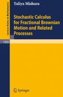
Fig. 3.1. The Haar functions 𝐻2𝑗 +𝑘 and the Schauder functions 𝑆2𝑗 +𝑘 .
3.2 The Lévy–Ciesielski construction This approach goes back to Lévy [144, pp. 492–494] but it got its definitive form in the hands of Ciesielski, cf. [34; 35]. Following Ciesielski we use the Haar orthonormal system in the random orthogonal series from Section 3.1. Write (𝐻𝑛 )𝑛⩾0 and (𝑆𝑛 )𝑛⩾0 for the families of Haar and Schauder functions, respectively. If 𝑛 = 0 and 𝑛 = 2𝑗 + 𝑘, 𝑗 ⩾ 0, 𝑘 = 0, 1, . . . , 2𝑗 − 1, they are defined as 𝑆0 (𝑡) = 𝑡
𝐻0 (𝑡) = 1, 𝑗
) +2 2 , on [ 2𝑘𝑗 , 2𝑘+1 { 2𝑗+1 { { { { { 𝑗 𝐻2𝑗 +𝑘 (𝑡) = {−2 2 , on [ 2𝑘+1 ), , 𝑘+1 2𝑗+1 2𝑗 { { { { { otherwise {0,
𝑆2𝑗 +𝑘 (𝑡) = ⟨𝟙[0,𝑡] , 𝐻2𝑗 +𝑘 ⟩𝐿2 𝑡
= ∫ 𝐻2𝑗 +𝑘 (𝑠) 𝑑𝑠, 0
supp 𝑆𝑛 = supp 𝐻𝑛 .
For 𝑛 = 2𝑗 + 𝑘 the graphs of the Haar and Schauder functions are shown in Figure 3.1. 1 Obviously, ∫0 𝐻𝑛 (𝑡) 𝑑𝑡 = 0 for all 𝑛 ⩾ 1 and 𝐻2𝑗 +𝑘 𝐻2𝑗 +ℓ = 𝑆2𝑗 +𝑘 𝑆2𝑗 +ℓ = 0 for all 𝑗 ⩾ 0, 𝑘 ≠ ℓ. The Schauder functions 𝑆2𝑗 +𝑘 are tent-functions with support [𝑘2−𝑗 , (𝑘+1)2−𝑗 ] and maximal value 12 2−𝑗/2 at the tip of the tent. The Haar functions are also an orthonormal system in 𝐿2 = 𝐿2 ([0, 1], 𝑑𝑡), i. e. 1
{1, ⟨𝐻𝑛 , 𝐻𝑚 ⟩𝐿2 = ∫ 𝐻𝑛 (𝑡)𝐻𝑚 (𝑡) 𝑑𝑡 = { 0, 0 {
𝑚=𝑛 𝑚 ≠ 𝑛,
for all 𝑛, 𝑚 ⩾ 0,
3.2 The Lévy–Ciesielski construction
| 23
and they are a basis of 𝐿2 ([0, 1], 𝑑𝑠), i. e. a complete orthonormal system, see Theorem A.48 in the appendix. 3.2 Theorem (Lévy 1940; Ciesielski 1959). There is a probability space (𝛺, A , ℙ) and Ex. 3.3 a sequence of iid standard normal random variables (𝐺𝑛 )𝑛⩾0 such that ∞
𝑊(𝑡, 𝜔) = ∑ 𝐺𝑛 (𝜔)⟨𝟙[0,𝑡) , 𝐻𝑛 ⟩𝐿2 ,
𝑡 ∈ [0, 1],
(3.1)
𝑛=0
is a Brownian motion. Proof. Let 𝑊(𝑡) be as in Lemma 3.1 where we take the Haar functions 𝐻𝑛 as orthonormal system in 𝐿2 (𝑑𝑡). As probability space (𝛺, A , ℙ) we use the probability space which supports the (countably many) independent Gaussian random variables (𝐺𝑛 )𝑛⩾0 from the construction of 𝑊(𝑡). It is enough to prove that the sample paths 𝑡 → 𝑊(𝑡, 𝜔) are continuous. By definition, the partial sums 𝑁−1
𝑁−1
𝑡 → 𝑊𝑁 (𝑡, 𝜔) = ∑ 𝐺𝑛 (𝜔)⟨𝟙[0,𝑡) , 𝐻𝑛 ⟩𝐿2 = ∑ 𝐺𝑛 (𝜔)𝑆𝑛 (𝑡). 𝑛=0
(3.2)
𝑛=0
are continuous for all 𝑁 ⩾ 1, and it is sufficient to prove that (a subsequence of) (𝑊𝑁 (𝑡))𝑁⩾0 converges uniformly to 𝑊(𝑡). The next step of the proof is similar to the proof of the Riesz-Fischer theorem on the completeness of 𝐿𝑝 spaces, see e. g. [204, Theorem 12.7]. Consider the random variable 2𝑗 −1
𝛥 𝑗 (𝑡) := 𝑊2𝑗+1 (𝑡) − 𝑊2𝑗 (𝑡) = ∑ 𝐺2𝑗 +𝑘 𝑆2𝑗 +𝑘 (𝑡). 𝑘=0
If 𝑘 ≠ ℓ, then 𝑆2𝑗 +𝑘 𝑆2𝑗 +ℓ = 0, and we see 2𝑗 −1
|𝛥 𝑗 (𝑡)|4 = ∑
𝐺2𝑗 +𝑘 𝐺2𝑗 +ℓ 𝐺2𝑗 +𝑝 𝐺2𝑗 +𝑞 𝑆2𝑗 +𝑘 (𝑡)𝑆2𝑗 +ℓ (𝑡)𝑆2𝑗 +𝑝 (𝑡)𝑆2𝑗 +𝑞 (𝑡)
𝑘,ℓ,𝑝,𝑞=0 2𝑗 −1
= ∑ 𝐺24𝑗 +𝑘 |𝑆2𝑗 +𝑘 (𝑡)|4 𝑘=0
2𝑗 −1
⩽ ∑ 𝐺24𝑗 +𝑘 2−2𝑗 . 𝑘=0
Since the right-hand side does not depend on 𝑡 ∈ [0, 1] and since 𝔼 𝐺𝑛4 = 3 (use 2.3 for 𝐺𝑛 ∼ N(0, 1)) we get 4
2𝑗 −1
𝔼 [ sup |𝛥 𝑗 (𝑡)| ] ⩽ 3 ∑ 2−2𝑗 = 3 ⋅ 2−𝑗 𝑡∈[0,1]
𝑘=0
for all 𝑗 ⩾ 1.
24 | 3 Constructions of Brownian motion For 𝑛 < 𝑁 we find using Minkowski’s inequality in 𝐿4 (ℙ) ∞ sup sup 𝑊2𝑁 (𝑡) − 𝑊2𝑛 (𝑡) ⩽ ∑ sup ⏟⏟⏟⏟⏟⏟⏟⏟⏟⏟⏟⏟⏟⏟⏟⏟⏟⏟⏟⏟⏟⏟⏟⏟⏟⏟⏟⏟⏟⏟⏟⏟⏟ 𝑊 𝑗 (𝑡) − 𝑊2𝑗−1 (𝑡) 2 4 𝑁>𝑛 𝑡∈[0,1] 𝐿4 𝐿 𝑗=𝑛+1 𝑡∈[0,1] =|𝛥 𝑗−1 (𝑡)| ∞ ⩽ ∑ sup 𝛥 𝑗−1 (𝑡) 𝐿4 𝑡∈[0,1] 𝑗=𝑛+1 ∞
⩽ 31/4 ∑ 2−(𝑗−1)/4 → 0. 𝑗=𝑛+1
𝑛→∞
By monotone convergence we get lim sup sup 𝑊2𝑁 (𝑡) − 𝑊2𝑛 (𝑡) = lim sup sup 𝑊2𝑁 (𝑡) − 𝑊2𝑛 (𝑡) = 0. 4 𝑛→∞ 𝑁>𝑛 𝑡∈[0,1] 4 𝑛→∞ 𝑁>𝑛 𝑡∈[0,1] 𝐿 𝐿 This shows that there exists a subset 𝛺0 ⊂ 𝛺 with ℙ(𝛺0 ) = 1 such that Ex. 3.4
lim sup sup 𝑊2𝑁 (𝑡, 𝜔) − 𝑊2𝑛 (𝑡, 𝜔) = 0 for all 𝜔 ∈ 𝛺0 .
𝑛→∞ 𝑁>𝑛
𝑡∈[0,1]
By the completeness of the space of continuous functions, there is a subsequence of (𝑊2𝑗 (𝑡, 𝜔))𝑗⩾1 which converges uniformly in 𝑡 ∈ [0, 1]. Since we know that 𝑊(𝑡, 𝜔) is the limiting function, we conclude that 𝑊(𝑡, 𝜔) inherits the continuity of the 𝑊2𝑗 (𝑡, 𝜔) for all 𝜔 ∈ 𝛺0 . It remains to define Brownian motion everywhere on 𝛺. We set {𝑊(𝑡, 𝜔), ̃ 𝜔) := 𝑊(𝑡, { 0, {
𝜔 ∈ 𝛺0 𝜔 ∉ 𝛺0 .
̃ 𝜔) is a oneAs ℙ(𝛺 \ 𝛺0 ) = 0, Lemma 3.1 remains valid for 𝑊̃ which means that 𝑊(𝑡, dimensional Brownian motion indexed by [0, 1]. Strictly speaking, 𝑊 is not a Brownian motion but has a restriction 𝑊̃ which is a Brownian motion. 3.3 Definition. Let (𝑋𝑡 )𝑡∈𝐼 and (𝑌𝑡 )𝑡∈𝐼 be two ℝ𝑑 -valued stochastic processes with the same index set. We call 𝑋 and 𝑌 Ex. 3.6 indistinguishable if they are defined on the same probability space and if
ℙ(𝑋𝑡 = 𝑌𝑡
∀𝑡 ∈ 𝐼) = 1;
Ex. 3.5 modifications if they are defined on the same probability space and
ℙ(𝑋𝑡 = 𝑌𝑡 ) = 1 for all 𝑡 ∈ 𝐼; equivalent if they have the same finite dimensional distributions, i. e. (𝑋𝑡1 , . . . , 𝑋𝑡𝑛 ) ∼ (𝑌𝑡1 , . . . , 𝑌𝑡𝑛 )
for all 𝑡1 , . . . , 𝑡𝑛 ∈ 𝐼, 𝑛 ⩾ 1
(𝑋, 𝑌 need not be defined on the same probability space).
3.2 The Lévy–Ciesielski construction
| 25
Now it is easy to construct a real-valued Brownian motion for all 𝑡 ⩾ 0. 3.4 Corollary. Let (𝑊𝑘 (𝑡))𝑡∈[0,1] , 𝑘 ⩾ 0, be independent real-valued Brownian motions on the same probability space. Then 𝑊0 (𝑡), 𝑡 ∈ [0, 1); { { { { { { {𝑊0 (1) + 𝑊1 (𝑡 − 1), 𝑡 ∈ [1, 2); 𝐵(𝑡) := { { 𝑘−1 { { { { ∑ 𝑊𝑗 (1) + 𝑊𝑘 (𝑡 − 𝑘), 𝑡 ∈ [𝑘, 𝑘 + 1), 𝑘 ⩾ 2. { { 𝑗=0
(3.3)
is a BM1 indexed by 𝑡 ∈ [0, ∞). Proof. Let 𝐵𝑘 be a copy of the process 𝑊 from Theorem 3.2 and denote the corresponding probability space by (𝛺𝑘 , A𝑘 , ℙ𝑘 ). On the product space (𝛺, A , ℙ) = ⨂𝑘⩾1 (𝛺𝑘 , A𝑘 , ℙ𝑘 ), 𝜔 = (𝜔1 , 𝜔2 , . . .), we define processes 𝑊𝑘 (𝜔) := 𝐵𝑘 (𝜔𝑘 ); by construction, these are independent Brownian motions on (𝛺, A , ℙ). Let us check (B0)–(B4) for the process (𝐵(𝑡))𝑡⩾0 defined by (3.3). The properties (B0) and (B4) are obvious. Let 𝑠 < 𝑡 and assume that 𝑠 ∈ [ℓ, ℓ + 1), 𝑡 ∈ [𝑚, 𝑚 + 1) where ℓ ⩽ 𝑚. Then 𝑚−1
ℓ−1
𝑗=0
𝑗=0
𝐵(𝑡) − 𝐵(𝑠) = ∑ 𝑊𝑗 (1) + 𝑊𝑚 (𝑡 − 𝑚) − ∑ 𝑊𝑗 (1) − 𝑊ℓ (𝑠 − ℓ) 𝑚−1
= ∑ 𝑊𝑗 (1) + 𝑊𝑚 (𝑡 − 𝑚) − 𝑊ℓ (𝑠 − ℓ) 𝑗=ℓ
𝑊𝑚 (𝑡 − 𝑚) − 𝑊𝑚 (𝑠 − 𝑚) ∼ N(0, 𝑡 − 𝑠), { { { ={ 𝑚−1 { { ℓ ℓ (𝑊 ∑ 𝑊𝑗 (1) + 𝑊𝑚 (𝑡 − 𝑚), (1) − 𝑊 (𝑠 − ℓ)) + { 𝑗=ℓ+1 ⏟⏟⏟⏟⏟⏟⏟⏟⏟⏟⏟⏟⏟⏟⏟⏟⏟⏟⏟⏟⏟⏟⏟⏟⏟⏟⏟⏟⏟⏟⏟⏟⏟⏟⏟⏟⏟⏟⏟⏟⏟⏟⏟⏟⏟⏟⏟⏟⏟⏟⏟⏟⏟⏟⏟⏟⏟⏟⏟⏟⏟⏟⏟⏟⏟⏟⏟⏟⏟⏟⏟⏟⏟⏟⏟⏟⏟⏟⏟⏟⏟⏟⏟⏟⏟⏟⏟⏟⏟⏟⏟⏟⏟
ℓ=𝑚 ℓ < 𝑚.
indep ∼ N(0,1−𝑠+ℓ)⋆N(0,1)⋆𝑚−ℓ−1 ⋆N(0,𝑡−𝑚)=N(0,𝑡−𝑠)
This proves (B2). We show (B1) only for two increments 𝐵(𝑢)−𝐵(𝑡) and 𝐵(𝑡)−𝐵(𝑠) where 𝑠 < 𝑡 < 𝑢. As before, 𝑠 ∈ [ℓ, ℓ + 1), 𝑡 ∈ [𝑚, 𝑚 + 1) and 𝑢 ∈ [𝑛, 𝑛 + 1) where ℓ ⩽ 𝑚 ⩽ 𝑛. Then 𝑊𝑚 (𝑢 − 𝑚) − 𝑊𝑚 (𝑡 − 𝑚), 𝑚=𝑛 { { { 𝑛−1 𝐵(𝑢) − 𝐵(𝑡) = { 𝑚 {(𝑊 (1) − 𝑊𝑚 (𝑡 − 𝑚)) + ∑ 𝑊𝑗 (1) + 𝑊𝑛 (𝑢 − 𝑛), 𝑚 < 𝑛. { 𝑗=𝑚+1 { By assumption, the random variables appearing in the representation of the increments 𝐵(𝑢) − 𝐵(𝑡) and 𝐵(𝑡) − 𝐵(𝑠) are independent which means that the increments are independent. The case of finitely many, not necessarily adjacent, increments is similar.
26 | 3 Constructions of Brownian motion
3.3 Wiener’s construction This is also a series approach, but Wiener used the trigonometric functions (𝑒𝑖𝑛𝜋𝑡 )𝑛∈ℤ as orthonormal basis for 𝐿2 [0, 1]. In this case we obtain Brownian motion on [0, 1] as a Wiener-Fourier series ∞
𝑊(𝑡, 𝜔) := 𝑡𝐺0 (𝜔) + √2 ∑
𝑛=1
sin(𝑛𝜋𝑡) 𝐺𝑛 (𝜔), 𝑛𝜋
(3.4)
where (𝐺𝑛 )𝑛⩾0 are iid standard normal random variables. Lemma 3.1 remains valid for (3.4) and shows that the series converges in 𝐿2 and that the limit satisfies (B0)–(B3). 3.5 Theorem (Wiener 1923, 1924). The random process (𝑊𝑡 )𝑡∈[0,1] defined by (3.4) is a one-dimensional Brownian motion. Using Corollary 3.4 we can extend the construction of Theorem 3.5 to get a Brownian motion with time set [0, ∞). Proof of Theorem 3.5. It is enough to prove that (3.4) defines a continuous random process. Let 𝑁 sin(𝑛𝜋𝑡) 𝑊𝑁 (𝑡, 𝜔) := 𝑡𝐺0 (𝜔) + √2 ∑ 𝐺𝑛 (𝜔). 𝑛𝜋 𝑛=1 We will show that (𝑊2𝑛 )𝑛⩾1 is a Cauchy sequence in 𝐿2 (ℙ) uniformly for all 𝑡 ∈ [0, 1]. Set 𝛥 𝑗 (𝑡) := 𝑊2𝑗+1 (𝑡) − 𝑊2𝑗 (𝑡). Using | Im 𝑧| ⩽ |𝑧| for 𝑧 ∈ ℂ, we see 2 2𝑗+1 𝑖𝑘𝜋𝑡 2 sin(𝑘𝜋𝑡) 𝑒 |𝛥 𝑗 (𝑡)| = ( ∑ 𝐺𝑘 ) ⩽ ∑ 𝐺𝑘 , 𝑘 𝑘=2𝑗 +1 𝑘 𝑘=2𝑗 +1 2𝑗+1
2
and since |𝑧|2 = 𝑧𝑧̄ we get |𝛥 𝑗 (𝑡)|2
⩽
2𝑗+1
2𝑗+1
∑
∑
𝑘=2𝑗 +1 ℓ=2𝑗 +1
𝑒𝑖𝑘𝜋𝑡 𝑒−𝑖ℓ𝜋𝑡 𝐺𝑘 𝐺ℓ 𝑘ℓ
2𝑗+1
= 𝑚=𝑘−ℓ
=
⩽
𝑗+1
2 𝑘−1 𝐺2 𝑒𝑖𝑘𝜋𝑡 𝑒−𝑖ℓ𝜋𝑡 ∑ 2𝑘 + 2 ∑ ∑ 𝐺𝑘 𝐺ℓ 𝑘 𝑘ℓ 𝑘=2𝑗 +1 𝑘=2𝑗 +1 ℓ=2𝑗 +1 2𝑗+1
𝑗
𝑗+1
2 −1 2 −𝑚 𝐺𝑘2 𝑒𝑖𝑚𝜋𝑡 𝐺ℓ 𝐺ℓ+𝑚 +2 ∑ ∑ 2 𝑘 𝑚=1 ℓ=2𝑗 +1 ℓ(ℓ + 𝑚) 𝑘=2𝑗 +1 2𝑗+1 2𝑗 −1 2𝑗+1 −𝑚 𝐺𝑘2 𝐺ℓ 𝐺ℓ+𝑚 . ∑ 2 + 2 ∑ ∑ 𝑘 𝑚=1 ℓ=2𝑗 +1 ℓ(ℓ + 𝑚) 𝑘=2𝑗 +1
∑
3.3 Wiener’s construction
| 27
Note that the right-hand side is independent of 𝑡. On both sides we can therefore take the supremum over all 𝑡 ∈ [0, 1] and then the mean value 𝔼(⋅ ⋅ ⋅ ). From Jensen’s inequality, 𝔼 |𝑍| ⩽ √𝔼 |𝑍|2 , we conclude 2𝑗 −1 2𝑗+1 −𝑚 𝔼 𝐺𝑘2 𝐺ℓ 𝐺ℓ+𝑚 + 2 ∑ 𝔼 ∑ 𝔼 ( sup |𝛥 𝑗 (𝑡)| ) ⩽ ∑ 𝑘2 ℓ=2𝑗 +1 ℓ(ℓ + 𝑚) 𝑡∈[0,1] 𝑚=1 𝑘=2𝑗 +1 2
2𝑗+1
2𝑗+1
𝑗
2
2 −1 2 −𝑚 𝔼 𝐺𝑘2 √𝔼 ( ∑ 𝐺ℓ 𝐺ℓ+𝑚 ) . ∑ ⩽ ∑ + 2 𝑘2 ℓ(ℓ + 𝑚) 𝑚=1 𝑘=2𝑗 +1 ℓ=2𝑗 +1 𝑗+1
If we expand the square we get expressions of the form 𝔼(𝐺ℓ 𝐺ℓ+𝑚 𝐺ℓ 𝐺ℓ +𝑚 ); these expectations are zero whenever ℓ ≠ ℓ . Thus, 2𝑗+1
𝔼 ( sup |𝛥 𝑗 (𝑡)|2 ) = ∑ 𝑡∈[0,1]
𝑘=2𝑗 +1 2𝑗+1
= ∑ 𝑘=2𝑗 +1 2𝑗+1
⩽ ∑ 𝑘=2𝑗 +1
𝑗
𝑗+1
𝑗
𝑗+1
2 2 −1 2 −𝑚 𝐺𝐺 1 √ ∑ 𝔼 ( ℓ ℓ+𝑚 ) . ∑ + 2 𝑘2 ℓ(ℓ + 𝑚) 𝑚=1 ℓ=2𝑗 +1 2 −1 2 −𝑚 1 1 ∑√ ∑ 2 + 2 𝑘2 ℓ (ℓ + 𝑚)2 𝑗 𝑚=1 ℓ=2 +1 𝑗
𝑗+1
2 −1 2 −𝑚 1 1 +2 ∑ √ ∑ 𝑗 2 𝑗 )2 (2𝑗 )2 (2 ) (2 𝑚=1 ℓ=2𝑗 +1
⩽ 2𝑗 ⋅ 2−2𝑗 + 2 ⋅ 2𝑗 ⋅ √2𝑗 ⋅ 2−4𝑗 ⩽ 3 ⋅ 2−𝑗/2 . From this point onwards we can follow the proof of Theorem 3.2: For 𝑛 < 𝑁 we find using Minkowski’s inequality in 𝐿2 (ℙ) ∞ sup sup 𝑊2𝑁 (𝑡) − 𝑊2𝑛 (𝑡) ⩽ ∑ sup ⏟⏟⏟⏟⏟⏟⏟⏟⏟⏟⏟⏟⏟⏟⏟⏟⏟⏟⏟⏟⏟⏟⏟⏟⏟⏟⏟⏟⏟⏟⏟⏟⏟ 𝑊 (𝑡) − 𝑊 (𝑡) 𝑗 𝑗−1 2 2 𝑁>𝑛 𝑡∈[0,1] 2 𝐿2 𝐿 𝑗=𝑛+1 𝑡∈[0,1] =|𝛥 (𝑡)| 𝑗−1
⩽ ∑ sup 𝛥 𝑗−1 (𝑡) 𝐿2 𝑡∈[0,1] 𝑗=𝑛+1 ∞
∞
⩽ 31/4 ∑ 2−(𝑗−1)/4 → 0. 𝑗=𝑛+1
𝑛→∞
By monotone convergence we get lim sup sup 𝑊2𝑁 (𝑡) − 𝑊2𝑛 (𝑡) = lim | sup sup 𝑊2𝑁 (𝑡) − 𝑊2𝑛 (𝑡) = 0. 2 𝑛→∞ 𝑁>𝑛 𝑡∈[0,1] 2 𝑛→∞ 𝑁>𝑛 𝑡∈[0,1] 𝐿 𝐿 This shows that there exists a subset 𝛺0 ⊂ 𝛺 with ℙ(𝛺0 ) = 1 such that lim sup sup 𝑊2𝑁 (𝑡, 𝜔) − 𝑊2𝑛 (𝑡, 𝜔) = 0 for all 𝜔 ∈ 𝛺0 .
𝑛→∞ 𝑁>𝑛
𝑡∈[0,1]
Ex. 3.4
28 | 3 Constructions of Brownian motion By the completeness of the space of continuous functions, there is a subsequence of (𝑊2𝑗 (𝑡, 𝜔))𝑗⩾1 which converges uniformly in 𝑡 ∈ [0, 1]. Since we know that 𝑊(𝑡, 𝜔) is the limiting function, we conclude that 𝑊(𝑡, 𝜔) inherits the continuity of the 𝑊2𝑗 (𝑡, 𝜔) for all 𝜔 ∈ 𝛺0 . It remains to define the Brownian motion everywhere on 𝛺. We set {𝑊(𝑡, 𝜔), ̃ 𝜔) := 𝑊(𝑡, { 0, {
𝜔 ∈ 𝛺0 𝜔 ∉ 𝛺0 .
̃ 𝜔) is a Since ℙ(𝛺 \ 𝛺0 ) = 0, Lemma 3.1 remains valid for 𝑊̃ which means that 𝑊(𝑡, one-dimensional Brownian motion indexed by [0, 1].
3.4 Lévy’s original argument Lévy’s original argument is based on interpolation. Let 𝑡0 < 𝑡 < 𝑡1 and assume that (𝑊𝑡 )𝑡∈[0,1] is a Brownian motion. Then 𝐺 := 𝑊(𝑡) − 𝑊(𝑡0 )
and
𝐺 := 𝑊(𝑡1 ) − 𝑊(𝑡)
are independent Gaussian random variables with mean 0 and variances 𝑡 − 𝑡0 and 𝑡1 −𝑡, respectively. In order to simulate the positions 𝑊(𝑡0 ), 𝑊(𝑡), 𝑊(𝑡1 ) we could either determine 𝑊(𝑡0 ) and then 𝐺 and 𝐺 independently or, equivalently, simulate first 𝑊(𝑡0 ) and 𝑊(𝑡1 ) − 𝑊(𝑡0 ), and obtain 𝑊(𝑡) by interpolation. Let 𝛤 be a further standard normal random variable which is independent of 𝑊(𝑡0 ) and 𝑊(𝑡1 ) − 𝑊(𝑡0 ). Then (𝑡1 − 𝑡)𝑊(𝑡0 ) + (𝑡 − 𝑡0 )𝑊(𝑡1 ) (𝑡 − 𝑡0 )(𝑡1 − 𝑡) +√ 𝛤 𝑡1 − 𝑡0 𝑡1 − 𝑡0 = 𝑊(𝑡0 ) +
(𝑡 − 𝑡0 )(𝑡1 − 𝑡) 𝑡 − 𝑡0 (𝑊(𝑡1 ) − 𝑊(𝑡0 )) + √ 𝛤 𝑡1 − 𝑡0 𝑡1 − 𝑡0
is – because of the independence of 𝑊(𝑡0 ), 𝑊(𝑡1 ) − 𝑊(𝑡0 ) and 𝛤 – a Gaussian random variable with mean zero and variance 𝑡. Thus, we get a random variable with the same Ex. 3.8 distribution as 𝑊(𝑡) and so ℙ(𝑊(𝑡) ∈ ⋅ |𝑊(𝑡0 ) = 𝑥0 , 𝑊(𝑡1 ) = 𝑥1 ) = N(𝑚𝑡 , 𝜎𝑡2 ) 𝑚𝑡 =
(𝑡1 − 𝑡)𝑥0 + (𝑡 − 𝑡0 )𝑥1 𝑡1 − 𝑡0
and 𝜎𝑡2 =
(𝑡 − 𝑡0 )(𝑡1 − 𝑡) . 𝑡1 − 𝑡0
(3.5)
If 𝑡 is the midpoint of [𝑡0 , 𝑡1 ], Lévy’s method leads to the following prescription: 3.6 Algorithm. Set 𝑊(0) = 0 and let 𝑊(1) be an N(0, 1) distributed random variable. Let 𝑛 ⩾ 1 and assume that the random variables 𝑊(𝑘2−𝑛 ), 𝑘 = 1, . . . , 2𝑛 − 1 have already
3.4 Lévy’s original argument
| 29
𝑊1 2
𝑊1
𝑊1
1 2
1 𝑊1
𝑊1
𝑊1
𝑊1
𝑊1
𝑊1
𝑊3
𝑊3
2
1
2
4
4
4
4
1 4
1 2
3 4
1
1 4
1 2
3 4
1
Fig. 3.2. The first four interpolation steps in Lévy’s construction of Brownian motion.
been constructed. Then {𝑊(𝑘2−𝑛 ), ℓ = 2𝑘, 𝑊(ℓ2−𝑛−1 ) := { 1 −𝑛 −𝑛 (𝑊(𝑘2 ) + 𝑊((𝑘 + 1)2 )) + 𝛤2𝑛 +𝑘 , ℓ = 2𝑘 + 1, {2 where 𝛤2𝑛 +𝑘 is an independent (of everything else) Gaussian random variable with mean zero and variance 2−𝑛 /4, cf. Figure 3.3. In-between the nodes we use piecewise-linear interpolation: 𝑊2𝑛 (𝑡, 𝜔) := Linear interpolation of (𝑊(𝑘2−𝑛 , 𝜔), 𝑘 = 0, 1, . . . , 2𝑛 ),
𝑛 ⩾ 1.
At the dyadic points 𝑡 = 𝑘2−𝑗 we get the ‘true’ value of 𝑊(𝑡, 𝜔), while the linear interpolation is an approximation, see Figure 3.2. We will now see that these piecewise linear functions converge to the random function 𝑡 → 𝑊(𝑡, 𝜔). 3.7 Theorem (Lévy 1940). The series ∞
𝑊(𝑡, 𝜔) := ∑ (𝑊2𝑛+1 (𝑡, 𝜔) − 𝑊2𝑛 (𝑡, 𝜔)) + 𝑊1 (𝑡, 𝜔), 𝑛=0
converges a. s. uniformly. In particular (𝑊(𝑡))𝑡∈[0,1] is a BM1 .
𝑡 ∈ [0, 1],
30 | 3 Constructions of Brownian motion
𝑊2𝑛+1 (𝑡)
𝛥 𝑛 (𝑡)
𝑊2𝑛 (𝑡)
2𝑘−1 2𝑛+1
𝑘−1 2𝑛
Fig. 3.3. The 𝑛th interpolation step in Lévy’s construction. 𝛥 𝑛 (𝑡) = 𝑊2𝑛+1 (𝑡) − 𝑊2𝑛 (𝑡)
𝑘 2𝑛
Using Corollary 3.4 we can extend the construction of Theorem 3.7 to get a Brownian motion with time set [0, ∞). Proof of Theorem 3.7. Set 𝛥 𝑛 (𝑡, 𝜔) := 𝑊2𝑛+1 (𝑡, 𝜔) − 𝑊2𝑛 (𝑡, 𝜔). By construction, 𝛥 𝑛 ((2𝑘 − 1)2−𝑛−1 , 𝜔) = 𝛤2𝑛 +(𝑘−1) (𝜔),
𝑘 = 1, 2, . . . , 2𝑛 ,
are iid N(0, 2−(𝑛+2) ) distributed random variables. Therefore, ℙ ( max𝑛 𝛥 𝑛 ((2𝑘 − 1)2−𝑛−1 ) > 1⩽𝑘⩽2
𝑥𝑛 ) ⩽ 2𝑛 ℙ (√2𝑛+2 𝛥 𝑛 (2−𝑛−1 ) > 𝑥𝑛 ) √2𝑛+2
and the right-hand side equals ∞
∞
𝑛
𝑛
2 𝑟 −𝑟2 /2 2𝑛+1 2𝑛+1 −𝑥𝑛2 /2 2 ⋅ 2𝑛 ∫ 𝑒−𝑟 /2 𝑑𝑟 ⩽ ∫ 𝑒 𝑑𝑟 = . 𝑒 √2𝜋 √2𝜋 𝑥𝑛 𝑥𝑛 √2𝜋 𝑥 𝑥
Choose 𝑐 > 1 and 𝑥𝑛 := 𝑐√2𝑛 log 2. Then ∞
∑ ℙ ( max𝑛 𝛥 𝑛 ((2𝑘 − 1)2−𝑛−1 ) >
𝑛=1
1⩽𝑘⩽2
∞ 𝑥𝑛 2𝑛+1 −𝑐2 log 2𝑛 )⩽∑ 𝑒 √2𝑛+2 𝑛=1 𝑐√2𝜋
=
2 ∞ −(𝑐2 −1)𝑛 ∑2 < ∞. 𝑐√2𝜋 𝑛=1
Using the Borel–Cantelli lemma we find a set 𝛺0 ⊂ 𝛺 with ℙ(𝛺0 ) = 1 such that for every 𝜔 ∈ 𝛺0 there is some 𝑁(𝜔) ⩾ 1 with 𝑛 log 2 max𝑛 𝛥 𝑛 ((2𝑘 − 1)2−𝑛−1 ) ⩽ 𝑐√ 𝑛+1 1⩽𝑘⩽2 2
for all 𝑛 ⩾ 𝑁(𝜔).
3.4 Lévy’s original argument
| 31
𝛥 𝑛 (𝑡) is the distance between the polygonal arcs 𝑊2𝑛+1 (𝑡) and 𝑊2𝑛 (𝑡); the maximum is attained at one of the midpoints of the intervals [(𝑘 − 1)2−𝑛 , 𝑘2−𝑛 ], 𝑘 = 1, . . . , 2𝑛 , see Figure 3.3. Thus sup 𝑊2𝑛+1 (𝑡, 𝜔) − 𝑊2𝑛 (𝑡, 𝜔) ⩽ max𝑛 𝛥 𝑛 ((2𝑘 − 1)2−𝑛−1 , 𝜔) 1⩽𝑘⩽2
0⩽𝑡⩽1
⩽ 𝑐√
𝑛 log 2 2𝑛+1
for all 𝑛 ⩾ 𝑁(𝜔),
which shows that the limit ∞
𝑊(𝑡, 𝜔) := lim 𝑊2𝑁 (𝑡, 𝜔) = ∑ (𝑊2𝑛+1 (𝑡, 𝜔) − 𝑊2𝑛 (𝑡, 𝜔)) + 𝑊1 (𝑡, 𝜔) 𝑁→∞
𝑛=0
exists for all 𝜔 ∈ 𝛺0 uniformly in 𝑡 ∈ [0, 1]. Therefore, 𝑡 → 𝑊(𝑡, 𝜔), 𝜔 ∈ 𝛺0 , inherits the continuity of the polygonal arcs 𝑡 → 𝑊2𝑛 (𝑡, 𝜔). Set {𝑊(𝑡, 𝜔), ̃ 𝜔) := 𝑊(𝑡, { 0, {
𝜔 ∈ 𝛺0 , 𝜔 ∉ 𝛺0 .
By construction, we find for all 0 ⩽ 𝑗 ⩽ 𝑘 ⩽ 2𝑛 −𝑛 ̃ ̃ −𝑛 ) = 𝑊2𝑛 (𝑘2−𝑛 ) − 𝑊2𝑛 (𝑗2−𝑛 ) 𝑊(𝑘2 ) − 𝑊(𝑗2 𝑘
= ∑ (𝑊2𝑛 (ℓ2−𝑛 ) − 𝑊2𝑛 ((ℓ − 1)2−𝑛 )) ℓ=𝑗+1
∼ N(0, (𝑘 − 𝑗)2−𝑛 ).
iid
̃ is continuous and since the dyadic numbers are dense in [0, 𝑡], we conSince 𝑡 → 𝑊(𝑡) ̃ 𝑗 ) − 𝑊(𝑡 ̃ 𝑗−1 ), 0 = 𝑡0 < 𝑡1 < ⋅ ⋅ ⋅ < 𝑡𝑁 ⩽ 1 are independent clude that the increments 𝑊(𝑡 ̃ N(0, 𝑡𝑗 − 𝑡𝑗−1 ) distributed random variables. This shows that (𝑊(𝑡)) 𝑡∈[0,1] is a Brownian motion. 3.8 Rigorous proof of (3.5). We close this section with a rigorous proof of Lévy’s for- Ex. 3.8 mula (3.5). Observe that for all 0 ⩽ 𝑠 < 𝑡 and 𝜉 ∈ ℝ 𝔼 (𝑒𝑖𝜉𝑊(𝑡) 𝑊(𝑠)) = 𝑒𝑖𝜉𝑊(𝑠) 𝔼 (𝑒𝑖𝜉(𝑊(𝑡)−𝑊(𝑠)) 𝑊(𝑠)) (B1)
= 𝑒𝑖𝜉𝑊(𝑠) 𝔼 (𝑒𝑖𝜉(𝑊(𝑡)−𝑊(𝑠)) )
(B2)
1
2
= 𝑒− 2 (𝑡−𝑠)𝜉 𝑒𝑖𝜉𝑊(𝑠) .
(2.5)
If we apply this equality to the projectively reflected (cf. 2.17) Brownian motion (𝑡𝑊(1/𝑡))𝑡>0 , we get 1 2 𝔼 (𝑒𝑖𝜉𝑡𝑊(1/𝑡) 𝑊(1/𝑠)) = 𝔼 (𝑒𝑖𝜉𝑡𝑊(1/𝑡) 𝑠𝑊(1/𝑠)) = 𝑒− 2 (𝑡−𝑠)𝜉 𝑒𝑖𝜉𝑠𝑊(1/𝑠) .
32 | 3 Constructions of Brownian motion Now set 𝑏 :=
1 𝑠
>
1 𝑡
=: 𝑎 and 𝜂 := 𝜉/𝑎 = 𝜉𝑡. Then
1 1 𝑎 1 𝔼 (𝑒𝑖𝜂𝑊(𝑎) 𝑊(𝑏)) = exp [− 𝑎2 ( − ) 𝜂2 ] exp [𝑖𝜂 𝑊(𝑏)] 2 𝑎 𝑏 𝑏 (3.6) 𝑎 1𝑎 2 = exp [− (𝑏 − 𝑎)𝜂 ] exp [𝑖𝜂 𝑊(𝑏)] . 2𝑏 𝑏 This is (3.5) for the case where (𝑡0 , 𝑡, 𝑡1 ) = (0, 𝑎, 𝑏) and 𝑥0 = 0. Now we fix 0 ⩽ 𝑡0 < 𝑡 < 𝑡1 and observe that 𝑊(𝑠 + 𝑡0 ) − 𝑊(𝑡0 ), 𝑠 ⩾ 0, is again a Brownian motion. Applying (3.6) yields 𝑡−𝑡 𝑡−𝑡0 −1 (𝑡 −𝑡)𝜂2 𝑖𝜂 𝑡 −𝑡0 (𝑊(𝑡1 )−𝑊(𝑡0 )) 𝔼 (𝑒𝑖𝜂(𝑊(𝑡)−𝑊(𝑡0 )) 𝑊(𝑡1 ) − 𝑊(𝑡0 )) = 𝑒 2 𝑡1 −𝑡0 1 𝑒 1 0 .
On the other hand, 𝑊(𝑡0 ) ⊥ ⊥(𝑊(𝑡) − 𝑊(𝑡0 ), 𝑊(𝑡1 ) − 𝑊(𝑡0 )) and 𝑖𝜂(𝑊(𝑡)−𝑊(𝑡0 )) 𝔼 (𝑒 𝑊(𝑡1 ) − 𝑊(𝑡0 )) 𝑖𝜂(𝑊(𝑡)−𝑊(𝑡0 )) (𝑒 =𝔼 𝑊(𝑡1 ) − 𝑊(𝑡0 ), 𝑊(𝑡0 )) 𝑖𝜂(𝑊(𝑡)−𝑊(𝑡0 )) = 𝔼 (𝑒 𝑊(𝑡1 ), 𝑊(𝑡0 )) −𝑖𝜂𝑊(𝑡0 ) 𝑖𝜂𝑊(𝑡) 𝔼 (𝑒 =𝑒 𝑊(𝑡1 ), 𝑊(𝑡0 )) . This proves 𝑡−𝑡 𝑡−𝑡0 (𝑡 −𝑡)𝜂2 𝑖𝜂 𝑡 −𝑡0 (𝑊(𝑡1 )−𝑊(𝑡0 )) 𝑖𝜂𝑊(𝑡0 ) −1 𝑒 1 0 𝑒 , 𝔼 (𝑒𝑖𝜂𝑊(𝑡) 𝑊(𝑡1 ), 𝑊(𝑡0 )) = 𝑒 2 𝑡1 −𝑡0 1
and (3.5) follows. 3.9 Remark. The polygonal arc 𝑊2𝑛 (𝑡, 𝜔) can be expressed by Schauder functions, cf. Figure 3.1. From (3.2) and the proof of Theorem 3.2 we know that ∞ 2𝑛 −1
𝑊(𝑡, 𝜔) = 𝐺0 (𝜔)𝑆0 (𝑡) + ∑ ∑ 𝐺2𝑛 +𝑘 (𝜔) 𝑆2𝑛 +𝑘 (𝑡), 𝑘=0 ⏟⏟⏟⏟⏟⏟⏟⏟⏟⏟⏟⏟⏟⏟⏟⏟⏟⏟⏟ 𝑛=0 ⏟⏟⏟⏟⏟⏟⏟⏟⏟⏟⏟⏟⏟⏟⏟⏟⏟⏟⏟⏟⏟⏟⏟⏟⏟⏟⏟⏟⏟⏟⏟⏟⏟⏟⏟⏟⏟⏟⏟ =𝑊1 (𝑡,𝜔)
=𝑊2𝑛+1 (𝑡,𝜔)−𝑊2𝑛 (𝑡,𝜔)
where 𝑆𝑛 (𝑡) are the Schauder functions. This shows that Lévy’s construction and the Lévy–Ciesielski constructions are essentially the same. For dyadic 𝑡 = 𝑘/2𝑛 , the expansion of 𝑊𝑡 is finite. Observe that 1o —
𝑊(1, 𝜔) = 𝐺0 (𝜔)𝑆0 (1)
o
1 1 𝑊( 12 , 𝜔) = 𝐺 0 (𝜔)𝑆0 ( 2 ) + 𝐺 1 (𝜔)𝑆1 ( 2 ) ⏟⏟⏟⏟⏟⏟⏟⏟⏟⏟⏟⏟⏟⏟⏟⏟⏟⏟⏟⏟⏟ ⏟⏟⏟⏟⏟⏟⏟⏟⏟⏟⏟⏟⏟⏟⏟⏟⏟⏟⏟⏟⏟
o
𝑊( 14 , 𝜔)
2 —
interpolation
3 —
𝑊( 34 , 𝜔)
=
= 𝛤1 ∼ N(0,1/4)
1 1 1 𝐺 0 (𝜔)𝑆0 ( 4 ) + 𝐺1 (𝜔)𝑆1 ( 4 ) + 𝐺 2 (𝜔)𝑆2 ( 4 ) ⏟⏟⏟⏟⏟⏟⏟⏟⏟⏟⏟⏟⏟⏟⏟⏟⏟⏟⏟⏟⏟⏟⏟⏟⏟⏟⏟⏟⏟⏟⏟⏟⏟⏟⏟⏟⏟⏟⏟⏟⏟⏟⏟⏟⏟⏟⏟⏟⏟ ⏟⏟⏟⏟⏟⏟⏟⏟⏟⏟⏟⏟⏟⏟⏟⏟⏟⏟⏟⏟⏟ interpolation = 𝛤2 ∼ N(0,1/8)
= 𝛤 ∼ N(0,1/8)
3 ⏞⏞⏞⏞⏞⏞⏞⏞⏞⏞⏞⏞⏞⏞⏞⏞⏞⏞⏞⏞⏞⏞⏞⏞⏞⏞⏞⏞⏞⏞⏞⏞⏞⏞⏞⏞⏞⏞⏞⏞⏞⏞⏞⏞⏞⏞⏞⏞⏞ ⏞⏞⏞⏞⏞⏞⏞⏞⏞⏞⏞⏞⏞⏞⏞⏞⏞⏞⏞⏞⏞ 3 3 = 𝐺0 (𝜔)𝑆0 ( 34 ) + 𝐺1 (𝜔)𝑆1 ( 34 ) +𝐺2 (𝜔) 𝑆⏟⏟⏟⏟⏟⏟⏟⏟⏟ 2 ( 4 ) + 𝐺3 (𝜔)𝑆3 ( 4 )
=0
4o —
...
The 2𝑛 th partial sum, 𝑊2𝑛 (𝑡, 𝜔), is therefore a piecewise linear interpolation of the Brownian path 𝑊𝑡 (𝜔) at the points (𝑘2−𝑛 , 𝑊(𝑘2−𝑛 , 𝜔)), 𝑘 = 0, 1, . . . , 2𝑛 .
3.5 Donsker’s construction
S5t
| 33
S10 t
1
1
1
t
−1
1
t
1
t
−1
St100
St1000
1
1
1
t
−1
−1
Fig. 3.4. The first few approximation steps in Donsker’s construction: 𝑛 = 5, 10, 100 and 1000.
3.5 Donsker’s construction Donsker’s invariance theorem shows that Brownian motion is a limit of linearly interpolated random walks – pretty much in the way we have started the discussion in Chapter 1. As before, the difficult point is to prove the sample continuity of the limiting process. On a probability space (𝛺, A , ℙ) let 𝜖𝑛 , 𝑛 ⩾ 1, be iid Bernoulli random variables such that ℙ(𝜖1 = 1) = ℙ(𝜖1 = −1) = 12 . Then 𝑆𝑛 := 𝜖1 + ⋅ ⋅ ⋅ + 𝜖𝑛 is a simple random walk. Interpolate linearly and apply Gaussian scaling 𝑆𝑛 (𝑡) :=
1 (𝑆 − (𝑛𝑡 − ⌊𝑛𝑡⌋)𝜖⌊𝑛𝑡⌋+1 ) , √𝑛 ⌊𝑛𝑡⌋
𝑡 ∈ [0, 1],
see Figure 3.4 illustrating this for 𝑛 = 5, 10, 100 and 1000 steps. In particular, 𝑆𝑛 (𝑗/𝑛) = 𝑆𝑗 /√𝑛. If 𝑗 = 𝑗(𝑛) and 𝑗/𝑛 = 𝑠 = const., the central limit 𝑑
theorem shows that 𝑆𝑛 (𝑗/𝑛) = √𝑠 𝑆𝑗 /√𝑗 → √𝑠 𝐺 as 𝑛 → ∞ where 𝐺 is a standard normal random variable. Moreover, for 𝑠 = 𝑗/𝑛 and 𝑡 = 𝑘/𝑛, 0 ⩽ 𝑗 < 𝑘 ⩽ 𝑛, the increment 𝑆𝑛 (𝑡) − 𝑆𝑛 (𝑠) = (𝑆𝑘 − 𝑆𝑗 )/√𝑛 is independent of 𝜖1 , . . . , 𝜖𝑗 , and therefore of all earlier increments of the same form. Moreover, 𝔼 (𝑆𝑛 (𝑡) − 𝑆𝑛 (𝑠)) = 0 and
𝕍 (𝑆𝑛 (𝑡) − 𝑆𝑛 (𝑠)) =
𝑘−𝑗 𝑛
= 𝑡 − 𝑠;
34 | 3 Constructions of Brownian motion in the limit we get a Gaussian increment with mean zero and variance 𝑡 − 𝑠. Since independence and stationarity of the increments are distributional properties, they are inherited by the limiting process – which we will denote by (𝐵𝑡 )𝑡∈[0,1] . We have seen that (𝐵𝑞 )𝑞∈[0,1]∩ℚ would have the properties (B0)–(B3) and it qualifies as a candidate for Brownian motion. If it had continuous sample paths, (B0)–(B3) would hold not only for rational times but for all 𝑡 ⩾ 0. That the limit exists and is uniform in 𝑡 is the essence of Donsker’s invariance principle. 3.10 Theorem (Donsker 1951). Let (𝐵(𝑡))𝑡∈[0,1] be a one-dimensional Brownian motion, (𝑆𝑛 (𝑡))𝑡∈[0,1] , 𝑛 ⩾ 1, be as above and 𝛷 : C([0, 1], ℝ) → ℝ a uniformly continuous bounded functional. Then lim 𝔼 𝛷(𝑆𝑛 (⋅)) = 𝔼 𝛷(𝐵(⋅)), 𝑛→∞
𝑛
i. e. 𝑆 (⋅) converges weakly to 𝐵(⋅). We will give a proof Donsker’s theorem in Chapter 14, Theorem 14.5. Since our proof relies on the existence of a Brownian motion, we cannot use it to construct (𝐵𝑡 )𝑡⩾0 . Nevertheless, it is an important result for the intuitive understanding of a Brownian motion as limit of random walks as well as for (simple) proofs of various limit theorems.
3.6 The Bachelier–Kolmogorov point of view The starting point of this construction is the observation that the finite dimensional marginal distributions of a Brownian motion are Gaussian random variables. More precisely, for any number of times 𝑡0 = 0 < 𝑡1 < ⋅ ⋅ ⋅ < 𝑡𝑛 , 𝑡𝑗 ∈ 𝐼, and all Borel sets 𝐴 1 , . . . , 𝐴 𝑛 ∈ B(ℝ) the finite dimensional distributions 𝑝𝑡1 ,...,𝑡𝑛 (𝐴 1 × ⋅ ⋅ ⋅ × 𝐴 𝑛 ) = ℙ(𝐵𝑡1 ∈ 𝐴 1 , . . . , 𝐵𝑡𝑛 ∈ 𝐴 𝑛 ) are mean-zero normal laws with covariance matrix 𝐶 = (𝑡𝑗 ∧ 𝑡𝑘 )𝑗,𝑘=1,...,𝑛 . From Theorem 2.6 we know that they are given by 𝑝𝑡1 ,...,𝑡𝑛 (𝐴 1 × ⋅ ⋅ ⋅ × 𝐴 𝑛 ) 1 1 = (2𝜋)𝑛/2 √det 𝐶 =
1
∫ 𝐴 1 ×⋅⋅⋅×𝐴 𝑛
1 exp (− ⟨𝑥, 𝐶−1 𝑥⟩) 𝑑𝑥 2 ∫
(2𝜋)𝑛/2 √∏𝑛𝑗=1 (𝑡𝑗 − 𝑡𝑗−1 ) 𝐴 1 ×⋅⋅⋅×𝐴 𝑛
2 1 𝑛 (𝑥𝑗 − 𝑥𝑗−1 ) ) 𝑑𝑥. exp (− ∑ 2 𝑗=1 𝑡𝑗 − 𝑡𝑗−1
We will characterize a stochastic process in terms of its finite dimensional distributions – and we will discuss this approach in Chapter 4 below. The idea is to identify a stochastic process with an infinite dimensional measure ℙ on the space of all sample
Problems
| 35
Bt
A2 t2
A4
t5
t
A1 A3 A5 Fig. 3.5. Brownian paths meeting (and missing) the sets 𝐴 1 , . . . , 𝐴 5 at times 𝑡1 , . . . , 𝑡5
paths 𝛺 such that the finite dimensional projections of ℙ are exactly the finite dimensional distributions. 3.11 Further reading. Yet another construction of Brownian motion, using interpolation arguments and Bernstein polynomials, can be found in the well-written paper [131]. Donsker’s theorem, without assuming the existence of BM, is e. g. proved in the classic monograph [14]; in a more general context it is contained in [56], the presentation in [119] is probably the easiest to read. Ciesielski’s construction became popular through his very influential Aarhus lecture notes [35], one of the first books on Brownian motion after Wiener [230] and Lévy [145]. Good sources on random Fourier series and wavelet expansions are [115] and [179]. Constructions of Brownian motion in infinite dimensions, e. g. cylindrical Brownian motions etc., can be found in [183] and [43], but this needs a good knowledge of functional analysis. [14] [35] [43] [56] [115] [119] [131] [179] [183]
Billingsley: Convergence of Probability Measures. Ciesielski: Lectures on Brownian Motion, Heat Conduction and Potential Theory. DaPrato, Zabczyk: Stochastic Equations in Infinite Dimensions. Dudley: Uniform Central Limit Theorems. Kahane: Some Random Series of Functions. Karatzas, Shreve: Brownian Motion and Stochastic Calculus. Kowalski: Bernstein Polynomials and Brownian Motion. Pinsky: Introduction to Fourier Analysis and Wavelets. Prevôt, Röckner: A Concise Course on Stochastic Partial Differential Equations.
Problems 1.
Use the Lévy–Ciesielski representation 𝐵(𝑡) = ∑∞ 𝑛=0 𝐺𝑛 𝑆𝑛 (𝑡), 𝑡 ∈ [0, 1], to obtain a 1 series representation for 𝑋 := ∫0 𝐵(𝑡) 𝑑𝑡 and find the distribution of 𝑋.
36 | 3 Constructions of Brownian motion 2.
(Random orthogonal measures) Let (𝐺𝑛 )𝑛⩾0 be a sequence of iid Gaussian N(0, 1) random variables, (𝜙𝑛 )𝑛⩾0 be a complete ONS in 𝐿2 ([0, 1], 𝑑𝑡), 𝐵 ∈ B[0, 1] be a measurable set and define 𝑊𝑁 (𝐵) := ∑𝑁−1 𝑛=0 𝐺𝑛 ⟨𝟙𝐵 , 𝜙𝑛 ⟩𝐿2 . (a) Show that the limit 𝑊(𝐵) := lim𝑁→∞ 𝑊𝑁 (𝐵) exists in 𝐿2 (ℙ). (b) Find 𝔼 𝑊(𝐴)𝑊(𝐵) for sets 𝐴, 𝐵 ∈ B[0, 1]. (c) Show that 𝐵 → 𝜇(𝐵) := 𝔼 (|𝑊(𝐵)|2 ) is a measure. Is 𝐵 → 𝑊(𝐵) a measure? (d) Let S denote all step functions of the form 𝑓(𝑡) := ∑𝑗 𝑥) ⩽ 2(2𝜋)−1/2 𝑥−1 𝑒−𝑥
/2
, 𝑥 > 0, and the Borel–Cantelli lemma.
4. Let (𝑆, 𝑑) be a complete metric space equipped with the 𝜎-algebra B(𝑆) of its Borel sets. Assume that (𝑋𝑛 )𝑛⩾1 is a sequence of 𝑆-valued random variables such that lim sup 𝔼 (𝑑(𝑋𝑛 , 𝑋𝑚 )𝑝 ) = 0
𝑛→∞ 𝑚⩾𝑛
for some 𝑝 ∈ [1, ∞). Show that there is a subsequence (𝑛𝑘 )𝑘⩾1 and a random variable 𝑋 such that lim𝑘→∞ 𝑋𝑛𝑘 = 𝑋 almost surely. 5.
Let (𝑋𝑡 )𝑡⩾0 and (𝑌𝑡 )𝑡⩾0 be two stochastic processes which are modifications of each other. Show that they have the same finite dimensional distributions.
6.
Let (𝑋𝑡 )𝑡∈𝐼 and (𝑌𝑡 )𝑡∈𝐼 be two processes with the same index set 𝐼 ⊂ [0, ∞) and state space. Show that 𝑋, 𝑌 indistinguishable ⇒ 𝑋, 𝑌 modifications ⇒ 𝑋, 𝑌 equivalent. Assume that the processes are defined on the same probability space and 𝑡 → 𝑋𝑡 and 𝑡 → 𝑌𝑡 are right-continuous (or that 𝐼 is countable). Do the reverse implications hold, too?
7.
Let (𝐵𝑡 )𝑡⩾0 be a real-valued stochastic process with exclusively continuous sample paths. Assume that (𝐵𝑞 )𝑞∈ℚ∩[0,∞) satisfies (B0)–(B3). Show that (𝐵𝑡 )𝑡⩾0 is a BM.
Problems
| 37
8. Give a direct proof of the formula (3.5) using the joint probability distribution (𝑊(𝑡0 ), 𝑊(𝑡), 𝑊(𝑡1 )) of the Brownian motion 𝑊(𝑡).
4 The canonical model Ex. 4.1 Often we encounter the statement ‘Let 𝑋 be a random variable with law 𝜇’ where 𝜇
is an a priori given probability distribution. There is no reference to the underlying probability space (𝛺, A , ℙ), and actually the nature of this space is not important: While 𝑋 is defined by the probability distribution, there is considerable freedom in the choice of our model (𝛺, A , ℙ). The same situation is true for stochastic processes: Brownian motion is defined by distributional properties and our construction of BM, see e. g. Theorem 3.2, not only furnished us with a process but also a suitable probability space. By definition, a 𝑑-dimensional stochastic process (𝑋(𝑡))𝑡∈𝐼 is a family of ℝ𝑑 -valued Ex. 4.2 random variables on the space (𝛺, A , ℙ). Alternatively, we may understand a process as a map (𝑡, 𝜔) → 𝑋(𝑡, 𝜔) from 𝐼 × 𝛺 to ℝ𝑑 or as a map 𝜔 → {𝑡 → 𝑋(𝑡, 𝜔)} from 𝛺 into the space (ℝ𝑑 )𝐼 = {𝑤, 𝑤 : 𝐼 → ℝ𝑑 }. If we go one step further and identify 𝛺 with (a subset of) (ℝ𝑑 )𝐼 , we get the so-called canonical model. Of course, it is a major task to identify the correct 𝜎-algebra and measure in (ℝ𝑑 )𝐼 . For Brownian motion it is enough to consider the subspace C(o) [0, ∞) ⊂ (ℝ𝑑 )[0,∞) , C(o) := C(o) [0, ∞) := {𝑤 : [0, ∞) → ℝ𝑑 : 𝑤 is continuous and 𝑤(0) = 0} . In the first part of this chapter we will see how we can obtain a canonical model for BM defined on the space of continuous functions; in the second part we discuss Kolmogorov’s construction of stochastic processes with given finite dimensional distributions.
4.1 Wiener measure Let 𝐼 = [0, ∞) and denote by 𝜋𝑡 : (ℝ𝑑 )𝐼 → ℝ𝑑 , 𝑤 → 𝑤(𝑡), the canonical projection onto the 𝑡th coordinate. The natural 𝜎-algebra on the infinite product (ℝ𝑑 )𝐼 is the product 𝜎-algebra B 𝐼 (ℝ𝑑 ) = 𝜎 {𝜋𝑡−1 (𝐵) : 𝐵 ∈ B(ℝ𝑑 ), 𝑡 ∈ 𝐼} = 𝜎{𝜋𝑡 : 𝑡 ∈ 𝐼}; this shows that B 𝐼 (ℝ𝑑 ) is the smallest 𝜎-algebra which makes all projections 𝜋𝑡 measurable. Since Brownian motion has exclusively continuous sample paths, it is natural to replace (ℝ𝑑 )𝐼 by C(o) . Unfortunately, cf. Corollary 4.6, C(o) is not contained in B 𝐼 (ℝ𝑑 ); therefore, we have to consider the trace 𝜎-algebra C(o) ∩ B 𝐼 (ℝ𝑑 ) = 𝜎 (𝜋𝑡 |C(o) : 𝑡 ∈ 𝐼) . If we equip C(o) with the metric of locally uniform convergence, ∞
𝜌(𝑤, 𝑣) = ∑ (1 ∧ sup |𝑤(𝑡) − 𝑣(𝑡)|) 2−𝑛 , 𝑛=1
0⩽𝑡⩽𝑛
4.1 Wiener measure
| 39
C(o) becomes a complete separable metric space. Denote by O𝜌 the topology induced by 𝜌 and consider the Borel 𝜎-algebra B(C(o) ) := 𝜎(O𝜌 ) on C(o) . 4.1 Lemma. We have C(o) ∩ B 𝐼 (ℝ𝑑 ) = B(C(o) ).
Ex. 4.4
Proof. Under the metric 𝜌 the map C(o) ∋ 𝑤 → 𝜋𝑡 (𝑤) is (Lipschitz) continuous for every 𝑡, hence measurable with respect to the topological 𝜎-algebra B(C(o) ). This means that 𝜎 (𝜋𝑡 |C(o) ) ⊂ B(C(o) ) ∀ 𝑡 ∈ 𝐼,
and so, 𝜎 (𝜋𝑡 |C(o) : 𝑡 ∈ 𝐼) ⊂ B(C(o) ).
Conversely, we have for 𝑣, 𝑤 ∈ C(o) ∞
𝜌(𝑣, 𝑤) = ∑ (1 ∧ 𝑛=1 ∞
= ∑ (1 ∧ 𝑛=1
sup |𝑤(𝑡) − 𝑣(𝑡)|) 2−𝑛
𝑡∈[0,𝑛]∩ℚ
(4.1) −𝑛
sup |𝜋𝑡 (𝑤) − 𝜋𝑡 (𝑣)|) 2 .
𝑡∈[0,𝑛]∩ℚ
Thus, 𝑣 → 𝜌(𝑣, 𝑤) is measurable with respect to 𝜎 (𝜋𝑡 |C(o) : 𝑡 ∈ ℚ+ ) and, consequently,
with respect to C(o) ∩B 𝐼 (ℝ𝑑 ). Since (C(o) , 𝜌) is separable, there exists a countable dense set D ⊂ C(o) and it is easy to see that every 𝑈 ∈ O𝜌 can be written as a countable union of the form ⋃ 𝔹(𝜌) (𝑤, 𝑟) 𝑈= 𝔹(𝜌) (𝑤,𝑟)⊂𝑈 𝑤∈D, 𝑟∈ℚ+
where 𝔹(𝜌) (𝑤, 𝑟) = {𝑣 ∈ C(o) : 𝜌(𝑣, 𝑤) < 𝑟} is an open ball in the metric 𝜌. Since 𝔹(𝜌) (𝑤, 𝑟) ∈ C(o) ∩ B 𝐼 (ℝ𝑑 ), we get O𝜌 ⊂ C(o) ∩ B 𝐼 (ℝ𝑑 )
and therefore
B(C(o) ) = 𝜎(O𝜌 ) ⊂ C(o) ∩ B 𝐼 (ℝ𝑑 ).
Let (𝐵𝑡 )𝑡⩾0 be a Brownian motion on some probability space (𝛺, A , ℙ) and consider the map 𝛹 : 𝛺 → C(o) , 𝜔 → 𝑤 := 𝛹(𝜔) := 𝐵(⋅, 𝜔). (4.2) The metric balls 𝔹(𝜌) (𝑣, 𝑟) ⊂ C(o) generate B(C(o) ). From (4.1) we conclude that the map 𝜔 → 𝜌(𝐵(⋅, 𝜔), 𝑣) is A measurable; therefore {𝜔 : 𝛹(𝜔) ∈ 𝔹(𝜌) (𝑣, 𝑟)} = {𝜔 : 𝜌(𝐵(⋅, 𝜔), 𝑣) < 𝑟} shows that 𝛹 is A /B(C(o) ) measurable. The image measure 𝜇(𝛤) := ℙ (𝛹−1 (𝛤)) = ℙ(𝛹 ∈ 𝛤),
𝛤 ∈ B(C(o) ),
is a measure on C(o) . Assume that 𝛤 is a cylinder set, i. e. a set of the form 𝛤 = {𝑤 ∈ C(o) : 𝑤(𝑡1 ) ∈ 𝐶1 , . . . , 𝑤(𝑡𝑛 ) ∈ 𝐶𝑛 } = {𝑤 ∈ C(o) : 𝜋𝑡1 (𝑤) ∈ 𝐶1 , . . . , 𝜋𝑡𝑛 (𝑤) ∈ 𝐶𝑛 }
(4.3)
40 | 4 The canonical model where 𝑛 ⩾ 1, 𝑡1 < 𝑡2 < ⋅ ⋅ ⋅ < 𝑡𝑛 and 𝐶1 , . . . , 𝐶𝑛 ∈ B(ℝ𝑑 ). Because of 𝑤 = 𝛹(𝜔) and 𝜋𝑡 (𝑤) = 𝑤(𝑡) = 𝐵(𝑡, 𝜔) we see 𝜇(𝛤) = 𝜇 (𝜋𝑡1 ∈ 𝐶1 , . . . , 𝜋𝑡𝑛 ∈ 𝐶𝑛 ) = ℙ (𝐵(𝑡1 ) ∈ 𝐶1 , . . . , 𝐵(𝑡𝑛 ) ∈ 𝐶𝑛 ) .
(4.4)
The family of all cylinder sets is a ∩-stable generator of the 𝜎-algebra C(o) ∩ B 𝐼 (ℝ𝑑 ). Therefore, the finite dimensional distributions (4.4) uniquely determine the measure 𝜇 (and ℙ). This proves the following theorem. 4.2 Theorem. On the probability space (C(o) , B(C(o) ), 𝜇) the family of projections (𝜋𝑡 )𝑡⩾0 satisfies (B0)–(B4), i. e. (𝜋𝑡 )𝑡⩾0 is a Brownian motion. Theorem 4.2 says that every Brownian motion (𝛺, A , ℙ, 𝐵𝑡 , 𝑡 ⩾ 0) admits an equivalent Brownian motion (𝑊𝑡 )𝑡⩾0 on the probability space (C(o) , B(C(o) ), 𝜇). Since 𝑊(𝑡) is just the projection 𝜋𝑡 , we can identify 𝑊(𝑡, 𝑤) with its sample path 𝑤(𝑡). 4.3 Definition. Let (C(o) , B(C(o) ), 𝜇, 𝜋𝑡 ) be as in Theorem 4.2. The measure 𝜇 is called the Wiener measure, (C(o) , B(C(o) ), 𝜇) is called Wiener space or path space, and (𝜋𝑡 )𝑡⩾0 is the canonical (model of the) Brownian motion process. We will write (C(o) (𝐼), B(C(o) (𝐼)), 𝜇) if we consider Brownian motion on an interval 𝐼 other than [0, ∞). 4.4 Remark. We have seen in Section 2.3 that a Brownian motion is invariant under reflection, scaling, renewal, time inversion and projective reflection at 𝑡 = ∞. Since these operations leave the finite dimensional distributions unchanged, and since the Wiener measure 𝜇 is uniquely determined by the finite dimensional distributions, 𝜇 will also be invariant. This observation justifies arguments of the type ℙ(𝐵(⋅) ∈ 𝐴) = ℙ(𝑊(⋅) ∈ 𝐴) where 𝐴 ∈ A and 𝑊 is the (path-by-path) transformation of 𝐵 under any of the above operations. Below is an overview on the transformations both at the level of the sample paths and the canonical space C(o) . Note that the maps 𝑆 : C(o) → C(o) in Table 4.1 are bijective. Let us finally show that the product 𝜎-algebra B 𝐼 (ℝ𝑑 ) is fairly small in the sense that the set C(o) is not measurable. We begin with an auxiliary result which shows that 𝛤 ∈ B 𝐼 (ℝ𝑑 ) is uniquely determined by countably many indices. 𝐼
𝑑
Ex. 4.4 4.5 Lemma. Let 𝐼 = [0, ∞). For every 𝛤 ∈ B (ℝ ) there is a countable set 𝑆 = 𝑆𝛤 ⊂ 𝐼
such that 𝑓 ∈ (ℝ𝑑 )𝐼 , 𝑤 ∈ 𝛤 : 𝑓|𝑆 = 𝑤|𝑆 ⇒ 𝑓 ∈ 𝛤. 𝑑 𝐼
(4.5)
Proof. Set 𝛴 := {𝛤 ⊂ (ℝ ) : (4.5) holds for some countable set 𝑆 = 𝑆𝛤 }. We claim that 𝛴 is a 𝜎-algebra. • Clearly, 0 ∈ 𝛴;
| 41
4.2 Kolmogorov’s construction
Table 4.1. Transformations of Brownian motion. time set 𝐼
paths 𝑊(𝑡, 𝜔)
𝑤 ∈ C(o) (𝐼), 𝑤 → 𝑆𝑤(⋅)
Reflection
[0, ∞)
−𝐵(𝑡, 𝜔)
−𝑤(𝑡)
Renewal
[0, ∞)
𝐵(𝑡 + 𝑎, 𝜔) − 𝐵(𝑎, 𝜔)
𝑤(𝑡 + 𝑎) − 𝑤(𝑎)
Time inversion
[0, 𝑎]
𝐵(𝑎 − 𝑡, 𝜔) − 𝐵(𝑎, 𝜔)
𝑤(𝑎 − 𝑡) − 𝑤(𝑎)
Scaling
[0, ∞)
√𝑐 𝐵( 𝑐𝑡 , 𝜔)
√𝑐 𝑤( 𝑐𝑡 )
Proj. reflection
[0, ∞)
𝑡 𝐵( 1𝑡 , 𝜔)
𝑡 𝑤( 1𝑡 )
•
Let 𝛤 ∈ 𝛴 with 𝑆 = 𝑆𝛤 . Then we find for 𝛤𝑐 and 𝑆 that 𝑓 ∈ (ℝ𝑑 )𝐼 , 𝑤 ∈ 𝛤𝑐 , 𝑓|𝑆 = 𝑤|𝑆 ⇒ 𝑓 ∉ 𝛤
•
(otherwise, we would have 𝑓 ∈ 𝛤 and then (4.5) would imply that 𝑤 ∈ 𝛤). This means that (4.5) holds for 𝛤𝑐 with 𝑆 = 𝑆𝛤 = 𝑆𝛤𝑐 , i. e. 𝛤𝑐 ∈ 𝛴. Let 𝛤1 , 𝛤2 , . . . ∈ 𝛴 and set 𝑆 := ⋃𝑗⩾1 𝑆𝛤𝑗 . Obviously, 𝑆 is countable and 𝑓 ∈ (ℝ𝑑 )𝐼 , 𝑤 ∈ ⋃ 𝛤𝑗 , 𝑓|𝑆 = 𝑤|𝑆 ⇒ ∃𝑗0 : 𝑤 ∈ 𝛤𝑗0 , 𝑓|𝑆𝛤 = 𝑤|𝑆𝛤 𝑗0
𝑗⩾1
𝑗0
(4.5)
⇒ 𝑓 ∈ 𝛤𝑗0 hence 𝑓 ∈ ⋃ 𝛤𝑗 . 𝑗⩾1
This proves ⋃𝑗⩾1 𝛤𝑗 ∈ 𝛴. Since all sets of the form {𝜋𝑡 ∈ 𝐶}, 𝑡 ∈ 𝐼, 𝐶 ∈ B(ℝ𝑑 ) are contained in 𝛴, we find B 𝐼 (ℝ𝑑 ) = 𝜎(𝜋𝑡 : 𝑡 ∈ 𝐼) ⊂ 𝜎(𝛴) = 𝛴. 4.6 Corollary. If 𝐼 = [0, ∞) then C(o) ∉ B 𝐼 (ℝ𝑑 ). Proof. Assume that C(o) ∈ B 𝐼 (ℝ𝑑 ). By Lemma 4.5 there exists a countable set 𝑆 ⊂ 𝐼 such that 𝑓 ∈ (ℝ𝑑 )𝐼 , 𝑤 ∈ C(o) : 𝑓|𝑆 = 𝑤|𝑆 ⇒ 𝑓 ∈ C(o) . Fix 𝑤 ∈ C(o) , pick 𝑡0 ∉ 𝑆, 𝛾 ∈ ℝ𝑑 \ {𝑤(𝑡0 )} and define a new function by {𝑤(𝑡), 𝑡 ≠ 𝑡0 𝑓(𝑡) := { . 𝛾, 𝑡 = 𝑡0 { Then 𝑓|𝑆 = 𝑤|𝑆 , but 𝑓 ∉ C(o) , contradicting our assumption.
4.2 Kolmogorov’s construction We have seen in the previous section that the finite dimensional distributions of a ddimensional Brownian motion (𝐵𝑡 )𝑡⩾0 uniquely determine a measure 𝜇 on the space
42 | 4 The canonical model of all sample paths, such that the projections (𝜋𝑡 )𝑡⩾0 are, under 𝜇, a Brownian motion. This measure 𝜇 is uniquely determined by the (finite dimensional) projections 𝜋𝑡1 ,...,𝑡𝑛 (𝑤) := (𝑤(𝑡1 ), . . . , 𝑤(𝑡𝑛 )) and the corresponding finite dimensional distributions 𝑝𝑡1 ,...,𝑡𝑛 (𝐶1 × ⋅ ⋅ ⋅ × 𝐶𝑛 ) = 𝜇(𝜋𝑡1 ,...,𝑡𝑛 ∈ 𝐶1 × ⋅ ⋅ ⋅ × 𝐶𝑛 ) where 𝑡1 , . . . , 𝑡𝑛 ∈ 𝐼 and 𝐶1 , . . . , 𝐶𝑛 ∈ B(ℝ𝑑 ). From (4.4) it is obvious that the conditions 𝑝𝑡1 ,...,𝑡𝑛 (𝐶1 × ⋅ ⋅ ⋅ × 𝐶𝑛 ) = 𝑝𝑡𝜎(1) ,...,𝑡𝜎(𝑛) (𝐶𝜎(1) × ⋅ ⋅ ⋅ × 𝐶𝜎(𝑛) )
} } } for all permutations 𝜎 : {1, 2, . . . , 𝑛} → {1, 2, . . . , 𝑛} } } } 𝑝𝑡1 ,...,𝑡𝑛−1 ,𝑡𝑛 (𝐶1 × ⋅ ⋅ ⋅ × 𝐶𝑛−1 × ℝ𝑑 ) = 𝑝𝑡1 ,...,𝑡𝑛−1 (𝐶1 × ⋅ ⋅ ⋅ × 𝐶𝑛−1 )}
(4.6)
are necessary for a family 𝑝𝑡1 ,...,𝑡𝑛 , 𝑛 ⩾ 1, 𝑡1 , . . . , 𝑡𝑛 ∈ 𝐼 to be finite dimensional distributions of a stochastic process. 4.7 Definition. Assume that for every 𝑛 ⩾ 1 and all 𝑡1 , . . . , 𝑡𝑛 ∈ 𝐼, 𝑝𝑡1 ,...,𝑡𝑛 is a probability measure on ((ℝ𝑑 )𝑛 , B((ℝ𝑑 )𝑛 )). If these measures satisfy the consistency conditions (4.6), we call them consistent or projective. In fact, the consistency conditions (4.6) are even sufficient for 𝑝𝑡1 ,...,𝑡𝑛 to be finite dimensional distributions of some stochastic process. The following deep theorem is due to Kolmogorov. A proof is given in the Appendix A.1. 4.8 Theorem (Kolmogorov 1933). Let 𝐼 ⊂ [0, ∞) and 𝑝𝑡1 ,...,𝑡𝑛 be probability measures defined on ((ℝ𝑑 )𝑛 , B((ℝ𝑑 )𝑛 )) for all 𝑡1 , . . . , 𝑡𝑛 ∈ 𝐼, 𝑛 ⩾ 1. If the family of measures is consistent, then there exists a probability measure 𝜇 on ((ℝ𝑑 )𝐼 , B 𝐼 (ℝ𝑑 )) such that 𝑝𝑡1 ,...,𝑡𝑛 (𝐶) = 𝜇(𝜋𝑡−1 (𝐶)) for all 𝐶 ∈ B((ℝ𝑑 )𝑛 ). 1 ,...,𝑡𝑛 Using Theorem 4.8 we can construct a stochastic process for any family of consistent finite dimensional probability distributions. Ex. 4.2 4.9 Corollary (Canonical process). Let 𝐼 ⊂ [0, ∞) and 𝑝𝑡1 ,...,𝑡𝑛 be probability measures Ex. 4.5 defined on ((ℝ𝑑 )𝑛 , B((ℝ𝑑 )𝑛 )) for all 𝑡 , . . . , 𝑡 ∈ 𝐼, 𝑛 ⩾ 1. If the family of measures is con1
𝑛
sistent, there exist a probability space (𝛺, A , ℙ) and a 𝑑-dimensional stochastic process (𝑋𝑡 )𝑡⩾0 such that for all 𝐶1 , . . . , 𝐶𝑛 ∈ B(ℝ𝑑 ) ℙ(𝑋(𝑡1 ) ∈ 𝐶1 , . . . , 𝑋(𝑡𝑛 ) ∈ 𝐶𝑛 ) = 𝑝𝑡1 ,...,𝑡𝑛 (𝐶1 × ⋅ ⋅ ⋅ × 𝐶𝑛 ). Proof. We take 𝛺 = (ℝ𝑑 )𝐼 , the product 𝜎-algebra A = B 𝐼 (ℝ𝑑 ) and ℙ = 𝜇, where 𝜇 is the measure constructed in Theorem 4.8. Then 𝑋𝑡 := 𝜋𝑡 defines a stochastic process with finite dimensional distributions 𝜇 ∘ (𝜋𝑡1 , . . . , 𝜋𝑡𝑛 )−1 = 𝑝𝑡1 ,...,𝑡𝑛 .
4.2 Kolmogorov’s construction
| 43
Bt
A2 A4
t2 A1
t5 t
A3 A5
Fig. 4.1. A Brownian path meeting (and missing) the sets 𝐴 1 , . . . , 𝐴 5 at times 𝑡1 , . . . , 𝑡5
4.10 Kolmogorov’s construction of BM. For 𝑑 = 1 and 0 < 𝑡1 < ⋅ ⋅ ⋅ < 𝑡𝑛 the 𝑛-variate Gaussian measures 1 −1 1 1 𝑛/2 ∫ 𝑒− 2 ⟨𝑥, 𝐶 𝑥⟩ 𝑑𝑥 𝑝𝑡1 ,...,𝑡𝑛 (𝐴 1 × ⋅ ⋅ ⋅ × 𝐴 𝑛 ) = ( ) (4.7) 2𝜋 √det 𝐶 𝐴 1 ×⋅⋅⋅×𝐴 𝑛
with 𝐶 = (𝑡𝑗 ∧ 𝑡𝑘 )𝑗,𝑘=1,...,𝑛 , are probability measures. If 𝑡1 = 0, we use 𝛿0 ⊗ 𝑝𝑡2 ,...,𝑡𝑛 instead. It is not difficult to check that the family (4.7) is consistent. Therefore, Corollary 4.9 proves that there exists an ℝ-valued stochastic process (𝐵𝑡 )𝑡⩾0 . By construction, (B0) and (B3) are satisfied. From (B3) we get immediately (B2); (B1) follows if we read (2.11) backwards: Let 𝐶 = (𝑡𝑗 ∧ 𝑡𝑘 )𝑗,𝑘=1,...,𝑛 where 0 < 𝑡1 < ⋅ ⋅ ⋅ < 𝑡𝑛 < ∞; then we have for all 𝜉 = (𝜉1 , . . . , 𝜉𝑛 )⊤ ∈ ℝ𝑛 𝑛 1 𝔼 [exp (𝑖 ∑ 𝜉𝑗 𝐵𝑡𝑗 )] = exp (− ⟨𝜉, 𝐶𝜉⟩) 2 𝑗=1 𝑛 1 = ∏ exp (− (𝑡𝑗 − 𝑡𝑗−1 )(𝜉𝑗 + ⋅ ⋅ ⋅ + 𝜉𝑛 )2 ) 2 𝑗=1
(2.12)
(B2)
𝑛
= ∏ 𝔼 [exp (𝑖(𝐵𝑡𝑗 − 𝐵𝑡𝑗−1 )(𝜉𝑗 + ⋅ ⋅ ⋅ + 𝜉𝑛 ))] .
(2.5) 𝑗=1
On the other hand, we can easily rewrite the expression on the left-hand side as 𝑛
𝑛
𝔼 [exp (𝑖 ∑ 𝜉𝑗 𝐵𝑡𝑗 )] = 𝔼 [exp (𝑖 ∑ (𝐵𝑡𝑗 − 𝐵𝑡𝑗−1 )(𝜉𝑗 + ⋅ ⋅ ⋅ + 𝜉𝑛 ))] . 𝑗=1
𝑗=1
Using the substitution 𝜂𝑗 := 𝜉𝑗 + ⋅ ⋅ ⋅ + 𝜉𝑛 we see that 𝑛
𝑛
𝔼 [exp (𝑖 ∑ 𝜂𝑗 (𝐵𝑡𝑗 − 𝐵𝑡𝑗−1 ))] = ∏ 𝔼 [exp (𝑖𝜂𝑗 (𝐵𝑡𝑗 − 𝐵𝑡𝑗−1 ))] 𝑗=1
𝑗=1
for all 𝜂1 , . . . , 𝜂𝑛 ∈ ℝ which finally proves (B1).
44 | 4 The canonical model This gives a new way to prove the existence of a Brownian motion. The problem is, as in all other constructions of Brownian motion, to check the continuity of the sample paths (B4). This follows from yet another theorem of Kolmogorov. Ex. 10.1 4.11 Theorem (Kolmogorov 1934; Slutsky 1937; Chentsov 1956). Denote by (𝑋𝑡 )𝑡⩾0 a
stochastic process on (𝛺, A , ℙ) taking values in ℝ𝑑 . If 𝔼 (|𝑋(𝑡) − 𝑋(𝑠)|𝛼 ) ⩽ 𝑐 |𝑡 − 𝑠|1+𝛽
for all 𝑠, 𝑡 ⩾ 0
(4.8)
holds for some constants 𝑐 > 0 and 𝛼, 𝛽 > 0, then (𝑋𝑡 )𝑡⩾0 has a modification (𝑋𝑡 )𝑡⩾0 which has only continuous sample paths. We will give the proof in a different context in Chapter 10 below. For a process satisfying (B0)–(B3), we can take 𝛼 = 4 and 𝛽 = 1 since, cf. (2.8), 𝔼 (|𝐵(𝑡) − 𝐵(𝑠)|4 ) = 𝔼 (|𝐵(𝑡 − 𝑠)|4 ) = 3 |𝑡 − 𝑠|2 . 4.12 Further reading. The concept of Wiener space has been generalized in many directions. Here we only mention Gross’ concept of abstract Wiener space [137], [237], [151] and the Malliavin calculus, i. e. stochastic calculus of variations on an (abstract) Wiener space [152]. The results of Cameron and Martin are nicely summed up in [230]. [137] [151] [152] [230] [237]
Kuo: Gaussian Measures in Banach Spaces. Malliavin: Integration and Probability. Malliavin: Stochastic Analysis. Wiener et al.: Differential Space, Quantum Systems, and Prediction. Yamasaki: Measures on infinite dimensional spaces.
Problems 1.
Let 𝐹 : ℝ → [0, 1] be a distribution function. (a) Show that there exists a probability space (𝛺, A , ℙ) and a random variable 𝑋 such that 𝐹(𝑥) = ℙ(𝑋 ⩽ 𝑥). (b) Show that there exists a probability space (𝛺, A , ℙ) and an iid sequence of random variables 𝑋𝑛 such that 𝐹(𝑥) = ℙ(𝑋𝑛 ⩽ 𝑥). (c) State and prove the corresponding assertions for the 𝑑-dimensional case.
2.
Show that there exists a stochastic process (𝑋𝑡 )𝑡⩾0 such that the random variables 𝑋𝑡 are independent N(0, 𝑡) random variables. This process also satisfies ℙ( lim𝑠→𝑡 𝑋𝑠 exists) = 0 for every 𝑡 > 0.
3.
Let 𝑆 be any set and E be a family of subsets of 𝑆. Show that 𝜎(E ) = ⋃{𝜎(C ) : C ⊂ E , C is countable}.
Problems
| 45
4. Let 0 ≠ 𝐸 ∈ B(ℝ𝑑 ) contain at least two elements, and 0 ≠ 𝐼 ⊂ [0, ∞) be any index set. We denote by 𝐸𝐼 the product space 𝐸𝐼 = {𝑓 : 𝑓 : 𝐼 → 𝐸} which we equip with its natural product topology (i. e. 𝑓𝑛 → 𝑓 if, and only if, 𝑓𝑛 (𝑡) → 𝑓(𝑡) for every 𝑡 ∈ 𝐼). Then we can define the Borel 𝜎-algebra B(𝐸𝐼 ) and the product 𝜎-algebra B 𝐼 (𝐸) := 𝜎(𝜋𝑡 : 𝑡 ∈ 𝐼) where 𝜋𝑡 : 𝐸𝐼 → 𝐸, 𝜋𝑡 (𝑓) := 𝑓(𝑡) is the canonical projection onto the 𝑡th coordinate. (a) Show that for every 𝐵 ∈ B 𝐼 (𝐸) there exists a countable set 𝐽 ⊂ 𝐼 and a set 𝐴 ∈ B 𝐽 (𝐸) such that 𝐵 = 𝜋𝐽−1 (𝐴). (𝜋𝐽 is the coordinate projection 𝜋𝐽 : 𝐸𝐼 → 𝐸𝐽 .) Hint: Problem 4.3.
(b) If 𝐼 is not countable, then each 0 ≠ 𝐵 ∈ B 𝐼 (𝐸) is not countable. Hint: Part a)
(c) Show that B 𝐼 (𝐸) ⊂ B(𝐸𝐼 ). Hint: Part b)
(d) If 𝐼 is not countable, then B 𝐼 (𝐸) ≠ B(𝐸𝐼 ). (e) If 𝐼 is countable, then B 𝐼 (𝐸) = B(𝐸𝐼 ). 5.
Let 𝜇 be a probability measure on (ℝ𝑑 , B(ℝ𝑑 )), 𝑣 ∈ ℝ𝑑 and consider the 𝑑dimensional stochastic process 𝑋𝑡 (𝜔) := 𝜔 + 𝑡𝑣, 𝑡 ⩾ 0, on the probability space (ℝ𝑑 , B(ℝ𝑑 ), 𝜇). Give an interpretation of 𝑋𝑡 if 𝜇 = 𝛿𝑥 for some 𝑥 ∈ ℝ𝑑 and determine the family of finite-dimensional distributions of (𝑋𝑡 )𝑡⩾0 .
5 Brownian motion as a martingale Let 𝐼 be some subset of [0, ∞] and (F𝑡 )𝑡∈𝐼 a filtration, i. e. an increasing family of sub𝜎-algebras of A . Recall that a martingale (𝑋𝑡 , F𝑡 )𝑡∈𝐼 is a real or complex stochastic process 𝑋𝑡 : 𝛺 → ℝ𝑑 or 𝑋𝑡 : 𝛺 → ℂ satisfying a) 𝔼 |𝑋𝑡 | < ∞ for all 𝑡 ∈ 𝐼; b) 𝑋𝑡 is F𝑡 measurable for every 𝑡 ∈ 𝐼; c) 𝔼(𝑋𝑡 | F𝑠 ) = 𝑋𝑠 for all 𝑠, 𝑡 ∈ 𝐼, 𝑠 ⩽ 𝑡. If 𝑋𝑡 is real-valued and if we have in c) ‘⩾’ or ‘⩽’ instead of ‘=’, we call (𝑋𝑡 , F𝑡 )𝑡∈𝐼 a subor supermartingale, respectively. We call a stochastic process (𝑋𝑡 )𝑡∈𝐼 adapted to the filtration (F𝑡 )𝑡∈𝐼 if 𝑋𝑡 is for each 𝑡 ∈ 𝐼 an F𝑡 measurable random variable. We write briefly (𝑋𝑡 , F𝑡 )𝑡⩾0 for an adapted process. Clearly, 𝑋 is F𝑡 adapted if, and only if, F𝑡𝑋 ⊂ F𝑡 for all 𝑡 ∈ 𝐼 where F𝑡𝑋 is the natural filtration 𝜎(𝑋𝑠 : 𝑠 ∈ 𝐼, 𝑠 ⩽ 𝑡) of the process 𝑋.
5.1 Some ‘Brownian’ martingales Brownian motion is a martingale with respect to its natural filtration, i. e. the family of 𝜎-algebras F𝑡𝐵 := 𝜎(𝐵𝑠 : 𝑠 ⩽ 𝑡). Recall that, by Lemma 2.14, ⊥ F𝑠𝐵 𝐵𝑡 − 𝐵𝑠 ⊥
for all 0 ⩽ 𝑠 ⩽ 𝑡.
(5.1)
It is often necessary to enlarge the canonical filtration (F𝑡𝐵 )𝑡⩾0 of a Brownian motion (𝐵𝑡 )𝑡⩾0 . The property (5.1) is equivalent to the independent increments property (B1) of (𝐵𝑡 )𝑡⩾0 , see Lemma 2.14 and Problem 2.18, and it is this property which preserves the Brownian character of a filtration. Ex. 5.1 5.1 Definition. Let (𝐵𝑡 )𝑡⩾0 be a 𝑑-dimensional Brownian motion. A filtration (F𝑡 )𝑡⩾0 is Ex. 5.2 called admissible, if
a) F𝑡𝐵 ⊂ F𝑡 for all 𝑡 ⩾ 0; b) 𝐵𝑡 − 𝐵𝑠 ⊥ ⊥ F𝑠 for all 0 ⩽ 𝑠 ⩽ 𝑡. If F0 contains all subsets of ℙ null sets, (F𝑡 )𝑡⩾0 is an admissible complete filtration. The natural filtration (F𝑡𝐵 )𝑡⩾0 is always admissible. We will discuss further examples of admissible filtrations in Lemma 6.20. 5.2 Example. Let (𝐵𝑡 )𝑡⩾0 , 𝐵𝑡 = (𝐵𝑡1 , . . . , 𝐵𝑡𝑑 ), be a 𝑑-dimensional Brownian motion and (F𝑡 )𝑡⩾0 an admissible filtration. a) (𝐵𝑡 )𝑡⩾0 is a martingale with respect to F𝑡 . Indeed: Let 0 ⩽ 𝑠 ⩽ 𝑡. Using the conditions 5.1 a) and b) we get 𝔼(𝐵𝑡 | F𝑠 ) = 𝔼(𝐵𝑡 − 𝐵𝑠 | F𝑠 ) + 𝔼(𝐵𝑠 | F𝑠 ) = 𝔼(𝐵𝑡 − 𝐵𝑠 ) + 𝐵𝑠 = 𝐵𝑠 .
5.1 Some ‘Brownian’ martingales |
47
b) 𝑀(𝑡) := |𝐵𝑡 |2 is a positive submartingale with respect to F𝑡 . Indeed: For all 0 ⩽ 𝑠 < 𝑡 we can use (the conditional form of) Jensen’s inequality to get 𝑑
𝑑
𝑗
𝑑
𝑗
𝔼(𝑀𝑡 | F𝑠 ) = ∑ 𝔼((𝐵𝑡 )2 | F𝑠 ) ⩾ ∑ 𝔼(𝐵𝑡 | F𝑠 )2 = ∑ (𝐵𝑠𝑗 )2 = 𝑀𝑠 . 𝑗=1
𝑗=1
𝑗=1
c) 𝑀𝑡 := |𝐵𝑡 |2 − 𝑑 ⋅ 𝑡 is a martingale with respect to F𝑡 . 𝑗 Indeed: Since |𝐵𝑡 |2 − 𝑑 ⋅ 𝑡 = ∑𝑑𝑗=1 ((𝐵𝑡 )2 − 𝑡) it is enough to consider 𝑑 = 1. For 𝑠 < 𝑡 we see 𝔼 [𝐵𝑡2 − 𝑡 F𝑠 ]
=
2 𝔼 [((𝐵𝑡 − 𝐵𝑠 ) + 𝐵𝑠 ) − 𝑡 F𝑠 ]
=
𝔼 [(𝐵𝑡 − 𝐵𝑠 )2 + 2𝐵𝑠 (𝐵𝑡 − 𝐵𝑠 ) + 𝐵𝑠2 − 𝑡 F𝑠 ]
𝐵𝑡 −𝐵𝑠 ⊥ ⊥ F𝑠
=
[(𝐵𝑡 − 𝐵𝑠 )2 ] +2𝐵𝑠 ⏟⏟⏟⏟⏟⏟⏟⏟⏟⏟⏟⏟⏟⏟⏟⏟⏟⏟⏟⏟⏟ 𝔼 𝔼 [𝐵𝑡 − 𝐵𝑠 ] +𝐵𝑠2 − 𝑡 ⏟⏟⏟⏟⏟⏟⏟⏟⏟⏟⏟⏟⏟⏟⏟⏟⏟⏟⏟⏟⏟⏟⏟⏟⏟ = 𝑡−𝑠
𝐵𝑠2
= 𝑡
=0
− 𝑠.
2
d) 𝑀𝜉 (𝑡) := 𝑒𝑖⟨𝜉, 𝐵(𝑡)⟩+ 2 |𝜉| is for all 𝜉 ∈ ℝ𝑑 a complex-valued martingale with respect Ex. 5.5 to F𝑡 . Indeed: For 0 ⩽ 𝑠 < 𝑡 we have, cf. Example a), 𝔼(𝑀𝜉 (𝑡) | F𝑠 )
= 𝐵𝑡 −𝐵𝑠 ⊥ ⊥ F𝑠
𝑡
2
𝑡
2
𝑡
2
𝑒 2 |𝜉| 𝔼(𝑒𝑖⟨𝜉, 𝐵(𝑡)−𝐵(𝑠)⟩ | F𝑠 ) 𝑒𝑖⟨𝜉, 𝐵(𝑠)⟩
=
𝑒 2 |𝜉| 𝔼(𝑒𝑖⟨𝜉, 𝐵(𝑡−𝑠)⟩ ) 𝑒𝑖⟨𝜉, 𝐵(𝑠)⟩
=
𝑒 2 |𝜉| 𝑒−
𝐵𝑡 −𝐵𝑠 ∼𝐵𝑡−𝑠
=
𝑡−𝑠 2
|𝜉|2 𝑖⟨𝜉, 𝐵(𝑠)⟩
𝑒
𝜉
𝑀 (𝑠).
e) 𝑀𝜁 (𝑡) := exp (∑𝑑𝑗=1 (𝜁𝑗 𝐵𝑗 (𝑡) − 2𝑡 𝜁𝑗2 )) is for all 𝜁 ∈ ℂ𝑑 a complex-valued martingale Ex. 5.6 Ex. 5.7 with respect to F𝑡 . |𝜁||𝐵(𝑡)| 𝑑 Indeed: Since 𝔼 𝑒 < ∞ for all 𝜁 ∈ ℂ , cf. (2.6), we can use the argument of Example d). Since Brownian motion is a martingale we have all martingale tools at our disposal. The following maximal estimate will be particularly useful. It is a direct consequence of Doob’s maximal inequality A.10 and the observation that for a process with continuous sample paths sup𝑠∈𝐷∩[0,𝑡] |𝐵𝑠 | = sup𝑠∈[0,𝑡] |𝐵𝑠 | holds for any dense subset 𝐷 ⊂ [0, ∞). 5.3 Lemma. Let (𝐵𝑡 )𝑡⩾0 be a 𝑑-dimensional Brownian motion. Then we have for all 𝑡 ⩾ 0 and 𝑝 > 1 𝑝 𝑝 ) 𝔼[|𝐵𝑡 |𝑝 ]. 𝔼 [ sup |𝐵𝑠 |𝑝 ] ⩽ ( 𝑝−1 𝑠⩽𝑡 The following characterization of a Brownian motion through conditional characteristic functions is quite useful.
48 | 5 Brownian motion as a martingale 5.4 Lemma. Let (𝑋𝑡 )𝑡⩾0 be a continuous ℝ𝑑 -valued stochastic process with 𝑋0 = 0 and which is adapted to the filtration (F𝑡 )𝑡⩾0 . Then (𝑋𝑡 , F𝑡 )𝑡⩾0 is a BM𝑑 if, and only if, for all 0 ⩽ 𝑠 ⩽ 𝑡 and 𝜉 ∈ ℝ𝑑 1 2 𝔼[𝑒𝑖⟨𝜉, 𝑋𝑡 −𝑋𝑠 ⟩ | F𝑠 ] = 𝑒− 2 |𝜉| (𝑡−𝑠) . (5.2) Proof. We verify (2.15), i. e. for all 𝑛 ⩾ 0, 0 = 𝑡0 < 𝑡1 < ⋅ ⋅ ⋅ < 𝑡𝑛 , 𝜉0 , . . . , 𝜉𝑛 ∈ ℝ𝑑 and 𝑋𝑡−1 := 0: 𝑛 1 𝑛 𝔼 [exp (𝑖 ∑ ⟨𝜉𝑗 , 𝑋𝑡𝑗 − 𝑋𝑡𝑗−1 ⟩)] = exp [− ∑ |𝜉𝑗 |2 (𝑡𝑗 − 𝑡𝑗−1 )] . 2 𝑗=1 𝑗=0
Using the tower property we find 𝑛
𝔼 [exp (𝑖 ∑ ⟨𝜉𝑗 , 𝑋𝑡𝑗 − 𝑋𝑡𝑗−1 ⟩)] 𝑗=0
𝑛−1 = 𝔼 [𝔼 (exp (𝑖 ⟨𝜉𝑛 , 𝑋𝑡𝑛 − 𝑋𝑡𝑛−1 ⟩) F𝑡𝑛−1 ) exp (𝑖 ∑ ⟨𝜉𝑗 , 𝑋𝑡𝑗 − 𝑋𝑡𝑗−1 ⟩)] 𝑗=0 𝑛−1 1 = exp (− |𝜉𝑛 |2 (𝑡𝑛 − 𝑡𝑛−1 )) 𝔼 [exp (𝑖 ∑ ⟨𝜉𝑗 , 𝑋𝑡𝑗 − 𝑋𝑡𝑗−1 ⟩)] . 2 𝑗=0
Iterating this step we get (2.15), and the claim follows from Lemma 2.8. All examples in 5.2 were of the form ‘𝑓(𝐵𝑡 )’. We can get many more examples of this type. For this we begin with a real-variable lemma. −𝑑/2
Ex. 5.8 5.5 Lemma. Let 𝑝(𝑡, 𝑥) := (2𝜋𝑡)
exp(−|𝑥|2 /2𝑡) be the transition density of a 𝑑-
dimensional Brownian motion. Then 𝜕 1 𝑝(𝑡, 𝑥) = 𝛥 𝑥 𝑝(𝑡, 𝑥) for all 𝑥 ∈ ℝ𝑑 , 𝑡 > 0, 𝜕𝑡 2 where 𝛥 = 𝛥 𝑥 = ∑𝑑𝑗=1
𝜕2 𝜕𝑥𝑗2
(5.3)
is the 𝑑-dimensional Laplace operator. Moreover,
1 1 ∫ 𝑝(𝑡, 𝑥) 𝛥 𝑥 𝑓(𝑡, 𝑥) 𝑑𝑥 = ∫ 𝑓(𝑡, 𝑥) 𝛥 𝑥 𝑝(𝑡, 𝑥) 𝑑𝑥 2 2 𝜕 = ∫ 𝑓(𝑡, 𝑥) 𝑝(𝑡, 𝑥) 𝑑𝑥 𝜕𝑡
(5.4)
for all functions 𝑓 ∈ C1,2 ((0, ∞) × ℝ𝑑 ) ∩ C ([0, ∞) × ℝ𝑑 ) satisfying 𝑑 2 𝜕𝑓(𝑡, 𝑥) 𝑑 𝜕𝑓(𝑡, 𝑥) + ∑ 𝜕 𝑓(𝑡, 𝑥) ⩽ 𝑐(𝑡) 𝑒𝐶|𝑥| |𝑓(𝑡, 𝑥)| + + ∑ 𝜕𝑡 𝑗=1 𝜕𝑥𝑗 𝑗,𝑘=1 𝜕𝑥𝑗 𝜕𝑥𝑘
(5.5)
for all 𝑡 > 0, 𝑥 ∈ ℝ𝑑 , some 𝐶 > 0 and a locally bounded function 𝑐 : (0, ∞) → [0, ∞).
5.1 Some ‘Brownian’ martingales |
49
Proof. The identity (5.3) can be directly verified. We leave this (lengthy but simple) computation to the reader. The first equality in (5.4) follows if we integrate by parts (twice); note that the condition (5.5) imposed on 𝑓(𝑡, 𝑥) guarantees that the marginal terms vanish and that all integrals exist. Finally, the second equality in (5.4) follows if we plug (5.3) into the second integral. 5.6 Theorem. Let (𝐵𝑡 , F𝑡 )𝑡⩾0 be a 𝑑-dimensional Brownian motion and assume that the Ex. 5.10 Ex. 17.7 function 𝑓 ∈ C1,2 ((0, ∞) × ℝ𝑑 , ℝ) ∩ C([0, ∞) × ℝ𝑑 , ℝ) satisfies (5.5). Then 𝑡 𝑓 𝑀𝑡
:= 𝑓(𝑡, 𝐵𝑡 ) − 𝑓(0, 𝐵0 ) − ∫ 𝐿𝑓(𝑟, 𝐵𝑟 ) 𝑑𝑟,
𝑡 ⩾ 0,
(5.6)
0
is an F𝑡 martingale. Here 𝐿𝑓(𝑡, 𝑥) =
𝜕 𝑓(𝑡, 𝑥) 𝜕𝑡
+ 12 𝛥 𝑥 𝑓(𝑡, 𝑥). 𝑡
𝑓
Proof. Observe that 𝑀𝑡 − 𝑀𝑠𝑓 = 𝑓(𝑡, 𝐵𝑡 ) − 𝑓(𝑠, 𝐵𝑠 ) − ∫𝑠 𝐿𝑓(𝑟, 𝐵𝑟 ) 𝑑𝑟 for 0 ⩽ 𝑠 < 𝑡. We have 𝑓 to show 𝔼 (𝑀𝑡 − 𝑀𝑠𝑓 F𝑠 ) = 0. Using 𝐵𝑡 − 𝐵𝑠 ⊥ ⊥ F𝑠 we see from Lemma A.3 that 𝑓 𝔼 (𝑀𝑡 − 𝑀𝑠𝑓 F𝑠 ) 𝑡
= 𝔼 (𝑓(𝑡, 𝐵𝑡 ) − 𝑓(𝑠, 𝐵𝑠 ) − ∫ 𝐿𝑓(𝑟, 𝐵𝑟 ) 𝑑𝑟 F𝑠 ) 𝑠
𝑡
= 𝔼 (𝑓(𝑡, (𝐵𝑡 − 𝐵𝑠 ) + 𝐵𝑠 ) − 𝑓(𝑠, 𝐵𝑠 ) − ∫ 𝐿𝑓(𝑟, (𝐵𝑟 − 𝐵𝑠 ) + 𝐵𝑠 ) 𝑑𝑟 F𝑠 ) 𝑠
𝑡
= 𝔼 (𝑓(𝑡, (𝐵𝑡 − 𝐵𝑠 ) + 𝑧) − 𝑓(𝑠, 𝑧) − ∫ 𝐿𝑓(𝑟, (𝐵𝑟 − 𝐵𝑠 ) + 𝑧) 𝑑𝑟) . 𝑧=𝐵 𝑠 𝑠
𝐴.3
Set 𝜙(𝑡, 𝑥) = 𝜙𝑠,𝑧 (𝑡, 𝑥) := 𝑓(𝑡 + 𝑠, 𝑥 + 𝑧), 𝑠 > 0, and observe that 𝐵𝑡 − 𝐵𝑠 ∼ 𝐵𝑡−𝑠 . Since 𝑓 ∈ C1,2 ((0, ∞) × ℝ𝑑 ), the shifted function 𝜙 satisfies (5.5) on [0, 𝑇] × ℝ𝑑 where we can take 𝐶 = 𝑐(𝑡) ≡ 𝛾 and the constant 𝛾 depends only on 𝑠, 𝑇 and 𝑧. We have to show that for all 𝑧 ∈ ℝ 𝑡−𝑠 𝜙
𝜙
𝔼 (𝑀𝑡−𝑠 − 𝑀0 ) = 𝔼 (𝜙(𝑡 − 𝑠, 𝐵𝑡−𝑠 ) − 𝜙(0, 𝐵0 ) − ∫ 𝐿𝜙(𝑟, 𝐵𝑟 ) 𝑑𝑟) = 0. 0
Let 0 < 𝜖 < 𝑢. Then 𝑢
𝔼 (𝑀𝑢𝜙 − 𝑀𝜖𝜙 ) = 𝔼 (𝜙(𝑢, 𝐵𝑢 ) − 𝜙(𝜖, 𝐵𝜖 ) − ∫ 𝐿𝜙(𝑟, 𝐵𝑟 ) 𝑑𝑟) 𝜖 (∗)
= ∫ (𝑝(𝑢, 𝑥)𝜙(𝑢, 𝑥) − 𝑝(𝜖, 𝑥)𝜙(𝜖, 𝑥)) 𝑑𝑥 𝑢
− ∫ ∫ 𝑝(𝑟, 𝑥) ( 𝜖
𝜕𝜙(𝑟, 𝑥) 1 + 𝛥 𝑥 𝜙(𝑟, 𝑥)) 𝑑𝑥 𝑑𝑟 𝜕𝑟 2
50 | 5 Brownian motion as a martingale 5.5
= ∫ (𝑝(𝑢, 𝑥)𝜙(𝑢, 𝑥) − 𝑝(𝜖, 𝑥)𝜙(𝜖, 𝑥)) 𝑑𝑥 𝑢
− ∫ ∫ (𝑝(𝑟, 𝑥) 𝜖
𝜕𝜙(𝑟, 𝑥) 𝜕𝑝(𝑟, 𝑥) ) 𝑑𝑥 𝑑𝑟 + 𝜙(𝑟, 𝑥) 𝜕𝑟 𝜕𝑟 𝑢
= ∫ (𝑝(𝑢, 𝑥)𝜙(𝑢, 𝑥) − 𝑝(𝜖, 𝑥)𝜙(𝜖, 𝑥)) 𝑑𝑥 − ∫ ∫ 𝜖 𝑢
(∗)
= ∫ (𝑝(𝑢, 𝑥)𝜙(𝑢, 𝑥) − 𝑝(𝜖, 𝑥)𝜙(𝜖, 𝑥)) 𝑑𝑥 − ∫ ∫ 𝜖
𝜕 (𝑝(𝑟, 𝑥)𝜙(𝑟, 𝑥)) 𝑑𝑥 𝑑𝑟 𝜕𝑟 𝜕 (𝑝(𝑟, 𝑥)𝜙(𝑟, 𝑥)) 𝑑𝑟 𝑑𝑥 𝜕𝑟
and this equals zero. In the lines marked with an asterisk (∗) we used Fubini’s theorem which is indeed applicable because of (5.5) and 𝜖 > 0. Moreover, 𝜙 𝜙 𝛾|𝐵 | 𝛾|𝐵 | 𝛾|𝐵 | 𝛾|𝐵 | 𝑀𝑢 − 𝑀𝜖 ⩽ 𝛾𝑒 𝑢 + 𝛾𝑒 𝜖 + (𝑢 − 𝜖) sup 𝛾𝑒 𝑟 ⩽ (2 + 𝑢)𝛾 sup 𝑒 𝑟 . 𝜖⩽𝑟⩽𝑢
0⩽𝑟⩽𝑢
By Doob’s maximal inequality for 𝑝 = 𝛾 – without loss of generality we can assume that 𝛾 > 1 – and for the submartingale 𝑒|𝐵𝑟 | we see that 𝔼 ( sup 𝑒𝛾|𝐵𝑟 | ) ⩽ ( 0⩽𝑟⩽𝑢
𝛾 𝛾 ) 𝔼 (𝑒𝛾|𝐵𝑢 | ) < ∞. 𝛾−1
Now we can use dominated convergence to get 𝜙
𝔼 (𝑀𝑢𝜙 − 𝑀0 ) = lim 𝔼 (𝑀𝑢𝜙 − 𝑀𝜖𝜙 ) = 0. 𝜖↓0
5.2 Stopping and sampling If we want to know when a Brownian motion (𝐵𝑡 )𝑡⩾0 • leaves or enters a set for the first time, • hits its running maximum, • returns to zero, we have to look at random times. A random time 𝜏 : 𝛺 → [0, ∞] is a stopping time (with respect to (F𝑡 )𝑡⩾0 ) if {𝜏 ⩽ 𝑡} ∈ F𝑡
for all 𝑡 ⩾ 0.
(5.7)
Ex. 5.12 Typical examples of stopping times are entry and hitting times of a process (𝑋𝑡 )𝑡⩾0 into
a set 𝐴 ∈ B(ℝ𝑑 ): (first) entry time into 𝐴: (first) hitting time of 𝐴: (first) exit time from 𝐴:
𝜏𝐴∘ := inf{𝑡 ⩾ 0 : 𝑋𝑡 ∈ 𝐴}, 𝜏𝐴 := inf{𝑡 > 0 : 𝑋𝑡 ∈ 𝐴}, 𝜏𝐴𝑐 := inf{𝑡 > 0 : 𝑋𝑡 ∉ 𝐴},
(inf 0 = ∞)
5.2 Stopping and sampling | 51
Note that 𝜏𝐴∘ ⩽ 𝜏𝐴 . If 𝑡 → 𝑋𝑡 and (F𝑡 )𝑡⩾0 are sufficiently regular, 𝜏𝐴∘ , 𝜏𝐴 are stopping times for every Borel set 𝐴 ∈ B(ℝ𝑑 ). In this generality, the proof is very hard, cf. [18, Chapter I.10]. For our purposes it is enough to consider closed and open sets 𝐴. The natural filtration F𝑡𝑋 := 𝜎(𝑋𝑠 : 𝑠 ⩽ 𝑡) of a stochastic process (𝑋𝑡 )𝑡⩾0 is relatively small. For many interesting stopping times we have to consider the slightly larger filtration 𝑋 𝑋 F𝑡+ := ⋂ F𝑢𝑋 = ⋂ F𝑡+ 1. 𝑢>𝑡
(5.8)
𝑛
𝑛⩾1
5.7 Lemma. Let (𝑋𝑡 )𝑡⩾0 be a 𝑑-dimensional stochastic process with right-continuous sample paths and 𝑈 ⊂ ℝ𝑑 an open set. The first hitting time 𝜏𝑈 satisfies {𝜏𝑈 < 𝑡} ∈ F𝑡𝑋
and
𝑋 {𝜏𝑈 ⩽ 𝑡} ∈ F𝑡+
for all 𝑡 ⩾ 0,
𝑋 . i. e. it is a stopping time with respect to F𝑡+
It is not difficult to see that, for open sets 𝑈, the stopping times 𝜏𝑈∘ and 𝜏𝑈 coincide.
Ex. 5.13
Proof. The second assertion follows immediately from the first as 𝑋 {𝜏𝑈 ⩽ 𝑡} = ⋂ {𝜏𝑈 < 𝑡 + 𝑛1 } ∈ ⋂ F 𝑋 1 = F𝑡+ . 𝑛⩾1
𝑛⩾1
𝑡+
(5.9)
𝑛
For the first assertion we claim that for all 𝑡 > 0 {𝜏𝑈 < 𝑡} = ⋃ {𝑋(𝑟) ∈ 𝑈} ∈ F𝑡𝑋 . ⏟⏟⏟⏟⏟⏟⏟⏟⏟⏟⏟⏟⏟⏟⏟⏟⏟⏟⏟⏟⏟ ℚ+ ∋𝑟 𝑡.
ℚ+ ∋𝑟⩽𝑡
paths
For 𝜏𝐹 we set 𝜏𝑛 := inf {𝑠 ⩾ 0 : 𝑋1/𝑛+𝑠 ∈ 𝐹}. Then 𝜏𝐹 = inf inf {𝑡 ⩾ 𝑛⩾1
and {𝜏𝐹 < 𝑡} = ⋃𝑛⩾1 {𝜏𝑛 < 𝑡 −
1 } 𝑛
∈
F𝑡𝑋 .
1 𝑛
: 𝑋𝑡 ∈ 𝐹} = inf ( 𝑛1 + 𝜏𝑛 ) 𝑛⩾1
𝑋 As in (5.9) we see that {𝜏𝐹 ⩽ 𝑡} ∈ F𝑡+ .
∘ 5.9 Example (First passage time). For a BM1 (𝐵𝑡 )𝑡⩾0 the entry time 𝜏𝑏 := 𝜏{𝑏} into the closed set {𝑏} is often called first passage time. Observe that
sup 𝐵𝑡 ⩾ sup 𝐵𝑛 = sup(𝜉1 + 𝜉2 + ⋅ ⋅ ⋅ + 𝜉𝑛 ) 𝑡⩾0
𝑛⩾1
𝑛⩾1
where the random variables 𝜉𝑗 = 𝐵𝑗 − 𝐵𝑗−1 are iid standard normal random variables. Then 𝑆 := sup(𝜉1 + 𝜉2 + ⋅ ⋅ ⋅ + 𝜉𝑛 ) = 𝜉1 + sup(𝜉2 + ⋅ ⋅ ⋅ + 𝜉𝑛 ) =: 𝜉1 + 𝑆 . 𝑛⩾1
𝑛⩾2
⊥ 𝑆 . Since 𝜉1 ∼ N(0, 1) is not trivial, By the iid property of the 𝜉𝑗 we get that 𝑆 ∼ 𝑆 and 𝜉1 ⊥ we conclude that 𝑆 = ∞ a. s. The same argument applies to the infimum inf 𝑡⩾0 𝐵𝑡 and we get ℙ (sup 𝐵𝑡 = +∞,
(5.10)
inf 𝐵𝑡 = −∞) = 1, 𝑡⩾0
𝑡⩾0
hence ℙ (𝜏𝑏 < ∞) = 1 for all 𝑏 ∈ ℝ.
(5.11)
For an alternative martingale proof of this fact, see Theorem 5.13 below. Because of the continuity of the sample paths, (5.10) immediately implies that the random set {𝑡 ⩾ 0 : 𝐵𝑡 (𝜔) = 𝑏} is a. s. unbounded. In particular, a one-dimensional Brownian motion is point recurrent, i. e. it returns to each level 𝑏 ∈ ℝ time and again. Ex. 5.15 As usual, we can associate 𝜎-algebras with an F𝑡 stopping time 𝜏: Ex. 5.16
F𝜏(+) := {𝐴 ∈ F∞ := 𝜎( ⋃𝑡⩾0 F𝑡 ) : 𝐴 ∩ {𝜏 ⩽ 𝑡} ∈ F𝑡(+) ∀𝑡 ⩾ 0} . Note that, despite the slightly misleading notation, F𝜏 is a family of sets and F𝜏 does not depend on 𝜔. If we apply the optional stopping theorem, see A.18, we obtain rather surprising results. 1
Ex. 5.6 5.10 Theorem (Wald’s identities. Wald 1944). Let (𝐵𝑡 , F𝑡 )𝑡⩾0 be a BM and assume that Ex. 5.19 𝜏 is an F stopping time. If 𝔼 𝜏 < ∞, then 𝐵 ∈ 𝐿2 (ℙ) and we have 𝑡
𝜏
𝔼 𝐵𝜏 = 0 and
𝔼 𝐵𝜏2 = 𝔼 𝜏.
5.2 Stopping and sampling | 53
Proof. Since (𝜏 ∧ 𝑡)𝑡⩾0 is a family of bounded stopping times, the optional stopping theorem (Theorem A.18) applies and shows that (𝐵𝜏∧𝑡 , F𝜏∧𝑡 )𝑡⩾0 is a martingale. In particular, 𝔼 𝐵𝜏∧𝑡 = 𝔼 𝐵0 = 0. Using Lemma 5.3 for 𝑝 = 2 we see that 2 ] ⩽ 𝔼 [sup𝐵𝑠2 ] ⩽ 4 𝔼 [𝐵𝑡2 ] = 4𝑡, 𝔼 [𝐵𝜏∧𝑡 𝑠⩽𝑡
i. e. 𝐵𝜏∧𝑡 ∈ 𝐿2 (ℙ). Again by optional stopping we conclude with Example 5.2 c) that 2 (𝑀𝑡2 := 𝐵𝜏∧𝑡 − 𝜏 ∧ 𝑡, F𝜏∧𝑡 )𝑡⩾0 is a martingale, hence 𝔼 [𝑀𝑡2 ] = 𝔼 [𝑀02 ] = 0 or
2 ] = 𝔼(𝜏 ∧ 𝑡). 𝔼 [𝐵𝜏∧𝑡
2 ] for all 𝑠 ⩽ 𝑡, i. e. By the martingale property we see 𝔼 [𝐵𝜏∧𝑡 𝐵𝜏∧𝑠 ] = 𝔼 [𝐵𝜏∧𝑠 dom. conv.
2 2 ] = 𝔼(𝜏 ∧ 𝑡 − 𝜏 ∧ 𝑠) → 0. 𝔼 [(𝐵𝜏∧𝑡 − 𝐵𝜏∧𝑠 )2 ] = 𝔼 [𝐵𝜏∧𝑡 − 𝐵𝜏∧𝑠 𝑠,𝑡→∞
2
Thus, (𝐵𝜏∧𝑡 )𝑡⩾0 is an 𝐿 -Cauchy sequence; the fact that 𝜏 < ∞ a. s. and the continuity of Brownian motion yield 𝐿2 -lim𝑡→∞ 𝐵𝜏∧𝑡 = 𝐵𝜏 . In particular, we have 𝐵𝜏 ∈ 𝐿2 (ℙ) and, by monotone convergence, 2 ] = lim 𝔼[𝜏 ∧ 𝑡] = 𝔼 𝜏. 𝔼 [𝐵𝜏2 ] = lim 𝔼 [𝐵𝜏∧𝑡 𝑡→∞
𝑡→∞
In particular, we see that 𝔼 𝐵𝜏 = lim𝑡→∞ 𝔼 𝐵𝑡∧𝜏 = 0, as 𝐿2 -convergence implies 𝐿1 convergence. The following corollaries are typical applications of Wald’s identities. 5.11 Corollary. Let (𝐵𝑡 )𝑡⩾0 be a BM1 and 𝜏 = inf{𝑡 ⩾ 0 : 𝐵𝑡 ∉ (−𝑎, 𝑏)} be the first entry Ex. 5.17 time into the set (−𝑎, 𝑏)𝑐 , 𝑎, 𝑏 ⩾ 0. Then 𝑏 𝑎 , ℙ(𝐵𝜏 = 𝑏) = and 𝔼 𝜏 = 𝑎𝑏. (5.12) 𝑎+𝑏 𝑎+𝑏 Proof. Note that 𝑡 ∧ 𝜏 is a bounded stopping time. Because of 𝐵𝑡∧𝜏 ∈ [−𝑎, 𝑏], we have |𝐵𝑡∧𝜏 | ⩽ 𝑎 ∨ 𝑏, and so ℙ(𝐵𝜏 = −𝑎) =
5.10
2 ) ⩽ 𝑎 2 ∨ 𝑏2 . 𝔼(𝑡 ∧ 𝜏) = 𝔼 (𝐵𝑡∧𝜏
By monotone convergence 𝔼 𝜏 ⩽ 𝑎2 ∨ 𝑏2 < ∞. We can apply Theorem 5.10 and get −𝑎 ℙ(𝐵𝜏 = −𝑎) + 𝑏 ℙ(𝐵𝜏 = 𝑏) = 𝔼 𝐵𝜏 = 0. Since 𝜏 < ∞ a. s., we also know ℙ(𝐵𝜏 = −𝑎) + ℙ(𝐵𝜏 = 𝑏) = 1. Solving this system of equations yields 𝑎 𝑏 and ℙ(𝐵𝜏 = 𝑏) = . 𝑎+𝑏 𝑎+𝑏 The second identity from Theorem 5.10 finally gives ℙ(𝐵𝜏 = −𝑎) =
𝔼 𝜏 = 𝔼 (𝐵𝜏2 ) = 𝑎2 ℙ(𝐵𝜏 = −𝑎) + 𝑏2 ℙ(𝐵𝜏 = −𝑎) = 𝑎𝑏.
54 | 5 Brownian motion as a martingale The next result is quite unexpected: A one-dimensional Brownian motion hits 1 infinitely often with probability one – but the average time the Brownian motion needs to get there is infinite. 5.12 Corollary. Let (𝐵𝑡 )𝑡⩾0 be a BM1 and 𝜏1 = inf{𝑡 ⩾ 0 : 𝐵𝑡 = 1} be the first passage time of the level 1. Then 𝔼 𝜏1 = ∞. Proof. We know from Example 5.9 that 𝜏1 < ∞ almost surely. Therefore, 𝐵𝜏1 = 1 and 𝔼 𝐵𝜏1 = 𝔼 𝐵𝜏2 = 1. In view of Wald’s identities, Theorem 5.10, this is only possible if 1
𝔼 𝜏1 = ∞.
5.3 The exponential Wald identity ∘ Let (𝐵𝑡 )𝑡⩾0 be a BM1 and 𝜏𝑏 = 𝜏{𝑏} the first passage time of the level 𝑏. Recall from 1
2
Example 5.2 d) that 𝑀𝜉 (𝑡) := 𝑒𝜉𝐵(𝑡)− 2 𝜉 𝑡 , 𝑡 ⩾ 0 and 𝜉 > 0, is a martingale. Applying the optional stopping theorem (Theorem A.18) to the bounded stopping times 𝑡 ∧ 𝜏𝑏 we see that 1 2 1 = 𝔼 𝑀𝜉 (0) = 𝔼 𝑀𝜉 (𝑡 ∧ 𝜏𝑏 ) = 𝔼 [𝑒𝜉𝐵(𝑡∧𝜏𝑏 )− 2 𝜉 (𝑡∧𝜏𝑏 ) ] . 1
Since 𝐵(𝑡 ∧ 𝜏𝑏 ) ⩽ 𝑏 for 𝑏 > 0, we have 0 ⩽ 𝑒𝜉𝐵(𝑡∧𝜏𝑏 )− 2 𝜉 𝑒−∞ = 0 we get 1
𝜉𝐵(𝑡∧𝜏𝑏 )− 12 𝜉2 (𝑡∧𝜏𝑏 )
lim 𝑒
𝑡→∞
2
(𝑡∧𝜏𝑏 )
⩽ 𝑒𝜉𝑏 . Using the fact that
2
{𝑒𝜉𝐵(𝜏𝑏 )− 2 𝜉 𝜏𝑏 , if 𝜏𝑏 < ∞, ={ 0, if 𝜏𝑏 = ∞. {
Thus, 1
1 = 𝔼 [𝑒𝜉𝐵(𝑡∧𝜏𝑏 )− 2 𝜉
2
(𝑡∧𝜏𝑏 )
1
dom. conv.
2
] → 𝑒𝜉𝑏 𝔼 [𝟙{𝜏 0, i. e. (𝑀𝑡 )𝑡⩾0 is uniformly integrable. Therefore we can let 𝑡 → ∞ and find, using uniform integrability and Hölder’s inequality for the exponents 1/𝑐 and 1/(1 − 𝑐), 1
2
1 = 𝔼 𝑒𝑐𝐵𝜏 − 2 𝑐
𝜏
1
1
1
𝑐
1
= 𝔼 [𝑒𝑐𝐵𝜏 − 2 𝑐𝜏 𝑒 2 𝑐(1−𝑐)𝜏 ] ⩽ [𝔼 𝑒𝐵𝜏 − 2 𝜏 ] [𝔼 𝑒 2 𝑐𝜏 ]
Since the last factor is bounded by (𝔼 𝑒𝜏/2 ) 1
1−𝑐
1−𝑐
.
→ 1, we find as 𝑐 → 1 𝑐→1
1
1
1 ⩽ 𝔼 𝑒𝐵𝜏 − 2 𝜏 = 𝔼 [ lim 𝑒𝐵𝑡∧𝜏 − 2 (𝑡∧𝜏) ] ⩽ lim 𝔼 [𝑒𝐵𝑡∧𝜏 − 2 (𝑡∧𝜏) ] = 1, 𝑡→∞
𝑡→∞
and the assertion follows. 5.15 Remark. A close inspection of the proof of Theorem 5.14 shows that we have ac1 2 tually shown 𝔼 𝑒𝑐𝐵(𝜏)− 2 𝑐 𝜏 = 1 for all 0 ⩽ 𝑐 ⩽ 1 and all stopping times 𝜏 satisfying 𝔼 𝑒𝜏/2 < ∞. If we replace in this calculation 𝐵 by −𝐵, we get 1
𝔼 𝑒𝜉𝐵(𝜏)− 2 𝜉
2
𝜏
= 1 for all − 1 ⩽ 𝜉 ⩽ 1.
5.16 Further reading. The monograph [189] is one of the best and most comprehensive sources on martingales in connection with Brownian motion. A completely ‘martingale’ view of the world and everything else can be found in (the second volume of) [195]. Applications of Brownian motion and martingales to analysis are in [60]. [60] [189] [195]
Durrett: Brownian Motion and Martingales in Analysis. Revuz, Yor: Continuous Martingales and Brownian Motion Rogers, Williams: Diffusions, Markov Processes and Martingales.
56 | 5 Brownian motion as a martingale
Problems 1.
Let (𝐵𝑡 )𝑡⩾0 be a BM𝑑 and assume that 𝑋 is a 𝑑-dimensional random variable which 𝐵 is independent of F∞ . ̃ := 𝜎(𝑋, 𝐵 : 𝑠 ⩽ 𝑡) defines an admissible filtration for (𝐵 ) . (a) Show that F 𝑡 𝑠 𝑡 𝑡⩾0 𝐵
(b) The completion F 𝑡 of F𝑡𝐵 is the smallest 𝜎-algebra which contains F𝑡𝐵 and 𝐵
all subsets of ℙ null sets. Show that (F 𝑡 )𝑡⩾0 is admissible. 2.
Let (F𝑡 )𝑡⩾0 be an admissible filtration for the Brownian motion (𝐵𝑡 )𝑡⩾0 . Mimic the 𝑊 proof of Lemma 2.14 and show that F𝑡 ⊥ ⊥ F[𝑡,∞) := 𝜎(𝐵𝑢 − 𝐵𝑡 : 𝑢 ⩾ 𝑡) for each 𝑡 > 0.
3.
Let (𝑋𝑡 , F𝑡 )𝑡⩾0 be a martingale and denote by F𝑡∗ be the completion of F𝑡 (completion means to add all subsets of ℙ-null sets). (a) Show that (𝑋𝑡 , F𝑡∗ )𝑡⩾0 is a martingale. ̃𝑡 , F ∗ )𝑡⩾0 is a martingale. ̃𝑡 )𝑡⩾0 be a modification of (𝑋𝑡 )𝑡⩾0 . Show that (𝑋 (b) Let (𝑋 𝑡
4. Let (𝑋𝑡 , F𝑡 )𝑡⩾0 be a sub-martingale with continuous paths and F𝑡+ = ⋂𝑢>𝑡 F𝑢 . Show that (𝑋𝑡 , F𝑡+ )𝑡⩾0 is again a sub-martingale. 5.
Let (𝐵𝑡 )𝑡⩾0 be a BM1 . Find a polynomial 𝜋(𝑡, 𝑥) in 𝑥 and 𝑡 which is of order 4 in the variable 𝑥 such that 𝜋(𝑡, 𝐵𝑡 ) is a martingale. Hint: One possibility is to use the exponential Wald identity 𝔼 exp (𝜉𝐵𝜏 −
1 2
𝜉2 𝜏) = 1, −1 ⩽ 𝜉 ⩽ 1
for a suitable stopping time 𝜏 and use a power-series expansion of the left-hand side in 𝜉.
6.
This exercise contains a recipe how to obtain ‘polynomial’ martingales with leading term 𝐵𝑡𝑛 , where (𝐵𝑡 , F𝑡 )𝑡⩾0 is a BM1 . (a) We know that 𝑀𝑡𝜉 := exp (𝜉𝐵𝑡 − 12 𝜉2 𝑡), 𝑡 ⩾ 0, 𝜉 ∈ ℝ, is a martingale. Differentiate 𝔼(𝑀𝑡𝜉 𝟙𝐹 ) = 𝔼(𝑀𝑠𝜉 𝟙𝐹 ), 𝐹 ∈ F𝑠 , 𝑠 ⩽ 𝑡, at 𝜉 = 0 and show that 𝐵𝑡2 − 𝑡,
𝐵𝑡3 − 3𝑡𝐵𝑡 ,
𝐵𝑡4 − 6𝑡𝐵𝑡2 + 3𝑡2 ,
...
are martingales. (b) Find a general expression for the polynomial 𝑏 → 𝑃𝑛 (𝑏, 𝜉) of degree 𝑛 such that 𝑃𝑛 (𝐵𝑡 , 0) is a martingale. (c) Let 𝜏 = 𝜏(−𝑎,𝑏)𝑐 be the first exit time of a Brownian motion (𝐵𝑡 )𝑡⩾0 from the interval (−𝑎, 𝑏) with −𝑎 < 0 < 𝑏. Show that 𝔼(𝜏2 ) ⩽ 4 𝔼(𝐵𝜏4 ) 7.
and
𝔼(𝐵𝜏4 ) ⩽ 36 𝔼(𝜏2 ). 2
Let (𝐵𝑡 )𝑡⩾0 be a BM𝑑 . Find all 𝑐 ∈ ℝ such that 𝔼 𝑒𝑐 |𝐵𝑡 | and 𝔼 𝑒𝑐 |𝐵𝑡 | are finite.
8. Let 𝑝(𝑡, 𝑥) = (2𝜋𝑡)−𝑑/2 exp (−|𝑥|2 /(2𝑡)), 𝑥 ∈ ℝ𝑑 , 𝑡 > 0, be the transition density of a 𝑑-dimensional Brownian motion.
Problems
| 57
(a) Show that 𝑝(𝑡, 𝑥) is a solution for the heat equation, i. e. 1 𝜕 1 𝑑 𝜕2 𝑝(𝑡, 𝑥) = 𝛥 𝑥 𝑝(𝑡, 𝑥) = ∑ 2 𝑝(𝑡, 𝑥), 𝜕𝑡 2 2 𝑗=1 𝜕𝑥𝑗
𝑥 ∈ ℝ𝑑 , 𝑡 > 0.
(b) Let 𝑓 ∈ C1,2 ((0, ∞) × ℝ𝑑 ) ∩ C([0, ∞) × ℝ𝑑 ) be such that for some constants 𝑐, 𝑐𝑡 > 0 and all 𝑥 ∈ ℝ𝑑 , 𝑡 > 0 𝑑 2 𝜕𝑓(𝑡, 𝑥) 𝑑 𝜕𝑓(𝑡, 𝑥) + ∑ 𝜕 𝑓(𝑡, 𝑥) ⩽ 𝑐 𝑒𝑐|𝑥| . |𝑓(𝑡, 𝑥)| + + ∑ 𝜕𝑡 𝑗=1 𝜕𝑥𝑗 𝑗,𝑘=1 𝜕𝑥𝑗 𝜕𝑥𝑘 𝑡 Show that 1 1 ∫ 𝑝(𝑡, 𝑥) 𝛥 𝑥 𝑓(𝑡, 𝑥) 𝑑𝑥 = ∫ 𝑓(𝑡, 𝑥) 𝛥 𝑥 𝑝(𝑡, 𝑥) 𝑑𝑥. 2 2 9.
Let (𝐵𝑡 , F𝑡 )𝑡⩾0 be a BM1 . Show that 𝑋𝑡 = exp(𝑎𝐵𝑡 + 𝑏𝑡), 𝑡 ⩾ 0, is a martingale if, and only if, 𝑎2 /2 + 𝑏 = 0.
10. Let (𝐵𝑡 , F𝑡 )𝑡⩾0 be a one-dimensional Brownian motion. Which of the following processes are martingales? 𝑡
(a)
𝑈𝑡 = 𝑒𝑐𝐵𝑡 , 𝑐 ∈ ℝ;
(b)
𝑉𝑡 = 𝑡𝐵𝑡 − ∫0 𝐵𝑠 𝑑𝑠;
(c)
𝑊𝑡 = 𝐵𝑡3 − 𝑡𝐵𝑡 ;
(d)
𝑋𝑡 = 𝐵𝑡3 − 3 ∫0 𝐵𝑠 𝑑𝑠;
(e)
𝑌𝑡 =
1 3
𝐵𝑡3 − 𝑡𝐵𝑡 ;
11. Let (𝐵𝑡 , F𝑡 )𝑡⩾0 be a BM𝑑 . Show that 𝑋𝑡 =
𝑡
(f) 𝑍𝑡 = 𝑒𝐵𝑡 −𝑐𝑡 , 𝑐 ∈ ℝ. 1 𝑑
|𝐵𝑡 |2 − 𝑡, 𝑡 ⩾ 0, is a martingale.
12. Let (𝑋𝑡 , F𝑡 )𝑡⩾0 be a 𝑑-dimensional stochastic process and 𝐴, 𝐴 𝑛 , 𝐶 ∈ B(ℝ𝑑 ), 𝑛 ⩾ 1. Then (a) 𝐴 ⊂ 𝐶 implies 𝜏𝐴∘ ⩾ 𝜏𝐶∘ and 𝜏𝐴 ⩾ 𝜏𝐶 ; ∘ (b) 𝜏𝐴∪𝐶 = min{𝜏𝐴∘ , 𝜏𝐶∘ } and 𝜏𝐴∪𝐶 = min{𝜏𝐴 , 𝜏𝐶 }; ∘ (c) 𝜏𝐴∩𝐶 ⩾ max{𝜏𝐴∘ , 𝜏𝐶∘ } and 𝜏𝐴∩𝐶 ⩾ max{𝜏𝐴 , 𝜏𝐶 };
(d) 𝐴 = ⋃𝑛⩾1 𝐴 𝑛 , then 𝜏𝐴∘ = inf 𝑛⩾1 𝜏𝐴∘ 𝑛 and 𝜏𝐴 = inf 𝑛⩾1 𝜏𝐴 𝑛 ; (e) 𝜏𝐴 = inf 𝑛⩾1 ( 𝑛1 + 𝜏𝑛∘ ) where 𝜏𝑛∘ = inf{𝑠 ⩾ 0 : 𝑋𝑠+1/𝑛 ∈ 𝐴}; (f) find an example of a set 𝐴 such that 𝜏𝐴∘ < 𝜏𝐴 . 13. Let 𝑈 ⊂ ℝ𝑑 be an open set and assume that (𝑋𝑡 )𝑡⩾0 is a stochastic process with continuous paths. Show that 𝜏𝑈 = 𝜏𝑈∘ . 14. Show that the function 𝑑(𝑥, 𝐴) := inf 𝑦∈𝐴 |𝑥 − 𝑦|, 𝐴 ⊂ ℝ𝑑 , is continuous. 15. Let 𝜏 be a stopping time. Check that F𝜏 and F𝜏+ are 𝜎-algebras. 16. Let 𝜏 be a stopping time for the filtration (F𝑡 )𝑡⩾0 . Show that (a) 𝐹 ∈ F𝜏+ ⇐⇒ ∀𝑡 ⩾ 0 : 𝐹 ∩ {𝜏 < 𝑡} ∈ F𝑡 ;
58 | 5 Brownian motion as a martingale (b) {𝜏 ⩽ 𝑡} ∈ F𝜏∧𝑡 for all 𝑡 ⩾ 0. ∘ 1 𝑐 17. Let 𝜏 := 𝜏(−𝑎,𝑏) 𝑐 be the first entry time of a BM into the set (−𝑎, 𝑏) . (a) Show that 𝜏 has finite moments 𝔼 𝜏𝑛 of any order 𝑛 ⩾ 1.
Hint: Use Example 5.2 d) and show that 𝔼 𝑒𝑐𝜏 < ∞ for some 𝑐 > 0. 𝜏
(b) Evaluate 𝔼 ∫0 𝐵𝑠 𝑑𝑠.
𝑡
Hint: Find a martingale which contains ∫0 𝐵𝑠 𝑑𝑠.
18. Let (𝐵𝑡 )𝑡⩾0 be a BM𝑑 . Find 𝔼 𝜏𝑅 where 𝜏𝑅 = inf {𝑡 ⩾ 0 : |𝐵𝑡 | = 𝑅}. 19. Let (𝐵𝑡 )𝑡⩾0 be a BM1 and 𝜎, 𝜏 be two stopping times such that 𝔼 𝜏, 𝔼 𝜎 < ∞. (a) Show that 𝜎 ∧ 𝜏 is a stopping time. (b) Show that {𝜎 ⩽ 𝜏} ∈ F𝜎∧𝜏 . (c) Show that 𝔼(𝐵𝜏 𝐵𝜎 ) = 𝔼 𝜏 ∧ 𝜎 Hint: Consider 𝔼(𝐵𝜎 𝐵𝜏 𝟙{𝜎⩽𝜏} ) = 𝔼(𝐵𝜎∧𝜏 𝐵𝜏 𝟙{𝜎⩽𝜏} ) and use optional stopping.
(d) Deduce from c) that 𝔼(|𝐵𝜏 − 𝐵𝜎 |2 ) = 𝔼 |𝜏 − 𝜎|.
6 Brownian motion as a Markov process We have seen in 2.13 that for a 𝑑-dimensional Brownian motion (𝐵𝑡 )𝑡⩾0 and any 𝑠 > 0 the shifted process 𝑊𝑡 := 𝐵𝑡+𝑠 − 𝐵𝑠 , 𝑡 ⩾ 0, is again a BM𝑑 which is independent of (𝐵𝑡 )0⩽𝑡⩽𝑠 . Since 𝐵𝑡+𝑠 = 𝑊𝑡 + 𝐵𝑠 , we can interpret this as a renewal property: Rather than going from 0 = 𝐵0 straight away to 𝑥 = 𝐵𝑡+𝑠 in (𝑡 + 𝑠) units of time, we stop after time 𝑠 at 𝑥 = 𝐵𝑠 and move, using a further Brownian motion 𝑊𝑡 for 𝑡 units of time, from 𝑥 to 𝑥 = 𝐵𝑡+𝑠 . This situation is shown in Figure 6.1:
Bt
Wt
t
s
t
Fig. 6.1. 𝑊𝑡 := 𝐵𝑡+𝑠 − 𝐵𝑠 , 𝑡 ⩾ 0, is a Brownian motion in the new coordinate system with origin (𝑠, 𝐵𝑠 ).
6.1 The Markov property In fact, we know from Lemma 2.14 that the paths up to time 𝑠 and thereafter are 𝑊 stochastically independent, i. e. F𝑠𝐵 ⊥ ⊥ F∞ := 𝜎(𝐵𝑡+𝑠 − 𝐵𝑠 : 𝑡 ⩾ 0). If we use any admissible filtration (F𝑡 )𝑡⩾0 instead of the natural filtration (F𝑡𝐵 )𝑡⩾0 , the argument of Lemma 2.14 remains valid, and we get Ex. 5.2 6.1 Theorem (Markov property of BM). Let (𝐵𝑡 )𝑡⩾0 be a BM𝑑 and (F𝑡 )𝑡⩾0 some admissi- Ex. 6.1 ble filtration. For every 𝑠 > 0, the process 𝑊𝑡 := 𝐵𝑡+𝑠 − 𝐵𝑠 , 𝑡 ⩾ 0, is also a BM𝑑 and (𝑊𝑡 )𝑡⩾0 Ex. 6.2 𝑊 is independent of F𝑠 , i. e. F∞ = 𝜎(𝑊𝑡 , 𝑡 ⩾ 0) ⊥ ⊥ F𝑠 . Theorem 6.1 justifies our intuition that we can split a Brownian path into two independent pieces 𝐵(𝑡 + 𝑠) = 𝐵(𝑡 + 𝑠) − 𝐵(𝑠) + 𝐵(𝑠) = 𝑊(𝑡) + 𝑦 𝑦=𝐵(𝑠) .
60 | 6 Brownian motion as a Markov process Observe that 𝑊(𝑡) + 𝑦 is a Brownian motion started at 𝑦 ∈ ℝ𝑑 . Let us introduce the following notation ℙ𝑥 (𝐵𝑡1 ∈ 𝐴 1 , . . . , 𝐵𝑡𝑛 ∈ 𝐴 𝑛 ) := ℙ(𝐵𝑡1 + 𝑥 ∈ 𝐴 1 , . . . , 𝐵𝑡𝑛 + 𝑥 ∈ 𝐴 𝑛 )
(6.1)
where 0 ⩽ 𝑡1 < ⋅ ⋅ ⋅ < 𝑡𝑛 and 𝐴 1 , . . . , 𝐴 𝑛 ∈ B(ℝ𝑑 ). We will write 𝔼𝑥 for the corresponding mathematical expectation. Clearly, ℙ0 = ℙ and 𝔼0 = 𝔼. This means that ℙ𝑥 (𝐵𝑠 ∈ 𝐴) denotes the probability that a Brownian particle starts at time 𝑡 = 0 at the point 𝑥 and travels in 𝑠 units of time into the set 𝐴. Since the finite dimensional distributions (6.1) determine ℙ𝑥 uniquely, cf. Theorem 4.8, ℙ𝑥 is a well-defined measure on (𝛺, F∞ ).1 Ex. 6.3 Moreover, 𝑥 → 𝔼𝑥 𝑢(𝐵𝑡 ) = 𝔼0 𝑢(𝐵𝑡 + 𝑥) is for all 𝑢 ∈ B𝑏 (ℝ𝑑 ) a measurable function. We will need the following formulae for conditional expectations, a proof of which can be found in the appendix, Lemma A.3. Assume that X ⊂ A and Y ⊂ A are independent 𝜎-algebras. If 𝑋 is an X /B(ℝ𝑑 ) and 𝑌 a Y /B(ℝ𝑑 ) measurable random variable, then 𝔼 [𝛷(𝑋, 𝑌) X ] = 𝔼 𝛷(𝑥, 𝑌)𝑥=𝑋 = 𝔼 [𝛷(𝑋, 𝑌) 𝑋]
(6.2)
for all bounded Borel measurable functions 𝛷 : ℝ𝑑 × ℝ𝑑 → ℝ. If 𝛹 : ℝ𝑑 × 𝛺 → ℝ is bounded and B(ℝ𝑑 ) ⊗ Y /B(ℝ) measurable, then 𝔼 [𝛹(𝑋(⋅), ⋅) X ] = 𝔼 𝛹(𝑥, ⋅)𝑥=𝑋 = 𝔼 [𝛹(𝑋(⋅), ⋅) 𝑋].
(6.3)
6.2 Theorem (Markov property). Let (𝐵𝑡 )𝑡⩾0 be a BM𝑑 with admissible filtration (F𝑡 )𝑡⩾0 . Then 𝔼 [𝑢(𝐵𝑡+𝑠 ) F𝑠 ] = 𝔼 [𝑢(𝐵𝑡 + 𝑥)] = 𝔼𝐵𝑠 [𝑢(𝐵𝑡 )] (6.4) 𝑥=𝐵𝑠 holds for all bounded measurable functions 𝑢 : ℝ𝑑 → ℝ and = 𝔼𝐵𝑠 [𝛹(𝐵• )] 𝔼 [𝛹(𝐵•+𝑠 ) F𝑠 ] = 𝔼 [𝛹(𝐵• + 𝑥)] 𝑥=𝐵𝑠
(6.5)
holds for all bounded B(C)/B(ℝ) measurable functionals 𝛹 : C[0, ∞) → ℝ which may depend on the whole Brownian path. Proof. We write 𝑢(𝐵𝑡+𝑠 ) = 𝑢(𝐵𝑠 + 𝐵𝑡+𝑠 − 𝐵𝑠 ) = 𝑢(𝐵𝑠 + (𝐵𝑡+𝑠 − 𝐵𝑠 )). Then (6.4) follows from (6.2) and (B1) with 𝛷(𝑥, 𝑦) = 𝑢(𝑥 + 𝑦), 𝑋 = 𝐵𝑠 , 𝑌 = 𝐵𝑡+𝑠 − 𝐵𝑠 and X = F𝑠 . 𝑊 In the same way we can derive (6.5) from (6.3) and 2.14 if we take Y = F∞ where 𝑊𝑡 := 𝐵𝑡+𝑠 − 𝐵𝑠 , X = F𝑠 and 𝑋 = 𝐵𝑠 . 6.3 Remark. a) Theorem 6.1 really is a result for processes with stationary and independent increments, whereas Theorem 6.2 is not necessarily restricted to such
1 The corresponding canonical Wiener measure 𝜇𝑥 from Theorem 4.2 is, consequently, concentrated on the continuous functions 𝑤 : [0, ∞) → ℝ𝑑 satisfying 𝑤(0) = 𝑥.
6.1 The Markov property |
61
processes. In general any 𝑑-dimensional, F𝑡 adapted stochastic process (𝑋𝑡 )𝑡⩾0 with (right-)continuous paths is called a Markov process if it satisfies 𝔼 [𝑢(𝑋𝑡+𝑠 ) F𝑠 ] = 𝔼 [𝑢(𝑋𝑡+𝑠 ) 𝑋𝑠 ]
for all 𝑠, 𝑡 ⩾ 0, 𝑢 ∈ B𝑏 (ℝ𝑑 ).
(6.4a)
Since we can express 𝔼 [𝑢(𝑋𝑡+𝑠 )𝑋𝑠 ] as an (essentially unique) function of 𝑋𝑠 , say 𝑔𝑢,𝑠,𝑡+𝑠 (𝑋𝑠 ), we have 𝔼 [𝑢(𝑋𝑡+𝑠 ) F𝑠 ] = 𝔼𝑠,𝑋𝑠 [𝑢(𝑋𝑡+𝑠 )] with 𝔼𝑠,𝑥 [𝑢(𝑋𝑡+𝑠 )] := 𝑔𝑢,𝑠,𝑡+𝑠 (𝑥).
(6.4b)
Note that we can always select a Borel measurable version of 𝑔𝑢,𝑠,𝑡+𝑠 (⋅). If 𝑔𝑢,𝑠,𝑡+𝑠 depends only on the difference (𝑡 + 𝑠) − 𝑠 = 𝑡, we call the Markov process homogeneous and we write 𝔼 [𝑢(𝑋𝑡+𝑠 ) F𝑠 ] = 𝔼𝑋𝑠 [𝑢(𝑋𝑡 )]
with
𝔼𝑥 [𝑢(𝑋𝑡 )] := 𝑔𝑢,𝑡 (𝑥).
(6.4c)
Obviously (6.4) implies both (6.4a) and (6.4c), i. e. Brownian motion is also a Markov process in this more general sense. For homogeneous Markov processes we have 𝔼 [𝛹(𝑋•+𝑠 ) F𝑠 ] = 𝔼 [𝛹(𝑋•+𝑠 )𝑋𝑠 ] = 𝔼𝑋𝑠 [𝛹(𝑋• )]
(6.5a)
for bounded measurable functionals 𝛹 : C[0, ∞) → ℝ of the sample paths. Although this relation seems to be more general than (6.4a), (6.4b), it is actually possible to derive (6.5a) directly from (6.4a), (6.4b) by standard measure-theoretic techniques. b) It is useful to write (6.4) in integral form and with all 𝜔: 𝔼 [𝑢(𝐵𝑡+𝑠 ) F𝑠 ](𝜔) = ∫ 𝑢(𝐵𝑡 (𝜔 ) + 𝐵𝑠 (𝜔)) ℙ(𝑑𝜔 ) 𝛺
= ∫ 𝑢(𝐵𝑡 (𝜔 )) ℙ𝐵𝑠 (𝜔) (𝑑𝜔 ) 𝛺
= 𝔼𝐵𝑠 (𝜔) [𝑢(𝐵𝑡 )]. Markov processes are often used in the literature. In fact, the Markov property (6.4a), (6.4b) can be seen as a means to obtain the finite dimensional distributions from onedimensional distributions. We will show this for a Brownian motion (𝐵𝑡 )𝑡⩾0 where we only use the property (6.4). The guiding idea is as follows: If a particle starts at 𝑥 and is by time 𝑡 in a set 𝐴 and by time 𝑢 in 𝐶, we can realize this as time 𝑡
𝑥 → 𝐴 Brownian motion
{
stop there at 𝐵𝑡 = 𝑎, } then restart from 𝑎 ∈ 𝐴
time 𝑢−𝑡
→ 𝐶. Brownian motion
62 | 6 Brownian motion as a Markov process Let us become a bit more rigorous. Let 0 ⩽ 𝑠 < 𝑡 < 𝑢 and let 𝜙, 𝜓, 𝜒 : ℝ𝑑 → ℝ bounded measurable functions. Then 𝔼 [𝜙(𝐵𝑠 ) 𝜓(𝐵𝑡 ) 𝜒(𝐵𝑢 )] = 𝔼 [𝜙(𝐵𝑠 ) 𝜓(𝐵𝑡 ) 𝔼 (𝜒(𝐵𝑢 ) F𝑡 )] (6.4)
= 𝔼 [𝜙(𝐵𝑠 ) 𝜓(𝐵𝑡 ) 𝔼𝐵𝑡 𝜒(𝐵𝑢−𝑡 )]
(6.4)
𝐵𝑠 (𝜓(𝐵𝑡−𝑠 ) 𝔼𝐵𝑡−𝑠 𝜒(𝐵𝑢−𝑡 )) ]. = 𝔼 [𝜙(𝐵𝑠 ) 𝔼 ⏟⏟⏟⏟⏟⏟⏟⏟⏟⏟⏟⏟⏟⏟⏟⏟⏟⏟⏟⏟⏟⏟⏟⏟⏟⏟⏟⏟⏟⏟⏟⏟⏟⏟⏟⏟⏟⏟⏟⏟⏟⏟⏟⏟⏟⏟⏟⏟⏟⏟⏟ =∫ 𝜓(𝑎) ∫ 𝜒(𝑏) ℙ𝑎 (𝐵𝑢−𝑡 ∈𝑑𝑏) ℙ𝐵𝑠 (𝐵𝑡−𝑠 ∈𝑑𝑎)
If we rewrite all expectations as integrals we get ∭𝜙(𝑥)𝜓(𝑦)𝜒(𝑧)ℙ(𝐵𝑠 ∈ 𝑑𝑥, 𝐵𝑡 ∈ 𝑑𝑦, 𝐵𝑢 ∈ 𝑑𝑧) = ∫ [𝜙(𝑐)∫𝜓(𝑎)∫𝜒(𝑏) ℙ𝑎 (𝐵𝑢−𝑡 ∈ 𝑑𝑏) ℙ𝑐 (𝐵𝑡−𝑠 ∈ 𝑑𝑎)] ℙ(𝐵𝑠 ∈ 𝑑𝑐). This shows that we find the joint distribution of the vector (𝐵𝑠 , 𝐵𝑡 , 𝐵𝑢 ) if we know the one-dimensional distributions of each 𝐵𝑡 . For 𝑠 = 0 and 𝜙(0) = 1 these relations are also known as Chapman-Kolmogorov equations. By iteration we get 6.4 Theorem. Let (𝐵𝑡 )𝑡⩾0 be a 𝑑-dimensional Brownian motion (or a general Markov process), 𝑥0 = 0 and 𝑡0 = 0 < 𝑡1 < ⋅ ⋅ ⋅ < 𝑡𝑛 . Then 𝑛
ℙ0 (𝐵𝑡1 ∈ 𝑑𝑥1 , . . . , 𝐵𝑡𝑛 ∈ 𝑑𝑥𝑛 ) = ∏ ℙ𝑥𝑗−1 (𝐵𝑡𝑗 −𝑡𝑗−1 ∈ 𝑑𝑥𝑗 ).
(6.6)
𝑗=1
6.2 The strong Markov property Let us now show that (6.4) remains valid if we replace 𝑠 by a stopping time 𝜎(𝜔). Since stopping times can attain the value +∞, we have to take care that 𝐵𝜎 is defined even in this case. If (𝑋𝑡 )𝑡⩾0 is a stochastic process and 𝜎 a stopping time, we set if 𝜎(𝜔) < ∞, {𝑋𝜎(𝜔) (𝜔) { { 𝑋𝜎 (𝜔) := {lim𝑡→∞ 𝑋𝑡 (𝜔) if 𝜎(𝜔) = ∞ and if the limit exists, { { in all other cases. {0 6.5 Theorem (Strong Markov property). Let (𝐵𝑡 )𝑡⩾0 be a BM𝑑 with admissible filtration (F𝑡 )𝑡⩾0 and 𝜎 < ∞ some a. s. finite stopping time. Then (𝑊𝑡 )𝑡⩾0 , where 𝑊𝑡 := 𝐵𝜎+𝑡 − 𝐵𝜎 , is again a BM𝑑 , which is independent of F𝜎+ . Proof. We know, cf. Lemma A.16, that 𝜎𝑗 := (⌊2𝑗 𝜎⌋ + 1)/2𝑗 is a decreasing sequence of stopping times such that inf 𝑗⩾1 𝜎𝑗 = 𝜎. For all 0 ⩽ 𝑠 < 𝑡, 𝜉 ∈ ℝ𝑑 and all 𝐹 ∈ F𝜎+ we find
6.2 The strong Markov property |
63
by the continuity of the sample paths 𝔼 [𝑒𝑖⟨𝜉, 𝐵𝜎+𝑡 −𝐵𝜎+𝑠 ⟩ 𝟙𝐹 ] = lim 𝔼 [𝑒𝑖⟨𝜉, 𝐵𝜎𝑗 +𝑡 −𝐵𝜎𝑗 +𝑠 ⟩ 𝟙𝐹 ] 𝑗→∞
∞
= lim ∑ 𝔼 [𝑒𝑖⟨𝜉, 𝐵𝑘2−𝑗 +𝑡 −𝐵𝑘2−𝑗 +𝑠 ⟩ 𝟙{𝜎𝑗 =𝑘2−𝑗 } ⋅ 𝟙𝐹 ] 𝑗→∞
𝑘=1 ∞
⊥ ⊥ F𝑘2−𝑗 , ∼ 𝐵𝑡−𝑠 by (B1)/5.1b), (B2)
⏞⏞⏞⏞⏞⏞⏞⏞⏞⏞⏞⏞⏞⏞⏞⏞⏞⏞⏞⏞⏞⏞⏞⏞⏞⏞⏞⏞⏞⏞⏞ = lim ∑ 𝔼 [ 𝑒𝑖⟨𝜉, 𝐵𝑘2−𝑗 +𝑡 −𝐵𝑘2−𝑗 +𝑠 ⟩ 𝟙 {(𝑘−1)2−𝑗 ⩽𝜎 0}) 𝑏
𝑏
𝑏
= ℙ(𝜏𝑏 ⩽ 𝑡, 𝐵𝑡 > 𝑏) and so, for all 𝑏 > 0, ℙ(𝜏𝑏 ⩽ 𝑡) = ℙ(𝜏𝑏 ⩽ 𝑡, 𝐵𝑡 ⩾ 𝑏) + ℙ(𝜏𝑏 ⩽ 𝑡, 𝐵𝑡 < 𝑏) = ℙ(𝜏𝑏 ⩽ 𝑡, 𝐵𝑡 ⩾ 𝑏) + ℙ(𝜏𝑏 ⩽ 𝑡, 𝐵𝑡 > 𝑏) = ℙ(𝐵𝑡 ⩾ 𝑏) + ℙ(𝐵𝑡 > 𝑏) = 2ℙ(𝐵𝑡 ⩾ 𝑏). Observe that {𝜏𝑏 ⩽ 𝑡} = {𝑀𝑡 ⩾ 𝑏} where 𝑀𝑡 := sup𝑠⩽𝑡 𝐵𝑠 . Therefore, ℙ(𝑀𝑡 ⩾ 𝑏) = ℙ(𝜏𝑏 ⩽ 𝑡) = 2ℙ(𝐵𝑡 ⩾ 𝑏) for all 𝑏 > 0.
(6.11)
From this we can calculate the probability distributions of various functionals of a Brownian motion. 6.9 Theorem (Lévy 1939). Let (𝐵𝑡 )𝑡⩾0 be a BM1 , 𝑏 ∈ ℝ, and set 𝜏𝑏 = inf{𝑡 ⩾ 0 : 𝐵𝑡 = 𝑏},
𝑀𝑡 := sup 𝐵𝑠 , 𝑠⩽𝑡
and
Ex. 6.5 Ex. 6.6 Ex. 6.7
𝑚𝑡 := inf 𝐵𝑠 . 𝑠⩽𝑡
Then, for all 𝑥 ⩾ 0, 𝑀𝑡 ∼ |𝐵𝑡 | ∼ −𝑚𝑡 ∼ 𝑀𝑡 − 𝐵𝑡 ∼ 𝐵𝑡 − 𝑚𝑡 ∼ √
2 −𝑥2 /(2𝑡) 𝑒 𝑑𝑥 𝜋𝑡
(6.12)
and for 𝑡 > 0 𝜏𝑏 ∼
2 |𝑏| 𝑒−𝑏 /(2𝑡) 𝑑𝑡. √2𝜋𝑡3
(6.13)
Proof. The equalities (6.11) immediately show that 𝑀𝑡 ∼ |𝐵𝑡 |. Using the symmetry 2.12 of a Brownian motion we get 𝑚𝑡 = inf 𝑠⩽𝑡 𝐵𝑠 = − sup𝑠⩽𝑡 (−𝐵𝑠 ) ∼ −𝑀𝑡 . The invariance of BM1 under time reversals, cf. 2.15, gives 𝑀𝑡 − 𝐵𝑡 = sup(𝐵𝑠 − 𝐵𝑡 ) = sup(𝐵𝑡−𝑠 − 𝐵𝑡 ) ∼ sup 𝐵𝑠 = 𝑀𝑡 , 𝑠⩽𝑡
𝑠⩽𝑡
𝑠⩽𝑡
and if we combine this again with the symmetry 2.12 we get 𝑀𝑡 − 𝐵𝑡 ∼ 𝐵𝑡 − 𝑚𝑡 . The formula (6.13) follows for 𝑏 > 0 from the fact that {𝜏𝑏 > 𝑡} = {𝑀𝑡 < 𝑏} if we differentiate the relation 𝑏 2 2 √ ∫ 𝑒−𝑥 /(2𝑡) 𝑑𝑥. ℙ(𝜏𝑏 > 𝑡) = ℙ(𝑀𝑡 < 𝑏) = 𝜋𝑡 0
For 𝑏 < 0 we use the symmetry of a Brownian motion.
66 | 6 Brownian motion as a Markov process 6.10 Remark. (6.12) tells us that for each single instant of time the random variables, e. g. 𝑀𝑡 and |𝐵𝑡 |, have the same distribution. This is no longer true if we consider the finite dimensional distributions, i. e. the laws of processes (𝑀𝑡 )𝑡⩾0 and (|𝐵𝑡 |)𝑡⩾0 are different. In our example this is obvious since 𝑡 → 𝑀𝑡 is a. s. increasing while 𝑡 → |𝐵𝑡 | is positive but not necessarily monotone. On the other hand, the processes −𝑚 and 𝑀 are equivalent, i. e. they do have the same law. In order to derive (6.11) we used the Markov property of a Brownian motion, i. e. the 𝑊 fact that F𝑠𝐵 and F∞ , 𝑊𝑡 = 𝐵𝑡+𝑠 − 𝐵𝑠 are independent. Often the proof is based on (6.7) but this leads to the following difficulty: ℙ(𝜏𝑏 ⩽ 𝑡, 𝐵𝑡 < 𝑏) = 𝔼 (𝟙{𝜏 ⩽𝑡} 𝔼 [𝟙(−∞,0) (𝐵𝑡 − 𝑏) F𝜏𝐵 ]) 𝑏
𝑏
𝐵𝜏
?!
= 𝔼 (𝟙{𝜏 ⩽𝑡} 𝔼 𝑏
𝑏
[𝟙(−∞,0) (𝐵𝑡−𝜏 − 𝑏)]) 𝑏
= 𝔼 (𝟙{𝜏 ⩽𝑡} 𝔼𝑏 [𝟙(−∞,0) (𝐵𝑡−𝜏 − 𝑏)]) 𝑏
𝑏
= 𝔼 (𝟙{𝜏 ⩽𝑡} 𝔼 [𝟙(−∞,0) (𝐵𝑡−𝜏 )]) 𝑏
𝑏
= 𝔼 (𝟙{𝜏 ⩽𝑡} 𝔼 [𝟙(0,∞) (𝐵𝑡−𝜏 )]). 𝑏
𝑏
Notice that in the step marked by ‘?!’ there appears the expression 𝑡 − 𝜏𝑏 . As it is written, we do not know whether 𝑡 − 𝜏𝑏 is positive – and if it were, our calculation would certainly not be covered by (6.7). In order to make such arguments work we need the following stronger version of the strong Markov property. Mind the dependence of the random times on the fixed path 𝜔 in the expression below! 𝐵 6.11 Theorem. Let (𝐵𝑡 )𝑡⩾0 be a BM𝑑 , 𝜏 an F𝑡𝐵 stopping time and 𝜂 ⩾ 𝜏 where 𝜂 is an F𝜏+ 𝑑 measurable random time. Then we have for all 𝜔 ∈ {𝜂 < ∞} and all 𝑢 ∈ B𝑏 (ℝ )
𝐵 ](𝜔) = 𝔼𝐵𝜏 (𝜔) [𝑢(𝐵𝜂(𝜔)−𝜏(𝜔) (⋅))] 𝔼 [𝑢(𝐵𝜂 ) F𝜏+
(6.14)
= ∫ 𝑢(𝐵𝜂(𝜔)−𝜏(𝜔) (𝜔 )) ℙ𝐵𝜏 (𝜔) (𝑑𝜔 ). The requirement that 𝜏 is a stopping time and 𝜂 is a F𝜏+ measurable random time with 𝜂 ⩾ 𝜏 looks artificial. Typical examples of (𝜏, 𝜂) pairs are (𝜏, 𝜏 + 𝑡), (𝜏, 𝜏 ∨ 𝑡) or (𝜎 ∧ 𝑡, 𝑡) where 𝜎 is a further stopping time. Proof of Theorem 6.11. Replacing 𝑢(𝐵𝜂 ) by 𝑢(𝐵𝜂 )𝟙{𝜂 0 { 1, ℙ𝑥 (𝜏{0} < ∞) = { 0, {
if 𝑑 = 1,
(6.17)
if 𝑑 ⩾ 2,
{1, if 𝑑 = 1, 2, ℙ𝑥 (𝜏𝔹(0,𝑟) < ∞) = { |𝑥| 2−𝑑 ( ) , if 𝑑 ⩾ 3. { 𝑟
(6.18)
If 𝑥 = 0, 𝜏{0} is the first return time to 0, and (6.17) is still true: {𝜏{0} < ∞} = {∃ 𝑡 > 0 : 𝐵𝑡 = 0} = ⋃ {∃ 𝑡 > 1/𝑛 : 𝐵𝑡 = 0}. 𝑛⩾1
By the Markov property, and the fact that ℙ0 (𝐵1/𝑛 = 0) = 0, we have ℙ𝐵1/𝑛 (𝜏{0} < ∞) ℙ0 (∃ 𝑡 > 1/𝑛 : 𝐵𝑡 = 0) = 𝔼0 ℙ𝐵1/𝑛 (∃ 𝑡 > 0 : 𝐵𝑡 = 0) = 𝔼0 ⏟⏟⏟⏟⏟⏟⏟⏟⏟⏟⏟⏟⏟⏟⏟⏟⏟⏟⏟⏟⏟⏟⏟⏟⏟⏟⏟⏟⏟⏟⏟ =0 or 1 by (6.17)
which is 0 or 1 according to 𝑑 = 1 or 𝑑 ⩾ 2. By the (strong) Markov property, a re-started Brownian motion is again a Brownian motion. This is the key to the following result.
6.5 Lévy’s triple law |
71
6.17 Corollary. Let (𝐵(𝑡))𝑡⩾0 be a BM𝑑 and 𝑥 ∈ ℝ𝑑 . a) If 𝑑 = 1, Brownian motion is point recurrent, i. e. ℙ𝑥 (𝐵(𝑡) = 0 infinitely often) = 1. b) If 𝑑 = 2, Brownian motion is neighbourhood recurrent, i. e. ℙ𝑥 (𝐵(𝑡) ∈ 𝔹(0, 𝑟) infinitely often) = 1 for every 𝑟 > 0. c) If 𝑑 ⩾ 3, Brownian motion is transient, i. e. ℙ𝑥 ( lim𝑡→∞ |𝐵(𝑡)| = ∞) = 1. Proof. Let 𝑑 = 1, 2, 𝑟 > 0 and denote by 𝜏𝔹(0,𝑟) the first hitting time of 𝔹(0, 𝑟) for (𝐵(𝑡))𝑡⩾0 . We know from Corollary 6.16 that 𝜏𝔹(0,𝑟) is a. s. finite. By the strong Markov property, Theorem 6.6, we find (6.18)
ℙ0 (∃𝑡 > 0 : 𝐵(𝑡 + 𝜏𝔹𝑐 (0,𝑟) ) ∈ 𝔹(0, 𝑟)) = 𝔼0 (ℙ𝐵(𝜏𝔹𝑐 (0,𝑟) ) (𝜏𝔹(0,𝑟) < ∞)) = 1. This means that (𝐵(𝑡))𝑡⩾0 visits every neighbourhood 𝔹(0, 𝑟) time and again. Since 𝐵(𝑡) − 𝑦, 𝑦 ∈ ℝ𝑑 , is also a Brownian motion, the same argument shows that (𝐵(𝑡))𝑡⩾0 visits any ball 𝔹(𝑦, 𝑟) infinitely often. In one dimension this is, because of the continuity of the paths of a Brownian motion, only possible if every point is visited infinitely often. Let 𝑑 ⩾ 3. By the strong Markov property, Theorem 6.6, and Corollary 6.16 we find for all 𝑟 < 𝑅 𝑟 𝑑−2 ℙ0 (∃𝑡 ⩾ 𝜏𝔹𝑐 (0,𝑅) : 𝐵(𝑡) ∈ 𝔹(0, 𝑟)) = 𝔼0 (ℙ𝐵(𝜏𝔹𝑐 (0,𝑅) ) (𝜏𝔹(0,𝑟) < ∞)) = ( ) . 𝑅 Take 𝑟 = √𝑅 and let 𝑅 → ∞. This shows that the return probability of (𝐵(𝑡))𝑡⩾0 to any compact neighbourhood of 0 is zero, i. e. lim𝑡→∞ |𝐵(𝑡)| = ∞.
6.5 Lévy’s triple law In this section we show how we can apply the reflection principle repeatedly to obtain for a BM1 , (𝐵𝑡 )𝑡⩾0 , the joint distribution of 𝐵𝑡 , the running minimum 𝑚𝑡 = inf 𝑠⩽𝑡 𝐵𝑠 and maximum 𝑀𝑡 = sup𝑠⩽𝑡 𝐵𝑠 . This is known as P. Lévy’s loi à trois variables, [145, VI.42.6, 4o , p. 213]. In a different context this formula appears already in Bachelier [7, Nos. 413 and 504]. An interesting application of the triple law can be found in Section 12.2, footnote 1. 6.18 Theorem (Lévy 1948). Let (𝐵𝑡 )𝑡⩾0 be a BM1 and denote by 𝑚𝑡 and 𝑀𝑡 its running Ex. 6.8 minimum and maximum respectively. Then ℙ(𝑚𝑡 > 𝑎, 𝑀𝑡 < 𝑏, 𝐵𝑡 ∈ 𝑑𝑥) 𝑑𝑥 ∞ − (𝑥+2𝑛(𝑏−𝑎)) − (𝑥−2𝑎−2𝑛(𝑏−𝑎)) 2𝑡 2𝑡 ) ∑ (𝑒 −𝑒 √2𝜋𝑡 𝑛=−∞ 2
=
for all 𝑡 > 0 and 𝑎 < 0 < 𝑏.
2
(6.19)
72 | 6 Brownian motion as a Markov process Proof. Let 𝑎 < 0 < 𝑏, denote by 𝜏 = inf{𝑡 ⩾ 0 : 𝐵𝑡 ∉ (𝑎, 𝑏)} the first exit time from the interval (𝑎, 𝑏), and pick 𝐼 = [𝑐, 𝑑] ⊂ (𝑎, 𝑏). We know from Corollary 5.11 that 𝜏 is an a. s. finite stopping time. Since {𝜏 > 𝑡} = {𝑚𝑡 > 𝑎, 𝑀𝑡 < 𝑏} we have ℙ(𝑚𝑡 > 𝑎, 𝑀𝑡 < 𝑏, 𝐵𝑡 ∈ 𝐼) = ℙ(𝜏 > 𝑡, 𝐵𝑡 ∈ 𝐼) = ℙ(𝐵𝑡 ∈ 𝐼) − ℙ(𝜏 ⩽ 𝑡, 𝐵𝑡 ∈ 𝐼) = ℙ(𝐵𝑡 ∈ 𝐼) − ℙ(𝐵𝜏 = 𝑎, 𝜏 ⩽ 𝑡, 𝐵𝑡 ∈ 𝐼) − ℙ(𝐵𝜏 = 𝑏, 𝜏 ⩽ 𝑡, 𝐵𝑡 ∈ 𝐼). For the last step we used the fact that {𝐵𝜏 = 𝑎} and {𝐵𝜏 = 𝑏} are, up to the null set {𝜏 = ∞}, a disjoint partition of 𝛺. We want to use the reflection principle repeatedly. Denote by r𝑎 𝑥 := 2𝑎 − 𝑥 and r𝑏 𝑥 := 2𝑏 − 𝑥 the reflection in the (𝑥, 𝑡)-plane with respect to the line 𝑥 = 𝑎 and 𝑥 = 𝑏, respectively, cf. Figure 6.4. Using Theorem 6.11 we find ℙ(𝐵𝜏 = 𝑏, 𝜏 ⩽ 𝑡, 𝐵𝑡 ∈ 𝐼 F𝜏 )(𝜔) = 𝟙{𝐵𝜏 =𝑏}∩{𝜏⩽𝑡} (𝜔)ℙ𝐵𝜏 (𝜔) (𝐵𝑡−𝜏(𝜔) ∈ 𝐼). Because of the symmetry of Brownian motion, ℙ𝑏 (𝐵𝑡−𝜏(𝜔) ∈ 𝐼) = ℙ(𝐵𝑡−𝜏(𝜔) ∈ 𝐼 − 𝑏) = ℙ(𝐵𝑡−𝜏(𝜔) ∈ 𝑏 − 𝐼) = ℙ𝑏 (𝐵𝑡−𝜏(𝜔) ∈ r𝑏 𝐼), and, therefore, ℙ(𝐵𝜏 = 𝑏, 𝜏 ⩽ 𝑡, 𝐵𝑡 ∈ 𝐼 F𝜏 )(𝜔) = 𝟙{𝐵𝜏 =𝑏}∩{𝜏⩽𝑡} (𝜔)ℙ𝐵𝜏 (𝜔) (𝐵𝑡−𝜏(𝜔) ∈ r𝑏 𝐼) = ℙ(𝐵𝜏 = 𝑏, 𝜏 ⩽ 𝑡, 𝐵𝑡 ∈ r𝑏 𝐼 F𝜏 )(𝜔). This shows that ℙ (𝐵𝜏 = 𝑏, 𝜏 ⩽ 𝑡, 𝐵𝑡 ∈ 𝐼) = ℙ (𝐵𝜏 = 𝑏, 𝜏 ⩽ 𝑡, 𝐵𝑡 ∈ r𝑏 𝐼) = ℙ (𝐵𝜏 = 𝑏, 𝐵𝑡 ∈ r𝑏 𝐼) .
Further applications of the reflection principle yield ℙ(𝐵𝜏 = 𝑏, 𝐵𝑡 ∈ r𝑏 𝐼) = ℙ(𝐵𝑡 ∈ r𝑏 𝐼) − ℙ(𝐵𝜏 = 𝑎, 𝐵𝑡 ∈ r𝑏 𝐼) = ℙ(𝐵𝑡 ∈ r𝑏 𝐼) − ℙ(𝐵𝜏 = 𝑎, 𝐵𝑡 ∈ r𝑎 r𝑏 𝐼) = ℙ(𝐵𝑡 ∈ r𝑏 𝐼) − ℙ(𝐵𝑡 ∈ r𝑎 r𝑏 𝐼) + ℙ(𝐵𝜏 = 𝑏, 𝐵𝑡 ∈ r𝑎 r𝑏 𝐼) and, finally, ℙ(𝐵𝜏 = 𝑏, 𝜏 ⩽ 𝑡, 𝐵𝑡 ∈ 𝐼) = ℙ(𝐵𝑡 ∈ r𝑏 𝐼) − ℙ(𝐵𝑡 ∈ r𝑎 r𝑏 𝐼) + ℙ(𝐵𝑡 ∈ r𝑏 r𝑎 r𝑏 𝐼) − + ⋅ ⋅ ⋅
6.6 An arc-sine law
| 73
Bt rbI b I
τ
Fig. 6.4. A [reflected] Brownian path visiting the [reflected] interval at time 𝑡.
t
a
Since the quantities 𝑎 and 𝑏 play exchangeable roles in all calculations up to this point, we get ℙ(𝑚𝑡 > 𝑎, 𝑀𝑡 < 𝑏, 𝐵𝑡 ∈ 𝐼) = ℙ(𝐵𝑡 ∈ 𝐼) − ℙ(𝐵𝑡 ∈ r𝑏 𝐼) + ℙ(𝐵𝑡 ∈ r𝑎 r𝑏 𝐼) − ℙ(𝐵𝑡 ∈ r𝑏 r𝑎 r𝑏 𝐼) + − ⋅ ⋅ ⋅ − ℙ(𝐵𝑡 ∈ r𝑎 𝐼) + ℙ(𝐵𝑡 ∈ r𝑏 r𝑎 𝐼) − ℙ(𝐵𝑡 ∈ r𝑎 r𝑏 r𝑎 𝐼) + − ⋅ ⋅ ⋅ = ℙ(𝐵𝑡 ∈ 𝐼) − ℙ(r𝑎 𝐵𝑡 ∈ r𝑎 r𝑏 𝐼) + ℙ(𝐵𝑡 ∈ r𝑎 r𝑏 𝐼) − ℙ(r𝑎 𝐵𝑡 ∈ (r𝑎 r𝑏 )2 𝐼) + − ⋅ ⋅ ⋅ − ℙ(r𝑎 𝐵𝑡 ∈ 𝐼) + ℙ(𝐵𝑡 ∈ r𝑏 r𝑎 𝐼) − ℙ(r𝑎 𝐵𝑡 ∈ r𝑏 r𝑎 𝐼) + − ⋅ ⋅ ⋅ In the last step we used that r𝑎 r𝑎 = id. All probabilities in these identities are probabilities of mutually disjoint events, i. e. the series converges absolutely (with a sum < 1); therefore we may rearrange the terms in the series. Since r𝑎 𝐼 = 2𝑎 − 𝐼 and r𝑏 r𝑎 𝐼 = 2𝑏 − (2𝑎 − 𝐼) = 2(𝑏 − 𝑎) + 𝐼, we get for all 𝑛 ⩾ 0 (r𝑏 r𝑎 )𝑛 𝐼 = 2𝑛(𝑏 − 𝑎) + 𝐼 and
(r𝑎 r𝑏 )𝑛 𝐼 = 2𝑛(𝑎 − 𝑏) + 𝐼 = 2(−𝑛)(𝑏 − 𝑎) + 𝐼.
Therefore, ℙ(𝑚𝑡 > 𝑎, 𝑀𝑡 < 𝑏, 𝐵𝑡 ∈ 𝐼) ∞
∞
= ∑ ℙ(𝐵𝑡 ∈ 2𝑛(𝑎 − 𝑏) + 𝐼) − ∑ ℙ(2𝑎 − 𝐵𝑡 ∈ 2𝑛(𝑎 − 𝑏) + 𝐼) 𝑛=−∞ ∞
= ∑ 𝑛=−∞
𝑛=−∞
2 − (𝑥−2𝑛(𝑎−𝑏)) 2𝑡 ∫ (𝑒
−
2 − (2𝑎−𝑥−2𝑛(𝑎−𝑏)) 2𝑡 𝑒
𝐼
)
𝑑𝑥 √2𝜋𝑡
which is the same as (6.19).
6.6 An arc-sine law There are quite a few functionals of a Brownian path which follow an arc-sine distribution. Most of them are more or less connected with the zeros of (𝐵𝑡 )𝑡⩾0 . Consider, for example, the largest zero of 𝐵𝑠 in the interval [0, 𝑡]: 𝜉𝑡 := sup{𝑠 ⩽ 𝑡 : 𝐵𝑠 = 0}.
74 | 6 Brownian motion as a Markov process Obviously, 𝜉𝑡 is not a stopping time since {𝜉𝑡 ⩽ 𝑟}, 𝑟 < 𝑡, cannot be contained in F𝑟𝐵 ; otherwise we could forecast on the basis of [0, 𝑟] ∋ 𝑠 → 𝐵𝑠 whether 𝐵𝑠 = 0 for some future time 𝑠 ∈ (𝑟, 𝑡) or not. Nevertheless we can determine the probability distribution of 𝜉𝑡 . 1
Ex. 6.11 6.19 Theorem. Let (𝐵𝑡 )𝑡⩾0 be a BM and write 𝜉𝑡 for the largest zero of 𝐵𝑠 in the interval Ex. 6.12 [0, 𝑡]. Then Ex. 6.13 𝑠 2
ℙ(𝜉𝑡 < 𝑠) =
arcsin √
𝜋
𝑡
for all 0 ⩽ 𝑠 ⩽ 𝑡.
(6.20)
Proof. Set ℎ(𝑠) := ℙ(𝜉𝑡 < 𝑠). By the Markov property we get ℎ(𝑠) = ℙ(𝐵𝑢 ≠ 0 for all 𝑢 ∈ [𝑠, 𝑡]) = ∫ ℙ𝐵𝑠 (𝜔) (𝐵𝑢−𝑠 ≠ 0 for all 𝑢 ∈ [𝑠, 𝑡]) ℙ(𝑑𝜔) = ∫ ℙ𝑏 (𝐵𝑢−𝑠 ≠ 0 for all 𝑢 ∈ [𝑠, 𝑡]) ℙ(𝐵𝑠 ∈ 𝑑𝑏) = ∫ ℙ0 (𝐵𝑣 ≠ −𝑏
for all 𝑣 ∈ [0, 𝑡 − 𝑠]) ℙ(𝐵𝑠 ∈ 𝑑𝑏)
= ∫ ℙ0 (𝜏−𝑏 ⩾ 𝑡 − 𝑠) ℙ(𝐵𝑠 ∈ 𝑑𝑏), where 𝜏−𝑏 is the first passage time for −𝑏. Using 𝑏
and
ℙ(𝐵𝑠 ∈ 𝑑𝑏) = ℙ(𝐵𝑠 ∈ −𝑑𝑏)
ℙ(𝜏𝑏 ⩾ 𝑡 − 𝑠) = √
2 2 ∫ 𝑒−𝑥 /2(𝑡−𝑠) 𝑑𝑥, 𝜋(𝑡 − 𝑠)
0
cf. Theorem 6.9, we get ∞
𝑏
ℎ(𝑠) = 2 ∫ √ 0
𝑥2 𝑏2 2 1 ∫ 𝑒− 2(𝑡−𝑠) 𝑑𝑥 𝑒− 2𝑠 𝑑𝑏 𝜋(𝑡 − 𝑠) √2𝜋𝑠
0
𝑠
∞ 𝛽√ 𝑡−𝑠
𝛽2 𝜉2 2 = ∫ ∫ 𝑒− 2 𝑑𝜉 𝑒− 2 𝑑𝛽. 𝜋
0
0
If we differentiate the last expression with respect to 𝑠 we find ∞
ℎ (𝑠) =
𝛽2 𝛽2 1 ∫ 𝑒− 2 𝑒− 2 𝜋
𝑠 𝑡−𝑠
𝛽 1 1 𝑡 𝑑𝛽 = , 0 < 𝑠 < 𝑡. 𝑡 − 𝑠 √𝑠(𝑡 − 𝑠) 𝜋 √𝑠(𝑡 − 𝑠)
𝜋 2
ℎ (𝑠) and 0 = arcsin 0 = ℎ(0), we are done.
0
Since
𝑑 𝑑𝑠
arcsin √ 𝑠𝑡 =
1 1 2 √𝑠(𝑡−𝑠)
=
6.7 Some measurability issues |
75
6.7 Some measurability issues Let (𝐵𝑡 )𝑡⩾0 be a BM1 . Recall from Definition 5.1 that a filtration (G𝑡 )𝑡⩾0 is admissible if F𝑡𝐵 ⊂ G𝑡
and
𝐵𝑡 − 𝐵𝑠 ⊥ ⊥ G𝑠
for all 𝑠 < 𝑡.
Typically, one considers the following types of enlargements: G𝑡 := 𝜎(F𝑡𝐵 , 𝑋)
𝐵 where 𝑋 ⊥ ⊥ F∞ is a further random variable,
𝐵 := ⋂ F𝑢𝐵 , G𝑡 := F𝑡+ 𝑢>𝑡
G𝑡 :=
𝐵 F𝑡
:= 𝜎(F𝑡𝐵 , N )
where N = {𝑀 ⊂ 𝛺 : ∃𝑁 ∈ A , 𝑀 ⊂ 𝑁, ℙ(𝑁) = 0} is the system of all subsets of 𝐵 measurable ℙ null sets; F 𝑡 is the completion of F𝑡𝐵 . 𝐵
𝐵 6.20 Lemma. Let (𝐵𝑡 )𝑡⩾0 be a BM𝑑 . Then F𝑡+ and F 𝑡 are admissible in the sense of Ex. 5.1 Definition 5.1. 𝐵 Proof. 1o F𝑡+ is admissible: Let 0 ⩽ 𝑡 ⩽ 𝑢, 𝐹 ∈ F𝑡+ , and 𝑓 ∈ C𝑏 (ℝ𝑑 ). Since 𝐹 ∈ F𝑡+𝜖 for all 𝜖 > 0, we find with (5.1)
𝔼 [𝟙𝐹 ⋅ 𝑓(𝐵(𝑢 + 𝜖) − 𝐵(𝑡 + 𝜖))] = 𝔼 [𝟙𝐹 ] ⋅ 𝔼 [𝑓(𝐵(𝑢 + 𝜖) − 𝐵(𝑡 + 𝜖))] . Letting 𝜖 → 0 proves 5.1 b); condition 5.1 a) is trivially satisfied. 𝐵
2o F 𝑡 is admissible: Let 0 ⩽ 𝑡 ⩽ 𝑢. By the very definition of the completion we can 𝐵 find for every 𝐹̃ ∈ F 𝑡 some 𝐹 ∈ F𝑡𝐵 and 𝑁 ∈ N such that the symmetric difference ̃ is in N . Therefore, (𝐹̃ \ 𝐹) ∪ (𝐹 \ 𝐹) (5.1)
𝔼(𝟙𝐹̃ ⋅ (𝐵𝑢 − 𝐵𝑡 )) = 𝔼(𝟙𝐹 ⋅ (𝐵𝑢 − 𝐵𝑡 )) = ℙ(𝐹) 𝔼(𝐵𝑢 − 𝐵𝑡 ) ̃ 𝔼(𝐵𝑢 − 𝐵𝑡 ), = ℙ(𝐹) which proves 5.1 b); condition 5.1 a) is clear. 𝐵
6.21 Theorem. Let (𝐵𝑡 )𝑡⩾0 be a BM𝑑 . Then (F 𝑡 )𝑡⩾0 is a right-continuous filtration, i. e. 𝐵 F 𝑡+
=
𝐵 F𝑡
holds for all 𝑡 ⩾ 0. 𝐵
𝐵
Proof. Let 𝐹 ∈ F 𝑡+ . It is enough to show that 𝟙𝐹 = 𝔼 [𝟙𝐹 | F 𝑡 ] almost surely. If this 𝐵
𝐵
𝐵
is true, 𝟙𝐹 is, up to a set of measure zero, F 𝑡 measurable. Since N ⊂ F 𝑡 ⊂ F 𝑡+ , we 𝐵
𝐵
get F 𝑡+ ⊂ F 𝑡 . Fix 𝑡 < 𝑢 and pick 0 ⩽ 𝑠1 < ⋅ ⋅ ⋅ < 𝑠𝑚 ⩽ 𝑡 < 𝑢 = 𝑡0 ⩽ 𝑡1 < ⋅ ⋅ ⋅ < 𝑡𝑛 and 𝜂1 , . . . , 𝜂𝑚 , 𝜉1 , . . . , 𝜉𝑛 ∈ ℝ𝑑 , 𝑚, 𝑛 ⩾ 1. Then we have 𝑚 𝑚 𝑚 𝐵 𝐵 𝔼 [𝑒𝑖 ∑𝑗=1 ⟨𝜂𝑗 , 𝐵(𝑠𝑗 )⟩ F 𝑡 ] = 𝑒𝑖 ∑𝑗=1 ⟨𝜂𝑗 , 𝐵(𝑠𝑗 )⟩ = 𝔼 [𝑒𝑖 ∑𝑗=1 ⟨𝜂𝑗 , 𝐵(𝑠𝑗 )⟩ F 𝑡+ ] .
(6.21)
76 | 6 Brownian motion as a Markov process As in the proof of Theorem 6.1 we get 𝑛
𝑛
∑ ⟨𝜉𝑗 , 𝐵(𝑡𝑗 )⟩ = ∑ ⟨𝜁𝑘 , 𝐵(𝑡𝑘 ) − 𝐵(𝑡𝑘−1 )⟩ + ⟨𝜁1 , 𝐵(𝑢)⟩ ,
𝑗=1
𝜁𝑘 = 𝜉𝑘 + ⋅ ⋅ ⋅ + 𝜉𝑛 .
𝑘=1
Therefore, 𝑛 𝑛 𝐵 𝔼 [𝑒𝑖 ∑𝑗=1 ⟨𝜉𝑗 , 𝐵(𝑡𝑗 )⟩ F 𝑢 ] = 𝔼 [𝑒𝑖 ∑𝑘=1 ⟨𝜁𝑘 , 𝐵(𝑡𝑘 )−𝐵(𝑡𝑘−1 )⟩
6.20
𝐵 𝑖⟨𝜁1 , 𝐵(𝑢)⟩ F ] 𝑒 𝑢
𝑛
= ∏ 𝔼 [𝑒𝑖⟨𝜁𝑘 , 𝐵(𝑡𝑘 )−𝐵(𝑡𝑘−1 )⟩ ] 𝑒𝑖⟨𝜁1 , 𝐵(𝑢)⟩
(B1)
𝑘=1 𝑛 (2.15)
1
2
= ∏ 𝑒− 2 (𝑡𝑘 −𝑡𝑘−1 )|𝜁𝑘 | 𝑒𝑖⟨𝜁1 , 𝐵(𝑢)⟩ . 𝑘=1
Exactly the same calculation with 𝑢 replaced by 𝑡 and 𝑡0 = 𝑡 tells us 𝑛 𝑛 1 2 𝐵 𝔼 [𝑒𝑖 ∑𝑗=1 ⟨𝜉𝑗 , 𝐵(𝑡𝑗 )⟩ F 𝑡 ] = ∏ 𝑒− 2 (𝑡𝑘 −𝑡𝑘−1 )|𝜁𝑘 | 𝑒𝑖⟨𝜁1 , 𝐵(𝑡)⟩ . 𝑘=1
Now we can use the backwards martingale convergence Theorem A.8 and let 𝑢 ↓ 𝑡 (along a countable sequence) in the first calculation. This gives 𝑛 𝑛 𝐵 𝐵 𝔼 [𝑒𝑖 ∑𝑗=1 ⟨𝜉𝑗 , 𝐵(𝑡𝑗 )⟩ F 𝑡+ ] = lim 𝔼 [𝑒𝑖 ∑𝑗=1 ⟨𝜉𝑗 , 𝐵(𝑡𝑗 )⟩ F 𝑢 ] 𝑢↓𝑡 𝑛
1
2
= lim ∏ 𝑒− 2 (𝑡𝑘 −𝑡𝑘−1 )|𝜁𝑘 | 𝑒𝑖⟨𝜁1 , 𝐵(𝑢)⟩ 𝑢↓𝑡
𝑘=1
𝑛
= ∏𝑒
(6.22)
− 12 (𝑡𝑘 −𝑡𝑘−1 )|𝜁𝑘 |2 𝑖⟨𝜁1 , 𝐵(𝑡)⟩
𝑒
𝑘=1 𝑛 𝐵 = 𝔼 [𝑒𝑖 ∑𝑗=1 ⟨𝜉𝑗 , 𝐵(𝑡𝑗 )⟩ F 𝑡 ] .
Given 0 ⩽ 𝑢1 < 𝑢2 < ⋅ ⋅ ⋅ < 𝑢𝑁 , 𝑁 ⩾ 1, and 𝑡 ⩾ 0, then 𝑡 splits the times 𝑢𝑗 into two subfamilies, 𝑠1 < ⋅ ⋅ ⋅ < 𝑠𝑚 ⩽ 𝑡 < 𝑡1 < ⋅ ⋅ ⋅ < 𝑡𝑛 , where 𝑚 + 𝑛 = 𝑁 and {𝑢1 , . . . , 𝑢𝑁 } = {𝑠1 , . . . , 𝑠𝑚 } ∪ {𝑡1 , . . . , 𝑡𝑛 }. If we combine the equalities (6.21) and (6.22), we see for 𝛤 := (𝐵(𝑢1 ), . . . , 𝐵(𝑢𝑁 )) ∈ ℝ𝑁𝑑 and all 𝜃 ∈ ℝ𝑁𝑑 𝐵 𝐵 𝔼 [𝑒𝑖⟨𝜃, 𝛤⟩ F 𝑡+ ] = 𝔼 [𝑒𝑖⟨𝜃, 𝛤⟩ F 𝑡 ] . Using the definition and then the 𝐿2 symmetry of the conditional expectation we get 𝐵 for all 𝐹 ∈ F 𝑡+ 𝐵 ∫ 𝟙𝐹 ⋅ 𝑒𝑖⟨𝜃, 𝛤⟩ 𝑑ℙ = ∫ 𝟙𝐹 ⋅ 𝔼 [𝑒𝑖⟨𝜃, 𝛤⟩ F 𝑡 ] 𝑑ℙ = ∫ 𝔼 [𝟙𝐹
𝐵 F ] ⋅ 𝑒𝑖⟨𝜃, 𝛤⟩ 𝑑ℙ. 𝑡 𝐵 and (𝔼 [𝟙𝐹 F 𝑡 ] ℙ) ∘ 𝛤−1 have the
This shows that the image measures (𝟙𝐹 ℙ) ∘ 𝛤−1 same characteristic functions, i. e. 𝐵 ∫ 𝟙𝐹 𝑑ℙ = ∫ 𝔼 [𝟙𝐹 F 𝑡 ] 𝑑ℙ 𝐴
𝐴
(6.23)
6.7 Some measurability issues |
77
holds for all 𝐴 ∈ 𝜎(𝛤) = 𝜎(𝐵(𝑢1 ), . . . , 𝐵(𝑢𝑁 )) and all 0 ⩽ 𝑢1 < ⋅ ⋅ ⋅ < 𝑢𝑁 and 𝑁 ⩾ 1. 𝐵 Since ⋃𝑢1 𝛿) = 0 for all 𝛿 > 0. (7.4) 𝑡→0
𝑥∈ℝ𝑑
Proof. This follows immediately from the translation invariance of a Brownian motion and Chebyshev’s inequality ℙ𝑥 (|𝐵𝑡 − 𝑥| > 𝛿) = ℙ(|𝐵𝑡 | > 𝛿) ⩽
𝔼 |𝐵𝑡 |2 𝑡𝑑 = 2. 𝛿2 𝛿
After this preparation we can discuss the properties of the semigroup (𝑃𝑡 )𝑡⩾0 . Ex. 7.2 7.3 Proposition. Let (𝑃𝑡 )𝑡⩾0 be the transition semigroup of a 𝑑-dimensional Brownian 𝑑 𝑑 𝑑 Ex. 7.3 motion (𝐵 ) 𝑡 𝑡⩾0 and C∞ = C∞ (ℝ ), C𝑏 = C𝑏 (ℝ ) and B𝑏 = B𝑏 (ℝ ). For all 𝑡 ⩾ 0 Ex. 7.4 a) 𝑃 𝑡 is conservative: 𝑃𝑡 1 = 1. Ex. 7.5
b) c) d) e) f) g)
𝑃𝑡 is a contraction on B𝑏 : ‖𝑃𝑡 𝑢‖∞ ⩽ ‖𝑢‖∞ for all 𝑢 ∈ B𝑏 . 𝑃𝑡 is positivity preserving: For 𝑢 ∈ B𝑏 we have 𝑢 ⩾ 0 ⇒ 𝑃𝑡 𝑢 ⩾ 0; 𝑃𝑡 is sub-Markovian: For 𝑢 ∈ B𝑏 we have 0 ⩽ 𝑢 ⩽ 1 ⇒ 0 ⩽ 𝑃𝑡 𝑢 ⩽ 1; 𝑃𝑡 has the Feller property: If 𝑢 ∈ C∞ then 𝑃𝑡 𝑢 ∈ C∞ ; 𝑃𝑡 is strongly continuous on C∞ : lim𝑡→0 ‖𝑃𝑡 𝑢 − 𝑢‖∞ = 0 for all 𝑢 ∈ C∞ ; 𝑃𝑡 has the strong Feller property: If 𝑢 ∈ B𝑏 , then 𝑃𝑡 𝑢 ∈ C𝑏 .
7.4 Remark. A semigroup of operators (𝑃𝑡 )𝑡⩾0 on B𝑏 (ℝ𝑑 ) which satisfies a)–d) is called a Markov semigroup; b)–d) is called a sub-Markov semigroup; b)–f) is called a Feller semigroup; b)–d), g) is called a strong Feller semigroup. Proof of Proposition 7.3. a) We have 𝑃𝑡 1(𝑥) = 𝔼𝑥 𝟙ℝ𝑑 (𝐵𝑡 ) = ℙ𝑥 (𝐵𝑡 ∈ ℝ𝑑 ) = 1 for all 𝑥 ∈ ℝ𝑑 . b) We have |𝑃𝑡 𝑢(𝑥)| = | 𝔼𝑥 𝑢(𝐵𝑡 )| ⩽ ∫ |𝑢(𝐵𝑡 )| 𝑑ℙ𝑥 ⩽ ‖𝑢‖∞ for all 𝑥 ∈ ℝ𝑑 . c) Since 𝑢 ⩾ 0 we see that 𝑃𝑡 𝑢(𝑥) = 𝔼𝑥 𝑢(𝐵𝑡 ) ⩾ 0. d) Positivity follows from c). The proof of b) shows that 𝑃𝑡 𝑢 ⩽ 1 if 𝑢 ⩽ 1.
7.1 The semigroup |
83
e) Note that 𝑃𝑡 𝑢(𝑥) = 𝔼𝑥 𝑢(𝐵𝑡 ) = 𝔼 𝑢(𝐵𝑡 + 𝑥). Since |𝑢(𝐵𝑡 + 𝑥)| ⩽ ‖𝑢‖∞ is integrable, the dominated convergence theorem, can be used to show and
lim 𝔼 𝑢(𝐵𝑡 + 𝑥) = 𝔼 𝑢(𝐵𝑡 + 𝑦)
𝑥→𝑦
lim 𝔼 𝑢(𝐵𝑡 + 𝑥) = 0.
|𝑥|→∞
f) Fix 𝜖 > 0. Since 𝑢 ∈ C∞ (ℝ𝑑 ) is uniformly continuous, there is some 𝛿 > 0 such that |𝑢(𝑥) − 𝑢(𝑦)| < 𝜖
for all |𝑥 − 𝑦| < 𝛿.
Thus, ‖𝑃𝑡 𝑢 − 𝑢‖∞ = sup 𝔼𝑥 𝑢(𝐵𝑡 ) − 𝑢(𝑥) 𝑑 𝑥∈ℝ 𝑥
⩽ sup 𝔼 𝑢(𝐵𝑡 ) − 𝑢(𝑥) 𝑑 𝑥∈ℝ
⩽ sup ( 𝑥∈ℝ𝑑
𝑥 𝑢(𝐵𝑡 ) − 𝑢(𝑥) 𝑑ℙ +
∫ |𝐵𝑡 −𝑥| 0. Let 𝑢 ∈ B𝑏 (ℝ𝑑 ). Then 𝑃𝑡 𝑢 is given by 𝑃𝑡 𝑢(𝑧) = 𝑝𝑡 ⋆ 𝑢(𝑧) =
2 1 ∫ 𝑢(𝑦) 𝑒−|𝑧−𝑦| /2𝑡 𝑑𝑦. 𝑑/2 (2𝜋𝑡)
If |𝑦| ⩾ 2𝑅 we get |𝑧 − 𝑦|2 ⩾ (|𝑦| − |𝑧|)2 ⩾ bounded by |𝑢(𝑦)| 𝑒−|𝑧−𝑦|
2
/2𝑡
1 |𝑦|2 4
which shows that the integrand is
⩽ ‖𝑢‖∞ (𝟙𝔹(0,2𝑅) (𝑦) + 𝑒−|𝑦|
2
/8𝑡
𝟙𝔹𝑐 (0,2𝑅) (𝑦))
and the right-hand side is integrable. Therefore we can use dominated convergence to get lim𝑧→𝑥 𝑃𝑡 𝑢(𝑧) = 𝑃𝑡 𝑢(𝑥). This proves that 𝑃𝑡 𝑢 ∈ C𝑏 (ℝ𝑑 ). The semigroup notation offers a simple way to express the finite dimensional distributions of a Markov process. Let (𝐵𝑡 )𝑡⩾0 be a 𝑑-dimensional Brownian motion, 𝑠 < 𝑡 and 𝑓, 𝑔 ∈ B𝑏 (ℝ𝑑 ). Then 𝔼𝑥 [𝑓(𝐵𝑠 )𝑔(𝐵𝑡 )] = 𝔼𝑥 [𝑓(𝐵𝑠 ) 𝔼𝐵𝑠 𝑔(𝐵𝑡−𝑠 )] = 𝔼𝑥 [𝑓(𝐵𝑠 )𝑃𝑡−𝑠 𝑔(𝐵𝑠 )] = 𝑃𝑠 [𝑓𝑃𝑡−𝑠 𝑔](𝑥). If we iterate this, we get the following counterpart of Theorem 6.4.
84 | 7 Brownian motion and transition semigroups 7.5 Theorem. Let (𝐵𝑡 )𝑡⩾0 be a BM𝑑 , 𝑡0 = 0 < 𝑡1 < ⋅ ⋅ ⋅ < 𝑡𝑛 , 𝐶1 , . . . , 𝐶𝑛 ∈ B(ℝ𝑑 ) and 𝑥 ∈ ℝ𝑑 . If (𝑃𝑡 )𝑡⩾0 is the transition semigroup of (𝐵𝑡 )𝑡⩾0 , then ℙ𝑥 (𝐵𝑡1 ∈ 𝐶1 , . . . , 𝐵𝑡𝑛 ∈ 𝐶𝑛 ) = 𝑃𝑡1 [𝟙𝐶1 𝑃𝑡2 −𝑡1 [𝟙𝐶2 . . . 𝑃𝑡𝑛 −𝑡𝑛−1 𝟙𝐶𝑛 ] . . . ](𝑥). Ex. 7.6 7.6 Remark (From semigroups to processes). So far we have considered semigroups
given by a Brownian motion. It is an interesting question whether we can construct a Markov process starting from a semigroup of operators. If (𝑇𝑡 )𝑡⩾0 is a Markov semigroup where 𝑝𝑡 (𝑥, 𝐶) := 𝑇𝑡 𝟙𝐶 (𝑥) is an everywhere defined kernel such that 𝐶 → 𝑝𝑡 (𝑥, 𝐶) (𝑡, 𝑥) → 𝑝𝑡 (𝑥, 𝐶)
is a probability measure for all 𝑥 ∈ ℝ𝑑 , is measurable for all 𝐶 ∈ B(ℝ𝑑 ),
this is indeed possible. We can use the formula from Theorem 7.5 to define for every 𝑥 ∈ ℝ𝑑 𝑝𝑡𝑥1 ,...,𝑡𝑛 (𝐶1 × . . . × 𝐶𝑛 ) := 𝑇𝑡1 [𝟙𝐶1 𝑇𝑡2 −𝑡1 [𝟙𝐶2 . . . 𝑇𝑡𝑛 −𝑡𝑛−1 𝟙𝐶𝑛 ] . . . ](𝑥) where 0 ⩽ 𝑡1 < 𝑡2 < ⋅ ⋅ ⋅ < 𝑡𝑛 and 𝐶1 , . . . , 𝐶𝑛 ∈ B(ℝ𝑑 ). For fixed 𝑥 ∈ ℝ𝑑 , this de𝑑⋅𝑛 𝑛 𝑑 Ex. 7.7 fines a family of finite dimensional measures on (ℝ , B (ℝ )) which satisfies the Kolmogorov consistency conditions (4.6). The permutation property is obvious, while the projectivity condition follows from the semigroup property: 𝑝𝑡𝑥1 ,...,𝑡𝑘 ,...,𝑡𝑛 (𝐶1 × . . . × ℝ𝑑 × . . . × 𝐶𝑛 ) = 𝑇𝑡1 [𝟙𝐶1 𝑇𝑡2 −𝑡1 [𝟙𝐶2 . . . 𝟙𝐶𝑘−1 ⏟⏟⏟⏟⏟⏟⏟⏟⏟⏟⏟⏟⏟⏟⏟⏟⏟⏟⏟⏟⏟⏟⏟⏟⏟⏟⏟⏟⏟⏟⏟⏟⏟ 𝑇𝑡𝑘 −𝑡𝑘−1 𝟙ℝ𝑑 𝑇𝑡𝑘+1 −𝑡𝑘 𝟙𝐶𝑘+1 . . . 𝑇𝑡𝑛 −𝑡𝑛−1 𝟙𝐶𝑛 ] . . . ](𝑥) = 𝑇𝑡𝑘 −𝑡𝑘−1 𝑇𝑡𝑘+1 −𝑡𝑘 = 𝑇𝑡𝑘+1 −𝑡𝑘−1 = 𝑇𝑡1 [𝟙𝐶1 𝑇𝑡2 −𝑡1 [𝟙𝐶2 . . . 𝟙𝐶𝑘−1 𝑇𝑡𝑘+1 −𝑡𝑘−1 𝟙𝐶𝑘+1 . . . 𝑇𝑡𝑛 −𝑡𝑛−1 𝟙𝐶𝑛 ] . . . ](𝑥) = 𝑝𝑡𝑥1 ,...,𝑡𝑘−1 ,𝑡𝑘+1 ,...,𝑡𝑛 (𝐶1 × . . . × 𝐶𝑘−1 × 𝐶𝑘+1 × . . . × 𝐶𝑛 ). Now we can use Kolmogorov’s construction, cf. Theorem 4.8 and Corollary 4.9, to get measures ℙ𝑥 and a canonical process (𝑋𝑡 )𝑡⩾0 such that ℙ𝑥 (𝑋0 = 𝑥) = 1 for every 𝑥 ∈ ℝ𝑑 . We still have to check that the process 𝑋 = (𝑋𝑡 )𝑡⩾0 is a Markov process. Denote by F𝑡 := 𝜎(𝑋𝑠 : 𝑠 ⩽ 𝑡) the canonical filtration of 𝑋. We will show that 𝑝𝑡−𝑠 (𝑋𝑠 , 𝐶) = ℙ𝑥 (𝑋𝑡 ∈ 𝐶 | F𝑠 )
for all 𝑠 < 𝑡 and 𝐶 ∈ B(ℝ𝑑 ).
(7.5)
A further application of the tower property gives (6.4a). Since F𝑠 is generated by an ∩-stable generator G consisting of sets of the form 𝑚
𝑚 ⩾ 1, 0 ⩽ 𝑠1 < ⋅ ⋅ ⋅ < 𝑠𝑚 = 𝑠, 𝐶1 , . . . , 𝐶𝑚 ∈ B(ℝ𝑑 ),
𝐺 = ⋂{𝑋𝑠𝑗 ∈ 𝐶𝑗 }, 𝑗=1
it is enough to show that for every 𝐺 ∈ G ∫ 𝑝𝑡−𝑠 (𝑋𝑠 , 𝐶) 𝑑ℙ𝑥 = ∫ 𝟙𝐶 (𝑋𝑡 ) 𝑑ℙ𝑥 . 𝐺
𝐺
7.1 The semigroup |
85
Because of the form of 𝐺 and since 𝑠 = 𝑠𝑚 , this is the same as 𝑚
𝑚
𝑗=1
𝑗=1
∫ ∏ 𝟙𝐶𝑗 (𝑋𝑠𝑗 )𝑝𝑡−𝑠𝑚 (𝑋𝑠𝑚 , 𝐶) 𝑑ℙ𝑥 = ∫ ∏ 𝟙𝐶𝑗 (𝑋𝑠𝑗 )𝟙𝐶 (𝑋𝑡 ) 𝑑ℙ𝑥 . By the definition of the finite dimensional distributions we see 𝑚
∫ ∏𝟙𝐶𝑗 (𝑋𝑠𝑗 )𝑝𝑡−𝑠𝑚 (𝑋𝑠𝑚 , 𝐶) 𝑑ℙ𝑥 𝑗=1
= 𝑇𝑠1 [𝟙𝐶1 𝑇𝑠2 −𝑠1 [𝟙𝐶2 . . . 𝟙𝐶𝑚−1 𝑇𝑠𝑚 −𝑠𝑚−1 [𝟙𝐶𝑚 𝑝𝑡−𝑠𝑚 ( ⋅ , 𝐶)] . . . ]](𝑥) = 𝑇𝑠1 [𝟙𝐶1 𝑇𝑠2 −𝑠1 [𝟙𝐶2 . . . 𝟙𝐶𝑚−1 𝑇𝑠𝑚 −𝑠𝑚−1 [𝟙𝐶𝑚 𝑇𝑡−𝑠𝑚 𝟙𝐶 ] . . . ]](𝑥) = 𝑝𝑠𝑥1 ,...,𝑠𝑚 ,𝑡 (𝐶1 × . . . × 𝐶𝑚−1 × 𝐶𝑚 × 𝐶) 𝑚
= ∫ ∏ 𝟙𝐶𝑗 (𝑋𝑠𝑗 )𝟙𝐶 (𝑋𝑡 ) 𝑑ℙ𝑥 . 𝑗=1
7.7 Remark. Feller processes. Denote by (𝑇𝑡 )𝑡⩾0 a Feller semigroup on C∞ (ℝ𝑑 ). Remark 7.6 allows us to construct a 𝑑-dimensional Markov process (𝑋𝑡 )𝑡⩾0 whose transition semigroup is (𝑇𝑡 )𝑡⩾0 . The process (𝑋𝑡 )𝑡⩾0 is called a Feller process. Let us briefly outline this construction: By the Riesz representation theorem, cf. e. g. Rudin [198, Theorem 2.14], there exists a unique (compact inner regular) kernel 𝑝𝑡 (𝑥, ⋅) such that 𝑇𝑡 𝑢(𝑥) = ∫ 𝑢(𝑦) 𝑝𝑡 (𝑥, 𝑑𝑦),
𝑢 ∈ C∞ (ℝ𝑑 ).
(7.6)
Obviously, (7.6) extends 𝑇𝑡 to B𝑏 (ℝ𝑑 ), and (𝑇𝑡 )𝑡⩾0 becomes a Feller semigroup in the sense of Remark 7.4. Let 𝐾 ⊂ ℝ𝑑 be compact. Then 𝑈𝑛 := {𝑥 + 𝑦 : 𝑥 ∈ 𝐾, 𝑦 ∈ 𝔹(0, 1/𝑛)} is open and Ex. 7.8 𝑢𝑛 (𝑥) :=
𝑑(𝑥, 𝑈𝑛𝑐 ) , 𝑑(𝑥, 𝐾) + 𝑑(𝑥, 𝑈𝑛𝑐 )
where
𝑑(𝑥, 𝐴) := inf |𝑥 − 𝑎|, 𝑎∈𝐴
(7.7)
is a sequence of continuous functions such that inf 𝑛⩾1 𝑢𝑛 = 𝟙𝐾 . By monotone convergence, 𝑝𝑡 (𝑥, 𝐾) = inf 𝑛⩾1 𝑇𝑡 𝑢𝑛 (𝑥), and (𝑡, 𝑥) → 𝑝𝑡 (𝑥, 𝐾) is measurable. This follows from the joint continuity of (𝑡, 𝑥) → 𝑇𝑡 𝑢(𝑥) for 𝑢 ∈ C∞ (ℝ𝑑 ), cf. Problem 7.9. Since the kernel Ex. 7.9 is inner regular, we have 𝑝𝑡 (𝑥, 𝐶) = sup{𝑝𝑡 (𝑥, 𝐾) : 𝐾 ⊂ 𝐶, 𝐾 compact} for all Borel sets 𝐶 ⊂ ℝ𝑑 and, therefore, (𝑡, 𝑥) → 𝑝𝑡 (𝑥, 𝐶) is measurable. Obviously, 𝑝𝑡 (𝑥, ℝ𝑑 ) ⩽ 1. If 𝑝𝑡 (𝑥, ℝ𝑑 ) < 1, the following trick can be used to make Remark 7.6 work: Consider the one-point compactification of ℝ𝑑 by adding the point 𝜕 and define 𝜕 𝑑 𝑑 {𝑝𝑡 (𝑥, {𝜕}) := 1 − 𝑝𝑡 (𝑥, ℝ ) for 𝑥 ∈ ℝ , 𝑡 ⩾ 0, { { 𝜕 𝑝𝑡 (𝜕, 𝐶) := 𝛿𝜕 (𝐶) for 𝐶 ∈ B(ℝ𝑑 ∪ {𝜕}), 𝑡 ⩾ 0 { { { 𝜕 for 𝑥 ∈ ℝ𝑑 , 𝐶 ∈ B(ℝ𝑑 ), 𝑡 ⩾ 0. {𝑝𝑡 (𝑥, 𝐶) := 𝑝𝑡 (𝑥, 𝐶)
(7.8)
86 | 7 Brownian motion and transition semigroups With some effort we can always get a version of (𝑋𝑡 )𝑡⩾0 with right-continuous sample paths. Moreover, a Feller process is a strong Markov process, cf. Section A.5 in the appendix.
7.2 The generator Let 𝜙 : [0, ∞) → ℝ be a continuous function which satisfies the functional equation 𝜙(𝑡)𝜙(𝑠) = 𝜙(𝑡 + 𝑠) and 𝜙(0) = 1. Then there is a unique 𝑎 ∈ ℝ such that 𝜙(𝑡) = 𝑒𝑎𝑡 . Obviously, 𝜙(𝑡) − 1 𝑑+ 𝑎= 𝜙(𝑡) = lim . 𝑡=0 𝑡→0 𝑑𝑡 𝑡 Since a strongly continuous semigroup (𝑃𝑡 )𝑡⩾0 on a Banach space (B, ‖ ⋅ ‖) also satisfies the functional equation 𝑃𝑡 𝑃𝑠 𝑢 = 𝑃𝑡+𝑠 𝑢 it is not too wild a guess that – in an appropriate sense – 𝑃𝑡 𝑢 = 𝑒𝑡𝐴 𝑢 for some operator 𝐴 in B. In order to keep things technically simple, we will only consider Feller semigroups. 7.8 Definition. Let (𝑃𝑡 )𝑡⩾0 be a Feller semigroup on C∞ (ℝ𝑑 ). Then 𝑃𝑡 𝑢 − 𝑢 𝑡
(the limit is taken in (C∞ (ℝ𝑑 ), ‖ ⋅ ‖∞ )) 𝑃 𝑢 − 𝑢 − 𝑔 = 0} D(𝐴) := {𝑢 ∈ C∞ (ℝ𝑑 ) ∃ 𝑔 ∈ C∞ (ℝ𝑑 ) : lim 𝑡 𝑡 𝑡→0 ∞ 𝐴𝑢 := lim 𝑡→0
(7.9a) (7.9b)
is the (infinitesimal) generator of the semigroup (𝑃𝑡 )𝑡⩾0 . 𝑑
Ex. 7.10 Clearly, (7.9) defines a linear operator 𝐴 : D(𝐴) → C∞ (ℝ ).
7.9 Example. Let (𝐵𝑡 )𝑡⩾0 , 𝐵𝑡 = (𝐵𝑡1 , . . . , 𝐵𝑡𝑑 ), be a 𝑑-dimensional Brownian motion and denote by 𝑃𝑡 𝑢(𝑥) = 𝔼𝑥 𝑢(𝐵𝑡 ) the transition semigroup and by (𝐴, D(𝐴)) the generator. Then C2∞ (ℝ𝑑 ) ⊂ D(𝐴) where 𝐴|C2∞ (ℝ𝑑 ) =
1 1 𝑑 𝛥 = ∑ 𝜕𝑗2 , 2 2 𝑗=1
𝜕𝑗 =
𝜕 , 𝜕𝑥𝑗
and C2∞ (ℝ𝑑 ) := {𝑢 ∈ C∞ (ℝ𝑑 ) : 𝜕𝑗 𝑢, 𝜕𝑗 𝜕𝑘 𝑢 ∈ C∞ (ℝ𝑑 ), 𝑗, 𝑘 = 1, . . . , 𝑑} . Let 𝑢 ∈ C2∞ (ℝ𝑑 ). By the Taylor formula we get for some point 𝜉𝑡 = 𝜉(𝑥, 𝑡, 𝜔) between 𝑥 and 𝑥 + 𝐵𝑡 (𝜔) 𝑑 𝔼 [ 𝑢(𝐵𝑡 + 𝑥) − 𝑢(𝑥) − 1 ∑ 𝜕2 𝑢(𝑥)] 𝑗 𝑡 2 𝑗=1 𝑑 𝑑 𝑑 1 1 1 𝑗 𝑗 𝑘 2 ∑ 𝜕𝑗 𝜕𝑘 𝑢(𝜉𝑡 )𝐵𝑡 𝐵𝑡 − ∑ 𝜕𝑗 𝑢(𝑥)] = 𝔼 [ ∑ 𝜕𝑗 𝑢(𝑥)𝐵𝑡 + 𝑡 𝑗=1 2𝑡 𝑗,𝑘=1 2 𝑗=1 [ ] 𝑗 𝑑 𝐵 𝐵𝑘 1 = 𝔼 [ ∑ (𝜕𝑗 𝜕𝑘 𝑢(𝜉𝑡 ) − 𝜕𝑗 𝜕𝑘 𝑢(𝑥)) 𝑡 𝑡 ] 2 𝑗,𝑘=1 𝑡
7.2 The generator 𝑗
|
87
𝑗
In the last equality we used 𝔼 𝐵𝑡 = 0 and 𝔼 𝐵𝑡 𝐵𝑡𝑘 = 𝛿𝑗𝑘 𝑡. From the integral representa1
tion of the remainder term in the Taylor formula, 12 𝜕𝑗 𝜕𝑘 𝑢(𝜉𝑡 ) = ∫0 𝜕𝑗 𝜕𝑘 𝑢(𝑥+𝑟𝐵𝑡 )(1−𝑟) 𝑑𝑟, we see that 𝜔 → 𝜕𝑗 𝜕𝑘 𝑢(𝜉𝑡 (𝜔)) is measurable. Applying the Cauchy–Schwarz inequality two times, we find 1
2
𝑗
1
𝑑 𝑑 2 (𝐵𝑡 𝐵𝑡𝑘 ) 2 1 2 ) ] ⩽ 𝔼 [ ( ∑ 𝜕𝑗 𝜕𝑘 𝑢(𝜉𝑡 ) − 𝜕𝑗 𝜕𝑘 𝑢(𝑥) ) ( ∑ 2 𝑡2 𝑗,𝑘=1 𝑗,𝑘=1 ⏟⏟⏟⏟⏟⏟⏟⏟⏟⏟⏟⏟⏟⏟⏟⏟⏟⏟⏟⏟⏟⏟⏟⏟⏟⏟⏟⏟⏟⏟⏟⏟⏟ ] [ 2 =∑𝑑𝑙=1 (𝐵𝑡𝑙 ) /𝑡=|𝐵𝑡 |2 /𝑡 1
1
2 𝑑 𝔼 (|𝐵𝑡 |4 ) 2 1 2 ) . ⩽ ( ∑ 𝔼 (𝜕𝑗 𝜕𝑘 𝑢(𝜉𝑡 ) − 𝜕𝑗 𝜕𝑘 𝑢(𝑥) )) ( 2 𝑗,𝑘=1 𝑡2
By the scaling property 2.16, 𝔼(|𝐵𝑡 |4 ) = 𝑡2 𝔼(|𝐵1 |4 ) < ∞. Since 2 2 𝜕𝑗 𝜕𝑘 𝑢(𝜉𝑡 ) − 𝜕𝑗 𝜕𝑘 𝑢(𝑥) ⩽ 4‖𝜕𝑗 𝜕𝑘 𝑢‖∞
for all 𝑗, 𝑘 = 1, . . . , 𝑑,
and since the expression on the left converges (uniformly in 𝑥) to 0 as 𝑡 → 0, we get by dominated convergence 𝑢(𝐵𝑡 + 𝑥) − 𝑢(𝑥) 1 𝑑 2 lim sup 𝔼 [ − ∑ 𝜕𝑗 𝑢(𝑥)] = 0. 𝑡→0 𝑡 2 𝑗=1 𝑥∈ℝ𝑑 This shows that C2∞ (ℝ𝑑 ) ⊂ D(𝐴) and 𝐴 = 12 𝛥 on C2∞ (ℝ𝑑 ). We will see in Example 7.16 below that D(𝐴) = C2∞ (ℝ) and 𝐴 = 12 𝛥 if 𝑑 = 1. For 𝑑 > 1 we have D(𝐴) ⊊ C2∞ (ℝ𝑑 ), cf. [105, pp. 234–5] and Example 7.25. In general, D(𝐴) is the Sobolev-type space {𝑢 ∈ 𝐿2 (ℝ𝑑 ) : 𝑢, 𝛥𝑢 ∈ C∞ (ℝ𝑑 )} where 𝛥𝑢 is understood in the sense of distributions, cf. Example 7.17. Since every Feller semigroup (𝑃𝑡 )𝑡⩾0 is given by a family of measurable kernels, cf. Re𝑡 mark 7.7, we can define linear operators of the type 𝐿 = ∫0 𝑃𝑠 𝑑𝑠 in the following way: For 𝑢 ∈ B𝑏 (ℝ𝑑 ) 𝑡
𝐿𝑢 is a Borel function given by 𝑥 → 𝐿𝑢(𝑥) := ∫∫ 𝑢(𝑦) 𝑝𝑠 (𝑥, 𝑑𝑦) 𝑑𝑠. 0
The following lemma describes the fundamental relation between generators and semigroups. 7.10 Lemma. Let (𝑃𝑡 )𝑡⩾0 be a Feller semigroup with generator (𝐴, D(𝐴)). a) For all 𝑢 ∈ D(𝐴) and 𝑡 > 0 we have 𝑃𝑡 𝑢 ∈ D(𝐴). Moreover, 𝑑 𝑃 𝑢 = 𝐴𝑃𝑡 𝑢 = 𝑃𝑡 𝐴𝑢 𝑑𝑡 𝑡
for all 𝑢 ∈ D(𝐴), 𝑡 > 0.
(7.10)
88 | 7 Brownian motion and transition semigroups 𝑡
b) For all 𝑢 ∈ C∞ (ℝ𝑑 ) we have ∫0 𝑃𝑠 𝑢 𝑑𝑠 ∈ D(𝐴) and 𝑡
𝑃𝑡 𝑢 − 𝑢 = 𝐴 ∫ 𝑃𝑠 𝑢 𝑑𝑠,
𝑢 ∈ C∞ (ℝ𝑑 ), 𝑡 > 0
(7.11a)
𝑢 ∈ D(𝐴), 𝑡 > 0
(7.11b)
𝑢 ∈ D(𝐴), 𝑡 > 0.
(7.11c)
0 𝑡
= ∫ 𝐴𝑃𝑠 𝑢 𝑑𝑠, 0 𝑡
= ∫ 𝑃𝑠 𝐴𝑢 𝑑𝑠, 0
Proof. a) Let 0 < 𝜖 < 𝑡 and 𝑢 ∈ D(𝐴). The semigroup and contraction properties give 𝑃 𝑃 𝑢 − 𝑃 𝑢 𝑡 = 𝑃𝑡+𝜖 𝑢 − 𝑃𝑡 𝑢 − 𝑃𝑡 𝐴𝑢 𝜖 𝑡 − 𝑃 𝐴𝑢 𝑡 𝜖 𝜖 ∞ ∞ 𝑃 𝑢 − 𝑢 𝜖 = 𝑃𝑡 − 𝑃𝑡 𝐴𝑢 𝜖 ∞ 𝑃 𝑢 − 𝑢 𝜖 − 𝐴𝑢 → 0. ⩽ ∞ 𝜖→0 𝜖 +
By the definition of the generator, 𝑃𝑡 𝑢 ∈ D(𝐴) and 𝑑𝑑𝑡 𝑃𝑡 𝑢 = 𝐴𝑃𝑡 𝑢 = 𝑃𝑡 𝐴𝑢. Similarly, 𝑃 𝑢 − 𝑃 𝑢 𝑡 𝑡−𝜖 − 𝑃𝑡 𝐴𝑢 ∞ 𝜖 𝑃 𝑢 − 𝑢 − 𝑃𝑡−𝜖 𝐴𝑢 + 𝑃𝑡−𝜖 𝐴𝑢 − 𝑃𝑡−𝜖 𝑃𝜖 𝐴𝑢∞ ⩽ 𝑃𝑡−𝜖 𝜖 ∞ 𝜖 𝑃 𝑢 − 𝑢 − 𝐴𝑢 + 𝐴𝑢 − 𝑃𝜖 𝐴𝑢∞ → 0. ⩽ 𝜖 𝜖→0 ∞ 𝜖 where we used the strong continuity in the last step. − This shows that we have 𝑑𝑑𝑡 𝑃𝑡 𝑢 = 𝐴𝑃𝑡 𝑢 = 𝑃𝑡 𝐴𝑢. b) Let 𝑢 ∈ B𝑏 (ℝ𝑑 ) and 𝑡, 𝜖 > 0. By Fubini’s theorem 𝑡
𝑡
𝑃𝜖 ∫ 𝑃𝑠 𝑢(𝑥) 𝑑𝑠 = ∫∫∫ 𝑢(𝑦)𝑝𝑠 (𝑧, 𝑑𝑦) 𝑑𝑠 𝑝𝜖 (𝑥, 𝑑𝑧) 0
0 𝑡
𝑡
= ∫∫∫ 𝑢(𝑦)𝑝𝑠 (𝑧, 𝑑𝑦) 𝑝𝜖 (𝑥, 𝑑𝑧) 𝑑𝑠 = ∫ 𝑃𝜖 𝑃𝑠 𝑢(𝑥) 𝑑𝑠, 0
0
and so, 𝑡
𝑡
0
0
𝑃𝜖 − id 1 ∫ 𝑃𝑠 𝑢(𝑥) 𝑑𝑠 = ∫ (𝑃𝑠+𝜖 𝑢(𝑥) − 𝑃𝑠 𝑢(𝑥)) 𝑑𝑠 𝜖 𝜖 =
𝑡+𝜖
𝜖
𝑡
0
1 1 ∫ 𝑃𝑠 𝑢(𝑥) 𝑑𝑠 − ∫ 𝑃𝑠 𝑢(𝑥) 𝑑𝑠. 𝜖 𝜖
7.2 The generator
|
89
The contraction property and the strong continuity give for 𝑟 ⩾ 0 𝑟+𝜖 1 𝑟+𝜖 1 ∫ 𝑃𝑠 𝑢(𝑥) 𝑑𝑠 − 𝑃𝑟 𝑢(𝑥) ⩽ ∫ 𝑃𝑠 𝑢(𝑥) − 𝑃𝑟 𝑢(𝑥) 𝑑𝑠 𝜖 𝜖 𝑟 𝑟 ⩽ sup ‖𝑃𝑠 𝑢 − 𝑃𝑟 𝑢‖∞
(7.12)
𝑟⩽𝑠⩽𝑟+𝜖
⩽ sup ‖𝑃𝑠 𝑢 − 𝑢‖∞ → 0. 𝜖→0
𝑠⩽𝜖
𝑡
This shows that ∫0 𝑃𝑠 𝑢 𝑑𝑠 ∈ D(𝐴) as well as (7.11a). If 𝑢 ∈ D(𝐴), then 𝑡
𝑡
𝑡
(7.10)
(7.10)
∫ 𝑃𝑠 𝐴𝑢(𝑥) 𝑑𝑠 = ∫ 𝐴𝑃𝑠 𝑢(𝑥) 𝑑𝑠 = ∫ 0
0
0
𝑑 𝑃 𝑢(𝑥) 𝑑𝑠 = 𝑃𝑡 𝑢(𝑥) − 𝑢(𝑥) 𝑑𝑠 𝑠 𝑡 (7.11a)
= 𝐴 ∫ 𝑃𝑠 𝑢(𝑥) 𝑑𝑠. 0
This proves (7.11c) and (7.11b). 7.11 Corollary. Let (𝑃𝑡 )𝑡⩾0 be a Feller semigroup with generator (𝐴, D(𝐴)). a) D(𝐴) is a dense subset of C∞ (ℝ𝑑 ). b) (𝐴, D(𝐴)) is a closed operator, i. e. (𝑢𝑛 )𝑛⩾1 ⊂ D(𝐴), lim𝑛→∞ 𝑢𝑛 = 𝑢, (𝐴𝑢𝑛 )𝑛⩾1 is a Cauchy sequence
}
{
⇒
𝑢 ∈ D(𝐴) and 𝐴𝑢 = lim 𝐴𝑢𝑛 .
Ex. 21.3
(7.13)
𝑛→∞
c) If (𝑇𝑡 )𝑡⩾0 is another Feller semigroup with generator (𝐴, D(𝐴)), then 𝑃𝑡 = 𝑇𝑡 . 𝜖
Proof. a) Let 𝑢 ∈ C∞ (ℝ𝑑 ). From Lemma 7.10 b) we see 𝑢𝜖 := 𝜖−1 ∫0 𝑃𝑠 𝑢 𝑑𝑠 ∈ D(𝐴) and, by an argument similar to (7.12), we find lim𝜖→0 ‖𝑢𝜖 − 𝑢‖∞ = 0. b) Let (𝑢𝑛 )𝑛⩾1 ⊂ D(𝐴) be such that lim𝑛→∞ 𝑢𝑛 = 𝑢 and lim𝑛→∞ 𝐴𝑢𝑛 = 𝑤 uniformly. Therefore 𝑃𝑡 𝑢(𝑥) − 𝑢(𝑥) =
lim (𝑃𝑡 𝑢𝑛 (𝑥) − 𝑢𝑛 (𝑥))
𝑛→∞
𝑡
𝑡 (7.11c)
=
lim ∫ 𝑃𝑠 𝐴𝑢𝑛 (𝑥) 𝑑𝑠 = ∫ 𝑃𝑠 𝑤(𝑥) 𝑑𝑠.
𝑛→∞
0
0
As in (7.12) we find 𝑡
𝑃 𝑢(𝑥) − 𝑢(𝑥) 1 lim 𝑡 = lim ∫ 𝑃𝑠 𝑤(𝑥) 𝑑𝑠 = 𝑤(𝑥) 𝑡→0 𝑡 𝑡→0 𝑡 0
uniformly for all 𝑥, thus 𝑢 ∈ D(𝐴) and 𝐴𝑢 = 𝑤.
90 | 7 Brownian motion and transition semigroups c) Let 0 < 𝑠 < 𝑡 and assume that 0 < |ℎ| < min{𝑡 − 𝑠, 𝑠}. Then we have for 𝑢 ∈ D(𝐴) 𝑇 𝑢 − 𝑇𝑠−ℎ 𝑢 𝑃𝑡−𝑠 𝑇𝑠 𝑢 − 𝑃𝑡−𝑠+ℎ 𝑇𝑠−ℎ 𝑢 𝑃𝑡−𝑠 − 𝑃𝑡−𝑠+ℎ = 𝑇𝑠 𝑢 + 𝑃𝑡−𝑠+ℎ 𝑠 . ℎ ℎ ℎ Ex. 7.11 Letting ℎ → 0, Lemma 7.10 shows that the function 𝑠 → 𝑃𝑡−𝑠 𝑇𝑠 𝑢, 𝑢 ∈ D(𝐴), is differen-
tiable, and 𝑑 𝑑 𝑑 𝑃 𝑇 𝑢 = ( 𝑃𝑡−𝑠 ) 𝑇𝑠 𝑢 + 𝑃𝑡−𝑠 𝑇𝑠 𝑢 = −𝑃𝑡−𝑠 𝐴𝑇𝑠 𝑢 + 𝑃𝑡−𝑠 𝐴𝑇𝑠 𝑢 = 0. 𝑑𝑠 𝑡−𝑠 𝑠 𝑑𝑠 𝑑𝑠 Thus,
𝑡
0=∫ 0
𝑠=𝑡 𝑑 𝑃𝑡−𝑠 𝑇𝑠 𝑢(𝑥) 𝑑𝑠 = 𝑃𝑡−𝑠 𝑇𝑠 𝑢(𝑥) = 𝑇𝑡 𝑢(𝑥) − 𝑃𝑡 𝑢(𝑥). 𝑠=0 𝑑𝑠
Therefore, 𝑇𝑡 𝑢 = 𝑃𝑡 𝑢 for all 𝑡 > 0 and 𝑢 ∈ D(𝐴). Since D(𝐴) is dense in C∞ (ℝ𝑑 ), we can approximate 𝑢 ∈ C∞ (ℝ𝑑 ) by a sequence (𝑢𝑗 )𝑗⩾1 ⊂ D(𝐴), i. e. 𝑇𝑡 𝑢 = lim 𝑇𝑡 𝑢𝑗 = lim 𝑃𝑡 𝑢𝑗 = 𝑃𝑡 𝑢. 𝑗→∞
𝑗→∞
7.3 The resolvent Let (𝑃𝑡 )𝑡⩾0 be a Feller semigroup. Then the integral ∞
𝑈𝛼 𝑢(𝑥) := ∫ 𝑒−𝛼𝑡 𝑃𝑡 𝑢(𝑥) 𝑑𝑡,
𝛼 > 0, 𝑥 ∈ ℝ𝑑 , 𝑢 ∈ B𝑏 (ℝ𝑑 ),
(7.14)
0
exists and defines a linear operator 𝑈𝛼 : B𝑏 (ℝ𝑑 ) → B𝑏 (ℝ𝑑 ). 7.12 Definition. Let (𝑃𝑡 )𝑡⩾0 be a Feller semigroup and 𝛼 > 0. The operator 𝑈𝛼 given by (7.14) is the 𝛼-potential operator. The 𝛼-potential operators share many properties of the semigroup. In particular, we have the following counterpart of Proposition 7.3. Ex. 7.13 7.13 Proposition. Let (𝑃𝑡 )𝑡⩾0 be a Feller semigroup with 𝛼-potential operators (𝑈𝛼 )𝛼>0 Ex. 7.14 and generator (𝐴, D(𝐴)). Ex. 7.16 a) 𝛼𝑈
b) c) d) e) f)
𝛼 is conservative whenever (𝑃𝑡 )𝑡⩾0 is conservative: 𝛼𝑈𝛼 1 = 1; 𝛼𝑈𝛼 is a contraction on B𝑏 : ‖𝛼𝑈𝛼 𝑢‖∞ ⩽ ‖𝑢‖∞ for all 𝑢 ∈ B𝑏 ; 𝛼𝑈𝛼 is positivity preserving: For 𝑢 ∈ B𝑏 we have 𝑢 ⩾ 0 ⇒ 𝛼𝑈𝛼 𝑢 ⩾ 0; 𝛼𝑈𝛼 has the Feller property: If 𝑢 ∈ C∞ , then 𝛼𝑈𝛼 𝑢 ∈ C∞ ; 𝛼𝑈𝛼 is strongly continuous on C∞ : lim𝛼→∞ ‖𝛼𝑈𝛼 𝑢 − 𝑢‖∞ = 0; (𝑈𝛼 )𝛼>0 is the resolvent: For all 𝛼 > 0, 𝛼 id −𝐴 is invertible with a bounded inverse 𝑈𝛼 = (𝛼 id −𝐴)−1 ;
7.3 The resolvent
| 91
g) Resolvent equation: 𝑈𝛼 𝑢 − 𝑈𝛽 𝑢 = (𝛽 − 𝛼)𝑈𝛽 𝑈𝛼 𝑢 for all 𝛼, 𝛽 > 0 and 𝑢 ∈ B𝑏 . In particular, lim𝛽→𝛼 ‖𝑈𝛼 𝑢 − 𝑈𝛽 𝑢‖∞ = 0 for all 𝑢 ∈ B𝑏 . h) There is a one-to-one relationship between (𝑃𝑡 )𝑡⩾0 and (𝑈𝛼 )𝛼>0 . i) The resolvent (𝑈𝛼 )𝛼>0 is sub-Markovian if, and only if, (𝑃𝑡 )𝑡⩾0 is sub-Markovian: Let 0 ⩽ 𝑢 ⩽ 1. Then 0 ⩽ 𝑃𝑡 𝑢 ⩽ 1 ∀𝑡 ⩾ 0 if, and only if, 0 ⩽ 𝛼𝑈𝛼 𝑢 ⩽ 1 ∀𝛼 > 0. Proof. a)–c) follow immediately from the integral formula (7.14) for 𝑈𝛼 𝑢(𝑥) and the corresponding properties of the Feller semigroup (𝑃𝑡 )𝑡⩾0 . d) Since 𝑃𝑡 𝑢 ∈ C∞ and |𝛼𝑒−𝛼𝑡 𝑃𝑡 𝑢(𝑥)| ⩽ 𝛼𝑒−𝛼𝑡 ‖𝑢‖∞ ∈ 𝐿1 (𝑑𝑡), this follows from dominated convergence. e) By the integral representation (7.14) and the triangle inequality we find ∞
∞
‖𝛼𝑈𝛼 𝑢 − 𝑢‖∞ ⩽ ∫ 𝛼𝑒
−𝛼𝑡
‖𝑃𝑡 𝑢 − 𝑢‖∞ 𝑑𝑡 = ∫ 𝑒−𝑠 ‖𝑃𝑠/𝛼 𝑢 − 𝑢‖∞ 𝑑𝑠.
0
0
As ‖𝑃𝑠/𝛼 𝑢−𝑢‖∞ ⩽ 2‖𝑢‖∞ and lim𝛼→∞ ‖𝑃𝑠/𝛼 𝑢−𝑢‖∞ = 0, the claim follows with dominated convergence. f) For every 𝜖 > 0, 𝛼 > 0 and 𝑢 ∈ C∞ (ℝ𝑑 ) we have ∞
1 1 (𝑃 (𝑈 𝑢) − 𝑈𝛼 𝑢) = ∫ 𝑒−𝛼𝑡 (𝑃𝑡+𝜖 𝑢 − 𝑃𝑡 𝑢) 𝑑𝑡 𝜖 𝜖 𝛼 𝜖 0
∞
∞
1 1 = ∫ 𝑒−𝛼(𝑠−𝜖) 𝑃𝑠 𝑢 𝑑𝑠 − ∫ 𝑒−𝛼𝑠 𝑃𝑠 𝑢 𝑑𝑠 𝜖 𝜖 𝜖
0
∞
𝜖
𝑒𝛼𝜖 − 1 𝑒𝛼𝜖 ∫ 𝑒−𝛼𝑠 𝑃𝑠 𝑢 𝑑𝑠 − ∫ 𝑒−𝛼𝑠 𝑃𝑠 𝑢 𝑑𝑠. = ⏟⏟⏟⏟⏟⏟⏟⏟⏟⏟⏟⏟⏟ 𝜖 𝜖 0 ⏟⏟⏟⏟⏟⏟⏟⏟⏟⏟⏟⏟⏟⏟⏟⏟⏟⏟⏟⏟⏟⏟⏟⏟⏟⏟⏟⏟⏟⏟⏟ →𝛼, 𝜖→0 0 →𝑢, 𝜖→0 as in (7.12)
This shows that we have in the sense of uniform convergence lim
𝜖→0
𝑃𝜖 𝑈𝛼 𝑢 − 𝑈𝛼 𝑢 = 𝛼𝑈𝛼 𝑢 − 𝑢, 𝜖
i. e. 𝑈𝛼 𝑢 ∈ D(𝐴) and 𝐴𝑈𝛼 𝑢 = 𝛼𝑈𝛼 𝑢 − 𝑢. Hence, (𝛼 id −𝐴)𝑈𝛼 𝑢 = 𝑢 for all 𝑢 ∈ C∞ . Since for 𝑢 ∈ D(𝐴) ∞
∞ −𝛼𝑡
𝑈𝛼 𝐴𝑢 = ∫ 𝑒 0
(7.11)
𝑃𝑡 𝐴𝑢 𝑑𝑡 = 𝐴 ∫ 𝑒−𝛼𝑡 𝑃𝑡 𝑢 𝑑𝑡 = 𝐴𝑈𝛼 𝑢, 0
it is easy to see that 𝑢 = (𝛼 id −𝐴)𝑈𝛼 𝑢 = 𝑈𝛼 (𝛼 id −𝐴)𝑢. This shows that 𝑈𝛼 is the left- and right-inverse of 𝛼 id −𝐴. Since 𝑈𝛼 is bounded, 𝛼 id −𝐴 has a bounded inverse, i. e. 𝛼 > 0 is in the resolvent set of 𝐴, and (𝑈𝛼 )𝛼>0 is the resolvent.
92 | 7 Brownian motion and transition semigroups g) Let 𝛼, 𝛽 > 0 and 𝑢 ∈ B𝑏 . Using the definition of 𝑈𝛼 and Fubini’s theorem we see that ∞∞
𝑈𝛼 𝑈𝛽 𝑢(𝑥) = ∫ ∫ 𝑒−𝛼𝑡 𝑒−𝛽𝑠 𝑃𝑡 𝑃𝑠 𝑢(𝑥) 𝑑𝑠 𝑑𝑡 0 0 ∞∞
= ∫ ∫ 𝑒−𝛽𝑠 𝑒−𝛼𝑡 𝑃𝑠 𝑃𝑡 𝑢(𝑥) 𝑑𝑡 𝑑𝑠 = 𝑈𝛽 𝑈𝛼 𝑢(𝑥). 0 0
Thus, by part f),
𝑈𝛼 𝑢 − 𝑈𝛽 𝑢 = (𝛽 id −𝐴)𝑈𝛽 𝑈𝛼 𝑢 − (𝛼 id −𝐴)𝑈𝛼 𝑈𝛽 𝑢 = (𝛽 − 𝛼)𝑈𝛽 𝑈𝛼 𝑢. Since 𝛼𝑈𝛼 and 𝛽𝑈𝛽 are contractive, we find ‖𝑈𝛼 𝑢 − 𝑈𝛽 𝑢‖∞ =
1 1 |𝛽 − 𝛼| ‖𝛼𝑈𝛼 𝛽𝑈𝛽 𝑢‖∞ ⩽ − ‖𝑢‖∞ → 0. 𝛼 𝛽 𝛽→𝛼 𝛽𝛼
h) Formula (7.14) shows that (𝑃𝑡 )𝑡⩾0 defines (𝑈𝛼 )𝛼>0 . On the other hand, (7.14) means that 𝜈(𝛼) := 𝑈𝛼 𝑢(𝑥) is the Laplace transform of 𝜙(𝑡) := 𝑃𝑡 𝑢(𝑥) for every 𝑥 ∈ ℝ𝑑 . Therefore, 𝜈 determines 𝜙(𝑡) for Lebesgue almost all 𝑡 ⩾ 0, cf. [205, Proposition 1.2] for the uniqueness of the Laplace transform. Since 𝜙(𝑡) = 𝑃𝑡 𝑢(𝑥) is continuous for 𝑢 ∈ C∞ , this shows that 𝑃𝑡 𝑢(𝑥) is uniquely determined for all 𝑢 ∈ C∞ , and so is (𝑃𝑡 )𝑡⩾0 , cf. Remark 7.7. i) Assume that 𝑢 ∈ B𝑏 satisfies 0 ⩽ 𝑢 ⩽ 1. From (7.14) we get that 0 ⩽ 𝑃𝑡 𝑢 ⩽ 1, 𝑡 ⩾ 0, implies 0 ⩽ 𝛼𝑈𝛼 𝑢 ⩽ 1. Conversely, let 0 ⩽ 𝑢 ⩽ 1 and 0 ⩽ 𝛼𝑈𝛼 𝑢 ⩽ 1 for all 𝛼 > 0. From the resolvent equation g) we see for all 𝑢 ∈ B𝑏 with 𝑢 ⩾ 0 𝑈𝛼 𝑢(𝑥) − 𝑈𝛽 𝑢(𝑥) g) 𝑑 𝑈𝛼 𝑢(𝑥) = lim = − lim 𝑈𝛽 𝑈𝛼 𝑢(𝑥) = −𝑈𝛼2 𝑢(𝑥) ⩽ 0. 𝛽→𝛼 𝛽→𝛼 𝑑𝛼 𝛼−𝛽 𝑛 𝑑𝑛
Ex. 7.15 Iterating this shows that (−1) 𝑑𝛼𝑛 𝑈𝛼 𝑢(𝑥) ⩾ 0. This means that 𝜈(𝛼) := 𝑈𝛼 𝑢(𝑥) is com-
pletely monotone, hence the Laplace transform of a positive measure, cf. Bernstein’s ∞ theorem [205, Theorem 1.4]. As 𝑈𝛼 𝑢(𝑥) = ∫0 𝑒−𝛼𝑡 𝑃𝑡 𝑢(𝑥) 𝑑𝑡, we infer that 𝑃𝑡 𝑢(𝑥) ⩾ 0 for Lebesgue almost all 𝑡 > 0. 𝑑 The formula for the derivative of 𝑈𝛼 yields 𝑑𝛼 𝛼𝑈𝛼 𝑢(𝑥) = (id −𝛼𝑈𝛼 )𝑈𝛼 𝑢(𝑥). By itera𝑛
𝑑 𝑛 tion we get (−1)𝑛+1 𝑑𝛼 𝑛 𝛼𝑈𝛼 𝑢(𝑥) = 𝑛!(id −𝛼𝑈𝛼 )𝑈𝛼 𝑢(𝑥). Plug in 𝑢 ≡ 1; then it follows that ∞
𝛶(𝛼) := 1 − 𝛼𝑈𝛼 1(𝑥) = ∫0 𝛼𝑒−𝛼𝑡 (1 − 𝑃𝑡 1(𝑥)) 𝑑𝑡 is completely monotone. Thus, 𝑃𝑡 1(𝑥) ⩽ 1 for Lebesgue almost all 𝑡 > 0, and using the positivity of 𝑃𝑡 for the positive function 1 − 𝑢, we get 𝑃𝑡 𝑢 ⩽ 𝑃𝑡 1 ⩽ 1 for almost all 𝑡 > 0. Since 𝑡 → 𝑃𝑡 𝑢(𝑥) is continuous if 𝑢 ∈ C∞ , we see that 0 ⩽ 𝑃𝑡 𝑢(𝑥) ⩽ 1 for all 𝑡 > 0 if 𝑢 ∈ C∞ and 0 ⩽ 𝑢 ⩽ 1, and we extend this to 𝑢 ∈ B𝑏 with the help of Remark 7.7. 7.14 Example. Let (𝐵𝑡 )𝑡⩾0 be a Brownian motion and denote by (𝑈𝛼 )𝛼>0 the resolvent. Then 𝑈𝛼 𝑢(𝑥) = 𝐺𝛼,𝑑 ∗ 𝑢(𝑥) = ∫ 𝐺𝛼,𝑑 (𝑦)𝑢(𝑥 − 𝑦) 𝑑𝑦 for all 𝑢 ∈ B𝑏 (ℝ𝑑 )
7.3 The resolvent
with the convolution kernel 𝐺𝛼,𝑑 (𝑦) =
𝑑
1 𝜋𝑑/2
√2𝛼 2 ) ( 2|𝑦|
| 93
−1
𝐾 𝑑 −1 (√2𝛼 |𝑦|), 2
𝑑 ⩾ 1,
(7.15)
where 𝐾𝜈 (𝑥) is a Bessel function of the third kind, cf. [167, 10.32.10, p. 253 and 10.39.2 p. 254]. For 𝑑 = 1, 2 (7.15) becomes √
𝐺𝛼,1 (𝑦) =
𝑒− 2𝛼 |𝑦| √2𝛼
and
𝐺𝛼,2 (𝑦) =
1 𝐾 (√2𝛼 |𝑦|). 𝜋 0
Indeed: Let 𝑑 = 1 and denote by (𝑃𝑡 )𝑡⩾0 the transition semigroup. Using Fubini’s theorem we find for 𝛼 > 0 and 𝑢 ∈ B𝑏 (ℝ) ∞
∞
𝑈𝛼 𝑢(𝑥) = ∫ 𝑒−𝛼𝑡 𝑃𝑡 𝑢(𝑥) 𝑑𝑡 = ∫ 𝑒−𝛼𝑡 𝔼 𝑢(𝑥 + 𝐵𝑡 ) 𝑑𝑡 0
0 ∞
= ∫∫ 𝑒−𝛼𝑡 𝑢(𝑥 + 𝑦) 0
2 1 𝑒−𝑦 /2𝑡 𝑑𝑡 𝑑𝑦 √2𝜋𝑡
= ∫ 𝑟𝛼 (𝑦2 ) 𝑢(𝑥 − 𝑦) 𝑑𝑦 where
∞
∞
0
0
2 1 𝛼 𝑒−√2𝛼𝜂 √𝛼𝑡−√𝜂/2𝑡) ∫ √ 𝑒 −( 𝑑𝑡. 𝑟𝛼 (𝜂) = ∫ 𝑒−(𝛼𝑡+𝜂/2𝑡) 𝑑𝑡 = 𝜋𝑡 √2𝜋𝑡 √2𝛼
Changing variables according to 𝑡 = 𝜂/(2𝛼𝑠) and 𝑑𝑡 = −𝜂/(2𝛼𝑠2 ) 𝑑𝑠 gives ∞
𝑟𝛼 (𝜂) =
𝜂 −(√𝜂/2𝑠−√𝛼𝑠)2 𝑒−√2𝛼𝜂 ∫√ 𝑒 𝑑𝑠. 2𝜋𝑠3 √2𝛼 0
If we add these two equalities and divide by 2, we get ∞
2 𝜂 1 𝛼 𝑒−√2𝛼𝜂 1 √𝛼𝑠−√𝜂/2𝑠) ∫ (√ + √ 3 ) 𝑒−( 𝑑𝑠. 𝑟𝛼 (𝜂) = 𝑠 2𝑠 √2𝛼 √𝜋 2
0
𝜂 A further change of variables, 𝑦 = √𝛼𝑠 − √𝜂/2𝑠 and 𝑑𝑦 = 12 (√ 𝛼𝑠 + √ 2𝑠3 ) 𝑑𝑠, reveals that ∞ 2 𝑒−√2𝛼𝜂 1 𝑒−√2𝛼𝜂 ∫ 𝑒−𝑦 𝑑𝑦 = 𝑟𝛼 (𝜂) = . √2𝛼 √𝜋 √2𝛼 −∞
For a 𝑑-dimensional Brownian motion, 𝑑 ⩾ 2, a similar calculation leads to the kernel ∞ 𝑑 1 1 𝛼 4−2 1 −(𝛼𝑡+𝜂/2𝑡) ) ( 𝑟𝛼 (𝜂) = ∫ 𝑒 𝑑𝑡 = 𝐾 𝑑 −1 (√2𝛼𝜂) 2 (2𝜋𝑡)𝑑/2 𝜋𝑑/2 2𝜂 0
which cannot be expressed by elementary functions if 𝑑 ⩾ 2.
94 | 7 Brownian motion and transition semigroups The following result is often helpful if we want to determine the domain of the generator. 7.15 Theorem (Dynkin 1956; Reuter 1957). Let (𝐴, D(𝐴)) be the generator of a Feller semigroup and assume that (𝐿, D(𝐿)), D(𝐿) ⊂ C∞ (ℝ𝑑 ), extends (𝐴, D(𝐴)), i. e. D(𝐴) ⊂ D(𝐿)
and
(7.16)
𝐿|D(𝐴) = 𝐴.
If for any 𝑢 ∈ D(𝐿) (7.17)
𝐿𝑢 = 𝑢 ⇒ 𝑢 = 0, then (𝐴, D(𝐴)) = (𝐿, D(𝐿)). Proof. Pick 𝑢 ∈ D(𝐿) and set ℎ := (id −𝐴)−1 𝑔 ∈ D(𝐴).
𝑔 := 𝑢 − 𝐿𝑢 and Then (7.16)
ℎ − 𝐿ℎ = ℎ − 𝐴ℎ = (id −𝐴)(id −𝐴)−1 𝑔 = 𝑔 = 𝑢 − 𝐿𝑢. def
Thus, ℎ − 𝑢 = 𝐿(ℎ − 𝑢) and, by (7.17), ℎ = 𝑢. Since ℎ ∈ D(𝐴) we get that 𝑢 ∈ D(𝐴), and so D(𝐿) ⊂ D(𝐴). 7.16 Example. Let (𝐴, D(𝐴)) be the generator of the transition semigroup (𝑃𝑡 )𝑡⩾0 of a BM𝑑 . We know from Example 7.9 that C2∞ (ℝ𝑑 ) ⊂ D(𝐴). If 𝑑 = 1, then D(𝐴) = C2∞ (ℝ) = {𝑢 ∈ C∞ (ℝ) : 𝑢, 𝑢 , 𝑢 ∈ C∞ (ℝ)}. Ex. 7.12 Proof. We know from Proposition 7.13 f) that 𝑈𝛼 is the inverse of 𝛼 id −𝐴. In particular,
𝑈𝛼 (C∞ (ℝ)) = D(𝐴). This means that any 𝑢 ∈ D(𝐴) can be written as 𝑢 = 𝑈𝛼 𝑓 for some 𝑓 ∈ C∞ (ℝ). Using the formula (7.15) for 𝑈𝛼 from Example 7.14, we see for all 𝑓 ∈ C∞ (ℝ) ∞
1 √ ∫ 𝑒− 2𝛼 |𝑦−𝑥| 𝑓(𝑦) 𝑑𝑦. 𝑈𝛼 𝑓(𝑥) = √2𝛼 −∞
By the differentiability lemma for parameter-dependent integrals, cf. [204, Theorem 11.5], we find ∞
𝑑 √ 𝑈 𝑓(𝑥) = ∫ 𝑒− 2𝛼 |𝑦−𝑥| sgn(𝑦 − 𝑥) 𝑓(𝑦) 𝑑𝑦 𝑑𝑥 𝛼 −∞ ∞
𝑥 −√2𝛼 (𝑦−𝑥)
= ∫𝑒 𝑥
√2𝛼 (𝑥−𝑦)
𝑓(𝑦) 𝑑𝑦 − ∫ 𝑒−
𝑓(𝑦) 𝑑𝑦,
−∞ ∞
𝑑2 √ 𝑈 𝑓(𝑥) = √2𝛼 ∫ 𝑒− 2𝛼|𝑦−𝑥| 𝑓(𝑦) 𝑑𝑦 − 2𝑓(𝑥). 𝑑𝑥2 𝛼 −∞
𝑑 𝑑2 𝑈𝛼 𝑓(𝑥) ⩽ 2√2𝛼𝑈𝛼 |𝑓|(𝑥) and 𝑑𝑥 Since 𝑑𝑥 2 𝑈𝛼 𝑓(𝑥) = 2𝛼𝑈𝛼 𝑓(𝑥) − 2𝑓(𝑥), Proposition 7.13 d) shows that 𝑈𝛼 𝑓 ∈ C∞ (ℝ), thus C2∞ (ℝ) ⊃ D(𝐴).
7.3 The resolvent
| 95
If 𝑑 > 1, the arguments of Example 7.16 are no longer valid. 7.17 Example. We have seen in Example 7.9 that the generator (𝐴, D(𝐴)) of a 𝑑-dimensional Brownian motion satisfies C2∞ (ℝ𝑑 ) ⊂ D(𝐴). Using Theorem 7.15 we can describe the generator precisely: (𝐴, D(𝐴)) = ( 12 ∇𝑥2 , D(∇𝑥2 )) where D(∇𝑥2 ) = {𝑢 ∈ C∞ (ℝ𝑑 ) : ∇𝑥2 𝑢 ∈ D (ℝ𝑑 ) ∩ C∞ (ℝ𝑑 )}
(7.18)
and ∇𝑥2 denotes the distributional (weak) derivative in the space D (ℝ𝑑 ) of Schwartz distributions or generalized functions. Recall that the Schwartz distributions D (ℝ𝑑 ) are the topological dual of the test 𝑑 functions D(ℝ𝑑 ) = C∞ 𝑐 (ℝ ), see for example [199, Chapter 6]. From Hölder’s inequality (𝑝 = 1, 𝑞 = ∞) it follows immediately that 1 2 ∇ 𝑢[𝜙] := ∫ 𝑢(𝑥) ⋅ 12 𝛥𝜙(𝑥) 𝑑𝑥, 2 𝑥
𝑑 𝑢 ∈ C∞ (ℝ𝑑 ), 𝜙 ∈ C∞ 𝑐 (ℝ )
(7.19)
defines a generalized function 12 ∇𝑥2 𝑢 ∈ D (ℝ𝑑 ). If 𝑢 ∈ C2∞ (ℝ𝑑 ), then (7.19) is just the familiar integration by parts formula 𝑑 𝑢 ∈ C2∞ (ℝ𝑑 ), 𝜙 ∈ C∞ 𝑐 (ℝ ).
∫ 12 𝛥𝑢(𝑥) ⋅ 𝜙(𝑥) 𝑑𝑥 = ∫ 𝑢(𝑥) ⋅ 12 𝛥𝜙(𝑥) 𝑑𝑥, Therefore, 12 ∇𝑥2 C
∞ (ℝ
𝑑)
extends 12 𝛥C2
𝑑 ∞ (ℝ )
= 𝐴C2
𝑑 ∞ (ℝ )
(7.20)
; in fact, it even extends (𝐴, D(𝐴)).
To see this, we note that by Proposition 7.13 f) D(𝐴) = 𝑈1 (C∞ (ℝ𝑑 )) and every func𝑑 tion 𝑢 ∈ D(𝐴) can be represented as 𝑢 = 𝑈1 𝑓 with 𝑓 = 𝑢−𝐴𝑢. Since 𝐴 = 12 𝛥 on C∞ 𝑐 (ℝ ), ∞ 𝑑 we get for 𝜙 ∈ C𝑐 (ℝ ) (𝑢 − 12 ∇𝑥2 𝑢)[𝜙] = ∫ 𝑢(𝑥) ⋅ (𝜙(𝑥) − 12 𝛥𝜙(𝑥)) 𝑑𝑥 = ∫ 𝐺1,𝑑 ∗ 𝑓(𝑥) ⋅ (𝜙(𝑥) − 12 𝛥𝜙(𝑥)) 𝑑𝑥 = ∫ 𝑓(𝑥) ⋅ 𝐺1,𝑑 ∗ (𝜙(𝑥) − 12 𝛥𝜙(𝑥)) 𝑑𝑥 = ∫ 𝑓(𝑥) ⋅ 𝑈1 ( id − 12 𝛥)𝜙(𝑥) 𝑑𝑥 = ∫ 𝑓(𝑥) ⋅ 𝜙(𝑥) 𝑑𝑥.
This shows that 𝑢 − 12 ∇𝑥2 𝑢 ∈ D (ℝ𝑑 ) is represented by 𝑓 = 𝑢 − 𝐴𝑢, i. e. ( 12 ∇𝑥2 , D(∇𝑥2 )),
D(∇𝑥2 ) = {𝑢 ∈ C∞ (ℝ𝑑 ) : ∇𝑥2 𝑢 ∈ D (ℝ𝑑 ) ∩ C∞ (ℝ𝑑 )}
extends (𝐴, D(𝐴)). 𝑑 Now let 𝑢 ∈ D(∇𝑥2 ) such that 𝑢 − 12 ∇𝑥2 𝑢 = 0. Therefore, we find for all 𝜙 ∈ C∞ 𝑐 (ℝ ) and all 𝑧 ∈ ℝ𝑑 (𝑢 − 12 ∇𝑥2 𝑢)[𝜏𝑧 𝜙] = 0 with 𝜏𝑧 𝜙(𝑥) := 𝜙(𝑥 − 𝑧).
96 | 7 Brownian motion and transition semigroups Since 𝜏𝑧 𝜙 has compact support, we can integrate this identity with respect to the kernel 𝐺1,𝑑 (𝑧) of the convolution operator 𝑈1 , and get 0 = ∬ (𝑢(𝑥) − 12 ∇𝑥2 𝑢(𝑥))𝜙(𝑥 − 𝑧)𝐺1,𝑑 (𝑧) 𝑑𝑧 𝑑𝑥 = ∫ 𝑢(𝑥)𝑈1 ( id − 12 𝛥)𝜙(𝑥) 𝑑𝑥 = ∫ 𝑢(𝑥)𝜙(𝑥) 𝑑𝑥. This shows that 𝑢 = 0 (Lebesgue almost everywhere), and Theorem 7.15 proves that ( 12 ∇𝑥2 , D(∇𝑥2 )) = (𝐴, D(𝐴)). 7.18 Remark. If we combine Examples 7.16 and 7.17, we find C2∞ (ℝ) = {𝑢 ∈ C∞ (ℝ) : ∇𝑥2 𝑢 ∈ D (ℝ) ∩ C∞ (ℝ)} . This is also a consequence of the (local) regularity of solutions of Poisson’s equation 𝛥𝑢 = 𝑓. For 𝑑 = 1 the situation is easy since we deal with an ODE 𝑢 = 𝑓. In higher dimensions the situation is entirely different. If 𝑢 is a radial solution, i. e. depending only on |𝑥|, then 𝛥𝑢 = 𝑓 ∈ C∞ (ℝ𝑑 ),
𝑢 radial ⇒ 𝑢 ∈ C2∞ (ℝ𝑑 ).
In general, this is wrong, see also the discussion in Example 7.25. As soon as we assume, however, that 𝑓 ∈ C𝛼∞ (ℝ𝑑 ) is Hölder continuous of order 𝛼 ∈ (0, 1], then 𝛥𝑢 = 𝑓,
𝑑 𝑓 ∈ C𝛼∞ (ℝ𝑑 ) ⇒ 𝑢 ∈ C2+𝛼 ∞ (ℝ )
𝑑 2 𝑑 𝛼 𝑑 where 𝑢 ∈ C2+𝛼 ∞ (ℝ ) means that 𝑢 ∈ C∞ (ℝ ) and 𝜕𝑗 𝜕𝑘 𝑢 ∈ C∞ (ℝ ) for 𝑗, 𝑘 = 1, . . . , 𝑑. Proofs can be found in Dautray–Lions [42, Chapter II.2, pp. 283–296], a classical presentation is in Günter [91, §14, pp. 82–86].
7.4 The Hille-Yosida theorem and positivity We will now discuss the structure of generators of strongly continuous contraction semigroups and Feller semigroups. 7.19 Theorem (Hille 1948; Yosida 1948; Lumer–Phillips 1961). Let (B, ‖⋅‖) be a Banach space. A linear operator (𝐴, D(𝐴)) is the infinitesimal generator of a strongly continuous contraction semigroup if, and only if, a) D(𝐴) is a dense subset of B; b) 𝐴 is dissipative, i. e. ∀𝜆 > 0, 𝑢 ∈ D(𝐴) : ‖𝜆𝑢 − 𝐴𝑢‖ ⩾ 𝜆‖𝑢‖; c) R(𝜆 id −𝐴) = B for some (or all) 𝜆 > 0.
7.4 The Hille-Yosida theorem and positivity |
97
We do not give a proof of this theorem but refer the interested reader to Ethier–Kurtz [72] and Pazy [173]. In fact, Theorem 7.19 is too general for transition semigroups of stochastic processes. Let us now show which role is played by the positivity and subMarkovian property of such semigroups. To keep things simple, we restrict ourselves to the Banach space B = C∞ and Feller semigroups. 7.20 Lemma. Let (𝑃𝑡 )𝑡⩾0 be a Feller semigroup with generator (𝐴, D(𝐴)). Then 𝐴 satisfies the positive maximum principle (PMP) 𝑢 ∈ D(𝐴), 𝑢(𝑥0 ) = sup 𝑢(𝑥) ⩾ 0 ⇒ 𝐴𝑢(𝑥0 ) ⩽ 0.
(7.21)
𝑥∈ℝ𝑑
For the Laplace operator (7.21) is quite familiar: At a (global) maximum the second derivative is negative. Proof. Let 𝑢 ∈ D(𝐴) and assume that 𝑢(𝑥0 ) = sup 𝑢 ⩾ 0. Since 𝑃𝑡 preserves positivity, we get 𝑢+ − 𝑢 ⩾ 0 and 𝑃𝑡 (𝑢+ − 𝑢) ⩾ 0 or 𝑃𝑡 𝑢+ ⩾ 𝑃𝑡 𝑢. Since 𝑢(𝑥0 ) is positive, 𝑢(𝑥0 ) = 𝑢+ (𝑥0 ) and so 1 1 1 (𝑃 𝑢(𝑥 ) − 𝑢(𝑥0 )) ⩽ (𝑃𝑡 𝑢+ (𝑥0 ) − 𝑢+ (𝑥0 )) ⩽ (‖𝑢+ ‖∞ − 𝑢+ (𝑥0 )) = 0. 𝑡 𝑡 0 𝑡 𝑡 Letting 𝑡 → 0 therefore shows 𝐴𝑢(𝑥0 ) = lim𝑡→0 𝑡−1 (𝑃𝑡 𝑢(𝑥0 ) − 𝑢(𝑥0 )) ⩽ 0. In fact, the converse of Lemma 7.20 is also true. 7.21 Lemma. Assume that the linear operator (𝐴, D(𝐴)) satisfies conditions a) and c) of Theorem 7.19 and the PMP (7.21). Then 7.19 b) holds, in particular 𝜆 id −𝐴 is invertible, and both the resolvent 𝑈𝜆 = (𝜆 id −𝐴)−1 and the semigroup generated by 𝐴 are positivity preserving. Proof. Let 𝑢 ∈ D(𝐴) and 𝑥0 be such that |𝑢(𝑥0 )| = sup𝑥∈ℝ𝑑 |𝑢(𝑥)|. We may assume that 𝑢(𝑥0 ) ⩾ 0, otherwise we could consider −𝑢. Then we find for all 𝜆 > 0 ‖𝜆𝑢 − 𝐴𝑢‖∞ ⩾ 𝜆𝑢(𝑥0 ) − ⏟⏟⏟⏟⏟⏟⏟⏟⏟⏟⏟⏟⏟ 𝐴𝑢(𝑥0 ) ⩾ 𝜆𝑢(𝑥0 ) = 𝜆‖𝑢‖∞ . ⩽0 by PMP
This is 7.19 b). Because of Proposition 7.13 i) it is enough to show that 𝑈𝜆 preserves positivity. If we use the PMP for −𝑢, we get Feller’s minimum principle: 𝑣 ∈ D(𝐴), 𝑣(𝑥0 ) = inf 𝑣(𝑥) ⩽ 0 ⇒ 𝐴𝑣(𝑥0 ) ⩾ 0. 𝑥∈ℝ𝑑
Now assume that 𝑣 ⩾ 0. If 𝑈𝜆 𝑣 does not attain its infimum, we see that 𝑈𝜆 𝑣 ⩾ 0 as 𝑈𝜆 𝑣 is continuous and vanishes at infinity. Otherwise, let 𝑥0 be a minimum point of 𝑈𝜆 𝑣, then 𝑈𝜆 𝑣(𝑥0 ) ⩽ 0 since 𝑈𝜆 𝑣 vanishes at infinity. By Feller’s minimum principle 7.13 f)
𝜆𝑈𝜆 𝑣(𝑥0 ) − 𝑣(𝑥0 ) = 𝐴𝑈𝜆 𝑣(𝑥0 ) ⩾ 0 and, therefore, 𝜆𝑈𝜆 𝑣(𝑥) ⩾ inf 𝑥 𝜆𝑈𝜆 𝑣(𝑥) = 𝜆𝑈𝜆 𝑣(𝑥0 ) ⩾ 𝑣(𝑥0 ) ⩾ 0.
98 | 7 Brownian motion and transition semigroups The next result shows that positivity allows us to determine the domain of the generator using pointwise rather than uniform convergence. 7.22 Theorem. Let (𝑃𝑡 )𝑡⩾0 be a Feller semigroup generated by (𝐴, D(𝐴)). Then 𝑃 𝑢(𝑥) − 𝑢(𝑥) D(𝐴) = {𝑢 ∈ C∞ (ℝ𝑑 ) ∃ 𝑔 ∈ C∞ (ℝ𝑑 ) ∀ 𝑥 : lim 𝑡 = 𝑔(𝑥)} . 𝑡→0 𝑡
(7.22)
Proof. We define the weak generator of (𝑃𝑡 )𝑡⩾0 as 𝐴 𝑤 𝑢(𝑥) := lim 𝑡→0
𝑃𝑡 𝑢(𝑥) − 𝑢(𝑥) 𝑡
for all 𝑢 ∈ D(𝐴 𝑤 ) and 𝑥 ∈ ℝ𝑑 ,
where D(𝐴 𝑤 ) is set on the right-hand side of (7.22). Clearly, (𝐴 𝑤 , D(𝐴 𝑤 )) extends (𝐴, D(𝐴)) and the calculation in the proof of Lemma 7.20 shows that (𝐴 𝑤 , D(𝐴 𝑤 )) also satisfies the positive maximum principle. Using the argument of (the first part of the proof of) Lemma 7.21 we infer that (𝐴 𝑤 , D(𝐴 𝑤 )) is dissipative. In particular, we find for all 𝑢 ∈ D(𝐴 𝑤 ) 𝐴 𝑤 𝑢 = 𝑢 ⇒ 0 = ‖𝑢 − 𝐴 𝑤 𝑢‖ ⩾ ‖𝑢‖ ⇒ ‖𝑢‖ = 0 ⇒ 𝑢 = 0. Therefore, Theorem 7.15 shows that (𝐴 𝑤 , D(𝐴 𝑤 )) = (𝐴, D(𝐴)).
7.5 The potential operator Let (𝑃𝑡 )𝑡⩾0 be a Feller semigroup with generator (𝐴, D(𝐴)) and 𝛼-potential operators (𝑈𝛼 )𝛼>0 . We have seen in Proposition 7.13 f) that the 𝛼-potential operator 𝑈𝛼 gives a representation of the solution of the equation 𝛼𝑢 − 𝐴𝑢 = 𝑓 ∈ C∞ (ℝ𝑑 ) ⇒ 𝑢 = 𝑈𝛼 𝑓 ∈ D(𝐴). Now we are interested in the equation 𝐴𝑢 = 𝑓 where 𝛼 = 0. It is a natural guess that 𝑢 = − lim𝛼→0 𝑈𝛼 𝑓; this is indeed true, but we need a few preparations. 7.23 Definition (Yosida 1965). Let (𝑃𝑡 )𝑡⩾0 be a Feller semigroup on C∞ (ℝ𝑑 ) with 𝛼potential operators (𝑈𝛼 )𝛼>0 . The operator (𝑈0 , D(𝑈0 )) defined by 𝑈0 𝑢 := lim 𝑈𝛼 𝑢 𝛼→0
(the limit is taken in (C∞ (ℝ𝑑 ), ‖ ⋅ ‖∞ ))
D(𝑈0 ) := {𝑢 ∈ C∞ (ℝ𝑑 ) ∃ 𝑔 ∈ C∞ (ℝ𝑑 ) : lim 𝑈𝛼 𝑢 − 𝑔∞ = 0} 𝛼→0
(7.23a) (7.23b)
is called the potential operator or zero-resolvent of the semigroup (𝑃𝑡 )𝑡⩾0 . Clearly, (7.23) defines a linear operator 𝑈0 : D(𝑈0 ) → C∞ (ℝ𝑑 ). The potential operator 𝑈0 behaves like the 𝛼-potential operators (𝑈𝛼 )𝛼>0 . 7.24 Lemma. Let (𝑃𝑡 )𝑡⩾0 be a Feller semigroup with generator (𝐴, D(𝐴)) and potential operators (𝑈𝛼 )𝛼>0 , (𝑈0 , D(𝑈0 )).
7.5 The potential operator
a) b) c) d) e)
|
99
𝑈𝛼 (D(𝑈0 )) ⊂ D(𝑈0 ) for all 𝛼 > 0; 𝑈0 𝑢 − 𝑈𝛼 𝑢 = 𝛼𝑈0 𝑈𝛼 𝑢 = 𝛼𝑈𝛼 𝑈0 𝑢 for all 𝑢 ∈ D(𝑈0 ) and 𝛼 > 0; 𝑈0 (D(𝑈0 )) ⊂ D(𝐴) and 𝐴𝑈0 𝑢 = −𝑢 for all 𝑢 ∈ D(𝑈0 ); {𝑢 ∈ C∞ (ℝ𝑑 ) : 𝑢 ⩾ 0, sup𝛼>0 𝑈𝛼 𝑢 ∈ C∞ (ℝ𝑑 )} ⊂ D(𝑈0 ); If lim𝛼→0 ‖𝛼𝑈𝛼 𝑢‖∞ = 0 for all 𝑢 ∈ C∞ (ℝ𝑑 ), then D(𝑈0 ) is dense in C∞ (ℝ𝑑 ). Moreover, D(𝑈0 ) = R(𝐴) and 𝑈0 = −𝐴−1 .
Proof. a) & b) Let 𝑢 ∈ D(𝑈0 ). By the resolvent equation, Proposition 7.13 g), we get lim 𝑈𝛽 𝑈𝛼 𝑢 = lim
𝛽→0
𝛽→0
1 1 (𝑈 𝑢 − 𝑈𝛽 𝑢) = − (𝑈𝛼 𝑢 − 𝑈0 𝑢). 𝛽−𝛼 𝛼 𝛼
This proves that 𝑈𝛼 𝑢 ∈ D(𝑈0 ). Moreover, since lim𝛽→0 𝑈𝛽 𝑈𝛼 𝑢 = 𝑈0 𝑈𝛼 𝑢, we get the first equality in b). The second equality follows from the same calculation if we interchange 𝛼 and 𝛽, and use that 𝑈𝛼 is a continuous operator, cf. Proposition 7.13 b). c) Since 𝑈𝛼 = (𝛼 id −𝐴)−1 , cf. Proposition 7.13 f), we have 𝐴𝑈𝛼 𝑢 = −𝑢 + 𝛼𝑈𝛼 𝑢. For each 𝑢 ∈ D(𝑈0 ), we get lim 𝑈𝛼 𝑢 = 𝑈0 𝑢
𝛼→0
and
lim 𝐴𝑈𝛼 𝑢 = −𝑢 + lim 𝛼𝑈𝛼 𝑢 = −𝑢.
𝛼→0
𝛼→0
As (𝐴, D(𝐴)) is a closed operator, see Corollary 7.11, we conclude that 𝑈0 𝑢 ∈ D(𝐴) and 𝐴𝑈0 𝑢 = −𝑢. d) Since 𝑢 ⩾ 0, 𝑃𝑡 𝑢 ⩾ 0 and we can use monotone convergence to get a (pointwise) extension of 𝑈0 ∞
∞
̃0 𝑢(𝑥) := sup ∫ 𝑒−𝛼𝑡 𝑃𝑡 𝑢(𝑥) 𝑑𝑡 = ∫ 𝑃𝑡 𝑢(𝑥) 𝑑𝑡 𝑈 𝛼>0
0
for all 𝑥 ∈ ℝ𝑑 , 𝑢 ∈ C+∞ (ℝ𝑑 ).
0
𝑑
̃0 𝑢 ∈ C∞ (ℝ ), (a variant of) Dini’s theorem [197, Theorem 7.13, p. 150] shows that Ex. 7.16 If 𝑈 ̃0 𝑢 is uniform, which means that 𝑢 ∈ D(𝑈0 ) and 𝑈0 𝑢 = 𝑈 ̃0 𝑢. the limit lim𝛼→0 𝑈𝛼 𝑢 = 𝑈 e) Assume that lim𝛼→0 𝛼𝑈𝛼 𝑢 = 0 for all 𝑢 ∈ C∞ (ℝ𝑑 ). Since 𝑈𝛼 is the resolvent, we get 𝐴𝑈𝛼 𝑢 = 𝑈𝛼 𝐴𝑢 = −𝑢 + 𝛼𝑈𝛼 𝑢
for all 𝑢 ∈ D(𝐴)
and so lim 𝑈𝛼 𝐴𝑢 = lim (−𝑢 + 𝛼𝑈𝛼 𝑢) = −𝑢.
𝛼→0
𝛼→0
This proves that 𝐴𝑢 ∈ D(𝑈0 ) and 𝑈0 𝐴𝑢 = −𝑢. Together with c) we see that 𝑈0 and 𝐴 are inverses of each other and D(𝑈0 ) = R(𝐴). Let 𝑢 ∈ D(𝐴). As 𝐴𝑢 ∈ D(𝑈0 ), we have by part a) that 𝑈𝛼 𝐴𝑢 ∈ D(𝑈0 ), and our calculation shows lim𝛼→0 𝐴𝑈𝛼 𝑢 = −𝑢. Since 𝐴𝑈𝛼 𝑢 = 𝑈𝛼 𝐴𝑢 ∈ D(𝑈0 ), we conclude that D(𝐴) ⊂ D(𝑈0 ), hence D(𝐴) = D(𝑈0 ) = C∞ (ℝ𝑑 ). 7.25 Example (Günter 1934, 1957). Let (𝐵𝑡 )𝑡⩾0 be a BM𝑑 with semigroup (𝑃𝑡 )𝑡⩾0 , generator (𝐴, D(𝐴)) and resolvent (𝑈𝛼 )𝛼>0 . Then C2∞ (ℝ𝑑 ) ⊊ D(𝐴)
for all 𝑑 ⩾ 3.
100 | 7 Brownian motion and transition semigroups Indeed: Because of Lemma 7.24 c),d) it is enough to show that there are positive functions 𝑢, 𝑣 ∈ C∞ (ℝ𝑑 ) such that sup 𝑈𝛼 𝑢, sup 𝑈𝛼 𝑣 ∈ C∞ (ℝ𝑑 ) 𝛼>0
𝑈0 (𝑢 − 𝑣)(𝑥) = sup 𝑈𝛼 𝑢(𝑥) − sup 𝑈𝛼 𝑣(𝑥) ∉ C2 (ℝ𝑑 ).
but
𝛼>0
𝛼>0
𝛼>0
Using monotone convergence and Tonelli’s theorem we get for any 𝑢 ∈ C+∞ (ℝ𝑑 ) and 𝑑⩾3 ∞
sup 𝑈𝛼 𝑢(𝑥)
∫ 𝑃𝑡 𝑢(𝑥) 𝑑𝑡
=
𝛼>0
0 ∞
∫∫
=
0 ℝ𝑑 ∞
∫∫
=
ℝ𝑑 0 𝑟=|𝑦|2 /2𝑡
=
2 1 𝑒−|𝑦| /2𝑡 𝑑𝑡 𝑢(𝑥 − 𝑦) 𝑑𝑦 𝑑/2 (2𝜋𝑡)
∞
∫ ℝ𝑑
∫
=
2 1 𝑒−|𝑦| /2𝑡 𝑢(𝑥 − 𝑦) 𝑑𝑦 𝑑𝑡 (2𝜋𝑡)𝑑/2
𝑑 1 ∫ 𝑟 2 −2 𝑒−𝑟 𝑑𝑟 |𝑦|2−𝑑 𝑢(𝑥 − 𝑦) 𝑑𝑦 2 𝜋𝑑/2
0
𝛤( 𝑑2
− 1)
2 𝜋𝑑/2
ℝ𝑑
|𝑦|2−𝑑 𝑢(𝑥 − 𝑦) 𝑑𝑦
𝑐𝑑 ∫ |𝑦|2−𝑑 𝑢(𝑥 − 𝑦) 𝑑𝑦
=
ℝ𝑑
with 𝑐𝑑 = 𝜋−𝑑/2 𝛤( 𝑑2 )/(𝑑 − 2). Since ∫|𝑦|⩽1 |𝑦|2−𝑑 𝑑𝑦 < ∞, we see with dominated conver-
gence that the function 𝑈0 𝑢(𝑥) is in C∞ (ℝ𝑑 ) for all 𝑢 ∈ C+∞ (ℝ𝑑 ) ∩ 𝐿1 (𝑑𝑦). For the following calculation we assume 𝑑 = 3. In Problem 7.17 we sketch how to Ex. 7.17 deal with 𝑑 ⩾ 4. Pick any positive 𝑓 ∈ C𝑐 ([0, 1)) such that 𝑓(0) = 0. We denote by (𝑥, 𝑦, 𝑧) points in 3 ℝ and set 𝑟2 := 𝑥2 + 𝑦2 + 𝑧2 . Then let 𝑢(𝑥, 𝑦, 𝑧) :=
3𝑧2 𝑓(𝑟), 𝑟2
𝑣(𝑥, 𝑦, 𝑧) := 𝑓(𝑟),
𝑤(𝑥, 𝑦, 𝑧) := 𝑢(𝑥, 𝑦, 𝑧) − 𝑣(𝑥, 𝑦, 𝑧).
We will show that there is some 𝑓 such that 𝑤 ∈ D(𝑈0 ) and 𝑈0 𝑤 ∉ C2 (ℝ3 ). The first assertion follows directly from Lemma 7.24 d). Using the integral formula for 𝑈0 𝑢 and 𝑈0 𝑣 and, introducing polar coordinates, we get for 𝑧 ∈ (0, 1/2) 1
𝜋
𝑈0 𝑤(0, 0, 𝑧) = ∫ 𝑟2 𝑓(𝑟) (∫ 0
0
(3 cos2 𝜃 − 1) sin 𝜃 𝑑𝜃) 𝑑𝑟. √𝑧2 + 𝑟2 − 2𝑟𝑧 cos 𝜃
7.5 The potential operator
|
101
Changing variables according to 𝑡 = √𝑧2 + 𝑟2 − 2𝑧𝑟 cos 𝜃 gives for the inner integral 𝜋
∫ 0
𝑧+𝑟
2
1 (3 cos2 𝜃 − 1) sin 𝜃 𝑧2 + 𝑟2 − 𝑡2 ) − 1] 𝑑𝑡 ∫ [3 ( 𝑑𝜃 = 𝑟𝑧 2𝑧𝑟 √𝑧2 + 𝑟2 − 2𝑟𝑧 cos 𝜃 |𝑧−𝑟|
4 𝑟2 { { 5 𝑧3
for 𝑟 < 𝑧,
𝑧2 𝑟3
for 𝑟 ⩾ 𝑧.
={ {4 {5 Thus, 𝑈0 𝑤(0, 0, 𝑧) =
𝑧
1
0
𝑧
𝑓(𝑟) 4 1 ( ∫ 𝑟4 𝑓(𝑟) 𝑑𝑟 + 𝑧2 ∫ 𝑑𝑟) . 5 𝑧3 𝑟
We may differentiate this function in 𝑧 and get 𝑧
1
0
𝑧
𝑓(𝑟) 3 4 𝑑 𝑈 𝑤(0, 0, 𝑧) = (− 4 ∫ 𝑟4 𝑓(𝑟) 𝑑𝑟 + 2𝑧 ∫ 𝑑𝑟) . 𝑑𝑧 0 5 𝑧 𝑟 𝑑 𝑈0 𝑤(0, 0, 𝑧) = 0. In order to calculate the second It is not hard to see that lim𝑧→0+ 𝑑𝑧 derivative in 𝑧-direction at 𝑧 = 0 we consider 𝑑 𝑈 𝑤(0, 0, 𝑧) 𝑑𝑧 0
−
𝑑 𝑈 𝑤(0, 0, 0) 𝑑𝑧 0
𝑧
𝑧
1
0
𝑧
𝑓(𝑟) 4 3 = (− 5 ∫ 𝑟4 𝑓(𝑟) 𝑑𝑟 + 2 ∫ 𝑑𝑟) . 5 𝑧 𝑟
Letting 𝑧 → 0 yields lim
𝑧→0+
𝑑 𝑈 𝑤(0, 0, 𝑧) 𝑑𝑧 0
− 𝑧
𝑑 𝑈 𝑤(0, 0, 0) 𝑑𝑧 0
1
=
𝑓(𝑟) 4 3 (− 𝑓(0) + 2 lim ∫ 𝑑𝑟) . 𝑧→0+ 5 5 𝑟 𝑧
1
All we have to do is to pick a positive 𝑓 ∈ C𝑐 ([0, 1)) such that the integral ∫0+ 𝑓(𝑟) 𝑑𝑟𝑟 diverges; a canonical candidate is 𝑓(𝑟) = | log 𝑟|−1 𝜒(𝑟) with a suitable cut-off function 𝜒 ∈ C+𝑐 ([0, 1)) and 𝜒|[0,1/2] ≡ 1. This shows that 𝑈0 𝑤 ∉ C2 (ℝ3 ), but 𝑈0 𝑤 is in the domain of the generator of threedimensional Brownian motion. 7.26 Lemma. Let (𝐵𝑡 )𝑡⩾0 be a BM𝑑 , and denote the corresponding resolvent by (𝑈𝛼 )𝛼>0 . Then the condition of Lemma 7.24 e) holds, i. e. lim𝛼→0 ‖𝛼𝑈𝛼 𝑢‖∞ = 0 for all 𝑢 ∈ C∞ (ℝ𝑑 ). Proof. Fix 𝜖 > 0. Since C𝑐 (ℝ𝑑 ) is dense in C∞ (ℝ𝑑 ), there is some 𝑢𝜖 ∈ C𝑐 (ℝ𝑑 ) such that ‖𝑢𝜖 − 𝑢‖∞ < 𝜖. By Lemma 7.13 b) we get ‖𝛼𝑈𝛼 𝑢‖∞ ⩽ ‖𝛼𝑈𝛼 𝑢𝜖 ‖∞ + ⏟⏟ ‖𝛼𝑈 −⏟⏟⏟⏟⏟⏟⏟⏟⏟⏟⏟⏟ 𝑢𝜖 )‖∞⏟⏟ ⩽ ‖𝛼𝑈𝛼 𝑢𝜖 ‖∞ + 𝜖. ⏟⏟⏟⏟⏟⏟⏟⏟⏟⏟⏟⏟ 𝛼 (𝑢⏟⏟⏟ ⩽‖𝑢−𝑢𝜖 ‖∞
Therefore, it is enough to prove the claim for 𝑢 ∈ C𝑐 (ℝ𝑑 ) with, say, supp 𝑢 ⊂ 𝔹(0, 𝑅). From Example 7.14 we know that 𝑈𝛼 𝑢(𝑥) = 𝐺𝛼,𝑑 ∗ 𝑢(𝑥) for all 𝑢 ∈ C∞ (ℝ𝑑 ). Using the
102 | 7 Brownian motion and transition semigroups explicit representation (7.15) and a simple change of variables yield 𝛼𝑈𝛼 𝑢(𝑥) =
𝑑 1 ∫ (2|𝑧|)1− 2 𝐾 𝑑 −1 (|𝑧|) 𝑢(𝑥 − 𝑧/√2𝛼) 𝑑𝑧. 𝑑/2 2 2𝜋
ℝ𝑑
By Proposition 7.13 d) 𝛼𝑈𝛼 ∈ C∞ (ℝ𝑑 ), and so there is some 𝑆 = 𝑆𝜖 > 0 such that ‖𝛼𝑈𝛼 𝑢‖∞ ⩽ sup |𝛼𝑈𝛼 𝑢(𝑥)| + 𝜖. |𝑥|⩽𝑆
Observe that
𝑧 1 −𝑆 𝑥 − ⩾ √2𝛼 𝑅√2𝛼
for all |𝑥| ⩽ 𝑆, |𝑧| ⩾
1 . 𝑅
Therefore, we have for small 𝛼 ⩽ 𝑐 = 𝑐(𝑅, 𝑆) 𝛼𝑈𝛼 𝑢(𝑥) =
𝑑 1 ( ∫ + ∫ )(2|𝑧|)1− 2 𝐾 𝑑 −1 (|𝑧|) 𝑢(𝑥 − 𝑑/2 2 2𝜋
|𝑧| 𝑅𝜖 is large, sup|𝑥|⩽𝑆 |𝛼𝑈𝛼 𝑢(𝑥)| ⩽ 𝜖. This proves lim𝛼→0 ‖𝛼𝑈𝛼 𝑢‖∞ = 0 for any 𝑢 ∈ C𝑐 (ℝ𝑑 ). 7.27 Theorem (Yosida 1970). Let (𝐵𝑡 )𝑡⩾0 be a BM𝑑 , and denote the corresponding resolvent by (𝑈𝛼 )𝛼>0 . Then the potential operator is densely defined and it is the inverse of the generator of (𝐵𝑡 )𝑡⩾0 : 𝑈0 = −𝐴−1 . Moreover, 𝑈0 𝑢(𝑥) = 𝐺0 ∗ 𝑢(𝑥) = ∫ 𝐺0 (𝑦)𝑢(𝑥 − 𝑦) 𝑑𝑦
(7.24)
for all 𝑢 ∈ D(𝑈0 ) ∩ C𝑐 (ℝ𝑑 ) (with ∫ 𝑢(𝑥) 𝑑𝑥 = 0 if 𝑑 = 1, 2) where −|𝑦| { { { { { { 1 𝐺0 (𝑦) = 𝐺0,𝑑 (𝑦) = { 𝜋1 log |𝑦| { { { { { 𝛤(𝑑/2) 2−𝑑 { 𝜋𝑑/2 (𝑑−2) |𝑦|
if 𝑑 = 1
(linear potential);
if 𝑑 = 2
(logarithmic potential);
if 𝑑 ⩾ 3
(Newton potential).
(7.25)
7.5 The potential operator
|
103
Proof. Lemmas 7.24 e) and 7.26 show that D(𝑈0 ) is dense in C∞ (ℝ𝑑 ) and 𝑈0 = −𝐴−1 . The formula for 𝐺0,𝑑 (𝑦) in dimension 𝑑 ⩾ 3 follows from the calculation in Example 7.25: Just write 𝑢 ∈ D(𝑈0 ) ∩ C𝑐 (ℝ𝑑 ) as 𝑢 = 𝑢+ − 𝑢− . Now we consider the case 𝑑 = 1. Let 𝑢 ∈ D(𝑈0 ) ∩ C𝑐 (ℝ) with ∫ 𝑢(𝑦) 𝑑𝑦 = 0. Then, by dominated convergence, √2𝛼|𝑥−𝑦|
𝑈0 𝑢(𝑥) = lim ∫ 𝛼→0
𝑒−
𝑢(𝑦) 𝑑𝑦
√2𝛼
ℝ
√2𝛼|𝑥−𝑦|
= lim ∫ 𝛼→0
𝑒−
ℝ
−1
√2𝛼
𝑢(𝑦) 𝑑𝑦 = ∫ −|𝑥 − 𝑦|𝑢(𝑦) 𝑑𝑦. ℝ
2
Finally, let 𝑑 = 2 and 𝑢 ∈ D(𝑈0 ) ∩ C𝑐 (ℝ ) such that ∫ 𝑢(𝑦) 𝑑𝑦 = 0. Observe that 𝜋
1 1 √ 𝐺𝛼,2 (𝑦) = 𝐾0 (√2𝛼|𝑦|) = − 2 ∫ 𝑒 2𝛼|𝑦| cos 𝜃 [𝛾 + log (2√2𝛼|𝑦| sin2 𝜃)] 𝑑𝜃 𝜋 𝜋 0
where 𝛾 = 0.57721 . . . is Euler’s constant, cf. [167, 10.32.5, p. 252]. Then, 𝑈0 𝑢(𝑥) 𝜋
=−
1 √ lim ∫ ∫ 𝑒 2𝛼|𝑥−𝑦| cos 𝜃 [𝛾 + log (2√2𝛼 sin2 𝜃) + log |𝑥 − 𝑦|] 𝑑𝜃 𝑢(𝑦) 𝑑𝑦 𝜋2 𝛼→0 ℝ2 0
=−
1 ∫ log |𝑥 − 𝑦| 𝑢(𝑦) 𝑑𝑦 𝜋 ℝ2
𝜋
√2𝛼|𝑥−𝑦| cos 𝜃
1 𝑒 − 2 lim √2𝛼 log √2𝛼 ∫ [∫ 𝜋 𝛼→0 ℝ2 [ 0 1 = − ∫ log |𝑥 − 𝑦| 𝑢(𝑦) 𝑑𝑦. 𝜋
−1
√2𝛼
𝑑𝜃] 𝑢(𝑦) 𝑑𝑦 ]
ℝ2
Using the positivity of the semigroup (𝑃𝑡 )𝑡⩾0 , there is a natural (pointwise) extension of 𝑈0 to positive measurable functions 𝑢 ∈ B+𝑏 (ℝ𝑑 ). ∞
𝑟
𝑈0 𝑢(𝑥) = sup ∫ 𝑒−𝛼𝑡 𝑃𝑡 𝑢(𝑥) 𝑑𝑡 = sup sup ∫ 𝑒−𝛼𝑡 𝑃𝑡 𝑢(𝑥) 𝑑𝑡 𝛼>0
0
𝛼>0 𝑟>0
0 𝑟
= sup sup ∫ 𝑒−𝛼𝑡 𝑃𝑡 𝑢(𝑥) 𝑑𝑡 𝑟>0 𝛼>0
0
𝑟
= sup ∫ 𝑃𝑡 𝑢(𝑥) 𝑑𝑡 ∈ [0, ∞]. 𝑟>0
0
The last expression yields an alternative way to define the potential operator.
104 | 7 Brownian motion and transition semigroups 7.28 Definition (Hunt 1957). Let (𝑃𝑡 )𝑡⩾0 be a Feller semigroup on C∞ (ℝ𝑑 ). The operator (𝐺, D(𝐺)) defined by 𝑟
𝐺𝑢 := lim ∫ 𝑃𝑡 𝑢 𝑑𝑡 𝑟→∞
(the limit is taken in (C∞ (ℝ𝑑 ), ‖ ⋅ ‖∞ ))
(7.26a)
0
𝑟 D(𝐺) := {𝑢 ∈ C∞ (ℝ𝑑 ) ∃ 𝑔 ∈ C∞ (ℝ𝑑 ) : lim ∫0 𝑃𝑡 𝑢 𝑑𝑡 − 𝑔∞ = 0} 𝑟→∞
(7.26b)
is called Hunt’s potential operator of the semigroup (𝑃𝑡 )𝑡⩾0 . If we consider 𝑈0 and 𝐺 as operators in the Banach space (C∞ (ℝ𝑑 ), ‖⋅‖∞ ), then Yosida’s definition is more general than Hunt’s. 7.29 Theorem (Berg 1974). Let (𝑃𝑡 )𝑡⩾0 be a Feller semigroup on C∞ (ℝ𝑑 ) with generator (𝐴, D(𝐴)), potential operators (𝑈𝛼 )𝛼>0 , (𝑈0 , D(𝑈0 )) and Hunt’s potential operator (𝐺, D(𝐺)). a) (𝑈0 , D(𝑈0 )) extends (𝐺, D(𝐺)), i. e. D(𝐺) ⊂ D(𝑈0 ) and 𝑈0 |D(𝐺) = 𝐺. b) If lim𝑡→∞ ‖𝑃𝑡 𝑢‖∞ = 0 for all 𝑢 ∈ C∞ (ℝ𝑑 ), then 𝐺 = 𝑈0 = −𝐴−1 . 𝑟
Proof. a) Pick 𝑢 ∈ D(𝐺) and set 𝐺𝑟 𝑢 := ∫0 𝑃𝑡 𝑢 𝑑𝑡 for 𝑟 > 0. Integrating by parts yields 𝑟
𝑟 𝑟
∫ 𝑒−𝑡𝛼 𝑃𝑡 𝑢 𝑑𝑡 = [𝑒−𝑡𝛼 𝐺𝑡 𝑢]𝑡=0 + ∫ 𝛼𝑒−𝑡𝛼 𝐺𝑡 𝑢 𝑑𝑡. 0
0
Letting 𝑟 → ∞ shows (all limits are taken in C∞ (ℝ𝑑 )) ∞
∞
𝑈𝛼 𝑢 = ∫ 𝑒
−𝑡𝛼
𝑃𝑡 𝑢 𝑑𝑡 = ∫ 𝛼𝑒
0
0
∞ −𝑡𝛼
𝑠=𝑡𝛼
𝐺𝑡 𝑢 𝑑𝑡 = ∫ 𝑒−𝑠 𝐺𝑠/𝛼 𝑢 𝑑𝑠. 0
𝑠/𝛼
By assumption, 𝐺𝑠/𝛼 𝑢 = ∫0 𝑃𝑡 𝑢 𝑑𝑡 → 𝐺𝑢 uniformly as 𝛼 → 0. So, lim𝛼→0 𝑈𝛼 𝑢 = 𝐺𝑢, and this proves 𝑢 ∈ D(𝑈0 ) and 𝑈0 𝑢 = 𝐺𝑢. b) Lemma 7.24 e) shows that D(𝑈0 ) = R(𝐴) and 𝑈0 = −𝐴−1 . Therefore, it is enough to 𝑡 show that D(𝐺) = R(𝐴) and 𝐺 = −𝐴−1 . Let 𝐺𝑡 𝑢 := ∫0 𝑃𝑠 𝑢 𝑑𝑠. From (7.11c) we see 𝑡
𝑃𝑡 𝑢 − 𝑢 = ∫ 𝑃𝑠 𝐴𝑢 𝑑𝑠 = 𝐺𝑡 𝐴𝑢 for all 𝑢 ∈ D(𝐴) 0
and, if 𝑡 → ∞, we get 𝐴𝑢 ∈ D(𝐺) and −𝑢 = 𝐺𝐴𝑢. On the other hand, by (7.11a), 𝑡
𝑃𝑡 𝑢 − 𝑢 = 𝐴 ∫ 𝑃𝑠 𝑢 𝑑𝑠 = 𝐴𝐺𝑡 𝑢
for all 𝑢 ∈ D(𝐺) ⊂ C∞ (ℝ𝑑 ).
0
Letting 𝑡 → ∞ yields, because of the closedness of 𝐴, that 𝐺𝑢 = lim𝑡→∞ 𝐺𝑡 𝑢 ∈ D(𝐴) and −𝑢 = 𝐴𝐺𝑢. Thus, D(𝐺) = R(𝐴) and 𝐺 = −𝐴−1 .
7.6 Dynkin’s characteristic operator |
105
7.6 Dynkin’s characteristic operator We will now give a probabilistic characterization of the infinitesimal generator. As so often, a simple martingale relation turns out to be extremely helpful. The following theorem should be compared with Theorem 5.6. Recall that a Feller process is a (strong1 ) Markov process with right-continuous trajectories whose transition semigroup (𝑃𝑡 )𝑡⩾0 is a Feller semigroup. Of course, a Brownian motion is a Feller process. 7.30 Theorem. Let (𝑋𝑡 , F𝑡 )𝑡⩾0 be a Feller process on ℝ𝑑 with transition semigroup (𝑃𝑡 )𝑡⩾0 Ex. 7.18 and generator (𝐴, D(𝐴)). Then 𝑡
𝑀𝑡𝑢
:= 𝑢(𝑋𝑡 ) − 𝑢(𝑥) − ∫ 𝐴𝑢(𝑋𝑟 ) 𝑑𝑟
for all 𝑢 ∈ D(𝐴)
0
is an F𝑡 martingale.
Proof. Let 𝑢 ∈ D(𝐴), 𝑥 ∈ ℝ𝑑 and 𝑠, 𝑡 > 0. By the Markov property (6.4c), 𝑠+𝑡 𝑢 𝑥 𝔼𝑥 (𝑀𝑠+𝑡 F𝑡 ) = 𝔼 (𝑢(𝑋𝑠+𝑡 ) − 𝑢(𝑥) − ∫ 𝐴𝑢(𝑋𝑟 ) 𝑑𝑟 F𝑡 ) 0 𝑡
𝑠+𝑡
= 𝔼 𝑢(𝑋𝑠 ) − 𝑢(𝑥) − ∫ 𝐴𝑢(𝑋𝑟 ) 𝑑𝑟 − 𝔼 ( ∫ 𝐴𝑢(𝑋𝑟 ) 𝑑𝑟 F𝑡 ) 𝑡 0 𝑋𝑡
𝑥
𝑠
𝑡
= 𝑃𝑠 𝑢(𝑋𝑡 ) − 𝑢(𝑥) − ∫ 𝐴𝑢(𝑋𝑟 ) 𝑑𝑟 − 𝔼𝑋𝑡 (∫ 𝐴𝑢(𝑋𝑟 ) 𝑑𝑟) 0 𝑡
0 𝑠
= 𝑃𝑠 𝑢(𝑋𝑡 ) − 𝑢(𝑥) − ∫ 𝐴𝑢(𝑋𝑟 ) 𝑑𝑟 − ∫ 𝔼𝑋𝑡 (𝐴𝑢(𝑋𝑟 )) 𝑑𝑟 0
0
𝑡
𝑠
= 𝑃𝑠 𝑢(𝑋𝑡 ) − 𝑢(𝑥) − ∫ 𝐴𝑢(𝑋𝑟 ) 𝑑𝑟 − ∫ 𝑃𝑟 𝐴𝑢(𝑋𝑡 ) 𝑑𝑟 0 0 ⏟⏟⏟⏟⏟⏟⏟⏟⏟⏟⏟⏟⏟⏟⏟⏟⏟⏟⏟⏟⏟⏟⏟⏟⏟⏟⏟ =𝑃𝑠 𝑢(𝑋𝑡 )−𝑢(𝑋𝑡 ) by (7.11c) 𝑡
= 𝑢(𝑋𝑡 ) − 𝑢(𝑥) − ∫ 𝐴𝑢(𝑋𝑟 ) 𝑑𝑟 0
= 𝑀𝑡𝑢 . The following result, due to Dynkin, could be obtained from Theorem 7.30 by optional Ex. 7.19 stopping, but we prefer to give an independent proof. 7.31 Proposition (Dynkin 1956). Let (𝑋𝑡 , F𝑡 )𝑡⩾0 be a Feller process on ℝ𝑑 with transition semigroup (𝑃𝑡 )𝑡⩾0 , resolvent (𝑈𝛼 )𝛼>0 and generator (𝐴, D(𝐴)). If 𝜎 is an almost surely
1 Feller processes have the strong Markov property, see Theorem A.25 in the appendix.
106 | 7 Brownian motion and transition semigroups finite F𝑡 stopping time, then 𝜎 𝑥
𝑈𝛼 𝑓(𝑥) = 𝔼 (∫ 𝑒−𝛼𝑡 𝑓(𝑋𝑡 ) 𝑑𝑡) + 𝔼𝑥 (𝑒−𝛼𝜎 𝑈𝛼 𝑓(𝑋𝜎 )) ,
𝑓 ∈ B𝑏 (ℝ𝑑 )
(7.27)
0
for all 𝑥 ∈ ℝ𝑑 . If 𝔼𝑥 𝜎 < ∞, then Dynkin’s formula holds 𝜎 𝑥
𝑥
𝔼 𝑢(𝑋𝜎 ) − 𝑢(𝑥) = 𝔼 (∫ 𝐴𝑢(𝑋𝑡 ) 𝑑𝑡) ,
𝑢 ∈ D(𝐴).
(7.28)
0
Proof. Since 𝜎 < ∞ a. s., we get ∞ 𝑥
𝑈𝛼 𝑓(𝑥) = 𝔼 (∫ 𝑒−𝛼𝑡 𝑓(𝑋𝑡 ) 𝑑𝑡) 0 𝜎
∞
= 𝔼𝑥 (∫ 𝑒−𝛼𝑡 𝑓(𝑋𝑡 ) 𝑑𝑡) + 𝔼𝑥 (∫ 𝑒−𝛼𝑡 𝑓(𝑋𝑡 ) 𝑑𝑡) . 𝜎
0
Using the strong Markov property (6.7), the second integral becomes ∞
∞
𝔼𝑥 (∫ 𝑒−𝛼𝑡 𝑓(𝑋𝑡 ) 𝑑𝑡) = 𝔼𝑥 (∫ 𝑒−𝛼(𝑡+𝜎) 𝑓(𝑋𝑡+𝜎 ) 𝑑𝑡) 𝜎
0 ∞
= ∫ 𝔼𝑥 (𝑒−𝛼(𝑡+𝜎) 𝔼𝑥 [𝑓(𝑋𝑡+𝜎 ) | F𝜎+ ]) 𝑑𝑡 0 ∞
= ∫ 𝑒−𝛼𝑡 𝔼𝑥 (𝑒−𝛼𝜎 𝔼𝑋𝜎 𝑓(𝑋𝑡 )) 𝑑𝑡 0 ∞ 𝑥
−𝛼𝜎
= 𝔼 (𝑒
∫ 𝑒−𝛼𝑡 𝑃𝑡 𝑓(𝑋𝜎 ) 𝑑𝑡) 0
𝑥
−𝛼𝜎
= 𝔼 (𝑒
𝑈𝛼 𝑓(𝑋𝜎 )) .
If 𝑢 ∈ D(𝐴), there is some 𝑓 ∈ C∞ (ℝ𝑑 ) such that 𝑢 = 𝑈𝛼 𝑓, hence 𝑓 = 𝛼𝑢 − 𝐴𝑢. Using the first identity, we find by dominated convergence – we use 𝔼𝑥 𝜎 < ∞ in the step (∗) below to get an integrable majorant –: 𝜎
𝑢(𝑥) = 𝔼𝑥 (∫ 𝑒−𝛼𝑡 𝑓(𝑋𝑡 ) 𝑑𝑡) + 𝔼𝑥 (𝑒−𝛼𝜎 𝑢(𝑋𝜎 )) 0 (∗)
𝜎
= 𝔼𝑥 (∫ 𝑒−𝛼𝑡 (𝛼𝑢(𝑋𝑡 ) − 𝐴𝑢(𝑋𝑡 )) 𝑑𝑡) + 𝔼𝑥 (𝑒−𝛼𝜎 𝑢(𝑋𝜎 )) 0 𝜎 𝑥
→ − 𝔼 (∫ 𝐴𝑢(𝑋𝑡 ) 𝑑𝑡) + 𝔼𝑥 (𝑢(𝑋𝜎 )) . 𝛼→0
0
7.6 Dynkin’s characteristic operator |
107
Assume that the filtration (F𝑡 )𝑡⩾0 is right-continuous. Then the first hitting time of the open set ℝ𝑑 \ {𝑥}, 𝜏𝑥 := inf{𝑡 > 0 : 𝑋𝑡 ≠ 𝑥}, is a stopping time, cf. Lemma 5.7. One can show that ℙ𝑥 (𝜏𝑥 ⩾ 𝑡) = exp(−𝜆(𝑥)𝑡) for some exponent 𝜆(𝑥) ∈ [0, ∞], see Theorem A.26 in the appendix. For a Brownian motion we have 𝜆(𝑥) ≡ ∞, since for 𝑡 > 0 ℙ𝑥 (𝜏𝑥 ⩾ 𝑡) = ℙ𝑥 ( sup |𝐵𝑠 − 𝑥| = 0) ⩽ ℙ𝑥 (|𝐵𝑡 − 𝑥| = 0) = ℙ(𝐵𝑡 = 0) = 0. 𝑠⩽𝑡
𝑥
Under ℙ the random time 𝜏𝑥 is the waiting time of the process at the starting point. Therefore, 𝜆(𝑥) tells us how quickly a process leaves its starting point, and we can use it to give a classification of the starting points. 7.32 Definition. Let (𝑋𝑡 )𝑡⩾0 be a Feller process. A point 𝑥 ∈ ℝ𝑑 is said to be a) an exponential holding point if 0 < 𝜆(𝑥) < ∞, b) an instantaneous point if 𝜆(𝑥) = ∞, c) an absorbing point if 𝜆(𝑥) = 0. 7.33 Lemma. Let (𝑋𝑡 , F𝑡 )𝑡⩾0 be a Feller process with a right-continuous filtration, transition semigroup (𝑃𝑡 )𝑡⩾0 and generator (𝐴, D(𝐴)). If 𝑥0 is not absorbing, then a) there exists some 𝑢 ∈ D(𝐴) such that 𝐴𝑢(𝑥0 ) ≠ 0; b) there is an open neighbourhood 𝑈 = 𝑈(𝑥0 ) of 𝑥0 such that for 𝑉 := ℝ𝑑 \ 𝑈 the first hitting time 𝜏𝑉 := inf{𝑡 > 0 : 𝑋𝑡 ∈ 𝑉} satisfies 𝔼𝑥0 𝜏𝑉 < ∞. Proof. a) We show that 𝐴𝑤(𝑥0 ) = 0 for all 𝑤 ∈ D(𝐴) implies that 𝑥0 is an absorbing point. Let 𝑢 ∈ D(𝐴). By Lemma 7.10 a) 𝑤 = 𝑃𝑡 𝑢 ∈ D(𝐴) and 𝑑 𝑃 𝑢(𝑥 ) = 𝐴𝑃𝑡 𝑢(𝑥0 ) = 0 for all 𝑡 ⩾ 0. 𝑑𝑡 𝑡 0 Thus, (7.11b) shows that 𝑃𝑡 𝑢(𝑥0 ) = 𝑢(𝑥0 ). Since D(𝐴) is dense in C∞ (ℝ𝑑 ) we get 𝔼𝑥0 𝑢(𝑋𝑡 ) = 𝑃𝑡 𝑢(𝑥0 ) = 𝑢(𝑥0 ) for all 𝑢 ∈ C∞ (ℝ𝑑 ). Using the sequence from (7.7), we can approximate 𝑥 → 𝟙{𝑥0 } (𝑥) from above by (𝑢𝑛 )𝑛⩾0 ⊂ C∞ (ℝ𝑑 ). By monotone convergence, ℙ𝑥0 (𝑋𝑡 = 𝑥0 ) = lim ⏟⏟⏟⏟⏟⏟⏟⏟⏟⏟⏟⏟⏟⏟⏟⏟⏟⏟⏟ 𝔼𝑥0 𝑢𝑛 (𝑋𝑡 ) = lim 𝑢𝑛 (𝑥0 ) = 𝟙{𝑥0 } (𝑥0 ) = 1. 𝑛→∞
=𝑢𝑛 (𝑥0 )
𝑛→∞
Since 𝑡 → 𝑋𝑡 is a. s. right-continuous, we find
Ex. 7.20 𝑥0
𝑥0
1 = ℙ (𝑋𝑞 = 𝑥0 ∀𝑞 ∈ ℚ ∩ [0, ∞)) = ℙ (𝑋𝑡 = 𝑥0 ∀𝑡 ∈ [0, ∞)) which means that 𝑥0 is an absorbing point. b) If 𝑥0 is not absorbing, then part a) shows that there is some 𝑢 ∈ D(𝐴) such that 𝐴𝑢(𝑥0 ) > 0. Since 𝐴𝑢 is continuous, there exists some 𝜖 > 0 and an open neighbourhood 𝑈 = 𝑈(𝑥0 , 𝜖) such that 𝐴𝑢|𝑈 ⩾ 𝜖 > 0. Let 𝜏𝑉 be the first hitting time of the open set 𝑉 = ℝ𝑑 \ 𝑈. From Dynkin’s formula (7.28) with 𝜎 = 𝜏𝑉 ∧ 𝑛, 𝑛 ⩾ 1, we deduce 𝜏𝑉 ∧𝑛 𝑥0
𝑥0
𝜖 𝔼 (𝜏𝑉 ∧ 𝑛) ⩽ 𝔼 ( ∫ 𝐴𝑢(𝑋𝑠 ) 𝑑𝑠) = 𝔼𝑥0 𝑢(𝑋𝜏𝑉 ∧𝑛 ) − 𝑢(𝑥0 ) ⩽ 2‖𝑢‖∞ . 0
108 | 7 Brownian motion and transition semigroups Finally, monotone convergence shows that 𝔼𝑥0 𝜏𝑉 ⩽ 2‖𝑢‖∞ /𝜖 < ∞. 7.34 Definition (Dynkin 1956). Let (𝑋(𝑡))𝑡⩾0 be a Feller process and 𝜏𝑟𝑥 := 𝜏𝔹𝑐 (𝑥,𝑟) the first 𝑐
hitting time of the set 𝔹 (𝑥, 𝑟). Dynkin’s characteristic operator is the linear operator defined by 𝔼𝑥 𝑢(𝑋(𝜏𝑟𝑥 )) − 𝑢(𝑥) { , {lim 𝔼𝑥 𝜏𝑟𝑥 A𝑢(𝑥) := {𝑟→0 { {0,
if 𝑥 is not absorbing,
(7.29)
if 𝑥 is absorbing,
on the set D(A) consisting of all 𝑢 ∈ B𝑏 (ℝ𝑑 ) such that the limit in (7.29) exists for each non-absorbing point 𝑥 ∈ ℝ𝑑 . Note that, by Lemma 7.33, 𝔼𝑥 𝜏𝑟𝑥 < ∞ for sufficiently small 𝑟 > 0. 7.35 Theorem. Let (𝑋𝑡 )𝑡⩾0 be a Feller process with generator (𝐴, D(𝐴)) and characteristic operator (A, D(A)). a) A is an extension of 𝐴; b) (A, D) = (𝐴, D(𝐴)) if D = {𝑢 ∈ D(A) : 𝑢, A𝑢 ∈ C∞ (ℝ𝑑 )}. Proof. a) Let 𝑢 ∈ D(𝐴) and assume that 𝑥 is not an absorbing point. Since we have 𝐴𝑢 ∈ C∞ (ℝ𝑑 ), there exists for every 𝜖 > 0 an open neighbourhood 𝑈0 = 𝑈0 (𝜖, 𝑥) of 𝑥 such that |𝐴𝑢(𝑦) − 𝐴𝑢(𝑥)| < 𝜖 for all 𝑦 ∈ 𝑈0 . Since 𝑥 is not absorbing, we find some open neighbourhood 𝑈1 ⊂ 𝑈1 ⊂ 𝑈0 of 𝑥 such that 𝔼𝑥 𝜏𝑈𝑐 < ∞. By Dynkin’s formula (7.28) for the stopping time 𝜎 = 𝜏𝔹𝑐 (𝑥,𝑟) where 1 𝔹(𝑥, 𝑟) ⊂ 𝑈1 ⊂ 𝑈0 we see 𝑥 𝔼 𝑢(𝑋𝜏 𝑐 ) − 𝑢(𝑥) − 𝐴𝑢(𝑥) 𝔼 𝜏𝔹𝑐 (𝑥,𝑟) 𝔹 (𝑥,𝑟) ⩽ 𝔼𝑥 (
∫ [0,𝜏𝔹𝑐 (𝑥,𝑟) )
Thus, lim𝑟→0 ( 𝔼𝑥 𝑢(𝑋𝜏
𝑐 𝔹 (𝑥,𝑟)
𝑥 |𝐴𝑢(𝑋 ⏟⏟⏟⏟⏟⏟⏟⏟⏟⏟⏟⏟⏟⏟⏟⏟⏟⏟⏟⏟⏟⏟⏟⏟⏟⏟⏟⏟⏟⏟⏟⏟⏟ 𝑠 ) − 𝐴𝑢(𝑥)| 𝑑𝑠) ⩽ 𝜖 𝔼 𝜏𝔹𝑐 (𝑥,𝑟) . ⩽𝜖
) − 𝑢(𝑥))/ 𝔼𝑥 𝜏𝔹𝑐 (𝑥,𝑟) = 𝐴𝑢(𝑥).
If 𝑥 is an absorbing point, 𝐴𝑢(𝑥) = 0 by Lemma 7.33 a), hence 𝐴𝑢 = A𝑢 for all 𝑢 ∈ D(𝐴). b) Since (A, D) satisfies the positive maximum principle (7.21), the claim follows like Theorem 7.22. Let us finally show that processes with continuous sample paths are generated by differential operators. 7.36 Definition. Let 𝐿 : D(𝐿) ⊂ B𝑏 (ℝ𝑑 ) → B𝑏 (ℝ𝑑 ) be a linear operator. It is called local if for every 𝑥 ∈ ℝ𝑑 and 𝑢, 𝑤 ∈ D(𝐿) satisfying 𝑢|𝔹(𝑥,𝜖) ≡ 𝑤|𝔹(𝑥,𝜖) in some open neighbourhood 𝔹(𝑥, 𝜖) of 𝑥 we have 𝐿𝑢(𝑥) = 𝐿𝑤(𝑥).
7.6 Dynkin’s characteristic operator |
109
Typical local operators are differential operators and multiplication operators, e. g. 𝑢 → ∑𝑖,𝑗 𝑎𝑖𝑗 (⋅)𝜕𝑖 𝜕𝑗 𝑢(⋅) + ∑𝑗 𝑏𝑗 (⋅)𝜕𝑗 𝑢(⋅) + 𝑐(⋅)𝑢(⋅). A typical non-local operator is an integral operator, e. g. 𝑢 → ∫ℝ𝑑 𝑘(𝑥, 𝑦) 𝑢(𝑦) 𝑑𝑦. A deep result by J. Peetre says that local operators are essentially differential operators: 𝑑 𝑘 𝑑 7.37 Theorem (Peetre 1960). Suppose that 𝐿 : C∞ 𝑐 (ℝ ) → C𝑐 (ℝ𝛼 ) is a linear operator 𝜕 where 𝑘 ⩾ 0 is fixed. If supp 𝐿𝑢 ⊂ supp 𝑢, then 𝐿𝑢 = ∑𝛼∈ℕ𝑑0 𝑎𝛼 (⋅) 𝜕𝑥 𝛼 𝑢 with finitely many, 𝑑 uniquely determined distributions 𝑎𝛼 ∈ D (ℝ𝑑 ) (i. e. the topological dual of C∞ 𝑐 (ℝ )) 𝑘 which are locally represented by functions of class C .
Let 𝐿 be as in Theorem 7.37 and assume that 𝐿 = 𝐴|C∞ 𝑑 where (𝐴, D(𝐴)) is the gener𝑐 (ℝ ) ator of a Markov process. Then 𝐿 has to satisfy the positive maximum principle (7.21). In particular, 𝐿 is at most a second order differential operator. This follows from the 𝑑 fact that we can find test functions 𝜙 ∈ C∞ 𝑐 (ℝ ) such that 𝑥0 is a global maximum while 𝜕𝑗 𝜕𝑘 𝜕𝑙 𝜙(𝑥0 ) has arbitrary sign. Every Feller process with continuous sample paths has a local generator. 7.38 Theorem. Let (𝑋𝑡 )𝑡⩾0 be a Feller process with continuous sample paths. Then the generator (𝐴, D(𝐴)) is a local operator. Proof. Because of Theorem 7.35 it is enough to show that (A, D(A)) is a local operator. If 𝑥 is absorbing, this is clear. Assume, therefore, that 𝑥 is not absorbing. If the functions 𝑢, 𝑤 ∈ D(A) coincide in 𝔹(𝑥, 𝜖) for some 𝜖 > 0, we know for all 𝑟 < 𝜖 𝑢(𝑋(𝜏𝔹𝑐 (𝑥,𝑟) )) = 𝑤(𝑋(𝜏𝔹𝑐 (𝑥,𝑟) )) where we used that 𝑋(𝜏𝔹𝑐 (𝑥,𝑟) ) ∈ 𝔹(𝑥, 𝑟) ⊂ 𝔹(𝑥, 𝜖) because of the continuity of the trajectories. Thus, A𝑢(𝑥) = A𝑤(𝑥). 𝑑 If the domain D(𝐴) is sufficiently rich, e. g. if it contains the test functions C∞ 𝑐 (ℝ ), then the local property of 𝐴 follows from the speed of the process moving away from its starting point. 𝑑 7.39 Theorem. Let (𝑋𝑡 )𝑡⩾0 be a Feller process such that C∞ 𝑐 (ℝ ) is in the domain of the ∞ 𝑑 generator (𝐴, D(𝐴)). Then (𝐴, C𝑐 (ℝ )) is a local operator if, and only if,
∀𝜖 > 0, 𝑟 > 0, 𝐾 ⊂ ℝ𝑑 compact : lim sup sup ℎ→0 𝑡⩽ℎ 𝑥∈𝐾
1 𝑥 ℙ (𝑟 > |𝑋𝑡 − 𝑥| > 𝜖) = 0. ℎ
(7.30)
𝑑 Proof. Conversely, assume that (𝐴, C∞ 𝑐 (ℝ )) is local. Fix 𝜖 > 0, 𝑟 > 3𝜖, pick any compact set 𝐾 and cover it by finitely many balls 𝔹(𝑥𝑗 , 𝜖), 𝑗 = 1, . . . , 𝑁. 𝑑 ∞ 𝑑 Since C∞ Ex. 7.8 𝑐 (ℝ ) ⊂ D(𝐴), there exist functions 𝑢𝑗 ∈ C𝑐 (ℝ ), 𝑗 = 1, . . . , 𝑁, with
𝑢𝑗 ⩾ 0, and
𝑢𝑗 |𝔹(𝑥𝑗 ,𝜖) ≡ 0 and
𝑢𝑗 |𝔹(𝑥𝑗 ,𝑟+𝜖)\𝔹(𝑥𝑗 ,2𝜖) ≡ 1
1 lim (𝑃𝑡 𝑢𝑗 − 𝑢𝑗 ) − 𝐴𝑢𝑗 = 0 for all 𝑗 = 1, . . . , 𝑁. 𝑡→0 𝑡 ∞
110 | 7 Brownian motion and transition semigroups Therefore, there is for every 𝛿 > 0 and all 𝑗 = 1, . . . , 𝑁 some ℎ = ℎ𝛿 > 0 such that for all 𝑡 < ℎ and all 𝑥 ∈ ℝ𝑑 1 𝑥 𝔼 𝑢𝑗 (𝑋𝑡 ) − 𝑢𝑗 (𝑥) − 𝑡𝐴𝑢𝑗 (𝑥) ⩽ 𝛿. 𝑡 If 𝑥 ∈ 𝔹(𝑥𝑗 , 𝜖), then 𝑢𝑗 (𝑥) = 0 and, by locality, 𝐴𝑢𝑗 (𝑥) = 0. Thus 1 𝑥 𝔼 𝑢𝑗 (𝑋𝑡 ) ⩽ 𝛿; 𝑡 for 𝑥 ∈ 𝔹(𝑥𝑗 , 𝜖) and 𝑟 > |𝑋𝑡 − 𝑥| > 3𝜖 we have 𝑟 + 𝜖 > |𝑋𝑡 − 𝑥𝑗 | > 2𝜖, therefore 1 1 1 𝑥 ℙ (𝑟 > |𝑋𝑡 − 𝑥| > 3𝜖) ⩽ ℙ𝑥 (𝑟 + 𝜖 > |𝑋𝑡 − 𝑥𝑗 | > 2𝜖) ⩽ 𝑃𝑡 𝑢𝑗 (𝑥) ⩽ 𝛿. 𝑡 𝑡 𝑡 This proves 1 lim sup sup ℙ𝑥 (𝑟 > |𝑋𝑡 − 𝑥| > 3𝜖) ℎ→0 ℎ 𝑥∈𝐾 𝑡⩽ℎ 1 ⩽ lim sup sup ℙ𝑥 (𝑟 > |𝑋𝑡 − 𝑥| > 3𝜖) ⩽ 𝛿. ℎ→0 𝑥∈𝐾 𝑡⩽ℎ 𝑡 𝑑 Conversely, Fix 𝑥 ∈ ℝ𝑑 and assume that 𝑢, 𝑤 ∈ C∞ 𝑐 (ℝ ) ⊂ D(𝐴) coincide on 𝔹(𝑥, 𝜖) for some 𝜖 > 0. Moreover, pick 𝑟 in such a way that supp 𝑢 ∪ supp 𝑤 ⊂ 𝔹(𝑥, 𝑟). Then 𝔼𝑥 𝑢(𝑋 ) − 𝑢(𝑥) 𝔼𝑥 𝑤(𝑋 ) − 𝑤(𝑥) 𝑡 𝑡 − |𝐴𝑢(𝑥) − 𝐴𝑤(𝑥)| = lim 𝑡→0 𝑡 𝑡 1 𝑥 = lim 𝔼 (𝑢(𝑋𝑡 ) − 𝑤(𝑋𝑡 )) 𝑡→0 𝑡 1 |𝑢(𝑦) − 𝑤(𝑦)| ℙ𝑥 (𝑋𝑡 ∈ 𝑑𝑦) ⩽ lim ∫ ⏟⏟⏟⏟⏟⏟⏟⏟⏟⏟⏟⏟⏟⏟⏟⏟⏟⏟⏟⏟⏟⏟⏟⏟⏟ 𝑡→0 𝑡 =0 for |𝑦 − 𝑥| < 𝜖 or |𝑦 − 𝑥| ⩾ 𝑟
ℝ𝑑
⩽ ‖𝑢 − 𝑤‖∞
1 (7.30) lim ℙ𝑥 (𝑟 > |𝑋𝑡 − 𝑥| > 𝜖) = 0, 𝑡→0 𝑡
𝑑 proving that (𝐴, C∞ 𝑐 (ℝ )) is a local operator.
7.40 Further reading. Semigroups in probability theory are nicely treated in the first chapter of [72]; the presentation in (the first volume of) [65] is still up-to-date. Both sources approach things from the analysis side. The survey paper [102] gives a brief self-contained introduction from a probabilistic point of view. The Japanese school has a long tradition approaching stochastic processes through semigroups, see for example [103] and [104]. We did not touch the topic of quadratic forms induced by a generator, so-called Dirichlet forms. The classic text is [85]. The monograph by Port–Stone [182] contains a detailed discussion of potentials from Hunt’s perspective. [65] [72] [85] [102] [103] [104] [182]
Dynkin: Markov Processes (volume 1). Ethier, Kurtz: Markov Processes. Characterization and Convergence. Fukushima, Oshima, Takeda: Dirichlet Forms and Symmetric Markov Processes. Itô: Semigroups in Probability Theory. Itô: Stochastic Processes. Itô: Essentials of Stochastic Processes. Port, Stone: Brownian Motion and Classical Potential Theory.
Problems
| 111
Problems 1.
Show that C∞ := {𝑢 : ℝ𝑑 → ℝ : continuous and lim|𝑥|→∞ 𝑢(𝑥) = 0} equipped with the uniform topology is a Banach space. Show that in this topology C∞ is the closure of C𝑐 , i. e. the family of continuous functions with compact support.
2.
Let (𝐵𝑡 )𝑡⩾0 be a BM𝑑 with transition semigroup (𝑃𝑡 )𝑡⩾0 . Show, using arguments similar to those in the proof of Proposition 7.3 f), that (𝑡, 𝑥, 𝑢) → 𝑃𝑡 𝑢(𝑥) is continuous. As usual, we equip [0, ∞) × ℝ𝑑 × C∞ (ℝ𝑑 ) with the norm |𝑡| + |𝑥| + ‖𝑢‖∞ .
3.
Let (𝑋𝑡 )𝑡⩾0 be a 𝑑-dimensional Feller process and let 𝑓, 𝑔 ∈ C∞ (ℝ𝑑 ). Show that the function 𝑥 → 𝔼𝑥 (𝑓(𝑋𝑡 )𝑔(𝑋𝑡+𝑠 )) is also in C∞ (ℝ𝑑 ). Hint: Markov property.
4. Let (𝐵𝑡 )𝑡⩾0 be a BM𝑑 and set 𝑢(𝑡, 𝑥) := 𝑃𝑡 𝑢(𝑥). Adapt the proof of Proposition 7.3 g) and show that for 𝑢 ∈ B𝑏 (ℝ𝑑 ) the function 𝑢(𝑡, ⋅) ∈ C∞ and 𝑢 ∈ C1,2 (i. e. once continuously differentiable in 𝑡, twice continuously differentiable in 𝑥). 5.
Let (𝑃𝑡 )𝑡⩾0 be the transition semigroup of a BM𝑑 and denote by 𝐿𝑝 , 1 ⩽ 𝑝 < ∞, the space of 𝑝th power integrable functions with respect to Lebesgue measure on ℝ𝑑 . Set 𝑢𝑛 := (−𝑛) ∨ 𝑢 ∧ 𝑛 for every 𝑢 ∈ 𝐿𝑝 . Verify that (a) 𝑢𝑛 ∈ B𝑏 (ℝ𝑑 ) ∩ 𝐿𝑝 (ℝ𝑑 ) and 𝐿𝑝 -lim𝑛→∞ 𝑢𝑛 = 𝑢. (b) 𝑃𝑡̃ 𝑢 := lim𝑛→∞ 𝑃𝑡 𝑢𝑛 extends 𝑃𝑡 and gives a contraction semigroup on 𝐿𝑝 . Hint: Use Young’s inequality for convolutions, see e. g. [204, Theorem 14.6].
(c) 𝑃𝑡̃ is sub-Markovian, i. e. if 𝑢 ∈ 𝐿𝑝 and 0 ⩽ 𝑢 ⩽ 1 a. e., then 0 ⩽ 𝑃𝑡̃ 𝑢 ⩽ 1 a. e. (d) 𝑃𝑡̃ is strongly continuous, i. e. lim𝑡→0 ‖𝑃𝑡 𝑢 − 𝑢‖𝐿𝑝 = 0 for all 𝑢 ∈ 𝐿𝑝 .
Hint: For 𝑢 ∈ 𝐿𝑝 , 𝑦 → ‖𝑢(⋅ + 𝑦) − 𝑢‖𝐿𝑝 is continuous, cf. [204, Theorem 14.8].
6.
Let (𝑇𝑡 )𝑡⩾0 be a Markov semigroup given by 𝑇𝑡 𝑢(𝑥) = ∫ℝ𝑑 𝑢(𝑦) 𝑝𝑡 (𝑥, 𝑑𝑦) where 𝑝𝑡 (𝑥, 𝐶) is a kernel in the sense of Remark 7.6. Show that the semigroup property of (𝑇𝑡 )𝑡⩾0 entails the Chapman–Kolmogorov equations 𝑝𝑡+𝑠 (𝑥, 𝐶) = ∫ 𝑝𝑡 (𝑦, 𝐶) 𝑝𝑠 (𝑥, 𝑑𝑦)
7.
for all
𝑥 ∈ ℝ𝑑
and 𝐶 ∈ B(ℝ𝑑 ).
Show that 𝑝𝑡𝑥1 ,...,𝑡𝑛 (𝐶1 × ⋅ ⋅ ⋅ × 𝐶𝑛 ) of Remark 7.6 define measures on B(ℝ𝑑⋅𝑛 ).
8. (a) Let 𝑑(𝑥, 𝐴) := inf 𝑎∈𝐴 |𝑥 − 𝑎| be the distance between the point 𝑥 ∈ ℝ𝑑 and the set 𝐴 ∈ B(ℝ𝑑 ). Show that 𝑥 → 𝑑(𝑥, 𝐴) is continuous. (b) Let 𝑢𝑛 be as in (7.7). Show that 𝑢𝑛 ∈ C𝑐 (ℝ𝑑 ) and inf 𝑢𝑛 (𝑥) = 𝟙𝐾 . Draw a picture if 𝑑 = 1 and 𝐾 = [0, 1]. 𝑑 (c) Let 𝜒𝑛 be a sequence of type 𝛿, i. e. 𝜒𝑛 ∈ C∞ 𝑐 (ℝ ), supp 𝜒𝑛 ⊂ 𝔹(0, 1/𝑛), 𝜒𝑛 ⩾ 0 𝑑 and ∫ 𝜒𝑛 (𝑥) 𝑑𝑥 = 1. Show that 𝑣𝑛 := 𝜒𝑛 ⋆ 𝑢𝑛 ∈ C∞ 𝑐 (ℝ ) are smooth functions such that lim𝑛→∞ 𝑣𝑛 = 𝟙𝐾 .
112 | 7 Brownian motion and transition semigroups 9.
Let (𝑇𝑡 )𝑡⩾0 be a Feller semigroup, i. e. a strongly continuous, positivity preserving sub-Markovian semigroup on (C∞ (ℝ𝑑 ), ‖ ⋅ ‖∞ ), cf. Remark 7.4. (a) Show that (𝑡, 𝑥) → 𝑇𝑡 𝑢(𝑥) is jointly continuous for 𝑡 ⩾ 0, 𝑥 ∈ ℝ𝑑 and every 𝑢 ∈ C∞ (ℝ𝑑 ). (b) Conclude that for every compact set 𝐾 ⊂ ℝ𝑑 the function (𝑡, 𝑥) → 𝑇𝑡 𝟙𝐾 (𝑥) is measurable. (c) Show that (𝑡, 𝑥, 𝑢) → 𝑇𝑡 𝑢(𝑥) is jointly continuous for all 𝑡 ⩾ 0, 𝑥 ∈ ℝ𝑑 and 𝑢 ∈ C∞ (ℝ𝑑 ).
𝑗 10. Let 𝐴, 𝐵 ∈ ℝ𝑑×𝑑 and set 𝑃𝑡 := exp(𝑡𝐴) := ∑∞ 𝑗=0 (𝑡𝐴) /𝑗!. (a) Show that 𝑃𝑡 is a strongly continuous semigroup. Is it contractive?
(b) Show that
𝑑 𝑡𝐴 𝑒 𝑑𝑡
exists and that
𝑑 𝑡𝐴 𝑒 𝑑𝑡
= 𝐴𝑒𝑡𝐴 = 𝑒𝑡𝐴 𝐴.
(c) Show that 𝑒𝑡𝐴 𝑒𝑡𝐵 = 𝑒𝑡𝐵 𝑒𝑡𝐴 ∀𝑡 ⇐⇒ 𝐴𝐵 = 𝐵𝐴. Hint: Differentiate 𝑒𝑡𝐴 𝑒𝑠𝐵 at 𝑡 = 0 and 𝑠 = 0.
(d) (Trotter product formula) Show that 𝑒𝐴+𝐵 = lim𝑘→∞ (𝑒𝐴/𝑘 𝑒𝐵/𝑘 )𝑘 . 11. Let (𝑃𝑡 )𝑡⩾0 and (𝑇𝑡 )𝑡⩾0 be two Feller semigroups with generators 𝐴, resp., 𝐵. 𝑑 (a) Show that 𝑑𝑠 𝑃𝑡−𝑠 𝑇𝑠 = −𝑃𝑡−𝑠 𝐴𝑇𝑠 + 𝑃𝑡−𝑠 𝐵𝑇𝑠 . (b) Is it possible that 𝑈𝑡 := 𝑇𝑡 𝑃𝑡 is again a Feller semigroup? (c) (Trotter product formula) Assume that 𝑈𝑡 𝑓 := lim𝑛→∞ (𝑇𝑡/𝑛 𝑃𝑡/𝑛 )𝑛 𝑓 exists strongly and locally uniformly for 𝑡. Show that 𝑈𝑡 is a Feller semigroup and determine its generator. 12. Complete the following alternative argument for Example 7.16. Let (𝑢𝑛 )𝑛⩾1 ⊂ C2∞ (ℝ) such that 12 𝑢𝑛 is a Cauchy sequence in C∞ and that 𝑢𝑛 converges uniformly to 𝑢. 𝑥 𝑦 𝑥 𝑦 (a) Show that 𝑢𝑛 (𝑥) − 𝑢𝑛 (0) − 𝑥𝑢𝑛 (0) = ∫0 ∫0 𝑢𝑛 (𝑧) 𝑑𝑧 𝑑𝑦 → ∫0 ∫0 2𝑔(𝑧) 𝑑𝑧 𝑑𝑦 uni formly. Conclude that 𝑐 := lim𝑛→∞ 𝑢𝑛 (0) exists. 𝑥
(b) Show that 𝑢𝑛 (𝑥) − 𝑢𝑛 (0) → ∫0 2𝑔(𝑧) 𝑑𝑧 uniformly. Deduce from this and part 𝑥
0
a) that 𝑢𝑛 (𝑥) converges uniformly to ∫0 2𝑔(𝑧) 𝑑𝑧 + 𝑐 where 𝑐 = ∫−∞ 2𝑔(𝑧) 𝑑𝑧. 𝑥
𝑦
(c) Use a) and b) to show that 𝑢𝑛 (𝑥) − 𝑢𝑛 (0) → ∫0 ∫−∞ 2𝑔(𝑧) 𝑑𝑧 uniformly and 𝑥
𝑦
argue that 𝑢𝑛 (𝑥) has the uniform limit ∫−∞ ∫−∞ 2𝑔(𝑧) 𝑑𝑧 𝑑𝑦. 13. Let 𝑈𝛼 be the 𝛼-potential operator of a BM𝑑 . Give a probabilistic interpretation of 𝑈𝛼 𝟙𝐶 and lim𝛼→0 𝑈𝛼 𝟙𝐶 if 𝐶 ⊂ ℝ𝑑 is a Borel set. 14. Use the definition (7.14) of 𝑈𝛼 and Fubini’s theorem to prove the resolvent equation from Proposition 7.13 g) by a direct calculation without using Proposition 7.13 f). Hint: Start with (𝛽 − 𝛼)𝑈𝛼 𝑈𝛽 .
Problems
| 113
15. Let (𝑈𝛼 )𝛼>0 be the 𝛼-potential operator of a BM𝑑 . Use the resolvent equation to prove the following formulae for 𝑓 ∈ B𝑏 and 𝑥 ∈ ℝ𝑑 : 𝑑𝑛 𝑈 𝑓(𝑥) = 𝑛!(−1)𝑛 𝑈𝛼𝑛+1 𝑓(𝑥) 𝑑𝛼𝑛 𝛼 and
𝑑𝑛 (𝛼𝑈𝛼 )𝑓(𝑥) = 𝑛! (−1)𝑛+1 (id −𝛼𝑈𝛼 )𝑈𝛼𝑛 𝑓(𝑥). 𝑑𝛼𝑛 16. (Dini’s theorem for C∞ ) Let (𝑓𝑛 )𝑛⩾1 ⊂ C∞ (ℝ𝑑 ) be a sequence of functions such that 0 ⩽ 𝑓𝑛 ⩽ 𝑓𝑛+1 and 𝑓 := sup𝑛 𝑓𝑛 ∈ C∞ (ℝ𝑑 ). Show that lim𝑛→∞ ‖𝑓 − 𝑓𝑛 ‖∞ = 0. 17. Let (𝐴, D(𝐴)) be the generator of a BM𝑑 . Adapt the arguments of Example 7.25 and show that C2∞ (ℝ𝑑 ) ⊊ D(𝐴) for any dimension 𝑑 ⩾ 3. Instructions. Use in Example 7.25 𝑑-dimensional polar coordinates 𝑦𝑑 𝑦𝑑−1 𝑦𝑑−2 𝑦2 𝑦1
= = = .. . = =
𝑟 cos 𝜃𝑑−2 , 𝑟 cos 𝜃𝑑−3 ⋅ sin 𝜃𝑑−2 , 𝑟 cos 𝜃𝑑−4 ⋅ sin 𝜃𝑑−3 ⋅ sin 𝜃𝑑−2 , 𝑟 cos 𝜙 sin 𝜃1 ⋅ . . . ⋅ sin 𝜃𝑑−2 , 𝑟 sin 𝜙 sin 𝜃1 ⋅ . . . ⋅ sin 𝜃𝑑−2 ,
where (𝑟, 𝜙, 𝜃1 , . . . , 𝜃𝑑−2 ) ∈ (0, ∞) × (0, 2𝜋) × (0, 𝜋)𝑑−2 . The functional determinant is 𝑟𝑑−1 (sin 𝜃1 )1 (sin 𝜃2 )2 . . . (sin 𝜃𝑑−2 )𝑑−2 . The calculations will lead to the following integrals (|𝑥| < 1) 𝜋
∫ 0
(sin 𝜃)𝑑−2 𝑑𝜃 (1 + 𝑥2 − 2𝑥 cos 𝜃)(𝑑−2)/2
𝜋
and
∫ 0
(sin 𝜃)𝑑 𝑑𝜃 (1 + 𝑥2 − 2𝑥 cos 𝜃)(𝑑−2)/2
(*)
which have the values 𝑎𝑑 and 𝑏𝑑 𝑥2 + 𝑐𝑑 , respectively, with constants 𝑎𝑑 , 𝑏𝑑 , 𝑐𝑑 ∈ ℝ depending on the dimension, cf. Gradshteyn–Ryzhik [89, 3.665.2, p. 384]. Remark. A simple evaluation of the integrals (*) is only possible in 𝑑 = 3. For 𝑑 > 3 these are most elegantly evaluated using Gegenbauer polynomials, cf. [89, 8.93, pp. 1029–1031] and the discussion on ‘stack exchange’ http://math.stackexchange.com/questions/395336.
18. Let (𝐵𝑡 )𝑡⩾0 be a BM1 and consider the two-dimensional process 𝑋𝑡 := (𝑡, 𝐵𝑡 ), 𝑡 ⩾ 0. (a) Show that (𝑋𝑡 )𝑡⩾0 is a Feller process. (b) Determine the associated transition semigroup, resolvent and generator. (c) State and prove Theorem 7.30 for this process and compare the result with Theorem 5.6 19. Show that Dynkin’s formula (7.28) in Proposition 7.31 follows from Theorem 7.30. 20. Let 𝑡 → 𝑋𝑡 be a right-continuous stochastic process. Show that for closed sets 𝐹 ℙ(𝑋𝑡 ∈ 𝐹 ∀𝑡 ∈ ℝ+ ) = ℙ(𝑋𝑞 ∈ 𝐹 ∀𝑞 ∈ ℚ+ ).
8 The PDE connection We want to discuss some relations between partial differential equations (PDEs) and Brownian motion. For many classical PDE problems probability theory yields concrete representation formulae for the solutions in the form of expected values of a Brownian functional. These formulae can be used to get generalized solutions of PDEs (which require less smoothness of the initial/boundary data or the boundary itself) and they are amenable to Monte–Carlo simulations. Purely probabilistic existence proofs for classical PDE problems are, however, rare: Classical solutions require smoothness, which does usually not follow from martingale methods.1 This explains the role of Proposition 7.3 g) and Proposition 8.10. Let us point out that 12 𝛥 has two meanings: It is the restriction of the generator (𝐴, D(𝐴)) of a Brownian motion, 𝐴|C2∞ = 12 𝛥|C2∞ , but it can also be seen as partial differential operator 𝐿 = ∑𝑑𝑗,𝑘=1
𝜕2 𝜕𝑥𝑗 𝜕𝑥𝑘
which acts on all C2
functions. Of course, on C2∞ both meanings coincide, and it is this observation which makes the method work. Throughout this chapter (𝐴, D(𝐴)) denotes the generator of a BM𝑑 . The origin of the probabilistic approach are the pioneering papers by Kakutani [116; 117], Kac [110; 111] and Doob [51]. As an illustration of the method we begin with the elementary (inhomogeneous) heat equation. In this context, classical PDE methods are certainly superior to the clumsy-looking Brownian motion machinery. Its elegance and effectiveness become obvious in the Feynman–Kac formula and the Dirichlet problem which we discuss in Sections 8.3 and 8.4. Moreover, since many secondorder differential operators generate diffusion processes, see Chapter 21, only minor changes in our proofs yield similar representation formulae for the corresponding PDE problems. A martingale relation is the key ingredient. Let (𝐵𝑡 , F𝑡 )𝑡⩾0 be a BM𝑑 . Recall from Theorem 5.6 that for 𝑢 ∈ C1,2 ((0, ∞) × ℝ𝑑 ) ∩ C([0, ∞) × ℝ𝑑 ) satisfying 𝑑 2 𝜕𝑢(𝑡, 𝑥) 𝑑 𝜕𝑢(𝑡, 𝑥) + ∑ 𝜕 𝑢(𝑡, 𝑥) ⩽ 𝑐(𝑡) 𝑒𝐶|𝑥| |𝑢(𝑡, 𝑥)| + + ∑ 𝜕𝑡 𝑗=1 𝜕𝑥𝑗 𝑗,𝑘=1 𝜕𝑥𝑗 𝜕𝑥𝑘
(8.1)
for all 𝑡 > 0 and 𝑥 ∈ ℝ𝑑 with some constant 𝐶 > 0 and a locally bounded function 𝑐 : (0, ∞) → [0, ∞), the process 𝑠
𝑀𝑠𝑢 = 𝑢(𝑡 − 𝑠, 𝐵𝑠 ) − 𝑢(𝑡, 𝐵0 ) + ∫ ( 0
𝜕 1 − 𝛥 ) 𝑢(𝑡 − 𝑟, 𝐵𝑟 ) 𝑑𝑟, 𝑠 ∈ [0, 𝑡), 𝜕𝑡 2 𝑥
(8.2)
is an F𝑠 martingale for every measure ℙ𝑥 , i. e. for every starting point 𝐵0 = 𝑥 of a Brownian motion.
1 A notable exception is, of course, Malliavin’s calculus, cf. [150; 152].
8.1 The heat equation
| 115
8.1 The heat equation In Chapter 7 we have seen that the generator (𝐴, D(𝐴)) of a Brownian motion extends the Laplacian ( 12 𝛥, C2∞ (ℝ𝑑 )). In fact, applying Lemma 7.10 to a Brownian motion yields 𝑑 𝑃 𝑓(𝑥) = 𝐴𝑃𝑡 𝑓(𝑥) 𝑑𝑡 𝑡
for all 𝑓 ∈ D(𝐴).
Since 𝑃𝑡 𝑓(𝑥) = 𝔼𝑥 𝑓(𝐵𝑡 ) is smooth, cf. Problem 7.4, we get 12 𝛥 𝑥 𝑃𝑡 𝑢(𝑥) = 𝐴𝑃𝑡 𝑓(𝑥). Setting Ex. 7.4 𝑢(𝑡, 𝑥) := 𝑃𝑡 𝑓(𝑥) = 𝔼𝑥 𝑓(𝐵𝑡 ) this almost proves the following lemma. 8.1 Lemma. Let (𝐵𝑡 )𝑡⩾0 be a BM𝑑 , 𝑓 ∈ D(𝐴) and 𝑢(𝑡, 𝑥) := 𝔼𝑥 𝑓(𝐵𝑡 ). Then 𝑢(𝑡, 𝑥) is the unique bounded solution of the heat equation with initial value 𝑓, 𝜕 1 𝑢(𝑡, 𝑥) − 𝛥 𝑥 𝑢(𝑡, 𝑥) = 0, 𝜕𝑡 2 𝑢(0, 𝑥) = 𝑓(𝑥).
(8.3a) (8.3b)
Proof. It remains to show uniqueness. Let 𝑢(𝑡, 𝑥) be a bounded solution of (8.3). Its Laplace transform is given by ∞
𝑣𝜆 (𝑥) = ∫ 𝑢(𝑡, 𝑥) 𝑒−𝜆𝑡 𝑑𝑡. 0
Since we may differentiate under the integral sign, we get ∞
1 1 𝜆𝑣𝜆 (𝑥) − 𝛥 𝑥 𝑣𝜆 (𝑥) = 𝜆𝑣𝜆 (𝑥) − ∫ 𝛥 𝑥 𝑢(𝑡, 𝑥) 𝑒−𝜆𝑡 𝑑𝑡 2 2 0 ∞
= 𝜆𝑣𝜆 (𝑥) − ∫ 0
𝜕 𝑢(𝑡, 𝑥) 𝑒−𝜆𝑡 𝑑𝑡. 𝜕𝑡
Integration by parts and (8.3b) yield ∞
𝑡=∞ 1 𝜕 (𝜆 id − 𝛥 𝑥 ) 𝑣𝜆 (𝑥) = 𝜆𝑣𝜆 (𝑥) + ∫ 𝑢(𝑡, 𝑥) 𝑒−𝜆𝑡 𝑑𝑡 − 𝑢(𝑡, 𝑥)𝑒−𝜆𝑡 = 𝑓(𝑥). 𝑡=0 2 𝜕𝑡 0
Since the equation (𝜆 id − 12 𝛥 𝑥 )𝑣𝜆 = 𝑓 has for all 𝑓 ∈ D(𝐴) and 𝜆 > 0 the unique solution 𝑣𝜆 = 𝑈𝜆 𝑓 where 𝑈𝜆 is the resolvent operator, and since the Laplace transform is unique, cf. [205, Proposition 1.2], we conclude that 𝑢(𝑡, 𝑥) is unique. Lemma 8.1 is a PDE proof. Let us sketch a further, more probabilistic approach, which Ex. 8.1 will be important if we consider more complicated PDEs. It is, admittedly, too complicated for the simple setting considered in Lemma 8.1, but it allows us to remove the restriction that 𝑓 ∈ D(𝐴), see the discussion in Remark 8.4 below.
116 | 8 The PDE connection 8.2 Probabilistic proof of Lemma 8.1. Uniqueness: Assume that 𝑢(𝑡, 𝑥) satisfies (8.1) and |𝑢(𝑡, 𝑥)| ⩽ 𝑐 𝑒𝑐|𝑥| on [0, 𝑇] × ℝ𝑑 where 𝑐 = 𝑐𝑇 . By (8.2), 𝑠
𝑀𝑠𝑢
𝜕 1 := 𝑢(𝑡 − 𝑠, 𝐵𝑠 ) − 𝑢(𝑡, 𝐵0 ) + ∫ ( − 𝛥 𝑥 ) 𝑢(𝑡 − 𝑟, 𝐵𝑟 ) 𝑑𝑟, 𝜕𝑡 2 ⏟⏟⏟⏟⏟⏟⏟⏟⏟⏟⏟⏟⏟⏟⏟⏟⏟⏟⏟⏟⏟⏟⏟⏟⏟⏟⏟⏟⏟⏟⏟⏟⏟⏟⏟⏟⏟⏟⏟⏟⏟⏟⏟⏟⏟⏟⏟ 0
=0 by (8.3a)
is a martingale w. r. t. (F𝑠 )𝑠∈[0,𝑡) , and so is 𝑁𝑠𝑢 := 𝑢(𝑡 − 𝑠, 𝐵𝑠 ), 𝑠 ∈ [0, 𝑡). By assumption, 𝑢 is exponentially bounded. Therefore, (𝑁𝑠𝑢 )𝑠∈[0,𝑡) is dominated by the integrable function 𝑐 sup0⩽𝑠⩽𝑡 exp(𝑐 |𝐵𝑠 |), hence uniformly integrable. By the martingale convergence theorem, Theorem A.6, the limit lim𝑠→𝑡 𝑁𝑠𝑢 exists a. s. and in 𝐿1 . Thus, (8.3b)
𝑢(𝑡, 𝑥) = 𝔼𝑥 𝑢(𝑡, 𝐵0 ) = 𝔼𝑥 𝑁0𝑢 = lim 𝔼𝑥 𝑁𝑠𝑢 = 𝔼𝑥 𝑁𝑡𝑢 = 𝔼𝑥 𝑓(𝐵𝑡 ), 𝑠→𝑡
which shows that the initial condition 𝑓 uniquely determines the solution. Existence: Set 𝑢(𝑡, 𝑥) := 𝔼𝑥 𝑓(𝐵𝑡 ) = 𝑃𝑡 𝑓(𝑥) and assume that 𝑓 ∈ D(𝐴). Lemma 7.10 together with an obvious modification of the proof of Proposition 7.3 g) show that 𝑢 is in C1,2 ((0, ∞) × ℝ𝑑 ) ∩ C([0, ∞) × ℝ𝑑 ) and satisfies (8.1). Therefore, (8.2) tells us that 𝑠
𝑀𝑠𝑢 := 𝑢(𝑡 − 𝑠, 𝐵𝑠 ) − 𝑢(𝑡, 𝐵0 ) + ∫ ( 0
𝜕 1 − 𝛥 ) 𝑢(𝑡 − 𝑟, 𝐵𝑟 ) 𝑑𝑟 𝜕𝑡 2 𝑥
is a martingale. On the other hand, the Markov property reveals that 𝑢(𝑡 − 𝑠, 𝐵𝑠 ) = 𝔼𝐵𝑠 𝑓(𝐵𝑡−𝑠 ) = 𝔼𝑥 (𝑓(𝐵𝑡 ) | F𝑠 ), 𝑠
𝜕
0 ⩽ 𝑠 ⩽ 𝑡,
1
Ex. 8.2 is a martingale, and so is ∫ ( 𝜕𝑡 − 2 𝛥 𝑥 ) 𝑢(𝑡 − 𝑟, 𝐵𝑟 ) 𝑑𝑟, 𝑠 ⩽ 𝑡. Since it has continuous 0
paths of bounded variation, it is identically zero on [0, 𝑡), cf. Proposition A.22, and (8.3a) follows. The proof of Proposition 7.3 g) shows that (𝑡, 𝑥) → 𝑃𝑡 𝑓(𝑥) = 𝔼𝑥 𝑓(𝐵𝑡 ), 𝑡 > 0, 𝑥 ∈ ℝ𝑑 , is smooth. This allows us to extend the probabilistic approach using a localization technique described in Remark 8.4 below. 8.3 Theorem. Let (𝐵𝑡 )𝑡⩾0 be a BM𝑑 and 𝑓 ∈ B(ℝ𝑑 ) such that |𝑓(𝑥)| ⩽ 𝐶 𝑒𝐶|𝑥| . Then 𝑢(𝑡, 𝑥) := 𝔼𝑥 𝑓(𝐵𝑡 ) is the unique solution to the heat equation (8.3) satisfying the growth estimate |𝑢(𝑡, 𝑥)| ⩽ 𝐶𝑒𝐶|𝑥| . The growth estimate in the statement of Theorem 8.3 is essential for the uniqueness, cf. John [109, Chapter 7.1]. 8.4 Remark (Localization). Let (𝐵𝑡 )𝑡⩾0 be a BM𝑑 , 𝑢 ∈ C1,2 ((0, ∞) × ℝ𝑑 ) ∩ C([0, ∞) × ℝ𝑑 ), fix 𝑡 > 0, and consider the following sequence of stopping times 𝜏𝑛 := inf {𝑠 > 0 : |𝐵𝑠 | ⩾ 𝑛} ∧ (𝑡 − 𝑛−1 ),
𝑛 ⩾ 1/𝑡.
(8.4)
8.1 The heat equation
| 117
For every 𝑛 ⩾ 1/𝑡 we pick some cut-off function 𝜒𝑛 ∈ C1,2 ([0, ∞) × ℝ𝑑 ) with compact support, 𝜒𝑛 |[0,1/2𝑛]×ℝ𝑑 ≡ 0 and 𝜒𝑛 |[1/𝑛,𝑡]×𝔹(0,𝑛) ≡ 1. Clearly, for 𝑀𝑠𝑢 as in (8.2), 𝜒 𝑢
𝑢 𝑛 𝑀𝑠∧𝜏 = 𝑀𝑠∧𝜏 , 𝑛 𝑛
for all 𝑠 ∈ [0, 𝑡)
and 𝑛 ⩾ 1/𝑡.
Since 𝜒𝑛 𝑢 ∈ C1,2 satisfies (8.1), (𝑀𝑠𝜒𝑛 𝑢 , F𝑠 )𝑠∈[0,𝑡) is, for each 𝑛 ⩾ 1/𝑡, a bounded martin𝑏 gale. By optional stopping, Remark A.21, 𝑢 (𝑀𝑠∧𝜏 , F𝑠 )𝑠∈[0,𝑡) 𝑛
is a bounded martingale for all 𝑢 ∈ C1,2 and 𝑛 ⩾ 1/𝑡.
(8.5)
Assume that 𝑢 ∈ C1,2 ((0, ∞) × ℝ𝑑 ). Replacing in the probabilistic proof 8.2 𝐵𝑠 , 𝑀𝑠𝑢 𝑢 𝑢 and 𝑁𝑠𝑢 by the stopped versions 𝐵𝑠∧𝜏𝑛 , 𝑀𝑠∧𝜏 and 𝑁𝑠∧𝜏 , we see that2 𝑛
𝑛
𝑠∧𝜏𝑛
𝑢 𝑀𝑠∧𝜏 𝑛
𝜕 1 = 𝑢(𝑡 − 𝑠 ∧ 𝜏𝑛 , 𝐵𝑠∧𝜏𝑛 ) − 𝑢(𝑡, 𝐵0 ) + ∫ ( − 𝛥 𝑥 ) 𝑢(𝑡 − 𝑟, 𝐵𝑟 ) 𝑑𝑟, 𝜕𝑡 2 ⏟⏟⏟⏟⏟⏟⏟⏟⏟⏟⏟⏟⏟⏟⏟⏟⏟⏟⏟⏟⏟⏟⏟⏟⏟⏟⏟⏟⏟⏟⏟⏟⏟⏟⏟⏟⏟⏟⏟⏟⏟⏟⏟⏟⏟⏟⏟ 0
=0 by (8.3a)
𝑢 and 𝑁𝑠∧𝜏 = 𝑢(𝑡 − 𝑠 ∧ 𝜏𝑛 , 𝐵𝑠∧𝜏𝑛 ), 𝑠 ∈ [0, 𝑡), are for every 𝑛 ⩾ 1/𝑡 bounded martingales. 𝑛 𝑢 In particular, 𝔼𝑥 𝑁0𝑢 = 𝔼𝑥 𝑁𝑠∧𝜏 for all 𝑠 ∈ [0, 𝑡), and by the martingale convergence 𝑛 theorem we get 𝑢 𝑢 𝑢(𝑡, 𝑥) = 𝔼𝑥 𝑢(𝑡, 𝐵0 ) = 𝔼𝑥 𝑁0𝑢 = lim 𝔼𝑥 𝑁𝑠∧𝜏 = 𝔼𝑥 𝑁𝑡∧𝜏 . 𝑛 𝑛 𝑠→𝑡
As lim𝑛→∞ 𝜏𝑛 = 𝑡 a. s., we see (8.3b)
𝑢 = lim 𝔼𝑥 𝑢(𝑡 − 𝑡 ∧ 𝜏𝑘 , 𝐵𝑡∧𝜏 ) = 𝔼𝑥 𝑢(0, 𝐵𝑡 ) = 𝔼𝑥 𝑓(𝐵𝑡 ), 𝑢(𝑡, 𝑥) = 𝔼𝑥 𝑁𝑡∧𝜏 𝑛 𝑘→∞
𝑘
which shows that the solution is unique. To see that 𝑢(𝑡, 𝑥) := 𝑃𝑡 𝑓(𝑥) is a solution, we assume that |𝑓(𝑥)| ⩽ 𝐶𝑒𝐶|𝑥| . We can adapt the proof of Proposition 7.3 g) to see that 𝑢 ∈ C1,2 ((0, ∞) × ℝ𝑑 ). Therefore, (8.5) 𝑢 shows that (𝑀𝑠∧𝜏 , F𝑠 )𝑠∈[0,𝑡) is, for every 𝑛 ⩾ 1/𝑡, a bounded martingale. By the Markov 𝑛 property 𝑢(𝑡 − 𝑠, 𝐵𝑠 ) = 𝔼𝐵𝑠 𝑓(𝐵𝑡−𝑠 ) = 𝔼𝑥 (𝑓(𝐵𝑡 ) | F𝑠 ), 0 ⩽ 𝑠 ⩽ 𝑡, and by optional stopping (𝑢(𝑡 − 𝑠 ∧ 𝜏𝑛 , 𝐵𝑠∧𝜏𝑛 ), F𝑠 )𝑠∈[0,𝑡) is for every 𝑛 ⩾ 1/𝑡 a martingale. 𝑠∧𝜏𝑛
This implies that ∫0
( 𝜕𝑡𝜕 − 12 𝛥 𝑥 ) 𝑢(𝑡 − 𝑟, 𝐵𝑟 ) 𝑑𝑟 is a martingale with
continuous paths of bounded variation. Hence, it is identically zero on [0, 𝑡 ∧ 𝜏𝑛 ), cf. Ex. 8.2 Proposition A.22. As lim𝑛→∞ 𝜏𝑛 = 𝑡, (8.3a) follows.
𝑠∧𝜏𝑛
2 Note that ∫0
⋅ ⋅ ⋅ 𝑑𝑟 = ∫[0,𝑠∧𝜏 ) ⋅ ⋅ ⋅ 𝑑𝑟. 𝑛
118 | 8 The PDE connection
8.2 The inhomogeneous initial value problem If we replace the right-hand side of the heat equation (8.3a) with some function 𝑔(𝑡, 𝑥), we get the following inhomogeneous initial value problem. 𝜕 1 𝑣(𝑡, 𝑥) − 𝛥 𝑥 𝑣(𝑡, 𝑥) = 𝑔(𝑡, 𝑥), 𝜕𝑡 2 𝑣(0, 𝑥) = 𝑓(𝑥).
(8.6a) (8.6b)
Assume that 𝑢 solves the corresponding homogeneous problem (8.3). If 𝑤 solves the inhomogeneous problem (8.6) with zero initial condition 𝑓 = 0, then 𝑣 = 𝑢 + 𝑤 is a solution of (8.6). Therefore, it is customary to consider 𝜕 1 𝑣(𝑡, 𝑥) − 𝛥 𝑥 𝑣(𝑡, 𝑥) = 𝑔(𝑡, 𝑥), 𝜕𝑡 2 𝑣(0, 𝑥) = 0
(8.7a) (8.7b)
instead of (8.6). Let us use the probabilistic approach of Section 8.1 to develop an educated guess about the solution to (8.7). Let 𝑣(𝑡, 𝑥) be a solution to (8.7) which is bounded and sufficiently smooth (C1,2 and (8.1) will do). Then, for 𝑠 ∈ [0, 𝑡), 𝑠
𝜕 1 𝑀𝑠𝑣 := 𝑣(𝑡 − 𝑠, 𝐵𝑠 ) − 𝑣(𝑡, 𝐵0 ) + ∫ ( 𝑣(𝑡 − 𝑟, 𝐵𝑟 ) − 𝛥 𝑥 𝑣(𝑡 − 𝑟, 𝐵𝑟 )) 𝑑𝑟 𝜕𝑡 2 ⏟⏟⏟⏟⏟⏟⏟⏟⏟⏟⏟⏟⏟⏟⏟⏟⏟⏟⏟⏟⏟⏟⏟⏟⏟⏟⏟⏟⏟⏟⏟⏟⏟⏟⏟⏟⏟⏟⏟⏟⏟⏟⏟⏟⏟⏟⏟⏟⏟⏟⏟⏟⏟⏟⏟⏟⏟⏟⏟⏟⏟⏟⏟⏟⏟⏟⏟ 0
=𝑔(𝑡−𝑟,𝐵𝑟 ) by (8.7a) 𝑠
is a martingale, and so is 𝑁𝑠𝑣 := 𝑣(𝑡 − 𝑠, 𝐵𝑠 ) + ∫0 𝑔(𝑡 − 𝑟, 𝐵𝑟 ) 𝑑𝑟, 𝑠 ∈ [0, 𝑡); in particular, 𝔼𝑥 𝑁0𝑣 = 𝔼𝑥 𝑁𝑠𝑣 for all 𝑠 ∈ [0, 𝑡). If we can use the martingale convergence theorem, e. g. if the martingale is uniformly integrable, we can let 𝑠 → 𝑡 and get 𝑡 𝑥
𝑣(𝑡, 𝑥) = 𝔼
𝑁0𝑣
𝑥
= lim 𝔼 𝑠→𝑡
𝑁𝑠𝑣
=𝔼
𝑥
(8.7b) 𝑁𝑡𝑣 =
𝑥
𝔼 (∫ 𝑔(𝑡 − 𝑟, 𝐵𝑟 ) 𝑑𝑟) . 0
This consideration already yields uniqueness. For the existence we have to make sure that we may perform all manipulations in the above calculation. With some effort we can justify everything if 𝑔(𝑡, 𝑥) is bounded or if 𝑔 = 𝑔(𝑥) is from the so-called Kato class. For the sake of clarity, we content ourselves with the following simple version. 𝑑
Ex. 8.4 8.5 Theorem. Let (𝐵𝑡 )𝑡⩾0 be a BM and 𝑔 ∈ D(𝐴). Then the unique solution of the inho-
mogeneous initial value problem (8.7) with 𝑔 = 𝑔(𝑥) satisfying |𝑣(𝑡, 𝑥)| ⩽ 𝐶 𝑡 is given by 𝑡 𝑣(𝑡, 𝑥) = 𝔼𝑥 ∫0 𝑔(𝐵𝑠 ) 𝑑𝑠. 𝑡
𝑡
Proof. Since 𝑣(𝑡, 𝑥) = ∫0 𝔼𝑥 𝑔(𝐵𝑠 ) 𝑑𝑠 = ∫0 𝑃𝑠 𝑔(𝑥) 𝑑𝑠, Lemma 7.10 and a variation of the proof of Proposition 7.3 g) imply that 𝑣 ∈ C1,2 ((0, ∞)×ℝ𝑑 ). This means that the heuristic derivation of 𝑣(𝑡, 𝑥) furnishes a uniqueness proof.
8.2 The inhomogeneous initial value problem
| 119
To see that 𝑣(𝑡, 𝑥) is indeed a solution, we use (8.2) and conclude that 𝑠
𝑀𝑠𝑣 = 𝑣(𝑡 − 𝑠, 𝐵𝑠 ) − 𝑣(𝑡, 𝐵0 ) + ∫ ( 0
𝜕 1 − 𝛥 ) 𝑣(𝑡 − 𝑟, 𝐵𝑟 ) 𝑑𝑟 𝜕𝑡 2 𝑥
𝑠
= 𝑣(𝑡 − 𝑠, 𝐵𝑠 ) + ∫ 𝑔(𝐵𝑟 ) 𝑑𝑟 − 𝑣(𝑡, 𝐵0 ) 0 𝑠
+ ∫ [( 0
𝜕 1 − 𝛥 ) 𝑣(𝑡 − 𝑟, 𝐵𝑟 ) − 𝑔(𝐵𝑟 )] 𝑑𝑟 𝜕𝑡 2 𝑥
is a martingale. On the other hand, the Markov property gives for all 𝑠 ⩽ 𝑡, 𝑡 𝑠 𝑡 𝔼𝑥 (∫ 𝑔(𝐵𝑟 ) 𝑑𝑟 F𝑠 ) = ∫ 𝑔(𝐵𝑟 ) 𝑑𝑟 + 𝔼𝑥 (∫ 𝑔(𝐵𝑟 ) 𝑑𝑟 F𝑠 ) 𝑠 0 0 𝑠 𝑡−𝑠 = ∫ 𝑔(𝐵𝑟 ) 𝑑𝑟 + 𝔼𝑥 ( ∫ 𝑔(𝐵𝑟+𝑠 ) 𝑑𝑟 F𝑠 ) 0 0 𝑠
𝑡−𝑠 𝐵𝑠
= ∫ 𝑔(𝐵𝑟 ) 𝑑𝑟 + 𝔼 ( ∫ 𝑔(𝐵𝑟 ) 𝑑𝑟) 0
0
𝑠
= ∫ 𝑔(𝐵𝑟 ) 𝑑𝑟 + 𝑣(𝑡 − 𝑠, 𝐵𝑠 ). 0
This shows that the right-hand side is for 𝑠 ⩽ 𝑡 a martingale. Consequently, 𝑠
∫( 0
𝜕 1 𝑣(𝑡 − 𝑟, 𝐵𝑟 ) − 𝛥 𝑥 𝑣(𝑡 − 𝑟, 𝐵𝑟 ) − 𝑔(𝐵𝑟 )) 𝑑𝑟, 𝜕𝑡 2
𝑠 ∈ [0, 𝑡),
is a martingale with continuous paths of bounded variation; by Proposition A.22 it is Ex. 8.2 zero on [0, 𝑡), and (8.7a) follows. If 𝑔 = 𝑔(𝑥) does not depend on time, we can use the localization technique described in Remark 8.4 to show that Theorem 8.5 remains valid if 𝑔 ∈ B𝑏 (ℝ𝑑 ). This requires a 𝑡 modification of the proof of Proposition 7.3 g) to see that 𝑣(𝑡, 𝑥) := 𝔼𝑥 ∫0 𝑔(𝐵𝑟 ) 𝑑𝑟 is in C1,2 ((0, ∞) × ℝ𝑑 ). Then the proof is similar to the one for the heat equation described in Remark 8.4. As soon as 𝑔 depends on time, 𝑔 = 𝑔(𝑡, 𝑥), things become messy, cf. [60, Chapter 8.2].
120 | 8 The PDE connection
8.3 The Feynman–Kac formula We have seen in Section 8.2 that the inhomogeneous initial value problem (8.7) is 𝑡 solved by the expectation of the random variable 𝐺𝑡 = ∫0 𝑔(𝐵𝑟 ) 𝑑𝑟. It is an interesting question whether we can find out more about the probability distributions of 𝐺𝑡 and (𝐵𝑡 , 𝐺𝑡 ). A natural approach would be to compute the joint characteristic function 𝔼𝑥 [exp(𝑖𝜉𝐺𝑡 + 𝑖⟨𝜂, 𝐵𝑡 ⟩)]. Let us consider the more general problem to calculate 𝑡
𝑤(𝑡, 𝑥) := 𝔼𝑥 (𝑓(𝐵𝑡 )𝑒𝐶𝑡 )
where 𝐶𝑡 := ∫ 𝑐(𝐵𝑟 ) 𝑑𝑟 0
𝑑
𝑖⟨𝜂,𝑥⟩
and 𝑐(𝑥) = 𝑖𝜉𝑔(𝑥) brings us for some functions 𝑓, 𝑐 : ℝ → ℂ. Setting 𝑓(𝑥) = 𝑒 back to the original question. We will show that, under suitable conditions on 𝑓 and 𝑐, the function 𝑤(𝑡, 𝑥) is the unique solution to the following initial value problem 𝜕 1 𝑤(𝑡, 𝑥) − 𝛥 𝑥 𝑤(𝑡, 𝑥) − 𝑐(𝑥)𝑤(𝑡, 𝑥) = 0, 𝜕𝑡 2 𝑤(𝑡, 𝑥) is continuous and 𝑤(0, 𝑥) = 𝑓(𝑥).
(8.8a) (8.8b)
Considering real and imaginary parts separately, we may assume that 𝑓 and 𝑐 are realvalued. Let us follow the strategy of Sections 8.1 and 8.2. Assume that 𝑤 ∈ C1,2 solves (8.8) and satisfies (8.1). If 𝑐(𝑥) is bounded, we can apply (8.2) to 𝑤(𝑡 − 𝑠, 𝑥) exp(𝐶𝑠 ) for 𝑠 ∈ [0, 𝑡). Since 𝑑𝑡𝑑 exp(𝐶𝑡 ) = 𝑐(𝐵𝑡 ) exp(𝐶𝑡 ), we see that for 𝑠 ∈ [0, 𝑡) 𝑠
𝑀𝑠𝑤
:= 𝑤(𝑡 − 𝑠, 𝐵𝑠 )𝑒
𝐶𝑠
𝜕 1 − 𝑤(𝑡, 𝐵0 ) + ∫( − 𝛥 𝑥 − 𝑐(𝐵𝑟 )) 𝑤(𝑡 − 𝑟, 𝐵𝑟 ) 𝑒𝐶𝑟 𝑑𝑟 𝜕𝑡 2 ⏟⏟⏟⏟⏟⏟⏟⏟⏟⏟⏟⏟⏟⏟⏟⏟⏟⏟⏟⏟⏟⏟⏟⏟⏟⏟⏟⏟⏟⏟⏟⏟⏟⏟⏟⏟⏟⏟⏟⏟⏟⏟⏟⏟⏟⏟⏟⏟⏟⏟⏟⏟⏟⏟⏟⏟⏟⏟⏟⏟⏟⏟⏟ 0
=0 by (8.8a)
is a uniformly integrable martingale under the filtration (F𝑠 )𝑠∈[0,𝑡) , and the same holds for 𝑁𝑤 := (𝑤(𝑡 − 𝑠, 𝐵𝑠 ) exp(𝐶𝑠 ))𝑠∈[0,𝑡) . Since 𝔼𝑥 𝑁0𝑤 = 𝔼𝑥 𝑁𝑠𝑤 for all 𝑠 ∈ [0, 𝑡), the martingale convergence theorem, Theorem A.7, gives (8.8b)
𝑤(𝑡, 𝑥) = 𝔼𝑥 𝑤(𝑡, 𝐵0 ) = 𝔼𝑥 𝑁0𝑤 = lim 𝔼𝑥 𝑁𝑠𝑤 = 𝔼𝑥 𝑁𝑡𝑤 = 𝔼𝑥 (𝑓(𝐵𝑡 )𝑒𝐶𝑡 ) . 𝑠→𝑡
This reveals both the structure of the solution and its uniqueness. To show with martingale methods that 𝑤(𝑡, 𝑥) := 𝔼𝑥 (𝑓(𝐵𝑡 )𝑒𝐶𝑡 ) solves (8.8) requires a priori knowledge that 𝑤 is smooth, e. g. 𝑤 ∈ C1,2 – but this is quite hard to check, even if 𝑓 ∈ D(𝐴) and 𝑐 ∈ C𝑏 (ℝ𝑑 ). Therefore, we use semigroup methods to show the next theorem. 8.6 Theorem (Kac 1949). Let (𝐵𝑡 )𝑡⩾0 be a BM𝑑 , 𝑓 ∈ D(𝐴) and 𝑐 ∈ C𝑏 (ℝ𝑑 ). The unique solution to the initial value problem (8.8) is given by 𝑡 𝑥
𝑤(𝑡, 𝑥) = 𝔼 [𝑓(𝐵𝑡 ) exp ( ∫ 𝑐(𝐵𝑟 ) 𝑑𝑟)]. 0
This solution is bounded by 𝑒𝛼𝑡 where 𝛼 = sup𝑥∈ℝ𝑑 𝑐(𝑥).
(8.9)
8.3 The Feynman–Kac formula
| 121
The representation formula (8.9) is called Feynman–Kac formula. 𝑡
Proof of Theorem 8.6. Denote by 𝑃𝑡 the Brownian semigroup. Set 𝐶𝑡 := ∫0 𝑐(𝐵𝑟 ) 𝑑𝑟 and 𝑇𝑡 𝑢(𝑥) := 𝔼𝑥 (𝑢(𝐵𝑡 )𝑒𝐶𝑡 ). If we can show that (𝑇𝑡 )𝑡⩾0 is a Feller semigroup with generator 𝐿𝑢 = 𝐴𝑢 + 𝑐𝑢, we are done: Existence follows from Lemma 7.10, uniqueness from the fact that 𝐴 has a resolvent which is uniquely determined by 𝑇𝑡 , cf. Proposition 7.13. Since |𝑇𝑡 𝑢(𝑥)| ⩽ 𝑒𝑡 sup𝑥∈ℝ𝑑 𝑐(𝑥) 𝔼𝑥 |𝑢(𝐵𝑡 )| ⩽ 𝑒𝑡𝛼 ‖𝑢‖∞ , the operator 𝑇𝑡 is, in general, only a contraction if 𝛼 ⩽ 0. Let us assume this for the time being and show that (𝑇𝑡 )𝑡⩾0 is a Feller semigroup. a) Positivity is clear from the very definition. b) Feller property: For all 𝑢 ∈ C∞ (ℝ𝑑 ) we have 𝑡
𝑇𝑡 𝑢(𝑥) = 𝔼𝑥 [𝑢(𝐵𝑡 ) exp ( ∫ 𝑐(𝐵𝑟 ) 𝑑𝑟)] 0 [ ] 𝑡
= 𝔼 [𝑢(𝐵𝑡 + 𝑥) exp ( ∫ 𝑐(𝐵𝑟 + 𝑥) 𝑑𝑟)] . 0
[
]
Using the dominated convergence theorem yields lim𝑦→𝑥 𝑇𝑡 𝑢(𝑦) = 𝑇𝑡 𝑢(𝑥) and lim|𝑥|→∞ 𝑇𝑡 𝑢(𝑥) = 0. Thus, 𝑇𝑡 𝑢 ∈ C∞ (ℝ𝑑 ). c) Strong continuity: Let 𝑢 ∈ C∞ (ℝ𝑑 ) and 𝑡 ⩾ 0. Using the elementary inequality 1 − 𝑒𝑐 ⩽ |𝑐| for all 𝑐 ⩽ 0, we get |𝑇𝑡 𝑢(𝑥) − 𝑢(𝑥)| ⩽ 𝔼𝑥 (𝑢(𝐵𝑡 )(𝑒𝐶𝑡 − 1)) + 𝔼𝑥 (𝑢(𝐵𝑡 ) − 𝑢(𝑥)) ⩽ ‖𝑢‖∞ 𝔼𝑥 |𝐶𝑡 | + ‖𝑃𝑡 𝑢 − 𝑢‖∞ ⩽ 𝑡 ‖𝑢‖∞ ‖𝑐‖∞ + ‖𝑃𝑡 𝑢 − 𝑢‖∞ . Since the Brownian semigroup (𝑃𝑡 )𝑡⩾0 is strongly continuous on C∞ (ℝ𝑑 ), the strong continuity of (𝑇𝑡 )𝑡⩾0 follows. d) Semigroup property: Let 𝑠, 𝑡 ⩾ 0 and 𝑢 ∈ C∞ (ℝ𝑑 ). Using the tower property of conditional expectation and the Markov property, we see 𝑡+𝑠
𝑇𝑡+𝑠 𝑢(𝑥) = 𝔼𝑥 [𝑢(𝐵𝑡+𝑠 )𝑒∫0
𝑐(𝐵𝑟 ) 𝑑𝑟
= 𝔼𝑥 [𝔼𝑥 (𝑢(𝐵𝑡+𝑠 )𝑒
𝑡+𝑠 ∫𝑠
] 𝑠
𝑐(𝐵𝑟 ) 𝑑𝑟 ∫0 𝑐(𝐵𝑟 ) 𝑑𝑟
𝑒
F𝑠 )]
𝑡 𝑠 = 𝔼𝑥 [𝔼𝑥 (𝑢(𝐵𝑡+𝑠 )𝑒∫0 𝑐(𝐵𝑟+𝑠 ) 𝑑𝑟 F𝑠 ) 𝑒∫0 𝑐(𝐵𝑟 ) 𝑑𝑟 ] 𝑡
𝑠
= 𝔼𝑥 [𝔼𝐵𝑠 (𝑢(𝐵𝑡 )𝑒∫0 𝑐(𝐵𝑟 ) 𝑑𝑟 ) 𝑒∫0 𝑐(𝐵𝑟 ) 𝑑𝑟 ] 𝑠
= 𝔼𝑥 [𝑇𝑡 𝑢(𝐵𝑠 )𝑒∫0 𝑐(𝐵𝑟 ) 𝑑𝑟 ] = 𝑇𝑠 𝑇𝑡 𝑢(𝑥).
122 | 8 The PDE connection Because of Theorem 7.22, we may calculate the generator 𝐿 using pointwise convergence: For all 𝑢 ∈ D(𝐴) and 𝑥 ∈ ℝ𝑑 lim 𝑡→0
𝑇𝑡 𝑢(𝑥) − 𝑢(𝑥) 𝑇 𝑢(𝑥) − 𝑃𝑡 𝑢(𝑥) 𝑃 𝑢(𝑥) − 𝑢(𝑥) = lim 𝑡 + lim 𝑡 . 𝑡→0 𝑡→0 𝑡 𝑡 𝑡
The second limit equals 𝐴𝑢(𝑥); since (𝑒𝐶𝑡 − 1)/𝑡 → 𝑐(𝐵0 ) boundedly – cf. the estimate in the proof of the strong continuity c) – we can use dominated convergence and find lim 𝔼𝑥 (𝑢(𝐵𝑡 ) 𝑡→0
Ex. 7.11
𝑒𝐶𝑡 − 1 ) = 𝔼𝑥 (𝑢(𝐵0 )𝑐(𝐵0 )) = 𝑢(𝑥)𝑐(𝑥). 𝑡
This completes the proof in the case 𝛼 ⩽ 0. If 𝛼 > 0 we can consider the following auxiliary problem: Replace in (8.8) the function 𝑐(𝑥) by 𝑐(𝑥) − 𝛼. From the first part we know that 𝑒−𝛼𝑡 𝑇𝑡 𝑓 = 𝔼𝑥 (𝑓(𝐵𝑡 )𝑒𝐶𝑡 −𝛼𝑡 ) is the unique solution of the auxiliary problem (
𝜕 1 − 𝛥 − 𝑐(⋅) + 𝛼) 𝑒−𝛼𝑡 𝑇𝑡 𝑓 = 0. 𝜕𝑡 2
On the other hand, 𝑑 −𝛼𝑡 𝑑 𝑒 𝑇𝑡 𝑓 = −𝛼𝑒−𝛼𝑡 𝑇𝑡 𝑓 + 𝑒−𝛼𝑡 𝑇𝑡 𝑓, 𝑑𝑡 𝑑𝑡 and this shows that 𝑇𝑡 𝑓 is the unique solution of the original problem. 8.7 An Application: Lévy’s arc-sine law (Lévy 1939. Kac 1949). Let (𝐵𝑡 )𝑡⩾0 be a BM1 and 𝑡 𝐺𝑡 := ∫0 𝟙(0,∞) (𝐵𝑠 ) 𝑑𝑠 the total amount of time a Brownian motion spends in the positive half-axis up to time 𝑡. Lévy showed in [143] that 𝐺𝑡 has an arc-sine distribution: 𝑡
ℙ0 ( ∫ 𝟙(0,∞) (𝐵𝑠 ) 𝑑𝑠 ⩽ 𝑥) = 0
𝑥 2 arcsin √ , 𝜋 𝑡
(8.10)
0 ⩽ 𝑥 ⩽ 𝑡.
We calculate the Laplace transform 𝑔𝛼 (𝑡) = 𝔼0 𝑒−𝛼𝐺𝑡 , 𝛼 ⩾ 0, to identify the probability distribution of 𝐺𝑡 . Define for 𝜆 > 0 and 𝑥 ∈ ℝ ∞
𝑣𝜆 (𝑥) := ∫ 𝑒 0
∞ −𝜆𝑡
𝑥 −𝛼𝐺𝑡
𝔼 𝑒
𝑡
𝑑𝑡 = ∫ 𝑒−𝜆𝑡 𝔼𝑥 (𝟙ℝ (𝐵𝑡 ) ⋅ 𝑒−𝛼 ∫0 𝟙(0,∞) (𝐵𝑠 ) 𝑑𝑠 ) 𝑑𝑡. 0
Assume that we could apply Theorem 8.6 with 𝑓(𝑥) = 𝟙ℝ (𝑥) and 𝑐(𝑥) = −𝛼𝟙(0,∞) (𝑥). 𝑡
Then 𝜆 → 𝑣𝜆 (𝑥) is be the Laplace transform of 𝑤(𝑡, 𝑥) = 𝔼𝑥 (𝟙ℝ (𝐵𝑡 ) ⋅ 𝑒−𝛼 ∫0 𝟙(0,∞) (𝐵𝑠 ) 𝑑𝑠 ) which, by Theorem 8.6, is the solution of the initial value problem (8.8). A short calculation shows that the Laplace transform satisfies the following linear ODE: 1 𝑣 (𝑥) − 𝛼𝟙(0,∞) (𝑥)𝑣𝜆 (𝑥) = 𝜆𝑣𝜆 (𝑥) − 𝟙ℝ (𝑥) for all 𝑥 ∈ ℝ \ {0}. 2 𝜆
(8.11)
This ODE is, with suitable initial conditions, uniquely solvable in (−∞, 0) and (0, ∞). It will become clear from the approximation below that 𝑣𝜆 is of class C1 ∩ C𝑏 on the
8.3 The Feynman–Kac formula
| 123
whole real line. Therefore we can prescribe conditions in 𝑥 = 0 such that 𝑣𝜆 is the unique bounded C1 solution of (8.11). With the usual Ansatz for linear second-order ODEs, we get 1 √ √ { + 𝐶1 𝑒 2𝜆𝑥 + 𝐶2 𝑒− 2𝜆𝑥 , { { {𝜆 𝑣𝜆 (𝑥) = { { { { 1 + 𝐶 𝑒√2(𝛼+𝜆)𝑥 + 𝐶 𝑒−√2(𝛼+𝜆)𝑥 , 3 4 {𝛼 + 𝜆
𝑥 < 0, 𝑥 > 0.
Let us determine the constants 𝐶𝑗 , 𝑗 = 1, 2, 3, 4. The boundedness of the function 𝑣𝜆 gives 𝐶2 = 𝐶3 = 0. Since 𝑣𝜆 and 𝑣𝜆 are continuous at 𝑥 = 0, we get 1 1 + 𝐶4 = + 𝐶1 = 𝑣𝜆 (0−), 𝛼+𝜆 𝜆 𝑣𝜆 (0+) = −√2(𝛼 + 𝜆) 𝐶4 = √2𝜆 𝐶1 = 𝑣𝜆 (0−). 𝑣𝜆 (0+) =
Solving for 𝐶1 gives 𝐶1 = −𝜆−1 + (𝜆(𝜆 + 𝛼))−1/2 , and so ∞
𝑣𝜆 (0) = ∫ 𝑒−𝜆𝑡 𝔼0 (𝑒−𝛼𝐺𝑡 ) 𝑑𝑡 = 0
1 . √𝜆(𝜆 + 𝛼) ∞
On the other hand, by Fubini’s theorem and the formula ∫0 ∞
∫ 𝑒−𝜆𝑡 0
𝜋/2
∞
0
0 ∞
1 √𝜋𝑡
𝑒−𝑐𝑡 𝑑𝑡 =
1 : √𝑐
𝑡
2 2 𝑒−𝛼𝑟 ∫ 𝑒−𝛼𝑡 sin 𝜃 𝑑𝜃 𝑑𝑡 = ∫ 𝑒−𝜆𝑡 ∫ 𝑑𝑟 𝑑𝑡 𝜋 𝜋√𝑟(𝑡 − 𝑟)
0
−𝛼𝑟
∞
𝑒 𝑒−𝜆𝑡 ∫ 𝑑𝑡 𝑑𝑟 =∫ √𝜋𝑟 √𝜋(𝑡 − 𝑟) 𝑟 0 ∞
∞
0
0
𝑒−(𝛼+𝜆)𝑟 𝑒−𝜆𝑠 1 . =∫ 𝑑𝑟 ∫ 𝑑𝑠 = √𝜋𝑟 √𝜋𝑠 √(𝜆 + 𝛼)𝜆 Because of the uniqueness of the Laplace transform, cf. [205, Proposition 1.2], we conclude 0 −𝛼𝐺𝑡
𝑔𝛼 (𝑡) = 𝔼 𝑒
𝜋/2
𝑡
0
0
2 𝑥 2 2 ∫ 𝑒−𝛼𝑡 sin 𝜃 𝑑𝜃 = ∫ 𝑒−𝛼𝑥 𝑑𝑥 arcsin √ , = 𝜋 𝜋 𝑡
and, again by the uniqueness of the Laplace transform, we get (8.10). Let us now justify the formal manipulations that led to (8.11). In order to apply Theorem 8.6, we cut and smooth the functions 𝑓(𝑥) = 𝟙ℝ (𝑥) and 𝑔(𝑥) = 𝟙(0,∞) (𝑥). Pick a sequence of cut-off functions 𝜒𝑛 ∈ C𝑐 (ℝ) such that 𝟙[−𝑛,𝑛] ⩽ 𝜒𝑛 ⩽ 1, and define 𝑔𝑛 (𝑥) = 0 ∨ (𝑛𝑥) ∧ 1. Then 𝜒𝑛 ∈ D(𝐴), 𝑔𝑛 ∈ C𝑏 (ℝ), sup𝑛⩾1 𝜒𝑛 = 𝟙ℝ and sup𝑛⩾0 𝑔𝑛 = 𝑔. By Theorem 8.6, 𝑡
𝑤𝑛 (𝑡, 𝑥) := 𝔼𝑥 (𝜒𝑛 (𝐵𝑡 )𝑒−𝛼 ∫0 𝑔𝑛 (𝐵𝑠 ) 𝑑𝑠 ) ,
𝑡 > 0, 𝑥 ∈ ℝ,
124 | 8 The PDE connection is, for each 𝑛 ⩾ 1, the unique bounded solution of the initial value problem (8.8) with 𝑓 = 𝑓𝑛 and 𝑐 = 𝑔𝑛 ; note that the bound from Theorem 8.6 does not depend on 𝑛 ⩾ 1. The Laplace transform 𝜆 → 𝑣𝑛,𝜆 (𝑥) of 𝑤𝑛 (𝑡, 𝑥) is the unique bounded solution of the ODE 1 (8.12) 𝑣 (𝑥) − 𝛼𝜒𝑛 (𝑥)𝑣𝑛,𝜆 (𝑥) = 𝜆𝑣𝑛,𝜆 (𝑥) − 𝑔𝑛 (𝑥), 𝑥 ∈ ℝ. 2 𝑛,𝜆 Ex. 8.3 Integrating two times, we see that lim𝑛→∞ 𝑣𝑛,𝜆 (𝑥) = 𝑣𝜆 (𝑥), lim𝑛→∞ 𝑣𝑛,𝜆 (𝑥) = 𝑣𝜆 (𝑥) for 1 all 𝑥 ∈ ℝ and lim𝑛→∞ 𝑣𝑛,𝜆 (𝑥) = 𝑣𝜆 (𝑥) for all 𝑥 ≠ 0; moreover, we have 𝑣𝜆 ∈ C (ℝ), cf. Problem 8.3.
8.4 The Dirichlet problem Up to now we have considered parabolic initial value problems. In this section we focus on the most basic elliptic boundary value problem, Dirichlet’s problem for the Laplace operator with zero boundary data. Throughout this section 𝐷 ⊂ ℝ𝑑 is a bounded open and connected domain, and we write 𝜕𝐷 = 𝐷 \ 𝐷 for its boundary; (𝐵𝑡 )𝑡⩾0 is a BM𝑑 starting from 𝐵0 = 𝑥, and 𝜏 = 𝜏𝐷𝑐 = inf{𝑡 > 0 : 𝐵𝑡 ∉ 𝐷} is the first exit time from the set 𝐷. We assume that the (𝐵𝑡 )𝑡⩾0 is adapted to a right-continuous filtration (F𝑡 )𝑡⩾0 .3 We are interested in the following question: Find some function 𝑢 Ex. 8.5 on 𝐷 with the following properties 𝛥𝑢(𝑥) = 0
for 𝑥 ∈ 𝐷
(8.13a)
for 𝑥 ∈ 𝜕𝐷
(8.13b)
𝑢(𝑥) = 𝑓(𝑥)
𝑢 is continuous in 𝐷.
(8.13c)
To get a feeling for the problem, we use similar heuristic arguments as in Sections 8.1– 8.3. Assume that 𝑢 is a solution of the Dirichlet problem (8.13). If 𝜕𝐷 is smooth, we can extend 𝑢 onto ℝ𝑑 in such a way that 𝑢 ∈ C2 (ℝ𝑑 ) with supp 𝑢 compact. Therefore, we can apply (8.2) with 𝑢 = 𝑢(𝑥) to see that 𝑡
𝑀𝑡𝑢
1 = 𝑢(𝐵𝑡 ) − 𝑢(𝐵0 ) − ∫ 𝛥𝑢(𝐵𝑟 ) 𝑑𝑟 2 0
is a bounded martingale. 𝑢 By the optional stopping theorem, Theorem A.18 and Remark A.21, (𝑀𝑡∧𝜏 , F𝑡 )𝑡⩾0 is a 4 martingale, and we see that 𝑡∧𝜏 𝑢 𝑀𝑡∧𝜏
= 𝑢(𝐵𝑡∧𝜏 ) − 𝑢(𝐵0 ) − ∫
1 𝛥𝑢(𝐵𝑟 ) 𝑑𝑟 = 𝑢(𝐵𝑡∧𝜏 ) − 𝑢(𝐵0 ). ⏟⏟⏟⏟⏟⏟⏟⏟⏟⏟⏟⏟⏟⏟⏟ 2
0 =0 by (8.13a)
3 A condition for this can be found in Theorem 6.21. 𝑡∧𝜏 4 Note that ∫0 ⋅ ⋅ ⋅ 𝑑𝑟 = ∫[0,𝑡∧𝜏) ⋅ ⋅ ⋅ 𝑑𝑟.
8.4 The Dirichlet problem | 125
Fig. 8.1. Exit time and position of a Brownian motion from the set 𝐷. 𝑢 𝑢 Therefore, 𝑁𝑡∧𝜏 := 𝑢(𝐵𝑡∧𝜏 ) is a bounded martingale. In particular, 𝔼𝑥 𝑁0𝑢 = 𝔼𝑥 𝑁𝑡∧𝜏 for all 𝑡 ⩾ 0. If 𝜏 = 𝜏𝐷𝑐 < ∞, the martingale convergence theorem yields 𝑢 𝑢(𝑥) = 𝔼𝑥 𝑁0𝑢 = lim 𝔼𝑥 𝑁𝑡∧𝜏 = 𝔼𝑥 𝑁𝜏𝑢 = 𝔼𝑥 𝑢(𝐵𝜏 ) 𝑡→∞
(8.13b)
=
𝔼𝑥 𝑓(𝐵𝜏 ).
This shows that 𝔼𝑥 𝑓(𝐵𝜏 ) is a good candidate for the solution of (8.13). But before we go on, let us quickly check that 𝜏 is indeed a. s. finite. The following result is similar to Lemma 7.33. 8.8 Lemma. Let (𝐵𝑡 )𝑡⩾0 be a BM𝑑 and 𝐷 ⊂ ℝ𝑑 be an open and bounded set. Then Ex. 8.6 𝔼𝑥 𝜏𝐷𝑐 < ∞ where 𝜏𝐷𝑐 is the first hitting time of 𝐷𝑐 . Proof. Because of Lemma 5.8, 𝜏 = 𝜏𝐷𝑐 is a stopping time. Since 𝐷 is a bounded set, there exists some 𝑟 > 0 such that 𝐷 ⊂ 𝔹(0, 𝑟). Define 𝑢(𝑥) := − exp(−|𝑥|2 /4𝑟2 ). Then 𝑢 ∈ C2∞ (ℝ𝑑 ) ⊂ D(𝐴) and, for all |𝑥| < 𝑟, 2 2 |𝑥|2 1 𝑑 1 1 1 𝑑 𝛥𝑢(𝑥) = ( 2 − 4 ) 𝑒−|𝑥| /4𝑟 ⩾ ( 2 − 2 ) 𝑒−1/4 =: 𝜅 > 0. 2 2 2𝑟 4𝑟 2 2𝑟 4𝑟
Therefore, we can use Dynkin’s formula (7.28) with 𝜎 = 𝜏 ∧ 𝑛 to get 𝜏∧𝑛
𝜅 𝔼𝑥 (𝜏 ∧ 𝑛) ⩽ 𝔼𝑥 ( ∫ 0
1 𝛥𝑢(𝐵𝑟 ) 𝑑𝑟) = 𝔼𝑥 𝑢(𝐵𝜏∧𝑛 ) − 𝑢(𝑥) ⩽ 2‖𝑢‖∞ = 2. 2
By Fatou’s lemma, 𝔼𝑥 𝜏 ⩽ lim𝑛→∞ 𝔼𝑥 (𝜏 ∧ 𝑛) ⩽ 2/𝜅 < ∞. 𝑥
Let us now show that 𝑢(𝑥) = 𝔼 𝑓(𝐵𝜏 ) is a solution of (8.13). For the behaviour in the interior, i. e. (8.13a), the following classical notion turns out to be the key ingredient. 8.9 Definition. Let 𝐷 ⊂ ℝ𝑑 be an open set. A function 𝑢 : 𝐷 → ℝ is harmonic (in the set 𝐷), if 𝑢 ∈ C2 (𝐷) and 𝛥𝑢(𝑥) = 0. In fact, harmonic functions are arbitrarily often differentiable. This is an interesting by-product of the proof of the next result. 8.10 Proposition. Let 𝐷 ⊂ ℝ𝑑 be an open and connected set and 𝑢 : 𝐷 → ℝ a locally bounded function. Then the following assertions are equivalent. a) 𝑢 is harmonic on 𝐷.
Ex. 8.7
126 | 8 The PDE connection b) 𝑢 has the (spherical) mean value property: For all 𝑥 ∈ 𝐷 and 𝑟 > 0 such that 𝔹(𝑥, 𝑟) ⊂ 𝐷 one has 𝑢(𝑥) =
∫ 𝑢(𝑥 + 𝑧) 𝜋𝑟 (𝑑𝑧)
(8.14)
𝜕𝔹(0,𝑟)
where 𝜋𝑟 is the normalized uniform measure on the sphere 𝜕𝔹(0, 𝑟). c) 𝑢 is continuous and (𝑢(𝐵𝑡∧𝜏 𝑐 ), F𝑡 )𝑡⩾0 is a martingale w. r. t. the law ℙ𝑥 of a Brownian 𝐺 motion (𝐵𝑡 , F𝑡 )𝑡⩾0 started at any 𝑥 ∈ 𝐺; here 𝐺 is a bounded open set such that 𝐺 ⊂ 𝐷, and 𝜏𝐺𝑐 is the first exit time from the set 𝐺. Proof. c)⇒b): Fix 𝑥 ∈ 𝐷 and 𝑟 > 0 such that 𝔹(𝑥, 𝑟) ⊂ 𝐷, and set 𝜎 := 𝜏𝔹𝑐 (𝑥,𝑟) . Clearly, there is some bounded open set 𝐺 such that 𝔹(𝑥, 𝑟) ⊂ 𝐺 ⊂ 𝐷. By assumption, (𝑢(𝐵𝑡∧𝜏 𝑐 ), F𝑡 )𝑡⩾0 is a ℙ𝑥 -martingale. 𝐺 Since 𝜎 < ∞, cf. Lemma 8.8, we find by optional stopping (Theorem A.18) that (𝑢(𝐵𝑡∧𝜎∧𝜏 𝑐 ))𝑡⩾0 is a martingale. Using 𝜎 ⩽ 𝜏𝐺𝑐 we get 𝐺
𝑢(𝑥) = 𝔼𝑥 𝑢(𝐵0 ) = 𝔼𝑥 𝑢(𝐵𝑡∧𝜎 ). Now |𝑢(𝐵𝑡∧𝜎 )| ⩽ sup𝑦∈𝔹(𝑥,𝑟) |𝑢(𝑦)| < ∞, and by dominated convergence and the continuity of Brownian paths 𝑢(𝑥) = lim 𝔼𝑥 𝑢(𝐵𝑡∧𝜎 ) = 𝔼𝑥 𝑢(𝐵𝜎 ) = ∫ 𝑢(𝑦) ℙ𝑥 (𝐵𝜎 ∈ 𝑑𝑦) 𝑡→∞
= ∫ 𝑢(𝑧 + 𝑥) ℙ0 (𝐵𝜏 ∈ 𝑑𝑧), where 𝜏 = 𝜏𝔹𝑐 (0,𝑟) . By the rotational symmetry of Brownian motion, cf. Lemma 2.8, 0
Ex. 2.12 ℙ (𝐵𝜏 ∈ 𝑑𝑧) is a uniformly distributed probability measure on the sphere 𝜕𝔹(0, 𝑟), and
(8.14) follows.5 b)⇒a): Fix 𝑥 ∈ 𝐷 and 𝛿 > 0 such that 𝔹(𝑥, 𝛿) ⊂ 𝐷. Pick 𝜙𝛿 ∈ C∞ (0, ∞) such that 𝛿
𝜙𝛿 |[𝛿2 ,∞) ≡ 0 and set 𝑐𝑑 := ∫0 𝜙𝛿 (𝑟2 ) 𝑟𝑑−1 𝑑𝑟. By Fubini’s theorem and changing to polar coordinates 𝛿
𝛿
1 (8.14) 1 ∫ ∫ 𝜙𝛿 (𝑟2 ) 𝑟𝑑−1 𝑢(𝑧 + 𝑥) 𝜋𝑟 (𝑑𝑧) 𝑑𝑟 𝑢(𝑥) = ∫ 𝜙𝛿 (𝑟2 ) 𝑟𝑑−1 𝑢(𝑥) 𝑑𝑟 = b) 𝑐𝑑 𝑐𝑑 0
0 𝜕𝔹(0,𝑟)
1 = ∫ 𝜙𝛿 (|𝑦|2 ) 𝑢(𝑦 + 𝑥) 𝑑𝑦 𝑐𝑑 𝔹(0,𝛿)
1 = 𝑐𝑑
∫ 𝜙𝛿 (|𝑦 − 𝑥|2 ) 𝑢(𝑦) 𝑑𝑦. 𝔹(𝑥,𝛿)
5 For a rotation 𝑄 : ℝ𝑑 × ℝ𝑑 , (𝑄𝐵𝑡 )𝑡⩾0 is again a BM𝑑 . Let 𝜏 = 𝜏𝔹𝑐 (0,𝑟) and 𝐶 ∈ B(𝜕𝔹(0, 𝑟)). Then ℙ0 (𝐵𝜏 ∈ 𝐶) = ℙ0 (𝑄𝐵𝜏 ∈ 𝐶) = ℙ0 (𝐵𝜏 ∈ 𝑄−1 𝐶) which shows that ℙ0 (𝐵𝜏 ∈ 𝑑𝑧) must be the (normalized) surface measure on the sphere 𝜕𝔹(0, 𝑟).
8.4 The Dirichlet problem | 127
As 𝑢 is locally bounded, the differentiation lemma for parameter dependent integrals, e. g. [204, Theorem 11.5], shows that the last integral is arbitrarily often differentiable at the point 𝑥. Since 𝑥 ∈ 𝐷 is arbitrary, we have 𝑢 ∈ C∞ (𝐷). Fix 𝑥0 ∈ 𝐷 and assume that 𝛥𝑢(𝑥0 ) > 0. Because 𝐷 is open and 𝛥𝑢 continuous, there is some 𝛿 > 0 such that 𝔹(𝑥0 , 𝛿) ⊂ 𝐷 and 𝛥𝑢|𝔹(𝑥0 ,𝛿) > 0. Set 𝜎 := 𝜏𝔹𝑐 (𝑥0 ,𝛿) and take 𝜒 ∈ C∞ 𝑐 (𝐷) such that 𝟙𝔹(𝑥0 ,𝛿) ⩽ 𝜒 ⩽ 𝟙𝐷 . Then we can use (8.2) for the smooth and bounded function 𝑢𝜒 := 𝜒𝑢. Using an optional stopping argument we conclude that 𝑢𝜒 𝑀𝑡∧𝜎
𝑡∧𝜎
= 𝑢𝜒 (𝐵𝑡∧𝜎 ) − 𝑢𝜒 (𝐵0 ) − ∫ 0 𝑡∧𝜎
= 𝑢(𝐵𝑡∧𝜎 ) − 𝑢(𝐵0 ) − ∫ 0
1 𝛥𝑢 (𝐵 ) 𝑑𝑟 2 𝜒 𝑟
1 𝛥𝑢(𝐵𝑟 ) 𝑑𝑟 2
𝑢
𝜒 (use 𝜒|𝔹(𝑥0 ,𝛿) ≡ 1) is a martingale. Therefore, 𝔼 𝑀𝑡∧𝜎 = 0, and letting 𝑡 → ∞ we get
𝜎
1 𝔼 𝑢(𝐵𝜎 ) − 𝑢(𝑥0 ) = 𝔼𝑥0 (∫ 𝛥𝑢(𝐵𝑟 ) 𝑑𝑟) > 0. 2 𝑥0
0
The mean-value property shows that the left-hand side equals 0 and we have a contradiction. Similarly one shows that 𝛥𝑢(𝑥0 ) < 0 gives a contradiction, thus 𝛥𝑢(𝑥) = 0 for all 𝑥 ∈ 𝐷. a)⇒c): Fix any open and bounded set 𝐺 such that 𝐺 ⊂ 𝐷 and pick a cut-off function 𝜒 ∈ C∞ 𝑐 such that 𝟙𝐺 ⩽ 𝜒 ⩽ 𝟙𝐷 . Set 𝜎 := 𝜏𝐺𝑐 and 𝑢𝜒 (𝑥) := 𝜒(𝑥)𝑢(𝑥). By (8.2), 𝑢 𝑀𝑡 𝜒
𝑡
1 = 𝑢𝜒 (𝐵𝑡 ) − 𝑢𝜒 (𝐵0 ) − ∫ 𝛥𝑢𝜒 (𝐵𝑟 ) 𝑑𝑟 2 0
is a uniformly integrable martingale. Therefore, we can use optional stopping and the fact that 𝜒|𝐺 ≡ 1 to see that 𝑡∧𝜎
𝑢
𝜒 𝑀𝑡∧𝜎 = 𝑢(𝐵𝑡∧𝜎 ) − 𝑢(𝐵0 ) − ∫
0
1 a) 𝛥𝑢(𝐵𝑟 ) 𝑑𝑟 = 𝑢(𝐵𝑡∧𝜎 ) − 𝑢(𝐵0 ) 2
is a martingale. This proves c). Let us note another classical consequence of the mean-value property. 8.11 Corollary (Maximum principle). Let 𝐷 ⊂ ℝ𝑑 be a bounded, open and connected domain and 𝑢 ∈ C(𝐷) ∩ C2 (𝐷) be a harmonic function. Then ∃ 𝑥0 ∈ 𝐷 : 𝑢(𝑥0 ) = sup 𝑢(𝑥) ⇒ 𝑢 ≡ 𝑢(𝑥0 ). 𝑥∈𝐷
128 | 8 The PDE connection In other words: A non-constant harmonic function may attain its maximum only on the boundary of 𝐷. Proof. Assume that 𝑢 is a harmonic function in 𝐷 and 𝑢(𝑥0 ) = sup𝑥∈𝐷 𝑢(𝑥) for some 𝑥0 ∈ 𝐷. Since 𝑢(𝑥) enjoys the spherical mean-value property (8.14), we see that 𝑢|𝜕𝔹(𝑥0 ,𝑟) ≡ 𝑢(𝑥0 ) for all 𝑟 > 0 such that 𝔹(𝑥0 , 𝑟) ⊂ 𝐷. Thus, 𝑢|𝔹(𝑥0 ,𝑟) ≡ 𝑢(𝑥0 ), and we see that the set 𝑀 := {𝑥 ∈ 𝐷 : 𝑢(𝑥) = 𝑢(𝑥0 )} is open. Since 𝑢 is continuous, 𝑀 is also closed, and the connectedness of 𝐷 shows that 𝐷 = 𝑀 as 𝑀 is not empty. When we solve the Dirichlet problem, cf. Theorem 8.17 below, we use Proposition 8.10 to get (8.13a), and Corollary 8.11 for the uniqueness of the solution; the condition (8.13b), i. e. lim𝐷∋𝑥→𝑥0 𝔼𝑥 𝑓(𝐵𝜏 ) = 𝑓(𝑥0 ) for 𝑥0 ∈ 𝜕𝐷, requires some kind of regularity for the hitting time 𝜏 = 𝜏𝐷𝑐 . 8.12 Definition. A point 𝑥0 ∈ 𝜕𝐷 is called regular (for 𝐷𝑐 ) if ℙ𝑥0 (𝜏𝐷𝑐 = 0) = 1. Every non-regular point is called singular. At a regular point 𝑥0 , Brownian motion leaves the domain 𝐷 immediately; typical situations are shown in Example 8.15 below. The point 𝑥0 ∈ 𝜕𝐷 is singular for 𝐷𝑐 if, and only if, ℙ𝑥0 (𝜏𝐷𝑐 > 0) = 1. If 𝐸 ⊃ 𝐷 such that 𝑥0 ∈ 𝜕𝐸, the point 𝑥0 is also singular for 𝐸𝑐 . This follows from 𝐸𝑐 ⊂ 𝐷𝑐 and 𝜏𝐸𝑐 ⩾ 𝜏𝐷𝑐 . 8.13 Lemma. 𝑥0 ∈ 𝜕𝐷 is singular for 𝐷𝑐 if, and only if, ℙ𝑥0 (𝜏𝐷𝑐 = 0) = 0. Proof. By definition, any singular point 𝑥0 satisfies ℙ𝑥0 (𝜏𝐷𝑐 = 0) < 1. On the other hand, ∞ ∞ {𝜏𝐷𝑐 = 0} = ⋂ {𝜏𝐷𝑐 ⩽ 1/𝑛} ∈ ⋂ F1/𝑛 = F0+ , 𝑛=1
𝑛=1
𝑥0
and by Blumenthal’s 0-1–law, Corollary 6.22, ℙ (𝜏𝐷𝑐 = 0) ∈ {0, 1}. The following simple regularity criterion is good enough for most situations. Recall that a truncated cone in ℝ𝑑 with opening 𝑟 > 0, vertex 𝑥0 and direction 𝑥1 is the set 𝑉 = {𝑥 ∈ ℝ𝑑 : 𝑥 = 𝑥0 + ℎ 𝔹(𝑥1 , 𝑟), 0 < ℎ < 𝜖} for some 𝜖 > 0. 8.14 Lemma (Outer cone condition. Poincaré 1890, Zaremba 1911). Suppose 𝐷 ⊂ ℝ𝑑 , 𝑑 ⩾ 2, is an open domain and (𝐵𝑡 )𝑡⩾0 a BM𝑑 . If we can touch 𝑥0 ∈ 𝜕𝐷 with the vertex of a truncated cone 𝑉 such that 𝑉 ⊂ 𝐷𝑐 , then 𝑥0 is a regular point for 𝐷𝑐 . Proof. Assume that 𝑥0 is singular. Denote by 𝜏𝑉 := inf{𝑡 > 0 : 𝐵𝑡 ∈ 𝑉} the first hitting time of the open cone 𝑉. Since 𝑉 ⊂ 𝐷𝑐 , we have 𝜏𝑉 ⩾ 𝜏𝐷𝑐 , i. e. ℙ𝑥0 (𝜏𝑉 > 0) ⩾ ℙ𝑥0 (𝜏𝐷𝑐 > 0) = 1. Pick 𝜖 > 0 so small that 𝔹(𝑥0 , 𝜖) \ {𝑥0 } is covered by finitely many copies of the cone 𝑉 = 𝑉0 and its rotations 𝑉1 , . . . , 𝑉𝑛 about the vertex 𝑥0 . Since a Brownian motion is
8.4 The Dirichlet problem | 129
Fig. 8.2. The outer cone condition. A point 𝑥 ∈ 𝐷 is regular, if we can touch it with a (truncated) cone which is in 𝐷𝑐 .
invariant under rotations – this follows immediately from Lemma 2.8 – , we conclude that ℙ𝑥0 (𝜏𝑉𝑗 > 0) = ℙ𝑥0 (𝜏𝑉0 > 0) = 1 for all 𝑗 = 1, . . . , 𝑛. Observe that ⋃𝑛𝑗=0 𝑉𝑗 ⊃ 𝔹(𝑥0 , 𝜖) \ {𝑥0 }; thus, min0⩽𝑗⩽𝑛 𝜏𝑉𝑗 ⩽ 𝜏𝔹(𝑥0 ,𝜖)\{𝑥0 } , i. e. ℙ𝑥0 (𝜏𝔹(𝑥0 ,𝜖)\{𝑥0 } > 0) ⩾ ℙ𝑥0 ( min 𝜏𝑉𝑗 > 0) = 1 0⩽𝑗⩽𝑛
which is impossible since ℙ𝑥0 (𝐵𝑡 = 𝑥0 ) = 0 for every 𝑡 > 0. 8.15 Example. Unless indicated otherwise, we assume that 𝑑 ⩾ 2. The following pictures show typical examples of singular points.
a) singular (𝑑 ⩾ 2)
b) singular (𝑑 ⩾ 2)
c) singular (𝑑 ⩾ 3)
e) singular (𝑑 ⩾ 3) regular (𝑑 = 2)
Fig. 8.3. Examples of singular points.
a) The boundary point 0 of 𝐷 = 𝔹(0, 1) \ {0} is singular. This was the first example of a singular point and it is due to Zaremba [242]. This is easy to see since 𝜏{0} = ∞ almost surely: By the Markov property ℙ0 (𝜏{0} < ∞) = ℙ0 (∃ 𝑡 > 0 : 𝐵𝑡 = 0) = lim ℙ0 (∃ 𝑡 > 𝑛→∞
1 𝑛
: 𝐵𝑡 = 0)
𝐵1/𝑛 (∃ 𝑡 > 0 : 𝐵𝑡 = 0) ) = 0. = lim 𝔼0 ( ℙ ⏟⏟⏟⏟⏟⏟⏟⏟⏟⏟⏟⏟⏟⏟⏟⏟⏟⏟⏟⏟⏟⏟⏟⏟⏟⏟⏟⏟⏟⏟⏟⏟⏟⏟⏟⏟⏟⏟⏟⏟⏟⏟⏟⏟⏟ 𝑛→∞
=0, Corollary 6.16
Therefore, ℙ0 (𝜏𝐷𝑐 = 0) = ℙ0 (𝜏{0} ∧ 𝜏𝔹𝑐 (0,1) = 0) = ℙ0 (𝜏𝔹𝑐 (0,1) = 0) = 0.
130 | 8 The PDE connection
2 cn e1 1
K(cn , rn ) 0
rn Fig. 8.4. Brownian motion has to exit 𝔹(0, 1) before it leaves 𝔹(𝑐𝑛 𝑒1 , 2).
b) Let (𝑟𝑛 )𝑛⩾1 and (𝑐𝑛 )𝑛⩾1 be sequences with 0 < 𝑟𝑛 , 𝑐𝑛 < 1 which decrease to 0. We set 𝐾(𝑐𝑛 , 𝑟𝑛 ) := 𝔹(𝑐𝑛 𝑒1 , 𝑟𝑛 ) ⊂ ℝ2 and 𝑒1 = (1, 0) ∈ ℝ2 . Run a Brownian motion in the set 𝐷 := 𝔹(0, 1) \ ⋃𝑛⩾1 𝐾(𝑐𝑛 , 𝑟𝑛 ) obtained by removing the circles 𝐾(𝑐𝑛 , 𝑟𝑛 ) from the unit ball. Clearly, the Brownian motion has to leave 𝔹(0, 1) before it leaves 𝔹(𝑐𝑛 𝑒1 , 2), see Figure 8.4. Thus, ℙ0 (𝜏𝐾(𝑐𝑛 ,𝑟𝑛 ) < 𝜏𝔹𝑐 (0,1) ) ⩽ ℙ0 (𝜏𝐾(𝑐𝑛 ,𝑟𝑛 ) < 𝜏𝔹𝑐 (𝑐𝑛 𝑒1 ,2) ) = ℙ−𝑐𝑛 𝑒1 (𝜏𝐾(0,𝑟𝑛 ) < 𝜏𝔹𝑐 (0,2) ). Since 𝐾(0, 𝑟𝑛 ) = 𝔹(0, 𝑟𝑛 ), this probability is known from Theorem 6.15: ℙ0 (𝜏𝐾(𝑐𝑛 ,𝑟𝑛 ) < 𝜏𝔹𝑐 (0,1) ) ⩽
log 2 − log 𝑐𝑛 . log 2 − log 𝑟𝑛
3
Take 𝑐𝑛 = 2−𝑛 , 𝑟𝑛 = 2−𝑛 , 𝑛 ⩾ 2, and sum the respective probabilities; then ∞
∞
𝑛=2
𝑛=2
∑ ℙ0 (𝜏𝐾(𝑐𝑛 ,𝑟𝑛 ) < 𝜏𝔹𝑐 (0,1) ) ⩽ ∑
𝑛+1 < ∞. 𝑛3 + 1
The Borel–Cantelli lemma shows that Brownian motion visits at most finitely many of the balls 𝐾(𝑐𝑛 , 𝑟𝑛 ) before it exits 𝔹(0, 1). Since 0 ∉ 𝐾(𝑐𝑛 , 𝑟𝑛 ), this means that ℙ0 (𝜏𝐷𝑐 > 0) = 1, i. e. 0 is a singular point. c) (Lebesgue’s spine) In 1913 Lebesgue gave the following example of a singular point. Consider in 𝑑 = 3 the open unit ball and remove a(n exponentially) sharp spine, e. g. a closed cusp 𝑆 which is obtained by rotating an exponentially decaying curve 𝑦 = ℎ(𝑥) about the positive 𝑥–axis: 𝐸 := 𝔹(0, 1) \ 𝑆. Then 0 is a singular point for 𝐸𝑐 . For this, we use a similar construction as in b): We remove from 𝔹(0, 1) the sets 𝐾𝑛 , 𝐷 := 𝔹(0, 1) \ ⋃∞ 𝑛=1 𝐾𝑛 , but the sets 𝐾𝑛 are chosen in such a way that they cover the spine 𝑆, i. e. 𝐷 ⊂ 𝐸.
8.4 The Dirichlet problem | 131
h(x) B1 (0)
K1 K2
Fig. 8.5. A ‘cubistic’ version of Lebesgue’s spine.
Let 𝐾𝑛 = [2−𝑛 , 2−𝑛+1 ] × 𝔹(0, 𝑟𝑛 ) be a cylinder in ℝ3 . The probability that a Brownian motion hits 𝐾𝑛 can be made arbitrarily small, if we choose 𝑟𝑛 small enough, see the technical wrap-up at the end of this paragraph. So we can arrange things in such a way that ℙ0 (𝜏𝐾𝑛 < 𝜏𝔹𝑐 (0,1) ) ⩽ 𝑝𝑛
∞
and
∑ 𝑝𝑛 < ∞.
𝑛=1
As in b) we see that a Brownian motion visits at most finitely many of the cylinders 𝐾𝑛 before exiting 𝔹(0, 1), i. e. ℙ0 (𝜏𝐷𝑐 > 0) = 1. Therefore, 0 is singular for 𝐷𝑐 and for 𝐸𝑐 ⊂ 𝐷𝑐 . Technical wrap-up. Set 𝐾𝜖𝑛 = [2−𝑛 , 2−𝑛+1 ] × 𝔹(0, 𝜖), 𝜏𝑛,𝜖 := 𝜏𝐾𝜖𝑛 , 𝐵𝑡 = (𝑤𝑡 , 𝑏𝑡 , 𝛽𝑡 ) and 𝜎𝑛 = inf{𝑡 > 0 : 𝑤𝑡 ⩾ 2−𝑛 }. From Corollary 6.17 we deduce that 0 < 𝜎𝑛 , 𝜏𝔹𝑐 (0,1) < ∞ a. s. Moreover, for fixed 𝑛 ⩾ 1 and any 𝜖 ⩽ 𝜖 we have 𝜎𝑛 ⩽ 𝜏𝑛,𝜖 ⩽ 𝜏𝑛,𝜖 , and so {𝜎𝑛 ⩽ 𝜏𝑛,𝜖 ⩽ 𝜏𝔹𝑐 (0,1) } ⊂ {𝜎𝑛 ⩽ 𝜏𝑛,𝜖 ⩽ 𝜏𝔹𝑐 (0,1) }. Since the interval [𝜎𝑛 , 𝜏𝔹𝑐 (0,1) ] is compact we get ⋂{𝜎𝑛 ⩽ 𝜏𝑛,𝜖 ⩽ 𝜏𝔹𝑐 (0,1) } ⊂ {∃ 𝑡 ∈ [𝜎𝑛 , 𝜏𝔹𝑐 (0,1) ] : 𝑏𝑡 = 𝛽𝑡 = 0}.
𝜖>0
As
ℙ0 (𝜏𝑛,𝜖 ⩽ 𝜏𝔹𝑐 (0,1) ) = ℙ0 (𝜎𝑛 ⩽ 𝜏𝑛,𝜖 ⩽ 𝜏𝔹𝑐 (0,1) )
and
ℙ0 (∃ 𝑡 > 0 : 𝑏𝑡 = 𝛽𝑡 = 0) = 0,
see Corollary 6.16, we conclude that lim𝜖→0 ℙ0 (𝜏𝑛,𝜖 ⩽ 𝜏𝔹𝑐 (0,1) ) = 0 and this is all we need. ◻ Our construction shows that the spine will be exponentially sharp. Lebesgue used the function ℎ(𝑥) = exp(−1/𝑥), 𝑥 > 0, see [123, p. 285, p. 334].
132 | 8 The PDE connection d) Let (𝑏(𝑡))𝑡⩾0 be a BM1 and 𝜏{0} = inf{𝑡 > 0 : 𝑏(𝑡) = 0} the first return time to the origin. Then ℙ0 (𝜏{0} = 0) = 1. This means that in 𝑑 = 1 a Brownian motion path oscillates infinitely often around its starting point. To see this, we begin with the Ex. 8.8 remark that, because of the symmetry of a Brownian motion, ℙ0 (𝑏(𝑡) ⩾ 0) = ℙ0 (𝑏(𝑡) ⩽ 0) =
Ex. 5.12
1 2
for all 𝑡 ∈ (0, 𝜖], 𝜖 > 0.
Thus, ℙ0 (𝑏(𝑡) ⩾ 0 ∀𝑡 ∈ [0, 𝜖]) ⩽ 1/2 and ℙ0 (𝜏(−∞,0] ⩽ 𝜖) ⩾ 1/2 for all 𝜖 > 0. Letting 𝜖 → 0 we get ℙ0 (𝜏(−∞,0] = 0) ⩾ 1/2 and, by Blumenthal’s 0-1–law, Corollary 6.22, ℙ0 (𝜏(−∞,0] = 0) = 1. The same argument applies to the interval [0, ∞) and we get ℙ0 (𝜏{0} = 0) = ℙ0 (𝜏(−∞,0] ∨ 𝜏[0,∞) = 0) = 1.
e) (Zaremba’s needle) Let 𝑒2 = (0, 1, 0, . . . , 0) ∈ ℝ𝑑 , 𝑑 ⩾ 2. The argument from c) shows that for the set 𝐷 = 𝔹(0, 1) \ [0, ∞)𝑒2 the point 0 is singular if 𝑑 ⩾ 3. In two dimensions the situation is different: 0 is regular! Ex. 8.9 Indeed: Let 𝐵(𝑡) = (𝑏(𝑡), 𝛽(𝑡)), 𝑡 ⩾ 0, be a BM2 ; we know that the coordinate processes 𝑏 = (𝑏(𝑡))𝑡⩾0 and 𝛽 = (𝛽(𝑡))𝑡⩾0 are independent one-dimensional Brownian motions. Set 𝜎𝑛 = inf{𝑡 > 1/𝑛 : 𝑏(𝑡) = 0}. Since 0 ∈ ℝ is regular for {0} ⊂ ℝ, see d), we get that lim𝑛→∞ 𝜎𝑛 = 𝜏{0} = 0 almost surely with respect to ℙ0 . Since 𝛽 ⊥ ⊥ 𝑏, the random variable 𝛽(𝜎𝑛 ) is symmetric, and so Ex. 8.10 ℙ0 (𝛽(𝜎𝑛 ) ⩾ 0) = ℙ0 (𝛽(𝜎𝑛 ) ⩽ 0) ⩾
1 . 2
Clearly, 𝐵(𝜎𝑛 ) = (𝑏(𝜎𝑛 ), 𝛽(𝜎𝑛 )) = (0, 𝛽(𝜎𝑛 )) and {𝛽(𝜎𝑛 ) ⩾ 0} ⊂ {𝜏𝐷𝑐 ⩽ 𝜎𝑛 }, so ℙ0 (𝜏𝐷𝑐 = 0) = lim ℙ0 (𝜏𝐷𝑐 ⩽ 𝜎𝑛 ) ⩾ lim ℙ0 (𝛽(𝜎𝑛 ) ⩾ 0) ⩾ 𝑛→∞
𝑛→∞
1 . 2
Now Blumenthal’s 0–1-law, Corollary 6.22, applies and gives ℙ0 (𝜏𝐷𝑐 = 0) = 1. 8.16 Theorem. Let 𝑥0 ∈ 𝜕𝐷 be a regular point and 𝜏 = 𝜏𝐷𝑐 . Then lim ℙ𝑥 (𝜏 > ℎ) = 0 for all ℎ > 0.
𝐷∋𝑥→𝑥0
Proof. Fix ℎ > 0. Since 𝐷 is open, we find for every 𝑥 ∈ ℝ𝑑 ℙ𝑥 (𝜏 > ℎ) = ℙ𝑥 (∀ 𝑠 ∈ (0, ℎ] : 𝐵(𝑠) ∈ 𝐷) = inf ℙ𝑥 (∀ 𝑠 ∈ (1/𝑛, ℎ] : 𝐵(𝑠) ∈ 𝐷) 𝑛 𝔼𝑥 (ℙ𝐵(1/𝑛) (∀ 𝑠 ∈ (0, ℎ − 1/𝑛] : 𝐵(𝑠) ∈ 𝐷)) = inf 𝑛
(8.15)
𝔼𝑥 (ℙ𝐵(1/𝑛) (𝜏 > ℎ − 1/𝑛)) . = inf 𝑛 𝑦
𝑑
Ex. 6.3 Set 𝜙(𝑦) := ℙ (𝜏 > ℎ − 1/𝑛). Since 𝜙 ∈ B𝑏 (ℝ ), the strong Feller property, Proposi-
tion 7.3 g), shows that 𝑥 → 𝔼𝑥 (ℙ𝐵(1/𝑛) (𝜏 > ℎ − 1/𝑛)) = 𝔼𝑥 𝜙(𝐵(1/𝑛))
8.4 The Dirichlet problem | 133
is a continuous function. Therefore, lim ℙ𝑥 (𝜏 > ℎ) =
𝐷∋𝑥→𝑥0
lim inf 𝔼𝑥 (ℙ𝐵(1/𝑛) (𝜏 > ℎ − 1/𝑛))
𝐷∋𝑥→𝑥0 𝑛
⩽ inf lim 𝔼𝑥 (ℙ𝐵(1/𝑘) (𝜏 > ℎ − 1/𝑘)) 𝑘 𝐷∋𝑥→𝑥0
= inf 𝔼𝑥0 (ℙ𝐵(1/𝑘) (𝜏 > ℎ − 1/𝑘))
cts.
𝑘
(8.15)
= ℙ𝑥0 (𝜏 > ℎ) = 0,
since 𝑥0 is regular. We are now ready for the main theorem of this section. 8.17 Theorem. Let (𝐵𝑡 )𝑡⩾0 be a 𝑑-dimensional Brownian motion, 𝐷 a connected, open and bounded domain and 𝜏 = 𝜏𝐷𝑐 the first hitting time of 𝐷𝑐 . If every point in 𝜕𝐷 is regular for 𝐷𝑐 and if 𝑓 : 𝜕𝐷 → ℝ is continuous, then 𝑢(𝑥) = 𝔼𝑥 𝑓(𝐵𝜏 ) is the unique bounded solution of the Dirichlet problem (8.13). Proof. We know already that 𝑢(𝑥) = 𝔼𝑥 𝑓(𝐵𝜏 ) is well-defined for 𝑥 ∈ 𝐷. 1o 𝑢 is harmonic in 𝐷. Let 𝑥 ∈ 𝐷. Since 𝐷 is open, there is some 𝛿 > 0 such that 𝔹(𝑥, 𝛿) ⊂ 𝐷. Set 𝜎 := 𝜎𝑟 := inf{𝑡 > 0 : 𝐵𝑡 ∉ 𝔹(𝑥, 𝑟)} for 0 < 𝑟 < 𝛿. By the strong Markov property (6.9) 𝑢(𝑥) = 𝔼𝑥 𝑓(𝐵𝜏 ) = 𝔼𝑥 (𝔼𝐵𝜎 𝑓(𝐵𝜏 )) = 𝔼𝑥 𝑢(𝐵𝜎 ) where 𝜏 := inf{𝑡 > 𝜎 : 𝐵𝑡 ∉ 𝐷} is the first exit time from 𝐷 of an independent Brownian motion (𝐵𝑡 )𝑡⩾0 started at 𝐵𝜎 . Therefore, 𝑢 enjoys the spherical mean-value property (8.14) and we infer with Proposition 8.10 that 𝑢 is harmonic in 𝐷, i. e. (8.13a) holds. 2o lim𝑥→𝑥0 𝑢(𝑥) = 𝑓(𝑥0 ) for all 𝑥0 ∈ 𝜕𝐷: Fix 𝜖 > 0. Since 𝑓 is continuous, there is some 𝛿 > 0 such that |𝑓(𝑥) − 𝑓(𝑥0 )| ⩽ 𝜖 for all 𝑥 ∈ 𝔹(𝑥0 , 𝛿) ∩ 𝜕𝐷. Therefore, we find for every ℎ > 0 |𝑢(𝑥) − 𝑓(𝑥0 )| = 𝔼𝑥 (𝑓(𝐵𝜏 ) − 𝑓(𝑥0 )) ⩽ 𝔼𝑥 (𝑓(𝐵𝜏 ) − 𝑓(𝑥0 ) ⋅ 𝟙{𝜏 0 we call 𝑆𝑝𝛱 (𝑓; 𝑡) :=
𝑛
∑ 𝑡𝑗−1 ,𝑡𝑗 ∈𝛱
|𝑓(𝑡𝑗 ) − 𝑓(𝑡𝑗−1 )|𝑝 = ∑ |𝑓(𝑡𝑗 ) − 𝑓(𝑡𝑗−1 )|𝑝
(9.1)
𝑗=1
the 𝑝-variation sum for 𝛱. The supremum over all finite partitions is the strong or total 𝑝-variation, VAR𝑝 (𝑓; 𝑡) := sup {𝑆𝑝𝛱 (𝑓; 𝑡) : 𝛱 finite partition of [0, 𝑡]} .
(9.2)
Ex. 9.1 If VAR1 (𝑓; 𝑡) < ∞, the function 𝑓 is said to be of bounded or finite (total) variation.
Often the following notion of 𝑝-variation along a given sequence of finite partitions (𝛱𝑛 )𝑛⩾1 of [0, 𝑡] with lim𝑛→∞ |𝛱𝑛 | = 0 is used: var𝑝 (𝑓; 𝑡) := lim 𝑆𝑝𝛱𝑛 (𝑓; 𝑡). |𝛱𝑛 |→0
(9.3)
Note that VAR𝑝 (𝑓; 𝑡) is always defined; if var𝑝 (𝑓; 𝑡) exists, VAR𝑝 (𝑓; 𝑡) ⩾ var𝑝 (𝑓; 𝑡). When a random function 𝑋(𝑠, 𝜔) is used in place of 𝑓(𝑠), we can speak of var𝑝 (𝑋(⋅, 𝜔); 𝑡) as a limit in law, in probability, in 𝑘th mean, and a. s. Note, however, that the sequence of partitions (𝛱𝑛 )𝑛⩾1 must not depend on 𝜔. If 𝑓 is continuous, it is no restriction to require that the endpoints 0, 𝑡 of the interval [0, 𝑡] are contained in every finite partition 𝛱. Moreover, we may restrict ourselves to partitions with rational points or points from any other dense subset (plus the endEx. 9.3 point 𝑡). This follows from the fact that we find for every 𝜖 > 0 and every partition Ex. 9.4 𝛱 = {𝑡 = 0 < 𝑡 < ⋅ ⋅ ⋅ < 𝑡 = 𝑡} some 𝛱 = {𝑞 = 0 < 𝑞 < ⋅ ⋅ ⋅ < 𝑞 = 𝑡} with points from 0 1 𝑛 0 1 𝑛 the dense subset such that 𝑛
∑ |𝑓(𝑡𝑗 ) − 𝑓(𝑞𝑗 )|𝑝 ⩽ 𝜖.
𝑗=0
9.1 The quadratic variation |
137
Thus, |𝑆𝑝𝛱 (𝑓; 𝑡) − 𝑆𝑝𝛱 (𝑓; 𝑡)| ⩽ 𝑐𝑝,𝑑 𝜖 with a constant depending only on 𝑝 and the dimension 𝑑; since VAR𝑝 (𝑓; 𝑡) = sup sup {𝑆𝑝𝛱 (𝑓; 𝑡) : 𝛱 partition of [0, 𝑡] with #𝛱 = 𝑛} , 𝑛
we see that it is enough to calculate VAR𝑝 (𝑓; 𝑡) along rational points.
9.1 The quadratic variation Let us determine the quadratic variation var2 (𝐵; 𝑡) = var2 (𝐵(⋅, 𝜔); 𝑡) of a Brownian motion 𝐵(𝑡), 𝑡 ⩾ 0. In view of the results of Section 2.2 it is enough to consider a one- Ex. 9.2 dimensional Brownian motion throughout this section. 9.1 Theorem. Let (𝐵𝑡 )𝑡⩾0 be a BM1 and (𝛱𝑛 )𝑛⩾1 be any sequence of finite partitions of [0, 𝑡] satisfying lim𝑛→∞ |𝛱𝑛 | = 0. Then the following mean-square limit exists: 𝛱
var2 (𝐵; 𝑡) = 𝐿2 (ℙ)- lim 𝑆2 𝑛 (𝐵; 𝑡) = 𝑡. 𝑛→∞
Usually var2 (𝐵; 𝑡) is called the quadratic variation of a Brownian motion. Proof. Let 𝛱 = {𝑡0 = 0 < 𝑡1 < ⋅ ⋅ ⋅ < 𝑡𝑛 ⩽ 𝑡} be some partition of [0, 𝑡]. Then we have 𝑛
𝑛
𝑗=1
𝑗=1
𝔼 𝑆2𝛱 (𝐵; 𝑡) = ∑ 𝔼 [(𝐵(𝑡𝑗 ) − 𝐵(𝑡𝑗−1 ))2 ] = ∑ (𝑡𝑗 − 𝑡𝑗−1 ) = 𝑡. Therefore, 𝑛
2
𝔼 [(𝑆2𝛱 (𝐵; 𝑡) − 𝑡) ] = 𝕍 [𝑆2𝛱 (𝐵; 𝑡)] = 𝕍 [ ∑ (𝐵(𝑡𝑗 ) − 𝐵(𝑡𝑗−1 ))2 ] . 𝑗=1
By (B1) the random variables (𝐵(𝑡𝑗 ) − 𝐵(𝑡𝑗−1 ))2 , 𝑗 = 1, . . . , 𝑛, are independent with mean 𝑡𝑗 − 𝑡𝑗−1 . With Bienaymé’s identity we find 2
(B1)
𝑛
𝔼 [(𝑆2𝛱 (𝐵; 𝑡) − 𝑡) ] = ∑ 𝕍 [(𝐵(𝑡𝑗 ) − 𝐵(𝑡𝑗−1 ))2 ] 𝑗=1 𝑛
2
= ∑ 𝔼 [{(𝐵(𝑡𝑗 ) − 𝐵(𝑡𝑗−1 ))2 − (𝑡𝑗 − 𝑡𝑗−1 )} ] 𝑗=1
(B2)
𝑛
2
= ∑ 𝔼 [{𝐵(𝑡𝑗 − 𝑡𝑗−1 )2 − (𝑡𝑗 − 𝑡𝑗−1 )} ] 𝑗=1
2.16
𝑛
2
= ∑ (𝑡𝑗 − 𝑡𝑗−1 )2 𝔼 [{𝐵(1)2 − 1} ] ⏟⏟⏟⏟⏟⏟⏟⏟⏟⏟⏟⏟⏟⏟⏟⏟⏟⏟⏟⏟⏟⏟⏟⏟⏟⏟⏟⏟⏟⏟⏟ 𝑗=1
=2 cf. 2.3 𝑛
⩽ 2 |𝛱| ∑ (𝑡𝑗 − 𝑡𝑗−1 ) = 2 |𝛱| 𝑡 → 0. 𝑗=1
|𝛱|→0
138 | 9 The variation of Brownian paths 9.2 Corollary. Almost all Brownian paths are of infinite total variation. In fact, we have VAR𝑝 (𝐵; 𝑡) = ∞ a. s. for all 𝑝 < 2. Proof. Let 𝑝 = 2 − 𝛿 for some 𝛿 > 0. Let 𝛱𝑛 be any sequence of partitions of [0, 𝑡] with |𝛱𝑛 | → 0. Then ∑ 𝑡𝑗−1 ,𝑡𝑗 ∈𝛱𝑛
(𝐵(𝑡𝑗 ) − 𝐵(𝑡𝑗−1 ))2 ⩽ max |𝐵(𝑡𝑗 ) − 𝐵(𝑡𝑗−1 )|𝛿 ∑ |𝐵(𝑡𝑗 ) − 𝐵(𝑡𝑗−1 )|2−𝛿 𝑡𝑗−1 ,𝑡𝑗 ∈𝛱𝑛
𝑡𝑗−1 ,𝑡𝑗 ∈𝛱𝑛
𝛿
⩽ max |𝐵(𝑡𝑗 ) − 𝐵(𝑡𝑗−1 )| VAR2−𝛿 (𝐵; 𝑡). 𝑡𝑗−1 ,𝑡𝑗 ∈𝛱𝑛
The left-hand side converges, at least for a subsequence, almost surely to 𝑡. On the other hand, lim|𝛱𝑛 |→0 max𝑡𝑗−1 ,𝑡𝑗 ∈𝛱𝑛 |𝐵(𝑡𝑗 ) − 𝐵(𝑡𝑗−1 )|𝛿 = 0 since the Brownian paths are (uniformly) continuous on [0, 𝑡]. This shows that VAR2−𝛿 (𝐵; 𝑡) = ∞ almost surely. It is not hard to adapt the above results for intervals of the form [𝑎, 𝑏]. Either we argue directly, or we observe that if (𝐵𝑡 )𝑡⩾0 is a Brownian motion, then so is the process 𝑊(𝑡) := 𝐵(𝑡 + 𝑎) − 𝐵(𝑎), 𝑡 ⩾ 0, see Paragraph 2.13. Recall that a function 𝑓 : [0, ∞) → ℝ is called (locally) Hölder continuous of order 𝛼 > 0, if for every compact interval [𝑎, 𝑏] there exists a constant 𝑐 = 𝑐(𝑓, 𝛼, [𝑎, 𝑏]) such that |𝑓(𝑡) − 𝑓(𝑠)| ⩽ 𝑐 |𝑡 − 𝑠|𝛼 for all 𝑠, 𝑡 ∈ [𝑎, 𝑏]. (9.4) Ex. 9.6 9.3 Corollary. Almost all Brownian paths are nowhere (locally) Hölder continuous of
order 𝛼 > 12 . Proof. Fix some interval [𝑎, 𝑏] ⊂ [0, ∞), 𝑎 < 𝑏 are rational, 𝛼 > holds with 𝑓(𝑡) = 𝐵(𝑡, 𝜔) and some constant 𝑐 = 𝑐(𝜔, 𝛼, [𝑎, 𝑏]). Then we find for all finite partitions 𝛱 of [𝑎, 𝑏] 𝑆2𝛱 (𝐵(⋅, 𝜔); [𝑎, 𝑏]) =
∑ 𝑡𝑗−1 ,𝑡𝑗 ∈𝛱
⩽ 𝑐(𝜔)2
(𝐵(𝑡𝑗 , 𝜔) − 𝐵(𝑡𝑗−1 , 𝜔))
1 2
and assume that (9.4)
2
∑ (𝑡𝑗 − 𝑡𝑗−1 )2𝛼 ⩽ 𝑐(𝜔)2 (𝑏 − 𝑎)|𝛱|2𝛼−1 .
𝑡𝑗−1 ,𝑡𝑗 ∈𝛱
In view of Theorem 9.1 we know that the left-hand side converges almost surely to 𝑏 − 𝑎 for some subsequence 𝛱𝑛 with |𝛱𝑛 | → 0. Since 2𝛼 − 1 > 0, the right-hand side tends to 0, and we have a contradiction. This shows that (9.4) can only hold on a ℙ-null set 𝑁𝑎,𝑏 ⊂ 𝛺. But the union of null sets ⋃0⩽𝑎 0 ∞ 2𝑡 ∞ 𝛱 ∑ ℙ (𝑆2 𝑛 (𝐵; 𝑡) − 𝑡 > 𝜖) ⩽ 2 ∑ |𝛱𝑛 | < ∞. 𝜖 𝑛=1 𝑛=1
By the (easy direction of the) Borel–Cantelli lemma we conclude that there is a set 𝛺𝜖 such that ℙ(𝛺𝜖 ) = 1 and for all 𝜔 ∈ 𝛺𝜖 there is some 𝑁(𝜔) such that 𝛱𝑛 𝑆2 (𝐵(⋅, 𝜔); 𝑡) − 𝑡 ⩽ 𝜖 for all 𝑛 ⩾ 𝑁(𝜔). This proves that var2 (𝐵; 𝑡) = 𝑡 on 𝛺0 := ⋂𝑘⩾1 𝛺1/𝑘 along the sequence (𝛱𝑛 )𝑛⩾1 . Since ℙ(𝛺0 ) = 1, we are done. The summability condition ∑∞ 𝑛=1 |𝛱𝑛 | < ∞ used in Theorem 9.4 is essentially an assertion on the decay of the sequence |𝛱𝑛 |. If the mesh sizes decrease, we have 𝑛
∞
𝑛|𝛱𝑛 | ⩽ ∑ |𝛱𝑗 | ⩽ ∑ |𝛱𝑗 |, 𝑗=1
𝑗=1
hence |𝛱𝑛 | = 𝑂(1/𝑛). The following result of Dudley, [55, p. 89], shows that the condition |𝛱𝑛 | = 𝑜(1/ log 𝑛) is sufficient, i. e. lim𝑛→∞ |𝛱𝑛 | log 𝑛 = 0. 9.5 Theorem (Dudley 1973). Let (𝐵𝑡 )𝑡⩾0 be a BM1 and assume that 𝛱𝑛 is a sequence of partitions of [0, 𝑡] such that |𝛱𝑛 | = 𝑜(1/ log 𝑛). Then 𝛱
var2 (𝐵; 𝑡) = lim 𝑆2 𝑛 (𝐵; 𝑡) = 𝑡
almost surely.
𝑛→∞
Proof. To simplify notation, we write in this proof 𝛱
𝛱
𝑆2 𝑛 = 𝑆2 𝑛 (𝐵; 𝑡),
𝑠𝑗 = 𝑡𝑗 − 𝑡𝑗−1
and
𝑊𝑗 =
𝐵(𝑡𝑗 ) − 𝐵(𝑡𝑗−1 ) √𝑡𝑗 − 𝑡𝑗−1
.
Then 𝛱
𝑆2 𝑛 − 𝑡 =
=
∑ 𝑡𝑗−1 ,𝑡𝑗 ∈𝛱𝑛
∑ 𝑡𝑗−1 ,𝑡𝑗 ∈𝛱𝑛
2
[(𝐵(𝑡𝑗 ) − 𝐵(𝑡𝑗−1 )) − (𝑡𝑗 − 𝑡𝑗−1 )]
(𝑡𝑗 − 𝑡𝑗−1 )[
(𝐵(𝑡𝑗 ) − 𝐵(𝑡𝑗−1 )) 𝑡𝑗 − 𝑡𝑗−1
2
− 1] =
∑ 𝑡𝑗−1 ,𝑡𝑗 ∈𝛱𝑛
𝑠𝑗 [𝑊𝑗2 − 1] .
140 | 9 The variation of Brownian paths Note that the 𝑊𝑗 are iid N(0, 1) random variables. For every 𝜖 > 0 𝛱 𝛱 𝛱 ℙ (𝑆2 𝑛 − 𝑡 > 𝜖) ⩽ ℙ (𝑆2 𝑛 − 𝑡 > 𝜖) + ℙ (𝑡 − 𝑆2 𝑛 > 𝜖) ; we estimate the right-hand side with the Markov inequality. For the first term we find 𝛱𝑛
𝛱
ℙ (𝑆2 𝑛 − 𝑡 > 𝜖) ⩽ 𝑒−𝜖𝜃 𝔼 𝑒𝜃(𝑆2
−𝑡) 2
2
= 𝑒−𝜖𝜃 𝔼 𝑒𝜃 ∑𝑗 𝑠𝑗 (𝑊𝑗 −1) = 𝑒−𝜖𝜃 ∏ 𝔼 𝑒𝜃𝑠𝑗 (𝑊𝑗 −1) . 𝑗
(Below we will pick 𝜃 such that the right-hand side is finite.) If we combine the elementary inequality |𝑒𝜆𝑥 − 𝜆𝑥 − 1| ⩽ 𝜆2 𝑥2 𝑒|𝜆𝑥| , 𝑥, 𝜆 ∈ ℝ, with the fact that 𝔼(𝑊2 − 1) = 0, we get 2
𝛱
ℙ (𝑆2 𝑛 − 𝑡 > 𝜖) ⩽ 𝑒−𝜖𝜃 ∏ [1 + 𝔼 (𝑒𝜃𝑠𝑗 (𝑊𝑗 −1) − 𝜃𝑠𝑗 (𝑊𝑗2 − 1) − 1)] 𝑗
−𝜖𝜃
⩽𝑒
2
2
∏ [1 + 𝔼 (𝜃2 𝑠𝑗2 (𝑊𝑗2 − 1) 𝑒|𝜃𝑠𝑗 |⋅|𝑊𝑗 −1| )] . 𝑗
Ex. 9.7 A direct calculation reveals that for each 0 < 𝜆 0 < 1/2 there is a constant 𝐶 = 𝐶(𝜆 0 )
such that 2
2
𝔼 [(𝑊𝑗2 − 1) 𝑒|𝜆|⋅|𝑊𝑗 −1| ] ⩽ 𝐶 < ∞
for all 1 ⩽ 𝑗 ⩽ 𝑛, |𝜆| ⩽ 𝜆 0
𝜖) ⩽ 𝑒−𝜖𝜃 ∏ [𝐶𝜃2 𝑠𝑗2 + 1] ⩽ 𝑒−𝜖𝜃 ∏ 𝑒𝐶𝜃 𝑗
2 2
= 𝑒−𝜖𝜃+𝐶𝜃
𝑠
𝑗
where 𝑠2 := ∑𝑗 𝑠𝑗2 . If we choose 𝜃 = 𝜃0 := min {
𝜆 𝜖 , 0 }, 2𝐶𝑠2 |𝛱𝑛 |
then |𝑠𝑗 𝜃0 | ⩽ 𝜆 0 , and all expectations in the calculations above are finite. Moreover, 2
𝛱
𝜖𝜆 0
1
ℙ(𝑆2 𝑛 − 𝑡 > 𝜖) ⩽ 𝑒−𝜃0 (𝜖−𝐶𝜃0 𝑠 ) ⩽ 𝑒− 2 𝜖𝜃0 ⩽ 𝑒− 2 |𝛱𝑛 | . 𝛱
The same estimate holds for ℙ(𝑡 − 𝑆2 𝑛 > 𝜖), and we see 𝜖𝜆 0 𝛱 ). ℙ (𝑆2 𝑛 − 𝑡 > 𝜖) ⩽ 2 exp (− 2 |𝛱 | 𝑛
Since |𝛱𝑛 | = 𝑜(1/ log 𝑛), we have |𝛱𝑛 | = 𝜖𝑛 / log 𝑛 where 𝜖𝑛 → 0 as 𝑛 → ∞. Thus, 𝜖𝜆 0 2 𝛱 ℙ (𝑆2 𝑛 − 𝑡 > 𝜖) ⩽ 2𝑛− 2𝜖𝑛 ⩽ 2 𝑛
for all 𝑛 ⩾ 𝑛0 .
The conclusion follows now, as in the proof of Theorem 9.4, from the Borel–Cantelli lemma.
9.2 Almost sure convergence of the variation sums |
141
Yet another possibility to get almost sure convergence of the variation sums is to consider nested partitions. The proof relies on the a. s. martingale convergence theorem for backwards martingales, cf. Corollary A.8 in the appendix. We begin with an auxiliary result. 9.6 Lemma. Let (𝐵𝑡 )𝑡⩾0 be a BM1 and G𝑠 := 𝜎(𝐵𝑟 , 𝑟 ⩽ 𝑠; (𝐵𝑢 − 𝐵𝑣 )2 , 𝑢, 𝑣 ⩾ 𝑠). Then 𝔼 (𝐵𝑡 − 𝐵𝑠 G𝑠 ) = 0 for all 0 ⩽ 𝑠 < 𝑡. 𝐵 Proof. From Lemma 2.14 we know that F𝑠𝐵 = 𝜎(𝐵𝑟 , 𝑟 ⩽ 𝑠) and F[𝑠,∞) := 𝜎(𝐵𝑡 − 𝐵𝑠 , 𝑡 ⩾ 𝑠) are independent 𝜎-algebras. A typical set from a ∩-stable generator of G𝑠 is of the form 𝑀
𝑁
𝑗=1
𝑘=1
𝛤 = ⋂ {𝐵𝑟𝑗 ∈ 𝐶𝑗 } ∩ ⋂ {(𝐵𝑣𝑘 − 𝐵𝑢𝑘 )2 ∈ 𝐷𝑘 } 𝐵 ⊥ F[𝑠,∞) and 𝐵̃ := −𝐵 where 𝑀, 𝑁 ⩾ 1, 𝑟𝑗 ⩽ 𝑠 ⩽ 𝑢𝑘 ⩽ 𝑣𝑘 and 𝐶𝑗 , 𝐷𝑘 ∈ B(ℝ). Since F𝑠𝐵 ⊥ is again a Brownian motion, we get 𝑁
𝑀
∫(𝐵𝑡 − 𝐵𝑠 ) 𝑑ℙ = ∫ (𝐵𝑡 − 𝐵𝑠 ) ∏ 𝟙𝐷𝑘 ((𝐵𝑣𝑘 − 𝐵𝑢𝑘 )2 ) ⋅ ∏ 𝟙𝐶𝑗 (𝐵𝑟𝑗 ) 𝑑ℙ 𝑗=1 𝑘=1 ⏟⏟⏟⏟⏟⏟⏟⏟⏟⏟⏟⏟⏟⏟⏟⏟⏟⏟⏟⏟⏟⏟⏟⏟⏟⏟⏟⏟⏟⏟⏟⏟⏟⏟⏟⏟⏟⏟⏟⏟⏟⏟⏟⏟⏟⏟⏟⏟⏟⏟⏟⏟⏟⏟⏟⏟⏟ ⏟⏟⏟⏟⏟⏟⏟⏟⏟⏟⏟⏟⏟⏟⏟⏟⏟⏟⏟⏟⏟ 𝛤 𝐵 F[𝑠,∞) measurable
F𝑠𝐵 measurable
𝑁
𝑀
𝑘=1
𝑗=1
𝑁
𝑀
𝑘=1
𝑗=1
𝑁
𝑀
𝑘=1
𝑗=1
= ∫(𝐵𝑡 − 𝐵𝑠 ) ∏ 𝟙𝐷𝑘 ((𝐵𝑣𝑘 − 𝐵𝑢𝑘 )2 ) 𝑑ℙ ⋅ ∫ ∏ 𝟙𝐶𝑗 (𝐵𝑟𝑗 ) 𝑑ℙ = ∫(𝐵̃𝑡 − 𝐵̃𝑠 ) ∏ 𝟙𝐷𝑘 ((𝐵̃𝑣𝑘 − 𝐵̃𝑢𝑘 )2 ) 𝑑ℙ ⋅ ∫ ∏ 𝟙𝐶𝑗 (𝐵𝑟𝑗 ) 𝑑ℙ = ∫(𝐵𝑠 − 𝐵𝑡 ) ∏ 𝟙𝐷𝑘 ((𝐵𝑢𝑘 − 𝐵𝑣𝑘 )2 ) 𝑑ℙ ⋅ ∫ ∏ 𝟙𝐶𝑗 (𝐵𝑟𝑗 ) 𝑑ℙ = ⋅ ⋅ ⋅ = − ∫(𝐵𝑡 − 𝐵𝑠 ) 𝑑ℙ. 𝛤
This yields 𝔼(𝐵𝑡 − 𝐵𝑠 | G𝑠 ) = 0. 9.7 Theorem (Lévy 1940). Let (𝐵𝑡 )𝑡⩾0 be a one-dimensional Brownian motion and let 𝛱𝑛 be a sequence of nested partitions of [0, 𝑡], i. e. 𝛱𝑛 ⊂ 𝛱𝑛+1 ⊂ . . ., with lim𝑛→∞ |𝛱𝑛 | = 0. Then 𝛱 var2 (𝐵; 𝑡) = lim 𝑆2 𝑛 (𝐵; 𝑡) = 𝑡 almost surely. 𝑛→∞
Proof. We can assume that #(𝛱𝑛+1 \ 𝛱𝑛 ) = 1, otherwise we add the missing intermediate partitions. 𝛱 We show that the variation sums 𝑆−𝑛 := 𝑆2 𝑛 (𝐵, 𝑡) are a martingale for the filtration H−𝑛 := 𝜎(𝑆−𝑛 , 𝑆−𝑛−1 , 𝑆−𝑛−2 , . . .). Fix 𝑛 ⩾ 1; then 𝛱𝑛+1 = 𝛱𝑛 ∪ {𝑠} and there are two
142 | 9 The variation of Brownian paths consecutive points 𝑡𝑗 , 𝑡𝑗+1 ∈ 𝛱𝑛 such that 𝑡𝑗 < 𝑠 < 𝑡𝑗+1 . Then 𝑆−𝑛 − 𝑆−𝑛−1 = (𝐵𝑡𝑗+1 − 𝐵𝑡𝑗 )2 − (𝐵𝑠 − 𝐵𝑡𝑗 )2 − (𝐵𝑡𝑗+1 − 𝐵𝑠 )2 = 2(𝐵𝑡𝑗+1 − 𝐵𝑠 )(𝐵𝑠 − 𝐵𝑡𝑗 ). Thus, with Lemma 9.6, 𝔼 ((𝐵𝑡𝑗+1 − 𝐵𝑠 )(𝐵𝑠 − 𝐵𝑡𝑗 ) G𝑠 ) = (𝐵𝑠 − 𝐵𝑡𝑗 ) 𝔼 ((𝐵𝑡𝑗+1 − 𝐵𝑠 ) G𝑠 ) = 0 and, since H−𝑛−1 ⊂ G𝑠 , we can use the tower property to see 𝔼 (𝑆−𝑛 − 𝑆−𝑛−1 H−𝑛−1 ) = 𝔼 ( 𝔼 (𝑆−𝑛 − 𝑆−𝑛−1 G𝑠 ) H−𝑛−1 ) = 0. Thus (𝑆−𝑛 , H−𝑛 )𝑛⩾1 is a (backwards) martingale and by the martingale convergence the𝛱 orem, Corollary A.8, we see that the lim𝑛→∞ 𝑆−𝑛 = lim𝑛→∞ 𝑆2 𝑛 (𝐵; 𝑡) exists almost surely. Since the 𝐿2 limit of the variation sums is 𝑡, cf. Theorem 9.1, we get that the a. s. limit is again 𝑡.
9.3 Almost sure divergence of the variation sums So far we have only considered variation sums where the underlying partition 𝛱 does not depend on 𝜔, i. e. on the particular Brownian path. This means, in particular, that we cannot make assertions on the strong quadratic variation VAR2 (𝐵(⋅, 𝜔); 1) of a Brownian motion. We are going to show that, in fact, the strong quadratic variation of almost all Brownian paths is infinite. This is an immediate consequence of the following result. 9.8 Theorem (Lévy 1948). Let (𝐵𝑡 )𝑡⩾0 be a BM1 . For almost all 𝜔 ∈ 𝛺 there is a nested sequence of random partitions (𝛱𝑛 (𝜔))𝑛⩾1 such that |𝛱𝑛 (𝜔)| → 0 𝑛→∞
and
𝛱 (𝜔)
var2 (𝐵(⋅, 𝜔); 1) = lim 𝑆2 𝑛 𝑛→∞
(𝐵(⋅, 𝜔); 1) = +∞.
The strong variation is, by definition, the supremum of the variation sums for all finite partitions. Thus, 9.9 Corollary (Lévy 1948). Let (𝐵𝑡 )𝑡⩾0 be a one-dimensional Brownian motion. Then VAR2 (𝐵(⋅, 𝜔); 1) = ∞ for almost all 𝜔 ∈ 𝛺. Proof of Theorem 9.8 (Freedman 1971). Let 𝑤(𝑡) := 𝐵(𝑡, 𝜔), 𝑡 ∈ [0, 1], be a fixed trajectory, write 𝛱𝑛 := {𝑡𝑗 : 𝑡𝑗 = 𝑗/𝑛, 𝑗 = 0, 1, . . . , 𝑛} and set J𝑛 := {[𝑡𝑗−1 , 𝑡𝑗 ] : 𝑗 = 1, . . . , 𝑛}. An interval 𝐼 = [𝑎, 𝑏] is a 𝑘-fast interval for 𝑤, if (𝑤(𝑏) − 𝑤(𝑎))2 ⩾ 2𝑘(𝑏 − 𝑎). 1o If we can show that ∀ 𝑘 ⩾ 1 ∃ 𝑛 = 𝑛(𝑘) ⩾ 𝑘 ∀ 𝐼 ∈ J𝑛 : 𝐼 is a 𝑘-fast interval for 𝑤
(9.5)
9.3 Almost sure divergence of the variation sums |
then 𝛱
𝑛(𝑘)
𝑛(𝑘)
𝑗=1
𝑗=1
𝑆2 𝑛(𝑘) (𝑤; 1) = ∑ |𝑤(𝑡𝑗 ) − 𝑤(𝑡𝑗−1 )|2 ⩾ 2𝑘 ∑
143
1 = 2𝑘, 𝑛(𝑘)
𝛱 lim𝑘→∞ 𝑆2 𝑛(𝑘) (𝑤; 1)
and so = ∞. On the other hand, Theorem 9.1 shows that for a Brownian motion we cannot expect that all intervals are 𝑘-fast intervals. We will, however, show that – depending on 𝜔 – there are still sufficiently many 𝑘-fast intervals. For this we have to relax the condition (9.5). 2o The following condition ∃ (𝛼𝑘 )𝑘⩾1 ⊂ (0, 1) ∀ 𝑘 ⩾ 1, 𝑚 ⩾ 1 ∃ 𝑛 = 𝑛(𝑘, 𝑚) ⩾ 𝑘 ∀ 𝐼 ∈ J𝑚 : 𝐼 contains at least ⌊𝛼𝑘 𝑛⌋ + 1 many 𝑘-fast intervals from J𝑚𝑛
(9.6)
allows us to construct a nested sequence of partitions (𝛱𝑛 )𝑛⩾1 such that |𝛱𝑛 | → 0 and 𝛱 𝑆2 𝑛 (𝑤; 1) → ∞. Assume that (9.6) holds. Fix 𝑘 ⩾ 1, 𝑚 = 𝑚𝑘 ⩾ 1 and pick the smallest integer 𝑠𝑘 ⩾ 1 such that (1 − 𝛼𝑘 )𝑠𝑘 ⩽ 12 . For 𝐼 ∈ J𝑚 we find some 𝑛1 = 𝑛1 (𝑘, 𝑚) such that each 𝐼 ∈ J𝑚 contains at least ⌊𝛼𝑘 𝑛1 ⌋ + 1 𝑘-fast intervals 𝐼 ∈ J𝑚𝑛1 . Denote these intervals by J∗(𝑚,𝑛1 ) . By our construction, J𝑚𝑛1 \ J∗(𝑚,𝑛1 ) has no more than (𝑛1 − ⌊𝛼𝑘 𝑛1 ⌋ − 1)𝑚 elements. Applying (9.6) to the intervals from J𝑚𝑛1 \ J∗(𝑚,𝑛1 ) yields that there is some 𝑛2 such that each 𝐼 ∈ J𝑚𝑛1 \ J∗(𝑚,𝑛1 ) contains at least ⌊𝛼𝑘 𝑛2 ⌋ + 1 𝑘-fast intervals 𝐼 ∈ J𝑚𝑛1 𝑛2 . Denote these intervals by J∗(𝑚,𝑛1 ,𝑛2 ) . By construction, J𝑚𝑛1 𝑛2 \ J∗(𝑚,𝑛1 ,𝑛2 ) has no more than (𝑛2 − ⌊𝛼𝑘 𝑛2 ⌋ − 1)(𝑛1 − ⌊𝛼𝑘 𝑛1 ⌋ − 1)𝑚 elements. If we repeat this procedure 𝑠𝑘 times, there are no more than 𝑠𝑘
𝑚 ∏(𝑛𝑗 − ⌊𝛼𝑘 𝑛𝑗 ⌋ − 1) 𝑗=1
intervals left in J𝑚𝑛1 ⋅⋅⋅𝑛𝑠 \ J∗(𝑚,𝑛1 ,⋅⋅⋅ ,𝑛𝑠 ) ; their total length is at most 𝑘
𝑘
𝑠𝑘
𝑚 ∏(𝑛𝑗 − ⌊𝛼𝑘 𝑛𝑗 ⌋ − 1) 𝑗=1
1 𝑠𝑘
⩽ (1 − 𝛼𝑘 )𝑠𝑘 ⩽
𝑚 ∏ 𝑛𝑗
1 . 2
𝑗=1
The partition 𝛱𝑘 contains all points of the form 𝑡 = 𝑗/𝑚, 𝑗 = 0, . . . , 𝑚, as well as the endpoints of the intervals from J∗(𝑚,𝑛1 ) ∪ J∗(𝑚,𝑛1 ,𝑛2 ) ∪ ⋅ ⋅ ⋅ ∪ J∗(𝑚,𝑛1 ,𝑛2 ,...,𝑛𝑠 ) . 𝑘
144 | 9 The variation of Brownian paths Since all intervals are 𝑘-fast and since their total length is at least 12 , we get 𝛱
𝑆2 𝑘 (𝑤; 1) ⩾ 2𝑘
1 = 𝑘. 2
3o In order to construct 𝛱𝑘+1 , we repeat the construction from the second step with 𝑚 = 𝑚𝑘 ⋅ 𝑛1 ⋅ 𝑛2 ⋅ . . . ⋅ 𝑛𝑠𝑘 . This ensures that 𝛱𝑘+1 ⊃ 𝛱𝑘 . 4o All that remains is to show that almost all Brownian paths satisfy the condition (9.6) for a suitable sequence (𝛼𝑘 )𝑘⩾1 ⊂ (0, 1). Since a Brownian motion has stationary and independent increments, the random variables 𝑍𝑙(𝑛) = #{1 ⩽ 𝑗 ⩽ 𝑛 : [𝐵( 𝑚𝑙 +
𝑗 , ⋅) 𝑚𝑛
− 𝐵( 𝑚𝑙 +
2 𝑗−1 , ⋅)] 𝑚𝑛
⩾ 2𝑘
1 } 𝑚𝑛
(𝑙 = 0, 1, . . . , 𝑚 − 1) are iid binomial random variables with the parameters 𝑛 and 𝑝𝑘 = ℙ ([𝐵( 𝑚𝑙 +
𝑗 , ⋅) 𝑚𝑛
− 𝐵( 𝑚𝑙 +
2 𝑗−1 , ⋅)] 𝑚𝑛
⩾ 2𝑘
1 ) 𝑚𝑛
= ℙ(|𝐵(1)|2 ⩾ 2𝑘).
In the last equality we used the scaling property 2.16 of a Brownian motion. Observe that 𝔼 𝑍𝑙(𝑛) = 𝑝𝑘 𝑛; by the central limit theorem, 𝑚−1
𝑚−1
𝑙=0
𝑙=0
ℙ ( ⋂ {𝑍𝑙(𝑛) ⩾ ⌊ 12 𝑝𝑘 𝑛⌋ + 1}) = ∏ ℙ(𝑍𝑙(𝑛) ⩾ ⌊ 12 𝑝𝑘 𝑛⌋ + 1) → 1, and so
𝑛→∞
∞ 𝑚−1
ℙ ( ⋃ ⋂ {𝑍𝑙(𝑛) ⩾ ⌊ 12 𝑝𝑘 𝑛⌋ + 1}) = 1. 𝑛=1 𝑙=0
This shows that
∞ ∞ ∞ 𝑚−1
ℙ ( ⋂ ⋂ ⋃ ⋂ {𝑍𝑙(𝑛) ⩾ ⌊ 12 𝑝𝑘 𝑛⌋ + 1}) = 1 𝑘=1 𝑚=1 𝑛=1 𝑙=0
which is just (9.6) for the sequence 𝛼𝑘 =
1 2
ℙ(|𝐵(1)|2 ⩾ 2𝑘).
9.4 Lévy’s characterization of Brownian motion Theorem 9.1 remains valid for all continuous martingales (𝑋𝑡 , F𝑡 )𝑡⩾0 with the property that (𝑋𝑡2 − 𝑡, F𝑡 )𝑡⩾0 is a martingale. In fact, this is equivalent to saying that 𝔼 [𝑋𝑡 − 𝑋𝑠 F𝑠 ] = 0 for all 𝑠 ⩽ 𝑡,
(9.7)
and, since 𝔼[𝑋𝑠 𝑋𝑡 | F𝑠 ] = 𝑋𝑠 𝔼[𝑋𝑡 | F𝑠 ] = 𝑋𝑠2 , 𝔼 [(𝑋𝑡 − 𝑋𝑠 )2 F𝑠 ] = 𝑡 − 𝑠
for all 𝑠 ⩽ 𝑡.
(9.8)
9.10 Lemma. Let (𝑋𝑡 , F𝑡 )𝑡⩾0 be a real-valued martingale with continuous sample paths such that (𝑋𝑡2 − 𝑡, F𝑡 )𝑡⩾0 is a martingale. Then 𝔼 𝑋𝑡4 < ∞ and 𝔼 [(𝑋𝑡 − 𝑋𝑠 )4 F𝑠 ] ⩽ 4(𝑡 − 𝑠)2
for all 𝑠 < 𝑡.
(9.9)
9.4 Lévy’s characterization of Brownian motion |
145
𝑗
Proof. Set 𝑡𝑗 := 𝑠 + (𝑡 − 𝑠) 𝑛 , 𝑗 = 0, 1, . . . , 𝑛, and 𝛿𝑗 := 𝑋𝑡𝑗 − 𝑋𝑡𝑗−1 . Obviously,1 2
𝑛
2
𝑛
(𝑋𝑡 −𝑋𝑠 )4 = ( ∑ 𝛿𝑗 ) (∑ 𝛿𝑙 ) 𝑗=1
𝑙=1
𝑛
𝑛
𝑛
𝑛
= ( ∑ 𝛿𝑗2 + 2 ∑ ∑ 𝛿𝑗 𝛿𝑘 ) ( ∑ 𝛿𝑙2 + 2 ∑ ∑ 𝛿𝑙 𝛿𝑚 ) 𝑗=1
𝑘=1 𝑗 0. Because of the subadditivity of an outer measure it is clearly enough to show that H 𝛼 (𝐸 ∪ 𝐹) ⩾ H 𝛼 (𝐸) + H 𝛼 (𝐹); in particular, we may assume that H 𝛼 (𝐸 ∪ 𝐹) < ∞. Take any 𝛿-cover (𝐴 𝑗 )𝑗⩾1 of 𝐸 ∪ 𝐹 with 𝛿 < 𝛿0 . By the definition of 𝛿0 it is clear that each 𝐴 𝑗 can only intersect either 𝐸 or 𝐹, so there is a natural split into 𝛿-covers of 𝐸 and 𝐹, respectively. We get ∑ |𝐴 𝑗 |𝛼 =
𝑗⩾1
Thus,
H𝛿𝛼 (𝐸
∪ 𝐹) ⩾
∑ |𝐴 𝑗 |𝛼 + ∑ |𝐴 𝑗 |𝛼 ⩾ H𝛿𝛼 (𝐸) + H𝛿𝛼 (𝐹).
𝐴 𝑗 ∩𝐸=0̸
H𝛿𝛼 (𝐸)
+
𝐴 𝑗 ∩𝐹=0̸
H𝛿𝛼 (𝐹),
and the claim follows as 𝛿 → 0.
This, combined with Carathéodory’s extension theorem for measures, shows that H 𝛼 , restricted to the Borel sets B(ℝ𝑑 ), is a Borel measure. Since H 𝛼 is invariant under translations and 0 < H 𝑑 (𝔹(0, 1)) < ∞, it is clear that H 𝑑 is a constant multiple of 𝑑- Ex. 11.2 dimensional Lebesgue measure 𝜆𝑑 . In order to work out the exact constant – we have to show that H 𝑑 (𝔹(0, 1)) = 1 – we need the isodiametric inequality, cf. [74, Chapter 2.2, Theorem 1, p. 69]. 11.3 Lemma. H 𝛼 is outer regular, i. e. H 𝛼 (𝐸) = inf {H 𝛼 (𝐵) : 𝐵 ⊃ 𝐸, 𝐵 ∈ B(ℝ𝑑 )}
for all 𝐸 ⊂ ℝ𝑑 .
Proof. We will construct a set 𝐵 ∈ B(ℝ𝑑 ) such that 𝐵 ⊃ 𝐸 and H 𝛼 (𝐵) = H 𝛼 (𝐸). If H 𝛼 (𝐸) = ∞, take 𝐵 = ℝ𝑑 . In all other cases there is for each 𝑛 ⩾ 1 some 𝛿-cover (𝐸𝑗𝑛 )𝑗⩾1 of 𝐸 satisfying ∑ |𝐸𝑗𝑛 |𝛼 ⩽ H𝛿𝛼 (𝐸) +
𝑗⩾1
1 1 ⩽ H 𝛼 (𝐸) + . 𝑛 𝑛
Since |𝐸𝑗𝑛 | = |𝐸𝑗𝑛̄ | we may assume that the sets 𝐸𝑗𝑛 are closed, hence Borel sets. Then 𝐵𝑛 := ⋃ 𝐸𝑗𝑛
and
𝐵 := ⋂ 𝐵𝑛 := ⋂ ⋃ 𝐸𝑗𝑛 ⊃ 𝐸, 𝑛⩾1
𝑗⩾1
𝑛⩾1 𝑗⩾1
and we see 1 H𝛿𝛼 (𝐸) ⩽ H𝛿𝛼 (𝐵) ⩽ H𝛿𝛼 (𝐵𝑛 ) ⩽ ∑ |𝐸𝑗𝑛 |𝛼 ⩽ H 𝛼 (𝐸) + . 𝑛 𝑗⩾1 The claim follows letting first 𝑛 → ∞ and then 𝛿 → 0. The function 𝛼 → H 𝛼 (𝐸) is most of the time either 0 or +∞. Indeed, if (𝐸𝑗 )𝑗⩾1 is a 𝛿-cover of 𝐸, then we get H𝛿𝛼+𝜖 (𝐸) ⩽ ∑ |𝐸𝑗 |𝛼+𝜖 ⩽ 𝛿𝜖 ∑ |𝐸𝑗 |𝛼 , 𝑗⩾1
𝑗⩾1
Letting 𝛿 → 0 proves the next lemma.
hence,
H𝛿𝛼+𝜖 (𝐸) ⩽ 𝛿𝜖 ⋅ H𝛿𝛼 (𝐸).
162 | 11 Brownian motion as a random fractal 11.4 Lemma. If H 𝛼 (𝐸) < ∞, then H 𝛼+𝜖 (𝐸) = 0 for all 𝛼, 𝜖 > 0. In particular, #{𝛼 : 0 < H 𝛼 (𝐸) < ∞} ⩽ 1. The value where H 𝛼 (𝐸) jumps from +∞ to 0 is the dimension of 𝐸. Ex. 11.3 11.5 Definition (Hausdorff 1919). The Hausdorff (or Hausdorff–Besicovitch) dimension
of a set 𝐸 ⊂ ℝ𝑑 is the unique number dim 𝐸 = sup {𝛼 ⩾ 0 : H 𝛼 (𝐸) = ∞} = inf {𝛼 ⩾ 0 : H 𝛼 (𝐸) = 0} (sup 0 := 0). If 𝛼 = dim 𝐸, the Hausdorff measure H 𝛼 (𝐸) can have any value in [0, ∞]. Later on, we want to calculate the Hausdorff dimension of certain (random) sets. In the following remark we collect some useful techniques for this. 11.6 Remark (Determining the Hausdorff dimension). Let 𝐸 ⊂ ℝ𝑑 and 𝑓 : ℝ𝑑 → ℝ𝑛 . a) Upper bound: H 𝛼 (𝐸) = 0 ⇒ dim 𝐸 ⩽ 𝛼. Showing that H 𝛼 (𝐸) = 0 is often simple, since it is enough to construct a sequence of 𝛿-covers (with 𝛿 = 𝛿𝑛 → 0) such that ∑𝑗⩾1 |𝐸𝑗𝑛 |𝛼 becomes small as 𝑛 → ∞. b) Lower bound: H 𝛽 (𝐸) > 0 ⇒ dim 𝐸 ⩾ 𝛽. It is usually hard to check that H 𝛽 (𝐸) > 0 since we have to show that ∑𝑗⩾1 |𝐸𝑗 |𝛽 is uniformly bounded from below for all possible 𝛿-covers of 𝐸. This requires clever covering strategies or capacitary methods. Ex. 11.6 c)
If 𝑓 is Hölder continuous with exponent 𝛾 ∈ (0, 1], i. e. |𝑓(𝑥) − 𝑓(𝑦)| ⩽ 𝐿|𝑥 − 𝑦|𝛾 for all 𝑥, 𝑦 ∈ ℝ𝑑 , then dim 𝑓(𝐸) ⩽ 𝛾−1 dim 𝐸. Proof. By the Hölder continuity |𝑓(𝐸𝑗 )| ⩽ 𝐿 |𝐸𝑗 |𝛾 , and for any 𝛿-cover (𝐸𝑗 )𝑗⩾1 of 𝐸, (𝑓(𝐸𝑗 ))𝑗⩾1 is an 𝐿𝛿𝛾 -cover of 𝑓(𝐸). If 𝛼𝛾 > dim 𝐸, then H 𝛼𝛾 (𝐸) = 0 and, for some suitable 𝛿-cover (𝐸𝑗 )𝑗⩾1 , we see 𝐿−𝛼 ∑ |𝑓(𝐸𝑗 )|𝛼 ⩽ ∑ |𝐸𝑗 |𝛼𝛾 ⩽ 𝜖. 𝑗⩾1
𝑗⩾1
Using part a), we get dim 𝑓(𝐸) ⩽ 𝛼. The claim follows if we let 𝛼 → 𝛾−1 dim 𝐸. d) Mass distribution principle. Let 𝐸 ⊂ ℝ𝑑 , 𝛼 > 0 and assume that there is a non-trivial finite measure 𝜇 supported in 𝐸. If there exist constants 𝑐 > 0 and 𝜖 > 0 such that 𝜇(𝐹) ⩽ 𝑐 |𝐹|𝛼
for all closed sets 𝐹 ⊂ ℝ𝑑 with |𝐹| ⩽ 𝜖,
then H 𝛼 (𝐸) > 0 and dim 𝐸 ⩾ 𝛼. Proof. Let 𝛿 ⩽ 𝜖 and consider any 𝛿-covering of 𝐸 by closed sets (𝐹𝑗 )𝑗⩾1 . By assumption ∞
∞
0 < 𝜇(𝐸) ⩽ ∑ 𝜇(𝐹𝑗 ) ⩽ ∑ 𝑐 |𝐹𝑗 |𝛼 , 𝑗=1
and this implies
H𝛿𝛼 (𝐸)
−1
𝑗=1
𝛼
⩾ 𝑐 𝜇(𝐸) and H (𝐸) ⩾ 𝑐−1 𝜇(𝐸) > 0.
11.2 The Hausdorff dimension of Brownian paths |
163
e) Self-similarity. A set 𝐸 ⊂ ℝ𝑑 is said to be self-similar, if there are finitely many Ex. 11.7 functions 𝑓𝑗 : ℝ𝑑 → ℝ𝑑 , 𝑗 = 1, . . . , 𝑛, such that |𝑓𝑗 (𝑥) − 𝑓𝑗 (𝑦)| = 𝑐𝑗 |𝑥 − 𝑦|, 𝑥, 𝑦 ∈ ℝ𝑑 , and 𝐸 = 𝑓1 (𝐸) ∪ . . . ∪ 𝑓𝑛 (𝐸). If the sets 𝑓𝑗 (𝐸) do not overlap, then 𝑛
H 𝛼 (𝐸) = ∑ 𝑐𝑗𝛼 H 𝛼 (𝐸). 𝑗=1
Assume that 𝛼 = dim 𝐸 and 0 < H 𝛼 (𝐸) < ∞. Then we can calculate 𝛼 from the equality 1 = ∑𝑛𝑗=1 𝑐𝑗𝛼 . f)
Energy criterion (Frostman 1935; McKean 1955; Blumenthal & Getoor 1960). Let 𝜇 be a probability measure on 𝐸. Then ∬ 𝐸×𝐸
𝜇(𝑑𝑥) 𝜇(𝑑𝑦) < ∞ ⇒ H 𝛼 (𝐸) > 0 ⇒ dim 𝐸 ⩾ 𝛼. |𝑥 − 𝑦|𝛼
Proof. See Section A.8.1 in the appendix. g) Frostman’s theorem (Frostman 1935). Let 𝐾 be a compact set. Then 𝛼 < dim 𝐾 ⇒ H 𝛼 (𝐾) > 0 ⇒ ∃ finite measure 𝜎 ∀𝛽 < 𝛼 : ∬ 𝐾×𝐾
𝜎(𝑑𝑥) 𝜎(𝑑𝑦) < ∞. |𝑥 − 𝑦|𝛽
Proof. See Section A.8.1 in the appendix.
11.2 The Hausdorff dimension of Brownian paths Recall that almost all Brownian motion paths satisfy a Hölder condition of any index 0 < 𝛾 < 12 : |𝐵𝑡 (𝜔) − 𝐵𝑠 (𝜔)| ⩽ 𝐿 𝛾 (𝜔)|𝑡 − 𝑠|𝛾 , 0 < 𝛾 < 12 , 𝜔 ∈ 𝛺0 . (11.2) Here ℙ(𝛺0 ) = 1 independently of 𝛾 and ℙ(𝐿 𝛾 < ∞) = 1. This follows from Corollary 10.2, but for the readers’ convenience we provide a different proof which is closer to the original arguments by Wiener [229, §13] and Paley & Wiener [171, Theorem XLVII, pp. 160–162]. 11.7 Lemma (Wiener 1930; Paley & Wiener 1934). BM𝑑 is almost surely Hölder continuous for any index 𝛾 ∈ (0, 12 ). Proof. The coordinates of a 𝑑-dimensional Brownian motion are one-dimensional Brownian motions, cf. Corollary 2.9, and so we may assume that (𝐵𝑡 )𝑡⩾0 is real-valued.
164 | 11 Brownian motion as a random fractal Since (𝐵𝑡+1 − 𝐵1 )𝑡⩾0 is again a BM1 , it is enough to show Hölder continuity for every 𝑡 ∈ [0, 1]. Fix 𝛾 ∈ (0, 12 ); using 𝐵𝑡+ℎ − 𝐵𝑡 ∼ 𝐵ℎ ∼ √ℎ 𝐵1 , we get ∞
1
ℙ (|𝐵𝑡+ℎ − 𝐵𝑡 | > ℎ𝛾 ) = ℙ (|𝐵1 | > ℎ𝛾− 2 ) = √
1 2 2 ∫ 𝑒− 2 𝑥 𝑑𝑥 𝜋
ℎ𝛾−1/2
∞
⩽√
1 2 2 12 −𝛾 ∫ 𝑥𝑒− 2 𝑥 𝑑𝑥 ℎ 𝜋
=√
2 ℎ 𝜋
ℎ𝛾−1/2
1 −𝛾 2
1 2𝛾−1
𝑒− 2 ℎ
⩽ 𝑐ℎ2
for some constant 𝑐 > 0. For ℎ = 2−𝑛 , 𝑛 ⩾ 1, we find ∞ ℙ (⋃ ⋃ {𝐵𝑗2−𝑛 − 𝐵(𝑗−1)2−𝑛 > 2−𝑛𝛾 }) ⩽ 𝑐 ∑ 2𝑛 2−2𝑛 = 𝑐2−𝑘+1 → 0. 𝑘→∞ 𝑛 𝑛⩾𝑘 1⩽𝑗⩽2
𝑛=𝑘
By a standard Borel–Cantelli argument, there is a set 𝛺𝛾 with ℙ(𝛺𝛾 ) = 1 such that 𝐵𝑗2−𝑛 (𝜔) − 𝐵(𝑗−1)2−𝑛 (𝜔) ⩽ 2−𝑛𝛾
for all 𝑛 ⩾ 𝑁(𝜔), 𝑗 = 1, . . . , 2𝑛 , 𝜔 ∈ 𝛺𝛾 .
If [𝑡, 𝑡 + ℎ] ⊂ [0, 1], ℎ < 2−𝑁(𝜔) , we see that (𝑡, 𝑡 + ℎ) ⊂ ⋃𝑘⩾1 𝐼𝑘 where the 𝐼𝑘 are nonoverlapping intervals of length 2−𝑛(𝑘) and with dyadic end-points. Note that at most two intervals of any one length appear in the union. Indeed, 𝐼1 = [𝑟, 𝑠] is the largest
𝐼6 𝑡
𝐼4
𝐼2
𝐼3
𝐼1 𝑟
𝑠
𝐼5 𝑡+ℎ
Fig. 11.1. Exhausting the interval [𝑡, 𝑡+ℎ] by non-overlapping dyadic intervals. Dots “∙” denote dyadic numbers. Observe that at most two dyadic intervals of any one length can occur.
possible dyadic interval fitting into [𝑡, 𝑡 + ℎ]; its length is 𝑠 − 𝑟 = 2−𝑛(1) , where 𝑛(1) is the smallest integer with 2−𝑛(1) < ℎ. Expanding 𝑟 − 𝑡 and 𝑡 + ℎ − 𝑠 as dyadic series shows how to construct all further dyadic intervals to the left and right, respectively: They are directly adjacent to 𝐼1 and their length is given by the first (second, third etc.) non-zero coefficient in the dyadic expansion, see Figure 11.1. Applying the above estimate to the (endpoints of the) intervals 𝐼𝑘 we see, by the continuity of Brownian motion, that for all 𝜔 ∈ 𝛺𝛾 ∞
|𝐵𝑡+ℎ (𝜔) − 𝐵𝑡 (𝜔)| ⩽ 2 ∑ 2−𝑗𝛾 = 𝑗=𝑛(1)
2 2 2−𝑛(1)𝛾 ⩽ ℎ𝛾 . 1 − 2−𝛾 1 − 2−𝛾
11.2 The Hausdorff dimension of Brownian paths |
165
This proves Hölder continuity on [0, 1] of order 𝛾 < 12 . Since 𝛺0 := ⋂𝑘⩾3 𝛺 1 − 1 has full 2 𝑘 measure, ℙ(𝛺0 ) = 1, and since Hölder continuity is inherited by smaller exponents, the above argument shows that all Brownian paths 𝑡 → 𝐵𝑡 (𝜔), 𝜔 ∈ 𝛺0 , are Hölder continuous of all orders 𝛾 < 12 . We are interested in the Hausdorff dimension of the range (or image) 𝐵(𝐸, 𝜔) and the graph Gr 𝐵(𝐸, 𝜔) of a 𝑑-dimensional Brownian motion: 𝐵(𝐸, 𝜔) := {𝐵𝑡 (𝜔) : 𝑡 ∈ 𝐸} , Gr 𝐵(𝐸, 𝜔) := {(𝑡, 𝐵𝑡 (𝜔)) : 𝑡 ∈ 𝐸} ,
𝐸 ∈ B[0, 1],
Dimension results for the range with 𝐸 = [0, 1] are due to Taylor [218], the general case is due to McKean [159]. 11.8 Theorem (Taylor 1953; McKean 1955). Let (𝐵𝑡 )𝑡⩾0 be a BM𝑑 and 𝐹 ⊂ [0, 1] a closed set. Then dim 𝐵(𝐹) = min {𝑑, 2 dim 𝐹} = {
2 dim 𝐹,
𝑑 ⩾ 2,
min {1, 2 dim 𝐹} ,
𝑑 = 1.
a. s.
(11.3)
Proof. 1o The upper bound in (11.3) follows at once from the Hölder continuity of Brownian motion (11.2) using Remark 11.6 c). For all 𝛾 < 12 we have for any Borel set 𝐸 ⊂ [0, 1] dim 𝐵(𝐸) ⩽
1 dim 𝐸 a. s. 𝛾
Letting 𝛾 → 12 along a countable sequence, we get dim 𝐵(𝐸) ⩽ 2 dim 𝐸 a. s. Since dim 𝐵(𝐸) ⩽ 𝑑 is trivial, the upper bound on Hausdorff dimension follows. Note that, in this case, the exceptional null set is the same for all 𝐸 ⊂ [0, 1]. 2o The proof of the lower bound in (11.3) requires methods from potential theory, cf. Remark 11.6 f) and g). Let 𝐹 ⊂ [0, 1] be a closed set and pick 𝛼 < dim 𝐹. By definition, H 𝛼 (𝐹) > 0 and by Frostman’s theorem, Remark 11.6 g), there is a finite measure 𝜎 on 𝐹 such that 𝜎(𝑑𝑡) 𝜎(𝑑𝑠) ∬ < ∞. |𝑡 − 𝑠|𝛼 𝐹×𝐹
In order to determine the Hausdorff dimension of 𝐵(𝐹), we consider the occupation measure, i. e. the time (measured with 𝜎) (𝐵𝑡 )𝑡⩾0 spends in a Borel set 𝐴 ∈ B(ℝ𝑑 ): 𝜇𝜎𝐵 (𝐴) = ∫ 𝟙𝐴 (𝐵𝑡 ) 𝜎(𝑑𝑡). 𝐹
Assume, in addition, that 𝜆 := 2𝛼 < min {𝑑, 2 dim 𝐹}. Then, by Tonelli’s theorem 𝔼(
∬
𝐵(𝐹)×𝐵(𝐹)
𝜇𝜎𝐵 (𝑑𝑥) 𝜇𝜎𝐵 (𝑑𝑦) 𝜎(𝑑𝑡) 𝜎(𝑑𝑠) 1 ) = 𝔼 (∬ ) = ∬ 𝔼( ) 𝜎(𝑑𝑡) 𝜎(𝑑𝑠). |𝑥 − 𝑦|𝜆 |𝐵𝑡 − 𝐵𝑠 |𝜆 |𝐵𝑡 − 𝐵𝑠 |𝜆 𝐹×𝐹
𝐹×𝐹
166 | 11 Brownian motion as a random fractal Using stationary increments and scaling, 𝐵𝑡 − 𝐵𝑠 ∼ 𝐵𝑡−𝑠 ∼ √𝑡 − 𝑠 𝐵1 we see 𝔼(
∬
𝐵(𝐹)×𝐵(𝐹)
𝜇𝜎𝐵 (𝑑𝑥) 𝜇𝜎𝐵 (𝑑𝑦) 𝜎(𝑑𝑡) 𝜎(𝑑𝑠) ) = 𝔼 (|𝐵1 |−𝜆 ) ∬ . |𝑥 − 𝑦|𝜆 |𝑡 − 𝑠|𝜆/2 𝐹×𝐹
−𝜆
) < ∞ for 𝜆 < 𝑑, while the double integral appearing on the right is finite since 𝛼 = 12 𝜆 < dim 𝐹. The energy criterion, see Remark 11.6 f), now proves that dim 𝐵(𝐹) ⩾ 𝜆 a. s. Letting 𝜆 → min {𝑑, 2 dim 𝐹} along a countable sequence, gives the lower bound of (11.3). Note, however, that the null set may depend on 𝐹.
Ex. 11.8 It is not hard to check that 𝔼 (|𝐵1 |
The graph Gr 𝐵(𝐸, 𝜔) of Brownian motion was studied by Taylor [219] for 𝐸 = [0, 1], for general 𝐸 ∈ B[0, 1] we refer to Kahane [115, Chapter 18, §7]. 11.9 Theorem (Taylor 1955). Let (𝐵𝑡 )𝑡⩾0 be a BM𝑑 and 𝐹 ⊂ [0, 1] a closed set. Then dim 𝐹 + 12 , 𝑑 = 1, dim 𝐹 ⩾ 12 , { { { dim Gr 𝐵(𝐹) = min {2 dim 𝐹, dim 𝐹 + 12 𝑑} = {2 dim 𝐹, 𝑑 = 1, dim 𝐹 ⩽ 12 , { { 𝑑 ⩾ 2, {2 dim 𝐹,
a. s.
Proof. 1o The upper bound uses two different coverings of the graph. Pick 𝛼 > dim 𝐹. Then there is some 𝛿-covering (𝐹𝑗 )𝑗⩾1 of 𝐹 by closed sets with diameters |𝐹𝑗 | =: 𝛿𝑗 ⩽ 𝛿. Observe that Gr 𝐵(𝐹𝑗 ) ⊂ 𝐹𝑗 × 𝐵(𝐹𝑗 ); using the Hölder continuity (11.2) of Brownian motion, we get for all 𝛾 ∈ (0, 12 ) 𝛾 𝛾 Gr 𝐵(𝐹𝑗 ) ⩽ |𝐹𝑗 | + |𝐵(𝐹𝑗 )| ⩽ |𝐹𝑗 | + 𝐿 𝛾 |𝐹𝑗 | ⩽ (𝐿 𝛾 + 1) 𝛿 . This shows that the closed sets (𝐹𝑗 × 𝐵(𝐹𝑗 ))𝑗⩾1 are an (𝐿 𝛾 + 1)𝛿𝛾 -covering of Gr 𝐵(𝐹) and ∞
∞
𝑗=1
𝑗=1
𝛼/𝛾 ∑ Gr 𝐵(𝐹𝑗 ) ⩽ (𝐿 𝛾 + 1)𝛼/𝛾 ∑ |𝐹𝑗 |𝛼 < ∞
i. e. dim Gr 𝐵(𝐹) ⩽ 𝛾−1 dim 𝐹 a. s. Letting 𝛾 → 12 via a countable sequence, shows dim Gr 𝐵(𝐹) ⩽ 2 dim 𝐹 a. s. On the other hand, using the Hölder continuity of 𝑡 → 𝐵𝑡 , it is not hard to see (𝛾−1)𝑑 that each 𝐹𝑗 × 𝐵(𝐹𝑗 ) is also covered by 𝑐𝛿𝑗 many cubes of diameter 𝛿𝑗 . This gives a further 𝛿-covering of Gr 𝐵(𝐹) satisfying ∞
(𝛾−1)𝑑
∑ (𝑐𝛿𝑗
𝑗=1
𝛼+(1−𝛾)𝑑
) 𝛿𝑗
∞
= 𝑐 ∑ 𝛿𝑗𝛼 < ∞, 𝑗=1
thus H 𝛼+(1−𝛾)𝑑 (Gr 𝐵(𝐹)) < ∞ and dim Gr 𝐵(𝐹) ⩽ 𝛼 + (1 − 𝛾)𝑑 a. s. Letting 𝛼 → dim 𝐹 and 𝛾 → 12 along countably many values proves dim Gr 𝐵(𝐹) ⩽ dim 𝐹 + 12 𝑑 a. s. Combining both estimates gives the upper bound.
11.2 The Hausdorff dimension of Brownian paths |
167
2o For the lower bound we use potential theoretic arguments. Assume first that dim 𝐹 ⩽ 12 𝑑. Since 𝐵(𝐹) is the projection of Gr 𝐵(𝐹) onto ℝ𝑑 , and since projections are Lipschitz continuous (i. e. Hölder continuous with 𝛾 = 1), we see with Theorem 11.8 dim Gr 𝐵(𝐹) ⩾ dim 𝐵(𝐹) ⩾ 2 dim 𝐹 ⩾ min {2 dim 𝐹, dim 𝐹 + 12 𝑑}
a. s.
The situation dim 𝐹 > 12 𝑑 can only occur if 𝑑 = 1; if so, dim Gr 𝐵(𝐹) ⩾ dim 𝐹 + 12 a. s. In order to see this, fix 𝛾 ∈ (1, dim 𝐹 + 12 ). Since 𝛾 − 12 < dim 𝐹, we conclude from Frostman’s theorem, Remark 11.6 g), that there is some finite measure 𝜎 on 𝐹 with ∬ 𝐹×𝐹
𝜎(𝑑𝑡) 𝜎(𝑑𝑠) < ∞. |𝑡 − 𝑠|𝛾−1/2
Consider the occupation measure 𝜇𝜎Gr 𝐵 (𝐴) = ∫ 𝟙𝐴 (𝑡, 𝐵𝑡 ) 𝜎(𝑑𝑡),
𝐴 ∈ B(ℝ2 ).
𝐹
As in the proof of Theorem 11.8 we see 𝔼 (∬
𝜇𝜎Gr 𝐵 (𝑑𝑥) 𝜇𝜎Gr 𝐵 (𝑑𝑦) 𝜎(𝑑𝑠) 𝜎(𝑑𝑡) 𝜎(𝑑𝑠) 𝜎(𝑑𝑡) ) = 𝔼 (∬ ) ⩽ 𝔼 (∬ ). 𝛾/2 2 2 |𝑥 − 𝑦|𝛾 |𝐵𝑡 − 𝐵𝑠 |𝛾 (|𝑡 − 𝑠| + |𝐵𝑡 − 𝐵𝑠 | ) 𝐹×𝐹 𝐹×𝐹
Using Brownian scaling |𝐵𝑡 − 𝐵𝑠 | ∼ √|𝑡 − 𝑠||𝐵1 | yields, as in the proof of Theorem 11.8, 𝔼 (∬
𝜇𝜎Gr 𝐵 (𝑑𝑥) 𝜇𝜎Gr 𝐵 (𝑑𝑦) 𝜎(𝑑𝑠) 𝜎(𝑑𝑡) 𝜎(𝑑𝑠) 𝜎(𝑑𝑡) ) ⩽ 𝑐𝛾 ∬ ⩽ 𝑐𝛾 ∬ < ∞. 𝛾 𝛾/2 |𝑥 − 𝑦| |𝑡 − 𝑠| |𝑡 − 𝑠|𝛾−1/2 𝐹×𝐹
𝐹×𝐹
The last inequality follows from the fact that |𝑡 − 𝑠| ⩽ 1 and 12 𝛾 ⩽ 𝛾 − 12 . The energy criterion, cf. Remark 11.6 f), now shows that dim Gr 𝐵(𝐹) ⩾ 𝛾 a. s., and the claim follows as 𝛾 → dim 𝐹 + 12 along countably many values. The exceptional set in Theorem 11.8 may depend on the set of times 𝐹. Kaufman [120] showed that for Brownian motion in dimension 𝑑 ⩾ 2 this null set can be chosen independently of 𝐹. Kaufman’s beautiful proof does not rely on capacitary arguments; at the same time it holds for arbitrary Borel sets 𝐸 ∈ B[0, 1]. The key ingredient of the proof is the following technical lemma. Denote by 𝐷(𝑟) ⊂ ℝ𝑑 an open ball of radius 𝑟 > 0 and by 𝐵−1 (𝐷, 𝜔) = {𝑡 : 𝐵𝑡 (𝜔) ∈ 𝐷} the pre-image of 𝐷. 11.10 Lemma (Kaufman 1969). Let (𝐵𝑡 )𝑡⩾0 be a BM𝑑 , 𝑑 ⩾ 2, set 𝐼𝑛𝑘 = [(𝑘 − 1)4−𝑛 , 𝑘4−𝑛 ], 𝑘 = 1, . . . , 4𝑛 , and denote by 𝐴 𝑛 ⊂ 𝛺 the event 𝐴 𝑛 = {𝜔 ∈ 𝛺 ∃ 𝐷 = 𝐷(2−𝑛 ) : #{𝑘 : 𝐵−1 (𝐷, 𝜔) ∩ 𝐼𝑛𝑘 ≠ 0} ⩾ 𝑛2𝑑 } . Then 𝑁0 := lim sup𝑛→∞ 𝐴 𝑛 is a ℙ-null set.
168 | 11 Brownian motion as a random fractal Proof. For sufficiently large 𝑛 ⩾ 1, e. g. 𝑛 ⩾ 4𝑑2 , we set 𝐴∗𝑛 = {𝜔 ∈ 𝛺 ∃ 𝐷 = 𝐷(2√𝑛 2−𝑛 ) : #{𝑘 : 𝐵𝑘4−𝑛 (𝜔) ∈ 𝐷} ⩾ 𝑛2𝑑 } . Let us show that 𝐴 𝑛 ⊂ 𝐴∗𝑛 . Write 𝑦0 for the centre of the ball 𝐷 = 𝐷(2−𝑛 ) from the definition of 𝐴 𝑛 . Using Lévy’s modulus of continuity, Theorem 10.6, we find for every 𝑡0 ∈ 𝐵−1 (𝐷, 𝜔) ∩ 𝐼𝑛𝑘 and any constant 𝑐 > 1 |𝐵𝑘4−𝑛 − 𝐵𝑡0 | ⩽ 𝑐√2 ⋅ 4−𝑛 log 4𝑛 ⩽ 32 √𝑛 2−𝑛 . Thus, |𝐵𝑘4−𝑛 − 𝑦0 | ⩽ |𝐵𝑘4−𝑛 − 𝐵𝑡0 | + |𝐵𝑡0 − 𝑦0 | < 2√𝑛 2−𝑛 and 𝐵𝑘4−𝑛 ∈ 𝐷(2√𝑛 2−𝑛 ); this proves 𝐴 𝑛 ⊂ 𝐴∗𝑛 . Set 𝑛−1
𝐴∗(𝑘1 ,...,𝑘𝑛 ) := ⋂ {𝐵𝑘𝑗+1 4−𝑛 − 𝐵𝑘𝑗 4−𝑛 < 4√𝑛 2−𝑛 } ,
(11.4)
𝑗=1
where 1 ⩽ 𝑘1 < 𝑘2 < . . . < 𝑘𝑛 ⩽ 4𝑛 are arbitrary integers. The probability of each set in the intersection on the right-hand side can be estimated by ℙ (𝐵𝑘𝑗+1 4−𝑛 − 𝐵𝑘𝑗 4−𝑛 < 4√𝑛 2−𝑛 ) = ℙ (|𝐵1 | < 4√𝑛/√𝑘𝑗+1 − 𝑘𝑗 ) ⩽ 4𝑑 𝑐𝑑 𝑛𝑑/2 (𝑘𝑗+1 − 𝑘𝑗 )
−𝑑/2
.
Here we used 𝐵𝑡 − 𝐵𝑠 ∼ √𝑡 − 𝑠 𝐵1 , and the estimate follows from ℙ(|𝐵1 | < 𝑟) =
1 1 2 2 2 Leb(𝔹(0, 1)) 1 𝑟𝑑 ∫ 𝑒− 2 |𝑥| 𝑑𝑥 = ∫ 𝑒− 2 𝑟 |𝑦| 𝑑𝑦 ⩽ 𝑟𝑑 . 𝑑/2 𝑑/2 (2𝜋) (2𝜋) (2𝜋)𝑑/2
|𝑥| 𝑥 − 𝑛 } ∩ {𝐵𝑠 < 𝑥 + 𝑛 } , {𝑛=1 𝑠∈(𝑞,𝑡]∩ℚ
if 𝑡 < 𝑞, if 𝑡 ⩾ 𝑞,
we see that 𝜏𝑥𝑞 is a stopping time, and from part b) we know that ℙ(𝜏𝑥𝑞 < ∞) = 1. Set 𝐴 𝑞 := {𝜔 ∈ 𝛺 : 𝜏𝑥𝑞 (𝜔) is an accumulation point of 𝑇(𝑥, 𝜔)}. Then ⋂
𝐴 𝑞 ⊂ {𝑇(𝑥, ⋅) has no isolated points} .
𝑞∈[0,∞)∩ℚ
In order to see this inclusion, we assume that for fixed 𝜔 the point 𝑡0 ∈ 𝑇(𝑥, 𝜔) is an isolated point. By its very definition, there exists some rational 𝑞 ⩾ 0 such that (𝑞, 𝑡0 ) ∩ 𝑇(𝑥, 𝜔) = 0, so 𝜏𝑥𝑞 (𝜔) = 𝑡0 ; since 𝑡0 is no accumulation point, 𝜔 ∉ 𝐴 𝑞 . By the strong Markov property 𝐵𝜏𝑥𝑞 +𝑡 − 𝑥 is again a Brownian motion and from Lemma 11.19 we see that ℙ(𝐴 𝑞 ) = 1 for all rational 𝑞 ⩾ 0. Since the above intersection is countable, the claim follows. e) This follows from Theorem 11.14 or Theorem 11.22 below. The role of the exceptional sets appearing in Theorem 11.21 must not be neglected. For instance, consider the set 𝑁𝑥 := {𝜔 ∈ 𝛺 : 𝑇(𝑥, 𝜔) has isolated points} . Then ℙ (⋃𝑥∈ℝ 𝑁𝑥 ) = 1, since every 𝑡0 (𝜔) where a local maximum 𝑥0 = 𝑥0 (𝜔) is reached is necessarily an isolated point of 𝑇(𝑥0 , 𝜔): This is a consequence of Lemma 11.17 as Brownian local maxima are strict local maxima.
11.5 Roots and records Let (𝐵𝑡 )𝑡⩾0 be a BM1 . As in Chapter 6 we write ℙ𝑥 for the law of 𝐵 + 𝑥 = (𝐵𝑡 + 𝑥)𝑡⩾0 (the Brownian motion started at 𝑥) and ℙ = ℙ0 . The 0-level set 𝑇𝐵+𝑥 (0, 𝜔) of 𝐵 + 𝑥 is the
11.5 Roots and records
| 175
(−𝑥)-level set 𝑇𝐵 (−𝑥, 𝜔) of 𝐵. This means that we can reduce the study of the level sets to studying the zero set −1
Z(𝜔) = 𝐵 ({0}, 𝜔) = {𝑡 ∈ [0, ∞) : 𝐵𝑡 (𝜔) = 0}
under ℙ𝑥 . Closely related to the zeros of a Brownian motion are the records, i. e. the times where a Brownian motion reaches its running maximum 𝑀𝑡 = sup𝑠⩽𝑡 𝐵𝑠 , R(𝜔) = {𝑡 ∈ [0, ∞) : 𝐵𝑡 (𝜔) = 𝑀𝑡 (𝜔)} .
From the reflection principle, Theorem 6.9, we know that 𝑀𝑡 −𝐵𝑡 ∼ |𝐵𝑡 |. Both 𝑀−𝐵 and |𝐵| are Markov processes, cf. Problem 6.1, and we find that the processes (𝑀𝑡 − 𝐵𝑡 )𝑡⩾0 Ex. 6.1 and (|𝐵𝑡 |)𝑡⩾0 ) have the same distributions. This means, however, that the roots Z(⋅) and the records R(⋅) of a BM1 have the same distributional properties. This was first observed by Lévy [143] who gave a penetrating study of the structure of Z(𝜔) using R(𝜔). Here is a typical example of this strategy. 11.22 Theorem. Let (𝐵𝑡 )𝑡⩾0 be a BM1 . Then ℙ (dim(Z(⋅) ∩ [0, 1]) = 12 ) = 1. Proof. 1o (Lower bound). Since Z(⋅) and R(⋅) follow the same probability law, we show that dim(R(⋅) ∩ [0, 1]) ⩾ 12 a. s. Define a measure 𝜇𝜔 on R(𝜔) by setting 𝜇𝜔 (𝑠, 𝑡] = 𝑀𝑡 (𝜔) − 𝑀𝑠 (𝜔). Since (𝐵𝑡 )𝑡⩾0 is a. s. nowhere monotone, 𝜇𝜔 is supported in R(𝜔). Brownian motion is a. s. Hölder continuous of order 𝛾 for any 𝛾 ∈ (0, 12 ), cf. (11.2), and so 𝜇𝜔 (𝑠, 𝑡] = 𝑀𝑡 (𝜔) − 𝑀𝑠 (𝜔) ⩽ sup (𝐵𝑠+ℎ (𝜔) − 𝐵𝑠 (𝜔)) ⩽ 𝐿 𝛾 (𝜔)(𝑡 − 𝑠)𝛾 0⩽ℎ⩽𝑡−𝑠
for all 𝑠, 𝑡 ∈ [0, 1] and 𝜔 ∈ 𝛺𝛾 where ℙ(𝛺𝛾 ) = 1. Now we can use Example 11.6 d) to conclude that dim (R(𝜔) ∩ [0, 1]) ⩾ 𝛾 for all 𝜔 ∈ 𝛺𝛾 . Letting 𝛾 → 12 along countably many values yields the lower bound. 2o (Upper bound) Let (𝛽𝑡 )𝑡⩾0 be a further BM1 independent of (𝐵𝑡 )𝑡⩾0 . Applying Kaufman’s theorem in the form of Corollary 11.12, to the two-dimensional Brownian motion 𝑊𝑡 = (𝐵𝑡 , 𝛽𝑡 ) we find dim (Z(𝜔) ∩ [0, 1]) ⩽ dim 𝐵−1 ({0}, 𝜔) = dim 𝑊−1 ({0} × ℝ, 𝜔) ⩽
1 2
dim({0} × ℝ) = 12 .
For the rest of this section we will not follow Lévy’s idea, but we use a direct attack on Z(𝜔) without taking recourse to R(𝜔). The trouble with Z(𝜔) is that each Brownian zero is an accumulation point of other zeros, cf. Theorem 11.21, which means that we cannot move from a fixed zero to the ‘next’ zero, see Figure 11.2. Since Z(𝜔) is a closed set, its complement is open and Z𝑐 (𝜔) = ⋃𝑛⩾1 𝑈𝑛 (𝜔) is a countable union of open intervals 𝑈𝑛 (𝜔) ⊂ [0, ∞). We call the intervals 𝑈𝑛 (𝜔) excursion intervals. In order to describe 𝑈𝑛 (𝜔), we introduce the following random times 𝜉𝑡 (𝜔) := sup {𝑠 ⩽ 𝑡 : 𝐵𝑠 (𝜔) = 0}
and
𝜂𝑡 (𝜔) := inf {𝑠 ⩾ 𝑡 : 𝐵𝑠 (𝜔) = 0}
176 | 11 Brownian motion as a random fractal
Bt
Fig. 11.2. A typical excursion interval: 𝜉𝑡 and 𝜂𝑡 are the last zero before 𝑡 > 0 and the first zero after 𝑡 > 0.
t ηt
ξt un
which are the last zero before 𝑡 and the first zero after 𝑡; this is shown in Figure 11.2. Since ℙ(𝐵𝑡 = 0) = 0 we see that 𝜉𝑡 < 𝑡 < 𝜂𝑡 almost surely. While 𝜂𝑡 is a stopping time, 𝜉𝑡 is not since it depends on the knowledge of the whole path in [0, 𝑡] (otherwise we could not decide if a given zero is the last zero before time 𝑡), see also the discussion in Section 6.6. Clearly, (𝜉𝑡 , 𝜂𝑡 ) is exactly the interval 𝑈𝑛 (𝜔) which contains 𝑡 > 0, hence Z𝑐 (𝜔) = ⋃𝑞∈ℚ,𝑞>0 (𝜉𝑞 (𝜔), 𝜂𝑞 (𝜔)). One of the main ingredients in studying Z(𝜔) is the law of the first passage distribution 𝜏𝑥 of the level 𝑥 ∈ ℝ, cf. Theorem 6.9: ℙ0 (𝜏𝑥 ∈ 𝑑𝑠) =
|𝑥| −𝑥2 /(2𝑠) 𝑒 𝑑𝑠 = ℙ𝑥 (𝜏0 ∈ 𝑑𝑠) √2𝜋𝑠3
(the second equality follows from the symmetry and translation invariance of Brownian motion). Ex. 11.11 11.23 Lemma (Lévy 1948). Let (𝐵𝑡 )𝑡⩾0 be a one-dimensional Brownian motion. Then
ℙ (𝐵𝑠 = 0 for some 𝑠 ∈ (𝑡, 𝑡 + ℎ)) = ℙ (Z(⋅) ∩ (𝑡, 𝑡 + ℎ) ≠ 0) =
𝑡 2 arccos √ . 𝜋 𝑡+ℎ
Proof. By the Markov property we get ℙ (𝐵𝑠 = 0 for some 𝑠 ∈ (𝑡, 𝑡 + ℎ)) = 𝔼 (ℙ𝐵𝑡 (𝜏0 < ℎ)) ℎ
= 𝔼 (∫ 0
|𝐵𝑡 | −𝐵𝑡2 /(2𝑠) 𝑒 𝑑𝑠) √2𝜋𝑠3
ℎ ∞
=
|𝑦| − 12 ( 1𝑠 + 1𝑡 )𝑦2 1 ∫ ∫ 𝑒 𝑑𝑦 𝑑𝑠 2𝜋 √𝑡𝑠3 −∞ 0
ℎ
=
√𝑡 1 ∫ 𝑑𝑠. 𝜋 (𝑠 + 𝑡)√𝑠 0
11.5 Roots and records
| 177
Changing variables according to 𝑠 = 𝑡𝑢2 yields √ℎ/𝑡
ℙ (𝐵𝑠 = 0 for some 𝑠 ∈ (𝑡, 𝑡 + ℎ)) =
𝑑𝑢 ℎ 2 2 ∫ = arctan √ . 𝜋 1 + 𝑢2 𝜋 𝑡 0
𝑡 From 𝑡 = (𝑡 + ℎ) cos2 (arctan √ ℎ𝑡 ) we conclude that arctan √ ℎ𝑡 = arccos √ 𝑡+ℎ .
11.24 Lemma. Let (𝐵𝑡 )𝑡⩾0 be a BM1 and 𝜂𝑡 the first zero after time 𝑡 > 0. Then ℙ (𝐵𝑡 ∈ 𝑑𝑦, 𝜂𝑡 ∈ 𝑑𝑠) = 𝑓(𝐵𝑡 ,𝜂𝑡 ) (𝑦, 𝑠) 𝑑𝑦 𝑑𝑠 =
𝑠𝑦2
|𝑦|
𝑒− 2𝑡(𝑠−𝑡) 𝟙(𝑡,∞) (𝑠) 𝑑𝑠 𝑑𝑦.
2𝜋√𝑡(𝑠 − 𝑡)3
Proof. By definition, 𝜂𝑡 − 𝑡 is just the first passage time 𝜏0 of the Brownian motion restarted at time 𝑡 > 0. Using the Markov property we get for any 𝐴 ∈ B(ℝ) and 𝑎 > 𝑡 ℙ(𝐵𝑡 ∈ 𝐴, 𝜏𝑡 ⩾ 𝑎) = 𝔼 (𝟙𝐴 (𝐵𝑡 ) ℙ𝐵𝑡 (𝜏0 ⩾ 𝑎 − 𝑡)) ∞
= 𝔼 (𝟙𝐴 (𝐵𝑡 ) ∫ 𝑎−𝑡 ∞
= ∫∫ 𝐴 𝑎
|𝐵𝑡 | −𝐵𝑡2 /(2𝑠) 𝑒 𝑑𝑠) √2𝜋𝑠3
|𝑦| 2𝜋√𝑡(𝑠 −
2
𝑡)3
𝑒−𝑦
/(2(𝑠−𝑡)) −𝑦2 /(2𝑡)
𝑒
𝑑𝑠 𝑑𝑦.
If (𝐵𝑡 )𝑡⩾0 is a Brownian motion, so is its projective reflection 𝑊𝑡 := 𝑡𝐵1/𝑡 , (𝑡 > 0), and 𝑊0 = 0, cf. Paragraph 2.17. Since time is running backwards, the roles of the last zero before 𝑡 and the first zero after 𝑡 are reversed. This is the idea behind the following fundamental relation. 11.25 Theorem (Lévy 1939; Chung 1976). Let (𝐵𝑡 )𝑡⩾0 be a BM1 and 𝜉𝑡 the last zero before time 𝑡 > 0. Then ℙ(|𝐵𝑡 | ∈ 𝑑𝑦, 𝜉𝑡 ∈ 𝑑𝑠) =
2 𝑦 𝑒−𝑦 /(2(𝑡−𝑠)) 𝑑𝑠 𝑑𝑦, 3 √ 𝜋 𝑠(𝑡 − 𝑠)
𝑠 < 𝑡, 𝑦 > 0.
Proof. Let 𝑊𝑡 be the projective reflection of 𝐵𝑡 and denote by 𝜉𝑡𝑊 the last zero of 𝑊 before time 𝑡 > 0. We will use the following abbreviations: 𝑡∗ := 1/𝑡, 𝑠∗ = 1/𝑠 and 𝑢∗ := 1/𝑢. For all 𝑥 > 0 and 𝑠 < 𝑡 we have ℙ (|𝑊𝑡 | ⩾ 𝑥, 𝜉𝑡𝑊 ⩽ 𝑠) = ℙ (|𝑊𝑡 | ⩾ 𝑥, 𝑊𝑢 ≠ 0
∀𝑢 ∈ (𝑠, 𝑡])
∗
= ℙ (|𝐵𝑡∗ | ⩾ 𝑥𝑡 , 𝐵𝑢∗ ≠ 0
∀𝑢∗ ∈ [𝑡∗ , 𝑠∗ ))
= ℙ (|𝐵𝑡∗ | ⩾ 𝑥𝑡∗ , 𝜂𝑡∗ ⩾ 𝑠∗ ) ∞ ∞
= 2 ∫ ∫ 𝑓(𝐵𝑡∗ ,𝜂𝑡∗ ) (𝑦, 𝑟) 𝑑𝑟 𝑑𝑦 𝑥𝑡∗ 𝑠∗
Ex. 11.13
178 | 11 Brownian motion as a random fractal where 𝑓(𝐵𝑡∗ ,𝜂𝑡∗ ) (𝑦, 𝑟) is the joint density from Lemma 11.24. Differentiating the righthand side with respect to 𝑑/𝑑𝑥 and 𝑑/𝑑𝑠 gives 𝑔(|𝑊𝑡 |,𝜉𝑡𝑊 ) (𝑦, 𝑠) = 2𝑓(𝐵𝑡∗ ,𝜂𝑡∗ ) (𝑦𝑡∗ , 𝑠∗ )
𝑡∗ . 𝑠2
Since (𝑊, 𝜉𝑊 ) ∼ (𝐵, 𝜉), the claim follows if we substitute 𝑠∗ = 1/𝑠 and 𝑡∗ = 1/𝑡. From Theorem 11.25 we can get various distributional identities for the zero set of a Brownian motion. Ex. 11.12 11.26 Corollary. Let 𝜉𝑡 and 𝜂𝑡 the last zero before and the first zero after time 𝑡 > 0. Then
ℙ (𝜉𝑡 ∈ 𝑑𝑠, 𝜂𝑡 ∈ 𝑑𝑢) =
𝑑𝑠 𝑑𝑢 , √ 2𝜋 𝑠(𝑢 − 𝑠)3
0 < 𝑠 < 𝑡 < 𝑢.
Proof. Using a standard formula for conditional densities, we get ℙ (𝜉𝑡 ∈ 𝑑𝑠, 𝜂𝑡 ∈ 𝑑𝑢, |𝐵𝑡 | ∈ 𝑑𝑦) = ℙ (𝜂𝑡 ∈ 𝑑𝑢 𝜉𝑡 = 𝑠, |𝐵𝑡 | = 𝑦) ℙ (𝜉𝑡 ∈ 𝑑𝑠, |𝐵𝑡 | ∈ 𝑑𝑦) = ℙ (𝜂𝑡 ∈ 𝑑𝑢 |𝐵𝑡 | = 𝑦) ℙ (𝜉𝑡 ∈ 𝑑𝑠, |𝐵𝑡 | ∈ 𝑑𝑦) . The last equality follows from the fact that 𝜉𝑡 is F𝑡 measurable and the Markov property. Since for fixed 𝑡, 𝑊𝑡 := 𝐵𝑡+𝑠 − 𝐵𝑡 is a Brownian motion, we can easily work out the conditional probability: ℙ (𝜂𝑡 ∈ 𝑑𝑢 |𝐵𝑡 | = 𝑦) = ℙ𝑦 (𝜏0 ∈ 𝑑𝑢 − 𝑡) =
𝑦 √2𝜋(𝑢 −
𝑡)3
𝑒−𝑦
2
/(2(𝑢−𝑡))
𝑑𝑢,
𝑢 > 𝑡,
while Theorem 11.25 gives the density for ℙ (𝜉𝑡 ∈ 𝑑𝑠, |𝐵𝑡 | ∈ 𝑑𝑦). Integrating out 𝑑𝑦 we thus get for 0 < 𝑠 < 𝑡 < 𝑢 ∞
2 2 ℙ (𝜉𝑡 ∈ 𝑑𝑠, 𝜂𝑡 ∈ 𝑑𝑢) 𝑦 𝑦 =∫ 𝑒−𝑦 /(2(𝑢−𝑡)) 𝑒−𝑦 /(2(𝑡−𝑠)) 𝑑𝑦 3 3 𝑑𝑠 𝑑𝑢 √2𝜋(𝑢 − 𝑡) 𝜋√𝑠(𝑡 − 𝑠)
0
∞
=
1 2 (𝑡−𝑠)(𝑢−𝑡) 1 1 1 ∫ 𝑦2 𝑒− 2 𝑦 / 𝑢−𝑠 𝑑𝑢 3 3 2𝜋 √2𝜋 √𝑠(𝑡 − 𝑠) √(𝑢 − 𝑡) −∞
∞
=
1 2 (𝑡−𝑠)(𝑢−𝑡) 1 1 1 ∫ 𝑦2 𝑒− 2 𝑦 / 𝑢−𝑠 𝑑𝑢 2𝜋(𝑡 − 𝑠)(𝑢 − 𝑡) √𝑠(𝑢 − 𝑠) √2𝜋√ (𝑡−𝑠)(𝑢−𝑡) −∞ 𝑢−𝑠 ⏟⏟⏟⏟⏟⏟⏟⏟⏟⏟⏟⏟⏟⏟⏟⏟⏟⏟⏟⏟⏟⏟⏟⏟⏟⏟⏟⏟⏟⏟⏟⏟⏟⏟⏟⏟⏟⏟⏟⏟⏟⏟⏟⏟⏟⏟⏟⏟⏟⏟⏟⏟⏟⏟⏟⏟⏟⏟⏟⏟⏟⏟⏟⏟⏟⏟⏟⏟⏟⏟⏟
=𝔼 𝐵𝑐2 =𝑐,
= as we have claimed.
1 1 2𝜋 √𝑠(𝑢 − 𝑠)3
𝑐= (𝑡−𝑠)(𝑢−𝑡) 𝑢−𝑠
Problems
| 179
11.27 Further reading. The interplay between Hausdorff dimension and capacity is a classic topic of potential theory, going back to Frostman’s PhD thesis [83]. Good modern introductions can be found in [26] and [1], see also [115, Chapter 10]. Much more is known on Hausdorff dimension and (the exact) Hausdorff measure of Brownian paths. Excellent surveys on these topics are [236] and [221]. Fractals and fractal geometry, in general, are nicely covered in [76] (sometimes a bit handwaving, though) and [157]. In the hands of Itô and Williams, excursion theory became a most powerful tool. Lévy’s paper [143] and Chapter VI in [145] – which started all this – are more visionary than rigorous. A lucid introduction is given in [30], for a thorough study we recommend [189, Chapter XII]. Aikawa, Essén: Potential Theory – Selected Topics. Carleson: Selected Problems on Exceptional Sets. Chung: Excursions in Brownian motion. Falconer: Fractal Geometry. Frostman: Potentiel d’équilibre et capacité des ensembles avec quelques applications a la théorie des fonctions. [115] Kahane: Some Random Series of Functions. [157] Mattila: Geometry of Sets and Measures in Euclidean Spaces. [189] Revuz, Yor: Continuous Martingales and Brownian Motion. [221] Taylor: The measure theory of random fractals. [236] Xiao: Random fractals and Markov processes.
[1] [26] [30] [76] [83]
Problems 1.
Verify that 𝑠-dimensional Hausdorff measure is an outer measure.
2.
Show that the 𝑑-dimensional Hausdorff measure of a bounded open set 𝑈 ⊂ ℝ𝑑 is finite and positive: 0 < H 𝑑 (𝑈) < ∞. In particular, dim 𝑈 = 𝑑. Hint: Since Hausdorff measure is monotone, it is enough to show that for an axis-parallel cube 𝑄 ⊂ ℝ𝑑 we have 0 < H 𝑑 (𝑄) < ∞. Without loss, assume that 𝑄 = [0, 1]𝑑 . The upper bound follows by covering 𝑄 with small cubes of side-length 1/𝑛. The lower bound follows since every 𝛿-cover (𝐸𝑗 )𝑗⩾1 of 𝑄 gives rise to a cover by cubes whose side-length is at most 2𝛿.
3.
Let 𝐸 ⊂ ℝ𝑑 . Show that Hausdorff dimension dim 𝐸 coincides with the numbers sup {𝛼 ⩾ 0 : H 𝛼 (𝐸) = ∞} ,
sup {𝛼 ⩾ 0 : H 𝛼 (𝐸) > 0}
inf {𝛼 ⩾ 0 : H 𝛼 (𝐸) < ∞} ,
inf {𝛼 ⩾ 0 : H 𝛼 (𝐸) = 0} .
4. Let (𝐸𝑗 )𝑗⩾1 be subsets of ℝ𝑑 and 𝐸 := ⋃𝑗⩾1 𝐸𝑗 . Show that dim 𝐸 = sup𝑗⩾1 dim 𝐸𝑗 . 5.
Let 𝐸 ⊂ ℝ𝑑 . Show that dim(𝐸 × ℝ𝑛 ) = dim 𝐸 + 𝑛. Does a similar formula hold for 𝐸 × 𝐹 where 𝐸 ⊂ ℝ𝑑 and 𝐹 ⊂ ℝ𝑛 ?
6.
Let 𝑓 : ℝ𝑑 → ℝ𝑛 be a bi-Lipschitz map, i. e. both 𝑓 and 𝑓−1 are Lipschitz continuous. Show that dim 𝑓(𝐸) = dim 𝐸. Is this also true for a Hölder continuous map with index 𝛾 ∈ (0, 1)?
180 | 11 Brownian motion as a random fractal 7.
Let 𝐶 denote Cantor’s discontinuum, which is obtained if we remove recursively the open middle third of any remaining interval: [0, 1] [0,
1 ] 3
∪ [ 23 , 1] [0,
1 ] 9
∪ [ 29 ,
1 ] 3
∪ [ 23 ,
7 ] 9
∪ [ 89 , 1] . . . ,
see e. g. [204, Problem 7.10]. Show that 𝐶 = 𝑓1 (𝐶) ∪ 𝑓2 (𝐶) with 𝑓1 (𝑥) = 𝑓2 (𝑥) = 13 𝑥 + 23 and dim 𝐶 = log 2/ log 3.
1 𝑥 3
and
8. Let (𝐵𝑡 )𝑡⩾0 be a BM𝑑 . Show that for 𝜆 < 𝑑 the expectation 𝔼 (|𝐵1 |−𝜆 ) is finite. 9.
Let (𝐵𝑡 )𝑡⩾0 be a one-dimensional Brownian motion. Show that dim 𝐵−1 (𝐴) ⩽
1 2
+
1 2
dim 𝐴 a. s. for all 𝐴 ∈ B(ℝ).
Hint: Apply Corollary 11.12 to 𝑊𝑡 = (𝐵𝑡 , 𝛽𝑡 ) where 𝛽 is a further, independent BM1 ; observe that 𝐵−1 (𝐴) = 𝑊−1 (𝐴 × ℝ).
10. Let 𝐹 ⊂ ℝ be a non-void perfect set, i. e. a closed set such that each point in 𝐹 is an accumulation point of 𝐹. Show that a perfect set is uncountable. 11. Let (𝐵𝑡 )𝑡⩾0 be a BM1 and denote by 𝜉𝑡 the last zero before time 𝑡 > 0. (a) Use Theorem 11.25 to give a further proof of Lévy’s arc-sine law (cf. Theorem 6.19): ℙ(𝜉𝑡 < 𝑠) = 𝜋2 arcsin √ 𝑠𝑡 for all 𝑠 ∈ [0, 𝑡]. (b) Find the conditional density ℙ(|𝐵𝑡 | ∈ 𝑑𝑦 | 𝜉𝑡 = 𝑠). (c) Integrate the formula appearing in Theorem 11.25 to get 𝑡
√
2 𝑦 2 −𝑦2 /(2𝑡) 2 𝑒 = ∫√ 𝑒−𝑦 /(2(𝑡−𝑠)) 𝑑𝑠 3 𝜋𝑡 𝜋𝑠 √2𝜋(𝑡 − 𝑠)
0
and give a probabilistic interpretation of this identity. 12. Show that Corollary 11.26 also follows from Lemma 11.23. Hint: Calculate
𝑠 𝜕2 2 (1 − arccos √ ). 𝜕𝑢 𝜕𝑠 𝜋 𝑢
13. Let (𝐵𝑡 )𝑡⩾0 , 𝜂𝑡 and 𝜉𝑡 be as in Corollary 11.26. Define 𝐿−𝑡 := 𝑡 − 𝜉𝑡
and
𝐿 𝑡 := 𝜂𝑡 − 𝜉𝑡 .
Find the laws of (𝐿−𝑡 , 𝐿 𝑡 ), 𝐿−𝑡 , 𝐿 𝑡 and 𝐿 𝑡 conditional on 𝐿−𝑡 = 𝑟. Find the probability that ℙ(𝐿 𝑡 > 𝑟 + 𝑠 | 𝐿−𝑡 = 𝑟), i. e. the probability that an excursion continues for 𝑠 units of time if we know that it is already 𝑟 units of time under way.
12 The growth of Brownian paths In this chapter we study the question how fast a Brownian path grows as 𝑡 → ∞. Since for a BM1 (𝐵(𝑡))𝑡⩾0 , the process (𝑡𝐵(𝑡−1 ))𝑡>0 , is again a Brownian motion, we get from the growth at infinity automatically local results for small 𝑡 and vice versa. A first estimate follows from the strong law of large numbers. Write for 𝑛 ⩾ 1 𝑛
𝐵(𝑛𝑡) = ∑ [𝐵(𝑗𝑡) − 𝐵((𝑗 − 1)𝑡)] , 𝑗=1
and observe that the increments of a Brownian motion are stationary and independent random variables. By the strong law of large numbers we get that 𝐵(𝑡, 𝜔) ⩽ 𝜖𝑡 for any 𝜖 > 0 and all 𝑡 ⩾ 𝑡0 (𝜖, 𝜔). Lévy’s modulus of continuity, Theorem 10.6, gives a better bound. For all 𝜖 > 0 and almost all 𝜔 ∈ 𝛺 there is some ℎ0 = ℎ0 (𝜖, 𝜔) such that Ex. 12.1 |𝐵(ℎ, 𝜔)| ⩽ sup |𝐵(𝑡 + ℎ, 𝜔) − 𝐵(𝑡, 𝜔)| ⩽ (1 + 𝜖)√2ℎ| log ℎ| 0⩽𝑡⩽1−ℎ
for all ℎ < ℎ0 . Since 𝑡𝐵( 1𝑡 ) is again a Brownian motion, cf. 2.17, we see that |𝐵(𝑡, 𝜔)| ⩽ (1 + 𝜖)√2𝑡 log 𝑡 for all 𝑡 > 𝑡0 = ℎ0−1 . But also this bound is not optimal.
12.1 Khintchine’s law of the iterated logarithm We will show now that the function 𝛬(𝑡) := √2𝑡 log log 𝑡, 𝑡 ⩾ 3, neatly describes the behaviour of the sample paths as 𝑡 → ∞. Still better results can be obtained from Kolmogorov’s integral test which we state (without proof) at the end of this section. The key for the proof of the next theorem is a tail estimate for the normal distribution which we know from Lemma 10.5: 2 1 𝑥 1 1 −𝑥2 /2 𝑒−𝑥 /2 ⩽ ℙ(𝐵(1) > 𝑥) ⩽ 𝑒 , √2𝜋 𝑥2 + 1 √2𝜋 𝑥
𝑥 > 0,
(12.1)
and the following maximal estimate which is, for example, a consequence of the re- Ex. 12.2 flection principle, Theorem 6.9: ℙ( sup 𝐵(𝑠) > 𝑥) ⩽ 2ℙ(𝐵(𝑡) > 𝑥), 𝑠⩽𝑡
𝑥 > 0, 𝑡 > 0.
(12.2)
Because of the form of the numerator the next result is often called the law of the iterated logarithm (LIL).
182 | 12 The growth of Brownian paths 1
Ex. 12.3 12.1 Theorem (LIL. Khintchine 1933). Let (𝐵(𝑡))𝑡⩾0 be a BM . Then
ℙ ( lim
𝑡→∞
𝐵(𝑡) = 1) = 1. √2𝑡 log log 𝑡
(12.3)
Since (−𝐵(𝑡))𝑡⩾0 and (𝑡𝐵(𝑡−1 ))𝑡>0 are again Brownian motions, we can immediately get versions of the Khintchine LIL for the limit inferior and for 𝑡 → 0. 12.2 Corollary. Let (𝐵𝑡 )𝑡⩾0 be a BM1 . Then, almost surely, 𝐵(𝑡) = 1, √2𝑡 log log 𝑡 𝐵(𝑡) lim = −1, 𝑡→∞ √2𝑡 log log 𝑡 lim
𝑡→∞
𝐵(𝑡) = 1, √2𝑡 log | log 𝑡| 𝐵(𝑡) lim = −1. 𝑡→0 √2𝑡 log | log 𝑡|
lim 𝑡→0
Proof of Theorem 12.1. 1o (Upper bound). Fix 𝜖 > 0, 𝑞 > 1 and set 𝐴 𝑛 := { sup 𝐵(𝑠) ⩾ (1 + 𝜖)√2𝑞𝑛 log log 𝑞𝑛 } . 0⩽𝑠⩽𝑞𝑛
From the maximal estimate (12.2), we see that ℙ(𝐴 𝑛 ) ⩽ 2ℙ (𝐵(𝑞𝑛 ) ⩾ (1 + 𝜖)√2𝑞𝑛 log log 𝑞𝑛 ) = 2ℙ (
𝐵(𝑞𝑛 ) ⩾ (1 + 𝜖)√2 log log 𝑞𝑛 ) . √𝑞𝑛
Since 𝐵(𝑞𝑛 )/√𝑞𝑛 ∼ 𝐵(1), we can use the upper bound from (12.1) and find ℙ(𝐴 𝑛 ) ⩽
2 𝑛 2 1 𝑒−(1+𝜖) log log 𝑞 ⩽ 𝑐 (𝑛 log 𝑞)−(1+𝜖) . 𝑛 (1 + 𝜖)√𝜋 √ log log 𝑞
This shows that ∑∞ 𝑛=1 ℙ(𝐴 𝑛 ) < ∞. Therefore, we can apply the Borel–Cantelli lemma and deduce that sup0⩽𝑠⩽𝑞𝑛 𝐵(𝑠) lim ⩽ (1 + 𝜖) a. s. 𝑛→∞ √2𝑞𝑛 log log 𝑞𝑛 Every 𝑡 > 1 is in some interval of the form [𝑞𝑛−1 , 𝑞𝑛 ], and since 𝛬(𝑡) = √2𝑡 log log 𝑡 is an increasing function for 𝑡 > 3, we find for all 𝑡 ⩾ 𝑞𝑛−1 > 3 sup𝑠⩽𝑞𝑛 𝐵(𝑠) √2𝑞𝑛 log log 𝑞𝑛 𝐵(𝑡) . ⩽ 𝑛 𝑛 √2𝑡 log log 𝑡 √2𝑞 log log 𝑞 √2𝑞𝑛−1 log log 𝑞𝑛−1 Therefore lim
𝑡→∞
𝐵(𝑡) ⩽ (1 + 𝜖)√𝑞 a. s. √2𝑡 log log 𝑡
Letting 𝜖 → 0 and 𝑞 → 1 along countable sequences, we get the upper bound in (12.3).
12.1 Khintchine’s law of the iterated logarithm |
183
2o If we use the estimate of step 1o for the Brownian motion (−𝐵(𝑡))𝑡⩾0 and 𝜖 = 1, we see that 2 √2𝑞𝑛 log log 𝑞𝑛 a. s. −𝐵(𝑞𝑛−1 ) ⩽ 2√2𝑞𝑛−1 log log 𝑞𝑛−1 ⩽ √𝑞 for all sufficiently large 𝑛 ⩾ 𝑛0 (𝜖, 𝜔). 3o (Lower bound). So far we have not used the independence and stationarity of the increments of a Brownian motion. The independence of the increments shows that the sets 𝐶𝑛 := {𝐵(𝑞𝑛 ) − 𝐵(𝑞𝑛−1 ) ⩾ √2(𝑞𝑛 − 𝑞𝑛−1 ) log log 𝑞𝑛 } , 𝑛 ⩾ 1, are independent, and the stationarity of the increments implies ℙ(𝐶𝑛 ) = ℙ (
𝐵(𝑞𝑛 ) − 𝐵(𝑞𝑛−1 ) √𝑞𝑛 − 𝑞𝑛−1
⩾ √2 log log 𝑞𝑛 ) = ℙ (
𝐵(𝑞𝑛 − 𝑞𝑛−1 ) √𝑞𝑛 − 𝑞𝑛−1
⩾ √2 log log 𝑞𝑛 ) .
Since 𝐵(𝑞𝑛 − 𝑞𝑛−1 )/√𝑞𝑛 − 𝑞𝑛−1 ∼ 𝐵(1) and 2𝑥/(1 + 𝑥2 ) ⩾ 𝑥−1 for all 𝑥 > 1, we get from the lower tail estimate of (12.1) that ℙ(𝐶𝑛 ) ⩾
𝑛 1 1 𝑐 . 𝑒− log log 𝑞 ⩾ √8𝜋 √2 log log 𝑞𝑛 𝑛√log 𝑛
Therefore, ∑∞ 𝑛=1 ℙ(𝐶𝑛 ) = ∞, and since the sets 𝐶𝑛 are independent, the Borel–Cantelli lemma applies and shows that, for infinitely many 𝑛 ⩾ 1, 𝐵(𝑞𝑛 ) ⩾ √2(𝑞𝑛 − 𝑞𝑛−1 ) log log 𝑞𝑛 + 𝐵(𝑞𝑛−1 ) 2o
⩾ √2(𝑞𝑛 − 𝑞𝑛−1 ) log log 𝑞𝑛 −
2 √2𝑞𝑛 log log 𝑞𝑛 . √𝑞
Now we divide both sides by √2𝑞𝑛 log log 𝑞𝑛 and get for all 𝑞 > 1 lim
𝑡→∞
𝐵(𝑞𝑛 ) 𝐵(𝑡) 4 1 ⩾ √1 − − √ ⩾ lim 𝑞 𝑞 √2𝑡 log log 𝑡 𝑛→∞ √2𝑞𝑛 log log 𝑞𝑛
almost surely. Letting 𝑞 → ∞ along a countable sequence concludes the proof of the lower bound. 12.3 Remark (Fast and slow points). For every 𝑡 > 0 𝑊(ℎ) := 𝐵(𝑡 + ℎ) − 𝐵(𝑡) is again a Brownian motion. Therefore, Corollary 12.2 shows that lim
ℎ→0
|𝐵(𝑡 + ℎ) − 𝐵(𝑡)| =1 √2ℎ log | log ℎ|
(12.4)
almost surely for every fixed 𝑡 ∈ [0, 1]. Using Fubini’s theorem, we can choose the same exceptional set for (Lebesgue) almost all 𝑡 ∈ [0, 1]. It is instructive to compare (12.4) with Lévy’s modulus of continuity, Theorem 10.6: lim
ℎ→0
sup0⩽𝑡⩽1−ℎ |𝐵(𝑡 + ℎ) − 𝐵(𝑡)| √2ℎ| log ℎ|
= 1.
(12.5)
184 | 12 The growth of Brownian paths By (12.4), the local modulus of continuity of a Brownian motion is √2ℎ log | log ℎ|; on the other hand, (12.5) means that globally (and at some necessarily random points) the modulus of continuity will be larger than √2ℎ| log ℎ|. Therefore, a Brownian path must violate the LIL at some random points. The random set of all times where the LIL fails, 𝐸(𝜔) := {𝑡 ⩾ 0 : lim
ℎ→0
|𝐵(𝑡 + ℎ, 𝜔) − 𝐵(𝑡, 𝜔)| ≠ 1} , √2ℎ log | log ℎ|
is almost surely uncountable and dense in [0, ∞); this surprising result is due to S. J. Taylor [220], see also Orey and Taylor [169]. At the points 𝜏 ∈ 𝐸(𝜔), Brownian motion is faster than usual. Therefore, these points are also called fast points. On the other hand, there are also slow points. A result by Kahane [113; 114] says that almost surely there exists a 𝑡 ∈ [0, 1] such that lim
ℎ→0
|𝐵(𝑡 + ℎ) − 𝐵(𝑡)| < ∞. √ℎ
12.4 Remark. Blumenthal’s 0-1–law, Corollary 6.22, implies that for any positive continuous function 𝜅(𝑡) ℙ(𝐵(𝑡) < 𝜅(𝑡) for all sufficiently small 𝑡) ∈ {0, 1}. If the probability is 1, we call 𝜅 an upper function. The following result due to Kolmogorov gives a sharp criterion whether 𝜅 is an upper function. 1
Ex. 12.4 12.5 Theorem (Kolmogorov’s test). Let (𝐵𝑡 )𝑡⩾0 be a BM and 𝜅 : (0, 1] → (0, ∞) a conEx. 12.5 tinuous function. If 𝜅(𝑡) is increasing and 𝜅(𝑡)/√𝑡 decreasing, then 𝜅 is an upper function
if, and only if, 1
∫ 0
𝜅(𝑡) −𝜅2 (𝑡)/2𝑡 𝑒 𝑑𝑡 𝑡3/2
converges.
(12.6)
Kolmogorov’s original proof was never published, and the first proof of this result appeared in Petrovsky [175]. Motoo’s elegant approach from 1959 [163] can be found in Itô and McKean [105, 1.8, p. 33–36 and 4.12 pp. 161–164]. Here we show only the easier part of the assertion: The condition (12.6) is sufficient for 𝜅 to be an upper function. Proof (Itô–McKean). Obviously, we have {𝐵(𝑡) < 𝜅(𝑡)
for all small 𝑡 > 0} ⊂ ⋃ {𝐵(𝑡) < 𝜅(𝑡)
∀𝑡 ∈ (0, 𝛿]}
𝛿>0
and we are going to prove that Kolmogorov’s condition (12.6) implies that lim ℙ (∃ 𝑡 ∈ (0, 𝛿] : 𝐵(𝑡) ⩾ 𝜅(𝑡)) = 0.
𝛿→0
Pick any 𝑛 ⩾ 1 and 0 < 𝑎 = 𝑡1 < 𝑡2 < . . . < 𝑡𝑛 = 𝑏 ⩽ 1. The monotonicity of 𝜅 shows that the first passage times 𝜏𝜅(𝑡) = inf {𝑠 > 0 : 𝐵(𝑠) ⩾ 𝜅(𝑡)} ,
𝑡 > 0,
12.1 Khintchine’s law of the iterated logarithm |
185
Fig. 12.1. The time 𝑡 = 𝜏𝜅(𝑡) is the first instance when the Brownian path [𝑎, 𝑏] ∋ 𝑠 → 𝐵(𝑠) reaches the graph of [𝑎, 𝑏] ∋ 𝑠 → 𝜅(𝑠).
are increasing as 𝑡 increases. Note that 𝑡 = 𝜏𝜅(𝑡) is the first instance when the Brownian path 𝑠 → 𝐵(𝑠) reaches the boundary defined by 𝑠 → 𝜅(𝑠). This is shown in Figure 12.1.Assume that 𝐵(𝑡) = 𝜅(𝑡) for some 𝑡 = 𝑡(𝜔) ∈ [𝑎, 𝑏]; by construction there exists some 𝑘 = 𝑘(𝜔) such that 𝑡 ∈ (𝑡𝑘 , 𝑡𝑘+1 ] or 𝑡 = 𝑎. In the latter case, we have 𝜏𝜅(𝑡1 ) = 𝜏𝜅(𝑎) ⩽ 𝑎. Otherwise, we get from the definition of the first passage time that 𝜏𝜅(𝑡) ⩽ 𝑡 ⩽ 𝑡𝑘+1 . By the monotonicity of 𝜅 we see 𝜏𝜅(𝑡𝑘 ) ⩽ 𝜏𝜅(𝑡) ⩽ 𝑡𝑘+1 . On the other hand, 𝑡𝑘 ⩾ 𝜏𝜅(𝑡𝑘 ) is not possible, since then the path would have crossed the 𝜅(⋅)-threshold before time 𝑡! Thus 𝑡𝑘 < 𝜏𝜅(𝑡𝑘 ) ⩽ 𝑡𝑘+1 . Therefore, 𝑛−1
{∃ 𝑡 ∈ [𝑎, 𝑏] : 𝐵(𝑡) ⩾ 𝜅(𝑡)} ⊂ {𝜏𝜅(𝑡1 ) ⩽ 𝑎} ∪ ⋃ {𝑡𝑗 < 𝜏𝜅(𝑡𝑗 ) ⩽ 𝑡𝑗+1 } 𝑗=1
2
and, since we know from Theorem 6.9 that |𝜅|(2𝜋𝑠3 )−1/2 𝑒−𝜅
/2𝑠
𝑑𝑠 is the density of 𝜏𝜅 ,
𝑛−1
ℙ(∃ 𝑡 ∈ [𝑎, 𝑏] : 𝐵(𝑡) ⩾ 𝜅(𝑡)) ⩽ ℙ (𝜏𝜅(𝑡1 ) ⩽ 𝑎) + ∑ ℙ (𝑡𝑗 < 𝜏𝜅(𝑡𝑗 ) ⩽ 𝑡𝑗+1 ) 𝑗=1
𝑡𝑗+1
𝑎
𝑛−1 𝜅(𝑡𝑗 ) −𝜅2 (𝑡 )/2𝑠 𝜅(𝑎) −𝜅2 (𝑎)/2𝑠 𝑗 𝑒 𝑑𝑠 + ∑ ∫ 𝑒 𝑑𝑠 =∫ √2𝜋𝑠3 √ 2𝜋𝑠3 𝑗=1 𝑡 0
𝑎
⩽∫ 0
𝑗
𝑡𝑗+1
𝑛−1 𝜅(𝑎) −𝜅2 (𝑎)/2𝑠 𝜅(𝑠) −𝜅2 (𝑡𝑗 )/2𝑠 𝑒 𝑑𝑠 + ∑ ∫ 𝑒 𝑑𝑠. 3 √2𝜋𝑠3 𝑗=1 𝑡 √2𝜋𝑠 𝑗
If the mesh max1⩽𝑗⩽𝑛−1 (𝑡𝑗+1 − 𝑡𝑗 ) → 0 as 𝑛 → ∞, we can use dominated convergence and the continuity of 𝜅 to get 𝑎
ℙ(∃ 𝑡 ∈ [𝑎, 𝑏] : 𝐵(𝑡) ⩾ 𝜅(𝑡)) ⩽ ∫ 0
𝑏
𝜅(𝑎) −𝜅2 (𝑎)/2𝑠 𝜅(𝑠) −𝜅2 (𝑠)/2𝑠 𝑒 𝑑𝑠 + ∫ 𝑒 𝑑𝑠. 3 √2𝜋𝑠 √2𝜋𝑠3 𝑎
186 | 12 The growth of Brownian paths 1
Since 𝜅2 (𝑠)/𝑠 decreasing and ∫0 𝜅(𝑠)𝑠−3/2 𝑒−𝜅 hence 𝑎
𝜅(𝑎) −𝜅2 (𝑎)/2𝑠 ∫ 𝑒 𝑑𝑠 = √2𝜋𝑠3
2
(𝑠)/2𝑠
𝑎/𝜅2 (𝑎)
∫
0
0
𝑑𝑠 < ∞, we see lim𝑡→0 1𝑡 𝜅2 (𝑡) = ∞,
1 √2𝜋𝑢3
and
𝑏
ℙ(∃ 𝑡 ∈ (0, 𝑏] : 𝐵(𝑡) ⩾ 𝜅(𝑡)) ⩽ ∫ 0
𝑒−1/2𝑢 𝑑𝑢 → 0, 𝑎→0
𝜅(𝑠) −𝜅2 (𝑠)/2𝑠 𝑒 𝑑𝑠. √2𝜋𝑠3
The claim follows as 𝑏 → 0.
12.2 Chung’s ‘other’ law of the iterated logarithm Let (𝑋𝑗 )𝑗⩾1 be iid random variables such that 𝔼 𝑋1 = 0 and 𝔼 𝑋12 < ∞. K. L. Chung [29] proved for the maximum of the absolute value of the partial sums the following law of the iterated logarithm max1⩽𝑗⩽𝑛 |𝑋1 + ⋅ ⋅ ⋅ + 𝑋𝑗 | 𝜋 lim = . √8 √𝑛/ log log 𝑛 𝑛→∞ A similar result holds for the running maximum of the modulus of a Brownian path. The proof resembles Khintchine’s LIL for Brownian motion, but we need a more subtle estimate for the distribution of the maximum. Using Lévy’s triple law (6.19) for 𝑎 = −𝑥, 𝑏 = 𝑥 and 𝑡 = 1, we see ℙ (sup |𝐵𝑠 | < 𝑥) = ℙ (inf 𝐵𝑠 > −𝑥, sup 𝐵𝑠 < 𝑥, 𝐵1 ∈ (−𝑥, 𝑥)) 𝑠⩽1
𝑠⩽1
𝑥
=
𝑠⩽1
∞
2 1 ∫ ∑ (−1)𝑗 𝑒−(𝑦+2𝑗𝑥) /2 𝑑𝑦 √2𝜋 𝑗=−∞
−𝑥
=
∞ 1 ∑ (−1)𝑗 √2𝜋 𝑗=−∞
(2𝑗+1)𝑥
∫ 𝑒−𝑦
2
/2
𝑑𝑦
(2𝑗−1)𝑥
∞
=
2 1 ∫ ∑ (−1)𝑗 𝟙((2𝑗−1)𝑥, (2𝑗+1)𝑥) (𝑦) 𝑒−𝑦 /2 𝑑𝑦. √2𝜋 𝑗=−∞ ℝ ⏟⏟⏟⏟⏟⏟⏟⏟⏟⏟⏟⏟⏟⏟⏟⏟⏟⏟⏟⏟⏟⏟⏟⏟⏟⏟⏟⏟⏟⏟⏟⏟⏟⏟⏟⏟⏟⏟⏟⏟⏟⏟⏟⏟⏟⏟⏟⏟⏟⏟⏟⏟⏟⏟⏟
=𝑓(𝑦)
The 4𝑥-periodic even function 𝑓 is given by the following Fourier cosine series1 𝑓(𝑦) =
4 ∞ (−1)𝑘 2𝑘 + 1 ∑ cos ( 𝜋𝑦) . 𝜋 𝑘=0 2𝑘 + 1 2𝑥
1 Although we have used Lévy’s formula (6.19) for the joint distribution of (𝑚𝑡 , 𝑀𝑡 , 𝐵𝑡 ), it is not suitable to study the asymptotic behaviour of ℙ(𝑚𝑡 < 𝑎, 𝑀𝑡 > 𝑏, 𝐵𝑡 ∈ [𝑐, 𝑑]) as 𝑡 → ∞. Our approach based on a Fourier expansion leads essentially to the following expression which is also due to Lévy [145,
12.2 Chung’s ‘other’ law of the iterated logarithm |
187
Therefore, we find 2 4 ∞ 1 (−1)𝑘 2𝑘 + 1 ∑ ∫ cos ( 𝜋𝑦) 𝑒−𝑦 /2 𝑑𝑦 𝜋 𝑘=0 √2𝜋 2𝑘 + 1 2𝑥
ℙ (sup |𝐵𝑠 | < 𝑥) = 𝑠⩽1
ℝ
4 ∞ (−1)𝑘 −𝜋2 (2𝑘+1)2 /(8𝑥2 ) ∑ 𝑒 = . 𝜋 𝑘=0 2𝑘 + 1
(2.5)
This proves the following lemma. 12.6 Lemma. Let (𝐵(𝑡))𝑡⩾0 be a BM1 . Then lim ℙ (sup |𝐵(𝑠)| < 𝑥) /
𝑥→0
𝑠⩽1
4 −𝜋2 /(8𝑥2 ) 𝑒 = 1. 𝜋
(12.7)
12.7 Theorem (Chung 1948). Let (𝐵(𝑡))𝑡⩾0 be a BM1 . Then ℙ ( lim
𝑡→∞
sup𝑠⩽𝑡 |𝐵(𝑠)| √𝑡/ log log 𝑡
=
𝜋 ) = 1. √8
(12.8)
Proof. 1o (Upper bound) Set 𝑡𝑛 := 𝑛𝑛 and 𝐶𝑛 := { sup |𝐵(𝑠) − 𝐵(𝑡𝑛−1 )| < 𝑡𝑛−1 ⩽𝑠⩽𝑡𝑛
𝑡𝑛 𝜋 √ }. √8 log log 𝑡𝑛
By the stationarity of the increments we see sup𝑡𝑛−1 ⩽𝑠⩽𝑡𝑛 |𝐵(𝑠) − 𝐵(𝑡𝑛−1 )| √𝑡𝑛
∼
sup𝑠⩽𝑡𝑛 −𝑡𝑛−1 |𝐵(𝑠)| √𝑡𝑛
⩽
sup𝑠⩽𝑡𝑛 −𝑡𝑛−1 |𝐵(𝑠)| √𝑡𝑛 − 𝑡𝑛−1
;
using Lemma 12.6 for 𝑥 = 𝜋/√8 log log 𝑡𝑛 , we get for sufficiently large 𝑛 ⩾ 1 ℙ(𝐶𝑛 ) ⩾ ℙ (
sup𝑠⩽𝑡𝑛 −𝑡𝑛−1 |𝐵(𝑠)| √𝑡𝑛 − 𝑡𝑛−1
1 1 4 𝜋 )⩾𝑐 . 𝜋 𝑛 log 𝑛 √8 √ log log 𝑡𝑛
𝑎, 𝑀𝑡 < 𝑏, 𝐵𝑡 ∈ 𝐼) = ∑ 𝑒−𝜆 𝑗 𝑡 𝜙𝑗 (0) ∫ 𝜙𝑗 (𝑦) 𝑑𝑦 𝑗=1
𝐼
where 𝜆 𝑗 and 𝜙𝑗 , 𝑗 ⩾ 1, are the eigenvalues and normalized eigenfunctions of the boundary value problem 1 𝑓 (𝑥) = 𝜆𝑓(𝑥) for 𝑎 < 𝑥 < 𝑏 2
and
𝑓(𝑥) = 0 for 𝑥 = 𝑎, 𝑥 = 𝑏.
It is not difficult to see that 𝜆 𝑗 = 𝑗2 𝜋2 /2(𝑏 − 𝑎)2 and 𝑗𝜋
2 cos ( 𝑏−𝑎 [𝑥 − 𝜙𝑗 (𝑥) = √ 𝑏−𝑎
for odd and even indices 𝑗, respectively.
𝑎+𝑏 ]) 2
𝑗𝜋
2 and 𝜙𝑗 (𝑥) = √ 𝑏−𝑎 sin ( 𝑏−𝑎 [𝑥 −
𝑎+𝑏 ]). 2
188 | 12 The growth of Brownian paths Therefore, ∑𝑛 ℙ(𝐶𝑛 ) = ∞; since the sets 𝐶𝑛 are independent, the Borel–Cantelli lemma applies and shows that sup𝑡𝑛−1 ⩽𝑠⩽𝑡𝑛 |𝐵(𝑠) − 𝐵(𝑡𝑛−1 )|
lim
√𝑡𝑛 / log log 𝑡𝑛
𝑛→∞
⩽
𝜋 . √8
o
Ex. 12.3 The argument in Step 1 of the proof of Khintchine’s LIL, Theorem 12.1, yields
lim
𝑛→∞
sup𝑠⩽𝑡𝑛−1 |𝐵(𝑠)|
= lim
𝑛→∞
√𝑡𝑛 / log log 𝑡𝑛
sup𝑠⩽𝑡𝑛−1 |𝐵(𝑠)| √𝑡𝑛−1 log log 𝑡𝑛−1 √𝑡𝑛−1 log log 𝑡𝑛−1 √𝑡𝑛 / log log 𝑡𝑛
= 0.
Finally, using sup𝑠⩽𝑡𝑛 |𝐵(𝑠)| ⩽ 2 sup𝑠⩽𝑡𝑛−1 |𝐵(𝑠)| + sup𝑡𝑛−1 ⩽𝑠⩽𝑡𝑛 |𝐵(𝑠) − 𝐵(𝑡𝑛−1 )| we get lim
sup𝑠⩽𝑡𝑛 |𝐵(𝑠)|
⩽ lim
𝑛→∞
𝑛→∞ √𝑡𝑛 / log log 𝑡𝑛
2 sup𝑠⩽𝑡𝑛−1 |𝐵(𝑠)| √𝑡𝑛 / log log 𝑡𝑛
+ lim
sup𝑡𝑛−1 ⩽𝑠⩽𝑡𝑛 |𝐵(𝑠) − 𝐵(𝑡𝑛−1 )| √𝑡𝑛 / log log 𝑡𝑛
𝑛→∞
⩽
𝜋 √8
which proves that lim𝑡→∞ sup𝑠⩽𝑡 |𝐵(𝑠)|/√𝑡/ log log 𝑡 ⩽ 𝜋/√8 a. s. 2o (Lower bound) Fix 𝜖 > 0 and 𝑞 > 1 and set 𝐴 𝑛 := {sup |𝐵(𝑠)| < (1 − 𝜖) 𝑠⩽𝑞𝑛
𝑞𝑛 𝜋 √ }. √8 log log 𝑞𝑛
Lemma 12.6 with 𝑥 = (1 − 𝜖)𝜋/√8 log log 𝑞𝑛 gives for large 𝑛 ⩾ 1 ℙ(𝐴 𝑛 ) = ℙ (
sup𝑠⩽𝑞𝑛 |𝐵(𝑠)| √𝑞𝑛
2
< (1 − 𝜖)
1/(1−𝜖) 1 1 4 𝜋 ( ) ) ⩽ 𝑐 . 𝜋 𝑛 log 𝑞 √8 √ log log 𝑞𝑛
Thus, ∑𝑛 ℙ(𝐴 𝑛 ) < ∞, and the Borel–Cantelli lemma yields that ℙ (sup |𝐵(𝑠)| < (1 − 𝜖) 𝑠⩽𝑞𝑛
𝑞𝑛 𝜋 √ for infinitely many 𝑛) = 0, √8 log log 𝑞𝑛
i. e. we have almost surely that lim
𝑛→∞
sup𝑠⩽𝑞𝑛 |𝐵(𝑠)| √𝑞𝑛 / log log 𝑞𝑛
⩾ (1 − 𝜖)
𝜋 . √8
For 𝑡 ∈ [𝑞𝑛−1 , 𝑞𝑛 ] and large 𝑛 ⩾ 1 we get sup𝑠⩽𝑡 |𝐵(𝑠)| √𝑡/ log log 𝑡
⩾
sup𝑠⩽𝑞𝑛−1 |𝐵(𝑠)| √𝑞𝑛 / log log 𝑞𝑛
=
sup𝑠⩽𝑞𝑛−1 |𝐵(𝑠)|
√𝑞𝑛−1 / log log 𝑞𝑛−1
√𝑞𝑛 / log log 𝑞𝑛 √𝑞𝑛−1 / log log 𝑞𝑛−1 ⏟⏟⏟⏟⏟⏟⏟⏟⏟⏟⏟⏟⏟⏟⏟⏟⏟⏟⏟⏟⏟⏟⏟⏟⏟⏟⏟⏟⏟⏟⏟⏟⏟⏟⏟⏟⏟
.
→1/√𝑞 as 𝑛 → ∞
This proves lim
𝑡→∞
sup𝑠⩽𝑡 |𝐵(𝑠)| √𝑡/ log log 𝑡
⩾
1−𝜖 𝜋 √𝑞 √8
almost surely. Letting 𝜖 → 0 and 𝑞 → 1 along countable sequences, we get the lower bound in (12.8).
Problems
| 189
If we replace in Theorem 12.7 log log 𝑡 by log | log 𝑡|, and if we use in the proof 𝑛−𝑛 and 𝑞 < 1 instead of 𝑛𝑛 and 𝑞 > 1, respectively, we get the analogue of (12.8) for 𝑡 → 0. Combining this with shifting 𝐵(𝑡 + ℎ) − 𝐵(ℎ), we obtain 12.8 Corollary. Let (𝐵(𝑡))𝑡⩾0 be a BM1 . Then lim 𝑡→0
lim 𝑡→0
sup𝑠⩽𝑡 |𝐵(𝑠)| √𝑡/ log | log 𝑡|
sup𝑠⩽𝑡 |𝐵(𝑠 + ℎ) − 𝐵(ℎ)| √𝑡/ log | log 𝑡|
=
𝜋 √8
a. s.,
=
𝜋 √8
a. s. for all ℎ ⩾ 0.
Using similar methods Csörgo and Révész [40, pp. 44–47] show that lim inf sup
ℎ→0 𝑠⩽1−ℎ 𝑡⩽ℎ
|𝐵(𝑠 + 𝑡) − 𝐵(𝑠)| 𝜋 . = √8 √ℎ/| log ℎ|
(12.9)
This is the exact modulus of non-differentiability of a Brownian motion. 12.9 Further reading. Path properties of the LIL-type are studied in [40], [79] and [188]. Apart from the original papers which are mentioned in Remark 12.3, exceptional sets are beautifully treated in [162]. [40] [79] [162] [188]
Csörgő, Révész: Strong Approximations in Probability and Statistics. Freedman: Brownian Motion and Diffusion. Mörters, Peres: Brownian Motion. Révész: Random Walk in Random and Non-Random Environments.
Problems 1.
Let (𝐵𝑡 )𝑡⩾0 be a BM1 . Use the Borel-Cantelli lemma to show that the running maximum 𝑀𝑛 := sup0⩽𝑡⩽𝑛 𝐵𝑡 cannot grow faster than 𝐶√𝑛 log 𝑛 for any 𝐶 > 2. Use this to show that 𝑀𝑡 lim ⩽ 1 a. s. 𝑡→∞ 𝐶√𝑡 log 𝑡 Hint: Show that 𝑀𝑛 (𝜔) ⩽ 𝐶√𝑛 log 𝑛 for sufficiently large 𝑛 ⩾ 𝑛0 (𝜔).
2.
Let (𝐵𝑡 )𝑡⩾0 be a BM1 . Apply Doob’s maximal inequality (A.13) to the exponential 1 2 martingale 𝑀𝑡𝜉 := 𝑒𝜉𝐵𝑡 − 2 𝜉 𝑡 to show that for all 𝑥, 𝜉 > 0 ℙ (sup (𝐵𝑠 − 12 𝜉𝑠) > 𝑥) ⩽ 𝑒−𝑥𝜉 . 𝑠⩽𝑡
(This inequality can be used for the upper bound in the proof of Theorem 12.1, avoiding the combination of (12.2) and the upper bound in (12.1).)
190 | 12 The growth of Brownian paths 3.
Show that the proof of Khinchine’s LIL, Theorem 12.1, can be modified to give lim
𝑡→∞
sup𝑠⩽𝑡 |𝐵(𝑠)| √2𝑡 log log 𝑡
⩽ 1.
Hint: Use in Step 1o of the proof ℙ (sup𝑠⩽𝑡 |𝐵(𝑠)| ⩾ 𝑥) ⩽ 4ℙ(|𝐵(𝑡)| ⩾ 𝑥).
4. Let (𝐵𝑡 )𝑡⩾0 be a BM1 . Use Theorem 12.5 to show that 𝜅(𝑡) = (1 + 𝜖)√2𝑡 log | log 𝑡| is an upper function for 𝑡 → 0. 5.
Let (𝐵𝑡 )𝑡⩾0 be a BM1 . Deduce from Theorem 12.5 the following test for upper functions in large time. Assume that 𝜅 ∈ C[1, ∞) is a positive function such that 𝜅(𝑡)/𝑡 is decreasing and 𝜅(𝑡)/√𝑡 is increasing. Then 0 ℙ (𝐵(𝑡) < 𝜅(𝑡) as 𝑡 → ∞) = 1
6.
∞
according to
∫ 1
𝜅(𝑠) −𝜅2 (𝑠)/2𝑠 𝑒 𝑑𝑠 𝑠3/2
= ∞ . < ∞
(Wentzell [226, p. 176]) Let (𝐵𝑡 )𝑡⩾0 be a one-dimensional Brownian motion, 𝑎, 𝑏 > 0 and 𝜏 := inf {𝑡 ⩾ 0 : |𝐵𝑡 | = 𝑏√𝑎 + 𝑡}. Show that (a) ℙ(𝜏 < ∞) = 1; (b) 𝔼 𝜏 = ∞
(𝑏 ⩾ 1);
(c) 𝔼 𝜏 < ∞
(𝑏 < 1).
Hint: Use in b) Wald’s identities. For c) show that 𝔼(𝜏 ∧ 𝑛) ⩽ 𝑎𝑏2 (1 − 𝑏2 )−1 for 𝑛 ⩾ 1.
13 Strassen’s functional law of the iterated logarithm From Khintchine’s law of the iterated logarithm (LIL), Corollary 12.2, we know that for a one-dimensional Brownian motion −1 = lim
𝑠→∞
𝐵(𝑠) 𝐵(𝑠) < lim = 1. √2𝑠 log log 𝑠 𝑠→∞ √2𝑠 log log 𝑠
Since Brownian paths are a. s. continuous, it is clear that the set of limit points of {𝐵(𝑠)/√2𝑠 log log 𝑠 : 𝑠 > 𝑒} as 𝑠 → ∞ is the whole interval [−1, 1]. This observation is the starting point for an extension of Khintchine’s LIL, due to Strassen [211], which characterizes the set of limit points as 𝑠 → ∞ of the family {𝑍𝑠 (⋅) : 𝑠 > 𝑒} ⊂ C(o) [0, 1] where
𝑍𝑠 (𝑡) :=
𝐵(𝑠𝑡) , 0 ⩽ 𝑡 ⩽ 1. √2𝑠 log log 𝑠
(C(o) [0, 1] denotes the set of all continuous functions 𝑤 : [0, 1] → ℝ with 𝑤(0) = 0.) If 𝑤0 ∈ C(o) [0, 1] is a limit point it is necessary that for every fixed 𝑡 ∈ [0, 1] the number Ex. 13.1 𝑤0 (𝑡) is a limit point of the family {𝑍𝑠 (𝑡) : 𝑠 > 𝑒} ⊂ ℝ. Using Khintchine’s LIL and the scaling property 2.16 of Brownian motion it is straightforward that the limit points of {𝑍𝑠 (𝑡) : 𝑠 > 𝑒} are the whole interval [−√𝑡, √𝑡], i. e. −√𝑡 ⩽ 𝑤0 (𝑡) ⩽ √𝑡. In fact, we have 13.1 Theorem (Strassen 1964). Let (𝐵𝑡 )𝑡⩾0 be a one-dimensional Brownian motion and set 𝑍𝑠 (𝑡, 𝜔) := 𝐵(𝑠𝑡, 𝜔)/√2𝑠 log log 𝑠. For almost all 𝜔 ∈ 𝛺, {𝑍𝑠 (⋅, 𝜔) : 𝑠 > 𝑒} is a relatively compact subset of (C(o) [0, 1], ‖ ⋅ ‖∞ ), and the set of all limit points (as 𝑠 → ∞) is given by 1
K = {𝑤 ∈ C(o) [0, 1] : 𝑤 is absolutely continuous and ∫ |𝑤 (𝑡)|2 𝑑𝑡 ⩽ 1}. 0
Using the Cauchy-Schwarz inequality it is not hard to see that every 𝑤 ∈ K satisfies Ex. 13.2 |𝑤(𝑡)| ⩽ √𝑡 for all 0 ⩽ 𝑡 ⩽ 1. Theorem 13.1 contains two statements: With probability one, a) the family {[0, 1] ∋ 𝑡 → 𝐵(𝑠𝑡, 𝜔)/√2𝑠 log log 𝑠 : 𝑠 > 𝑒} ⊂ C(o) [0, 1] contains a sequence which converges uniformly for all 𝑡 ∈ [0, 1] to a function in the set K; b) every function from the (non-random) set K is the uniform limit of a suitable sequence (𝐵(𝑠𝑛 𝑡, 𝜔)/√2𝑠𝑛 log log 𝑠𝑛 )𝑛⩾1 . For a limit point 𝑤0 it is necessary that the probability ℙ (‖𝑍𝑠 (⋅) − 𝑤0 (⋅)‖∞ < 𝛿)
as 𝑠 → ∞
192 | 13 Strassen’s functional law of the iterated logarithm is sufficiently large for any 𝛿 > 0. From the scaling property of a Brownian motion we see that 𝐵(⋅) 𝑍𝑠 (⋅) − 𝑤0 (⋅) ∼ − 𝑤0 (⋅). √2 log log 𝑠 This means that we have to calculate probabilities involving a Brownian motion with a nonlinear drift, 𝐵(𝑡) − √2 log log 𝑠 𝑤0 (𝑡) and estimate it at an exponential scale, as we will see later. Both topics are interesting in their own right, and we will treat them separately in the following two sections. After that we return to our original problem, the proof of Strassen’s Theorem 13.1.
13.1 The Cameron–Martin formula In Chapter 4 we have introduced the Wiener space (C(o) , B(C(o) ), 𝜇) as canonical probability space of a Brownian motion indexed by [0, ∞). In the same way we can study a Brownian motion with index set [0, 1] and the Wiener space (C(o) [0, 1], B(C(o) [0, 1]),𝜇) where C(o) = C(o) [0, 1] denotes the space of continuous functions 𝑤 : [0, 1] → ℝ such that 𝑤(0) = 0. The Cameron–Martin theorem is about the absolute continuity of the Wiener measure under shifts in the space C(o) [0, 1]. For 𝑤0 ∈ C(o) [0, 1] we set 𝑈𝑤(𝑡) := 𝑤(𝑡) + 𝑤0 (𝑡),
𝑡 ∈ [0, 1], 𝑤 ∈ C(o) [0, 1].
Clearly, 𝑈 maps C(o) [0, 1] into itself and induces an image measure of the Wiener measure 𝜇𝑈 (𝐴) = 𝜇(𝑈−1 𝐴) for all 𝐴 ∈ B(C(o) [0, 1]); this is equivalent to saying ∫ 𝐹(𝑤 + 𝑤0 ) 𝜇(𝑑𝑤) = ∫ 𝐹(𝑈𝑤) 𝜇(𝑑𝑤) = ∫ 𝐹(𝑤) 𝜇𝑈 (𝑑𝑤) C(o)
C(o)
(13.1)
C(o)
for all bounded continuous functionals 𝐹 : C(o) [0, 1] → ℝ. We will see that 𝜇𝑈 is absolutely continuous with respect to 𝜇 if the shifts 𝑤0 are absolutely continuous (a. c.) functions such that the (Lebesgue almost everywhere existing) derivative 𝑤0 is square integrable. This is the Cameron–Martin space which we denote by 1
H1 := {𝑢 ∈ C(o) [0, 1] : 𝑢 is a. c. and ∫ |𝑢 (𝑡)|2 𝑑𝑡 < ∞}.
(13.2)
0
13.2 Lemma. For 𝑢 : [0, 1] → ℝ the following assertions are equivalent: a) 𝑢 ∈ H1 ; b) 𝑢 ∈ C(o) [0, 1] and 𝑀 := sup𝛱 ∑𝑡𝑗−1 ,𝑡𝑗 ∈𝛱 |𝑢(𝑡𝑗 ) − 𝑢(𝑡𝑗−1 )|2 /(𝑡𝑗 − 𝑡𝑗−1 ) < ∞ where the supremum is taken over all finite partitions 𝛱 = {0 = 𝑡0 < 𝑡1 < ⋅ ⋅ ⋅ < 𝑡𝑛 = 1} of [0, 1]. 1 If a) or b) is true, then ∫0 |𝑢 (𝑡)|2 𝑑𝑡 = lim|𝛱|→0 ∑𝑡𝑗−1 ,𝑡𝑗 ∈𝛱 |𝑢(𝑡𝑗 ) − 𝑢(𝑡𝑗−1 )|2 /(𝑡𝑗 − 𝑡𝑗−1 ).
13.1 The Cameron–Martin formula
| 193
Proof. a)⇒ b): Assume that 𝑢 ∈ H1 and let 0 = 𝑡0 < 𝑡1 < ⋅ ⋅ ⋅ < 𝑡𝑛 = 1 be any partition of [0, 1]. Then 𝑛
∑[ 𝑗=1
𝑢(𝑡𝑗 ) − 𝑢(𝑡𝑗−1 ) 𝑡𝑗 − 𝑡𝑗−1
with
𝑛
𝑓𝑛 (𝑡) = ∑ [
1
2
] (𝑡𝑗 − 𝑡𝑗−1 ) = ∫ 𝑓𝑛 (𝑡) 𝑑𝑡 0
𝑢(𝑡𝑗 ) − 𝑢(𝑡𝑗−1 ) 𝑡𝑗 − 𝑡𝑗−1
𝑗=1
2
] 𝟙[𝑡𝑗−1 ,𝑡𝑗 ) (𝑡).
By the Cauchy–Schwarz inequality 2
𝑡𝑗
𝑛
𝑡𝑗
𝑛 1 1 ] ∫ 𝑢 (𝑠) 𝑑𝑠] 𝟙[𝑡𝑗−1 ,𝑡𝑗 ) (𝑡) ⩽ ∑ ∫ |𝑢 (𝑠)|2 𝑑𝑠 𝟙[𝑡𝑗−1 ,𝑡𝑗 ) (𝑡). 𝑡 − 𝑡 𝑡 − 𝑡 𝑗 𝑗−1 𝑗−1 𝑗=1 𝑗=1 𝑗 𝑡𝑗−1 𝑡𝑗−1 [ ]
[ 𝑓𝑛 (𝑡) = ∑ [
If we integrate this inequality with respect to 𝑡, we get 1
𝑡𝑗
𝑛
1
2
∫ 𝑓𝑛 (𝑡) 𝑑𝑡 ⩽ ∑ ∫ |𝑢 (𝑠)| 𝑑𝑠 = ∫ |𝑢 (𝑠)|2 𝑑𝑠, 𝑗=1 𝑡
0
0
𝑗−1
1
hence 𝑀 ⩽ ∫0 |𝑢 (𝑠)|2 𝑑𝑠 < ∞, and the estimate in b) follows. b)⇒ a): Conversely, assume that b) holds and denote by 𝑀 the value of the supremum in b). Let 0 ⩽ 𝑟1 < 𝑠1 ⩽ 𝑟2 < 𝑠2 ⩽ ⋅ ⋅ ⋅ ⩽ 𝑟𝑚 < 𝑠𝑚 ⩽ 1 be the endpoints of the intervals (𝑟𝑘 , 𝑠𝑘 ), 𝑘 = 1, . . . , 𝑚. By the Cauchy-Schwarz inequality 𝑚
1
𝑚
1
1
2 2 𝑚 |𝑢(𝑠𝑘 ) − 𝑢(𝑟𝑘 )|2 2 𝑚 ] [ ∑ (𝑠𝑘 − 𝑟𝑘 )] ⩽ √𝑀 [ ∑ (𝑠𝑘 − 𝑟𝑘 )] . ∑ |𝑢(𝑠𝑘 ) − 𝑢(𝑟𝑘 )| ⩽ [ ∑ 𝑠𝑘 − 𝑟𝑘 𝑘=1 𝑘=1 𝑘=1 𝑘=1
This means that 𝑢 is absolutely continuous and 𝑢 exists a. e. Let 𝑓𝑛 be as in the first part of the proof and assume that the underlying partitions {0 = 𝑡0 < 𝑡1 < ⋅ ⋅ ⋅ < 𝑡𝑛 = 1} have decreasing mesh. Then the sequence (𝑓𝑛 )𝑛⩾1 converges to (𝑢 )2 at all points where Ex. 13.3 𝑢 exists. By Fatou’s lemma 1
1
𝑛
∫ |𝑢 (𝑡)|2 𝑑𝑡 ⩽ lim ∫ 𝑓𝑛 (𝑡) 𝑑𝑡 = lim ∑ 𝑛→∞
0
𝑛→∞ 𝑗=1
0
|𝑢(𝑡𝑗 ) − 𝑢(𝑡𝑗−1 )|2 𝑡𝑗 − 𝑡𝑗−1
⩽ 𝑀.
Finally, 1
1
1
2
lim ∫ 𝑓𝑛 (𝑡) 𝑑𝑡 ⩽ 𝑀 ⩽ ∫ |𝑢 (𝑡)| 𝑑𝑡 ⩽ lim ∫ 𝑓𝑛 (𝑡) 𝑑𝑡.
𝑛→∞
0
0
𝑛→∞
0
In a first step we prove the absolute continuity of 𝜇𝑈 for shifts from a subset H∘1 of H1 , H∘1 := {𝑢 ∈ C(o) [0, 1] : 𝑢 ∈ C1 [0, 1] and 𝑢 has bounded variation } .
(13.3)
194 | 13 Strassen’s functional law of the iterated logarithm 13.3 Lemma. Let 𝑤0 : [0, 1] → ℝ be a function in H∘1 , 𝑛 ⩾ 1 and 𝑡𝑗 = 𝑗/𝑛. Then the linear functionals 𝑛
𝐺𝑛 (𝑤) := ∑ (𝑤(𝑡𝑗 ) − 𝑤(𝑡𝑗−1 ))
𝑤0 (𝑡𝑗 ) − 𝑤0 (𝑡𝑗−1 ) 𝑡𝑗 − 𝑡𝑗−1
𝑗=1
𝑛 ⩾ 1, 𝑤 ∈ C(o) [0, 1],
,
are uniformly bounded, i. e. |𝐺𝑛 (𝑤)| ⩽ 𝑐‖𝑤‖∞ for all 𝑛 ⩾ 1 and 𝑤 ∈ C(o) [0, 1]; moreover, the following Riemann–Stieltjes integral exists: 1
𝐺(𝑤) := lim 𝐺𝑛 (𝑤) = ∫ 𝑤0 (𝑡) 𝑑𝑤(𝑡). 𝑛→∞
0
Proof. The mean-value theorem shows that 𝑛
𝐺𝑛 (𝑤) = ∑ (𝑤(𝑡𝑗 ) − 𝑤(𝑡𝑗−1 ))
𝑤0 (𝑡𝑗 ) − 𝑤0 (𝑡𝑗−1 ) 𝑡𝑗 − 𝑡𝑗−1
𝑗=1
𝑛
= ∑ (𝑤(𝑡𝑗 ) − 𝑤(𝑡𝑗−1 )) 𝑤0 (𝜃𝑗 ) 𝑗=1
with suitable intermediate points 𝜃𝑗 ∈ [𝑡𝑗−1 , 𝑡𝑗 ]. It is not hard to see that 𝑛
𝐺𝑛 (𝑤) = 𝑤0 (𝜃𝑛+1 )𝑤(𝑡𝑛 ) − ∑ 𝑤(𝑡𝑗 )(𝑤0 (𝜃𝑗+1 ) − 𝑤0 (𝜃𝑗 )) 𝑗=1
(𝜃𝑛+1 := 1)
From this we conclude that |𝐺𝑛 (𝑤)| ⩽ (‖𝑤0 ‖∞ + VAR1 (𝑤0 ; 1))‖𝑤‖∞ as well as
1
lim 𝐺𝑛 (𝑤) =
𝑛→∞
𝑤0 (1)𝑤(1)
−
1
∫ 𝑤(𝑡) 𝑑𝑤0 (𝑡) 0
= ∫ 𝑤0 (𝑡) 𝑑𝑤(𝑡). 0
We can now state and prove the Cameron–Martin formula for shifts in H∘1 . 13.4 Theorem (Cameron, Martin 1944). Let (C(o) [0, 1], B(C(o) [0, 1]), 𝜇) be the Wiener space and 𝑈𝑤 := 𝑤+𝑤0 the shift by 𝑤0 ∈ H∘1 . Then the image measure 𝜇𝑈 (𝐴) := 𝜇(𝑈−1 𝐴), 𝐴 ∈ B(C(o) [0, 1]), is absolutely continuous with respect to 𝜇, and for every bounded continuous functional 𝐹 : C(o) [0, 1] → ℝ we have ∫
𝐹(𝑤) 𝜇𝑈 (𝑑𝑤) =
C(o) [0,1]
∫
𝐹(𝑈𝑤) 𝜇(𝑑𝑤)
C(o) [0,1]
=
∫
𝑑𝜇𝑈 (𝑤)
𝐹(𝑤)
𝑑𝜇
C(o) [0,1]
(13.4) 𝜇(𝑑𝑤)
with the Radon-Nikodým density 𝑑𝜇𝑈 (𝑤) 𝑑𝜇
1
1
0
0
1 = exp (− ∫ |𝑤0 (𝑡)|2 𝑑𝑡 + ∫ 𝑤0 (𝑡) 𝑑𝑤(𝑡)) . 2
(13.5)
13.1 The Cameron–Martin formula
| 195
Proof. In order to deal with the infinite dimensional integrals appearing in (13.4) we use finite dimensional approximations. Set 𝑡𝑗 = 𝑗/𝑛, 𝑗 = 0, 1, . . . , 𝑛, 𝑛 ⩾ 1, and denote by {𝑤(𝑡𝑗 ), if 𝑡 = 𝑡𝑗 , 𝑗 = 0, 1, . . . , 𝑛 𝛱𝑛 𝑤(𝑡) := { linear, for all other 𝑡 { the piecewise linear approximation of 𝑤 on the grid 𝑡0 , 𝑡1 , . . . , 𝑡𝑛 . Obviously, we have 𝛱𝑛 𝑤 ∈ C(o) [0, 1] and lim𝑛→∞ 𝛱𝑛 𝑤(𝑡) = 𝑤(𝑡) uniformly for all 𝑡. Let 𝐹 : C(o) [0, 1] → ℝ be a bounded continuous functional. Since 𝛱𝑛 𝑤 is uniquely determined by 𝑥 = (𝑤(𝑡1 ), . . . , 𝑤(𝑡𝑛 )) ∈ ℝ𝑛 , there exists a bounded continuous function 𝐹𝑛 : ℝ𝑛 → ℝ such that where
𝐹𝑛 (𝑥) = 𝐹(𝛱𝑛 𝑤) 0
Write 𝑥 = (𝑤0 (𝑡1 ), . . . , 𝑤0 (𝑡𝑛 )) and 𝑥0 = ∫
𝑥00
𝑥𝑗 = 𝑤(𝑡𝑗 ).
:= 0. Then
𝐹(𝛱𝑛 𝑈𝑤) 𝜇(𝑑𝑤)
C(o) [0,1]
= 𝔼 [𝐹𝑛 (𝐵(𝑡1 ) + 𝑤0 (𝑡1 ), . . . , 𝐵(𝑡𝑛 ) + 𝑤0 (𝑡𝑛 ))] (2.10a)
=
𝑛
1
2
− 2 𝑛 ∑ (𝑥𝑗 −𝑥𝑗−1 ) 1 ∫ 𝐹𝑛 (𝑥 + 𝑥0 ) 𝑒 𝑗=1 𝑑𝑥 𝑛/2 (2𝜋/𝑛) 𝑛 ℝ
1
=
𝑛
0
0
2
− 2 𝑛 ∑ ((𝑦𝑗 −𝑦𝑗−1 )−(𝑥𝑗 −𝑥𝑗−1 )) 1 𝑗=1 ∫ 𝐹 (𝑦) 𝑒 𝑑𝑦 𝑛 (2𝜋/𝑛)𝑛/2 𝑛 ℝ
𝑛
=
𝑒
0 − 12 𝑛 ∑ (𝑥𝑗0 −𝑥𝑗−1 )2 𝑗=1
(2𝜋/𝑛)𝑛/2
∫ 𝐹𝑛 (𝑦) 𝑒
𝑛
𝑛
𝑗=1
𝑗=1
0 𝑛 ∑ (𝑦𝑗 −𝑦𝑗−1 )(𝑥𝑗0 −𝑥𝑗−1 ) − 12 𝑛 ∑ (𝑦𝑗 −𝑦𝑗−1 )2
𝑒
𝑑𝑦.
ℝ𝑛
If we set 𝑛
𝐺𝑛 (𝑤) := ∑ (𝑤(𝑡𝑗 ) − 𝑤(𝑡𝑗−1 ))
𝑤0 (𝑡𝑗 ) − 𝑤0 (𝑡𝑗−1 ) 1 𝑛
𝑗=1 𝑛
𝛼𝑛 (𝑤0 ) := ∑
(𝑤0 (𝑡𝑗 ) − 𝑤0 (𝑡𝑗−1 ))2 1 𝑛
𝑗=1
we find ∫
1
𝐹(𝛱𝑛 𝑈𝑤) 𝜇(𝑑𝑤) = 𝑒− 2 𝛼𝑛 (𝑤0 )
C(o) [0,1]
,
,
∫
𝐹(𝛱𝑛 𝑤)𝑒𝐺𝑛 (𝑤) 𝜇(𝑑𝑤).
(13.6)
C(o) [0,1]
Since 𝐹 is bounded and continuous and lim𝑛→∞ 𝛱𝑛 𝑈𝑤 = 𝑈𝑤, the left-hand side converges to ∫C [0,1] 𝐹(𝑈𝑤) 𝜇(𝑑𝑤). By construction, 𝑡𝑗 − 𝑡𝑗−1 = 𝑛1 ; therefore, Lemmas 13.2 (o)
and 13.3 show that 1
lim 𝛼𝑛 (𝑤0 ) =
𝑛→∞
∫ |𝑤0 (𝑡)|2 0
1
𝑑𝑡
and
lim 𝐺𝑛 (𝑤) = ∫ 𝑤0 (𝑡) 𝑑𝑤(𝑡).
𝑛→∞
0
196 | 13 Strassen’s functional law of the iterated logarithm Moreover, by Lemma 13.3, 𝑒𝐺𝑛 (𝑤) ⩽ 𝑒𝑐‖𝑤‖∞ ⩽ 𝑒𝑐 sup𝑡⩽1 𝑤(𝑡) + 𝑒−𝑐 inf 𝑡⩽1 𝑤(𝑡) . By the reflection principle, Theorem 6.9, sup𝑡⩽1 𝐵(𝑡) ∼ − inf 𝑡⩽1 𝐵(𝑡) ∼ |𝐵(1)|. Thus 𝑒𝐺𝑛 (𝑤) 𝜇(𝑑𝑤) ⩽ 𝔼 [𝑒𝑐 sup𝑡⩽1 𝐵(𝑡) ] + 𝔼 [𝑒−𝑐 inf 𝑡⩽1 𝐵(𝑡) ] = 2 𝔼 [𝑒𝑐|𝐵(1)| ].
∫ C(o) [0,1]
Therefore, we can use the dominated convergence theorem to deduce that the righthand side of (13.6) converges to 1
1
2
𝑒− 2 ∫0 |𝑤0 (𝑡)|
𝑑𝑡
1
∫
𝐹(𝑤) 𝑒∫0 𝑤0 (𝑡) 𝑑𝑤(𝑡) 𝜇(𝑑𝑤).
C(o) [0,1]
We want to show that Theorem 13.4 remains valid for 𝑤0 ∈ H1 . This is indeed possible, if we use a stochastic approximation technique. The drawback, however, will be that we do not have any more an explicit formula for the limit lim𝑛→∞ 𝐺𝑛 (𝑤) as a Riemann– Stieltjes integral. The trouble is that the integral 1
1
∫ 𝑤0 (𝑡) 𝑑𝑤(𝑡) = 𝑤(1)𝑤0 (1) − ∫ 𝑤(𝑡) 𝑑𝑤0 (𝑡) 0
0
is for all integrands 𝑤 ∈ C(o) [0, 1] only defined in the Riemann–Stieltjes sense, if 𝑤0 is of bounded variation, cf. Corollary A.41. 13.5 Paley–Wiener–Zygmund integrals (Paley, Wiener, Zygmund 1933). Denote by BV[0, 1] the set of all functions of bounded variation on [0, 1]. For 𝜙 ∈ BV[0, 1] the
Riemann–Stieltjes integral 1
1
𝐺𝜙 (𝑤) = ∫ 𝜙(𝑠) 𝑑𝑤(𝑠) = 𝜙(1)𝑤(1) − ∫ 𝑤(𝑠) 𝑑𝜙(𝑠), 0
𝑤 ∈ C(o) [0, 1],
0 𝜙
is well-defined. If we write 𝐺 as the limit of a Riemann–Stieltjes sum, it is not hard to Ex. 13.4 see that, on the Wiener space (C(o) [0, 1], B(C(o) [0, 1]), 𝜇), 1 𝜙
𝐺 is a normal random variable, mean 0, variance ∫ 𝜙2 (𝑠) 𝑑𝑠;
(13.7a)
0 1
∫ C(o) [0,1]
𝐺𝜙 (𝑤)𝐺𝜓 (𝑤) 𝜇(𝑑𝑤) = ∫ 𝜙(𝑠)𝜓(𝑠) 𝑑𝑠 if 𝜙, 𝜓 ∈ BV[0, 1]. 0
Therefore, the map 𝐿2 [0, 1] ⊃ BV[0, 1] ∋ 𝜙 → 𝐺𝜙 ∈ 𝐿2 (C(o) [0, 1], B(C(o) [0, 1]), 𝜇)
(13.7b)
13.1 The Cameron–Martin formula
| 197
is a linear isometry. As BV[0, 1] is a dense subset of 𝐿2 [0, 1], we find for every function 𝜙 ∈ 𝐿2 [0, 1] a sequence (𝜙𝑛 )𝑛⩾1 ⊂ BV[0, 1] such that 𝐿2 -lim𝑛→∞ 𝜙𝑛 = 𝜙. In particular, (𝜙𝑛 )𝑛⩾1 is a Cauchy sequence in 𝐿2 [0, 1] and, therefore, (𝐺𝜙𝑛 )𝑛⩾1 is a Cauchy sequence in 𝐿2 (C(o) [0, 1], B(C(o) [0, 1]), 𝜇). Thus, 1 𝜙
𝐺 (𝑤) := ∫ 𝜙(𝑠) 𝑑𝑤(𝑠) := 𝐿2 - lim 𝐺𝜙𝑛 (𝑤),
𝑤 ∈ C(o) [0, 1]
𝑛→∞
0
defines a linear functional on C(o) [0, 1]. Note that the integral notation is symbolical and has no meaning as a Riemann–Stieltjes integral unless 𝜙 ∈ BV[0, 1]. Obviously the properties (13.7) are preserved under 𝐿2 limits. The functional 𝐺𝜙 is often called the Paley–Wiener–Zygmund integral. It is a special case of the Itô integral which we will Ex. 13.5 Ex. 13.6 encounter in Chapter 15. Ex. 15.13
13.6 Corollary (Cameron, Martin 1944). Let (C(o) [0, 1], B(C(o) [0, 1]), 𝜇) be the Wiener space and 𝑈𝑤 := 𝑤 + 𝑤0 the shift by 𝑤0 ∈ H1 . Then 𝜇𝑈 (𝐴) := 𝜇(𝑈−1 𝐴), 𝐴 ∈ B(C(o) [0, 1]) is absolutely continuous with respect to 𝜇 and for every bounded Borel measurable functional 𝐹 : C(o) [0, 1] → ℝ we have ∫
𝐹(𝑤) 𝜇𝑈 (𝑑𝑤) =
C(o) [0,1]
∫
𝐹(𝑈𝑤) 𝜇(𝑑𝑤)
C(o) [0,1]
=
∫
𝐹(𝑤)
𝑑𝜇𝑈 (𝑤) 𝑑𝜇
C(o) [0,1]
(13.8) 𝜇(𝑑𝑤)
with the Radon-Nikodým density 𝑑𝜇𝑈 (𝑤) 𝑑𝜇
1
1
1 = exp (− ∫ |𝑤0 (𝑡)|2 𝑑𝑡 + ∫ 𝑤0 (𝑡) 𝑑𝑤(𝑡)) 2 0
(13.9)
0
where the second integral is a Paley–Wiener–Zygmund integral. Proof. Let 𝑤0 ∈ H1 and (𝜙𝑛 )𝑛⩾0 be a sequence in H∘1 with 𝐿2 -lim𝑛→∞ 𝜙𝑛 = 𝑤0 . If 𝐹 is a continuous functional, Theorem 13.4 shows for all 𝑛 ⩾ 1 ∫
𝐹(𝑤 + 𝜙𝑛 ) 𝜇(𝑑𝑤) =
C(o) [0,1]
∫ C(o) [0,1]
1
1
0
0
1 𝐹(𝑤) exp (− ∫ |𝜙𝑛 (𝑡)|2 𝑑𝑡 + ∫ 𝜙𝑛 (𝑡) 𝑑𝑤(𝑡)) 𝜇(𝑑𝑤). 2
It is, therefore, enough to show that the right-hand side converges as 𝑛 → ∞. Set 1
𝐺(𝑤) :=
∫ 𝑤0 (𝑠) 𝑑𝑤(𝑠) 0
1
and
𝐺𝑛 (𝑤) := ∫ 𝜙𝑛 (𝑠) 𝑑𝑤(𝑠). 0
198 | 13 Strassen’s functional law of the iterated logarithm Since 𝐺𝑛 and 𝐺 are normal random variables on the Wiener space, we find for all 𝑐 > 0 ∫
𝐺𝑛 (𝑤) 𝑒 − 𝑒𝐺(𝑤) 𝜇(𝑑𝑤)
C(o) [0,1]
=
𝐺𝑛 (𝑤)−𝐺(𝑤) 𝑒 − 1 𝑒𝐺(𝑤) 𝜇(𝑑𝑤)
∫ C(o) [0,1]
= ( ∫ + ∫ ) 𝑒𝐺𝑛 (𝑤)−𝐺(𝑤) − 1 𝑒𝐺(𝑤) 𝜇(𝑑𝑤) {|𝐺|>𝑐}
{|𝐺|⩽𝑐} 1
1
2 2 𝐺𝑛 (𝑤)−𝐺(𝑤) 2 𝑒 𝜇(𝑑𝑤)) ( ∫ 𝑒2𝐺(𝑤) 𝜇(𝑑𝑤)) − 1
⩽( ∫ C(o) [0,1]
{|𝐺|>𝑐}
+ 𝑒𝑐
𝐺𝑛 (𝑤)−𝐺(𝑤) 𝑒 − 1 𝜇(𝑑𝑤)
∫ C(o) [0,1]
2𝑦 −𝑦2 /(2𝑎)
⩽ 𝐶( ∫ 𝑒 𝑒
1 2
𝑑𝑦) +
2 𝑒𝑐 ∫ 𝑒𝜎𝑛 𝑦 − 1 𝑒−𝑦 /2 𝑑𝑦 √2𝜋
ℝ
|𝑦|>𝑐 1
1
where 𝜎𝑛2 = ∫0 |𝜙𝑛 (𝑠) − 𝑤0 (𝑠)|2 𝑑𝑠 and 𝑎 = ∫0 |𝑤0 (𝑠)|2 𝑑𝑠. Thus, lim
𝑛→∞
𝐺𝑛 (𝑤) 𝑒 − 𝑒𝐺(𝑤) 𝜇(𝑑𝑤) = 0.
∫ C(o) [0,1]
Using standard approximation arguments from measure theory, the formula (13.8) is easily extended from continuous 𝐹 to all bounded measurable 𝐹. 13.7 Remark. It is useful to rewrite Corollary 13.6 in the language of stochastic processes. Let (𝐵𝑡 )𝑡⩾0 be a BM1 and define a new stochastic process by 𝑋𝑡 (𝜔) := 𝑈−1 𝐵𝑡 (𝜔) = 𝐵𝑡 (𝜔) − 𝑤0 (𝑡),
𝑤0 ∈ H1 .
Then 𝑋𝑡 is a Brownian motion under the new probability measure 1
1
0
0
1 ℚ(𝑑𝜔) = exp (− ∫ |𝑤0 (𝑠)|2 𝑑𝑠 + ∫ 𝑤0 (𝑠) 𝑑𝐵𝑠 (𝜔)) ℙ(𝑑𝜔). 2 This is a deterministic version of the Girsanov transformation, cf. Section 18.3. In fact, the converse of Corollary 13.6 is also true. 13.8 Theorem. Let (C(o) [0, 1], B(C(o) [0, 1]), 𝜇) be the Wiener space and 𝑈𝑤 := 𝑤 + ℎ the shift by ℎ ∈ C(o) [0, 1]. If the image measure 𝜇𝑈 (𝐴) := 𝜇(𝑈−1 𝐴), 𝐴 ∈ B(C(o) [0, 1]), is absolutely continuous with respect to 𝜇, then ℎ ∈ H1 .
13.2 Large deviations (Schilder’s theorem)
| 199
Proof. Assume that ℎ ∉ H1 . Then there exists a sequence of functions (𝜙𝑛 )𝑛⩾1 ⊂ H∘1 such that 1
1
2 2 𝜙𝑛 H1 = ∫ |𝜙𝑛 (𝑠)| 𝑑𝑠 = 1
and
⟨𝜙𝑛 , ℎ⟩H1 = ∫ 𝜙𝑛 (𝑠) 𝑑ℎ(𝑠) ⩾ 2𝑛
0
0
1
∫0 𝜙𝑛 (𝑠) 𝑑ℎ(𝑠)
where ⟨𝜙𝑛 , ℎ⟩H1 = is a Paley–Wiener–Zygmund integral 𝐺𝜙𝑛 (ℎ). This follows easily from the well-known formula for the norm in a Hilbert space ‖ℎ‖H1 = sup𝜙∈H∘1 , ‖𝜙‖ 1 =1 ⟨𝜙, ℎ⟩H1 since H∘1 is a dense subset of H1 . H We will construct a set 𝐴 ∈ B(C(o) [0, 1]) such that 𝜇(𝐴) = 1 and 𝜇𝑈 (𝐴) = 0, i. e. 𝜇 and 𝜇𝑈 are singular. Set 1
{ } 𝐴 𝑛 := {𝑤 ∈ C(o) [0, 1] : ∫ 𝜙𝑛 (𝑠) 𝑑𝑤𝑠 ⩽ 𝑛} 0 { }
∞ ∞
and 𝐴 := ⋂ ⋃ 𝐴 𝑘 . 𝑛=1 𝑘=𝑛 1
𝜙𝑛
By 13.5, the Paley–Wiener–Zygmund integral 𝐺 (𝑤) = ∫0 𝜙𝑛 (𝑠) 𝑑𝑤𝑠 is a normal random variable with mean zero and variance one on the Wiener space. Thus, 𝜇(𝐴 𝑛 ) → 1 as 𝑛 → ∞. Therefore, 𝜇(𝐴) = lim 𝜇 (⋃𝑘⩾𝑛 𝐴 𝑘 ) ⩾ lim 𝜇(𝐴 𝑛 ) = 1. 𝑛→∞
𝑛→∞
On the other hand, 1
𝜇𝑈 (𝐴 𝑛 ) = 𝜇{𝑤 : ∫ 𝜙𝑛 (𝑠) 𝑑(𝑤 + ℎ)𝑠 ⩽ 𝑛} 0 1
= 𝜇{𝑤 :
1
∫ 𝜙𝑛 (𝑠) 𝑑𝑤𝑠 0
⩽ 𝑛 − ∫ 𝜙𝑛 (𝑠) 𝑑ℎ𝑠 } 0 ⏟⏟⏟⏟⏟⏟⏟⏟⏟⏟⏟⏟⏟⏟⏟⏟⏟⏟⏟⏟⏟⏟⏟⏟⏟⏟⏟ ⩽𝑛−2𝑛=−𝑛
1
⩽ 𝜇{𝑤 : − ∫ 𝜙𝑛 (𝑠) 𝑑𝑤𝑠 ⩾ 𝑛} 0
1 ⩽ 2. 𝑛 1
In the last step we used again that 𝐺𝜙𝑛 (𝑤) = ∫0 𝜙𝑛 (𝑠) 𝑑𝑤𝑠 has a normal distribution under 𝜇 with mean zero and variance one, as well as the Markov inequality. Thus, 1 = 0. 2 𝑘 𝑘⩾𝑛
𝜇𝑈 (𝐴) = lim 𝜇𝑈 (⋃𝑘⩾𝑛 𝐴 𝑘 ) ⩽ lim ∑ 𝜇𝑈 (𝐴 𝑘 ) ⩽ lim ∑ 𝑛→∞
𝑛→∞
𝑘⩾𝑛
𝑛→∞
13.2 Large deviations (Schilder’s theorem) The term large deviations generally refers to small probabilities on an exponential scale. We are interested in lower and upper (exponential) estimates of the probability
Ex. 13.5
200 | 13 Strassen’s functional law of the iterated logarithm that the whole Brownian path is in the neighbourhood of a deterministic function 𝑢 ≠ 0. Estimates of this type have been studied by Schilder and were further developed by Borovkov, Varadhan, Freidlin and Wentzell; our presentation follows the monograph [81] by Freidlin and Wentzell. 13.9 Definition. Let 𝑢 ∈ C(o) [0, 1]. The functional 𝐼 : C(o) [0, 1] → [0, ∞], 1
{ 1 ∫ |𝑢 (𝑠)|2 𝑑𝑠, if 𝑢 is absolutely continuous 𝐼(𝑢) := { 2 0 +∞, otherwise { is the action functional of the Brownian motion (𝐵𝑡 )𝑡∈[0,1] . The action functional 𝐼 will be the exponent in the large deviation estimates for 𝐵𝑡 . For this we need a few properties. 13.10 Lemma. The action functional 𝐼 : C(o) [0, 1] → [0, ∞] is lower semicontinuous, i. e. for every sequence (𝑤𝑛 )𝑛⩾1 ⊂ C(o) [0, 1] which converges uniformly to 𝑤 ∈ C(o) [0, 1] we have lim𝑛→∞ 𝐼(𝑤𝑛 ) ⩾ 𝐼(𝑤). Proof. Let (𝑤𝑛 )𝑛⩾1 and 𝑤 be as in the statement of the lemma. We may assume that lim𝑛→∞ 𝐼(𝑤𝑛 ) < ∞. For any finite partition 𝛱 = {0 = 𝑡0 < 𝑡1 < ⋅ ⋅ ⋅ < 𝑡𝑚 = 1} of [0, 1] we have sup ∑
𝛱 𝑡 ∈𝛱 𝑗
|𝑤(𝑡𝑗 ) − 𝑤(𝑡𝑗−1 )|2 𝑡𝑗 − 𝑡𝑗−1
= sup lim ∑
|𝑤𝑛 (𝑡𝑗 ) − 𝑤𝑛 (𝑡𝑗−1 )|2
𝛱 𝑛→∞ 𝑡 ∈𝛱 𝑗
⩽ lim sup ∑
𝑡𝑗 − 𝑡𝑗−1 |𝑤𝑛 (𝑡𝑗 ) − 𝑤𝑛 (𝑡𝑗−1 )|2
𝑛→∞ 𝛱 𝑡 ∈𝛱 𝑗
𝑡𝑗 − 𝑡𝑗−1
.
Using Lemma 13.2, we see that 𝐼(𝑤) ⩽ lim𝑛→∞ 𝐼(𝑤𝑛 ). As usual, we write 𝑤 ∈ C(o) [0, 1]
𝑑(𝑤, 𝐴) := inf {‖𝑤 − 𝑢‖∞ : 𝑢 ∈ 𝐴},
and 𝐴 ⊂ C(o) [0, 1]
for the distance of the point 𝑤 to the set 𝐴. Denote by 𝛷(𝑟) := {𝑤 ∈ C(o) [0, 1] : 𝐼(𝑤) ⩽ 𝑟},
𝑟 ⩾ 0,
the sub-level sets of the action functional 𝐼. 13.11 Lemma. The sub-level sets 𝛷(𝑟), 𝑟 ⩾ 0, of the action functional 𝐼 are compact subsets of C(o) [0, 1]. Proof. Since 𝐼 is lower semicontinuous, the sub-level sets are closed. For any 𝑟 > 0, 0 ⩽ 𝑠 < 𝑡 ⩽ 1 and 𝑤 ∈ 𝛷(𝑟) we find using the Cauchy-Schwarz inequality 1 𝑡 𝑡 2 |𝑤(𝑡) − 𝑤(𝑠)| = ∫ 𝑤 (𝑥) 𝑑𝑥 ⩽ (∫ |𝑤 (𝑥)|2 𝑑𝑥) √𝑡 − 𝑠 𝑠 𝑠
⩽ √2𝐼(𝑤) √𝑡 − 𝑠 ⩽ √2𝑟 √𝑡 − 𝑠.
13.2 Large deviations (Schilder’s theorem)
|
201
This shows that the family 𝛷(𝑟) is equi-bounded and equicontinuous. By Ascoli’s theorem, 𝛷(𝑟) is compact. We are now ready for the upper large deviation estimate. 13.12 Theorem (Schilder 1966). Let (𝐵𝑡 )𝑡∈[0,1] be a BM1 and denote by 𝛷(𝑟) the sublevel sets of the action functional 𝐼. For every 𝛿 > 0, 𝛾 > 0 and 𝑟0 > 0 there exists some 𝜖0 = 𝜖0 (𝛿, 𝛾, 𝑟0 ) such that ℙ(𝑑(𝜖𝐵, 𝛷(𝑟)) ⩾ 𝛿) ⩽ exp [−
𝑟−𝛾 ] 𝜖2
(13.10)
for all 0 < 𝜖 ⩽ 𝜖0 and 0 ⩽ 𝑟 ⩽ 𝑟0 . Proof. Set 𝑡𝑗 = 𝑗/𝑛, 𝑗 = 0, 1, . . . , 𝑛, 𝑛 ⩾ 1, and denote by {𝜖𝐵(𝑡𝑗 , 𝜔), 𝛱𝑛 [𝜖𝐵](𝑡, 𝜔) := { linear, {
if 𝑡 = 𝑡𝑗 , 𝑗 = 0, 1, . . . , 𝑛, for all other 𝑡,
the piecewise linear approximation of the continuous function 𝜖𝐵𝑡 (𝜔) on the grid 𝑡0 , 𝑡1 , . . . , 𝑡𝑛 . Obviously, for all 𝑡 ∈ [𝑡𝑘−1 , 𝑡𝑘 ] and 𝑘 = 1, . . . , 𝑛, 𝛱𝑛 [𝜖𝐵](𝑡) = 𝜖𝐵(𝑡𝑘−1 ) + (𝑡 − 𝑡𝑘−1 )
𝜖𝐵(𝑡𝑘 ) − 𝜖𝐵(𝑡𝑘−1 ) . 𝑡𝑘 − 𝑡𝑘−1
Since the approximations 𝛱𝑛 [𝜖𝐵](𝑡) are absolutely continuous, we can calculate the action functional 𝐼(𝛱𝑛 [𝜖𝐵]) =
1 𝑛 2 𝜖2 𝑛 2 ∑ 𝑛𝜖 (𝐵(𝑡𝑘 ) − 𝐵(𝑡𝑘−1 ))2 = ∑𝜉 2 𝑘=1 2 𝑘=1 𝑘
(13.11)
where 𝜉𝑘 = √𝑛(𝐵(𝑡𝑘 ) − 𝐵(𝑡𝑘−1 )) ∼ N(0, 1) are iid standard normal random variables. Note that {𝑑(𝜖𝐵, 𝛷(𝑟)) ⩾ 𝛿} = {𝑑(𝜖𝐵, 𝛷(𝑟)) ⩾ 𝛿, 𝑑(𝛱𝑛 [𝜖𝐵], 𝜖𝐵) < 𝛿} ∪ {𝑑(𝜖𝐵, 𝛷(𝑟)) ⩾ 𝛿, 𝑑(𝛱𝑛 [𝜖𝐵], 𝜖𝐵) ⩾ 𝛿} {𝛱𝑛 [𝜖𝐵] ∉ 𝛷(𝑟)} ∪ {𝑑(𝛱 ⊂ ⏟⏟⏟⏟⏟⏟⏟⏟⏟⏟⏟⏟⏟⏟⏟⏟⏟⏟⏟⏟⏟⏟⏟⏟⏟⏟⏟⏟⏟⏟⏟ ⏟⏟⏟⏟⏟⏟⏟⏟⏟⏟⏟⏟⏟⏟⏟⏟⏟⏟⏟⏟⏟⏟⏟⏟⏟⏟⏟⏟⏟⏟⏟⏟⏟⏟⏟⏟⏟ 𝑛 [𝜖𝐵], 𝜖𝐵) ⩾ 𝛿} . =: 𝐴 𝑛
=: 𝐶𝑛
We will estimate ℙ(𝐴 𝑛 ) and ℙ(𝐶𝑛 ) separately. Combining (13.11) with Chebychev’s inequality gives for all 0 < 𝛼 < 1 1 𝑛 𝑟 ℙ(𝐴 𝑛 ) = ℙ(𝐼(𝛱𝑛 [𝜖𝐵]) > 𝑟) = ℙ ( ∑ 𝜉𝑘2 > 2 ) 2 𝑘=1 𝜖 = ℙ (exp [ iid
⩽ exp [−
1−𝛼 𝑛 2 𝑟 ∑ 𝜉 ] > exp [ 2 (1 − 𝛼)]) 2 𝑘=1 𝑘 𝜖
𝑟 1−𝛼 2 𝑛 (𝔼 [ (1 − 𝛼)] exp 𝜉 ]) . ⏟⏟⏟⏟⏟⏟⏟⏟⏟⏟⏟⏟⏟⏟⏟⏟⏟⏟⏟⏟⏟⏟⏟⏟⏟⏟⏟⏟⏟⏟⏟⏟⏟⏟⏟⏟⏟⏟⏟ 𝜖2 2 1 =𝑒𝑛(1−𝛼)
2 /8
by (2.6)
202 | 13 Strassen’s functional law of the iterated logarithm Therefore, we find for all 𝑛 ⩾ 1, 𝑟0 > 0 and 𝛾 > 0 some 𝜖0 > 0 such that ℙ(𝐴 𝑛 ) ⩽
𝛾 𝑟 1 exp [− 2 + 2 ] 2 𝜖 𝜖
for all 0 < 𝜖 ⩽ 𝜖0 , 0 ⩽ 𝑟 ⩽ 𝑟0 .
In order to estimate ℙ(𝐶𝑛 ) we use the fact that Brownian motion has stationary increments. ℙ(𝐶𝑛 ) = ℙ ( sup |𝜖𝐵(𝑡) − 𝛱𝑛 [𝜖𝐵](𝑡)| ⩾ 𝛿) 0⩽𝑡⩽1
𝑛
⩽ ∑ ℙ( sup 𝜖𝐵(𝑡) − 𝜖𝐵(𝑡𝑘−1 ) − (𝑡 − 𝑡𝑘−1 )𝑛𝜖(𝐵(𝑡𝑘 )−𝐵(𝑡𝑘−1 )) ⩾ 𝛿) 𝑘=1
𝑡𝑘−1 ⩽𝑡⩽𝑡𝑘
= 𝑛ℙ ( sup 𝜖𝐵(𝑡) − 𝑛𝜖𝑡𝐵(1/𝑛) ⩾ 𝛿) 𝑡⩽1/𝑛
⩽ 𝑛ℙ ( sup |𝐵(𝑡)| + |𝐵(1/𝑛)| ⩾ 𝑡⩽1/𝑛
⩽ 𝑛ℙ ( sup |𝐵(𝑡)| ⩾
𝛿 ) 2𝜖
⩽ 2𝑛ℙ ( sup 𝐵(𝑡) ⩾
𝛿 ). 2𝜖
𝑡⩽1/𝑛
𝑡⩽1/𝑛
𝛿 ) 𝜖
We can now use the following maximal estimate which is, for example, a consequence of the reflection principle, Theorem 6.9, and the Gaussian tail estimate from Lemma 10.5 ℙ (sup 𝐵(𝑠) ⩾ 𝑥) ⩽ 2ℙ(𝐵(𝑡) ⩾ 𝑥) ⩽ 𝑠⩽𝑡
2 1 −𝑥2 /(2𝑡) , 𝑒 √2𝜋𝑡 𝑥
𝑥 > 0, 𝑡 > 0,
to deduce ℙ(𝐶𝑛 ) ⩽ 4𝑛ℙ (𝐵(1/𝑛) ⩾
2𝜖 𝛿2 𝑛 𝛿 ) ⩽ 4𝑛 exp [− 2 ] . 2𝜖 8𝜖 √2𝜋/𝑛 𝛿
Finally, pick 𝑛 ⩾ 1 such that 𝛿2 𝑛/8 > 𝑟0 and 𝜖0 small enough such that ℙ(𝐶𝑛 ) is less 𝛾 than 12 exp [− 𝜖𝑟2 + 𝜖2 ] for all 0 < 𝜖 ⩽ 𝜖0 and 0 ⩽ 𝑟 ⩽ 𝑟0 . 13.13 Corollary. Let (𝐵𝑡 )𝑡∈[0,1] be a BM1 and 𝐼 the action functional. Then lim 𝜖2 log ℙ (𝜖𝐵 ∈ 𝐹) ⩽ − inf 𝐼(𝑤)
𝜖→0
𝑤∈𝐹
(13.12)
for every closed set 𝐹 ⊂ C(o) [0, 1]. Proof. By the definition of 𝛷(𝑟) we have 𝛷(𝑟) ∩ 𝐹 = 0 for all 𝑟 < inf 𝑤∈𝐹 𝐼(𝑤). Since 𝛷(𝑟) is compact, 𝑑(𝛷(𝑟), 𝐹) = inf 𝑑(𝑤, 𝐹) =: 𝛿𝑟 > 0. 𝑤∈𝛷(𝑟)
13.2 Large deviations (Schilder’s theorem)
|
203
From Theorem 13.12 we know for all 0 < 𝜖 ⩽ 𝜖0 that ℙ[𝜖𝐵 ∈ 𝐹] ⩽ ℙ[𝑑(𝜖𝐵, 𝛷(𝑟)) > 𝛿𝑟 ] ⩽ exp [−
𝑟−𝛾 ], 𝜖2
and so lim 𝜖2 log ℙ(𝜖𝐵 ∈ 𝐹) ⩽ −𝑟.
𝜖→0
Since 𝑟 < inf 𝑤∈𝐹 𝐼(𝑤) is arbitrary, the claim follows. Next we prove the lower large deviation inequality. 13.14 Theorem (Schilder 1966). Let (𝐵𝑡 )𝑡∈[0,1] be a BM1 and 𝐼 the action functional. For every 𝛿 > 0, 𝛾 > 0 and 𝑐 > 0 there is some 𝜖0 = 𝜖0 (𝛿, 𝛾, 𝑐) such that ℙ(‖𝜖𝐵 − 𝑤0 ‖∞ < 𝛿) > exp (−(𝐼(𝑤0 ) + 𝛾)/𝜖2 )
(13.13)
for all 0 < 𝜖 ⩽ 𝜖0 and 𝑤0 ∈ C(o) [0, 1] with 𝐼(𝑤0 ) ⩽ 𝑐. Proof. By the Cameron–Martin formula (13.8), (13.9) we see that 1
2
1
ℙ(‖𝜖𝐵 − 𝑤0 ‖∞ < 𝛿) = 𝑒−𝐼(𝑤0 )/𝜖 ∫ 𝑒− 𝜖 ∫0 𝑤0 (𝑠)𝑑𝑤(𝑠) 𝜇(𝑑𝑤) 𝐴
where 𝐴 := {𝑤 ∈ C(o) [0, 1] : ‖𝑤‖∞ < 𝛿/𝜖}. 1
Let 𝐶 := {𝑤 ∈ C(o) [0, 1] : ∫0 𝑤0 (𝑠)𝑑𝑤(𝑠) ⩽ 2√2𝐼(𝑤0 ) }. Then 1
1
1
1
2
∫ 𝑒− 𝜖 ∫0 𝑤0 (𝑠)𝑑𝑤(𝑠) 𝜇(𝑑𝑤) ⩾ ∫ 𝑒− 𝜖 ∫0 𝑤0 (𝑠)𝑑𝑤(𝑠) 𝜇(𝑑𝑤) ⩾ 𝑒− 𝜖 𝐴
√2𝐼(𝑤0 )
𝜇(𝐴 ∩ 𝐶).
𝐴∩𝐶
Pick 𝜖0 so small that ℙ(𝐴) = ℙ (sup |𝐵(𝑡)| < 𝑡⩽1
3 𝛿 )⩾ 𝜖 4
for all 0 < 𝜖 ⩽ 𝜖0 .
Now we can use Chebyshev’s inequality to find 1
} { 𝜇(𝛺 \ 𝐶) = 𝜇 {𝑤 ∈ C(o) [0, 1] : ∫ 𝑤0 (𝑠) 𝑑𝑤(𝑠) > 2√2𝐼(𝑤0 )} 0 } { ⩽
1 8𝐼(𝑤0 )
2
1
∫
[∫ 𝑤 (𝑠) 𝑑𝑤(𝑠)] 0
C(o) [0,1] [ 0
𝜇(𝑑𝑤)
]
1
(13.7a)
=
1 1 ∫ |𝑤0 (𝑠)|2 𝑑𝑠 = . 8𝐼(𝑤0 ) 4 0
3 4
Thus, 𝜇(𝐶) ⩾ and, therefore, 𝜇(𝐴 ∩ 𝐶) = 𝜇(𝐴) + 𝜇(𝐶) − 𝜇(𝐴 ∪ 𝐶) ⩾ 1/2. If we make 𝜖0 even smaller, we can make sure that 𝛾 1 2 exp [− √2𝐼(𝑤0 )] ⩾ exp [− 2 ] 2 𝜖 𝜖 for all 0 < 𝜖 ⩽ 𝜖0 and 𝑤0 with 𝐼(𝑤0 ) ⩽ 𝑐.
204 | 13 Strassen’s functional law of the iterated logarithm 13.15 Corollary. Let (𝐵𝑡 )𝑡∈[0,1] be a BM1 and 𝐼 the action functional. Then lim 𝜖2 log ℙ (𝜖𝐵 ∈ 𝑈) ⩾ − inf 𝐼(𝑤) 𝑤∈𝑈
𝜖→0
(13.14)
for every open set 𝑈 ⊂ C(o) [0, 1]. Proof. For every 𝑤0 ∈ 𝑈 there is some 𝛿0 > 0 such that {𝑤 ∈ C(o) [0, 1] : ‖𝑤 − 𝑤0 ‖∞ < 𝛿0 } ⊂ 𝑈. Theorem 13.14 shows that ℙ(𝜖𝐵 ∈ 𝑈) ⩾ ℙ(‖𝜖𝐵 − 𝑤0 ‖ < 𝛿0 ) ⩾ exp (−
1 (𝐼(𝑤0 ) + 𝛾)) , 𝜖2
and so lim 𝜖2 log ℙ(𝜖𝐵 ∈ 𝑈) ⩾ −𝐼(𝑤0 );
𝜖→0
since 𝑤0 ∈ 𝑈 is arbitrary, the claim follows.
13.3 The proof of Strassen’s theorem Before we start with the rigorous argument we want to add 13.16 Some heuristic considerations. Let (𝐵𝑡 )𝑡⩾0 be a BM1 and 𝑍𝑠 (𝑡, 𝜔) =
𝐵(𝑠𝑡, 𝜔) 𝐵(𝑡, 𝜔) ∼ , √2𝑠 log log 𝑠 √2 log log 𝑠
𝑡 ∈ [0, 1], 𝑠 > 𝑒.
In order to decide whether 𝑤0 ∈ C(o) [0, 1] is a limit point of {𝑍𝑠 : 𝑠 > 𝑒}, we have to estimate the probability ℙ(‖𝑍𝑠 (⋅) − 𝑤0 (⋅)‖∞ < 𝛿)
as 𝑠 → ∞
for all 𝛿 > 0. Using the canonical version of the Brownian motion on the Wiener space (C(o) [0, 1], B(C(o) [0, 1]), 𝜇) we see for 𝜖 := 1/√2 log log 𝑠. ℙ(‖𝑍𝑠 (⋅) − 𝑤0 (⋅)‖∞ < 𝛿) = ℙ(‖𝜖𝐵(⋅) − 𝑤0 (⋅)‖∞ < 𝛿) = 𝜇 {𝑤 ∈ C(o) [0, 1] : ‖𝑤 − 𝜖−1 𝑤0 ‖∞ < 𝛿/𝜖} . Now assume that 𝑤0 ∈ H1 and set 𝐴 := {𝑤 ∈ C(o) [0, 1] : ‖𝑤‖∞ < 𝛿/𝜖}. The Cameron– Martin formula (13.8), (13.9) shows ℙ(‖𝑍𝑠 (⋅) − 𝑤0 (⋅)‖∞ < 𝛿) 1
= exp (−
1
1 1 ∫ |𝑤0 (𝑡)|2 𝑑𝑡) ∫ exp (− ∫ 𝑤0 (𝑠) 𝑑𝑤(𝑠)) 𝜇(𝑑𝑤). 2𝜖2 𝜖 0
𝐴
0
13.3 The proof of Strassen’s theorem
|
205
Using the large deviation estimates from Corollaries 13.13 and 13.15 we see that the first term on the right-hand side is the dominating factor as 𝜖 → 0 (i. e. 𝑠 → ∞) and that 1
ℙ (‖𝑍𝑠 (⋅) − 𝑤0 (⋅)‖∞ < 𝛿) ≈ (log 𝑠)
− ∫ |𝑤0 (𝑡)|2 𝑑𝑡 0
as 𝑠 → ∞.
(13.15)
1
Thus, the probability on the left is only larger than zero if ∫0 |𝑤0 (𝑡)|2 𝑑𝑡 < ∞, i. e. if 𝑤0 ∈ H1 . Consider now, as in the proof of Khintchine’s LIL, sequences of the form 𝑠 = 𝑠𝑛 = 𝑞𝑛 , 𝑛 ⩾ 1, where 𝑞 > 1. Then (13.15) shows that ∑ ℙ (‖𝑍𝑠𝑛 (⋅) − 𝑤0 (⋅)‖∞ < 𝛿) = +∞
or
𝑛
1
< +∞
1
according to ∫0 |𝑤0 (𝑡)|2 𝑑𝑡 ⩽ 1 or ∫0 |𝑤0 (𝑡)|2 𝑑𝑡 > 1, respectively. By the Borel–Cantelli lemma we infer that the family 1 1
K = {𝑤 ∈ H : ∫ |𝑤 (𝑡)|2 𝑑𝑡 ⩽ 1} 0
is indeed a good candidate for the set of limit points. We will now give a rigorous proof of Theorem 13.1. As in Section 13.2 we write 𝐼(𝑢) for the action functional and 𝛷(𝑟) = {𝑤 ∈ C(o) [0, 1] : 𝐼(𝑤) ⩽ 𝑟} for its sub-level sets; with this notation K = 𝛷 ( 12 ). Finally, set L(𝜔) := {𝑤 ∈ C(o) [0, 1] : 𝑤 is a limit point of {𝑍𝑠 (⋅, 𝜔) : 𝑠 > 𝑒} as 𝑠 → ∞}. We have to show that L(𝜔) = 𝛷 ( 12 ). We split the argument in a series of lemmas. 13.17 Lemma. L(𝜔) ⊂ 𝛷 ( 12 ) for almost all 𝜔 ∈ 𝛺. Proof. Since 𝛷 ( 12 ) = ⋂𝜂>0 𝛷 ( 12 + 𝜂) it is clearly enough to show that L(𝜔) ⊂ 𝛷 ( 12 + 𝜂)
for all 𝜂 > 0.
1o Consider the sequence (𝑍𝑞𝑛 (⋅, 𝜔))𝑛⩾1 for some 𝑞 > 1. From Theorem 13.12 we find for any 𝛿 > 0 and 𝛾 < 𝜂 ℙ [𝑑 (𝑍𝑞𝑛 , 𝛷 ( 12 + 𝜂)) > 𝛿] = ℙ [𝑑 ((2 log log 𝑞𝑛 )−1/2 𝐵, 𝛷 ( 12 + 𝜂)) > 𝛿] ⩽ exp [−2(log log 𝑞𝑛 ) ( 12 + 𝜂 − 𝛾)] . Consequently, ∑ ℙ [𝑑 (𝑍𝑞𝑛 , 𝛷 ( 12 + 𝜂)) > 𝛿] < ∞, 𝑛
and the Borel–Cantelli lemma implies that, for almost all 𝜔 ∈ 𝛺, 𝑑 (𝑍𝑞𝑛 (⋅, 𝜔), 𝛷 ( 12 + 𝜂)) ⩽ 𝛿 for all 𝑛 ⩾ 𝑛0 (𝜔).
206 | 13 Strassen’s functional law of the iterated logarithm 2o Let us now fill the gaps in the sequence (𝑞𝑛 )𝑛⩾1 . Set 𝐿(𝑡) = √2𝑡 log log 𝑡. Then sup ‖𝑍𝑡 − 𝑍𝑞𝑛 ‖∞ =
𝑞𝑛−1 ⩽𝑡⩽𝑞𝑛
⩽
𝐵(𝑟𝑡) 𝐵(𝑟𝑞𝑛 ) − sup 𝐿(𝑞𝑛 ) 𝑞𝑛−1 ⩽𝑡⩽𝑞𝑛 0⩽𝑟⩽1 𝐿(𝑡) sup
|𝐵(𝑟𝑡) − 𝐵(𝑟𝑞𝑛 )| |𝐵(𝑟𝑡)| 𝐿(𝑞𝑛 ) ( − 1) . + sup sup sup sup 𝑛) 𝐿(𝑞𝑛 ) 𝐿(𝑡) 𝑞𝑛−1 ⩽𝑡⩽𝑞𝑛 0⩽𝑟⩽1 ⏟⏟⏟⏟⏟⏟⏟⏟⏟⏟⏟⏟⏟⏟⏟⏟⏟⏟⏟⏟⏟⏟⏟⏟⏟⏟⏟⏟ 𝑞𝑛−1 ⩽𝑡⩽𝑞𝑛 0⩽𝑟⩽1 𝐿(𝑞 ⏟⏟ ⏟⏟⏟⏟⏟⏟⏟⏟⏟⏟⏟⏟⏟⏟⏟⏟⏟⏟⏟⏟⏟⏟⏟⏟⏟ ⏟⏟ ⏟⏟ ⏟⏟⏟⏟⏟⏟⏟⏟⏟⏟⏟⏟⏟⏟⏟⏟⏟⏟⏟⏟⏟⏟⏟⏟⏟⏟⏟⏟⏟ ⏟⏟⏟⏟⏟⏟⏟⏟⏟⏟⏟⏟⏟⏟⏟⏟⏟⏟⏟⏟⏟⏟⏟⏟⏟⏟⏟⏟⏟⏟⏟⏟ ⏟⏟ =: 𝑋𝑛
=: 𝑌𝑛
Since 𝐿(𝑡), 𝑡 > 3, is increasing, we see that for sufficiently large 𝑛 ⩾ 1 𝑌𝑛 ⩽ sup 𝑠⩽𝑞𝑛
|𝐵(𝑠)| 𝐿(𝑞𝑛 ) ( − 1) . 𝐿(𝑞𝑛 ) 𝐿(𝑞𝑛−1 )
Khintchine’s LIL, Theorem 12.1, shows that the first factor is almost surely bounded for all 𝑛 ⩾ 𝑛0 (𝜔). Moreover, lim𝑛→∞ 𝐿(𝑞𝑛 )/𝐿(𝑞𝑛−1 ) = 1, which means that we have 𝑌𝑛 ⩽
𝛿 2
for all 𝑛 ⩾ 𝑛0 (𝜔, 𝛿, 𝑞)
with 𝛿 > 0 as in step 1o . For the estimate of 𝑋𝑛 we use the scaling property of a Brownian motion to get ℙ (𝑋𝑛 >
𝛿 𝛿 ) = ℙ ( sup sup 𝐵(𝑡𝑞−𝑛 𝑟) − 𝐵(𝑟) > √2 log log 𝑞𝑛 ) 2 2 𝑞𝑛−1 ⩽𝑡⩽𝑞𝑛 0⩽𝑟⩽1 𝛿 = ℙ ( sup sup 𝐵(𝑐𝑟) − 𝐵(𝑟) > √2 log log 𝑞𝑛 ) 2 −1 𝑞 ⩽𝑐⩽1 0⩽𝑟⩽1 ⩽ ℙ(𝛾𝐵 ∈ 𝐹)
where 𝛾 := 2𝛿−1 (2 log log 𝑞𝑛 )−1/2 and 𝐹 := {𝑤 ∈ C(o) [0, 1] : sup sup |𝑤(𝑐𝑟) − 𝑤(𝑟)| ⩾ 1} . 𝑞−1 ⩽𝑐⩽1 0⩽𝑟⩽1
Ex. 13.7 Since 𝐹 ⊂ C(o) [0, 1] is a closed subset, we can use Corollary 13.13 and find
ℙ (𝑋𝑛 >
1 𝛿 ) ⩽ exp (− 2 ( inf 𝐼(𝑤) − ℎ)) 2 𝛾 𝑤∈𝐹
for any ℎ > 0. As inf 𝑤∈𝐹 𝐼(𝑤) = 𝑞/(2𝑞 − 2), cf. Lemma 13.18 below, we get ℙ (𝑋𝑛 >
𝑞 𝛿2 𝛿 ) ⩽ exp (− log log 𝑞𝑛 ⋅ ( − 2ℎ)) 2 4 𝑞−1
and, therefore, ∑𝑛 ℙ [𝑋𝑛 > 𝛿/2] < ∞ if 𝑞 is close to 1. Now the Borel–Cantelli lemma implies that 𝑋𝑛 ⩽ 𝛿/2 almost surely if 𝑛 ⩾ 𝑛0 (𝜔) and so sup ‖𝑍𝑠 (⋅, 𝜔) − 𝑍𝑞𝑛 (⋅, 𝜔)‖∞ ⩽ 𝛿 for all 𝑛 ⩾ 𝑛0 (𝜔, 𝛿, 𝑞).
𝑞𝑛−1 ⩽𝑠⩽𝑞𝑛
13.3 The proof of Strassen’s theorem
|
207
3o Steps 1o and 2o show that for every 𝛿 > 0 there is some 𝑞 > 1 such that there is for almost all 𝜔 ∈ 𝛺 some 𝑠0 = 𝑠0 (𝜔) = 𝑞𝑛0 (𝜔)+1 with 𝑑 (𝑍𝑠 (⋅, 𝜔), 𝛷 ( 12 + 𝜂)) ⩽ ‖𝑍𝑠 (⋅, 𝜔) − 𝑍𝑞𝑛 (⋅, 𝜔)‖∞ + 𝑑 (𝑍𝑞𝑛 (⋅, 𝜔), 𝛷 ( 12 + 𝜂)) ⩽ 2𝛿 for all 𝑠 ⩾ 𝑠0 . Since 𝛿 > 0 is arbitrary and 𝛷 ( 12 + 𝜂) is closed, we get L(𝜔) ⊂ 𝛷 ( 12 + 𝜂) = 𝛷 ( 12 + 𝜂) . 13.18 Lemma. Let 𝐹 = {𝑤 ∈ C(o) [0, 1] : sup𝑞−1 ⩽𝑐⩽1 sup0⩽𝑟⩽1 |𝑤(𝑐𝑟) − 𝑤(𝑟)| ⩾ 1}, 𝑞 > 1, and 𝐼(⋅) be the action functional of a Brownian motion. Then inf 𝐼(𝑤) =
𝑤∈𝐹
Proof. The function 𝑤0 (𝑡) :=
𝑞𝑡−1 𝑞−1
1 𝑞 . 2 𝑞−1
𝟙[1/𝑞,1] (𝑡) is in 𝐹, and 1
2𝐼(𝑤0 ) = ∫ ( 1/𝑞
2 𝑞 𝑞 ) 𝑑𝑡 = . 𝑞−1 𝑞−1
Therefore, 2 inf 𝑤∈𝐹 𝐼(𝑤) ⩽ 2𝐼(𝑤0 ) = 𝑞/(𝑞 − 1). On the other hand, for every 𝑤 ∈ 𝐹 there are 𝑥 ∈ [0, 1] and 𝑐 ⩾ 𝑞−1 such that 1 𝑥 2 1 ⩽ |𝑤(𝑥) − 𝑤(𝑐𝑥)|2 = ∫ 𝑤 (𝑠) 𝑑𝑠 ⩽ (𝑥 − 𝑐𝑥) ∫ |𝑤 (𝑠)|2 𝑑𝑠 ⩽ 2(1 − 𝑞−1 )𝐼(𝑤). 𝑐𝑥 0
13.19 Corollary. The set {𝑍𝑠 (⋅, 𝜔) : 𝑠 > 𝑒} is for almost all 𝜔 ∈ 𝛺 a relatively compact subset of C(o) [0, 1]. Proof. Let (𝑠𝑗 )𝑗⩾1 be a sequence in (0, ∞). Without loss of generality we can assume that (𝑠𝑗 )𝑗⩾1 is unbounded. Pick a further sequence (𝛿𝑛 )𝑛⩾1 ⊂ (0, ∞) such that lim𝑛→∞ 𝛿𝑛 = 0. Because of step 3o in the proof of Lemma 13.17 there exists for every 𝑛 ⩾ 1 some 𝑤𝑛 ∈ 𝛷 ( 12 + 𝜂) and an index 𝑗(𝑛) such that ‖𝑍𝑠𝑗(𝑛) (⋅, 𝜔) − 𝑤𝑛 ‖∞ ⩽ 𝛿𝑛 .
Since 𝛷 ( 12 + 𝜂) is a compact set, there is a subsequence (𝑠𝑗(𝑛) )𝑛⩾1 ⊂ (𝑠𝑗(𝑛) )𝑛⩾1 such that (𝑍𝑠 (⋅, 𝜔))𝑛⩾1 converges in C(o) [0, 1]. 𝑗(𝑛)
13.20 Lemma. L(𝜔) ⊃ 𝛷 ( 12 ) for almost all 𝜔 ∈ 𝛺. Proof. 1o The sub-level sets 𝛷(𝑟) are compact, cf. Lemma 13.11, and 𝛷(𝑟) ⊂ 𝛷(𝑟 ) if 𝑟 ⩽ 𝑟 ; it follows that ⋃𝑟 0 there is a sequence (𝑠𝑛 )𝑛⩾1 , 𝑠𝑛 → ∞, such that ℙ [‖𝑍𝑠𝑛 (⋅) − 𝑤(⋅)‖∞ < 𝜖 for all 𝑛 ⩾ 1] = 1. 2o As in the proof of Khintchine’s LIL we set 𝑠𝑛 = 𝑞𝑛 , 𝑛 ⩾ 1, for some 𝑞 > 1, and 𝐿(𝑠) = √2𝑠 log log 𝑠. Then 𝐵(𝑡𝑠 ) 𝑛 ‖𝑍𝑠𝑛 (⋅) − 𝑤(⋅)‖∞ = sup − 𝑤(𝑡) 0⩽𝑡⩽1 𝐿(𝑠𝑛 ) 𝐵(𝑡𝑠 ) − 𝐵(𝑠 ) 𝑛 𝑛−1 − 𝑤(𝑡) ⩽ sup 𝐿(𝑠𝑛 ) 𝑞−1 ⩽𝑡⩽1 +
|𝐵(𝑠𝑛−1 )| |𝐵(𝑡𝑠𝑛 )| + sup |𝑤(𝑡)| + sup . 𝐿(𝑠𝑛 ) 𝐿(𝑠𝑛 ) −1 −1 𝑡⩽𝑞 𝑡⩽𝑞
We will estimate the terms separately. Since Brownian motion has independent increments, we see that the sets 𝐵(𝑡𝑠 ) − 𝐵(𝑠 ) 𝜖 𝑛 𝑛−1 𝐴 𝑛 = { sup − 𝑤(𝑡) < } , 4 𝐿(𝑠𝑛 ) 𝑞−1 ⩽𝑡⩽1
𝑛 ⩾ 1,
are independent. Combining the stationarity of the increments, the scaling property 2.16 of a Brownian motion and Theorem 13.14 yields for all 𝑛 ⩾ 𝑛0 𝐵(𝑡 − 𝑞−1 ) 𝜖 ℙ(𝐴 𝑛 ) = ℙ ( sup − 𝑤(𝑡) < ) −1 4 √2 log log 𝑠 𝑞 ⩽𝑡⩽1 𝑛 𝐵(𝑡) 𝜖 < ) − 𝑣(𝑡) 8 −1 √2 log log 𝑠 0⩽𝑡⩽1−𝑞 𝑛 𝐵(𝑡) 𝜖 − 𝑣(𝑡) < ) ⩾ ℙ ( sup 8 0⩽𝑡⩽1 √2 log log 𝑠𝑛
⩾ ℙ ( sup
⩾ exp ( − 2 log log 𝑠𝑛 ⋅ (𝐼(𝑣) + 𝜂)) =(
2(𝐼(𝑣)+𝜂) 1 ) ; 𝑛 log 𝑞
here we choose 𝑞 > 1 so large that |𝑤(𝑞−1 )| ⩽ 𝜖/8, and use 1 1 1 {𝑤(𝑡 + 𝑞 ) − 𝑤( 𝑞 ), if 0 ⩽ 𝑡 ⩽ 1 − 𝑞 , 𝑣(𝑡) = { 1 if 1 − 𝑞1 ⩽ 𝑡 ⩽ 1. {𝑤(1) − 𝑤( 𝑞 ),
Since 𝜂 > 0 is arbitrary and 1−1/𝑞
1
1
1/𝑞
0
1 1 1 1 ∫ |𝑣 (𝑡)|2 𝑑𝑡 = ∫ |𝑤 (𝑠)|2 𝑑𝑠 ⩽ ∫ |𝑤 (𝑠)|2 𝑑𝑠 ⩽ 𝑟 < , 𝐼(𝑣) = 2 2 2 2 0
Problems
| 209
we find ∑𝑛 ℙ(𝐴 𝑛 ) = ∞. The Borel–Cantelli lemma implies that for large 𝑞 > 1 𝜖 𝐵(𝑡𝑠𝑛 ) − 𝐵(𝑠𝑛−1 ) − 𝑤(𝑡) ⩽ . lim sup 4 𝑛→∞ 𝑞−1 ⩽𝑡⩽1 √2𝑠𝑛 log log 𝑠𝑛 Selecing a subsequence of (𝑠𝑛 )𝑛⩾1 , if necessary, we can assume that the lim inf is actually a limit. 3o Finally,
Ex. 13.8
ℙ(
|𝐵(𝑠𝑛−1 )| 𝜖 𝜖 > ) = ℙ (|𝐵(1)| > √2𝑞 log log 𝑞𝑛 ) , 𝐿(𝑠𝑛 ) 4 4 1/𝑞
sup |𝑤(𝑡)| ⩽ ∫ |𝑤 (𝑠)| 𝑑𝑠 ⩽
𝑡⩽𝑞−1
0
√2𝑟 1 < , √𝑞 √𝑞
|𝐵(𝑡𝑠𝑛 )| 𝜖 𝜖 > ) ⩽ 2ℙ (|𝐵(1)| > √2𝑞 log log 𝑞𝑛 ) , ℙ ( sup 4 4 0⩽𝑡⩽𝑞−1 𝐿(𝑠𝑛 ) and the Borel–Cantelli lemma shows that for sufficiently large 𝑞 > 1 lim (
𝑛→∞
|𝐵(𝑠𝑛−1 )| |𝐵(𝑡𝑠𝑛 )| 3 ) < 𝜖. + sup |𝑤(𝑡)| + sup 𝐿(𝑠𝑛 ) 𝐿(𝑠 ) 4 −1 −1 𝑡⩽𝑞 𝑡⩽𝑞 𝑛
This finishes the proof. 13.21 Further reading. The Cameron–Martin formula is the basis for many further developments in the analysis in Wiener and abstract Wiener spaces, see the Further reading section in Chapter 4; worth reading is the early account in [230]. There is an extensive body of literature on the topic of large deviations. A good starting point are the lecture notes [224] to get an idea of the topics and methods behind ‘large deviations’. Since the topic is quite technical, it is very difficult to find easy introductions. Our favourites are [45] and [81] (which we use here), a standard reference is the classic monograph [46]. [45] [46] [81] [224] [230]
Dembo, Zeitouni: Large Deviations Techniques and Applications. Deuschel, Stroock: Large Deviations. Freidlin, Wentzell: Random Perturbations of Dynamical Systems. Varadhan: Large Deviations and Applications. Wiener et al.: Differential Space, Quantum Systems, and Prediction.
Problems 1.
Let 𝑤 ∈ C(o) [0, 1] and assume that for every fixed 𝑡 ∈ [0, 1] the number 𝑤(𝑡) is a limit point of the family {𝑍𝑠 (𝑡) : 𝑠 > 𝑒} ⊂ ℝ. Show that this is not sufficient for 𝑤 to be a limit point of C(o) [0, 1].
210 | 13 Strassen’s functional law of the iterated logarithm 2.
Let K be the set from Theorem 13.1. Show that for 𝑤 ∈ K the estimate |𝑤(𝑡)| ⩽ √𝑡, 𝑡 ∈ [0, 1] holds.
3.
Let 𝑢 ∈ H1 and denote by 𝛱𝑛 , 𝑛 ⩾ 1, a sequence of partitions of [0, 1] such that lim𝑛→∞ |𝛱𝑛 | = 0. Show that the functions 𝑓𝑛 (𝑡) =
∑
𝑡𝑗 ,𝑡𝑗−1 ∈𝛱𝑛
𝑗
2
𝑡
[ 𝑡 −𝑡1
𝑗−1
∫𝑡 𝑗 𝑢 (𝑠) 𝑑𝑠] 𝟙[𝑡𝑗−1 ,𝑡𝑗 ) (𝑡),
𝑛 ⩾ 1,
𝑗−1
2
converge for 𝑛 → ∞ to [𝑢 (𝑡)] for Lebesgue almost all 𝑡. 4. Let 𝜙 ∈ BV[0, 1] and consider the following Riemann-Stieltjes integral 1
𝐺𝜙 (𝑤) = 𝜙(1)𝑤(1) − ∫ 𝑤(𝑠) 𝑑𝜙(𝑠), 0
𝑤 ∈ C(o) [0, 1].
Show that 𝐺𝜙 is a linear functional on (C(o) [0, 1], B(C(o) [0, 1]), 𝜇) satisfying 1
(a) 𝐺𝜙 is a normal random variable, mean 0, variance ∫0 𝜙2 (𝑠) 𝑑𝑠; 1
(b) ∫C
(o) [0,1]
𝐺𝜙 (𝑤)𝐺𝜓 (𝑤) 𝜇(𝑑𝑤) = ∫0 𝜙(𝑠)𝜓(𝑠) 𝑑𝑠 for all 𝜙, 𝜓 ∈ BV[0, 1];
(c) If (𝜙𝑛 )𝑛⩾1 ⊂ BV[0, 1] converges in 𝐿2 to 𝜙, then 𝐺𝜙 := lim𝑛→∞ 𝐺𝜙𝑛 exists as the 𝐿2 -limit and defines a linear functional which satisfies a) and b). 5.
Denote by H1 the Cameron–Martin space (13.2) and by H∘1 the set defined in (13.3). 1
(a) Show that H1 is a Hilbert space with the canonical norm ‖ℎ‖2H1 := ∫0 |ℎ (𝑠)|2 𝑑𝑠 1
and scalar product ⟨𝜙, ℎ⟩H1 = ∫0 𝜙 (𝑠) 𝑑ℎ(𝑠) (this is a Paley–Wiener–Zygmund integral, cf. 13.5).
(b) Show that H∘1 is a dense subset of H1 . (c) Show that ‖ℎ‖H1 = sup𝜙∈H1 , ‖𝜙‖
H1
=1
⟨𝜙, ℎ⟩H1 = sup𝜙∈H∘1 , ‖𝜙‖
H1
=1
⟨𝜙, ℎ⟩H1 .
(d) Let ℎ ∈ C(o) [0, 1]. Show that ℎ ∉ H1 if, and only if, there exists a sequence (𝜙𝑛 )𝑛⩾1 ⊂ H∘1 such that ‖𝜙𝑛 ‖H1 = 1 and ⟨𝜙𝑛 , ℎ⟩H1 ⩾ 2𝑛. 6.
Let 𝑤 ∈ C(o) [0, 1]. Find the densities of the following bi-variate random variables: 𝑡
(a) (∫1/2 𝑠2 𝑑𝑤(𝑠), 𝑤(1/2)) for 1/2 ⩽ 𝑡 ⩽ 1; 𝑡
(b) (∫1/2 𝑠2 𝑑𝑤(𝑠), 𝑤(𝑢 + 1/2)) for 0 ⩽ 𝑢 ⩽ 𝑡/2, 1/2 ⩽ 𝑡 ⩽ 1; 𝑡
𝑡
(c) (∫1/2 𝑠2 𝑑𝑤(𝑠), ∫1/2 𝑠 𝑑𝑤(𝑠)) for 1/2 ⩽ 𝑡 ⩽ 1; 1
(d) (∫1/2 𝑒𝑠 𝑑𝑤(𝑠), 𝑤(1) − 𝑤(1/2)). 7.
Show that 𝐹 := {𝑤 ∈ C(o) [0, 1] : sup𝑞−1 ⩽𝑐⩽1 sup0⩽𝑟⩽1 |𝑤(𝑐𝑟) − 𝑤(𝑟)| ⩾ 1} is for every 𝑞 > 1 a closed subset of C(o) [0, 1].
8. Check the (in)equalities from step 3o in the proof of Lemma 13.20.
14 Skorokhod representation ∘ Let (𝐵𝑡 )𝑡⩾0 be a one-dimensional Brownian motion. Denote by 𝜏 = 𝜏(−𝑎,𝑏) 𝑐 , 𝑎, 𝑏 > 0, the 𝑐 first entry time into the interval (−𝑎, 𝑏) . We know from Corollary 5.11 that
𝑏 𝑎 𝛿 + 𝛿 and 𝑎 + 𝑏 −𝑎 𝑎 + 𝑏 𝑏 𝑏 𝐹−𝑎,𝑏 (𝑥) = ℙ(𝐵𝜏 ⩽ 𝑥) = 𝟙 (𝑥) + 𝟙[𝑏,∞) (𝑥). 𝑎 + 𝑏 [−𝑎,𝑏) 𝐵𝜏 ∼
(14.1)
We will now study the problem which probability distributions can be obtained in this way. More precisely, let 𝑋 be a random variable with probability distribution function 𝐹(𝑥) = ℙ(𝑋 ⩽ 𝑥). We want to know if there is a Brownian motion (𝐵𝑡 )𝑡⩾0 and a stopping time 𝜏 such that 𝑋 ∼ 𝐵𝜏 . If this is the case, we say that 𝑋 (or 𝐹) can be embedded into a Brownian motion. The question and its solution (for continuous 𝐹) go back to Skorokhod [207, Chapter 7]. To simplify things, we do not require that 𝜏 is a stopping time for the natural filtration (F𝑡𝐵 )𝑡⩾0 , F𝑡𝐵 = 𝜎(𝐵𝑠 : 𝑠 ⩽ 𝑡), but for a larger admissible filtration (F𝑡 )𝑡⩾0 , cf. Definition 5.1. If 𝑋 can be embedded into (𝐵𝑡 )𝑡⩾0 , it is clear that 𝔼(𝑋𝑘 ) = 𝔼(𝐵𝜏𝑘 ) whenever the moments exist. Moreover, if 𝔼 𝜏 < ∞, Wald’s identities, cf. Theorem 5.10, entail 𝔼 𝐵𝜏 = 0 and 𝔼(𝐵𝜏2 ) = 𝔼 𝜏. Thus, 𝑋 is necessarily centred: 𝔼 𝑋 = 0. On the other hand, every centred distribution function 𝐹 can be obtained as a mixture of two-point distribution functions 𝐹−𝑎,𝑏 . This allows us to reduce the general embedding problem to the case considered in (14.1). The elegant proof of the following lemma is due to Breiman [19]. 14.1 Lemma. Let 𝐹 be a distribution function with ∫ℝ |𝑥| dF(𝑥) < ∞ and ∫ℝ 𝑥 dF(𝑥) = 0. Then 𝐹(𝑥) = ∬ 𝐹𝑢,𝑤 (𝑥) 𝜈(𝑑𝑢, 𝑑𝑤) ℝ2
with the mixing probability distribution 𝜈(𝑑𝑢, 𝑑𝑤) = and 𝛼 :=
1 2
1 (𝑤 − 𝑢)𝟙{𝑢⩽0 𝑛) 𝑛=1
0⩽𝑠⩽𝜏1
Doob
2 ) ⩽ 4 𝔼 (𝐵𝜏2 ) = 4 𝔼 (𝑋12 ) < ∞. ⩽ 𝔼( sup 𝐵𝑠2 ) = 𝔼(sup 𝐵𝑠∧𝜏 𝑠⩾0
0⩽𝑠⩽𝜏1
1
(A.14)
1
Now we can use the (simple direction of the) Borel–Cantelli lemma to deduce, for sufficiently large values of 𝑛, sup 𝐵𝑠+𝜏𝑛−1 − 𝐵𝜏𝑛−1 ⩽ 𝐶√𝑛. 0⩽𝑠⩽𝜏𝑛 −𝜏𝑛−1
This inequality holds in particular for 𝑠 = 𝜏𝑛 − 𝜏𝑛−1 , and the triangle inequality gives (14.2). We have seen in Section 3.5 that Brownian motion can be constructed as the limit of random walks. For every finite family (𝐵𝑡1 , . . . , 𝐵𝑡𝑘 ), 𝑡1 < ⋅ ⋅ ⋅ < 𝑡𝑘 , this follows from the classical central limit theorem: Let (𝜖𝑗 )𝑗⩾1 be iid Bernoulli random variables such that ℙ(𝜖1 = ±1) = 12 and 𝑆𝑛 := 𝜖1 + ⋅ ⋅ ⋅ + 𝜖𝑛 , then1 𝑆⌊𝑛𝑡⌋ √𝑛
weakly
→ 𝐵𝑡 𝑛→∞
for all 𝑡 ∈ (0, 1].
1 In fact, it is enough to assume that the 𝜖𝑗 are iid random variables with mean zero and finite variance. This universality is the reason why Theorem 14.5 is usually called invariance principle.
216 | 14 Skorokhod representation We are interested in approximations of the whole path [0, 1] ∋ 𝑡 → 𝐵𝑡 (𝜔) of a Brownian motion, and the above convergence will give pointwise but not uniform results. To get uniform results, it is useful to interpolate the partial sums 𝑆⌊𝑛𝑡⌋ /√𝑛 𝑆𝑛 (𝑡) :=
1 (𝑆 − (𝑛𝑡 − ⌊𝑛𝑡⌋)𝜖⌊𝑛𝑡⌋+1 ) , √𝑛 ⌊𝑛𝑡⌋
𝑡 ∈ [0, 1].
This is a piecewise linear continuous function which is equal to 𝑆𝑗 /√𝑛 if 𝑡 = 𝑗/𝑛. We are interested in the convergence of 𝛷(𝑆𝑛 (⋅)) → 𝛷(𝐵(⋅)) 𝑛→∞
where 𝛷 : (C[0, 1], ℝ) → ℝ is a (not necessarily linear) bounded functional which is uniformly continuous with respect to uniform convergence. Although the following theorem implies Theorem 3.10, we cannot use it to construct Brownian motion since the proof already uses the existence of a Brownian motion. Nevertheless the result is important as it helps to understand Brownian motion intuitively and permits simple proofs of various limit theorems. 14.5 Theorem (Invariance principle. Donsker 1951). Let (𝐵𝑡 )𝑡∈[0,1] be a one-dimensional Brownian motion, (𝑆𝑛 (𝑡))𝑡∈[0,1] , 𝑛 ⩾ 1, be the sequence of processes from above, and 𝛷 : C([0, 1], ℝ) → ℝ a uniformly continuous bounded functional. Then lim 𝔼 𝛷(𝑆𝑛 (⋅)) = 𝔼 𝛷(𝐵(⋅)),
𝑛→∞
i. e. 𝑆𝑛 (⋅) converges weakly to 𝐵(⋅). Proof. Denote by (𝑊𝑡 )𝑡⩾0 the Brownian motion into which we can embed the random walk (𝑆𝑛 )𝑛⩾1 , i. e. 𝑊𝜏𝑛 ∼ 𝑆𝑛 for an increasing sequence of stopping times 𝜏1 ⩽ 𝜏2 ⩽ ⋅ ⋅ ⋅ , cf. Corollary 14.3. Since our claim is a statement on the probability distributions, we can assume that 𝑆𝑛 = 𝑊𝜏𝑛 . By assumption, we find for all 𝜖 > 0 some 𝜂 > 0 such that |𝛷(𝑓) − 𝛷(𝑔)| < 𝜖 for all ‖𝑓 − 𝑔‖∞ < 𝜂. The assertion follows if we can prove, for all 𝜖 > 0 and for sufficiently large values of 𝑛 ⩾ 𝑁𝜖 , that the Brownian motions defined by 𝐵𝑛 (𝑡) := 𝑛−1/2 𝑊𝑛𝑡 ∼ 𝐵𝑡 , 𝑡 ∈ [0, 1], satisfy ℙ (𝛷(𝑆𝑛 (⋅)) − 𝛷(𝐵𝑛 (⋅)) > 𝜖) ⩽ ℙ ( sup 𝑆𝑛 (𝑡) − 𝐵𝑛 (𝑡) > 𝜂) ⩽ 𝜖. 0⩽𝑡⩽1
𝑛
𝑛
This means that 𝛷(𝑆 (⋅)) − 𝛷(𝐵 (⋅)) converges in probability to 0, therefore 𝐵𝑛 ∼𝐵
| 𝔼 𝛷(𝑆𝑛 (⋅)) − 𝔼 𝛷(𝐵(⋅))| = | 𝔼 𝛷(𝑆𝑛 (⋅)) − 𝔼 𝛷(𝐵𝑛 (⋅))| → 0. 𝑛→∞
In order to see the estimate we need three simple observations. Pick 𝜖, 𝜂 > 0 as above.
14 Skorokhod representation
| 217
1o Since a Brownian motion has continuous sample paths, there is some 𝛿 > 0 such that 𝜖 ℙ(∃ 𝑠, 𝑡 ∈ [0, 1], |𝑠 − 𝑡| ⩽ 𝛿 : |𝑊𝑡 − 𝑊𝑠 | > 𝜂) ⩽ . 2 2o From Corollary 14.3 and Wald’s identities it follows that (𝜏𝑛 )𝑛⩾1 is a random walk with mean 𝔼 𝜏𝑛 = 𝔼(𝐵𝜏2 ) = 𝔼(𝑆𝑛2 ) < ∞. Therefore, the strong law of large numbers tells 𝑛 us that 𝜏 lim 𝑛 = 𝔼 𝜏1 = 1 a. s. 𝑛→∞ 𝑛 Thus, there is some 𝑀(𝜂) such that for all 𝑛 > 𝑚 ⩾ 𝑀(𝜂) 𝜏 1 1 max |𝜏𝑘 − 𝑘| ⩽ max |𝜏𝑘 − 𝑘| + max 𝑘 − 1 𝑚⩽𝑘⩽𝑛 𝑘 𝑛 1⩽𝑘⩽𝑛 𝑛 1⩽𝑘⩽𝑚 1 ⩽ max |𝜏𝑘 − 𝑘| + 𝜂 → 𝜂 → 0. 𝑛→∞ 𝜂→0 𝑛 1⩽𝑘⩽𝑚 Consequently, for some 𝑁(𝜖, 𝜂) and all 𝑛 ⩾ 𝑁(𝜖, 𝜂) ℙ(
𝜖 𝛿 1 max |𝜏 − 𝑘| > ) ⩽ . 𝑛 1⩽𝑘⩽𝑛 𝑘 3 2
3o For every 𝑡 ∈ [𝑘/𝑛, (𝑘 + 1)/𝑛] there is a 𝑢 ∈ [𝜏𝑘 /𝑛, 𝜏𝑘+1 /𝑛], 𝑘 = 0, 1, . . . , 𝑛 − 1, such that 𝑆𝑛 (𝑡) = 𝑛−1/2 𝑊𝑛𝑢 = 𝐵𝑛 (𝑢). Indeed: 𝑆𝑛 (𝑡) interpolates 𝐵𝑛 (𝜏𝑘 /𝑛) and 𝐵𝑛 (𝜏𝑘+1 /𝑛) linearly, i. e. 𝑆𝑛 (𝑡) is between the minimum and the maximum of 𝐵𝑛 (𝑠), 𝜏𝑘 ⩽ 𝑠 ⋅ 𝑛 ⩽ 𝜏𝑘+1 . Since 𝑠 → 𝐵𝑛 (𝑠) is continuous, there is some intermediate value 𝑢 such that 𝑆𝑛 (𝑡) = 𝐵𝑛 (𝑢). This situation is shown in Figure 14.1. Clearly, we have ℙ ( sup 𝑆𝑛 (𝑡) − 𝐵𝑛 (𝑡) > 𝜂) 0⩽𝑡⩽1
𝜏 𝛿 𝑙 𝛿 1 ⩽ ℙ ( sup 𝑆𝑛 (𝑡) − 𝐵𝑛 (𝑡) > 𝜂, max 𝑙 − ⩽ ) + ℙ( max |𝜏𝑙 − 𝑙| > ). 1⩽𝑙⩽𝑛 𝑛 𝑛 3 𝑛 1⩽𝑙⩽𝑛 3 0⩽𝑡⩽1 If 𝑆𝑛 (𝑡) − 𝐵𝑛 (𝑡) > 𝜂 for some 𝑡 ∈ [𝑘/𝑛, (𝑘 + 1)/𝑛], then we find by Step 3o some value 𝑢 ∈ [𝜏𝑘 /𝑛, 𝜏𝑘+1 /𝑛] with 𝐵𝑛 (𝑢) − 𝐵𝑛 (𝑡) > 𝜂. Moreover, 𝛿 𝛿 1 𝜏 𝜏 𝑘 𝑘 |𝑢 − 𝑡| ⩽ 𝑢 − 𝑘 + 𝑘 − + − 𝑡 ⩽ + + ⩽ 𝛿 ⏟⏟⏟⏟⏟⏟⏟⏟⏟⏟𝑛⏟⏟⏟⏟⏟ 𝑛 𝑛 𝑛 3 3 𝑛 →0, 𝑛→∞ by 2o
218 | 14 Skorokhod representation
Bn
●
●
●
●
τk
t
n
τk+1
u
n
t
Fig. 14.1. For each value 𝑆𝑛 (𝑡) of the line segment connecting 𝐵𝑛 (𝜏𝑘 /𝑛) and 𝐵𝑛 (𝜏𝑘+1 /𝑛) there is some 𝑢 such that 𝑆𝑛 (𝑡) = 𝐵𝑛 (𝑢).
𝜏 if 𝑛 ⩾ 𝑁(𝜖, 𝜂) ∨ (3/𝛿) and max1⩽𝑙⩽𝑛 𝑛𝑙 − 𝑛𝑙 ⩽ 𝛿/3. This, 2o and 1o give for all sufficiently large 𝑛 ℙ( sup 𝑆𝑛 (𝑡) − 𝐵𝑛 (𝑡) > 𝜂) 0⩽𝑡⩽1
𝜖 ⩽ ℙ (∃ 𝑢, 𝑡 ∈ [0, 1], |𝑢 − 𝑡| ⩽ 𝛿 : 𝐵𝑛 (𝑢) − 𝐵𝑛 (𝑡) > 𝜂) + ⩽ 𝜖. 2 Typical examples of uniformly continuous functionals are 𝛷0 (𝑓) = 𝑓(1), 1
𝛷2 (𝑓) = ∫ |𝑓(𝑡)|𝑝 𝑑𝑡, 0
𝛷1 (𝑓) = sup |𝑓(𝑡) − 𝑎𝑡|, 0⩽𝑡⩽1
1
𝛷3 (𝑓) = ∫ |𝑓(𝑡) − 𝑡𝑓(1)|4 𝑑𝑡. 0
With a bit of extra work one can prove Theorem 14.5 for all 𝛷 : C([0, 1], ℝ) → ℝ which are continuous with respect to uniform convergence at almost every Brownian path. This version includes the following functionals 𝛷4 (𝑓) = 𝟙{sup0⩽𝑡⩽1 |𝑓(𝑡)|⩽1} , 𝛷6 (𝑓) = 𝟙{∀𝑡 : 𝑎(𝑡) 𝑚 ⩾ 0, 2 𝔼 [(𝑋𝑛 − 𝑋𝑚 )2 F𝑚 ] = 𝔼 [𝑋𝑛2 − 𝑋𝑚 F𝑚 ] = 𝔼 [⟨𝑋⟩𝑛 − ⟨𝑋⟩𝑚 F𝑚 ].
(15.3)
In particular, 𝑛
𝑛
𝑗=1
𝑗=1
2 ⟨𝑋⟩𝑛 = ∑ 𝔼 [(𝑋𝑗 − 𝑋𝑗−1 )2 F𝑗−1 ] = ∑ 𝔼 [𝑋𝑗2 − 𝑋𝑗−1 F𝑗−1 ].
(15.4)
Proof. Note that for all 𝑛 > 𝑚 ⩾ 0 𝔼 [(𝑋𝑛 − 𝑋𝑚 )2 F𝑚 ] 2 = 𝔼 [𝑋𝑛2 − 2𝑋𝑛 𝑋𝑚 + 𝑋𝑚 F𝑚 ] 2 2 𝔼 [𝑋𝑛 F𝑚 ] +𝑋𝑚 = 𝔼 [𝑋𝑛 F𝑚 ] − 2𝑋𝑚 ⏟⏟⏟⏟⏟⏟⏟⏟⏟⏟⏟⏟⏟⏟⏟⏟⏟⏟⏟⏟⏟⏟⏟ =𝑋𝑚 , martingale
= = =
2 𝔼 [𝑋𝑛2 F𝑚 ] − 𝑋𝑚 2 𝔼 [𝑋𝑛2 − 𝑋𝑚 F𝑚 ] 2 2 𝔼[𝑋 ⏟⏟⏟⏟⏟⏟⏟⏟⏟⏟⏟⏟⏟⏟⏟⏟⏟⏟⏟ 𝑛 − ⟨𝑋⟩𝑛 −(𝑋𝑚 martingale
− ⟨𝑋⟩𝑚 ) F𝑚 ] + 𝔼 [⟨𝑋⟩𝑛 − ⟨𝑋⟩𝑚 F𝑚 ]
= 𝔼 [⟨𝑋⟩𝑛 − ⟨𝑋⟩𝑚 F𝑚 ]. Since ⟨𝑋⟩𝑗 is F𝑗−1 measurable, we get (15.4) from (15.3) if we set 𝑛 = 𝑗, 𝑚 = 𝑗 − 1, and sum over 𝑗 = 1, . . . , 𝑛. 15.3 Definition. Let (𝑋𝑛 , F𝑛 )𝑛⩾0 be a martingale and (𝐶𝑛 , F𝑛 )𝑛⩾0 an adapted process. Then 𝑛
𝐶 ∙ 𝑋𝑛 := ∑ 𝐶𝑗−1 (𝑋𝑗 − 𝑋𝑗−1 ), 𝑗=1
𝐶 ∙ 𝑋0 := 0,
𝑛 ⩾ 1,
(15.5)
is called a martingale transform. Let us review a few properties of the martingale transform. 15.4 Theorem. Let (𝑀𝑛 , F𝑛 )𝑛⩾0 be an 𝐿2 martingale and (𝐶𝑛 , F𝑛 )𝑛⩾0 be a bounded adapted process. Then a) 𝐶 ∙ 𝑀 is an 𝐿2 martingale, i. e. 𝐶∙ : M2 → M2 ; b) 𝐶 → 𝐶 ∙ 𝑀 is linear; 2 c) ⟨𝐶 ∙ 𝑀⟩𝑛 = 𝐶2 ∙ ⟨𝑀⟩𝑛 := ∑𝑛𝑗=1 𝐶𝑗−1 (⟨𝑀⟩𝑗 − ⟨𝑀⟩𝑗−1 ) for all 𝑛 ⩾ 1; 2 d) 𝔼 [(𝐶 ∙ 𝑀𝑛 − 𝐶 ∙ 𝑀𝑚 ) F𝑚 ] = 𝔼 [𝐶2 ∙ ⟨𝑀⟩𝑛 − 𝐶2 ∙ ⟨𝑀⟩𝑚 F𝑚 ] for 𝑛 > 𝑚 ⩾ 0. In particular, 𝔼 [(𝐶 ∙ 𝑀𝑛 )2 ] = 𝔼 [𝐶2 ∙ ⟨𝑀⟩𝑛 ]
(15.6)
𝑛
2 (𝑀𝑗 − 𝑀𝑗−1 )2 ] . = 𝔼 [ ∑ 𝐶𝑗−1 𝑗=1
(15.7)
222 | 15 Stochastic integrals: 𝐿2 -Theory Proof. a) By assumption, there is some constant 𝐾 > 0 such that |𝐶𝑗 | ⩽ 𝐾 a. s. for all 𝑛 ⩾ 0. Thus, |𝐶𝑗−1 (𝑀𝑗 − 𝑀𝑗−1 )| ⩽ 𝐾(|𝑀𝑗−1 | + |𝑀𝑗 |) ∈ 𝐿2 , which means that 𝐶 ∙ 𝑀𝑛 ∈ 𝐿2 . Let us check that 𝐶 ∙ 𝑀 is a martingale. For all 𝑛 ⩾ 1 𝔼 (𝐶 ∙ 𝑀𝑛 F𝑛−1 ) = 𝔼 (𝐶 ∙ 𝑀𝑛−1 + 𝐶𝑛−1 (𝑀𝑛 − 𝑀𝑛−1 ) F𝑛−1 ) = 𝐶 ∙ 𝑀𝑛−1 + 𝐶𝑛−1 ⏟⏟⏟⏟⏟⏟⏟⏟⏟⏟⏟⏟⏟⏟⏟⏟⏟⏟⏟⏟⏟⏟⏟⏟⏟⏟⏟⏟⏟⏟⏟⏟⏟⏟⏟⏟⏟⏟⏟⏟⏟⏟⏟⏟⏟⏟⏟ 𝔼 ((𝑀𝑛 − 𝑀𝑛−1 ) F𝑛−1 ) = 𝐶 ∙ 𝑀𝑛−1 .
=0, martingale
b) The linearity of 𝐶 → 𝐶 ∙ 𝑀 is obvious. c) If we apply Lemma 15.2 to the 𝐿2 martingale 𝑋 = 𝐶 ∙ 𝑀, we get 𝑛
(15.4) ⟨𝐶 ∙ 𝑀⟩𝑛 = ∑ 𝔼 [(𝐶 ∙ 𝑀𝑗 − 𝐶 ∙ 𝑀𝑗−1 )2 F𝑗−1 ] 𝑗=1 𝑛
2 = ∑ 𝔼 [𝐶𝑗−1 (𝑀𝑗 − 𝑀𝑗−1 )2 F𝑗−1 ] 𝑗=1 𝑛
2 = ∑ 𝐶𝑗−1 𝔼 [(𝑀𝑗 − 𝑀𝑗−1 )2 F𝑗−1 ] 𝑗=1 𝑛
2 = ∑ 𝐶𝑗−1 𝔼 [⟨𝑀⟩𝑗 − ⟨𝑀⟩𝑗−1 F𝑗−1 ]
(15.3)
𝑗=1 𝑛
2 (⟨𝑀⟩𝑗 − ⟨𝑀⟩𝑗−1 ) = ∑ 𝐶𝑗−1 𝑗=1
= 𝐶2 ∙ ⟨𝑀⟩𝑛 . d) Using c) and Lemma 15.2 for the 𝐿2 martingale 𝐶 ∙ 𝑀 gives 𝔼 ((𝐶 ∙ 𝑀𝑛 − 𝐶 ∙ 𝑀𝑚 )2 F𝑚 ) = 𝔼 ((𝐶 ∙ 𝑀𝑛 )2 − (𝐶 ∙ 𝑀𝑚 )2 F𝑚 ) = 𝔼 (𝐶2 ∙ ⟨𝑀⟩𝑛 − 𝐶2 ∙ ⟨𝑀⟩𝑚 F𝑚 ). If we take 𝑚 = 0, we get (15.6). If we use Lemma 15.2 for the 𝐿2 martingale 𝑀, we see 𝔼(⟨𝑀⟩𝑗 − ⟨𝑀⟩𝑗−1 | F𝑗−1 ) = 𝔼((𝑀𝑗 − 𝑀𝑗−1 )2 | F𝑗−1 ). Therefore, (15.7) follows from (15.6) by the tower property. Note that 𝑀 → ⟨𝑀⟩ is a quadratic form. Therefore, we can use polarization to get the quadratic covariation which is a bilinear form: ⟨𝑀, 𝑁⟩ :=
1 (⟨𝑀 + 𝑁⟩ − ⟨𝑀 − 𝑁⟩) for all 𝑀, 𝑁 ∈ M2 . 4
(15.8)
Ex. 15.1 By construction, ⟨𝑀, 𝑀⟩ = ⟨𝑀⟩. Using polarization, we see that (𝑀𝑛 𝑁𝑛 − ⟨𝑀, 𝑁⟩𝑛 )𝑛⩾0
is a martingale. Moreover
223
15.1 Discrete stochastic integrals |
15.5 Lemma. Let (𝑀𝑛 , F𝑛 )𝑛⩾0 , (𝑁𝑛 , F𝑛 )𝑛⩾0 be 𝐿2 martingales and (𝐶𝑛 , F𝑛 )𝑛⩾0 a bounded adapted process. Then 𝑛
(15.9)
⟨𝐶 ∙ 𝑀, 𝑁⟩𝑛 = 𝐶 ∙ ⟨𝑀, 𝑁⟩𝑛 = ∑ 𝐶𝑗−1 (⟨𝑀, 𝑁⟩𝑗 − ⟨𝑀, 𝑁⟩𝑗−1 ). 𝑗=1
Moreover, if for some 𝐼 ∈ M2 with 𝐼0 = 0 ⟨𝐼, 𝑁⟩𝑛 = 𝐶 ∙ ⟨𝑀, 𝑁⟩𝑛
for all 𝑁 ∈ M2 , 𝑛 ⩾ 1,
(15.10)
then 𝐼 = 𝐶 ∙ 𝑀. Lemma 15.5 shows that 𝐶 ∙ 𝑀 is the only 𝐿2 martingale with 𝐶 ∙ 𝑀0 = 0 satisfying (15.10). Proof. Since 𝑀𝑁 − ⟨𝑀, 𝑁⟩, 𝑀 and 𝑁 are martingales, we find for all 𝑗 = 1, . . . , 𝑛 ⟨𝑀, 𝑁⟩𝑗 − ⟨𝑀, 𝑁⟩𝑗−1 = 𝔼 (𝑀𝑗 𝑁𝑗 − 𝑀𝑗−1 𝑁𝑗−1 F𝑗−1 ) = 𝔼 (𝑀𝑗 𝑁𝑗 − 𝑀𝑗−1 𝑁𝑗 − 𝑀𝑗 𝑁𝑗−1 + 𝑀𝑗−1 𝑁𝑗−1 F𝑗−1 ) = 𝔼 ((𝑀𝑗 − 𝑀𝑗−1 )(𝑁𝑗 − 𝑁𝑗−1 ) F𝑗−1 ) (compare this calculation with the proof of Lemma 15.2). Replacing 𝑀 by 𝐶 ∙ 𝑀 yields ⟨𝐶 ∙ 𝑀, 𝑁⟩𝑗 − ⟨𝐶 ∙ 𝑀, 𝑁⟩𝑗−1 = 𝔼 ((𝐶 ∙ 𝑀𝑗 − 𝐶 ∙ 𝑀𝑗−1 )(𝑁𝑗 − 𝑁𝑗−1 ) F𝑗−1 ) = 𝔼 (𝐶𝑗−1 (𝑀𝑗 − 𝑀𝑗−1 )(𝑁𝑗 − 𝑁𝑗−1 ) F𝑗−1 ) = 𝐶𝑗−1 𝔼 ((𝑀𝑗 − 𝑀𝑗−1 )(𝑁𝑗 − 𝑁𝑗−1 ) F𝑗−1 )
pull out
= 𝐶𝑗−1 (⟨𝑀, 𝑁⟩𝑗 − ⟨𝑀, 𝑁⟩𝑗−1 ). If we sum over 𝑗 = 1, . . . , 𝑛 we get (15.9). 1 In particular, (15.10) holds for 𝐼 = 𝐶 ∙ 𝑀. Now assume that (15.10) is true. Then (15.10)
(15.9)
⟨𝐼, 𝑁⟩ = 𝐶 ∙ ⟨𝑀, 𝑁⟩ = ⟨𝐶 ∙ 𝑀, 𝑁⟩ or ⟨𝐼 − 𝐶 ∙ 𝑀, 𝑁⟩ = 0 for all 𝑁 ∈ M2 . Since 𝐼 − 𝐶 ∙ 𝑀 ∈ M2 , we can set 𝑁 = 𝐼 − 𝐶 ∙ 𝑀 and find ⟨𝐼 − 𝐶 ∙ 𝑀, 𝐼 − 𝐶 ∙ 𝑀⟩ = ⟨𝐼 − 𝐶 ∙ 𝑀⟩ = 0. Thus, 𝔼 [(𝐼𝑛 − 𝐶 ∙ 𝑀𝑛 )2 ] = 𝔼 [⟨𝐼 − 𝐶 ∙ 𝑀⟩𝑛 ] = 0, which shows that 𝐼𝑛 = 𝐶 ∙ 𝑀𝑛 a. s. for all 𝑛 ⩾ 0.
1 We learned this short proof of (15.9) from Ms. Franziska Kühn.
224 | 15 Stochastic integrals: 𝐿2 -Theory
15.2 Simple integrands We can now consider stochastic integrals with respect to a Brownian motion. Throughout the rest of this chapter (𝐵𝑡 )𝑡⩾0 is a BM1 , (F𝑡 )𝑡⩾0 is an admissible filtration such that 𝐵
each F𝑡 contains all ℙ-null sets, e. g. the completed natural filtration F𝑡 = F 𝑡 (cf. Theorem 6.21), and [0, 𝑇], 𝑇 < ∞, a finite interval. Although we do not explicitly state it, most results remain valid for 𝑇 = ∞ and [0, ∞). In line with the notation introduced in Section 15.1 we use • 𝑋𝜏 and 𝑋𝑠𝜏 := 𝑋𝜏∧𝑠 for the stopped process (𝑋𝑡 )𝑡⩾0 ; • M2𝑇 for the family of F𝑡 martingales (𝑀𝑡 )0⩽𝑡⩽𝑇 ⊂ 𝐿2 (ℙ); 2 • M2,𝑐 𝑇 for the 𝐿 martingales with (almost surely) continuous sample paths; 2 • 𝐿 (𝜆 𝑇 ⊗ ℙ) = 𝐿2 ([0, 𝑇] × 𝛺, 𝜆 𝑇 ⊗ ℙ) for the family of (equivalence classes of) all B[0, 𝑇] ⊗ A measurable random functions 𝑓 : [0, 𝑇] × 𝛺 → ℝ equipped with the 𝑇 norm ‖𝑓‖2𝐿2 (𝜆 𝑇 ⊗ℙ) = ∫0 [𝔼(|𝑓(𝑠)|2 )] 𝑑𝑠 < ∞. 15.6 Definition. A real-valued stochastic process (𝑓(𝑡, ⋅))𝑡∈[0,𝑇] of the form 𝑛
(15.11)
𝑓(𝑡, 𝜔) = ∑ 𝜙𝑗−1 (𝜔)𝟙[𝑠𝑗−1 ,𝑠𝑗 ) (𝑡) 𝑗=1
where 𝑛 ⩾ 1, 0 = 𝑠0 ⩽ 𝑠1 ⩽ ⋅ ⋅ ⋅ ⩽ 𝑠𝑛 ⩽ 𝑇 and 𝜙𝑗 ∈ 𝐿∞ (F𝑠𝑗 ) are bounded F𝑠𝑗 measurable random variables, 𝑗 = 0, . . . , 𝑛 − 1, is called a (right-continuous) simple process. We write S𝑇 for the family of all simple processes on [0, 𝑇]. Note that we can, a bit tautologically, rewrite (15.11) as 𝑛
(15.12)
𝑓(𝑡, 𝜔) = ∑ 𝑓(𝑠𝑗−1 , 𝜔)𝟙[𝑠𝑗−1 ,𝑠𝑗 ) (𝑡). 𝑗=1
2 15.7 Definition. Let 𝑀 ∈ M2,𝑐 𝑇 be a continuous 𝐿 martingale and 𝑓 ∈ S𝑇 . Then 𝑛
𝑓 ∙ 𝑀𝑇 = ∑ 𝑓(𝑠𝑗−1 )(𝑀(𝑠𝑗 ) − 𝑀(𝑠𝑗−1 ))
(15.13)
𝑗=1
𝑇
is called the stochastic integral of 𝑓 ∈ S𝑇 . Instead of 𝑓 ∙ 𝑀𝑇 we also write ∫0 𝑓(𝑠) 𝑑𝑀𝑠 . Ex. 15.2 Since (15.13) is linear, it is obvious that (15.13) does not depend on the particular rep-
resentation of the simple process 𝑓 ∈ S𝑇 . It is not hard to see that (𝑓 ∙ 𝑀𝑠𝑗 )𝑗=0,...,𝑛 is a martingale transform in the sense of Definition 15.3: Just take 𝐶𝑗 = 𝑓(𝑠𝑗 ) = 𝜙𝑗 and 𝑀𝑗 = 𝑀(𝑠𝑗 ). In order to use the results of Section 15.1 we note that for a Brownian motion (15.3) 2 ⟨𝐵⟩𝑠𝑗 − ⟨𝐵⟩𝑠𝑗−1 = 𝔼 [(𝐵(𝑠𝑗 ) − 𝐵(𝑠𝑗−1 )) F𝑠𝑗−1 ] (B1)
2
= 𝔼 [(𝐵(𝑠𝑗 ) − 𝐵(𝑠𝑗−1 )) ] = 𝑠𝑗 − 𝑠𝑗−1 .
(5.1)
(15.14)
| 225
15.2 Simple integrands
Since ⟨𝐵⟩0 = 0, and since 0 = 𝑠0 < 𝑠1 < ⋅ ⋅ ⋅ < 𝑠𝑛 ⩽ 𝑇 is an arbitrary partition, we see that ⟨𝐵⟩𝑡 = 𝑡. We can now use Theorem 15.4 to describe the properties of the stochastic integral for simple processes. 15.8 Theorem. Let (𝐵𝑡 )𝑡⩾0 be a BM1 , (𝑀𝑡 )𝑡⩽𝑇 ∈ M2,𝑐 𝑇 , (F𝑡 )𝑡⩾0 be an admissible filtration and 𝑓 ∈ S𝑇 . Then a) 𝑓 → 𝑓 ∙ 𝑀𝑇 ∈ 𝐿2 (ℙ) is linear; 𝑇 b) ⟨𝑓 ∙ 𝐵⟩𝑇 = 𝑓2 ∙ ⟨𝐵⟩𝑇 = ∫0 |𝑓(𝑠)|2 𝑑𝑠; c) For all 𝑓 ∈ S𝑇 𝑇
2 2 2 2 𝑓 ∙ 𝐵𝑇 𝐿2 (ℙ) = 𝔼 [(𝑓 ∙ 𝐵)𝑇 ] = 𝔼 [∫ |𝑓(𝑠)| 𝑑𝑠] = 𝑓𝐿2 (𝜆 𝑇 ⊗ℙ) . [0 ]
(15.15)
Proof. Let 𝑓 be a simple process given by (15.11). Without loss of generality we can assume that 𝑠𝑛 = 𝑇. All assertions follow immediately from the corresponding statements for the martingale transform, cf. Theorem 15.4. For b) we observe that 𝑛
(15.14)
2
𝑠𝑛
𝑛
(15.12)
∑ |𝑓(𝑠𝑗−1 )| (⟨𝐵⟩𝑠𝑗 − ⟨𝐵⟩𝑠𝑗−1 ) = ∑ |𝑓(𝑠𝑗−1 )| (𝑠𝑗 − 𝑠𝑗−1 ) = ∫ |𝑓(𝑠)|2 𝑑𝑠,
𝑗=1
2
𝑗=1
0
and c) follows if we take expectations and use that ((𝑓 ∙ 𝐵𝑠𝑗 )2 − ⟨𝑓 ∙ 𝐵⟩𝑠𝑗 ) martingale, i. e. for 𝑠𝑛 = 𝑇 we have 𝔼(𝑓 ∙ 𝐵𝑇2 ) = 𝔼⟨𝑓 ∙ 𝐵⟩𝑇 .
𝑗=0,...,𝑛
is a
Note that for 𝑇 < ∞ we always have S𝑇 ⊂ 𝐿2 (𝜆 𝑇 ⊗ ℙ), i. e. (15.15) is always finite and 𝑓 ∙ 𝐵𝑇 ∈ 𝐿2 (ℙ) always holds true. For 𝑇 = ∞ this remains true if we assume that 𝑓 ∈ 𝐿2 (𝜆 𝑇 ⊗ ℙ) and 𝑠𝑛 < 𝑇 = ∞. Therefore one should understand the equality in Theorem 15.8 c) as an isometry between (S𝑇 , ‖•‖𝐿2 (𝜆 𝑇 ⊗ℙ) ) and a subspace of 𝐿2 (ℙ). 𝑇
It is natural to study 𝑇 → 𝑓 ∙ 𝑀𝑇 = ∫0 𝑓(𝑠) 𝑑𝑀𝑠 as a function of time. Since for every F𝑡 stopping time 𝜏 the stopped martingale 𝑀𝜏 = (𝑀𝑠∧𝜏 )𝑠⩽𝑇 is again in M2,𝑐 𝑇 , see Theorem A.18 and Corollary A.20, we can define 𝑛
𝑓 ∙ 𝑀𝜏 := 𝑓 ∙ (𝑀𝜏 )𝑇 = ∑ 𝑓(𝑠𝑗−1 )(𝑀𝜏∧𝑠𝑗 − 𝑀𝜏∧𝑠𝑗−1 ).
(15.16)
𝑗=1
𝑇
As usual, we write def
𝑓 ∙ 𝑀𝜏 =
𝜏
∫ 𝑓(𝑠) 𝑑𝑀𝑠𝜏
= ∫ 𝑓(𝑠) 𝑑𝑀𝑠 .
0
0
This holds, in particular, for the constant stopping time 𝜏 ≡ 𝑡, 0 ⩽ 𝑡 ⩽ 𝑇. 15.9 Theorem. Let (𝐵𝑡 )𝑡⩾0 be a BM1 , (𝑀𝑡 )𝑡⩽𝑇 ∈ M2,𝑐 𝑇 , (F𝑡 )𝑡⩾0 be an admissible filtration and 𝑓 ∈ S𝑇 . Then a) (𝑓 ∙ 𝑀𝑡 )𝑡⩽𝑇 is a continuous 𝐿2 martingale; in particular 𝑡
𝔼 [(𝑓 ∙ 𝐵𝑡 − 𝑓 ∙ 𝐵𝑠 ) F𝑠 ] = 𝔼 [∫ |𝑓(𝑟)|2 𝑑𝑟 F𝑠 ] , ] [𝑠 2
𝑠 < 𝑡 ⩽ 𝑇.
226 | 15 Stochastic integrals: 𝐿2 -Theory b) Localization in time. For every F𝑡 stopping time 𝜏 with finitely many values (𝑓 ∙ 𝑀)𝜏𝑡 = 𝑓 ∙ (𝑀𝜏 )𝑡 = (𝑓𝟙[0,𝜏) ) ∙ 𝑀𝑡 . c) Localization in space. If 𝑓, 𝑔 ∈ S𝑇 are simple processes with 𝑓(𝑠, 𝜔) = 𝑔(𝑠, 𝜔) for all (𝑠, 𝜔) ∈ [0, 𝑡] × 𝐹 for some 𝑡 ⩽ 𝑇 and 𝐹 ∈ F∞ , then (𝑓 ∙ 𝑀𝑠 )𝟙𝐹 = (𝑔 ∙ 𝑀𝑠 )𝟙𝐹 ,
0 ⩽ 𝑠 ⩽ 𝑡.
Proof. a) Let 0 ⩽ 𝑠 < 𝑡 ⩽ 𝑇 and 𝑓 ∈ S𝑇 . We may assume that 𝑠, 𝑡 ∈ {𝑠0 , . . . , 𝑠𝑛 } where the 𝑠𝑗 are as in (15.11); otherwise we add 𝑠 and 𝑡 to the partition. From Theorem 15.4 we know that (𝑓 ∙ 𝑀𝑠𝑗 )𝑗 is a martingale, thus 𝔼 (𝑓 ∙ 𝑀𝑡 F𝑠 ) = 𝑓 ∙ 𝑀𝑠 . Since 𝑠, 𝑡 are arbitrary, we conclude that (𝑓 ∙ 𝑀𝑡 )𝑡⩽𝑇 ∈ M2𝑇 . The very definition of 𝑡 → 𝑓∙𝑀𝑡 , see (15.16), shows that (𝑓∙𝑀𝑡 )𝑡⩽𝑇 is a continuous process. Using Lemma 15.2 or Theorem 15.4 d) we get 2 𝔼 [(𝑓 ∙ 𝐵𝑡 − 𝑓 ∙ 𝐵𝑠 ) F𝑠 ] = 𝔼 [⟨𝑓 ∙ 𝐵⟩𝑡 − ⟨𝑓 ∙ 𝐵⟩𝑠 F𝑠 ] 𝑡
𝑠
= 𝔼 [∫ |𝑓(𝑟)|2 𝑑𝑟 − ∫ |𝑓(𝑟)|2 𝑑𝑟 F𝑠 ] . b) 0 [0 ]
15.8
b) Write 𝑓 ∈ S𝑇 in the form (15.12). Then we have for all stopping times 𝜏 𝑛
(𝑓 ∙ 𝑀)𝜏𝑡 = (𝑓 ∙ 𝑀)𝑡∧𝜏 = ∑ 𝑓(𝑠𝑗−1 )(𝑀𝑠𝑗 ∧𝜏∧𝑡 − 𝑀𝑠𝑗−1 ∧𝜏∧𝑡 ) 𝑗=1 𝑛
= ∑ 𝑓(𝑠𝑗−1 )(𝑀𝑠𝜏𝑗 ∧𝑡 − 𝑀𝑠𝜏𝑗−1 ∧𝑡 ) = 𝑓 ∙ (𝑀𝜏 )𝑡 . 𝑗=1
If 𝜏 takes only finitely many values, we may assume that 𝜏(𝜔) ∈ {𝑠0 , 𝑠1 , . . . , 𝑠𝑛 } with 𝑠𝑗 from the representation (15.11) of 𝑓. Thus, 𝜏(𝜔) > 𝑠𝑗−1 implies 𝜏(𝜔) ⩾ 𝑠𝑗 , and 𝑛
𝑓(𝑠)𝟙[0,𝜏) (𝑠) = ∑ 𝑓(𝑠𝑗−1 )𝟙[0,𝜏) (𝑠)𝟙[𝑠𝑗−1 ,𝑠𝑗 ) (𝑠) 𝑗=1 𝑛
= ∑ (𝑓(𝑠 𝟙⏟⏟⏟⏟⏟⏟⏟⏟ (𝑠) . 𝑗−1 )𝟙{𝜏>𝑠𝑗−1 } ) ⏟⏟ [𝑠𝑗−1⏟,𝜏∧𝑠 𝑗 ) ⏟⏟ ⏟⏟⏟⏟⏟⏟⏟⏟⏟⏟⏟⏟⏟⏟⏟⏟⏟⏟⏟⏟⏟⏟⏟⏟⏟⏟⏟⏟⏟⏟⏟ ⏟⏟⏟⏟⏟⏟⏟⏟⏟⏟ 𝑗=1
F𝑠𝑗−1 mble
𝜏∧𝑠𝑗 =𝑠𝑗
This shows that 𝑓𝟙[0,𝜏) ∈ S𝑇 as well as 𝑛
(𝑓𝟙[0,𝜏) ) ∙ 𝑀𝑡 = ∑ 𝑓(𝑠𝑗−1 )𝟙{𝜏>𝑠𝑗−1 } (𝑀𝑠𝑗 ∧𝑡 − 𝑀𝑠𝑗−1 ∧𝑡 ) 𝑗=1 𝑛
𝜏 = ∑ 𝑓(𝑠𝑗−1 ) (𝑀 𝑠𝑗 ∧𝜏∧𝑡 − 𝑀𝑠𝑗−1 ∧𝜏∧𝑡 ) = 𝑓 ∙ (𝑀 )𝑡 . ⏟⏟⏟⏟⏟⏟⏟⏟⏟⏟⏟⏟⏟⏟⏟⏟⏟⏟⏟⏟⏟⏟⏟⏟⏟⏟⏟⏟⏟⏟⏟⏟⏟⏟⏟⏟⏟⏟⏟ 𝑗=1
=0, if 𝜏⩽𝑠𝑗−1
15.3 Extension of the stochastic integral to L2𝑇
| 227
c) Because of b) we can assume that 𝑡 = 𝑇, otherwise we replace 𝑓 and 𝑔 by 𝑓𝟙[0,𝑡) and 𝑔𝟙[0,𝑡) , respectively. Refining the partitions, if necessary, 𝑓, 𝑔 ∈ S𝑇 can have the same support points 0 = 𝑠0 < 𝑠1 < ⋅ ⋅ ⋅ < 𝑠𝑛 ⩽ 𝑇 in their representation (15.11). Since we know that 𝑓(𝑠𝑗 )𝟙𝐹 = 𝑔(𝑠𝑗 )𝟙𝐹 , we get 𝑛
(𝑓 ∙ 𝑀𝑇 )𝟙𝐹 = ∑ 𝑓(𝑠𝑗−1 )𝟙𝐹 ⋅ (𝑀𝑠𝑗 − 𝑀𝑠𝑗−1 ) 𝑗=1 𝑛
= ∑ 𝑔(𝑠𝑗−1 )𝟙𝐹 ⋅ (𝑀𝑠𝑗 − 𝑀𝑠𝑗−1 ) = (𝑔 ∙ 𝑀𝑇 )𝟙𝐹 . 𝑗=1
15.3 Extension of the stochastic integral to L 2𝑇 We have seen in the previous section that the map 𝑓 → 𝑓 ∙ 𝐵 is a linear isometry from S𝑇 to M2,𝑐 𝑇 . Therefore, we can use standard arguments to extend this mapping to the closure of S𝑇 with respect to the norm in 𝐿2 (𝜆 𝑇 ⊗ ℙ). As before, most results remain valid for 𝑇 = ∞ and [0, ∞) but, for simplicity, we restrict ourselves to the case 𝑇 < ∞. 1
2 2 2,𝑐 15.10 Lemma. Let 𝑀 ∈ M2,𝑐 𝑇 . Then ‖𝑀‖M2𝑇 := (𝔼 [sup𝑠⩽𝑇 |𝑀𝑠 | ]) is a norm on M𝑇 and 2,𝑐 M𝑇 is closed under this norm. Moreover,
𝔼 [ sup |𝑀𝑠 |2 ] ≍ 𝔼 [|𝑀𝑇 |2 ] = sup 𝔼 [|𝑀𝑠 |2 ] . 𝑠⩽𝑇
(15.17)
𝑠⩽𝑇
Proof. By Doob’s maximal inequality A.10 we get that (A.14)
(A.14)
𝔼 [|𝑀𝑇 |2 ] ⩽ 𝔼 [ sup |𝑀𝑠 |2 ] ⩽ 4 sup 𝔼 [|𝑀𝑠 |2 ] = 4 𝔼 [|𝑀𝑇 |2 ] . 𝑠⩽𝑇
𝑠⩽𝑇
This proves (15.17) since (|𝑀𝑡 |2 )𝑡⩽𝑇 is a submartingale, i. e. 𝑡 → 𝔼(|𝑀𝑡 |2 ) is increasing. Since ‖ ⋅ ‖M2𝑇 is the 𝐿2 (𝛺, ℙ; C[0, 𝑇])-norm, i. e. the 𝐿2 (ℙ) norm (of the supremum norm)
of C[0, 𝑇]-valued random variables, it is clear that it is again a norm. Ex. 15.3 2 = 0. In particular we see that for a subseLet 𝑀𝑛 ∈ M2,𝑐 with lim ‖𝑀 − 𝑀‖ 𝑛→∞ 𝑛 M 𝑇 𝑇 quence 𝑛(𝑗) lim sup |𝑀𝑛(𝑗) (𝑠, 𝜔) − 𝑀(𝑠, 𝜔)| = 0 for almost all 𝜔. 𝑗→∞ 𝑠⩽𝑇
This shows that 𝑠 → 𝑀(𝑠, 𝜔) is continuous. Since 𝐿2 (ℙ)-lim𝑛→∞ 𝑀𝑛 (𝑠) = 𝑀(𝑠) for every 𝑠 ⩽ 𝑇, we find ∫ 𝑀(𝑠) 𝑑ℙ = lim ∫ 𝑀𝑛 (𝑠) 𝑑ℙ 𝑛→∞
𝐹
𝐹
martin-
=
gale
lim ∫ 𝑀𝑛 (𝑇) 𝑑ℙ = ∫ 𝑀(𝑇) 𝑑ℙ
𝑛→∞
𝐹
for all 𝑠 ⩽ 𝑇 and 𝐹 ∈ F𝑠 . Thus, 𝑀 is a martingale, and 𝑀 ∈
𝐹
M2,𝑐 𝑇 .
Itô’s isometry (15.15) allows us to extend the stochastic integral from the simple integrands S𝑇 ⊂ 𝐿2 (𝜆 𝑇 ⊗ ℙ) to the closure S𝑇 in 𝐿2 (𝜆 𝑇 ⊗ ℙ).
228 | 15 Stochastic integrals: 𝐿2 -Theory 15.11 Definition. By L2𝑇 we denote the closure S𝑇 of the simple processes S𝑇 with respect to the norm in 𝐿2 (𝜆 𝑇 ⊗ ℙ). Using (15.15) we find for any sequence (𝑓𝑛 )𝑛⩾1 ⊂ S𝑇 with limit 𝑓 ∈ L2𝑇 that 𝑇
2 2 𝑓𝑛 ∙ 𝐵𝑇 − 𝑓𝑚 ∙ 𝐵𝑇 𝐿2 (ℙ) = 𝔼 [∫ 𝑓𝑛 (𝑠, ⋅) − 𝑓𝑚 (𝑠, ⋅) 𝑑𝑠] [0 ] 2 = 𝑓𝑛 − 𝑓𝑚 𝐿2 (𝜆 ⊗ℙ) → 0. 𝑇
𝑚,𝑛→∞
Therefore, for each 0 ⩽ 𝑡 ⩽ 𝑇, the limit 𝐿2 (ℙ)- lim 𝑓𝑛 ∙ 𝐵𝑡
(15.18)
𝑛→∞
Ex. 15.4 exists and does not depend on the approximating sequence. By Lemma 15.10, (15.18) 2 defines an element in M2,𝑐 𝑇 . We will see later on (cf. Section 15.5) that L𝑇 is the set of 2 all (equivalence classes of) processes from 𝐿 (𝜆 𝑇 ⊗ ℙ) which have an progressively measurable representative.
15.12 Definition. Let (𝐵𝑡 )𝑡⩾0 be a BM1 and let 𝑓 ∈ L2𝑇 . Then the stochastic integral (or Itô integral) is defined as 𝑡
𝑓 ∙ 𝐵𝑡 = ∫ 𝑓(𝑠) 𝑑𝐵𝑠 := 𝐿2 (ℙ)- lim 𝑓𝑛 ∙ 𝐵𝑡 , 𝑛→∞
(15.19)
0 ⩽ 𝑡 ⩽ 𝑇,
0
where (𝑓𝑛 )𝑛⩾1 ⊂ S𝑇 is any sequence approximating 𝑓 ∈ L2𝑇 in 𝐿2 (𝜆 𝑇 ⊗ ℙ). The stochastic integral is constructed in such a way that all properties from Theorems 15.8 and 15.9 carry over to integrands from 𝑓 ∈ L2𝑇 . 1
2
Ex. 15.6 15.13 Theorem. Let (𝐵𝑡 )𝑡⩾0 be a BM , (F𝑡 )𝑡⩾0 be an admissible filtration and 𝑓 ∈ L𝑇 . Ex. 15.7 Then we have for all 𝑡 ⩽ 𝑇 2,𝑐 2 Ex. 15.9 a) 𝑓 → 𝑓 ∙ 𝐵 is a linear map from L2 𝑇 into M𝑇 , i. e. (𝑓 ∙ 𝐵𝑡 )𝑡⩽𝑇 is a continuous 𝐿 Ex. 15.10
martingale;
𝑡
b) (𝑓 ∙ 𝐵)2 − ⟨𝑓 ∙ 𝐵⟩ is a martingale where ⟨𝑓 ∙ 𝐵⟩𝑡 := 𝑓2 ∙ ⟨𝐵⟩𝑡 = ∫0 |𝑓(𝑠)|2 𝑑𝑠;2 in particular, 𝑡
𝔼 [(𝑓 ∙ 𝐵𝑡 − 𝑓 ∙ 𝐵𝑠 ) F𝑠 ] = 𝔼 [∫ |𝑓(𝑟)|2 𝑑𝑟 F𝑠 ] , ] [𝑠 c) Itô’s isometry. 2
𝑠 < 𝑡 ⩽ 𝑇.
(15.20)
𝑇
‖𝑓 ∙ 𝐵𝑇 ‖2𝐿2 (ℙ) = 𝔼 [(𝑓 ∙ 𝐵)2𝑇 ] = 𝔼 [∫ |𝑓(𝑠)|2 𝑑𝑠] = ‖𝑓‖2𝐿2 (𝜆 𝑇 ⊗ℙ) . [0 ]
(15.21)
2 Observe that we have defined the angle bracket ⟨•⟩ only for discrete martingales. Therefore we have to define the quadratic variation here. For each fixed 𝑡 this new definition is in line with 15.8 b).
15.3 Extension of the stochastic integral to L2𝑇
| 229
d) Maximal inequalities. 𝑡
𝑇
𝑇
2
𝔼 [∫ |𝑓(𝑠)|2 𝑑𝑠] ⩽ 𝔼 [sup ( ∫ 𝑓(𝑠) 𝑑𝐵𝑠 ) ] ⩽ 4 𝔼 [∫ |𝑓(𝑠)|2 𝑑𝑠] . 𝑡⩽𝑇 0 ] [ ] ] [0 [0
(15.22)
e) Localization in time. Let 𝜏 be an F𝑡 stopping time. Then (𝑓 ∙ 𝐵)𝜏𝑡 = 𝑓 ∙ (𝐵𝜏 )𝑡 = (𝑓𝟙[0,𝜏) ) ∙ 𝐵𝑡 f)
for all 𝑡 ⩽ 𝑇.
Localization in space. If 𝑓, 𝑔 ∈ L2𝑇 are integrands such that 𝑓(𝑠, 𝜔) = 𝑔(𝑠, 𝜔) for all (𝑠, 𝜔) ∈ [0, 𝑡] × 𝐹 where 𝑡 ⩽ 𝑇 and 𝐹 ∈ F∞ , then (𝑓 ∙ 𝐵𝑠 )𝟙𝐹 = (𝑔 ∙ 𝐵𝑠 )𝟙𝐹 ,
0 ⩽ 𝑠 ⩽ 𝑡.
Proof. Throughout the proof we fix 𝑓 ∈ L2𝑇 and some sequence 𝑓𝑛 ∈ S𝑇 , such that 𝐿2 (𝜆 𝑇 ⊗ ℙ)-lim𝑛→∞ 𝑓𝑛 = 𝑓. Clearly, all statements are true for 𝑓𝑛 ∙ 𝐵 and we only have to see that the 𝐿2 limits preserve them. a) follows from Theorem 15.9, Lemma 15.10 and the linearity of 𝐿2 limits. b) Note that
𝑡
(𝑓𝑛 ∙ 𝐵𝑡 )2 − ⟨𝑓𝑛 ∙ 𝐵⟩𝑡 = (𝑓𝑛 ∙ 𝐵𝑡 )2 − ∫ |𝑓𝑛 (𝑠)|2 𝑑𝑠 0
is a sequence of martingales, cf. Theorem 15.8 b). Note that ⟨𝑓𝑛 ∙ 𝐵⟩𝑡 − ⟨𝑓 ∙ 𝐵⟩𝑡 𝑡
⩽ ∫ |𝑓𝑛 (𝑠)|2 − |𝑓(𝑠)|2 𝑑𝑠 0 𝑡
= ∫ |𝑓𝑛 (𝑠) + 𝑓(𝑠)| ⋅ |𝑓𝑛 (𝑠) − 𝑓(𝑠)| 𝑑𝑠 0 𝑡
1 2
𝑡
1 2
⩽ (∫ |𝑓𝑛 (𝑠) + 𝑓(𝑠)|2 𝑑𝑠) (∫ |𝑓𝑛 (𝑠) − 𝑓(𝑠)|2 𝑑𝑠) . 0
0
Taking expectations on both sides reveals that the second expression tends to zero while the first bracket stays uniformly bounded. This follows from our assumption as 𝐿2 (𝜆 𝑇 ⊗ ℙ)-lim𝑛→∞ 𝑓𝑛 = 𝑓. With essentially the same calculation we get that 𝐿2 (ℙ)-lim𝑛→∞ 𝑓𝑛 ∙ 𝐵𝑡 = 𝑓 ∙ 𝐵𝑡 Ex. 15.11 implies 𝐿1 (ℙ)-lim𝑛→∞ (𝑓𝑛 ∙ 𝐵𝑡 )2 = (𝑓 ∙ 𝐵𝑡 )2 . As 𝐿1 -limits preserve martingales, we get that (𝑓 ∙ 𝐵)2 − 𝑓2 ∙ ⟨𝐵⟩ is again a martingale. Finally, noting that 𝑓 ∙ 𝐵 is a martingale, the technique used in the proof of Lemma 15.2 applies and yields (15.20).
230 | 15 Stochastic integrals: 𝐿2 -Theory c) is a consequence of the same equalities in Theorem 15.8 and the completion. d) Apply Lemma 15.10 to the 𝐿2 martingale (𝑓 ∙ 𝐵𝑡 )𝑡⩽𝑇 and use c): 𝑡
2
𝑇
2
(15.17)
𝑇
c) 𝔼 [sup ( ∫ 𝑓(𝑠) 𝑑𝐵𝑠 ) ] ≍ 𝔼 [( ∫ 𝑓(𝑠) 𝑑𝐵𝑠 ) ] = 𝔼 [∫ |𝑓(𝑠)|2 𝑑𝑠] . 𝑡⩽𝑇 0 [ [ 0 [0 ] ] ]
e) From the proof of Theorem 15.9 b) we know that 𝑓𝑛 ∙ (𝐵𝜏 )𝑡 = (𝑓𝑛 ∙ 𝐵)𝜏𝑡 holds for all stopping times 𝜏 and 𝑓𝑛 ∈ S𝑇 . Using the maximal inequality d) we find 2 2 𝔼 [sup 𝑓𝑛 ∙ (𝐵𝜏 )𝑠 − 𝑓𝑚 ∙ (𝐵𝜏 )𝑠 ] = 𝔼 [sup 𝑓𝑛 ∙ 𝐵𝑠∧𝜏 − 𝑓𝑚 ∙ 𝐵𝑠∧𝜏 ] 𝑠⩽𝑇
𝑠⩽𝑇
2 ⩽ 𝔼 [sup 𝑓𝑛 ∙ 𝐵𝑠 − 𝑓𝑚 ∙ 𝐵𝑠 ] 𝑠⩽𝑇
𝑇
d)
2 ⩽ 4 𝔼 [∫ 𝑓𝑛 (𝑠) − 𝑓𝑚 (𝑠) 𝑑𝑠] [0 ]
→ 0. 𝑚,𝑛→∞
Since M2,𝑐 𝑇 is complete, we conclude that M2,𝑐 𝑇
(𝑓𝑛 ∙ 𝐵)𝜏 = 𝑓𝑛 ∙ (𝐵𝜏 ) → 𝑓 ∙ (𝐵𝜏 ). 𝑛→∞
On the other hand, lim𝑛→∞ 𝑓𝑛 ∙ 𝐵 = 𝑓 ∙ 𝐵, hence lim𝑛→∞ (𝑓𝑛 ∙ 𝐵)𝜏 = (𝑓 ∙ 𝐵)𝜏 . This gives the first equality. For the second equality we assume that 𝜏 is a discrete stopping time. Then we know from Theorem 15.9 b) M2,𝑐 𝑇
(𝑓𝑛 𝟙[0,𝜏) ) ∙ 𝐵 = (𝑓𝑛 ∙ 𝐵)𝜏 → (𝑓 ∙ 𝐵)𝜏 . 𝑛→∞
By the maximal inequality d) we get 2 𝔼 [ sup(𝑓𝑛 𝟙[0,𝜏) ) ∙ 𝐵𝑠 − (𝑓𝟙[0,𝜏) ) ∙ 𝐵𝑠 ] 𝑠⩽𝑇
𝑇
2 ] → 0. ⩽ 4 𝔼 [∫ 𝑓𝑛 (𝑠) − 𝑓(𝑠) 𝟙 [0,𝜏) (𝑠) 𝑑𝑠 ⏟⏟⏟⏟⏟⏟⏟⏟⏟⏟⏟⏟⏟ 𝑛→∞ ⩽ 1 ] [0 This shows that 𝑓𝟙[0,𝜏) ∈ L2𝑇 and M2,𝑐 𝑇 -lim𝑛→∞ (𝑓𝑛 𝟙[0,𝜏) ) ∙ 𝐵 = (𝑓𝟙[0,𝜏) ) ∙ 𝐵.
15.4 Evaluating Itô integrals |
231
Finally, let 𝜏𝑗 ↓ 𝜏 be discrete stopping times, e. g. 𝜏𝑗 = (⌊2𝑗 𝜏⌋ + 1)/2𝑗 as in Lemma A.16. With calculations similar to those above we get 2 𝔼 [ sup(𝑓𝟙[0,𝜏) ) ∙ 𝐵𝑠 − (𝑓𝟙[0,𝜏𝑗 ) ) ∙ 𝐵𝑠 ] 𝑠⩽𝑇
𝑇
2 ⩽ 4 𝔼 [∫ 𝑓(𝑠)𝟙[0,𝜏) (𝑠) − 𝑓(𝑠)𝟙[0,𝜏𝑗 ) (𝑠) 𝑑𝑠] ] [0 𝑇
2 ⩽ 4 𝔼 [∫ 𝑓(𝑠)𝟙[𝜏,𝜏𝑗 ) (𝑠) 𝑑𝑠] [0 ] and the last expression tends to zero as 𝑗 → ∞ by dominated convergence. Since 𝜏
𝑓 ∙ 𝐵𝑡 𝑗 → 𝑓 ∙ 𝐵𝜏 is obvious (by continuity of the paths), the assertion follows. f) Let 𝑓𝑛 , 𝑔𝑛 ∈ S𝑇 be approximations of 𝑓, 𝑔 ∈ L2𝑇 . We will see in the proof of Theorem 15.20 below, that we can choose 𝑓𝑛 , 𝑔𝑛 in such a way that 𝑓𝑛 (𝑠, 𝜔) = 𝑔𝑛 (𝑠, 𝜔)
for all 𝑛 ⩾ 1
and (𝑠, 𝜔) ∈ [0, 𝑡] × 𝐹.
Since 2 2 𝔼 [sup (𝑓𝑛 ∙ 𝐵𝑠 )𝟙𝐹 − (𝑓 ∙ 𝐵𝑠 )𝟙𝐹 ] ⩽ 𝔼 [sup 𝑓𝑛 ∙ 𝐵𝑠 − 𝑓 ∙ 𝐵𝑠 ] 𝑠⩽𝑡
𝑠⩽𝑡
d)
𝑡
2 ⩽ 4 𝔼 [∫ 𝑓𝑛 (𝑠) − 𝑓(𝑠) 𝑑𝑠] , [0 ] we see that the corresponding assertion for step functions, Theorem 15.9 c), remains valid for the 𝐿2 limit.
15.4 Evaluating Itô integrals Using integrands from S𝑇 allows us to calculate only very few Itô integrals. For exam𝑇 ple, up to now we have the natural formula ∫0 𝜉 ⋅ 𝟙[𝑎,𝑏) (𝑠) 𝑑𝐵𝑠 = 𝜉 ⋅ (𝐵𝑏 − 𝐵𝑎 ) only for bounded F𝑎 measurable random variables 𝜉. 15.14 Lemma. Let (𝐵𝑡 )𝑡⩾0 be a BM1 , 0 ⩽ 𝑎 < 𝑏 ⩽ 𝑇 and 𝜉 ∈ 𝐿2 (ℙ) be F𝑎 measurable. Then 𝜉 ⋅ 𝟙[𝑎,𝑏) ∈ L2𝑇 and 𝑇
∫ 𝜉 ⋅ 𝟙[𝑎,𝑏) (𝑠) 𝑑𝐵𝑠 = 𝜉 ⋅ (𝐵𝑏 − 𝐵𝑎 ). 0
Proof. Clearly, [(−𝑘) ∨ 𝜉 ∧ 𝑘]𝟙[𝑎,𝑏) ∈ S𝑇 for every 𝑘 ⩾ 1. Dominated convergence yields 𝑇
2 2 𝔼 [∫ (−𝑘) ∨ 𝜉 ∧ 𝑘 − 𝜉 𝟙[𝑎,𝑏) (𝑠) 𝑑𝑠] = (𝑏 − 𝑎) 𝔼 [(−𝑘) ∨ 𝜉 ∧ 𝑘 − 𝜉 ] → 0, 𝑘→∞ ] [0
232 | 15 Stochastic integrals: 𝐿2 -Theory i. e. 𝜉 ⋅ 𝟙[𝑎,𝑏) ∈ L2𝑇 . By the definition of the Itô integral we find 𝑇
𝑇
∫ 𝜉 ⋅ 𝟙[𝑎,𝑏) (𝑠) 𝑑𝐵𝑠 = 𝐿2 (ℙ)- lim ∫ ((−𝑘) ∨ 𝜉 ∧ 𝑘)𝟙[𝑎,𝑏) (𝑠) 𝑑𝐵𝑠 𝑘→∞
0
0
2
= 𝐿 (ℙ)- lim ((−𝑘) ∨ 𝜉 ∧ 𝑘)(𝐵𝑏 − 𝐵𝑎 ) 𝑘→∞
= 𝜉 ⋅ (𝐵𝑏 − 𝐵𝑎 ). Let us now discuss an example that shows how to calculate a stochastic integral explicitly. 1
Ex. 15.12 15.15 Example. Let (𝐵𝑡 )𝑡⩾0 be a BM and 𝑇 > 0. Then 𝑇
∫ 𝐵𝑡 𝑑𝐵𝑡 = 0
1 2 (𝐵 − 𝑇). 2 𝑇
(15.23)
As a by-product of our proof we will see that (𝐵𝑡 )𝑡⩽𝑇 ∈ L2𝑇 . Note that (15.23) differs from what we expect from calculus. If 𝑢(𝑡) is differentiable and 𝑢(0) = 0, we get 𝑇
𝑇
∫ 𝑢(𝑡) 𝑑𝑢(𝑡) = ∫ 𝑢(𝑡)𝑢 (𝑡) 𝑑𝑡 = 0
0 1 2
1 2 𝑇 1 𝑢 (𝑡) = 𝑢2 (𝑇), 𝑡=0 2 2
rather than 12 (𝐵𝑇2 − 𝑇). On the other hand, the stochastic i. e. we would expect integral must be a martingale, see Theorem 15.13 a); and the correction ‘−𝑇’ turns the submartingale 𝐵𝑇2 into a bone fide martingale. Let us now verify (15.23). Pick any partition 𝛱 = {0 = 𝑠0 < 𝑠1 < ⋅ ⋅ ⋅ < 𝑠𝑛 = 𝑇} with mesh |𝛱| = max1⩽𝑗⩽𝑛 (𝑠𝑗 − 𝑠𝑗−1 ) and set 𝐵𝑇2
𝑛
𝑓𝛱 (𝑡, 𝜔) := ∑ 𝐵(𝑠𝑗−1 , 𝜔)𝟙[𝑠𝑗−1 ,𝑠𝑗 ) (𝑡). 𝑗=1
Applying Lemma 15.14 𝑛 times, we get 𝑇
𝑓𝛱 ∈ L2𝑇
and
𝑛
∫ 𝑓𝛱 (𝑡) 𝑑𝐵𝑡 = ∑ 𝐵(𝑠𝑗−1 )(𝐵(𝑠𝑗 ) − 𝐵(𝑠𝑗−1 )). 𝑗=1
0
Observe that 𝑠𝑗
𝑇
𝑛 2 𝔼 [∫ 𝑓𝛱 (𝑡) − 𝐵(𝑡) 𝑑𝑡] = ∑ 𝔼 [ ∫ [0 ] 𝑗=1 [𝑠𝑗−1 𝑠𝑗
𝑛
2 𝐵(𝑠𝑗−1 ) − 𝐵(𝑡) 𝑑𝑡] ]
2 = ∑ ∫ 𝔼 [𝐵(𝑠𝑗−1 ) − 𝐵(𝑡) ] 𝑑𝑡 𝑗=1 𝑠
𝑗−1
𝑠𝑗
𝑛
= ∑ ∫ (𝑡 − 𝑠𝑗−1 ) 𝑑𝑡 = 𝑗=1 𝑠
𝑗−1
1 𝑛 ∑ (𝑠 − 𝑠 )2 → 0. 2 𝑗=1 𝑗 𝑗−1 |𝛱|→0
15.4 Evaluating Itô integrals |
233
Since L2𝑇 is by definition closed (w. r. t. the norm in 𝐿2 (𝜆 𝑇 ⊗ ℙ)), we conclude that (𝐵𝑡 )𝑡⩽𝑇 ∈ L2𝑇 . By Itô’s isometry (15.21) 𝑇
𝑇
2
2 𝔼 [( ∫ (𝑓𝛱 (𝑡) − 𝐵𝑡 ) 𝑑𝐵𝑡 ) ] = 𝔼 [∫ 𝑓𝛱 (𝑡) − 𝐵(𝑡) 𝑑𝑡] [ 0 ] ] [0 1 𝑛 ∑ (𝑠 − 𝑠 )2 → 0. 2 𝑗=1 𝑗 𝑗−1 |𝛱|→0
= Therefore,
𝑇
𝑛
∫ 𝐵𝑡 𝑑𝐵𝑡 = 𝐿2 (ℙ)- lim ∑ 𝐵(𝑠𝑗−1 )(𝐵(𝑠𝑗 ) − 𝐵(𝑠𝑗−1 )), |𝛱|→0
0
𝑗=1
i. e. we can approximate the stochastic integral in a concrete way by Riemann–Stieltjes sums. Finally, 𝑛
𝑛 𝑗−1
𝑗=1
𝑗=1 𝑘=1
𝐵𝑇2 = ∑ (𝐵𝑠𝑗 − 𝐵𝑠𝑗−1 )2 + 2 ∑ ∑ (𝐵𝑠𝑗 − 𝐵𝑠𝑗−1 )(𝐵𝑠𝑘 − 𝐵𝑠𝑘−1 ) 𝑛
𝑛
= ∑ (𝐵𝑠𝑗 − 𝐵𝑠𝑗−1 )2 +2 ∑ (𝐵𝑠𝑗 − 𝐵𝑠𝑗−1 )𝐵𝑠𝑗−1 𝑗=1 ⏟⏟⏟⏟⏟⏟⏟⏟⏟⏟⏟⏟⏟⏟⏟⏟⏟⏟⏟⏟⏟⏟⏟⏟⏟⏟⏟⏟⏟ ⏟⏟𝑗=1 ⏟⏟⏟⏟⏟⏟⏟⏟⏟⏟⏟⏟⏟⏟⏟⏟⏟⏟⏟⏟⏟⏟⏟⏟⏟⏟⏟⏟⏟⏟⏟⏟⏟⏟⏟ 𝑇
→𝑇, |𝛱|→0, Thm. 9.1
→∫0 𝐵𝑡 𝑑𝐵𝑡 , |𝛱|→0
𝑇
in 𝐿2 (ℙ) and, therefore, 𝐵𝑇2 − 𝑇 = 2 ∫0 𝐵𝑡 𝑑𝐵𝑡 . In the calculation of Example 15.15 we used (implicitly) the following result which is interesting on its own. 15.16 Proposition. Let 𝑓 ∈ L2𝑇 be a process which is, as a function of 𝑡, mean-square Ex. 15.14 continuous, i. e. lim 𝔼 [|𝑓(𝑠, ⋅) − 𝑓(𝑡, ⋅)|2 ] = 0, 𝑡 ∈ [0, 𝑇]. [0,𝑇]∋𝑠→𝑡
Then
𝑇
𝑛
∫ 𝑓(𝑡) 𝑑𝐵𝑡 = 𝐿2 (ℙ)- lim ∑ 𝑓(𝑠𝑗−1 )(𝐵𝑠𝑗 − 𝐵𝑠𝑗−1 ) |𝛱|→0
0
𝑗=1
holds for any sequence of partitions 𝛱 = {𝑠0 = 0 < 𝑠1 < ⋅ ⋅ ⋅ < 𝑠𝑛 = 𝑇} with mesh |𝛱| → 0. Proof. As in Example 15.15 we consider the following discretization of the integrand 𝑓 𝑛
𝑓𝛱 (𝑡, 𝜔) := ∑ 𝑓(𝑠𝑗−1 , 𝜔)𝟙[𝑠𝑗−1 ,𝑠𝑗 ) (𝑡). 𝑗=1
234 | 15 Stochastic integrals: 𝐿2 -Theory Since 𝑓(𝑡) ∈ 𝐿2 (ℙ), we can use Lemma 15.14 to see 𝑓𝛱 ∈ L2𝑇 . By Itô’s isometry, 𝑇 𝑇 2 2 𝛱 [ ] 𝔼 ∫ [𝑓(𝑡) − 𝑓 (𝑡)] 𝑑𝐵𝑡 = ∫ 𝔼 [𝑓(𝑡) − 𝑓𝛱 (𝑡) ] 𝑑𝑡 [ 0 ] 0 𝑠𝑗
𝑛
2 = ∑ ∫ 𝔼 [𝑓(𝑡) − 𝑓(𝑠𝑗−1 ) ] 𝑑𝑡 𝑗=1 𝑠
𝑗−1
𝑠𝑗
𝑛
⩽∑ ∫ 𝑗=1 𝑠
𝑗−1
sup
2 𝔼 [𝑓(𝑢) − 𝑓(𝑣) ] 𝑑𝑡
𝑢,𝑣∈[𝑠 𝑗−1 ,𝑠𝑗 ] ⏟⏟⏟⏟⏟⏟⏟⏟⏟⏟⏟⏟⏟⏟⏟⏟⏟⏟⏟⏟⏟⏟⏟⏟⏟⏟⏟⏟⏟⏟⏟⏟⏟⏟⏟⏟⏟⏟⏟⏟⏟⏟⏟⏟⏟⏟⏟⏟⏟⏟⏟⏟⏟ →0, |𝛱|→0
→ 0. |𝛱|→0
Combining this with Lemma 15.14 finally gives 𝑇
𝑛
𝐿2 (ℙ)
𝑇
∑ 𝑓(𝑠𝑗−1 ) ⋅ (𝐵𝑠𝑗 − 𝐵𝑠𝑗−1 ) = ∫ 𝑓𝛱 (𝑡) 𝑑𝐵𝑡 → ∫ 𝑓(𝑡) 𝑑𝐵𝑡 .
𝑗=1
0
|𝛱|→0
0
15.5 What is the closure of S 𝑇 ? Let us now see how big L2𝑇 = S𝑇 really is. For this we need some preparations 1
Ex. 15.16 15.17 Definition. Let (𝐵𝑡 )𝑡⩾0 be a BM and (F𝑡 )𝑡⩾0 an admissible filtration. The progresEx. 15.17 sive 𝜎-algebra P is the family of all sets 𝛤 ⊂ [0, 𝑇] × 𝛺 such that
𝛤 ∩ ([0, 𝑡] × 𝛺) ∈ B[0, 𝑡] ⊗ F𝑡 Ex. 15.18
for all 𝑡 ⩽ 𝑇.
(15.24)
By 𝐿2P (𝜆 𝑇 ⊗ ℙ) we denote those equivalence classes in 𝐿2 ([0, 𝑇] × 𝛺, 𝜆 𝑇 ⊗ ℙ) which have a P measurable representative. In Lemma 6.24 we have already seen that Brownian motion itself is P measurable. 15.18 Lemma. Let 𝑇 > 0. Then (𝐿2P (𝜆 𝑇 ⊗ ℙ), ‖ ⋅ ‖𝐿2 (𝜆 𝑇 ⊗ℙ) ) is a Hilbert space. Proof. By definition, 𝐿2P (𝜆 𝑇 ⊗ ℙ) ⊂ 𝐿2 (𝜆 𝑇 ⊗ ℙ) is a subspace and 𝐿2 (𝜆 𝑇 ⊗ ℙ) is a Hilbert space for the norm ‖ ⋅ ‖𝐿2 (𝜆 𝑇 ⊗ℙ) . It is, therefore, enough to show that for any sequence (𝑓𝑛 )𝑛⩾0 ⊂ 𝐿2P (𝜆 𝑇 ⊗ ℙ) such that 𝐿2 (𝜆 𝑇 ⊗ ℙ)-lim𝑛→∞ 𝑓𝑛 = 𝑓, the limit 𝑓 has a P measurable representative. We may assume that the processes 𝑓𝑛 are P measurable. Since 𝑓𝑛 converges in 𝐿2 , there exists a subsequence (𝑓𝑛(𝑗) )𝑗⩾1 such that lim𝑗→∞ 𝑓𝑛(𝑗) = 𝑓 𝜆 ⊗ ℙ almost everywhere. Therefore, the upper limit 𝜙(𝑡, 𝜔) := lim𝑗→∞ 𝑓𝑛(𝑗) (𝑡, 𝜔) is a P measurable representative of 𝑓. Our aim is to show that L2𝑇 = 𝐿2P (𝜆 𝑇 ⊗ ℙ). For this we need a simple deterministic lemma. As before we set 𝐿2 (𝜆 𝑇 ) = 𝐿2 ([0, 𝑇], B[0, 𝑇], 𝜆).
15.5 What is the closure of S𝑇 ?
| 235
15.19 Lemma. Let 𝜙 ∈ 𝐿2 (𝜆 𝑇 ) and 𝑇 > 0. Then 𝑛−1
(15.25)
𝛩𝑛 [𝜙](𝑡) := ∑ 𝜉𝑗−1 𝟙[𝑡𝑗−1 ,𝑡𝑗 ) (𝑡) 𝑗=1
where 𝑗𝑇 , 𝑡𝑗 = 𝑛
𝑡𝑗−1
𝑗 = 0, . . . , 𝑛,
𝜉0 = 0 and
𝜉𝑗−1
𝑛 ∫ 𝜙(𝑠) 𝑑𝑠, 𝑗 ⩾ 2, = 𝑇 𝑡𝑗−2
is a sequence of step functions with 𝐿2 (𝜆 𝑇 )-lim𝑛→∞ 𝛩𝑛 [𝜙] = 𝜙. Proof. If 𝜙 is a step function, it has only finitely many jumps, say 𝜎1 < 𝜎2 < ⋅ ⋅ ⋅ < 𝜎𝑚 , and set 𝜎0 := 0. Choose 𝑛 so large that in each interval [𝑡𝑗−1 , 𝑡𝑗 ) there is at most one jump 𝜎𝑘 . From the definition of 𝛩𝑛 [𝜙] it is easy to see that 𝜙 and 𝛩𝑛 [𝜙] differ exactly in the first, the last and in those intervals [𝑡𝑗−1 , 𝑡𝑗 ) which contain some 𝜎𝑘 or whose predecessor [𝑡𝑗−2 , 𝑡𝑗−1 ) contains some 𝜎𝑘 . Formally, 𝑚
𝜙(𝑡) = 𝛩𝑛 [𝜙](𝑡) for all 𝑡 ∉ ⋃ [𝜎𝑗 − 𝑇𝑛 , 𝜎𝑗 + 𝑗=0
2𝑇 ) 𝑛
∪ [0, 𝑇𝑛 ) ∪ [ 𝑛−1 𝑇, 𝑇]. 𝑛
This is shown in Figure 15.1. Therefore, lim𝑛→∞ 𝛩𝑛 [𝜙] = 𝜙 Lebesgue almost everywhere and in 𝐿2 (𝜆 𝑇 ).
𝜙
𝛩𝑛[𝜙]
𝑡1
𝜎1
𝜎2
𝑡𝑛−1
𝑇
Fig. 15.1. Approximation of a simple function by a left-continuous simple function.
Since the step functions are dense in 𝐿2 (𝜆 𝑇 ), we get for every 𝜙 ∈ 𝐿2 (𝜆 𝑇 ) a sequence of step functions 𝐿2 (𝜆 𝑇 )-lim𝑘→∞ 𝜙𝑘 = 𝜙. Now let 𝛩𝑛 [𝜙] and 𝛩𝑛 [𝜙𝑘 ] be the step functions
236 | 15 Stochastic integrals: 𝐿2 -Theory defined in (15.25). Then 𝛩𝑛 [⋅] is a contraction, 𝑇
∫ |𝛩𝑛 [𝜙](𝑠)|2 𝑑𝑠
𝑛−1
2 ∑ 𝜉𝑗−1 (𝑡𝑗 − 𝑡𝑗−1 )
=
𝑗=1
0
2
𝑡𝑗−1
𝑛−1
1 ∑ (𝑡𝑗 − 𝑡𝑗−1 ) [ ∫ 𝜙(𝑠) 𝑑𝑠] 𝑡𝑗−1 − 𝑡𝑗−2 𝑗=2 𝑡𝑗−2 [ ]
=
Jensen 𝑛−1
∑
⩽
𝑡𝑗 − 𝑡𝑗−1
𝑡𝑗−1
∫ |𝜙(𝑠)|2 𝑑𝑠
𝑡𝑗−1 − 𝑡𝑗−2 𝑗=2 ⏟⏟⏟⏟⏟⏟⏟⏟⏟⏟⏟⏟⏟⏟⏟⏟⏟⏟⏟ 𝑡𝑗−2 =1 𝑇
∫ |𝜙(𝑠)|2 𝑑𝑠,
⩽
0
and, by the triangle inequality and the contractivity of 𝛩𝑛 [⋅], ‖𝜙 − 𝛩𝑛 [𝜙]‖𝐿2 ⩽ ‖𝜙 − 𝜙𝑘 ‖𝐿2 + ‖𝜙𝑘 − 𝛩𝑛 [𝜙𝑘 ]‖𝐿2 + ‖𝛩𝑛 [𝜙𝑘 ] − 𝛩𝑛 [𝜙]‖𝐿2 = ‖𝜙 − 𝜙𝑘 ‖𝐿2 + ‖𝜙𝑘 − 𝛩𝑛 [𝜙𝑘 ]‖𝐿2 + ‖𝛩𝑛 [𝜙𝑘 − 𝜙]‖𝐿2 ⩽ ‖𝜙 − 𝜙𝑘 ‖𝐿2 + ‖𝜙𝑘 − 𝛩𝑛 [𝜙𝑘 ]‖𝐿2 + ‖𝜙𝑘 − 𝜙‖𝐿2 . Letting 𝑛 → ∞ (with 𝑘 fixed) we get lim𝑛→∞ ‖𝜙 − 𝛩𝑛 [𝜙]‖𝐿2 ⩽ 2‖𝜙𝑘 − 𝜙‖𝐿2 ; now 𝑘 → ∞ shows that the whole expression tends to zero. 15.20 Theorem. The 𝐿2 (𝜆 𝑇 ⊗ ℙ) closure of S𝑇 is 𝐿2P (𝜆 𝑇 ⊗ ℙ). Proof. Write L2𝑇 = S𝑇 . Obviously, S𝑇 ⊂ 𝐿2P (𝜆 𝑇 ⊗ℙ). By Lemma 15.18, the set 𝐿2P (𝜆 𝑇 ⊗ℙ) is closed under the norm ‖ ⋅ ‖L2𝑇 , thus S𝑇 = L2𝑇 ⊂ 𝐿2P (𝜆 𝑇 ⊗ ℙ). All that remains to be shown is 𝐿2P (𝜆 𝑇 ⊗ ℙ) ⊂ L2𝑇 . Let 𝑓(𝑡, 𝜔) be (the progressive representative of) a process in 𝐿2P (𝜆 𝑇 ⊗ ℙ). By dominated convergence we see that the truncated process 𝑓𝐶 := −𝐶 ∨ 𝑓 ∧ 𝐶 converges in 𝐿2 (𝜆 𝑇 ⊗ ℙ) to 𝑓 as 𝐶 → ∞. Therefore, we can assume that 𝑓 is bounded. Define for each 𝜔 a simple process 𝛩𝑛 [𝑓](𝑡, 𝜔), where 𝛩𝑛 is as in Lemma 15.19, i. e. 𝑡
𝑗−1 { 𝑛 ∫ 𝑓(𝑠, 𝜔) 𝑑𝑠, if the integral exists 𝜉𝑗−1 (𝜔) := { 𝑇 𝑡𝑗−2 else. {0,
Note that the set of 𝜔 for which the integral does not exist is an F𝑡𝑗−1 measurable null set, since 𝑓(⋅, 𝜔) is P measurable and 𝑡𝑗−1
𝑇
𝔼 [ ∫ |𝑓(𝑠, ⋅)|2 𝑑𝑠] ⩽ 𝔼 [∫ |𝑓(𝑠, ⋅)|2 𝑑𝑠] < ∞, ] [0 ] [𝑡𝑗−2
𝑗 ⩾ 2.
15.6 The stochastic integral for martingales |
237
Thus, 𝛩𝑛 [𝑓] ∈ S𝑇 . By the proof of Lemma 15.19, we have for ℙ almost all 𝜔 𝑇
𝑇
2 ∫ 𝛩𝑛 [𝑓](𝑡, 𝜔) 𝑑𝑡 ⩽ ∫ |𝑓(𝑡, 𝜔)|2 𝑑𝑡, 0
(15.26)
0
𝑇
2 ∫ 𝛩𝑛 [𝑓](𝑡, 𝜔) − 𝑓(𝑡, 𝜔) 𝑑𝑡 → 0. 𝑛→∞
(15.27)
0
If we take expectations in (15.27), we get by dominated convergence – the majorant is guaranteed by (15.26) – that 𝐿2 (𝜆 𝑇 ⊗ ℙ)-lim𝑛→∞ 𝛩𝑛 [𝑓] = 𝑓, thus 𝑓 ∈ L2𝑇 .
15.6 The stochastic integral for martingales Up to now we have defined the stochastic integral with respect to a Brownian motion and for integrands in the closure of the simple processes L2𝑇 = S𝑇 . For 𝑓 ∈ S𝑇 , we can define the stochastic integral for any continuous 𝐿2 martingale 𝑀 ∈ M2,𝑐 𝑇 , cf. Definition 15.6; only in the completion procedure, see Section 15.3, we used that (𝐵𝑡2 −𝑡, F𝑡 )𝑡⩽𝑇 is a martingale, that is ⟨𝐵⟩𝑡 = 𝑡. If we assume3 that (𝑀𝑡 , F𝑡 )𝑡⩽𝑇 is a continuous squareintegrable martingale such that (𝑀𝑡2 − 𝐴 𝑡 , F𝑡 )𝑡⩽𝑇
is a martingale for some
adapted, continuous and increasing process (𝐴 𝑡 )𝑡⩽𝑇
()
then we can define 𝑓 ∙ 𝑀 for 𝑓 from a suitable completion of S𝑇 . As before, (F𝑡 )𝑡⩽𝑇 is a complete filtration. Unless otherwise stated, we assume that all processes are adapted to this filtration and that all martingales are martingales w. r. t. this filtration. Let 𝑀 ∈ M2,𝑐 𝑇 be such that () holds and 0 = 𝑡0 < 𝑡1 < ⋅ ⋅ ⋅ < 𝑡𝑛 = 𝑇 be any partition of [0, 𝑇]. Then (𝑀𝑡𝑗 )𝑗 is a martingale and () shows, because of the uniqueness of the Doob decomposition, that 𝐴 𝑡𝑗 = ⟨𝑀⟩𝑡𝑗 . This allows us to use the proof of Theorem 15.8 c) and to see that the following Itô isometry holds for all simple processes 𝑓 ∈ S𝑇 : 𝑇
‖𝑓 ∙ 𝑀𝑇 ‖2𝐿2 (ℙ) = 𝔼 [(𝑓 ∙ 𝑀)2𝑇 ] = 𝔼 [∫ |𝑓(𝑠)|2 𝑑𝐴 𝑠 ] =: ‖𝑓‖2𝐿2 (𝜇𝑇 ⊗ℙ) . [0 ]
(15.28)
For fixed 𝜔 we denote by 𝜇𝑇 (𝜔, 𝑑𝑠) = 𝑑𝐴 𝑠 (𝜔) the measure on [0, 𝑇] induced by the increasing function 𝑠 → 𝐴 𝑠 (𝜔), i. e. 𝜇𝑇 (𝜔, [𝑠, 𝑡)) = 𝐴 𝑡 (𝜔) − 𝐴 𝑠 (𝜔) for all 𝑠 ⩽ 𝑡 ⩽ 𝑇. This observation allows us to follow the procedure set out in Section 15.3 to define a stochastic integral for continuous square-integrable martingales.
3 In fact, every martingale 𝑀 ∈ M2,𝑐 satisfies (), see Section A.6 in the appendix. 𝑇
238 | 15 Stochastic integrals: 𝐿2 -Theory 2 15.21 Definition. Let 𝑀 ∈ M2,𝑐 𝑇 satisfying () and set L𝑇 (𝑀) := S𝑇 where the closure 2 is taken in the space 𝐿 (𝜇𝑇 ⊗ ℙ). Then the stochastic integral (or Itô integral) is defined as 𝑡
𝑓 ∙ 𝑀𝑡 = ∫ 𝑓(𝑠) 𝑑𝑀𝑠 := 𝐿2 (ℙ)- lim 𝑓𝑛 ∙ 𝑀𝑡 ,
0 ⩽ 𝑡 ⩽ 𝑇,
𝑛→∞
(15.29)
0
where (𝑓𝑛 )𝑛⩾1 ⊂ S𝑇 is any sequence which approximates 𝑓 ∈ L2𝑇 (𝑀) in the 𝐿2 (𝜇𝑇 ⊗ ℙ)norm. Exactly the same arguments as in Section 15.3 can be used to show the analogue of Theorem 15.13. 2,𝑐
Ex. 15.19 15.22 Theorem. Let (𝑀𝑡 , F𝑡 )𝑡⩽𝑇 be in M𝑇 satisfying (), write 𝜇𝑇 for the measure in-
duced by the increasing process 𝐴 𝑠 , and let 𝑓 ∈ L2𝑇 (𝑀). Then we have for all 𝑡 ⩽ 𝑇 2 a) 𝑓 → 𝑓 ∙ 𝑀 is a linear map from L2𝑇 (𝑀) into M2,𝑐 𝑇 , i. e. (𝑓 ∙ 𝑀𝑡 )𝑡⩽𝑇 is a continuous 𝐿 martingale; 𝑡
b) (𝑓 ∙ 𝑀)2 − 𝑓2 ∙ 𝐴 is a martingale where 𝑓2 ∙ 𝐴 𝑡 := ∫0 |𝑓(𝑠)|2 𝑑𝐴 𝑠 ; in particular 𝑡 2 𝔼 [(𝑓 ∙ 𝑀𝑡 − 𝑓 ∙ 𝑀𝑠 ) F𝑠 ] = 𝔼 [∫ |𝑓(𝑟)|2 𝑑𝐴 𝑟 [𝑠
F ] , 𝑠 ]
𝑠 < 𝑡 ⩽ 𝑇.
(15.30)
c) Itô’s isometry. 𝑇
‖𝑓 ∙ 𝑀𝑇 ‖2𝐿2 (ℙ) = 𝔼 [(𝑓 ∙ 𝑀)2𝑇 ] = 𝔼 [∫ |𝑓(𝑠)|2 𝑑𝐴 𝑠 ] = ‖𝑓‖2𝐿2 (𝜇𝑇 ⊗ℙ) . ] [0
(15.31)
d) Maximal inequalities. 𝑇
𝑡
𝑇
2
𝔼 [∫ |𝑓(𝑠)|2 𝑑𝐴 𝑠 ] ⩽ 𝔼 [sup ( ∫ 𝑓(𝑠) 𝑑𝑀𝑠 ) ] ⩽ 4 𝔼 [∫ |𝑓(𝑠)|2 𝑑𝐴 𝑠 ] . 𝑡⩽𝑇 0 ] [ ] [0 ] [0
(15.32)
e) Localization in time. Let 𝜏 be an F𝑡 stopping time. Then (𝑓 ∙ 𝑀)𝜏𝑡 = 𝑓 ∙ (𝑀𝜏 )𝑡 = (𝑓𝟙[0,𝜏) ) ∙ 𝑀𝑡
f)
for all 𝑡 ⩽ 𝑇.
Localization in space. Assume that 𝑓, 𝑔 ∈ L2𝑇 (𝑀) satisfy 𝑓(𝑠, 𝜔) = 𝑔(𝑠, 𝜔) for all (𝑠, 𝜔) ∈ [0, 𝑡] × 𝐹 for some 𝑡 ⩽ 𝑇 and 𝐹 ∈ F∞ . Then (𝑓 ∙ 𝑀𝑠 )𝟙𝐹 = (𝑔 ∙ 𝑀𝑠 )𝟙𝐹 ,
0 ⩽ 𝑠 ⩽ 𝑡.
15.6 The stochastic integral for martingales |
239
The characterization of S𝑇 , see Section 15.5, relies on a deterministic approximation result, Lemma 15.19, and this remains valid in the general martingale setting. 15.23 Theorem. The 𝐿2 (𝜇𝑇 ⊗ ℙ) closure of S𝑇 is 𝐿2P (𝜇𝑇 ⊗ ℙ), i. e. the family of all equivalence classes in 𝐿2 (𝜇𝑇 ⊗ ℙ) which have a progressively measurable representative. Sketch of the proof. Replace in Lemma 15.19 the measure 𝜆 𝑇 by 𝜇𝑇 and the partition points 𝑡𝑗 by the random times 𝜏𝑗 (𝜔) := inf{𝑠 ⩾ 0 : 𝐴 𝑠 (𝜔) > 𝑗𝑇/𝑛} ∧ 𝑇, 𝑗 ⩾ 1, and 𝜏0 (𝜔) = 0. The continuity of 𝑠 → 𝐴 𝑠 ensures that 𝐴 𝜏𝑗 − 𝐴 𝜏𝑗−1 = 𝑇/𝑛 for all 1 ⩽ 𝑗 ⩽ ⌊𝑛𝐴 𝑇 /𝑇⌋. Therefore, the proof of Lemma 15.19 remains valid. Moreover, {𝜏𝑗 ⩽ 𝑡} = {𝐴 𝑡 ⩾ 𝑗𝑇/𝑛} ∈ F𝑡 , i. e. the 𝜏𝑗 are stopping times. Since
𝐿2P (𝜇𝑇 ⊗ ℙ) is closed (Lemma 15.18), the inclusion S𝑇 ⊂ 𝐿2P (𝜇𝑇 ⊗ ℙ) is clear. For the other direction we can argue as in Theorem 15.20 and see that every 𝑓 ∈ 𝐿2P (𝜇𝑇 ⊗ ℙ) can be approximated by a sequence of random step functions of the form ∞
∑ 𝜉𝑗−1 (𝜔)𝟙[𝜏𝑗−1 (𝜔),𝜏𝑗 (𝜔)) (𝑡),
𝑗=1
𝜉𝑗−1 is F𝜏𝑗−1 mble, |𝜉𝑗−1 | ⩽ 𝐶.
We are done if we can show that any process 𝜉(𝜔)𝟙[𝜎(𝜔),𝜏(𝜔)) (𝑡), where 𝜎 ⩽ 𝜏 ⩽ 𝑇 are stopping times and 𝜉 is a bounded and F𝜎 measurable random variable, can be approximated in 𝐿2 (𝜇𝑇 ⊗ ℙ) by a sequence from S𝑇 . ⌊𝑚𝑇⌋ 𝑘 𝑚 Set 𝜎𝑚 := ∑⌊𝑚𝑇⌋ 𝑘=1 𝑚 𝟙[(𝑘−1)/𝑚, 𝑘/𝑚) (𝜎) + 𝑚 𝟙[⌊𝑚𝑇⌋/𝑚, 𝑇] (𝜎) and define 𝜏 in the same way. Then ⌊𝑚𝑇⌋
𝜉(𝜔)𝟙[𝜎𝑚 (𝜔),𝜏𝑚 (𝜔)) (𝑡) = ∑ 𝜉(𝜔)𝟙 𝑘=1
{𝜎< 𝑘−1 𝑚 ⩽𝜏}
(𝜔)𝟙
𝑘 [ 𝑘−1 𝑚 ,𝑚)
(𝑡) + 𝜉(𝜔)𝟙 ⌊𝑚𝑇⌋ (𝜔)𝟙 ⌊𝑚𝑇⌋ (𝑡). {𝜎< 𝑚 ⩽𝜏} [ 𝑚 ,𝑇]
Because for all Borel sets 𝐵 ⊂ ℝ and 𝑘 = 1, 2, . . . , ⌊𝑚𝑇⌋ + 1 ∈F
𝜎 ⏞⏞⏞⏞⏞⏞⏞⏞⏞⏞⏞⏞⏞ {𝜉 ∈ 𝐵} ∩{𝜎 < (𝑘 − 1)/𝑚} ∩{(𝑘 − 1)/𝑚 ⩽ 𝜏} ∈ F(𝑘−1)/𝑚 , ⏟⏟⏟⏟⏟⏟⏟⏟⏟⏟⏟⏟⏟⏟⏟⏟⏟⏟⏟⏟⏟⏟⏟⏟⏟⏟⏟⏟⏟⏟⏟⏟⏟⏟⏟⏟⏟⏟⏟⏟⏟⏟⏟⏟⏟⏟⏟
∈F(𝑘−1)/𝑚
we see that 𝜉(𝜔)𝟙[𝜎𝑚 (𝜔),𝜏𝑚 (𝜔)) (𝑡) is in S𝑇 . Finally, 𝑇
2 𝔼 [∫ 𝜉𝟙[𝜎𝑚 ,𝜏𝑚 ) (𝑡) − 𝜉𝟙[𝜎,𝜏) (𝑡) 𝑑𝐴 𝑡 ] ⩽ 2𝐶2 [𝔼(𝐴 𝜏𝑚 − 𝐴 𝜏 ) + 𝔼(𝐴 𝜎𝑚 − 𝐴 𝜎 )] , [0 ] and this tends to zero as 𝑚 → ∞. 15.24 Further reading. Most books consider stochastic integrals immediately for continuous martingales. A particularly nice and quite elementary presentation is [134]. The approach of [189] is short and mathematically elegant. For discontinuous martingales standard references are [100] who use a point-process perspective, and [184] who starts out with semi-martingales as ‘good’ stochastic integrators. [132] and [133] construct the stochastic integral using random orthogonal measures. This leads to a unified treatment of Brownian motion and stationary processes.
240 | 15 Stochastic integrals: 𝐿2 -Theory [100] [132] [133] [134] [184] [189]
Ikeda, Watanabe: Stochastic Differential Equations and Diffusion Processes. Krylov: Introduction to the Theory of Diffusion Processes. Krylov: Introduction to the Theory of Random Processes. Kunita: Stochastic Flows and Stochastic Differential Equations. Protter: Stochastic Integration and Differential Equations. Revuz, Yor: Continuous Martingales and Brownian Motion.
Problems 1.
Let (𝑀𝑛 , F𝑛 )𝑛⩾0 and (𝑁𝑛 , F𝑛 )𝑛⩾0 be 𝐿2 martingales; then (𝑀𝑛 𝑁𝑛 − ⟨𝑀, 𝑁⟩𝑛 , F𝑛 )𝑛⩾0 is a martingale.
2.
Let 𝑓 ∈ S𝑇 be a simple process and 𝑀 ∈ M2,𝑐 𝑇 . Show that the definition of the 𝑇
stochastic integral ∫0 𝑓(𝑠) 𝑑𝑀𝑠 (cf. Definition 15.7) does not depend on the particular representation of the simple process (15.11). 1
3.
Show that ‖𝑀‖M2𝑇 := (𝔼 [sup𝑠⩽𝑇 |𝑀𝑠 |2 ]) 2 is a norm in the family M2𝑇 of equivã are said to be equivalent if, and only if, lence classes of 𝐿2 martingales (𝑀 and 𝑀 ̃ sup0⩽𝑡⩽𝑇 |𝑀𝑡 − 𝑀𝑡 | = 0 a. s.).
4. Show that the limit (15.18) does not depend on the approximating sequence. 5.
Let (𝐵𝑡 , F𝑡 )𝑡⩾0 be a BM1 and 𝜏 a stopping time. Find ⟨𝐵𝜏 ⟩𝑡 .
6.
Let (𝐵𝑡 )𝑡⩾0 be a BM1 and 𝑓, 𝑔 ∈ L2𝑇 . Show that
𝑡 (a) 𝔼(𝑓 ∙ 𝐵𝑡 ⋅ 𝑔 ∙ 𝐵𝑡 | F𝑠 ) = 𝔼 [∫𝑠 𝑓(𝑢, ⋅)𝑔(𝑢, ⋅) 𝑑𝑢 F𝑠 ] if 𝑓, 𝑔 vanish on [0, 𝑠].
(b) 𝔼 [𝑓 ∙ 𝐵𝑡 F𝑠 ] = 0 if 𝑓 vanishes on [0, 𝑠]. (c) 𝑓(𝑡, 𝜔) = 0 for all 𝜔 ∈ 𝐴 ∈ F𝑇 and all 𝑡 ⩽ 𝑇 implies 𝑓 ∙ 𝐵(𝜔) = 0 for all 𝜔 ∈ 𝐴. 7.
Let (𝐵𝑡 )𝑡⩾0 be a BM1 and (𝑓𝑛 )𝑛⩾1 a sequence in L2𝑇 such that 𝑓𝑛 → 𝑓 in 𝐿2 (𝜆 𝑇 ⊗ ℙ). Then 𝑓𝑛 ∙ 𝐵 → 𝑓 ∙ 𝐵 in M2,𝑐 𝑇 .
8. Let (𝐵𝑡 )𝑡⩾0 be a BM1 and 𝑓 ∈ 𝐿2 (𝜆 𝑇 ⊗ ℙ) for some 𝑇 > 0. Assume that the limit lim𝜖→0 𝑓(𝜖) = 𝑓(0) exists in 𝐿2 (ℙ). Show that 𝜖
ℙ 1 ∫ 𝑓(𝑠) 𝑑𝐵𝑠 → 𝑓(0). 𝜖→0 𝐵𝜖 0
9.
Use the fact that any continuous, square-integrable martingale with bounded variation paths is constant (cf. Proposition A.22) to show the following: 𝑡 ⟨𝑓 ∙ 𝐵⟩𝑡 := ∫0 |𝑓(𝑠)|2 𝑑𝑠 is the unique continuous and increasing process such that (𝑓 ∙ 𝐵)2 − 𝑓2 ∙ ⟨𝐵⟩ is a martingale.
Problems
| 241
10. The quadratic covariation of two continuous 𝐿2 martingales 𝑀, 𝑁 ∈ M2,𝑐 𝑇 is defined as in the discrete case by the polarization formula (15.8). 𝑡 Let (𝐵𝑡 )𝑡⩾0 be a BM1 and 𝑓, 𝑔 ∈ L2𝑇 . Show that ⟨𝑓 ∙ 𝐵, 𝑔 ∙ 𝐵⟩𝑡 = ∫0 𝑓(𝑠)𝑔(𝑠) 𝑑𝑠 for all 𝑡 ∈ [0, 𝑇]. 11. Let (𝑋𝑛 )𝑛⩾0 be a sequence of r. v. in 𝐿2 (ℙ). Show that 𝐿2 -lim𝑛→∞ 𝑋𝑛 = 𝑋 implies 𝐿1 -lim𝑛→∞ 𝑋𝑛2 = 𝑋2 . 𝑇
12. Let (𝐵𝑡 )𝑡⩾0 be a BM1 . Show that ∫0 𝐵𝑠2 𝑑𝐵𝑠 =
1 3
𝑇
𝐵𝑇3 − ∫0 𝐵𝑠 𝑑𝑠, 𝑇 > 0.
13. Let (𝐵𝑡 )𝑡⩾0 be a BM1 and 𝑓 ∈ BV[0, 𝑇], 𝑇 < ∞, a non-random function. Prove that 𝑇
𝑇
∫0 𝑓(𝑠) 𝑑𝐵𝑠 = 𝑓(𝑇)𝐵𝑇 − ∫0 𝐵𝑠 𝑑𝑓(𝑠) (the latter integral is understood as the meansquare limit of Riemann–Stieltjes sums). Conclude from this that the Itô integral extends the Paley–Wiener–Zygmund integral, cf. Paragraph 13.5. 14. Adapt the proof of Proposition 15.16 and prove that we also have 2 𝑡 𝑛 lim 𝔼 [sup ∫ 𝑓(𝑠) 𝑑𝐵𝑠 − ∑ 𝑓(𝑠𝑗−1 )(𝐵𝑠𝑗 ∧𝑡 − 𝐵𝑠𝑗−1 ∧𝑡 ) ] = 0. |𝛱|→0 𝑡⩽𝑇 𝑗=1 0 [ ] 15. Let (𝐵𝑡 , F𝑡 )𝑡⩾0 be a one-dimensional Brownian motion, 𝑇 < ∞ and 𝛱𝑛 , 𝑛 ⩾ 1, a sequence of partitions of [0, 𝑇]: 0 = 𝑡𝑛,0 < 𝑡𝑛,1 < ⋅ ⋅ ⋅ < 𝑡𝑛,𝑘(𝑛) = 𝑇. Assume that 𝛼 lim𝑛→∞ |𝛱𝑛 | = 0 and define intermediate points 𝜃𝑛,𝑘 := 𝑡𝑛,𝑘 + 𝛼(𝑡𝑛,𝑘+1 − 𝑡𝑛,𝑘 ) for some fixed 0 ⩽ 𝛼 ⩽ 1. Show that the Riemann–Stieltjes sums 𝑘(𝑛)−1
𝛼 ∑ 𝐵(𝜃𝑛,𝑘 )(𝐵(𝑡𝑛,𝑘+1 ) − 𝐵(𝑡𝑛,𝑘 ))
𝑘=0
converge in 𝐿2 (ℙ) and find the limit 𝐿 𝑇 (𝛼). For which 𝛼 is 𝐿 𝑡 (𝛼), 0 ⩽ 𝑡 ⩽ 𝑇 a martingale? 16. Let (𝐵𝑡 , F𝑡 )𝑡⩾0 be a one-dimensional Brownian motioin and 𝜏 a stopping time. Show that 𝑓(𝑠, 𝜔) := 𝟙[0,𝑇∧𝜏(𝜔)) (𝑠), 0 ⩽ 𝑠 ⩽ 𝑇 < ∞ is progressively measurable. 𝑇
Use the very definition of the Itô integral to calculate ∫0 𝑓(𝑠) 𝑑𝐵𝑠 and compare the result with the localization principle of Theorem 15.13. 17. Show that P = {𝛤 : 𝛤 ⊂ [0, 𝑇] × 𝛺, 𝛤 ∩ ([0, 𝑡] × 𝛺) ∈ B[0, 𝑡] ⊗ F𝑡
for all 𝑡 ⩽ 𝑇}
is a 𝜎-algebra. 18. Show that every right- or left-continuous adapted process is P measurable. 𝑡
19. Show that the process 𝑓2 ∙ 𝐴 𝑡 := ∫0 |𝑓(𝑠)|2 𝑑𝐴 𝑠 appearing in Theorem 15.22 b) is adapted.
16 Stochastic integrals: beyond L2𝑇 Let (𝐵𝑡 )𝑡⩾0 be a one-dimensional Brownian motion and F𝑡 an admissible, right-contin𝐵
uous complete filtration, e. g. F𝑡 = F 𝑡 , cf. Theorem 6.21. We have seen in Chapter 15 𝑇
that the Itô integral ∫0 𝑓(𝑠) 𝑑𝐵𝑠 exists for all integrands 𝑓 ∈ L2𝑇 = 𝐿2P (𝜆 𝑇 ⊗ ℙ), i. e. for all stochastic processes 𝑓 which have a representative which is P measurable, cf. Definition 15.17, and satisfy 𝑇
𝔼 [∫ |𝑓(𝑠, ⋅)|2 𝑑𝑠] < ∞. [0
(16.1)
]
It is possible to weaken (16.1) and to extend the family of possible integrands. 16.1 Definition. We say that 𝑓 ∈ L2𝑇,loc , if there exists a sequence (𝜎𝑛 )𝑛⩾0 of F𝑡 stopping times such that 𝜎𝑛 ↑ ∞ a. s. and 𝑓𝟙[0,𝜎𝑛 ) ∈ L2𝑇 for all 𝑛 ⩾ 0. The sequence (𝜎𝑛 )𝑛⩾0 is called a localizing sequence. The family L0𝑇 consists of all P measurable processes 𝑓 such that 𝑇
∫ |𝑓(𝑠, ⋅)|2 𝑑𝑠 < ∞ a. s.
(16.2)
0 𝑡
16.2 Lemma. Let 𝑓 ∈ L0𝑇 . Then ∫0 |𝑓(𝑠, ⋅)|2 𝑑𝑠 is F𝑡 measurable for all 𝑡 ⩽ 𝑇. Proof. For every 𝑓 ∈ L0𝑇 we see that |𝑓|2 is P measurable. Therefore, (𝑠, 𝜔) → |𝑓(𝑠, 𝜔)|2 𝟙[0,𝑡] (𝑠) is B[0, 𝑡] ⊗ F𝑡 measurable for all 𝑡 ∈ [0, 𝑇], 𝑡
and Tonelli’s theorem shows that ∫0 |𝑓(𝑠, ⋅)|2 𝑑𝑠 is F𝑡 measurable. 2
0
2
Ex. 16.1 16.3 Lemma. L𝑇 ⊂ L𝑇 ⊂ L𝑇,loc .
Proof. Since a square-integrable random variable is a. s. finite, the first inclusion is clear. To see the other inclusion, we assume that 𝑓 ∈ L0𝑇 and define 𝑡
𝜎𝑛 = inf {𝑡 ⩽ 𝑇 : ∫ |𝑓(𝑠, ⋅)|2 𝑑𝑠 ⩾ 𝑛},
𝑛 ⩾ 1,
(16.3)
0
(inf 0 = ∞). Clearly, 𝜎𝑛 ↑ ∞. Moreover, 𝑡
𝜎𝑛 (𝜔) > 𝑡 ⇐⇒ ∫ |𝑓(𝑠, 𝜔)|2 𝑑𝑠 < 𝑛. 0
By Lemma 16.2, the integral is F𝑡 measurable; thus, {𝜎𝑛 ⩽ 𝑡} = {𝜎𝑛 > 𝑡}𝑐 ∈ F𝑡 . This means that 𝜎𝑛 is a stopping time.
16 Stochastic integrals: beyond L2T
|
243
Note that 𝑓𝟙[0,𝜎𝑛 ) is P measurable since it is the product of two P measurable Ex. 15.16 random variables. From 𝜎𝑛
𝑇
2 𝔼 [∫ 𝑓(𝑠)𝟙[0,𝜎𝑛 ) (𝑠) 𝑑𝑠] = 𝔼 [∫ |𝑓(𝑠)|2 𝑑𝑠] ⩽ 𝔼 𝑛 = 𝑛, [0 ] [0 ] we conclude that 𝑓𝟙[0,𝜎𝑛 ) ∈ L2𝑇 . 16.4 Lemma. Let 𝑓 ∈ L2𝑇,loc and set 𝑓𝑛 := 𝑓𝟙[0,𝜎𝑛 ) for a localizing sequence (𝜎𝑛 )𝑛⩾0 . Then 𝜎
(𝑓𝑛 ∙ 𝐵)𝑡 𝑚 = 𝑓𝑚 ∙ 𝐵𝑡
for all 𝑚 ⩽ 𝑛 and
𝑡 ⩽ 𝜎𝑚 .
Proof. Using Theorem 15.13 e) for 𝑓𝑛 , 𝑓𝑚 ∈ L2𝑇 we get for all 𝑡 ⩽ 𝜎𝑚 𝜎
(𝑓𝑛 ∙ 𝐵)𝑡 𝑚 = (𝑓𝑛 𝟙[0,𝜎𝑚 ) ) ∙ 𝐵𝑡 = (𝑓𝟙[0,𝜎𝑛 ) 𝟙[0,𝜎𝑚 ) ) ∙ 𝐵𝑡 = (𝑓𝟙[0,𝜎𝑚 ) ) ∙ 𝐵𝑡 = 𝑓𝑚 ∙ 𝐵𝑡 . Lemma 16.4 allows us to define the stochastic integral for integrands in L2𝑇,loc . 16.5 Definition. Let 𝑓 ∈ L2𝑇,loc with localizing sequence (𝜎𝑛 )𝑛⩾0 . Then 𝑓 ∙ 𝐵𝑡 (𝜔) := (𝑓𝟙[0,𝜎𝑛 ) ) ∙ 𝐵𝑡 (𝜔)
for all 𝑡 ⩽ 𝜎𝑛 (𝜔)
(16.4)
is called the (extended) stochastic integral or (extended) Itô integral. We also write 𝑡 ∫0 𝑓(𝑠) 𝑑𝐵𝑠 := 𝑓 ∙ 𝐵𝑡 . Lemma 16.4 guarantees that this definition is consistent and independent of the localizing sequence: Indeed for any two localizing sequences (𝜎𝑛 )𝑛⩾0 and (𝜏𝑛 )𝑛⩾0 we see easily that 𝜌𝑛 := 𝜎𝑛 ∧ 𝜏𝑛 is again such a sequence and then the telescoping argument of Lemma 16.4 applies. We can also localize the notion of a martingale. 16.6 Definition. A local martingale is an adapted right-continuous process (𝑀𝑡 , F𝑡 )𝑡⩽𝑇 for which there exists a sequence of stopping times (𝜎𝑛 )𝑛⩾0 such that 𝜎𝑛 ↑ ∞ a. s. and 𝜎 for every 𝑛 ⩾ 0, (𝑀𝑡 𝑛 𝟙{𝜎𝑛 >0} , F𝑡 )𝑡⩽𝑇 is a martingale. The sequence (𝜎𝑛 )𝑛⩾0 is called a localizing sequence. We denote by M𝑐𝑇,loc the continuous local martingales and by M2,𝑐 those local 𝑇,loc martingales where 𝑀𝜎𝑛 𝟙{𝜎𝑛 >0} ∈ M2,𝑐 . 𝑇 Let us briefly review the properties of the extended stochastic integral. The following theorem should be compared with its L2𝑇 analogue, Theorem 15.13 16.7 Theorem. Let (𝐵𝑡 )𝑡⩾0 be a BM1 , (F𝑡 )𝑡⩾0 an admissible filtration and 𝑓 ∈ L2𝑇,loc . Then we have for all 𝑡 ⩽ 𝑇 a) 𝑓 → 𝑓 ∙ 𝐵 is a linear map from L2𝑇,loc to M2,𝑐 , i. e. (𝑓 ∙ 𝐵𝑡 )𝑡⩽𝑇 is a continuous local 𝑇,loc 2 𝐿 martingale; b) (𝑓 ∙ 𝐵)2 − ⟨𝑓 ∙ 𝐵⟩ is a local martingale where 𝑡 2
⟨𝑓 ∙ 𝐵⟩𝑡 := 𝑓 ∙ ⟨𝐵⟩𝑡 = ∫ |𝑓(𝑠)|2 𝑑𝑠; 0
244 | 16 Stochastic integrals: beyond L2T c) ⟨no equivalent of Itô’s isometry⟩ 𝑇 𝑡 4𝐶 d) ℙ (sup ∫ 𝑓(𝑠) 𝑑𝐵𝑠 > 𝜖) ⩽ 2 + ℙ (∫ |𝑓(𝑠)|2 𝑑𝑠 ⩾ 𝐶) , 𝜖 𝑡⩽𝑇 0 0
𝜖 > 0, 𝐶 > 0.
e) Localization in time. Let 𝜏 be a F𝑡 stopping time. Then (𝑓 ∙ 𝐵)𝜏𝑡 = 𝑓 ∙ (𝐵𝜏 )𝑡 = (𝑓𝟙[0,𝜏) ) ∙ 𝐵𝑡 f)
for all 𝑡 ⩽ 𝑇.
Localization in space. If the processes 𝑓, 𝑔 ∈ L2𝑇,loc satisfy 𝑓(𝑠, 𝜔) = 𝑔(𝑠, 𝜔) for all (𝑠, 𝜔) ∈ [0, 𝑡] × 𝐹 for some 𝑡 ⩽ 𝑇 and 𝐹 ∈ F∞ , then (𝑓 ∙ 𝐵𝑠 )𝟙𝐹 = (𝑔 ∙ 𝐵𝑠 )𝟙𝐹 ,
0 ⩽ 𝑠 ⩽ 𝑡.
Proof. Throughout the proof we fix some localizing sequence (𝜎𝑛 )𝑛⩾1 . We begin with the assertion e). By the definition of the extended Itô integral and Theorem 15.13 e) we have for all 𝑛 ⩾ 1 𝜏 ((𝑓𝟙[0,𝜎𝑛 ) ) ∙ 𝐵)𝜏 = (𝑓𝟙 [0,𝜎𝑛 ) 𝟙[0,𝜏) ) ∙ 𝐵 = (𝑓𝟙[0,𝜎𝑛 ) ) ∙ (𝐵 ). ⏟⏟⏟⏟⏟⏟⏟⏟⏟⏟⏟⏟⏟⏟⏟⏟⏟⏟⏟⏟⏟⏟⏟⏟⏟⏟⏟⏟⏟⏟⏟⏟⏟ =((𝑓𝟙[0,𝜏) )𝟙[0,𝜎𝑛 ) )∙𝐵
Now a) follows directly from its counterpart in Theorem 15.13. To see b), we note 𝜎 ∧∙ that by Theorem 15.13 b), applied to 𝑓𝟙[0,𝜎𝑛 ) , (𝑓 ∙ 𝐵𝜎𝑛 )2 − ∫0 𝑛 |𝑓(𝑠)|2 𝑑𝑠, is a martingale for each 𝑛 ⩾ 1. 𝑡 For d) we define 𝜏 := inf {𝑡 ⩽ 𝑇 : ∫0 |𝑓(𝑠, ⋅)|2 𝑑𝑠 ⩾ 𝐶}. As in Lemma 16.3 we see that 𝜏 is a stopping time. Therefore we get by e) and the maximal inequality (15.22) ℙ (sup |𝑓 ∙ 𝐵𝑡 | > 𝜖) = ℙ (sup |𝑓 ∙ 𝐵𝑡 | > 𝜖, 𝑇 < 𝜏) + ℙ (sup |𝑓 ∙ 𝐵𝑡 | > 𝜖, 𝑇 ⩾ 𝜏) 𝑡⩽𝑇
𝑡⩽𝑇
𝑡⩽𝑇
e)
⩽ ℙ (sup |(𝑓𝟙[0,𝜏) ) ∙ 𝐵𝑡 | > 𝜖) + ℙ(𝑇 ⩾ 𝜏) 𝑡⩽𝑇
𝑇
⩽
4 2 𝔼 [(𝑓𝟙[0,𝜏) ) ∙ 𝐵𝑇 ] + ℙ (∫ |𝑓(𝑠)|2 𝑑𝑠 ⩾ 𝐶) 𝜖2 0
𝑇∧𝜏
𝑇
=
4 𝔼 [ ∫ |𝑓(𝑠)|2 𝑑𝑠] + ℙ (∫ |𝑓(𝑠)|2 𝑑𝑠 ⩾ 𝐶) 𝜖2 0 [0 ]
⩽
4𝐶 + ℙ (∫ |𝑓(𝑠)|2 𝑑𝑠 ⩾ 𝐶) , 𝜖2
𝑇
0
and d) follows. Let 𝑓, 𝑔 ∈ L2𝑇,loc with localizing sequences (𝜎𝑛 )𝑛⩾0 and (𝜏𝑛 )𝑛⩾0 , respectively. Then 𝜎𝑛 ∧ 𝜏𝑛 localizes both 𝑓 and 𝑔, and by Theorem 15.13 f), (𝑓𝟙[0,𝜎𝑛 ∧𝜏𝑛 ) ) ∙ 𝐵𝟙𝐹 = (𝑔𝟙[0,𝜎𝑛 ∧𝜏𝑛 ) ) ∙ 𝐵𝟙𝐹
for all 𝑛 ⩾ 0.
Because of the definition of the extended Itô integral this is just f).
16 Stochastic integrals: beyond L2T
|
245
For the extended Itô integral we also have a Riemann–Stieltjes-type approximation, cf. Proposition 15.16. 16.8 Theorem. Let 𝑓 be an F𝑡 adapted right-continuous process with left limits. Then 𝑓 ∈ L2𝑇,loc . For every sequence (𝛱𝑘 )𝑘⩾1 of partitions of [0, 𝑇] such that lim𝑘→∞ |𝛱𝑘 | = 0, the Riemann–Stieltjes sums 𝛱𝑘
𝑌𝑡
:=
∑ 𝑠𝑗 ,𝑠𝑗+1 ∈𝛱𝑘
𝑓(𝑠𝑗 )(𝐵𝑠𝑗+1 ∧𝑡 − 𝐵𝑠𝑗 ∧𝑡 )
converge uniformly (on compact 𝑡-sets) in probability to 𝑓 ∙ 𝐵𝑡 , 𝑡 ⩽ 𝑇: 𝑡 𝛱 lim ℙ ( sup 𝑌𝑡 𝑘 − ∫ 𝑓(𝑠) 𝑑𝐵𝑠 > 𝜖) = 0 for all 𝜖 > 0. 𝑘→∞ 0⩽𝑡⩽𝑇 0
(16.5)
Proof. Since 𝑓 is right-continuous with left limits, it is bounded on compact 𝑡-sets. Therefore 𝜏𝑛 := inf {𝑠 ⩾ 0 : |𝑓(𝑠)|2 ⩾ 𝑛} ∧ 𝑛 is a sequence of finite stopping times with 𝜏𝑛 ↑ ∞ a. s. Let 𝑓𝛱𝑘 (𝑡) := ∑𝑠𝑗−1 ,𝑠𝑗 ∈𝛱𝑘 𝑓(𝑠𝑗−1 )𝟙[𝑠𝑗−1 ,𝑠𝑗 ) (𝑡). Using the stopping times (𝜏𝑛 )𝑛⩾1 we infer 𝛱𝑘
from Lemma 15.14 that 𝑓𝛱𝑘 ∈ L2𝑇,loc and 𝑌𝑡 Moreover, 𝜏𝑛 ∧𝑇
= 𝑓𝛱𝑘 ∙ 𝐵𝑡 .
𝜏𝑛 ∧𝑇
𝑇
𝔼 [ ∫ |𝑓(𝑠)|2 𝑑𝑠] ⩽ 𝔼 [ ∫ 𝑛 𝑑𝑠] ⩽ 𝔼 [∫ 𝑛 𝑑𝑠] ⩽ 𝑇𝑛, [ 0 ] [ 0 ] [0 ] i. e. 𝜏𝑛 is also a localizing sequence for the stochastic integral. Therefore, by Theorem 16.7 a) and e) and Theorem 15.13 c) and d), 𝑡∧𝜏𝑛 2 𝛱𝑘 2 [ 𝔼 sup 𝑌𝑡∧𝜏 − ∫ 𝑓(𝑠) 𝑑𝐵𝑠 ] = 𝔼 [sup (𝑓𝛱𝑘 − 𝑓) ∙ 𝐵𝑡∧𝜏𝑛 ] 𝑛 𝑡⩽𝑇 𝑡⩽𝑇 0 [ ]
2 ⩽ 4 𝔼 [(𝑓𝛱𝑘 − 𝑓) ∙ 𝐵𝑇∧𝜏𝑛 ]
(15.22)
𝜏𝑛 ∧𝑇 (15.21)
= 4 𝔼 [ ∫ |𝑓𝛱𝑘 (𝑠) − 𝑓(𝑠)|2 𝑑𝑠] . [ 0 ]
For 0 ⩽ 𝑠 ⩽ 𝜏𝑛 ∧ 𝑇 the integrand is bounded by 4𝑛 and converges, as 𝑘 → ∞, to 0. By dominated convergence we see that the integral tends to 0 as 𝑘 → ∞. Finally, 𝑓 is right-continuous with finite left-hand limits and, therefore, the set of discontinuity points {𝑠 ∈ [0, 𝑇] : 𝑓(𝑠, 𝜔) ≠ 𝑓(𝑠−, 𝜔)} is a Lebesgue null set. Since lim𝑛→∞ 𝜏𝑛 = ∞ a. s., we see that ∀𝛿 > 0
∃ 𝑁𝛿
∀ 𝑛 ⩾ 𝑁𝛿 : ℙ(𝜏𝑛 < 𝑇) < 𝛿.
246 | 16 Stochastic integrals: beyond L2T Thus, by Chebyshev’s inequality, Theorem 16.7 e) and the above calculation 𝑡 𝛱 ℙ( sup 𝑌𝑡 𝑘 − ∫ 𝑓(𝑠) 𝑑𝐵𝑠 > 𝜖) 𝑡⩽𝑇 0 𝑡 𝛱𝑘 ⩽ ℙ( sup 𝑌𝑡 − ∫ 𝑓(𝑠) 𝑑𝐵𝑠 > 𝜖, 𝜏𝑛 ⩾ 𝑇) + ℙ(𝜏𝑛 < 𝑇) 𝑡⩽𝑇 0 𝑡∧𝜏𝑛 𝛱𝑘 ⩽ ℙ( sup 𝑌𝑡∧𝜏 − ∫ 𝑓(𝑠) 𝑑𝐵𝑠 > 𝜖) + ℙ(𝜏𝑛 < 𝑇) 𝑛 𝑡⩽𝑇 0 𝑇∧𝜏𝑛
⩽
4 𝔼 [ ∫ |𝑓𝛱𝑘 (𝑠) − 𝑓(𝑠)|2 𝑑𝑠] + 𝛿 → 𝛿 → 0. 𝑘→∞ 𝛿→0 𝜖2 [ 0 ]
Let (𝑔𝑛 )𝑛⩾1 ⊂ L2𝑇,loc be a sequence of adapted processes and assume that there is a common localizing sequence (𝜏𝑘 )𝑘⩾1 for all 𝑔𝑛 . A sufficient condition for this is, e. g. a majorization condition |𝑔𝑛 | ⩽ 𝐺 where 𝐺 ∈ L2𝑇,loc is independent of 𝑛 ⩾ 1. The sequence (𝑔𝑛 )𝑛⩾1 converges locally in L2𝑇,loc , if for each 𝑘 ⩾ 1 the sequence (𝑔𝑛 𝟙[0,𝜏𝑘 ) )𝑛⩾1 converges in L2𝑇 . This is equivalent to saying that 𝑇∧𝜏𝑘
lim 𝔼 [ ∫ |𝑔𝑛 (𝑠) − 𝑔𝑚 (𝑠)|2 𝑑𝑠] = 0 for all 𝑘 ⩾ 1. 𝑚,𝑛→∞ [ 0 ] This shows that the limit 𝑔 is in L2𝑇,loc and that (𝜏𝑘 )𝑘⩾1 is a localizing sequence for 𝑔. We will see that convergence in L2𝑇,loc turns into convergence in probability of the stochastic integrals. 16.9 Corollary. Let (𝐵𝑡 )𝑡⩾0 be a BM1 , (F𝑡 )𝑡⩾0 an admissible filtration and (𝑔𝑛 )𝑛⩾1 ⊂ L2𝑇,loc with a common localizing sequence (𝜏𝑘 )𝑘⩾1 . If the sequence (𝑔𝑛 )𝑛⩾1 converges locally in L2𝑇 to 𝑔 ∈ L2𝑇,loc , then the sequence of stochastic integrals (𝑔𝑛 ∙ 𝐵)𝑛⩾1 converges uniformly in probability to 𝑔 ∙ 𝐵, i. e. 𝑡 lim ℙ (sup ∫(𝑔𝑛 (𝑠) − 𝑔(𝑠)) 𝑑𝐵𝑠 > 𝜖) = 0 for all 𝜖 > 0. 𝑛→∞ 𝑡⩽𝑇 0
(16.6)
Proof. Denote by (𝜏𝑘 )𝑘⩾1 the common localizing sequence for (𝑔𝑛 )𝑛⩾1 and 𝑔. Using Theorem 16.7 d) we get for all 𝜖 > 0, 𝐶 > 0 and 𝑘, 𝑛 ⩾ 1 𝑡 ℙ( sup ∫(𝑔𝑛 (𝑠) − 𝑔(𝑠)) 𝑑𝐵𝑠 > 𝜖) 𝑡⩽𝑇 0 𝑇
4𝐶 ⩽ 2 + ℙ( ∫ |𝑔𝑛 (𝑠) − 𝑔(𝑠)|2 𝑑𝑠 ⩾ 𝐶) 𝜖 0
Problems
| 247
𝑇
⩽
4𝐶 + ℙ( ∫ |𝑔𝑛 (𝑠) − 𝑔(𝑠)|2 𝑑𝑠 ⩾ 𝐶, 𝜏𝑘 > 𝑇) + ℙ(𝜏𝑘 ⩽ 𝑇) 𝜖2 0
𝑇∧𝜏𝑘
4𝐶 ⩽ 2 + ℙ( ∫ |𝑔𝑛 (𝑠) − 𝑔(𝑠)|2 𝑑𝑠 ⩾ 𝐶) + ℙ(𝜏𝑘 ⩽ 𝑇) 𝜖 0
𝑇∧𝜏𝑘
4𝐶 1 ⩽ 2 + 𝔼 ( ∫ |𝑔𝑛 (𝑠) − 𝑔(𝑠)|2 𝑑𝑠) + ℙ(𝜏𝑘 ⩽ 𝑇) 𝜖 𝐶 0
keeping 𝜖, 𝐶 and 𝑘 fixed, we can let 𝑛 → ∞ and get 4𝐶 4𝐶 → 2 + ℙ(𝜏𝑘 ⩽ 𝑇) → 2 → 0, 𝑛→∞ 𝜖 𝐶→0 𝑘→∞ 𝜖 where we used in the last line the fact that 𝜏𝑘 converges to infinity as 𝑘 → ∞. 16.10 Further reading. Localized stochastic integrals are covered by most of the books mentioned in the Further reading section of Chapter 15. Theorem 16.8 has variants where the driving noise is an approximation of Brownian motion. Such Wong–Zakai results are important for practitioners. A good source are the original papers [235] and [99]. [99] [235]
Ikeda, Nakao, Yamato: A class of approximations of Brownian motion. Wong, Zakai: Riemann–Stieltjes approximations of stochastic integrals.
Problems 1.
Let 𝑇 < ∞. Do we have L0𝑇 = L2𝑇,loc ?
2.
Let 𝜏 be a stopping time. Show that 𝟙[0,𝜏) is P measurable.
3.
If 𝜎𝑛 is localizing for a local martingale, so is 𝜏𝑛 := 𝜎𝑛 ∧ 𝑛.
4. Let (𝐼𝑡 , F𝑡 )𝑡⩾0 be a continuous adapted process with values in [0, ∞) and a. s. increasing sample paths. Set for 𝑢 ⩾ 0 𝜎𝑢 (𝜔) := inf {𝑡 ⩾ 0 : 𝐼𝑡 (𝜔) > 𝑢} Show that (a) 𝜎𝑢 ⩾ 𝑡 ⇐⇒ 𝐼𝑡 ⩽ 𝑢
and
and
𝜏𝑢 (𝜔) := inf {𝑡 ⩾ 0 : 𝐼𝑡 (𝜔) ⩾ 𝑢}.
𝜏𝑢 > 𝑡 ⇐⇒ 𝐼𝑡 < 𝑢.
(b) 𝜏𝑢 is an F𝑡 stopping time and 𝜎𝑢 is an F𝑡+ stopping time. (c) 𝑢 → 𝜎𝑢 is right-continuous and 𝑢 → 𝜏𝑢 is left-continuous. (d) 𝜏𝑢 = 𝜎𝑢− = lim𝜖↓0 𝜎𝑢−𝜖 . (e) 𝑢 → 𝜏𝑢 , 𝑢 → 𝜎𝑢 are continuous, if 𝑡 → 𝐼𝑡 is strictly increasing.
17 Itô’s formula An important consequence of the fundamental theorem of integral and differential calculus is the fact every differentiation rule has an integration counterpart. Consider, for example, the chain rule (𝑓 ∘ 𝑔) (𝑡) = 𝑓 (𝑔(𝑡)) ⋅ 𝑔 (𝑡). Then 𝑡
𝑡
𝑓(𝑔(𝑡)) − 𝑓(𝑔(0)) = ∫ 𝑓 (𝑔(𝑠)) ⋅ 𝑔 (𝑠) 𝑑𝑠 = ∫ 𝑓 (𝑔(𝑠)) 𝑑𝑔(𝑠) 0
0
which is just the substitution or change-of-variable rule for integrals. Moreover, it provides a useful calculus formula if we want to evaluate integrals. Let (𝐵𝑡 )𝑡⩾0 be a BM1 and (F𝑡 )𝑡⩾0 an admissible, right-continuous complete filtra𝐵
tion, e. g. F𝑡 = F 𝑡 , cf. Theorem 6.21. Itô’s formula is the stochastic counterpart of the chain rule; it is also known as the change-of-variable-formula or Itô’s Lemma. The unbounded variation of Brownian sample paths leaves, again, its traces: The chain rule has a correction term involving the quadratic variation of (𝐵𝑡 )𝑡⩾0 and the second derivative of the function 𝑓. Here is the statement of the basic result. 17.1 Theorem (Itô 1942). Let (𝐵𝑡 )𝑡⩾0 be a BM1 and let 𝑓 : ℝ → ℝ be a C2 -function. Then we have for all 𝑡 ⩾ 0 almost surely 𝑡
𝑡
1 𝑓(𝐵𝑡 ) − 𝑓(𝐵0 ) = ∫ 𝑓 (𝐵𝑠 ) 𝑑𝐵𝑠 + ∫ 𝑓 (𝐵𝑠 ) 𝑑𝑠. 2
0
(17.1)
0
Before we prove Theorem 17.1, we need to discuss Itô processes and Itô differentials.
17.1 Itô processes and stochastic differentials Let 𝑇 ∈ [0, ∞]. Stochastic processes of the form 𝑡
𝑡
𝑋𝑡 = 𝑋0 + ∫ 𝜎(𝑠) 𝑑𝐵𝑠 + ∫ 𝑏(𝑠) 𝑑𝑠, 0
𝑡 < 𝑇,
(17.2)
0
are called Itô processes. If the integrands satisfy 𝜎 ∈ L2𝑇,loc and, for almost all 𝜔, 𝑏(⋅, 𝜔) ∈ 𝐿1 ([0, 𝑇], 𝑑𝑠) (or 𝑏(⋅, 𝜔) ∈ 𝐿1loc ([0, ∞), 𝑑𝑠) if 𝑇 = ∞) then all integrals in (17.2) make sense. Roughly speaking, an Itô process is locally a Brownian motion with standard deviation 𝜎(𝑠, 𝜔) plus a drift with mean value 𝑏(𝑠, 𝜔). Note that these parameters change infinitesimally over time. In dimensions other than 𝑑 = 1, the stochastic integral is defined for each coordinate and we can read (17.2) as matrix and vector equality, i. e. 𝑗 𝑋𝑡
=
𝑗 𝑋0
𝑑
+∑
𝑡
∫ 𝜎𝑗𝑘 (𝑠) 𝑑𝐵𝑠𝑘
𝑘=1 0
𝑡
+ ∫ 𝑏𝑗 (𝑠) 𝑑𝑠, 0
𝑡 < 𝑇, 𝑗 = 1, . . . , 𝑚,
(17.3)
17.1 Itô processes and stochastic differentials |
249
where 𝑋𝑡 = (𝑋𝑡1 , . . . , 𝑋𝑡𝑚 )⊤ , 𝐵𝑡 = (𝐵𝑡1 , . . . , 𝐵𝑡𝑑 )⊤ is a BM𝑑 , 𝜎(𝑡, 𝜔) = (𝜎𝑗𝑘 (𝑡, 𝜔))𝑗𝑘 ∈ ℝ𝑚×𝑑 is a matrix-valued stochastic process and 𝑏(𝑡, 𝜔) = (𝑏1 (𝑡, 𝜔), . . . , 𝑏𝑚 (𝑡, 𝜔))⊤ ∈ ℝ𝑚 is a vectorvalued stochastic process; the coordinate processes 𝜎𝑗𝑘 and 𝑏𝑗 are chosen in such a way that all (stochastic) integrals in (17.3) are defined. 17.2 Definition. Let (𝐵𝑡 )𝑡⩾0 be a BM𝑑 , (𝜎𝑡 )𝑡⩾0 and (𝑏𝑡 )𝑡⩾0 be two progressively measurable ℝ𝑚×𝑑 and ℝ𝑚 -valued locally bounded processes. Then 𝑡
𝑡
𝑋𝑡 = 𝑋0 + ∫ 𝜎𝑠 𝑑𝐵𝑠 + ∫ 𝑏𝑠 𝑑𝑠, 0
𝑡 ⩾ 0,
0
is an 𝑚-dimensional Itô process. 17.3 Remark. a) If we know that 𝜎 and 𝑏 are locally bounded, i. e. there is some 𝛺0 ⊂ 𝛺 with ℙ(𝛺0 ) = 1 and max sup |𝜎𝑗𝑘 (𝑡, 𝜔)| + max sup |𝑏𝑗 (𝑡, 𝜔)| < ∞ for all 𝑇 > 0, 𝜔 ∈ 𝛺0 , 𝑗,𝑘
𝑗
𝑡⩽𝑇
𝑡⩽𝑇
1
then 𝑏𝑗 (⋅, 𝜔) ∈ 𝐿 ([0, 𝑇], 𝑑𝑡), 𝑇 > 0, almost surely; moreover, the stopping times 𝑡
{ } 𝜏𝑛 (𝜔) := min inf {𝑡 ⩾ 0 : ∫ |𝜎𝑗𝑘 (𝑠, 𝜔)|2 𝑑𝑠 ⩾ 𝑛} 𝑗,𝑘 0 { } satisfy 𝜏𝑛 ↑ ∞ almost surely, i. e. 𝜏𝑛 ∧𝑇
𝔼 [ ∫ |𝜎𝑗𝑘 (𝑠, ⋅)|2 𝑑𝑠] ⩽ 𝑛 [ 0 ] which proves that 𝜎𝑗𝑘 ∈ L2𝑇,loc for all 𝑇 > 0. b) From Chapter 16 we know that 𝑋𝑡 = 𝑀𝑡 +𝐴 𝑡 where 𝑀𝑡 is a (vector-valued) continuous local martingale and the coordinates of the continuous process 𝐴 𝑡 satisfy 𝑡 𝑗
|𝐴 𝑡 (𝜔) − 𝐴𝑗𝑠 (𝜔)| ⩽ ∫ |𝑏𝑗 (𝑠, 𝜔)| 𝑑𝑠 ⩽ 𝐶𝑇 (𝜔)(𝑡 − 𝑠) for all 𝑠, 𝑡 < 𝑇, 𝑠
i. e. 𝐴 𝑡 is locally of bounded variation. It is convenient to rewrite (17.2) in differential form, i. e. as 𝑑𝑋𝑡 (𝜔) = 𝜎(𝑡, 𝜔) 𝑑𝐵𝑡 (𝜔) + 𝑏(𝑡, 𝜔) 𝑑𝑡 where we use again, if appropriate, vector and matrix notation. In this new notation, Example 15.15 reads 𝑡 2
(𝐵𝑡 ) = 2 ∫ 𝐵𝑠 𝑑𝐵𝑠 + 𝑡, 0
hence,
𝑑(𝐵𝑡 )2 = 2𝐵𝑡 𝑑𝐵𝑡 + 𝑑𝑡
(17.4)
250 | 17 Itô’s formula and we see that this is a special case of Itô’s formula (17.1) with 𝑓(𝑥) = 𝑥2 : 𝑑𝑓(𝐵𝑡 ) = 𝑓 (𝐵𝑡 ) 𝑑𝐵𝑡 +
1 𝑓 (𝐵𝑡 ) 𝑑𝑡. 2
17.2 The heuristics behind Itô’s formula Let us give an intuitive argument why stochastic calculus differs from the usual calculus. Note that 𝛥𝐵𝑡 = √𝛥𝑡
𝐵𝑡+𝛥𝑡 − 𝐵𝑡 ∼ √𝛥𝑡 𝐺 √𝛥𝑡
and (𝛥𝐵𝑡 )2 = 𝛥𝑡 𝐺2
where 𝐺 ∼ N(0, 1) is a standard normal random variable. Since 𝔼 |𝐺| = √2/𝜋 and 𝔼 𝐺2 = 1, we get from 𝛥𝑡 → 0 |𝑑𝐵𝑡 | ≈ √
2 𝑑𝑡 and 𝜋
(𝑑𝐵𝑡 )2 ≈ 𝑑𝑡.
This means that Itô’s formula is essentially a second-order Taylor formula while in ordinary calculus we only go up to order one. Terms of higher order, for example (𝑑𝐵𝑡 )3 ≈ (𝑑𝑡)3/2 and 𝑑𝑡 𝑑𝐵𝑡 ≈ (𝑑𝑡)3/2 , do not give any contributions since integrals against (𝑑𝑡)3/2 correspond to an integral sum with (𝛥𝑡)−1 -many terms which are all 3/2 Ex. 17.2 of the order (𝛥𝑡) – and such a sum tends to zero as 𝛥𝑡 → 0. The same argument also explains why we do not have terms of second order, i. e. (𝑑𝑡)2 , in ordinary calculus. In Section 17.5 we consider Itô’s formula for a 𝑑-dimensional Brownian motion. 𝑗 Then we will encounter differentials of the form 𝑑𝑡 𝑑𝐵𝑡𝑘 and 𝑑𝐵𝑡 𝑑𝐵𝑡𝑘 . Clearly, 𝑑𝑡 𝑑𝐵𝑡𝑘 ≈ (𝑑𝑡)3/2 is negligible, while for 𝑗 ≠ 𝑘 𝑗
𝑗
𝑘 − 𝐵𝑡𝑘 ) = 𝛥𝑡 (𝐵𝑡+𝛥𝑡 − 𝐵𝑡 )(𝐵𝑡+𝛥𝑡
𝑗
𝑗
𝑘 (𝐵𝑡+𝛥𝑡 − 𝐵𝑡 ) (𝐵𝑡+𝛥𝑡 − 𝐵𝑡𝑘 ) ∼ 𝛥𝑡 𝐺 𝐺 √𝛥𝑡 √𝛥𝑡
where 𝐺 and 𝐺 are independent N(0, 1) distributed random variables. Note that 𝛥𝑡 𝐺 𝐺 = 1
2
2
1 𝐺 − 𝐺 𝐺 + 𝐺 ) −( ) ]. 𝛥𝑡 [( 2 √2 √2
Ex. 1.7 Since √ (𝐺±𝐺 ) are independent N(0, 1) random variables (cf. Problem 1.7), both terms 2
yield, as 𝛥𝑡 → 0, the same contribution towards the quadratic variation, and we get {0, 𝑗 ≠ 𝑘, 𝑗 𝑑𝐵𝑡 𝑑𝐵𝑡𝑘 ≈ 𝛿𝑗𝑘 𝑑𝑡 = { 𝑑𝑡, 𝑗 = 𝑘, { (cf. the argument at end of the proof of Theorem 17.8). This can be nicely summed up in a multiplication table, Table 17.1.
17.3 Proof of Itô’s formula (Theorem 17.1) |
251
Table 17.1. Multiplication table for stochastic differentials. 𝑗
𝑗 ≠ 𝑘
𝑑𝑡
𝑑𝐵𝑡
𝑑𝐵𝑡𝑘
𝑑𝑡
0
0
0
𝑗 𝑑𝐵𝑡
0
𝑑𝑡
0
𝑑𝐵𝑡𝑘
0
0
𝑑𝑡
17.3 Proof of Itô’s formula (Theorem 17.1) We begin with an auxiliary result on Riemann–Stieltjes-type approximations of (stochastic) integrals. As a by-product we get a rigorous proof for (𝑑𝐵𝑡 )2 ≈ 𝑑𝑡, compare Section 17.2. 17.4 Lemma. Let (𝐵𝑡 )𝑡⩾0 be a BM1 , 𝛱 = {0 = 𝑡0 < 𝑡1 < . . . < 𝑡𝑁 = 𝑇} a generic partition of the interval [0, 𝑇] with mesh |𝛱| = max𝑙 |𝑡𝑙 − 𝑡𝑙−1 | and 𝑔 ∈ C𝑏 (ℝ). Then 𝑁
ℙ
𝑇
∑ 𝑔(𝐵𝑡𝑙−1 )(𝐵𝑡𝑙 − 𝐵𝑡𝑙−1 ) → ∫ 𝑔(𝐵𝑠 ) 𝑑𝐵𝑠 |𝛱|→0
𝑙=1
(17.5)
0
and 𝑁
ℙ
𝑇
∑ 𝑔(𝜉𝑙 )(𝐵𝑡𝑙 − 𝐵𝑡𝑙−1 )2 → ∫ 𝑔(𝐵𝑠 ) 𝑑𝑠 |𝛱|→0
𝑙=1
(17.6)
0
where 𝜉𝑙 (𝜔) = 𝐵𝑡𝑙−1 (𝜔) + 𝜃𝑙 (𝜔)(𝐵𝑡𝑙 (𝜔) − 𝐵𝑡𝑙−1 (𝜔)), 0 ⩽ 𝜃𝑙 ⩽ 1, 𝑙 = 1, . . . , 𝑁, are intermediate values such that 𝑔(𝜉𝑙 ) is measurable. Proof. By Proposition 15.16 (or Theorem 16.8) we may use a Riemann-sum approximation of the stochastic integral provided that 𝑠 → 𝑔(𝐵𝑠 ) is continuous in 𝐿2 (ℙ)-sense. This, however, follows from ‖𝑔‖∞ < ∞ and the continuity of 𝑥 → 𝑔(𝑥) and 𝑠 → 𝐵𝑠 ; for all sequences (𝑠𝑛 )𝑛⩾1 with 𝑠𝑛 → 𝑠, we have by dominated convergence 2
lim 𝔼 {(𝑔(𝐵𝑠𝑛 ) − 𝑔(𝐵𝑠 )) } = 0;
𝑛→∞
this proves (17.5). The integral appearing on the right-hand side of (17.6) is, for each 𝜔, a Riemann integral. Since 𝑠 → 𝑔(𝐵𝑠 ) is bounded and continuous, we may approximate the integral by Riemann sums 𝑁
𝑇
lim ∑ 𝑔(𝐵𝑡𝑙−1 )(𝑡𝑙 − 𝑡𝑙−1 ) = ∫ 𝑔(𝐵𝑠 ) 𝑑𝑠
|𝛱|→0
𝑙=1
0
252 | 17 Itô’s formula almost surely, hence in probability. Therefore, the assertion follows if we can show that the following expression converges to 0 in probability: 𝑁
𝑁
∑𝑔(𝜉𝑙 )(𝐵𝑡𝑙 − 𝐵𝑡𝑙−1 )2 − ∑ 𝑔(𝐵𝑡𝑙−1 )(𝑡𝑙 − 𝑡𝑙−1 ) 𝑙=1
𝑙=1
𝑁
= ∑ 𝑔(𝐵𝑡𝑙−1 ){(𝐵𝑡𝑙 − 𝐵𝑡𝑙−1 )2 − (𝑡𝑙 − 𝑡𝑙−1 )} 𝑙=1
𝑁
+ ∑ (𝑔(𝜉𝑙 ) − 𝑔(𝐵𝑡𝑙−1 ))(𝐵𝑡𝑙 − 𝐵𝑡𝑙−1 )2 =: J1 + J2 . 𝑙=1
For the second term we have 𝑁
𝑁
2 2 |J2 | ⩽ ∑ 𝑔(𝜉𝑙 ) − 𝑔(𝐵𝑡𝑙−1 )(𝐵𝑡𝑙 − 𝐵𝑡𝑙−1 ) ⩽ max 𝑔(𝜉𝑙 ) − 𝑔(𝐵𝑡𝑙−1 ) ∑ (𝐵𝑡𝑙 − 𝐵𝑡𝑙−1 ) . 1⩽𝑙⩽𝑁 𝑙=1 𝑙=1 ⏟⏟⏟⏟⏟⏟⏟⏟⏟⏟⏟⏟⏟⏟⏟⏟⏟⏟⏟⏟⏟⏟⏟⏟⏟⏟⏟⏟⏟ =𝑆2𝛱 (𝐵;𝑇) cf. (9.1)
Taking expectations and using the Cauchy-Schwarz inequality we get 2 𝔼 |J2 | ⩽ √𝔼 ( max 𝑔(𝜉𝑙 ) − 𝑔(𝐵𝑡𝑙−1 ) ) √ 𝔼 [(𝑆2𝛱 (𝐵; 𝑇))2 ]. 1⩽𝑙⩽𝑁
(17.7)
By Theorem 9.1, 𝐿2 (ℙ)-lim|𝛱|→0 𝑆2𝛱 (𝐵; 𝑇) = 𝑇; since 𝑠 → 𝑔(𝐵𝑠 ) is uniformly continuous on [0, 𝑇] and bounded by ‖𝑔‖∞ , we can use dominated convergence to get lim|𝛱|→0 𝔼 |J2 | = 0; therefore J2 → 0 in 𝐿1 (ℙ) and in probability. For the first term we get 𝑁
2
𝔼(J21 ) = 𝔼 [( ∑ 𝑔(𝐵𝑡𝑙−1 )[(𝐵𝑡𝑙 − 𝐵𝑡𝑙−1 )2 − (𝑡𝑙 − 𝑡𝑙−1 )]) ] 𝑙=1
𝑁
2 2 = 𝔼 [∑ 𝑔(𝐵𝑡𝑙−1 ) [(𝐵𝑡𝑙 − 𝐵𝑡𝑙−1 )2 − (𝑡𝑙 − 𝑡𝑙−1 )] ] . 𝑙=1
In the last equality only the pure squares survive when we multiply out the outer square. This is due to the fact that (𝐵𝑡2 − 𝑡)𝑡⩾0 is a martingale: Indeed, if 𝑙 < 𝑚, then 𝑡𝑙−1 < 𝑡𝑙 ⩽ 𝑡𝑚−1 < 𝑡𝑚 . For brevity we write 𝑔𝑙−1 := 𝑔(𝐵𝑡𝑙−1 ),
𝛥 𝑙 𝐵 := 𝐵𝑡𝑙 − 𝐵𝑡𝑙−1 ,
𝛥 𝑙 𝑡 := 𝑡𝑙 − 𝑡𝑙−1 .
By the tower property, 𝔼 (𝑔𝑙−1 {(𝛥 𝑙 𝐵)2 − 𝛥 𝑙 𝑡}𝑔𝑚−1 {(𝛥 𝑚 𝐵)2 − 𝛥 𝑚 𝑡}) = 𝔼 ( 𝔼 [𝑔𝑙−1 {(𝛥 𝑙 𝐵)2 − 𝛥 𝑙 𝑡}𝑔𝑚−1 {(𝛥 𝑚 𝐵)2 − 𝛥 𝑚 𝑡} F𝑡𝑚−1 ]) = 𝔼 ( 𝑔𝑙−1 {(𝛥 𝑙 𝐵)2 − 𝛥 𝑙 𝑡}𝑔𝑚−1 ⋅ 𝔼 [{(𝛥 𝑚 𝐵)2 − 𝛥 𝑚 𝑡} F𝑡𝑚−1 ] ) = 0, ⏟⏟⏟⏟⏟⏟⏟⏟⏟⏟⏟⏟⏟⏟⏟⏟⏟⏟⏟⏟⏟⏟⏟⏟⏟⏟⏟⏟⏟⏟⏟⏟⏟⏟⏟⏟⏟⏟⏟⏟⏟⏟⏟ ⏟⏟⏟⏟⏟⏟⏟⏟⏟⏟⏟⏟⏟⏟⏟⏟⏟⏟⏟⏟⏟⏟⏟⏟⏟⏟⏟⏟⏟⏟⏟⏟⏟⏟⏟⏟⏟⏟⏟⏟⏟⏟⏟⏟⏟⏟⏟⏟⏟⏟⏟⏟⏟ ⏟⏟ F𝑡𝑚−1 measurable
=0 martingale, cf. 5.2 c)
17.3 Proof of Itô’s formula (Theorem 17.1) |
253
i. e. the mixed terms break away. From (the proof of) Theorem 9.1 we get 𝑁
2
𝔼(J21 ) ⩽ ‖𝑔‖2∞ 𝔼 [∑ [(𝐵𝑡𝑙 − 𝐵𝑡𝑙−1 )2 − (𝑡𝑙 − 𝑡𝑙−1 )] ] 𝑙=1
⩽
2‖𝑔‖2∞
(17.8)
𝑁
|𝛱| ∑(𝑡𝑙 − 𝑡𝑙−1 ) = 𝑙=1
2‖𝑔‖2∞
|𝛱| 𝑇 → 0. |𝛱|→0
This proves 𝐿2 (ℙ)-convergence and, consequently, convergence in probability. Proof of Theorem 17.1. 1o Let us first assume that supp 𝑓 ⊂ [−𝐾, 𝐾] is compact. Then 𝐶𝑓 := ‖𝑓‖∞ + ‖𝑓 ‖∞ + ‖𝑓 ‖∞ < ∞. For any 𝛱 := {𝑡0 = 0 < 𝑡1 < . . . < 𝑡𝑁 = 𝑡} with mesh |𝛱| = max𝑙 (𝑡𝑙 − 𝑡𝑙−1 ) we get by Taylor’s theorem 𝑁
𝑓(𝐵𝑡 ) − 𝑓(𝐵0 ) = ∑ (𝑓(𝐵𝑡𝑙 ) − 𝑓(𝐵𝑡𝑙−1 )) 𝑙=1 𝑁
= ∑ 𝑓 (𝐵𝑡𝑙−1 )(𝐵𝑡𝑙 − 𝐵𝑡𝑙−1 ) + 𝑙=1
1 𝑁 ∑ 𝑓 (𝜉𝑙 )(𝐵𝑡𝑙 − 𝐵𝑡𝑙−1 )2 2 𝑙=1
=: J1 + J2 . Here 𝜉𝑙 = 𝜉𝑙 (𝜔) is an intermediate point between 𝐵𝑡𝑙−1 and 𝐵𝑡𝑙 . From the integral representation of the remainder term in the Taylor formula, 1
1 𝑓 (𝜉𝑙 ) = ∫ 𝑓 (𝐵𝑡𝑙−1 + 𝑟(𝐵𝑡𝑙 − 𝐵𝑡𝑙−1 ))(1 − 𝑟) 𝑑𝑟, 2 0
we see that 𝑓 (𝜉𝑙 ) is measurable. 𝑡
2o By (17.5) we know that J1 → ∫0 𝑓 (𝐵𝑠 ) 𝑑𝐵𝑠 in probability as |𝛱| → 0. 3o By (17.6) we know that J2 →
1 2
𝑡
∫0 𝑓 (𝐵𝑠 ) 𝑑𝑠 in probability as |𝛱| → 0.
4o So far we have shown (17.1) for functions 𝑓 ∈ C2 such that 𝐶𝑓 < ∞. For a general 𝑓 ∈ C2 we fix ℓ ⩾ 0, pick a cut-off function 𝜒ℓ ∈ C2𝑐 satisfying 𝟙𝔹(0,ℓ) ⩽ 𝜒ℓ ⩽ 𝟙𝔹(0,ℓ+1) and set 𝑓ℓ (𝑥) := 𝑓(𝑥)𝜒ℓ (𝑥). Clearly, 𝐶𝑓ℓ < ∞, and therefore 𝑡
𝑓ℓ (𝐵𝑡 ) − 𝑓ℓ (𝐵0 ) = ∫ 𝑓ℓ (𝐵𝑠 ) 𝑑𝐵𝑠 + 0
𝑡
1 ∫ 𝑓ℓ (𝐵𝑠 ) 𝑑𝑠. 2 0
Consider the stopping times 𝜏(ℓ) := inf{𝑠 > 0 : |𝐵𝑠 | ⩾ ℓ},
ℓ ⩾ 1,
254 | 17 Itô’s formula and note that 𝑡⩾0
𝑑𝑗 𝑓 (𝐵 ) 𝑑𝑥𝑗 ℓ 𝑠∧𝜏(ℓ)
= 𝑓(𝑗) (𝐵𝑠∧𝜏(ℓ) ), 𝑗 = 0, 1, 2. Thus, Theorem 16.7 shows for all 𝑡∧𝜏(ℓ)
𝑡∧𝜏(ℓ)
𝑓(𝐵𝑡∧𝜏(ℓ) ) − 𝑓(𝐵0 ) = ∫ 𝑓ℓ (𝐵𝑠 ) 𝑑𝐵𝑠 + 0
1 ∫ 𝑓ℓ (𝐵𝑠 ) 𝑑𝑠 2 0
𝑡 16.7 e)
=
𝑡
∫ 𝑓ℓ (𝐵𝑠 )𝟙[0,𝜏(ℓ)) (𝑠) 𝑑𝐵𝑠 0
1 + ∫ 𝑓ℓ (𝐵𝑠 )𝟙[0,𝜏(ℓ)) (𝑠) 𝑑𝑠 2 0
𝑡
𝑡
1 = ∫ 𝑓 (𝐵𝑠 )𝟙[0,𝜏(ℓ)) (𝑠) 𝑑𝐵𝑠 + ∫ 𝑓 (𝐵𝑠 )𝟙[0,𝜏(ℓ)) (𝑠) 𝑑𝑠 2
0
0
𝑡∧𝜏(ℓ)
𝑡∧𝜏(ℓ) 16.7 e)
= ∫ 𝑓 (𝐵𝑠 ) 𝑑𝐵𝑠 + 0
1 ∫ 𝑓 (𝐵𝑠 ) 𝑑𝑠. 2 0
Since limℓ→∞ 𝜏(ℓ) = ∞ almost surely – Brownian motion does not explode in finite time – and since the (stochastic) integrals are continuous as functions of their upper boundary, the proof of Theorem 17.1 is complete.
17.4 Itô’s formula for stochastic differentials We will now derive Itô’s formula for one-dimensional Itô processes, i. e. processes of the form 𝑑𝑋𝑡 = 𝜎(𝑡) 𝑑𝐵𝑡 + 𝑏(𝑡) 𝑑𝑡 where 𝜎, 𝑏 are locally bounded (in 𝑡) and progressively measurable. We have seen in Remark 17.3 that under this assumption 𝑏 ∈ 𝐿1 ([0, 𝑇], 𝑑𝑡) a. s. and 𝜎 ∈ L2𝑇,loc for all 𝑇 > 0. We can also show that 𝑏 ∈ L2𝑇,loc . Fix some common localization sequence 𝜏𝑛 . Since S𝑇 = L2𝑇 we find, for every 𝑛, sequences of simple processes (𝑏𝛱 )𝛱 , (𝜎𝛱 )𝛱 ⊂ S𝑇 such that 𝐿2 (𝜆 𝑇 ⊗ℙ)
𝜎𝛱 𝟙[0,𝜏𝑛 ) → 𝜎𝟙[0,𝜏𝑛 ) |𝛱|→0
𝐿2 (𝜆 𝑇 ⊗ℙ)
and
𝑏𝛱 𝟙[0,𝜏𝑛 ) → 𝑏𝟙[0,𝜏𝑛 ) . |𝛱|→0
Using a diagonal procedure we can achieve that the sequences (𝑏𝛱 )𝛱 , (𝜎𝛱 )𝛱 are independent of 𝑛. 𝑡
𝑡
17.5 Lemma. Let 𝑋𝑡𝛱 = 𝑋0 + ∫0 𝜎𝛱 (𝑠) 𝑑𝐵𝑠 + ∫0 𝑏𝛱 (𝑠) 𝑑𝑠. Then 𝑋𝑡𝛱 → 𝑋𝑡 uniformly in probability as |𝛱| → 0, i. e. we have lim ℙ (sup𝑋𝑡𝛱 − 𝑋𝑡 > 𝜖) = 0 for all 𝜖 > 0, 𝑇 > 0.
|𝛱|→0
𝑡⩽𝑇
(17.9)
17.4 Itô’s formula for stochastic differentials
| 255
Proof. The argument is similar to the one used to prove Corollary 16.9. Let 𝜏𝑛 be some localizing sequence and fix 𝑛 ⩾ 0, 𝑇 > 0 and 𝜖 > 0. Then 𝑡 ℙ (sup ∫ (𝜎𝛱 (𝑠) − 𝜎(𝑠)) 𝑑𝐵𝑠 > 𝜖) 𝑡⩽𝑇 0 ⩽
𝑡 ℙ (sup ∫ (𝜎𝛱 (𝑠) − 𝜎(𝑠)) 𝑑𝐵𝑠 > 𝜖, 𝜏𝑛 > 𝑇) + ℙ(𝜏𝑛 ⩽ 𝑇) 𝑡⩽𝑇 0
⩽
𝑡∧𝜏𝑛 ℙ (sup ∫ (𝜎𝛱 (𝑠) − 𝜎(𝑠)) 𝑑𝐵𝑠 > 𝜖) + ℙ(𝜏𝑛 ⩽ 𝑇) 𝑡⩽𝑇 0
Chebyshev
⩽ Doob
(15.21)
⩽
𝑇∧𝜏𝑛 2 4 [ ∫ (𝜎 (𝑠) − 𝜎(𝑠)) 𝑑𝐵𝑠 ] + ℙ(𝜏 ⩽ 𝑇) 𝔼 𝑛 𝛱 𝜖2 ] [ 0 𝑇∧𝜏𝑛
4 2 𝔼 [ ∫ 𝜎𝛱 (𝑠) − 𝜎(𝑠) 𝑑𝑠] + ℙ(𝜏𝑛 ⩽ 𝑇) 𝜖2 [ 0 ]
𝑛 fixed
→ ℙ(𝜏𝑛 ⩽ 𝑇) → 0. 𝑛→∞
|𝛱|→0
A similar, but simpler, calculation yields 𝑡 ℙ (sup ∫ (𝑏𝛱 (𝑠) − 𝑏(𝑠)) 𝑑𝑠 > 𝜖) → 0. |𝛱|→0 𝑡⩽𝑇 0 Finally, for any two random variables 𝑋, 𝑌 : 𝛺 → [0, ∞), ℙ(𝑋 + 𝑌 > 𝜖) ⩽ ℙ(𝑋 > 𝜖/2) + ℙ(𝑌 > 𝜖/2), and the claim follows since the supremum is subadditive. 𝑡
𝑡
𝑡
𝑡
17.6 Lemma. Let 𝑋𝑡 = 𝑋0 + ∫0 𝜎(𝑠) 𝑑𝐵𝑠 + ∫0 𝑏(𝑠) 𝑑𝑠 and 𝑌𝑡 = 𝑌0 + ∫0 𝜏(𝑠) 𝑑𝐵𝑠 + ∫0 𝑐(𝑠) 𝑑𝑠, 𝑡 ∈ [0, 𝑇], be two Itô processes with 𝜎, 𝑏 ∈ L2𝑇 and 𝜏, 𝑐 ∈ S𝑇 , respectively. Denote by 𝛱 = {0 = 𝑡0 < 𝑡1 < . . . < 𝑡𝑁 = 𝑇} a partition of the interval [0, 𝑇] and 𝑔 ∈ C𝑏 (ℝ). Then 𝑁
ℙ
𝑇
𝑇
∑ 𝑔(𝑋𝑡𝑙−1 )(𝑌𝑡𝑙 − 𝑌𝑡𝑙−1 ) → ∫ 𝑔(𝑋𝑠 )𝜏(𝑠) 𝑑𝐵𝑠 + ∫ 𝑔(𝑋𝑠 )𝑐(𝑠) 𝑑𝑠 𝑙=1
𝑁
|𝛱|→0
ℙ
0
𝑙=1
0
𝑇
∑ 𝑔(𝜉𝑙 )(𝑌𝑡𝑙 − 𝑌𝑡𝑙−1 )2 → ∫ 𝑔(𝑋𝑠 )𝜏2 (𝑠) 𝑑𝑠 |𝛱|→0
(17.10)
(17.11)
0
where 𝜉𝑙 (𝜔) = 𝑋𝑡𝑙−1 (𝜔) + 𝜃𝑙 (𝜔)(𝑋𝑡𝑙 (𝜔) − 𝑋𝑡𝑙−1 (𝜔)), 0 ⩽ 𝜃𝑙 ⩽ 1, 𝑙 = 1, . . . , 𝑁, are intermediate values such that 𝑔(𝜉𝑙 ) is measurable.
256 | 17 Itô’s formula We define the stochastic integral for an Itô process 𝑑𝑋𝑡 = 𝜎(𝑡) 𝑑𝐵𝑡 + 𝑏(𝑡) 𝑑𝑡 as 𝑡
𝑡
𝑡
(17.12)
∫ 𝑓(𝑠) 𝑑𝑋𝑠 := ∫ 𝑓(𝑠)𝜎(𝑠) 𝑑𝐵𝑠 + ∫ 𝑓(𝑠)𝑏(𝑠) 𝑑𝑠 0
0
0
whenever the right-hand side makes sense. It is possible to define the Itô integral for the integrator 𝑑𝑋𝑡 directly in the sense of Chapters 15 and 16 and to derive the equality (17.12) rather than to use it as a definition. Proof of Lemma 17.6. Denote by 𝛥 the common refinement of the partitions of the simple processes 𝜏 and 𝑐. Let 𝛱 = {0 = 𝑡0 < 𝑡1 < . . . < 𝑡𝑁 = 𝑇} be partitions of [0, 𝑇]. Without loss of generality we can assume that 𝛥 ⊂ 𝛱. Since the processes 𝑠 → 𝑔(𝑋𝑠 )𝜏(𝑠) and 𝑠 → 𝑔(𝑋𝑠 )𝑐(𝑠) are bounded, right-continuous and have only finitely many discontinuities, we see from Theorem 16.8 (or Proposition 15.16) and an approximation by Riemann sums that 𝑁
𝑁
𝑁
∑ 𝑔(𝑋𝑡𝑙−1 )(𝑌𝑡𝑙 − 𝑌𝑡𝑙−1 ) = ∑ 𝑔(𝑋𝑡𝑙−1 )𝜏(𝑡𝑙−1 )(𝐵𝑡𝑙 − 𝐵𝑡𝑙−1 ) + ∑ 𝑔(𝑋𝑡𝑙−1 )𝑐(𝑡𝑙−1 )(𝑡𝑙 − 𝑡𝑙−1 ) 𝑙=1
𝑙=1
𝑙=1
𝑇
𝑇
ℙ
→ ∫ 𝑔(𝑋𝑠 )𝜏(𝑠) 𝑑𝐵𝑠 + ∫ 𝑔(𝑋𝑠 )𝑐(𝑠) 𝑑𝑠; |𝛱|→0
0
0
this proves (17.10). In order to see (17.11) we observe that 𝑁
𝑁
2
∑𝑔(𝜉𝑙 )(𝑌𝑡𝑙 − 𝑌𝑡𝑙−1 )2 = ∑ 𝑔(𝜉𝑙 )(𝜏(𝑡𝑙−1 )(𝐵𝑡𝑙 − 𝐵𝑡𝑙−1 ) + 𝑐(𝑡𝑙−1 )(𝑡𝑙 − 𝑡𝑙−1 )) 𝑙=1
𝑙=1
𝑁
= ∑ 𝑔(𝜉𝑙 )𝜏2 (𝑡𝑙−1 )(𝐵𝑡𝑙 − 𝐵𝑡𝑙−1 )2 𝑙=1
𝑁
+ 2 ∑ 𝑔(𝜉𝑙 )𝜏(𝑡𝑙−1 )𝑐(𝑡𝑙−1 )(𝑡𝑙 − 𝑡𝑙−1 )(𝐵𝑡𝑙 − 𝐵𝑡𝑙−1 ) 𝑙=1
𝑁
+ ∑ 𝑔(𝜉𝑙 )𝑐2 (𝑡𝑙−1 )(𝑡𝑙 − 𝑡𝑙−1 )2 𝑙=1
=: J1 + J2 + J3 . The proof of (17.6) still works, almost literally, if we have 𝑔(𝜉ℓ )𝜏(𝑡𝑙−1 ) instead of 𝑔(𝜉ℓ ) where 𝜏(𝑡𝑙−1 ) is bounded and F𝜏𝑙−1 measurable. Since 𝑠 → 𝑔(𝑋𝑠 )𝜏2 (𝑠) is piecewise con𝑇
tinuous with finitely many discontinuities, we see lim|𝛱|→0 J1 = ∫0 𝑔(𝑋𝑠 )𝜏2 (𝑠) 𝑑𝑠 in probability. Moreover, 𝑁
|J2 | ⩽ 2 ∑ ‖𝑔‖∞ ‖𝜏‖∞ ‖𝑐‖∞ (𝑡𝑙 − 𝑡𝑙−1 ) max |𝐵𝑡𝑘 − 𝐵𝑡𝑘−1 | 𝑘
𝑙=1
= 2 ‖𝑔‖∞ ‖𝜏‖∞ ‖𝑐‖∞ 𝑇 max |𝐵𝑡𝑘 − 𝐵𝑡𝑘−1 |, 𝑘
17.4 Itô’s formula for stochastic differentials
| 257
and, as Brownian motion is a. s. uniformly continuous on [0, 𝑇], we get J2 → 0 a. s. and in probability; a similar calculation gives J3 → 0 a. s. and in probability. 17.7 Theorem (Itô 1942). Let 𝑋𝑡 be a one-dimensional Itô process in the sense of Definition 17.2 such that 𝑑𝑋𝑡 = 𝜎(𝑡) 𝑑𝐵𝑡 + 𝑏(𝑡) 𝑑𝑡 and let 𝑓 : ℝ → ℝ be a C2 -function. Then we have for all 𝑡 ⩾ 0 almost surely 𝑡
𝑡
𝑡
1 𝑓(𝑋𝑡 ) − 𝑓(𝑋0 ) = ∫ 𝑓 (𝑋𝑠 )𝜎(𝑠) 𝑑𝐵𝑠 + ∫ 𝑓 (𝑋𝑠 )𝑏(𝑠) 𝑑𝑠 + ∫ 𝑓 (𝑋𝑠 )𝜎2 (𝑠) 𝑑𝑠 2
0
0
𝑡
0
𝑡
(17.13)
1 =: ∫ 𝑓 (𝑋𝑠 ) 𝑑𝑋𝑠 + ∫ 𝑓 (𝑋𝑠 )𝜎2 (𝑠) 𝑑𝑠. 2
0
0
o
Proof. 1 As in the proof of Theorem 17.1 it is enough to show (17.13) locally for 𝑡 ⩽ 𝜏(ℓ) where 𝜏(ℓ) = inf{𝑠 > 0 : |𝑋𝑠 | ⩾ ℓ}. This means that we can assume, without loss of generality, that ‖𝑓‖∞ + ‖𝑓 ‖∞ + ‖𝑓 ‖∞ + ‖𝜎‖∞ + ‖𝑏‖∞ ⩽ 𝐶 < ∞. 2o Lemma 17.5 shows that we can approximate 𝜎 and 𝑏 by elementary processes 𝜎𝛱 and 𝑏𝛱 . Denote the corresponding Itô process by 𝑋𝛱 . Since 𝑓 ∈ C2𝑏 , the following limits are uniform in probability: 𝑋𝛱 → 𝑋, |𝛱|→0
𝑓(𝑋𝛱 ) → 𝑓(𝑋). |𝛱|→0
𝛱
The right-hand side of (17.13) with 𝜎𝛱 , 𝑏𝛱 and 𝑋 also converges uniformly in probability by (an obvious modification of) Lemma 17.5. Ex. 17.15 This means that we have to show (17.13) only for Itô processes where 𝜎 and 𝑏 are from S𝑇 for some 𝑇 > 0. 3o Assume that 𝜎, 𝑏 ∈ S𝑇 and that 𝛱 = {𝑡0 = 0 < 𝑡1 < . . . < 𝑡𝑁 = 𝑇} is the joint refinement of the underlying partitions. Fix 𝑡 ⩽ 𝑇 and assume, without loss of generality, that 𝑡 = 𝑡𝑘 ∈ 𝛱. As in step 1o of the proof of Theorem 17.1, we get by Taylor’s theorem 𝑘
𝑓(𝑋𝑡 ) − 𝑓(𝑋0 ) = ∑ 𝑓 (𝑋𝑡𝑙−1 )(𝑋𝑡𝑙 − 𝑋𝑡𝑙−1 ) + 𝑙=1
1 𝑘 ∑ 𝑓 (𝜉𝑙 )(𝑋𝑡𝑙 − 𝑋𝑡𝑙−1 )2 2 𝑙=1
=: J1 + J2 where 𝜉𝑙 is an intermediate point between 𝑋𝑡𝑙−1 and 𝑋𝑡𝑙 such that 𝑓 (𝜉𝑙 ) is measurable. Since 𝜎 and 𝑏 are simple processes, we can use Lemma 17.6 to conclude that ℙ
𝑡
J1 → ∫ 𝑓 (𝑋𝑠 ) 𝑑𝑋𝑠 |𝛱|→0
0
and
𝑡
1 2 J2 → ∫ 𝑓 (𝑋𝑠 )𝜎 (𝑠) 𝑑𝑠. |𝛱|→0 2 ℙ
0
258 | 17 Itô’s formula
17.5 Itô’s formula for Brownian motion in ℝ𝑑 Assume that 𝐵 = (𝐵1 , . . . , 𝐵𝑑 ) is a BM𝑑 . Recall that the stochastic integral with respect to 𝑑𝐵 is defined for each coordinate, cf. Section 17.1. With this convention, the multidimensional version of Itô’s formula becomes 17.8 Theorem (Itô 1942). Let (𝐵𝑡 )𝑡⩾0 , 𝐵𝑡 = (𝐵𝑡1 , . . . , 𝐵𝑡𝑑 ), be a 𝑑-dimensional Brownian 𝑡 𝑡 motion and 𝑋𝑡 = 𝑋0 + ∫0 𝜎(𝑠) 𝑑𝐵𝑠 + ∫0 𝑏(𝑠) 𝑑𝑠 an 𝑚-dimensional Itô process. For every C2 -function 𝑓 : ℝ𝑚 → ℝ be a C2 -function 𝑑
𝑡
𝑚
𝑚
𝑡
𝑓(𝑋𝑡 ) − 𝑓(𝑋0 ) = ∑ ∫ [ ∑ 𝜕𝑗 𝑓(𝑋𝑠 )𝜎𝑗𝑘 (𝑠)] 𝑑𝐵𝑠𝑘 + ∑ ∫ 𝜕𝑗 𝑓(𝑋𝑠 )𝑏𝑗 (𝑠) 𝑑𝑠 𝑗=1
𝑘=1 0
𝑗=1 0
𝑡
+
𝑑 1 𝑚 ∑ ∫ 𝜕𝑖 𝜕𝑗 𝑓(𝑋𝑠 ) ∑ 𝜎𝑖𝑘 (𝑠)𝜎𝑗𝑘 (𝑠) 𝑑𝑠. 2 𝑖,𝑗=1 𝑘=1
(17.14)
0
Sketch of the proof. The argument is similar to the proof of the one-dimensional version in Theorem 17.7. Since Lemma 17.5 remains valid for 𝑚-dimensional Itô processes, the first two steps, 1o and 2o of the proof of Theorem 17.7 remain the same. In step 3o we use now Taylor’s formula for functions in ℝ𝑚 . Let 𝜎𝑗𝑘 , 𝑏𝑗 ∈ S𝑇 , 𝑗 = 1, . . . , 𝑚, 𝑘 = 1, . . . , 𝑑 and 𝛱 = {𝑡0 = 0 < 𝑡1 < . . . < 𝑡𝑁 = 𝑇} be the joint refinement of all underlying partitions. Fix 𝑡 ⩽ 𝑇 and assume, without loss of generality, that 𝑡 = 𝑡𝑛 ∈ 𝛱. As in step 1o of the proof of Theorem 17.1, we have 𝑛
𝑓(𝑋𝑡 ) − 𝑓(𝑋0 ) = ∑ (𝑓(𝑋𝑡𝑙 ) − 𝑓(𝑋𝑡𝑙−1 )) 𝑙=1
and if we apply Taylor’s theorem to each increment, we see for 𝑙 = 1, . . . , 𝑛 𝑓(𝑋𝑡𝑙 ) − 𝑓(𝑋𝑡𝑙−1 ) 𝑚
𝑗
𝑗
= ∑ 𝜕𝑗 𝑓(𝑋𝑡𝑙−1 )(𝑋𝑡𝑙 − 𝑋𝑡𝑙−1 ) + 𝑗=1
1 𝑚 𝑗 𝑗 ∑ 𝜕 𝜕 𝑓(𝜉 )(𝑋𝑡𝑖 𝑙 − 𝑋𝑡𝑖 𝑙−1 )(𝑋𝑡𝑙 − 𝑋𝑡𝑙−1 ) 2 𝑖,𝑗=1 𝑖 𝑗 𝑙
where 𝜉𝑙 = 𝜉𝑙 (𝜔) is an intermediate point between 𝑋𝑡𝑙−1 and 𝑋𝑡𝑙 . From the integral representation of the remainder term in the Taylor formula, 1
1 𝜕 𝜕 𝑓(𝜉 ) = ∫ 𝜕𝑖 𝜕𝑗 𝑓(𝑋𝑡𝑙−1 + 𝑟(𝑋𝑡𝑙 − 𝑋𝑡𝑙−1 ))(1 − 𝑟) 𝑑𝑟 2 𝑖 𝑗 𝑙 0
we see that 𝜕𝑖 𝜕𝑗 𝑓(𝜉𝑙 ) is measurable. Recall that 𝑗
𝑗
𝑑
𝑋𝑡𝑙 − 𝑋𝑡𝑙−1 = ∑ 𝜎𝑗𝑘 (𝑡𝑙−1 )(𝐵𝑡𝑘𝑙 − 𝐵𝑡𝑘𝑙−1 ) + 𝑏𝑗 (𝑡𝑙−1 )(𝑡𝑙 − 𝑡𝑙−1 ). 𝑘=1
17.5 Itô’s formula for Brownian motion in ℝ𝑑
| 259
Using the shorthand 𝛥 𝑙 𝐵𝑘 = 𝐵𝑡𝑘𝑙 − 𝐵𝑡𝑘𝑙−1 and 𝛥 𝑙 𝑡 = 𝑡𝑙 − 𝑡𝑙−1 , we see 𝑗
𝑑
𝑗
(𝑋𝑡𝑖 𝑙 − 𝑋𝑡𝑖 𝑙−1 )(𝑋𝑡𝑙 − 𝑋𝑡𝑙−1 ) = ∑ 𝜎𝑗𝑘 (𝑡𝑙−1 )𝜎𝑖𝑘 (𝑡𝑙−1 ) 𝛥 𝑙 𝐵𝑘 𝛥 𝑙 𝐵𝑘 𝑘,𝑘 =1 𝑑
+ ∑ 𝜎𝑗𝑘 (𝑡𝑙−1 )𝑏𝑖 (𝑡𝑙−1 ) 𝛥 𝑙 𝐵𝑘 𝛥 𝑙 𝑡 𝑘=1 𝑑
+ ∑ 𝜎𝑖𝑘 (𝑡𝑙−1 )𝑏𝑗 (𝑡𝑙−1 ) 𝛥 𝑙 𝐵𝑘 𝛥 𝑙 𝑡 𝑘 =1
+ 𝑏𝑖 (𝑡𝑙−1 )𝑏𝑗 (𝑡𝑙−1 )(𝛥 𝑙 𝑡)2 . Inserting this into Taylor’s formula, we get six different groups of terms, 1 𝑓(𝑋𝑡 ) − 𝑓(𝑋0 ) = J0 + (J1 + ⋅ ⋅ ⋅ + J5 ), 2 which we consider separately. By Lemma 17.6, (17.10), 𝑛
𝑚
J0 =
𝑗 ∑ ∑ 𝜕𝑗 𝑓(𝑋𝑡𝑙−1 )(𝑋𝑡𝑙 𝑗=1 𝑙=1
−
𝑗 𝑋𝑡𝑙−1 )
𝑚
ℙ
𝑡
→ ∑ ∫ 𝜕𝑗 𝑓(𝑋𝑠 ) 𝑑𝑋𝑠𝑗 . |𝛱|→0
𝑗=1 0
The last three groups, 𝑛
𝑚
J5 = ∑ ∑ 𝜕𝑖 𝜕𝑗 𝑓(𝜉𝑙 )𝑏𝑖 (𝑡𝑙−1 )𝑏𝑗 (𝑡𝑙−1 )(𝛥 𝑙 𝑡)
2
𝑖,𝑗=1 𝑙=1
𝑛
𝑚
𝑑
𝑘
J3 + J4 = 2 ∑ ∑ 𝜕𝑖 𝜕𝑗 𝑓(𝜉𝑙 )𝑏𝑖 (𝑡𝑙−1 ) ∑ 𝜎𝑗𝑘 (𝑡𝑙−1 ) 𝛥 𝑙 𝐵 𝛥 𝑙 𝑡 𝑖,𝑗=1 𝑙=1
𝑘=1
tend to zero as |𝛱| → 0 because of the argument used in the proof of (17.11) from Lemma 17.6. Again by (17.11), 𝑚
𝑛
ℙ
𝑘 2
J1 = ∑ ∑ 𝜕𝑖 𝜕𝑗 𝑓(𝜉𝑙 ) ∑ 𝜎𝑗𝑘 (𝑡𝑙−1 )𝜎𝑖𝑘 (𝑡𝑙−1 )(𝛥 𝑙 𝐵 ) → 𝛴 𝑖,𝑗=1 𝑙=1
|𝛱|→0
𝑘
where 𝑚
𝑡
𝛴 := ∑ ∫ 𝜕𝑖 𝜕𝑗 𝑓(𝑋𝑠 ) ∑ 𝜎𝑗𝑘 (𝑠)𝜎𝑖𝑘 (𝑠) 𝑑𝑠. 𝑖,𝑗=1 0
𝑘
Finally, 𝑚
𝑛
𝑘
J2 = ∑ ∑ 𝜕𝑖 𝜕𝑗 𝑓(𝜉𝑙 ) ∑ 𝜎𝑗𝑘 (𝑡𝑙−1 )𝜎𝑖𝑘 (𝑡𝑙−1 ) 𝛥 𝑙 𝐵 𝛥 𝑙 𝐵 𝑖,𝑗=1 𝑙=1
𝑘=𝑘 ̸
𝑘
ℙ
→ 𝛴 − 𝛴 = 0. |𝛱|→0
260 | 17 Itô’s formula
This follows from the convergence of J1 and the independence of 𝐵𝑘 and 𝐵𝑘 : we have
2 (𝛥 𝑙 𝐵𝑘 ) (𝛥 𝑙 𝐵𝑘 ) = [𝛥 𝑙 ( where
1 (𝐵𝑘 √2
2
2
𝐵𝑘 + 𝐵𝑘 𝐵𝑘 − 𝐵𝑘 )] − [𝛥 𝑙 ( )] √2 √2
± 𝐵𝑘 ) are independent one-dimensional Brownian motions.
17.9 Remark. a) The calculations in the proof of Theorem 17.8 show that we can write Itô’s formula using stochastic differentials which is much easier to memorize than (17.14) 𝑚 1 𝑚 𝑗 𝑗 𝑑𝑓(𝑋𝑡 ) = ∑ 𝜕𝑗 𝑓(𝑋𝑡 ) 𝑑𝑋𝑡 + ∑ 𝜕𝑖 𝜕𝑗 𝑓(𝑋𝑡 ) 𝑑𝑋𝑡𝑖 𝑑𝑋𝑡 (17.15) 2 𝑖,𝑗=1 𝑗=1 𝑗
and the ‘product’ 𝑑𝑋𝑡𝑖 𝑑𝑋𝑡 can be formally expanded using Itô’s multiplication table from Section 17.2. (Note that the proof of Theorem 17.8 justifies the rules of this table.) b) In the literature often the following matrix and vector version of (17.14) is used: 𝑡
𝑡 ⊤
𝑓(𝑋𝑡 ) − 𝑓(𝑋0 ) = ∫ ∇𝑓(𝑋𝑠 ) 𝜎(𝑠) 𝑑𝐵𝑠 + ∫ ∇𝑓(𝑋𝑠 )⊤ 𝑏(𝑠) 𝑑𝑠 0
0 𝑡
(17.16)
1 + ∫ trace(𝜎(𝑠)⊤ 𝐷2 𝑓(𝑋𝑠 )𝜎(𝑠)) 𝑑𝑠 2 0
⊤
where ∇ = (𝜕1 , . . . , 𝜕𝑚 ) is the gradient, 𝐷2 𝑓 = (𝜕𝑗 𝜕𝑘 𝑓)𝑚 𝑗,𝑘=1 is the Hessian, and 𝑑𝐵𝑠 is understood as a column vector from ℝ𝑑 . In differential notation this becomes 𝑑𝑓(𝑋𝑡 ) = ∇𝑓(𝑋𝑡 )⊤ 𝜎(𝑡) 𝑑𝐵𝑡 + ∇𝑓(𝑋𝑡 )⊤ 𝑏(𝑡) 𝑑𝑡 1 + trace(𝜎(𝑡)⊤ 𝐷2 𝑓(𝑋𝑡 )𝜎(𝑡)) 𝑑𝑡. 2
(17.17)
17.6 The time-dependent Itô formula We will finally come to our final extension of Itô’s formula where we allow the function 𝑓 to depend also on time: 𝑓 = 𝑓(𝑡, 𝑋𝑡 ). With a simple trick we can see that we can treat this in the framework of Section 17.5. If 𝑋 is an 𝑚-dimensional Itô process, 𝑡
𝑡
𝑋𝑡 = 𝑋0 + ∫ 𝜎(𝑠) 𝑑𝐵𝑠 + ∫ 𝑏(𝑠) 𝑑𝑠 where 𝜎 ∈ ℝ𝑚×𝑑 , 𝑏 ∈ ℝ𝑚 , 0
0
then we see that 𝑡
𝑡
0
0
𝑡 ̂ 𝑑𝑠 where 𝜎̂ = ( 0 ) ∈ ℝ(𝑚+1)×𝑑 , 𝑏̂ = (1) ∈ ℝ𝑚+1 ̂ 𝑑𝐵𝑠 + ∫ 𝑏(𝑠) ( ) = ∫ 𝜎(𝑠) 𝜎 𝑏 𝑋𝑡
17.6 The time-dependent Itô formula |
261
is an (𝑚 + 1)-dimensional Itô process. Since 𝑑𝑡 𝑑𝐵𝑡𝑘 = 0, cf. Remark 17.9 a), we get immediately the following result. 17.10 Corollary (Itô 1942). Let (𝐵𝑡 )𝑡⩾0 , 𝐵𝑡 = (𝐵𝑡1 , . . . , 𝐵𝑡𝑑 ), be a 𝑑-dimensional Brownian 𝑡 𝑡 motion and 𝑋𝑡 = 𝑋0 + ∫0 𝜎(𝑠) 𝑑𝐵𝑠 + ∫0 𝑏(𝑠) 𝑑𝑠 an 𝑚-dimensional Itô process. For every C2 -function 𝑓 : [0, ∞) × ℝ𝑚 → ℝ 𝑚
𝑑
𝑚
𝑑𝑓(𝑡, 𝑋𝑡 ) = 𝜕𝑡 𝑓(𝑡, 𝑋𝑡 ) 𝑑𝑡 + ∑ 𝜕𝑗 𝑓(𝑡, 𝑋𝑡 )𝑏𝑗 (𝑡) 𝑑𝑡 + ∑ ∑ 𝜕𝑗 𝑓(𝑡, 𝑋𝑡 )𝜎𝑗𝑘 (𝑡) 𝑑𝐵𝑡𝑘 𝑗=1
𝑚
+
𝑘=1 𝑗=1
𝑑
1 ∑ 𝜕 𝜕 𝑓(𝑡, 𝑋𝑡 ) ∑ 𝜎𝑖𝑘 (𝑡)𝜎𝑗𝑘 (𝑡) 𝑑𝑡. 2 𝑖,𝑗=1 𝑖 𝑗 𝑘=1
(17.18)
In formula (17.18) the second derivative 𝜕𝑡2 𝑓(𝑡, 𝑥) does not appear, and it is natural to assume that (17.18) remains valid for functions 𝑓 ∈ C1,2 ([0, ∞) × ℝ𝑚 ). 17.11 Theorem (Itô 1942). The time-dependent Itô-formula (17.18) holds for all 𝑓 ∈ C1,2 , i. e. 𝑓 : [0, ∞) × ℝ𝑚 → ℝ, (𝑡, 𝑥) → 𝑓(𝑡, 𝑥), which are continuously differentiable in 𝑡 and twice continuously differentiable in 𝑥. Sketch of the proof.. We indicate two possibilities how we can obtain this improvement of Corollary 17.10. Method 1: For every 𝑓 ∈ C1,2 there is a sequence of functions 𝑓𝑛 : [0, ∞) × ℝ𝑚 → ℝ such that 𝑓𝑛 ∈ C2
and
locally uniformly
𝑓𝑛 , 𝜕𝑡 𝑓𝑛 , 𝜕𝑗 𝑓𝑛 , 𝜕𝑖 𝜕𝑗 𝑓𝑛 → 𝑓, 𝜕𝑡 𝑓, 𝜕𝑗 𝑓, 𝜕𝑖 𝜕𝑗 𝑓. 𝑛→∞
Set 𝑔𝑛 (𝑠) := 𝜕𝑡 𝑓𝑛 (𝑠, 𝑋𝑠 ) (similarly: 𝜕𝑗 𝑓𝑛 (𝑠, 𝑋𝑠 ), 𝜕𝑖 𝜕𝑗 𝑓𝑛 (𝑠, 𝑋𝑠 )) and observe that 𝑔𝑛 ∈ L2𝑇,loc (cf. Theorem 16.8) and 𝑔𝑛 (𝑠) → 𝑔(𝑠) = 𝜕𝑡 𝑓(𝑠, 𝑋𝑠 ) in L2𝑇,loc . Since (17.18) holds for 𝑓𝑛 ∈ C2 , we can use Corollary 16.9 or the argument from Lemma 17.5 to see that the stochastic integrals appearing on the right-hand side of (17.18) converge in probability as 𝑛 → ∞. The left-hand side 𝑓𝑛 (𝑡, 𝑋𝑡 ) − 𝑓𝑛 (0, 𝑋0 ) converges to 𝑓(𝑡, 𝑋𝑡 ) − 𝑓(0, 𝑋0 ) a. s., and the proof is finished. Method 2: We can avoid the approximation argument of the first proof if we inspect the proof of Theorem 17.8. The Taylor expansion for the increment 𝑓(𝑋𝑡𝑙 ) − 𝑓(𝑋𝑡𝑙−1 ) is replaced by the following calculation: for 𝑙 = 1, . . . , 𝑛 𝑓(𝑡𝑙 , 𝑋𝑡𝑙 ) − 𝑓(𝑡𝑙−1 , 𝑋𝑡𝑙−1 ) = (𝑓(𝑡𝑙 , 𝑋𝑡𝑙 ) − 𝑓(𝑡𝑙−1 , 𝑋𝑡𝑙 )) + (𝑓(𝑡𝑙−1 , 𝑋𝑡𝑙 ) − 𝑓(𝑡𝑙−1 , 𝑋𝑡𝑙−1 )) 𝑚
𝑗
𝑗
= 𝜕𝑡 𝑓(𝜃𝑙 , 𝑋𝑡𝑙 )(𝑡𝑙 − 𝑡𝑙−1 ) + ∑ 𝜕𝑗 𝑓(𝑡𝑙−1 , 𝑋𝑡𝑙−1 )(𝑋𝑡𝑙 − 𝑋𝑡𝑙−1 ) 𝑗=1
+
1 𝑚 𝑗 𝑗 ∑ 𝜕 𝜕 𝑓(𝑡 , 𝜉 )(𝑋𝑡𝑖 𝑙 − 𝑋𝑡𝑖 𝑙−1 )(𝑋𝑡𝑙 − 𝑋𝑡𝑙−1 ) 2 𝑖,𝑗=1 𝑖 𝑗 𝑙−1 𝑙
where 𝜃𝑙 = 𝜃𝑙 (𝜔) and 𝜉𝑙 = 𝜉𝑙 (𝜔) are convex combinations of 𝑡𝑙−1 , 𝑡𝑙 and 𝑋𝑡𝑙−1 , 𝑋𝑡𝑙 , respectively, such that 𝜕𝑡 𝑓(𝜃𝑙 , 𝑋𝑡𝑙 ) and 𝜕𝑖 𝜕𝑗 𝑓(𝑡𝑙−1 , 𝜉𝑙 ) are measurable. The rest of the proof is now similar to the proof of Theorem 17.8.
262 | 17 Itô’s formula
17.7 Tanaka’s formula and local time Itô’s formula has been extended in various directions. Here we discuss the prototype of generalizations which relax the smoothness assumptions for the function 𝑓. The key point is that we retain some control on the (generalized) second derivative of 𝑓, e. g. 𝑥 if 𝑓 is convex or if 𝑓(𝑥) = ∫0 𝜙(𝑦) 𝑑𝑦 where 𝜙 ∈ B𝑏 (ℝ) as in the Bouleau–Yor formula [184, Theorem IV.77]. In this section we consider one-dimensional Brownian motion (𝐵𝑡 )𝑡⩾0 and the function 𝑓(𝑥) = |𝑥|. Differentiating 𝑓 (in the sense of generalized functions) yields 𝑓 (𝑥) = sgn(𝑥) and 𝑓 (𝑥) = 𝛿0 (𝑥). A formal application of Itô’s formula (17.1) gives 𝑡
𝑡
|𝐵𝑡 | = ∫ sgn(𝐵𝑠 ) 𝑑𝐵𝑠 + 0
1 ∫ 𝛿0 (𝐵𝑠 ) 𝑑𝑠. 2
(17.19)
0
In order to justify (17.19), we have to smooth out the function 𝑓(𝑥) = |𝑥|. For 𝜖 > 0 {|𝑥| − 1 𝜖, |𝑥| > 𝜖, 𝑓𝜖 (𝑥) := { 1 2 2 𝑥, |𝑥| ⩽ 𝜖, { 2𝜖
{sgn(𝑥), 𝑓𝜖 (𝑥) = { 1 𝑥, {𝜖
{0, |𝑥| > 𝜖, 𝑓𝜖 (𝑥) = { 1 , |𝑥| < 𝜖. {𝜖
|𝑥| > 𝜖, |𝑥| ⩽ 𝜖,
The approximations 𝑓𝜖 are not yet C2 functions. Therefore, we use a Friedrichs mollifier: Pick any 𝜒 ∈ C∞ 𝑐 (−1, 1) with 0 ⩽ 𝜒 ⩽ 1, 𝜒(0) = 1 and ∫ 𝜒(𝑥) 𝑑𝑥 = 1, and set for 𝑛 ⩾ 1 𝜒𝑛 (𝑥) := 𝑛𝜒(𝑛𝑥)
and
𝑓𝜖,𝑛 (𝑥) := 𝑓𝜖 ⋆ 𝜒𝑛 (𝑥) = ∫ 𝜒𝑛 (𝑥 − 𝑦)𝑓𝜖 (𝑦) 𝑑𝑦.
Ex. 17.12 It is a not hard to see that lim𝑛→∞ 𝑓𝜖,𝑛 = 𝑓𝜖 and lim𝑛→∞ 𝑓𝜖,𝑛 = 𝑓𝜖 uniformly while lim𝑛→∞ 𝑓𝜖,𝑛 (𝑥)
𝑓𝜖 (𝑥)
= for all 𝑥 ≠ ±𝜖. If we apply Itô’s formula (17.1) we get 𝑡
𝑓𝜖,𝑛 (𝐵𝑡 ) =
𝑡
∫ 𝑓𝜖,𝑛 (𝐵𝑠 ) 𝑑𝐵𝑠 0
1 + ∫ 𝑓𝜖,𝑛 (𝐵𝑠 ) 𝑑𝑠 2
a. s.
0
𝜖−1
1
𝜖/2 −𝜖
𝜖
−𝜖
𝜖
Fig. 17.1. Smooth approximation of the function 𝑥 → |𝑥| and its derivatives.
−𝜖
𝜖
17.7 Tanaka’s formula and local time |
263
On the left-hand side we see lim𝜖→0 lim𝑛→∞ 𝑓𝜖,𝑛 (𝐵𝑡 ) = |𝐵𝑡 | a. s. and in probability. For the expression on the right we have 𝑡 𝑡 2 2 𝔼 [ ∫(𝑓𝜖,𝑛 (𝐵𝑠 ) − sgn(𝐵𝑠 )) 𝑑𝐵𝑠 ] = 𝔼 [∫ 𝑓𝜖,𝑛 (𝐵𝑠 ) − sgn(𝐵𝑠 ) 𝑑𝑠] . [ 0 ] ] [0
Letting first 𝑛 → ∞ and then 𝜖 → 0, the right-hand side converges to 𝑡 2 dom. conv. 𝔼 [∫ 𝑓𝜖 (𝐵𝑠 ) − sgn(𝐵𝑠 ) 𝑑𝑠] → 0; 𝜖→0 [0 ] 𝑡
𝑡
in particular, ℙ-lim𝜖→0 ∫0 𝑓𝜖 (𝐵𝑠 ) 𝑑𝐵𝑠 = ∫0 sgn(𝐵𝑠 ) 𝑑𝐵𝑠 . Finally, set 𝛺𝑠 := {𝜔 : lim 𝑓𝜖,𝑛 (𝐵𝑠 (𝜔)) = 𝑓𝜖 (𝐵𝑠 (𝜔))} . 𝑛→∞
As ℙ(𝐵𝑠 = ±𝜖) = 0, we know that ℙ(𝛺𝑠 ) = 1 for each 𝑠 ∈ [0, 𝑡]. By Fubini’s theorem 𝑡
ℙ ⊗ Leb{(𝜔, 𝑠) : 𝑠 ∈ [0, 𝑡], 𝜔 ∉ 𝛺𝑠 } = ∫ ℙ(𝛺 \ 𝛺𝑠 ) 𝑑𝑠 = 0, 0 ‖∞ ⩽ 𝜖−1 , the dominated and so Leb{𝑠 ∈ [0, 𝑡] : 𝜔 ∈ 𝛺𝑠 } = 𝑡 for ℙ almost all 𝜔. Since ‖𝑓𝜖,𝑛 convergence theorem yields 𝑡
𝑡
𝑡
𝐿2 - lim ∫ 𝑓𝜖,𝑛 (𝐵𝑠 ) 𝑑𝑠 = ∫ 𝑓𝜖 (𝐵𝑠 ) 𝑑𝑠 = 𝑛→∞
0
0
1 ∫ 𝟙(−𝜖,𝜖) (𝐵𝑠 ) 𝑑𝑠. 𝜖 0
Therefore, we have shown that 𝑡
𝑡
0
0
1 ∫ 𝟙(−𝜖,𝜖) (𝐵𝑠 ) 𝑑𝑠 = |𝐵𝑡 | − ∫ sgn(𝐵𝑠 ) 𝑑𝐵𝑠 ℙ- lim 𝜖→0 2𝜖 exists and defines a stochastic process. The same argument applies for the shifted function 𝑓(𝑥) = |𝑥 − 𝑎|, 𝑎 ∈ ℝ. Therefore, the following definition makes sense. 17.12 Definition (Brownian local time. Lévy 1939). Let (𝐵𝑡 )𝑡⩾0 be a BM1 and 𝑎 ∈ ℝ. The local time at the level 𝑎 up to time 𝑡 is the random process 𝑡
𝐿𝑎𝑡 := ℙ- lim
𝜖→0
1 ∫ 𝟙(−𝜖,𝜖) (𝐵𝑠 − 𝑎) 𝑑𝑠. 2𝜖
(17.20)
0
The local time 𝐿𝑎𝑡 represents the total amount of time Brownian motion spends at the level 𝑎 up to time 𝑡: 𝑡
1 1 ∫ 𝟙(−𝜖,𝜖) (𝐵𝑠 − 𝑎) 𝑑𝑠 = Leb{𝑠 ∈ [0, 𝑡] : 𝐵𝑠 ∈ (𝑎 − 𝜖, 𝑎 + 𝜖)}. 2𝜖 2𝜖 0
We are now ready for the next result.
264 | 17 Itô’s formula 17.13 Theorem (Tanaka’s formula. Tanaka 1963). Let (𝐵𝑡 )𝑡⩾0 denote a one-dimensional Brownian motion. Then we have for every 𝑎 ∈ ℝ 𝑡
|𝐵𝑡 − 𝑎| = |𝑎| + ∫ sgn(𝐵𝑠 − 𝑎) 𝑑𝐵𝑠 + 𝐿𝑎𝑡
(17.21)
0
where 𝐿𝑎𝑡 is Brownian local time at the level 𝑎. In particular, (𝑡, 𝑎) → 𝐿𝑎𝑡 (has a version which) is continuous. Proof. The formula (17.21) follows from the preceding discussion for the shifted function 𝑓(𝑥) = |𝑥 − 𝑎|. The continuity of (𝑡, 𝑎) → 𝐿𝑎𝑡 is now obvious since both Brownian motion and the stochastic integral have continuous versions. Tanaka’s formula is the starting point for many further investigations. For example, 𝑡
Ex. 17.13 it is possible to show that 𝛽𝑡 = ∫ sgn(𝐵𝑠 ) 𝑑𝐵𝑠 is again a one-dimensional Brownian 0
motion and 𝐿0𝑡 = sup𝑠⩽𝑡 (−𝛽𝑠 ). Moreover, ℙ0 (𝐿𝑎∞ = ∞) = 1 for any 𝑎 ∈ ℝ.
17.14 Further reading. All books mentioned in the Further reading section of Chapter 15 contain proofs of Itô’s formula. Local times are treated in much greater detail in [119] and [189]. An interesting alterEx. 17.4 native proof of Itô’s formula is given in [132], see also Problem 17.4. [119] [132] [189]
Karatzas, Shreve: Brownian Motion and Stochastic Calculus. Krylov: Introduction to the Theory of Diffusion Processes. Revuz, Yor: Continuous Martingales and Brownian Motion.
Problems 1.
Let (𝐵𝑡 )𝑡⩾0 be a BM1 . Use Itô’s formula to obtain representations of 𝑡
𝑡
𝑋𝑡 = ∫ exp(𝐵𝑠 ) 𝑑𝐵𝑠
and
𝑌𝑡 = ∫ 𝐵𝑠 exp(𝐵𝑠2 ) 𝑑𝐵𝑠
0
0
which do not contain Itô integrals. 2.
Let 𝛱 = {0 = 𝑡0 < 𝑡1 < . . . < 𝑡𝑁 = 𝑇} be a generic partition of the interval [0, 𝑇] and denote by |𝛱| = max𝑗 |𝑡𝑗 − 𝑡𝑗−1 | the mesh of the partition. Show that the limit 𝑁
lim ∑ (𝑡𝑗 − 𝑡𝑗−1 )𝛾
|𝛱|→0
𝑗=1
is ∞, 𝑇 or 0 according to 𝛾 < 1, 𝛾 = 1 or 𝛾 > 1. 3.
Show that the limits (17.5) and (17.6) actually hold in 𝐿2 (ℙ) and uniformly for 𝑇 from compact sets. Hint: To show that the limits hold uniformly, use Doob’s maximal inequality. For the 𝐿2 -version of (17.6) show first that 𝔼 [( ∑𝑗 (𝐵𝑡𝑗 − 𝐵𝑡𝑗−1 )2 )4 ] converges to 𝑐 𝑇4 for some constant 𝑐.
Problems
| 265
4. The following exercise contains an alternative proof of Itô’s formula (17.1) for a one-dimensional Brownian motion (𝐵𝑡 )𝑡⩾0 . (a) Let 𝑓 ∈ C1 (ℝ). Show that for 𝛱 = {𝑡0 = 0 < 𝑡1 < . . . < 𝑡𝑛 = 𝑡} and suitable intermediate values 𝜉𝑙 𝐵𝑡 𝑓(𝐵𝑡 ) = ∑ 𝐵𝑡𝑙 (𝑓(𝐵𝑡𝑙 ) − 𝑓(𝐵𝑡𝑙−1 )) + ∑ 𝑓(𝐵𝑡𝑙−1 )(𝐵𝑡𝑙 − 𝐵𝑡𝑙−1 ) 𝑙
𝑙
2
+ ∑ 𝑓 (𝜉𝑙 )(𝐵𝑡𝑙 − 𝐵𝑡𝑙−1 ) . 𝑙
Conclude from this that the differential expression 𝐵𝑡 𝑑𝑓(𝐵𝑡 ) is well-defined. (b) Show that 𝑑(𝐵𝑡 𝑓(𝐵𝑡 )) = 𝐵𝑡 𝑑𝑓(𝐵𝑡 ) + 𝑓(𝐵𝑡 ) 𝑑𝐵𝑡 + 𝑓 (𝐵𝑡 ) 𝑑𝑡. (c) Use (b) to find a formula for 𝑑𝐵𝑡𝑛 , 𝑛 ⩾ 2, and show that for every polynomial 𝑝(𝑥) Itô’s formula holds: 𝑑𝑝(𝐵𝑡 ) = 𝑝 (𝐵𝑡 ) 𝑑𝐵𝑡 +
1 𝑝 (𝐵𝑡 ) 𝑑𝑡. 2
(d) Show the following stability result for Itô integrals: 𝑇
𝑇 2
𝐿 (ℙ)- lim ∫ 𝑔𝑛 (𝑠) 𝑑𝐵𝑠 = ∫ 𝑔(𝑠) 𝑑𝐵𝑠 𝑛→∞
0
0
for any sequence (𝑔𝑛 )𝑛⩾1 which converges in L2𝑇 . (e) Use a suitable version of Weierstraß’ approximation theorem and the stopping technique from the proof of Theorem 17.1, step 4o , to deduce from c) Itô’s formula for 𝑓 ∈ C2 . 5.
(a) Use the (two-dimensional, deterministic) chain rule 𝑑(𝐹 ∘ 𝐺) = 𝐹 ∘ 𝐺 𝑑𝐺 to deduce the formula for integration by parts for Stieltjes integrals: 𝑡
𝑡
∫ 𝑓(𝑠) 𝑑𝑔(𝑠) = 𝑓(𝑡)𝑔(𝑡) − 𝑓(0)𝑔(0) − ∫ 𝑔(𝑠) 𝑑𝑓(𝑠) for all 𝑓, 𝑔 ∈ C1 ([0, ∞), ℝ). 0
0
(b) Use the Itô formula for a Brownian motion (𝑏𝑡 , 𝛽𝑡 )𝑡⩾0 in ℝ2 to show that 𝑡
𝑡
∫ 𝑏𝑠 𝑑𝛽𝑠 = 𝑏𝑡 𝛽𝑡 − ∫ 𝛽𝑠 𝑑𝑏𝑠 , 0
𝑡 ⩾ 0.
0
What happens if 𝑏 and 𝛽 are not independent? 6.
Prove the following time-dependent version of Itô’s formula: Let (𝐵𝑡 )𝑡⩾0 be a BM1 and 𝑓 : [0, ∞) × ℝ → ℝ be a function of class C1,2 . Then 𝑡
𝑡
0
0
𝜕𝑓 𝜕𝑓 1 𝜕2 𝑓 (𝑠, 𝐵𝑠 )) 𝑑𝑠. 𝑓(𝑡, 𝐵𝑡 ) − 𝑓(0, 0) = ∫ (𝑠, 𝐵𝑠 ) 𝑑𝐵𝑠 + ∫ ( (𝑠, 𝐵𝑠 ) + 𝜕𝑥 𝜕𝑡 2 𝜕𝑥2
266 | 17 Itô’s formula Prove and state the 𝑑-dimensional counterpart. Hint: Use the Itô formula for the (𝑑 + 1)-dimensional Itô process (𝑡, 𝐵𝑡1 , . . . , 𝐵𝑡𝑑 ).
7.
Prove Theorem 5.6 using Itô’s formula.
8. Let (𝐵𝑡 , F𝑡 )𝑡⩾0 be a BM1 . Use Itô’s formula to verify that the following processes are martingales: 𝑋𝑡 = 𝑒𝑡/2 cos 𝐵𝑡 9.
and
𝑌𝑡 = (𝐵𝑡 + 𝑡) exp (−𝐵𝑡 − 𝑡/2) .
Let 𝐵𝑡 = (𝑏𝑡 , 𝛽𝑡 ), 𝑡 ⩾ 0 be a BM2 and set 𝑟𝑡 := |𝐵𝑡 | = √𝑏𝑡2 + 𝛽𝑡2 . 𝑡
𝑡
(a) Show that the stochastic integrals ∫0 𝑏𝑠 /𝑟𝑠 𝑑𝑏𝑠 and ∫0 𝛽𝑠 /𝑟𝑠 𝑑𝛽𝑠 exist. 𝑡
𝑡
(b) Show that 𝑊𝑡 := ∫0 𝑏𝑠 /𝑟𝑠 𝑑𝑏𝑠 + ∫0 𝛽𝑠 /𝑟𝑠 𝑑𝛽𝑠 is a BM1 . 10. Let 𝐵𝑡 = (𝑏𝑡 , 𝛽𝑡 ), 𝑡 ⩾ 0 be a BM2 and 𝑓(𝑥 + 𝑖𝑦) = 𝑢(𝑥, 𝑦) + 𝑖𝑣(𝑥, 𝑦), 𝑥, 𝑦 ∈ ℝ, an analytic function. If 𝑢𝑥2 + 𝑢𝑦2 = 1, then (𝑢(𝑏𝑡 , 𝛽𝑡 ), 𝑣(𝑏𝑡 , 𝛽𝑡 )), 𝑡 ⩾ 0, is a BM2 . 11. Show that the 𝑑-dimensional Itô formula remains valid if we replace the realvalued function 𝑓 : ℝ𝑑 → ℝ by a complex function 𝑓 = 𝑢 + 𝑖𝑣 : ℝ𝑑 → ℂ. 12. (Friedrichs mollifier) Let 𝜒 ∈ C∞ 𝑐 (−1, 1) with 0 ⩽ 𝜒 ⩽ 1, 𝜒(0) = 1 and ∫ 𝜒(𝑥) 𝑑𝑥 = 1. Set 𝜒𝑛 (𝑥) := 𝑛𝜒(𝑛𝑥). (a) Show that supp 𝜒𝑛 ⊂ [−1/𝑛, 1/𝑛] and ∫ 𝜒𝑛 (𝑥) 𝑑𝑥 = 1. (b) Let 𝑓 ∈ C(ℝ) and 𝑓𝑛 := 𝑓 ⋆ 𝜒𝑛 . Show that |𝜕𝑘 𝑓𝑛 (𝑥)| ⩽ 𝑛𝑘 sup𝑦∈𝔹(𝑥,1/𝑛) |𝑓(𝑦)|‖𝜕𝑘 𝜒‖𝐿1 . (c) Let 𝑓 ∈ C(ℝ) uniformly continuous. Show that lim𝑛→∞ ‖𝑓 ⋆ 𝜒𝑛 − 𝑓‖∞ = 0. What can be said if 𝑓 is continuous but not uniformly continuous? (d) Let 𝑓 be piecewise continuous. Show that lim𝑛→∞ 𝑓 ⋆ 𝜒𝑛 (𝑥) = 𝑓(𝑥) at all 𝑥 where 𝑓 is continuous. 𝑡
13. Show that 𝛽𝑡 = ∫0 sgn(𝐵𝑠 ) 𝑑𝐵𝑠 is a BM1 .
Hint: Use Lévy’s characterization of a BM1 , Theorem 9.12 or 18.5.
14. Let (𝐵𝑡 )𝑡⩾0 be a BM1 , 𝛷 ∈ C2𝑏 (ℝ), 𝛷(0) = 0 and 𝑓, 𝑔 ∈ L2𝑇 for some 𝑇 > 0. Show that for all 𝑡 ∈ [0, 𝑇] 𝑡
𝑡
𝔼 [∫ 𝑓(𝑟) 𝑑𝐵𝑟 ⋅ 𝛷( ∫ 𝑔(𝑟) 𝑑𝐵𝑟 )] 0 [0 ] 𝑠
𝑡
= 𝔼 [∫ 𝑓(𝑠)𝑔(𝑠)𝛷 ( ∫ 𝑔(𝑟) 𝑑𝐵𝑟 ) 𝑑𝑠] 0 [0 ] 𝑡 𝑠
𝑠
1 + 𝔼 [∫ ∫ 𝑓(𝑟) 𝑑𝐵𝑟 𝛷 ( ∫ 𝑔(𝑟) 𝑑𝐵𝑟 )𝑔2 (𝑠) 𝑑𝑠] . 2 0 ] [0 0
Problems
| 267
15. Let 𝜎𝛱 , 𝑏𝛱 ∈ S𝑇 which approximate 𝜎, 𝑏 ∈ L2𝑇 as |𝛱| → 0, and consider the Itô 𝑡
𝑡
𝑡
𝑡
processes 𝑋𝑡𝛱 = 𝑋0 + ∫0 𝜎𝛱 (𝑠) 𝑑𝐵𝑠 + ∫0 𝑏𝛱 (𝑠) 𝑑𝑠 and 𝑋𝑡 = 𝑋0 + ∫0 𝜎(𝑠) 𝑑𝐵𝑠 + ∫0 𝑏(𝑠) 𝑑𝑠. Adapt the proof of Lemma 17.5 to show that 𝑇
∫ 𝑔(𝑋𝑠𝛱 ) 𝑑𝑋𝑠𝛱 0
ℙ
𝑇
→ ∫ 𝑔(𝑋𝑠 ) 𝑑𝑋𝑠 |𝛱|→0
0
for all 𝑔 ∈ C𝑏 (ℝ).
18 Applications of Itô’s formula Itô’s formula has many applications and we restrict ourselves to a few of them. We will use it to obtain a characterization of a Brownian motion as a martingale (Lévy’s theorem 18.5) and to describe the structure of ‘Brownian’ martingales (Theorems 18.11, 18.13 and 18.16). In some sense, this will show that a Brownian motion is both a very particular martingale and the typical martingale. Girsanov’s theorem 18.8 allows us to change the underlying probability measure which will become important if we want to solve stochastic differential equations. Finally, the Burkholder–Davis–Gundy inequalities, Theorem 18.17, provide moment estimates for stochastic integrals. Throughout this section (𝐵𝑡 , F𝑡 )𝑡⩾0 is a BM with an admissible complete filtration, 𝐵
e. g. F 𝑡 , see Theorem 6.21. Recall that L2𝑇 = 𝐿2P (𝜆 𝑇 ⊗ ℙ).
18.1 Doléans–Dade exponentials Let (𝐵𝑡 , F𝑡 )𝑡⩾0 be a Brownian motion on ℝ. We have seen in Example 5.2 e) that 𝑡 2 (𝑀𝑡𝜉 , F𝑡 )𝑡⩾0 is a martingale where 𝑀𝑡𝜉 := 𝑒𝜉𝐵𝑡 − 2 𝜉 , 𝜉 ∈ ℝ. Using Itô’s formula we find that 𝑀𝑡𝜉 satisfies the following integral equation 𝑡
𝑀𝑡𝜉
= 1 + ∫ 𝜉 𝑀𝑠𝜉 𝑑𝐵𝑠
or 𝑑𝑀𝑡𝜉 = 𝜉 𝑀𝑡𝜉 𝑑𝐵𝑡 .
0
In the usual calculus the differential equation 𝑑𝑦(𝑡) = 𝑦(𝑡) 𝑑𝑥(𝑡), 𝑦(0) = 𝑦0 has the unique solution 𝑦(𝑡) = 𝑦0 𝑒𝑥(𝑡)−𝑥(0) . If we compare this with the Brownian setting, we see that there appears the additional factor − 12 𝜉2 𝑡 = − 12 ⟨𝜉𝐵⟩𝑡 which is due to the second order term in Itô’s formula. On the other hand, it is this factor which makes 𝑀𝜉 into a martingale. Because of this analogy it is customary to call 1 E(𝑀)𝑡 := exp (𝑀𝑡 − ⟨𝑀⟩𝑡 ) , 2
𝑡 ⩾ 0,
(18.1)
for any continuous 𝐿2 martingale (𝑀𝑡 )𝑡⩾0 the stochastic or Doléans–Dade exponential. If we use Itô’s formula for the stochastic integral for martingales from Section 15.6, it is not hard to see that E(𝑀)𝑡 is itself a local martingale. Here we consider only some special cases which can be directly written in terms of a Brownian motion. 1
2
Ex. 18.1 18.1 Lemma. Let (𝐵𝑡 , F𝑡 )𝑡⩾0 be a BM , 𝑓 ∈ 𝐿 P (𝜆 𝑇 ⊗ ℙ) for all 𝑇 > 0, and assume that
|𝑓(𝑠, 𝜔)| ⩽ 𝐶 for some 𝐶 > 0 and all 𝑠 ⩾ 0 and 𝜔 ∈ 𝛺. Then 𝑡
exp ( ∫ 𝑓(𝑠) 𝑑𝐵𝑠 − 0
is a martingale for the filtration (F𝑡 )𝑡⩾0 .
𝑡
1 ∫ 𝑓2 (𝑠) 𝑑𝑠), 2 0
𝑡 ⩾ 0,
(18.2)
18.1 Doléans–Dade exponentials | 269 𝑡
Proof. Set 𝑋𝑡 = ∫0 𝑓(𝑠) 𝑑𝐵𝑠 −
𝑡
1 2
∫0 𝑓2 (𝑠) 𝑑𝑠. Itô’s formula, Theorem 17.7, yields1
𝑡
𝑡
𝑒𝑋𝑡 − 1 = ∫ 𝑒𝑋𝑠 𝑓(𝑠) 𝑑𝐵𝑠 − 0
𝑡
1 1 ∫ 𝑒𝑋𝑠 𝑓2 (𝑠) 𝑑𝑠 + ∫ 𝑒𝑋𝑠 𝑓2 (𝑠) 𝑑𝑠 2 2 0
0
𝑡
𝑠
𝑠
0
0
0
(18.3)
1 = ∫ exp ( ∫ 𝑓(𝑟) 𝑑𝐵𝑟 − ∫ 𝑓2 (𝑟) 𝑑𝑟)𝑓(𝑠) 𝑑𝐵𝑠 . 2 If we can show that the integrand is in 𝐿2P (𝜆 𝑇 ⊗ ℙ) for every 𝑇 > 0, then Theorem 15.13 applies and shows that the stochastic integral, hence 𝑒𝑋𝑡 , is a martingale. We begin with an estimate for simple processes. Fix 𝑇 > 0 and assume that 𝑔 ∈ S𝑇 . Then 𝑔(𝑠, 𝜔) = ∑𝑛𝑗=1 𝑔(𝑠𝑗−1 , 𝜔)𝟙[𝑠𝑗−1 ,𝑠𝑗 ) (𝑠) for some partition 0 = 𝑠0 < ⋅ ⋅ ⋅ < 𝑠𝑛 = 𝑇 of [0, 𝑇] and |𝑔(𝑠, 𝜔)| ⩽ 𝐶 for some constant 𝐶 < ∞. Since 𝑔(𝑠𝑗−1 ) is F𝑠𝑗−1 measurable and 𝐵𝑠𝑗 − 𝐵𝑠𝑗−1 ⊥ ⊥ F𝑠𝑗−1 , we find 𝑇
𝔼 [𝑒2 ∫0
𝑔(𝑟) 𝑑𝐵𝑟
𝑛
2𝑔(𝑠𝑗−1 )(𝐵𝑠𝑗 −𝐵𝑠𝑗−1 )
] = 𝔼 [∏ 𝑒
]
𝑗=1 𝑛−1
tower
= 𝔼 [∏ 𝑒
2𝑔(𝑠𝑗−1 )(𝐵𝑠𝑗 −𝐵𝑠𝑗−1 )
𝑗=1
⩽ 𝑒2𝐶
2
𝔼 (𝑒2𝑔(𝑠𝑛−1 )(𝐵𝑠𝑛 −𝐵𝑠𝑛−1 ) F𝑠𝑛−1 ) ] ⏟⏟⏟⏟⏟⏟⏟⏟⏟⏟⏟⏟⏟⏟⏟⏟⏟⏟⏟⏟⏟⏟⏟⏟⏟⏟⏟⏟⏟⏟⏟⏟⏟⏟⏟⏟⏟⏟⏟⏟⏟⏟⏟⏟⏟⏟⏟⏟⏟⏟⏟⏟⏟ (A.4) = exp[2𝑔2 (𝑠𝑛−1 )(𝑠𝑛 −𝑠𝑛−1 )] 2.2
(𝑠𝑛 −𝑠𝑛−1 )
𝑛−1
𝔼 [∏ 𝑒
2𝑔(𝑠𝑗−1 )(𝐵𝑠𝑗 −𝐵𝑠𝑗−1 )
].
𝑗=1
Further applications of the tower property yield 𝑇
𝔼 [𝑒2 ∫0
𝑔(𝑟) 𝑑𝐵𝑟
𝑛
] ⩽ ∏ 𝑒2𝐶
2
(𝑠𝑗 −𝑠𝑗−1 )
2
= 𝑒2𝐶 𝑇 .
𝑗=1
If 𝑓 ∈ 𝐿2P (𝜆 𝑇 ⊗ ℙ), there is a sequence of simple processes (𝑓𝑛 )𝑛⩾1 ⊂ S𝑇 such that 𝑡 𝑡 lim𝑛→∞ 𝑓𝑛 = 𝑓 in 𝐿2P (𝜆 𝑇 ⊗ ℙ) and lim𝑛→∞ ∫0 𝑓𝑛 (𝑠) 𝑑𝐵𝑠 = ∫0 𝑓(𝑠) 𝑑𝐵𝑠 for any 𝑡 ∈ [0, 𝑇] in 𝐿2 (ℙ) and, for a subsequence, almost surely. We can assume that |𝑓𝑛 (𝑠, 𝜔)| ⩽ 𝐶, otherwise we would consider −𝐶 ∨ 𝑓𝑛 ∧ 𝐶. Then 𝑡 1 𝑡 2 2 𝑡 𝔼 [𝑒∫0 𝑓(𝑟) 𝑑𝐵𝑟 − 2 ∫0 𝑓 (𝑟) 𝑑𝑟 𝑓(𝑡) ] ⩽ 𝐶2 𝔼 [𝑒2 ∫0 𝑓(𝑟) 𝑑𝐵𝑟 ]
By Fatou’s lemma and the estimate for simple processes from above we get for 𝑡 ∈ [0, 𝑇] 𝑡
𝑡
2
𝔼 [ lim 𝑒2 ∫0 𝑓𝑛 (𝑟) 𝑑𝐵𝑟 ] ⩽ lim 𝔼 [𝑒2 ∫0 𝑓𝑛 (𝑟) 𝑑𝐵𝑟 ] ⩽ 𝑒2𝐶 𝑡 . 𝑛→∞
𝑛→∞
1 Compare the following equality (18.3) with (18.1).
270 | 18 Applications of Itô’s formula If we integrate the resulting inequality 𝑡
1
𝑡
2
𝔼 [𝑒∫0 𝑓(𝑟) 𝑑𝐵𝑟 − 2 ∫0 𝑓
(𝑟) 𝑑𝑟
2
2 𝑓(𝑡) ] ⩽ 𝐶2 𝑒2𝐶
𝑡
𝑇
with respect to ∫0 . . . 𝑑𝑡, the claim follows. It is clear that Lemma 18.1 also holds for BM𝑑 and 𝑑-dimensional integrands. More interesting is the observation that we can replace the condition that the integrand is bounded by an integrability condition. 18.2 Theorem. Let (𝐵𝑡 , F𝑡 )𝑡⩾0 , 𝐵𝑡 = (𝐵𝑡1 , . . . , 𝐵𝑡𝑑 ), be a BM𝑑 and 𝑓 = (𝑓1 , . . . , 𝑓𝑑 ) be a 𝑑-dimensional P measurable process such that 𝑓𝑗 ∈ 𝐿2P (𝜆 𝑇 ⊗ ℙ) for all 𝑇 > 0 and 𝑗 = 1, . . . , 𝑑. Then 𝑑
𝑡
𝑡
𝑀𝑡 = exp ( ∑ ∫ 𝑓𝑗 (𝑠) 𝑑𝐵𝑠𝑗 − 𝑗=1 0
1 ∫ |𝑓(𝑠)|2 𝑑𝑠) 2
(18.4)
0
is a martingale for the filtration (F𝑡 )𝑡⩾0 if, and only if, 𝔼 𝑀𝑡 = 1. Proof. The necessity is obvious since 𝑀0 = 1. Since 𝑓 ∈ 𝐿2P (𝜆 𝑇 ⊗ ℙ) for all 𝑇 > 0, we see with the 𝑑-dimensional version of Itô’s formula (17.14) applied to the process 𝑡 𝑡 𝑋𝑡 = ∑𝑑𝑗=1 ∫0 𝑓𝑗 (𝑠) 𝑑𝐵𝑠𝑗 − 12 ∫0 |𝑓(𝑠)|2 𝑑𝑠 that 𝑑
𝑡
𝑒𝑋𝑡 = 1 + ∑ ∫ 𝑓𝑗 (𝑠) 𝑒𝑋𝑠 𝑑𝐵𝑠𝑗 𝑗=1 0 𝑑
𝑡
𝑑
= 1 + ∑ ∫ 𝑓𝑗 (𝑠) 𝑗=1 0
𝑠
𝑠
exp ( ∑ ∫ 𝑓𝑗 (𝑟) 𝑑𝐵𝑟𝑗 𝑗=1 0
1 − ∫ |𝑓(𝑟)|2 𝑑𝑟)𝑑𝐵𝑠𝑗 . 2 0
Let 𝜏𝑛 = inf {𝑠 ⩾ 0 : | exp(𝑋𝑠 )| ⩾ 𝑛}∧𝑛; since 𝑠 → exp(𝑋𝑠 ) is continuous, 𝜏𝑛 is a stopping 𝜏
time and exp(𝑋𝑠 𝑛 ) ⩽ 𝑛. Therefore, 𝑓𝜏𝑛 ⋅ exp(𝑋𝜏𝑛 ) is in 𝐿2P (𝜆 𝑇 ⊗ ℙ) for all 𝑇 > 0, and Theorem 15.13 e) shows that 𝑀𝜏𝑛 = exp(𝑋𝜏𝑛 ) is a martingale. Clearly, lim𝑛→∞ 𝜏𝑛 = ∞ which means that 𝑀𝑡 is a local martingale, cf. Definition 16.6. Proposition 18.3 below shows that any positive local martingale with 𝔼 𝑀𝑡 = 1 is already a martingale, and the claim follows. The last step in the proof of Theorem 18.2 is interesting on its own: 18.3 Proposition. a) Every positive local martingale (𝑀𝑡 , F𝑡 )𝑡⩾0 is a (positive) supermartingale. b) Let (𝑀𝑡 , F𝑡 )𝑡⩾0 be a supermartingale with 𝔼 𝑀𝑡 = 𝔼 𝑀0 for all 𝑡 ⩾ 0, then (𝑀𝑡 , F𝑡 )𝑡⩾0 is a martingale. Proof. a) Let 𝜏𝑛 bei a localizing sequence for (𝑀𝑡 )𝑡⩾0 . By Fatou’s lemma we see that 𝔼 𝑀𝑡 = 𝔼 ( lim 𝑀𝑡∧𝜏𝑛 ) ⩽ lim 𝔼 𝑀𝑡∧𝜏𝑛 = 𝔼 𝑀0 < ∞, 𝑛→∞
𝑛→∞
18.1 Doléans–Dade exponentials
| 271
since 𝑀𝜏𝑛 is a martingale. The conditional version of Fatou’s lemma shows for all 𝑠 ⩽ 𝑡 𝔼 (𝑀𝑡 F𝑠 ) ⩽ lim 𝔼 (𝑀𝑡∧𝜏𝑛 F𝑠 ) = lim 𝑀𝑠∧𝜏𝑛 = 𝑀𝑠 , 𝑛→∞ 𝑛→∞ i. e. (𝑀𝑡 )𝑡⩾0 is a supermartingale. b) Let 𝑠 ⩽ 𝑡 and 𝐹 ∈ F𝑠 . By assumption, ∫𝐹 𝑀𝑠 𝑑ℙ ⩾ ∫𝐹 𝑀𝑡 𝑑ℙ. Subtracting from both sides 𝔼 𝑀𝑠 = 𝔼 𝑀𝑡 gives ∫ 𝑀𝑠 𝑑ℙ − 𝔼 𝑀𝑠 ⩾ ∫ 𝑀𝑡 𝑑ℙ − 𝔼 𝑀𝑡 . 𝐹
Therefore,
𝐹
∫ 𝑀𝑠 𝑑ℙ ⩽ ∫ 𝑀𝑡 𝑑ℙ for all 𝑠 ⩽ 𝑡, 𝐹𝑐 ∈ F𝑠 . 𝐹𝑐
𝐹𝑐
This means that (𝑀𝑡 )𝑡⩾0 is a submartingale, hence a martingale. We close this section with the Novikov condition which gives a sufficient criterion for 𝔼 𝑀𝑡 = 1. The following proof is essentially the proof which we used for the exponential Wald identity, cf. Theorem 5.14. We prove only the one-dimensional version, the extension to higher dimensions is obvious. 18.4 Theorem (Novikov 1972). Let (𝐵𝑡 )𝑡⩾0 be a BM1 and 𝑓 ∈ 𝐿2P (𝜆 𝑇 ⊗ ℙ) for all 𝑇 > 0. ∞ If 1 𝔼 [ exp ( ∫ |𝑓(𝑠)|2 𝑑𝑠)] < ∞, (18.5) 2 0
then 𝔼 𝑀𝑡 = 1 where 𝑀𝑡 is the the stochastic exponential 𝑡
𝑡
0
0
1 𝑀𝑡 = exp ( ∫ 𝑓(𝑠) 𝑑𝐵𝑠 − ∫ |𝑓(𝑠)|2 𝑑𝑠). 2 Proof. We have seen in the proof of Theorem 18.2 that 𝑀𝑡 is a positive local martingale, and by Proposition 18.3 a) it is a supermartingale. In particular, 𝔼 𝑀𝑡 ⩽ 𝔼 𝑀0 = 1. 𝑡 𝑡 For the converse inequality write 𝑋𝑡 = ∫0 𝑓(𝑠) 𝑑𝐵𝑠 and ⟨𝑋⟩𝑡 = ∫0 |𝑓(𝑠)|2 𝑑𝑠. Then 1
1
𝑀𝑡 = 𝑒𝑋𝑡 − 2 ⟨𝑋⟩𝑡 = E(𝑋)𝑡 and the condition (18.5) reads 𝔼[𝑒 2 ⟨𝑋⟩∞ ] < ∞. Let (𝜏𝑛 )𝑛⩾1 be a localizing sequence for the local martingale 𝑀, fix some 𝑐 ∈ (0, 1) 1 (⩽ 1𝑐 ). and pick 𝑝 = 𝑝(𝑐) > 1 such that 𝑝 < 𝑐(2−𝑐) 𝜏
𝜏
𝜏
Then 𝑀𝑡 𝑛 = exp[𝑋𝑡 𝑛 − 12 ⟨𝑋⟩𝑡 𝑛 ] is a martingale such that 𝔼 𝑀𝑡∧𝜏𝑛 = 𝔼 𝑀0 = 1. So, 𝜏𝑛
𝑝
𝔼 [E(𝑐𝑋𝜏𝑛 )𝑡 ] = 𝔼 [𝑒𝑝𝑐𝑋𝑡
𝜏
− 12 𝑝𝑐2 ⟨𝑋⟩𝑡 𝑛
𝜏𝑛
] = 𝔼 [𝑒𝑝𝑐(𝑋𝑡
𝜏
− 12 ⟨𝑋⟩𝑡 𝑛 )
𝜏𝑛
1
𝑒 2 𝑝𝑐(1−𝑐)⟨𝑋⟩𝑡 ] ,
and from the Hölder inequality for the exponents 1/𝑝𝑐 and 1/(1 − 𝑝𝑐) we find 𝜏𝑛
𝜏𝑛
1
𝑝𝑐
1 𝑝𝑐(1−𝑐) 1−𝑝𝑐
⩽ [𝔼 𝑒𝑋𝑡 − 2 ⟨𝑋⟩𝑡 ] [𝔼 𝑒 2 ⏟⏟⏟⏟⏟⏟⏟⏟⏟⏟⏟⏟⏟⏟⏟⏟⏟⏟⏟⏟⏟⏟⏟⏟⏟⏟⏟⏟⏟⏟⏟⏟⏟ =[𝔼 𝑀𝑡∧𝜏 ]𝑝𝑐 =1 𝑛
⟨𝑋⟩𝑡
1−𝑝𝑐
]
1
1−𝑝𝑐
⩽ [𝔼 𝑒 2 ⟨𝑋⟩∞ ]
.
272 | 18 Applications of Itô’s formula In the last step we used that 𝑝𝑐(1 − 𝑐)/(1 − 𝑝𝑐) ⩽ 1. This shows that the 𝑝th moment of 𝜏
the family (𝑀𝑡 𝑛 )𝑛⩾1 is uniformly bounded, hence it is uniformly integrable. Therefore, we can let 𝑛 → ∞ and find, using uniform integrability and Hölder’s inequality for the exponents 1/𝑐 and 1/(1 − 𝑐) 𝜏𝑛
1 = 𝔼 [𝑒𝑐𝑋𝑡
𝜏
− 12 𝑐2 ⟨𝑋⟩𝑡 𝑛
1
1
] = 𝔼 [𝑒𝑐𝑋𝑡 − 2 𝑐 ⟨𝑋⟩𝑡 𝑒 2 𝑐(1−𝑐)⟨𝑋⟩𝑡 ] 1
𝑐
1
1−𝑐
⩽ [𝔼 𝑒𝑋𝑡 − 2 ⟨𝑋⟩𝑡 ] [𝔼 𝑒 2 𝑐 ⟨𝑋⟩𝑡 ] Since the last factor is bounded by ( 𝔼 𝑒⟨𝑋⟩∞ ) 1 ⩽ 𝔼𝑒
𝑋𝑡 − 12
1−𝑐
⟨𝑋⟩𝑡
.
, we find as 𝑐 → 1,
= 𝔼 𝑀𝑡 .
18.2 Lévy’s characterization of Brownian motion In the hands of Kunita and Watanabe [136] Itô’s formula became a most powerful tool. We will follow their ideas and give an elegant proof of the following theorem due to P. Lévy. Ex. 18.2 18.5 Theorem (Lévy 1948). Let (𝑋𝑡 , F𝑡 )𝑡⩾0 , 𝑋0 = 0, be a real-valued, adapted process 2 Ex. 18.3 with continuous sample paths. If both (𝑋 , F ) 𝑡 𝑡 𝑡⩾0 and (𝑋𝑡 − 𝑡, F𝑡 )𝑡⩾0 are martingales,
then (𝑋𝑡 )𝑡⩾0 is a Brownian motion with filtration (F𝑡 )𝑡⩾0 . Theorem 18.5 means, in particular, that BM1 is the only continuous martingale with quadratic variation ⟨𝐵⟩𝑡 ≡ 𝑡. The way we have stated Itô’s formula, we cannot use it for (𝑋𝑡 )𝑡⩾0 as in Theorem 18.5. Nevertheless, a close inspection of the construction of the stochastic integral in Chapters 15 and 16 shows that all results remain valid if the integrator 𝑑𝐵𝑡 is replaced by 𝑑𝑋𝑡 where (𝑋𝑡 )𝑡⩾0 is a continuous martingale with quadratic variation ⟨𝑋⟩𝑡 = 𝑡. For steps 2o and 3o of the proof of Theorem 17.1, cf. (17.7) and (17.8) in the the proof of Lemma 17.4, we have to replace Theorem 9.1 by Corollary 9.11. In fact, Theorem 18.5 is an ex-post vindication for this since such martingales already are Brownian motions. In order not to end up with a circular conclusion, we have to go through the proofs of Chapters 15–17 again, though. After this word of caution we can use (17.1) in the setting of Theorem 18.5 and start with the Proof of Theorem 18.5 (Kunita, Watanabe 1967). We have to show that 𝑋𝑡 − 𝑋𝑠 ⊥ ⊥ F𝑠
and
𝑋𝑡 − 𝑋𝑠 ∼ N(0, 𝑡 − 𝑠)
for all 0 ⩽ 𝑠 ⩽ 𝑡.
This is equivalent to 1
2
𝔼 (𝑒𝑖𝜉(𝑋𝑡 −𝑋𝑠 ) 𝟙𝐹 ) = 𝑒− 2 (𝑡−𝑠)𝜉 ℙ(𝐹) for all 𝑠 ⩽ 𝑡, 𝐹 ∈ F𝑠 .
(18.6)
273
18.2 Lévy’s characterization of Brownian motion |
In fact, setting 𝐹 = 𝛺 yields 1
2
𝔼 (𝑒𝑖𝜉(𝑋𝑡 −𝑋𝑠 ) ) = 𝑒− 2 (𝑡−𝑠)𝜉 , i. e. 𝑋𝑡 − 𝑋𝑠 ∼ 𝑋𝑡−𝑠 ∼ N(0, 𝑡 − 𝑠), and (18.6) becomes 𝔼 (𝑒𝑖𝜉(𝑋𝑡 −𝑋𝑠 ) 𝟙𝐹 ) = 𝔼 (𝑒𝑖𝜉(𝑋𝑡 −𝑋𝑠 ) ) ℙ(𝐹)
Ex. 9.8
for all 𝑠 ⩽ 𝑡, 𝐹 ∈ F𝑠 ;
⊥ 𝐹 for all 𝐹 ∈ F𝑠 . this proves that 𝑋𝑡 − 𝑋𝑠 ⊥ Let us now prove (18.6). Note that 𝑓(𝑥) := 𝑒𝑖𝜉𝑥 is a C2 -function with 𝑓(𝑥) = 𝑒𝑖𝑥𝜉 ,
𝑓 (𝑥) = 𝑖𝜉𝑒𝑖𝑥𝜉 ,
𝑓 (𝑥) = −𝜉2 𝑒𝑖𝑥𝜉 .
Applying (17.1) to 𝑓(𝑋𝑡 ) and 𝑓(𝑋𝑠 ) and subtracting the respective results yields 𝑡
𝑒
𝑖𝜉𝑋𝑡
𝑖𝜉𝑋𝑠
−𝑒
= 𝑖𝜉 ∫ 𝑒
𝑡
𝑖𝜉𝑋𝑟
𝑠
𝜉2 ∫ 𝑒𝑖𝜉𝑋𝑟 𝑑𝑟. 𝑑𝑋𝑟 − 2
(18.7)
𝑠
Since |𝑒𝑖𝜂 | = 1, the real and imaginary parts of the integrands are 𝐿2P (𝜆 𝑇 ⊗ℙ)-functions 𝑡 for any 𝑡 ⩽ 𝑇 and, using Theorem 15.13 a) with 𝑋 instead of 𝐵, we see that ∫0 𝑒𝑖𝜉𝑋𝑟 𝑑𝑋𝑟 is a martingale. Hence, 𝑡
𝔼 ( ∫ 𝑒𝑖𝜉𝑋𝑟 𝑑𝑋𝑟 F𝑠 ) = 0 a. s. 𝑠
Multiplying both sides of (18.7) by 𝑒−𝑖𝜉𝑋𝑠 𝟙𝐹 , where 𝐹 ∈ F𝑠 , and then taking expectations gives 𝑡
𝔼 (𝑒𝑖𝜉(𝑋𝑡 −𝑋𝑠 ) 𝟙𝐹 ) − ℙ(𝐹) = −
𝜉2 ∫ 𝔼 (𝑒𝑖𝜉(𝑋𝑟 −𝑋𝑠 ) 𝟙𝐹 ) 𝑑𝑟. 2 𝑠
𝑖𝜉(𝑋𝑡 −𝑋𝑠 )
This means that 𝜙(𝑡) := 𝔼 (𝑒
𝟙𝐹 ), 𝑠 ⩽ 𝑡, is a solution of the integral equation 𝑡
𝛷(𝑡) = ℙ(𝐹) −
𝜉2 ∫ 𝛷(𝑟) 𝑑𝑟. 2
(18.8)
𝑠
1
2
On the other hand, it is easy to see that (18.8) is also solved by 𝜓(𝑡) := ℙ(𝐹) 𝑒− 2 (𝑡−𝑠)𝜉 . Since 𝑡 𝑡 𝜉2 𝜉2 ∫ 𝜙(𝑟) − 𝜓(𝑟) 𝑑𝑟, |𝜙(𝑡) − 𝜓(𝑡)| = ∫(𝜙(𝑟) − 𝜓(𝑟)) 𝑑𝑟 ⩽ 2 2 𝑠
𝑠
we can use Gronwall’s lemma, Theorem A.47, with 𝑢 = |𝜙 − 𝜓|, 𝑎 ≡ 0 and 𝑏 ≡ 𝜉2 /2, to get |𝜙(𝑡) − 𝜓(𝑡)| ⩽ 0 for all 𝑡 ⩾ 0. This shows that 𝜙(𝑡) = 𝜓(𝑡), i. e. (18.8) admits only one solution, and (18.6) follows.
274 | 18 Applications of Itô’s formula
18.3 Girsanov’s theorem Let (𝐵𝑡 )𝑡⩾0 be a real Brownian motion. The process 𝑊𝑡 := 𝐵𝑡 − ℓ𝑡, ℓ ∈ ℝ, is called Brownian motion with drift. It describes a uniform motion with speed −ℓ which is perturbed by a Brownian motion 𝐵𝑡 . Girsanov’s theorem provides a very useful transformation of the underlying probability measure ℙ such that, under the new measure, 𝑊𝑡 is itself a Brownian motion. This is very useful if we want to calculate, e. g. the distribution of the random variable sup𝑠⩽𝑡 𝑊𝑠 and other functionals of 𝑊. 18.6 Example. Let 𝐺 ∼ N(𝑚, 𝜎2 ) be on (𝛺, A , ℙ) a real-valued normal random variable with mean 𝑚 and variance 𝜎2 . We want to transform 𝐺 into a mean zero normal random variable. Obviously, 𝐺 𝐺 − 𝑚 would do the trick on (𝛺, A , ℙ) but this would also change 𝐺. Another possibility is to change the probability measure ℙ. 1 2 2 Observe that 𝔼 𝑒𝑖𝜉𝐺 = 𝑒− 2 𝜎 𝜉 +𝑖𝑚𝜉 . Since 𝐺 has exponential moments, cf. Corollary 2.2, we can insert 𝜉 = 𝑖𝑚/𝜎2 and find 𝔼 exp (− 𝜎𝑚2 𝐺) = exp (− 12
𝑚2 ). 𝜎2
2
Therefore, ℚ(𝑑𝜔) := exp(− 𝜎𝑚2 𝐺(𝜔) + 12 𝑚𝜎2 ) ℙ(𝑑𝜔) is a probability measure, and we find for the corresponding mathematical expectation 𝔼ℚ = ∫𝛺 ⋅ ⋅ ⋅ 𝑑ℚ 𝔼ℚ 𝑒𝑖𝜉𝐺 = ∫ 𝑒𝑖𝜉𝐺 exp (− 𝜎𝑚2 𝐺 + =
1 𝑚2 ) 2 𝜎2
2 exp ( 12 𝑚𝜎2 ) ∫ exp (𝑖 (𝜉
= exp ( 12
2
𝑚 𝜎2
+
𝑑ℙ
𝑖 𝜎𝑚2 ) 𝐺)
) exp (− 12 (𝜉 +
2 𝑖 𝜎𝑚2 )
𝑑ℙ
𝜎2 + 𝑖𝑚(𝜉 + 𝑖 𝜎𝑚2 ))
= exp (− 12 𝜎2 𝜉2 ) . This means that, under ℚ, we have 𝐺 ∼ N(0, 𝜎2 ). The case of a Brownian motion with drift is similar. First we need a formula which shows how conditional expectations behave under changes of measures. Let 𝛽 be a positive random variable with 𝔼 𝛽 = 1. Then ℚ(𝑑𝜔) := 𝛽(𝜔)ℙ(𝑑𝜔) is a new probability measure. If F is a 𝜎-algebra in A , then ∫ 𝔼(𝛽 | F ) 𝑑ℙ = ∫ 𝛽 𝑑ℙ = ℚ(𝐹) 𝐹
i. e. ℚ|F = 𝔼(𝛽 | F )ℙ|F .
𝐹
If we write 𝔼ℚ for the expectation w. r. t. the measure ℚ, we see for all 𝐹 ∈ F F mble
⏞⏞⏞⏞⏞⏞⏞⏞⏞⏞⏞⏞⏞⏞⏞⏞⏞⏞⏞⏞⏞⏞⏞⏞⏞⏞⏞ 𝔼(𝑋𝛽 | F ) 𝔼ℚ (𝟙𝐹 𝑋) = 𝔼(𝟙𝐹 𝑋𝛽) = 𝔼 (𝟙𝐹 𝔼(𝑋𝛽 | F )) = 𝔼 ( 𝟙𝐹 𝔼(𝛽 | F )) 𝔼(𝛽 | F ) = 𝔼ℚ (𝟙𝐹 This means that 𝔼ℚ (𝑋 | F ) = 𝔼(𝑋𝛽 | F )/ 𝔼(𝛽 | F ).
𝔼(𝑋𝛽 | F ) ). 𝔼(𝛽 | F )
18.3 Girsanov’s theorem
| 275 2
18.7 Example. Let (𝐵𝑡 , F𝑡 )𝑡⩾0 be a BM1 and set 𝛽 = 𝛽𝑇 where 𝛽𝑡 = 𝑒ℓ𝐵𝑡 −ℓ 𝑡/2 . From Example 5.2 e) we know that (𝛽𝑠 )𝑠⩽𝑇 is a martingale for the filtration (F𝑡 )𝑡⩾0 . Therefore, 𝔼 𝛽𝑇 = 1 and ℚ := 𝛽𝑇 ℙ is a probability measure. We want to calculate the conditional characteristic function of 𝑊𝑡 := 𝐵𝑡 − ℓ𝑡 under 𝔼ℚ . Let 𝜉 ∈ ℝ and 𝑠 ⩽ 𝑡 ⩽ 𝑇. By the tower property we get 𝔼ℚ [𝑒𝑖𝜉(𝑊𝑡 −𝑊𝑠 ) F𝑠 ]
𝔼 [𝑒𝑖𝜉(𝑊𝑡 −𝑊𝑠 ) 𝛽𝑇 F𝑠 ]/ 𝔼[𝛽𝑇 | F𝑠 ]
= =
𝔼 [𝑒𝑖𝜉(𝑊𝑡 −𝑊𝑠 ) 𝔼 (𝛽𝑇 | F𝑡 ) F𝑠 ]/𝛽𝑠
=
𝔼 [𝑒𝑖𝜉(𝑊𝑡 −𝑊𝑠 ) 𝛽𝑡 F𝑠 ]/𝛽𝑠
=
𝑒−𝑖ℓ𝜉(𝑡−𝑠)− 2 ℓ
tower
1 2
(𝑡−𝑠)
𝔼 [𝑒𝑖𝜉(𝐵𝑡 −𝐵𝑠 ) 𝑒ℓ(𝐵𝑡 −𝐵𝑠 ) F𝑠 ]
1 2
(𝑡−𝑠)
𝔼 [𝑒𝑖𝜉(𝐵𝑡 −𝐵𝑠 ) 𝑒ℓ(𝐵𝑡 −𝐵𝑠 ) ]
1 2
(𝑡−𝑠)
𝑒 2 (𝑖𝜉+ℓ)
(B1),(5.1)
𝑒−𝑖ℓ𝜉(𝑡−𝑠)− 2 ℓ
(2.6)
=
𝑒−𝑖ℓ𝜉(𝑡−𝑠)− 2 ℓ
=
𝑒− 2 (𝑡−𝑠)𝜉 .
=
1
1
2
(𝑡−𝑠)
2
Lemma 5.4 shows that (𝑊𝑡 , F𝑡 )𝑡⩽𝑇 is a Brownian motion under ℚ. We will now consider the general case. 18.8 Theorem (Girsanov 1960). Let (𝐵𝑡 , F𝑡 )𝑡⩾0 , 𝐵𝑡 = (𝐵𝑡1 , . . . , 𝐵𝑡𝑑 ), be a BM𝑑 and assume Ex. 18.4 that 𝑓 = (𝑓1 , . . . , 𝑓𝑑 ) is a P measurable process such that 𝑓𝑗 ∈ 𝐿2P (𝜆 𝑇 ⊗ ℙ) for all 0 < 𝑇 < ∞ and 𝑗 = 1, . . . , 𝑑. If 𝑑
𝑡
𝑡
𝑞𝑡 = exp ( ∑ ∫ 𝑓𝑗 (𝑠) 𝑑𝐵𝑠𝑗 − 𝑗=1 0
1 ∫ |𝑓(𝑠)|2 𝑑𝑠) 2
(18.9)
0
is integrable and 𝔼 𝑞𝑡 ≡ 1, then for every 𝑇 > 0 the process 𝑡
𝑊𝑡 := 𝐵𝑡 − ∫ 𝑓(𝑠) 𝑑𝑠,
𝑡 ⩽ 𝑇,
(18.10)
0
is a BM𝑑 under the new probability measure ℚ = ℚ𝑇 (18.11)
ℚ(𝑑𝜔) := 𝑞𝑇 (𝜔) ℙ(𝑑𝜔).
Notice that the new probability measure ℚ in Theorem 18.8 depends on the right endpoint 𝑇. Proof. Since 𝑓𝑗 ∈ 𝐿2P (𝜆 𝑇 ⊗ ℙ) for all 𝑇 > 0, the processes 𝑡 𝑗 𝑋𝑡
:=
∫ 𝑓𝑗 (𝑠) 𝑑𝐵𝑠𝑗 0
𝑡
1 − ∫ 𝑓𝑗2 (𝑠) 𝑑𝑠, 2 0
𝑗 = 1, . . . , 𝑑,
276 | 18 Applications of Itô’s formula are well-defined, and Theorem 18.2 shows that under the condition 𝔼 𝑞𝑡 = 1 the process (𝑞𝑡 , F𝑡 )𝑡⩽𝑇 is a martingale. Set 𝛽𝑡 := exp [𝑖⟨𝜉, 𝑊(𝑡)⟩ +
1 𝑡 |𝜉|2 ] 2
𝑡
where 𝑊𝑡 = 𝐵𝑡 − ∫0 𝑓(𝑠) 𝑑𝑠 is as in (18.10). If we knew that (𝛽𝑡 )𝑡⩽𝑇 is a martingale on the probability space (𝛺, F𝑇 , ℚ = ℚ𝑇 ), then 𝔼ℚ (exp[𝑖⟨𝜉, 𝑊(𝑡) − 𝑊(𝑠)⟩] F𝑠 ) = 𝔼ℚ (𝛽𝑡 exp [−𝑖⟨𝜉, 𝑊(𝑠)⟩] exp [− 12 𝑡 |𝜉|2 ] F𝑠 ) = 𝔼ℚ (𝛽𝑡 F𝑠 ) exp [−𝑖⟨𝜉, 𝑊(𝑠)⟩] exp [− 12 𝑡 |𝜉|2 ] = 𝛽𝑠 exp [−𝑖⟨𝜉, 𝑊(𝑠)⟩] exp [− 12 𝑡 |𝜉|2 ] = exp [− 12 (𝑡 − 𝑠) |𝜉|2 ] . Lemma 5.4 shows that 𝑊(𝑡) is a Brownian motion under the probability measure ℚ. Let us check that (𝛽𝑡 )𝑡⩽𝑇 is a martingale. We have 𝑡
𝑡
𝑡
𝑑 𝑑 𝑑 1 1 𝑗 ∑ ∫ 𝑓𝑗 (𝑠) 𝑑𝐵𝑠𝑗 − ∫ |𝑓(𝑠)|2 𝑑𝑠 + 𝑖 ∑ 𝜉𝑗 𝐵𝑡 − 𝑖 ∑ ∫ 𝜉𝑗 𝑓𝑗 (𝑠) 𝑑𝑠 + |𝜉|2 𝑡 2 2 𝑗=1 0 𝑗=1 𝑗=1 0 0 ⏟⏟⏟⏟⏟⏟⏟⏟⏟⏟⏟⏟⏟⏟⏟⏟⏟⏟⏟⏟⏟⏟⏟⏟⏟⏟⏟⏟⏟⏟⏟⏟⏟⏟⏟⏟⏟⏟⏟⏟⏟⏟⏟⏟⏟⏟⏟⏟⏟⏟⏟⏟⏟⏟⏟⏟⏟⏟⏟ ⏟⏟⏟⏟⏟⏟⏟⏟⏟⏟⏟⏟⏟⏟⏟⏟⏟⏟⏟⏟⏟⏟⏟⏟⏟⏟⏟⏟⏟⏟⏟⏟⏟⏟⏟⏟⏟⏟⏟⏟⏟⏟⏟⏟⏟⏟⏟⏟⏟⏟⏟⏟⏟⏟⏟⏟⏟⏟⏟⏟⏟⏟⏟⏟⏟⏟⏟⏟⏟⏟⏟ exponent of 𝑞𝑡
exponent of 𝛽𝑡
𝑡
𝑑
𝑡
= ∑ ∫(𝑓𝑗 (𝑠) + 𝑖𝜉𝑗 ) 𝑑𝐵𝑠𝑗 − 𝑗=1 0
This shows that
1 ∫ ⟨𝑓(𝑠) + 𝑖𝜉, 𝑓(𝑠) + 𝑖𝜉⟩ 𝑑𝑠. 2 0
𝑡
𝑡
𝑑 1 𝑞𝑡 𝛽𝑡 = exp [ ∑ ∫(𝑓𝑗 (𝑠) + 𝑖𝜉𝑗 ) 𝑑𝐵𝑠𝑗 − ∫ ⟨𝑓(𝑠) + 𝑖𝜉, 𝑓(𝑠) + 𝑖𝜉⟩ 𝑑𝑠] , 2 0 ] [𝑗=1 0
and, just as for 𝑞𝑡 , we find for the product 𝑞𝑡 𝛽𝑡 by Itô’s formula that 𝑑
𝑡
𝑞𝑡 𝛽𝑡 = 1 + ∑ ∫ 𝑞𝑠 𝛽𝑠 (𝑓𝑗 (𝑠) + 𝑖𝜉𝑗 ) 𝑑𝐵𝑠𝑗 . 𝑗=1 0
Therefore, (𝑞𝑡 𝛽𝑡 )𝑡⩾0 is a local martingale. If (𝜏𝑘 )𝑘⩾1 is a localizing sequence, we get for 𝑘 ⩾ 1, 𝐹 ∈ F𝑠 and 𝑠 ⩽ 𝑡 ⩽ 𝑇 def
𝔼ℚ (𝛽𝑡∧𝜏 𝟙𝐹 ) = 𝔼 (𝑞𝑇 𝛽𝑡∧𝜏 𝟙𝐹 ) 𝑘
𝑘
= 𝔼 [𝔼 (𝑞𝑇 𝛽𝑡∧𝜏 𝟙𝐹 F𝑡 )] 𝑘 = 𝔼 [ ⏟⏟⏟⏟⏟⏟⏟⏟⏟⏟⏟⏟⏟⏟⏟⏟⏟⏟⏟⏟⏟ 𝔼 (𝑞𝑇 F𝑡 ) 𝛽𝑡∧𝜏 𝟙𝐹 ] 𝑘
tower
= 𝑞𝑡 , martingale
= 𝔼 [(𝑞𝑡 − 𝑞𝑡∧𝜏 )𝛽𝑡∧𝜏 𝟙𝐹 ] + 𝔼 [𝑞𝑡∧𝜏 𝛽𝑡∧𝜏 𝟙𝐹 ] 𝑘
𝑘
𝑘
𝑘
= 𝔼 [(𝑞𝑡 − 𝑞𝑡∧𝜏 )𝛽𝑡∧𝜏 𝟙𝐹 ] + 𝔼 [𝑞𝑠∧𝜏 𝛽𝑠∧𝜏 𝟙𝐹 ] . 𝑘
𝑘
𝑘
𝑘
18.4 Martingale representation – 1 |
277
In the last step we used the fact that (𝑞𝑡 𝛽𝑡 , F𝑡 )𝑡⩾0 is a local martingale. Since 𝑡 → 𝑞𝑡 is continuous and 𝑞𝑡∧𝜏 = 𝔼(𝑞𝑡 | F𝑡∧𝜏 ), we know that (𝑞𝑡∧𝜏 , F𝑡∧𝜏 )𝑘⩾1 is a uniformly 𝑘
𝑘
𝑘
𝑘
integrable martingale, thus, lim𝑘→∞ 𝑞𝑡∧𝜏 = 𝑞𝑡 a. s. and in 𝐿1 (ℙ). Moreover, we have 1
1
2
𝑘
2
that |𝛽𝑡 | = 𝑒 2 |𝜉| 𝑡 ⩽ 𝑒 2 |𝜉| 𝑇 . By dominated convergence, 𝔼ℚ (𝛽𝑡 𝟙𝐹 ) = lim 𝔼ℚ (𝛽𝑡∧𝜏 𝟙𝐹 ) 𝑘→∞
𝑘
= lim 𝔼 [(𝑞𝑡 − 𝑞𝑡∧𝜏 )𝛽𝑡∧𝜏 𝟙𝐹 ] + lim 𝔼 [𝑞𝑠∧𝜏 𝛽𝑠∧𝜏 𝟙𝐹 ] 𝑘→∞
𝑘
𝑘→∞
𝑘
𝑘
𝑘
= 𝔼 [𝑞𝑠 𝛽𝑠 𝟙𝐹 ] . If we use the last equality with 𝑡 = 𝑠, we get 𝑡=𝑠
𝔼ℚ (𝛽𝑡 𝟙𝐹 ) = 𝔼 [𝑞𝑠 𝛽𝑠 𝟙𝐹 ] = 𝔼ℚ (𝛽𝑠 𝟙𝐹 )
for all 𝐹 ∈ F𝑠 , 0 ⩽ 𝑠 ⩽ 𝑇,
i. e. (𝛽𝑡 , F𝑡 )0⩽𝑡⩽𝑇 is a martingale under ℚ for every 𝑇 > 0.
18.4 Martingale representation – 1 Let (𝐵𝑡 )𝑡⩾0 be a BM1 and (F𝑡 )𝑡⩾0 an admissible complete filtration. From Theorem 15.13 we know that for every 𝑇 ∈ [0, ∞] and 𝑋 ∈ 𝐿2P (𝜆 𝑇 ⊗ ℙ) the stochastic integral 𝑡
𝑀𝑡 = 𝑥 + ∫ 𝑋𝑠 𝑑𝐵𝑠 ,
𝑡 ∈ [0, 𝑇], 𝑥 ∈ ℝ,
(18.12)
0 2
is a continuous 𝐿 martingale for the filtration (F𝑡 )𝑡⩽𝑇 of the underlying Brownian motion. We will now show the converse: If (𝑀𝑡 , F𝑡 )𝑡⩽𝑇 is an 𝐿2 martingale for the complete Brownian filtration (F𝑡 )𝑡⩾0 , then 𝑀𝑡 must be of the form (18.12) for some 𝑋 ∈ 𝐿2P (𝜆 𝑇 ⊗ ℙ). For this we define the set 𝑇
H𝑇2
{ } := {𝑀𝑇 : 𝑀𝑇 = 𝑥 + ∫ 𝑋𝑠 𝑑𝐵𝑠 , 𝑥 ∈ ℝ, 𝑋 ∈ 𝐿2P (𝜆 𝑇 ⊗ ℙ)} . 0 { }
18.9 Lemma. The space H𝑇2 is a closed linear subspace of 𝐿2 (𝛺, F𝑇 , ℙ). Proof. H𝑇2 is obviously a linear space and, by Theorem 15.13, it is contained in 𝐿2 (𝛺, F𝑇 , ℙ). We show that it is a closed subspace. Let (𝑀𝑇𝑛 )𝑛⩾1 ⊂ H𝑇2 , 𝑇
𝑀𝑇𝑛
𝑛
= 𝑥 + ∫ 𝑋𝑠𝑛 𝑑𝐵𝑠 , 0
be an 𝐿2 Cauchy sequence; since 𝐿2 (𝛺, F𝑇 , ℙ) is complete, the sequence converges to some limit 𝑀 ∈ 𝐿2 (𝛺, F𝑇 , ℙ). We have to show that 𝑀 ∈ H𝑇2 . Using the Itô isometry
278 | 18 Applications of Itô’s formula (15.21) we see for all 𝑚, 𝑛 ⩾ 1 𝑇
𝑇
2
2 𝔼 [((𝑀𝑇𝑛 − 𝑥𝑛 ) − (𝑀𝑇𝑚 − 𝑥𝑚 )) ] = 𝔼 [(∫(𝑋𝑠𝑛 − 𝑋𝑠𝑚 ) 𝑑𝐵𝑠 ) ] = 𝔼 [∫ |𝑋𝑠𝑛 − 𝑋𝑠𝑚 |2 𝑑𝑠] . ] [0 ] [ 0
This shows that (𝑋𝑠𝑛 )𝑠⩽𝑇 is a Cauchy sequence in 𝐿2 (𝜆 𝑇 ⊗ ℙ). Because of the completeness of 𝐿2 (𝜆 𝑇 ⊗ ℙ) the sequence converges to some process (𝑋𝑠 )𝑠⩽𝑇 and, for some subsequence, we get lim 𝑋𝑠𝑛(𝑘) (𝜔) = 𝑋𝑠 (𝜔)
for 𝜆 𝑇 ⊗ ℙ almost all (𝑠, 𝜔) and in 𝐿2 (𝜆 𝑇 ⊗ ℙ).
𝑘→∞
Since pointwise limits preserve measurability, we have (𝑋𝑠 )𝑠⩽𝑇 ∈ 𝐿2P (𝜆 𝑇 ⊗ ℙ). Using again Itô’s isometry, we find 𝑇
𝑇
𝐿2 (𝛺,F𝑇 ,ℙ)
∫ 𝑋𝑠𝑛
𝑑𝐵𝑠 → ∫ 𝑋𝑠 𝑑𝐵𝑠 . 𝑛→∞
0
0
As 𝐿2 -convergence implies 𝐿1 -convergence, we get 𝑇 15.13 a)
lim 𝑥𝑛
=
𝑛→∞
lim 𝔼 [𝑥𝑛 + ∫ 𝑋𝑠𝑛 𝑑𝐵𝑠 ] = 𝔼 𝑀, 𝑛→∞ 0 [ ] 𝑇
and this shows that 𝑀 = 𝔼 𝑀 + ∫0 𝑋𝑠 𝑑𝐵𝑠 ∈ H𝑇2 . 𝑇
2
𝑖 ∫0 𝑓(𝑡) 𝑑𝐵𝑡
Ex. 18.7 18.10 Lemma. Let 𝑓 ∈ 𝐿 ([0, 𝑇], 𝑑𝑡) be a (non-random) function. Then 𝑒
H𝑇2
⊕
is in
𝑖H𝑇2 .
Proof. Clearly, 𝑓 ∈ L2𝑇 so that all (stochastic) integrals are well-defined. 𝑡 𝑡 Set 𝑀𝑡 := 𝑖 ∫0 𝑓(𝑠) 𝑑𝐵𝑠 + 12 ∫0 𝑓2 (𝑠) 𝑑𝑠 and apply Itô’s formula to 𝑒𝑀𝑡 : 𝑇 𝑀𝑇
𝑒
𝑇
𝑀𝑠
= 1 + ∫𝑒 0
1 1 (𝑖𝑓(𝑠) 𝑑𝐵𝑠 + 𝑓2 (𝑠) 𝑑𝑠) − ∫ 𝑒𝑀𝑠 𝑓2 (𝑠) 𝑑𝑠 2 2 0
𝑇
= 1 + ∫ 𝑖𝑒𝑀𝑠 𝑓(𝑠) 𝑑𝐵𝑠 . 0
Thus,
1
𝑇
𝑒𝑖𝑓∙𝐵𝑇 = 𝑒− 2 ∫0
𝑇 𝑓2 (𝑠) 𝑑𝑠
1
𝑇
+ ∫ 𝑖𝑓(𝑡)𝑒𝑖𝑓∙𝐵𝑡 − 2 ∫𝑡
𝑓2 (𝑠) 𝑑𝑠
𝑑𝐵𝑡
0
and the integrand is obviously in 𝐿2P (𝜆 𝑇 ⊗ ℙ) ⊕ 𝑖𝐿2P (𝜆 𝑇 ⊗ ℙ). We are going to use Lemma 18.10 for step functions of the form 𝑛
𝑔(𝑠) = ∑ (𝜉𝑗 + . . . + 𝜉𝑛 )𝟙[𝑡𝑗−1 ,𝑡𝑗 ) (𝑠) 𝑗=1
(18.13)
18.4 Martingale representation – 1 |
279
where 𝑛 ⩾ 1, 𝜉1 , . . . , 𝜉𝑛 ∈ ℝ and 0 = 𝑡0 < 𝑡1 < . . . < 𝑡𝑛 = 𝑇. It is not hard to see that 𝑇
𝑛
(18.14)
𝑔 ∙ 𝐵𝑇 = ∫ 𝑔(𝑠) 𝑑𝐵𝑠 = ∑ 𝜉𝑗 𝐵𝑡𝑗 . 𝑗=1
0
𝐵
18.11 Theorem. Let (𝐵𝑡 )𝑡⩾0 be a BM1 and F𝑡 := F 𝑡 the completed natural filtration. 𝑇
Every 𝑌 ∈ 𝐿2 (𝛺, F𝑇 , ℙ) is of the form 𝑌 = 𝑦 + ∫0 𝑋𝑠 𝑑𝐵𝑠 for some 𝑋 ∈ 𝐿2P (𝜆 𝑇 ⊗ ℙ) and 𝑦 ∈ ℝ.
Proof. We have to show that H𝑇2 = 𝐿2 (𝛺, F𝑇 , ℙ). Since H𝑇2 is a closed subspace of 𝐿2 (𝛺, F𝑇 , ℙ), it is enough to prove that H𝑇2 is dense in 𝐿2 (𝛺, F𝑇 , ℙ). To do so, we take any 𝑌 ∈ 𝐿2 (𝛺, F𝑇 , ℙ) and show that 𝑌 ⊥ H𝑇2 ⇒ 𝑌 = 0. Recall that 𝑌 ⊥ H𝑇2 means that 𝔼(𝑌𝐻) = 0 for all 𝐻 ∈ H𝑇2 . Take 𝐻 = 𝑒𝑖𝑔∙𝐵𝑇 where 𝑔 is of the form (18.13). Write 𝜉 = (𝜉1 , . . . , 𝜉𝑛 ) and 𝛤 = (𝐵𝑡1 , . . . , 𝐵𝑡𝑛 ). As 𝐻 ∈ H𝑇2 ⊕ 𝑖H𝑇2 , we get with (18.14) 𝑖 ∑𝑛𝑗=1 𝜉𝑗 𝐵𝑡𝑗
0 = 𝔼 [𝑒
𝑌] = 𝔼 [𝑒𝑖⟨𝜉,𝛤⟩ 𝔼(𝑌 | 𝛤)] = 𝔼 [𝑒𝑖⟨𝜉,𝛤⟩ 𝑢(𝛤)] .
Here we used the tower property and the fact that 𝔼(𝑌 | 𝛤) can be expressed as a function 𝑢 of 𝛤 = (𝐵𝑡1 , . . . , 𝐵𝑡𝑛 ). This shows ∫ 𝑒𝑖⟨𝜉,𝑥⟩ 𝑢(𝑥) ℙ(𝛤 ∈ 𝑑𝑥) = ∫ 𝑒𝑖⟨𝜉,𝑥⟩ 𝑢(𝑥)𝑝𝛤 (𝑥) 𝑑𝑥 = 0, ℝ𝑛
where 𝑝𝛤 (𝑥) is the (strictly positive) density of the random vector 𝛤 = (𝐵𝑡1 , . . . , 𝐵𝑡𝑛 ), cf. (2.10b). Therefore, the Fourier transform of the function 𝑢(𝑥)𝑝𝛤 (𝑥) is zero. This means that 𝑢(𝑥)𝑝𝛤 (𝑥) = 0, hence 𝑢(𝑥) = 0 for Lebesgue almost all 𝑥. We conclude that 𝔼(𝑌 | 𝐵𝑡1 , . . . , 𝐵𝑡𝑛 ) = 0 a. s. for all 0 ⩽ 𝑡1 < . . . < 𝑡𝑛 = 𝑇, Ex. 18.8 and so – for example using Lévy’s martingale convergence theorem and the fact that ⋃𝑡1 𝑡}; 𝑎(𝜏(𝑠)) = sup{𝑢 ⩾ 𝑠 : 𝜏(𝑢) = 𝜏(𝑠)}; 𝜏(𝑎(𝑡)) = sup{𝑤 ⩾ 𝑡 : 𝑎(𝑤) = 𝑎(𝑡)}; if 𝑎 is continuous, 𝑎(𝜏(𝑠)) = 𝑠 for all 𝑠 ∈ 𝑎([0, ∞)).
Proof. Before we begin with the formal proof, it is helpful to draw a picture of the situation, cf. Figure 18.1. All assertions are clear if 𝑡 is a point of strict increase for the function 𝑎. Moreover, if 𝑎 is flat, the inverse 𝜏 makes a jump, and vice versa. a) It is obvious from the definition that 𝜏 is increasing. Note that {𝑡 : 𝑎(𝑡) > 𝑠} = ⋃{𝑡 : 𝑎(𝑡) > 𝑠 + 𝜖}. 𝜖>0
Therefore, inf{𝑡 ⩾ 0 : 𝑎(𝑡) > 𝑠} = inf 𝜖>0 inf{𝑡 ⩾ 0 : 𝑎(𝑡) > 𝑠 + 𝜖} proving rightcontinuity. b) Since 𝑎(𝑢) ⩾ 𝑠 for all 𝑢 > 𝜏(𝑠), we see that 𝑎(𝜏(𝑠)) ⩾ 𝑠.
18.6 Martingales as time-changed Brownian motion |
283
𝜏(𝑠)
𝑎(𝑡)
𝑤+ 𝜏(𝑤)
𝑤 𝑤
−
𝜏(𝑣) 𝑣 𝜏(𝑣−) 𝑢
𝜏(𝑢) 𝜏(𝑢)
𝜏(𝑣−)
𝜏(𝑣)
𝜏(𝑤)
𝑢
𝑡
𝑣
𝑤− 𝑤 𝑤+
𝑠
Fig. 18.1. An increasing right-continuous function and its generalized right-continuous inverse.
c) By the very definition of the generalized inverse 𝜏 we have 𝑎(𝑡) ⩾ 𝑠 ⇐⇒ 𝑎(𝑡) > 𝑠 − 𝜖 ∀ 𝜖 > 0 ⇐⇒ 𝜏(𝑠 − 𝜖) ⩽ 𝑡 ∀ 𝜖 > 0 ⇐⇒ 𝜏(𝑠−) ⩽ 𝑡. d) From c) we see that 𝑐)
𝑎(𝑡) = sup{𝑠 ⩾ 0 : 𝑎(𝑡) ⩾ 𝑠} = sup{𝑠 ⩾ 0 : 𝜏(𝑠−) ⩽ 𝑡} = inf{𝑠 ⩾ 0 : 𝜏(𝑠) > 𝑡}. e) Assume that 𝑢 ⩾ 𝑠 and 𝜏(𝑢) = 𝜏(𝑠). Then 𝑎(𝜏(𝑠)) = 𝑎(𝜏(𝑢)) ⩾ 𝑢 ⩾ 𝑠, and therefore 𝑎(𝜏(𝑠)) ⩾ sup{𝑢 ⩾ 𝑠 : 𝜏(𝑢) = 𝜏(𝑠)}. For the converse, we use d) and find 𝑎(𝜏(𝑠)) = inf{𝑟 ⩾ 0 : 𝜏(𝑟) > 𝜏(𝑠)} ⩽ sup{𝑢 ⩾ 𝑠 : 𝜏(𝑢) = 𝜏(𝑠)}. f)
Follows as e) since 𝑎 and 𝜏 play symmetric roles.
g) Because of b) it is enough to show that 𝑎(𝜏(𝑠)) ⩽ 𝑠. If 𝜏(𝑠) = 0, this is trivial. Otherwise we find 𝜖 > 0 such that 0 < 𝜖 < 𝜏(𝑠) and 𝑎(𝜏(𝑠) − 𝜖) ⩽ 𝑠 by the definition of 𝜏(𝑠). Letting 𝜖 → 0, we obtain 𝑎(𝜏(𝑠)) ⩽ 𝑠 by the continuity of 𝑎. The following theorem was discovered by Doeblin in 1940. Doeblin never published this result but deposited it in a pli cacheté with the Academy of Sciences in Paris. The pli was finally opened in the year 2000, see the historical notes by Bru and Yor [22]. Around 25 years after Doeblin, the result was in 1965 rediscovered by Dambis and by Dubins and Schwarz in a more general context. 18.16 Theorem (Doeblin 1940; Dambis 1965; Dubins–Schwarz 1965). Let (𝑀𝑡 , F𝑡 )𝑡⩾0 , 𝑀𝑡 ∈ 𝐿2 (ℙ), be a continuous martingale with a right-continuous filtration, i. e. F𝑡 = F𝑡+ ,
284 | 18 Applications of Itô’s formula 𝑡 ⩾ 0, and ⟨𝑀⟩∞ = lim𝑡→∞ ⟨𝑀⟩𝑡 = ∞. Denote by 𝜏𝑠 = inf{𝑡 ⩾ 0 : ⟨𝑀⟩𝑡 > 𝑠} the generalized inverse of ⟨𝑀⟩. Then (𝐵𝑡 , G𝑡 )𝑡⩾0 := (𝑀𝜏𝑠 , F𝜏𝑠 )𝑠⩾0 is a Brownian motion and 𝑀𝑡 = 𝐵⟨𝑀⟩𝑡
for all 𝑡 ⩾ 0.
Proof. Define 𝐵𝑠 := 𝑀𝜏𝑠 and G𝑡 := F𝜏𝑡 . Since 𝜏𝑠 is the first entry time into (𝑠, ∞) for the process ⟨𝑀⟩, it is an F𝑡+ stopping time, cf. Lemma 5.7, which is almost surely finite Ex. 18.11 because of ⟨𝑀⟩∞ = ∞. Let 𝛺∗ = {𝜔 ∈ 𝛺 : 𝑀• (𝜔) and ⟨𝑀⟩• (𝜔) are constant on the same intervals}. From the definition of the quadratic variation, Theorem A.31, one can show that ℙ(𝛺∗ ) = 1, see Corollary A.32 in the appendix. In particular, 𝑠 → 𝑀𝜏𝑠 (𝜔) is almost surely continuous: If 𝑠 is a continuity point of 𝜏𝑠 , this is obvious. Otherwise 𝜏𝑠− < 𝜏𝑠 , but for 𝜔 ∈ 𝛺∗ and all 𝜏𝑠− (𝜔) ⩽ 𝑟 ⩽ 𝜏𝑠 (𝜔) we have 𝑀𝜏𝑠− (𝜔) = 𝑀𝑟 (𝜔) = 𝑀𝜏𝑠 (𝜔). For all 𝑘 ⩾ 1 and 𝑠 ⩾ 0 we find Doob
𝔼 (𝑀𝜏2𝑠 ∧𝑘 ) ⩽ 𝔼 ( sup𝑢⩽𝑘 𝑀𝑢2 ) ⩽ 4 𝔼 𝑀𝑘2 < ∞. (A.14)
The optional stopping Theorem A.18 and Corollary A.20 show that (𝑀𝜏𝑠 ∧𝑘 )𝑠⩾0 is a martingale for the filtration (G𝑠 )𝑠⩾0 with G𝑠 := F𝜏𝑠 . Thus, 𝔼 (𝑀𝜏2𝑠 ∧𝑘 ) = 𝔼 (⟨𝑀⟩𝜏𝑠 ∧𝑘 ) ⩽ 𝔼 (⟨𝑀⟩𝜏𝑠 ) = 𝑠, showing that for every 𝑠 ⩾ 0 the family (𝑀𝜏𝑠 ∧𝑘 )𝑘⩾1 is uniformly integrable. By the continuity of 𝑀 we see 𝐿1 and a. e.
𝑀𝜏𝑠 ∧𝑘 → 𝑀𝜏𝑠 =: 𝐵𝑠 . 𝑘→∞
In particular, (𝐵𝑠 , G𝑠 )𝑠⩾0 is a martingale. Fatou’s lemma shows that 𝔼 𝐵𝑠2 ⩽ lim 𝔼 𝑀𝜏2𝑠 ∧𝑘 ⩽ 𝑠, 𝑘→∞
i. e. 𝐵𝑠 is also in 𝐿2 (ℙ). If we apply optional stopping to the martingale (𝑀𝑡2 − ⟨𝑀⟩𝑡 )𝑡⩾0 , we find 𝔼 [(𝐵𝑡 − 𝐵𝑠 )2 G𝑠 ] = 𝔼 [(𝑀𝜏𝑡 − 𝑀𝜏𝑠 )2 F𝜏𝑠 ] = 𝔼 [⟨𝑀⟩𝜏𝑡 − ⟨𝑀⟩𝜏𝑠 F𝜏𝑠 ] = 𝑡 − 𝑠. Thus (𝐵𝑠 , G𝑠 )𝑠⩾0 is a continuous martingale whose quadratic variation process is 𝑠. Lévy’s characterization of a Brownian motion, Theorem 18.5, applies and we see that (𝐵𝑠 , G𝑠 )𝑠⩾0 is a BM1 . Finally, 𝐵⟨𝑀⟩𝑡 = 𝑀𝜏 = 𝑀𝑡 for all 𝑡 ⩾ 0. ⟨𝑀⟩𝑡
18.7 Burkholder–Davis–Gundy inequalities The Burkholder–Davis–Gundy inequalities are estimates for the 𝑝th moment of a continuous martingale 𝑋 in terms of the 𝑝th norm of √⟨𝑋⟩: 𝑝/2
𝑝/2
𝑐𝑝 𝔼 [⟨𝑋⟩𝑇 ] ⩽ 𝔼 [ sup |𝑋𝑡 |𝑝 ] ⩽ 𝐶𝑝 𝔼 [⟨𝑋⟩𝑇 ], 𝑡⩽𝑇
0 < 𝑝 < ∞.
(18.16)
18.7 Burkholder–Davis–Gundy inequalities |
285
The constants can be made explicit and they depend only on 𝑝. In fact, (18.16) holds for continuous local martingales; we restrict ourselves to Brownian 𝐿2 martingales, i. e. to martingales of the form 𝑡
𝑡
𝑋𝑡 = ∫ 𝑓(𝑠) 𝑑𝐵𝑠
and
⟨𝑋⟩𝑡 = ∫ |𝑓(𝑠)|2 𝑑𝑠
0
0
where (𝐵𝑡 )𝑡⩾0 is a BM1 and 𝑓 ∈ 𝐿2P (𝜆 𝑇 ⊗ ℙ) for all 𝑇 > 0, see also Sections 18.4 and 18.5. We will first consider the case where 𝑝 ⩾ 2. 18.17 Theorem (Burkholder 1966). Let (𝐵𝑡 )𝑡⩾0 be a BM1 and 𝑓 ∈ 𝐿2P (𝜆 𝑇 ⊗ ℙ) for all 𝑇 > 0. Then, we have for all 𝑝 ⩾ 2 and 𝑞 = 𝑝/(𝑝 − 1) 𝑇 𝑝/2 𝑡 𝑝 ] [ [ 𝔼 sup ∫ 𝑓(𝑠) 𝑑𝐵𝑠 ⩽ 𝐶𝑝 𝔼 ( ∫ |𝑓(𝑠)|2 𝑑𝑠) ] , 𝑡⩽𝑇 0 [ 0 ] ] [
where 𝐶𝑝 = [𝑞𝑝 𝑝(𝑝 − 1)/2]
𝑝/2
𝑝 ⩾ 2,
(18.17)
𝑝 ⩾ 2,
(18.18)
, and
𝑇 𝑡 𝑝 𝑝/2 𝔼 [sup ∫ 𝑓(𝑠) 𝑑𝐵𝑠 ] ⩾ 𝑐𝑝 𝔼 [( ∫ |𝑓(𝑠)|2 𝑑𝑠) ] , 𝑡⩽𝑇 0 [ 0 ] ] [
where 𝑐𝑝 = 1/(2𝑝)𝑝/2 . 𝑡
𝑡
Proof. Set 𝑋𝑡 := ∫0 𝑓(𝑠) 𝑑𝐵𝑠 and ⟨𝑋⟩𝑡 = ∫0 |𝑓(𝑠)|2 𝑑𝑠, cf. Theorem 15.13. If we combine Doob’s maximal inequality (A.14) and Itô’s isometry (15.21) we get 𝔼 [⟨𝑋⟩𝑇 ] = 𝔼 [|𝑋𝑇 |2 ] ⩽ 𝔼 [ sup |𝑋𝑠 |2 ] ⩽ 4 sup 𝔼 [|𝑋𝑠 |2 ] = 4 𝔼 [⟨𝑋⟩𝑇 ]. 𝑠⩽𝑇
𝑠⩽𝑇
This shows that (18.17) and (18.18) hold for 𝑝 = 2 with 𝐶𝑝 = 4 and 𝑐𝑝 = 1/4, respectively. Assume that 𝑝 > 2. By stopping with the stopping time 𝜏𝑛 := inf {𝑡 ⩾ 0 : |𝑋𝑡 |2 + ⟨𝑋⟩𝑡 ⩾ 𝑛} , (note that 𝑋2 +⟨𝑋⟩ is a continuous process) we can, without loss of generality, assume that both 𝑋 and ⟨𝑋⟩ are bounded. Since 𝑥 → |𝑥|𝑝 , 𝑝 > 2, is a C2 -function, Itô’s formula, Theorem 17.8, yields 𝑡
𝑡 𝑝
|𝑋𝑡 | = 𝑝 ∫ |𝑋𝑠 | 0
𝑝−1
1 𝑑𝑋𝑠 + 𝑝(𝑝 − 1) ∫ |𝑋𝑠 |𝑝−2 𝑑⟨𝑋⟩𝑠 2 0
where we use that 𝑑⟨𝑋⟩𝑠 = |𝑓(𝑠)|2 𝑑𝑠. Because of the boundedness of |𝑋𝑠 |𝑝−1 , the first integral on the right-hand side is a martingale and we see with Doob’s maximal in-
286 | 18 Applications of Itô’s formula equality and the Hölder inequality for 𝑝/(𝑝 − 2) and 𝑝/2 𝑇
𝑝(𝑝 − 1) [ 𝔼 [sup |𝑋𝑠 | ] ⩽ 𝑞 𝔼 ∫ |𝑋𝑠 |𝑝−2 𝑑⟨𝑋⟩𝑠 ] 2 𝑠⩽𝑇 [0 ] 𝑝(𝑝 − 1) 𝔼 [sup |𝑋𝑠 |𝑝−2 ⟨𝑋⟩𝑇 ] ⩽ 𝑞𝑝 2 𝑠⩽𝑇 (A.14)
𝑝
𝑝
⩽ 𝑞𝑝
1−2/𝑝
𝑝(𝑝 − 1) (𝔼 [sup |𝑋𝑠 |𝑝 ]) 2 𝑠⩽𝑇
If we divide by (𝔼 [sup𝑠⩽𝑇 |𝑋𝑠 |𝑝 ])
1−2/𝑝
(𝔼 [sup |𝑋𝑠 |𝑝 ])
2/𝑝
.
we find
2/𝑝
𝑠⩽𝑇
𝑝/2
(𝔼 [⟨𝑋⟩𝑇 ])
⩽ 𝑞𝑝
𝑝(𝑝 − 1) 𝑝/2 2/𝑝 (𝔼 [⟨𝑋⟩𝑇 ]) 2
and (18.17) follows with 𝐶𝑝 = [𝑞𝑝 𝑝(𝑝 − 1)/2] For the lower estimate (18.18) we set
𝑝/2
.
𝑡
𝑌𝑡 := ∫⟨𝑋⟩(𝑝−2)/4 𝑑𝑋𝑠 . 𝑠 0
Ex. 18.12 From Theorem 15.22 (or with Theorem 15.13 observing that 𝑑𝑋𝑠 = 𝑓(𝑠) 𝑑𝐵𝑠 ) we see that 𝑇
⟨𝑌⟩𝑇 = ∫⟨𝑋⟩(𝑝−2)/2 𝑑⟨𝑋⟩𝑠 = 𝑠 0
and
𝑝/2
𝔼 [⟨𝑋⟩𝑇 ] =
2 𝑝/2 ⟨𝑋⟩𝑇 𝑝
𝑝 𝑝 𝔼 [⟨𝑌⟩𝑇 ] = 𝔼 [|𝑌𝑇 |2 ] . 2 2 (𝑝−2)/4
Using Itô’s formula (17.14) for the function 𝑓(𝑥, 𝑦) = 𝑥𝑦 and the process (𝑋𝑡 , ⟨𝑋⟩𝑡 we obtain 𝑇 (𝑝−2)/4
𝑋𝑇 ⟨𝑋⟩𝑇
𝑇
)
𝑇
= ∫⟨𝑋⟩(𝑝−2)/4 𝑑𝑋𝑠 + ∫ 𝑋𝑠 𝑑⟨𝑋⟩(𝑝−2)/4 = 𝑌𝑇 + ∫ 𝑋𝑠 𝑑⟨𝑋⟩(𝑝−2)/4 . 𝑠 𝑠 𝑠 0
0
0 (𝑝−2)/4
If we rearrange this equality we get |𝑌𝑇 | ⩽ 2 sup𝑠⩽𝑇 |𝑋𝑠 | ⟨𝑋⟩𝑇 Hölder’s inequality with 𝑝/2 and 𝑝/(𝑝 − 2),
. Finally, using
2 𝑝/2 (𝑝−2)/2 ] 𝔼 [⟨𝑋⟩𝑇 ] = 𝔼 [|𝑌𝑇 |2 ] ⩽ 4 𝔼 [ sup |𝑋𝑠 |2 ⟨𝑋⟩𝑇 𝑝 𝑠⩽𝑇 2/𝑝
⩽ 4( 𝔼 [ sup |𝑋𝑠 |𝑝 ]) 𝑠⩽𝑇
𝑝/2
𝑝/2
1−2/𝑝
(𝔼 [⟨𝑋⟩𝑇 ])
Dividing on both sides by (𝔼[⟨𝑋⟩𝑇 ])1−2/𝑝 gives (18.18) with 𝑐𝑝 = (2𝑝)−𝑝/2 .
.
18.7 Burkholder–Davis–Gundy inequalities |
287
The inequalities for 0 < 𝑝 < 2 can be proved with the following useful lemma. 18.18 Lemma. Let 𝑋 and 𝐴 be positive random variables and 𝜌 ∈ (0, 1). If ℙ(𝑋 > 𝑥, 𝐴 ⩽ 𝑥) ⩽
1 𝔼(𝐴 ∧ 𝑥) for all 𝑥 > 0, 𝑥
then 𝔼(𝑋𝜌 ) ⩽
(18.19)
2−𝜌 𝔼(𝐴𝜌 ). 1−𝜌
Proof. Using (18.19) and Tonelli’s theorem we find ∞ 𝜌
𝔼(𝑋 ) = 𝜌 ∫ ℙ(𝑋 > 𝑥) 𝑥𝜌−1 𝑑𝑥 0 ∞
⩽ 𝜌 ∫ [ℙ(𝑋 > 𝑥, 𝐴 ⩽ 𝑥) + ℙ(𝐴 > 𝑥)] 𝑥𝜌−1 𝑑𝑥 0 ∞
1 ⩽ 𝜌 ∫ [ 𝔼(𝐴 ∧ 𝑥) + ℙ(𝐴 > 𝑥)] 𝑥𝜌−1 𝑑𝑥 𝑥 0
∞
= 𝔼 [∫(𝐴 ∧ 𝑥)𝜌𝑥𝜌−2 𝑑𝑥] + 𝔼 [𝐴𝜌 ] ] [0 𝐴
∞
= 𝔼 [∫ 𝜌𝑥𝜌−1 𝑑𝑥 + ∫ 𝐴𝜌𝑥𝜌−2 𝑑𝑥] + 𝔼 [𝐴𝜌 ] 𝐴 [0 ] 𝜌 2 −𝜌 𝜌 𝐴 ] + 𝔼 [𝐴𝜌 ] = 𝔼(𝐴𝜌 ). = 𝔼 [𝐴𝜌 − 𝜌−1 1−𝜌 𝑠 2 We are going to apply Lemma 18.18 with 𝑋 = sup𝑠⩽𝑇 |𝑋𝑠 |2 = sup𝑠⩽𝑇 ∫0 𝑓(𝑟) 𝑑𝐵𝑟 and 𝑇
𝐴 = ⟨𝑋⟩𝑇 = ∫0 |𝑓(𝑠)|2 𝑑𝑠. Define 𝜏 := inf {𝑡 ⩾ 0 : ⟨𝑋⟩𝑡 ⩾ 𝑥}. Then
𝑃 := ℙ( sup |𝑋𝑠 |2 > 𝑥, ⟨𝑋⟩𝑇 ⩽ 𝑥) = ℙ( sup |𝑋𝑠 |2 > 𝑥, 𝜏 ⩾ 𝑇) 𝑠⩽𝑇
𝑠⩽𝑇
⩽ ℙ( sup |𝑋𝑠 |2 > 𝑥) 𝑠⩽𝑇∧𝜏
and with Doob’s maximal inequality (A.13) we find 𝑃⩽
(∗) 1 1 1 𝔼 (|𝑋𝑇∧𝜏 |2 ) = 𝔼 (⟨𝑋⟩𝑇∧𝜏 ) = 𝔼 (⟨𝑋⟩𝑇 ∧ 𝑥). 𝑥 𝑥 𝑥
For the equality (∗) we used optional stopping and the fact that (𝑋𝑡2 − ⟨𝑋⟩𝑡 )𝑡⩾0 is a martingale. Now we can apply Lemma 18.18 and get 𝔼 [ sup |𝑋𝑠 |2𝜌 ] ⩽ 𝑠⩽𝑇
2−𝜌 𝜌 𝔼 [⟨𝑋⟩𝑇 ] 1−𝜌
288 | 18 Applications of Itô’s formula which is the analogue of (18.17) for 0 < 𝑝 < 2. 𝑇 In a similar way we can apply Lemma 18.18 with 𝑋 = ⟨𝑋⟩𝑇 = ∫0 |𝑓(𝑠)|2 𝑑𝑠 and 𝑠 2 𝐴 = sup𝑠⩽𝑇 |𝑋𝑠 |2 = sup𝑠⩽𝑇 ∫0 𝑓(𝑟) 𝑑𝐵𝑟 . Define 𝜎 := inf{𝑡 > 0 : |𝑋𝑡 |2 ⩾ 𝑥}. Then 𝑃 := ℙ(⟨𝑋⟩𝑇 > 𝑥, sup |𝑋𝑠 |2 ⩽ 𝑥) ⩽ ℙ(⟨𝑋⟩𝑇 > 𝑥, 𝜎 ⩾ 𝑇) ⩽ ℙ(⟨𝑋⟩𝑇∧𝜎 > 𝑥). 𝑠⩽𝑇
Using the Markov inequality we get 𝑃 ⩽
1 1 1 𝔼 [⟨𝑋⟩𝑇∧𝜎 ] ⩽ 𝔼 [ sup |𝑋𝑠 |2 ] ⩽ 𝔼 [sup |𝑋𝑠 |2 ∧ 𝑥] , 𝑥 𝑥 𝑥 𝑠⩽𝑇∧𝜎 𝑠⩽𝑇
and Lemma 18.18 gives 𝔼 [sup |𝑋𝑠 |2𝜌 ] ⩾ 𝑠⩽𝑇
1−𝜌 𝜌 𝔼 [⟨𝑋⟩𝑇 ] 2−𝜌
which is the analogue of (18.18) for 0 < 𝑝 < 2. Combining this with Theorem 18.17 we have shown Ex. 18.13 18.19 Theorem (Burkholder, Davis, Gundy 1972). Let (𝐵𝑡 )𝑡⩾0 denote a one-dimensional
Brownian motion and 𝑓 ∈ 𝐿2P (𝜆 𝑇 ⊗ ℙ) for all 𝑇 > 0. Then, we have for 0 < 𝑝 < ∞ 𝑇
𝑝/2
𝔼 [( ∫ |𝑓(𝑠)|2 𝑑𝑠) [ 0
𝑡 𝑝 ] ≍ 𝔼 [sup ∫ 𝑓(𝑠) 𝑑𝐵𝑠 ] 𝑡⩽𝑇 ] 0 ] [
(18.20)
with finite comparison constants which depend only on 𝑝 ∈ (0, ∞). 18.20 Further reading. Further applications, e. g. to reflecting Brownian motion |𝐵𝑡 |, excursions, lo-
cal times etc. are given in [100]. The monograph [132] proves Burkholder’s inequalities in ℝ𝑑 with dimension-free constants. A concise introduction to Malliavin’s calculus and stochastic analysis is [206]. [100] Ikeda, Watanabe: Stochastic Differential Equations and Diffusion Processes. [132] Krylov: Introduction to the Theory of Diffusion Processes. [206] Shigekawa: Stochastic Analysis.
Problems 1.
State and prove the 𝑑-dimensional version of Lemma 18.1.
2.
Let (𝑁𝑡 )𝑡⩾0 be a Poisson process with intensity 𝜆 = 1 (see Problem 10.1 for the definition). Show that for F𝑡𝑁 := 𝜎(𝑁𝑟 : 𝑟 ⩽ 𝑡) both 𝑋𝑡 := 𝑁𝑡 − 𝑡 and 𝑋𝑡2 − 𝑡 are martingales. Explain why this does not contradict Theorem 18.5.
Problems
3.
| 289
Let 𝐵𝑡 = (𝑏𝑡 , 𝛽𝑡 ), 𝑡 ⩾ 0, be a two-dimensional Brownian motion, i. e. (𝑏𝑡 )𝑡⩾0 , (𝛽𝑡 )𝑡⩾0 are independent one-dimensional Brownian motions. Show that for all 𝜎1 , 𝜎2 > 0 𝜎1 𝜎2 𝑊𝑡 := 𝑏𝑡 + 𝛽𝑡 , 𝑡 ⩾ 0, √𝜎12 + 𝜎22 √𝜎12 + 𝜎22 is a one-dimensional Brownian motion.
4. Let (𝐵(𝑡))𝑡⩾0 be a BM1 and 𝑇 < ∞. Define 𝛽𝑇 = exp (𝜉𝐵(𝑇) − 12 𝜉2 𝑇), ℚ := 𝛽𝑇 ℙ and 𝑊(𝑡) := 𝐵(𝑡)−𝜉𝑡, 𝑡 ∈ [0, 𝑇]. Verify by a direct calculation that for all 0 < 𝑡1 < ⋅ ⋅ ⋅ < 𝑡𝑛 and 𝐴 1 , . . . , 𝐴 𝑛 ∈ B(ℝ) ℚ(𝑊(𝑡1 ) ∈ 𝐴 1 , . . . , 𝑊(𝑡𝑛 ) ∈ 𝐴 𝑛 ) = ℙ(𝐵(𝑡1 ) ∈ 𝐴 1 , . . . , 𝐵(𝑡𝑛 ) ∈ 𝐴 𝑛 ). 5.
Let (𝐵𝑡 )𝑡⩾0 be a BM1 , 𝛷(𝑦) := ℙ(𝐵1 ⩽ 𝑦), and set 𝑋𝑡 := 𝐵𝑡 + 𝛼𝑡 for some 𝛼 ∈ ℝ. Use Girsanov’s theorem to show for all 0 ⩽ 𝑥 ⩽ 𝑦, 𝑡 > 0 ℙ(𝑋𝑡 ⩽ 𝑥, sup 𝑋𝑠 ⩽ 𝑦) = 𝛷 ( 𝑠⩽𝑡
6.
𝑥 − 2𝑦 − 𝛼𝑡 𝑥 − 𝛼𝑡 ) − 𝑒2𝛼𝑦 𝛷 ( ). √𝑡 √𝑡
Let 𝑋𝑡 be as in Problem 18.5 and set 𝜏̂𝑏 := inf{𝑡 ⩾ 0 : 𝑋𝑡 = 𝑏}. (a) Use Problem 18.5 to find the probability density of 𝜏̂𝑏 if 𝛼, 𝑏 > 0. (b) Find ℙ(̂ 𝜏𝑏 < ∞) for 𝛼 < 0 and 𝛼 ⩾ 0, respectively.
7.
Let (𝐵𝑡 )𝑡⩾0 be a BM1 , denote by H𝑇2 the space used in Lemma 18.9 and pick 𝜉1 , . . . , 𝜉𝑛 ∈ ℝ and 0 = 𝑡0 < 𝑡1 < . . . < 𝑡𝑛 = 𝑇. Show that exp [𝑖 ∑𝑛𝑗=1 𝜉𝑗 𝐵𝑡𝑗 ] is contained in H𝑇2 ⊕ 𝑖H𝑇2 .
8. Let (𝐵𝑡 )𝑡⩾0 be a BM1 , 𝑛 ⩾ 1, 0 ⩽ 𝑡1 < . . . < 𝑡𝑛 = 𝑇 and let 𝑌 an F𝑇 measurable, integrable random variable. Assume that 𝔼 [𝑌 | 𝜎(𝐵𝑡1 , . . . , 𝐵𝑡𝑛 )] = 0 for any choice of 𝑛 ⩾ 1 and 0 ⩽ 𝑡1 < . . . 𝑡𝑛 = 𝑇. Show that 𝑌 = 0 a. s. 9.
Assume that (𝐵𝑡 , G𝑡 )𝑡⩾0 and (𝑀𝑡 , F𝑡 )𝑡⩾0 are independent martingales. Show that (𝑀𝑡 )𝑡⩽𝑇 and (𝐵𝑡 )𝑡⩽𝑇 are martingales for the enlarged filtration H𝑡 := 𝜎(F𝑡 , G𝑡 ).
10. Show the following addition to Lemma 18.15: 𝜏(𝑡−) = inf{𝑠 ⩾ 0 : 𝑎(𝑠) ⩾ 𝑡}
and
𝑎(𝑡−) = inf{𝑠 ⩾ 0 : 𝜏(𝑠) ⩾ 𝑡}
and 𝜏(𝑠) ⩾ 𝑡 ⇐⇒ 𝑎(𝑡−) ⩽ 𝑠. 11. Show that, in Theorem 18.16, the quadratic variation ⟨𝑀⟩𝑡 is a G𝜏𝑠 stopping time. Hint: Direct calculation, use Lemma 18.15 c) and A.15
12. Let 𝑓 : [0, ∞) → ℝ be absolutely continuous. Show that ∫ 𝑓𝑎−1 𝑑𝑓 = 𝑓𝑎 /𝑎 for all 𝑎 > 0. 13. State and prove a 𝑑-dimensional version of the Burkholder–Davis–Gundy inequalities (18.20) if 𝑝 ∈ [2, ∞). Hint: Use the fact that all norms in ℝ𝑑 are equivalent
19 Stochastic differential equations 𝑑 The ordinary differential equation 𝑑𝑠 𝑥𝑠 = 𝑏(𝑠, 𝑥𝑠 ), 𝑥(0) = 𝑥0 , describes the position 𝑥𝑡 of a particle which moves with speed 𝑏(𝑠, 𝑥) depending on time and on the current position. One possibility to take into account random effects, e. g. caused by measurement errors or hidden parameters, is to add a random perturbation which may depend on the current position. This leads to an equation of the form
𝑋(𝑡 + 𝛥𝑡) − 𝑋(𝑡) = 𝑏(𝑡, 𝑋(𝑡))𝛥𝑡 + 𝜎(𝑡, 𝑋(𝑡))(𝐵(𝑡 + 𝛥𝑡) − 𝐵(𝑡)). Letting 𝛥𝑡 → 0 we get the following equation for stochastic differentials, cf. Section 17.1, 𝑑𝑋𝑡 = 𝑏(𝑡, 𝑋𝑡 ) 𝑑𝑡 + 𝜎(𝑡, 𝑋𝑡 ) 𝑑𝐵𝑡 . (19.1) Since (19.1) is a formal way of writing things, we need a precise definition of the solution of the stochastic differential equation (19.1). 19.1 Definition. Let (𝐵𝑡 , F𝑡 )𝑡⩾0 be a 𝑑-dimensional Brownian motion with admissible filtration (F𝑡 )𝑡⩾0 , and let 𝑏 : [0, ∞) × ℝ𝑛 → ℝ𝑛 and 𝜎 : [0, ∞) × ℝ𝑛 → ℝ𝑛×𝑑 be measurable functions. A solution of the stochastic differential equation (SDE) (19.1) with initial condition 𝑋0 = 𝜉 is a progressively measurable stochastic process (𝑋𝑡 )𝑡⩾0 , 𝑋𝑡 = (𝑋𝑡1 , . . . , 𝑋𝑡𝑛 ) ∈ ℝ𝑛 , such that the following integral equation holds 𝑡
𝑡
𝑋𝑡 = 𝜉 + ∫ 𝑏(𝑠, 𝑋𝑠 ) 𝑑𝑠 + ∫ 𝜎(𝑠, 𝑋𝑠 ) 𝑑𝐵𝑠 , 0
𝑡 ⩾ 0,
(19.2)
0
i. e. for all 𝑗 = 1, . . . , 𝑛, 𝑡 𝑗
𝑑
𝑡
𝑋𝑡 = 𝜉𝑗 + ∫ 𝑏𝑗 (𝑠, 𝑋𝑠 ) 𝑑𝑠 + ∑ ∫ 𝜎𝑗𝑘 (𝑠, 𝑋𝑠 ) 𝑑𝐵𝑠𝑘 , 0
𝑡 ⩾ 0.
(19.3)
𝑘=1 0
(It is implicit in the definition that all stochastic integrals make sense.) Throughout this chapter we use the Euclidean norms |𝑏|2 = ∑𝑛𝑗=1 𝑏𝑗2 , |𝑥|2 = ∑𝑑𝑘=1 𝑥𝑘2 and
2 for vectors 𝑏 ∈ ℝ𝑛 , 𝑥 ∈ ℝ𝑑 and matrices 𝜎 ∈ ℝ𝑛×𝑑 , respectively. The |𝜎|2 = ∑𝑛𝑗=1 ∑𝑑𝑘=1 𝜎𝑗𝑘 Cauchy-Schwarz inequality shows that for these norms |𝜎𝑥| ⩽ |𝜎| ⋅ |𝑥| holds.
The expectation 𝔼 and the probability measure ℙ are given by the driving Brownian motion; in particular ℙ(𝐵0 = 0) = 1.
19.1 The heuristics of SDEs We have introduced the SDE (19.1) as a random perturbation of the ODE 𝑥𝑡̇ = 𝑏(𝑡, 𝑥𝑡 ) by a multiplicative noise: 𝜎(𝑡, 𝑋𝑡 ) 𝑑𝐵𝑡 . The following heuristic reasoning explains why
19.1 The heuristics of SDEs | 291
multiplicative noise is actually a natural choice for many applications. We learned this argument from Michael Röckner. Denote by 𝑥𝑡 the position of a particle at time 𝑡. After 𝛥𝑡 units of time, the particle is at 𝑥𝑡+𝛥𝑡 . We assume that the motion can be described by an equation of the form 𝛥𝑥𝑡 = 𝑥𝑡+𝛥𝑡 − 𝑥𝑡 = 𝑓(𝑡, 𝑥𝑡 ; 𝛥𝑡) where 𝑓 is a function which depends on the initial position 𝑥𝑡 and the time interval [𝑡, 𝑡+𝛥𝑡]. Unknown influences on the movement, e. g. caused by hidden parameters or measurement errors, can be modelled by adding some random noise 𝛤𝑡,𝛥𝑡 . This leads to 𝑋𝑡+𝛥𝑡 − 𝑋𝑡 = 𝐹(𝑡, 𝑋𝑡 ; 𝛥𝑡, 𝛤𝑡,𝛥𝑡 ) where 𝑋𝑡 is now a random process. Note that 𝐹(𝑡, 𝑋𝑡 ; 0, 𝛤𝑡,0 ) = 0. In many applications it makes sense to assume that the random variable 𝛤𝑡,𝛥𝑡 is independent of 𝑋𝑡 , that it has zero mean, and that it depends only on the increment 𝛥𝑡. If we have no further information on the nature of the noise, we should strive for a random variable which is maximally uncertain. One possibility to measure uncertainty is entropy. We know from information theory that, among all probability densities 𝑝(𝑥) with a fixed variance 𝜎2 , ∞ the Gaussian density maximizes the entropy 𝐻(𝑝) = − ∫−∞ 𝑝(𝑥) log 𝑝(𝑥) 𝑑𝑥, cf. Ash [4, Theorem 8.3.3]. Therefore, we assume that 𝛤𝑡,𝛥𝑡 ∼ N(0, 𝜎2 (𝛥𝑡)). By the same argument, the random variables 𝛤𝑡,𝛥𝑡 and 𝛤𝑡+𝛥𝑡,𝛥𝑠 are independent and 𝛤𝑡,𝛥𝑡+𝛥𝑠 ∼ 𝛤𝑡,𝛥𝑡 + 𝛤𝑡+𝛥𝑡,𝛥𝑠 . Thus, 𝜎2 (𝛥𝑡 + 𝛥𝑠) = 𝜎2 (𝛥𝑡) + 𝜎2 (𝛥𝑠), and if 𝜎2 (⋅) is continuous, we see that 𝜎2 (⋅) is a linear function. Without loss of generality we can assume that 𝜎2 (𝑡) = 𝑡; therefore 𝛤𝑡,𝛥𝑡 ∼ 𝛥𝐵𝑡 := 𝐵𝑡+𝛥𝑡 − 𝐵𝑡 where (𝐵𝑡 )𝑡⩾0 is a one-dimensional Brownian motion and we can write 𝑋𝑡+𝛥𝑡 − 𝑋𝑡 = 𝐹(𝑡, 𝑋𝑡 ; 𝛥𝑡, 𝛥𝐵𝑡 ). If 𝐹 is sufficiently smooth, a Taylor expansion of 𝐹 in the last two variables (𝜕𝑗 denotes the partial derivative w. r. t. the 𝑗th variable) yields 𝑋𝑡+𝛥𝑡 − 𝑋𝑡 = 𝜕4 𝐹(𝑡, 𝑋𝑡 ; 0, 0) 𝛥𝐵𝑡 + 𝜕3 𝐹(𝑡, 𝑋𝑡 ; 0, 0) 𝛥𝑡 1 1 + 𝜕42 𝐹(𝑡, 𝑋𝑡 ; 0, 0)(𝛥𝐵𝑡 )2 + 𝜕32 𝐹(𝑡, 𝑋𝑡 ; 0, 0)(𝛥𝑡)2 2 2 + 𝜕3 𝜕4 𝐹(𝑡, 𝑋𝑡 ; 0, 0)𝛥𝑡 𝛥𝐵𝑡 + 𝑅(𝛥𝑡, 𝛥𝐵𝑡 ). The remainder term 𝑅 is given by 1
3 𝑗 ∫(1 − 𝜃)2 𝜕3 𝜕4𝑘 𝐹(𝑡, 𝑋𝑡 ; 𝜃𝛥𝑡, 𝜃𝛥𝐵𝑡 ) 𝑑𝜃 ⋅ (𝛥𝑡)𝑗 (𝛥𝐵𝑡 )𝑘 . 𝑅(𝛥𝑡, 𝛥𝐵𝑡 ) = ∑ 𝑗! 𝑘! 0⩽𝑗,𝑘⩽3 𝑗+𝑘=3
0
292 | 19 Stochastic differential equations Since 𝛥𝐵𝑡 ∼ √𝛥𝑡𝐵1 , we get 𝑅 = o (𝛥𝑡) and 𝛥𝑡 𝛥𝐵𝑡 = o((𝛥𝑡)3/2 ). Neglecting all terms of order o(𝛥𝑡) and using (𝛥𝐵𝑡 )2 ≈ 𝛥𝑡, we get for small increments 𝛥𝑡 1 𝑋𝑡+𝛥𝑡 − 𝑋𝑡 = (𝜕3 𝐹(𝑡, 𝑋𝑡 ; 0, 0) + 𝜕42 𝐹(𝑡, 𝑋𝑡 ; 0, 0)) 𝛥𝑡 + 𝜕4 𝐹(𝑡, 𝑋𝑡 ; 0, 0) 𝛥𝐵𝑡 . ⏟⏟⏟⏟⏟⏟⏟⏟⏟⏟⏟⏟⏟⏟⏟⏟⏟⏟⏟⏟⏟⏟⏟⏟⏟⏟⏟⏟⏟⏟⏟⏟⏟⏟⏟⏟⏟2⏟⏟⏟⏟⏟⏟⏟⏟⏟⏟⏟⏟⏟⏟⏟⏟⏟⏟⏟⏟⏟⏟⏟⏟⏟⏟⏟⏟⏟⏟⏟⏟⏟⏟ ⏟⏟⏟⏟⏟⏟⏟⏟⏟⏟⏟⏟⏟⏟⏟⏟⏟⏟⏟⏟⏟⏟⏟⏟⏟⏟⏟ =: 𝑏(𝑡, 𝑋𝑡 ) =: 𝜎(𝑡, 𝑋𝑡 ) Letting 𝛥𝑡 → 0, we get (19.1).
19.2 Some examples Before we study general existence and uniqueness results for the SDE (19.1), we will review a few examples where we can find the solution explicitly. Of course, we must make sure that all integrals in (19.2) exist, i. e. 𝑇
𝑇
∫ |𝜎(𝑠, 𝑋𝑠 )|2 𝑑𝑠
and
0
∫ |𝑏(𝑠, 𝑋𝑠 )| 𝑑𝑠 0
should have an expected value or be at least almost surely finite, cf. Chapter 16. We will assume this throughout this section. In order to keep things simple we discuss only the one-dimensional situation 𝑑 = 𝑛 = 1. 1
Ex. 19.1 19.2 Example. Let (𝐵𝑡 )𝑡⩾0 be a BM . We consider the SDE 𝑡
𝑡
(19.4)
𝑋𝑡 − 𝑥 = ∫ 𝑏(𝑠) 𝑑𝑠 + ∫ 𝜎(𝑠) 𝑑𝐵𝑠 0
0
with deterministic coefficients 𝑏, 𝜎 : [0, ∞) → ℝ. It is clear that 𝑋𝑡 is a normal random variable and that (𝑋𝑡 )𝑡⩾0 inherits the independent increments property from the driving Brownian motion (𝐵𝑡 )𝑡⩾0 . Therefore, it is enough to calculate 𝔼 𝑋𝑡 and 𝕍 𝑋𝑡 in order to characterize the solution: 𝑡
𝑡
𝑡
𝔼(𝑋𝑡 − 𝑋0 ) = ∫ 𝑏(𝑠) 𝑑𝑠 + 𝔼 [∫ 𝜎(𝑠) 𝑑𝐵𝑠 ] 0 ] [0
15.13 a)
=
∫ 𝑏(𝑠) 𝑑𝑠 0
and 𝑡
2
𝑡
2
𝑡
(15.21) 𝕍(𝑋𝑡 − 𝑋0 ) = 𝔼 [(𝑋𝑡 − 𝑋0 − ∫ 𝑏(𝑠) 𝑑𝑠) ] = 𝔼 [( ∫ 𝜎(𝑠) 𝑑𝐵𝑠 ) ] = ∫ 𝜎2 (𝑠) 𝑑𝑠. 0 0 [ ] [ 0 ]
We will now use the time-dependent Itô formula to solve SDEs. 19.3 An Ansatz. Recall, cf. (17.18) and Theorem 17.11, that for 𝑓 ∈ C1,2 (i. e. 𝜕𝑡 𝑓, 𝜕𝑥 𝑓, 𝜕𝑥2 𝑓 exist and are continuous) we have 1 𝑑𝑓(𝑡, 𝐵𝑡 ) = 𝜕𝑡 𝑓(𝑡, 𝐵𝑡 ) 𝑑𝑡 + 𝜕𝑥 𝑓(𝑡, 𝐵𝑡 ) 𝑑𝐵𝑡 + 𝜕𝑥2 𝑓(𝑡, 𝐵𝑡 ) 𝑑𝑡. 2
19.2 Some examples
| 293
In order to solve the one-dimensional SDE (19.1) 𝑑𝑋𝑡 = 𝑏(𝑡, 𝑋𝑡 ) 𝑑𝑡 + 𝜎(𝑡, 𝑋𝑡 ) 𝑑𝐵𝑡 ,
𝑋0 = 𝑥,
we make the following Ansatz: 𝑋𝑡 = 𝑓(𝑡, 𝐵𝑡 ), apply Itô’s formula, and compare coefficients. This leads to the following system of (partial) differential equations 1 2 𝜕 𝑓(𝑡, 𝑥), 2 𝑥 𝜎(𝑡, 𝑓(𝑡, 𝑥)) = 𝜕𝑥 𝑓(𝑡, 𝑥).
𝑏(𝑡, 𝑓(𝑡, 𝑥)) = 𝜕𝑡 𝑓(𝑡, 𝑥) +
(19.5)
This will often yield necessary conditions for the solution (hence, uniqueness) as well as a hint to the general form of the solution; do not forget to check that the result 𝑓(𝑡, 𝐵𝑡 ) is indeed a solution by using Itô’s formula. 19.4 Example (Geometric Brownian motion). A geometric Brownian motion is the so- Ex. 19.3 lution of the following SDE 𝑡
𝑡
𝑋𝑡 = 𝑋0 + 𝑏 ∫ 𝑋𝑠 𝑑𝑠 + 𝜎 ∫ 𝑋𝑠 𝑑𝐵𝑠 , 0
𝑋0 = 𝑥0 ∈ ℝ
0
where 𝑏 ∈ ℝ and 𝜎 > 0 are constants. It is given by 𝑋𝑡 = 𝑥0 exp [(𝑏 − 12 𝜎2 ) 𝑡 + 𝜎𝐵𝑡 ] ,
𝑡 ⩾ 0.
(19.6)
The easiest way to verify that (19.6) is indeed a solution to the SDE, is to use Itô’s formula and to check directly that (19.6) satisfies the SDE. This, however, does not guarantee uniqueness and this method only works if we already know the solution. Using the Ansatz 19.3 we can show that the solution is indeed unique and of the form (19.5): From (19.5) we get !
𝑏𝑓(𝑡, 𝑥) = 𝜕𝑡 𝑓(𝑡, 𝑥) +
1 2 𝜕 𝑓(𝑡, 𝑥); 2 𝑥
!
(19.7) (19.8)
𝜎𝑓(𝑡, 𝑥) = 𝜕𝑥 𝑓(𝑡, 𝑥). Now (19.8) yields (19.8)
(19.8)
𝜕𝑥2 𝑓(𝑡, 𝑥) = 𝜎𝜕𝑥 𝑓(𝑡, 𝑥) = 𝜎2 𝑓(𝑡, 𝑥) and inserting this into (19.7) we get (𝑏 − 12 𝜎2 )𝑓(𝑡, 𝑥) = 𝜕𝑡 𝑓(𝑡, 𝑥)
and
𝜎𝑓(𝑡, 𝑥) = 𝜕𝑥 𝑓(𝑡, 𝑥).
The usual separation method 𝑓(𝑡, 𝑥) = 𝑔(𝑡)ℎ(𝑥) reveals 1
2
𝑔(𝑡) = 𝑔(0)𝑒(𝑏− 2 𝜎
)𝑡
and
ℎ(𝑥) = ℎ(0)𝑒𝜎𝑥
and we get (19.6). The calculation clearly shows that the conditions are necessary and one still has to check that the result is indeed a solution. This is left to the reader.
294 | 19 Stochastic differential equations The following example shows that the solution of an SDE need not be of the form 𝑓(𝑡, 𝐵𝑡 ), i. e. the Ansatz 19.3 is not always suitable. Ex. 19.5 19.5 Example (Ornstein–Uhlenbeck process). An Ornstein–Uhlenbeck process is the
solution of Langevin’s SDE1 𝑡
𝑡
𝑋𝑡 = 𝑋0 + 𝑏 ∫ 𝑋𝑠 𝑑𝑠 + 𝜎 ∫ 𝑑𝐵𝑠 , 0
𝑋0 = 𝑥0 ∈ ℝ
0
where 𝑏, 𝜎 ∈ ℝ are constants. The solution is given by 𝑡
𝑋𝑡 = 𝑒𝑏𝑡 𝑥0 + 𝜎𝑒𝑏𝑡 ∫ 𝑒−𝑏𝑠 𝑑𝐵𝑠 ,
(19.9)
𝑡 ⩾ 0.
0
Example 19.2 shows that the Ornstein–Uhlenbeck process is a Gaussian process. Using the Ansatz 19.3 naively, yields !
𝑏𝑓(𝑡, 𝑥) = 𝜕𝑡 𝑓(𝑡, 𝑥) +
1 2 𝜕 𝑓(𝑡, 𝑥), 2 𝑥
(19.10)
!
(19.11)
𝜎 = 𝜕𝑥 𝑓(𝑡, 𝑥). The second equation implies 𝜕𝑥2 𝑓 = 𝜕𝑥 𝜕𝑡 𝑓 = 0, and so, 𝑏𝑓 = 𝜕𝑡 𝑓
and
𝜎 = 𝜕𝑥 𝑓 ⇒ 𝑏𝜕𝑥 𝑓 = 𝜕𝑥 𝜕𝑡 𝑓 = 0.
This gives (19.11)
(19.11)
𝑏𝜎 = 𝑏𝜕𝑥 𝑓 = 𝜕𝑥 𝜕𝑡 𝑓 = 0 (19.10)
or 𝑏𝜎 = 0. Thus, 𝑏 = 0 and 𝑓(𝑡, 𝑥) = 𝜎𝑥 + const., and we get just a trivial solution. In order to avoid this mistake, we consider first the deterministic equation 𝑡
𝑥𝑡 = 𝑥0 + 𝑏 ∫ 𝑥𝑠 𝑑𝑠 0
which is solved by 𝑥𝑡 = 𝑥0 𝑒𝑏𝑡 or 𝑒−𝑏𝑡 𝑥𝑡 = 𝑥0 = const. This indicates that we should use the Ansatz 𝑌𝑡 := 𝑒−𝑏𝑡 𝑋𝑡 = 𝑓(𝑡, 𝑋𝑡 ) with 𝑓(𝑡, 𝑥) = 𝑒−𝑏𝑡 𝑥.
1 This shows, incidentally, that an Ornstein–Uhlenbeck process is the continuous-time analogue of an autoregressive time series. This follows if we formally set 𝑑𝑋𝑡 = 𝑋𝑡+𝑑𝑡 − 𝑋𝑡 , 𝑑𝐵𝑡 = 𝐵𝑡+𝑑𝑡 − 𝐵𝑡 and 𝑑𝑡 = 1. Then 𝑋𝑡+1 − 𝑋𝑡 = 𝑏𝑋𝑡 + 𝜎(𝐵𝑡+1 − 𝐵𝑡 ) ⇐⇒ 𝑋𝑡+1 = (𝑏 + 1)𝑋𝑡 + ⏟⏟𝑍 ⏟⏟⏟𝑡⏟⏟ . ∼ N(0, 𝜎2 ), iid
19.3 The general linear SDE |
295
It is easy to calculate the partial derivatives 𝜕𝑡 𝑓(𝑡, 𝑥) = −𝑏𝑓(𝑡, 𝑥) = −𝑏𝑥𝑒−𝑏𝑡 ,
𝜕𝑥 𝑓(𝑡, 𝑥) = 𝑒−𝑏𝑡 ,
𝜕𝑥2 𝑓(𝑡, 𝑥) = 0,
and we find, using the time-dependent Itô formula (17.18), 𝑡
𝑡
1 2 2 𝑌𝑡 − 𝑌0 = ∫ ( ⏟⏟⏟⏟⏟⏟⏟⏟⏟⏟⏟⏟⏟⏟⏟⏟⏟⏟⏟⏟⏟⏟⏟⏟⏟⏟⏟⏟⏟⏟⏟⏟⏟⏟⏟⏟⏟⏟⏟⏟⏟⏟⏟⏟⏟⏟⏟⏟⏟⏟⏟ 𝜕𝑡 𝑓(𝑠, 𝑋𝑠 ) + 𝑏𝑋𝑠 𝜕𝑥 𝑓(𝑠, 𝑋𝑠 ) + ⏟⏟⏟⏟⏟⏟⏟⏟⏟⏟⏟⏟⏟⏟⏟⏟⏟⏟⏟⏟⏟⏟⏟⏟⏟⏟⏟ 𝜎 𝜕𝑥 𝑓(𝑠, 𝑋𝑠 ) ) 𝑑𝑠 + ∫ 𝜎𝜕𝑥 𝑓(𝑠, 𝑋𝑠 ) 𝑑𝐵𝑠 2 =0
0
=0
0
𝑡
= ∫ 𝜎𝑒−𝑏𝑠 𝑑𝐵𝑠 , 0
and this gives (19.9). Problem 19.5 extends this example to random variables 𝑋0 = 𝜉.
Ex. 19.5
19.3 The general linear SDE We will now study linear SDEs in a more systematic way. 19.6 Example (Homogeneous linear SDEs). A homogeneous linear SDE is an SDE of the form 𝑑𝑋𝑡 = 𝛽(𝑡)𝑋𝑡 𝑑𝑡 + 𝛿(𝑡)𝑋𝑡 𝑑𝐵𝑡 with non-random coefficients 𝛽, 𝛿 : [0, ∞) → ℝ. Let us assume that the initial condition is positive: 𝑋0 > 0. Since the solution has continuous sample paths, it is clear that 𝑋𝑡 > 0 for sufficiently small values of 𝑡 > 0. Therefore it is plausible to set 𝑍𝑡 := log 𝑋𝑡 . By Itô’s formula (17.13) we get, at least formally, 𝑑𝑍𝑡 =
1 1 1 1 2 𝛽(𝑡)𝑋𝑡 𝑑𝑡 + 𝛿(𝑡)𝑋𝑡 𝑑𝐵𝑡 − 𝛿 (𝑡)𝑋𝑡2 𝑑𝑡 𝑋𝑡 𝑋𝑡 2 𝑋𝑡2
= (𝛽(𝑡) − Thus,
1 2
𝑡
𝛿2 (𝑡)) 𝑑𝑡 + 𝛿(𝑡) 𝑑𝐵𝑡 . 𝑡
𝑋𝑡 = 𝑋0 exp [∫ (𝛽(𝑠) − 12 𝛿2 (𝑠)) 𝑑𝑠] exp [∫ 𝛿(𝑠) 𝑑𝐵𝑠 ] . ] [0 ] [0 Now we can verify by a direct calculation that 𝑋𝑡 is indeed a solution of the SDE – even if 𝑋0 < 0. If 𝛽 ≡ 0, we get the formula for the stochastic exponential, see Section 18.1. 19.7 Example (Linear SDEs). A linear SDE is an SDE of the form 𝑑𝑋𝑡 = (𝛼(𝑡) + 𝛽(𝑡)𝑋𝑡 ) 𝑑𝑡 + (𝛾(𝑡) + 𝛿(𝑡)𝑋𝑡 ) 𝑑𝐵𝑡 , with non-random coefficients 𝛼, 𝛽, 𝛾, 𝛿 : [0, ∞) → ℝ. Let 𝑋𝑡∘ be a random process such that 1/𝑋𝑡∘ is the solution of the homogeneous equation (i. e. where 𝛼 = 𝛾 = 0) for the
Ex. 19.4
296 | 19 Stochastic differential equations initial value 𝑋0∘ = 1. From the explicit formula for 1/𝑋𝑡∘ of Example 19.6 it is easily seen that 𝑑𝑋𝑡∘ = (−𝛽(𝑡) + 𝛿2 (𝑡))𝑋𝑡∘ 𝑑𝑡 − 𝛿(𝑡)𝑋𝑡∘ 𝑑𝐵𝑡 or 𝑡
𝑋𝑡∘
𝑡
= exp [− ∫ (𝛽(𝑠) − 12 𝛿2 (𝑠)) 𝑑𝑠 − ∫ 𝛿(𝑠) 𝑑𝐵𝑠 ] 0 [ 0 ]
Set 𝑍𝑡 := 𝑋𝑡∘ 𝑋𝑡 ; using Itô’s formula (17.14) for the two-dimensional Itô process (𝑋𝑡 , 𝑋𝑡∘ ), we see 𝑑𝑍𝑡 = 𝑋𝑡 𝑑𝑋𝑡∘ + 𝑋𝑡∘ 𝑑𝑋𝑡 − (𝛾(𝑡) + 𝛿(𝑡)𝑋𝑡 )𝛿(𝑡)𝑋𝑡∘ 𝑑𝑡 and this becomes, if we insert the formulae for 𝑑𝑋𝑡 and 𝑑𝑋𝑡∘ , 𝑑𝑍𝑡 = (𝛼(𝑡) − 𝛾(𝑡)𝛿(𝑡))𝑋𝑡∘ 𝑑𝑡 + 𝛾(𝑡)𝑋𝑡∘ 𝑑𝐵𝑡 . Since we know 𝑋𝑡∘ from Example 19.6, we can thus get a formula for 𝑍𝑡 and then for 𝑋𝑡 = 𝑍𝑡 /𝑋𝑡∘ : 𝑡
𝑡
𝑋𝑡 = exp [∫ (𝛽(𝑠) − 12 𝛿2 (𝑠)) 𝑑𝑠 + ∫ 𝛿(𝑠) 𝑑𝐵𝑠 ] × 0 [0 ] 𝑡
𝑠
𝑠
{ × {𝑋0 + ∫ exp [− ∫ (𝛽(𝑟) − 12 𝛿2 (𝑟)) 𝑑𝑟 − ∫ 𝛿(𝑟) 𝑑𝐵𝑟 ] 𝛾(𝑠) 𝑑𝐵𝑠 + 0 0 ] [ 0 { 𝑡
𝑠
𝑠
} + ∫ exp [− ∫ (𝛽(𝑟) − 12 𝛿2 (𝑟)) 𝑑𝑟 − ∫ 𝛿(𝑟) 𝑑𝐵𝑟 ] (𝛼(𝑠) − 𝛾(𝑠)𝛿(𝑠)) 𝑑𝑠} 0 0 [ 0 ] }
19.4 Transforming an SDE into a linear SDE We will now study some transformations of an SDE which help us to reduce a general SDE (19.1) to a linear SDE or an SDE with non-random coefficients. Assume that (𝑋𝑡 )𝑡⩾0 is a solution of the SDE (19.1) and denote by 𝑓 : [0, ∞)×ℝ → ℝ a function such that • 𝑥 → 𝑓(𝑡, 𝑥) is monotone; • the derivatives 𝑓𝑡 (𝑡, 𝑥), 𝑓𝑥 (𝑡, 𝑥) and 𝑓𝑥𝑥 (𝑡, 𝑥) exist and are continuous; • 𝑔(𝑡, ⋅) := 𝑓−1 (𝑡, ⋅) exists for each 𝑡, i. e. 𝑓(𝑡, 𝑔(𝑡, 𝑥)) = 𝑔(𝑡, 𝑓(𝑡, 𝑥)) = 𝑥.
19.4 Transforming an SDE into a linear SDE
| 297
We set 𝑍𝑡 := 𝑓(𝑡, 𝑋𝑡 ) and use Itô’s formula (17.13) to find the stochastic differential Ex. 17.6 equation corresponding to the process (𝑍𝑡 )𝑡⩾0 : 1 𝑑𝑍𝑡 = 𝑓𝑡 (𝑡, 𝑋𝑡 ) 𝑑𝑡 + 𝑓𝑥 (𝑡, 𝑋𝑡 ) 𝑑𝑋𝑡 + 𝑓𝑥𝑥 (𝑡, 𝑋𝑡 )𝜎2 (𝑡, 𝑋𝑡 ) 𝑑𝑡 2 1 = [𝑓𝑡 (𝑡, 𝑋𝑡 ) + 𝑓𝑥 (𝑡, 𝑋𝑡 )𝑏(𝑡, 𝑋𝑡 ) + 𝑓𝑥𝑥 (𝑡, 𝑋𝑡 )𝜎2 (𝑡, 𝑋𝑡 )] 𝑑𝑡 + 𝑓𝑥 (𝑡, 𝑋𝑡 )𝜎(𝑡, 𝑋𝑡 ) 𝑑𝐵𝑡 ⏟⏟⏟⏟⏟⏟⏟⏟⏟⏟⏟⏟⏟⏟⏟⏟⏟⏟⏟⏟⏟⏟⏟⏟⏟⏟⏟⏟⏟⏟⏟⏟⏟⏟⏟⏟⏟⏟⏟⏟⏟⏟⏟⏟⏟⏟⏟⏟⏟⏟⏟⏟⏟⏟⏟⏟⏟⏟⏟⏟⏟⏟⏟⏟⏟⏟⏟⏟⏟⏟⏟⏟⏟⏟⏟⏟⏟⏟⏟⏟⏟⏟⏟⏟⏟⏟⏟⏟⏟⏟⏟⏟⏟⏟⏟⏟⏟⏟⏟⏟⏟ ⏟⏟ ⏟⏟⏟⏟⏟⏟⏟⏟⏟⏟⏟⏟⏟⏟⏟⏟⏟⏟⏟⏟⏟⏟⏟⏟⏟⏟⏟⏟⏟⏟⏟ 2 =: 𝜎(𝑡,𝑍𝑡 )
=: 𝑏(𝑡,𝑍𝑡 )
where the new coefficients 𝑏(𝑡, 𝑍𝑡 ) and 𝜎(𝑡, 𝑍𝑡 ) are given by 𝑏(𝑡, 𝑍𝑡 ) = 𝑓𝑡 (𝑡, 𝑋𝑡 ) + 𝑓𝑥 (𝑡, 𝑋𝑡 )𝑏(𝑡, 𝑋𝑡 ) +
1 𝑓 (𝑡, 𝑋𝑡 )𝜎2 (𝑡, 𝑋𝑡 ), 2 𝑥𝑥
𝜎(𝑡, 𝑍𝑡 ) = 𝑓𝑥 (𝑡, 𝑋𝑡 )𝜎(𝑡, 𝑋𝑡 ) with 𝑋𝑡 = 𝑔(𝑡, 𝑍𝑡 ). We will now try to choose 𝑓 and 𝑔 in such a way that the transformed SDE 𝑑𝑍𝑡 = 𝑏(𝑡, 𝑍𝑡 ) 𝑑𝑡 + 𝜎(𝑡, 𝑍𝑡 ) 𝑑𝐵𝑡 (19.12) has an explicit solution from which we obtain the solution 𝑋𝑡 = 𝑔(𝑡, 𝑍𝑡 ) of (19.1). There are two obvious choices: Variance transform. Assume that 𝜎(𝑡, 𝑧) ≡ 1. This means that 𝑥
𝑑𝑦 1 ⇐⇒ 𝑓(𝑡, 𝑥) = ∫ + 𝑐. 𝑓𝑥 (𝑡, 𝑥)𝜎(𝑡, 𝑥) ≡ 1 ⇐⇒ 𝑓𝑥 (𝑡, 𝑥) = 𝜎(𝑡, 𝑥) 𝜎(𝑡, 𝑦) 0
This can be done if 𝜎(𝑡, 𝑥) > 0 and if the derivatives 𝜎𝑡 and 𝜎𝑥 exist and are continuous. Drift transform. Assume that 𝑏(𝑡, 𝑧) ≡ 0. In this case 𝑓(𝑡, 𝑥) satisfies the partial differential equation 𝑓𝑡 (𝑡, 𝑥) + 𝑏(𝑡, 𝑥)𝑓𝑥 (𝑡, 𝑥) +
1 2 𝜎 (𝑡, 𝑥)𝑓𝑥𝑥 (𝑡, 𝑥) = 0. 2
If 𝑏(𝑡, 𝑥) = 𝑏(𝑥) and 𝜎(𝑡, 𝑥) = 𝜎(𝑥), we have 𝑏𝑡 = 𝜎𝑡 = 𝑓𝑡 = 0, and the partial differential equation becomes an ordinary differential equation 𝑏(𝑥)𝑓 (𝑥) +
1 2 𝜎 (𝑥)𝑓 (𝑥) = 0 2
which has the following explicit solution 𝑥
𝑦
𝑓(𝑥) = 𝑐1 + 𝑐2 ∫ exp(− ∫ 0
0
2𝑏(𝑣) 𝑑𝑣) 𝑑𝑦. 𝜎2 (𝑣)
298 | 19 Stochastic differential equations 19.8 Lemma. Let (𝐵𝑡 )𝑡⩾0 be a BM1 . The SDE 𝑑𝑋𝑡 = 𝑏(𝑡, 𝑋𝑡 ) 𝑑𝑡 + 𝜎(𝑡, 𝑋𝑡 ) 𝑑𝐵𝑡 can be transformed into the form 𝑑𝑍𝑡 = 𝑏(𝑡) 𝑑𝑡 + 𝜎(𝑡) 𝑑𝐵𝑡 if, and only if, the coefficients satisfy the condition 𝜎 (𝑡, 𝑥) 𝜕 𝜕 𝑏(𝑡, 𝑥) 1 {𝜎(𝑡, 𝑥) ( 2𝑡 0= − + 𝜎 (𝑡, 𝑥))} . (19.13) 𝜕𝑥 𝜎 (𝑡, 𝑥) 𝜕𝑥 𝜎(𝑡, 𝑥) 2 𝑥𝑥 Proof. If we use the transformation 𝑍𝑡 = 𝑓(𝑡, 𝑋𝑡 ) from above, it is necessary that 𝑏(𝑡) = 𝑓𝑡 (𝑡, 𝑥) + 𝑏(𝑡, 𝑥)𝑓𝑥 (𝑡, 𝑥) +
1 𝑓 (𝑡, 𝑥)𝜎2 (𝑡, 𝑥) 2 𝑥𝑥
(19.14a) (19.14b)
𝜎(𝑡) = 𝑓𝑥 (𝑡, 𝑥)𝜎(𝑡, 𝑥) with 𝑥 = 𝑔(𝑡, 𝑧) = 𝑓−1 (𝑡, 𝑧). Now we get from (19.14b) 𝑓𝑥 (𝑡, 𝑥) =
𝜎(𝑡) 𝜎(𝑡, 𝑥)
and therefore 𝑓𝑥𝑡 (𝑡, 𝑥) =
𝜎𝑡 (𝑡)𝜎(𝑡, 𝑥) − 𝜎(𝑡)𝜎𝑡 (𝑡, 𝑥) 𝜎2 (𝑡, 𝑥)
and 𝑓𝑥𝑥 (𝑡, 𝑥) =
−𝜎(𝑡)𝜎𝑥 (𝑡, 𝑥) . 𝜎2 (𝑡, 𝑥)
Differentiate (19.14a) in 𝑥, 0 = 𝑓𝑡𝑥 (𝑡, 𝑥) +
𝜕 1 (𝑏(𝑡, 𝑥)𝑓𝑥 (𝑡, 𝑥) + 𝜎2 (𝑡, 𝑥)𝑓𝑥𝑥 (𝑡, 𝑥)) , 𝜕𝑥 2
and plug in the formulae for 𝑓𝑥 , 𝑓𝑡𝑥 and 𝑓𝑥𝑥 to obtain 𝜎𝑡 (𝑡) 𝜎 (𝑡, 𝑥) 𝜕 𝑏(𝑡, 𝑥) 1 = 𝜎(𝑡, 𝑥) ( 2𝑡 − + 𝜎 (𝑡, 𝑥)) . 𝜎(𝑡) 𝜎 (𝑡, 𝑥) 𝜕𝑥 𝜎(𝑡, 𝑥) 2 𝑥𝑥 If we differentiate this expression in 𝑥 we finally get (19.13). Since we can, with suitable integration constants, perform all calculations in reversed order, it turns out that (19.13) is a necessary and sufficient condition to transform the SDE. Ex. 19.6 19.9 Example. Assume that 𝑏(𝑡, 𝑥) = 𝑏(𝑥) and 𝜎(𝑡, 𝑥) = 𝜎(𝑥) and that condition (19.13)
holds, i. e. 0=
𝑑 𝑑 𝑏(𝑥) 1 {𝜎(𝑥) (− + 𝜎 (𝑥))} . 𝑑𝑥 𝑑𝑥 𝜎(𝑥) 2
Then the transformation
𝑋𝑡 𝑐𝑡
𝑍𝑡 = 𝑓(𝑡, 𝑋𝑡 ) = 𝑒 ∫ 0
𝜎(𝑥) [ 12 𝜎 (𝑥)
𝑑 𝑏(𝑥) ] 𝑑𝑥 𝜎(𝑥)
𝑑𝑦 𝜎(𝑦)
converts 𝑑𝑋𝑡 = 𝑏(𝑋𝑡 ) 𝑑𝑡 + 𝜎(𝑋𝑡 ) 𝑑𝐵𝑡 into − with the constant 𝑐 = 𝑑𝑍𝑡 = 𝑒𝑐𝑡 𝑑𝐵𝑡 . This equation can be solved as in Example 19.2.
19.4 Transforming an SDE into a linear SDE
| 299
19.10 Lemma. Let (𝐵𝑡 )𝑡⩾0 be a BM1 . The SDE 𝑑𝑋𝑡 = 𝑏(𝑋𝑡 ) 𝑑𝑡 + 𝜎(𝑋𝑡 ) 𝑑𝐵𝑡 with coefficients Ex. 19.10 𝑏, 𝜎 : ℝ → ℝ can be transformed into a linear SDE 𝑑𝑍𝑡 = (𝛼 + 𝛽𝑍𝑡 ) 𝑑𝑡 + (𝛾 + 𝛿𝑍𝑡 ) 𝑑𝐵𝑡 ,
𝛼, 𝛽, 𝛾, 𝛿 ∈ ℝ,
if, and only if, 𝑑 (𝜅 (𝑥)𝜎(𝑥)) 𝑑 𝑏(𝑥) 1 ( 𝑑𝑥 ) = 0 where 𝜅(𝑥) = − 𝜎 (𝑥). 𝑑𝑥 𝜅 (𝑥) 𝜎(𝑥) 2
(19.15)
𝑥
𝑑 (𝜅 (𝑥)𝜎(𝑥))] /𝜅 (𝑥). The transformation 𝑍𝑡 = 𝑓(𝑋𝑡 ) Set 𝑑(𝑥) = ∫0 𝑑𝑦/𝜎(𝑦) and 𝛿 = − [ 𝑑𝑥 is given by {𝑒𝛿𝑑(𝑥) , if 𝛿 ≠ 0, 𝑓(𝑥) = { 𝛾𝑑(𝑥), if 𝛿 = 0. {
Proof. Since the coefficients do not depend on 𝑡, it is clear that the transformation 𝑍𝑡 = 𝑓(𝑋𝑡 ) should not depend on 𝑡. Using the general transformation scheme from above we see that the following relations are necessary: 𝑏(𝑥)𝑓 (𝑥) +
1 2 𝜎 (𝑥)𝑓 (𝑥) = 𝛼 + 𝛽𝑓(𝑥) 2 𝜎(𝑥)𝑓 (𝑥) = 𝛾 + 𝛿𝑓(𝑥)
(19.16a) (19.16b)
where 𝑥 = 𝑔(𝑧), 𝑧 = 𝑓(𝑥), i. e. 𝑔(𝑧) = 𝑓−1 (𝑧). 𝑥
Case 1. If 𝛿 ≠ 0, we set 𝑑(𝑥) = ∫0 𝑑𝑦/𝜎(𝑦); then 𝑓(𝑥) = 𝑐𝑒𝛿𝑑(𝑥) −
𝛾 𝛿
is a solution to the ordinary differential equation (19.16b). Inserting this into (19.16a) yields 𝛽𝛾 𝛿𝜎 (𝑥) 𝛿2 𝛿𝑏(𝑥) 1 2 )] 𝑐𝑒𝛿𝑑(𝑥) = 𝛽𝑐𝑒𝛿𝑑(𝑥) − [ + 𝜎 (𝑥) ( 2 − 2 +𝛼 𝜎(𝑥) 2 𝜎 (𝑥) 𝜎 (𝑥) 𝛿 which becomes [
𝛼𝛿 − 𝛾𝛽 𝛿 𝛿𝑏(𝑥) 1 2 + 𝛿 − 𝛽 − 𝜎 (𝑥)] 𝑒𝛿𝑑(𝑥) = . 𝜎(𝑥) 2 2 𝑐𝛿
Set 𝜅(𝑥) := 𝑏(𝑥)/𝜎(𝑥) −
1 2
𝜎 (𝑥). Then this relation reads [𝛿𝜅(𝑥) +
𝛼𝛿 − 𝛾𝛽 1 2 𝛿 − 𝛽] 𝑒𝛿𝑑(𝑥) = . 2 𝑐𝛿
Now we differentiate this equality in order to get rid of the constant 𝑐: 𝛿𝜅 (𝑥)𝑒𝛿𝑑(𝑥) + [𝛿𝜅(𝑥) +
1 2 𝛿 𝛿 − 𝛽] 𝑒𝛿𝑑(𝑥) =0 2 𝜎(𝑥)
300 | 19 Stochastic differential equations which is the same as 𝛿𝜅(𝑥) +
1 2 𝛿 − 𝛽 = −𝜅 (𝑥)𝜎(𝑥). 2
Differentiating this equality again yields (19.15); the formulae for 𝛿 and 𝑓(𝑥) now follow by integration. Case 2. If 𝛿 = 0 then (19.16b) becomes
and so
𝜎(𝑥)𝑓 (𝑥) = 𝛾
𝑥
𝑓(𝑥) = 𝛾 ∫ 0
𝑑𝑦 + 𝑐. 𝜎(𝑦)
Inserting this into (19.16a) shows 𝜅(𝑥)𝛾 = 𝛽𝛾𝑑(𝑥) + 𝑐 𝑑 (𝜎(𝑥)𝜅 (𝑥)) = 0, which implies and if we differentiate this we get 𝜎(𝑥)𝜅 (𝑥) ≡ 𝛽, i. e. 𝑑𝑥 (19.15). The sufficiency of (19.15) is now easily verified by a (lengthy) direct calculation with the given transformation.
19.5 Existence and uniqueness of solutions The main question, of course, is whether an SDE has a solution and, if so, whether the solution is unique. If 𝜎 ≡ 0, the SDE becomes an ordinary differential equation, and it is well known that existence and uniqueness results for ordinary differential equations usually require a Lipschitz condition for the coefficients. Therefore it seems reasonable to require 𝑛
𝑛
𝑑
∑ |𝑏𝑗 (𝑡, 𝑥) − 𝑏𝑗 (𝑡, 𝑦)|2 + ∑ ∑ |𝜎𝑗𝑘 (𝑡, 𝑥) − 𝜎𝑗𝑘 (𝑡, 𝑦)|2 ⩽ 𝐿2 |𝑥 − 𝑦|2
𝑗=1
(19.17)
𝑗=1 𝑘=1
for all 𝑥, 𝑦 ∈ ℝ𝑛 , 𝑡 ∈ [0, 𝑇] and with a (global) Lipschitz constant 𝐿 = 𝐿 𝑇 . If we pick 𝑦 = 0, the global Lipschitz condition implies the following linear growth condition 𝑛
𝑛
𝑑
∑ |𝑏𝑗 (𝑡, 𝑥)|2 + ∑ ∑ |𝜎𝑗𝑘 (𝑡, 𝑥)|2 ⩽ 𝑀2 (1 + |𝑥|)2
𝑗=1
(19.18)
𝑗=1 𝑘=1
𝑛
Ex. 19.11 for all 𝑥 ∈ ℝ and with some constant 𝑀 = 𝑀𝑇 which can be estimated from below by
𝑀 ⩾ 2𝐿 + 2 ∑𝑛𝑗=1 sup𝑡⩽𝑇 |𝑏𝑗 (𝑡, 0)|2 + 2 ∑𝑛𝑗=1 ∑𝑑𝑘=1 sup𝑡⩽𝑇 |𝜎𝑗𝑘 (𝑡, 0)|2 . We begin with a stability and uniqueness result. 2
2
19.11 Theorem (Stability). Let (𝐵𝑡 , F𝑡 )𝑡⩾0 be a 𝑑-dimensional Brownian motion and assume that the coefficients 𝑏 : [0, ∞) × ℝ𝑛 → ℝ𝑛 and 𝜎 : [0, ∞) × ℝ𝑛 → ℝ𝑛×𝑑 of the SDE (19.1) satisfy the Lipschitz condition (19.17) for all 𝑥, 𝑦 ∈ ℝ𝑛 with the global Lipschitz constant 𝐿 = 𝐿 𝑇 for 𝑇 > 0. If (𝑋𝑡 )𝑡⩾0 and (𝑌𝑡 )𝑡⩾0 are any two solutions of the SDE (19.1)
19.5 Existence and uniqueness of solutions
|
301
with F0 measurable initial conditions 𝑋0 = 𝜉 ∈ 𝐿2 (ℙ) and 𝑌0 = 𝜂 ∈ 𝐿2 (ℙ), respectively; then 2
𝔼 [sup |𝑋𝑡 − 𝑌𝑡 |2 ] ⩽ 3 𝑒3𝐿
(𝑇+4)𝑇
𝑡⩽𝑇
𝔼 [|𝜉 − 𝜂|2 ] .
(19.19)
The expectation 𝔼 is given by the Brownian motion started at 𝐵0 = 0. Proof. Note that 𝑡
𝑡
𝑋𝑡 − 𝑌𝑡 = (𝜉 − 𝜂) + ∫ (𝑏(𝑠, 𝑋𝑠 ) − 𝑏(𝑠, 𝑌𝑠 )) 𝑑𝑠 + ∫ (𝜎(𝑠, 𝑋𝑠 ) − 𝜎(𝑠, 𝑌𝑠 )) 𝑑𝐵𝑠 . 0
0
The elementary estimate (𝑎 + 𝑏 + 𝑐)2 ⩽ 3𝑎2 + 3𝑏2 + 3𝑐2 yields 𝔼 [sup |𝑋𝑡 − 𝑌𝑡 |2 ] ⩽ 3 𝔼 [|𝜉 − 𝜂|2 ] 𝑡⩽𝑇
𝑡
2 + 3 𝔼 [sup ∫ (𝑏(𝑠, 𝑋𝑠 ) − 𝑏(𝑠, 𝑌𝑠 )) 𝑑𝑠 ] 𝑡⩽𝑇 0 [ ] 𝑡 2 + 3 𝔼 [sup ∫ (𝜎(𝑠, 𝑋𝑠 ) − 𝜎(𝑠, 𝑌𝑠 )) 𝑑𝐵𝑠 ] . 𝑡⩽𝑇 0 [ ] Using the Cauchy-Schwarz inequality and (19.17), we find for the middle term 𝑡
2 𝔼 [sup ∫ (𝑏(𝑠, 𝑋𝑠 ) − 𝑏(𝑠, 𝑌𝑠 )) 𝑑𝑠 ] 𝑡⩽𝑇 0 [ ] 𝑇
2
⩽ 𝔼 [( ∫ 𝑏(𝑠, 𝑋𝑠 ) − 𝑏(𝑠, 𝑌𝑠 ) 𝑑𝑠) ] [ 0 ] 𝑇
(19.20)
2 ⩽ 𝑇 𝔼 [∫ 𝑏(𝑠, 𝑋𝑠 ) − 𝑏(𝑠, 𝑌𝑠 ) 𝑑𝑠] [0 ] 𝑇
⩽ 𝐿2 𝑇 ∫ 𝔼 [|𝑋𝑠 − 𝑌𝑠 |2 ] 𝑑𝑠. 0
For the third term we use the maximal inequality for stochastic integrals, (15.22) in Theorem 15.13 d), and (19.17) and get 𝑇 𝑡 2 𝔼 [sup ∫ (𝜎(𝑠, 𝑋𝑠 ) − 𝜎(𝑠, 𝑌𝑠 )) 𝑑𝐵𝑠 ] ⩽ 4 ∫ 𝔼 [|𝜎(𝑠, 𝑋𝑠 ) − 𝜎(𝑠, 𝑌𝑠 )|2 ] 𝑑𝑠 𝑡⩽𝑇 0 0 [ ] 𝑇
⩽ 4𝐿2 ∫ 𝔼 [|𝑋𝑠 − 𝑌𝑠 |2 ] 𝑑𝑠. 0
(19.21)
302 | 19 Stochastic differential equations This proves 𝑇
𝔼 [sup |𝑋𝑡 − 𝑌𝑡 | ] ⩽ 3 𝔼 [|𝜉 − 𝜂| ] + 3𝐿 (𝑇 + 4) ∫ 𝔼 [|𝑋𝑠 − 𝑌𝑠 |2 ] 𝑑𝑠 2
2
2
𝑡⩽𝑇
0 𝑇
⩽ 3 𝔼 [|𝜉 − 𝜂|2 ] + 3𝐿2 (𝑇 + 4) ∫ 𝔼 [sup |𝑋𝑟 − 𝑌𝑟 |2 ] 𝑑𝑠. 0
𝑟⩽𝑠
Now Gronwall’s inequality, Theorem A.47, applied to 𝑢(𝑇) = 𝔼 [sup𝑡⩽𝑇 |𝑋𝑡 − 𝑌𝑡 |2 ], and 𝑎(𝑠) = 3 𝔼[|𝜉 − 𝜂|2 ] and 𝑏(𝑠) = 3𝐿2 (𝑇 + 4), yields 2
𝔼 [sup |𝑋𝑡 − 𝑌𝑡 |2 ] ⩽ 3 𝑒3𝐿
(𝑇+4)𝑇
𝑡⩽𝑇
𝔼 [|𝜉 − 𝜂|2 ] .
19.12 Corollary (Uniqueness). Let (𝐵𝑡 , F𝑡 )𝑡⩾0 be a BM𝑑 and assume that the coefficients 𝑏 : [0, ∞) × ℝ𝑛 → ℝ𝑛 and 𝜎 : [0, ∞) × ℝ𝑛 → ℝ𝑛×𝑑 of the SDE (19.1) satisfy the Lipschitz condition (19.17) for all 𝑥, 𝑦 ∈ ℝ𝑛 with the global Lipschitz constant 𝐿 = 𝐿 𝑇 for 𝑇 > 0. Any two solutions (𝑋𝑡 )𝑡⩾0 and (𝑌𝑡 )𝑡⩾0 of the SDE (19.1) with the same F0 measurable initial condition 𝑋0 = 𝑌0 = 𝜉 ∈ 𝐿2 (ℙ) are indistinguishable. Proof. The estimate (19.19) shows that ℙ(∀ 𝑡 ∈ [0, 𝑛] : 𝑋𝑡 = 𝑌𝑡 ) = 1 for any 𝑛 ⩾ 1. Therefore, ℙ(∀ 𝑡 ⩾ 0 : 𝑋𝑡 = 𝑌𝑡 ) = 1. In order to show the existence of the solution of the SDE we can use the Picard iteration scheme from the theory of ordinary differential equations. 19.13 Theorem (Existence). Let (𝐵𝑡 , F𝑡 )𝑡⩾0 be a BM𝑑 and assume that the coefficients 𝑏 : [0, ∞) × ℝ𝑛 → ℝ𝑛 and 𝜎 : [0, ∞) × ℝ𝑛 → ℝ𝑛×𝑑 of the SDE (19.1) satisfy the Lipschitz condition (19.17) for all 𝑥, 𝑦 ∈ ℝ𝑛 with the global Lipschitz constant 𝐿 = 𝐿 𝑇 for 𝑇 > 0 and the linear growth condition (19.18) with the constant 𝑀 = 𝑀𝑇 for 𝑇 > 0. For every F0 measurable initial condition 𝑋0 = 𝜉 ∈ 𝐿2 (ℙ) there exists a unique solution (𝑋𝑡 )𝑡⩾0 ; this solution satisfies 𝔼 [sup |𝑋𝑠 |2 ] ⩽ 𝜅𝑇 𝔼 [(1 + |𝜉|)2 ]
for all 𝑇 > 0.
𝑠⩽𝑇
Proof. The uniqueness of the solution follows from Corollary 19.12. To prove the existence we use Picard’s iteration scheme. Set 𝑋0 (𝑡) := 𝜉, 𝑡
𝑡
𝑋𝑛+1 (𝑡) := 𝜉 + ∫ 𝜎(𝑠, 𝑋𝑛 (𝑠)) 𝑑𝐵𝑠 + ∫ 𝑏(𝑠, 𝑋𝑛 (𝑠)) 𝑑𝑠. 0
0
1o Since (𝑎 + 𝑏)2 ⩽ 2𝑎2 + 2𝑏2 , we see that 𝑡 𝑡 2 2 |𝑋𝑛+1 (𝑡) − 𝜉|2 ⩽ 2 ∫ 𝑏(𝑠, 𝑋𝑛 (𝑠)) 𝑑𝑠 + 2 ∫ 𝜎(𝑠, 𝑋𝑛 (𝑠)) 𝑑𝐵𝑠 . 0 0
(19.22)
19.5 Existence and uniqueness of solutions
|
303
With the calculations (19.20) and (19.21) – cf. the proof of Theorem 19.11 – where we set 𝑋𝑠 = 𝑋𝑛 (𝑠) and omit the 𝑌-terms, and with the linear growth condition (19.18) instead of the Lipschitz condition (19.17), we get 𝑇
𝔼 [sup |𝑋𝑛+1 (𝑡) − 𝜉|2 ] ⩽ 2𝑀2 (𝑇 + 4) ∫ 𝔼 [(1 + |𝑋𝑛 (𝑠)|)2 ] 𝑑𝑠 𝑡⩽𝑇
0 2
⩽ 2𝑀 (𝑇 + 4)𝑇 𝔼 [sup(1 + |𝑋𝑛 (𝑠)|)2 ] . 𝑠⩽𝑇
Starting with 𝑛 = 0, we see recursively that the processes 𝑋𝑛+1 , 𝑛 = 0, 1, . . ., are welldefined. 2o As in step 1o we see 𝑡 2 |𝑋𝑛+1 (𝑡) − 𝑋𝑛 (𝑡)|2 ⩽ 2 ∫ [𝑏(𝑠, 𝑋𝑛 (𝑠)) − 𝑏(𝑠, 𝑋𝑛−1 (𝑠))] 𝑑𝑠 0 𝑡 2 + 2 ∫ [𝜎(𝑠, 𝑋𝑛 (𝑠)) − 𝜎(𝑠, 𝑋𝑛−1 (𝑠))] 𝑑𝐵𝑠 . 0 Using again (19.20) and (19.21) with 𝑋 = 𝑋𝑛 and 𝑌 = 𝑋𝑛−1 we get 𝑇 2
2
𝔼 [sup |𝑋𝑛+1 (𝑡) − 𝑋𝑛 (𝑡)| ] ⩽ 2𝐿 (𝑇 + 4) ∫ 𝔼 [|𝑋𝑛 (𝑠) − 𝑋𝑛−1 (𝑠)|2 ] 𝑑𝑠. 𝑡⩽𝑇
0
Set 𝜙𝑛 (𝑇) := 𝔼 [sup𝑡⩽𝑇 |𝑋𝑛+1 (𝑡) − 𝑋𝑛 (𝑡)|2 ] and 𝑐𝑇 = 2𝐿2 (𝑇 + 4). Several iterations of this inequality yield 𝜙𝑛 (𝑇) ⩽ 𝑐𝑇𝑛 ∫ ⋅ ⋅ ⋅ ∫ 𝜙0 (𝑡0 ) 𝑑𝑡0 . . . 𝑑𝑡𝑛−1 𝑡1 ⩽⋅⋅⋅⩽𝑡𝑛−1 ⩽𝑇
𝑇𝑛 𝜙 (𝑇). 𝑛! 0
⩽ 𝑐𝑇𝑛 ∫ ⋅ ⋅ ⋅ ∫ 𝑑𝑡0 . . . 𝑑𝑡𝑛−1 𝜙0 (𝑇) = 𝑐𝑇𝑛 𝑡1 ⩽⋅⋅⋅⩽𝑡𝑛−1 ⩽𝑇
The estimate from 1o for 𝑛 = 0 shows 𝜙0 (𝑇) = 𝔼 [sup |𝑋1 (𝑠) − 𝜉|2 ] ⩽ 2𝑀2 (𝑇 + 4)𝑇 𝔼 [(1 + |𝜉|)2 ] 𝑠⩽𝑇
and this means that for some constant 𝐶𝑇 = 𝐶(𝐿, 𝑀, 𝑇) ∞
2
1 2
∞
∑ {𝔼 [sup |𝑋𝑛+1 (𝑡) − 𝑋𝑛 (𝑡)| ]} ⩽ ∑
𝑛=0
𝑡⩽𝑇
𝑛=0
1
(𝑐𝑇𝑛
2 𝑇𝑛 𝜙 (𝑇)) ⩽ 𝐶𝑇 √𝔼 [(1 + |𝜉|)2 ]. 𝑛! 0
304 | 19 Stochastic differential equations 3o For 𝑛 ⩾ 𝑚 we find 1 2
1 2
∞
{𝔼 [sup |𝑋𝑛 (𝑠) − 𝑋𝑚 (𝑠)|2 ]} ⩽ ∑ {𝔼 [sup |𝑋𝑗 (𝑠) − 𝑋𝑗−1 (𝑠)|2 ]} . 𝑠⩽𝑇
𝑠⩽𝑇
𝑗=𝑚+1
Therefore, (𝑋𝑛 )𝑛⩾0 is a Cauchy sequence in 𝐿2 ; denote its limit by 𝑋. The above inequality shows that there is a subsequence 𝑚(𝑘) such that lim sup |𝑋(𝑠) − 𝑋𝑚(𝑘) (𝑠)|2 = 0 a. s.
𝑘→∞ 𝑠⩽𝑇
Since 𝑋𝑚(𝑘) (⋅) is continuous and adapted, we see that 𝑋(⋅) is also continuous and adapted. Moreover, 1 2
1 2
∞
{𝔼 [sup |𝑋(𝑠) − 𝜉|2 ]} ⩽ ∑ {𝔼 [sup |𝑋𝑛+1 (𝑡) − 𝑋𝑛 (𝑡)|2 ]} ⩽ 𝐶𝑇 √𝔼 [(1 + |𝜉|)2 ], 𝑠⩽𝑇
𝑡⩽𝑇
𝑛=0
and (19.22) follows with 𝜅𝑇 =
𝐶𝑇2 𝑡
+ 1. 𝑡
4o Recall that 𝑋𝑛+1 (𝑡) = 𝜉 + ∫0 𝜎(𝑠, 𝑋𝑛 (𝑠)) 𝑑𝐵𝑠 + ∫0 𝑏(𝑠, 𝑋𝑛 (𝑠)) 𝑑𝑠. Let 𝑛 = 𝑚(𝑘); because of the estimate (19.22) we can use the dominated convergence theorem to get 𝑡
𝑡
𝑋(𝑡) = 𝜉 + ∫ 𝜎(𝑠, 𝑋(𝑠)) 𝑑𝐵𝑠 + ∫ 𝑏(𝑠, 𝑋(𝑠)) 𝑑𝑠 0
0
which shows that 𝑋 is indeed a solution of the SDE. 19.14 Remark. The proof of the existence of a solution of the SDE (19.1) shows, in particular, that the solution depends measurably on the initial condition. More precisely, if 𝑋𝑡𝑥 denotes the unique solution of the SDE with initial condition 𝑥 ∈ ℝ𝑛 , then (𝑠, 𝑥, 𝜔) → 𝑋𝑠𝑥 (𝜔), (𝑠, 𝑥) ∈ [0, 𝑡] × ℝ𝑛 is for every 𝑡 ⩾ 0 measurable with respect to B[0, 𝑡] ⊗ B(ℝ𝑛 ) ⊗ F𝑡 . It is enough to show this for the Picard approximations 𝑋𝑛𝑥 (𝑡, 𝜔) since the measurability is preserved under pointwise limits. For 𝑛 = 0 we have 𝑋𝑛𝑥 (𝑡, 𝜔) = 𝑥 and there is nothing to show. Assume we know already that 𝑋𝑛𝑥 (𝑡, 𝜔) is B[0, 𝑡] ⊗ B(ℝ𝑛 ) ⊗ F𝑡 measurable. Since 𝑡 𝑥 (𝑡) 𝑋𝑛+1
=𝑥+
𝑡
∫ 𝑏(𝑠, 𝑋𝑛𝑥 (𝑠)) 𝑑𝑠 0
+ ∫ 𝜎(𝑠, 𝑋𝑛𝑥 (𝑠)) 𝑑𝐵𝑠 0
we are done, if we can show that both integral terms have the required measurability. For the Lebesgue integral this is obvious from the measurability of the integrand and the continuous dependence on the upper integral limit 𝑡. To see the measurability of the stochastic integral, it is enough to assume 𝑑 = 𝑛 = 1 and that 𝜎 is a step function. 𝑡 Then 𝑚 ∫ 𝜎(𝑠, 𝑋𝑛𝑥 (𝑠)) 𝑑𝐵𝑠 = ∑ 𝜎(𝑠𝑗−1 , 𝑋𝑛𝑥 (𝑠𝑗−1 ))(𝐵(𝑠𝑗 ) − 𝐵(𝑠𝑗−1 )) 0
𝑗=1
where 0 = 𝑠0 < 𝑠1 < ⋅ ⋅ ⋅ < 𝑠𝑚 = 𝑡 and this shows the required measurability.
19.6 Further examples and counterexamples
| 305
19.6 Further examples and counterexamples Throughout this section we consider one-dimensional time-homogeneous SDEs of the form 𝑑𝑋𝑡 = 𝑏(𝑋𝑡 ) 𝑑𝑡 + 𝜎(𝑋𝑡 ) 𝑑𝐵𝑡 , 𝑋0 = 𝑥 ∈ ℝ (19.23) where (𝐵𝑡 , F𝑡 )𝑡⩾0 is a BM1 with an admissible complete filtration. If the coefficients 𝑏 and 𝜎 satisfy some (local) Hölder and global growth condition, then the equation (19.23) has a unique solution. We will present a few examples that illustrate what may happen if these conditions do not hold. The first example is the classical example for an ODE without a solution; setting 𝜎 ≡ 0, we see that ODEs are particular SDEs. 19.15 Example. The one-dimensional ODE 𝑑𝑥𝑡 = − sgn 𝑥𝑡 𝑑𝑡,
𝑥0 = 0,
sgn 𝑥 = 𝟙(0,∞) (𝑥) − 𝟙(−∞,0] (𝑥),
(19.24)
does not have a solution. Proof. Assume that 𝑥𝑡 is a solution of (19.24) and that there are 𝜉 ≠ 0 and 𝑡0 > 0 such that 𝑥𝑡0 = 𝜉. Define and
𝜏 := inf {𝑡 ⩾ 0 : 𝑥𝑡 = 𝜉}
𝜎 := sup {0 ⩽ 𝑡 ⩽ 𝜏 : 𝑥𝑡 = 0}
Inserting these times into the ODE yields 𝜏
𝜉 = 𝑥𝜏 − 𝑥𝜎 = − ∫ sgn 𝑥𝑠 𝑑𝑠 = −(𝜏 − 𝜎) sgn 𝜉. 𝜎
This leads to a contradiction. Thus, only 𝑥𝑡 ≡ 0 qualifies as a solution, but this does not solve (19.24). If we replace 𝑑𝑡 by 𝑑𝐵𝑡 in (19.24) we get a similar result: 19.16 Example (Tanaka 1963). The one-dimensional SDE 𝑑𝑋𝑡 = − sgn 𝑋𝑡 𝑑𝐵𝑡 ,
𝑋0 = 0,
sgn 𝑥 = 𝟙(0,∞) (𝑥) − 𝟙(−∞,0] (𝑥),
(19.25)
does not have a solution. Proof. We may assume that F𝑡 is the completion of the natural filtration F𝑡𝐵 , otherwise we could reduce the filtration. Let (𝑋𝑡 , F𝑡𝑋 )𝑡⩾0 be a solution to (19.25); we may assume that (F𝑡𝑋 )𝑡⩾0 is complete. By definition, F𝑡𝑋 ⊂ F𝑡 and 𝑋 is a continuous martingale. Its quadratic variation is given by ∙
𝑡
⟨𝑋⟩𝑡 = ⟨− ∫ sgn 𝑋𝑠 𝑑𝐵𝑠 ⟩ = ∫ sgn2 𝑋𝑠 𝑑𝑠 = 𝑡. 0
𝑡
0
306 | 19 Stochastic differential equations By Lévy’s characterization of Brownian motion, Theorem 9.12 or Theorem 18.5, we see that (𝑋𝑡 , F𝑡𝑋 )𝑡⩾0 is a BM1 . Applying Tanaka’s formula (17.21) to 𝑋 shows 𝑡
𝑡
2
|𝑋𝑡 | − 𝐿0𝑡 (𝑋) = ∫ sgn 𝑋𝑠 𝑑𝑋𝑠 = − ∫ (sgn 𝑋𝑠 ) 𝑑𝐵𝑠 = −𝐵𝑡 , 0
where
𝐿0𝑡 (𝑋)
0
is the local time (at 0) of the Brownian motion 𝑋. Since 𝑡
𝐿0𝑡 (𝑋)
1 ∫ 𝟙[0,𝜖) (|𝑋𝑠 |) 𝑑𝑠, = ℙ- lim 𝜖→0 2𝜖 0
F𝑡|𝑋|
F𝑡|𝑋|
where is the completed canonical filtration of cf. (17.20), we see that F𝑡 ⊂ the process (|𝑋𝑡 |)𝑡⩾0 . Since (𝑋𝑡 , F𝑡𝑋 )𝑡⩾0 is a solution of (19.25), we also have F𝑡𝑋 ⊂ F𝑡 , which means that F𝑡𝑋 ⊂ F𝑡|𝑋| . This is impossible, since 𝑋 is a Brownian motion. In fact, one can even show that there are SDEs of the form 𝑑𝑋𝑡 = 𝜎(𝑋𝑡 ) 𝑑𝐵𝑡 without a solution, where 𝜎 is continuous, bounded and strictly positive, see Barlow [11]. The one-sided version of the SDE (19.25) admits, however, a solution. 19.17 Example. The one-dimensional SDE 𝑑𝑋𝑡 = 𝟙(0,∞) (𝑋𝑡 ) 𝑑𝐵𝑡 ,
𝑋0 = 𝑥 ∈ ℝ,
(19.26)
has a solution. Proof. Consider the stopping time 𝜏 = inf{𝑡 ⩾ 0 : 𝑥 + 𝐵𝑡 ⩽ 0}, and set 𝑋𝑡 := 𝑥 + 𝐵𝑡∧𝜏 . Obviously, (𝑋𝑡 )𝑡⩾0 is continuous, F𝑡 -adapted, and we have 𝑡
𝑡
𝑡
𝑋𝑡 − 𝑋0 = ∫ 𝟙{𝜏>𝑠} 𝑑𝐵𝑠 = ∫ 𝟙(0,∞) (𝑥 + 𝐵𝑠∧𝜏 ) 𝑑𝐵𝑠 = ∫ 𝟙(0,∞) (𝑋𝑠 ) 𝑑𝐵𝑠 . 0
0
0
This argument still holds if the initial condition 𝑋0 is an independent (of (𝐵𝑡 )𝑡⩾0 ) random variable. If we compare Example 19.15 with Example 19.16, we see that in the latter example the 𝑡 non-existence is a measurability issue: Use 𝑊𝑡 = − ∫0 sgn 𝑋𝑠 𝑑𝑋𝑠 , where (𝑋𝑡 , F𝑡𝑋 )𝑡⩾0 is an arbitrary Brownian motion, instead of the given Brownian motion (𝐵𝑡 )𝑡⩾0 . By Lévy’s theorem, (𝑊𝑡 , F𝑡𝑋 )𝑡⩾0 is also a Brownian motion, and we have 𝑑𝑊𝑡 = − sgn 𝑋𝑡 𝑑𝑋𝑡 or 𝑑𝑋𝑡 = − sgn 𝑋𝑡 𝑑𝑊𝑡 . If we relax the Definition 19.1 of the solution to an SDE, we can take such situations into account. 19.18 Definition (Skorokhod 1965). A weak solution to the SDE (19.23) consists of some Brownian motion (𝑊𝑡 , F𝑡𝑊 )𝑡⩾0 and a progressively measurable process (𝑋𝑡 , F𝑡𝑊 )𝑡⩾0 such that (F𝑡𝑊 )𝑡⩾0 is a complete admissible filtration and 𝑡
𝑡
𝑋𝑡 = 𝑥 + ∫ 𝑏(𝑋𝑠 ) 𝑑𝑠 + ∫ 𝜎(𝑋𝑠 ) 𝑑𝑊𝑠 . 0
0
19.6 Further examples and counterexamples
| 307
(As in Definition 19.1, it is implicit that all (stochastic) integrals make sense). Every (strong) solution in the sense of Definition 19.1 is also a weak solution. We do not want to follow this line of discussion, but refer to Karatzas & Shreve [119, Chapter 5.3], Ikeda & Watanabe [100, Chapter IV.1–3] and Cherny & Engelbert [28] for properties of weak solutions. In the following examples solution always means a strong solution in the sense of Definition 19.1. 19.19 Example (Zvonkin 1974). The one-dimensional SDE 𝑑𝑋𝑡 = −
1 𝟙 (𝑋 ) 𝑑𝑡 + 𝑑𝐵𝑡 , 2𝑋𝑡 ℝ\{0} 𝑡
𝑋0 = 0,
(19.27)
has no solution (and also no weak solution). Proof. Assume that 𝑋𝑡 is a (weak) solution of (19.27). Let 𝜙 ∈ C∞ 𝑐 (ℝ) such that 0 ⩽ 𝜙 ⩽ 1 and 𝜙|(−1,1) = 1. Set 𝜙𝜖 (𝑥) := 𝜙(𝑥/𝜖); then 2 2 𝜙𝜖 (𝑥) + 𝑥𝜙𝜖 (𝑥) + 𝑥 𝜙𝜖 (𝑥) = 𝜙 ( 𝑥𝜖 ) + 𝑥𝜖 𝜙 ( 𝑥𝜖 ) + 𝑥𝜖2 𝜙 ( 𝑥𝜖 ) ⩽ sup 𝜙(𝑦) + sup 𝑦𝜙 (𝑦) + sup 𝑦2 𝜙 (𝑦) < ∞. 𝑦∈ℝ
𝑦∈ℝ
𝑦∈ℝ
By Itô’s formula – which also holds for weak solutions with the Brownian motion specified in the definition of the weak solution – we get 𝑋𝑡2 𝜙𝜖 (𝑋𝑡 ) 𝑡
𝑡
1 ∫ (2𝜙𝜖 (𝑋𝑠 ) + 4𝑋𝑠 𝜙𝜖 (𝑋𝑠 ) + 𝑋𝑠2 𝜙𝜖 (𝑋𝑠 )) 𝑑𝑠 2
= ∫ (2𝑋𝑠 𝜙𝜖 (𝑋𝑠 ) + 𝑋𝑠2 𝜙𝜖 (𝑋𝑠 )) 𝑑𝑋𝑠 + 0
0
𝑡
𝑡
0
0
3 1 2 = ∫ (2𝑋𝑠 𝜙𝜖 (𝑋𝑠 ) + 𝑋𝑠2 𝜙𝜖 (𝑋𝑠 )) 𝑑𝐵𝑠 + ∫(𝜙 𝜖 (𝑋𝑠 )𝟙{0} (𝑋𝑠 ) + 𝑋𝑠 𝜙𝜖 (𝑋𝑠 ) + 𝑋𝑠 𝜙𝜖 (𝑋𝑠 )) 𝑑𝑠. ⏟⏟⏟⏟⏟⏟⏟⏟⏟⏟⏟⏟⏟⏟⏟⏟⏟⏟⏟⏟⏟⏟⏟⏟⏟⏟⏟ 2 2 =𝟙{0} (𝑋𝑠 )
Since all integrands are bounded, the stochastic integral is a martingale and we can take expectations: 𝑡
𝔼 [𝑋𝑡2 𝜙𝜖 (𝑋𝑡 )]
𝑡
3 1 = 𝔼 [∫ 𝟙{0} (𝑋𝑠 ) 𝑑𝑠] + 𝔼 [∫ ( 𝑋𝑠 𝜙𝜖 (𝑋𝑠 ) + 𝑋𝑠2 𝜙𝜖 (𝑋𝑠 )) 𝑑𝑠] . 2 2 [0 ] [0 ]
Using dominated convergence, we can let 𝜖 → 0 to conclude that for all 𝑡 > 0 𝑡
𝑡
0 = 𝔼 [∫ 𝟙{0} (𝑋𝑠 ) 𝑑𝑠] , ] [0
and so,
∫ 𝟙{0} (𝑋𝑠 ) 𝑑𝑠 = 0 a. s. 0
Applying Itô’s formula again yields 𝑡
𝑡
𝑡
𝑋𝑡2 = ∫ 𝟙{0} (𝑋𝑠 ) 𝑑𝑠 + ∫ 2𝑋𝑠 𝑑𝐵𝑠 = ∫ 2𝑋𝑠 𝑑𝐵𝑠 . 0
0
0
308 | 19 Stochastic differential equations Thus, (𝑋𝑡2 )𝑡⩾0 is a positive local martingale. As such, it is a supermartingale, cf. Proposition 18.3 a), and we find for all 𝑡 > 0 𝔼 (𝑋𝑡2 ) ⩽ 𝔼 (𝑋02 ) = 0,
hence, 𝑋𝑡 = 0 a. s. 𝑡
Since 𝑡 → 𝑋𝑡 is continuous, this contradicts the fact that ∫0 𝟙{0} (𝑋𝑠 ) 𝑑𝑠 = 0. 19.20 Example (Zvonkin 1974). The one-dimensional SDE 𝑑𝑋𝑡 = − sgn 𝑋𝑡 𝑑𝑡 + 𝑑𝐵𝑡 ,
𝑋0 = 𝑥 ∈ ℝ
(19.28)
has a unique solution. This is a non-trivial result. It is a special case of the fact that the SDE 𝑑𝑋𝑡 = 𝑏(𝑋𝑡 ) 𝑑𝑡 + 𝑑𝐵𝑡 , 𝑋0 = 𝑥 ∈ ℝ, 𝑏 ∈ B𝑏 (ℝ), (19.29) has a unique (strong) solution, cf. Zvonkin [243]. 19.21 Example (Maruyama’s drift transformation; Maruyama 1954). Using Girsanov’s theorem it is straightforward to show that the SDE (19.29) from Example 19.20 admits a weak solution in the sense of Definition 19.18. Let (𝐵𝑡 , F𝑡 )𝑡⩾0 be any BM1 with an admissible, complete filtration. We set 𝑋𝑡 := 𝑥 + 𝐵𝑡 , 𝑡
𝑡
0
0
1 𝑀𝑡 := exp (∫ 𝑏(𝑋𝑠 ) 𝑑𝐵𝑠 − ∫ 𝑏2 (𝑋𝑠 ) 𝑑𝑠) , 2 ℚ|F𝑡 := 𝑀𝑡 ⋅ ℙ|F𝑡 . By Girsanov’s theorem, Theorem 18.8, (𝑊𝑡 , F𝑡 )𝑡⩽𝑇 is a Brownian motion where 𝑇 > 0 𝑡 and 𝑊𝑡 := 𝐵𝑡 − ∫0 𝑏(𝑋𝑠 ) 𝑑𝑠 on the probability space (𝛺, A , ℚ = ℚ|F𝑇 ). In particular, ((𝑊𝑡 , F𝑡 )𝑡⩾0 , (𝑋𝑡 , F𝑡 )𝑡⩾0 ) is a weak solution since 𝑡
𝑑𝑋𝑡 = 𝑑𝐵𝑡 = 𝑑𝑊𝑡 + 𝑑 ∫ 𝑏(𝑋𝑠 ) 𝑑𝑠 = 𝑑𝑊𝑡 + 𝑏(𝑋𝑡 ) 𝑑𝑡
and 𝑋0 = 𝑥.
0
If we replace the function 𝑏(𝑥) by a functional 𝛽(𝑡, 𝜔) which depends on the whole path [0, 𝑡] ∋ 𝑠 → 𝑋𝑠 (𝜔) up to time 𝑡, then there need not be a solution, cf. Tsirelson [222]. 19.22 Example. The one-dimensional SDE 𝑑𝑋𝑡 = 𝟙ℝ\{0} (𝑋𝑡 ) 𝑑𝐵𝑡 ,
𝑋0 = 0,
has more than one solution. Proof. Note that both 𝑋𝑡 ≡ 0 and 𝑋𝑡 = 𝐵𝑡 solve (19.30).
(19.30)
19.7 Solutions as Markov processes |
309
19.7 Solutions as Markov processes Recall, cf. Remark 6.3 a), that a Markov process is an 𝑛-dimensional, adapted stochastic process (𝑋𝑡 , F𝑡 )𝑡⩾0 with (right-)continuous paths such that 𝔼 [𝑢(𝑋𝑡 ) F𝑠 ] = 𝔼 [𝑢(𝑋𝑡 ) 𝑋𝑠 ]
for all 𝑡 ⩾ 𝑠 ⩾ 0, 𝑢 ∈ B𝑏 (ℝ𝑛 ).
(19.31)
19.23 Theorem. Let (𝐵𝑡 , F𝑡 )𝑡⩾0 be a 𝑑-dimensional Brownian motion and assume that the coefficients 𝑏(𝑠, 𝑥) ∈ ℝ𝑛 and 𝜎(𝑠, 𝑥) ∈ ℝ𝑛×𝑑 of the SDE (19.1) satisfy the global Lipschitz condition (19.17). Then the unique solution of the SDE is a Markov process. Proof. Consider for fixed 𝑠 ⩾ 0 and 𝑥 ∈ ℝ𝑛 the following SDE 𝑡
𝑡
𝑋𝑡 = 𝑥 + ∫ 𝑏(𝑟, 𝑋𝑟 ) 𝑑𝑟 + ∫ 𝜎(𝑟, 𝑋𝑟 ) 𝑑𝐵𝑟 , 𝑠
𝑡 ⩾ 𝑠.
𝑠
It is not hard to see that the existence and uniqueness results of Section 19.5 also hold for this SDE and we denote by (𝑋𝑡𝑠,𝑥 )𝑡⩾𝑠 its unique solution. On the other hand, we find for every F0 measurable initial condition 𝜉 ∈ 𝐿2 (ℙ) that 𝑡
𝑡
𝑋𝑡0,𝜉 = 𝜉 + ∫ 𝑏(𝑟, 𝑋𝑟0,𝜉 ) 𝑑𝑟 + ∫ 𝜎(𝑟, 𝑋𝑟0,𝜉 ) 𝑑𝐵𝑟 , 0
and so
𝑡
𝑋𝑡0,𝜉
=
𝑋𝑠0,𝜉
+
𝑡 ⩾ 0,
0 𝑡
∫ 𝑏(𝑟, 𝑋𝑟0,𝜉 ) 𝑑𝑟 𝑠
+ ∫ 𝜎(𝑟, 𝑋𝑟0,𝜉 ) 𝑑𝐵𝑟 ,
𝑡 ⩾ 𝑠.
𝑠
Because of the uniqueness of the solution, we get 𝑠,𝑋𝑠0,𝜉
𝑋𝑡0,𝜉 = 𝑋𝑡
a. s. for all 𝑡 ⩾ 𝑠.
Moreover, 𝑋𝑡0,𝜉 (𝜔) is of the form 𝛷(𝑋𝑠0,𝜉 (𝜔), 𝑠, 𝑡, 𝜔) and the functional 𝛷 is measurable with respect to G𝑠 := 𝜎(𝐵𝑟 − 𝐵𝑠 : 𝑟 ⩾ 𝑠). Since (𝐵𝑡 )𝑡⩾0 has independent increments, we know that F𝑠 ⊥ ⊥ G𝑠 , cf. Lemma 2.14 or Theorem 6.1. Therefore, we get for all 𝑠 ⩽ 𝑡 and 𝑢 ∈ B𝑏 (ℝ𝑛 ) 𝔼 [𝑢(𝑋𝑡0,𝜉 ) F𝑠 ]
=
𝔼 [𝑢(𝛷(𝑋𝑠0,𝜉 , 𝑠, 𝑡, ⋅)) F𝑠 ]
=
𝔼 [𝑢(𝛷(𝑦, 𝑠, 𝑡, ⋅))] 𝑦=𝑋0,𝜉
=
𝑠,𝑦 𝔼 [𝑢(𝑋𝑡 )] 𝑦=𝑋0,𝜉 . 𝑠
(A.5) 𝛷⊥ ⊥ F𝑠
𝑠
Using the tower property for conditional expectations we see now 𝔼 [𝑢(𝑋𝑡0,𝜉 ) F𝑠 ] = 𝔼 [𝑢(𝑋𝑡0,𝜉 ) 𝑋𝑠0,𝜉 ].
310 | 19 Stochastic differential equations For 𝑢 = 𝟙𝐵 , 𝐵 ∈ B(ℝ𝑛 ) the proof of Theorem 19.23 actually shows 𝑠,𝑦 𝑝(𝑠, 𝑋𝑠0,𝜉 ; 𝑡, 𝐵) := ℙ(𝑋𝑡0,𝜉 ∈ 𝐵 F𝑠 ) = ℙ(𝑋𝑡 ∈ 𝐵)𝑦=𝑋0,𝜉 . 𝑠
The family of measures 𝑝(𝑠, 𝑥; 𝑡, ⋅) is the transition function of the Markov process 𝑋. If 𝑝(𝑠, 𝑥; 𝑡, ⋅) depends only on the difference 𝑡 − 𝑠, we say that the Markov process is homogeneous. In this case we write 𝑝(𝑡 − 𝑠, 𝑥; ⋅). 19.24 Corollary. Let (𝐵𝑡 , F𝑡 )𝑡⩾0 be a BM𝑑 and assume that the coefficients 𝑏(𝑥) ∈ ℝ𝑛 and 𝜎(𝑥) ∈ ℝ𝑛×𝑑 of the SDE (19.1) are autonomous (i. e. they do not depend on time) and satisfy the global Lipschitz condition (19.17). Then the unique solution of the SDE is a (homogeneous) Markov process with the transition function 𝑝(𝑡, 𝑥; 𝐵) = ℙ(𝑋𝑡𝑥 ∈ 𝐵),
𝑡 ⩾ 0, 𝑥 ∈ ℝ𝑛 , 𝐵 ∈ B(ℝ𝑛 ).
Proof. As in the proof of Theorem 19.23 we see for all 𝑥 ∈ ℝ𝑛 and 𝑠, 𝑡 ⩾ 0 𝑠+𝑡
𝑠+𝑡
𝑠,𝑥 = 𝑥 + ∫ 𝑏(𝑋𝑟𝑠,𝑥 ) 𝑑𝑟 + ∫ 𝜎(𝑋𝑟𝑠,𝑥 ) 𝑑𝐵𝑟 𝑋𝑠+𝑡 𝑠
𝑠
𝑡
𝑡
𝑠,𝑥 𝑠,𝑥 = 𝑥 + ∫ 𝑏(𝑋𝑠+𝑣 ) 𝑑𝑣 + ∫ 𝜎(𝑋𝑠+𝑣 ) 𝑑𝑊𝑣 0
0
𝑠,𝑥 where 𝑊𝑣 := 𝐵𝑠+𝑣 − 𝐵𝑠 , 𝑣 ⩾ 0, is again a Brownian motion. Thus, (𝑋𝑠+𝑡 )𝑡⩾0 is the unique solution of the SDE 𝑡
𝑡
𝑌𝑡 = 𝑥 + ∫ 𝑏(𝑌𝑣 ) 𝑑𝑣 + ∫ 𝜎(𝑌𝑣 ) 𝑑𝑊𝑣 . 0
0
Since 𝑊 and 𝐵 have the same probability distribution, we conclude that 𝑠,𝑥 ∈ 𝐵) = ℙ (𝑋𝑡0,𝑥 ∈ 𝐵) ℙ (𝑋𝑠+𝑡
for all 𝑠 ⩾ 0, 𝐵 ∈ B(ℝ𝑛 ).
The claim follows if we set 𝑝(𝑡, 𝑥; 𝐵) := ℙ(𝑋𝑡𝑥 ∈ 𝐵) := ℙ(𝑋𝑡0,𝑥 ∈ 𝐵).
19.8 Localization procedures We will show that the existence and uniqueness theorem for the solution of an SDE still holds under a local Lipschitz condition (19.17) and a global linear growth condition (19.18). We begin with a useful localization result for stochastic differential equations. 19.25 Lemma (Localization). Let (𝐵𝑡 , F𝑡 )𝑡⩾0 be a BM𝑑 . Consider the SDEs 𝑗
𝑗
𝑗
𝑑𝑋𝑡 = 𝑏𝑗 (𝑡, 𝑋𝑡 ) 𝑑𝑡 + 𝜎𝑗 (𝑡, 𝑋𝑡 ) 𝑑𝐵𝑡 ,
𝑗 = 1, 2,
with initial condition 𝑋01 = 𝑋02 = 𝜉 ∈ 𝐿2 . Assume that 𝜉 is F0 measurable and that the coefficients 𝑏𝑗 : [0, ∞) × ℝ𝑛 → ℝ𝑛 and 𝜎𝑗 : [0, ∞) × ℝ𝑛 → ℝ𝑛×𝑑 satisfy the Lipschitz
19.8 Localization procedures |
311
condition (19.17) for all 𝑥, 𝑦 ∈ ℝ𝑛 with a global Lipschitz constant 𝐿. If for some 𝑇 > 0 and 𝑅 > 0 𝑏1 |[0,𝑇]×𝔹(0,𝑅) = 𝑏2 |[0,𝑇]×𝔹(0,𝑅)
and
𝜎1 |[0,𝑇]×𝔹(0,𝑅) = 𝜎2 |[0,𝑇]×𝔹(0,𝑅) , 𝑗
then we have for the stopping times 𝜏𝑗 = inf{𝑡 ⩾ 0 : |𝑋𝑡 | ⩾ 𝑅} ∧ 𝑇 ℙ(𝜏1 = 𝜏2 ) = 1 and
ℙ( sup |𝑋𝑠1 − 𝑋𝑠2 | = 0) = 1.
(19.32)
𝑠⩽𝜏1
Proof. Since the solutions of the SDEs are continuous processes, 𝜏1 and 𝜏2 are indeed stopping times, cf. Lemma 5.8. Observe that 𝑡∧𝜏1 1 𝑋𝑡∧𝜏 1
−
2 𝑋𝑡∧𝜏 1
𝑡∧𝜏1
[𝑏1 (𝑠, 𝑋𝑠1 )
= ∫
−
𝑏2 (𝑠, 𝑋𝑠2 )] 𝑑𝑠
+ ∫ [𝜎1 (𝑠, 𝑋𝑠1 ) − 𝜎2 (𝑠, 𝑋𝑠2 )] 𝑑𝐵𝑠
0
0
𝑡∧𝜏1 1 1 1 2 = ∫ [ 𝑏⏟⏟⏟⏟⏟⏟⏟⏟⏟⏟⏟⏟⏟⏟⏟⏟⏟⏟⏟⏟⏟⏟⏟⏟⏟⏟⏟⏟⏟⏟⏟⏟⏟⏟⏟⏟⏟ 1 (𝑠, 𝑋𝑠 ) − 𝑏2 (𝑠, 𝑋𝑠 ) +𝑏2 (𝑠, 𝑋𝑠 ) − 𝑏2 (𝑠, 𝑋𝑠 )] 𝑑𝑠 =0
0 𝑡∧𝜏1
1 1 1 2 + ∫ [𝜎 ⏟⏟⏟⏟⏟⏟⏟⏟⏟⏟⏟⏟⏟⏟⏟⏟⏟⏟⏟⏟⏟⏟⏟⏟⏟⏟⏟⏟⏟⏟⏟⏟⏟⏟⏟⏟⏟⏟⏟ 1 (𝑠, 𝑋𝑠 ) − 𝜎2 (𝑠, 𝑋𝑠 ) +𝜎2 (𝑠, 𝑋𝑠 ) − 𝜎2 (𝑠, 𝑋𝑠 )] 𝑑𝐵𝑠 . 0
=0
Now we can use the elementary inequality (𝑎 + 𝑏)2 ⩽ 2𝑎2 + 2𝑏2 and (19.20), (19.21) from the proof of the stability Theorem 19.11, with 𝑋 = 𝑋1 and 𝑌 = 𝑋2 to deduce 𝑇
1 1 2 2 2 2 2 − 𝑋𝑡∧𝜏 𝔼 [sup 𝑋𝑡∧𝜏 ] ⩽ 2𝐿 (𝑇 + 4) ∫ 𝔼 [sup 𝑋𝑟∧𝜏1 − 𝑋𝑟∧𝜏1 ] 𝑑𝑠. 1 1 𝑡⩽𝑇
0
𝑟⩽𝑠
Gronwall’s inequality, Theorem A.47 with 𝑎(𝑠) = 0 and 𝑏(𝑠) = 2𝐿2 (𝑇 + 4) yields 1 2 2 𝔼 [sup 𝑋𝑟∧𝜏 − 𝑋𝑟∧𝜏 ] = 0 for all 𝑠 ⩽ 𝑇. 1 1 𝑟⩽𝑠
1 2 = 𝑋∙∧𝜏 almost surely and, in particular, 𝜏1 ⩽ 𝜏2 . Swapping the roles Therefore, 𝑋∙∧𝜏 1
1
of 𝑋1 and 𝑋2 we find 𝜏2 ⩽ 𝜏1 a. s., and the proof is finished.
We will use Lemma 19.25 to prove local uniqueness and existence results. 19.26 Theorem. Let (𝐵𝑡 , F𝑡 )𝑡⩾0 be a 𝑑-dimensional Brownian motion and assume that the coefficients 𝑏 : [0, ∞) × ℝ𝑛 → ℝ𝑛 and 𝜎 : [0, ∞) × ℝ𝑛 → ℝ𝑛×𝑑 of the SDE (19.1) satisfy the linear growth condition (19.18) for all 𝑥 ∈ ℝ𝑛 and the Lipschitz condition (19.17) for all 𝑥, 𝑦 ∈ 𝐾 for every compact set 𝐾 ⊂ ℝ𝑛 with the local Lipschitz constants 𝐿 𝑇,𝐾 . For every F0 measurable initial condition 𝑋0 = 𝜉 ∈ 𝐿2 (ℙ) there exists a unique solution (𝑋𝑡 )𝑡⩾0 , and this solution satisfies 𝔼 [sup |𝑋𝑠 |2 ] ⩽ 𝜅𝑇 𝔼 [(1 + |𝜉|)2 ] 𝑠⩽𝑇
for all 𝑇 > 0.
(19.33)
312 | 19 Stochastic differential equations 𝑛 Proof. Fix 𝑇 > 0. For 𝑅 > 0 we find a cut-off function 𝜒𝑅 ∈ C∞ 𝑐 (ℝ ) with 𝟙𝔹(0,𝑅) ⩽ 𝜒𝑅 ⩽ 1. Set 𝑏𝑅 (𝑡, 𝑥) := 𝑏(𝑡, 𝑥)𝜒𝑅 (𝑥) and 𝜎𝑅 (𝑡, 𝑥) := 𝜎(𝑡, 𝑥)𝜒𝑅 (𝑥).
By Theorem 19.13 the SDE 𝑑𝑌𝑡 = 𝑏𝑅 (𝑡, 𝑌𝑡 ) 𝑑𝑡 + 𝜎𝑅 (𝑡, 𝑌𝑡 ) 𝑑𝐵𝑡 ,
𝑌0 = 𝜒𝑅 (𝜉)𝜉
has a unique solution 𝑋𝑡𝑅 . Set 𝜏𝑅 := inf {𝑠 ⩾ 0 : 𝑋𝑠𝑅 ⩾ 𝑅} . For 𝑆 > 𝑅 and all 𝑡 ⩾ 0 we have 𝑏𝑅 |[0,𝑡]×𝔹(0,𝑅) = 𝑏𝑆 |[0,𝑡]×𝔹(0,𝑅)
and 𝜎𝑅 |[0,𝑡]×𝔹(0,𝑅) = 𝜎𝑆 |[0,𝑡]×𝔹(0,𝑅) .
With Lemma 19.25 we conclude that ℙ( sup 𝑋𝑡𝑅 − 𝑋𝑡𝑆 > 0) ⩽ ℙ(𝜏𝑅 < 𝑇) = ℙ( sup 𝑋𝑡𝑅 ⩾ 𝑅). 𝑡⩽𝑇
𝑡⩽𝑇
Therefore it is enough to show that (19.34)
lim ℙ (𝜏𝑅 < 𝑇) = 0.
𝑅→∞
Once (19.34) is established, we see that 𝑋𝑡 := lim𝑅→∞ 𝑋𝑡𝑅 exists uniformly for 𝑡 ∈ [0, 𝑇] 𝑅 and 𝑋𝑡∧𝜏𝑅 = 𝑋𝑡∧𝜏 . Therefore, (𝑋𝑡 )𝑡⩾0 is a continuous stochastic process. Moreover, 𝑅
𝑡∧𝜏𝑅
𝑅 𝑋𝑡∧𝜏 𝑅
= 𝜒𝑅 (𝜉)𝜉 + ∫
𝑡∧𝜏𝑅
𝑏𝑅 (𝑠, 𝑋𝑠𝑅 ) 𝑑𝑠
+ ∫ 𝜎𝑅 (𝑠, 𝑋𝑠𝑅 ) 𝑑𝐵𝑠
0 𝑡∧𝜏𝑅
0 𝑡∧𝜏𝑅
= 𝜒𝑅 (𝜉)𝜉 + ∫ 𝑏(𝑠, 𝑋𝑠 ) 𝑑𝑠 + ∫ 𝜎(𝑠, 𝑋𝑠 ) 𝑑𝐵𝑠 . 0
0
Letting 𝑅 → ∞ shows that 𝑋𝑡 solves the SDE (19.1). Let us now show (19.34). Since 𝜉 ∈ 𝐿2 (ℙ), we can use Theorem 19.13 to get 2 𝔼 [ sup 𝑋𝑡𝑅 ] ⩽ 𝜅𝑇 𝔼 [(1 + |𝜒𝑅 (𝜉)𝜉|)2 ] ⩽ 𝜅𝑇 𝔼 [(1 + |𝜉|)2 ] < ∞, 𝑡⩽𝑇
and with Markov’s inequality, 𝜅 → 0. ℙ(𝜏𝑅 < 𝑇) = ℙ( sup 𝑋𝑠𝑅 ⩾ 𝑅) ⩽ 𝑇2 𝔼 [(1 + |𝜉|)2 ] 𝑅→∞ 𝑅 𝑠⩽𝑇 To see uniqueness, assume that 𝑋 and 𝑌 are any two solutions. Since 𝑋𝑅 is unique, we conclude that 𝑅 𝑋𝑡∧𝜏𝑅 ∧𝑇𝑅 = 𝑌𝑡∧𝜏𝑅 ∧𝑇𝑅 = 𝑋𝑡∧𝜏 ∧𝑇𝑅 𝑅
if 𝜏𝑅 := inf{𝑠 ⩾ 0 : |𝑋𝑠 | ⩾ 𝑅} and 𝑇𝑅 := inf{𝑠 ⩾ 0 : |𝑌𝑠 | ⩾ 𝑅}. Thus, 𝑋𝑡 = 𝑌𝑡 for all 𝑡 ⩽ 𝜏𝑅 ∧ 𝑇𝑅 . Since 𝜏𝑅 , 𝑇𝑅 → ∞ as 𝑅 → ∞, we see that 𝑋 = 𝑌.
19.9 Dependence on the initial values
| 313
19.9 Dependence on the initial values Often it is important to know how the solution (𝑋𝑡𝑥 )𝑡⩾0 of the SDE (19.1) depends on the starting point 𝑋0 = 𝑥. Typically, one is interested whether 𝑥 → 𝑋𝑡𝑥 is continuous or differentiable. A first weak continuity result follows already from the stability Theorem 19.11. 19.27 Corollary (Feller continuity). Let (𝐵𝑡 , F𝑡 )𝑡⩾0 be a BM𝑑 . Assume that the coefficients 𝑏 : [0, ∞) × ℝ𝑛 → ℝ𝑛 and 𝜎 : [0, ∞) × ℝ𝑛 → ℝ𝑛×𝑑 of the SDE (19.1) satisfy the Lipschitz condition (19.17) for all 𝑥, 𝑦 ∈ ℝ𝑛 with the global Lipschitz constant 𝐿. Denote by (𝑋𝑡𝑥 )𝑡⩾0 the solution of the SDE (19.1) with initial condition 𝑋0 ≡ 𝑥 ∈ ℝ𝑛 . Then 𝑥 → 𝔼 [𝑓(𝑋𝑡𝑥 )]
is continuous for all 𝑓 ∈ C𝑏 (ℝ𝑛 ).
Proof. Assume that 𝑓 ∈ C𝑐 (ℝ𝑛 ) is a continuous function with compact support. Since 𝑓 is uniformly continuous, we find for any 𝜖 > 0 some 𝛿 > 0 such that |𝜉−𝜂| < 𝛿 implies |𝑓(𝜉) − 𝑓(𝜂)| ⩽ 𝜖. Now consider for 𝑥, 𝑦 ∈ ℝ𝑛 𝑦 𝔼 [𝑓(𝑋𝑡𝑥 ) − 𝑓(𝑋𝑡 )] 𝑦 𝑦 = 𝔼 [𝑓(𝑋𝑡𝑥 ) − 𝑓(𝑋𝑡 ) 𝟙{|𝑋𝑡𝑥 −𝑋𝑡𝑦 |⩾𝛿} ] + 𝔼 [𝑓(𝑋𝑡𝑥 ) − 𝑓(𝑋𝑡 ) 𝟙{|𝑋𝑡𝑥 −𝑋𝑡𝑦 | 0,
(19.35)
𝑠⩽𝑇
|𝑥 − 𝑦|𝑝 𝔼 [sup |𝑋𝑠𝑥 − 𝑋𝑠𝑦 |𝑝 ] ⩽ 𝑐𝑝,𝑇
for all 𝑇 > 0.
𝑠⩽𝑇
(19.36)
In particular, 𝑥 → 𝑋𝑡𝑥 (has a modification which) is continuous. Proof. The proof of (19.35) is very similar to the proof of (19.36). Note that the global Lipschitz condition (19.17) implies the linear growth condition (19.18) which will be needed for (19.35). Therefore, we will only prove (19.36). Note that 𝑡
𝑋𝑡𝑥
−
𝑦 𝑋𝑡
= (𝑥 − 𝑦) +
𝑡
∫(𝑏(𝑠, 𝑋𝑠𝑥 )
−
𝑏(𝑠, 𝑋𝑠𝑦 )) 𝑑𝑠
+ ∫(𝜎(𝑠, 𝑋𝑠𝑥 ) − 𝜎(𝑠, 𝑋𝑠𝑦 )) 𝑑𝐵𝑠 .
0
0
From Hölder’s inequality we see that (𝑎 + 𝑏 + 𝑐)𝑝 ⩽ 3𝑝−1 (𝑎𝑝 + 𝑏𝑝 + 𝑐𝑝 ). Thus, 𝑦
𝔼 [sup |𝑋𝑡𝑥 − 𝑌𝑡 |𝑝 ] ⩽ 3𝑝−1 |𝑥 − 𝑦|𝑝 𝑡⩽𝑇
𝑝−1
+3
𝑝 𝑡 [ 𝔼 sup ∫ (𝑏(𝑠, 𝑋𝑠𝑥 ) − 𝑏(𝑠, 𝑋𝑠𝑦 )) 𝑑𝑠 ] 𝑡⩽𝑇 0 [ ]
𝑡 𝑝 + 3𝑝−1 𝔼 [sup ∫ (𝜎(𝑠, 𝑋𝑠𝑥 ) − 𝜎(𝑠, 𝑋𝑠𝑦 )) 𝑑𝐵𝑠 ] . 𝑡⩽𝑇 0 ] [ Using the Hölder inequality and (19.17), we find for the middle term 𝑡
𝑇
𝑝 𝑝 𝔼 [sup ∫ (𝑏(𝑠, 𝑋𝑠𝑥 ) − 𝑏(𝑠, 𝑋𝑠𝑦 )) 𝑑𝑠 ] ⩽ 𝔼 [( ∫ 𝑏(𝑠, 𝑋𝑠𝑥 ) − 𝑏(𝑠, 𝑋𝑠𝑦 ) 𝑑𝑠) ] 𝑡⩽𝑇 0 ] [ 0 ] [ 𝑇 𝑝−1
⩽ 𝑇
𝑝 𝔼 [∫ 𝑏(𝑠, 𝑋𝑠𝑥 ) − 𝑏(𝑠, 𝑋𝑠𝑦 ) 𝑑𝑠] [0 ] 𝑇
(19.17)
⩽ 𝐿𝑝 𝑇𝑝−1 ∫ 𝔼 [|𝑋𝑠𝑥 − 𝑋𝑠𝑦 |𝑝 ] 𝑑𝑠 0 𝑇 𝑝 𝑝−1
⩽ 𝐿 𝑇
∫ 𝔼 [sup |𝑋𝑟𝑥 − 𝑋𝑟𝑦 |𝑝 ] 𝑑𝑠. 0
𝑟⩽𝑠
19.9 Dependence on the initial values
| 315
For the third term we combine Burkholder’s inequality (applied to the coordinate processes), the estimate (19.17) and Hölder’s inequality to get 𝑇 𝑝/2 𝑡 𝑝 (18.17) 𝑥 𝑦 𝑥 𝑦 2 [ [ ] 𝔼 sup ∫ (𝜎(𝑠, 𝑋𝑠 ) − 𝜎(𝑠, 𝑋𝑠 )) 𝑑𝐵𝑠 ⩽ 𝐶𝑝 𝔼 ( ∫ |𝜎(𝑠, 𝑋𝑠 ) − 𝜎(𝑠, 𝑋𝑠 )| 𝑑𝑠) ] 𝑡⩽𝑇 0 [ [ 0 ] ] 𝑇
(19.17)
𝑝/2
⩽ 𝐶𝑝 𝐿𝑝 𝔼 [( ∫ |𝑋𝑠𝑥 − 𝑋𝑠𝑦 |2 𝑑𝑠) [ 0 𝑇
] ] 𝑝/2
𝑝
⩽ 𝐶𝑝 𝐿 𝔼 [( ∫ sup |𝑋𝑟𝑥 − 𝑋𝑟𝑦 |2 𝑑𝑠) 𝑟⩽𝑠 [ 0
] ]
𝑇
⩽ 𝐶𝑝 𝐿𝑝 𝑇𝑝/2−1 ∫ 𝔼 [sup |𝑋𝑟𝑥 − 𝑋𝑟𝑦 |𝑝 ] 𝑑𝑠. 0
𝑟⩽𝑠
This shows that 𝑇
𝔼 [sup |𝑋𝑡𝑥 𝑡⩽𝑇
−
𝑦 𝑌𝑡 |𝑝 ]
𝑝
⩽ 𝑐|𝑥 − 𝑦| + 𝑐 ∫ 𝔼 [sup |𝑋𝑟𝑥 − 𝑌𝑟𝑦 |𝑝 ] 𝑑𝑠 0
𝑟⩽𝑠
with a constant 𝑐 = 𝑐(𝑇, 𝑝, 𝐿). Gronwall’s inequality, Theorem A.47, yields when ap𝑦 plied to 𝑢(𝑇) = 𝔼[sup𝑡⩽𝑇 |𝑋𝑡𝑥 − 𝑋𝑡 |𝑝 ], 𝑎(𝑠) = 𝑐 |𝑥 − 𝑦|𝑝 and 𝑏(𝑠) = 𝑐, 𝑦
𝔼 [sup |𝑋𝑡𝑥 − 𝑋𝑡 |𝑝 ] ⩽ 𝑐 𝑒𝑐 𝑇 |𝑥 − 𝑦|𝑝 . 𝑡⩽𝑇
The assertion follows from the Kolmogorov–Chentsov theorem, Theorem 10.1, where we use 𝛼 = 𝛽 + 𝑛 = 𝑝. 19.29 Remark. a) A weaker form of the boundedness estimate (19.35) from Theorem 19.28 holds for all 𝑝 ∈ ℝ: 𝔼 [(1 + |𝑋𝑡𝑥 |)𝑝 ] ⩽ 𝑐𝑝,𝑇 (1 + |𝑥|2 )𝑝/2
for all 𝑥 ∈ ℝ𝑛 , 𝑡 ⩽ 𝑇, 𝑝 ∈ ℝ.
(19.37)
Let us sketch the argument for 𝑑 = 𝑛 = 1. Outline of the proof. Since (1 + |𝑥|)𝑝 ⩽ (1 + 2𝑝/2 )(1 + |𝑥|2 )𝑝/2 for all 𝑝 ∈ ℝ, it is enough to prove (19.37) for 𝔼 [(1 + |𝑋𝑡𝑥 |2 )𝑝/2 ]. Set 𝑓(𝑥) = (1 + 𝑥2 )𝑝/2 . Then 𝑓 ∈ C2 (ℝ) and we find that 𝑓 (𝑥) = 𝑝𝑥(1 + 𝑥2 )𝑝/2−1 and 𝑓 (𝑥) = 𝑝(1 − 𝑥2 + 𝑝𝑥2 )(1 + 𝑥2 )𝑝/2−2 , i. e. |(1 + 𝑥2 )1/2 𝑓 (𝑥)| ⩽ 𝐶𝑝 𝑓(𝑥) and |(1 + 𝑥2 )𝑓 (𝑥)| ⩽ 𝐶𝑝 𝑓(𝑥) for some absolute constant 𝐶𝑝 . Itô’s formula (17.1) yields 𝑡
𝑡
𝑓(𝑋𝑡𝑥 ) − 𝑓(𝑥) = ∫ 𝑓 (𝑋𝑟𝑥 )𝑏(𝑟, 𝑋𝑟𝑥 ) 𝑑𝑟 + ∫ 𝑓 (𝑋𝑟𝑥 )𝜎(𝑟, 𝑋𝑟𝑥 ) 𝑑𝐵𝑟 + 0
0
𝑡
1 ∫ 𝑓 (𝑋𝑟𝑥 )𝜎2 (𝑟, 𝑋𝑟𝑥 ) 𝑑𝑟. 2 0
316 | 19 Stochastic differential equations The second term on the right is a local martingale, cf. Theorem 16.7 and Remark 17.3. Using a localizing sequence (𝜎𝑘 )𝑘⩾0 and the fact that 𝑏(𝑟, 𝑥) and 𝜎(𝑟, 𝑥) satisfy the linear growth condition (19.18), we get for all 𝑘 ⩾ 0 and 𝑡 ⩽ 𝑇 𝑡∧𝜎𝑘 2 𝑥 ) ⩽ 𝑓(𝑥) + 𝔼 [ ∫ (𝑀(1 + |𝑋𝑟𝑥 |)𝑓 (𝑋𝑟𝑥 ) + 𝑀2 (1 + |𝑋𝑟𝑥 |) 𝑓 (𝑋𝑟𝑥 )) 𝑑𝑟] 𝔼 𝑓(𝑋𝑡∧𝜎 𝑘 [ 0 ] 𝑡
⩽ 𝑓(𝑥) + 𝐶(𝑝, 𝑀) ∫ 𝔼 𝑓(𝑋𝑟𝑥 ) 𝑑𝑟. 0 𝑥 By Fatou’s lemma 𝔼 𝑓(𝑋𝑡𝑥 ) ⩽ lim𝑘→∞ 𝔼 𝑓(𝑋𝑡∧𝜎 ), and we can apply Gronwall’s lemma, 𝑘 Theorem A.47. This shows for all 𝑥 and 𝑡 ⩽ 𝑇
𝔼 𝑓(𝑋𝑡𝑥 ) ⩽ 𝑒𝐶(𝑝,𝑀)𝑇 𝑓(𝑥). b) For the differentiability of the solution with respect to the initial conditions, we can still use the idea of the proof of Theorem 19.26. We consider the (directional) difference quotients 𝑥 𝑥+ℎ𝑒 𝑗 𝑋𝑡 − 𝑋𝑡 𝑗 ⏞⏞⏞⏞⏞⏞⏞⏞⏞⏞⏞⏞⏞⏞⏞⏞⏞ , ℎ > 0, 𝑒𝑗 = (0, . . . , 0, 1, 0, . . .) ∈ ℝ𝑛 , ℎ and show that, as ℎ → 0, the partial derivatives 𝜕𝑗 𝑋𝑡𝑥 , 𝑗 = 1, . . . , 𝑛, exist and satisfy the formally differentiated SDE ∈ℝ𝑛×𝑛
𝑑𝜕𝑗 𝑋𝑡𝑥
∈ℝ𝑛×𝑛 ∀ℓ
ℓth coordinate, ∈ℝ
𝑑 ⏞⏞⏞⏞⏞⏞⏞⏞⏞⏞⏞⏞⏞⏞⏞⏞⏞⏞⏞⏞⏞ ⏞⏞⏞⏞⏞⏞⏞⏞⏞⏞⏞⏞⏞⏞⏞ ⏞⏞⏞⏞⏞⏞ℓ⏞ = 𝐷𝑧 𝑏(𝑡, 𝑧) 𝑥 𝜕⏟⏟⏟𝑗⏟⏟⏟ 𝑋⏟𝑡𝑥⏟ 𝑑𝑡 + ∑ 𝐷𝑧 𝜎 𝑋⏟⏟⏟𝑡𝑥 . 𝑑𝐵𝑡 𝜕⏟⏟⏟𝑗⏟⏟ ∙,ℓ (𝑡, 𝑧) ⏟⏟⏟⏟⏟⏟⏟⏟⏟⏟⏟⏟⏟⏟⏟ 𝑥 𝑧=𝑋𝑡 𝑧=𝑋𝑡 𝑛 ℓ=1 ∈ℝ𝑛
∈ℝ𝑛
ℓth column, ∈ℝ
As one would expect, we need now (global) Lipschitz and growth conditions also for the derivatives of the coefficients. We will not go into further details but refer to Kunita [134, Chapter 4.6] and [135, Chapter 3]. 19.30 Corollary. Let (𝐵𝑡 , F𝑡 )𝑡⩾0 be a 𝑑-dimensional Brownian motion. Assume that the coefficients 𝑏 : [0, ∞) × ℝ𝑛 → ℝ𝑛 and 𝜎 : [0, ∞) × ℝ𝑛 → ℝ𝑛×𝑑 of the SDE (19.1) satisfy the Lipschitz condition (19.17) for all 𝑥, 𝑦 ∈ ℝ𝑛 with the global Lipschitz constant 𝐿. Denote by (𝑋𝑡𝑥 )𝑡⩾0 the solution of the SDE (19.1) with initial condition 𝑋0 ≡ 𝑥 ∈ ℝ𝑛 . Then we have for all 𝑝 ⩾ 2, 𝑠, 𝑡 ∈ [0, 𝑇] and 𝑥, 𝑦 ∈ ℝ𝑛 𝑦
𝔼 [|𝑋𝑠𝑥 − 𝑋𝑡 |𝑝 ] ⩽ 𝐶𝑝,𝑇 (|𝑥 − 𝑦|𝑝 + (1 + |𝑥| + |𝑦|)𝑝 |𝑠 − 𝑡|𝑝/2 ) . In particular, (𝑡, 𝑥) → 𝑋𝑡𝑥 (has a modification which) is continuous. Proof. Assume that 𝑠 ⩽ 𝑡. Then the inequality (𝑎 + 𝑏)𝑝 ⩽ 2𝑝−1 (𝑎𝑝 + 𝑏𝑝 ) gives 𝑦
𝑦
𝔼 [|𝑋𝑠𝑥 − 𝑋𝑡 |𝑝 ] ⩽ 2𝑝−1 𝔼 [|𝑋𝑠𝑥 − 𝑋𝑠𝑦 |𝑝 ] + 2𝑝−1 𝔼 [|𝑋𝑠𝑦 − 𝑋𝑡 |𝑝 ] .
(19.38)
19.9 Dependence on the initial values
| 317
|𝑥 − 𝑦|𝑝 . For the second term we note The first term can be estimated by (19.36) with 𝑐𝑝,𝑇 that 𝑡 𝑡 𝑝 𝑦 |𝑋𝑠𝑦 − 𝑋𝑡 |𝑝 = ∫ 𝑏(𝑟, 𝑋𝑟𝑦 ) 𝑑𝑟 + ∫ 𝜎(𝑟, 𝑋𝑟𝑦 ) 𝑑𝐵𝑟 . 𝑠
𝑠
Now we argue as in Theorem 19.28: Because of (𝑎 + 𝑏)𝑝 ⩽ 2𝑝−1 (𝑎𝑝 + 𝑏𝑝 ), it is enough to estimate the integrals separately. The linear growth condition (19.18) (which follows from the global Lipschitz condition) and similar arguments as in the proof of Theorem 19.28 yield 𝑡 𝑡 𝑝 𝑦 𝑝−1 [ ] [ 𝔼 ∫ 𝑏(𝑟, 𝑋𝑟 ) 𝑑𝑟 ⩽ |𝑡 − 𝑠| 𝔼 ∫ |𝑏(𝑟, 𝑋𝑟𝑦 )|𝑝 𝑑𝑟] [ 𝑠 ] [𝑠 ] (19.18)
𝑡
⩽ |𝑡 − 𝑠|
𝑝−1
𝑝
𝑀 𝔼 [∫(1 + |𝑋𝑟𝑦 )|)𝑝 𝑑𝑟] [𝑠 ]
(19.39)
⩽ |𝑡 − 𝑠|𝑝 𝑀𝑝 𝔼 [sup(1 + |𝑋𝑟𝑦 )|)𝑝 ] 𝑟⩽𝑇
(19.35)
⩽ |𝑡 − 𝑠|𝑝 𝑀𝑝 𝑐𝑝,𝑇 (1 + |𝑦|)𝑝 .
For the second integral we find with Burkholder’s inequality (applied to the coordinate processes) 𝑡
𝑡
𝑝/2 𝑝 (18.17) 𝔼 [ ∫ 𝜎(𝑟, 𝑋𝑟𝑦 ) 𝑑𝐵𝑟 ] ⩽ 𝐶𝑝 𝔼 [( ∫ |𝜎(𝑟, 𝑋𝑟𝑦 )|2 𝑑𝑟) ] [ 𝑠 ] ] [ 𝑠
⩽ |𝑡 − 𝑠|𝑝/2 𝐶𝑝 𝑀𝑝 𝑐𝑝,𝑇 (1 + |𝑦|)𝑝 where the last estimate follows as (19.39) with |𝑏| |𝜎|2 and 𝑝 𝑝/2. Thus, 𝑦
(|𝑥 − 𝑦|𝑝 + |𝑡 − 𝑠|𝑝 (1 + |𝑦|)𝑝 + |𝑡 − 𝑠|𝑝/2 (1 + |𝑦|)𝑝 ) . 𝔼 [|𝑋𝑠𝑥 − 𝑋𝑡 |𝑝 ] ⩽ 𝑐𝑝,𝑇
Since 𝑡 − 𝑠 ⩽ 𝑇, we have |𝑡 − 𝑠|𝑝 ⩽ 𝑇𝑝/2 |𝑡 − 𝑠|𝑝/2 . If 𝑡 ⩽ 𝑠, the starting points 𝑥 and 𝑦 change their roles in the above calculation, and we see that (19.38) is just a symmetric (in 𝑥 and 𝑦) formulation of the last estimate. The existence of a jointly continuous modification (𝑡, 𝑥) → 𝑋𝑡𝑥 follows from the Kolmogorov–Chentsov theorem, Theorem 10.1, for the index set ℝ𝑛 × [0, ∞) ⊂ ℝ𝑛+1 and with 𝑝 = 𝛼 = 2(𝛽 + 𝑛 + 1). 19.31 Corollary. Let (𝐵𝑡 , F𝑡 )𝑡⩾0 be a 𝑑-dimensional Brownian motion and assume that Ex. 19.12 the coefficients 𝑏 : [0, ∞) × ℝ𝑛 → ℝ𝑛 and 𝜎 : [0, ∞) × ℝ𝑛 → ℝ𝑛×𝑑 of the SDE (19.1) satisfy the Lipschitz condition (19.17) for all 𝑥, 𝑦 ∈ ℝ𝑛 with the global Lipschitz constant 𝐿. Denote by (𝑋𝑡𝑥 )𝑡⩾0 the solution of the SDE (19.1) with initial condition 𝑋0 ≡ 𝑥 ∈ ℝ𝑛 . Then lim |𝑋𝑡𝑥 (𝜔)| = ∞ almost surely for every 𝑡 ⩾ 0. (19.40) |𝑥|→∞
318 | 19 Stochastic differential equations Proof. For 𝑥 ∈ ℝ𝑛 \ {0} we set 𝑥̂ := 𝑥/|𝑥|2 ∈ ℝ𝑛 , and define for every 𝑡 ⩾ 0 {(1 + |𝑋𝑡𝑥 |)−1 𝑌𝑡𝑥̂ = { 0 {
if 𝑥̂ ≠ 0, if 𝑥̂ = 0.
Observe that |𝑥|̂ → 0 if, and only if, |𝑥| → ∞. If 𝑥,̂ 𝑦̂ ≠ 0 we find for all 𝑝 ⩾ 2 𝑦 ̂ 𝑝 𝑦 𝑝 𝑦 𝑝 𝑥 ̂ 𝑝 𝑦 ̂ 𝑝 𝑥 𝑥 ̂ 𝑝 𝑦 ̂ 𝑝 𝑥 𝑥̂ 𝑌𝑡 − 𝑌𝑡 = 𝑌𝑡 ⋅ 𝑌𝑡 ⋅ |𝑋𝑡 | − |𝑋𝑡 | ⩽ 𝑌𝑡 ⋅ 𝑌𝑡 ⋅ 𝑋𝑡 − 𝑋𝑡 ,
and applying Hölder’s inequality two times we get 1/4 1/4 1/2 𝑦 ̂ 𝑝 𝑦̂ 𝑦 𝔼 [𝑌𝑡𝑥̂ − 𝑌𝑡 ] ⩽ ( 𝔼 [|𝑌𝑡𝑥̂ |4𝑝 ]) ( 𝔼 [|𝑌𝑡 |4𝑝 ]) ( 𝔼 [|𝑋𝑡𝑥 − 𝑋𝑡 |2𝑝 ]) .
From Theorem 19.28 and Remark 19.29 a) we infer 𝑦 ̂ 𝑝 𝔼 [𝑌𝑡𝑥̂ − 𝑌𝑡 ] ⩽ 𝑐𝑝,𝑇 (1 + |𝑥|)−𝑝 (1 + |𝑦|)−𝑝 |𝑥 − 𝑦|𝑝 ⩽ 𝑐𝑝,𝑇 |𝑥̂ − 𝑦|̂ 𝑝 .
Ex. 19.13 In the last estimate we used the inequality
𝑥 𝑦 |𝑥 − 𝑦| ⩽ 2 − 2 , (1 + |𝑥|)(1 + |𝑦|) |𝑥| |𝑦|
𝑥, 𝑦 ∈ ℝ𝑛 .
The case where 𝑥̂ = 0 is similar but easier as we use only (19.37) from Remark 19.29 a). The Kolmogorov–Chentsov theorem, Theorem 10.1, shows that 𝑥̂ → 𝑌𝑡𝑥̂ is continuous at 𝑥̂ = 0, and the claim follows. 19.32 Further reading. The classic book by [87] is still a very good treatise on the 𝐿2 theory of strong solutions. Weak solutions and extensions of existence and uniqueness results are studied in [119] or [100]. For degenerate SDEs you should consult [71]. The dependence on the initial value and more advanced flow properties can be found in [134] for processes with continuous paths and, for jump processes, in [135]. The viewpoint from random dynamical systems is explained in [3]. [3] [71] [87] [100] [119] [134] [135]
Arnold: Random Dynamical Systems. Engelbert, Cherny: Singular Stochastic Differential Equations. Gikhman, Skorokhod: Stochastic Differential Equations. Ikeda, Watanabe: Stochastic Differential Equations and Diffusion Processes. Karatzas, Shreve: Brownian Motion and Stochastic Calculus. Kunita: Stochastic Flows and Stochastic Differential Equations. Kunita: Stochastic differential equations based on Lévy processes and stochastic flows of diffeomorphisms.
Problems 1.
Let 𝑋 = (𝑋𝑡 )𝑡⩾0 be the process from Example 19.2. Show that 𝑋 is a Gaussian process with independent increments and find 𝐶(𝑠, 𝑡) = 𝔼 𝑋𝑠 𝑋𝑡 , 𝑠, 𝑡 ⩾ 0. Hint: Let 0 = 𝑡0 < 𝑡1 < ⋅ ⋅ ⋅ < 𝑡𝑛 = 𝑡. Find the characteristic function of the random variables (𝑋𝑡1 − 𝑋𝑡0 , . . . , 𝑋𝑡𝑛 − 𝑋𝑡𝑛−1 ) and (𝑋𝑡1 , . . . , 𝑋𝑡𝑛 ).
Problems
2.
| 319
Let (𝐵(𝑡))𝑡∈[0,1] be a BM1 and set 𝑡𝑘 = 𝑘/2𝑛 for 𝑘 = 0, 1, . . . , 2𝑛 and 𝛥𝑡 = 2−𝑛 . Consider the difference equation 1 𝛥𝑋𝑛 (𝑡𝑘 ) = − 𝑋𝑛 (𝑡𝑘 )𝛥𝑡 + 𝛥𝐵(𝑡𝑘 ), 2
𝑋𝑛 (0) = 𝐴,
where 𝛥𝑋𝑛 (𝑡𝑘 ) = 𝑋𝑛 (𝑡𝑘 +𝛥𝑡)−𝑋𝑛 (𝑡𝑘 ) and 𝛥𝐵(𝑡𝑘 ) = 𝐵(𝑡𝑘 +𝛥𝑡)−𝐵(𝑡𝑘 ) for 0 ⩽ 𝑘 ⩽ 2𝑛 −1 and 𝐴 ∼ N(0, 1) is independent of (𝐵𝑡 )𝑡∈[0,1] . (a) Find an explicit formula for 𝑋𝑛 (𝑡𝑘 ), determine the distribution of 𝑋𝑛 (1/2) and the asymptotic distribution as 𝑛 → ∞. (b) Letting 𝑛 → ∞ turns the difference equation into the SDE 1 𝑑𝑋(𝑡) = − 𝑋(𝑡) 𝑑𝑡 + 𝑑𝐵(𝑡), 2
𝑋(0) = 𝐴.
Solve this SDE and determine the distribution of 𝑋(1/2) as well as the correlation function 𝐶(𝑠, 𝑡) = 𝔼 𝑋𝑠 𝑋𝑡 , 𝑠, 𝑡 ∈ [0, 1]. 3.
Let 𝐵𝑡 = (𝑏𝑡 , 𝛽𝑡 ) be a BM2 . Solve the SDE 𝑡
𝑡
𝑡
𝑋𝑡 = 𝑥 + 𝑏 ∫ 𝑋𝑠 𝑑𝑠 + 𝜎1 ∫ 𝑋𝑠 𝑑𝑏𝑠 + 𝜎2 ∫ 𝑋𝑠 𝑑𝛽𝑠 0
0
0
with 𝑥, 𝑏 ∈ ℝ and 𝜎1 , 𝜎2 > 0. Hint: Rewrite the SDE using the result of Problem 18.3 and then apply Example 19.4.
4. Show that in Example 19.7 𝑡
𝑡
𝑋𝑡∘ = exp ( − ∫(𝛽(𝑠) − 𝛿2 (𝑠)/2) 𝑑𝑠) exp ( − ∫ 𝛿(𝑠) 𝑑𝐵𝑠 ), 0
0
and verify the expression given for
𝑑𝑋𝑡∘ .
Moreover, show that
𝑡
𝑡
0
0
1 𝑋𝑡 = ∘ (𝑋0 + ∫(𝛼(𝑠) − 𝛾(𝑠)𝛿(𝑠))𝑋𝑠∘ 𝑑𝑠 + ∫ 𝛾(𝑠)𝑋𝑠∘ 𝑑𝐵𝑠 ). 𝑋𝑡 5.
Let (𝐵𝑡 )𝑡⩾0 be a BM1 . The solution of the SDE 𝑑𝑋𝑡 = −𝛽𝑋𝑡 𝑑𝑡 + 𝜎𝑑𝐵𝑡 ,
𝑋0 = 𝜉
with 𝛽 > 0 and 𝜎 ∈ ℝ is an Ornstein–Uhlenbeck process. (a) Find 𝑋𝑡 explicitly. (b) Determine the distribution of 𝑋𝑡 . Is (𝑋𝑡 )𝑡⩾0 a Gaussian process? Find the correlation function 𝐶(𝑠, 𝑡) = 𝔼 𝑋𝑠 𝑋𝑡 , 𝑠, 𝑡 ⩾ 0. (c) Determine the asymptotic distribution 𝜇 of 𝑋𝑡 as 𝑡 → ∞.
320 | 19 Stochastic differential equations (d) Assume that the initial condition 𝜉 is a random variable which is independent of (𝐵𝑡 )𝑡⩾0 and assume that 𝜉 ∼ 𝜇 with 𝜇 from above. Find the characteristic function of (𝑋𝑡1 , . . . , 𝑋𝑡𝑛 ) for all 0 ⩽ 𝑡1 < 𝑡2 < ⋅ ⋅ ⋅ < 𝑡𝑛 < ∞. 𝜎 𝑒−𝛽𝑡 𝐵(𝑒2𝛽𝑡 − 1), has the same (e) Show that the process (𝑈𝑡 )𝑡⩾0 , where 𝑈𝑡 := √2𝛽 finite dimensional distributions as (𝑋𝑡 )𝑡⩾0 with initial condition 𝑋0 = 0.
6.
Verify the claim made in Example 19.9 using Itô’s formula. Derive from the proof of Lemma 19.8 explicitly the form of the transformation and the coefficients in Example 19.9. Hint: Integrate the condition (19.13) and retrace the steps of the proof of Lemma 19.8 from the end to the beginning.
7.
Let (𝐵𝑡 )𝑡⩾0 be a BM1 . Find an SDE which has 𝑋𝑡 = 𝑡𝐵𝑡 , 𝑡 ⩾ 0, as unique solution.
8. Let (𝐵𝑡 )𝑡⩾0 be a BM1 . Find for each of the following processes an SDE which is solved by it: (a) 9.
𝑈𝑡 =
𝐵𝑡 ; 1+𝑡
(b)
𝑎 cos 𝐵𝑡 𝑋 ), ( 𝑡) = ( 𝑌𝑡 𝑏 sin 𝐵𝑡
(c)
𝑉𝑡 = sin 𝐵𝑡 ;
𝑎, 𝑏 ≠ 0.
Let (𝐵𝑡 )𝑡⩾0 be a BM1 . Solve the following SDEs (a) 𝑑𝑋𝑡 = 𝑏 𝑑𝑡 + 𝜎𝑋𝑡 𝑑𝐵𝑡 , 𝑋0 = 𝑥0 and 𝑏, 𝜎 ∈ ℝ; (b) 𝑑𝑋𝑡 = (𝑚 − 𝑋𝑡 ) 𝑑𝑡 + 𝜎 𝑑𝐵𝑡 , 𝑋0 = 𝑥0 and 𝑚, 𝜎 > 0.
10. Let (𝐵𝑡 )𝑡⩾0 be a BM1 . Use Lemma 19.10 to find the solution of the following SDE: 𝑑𝑋𝑡 = (√1 + 𝑋𝑡2 +
1 2
𝑋𝑡 ) 𝑑𝑡 + √1 + 𝑋𝑡2 𝑑𝐵𝑡 .
11. Show that the constant 𝑀 in (19.18) can be chosen in the following way: 𝑛
𝑛
𝑑
𝑀2 ⩾ 2𝐿2 + 2 ∑ sup |𝑏𝑗 (𝑡, 0)|2 + 2 ∑ ∑ sup |𝜎𝑗𝑘 (𝑡, 0)|2 𝑗=1 𝑡⩽𝑇
𝑗=1 𝑘=1 𝑡⩽𝑇
12. The linear growth of the coefficients is essential for Corollary 19.31. (a) Consider the case where 𝑑 = 𝑛 = 1, 𝑏(𝑥) = −𝑒𝑥 and 𝜎(𝑥) = 0. Find the solution of this deterministic ODE and compare your findings for 𝑥 → +∞ with Corollary 19.31 (b) Assume that |𝑏(𝑥)|+|𝜎(𝑥)| ⩽ 𝑀 for all 𝑥. Find a simpler proof of Corollary 19.31. 𝑡 Hint: Find an estimate for ℙ (∫0 𝜎(𝑋𝑠𝑥 ) 𝑑𝐵𝑠 > 𝑟).
(c) Assume that |𝑏(𝑥)| + |𝜎(𝑥)| grow, as |𝑥| → ∞, like |𝑥|1−𝜖 for some 𝜖 > 0. Show that one can still find a (relatively) simple proof of Corollary 19.31. 13. Show for all 𝑥, 𝑦 ∈ ℝ𝑛 the inequality |𝑥 − 𝑦|(1 + |𝑥|)−1 (1 + |𝑦|)−1 ⩽ |𝑥|−2 𝑥 − |𝑦|−2 𝑦 . Hint: Use a direct calculation after squaring both sides.
Problems
| 321
14. Let (𝐵𝑡 )𝑡⩾0 be a BM1 and 𝑏(𝑥), 𝜎(𝑥) autonomous and globally Lipschitz continuous coefficients. We have seen in Corollary 19.24 that the solution of the stochastic differential equation 𝑑𝑋𝑡 = 𝑏(𝑋𝑡 ) 𝑑𝑡 +𝜎(𝑋𝑡 ) 𝑑𝐵𝑡 is a Markov process. Recall that C𝑏 (ℝ) and C∞ (ℝ) are the bounded continuous functions and the continuous functions vanishing at infinity. (a) Find the transition semigroup 𝑇𝑡 of this Markov process and show that 𝑇𝑡 maps C𝑏 (ℝ) into itself. (b) Use Corollary 19.31 to show that 𝑇𝑡 maps C∞ (ℝ) into itself. (c) Find the infinitesimal generator 𝐴 of 𝑇𝑡 on C2𝑐 (ℝ). Show that 𝐴 has an extension onto C2𝑏 (ℝ). Hint: Use Itô’s formula.
(d) Prove the following generalization of Dynkin’s formula: if 𝑏, 𝜎 are bounded and if 𝜏 is a stopping time with 𝔼𝑥 𝜏 < ∞ and 𝑢 ∈ C1,2 , 𝑢 = 𝑢(𝑡, 𝑥), then 𝑏 𝜏
𝔼𝑥 [𝑢(𝜏, 𝑋𝜏 )] − 𝑢(0, 𝑥) = 𝔼𝑥 [∫ (𝜕𝑠 𝑢(𝑠, 𝑋𝑠 ) + 𝐴 𝑥 𝑢(𝑠, 𝑋𝑠 )) 𝑑𝑠] . [0 ]
20 Stratonovich’s stochastic calculus Itô’s integral does not obey the usual rules from classical deterministic differential calculus. This is sometimes disconcerting and a small variation in the definition of the stochastic integral can change this. We will, however, loose the property that the stochastic integral is a martingale. A good starting point is Problem 15.15 (see also Example 15.15) where you have Ex. 15.15 shown that ℙ 1 ∑ 𝐵𝜃𝑙 (𝐵𝑡𝑙 − 𝐵𝑡𝑙−1 ) → (𝐵𝑇2 + (2𝛼 − 1)𝑇) |𝛱|→0 2 𝑡 ,𝑡 ∈𝛱 𝑙−1 𝑙
with a partition 𝛱 = {0 = 𝑡0 < 𝑡1 < . . . < 𝑡𝑁 = 𝑇} and 𝜃𝑙 = 𝑡𝑙−1 + 𝛼(𝑡𝑙 − 𝑡𝑙−1 ) for some 𝛼 ∈ [0, 1]. This means that the character of the integral depends on the supporting point 𝜃𝑙 ∈ [𝑡𝑙−1 , 𝑡𝑙 ] where we evaluate the integrand. For 𝛼 = 0 we get the left-end point and Itô’s integral, for 𝛼 = 12 we get the mid-point of the interval and an integral that will reproduce the usual calculus rules, but we loose the martingale property. This observation is due to Stratonovich, and we will now discuss the so-called Stratonovich integral and its relation to Itô’s integral.
20.1 The Stratonovich integral We begin with the following stronger version of Lemma 17.6. 20.1 Lemma. Let (𝐵𝑡 )𝑡⩾0 be a one-dimensional Brownian motion, 𝑏, 𝑐, 𝜎, 𝜏 ∈ L2𝑇 and 𝑡 𝑡 𝑡 𝑡 𝑋𝑡 := 𝑋0 + ∫0 𝜎(𝑠) 𝑑𝐵𝑠 + ∫0 𝑏(𝑠) 𝑑𝑠, 𝑌𝑡 := 𝑌0 + ∫0 𝜏(𝑠) 𝑑𝐵𝑠 + ∫0 𝑐(𝑠) 𝑑𝑠 be the corresponding Itô processes. Denote by 𝛱 = {0 = 𝑡0 < 𝑡1 < . . . < 𝑡𝑁 = 𝑇} a generic partition of the interval [0, 𝑇]. Then 𝑁
𝑇
ℙ
∑ 𝑔(𝑋𝑡𝑙−1 )(𝐵𝑡𝑙 − 𝐵𝑡𝑙−1 ) → ∫ 𝑔(𝑋𝑠 ) 𝑑𝐵𝑠 |𝛱|→0
𝑙=1
(20.1)
0
holds for all 𝑔 ∈ C𝑏 (ℝ). Moreover, for all 𝑔 ∈ C𝑏 (ℝ) 𝑁
2
ℙ
𝑇
∑ 𝑔(𝜉𝑙 )(𝑌𝑡𝑙 − 𝑌𝑡𝑙−1 ) → ∫ 𝑔(𝑋𝑠 )𝜏2 (𝑠) 𝑑𝑠 𝑙=1
𝑁
|𝛱|→0
ℙ
𝑇
∑ 𝑔(𝜉𝑙 )(𝑌𝑡𝑙 − 𝑌𝑡𝑙−1 )(𝐵𝑡𝑙 − 𝐵𝑡𝑙−1 ) → ∫ 𝑔(𝑋𝑠 )𝜏(𝑠) 𝑑𝑠 𝑙=1
(20.2)
0
|𝛱|→0
(20.3)
0
where 𝜉𝑙 (𝜔) = 𝑋𝑡𝑙−1 (𝜔) + 𝜃𝑙 (𝜔)(𝑋𝑡𝑙 (𝜔) − 𝑋𝑡𝑙−1 (𝜔)), 0 ⩽ 𝜃𝑙 ⩽ 1, 𝑙 = 1, . . . , 𝑁 are intermediate values such that 𝑔(𝜉𝑙 ) is measurable.
20.1 The Stratonovich integral |
323
Proof. Note that 𝑌±𝐵 are again Itô processes with the coefficients 𝜏±𝟙[0,𝑇] and 𝑐. Thus, (20.3) follows from (20.2) by polarization: 4(𝑌𝑡 − 𝑌𝑠 )(𝐵𝑡 − 𝐵𝑠 ) = ((𝑌 + 𝐵)𝑡 − (𝑌 + 𝐵)𝑠 )2 − ((𝑌 − 𝐵)𝑡 − (𝑌 − 𝐵)𝑠 )2 and
4𝜏(𝑠) = (𝜏(𝑠) + 𝟙[0,𝑇] (𝑠))2 − (𝜏(𝑠) − 𝟙[0,𝑇] (𝑠))2 ,
𝑠 ∈ [0, 𝑇].
For simple coefficients 𝜏, 𝑐 ∈ S𝑇 , (20.2) is exactly (17.11) of Lemma 17.6. For general 𝜏, 𝑐 ∈ L2𝑇 we pick some approximating sequences (𝜏𝛥 )𝛥 , (𝑐𝛥 )𝛥 ⊂ S𝑇 indexed by the 𝑡 𝑡 partitions 𝛥 of the simple processes. We set 𝑌𝑡𝛥 := 𝑌0 + ∫0 𝜏𝛥 (𝑠) 𝑑𝐵𝑠 + ∫0 𝑐𝛥 (𝑠) 𝑑𝑠. For any fixed 𝛥 we may assume that 𝛥 ⊂ 𝛱. Then 𝑇
𝑁
2
∑ 𝑔(𝜉𝑙 )(𝑌𝑡𝑙 − 𝑌𝑡𝑙−1 ) − ∫ 𝑔(𝑋𝑠 ) 𝜏2 (𝑠) 𝑑𝑠 𝑙=1
0 𝑁
= ∑ 𝑔(𝜉𝑙 )(𝑌𝑡𝑙 − 𝑌𝑡𝑙−1 − 𝑌𝑡𝛥𝑙 + 𝑌𝑡𝛥𝑙−1 )
2
𝑙=1
𝑇
𝑁
2
+ ∑ 𝑔(𝜉𝑙 )(𝑌𝑡𝛥𝑙 − 𝑌𝑡𝛥𝑙−1 ) − ∫ 𝑔(𝑋𝑠 )𝜏𝛥2 (𝑠) 𝑑𝑠 𝑙=1
(20.4)
0
𝑁
+ 2 ∑ 𝑔(𝜉𝑙 )(𝑌𝑡𝑙 − 𝑌𝑡𝑙−1 − 𝑌𝑡𝛥𝑙 + 𝑌𝑡𝛥𝑙−1 )(𝑌𝑡𝛥𝑙 − 𝑌𝑡𝛥𝑙−1 ) 𝑙=1
𝑇
𝑇
∫ 𝑔(𝑋𝑠 )𝜏𝛥2 (𝑠) 𝑑𝑠
+
0
− ∫ 𝑔(𝑋𝑠 )𝜏2 (𝑠) 𝑑𝑠 0
𝑇
=: J1 (𝑔) + [J2 (𝑔) − ∫0 𝑔(𝑋𝑠 )𝜏𝛥2 (𝑠) 𝑑𝑠] + J3 (𝑔) + J4 (𝑔). Note that |J𝑘 (𝑔)| ⩽ ‖𝑔‖∞ J𝑘 (1) for 𝑘 = 1, 2. By definition, and with the elementary inequality (𝑎 + 𝑏)2 ⩽ 2(𝑎2 + 𝑏2 ), 𝑡𝑙
𝑁
𝑡𝑙
2
J1 (1) = ∑ ( ∫ (𝜏(𝑠) − 𝜏𝛥 (𝑠)) 𝑑𝐵𝑠 + ∫ (𝑐(𝑠) − 𝑐𝛥 (𝑠)) 𝑑𝑠) 𝑙=1
𝑡𝑙−1
𝑡𝑙−1 𝑡𝑙
𝑁
2
𝑡𝑙
2
[ ] ⩽ 2 ∑ [( ∫ (𝜏(𝑠) − 𝜏𝛥 (𝑠)) 𝑑𝐵𝑠 ) + ( ∫ (𝑐(𝑠) − 𝑐𝛥 (𝑠)) 𝑑𝑠) ] . 𝑙=1
[
𝑡𝑙−1
𝑡𝑙−1
]
Taking expectations, we get using Itô’s isometry, the Cauchy-Schwarz inequality and with |𝛱| := max1⩽𝑙⩽𝑁 (𝑡𝑙 − 𝑡𝑙−1 ) 𝑇
𝑇
𝔼 |J1 (1)| ⩽ 2 𝔼 ( ∫(𝜏(𝑠) − 𝜏𝛥 (𝑠))2 𝑑𝑠) + 2|𝛱| 𝔼 ( ∫(𝑐(𝑠) − 𝑐𝛥 (𝑠))2 𝑑𝑠). 0
0
324 | 20 Stratonovich’s stochastic calculus Since 𝜏𝛥 and 𝑐𝛥 approximate 𝜏 and 𝑐, respectively, we see that lim 𝔼 |J1 (𝑔)| = 𝜖(𝛥)
where
|𝛱|→0
lim 𝜖(𝛥) = 0.
|𝛥|→0
In particular, lim|𝛥|→0 lim|𝛱|→0 J1 (𝑔) = 0 in probability. A similar, but simpler, calculation shows that 𝑇
𝔼 |J2 (1)| ⩽
𝑇
2 𝔼 ( ∫ 𝜏𝛥2 (𝑠) 𝑑𝑠)
+ 2|𝛱| 𝔼 ( ∫ 𝑐𝛥2 (𝑠) 𝑑𝑠) ⩽ 𝑀 < ∞.
0
0
Since |𝛱| ⩽ 𝑇 and (𝜏𝛥 )𝛥 , (𝑐𝛥 )𝛥 approximate 𝜏 and 𝑐, respectively, the bound 𝑀 can be chosen independently of 𝛱 and 𝛥. Moreover, for fixed 𝛥, we see from (17.11) that 𝑇 lim|𝛱|→0 J2 (𝑔) = ∫0 𝑔(𝑋𝑠 )𝜏𝛥2 (𝑠) 𝑑𝑠 in probability. By the Cauchy-Schwarz inequality we get uniformly in 𝛱 𝔼 |J3 (𝑔)| ⩽ 2 ‖𝑔‖∞ √𝔼 |J1 (1)|√𝔼 |J2 (1)| ⩽ 2 ‖𝑔‖∞ √𝜖(𝛥)√𝑀 → 0. |𝛥|→0
1
Finally, lim|𝛥|→0 J4 (𝑔) = 0 in 𝐿 and in probability by the construction of the sequence (𝜏𝛥 )𝛥 . If we combine the results for J1 (𝑔), . . . , J4 (𝑔) and let in (20.4) first |𝛱| → 0 and then |𝛥| → 0, we get (20.2). 𝑡
𝑡
20.2 Theorem. Let 𝑋𝑡 := 𝑋0 + ∫0 𝜎(𝑠) 𝑑𝐵𝑠 + ∫0 𝑏(𝑠) 𝑑𝑠 be a one-dimensional Itô process and 𝑏, 𝜎 ∈ L2𝑇 . Denote by 𝛱 = {0 = 𝑡0 < 𝑡1 < . . . < 𝑡𝑁 = 𝑇} a generic partition of the interval [0, 𝑇]. Then the limit 𝑁
ℙ
𝑇
∑ 𝑔( 12 𝑋𝑡𝑙−1 + 12 𝑋𝑡𝑙 )(𝐵𝑡𝑙 − 𝐵𝑡𝑙−1 ) → ∫ 𝑔(𝑋𝑠 ) 𝑑𝐵𝑠 + |𝛱|→0
𝑙=1
exists for all 𝑔 ∈
0
𝑇
1 ∫ 𝑔 (𝑋𝑠 )𝜎(𝑠) 𝑑𝑠 2
(20.5)
0
C1𝑏 (ℝ).
Proof. For 𝑠 < 𝑡 and some intermediate value 𝜉 between 𝑋𝑠 and 12 (𝑋𝑠 + 𝑋𝑡 ), we find by Taylor’s formula 𝑔( 12 𝑋𝑠 + 12 𝑋𝑡 )(𝐵𝑡 − 𝐵𝑠 ) = 𝑔(𝑋𝑠 )(𝐵𝑡 − 𝐵𝑠 ) + 12 𝑔 (𝜉)(𝑋𝑡 − 𝑋𝑠 )(𝐵𝑡 − 𝐵𝑠 ). The integral form of the remainder term in Taylor’s formula reveals that 𝜔 → 𝑔 (𝜉(𝜔)) is measurable, compare step 1o in the proof of Theorem 17.1. Thus, the assertion follows from Lemma 20.1. 𝑡
𝑡
20.3 Definition (Stratonovich 1964, 1966). Let 𝑋𝑡 := 𝑋0 + ∫0 𝜎(𝑠) 𝑑𝐵𝑠 + ∫0 𝑏(𝑠) 𝑑𝑠 be a one-dimensional Itô process with 𝑏, 𝜎 ∈ L2𝑇 . Let 𝛱 = {0 = 𝑡0 < 𝑡1 < . . . < 𝑡𝑁 = 𝑇} be a generic partition of the interval [0, 𝑇] and 𝑔 : [0, 𝑇] × ℝ → ℝ a continuous function. If the limit 𝑁
ℙ- lim ∑ 𝑔(𝑡𝑙−1 , 12 𝑋𝑡𝑙−1 + 12 𝑋𝑡𝑙 )(𝐵𝑡𝑙 ∧𝑡 − 𝐵𝑡𝑙−1 ∧𝑡 ), |𝛱|→0
𝑙=1
𝑡 ∈ [0, 𝑇],
(20.6)
20.1 The Stratonovich integral |
325
exists in probability, it is called the Stratonovich or symmetrized stochastic integral. 𝑡 Notation: ∫0 𝑔(𝑠, 𝑋𝑠 ) ∘𝑑𝐵𝑠 ; ‘∘’ is often called Stratonovich’s circle. With the usual stopping techniques, see Chapter 16, it is not hard to see that the results of this section still hold for 𝑏, 𝜎 ∈ L2𝑇,loc . 𝑡
𝑡
20.4 Relation of Itô and Stratonovich integrals. Let 𝑋𝑡 = 𝑋0 + ∫0 𝜎(𝑠) 𝑑𝐵𝑠 + ∫0 𝑏(𝑠) 𝑑𝑠 be an Itô process with 𝜎, 𝑏 ∈ L2𝑇 . a) Theorem 20.2 shows that for every 𝑔 ∈ C1𝑏 (ℝ) which does not depend on 𝑡, the Stratonovich integral exists and 𝑡
𝑡
𝑡
0
0
0
1 ∫ 𝑔(𝑋𝑠 ) ∘𝑑𝐵𝑠 = ∫ 𝑔(𝑋𝑠 ) 𝑑𝐵𝑠 + ∫ 𝑔 (𝑋𝑠 )𝜎(𝑠) 𝑑𝑠. 2 With a bit more effort, we can show that the Stratonovich integral exists for timedependent 𝑔 : [0, 𝑇] × ℝ → ℝ such that 𝑔(⋅, 𝑥), 𝑔(𝑡, ⋅) and 𝜕𝑥 𝑔(𝑡, ⋅) are bounded continuous functions; in this case 𝑡
𝑡
𝑡
0
0
0
1 ∫ 𝑔(𝑠, 𝑋𝑠 ) ∘𝑑𝐵𝑠 = ∫ 𝑔(𝑠, 𝑋𝑠 ) 𝑑𝐵𝑠 + ∫ 𝜕𝑥 𝑔(𝑠, 𝑋𝑠 )𝜎(𝑠) 𝑑𝑠. 2
(20.7)
For a proof we refer to Stratonovich [212] and [213, Chapter 2.1]. Using the stopping technique of step 4o in the proof of Theorem 17.1, we can remove the boundedness assumption on 𝑔 and its derivative. Thus, (20.7) remains true for 𝑔 ∈ C0,1 ([0, 𝑇] × ℝ). b) The correction term which describes the relation between Itô’s and Stratonovich’s integral in (20.7) can be formally written as 𝜕𝑥 𝑔(𝑡, 𝑋𝑡 )𝜎(𝑡) 𝑑𝑡 = 𝑑𝐵𝑡 𝑑𝑔(𝑡, 𝑋𝑡 ) ∙
or
∙
∫ 𝜕𝑥 𝑔(𝑠, 𝑋𝑠 )𝜎(𝑠) 𝑑𝑠 = ⟨∫ 𝜕𝑥 𝑔(𝑠, 𝑋𝑠 ) 𝑑𝐵𝑠 , 𝑋⟩ 0
0
where ⟨𝐼, 𝑋⟩ denotes the quadratic co-variation, cf. (15.8). 20.5 Remark. a) The Stratonovich integral satisfies the classical chain rule. Indeed, if Ex. 20.1 𝑓 ∈ C2 (ℝ) and 𝑑𝑋𝑡 = 𝜎(𝑡) 𝑑𝐵𝑡 + 𝑏(𝑡) 𝑑𝑡 is an Itô process, we get (17.13)
𝑑𝑓(𝑋𝑡 ) = 𝑓 (𝑋𝑡 ) 𝑑𝑋𝑡 +
1 2
𝑓 (𝑋𝑡 ) (𝑑𝑋𝑡 )2
= 𝑓 (𝑋𝑡 )𝜎(𝑡) 𝑑𝐵𝑡 + 𝑓 (𝑋𝑡 )𝑏(𝑡) 𝑑𝑡 + (20.7)
= 𝑓 (𝑋𝑡 )𝜎(𝑡) ∘𝑑𝐵𝑡 + 𝑓 (𝑋𝑡 )𝑏(𝑡) 𝑑𝑡.
1 2
𝑓 (𝑋𝑡 )𝜎2 (𝑡) 𝑑𝑡
326 | 20 Stratonovich’s stochastic calculus On the other hand, if ̇ + 𝑏(𝑡) or ̇ = 𝜎(𝑡)𝛽(𝑡) 𝑥(𝑡)
𝑑𝑥(𝑡) = 𝜎(𝑡) 𝑑𝛽(𝑡) + 𝑏(𝑡) 𝑑𝑡
for some continuously differentiable function 𝛽(𝑡) with 𝛽(0) = 0, then 𝑑𝑓(𝑥(𝑡)) = 𝑓 (𝑥(𝑡)) 𝑑𝑥(𝑡) = 𝑓 (𝑥(𝑡))𝜎(𝑡) 𝑑𝛽(𝑡) + 𝑓 (𝑥(𝑡))𝑏(𝑡) 𝑑𝑡. Substituting 𝑥(𝑡) 𝑋𝑡 and 𝑑𝛽(𝑡) ∘𝑑𝐵𝑡 shows that both expressions coincide formally. b) For an applied scientist or an engineer it is natural to sample a Brownian motion at the points 𝛱 = {0 = 𝑡0 < 𝑡1 < . . . < 𝑡𝑛 = 𝑇} and to think of Brownian motion as a piecewise linear interpolation (𝐵𝑡𝛱 )𝑡∈[0,𝑇] of the points (𝑡𝑙 , 𝐵𝑡𝑙 )𝑡𝑙 ∈𝛱 . This is indeed a good approximation of a Brownian path which converges uniformly almost surely and in 𝐿2 (ℙ) to (𝐵𝑡 )𝑡∈[0,𝑇] , see e. g. the Lévy–Ciesielski construction of Brownian motion in Ex. 3.3 Chapter 3.2 or Problem 3.3, but with stochastic integrals some caution is needed. Since 𝑡 → 𝐵𝑡𝛱 is for any partition piecewise differentiable, we get 𝑇
𝑇
∫ 𝑓(𝐵𝑡𝛱 (𝜔)) 𝑑𝐵𝑡𝛱 (𝜔)
= ∫ 𝑓(𝐵𝑡𝛱 (𝜔))
0
0
𝑇 𝑑𝐵𝑡𝛱 (𝜔) 𝑑𝑡 = 𝐹(𝐵𝑡𝛱 (𝜔)) = 𝐹(𝐵𝑇𝛱 (𝜔)) 0 𝑑𝑡
where 𝐹 is a primitive of 𝑓 such that 𝐹(0) = 0. This shows that the limit 𝑇
lim ∫ 𝑓(𝐵𝑡𝛱 ) 𝑑𝐵𝑡𝛱 = lim 𝐹(𝐵𝑇𝛱 ) = 𝐹(𝐵𝑇 )
|𝛱|→0
|𝛱|→0
0
exists a. s. On the other hand, if 𝐹 ∈ C2 (ℝ), Itô’s formula (17.1) yields 𝑇
𝐹(𝐵𝑇 ) = ∫ 𝑓(𝐵𝑡 ) 𝑑𝐵𝑡 + 0
𝑇
𝑇
1 (20.7) ∫ 𝑓 (𝐵𝑡 ) 𝑑𝑡 = ∫ 𝑓(𝐵𝑡 ) ∘𝑑𝐵𝑡 2 0
0
𝑇
which means that, in the limit, the integrals ∫0 𝑓(𝐵𝑡𝛱 (𝜔)) 𝑑𝐵𝑡𝛱 (𝜔) lead to a Stratonovich integral and not to an Itô integral.
20.2 Solving SDEs with Stratonovich’s calculus The observation from Remark 20.5 a) that the chain rule for Stratonovich integrals coincides (formally) with the classical chain rule can be used to find solutions to certain stochastic differential equations. 20.6 Some heuristic considerations. Let (𝐵𝑡 )𝑡⩾0 be a BM1 and consider the following SDE 𝑑𝑋𝑡 = 𝜎(𝑡, 𝑋𝑡 ) 𝑑𝐵𝑡 + 𝑏(𝑡, 𝑋𝑡 ) 𝑑𝑡, 𝑋0 = 𝑥0 . (20.8) We assume that it has a unique solution, cf. Chapter 19.5 for sufficient conditions.
327
20.2 Solving SDEs with Stratonovich’s calculus |
1o Find the associated Stratonovich SDE: Using (20.7) we get 1 𝜎(𝑡, 𝑋𝑡 )𝜕𝑥 𝜎(𝑡, 𝑋𝑡 ) 𝑑𝑡 + 𝑏(𝑡, 𝑋𝑡 ) 𝑑𝑡, 2
𝑑𝑋𝑡 = 𝜎(𝑡, 𝑋𝑡 ) ∘𝑑𝐵𝑡 −
𝑋0 = 𝑥0 .
(20.9)
̇ 𝑑𝑡 where 𝛽 2o Find the associated ODE: Replace in (20.9) 𝑋𝑡 by 𝑥(𝑡) and ∘𝑑𝐵𝑡 by 𝛽(𝑡) is assumed to be continuously differentiable and 𝛽(0) = 0. This gives 1 𝜎(𝑡, 𝑥(𝑡))𝜕𝑥 𝜎(𝑡, 𝑥(𝑡)) + 𝑏(𝑡, 𝑥(𝑡)), 2
̇ − ̇ = 𝜎(𝑡, 𝑥(𝑡))𝛽(𝑡) 𝑥(𝑡)
𝑥(0) = 𝑥0 .
(20.10)
3o Find the solution to the ODE: 𝑥(𝑡) = 𝑢(𝛽(𝑡), ⊛) and re-substitute 𝛽(𝑡) 𝐵𝑡 and 𝑥(𝑡) 𝑋𝑡 . Obviously, step 3o is problematic since we need to make sure that the ODE has a unique solution and we need to know the quantities, symbolically denoted by ‘⊛’, which determine this solution. Before we give a general result in this direction, let us study a few examples. 20.7 Example. Let (𝐵𝑡 )𝑡⩾0 be a BM1 and assume that 𝜎 ∈ C2𝑏 (ℝ) is either strictly positive or strictly negative. Then the SDE 𝑑𝑋𝑡 = 𝜎(𝑋𝑡 ) 𝑑𝐵𝑡 +
1 𝜎(𝑋𝑡 )𝜎 (𝑋𝑡 ) 𝑑𝑡, 2
𝑋0 = 𝑥0 ,
has a unique solution given by 𝑋𝑡 = 𝑢(𝐵𝑡 )
where 𝑢(𝑦) = 𝑔−1 (𝑦)
and
𝑔=∫
𝑑𝑥 𝜎(𝑥)
such that 𝑔(𝑥0 ) = 0.
Proof. Without loss of generality we assume that 𝜎 > 0. Since 𝜎, 𝜎 and 𝜎 are bounded and continuous, it is obvious that the coefficients of the SDE satisfy the usual Lipschitz and linear growth conditions from Chapter 19.5. Thus there exists a unique solution. Rather than verifying that the solution provided in the example is indeed a solution, let us show how we can derive it using the Stratonovich chain rule as in the previous paragraph § 20.6. Since we use exclusively the chain rule, this already proves that the thus found expression is indeed the solution. The associated Stratonovich SDE with initial condition 𝑋0 = 𝑥0 is 𝑑𝑋𝑡 = 𝜎(𝑋𝑡 ) ∘𝑑𝐵𝑡 −
1 1 𝜎(𝑋𝑡 )𝜎 (𝑋𝑡 ) 𝑑𝑡 + 𝜎(𝑋𝑡 )𝜎 (𝑋𝑡 ) 𝑑𝑡 = 𝜎(𝑋𝑡 ) ∘𝑑𝐵𝑡 , 2 2
and the corresponding ODE is ̇ ̇ = 𝜎(𝑥(𝑡))𝛽(𝑡), 𝑥(𝑡)
𝑥(0) = 𝑥0 , 𝛽(0) = 0.
Since 𝜎 is continuously differentiable, we can use separation of variables to get the unique solution of the ODE 𝑡
𝑥(𝑡)
̇ 𝑑𝑠 = ∫ 𝑑𝑦 = 𝑔(𝑥(𝑡)) − 𝑔(𝑥 ). 𝛽(𝑡) = ∫ 𝛽(𝑠) 0 𝜎(𝑦) 0
𝑥0
328 | 20 Stratonovich’s stochastic calculus Without loss we may assume that the primitive satisfies 𝑔(𝑥0 ) = 0. Since 𝜎 > 0, we can invert 𝑔 and get 𝑥(𝑡) = 𝑔−1 (𝛽(𝑡)) or 𝑋𝑡 = 𝑢(𝐵𝑡 ) with 𝑢 = 𝑔−1 . Example 20.7 works because the drift term of the SDE has a very special structure. The next example shows that we can introduce small perturbations. 20.8 Example. Let (𝐵𝑡 )𝑡⩾0 be a BM1 , 𝑎 : [0, ∞) → ℝ be integrable, and assume that 𝜎 ∈ C2𝑏 (ℝ) is either strictly positive or strictly negative. Then the SDE 1 𝜎(𝑋𝑡 )𝜎 (𝑋𝑡 )) 𝑑𝑡, 2 has unique solution of the form 𝑋𝑡 = 𝑢(𝐵𝑡 + 𝐴(𝑡)) where 𝑑𝑋𝑡 = 𝜎(𝑋𝑡 ) 𝑑𝐵𝑡 + (𝑎(𝑡)𝜎(𝑋𝑡 ) +
𝑢(𝑦) = 𝑔−1 (𝑦),
𝑔=∫
𝑑𝑥 , 𝜎(𝑥)
𝑋0 = 𝑥0 ,
𝐴 = ∫ 𝑎(𝑠) 𝑑𝑠 and 𝑔(𝑥0 ) = 𝐴(0) = 0.
Proof. As in Example 20.7 we see that there is a unique solution and that the associated Stratonovich SDE and ODE are given by 𝑑𝑋𝑡 = 𝑎(𝑡)𝜎(𝑋𝑡 ) 𝑑𝑡 + 𝜎(𝑋𝑡 ) ∘𝑑𝐵𝑡 , ̇ ̇ = 𝑎(𝑡)𝜎(𝑥(𝑡)) + 𝜎(𝑥(𝑡))𝛽(𝑡). 𝑥(𝑡) Again by separation of variables we get 𝑡
𝑥(𝑡)
̇ 𝑑𝑠 = ∫ 𝛽(𝑡) = ∫ 𝛽(𝑠) 0
𝑥0
𝑡
𝑑𝑦 − ∫ 𝑎(𝑠) 𝑑𝑠 = 𝑔(𝑥(𝑡)) − 𝑔(𝑥0 ) − 𝐴(𝑡) + 𝐴(0). 𝜎(𝑦) 0
Without loss we may assume that the primitives satisfy 𝐴(0) = 0 = 𝑔(𝑥0 ) and 𝜎 > 0. Therefore, we can invert 𝑔 and get 𝑥(𝑡) = 𝑔−1 (𝛽(𝑡) + 𝐴(𝑡)) or 𝑋𝑡 = 𝑢(𝐵𝑡 + 𝐴(𝑡)) with 𝑢 = 𝑔−1 . The simple arguments in Examples 20.7 and 20.8 are due to the fact that the associated ODE can be explicitly solved by separation of variables and that the solution of the SDE is, essentially, a function of the driving Brownian motion 𝑋𝑡 = 𝑢(𝐵𝑡 ) sampled at a single instance. The following theorem extends these examples; the price we have to pay is that now 𝑢 depends on 𝐵𝑡 and another ‘control’ process 𝑌𝑡 and that 𝑢 is not any longer explicit. On the other hand, it is good to know that the solution 𝑋𝑡 is a (still rather simple) function of the driving noise. 20.9 Theorem (Doss 1978, Sussmann 1977). Let (𝐵𝑡 )𝑡⩾0 be a BM1 , 𝜎 ∈ C(ℝ) such that 𝜎 , 𝜎 ∈ C𝑏 (ℝ) and 𝑏 : ℝ → ℝ be globally Lipschitz continuous. Then the SDE 𝑑𝑋𝑡 = 𝜎(𝑋𝑡 ) 𝑑𝐵𝑡 + (𝑏(𝑋𝑡 ) +
1 𝜎(𝑋𝑡 )𝜎 (𝑋𝑡 )) 𝑑𝑡, 2
𝑋0 = 𝑥0 ,
(20.11)
has a unique solution given by 𝑋𝑡 (𝜔) = 𝑢(𝐵𝑡 (𝜔), 𝑌𝑡 (𝜔)),
𝑡 ∈ [0, ∞), 𝜔 ∈ 𝛺,
where 𝑢 : ℝ2 → ℝ is a continuous function, and the control process (𝑌𝑡 (𝜔))𝑡⩾0 is, for each 𝜔 ∈ 𝛺, the solution of an ODE.
20.2 Solving SDEs with Stratonovich’s calculus |
329
Proof. By assumption, the coefficients 𝑏 and 𝜎 satisfy the usual (global) Lipschitz conditions needed for the existence and uniqueness of the solution to (20.11), see Chapter 19.5. Using (20.7) we rewrite the SDE (20.11) as an Stratonovich SDE: 𝑑𝑋𝑡 = 𝜎(𝑋𝑡 ) ∘𝑑𝐵𝑡 + 𝑏(𝑋𝑡 ) 𝑑𝑡,
𝑋0 = 𝑥0 .
The corresponding ODE is ̇ + 𝑏(𝑥(𝑡)), ̇ = 𝜎(𝑥(𝑡))𝛽(𝑡) 𝑥(𝑡)
𝑥(0) = 𝑥0 .
Since the coefficients are Lipschitz continuous, it has a unique solution. In order to find the solution, we make the Ansatz 𝑥(𝑡) = 𝑢(𝛽(𝑡), 𝑦(𝑡)) where 𝑦(𝑡) and 𝛽(𝑡) are differentiable with 𝛽(0) = 0 and 𝑢 : ℝ2 → ℝ is sufficiently regular. By the chain rule ̇ + 𝜕 𝑢(𝛽(𝑡), 𝑦(𝑡)) 𝑦(𝑡), ̇ ̇ = 𝜕𝑥 𝑢(𝛽(𝑡), 𝑦(𝑡)) 𝛽(𝑡) 𝑥(𝑡) 𝑦 ̇ and, comparing this with the previous formula for 𝑥(𝑡), we get with 𝑢 = 𝑢(𝛽(𝑡), 𝑦(𝑡)) 𝜕𝑥 𝑢 = 𝜎(𝑢)
and
̇ = 𝑦(𝑡)
𝑏(𝑢) . 𝜕𝑦 𝑢
(20.12)
From 𝜕𝑦 𝜕𝑥 𝑢 = 𝜕𝑦 𝜎(𝑢) = 𝜎 (𝑢)𝜕𝑦 𝑢 we get 𝑥
𝜕𝑦 𝑢(𝑥, 𝑦) = 𝜕𝑦 𝑢(0, 𝑦) exp ( ∫ 𝜎 (𝑢(𝑧, 𝑦)) 𝑑𝑧)
(20.13)
0
which means that 𝜕𝑦 𝑢(0, 𝑦) = 1 or 𝑢(0, 𝑦) = 𝑦 is a very convenient choice of the initial condition in (20.12) which allows us to solve the ODE 𝜕𝑥 𝑢 = 𝜎(𝑢) uniquely (𝜎 is globally Lipschitz continuous). In order to solve the second ODE in (20.12) we need that 𝑓(𝑥, 𝑦) :=
𝑏(𝑢(𝑥, 𝑦)) 𝜕𝑦 𝑢(𝑥, 𝑦)
is, for fixed 𝑥, Lipschitz continuous and grows at most linearly. This we will check in Lemma 20.10 below. The correct initial condition is fixed by 𝑥0 = 𝑢(𝛽(0), 𝑦(0)) = 𝑢(0, 𝑦(0)) = 𝑦(0). Thus, there is a unique solution 𝑦(𝑡) of ̇ = 𝑓(𝛽(𝑡), 𝑦(𝑡)), 𝑦(𝑡)
𝑦(0) = 𝑥0 ,
and this proves that 𝑥(𝑡) = 𝑢(𝛽(𝑡), 𝑦(𝑡)) solves the associated ODE. Finally, 𝑋𝑡 (𝜔) = 𝑢(𝐵𝑡 (𝜔), 𝑌𝑡 (𝜔)) solves the Stratonovich SDE, hence (20.11); for fixed 𝜔 the control process is given by 𝑌𝑡̇ (𝜔) = 𝑓(𝐵𝑡 (𝜔), 𝑌𝑡 (𝜔)) and 𝑌0 (𝜔) = 𝑥0 .
330 | 20 Stratonovich’s stochastic calculus 20.10 Lemma. The function 𝑦 → 𝑓(𝑥, 𝑦) := 𝑏(𝑢(𝑥, 𝑦))/𝜕𝑦 𝑢(𝑥, 𝑦) appearing in the proof of Theorem 20.9 is, for fixed 𝑥, locally Lipschitz continuous and grows at most linearly. Proof. Set 𝑐 := ‖𝜎 ‖∞ + ‖𝜎 ‖∞ . By assumption, 𝑐 < ∞ and 𝜕𝑦 𝑢(0, 𝑦) = 1, so 𝑥
−𝑐|𝑥|
𝑒
1 = exp ( − ∫ 𝜎 (𝑢(𝑧, 𝑦)) 𝑑𝑧) ⩽ 𝑒𝑐|𝑥| , ⩽ 𝜕𝑦 𝑢(𝑥, 𝑦)
𝑥 ∈ ℝ.
0
If 𝐿 is the (global) Lipschitz constant of 𝑏, we get for 𝑥, 𝑦, 𝑦 ∈ ℝ |𝑏(𝑢(𝑥, 𝑦)) − 𝑏(𝑢(𝑥, 𝑦 ))| ⩽ 𝐿|𝑢(𝑥, 𝑦) − 𝑢(𝑥, 𝑦 )| ⩽ 𝐿𝑒𝑐|𝑥| |𝑦 − 𝑦 |. Moreover, by the mean value theorem 1 1 1 |𝑦 − 𝑦 |. ) ( − ⩽ 𝜕 𝑦 𝜕𝑦 𝑢(𝑥, 𝑦) 𝜕𝑦 𝑢(𝑥, 𝑦 ) 𝜕𝑦 𝑢(𝑥, ⋅) ∞ From the explicit formula (20.13) for 𝜕𝑦 𝑢(𝑥, 𝑦) we see |𝑥| ∫𝑥 𝜎 (𝑢(𝑧, 𝑦)) 𝜕 𝑢(𝑧, 𝑦) 𝑑𝑧 1 0 𝑦 = ⩽ 𝑒𝑐|𝑥| 𝑐 ∫ 𝑒𝑐𝑧 𝑑𝑧. 𝜕𝑦 ( ) 𝜕𝑦 𝑢(𝑥, 𝑦) 𝜕𝑦 𝑢(𝑥, 𝑦) 0
Finally, since |𝜕𝑦 𝑢(𝑥, 𝑦)| ⩾ 𝑒−𝑐|𝑥| > 0 for every 𝑥, we see that 1/𝜕𝑦 𝑢(𝑥, 𝑦) is bounded as a function of 𝑦. Thus, 𝑓(𝑥, 𝑦) is the product of two globally Lipschitz continuous functions, one Ex. 20.3 of which is bounded. As such it is locally Lipschitz continuous and grows at most linearly. 20.11 Further reading. A good discussion of the Stratonovich integral and its applications can be found in [2]. The most comprehensive source for approximations of stochastic integrals and SDEs, including Stratonovich integrals and SDEs is [100, Chapter VI.7, pp. 480–517]. The original papers by Wong and Zakai [233; 234; 235] are very intuitively written and still make a formidable reading. Arnold: Stochastic Differential Equations: Theory and Applications. Ikeda, Watanabe: Stochastic Differential Equations and Diffusion Processes. Stratonovich: Conditional Markov Processes and Their Application to the Theory of Optimal Control. [233] Wong, Zakai: On the convergence of ordinary integrals to stochastic integrals. [234] Wong, Zakai: On the relation between ordinary and stochastic differential equations. [235] Wong, Zakai: Riemann–Stieltjes approximations of stochastic integrals. [2] [100] [213]
Problems 1.
Show that Remark 20.5 a) remains valid if we replace 𝑓(𝑥) by 𝑓(𝑠, 𝑥).
Problems
| 331
2.
Show that Example 20.7 remains valid if we assume that 𝜎(0) = 0 and 𝜎(𝑥) > 0 for 𝑥 ≠ 0.
3.
Let 𝑓, 𝑔 : ℝ → ℝ be two globally Lipschitz continuous functions. If 𝑓 is bounded, then ℎ(𝑥) := 𝑓(𝑥)𝑔(𝑥) is locally Lipschitz continuous and at most linearly growing.
21 On diffusions Diffusion is a physical phenomenon which describes the tendency of two (or more) substances, e. g. gases or liquids, to reach an equilibrium: Particles of one type, say 𝐵, move or ‘diffuse’ in(to) another substance, say 𝑆, leading to a more uniform distribution of the type 𝐵 particles within 𝑆. Since the particles are physical objects, it is reasonable to assume that their trajectories are continuous (in fact, differentiable) and that the movement is influenced by various temporal and spatial (in-)homogeneities which depend on the nature of the substance 𝑆. Diffusion phenomena are governed by Fick’s law. Denote by 𝑝 = 𝑝(𝑡, 𝑥) the concentration of the 𝐵 particles at a space-time point (𝑡, 𝑥), and by 𝐽 = 𝐽(𝑡, 𝑥) the flow of particles. Then 𝐽 = −𝐷
𝜕𝑝 𝜕𝑥
and
𝜕𝑝 𝜕𝐽 =− 𝜕𝑡 𝜕𝑥
where 𝐷 is called the diffusion constant which takes into account the geometry and the properties of the substances 𝐵 and 𝑆. Einstein considered in 1905 the particle movement observed by Brown and – under the assumption that the movement is temporally and spatially homogeneous – he showed that it can be described as a diffusion phenomenon: 𝜕𝑝(𝑡, 𝑥) 𝜕2 𝑝(𝑡, 𝑥) =𝐷 𝜕𝑡 𝜕𝑥2
hence 𝑝(𝑡, 𝑥) =
𝑥2 1 𝑒− 4𝐷𝑡 . √4𝜋𝐷
1 depends on the absolute temperature 𝑇, the uniThe diffusion coefficient 𝐷 = 𝑅𝑇 𝑁 6𝜋𝑘𝑃 versal gas constant 𝑅, Avogadro’s number 𝑁, the friction coefficient 𝑘 and the radius of the particles (i. e. atoms) 𝑃. If the diffusion coefficient depends on time and space, 𝐷 = 𝐷(𝑡, 𝑥), Fick’s law leads to a differential equation of the type
𝜕𝑝(𝑡, 𝑥) 𝜕2 𝑝(𝑡, 𝑥) 𝜕𝐷(𝑡, 𝑥) 𝜕𝑝(𝑡, 𝑥) = 𝐷(𝑡, 𝑥) . + 𝜕𝑡 𝜕𝑥2 𝜕𝑥 𝜕𝑥 In a mathematical model of a diffusion we could either use a macroscopic approach and model the particle density 𝑝(𝑡, 𝑥), or a microscopic point of view modelling the movement of the particles themselves and determine the particle density. Using probability theory we can describe the (random) position and trajectories of the particles by a stochastic process. In view of the preceding discussion it is reasonable to require that the stochastic process • has continuous trajectories 𝑡 → 𝑋𝑡 (𝜔); • has a generator which is a second-order differential operator. Nevertheless there is no standard definition of a diffusion process. Depending on the model, one will prefer one assumption over the other or add further requirements. Throughout this chapter we use the following definition.
21 On diffusions |
333
21.1 Definition. A diffusion process is a Feller process (𝑋𝑡 )𝑡⩾0 with values in ℝ𝑑 , contin- Ex. 21.1 𝑑 uous trajectories and an infinitesimal generator (𝐴, D(𝐴)) such that C∞ 𝑐 (ℝ ) ⊂ D(𝐴) ∞ 𝑑 and for 𝑢 ∈ C𝑐 (ℝ ) 𝐴𝑢(𝑥) = 𝐿(𝑥, 𝐷)𝑢(𝑥) =
𝑑 𝜕2 𝑢(𝑥) 𝜕𝑢(𝑥) 1 𝑑 ∑ 𝑎𝑖𝑗 (𝑥) + ∑ 𝑏𝑗 (𝑥) . 2 𝑖,𝑗=1 𝜕𝑥𝑖 𝜕𝑥𝑗 𝑗=1 𝜕𝑥𝑗
(21.1)
The symmetric, positive semidefinite matrix 𝑎(𝑥) = (𝑎𝑖𝑗 (𝑥))𝑑𝑖,𝑗=1 ∈ ℝ𝑑×𝑑 is called the diffusion matrix, and 𝑏(𝑥) = (𝑏1 (𝑥), . . . , 𝑏𝑑 (𝑥)) ∈ ℝ𝑑 is called the drift vector.
𝑑 𝑑 Since (𝑋𝑡 )𝑡⩾0 is a Feller process, 𝐴 maps C∞ 𝑐 (ℝ ) into C∞ (ℝ ), therefore 𝑎(⋅) and 𝑏(⋅) have to be continuous functions.
21.2 Remark. Continuity of paths and local operators. Let (𝑋𝑡 )𝑡⩾0 be a Feller pro𝑑 cess with generator (𝐴, D(𝐴)) such that C∞ 𝑐 (ℝ ) ⊂ D(𝐴). By Theorems 7.38 and 7.37, the continuity of the trajectories implies that 𝐴 is a local operator, hence a second-order differential operator. The converse is true if (𝑋𝑡 )𝑡⩾0 takes values in a compact space. For this, we need the Dynkin–Kinney criterion for the continuity of the sample paths. A proof can be found in Dynkin [64, Chapter 6 § 5] or Wentzell [226, Chapter 9]. By ℝ𝑑 ∪ {𝜕} we denote the one-point compactification of ℝ𝑑 . 21.3 Theorem (Dynkin 1952, Kinney 1953). Let (𝑋𝑡 )𝑡⩾0 be a strong Markov process with state space 𝐸 ⊂ ℝ𝑑 ∪ {𝜕}. If ∀𝛿 > 0
lim
ℎ→0
1 sup sup ℙ𝑥 (|𝑋𝑡 − 𝑥| > 𝛿) = 0, ℎ 𝑡⩽ℎ 𝑥∈𝐸
(21.2)
then there is a modification of (𝑋𝑡 )𝑡⩾0 which has continuous trajectories in 𝐸. The continuity of the trajectories implies that the generator is a local operator, cf. Theorem 7.38. If the state space 𝐸 is compact, (an obvious modification of) Theorem 7.39 shows that this is the same as to say that ∀𝛿 > 0
lim 𝑡→0
1 sup ℙ𝑥 (|𝑋𝑡 − 𝑥| > 𝛿) = 0. 𝑡 𝑥∈𝐸
(21.3)
Since ℎ−1 𝑃(ℎ) ⩽ ℎ−1 sup𝑡⩽ℎ 𝑃(𝑡) ⩽ sup𝑡⩽ℎ 𝑡−1 𝑃(𝑡) we see that (21.2) and (21.3) are equivalent conditions. We might apply this to (𝑋𝑡 )𝑡⩾0 with paths in 𝐸 = ℝ𝑑 ∪ {𝜕}, but the trouble is that continuity of 𝑡 → 𝑋𝑡 in ℝ𝑑 and ℝ𝑑 ∪ {𝜕} are quite different notions: The latter allows explosion in finite time as well as sample paths coming back from 𝜕, while continuity in ℝ𝑑 means infinite life-time: ℙ𝑥 (∀𝑡 ⩾ 0 : 𝑋𝑡 ∈ ℝ𝑑 ) = 1.
334 | 21 On diffusions
21.1 Kolmogorov’s theory Kolmogorov’s seminal paper [128] Über die analytischen Methoden der Wahrscheinlichkeitsrechnung marks the beginning of the mathematically rigorous theory of stochastic processes in continuous time. In §§13, 14 of this paper Kolmogorov develops the foundations of the theory of diffusion processes and, we will now follow Kolmogorov’s ideas. 21.4 Theorem (Kolmogorov 1933). Let (𝑋𝑡 )𝑡⩾0 , 𝑋𝑡 = (𝑋𝑡1 , . . . , 𝑋𝑡𝑑 ), be a Feller process with values in ℝ𝑑 such that for all 𝛿 > 0 and 𝑖, 𝑗 = 1, . . . , 𝑑 1 sup ℙ𝑥 (|𝑋𝑡 − 𝑥| > 𝛿) = 0, 𝑡 𝑥∈ℝ𝑑 1 𝑗 lim 𝔼𝑥 ((𝑋𝑡 − 𝑥𝑗 ) 𝟙{|𝑋𝑡 −𝑥|⩽𝛿} ) = 𝑏𝑗 (𝑥), 𝑡→0 𝑡 1 𝑗 lim 𝔼𝑥 ((𝑋𝑡𝑖 − 𝑥𝑖 )(𝑋𝑡 − 𝑥𝑗 ) 𝟙{|𝑋𝑡 −𝑥|⩽𝛿} ) = 𝑎𝑖𝑗 (𝑥). 𝑡→0 𝑡 lim 𝑡→0
(21.4a) (21.4b) (21.4c)
Then (𝑋𝑡 )𝑡⩾0 is a diffusion process in the sense of Definition 21.1. Proof. The Dynkin–Kinney criterion, see the discussion in Remark 21.2, shows that (21.4a) guarantees the continuity of the trajectories. 𝑑 We are going to show that C∞ 𝑑 is a differential oper𝑐 (ℝ ) ⊂ D(𝐴) and that 𝐴|C∞ 𝑐 (ℝ ) ator of the form (21.1). The proof is similar to Example 7.9. 𝑑 Let 𝑢 ∈ C∞ 𝑐 (ℝ ). Since 𝜕𝑗 𝜕𝑘 𝑢 is uniformly continuous, ∀𝜖 > 0
∃ 𝛿 > 0 : max sup |𝜕𝑖 𝜕𝑗 𝑢(𝑥) − 𝜕𝑖 𝜕𝑗 𝑢(𝑦)| ⩽ 𝜖. 1⩽𝑖,𝑗⩽𝑑 |𝑥−𝑦|⩽𝛿
Fix 𝜖 > 0, choose 𝛿 > 0 as above and set 𝑇𝑡 𝑢(𝑥) := 𝔼𝑥 𝑢(𝑋𝑡 ), 𝛺𝛿 := {|𝑋𝑡 − 𝑥| ⩽ 𝛿}. Then 𝑇𝑡 𝑢(𝑥) − 𝑢(𝑥) 1 𝑥 1 = 𝔼 ([𝑢(𝑋𝑡 ) − 𝑢(𝑥)] 𝟙𝛺𝛿 ) + 𝔼𝑥 ([𝑢(𝑋𝑡 ) − 𝑢(𝑥)] 𝟙𝛺𝑐 ) . 𝛿 ⏟⏟⏟⏟⏟⏟⏟⏟⏟⏟⏟⏟⏟⏟⏟⏟⏟⏟⏟⏟⏟⏟⏟⏟⏟⏟⏟⏟⏟⏟⏟⏟⏟⏟⏟⏟⏟⏟⏟⏟⏟⏟⏟⏟⏟⏟⏟⏟⏟⏟⏟ ⏟⏟⏟⏟⏟⏟⏟⏟⏟⏟⏟⏟⏟⏟⏟⏟⏟⏟⏟⏟⏟⏟⏟⏟⏟⏟⏟⏟⏟⏟⏟⏟⏟⏟⏟⏟⏟⏟⏟⏟⏟⏟⏟⏟⏟⏟⏟⏟⏟⏟⏟ 𝑡 𝑡 𝑡 =J
=J
It is enough to show that lim𝑡→0 (𝑇𝑡 𝑢(𝑥) − 𝑢(𝑥))/𝑡 = 𝐴𝑢(𝑥) holds for every 𝑥 ∈ ℝ𝑑 , all 𝑑 𝑢 ∈ C∞ 𝑐 (ℝ ) and the operator 𝐴 from (21.1), see Theorem 7.22. The second term can be estimated by (21.4a) 1 |J | ⩽ 2 ‖𝑢‖∞ ℙ𝑥 (|𝑋𝑡 − 𝑥| > 𝛿) → 0. 𝑡→0 𝑡
Now we consider J. By Taylor’s formula there is some 𝜃 ∈ (0, 1) such that for the intermediate point 𝛩 = (1 − 𝜃)𝑥 + 𝜃𝑋𝑡 𝑑
𝑗
𝑢(𝑋𝑡 ) − 𝑢(𝑥) = ∑ (𝑋𝑡 − 𝑥𝑗 ) 𝜕𝑗 𝑢(𝑥) + 𝑗=1
+
1 𝑑 𝑗 ∑ (𝑋 − 𝑥𝑗 )(𝑋𝑡𝑘 − 𝑥𝑘 ) 𝜕𝑗 𝜕𝑘 𝑢(𝑥) 2 𝑗,𝑘=1 𝑡
1 𝑑 𝑗 ∑ (𝑋 − 𝑥𝑗 )(𝑋𝑡𝑘 − 𝑥𝑘 ) (𝜕𝑗 𝜕𝑘 𝑢(𝛩) − 𝜕𝑗 𝜕𝑘 𝑢(𝑥)). 2 𝑗,𝑘=1 𝑡
21.1 Kolmogorov’s theory
| 335
Denote the terms on the right-hand side by J1 , J2 and J3 , respectively. Since 𝜕𝑗 𝜕𝑘 𝑢 is uniformly continuous, the elementary inequality 2|𝑎𝑏| ⩽ 𝑎2 + 𝑏2 yields 1 𝑥 𝜖 𝑑 1 𝑗 𝔼 (|J3 | 𝟙𝛺𝛿 ) ⩽ ∑ 𝔼𝑥 [|(𝑋𝑡𝑖 − 𝑥𝑖 )(𝑋𝑡 − 𝑥𝑗 )| 𝟙𝛺𝛿 ] 𝑡 2 𝑖,𝑗=1 𝑡 ⩽
𝑑 (21.4c) 𝜖𝑑 𝜖𝑑 𝑑 1 𝑥 𝑗 ∑ 𝔼 [(𝑋𝑡 − 𝑥𝑗 )2 𝟙𝛺𝛿 ] → ∑ 𝑎𝑗𝑗 (𝑥). 𝑡→0 2 𝑗=1 𝑡 2 𝑗=1
Moreover, 1 𝑥 1 𝑑 1 𝑗 𝔼 (J2 𝟙𝛺𝛿 ) = ∑ 𝔼𝑥 [(𝑋𝑡 − 𝑥𝑗 )(𝑋𝑡𝑘 − 𝑥𝑘 )𝟙𝛺𝛿 ] 𝜕𝑗 𝜕𝑘 𝑢(𝑥) 𝑡 2 𝑗,𝑘=1 𝑡 (21.4c)
→ 𝑡→0
1 𝑑 ∑ 𝑎 (𝑥) 𝜕𝑖 𝜕𝑗 𝑢(𝑥), 2 𝑖,𝑗=1 𝑖𝑗
and 𝑑 𝑑 (21.4b) 1 1 𝑥 𝑗 𝔼 (J1 𝟙𝛺𝛿 ) = ∑ 𝔼𝑥 [(𝑋𝑡 − 𝑥𝑗 )𝟙𝛺𝛿 ] 𝜕𝑗 𝑢(𝑥) → ∑ 𝑏𝑗 (𝑥) 𝜕𝑗 𝑢(𝑥). 𝑡→0 𝑡 𝑗=1 𝑡 𝑗=1
Since 𝜖 > 0 is arbitrary, the claim follows. If (𝑋𝑡 )𝑡⩾0 has a transition density, i. e. if ℙ𝑥 (𝑋𝑡 ∈ 𝐴) = ∫𝐴 𝑝(𝑡, 𝑥, 𝑦) 𝑑𝑦 for all 𝑡 > 0 and 𝐴 ∈ B(ℝ𝑑 ), then we can express the dynamics of the movement as a Cauchy problem. Depending on the point of view, we get Kolmogorov’s first and second differential equation, cf. [128, §§ 12–14]. 21.5 Proposition (Backward equation. Kolmogorov 1931). Let (𝑋𝑡 )𝑡⩾0 denote a diffusion with generator (𝐴, D(𝐴)) such that 𝐴|C∞ 𝑑 is given by (21.1) with bounded drift and 𝑐 (ℝ ) 𝑑 𝑑 diffusion coefficients 𝑏 ∈ C𝑏 (ℝ , ℝ ) and 𝑎 ∈ C𝑏 (ℝ𝑑 , ℝ𝑑×𝑑 ). Assume that (𝑋𝑡 )𝑡⩾0 has a transition density 𝑝(𝑡, 𝑥, 𝑦), 𝑡 > 0, 𝑥, 𝑦 ∈ ℝ𝑑 , satisfying 𝑝, 𝑝(𝑡, ⋅, ⋅),
𝜕2 𝑝 𝜕𝑝 𝜕𝑝 , , ∈ C((0, ∞) × ℝ𝑑 × ℝ𝑑 ), 𝜕𝑡 𝜕𝑥𝑗 𝜕𝑥𝑗 𝜕𝑥𝑘 𝜕𝑝(𝑡, ⋅, ⋅) 𝜕𝑝(𝑡, ⋅, ⋅) 𝜕2 𝑝(𝑡, ⋅, ⋅) , , ∈ C∞ (ℝ𝑑 × ℝ𝑑 ) 𝜕𝑡 𝜕𝑥𝑗 𝜕𝑥𝑗 𝜕𝑥𝑘
for all 𝑡 > 0. Then Kolmogorov’s first or backward equation holds: 𝜕𝑝(𝑡, 𝑥, 𝑦) = 𝐿(𝑥, 𝐷𝑥 )𝑝(𝑡, 𝑥, 𝑦) for all 𝑡 > 0, 𝑥, 𝑦 ∈ ℝ𝑑 . 𝜕𝑡
(21.5)
Proof. Denote by 𝐿(𝑥, 𝐷𝑥 ) the second-order differential operator given by (21.1). By 𝑑 assumption, 𝐴 = 𝐿(𝑥, 𝐷) on C∞ 𝑐 (ℝ ). Since 𝑝(𝑡, 𝑥, 𝑦) is the transition density, we know that the transition semigroup is given by 𝑇𝑡 𝑢(𝑥) = ∫ 𝑝(𝑡, 𝑥, 𝑦)𝑢(𝑦) 𝑑𝑦.
336 | 21 On diffusions Using dominated convergence it is not hard to see that the conditions on 𝑝(𝑡, 𝑥, 𝑦) 𝑑 2 𝑑 are such that 𝑇𝑡 maps C∞ 𝑐 (ℝ ) to C∞ (ℝ ). Since the coefficients 𝑏 and 𝑎 are bounded, ‖𝐴𝑢‖∞ ⩽ 𝜅‖𝑢‖(2) , where we use the Ex. 21.3 norm ‖𝑢‖(2) = ‖𝑢‖∞ + ∑𝑗 ‖𝜕𝑗 𝑢‖∞ + ∑𝑗,𝑘 ‖𝜕𝑗 𝜕𝑘 𝑢‖∞ in C2∞ (ℝ𝑑 ), and 𝜅 = 𝜅(𝑏, 𝑎) is a con𝑑 stant. Since C∞ 𝑐 (ℝ ) ⊂ D(𝐴) and (𝐴, D(𝐴)) is closed, cf. Corollary 7.11, it follows that 2 𝑑 C∞ (ℝ ) ⊂ D(𝐴) and 𝐴|C2∞ (ℝ𝑑 ) = 𝐿(𝑥, 𝐷)|C2∞ (ℝ𝑑 ) .
Ex. 21.2
Therefore, Lemma 7.10 shows that
𝑑 𝑇𝑢 𝑑𝑡 𝑡
= 𝐴𝑇𝑡 𝑢 = 𝐿(⋅, 𝐷)𝑇𝑡 𝑢, i. e.
𝜕 ∫ 𝑝(𝑡, 𝑥, 𝑦)𝑢(𝑦) 𝑑𝑦 = 𝐿(𝑥, 𝐷𝑥 ) ∫ 𝑝(𝑡, 𝑥, 𝑦)𝑢(𝑦) 𝑑𝑦 𝜕𝑡 = ∫ 𝐿(𝑥, 𝐷𝑥 )𝑝(𝑡, 𝑥, 𝑦)𝑢(𝑦) 𝑑𝑦 𝑑 for all 𝑢 ∈ C∞ 𝑐 (ℝ ). The last equality is a consequence of the continuity and smoothness assumptions on 𝑝(𝑡, 𝑥, 𝑦) which allow us to use the differentiation lemma for parameter-dependent integrals, see e. g. [204, Theorem 11.5]. Applying it to the 𝑡derivative, we get
∫(
𝜕𝑝(𝑡, 𝑥, 𝑦) − 𝐿(𝑥, 𝐷𝑥 )𝑝(𝑡, 𝑥, 𝑦)) 𝑢(𝑦) 𝑑𝑦 = 0 𝜕𝑡
𝑑 for all 𝑢 ∈ C∞ 𝑐 (ℝ )
which implies (21.5). Ex. 21.4 If 𝐿(𝑥, 𝐷𝑥 ) is a second-order differential operator of the form (21.1), then the formal
adjoint operator is 𝐿∗ (𝑦, 𝐷𝑦 )𝑢(𝑦) =
𝑑 𝜕2 𝜕 1 𝑑 (𝑎𝑖𝑗 (𝑦)𝑢(𝑦)) − ∑ (𝑏𝑗 (𝑦)𝑢(𝑦)) ∑ 2 𝑖,𝑗=1 𝜕𝑦𝑖 𝜕𝑦𝑗 𝜕𝑦 𝑗 𝑗=1
provided that the coefficients 𝑎 and 𝑏 are sufficiently smooth. Ex. 21.5 21.6 Proposition (Forward equation. Kolmogorov 1931). Let (𝑋𝑡 )𝑡⩾0 denote a diffusion
with generator (𝐴, D(𝐴)) such that 𝐴|C∞ 𝑑 is given by (21.1) with drift and diffusion 𝑐 (ℝ ) 1 𝑑 𝑑 2 coefficients 𝑏 ∈ C (ℝ , ℝ ) and 𝑎 ∈ C (ℝ𝑑 , ℝ𝑑×𝑑 ). Assume that 𝑋𝑡 has a probability density 𝑝(𝑡, 𝑥, 𝑦) satisfying 𝑝,
𝜕𝑝 𝜕𝑝 𝜕2 𝑝 , , ∈ C((0, ∞) × ℝ𝑑 × ℝ𝑑 ). 𝜕𝑡 𝜕𝑦𝑗 𝜕𝑦𝑗 𝜕𝑦𝑘
Then Kolmogorov’s second or forward equation holds: 𝜕𝑝(𝑡, 𝑥, 𝑦) = 𝐿∗ (𝑦, 𝐷𝑦 )𝑝(𝑡, 𝑥, 𝑦) for all 𝑡 > 0, 𝑥, 𝑦 ∈ ℝ𝑑 . (21.6) 𝜕𝑡 Proof. This proof is similar to the proof of Proposition 21.5, where we use Lemma 7.10 𝑑 in the form 𝑑𝑡𝑑 𝑇𝑡 𝑢 = 𝑇𝑡 𝐴𝑢 = 𝑇𝑡 𝐿(⋅, 𝐷)𝑢 for 𝑢 ∈ C∞ 𝑐 (ℝ ), and then integration by parts in the resulting integral equality. The fact that we do not have to interchange the integral and the operator 𝐿(𝑥, 𝐷) as in the proof of Proposition 21.5, allows us to relax the boundedness assumptions on 𝑝, 𝑏 and 𝑎, but we pay a price in the form of differentiability assumptions for the drift and diffusion coefficients.
21.1 Kolmogorov’s theory
| 337
If 𝑎 and 𝑏 do not depend on 𝑥, the transition probability 𝑝(𝑡, 𝑥, 𝑦) depends only on the difference 𝑥 − 𝑦, and the corresponding stochastic process is spatially homogeneous, essentially a Brownian motion with a drift: 𝑎𝐵𝑡 + 𝑏𝑡. Kolmogorov [128, §16] mentions that in this case the forward equation (21.6) was discovered (but not rigorously proved) by Bachelier [6; 7]. Often it is called Fokker–Planck equation since it also appears in the context of statistical physics, cf. Fokker [78] and Planck [180]. In order to understand the names ‘backward’ and ‘forward’ we have to introduce the concept of a fundamental solution of a parabolic PDE. 21.7 Definition. Let 𝐿(𝑠, 𝑥, 𝐷) = ∑𝑑𝑖,𝑗=1 𝑎𝑖𝑗 (𝑠, 𝑥)𝜕𝑖 𝜕𝑗 + ∑𝑑𝑗=1 𝑏𝑗 (𝑠, 𝑥)𝜕𝑗 + 𝑐(𝑠, 𝑥) be a second-
order differential operator on ℝ𝑑 where (𝑎𝑖𝑗 (𝑠, 𝑥)) ∈ ℝ𝑑×𝑑 is symmetric and positive semidefinite. A fundamental solution of the parabolic differential operator 𝜕𝑠𝜕 +𝐿(𝑠, 𝑥, 𝐷) on the set [0, 𝑇] × ℝ𝑑 is a function 𝛤(𝑠, 𝑥; 𝑡, 𝑦) defined for all (𝑠, 𝑥), (𝑡, 𝑦) ∈ [0, 𝑇] × ℝ𝑑 with 𝑠 < 𝑡 such that for every 𝑓 ∈ C𝑐 (ℝ𝑑 ) the function 𝑢(𝑠, 𝑥) = ∫ 𝛤(𝑠, 𝑥; 𝑡, 𝑦)𝑓(𝑦) 𝑑𝑦 ℝ𝑑
satisfies −
𝜕𝑢(𝑠, 𝑥) = 𝐿(𝑠, 𝑥, 𝐷)𝑢(𝑠, 𝑥) for all 𝑥 ∈ ℝ𝑑 , 𝑠 < 𝑡 ⩽ 𝑇, 𝜕𝑠 lim 𝑢(𝑠, 𝑥) = 𝑓(𝑥) for all 𝑥 ∈ ℝ𝑑 . 𝑠↑𝑡
(21.7a) (21.7b)
Proposition 21.5 shows that 𝛤(𝑠, 𝑥; 𝑡, 𝑦) := 𝑝(𝑡 − 𝑠, 𝑥, 𝑦), 𝑠 < 𝑡, is the fundamental solution of the parabolic differential operator 𝐿(𝑥, 𝐷) + 𝜕𝑠𝜕 , whereas Proposition 21.6 means that 𝛤(𝑡, 𝑦; 𝑠, 𝑥) := 𝑝(𝑠 − 𝑡, 𝑦, 𝑥), 𝑡 < 𝑠 is the fundamental solution of the (formal) adjoint operator 𝐿∗ (𝑦, 𝐷) − 𝜕𝑡𝜕 . The backward equation has the time derivative at the left end of the time interval, and we solve the PDE in a forward direction with a condition at the right end lim𝑠↑𝑡 𝑝(𝑡 − 𝑠, 𝑥, 𝑦) = 𝛿𝑥 (𝑑𝑦). In the forward equation the time derivative takes place at the right end of the time interval, and we solve the PDE backwards with an initial condition lim𝑠↓𝑡 𝑝(𝑠 − 𝑡, 𝑦, 𝑥) = 𝛿𝑦 (𝑑𝑥). Of course, this does not really show in the timehomogeneous case. . . . At a technical level, the proofs of Propositions 21.5 and 21.6 reveal that all depends on the identity (7.10): in the backward case we use 𝑑𝑡𝑑 𝑇𝑡 = 𝐴𝑇𝑡 , in the forward case 𝑑𝑡𝑑 𝑇𝑡 = 𝑇𝑡 𝐴. Using probability theory we can give the following stochastic interpretation. Run the stochastic process in the time interval [0, 𝑡]. Using the Markov property we can perturb the movement at the beginning, i. e. on [0, ℎ] and then let it run from time ℎ to 𝑡, or we could run it up to time 𝑡 − ℎ, and then perturb it at the end in [𝑡 − ℎ, 𝑡]. In the first or backward case, the Markov property gives for all 𝐶 ∈ B(ℝ𝑑 ) ℙ𝑥 (𝑋𝑡 ∈ 𝐶) − ℙ𝑥 (𝑋𝑡−ℎ ∈ 𝐶) = 𝔼𝑥 ℙ𝑋ℎ (𝑋𝑡−ℎ ∈ 𝐶) − ℙ𝑥 (𝑋𝑡−ℎ ∈ 𝐶) = (𝑇ℎ − id)ℙ(⋅) (𝑋𝑡−ℎ ∈ 𝐶)(𝑥).
338 | 21 On diffusions ℝ𝑑
ℝ𝑑
𝐶
𝑥
0
𝑡
ℎ
𝐶
𝑥
0
𝑡−ℎ
𝑡
Fig. 21.1. Derivation of the backward and forward Kolmogorov equations.
If ℙ𝑥 (𝑋𝑡 ∈ 𝐶) = ∫𝐶 𝑝(𝑡, 𝑥, 𝑦) 𝑑𝑦 with a sufficiently smooth density, we get 𝑝(𝑡, 𝑥, 𝑦) − 𝑝(𝑡 − ℎ, 𝑥, 𝑦) 𝑇ℎ − id = 𝑝(𝑡 − ℎ, ⋅, 𝑦)(𝑥) ℎ ℎ 𝜕 𝑝(𝑡, 𝑥, 𝑦) = 𝐴 𝑥 𝑝(𝑡, 𝑥, 𝑦), i. e. the backward equation. 𝜕𝑡 In the second or forward case we get
which, as ℎ → 0, yields
ℙ𝑥 (𝑋𝑡 ∈ 𝐶) − ℙ𝑥 (𝑋𝑡−ℎ ∈ 𝐶) = 𝔼𝑥 ℙ𝑋𝑡−ℎ (𝑋ℎ ∈ 𝐶) − ℙ𝑥 (𝑋𝑡−ℎ ∈ 𝐶) = 𝔼𝑥 ((𝑇ℎ − id)𝟙𝐶 (𝑋𝑡−ℎ )). Passing to the transition densities and dividing by ℎ, we get 𝑝(𝑡, 𝑥, 𝑦) − 𝑝(𝑡 − ℎ, 𝑥, 𝑦) 𝑇ℎ∗ − id = 𝑝(𝑡 − ℎ, 𝑥, ⋅)(𝑦) ℎ ℎ and ℎ → 0 yields
𝜕 𝑝(𝑡, 𝑥, 𝑦) = 𝐴∗𝑦 𝑝(𝑡, 𝑥, 𝑦) (𝑇𝑡∗ , 𝐴∗ are the formally adjoint operators). 𝜕𝑡
The obvious question is, of course, which conditions on 𝑏 and 𝑎 ensure that 𝑑 there is a (unique) diffusion process such that the generator, restricted to C∞ 𝑐 (ℝ ), is a second order differential operator (21.1). If we can show that 𝐿(𝑥, 𝐷) generates a Feller semigroup or has a nice fundamental solution for the corresponding forward or backward equation for 𝐿(𝑥, 𝐷), then we could use Kolmogorov’s construction, cf. Section 4.2 or Remark 7.6, to construct the corresponding process. One possibility is to use the Hille–Yosida theorem (Theorem 7.19 and Lemma 7.21); the trouble is then to verify condition c) from Theorem 7.19 which amounts to finding a solution to an elliptic partial differential equation of the type 𝜆𝑢(𝑥)−𝐿(𝑥, 𝐷)𝑢(𝑥) = 𝑓(𝑥) for 𝑓 ∈ C∞ (ℝ𝑑 ). In a non-Hilbert space setting, this is not an easy task. Another possibility would be to construct a fundamental solution for the backward equation. Here is a standard result in this direction. For a proof we refer to Friedman [82, Chapter I.6].
21.2 Itô’s theory
| 339
21.8 Theorem. Let 𝐿(𝑥, 𝐷) = ∑𝑑𝑖,𝑗=1 𝑎𝑖𝑗 (𝑥)𝜕𝑖 𝜕𝑗 + ∑𝑑𝑗=1 𝑏𝑗 (𝑥)𝜕𝑗 + 𝑐(𝑥) be a differential operator on ℝ𝑑 such that 𝑑
∑ 𝑎𝑖𝑗 (𝑥)𝜉𝑖 𝜉𝑗 ⩾ 𝜅 |𝜉|2 for some constant 𝜅 and all 𝑥, 𝜉 ∈ ℝ𝑑 ,
𝑖,𝑗=1
𝑎𝑖𝑗 (⋅), 𝑏𝑗 (⋅), 𝑐(⋅) ∈ C𝑏 (ℝ𝑑 ) are locally Hölder continuous. Then there exists a fundamental solution 𝛤(𝑠, 𝑥; 𝑡, 𝑦) such that 𝜕2 𝛤 𝜕𝛤 𝜕𝛤 , and are continuous in (𝑠, 𝑥; 𝑡, 𝑦); • 𝛤, 𝜕𝑠 𝜕𝑥𝑗 𝜕𝑥𝑗 𝜕𝑥𝑘 •
2
𝛤(𝑠, 𝑥; 𝑡, 𝑦) ⩽ 𝑐(𝑡 − 𝑠)−𝑑/2 𝑒−𝐶|𝑥−𝑦|
/(𝑡−𝑠)
𝜕𝛤(𝑠, 𝑥; 𝑡, 𝑦) ⩽ 𝑐(𝑡 − 𝑠)−(𝑑+1)/2 𝑒−𝐶|𝑥−𝑦| 𝜕𝑥𝑗
,
2
/(𝑡−𝑠)
;
𝜕𝛤(𝑠, 𝑥; 𝑡, 𝑦) = 𝐿(𝑥, 𝐷𝑥 )𝛤(𝑠, 𝑥; 𝑡, 𝑦); 𝜕𝑠
•
−
•
lim ∫ 𝛤(𝑠, 𝑥; 𝑡, 𝑦)𝑓(𝑥) 𝑑𝑥 = 𝑓(𝑦) for all 𝑓 ∈ C𝑏 (ℝ𝑑 ). 𝑠↑𝑡
21.2 Itô’s theory It is possible to extend Theorem 21.8 to increasing and degenerate coefficients, and we refer the interested reader to the exposition in Stroock and Varadhan [214, Chapter 3]. Here we will follow Itô’s idea to use stochastic differential equations (SDEs) and construct a diffusion directly. In Chapter 19 we have discussed the uniqueness, existence and regularity of SDEs of the form 𝑑𝑋𝑡 = 𝑏(𝑋𝑡 ) 𝑑𝑡 + 𝜎(𝑋𝑡 ) 𝑑𝐵𝑡 ,
𝑋0 = 𝑥,
(21.8)
for a BM𝑑 (𝐵𝑡 )𝑡⩾0 and coefficients 𝑏 : ℝ𝑑 → ℝ𝑑 , 𝜎 : ℝ𝑑 → ℝ𝑑×𝑑 . The key ingredient was the following global Lipschitz condition 𝑑
𝑑
𝑗=1
𝑗,𝑘=1
∑ |𝑏𝑗 (𝑥) − 𝑏𝑗 (𝑦)|2 + ∑ |𝜎𝑗𝑘 (𝑥) − 𝜎𝑗𝑘 (𝑦)|2 ⩽ 𝐶2 |𝑥 − 𝑦|2
for all 𝑥, 𝑦 ∈ ℝ𝑑 .
(21.9)
If we take 𝑦 = 0, (21.9) entails the linear growth condition. 21.9 Theorem. Let (𝐵𝑡 )𝑡⩾0 be a BM𝑑 and (𝑋𝑡𝑥 )𝑡⩾0 be the solution of the SDE (21.8). Assume that the coefficients 𝑏 and 𝜎 satisfy the global Lipschitz condition (21.9). Then (𝑋𝑡𝑥 )𝑡⩾0 is a diffusion process in the sense of Definition 21.1 with infinitesimal generator 𝐿(𝑥, 𝐷)𝑢(𝑥) = where 𝑎(𝑥) = 𝜎(𝑥)𝜎⊤ (𝑥).
𝑑 1 𝑑 𝜕2 𝑢(𝑥) 𝜕𝑢(𝑥) ∑ 𝑎𝑖𝑗 (𝑥) + ∑ 𝑏𝑗 (𝑥) 2 𝑖,𝑗=1 𝜕𝑥𝑖 𝜕𝑥𝑗 𝑗=1 𝜕𝑥𝑗
340 | 21 On diffusions Proof. The uniqueness, existence, and Markov property of (𝑋𝑡𝑥 )𝑡⩾0 follow from Corollary 19.12, Theorem 19.13 and Corollary 19.24, respectively. The (stochastic) integral is, as a function of its upper limit, continuous, cf. Theorem 15.13 or Theorem 16.7, and so 𝑡 → 𝑋𝑡𝑥 (𝜔) is continuous. From Corollary 19.31 we know that lim|𝑥|→∞ |𝑋𝑡𝑥 | = ∞ for every 𝑡 > 0. Therefore, we conclude with the dominated convergence theorem that Ex. 19.12
𝑥 → 𝑇𝑡 𝑢(𝑥) := 𝔼 𝑢(𝑋𝑡𝑥 ) is in C∞ (ℝ𝑑 ) for all 𝑡 ⩾ 0 and 𝑢 ∈ C∞ (ℝ𝑑 ). The operators 𝑇𝑡 are clearly sub-Markovian and contractive. Let us show that (𝑇𝑡 )𝑡⩾0 is strongly continuous, hence a Feller semigroup. Take 𝑢 ∈ C2𝑐 (ℝ𝑑 ) and apply Itô’s formula, Theorem 17.8. Then 𝑡
𝑑
𝑡
𝑑
𝑢(𝑋𝑡𝑥 ) − 𝑢(𝑥) = ∑ ∫ 𝜎𝑗𝑘 (𝑋𝑠𝑥 )𝜕𝑗 𝑢(𝑋𝑠𝑥 ) 𝑑𝐵𝑠𝑘 + ∑ ∫ 𝑏𝑗 (𝑋𝑠𝑥 )𝜕𝑗 𝑢(𝑋𝑠𝑥 ) 𝑑𝑠 𝑗=1 0
𝑗,𝑘=1 0
𝑡
+
1 𝑑 ∑ ∫ 𝑎𝑖𝑗 (𝑋𝑠𝑥 )𝜕𝑖 𝜕𝑗 𝑢(𝑋𝑠𝑥 ) 𝑑𝑠. 2 𝑖,𝑗=1 0
Since the first term on the right is a martingale, its expectation vanishes, and we get |𝑇𝑡 𝑢(𝑥) − 𝑢(𝑥)| = | 𝔼 𝑢(𝑋𝑡𝑥 ) − 𝑢(𝑥)| 𝑡 𝑡 𝑑 1 𝑑 ⩽ ∑ 𝔼 ∫ 𝑏𝑗 (𝑋𝑠𝑥 )𝜕𝑗 𝑢(𝑋𝑠𝑥 ) 𝑑𝑠 + ∑ 𝔼 ∫ 𝑎𝑖𝑗 (𝑋𝑠𝑥 )𝜕𝑖 𝜕𝑗 𝑢(𝑋𝑠𝑥 ) 𝑑𝑠 2 𝑗=1 0 𝑖,𝑗=1 0 𝑑
𝑑
⩽ 𝑡 ∑ ‖𝑏𝑗 𝜕𝑗 𝑢‖∞ + 𝑡 ∑ ‖𝑎𝑖𝑗 𝜕𝑖 𝜕𝑗 𝑢‖∞ → 0 𝑗=1
𝑖,𝑗=1
𝑡→0
Approximate 𝑢 ∈ C∞ (ℝ𝑑 ) by a sequence (𝑢𝑛 )𝑛⩾0 ⊂ C2𝑐 (ℝ𝑑 ). Then ‖𝑇𝑡 𝑢 − 𝑢‖∞ ⩽ ‖𝑇𝑡 (𝑢 − 𝑢𝑛 )‖∞ + ‖𝑇𝑡 𝑢𝑛 − 𝑢𝑛 ‖∞ + ‖𝑢 − 𝑢𝑛 ‖∞ ⩽ 2‖𝑢 − 𝑢𝑛 ‖∞ + ‖𝑇𝑡 𝑢𝑛 − 𝑢𝑛 ‖∞ . Letting first 𝑡 → 0 and then 𝑛 → ∞ proves strong continuity on C∞ (ℝ𝑑 ). We can now determine the generator of the semigroup. Because of Theorem 7.22 we only need to calculate the limit lim𝑡→0 (𝑇𝑡 𝑢(𝑥)−𝑢(𝑥))/𝑡 for each 𝑥 ∈ ℝ𝑑 . Using Itô’s formula as before, we see that 𝔼 𝑢(𝑋𝑡𝑥 ) − 𝑢(𝑥) 𝑡 𝑡
𝑡
𝑑 1 1 𝑑 1 = ∑ 𝔼 ( ∫ 𝑏𝑗 (𝑋𝑠𝑥 )𝜕𝑗 𝑢(𝑋𝑠𝑥 ) 𝑑𝑠) + ∑ 𝔼 ( ∫ 𝑎𝑖𝑗 (𝑋𝑠𝑥 )𝜕𝑖 𝜕𝑗 𝑢(𝑋𝑠𝑥 ) 𝑑𝑠) 𝑡 2 𝑡 𝑗=1 𝑖,𝑗=1 0
𝑑
→ ∑ 𝑏𝑗 (𝑥)𝜕𝑗 𝑢(𝑥) + 𝑡→0
𝑗=1
0
𝑑
1 ∑ 𝑎 (𝑥)𝜕𝑖 𝜕𝑗 𝑢(𝑥). 2 𝑖,𝑗=1 𝑖𝑗
For the limit in the last line we use the dominated convergence theorem and the fact 𝑡 that 𝑡−1 ∫0 𝜙(𝑠) 𝑑𝑠 → 𝜙(0+) as 𝑡 → 0.
21.2 Itô’s theory
|
341
Theorem 21.9 shows what we have to do, if we want to construct a diffusion with a given generator 𝐿(𝑥, 𝐷) of the form (21.1): the drift coefficient 𝑏 must be globally Lipschitz, and the positive definite diffusion matrix 𝑎 = (𝑎𝑖𝑗 ) ∈ ℝ𝑑×𝑑 should be of the form 𝑎 = 𝜎𝜎⊤ where 𝜎 = (𝜎𝑗𝑘 ) ∈ ℝ𝑑×𝑑 is globally Lipschitz continuous. Let 𝑀 ∈ ℝ𝑑×𝑑 and set ‖𝑀‖2 := sup|𝜉|=1 ⟨𝑀⊤ 𝑀𝜉, 𝜉⟩. Then ‖𝑀‖ is a submultiplicative matrix norm which is compatible with the Euclidean norm on ℝ𝑑 , i. e. ‖𝑀𝑁‖ ⩽ ‖𝑀‖ ⋅ ‖𝑁‖ and |𝑀𝑥| ⩽ ‖𝑀‖ ⋅ |𝑥| for all 𝑥 ∈ ℝ𝑑 . For a symmetric matrix 𝑀 we write 𝜆 min (𝑀) and 𝜆 max (𝑀) for the smallest and largest eigenvalue, respectively; we have ‖𝑀‖2 = 𝜆 max (𝑀𝑀⊤ ) and, if 𝑀 is semidefinite, ‖𝑀‖ = 𝜆 max (𝑀).1 21.10 Lemma (van Hemmen–Ando 1980). Assume that 𝐵, 𝐶 ∈ ℝ𝑑×𝑑 are two symmetric, positive semidefinite matrices such that 𝜆 min (𝐵)+𝜆 min (𝐶) > 0. Then their unique positive semidefinite square roots satisfy ‖𝐶 − 𝐵‖ √ 𝐶 − √𝐵 ⩽ max {𝜆1/2 (𝐵), 𝜆1/2 (𝐶)} . min min Proof. A simple change of variables shows that ∞
∞
1 𝑑𝑟 2 , = ∫ 2 √𝜆 𝜋 𝑟 + 𝜆
hence
0
√𝜆 = 2 ∫ 𝜆 𝑑𝑟 . 𝜋 𝑟2 + 𝜆 0
Since 𝐵, 𝐶 are positive semidefinite, we can use this formula to determine the square roots, e. g. for 𝐵, ∞
√𝐵 = 2 ∫ 𝐵(𝑠2 id +𝐵)−1 𝑑𝑠 𝜋 0
Set
𝑅𝑠𝐵
2
:= (𝑠 id +𝐵)
−1
and observe that 𝐵𝑅𝑠𝐵 − 𝐶𝑅𝑠𝐶 = 𝑠2 𝑅𝑠𝐵 (𝐵 − 𝐶)𝑅𝑠𝐶 . Thus, ∞
√𝐶 − √𝐵 = 2 ∫ 𝑠2 𝑅𝑠𝐶 (𝐶 − 𝐵)𝑅𝑠𝐵 𝑑𝑠. 𝜋 0
Since the matrix norm is submultiplicative and compatible with the Euclidean norm, we find for all 𝜉 ∈ ℝ𝑑 with |𝜉| = 1 using the Cauchy-Schwarz inequality ⟨𝑅𝑠𝐶 (𝐶 − 𝐵)𝑅𝑠𝐵 𝜉, 𝜉⟩ ⩽ 𝑅𝑠𝐶 (𝐶 − 𝐵)𝑅𝑠𝐵 𝜉 ⩽ 𝑅𝑠𝐵 ⋅ 𝑅𝑠𝐶 ⋅ 𝐶 − 𝐵. Moreover,
1 𝐵 𝑅𝑠 = 𝜆 max (𝑅𝑠𝐵 ) = 2 . 𝑠 + 𝜆 min (𝐵)
2 1 In fact, if 𝑀 = (𝑚𝑗𝑘 ), then ‖𝑀‖2 = ∑𝑗𝑘 𝑚𝑗𝑘 .
342 | 21 On diffusions Since 𝐶 and 𝐵 play symmetric roles, we may, without loss of generality, assume that 𝜆 min (𝐶) ⩾ 𝜆 min (𝐵). Thus, ∞
√ 2 𝐶 − √𝐵 ⩽ ∫ 𝑅𝑠𝐵 𝑅𝑠𝐶 𝑠2 𝑑𝑠 ⋅ ‖𝐶 − 𝐵‖ 𝜋 0 ∞
⩽
1 𝑠2 2 ∫ 2 𝑑𝑠 ⋅ ‖𝐶 − 𝐵‖ 2 𝜋 𝑠 + 𝜆 min (𝐵) 𝑠 + 𝜆 min (𝐶) 0 ∞
⩽
1 2 ∫ 2 𝑑𝑠 ⋅ ‖𝐶 − 𝐵‖ 𝜋 𝑠 + 𝜆 min (𝐶) 0
‖𝐶 − 𝐵‖ . = √𝜆 min (𝐶) 21.11 Corollary. Let 𝐿(𝑥, 𝐷) be the differential operator (21.1) and assume that the diffusion matrix 𝑎(𝑥) is globally Lipschitz continuous (Lipschitz constant 𝐶) and uniformly positive definite, i. e. inf 𝑥 𝜆 min (𝑎(𝑥)) = 𝜅 > 0. Moreover, assume that the drift vector is globally Lipschitz continuous. Then there exists a diffusion process in the sense of Defi𝑑 nition 21.1 such that its generator (𝐴, D(𝐴)) coincides on the test functions C∞ 𝑐 (ℝ ) with 𝐿(𝑥, 𝐷). Proof. Denote by 𝜎(𝑥) the unique positive definite square root of 𝑎(𝑥). Using Lemma 21.10 we find ‖𝜎(𝑥) − 𝜎(𝑦)‖ ⩽
1 𝐶 ‖𝑎(𝑥) − 𝑎(𝑦)‖ ⩽ |𝑥 − 𝑦|, 𝜅 𝜅
for all 𝑥, 𝑦 ∈ ℝ𝑑 .
On a finite dimensional vector space all norms are comparable, i. e. (21.9) holds for 𝜎 (possibly with a different Lipschitz constant). Therefore, we can apply Theorem 21.9 and obtain the diffusion process (𝑋𝑡 )𝑡⩾0 as the unique solution to the SDE (21.8). It is possible to replace the uniform positive definiteness of the matrix 𝑎(𝑥) by the weaker assumption that 𝑎𝑖𝑗 (𝑥) ∈ C2𝑏 (ℝ𝑑 , ℝ) for all 𝑖, 𝑗 = 1, . . . , 𝑑, cf. [100, Proposition IV.6.2] or [214, Theorem 5.2.3]. The square root 𝜎 is only unique if we require that it is also positive semidefinite. Let us briefly discuss what happens if 𝜎𝜎⊤ = 𝑎 = 𝜌𝜌⊤ where 𝜌 is some 𝑑×𝑑 matrix which need not be positive semidefinite. Let (𝜎, 𝑏, (𝐵𝑡 )𝑡⩾0 ) be as in Theorem 21.9 and denote by (𝑋𝑡𝑥 )𝑡⩾0 the unique solution of the SDE (21.8). Assume that (𝑊𝑡 )𝑡⩾0 is a further Brownian motion which is independent of (𝐵𝑡 )𝑡⩾0 and that (𝑌𝑡𝑥 )𝑡⩾0 is the unique solution of the SDE 𝑑𝑌𝑡 = 𝑏(𝑌𝑡 ) 𝑑𝑡 + 𝜌(𝑌𝑡 ) 𝑑𝑊𝑡 𝑌0 = 𝑥 ∈ ℝ𝑑 . The proof of Theorem 21.9 works literally for (𝑌𝑡𝑥 )𝑡⩾0 since we only need the existence and uniqueness of the solution of the SDE, and the equality 𝜌𝜌⊤ = 𝑎. This means that (𝑋𝑡𝑥 )𝑡⩾0 and (𝑌𝑡𝑥 )𝑡⩾0 are two Feller processes whose generators, (𝐴, D(𝐴)) and (𝐶, D(𝐶)),
Problems
| 343
say, coincide on the set C2𝑐 (ℝ𝑑 ). It is tempting to claim that the processes coincide, but for this we need to know that 𝐴|C2𝑐 = 𝐶|C2𝑐 implies (𝐴, D(𝐴)) = (𝐶, D(𝐶)). A sufficient criterion would be that C2𝑐 is an operator core for 𝐴 and 𝐶, i. e. 𝐴 and 𝐶 are the closures of 𝐴|C2𝑐 and 𝐶|C2𝑐 , respectively. This is far from obvious. Using the martingale problem technique of Stroock and Varadhan, one can show that – under even weaker conditions than those of Corollary 21.11 – the diffusion process (𝑋𝑡𝑥 )𝑡⩾0 is unique in the following sense: Every process whose generator coincides on C2𝑐 (ℝ𝑑 ) with 𝐿(𝑥, 𝐷), has the same finite dimensional distributions as (𝑋𝑡𝑥 )𝑡⩾0 . On the other hand, this is the best we can hope for. For example, we have 𝑎(𝑥) = 𝜎(𝑥)𝜎⊤ (𝑥) = 𝜌(𝑥)𝜌⊤ (𝑥)
if
𝜌(𝑥) = 𝜎(𝑥)𝑈
for any orthogonal matrix 𝑈 ∈ ℝ𝑑×𝑑 . If 𝑈 is not a function of 𝑥, we see that 𝑑𝑌𝑡 = 𝑏(𝑌𝑡 ) 𝑑𝑡 + 𝜌(𝑌𝑡 )𝑑𝐵𝑡 = 𝑏(𝑌𝑡 ) 𝑑𝑡 + 𝜎(𝑌𝑡 )𝑈𝑑𝐵𝑡 = 𝑏(𝑌𝑡 ) 𝑑𝑡 + 𝜎(𝑌𝑡 )𝑑(𝑈𝐵)𝑡 . Of course, (𝑈𝐵𝑡 )𝑡⩾0 is again a Brownian motion, but it is different from the original Brownian motion (𝐵𝑡 )𝑡⩾0 . This shows that the solution (𝑌𝑡𝑥 )𝑡⩾0 will, even in this simple case, not coincide with (𝑋𝑡𝑥 )𝑡⩾0 in a pathwise sense. Nevertheless, (𝑋𝑡𝑥 )𝑡⩾0 and (𝑌𝑡𝑥 )𝑡⩾0 have the same finite dimensional distributions. In other words: We cannot expect that there is a strong one-to-one relation between 𝐿 and the stochastic process. 21.12 Further reading. The interplay of PDEs and SDEs is nicely described in [10] and [80]. The contributions of Stroock and Varadhan, in particular, the characterization of stochastic processes via the martingale problem, opens up a whole new world. Good introductions are [72] and, with the focus on diffusion processes, [214]. The survey [12] gives a brief introduction to the ideas of Malliavin’s calculus, see also the Further reading recommendations in Chapter 4 and 18. [10] [12] [72] [80] [214]
Bass: Diffusions and Elliptic Operators. Bell: Stochastic differential equations and hypoelliptic operators. Ethier, Kurtz: Markov Processes: Characterization and Convergence. Freidlin: Functional Integration and Partial Differential Equations. Stroock, Varadhan: Multidimensional Diffusion Processes.
Problems 1.
Let (𝐴, D(𝐴)) be the generator of a diffusion process in the sense of Definition 21.1 and denote by 𝑎, 𝑏 the diffusion and drift coefficients. Show that 𝑎 ∈ C(ℝ𝑑 , ℝ𝑑×𝑑 ) and 𝑏 ∈ C(ℝ𝑑 , ℝ𝑑 ).
2.
Show that under the assumptions of Proposition 21.5 we can interchange inte2 2 gration and differentiation: 𝜕𝑥𝜕𝜕𝑥 ∫ 𝑝(𝑡, 𝑥, 𝑦)𝑢(𝑦) 𝑑𝑦 = ∫ 𝜕𝑥𝜕𝜕𝑥 𝑝(𝑡, 𝑥, 𝑦)𝑢(𝑦) 𝑑𝑦 and 𝑗
𝑘
that the resulting function is in C∞ (ℝ𝑑 ).
𝑗
𝑘
344 | 21 On diffusions 3.
𝑑 𝑑 Let 𝐴 : C∞ 𝑐 (ℝ ) → C∞ (ℝ ) be a closed operator such that ‖𝐴𝑢‖∞ ⩽ 𝐶 ‖𝑢‖(2) ; here 𝑑 ‖𝑢‖(2) = ‖𝑢‖∞ +∑𝑗 ‖𝜕𝑗 𝑢‖∞ +∑𝑗𝑘 ‖𝜕𝑗 𝜕𝑘 𝑢‖∞ . Show that C2∞ (ℝ𝑑 ) = C∞ 𝑐 (ℝ )
‖⋅‖(2)
⊂ D(𝐴).
4. Let 𝐿 = 𝐿(𝑥, 𝐷𝑥 ) = ∑𝑖𝑗 𝑎𝑖𝑗 (𝑥)𝜕𝑖 𝜕𝑗 + ∑𝑗 𝑏𝑗 (𝑥)𝜕𝑗 + 𝑐(𝑥) be a second order differential operator. Determine its formal adjoint 𝐿∗ (𝑦, 𝐷𝑦 ), i. e. the linear operator satisfy𝑑 ing ⟨𝐿𝑢, 𝜙⟩𝐿2 = ⟨𝑢, 𝐿∗ 𝜙⟩𝐿2 for all 𝑢, 𝜙 ∈ C∞ 𝑐 (ℝ ). What is the formal adjoint of the 𝜕 operator 𝐿(𝑥, 𝐷) + 𝜕𝑡 ? 5.
Complete the proof of Proposition 21.6 (Kolmogorov’s forward equation).
6.
Let (𝐵𝑡 )𝑡⩾0 be a BM1 . Show that 𝑋𝑡 := (𝐵𝑡 , ∫0 𝐵𝑠 𝑑𝑠) is a diffusion process and determine its generator.
7.
(Carré-du-champ operator) Let (𝑋𝑡 )𝑡⩾0 be a diffusion process with infinitesimal 𝑡 as in (21.1). Write 𝑀𝑡𝑢 = 𝑢(𝑋𝑡 ) − 𝑢(𝑋0 ) − ∫0 𝐿𝑢(𝑋𝑟 ) 𝑑𝑟. generator 𝐿 = 𝐿(𝑥, 𝐷) = 𝐴|C∞ 𝑐
𝑡
𝑑 (a) Show that 𝑀𝑢 = (𝑀𝑡𝑢 )𝑡⩾0 is an 𝐿2 -martingale for all 𝑢 ∈ C∞ 𝑐 (ℝ ). 𝑓
(b) Show that 𝑀𝑓 = (𝑀𝑡 )𝑡⩾0 is a local martingale for all 𝑓 ∈ C2 (ℝ𝑑 ). 𝑑 2 (c) Denote by ⟨𝑀𝑢 , 𝑀𝜙 ⟩𝑡 , 𝑢, 𝜙 ∈ C∞ 𝑐 (ℝ ), the quadratic covariation of the 𝐿 mar𝑢 𝜙 tingales 𝑀 and 𝑀 , cf. (15.8) and Theorem 15.13 b). Show that 𝑡
⟨𝑀𝑢 , 𝑀𝜙 ⟩𝑡 = ∫ (𝐿(𝑢𝜙) − 𝑢𝐿𝜙 − 𝜙𝐿𝑢)(𝑋𝑠 ) 𝑑𝑠 0 𝑡
= ∫ ∇𝑢(𝑋𝑠 ) ⋅ 𝑎(𝑋𝑠 )∇𝜙(𝑋𝑠 ) 𝑑𝑠. 0
(𝑥 ⋅ 𝑦 denotes the Euclidean scalar product and ∇ = (𝜕1 , . . . , 𝜕𝑑 )⊤ .) Remark: The operator 𝛤(𝑢, 𝜙) := 𝐿(𝑢𝜙) − 𝑢𝐿𝜙 − 𝜙𝐿𝑢 is called carré-du-champ or mean-field operator.
22 Simulation of Brownian motion by Björn Böttcher This chapter presents a concise introduction to simulation, in particular focusing on the normal distribution and Brownian motion.
22.1 Introduction Recall that for iid random variables 𝑋1 , . . . , 𝑋𝑛 with a common distribution 𝐹 for any 𝜔 ∈ 𝛺 the tuple (𝑋1 (𝜔), . . . , 𝑋𝑛 (𝜔)) is called a (true) sample of 𝐹. In simulations the following notion of a sample is commonly used. 22.1 Definition. A tuple of values (𝑥1 , . . . , 𝑥𝑛 ) which is indistinguishable from a true sample of 𝐹 by statistical inference is called a sample of 𝐹. An element of such a tuple is called a sample value of 𝐹, and it is denoted by 𝑠
𝑥𝑗 ∼ 𝐹. Note that the statistical inference has to ensure both the distributional properties and the independence. A naive idea to verify the distributional properties would be, for instance, the use of a Kolmogorov–Smirnov test on the distribution. But this is not a good test for the given problem, since a true sample would fail such a test with confidence level 𝛼 with probability 𝛼. Instead one should do at least repeated Kolmogorov– Smirnov tests and then test the 𝑝-values for uniformity. In fact, there is a wide range of possible tests, for example the NIST (National Institute of Standards and Technology)1 has defined a set of tests which should be applied for reliable results. In theory, letting 𝑛 tend to ∞ and allowing all possible statistical tests, only a true sample would be a sample. But in practice it is impossible to get a true sample of a continuous distribution, since a physical experiment as sample mechanism clearly yields measurement and discretization errors. Moreover for the generation of samples with the help of a computer we only have a discrete and finite set of possible values due to the internal number representation. Thus one considers 𝑛 large, but not arbitrarily large. Nevertheless, in simulations one treats a sample as if it were a true sample, i. e. any distributional relation is translated to samples. For example, given a distribution function 𝐹 and the uniform distribution U(0,1) we have 𝑋 ∼ U(0,1) ⇒ 𝐹−1 (𝑋) ∼ 𝐹 since
ℙ(𝐹−1 (𝑋) ⩽ 𝑥) = ℙ(𝑋 ⩽ 𝐹(𝑥)) = 𝐹(𝑥)
1 http://csrc.nist.gov/groups/ST/toolkit/rng/stats_tests.html
346 | 22 Simulation of Brownian motion 𝑠
𝑠
𝑥 ∼ U(0,1) ⇒ 𝐹−1 (𝑥) ∼ 𝐹
and thus
(22.1)
holds. This yields the following algorithm. 22.2 Algorithm (Inverse transform method). Let 𝐹 be a distribution function. 𝑠 1. Generate 𝑢 ∼ U(0,1) −1 2. Set 𝑥 := 𝐹 (𝑢) 𝑠 Then 𝑥 ∼ 𝐹. By this algorithm a sample of U(0,1) can be transformed to a sample of any other distribution. Therefore the generation of samples from the uniform distribution is the basis for all simulations. For this various algorithms are known and they are implemented in most of the common programming languages. Readers interested in the details of the generation of samples of the uniform distribution are referred to [140; 141]. 𝑠 From now on we will assume that we can generate 𝑥 ∼ U(0,1) . Thus we can apply Algorithm 22.2 to get samples of a given distribution as the following examples illustrate. 22.3 Example (Scaled and shifted Uniform distribution U(𝑎,𝑏) ). For 𝑎 < 𝑏 the distribution function of U(𝑎,𝑏) is given by 𝑥−𝑎 𝑏−𝑎
𝐹(𝑥) = and thus
𝑠
for 𝑥 ∈ [𝑎, 𝑏] 𝑠
𝑢 ∼ U(0,1) ⇒ (𝑏 − 𝑎)𝑢 + 𝑎 ∼ U(𝑎,𝑏) . 22.4 Example (Bernoulli distribution 𝛽𝑝 and U{0,1} , U{−1,1} ). Let 𝑝 ∈ [0, 1]. Given a uniform random variable 𝑈 ∼ U(0,1) , then 𝟙[0,𝑝] (𝑈) ∼ 𝛽𝑝 . In particular, we get 𝑠
𝑠
𝑢 ∼ U(0,1) ⇒ 𝟙[0, 1 ] (𝑢) ∼ U{0,1} 2
𝑠
and 2 ⋅ 𝟙[0, 1 ] (𝑢) − 1 ∼ U{−1,1} . 2
22.5 Example (Exponential distribution Exp𝜆 ). The distribution function of Exp𝜆 with parameter 𝜆 > 0 is 𝐹(𝑥) = 1 − 𝑒−𝜆𝑥 , 𝑥 ⩾ 0, and thus 1 𝐹−1 (𝑦) = − ln(1 − 𝑦). 𝜆 Now using 𝑈 ∼ U(0,1) ⇒ 1 − 𝑈 ∼ U(0,1) yields with the inverse transform method 1 𝑠 𝑠 𝑢 ∼ U(0,1) ⇒ − ln(𝑢) ∼ Exp𝜆 . 𝜆 Before focusing on the normal distribution, let us introduce two further algorithms which can be used to transform a sample of a distribution 𝐺 to a sample of a distribution 𝐹.
22.1 Introduction
|
347
22.6 Algorithm (Acceptance–rejection method). Let 𝐹 and 𝐺 be probability distribution functions with densities 𝑓 and 𝑔, such that there is a constant 𝑐 > 0 with 𝑓(𝑥) ⩽ 𝑐𝑔(𝑥) for all 𝑥. 𝑠 1. Generate 𝑦 ∼ 𝐺 𝑠 2. Generate 𝑢 ∼ U(0,1) 3. If 𝑢𝑐𝑔(𝑦) ⩽ 𝑓(𝑦), then 𝑥 := 𝑦 otherwise restart with 1. 𝑠 Then 𝑥 ∼ 𝐹. Proof. If 𝑌 ∼ 𝐺 and 𝑈 ∼ U(0,1) are independent, then the algorithm generates a sample value of the distribution 𝜇, given by ℙ(𝑌 ∈ 𝐴, 𝑈𝑐𝑔(𝑌) ⩽ 𝑓(𝑌)) 𝜇(𝐴) = ℙ(𝑌 ∈ 𝐴 𝑈𝑐𝑔(𝑌) ⩽ 𝑓(𝑌)) = = ∫ 𝑓(𝑦) 𝑑𝑦 ℙ(𝑈𝑐𝑔(𝑌) ⩽ 𝑓(𝑌)) 𝐴
for 𝐴 ∈ B(ℝ). This follows from the fact that 𝑔(𝑥) = 0 implies 𝑓(𝑥) = 0, and 1
ℙ(𝑌 ∈ 𝐴, 𝑈𝑐𝑔(𝑌) ⩽ 𝑓(𝑌)) = ∫ ∫ 𝟙{(𝑣,𝑧) : 𝑣𝑐𝑔(𝑧)⩽𝑓(𝑧)} (𝑢, 𝑦) 𝑔(𝑦) 𝑑𝑦 𝑑𝑢 0 𝐴 𝑓(𝑦) 𝑐𝑔(𝑦)
∫
=
∫ 𝑑𝑢 𝑔(𝑦) 𝑑𝑦
𝐴\{𝑔=0}
∫
=
𝐴\{𝑔=0}
= =
1 𝑐
0
𝑓(𝑦) 𝑔(𝑦) 𝑑𝑦 𝑐𝑔(𝑦)
∫
𝑓(𝑦) 𝑑𝑦
𝐴\{𝑔=0}
1 ∫ 𝑓(𝑦) 𝑑𝑦. 𝑐 𝐴
In particular, we see for 𝐴 = ℝ ℙ(𝑈𝑐𝑔(𝑌) ⩽ 𝑓(𝑌)) = ℙ(𝑌 ∈ ℝ, 𝑈𝑐𝑔(𝑌) ⩽ 𝑓(𝑌)) =
1 . 𝑐
22.7 Example (One-sided normal distribution). We can apply the acceptance–rejection method to the one-sided normal distribution 𝑓(𝑥) = 2
1 − 12 𝑥2 𝟙[0,∞) (𝑥), 𝑒 √2𝜋
and the Exp1 distribution 𝑔(𝑥) = 𝑒−𝑥 𝟙[0,∞) (𝑥) (for sampling see Example 22.5) with the smallest possible 𝑐 (such that 𝑓(𝑥) ⩽ 𝑐𝑔(𝑥) for all 𝑥) given by 𝑐 = sup 𝑥
𝑓(𝑥) 2 𝑥2 2𝑒 = sup √ 𝑒− 2 +𝑥 𝟙[0,∞) (𝑥) = √ ≈ 1.315 . 𝑔(𝑥) 𝜋 𝜋 𝑥
348 | 22 Simulation of Brownian motion The name of Algorithm 22.6 is due to the fact that in the first step a sample is proposed and in the third step this is either accepted or rejected. In the case of rejection a new sample is proposed until acceptance. The algorithm can be visualized as throwing darts onto the set 𝐵 = {(𝑥, 𝑦) ∈ ℝ2 : 0 ⩽ 𝑦 ⩽ 𝑐𝑔(𝑥)} uniformly. Then the 𝑥coordinate of the dart is taken as a sample (accepted) if, and only if, the dart is within 𝐶 = {(𝑥, 𝑦) ∈ ℝ2 : 0 ⩽ 𝑦 ⩽ 𝑓(𝑥)}; note that 𝐶 ⊂ 𝐵 is satisfied by our assumptions. This also shows that, on average, the algorithm proposes 𝜆2 (𝐵)/𝜆2 (𝐶) = 𝑐 times a sample until acceptance. In contrast, the following algorithm does not produce unused samples. 22.8 Algorithm (Composition method). Let 𝐹 be a distribution with density 𝑓 of the form 𝑓(𝑥) = ∫ 𝑔𝑦 (𝑥) 𝜇(𝑑𝑦) where 𝜇 is a probability measure and 𝑔𝑦 is for each 𝑦 a density. 1. 2.
𝑠
Generate 𝑦 ∼ 𝜇 𝑠 Generate 𝑥 ∼ 𝑔𝑦 𝑠
Then 𝑥 ∼ 𝐹. Proof. Let 𝑌 ∼ 𝜇 and, conditioned on {𝑌 = 𝑦}, let 𝑋 ∼ 𝑔𝑦 , i. e. 𝑥
𝑥
𝑃(𝑋 ⩽ 𝑥) = ∫ ℙ(𝑋 ⩽ 𝑥 | 𝑌 = 𝑦) 𝜇(𝑑𝑦) = ∫ ∫ 𝑔𝑦 (𝑧) 𝑑𝑧 𝜇(𝑑𝑦) = ∫ 𝑓(𝑧)𝑑𝑧. −∞
−∞
Thus we have 𝑋 ∼ 𝐹. 22.9 Example (Normal distribution). We can write the density of the standard normal distribution as 𝑓(𝑥) =
1 − 12 𝑥2 1 2 − 12 𝑥2 1 2 − 12 𝑥2 = 𝟙(−∞,0] (𝑥) + 𝟙(0,∞) (𝑥) 𝑒 𝑒 𝑒 2 ⏟⏟⏟⏟⏟⏟⏟⏟⏟⏟⏟⏟⏟⏟⏟⏟⏟⏟⏟⏟⏟⏟⏟⏟⏟⏟⏟⏟⏟⏟⏟⏟⏟⏟⏟⏟⏟⏟⏟⏟⏟ 2 ⏟⏟⏟⏟⏟⏟⏟⏟⏟⏟⏟⏟⏟⏟⏟⏟⏟⏟⏟⏟⏟⏟⏟⏟⏟⏟⏟⏟⏟⏟⏟⏟⏟⏟⏟⏟⏟⏟⏟ √2𝜋 √2𝜋 √2𝜋 = 𝑔−1 (𝑥)
= 𝑔1 (𝑥)
∞
i. e. 𝑓(𝑥) = ∫−∞ 𝑔𝑦 (𝑥) 𝜇(𝑑𝑦) with 𝜇(𝑑𝑦) = 12 𝛿−1 (𝑑𝑦) + 12 𝛿1 (𝑑𝑦). Note that 𝑋 ∼ 𝑔1 can be generated by Example 22.7 and that 𝑋 ∼ 𝑔1 ⇒ −𝑋 ∼ 𝑔−1 holds. Thus by Example 22.3 and the composition method we obtain the following algorithm. 22.10 Algorithm (Composition of one-sided normal samples). Let 𝑓 denote the density of the one-sided normal distribution, see Example 22.7. 𝑠 𝑠 1. Generate 𝑦 ∼ U{−1,1} , 𝑧 ∼ 𝑓 2. Set 𝑥 := 𝑦𝑧 𝑠 Then 𝑥 ∼ N(0, 1).
22.2 Normal distribution
| 349
In the next section we will see further algorithms to generate samples of the normal distribution.
22.2 Normal distribution For the one-dimensional standard normal distribution and 𝜇 ∈ ℝ, 𝜎 > 0 one has 𝑋 ∼ N(0, 1) ⇒ 𝜎𝑋 + 𝜇 ∼ N(𝜇, 𝜎2 ). Thus we have the following algorithm to transform samples of the standard normal distribution to samples of a general normal distribution. 22.11 Algorithm (Change of mean and variance). Let 𝜇 ∈ ℝ and 𝜎 > 0. 𝑠 1. Generate 𝑦 ∼ N(0, 1) 2. Set 𝑥 := 𝜎𝑦 + 𝜇 𝑠 Then 𝑥 ∼ N(𝜇, 𝜎2 ). Based on the above algorithm we can focus in the following on the generation of samples of N(0, 1). The standard approach is the inverse transform method, Algorithm 22.2, with a numerical inversion of the distribution function of the standard normal distribution. 22.12 Algorithm (Numerical inversion). 𝑠 1. Generate 𝑢 ∼ U(0,1) 2. Set 𝑥 := 𝐹−1 (𝑢) (where 𝐹 is the N(0, 1)-distribution function) 𝑠 Then 𝑥 ∼ N(0, 1). A different approach which generates two samples at once is the following 22.13 Algorithm (Box–Muller-method). 𝑠 1. Generate 𝑢1 , 𝑢2 ∼ U(0,1) 2. Set 𝑟 := √−2 ln(𝑢1 ), 𝑣 := 2𝜋𝑢2 3. Set 𝑥1 := 𝑟 cos(𝑣), 𝑥2 := 𝑟 sin(𝑣) 𝑠 Then 𝑥𝑗 ∼ N(0, 1). Proof. Let 𝑋1 , 𝑋2 ∼ N(0, 1) be independent normal random variables. Their joint density is 𝑓𝑋1 ,𝑋2 (𝑥1 , 𝑥2 ) = coordinates, i. e.
1 2𝜋
exp (−
𝑥12 +𝑥22 ). 2
Now we express the vector (𝑋1 , 𝑋2 ) in polar
𝑋1 𝑅 cos 𝑉 )=( ) 𝑋2 𝑅 sin 𝑉
(22.2)
(
and the probability density becomes, in polar coordinates, 𝑟 > 0, 𝑣 ∈ [0, 2𝜋) 𝑓𝑅,𝑉 (𝑟, 𝑣) = 𝑓𝑋1 ,𝑋2 (𝑟 cos 𝑣, 𝑟 sin 𝑣) det (
cos 𝑣 sin 𝑣
1 2 𝑟 −𝑟 sin 𝑣 ) = 𝑒− 2 𝑟 . 𝑟 cos 𝑣 2𝜋
350 | 22 Simulation of Brownian motion Thus 𝑅 and 𝑉 are independent, 𝑉 ∼ U[0,2𝜋) and the distribution of 𝑅2 is √𝑥
𝑥
1 2 1 1 1 ℙ(𝑅2 ⩽ 𝑥) = ∫ 𝑒− 2 𝑟 𝑟 𝑑𝑟 = ∫ 𝑒− 2 𝑠 𝑑𝑠 = 1 − 𝑒− 2 𝑥 , 2
0
0
2
i. e. 𝑅 ∼ Exp1/2 . The second step of the algorithm is just an application of the inverse transform method, Examples 22.3 and 22.5, to generate samples of 𝑅 and 𝑉, in the final step (22.2) is applied. A simple application of the central limit theorem can be used to get (approximately) standard normal distributed samples. 22.14 Algorithm (Central limit method). 𝑠 1. Generate 𝑢𝑗 ∼ U(0,1) , 𝑗 = 1, . . . , 12 12
2.
Set 𝑥 := ∑ 𝑢𝑗 − 6 𝑠
𝑗=1
Then 𝑥 ∼ N(0, 1) approximately. Proof. Let U𝑗 ∼ U(0,1) , 𝑗 = 1, 2, . . . , 12, be independent, then 𝔼(U𝑗 ) = 𝕍 U𝑗 = 𝔼 𝑈𝑗2 − (𝔼 𝑈𝑗 )2 =
1 2
and
4 3 1 𝑥3 1 1 − = − = . 3 0 4 12 12 12
By the central limit theorem ∑12 𝑗=1 U𝑗 − 12 𝔼 U1 √12 𝕍 U1
12
= ∑ U𝑗 − 6 ∼ N(0, 1) (approximately). 𝑗=1
Clearly one could replace the constant 12 in the first step of the above algorithm by any other integer 𝑛, but then the corresponding sum in step 2 would have to be rescaled 1 by (𝑛/12)− 2 and this would require a further calculation. In the above setting it can be shown that the pointwise difference of the standard normal distribution function and the distribution function of (∑12 𝑗=1 𝑈𝑗 − 12 𝔼 𝑈1 ) /√12 𝕍 𝑈1 for iid 𝑈𝑗 ∼ U(0,1) is always less than 0.0023, see [193, Section 3.1]. Now we have seen several ways to generate samples of the normal distribution, i. e. we know how to simulate increments of Brownian motion.
22.3 Brownian motion A simulation of a continuous time process is always based on a finite sample, since we can only generate finitely many values in finite time. Brownian motion is usually simulated on a discrete time grid 0 = 𝑡0 < 𝑡1 < ⋅ ⋅ ⋅ < 𝑡𝑛 , and it is common practice for
22.3 Brownian motion |
351
visualizations to interpolate the simulated values linearly. This is justified by the fact that Brownian Motion has continuous paths. Throughout this section (𝐵𝑡 )𝑡⩾0 denotes a one-dimensional standard Brownian motion. The simplest method to generate a Brownian path uses the property of stationary and independent increments. 22.15 Algorithm (Independent increments). Let 0 = 𝑡0 < 𝑡1 < ⋅ ⋅ ⋅ < 𝑡𝑛 be a time grid. Initialize 𝑏0 := 0 For 𝑗 = 1 to 𝑛 𝑠 1. Generate 𝑦 ∼ N(0, 𝑡𝑗 − 𝑡𝑗−1 ) 2. Set 𝑏𝑡𝑗 := 𝑏𝑡𝑗−1 + 𝑦 𝑠
Then (𝑏0 , 𝑏𝑡1 , . . . , 𝑏𝑡𝑛 ) ∼ (𝐵0 , 𝐵𝑡1 , . . . , 𝐵𝑡𝑛 ). This method works particularly well if the step size 𝛿 = 𝑡𝑗 − 𝑡𝑗−1 is constant for 𝑠
all 𝑗, in this case one only has to generate 𝑦 ∼ N(0, 𝛿) repeatedly. A drawback of the method is, that any refinement of the discretization yields a new simulation and, thus, a different path. To get a refinement of an already simulated path one can use the idea of Lévy’s original argument, see Section 3.4. 22.16 Algorithm (Interpolation. Lévy’s argument). Let 0 ⩽ 𝑠0 < 𝑠 < 𝑠1 be fixed times and (𝑏𝑠0 , 𝑏𝑠1 ) be a sample value of (𝐵𝑠0 , 𝐵𝑠1 ). 1.
𝑠
Generate 𝑏𝑠 ∼ N ( 𝑠
(𝑠1 −𝑠)𝑏𝑠0 +(𝑠−𝑠0 )𝑏𝑠1 𝑠1 −𝑠0
,
(𝑠−𝑠0 )(𝑠1 −𝑠) ) 𝑠1 −𝑠0
Then (𝑏𝑠0 , 𝑏𝑠 , 𝑏𝑠1 ) ∼ (𝐵𝑠0 , 𝐵𝑠 , 𝐵𝑠1 ) given that 𝐵𝑠0 = 𝑏𝑠0 and 𝐵𝑠1 = 𝑏𝑠1 . Proof. In Section 3.4 we have seen that in the above setting ℙ(𝐵𝑠 ∈ ⋅ 𝐵𝑠0 = 𝑏𝑠0 , 𝐵𝑠1 = 𝑏𝑠1 ) = N (𝑚𝑠 , 𝜎𝑠2 ) with 𝑚𝑠 =
(𝑠1 − 𝑠)𝑏𝑠0 + (𝑠 − 𝑠0 )𝑏𝑠1 𝑠1 − 𝑠0
𝜎𝑠2 =
and
(𝑠 − 𝑠0 )(𝑠1 − 𝑠) . 𝑠1 − 𝑠0
𝑠
Thus, for 0 = 𝑡0 < 𝑡1 < ⋅ ⋅ ⋅ < 𝑡𝑛 and (𝑏0 , 𝑏𝑡1 , . . . , 𝑏𝑡𝑛 ) ∼ (𝐵0 , 𝐵𝑡1 , . . . , 𝐵𝑡𝑛 ) we get 𝑠
(𝑏0 , 𝑏𝑡1 , . . . , 𝑏𝑡𝑗 , 𝑏𝑟 , 𝑏𝑡𝑗+1 , . . . , 𝑏𝑡𝑛 ) ∼ (𝐵0 , 𝐵𝑡1 , . . . , 𝐵𝑡𝑗 , 𝐵𝑟 , 𝐵𝑡𝑗+1 , . . . , 𝐵𝑡𝑛 ) for some 𝑟 ∈ (𝑡𝑗 , 𝑡𝑗+1 ) by generating the intermediate point 𝑏𝑟 given (𝑏𝑡𝑗 , 𝑏𝑡𝑗+1 ). Repeated applications yield an arbitrary refinement of a given discrete simulation of a Brownian path. Taking only the dyadic refinement of the unit interval we get the Lévy–Ciesielski representation, cf. Section 3.2.
352 | 22 Simulation of Brownian motion 22.17 Algorithm (Lévy–Ciesielski). Let 𝐽 ⩾ 1 be the order of refinement. Initialize 𝑏0 := 0 𝑠 Generate 𝑏1 ∼ N(0, 1) For 𝑗 = 0 to 𝐽 − 1 For 𝑙 = 0 to 2𝑗 − 1 𝑠 1. Generate 𝑦 ∼ N(0, 1) 𝑗 1 2. Set 𝑏(2𝑙+1)/2𝑗+1 = (𝑏𝑙/2𝑗 + 𝑏(𝑙+1)/2𝑗 ) + 2−( 2 +1) 𝑦 2 𝑠 Then (𝑏0 , 𝑏1/2𝐽 , 𝑏2/2𝐽 , . . . , 𝑏1 ) ∼ (𝐵0 , 𝐵1/2𝐽 , 𝐵2/2𝐽 , . . . , 𝐵1 ). Proof. As noted at the end of Section 3.4, the expansion of 𝐵𝑡 at dyadic times has only finitely many terms and 𝐵(2𝑙+1)/2𝑗+1 =
𝑗 1 (𝐵 𝑗 + 𝐵(𝑙+1)/2𝑗 ) + 2−( 2 +1) 𝑌 2 𝑙/2
where 𝑌 ∼ N(0, 1). Analogous to the central limit method for the normal distribution we can also use Donsker’s invariance principle, Theorem 3.10, to get an approximation to a Brownian path. 22.18 Algorithm (Donsker’s invariance principle). Let 𝑛 be the number of steps. Initialize 𝑏0 := 0 𝑠 1. Generate 𝑢𝑗 ∼ U{−1,1} , 𝑗 = 1, . . . , 𝑛 2. For 𝑘 = 1 to 𝑛 1 Set 𝑏𝑘/𝑛 = 𝑢 + 𝑏(𝑘−1)/𝑛 √𝑛 𝑘 𝑠 Then (𝑏0 , 𝑏1/𝑛 , . . . , 𝑏2/𝑛 , . . . , 𝑏1 ) ∼ (𝐵0 , 𝐵1/𝑛 , 𝐵2/𝑛 , . . . , 𝐵1 ) approximately. Proof. The result follows as in Section 3.5. Clearly one could also replace the Bernoulli random walk in the above algorithm by a different symmetric random walk with finite variance.
22.4 Multivariate Brownian motion Since a 𝑑-dimensional Brownian motion has independent one-dimensional Brownian motions as components, cf. Corollary 2.9, we can use the algorithms from the last section to generate the components separately. In order to generate a 𝑄-Brownian motion we need to simulate samples of a multivariate normal distribution with correlated components.
22.4 Multivariate Brownian motion | 353
22.19 Algorithm (Two-dimensional Normal distribution). Let an expectation vector 𝜇 ∈ ℝ2 , variances 𝜎12 , 𝜎22 > 0 and correlation 𝜌 ∈ [−1, 1] be given. 𝑠 1. Generate 𝑦1 , 𝑦2 , 𝑦3 ∼ N(0, 1) 2.
Set 𝑥1 := 𝜎1 (√1 − |𝜌| 𝑦1 + √|𝜌| 𝑦3 ) + 𝜇1 𝑥2 := 𝜎2 (√1 − |𝜌| 𝑦2 + sgn(𝜌)√|𝜌| 𝑦3 ) + 𝜇2 𝑠
Then (𝑥1 , 𝑥2 )⊤ ∼ N (𝜇, (
𝜎12 𝜌𝜎1 𝜎2
𝜌𝜎1 𝜎2 )) . 𝜎22
Proof. Let 𝑌1 , 𝑌2 , 𝑌3 ∼ N(0, 1) be independent random variables. Then 𝑌 0 𝜎1 𝑌3 ) 𝜎1 √1 − |𝜌| ( 1 ) + 𝜎2 √1 − |𝜌| ( ) + √|𝜌| ( 𝑌2 0 sgn(𝜌)𝜎2 𝑌3 is a normal random variable since it is a sum of independent N(0, .) distributed random vectors. Observe that the last vector is bivariate normal with completely dependent components. Calculating the covariance matrix yields the statement. This algorithm shows nicely how the correlation of the components is introduced into the sample. In the next algorithm this is less obvious, but the algorithm works in any dimension. 22.20 Algorithm (Multivariate Normal distribution). Let a positive semidefinite covariance matrix 𝑄 ∈ ℝ𝑑×𝑑 and an expectation vector 𝜇 ∈ ℝ𝑑 be given. Calculate the Cholesky decomposition 𝛴𝛴⊤ = 𝑄 𝑠 1. Generate 𝑦1 , . . . , 𝑦𝑑 ∼ N(0, 1) and let 𝑦 be the vector with components 𝑦1 , . . . , 𝑦𝑑 2. Set 𝑥 := 𝜇 + 𝛴𝑦 𝑠 Then 𝑥 ∼ N(𝜇, 𝑄). Proof. Compare with the discussion following Definition 2.11. Now we can simulate 𝑄-Brownian motion using the independence and stationarity of the increments. 22.21 Algorithm (𝑄-Brownian motion). Let 0 = 𝑡0 < 𝑡1 < ⋅ ⋅ ⋅ < 𝑡𝑛 be a time grid and 𝑄 ∈ ℝ𝑑×𝑑 be a positive semidefinite covariance matrix. Initialize 𝑏𝑘0 := 0, 𝑘 = 1, . . . , 𝑑 For 𝑗 = 1 to 𝑛 𝑠 1. Generate 𝑦 ∼ N (0, (𝑡𝑗 − 𝑡𝑗−1 )𝑄) 𝑡𝑗 𝑡𝑗−1 2. Set 𝑏 := 𝑏 + 𝑦 𝑠 Then (𝑏0 , 𝑏𝑡1 , . . . , 𝑏𝑡𝑛 ) ∼ (𝐵0 , 𝐵𝑡1 , . . . , 𝐵𝑡𝑛 ), where (𝐵𝑡 )𝑡⩾0 is a 𝑄-Brownian motion.
354 | 22 Simulation of Brownian motion
(2)
Bt
(1)
Bt
Fig. 22.1. Simulation of a twodimensional 𝑄-Brownian motion.
22.22 Example. Figure 22.1 shows the path of a 𝑄-Brownian motion for 𝑡 ∈ [0, 10] with 1 𝜌 ). Note that it seems as if step width 0.0001 and correlation 𝜌 = 0.8, i. e. 𝑄 = ( 𝜌 1 the correlation were visible, but – especially since it is just a single sample and the scaling of the axes is not given – one should be careful when drawing conclusions from samples.
22.5 Stochastic differential equations Based on Chapter 19 we consider in this section a process (𝑋𝑡 )𝑡⩾0 defined by the stochastic differential equation 𝑋0 = 𝑥0
and
𝑑𝑋𝑡 = 𝑏(𝑡, 𝑋𝑡 ) 𝑑𝑡 + 𝜎(𝑡, 𝑋𝑡 ) 𝑑𝐵𝑡 .
(22.3)
Corollary 19.12 and Theorem 19.13 provide conditions which ensure that (22.3) has a unique solution. We present two algorithms that allow us to simulate the solution. 22.23 Algorithm (Euler scheme). Assume that 𝑏 and 𝜎 in (22.3) satisfy for all 𝑥, 𝑦 ∈ ℝ, 0 ⩽ 𝑠 < 𝑡 ⩽ 𝑇 and some 𝐾 > 0 |𝑏(𝑡, 𝑥) − 𝑏(𝑡, 𝑦)| + |𝜎(𝑡, 𝑥) − 𝜎(𝑡, 𝑦)| ⩽ 𝐾 |𝑥 − 𝑦|, |𝑏(𝑡, 𝑥)| + |𝜎(𝑡, 𝑥)| ⩽ 𝐾(1 + |𝑥|), |𝑏(𝑡, 𝑥) − 𝑏(𝑠, 𝑥)| + |𝜎(𝑡, 𝑥) − 𝜎(𝑠, 𝑥)| ⩽ 𝐾(1 + |𝑥|)√𝑡 − 𝑠.
(22.4) (22.5) (22.6)
Let 𝑛 ⩾ 1, 0 = 𝑡0 < 𝑡1 < ⋅ ⋅ ⋅ < 𝑡𝑛 = 𝑇 be a time grid, and 𝑥0 be the initial position. For 𝑗 = 1 to 𝑛 𝑠 1. Generate 𝑦 ∼ N(0, 𝑡𝑗 − 𝑡𝑗−1 ) 2. Set 𝑥𝑡𝑗 := 𝑥𝑡𝑗−1 + 𝑏(𝑡𝑗−1 , 𝑥𝑡𝑗−1 )(𝑡𝑗 − 𝑡𝑗−1 ) + 𝜎(𝑡𝑗−1 , 𝑥𝑡𝑗−1 ) 𝑦 𝑠
Then (𝑥0 , 𝑥𝑡1 , . . . , 𝑥𝑡𝑛 ) ∼ (𝑋0 , 𝑋𝑡1 , . . . , 𝑋𝑡𝑛 ) approximately, where (𝑋𝑡 )𝑡⩾0 is the solution to (22.3).
22.5 Stochastic differential equations |
355
Note that the conditions (22.4) and (22.5) ensure the existence of a unique solution. The approximation error can be measured in various ways. For this denote, in the setting of the algorithm, the maximal step width by 𝛿 := max𝑗=1,...,𝑛 (𝑡𝑗 − 𝑡𝑗−1 ) and the sequence of random variables corresponding to step 2 by (𝑋𝑡𝛿𝑗 )𝑗=0,...,𝑛 . Given a Brownian
motion (𝐵𝑡 )𝑡⩾0 , we can define 𝑋𝑡𝛿𝑗 , by 𝑋𝑡𝛿0 := 𝑥0 , and for 𝑗 = 1, . . . , 𝑛 by
𝑋𝑡𝛿𝑗 := 𝑋𝑡𝛿𝑗−1 + 𝑏(𝑡𝑗−1 , 𝑋𝑡𝛿𝑗−1 )(𝑡𝑗 − 𝑡𝑗−1 ) + 𝜎(𝑡𝑗−1 , 𝑋𝑡𝛿𝑗−1 )(𝐵𝑡𝑗 − 𝐵𝑡𝑗−1 ).
(22.7)
The process (𝑋𝑡𝛿𝑗 )𝑗=0,...,𝑛 is called the Euler scheme approximation of the solution (𝑋𝑡 )𝑡⩾0 to the equation (22.3). We say that an approximation scheme has strong order of convergence 𝛽 if 𝔼 |𝑋𝑇𝛿 − 𝑋𝑇 | ⩽ 𝐶𝛿𝛽 . The following result shows that the algorithm provides an approximate solution to (22.3). 22.24 Theorem. In the setting of Algorithm 22.23 the strong order of convergence of the Euler scheme is 1/2. Moreover, the convergence is locally uniform, i. e. sup 𝔼 |𝑋𝑡𝛿 − 𝑋𝑡 | ⩽ 𝑐𝑇 √𝛿, 𝑡⩽𝑇
where (𝑋𝑡𝛿 )𝑡⩽𝑇 is the piecewise constant extension of the Euler scheme from the discrete time set 𝑡0 , . . . , 𝑡𝑛 to [0, 𝑇] defined by 𝑋𝑡𝛿 := 𝑋𝑡𝛿𝑛(𝑡) with 𝑛(𝑡) := max {𝑛 : 𝑡𝑛 ⩽ 𝑡}. In the same setting and with some additional technical conditions, cf. [5] and [127], one can show that the weak order of convergence of the Euler scheme is 1, i. e. 𝛿 𝔼 𝑔(𝑋𝑇 ) − 𝔼 𝑔(𝑋𝑇 ) ⩽ 𝑐𝑇 𝛿 for any 𝑔 ∈ C4 whose first four derivatives grow at most polynomially. Proof of Theorem 22.24.. Let 𝑏, 𝜎, 𝑇, 𝑛, be as in Algorithm 22.23. Furthermore let (𝑋𝑡 )𝑡⩾0 be the solution to the corresponding stochastic differential equation (22.3), (𝑋𝑡𝛿𝑗 )𝑗=0,...,𝑛
be the Euler scheme defined by (22.7) and (𝑋𝑡𝛿 )𝑡⩽𝑇 be its piecewise constant extension onto [0, 𝑇]. Note that this allows us to rewrite 𝑋𝑡𝛿 as 𝑡𝑛(𝑡)
𝑋𝑡𝛿
= 𝑥0 + ∫ 0
𝑡𝑛(𝑡)
𝑏(𝑡𝑛(𝑠) , 𝑋𝑡𝛿𝑛(𝑠) )
𝑑𝑠 + ∫ 𝜎(𝑡𝑛(𝑠) , 𝑋𝑡𝛿𝑛(𝑠) ) 𝑑𝐵𝑠 . 0
356 | 22 Simulation of Brownian motion Thus, we can calculate the error by 𝑍(𝑇) := sup 𝔼 [|𝑋𝑡𝛿 − 𝑋𝑡 |2 ] ⩽ 𝔼 [sup |𝑋𝑡𝛿 − 𝑋𝑡 |2 ] 𝑡⩽𝑇
𝑡⩽𝑇
(22.8)
⩽ 3𝑍1 (𝑇) + 3𝑍2 (𝑇) + 3𝑍3 (𝑇), where 𝑍1 , 𝑍2 and 𝑍3 will be given explicitly below. We begin with the first term and estimate it analogously to the proof of Theorem 19.11, see (19.20), (19.21), and apply the estimate (22.4). 𝑡𝑛(𝑡) [ 𝑍1 (𝑇) := 𝔼 sup ∫ (𝑏(𝑡𝑛(𝑠) , 𝑋𝑡𝛿𝑛(𝑠) ) − 𝑏(𝑡𝑛(𝑠) , 𝑋𝑠 )) 𝑑𝑠 𝑡⩽𝑇 0 [ 𝑡𝑛(𝑡)
2 + ∫ (𝜎(𝑡𝑛(𝑠) , 𝑋𝑡𝛿𝑛(𝑠) ) − 𝜎(𝑡𝑛(𝑠) , 𝑋𝑠 )) 𝑑𝐵𝑠 ] 0 ] 𝑇
2 ⩽ 2𝑇 ∫ 𝔼 [𝑏(𝑡𝑛(𝑠) , 𝑋𝑡𝛿𝑛(𝑠) ) − 𝑏(𝑡𝑛(𝑠) , 𝑋𝑠 ) ] 𝑑𝑠 0 𝑇
2 + 8 ∫ 𝔼 [𝜎(𝑡𝑛(𝑠) , 𝑋𝑡𝛿𝑛(𝑠) ) − 𝜎(𝑡𝑛(𝑠) , 𝑋𝑠 ) ] 𝑑𝑠 0 𝑇 2
2
⩽ (2𝑇𝐾 + 8𝐾 ) ∫ 𝔼 [|𝑋𝑡𝛿𝑛(𝑠) − 𝑋𝑠 |2 ] 𝑑𝑠 0 𝑇
⩽ 𝐶 ∫ 𝑍(𝑠) 𝑑𝑠. 0
The second term in (22.8) can be estimated in a similar way. 𝑡𝑛(𝑡) 𝑡𝑛(𝑡) 2 [ 𝑍2 (𝑇) := 𝔼 sup ∫ (𝑏(𝑡𝑛(𝑠) , 𝑋𝑠 ) − 𝑏(𝑠, 𝑋𝑠 )) 𝑑𝑠 + ∫ (𝜎(𝑡𝑛(𝑠) , 𝑋𝑠 ) − 𝜎(𝑠, 𝑋𝑠 )) 𝑑𝐵𝑠 ] 𝑡⩽𝑇 0 0 ] [ 𝑇
𝑇 2
⩽ 2𝑇 ∫ 𝔼 [|𝑏(𝑡𝑛(𝑠) , 𝑋𝑠 ) − 𝑏(𝑠, 𝑋𝑠 )| ] 𝑑𝑠 + 8 ∫ 𝔼 [|𝜎(𝑡𝑛(𝑠) , 𝑋𝑠 ) − 𝜎(𝑠, 𝑋𝑠 )|2 ] 𝑑𝑠 0
0 𝑇 2
2
⩽ (2𝑇𝐾2 + 8𝐾2 ) ∫ (1 + 𝔼 |𝑋𝑠 |) (√𝑠 − 𝑡𝑛(𝑠) ) 𝑑𝑠 0
⩽ 𝐶𝛿, where we used (22.6) for the second inequality, and |𝑠 − 𝑡𝑛(𝑠) | < 𝛿 and (19.22) for the last inequality. The terms 𝑍1 and 𝑍2 only consider the integral up to time 𝑡𝑛(𝑡) , thus the third term takes care of the remainder up to time 𝑡. It can be estimated using (22.5),
22.5 Stochastic differential equations |
357
|𝑠 − 𝑡𝑛(𝑠) | < 𝛿 and the estimate (19.22). 𝑡 𝑡 2 [ 𝑍3 (𝑇) := 𝔼 sup ∫ 𝑏(𝑠, 𝑋𝑠 ) 𝑑𝑠 + ∫ 𝜎(𝑠, 𝑋𝑠 ) 𝑑𝐵𝑠 ] 𝑡⩽𝑇 𝑡 𝑡 [ ] 𝑛(𝑡)
𝑛(𝑡)
𝑡
𝑡
⩽ 2𝛿 ∫ 𝔼 [|𝑏(𝑠, 𝑋𝑠 )|2 ] 𝑑𝑠 + 8 ∫ 𝔼 [|𝜎(𝑠, 𝑋𝑠 )|2 ] 𝑑𝑠 ⩽ 𝐶𝛿. 𝑡𝑛(𝑡)
𝑡𝑛(𝑡)
Note that all constants appearing in the estimates above may depend on 𝑇, but do not depend on 𝛿. Thus we have shown 𝑇
𝑍(𝑇) ⩽ 𝐶𝑇 𝛿 + 𝐶𝑇 ∫ 𝑍(𝑠) 𝑑𝑠, 0
where 𝐶𝑇 is independent of 𝛿. By Gronwall’s lemma, Theorem A.47, we obtain that 𝑍(𝑇) ⩽ 𝐶𝑇 𝑒𝑇𝐶𝑇 𝛿 and, finally, sup 𝔼 [|𝑋𝑡𝛿 − 𝑋𝑡 |] ⩽ √𝑍(𝑇) ⩽ 𝑐𝑇 √𝛿. 𝑡⩽𝑇
In the theory of ordinary differential equations one obtains higher order approximation schemes with the help of Taylor’s formula. Similarly for stochastic differential equations an application of a stochastic Taylor–Itô formula yields the following scheme, which converges with strong order 1 to the solution of (22.3), for a proof see [127]. There it is also shown that the weak order is 1, thus it is the same as for the Euler scheme. 22.25 Algorithm (Milstein scheme). Assume that 𝑏 and 𝜎 satisfy the conditions of Algorithm 22.23 and 𝜎(𝑡, ⋅) ∈ C2 . Let 𝑇 > 0, 𝑛 ⩾ 1, 0 = 𝑡0 < 𝑡1 < ⋅ ⋅ ⋅ < 𝑡𝑛 = 𝑇 be a time grid and 𝑥0 be the starting position. For 𝑗 = 1 to 𝑛 𝑠 1. Generate 𝑦 ∼ N(0, 𝑡𝑗 − 𝑡𝑗−1 ) 2. Set 𝑥𝑡𝑗 := 𝑥𝑡𝑗−1 + 𝑏(𝑡𝑗−1 , 𝑥𝑡𝑗−1 )(𝑡𝑗 − 𝑡𝑗−1 ) + 𝜎(𝑡𝑗−1 , 𝑥𝑡𝑗−1 ) 𝑦 1 + 𝜎(𝑡𝑗−1 , 𝑥𝑡𝑗−1 )𝜎(0,1) (𝑡𝑗−1 , 𝑥𝑡𝑗−1 )(𝑦2 − (𝑡𝑗 − 𝑡𝑗−1 )) 2 𝜕 (where 𝜎(0,1) (𝑡, 𝑥) := 𝜕𝑥 𝜎(𝑡, 𝑥)) 𝑠
Then (𝑥0 , 𝑥𝑡1 , . . . , 𝑥𝑡𝑛 ) ∼ (𝑋0 , 𝑋𝑡1 , . . . , 𝑋𝑡𝑛 ) approximately. In the literature one finds a variety of further algorithms for the numerical evaluation of SDEs. Some of them have higher orders of convergence than the Euler or Milstein scheme, see for example [127] and the references given therein. Depending on the actual simulation task one might be more interested in the weak or strong order of convergence. The strong order is important for pathwise approximations whereas the weak order is important if one is only interested in distributional quantities.
358 | 22 Simulation of Brownian motion We close this chapter by one of the most important applications of samples: The Monte Carlo method.
22.6 Monte Carlo method The Monte Carlo method is nothing but an application of the strong law of large numbers. Recall that for iid random variables (𝑌𝑗 )𝑗⩾1 with finite expectation 𝑛→∞ 1 𝑛 ∑ 𝑌𝑗 → 𝔼 𝑌1 𝑛 𝑗=1
almost surely.
Thus, if we are interested in the expectation of 𝑔(𝑋) where 𝑋 is a random variable and 𝑔 a measurable function, we can approximate 𝔼 𝑔(𝑋) by the following algorithm. 22.26 Algorithm (Monte Carlo method). Let 𝑋 be a random variable with distribution 𝐹 and 𝑔 be a function such that 𝔼 |𝑔(𝑋)| < ∞. Let 𝑛 ⩾ 1. 𝑠 1. Generate 𝑥𝑗 ∼ 𝐹, 𝑗 = 1, . . . , 𝑛 1 𝑛 2. Set 𝑦 := ∑ 𝑔(𝑥𝑗 ) 𝑛 𝑗=1 Then 𝑦 is an approximation of 𝔼 𝑔(𝑋). The approximation error is, by the central limit theorem and the theorem of Berry– Esseen, proportional to 1/√𝑛. 22.27 Example. In applications one often defines a model by an SDE of the form (22.3) and one is interested in the value of 𝔼 𝑔(𝑋𝑡 ), where 𝑔 is some function, and (𝑋𝑡 )𝑡⩾0 is the solution of the SDE. We know how to simulate the normal distributed increments of the underlying Brownian motion, e. g. by Algorithm 22.13. Hence we can simulate samples of 𝑋𝑡 by the Euler scheme, Algorithm 22.23. Doing this repeatedly corresponds to step 1 in the Monte Carlo method. Therefore, we get by step 2 an approximation of 𝔼 𝑔(𝑋𝑡 ). 22.28 Further reading. General monographs on simulation are [5] which focuses, in particular, on steady states, rare events, Gaussian processes and SDEs, and [196] which focuses in particular on Monte Carlo simulation, variance reduction and Markov chain Monte Carlo. More on the numerical treatment of SDEs can be found in [127]. A good starting point for the extension to Lévy processes and applications in finance is [38]. [5] [38] [127] [196]
Asmussen, Glynn: Stochastic Simulation: Algorithms and Analysis. Cont, Tankov: Financial modelling with jump processes. Kloeden, Platen: Numerical Solution of Stochastic Differential Equations. Rubinstein, Kroese: Simulation and the Monte Carlo Method Wiley.
A Appendix A.1 Kolmogorov’s existence theorem In this appendix we give a proof of Kolmogorov’s theorem, Theorem 4.8, on the existence of stochastic processes with prescribed finite dimensional distributions. In addition to the notation introduced in Chapter 4, we use 𝜋𝐽𝐿 : (ℝ𝑑 )𝐿 → (ℝ𝑑 )𝐽 for the projection onto the coordinates from 𝐽 ⊂ 𝐿 ⊂ 𝐼. Moreover, 𝜋𝐽 := 𝜋𝐽𝐼 and we write H for the family of all finite subsets of 𝐼. Finally Z := {𝜋𝐽−1 (𝐵) : 𝐽 ∈ H, 𝐵 ∈ B((ℝ𝑑 )𝐽 )} denotes the family of cylinder sets and we call 𝑍 = 𝜋𝐽−1 (𝐵) a 𝐽-cylinder with basis 𝐵. If 𝐽 ∈ H and #𝐽 = 𝑗, we can identify (ℝ𝑑 )𝐽 with ℝ𝑗𝑑 . For the proof of Theorem 4.8 we need the following auxiliary result. A.1 Lemma (Regularity). Every probability measure 𝜇 on (ℝ𝑛 , B(ℝ𝑛 )) is outer regular, 𝜇(𝐵) = inf {𝜇(𝑈) : 𝑈 ⊃ 𝐵, 𝑈 open}
(A.1)
and inner (compact) regular, 𝜇(𝐵) = sup {𝜇(𝐹) : 𝐹 ⊂ 𝐵, 𝐹 closed}
(A.2)
= sup {𝜇(𝐾) : 𝐾 ⊂ 𝐵, 𝐾 compact} . Proof. Consider the family 𝛴 := {𝐴 ⊂ ℝ𝑛 : ∀𝜖 > 0 ∃ 𝑈 open, 𝐹 closed, 𝐹 ⊂ 𝐴 ⊂ 𝑈, 𝜇(𝑈 \ 𝐹) < 𝜖}. It is easy to see that 𝛴 is a 𝜎-algebra1 which contains all closed sets. Indeed, if 𝐹 ⊂ ℝ𝑛 is closed, the sets 𝑈𝑛 := 𝐹 + 𝔹(0, 1/𝑛) = {𝑥 + 𝑦 : 𝑥 ∈ 𝐹, 𝑦 ∈ 𝔹(0, 1/𝑛)}
1 Indeed: 0 ∈ 𝛴 is obvious. Pick 𝐴 ∈ 𝛴. For every 𝜖 > 0 there are closed and open sets 𝐹𝜖 ⊂ 𝐴 ⊂ 𝑈𝜖 such that 𝜇(𝑈𝜖 \ 𝐹𝜖 ) < 𝜖. Observe that 𝑈𝜖𝑐 ⊂ 𝐴𝑐 ⊂ 𝐹𝜖𝑐 , that 𝑈𝜖𝑐 is closed, that 𝐹𝜖𝑐 is open and that 𝐹𝜖𝑐 \ 𝑈𝜖𝑐 = 𝐹𝜖𝑐 ∩ (𝑈𝜖𝑐 )𝑐 = 𝐹𝜖𝑐 ∩ 𝑈𝜖 = 𝑈𝜖 \ 𝐹𝜖 . Thus, 𝜇(𝐹𝜖𝑐 \ 𝑈𝜖𝑐 ) = 𝜇(𝑈𝜖 \ 𝐹𝜖 ) < 𝜖, and we find that 𝐴𝑐 ∈ 𝛴. Let 𝐴 𝑛 ∈ 𝛴, 𝑛 ⩾ 1. For 𝜖 > 0 there exist sets 𝐹𝑛 ⊂ 𝐴 𝑛 ⊂ 𝑈𝑛 satisfying 𝜇(𝑈𝑛 \ 𝐹𝑛 ) < 𝜖/2𝑛 . Therefore, open
closed
⏞⏞⏞⏞⏞⏞⏞⏞⏞⏞⏞⏞⏞⏞⏞⏞⏞⏞⏞⏞⏞⏞⏞⏞⏞⏞⏞⏞⏞⏞⏞⏞⏞⏞⏞⏞⏞⏞⏞ ⏞⏞⏞⏞⏞⏞⏞⏞⏞⏞⏞⏞⏞⏞⏞⏞⏞⏞⏞⏞⏞ 𝛷𝑁 := 𝐹1 ∪ ⋅ ⋅ ⋅ ∪ 𝐹𝑁 ⊂ 𝐴 1 ∪ ⋅ ⋅ ⋅ ∪ 𝐴 𝑁 ⊂ 𝑈 := ⋃ 𝑈𝑗 . 𝑗⩾1
Since ⋂ 𝑈 \ 𝛷𝑁 = ⋃ 𝑈𝑗 \ ⋃ 𝐹𝑘 = ⋃ (𝑈𝑗 \ ⋃ 𝐹𝑘 ) ⊂ ⋃ (𝑈𝑗 \ 𝐹𝑗 )
𝑁⩾1
𝑗⩾1
𝑘⩾1
𝑗⩾1
𝑘⩾1
𝑗⩾1
360 | Appendix are open and ⋂𝑛⩾1 𝑈𝑛 = 𝐹. By the continuity of measures, lim𝑛→∞ 𝜇(𝑈𝑛 ) = 𝜇(𝐹), which shows that 𝐹 ⊂ 𝑈𝑛 and 𝜇(𝑈𝑛 \ 𝐹) < 𝜖 for sufficiently large values of 𝑛 > 𝑁(𝜖). This proves 𝐹 ∈ 𝛴 and we conclude that B(ℝ𝑛 ) = 𝜎(closed subsets) ⊂ 𝜎(𝛴) = 𝛴. In particular, we can construct for every 𝐵 ∈ B(ℝ𝑛 ) sequences of open (𝑈𝑛 )𝑛 and closed (𝐹𝑛 )𝑛 sets such that 𝐹𝑛 ⊂ 𝐵 ⊂ 𝑈𝑛 and lim𝑛→∞ 𝜇(𝑈𝑛 \ 𝐹𝑛 ) = 0. Therefore, 𝜇(𝐵 \ 𝐹𝑛 ) + 𝜇(𝑈𝑛 \ 𝐵) ⩽ 2 𝜇(𝑈𝑛 \ 𝐹𝑛 ) → 0 𝑛→∞
which shows that the infimum in (A.1) and the supremum in the first equality of (A.2) are attained. Finally, replace in the last step the closed sets 𝐹𝑛 with the compact sets 𝐾𝑛 := 𝐹𝑛 ∩ 𝔹(0, 𝑅),
𝑅 = 𝑅(𝑛).
Using the continuity of measures, we get lim𝑅→∞ 𝜇(𝐹𝑛 \ 𝐹𝑛 ∩ 𝔹(0, 𝑅)) = 0, and for sufficiently large 𝑅 = 𝑅(𝑛) with 𝑅(𝑛) → ∞, 𝜇(𝐵 \ 𝐾𝑛 ) ⩽ 𝜇(𝐵 \ 𝐹𝑛 ) + 𝜇(𝐹𝑛 \ 𝐾𝑛 ) → 0. 𝑛→∞
This proves the second equality in (A.2). A.2 Theorem (Theorem 4.8. Kolmogorov 1933). Let 𝐼 ⊂ [0, ∞) and (𝑝𝐽 )𝐽∈H be a projective family of probability measures 𝑝𝐽 defined on ((ℝ𝑑 )𝐽 , B((ℝ𝑑 )𝐽 )), 𝐽 ∈ H. Then there exists a unique probability measure 𝜇 on the space ((ℝ𝑑 )𝐼 , B 𝐼 ) such that 𝑝𝐽 = 𝜇 ∘ 𝜋𝐽−1 where 𝜋𝐽 is the canonical projection of (ℝ𝑑 )𝐼 onto (ℝ𝑑 )𝐽 . The measure 𝜇 is often called the projective limit of the family (𝑝𝐽 )𝐽∈H . Proof. We use the family (𝑝𝐽 )𝐽∈H to define a (pre-)measure on the cylinder sets Z , 𝜇 ∘ ⏟⏟⏟⏟⏟⏟⏟⏟⏟⏟⏟ 𝜋𝐽−1 (𝐵) := 𝑝𝐽 (𝐵)
∀𝐵 ∈ B 𝐽 .
(A.3)
∈Z
Since Z is an algebra of sets, i. e. 0 ∈ Z and Z is stable under finite unions, intersections and complements, we can use Carathéodory’s extension theorem to extend 𝜇 onto B 𝐼 = 𝜎(Z ).
we find by the continuity and the 𝜎-subadditivity of the (finite) measure 𝜇 lim 𝜇(𝑈 \ 𝛷𝑁 ) = 𝜇( ⋃ 𝑈𝑗 \ ⋃ 𝐹𝑘 ) ⩽ ∑ 𝜇(𝑈𝑗 \ 𝐹𝑗 ) ⩽ ∑
𝑁→∞
𝑗⩾1
𝑘⩾1
𝑗⩾1
𝑗⩾1
𝜖 = 𝜖. 2𝑗
Thus, 𝜇(𝑈 \ 𝛷𝑁 ) ⩽ 2𝜖 for all sufficiently large 𝑁 > 𝑁(𝜖). This proves ⋃𝑛⩾1 𝐴 𝑛 ∈ 𝛴.
A.1 Kolmogorov’s existence theorem |
361
Let us, first of all, check that 𝜇 is well-defined and that it does not depend on the −1 particular representation of the cylinder set 𝑍. Assume that 𝑍 = 𝜋𝐽−1 (𝐵) = 𝜋𝐾 (𝐵 ) for 𝐽 𝐾 𝐽, 𝐾 ∈ H and 𝐵 ∈ B , 𝐵 ∈ B . We have to show that 𝑝𝐽 (𝐵) = 𝑝𝐾 (𝐵 ). Set 𝐿 := 𝐽 ∪ 𝐾 ∈ H. Then 𝑍 = 𝜋𝐽−1 (𝐵) = (𝜋𝐽𝐿 ∘ 𝜋𝐿 )−1 (𝐵) = 𝜋𝐿−1 ∘ (𝜋𝐽𝐿 )−1 (𝐵), −1 𝐿 𝐿 −1 𝑍 = 𝜋𝐾 (𝐵 ) = (𝜋𝐾 ∘ 𝜋𝐿 )−1 (𝐵 ) = 𝜋𝐿−1 ∘ (𝜋𝐾 ) (𝐵 ). 𝐿 −1 ) (𝐵 ) and the projectivity (4.6) of the family (𝑝𝐽 )𝐽∈H gives Thus, (𝜋𝐽𝐿 )−1 (𝐵) = (𝜋𝐾 𝐿 −1 ) (𝐵 )) = 𝑝𝐾 (𝐵 ). 𝑝𝐽 (𝐵) = 𝜋𝐽𝐿 (𝑝𝐿 )(𝐵) = 𝑝𝐿 ((𝜋𝐽𝐿 )−1 (𝐵)) = 𝑝𝐿 ((𝜋𝐾
Next we verify that 𝜇 is an additive set function: 𝜇(0) = 0 is obvious. Let 𝑍, 𝑍 ∈ Z −1 such that 𝑍 = 𝜋𝐽−1 (𝐵) and 𝑍 = 𝜋𝐾 (𝐵 ). Setting 𝐿 := 𝐽 ∪ 𝐾 we can find suitable basis 𝐿 sets 𝐴, 𝐴 ∈ B such that 𝑍 = 𝜋𝐿−1 (𝐴) and 𝑍 = 𝜋𝐿−1 (𝐴 ). If 𝑍 ∩ 𝑍 = 0 we see that 𝐴 ∩ 𝐴 = 0, and 𝜇 inherits its additivity from 𝑝𝐿 : 𝜇(𝑍 ∪⋅ 𝑍 ) = 𝜇(𝜋𝐿−1 (𝐴) ∪⋅ 𝜋𝐿−1 (𝐴 )) = 𝜇(𝜋𝐿−1 (𝐴 ∪⋅ 𝐴 )) = 𝑝𝐿 (𝐴 ∪⋅ 𝐴 ) = 𝑝𝐿 (𝐴) + 𝑝𝐿 (𝐴 ) = ⋅ ⋅ ⋅ = 𝜇(𝑍) + 𝜇(𝑍 ). Finally, we prove that 𝜇 is 𝜎-additive on Z . For this we show that 𝜇 is continuous at the empty set, i. e. for every decreasing sequence of cylinder sets (𝑍𝑛 )𝑛⩾1 ⊂ Z , ⋂𝑛⩾1 𝑍𝑛 = 0 we have lim𝑛→∞ 𝜇(𝑍𝑛 ) = 0. Equivalently, 𝑍𝑛 ∈ Z , 𝑍𝑛 ⊃ 𝑍𝑛+1 ⊃ ⋅ ⋅ ⋅ , 𝜇(𝑍𝑛 ) ⩾ 𝛼 > 0 ⇒ ⋂ 𝑍𝑛 ≠ 0. 𝑛⩾1
Write for such a sequence of cylinder sets 𝑍𝑛 = 𝜋𝐽−1 (𝐵𝑛 ) with suitable 𝐽𝑛 ∈ H and 𝑛 𝐵𝑛 ∈ B 𝐽𝑛 . Since for every 𝐽 ⊂ 𝐾 any 𝐽-cylinder is also a 𝐾-cylinder, we may assume without loss of generality that 𝐽𝑛 ⊂ 𝐽𝑛+1 . Note that (ℝ𝑑 )𝐽𝑛 ≅ (ℝ𝑑 )#𝐽𝑛 ; therefore we can use Lemma A.1 to see that 𝑝𝐽𝑛 is inner compact regular. Thus, there exist compact sets 𝐾𝑛 ⊂ 𝐵𝑛 :
𝑝𝐽𝑛 (𝐵𝑛 \ 𝐾𝑛 ) ⩽ 2−𝑛 𝛼.
Write 𝑍𝑛 := 𝜋𝐽−1 (𝐾𝑛 ) and observe that 𝑛 (𝐵𝑛 \ 𝐾𝑛 )) = 𝑝𝐽𝑛 (𝐵𝑛 \ 𝐾𝑛 ) ⩽ 2−𝑛 𝛼. 𝜇(𝑍𝑛 \ 𝑍𝑛 ) = 𝜇(𝜋𝐽−1 𝑛
362 | Appendix Although the 𝑍𝑛 are decreasing, this might not be the case for the 𝑍𝑛 ; therefore we ̂𝑛 := 𝑍 ∩ ⋅ ⋅ ⋅ ∩ 𝑍 ⊂ 𝑍𝑛 and find consider 𝑍 1 𝑛 𝑛
̂𝑛 ) = 𝜇(𝑍𝑛 ) − 𝜇( ⋃ ( 𝑍 ̂𝑛 ) = 𝜇(𝑍𝑛 ) − 𝜇(𝑍𝑛 \ 𝑍 𝜇(𝑍 ⏟⏟⏟⏟⏟⏟⏟⏟⏟⏟⏟⏟⏟ 𝑛 \ 𝑍𝑘 )) 𝑘=1
⊂𝑍𝑘 \𝑍𝑘
𝑛
⩾ 𝜇(𝑍𝑛 ) − ∑ 𝜇 (𝑍𝑘 \ 𝑍𝑘 ) 𝑘=1
𝑛
⩾ 𝛼 − ∑ 2−𝑘 𝛼 > 0. 𝑘=1
̂𝑛 ≠ 0. For this we construct We are done if we can show that ⋂𝑛⩾1 𝑍𝑛 = ⋂𝑛⩾1 𝑍 ̂𝑛 . some element 𝑧 ∈ ⋂𝑛⩾1 𝑍 ̂𝑚 . Since the sequence (𝑍 ̂𝑛 )𝑛⩾1 is decreasing, 1o For every 𝑚 ⩾ 1 we pick some 𝑓𝑚 ∈ 𝑍 ̂𝑛 ⊂ 𝑍 , hence 𝜋𝐽 (𝑓𝑚 ) ∈ 𝐾𝑛 for all 𝑚 ⩾ 𝑛 and 𝑛 ⩾ 1. 𝑓𝑚 ∈ 𝑍 𝑛 𝑛 Since projections are continuous, and since continuous maps preserve compactness, 𝐽
𝐽
𝜋𝑡 𝑛 (𝐾𝑛 ) for all 𝑚 ⩾ 𝑛, 𝑛 ⩾ 1 and 𝑡 ∈ 𝐽𝑛 . 𝜋𝑡 (𝑓𝑚 ) = 𝜋𝑡 𝑛 ∘ 𝜋𝐽𝑛 (𝑓𝑚 ) ∈ ⏟⏟⏟⏟⏟⏟⏟⏟⏟⏟⏟⏟⏟ compact
2o The index set 𝐻 := ⋃𝑛⩾1 𝐽𝑛 is countable; denote by 𝐻 = (𝑡𝑘 )𝑘⩾1 some enumeration. For each 𝑡𝑘 ∈ 𝐻 there is some 𝑛(𝑘) ⩾ 1 such that 𝑡𝑘 ∈ 𝐽𝑛(𝑘) . Moreover, by 1o , 𝐽
(𝜋𝑡𝑘 (𝑓𝑚 ))𝑚⩾𝑛(𝑘) ⊂ 𝜋𝑡𝑘𝑛(𝑘) (𝐾𝑛(𝑘) ). 𝐽
Since the sets 𝜋𝑡𝑘𝑛(𝑘) (𝐾𝑛(𝑘) ) are compact, we can take repeatedly subsequences, (𝜋𝑡1 (𝑓𝑚 ))𝑚⩾𝑛(1) ⊂ compact set
⇒ ∃(𝑓𝑚1 )𝑚 ⊂ (𝑓𝑚 )𝑚 : ∃lim 𝜋𝑡1 (𝑓𝑚1 )
(𝜋𝑡2 (𝑓𝑚1 ))𝑚⩾𝑛(2) ⊂ compact set
⇒ ∃(𝑓𝑚2 )𝑚 ⊂ (𝑓𝑚1 )𝑚 : ∃lim 𝜋𝑡2 (𝑓𝑚2 )
𝑚→∞ 𝑚→∞
.. . (𝜋𝑡𝑘 (𝑓𝑚𝑘−1 ))𝑚⩾𝑛(𝑘) ⊂ compact set ⇒ ∃(𝑓𝑚𝑘 )𝑚 ⊂ (𝑓𝑚𝑘−1 )𝑚 : ∃lim 𝜋𝑡𝑘 (𝑓𝑚𝑘 ). 𝑚→∞
The diagonal sequence
(𝑓𝑚𝑚 )𝑚⩾1
satisfies
∃ lim 𝜋 (𝑓𝑚 ) 𝑚→∞ 𝑡 𝑚
= 𝑧𝑡 for each 𝑡 ∈ 𝐻.
𝐽
3o By construction, 𝜋𝑡 (𝑓𝑚 ) ∈ 𝜋𝑡 𝑛 (𝐾𝑛 ) for all 𝑡 ∈ 𝐽𝑛 and 𝑚 ⩾ 𝑛. Therefore, 𝐽
𝜋𝑡 (𝑓𝑚𝑚 ) ∈ 𝜋𝑡 𝑛 (𝐾𝑛 ) for all 𝑚 ⩾ 𝑛 and 𝑡 ∈ 𝐽𝑛 . 𝐽
Since 𝐾𝑛 is compact, 𝜋𝑡 𝑛 (𝐾𝑛 ) is compact, hence closed, and we see that 𝐽
𝜋𝑡 (𝑓𝑚𝑚 ) ∈ 𝜋𝑡 𝑛 (𝐾𝑛 ) for every 𝑡 ∈ 𝐽𝑛 . 𝑧𝑡 = lim 𝑚
A.2 A property of conditional expectations |
363
Using the fact that 𝑛 ⩾ 1 is arbitrary, find {𝑧𝑡 𝑧(𝑡) := { ∗ {
if 𝑡 ∈ 𝐻; if 𝑡 ∈ 𝐼 \ 𝐻
(∗ stands for any element from ℝ𝑑 ) defines an element 𝑧 = (𝑧(𝑡))𝑡∈𝐼 ∈ (ℝ𝑑 )𝐼 with the property that for all 𝑛 ⩾ 1 ̂𝑛 . 𝜋𝐽𝑛 (𝑧) ∈ 𝐾𝑛 if, and only if, 𝑧 ∈ 𝜋𝐽−1 (𝐾𝑛 ) = 𝑍𝑛 ⊃ 𝑍 𝑛 ̂𝑛 and ⋂ 𝑍 ̂ This proves 𝑧 ∈ ⋂𝑛⩾1 𝑍𝑛 = ⋂𝑛⩾1 𝑍 𝑛⩾1 𝑛 ≠ 0.
A.2 A property of conditional expectations We assume that you have some basic knowledge of conditioning and conditional expectations with respect to a 𝜎-algebra. Several times we will use the following result which is not always contained in elementary expositions. Throughout this section let (𝛺, A , ℙ) be a probability space. A.3 Lemma. Let 𝑋 : (𝛺, A ) → (𝐷, D) and 𝑌 : (𝛺, A ) → (𝐸, E ) be two random variables. Assume that X , Y ⊂ A are 𝜎-algebras such that 𝑋 is X /D measurable, 𝑌 is Y /E measurable and X ⊥ ⊥ Y . Then 𝔼 [𝛷(𝑋, 𝑌) X ] = [𝔼 𝛷(𝑥, 𝑌)]|𝑥=𝑋 = 𝔼 [𝛷(𝑋, 𝑌) 𝑋] (A.4) holds for all bounded D × E /B(ℝ) measurable functions 𝛷 : 𝐷 × 𝐸 → ℝ. If 𝛹 : 𝐷 × 𝛺 → ℝ is bounded and D ⊗ Y /B(ℝ) measurable, then 𝔼 [𝛹(𝑋(⋅), ⋅) X ] = [𝔼 𝛹(𝑥, ⋅)]|𝑥=𝑋 = 𝔼 [𝛹(𝑋(⋅), ⋅) 𝑋] .
(A.5)
Proof. Assume first that 𝛷(𝑥, 𝑦) is of the form 𝜙(𝑥)𝜓(𝑦). Then 𝑌⊥ ⊥X 𝔼 [ 𝜙(𝑋)𝜓(𝑌) ⏟⏟⏟⏟⏟⏟⏟⏟⏟⏟⏟⏟⏟⏟⏟⏟⏟⏟⏟ X ] = 𝜙(𝑋) 𝔼 [𝜓(𝑌) X ] = 𝜙(𝑋) 𝔼 [𝜓(𝑌)] =𝛷(𝑋,𝑌)
=
𝔼 [ 𝜙(𝑥)𝜓(𝑌) ⏟⏟⏟⏟⏟⏟⏟⏟⏟⏟⏟⏟⏟⏟⏟⏟⏟ ]𝑥=𝑋 . =𝛷(𝑥,𝑌)
Now fix some 𝐹 ∈ X and pick 𝜙(𝑥) = 𝟙𝐴 (𝑥) and 𝜓(𝑦) = 𝟙𝐵 (𝑦), 𝐴 ∈ D, 𝐵 ∈ E . Our argument shows that ∫ 𝟙𝐴×𝐵 (𝑋(𝜔), 𝑌(𝜔)) ℙ(𝑑𝜔) = ∫ 𝔼 𝟙𝐴×𝐵 (𝑥, 𝑌)𝑥=𝑋(𝜔) ℙ(𝑑𝜔), 𝐹
𝐹∈X.
𝐹
Both sides of this equality (can be extended from D × E to) define measures on the product 𝜎-algebra D ⊗ E . By linearity, this becomes ∫ 𝛷(𝑋(𝜔), 𝑌(𝜔)) ℙ(𝑑𝜔) = ∫ 𝔼 𝛷(𝑥, 𝑌)𝑥=𝑋(𝜔) ℙ(𝑑𝜔), 𝐹
𝐹
𝐹∈X,
364 | Appendix for D ⊗ E measurable positive step functions 𝛷; using standard arguments from the theory of measure and integration, we get this equality for positive measurable functions and then for all bounded measurable functions. The latter is, however, equivalent to the first equality in (A.4). The second equality follows if we take conditional expectations 𝔼(⋅ ⋅ ⋅ | 𝑋) on both sides of the first equality and use the tower property of conditional expectation. The formulae (A.5) follow in a similar way. A simple consequence of Lemma A.3 are the following formulae. A.4 Corollary. Let 𝑋 : (𝛺, A ) → (𝐷, D) and 𝑌 : (𝛺, A ) → (𝐸, E ) be two random variables. Assume that X , Y ⊂ A are 𝜎-algebras such that 𝑋 is X /D measurable, 𝑌 is Y /E measurable and X ⊥ ⊥ Y . Then 𝔼 𝛷(𝑋, 𝑌) = ∫ 𝔼 𝛷(𝑥, 𝑌) ℙ(𝑋 ∈ 𝑑𝑥) = 𝔼 [∫ 𝛷(𝑥, 𝑌) ℙ(𝑋 ∈ 𝑑𝑥)]
(A.6)
holds for all bounded D × E /B(ℝ) measurable functions 𝛷 : 𝐷 × 𝐸 → ℝ. If 𝛹 : 𝐷 × 𝛺 → ℝ is bounded and D ⊗ Y /B(ℝ) measurable, then 𝔼 𝛹(𝑋(⋅), ⋅) = ∫ 𝔼 𝛹(𝑥, ⋅) ℙ(𝑋 ∈ 𝑑𝑥) = 𝔼 [∫ 𝛹(𝑥, ⋅) ℙ(𝑋 ∈ 𝑑𝑥)] .
(A.7)
A.3 From discrete to continuous time martingales We assume that you have some basic knowledge of discrete time martingales, e. g. as in [204]. The key to the continuous time setting is the following simple observation: If (𝑋𝑡 , F𝑡 )𝑡⩾0 is a martingale, then (𝑋𝑡𝑗 , F𝑡𝑗 )𝑗⩾1
is a martingale for any sequence 0 ⩽ 𝑡1 < 𝑡2 < 𝑡3 < ⋅ ⋅ ⋅
We are mainly interested in estimates and convergence results for martingales. Our strategy is to transfer the corresponding results from the discrete time setting to continuous time. The key result is Doob’s upcrossing estimate. Let (𝑋𝑡 , F𝑡 )𝑡⩾0 be a realvalued martingale, 𝐼 ⊂ [0, ∞) be a finite index set with 𝑡min = min 𝐼, 𝑡max = max 𝐼, and 𝑎 < 𝑏. Then ∃ 𝜎 < 𝜏 < 𝜎 < 𝜏 < ⋅ ⋅ ⋅ < 𝜎 < 𝜏 , 1 2 𝑚 1 2 𝑚 } 𝑈(𝐼; [𝑎, 𝑏]) = max {𝑚 𝜎𝑗 , 𝜏𝑗 ∈ 𝐼, 𝑋(𝜎𝑗 ) < 𝑎 < 𝑏 < 𝑋(𝜏𝑗 ) is the number of upcrossings of (𝑋𝑠 )𝑠∈𝐼 across the strip [𝑎, 𝑏]. Figure A.1 shows two upcrossings. Since (𝑋𝑠 , F𝑠 )𝑠∈𝐼 is a discrete time martingale, we know 𝔼 [𝑈(𝐼; [𝑎, 𝑏])] ⩽
1 𝔼 [(𝑋(𝑡max ) − 𝑎)+ ] . 𝑏−𝑎
(A.8)
A.3 From discrete to continuous time martingales |
𝜏1
365
𝜏2
𝑏
𝑎 𝜎2 𝜎1 𝑡min
𝑡max
Fig. A.1. Two upcrossings over the interval [𝑎, 𝑏].
A.5 Lemma (Upcrossing estimate). Let (𝑋𝑡 , F𝑡 )𝑡⩾0 be a real-valued submartingale and 𝐷 ⊂ [0, ∞) a countable subset. Then 𝔼 [𝑈(𝐷 ∩ [0, 𝑡]; [𝑎, 𝑏])] ⩽
1 𝔼 [(𝑋(𝑡) − 𝑎)+ ] 𝑏−𝑎
(A.9)
for all 𝑡 > 0 and −∞ < 𝑎 < 𝑏 < ∞. Proof. Let 𝐷𝑁 ⊂ 𝐷 be finite index sets such that 𝐷𝑁 ↑ 𝐷. If 𝑡max := max 𝐷𝑁 ∩ [0, 𝑡], we get from (A.8) with 𝐼 = 𝐷𝑁 ∩ [0, 𝑡] 𝔼 [𝑈(𝐷𝑁 ∩ [0, 𝑡]; [𝑎, 𝑏])] ⩽
1 1 𝔼 [(𝑋(𝑡max ) − 𝑎)+ ] ⩽ 𝔼 [(𝑋(𝑡) − 𝑎)+ ] . 𝑏−𝑎 𝑏−𝑎
For the last estimate observe that (𝑋𝑡 − 𝑎)+ is a submartingale since 𝑥 → 𝑥+ is convex and increasing. Since sup𝑁 𝑈(𝐷𝑁 ∩ [0, 𝑡]; [𝑎, 𝑏]) = 𝑈(𝐷 ∩ [0, 𝑡]; [𝑎, 𝑏]), (A.9) follows from monotone convergence. A.6 Theorem (Martingale convergence theorem. Doob 1953). Let (𝑋𝑡 , F𝑡 )𝑡⩾0 be a martingale in ℝ𝑑 or a submartingale in ℝ with continuous sample paths. If sup𝑡⩾0 𝔼 |𝑋𝑡 | < ∞, then the limit lim𝑡→∞ 𝑋𝑡 exists almost surely and defines a finite F∞ measurable random variable 𝑋∞ . If (𝑋𝑡 , F𝑡 )𝑡⩾0 is a martingale of the form 𝑋𝑡 = 𝔼(𝑍 | F𝑡 ) for some 𝑍 ∈ 𝐿1 (ℙ), then we have 𝑋∞ = 𝔼(𝑍 | F∞ ) and lim𝑡→∞ 𝑋𝑡 = 𝑋∞ almost surely and in 𝐿1 (ℙ). Proof. Since a 𝑑-dimensional function converges if, and only if, all coordinate functions converge, we may assume that 𝑋𝑡 is real valued. By Doob’s upcrossing estimate 𝔼 [𝑈(ℚ+ ; [𝑎, 𝑏])] ⩽
sup𝑡⩾0 𝔼 [(𝑋𝑡 − 𝑎)+ ] 0 and 𝐾 > 0 ∫
|𝑋𝑡 | 𝑑ℙ ⩽
{|𝑋𝑡 |>𝑅}
𝔼(|𝑋∞ | | F𝑡 ) 𝑑ℙ
∫ {|𝑋𝑡 |>𝑅}
=
∫
|𝑋∞ | 𝑑ℙ
{|𝑋𝑡 |>𝑅}
∫
=
|𝑋∞ | 𝑑ℙ +
{|𝑋𝑡 |>𝑅} ∩{|𝑋∞ |>𝐾}
⩽
∫
∫
|𝑋∞ | 𝑑ℙ
{|𝑋𝑡 |>𝑅} ∩{|𝑋∞ |⩽𝐾}
|𝑋∞ | 𝑑ℙ + 𝐾 ℙ(|𝑋𝑡 | > 𝑅)
{|𝑋∞ |>𝐾}
⩽
∫
|𝑋∞ | 𝑑ℙ +
𝐾 𝔼 |𝑋𝑡 | 𝑅
|𝑋∞ | 𝑑ℙ +
𝐾 𝔼 |𝑋∞ | 𝑅
{|𝑋∞ |>𝐾}
⩽
∫ {|𝑋∞ |>𝐾}
→ 𝑅→∞
∫ {|𝑋∞ |>𝐾}
dom. conv.
|𝑋∞ | 𝑑ℙ → 0. 𝐾→∞
For backwards submartingales, i. e. for submartingales with a decreasing index set, the assumptions of the convergence theorems A.6 and A.7 are always satisfied. A.8 Corollary (Backwards convergence theorem). Let (𝑋𝑡 , F𝑡 ) be a submartingale and let 𝑡1 ⩾ 𝑡2 ⩾ 𝑡3 ⩾ . . ., 𝑡𝑗 ↓ 𝑡∞ , be a decreasing sequence. Then (𝑋𝑡𝑗 , F𝑡𝑗 )𝑗⩾1 is a (backwards) submartingale which is uniformly integrable. In particular, the limit lim𝑗→∞ 𝑋𝑡𝑗 exists in 𝐿1 and almost surely.
Proof. That (𝑋𝑡𝑗 )𝑗⩾1 is a (backwards directed) submartingale is obvious. Now we use that 𝔼 𝑋0 ⩽ 𝔼 𝑋𝑡 and that (𝑋𝑡+ )𝑡⩾0 is a submartingale. Therefore, we get for 𝑡 ⩽ 𝑡1 𝔼 |𝑋𝑡 | = 2 𝔼 𝑋𝑡+ − 𝔼 𝑋𝑡 ⩽ 2 𝔼 𝑋𝑡+ − 𝔼 𝑋0 ⩽ 2 𝔼 𝑋𝑡+1 − 𝔼 𝑋0 which shows that sup𝑗⩾1 𝔼 |𝑋𝑡𝑗 | < ∞. Using Doob’s upcrossing estimate we can argue just as in the martingale convergence theorem, Theorem A.6, and conclude that lim𝑗→∞ 𝑋𝑡𝑗 = 𝑍 almost surely for some F𝑡∞ measurable random variable 𝑍 ∈ 𝐿1 (ℙ). For a submartingale 𝔼 𝑋𝑡𝑗 is decreasing, i. e. lim𝑗→∞ 𝔼 𝑋𝑡𝑗 = inf 𝑗⩾1 𝔼 𝑋𝑡𝑗 exists (and is finite). Thus, ∀𝜖 > 0 ∃𝑁 = 𝑁𝜖 ∀𝑗 ⩾ 𝑁 : | 𝔼 𝑋𝑡𝑗 − 𝔼 𝑋𝑡𝑁 | < 𝜖.
368 | Appendix This means that we get for all 𝑗 ⩾ 𝑁, i. e. 𝑡𝑗 ⩽ 𝑡𝑁 : ∫ {|𝑋𝑡𝑗 |⩾𝑅}
𝑋𝑡+𝑗 𝑑ℙ −
∫
|𝑋𝑡𝑗 | 𝑑ℙ = 2
{|𝑋𝑡𝑗 |⩾𝑅}
𝑋𝑡𝑗 𝑑ℙ
{|𝑋𝑡𝑗 |⩾𝑅}
𝑋𝑡+𝑗 𝑑ℙ − 𝔼 𝑋𝑡𝑗 +
∫
=2
∫
{|𝑋𝑡𝑗 |⩾𝑅}
∫
𝑋𝑡𝑗 𝑑ℙ
{|𝑋𝑡𝑗 | 0, 𝑡 ⩾ 0.
(A.13)
Proof. Let 𝐷𝑁 ⊂ 𝐷 be finite sets such that 𝐷𝑁 ↑ 𝐷. We use (A.12) with the index set 𝐼 = 𝐷𝑁 ∩ [0, 𝑡], 𝑡max = max 𝐷𝑁 ∩ [0, 𝑡] and observe that for the submartingale (|𝑋𝑡 |𝑝 , F𝑡 )𝑡⩾0 the estimate 𝔼 [|𝑋(𝑡max )|𝑝 ] ⩽ 𝔼 [|𝑋(𝑡)|𝑝 ] holds. Since { max
𝑠∈𝐷𝑁 ∩[0,𝑡]
|𝑋(𝑠)| ⩾ 𝑟} ↑ ↑ ↑ { sup |𝑋(𝑠)| ⩾ 𝑟} 𝑠∈𝐷∩[0,𝑡]
we obtain (A.13) by using (A.12) and the continuity of measures. Finally we can deduce Doob’s maximal inequality. A.10 Theorem (𝐿𝑝 maximal inequality. Doob 1953). Let (𝑋𝑡 , F𝑡 )𝑡⩾0 be a positive submartingale or a 𝑑-dimensional martingale, 𝑋𝑡 ∈ 𝐿𝑝 (ℙ) for some 𝑝 > 1 and 𝐷 ⊂ [0, ∞) a countable subset. Then for 𝑝−1 + 𝑞−1 = 1 and all 𝑡 > 0 𝔼 [ sup |𝑋𝑠 |𝑝 ] ⩽ 𝑞𝑝 sup 𝔼 [|𝑋𝑠 |𝑝 ] ⩽ 𝑞𝑝 𝔼 [|𝑋𝑡 |𝑝 ] . 𝑠∈𝐷∩[0,𝑡]
(A.14)
𝑠∈[0,𝑡]
If (𝑋𝑡 )𝑡⩾0 is continuous, (A.14) holds for 𝐷 = [0, ∞). Proof. Let 𝐷𝑁 ⊂ 𝐷 be finite index sets with 𝐷𝑁 ↑ 𝐷. The first estimate follows immediately from the discrete version of Doob’s inequality, 𝔼 [ sup
𝑠∈𝐷𝑁 ∩[0,𝑡]
|𝑋𝑠 |𝑝 ] ⩽ 𝑞𝑝
sup
𝑠∈𝐷𝑁 ∩[0,𝑡]
𝔼 [|𝑋𝑠 |𝑝 ] ⩽ 𝑞𝑝 sup 𝔼 [|𝑋𝑠 |𝑝 ] 𝑠∈[0,𝑡]
370 | Appendix and a monotone convergence argument. For the second estimate observe that we have 𝔼[|𝑋𝑠 |𝑝 ] ⩽ 𝔼[|𝑋𝑡 |𝑝 ] for all 𝑠 ⩽ 𝑡. Finally, if 𝑡 → 𝑋𝑡 is continuous and 𝐷 a dense subset of [0, ∞), we know that sup |𝑋𝑠 |𝑝 = sup |𝑋𝑠 |𝑝 .
𝑠∈𝐷∩[0,𝑡]
𝑠∈[0,𝑡]
A.4 Stopping and sampling Recall that a stochastic process (𝑋𝑡 )𝑡⩾0 is said to be adapted to the filtration (F𝑡 )𝑡⩾0 if 𝑋𝑡 is for each 𝑡 ⩾ 0 an F𝑡 measurable random variable.
A.4.1 Stopping times A.11 Definition. Let (F𝑡 )𝑡⩾0 be a filtration. A random time 𝜏 : 𝛺 → [0, ∞] is called an (F𝑡 -) stopping time if {𝜏 ⩽ 𝑡} ∈ F𝑡 for all 𝑡 ⩾ 0. (A.15) Here are a few rules for stopping times which should be familiar from the discrete time setting. A.12 Lemma. Let 𝜎, 𝜏, 𝜏𝑗 , 𝑗 ⩾ 1 be stopping times with respect to a filtration (F𝑡 )𝑡⩾0 . Then a) {𝜏 < 𝑡} ∈ F𝑡 ; b) 𝜏 + 𝜎, 𝜏 ∧ 𝜎, 𝜏 ∨ 𝜎, sup𝑗 𝜏𝑗 are F𝑡 stopping times; c) inf 𝜏𝑗 , lim 𝜏𝑗 , lim 𝜏𝑗 are F𝑡+ stopping times. 𝑗
𝑗
𝑗
Proof. The proofs are similar to the discrete time setting. Let 𝑡 ⩾ 0. a) {𝜏 < 𝑡} = ⋃ {𝜏 ⩽ 𝑡 − 𝑘1 } ∈ ⋃ F𝑡− 1 ⊂ F𝑡 . 𝑘⩾1
𝑘⩾1
𝑘
b) We have for all 𝑡 ⩾ 0 {𝜎 + 𝜏 > 𝑡} = {𝜎 = 0, 𝜏 > 𝑡} ∪ {𝜎 > 𝑡, 𝜏 = 0} ∪ {𝜎 > 0, 𝜏 ⩾ 𝑡} ∪ {0 < 𝜏 < 𝑡, 𝜏 + 𝜎 > 𝑡} = ⏟⏟⏟⏟⏟⏟⏟⏟⏟⏟⏟⏟⏟⏟⏟⏟⏟⏟⏟⏟⏟⏟⏟⏟⏟ {𝜎 = 0, 𝜏 > 𝑡} ∪ ⏟⏟⏟⏟⏟⏟⏟⏟⏟⏟⏟⏟⏟⏟⏟⏟⏟⏟⏟⏟⏟⏟⏟⏟⏟ {𝜎 > 0, 𝜏 ⩾ 𝑡} {𝜎 > 𝑡, 𝜏 = 0} ∪ ⏟⏟⏟⏟⏟⏟⏟⏟⏟⏟⏟⏟⏟⏟⏟⏟⏟⏟⏟⏟⏟⏟⏟⏟⏟ ={𝜎⩽0}∩{𝜏⩽𝑡}𝑐 ∈F𝑡
={𝜎⩽𝑡}𝑐 ∩{𝜏⩽0}∈F𝑡
={𝜎⩽0}𝑐 ∩{𝜏 𝑡 − 𝑟} . ⏟⏟⏟⏟⏟⏟⏟⏟⏟⏟⏟⏟⏟⏟⏟⏟⏟⏟⏟⏟⏟⏟⏟⏟⏟⏟⏟⏟⏟⏟⏟⏟⏟⏟⏟⏟⏟⏟⏟⏟⏟
𝑟∈(0,𝑡)∩ℚ ={𝜏⩽𝑟}𝑐 ∩{𝜏 𝑡}𝑐 ∈ F𝑡 for all 𝑡 ⩾ 0. Moreover, {𝜎 ∨ 𝜏 ⩽ 𝑡} = {𝜎 ⩽ 𝑡} ∩ {𝜏 ⩽ 𝑡} ∈ F𝑡 ; {𝜎 ∧ 𝜏 ⩽ 𝑡} = {𝜎 ⩽ 𝑡} ∪ {𝜏 ⩽ 𝑡} ∈ F𝑡 ; {sup𝑗 𝜏𝑗 ⩽ 𝑡} = ⋂𝑗 {𝜏𝑗 ⩽ 𝑡} ∈ F𝑡 ;
A.4 Stopping and sampling
| 371
c) Note that {inf 𝑗 𝜏𝑗 < 𝑡} = ⋃𝑗 {𝜏𝑗 < 𝑡} = ⋃𝑗 ⋃𝑘 {𝜏𝑗 ⩽ 𝑡 − 𝑘1 } ∈ F𝑡 ; thus, {inf 𝑗 𝜏𝑗 ⩽ 𝑡} = ⋂𝑛⩾1 {inf 𝑗 𝜏𝑗 < 𝑡 + 𝑛1 } ∈ ⋂𝑛⩾1 F𝑡+ 1 = F𝑡+ . 𝑛
Since lim𝑗 and lim𝑗 are combinations of inf and sup, the claim follows from the fact that inf 𝑗 𝜏𝑗 and sup𝑗 𝜏𝑗 are F𝑡+ stopping times. A.13 Example. The infimum of F𝑡 stopping times need not be an F𝑡 stopping time. To see this, let 𝜏 be an F𝑡+ stopping time (but not an F𝑡 stopping time). Then 𝜏𝑗 := 𝜏 + 1𝑗 are F𝑡 stopping times: {𝜏𝑗 ⩽ 𝑡} = {𝜏 ⩽ 𝑡 − 1𝑗 } ∈ F(𝑡− 1 )+ ⊂ F𝑡 . 𝑗
But 𝜏 = inf 𝑗 𝜏𝑗 is, by construction, not an F𝑡 stopping time. We will now associate a 𝜎-algebra with a stopping time. A.14 Definition. Let 𝜏 be an F𝑡 stopping time. Then F𝜏 := {𝐴 ∈ F∞ := 𝜎 (⋃𝑡⩾0 F𝑡 ) : 𝐴 ∩ {𝜏 ⩽ 𝑡} ∈ F𝑡 ∀𝑡 ⩾ 0} , F𝜏+ := {𝐴 ∈ F∞ := 𝜎 (⋃𝑡⩾0 F𝑡 ) : 𝐴 ∩ {𝜏 ⩽ 𝑡} ∈ F𝑡+ ∀𝑡 ⩾ 0} . It is not hard to see that F𝜏 and F𝜏+ are 𝜎-algebras and that for 𝜏 ≡ 𝑡 we have F𝜏 = F𝑡 . Note that, despite the slightly misleading notation, F𝜏 is a family of sets which does not depend on 𝜔. A.15 Lemma. Let 𝜎, 𝜏, 𝜏𝑗 , 𝑗 ⩾ 1 be F𝑡 stopping times. Then a) 𝜏 is F𝜏 measurable; b) if 𝜎 ⩽ 𝜏 then F𝜎 ⊂ F𝜏 ; c) if 𝜏1 ⩾ 𝜏2 ⩾ . . . ⩾ 𝜏𝑛 ↓ 𝜏, then F𝜏+ = ⋂𝑗⩾1 F𝜏𝑗 + . If (F𝑡 )𝑡⩾0 is right-continuous, then F𝜏 = ⋂𝑗⩾1 F𝜏𝑗 . Proof. a) We have to show that {𝜏 ⩽ 𝑠} ∈ F𝜏 for all 𝑠 ⩾ 0. But this follows from {𝜏 ⩽ 𝑠} ∩ {𝜏 ⩽ 𝑡} = {𝜏 ⩽ 𝑠 ∧ 𝑡} ∈ F𝑠∧𝑡 ⊂ F𝑡
∀𝑡 ⩾ 0.
b) Let 𝐹 ∈ F𝜎 . Then we have for all 𝑡 ⩾ 0 𝐹⏟⏟⏟⏟⏟⏟⏟ ∩ {𝜎 ⩽ 𝑡} {𝜏 ⩽ 𝑡} ∈ F𝑡 . 𝐹 ∩ {𝜏 ⩽ 𝑡} = 𝐹 ∩ {𝜏 ⩽ 𝑡} ∩ ⏟⏟⏟⏟⏟⏟⏟⏟⏟⏟⏟⏟⏟ {𝜎 ⩽ 𝜏} = ⏟⏟ ⏟⏟⏟⏟⏟⏟⏟⏟⏟⏟ ⏟⏟ ∩ ⏟⏟⏟⏟⏟⏟⏟⏟⏟⏟⏟ Thus, 𝐹 ∈ F𝜏 and F𝜎 ⊂ F𝜏 .
=𝛺
∈F𝑡 as 𝐹∈F𝜎
∈F𝑡
c) We know from Lemma A.12 that 𝜏 := inf 𝑗 𝜏𝑗 is an F𝑡+ stopping time. Applying b) to the filtration (F𝑡+ )𝑡⩾0 we get b)
𝜏𝑗 ⩾ 𝜏 ∀𝑗 ⩾ 1 ⇒ ⋂ F𝜏𝑗 + ⊃ F𝜏+ . 𝑗⩾1
372 | Appendix On the other hand, if 𝐹 ∈ F𝜏𝑗 + for all 𝑗 ⩾ 1, then 𝐹 ∩ {𝜏 < 𝑡} = 𝐹 ∩ ⋃{𝜏𝑗 < 𝑡} = ⋃ 𝐹 ∩ {𝜏𝑗 < 𝑡} ∈ F𝑡 𝑗⩾1
𝑗⩾1
where we use that 𝐹 ∩ {𝜏𝑗 < 𝑡} = ⋃ 𝐹 ∩ {𝜏𝑗 ⩽ 𝑡 − 𝑘1 } ∈ ⋃ F 𝑘⩾1
𝑘⩾1
𝑡−
1 𝑘
⊂ F𝑡 .
As in (5.9) we see now that 𝐹 ∩ {𝜏 ⩽ 𝑡} ∈ F𝑡+ . If (F𝑡 )𝑡⩾0 is right-continuous, we have F𝑡 = F𝑡+ and F𝜏 = F𝜏+ . We close this section with a result which allows us to approximate stopping times from above by a decreasing sequence of stopping times with countably many values. This helps us to reduce many assertions to the discrete time setting. A.16 Lemma. Let 𝜏 be an F𝑡 stopping time. Then there exists a decreasing sequence of F𝑡 stopping times with 𝜏1 ⩾ 𝜏2 ⩾ . . . ⩾ 𝜏𝑛 ↓ 𝜏 = inf 𝜏𝑗 𝑗
and each 𝜏𝑗 takes only countably many values: {𝜏(𝜔), if 𝜏(𝜔) = ∞; 𝜏𝑗 (𝜔) = { −𝑗 𝑘2 , if (𝑘 − 1)2−𝑗 ⩽ 𝜏(𝜔) < 𝑘2−𝑗 , 𝑘 ⩾ 1. { Moreover, 𝐹 ∩ {𝜏𝑗 = 𝑘2−𝑗 } ∈ F𝑘/2𝑗 for all 𝐹 ∈ F𝜏+ . Proof. Fix 𝑡 ⩾ 0 and 𝑗 ⩾ 1 and pick 𝑘 = 𝑘(𝑡, 𝑗) such that (𝑘 − 1)2−𝑗 ⩽ 𝑡 < 𝑘2−𝑗 . Then {𝜏𝑗 ⩽ 𝑡} = {𝜏𝑗 ⩽ (𝑘 − 1)2−𝑗 } = {𝜏 < (𝑘 − 1)2−𝑗 } ∈ F(𝑘−1)/2𝑗 ⊂ F𝑡 , i. e. the 𝜏𝑗 ’s are stopping times. From the definition it is obvious that 𝜏𝑗 ↓ 𝜏: Note that 𝜏𝑗 (𝜔)−𝜏(𝜔) ⩽ 2−𝑗 if 𝜏(𝜔) < ∞. Finally, if 𝐹 ∈ F𝜏+ , we have 𝐹 ∩ {𝜏𝑗 = 𝑘2−𝑗 } = 𝐹 ∩ {(𝑘 − 1)2−𝑗 ⩽ 𝜏 < 𝑘2−𝑗 } = 𝐹 ∩ {𝜏 < 𝑘2−𝑗 } ∩ {𝜏 < (𝑘 − 1)2−𝑗 }
𝑐 𝑐
= ⋃ (𝐹 ∩ {𝜏 ⩽ 𝑘2−𝑗 − 𝑛1 } ) ∩ {𝜏 < (𝑘 − 1)2−𝑗 } ∈ F𝑘/2𝑗 . ⏟⏟⏟⏟⏟⏟⏟⏟⏟⏟⏟⏟⏟⏟⏟⏟⏟⏟⏟⏟⏟⏟⏟⏟⏟⏟⏟⏟⏟⏟⏟⏟⏟⏟⏟⏟⏟⏟⏟⏟⏟ ⏟⏟⏟⏟⏟⏟⏟⏟⏟⏟⏟⏟⏟⏟⏟⏟⏟⏟⏟⏟⏟⏟⏟⏟⏟⏟⏟⏟⏟⏟⏟⏟⏟ 𝑛⩾1
∈F(𝑘/2𝑗 −1/𝑛)+ ⊂F𝑘/2𝑗
∈F𝑘/2𝑗
A.4.2 Optional sampling If we evaluate a continuous martingale at an increasing sequence of stopping times, we still have a martingale. The following technical lemma has exactly the same proof as Lemma 6.24 and its Corollary 6.25 – all we have to do is to replace in these proofs Brownian motion 𝐵 by the continuous process 𝑋.
A.4 Stopping and sampling
| 373
A.17 Lemma. Let (𝑋𝑡 , F𝑡 )𝑡⩾0 be a 𝑑-dimensional adapted stochastic process with continuous sample paths and let 𝜏 be an F𝑡 stopping time. Then 𝑋(𝜏)𝟙{𝜏𝑘} ] = 0, then 𝑘→∞
𝑋(𝜎) ⩽ 𝔼(𝑋(𝜏) | F𝜎 ).
(A.17)
Proof. Using Lemma A.16 we can approximate 𝜎 ⩽ 𝜏 by discrete-valued stopping times 𝜎𝑗 ↓ 𝜎 and 𝜏𝑗 ↓ 𝜏. The construction in Lemma A.16 shows that we still have 𝜎𝑗 ⩽ 𝜏𝑗 . Using the discrete version of Doob’s optional sampling theorem with 𝛼 = 𝜎𝑗 ∧ 𝑘 and 𝛽 = 𝜏𝑗 ∧ 𝑘 reveals that 𝑋(𝜎𝑗 ∧ 𝑘), 𝑋(𝜏𝑗 ∧ 𝑘) ∈ 𝐿1 (ℙ) and 𝑋(𝜎𝑗 ∧ 𝑘) ⩽ 𝔼 [𝑋(𝜏𝑗 ∧ 𝑘) F𝜎𝑗 ∧𝑘 ] . Since F𝜎∧𝑘 ⊂ F𝜎𝑗 ∧𝑘 , the tower property gives 𝔼 [𝑋(𝜎𝑗 ∧ 𝑘) F𝜎∧𝑘 ] ⩽ 𝔼 [𝑋(𝜏𝑗 ∧ 𝑘) F𝜎∧𝑘 ] .
(A.18)
By discrete optional sampling, (𝑋(𝜎𝑗 ∧ 𝑘), F𝜎𝑗 ∧𝑘 )𝑗⩾1 and (𝑋(𝜏𝑗 ∧ 𝑘), F𝜏𝑗 ∧𝑘 )𝑗⩾1 are backwards submartingales and as such, cf. Corollary A.8, uniformly integrable. Therefore, a. s., 𝐿1
𝑋(𝜎𝑗 ∧ 𝑘) → 𝑋(𝜎 ∧ 𝑘) 𝑗→∞
and
a. s., 𝐿1
𝑋(𝜏𝑗 ∧ 𝑘) → 𝑋(𝜏 ∧ 𝑘). 𝑗→∞
This shows that we have for all 𝐹 ∈ F𝜎∧𝑘 (A.18)
∫ 𝑋(𝜎 ∧ 𝑘) 𝑑ℙ = lim ∫ 𝑋(𝜎𝑗 ∧ 𝑘) 𝑑ℙ ⩽ 𝐹
𝑗→∞
𝐹
lim ∫ 𝑋(𝜏𝑗 ∧ 𝑘) 𝑑ℙ = ∫ 𝑋(𝜏 ∧ 𝑘) 𝑑ℙ
𝑗→∞
𝐹
𝐹
which proves (A.16). Assume now that 𝑋(𝜎), 𝑋(𝜏) ∈ 𝐿1 (ℙ). If 𝐹 ∈ F𝜎 , then 𝐹 ∩ {𝜎 ⩽ 𝑘} ∩ {𝜎 ∧ 𝑘 ⩽ 𝑡} = 𝐹 ∩ {𝜎 ⩽ 𝑘} ∩ {𝜎 ⩽ 𝑡} = 𝐹 ∩ {𝜎 ⩽ 𝑘 ∧ 𝑡} ∈ F𝑘∧𝑡 ⊂ F𝑡 ,
374 | Appendix which means that 𝐹 ∩ {𝜎 ⩽ 𝑘} ∈ F𝜎∧𝑘 . Since 𝜎 ⩽ 𝜏 < ∞ we have by assumption ∫
|𝑋(𝑘)| 𝑑ℙ ⩽ ∫ |𝑋(𝑘)| 𝑑ℙ ⩽ ∫ |𝑋(𝑘)| 𝑑ℙ → 0.
𝐹∩{𝜎>𝑘}
{𝜎>𝑘}
𝑘→∞
{𝜏>𝑘}
Using (A.16) we get by dominated convergence →∫ 𝑋(𝜎) 𝑑ℙ, 𝑘→∞
→0, 𝑘→∞
𝐹 ⏞⏞⏞⏞⏞⏞⏞⏞⏞⏞⏞⏞⏞⏞⏞⏞⏞⏞⏞⏞⏞⏞⏞⏞⏞⏞⏞⏞⏞⏞⏞⏞⏞⏞⏞⏞⏞ ⏞⏞⏞⏞⏞⏞⏞⏞⏞⏞⏞⏞⏞⏞⏞⏞⏞⏞⏞⏞⏞⏞⏞⏞⏞⏞⏞⏞⏞ ∫ 𝑋(𝜎 ∧ 𝑘) 𝑑ℙ = ∫ 𝑋(𝜎 ∧ 𝑘) 𝑑ℙ + ∫ 𝑋(𝑘) 𝑑ℙ
𝐹
𝐹∩{𝜎⩽𝑘}
⩽
∫
𝐹∩{𝜎>𝑘}
𝑋(𝜏 ∧ 𝑘) 𝑑ℙ +
𝐹∩{𝜎⩽𝑘}
=
∫
∫
𝑋(𝑘) 𝑑ℙ
𝐹∩{𝜎>𝑘}
𝑋(𝜏 ∧ 𝑘) 𝑑ℙ +
∫
𝑋(𝑘) 𝑑ℙ
𝐹∩{𝜏⩽𝑘} ⏟⏟⏟⏟⏟⏟⏟⏟⏟⏟⏟⏟⏟⏟⏟⏟⏟⏟⏟⏟⏟⏟⏟⏟⏟⏟⏟⏟⏟⏟⏟⏟⏟⏟⏟
𝐹∩{𝜏>𝑘} ⏟⏟⏟⏟⏟⏟⏟⏟⏟⏟⏟⏟⏟⏟⏟⏟⏟⏟⏟⏟⏟⏟⏟⏟⏟⏟⏟⏟⏟
→∫𝐹 𝑋(𝜏) 𝑑ℙ, 𝑘→∞
→0, 𝑘→∞
which is exactly (A.17). A.19 Corollary. Let (𝑋𝑡 , F𝑡 )𝑡⩾0 , 𝑋𝑡 ∈ 𝐿1 (ℙ), be an adapted process with continuous sample paths. The process (𝑋𝑡 , F𝑡 )𝑡⩾0 is a submartingale if, and only if, 𝔼 𝑋𝜎 ⩽ 𝔼 𝑋𝜏
for all bounded F𝑡 stopping times 𝜎 ⩽ 𝜏.
(A.19)
Proof. If (𝑋𝑡 , F𝑡 )𝑡⩾0 is a submartingale, then (A.19) follows at once from Doob’s optional stopping theorem. Conversely, assume that (A.19) holds true. Let 𝑠 < 𝑡, pick any 𝐹 ∈ F𝑠 and set 𝜌 := 𝑡𝟙𝐹𝑐 + 𝑠𝟙𝐹 . Obviously, 𝜌 is a bounded stopping time and if we use (A.19) with 𝜎 := 𝜌 and 𝜏 := 𝑡 we see 𝔼 (𝑋𝑠 𝟙𝐹 ) + 𝔼 (𝑋𝑡 𝟙𝐹𝑐 ) = 𝔼 𝑋𝜌 ⩽ 𝔼 𝑋𝑡 . Therefore, 𝔼 (𝑋𝑠 𝟙𝐹 ) ⩽ 𝔼 (𝑋𝑡 𝟙𝐹 )
for all 𝑠 < 𝑡
and 𝐹 ∈ F𝑠 ,
i. e. 𝑋𝑠 ⩽ 𝔼(𝑋𝑡 | F𝑠 ). A.20 Corollary. Let (𝑋𝑡 , F𝑡 )𝑡⩾0 be a submartingale which is uniformly integrable and has continuous paths. If 𝜎 ⩽ 𝜏 are stopping times with ℙ(𝜏 < ∞) = 1, then all assumptions of Theorem A.18 are satisfied. Proof. Since (𝑋𝑡 )𝑡⩾0 is uniformly integrable, we get sup𝑡⩾0 𝔼 |𝑋(𝑡)| ⩽ 𝑐 < ∞. Moreover, since 𝑋𝑡+ is a submartingale, we have for all 𝑘 ⩾ 0 (A.16)
𝔼 |𝑋(𝜎 ∧ 𝑘)| = 2 𝔼 𝑋+ (𝜎 ∧ 𝑘) − 𝔼 𝑋(𝜎 ∧ 𝑘) ⩽ 2 𝔼 𝑋+ (𝑘) − 𝔼 𝑋(0) ⩽ 2 𝔼 |𝑋(𝑘)| + 𝔼 |𝑋(0)| ⩽ 3𝑐.
A.4 Stopping and sampling
| 375
By Fatou’s lemma we get 𝔼 |𝑋(𝜎)| ⩽ lim 𝔼 |𝑋(𝜎 ∧ 𝑘)| ⩽ 3𝑐, 𝑘→∞
and, similarly, 𝔼 |𝑋(𝜏)| ⩽ 3𝑐. Finally, 𝔼 [|𝑋(𝑘)| 𝟙{𝜏>𝑘} ] = 𝔼 [|𝑋(𝑘)|(𝟙{𝜏>𝑘}∩{|𝑋(𝑘)|>𝑅} + 𝟙{𝜏>𝑘}∩{|𝑋(𝑘)|⩽𝑅} )] ⩽ sup 𝔼 [|𝑋(𝑛)| 𝟙{|𝑋(𝑛)|>𝑅} ] + 𝑅 ℙ(𝜏 > 𝑘) 𝑛
unif. integrable
→ sup 𝔼 [|𝑋(𝑛)| 𝟙{|𝑋(𝑛)|>𝑅} ] → 0. 𝑘→∞
𝑅→∞
𝑛
A.21 Remark. a) If (𝑋𝑡 , F𝑡 )𝑡⩾0 is a martingale, we have ‘=’ in (A.16), (A.17) and (A.19). b) Let (𝑋𝑡 , F𝑡 )𝑡⩾0 be a submartingale with continuous paths and 𝜌 an F𝑡 stopping time. 𝜌 𝜌 Then (𝑋𝑡 , F𝑡 ), 𝑋𝑡 := 𝑋𝜌∧𝑡 , is a submartingale. Indeed: 𝑋𝜌 is obviously adapted and continuous. For any two bounded stopping times 𝜎 ⩽ 𝜏 it is clear that 𝜌 ∧ 𝜎 ⩽ 𝜌 ∧ 𝜏 are bounded stopping times, too. Therefore, 𝐴.19
𝔼 𝑋𝜎𝜌 = 𝔼 𝑋𝜌∧𝜎 ⩽ 𝔼 𝑋𝜌∧𝜏 = 𝔼 𝑋𝜏𝜌 , def
def
and Corollary A.19 shows that 𝑋𝜌 is a submartingale for (F𝑡 )𝑡⩾0 . c) Note that (𝑋𝑡 = 𝑋𝑡+ , F𝑡+ ) is also a submartingale. If 𝜎 ⩽ 𝜏 are F𝑡+ stopping times, then (A.16) and (A.17) remain valid if we use F(𝜎∧𝑘)+ , F𝜎+ etc. We close this section with a uniqueness result for compensators. A.22 Proposition. Let (𝑋𝑡 , F𝑡 )𝑡⩾0 be a martingale with paths which are continuous and of bounded variation on compact intervals. Then 𝑋𝑡 = 𝑋0 a. s. for all 𝑡 ⩾ 0. Proof. Without loss of generality we may assume that 𝑋0 = 0. Denote by 𝑉𝑡 := VAR1 (𝑋; [0, 𝑡]) and
𝜏𝑛 = inf{𝑡 ⩾ 0 : 𝑉𝑡 ⩾ 𝑛}
the strong variation of (𝑋𝑡 )𝑡⩾0 and the stopping time when 𝑉𝑡 exceeds 𝑛 for the first time. Since 𝑡 → 𝑋𝑡 is continuous, so is 𝑡 → 𝑉𝑡 , cf. Paragraph A.34 f). 𝜏
By optional stopping, Theorem A.18, we know that (𝑋𝑡 𝑛 , F𝑡∧𝜏𝑛 )𝑡⩾0 is for all 𝑛 ⩾ 1 a martingale. An application of Doob’s maximal inequality yields (A.14)
𝜏
𝑁
𝜏
𝜏
𝑛 𝔼 [sup(𝑋𝑠𝜏𝑛 )2 ] ⩽ 4 𝔼 [(𝑋𝑡 𝑛 )2 ] = 𝔼 [ ∑ ((𝑋 𝑗𝑛 )2 − (𝑋 𝑗−1 )2 )]
𝑠⩽𝑡
𝑡 𝑁
𝑗=1 𝑁
𝑡
𝑁
𝜏
𝜏
2
𝑛 )] = 𝔼 [ ∑ (𝑋 𝑗𝑛 − 𝑋 𝑗−1
𝑗=1
𝑁
𝑡
𝑁
𝑡
𝜏𝑛 𝜏 ⩽ 𝔼 [𝑉𝑡 sup 𝑋 𝑗𝑛 − 𝑋 𝑗−1 ] 𝑡 𝑡 1⩽𝑗⩽𝑁
𝑁
𝑁
𝜏𝑛 𝜏 ⩽ 𝑛 𝔼 [ sup 𝑋 𝑗𝑛 − 𝑋 𝑗−1 ] ; 𝑡 𝑡 1⩽𝑗⩽𝑁
𝑁
𝑁
376 | Appendix in particular, the expectation on the left-hand side is finite. Since the paths are uniformly continuous on compact intervals, we find 𝜏𝑛 𝜏 sup 𝑋 𝑗𝑛 − 𝑋 𝑗−1 → 0 almost surely. 𝑡 𝑡 𝑁→∞
1⩽𝑗⩽𝑁
𝑁
𝑁
𝜏𝑛 𝜏 On the other hand, sup1⩽𝑗⩽𝑁 𝑋 𝑗𝑛 −𝑋 𝑗−1 ⩽ VAR(𝑋𝜏𝑛 ; [0, 𝑡]) ⩽ 𝑉𝑡∧𝜏𝑛 ⩽ 𝑛, and dominated 𝑡 𝑡 𝑁 𝑁 convergence gives 𝜏𝑛 𝜏 𝔼 [sup(𝑋𝑠𝜏𝑛 )2 ] ⩽ 𝑛 lim 𝔼 [ sup 𝑋 𝑗𝑛 − 𝑋 𝑗−1 ] = 0. 𝑡 𝑡 𝑁→∞ 𝑠⩽𝑡
1⩽𝑗⩽𝑁
𝑁
𝑁
Therefore, 𝑋𝑠 = 0 a. s. on [0, 𝑘 ∧ 𝜏𝑛 ] for all 𝑘 ⩾ 1 and 𝑛 ⩾ 1. The claim follows since 𝜏𝑛 ↑ ∞ almost surely as 𝑛 → ∞. A.23 Corollary. Let (𝑋𝑡 , F𝑡 )𝑡⩾0 be an 𝐿2 -martingale such that both (𝑋𝑡2 − 𝐴 𝑡 , F𝑡 )𝑡⩾0 and (𝑋𝑡2 − 𝐴𝑡 , F𝑡 )𝑡⩾0 are martingales for some adapted processes (𝐴 𝑡 )𝑡⩾0 and (𝐴𝑡 )𝑡⩾0 having continuous paths of bounded variation on compact sets and 𝐴 0 = 𝐴0 = 0. Then 𝐴 and 𝐴 are indistinguishable: ℙ (𝐴 𝑡 = 𝐴𝑡 ∀ 𝑡 ⩾ 0) = 1. Proof. By assumption 𝐴 𝑡 − 𝐴𝑡 = (𝑋𝑡2 − 𝐴𝑡 ) − (𝑋𝑡2 − 𝐴 𝑡 ), i. e. 𝐴 − 𝐴 is a martingale with continuous paths which are of bounded variation on compact sets. The claim follows from Proposition A.22.
A.5 Remarks on Feller processes A Markov process (𝑋𝑡 , F𝑡 )𝑡⩾0 is said to be a Feller process if the transition semigroup (7.1) has the Feller property, i. e. 𝑃𝑡 is a strongly continuous Markov semigroup on the space C∞ (ℝ𝑑 ) = {𝑢 ∈ C(ℝ𝑑 ) : lim|𝑥|→∞ 𝑢(𝑥) = 0}, cf. Remark 7.4. In Remark 7.6 we have seen how to construct a Feller process from any given Feller semigroup. Throughout this section we assume that the filtration is right-continuous, i. e. F𝑡 = F𝑡+ for all 𝑡 ⩾ 0, and complete. Let us briefly discuss some properties of Feller processes. A.24 Theorem. Let (𝑋𝑡 , F𝑡 )𝑡⩾0 be a Feller process. Then there exists a Feller process (𝑋̃ 𝑡 )𝑡⩾0 whose sample paths are right-continuous with finite left limits and which has the same finite dimensional distributions as (𝑋𝑡 )𝑡⩾0 . Proof. See Blumenthal and Getoor [18, Theorem I.9.4, p. 46] or Ethier and Kurtz [72, Theorem 4.2.7 p. 169]. From now on we will assume that every Feller process has right-continuous paths. A.25 Theorem. Every Feller process (𝑋𝑡 , F𝑡 )𝑡⩾0 has the strong Markov property (6.9). Proof. The argument is similar to the proof of Theorem 6.5. Let 𝜎 be a stopping time and approximate 𝜎 by the stopping times 𝜎𝑗 := (⌊2𝑗 𝜎⌋+1)/2𝑗 , cf. Lemma A.16. Let 𝑡 > 0,
A.5 Remarks on Feller processes
| 377
𝑥 ∈ ℝ𝑑 , 𝑢 ∈ C∞ (ℝ𝑑 ) and 𝐹 ∈ F𝜎+ . Since {𝜎 < ∞} = {𝜎𝑛 < ∞} we find by dominated convergence and the right-continuity of the sample paths 𝑢(𝑋𝑡+𝜎 ) 𝑑ℙ𝑥 = lim
∫
𝑗→∞
𝐹∩{𝜎 𝑠, sup |𝑋𝑟+𝑠 − 𝑋𝑠 | = 0) = 𝔼𝑥 (𝟙{𝜏𝑥 >𝑠} ℙ𝑋𝑠 [ sup |𝑋𝑟 − 𝑋0 | = 0]) 𝑟⩽𝑡
𝑟⩽𝑡
𝑋𝑠 =𝑥
= 𝔼𝑥 (𝟙{𝜏𝑥 >𝑠} ) ℙ𝑥 ( sup |𝑋𝑟 − 𝑥| = 0). 𝑟⩽𝑡
378 | Appendix Thus, ℙ𝑥 (𝜏𝑥 > 𝑡 + 𝑠) = ℙ𝑥 (𝜏𝑥 > 𝑠)ℙ𝑥 (𝜏𝑥 > 𝑡). As lim ℙ𝑥 (𝜏𝑥 > 𝑡 − 1/𝑛) = ℙ𝑥 (𝜏𝑥 ⩾ 𝑡),
𝑛→∞
we find for all 𝑠, 𝑡 > 0 that ℙ𝑥 (𝜏𝑥 ⩾ 𝑡 + 𝑠) = ℙ𝑥 (𝜏𝑥 ⩾ 𝑠)ℙ𝑥 (𝜏𝑥 ⩾ 𝑡). Since 𝑠 → ℙ𝑥 (𝜏𝑥 ⩾ 𝑠) is left-continuous and ℙ𝑥 (𝜏𝑥 ⩾ 0) = 1, this functional equation has a unique solution of the form 𝑒−𝜆(𝑥)𝑡 with some 𝜆(𝑥) ∈ [0, ∞].
A.6 The Doob–Meyer decomposition We will now show that every martingale 𝑀 ∈ M2,𝑐 𝑇 satisfies (𝑀𝑡2 − 𝐴 𝑡 , F𝑡 )𝑡⩽𝑇
is a martingale for some ()
adapted, continuous and increasing process (𝐴 𝑡 )𝑡⩽𝑇 . We begin with the uniqueness of the process 𝐴. This follows directly from Corollary A.23. A.27 Lemma. Assume that 𝑀 ∈ M2,𝑐 𝑇 and that there are two continuous and increasing processes (𝐴 𝑡 )𝑡⩽𝑇 and (𝐴𝑡 )𝑡⩽𝑇 such that both (𝑀𝑡2 − 𝐴 𝑡 )𝑡⩽𝑇 and (𝑀𝑡2 − 𝐴𝑡 )𝑡⩽𝑇 are martingales. Then 𝐴 𝑡 − 𝐴 0 = 𝐴𝑡 − 𝐴0 a. s. with the same null set for all 𝑡 ⩽ 𝑇. Let us now turn to the existence of the process 𝐴 from (). The following elementary proof is due to Kunita [134, Chapter 2.2]. We consider first bounded martingales. A.28 Theorem. Let 𝑀 ∈ M2,𝑐 𝑇 such that sup𝑡⩽𝑇 |𝑀𝑡 | ⩽ 𝜅 for some constant 𝜅 < ∞. Let (𝛱𝑛 )𝑛⩾1 be any sequence of finite partitions of [0, 𝑇] satisfying lim𝑛→∞ |𝛱𝑛 | = 0. Then the mean-square limit 2 𝐿2 (ℙ)- lim ∑ (𝑀𝑡∧𝑡𝑗 − 𝑀𝑡∧𝑡𝑗−1 ) 𝑛→∞
𝑡𝑗−1 ,𝑡𝑗 ∈𝛱𝑛
exists uniformly for all 𝑡 ⩽ 𝑇 and defines an increasing and continuous process (⟨𝑀⟩𝑡 )𝑡⩽𝑇 such that 𝑀2 − ⟨𝑀⟩ is a martingale. The proof is based on two lemmas. Let 𝛱 = {0 = 𝑡0 < 𝑡1 < ⋅ ⋅ ⋅ < 𝑡𝑛 = 𝑇} be a partition of [0, 𝑇] and denote by 𝑀𝛱,𝑡 = (𝑀𝑡𝑡𝑗 , F𝑡𝑗 ∧𝑡 )𝑡𝑗 ∈𝛱 , 0 ⩽ 𝑡 ⩽ 𝑇, where 𝑀𝑡𝑡𝑗 = 𝑀𝑡∧𝑡𝑗 . Consider the martingale transform 𝑛
𝑁𝑇𝛱,𝑡 := 𝑀𝛱,𝑡 ∙ 𝑀𝑇𝛱,𝑡 = ∑ 𝑀𝑡∧𝑡𝑗−1 (𝑀𝑡∧𝑡𝑗 − 𝑀𝑡∧𝑡𝑗−1 ). 𝑗=1
A.29 Lemma.
(𝑁𝑇𝛱,𝑡 , F𝑡 )𝑡⩽𝑇
is a continuous martingale and 𝔼 [(𝑁𝑇𝛱,𝑡 )2 ] ⩽ 𝜅4 . Moreover, 𝑛
𝑀𝑡2 − 𝑀02 = ∑ (𝑀𝑡∧𝑡𝑗 − 𝑀𝑡∧𝑡𝑗−1 )2 + 2𝑁𝑇𝛱,𝑡 , 𝑗=1
2
and 𝔼 [( ∑𝑛𝑗=1 (𝑀𝑡∧𝑡𝑗 − 𝑀𝑡∧𝑡𝑗−1 )2 ) ] ⩽ 16𝜅4 .
(A.20)
| 379
A.6 The Doob–Meyer decomposition
Proof. The martingale property is just Theorem 15.9 a). For the first estimate we use Theorem 15.4 (15.6)
𝔼 [(𝑁𝑇𝛱,𝑡 )2 ] = 𝔼 [(𝑀𝛱,𝑡 ∙ 𝑀𝑇𝛱,𝑡 )2 ] = 𝔼 [(𝑀𝛱,𝑡 )2 ∙ ⟨𝑀𝛱,𝑡 ⟩𝑇 ] ⩽ 𝜅2 𝔼 [⟨𝑀𝛱,𝑡 ⟩𝑇 ] = 𝜅2 𝔼 [𝑀𝑡2 − 𝑀02 ] ⩽ 𝜅4 . The identity (A.20) follows from 𝑛
2 2 ) 𝑀𝑡2 − 𝑀02 = ∑ (𝑀𝑡∧𝑡 − 𝑀𝑡∧𝑡 𝑗 𝑗−1 𝑗=1 𝑛
= ∑ (𝑀𝑡∧𝑡𝑗 + 𝑀𝑡∧𝑡𝑗−1 )(𝑀𝑡∧𝑡𝑗 − 𝑀𝑡∧𝑡𝑗−1 ) 𝑗=1 𝑛
2
= ∑ [(𝑀𝑡∧𝑡𝑗 − 𝑀𝑡∧𝑡𝑗−1 ) + 2𝑀𝑡∧𝑡𝑗−1 (𝑀𝑡∧𝑡𝑗 − 𝑀𝑡∧𝑡𝑗−1 )] 𝑗=1 𝑛
2
= ∑ (𝑀𝑡∧𝑡𝑗 − 𝑀𝑡∧𝑡𝑗−1 ) + 2𝑁𝑇𝛱,𝑡 . 𝑗=1
From this and the first estimate we get 𝑛
2
2
2 2 𝛱,𝑡 4 𝛱,𝑡 2 4 𝔼 [( ∑ (𝑀𝑡∧𝑡𝑗 − 𝑀𝑡∧𝑡𝑗−1 )2 ) ] = 𝔼 [( 𝑀 ⏟⏟⏟⏟⏟⏟⏟⏟⏟⏟⏟⏟⏟⏟⏟⏟⏟ 𝑡 − 𝑀0 −2𝑁𝑇 ) ] ⩽ 8𝜅 + 8 𝔼 [(𝑁𝑇 ) ] ⩽ 16𝜅 . 𝑗=1
⩽2 𝜅2
In the penultimate inequality we used the fact that (𝑎 + 𝑏)2 ⩽ 2𝑎2 + 2𝑏2 . A.30 Lemma. Let (𝛱𝑛 )𝑛⩾1 be a sequence of partitions of [0, 𝑇] such that the mesh size |𝛱𝑛 | = max𝑡𝑗−1 ,𝑡𝑗 ∈𝛱𝑛 (𝑡𝑗 − 𝑡𝑗−1 ) tends to 0 as 𝑛 → ∞. Then 𝛱 ,𝑡 2 𝛱 ,𝑡 lim 𝔼 [ sup 𝑁𝑇 𝑛 − 𝑁𝑇 𝑚 ] = 0.
𝑚,𝑛→∞
0⩽𝑡⩽𝑇
Proof. For any 𝛱 = {0 = 𝑡0 < 𝑡1 < ⋅ ⋅ ⋅ < 𝑡𝑛 = 𝑇} we define 𝑓𝑢𝛱,𝑡 := 𝑀𝑡∧𝑡𝑗−1 if 𝑡𝑗−1 ⩽ 𝑢 < 𝑡𝑗 .
Note that for any two partitions 𝛱, 𝛱 and all 𝑢 ⩽ 𝑇 we have
|𝑓𝑢𝛱,𝑡 − 𝑓𝑢𝛱 ,𝑡 | ⩽
sup
|𝑟−𝑠|⩽|𝛱|∨|𝛱 |
|𝑀𝑡∧𝑠 − 𝑀𝑡∧𝑟 |.
By the continuity of the sample paths, this quantity tends to zero as |𝛱|, |𝛱 | → 0. Fix two partitions 𝛱, 𝛱 of the sequence (𝛱𝑛 )𝑛⩾1 and denote the elements of 𝛱 by 𝑡𝑗 and those of 𝛱 ∪ 𝛱 by 𝑢𝑘 . The process 𝑓𝑢𝛱,𝑡 is constructed in such a way that 𝑁𝑇𝛱,𝑡 = 𝑀𝛱,𝑡 ∙ 𝑀𝑇𝛱,𝑡 = =
∑ 𝑡𝑗−1 ,𝑡𝑗 ∈𝛱
∑
𝑀𝑡∧𝑡𝑗−1 (𝑀𝑡∧𝑡𝑗 − 𝑀𝑡∧𝑡𝑗−1 )
(𝑀𝑡∧𝑢𝑘 − 𝑀𝑡∧𝑢𝑘−1 ) = 𝑓𝛱,𝑡 ∙ 𝑀𝑇𝛱∪𝛱 ,𝑡 . 𝑓𝑢𝛱,𝑡 𝑘−1
𝑢𝑘−1 ,𝑢𝑘 ∈𝛱∪𝛱
380 | Appendix Thus,
𝑁𝑇𝛱,𝑡 − 𝑁𝑇𝛱 ,𝑡 = (𝑓𝛱,𝑡 − 𝑓𝛱 ,𝑡 ) ∙ 𝑀𝑇𝛱∪𝛱 ,𝑡 , and we find by Doob’s maximal inequality A.10, 2 𝔼 [sup 𝑁𝑇𝛱,𝑠 − 𝑁𝑇𝛱 ,𝑠 ]
𝑠⩽𝑡
2 ⩽ 4 𝔼 [𝑁𝑇𝛱,𝑡 − 𝑁𝑇𝛱 ,𝑡 ]
2 = 4 𝔼 [(𝑓𝛱,𝑡 − 𝑓𝛱 ,𝑡 ) ∙ 𝑀𝑇𝛱∪𝛱 ,𝑡 ] (15.7)
= 4𝔼[
∑ 𝑢𝑘−1 ,𝑢𝑘
∈𝛱∪𝛱
2 ⩽ 4 𝔼[sup 𝑓𝑢𝛱,𝑡 − 𝑓𝑢𝛱 ,𝑡
𝑢⩽𝑇
2
2
(𝑓𝑢𝛱,𝑡 − 𝑓𝑢𝛱𝑘−1,𝑡 ) (𝑀𝑡∧𝑢𝑘 − 𝑀𝑡∧𝑢𝑘−1 ) ] 𝑘−1 ∑ 𝑢𝑘−1 ,𝑢𝑘
∈𝛱∪𝛱
(𝑀𝑡∧𝑢𝑘 − 𝑀𝑡∧𝑢𝑘−1 )2 ]
1 2
4 ⩽ 4(𝔼[sup 𝑓𝑢𝛱,𝑡 − 𝑓𝑢𝛱 ,𝑡 ]) (𝔼[(
𝑢⩽𝑇
2
∑ 𝑢𝑘−1 ,𝑢𝑘 ∈𝛱∪𝛱
2
1 2
(𝑀𝑡∧𝑢𝑘 − 𝑀𝑡∧𝑢𝑘−1 ) ) ]) .
The first term tends to 0 as |𝛱|, |𝛱 | → 0 while the second factor is bounded by 4𝜅2 , cf. Lemma A.29. Proof of Theorem A.28. Let (𝛱𝑛 )𝑛⩾0 be a sequence of refining partitions such that |𝛱𝑛 | → 0 and set 𝛱 := ⋃𝑛⩾0 𝛱𝑛 . 𝛱 ,𝑡 By Lemma A.30, the limit 𝐿2 -lim𝑛→∞ 𝑁𝑇 𝑛 exists uniformly for all 𝑡 ∈ [0, 𝑇] and the same is true, because of (A.20), for 𝐿2 -lim𝑛→∞ ∑𝑡𝑗−1 ,𝑡𝑗 ∈𝛱𝑛 (𝑀𝑡∧𝑡𝑗 − 𝑀𝑡∧𝑡𝑗−1 )2 . Therefore, there is a subsequence such that ⟨𝑀⟩𝑡 := lim
𝑘→∞
∑ 𝑡𝑗−1 ,𝑡𝑗 ∈𝛱𝑛(𝑘)
(𝑀𝑡∧𝑡𝑗 − 𝑀𝑡∧𝑡𝑗−1 )
2
exists a. s. uniformly for 𝑡 ∈ [0, 𝑇]; due to the uniform convergence, ⟨𝑀⟩𝑡 is a continuous process. For 𝑠, 𝑡 ∈ 𝛱 with 𝑠 < 𝑡 there is some 𝑘 ⩾ 1 such that 𝑠, 𝑡 ∈ 𝛱𝑛(𝑘) . Obviously, ∑ 𝑡𝑗−1 ,𝑡𝑗 ∈𝛱𝑛(𝑘)
2
(𝑀𝑠∧𝑡𝑗 − 𝑀𝑠∧𝑡𝑗−1 ) ⩽
∑ 𝑡𝑗−1 ,𝑡𝑗 ∈𝛱𝑛(𝑘)
(𝑀𝑡∧𝑡𝑗 − 𝑀𝑡∧𝑡𝑗−1 )
2
and, as 𝑘 → ∞, this inequality also holds for the limiting process ⟨𝑀⟩. Since 𝛱 is dense and 𝑡 → ⟨𝑀⟩𝑡 continuous, we get ⟨𝑀⟩𝑠 ⩽ ⟨𝑀⟩𝑡 for all 𝑠 ⩽ 𝑡. 2 From (A.20) we see that 𝑀𝑡2 − ∑𝑡𝑗−1 ,𝑡𝑗 ∈𝛱𝑛(𝑘) (𝑀𝑡∧𝑡𝑗 − 𝑀𝑡∧𝑡𝑗−1 ) is a martingale. From
Lemma 15.10 we know that the martingale property is preserved under 𝐿2 limits, and so 𝑀2 − ⟨𝑀⟩ is a martingale. Let us, finally, remove the assumption that 𝑀 is bounded.
A.6 The Doob–Meyer decomposition
| 381
A.31 Theorem (Doob–Meyer decomposition. Meyer 1962, 1963). For all square integrable martingales 𝑀 ∈ M2,𝑐 𝑇 there exists a unique adapted, continuous and increasing process (⟨𝑀⟩𝑡 )𝑡⩽𝑇 such that 𝑀2 − ⟨𝑀⟩ is a martingale and ⟨𝑀⟩0 = 0. If (𝛱𝑛 )𝑛⩾1 is any refining sequence of partitions of [0, 𝑇] with |𝛱𝑛 | → 0, then ⟨𝑀⟩ is given by 2 ⟨𝑀⟩𝑡 = lim ∑ (𝑀𝑡∧𝑡𝑗 − 𝑀𝑡∧𝑡𝑗−1 ) 𝑛→∞
𝑡𝑗−1 ,𝑡𝑗 ∈𝛱𝑛
where the limit is uniform (on compact 𝑡-sets) in probability. Proof. Define a sequence of stopping times 𝜏𝑛 := inf {𝑡 ⩽ 𝑇 : |𝑀𝑡 | ⩾ 𝑛}, 𝑛 ⩾ 1, 𝜏
𝑛 (inf 0 = ∞). Clearly, lim𝑛→∞ 𝜏𝑛 = ∞, 𝑀𝜏𝑛 ∈ M2,𝑐 𝑇 and |𝑀𝑡 | ⩽ 𝑛 for all 𝑡 ∈ [0, 𝑇]. Since for any partition 𝛱 of [0, 𝑇] and all 𝑚 ⩽ 𝑛
∑ 𝑡𝑗−1 ,𝑡𝑗 ∈𝛱
𝜏
𝑛 (𝑀𝑡∧𝜏
𝑚 ∧𝑡𝑗
2
𝜏
𝑛 − 𝑀𝑡∧𝜏
𝑚 ∧𝑡𝑗−1
) =
∑ 𝑡𝑗−1 ,𝑡𝑗 ∈𝛱
𝜏
2
𝜏
𝑚 𝑚 (𝑀𝑡∧𝑡 ) , − 𝑀𝑡∧𝑡 𝑗 𝑗−1
the following process is well-defined ⟨𝑀⟩𝑡 (𝜔) := ⟨𝑀𝜏𝑛 ⟩𝑡 (𝜔)
for all (𝜔, 𝑡) : 𝑡 ⩽ 𝜏𝑛 (𝜔) ∧ 𝑇 𝜏
and we find that ⟨𝑀⟩𝑡 is continuous and ⟨𝑀⟩𝑡 𝑛 = ⟨𝑀𝜏𝑛 ⟩𝑡 . Using Fatou’s lemma, the fact that (𝑀𝜏𝑛 )2 − ⟨𝑀𝜏𝑛 ⟩ is a martingale, and Doob’s maximal inequality A.10, we have 𝜏
𝜏
𝔼 (⟨𝑀⟩𝑇 ) = 𝔼 ( lim ⟨𝑀⟩𝑇𝑛 ) ⩽ lim 𝔼 (⟨𝑀𝜏𝑛 ⟩𝑇 ) = lim 𝔼 ((𝑀𝑇𝑛 )2 − 𝑀02 ) 𝑛→∞
𝑛→∞
𝑛→∞
⩽ 𝔼 ( sup 𝑀𝑡2 ) 𝑡⩽𝑇
⩽ 4 𝔼 (𝑀𝑇2 ) . Therefore, ⟨𝑀⟩𝑇 ∈ 𝐿1 (ℙ). Moreover, 𝔼 ( sup ⟨𝑀⟩𝑡 − ⟨𝑀𝜏𝑛 ⟩𝑡 ) = 𝔼 ( sup ⟨𝑀⟩𝑡 − ⟨𝑀⟩𝜏𝑛 𝟙{𝑡>𝜏𝑛 } ) ⩽ 𝔼 (⟨𝑀⟩𝑇 𝟙{𝑇>𝜏𝑛 } ) 𝑡⩽𝑇
𝑡⩽𝑇
𝜏
which shows, by the dominated convergence theorem, that 𝐿1 -lim𝑛→∞ ⟨𝑀⟩𝑡 𝑛 = ⟨𝑀⟩𝑡 uniformly for 𝑡 ∈ [0, 𝑇]. Similarly, 𝜏
𝔼 ( sup(𝑀𝑡 − 𝑀𝑡 𝑛 )2 ) = 𝔼 ( sup(𝑀𝑡 − 𝑀𝜏𝑛 )2 𝟙{𝑡>𝜏𝑛 } ) ⩽ 4 𝔼 ( sup 𝑀𝑡2 𝟙{𝑇>𝜏𝑛 } ). 𝑡⩽𝑇
𝑡⩽𝑇
𝑡⩽𝑇
Since, by Doob’s maximal inequality, sup𝑡⩽𝑇 𝑀𝑡2 ∈ 𝐿1 , we can use dominated conver𝜏
gence to see that 𝐿1 -lim𝑛→∞ (𝑀𝑡 𝑛 )2 = 𝑀𝑡2 uniformly for all 𝑡 ∈ [0, 𝑇].
382 | Appendix Since 𝐿1 -convergence preserves the martingale property, 𝑀2 −⟨𝑀⟩ is a martingale. 𝜏
Using that ⟨𝑀⟩𝑡 = ⟨𝑀⟩𝑡 𝑛 = ⟨𝑀𝜏𝑛 ⟩𝑡 for 𝑡 ⩽ 𝜏𝑛 , we find for every 𝜖 > 0 ℙ( sup ⟨𝑀⟩𝑡 − ∑ (𝑀𝑡∧𝑡𝑗 − 𝑀𝑡∧𝑡𝑗−1 )2 > 𝜖) 𝑡⩽𝑇 𝑡𝑗−1 ,𝑡𝑗 ∈𝛱
𝜏𝑛 𝜏𝑛 2 > 𝜖, 𝑇 ⩽ 𝜏𝑛 ) + ℙ(𝑇 > 𝜏𝑛 ) − 𝑀 ) ⩽ ℙ( sup ⟨𝑀𝜏𝑛 ⟩𝑡 −∑ (𝑀𝑡∧𝑡 𝑡∧𝑡 𝑗 𝑗−1 𝑡⩽𝑇 𝑡𝑗−1 ,𝑡𝑗 ∈𝛱
⩽
2 1 𝜏𝑛 𝜏𝑛 𝔼 (sup ⟨𝑀𝜏𝑛 ⟩𝑡 − ∑ (𝑀𝑡∧𝑡 − 𝑀𝑡∧𝑡 )2 ) + ℙ(𝑇 > 𝜏𝑛 ) 2 𝑗 𝑗−1 𝜖 𝑡⩽𝑇 𝑡 ,𝑡 ∈𝛱 𝑗−1 𝑗
Thm. A.28
→ ℙ(𝑇 > 𝜏𝑛 ) → 0. 𝑛→∞
|𝛱|→0
A.32 Corollary. Let (𝑀𝑡 , F𝑡 )𝑡⩾0 ⊂ 𝐿2 (ℙ) be a continuous martingale with respect to a right-continuous filtration. Then 𝑀• and the quadratic variation ⟨𝑀⟩• are, with probability one, constant on the same 𝑡-intervals. Proof. Fix 𝑇 > 0. We have to show that there is a set 𝛺∗ ⊂ 𝛺 such that ℙ(𝛺∗ ) = 1 and for all [𝑎, 𝑏] ⊂ [0, 𝑇] and 𝜔 ∈ 𝛺∗ 𝑀𝑡 (𝜔) = 𝑀𝑎 (𝜔) for all 𝑡 ∈ [𝑎, 𝑏] ⇐⇒ ⟨𝑀⟩𝑡 (𝜔) = ⟨𝑀⟩𝑎 (𝜔) for all 𝑡 ∈ [𝑎, 𝑏]. “⇒”: By Theorem A.31 there is a set 𝛺 ⊂ 𝛺 of full ℙ-measure and a sequence of partitions (𝛱𝑛 )𝑛⩾1 of [0, 𝑇] such that lim𝑛→∞ |𝛱𝑛 | = 0 and ⟨𝑀⟩𝑡 (𝜔) = lim
𝑛→∞
2
∑ 𝑡𝑗−1 ,𝑡𝑗 ∈𝛱𝑛
(𝑀𝑡𝑗 ∧𝑡 (𝜔) − 𝑀𝑡𝑗−1 ∧𝑡 (𝜔)) ,
𝜔 ∈ 𝛺 .
If 𝑀• is constant on [𝑎, 𝑏] ⊂ [0, 𝑇], we see that for all 𝑡 ∈ [𝑎, 𝑏] ⟨𝑀⟩𝑡 (𝜔) − ⟨𝑀⟩𝑎 (𝜔) = lim
𝑛→∞
∑ 𝑡𝑗−1 ,𝑡𝑗 ∈𝛱𝑛 ∩[𝑎,𝑏]
2
(𝑀𝑡𝑗 ∧𝑡 (𝜔) − 𝑀𝑡𝑗−1 ∧𝑡 (𝜔)) = 0
𝜔 ∈ 𝛺 .
“⇐”: Let 𝛺 be as above. The idea is to show that for every rational 𝑞 ∈ [0, 𝑇] there is a set 𝛺𝑞 ⊂ 𝛺 with ℙ(𝛺𝑞 ) = 1 and such that for every 𝜔 ∈ 𝛺𝑞 a ⟨𝑀⟩• (𝜔)-constancy interval of the form [𝑞, 𝑏] is also an interval of constancy for 𝑀• (𝜔). Then the claim follows for the set 𝛺∗ = ⋂𝑞∈ℚ∩[0,𝑇] 𝛺𝑞 . The shifted process 𝑁𝑡 := 𝑀𝑡+𝑞 − 𝑀𝑞 , 0 ⩽ 𝑡 ⩽ 𝑇 − 𝑞 is a continuous 𝐿2 martingale for the filtration (F𝑡+𝑞 )𝑡∈[0,𝑇−𝑞] ; moreover, ⟨𝑁⟩𝑡 = ⟨𝑀⟩𝑡+𝑞 − ⟨𝑀⟩𝑞 . Set 𝜏 = inf {𝑠 > 0 : ⟨𝑁⟩𝑠 > 0}, note that 𝜏 is a stopping time (since ⟨𝑁⟩ has continuous paths), and consider the stopped processes ⟨𝑁𝜏 ⟩𝑡 = ⟨𝑁⟩𝑡∧𝜏 and 𝑁𝑡𝜏 = 𝑁𝑡∧𝜏 . By definition, ⟨𝑁𝜏 ⟩𝑡 ≡ 0 almost surely, hence ⟨𝑀⟩𝑡∧𝜏+𝑞 ≡ ⟨𝑀⟩𝑞 almost surely. 2 Since 𝔼(𝑁𝜏∧𝑡 ) = 𝔼⟨𝑁𝜏 ⟩𝑡 = 0, we conclude that 𝑀𝑡∧𝜏+𝑞 − 𝑀𝑞 = 𝑁𝑡𝜏 = 0 a. s., i. e. there is a set 𝛺𝑞 of full measure such that for every 𝜔 ∈ 𝛺𝑞 every interval of constancy [𝑞, 𝑏] of ⟨𝑀⟩• is also an interval of constancy for 𝑀• . On the other hand, the direction “⇒” shows that a constancy interval of 𝑀• cannot be longer than that of ⟨𝑀⟩• , hence they coincide.
383
A.7 BV functions and Riemann–Stieltjes integrals |
A.7 BV functions and Riemann–Stieltjes integrals Here we collect some material on functions of bounded variation, BV-functions for short, and Riemann–Stieltjes integrals. Our main references are Hewitt & Stromberg [96, Chapters V.8, V.9, V.17], Kestelman [124, Chapter XI], Rudin [197, Chapter 6] and Riesz & Sz.-Nagy [192, Chapters I.4–9, III.49–60].
A.7.1 Functions of bounded variation Let 𝑓 : [𝑎, 𝑏] → ℝ be a function and let 𝛱 = {𝑡0 = 𝑎 < 𝑡1 < ⋅ ⋅ ⋅ < 𝑡𝑛 = 𝑏} be a finite partition of the interval [𝑎, 𝑏] ⊂ ℝ. By |𝛱| := max1⩽𝑗⩽𝑛 (𝑡𝑗 − 𝑡𝑗−1 ) we denote the mesh of 𝛱. We call 𝑆1𝛱 (𝑓; [𝑎, 𝑏]) :=
𝑛
∑ 𝑡𝑗 ,𝑡𝑗−1 ∈𝛱
|𝑓(𝑡𝑗 ) − 𝑓(𝑡𝑗−1 )| = ∑ |𝑓(𝑡𝑗 ) − 𝑓(𝑡𝑗−1 )|
(A.21)
𝑗=1
the variation sum. The supremum of the variation sums over all finite partitions VAR1 (𝑓; [𝑎, 𝑏]) := sup {𝑆1𝛱 (𝑓; [𝑎, 𝑏]) : 𝛱 finite partition of [𝑎, 𝑏]} ∈ [0, ∞]
(A.22)
is the strong variation or total variation. A.33 Definition. A function 𝑓 : [𝑎, 𝑏] → ℝ is said to be of bounded variation (also: finite variation) if VAR1 (𝑓; [𝑎, 𝑏]) < ∞. We denote by BV[𝑎, 𝑏] the set of all functions 𝑓 : [𝑎, 𝑏] → ℝ of bounded variation; if the domain is clear, we just write BV. Let us collect a few properties of functions of bounded variation. A.34 Properties of BV-functions. Let 𝑓, 𝑔 : [𝑎, 𝑏] → ℝ be real functions. a) If 𝑓 is monotone, then 𝑓 ∈ BV and VAR1 (𝑓; [𝑎, 𝑏]) = |𝑓(𝑏) − 𝑓(𝑎)|; b) If 𝑓 ∈ BV, then sup𝑡∈[𝑎,𝑏] |𝑓(𝑡)| < ∞; c) If 𝑓, 𝑔 ∈ BV, then 𝑓 ± 𝑔, 𝑓 ⋅ 𝑔 and 𝑓/(|𝑔| + 1) are of bounded variation; d) Let 𝑎 < 𝑐 < 𝑏. Then VAR1 (𝑓; [𝑎, 𝑏]) = VAR1 (𝑓; [𝑎, 𝑐]) + VAR1 (𝑓; [𝑐, 𝑏]) in [0, ∞]; e) 𝑓 ∈ BV if, and only if, there exist two increasing functions 𝜙, 𝜓 : [𝑎, 𝑏] → ℝ such that 𝑓 = 𝜙 − 𝜓. In particular, 𝑓 ∈ BV[𝑎, 𝑏] has for every 𝑡 ∈ (𝑎, 𝑏) finite left- and right-hand limits 𝑓(𝑡±), and the number of discontinuities is at most countable. f) If 𝑓 ∈ BV is continuous at 𝑡0 , then 𝑡 → VAR1 (𝑓; [𝑎, 𝑡]) is continuous at 𝑡 = 𝑡0 ; g) Every 𝑓 ∈ BV has a decomposition 𝑓(𝑡) = 𝑓𝑐 (𝑡) + 𝑓𝑠 (𝑡) where 𝑓𝑐 ∈ BV ∩ C and 𝑓𝑠 (𝑡) = [𝑓(𝑎+)−𝑓(𝑎)]+∑𝑎 0 and ∫ 𝐸
𝜇(𝑑𝑦) < 𝑀 for all 𝑥 ∈ 𝐵. |𝑥 − 𝑦|𝛼
Let (𝐵𝑗 )𝑗⩾1 be any cover of 𝐵 by Borel sets. Since |𝐵𝑗 |𝛼 ⩾ |𝑥 − 𝑦|𝛼 for all 𝑥, 𝑦 ∈ 𝐵𝑗 and each 𝑗 ⩾ 1, we get 𝜇(𝐵𝑗 ) ⩽ |𝐵𝑗 |𝛼 ∫ 𝐵𝑗
Thus, 0
0. The second implication follows directly from the definition of Hausdorff dimension. In fact, with a more careful analysis, one can even prove that H 𝛼 (𝐸) = ∞, cf. [76, Theorem 4.13 (a)]. A.44 Theorem (Frostman’s lemma. Frostman 1935). Let 𝐾 ⊂ ℝ𝑑 be compact. Then 𝛼 < dim 𝐾 ⇒ H 𝛼 (𝐾) > 0 ⇒ ∃ 𝜇 ∈ M+ (𝐾) ∀ balls 𝐵 ⊂ ℝ𝑑 : 𝜇(𝐵) ⩽ 𝑐𝛼,𝜇,𝑑 |𝐵|𝛼 . Proof. The first implication follows directly from the definition of Hausdorff dimension. Since 𝐾 is compact, we may assume without restriction that 𝐾 ⊂ [0, 1]𝑑 . If H 𝛼 (𝐾) > 0, we have H𝛿𝛼 (𝐾) > 0 for some 𝛿 > 0, and there is some 𝛾 > 0 such that for all 𝛿-covers (𝑄𝑗 )𝑗⩾1 of 𝐾 by cubes we have ∑𝑗⩾1 |𝑄𝑗 |𝛼 ⩾ 𝛾 > 0. Consider the dyadic cubes 𝑑
×[𝑝 2
Q𝑛 := {
𝑗=1
𝑗
−𝑛
, (𝑝𝑗 + 1)2−𝑛 ] : 𝑝𝑗 ∈ ℤ, 𝑗 = 1, . . . , 𝑑} ,
∞
Q := ⋃ Q𝑛 . 𝑛=0
Fix 𝑛 ⩾ 1 and define some measure 𝜈𝑛 on B(ℝ𝑑 ) satisfying |𝑄|𝛼 ,
for all 𝑄 ∈ Q𝑛 such that 𝑄 ∩ 𝐾 ≠ 0,
0,
for all 𝑄 ∈ Q𝑛 such that 𝑄 ∩ 𝐾 = 0.
𝜈𝑛 (𝑄) = {
|𝑄|𝛼 𝟙 (𝑥). Leb(𝑄) 𝑄 Q𝑛−1 , we define a measure 𝜈𝑛−1 on B(ℝ𝑑 )
For example, 𝜈𝑛 (𝑑𝑥) = 𝑔𝑛 (𝑥) 𝑑𝑥 with the density 𝑔𝑛 (𝑥) = ∑𝑄∈Q𝑛 , 𝑄∩𝐾=0̸
Looking at the next larger dyadic cubes 𝑄 ∈
388 | Appendix
Fig. A.2. The set 𝐾 is covered by dyadic cubes of different generations.
such that for all 𝑄 ∈ Q𝑛 with 𝑄 ⊂ 𝑄 and 𝜈𝑛 (𝑄 ) ⩽ |𝑄 |𝛼 , 𝜈 (𝑄), { { 𝑛 𝜈𝑛−1 (𝑄) = { |𝑄 |𝛼 { 𝜈𝑛 (𝑄), for all 𝑄 ∈ Q𝑛 with 𝑄 ⊂ 𝑄 and 𝜈𝑛 (𝑄 ) > |𝑄 |𝛼 . { 𝜈𝑛 (𝑄 ) Similar to 𝜈𝑛 we can represent 𝜈𝑛−1 by a density with respect to Lebesgue measure. Continuing all the way up, we get after 𝑛 steps a measure 𝜈0 on B(ℝ𝑑 ). Since 𝜈0 depends on the initially fixed 𝑛, we write 𝜈(𝑛) := 𝜈0 . The thus defined measures (𝜈(𝑛) )𝑛⩾1 satisfy: a) 𝜈(𝑛) (𝑄) ⩽ |𝑄|𝛼 for all 𝑄 ∈ Q0 ∪ . . . ∪ Q𝑛 . b) For each 𝑥 ∈ 𝐾 there is some 𝑄 ∈ Q with 𝑥 ∈ 𝑄 and 𝜈(𝑛) (𝑄) = |𝑄|𝛼 . Consider for each 𝑥 ∈ 𝐾 the largest cube such that b) holds. This gives a finite covering (𝑄𝑗 )𝑗⩾1 of 𝐾 by non-overlapping dyadic cubes, and we see 𝜈(𝑛) (ℝ𝑑 ) = ∑ 𝜈(𝑛) (𝑄𝑗 ) = ∑ |𝑄𝑗 |𝛼 ⩾ 𝛾 > 0. 𝑗⩾1
(𝑛)
(𝑛)
(𝑛)
𝑗⩾1
𝑑
Define 𝜇 (𝐵) := 𝜈 (𝐵)/𝜈 (ℝ ). Then 𝜇(𝑛) (𝑄) ⩽
1 𝛾
|𝑄|𝛼
for all 𝑄 ∈ Q0 ∪ . . . ∪ Q𝑛
and supp 𝜇(𝑛) ⊂ 𝐾 + 𝔹(0, 𝛿𝑛 ) where 𝛿𝑛 is the diameter of a cube in Q𝑛 . Using the Helly–Bray theorem, we can find some weakly convergent subsequence (𝑛𝑗 ) (𝜇 )𝑗⩾1 ⊂ (𝜇(𝑛) )𝑛⩾1 . Denoting the weak limit by 𝜇 we see that supp 𝜇 ⊂ 𝐾
and
𝜇(𝑄) ⩽
1 𝛾
|𝑄|𝛼
for all 𝑄 ∈ Q.
Since we may cover any line segment of length ℎ by at most 2 dyadic intervals of length 2−𝑘 with 12 2−𝑘 ⩽ ℎ < 2−𝑘 , we see that any ball 𝐵 ⊂ ℝ𝑑 of diameter |𝐵| = ℎ is covered by
A.8 Some tools from analysis |
389
at most 2𝑑 dyadic cubes 𝑄 ∈ Q𝑘 , whence 𝛼
𝛼
𝜇(𝐵) ⩽ 2𝑑 𝜇(𝑄) ⩽ 2𝑑 𝛾−1 |𝑄|𝛼 = 2𝑑 𝛾−1 (√𝑑2−𝑘 ) ⩽ 2𝑑 𝛾−1 (2√𝑑) |𝐵|𝛼 . Theorem A.44 actually holds for all analytic (i. e. Souslin) sets 𝐴 ⊂ ℝ𝑑 . For this one needs the fact that any analytic set with H 𝛼 (𝐴) > 0 contains a closed set 𝐹 ⊂ 𝐴 with 0 < H 𝛼 (𝐹) < ∞. This is a non-trivial result due to Davies [44]. A.45 Corollary (Frostman’s theorem. Frostman 1935). Let 𝐾 ⊂ ℝ𝑑 be a compact set. Then 𝛼 < dim 𝐾 ⇒ H 𝛼 (𝐾) > 0 ⇒ ∃ 𝜇 ∈ M+ (𝐾) ∀𝛽 < 𝛼 : ∬ 𝐾×𝐾
𝜇(𝑑𝑥) 𝜇(𝑑𝑦) < ∞. |𝑥 − 𝑦|𝛽
Proof. By Frostman’s lemma, Theorem A.44, there is a probability measure 𝜇 on 𝐾 such that 𝜇 {𝑥 : |𝑥 − 𝑦| ⩽ 𝜌} ⩽ 𝑐 𝜌𝛼 with an absolute constant 𝑐 > 0. For all 𝑦 ∈ 𝐾 and all 𝛽 < 𝛼 we find ∞
∞
0
0
𝜇(𝑑𝑥) ∫ = ∫ 𝜇 {𝑥 : |𝑥 − 𝑦|−𝛽 ⩾ 𝑟} 𝑑𝑟 = ∫ 𝜇 {𝑥 : |𝑥 − 𝑦| ⩽ 𝑟−1/𝛽 } 𝑑𝑟 |𝑥 − 𝑦|𝛽
𝐾
1
∞
⩽ ∫ 𝑑𝑟 + ∫ 𝜇 {𝑥 : |𝑥 − 𝑦| ⩽ 𝑟−1/𝛽 } 𝑑𝑟 0
1 ∞
⩽ 1 + 𝑐 ∫ 𝑟−𝛼/𝛽 𝑑𝑟 ⩽ 𝑐(𝜇, 𝛼, 𝛽) < ∞. 1
Since 𝜇 is a finite measure, we get 𝐼𝛽 (𝜇) = ∬𝐾×𝐾 |𝑥 − 𝑦|−𝛽 𝜇(𝑑𝑥) 𝜇(𝑑𝑦) < ∞. Similar to the Hausdorff dimension, Definition 11.5, one defines the capacitary dimension as the unique number where the capacity changes from strictly positive to zero: dimC 𝐸 := sup {𝛼 ⩾ 0 : Cap𝛼 𝐸 > 0} = inf {𝛼 ⩾ 0 : Cap𝛼 𝐸 = 0} . The following result is an easy consequence of Frostman’s theorem A.46 Corollary. Let 𝐾 ⊂ ℝ𝑑 be a compact set and 0 < 𝛽 < 𝛼 < 𝑑. Then H 𝛼 (𝐾) > 0 ⇒ Cap𝛽 (𝐾) > 0 ⇒ H 𝛽 (𝐾) > 0. In particular, Hausdorff and capacitary dimension coincide: dim 𝐾 = dimC 𝐾.
A.8.2 Gronwall’s lemma Gronwall’s lemma is a well-known result from ordinary differential equations. It is often used to get uniqueness of the solutions of certain ODEs.
390 | Appendix A.47 Theorem (Gronwall’s lemma). Let 𝑢, 𝑎, 𝑏 : [0, ∞) → [0, ∞) be positive measurable functions satisfying the inequality 𝑡
𝑢(𝑡) ⩽ 𝑎(𝑡) + ∫ 𝑏(𝑠)𝑢(𝑠) 𝑑𝑠 for all 𝑡 ⩾ 0.
(A.25)
0 𝑡
Then
𝑡
𝑢(𝑡) ⩽ 𝑎(𝑡) + ∫ 𝑎(𝑠)𝑏(𝑠) exp ( ∫ 𝑏(𝑟) 𝑑𝑟)𝑑𝑠
for all 𝑡 ⩾ 0.
(A.26)
𝑠
0
If 𝑎(𝑡) = 𝑎 and 𝑏(𝑡) = 𝑏 are constants, the estimate (A.26) simplifies and reads 𝑢(𝑡) ⩽ 𝑎𝑒𝑏𝑡
for all 𝑡 ⩾ 0.
(A.26 )
𝑡
Proof. Set 𝑦(𝑡) := ∫0 𝑏(𝑠)𝑢(𝑠) 𝑑𝑠. Since this is the primitive of 𝑏(𝑡)𝑢(𝑡) we can rewrite (A.25) for Lebesgue almost all 𝑡 ⩾ 0 as 𝑦 (𝑡) − 𝑏(𝑡)𝑦(𝑡) ⩽ 𝑎(𝑡)𝑏(𝑡).
(A.27)
𝑡
If we set 𝑧(𝑡) := 𝑦(𝑡) exp ( − ∫0 𝑏(𝑠) 𝑑𝑠) and substitute this into (A.27), we arrive at 𝑡
𝑧 (𝑡) ⩽ 𝑎(𝑡)𝑏(𝑡) exp(− ∫ 𝑏(𝑠) 𝑑𝑠) 0
Lebesgue almost everywhere. On the other hand, 𝑧(0) = 𝑦(0) = 0, hence we get by integration 𝑡
𝑠
𝑧(𝑡) ⩽ ∫ 𝑎(𝑠)𝑏(𝑠) exp(− ∫ 𝑏(𝑟) 𝑑𝑟) 𝑑𝑠 0
or
0 𝑡
𝑡
𝑦(𝑡) ⩽ ∫ 𝑎(𝑠)𝑏(𝑠) exp ( ∫ 𝑏(𝑟) 𝑑𝑟) 𝑑𝑠 0
𝑠
for all 𝑡 > 0. This implies (A.26) since 𝑢(𝑡) ⩽ 𝑎(𝑡) + 𝑦(𝑡).
A.8.3 Completeness of the Haar functions Denote by (𝐻𝑛 )𝑛⩾0 the Haar functions introduced in Section 3.2. We will show here that they are a complete orthonormal system in 𝐿2 ([0, 1], 𝑑𝑠), hence an orthonormal basis. For some background on Hilbert spaces and orthonormal bases see, e. g. [204, Chapters 21, 22]. A.48 Theorem. The Haar functions are an orthonormal basis of 𝐿2 ([0, 1], 𝑑𝑠).
A.8 Some tools from analysis
|
391
1
Proof. We show that any 𝑓 ∈ 𝐿2 with ⟨𝑓, 𝐻𝑛 ⟩𝐿2 = ∫0 𝑓(𝑠)𝐻𝑛 (𝑠) 𝑑𝑠 = 0 for all 𝑛 ⩾ 0 is Lebesgue almost everywhere zero. Indeed, if ⟨𝑓, 𝐻𝑛 ⟩𝐿2 = 0 for all 𝑛 ⩾ 0 we find by induction that (𝑘+1)/2𝑗
∫
𝑓(𝑠) 𝑑𝑠 = 0
for all 𝑘 = 0, 1, . . . , 2𝑗 − 1, 𝑗 ⩾ 0.
(A.28)
𝑘/2𝑗
Let us quickly verify the induction step. Assume that (A.28) is true for some 𝑗; fix ) supports the Haar function 𝐻2𝑗 +𝑘 , and 𝑘 ∈ {0, 1, . . . 2𝑗 − 1}. The interval 𝐼 = [ 2𝑘𝑗 , 𝑘+1 2𝑗 𝑘 2𝑘+1 on the left half of the interval, 𝐼1 = [ 2𝑗 , 2𝑗+1 ), it has the value 2𝑗/2 , on the right half, ), it is −2𝑗/2 . By assumption 𝐼2 = [ 2𝑘+1 , 𝑘+1 2𝑗+1 2𝑗 ⟨𝑓, 𝐻2𝑗 +𝑘 ⟩𝐿2 = 0,
thus,
∫ 𝑓(𝑠) 𝑑𝑠 = ∫ 𝑓(𝑠) 𝑑𝑠. 𝐼1
𝐼2
From the induction assumption (A.28) we know, however, that ∫ 𝑓(𝑠) 𝑑𝑠 = 0, 𝐼1 ∪𝐼2
thus,
∫ 𝑓(𝑠) 𝑑𝑠 = − ∫ 𝑓(𝑠) 𝑑𝑠. 𝐼1
𝐼2
This is only possible if ∫𝐼 𝑓(𝑠) 𝑑𝑠 = ∫𝐼 𝑓(𝑠) 𝑑𝑠 = 0. Since 𝐼1 , 𝐼2 are generic intervals of 1 2 the next refinement, the induction is complete. 𝑡 Because of the relations (A.28), the primitive 𝐹(𝑡) := ∫0 𝑓(𝑠) 𝑑𝑠 is zero for all dyadic −𝑗 𝑗 points 𝑡 = 𝑘2 , 𝑗 ⩾ 0, 𝑘 = 0, 1, . . . , 2 ; since the dyadic numbers are dense in [0, 1] and since 𝐹(𝑡) is continuous, we see that 𝐹(𝑡) ≡ 0 and, therefore, 𝑓 ≡ 0 almost everywhere.
Bibliography [1] [2] [3] [4] [5] [6] [7] [8] [9] [10] [11] [12] [13] [14] [15] [16] [17] [18] [19] [20] [21] [22] [23] [24]
Aikawa, H., Essén, M.: Potential Theory – Selected Topics. Springer, Lecture Notes in Mathematics 1633, Berlin 1996. Arnold, L.: Stochastic Differential Equations: Theory and Applications. Wiley-Interscience, New York 1974. Arnold, L.: Random Dynamical Systems. Springer, Berlin 2009. Ash, R. B.: Information Theory. Interscience Publishers, New York 1965. Reprinted by: Dover, New York 1990. Asmussen, S., Glynn, P. W.: Stochastic Simulation: Algorithms and Analysis. Springer, Berlin 2007. Bachelier, L.: Théorie de la spéculation. Ann. Sci. Ec. Norm. Super. 17 (1900) 21–86. English translations in [39] pp. 17–78 and [8]. Bachelier, L.: Calcul des Probabilités. Gauthier-Villars, Paris 1912. Reprinted by Éditions Jacques Gabay, Paris 1992. Bachelier, L., Davis, M. (ed.), Etheridge, A. (ed.): Louis Bachelier’s Theory of Speculation: The Origins of Modern Finance. Princeton University Press, Princeton (NJ) 2006. Bass, R.: Probabilistic Techniques in Analysis. Springer, New York 1995. Bass, R.: Diffusions and Elliptic Operators. Springer, New York 1998. Barlow, M.: One dimensional stochastic differential equations with no strong solution. J. London Math. Soc. 26 (1982) 335–347. Bell, D. R.: Stochastic differential equations and hypoelliptic operators. In: Rao, M. M. (ed.): Real and Stochastic Analysis. New Perspectives. Birkhäuser, Boston 2004, 9–42. Berg, C.: On the potential operators associated with a semigroup. Studia Math. 51 (1974) 111– 113. Billingsley, P.: Convergence of Probability Measures. Wiley, New York 1968. 2nd edn. Wiley, New York 1999. Billingsley, P.: Probability and Measure (3rd edn). Wiley, New York 1995. Blumenthal, R. M.: An extended Markov property. Trans. Am. Math. Soc. (1957) 82 52–72. Blumenthal, R. M., Getoor, R. K.: Some theorems on stable processes. Trans. Am. Math. Soc. 95 (1960) 263–273. Blumenthal, R. M., Getoor, R. K.: Markov Processes and Potential Theory. Academic Press, New York 1968. Reprinted by Dover, Mineola (NY) 2007. Breiman, L.: On the tail behavior of sums of independent random variables. Z. Wahrscheinlichkeitstheorie verw. Geb. 9 (1967) 20–25. Brown, R.: On the existence of active molecules in organic and inorganic bodies. The Philosophical Magazine and Annals of Philosophy (new Series) 4 (1828) 161–173. Brown, R.: Additional remarks on active molecules. The Philosophical Magazine and Annals of Philosophy (new Series) 6 (1828) 161–166. Bru, B., Yor, M.: Comments on the life and mathematical legacy of Wolfgang Doeblin. Finance and Stochastics 6 (2002) 3–47. Burkholder, D. L.: Martingale Transforms. Ann. Math. Statist. (1966) 37 1494–1504. Reprinted in [25]. Burkholder, D. L., Davis, B. J., Gundy, R. F.: Integral inequalities for convex functions of operators on martingales. In: Le Cam, L. et al. (eds.): Proceedings of the 6th Berkeley Symposium on Mathematical Statistics and Probability, Vol. II. University of California Press, Berkely (CA) 1972, 223–240. Reprinted in [25].
394 | Bibliography [25] [26] [27]
[28] [29] [30] [31] [32] [33] [34] [35] [36] [37] [38] [39] [40] [41] [42] [43] [44] [45] [46] [47] [48] [49] [50]
Burkholder, D. L., Davis, B. (ed.), Song, R. (ed.): Selected Works of Donald L. Burkholder. Springer, New York 2011. Carleson, L.: Selected Problems on Exceptional Sets. Van Nostrand, Princeton (NJ) 1967. Chentsov, N. N.: Weak convergence of stochastic processes whose trajectories have no discontinuities of the second kind and the “heuristic” approach to the Kolmogorov-Smirnov tests, Theor. Probab. Appl. 1 (1956) 140–144. Cherny, A. S., Engelbert, H.-J.: Singular Stochastic Differential Equations. Springer, Lecture Notes Math. 1858, Berlin 2005. Chung, K. L.: On the maximum partial sums of sequences of independent random variables. Trans. Am. Math. Soc. 61 (1948) 205–233. Chung, K. L.: Excursions in Brownian Motion. Ark. Mat. 14 (1976) 155–177. Chung, K. L.: Lectures from Markov Processes to Brownian Motion. Springer, New York 1982. Enlarged and reprinted as [32]. Chung, K. L., Walsh, J. B.: Markov Processes, Brownian Motion, and Time Symmetry (Second Edition). Springer, Berlin 2005. This is the 2nd edn. of [31]. Chung, K. L., Zhao, Z.: From Brownian Motion to Schrödinger’s Equation. Springer, Berlin 1995. Ciesielski, Z.: On Haar functions and on the Schauder basis of the space 𝐶⟨0,1⟩ . Bull. Acad. Polon. Sci. Sér. Math. Astronom. Phys. 7 (1959) 227–232. Ciesielski, Z.: Lectures on Brownian Motion, Heat Conduction and Potential Theory. Aarhus Matematisk Institut, Lecture Notes Ser. 3, Aarhus 1966. Ciesielski, Z., Kerkyacharian, G., Roynette, B.: Quelques espaces fonctionnels associés à des processus gaussienes. Studia Math. 107 (1993) 171–204. Cohen, L.: The history of noise. IEEE Signal Processing Magazine (November 2005) 20–45. Cont, R., Tankov, P.: Financial Modelling With Jump Processes. Chapman & Hall/CRC, Boca Raton 2004. Cootner, P. (ed.): The Random Character of Stock Market Prices. The MIT Press, Cambridge (MA) 1964. Csörgő, M., Révész, P.: Strong Approximations in Probability and Statistics. Academic Press, New York 1981. Dambis, K. E.: On the decomposition of continuous submartingales. Theory Probab. Appl. 10 (1965) 401–410. Dautray, R., Lions, J.-L.: Mathematical Analysis and Numerical Methods for Science and Technology. Volume 1: Physical Origins and Classical Methods. Springer, Berlin 1990. DaPrato, G., Zabczyk, J.: Stochastic Equations in Infinite Dimensions. Cambridge University Press, Cambridge 1992. Davies, R. O.: Subsets of finite measure in analytic sets. Indag. Math. 14 (1952) 488–489. Dembo, A., Zeitouni, O.: Large Deviations Techniques and Applications (2nd ed.). Springer, New York 1993. Deuschel, J.-D., Stroock, D. W.: Large Deviations. Academic Press 1989. Doeblin, W.: Sur l’équation de Kolmogoroff. C. R. Acad. Sci. Paris 331 (2000) 1059–1102. (First printing of the pli cacheté deposited with the Académie des Sciences in 1940) Doléans-Dade, C.: On the existence and unicity of solutions of stochastic integral equations. Z. Wahrscheinlichkeitstheorie verw. Geb. 36 (1976) 93–101. Donsker, M.: An invariance principle for certain probability limit theorems. Mem. Am. Math. Soc. 6 (1951) 12 pp. (paper no. 4) Doob, J. L.: Stochastic Processes. Interscience Publishers, New York 1953. Reprinted by Wiley, New York 1990.
Bibliography
[51] [52] [53] [54] [55] [56] [57] [58] [59] [60] [61] [62]
[63] [64] [65] [66]
[67] [68]
[69] [70] [71] [72] [73] [74] [75] [76]
| 395
Doob, J. L.: A probability approach to the heat equation. Trans. Am. Math. Soc. 80 (1955) 216– 280. Doob, J. L.: Classical Potential Theory and Its Probabilistic Counterpart. Springer, Berlin 1984. Doss, H.: Liens entre équations différentielles stochastiques et ordinaires. Ann. Inst. H. Poincaré, Sér. B 13 (1977) 99–125. Dubins, L. E., Schwarz, G.: On continuous martingales. Proc. Natl. Acad. Sci. USA 53 (1965) 913–916. Dudley, R. M.: Sample functions of the Gaussian process. Ann. Probab. 1 (1973) 66–103. Reprinted in [57]. Dudley, R. M.: Uniform Central Limit Theorems. Cambridge University Press, Cambridge 1999. Dudley, R. M., Giné, E. (ed.) et al.: Selected Works of R. M. Dudley. Springer, New York 2010. Dudley, R. M., Norvaiša, R.: An Introduction to 𝑝-variation and Young integrals. MaPhySto Lecture Notes 1, Aarhus 1998. Dudley, R. M., Norvaiša, R.: Differentiability of Six Operators on Nonsmooth Functions and 𝑝-Variation. Springer, Lecture Notes in Mathematics 1703, Berlin 1999. Durrett, R.: Brownian Motion and Martingales in Analysis. Wadsworth Advanced Books & Software, Belmont (CA) 1984. Durrett, R.: Probability: Theory and Examples (4th edn). Cambridge University Press, Cambridge 2010. Dynkin, E. B.: Criteria of continuity and of absence of discontinuities of the second kind for trajectories of a Markov stochastic process. Izv. Akad. Nauk SSSR, Ser. Matem. 16 (6) (1952) 563–572. (In Russian) Dynkin, E. B.: Infinitesimal operators of Markov processes. Theor. Probab. Appl. 1 (1956) 34– 54. Reprinted in [67] Dynkin, E. B.: Die Grundlagen der Theorie der Markoffschen Prozesse. Springer, Berlin 1961. English translation: Theory of Markov Processes, Dover, Mineola (NY) 2006. Dynkin, E. B.: Markov Processes (2 vols.). Springer, Berlin 1965. Dynkin, E. B., Yushkevich, A. A.: Markov Processes. Theorems and Problems. Plenum Press, New York 1969. Russian Original, German Translation: Sätze und Aufgaben über Markoffsche Prozesse, Springer 1969. Dynkin, E. B., Yushkevich, A. A. (ed.) et al.: Selected Papers of E. B. Dynkin with Commentary. American Mathematical Society, Providence (RI) 2000. Einstein, A.: Über die von der molekularkinetischen Theorie der Wärme geforderte Bewegung von in ruhenden Flüssigkeiten suspendierten Teilchen. Ann. Phys. 17 (1905) 549–560. Reprinted in [84], English translation in [69]. Einstein, A., Fürth, R. (ed.): Investigations on the Theory of the Brownian movement. Dover, New York 1956. Eliot, G.: Middlemarch. William Blackwood and Sons, Edinburgh 1871. Engelbert, H.-J., Cherny, A. S.: Singular Stochastic Differential Equations. Springer, Lecture Notes in Mathematics 1858, Berlin 2004. Ethier, S. N., Kurtz, T. G.: Markov Processes. Characterization and Convergence. Wiley, New York 1986. Evans, L. C.: Partial Differential Equations. American Mathematical Society, Providence (RI) 1998. Evans, L. C., Gariepy, R. F.: Measure Theory and Fine Properties of Functions. CRC Press, Boca Raton (FL) 1992. Falconer, K.: The Geometry of Fractal Sets. Cambridge University Press, Cambridge 1985. Falconer, K.: Fractal Geometry. Mathematical Foundations and Applications. Second Edition. Wiley, Chichester 2003.
396 | Bibliography [77]
Feyel, D., de La Pradelle, A.: On fractional Brownian processes. Potential Anal. 10 (1999) 273– 288. [78] Fokker, A. D.: Die mittlere Energie rotierender elektrischer Dipole im Strahlungsfeld. Ann. d. Phys. 43 (1914) 810–820. [79] Freedman, D.: Brownian Motion and Diffusion. Holden-Day, San Francisco (CA) 1971. Reprinted by Springer, New York 1982. [80] Freidlin, M.: Functional Integration and Partial Differential Equations. Princeton University Press, Ann. Math. Studies 109, Princeton (NJ) 1985. [81] Freidlin, M. I., Wentzell, A. D.: Random Perturbations of Dynamical Systems (Second Edition). Springer, New York 1998. [82] Friedman, A.: Partial Differential Equations of Parabolic Type. Prentice-Hall, Englewood Cliffs (NJ) 1964. Reprinted by Dover, Mineola (NY) 2008. [83] Frostman, O.: Potentiel d’équilibre et capacité des ensembles avec quelques applications a la théorie des fonctions. Meddelanden från Lunds Universitets Matematiska Seminarium Band 3, C. W. K. Gleerup, Lund 1953. [84] Fürth, R. (ed.), Einstein, A., Smoluchowski, M. von: Untersuchungen über die Theorie der Brownschen Bewegung – Abhandlung über die Brownsche Bewegung und verwandte Erscheinungen. Harri Deutsch, Ostwalds Klassiker Bd. 199 (reprint of the separate volumes 199 and 207), Frankfurt am Main 1997. English translation [69]. [85] Fukushima, M., Osima, Y., Takeda, M.: Dirichlet Forms and Symmetric Markov Processes (2nd edn). De Gruyter, Berlin 2011. [86] Garsia, A. M., Rodemich, E., Rumsey, H.: A real variable lemma and the continuity of paths of some Gaussian processes. Indiana Univ. Math. J. 20 (1970) 565–578. [87] Gikhman, I. I., Skorokhod, A. W.: Stochastic Differential Equations. Springer, Berlin 1972. [88] Girsanov, I. V.: On transforming a certain class of stochastic processes by absolutely continuous substitution of measures. Theor. Probab. Appl. 5 (1960) 285–301. [89] Gradshteyn, I. S., Ryzhik, I. M.: Table of Integrals, Series, and Products (4th corrected and enlarged edn). Academic Press, San Diego 1980. [90] Gunther (Günter), N. M.: La Théorie du Potentiel et ses Applications aux Problèmes Fondamentaux de la Physique Mathématique. Gauthier-Villars, Paris 1934. [91] Günter, N. M.: Die Potentialtheorie und ihre Anwendung auf Grundaufgaben der mathematischen Physik. B. G. Teubner, Leipzig 1957. Extended second edition of [90]. [92] Hausdorff, F.: Dimension und äußeres Maß. Math. Annalen 79 (1919) 157–179. Reprinted (with English commentary) in [93]. [93] Hausdorff, F., Chatterji, S. D. (ed.), Remmert, R. (ed.), Scharlau, W. (ed.): Felix Hausdorff – Gesammelte Werke. Band IV: Analysis, Algebra und Zahlentheorie. Springer, Berlin 2001. [94] Helms, L. L.: Introduction to Potential Theory. Wiley–Interscience, New York 1969. [95] Helms, L. L.: Potential Theory. Springer, London 2009. Extended version of [94]. [96] Hewitt, E., Stromberg, K.: Real and Abstract Analysis. Springer, New York 1965. [97] Hille, E.: Functional Analysis and Semi-groups. Am. Math. Society, New York 1948. (2nd ed. 1957 jointly with R. S. Phillips) [98] Hunt, G. H.: Markoff processes and potentials I, II. Illinois J. Math. 1 (1957) 44–93 and 316– 369. [99] Ikeda, N., Nakao, S., Yamato, Y.: A class of approximations of Brownian motion. Publ. RIMS Kyoto Univ. 13 (1977) 285–300. [100] Ikeda, N., Watanabe, S.: Stochastic Differential Equations and Diffusion Processes (Second Edn). North-Holland, Amsterdam 1989. [101] Itô, K.: Differential equations determining a Markoff process (in Japanese). J. Pan-Japan Math. Coll. 1077 (1942). Translation reprinted in [107].
Bibliography
| 397
[102] Itô, K.: Semigroups in Probability Theory. In: Functional Analysis and Related Topics, 1991. Proceedings of the International Conference in Memory of Professor Kôsaku Yosida held at RIMS, Kyoto University, Japan, July 29 - Aug. 2, 1991. Springer, Lecture Notes in Mathematics 1540, Berlin 1993, 69–83. [103] Itô, K.: Stochastic Processes. Lectures Given at Aarhus University. Springer, Berlin 2004. Reprint (with commentaries) of Itô’s 1969 lectures, Aarhus Lecture Notes Series 16. [104] Itô, K.: Essentials of Stochastic Processes. Am. Math. Society, Providence (RI) 2006. [105] Itô, K., McKean, H. P.: Diffusion Processes and Their Sample Paths, Springer, Berlin 1965. [106] Itô, K., Nisio, M.: On the convergence of sums of independent Banach space valued random variables. Osaka J. Math. 5 (1968) 35–48. [107] Itô, K., Stroock, D. W. (ed.), Varadhan, S. R. S. (ed.): Kiyosi Itô. Selected Papers. Springer, New York 1987. [108] Jacod, J., Protter, P.: Probability Essentials. Springer, Berlin 2000. [109] John, F.: Partial Differential Equations (4th edn). Springer, Berlin 1982. [110] Kac, M.: On distributions of certain Wiener functionals. Trans. Am. Math. Soc. (1949) 65 1–13. Reprinted in [112]. [111] Kac, M.: On some connections between probability theory and differential and integral equations. In: Neyman, J. (ed.): Proceedings of the Second Berkely Symposium on Mathematical Statistics and Probability, August 1950. University of California Press, Berkeley 1951, 189– 225. Reprinted in [112]. [112] Kac, M., Baclawski, K. (ed.), Donsker, M. D. (ed.): Mark Kac: Probability, Number Theory, and Statistical Physics. The MIT Press, Cambridge (MA) 1979. [113] Kahane, J.-P.: Sur l’irrégularité locale du mouvement brownien. C. R. Acad. Sci, Paris Sér. A 278 (1974) 331–333. [114] Kahane, J.-P.: Sur les zéros et les instants de ralentissement du mouvement brownien. C. R. Acad. Sci, Paris Sér. A 282 (1976) 431–433. [115] Kahane, J.-P: Some random series on functions (2nd edn). Cambridge University Press, Cambridge 1985. [116] Kakutani, S.: On Brownian motions in 𝑛-space. Proc. Imperial Acad. Japan 20 (1944) 648– 652. Reprinted in [118]. [117] Kakutani, S.: Two-dimensional Brownian motion and harmonic functions. Proc. Imperial Acad. Japan 20 (1944) 706–714. Reprinted in [118]. [118] Kakutani, S., Kallman, R. R. (ed.): Shizuo Kakutani – Selected Papers (2 vols.). Birkhäuser, Boston 1986. [119] Karatzas, I., Shreve, S. E.: Brownian Motion and Stochastic Calculus. Springer, New York 1988. [120] Kaufman, R.: Une propriété métrique du mouvement brownien. C. R. Acad. Sci, Paris Sér. A 268 (1969) 727–728. [121] Kaufman, R.: Temps locaux and dimensions. C. R. Acad. Sci, Paris Sér. I Math. 300 (1985) 281– 282. [122] Kaufman, R.: Dimensional properties of one-dimensional Brownian motion. Ann. Probab. 17 (1989) 189–193. [123] Kellogg, O. D.: Foundations of Modern Potential Theory. Springer, Berlin 1929. Reprinted by Dover, New York 1956. [124] Kestelman, H.: Modern Theories of Integration. Dover, New York 1960 (2nd edn). [125] Khintchine, A.: Asymptotische Gesetze der Wahrscheinlichkeitsrechnung. Springer, Ergeb. Math. Grenzgeb. Bd. 2, Heft 4, Berlin 1933. [126] Kinney, J. R.: Continuity criteria of sample functions of Markov processes. Trans. Am. Math. Soc. 74 (1953) 280–302.
398 | Bibliography [127] Kloeden, P. E., Platen, E.: Numerical Solution of Stochastic Differential Equations. Springer, Berlin 1992. [128] Kolomogoroff, A. N., Über die analytischen Methoden in der Wahrscheinlichkeitsrechnung. Math. Ann. 104 (1931) 415–458. English translation in [130]. [129] Kolmogoroff, A. N., Grundbegriffe der Wahrscheinlichkeitsrechnung. Springer, Ergeb. Math. Grenzgeb. Bd. 2, Heft 3, Berlin 1933. [130] Kolmogorov, A. N., Shiryayev, A. N. (ed.): Selected Works of A. N. Kolmogorov (3 vols.). Kluwer, Dordrecht 1993. [131] Kowalski, E.: Bernstein polynomials and Brownian Motion. Am. Math. Monthly 113 (2006) 865–886. [132] Krylov, N. V.: Introduction to the Theory of Diffusion Processes. American Mathematical Society, Providence (RI) 1995. [133] Krylov, N. V.: Introduction to the Theory of Random Processes. American Mathematical Society, Providence (RI) 2002. [134] Kunita, H.: Stochastic Flows and Stochastic Differential Equations. Cambridge University Press, Cambridge 1990. [135] Kunita, H.: Stochastic differential equations based on Lévy processes and stochastic flows of diffeomorphisms. In: Rao, M. M. (ed.): Real and Stochastic Analysis. New Perspectives. Birkhäuser, Boston 2004, 305–373. [136] Kunita, H., Watanabe, S.: On square integrable martingales. Nagoya Math. J. 30 (1967) 209– 245. [137] Kuo, H.-H.: Gaussian Measures in Banach Spaces. Springer, Lecture Notes in Mathematics 463, Berlin 1975. [138] Lebesgue, H.: Sur des cas d’impossibilité du problème du Dirichlet ordinaire. C. R. Séances Soc. Math. France 41 (1913). Reprinted in [139, Vol. IV, pp. 125–126] [139] Lebesgue, H.: Œvres Scientifiques En Cinq Volumes (5 vols.). L’enseignement mathématique & Institut de Mathématiques Université de Genève, Geneva 1973. [140] L’Ecuyer, P.: Uniform random number generation. Ann. Oper. Res. 53 (1994) 77–120. [141] L’Ecuyer, P., Panneton, F.: Fast random number generators based on linear recurrences modulo 2: overview and comparison. In: Kuhl, M. E., Steiger, N. M., Armstrong, F. B., Joines, J. A. (eds.): Proceedings of the 37th Winter Simulation Conference, Orlando, FL, 2005. ACM 2005. IEEE, New York 2006, 110–119. [142] Lévy, P.: Théorie de l’Addition des Variables Aléatoires. Gauthier-Villars, Paris 1937. [143] Lévy, P.: Sur certains processus stochastiques homogènes. Compositio Math. 7 (1939) 283– 339. Reprinted in [146, vol. 4]. [144] Lévy, P.: Le mouvement brownien plan. Am. J. Math. 62 (1940) 487–550. Reprinted in [146, vol. 5]. [145] Lévy, P.: Processus Stochastiques et Mouvement Brownien. Gauthier-Villars, Paris 1948. [146] Lévy, P., Dugué, D. (ed.): Œvres de Paul Lévy (6 vols.). Gauthier-Villars, Paris 1973–1980. [147] Lifshits, M. A.: Gaussian Random Functions. Kluwer, Dordrecht 1995. [148] Lumer, G., Phillips, R. S.: Dissipative operators in a Banach space. Pacific J. Math. 11 (1961) 679–698. [149] MacDonald, D. K. C.: Noise and Fluctuations. Wiley, New York 1962. Reprinted by Dover, Mineola (NY) 2006. [150] Malliavin, P.: Stochastic calculus of variation and hypoelliptic operators. In: Itô, K. (ed.): Proceedings Intnl. Symposium on SDEs, Kyoto 1976, Wiley, New York 1978, 195–263. [151] Malliavin, P.: Integration and Probability. Springer, Berlin 1995. [152] Malliavin, P.: Stochastic Analysis. Springer, Berlin 1997. [153] Mandelbrot, B. B.: The Fractal Geometry of Nature. Freeman, New York 1977.
Bibliography
| 399
[154] Marcus, M., Rosen, J.: Markov Processes, Gaussian Processes, and Local Times. Cambridge Universtiy Press, Cambridge 2006. [155] Maruyama, G.: On the transition probability functions of the Markov process. Natural Sci. Rep., Ochanomizu Univ. 5 (1954) 10–20. Reprinted in [156]. [156] Maruyama, G., Ikeda, N. (ed.), Tanaka, H. (ed.): Gisiro Maruyama. Selected Papers. Kaigai Publications, Tokyo 1988. [157] Mattila, P.: Geometry of Sets and Measures in Euclidean Spaces. Fractals and Rectifiability. Cambridge University Press, Cambridge 1995. [158] Mazo, R. M.: Brownian Motion. Fluctuations, Dynamics and Applications. Oxford University Press, Oxford 2002. [159] McKean, H. P.: Hausdorff–Besicovitch dimension of Brownian motion paths. Duke Math. J. 22 (1955) 229–234. [160] Meyer, P. A.: A decomposition theorem for supermartingales. Illinois J. Math. 6 (1962) 193– 205. [161] Meyer, P. A.: Decompositions of supermartingales. The uniqueness theorem. Illinois J. Math. 7 (1963) 1–17. [162] Mörters, P., Peres, Y.: Brownian Motion. Cambridge University Press, Cambridge 2010. [163] Motoo, M.: Proof of the law of iterated logarithm through diffusion equation. Ann. Inst. Math. Statist. 10 (1958) 21–28. [164] Nelson, E.: Dynamical Theories of Brownian Motion. Princeton University Press, Princeton (NJ) 1967. [165] Novikov, A. A.: On an identity for stochastic integrals. Theory Probab. Appl. 16 (1972) 717– 720. [166] Oblój, J.: The Skorokhod embedding problem and its offspring. Probab. Surveys 1 (2004) 321–390. [167] Olver, F. W. J. et al. (eds.): NIST Handbook of Mathematical Functions. Cambridge University Press, Cambridge 2010. (Free online access: http://dlmf.nist.gov/) [168] Orey, S.: Probabilistic methods in partial differential equations. In: Littman, W. (ed.): Studies in Partial Differential Equations. The Mathematical Association of America, 1982, 143–205. [169] Orey, S., Taylor, S. J.: How often on a Brownian path does the law of iterated logarithm fail? Proc. London Math. Soc. 28 (1974) 174–192. [170] Paley, R. E. A. C., Wiener, N., Zygmund, A.: Notes on random functions. Math. Z. 37 (1933) 647–668. [171] Paley, R. E. A. C., Wiener, N.: Fourier Transforms in the Complex Domain. American Mathematical Society, Providence (RI) 1934. [172] Partzsch, L.: Vorlesungen zum eindimensionalen Wienerschen Prozeß. Teubner, Texte zur Mathematik Bd. 66, Leipzig 1984. [173] Pazy, A.: Semigroups of Linear Operators and Applications to Partial Differential Equations. Springer, New York 1983. [174] Peetre, J.: Rectification à l’article “Une caractérisation abstraite des opérateurs différentiels”. Math. Scand. 8 (1960) 116–120. [175] Petrowsky, I.: Zur ersten Randwertaufgabe der Wärmeleitungsgleichung. Compositio Math. 1 (1935) 383–419. English translation in [176]. [176] Petrowsky, I. G., Oleinik, O. A. (ed.): I. G. Petrowsky. Selected Works. Part II: Differential Equations and Probability Theory. Gordon and Breach, Amsterdam 1996. [177] Perrin, J.: Mouvement brownien et réalité moléculaire. Ann. Chimie Physique (8ème sér.) 18 (1909) 5–114. [178] Perrin, J.: Les Atomes. Librairie Félix Alcan, Paris 1913.
400 | Bibliography [179] Pinsky, M. A.: Introduction to Fourier Analysis and Wavelets. Brooks/Cole, Pacific Grove (CA) 2002. [180] Planck, M.: Über einen Satz der statistischen Dynamik und seine Erweiterung in der Quantentheorie. Sitzungsber. Königl. Preuß. Akad. Wiss. phys.-math. Kl. 10.5 (1917) 324–341. [181] Poincaré, H.: Sur les équations aux dérivées partielles de la physique mathématique. Am. J. Math. 12 (1890) 211–294. [182] Port, S., Stone, S.: Brownian Motion and Classical Potential Theory. Academic Press, New York 1978. [183] Prevôt, C., Röckner, M.: A Concise Course on Stochastic Partial Differential Equations. Springer, Lecture Notes in Mathematics 1905, Berlin 2007. [184] Protter, P. E.: Stochastic Integration and Differential Equations (Second Edn.). Springer, Berlin 2004. [185] Rao, M.: Brownian Motion and Classical Potential Theory. Aarhus Universitet Matematisk Institut, Lecture Notes Series 47, Aarhus 1977. [186] Rényi, A.: Probability Theory. North Holland, Amsterdam 1970. Reprinted by Dover, Mineola (NY) 2007. [187] Reuter, G. E. H.: Denumerable Markov processes and the associated contraction semigroups on 𝑙. Acta Math. 97 (1957) 1–46. [188] Révész, P.: Random Walk in Random and Non-Random Environments (2nd ed.). World Scientific, New Jersey 2005. [189] Revuz, D., Yor, M.: Continuous Martingales and Brownian Motion. Springer, Berlin 2005 (3rd edn.). [190] Riesz, F.: Sur les opérations fonctionnelles linéaires. C. R. Acad. Sci. Paris 149 (1909) 974– 977. Reprinted in [191, pp. 400–403]. [191] Riesz, F., Csázár, Á. (ed.): Frédéric Riesz – Œuvres complètes. Gauthier-Villars, Paris 1960. [192] Riesz, F., Sz.-Nagy, B.: Leçons d’Analyse Fonctionnnelle. Akadémiai Kiadó, Budapest 1952. English translation: Functional Analysis. Dover, Mineola (NY) 1990. [193] Ripley, B. D.: Stochastic Simulation. Wiley, Series in Probab. Stat., Hoboken (NJ) 1987. [194] Rogers, C. A.: Hausdorff Measures. Cambridge University Press, Cambridge 1970. Unaltered 2nd edition 1998 in the Cambridge Mathematical Library with a new introduction by K. Falconer. [195] Rogers, L. C. G., Williams, D.: Diffusions, Markov Processes, and Martingales (2nd edn, 2 vols.). Wiley, Chichester 1987 & 1994. Reprinted by Cambridge University Press, Cambridge 2000. [196] Rubinstein, R. Y., Kroese, D. P.: Simulation and the Monte Carlo Method. Wiley, Hoboken (NJ) 2008. [197] Rudin, W.: Principles of Mathematical Analysis. McGraw-Hill, Auckland 1976 (3rd edn). [198] Rudin, W.: Real and Complex Analysis. McGraw-Hill, New York 1986 (3rd edn). [199] Rudin, W.: Functional Analysis. McGraw-Hill, New York 1991 (2nd edn). [200] Sawyer, S.: The Skorokhod Representation. Rocky Mountain J. Math. 4 (1974) 579–596. [201] Schilder, M.: Some asymptotic formulae for Wiener integrals. Trans. Am. Math. Soc. 125 (1966) 63–85. [202] Slutsky, E. E.: Qualche proposizione relativa alla teoria delle funzioni aleatorie. Giorn. Ist. Ital. Attuari 8 (1937) 183–199. [203] Schilling, R. L.: Sobolev embedding for stochastic processes. Expo. Math. 18 (2000) 239– 242. [204] Schilling, R. L.: Measures, Integrals and Martingales. Cambridge University Press, Cambridge 2005.
Bibliography
| 401
[205] Schilling, R. L., Song, R., Vondraček, Z.: Bernstein Functions. Theory and Applications. De Gruyter, Berlin 2010. [206] Shigekawa, I.: Stochastic Analysis. American Mathematical Society, Providence (RI) 2004. [207] Skorokhod, A. V.: Studies In The Theory Of Random Processes. Addison-Wesley, Reading (MA) 1965. [208] von Smoluchowski, M.: Zur kinetischen Theorie der Brownschen Molekularbewegung und der Suspensionen. Annalen der Physik (4. Folge) 21 (1906) 756–780. Reprinted in [84], English translation in [69]. [209] Stieltjes, T. J.: Recherches sur les fractions continues. Ann. Fac. Sci. Toulouse 8 (1894) 1–122 and 9 (1895) 1–47. Translated and reprinted in [210] vol. 2. [210] Stieltjes, T. J., van Dijk, G. (ed.): Thomas Jan Stieltjes - Œvres Complètes – Collected Papers (2 vols.). Springer, Berlin 1993. [211] Strassen, V.: An invariance principle for the law of the iterated logarithm. Z. Wahrscheinlichkeitstheorie verw. Geb. 3 (1964) 211–246. [212] Stratonovich, R. L.: A new representation for stochastic integrals and equations. SIAM J. Control 4 (1966) 362–371. Russian Original: Bull. Moscow Univ. Math. Mech. Ser. 1 (1964) 3–12. [213] Stratonovich, R. L.: Conditional Markov Processes and Their Application to the Theory of Optimal Control. American Elsevier Publishing Co., New York 1968. [214] Stroock, D. W., Varadhan, S. R. S.: Multidimensional Diffusion Processes. Springer, Berlin 1979. [215] Sussmann, H.: On the gap between deterministic and stochastic ordinary differential equations. Ann. Probab. 6 (1978) 19–41. [216] Tanaka, H.: Note on continuous additive functionals of the 1-dimensional Brownian path. Z. Wahrscheinlichkeitstheor. verw. Geb. 1 (1963) 251–257. Reprinted in [217] [217] Tanaka, H., Maejima, M. (ed.), Shiga, T. (ed.): Stochastic Processes. Selected Papers of Hiroshi Tanaka. World Scientific, New Jersey 2002. [218] Taylor, S. J.: The Hausdorff 𝛼-dimensional measure of Brownian paths in 𝑛-space. Proc. Cambridge Philos. Soc. 49 (1953) 31–39. [219] Taylor, S. J.: The 𝛼-dimensional measure of the graph and set of zeros of a Brownian path. Proc. Cambridge Philos. Soc. 51 (1955) 265–274. [220] Taylor, S. J.: Regularity of irregularities on a Brownian path. Ann. Inst. Fourier 24.2 (1974) 195–203. [221] Taylor, S. J.: The measure theory of random fractals. Math. Proc. Cambridge Philos. Soc. 100 (1986) 383–406. [222] Tsirelson, B.: An example of a stochastic differential equation with no strong solution. Theor. Probab. Appl. 20 (1975) 427–430. [223] van Hemmen, J. L., Ando, T.: An inequality for trace ideals. Commun. Math. Phys. 76 (1980) 143–148. [224] Varadhan, S. R. S.: Large Deviations and Applications. SIAM, CBMS-NSF Lecture Notes 46, Philadelphia (PA) 1984. [225] Wald, A.: On cumulative sums of random variables. Ann. Math. Statist. 15 (1944) 283–296. [226] Wentzell, A. D.: Theorie zufälliger Prozesse. Birkhäuser, Basel 1979. Russian original. English translation: Course in the Theory of Stochastic Processes, McGraw-Hill 1981. [227] Wiener, N.: Differential-space. J. Math. & Phys. (1923) 58, 131–174. Reprinted in [231] vol. 1. [228] Wiener, N.: Un problème de probabilités dénombrables. Bull. Soc. Math. France 11 (1924) 569–578. Reprinted in [231] vol. 1. [229] Wiener, N.: Generalized harmonic analysis. Acta Math. 55 (1930) 117–258. Reprinted in [231] vol. 2.
402 | Index [230] Wiener, N., Siegel, A., Rankin, B., Martin, W. T.: Differential Space, Quantum Systems, and Prediction. The MIT Press, Cambridge (MA) 1966. [231] Wiener, N., Masani, P. (ed.): Collected Works With Commentaries (4 vols.). The MIT Press, Cambridge (MA) 1976–86. [232] Williams, D.: Probability with Martingales. Cambridge University Press, Cambridge 1991. [233] Wong, E., Zakai, M.: On the convergence of ordinary integrals to stochastic integrals. Ann. Math. Statist. 36 (1965) 1560–1564. [234] Wong, E., Zakai, M.: On the relation between ordinary and stochastic differential equations. Int. J. Engng. Sci. 3 (1965) 213–229. [235] Wong, E., Zakai, M.: Riemann–Stieltjes approximations of stochastic integrals. Z. Wahrscheinlichkeitstheor. verw. Geb. 12 (1969) 87–97. [236] Xiao, Y.: Random fractals and Markov processes. In: Lapidus, M. L., van Frankenhuijsen, M. (eds.): Fractal Geometry and Applications: A Jubilee of Benoît Mandelbrot. Vol. 2. American Mathematical Society, Proc. Symp. Pure Math. 72.2, Providence (RI) 2004, 261–338. [237] Yamasaki, Y.: Measures on Infinite Dimensional Spaces. World Scientific, Singapore 1985. [238] Yosida, K.: On the differentiability and the representation of one-parameter semigroup of linear operators. J. Math. Soc. Japan 1 (1948) 244–253. Reprinted in [241]. [239] Yosida, K.: Positive pseudo-resolvents and potentials. Proc. Japan Acad. 41 (1965) 1–5. Reprinted in [241]. [240] Yosida, K.: On the potential operators associated with Brownian motions. J. Analyse Math. 23 (1970) 461–465. Reprinted in [241]. [241] Yosida, K., Itô, K. (ed.): Kôsaku Yosida Collected Papers. Springer, Tokyo 1992. [242] Zaremba, S.: Sur le principe de Dirichlet. Acta Math. (1911) 34 293–316. [243] Zvonkin, A. K.: A transformation of the phase space of a process that removes the drift. Math. USSR Sbornik (1974) 22 129–149.
Index The index should be used in conjunction with the Bibliography and the Index of Notation. Numbers following entries are page numbers which, if accompanied by (Pr. 𝑛), refer to Problem 𝑛 on that page. Within the index we use the abbreviations ‘BM’ for Brownian motion and ‘LIL’ for law of iterated logarithm. absorbing point, 107 acceptance–rejection method, 347 action functional, 200, 207 adapted, 46 admissible filtration, 46, 59, 75, 219 (Pr. 1) arc-sine law – for largest zero, 74, 176 – for the time in (0, ∞), 122 Banach–Steinhaus theorem, 385 Blumenthal’s 0-1–law, 77, 128 bounded variation, 136, 196, 220, 375, 383 Box–Muller-method, 349 Brownian bridge, 17 (Pr. 6) Brownian motion, 1, 4 – canonical model, 38, 40 – characteristic function, 7, 11–13 – characterization, 10–13 – Chung’s LIL, 187 – Ciesielski’s construction, 23, 352 – covariance, 8 – dimension of graph, 166 – dimension of image, 165, 169 – dimension of zero set, 175 – distribution of zeros, 176–178 – Donsker’s construction, 34, 216, 352 – with drift, 192, 274, 337 – embedding of random variable, 211 – excursion, 178 – exit from annulus, 69 – exit from ball, 70 – exit from interval, 53, 69 – exponential moments, 8 – fast point, 184 – first passage time, 54, 65 – is Gaussian process, 9, 10 – generator, 86–87, 94–96 – geometric, 293 – Hölder continuity, 138, 153, 158, 163 – independent components, 13 – interpolation, 28–30, 351
– invariance principle, 34, 216, 352 – Khintchine’s LIL, 182, 191 – Kolmogorov’s construction, 34–35 – large deviations, 202, 204 – law of (min, max, 𝐵), 71, 186 – law of first passage time, 65 – law of large numbers, 19 (Pr. 24), 181 – law of running min/max, 65 – level set, 172, 173 – Lévy’s construction, 28–30, 351 – Lévy’s modulus of continuity, 155 – LIL, 182, 187, 191, 204 – LIL fails, 184 – local modulus of continuity, 184 – local time, 263, 306 – Markov property, 14, 59, 60 – martingale characterization, 147, 272 – maximal inequality, 48 – modulus of non-differentiability, 189 – moments, 8 – nowhere differentiable, 153 – nowhere monotone, 170 – P measurable, 77 – projective reflection, 15, 41 – quadratic variation, 137, 149 (Pr. 5) – record set, 175 – reflected at 𝑏, 67 – reflection, 14, 41 – reflection principle, 64–65, 72 – renewal, 14, 41 – resolvent kernel, 93 – return to zero, 70 – scaling, 15, 41 – slow point, 184 – started at 𝑥, 4, 60 – Strassen’s LIL, 191, 204 – strong Markov property, 62–64, 66 – strong variation, 159 (Pr. 5) – tail estimate, 155, 181 – time inversion, 15, 41 – transition density, 9, 34
404 | Index – unique maximum, 171 – Wiener’s construction, 26 – zero set, 175 Brownian scaling, 15, 41 Burkholder inequalities, 285 Burkholder–Davis–Gundy inequalities, 284, 288 C(o) is not measurable, 41 Cameron–Martin – formula, 194, 197, 203 – space, 192, 198 canonical model, 38, 40 canonical process, 42, 84 carré-du-champ operator, 344 (Pr. 7) Cauchy problem, 118 central limit method, 350 Chapman–Kolmogorov equations, 62, 111 (Pr. 6) characteristic operator, 108 Chung’s LIL, 187 closed operator, 89 completion, 75 composition method, 348 conditional expectation – under change of measure, 274 cone condition, 128 – flat cone condition, 135 (Pr. 9) consistent probability measures, 42 covariance matrix, 7 cylinder set, 39, 359 diffusion coefficient/matrix, 3, 248, 297, 332, 333, 335, 336, 342 diffusion process, 333, 334 – backward equation, 335 – construction by SDE, 342 – defined by SDE, 339 – forward equation, 336 – generator, 333 Dirichlet problem, 124, 133 dissipative operator, 96 Doléans–Dade exponential, 268, 270 Donsker’s invariance principle, 34, 216, 352 Doob – decomposition, 220 – maximal inequality, 369 – optional stopping theorem, 373 Doob–Meyer decomposition, 237, 381 Doss–Sussmann theorem, 328
drift coefficient/vector, 248, 274, 297, 308, 333, 335, 336, 342 Dynkin’s formula, 106 Dynkin–Kinney criterion, 333 energy, 163, 387 Euler scheme, 354, 357 – strong order, 355 – weak order, 355 Feller process, 85, 376 – starting at 𝑥, 84 – strong Markov property, 376 Feller property, 82 – strong Feller property, 82 Feller’s minimum principle, 97 Feynman–Kac formula, 121 Fick’s law, 332 finite variation, see bounded variation first entry time, see first hitting time first hitting time, 51 – expected value, 53, 107, 125 – of balls, 69, 70 – properties, 57 (Pr. 12) – is stopping time, 51 first passage time, 52, 54, 65 Fokker–Planck equation, 336, 337 formal adjoint operator, 336 Friedrichs mollifier, 111 (Pr. 8), 262, 266 (Pr. 12) Frostman’s theorem, 163, 387, 389 fundamental solution, 337 – of diffusion equation, 337 – existence, 338 Gaussian – density (n-dimensional), 9 – process, 8 – random variable, 7 – tail estimate, 155, 181 generalized inverse, 282–283 generator, 86 – of Brownian motion, 86–87, 94–96 – is closed operator, 89 – is dissipative, 96 – Dynkin’s generator, 108 – Feller’s minimum principle, 97 – is local operator, 109 – no proper extension, 94 – pointwise definition, 98
Index |
– positive maximum principle, 97 – of the solution of an SDE, 339 – weak generator, 98 geometric BM, 293 Girsanov transform, 198, 275, 289 (Pr. 5), 308 Gronwall’s lemma, 390 Hölder continuity, 138 – Hölder continuity of a BM, 138, 153, 158, 163 Haar functions, 22 – completeness, 23, 390 – Haar–Fourier series, 23 harmonic function, 125 – and martingales, 126 – maximum principle, 127 – mean value property, 126 Hausdorff dimension, 162 – of a Brownian graph, 166 – of a Brownian path, 165, 169 – of Brownian zeros, 175 – vs. capacitary dimension, 389 Hausdorff measure, 160 heat equation, 115, 116 heuristics – for the Cauchy problem, 118 – for Dirichlet’s problem, 124–125 – for Itô’s formula, 250 – for Kolmogorov’s equations, 337–338 – for an SDE, 290 – for Strassen’s LIL, 204 – for Stratonovich SDE, 326 Hille–Yosida theorem, 96 holding point, 107 independent increments (B1), 4 infinitesimal generator, see generator instantaneous point, 107 inverse transform method, 346 Itô – differential see stoch. differential, – integral see stochastic integral, – isometry, 225, 228, 238, 244 – process, 248, 249, 257 Itô’s formula – for BM1 , 248 – for BM𝑑 , 258 – for Itô process, 257 – and local time, 264, 306 – Tanaka’s formula, 264, 306
405
– time-dependent, 261 Kaufman’s theorem, 169 Khintchine’s LIL, 182, 191 Kolmogorov – backward equation, 335 – consistency condition, 42 – construction of BM, 34–35, 42–44 – continuity criterion, 44, 150 – existence theorem, 360 – forward equation, 336 – test for upper function, 184 Kolmogorov–Chentsov thm, 44, 150 Langevin SDE, 294 Laplace operator, 48, 56 (Pr. 8), 97, 115, 118, 124 large deviation – lower bound, 204 – upper bound, 202 Lebesgue’s spine, 130–131 level set, 172, 173 Lévy’s modulus of continuity, 155 LIL, 182, 184, 186, 187, 191, 204 linear growth condition, 300 Lipschitz condition, 300 local martingale, 243 – is martingale, 270 local operator, 108 – and continuous paths, 109 – is differential operator, 109 – and diffusions, 333 local time, 263, 306 localizing sequence, 242, 243 Markov process, 61 – homogeneous Markov process, 61 – starting at 𝑥, 61 – strong Markov process, 64 Markov property, 14, 59, 60 – solution of SDE, 309, 310 martingale, 46 – backwards convergence theorem, 367 – backwards martingale, 141, 142, 367 – bounded variation, 375 – characterization of BM, 147, 272 – closure, 366 – convergence theorem, 365 – Doob–Meyer decomposition, 237, 381 – embedding into BM, 283
406 | Index – exit from interval, 69 – and generator, 49, 105, 114 – 𝐿2 martingale, 220, 224 – local martingale, 243 – maximal inequality, 369 , 227, 240 (Pr. 3) – norm in M2,𝑐 𝑇 – quadratic variation, 146, 220–221, 381 – upcrossing, 364 martingale representation – as time-changed BM, 283 – if the BM given, 279 – if the filtration is given, 280, 281 martingale transform, 221 – characterization, 223 Maruyama’s drift transformation, 308 mass distribution principle, 162 maximum principle, 127 mean value property, 126 modification, 24 modulus of continuity, 154–155 Monte Carlo simulation, 358 natural filtration, 46, 51 Novikov condition, 55, 271 optional stopping/sampling, 373 Ornstein–Uhlenbeck process, 17 (Pr. 8), 294 Paley–Wiener–Zygmund integral, 196–197, 241 (Pr. 13) path space, 40 Poisson process, 159 (Pr. 1), 288 (Pr. 2) positive maximum principle, 97 potential – linear potential, 102 – logarithmic potential, 102 – Newton potential, 102 potential operator, see resolvent, 98, 102, 104 progressive/progressively/P – measurable, 77, 241 (Pr. 18), 247 (Pr. 2) – 𝜎-algebra, 234, 241 (Pr. 17) projective family, 42, 360 projective limit, 360 𝑄-Brownian motion, 13 quadratic covariation, 222, 344 (Pr. 7) quadratic variation, 228, 248, 381 – a. s. convergence, 139, 141 – of BM, 137, 149 (Pr. 5)
– 𝐿2 -convergence, 137 – of martingale, 146 – strong q. v. diverges, 142 random measure, 36 (Pr. 2) random variable – embedded into BM, 211 random walk, 2–3, 33 – Chung’s LIL, 186 – embedded into BM, 213 – Khinchine’s LIL, 214–215 recurrence, 70 reflection principle, 64–65, 72 regular point, 128 – criterion for, 128, 135 (Pr. 9) resolvent, 81, 90 – resolvent equation, 91, 112 (Pr. 15) Riemann–Stieltjes integral, 197, 220, 383–385 Riesz representation theorem, 385 right-continuous filtration, 75 sample path, 4 sample value, 345 Schauder functions, 22 – completeness, 23, 390 Schilder’s theorem, 201, 203 semigroup, 81 – conservative, 82, 85 – contraction, 82 – Feller, 82 – Markov, 82 – positive, 82 – strong Feller, 82 – strongly continuous, 82 – sub-Markov, 82 simple process, 224 – closure, 236, 239 simulation of BM, 351, 352 singular point, 128 – examples, 129–132 Skorokhod’s embedding theorem, 212 state space, 4 – one-point compactification, 85, 333 stationary increments (B2), 4 stationary process, 18 (Pr. 20) stochastic differential, 249, 254 stochastic differential equation, 290 – continuity of solution, 313, 316 – counterexamples, 304–308
Index |
– dependence on initial value, 313, 316, 317 – deterministic coefficients, 292 – differentiability of solution, 316 – of diffusion process, 339 – drift transformation, 297, 308 – examples, 292–296, 304–308, 327–328 – existence of solution, 302 – Feller continuity, 313 – for given generator, 342 – heuristics, 290 – homogeneous linear SDE, 295 – Langevin equation, 294 – linear growth condition, 300 – linear SDE, 295 – Lipschitz condition, 300 – local existence and uniqueness, 311 – localization, 310 – Markov property of solutions, 309 – measurability of solution, 304 – moment estimate, 313, 315 – no solution, 304–308 – numerical solution, 354, 357 – Picard iteration, 302 – solution map, 328 – solution of SDE, 290 – stability of solutions, 300 – Stratonovich SDE, 326 – transformation into linear SDE, 299 – transformation of SDE, 292, 296–297 – transition function of solutions, 310 – uniqueness of solutions, 302, 308 – variance transformation, 297 – weak solution, 306 stochastic exponential, 268, 270 stochastic integral, 228 – Itô isometry, 228 – localization, 229 – is martingale, 228 – maximal inequalities, 229 – mean-square cont. integrand, 233 – Riemann approximation, 233, 245 – Stratonovich integral, 324 stochastic integral (for M2,𝑐 ), 238 𝑇 – Itô isometry, 238 – localization, 238 – is martingale, 238 – maximal inequalities, 238 stochastic integral (localized), 243 – localization, 244
– is martingale, 243 – Riemann approximation, 245 stochastic integral (simple proc.), 224 – Itô isometry, 225 – localization, 226 – is martingale, 225 stochastic process, 4 – equivalent, 24 – independence of two processes, 11 – indistinguishable, 24 – modification, 24 – sample path, 4 – simple, 224 – state space, 4 stopping time, 50, 370 – approximation from above, 372 Strassen’s LIL, 191 Stratonovich – differential equation, 326 Stratonovich integral, 324 – vs. Itô integral, 325 strong Feller property, 82 strong Markov property, 62–64, 66, 376 strong order of convergence, 355 strong variation, 136, 220, 375, 383 Tanaka’s formula, 264, 306 trajectory, see sample path transience, 70 transition kernel, 84 transition semigroup, see semigroup true sample, 345 uppcrossing estimate, 364 upper function, 184 usual conditions, 77 variation – see also bounded variation, – see also quadratic variation, – see also strong variation, – 𝑝-variation, 136 – variation sum, 136, 383 Wald’s identity, 52, 69 – exponential Wald identity, 55 weak order of convergence, 355 Wiener measure, 40, 192 Wiener process, see Brownian motion
407
408 | Index Wiener space, 40, 192 Wiener–Fourier series, 26
– cone condition, 128
Zaremba
– needle, 132
– deleted ball, 129