Blake-Introduction to communication systems

Citation preview

01_639091_Delmar_Blake

8/16/01

CHAPTER

2:51 PM

1

1.1 Introduction 1.2 Elements of a Communication System

1.3 Time and Frequency Domains

1.4 Noise and Communications

1.5 Spectrum Analysis

Page 1

Introduction to Communication Systems OBJECTIVES After studying this chapter, you should be able to: • Describe the essential elements of a communication system, • Explain the need for modulation in communication systems, • Distinguish between baseband, carrier, and modulated signals and give examples of each, • Write the equation for a modulated signal and use it to list and explain the various types of continuous-wave modulation, • Describe time-division and frequency-division multiplexing, • Explain the relationship between channel bandwidth, baseband bandwidth, and transmission time, • List the requirements for distortionless transmission and describe some of the possible deviations from this ideal, • Use frequency-domain representations of signals and convert simple signals between time and frequency domains, • Use a table of Fourier series to find the frequency-domain representations of common waveforms, • Describe several types of noise and calculate the noise power and voltage for thermal noise, • Calculate signal-to-noise ratio, noise figure, and noise temperature for single and cascaded stages, • Use the spectrum analyzer for frequency, power, and signal-to-noise ratio measurements.

1 1

01_639091_Delmar_Blake

8/16/01

2:51 PM

E

LECTRONICS

…REWIND Communications: The Past

2

Page 2

ractical electrical communication began in 1837 with Samuel Morse’s telegraph system. It was not the first system to use electricity to send messages, but it was the first to be commercially successful. Though not electronic, it had all the essential elements of the communication systems we will study in this book. There was a transmitter, consisting of a telegraph key and a battery, to convert information into an electrical signal that could be sent along wires. There was a receiver, called a sounder, to convert the electrical signal into sound that could be perceived by the operator (a variant of this system used marks on a paper tape). There was also a transmission channel, which consisted of wire on poles. Later, beginning in 1866, telegraph cables were run under water. By 1898, there were twelve transatlantic cables in operation. Voice communication by electrical means began with the invention of the telephone by Alexander Graham Bell in 1876. Since that time, telephone systems have steadily expanded and have been linked together in complex ways. It is now possible to talk to someone almost anywhere in the world from nearly anywhere else. The electronic content of telephony has also increased. In its early days, the telephone system did not involve any electronics at all. Eventually the vacuum tube and later the transistor allowed the use of amplifiers to increase the distance over which signals could be sent. Radio links were installed to allow communication where cables were impractical. Changes to digital electronics in both signal transmission and switching systems are now under way. Radio is an important medium of communication. The theoretical framework was constructed by James Clerk Maxwell in 1865 and was verified experimentally by Heinrich Rudolph Hertz in 1887. Practical radiotelegraph systems were in use by the turn of the century, mainly for ship-to-shore and ship-to-ship service. The first transatlantic communication by radio was accomplished by Guglielmo Marconi in 1901. Early radio transmitters used spark gaps to generate radiation and were not well-suited to voice transmission. By 1906, some transmitters were using specially designed high-frequency alternators, and one of these was used experimentally to transmit voice. The one-kilowatt transmitter was modulated by connecting a microphone in series with the antenna. The microphone was allegedly water-cooled. Regular radio broadcasting did not begin until 1920, by which time transmitters and receivers used vacuum-tube technology. The diode tube had been invented by Sir John Ambrose Fleming in 1904, and the triode, which could work as an amplifier, by Lee De Forest in 1906. By the late 1920s, radio broadcasting was commonplace and experiments with television were under way. The United States and several European countries had experimental television services before World War II, and after the war it became a practical worldwide reality.

P

01_639091_Delmar_Blake

8/16/01

2:51 PM

Page 3

Section 1.2 ● Elements of a Communication System

1.1 Introduction Communication was one of the first applications of electrical technology. Today, in the age of fiber optics and satellite television, facsimile machines and cellular telephones, communication systems remain at the leading edge of electronics. Probably no other branch of electronics has as profound an effect on people’s everyday lives. This book will introduce you to the study of electronic communication systems. After a brief survey of the history of communications, this chapter will consider the basic elements that are common to any such system: a transmitter, a receiver, and a communication channel. We will also begin discussions of signals and noise that will continue throughout the book. Chapter 2 will review some of the fundamentals that you will need for later chapters and introduce you to some of the circuits that are commonly found in radio-frequency systems and with which you may not be familiar. We will then proceed, in succeeding chapters, to investigate the various ways of implementing each of the three basic elements. We begin with analog systems. The reader who is impatient to get on to digital systems should realize that many digital systems also require analog technology to function. The modern technologist needs to have at least a basic understanding of both analog and digital systems before specializing in one or the other. It is often said that we are living in the information age. Communication technology is absolutely vital to the generation, storage, and transmission of this information.

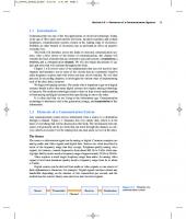
1.2 Elements of a Communication System Any communication system moves information from a source to a destination through a channel. Figure 1.1 illustrates this very simple idea, which is at the heart of everything that will be discussed in this book. The information from the source will generally not be in a form that can travel through the channel, so a device called a transmitter will be employed at one end, and a receiver at the other.

The Source The source or information signal can be analog or digital. Common examples are analog audio and video signals and digital data. Sources are often described in terms of the frequency range that they occupy. Telephone-quality analog voice signals, for instance, contain frequencies from about 300 Hz to 3 kHz, while analog high-fidelity music needs a frequency range of approximately 20 Hz to 20 kHz. Video requires a much larger frequency range than audio. An analog video signal of television-broadcast quality needs a frequency range from dc to about 4.2 MHz. Digital sources can be derived from audio or video signals or can consist of data (alphanumeric characters, for example). Digital signals can have almost any bandwidth depending on the number of bits transmitted per second, and the method used to convert binary ones and zeros into electrical signals.

Elements of a communication system

Figure 1.1 Source

Transmitter

Receiver Channel

Destination

3

01_639091_Delmar_Blake

4

8/16/01

2:51 PM

Page 4

Chapter 1 ● Introduction to Communication Systems

The Channel A communication channel can be almost anything: a pair of conductors or an optical fiber, for example. Much of this book deals with radio communication, in which free space serves as the channel. Sometimes a channel can carry the information signal directly. For example, an audio signal can be carried directly by a twisted-pair telephone cable. On the other hand, a radio link through free space cannot be used directly for voice signals. An antenna of enormous length would be required, and it would not be possible to transmit more than one signal without interference. Such situations require the use of a carrier signal whose frequency is such that it will travel, or propagate, through the channel. This carrier wave will be altered, or modulated, by the information signal in such a way that the information can be recovered at the destination. When a carrier is used, the information signal is also known as the modulating signal. Since the carrier frequency is generally much higher than that of the information signal, the frequency spectrum of the information signal is often referred to as the baseband. Thus, the three terms information signal, modulating signal, and baseband are equivalent in communication schemes involving modulated carriers.

Types of Modulation All systems of modulation are variations on a small number of possibilities. A carrier is generated at a frequency much higher than the highest baseband frequency. Usually, the carrier is a sine wave. The instantaneous amplitude of the baseband signal is used to vary some parameter of the carrier. A general equation for a sine-wave carrier is: e(t) ⫽ Ec sin (␻ct ⫹ ␪) where

e(t) Ec ␻c t ␪

⫽ ⫽ ⫽ ⫽ ⫽

(1.1)

instantaneous voltage as a function of time peak voltage frequency in radians per second time in seconds phase angle in radians

Using radians per second in the mathematics dealing with modulation makes the equations simpler. Of course, frequency is usually given in hertz, rather than in radians per second, when practical devices are being discussed. It is easy to convert between the two systems by recalling from basic ac theory that ␻ ⫽ 2␲f. In modulation, the parameters that can be changed are amplitude Ec , frequency ␻c , and phase ␪. Combinations are also possible; for example, many schemes for transmitting digital information use both amplitude and phase modulation. The modulation is done at the transmitter. An inverse process, called demodulation or detection, takes place at the receiver to restore the original baseband signal.

Signal Bandwidth An unmodulated sine-wave carrier would exist at only one frequency and so would have zero bandwidth. However, a modulated signal is no longer a single sine wave, and it therefore occupies a greater bandwidth. Exactly how much bandwidth is needed depends on the baseband frequency range (or data rate, in the case of digital communication) and the modulation scheme in use. Hartley’s

01_639091_Delmar_Blake

8/16/01

2:51 PM

Page 5

Section 1.2 ● Elements of a Communication System

Law is a general rule that relates bandwidth and information capacity. It states that the amount of information that can be transmitted in a given time is proportional to bandwidth for a given modulation scheme. (1.2)

I ⫽ ktB where

I ⫽ amount of information to be sent k ⫽ a constant that depends on the type of modulation t ⫽ time available B ⫽ channel bandwidth

Some modulation schemes use bandwidth more efficiently than others. The bandwidth of each type of modulated signal will be examined in detail in later chapters.

Frequency-Division Multiplexing One of the benefits of using modulated carriers, even with channels that are capable of carrying baseband signals, is that several carriers can be used at different frequencies. Each can be separately modulated with a different information signal, and filters at the receiver can separate the signals and demodulate whichever one is required. Multiplexing is the term used in communications to refer to the combining of two or more information signals. When the available frequency range is divided among the signals, the process is known as frequency-division multiplexing (FDM). Radio and television broadcasting, in which the available spectrum is divided among many signals, are everyday examples of FDM. There are limitations to the number of signals that can be crowded into a given frequency range because each requires a certain bandwidth. For example, a television channel occupies a bandwidth of 6 MHz. Figure 1.2 shows how FDM applies to the VHF television band.

Time-Division Multiplexing An alternative method for using a single communication channel to send many signals is to use time-division multiplexing (TDM). Instead of dividing the available bandwidth of the channel among many signals, the entire bandwidth is used for each signal, but only for a small part of the time. A glance at Equation (1.2) will confirm that time and bandwidth are equivalent in terms of information capacity. A nonelectronic example is the division of the total available time on a television channel among the various programs transmitted. Each program uses the whole bandwidth of the channel, but only for part of the time. Examples of TDM in electronic communication are not as common in everyday experience as FDM, but TDM is used extensively, especially with digital communication. The digital telephone system is a good example.

FM Radio Broadcasting 2 3 4 54

66 60

Other Services (Police, Aircraft, Amateur, etc.)

5 6

76 88 72 82

108

Channel 7 8 9 10 11 12 13 180 192 204 216 174 186 198 210

Frequency (MHz)

Frequency-division multiplexing in the VHF television band

Figure 1.2

5

01_639091_Delmar_Blake

6

8/16/01

2:51 PM

Page 6

Chapter 1 ● Introduction to Communication Systems

It is certainly possible to combine FDM and TDM. For example, the available bandwidth of a communication satellite is divided among a number of transmitterreceiver combinations called transponders. This is an example of FDM. A single transponder can be used to carry a large number of digital signals using TDM.

Frequency Bands Hertz’s early experiments in the laboratory used frequencies in the range of approximately 50 to 500 MHz. When others, such as Marconi, tried to apply his results to practical communication, they initially found that results were much better at lower frequencies. At that time, little was known about radio propagation (or about antenna design, for that matter). It is now known that frequencies ranging from a few kilohertz to many gigahertz all have their uses in radio communication systems. In the meantime, a system of labeling frequencies came into use. The frequencies most commonly used in the early days, those from about 300 kHz to 3 MHz, were called medium frequencies (MF). Names were assigned to each order of magnitude of frequency, both upward and downward, and these names persist to this day. Thus we have low frequencies (LF) from 30 to 300 kHz and very low frequencies (VLF) from 3 to 30 kHz. Going the other way, we have high frequencies (HF) from 3 to 30 MHz, very high frequencies (VHF) from 30 to 300 MHz, and so on. Figure 1.3 shows the entire usable spectrum, with the appropriate labels.

FREQUENCY 300 GHz Extremely High Frequencies (EHF) 30 GHz Super High Frequencies (SHF) 3 GHz Ultra High Frequencies (UHF) 300 MHz Very High Frequencies (VHF) 30 MHz High Frequencies (HF) 3 MHz Medium Frequencies (MF) 300 kHz Low Frequencies (LF) 30 kHz Very Low Frequencies (VLF) 3 kHz Voice Frequencies (VF) 300 Hz Extremely Low Frequencies (ELF) 30 Hz

WAVELENGTH 1 mm

SAMPLE USES

Millimeter Waves 1 cm Radar 10 cm Microwaves 1m

Communications Satellites, Microwave Ovens, Personal Communication Systems, Cellular Telephones TV Broadcast FM Broadcast

10 m Short Waves 100 m Medium Waves

Shortwave Broadcast Commercial AM Broadcast

1 km Long Waves 10 km

Navigation Submarine Communications

100 km Audio

1000 km 10,000 km

Figure 1.3

Power Transmission

The radio-frequency spectrum

01_639091_Delmar_Blake

8/16/01

2:51 PM

Page 7

Section 1.2 ● Elements of a Communication System

Radio waves can also be described according to their wavelength, which is the distance a wave travels in one period. The general equation that relates frequency to wavelength for any wave is: ␯ ⫽ f␭

(1.3)

where ␯ ⫽ velocity of the wave in meters per second f ⫽ frequency of the wave in hertz ␭ ⫽ wavelength in meters For a radio wave in free space, the velocity is the same as that of light, which is approximately 300 ⫻ 106 meters per second. The usual symbol for this quantity is c. Equation (1.3) then becomes c ⫽ f␭ where

(1.4)

c ⫽ speed of light, 300 ⫻ 106 m/s f ⫽ frequency in hertz ␭ ⫽ wavelength in meters

It can be seen from Equation (1.4) that a frequency of 300 MHz corresponds to a wavelength of 1 m and that wavelength is inversely proportional to frequency. Low-frequency signals are sometimes called long wave, high frequencies correspond to short wave, and so on. The reader is no doubt familiar with the term microwave to describe signals in the gigahertz range.

EXAMPLE 1.1 Calculate the wavelength in free space corresponding to a frequency of: (a) 1 MHz (AM radio broadcast band) (b) 27 MHz (CB radio band) (c) 4 GHz (used for satellite television) Solution Rearranging Equation (1.4).

c ⫽ f␭ ␭⫽ 300 ⫻ 106 m/s 1 ⫻ 106 Hz ⫽ 300 m 300 ⫻ 106 m/s (b) ␭ ⫽ 27 ⫻ 106 Hz ⫽ 11.1 m (a) ␭ ⫽

300 ⫻ 106 m/s 4 ⫻ 109 Hz ⫽ 0.075 m ⫽ 7.5 cm

(c) ␭ ⫽

c f

7

01_639091_Delmar_Blake

8

8/16/01

2:51 PM

Page 8

Chapter 1 ● Introduction to Communication Systems

Distortionless Transmission The receiver should restore the baseband signal exactly. Of course, there will be a time delay due to the distance over which communication takes place, and there will likely be a change in amplitude as well. Neither effect is likely to cause problems, though there are exceptions. The time delay involved in communication via geostationary satellite can be a nuisance in telephone communication. Even though radio waves propagate at the speed of light, the great distance over which the signal must travel (about 70,000 kilometers) causes a quarter-second delay. Any other changes in the baseband signal reflect distortion, which has a corrupting effect on the signal. There are many possible types of distortion. Some types are listed below, but not all of them will be immediately clear. Much of the rest of this book will be devoted to explaining them in more detail. Some possible types of distortion are: • Harmonic distortion: harmonics (multiples) of some of the baseband components are added to the original signal. • Intermodulation distortion: additional frequency components generated by combining (mixing) the frequency components in the original signal. Mixing will be described in Chapter 2. • Nonlinear frequency response: some baseband components are amplified more than others. • Nonlinear phase response: phase shift between components of the signal. • Noise: both the transmitter and the receiver add noise, and the channel is also noisy. This noise adds to the signal and masks it. Noise will be discussed later in this chapter. • Interference: if more than one signal uses the same transmission medium, the signals may interact with each other. One of the advantages of digital communication is the ability to regenerate a signal that has been corrupted by noise and distortion, provided that it is still identifiable as representing a one or a zero. In analog systems, however, noise and distortion tend to accumulate. In some cases distortion can be removed at a later point. If the frequency response of a channel is not flat but is known, for instance, equalization in the form of filters can be used to compensate. However, harmonic distortion, intermodulation, and noise, once present, are impossible to remove completely from an analog signal. A certain amount of immunity can be built into digital schemes, but excessive noise and distortion levels will be reflected in increased error rates.

●

SECTION 1.2 REVIEW QUESTION

Explain what modulation is, why it is necessary, and how it can be accomplished. ●

1.3 Time and Frequency Domains The reader is probably familiar with the time-domain representation of signals. An ordinary oscilloscope display, showing amplitude on one scale and time on the other, is a good example.

01_639091_Delmar_Blake

8/16/01

2:51 PM

Page 9

Section 1.3 ● Time and Frequency Domains

v (V)

1 0

1

t (ms)

(a) Time domain

1

1.0 f (kHz)

(b) Frequency domain

Sine wave in time and frequency domains Figure 1.4

Fourier Series Any well-behaved periodic waveform can be represented as a series of sine and/or cosine waves at multiples of its fundamental frequency plus (sometimes) a dc offset. This is known as a Fourier series. This very useful (and perhaps rather surprising) fact was discovered in 1822 by Joseph Fourier, a French mathematician, in the course of research on heat conduction. Not all signals used in communications are strictly periodic, but they are often close enough for practical purposes. Fourier’s discovery, applied to a time-varying signal, can be expressed mathematically as follows: A0 ⫹ A1 cos ␻t ⫹ B1 sin ␻t ⫹ A2 cos 2␻t 2 ⫹ B2 sin 2␻t ⫹ A3 cos 3␻t ⫹ B3 sin 3␻t ⫹ ⭈ ⭈ ⭈

f(t) ⫽

where

0.5

–1

Vp ( V )

Signals can also be described in the frequency domain. In a frequencydomain representation, amplitude or power is shown on one axis and frequency is displayed on the other. A spectrum analyzer gives a frequency-domain representation of signals. Any signal can be represented either way. For example, a 1 kHz sine wave is shown in both ways in Figure 1.4. The time-domain representation should need no explanation. As for the frequency domain, a sine wave has energy only at its fundamental frequency, so it can be shown as a straight line at that frequency. Notice that our way of representing the signal in the frequency domain fails to show one thing: the phase of the signal. The signal in Figure 1.4(b) could be a cosine wave just as easily as a sine wave. Frequency-domain representations are very useful in the study of communication systems. For instance, the bandwidth of a modulated signal generally has some fairly simple relationship to that of the baseband signal. This bandwidth can easily be found if the baseband signal can be represented in the frequency domain. As we proceed, we will see many other examples in which the ability to work with signals in the frequency domain will be required.

9

(1.5)

f(t) ⫽ any well-behaved function of time as described above. For our purposes, f(t) will generally be either a voltage v(t) or a current i(t). An and Bn ⫽ real-number coefficients; that is, they can be positive, negative, or zero. ␻ ⫽ radian frequency of the fundamental.

The radian frequency can be found from the time-domain representation of the signal by finding the period (that is, the time T after which the whole signal repeats exactly) and using the equations: f⫽

1 T

(1.6)

and ␻ ⫽ 2␲f

(1.7)

01_639091_Delmar_Blake

10

8/16/01

2:51 PM

Page 10

Chapter 1 ● Introduction to Communication Systems

The simplest ac signal is a sinusoid. The frequency-domain representation of a sine wave has already been described and is shown in Figure 1.4(b) for a voltage sine wave with a period of 1 ms and a peak amplitude of 1 V. For this signal, all the coefficients of Equation (1.5) are zero except for B1, which has a value of 1 V. The equation becomes ␯(t) ⫽ sin (2000␲) V which is certainly no surprise. The examples that follow use the equations for the various waveforms shown in Table 1.1.

Find and sketch the Fourier series corresponding to the square wave in Figure 1.5(a)

EXAMPLE 1.2

0.5

1

t (ms)

Vp (V)

v (V)

1

1

1

2

3

4

5

6

7

f (kHz)

(a) Time domain

(b) Frequency domain

Figure 1.5

Solution A square wave is another signal with a simple Fourier representa-

tion, although the representation is not quite as simple as that for a sine wave. For the signal shown in Figure 1.5(a), the frequency is 1 kHz, as before, and the peak voltage is 1 V. According to Table 1.1, this signal has components at an infinite number of frequencies: all odd multiples of the fundamental frequency of 1 kHz. However, the amplitude decreases with frequency, so that the third harmonic has an amplitude one-third that of the fundamental, the fifth harmonic an amplitude of one-fifth the fundamental, and so on. Mathematically, a square wave of voltage with a rising edge at t ⫽ 0 and no dc offset can be expressed as follows: ␯(t) ⫽ where

1 4V 1 asin ␻t ⫹ sin 3␻t ⫹ sin 5␻t ⫹ ⭈ ⭈ ⭈ b ␲ 3 5

V ⫽ peak amplitude of the square wave ␻ ⫽ radian frequency of the square wave t ⫽ time in seconds

(1.8)

01_639091_Delmar_Blake

8/16/01

2:51 PM

Page 11

Section 1.3 ● Time and Frequency Domains

For this example, Equation (1.8) becomes: ␯(t) ⫽

4 1 c sin (2␲ ⫻ 103t) ⫹ sin (6␲ ⫻ 103t) ␲ 3 1 3 ⫹ sin (10␲ ⫻ 10 t) ⫹ ⭈ ⭈ ⭈ d V 5

This equation shows that the signal has frequency components at odd multiples of 1 kHz, that is, at 1 kHz, 3 kHz, 5 kHz, and so on. The 1 kHz component has a peak amplitude of V1 ⫽

4 ⫽ 1.27 V ␲

The component at three times the fundamental frequency (3 kHz) has an amplitude one-third that of the fundamental, that at 5 kHz has an amplitude one-fifth that of the fundamental, and so on. V3 ⫽

4 ⫽ 0.424 V 3␲

4 ⫽ 0.255 V 5␲ 4 V7 ⫽ ⫽ 0.182 V 7␲ The result for the first four components is sketched in Figure 1.5(b). Theoretically, an infinite number of components would be required to describe the square wave completely, but, as the frequency increases, the amplitude of the components decreases rapidly. V5 ⫽

The representations in Figure 1.5(a) and 1.5(b) are not two different signals but merely two different ways of looking at the same signal. This can be shown graphically by adding the instantaneous values of several of the sine waves in the frequency-domain representation. If enough of these components are included, the result begins to look like the square wave in the time-domain representation. Figure 1.6 (page 14) shows the results for two, four, and ten components. It was created by simply taking the instantaneous values of all the components at the same time and adding them algebraically. This was done for a number of time values, resulting in the graphs in Figure 1.6. Doing these calculations by hand would be simple but rather tedious, so a computer was used to perform the calculations and plot the graphs. A perfectly accurate representation of the square wave would require an infinite number of components, but we can see from the figure that using ten components gives a very good representation because the amplitudes of the higher-frequency components of the signal are very small. It is possible to go back and forth at will between time and frequency domains, but it should be apparent that information about the relative phases of the frequency components in the Fourier representation of the signal is required to reconstruct the time-domain representation. The Fourier equations do have this

11

01_639091_Delmar_Blake

2:51 PM

Page 12

Chapter 1 ● Introduction to Communication Systems

TABLE 1.1

Fourier series for common repetitive waveforms

1. Half-wave rectified sine wave

v

V 0 T/2

T

V V 2V cos 2␻t cos 4␻t cos 6␻t ⫹ sin ␻t ⫺ a ⫹ ⫹ ⫹ ⭈ ⭈ ⭈b ␲ ␲ 1⫻3 2 3⫻5 5⫻7 2. Full-wave rectified sine wave (a) With time zero at voltage zero

␯(t) ⫽

v

V 0 T/2

T

T/2

T

4V cos 2␻t cos 4␻t cos 6␻t 2V ⫺ a ⫹ ⫹ ⫹ ⭈ ⭈ ⭈b ␲ ␲ 1⫻3 3⫻5 5⫻7 (b) With time zero at voltage peak

␯(t) ⫽

v

V 0

2 cos 2␻t 2 cos 4␻t 2 cos 6␻t 2V a1 ⫹ ⫺ ⫹ ⫺ ⭈ ⭈ ⭈b ␲ 1⫻3 3⫻5 5⫻7 3. Square wave (a) Odd function ␯(t) ⫽

v

V 0 T/2

T

−V

1 4V 1 asin ␻t ⫹ sin 3␻t ⫹ sin 5␻t ⫹ ⭈ ⭈ ⭈ b ␲ 3 5 (b) Even function ␯(t) ⫽

V v

12

8/16/01

0 T −V

␯(t) ⫽

1 4V 1 acos ␻t ⫺ cos 3␻t ⫹ cos 5␻t ⫺ ⭈ ⭈ ⭈ b ␲ 3 5 (continues)

Page 13

Section 1.3 ● Time and Frequency Domains

TABLE 1.1

Continued

4. Pulse train

τ

V v

0 −T

T

t

␯(t) ⫽

V␶ 2V␶ sin ␲␶/T sin 2␲␶/T sin 3␲␶/T ⫹ a cos ␻t ⫹ cos 2␻t ⫹ cos 3␻t ⫹ ⭈ ⭈ ⭈ b T T ␲␶/T 2␲␶/T 3␲␶/T

5. Triangle wave

V 0

v

2:51 PM

−T

T −V

t

␯(t) ⫽

8V 1 1 acos ␻t ⫹ 2 cos 3␻t ⫹ 2 cos 5␻t ⫹ ⭈ ⭈ ⭈ b ␲2 3 5

6. Sawtooth wave (a) With no dc offset

V 0

v

8/16/01

−T

T −V

t

␯(t) ⫽

1 2V 1 asin ␻t ⫺ sin 2␻t ⫹ sin 3␻t ⫺ ⭈ ⭈ ⭈ b ␲ 2 3

(b) Positive-going

V 0

v

01_639091_Delmar_Blake

−T

T −V

t

1 V V 1 ␯(t) ⫽ ⫺ asin ␻t ⫹ sin 2␻t ⫹ sin 3␻t ⫹ ⭈ ⭈ ⭈ b ␲ 2 2 3

13

01_639091_Delmar_Blake

2:51 PM

Page 14

Chapter 1 ● Introduction to Communication Systems

v2(t) (Volts)

2

−2 0

0.001

t (Seconds)

(a) Two components

v4(t) (Volts)

2

−2 0

0.001

t (Seconds)

(b) Four components

2

v10(t) (Volts) −2 0 Figure 1.6

0.001

t (Seconds)

(c) Ten

Construction of a square wave from Fourier components

3

v(t) (V)

14

8/16/01

−3 0 Figure 1.7

t (Seconds)

0.001

Addition of square-wave Fourier components with wrong phase angles

01_639091_Delmar_Blake

8/16/01

2:51 PM

Page 15

Section 1.3 ● Time and Frequency Domains

information, but the sketch in Figure 1.5(b) does not. If the phase relationships between frequency components are changed in a communication system, the signal will be distorted in the time domain. Figure 1.7 illustrates this point. The same ten coefficients were used as in Figure 1.6(c), but this time the waveforms alternated between sine and cosine: sine for the fundamental, cosine for the third harmonic, sine for the fifth, and so on. The result is a waveform that looks the same on the frequency-domain sketch of Figure 1.5(b) but very different in the time domain.

Find the Fourier series for the signal in Figure 1.8(a).

EXAMPLE 1.3

Solution The positive-going sawtooth wave of Figure 1.8(a) has a Fourier

series with a dc term and components at all multiples of the fundamental frequency. From Table 1.1, the general equation for such a wave is ␯(t) ⫽

A A 1 1 ⫺ a b asin ␻t ⫹ sin 2 ␻t ⫹ sin 3 ␻t ⫹ ⭈ ⭈ ⭈ b (1.9) ␲ 2 2 3

The first (dc) term is simply the average value of the signal. For the signal in Figure 1.8, which has a frequency of 1 kHz and a peak amplitude of 5 V, Equation (1.9) becomes: ␯(t) ⫽ 2.5 ⫺ 1.59 [sin (2␲ ⫻ 103t) ⫹ 0.5 sin (4␲ ⫻ 103t) ⫹ 0.33 sin (6␲ ⫻ 103t) ⫹ . . .] V

5 Vp (V)

v (V)

4 3 2 1

4 3.5 3 2.5 2 1.5 1 0.5 0

0 1

2

3

1

2

4

f (kHz)

t (ms)

(a) Time domain

3

(b) Frequency domain

Figure 1.8

Effect of Filtering on Signals As we have seen, many signals have a bandwidth that is theoretically infinite. Limiting the frequency response of a channel removes some of the frequency components of these signals and causes the time-domain representation to be distorted. An uneven frequency response will emphasize some components at the expense of others, again causing distortion. Nonlinear phase shift will also affect the time-domain representation. For instance, shifting the phase angles of some of the frequency components in the square-wave representation of Figure 1.7 changed the signal to something other than a square wave.

5

15

01_639091_Delmar_Blake

16

8/16/01

2:51 PM

Page 16

Chapter 1 ● Introduction to Communication Systems

However, Figure 1.6 shows that while an infinite bandwidth may theoretically be required, for practical purposes quite a good representation of a square wave can be obtained with a band-limited signal. In general, the wider the bandwidth, the better, but acceptable results can be obtained with a band-limited signal. This is welcome news, because practical systems always have finite bandwidth. Although real communication systems have a solid theoretical base, they also involve many practical considerations. There is always a trade-off between fidelity to the original signal (that is, the absence of any distortion of its waveform) and such factors as bandwidth and cost. Increasing the bandwidth often increases the cost of a communication system. Not only is the hardware likely to be more expensive, but bandwidth itself may be in short supply. In radio communication, for instance, spectral allocations are assigned by national regulatory bodies in keeping with international agreements. This task is handled in the United States by the Federal Communications Commission (FCC) and in Canada by the communications branch of Industry and Science Canada. The allocations are constantly being reviewed, and there never seems to be enough room in the usable spectrum to accommodate all potential users. In communication over cables, whether by electrical or optical means, the total bandwidth of a given cable is fixed by the technology employed. The more bandwidth used by each signal, the fewer signals can be carried by the cable. Consequently, some services are constrained by cost and/or government regulation to use less than optimal bandwidth. For example, telephone systems use about 3 kHz of baseband bandwidth for voice. This is obviously not distortionless transmission: the difference between a voice heard “live,” in the same room, and the same voice heard over the telephone is obvious. High-fidelity audio needs at least 15 kHz of baseband bandwidth. On the other hand, the main goal of telephone communication is the understanding of speech, and the bandwidth used is sufficient for this. Using a larger bandwidth would contribute little or nothing to intelligibility and would greatly increase the cost of nearly every part of the system.

●

SECTION 1.3 REVIEW QUESTION

What bandwidth is required to transmit the first seven components of a triangle wave with a fundamental frequency of 3 kHz? ●

1.4 Noise and Communications Noise in communication systems originates both in the channel and in the communication equipment. Noise consists of undesired, usually random, variations that interfere with the desired signals and inhibit communication. It cannot be avoided completely, but its effects can be reduced by various means, such as reducing the signal bandwidth, increasing the transmitter power, and using lownoise amplifiers for weak signals. It is helpful to divide noise into two types: internal noise, which originates within the communication equipment, and external noise, which is a property of the channel. (In this book, the channel will usually be a radio link.)

01_639091_Delmar_Blake

8/16/01

2:51 PM

Page 17

Section 1.4 ● Noise and Communications

External Noise If the channel is a radio link, there are many possible sources of noise. The reader is no doubt familiar with the “static” that afflicts AM radio broadcasting during thunderstorms. Interference from automobile ignition systems is another common problem. Domestic and industrial electrical equipment, from light dimmers to vacuum cleaners to computers, can also cause objectionable noise. Not so obvious, but of equal concern to the communications specialist, is noise produced by the sun and other stars. Equipment Noise Noise is generated by equipment that produces sparks. Examples include automobile engines and electric motors with brushes. Any fastrisetime voltage or current can also generate interference, even without arcing. Light dimmers and computers fall into this category. Noise of this type has a broad frequency spectrum, but its energy is not equally distributed over the frequency range. This type of interference is generally more severe at lower frequencies, but the exact frequency distribution depends upon the source itself and any conductors to which it is connected. Computers, for instance, may produce strong signals at multiples and submultiples of their clock frequency and little energy elsewhere. Man-made noise can propagate through space or along power lines. It is usually easier to control it at the source than at the receiver. A typical solution for a computer, for instance, involves shielding and grounding the case and all connecting cables and installing a low-pass filter on the power line where it enters the enclosure. Atmospheric Noise Atmospheric noise is often called static because lightning, which is a static-electricity discharge, is a principal source of atmospheric noise. This type of disturbance can propagate for long distances through space. Most of the energy of lightning is found at relatively low frequencies, up to several megahertz. Obviously nothing can be done to reduce atmospheric noise at the source. However, circuits are available to reduce its effect by taking advantage of the fact that this noise has a very high peak-to-average power ratio; that is, the noise occurs in short intense bursts with relatively long periods of time between bursts. It is often possible to improve communication by simply disabling the receiver for the duration of the burst. This technique is called noise blanking. Space Noise The sun is a powerful source of radiation over a wide range of frequencies, including the radio-frequency spectrum. Other stars also radiate noise called cosmic, stellar, or sky noise. Its intensity when received on the earth is naturally much less than for solar noise because of the greater distance. Solar noise can be a serious problem for satellite reception, which becomes impossible when the satellite is in a line between the antenna and the sun. Space noise is more important at higher frequencies (VHF and above) because atmospheric noise dominates at lower frequencies and because most of the space noise at lower frequencies is absorbed by the upper atmosphere.

Internal Noise Noise is generated in all electronic equipment. Both passive components (such as resistors and cables) and active devices (such as diodes, transistors, and tubes) can be noise sources. Several types of noise will be examined in this section, beginning with the most important, thermal noise.

17

01_639091_Delmar_Blake

18

8/16/01

2:51 PM

Page 18

Chapter 1 ● Introduction to Communication Systems

Thermal Noise Thermal noise is produced by the random motion of electrons in a conductor due to heat. The term “noise” is often used alone to refer to this type of noise, which is found everywhere in electronic circuitry. The power density of thermal noise is constant with frequency, from zero to frequencies well above those used in electronic circuits. That is, there is equal power in every hertz of bandwidth. Thermal noise is thus an equal mixture of noise of all frequencies. It is sometimes called white noise, in analogy with white light, which is an equal mixture of all colors. The noise power available from a conductor is a function of its temperature, as shown by the equation: PN ⫽ kTB

v

where

t

Power Density W/Hz

(a) Voltage as a function of time

kT

f (Hz) (b) Power density as a function of frequency Figure 1.9

Noise voltage and power

(1.10)

PN ⫽ noise power in watts k ⫽ Boltzmann’s constant, 1.38 ⫻ 10⫺23 joules/kelvin (J/K) T ⫽ absolute temperature in kelvins (K); this can be found by adding 273 to the celcius temperature B ⫽ noise power bandwidth in hertz

This equation is based on the assumption that power transfer is maximum. That is, the source (the resistance generating the noise) and the load (the amplifier or other device that receives the noise) are assumed to be matched in impedance. Equation (1.10) shows that noise power is directly related to bandwidth over which the noise is observed (the noise power bandwidth). Filters are often specified in terms of their bandwidth at half power, that is, at the points where the gain of the filter is 3 dB down from its gain in the center of the passband. An ideal bandpass filter would allow no noise to pass at frequencies outside the passband, so its noise power bandwidth would be equal to its half-power bandwidth. For a practical filter, the noise power bandwidth is generally greater than the half-power bandwidth, since some contribution is made to the total noise power by frequencies that are attenuated by more than 3 dB. An ordinary LC tuned circuit has a noise power bandwidth about 50% greater than its half-power bandwidth. The power referred to in the previous paragraph is average power. The instantaneous voltage and power are random, but over time the voltage will average out to zero, as it does for an ordinary ac signal, and the power will average to the value given by Equation (1.10). Figure 1.9 shows this effect.

EXAMPLE 1.4 A receiver has a noise power bandwidth of 10 kHz. A resistor that matches the receiver input impedance is connected across its antenna terminals. What is the noise power contributed by that resistor in the receiver bandwidth, if the resistor has a temperature of 27°C? Solution First, convert the temperature to kelvins:

T(K) ⫽ T(°C) ⫹ 273 ⫽ 27 ⫹ 273 ⫽ 300 K

01_639091_Delmar_Blake

8/16/01

2:51 PM

Page 19

Section 1.4 ● Noise and Communications

19

According to Equation (1.10), a conductor at a temperature of 300 K would contribute the following noise power in that 10 kHz bandwidth: PN ⫽ kTB ⫽ (1.38 ⫻ 10⫺23 J/K) (300 K) (10 ⫻ 103 Hz) ⫽ 4.14 ⫻ 10⫺17 W This is obviously not a great deal of power, but it can be significant at the signal levels dealt with in sensitive receiving equipment.

Thermal noise power exists in all conductors and resistors at any temperature above absolute zero. The only way to reduce it is to decrease the temperature or the bandwidth of a circuit (or both). Amplifiers used with very low level signals are often cooled artificially to reduce noise. This technique is called cryogenics and may involve, for example, cooling the first stage of a receiver for radio astronomy by immersing it in liquid nitrogen. The other method, bandwidth reduction, will be referred to many times throughout this book. Using a bandwidth greater than required for a given application is simply an invitation to noise problems. Thermal noise, as such, does not depend on the type of material involved or the amount of current passing through it. However, some materials and devices also produce other types of noise that do depend on current. Carbon-composition resistors are in this category, for example, and so are semiconductor junctions. Noise Voltage Often we are more interested in the noise voltage than in the power involved. The noise power depends only on bandwidth and temperature, as stated above. Power in a resistive circuit is given by the equation: P⫽

V2 R

(1.11)

From this, we see that: V 2 ⫽ PR V ⫽ 1PR

(1.12)

Equation (1.12) shows that the noise voltage in a circuit must depend on the resistances involved, as well as on the temperature and bandwidth. Figure 1.10 shows a resistor that serves as a noise source connected across another resistor, RL , that will be considered as a load. The noise voltage is represented as a voltage source VN, in series with a noiseless resistance RN. We know from Equation (1.10) that the noise power supplied to the load resistor, assuming a matched load, is:

VN/2

RN RL

VN /2

VN

PN ⫽ kTB In this situation, one-half the noise voltage appears across the load, and the rest is across the resistor that generates the noise. The root-mean-square (RMS) noise voltage across the load is given by: VL ⫽ 1PR ⫽ 1kTBR

Noisy Resistor Figure 1.10

Thermal noise voltage

01_639091_Delmar_Blake

20

8/16/01

2:51 PM

Page 20

Chapter 1 ● Introduction to Communication Systems

An equal noise voltage will appear across the source resistance, so the noise source shown in Figure 1.10 must have double this voltage or VN ⫽ 21kTBR ⫽ 14kTBR

(1.13)

EXAMPLE 1.5 A 300 ⍀ resistor is connected across the 300 ⍀ antenna input of a television receiver. The bandwidth of the receiver is 6 MHz, and the resistor is at room temperature (293 K or 20°C or 68°F). Find the noise power and noise voltage applied to the receiver input. Solution The noise power is given by Equation (1.10):

PN ⫽ kTB ⫽ (1.38 ⫻ 10⫺23 J/K) (293 K) (6 ⫻ 106 Hz) ⫽ 24.2 ⫻ 10⫺15 W ⫽ 24.2 fW The noise voltage is given by Equation (1.13): VN ⫽ 14kTBR ⫽ 14 (1.38 ⫻ 10⫺23 J/K) (293 K) (6 ⫻ 106 Hz) (300 ⍀) ⫽ 5.4 ⫻ 10⫺6 V ⫽ 5.4 ␮V Of course, only one-half this voltage appears across the antenna terminals; the other half appears across the source resistance. Therefore the actual noise voltage at the input is 2.7 ␮V.

Shot Noise This type of noise has a power spectrum that resembles that of thermal noise, having equal energy in every hertz of bandwidth, at frequencies from dc into the gigahertz region. However, the mechanism that creates shot noise is different. Shot noise is due to random variations in current flow in active devices such as tubes, transistors, and semiconductor diodes. These variations are caused by the fact that current is a flow of carriers (electrons or holes), each of which carries a finite amount of charge. Current can thus be considered as a series of pulses, each consisting of the charge carried by one electron. The name “shot noise” describes the random arrival of electrons arriving at the anode of a vacuum tube, like individual pellets of shot from a shotgun. One would expect that the resulting noise power would be proportional to the device current, and this is true both for vacuum tubes and for semiconductor junction devices. Shot noise is usually represented by a current source. The noise current for either a vacuum or a junction diode is given by the equation: IN ⫽ 12qI0B

(1.14)

01_639091_Delmar_Blake

8/16/01

2:51 PM

Page 21

Section 1.4 ● Noise and Communications

where

21

IN ⫽ RMS noise current, in amperes q ⫽ magnitude of the charge on an electron, equal to 1.6 ⫻ 10 ⫺19 coulomb I0 ⫽ dc bias current in the device, in amperes B ⫽ bandwidth over which the noise is observed, in hertz

This equation is valid for frequencies much less than the reciprocal of the carrier transit time for the device. The transit time is the time a charge carrier spends in the device. Depending on the device, Equation (1.14) may be valid for frequencies up to a few megahertz or several gigahertz. Since shot noise closely resembles thermal noise in its random amplitude and flat spectrum, it can be used as a substitute for thermal noise whenever a known level of noise is required. Such a noise source can be very useful, particularly when conducting measurements on receivers. A calibrated, variable noise generator can easily be constructed using a diode with adjustable bias current. Figure 1.11 shows a simplified circuit for such a generator.

EXAMPLE 1.6 A diode noise generator is required to produce 10 ␮V of noise in a receiver with an input impedance of 75 ⍀, resistive, and a noise power bandwidth of 200 kHz. (These values are typical of FM broadcast receivers.) What must the current through the diode be? Solution First, convert the noise voltage to current, using Ohm’s Law:

VN R 10 ␮V ⫽ 75 ⍀ ⫽ 0.133 ␮A

IN ⫽

Next, rearrange Equation (1.14) and solve for I0: IN ⫽ 12qI0B I 2N ⫽ 2qI0B I0 ⫽ ⫽

I 2N 2qB (0.133 ⫻ 10⫺6 A)2 2 (1.6 ⫻ 10⫺19 C) (200 ⫻ 103 Hz)

⫽ 0.276 A or 276 mA

Partition Noise Partition noise is similar to shot noise in its spectrum and mechanism of generation, but it occurs only in devices where a single current separates into two or more paths. An example of such a device is a bipolar junction transistor, where the emitter current is the sum of the collector and base currents. As the charge carriers divide into one stream or the other, a random element in the currents is produced. A similar effect can occur in vacuum tubes.

VN out

Figure 1.11

Diode noise generator

01_639091_Delmar_Blake

22

8/16/01

2:51 PM

Page 22

Chapter 1 ● Introduction to Communication Systems

The amount of partition noise depends greatly on the characteristics of the particular device, so no equation for calculating it will be given here. The same is true of shot noise in devices with three or more terminals. Device manufacturers provide noise figure information on their data sheets when a device is intended for use in circuits where signal levels are low and noise is important. Partition noise is not a problem in field-effect transistors, where the gate current is negligible. Excess Noise Excess noise is also called flicker noise or 1/f noise (because the noise power varies inversely with frequency). Sometimes it is called pink noise because there is proportionately more energy at the low-frequency end of the spectrum than with white noise, just as pink light has a higher proportion of red (the low-frequency end of the visible spectrum) than does white light. Excess noise is found in tubes but is a more serious problem in semiconductors and in carbon resistors. It is not fully understood, but it is believed to be caused by variations in carrier density. Excess noise is rarely a problem in communication circuits, because it declines with increasing frequency and is usually insignificant above approximately 1 kHz. You may meet the term “pink noise” again. It refers to any noise that has equal power per octave rather than per hertz. Pink noise is often used for testing and setting up audio systems. Transit-Time Noise Many junction devices produce more noise at frequencies approaching their cutoff frequencies. This high-frequency noise occurs when the time taken by charge carriers to cross a junction is comparable to the period of the signal. Some of the carriers may diffuse back across the junction, causing a fluctuating current that constitutes noise. Since most devices are used well below the frequency at which transit-time effects are significant, this type of noise is not usually important (except in some microwave devices).

Addition of Noise from Different Sources All of the noise sources we have looked at have random waveforms. The amplitude at a particular time cannot be predicted, though the average voltage is zero and the RMS voltage or current and average power are predictable (and not zero). Signals like this are said to be uncorrelated; that is, they have no definable phase relationship. In such a case, voltages and currents do not add directly, but the total voltage (of series circuits) or current (of parallel circuits) can be found by taking the square root of the sum of the squares of the individual voltages or currents. Mathematically, we can say, for voltage sources in series: VNt ⫽ 2V 2N1 ⫹ V 2N2 ⫹ V 2N3 ⫹ ⭈ ⭈ ⭈

(1.15)

and similarly, for current sources in parallel: INt ⫽ 2I 2N1 ⫹ I 2N2 ⫹ I 2N3 ⫹ ⭈ ⭈ ⭈

(1.16)

EXAMPLE 1.7 The circuit in Figure 1.12 shows two resistors in series at two different temperatures. Find the total noise voltage and noise power produced at the load, over a bandwidth of 100 kHz.

01_639091_Delmar_Blake

8/16/01

2:51 PM

Page 23

Section 1.4 ● Noise and Communications

Figure 1.12

R1 100 Ω 300 K RL 300 Ω

R2 200 Ω 400 K

Noise Source

Load

Solution The open-circuit noise voltage can be found from Equation (1.15) VNt ⫽ 2V 2R1 ⫹ V 2R2 ⫽ 3(24kTBR1)2 ⫹ 14kTBR2)2 ⫽ 24kT1BR1 ⫹ 4kT2BR2 ⫽ 14kB(T1R1 ⫹ T2R2) ⫽ 14 (1.38 ⫻ 10⫺23 J/K) (100 ⫻ 103 Hz) [(300 K) (100 ⍀) ⫹ (400 K) (200 ⍀)] ⫽ 779 nV

This is, of course, the open-circuit noise voltage for the resistor combination. Since in this case the load is equal in value to the sum of the resistors, one-half of this voltage, or 390 nV, will appear across the load. The easiest way to find the load power is from Equation (1.11): V2 R (390 nV)2 ⫽ 300 ⍀ ⫽ 0.506 ⫻ 10⫺15 W ⫽ 0.506 fW

P⫽

Signal-to-Noise Ratio The main reason for studying and calculating noise power or voltage is the effect that noise has on the desired signal. In an analog system, noise makes the signal unpleasant to watch or listen to and, in extreme cases, difficult to understand. In digital systems, noise increases the error rate. In either case, it is not really the amount of noise that concerns us but rather the amount of noise compared to the level of the desired signal. That is, it is the ratio of signal to noise power that is important, rather than the noise power alone. This signal-to-noise ratio, abbreviated S/N and usually expressed in decibels, is one of the most important specifications

23

01_639091_Delmar_Blake

24

8/16/01

2:51 PM

Page 24

Chapter 1 ● Introduction to Communication Systems

of any communication system. Typical values of S/N range from about 10 dB for barely intelligible speech to 90 dB or more for compact-disc audio systems. Note that the previous ratio is a power ratio, not a voltage ratio. Sometimes calculations result in a voltage ratio that must be converted to a power ratio in order to make meaningful comparisons. Of course, the value in decibels will be the same either way, provided that both signal and noise are measured in the same circuit, so that the impedances are the same. The two equations below are used for power ratios and voltage ratios, respectively: S/N (dB) ⫽ 10 log

PS PN

(1.17)

S/N (dB) ⫽ 20 log

VS VN

(1.18)

At this point, the reader who is not familiar with decibel notation should refer to Appendix A. Decibels are used constantly in communication theory and practice, and it is important to understand their use. Although the signal-to-noise ratio is a fundamental characteristic of any communication system, it is often difficult to measure. For instance, it may be possible to measure the noise power by turning off the signal, but it is not possible to turn off the noise in order to measure the signal power alone. Consequently, a variant of S/N, called (S ⫹ N)/N, is often found in receiver specifications. It stands for the ratio of signal-plus-noise power to noise power alone. There are other variations of the signal-to-noise ratio. For instance, there is the question of what to do about distortion. Though it is not a random effect like thermal noise, the effect on the intelligibility of a signal is rather similar. Consequently, it might be a good idea to include it with the noise when measuring. This leads to the expression SINAD which stands for (S ⫹ N ⫹ D)/(N ⫹ D), or signal-plusnoise and distortion, divided by noise and distortion. SINAD is usually used instead of S/N in specifications for FM receivers. Both (S ⫹ N)/N and SINAD are power ratios, and they are almost always expressed in decibels. Details on the measurement of (S ⫹ N)/N and SINAD will be provided in Chapter 6.

EXAMPLE 1.8 A receiver produces a noise power of 200 mW with no signal. The output level increases to 5 W when a signal is applied. Calculate (S ⫹ N)/N as a power ratio and in decibels. Solution The power ratio is

5W 0.2 W ⫽ 25

(S ⫹ N)/N ⫽

In decibels, this is (S ⫹ N)/N (dB) ⫽ 10 log 25 ⫽ 14 dB

01_639091_Delmar_Blake

8/16/01

2:51 PM

Page 25

Section 1.4 ● Noise and Communications

Noise Figure Since thermal noise is produced by all conductors and since active devices add their own noise as described previously, it follows that any stage in a communication system will add noise. An amplifier, for instance, will amplify equally both the signal and the noise at its input, but it will also add some noise. The signal-tonoise ratio at the output will therefore be lower than at the input. Noise figure (abbreviated NF or just F) is a figure of merit, indicating how much a component, stage, or series of stages degrades the signal-to-noise ratio of a system. The noise figure is, by definition: NF ⫽

(S/N)i (S/N)o

(1.19)

where (S/N )i = input signal-to-noise power ratio (not in dB) (S/N )o = output signal-to-noise power ratio (not in dB) Very often both S/N and NF are expressed in decibels, in which case we have: NF (dB) ⫽ (S/N)i (dB) ⫺ (S/N)o (dB)

(1.20)

Since we are dealing with power ratios, it should be obvious that: NF (dB) ⫽ 10 log NF (ratio)

(1.21)

Noise figure is occasionally called noise factor. Sometimes the term noise ratio (NR) is used for the simple ratio of Equation (1.19), reserving the term “noise figure” for the decibel form given by Equation (1.20).

EXAMPLE 1.9 The signal power at the input to an amplifier is 100 ␮W and the noise power is 1 ␮W. At the output, the signal power is 1 W and the noise power is 30 mW. What is the amplifier noise figure, as a ratio? Solution

100 ␮W ⫽ 100 1 ␮W 1W (S/N)o ⫽ ⫽ 33.3 0.03 W 100 NF (ratio) ⫽ ⫽3 33.5 (S/N)i ⫽

EXAMPLE 1.10 The signal at the input of an amplifier has an S/N of 42 dB. If the amplifier has a noise figure of 6 dB, what is the S/N at the output (in decibels)?

25

01_639091_Delmar_Blake

26

8/16/01

2:51 PM

Page 26

Chapter 1 ● Introduction to Communication Systems

Solution The S/N at the output can be found by rearranging Equation (1.20):

NF (dB) ⫽ (S/N)i (dB) ⫺ (S/N)o (dB) (S/N)o (dB) ⫽ (S/N)i (dB) ⫺ NF (dB) ⫽ 42 dB ⫺ 6 dB ⫽ 36 dB

Equivalent Noise Temperature

Power Gain A (S/N)i

(S/N)o

(a) Real (noisy) amplifier Power Gain A NF=0 dB (S/N)o

(S/N)i

Equivalent noise temperature is another way of specifying the noise performance of a device. Noise temperature has nothing to do with the actual operating temperature of the circuit. Rather, as shown in Figure 1.13, it is the absolute temperature of a resistor that, connected to the input of a noiseless amplifier of the same gain, would produce the same noise at the output as the device under discussion. Figure 1.13(a) shows a real amplifier which, of course, produces noise at its output, even with no input signal. Figure 1.13(b) shows a hypothetical noiseless amplifier with a noisy resistor at its input. The combination produces the same amount of a noise at its output as does the real amplifier of Figure 1.13(a). From Equation (1.19), the noise figure is given by:

Noiseless Amplifier Equivalent Noise Resistance

(S/N)i (S/N)o (Si/Ni) ⫽ So/No) SiNo ⫽ NiSo Si No ⫽ So Ni

NF ⫽

(b) Equivalent with noise resistance and ideal (noiseless) amplifier Figure 1.13

Equivalent noise

resistance

where

Si Ni So No

⫽ ⫽ ⫽ ⫽

(1.22)

signal power at input noise power at input signal power at output noise power at output

If we are going to refer all the amplifier noise to the input, then this noise, as well as the noise from the signal source, will be amplified by the gain of the amplifier. Let the amplifier power gain be A. Then: A⫽

So Si

(1.23)

Substituting this into Equation (1.22), we get NF ⫽

No Ni A

(1.24)

or No ⫽ (NF )Ni A Thus the total noise at the input is (NF)Ni.

(1.25)

01_639091_Delmar_Blake

8/16/01

2:51 PM

Page 27

Section 1.4 ● Noise and Communications

Assuming that the input source noise Ni is thermal noise, it has the expression, first shown in Equation (1.10): Ni ⫽ kTB The equivalent input noise generated by the amplifier must be Neq ⫽ (NF)Ni ⫺ Ni ⫽ (NF)kTB ⫺ kTB ⫽ (NF ⫺ 1)kTB

(1.26)

If we suppose that this noise is generated in a (fictitious) resistor at temperature Teq, and if we further suppose that the actual source is at a reference temperature T0 of 290 K, then we get: kTeqB ⫽ (NF ⫺ 1)kT0B Teq ⫽ (NF ⫺ 1)T0 ⫽ 290(NF ⫺ 1)

(1.27)

This may seem a trivial result, because it turns out that Teq can be found directly from the noise figure and thus contains no new information about the amplifier. However, Teq is very useful when we look at microwave receivers connected to antennas by transmission lines. The antenna has a noise temperature due largely to space noise intercepted by the antenna. The transmission line and the receiver will also have noise temperatures. It is possible to get an equivalent noise temperature for the whole system by simply adding the noise temperatures of the antenna, transmission line, and receiver. From this, we can calculate the system noise figure merely by rearranging Equation (1.27): Teq ⫽ 290(NF ⫺ 1) NF ⫺ 1 ⫽ NF ⫽

Teq

(1.28)

290 Teq 290

⫹1

Equivalent noise temperatures of low-noise amplifiers are quite low, often less than 100 K. Note that this does not mean the amplifier operates at this temperature. It is quite common for an amplifier operating at an actual temperature of 300 K to have an equivalent noise temperature of 100 K.

EXAMPLE 1.11 An amplifier has a noise figure of 2 dB. What is its equivalent noise temperature? Solution First, we need the noise figure expressed as a ratio. This can be

found from Equation (1.21): NF (dB) ⫽ 10 log NF (ratio)

27

01_639091_Delmar_Blake

28

8/16/01

2:51 PM

Page 28

Chapter 1 ● Introduction to Communication Systems

From which we get: NF (dB) 10 ⫽ antilog 0.2 ⫽ 1.585

NF (ratio) ⫽ antilog

Now we can use Equation (1.27) to find the noise temperature: Teq ⫽ 290(NF ⫺ 1) ⫽ 290(1.585 ⫺ 1) ⫽ 169.6 K

Cascaded Amplifiers When two or more stages are connected in cascade, as in a receiver, the noise figure of the first stage is the most important in determining the noise performance of the entire system because noise generated in the first stage is amplified in all succeeding stages. Noise produced in later stages is amplified less, and noise generated in the last stage is amplified least of all. While the first stage is the most important noise contributor, the other stages cannot be neglected. It is possible to derive an equation that relates the total noise figure to the gain and noise figure of each stage. In the following discussion, the power gains and noise figures are expressed as ratios, not in decibels. We will start with a two-stage amplifier like the one shown in Figure 1.14. The first stage has a gain A1 and a noise figure NF1, and the second-stage gain and noise figure are A2 and NF2, respectively. Let the noise power input to the first stage be Ni1 ⫽ kTB Then, according to Equation (1.25), the noise at the output of the first stage is: No1 ⫽ NF1Ni1A1 ⫽ NF1kTBA1

(1.29)

This noise appears at the input of the second stage. It is amplified by the second stage and appears at the output multiplied by A2. However, the second stage also contributes noise, which can be expressed, according to Equation (1.26), as: Neq2 ⫽ (NF2 ⫺ 1)(kTB)

Figure 1.14

Stage 1

Stage 2

Gain A1 Noise Figure NF1

Gain A2 Noise Figure NF2

Noise figure for a two-stage amplifier

(1.30)

01_639091_Delmar_Blake

8/16/01

2:51 PM

Page 29

Section 1.4 ● Noise and Communications

29

This noise also appears at the output, amplified by A2. Therefore the total noise power at the output of the two-stage system is: No2 ⫽ No1A2 ⫹ Neq2A2 ⫽ NF1A1kTBA2 ⫹ (NF2 ⫺ 1)kTBA2 ⫽ kTBA2(NF1A1 ⫹ NF1 ⫺ 1)

(1.31)

The noise figure for the whole system (NFT) is, according to Equation (1.24): NFT ⫽

No2 Ni1AT

Substituting the value for No2 found in Equation (1.31) and making use of the fact that the total gain AT is the product of the individual stage gains, we get NFT ⫽ ⫽

kTBA2(NF1A1 ⫹ NF2 ⫺ 1) kTBA1A2 NF1A1 ⫹ NF2 ⫺ 1 A1

⫽ NF1 ⫹

(1.32)

NF2 ⫺ 1 A1

This equation, known as Friis’ formula, can be generalized to any number of stages: NFT ⫽ NF1 ⫹

NF3 ⫺ 1 NF2 ⫺ 1 NF4 ⫺ 1 ⫹ ⫹ ⫹ ⭈ ⭈ ⭈ A1 A1A2 A1A2A3

(1.33)

This expression confirms our intuitive feeling by showing that the contribution of each stage is divided by the product of the gains of all the preceding stages. Thus the effect of the first stage is usually dominant. Note once again that the noise figures given in this section are ratios, not decibel values, and that the gains are power gains.

A three-stage amplifier has stages with the following specifications:

EXAMPLE 1.12

Calculate the power gain, noise figure, and noise temperature for the entire amplifier, assuming matched conditions. Solution The power gain is simply the product of the individual gains.

AT ⫽ 10 ⫻ 25 ⫻ 30 ⫽ 7500 The noise figure can be found from Equation (1.33): NF3 ⫺ 1 NF2 ⫺ 1 ⫹ A1 A1A2 4⫺1 5⫺1 ⫽2⫹ ⫹ 10 10 ⫻ 25 ⫽ 2.316

NFT ⫽ NF1 ⫹

Stage

Power Gain

Noise Figure

1 2 3

10 25 30

2 4 5

01_639091_Delmar_Blake

30

8/16/01

2:51 PM

Page 30

Chapter 1 ● Introduction to Communication Systems

If answers are required in decibels, they can easily be found: gain (dB) ⫽ 10 log 7500 ⫽ 38.8 dB NF (dB) ⫽ 10 log 2.316 ⫽ 3.65 dB The noise temperature can be found from Equation (1.27): Teq ⫽ 290(NF ⫺ 1) ⫽ 290(2.316 ⫺ 1) ⫽ 382 K

●

SECTION 1.4 REVIEW QUESTION

Why is it more important to have a low noise figure in the first stage of an amplifier than in other stages? ●

1.5 Spectrum Analysis

LED Column Displays for Each Channel

Input

Bandpass Filters Figure 1.15

analyzer

Real-time spectrum

In this chapter, we have discovered that there are two general ways of looking at signals: the time domain and the frequency domain. The ordinary oscilloscope is a convenient and versatile way of observing signals in the time domain, providing as it does a graph of voltage with respect to time. It would be logical to ask whether there is an equivalent instrument for the frequency domain: that is, something that could display a graph of voltage (or power) with respect to frequency. The answer to the question is yes: observation of signals in the frequency domain is the function of spectrum analyzers, which use one of two basic techniques. The first technique uses a number of fixed-tuned bandpass filters, spaced throughout the frequency range of interest. The display indicates the output level from each filter, often with a bar graph consisting of light-emitting diodes (LEDs). The more filters and the narrower the range, the better the resolution that can be obtained. This method is quite practical for audio frequencies, and in fact a crude version, with five to twenty filters, is often found as part of a stereo system. More elaborate systems are often used in professional acoustics and sound-reinforcement work. Devices of this type are called real-time spectrum analyzers, as all of the filters are active all the time. Figure 1.15 shows a block diagram of a real-time spectrum analyzer. When radio-frequency (RF) measurements are required, the limitations of real-time spectrum analyzers become very apparent. It is often necessary to observe signals over a frequency range with a width of megahertz or even gigahertz. Obviously, the number of filters required would be too large to be practical. For RF applications, it would be more logical to use only one, a tunable filter, and sweep it gradually across the frequency range of interest. This sweeping of the filter could coincide with the sweep of an electron beam across the face of a cathode-ray tube (CRT), and the vertical position of the beam could be made a function of the amplitude of the filter output. This is the essense of a sweptfrequency spectrum analyzer like the one shown in Figure 1.16.

01_639091_Delmar_Blake

8/16/01

2:51 PM

Page 31

Section 1.5 ● Spectrum Analysis

Figure 1.16

Swept-frequency spectrum analyzer (Photograph courtesy of Agilent

Corp).

In practice, narrow-band filters that are rapidly tunable over a wide range with constant bandwidth are difficult to build. It is easier to build a single, fixedfrequency filter with adjustable bandwidth and sweep the signal through the filter. Figure 1.17 shows how this can be done. The incoming signal is applied to a mixer, along with a swept-frequency signal generated by a local oscillator in the analyzer. Mixers will be described in the next chapter; for now, it is sufficient to know that a mixer will produce outputs at the sum and the difference of the two frequencies that are applied to its input. The filter can be arranged to be at either the sum or the difference frequency (usually the difference). As the oscillator frequency varies, the part of the spectrum that passes through the filter changes. The oscillator is a voltage-controlled oscillator (VCO) whose frequency is controlled by a sawtooth wave generator that also provides the horizontal sweep signal for the CRT. The filter output is an ac signal that must be rectified and amplified before it is applied to the vertical deflection plates of the CRT. If the amplification is linear, the

Attenuator

Mixer

Input

IF Filter

IF Amp

Envelope Detector

Bandwidth Control

Reference Level Control

Span Control VCO Center Frequency Control Figure 1.17

Vertical Amp

Horizontal Amp

Sawtooth Timebase Generator

Simplified block diagram for a swept-frequency spectrum analyzer

CRT

31

01_639091_Delmar_Blake

32

8/16/01

2:51 PM

Page 32

Chapter 1 ● Introduction to Communication Systems

vertical position of the trace will be proportional to the signal voltage amplitude at a given frequency. It is more common, however, to use logarithmic amplification, so that the display can be calibrated in decibels, with a reference level in decibels referenced to one milliwatt (dBm).

Using a Spectrum Analyzer

Reference Level

3 dB Bandwidth of IF Filter 10 dB / division

Noise Level Span Figure 1.18

display

Center Frequency

Spectrum analyzer

A typical swept-frequency spectrum analyzer has four main controls, which are shown on the block diagram of Figure 1.17. Their functions are described in the following paragraphs. The frequency control sets either the center frequency of the sweep or the frequency at which it begins, called the start frequency (this is the frequency corresponding to the left edge of the display). Some analyzers provide a switch so that the display can show either the start or the center frequency. The span control adjusts the range of frequencies on the display. There are two methods of specifying the span. Sometimes it is calibrated in kilohertz or megahertz per division. Other models give the span as the width of the whole display, which is normally ten divisions. Dividing this number by ten will give the span per division. The frequency of a displayed signal can be found by adjusting the frequency control (also called tuning control) until the signal is in the center of the display (assuming the start/center control, if present, is at center). The frequency of a signal not at the center can be found by counting divisions and multiplying by the span per division. The bandwidth control adjusts the filter bandwidth at the 3 dB points. Since the smaller the bandwidth, the better the potential resolution of the analyzer, it might seem logical to build the filter with as narrow a bandwidth as possible and use it that way at all times. However, sweeping a signal rapidly through a high-Q circuit (such as a narrow bandpass filter) gives rise to transients, which will reduce the accuracy of amplitude readings. If the frequency span being swept is small, a narrow bandwidth is necessary so that good resolution is obtained, but when a wide span is in use, narrow bandwidth is unnecessary. This is fortunate, for the sweep will naturally be faster, in terms of hertz per second, for the wider span. For wide spans, then, a wide bandwidth is appropriate, with narrow bandwidth being reserved for narrow span. Very often, the bandwidth and span controls are locked together, so that the correct filter bandwidth for a given span will be selected automatically. Provision is made for unlocking the span and bandwidth controls on the rare occasions when this is desirable. It is important to realize that as viewed on a spectrum analyzer, a sine wave or a component of a more complex signal does not always appear as a single vertical line. If the span is sufficiently narrow that the filter bandwidth is a significant portion of a division, the signal will appear to have a finite width. Such a display is shown in Figure 1.18. What is seen in the display is the width and shape of the filter passband, not that of the signal. The fourth major adjustment is the reference level control. Spectrum analyzers are set up so that amplitudes are measured with respect to a reference level at the top of the display (not the bottom, as one might assume). This level is set by the reference level control, which is normally calibrated in dBm. There will also be an adjustable attenuator at the input to reduce strong signals to a level that can be handled by the input mixer. The attenuator control is normally coupled with the reference level setting, so that changing the attenuation automatically alters the displayed reference level.

01_639091_Delmar_Blake

8/16/01

2:51 PM

Page 33

Section 1.5 ● Spectrum Analysis

–20

40

–30

30

–40

20

–50

10

–60

0

–70

–10

–80

–20

–90

–30 10 mV 10 µV

1 V 1 mV

100 mV 100 µV

10 V 10 mV

Voltage (rms)

Figure 1.19

Conversion chart, dBm to voltage (for 50 ⍀) (Courtesy Hewlett

Packard Co.)

A switch that sets the vertical scale factor is often closely associated with the reference level control. This switch typically has three settings: 10 dB/division, 1 dB/division, and linear. In the first position, one division vertically represents a 10 dB power difference at the input. The second position gives an expanded scale, with 1 dB per division. With either of these settings, the power of a signal can be measured in either of two ways: by setting the signal to the top of the display with the reference level controls and then reading the reference level from the controls, or by counting divisions down from the top of the screen to the signal, multiplying by 1 or 10 dB according to the switch setting, and subtracting the result from the reference level setting. The linear position is a little more complicated. The reference level is at the top of the screen, as before. However, this time the screen is a linear voltage scale. Zero voltage is at the bottom, and the voltage corresponding to the reference level is at the top. This can easily be calculated from the power in dBm and the spectrum analyzer impedance, or you can use the graph in Figure 1.19. Please note, however, that this graph is valid only if the analyzer has an input impedance of 50 ⍀, the most common value. Some analyzers allow the reference level to be set directly in volts. Once the voltage that corresponds to the reference level is known, the signal voltage can be found. If the reference level has been adjusted so that the signal is just at the top of the screen, then the signal voltage is that corresponding to the reference level. Otherwise the signal voltage can be found by using proportion. The signal voltage will be: Vsig ⫽

Vref Usig Ndiv

(1.34)

where Vsig = signal voltage in RMS volts Vref = RMS voltage corresponding to the reference level Usig = position of the signal in divisions up from the bottom of the screen Ndiv = number of divisions vertically on the display (usually 8) The linear scale is not used very often with spectrum analyzers, but it can be handy on occasion.

33

01_639091_Delmar_Blake

34

8/16/01

2:51 PM

Page 34

Chapter 1 ● Introduction to Communication Systems

EXAMPLE 1.13

(a) Reference level ⫺10dBm Vertical: 10 dB/division Center frequency 110 MHz Span: 10 kHz/division

For each of the spectrum-analyzer displays in Figure 1.20, find the frequency, power level (in dBm and watts), and voltage level of the signals. The input impedance of the analyzer is 50 ⍀.

(b) Reference level ⫹10 dBm Vertical: 1 dB/division

(c) Reference level ⫺20 dBm Vertical: linear

Center frequency 7.5 MHz Span: 100 kHz/division

Center frequency 543 MHz Span: 1 MHz/division

Figure 1.20

Solution

(a) The signal is in the center of the display horizontally, so its frequency is displayed on the analyzer’s frequency readout, assuming that it is set to read the center frequency. In this example it is, so the signal frequency is 110 MHz. The signal peak is two divisions below the reference level of ⫺10 dBm, with 10 dB/division, so its level is ⫺30 dBm. The equivalent power can be found from: P 1 mW dBm P (mW) ⫽ antilog 10 ⫺30 ⫽ antilog 10 ⫽ 1 ⫻ 10⫺3 mW ⫽ 1 ␮W

P (dBm) ⫽ 10 log

The voltage can be found from the graph in Figure 1.19, or it can be found more accurately from: P⫽

V2 R

V ⫽ 1PR ⫽ 11 ␮V ⫻ 50 ⍀ ⫽ 7.07 mV

(b) The signal is one division to the left of center, with 100 kHz/division. The frequency is 100 kHz less than the reference frequency of 7.5 MHz, so f ⫽ 7.5 MHz ⫺ 0.1 MHz ⫽ 7.4 MHz

01_639091_Delmar_Blake

8/16/01

2:51 PM

Page 35

Section 1.5 ● Spectrum Analysis

35

With regard to the amplitude, note that the scale is 1 dB/division and the signal is one division below the reference level, so the signal has a power level of P (dBm) ⫽ 10 dBm ⫺ 1 dB ⫽ 9 dBm This can be converted to watts and volts in the same way as in part (a): dBm 10 9 ⫽ antilog 10 ⫽ 7.94 mW V ⫽ 1PR ⫽ 17.94 mW ⫻ 50 ⍀ ⫽ 630 mV

P (mW) ⫽ antilog

(c) The signal is three divisions to the right of the center reference frequency of 543 MHz, with 1 MHz/division. Therefore, the frequency is: f ⫽ 543 MHz ⫹ 3 ⫻ 1 MHz ⫽ 546 MHz It is easier to find the signal voltage before finding the power, because the amplitude scale here is linear. To arrive at the signal voltage, we need the voltage that corresponds to the power level at the top of the screen. Either from the graph or analytically, we can easily find that the reference level of ⫺20 dBm corresponds to a power of 10 ␮W, which represents 22.4 mV. The level on the display is 86 of this, because the scale is linear with 8 divisions representing the reference level voltage. Therefore the signal level is: 6 ⫽ 16.8 mV 8 Now it is easy to find the power. In watts, it is: V ⫽ 22.4 mV ⫻

V2 R (16.8 mV)2 ⫽ 50 ⍀ ⫽ 5.64 ␮W

P⫽

Now we find the power in dBm: P 1 mW 5.64 ␮W ⫽ 10 log 1 mW ⫽ ⫺22.5 dBm

P (dBm) ⫽ 10 log

●

Why are swept-frequency spectrum analyzers preferred over real-time spectrum analyzers for radio-frequency use?

SECTION 1.5 REVIEW QUESTION ●

01_639091_Delmar_Blake

8/16/01

2:51 PM

Page 36

USING MATLAB

Purpose: To view a SIMULINK implementation of a full-wave rectified sine wave using a Fourier series approach. Background: MATLAB and its associated program SIMULINK can be used to model and implement various system behaviors. In this section, SIMULINK will be used to implement the following equation, which represents the first five terms of the Fourier series of a full-wave rectified sine wave. v(t) ⫽

4cos(4␻t) 4cos(2␻t) 2 ⫺ ⫺ ␲ ␲(1)(3) ␲(3)(5) ⫺

4cos(6␻t) 4cos(8␻t) ⫺ ␲(5)(7) ␲(7)(9)

where, with a frequency of 60 Hz (in this implementation): ␻ ⫽ 2␲f ⫽ (2)␲(60) The full-wave rectified sine wave equation indicates the need for the following SIMULINK blocks: • Constant block with a value 2/π.

36

• A sine block (A cosine is implemented by using a phase of π/2 radians. Use a sample time of 0.1 ms = 0.0001 sec). • Various gain blocks for the multipliers (e.g., –4/3π) • A sum block. In addition, the simulation results are displayed using the scope block Implementation: Start MATLAB and then type simulink at the command prompt to start the SIMULINK program. >> simulink Select the created model by using the File-> Open menu option to select and open the file "full_wave.mdl". Run the simulation by selecting the Simulation-> Start menu option in the model window. • Double-click on the scope to maximize it and view all six waveforms. (Double-clicking on a block allows one to view the various parameters and change them where permitted). Modify some of the block parameters to implement a 120-Hz full-wave rectified signal using three Fourier series terms.

01_639091_Delmar_Blake

8/16/01

2:51 PM

Page 37

atellite communication is a relatively new form of radio. The first artificial satellite, Sputnik I, was launched by the Soviet Union in 1957, but practical, reliable communication via satellite really began with the launch of Intelsat I in 1965. This satellite was still partly experimental; the first modern commercial geostationary satellite, Anik A-1, was launched by Canada in 1972. Modern communication systems have benefited from the invention of the transistor in 1948 and the integrated circuit in 1958. Modern equipment makes extensive use of both analog and digital solid-state technology, often in the same piece of equipment. The current cellular telephone system, for instance, uses analog FM radio coupled with an elaborate digital control system that would be completely impractical without microprocessors in the phones themselves and in the fixed stations in the network. The coming years are likely to bring more exciting developments. Optical fiber is already a very important communication medium, and its use is bound to increase. The trend toward digital communication, even for such “analog” sources as voice and video, will continue. It is impossible to predict accurately what will be developed in the future. Both cellular telephone and facsimile machines are improvements on systems that had been in use for many years and were regarded as not particularly exciting, yet their use has grown very quickly in the last several years. About the only thing that is certain about the future of communication technology is that it will be interesting.

S

Here are the main points to remember from this chapter:

ELECTRONICS … FAST FORWARD Communications: The Future

SUMMARY

1. Any communication system has three essential elements: the transmitter, the receiver, and the communication channel. 2. The design of the transmitter and receiver must take into account the characteristics of the channel, particularly noise, distortion, and limited bandwidth. 3. Modulation is necessary with many types of communication channels. In modulation some characteristic of a carrier waveform is changed in accordance with the amplitude of a lower-frequency signal known as the baseband, information signal, or modulating signal. 4. The carrier characteristics that can be modulated are amplitude, frequency, and phase. 5. Time-division and frequency-division multiplexing are two systems for sharing a channel among several information signals. 6. For a given modulation scheme, the amount of information that can be transmitted is proportional to the time taken and the channel bandwidth employed. 7. Signal transmission is said to be distortionless if the information signal at the receiver output is identical to that at the transmitter input, except for time delay and change in amplitude. Any other change is known as distortion. 37

01_639091_Delmar_Blake

38

8/16/01

2:51 PM

Page 38

Chapter 1 ● Introduction to Communication Systems

8. Signals can be represented in either the time or frequency domain. Fourier series can be used to find the frequency-domain representation of a periodic signal. Signals can be observed in the frequency domain using a spectrum analyzer. 9. Noise is present in all communication systems and has a degrading effect on the signal. There are many types of noise, but the most common is thermal noise, which is a characteristic of all electronic equipment.

IMPORTANT EQUATIONS Note: For handy reference, each chapter will contain a brief list of the most commonly used equations. These equations must not be used blindly: you must understand how and where to use them. Refer to the text when necessary. These are not the only equations you will need to solve the problems in each chapter. e(t) ⫽ Ec sin (␻ct ⫹ ␪)

(1.1)

␯ ⫽ f␭

(1.3)

f(t) ⫽ A0 /2 ⫹ A1 cos ␻t ⫹ B1 sin ␻t ⫹ A2 cos 2␻t ⫹ B2 sin 2␻t ⫹ A3 cos 3␻t ⫹ B3 sin 3␻t ⫹ ⭈ ⭈ ⭈

(1.5)

f ⫽ 1/T

(1.6)

␻ ⫽ 2␲f

(1.7)

PN ⫽ kTB

(1.10)

VN ⫽ 14kTBR

(1.13)

IN ⫽ 12qI0B

(1.14)

VNt ⫽ 1V 2N1 ⫹ V 2N2 ⫹ V 2N3 ⫹ ⭈ ⭈ ⭈

(1.15)

S/N (dB) ⫽ 10 log (PS/PN)

(1.17)

S/N (dB) ⫽ 20 log (VS/VN)

(1.18)

NF ⫽

(S/N)i (S/N)o

(1.19)

NF (dB) ⫽ (S/N)i (dB) ⫺ (S/N)o (dB)

(1.20)

Teq ⫽ 290(NF ⫺ 1)

(1.27)

NF3 ⫺ 1 NF2 ⫺ 1 ⫹ A1 A1A2 NF4 ⫺ 1 ⫹ ⫹ ⭈ ⭈ ⭈ A1A2A3

NFT ⫽ NF1 ⫹

(1.33)

GLOSSARY baseband The band of frequencies occupied by an information signal before it modulates the carrier.

modulation The process by which some characteristic of a carrier is varied by an information signal.

carrier signal.

multiplexing The transmission of more than one information signal over a single channel.

A signal that can be modulated by an information

channel A path for the transmission of signals. distortion Any undesirable change in an information signal.

noise Any undesired disturbance that is superimposed on a signal and obscures its information content.

Fourier series A way of representing periodic functions as a series of sinusoids.

noise figure Ratio of the input and output signal-to-noise ratios for a device.

frequency domain A representation of a signal’s power or amplitude as a function of frequency.

noise temperature Equivalent temperature of a passive system having the same noise-power output as a given system.

01_639091_Delmar_Blake

8/16/01

2:51 PM

Page 39

Questions

39

receiver Device to extract the information signal from the signal propagating along a channel.

time domain Representation of a signal’s amplitude as a function of time.

signal-to-noise ratio (S/N) Ratio of signal to noise power at a given point in a system.

transmission Transfer of an information signal from one location to another.

spectrum analyzer Device for displaying signals in the frequency domain.

transmitter Device that converts an information signal into a form suitable for propagation along a channel.

QUESTIONS 1. Identify the band of each of the following frequencies. (a) 10 MHz (used for standard time and frequency broadcasts)

8. Describe the way in which each of the following types of noise is generated: (a) equipment

(e) shot

(b) 2.45 GHz (used for microwave ovens)

(b) atmospheric

(f) partition

(c) 100 kHz (used for the LORAN navigation system for ships and aircraft)

(c) space

(g) excess

(d) thermal

(h) transit-time

(d) 4 GHz (used for satellite television) (e) 880 MHz (used for cellular telephones) 2. Suppose that a voice frequency of 400 Hz is transmitted on an AM radio station operating at 1020 kHz. Which of these frequencies is (a) the information frequency? (b) carrier frequency? (c) the baseband frequency? (d) the modulating frequency? 3. Which parameters of a sine-wave carrier can be modulated? 4. Explain briefly the concept of frequency-division multiplexing and give one practical example of its use. 5. Explain briefly the concept of time-division multiplexing and give one practical example of its use. 6. Describe what is meant by each of the following types of distortion: (a) harmonic distortion (b) nonlinear frequency response (c) nonlinear phase response 7. (a) What is the theoretical bandwidth of a 1 kHz square wave? (b) Suggest a bandwidth that would give reasonably good results in a practical transmission system. (c) Suppose that a 1 kHz square wave is transmitted through a channel that cannot pass frequencies above 2 kHz. What would the shape of the wave be after passing through the channel?

9. What is the difference between white and pink noise? 10. What is meant by the noise power bandwidth of a system? 11. Why is the noise power bandwidth greater than the halfpower bandwidth for a typical bandpass filter? 12. Why are amplifiers that must work with very weak signals sometimes cooled to extremely low temperatures? What is this process called? 13. What is meant by the signal-to-noise ratio? Why is it important in communication systems? 14. Give two ratios that are similar to the signal-to-noise ratio and are easier to measure. 15. Explain how noise figure is related to signal-to-noise ratio. 16. What is the relationship between noise figure and noise temperature? 17. Explain why the first stage in an amplifier is the most important in determining the noise figure for the entire amplifier. 18. Name the two basic types of spectrum analyzer, and briefly describe how each works. 19. Name the four most important controls on a sweptfrequency spectrum analyzer, and describe the function of each. 20. What happens to the noise level displayed on a spectrum analyzer as its bandwidth is increased? Why?

01_639091_Delmar_Blake

40

8/16/01

2:51 PM

Page 40

Chapter 1 ● Introduction to Communication Systems

PROBLEMS 26. Sketch the spectrum for the pulse train shown in Figure 1.23.

Section 1.2

22. Equation (1.3) applies to any kind of wave. The velocity of sound waves in air is about 344 m/s. Calculate the wavelength of a sound wave with a frequency of 1 kHz.

v (V)

21. Visible light consists of electromagnetic radiation with wavelengths between 400 and 700 nanometers (nm). Express this range in terms of frequency. 4 2

Section 1.3 23. Sketch the spectrum for the half-wave rectified signal in Figure 1.21, showing harmonics up to the fifth. Show the voltage and frequency scales, and indicate whether your voltage scale shows peak or RMS voltage.

0

10

20

30

40

50

60

t (ns)

v (V)

Figure 1.23

17 V

8.335

27. Sketch the spectrum for the sawtooth waveform in Figure 1.24. Explain why this waveform has no dc component, unlike the sawtooth waveform in Example 1.3.

16.67

t (ms) Figure 1.21 3

v (V)

24. Sketch the frequency spectrum for the triangle wave shown in Figure 1.22, for harmonics up to the fifth. Show the voltage and frequency scales.

0 1

2

3

4

5

6

−3

v (V)

3

t (ms) −4

4

8

12

Figure 1.24

Section 1.4 t (µS)

Figure 1.22

28. A 50 ⍀ resistor operates at room temperature (21°C). How much noise power does it provide to a matched load over the bandwidth of (a) a CB radio channel (10 kHz)?

25. A 1 kHz square wave passes through each of three communication channels whose bandwidths are given below. Sketch the output in the time domain for each case. (a) 0 to 10 kHz (b) 2 kHz to 4 kHz (c) 0 to 4 kHz

(b) a TV channel (6 MHz)? Express your answers in both watts and dBm. 29. What would be the noise voltage generated for each of the conditions in Problem 28? 30. Calculate the noise current for a diode with a bias current of 15 mA, observed over a 25 kHz bandwidth.

01_639091_Delmar_Blake

8/16/01

2:51 PM

Page 41

Problems

31. The signal-to-noise ratio is 30 dB at the input to an amplifier and 27.3 dB at the output. (a) What is the noise figure of the amplifier? (b) What is its noise temperature? 32. (a) The signal voltage at the input of an amplifier is 100 ␮V, and the noise voltage is 2 ␮V. What is the signal-to-noise ratio in decibels? (b) The signal-to-noise ratio at the output of the same amplifier is 30 dB. What is the noise figure of the amplifier?

41

Section 1.5 36. The display in Figure 1.25 shows the fundamental of a sine-wave oscillator and its second harmonic, as seen on a spectrum analyzer. The analyzer has an input impedance of 50 ⍀. Find: (a) the oscillator frequency (b) the amplitude of the signal, in dBm and in volts (c) the amount in decibels by which the second harmonic is less than the fundamental (usually expressed as “x dB down”)

33. (a) A receiver has a noise temperature of 100 K. What is its noise figure in decibels? (b) A competing company has a receiver with a noise temperature of 90 K. Assuming its other specifications are equal, is this receiver better or worse than the one in part (a)? Explain your answer. 34. Suppose the noise power at the input to a receiver is 1 nW in the bandwidth of interest. What would be the required signal power for a signal-to-noise ratio of 25 dB? 35. A three-stage amplifier has the following power gains and noise figures (as ratios, not in decibels) for each stage:

Stage

Power Gain

Noise Figure

1 2 3

10 20 30

3 4 5

Figure 1.25 Reference level 10 dBm Vertical: 10 dB/division Center frequency 100 MHz Span: 20 MHz/division

Calculate the total gain and noise figure, and convert both to decibels.

(a) Reference level ⫺30 dBm Vertical: 10 dB/division Center frequency 872 MHz Span: 10 MHz/division Figure 1.26

37. Find the frequency, power (both in dBm and in watts), and voltage for each of the signals shown in Figure 1.26.

(b) Reference level ⫺18 dBm Vertical: 1 dB/division Center frequency 79 MHz Span: 500 kHz/division

(c) Reference level ⫹12 dBm Vertical: linear Center frequency 270 MHz Span: 5 kHz/division

01_639091_Delmar_Blake

42

8/16/01

2:52 PM

Page 42

Chapter 1 ● Introduction to Communication Systems

Systems 38. The four stages of an amplifier have gains and noise figures (in decibels) as follows:

Stage

Power Gain

Noise Figure

1 2 3 4

12 dB 15 dB 20 dB 17 dB

2 dB 4 dB 6 dB 7 dB

41. The frequency response of an amplifier can be measured by applying white noise to the input and observing the output on a spectrum analyzer. When this was done for a certain amplifier, the display shown in Figure 1.27 was obtained. Find the upper and lower cutoff frequencies (at 3 dB down) and the bandwidth of the amplifier.

Calculate the overall noise figure in decibels. 39. A three-stage amplifier is to have an overall noise temperature no greater than 70 K. The overall gain of the amplifier is to be at least 45 dB. The amplifier is to be built by adding a low-noise first stage to an existing two-stage amplifier that has the gains and noise figures shown below. (The stage numbers refer to locations in the new amplifier.)

Stage

Power Gain

Noise Figure

2 3

20 dB 15 dB

3 dB 6 dB

(a) What is the minimum gain (in decibels) that the first stage can have? (b) Using the gain you calculated in part (a), calculate the maximum noise figure (in decibels) that the first stage can have. (c) Suppose the gain of the first stage could be increased by 3 dB without affecting its noise figure. What would be the effect on the noise temperature of the complete amplifier? 40. The (S ⫹ N ) /N ratio at the output of an amplifier can be measured by measuring the output voltage with and without an input signal. When this is done for a certain amplifier, it is found that the output is 2 V with the input signal switched on and 15 mV with it switched off. Calculate the (S ⫹ N ) /N ratio in decibels.

Figure 1.27 Reference level ⫺4 dBm Vertical: 1 dB/division Center frequency 210 MHz Span: 10 MHz/division

42. A receiver has a noise bandwidth of 200 kHz. A resistor is connected across its input. What is the noise power at the input if the resistor temperature is 20 degrees Celsius? Give your answer in dBf. 43. An amplifier has a noise figure of 3 dB. If the signal to noise ratio at its input is 30 dB, what is the signal to noise ratio at its output, in dB? 44. An amplifier consists of two stages. Stage one has a gain of 12 dB and a noise figure of 2 dB. Stage two has a gain of 20 dB and a noise figure of 5 dB. Calculate the noise figure, in decibels, and the equivalent noise temperature, in kelvins, for the amplifier. 45. What is the effect on the signal to noise ratio of a system, in dB, of doubling its bandwidth, other things being equal? Consider thermal noise only. 46. What is the effect on the signal to noise ratio of a system, in dB, of doubling the transmitter power?

ANSWERS TO SECTION REVIEW QUESTIONS Section 1.2

Section 1.4

Modulation is the use of the baseband signal amplitude to change some parameter of the transmitted signal. It is necessary to allow information to be transmitted at higher frequency and for many information channels to be multiplexed. The basic methods of modulation involve changing the amplitude, frequency or phase of the transmitted signal.

Noise introduced in the first stage will be amplified by all later stages.

Section 1.3 39 kHz

Section 1.5 Swept-frequency spectrum analyzers can cover a much wider frequency range than can real-time spectrum analyzers.