Applied Nonlinear Control 0130408905, 9780130408907
515 51 14MB
English Pages 461 [478] Year 1991
Recommend Papers


- Author / Uploaded
- Jean-Jacques Slotine
- Weiping Li
File loading please wait...
Citation preview
Applied
Nonlinear Control
JEAN-JACQUES E. SLOTINE Massachusetts institute of Technologr
WEIPING LI Massachusetts institute of Technolo~r
•
Prentice Hall Englewood Cliffs, New Jersey 07632
~
C? ,4 cro2. .J? .f 56
I .99f
Library of Congress Cataloging-in-Publication Data Slotine, J.-J. E. (Jean-Jacques E.) Applied nonlinear control I Jean-Jacques E. Slotine, Weiping Li
p. em. Includes bibliographical references. ISBN Q-IJ.040890.5 I, Nonlinear control theory. I. Li, Weiping. QA402.JS.S56 1991 629.8'312-dc20 • :._,.·'o ~ :~ .. ,.., ~....
.. 1 ·... ...,
~·
-:~....
.
Editorial/production supervision and interior design: JENNIFER WENZEL Cover design: KAREN STEPHENS Manufacturing Buyer: LORI BULWIN
C 1991 by Prentice-Hall. Inc. A Division of Simon & Schuster Englewood Cliffs, New Jersey 0'7632 All rights reserved. No part of this book may be reproduced, in any form or by any means. without permission in writing from the publisher.
Printed in the United States of Atnerica
10 9 8 7
ISBN
6
0-13-040890-S
Prentice-Hall International (UK) Limited, London Prentice-Hall of Australia Pty. Limited, Sydney Prentice-Hall Canada Inc .• Toronto Prentice-Hall Hispanoamericana, S.A., Mexico Prentice-Hall of India Private Limited, New Delhi Prentice-Hall of Japan. Inc .• Tokyo Simon & Schuster Asia Pte. Ltd .• Singapore Editora Prentice-Hall do Brasil. Ltda., Rio de Janeiro
11. Title. 9(}33365 CIP
To Our Parents
Contents
Preface
XI
1. Introduction 1.1 1.2 1.3 1.4
1
Why Nonlinear Control? Nonlinear System Behavior An Overview of the Book Notes and References
4 12 13
Part 1: Nonlinear Systems Analysis Introduction to Part I
14
14
2. Phase Plane Analysis
17
2.1 Concepts of Phase Plane Analysis
18
2.1 .I Phase Porrrairs
18 2 .1.2 Singular Points 20 2.1.3 Symmetry in Phase Plane Portraits
2.2 2.3 2.4 2.5 2.6 2.7 2.8 2.9
Constructing Phase Portraits Determining Time from Phase Portraits Phase Plane Analysis of Linear Systems Phase Plane Analysis of Nonlinear Systems Existence of Limit Cycles Summary Notes and References Exercises
22
23 29 30 32 36 38 38 38 vii
viii
3. Fundamentals of Lyapunov Theory 3. l 3.2 3.3 3.4
40 41 47
Nonlinear Systems and Equilibrium Points Concepts of Stability Linearization and Local Stability Lyapunov •s Direct Method
53
57
3 .4.1 Positive Definite Functions and Lyapunov Functions 61 3.4.2 Equilibrium Point Theorems 3.4.3 Invariant Set Theorems 68
58
76
3.5 System Analysis Based on Lyapunov's Direct Method 3.5. I 3.5 .2 3.5.3 3.5.4 3.5.5
3.6 3.7 3.8 3.9
Lyapunov Analysis of Linear Time-/nvariant Systems Krasovskii' s Method 83 The Variable Gradient Method 86 Physically Motivated Lyapunov Functions 88 Performance Analysis 91
Control Design Based on Lyapunov's Direct Method Summary Notes and References Exercises
94
95 96 97
100
4. Advanced Stability Theory 4.1 Concepts of Stability for Non-Autonomous Systems 4.2 Lyapunov Analysis of Non-Autonomous Systems
101 105
!05 4.2.1 Lyapunov' s Direct Method for Non-Autonomous Systems 4.2.2 Lyapunov Analysis of Linear Time-Varying Systems 11 -l 4.2.3 • The Linearization Method for Non-Autonomous Systems 116
4.3 * Instability Theorems 4.4 * Existence of Lyapunov Functions 4.5 Lyapunov-Li.ke Analysis Using Barbalat's Lemma 4.5 .I Asymptotic Properties of Functions and Their Derivatives 4.5.2 Barbalat's Lemma 123
122
126
4.6 Positive Linear Systems 4.6.1 PR and SPR Transfer Functions 4.6.2 The Kalman-Yakubovich Lemma 4.6.3 Positive Real Transfer Matrices
126 130 131
132
4.7 The Passivity Formalism 4.7.1 Block Combinations 132 4.7.2 Passivity in Linear Systems
117 120 122
137
ix 4.8 * Absolute Stability
142
4.9 *Establishing Boundedness of Signals
147
4.10 4.11 4.12 4.13
* Existence and Uniciry of Solutions Summary Notes and References Exercises
151 153 153 154
5. Describing Function Analysis
157
5.1 Describing Function Fundamentals
158
5.1.1 5.1 .2 5.1 .3 5.1.4 5.1 .5
An Example of Describing Function Analysis Applications Domain 162 Basic Assumptions 164 165 Basic Definitions Computing Describing Functions 167
158
5.2 Common Nonlinearities In Control Systems 5.3 Describing Functions of Common Nonlinearities 5.4 Describing Function Analysis of Nonlinear Systems 5.4.1 5.4.2 5.4.3 5.4.4
169 172 179
The Nyquist Criterion and Its Extension 180 182 Existence of Limit Cycles Stability of Limit Cycles 184 Reliability of Describing Function Analysis 186
5.5 Summary 5.6 Notes and References 5.7 Exercises
187 188 188
Part II: Nonlinear Control Systems Design Introduction to Parr//
191
191
207
6. Feedback Linearization 6.1 Intuitive Concepts 6.1 .1 Feedback Linearization And The Canonical Form 6.1 .2 Input-State Linearization 213 6.1 .3 Input-Output Linearization 216
6.2 Mathematical Tools 6.3 Input-State Linearization of SISO Systems
208 208
229 236
X
6.4 Input-Output Linearization of SISO Systems 6.5 6.6 6.7 6.8
246
* Multi-Input Systems Summary Notes and References Exercises
266 270 271 271
7. Sliding Control
276
7.1 Sliding Surfaces
277
7.1 .I 7.1 .2 7.1 .3 7.1.4
A Notational Simplification 278 * Filippov' s Construction of the Equivalent Dynamics Perfect Performance - At a Price 285 Direct Implementations of Switching Control Laws
·a··.;
-~
28~;
7.2 Continuous Approximations of Switching Control Laws 7.3 The Modeling/Performance Trade-Offs 7.4 7.5 7.6 7. 7
* Multi-Input Systems
303 306 307 307
Summary Notes and References Exercises
8. Adaptive Control
311
8.1 Basic Concepts in Adaptive Control 8 .1.1 Why Adaptive Control ? 312 8.1.2 What Is Adaptive Control? 315 8.1.3 How To Design Adaptive Controllers ?
290 301
312 323
8.2 Adaptive Control of First-Order Systems 8.3 Adaptive Control of Linear Systems With Full State Feedback 8.4 Adaptive Control of Linear Systems With Output Feedback 8.4.1 Linear Systems With Relative Degree One 8.4.2 Linear Systems With Higher Relative Degree
326 335 339
340 346
8.5 Adaptive! Control of Nonlinear Systems 8.6 Robustness of Adaptive Control Systems
350 353
8.7 *On-Line Parameter Estimation
358
8.7.1 8.7.2 8.7.3 8.7.4
Linear Parametrization Model 359 Prediction-Error-Based Estimation Methods 364 The Gradient Estimator 364 The Standard Least-Squares Estimator 370
xi 8.7.5 Least-Squares With Exponential Forgerring 374 8.7.6 Bounded-Gain Forgetting 376 8.7.7 Concluding Remarks and Implementation Issues 381
8.8 Composite Adaptation 8.9 Summary 8 .I 0 Notes and References 8.11 Exercises
382 388 389 389
9. Control of Multi-Input Physical Systems
392 393
9.1 Robotics as a Prototype 9.1.1 Position Control 9.1 .2 Trajectory Control
394 397
403
9.2 Adaptive Robot Trajectory Control 9.2.1 The Basic AlgoriThm 404 9.2.2 * Composite AdapTive Trajectory Control
411
9.3 Putting Physics in Control 9.3.1 High-Frequency Unmode/ed Dynamics 9.3.2 Consen·ath·e and DissipaTive Dynamics 419 9.3.3 Robotics as a Metaphor
416 416 418
9.4 Spacecraft Control 9.4.1 The SpacecrafT Model 422 9.4.2 AuiTude Control 425
422
9.5 Summary 9.6 Notes and References 9.7 Exercises
432 433 433
BIBLIOGRAPHY INDEX
437 459
Preface
In recent years, the availability of powerful low-cost microprocessors has spurred great advances in the theory and applications of nonlinear control. In terms of theory, major strides have been made in the areas of feedback linearization, sliding control, and nonlinear adaptation techniques. In terms of applications, many practical nonlinear control systems have been developed, ranging from digital "fly-by-wire" flight control systems for aircraft, to "drive-by-wire" automobiles, to advanced robotic and space systems. As a result, the subject of nonlinear control is occupying an increasingly important place in automatic control engineering, and has become a necessary part of the fundamental background of control engineers. This book, based on a course developed at MIT, is intended as a textbook for senior and graduate students, and as a self-study book for practicing engineers. Its objective is to present the fundamental results of modem nonlinear control while keeping the mathematical complexity to a minimum, and to demonstrate their use and implications in the design of practical nonlinear control systems. Although a major motivation of this book is to detail the many recent developments in nonlinear control, classical techniques such as phase plane analysis and the describing function method are also treated, because of their continued practical importance. In order to achieve our fundamental objective, we have tried to bring the following features to this book:
• Readability: Particular attention is paid to the readability of the book by carefully organizing the concepts, intuitively interpreting the major results, and selectively using the mathematical tools. The readers are only assumed to have had one introductory control course. No mathematical background beyond ordinary differential equations and elementary matrix algebra is required. For each new result, interpretation is emphasized rather than mathematics. For each major result, we try to ask and answer the following key questions: What does the result intuitively and physically mean? How can it be applied to practical problems? What is its relationship to other theorems? All major concepts and results are demonstrated by examples. We believe that learning and generalization from examples are crucial for proficiency in applying any theoretical result. • Practicality: The choice and emphasis of materials is guided by the basic xiii
xiv objective of making an engineer or student capable of dealing with pnct ical control problems in industry. Some results of mostly theoretical interest are not included. The selected materials, in one way or another. are intended to allow r1!adcrs to gain insights into the solution of real problems.
• Comprehensiveness: The book contains both classical matt: ;aJs, such as Lyapunov analysis and describing function techniques, and more :·1odem topics such as feedback linearization, adaptive control, and sliding control. To facilitate digestion, asterisks are used to indicate sections which, given their relative complexity, can be safely skipped in a first reading.
• Currentness: In the past few years. a number of major results have been obtained in nonlinear control, particularly in nonlinear control system dt:sign and in robotics. It is one of the objectives of this book to present these new ;lflj important developments, and their implications, in a clear, easily understan·,:.able fashion. The book can thus be used as a reference and a guide to the acth :! I iterature in these fields. The book is divided into two major parts. Chapters 2-5 present the major analytical tools that can be used to study a nonlinear system, while cha t>tcrs 6-9 treat the major nonlinear controller design techniques. Each chapter is ··;upplied with exercises, allowing the reader to further explore specific aspects m· the material discussed. A detailed index and a bibliography are provided at the end of the book. The material included exceeds what can be taught in one semester or selflearned in a short period. The book can be studied in many ways, ac,:ording to the particular interests of the reader or the instructor. We recommend that . l first reading include a detailed study of chapter 3 (basic Lyapunov theory), se,:tions 4.5-4.7 (Barbalat's lemma and passivity tools), section 6.1 and parts of se(·tions 6.2-6.4 (feedback linearization), chapter 7 (sliding control), sections 8.1-8.3 and 8.5 (adaptive control of linear and nonlinear systems), and chapter 9 (control of multi-mput physical systems). Conversely, sections denoted with an asterisk can be skip1>ed in a first reading. Many colleagues, students, and friends greatly contributed to this bc·ok through stimulating discussions and judicious suggestions. Karl Hedrick pro" id-ed us with continued enthusiasm and encouragement, and with many valuable comments and suggestions. Discussions with Karl Astrom and Semyon Meerkov bel ped us better define the tone of the book and its mathematical level. Harry Asada, Jo Bentsman, Marika DiBenedetto, Olav Egeland, Neville Hogan, Marija Ilic, Lars Nielsen, Ken Salisbury, Sajhendra Singh, Mark Spong, David Wormley, and Dar.a Yoerger provided many useful suggestions and much moral support. Barbara Hove created
XV
most of the nicer drawings in the book; Gunter Niemeyer's expertise and energy was invaluable in setting up the computing and word processing environments; Hyun Yang greatly helped with the computer simulations; all three provided us with extensive technical and editorial comments. The book also greatly benefited from the interest and enthusiasm of many students who took the course at MIT. Partial summer suppon for the first author towards the development of the book was provided by Gordon Funds. Finally, the energy and professionalism of Tim Bozik and Jennifer Wenzel at Prentice-Hall were very effective and highly appreciated.
Jean-Jacques E. Slotine Weiping Li
Applied Nonlinear Control
Chapter 1 Introduction
The subject of nonlinear control deals with the analysis and the design of nonlinear control systems, i.e .• of control systems containing at least one nonlinear component. In the analysis, a nonlinear closed-loop system is assumed to have been designed, and we wish to determine the characteristics of the system's behavior. In the design, we are given a nonlinear plant to be controUed and some specifications of closed-loop system behavior, and our task is to construct a controller so that the closed loop system meets the desired characteristics. In practice, of course, the issues of design and analysis are intertwined, because the design of a nonlinear control system usually involves an iterative process of analysis and design. This introductory chapter provides the background for the specific analysis and design methods to be discussed in the later chapters. Section 1.1 explains the motivations for embarking on a study of nonlinear control. The unique and rich behaviors exhibited by nonlinear systems are discussed in section 1.2. Finally, section 1.3 gives an overview of the organization of the book.
1.1 Why Nonlinear Control ? Linear control is a mature subject with a variety of powerful methods and a long history of successful industrial applications. Thus, it is natural for one to wonder why so many researchers and designers, from such broad areas as aircraft and spacecraft control, robotics, process control, and biomedical engineering, have recently showed 1
2
Introduction
Chap. 1
an active interest in the development and applications of non! :near control methodologies. Many reasons can be cited for this interest:
• Improvement of existing control systems: Linear control mt:thods rely on the key assumption of small range operation for the linear model to be valid. When the required operation range is large, a linear controller is likely to p~rform very poorly or to be unstable, because the nonlinearities in the system cannnt Je properly compensated for. Nonlinear controllers, on the other hand, rna:: handle the nonlinearities in large range operation directly. This point is easily de·nonstrated in robot motion control problems. When a linear controller is used to ccntrol robot motion, it neglects the nonlinear forces associated with the motion of the robot links. The controller's accuracy thus quickly degrades as the speed of motion increases, because many of the dynamic forces involved, such as Corio lis and cenr ripe tal forces, vary as the square of the speed. Therefore, in order to achieve a pre-specified accuracy in robot tasks such as pick-and-place, arc welding and laser cutting, the speed of robot motion, and thus productivity, has to be kept low. On thf other hand, a conceptually simple nonlinear controller, commonly called computed torque controller, can fully compensate the nonlinear forces in the robot motion and lead to high accuracy control for a very large range of robot speeds and a large workspace.
• Analysis of hard nonlinearities: Another assumption of linear .;o1trol is that the system model is indeed linearizable. However, in control systems there are many nonlinearities whose discontinuous nature does not allow linear approximation. These so-called "hard nonlinearities" include Coulomb friction, saturation. dead-zones, backlash, and hysteresis, and are often found in control engineering. Their effects cannot be derived from linear methods, and nonlinear analysis techniques must be developed to predict a system's performance in the presence of trtese inherent nonlinearities. Because such nonlinearities frequently cause undesirabl•! behavior of the control systems, such as instabilities or spurious limit cycles, their elfe:ts must be predicted and properly compensated for.
• Dealing with model uncertainties: In designing linear controllers, it is usually necessary to assume that the parameters of the system model are reasonably well known. However, many control problems involve uncertainties in the model parameters. This may be due to a slow time variation of the paramders (e.g., of ambient air pressure during an aircraft flight), or to an abrupt change in parameters (e.g, in the inertial parameters of a robot when a new object is graspt::d~. A linear controller based on inaccurate or obsolete values of the model parameter; rnay exhibit significant performance degradation or even instability. Nonlinearities can be intentionally introduced into the controller part of a control system so that model
Sect. 1.1
Why Nonlinear Control ?
3
uncertainties can be tolerated. Two classes of nonlinear controllers for this purpose are robust controllers and adaptive controllers. • Design Simplicity: Good nonlinear control designs may be simpler and more intuitive than their linear counterparts. This a priori paradoxical result comes from the fact that nonlinear controller designs are often deeply rooted in the physics of the plants. To take a very simple example, consider a swinging pendulum attached to a hinge, in the vertical plane. Starting from some arbitrary initial angle, the pendulum will oscillate and progressively stop along the vertical. Although the pendulum's behavior could be analyzed close to equilibrium by linearizing the system, physically its stability has very little to do with the eigenvalues of some linearized system matrix: it comes from the fact that the total mechanical energy of the system is progressively dissipated by various friction forces (e.g., at the hinge), so that the pendulum comes to rest at a position of minimal energy. There may be other related or unrelated reasons to use nonlinear control techniques, such as cost and performance optimality. In industrial settings. ad-hoc extensions of linear techniques to control advanced machines with significant nonlinearities may result in unduly costly and lengthy development periods, where the control code comes with little stability or performance guarantees and is extremely hard to transport to similar but different applications. Linear control may require high quality actuators and sensors to produce linear behavior in the specified operation range, while nonlinear control may permit the use of Jess expensive components with nonlinear characteristics. As for perfonnance optimality, we can cite bang-bang type controllers, which can produce fast response, but are inherently nonlinear. Thus, the subject of nonlinear control is an important area of automatic control. Learning basic techniques of nonlinear control analysis and design can significantly enhance the ability of a control engineer to deal with practical control problems effectively. It also provides a sharper understanding of the real world, which is inherently nonlinear. In the past. the application of nonlinear control methods had been limited by the computational difficulty associated with nonlinear control design and analysis. In recent years, however, advances in computer technology have greatly relieved this problem. Therefore. there is currently considerable enthusiasm for the research and application of nonlinear control methods. The topic of nonlinear control design for large range operation has attracted particular attention because, on the one hand, the advent of powerful microprocessors has made the implementation of nonlinear controllers a relatively simple matter, and, on the other hand, modem technology, such as high-speed high-accuracy robots or high-perfonnance aircrafts, is demanding control systems with much more stringent design specifications. Nonlinear control occupies an increasingly conspicuous position in control
4
Introduction
Chap. 1
engineering, as reflected by the ever-increasing number of papers and reports on nonlinear control research and applications.
1.2 Nonlinear System Behavior Physical systems are inherently nonlinear. Thus, all control systems aro.:~ nJnlinear to a certain extent. Nonlinear control systems can be described by nonJin,!ar differential equations. However, if the operating range of a control system is sr.mll. and if the involved nonlinearities are smooth, then the control system may be reasonably approximated by a linearized system, whose dynamics is described b) a set of linear differential equations.
NONLINEARITIES Nonlinearities can be classified as inherent (natura/) and intentior•al I artificial). Inherent nonlinearities are those which naturally come with the system·, hardware and motion. Examples of inherent nonlinearities include centripetal forces in rotational motion, and Coulomb friction between contacting surfaces. Usually, such nonlinearities have undesirable effects, and control systems hav,: to properly compensate for them. Intentional nonlinearities, on the other hand, are artificially introduced by the designer. Nonlinear control laws, such as adaptive cnmrol laws and bang-bang optimal control laws, are typical examples of intentional non· inearities. Nonlinearities can also be classified in terms of their mathematical properties, as continuous and discontinuous. Because discontinuous nonlineari:ie;; cannot be locally approximated by linear functions, they are also called "hard'' nonlinearities. Hard nonlinearities (such as, e.g., backlash, hysteresis, or stiction) ,m: commonly found in control systems, both in small range operation and large range operation. Whether a system in small range operation should be regarded as non linc!ar or linear depends on the magnitude of the hard nonlinearities and on the extent ~>f their effects on the system performance. A detailed discussion of hard nonlinearities is provided in section 5.2.
LINEAR SYSTEMS Linear control theory has been predominantly concerned with the study of linear timeinvariant (LTl) control systems, of the form
i=Ax
( 1.1)
with x being a vector of states and A being the system matrix. LTI syst;.'ms have quite simple properties, such as
Nonlinear System Behavior
Sect.1.2
5
• a linear system has a unique equilibrium point if A is nonsingular; • the equilibrium point is stable if all eigenvalues of A have negative real parts, regardless of initial conditions; • the transient response of a linear system is composed of the natural modes of the system, and the general solution can be solved analytically; • in the presence of an external input u(t), i.e., with
i=Ax+Bu
(1.2)
the system response has a number of interesting properties. First, it satisfies the principle of superposition. Second, the asymptotic stability of the system ( 1.1) implies bounded-input bounded-output stability in the presence of u. Third, a sinusoidal input leads to a sinusoidal output of the same frequency.
AN EXAMPLE OF NONLINEAR SYSTEM BEHAVIOR The behavior of nonlinear systems, however, is much more complex. Due to the lack of linearity and of the associated superposition property. nonlinear systems respond to external inputs quite differently from linear systems, as the following example illustrates. Example 1.1: A simplified model of the motion of an underwater vehicle can be written
\· + I I'll' = u where
I'
( 1.3)
is the vehicle velocity and u is the control input (the thrust provided by a propeller). The
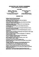
nonlinearity ll'll' corresponds to a typical "square-law" drag. Assume that we apply a unit step input in thrust u, followed 5 seconds later by a negative unit step input. The system response is plotted in Figure 1.1. We see that the system settles much faster in response to the positive unit step than it does in response to the subsequent negative unit step. Intuitively, this can be interpreted as reflecting the fact that the "apparent damping" coefficient ll'l is larger at high speeds than at low speeds. Assume now that we repeat the same experiment but with larger steps, of amplitude I 0. Predictably, the difference between the settling times in response to the positive and negative steps is even more marked (Figure I .2). Furthermore, the settling speed
"s in response to the first
step is not I0 times that obtained in response to the first unit step in the first experiment, as it would be in a linear system. This can again be understood intuitively, by writing that
6
Introduction :s
c;;
2
-
..c:
Chap. I >
1.0
>-
·g
0.8
C)
1.0 0.8
>
0.6-
0.6
0.4
0.4
0.2
0.2
0.0
s
0
0.0
10
s
0
10
-
15
20
cime(sec)
time(sec) Figure 1.1 : Response of system ( 1.3) to unit steps :s
-2 -
>
10.0
·-u
2:' ~
6.0
6.0
4.0 fo
4.0
2.0
2.0
0.0
s
0
0.0
10
0
10
time(sec)
-
15
20
time(sec)
Figure 1.2 : Response of system ( 1.3) to steps of amplitude I0 u=1
=>
o+ Ivs I vs = 1
=>
vs =I
Carefully understanding and effectively controlling this nonlinear behavior is particularly important if the vehicle is to move in a large dynamic range and change speeds co1tirtually, as is typical of industrial remotely-operated underwater vehicles (R.O.V. 's). D
SOME COMMON NONLINEAR SYSTEM BEHAVIORS Let us now discuss some common nonlinear system properties, so as to familiarize ourselves with the complex behavior of nonlinear systems and provide a useful background for our study in the rest of the book.
Nonlinear System Behavior
Sect. 1.2
7
Multiple Equilibrium Points Nonlinear systems frequently have more than one equilibrium point (an equilibrium point is a point where the system can stay forever without moving, as we shall fonnalize later). This can be seen by the following simple example. Example 1.2: A first-order system Consider the first order system
.\-=-x+x2
(1.4)
with initial condition x(O) = x 0 • Its linearization is ( 1.5)
x=-x
The solution of this linear equation is x(t) = x 0 e- 1 • It is plotted in Figure 1.3(a) for various initial conditions. The linearized system clearly has a unique equilibrium point at x = 0. By contrast, integrating equation dx/( -x + x2) =de, the actual response of the nonlinear dynamics ( 1.4) can be found to be
x0 e- 1
x(t)=----1 -X0 +X0 e-l
This response is plotted in Figure 1.3(b) for various initial conditions. The system has two equilibrium points. x
=0 and x = I , and its qualitative behavior strongly depends on its initial D
condition.
x(l)
(a)
(b)
Figure 1.3: Responses of the linearized system (a) and the nonlinear system (b)
8
Introduction
Chap. I
The issue of motion stability can also be discussed with the aid of the above example. For the linearized system, stability is seen by noting that f~"•r any initial condition, the motion always converges to the equilibrium point x = 0. However, consider now the actual nonlinear system. While motions starting with x0 < I will indeed converge to the equilibrium point x = 0, those starting with x 0 > I will go to infinity (actually in finite time, a phenomenon known as finite escap(:: time). This means that the stability of nonlinear systems may depend on initial condi :tons. In the presence of a bounded external input, stability may also be .iependent on the input value. This input dependence is highlighted by the so-called bil10ear system
.
x=xu If the input u is chosen to be - l, then the state x converges to 0. If u tends to infinity.
= I, then I x I
Limit Cycles Nonlinear systems can display oscillations of fixed amplitude and fixed period without external excitation. These oscillations are called limit cycles, or self-excited oscillations. This important phenomenon can be simply illustrated r:»y a famous oscillator dynamics, first studied in the 1920's by the Dutch electncal engineer Balthasar Vander Pol. Example 1.3: Van der Pol Equation The second-order nonlinear differential equation
mx+2c(x 2 -l ).r+kx=O
( 1.6)
where m, c and k are positive constants, is the famous Vander Pol equation. It car
bt~
regarded as
describing a mass-spring-damper system with a position-dependent damp1ng coefficient 2c(x2- I) (or, equivalently, an RLC electrical circuit with a nonlinear resistor). For large values
of x. the damping coefficient is positive and the damper removes energy from
tb·~
system. This
implies that the system motion has a convergent tendency. However, for small "alues of x, the damping coefficient is negative and the damper adds energy into the system. Tl: 1S :;uggests that the system motion has a divergent tendency. Therefore. because the nonlinear damping varies with x, the system motion can neither grow unboundedly nor decay to zero. Inste;.td. it displays a sustained oscillation independent of initial conditions, as illustrated in Figure 1.4 This so-called limit cycle is sustained by periodically releasing energy into and absorbing e11ergy from the environment, through the damping term. This is in contrast with the case of a cor:;ervative massspring system, which does not exchange energy with its environment during its vil··ration.
D
Nonlinear System Behavior
Sect. 1.2
9
X (I)
Figure 1.4: Responses of the Vander Pol oscillator
Of course, sustained oscillations can also be found in linear systems, in the case of marginally stable linear systems (such as a mass-spring system without damping) or in the response to sinusoidal inputs. However. limit cycles in nonlinear systems are different from linear oscillations in a number of fuRdamental aspects. First. the amplitude of the self-sustained excitation is independent of the initial condition. as seen in Figure 1.2, while the oscillation of a marginally stable linear system has its amplitude determined by its initial conditions. Second, marginally stable linear systems are very sensitive to changes in system parameters (with a slight change capable of leading either to stable convergence or to instability), while limit cycles are not easily affected by parameter changes. Limit cycles represent an important phenomenon in nonlinear systems. They can be found in many areas of enginering and nature. Aircraft wing fluttering, a limit cycle caused by the interaction of aerodynamic forces and structural vibrations, is frequently encountered and is sometimes dangerous. The hopping motion of a legged robot is another instance of a limit cycle. Limit cycles also occur in electrical circuits, e.g., in laboratory electronic oscillators. As one can see from these examples, limit cycles can be undesirable in some cases, but desirable in other cases. An engineer has to know how to eliminate them when they are undesirable, and conversely how to generate or amplify them when they are desirable. To do this, however, requires an understanding of the properties of limit cycles and a familiarity with the tools for manipulating them.
Bifurcations As the parameters of nonlinear dynamic systems are changed, the stability of the equilibrium point can change (as it does in linear systems) and so can the number of equilibrium points. Values of these parameters at which the qualitative nature of the
10
Introduction
Chap. I
system's motion changes are known as critical or bifurcation valu·~s. The /phenomenon of bifurcation, i.e., quantitative change of parameters leading to : · qualitative change of system properties, is the topic of bifurcation theory. For instance, the smoke rising from an incense stick (smok.:~slacks and cigarettes are old-fashioned) first accelerates upwards (because it is lighter than the ambient air), but beyond some critical velocity breaks into swirls. More prosaically, let us consider the system described by the so-called undamped Duffing ecuation
:r +ax+ x3 =0 (the damped Duffing equation is ~i + c,\- + ax+ ~x3 = 0, which may re:present a mass-damper-spring system with a hardening spring). We can plot the equilibrium points as a function of the parameter a. As a. varies from ~sitive to n•!gative, one -..J a. ). as sho,.o:n in Figure equilibrium point splits into three points ( xe = 0, 1.5(a). This represents a qualitative change in the dynamics and thus a= ~ 1 is a critical bifurcation value. This kind for bifurcation is known as a pitchfork, due to the shape of the equilibrium point plot in Figure 1.5(a).
-fr nonlinear systems satisfying some easy-to-check conditions. The method is mainly used to predict limit cycles in nonlinear S) ·;terns. Other applications include the prediction of subharmonic generation and the C:O!Wnnination of system response to sinusoidal excitation. The method has a number o' advantages. First, it can deal with low order and high order systems with the same stnig:htforward procedure. Second, because of its similarity to frequency-domain anal~ si~. of linear systems, it is conceptually simple and physically appealing, allowing users to exercise their physical and engineering insights about the control system. Third. it can deal with the "hard nonlinearities" frequently found in control systems ·.vithout any difficulty. As a result, it is an important tool for practical problems of nonlinear control analysis and design. The disadvantages of the method are Iinked to its approximate nature, and include the possibility of inaccurate predktions (false predictions may be made if certain conditions are not satisfied) and restril:ti•)ns on the systems to which it applies (for example, it has difficulties in dealing ·Nith systems with multiple nonlinearities).
Chapter 2 Phase Plane Analysis
Phase plane analysis is a graphical method for studying second-order systems. which was introduced well before the tum of the century by mathematicians such as Henri Poincare. The basic idea of the method is to generate. in the state space of a secondorder dynamic system (a two-dimensional plane called the phase plane), motion trajectories corresponding to various initial conditions, and then to examine the qualitative features of the trajectories. In such a way, information concerning stability and other motion patterns of the system can be obtained. In this chapter. our objective is to gain familiarity with nonlinear systems through this simple graphical method. Phase plane analysis has a number of useful properties. First, as a graphical method. it allows us to visualize what goes on in a nonlinear system starting from various initial conditions. without having to solve the nonlinear equations analytically. Second, it is not restricted to small or smooth nonlinearities, but applies equally well to strong nonlinearities and to "hard" nonlinearities. Finally, some practical control systems can indeed be adequately approximated as second-order systems, and the phase plane method can be used easily for their analysis. Conversely. of course. the fundamental disadvantage of the method is that it is restricted to second-order (or firstorder) systems, because the graphical study of higher-order systems is computationally and geometrically complex.
17
18
Phase Plane Analysis
Chap. 2
2.1 Concepts of Phase Plane Analysis 2.1.1 Phase Portraits The phase plane method is concerned with the graphical study of -;econd-order autonomous systems described by .\-1 = ft (xl • x2)
(2.la)
.\-2 = f2(x 1• x2)
(2.lb)
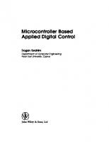
where x 1 and x 2 are the states of the system, and / 1 and h are nonlinear functions of the states. Geometrically, the state space of this system is a plane having x 1 and x2 as coordinates. We will call this plane the phase plane. Given a set of initial conditions x(O) = x0 , Equation (2.1) defint:s a solution x(t). With time t varied from zero to infinity, the solution x(r) can be rt!presented geometrically as a curve in the phase plane. Such a curve is called a phase plane trajectory. A family of phase plane trajectories corresponding to various initial conditions is called a phase portrait of a system. To illustrate the concept of phase portrait, let us consider the folkwing simple system. Exarjllple 2.1: Phase portrait of a mass-spring system The governing equation of the mass-spring system in Figure 2.l(a) is the familiar lirear secondorder differential equation
x+x=O
(2.2)
Assume that the mass is initially at rest, at length x0 • Then the solution of the equal ion is
Eliminating time 1 from the above equations, we obtain the equation of the trajectories
This represents a circle in the phase plane. Corresponding to different initial conditions. circles of different radii can be obtained. Plotting these circles on the phase plane, we .>btain a phase ponrait for the mass-spring system (Figure 2.l.b).
D
Sect. 2.1
Concepts of Phase Plllne Analysis
19
.
X
X
(a)
(b)
Figure 2.1 : A mass-spring system and its phase ponrait
The power of the phase portrait lies in the fact that once the phase portrait of a system is obtained. the nature of the system response corresponding to various initial conditions is directly displayed on the phase plane. In the above example, we easily see that the system trajectories neither converge to the origin nor diverge to infinity. They simply circle around the origin, indicating the marginal nature of the system's stability. A maJor class of second-order systems can be described by differential equations of the form
x+ j(x, i) = 0
(2.3)
In state space form, this dynamics can be represented as
.\'2 =- f(xl, x2) with x 1 = x and x 2 =.X. Most second-order systems in practice, such as mass-damperspring systems in mechanics, or resistor-coil-capacitor systems in electrical engineering, can be represented in or transformed into this form. For these systems, the states are x and its derivative i. Traditionally, the phase plane method is developed for the dynamics (2.3), and the phase plane is defined as the plane having x and i as coordinates. But it causes no difficulty to extend the method to more general dynamics of the form (2.1 ), with the (x 1 , x 2) plane as the phase plane, as we do in this chapter.
20
Phase Plane Analysis
Chap. 2
2.1.2 Singular Points An important concept in phase plane analysis is that of a singular poini. A singular point is an equilibrium point in the phase plane. Since an equilibrium p 0 if 9 < 0
(2.7)
which means that the thrusters push in the counterclockwise direction if 9 is positive, and vice versa. As the first step of the phase portrait generation, let us consider the phase portrait when the thrusters provide a positive torque U. The dynamics of the system is
which implies that
ada = u d9.
Therefore, the phase trajectories are a family or parabolas
defined by
where c 1 is a constant. The co.rresponding phase portrait of the system is shown in Figure 2.5(b ). When the thrusters provide a negative torque - U, the phase trajectories are similarly found to be
26
Phase Plane Analysis
Chap. 2 X
a
X
u :: . L' X
(a)
(b)
(c)
Figure 2.5 : Satellite control using on~off thrusters
with the corresponding phase ponrait shown in Figure 2.5(c).
parabolic trajectories
X
u = +U
u
= -U
switching line Figure 2.6 : Complete phase portrait of the control system
The complete phase ponrait of the closed-loop control system can be obr..ined simply by connecting the trajectories on the left half of the phase plane in 2.5(b) with those .m the right half of the phase plane in 2.5(c), as shown in Figure 2.6. The venical axis represents
.1
switching line,
because the control input and thus the phase trajectories are switched on that line. It is interesting to see that, staning from a nonzero initial angle. the satellite will oscillate in p·!ri:>dic motions
Constructing Phase Portraits
Sect. 2.2
27
under the action of the jets. One concludes from this phase ponrait that the system is marginally stable, similarly to the mass-spring system in Example 2.1. Convergence of the system to the zero angle can be obtained by adding rate feedback (Exercise 2.4).
0
THE METHOD OF ISOCLINES The basic idea in this method is that of isoclines. Consider the dynamics in (2.1 ). At a point (x 1, x 2) in the phase plane. the slope of the tangent to the trajectory can be detennined by (2.5). An isocline is defined to be the locus of the points with a given tangent slope. An isocline with slope a is thus defined to be
This is to say that points on the cuJVe
all have the same tangent slope
a.
In the method of isoclines. the phase portrait of a system is generated in two steps. In the first step. a field of directions of tangents to the trajectories is obtained. In the second step, phase plane trajectories are fonned from the field of directions. Let us explain the isocline method on the mass-spring system in (2.2). The slope of the trajectories is easily seen to be dx _
x
dxl
x2
2 -- -1
Therefore, the isocline equation for a slope a is
i.e .. a straight line. Along the line, we can draw a lot of short line segments with slope a. By taking a to be different values, a set of isoclines can be drawn, and a field of directions of tangents to trajectories are generated, as shown in Figure 2. 7. To obtain trajectories from the field of directions, we assume that the the tangent slopes are locally constant. Therefore, a trajectory starting from any point in the plane can be found by connecting a sequence of line segments. Let us use the method of isoclines to study the Van der Pol equation, a nonlinear equation.
Plulse Plane Analysis
28
Chap. 2
X
X 00
Figure 2.7 : Isoclines for the system
na~s-spring
Example 2.6: The Van der Pol equation For the Van der Pol equation
.X+ 0.2(x2- l).r +x = o an isocline of slope ex is defined by
dx 0.2(x2 -I )x+x -==ex dx • X
Therefore, the points on the curve 0.2(x2-l).r+x+ex.r=O all have the same slope ex. By taking ex of different values, different isoclines can be obtained, as plotte•.. in Figure 2.8. Shon line segments are drawn on the isoclines to generate a field of tangent directiOns. The phase portraits can then be obtained. as shown in the plot. It is interesting to note tha: there exists a closed curve in the ponrait. and the trajectories starting from both outside and ins de converge to this curve. This closed curve corresponds to a limit cycle, as will be discussed further in section
~-
0
Note that the same scales should be used for the x 1 axis and x2 axi ~· of the phase plane, so that the derivative dx2/dx 1 equals the geometric slope of the trajectories. Also note that, since in the second step of phase portrait construction '" e essentially assume that the slope of the phase plane trajectories is locally constant, r1ore isoclines should be plotted in regions where the slope varies quickly, to improve an;uracy.
Determining Time from Phase Portraits
Sect. 2.3
a=O
29
a=-1
.. a=-5 .!
a=l
,.
,\'
,t'
,\'
.r·
.•t'
trajectory ~
limit cycle
·'
. "
isoclines
Figure 2.8 : Phase ponrait of the Vander Pol equation
2.3 Determining Time from Phase Portraits Note that time t does not explicitly appear in the phase plane having x 1 and x 2 as coordinates. However, in some cases, we might be interested in the time information. For example, one might want to know the time history of the system states starting from a specific initial point. Another relevant situation is when one wants to know how long it takes for the system to move from a poinc to another point in a phase plane trajectory. We now describe two techniques for computing time history from phase ponraits. Both techniques involve a step-by step procedure for recovering time.
Obtaining time from !l t == !lx I ..t In a short time .1r, the change of xis approximately dx = xdt
(2.8)
where xis the velocity corresponding to the increment dx. Note that for a dx of finite magnitude, the average value of velocity during a time increment should be used to improve accuracy. From (2.8), the length of time corresponding to the increment ax
30
Phase Plane Analysis
Chap. 2
IS
.
X
The above reasoning implies that, in order to obtain the time corresp·.mding to the motion from one point to another point along a trajectory, one shou d divide the corresponding part of the trajectory into a number of small segments (n,>t necessarily equally spaced), tind the time associated with each segment. and then add up the results. To obtain the time history of states corresponding to a ·. ertain initial condition, one simply computes the time t for each point on the phase traj,!ctory, and then plots x with respect to t and .r with respect to r.
Obtaining time from t = f (1/x) dx Since.\-= dx/dt, we can write dt = dx/x. Therefore, t- to
r· (
=
1/.r) dx
.{(I
where x corresponds to time t and x 0 corresponds to time t0 . This equation implies that. if we plot a phase plane portrait with new coordinates x and ( 1/.r). th·!n the area under the resulting curve is the corresponding time interval.
2.4 Phase Plane Analysis of Linear Systems In this section, we describe the phase plane analysis of linear sysh:ms. Besides allowing us to visually observe the motion patterns of linear systems, :his will also help the development of nonlinear system analysis in the next sectkn. because a nonlinear systems behaves similarly to a linear system around each equil,·xium point. The general form of a linear second-order system is
=a X 1' + b X2
(2.9a)
x2=cx1 +dx2
(2.9b)
.\-1
To facilitate later discussions, let us transfonn this equation into a scalar second-order differential equation. Note from (2.9a) and (2.9b) that
b X2
=b CX 1 + d (X 1 -
a X 1)
Consequently, differentiation of (2.9a) and then substitution of (2.9b) leads to
/
Phase Plo.ne Analysis of Linear Systems
Sect. 2.4
31
.X 1 =(a +d)x 1 + (cb- ad)x 1 Therefore, we will simply consider the second-order linear system described by (2.10)
x+ax+bx=O
To obtain the phase portrait of this linear system, we first solve for the time history x(t) = k t e"-t 1 + k2 e"-1 1
for At
* A2
(2.11 a)
x(t) = kt e"-1 1 + k2 r e"-t 1
for At = ~
(2.11 b)
where the constants At and A2 are the solutions of the characteristic equation s2 + as + b = (s - At) (s - A2) =0
The roots At and ~ can be explicitly represented as
At
=(-a + ~ a2 - 4 b )/2
~ = (-a-~ a2 -
4 b )/2
For linear systems described by (2.1 0), there is only one singular point (assuming b 0), namely the origin. However. the trajectories in the vicinity of this singularity point can display quite different characteristics, depending on the values of a and b. The following cases can occur
*
1. At
and~
are both real and have the same sign (positive or negative)
2. A1 and ~ are both real and have opposite signs 3. At and ~ are complex conjugate with non-zero real pans 4. At and ~ are complex conjugates with real parts equal to zero We now briefly discuss each of the above four cases.
STABLE OR UNSTABLE NODE The first case corresponds to a node. A node can be stable or unstable. If the eigenvalues are negative, the singularity point is called a stable node because both x(r) and x(t) converge to zero exponentially, as shown in Figure 2.9(a). If both eigenvalues are positive, the point is called an unstable node, because both x(t) and x(t) diverge from zero exponentially, as shown in Figure 2.9(b). Since the eigenvalues are real, there is no oscillation in the trajectories.
32
Phase Plane Analysis
Chap. 2
SADDLE POINT
"-2
The second case (say A. 1 < 0 and > 0) corresponds to a saddle point 1Fgure 2.9(c)). The phase portrait of the system has the interesting "saddle" shape shown in Figure 2.9(c). Because of the unstable pole "-2 , almost all of the system trajectories diverge to intinity. In this figure, one also observes two straight lines passi -lg through the origin. The diverging line (with arrows pointing to infinity) corresporlds to initial conditions which make k 2 (i.e., the unstable component) equal zero. ·:·ht~ converging straight line corresponds to initial conditions which make k 1 equal zero
STABLE OR UNSTABLE FOCUS The third case corresponds to a focus. A stable focus occurs when the real part of the eigenvalues is negative, which implies that x(t) and x(t) both converg::: tJ zero. The system trajectories in the vicinity of a stable focus are depicted in Figure 2.9(d). Note that the trajectories encircle the origin one or more times before converging to it, unlike the situation for a stable node. If the real part of the eigenvalue~; is positive, then x(t) and .t(t) both diverge to infinity, and the singularity point is called an unstable focus. The trajectories corresponding to an unstable focus ••re sketched in Figure 2. 9( e).
CENTER POINT The last case corresponds to a center point, as shown in Figure 2.~J(f). The name comes from the fact that all trajectories are ellipses and the singulan :y point is the center of these ellipses. The phase portrait of the undamped mass . spring system belongs to this category. Note that the stability characteristics of linear systems are uniqudy determined by the nature of their singularity points. This, however, is not true for nonlinear systems.
2.5 Phase Plane Analysis of Nonlinear Systems In discussing the phase plane analysis of nonlinear systems, two points ·;hould be kept in mind. Phase plane analysis of nonlinear systems is related to that of Iin,!ar systems, because the local behavior of a nonlinear system can be approximated t·y the behavior of a linear system. Yet, nonlinear systems can display much mon: •::omplicated patterns in the phase plane, such as multiple equilibrium points and linit cycles. We now discuss these points in more detail.
Phase Plane Analysis of Nonlinear Systems
Sect. 2.5
X
stable node ~*'-*-+------a
(a) X
unstable node ------+-*'-*~
a (b) X
saddle point -"""'*--+----illt-----0 (c)
X
stable focus
X
----+------a X
(d) X
X
unstable focus
----+----~0
X
(e) X
center point
(f)
Figure 2.9 : Phase-ponraits of linear systems
33
34
Phase Plllne Analysis
Chap. 2
LOCAL BEHAVIOR OF NONLINEAR SYSTEMS In the phase portrait of Figure 2.2, one notes that. in contrast to linear 5ystems, there are two singular points, (0, 0) and (- 3, 0). However, we also note that ·:he features of the phase trajectories in the neighborhood of the two singular points look very much like those of linear systems, with the first point corresponding to a stabk focus and the second to a saddle point. This similarity to a linear system in the local region of each singular point can be formalized by linearizing the nonlinear system, as we now discuss. If the singular point of interest is not at the origin, by defining th•:: difference between the original state and the singular point as a new set of state variables, one can always shift the singular point to the origin. Therefore, without los:, o: generality, we may simply consider Equation (2.1) with a singular point at 0. C sing Taylor expansion, Equations (2.1 a) and (2.1 b) can be rewritten as
.X 1 = ax 1 + bx2 + g. 0, there exists r > 0, such that if llx(O)II < r, then llx(t)ll < R for all t ~ 0 . Orlterwise, the
equilibrium point is unstable. Essentially, stability (also called stability in the sense of Lyapunov, or Lyapunov stability) means that the system trajectory can be kept arbitrarily close to tht:: origin by starting sufficiently close to it. More formally, the definition states that the origin is stable, if, given that we do not want the state trajectory x(t) to get out of a ball of arbitrarily specified radius DR , a value r(R) can be found such that stanin.~ the state from within the ball Dr at time 0 guarantees that the state will stay within the ball DR thereafter. The geometrical implication of stability is indicated by curve 2 in Figure 3.3. Chapter 2 provides examples of stable equilibrium points in the ca~•! of secondorder systems, such as the origin for the mass-spring system of Example .:~. 1. or stable nodes or foci in the local linearization of a nonlinear system. Throughout the book, we shall use the standard mathematical abbreviation symbols: \:1 3
to mean "for any" for "there exists" e for "in the set" => for "implies that" Of course, we shall say interchangeably that A implies 8, or that A is a sufficient condition of 8, or that B is a necessary condition of A. If A => 8 and 8 => A, then A and B ace equivalent, which we shall denote by A B . Using these symbols, Definition 3.3 can be written
"i/ R > 0 , 3 r > 0 ,
II x(O) II < r => "i/ t
~0,
II x(t) II < R
or, equivalently
"i/ R > 0 , 3 r > 0 , x(O) e Br
=>
"i/ t
~ 0 , x(t) e
DR
Conversely, an equilibrium point is unstable if there exists at least one ball DR, such that for every r > 0, no matter how small, it is always possible fo~· t:1e system trajectory to start somewhere within the ball Br and eventually leave the ball DR (Figure 3.3). Unstable nodes or saddle points in second-order systems are examples of unstable equilibria. Instability of an equilibrium point is typically undesimble, because
Concepts of Stllbility
Sect. 3.2
49
it often leads the system into limit cycles or results in damage to the involved mechanical or electrical components.
curve 1 - asymptotically stable curve 2- marginally stable curve 3 - unstaule
Figure 3.3 : Concepts of stability
It is important to point out the qualitative difference between instability and the intuitive notion of "blowing up" (all trajectories close to origin move further and further away to infinity). In linear systems, instability is equivalent to blowing up, because unstable poles always lead to exponential growth of the system states. However, for nonlinear systems, blowing up is only one way of instability. The following example illustrates this point. Example 3.3: Instability of the Vander Pol Oscillator The Vander Pol oscillator of Example 2.6 is described by
One easily shows that the system has an equilibrium point at the origin. As pointed out in section 2.2 and seen in the phase ponrait of Figure 2.8, system trajectories staning from any non-zero initial states all asymptotically approach a limir cycle. This implies that, if we choose R in Definition 3.3 to be small enough for the circle of radius R to fall completely within the closed-curve of the limit cycle, then system trajectories staning near the origin will eventually get out of this circle (Figure 3.4). This implies instability of the origin. Thus, even though the state of the system does remain around the equilibrium point in a cenain sense, it cannot stay arbitrarily close to it. This is the fundamental distinction between 0 stability and instability.
so
Fundamentals of Lyapunov Theory
Chap. 3
trajectories
X
I
Figure 3.4 : Unstable origin of the Vander Pol Oscillator
ASYMPTOTIC STABILITY AND EXPONENTIAL STABILITY In many engineering applications, Lyapunov stability is not enough. ·:;or example, when a satellite's attitude is disturbed from its nominal position, we not ·.>n ly want the satellite to maintain its attitude in a range determined by the magnitude of the disturbance, i.e., Lyapunov stability, but also require that the attitude gradually go back to its original value. This type of engineering requirement is caotued by the concept of asymptotic stability. Definition 3.4 An equilibrium point 0 is asvmptotical/y stable if it is stab1e. and if in addition there exists some r > 0 such that II x(O) II< r implies that x(t) ~ I) '2S t ~ oo. Asymptotic stability means that the equilibrium is stable, and th~!t in addition, states started close to 0 actually converge to 0 as time t goes to infini!y. Figure 3.3 shows that system trajectories starting from within the ball Br converge to the origin. The ball Br is called a domain of attraction of the equilibrium point (wh1:e rhe domain of attraction of the equilibrium point refers to the largest such region, i.e , ro the set of all points such that trajectories initiated at these points eventually convt!rge to the origin). An equilibrium point which is Lyapunov stable but not asympwtically stable is called marginally stable. One may question the need for the explicit stability requirt~ment in the definition above, in view of the second condition of state convergence to the origin. However, it it easy to build counter-examples that show that state convergence does not necessarily imply stability. For instance, a simple system studied by Vinograd has trajectories of the form shown in Figure 3.5. All the trajectories starting fro;n non-zero
Concepts of Stability
Sect. 3.2
51
initial points within the unit disk first reach the curve C before conv~rging to the origin. Thus, the origin is unstable in the sense of Lyapunov, despite the state convergence. Calling such a system unstable is quite reasonable, since a curve such as C may be outside the region where the model is valid - for instance, the subsonic and supersonic dynamics of a high-performance aircraft are radically different, while, with the problem under study using subsonic dynamic models, C could be in the supersonic range.
Figure 3.5: State convergence does not imply stability
In many engineering applications, it is stiJJ not sufficient to know that a system will converge to the equilibrium point after infinite time. There is a need to estimate how fast the system trajectory approaches 0. The concept of exponenrial stability can be used for this purpose.
Definition 3.5
An equilibrium point 0 is exponential/}' stable strictly positive numbers a and Asuch that 'r;f t
> 0,
II x(t) II
$ a
if
there exist two
II x(O) II e-l..r
(3.9)
in some ball B,. around the origin.
In words, (3.9) means that the state vector of an exponentially stable system converges to the origin faster than an exponential function. The positive number A is often called the rate of exponential convergence. For instance, the system
x = - ( I + sin 2 x) x is exponentially convergent to x = 0 with a rate A= I . Indeed, its solution is
52
Fundamentals of Lyapunov Theory x(t) = x(O) exp(-
r[
Chap. 3
I+ sin2(x(t))] dt)
0
and therefore lx(t)l $ lx(O)I e- 1
Note that exponential stability implies asymptotic stability. Bl.t asymptotic stability does not guarantee exponential stability, as can be seen from the ·;ystem
.i- = -x2,
x(O) = I
(3.10)
whose solution is x = 1/( I + t), a function slower than any exponential :unction e-A.t (with A> 0). The definition of exponential convergence provides an explicit hound on the state at any time, as seen in (3.9). By writing the positive constant a as c = eA. to • it is easy to see that, after a time of t 0 + ( 1/A.) , the magnitude of the state vec::or decreases to less than 35% ( == e- I ) of its original value, similarly to the notion of ,.;me-constant in a linear system. After t 0 + (3/A.) , the state magnitude llx(t)ll will be less than 5% ( == e- 3 ) of llx(O)II.
LOCAL AND GLOBAL STABILITY The above definitions are formulated to characterize the local behavio~· of systems, i.e., how the state evolves after starting near the equilibrium point. Lol:al properties tell little about how the system will behave when the initial state is s. ··me distance away from the equilibrium, as seen for the nonlinear system in Exampk l.l. Global concepts are required for this purpose. Definition 3.6 If asymptotic (or exponential) stability holds for any init:~l states, the equilibrium point is said to be asymptotically (or exponentially) stable f.!.:· tf.e large. It is also called globally asymptotically (or exponentially) stable. For instance, in Example 1.2 the linearized system is globally a:-.ymptotically stable, but the original system is not. The simple system in (3.10) is .Js-J globally asymptotically stable, as can be seen from its solutions.
Linear time-invariant systems are either asymptotically stable, c:· marginally stable, or unstable, as can be be seen from the modal decomposition of l.near system solutions; linear asymptotic stability is always global and exponential, and linear instability always implies exponential blow-up. This explains why the re_rined notions of stability introduced here were not previously encountered in the st1.d) of linear systems. They are explicitly needed only for nonlinear systems.
Linearization and Local Slllbility
Sect. 3.3
53
3.3 Linearization and Local Stability Lyapunov's linearization method is concerned with the local stability of a nonlinear system. It is a fonnalization of the intuition that a nonlinear system should behave similarly to its linearized approximation for small range motions. Because all physical systems are inherently nonlinear, Lyapunov's linearization method serves as the fundamental justification of using linear control techniques in practice, i.e., shows that stable design by linear control guarantees the stability of the original physical system locally. Consider the autonomous system in (3.2), and assume that f(x) is continuously differentiable. Then the system dynamics can be written as
x = ( ~!) x=O
(3.11)
x + fh.o.r. 0. Then, since V is continuous and V(O) = 0, there exists a ball Br that the system trajectory never enters (Figure •
(I
3.llb). But then, since - V is also continuous and positive definite, and since BR is bounded,
- i1
must remain larger than some strictly positive number L 1• This is a contradiction, because it would imply that V(t) decreases from its initial value V0 to a value strictly smaller than L, in a finite time smaller than [V0
-
L)!L 1• Hence, all trajectories starting in Br asymptotically converge
0
to the origin.
In applying the above theorem for analysis of a nonlinear system, one goes through the two steps of choosing a positive definite function, and then determining its derivative along the path of the nonlinear systems. The following example illustrates this procedure. Example 3.7: Local Stability A simple pendulum with viscous damping is described by
Consider the following scalar function
.
')
V(x) = ( l-cos8) + 82
Fundamentals of Lyapunov Theory
64
Chap. 3
One easily verifies that this function is locally positive definite. As a matter of fact,
l1is
function
represents the total energy of the pendulum, composed of the sum of the potential en:rg:: :1nd the kinetic energy. Its time-derivative is easily found to be
V(x)
= 9 sin 9 + 99 = -9 2 ~ 0
Therefore, by invoking the above theorem, one concludes that the origin is a stable eq·Jilibrium point. In fact, using physical insight, one easily sees the reason why V(x) ~ 0, nan·ely that the damping tenn absorbs energy. Actually.
V is
precisely the power dissipated in th•: p·~ndulum.
However, with this Lyapunov function, one cannot draw conclusions on the of the system, because
asympt~-tic
stability
V(x) is only negative semi-definite.
0
The following example illustrates the asymptotic stability result. Example 3.8: Asymptotic stability Let us study the stability of the nonlinear system defined by
around its equilibrium point at the origin. Given the positive definite function
its derivative V along any system trajectory is
V= 2(x 12 +xl> (.t} +x~2- 2) Thus.
V is
locally negative definite in the 2-dimensional ball 8.,, i.e., in the regiol' d!fined by
.tl + xl < 2.
Therefore, the above theorem indicates that the origin is asymptoticalh stable.
0
LY APUNOV THEOREM FOR GLOBAL STABILITY The above theorem applies to the local analysis of stability. In order to as:;ez1 global asymptotic stability of a system, one might naturally expect that the ball BR in the 0 above local theorem has to be expanded to be the whole state-space. Thi .; i;; indeed necessary, but it is not enough. An additional condition on the function '· · has to be satisfied: V(x) must be radially unbounded, by which we mean that V( \:) --) oo as llxll ---+ oo (in other words, as x tends to infinity in any direction). We the11 obtain the following powerful result:
Lyapunov's Direct Method
Sect. 3.4
65
Theorem 3.3 (Global Stability) Assume that there exists a scalar function V of the state x, with continuous first order derivatives such that • V(x) is positive definite • V(x) is negative definite
• V(x) --+ 00
as
llxll --+ 00
then the equilibrium at the origin is globally asymptotically stable. Proof: The proof is the same as in the local case, by noticing that the radial unboundedness of V, combined with the negative definiteness of V, implies that, given any initial condition x0 , the trajectories remain in the bounded region defined by V(x) S V(x 0 ).
D
The reason for the radial unboundedness condition is to assure that the contour curves (or contour surfaces in the case of higher order systems) V(x) = Va correspond to closed curves. If the curves are not closed, it is possible for the state trajectories to drift away from the equilibrium point, even though the state keeps going through contours corresponding to smaller and smaller Va's. For example, for the positive definite function V = [ x 12/(1 + x 12)] + xl, the curves V(x) = V a for V a > I are open curves. Figure 3.12 shows the divergence of the state while moving toward lower and lower "energy" curves. Exercise 3.4 further illustrates this point on a specific system.
\'(X}
=
Figure 3.12 : Motivation of the radial unboundedness condition
66
("'h .... ap. 3
Fundamentals of Lyapunov Theory
Example 3.9: A class of first-order systems Consider the nonlinear system ,( + c(x)
=0
where c is any continuous function of the same sign as its scalar argument x. i.e., xc(x) > 0
for x;t:O
Intuitively, this condition indicates that - c(x) "pushes" the system back towards its rest position x =0, but is otherwise arbitrary. Since cis continuous, it also implies that c(O) =0 (Fi~;ure 3.13). Consider as the Lyapunov function candidate the square of the distance to the ori jn
The function Vis radially unbounded, since it tends to infinity as lxl
~
oo . Its deriv~ri,.·c! is
V =2 x .r ==- 2 x c(x) Thus
V< 0 as long as x '# 0, so that x = 0 is a globally asymptotically stable equilibri~.; ·n point.
X
Figure 3.13: The function c(x) For instance, the system
is globally asymptotically convergent to x = 0, since for x '# 0, sin 2 x S lsin x1 < ~tl. Similarly, the system
is globally asymptotically convergent to x =0. Notice that while this sysrern 's linear approximation (.X= 0) is inconclusive, even about local stability, the actual nonl1near system enjoys a strong stability property (global asymptotic stability).
0
Lyapunov's Direct Method
Sect. 3.4
67
Example 3.10: Consider the system
X• 2-
••
•• ( ••
-"'I - ""2 ""I
2 + •. 2) "'2
The origin of the state-space is an equilibrium point for this system. Let V be the positive definite function
The derivative of V along any system trajectory is
which is negative definite. Therefore, the origin is a globally asymptotically stable equilibrium point. Note that the globalness of this stability result also implies that the origin is the only equilibrium point of the system.
D
REMARKS Many Lyapunov functions may exist for the same system. For instance, if V is a Lyapunov function for a given system, so is
VI = pya where p is any strictly positive constant and a is any scalar (not necessarily an integer) larger than I. Indeed, the positive-definiteness of V implies that of V 1 , the positivedefiniteness (or positive semi-definiteness) of - V implies that of - V1 , and (the radial unboundedness of V (if applicable) implies that of V1 • More importantly, for a given system, specific choices of Lyapunov functions may yield more precise results than others. Consider again the pendulum of Example 3.7. The function
I ·2 +-(6+6) I • 2 +2(1-cos6) V(x)=-6
2
2
is also a Lyapunov function for the system, because locally V(x)=-(S2+6sin6) S 0 However, it is interesting to note that V is actually locally negative definite, and therefore, this modified choice of V, without obvious physical meaning, allows the asymptotic stability of the pendulum to be shown.
68
Fundamentals of Lyapunov Theory
Chap. 3
Along the same lines, it is important to realize that the theorems in Lyapunov analysis are all sufficiency theorems. If for a particular choice of Lyapun,·v function candidate V, the conditions on V are not met, one cannot draw any conclus 10ns on the stability or instability of the system - the only conclusion one should dn1.v is that a different Lyapunov function candidate should be tried.
3.4.3 Invariant Set Theorems Asymptotic stability of a control system is usually a very important property to be determined. However, the equilibrium point theorems just described are ofl·.!n difficult to apply in order to assert this property. The reason is that it often happen~ that V, the derivative of the Lyapunov function candidate, is only negative semi-defin.te. as seen in (3.15). In this kind of situation, fortunately, it is still possible to draw conclusions on asymptotic stability, with the help of the powerful invariant set theorem:.. attributed to La Salle. This section presents the local and global versions of the ir variant set theorems. The central concept in these theorems is that of invariant set, a the concept of equilibrium point.
gener:di~~ation
of
Definition 3.9 A set G is an invariant set for a dynamic system if e\. ·?r~: system trajectory which starts from a point in G remains in G for all future time. For instance, any equilibrium point is an invariant set. The domain of attr;; .;ti :m of an equilibrium point is also an invariant set. A trivial invariant set is the \\ 1ole statespace. For an autonomous system, any of the trajectories in state-space is ;:n invariant set. Since limit cycles are special cases of system trajectories (closed cu ·-ves in the phase plane), they are also invariant sets. Besides often yielding conclusions on asymptotic stability wlh!n V, the derivative of the Lyapunov function candidate, is only negative semi-d:.-finite, the invariant set theorems also allow us to extend the concept of Lyapunov fun,;tion so as to describe convergence to dynamic behaviors more general than equilit·riL.m, e.g., convergence to a limit cycle. Similarly to our earlier discussion of Lyapunov's direct method, we frst discuss the local version of the invariant set theorems, and then the global version.
LOCAL INVARIANT SET THEOREM The invariant set theorems reflect the intuition that the decrease of a L:tapunov function V has to gradually vanish (i.e., V has to converge to zero) because \.i is lower
Sect. 3.4
Lyapunov's Direct Method
69
bounded. A precise statement of this result is as follows.
Theorem 3.4 (Local Invariant Set Theorem) Consider an autonomous system of the form (3.2), with f continuous, and let V(x) be a scalar function with continuous first partial derivatives. Assume that • for some I > 0, the region 0.1 defined by V(x) < I is bounded • V(x) ~ 0 for all X in
n,
invariant set in R.
n,
=0 , and M be the largest Then, every solution x(t) originating in n1 tends toM as t ~ oo.
Let R be the set of all points within
where V(x)
Note that in the above theorem, the word "largest" is understood in the sense of set theory, i.e., M is the union of all invariant sets (e.g., equilibrium points or limit cycles) within R. In particular, if the set R is itself invariant (i.e., if once V =0, then V 0 for all future time), then M = R.
=
The geometrical meaning of the theorem is illustrated in Figure 3.14, where a trajectory starting from within the bounded region 1 is seen to converge to the largest invariant set M. Note that the set R is not necessarily connected, nor is the set M.
n
V=l
v
R~
Me Figure 3.14 : Convergence to the largest invariant set M
The theorem can be proven in two steps, by first sho~ing that V goes to zero, and then showing that the state converges to the largest invariant set within the set defined by V= 0. We shall simply give a sketch of the proof, since the detailed proof of the second part involves a number of concepts in topology and real analysis which are not prerequisites of this text.
70
Fundamentals of Lyapunov Theory
Chap. 3
Proor: The firsr pan of the proof involves showing that
V-+ 0 for any trajectory st.1rting
from a
point in 0 1• using a result in functional analysis known as Barbalafs lemma, wr 1ch we shall detail in section 4.3. Specifically, consider a trajectory starting from an arbitrary point x0 in 0 1• T1e trajectory must stay in 0 1 all the time, because V :s; 0 implies that V[x(r)j :s; V[x(O)J
.r = 0
or
X
=± I
Let us consider each of these cases:
x=o x=±l
=> =>
x = sin 1tX2 - x
:~: 0 except if x = 0 or x = ± I
x=o
Thus, the invariant set theorem indicates that the system converges globally to ~x :: l: .r = 0) or (x =- 1:
.r = 0), or to (x = 0: .i- = 0). The first two of these equilibrium points are ~1able. since they
correspond to local mimina of V (note again that linearization is
inconclu~- · ve
about their
stability). By contrast, the equilibrium point (x = 0; x= 0) is unstable, as can be shown from linearization (x
= ('lt/2 -
I) x), or simply by noticing that because that point is a lo•. al maximum of
V along the x axis, any small deviation in the x direction will drive the trajectory a·.va:.· from it.
0
As noticed earlier, several Lyapunov functions may exist for a .:~iven system, and therefore several associated invariant sets may be derived. The s:1stem then converges to the (necessarily non-empty) intersection of the invariant sets :\'I;, which may give a more precise result than that obtained from any of the Lyapt.:nov functions taken separately. Equivalently, one can notice that the sum of two Lyapunov functions for a given system is also a Lyapunov function, whose se·: R is the intersection of the individual sets Ri .
3.5 System Analysis Based on Lyapunov's Direct 1\:IE~thod With so many theorems and so many examples presented in the last sec(ion, one may feel confident enough to attack practical nonlinear control problems. Hc·wever, the theorems all make a basic assumption: an explicit Lyapunov function is somehow
Sect. 3.5
System Analysis Based on Lyapunov's Direct Method
77
known. The question is therefore how to find a Lyapunov function for a specific problem. Yet, there is no general way of finding Lyapunov functions for nonlinear systems. This is a fundamental drawback of the direct method. Therefore, faced with specific systems, one has to use experience, intuition, and physical insights to search for an appropriate Lyapunov function. In this section, we discuss a number of techniques which can facilitate the otherwise blind search of Lyapunov functions. We first show that, not surprisingly, Lyapunov functions can be systematically found to describe stable linear systems. Next, we discuss two of many mathematical methods that may be used to help finding a Lyapunov function for a given nonlinear system. We then consider the use of physical insights, which, when applicable, represents by far the most powerful and elegant way of approaching the problem, and is closest in spirit to the original intuition underlying the direct method. Finally, we discuss the use of Lyapunov functions in transient perfonnance analysis.
3.5.1 Lyapunov Analysis of Linear Time-Invariant Systems Stability analysis for linear time-invariant systems is well known. It is interesting. however, to develop Lyapunov functions for such systems. First, this allows us to describe both linear and nonlinear systems using a common language. allowing shared insights between the two classes. Second, as we shall detail later on, Lyapunov functions are "additive", like energy. In other words, Lyapunov functions for combinations of subsystems may be derived by adding the Lyapunov functions of the subsystems. Since nonlinear control systems may include linear components (whether in plant or in controller), we should be able to describe linear systems in the Lyapunov formalism. We first review some basic results on matrix algebra, since the development of Lyapunov functions for linear systems will make extensive use of quadratic forms. SYMMETRIC, MATRICES
SKEW-SYMMETRIC,
AND
POSITIVE
DEFINITE
Definition 3.10 A square matrix M is symmetric if M = MT (in olher words, 'V i,j Mij = Mji ). A square matrix M is skew-symmetric if M =- MT (i.e, 'V i,j Mij =- Mj; ).
if if
An interesting fact is that any square n x n matrix M can be represented as the sum of a symmetric matrix and a skew-symmetric matrix. This can be shown by the following decomposition
78
Fundamentals of Lyapunov Theory M = M + MT + 2
Chap. 3
_M_-_M_T
2
where the first tenn on the left side is symmetric and the second tenn 1s skewsymmetric. Another interesting fact is that the quadratic function associated w 1:h a skewsymmetric matrix is always zero. Specifically, let M be a nxn skew-symm•.~tric matrix and x an arbitrary nxl vector. Then the definition of a skew-symmetric ma1ri:c. implies that xTMx =- xTMT x Since xTMT xis a scalar, the right-hand side of the above equation can be ~!placed by its transpose. Therefore, xTMx=-xTMx This shows that
(3.16)
In designing some tracking control systems for robots, for instance, this
fact is very
useful because it can simplify the control law, as we shall see in chapter 9. Actually, property (3.16) is a necessary and sufficient condition for ~t matrix M to be skew-symmetric. This can be easily seen by applying (3.16) to the b.1sis vectors
e;:
and
[ "i/ (i,j), (e; + ej)TMs(e; + ej) = 0] => [ "i/ (i,j), M;; + Mij + Mj; + Ai'jj = 0] which, using the first result, implies that
"i/ (i J.) t
'
M·· =- M··lj Jl
In our later analysis of linear systems, we will often use quadratic lun:tions of the fonn xTM x as Lyapunov function candidates. In view of the above, eaC1 quadratic function of this fonn, whether M is symmetric or not, is always equal to :1 quadratic function with a symmetric matrix. Thus, in considering quadratic functions of the fonn xTM x as Lyapunov function candidates, one can always assume, with•.>u: loss of generality. that M is symmetric.
System Analysis Based on Lyapunov's Direct Method
Sect. 3.5
79
We are now in a position to introduce the important concept of positive definite matrices.
Definition 3.11 x
*0
A square n x n matrix M is positive definite (p.d.)
=>
if
xr M x > 0
In other words, a matrix M is positive definite if the quadratic function xTM x is a positive definite function. This defmition implies that to every positive definite matrix is associated a positive definite function. Obviously, the converse is not true. Geometrically, the definition of positive-definiteness can be interpreted as simply saying that the angle between a vector x and its image Mx is always less than 90° (Figure 3.18).
Mx
Figure 3.18 : Geometric interpretation of the positive-definiteness of a matrix M
A necessary condition for a square matrix M to be p.d. is that its diagonal elements be strictly positive, as can be seen by applying the above definition to the basis vectors. A famous matrix algebra result called Sylvester's theorem shows that, assuming that M is symmetric, a necessary and sufficient condition forM to be p.d. is that its principal minors (i.e., M 11 , M 1 1M22- M2 1 M l2, ... , det M ) all be strictly positive; or, equivalently, that aJJ its eigenvalues be strictly positive. In particular, a p.d. matrix is always invertible, because the above implies that its determinant is nonzero.
A positive definite matrix M can always be decomposed as (3.17)
where U is a matrix of eigenvectors and satisfies uru = I, and A is a diagonal matrix containing the eigenvalues of the matrix M. Let A.m;n{M) denote the smallest eigenvalue of M and "-maiM) the largest. Then, it follows from (3.17) that "-min(M) llxll 2 ~ xTMx ~ "-mtu·(M)IIxll 2
80
Fundamentals of Lyapunov Theory
Chap. 3
This is due to the following three facts:
• xTMx = xTur AUx = zT Az, where Ux = z • A.min(M) I S A S A.max(M) I • zTz =
11x112
The concepts of positive semi-definite, negative definite, and nt:~ga.tive semidefinite can be defined similarly. For instance, a square n x n matrix M is said to be positive semi-definite ( p.s.d.) if
'\1 x , xT M x ~ 0 By continuity, necessary and sufficient conditions for positive semi-definiteness are obtained by substituting "positive or zero" to "strictly positive" in the above conditions for positive definiteness. Similarly, a p.s.d. matrix is invertible only if it is actually p.d. Examples of p.s.d. matrices are n x n matrices of the form M = NTl' where N is a m x n matrix. Indeed,
A matrix inequality of the form
(where M 1 and M 2 are square matrices of the same dimension) means tl1at
i.e., that the matrix M 1 - M 2 is positive definite. Similar notations aJ:ply to the concepts of positive semi-definiteness, negative definiteness, and negative semidefiniteness.
A time-varying matrix M(t) is uniformly positive definite if 3
a > 0, '\1 t ~ 0, M(t) ~ ex I
A similar definition applies for uniform negative-definiteness of a time-varying matrix.
LY APUNOV FUNCTIONS FOR LINEAR TIME-INVARIANT SYSTEMS Given a linear system of the form function candidate
x =Ax
, let us consider a quadratic Lyapunov
System Analysis Based on Lyapunov 's Direct Method
Sect. 3.5
81
where P is a given symmetric positive definite matrix. Differentiating the positive definite function V along the system trajectory yields another quadratic form (3. I 8)
where
(3.19) The question, thus, is to determine whether the symmetric matrix Q defined by the socalled Lyapunov equation (3. I 9) above, is itself p.d. If this is the case, then V satisfies the conditions of the basic theorem of section 3.4, and the origin is globally asymptotically stable. However, this "natural" approach may lead to inconclusive result, i.e., Q may be not positive definite even for stable systems. Example 3.17: Consider a second-order linear system whose A matrix is
.4 =
0 4 [ -8 -12
J
If we take P = I, then
-4
- Q =p A + A Tp =[ 0 -4 -24
l
J
The matrix Q is not positive definite. Therefore, no conclusion can be drawn from the Lyapunov function on whether the system is stable or not.
D
A more useful way of studying a given linear system using scalar quadratic functions is, instead, to derive a positive definite matrix P from a given positive definite matrix Q, i.e.. • choose a positive definite matrix Q • solve for P from the Lyapunov equation (3.19)
• check whether Pis p.d If P is p.d., then xTPx is a Lyapunov function for the linear system and global asymptotical stability is guaranteed. Unlike the previous approach of going from a given P to a matrix Q, this technique of going from a given Q to a matrix P always leads to conclusive results for stable linear systems, as seen from the following theorem.
82
Fundamentals of Lyapunov Theory
Chap. 3
Theorem 3.6 A necessary and sufficient condition for a LTI system \ = Ax to be strictly stable is that, for any symmetric p.d. matrix Q, the unique matri.\ P solution of the Lyapunov equation (3.19) be symmetric positive definite. Proof: The above discussion shows that the condition is sufficient, thus we onJ·.• need to show that it is also necessary. We first show that given any symmetric p.d. matrix Q. there exists a symmetric p.d. matrix P verifying (3.19). We then show that for a given Q. he matrix P is actually unique. Let Q be a given symmetric positive definite matrix. and let 00
P=
J0
exp(AT I) Q exp(A 1) dl
(3.20)
One can easily show that this integral exists if and only if A is strictly stable. A!·;o note that the mO)
= 0), the
second from differentiating the exponentials explicitly, and the third from thr f:Jct that A is constant and therefore can be taken out of the integrals. The uniqueness of P can be verified similarly by noting that another solntic-n P 1 of the Lyapunov equation would necessarily verify
J
00
P1
=-
I=
=- f
0
1
00
1=0
=J
d[ exp(Ar t) P 1 exp(A t)
exp(AT t)( AT P 1 + P 1 A) exp(A t) 1dt
00
exp(AT t) Q exp(A t) dt
=P
0
An alternate proof of uniqueness is the elegant original proof given by L :· apunov, which makes direct use of fundamental algebra results.
The Lyapunov equation (3.19) can be
Sect. 3.5
System Analysis Based on Lyapunov's Direct Method
83
interpreted as defining a linear map from the n2 components of the matrix P to the n2 components of the matrix Q, where P and Q are arbitrary (not necessarily symmetric p.d.) square matrices. Since (3.20) actually shows the existence of a solution P for any square matrix Q, the range of. this linear map is full, and therefore its null-space is reduced to 0. Thus, for any Q, the solution P
D
is unique.
The above theorem shows that any positive definite matrix Q can be used to determine the stability of a linear system. A simple choice of Q is the identity matrix. Example 3.18: Consider again the second-order system of Example 3.17. Let us take Q = I and denote P by
p = [ PJJ
P12 ]
P21
P22
where, due to the symmetry of P. p 21 = p 12 • Then the Lyapunov equation is
whose solution is
The corresponding matrix
P=T61 [
5
1
1]
I
is positive definite, and therefore the linear system is globally asymptotically stable. Note that we have solved for P directly, without using the more cumbersome expression (3.20). 0
Even though the choice Q =I is motivated by computational simplicity, it has a surprising property: the resulting Lyapunov analysis allows us to get the best estimate of the state convergence rate, as we shall see in section 3.5.5.
3.5.2 Krasovskii's Method Let us now come back to the problem of finding Lyapunov functions for general nonlinear systems. Krasovskii's method suggests a simple fonn of Lyapunov function
84
Fundamentals of Lyapunov Theory
Chap. 3
candidate for autonomous nonlinear systems of the form (3.2). namely. \' = rTf. The basic idea of the method is simply to check whether this particular choice i r1deed leads to a Lyapunov function.
Theorem 3.7 (Krasovskii)
Consider the autonomous system defined b:. (3.2). with the equilibrium point of interest being the origin. Let A(x) denote the Jacobian matrix of the system, i.e.,
ar ax
A(x)=-
If the matrix F = A + AT is negative definite in a neighborhood !1, then the equilibrium point at the origin is asymptotically stable. A Lyapunov funco!o,., for this system is V(x) = fT(x) f(x)
If 0 is the entire state space and, in addition, V(x) equilibrium point is globally asymptotically stable.
~ oo
as llxll
Proof: First, let us prove that the negative definiteness ofF implies that f(x)
~
~ c:·~.
0 for \
~
then the
0.
Since the square matrix F(x) is negative definite for non-zero x. one can : 10 .v that the Jacobian matrix A(x) is invertible, by contradiction. Indeed. assume that A is singui:lr. Then one can find a non-zero vector y 0 such that A(x) y 0 = 0. Since
the singularity of A implies that y 0 TA y 0 = 0. which contradicts the assumed negativ .: ddiniteness ofF. The invertibility and continuity of A guarantee that the function f(x) car. be uniquely inverted. This implies that the dynamic system (3.2) has only one equilibriun point in 0 (otherwise different equilibrium points would correspond to the same value of 0. i.e! . thar f(x)
~
0
forx~O.
We can now show· the asymptotic stability of the origin. Given the above res Jt. the scalar function V(x) = fT(x) f(x) is positive definite. Using the fact that f = A f. the derivati·. e of V can be written
The negative definiteness of F implies the negative definiteness of
V.
Therefore. a 0. The function V can ;.e computed as (3.22)
This is indeed positive definite, and therefore the asymptotic stability is guaranteed. Note that (3.22) is not the only Lyapunov function obtainable by the variable gradient method. For example. by taking
we obtain the positive definite function
x,
2
3 2 3 V=-+-x 2 +x 1x 2
2
(3.23)
2
whose derivative is
One easily verities that
V is a locally
negative definite function (noting that the qu~1dratic terms
are dominant near the origin), and therefore. (3.23) represents another Lyapunov fun,. tic·n for the
~~m.
0
3.5.4 Physically Motivated Lyapunov Functions The Lyapunov functions in the above sections 3.5.1-3.5.3, and in a number of examples earlier in section 3.4, have been obtained from a mathematicd point of view, i.e., we examined the mathematical features of the given differential equations
Sect. 3.5
System Analysis Based on Lyapunov's Direct Method
89
and searched for Lyapunov function candidates V that can make V negative. We did not pay much attention to where the dynamic equations came from and what properties the physical systems had. However, this purely mathematical approach, though effective for simple systems. is often of little use for complicated dynamic equations. On the other hand, if engineering insight and physical properties are properly exploited, an elegant and powerful Lyapunov analysis may be possible for very complex systems. Example 3.21: Global asymptotic stability of a robot position controller A fundamental task in robotic applications is for robot manipulators to transfer objects from one point to another. the so-called robot position control problem. In the last decade, engineers had been routinely using P.O. (proportional plus derivative) controllers to control robot anns. However, there was no theoretical justification for the stability of such control systems, because the dynamics of a robot is highly nonlinear. A robot arm consists a number of links connected by rotational or translational joints, with the last link equipped with some end-effector (Figure 3. J9). The dynamics of an n-Jink robot arm can be expressed by a set of n equations. H(q)ij + b(q. q) + g(q)
=t
(3.24)
where q is an n-dimensional vector describing the joint positions of the robot, t is the vector of input torques. g is the vector of gravitational torques, b represents the Coriolis and centripeta1 forces caused by the motion of the links. and H the nxn inertia matrix of the robot arm. Consider a controller simply composed of a P.O. term and a gravity compensation term (3.25) where K0 and Kp are constant positive definite nxn matrices. It is almost impossible to use trial-and error to search for a Lyapunov function for the closed loop dynamics defined by (3.24) and (3.25), because (3.24) contains hundreds of tenns for the 5-Jink or 6-link robot arms commonly found in industry. Therefore. it seems very difficult to show that q ~ 0 and q ~ 0. With the aid of physical insights. however, a Lyapunov function can be successfully found for such complex robotic systems. First, note that the inertia matrix H(q) is positive definite for any q. Second, the P.O. control term can be interpreted as mimicking a combination of dampers and springs. This suggests the following Lyapunov function candidate
where the first tenn represents the kinetic energy of the manipulator, and the second term denotes the "anificial potential energy" associated with the vinual spring in the control law (3.25}.
90
Fundamentals of Lyapunov Theory
joint 2
Chap. 3
link2
A
link 1
~ I I
joint 1
Figure 3.19 : A robot manipulator In computing the derivative of this function, one can use the energy theorem m mechanics, which states that the rate of change of kinetic energy in a mechanical system is equa to the power provided by the external forces. Therefore,
V=i{ ( 't-g) + i{Kpq Substitution of the control law (3.25) in the above equation then leads to 'TK • • V =-q oQ
*
Since the ann cannot get "stuck" at any position such that q 0 (which can be ea,ily shown by noting that acceleration is non-zero in such situations), the robot ann must settle •:own at q =0 and q = 0, according to the invariant set theorem. Thus, the system is actt:.lll:r globally asymptotically stable.
0
Two lessons can be learned from this practical example. The firs~ is that one should use as many physical properties as possible in analyzing the behavior of a system. The second lesson is that physical concepts like energy may lead u~ to some uniquely powerful choices of Lyapunov functions. Physics will play a rr·.ajor role in the development of the multi-input nonlinear controllers of chapter 9.
91
System Analysis Based on Lyapunov's Direct Method
Sect. 3.5
3.5.5 Performance Analysis In the preceding sections, we have been primarily concerned with using Lyapunov functions for stability analysis. But sometimes Lyapunov functions can further provide estimates of the transient performance of stable systems. In particular, they can allow us to estimate the convergence rate of asymptotically stable linear or nonlinear systems. In this section, we first derive a simple lemma on differential inequalities. We then show how Lyapunov analysis may be used to detennine the convergence rates of linear and nonlinear systems.
A SIMPLE CONVERGENCE LEMMA
Lemma: If a real function W(t) satisfies the inequality W(t) + (l W(t)
where
s
0
(3.26)
a is a real number. Then W(t) S W(O) e-ar
Proof: Let us define a function Z(r) by Z(t)
=W+ aW
(3.27)
Equation (3.26) implies that Z(r) is non-positive. The solution of the first-order equation (3.27) is W(r)
= W(O)e-ar +
J r
e-az(r)dr
0
Because the second tenn in the right-hand-side of the above equation is non-positive, one has W(r) S W(O)e-ar
D
The above lemma implies that, if W is a non-negative function, the satisfaction of (3.26) guarantees the exponential convergence of W to zero. In using Lyapunov's direct method for stability analysis, it is sometimes possible to manipulate V into the form of (3.26). In such a case. the exponential convergence of V and the convergence rate can be inferred and, in tum, the exponential convergence rate of the state may then be determined. In later chapters, we will provide examples of using this lemma for estimating convergence rates of nonlinear or adaptive control systems.
ESTIMATING CONVERGENCE RATES FOR LINEAR SYSTEMS Now let us evaluate the convergence rate of a stable linear system based on the Lyapunov analysis described in section 3.5.1. Let us denote the largest eigenvalue of
92
Fundamentals of Lyapunov Theory
Chap. 3
the matrix P by ~ax(P). the smallest eigenvalue of Q by Amin(Q), an.:. their ratio "-m;n(Q)!Ama.x(P) by y. The positive definiteness of P and Q implies that t he::;e scalars are all strictly positive. Since matrix theory shows that
we have
T > Am;n(Q) T "1 > x Qx - A x ["-maiP)I]x _ yV ma.x(P)
This and (3.18) imply that
V~-yV This, according to lemma. means that
xTPx ~ V(O)e-'Y 1 This, together with the fact xTPx 2: Am;n(P)IIx(t)11 2 , implies that the state ·c converges to the origin with a rate of at least y/2. One might naturally wonder how this convergence rate estimate va:-ies with the choice of Q, and how it relates to the familiar notion of dominant pole in I: ne u theory. An interesting result is that the convergence rate estimate is largest for Q === I. Indeed, let P 0 be the solution of the Lyapunov equation corresponding to Q =I: ATP0 +P0
A=-1
and let P be the solution corresponding to some other choice of Q
Without loss of generality, we can assume that Am;n(Q 1) = 1, since resca: ing Q 1 will rescale P by the same factor, and therefore will not affect the v:llue of the corresponding y. Subtracting the above two equations yields AT (P - P0 )
+ (P - P0 ) A = - (Q 1 - I)
Now since Am;n(Q 1) = 1 = Amax(l), the matrix (Q 1 - I) is positive semi-definite, and hence the above equation implies that (P - P 0 ) is positive semi-definite. Ther·::fore Amax(P) ~ Amax(Po>
Since Amin(Q 1) = 1 = Am;n(l), the convergence rate estimate
Sect. 3.5
System Analysis Based on Lyapunov's Direct Method
93
Y== Amin(Q)!Amax(P) corresponding to Q =I is larger than (or equal to) that corresponding to Q = Q1.
If the stable matrix A is symmetric. then the meaning of this "optimal" value of y , corresponding to the choice Q =I, can be interpreted easily. Indeed, all eigenvalues of A are then real, and furthermore A is diagonalizable, i.e., there exists a change of state coordinates such that in these coordinates A is diagonal. One immediately verifies that, in these coordinates, the matrix P = - 112 A- I verifies the Lyapunov equation for Q =I, and that therefore the corresponding y/2 is simply the absolute value of the dominam pole of the linear system. Furthermore, y is obviously independent of the choice of state coordinates.
ESTIMATING CONVERGENCE RATES FOR NONLINEAR SYSTEMS The estimation of convergence rate for nonlinear systems also involves manipulating the expression of Vso as to obtain an explicit estimate of V. The difference lies in that. for nonlinear systems, V and Yare not necessarily quadratic functions of the states. Example 3.22: Consider again the system in Example 3.8. Given the chosen Lyapunov function candidate V
=llxll2, the derivative \1, can be written V=2V(V-1)
that is,
_d_V_=-2dr VCI- V)
The solution of this equation is easily found to be V(x)
-21
= _a_e__ I +ae-:!'
where V(O)
a=--1 - V(O)
If llx(O)II::!
=V(O) < l, i.e., if the trajectory stans inside the unit circle. then a> 0, and
V(t)
< ae- 2 '
This implies that the norm llx(t)ll of the state vector converges to zero exponentially, with a rate of I. However, if the trajectory stans outside the unit circle, i.e., if V(O) > I, then a< 0, so that
94
Fundamentals of Lyapunov Theory V(t) and therefore
llxll tend to infinity in a finite time (the system is said to exhibit
Chap. 3 I nile escape
0
time. or "explosion").
3.6 Control Design Based on Lyapunov's Direct Method The previous sections have been concerned with using Lyapunov's direct method for system analysis. In doing the analysis, we have implicitly presumed that certain control laws have been chosen for the systems. However, in many control ;:>roblems, the task is to find an appropriate control law for a given plant. In the folk·wing, we briefly discuss how to apply Lyapunov's direct method for designing stable control systems. Many of the controller design methods we will describe in chapters 6-9 are actually based on Lyapunov concepts. There are basically two ways of using Lyapunov's direct method lor control design, and both have a trial and error flavor. The first technique- i :wolves hypothesizing one form of control law and then finding a Lyapunov functi011 to justify the choice. The second technique, conversely, requires hypothesizing a :...yapunov function candidate and then finding a control law to make this candid . tte a real Lyapunov function. We saw an application of the first technique in the robotic P.C. control example in section 3.5.4, where a P.O. controller is chosen based on physica intuition, and a Lyapunov function is found to show the global asymptotic converge nc•! of the resulting closed-loop system. The second technique can be illustrated on the following simple example. Example 3.23: Regulator Design Consider the problem of stabilizing the system
i.e., to bring it to equilibrium at x
=0.
Based on Example 3.14, it is sufficient o :hoose a
continuous control law u of the form
where
.t- < o x(x 2 - u2(x)) > 0
for x ;e 0
The above inequalities also imply that globally stabilizing controllers can be des a ~ned even in
Sect. 3.7
Summary
95
the presence of some uncertainty on the dynamics. For instance, the system •.
X
•3
,
+ a. 1 X + 0.2 X ..
=ll
where the constants a. 1 and ~ are unknown, but such that stabilized using the control law
a. 1 > -
2 and 1~1 < 5, can be globally
D For some classes of nonlinear systems, systematic design procedures have been developed based on these above two techniques, as can be seen in chapter 7 on the sliding control design methodology. in chapter 8 on adaptive control, and in chapter 9 on physicaJiy-motivated designs. FinaJiy, it is important to notice that, just as a nonlinear system may be globally asymptotically stable while its linear approximation is only marginally stable, a nonlinear system may be controllable while its linear approximation is not. Consider for instance the system ~~
+ _xS =
x2 u
=-
This system can be made to converge asymptotically to zero simply by letting u x. However, its linear approximation at x = 0 and u = 0 is x = 0, and therefore is uncontrollable!
3.7 Summary Stability is a fundamental issue in control system analysis and design. Various concepts of stability, such as Lyapunov stability, asymptotic stability, exponential stability, and global asymptotic or exponential stability, must be defined in order to accurately characterize the complex and rich stability behaviors exhibited by nonlinear systems. Since analytical solutions of nonlinear differential equations usually cannot be obtained, the two methods of Lyapunov are of major importance in the determination of nonlinear system stability. The linearization method is concerned with the small motion of nonlinear systems around equilibrium points. It is mainly of theoretical value, justifying the use of linear control for the design and analysis of weakly nonlinear physical systems. The direct method, based on so-called Lyapunov functions, is not restricted to small motions. In principle, it is applicable to essentially all dynamic systems, whether
96
Fundamentals of Lyapunov Theory
Chap. 3
linear or nonlinear, continuous-time or discrete-time , of finite or infinite ·>rder. and in small or large motion. However, the method suffers from the common di ~ficulty of finding a Lyapunov function for a given system. Since there is no gener;tlly l!ffective approach for finding Lyapunov functions, one has to use trial-and-error. e \perience, and intuition to search for appropriate Lyapunov functions. Physical properties (such as energy conservation) and physical insights may be exploited in fc nnulating Lyapunov functions, and may lead to uniquely powerful choices. Simple rna1hematical techniques, such as, e.g., Krasovskii's method or the variable gradient method, can also be of help. Generally, the application of Lyapunov theory to controller de~..:gn is more easily rewarding. This is because, in design, one often has the freedom to ddiberately modify the dynamics (by designing the controller) in such a way that a c-l10sen scalar function becomes a Lyapunov function for the closed-loop system. In the second part of the book, we will see many applications of Lyapunov theory to the co~1struction of effective nonlinear control systems.
3.8 Notes and References In Lyapunov's original work [Lyapunov, 1892]. the linearization method (wht:h. today. is sometimes incorrectly referred to as the first method) is simply given as an example ol application of the direct (or second) method. The first method was the so-called method of
expon:~nts.
which is
used today in the analysis of chaos. Many references can be found on Lyapunov theory. e.g .• [La Salle and
Lefsch·~tz.
1961] (on
which the invariant set theorems are based), [Kalman and Bertram, 1960: Hahn, 19t ': ioshizawa. 19661. An inspiring discussion of the role of scalar summarizing functions in scienct: a.ong with a very readable introduction to elementary Lyapunov theory. can be found in [Luenbergc, 1979]. Examples 3.1 and 3.13 are adapted from [Luenberger, 1979]. Examples 3. i and 3.8 are adapted from [Vidyasagar, 1978]. The counterexample in Figure 3.12 is from
H3hn. 1967].
Example 3.14 is adapted from [La Salle and Lefschetz. 1961; Vidyasagar. 1978] The variable gradient method in subsection 3.5.3 is adapted from [Ogata, 1970]. The robotic exan1pk of section 3.5.4 is based on [Takegaki and Arimoto. 1981 ]. The remark on the "optimal" choice • f Q m section 3.5.5 is from [Vidyasagar, 1982]. A detailed study of Krasovskii's theorems car: bo! found in [Krasovskii, 1963].
Exercises
Sect. 3.9
97
3.9 Exercises 3.1 The nonn used in the definitions of stability need not be the usual Euclidian nonn. If the statespace is of finite dimension n (i.e., the state vector has n components), stability and its type are independent of the choice of nonn (all nonns are "equivalent"), although a particular choice of nonn may make analysis easier. For n = 2 , draw the unit balls corresponding to the following nonns: (i)
II x 112 = (xl)2 + (x2)2
(ii)
llxu~=(xl)
..,
2
(Euclidian nonn)
.., +5(x2)-
(iii) llxll=lx1l+lx21 (iv) II x II= Sup( lx 1 1.1x2l) Recall that a ball 8(x 0 , R) . of center x0 and radius R. is the set of x such that II x- x 0 11 S R , and that the unit ball is 8(0, 1). 3.2
For the following systems, find the equilibrium points and detennine their stability. Indicate
whether the stability is asymptotic, and whether it is global.
(b)
x=(5 -x} 5
(e)
.X + (x- I) 2 x7 + x = sin (7tx /2)
3.3 For the Van der Pol oscillator of Example 3.3, demonstrate the existence of a limit cycle using the linearization method. 3.4 This exercise, adapted from [Hahn, 1967], provides an example illustrating the motivation of the radial unboundedness condition in Theorem 3.3. Consider the second-order system
• 2(x 1 + x 2) x2=---:2
with : = I + x? On the hyperbola x~ = 2/(x 1 -
-J'2), the system trajectory slope is
98
Fundtlmentals of Lyapunov Theory xz
Chap. 3
-I
while the slope of the hyperbola is dxzh = dxl
Note that for x 1 >
- I I- z312x 1 + x 12/2
-{2, the
first expression is larger than the second, implying that the trajectories
cannot cut the branch of the hyperbola which lies in the first quadrant, in the directi•m toward the axes (since on the hyperbola we have x1 > 0 if x 1 > -{2). Thus, there are trajectorie~, wi1ich do not tend toward the origin, indicating the lack of global asymptotic stability. Use the scalar function XI V(x) = ;:
2
2
+ x2
to analyze the stability of the above system. 3.5 Determine regions of attraction of the pendulum, using as Lyapunov functions tl~e pendulum's total energy, and the modified Lyapunov function of page 67. Comment on the two res.llts. 3.6 Show that given a constant matrix M and any time-varying vector x, the scalar xT M x can be written
time-de~iv;ltive
of the
and that. if M is symmetric, it can also be written
3.7
Consider ann x n matrix M of the form M = NTN, where N is am x n matrix. Sho•.v that M is
p.d. if. and only if, m 3.8
~
n and N has full rank.
Show that if M is a symmetric matrix such that
then M =0. 3.9
Show that if symmetric p.d. matrices P and Q exist such that
then all the eigenvalues of A have a real part strictly less than - A.. (Adapted from [Luenberger,
Exercises
Sect. 3.9
99
1979).)
3.10
Consider the system
where the 2n x 1 vector x = [yT yT]T is the state, and the n x n matrices Aj are all symmetric positive definite. Show that the system is globally asymptotically stable, with 0 as a unique equilibrium point. 3.11
Consider the system i=Ax
y=cTx
Use the invariant set theorem to show that if the system is observable, and if there exists a symmetric p.d. matrix P such that
then the system is asymptotically stable. Can the result be derived using the direct method? (Adapted from [Luenberger, 1979).) 3.12
Use Krasovskii's theorem to justify Lyapunov's linearization method.
3.13
Consider the system
x = 4x 2 y- j 1(x) (x 2 + 2y2- 4) y = - 2x3- h (x2 + 2y2- 4) where the continuous functions / 1 and
h
have the same sign as their argument. Show that the
system tends towards a limit cycle independent of the explicit expressions of / 1 and h
.
3.14 The second law of thermodynamics states that the entropy of an isolated system can only increase with time. How does this relate to the notion of a Lyapunov function?
Chapter 4 Advanced Stability Theory
--------------------------------------------------------------In the previous chapter, we studied Lyapunov analysis of autonomous ~ys·:ems. In many practical problems, however, we encounter non-autonomous s:- stems. For instance, a rocket taking off is a non-autonomous system, because the parameters involved in its dynamic equations, such as air temperature and pressure. \'ary with time. Furthermore, as discussed earlier, determining the stability of a norr·, ina! motion for an autonomous system requires the stability analysis of an equi •:alent nonautonomous system around an equilibrium point. Therefore, stabil i :y analysis techniques for non-autonomous systems must be developed. This constituL~s r:he major topic of this chapter. After extending the concepts of stability and the Lyapunov stability th(~orems to non-autonomous systems, in sections 4.1 and 4.2, we discuss a number ol interesting related topics in advanced stability theory. Some Lyapunov theorems for concluding instability of nonlinear systems are provided in section 4.3. Section 4.4 discusses a number of so-called converse theorems asserting the existence of Lyapuno" functions. Besides their theoretical interest, these existence theorems can be valuahle in some nonlinear system analysis and design problems. In section 4.5, we desl·ribe a very simple mathematical result, known as Barbalat's lemma, which can be conveniently used to solve some asymptotic stability problems beyond the treatment o: Lyapunov stability theorems, and which we shall use extensively in chapters 8 and 9. In section 4.6, we discuss the so-called positive rea/linear systems and their uniqul_· properties, which shall be exploited later in the book, particularly in chapter 8. Section 4.7 describes passivity theory, a convenient way of interpreting, represl:nt.ing, and
100
Concepts of Stability for Non-Autonomous Systems
Sect. 4.1
101
combining Lyapunov or Lyapunov-like functions. Section 4.8 discusses a special class of nonlinear systems which can be systematically treated by Lyapunov analysis. Section 4.9 studies some non-Lyapunov techniques which can be used to establish boundedness of signals in nonlinear systems. Finally, section 4.10 discusses mathematical conditions for the existence and unicity of solutions of nonlinear differential equations.
4.1 Concepts of Stability for Non-Autonomous Systems The concepts of stability for non-autonomous systems are quite similar to those of autonomous systems. However, due to the dependence of non-autonomous system behavior on initial time t0 , the definitions of these stability concepts include t0 explicitly. Furthennore, a new concept, uniformity, is necessary to characterize nonautonomous systems whose behavior has a certain consistency for different values of initial time t0 • In this section, we concisely extend the stability concepts for autonomous systems to non-autonomous systems, and introduce the new concept of unifonnity.
EQUILIBRIUM POINTS AND INVARIANT SETS For non-autonomous systems, of the fonn
i = f(x, r)
(4.1)
equilibrium points x* are defined by
f(x*, t)
=0
(4.2)
Note that this equation must be satisfied "i/ t ~ t 0 , implying that the system should be able to stay at the point x* all the time. For instance, one easily sees that the linear time-varying system
i
=A(t)x
(4.3)
has a unique equilibrium point at the origin 0 unless A(t) is always singular. Example 4.1: The system •
a(t)x
x=--1 +x 2 has an equilibrium point at x = 0. However, the system
(4.4)
102
Advanced Stability Theory
Chap. 4
• a(t)x b( t ) x=---+ 2 I +x
with b(t)
(4.5)
* 0, does not have an equilibrium point. It can be regarded as a system unjer external
input or disturbance b(t). Since Lyapunov theory is mainly developed for the stabiJ, ty :>f nonlinear systems with respect to initial conditions, such problems of forced motion an 0
• a i. 0. Therefore, a is a class K function.
Becau~·!
cf 14.11 ),
(4.9) is satisfied.
The second pan of the lemma can be proven similarly, with the function
P
=
sup
OSIIxiiSp
pdefinecl by
V1(x)
(4.12)
D
where V 1(x) is the time-invariant positive function in Definition 4.8. Given the above lemma, we can now restate Theorem 4.1 as follows:
Theorem 4.1
Assume that, in a neighborhood of the equilibrium point 0. there exi •ts a scalar function V(x, t) with continuous first order derivatives and a class-K function a such that 'v'x ~ 0 /. V(x, t) ~ a(llxiD > 0
2a. V(x, t) S 0 then the origin 0 is Lyapunov stable.lf,furthermore, there is a scalar class-Kfunction
3. V(x, t) S f3(11xll)
P·.uch that
Lyapunov Analysis of Non-Autonomous Systems
Sect. 4.2
109
then 0 is uniformly stable. If conditions I and 3 are satisfied and condition 2a is replaced by condition 2b 2b.
V::;;- y(llxll> < 0
with 'Y being another class-K function, then 0 is uniformly asymptotically stable. If conditions 1, 2b and 3 are satisfied in the whole state space. and Jim
a(ll x II) -+ oo
X-+ 00
then 0 is globally uniformly asymptotically stable.
Proof: We derive the three pans of the theorem in sequence. Lyapunov stability: To establish Lyapunov stability, we must show that given R > 0, there exists r > 0 such that (4.6) is satisfied. Because of conditions 1 and 2a, a(llx(t)ID S V[x(t), t] S V[x(t0 ). t0 }
(4.13)
't/t;;:: t0
Because Vis continuous in terms of x and V(O, 10 )
=0, we can find r such that
This means that if llx(r0 )11 < r, then a(llxID < a(R), and, accordingly.llx(t)ll 0.
Advanced Stability Theory
110
0
R
r
Chap. 4
Figure 4.1 : A positive definite and decrescent function
llxll
and thus, that
which leads to a contradiction for large 1. Let us now detail the proof. Let llx(t0 ) II~ r. with r obtained as before. Let Jl be be any positive consta:1t ~;uch that 0 x2 ).
t 2
0
4
3
Figure 4.2 : The function g 2(t)
Now consider the first-order differential equation (4.15) If we choose V(x, t) in (4.14) as the Lyapunov function candidate, we easily find that
V=-x2 i.e., Vis negative definite. Yet, the general solution of (4.15) is x(t)
= g(t) x(t ) g(to)
o
D
and hence the origin is not asymptotically stable.
Since the positive definiteness of V and the negative semi-definitenes··~ cf V are already sufficient to guarantee the Lyapunov stability of the origin, one may wonder what additional property the negative definiteness of Vdoes provide. It can Je shown that, if V is negative definite, then an infinite sequence t;'s (i = 1, 2, ... ) can bt: found such that the corresponding state values x(t;) converge to zero as i mostly theoretical interest).
~ oo ( . t
result of
Another illustration that care is required before jumping to conclusion:; involves the following interesting second-order dynamics (4.16)
which can represent a mass-spring-damper system (of mass 1), where c(t 1 ~ 0 is a time-varying damping coefficient, and k0 is a spring constant. Physical intuttion may suggest that the equilibrium point (0,0) is asymptotically stable as long as the damping
Lyapunov Analysis of Non-Autonomous Systems
Sect. 4.2
113
c(t) remains larger than a strictly positive constant (implying constant dissipation of energy), as is the case for autonomous nonlinear mass-spring-damper systems. However, this is not necessarily true. Indeed, consider the system
x+(2+e1 )x+x=O One easily verifies that, for instance, with the initial condition x(O) = 2, x(O) =-I, the solution is x(t) = 1 + e- 1 , which tends to x = 1 instead! Here the damping increases so fast that the system gets "stuck" at x = I. Let us study the asymptotic stability of systems of the form of (4.16), using a Lyapunov analysis. Example 4.7: Asymptotic stability with time-varying damping Lyapunov stability of the system (although not its asymptotic stability) can be easily established using the mechanical energy of the system as a Lyapunov function. Let us now use a different Lyapunov function to detennine sufficient conditions for the asymptotic stability of the origin for the system (4.16). Considerthe following positive definite function • 2 b V(x 1) = (x +ax) + J..Q. x2
.
where
2
2
a is any positive constant smaller than b(1)
=k
0
-
F., and
a2 + ac(t)
Vcan be easily computed as
Thus, if there exist positive numbers c(t)
a and Psuch that
>a> 0
then V is negative definite. Assuming in addition that c(t) is upper bounded (guaranteeing the decrescence of l' ), the above conditions imply the asymptotic convergence of the system. It can be shown [Rouche, er a/., 1977] that. actually. the technical assumption that c(t) is
upper bounded is not necessary. Thus, for instance, the system
x+(2+8t)x+5x=O is asymptotically stable.
D
114
Advanced Stability Theory
Chap. 4
4.2.2 Lyapunov Analysis of Linear Time-Varying Syst erns None of the standard approaches for analyzing linear time-invariant systo.:rr s (e.g., eigenvalue determination) applies to linear time-varying systems. Thu:-, .t is of interest to consider the application of Lyapunov's direct method for studying the stability of linear time-varying systems. Indeed, a number of results are a·. ailable in this regard. In addition, in view of the relation between the stability ·>f a nonautonomous system and that of its (generally time-varying) linearizatitm to be discussed in section 4.2.3, such results on linear time-varying systems can :1lso be of practical importance for local stability analysis of nonlinear non-autonomow-. systems. Consider linear time-varying systems of the form
X= A(t) X
(4.17)
Since LTI systems are asymptotically stable if their eigenvalues all have ne~~;ative real parts, one might be tempted to conjecture that system (4.17) will be stabk: if at any time t;:: 0, the eigenvalues of A(t) all have negative real parts. If this were indeed the case, it would make the analysis of linear time-varying systems very easy. However, this conjecture is not true. Consider for instance the system
(4.18)
The eigenvalues of the matrix A(t) are both equal to- 1 at all times. Yet, schrng first for x 2 and then substituting in the 1 equation, one sees that the system verif c!s
x
x2 =x2(0) e -
1
x1 + x 1 =x2(0) e 1
and therefore is unstable, since x 1 can be viewed as the output of a first-()rder filter whose input x 2(0) e1 tends to infinity. A simple result, however, is that the time-varying system (4.17) is asymptotically stable if the eigenvalues of the symmetric matrix A(t) + A 1 (all of which are real) remain strictly in the left-half complex plane
:n
3 A.> 0, ":1 i, ":1 t ~ 0, A.;(A(t) + AT(t)) S-A. This can be readily shown using the Lyapunov function V = xrx, since
(4.19)
Lyapunov Analysis of Non-Autonomous Systems
Sect. 4.2
115
so that
and therefore x tends to zero exponentially. Of course, the above result also applies in case the manix A depends explicitly on the state. It is also important to notice that the result provides a sufficient condition for asymptotic stability (some asymptotically stable systems do not verify (4.19), see Exercise 4.8). A large number of more specialized theorems are available to determine the
stability of classes of linear time-varying systems. We now give two examples of such results. The first result concerns "perturbed" linear systems, i.e., systems of the form (4.17), where the matrix A (f) is a sum of a constant stable matrix and some "small" time-varying matrix. The second result is a more technical property of systems such that the matrix A(t) maintains all its eigenvalues in the left-half plane and satisfies certain smoothness conditions.
Perturbed linear systems Consider a linear time-varying system of the form
i = (A 1 + A2(t)) x
(4.20)
where the matrix A 1 is constant and Hurwitz (i.e., has all its eigenvalues strictly in the left-half plane), and the time-varying marrix A 2(t) is such that A 2(r)
~
0 as t
~
oo
and 00
J
II A2(t) II dt
O,'Vi,'Vt~O. A;[A(t)] ~-a
(4.21)
If, in addition, the matrix A(t) remains bounded, and 00
J
Ar(t)A(t) dt
< oo
(i.e, the integral exists and is finite)
()
then the system is globally exponentially stable.
4.2.3 *The Linearization Method for Non-Autonomous Systems Lyapunov's linearization method can also be developed for non-autonomou··· systems. Let a non-autonomous system be described by (4.1) and 0 be an equilibr: 'Jm point. Assume that f is continuously differentiable with respect to x. Let us denote A(t) = (
~)
dX
(4.22) x=O
Then for any fixed time t (i.e., regarding t as a parameter), a Taylor expansion of f leads to
x= A{t)x + fh.o. 1.(x,t) Iff can be well approximated by A{t)x for any timet, i.e.,
.
hm
sup
llxll-+0
II
rh.o.tn \'(x. t) such that • V(O, t)
=0
'r;f t ~ t0
• V(x, t0 ) can assume strictly positive values arbitrarily close to !i•e ~.wig in
• V(x, t) is positive definite (locally in .Q)
then the equilibrium point 0 at time t 0 is unstable. Note that the second condition is weaker than requiring the positive ddinireness of V. For example, the function V(x) =x 12- x2 2 is obviously not positiv;.: (.etinite, but it can assume positive values arbitrarily near the origin (V(x) = x 12 along :he line x2 = 0). Example 4.9: Consider the system (4.26) (4.27)
Linearization of this system yields .\· 1 = 2x2 and .l-2 =- 2x 1. The eigenvalues of thb system are + 2j and - 2j, indicating the inability of Lyapunov's linearization method for ;ais system. However, if we take I
2
1
.,
.,
V=-(x ~+x.,-}
-
its derivative is
V=
j --7 0
The fact thatf(t) has a finite limit as t ~ oo does not imply thatj(,') -~ 0. For instance, while the functionf(t) = e-1 sin(e2') tends to zero, its derivative j is unbounded. Note that this is not linked to the frequent sign changes of the
Lyapunov-Like Analysis Using Barbalat's Lemma
Sect. 4.5
function. Indeed, with/ (t) = e-1 sin 2(e21) ~ 0
123
,j is still unbounded.
• If f is lower bounded and decreasing ( j ~ 0), then it converges to a limit. This is a standard result in calculus. However, it does not say whether the slope of the curve will diminish or not.
4.5.2 Barbalat's Lemma Now, given that a function tends towards a finite limit, what additional requirement can guarantee that its derivative actually converges to zero? Barbalat's lemma indicates that the derivative itself should have some smoothness. More precisely, we have
Lemma 4.2 (Barbalat) 1~
oo, and if
j
If the differentiable function f (t) has a finite limit as is uniformly continuous, then j(r) ~ 0 as t ~ oo.
Before proving this result, let us define what we mean by uniform continuity. Recall that a function g(t) is continuous on [0, oo) if
A function g is said to be uniformly continuous on [0, oo) if
In other words, g is uniformly continuous if one can always find an 11 which does not depend on the specific point 11 - and in particular, such that 11 does not shrink as t 1 ~ oo,
as shall be important when proving the lemma. Note that t and t 1 play a symmetric role in the definition of uniform continuity.
Uniform continuity of a function is often awkward to assert directly from the above definition. A more convenient approach is to examine the function's derivative. Indeed, a very simple sufficient condition for a differentiable function to be uniformly continuous is that its derivative be bounded. This can be easily seen from the finite difference theorem 'V_ t ,''\/ t 1 ,
3 r2 (between t and t 1) such that
g(t) - g(t 1) = g(t2) (t - t 1)
and therefore, if R 1 > 0 is an upper bound on the function lgl , one can always use 11 = R!R 1 independently of 11 to verify the definition of uniform continuity.
124
Advanced Stability Theory
Chap. 4
Let us now prove Barbalat's lemma, by contradiction. Proof of Barbalat's lemma: Assume that j(c) does not approach zero as t -· oc•. Then 3 E0 > 0, 'V T > 0, 3 t > T, lj(t) I~ E0 • Therefore, we can get an infinite sequence ,,f :i '-; (such that t;--+ oo as i--+ OO) such that tj(t;) I~ R0 • Sincej(t) is assumed to be uniform(• co1tinuous, 3 11 > 0. such that for any t · and t" satisfying It'-t "t < 11 •
,
•
..
Eo
1/(t )-/(t )1-
2
Hence, for all t; , I
I ;+'l
,
J,,~ f(t)dt I =
J ;+T'I 1/l(t)dt , ~ I
£0
'r'l
2
where the left equality comes from the fact that
21'1
j
=£0 11
keeps a constant sign over the ir tegration
interval, due to the continuity ofjand the bound tj(r) I> £ 0 /2 > 0. This result would contradict the known fact that the integral
r
j(r)dr has a lirnit (equal to
0
D
j(oo) - j(O) ) as t --+ oo .
Given the simple sufficient condition for uniform continuity mentioned earlier, an immediate and practical corollary of Barbalat's lemma can be stated as follows: if the differentiable function f(t) has a finite limit as t--+ 00 , and is such tl!at exists and is bounded, thenj(t)--+ 0 as t--+ oo.
7
The following example illustrates how to assert the uniform corltinuity of signals in control systems. Example 4.12: Consider a strictly stable linear system whose input is bounded. Then the system output is unifonnly continuous. Indeed, write the system in the standard fonn
x = Ax+Bu y = Cx Since u is bounded and the linear system is strictly stable, thus the state xis bounded. lltis in tum implies from the flrst equation that :X is bounded, and therefore from the second e-quation that
Sect. 4.5
Lyapunov-Like Analysis Using Barbaltzt's Lemma
y = C i: is bounded. Thus the system output y is uniformly contmuous.
125
D
USING BARBALAT'S LEMMA FOR STABILITY ANALYSIS To apply Barbalat's lemma to the analysis of dynamic systems, one typically uses the following immediate corollary, which looks very much like an invariant set theorem in Lyapunov analysis:
Lemma 4.3 ("Lyapunov-Like Lemma")
If a scalar function V(x, t) satisfies the
following conditions • V(x, t) is lower bounded
• V(x, t) is negative semi-definite • V(x, t) is uniformly continuous in time then
V(x, r) ~ 0 as t ~ oo.
Indeed, V then approaches a finite limiting value V00 , such that V00 S V (x(O), 0) (this does not require unifonn continuity). The above lemma then follows from Barbalat's lemma. To illustrate this procedure, let us consider the asymptotic stability analysis of a simple adaptive control system. Example 4.13: As we shall detail in chapter 8, the closed-loop error dynamics of an adaptive control system for a first-order plant with one unknown parameter is e=-e+9w(t)
9=- ew(t) where e and 9 are the two states of the closed-loop dynamics, representing tracking error and parameter error, and w(t) is a bounded continuous function (in the general case, the dynamics has a similar form but with e, 9, and w(t) replaced by vector quantities).
Let us analyze the
asymptotic propenies of this system. Consider the lower bounded function
Its derivative is
V=2e( -e+9w) + 29(-ew{t)) =-2e2 S 0 This implies that V(t) ~ V(O), and therefore, that e and 9 are bounded. But the invariant set
126
Advanced Stability Theory
Chap. 4
theorems cannot be used to conclude the convergence of e, because the
dynanic~.
is non-
autonomous. To use Barbalat's lemma, let us check the unifonn continuity of V. The derivativ.:· o: Vis
V= -4e( -e+9w) This shows that Vis bounded, since w is bounded by hypothesis, and e and to be bounded.
Hence,
V is
unifonnly continuous.
e were !'hown above
Application of Barbalat's lemma then
indicates that e -+ 0 as t -+ oo. Note that, although e converges to zero, the system is not asymptotically stable. i>ec:ause only guaranteed to be bounded.
e is D
The analysis in the above example is quite similar to a Lyapunov analysis based on invariant set theorems. Such an analysis based on Barbalat's lemma shall be called a Lyapunov-like analysis. It presents two subtle but important differences with Lyapunov analysis, however. The first is that the function V can simply be a lower bounded function of x and t instead of a positive definite function. T1e second difference is that the derivative V must be shown to be uniformly conrinuous, in addition to being negative or zero. This is typically done by proving that Vi:-; bounded. Of course, in using the Lyapunov-like lemma for stability analysis, tbe primary difficulty is still the proper choice of the scalar function V.
4.6 Positive Linear Systems In the analysis and design of nonlinear systems, it is often possible anu useful to decompose the system into a linear subsystem and a nonlinear subsyste:n. If the transfer function (or transfer matrix) of the linear subsystem is so-called pcsitive real, then it has important properties which may lead to the generation of a Lyapunov function for the whole system. In this section, we study linear systems w r :h positive real transfer functions or transfer matrices, and their properties. Such system i, called positive linear systems, play a central role in the analysis and desigr: of many nonlinear control problems, as will be seen later in the book.
4.6.1 PR and SPR Transfer Functions We consider rational transfer functions of nth-order single-input single-OlJtp:Jt linear systems, represented in the fonn
Positive Linear Systems
Sect. 4.6
h(p) =
127
bm pm + bm-l pm-l + ... + ho I
pn +an-I pn- + ... + ao
The coefficients of the numerator and denominator polynomials are assumed to be real numbers and n ~ m. The difference n-m between the order of the denominator and that of the numerator is called the relative degree of the system.
Definition 4.10
A transfer function h(p) is positive real if
Re[h(p)];::: 0 for all Re[p] ;::: 0
(4.33)
It is strictlv positive real if h(p-E) is positive real for some E > 0. Condition (4.33), called the positive real condition, means that h(p) always has a positive (or zero) real part when p has positive (or zero) real part. Geometrically, it means that the rational function h(p) maps every point in the closed right half (i.e., including the imaginary axis) of the complex plane into the closed right half of the h(p) plane. The concept of positive real functions originally arose in the context of circuit theory, where the transfer function of a passive network (passive in the sense that no energy is generated in the network, e.g., a network consisting of only inductors, resistors, and capacitors) is rational and positive real. In section 4.7, we shall reconcile the PR concept with passivity. Example 4.14: A strictly positive real function Consider the rational function 1 h(p)=-
p+A
which is the transfer function of a first-order system, with A. > 0. Corresponding to the complex variable p = a + j oo,
Obviously. Re(h(p)];::: 0 if a;::: 0. Thus, h(p) is a positive real function. In fact, one can easily see that h(p) is strictly positive reaL for example by choosing£= f.../2 in Definition 4.9.
D
For higher-order transfer functions, it is often difficult to use the definition directly in order to test the positive realness condition, because this involves checking the positivity condition over the entire right-half of the complex plane. The following theorem can simplify the algebraic complexity.
128
Advanced Stability Theory
Theorem 4.10
A transfer function h(p) is strictly positive real (SPR)
Chap. 4 l.'~arrd
only if
i) h(p) is a strictly stable transfer function ii) the real part of h(p) is strictly positive along the jro axis, i.e.,
'v'
co~
0
Re[h(jco)] > 0
(4.34)
The proof of this theorem is presented in the next section. in connectic1 with the socalled passive systems. The above theorem implies simple necessary conditions for assening whether a given transfer function h(p) is SPR: • h(p) is strictly stable
• The Nyquist plot of h(jro) lies entirely in the right half c:omplex plane. Equivalently, the phase shift of the system in response to sinu:··oidal inputs is always less than 90° •
h(p) has relative degree 0 or I
• h(p) is strictly minimum-phase (i.e., all its zeros are stricti) in the lefthalf plane) The first and second conditions are immediate from the theorem. The last two conditions can be derived from the second condition simply by recalling the procedure for constructing Bode or Nyquist frequency response plots (system.;. with relative degree larger than 1 and non-minimum phase systems have phase shifts larger than 90° at high frequencies, or, equivalently have parts of the Nyquist pl•Jt lying in the left·half plane). Example 4.15: SPR and non-SPR transfer functions Consider the following systems P -l p2+ap + b -~-
hl(p)
=
h2(p)
=
h3(p)
= - -1- -
h4(p)
r +l = ~-
p +I p2 -p + 1
p2+ap+b
p2 + p + 1
Positive Linear Systems
Sect. 4.6
129
The transfer functions h 1• h2 • and h3 are not SPR. because h 1 is non-minimum phase, h2 is unstable, and h 3 has relative degree larger than I.
Is the (strictly stable, minimum-phase. and of relative degree 1) function h4 actually SPR? We have
(where the second equality is obtained by muhiplying numerator and denominator by the complex conjugate of the denominator) and thus
which shows that h4 is SPR (since it is also strictly stable). Of course, condition (4.34) can also
D
be checked directly on a computer.
The basic difference between PR and SPR transfer functions is that PR transfer functions may tolerate poles on the j co axis, while SPR functions cannot. Example 4.16: Consider the transfer function of an integrator, l p
h(p) =-
Its value corresponding top = o + j
w is
One easily sees from Definition 4.9 that h(p) is PR but not SPR.
D
More precisely, we have the fol1owing resuh, which complements Theorem 4.10.
Theorem 4.11
A transfer function h(p) is positive real if, and only if,
i) h(p) is a stable transfer function
(ii) The poleJ of h(p) on the jro axis are simple (i.e., distinct) and the
associated residues are real and non-negative iii) Re[h(iro)].;;::: 0 for any
co~
0 such that jro is not a pole of h(p)
130
Advanced Stability Theory
Chap. 4
4.6.2 The Kalman-Yakubovich Lemma If a transfer function of a system is SPR, there is an important mathemat,cal property associated with its state-space representation, which is summarized in tl~e :elebrated Kalman-Yakubovich (KY) lemma.
Lemma 4.4 (Kalman-Yakubovich) system
Consider a controllable linear time-invariant
x=Ax+bu
y =cTx The transfer function
h(p) = cT[pl- A]-1 b
(4.35)
is strictly positive real if, and only if, there exist positive definite matri( es P and Q such that ATP+PA Pb = c
= -Q
(4.36a) (4.36b)
The proof of this lemma is presented in section 4. 7 in connection with passivity in linear systems. Beyond its mathematical statement, which shall be extensively used in chapter 8 (Adaptive Control), the KY lemma has important physical in :erpretations and uses in generating Lyapunov functions, as discussed in section 4.7. The KY lemma can be easily extended to PR systems. For such S} stems, it can be shown that there exist a positive definite matrix P and a positive ·;emi-definite matrix Q such that (4.36a) and (4.36b) are verified. The usefulness of this re:;ult is that it is applicable to transfer functions containing a pure integrator 1 1/p in the frequency-domain), of which we shall see many in chapter 8 when we study adaptive controller design. The Kalman-Yakubovich lemma is also referred to as tt.e positive rea/lemma. In the KY lemma, the involved system is required to be asymptotically stable and completely controllable. A modified version of the KY lemma, ~elaxing the controllability condition, can be stated as follows:
Positive Linear Systems
Sect. 4.6
131
Lemma 4.5 (Meyer-Kalman-Yakubovich) Given a scalar 'Y~ 0, vectors band c, an asymptotically stable matrix A, and a symmetric positive definite matrix L, if the transfer function
is SPR, then there exist a scalar matrix P such that
E > 0,
a vector q, and a symmetric positive definite
ATP+PA = -qqT -EL Pb = c +
-fY q
This lemma is different from Lemma 4.4 in two aspects. First, the involved system now has the output equation V
.
= cT X + 1 u 2
Second, the system is only required to be stabilizable (but not necessarily controllable).
4.6.3 Positive Real Transfer Matrices The concept of positive real transfer function can be generalized to rational positive real matrices. Such generalization is useful for the analysis and design of multi-inputmulti-output nonlinear control systems.
Definition 4.11
An mxm transfer matrix H(p) is called PR
if
H(p) has elements which are anal_vticfor Re(p) > 0; H(p) + HT(p*) is positive semi-definite for Re(p) > 0.
where the asterisk * denotes the complex conjugate transpose. H(p -E) is PR for some E > 0.
H(p) is SPR
if
The Kalman-Yakubovich lemma and the Meyer-Kalman-Yakubovich lemma can be easily extended to positive real transfer matrices.
132
Advanced Stability Theory
Chap. 4
4.7 The Passivity Formalism As we saw earlier, Lyapunov functions are generalizations of the notion nf (~nergy in a dynamic system. Thus, intuitively, we expect Lyapunov functions to be ··additive", i.e .• Lyapunov functions for combinations of systems to be derived by s1mJiy adding the Lyapunov functions describing the subsystems. Passivity theory fc11malizes this intuition, and derives simple rules to describe combinations of subsystem:; or "blocks" expressed in a Lyapunov-like formalism. It also represents an approach to constructing Lyapunov functions or Lyapunov-like functions for feedba:k control purposes. As a motivation, recall first that the dynamics of state-determined physical systems. whether linear or nonlinear, satisfy energy-conservation equdions of the form d [Stored Energy] = [External Power Input] + [Internal Power Ceneration] dt
These equations actually form the basis of modeling techniques such as bond-graphs. The external power input term can be represented as the scalar product y"i u of an input ("effort" or "flow") u, and a output ("flow" or "effort") y. In the following, we shall more generally consider systems which verify equations of the form (4.37) where V 1(t) and g 1(t) are scalar functions of time, u 1 is the system input. and y 1 is its output. Note that, from a mathematical point of view, the above form is quite general (given an arbitrary system, of input u 1(I) and output y 1(t), we can let. for instance, g 1(t) 0 and V 1(t) = y 17 (r) u 1(r) dr ). It is the physical or "Ly.lpunov-like"
=
J' 0
properties that V1(t) and g 1(t) may have, and how they are transmitted through combinations with similar systems, that we shall be particularly interested in.
4. 7.1 Block Combinations Assume that we couple a system in the form (4.37). or power form, to •.me verifying the similar equation
V2(t) =Y2T u2
- g2(t)
in a feedback configuration, namely u 2 = Yt and u 1 =- y2 (Figure 4.4), assuming of
The Passivity Formalism
Sect. 4.7
133
course that the vectors u; and Yj are all of the same dimension. We then have d
dt[Vl(t)+V2(t)]
U1
=- Y2
,/
-
Y2
= -[gl(t)+g2(t)]
(4.38).
yl
vl.
81
v2.
82
Figure 4.4 : Two blocks of the form
u 2= y l
(4.37), in a feedback configuration
Let us assume that the function V 1 + v2 is lower bounded (e.g., is positive). Then, using the same reasoning as in section 4.5, we have
• If 't/ t and
J
oo [
0
~
0, g 1(t) + g2(t) ~ 0 , then the function V1 + V 2 is upper bounded,
g 1(t) + g2(t)] dt
134
Advanced Stability Theory
Chap. 4
Example 4.17: The nonlinear mass-spring-damper system
represents a dissipative mapping from external force F to velocity .i, since
d I ·2 +-x I 8 )=xF-x • 2·4 -(-mx x dr 2 8 Of course, here V 1 is simply the total (kinetic plus potential) energy stored in g1 is the dissipated power.
t~ e
system, and
0
Example 4.18: Consider the system (figure 4.5)
x+ Mr)x=u
(4.39)
y= h(x)
u
~
X
(4.39)
FILTER
y
NONLINEARITY Figure 4.5 : A passive single-input single-output system where the function h is of the same sign as its argument, although not A.{t) ~ 0. The mapping u ~ y is passive, since
-drd Jh(~)d~ = X
h(x)
necessaril~
continuous, and
x = y u- Mr) h(..t) x
0
with rh(~)~ ~ 0 and A.(r) h(x) X ~ 0 for all X. The mapping is actually disstpative if
Mr>
is
0
not identically zero.
Of course, the function
Mr)
may actually be of the fonn A.[..t{r)]. For instanc,:, the system
is a dissipative mapping from u toy.
[]
The Passivity Formalism
Sect. 4.7
135
A particularly convenient aspect of formalizing the construction of Lyapunovlike functions as above, is that parallel and feedback combinations of systems in the power form are still in the power form. Indeed, it is straightforward to verify that, for both the parallel combination and the feedback combination (Figure 4.6), one has yTu = YtT ul + Y2T u2
Namely, for the parallel combination yTu = ( Yt + Y2 )Tu= Y?u + Y2T u = YtT0 1 + Y2T 0 2
and for the feedback combination
Incidentally, this result is a particular case of what is known in circuit theory as Tellegen's power conservation theorem. Thus, we have, for the overall system
By induction, any combination of feedback and/or parallel combinations of systems in the power form can also be described in the power form, with the corresponding l' and g simply being equal to the sum of the individual V; and g;.
g= L,g;
V= LV;
i
i
u1 = u
vl · gl
yl
u
y=y1+Y2 u2= U
u
u1 = u- Y2
+ \,
v2 • R2
vl.
R1
Y2
Y1
v2. R2 Y2
U2= Yl
Figure 4.6 : Parallel and feedback combinations
136
Advanced Slllbilily Theory
Chap.4
The power of this simple result is, of course, that it does not subsystems be linear.
re~.uire
that the
Note that, assuming that V is lower bounded, the overall system can be passive while some of its components may be "active" ( g; < 0 ): for the system :o be passive, the sum of the g; has to be positive, i.e., there should be more o·:erall "power dissipation" in the system than there is "power generation". Also, 11ote that the passivity of a block is preserved if its input or its output is multiplied by a strictly positive constant (an input gain or an output gain), since this simply multiplies the associated V; and g; by the same constant. Thus we have, more generally
V=" £,. 0.· v. l
l
i
where O.; is the product of the input gain and the output gain for block i. Example 4.19: Consider again the adaptive control system of Example 4.13. The :·.let that
~ ~ e2 =
2 dt
e
e=
e 9 w(l)- e 2
can be interpreted as stating that the mapping 9 w(t)
~
e is dissipative. Funhernore. using the
parameter adaptation law
a=- e w(t)
(4.40)
then corresponds to inserting a passive feedback block between e and - 9 w(t). sin.;e
D
I d 9"- = - 8 w(t) e -2 dt
=
Note that, for a passive system, we may always assume that g C·, simply by adding g(r) dr to the original V. Hence, the definition of passivity is · ,ft:!n written
J' 0
as
3 a. > - oo , 'V t ~ 0 ,
J yT(r) u(r) dr ~ a. I
(4.41)
0
which simply says that there exists a lower bounded V such that g
=0 .
Also, note that the power fonn is expressed in tenns of the dot-product yTu. Therefore, if ua and ya are other choices of inputs and outputs for the syskm such that Ya T ua = yTu at all times, then they satisfy the same passivity properties as u and y. For instance, if the mapping u ~ y is passive, so is the mapping Au -~ A-Ty, where the matrix A is any (perhaps time-varying) invertible matrix. In particular,
The Passivity Formalism
Sect. 4.7
137
passivity is conserved through orthogonal transfonnations ( A AT= I ). Furthermore, note that the dimension of the vectors u0 and ya is not necessarily the same as that of the vectors u and y .
4. 7.2 Passivity in Linear Systems An important practical feature of the passivity fonnulation is that it is easy to characterize passive linear systems. This allows linear blocks to be straightforwardly incorporated or added in a nonJinear control problem formulated in terms of passive mappings. As we shall now show, a strictly stable linear SISO system is passive if, and only if,
'V ro;;:: 0 , Re[h(jro)] ;;:: 0
(4.42)
where h is the transfer function of the system (which we shall assume to be rational) and Re refers to the real part of a complex number. Geometrically, condition (4.42) can also be written as (Figure 4.7) (4.43) Thus, we see that a strictly stable linear SISO system is passive if, and only if its phase shift in response to a sinusoidal input is always less than (or equal to) 900.
Im h(jW)
Re
Figure 4. 7 : Geometric imerpretation of the passivity condition for a linear SISO system
Proor or condition (4.42): The proof is based on Parseval's theorem, which relates the timedomain and frequency-domain expressions of a signal's squared nonn or "energy", as well as those of the correlation of two signals. Consider a strictly stable linear SISO system, of transfer function y(p)/u(p) = h(p). initially at rest (y = 0) at t =0. Let us apply to this system an arbitrary control input between 1 =0 and
138
Advanced Stability Theory
Chap. 4
some positive time t, and no input afterwards. Recalling expression (4.41) of passivity, we compute
I
~
I
~
J y(r) u(r) dr = J-~ y(r) u(r) dr = -~ J-~ y(joo) u*(j(J)) doo 0
where the first equality comes from the fact that u is zero after timet (and. of cours. :·, both u andy are zero for negative time), and the second equality comes from Parseval's theecitic to the linear single-input case of more general properties of passive systems. T1e first result simply reflects the fact that the input u and the output y play a symmetric role in the definition of passivity. The last two results represent the linear single-inp Jt frequencydomain interpretation of our earlier general discussion on the combinat: •>n of passive blocks. Actually, if either h 1(p) or h2(p) is SPR, while the other is m•:!rely passive, then h(p) is SPR. This allows us to easily construct new SPR tran:-fer functions simply by taking any stable transfer function having a phase shift smalkr ~:han 90° at all frequencies, and putting it in feedback or in parallel configuration '·"it 1 any SPR transfer function.
4.8
* Absolute Stability The systems considered in this section have the interesting structure shown in Figure 4.8. The forward path is a linear time-invariant system, and the feedb;lC ( part is a memoryless nonlinearity, i.e., a nonlinear static mapping. The equar tons of such systems can be written as
x=Ax- bcj>(y)
(4.48a)
y =cTx
(4.48b)
where cj> is some nonlinear function and G(p) = cT[pl- A]-1 b . Many :;ystems of practical interest can be represented in this structure. e
y
G(p)
I cp
I
L I
Figure 4.8 : System structure i:1 a Jsolute stability problems
THE ISSUE OF ABSOLUTE STABILITY The nonlinear system in Figure 4.8 has a special structure. If the feedbac ~: path simply contains a constant gain, i.e., if cj>(y) =ex y. then the stability of the whde system, a linear feedback system, can be simply determined by examining the eigen values of the closed-loop system matrix A- abeT. However, the stability analysis •,f the whole system with an arbitrary nonlinear feedback function c1> is much more diff:;ult.
* Absolute Stllbility
Sect. 4.8
143
In analyzing this kind of system using Lyapunov's direct method, we usually require the nonlinearity to satisfy a so-called sector condition, whose definition is given below.
Definition 4.12 A continuous function ~ is said to belong to the sector [k 1, k2], if there exists two non-negative numbers k1 and k2 such that =>
~()') < k kI < - 2
(4.49)
y
Geometrically, condition (4.49) implies that the nonlinear function always lies between the two straight lines k 1y and k2y, as shown in Figure 4.9. Two properties are implied by equation (4.49). First, it implies that 0, such that
=
0 $
~(y) $
ky
(4.50)
Figure 4.9: The sector condition (4.49)
Assume that the nonlinearity c)>(v) is a function belonging to the sector [k 1, k2], and that the A matrix of the linear subsystem in the forward path is stable (i.e., Hurwitz). What additional constraints are needed to guarantee the stability of the whole system? In view of the fact that the nonlinearity in Figure 4.9 is bounded by the two straight lines, which correspond to constant gain feedback. it may be plausible that the stability of the nonlinear system should have some relation to the stability of constant gain feedback systems. In 1949, the Soviet scientist M.A. Aizerman made the following conjecture: if the matrix [A- beT k] is stable for all values of k in [k 1, k2]. then the nonlinear system is xloba/1}' asymptotically stable.
144
Advanced Stability Theory
Chap. 4
POPOV'S CRITERION Aizennan 'sis a very interesting conjecture. If it were true, it would allow us to deduce the stability of a nonlinear system by simply studying the stability of linear systems. However, several counter-examples show that this conjecture is Lis·::. After Aizennan. many researchers continued to seek conditions that guarantee the stability of the nonlinear system in Figure 4.8. Popov's criterion imposes additional ·::onditions on the linear subsystem, leading to a sufficient condition for asympt:lti•:: stability reminiscent of Nyquist's criterion (a necessary and sufficient conditi•1n) in linear system analysis. A number of versions have been developed for Popov's criterion. The following basic version is fairly simple and useful.
Theorem 4.12 (Popov's Criterion)
If the system described by (4.48) sMisfies the
conditions • the matrix A is Hurwitz (i.e., has all its eigenvalues strictly in the left halfplane) and the pair [A, b) is controllable • the nonlinearity q, belongs to the sector [0, k] • there exists a strictly positive number c:x such that Re[( I + jc:xro) G(jro)] +
~ ~
£
(4.51)
for an arbitrarily small£> 0. then the point 0 is globally asymptotically s.·ahle. Inequality (4.51) is called Popov's inequality. The criterion can te proven constructing a Lyapunov function candidate based on the KY lemma. Let us note the main features of Popov's criterion: • It only applies to autonomous systems. • It is restricted to a single memoryless nonlinearity. • The stability of the nonlinear system may be determined by exar.1ining the frequency-response functions of a linear subsystem, without l:ht: need of searching for explicit Lyapunov functions. • It only gives a sufficient condition. The criterion is most easy to apply by using its graphical interpretation. Let
• Absolute Stability
Sect. 4.8
145
Then expression (4.51) can be written (4.52) Now Jet us construct an associated transfer function WUro), with the same real part as GU ro), but an imaginary part equal to ro lm(GU ro)), i.e., W(jro)
=x + j y =G 1(ro) + jroG2(ro)
Then (4.52) implies that the nonlinear system is guaranteed to be globally asymptotically stable if, in the complex plane having x .and y as coordinates, the polar plot of W(jro) is (uniformly) below the line x- ay + (1/k) =0 (Figure 4.10). The polar plot of W is called a Popov plot. One easily sees the similarity of this criterion to the Nyquist criterion for linear systems. In the Nyquist criterion, the stability of a linear feedback system is determined by examining the position of the polar plot of G(jro) relative to the point (0,- 1), while in the Popov criterion, the stability of a nonlinear feedback system is determined by checking the position of the associated transfer function WUro) with respect to a line.
W(jw)
Re
Figure 4.10: The Popov plot Example 4.21: Let us detennine the stability of a nonlinear system of the fonn (4.48) where the linear subsystem is defined by G(jro) =
P+ 3
p 2 +7p+ 10
and the nonlinearity satisfies condition (4.50). First, the linear subsystem is strictly stable, because its poles are - 2 and - 5 . ll is also connollable, because there is no pole-zero cancellation. Let us now check the Popov inequality. The frequency response function G(jro) is
146
Advanced Stability Theory G(jw) =
Chap. 4
jw + 3
-w 2 +7wj+ 10 Therefore,
Substituting the above into (4.52) leads to
It is clear that this inequality can be satisfied by any strictly positive number a, .md any strictly positive number k, i.e., 0 < k < oo. Thus, the nonlinear system is globally asympteo!ically stable as long as the nonlinearity belongs to the first and third quadrants. D
THE CIRCLE CRITERION A more direct generalization of Nyquist's criterion to nonlinear system:-: is the circle criterion, whose basic version can be stated as follows.
Theorem 4.13 (Circle Criterion)
If the system (4.48) satisfies the condtions
• the matrix A has no eigenvalue on the joo axis, and has p eigenvalues strictly in the right half-plane; • the nonlinearity cj) belongs to the sector [k 1 ,k2 ); • one of the following is true
• 0 < k 1 S k2 , the Nyquist plot of G(joo) does not e•ua the disk
D(k 1, k2 ) and encircles it p times counter-clockwise;
• 0 = k 1 < k2 , and the Nyquist plot ofGUoo) stays in f.'te half-plane
Rep> -l/k2; • k 1 < 0 < k2 , and the Nyquist plot ofGUoo) stays in me interior of the disk D(k 1, k2); • k 1 < k2 < 0, the Nyquist plot of - GUoo) does not enter the disk D(- k 1, - k2 ) and encircles it p times counter-clockwise; then the equilibrium point 0 of the system is globally asymptotically stabll·.
• Establishing Boundedness of Signals
Sect. 4.9
147
Im G(j (J))
Re G(j (J)J
Figure 4.11 : The circle criterion
Thus we see that, essentially, the critical point - I I k in Nyquist's criterion is replaced in the circle criterion by the circle of Figure 4.11 (which tends towards the point - I I k 1 as k2 tends to k 1, i.e., as the conic sector gets thinner). Of course, the circle criterion states sufficient but not necessary conditions. The circle criterion can be extended to non-autonomous systems.
4.9 * Establishing Roundedness of Signals In the stability analysis or convergence analysis of nonlinear systems, a frequently encountered problem is that of establishing the boundedness of certain signals. For instance, in order to use Barbalat's lemma, one has to show the unifonn continuity of j, which can be most conveniently shown by proving the boundedness of f. Similarly, in studying the effects of disturbances, it is also desirable to prove the boundedness of system signals in the presence of disturbances. In this section, we provide two useful results for such purposes.
THE BELLMAN-GRONWALL LEMMA In system analysis, one can often manipulate the signal relations into an integral inequality of the form
J a(t)y(t)d'r + h(t) (
y(t) S
(4.53)
{j
where y(t), the variable of concern, appears on both sides of the inequality. The problem is to gain an explicit bound on the magnitude of y from the above inequality. The Bellman-Gronwalllemma can be used for this purpose.
148
Advanced Stability Theory
Chap. 4
Lemma 4.6 (Bellman-Gronwall) being known real functions. Then y(t) ~
Let a variable y(t) satisfy (4.53 )..virh a(t), b(t)
J a('t)b('t) exp[J a(r)dr]d't + b(t) I
I
0
t
If b( t) is differentiable. then y(t)
0
In particular,
r
~ b(O) exp[fa('t)d't]+ b('t) exp[fa(r)dr]d't 0
(4.54)
(4.55)
t
if b(t) is a constant, we simply have I
y(t) ~ b(O) exp [J a('t)d't]
(4.56)
0
Proor: The proof is based on defining a new variable and transfonning the integral inequality into a differential equation, which can be easily solved. Let
J a('t)y('t)d't I
v(t)
=
(4.57)
0
Then differentiation of v and use of (4.53) leads to v
=a(t) y(t) S a(t) v(t) + a(t) b(t)
Let
which is obviously a non-positive function. Then v(t) satisfies v(t) - a(t) v(t)
=a(t) b(t) + s(t)
Solving this equation with initial condition v(O) = 0, yields
J0 exp[Jt a(r)dr] [a('t)b('t) + s('t)]d't I
v(t) =
Since
sO
I
is a non-positive function.
Jexp[Jt a(r)dr] a('t)b('t)dt I
v(t) S
I
0
This. together with the definition of v and the inequality (4.53). leads to
(4.58)
* Establishing Boundedness of Signals
Sect. 4.9 y(t)
S
,
,
0
t
J exp[J
149
a(r)dr] a(t)b(t)dt + b(t)
If b(r) is differentiable. we obtain, by paniaf integration
I,exp[I' ()
a(r)dr] a(t)b(t)dt
=-
t
b(t) exp[
J' t
a(r)dr]
It-, t:O + I'.b(t)exp[J' a(r)dr]dt
D
t
()
TOTAL STABILITY Consider the nonlinear system
x+ 2.\·3 + 3x = d(t)
(4.59)
which represents a non-linear mass-spring-damper system with a disturbance d(t) (which may be due to unmodeled Coulomb friction, motor ripple, parameter variations. etc). Is .x bounded when the disturbance is bounded? This is the main question addressed by the so-called total stability theory (or stability under persistent disturbances). In total stability, the systems concerned are described in the form
i
=f(x, t) + g(x, t)
(4.60)
where g(x,t) is a perturbation term. Our objective is to derive a boundedness condition for the perturbed equation (4.60) from the stability properties of the associated unperturbed system
:i =f(x, t)
(4.61)
We assume that x = 0 is an equilibrium point for the unperturbed dynamics (4.61 ), i.e., f(O, t) = 0. But the origin is not necessarily an equilibrium point for the perturbed dynamics (4.60). The concept of total stability characterizes the ability of a system to withstand small persistent disturbances, and is defined as follows: Definition 4.13 The equilibrium point x = 0 for the unperturbed system (4.61) is said to be totallv stable if for every £ ~ 0, two numbers 01 and 2 exist such that llx(t)ll < 1 and llg(x,t)ll < 2 imply that every solution x(t) of the perturbed system (4.60) satisfies the condition llx(f)ll < £.
o
o
o
The above definition means that an equilibrium point is totally stable if the state of the perturbed system can be kept arbitrarily close to zero by restricting the initial state and the perturbation to be sufficiently small. Note that total stability is simply a local version (with smal1 input) of BIBO (bounded input bounded output) stability. It
150
Advanced Stability Theory
Chap. 4
is also useful to remark that if the unperturbed system is linear, then total st.lbility is guaranteed by the asymptotic stability of the unperturbed system. The following theorem is very useful to assert the total stability of system.
.l
nonlinear
Theorem 4.14 If the equilibrium point of (4.61) is uniformly asymptoti< 2f,·y stable. then iris totally stable. This theorem can be proven by using the converse Lyapunov theorem 4.L h means that uniformly asymptotically stable systems can withstand small d. sturbances. Because uniformly asymptotic stability can be asserted by the Lyapunov tl·.eorem 4.1. total stability of a system may be similarly established by theorem 4.1. ~-iote that asymptotic stability is not sufficient to guarantee the total stability of .l nonlinear system as can be verified by counter-examples. We also point out that e>:.pcnentially stable systems are always totally stable because exponential stability impi 1es uniform asymptotic stability. Example 4.22: Consider again the system (4.59). Let us analyze the stability of th·~ u 1perturbed system
tirst. Using the scalar function
and the invariant set theorem, one easily shows that the equilibrium poir: is globally asymptotically stable. Because the system is autonomous, the stability is also unikrm. Thus, the above theorem shows that the system can withstand small disturbances d(t).
D
Total stability guarantees boundedness to only small-disturbance, .mel requires only local uniform asymptotic stability of the equilibrium point. One m 1gr.t wonder whether the global uniform asymptotic stability can guarantee the boundedn·~ss of the state in the presence of large (though still bounded) perturbations. Tht! following counter-example demonstrates that this is not true. Example 4.23: The nonlinear equation ~i + /(.t)
+ x = w(t)
(4.62)
can be regarded as representing mass-spring-damper system containing nonlinea~ dtmping ft}c) and excitation force w(t), where that
f
is a first and third quadrant continuous nonlinear fu 1ction such
• Existence and Unicity of Solutions
Sect. 4.10
151
- oo < y < oo
1/(y) I ~ 1
as illustrated in Figure 4.12.
-1
Figure 4.12
A nonlinear damping
function The system is totally stable, because the equilibrium point can be shown to be globally uniformly asymptotically stable using the Lyapunov function V = (l/2)(.i-2 + x 2 ). Is the output bounded for bounded input?
Let us consider the response of the system to the excitation force w(r) =A sin t, A> 8/x. By writing (4.62) as x +x
=A sin r - j(x)
and solving this linear equation with (A sin 1 - j(x)) as input, we obtain x(t)
J'
= ~(sint-tcost)- sin(t- 't)j():) dt 2 0
~ ~(sint-tcost)2
J'0 lsin(t-t)ld't
The integral on the right-hand side can be shown to be smaller than (2/x)(l + E)t for any t ~ t0 , and E > 0 and some t0 x(rn)~
•
At In= (2n + l)1t,
(2n+ l)x(
A 2
2 -;rO +£)]
Therefore, if we' take A> 8/1t and E = 1/2. x(rn)
4.10
~
oo.
D
* Existence and Unicity of Solutions
This section discusses the mathematically important question of existence and unicity of solutions of nonlinear differential equations. We first describe a simple and quite general sufficient condition for a nonlinear differential equation to admit a solution, and then simple but conservative conditions for this solution to be unique.
152
Advanced Stability Theory
Chap.4
Theorem 4.15 (Cauchy existence theorem) Consider the differential equation x= f(x, t), with initial condition x(t0 ) = x0 . If the function f is continuous in ~·he dosed region
where T and R are strictly positive constants, then the equation has at le:JSt one solution x(t) which satisfies the initial condition and is continuous over a _:im.te time period [t 0 , t 1 ] (where t 1 > t0 ). The above theorem indicates that the continuity of f is sufficient for tre local existence of solutions. However, it does not guarantee the uniqueness of the -.;olution. Example 4.24: An equation with multiple solutions Consider the equation
with initial condition y(O) = 0. Two of its solutions are y(t) = 0 andy= r3.
0
The following theorem gives a sufficient condition for the unique exbtence of a solution.
Theorem 4.16 If the function f(x. t) is continuous in t, and if there exisr... a strictly positil·e constant L such that (4.63)
for all x 1 and x 2 in a finite neighborhood of the origin and all t in t}•,? :merval [t0 , t0 + (with T being a strictly positive constant). then = f(x, t) ha,•. u unique solution x(t) j()r sufficiently small initial states and in a sufficiently short tim.· interval.
n
x
Condition (4.63) is called a Lipschit: condition and L is known as t) ]
4
4 dt
so that the nonlinear block in Figure 5.1 can be approximated by the equivalent "quasi·linear" block in Figure 5.2. The "transfer function" of the quasi-linear block depends on the signal amplitude A, unlike a linear system transfer function (which is independent of the input magnitude). In the frequency domain, this corresponds to w= N(A, W) ( -x)
where
(5.2)
160
Describing Function Analysis
Chap. 5
QUASI-LINEAR APPROXIMATION ,--------1
I
I w I I 4 I I I_ _ _ _ _ _ _ _j
r=O -xI I + -,r-1
-
A2 -P
(l
X
2
p - t) + AJ sin3(oot)/2] sin(oot) d(mr) = A+ ~A3 8
Therefore. the fundamental is
and the describing function of this nonlinear component is
Common Nonlinearities In Control Systems
Sect. 5.2
169
N(A,ro) = N(A) = 1 + ~A2
Note that due to the odd nature of this nonlinearity, the describing function is real, being a D function only of the amplitude of the sinusoidal input.
5.2 Common Nonlinearities In Control Systems In this section, we take a closer look at the nonlinearities found in control systems. Consider the typical system block shown in Figure 5.7. It is composed of four parts: a plant to be controlled, sensors for measurement, actuators for control action, and a control law, usually implemented on a computer. Nonlinearities may occur in any part of the system, and thus make it a nonlinear control system. r (t)
+
o----
y (t)
controller
actuators
plant
sensors Figure 5.7: Block diagram of control systems
CONTINUOUS AND DISCONTINUOUS NONLINEARITIES Nonlinearities can be classified as continuous and discontinuous. Because discontinuous nonlinearities cannot be locally approximated by linear functions, they are also called "hard" nonlinearities. Hard nonlinearities are commonly found in control systems, both in small range operation and large range operation. Whether a system in small range operation should be regarded as nonlinear or linear depends on the magnitude of the hard nonlinearities and on the extent of their effects on the system performance. Because of the common occurence of hard nonlinearities, let us briefly discuss the characteristics and effects of some important ones.
Saturation When one increases the input to a physical device, the following phenomenon is often observed: when the input is small, its increase leads to a corresponding (often proportional) increase of output; but when the input reaches cenain level, its further
r
170
Describing Function Analysis
Chap.S
increase does produces little or no increase of the output. The output si nply stays around its maximum value. The device is said to be in saturation when th1.i happens. Simple examples are transistor amplitiers and magnetic amplifiers. A saturation nonlinearity is usually caused by limits on component size. properties of materials. and available power. A typical saturation nonlinearity is represemed in l"igure 5.8. where the thick line is the real nonlinearity and the thin line is an idealizec s < 1, and increases up to 1 with A/0. This increase indicates that the effect of the dead-zone gradually diminishes as the amplitude of the input signal is increased, consistently with intuition. N(A)Ik
1.0
............................·:.:.:·.·:.;.;··.-·.-·.
0.8 0.6
dead
--
-~-
1
converging to 1.0
0.4
0.2 0
].
5.
10.
N'6
Figure 5.15 : Describing function of the dead-zone nonlinearity
BACKLASH The evaluation of the describing functions for backlash nonlinearity is more tedious. Figure 5.16 shows a backlash nonlinearity. with slope k and width 2b. If the input amplitude is smaller than b, there is no output. In the fo11owing, let us consider the input being x(t) =A sin( rot), A ~b. The output w(t) of the nonlinearity is as shown in the figure. In one cycle. the function w(t) can be represented as w(t) =(A - b)k
w(t)
= (Asin(rot) + b)k
~ < rot< 1t - y
2
-
1t- y< rot::;;
3
7t
2
w(t) =-(A - b)k
3 7t u: amplitude and frequency ( N = N(A, ro) ), the method can be applied, but with mor•! complexity. Now the right-hand side of (5.15), - 1/N(A, ro) , corresponds to a famil:·: of curves on the complex plane with A as the running parameter and ro fixed for e 1c 1 curve, as shown in Figure 5.24. There are generally an infinite number of inter-.ec tion points between the G(jro) curve and the- 1/N(A, ro) curves. Only the intersecti •n points with matched ro indicate limit cycles. G(jro)
Im
Re
Figure 5.24 : Lim!t cycle delet.:tion for frequency-dependent describ· ng functions
To avoid the complexity of matching frequencies at intersection ::.oinrs. it may be advantageous to consider the graphical solution of (5.16) directly, based on the plots of G(jro)N(A, ro). With A fixed and ro varying from 0 to oo, we Pbt.lin a curve representing G(jro)N(A,ro). Different values of A correspond to a famil) of curves, as shown in Figure 5.25. A curve passing through the point(- 1,0) in the cmtplex plane indicates the existence of a limit cycle, with the value of A for the curve being the amplitude of the limit cycle, and the value of ro at the point (- I.J't being the frequency of the limit cycle. While this technique is much more straigh:forward than the previous one, it requires repetitive computation of the G(jro) in g·!nerating the family of curves, which may be handled easily by computer.
5.4.3 Stability of Limit Cycles As pointed out in chapter 2, limit cycles can be stable or unstable. In the above, we have discussed how to detect the existence of limit cycles. Let us now d 1scuss how to determine the stability of a limit cycle, based on the extended Nyqui:-t criterion in section 5.4.1. Consider the plots of frequency response and inverse describin:,; function in Figure 5.26. There are two intersection points in the figure, predicting that the system
Describing Function Analysis of Nonlinear Systems
Sect. 5.4
Figure S.:ZS
G(jro )N(A.W)
185
Solving equation (5.15)
graphically
has two limit cycles. Note that the value of A corresponding to point L 1 is smaller than the value of A corresponding to L 2. For simplicity of discussion, we assume that the linear transfer function G(p) has no unstable poles. G(jw)
Im
Re
Figure 5.26 : Limit Cycle Stability
Let us first discuss the stability of the limit cycle at point L 1• Assume that the system initially operates at point L 1, with the limit cycle amplitude being A 1, and its frequency being oo 1. Due to a slight disturbance, the amplitude of the input to the nonlinear element is slightly increased, and the system operating point is moved from L 1 to L 1•• Since the new point L 1' is encircled by the curve of GUw), according to the extended Nyquisl criterion mentioned in section 5.4. 1, the system at this operating point is unstable, and the amrlitudes of the system signals will increase. Therefore, the operating point will continue to move along the curve - 1/N(A ) toward the other limit cycle point L2. On the other hand, if the system is disturbed so that the amplitude A js decreased, with Lhe operating point moved to the point L 1", then A will continue to decrease and the operaling point moving away from L 1 in the other direction. This is
186
Describing Function Analysis
Chap. 5
because L 1" is not encircled by the curve G(joo) and thus the extended N:1quist plot asserts the stability of the system. The above discussion indicates ·:hat a slight disturbance can destroy the oscillation at point L 1 and. therefore, that this limit cycle is unstable. A similar analysis for the limit cycle at point L 2 indicates nat that limit cycle is stable. Summarizing the above discussion and the result in the previous stbsection. we obtain a criterion for existence and stability of limit cycles: Limit Cycle Criterion: Each intersection point of the curve G(jw) a:zd the curve - 1/N(A) corresponds to a limit cycle. If points near the intersection c.1d along the increasing-A side f~l the curve - 1I N(A) are not encircled by the curve G( joo) . then the corresponding limit cycle is stable. Otherwise, the limit cycle is tmsta:7h.
5.4.4 Reliability of Describing Function Analysis Empirical evidence over the last three decades, and later theoretical ju:aification, indicate that the describing function method can effectively solve a large number of practical control problems involving limit cycles. However, due to the approximate nature of the technique, it is not surprising that the analysis results are sc·m,!times not very accurate. Three kinds of inaccuracies are possible:
1. The amplitude and frequency of the predicted limit cycle accurate
;J
!·e not
2. A predicted limit cycle does not actually exist 3. An existing limit cycle is not predicted The first kind of inaccuracy is quite common. Generally, the predicted amplitude and frequency of a limit cycle always deviate somewhat f~Jm the true values. How much the predicted values differ from the true values depends on how well the nonlinear system satisfies the assumptions of the describing func rion method. In order to obtain accurate values of the predicted limit cycles, simu: ltion of the nonlinear system is necessary. The occurrence of the other two kinds of inaccuracy is less frequent but has more serious consequences. Usually. their occurrence can be detected b:1 t~xamining the linear element frequency response and the relative positions of tht~ G plot and - 1/N plot.
Violation of filtering hypothesis: The validity of the describing function rnethod relies on the filtering hypothesis defined by (5.5). For some linear elements, thi i hypothesis
Sect. 5.5
Summary
187
is not satisfied and errors may result in the describing function analysis. Indeed, a number of failed cases of describing function analysis occur in systems whose linear element has resonant peaks in its frequency response GUoo).
Graphical Conditions: If the GUoo) locus is tangent or almost tangent to the - 1/N locus, then the conclusions from a describing function analysis might be erroneous. Such an example is shown in Figure 5.27(a). This is because the effects of neglected higher hannonics or system model uncertainty may cause the change of the intersection situations, particularly when filtering in the linear element is weak. As a result, the second and third types of errors listed above may occur. A classic case of this problem involves a second-order servo with backlash studied by Nychols. While describing function analysis predicts two limit cycles (a stable one at high frequency and an unstable one at low frequency), it can be shown that the low-frequency unstable limit cycle does not exist. Im
Im G(jro)
G(jco)
Re
(a)
Re
(b)
Figure 5.27 : Reliability of limit cycle prediction
Conversely, if the - 1/N locus intersects the G locus almost perpendicularly, then the results of the describing function are usually good. An example of this situation is shown in Figure 5.27(b).
5.5 Summary The describing function method is an extension of the frequency response method of linear control. It can be used to approximately analyze and predict the behavior of important classes of nonlinear systems, including systems with hard nonlinearities. The desirable properties it inherits from the frequency response method, such as its
188
Describing Function Analysis
Chap. 5
graphical nature and the physically intuitive insights it can provide, make it an important tool for practicing engineers. Applications of the describing function method to the prediction of limit cycles were detailed. Other applicarions, such as predicting subharmonics, jump phenomena, and responses to exter:al sinusoidal inputs, can be found in the literature.
5.6 Notes and References An extensive and clear presentation of the describing function method can be found m [Gelb and VanderVelde, 19681. A more recent treatment is contained in [Hedrick. eta/., 19~21. which also discusses specific applications to nonlinear physical systems. The describing funcrion method was developed and successfully used well before its mathematical justification ·.'Ia~ completely formalized [Bergen and Franks. 1971]. Figures 5.14 and 5.16 are adapted from [Shin11er~. 1978]. The Vander Pol oscillator example is adapted from [Hsu and Meyer, 1968].
5.7 Exercises 5.1 Determine whether the system in Figure 5.28 exhibits a self-sustained osdliJti,Jn (a limit cycle). If so, determine the stability, frequency, and amplitude of the oscillation.
r
e
c ......
K p (p + 1) (p + 2)
Figure 5.28: A nonlinear system containing a relay 5.2 Determine whether the system in Figure 5.29 exhibits a self-sustained determine the stability, frequency, and amplitude of the oscillation.
o~.:il1;1tion.
If so,
5.3 Consider the nonlinear system of Figure 5.30. Determine the largest K whil:h preserves the stability of the system. If K = 2 Kma:c , find the amplitude and frequency of th::: self-sustained oscillation. SA
Consider the system of Figure 5.31, which is composed of a high-pass fi h:r. a saturation
function, and the inverse low-pass filter. Show that the system can be viewed as
.1
tittered
.
The second step is to construct input u so that the error dynamics is asymptoti.. at: y stable. Since e is known (by subtracting the known yd from the measured y), while its derivaJ: Vt!) are not, one can stabilize e by using standard linear techniques, e.g., pole-placement togt·:her with a Luenberger observer. A simpler way of deriving the control law is to let (11.10)
with C and D being polynomials of order (n-m). With this control law, the closed loc·p dynamics is (AC + 80) e =0
If the coefficients of C and Dare chosen properly, the poles of the closed-loop polynm· satisfy y{i)(O) =yl>(Q) (i = I, ... , r), and exponentially converges to zero if the initial condirtor.s do not satisfy these conditions. The block diagram of the closed-loop system is depicted in Figure 11.3. We c l . The discrete implementatin of the above equation, assuming e.g., a zero-order hold, is simply an addition: (11.12)
where the constants a 1 and a2 are defined as
Available Methods of Nonlinear Control Design at = -
203
CX. e-a.T
and T is the sampling period. Note that this approximate procedure can actually be interpreted as building a reduced-order observer for the system. However, it does not use an explicit model, so that the system can be nonlinear and its parameters unknown. An alternative choice of filter structure is studied in Exercise II.6. Numerical integration actually consists in simulating in real-time some (generally nonlinear) dynamic subcomponent required by the controller. Many methods can again be used. The simplest, which can work well at high sampling rates or for low-dimensional systems, is the so-called Euler integration Xnew= XoJd
+X T
where T is the sampling period. A more sophisticated approach, which is very effective in most cases but is more computationally involved than mere Euler integration, is two-step Adams-Bashforth integration x(t) =
x(r-n + ( ~.\-(r-n -!x(t-2n) T 2 2
More complex techniques may also be used, depending on the desired trade-off between accuracy and on-line computational efficiency.
11.4 Available Methods of Nonlinear Control Design As in the analysis of nonlinear control systems, there is no general method for designing nonlinear controllers. What we have is a rich collection of alternative and complementary techniques, each best applicable to particular classes of nonlinear control problems.
Trial-and-error Based on the analysis methods provided in Pan I, one can use trial-and-error to synthesize controllers, similarly to, e.g., linear lead-lag controller design based on Bode plots. The idea is to use the analysis tools to guide the search for a controller which can then be justified by analysis and simulations. The phase plane method, the describing function method, and Lyapunov analysis can all be used for this purpose. Experience and intuition are critical in this process. However. for complex systems trial-and-error often fails.
204
Nonlinear ControlSystems Design
Part II
Feedback linearization As discussed earlier, the first step in designing a control system for a given physical plant is to derive a meaningful model of the plant, i.e., a model that captur:!s the key dynamics of the plant in the operational range of interest. Models of physic .ll ;;ystems come in various forms. depending on the modeling approach and assumpticns. Some fonns, however, lend themselves more easily to controller design. Feedback linearization deals with techniques for transforming original system m.,do?/s into equil·alent models of a simpler form. Feedback linearization can be used as a nonlinear design methodo ogy. The basic idea is to first transform a nonlinear system into a (fully or partia.ly l linear system, and then use the well-known and powerful linear design techniques to complete the control design. The approach has been used to solve a 1urnber of practical nonlinear control problems. It applies to important classes of nonlinear systems (so-called input-state linearizable or minimum-phase systems), and t:1pically requires full state measurement. However, it does not guarantee robustness m ·:he face of parameter uncertainty or disturbances. Feedback linearization techniques can also be used as devices for robust or adaptive controllers, to be discussed next.
model-sim~Jiifying
Robust control In pure model-based nonlinear control (such as the basic feedback linearization control approach), the control law is designed based on a nominal mo'.:.el of the physical system. How the control system will behave in the presence of model uncertainties is not clear at the design stage. In robust nonlinear control (su-.:h as. e.g., sliding control), on the other hand, the controller is designed based on the consideration of both the the nominal model and some characterization of 1he: model uncertainties (such as the knowledge that the load to be picked up and carTied by a robot is between 2 kg and 10 kg). Robust nonlinear control techniques have proven very effective in a variety of practical control problems. They apply best t•) specific classes of nonlinear systems, and generally require state measurements. Adaptive control Adaptive control is an approach to dealing with uncertain systems or tin·.e-varying systems. Although the tenn "adaptive" can have broad meanings, currem adaptive control designs apply mainly to systems with known dynamic structure, but unknown constant or slowly-varying parameters. Adaptive controllers, whether devdoped for linear systems or for nonlinear systems, are inherently nonlinear.
Exercises
205
Systematic theories exist for the adaptive control of linear systems. Existing adaptive control techniques can also treat important classes of nonlinear systems, with measurable states and linearly parametrizable dynamics. For these nonlinear systems, adaptive control can be viewed as an alternative and complementary approach to robust nonlinear control techniques, with which it can be combined effectively. Although most adaptive control results are for single-input single-output systems, some important nonlinear physical systems with multiple-inputs have also been studied successfully.
Gain-scheduling Gain scheduling (see [Rugh, 1991] for a recent discussion, and references therein) is an attempt to apply the well developed linear control methodology to the control of nonlinear systems. It was originally developed for the trajectory control of aircraft. The idea of gain-scheduling is to select a number of operating points which cover the range of the system operation. Then, at each of these points, the designer makes a linear time-invariant approximation to the plant dynamics and designs a linear controller for each linearized plant. Between operating points, the parameters of the compensators are then interpolated, or scheduled. thus resulting in a global compensator. Gain scheduling is conceptually simple, and, indeed, practically successful for a number of applications. The main problem with gain scheduling is that has only limited theoretical guarantees of stability in nonlinear operation, but uses some loose practical guidelines such as "the scheduling variables should change slowly" and "the scheduling variables should capture the plant's nonlinearities". Another problem is the computational burden involved in a gain-scheduling design. due to the necessity of computing many linear controlJers.
11.5 Exercises 11.1
Why do linear systems with a right half-plane zero exhibit the so-called "undershooting"
phenomenon (the step response initially goes downward)? Is the inability of perfect tracking for nonminimum phase systems related to the undershooting phenomenon? Consider for instance the system y(p)
=
(I -p)
u
p 2 +2p+2 Sketch its step response and compare it with that of the system
y( p )
= .,(1 + p)
p- + 2p+ 2
u
206
Nonlinear Control Systems Design
Part II
What are the differences in frequency responses? What does the step response of a non-minimum phase linear system look like 1f it has two right half-plane zeros? Interpret and comment.
11.2
Assume that you are given a pendulum and the task of designing a control systen to track the
desired trajectory 9,j..t) =A sinoot
0t easy to see how the input u can be designed to control the tracking behavior of th..: output y. However, inspired by the results of section 6.1.1, one might guess that the di ffi;:ulty of the tracking control design can be reduced if we can find a direct and simpie .··elation bern:een the system output y and the control input u. Indeed, this idea con:-;tiutes the intuitive basis for the so-called input-output linearization approach to nonlinear control design. Let us again use an example to demonstrate this approach. Consider the third-order system
.r 1 = sin x 2 + .
= xl 5 + x3 . 2 x3 = x 1 + U x2
(x2 + 1) x 3
(6.20a) (6.20b) (6.20c) (6.20 0. 11 < oo. Furthermore, since the vector fields I g, adr g, adr 2g I are
constant, they form an involutive set. Therefore, the system in (6.64) is input-state linearizable. Third. let us find out the state transformation z = z(x) and the input transformation u = a(x) + ~(x) ,. so that input-state linearization is achieved. From (6.62), and given the above expression of the controllability matrix, the first component : 1 of the new state vector z should satisfy
Thus, : 1 must be a function of x 1 only. The simplest solution to the above equations is (6.65a) The other states can be obtained from : 1 =2
= V':l f = x2
(6.65b)
:3
. k = V'z 2 f = -MgL -1- smx 1 - 1 (x 1 -x3)
(6.65c)
244
Feedback Linearization
Chap. 6 (6.65d)
Accordingly, the input transformation is
which can be written explicitly as /J k
u = - ( v - a(x))
(6.66)
where
As a result of the above state and input transformations, we end up with the follov.mg sc!t of linear equations
thus completing the input-state linearization. Finally, note that • The above input-state linearization is actually global, because the diffellllC•rphism z(x) and the input transformation are well defined everywhere. Specifically, th:! ir verse of the state transformation (6.65) is
which is well defined and differentiable everywhere. The input transforraation (6.66) is also well defined everywhere, of course. • In this particular example, the transformed variables have physical meanings. We see that
Input-State Linearization of SISO Systems
Sect. 6.3
245
: 1 is
the link position, : 2 the link velocity, : 3 the link acceleration, and z4 the link jerk. This further illustrates our earlier remark that the complexity of a nonlinear physical model is
strongly dependent on the choice of state variables. • In hindsight, of course, we also see that the same result could have been derived simply by differentiating equation (6.64a) twice, i.e., from the input-output linearization
0
perspective of Lemma 6.3.
Note that inequality (6.62b) can be replaced by the normalization equation
Vz 1 adrn-lg = 1 without affecting the input-state linearization. This equation and (6.62a) constitute a total of n linear equations,
...
n-2
adr
ch't/dxl
0
dz 1/dx 2
0 =
g d: 1/dx11 _ 1
0
a:: 1!ax
11
Given the independence condition on the vector fields, the partial derivatives azl/a.rl ' ..... 'a::tfaxn can be computed uniquely from the above equations. The state variable z1 can then be found, in principle, by sequentially integrating these partial derivatives. Note that analytically solving this set of partial differential equations for : 1 may be a nontrivial step (although numerical solutions may be relatively easy due to the recursive nature of the equations).
CONTROLLER DESIGN BASED ON INPUT-STATE LINEARIZATION With the state equation transformed into a linear form, one can easily design controllers for either stabilization or tracking purposes. A stabilization example has already been provided in the intuitive section 6.1, where v is designed to place the poles of the equivalent linear dynamics, and the physical input u is then computed One can also design tracking using the corresponding input transformation. controllers based on the equivalent linear system, provided that the desired trajectory can be expressed in terms of the first linearizing state component : 1• Consider again the flexible link example. Its equivalent linear dynamics can be expressed as
246
Feedback Linearization
Chap. 6
Assume that it is desired to have the link position z 1 track a prespeci fied trajectory_ :dt (t). The control law
z
z
v = :dl (4)- a3 I (3)- a2 I (2)(where
z1 = z 1 -
a, i
I -
z
ao I
:dl ) leads to the tracking error dynamics
:,c4>+a3zt+a2:1+alit
+aoi't =0
The above dynamics is exponentially stable if the positive constants -'; are chosen properly. To find the physical input u, one then simply uses (6.66).
6.4 Input-Output Linearization of SISO Systems In this section, we discuss input-output linearization of single-input non near systems described by the state space representation
x= f(x) + g(x)u
(6.67a)
y= h(x)
(6.67b)
where y is the system output. By input-output linearization we mean the generation of a linear differential relation between the output y and a new input v (v her·! is similar to the equivalent input v in input-state linearization). Specifically, we sh~!ll discuss the following issues: • How to generate a linear input-output relation for a nonlinear ,ystem? • What are the internal dynamics and zero-dynamics associ..ted with the input-output linearization? • How to design stable controllers based on input-output lineari.J.arions?
GENERATING A LINEAR INPUT-OUTPUT RELATION As discussed in section 6.1.3, the basic approach of input-output line = Lr; h(x) + Lg Lri- 1 h(x)u until for some integer r
Lg Lrr-l h(x) ¢0 for some x = x 0 in nx. Then, by continuity, the above relation is verified in a finite the control law neighborhood of X() • In
n
u=
n.
J
Lg L(- 1h
(-
L( h + v)
(6.68)
applied to y(r)
= L{ h(x) + Lg L(- 1 h(x)u
(6.69)
yields the simple linear relation y(r)
=v
(6.70)
As discussed in section 6. 1.3, the number r of differentiations required for the input u to appear is called the relative degree of the system, an extension of the usual definition of relative degree for linear systems. As also noticed earlier, and as we shall soon formalize, one necessarily has r s; n (where n is the system order). If ,. = n ' then input-output linearization actually yields input-state linearization in n, as stated in Lemma 6.3.
248
Chap. 6
Feedback Linearization
Based on the above procedure, we can give the following fonnal derinition.
Definition 6.7 '1:/ X E 0
The SISO system is said to have relative degree r in
Lg Lr; h(x) = 0
0::;; i < r-l
Lg L{- 1h(x) ~ 0
r..;
region
n if,
(6.7la) (6.71 b)
The Case of Undefined Relative Degree It is often the case that one is a priori interested in the properties of the s~ )tt·m about a specific operating point x0 • The definition of the relative degree t11en requires particular care. As before, let us differentiate the output y until the input u appears i.e .. until the coefficient of u is not identically zero in a neighborhood of x0 ). Tllen, if the coefficient of u is nonzero at x0 Lg Lr'- 1h(x0 ) ~ 0 this also implies, by continuity, that (6.7Ib) is verified over a finite nei~hborhood of x0 • We shall then say that the system has relative degree r at the point " 1 . However, it is possible that when the input appears, it~ coefficient Lg Lr'- 1 h(x) is zero at x0 , but nonzero at some points x arbitrarily ,;kse to x0 . The relative degree of the nonlinear system is then undefined at x0 . This case is illustrated by the following simple example. Example 6.11"':" Consider the system
x = p(x,.t)
+ u
where p is some smooth nonlinear function of the state x = { x .\- ]r. If
y=x is defined as the output of interest, then the system is obviously in companion forn. with relative degree 2. However, if instead one takes
.,
y=xas output, then
Sect. 6.4
Input-Output Lineariwtion of SISO Systems
.
249
.
..,.
)'=.!.XX
•. .. ., . ., )' == 2 X X + - x-
") 2•1 = -X (p + 11) + x-
In other words,
and therefore, at x =0 and for this choice of output. the system has neither relative degree I nor 0 relalive degree 2.
In some particular cases, as above, a simple change of output will allow one to define an equivalent but easily solvable control problem. In general, however, inputoutput linearization at a point cannot be straightforwardly achieved when the relative degree is undefined. In the rest of this section, we consider only systems having a wel1 defined relative degree in a region 1l (which shall often be a neighborhood of an operating point of interest x0 ). NORMAL FORMS When the relative degree r is defined and r < n, the nonlinear system (6.67) can be transformed, using y, j•, ...• yn when the invertibility condition is violated, i.e., when E is singular. Both technic Je'i have an iterative nature, and formal conditions on the system (6.94) can be derived for them to converge in a finite number of steps (see e.g., [Isidori, 1989], and referer,.:e~; therein). The first technique, called dynamic extension, involves choosing some llt'l-1' inputs as the derivatives of some of the original system inputs, in a way that the c
(7.4)
=>
i =0, ... , n-1
__LU___-
~x n -1 blocks
Figure 7.1.a: Computing bounds on x
where e = 4> I A.n-1 . Indeed, by definition (7 .3 ), the tracking error i is obtained from s through a sequence of first-order lowpass filters (Figure 7 .I.a. where p =(d/dt) is the Laplace operator). Let y 1 be the output of the first filter. We have
From
Is I Sci> we thus get
,
ly 1(t)l s Cl>J e-A{A,)(l- e-'At) s Cl>(A, 0
We can apply the same reasoning to the second filter, and so on, all the way to Yn-I x. We then get
=
280
Sliding Control
I XI
~
4>/An-l = E
Similarly, :t(i) can be thought of as obtained through the sequence of Fi·::ure 7.1.b. From the previous result, one has I z 1 I ~ ct>/t...n-1-i • where .: 1 is the ou·put of the (n - i- I )th filter. Furthermore, noting that
_!!__ ::: p + A. - A. ::: I p+A. P + A.
A. P + 1..
i blocks
n-i-1 blocks
Figure 7.1.b :Computing bounds on x(i)
one sees that the sequence of Figure 7 .l.b implies that
I :i(i) I ~ (
q, . ) ( 1 + ~ )
A,n-l-t
')..
l
= (2A.)i E
i.e., bounds (7.4). Finally, in the case that i(O) :1:0, bounds (7.4) ar=! ;Jbtained asymptotically, i.e., within a short time-constant (n- I)/A.. Thus, we have in effect replaced an nth-order tracking problem by a I ~t-order stabilization problem, and have quantified with (7.4) the co,-~esponding transformations of performance measures. The simplified, 1st_order problem of keeping the scalar s at zero can now be achieved by choosing the control law u of (7 .I) such that outside of S(t) 1d 2 --s
2dt
~
-111s1
(7.5)
where 11 is a strictly positive constant. Essentially, (7 .5) states that 1he squared "distance" to the surface, as measured by s2, decreases along all system trajectories. Thus, it constrains trajectories to point towards the surface S(t), as illustrated .n Figure 7.2. In particular, once on the surface, the system trajectories remain on the surface. In other words, satisfying condition (7 .5 ), or sliding condition, makes tht.· surface an invarialll set. Furthermore, as we shall see, (7.5) also implies that some disturbances or dynamic uncertainties can be tolerated while still keeping the surface an invariant
Sect. 7.1
Sliding Surfaces
281
set. Graphically, this corresponds to the fact that in Figure 7.2 the trajectories off the surface can "move" while still pointing towards the surface. S(t) verifying (7 .5) is referred to as a sliding swtace, and the system's behavior once on the surface is called sliding regime or sliding mode.
Figure 7.2 : The sliding condition
The other interesting aspect of the invariant set S(t) is that once on it, the system trajectories are defined by the equation of the set itself, namely d
. n-I_
(dt +A)
X
= 0
In other words, the surface S(f) is both a place and a dynamics. This fact is simply the geometric interpretation of our earlier remark that definition (7.3) allows us, in effect, to replace an n1h-order problem by a 1st_order one. Finally, satisfying (7 .5) guarantees that if condition (7 .2) is not exactly verified, i.e., if x(t=O) is actually off x(}(t=O) , the surface S(t) will nonetheless be reached in a finite time smaller than ls(t=O)I/11. Indeed, assume for instance that s(t=O) > O,~and let treach be the time required to hit the surface s = 0. Integrating (7 .5) between t 0 and t treach leads to
=
=
0- s(t=O) = s(t=treach) - s(t=O) S -l)(treach- 0)
282
Sliding Control
Chap. 7
which implies that 1reach ~ s(t=O)frl
One would obtain a similar result starting with s(t=O) < 0 , and thus lreach ~ ls(t=O)I/11
Funhermore, definition (7.3) implies that once on the surface, the tracking C"ITC·r tends exponentially to zero, with a time constant (n - l ){A, (from the sequence •.>f (n - l) filters of time constants equal to l{A,). The typical system behavior implied by satisfying sliding conditio !I 17 .5) is illustrated in Figure 7.3 for n = 2. The sliding surface is a line in the phase plane, of slope - A and containing the (time-varying) point xd = [xd xd]T. Starting from any initial condition, the state trajectory reaches the time-varying surface in a I inite time smaller than ls(t=O)I/11, and then slides along the surface towards xd exp< 1nemially, with a time-constant equal to 1()..,.
•t
jinite-time reaching phase
sliding mode exponential convergence
s=?
Figure 7.3: Graphical interpretation of equations (7.3) and (7.5) (n = 2)
In summary, the idea behind equations (7.3) and (7.5) is to pick-up a wellbehaved function of the tracking error, s, according to (7.3), and then ->elect the feedback control law u in (7.1) such that s2 remains a Lyapunov-like functi·Jn of the closed-loop system, despite the presence of model imprecision and of disturbances. The controller design procedure then consists of two steps. First, as will be 1.lustrated in section 7.1.3, a feedback control law u is selected so as to verify sliding Go:1dition (7 .5). However, in order to account for the presence of modeling imprecisi·Jn and of
Sect. 7.1
Sliding Surfaces
283
disturbances, the control law has to be discontinuous across S(t). Since the implementation of the associated control switchings is necessarily imperfect (for instance, in practice switching is not instantaneous, and the value of s is not known with infinite precision), this leads to chattering (Figure 7.4). Now (with a few important exceptions that we shall discuss in section 7.1.4), chattering is undesirable in practice, since it involves high control activity and further may excite highfrequency dynamics neglected in the course of modeling (such as unmodeled structural modes, neglected time-delays, and so on). Thus, in a second step detailed in section 7.2, the discontinuous control law u is suitably smoothed to achieve an optimal trade-off between control bandwidth and tracking precision: while the first step accounts for parametric uncertainty, the second step achieves robustness to highfrequency unmodeled dynamics.
X
Figure 7.4 : Chattering as a result of imperfect control switchings
7.1.2 * Filippov's Construction of the Equivalent Dynamics The system's motion on the sliding surface can be given an interesting geometric interpretation, as an "average" of the system's dynamics on both sides of the surface. The dynamics while in sliding mode can be written as
(7.6) By solving the above equation formally for the control input, we obtain an expression for u called the equivalent control, ueq , which can be interpreted as the continuous
284
Sliding Control
Chap. 7
control law that would maintain instance, for a system of the fonn
s=0
if the dynamics were exactly kr.c)\vn.
For
x=f+u we have ueq- -!+
.
xd- u
and the system dynamics while in sliding mode is, of course,
x=f + ueq =xd- U Geometrically, the equivalent control can be constructed as ueq = a u+
(7.7)
+ (1 - a) u_
i.e., as a convex combination of the values of u on both sides of the surface S n. The value of a can again be obtained fonnally from (7 .6), which corresponds tc requiring that the system trajectories be tangent to the surface. This intuitive cons: '"Uction is summarized in Figure 7 .5, where f+ = [ x f + u+ ]T and similarly f_ .t f + u_ JT and feq = [ .t f + ueq ] . Its formal justification was derived in the early 1960's by the Russian mathematician A. F. Filippov.
=(
s(0) = T)/A. As in Example 7.2, we let T1 = 0.1 and A.= 20. Typically, the arbitrary constant 1l (which, formally, reflects the time to reach the boundary layer staning from the outside) is chosen to be small as compared to the average value of k(xd) , so as to fully exploit our knowledge of the structure of parametric uncenainty. The
296
Sliding Control
Chap. 7
I
Figure 7.10: The s-trajectories can convey much information on a single J=lot value of A. is selected based on the frequency range of unmodeled dynamics, as we 'hall discuss later. The tracking error, control input, and s-trajectories are plotted in Figure 7.11 ··Jr the same desired trajectory xd =sin (1t t /2) as in Example 7 .2. We see that while the maximum va ue of the time-varying boundary layer thickness is the same as that originally chosen (purposefully) as the constant value of in Example 7.2, the tracking error is consistently better
(u~·
to ~ times
better) than that in Example 7.2, because varying the thickness of the boundary layer .lllows us to
D
make better use of the available bandwidth.
::I Q.
...
g
6.0
.5
2 c0 u
2e-03
~
CIO
4.0
c
le-03
~
Oe+OO
~
-...
2.0 0.0
-le-03
-2.0
-2e-03
-4.0 0.0
2.0
3.0
4.0
-~
-3e-03 ~----~~----_.--------L------~ 1.0 2.0 3.C 4.0 0.0
time(sec)
Figure 7.lla : Control input and resulting tracking performance
time( sec)
Continuous Approximations of Switching Control lAws
Sect. 7.2 v: '-> ·;:::
c uu ·c;-
-.
297
0.08 0.06 0.04
I
v:
0.02 0.00 -0.02 -0.04 -0.06 -0.08 0.0
4.0 time( sec)
Figure 7.1lb : s-trajectories with time-varying boundary layers
In the case
that~ ;t
1, one can easily show that (7.31) and (7.32) become (with
~d= ~(xd))
k(xd)
~ ~~
=>
ci> + A. = ~dk(xd)
k (x) = k(x) - ci>!~
(7.33)
~~
=>
• A. + - = k(xd)l~d
k (x) = k(x)- ~ ci>
(7.34)
k(xd)::;
~a
with initial condition (O) defined as: (O) = ~d k(xtJ{O))/A.
(7.35)
Indeed, in order to satisfy (7.26) in the presence of uncertainty
Pon the control gain we let
k (x) = k(x)- d>t~
(7.36)
P
(7.37)
d> > 0
=>
< 0
=> k(x) = k(x)-
Furthermore, the balance condition can be written, instead of (7 .30). as
(7.38)
that is,
298
Sliding Control
Chap. 7
Applying this relation to (7.36), (7.37) leads to the desired behavior of cb:
~')
Such trade-off is quite similar to the situation encountered in linear time-invariant systems, but here applies to the more general nonlinear system structure (i'.l ), all along the desired trajectory. In particular, it shows that, in essence, the balance conditions specify the best tracking performance attainable, given the desir~:d control bandwidth and the extent of parameter uncertainty. Similarly, expression (7.20) allows one to easily quantify the trade-off between accuracy and speed along :t given path, for instance. Example 7.4: Let us consider again the underwater vehicle of Example 7.1, and smoothen the control input using time-varying boundary layer, as described above. The a priori b.:•urds on m and care ISmS 5 and, accordingly,
0.5 S c Sl.5
Continuous Approximations of Switching Control Laws
Sect. 7.2
299
1\
c=l
The actual values used in the simulation are
c = 1.2 + .2sin( li It)
m = 3 + 1.5sin(lilt)
which are used as a metaphor of the complexity of the actual hydrodynamic effects. We let 11 =0.1 and A.= 10. The desired trajectory consists of a constant-acceleration phase at 2 m/s2 for two seconds, a constant-velocity phase (at 4 m/s) for two seconds, and a constant-acceleration phase at- 2 m/s 2 for two seconds. The corresponding tracking error, control input, and s-trajectories are plotted in Figure 7.12. 0
.5 -ec: :;::1
Q,
... g
30
u
Q()
c
20
~
10
-
u
0
0 1.0
2.0
3.0
4.0
0.02 0.00
E -0.02 -0.04 -0.06 -0.08 -0.10 0.0
u
-10 0.0
0.04
5.0 time(sec)
1.0
2.0
3.0
4.0
5.0 6.0 time( sec)
Figure 7.12a : Control input and resulting tracking perfonnance II)
u ·;::
3.0
0
uu 2.0 "i!
I
II)
J.O
0.0 -1.0 -2.0 -3.0 0.0
1.0
2.0
3.0
5.0 timelsec)
Figure 7.12b : s-trajectories with time-varying boundary layers
300
S Uding Control
Chap. 7
REMARKS (i) The desired trajectory xd must itself be chosen smooth enough not tJ excite the high-frequency unmodeled dynamics. (ii) An argument similar to that of the above discussion shows that th~~ d1oice of dynamics (7 .3) used to define sliding surfaces is the "best-conditioned" am:>ng linear dynamics, in the sense that it guarantees the best tracking perfonnance given the desired control bandwidth and the extent of parameter uncertainty. (iii) If the model or its bounds are so imprecise that F can only be ctto:>en as a large constant, then t1> from (7.31) is constant and large, so that the tenn k sat(s/tl>) simply equals As/~ in the boundary layer, and therefore acts as a simple P.D. : there is no free lunch. (iv) A well-designed controller should be capable of gracefull) t andling exceptional disturbances, i.e., disturbances of intensity higher than the p~edicted bounds which are used in the derivation of the control law. For instance. ;o nebody may walk into the laboratory and push violently on the system "to see how stiff it is"; an industrial robot may get jammed by the failure of some other machine; an 1ctuator may saturate as the result of the specification of an unfeasible desired tra_p!c·:ory. If integral control is used in such cases, the integral tenn in the control z.,;tion may become unreasonably large, so that once the disturbance stops, the sy-.tem goes through large amplitude oscillations in order to return to the desired trajectory. This phenomenon, known as integrator windup, is a potential cause of instability because of saturation effects and physical limits on the motion. It can be simply avoided by stopping integration (i.e. maintaining the integral tenn constant) as long as ,·he system is outside the boundary layer. Indeed, under normal circumstances the s~ stt::m does remain in the boundary layer; on the other hand, when the conditions returr. to normal after an exceptional disturbance, integration can resume as soon as the syst:!m is back in the boundary layer, since the integral term is defined to within an arbitrar:• Ct)nstant. (v) In the case that A is time-varying (as further discussed in the next section), the term u' =- i
x
should be added to the corresponding ~. while augmenting gain k(x) accordingly by the quantity I u' I(~ - 1). The degree of simplification in the system model may be varied acco:·ding to the on-line computing power available: in essence, the balance conditions quantify the
Sect. 7.3
The Modeling/Performance Trade-Offs
301
trade-off between model precision and tracking accuracy, as further detailed next. Furthennore, the s-trajectories provide a measure of the validity of the assumptions on model uncertainty and of the adequacy of bound simplifications.
7.3 The Modeling/Performance Trade-Offs The balance conditions (7.33)-(7.34) have practical implications in term~ of design/modeling/performance trade-offs. Neglecting time-constants of order 1//..., conditions (7.33) and (7.34) imply that (7.39) as noticed in section 7 .2. If we now consider the structure of control law (7. 19), we see that the effects of parameter uncertainty on f have been "dumped" in gain k. Conversely, better knowledge of /reduces k by a comparable quantity. Thus (7.39) is particularly us·eful in an incremental mode, i.e.• to evaluate the effects of model simplification (or conversely of increased model sophistication) on tracking perl'ormance: (7.40) In particular, marginal gains in performance are criticalJy dependent on control bandwidth A.: if large A.'s are available, poor dynamic models may lead to respectable tracking performance. and conversely large modeling efforts produce only minor absolute improvements in tracking accuracy.
It is of course not overly surprising that system performance be very sensitive to control bandwidth /... : (7.1) only represents pan of the system dynamics - e.g., its rigid-body component - while A. accounts for the unmodeled part. In the right-hand side of (7 .40), the effects of parametric uncertainty in (7 .1) are reflected in the numerator, while the presence of dynamics neglected in the model is reflected in the denominator, since it both translates into the order n of the model, and imposes upper bounds on the choice of A.. Thus, given model (7.1 ), a key question is to determine how large A. can be chosen. Although the tuning of this single scalar may in practice be don~ experimentally, considerable insight on the overall design can be obtained by explicitly analyzing the various factors limiting A.. In mechanical systems, for instance, given clean measurements. A. is typically limited by three factors: (i) structural resonant modes: A. must be smaller than the frequency v R of the lowest unmodeled structural resonant mode; a reasonable interpretation of this
302
Sliding Control
Chap. 7
constraint is, classically (7.41)
although in practice this bound may be modulated by engineering judgm~nt. taking notably into account the natural damping of the structural modes. Furth!nnore, it may be worthwhile in certain cases to account for the fact that A.R mz.:~ actually vary with the task (e.g., given configuration or loads). (ii) neglected time delays: along the same lines, we have a condit ior. of the form (7.42)
when TA is the largest unmodeled time-delay (for instance in the actuator->). (iii) sampling rate: with a full-period processing delay, one gets a condition of the form 1
A. ::; A.s == 5 v sampling
(7.43)
where vsampling is the sampling rate. The desired control bandwidth A is the minimum of the three bounds (7..+ 1)-(7.43). Bound (7.41) essentially depends on the system's mechanical properties, w~tile (7.42) retlects limitations on the actuators, and (7.43) accounts for the available .::ornputing power. Ideally, the most effective design corresponds to matching these l1 mi tations, i.e .. having (7.44)
Now (7 .41) and (7 .42) are "hard" limitations, in the sense that they represent properties of the hardware itself, while (7.43) is "soft" as far as it reflects the performance of the computer environment and the complexity of the control algorithm. Assume for instance that bound (7 .43) is the most stringent, whict means that the system's mechanical potentials are not fully exploited. This may typically occur in modem high-performance robots (such as direct-drive arms) whic:h feature high mechanical stiffness and high resonant frequencies. It may be worthwh 1le, before embarking in the development of dedicated computer architectures, to first consider simplifying the dynamic model used in the control algorithm. This in tum allc,ws one to replace A= A.slow by a larger A.= Atast which varies inversely proportionally to the
*Multi-Input Systems
Sect. 7.4
303
required computation time. From (7.40) and assuming that neither of bounds (7.41) or (7 .42) is hit in the process, this operation is beneficial as long as
~(!3d kd) ~dkd
,;;
("'fast) 2 _ 1
(7.45)
As/ow
Conversely, equality in (7.45) defines the threshold at which model simplification starts degrading performance despite gains in sampling rate. This threshold is rarely reached in practice: even assuming that marginal gains in model precision depend linearly on the computation time involved, A- 2 still varies as the square of the required sampling period. Thus it is often advisable to reduce model complexity until computation can be achieved at a rate fully compatible with the mechanical capabilities of the arm, in other words until As is no longer the "active" limit on A. The performance increase resulting from this simple operation may in tum be adequate and avoid major development efforts on the computer hardware. The trade-off between modeling inaccuracy and performance can be further improved only by updating the model on-line. This can indeed be achieved when some components of the model depend linearly on unknown but constant parameters, allowing the corresponding uncertainties to be mapped in terms of a single unknown constant vector. This is the topic of chapter 8, adaptive control.
7.4
* Multi-Input Systems This section discusses extensions of the previous development to multi-input systems. The point of view taken here is essentially mathematical. In chapter 9, we shall discuss how the exploitation of known physical properties of the systems, such as conservation of energy, may often make such multi-input extensions simpler and more powerful. Consider a nonlinear multi-input system of the form m
x; = /;(x) +
I, b;/X) uj
i = I, ... , m
j = I, ... , m
j=l
where the vector u of components uj is the control input vector, and the state x is composed of the x;'s and their first (n;- 1) derivatives. As mentioned in chapter 6, such systems are called square systems, since they have as many control inputs uj as outputs to be controlled x;. We are interested again in the problem of having the state x track a desired time-varying state xd, in the presence of parametric uncertainties.
304
Sliding Control
Chap. 7
We make two assumptions. First, we assume that the matching : onditions discussed in chapter 6 are verified, i.e., that parametric uncertainties are '·'lithin the range space of the input matrix 8 (of components b;j). Since 8 is a square m x m matrix, this simply means that 8 is invertible over the whole state·space, a controllability-like assumption. Second. we assume that the estimated input matrix A A 8 is invertible, continuously dependent on parametric uncertainty, and such :ha: 8 = 8 in the absence of parametric uncertainty. As in the single-input case, we shall write uncertainties on f in addi1 ive form, and uncertainties on the input matrix 8 in multiplicative form A
l!; -!;Is. F;
i A
8 =(I+ d) 8
=1,
(7.46)
...• m
l d··If matrix manipulation. Let us define a vectors of components s; by S· I
=(!!..+A·) dt I
n·- 1
X·1
I
which, for notational compactness, we shall write S· I
= x.(n;- I) I
_
:c
.(n;- I)
• rl
This defines a vector xr F·I + k.J ~ D··lx . p 1 , then the above equation admits a unique solution y, whose components Y; are all non-negative. Applying the Frobenius-Perron theorem to the matrix of components Dij, and noticing that our second assumption on the system implies that p 1 < I, shows that equation (7.50) uniquely defines a set of non-negative k;. Thus, the control law (7.49), with k defined by (7 .50), satisfies the sliding condition in the presence of parametric uncertainties bounded by (7.46). As in the single-input case, the switching control laws derived above can be smoothly interpolated in boundary layers, so as to eliminate chattering, thus leading to a trade-off between parametric uncertainty and performance. The reader is referred to section 7.6 for details. Note that the point of view taken in this section is essentially mathematical.
306
Sliding Control
Chap. 7
Chapter 9 shall discuss how the exploitation of physical properties of the: : ystems, such as conservation of energy, often makes multi-input designs simpler ar.d more powerful. This will become particularly important in adaptive versions of the designs.
7.5 Summary The aim of a sliding controller is to (i) Design a control law to effectively account for
• parameter uncertainty. e.g.. imprecision on the mass properties or loads, inaccuracies on the torque constants of the actuator•, ::riction, and so on. • the presence of unmodeled dynamics, such as structura I resonant modes, neglected time-delays (in the actuators, for instance 1, or finite sampling rate. (ii) Quantify the resulting modeling/performance trade-offs, and in particular, the effect on tracking performance of discarding any particular tenn in the dynamic model. The methodology is based on a notational simplification, which a:-nounts to replacing an nth order tracking problem by a first order stabilization p:·oblem. Although "perfect" performance can in principle be achieved in the pn!S(:nce of arbitrary parameter inaccuracies, uncertainties in the model structure (i.e., u·1modeled dynamics) lead to a trade-off between tracking performance and panmetric uncertainty, given the available "bandwidth." In practice, this corresponds to replacing a switching, chattering control law by its smooth approximation. In specific applications where control chattering is acceptable, the pure switching co:-ttr•Jl laws can yield extremely high performance. Sliding controller design provides a systematic approach to the problem of maintaining stability in the face of modeling imprecisions. Furthermore, it qu 3.ntifies the modeling/performance trade-offs, and in that sense can illuminate the whole design and testing process. Finally, it offers the potential of simplifying hi~~ht~r-level programming, by accepting reduced information about both task and system.
Sect. 7.7
Exercises
307
.6 Notes and References The concept of a sliding surface originated in the Soviet literature [e.g., Aizerman and Gantmacher, 1957~
Emelyanov, 1957~ Filippov, 1960] (see also [Tsypkin, 1955~ Flugge-Lotz, et al., 1958]), mostly in the context of ''variable-structure" regulation of linear systems, see [Utkin, 1977] for a review (also [Young, 1978)). Classical sliding mode control, however. had important drawbacks limiting its practical applicability, such as chattering and large control authority. The development of sections 7.1-7.3 is based on [Siotine, 1984]. The combination of sliding controllers with state observers is discussed in [Bondarev, eta/., 1985] in the linear case, and [Hedrick and Ragavan, 1990] in the nonlinear case. Observers based on sliding surfaces are discussed in [Drakunov, 1983: Slotine, et al., 1986. 1987; Walcott and Zak, 1987]. The development of section 7.4 is adapted from [Slotine, 1985; Hedrick and Gopalswamy, 1989]. The reader is referred to, e.g .• [Luenberger, 1979] for a simple proof of the Frobenius-Perron theorem. Some details on boundary layer interpolations in the multi-input case can be found in [Slotine. 1985]. Practical implementations of sliding control are described, e.g., in [Yoerger, et al., 1986] (underwater vehicles), [Hedrick, et al., 1988] (automotive applications). [Harashima, et al., 1988] (robot manipulators). The literature in the field has been extremely active in the past few years. Related approaches to robust control include, e.g., [Corless and Leitmann, 1981; Gutman and Palmor. 1982; Ha and Gilbert, 1985] .
.7 Exercises 7.1 Consider the ·underwater vehicle of Example 7.4, and assume there is an unmodeled "pendulum mode" of the vehicle at 2Hz. Choose A accordingly, and simulate the vehicle's performance on the same trajectory as in Example 7 .4. What is the minimum sampling rate required to implement your design? Discuss the performance of the system on various trajectories, which you may want to generate using a reference model, as in equation (11.5). with k 1 = 2A.. k2 =A_:!. Simulate the unmodeled 2 Hz mode by first passing the control Jaw through a second-order lowpass filter of unit d.c. gain before actually inputting it in the system. Tune A "experimentally" around the value given by (7.41 ), for different values of the filter's damping. 7.2
For the system
308
Sliding Control
Chap. 7
design a controller to track an arbitrary desired trajectory xdl (I) . Assume that the staH: [ x 1 x 2 ]T is measured, that xd 1(t) •.i-d 1(t), xd 1(t) are all known, and that a 1(t) and ~(t) are urknown timevarying functions verifying the known bounds
Write the full expression of the controller, as a function of the measured state [x 1 '. 2 ! r. Check your design in simple simulations. (Hint: First feedback linearize the system by differ~·nt acing the first equation.) 7.3 Consider again the system of Exercise 7.1, but define s so as to use integra, control (as discussed in section 7.1.3). Simulate the controller's performance and compare with ti·e ·e~ults of Exercise 7.1. on various trajectories. Show that, besides allowing the system to always :, :ar: at s = 0, the integral control term keeps adjusting the control law as long as the effects ·>f bounded disturbances are not compensated. 7.4 Consider a system of the form (7 .1 ), but where b is now constant and of known constant positive bounds. Divide both sides of the equation by b. and write the sliding condition 2 dt
Show that equation (7.26) can be wrinen
~2 dt ~ sll2 :S
- Tllslll
(Adapted from {Siotine and Coetsee, 1986).) 7.9
In the context of tracking control, discuss alternate definitions of s. For instance, consider
choices based on Butterworth filters rather than (7.3), and how they would modify bounds (7.4). 7.10
Design a sliding controller for the system
where
a 1(t), ~(1). and b(t) are unknown time·varying functions verifying the known bounds I~(!) I :S 2
1 :S b(t) :S 4
310
Sliding Control
Chap. 7
Assume that the state is measured. and that the slowest unmodeled dynamics is the actuator dynamics. with a time-constant of about 1150. Simulate the performance of the system or various trajectories (which you may want to generate using a reference model).
Chapter 8 Adaptive Control
Many dynamic systems to be controlled have constant or slowly-varying uncertain parameters. For instance, robot manipulators may carry large objects with unknown inertial parameters. Power systems may be subjected to large variations in loading conditions. Fire-fighting aircraft may experience considerable mass changes as they load and unload large quantities of water. Adaptive control is a approach to the control of such systems. The basic idea in adaptive control is to estimate the uncertain plant parameters (or, equivalently, the corresponding controller parameters) on-line based on the measured system signals, and use the estimated parameters in the control input computation. An adaptive control system can thus be regarded as a control system with on-line parameter estimation. Since adaptive control systems, whether developed for linear plants or for nonlinear plants, are inherently nonlinear, their analysis and design is intimately connected with the materials presented in this book, and in particular with Lyapunov theory. Research in adaptive control started in the early 1950's in connection with the design of autopilots for high-performance aircraft, which operate at a wide range of speeds and altitudes and thus experience large parameter variations. Adaptive control was proposed as a way of automatically adjusting the controller parameters in the face of changing aircraft dynamics. But interest in the subject soon diminished due to the lack of insights and the crash of a test flight. It is only in the last decade that a coherent theory of adaptive control has been developed, using various tools from nonlinear control theory. These theoretical advances, together with the availability of cheap computation, have lead to many practical applications, in areas such as robotic 311
312
Adaptive Control
Chap. 8
manipulation, aircraft and rocket control, chemical processes, power systems, ship steering, and bioengineering. The objective of this chapter is to describe the main techniques and re suits in adaptive control. We shall start with intuitive concepts, and then study more systematically adaptive controller design and analysis for linear and nonlinear systems. The study in this chapter is mainly concerned with single-input systems. Adaptive control designs for some complex multi-input physical systems an:· discussed in chapter 9.
8.1 Basic Concepts in Adaptive Control In this section, we address a few basic questions, namely. why we need adaptive control, what the basic structures of adaptive control systems are, and how t·.~ go about designing adaptive control systems.
8.1.1 Why Adaptive Control ? In some control tasks. such as those in robot manipulation, the systems to be controlled have parameter uncertainty at the beginning of the control operati·~n. Unless such parameter uncertainty is gradually reduced on-line by an adaptation or ~st: mation mechanism, it may cause inaccuracy or instability for the control systems. In many other tasks, such as those in power systems, the system dynamics may ~tave well known dynamics at the beginning. but experience unpredictable parameter .,a_;ations as the control operation goes on. Without continuous "redesign" of the controller, the initially appropriate controller design may not be able to control the chan~ing plant well. Generally, the basic objective of adaptive control is to maintain ,:onsistent performance of a system in the presence of uncertainty or unknown variaticn in plant parameters. Since such parameter uncertainty or variation occurs in man) practical problems, adaptive control is useful in many industrial contexts. These include: • Robot manipulation: Robots have to manipulate loads of various sizes. weights, and mass distributions (Figure 8.1). It is very restrictive to assume that the inertial parameters of the loads are well known before a robot picks them up and moves them away. If controllers with constant gains are used and the load parame1:ers are not accurately known, robot motion can be either inaccurate or unstable. Adaptive control, on the other hand, allows robots to move loads of unknown parameters with high speed and high accuracy.
Sect. 8.1
Basic Concepts in Adllptive. Control
313
• Ship steering: On long courses, ships are usually put under automatic steering. However. the dynamic characteristics of a ship strongly depend ori many uncertain parameters, such as water depth, ship loading. and wind and wave conditions (Figure 8.2). Adaptive control can be used to achieve good control perfonnance under varying operating conditions, as well as to avoid energy loss due to excessive rudder motion. • Aircraft. control: The dynamic behavior of an aircraft depends on its altitude, speed, and configuration. The ratio of variations of some parameters can lie between 10 to 50 in a given flight. As mentioned earlier, adaptive control was originally developed to achieve consistent aircraft performance over a large flight envelope. • Process control: Models for metallurgical and chemical processes are usually complex and also hard to obtain. The parameters characterizing the processes vary from batch to batch. Furthermore, the working conditions are usually time-varying (e.g., reactor characteristics vary during the reactor's life, the raw materials entering the process are never exactly the same, atmospheric and climatic conditions also tend to change). In fact, process control is one of the most important and active application areas of adaptive control.
~stacles I
\ '-
Figure 8.1 : A robot carrying a load of uncenain mass properties
314
Adaptive Control
Chap.8
Adaptive control has also been applied to other areas, such as pov.-l~r systems and biomedical engineering. Most adaptive control applications are aimed tt handling inevitable parameter variation or parameter uncertainty. However. in some applications, particularly in process control, where hundreds of control looiJs may be present in a given system, adaptive control is also used to reduce the number of design parameters to be manually tuned, thus yielding an increase in engineering efficiency and practicality.
Figure 8.2 : A freight ship under various loadings and sea conditions
To gain insights about the behavior of the adaptive control systems and also to avoid mathematical difficulties, we shall assume the unknown plant parameters are constant in analyzing the adaptive control designs. In practice, the adaptive control systems are often used to handle time-varying unknown parameters. In or.:er for the analysis results to be applicable to these practical cases, the time-var:· ing plant parameters must vary considerably slower than the parameter adaptation. F-nunately, this is often satisfied in practice. Note that fast parameter variations may abo .ndicate that the modeling is inadequate and that the dynamics causing the parameh~r changes should be additionally modeled. Finally, let us note that robust control can also be used to deal with Jarameter uncertainty, as seen in chapter 7. Thus, one may naturally wonder about the differences and relations between the robust approach and the adaptive app~oach. In principle, adaptive control is superior to robust control in dealing with unce-taimies in constant or slowly-varying parameters. The basic reason lies in the leamin~ behavior of adaptive control systems: an adaptive controller improves its performance as adaptation goes on, while a robust controller simply attempts to keep GO 1sistent performance. Another reason is that an adaptive controller requires littk or no a priori information about the unknown parameters, while a robust controll~.:r usually requires reasonable a priori estimates of the parameter bounds. Converse ty. robust control has some desirable features which adaptive control does not have, :-.uch as its ability to deal with disturbances, quickly varying parameters, and unmodeled
Basic Concepts in Adaptive Control
Sect. 8.1
315
dynamics. Such features actually may be combined with adaptive control, leading to robust adaptive controllers in which uncertainties on constant or slowly-varying parameters is reduced by parameter adaptation and other sources of uncertainty are handled by robustification techniques. It is also important to point out that existing adaptive techniques for nonlinear systems generally require a linear parametrization of the plant dynamics, i.e., that parametric uncertainty be expressed linearly in terms of a set of unknown parameters. In some cases, full linear parametrization and thus adaptive control cannot be achieved, but robust control (or adaptive control with robustifying terms) may be possible.
8.1.2 What Is Adaptive Control ? An adaptive controller differs from an ordinary controller in that the controller parameters are variable, and there is a mechanism for adjusting these parameters online based on signals in the system. There are two main approaches for constructing adaptive controllers. One is the so-called model-reference adaptive control method, and the other is the so-called self-tuning method.
MODEL-REFERENCE ADAPTIVE CONTROL (MRAC) Generally, a model-reference adaptive control system can be schematically represented by Figure 8.3. It is composed of four parts: a plant containing unknown parameters, a reference model for compactly specifying the desired output of the control system, a feedback control law containing adjustable parameters, and an adaptation mechanism for updating the adjustable parameters. y
reference model
I
,.
r
controller
m
-
y
u
/"\
plant
e
+
I i adaptation law
i --- estimated parameters Figure 8.3 : A model-reference adaptive control system
316
Adaptive Control
Chap. 8
The plant is assumed to have a known structure, although the parameters are unknown. For linear plants, this means that the number of poles and the nu -nber of zeros are assumed to be known, but that the locations of these poles and zeros are not. For nonlinear plants, this implies that the structure of the dynamic equatiom is known, but that some parameters are not. A reference model is used to specify the ideal response of the adapt' ve control system to the external command. Intuitively, it provides the ideal plam r:!sponse which the adaptation mechanism should seek in adjusting the parameters. The choice of the reference model is part of the adaptive control system design. This ch·-,ice has to satisfy two requirements. On the one hand, it should reflect the pe!fc•nnance specification in the control tasks, such as rise time, settling time, ovc.:rs 1oot or frequency domain characteristics. On the other hand, this ideal behavior )h Juld be achievable for the adaptive control system, i.e., there are some inherent constnints on the structure of the reference model (e.g., its order and relative degree) given the assumed structure of the plant model. The controller is usually parameterized by a number of adjustable panmeters (implying that one may obtain a family of controllers by assigning variou~ values to the adjustable parameters). The controller should have perfect tracking c::1p1city in order to allow the possibility of tracking convergence. That is. when the plant parameters are exactly known, the corresponding controller parameters sh·:uld make the plant output identical to that of the reference model. When the plant panmeters are not known, the adaptation mechanism will adjust the control~er paramet;::rs so that perfect tracking is asymptotically achieved. If the control law is linear in terms of the adjustable parameters, it is said to be linearly parameterized. Existing adaptive control designs normally require linear parametrization of the controller in order to obtain adaptation mechanisms with guaranteed stability and tracking convert!ence. The adaptation mechanism is used to adjust the parameters in the co that the tracking errors converge to zero. For linear plants, many techniques are a vai Iable to estimate the unknown parameters of the plant. The most popular one i~ tt.e leastsquares method and its extensions. There are also many control technique" for linear plants, such as pole-placement, PID, LQR (linear quadratic control), minimum variance control, or 1-r designs. By coupling different control and :s1:imation schemes, one can obtain a variety of self-tuning regulators. The self-tuning method can also be applied to some nonlinear systems without any conceptual differeno::e.
In the basic approach to self-tuning control, one estimates the plant parameters and then computes the controller parameters. Such a scheme is often callc:d indirect adaptive control, because of the need to translate the estimated paran·.eters into controller parameters. It is possible to eliminate this part of the computation. To do this, one notes that the control law parameters and plant parameters are related to each other for a specific control method. This implies that we may reparameterize the plant model using controller parameters (which are also unknown, of course), and :hen use standard estimation techniques on such a model. Since no translation is needed in this scheme, it is caJJed a direct adaptive control scheme. In MRAC system~;. one can
Basic Concepts in Adaptive Control
Sect. 8.1
321
similarly consider direct and indirect ways of updating the controller parameters.
Example 8.2 : Self-tuning control of the unknown mass Consider the self-tuning control of the mass of Example 8.1. Let us still use the pole-placement (placing the poles of the tracking error dynamics) control law (8.3) for generating the control input, but let us now generate the estimated mass parameter using an estimation law. Assume, for simplicity, that the acceleration can be measured by an accelerometer. Since the only unknown variable in Equation (8.1) is m, the simplest way of estimating it is to simply divide the control input u(t) by the acceleration "
x, i.e.,
u(t)
(8.9}
m(t)=-
.. X
However, this is not a good method because there may be considerable noise in the measurement and, funhermore, the acceleration may be close to zero. A better approach is to estimate the
x,
parameter using a least-squares approach, i.e., choosing the estimate in such a way that the total prediction error I
J=
J e 2(r}dr
(8.10)
0
is minimal, with the prediction error e defined as e(t)
..
" = m(t)x(t}u(t)
The prediction error is simply the error in fitting the known input u using the estimated parameter ~- This total error minimization can potentially average out the effects of measurement noise. The resulting estimate is I
J wudr m= "
0
(8.11)
I
Jn w
2
dr
with w = ~~- If. actually, the unknown parameter m is slowly time-varying, the above estimate has to be recalculated at every new time instant. To increase computational efficiency, it is desirable to adopt a recursive formulation instead of repeatedly using (8.11 ). To do this, we define P(t)=--1
(8.12)
J w 2 dr 0
The function P(t) is called the estimation gain, and its update can be directly obtained by using
322
Adaptive Control
Chap. 8
~[P- 1 ]=w2
(8.13)
dt
Then, differentiation of Equation (8.11) (which can be written p-t:, = •
r
wudr) lead·; to
0
1\
(8.14)
m=-P(t)we
In implementation, the parameter estimate:, is obtained by numerically integratin~ equations (8.13) and (8.14), instead of using (8.11 ). Note that a number of other estimation metb J(h can be used to provide the estimate of the mass. Such methods and their properties are
discus~··!d
m more
detail in section 8.7, together with a technique for avoiding the use of acceleration m.:as,Jrement :(,using instead velocity or position measurements.
0
It is seen from this example that, in self-tuning control. estimator d·~sign and controller design are separated. The estimation law (using y and u) is indep,~ndent of the choice of the control law, unlike in MRAC design where the parameter 2da·Jtation law is affected by the choice of the control law (it is also interesting to no:•! that, in self-tuning control, saturation of the control input has no direct consequence on the convergence of parameter estimation). While this implies flexibility in design and simplicity in concept. the analysis of the convergence and stability of the sdf- tuning control system is usually more complicated. RELATIONS BETWEEN MRAC AND ST METHODS As described above, MRAC control and ST control arise from different per:.;pectives. with the parameters in MRAC systems being updated so as to minimize tht: tracking errors between the plant output and reference model output, and the paramett!rs in ST systems being updated so as to minimize the data-fitting error in input-output measurements. However. there are strong relations between the tw'·' design methodologies. Comparing Figures 8.3 and 8.6. we note that the two kinds of systems both have an inner loop for control and an outer loop for parameter estimation. From a theoretical point of view, it can actually be shown that MRAC and ST c::•ntrollers can be put under a unified framework. The two methods can be quite different in terms of anal_:· si:; and implementation. Compared with MRAC controllers, ST controllers are mor;: tlexible because of the possibility of coupling various controllers with various estimc.tors (i.e., the separation of control and estimation). However. the stability and convergence of self-tuning controllers are generally quite difficult to guarantee, often reqll iri 1g the signals in the system to be sufficiently rich so that the estimated parameters ~.:onverge to the true parameters. If the signals are not very rich (for example, if the ref~rence signal is zero or a constant), the estimated parameters may not be close to tt.e true pamareters, and the stability and convergence of the resulting control systerr may not
Sect. 8.1
Basic Concepts in Adaptive Control
323
be guaranteed. In this situation, one must either introduce perturbation signals in the input, or somehow modify the control law. In MRAC systems, however, the stability and tracking error convergence are usually guaranteed regardless of the richness of the signals.
Historically, the MRAC method was developed from optimal control of deterministic servomechanisms, while the ST method evolved from the study of stochastic regulation problems. MRAC systems have usually been considered in continuous-time form. and ST regulators in discrete time-form. In recent years, discrete-time version of MRAC controllers and continuous versions of ST controllers have also been developed. In this chapter, we shall mostly focus on MRAC systems in continuous form. Methods for generating estimated parameters for self-tuning control are discussed in section 8. 7.
8.1.3 How To Design Adaptive Controllers ? In conventional (non-adaptive) control design, a controller structure (e.g., pole placement) is chosen first, and the parameters of the controller are then computed based on the known parameters of the plant. In adaptive control, the major difference is that the plant parameters are unknown, so that the controller parameters have to be provided by an adaptation law. As a result, the adaptive control design is more involved. with the additional needs of choosing an adaptation law and proving the stability of the system with adaptation. The design of an adaptive controlJer usualJy involves the following three steps: • choose a control law containing variable parameters • choose an adaptation law for adjusting those parameters • analyze the convergence properties of the resulting control system These steps are clearly seen in Example 8.1. When one uses the self-tuning approach for linear systems, the first two steps are quite straightforward, with inventories of control and adaptation (estimation) laws available. The difficulty lies in the analysis. When one uses MRAC design, the adaptive controller is usually found by trial and error. Sometimes, the three steps are coordinated by the use of an appropriate Lyapunov function, or using some symbolic construction tools such as the passivity formalism. For instance, in designing the adaptive control system of Example 8.1, we actually start from guessing the Lyapunov function l' (as a representation of total error) in (8.7) and choose the control and
324
Adaptive Control
Chap. 8
adaptation laws so that V decreases. Generally, the choices of control and adaptation laws in MRAC can be quite complicated, while the analysis of the convergence properties are relatively simple. Before moving on to the application of the above procedure to adaptive ;;ontrol design for specific S)'Stems, let us derive a basic lemma which will be very m.eful in guiding our choice of adaptation laws for MRAC systems.
Lemma 8.1: Consider two signals e and+ related by the following dynamic .:qJAation e(t)
=H(p) £k+T(t) v(t)]
(8.15)
H'here e(t) is a scalar output signal, H(p) is a strictly positive real transfer f!mction, k is an unknown constant with known sign. +n law is in the fonn of (8.16).
8.2 Adaptive Control of First-Order Systems Let us now discuss the adaptive control of first-order plants using the MRAC rrethod, as an illustration of how to design and analyze an adaptive control system. The development can also have practical value in itself, because a number of 5imple systems of engineering interest may be represented by a first-order mode I. For example, the braking of an automobile, the discharge of an electronic flash, or the flow of fluid from a tank may be approximately represented by a firs1:-order differential equation (8.20) where y is the plant output, u is its input, and ap and bp are constant plant paramt!ters.
PROBLEM SPECIFICATION In the adaptive control problem, the plant parameters ap and bp are assumed to be unknown. Let the desired perfonnance of the adaptive control system be spedfied by a first -order reference model (8.21) where am and bm are constant parameters, and r(t) is a bounded external ~ef~rence signal. The parameter am is required to be strictly positive so that the referenl:e model is stable, and bm is chosen strictly positive without loss of generality. The ref·!rence model can be represented by its transfer function M -Mr Ym-
where
with p being the Laplace variable. Note that M is a SPR function. The objective of the adaptive control design is to fonnulate a control law. and
Adaptive Control of First-Order Systems
Sect. 8.2
327
an adaptation law, such that the resulting model following error y(t)- Ym asymptotically converges to zero. In order to accomplish this, we have to assume the sign of the parameter b to be known. This is a quite mild condition, which is often satisfied in practice. For example, for the braking of a car, this assumption amounts to the simple physical knowledge that braking slows down the car.
CHOICE OF CONTROL LAW As the first step in the adaptive controller design, let us choose the control law to be u
1\
1\
= a,.(t)r + ay 0, t+T
J t
vvTdr~a 1 I
(8.31)
To show parameter convergence, we note that multiplying (8.30) by v(t) and integrating the equation for a period of time T, leads to
Condition (8.31) implies that the only solution of this equation is i = 0,, .e .. parameter error being zero. Intuitively, the persistent excitation of v(t) implies that the vectors v(t) corresponding to different times t cannot always be linearly depende:lt. The only remaining question is the relation between r(t) and the persistent excitation of v(t). One can easily show that, in the case of the first order plant, the persistent excitation of v can be guaranteed, if r(t) contains at least one sinusoidal component.
Adaptive Control of First-Order Systems
Sect. 8.2
333
EXTENSION TO NONLINEAR PLANTS The same method of adaptive control design can be used for the nonlinear first-order plant described by the differential equation
Y•. =- aP·Y - cp f(y) + bp u
(8.32)
where f is any known nonlinear function. The nonlinearity in these dynamics is characterized by its linear parametrization in terms of the unknown constant c. Instead of using the control law (8.22), we now use the control law (8.33) where the second term is introduced with the intention of adaptively canceling the nonlinear term. Substituting this control law into the dynamics (8.32) and subtracting the resulting equation by (8.21 ), we obtain the error dynamics
where the parameter error a/is defined as -
1\
cp
a1 = a1 - -
bp
By choosing the adaptation law
.
1\
~Y
= - sgn(bp) ye y
(8.34a)
= - sgn(bp) yef
(8.34b)
rer
(8.34c)
1\
~! 1\
a,. ::: - sgn(bp)
one can similarly show that the tracking errore converges to zero. and the parameter error remains bounded. As for parameter convergence, similar arguments as before can reveal the convergence behavior of the estimated parameters. For constant reference input r = r0 , the estimated parameters converge to the line (with a still being the d.c. gain of the reference model)
r a, + a.v< according to the tracking errors. If the parameters are all known, this choice leads to the tracking error jynamics
hs + k s = o and therefore gives exponential convergence of s, which, m tum, guaran :ees the convergence of e. CHOICE OF ADAPTATION LAW For our adaptive control, the control law (8.71) is replaced by n
1\
u = hy,.- ks + L, ~;/;(x, t)
(8.72)
i=l
where h and the a; have been replaced by their estimated values. The tracking error from this control law can be easily shown to be n
hs
+k s =hy/n> +I a;t;
(8.73)
i=l
This can be rewritten as s=
1/h n [hy (n) + ~ {iJ.(x t)] 111 p + (k/h) r {:{ '
(8.74)
Since this represents an equation in the form of (8.15) with the transfc.:·r function obviously being SPR, Lemma 8.1 suggests us to choose the following adaptation law
. h =- y sgn(h) s y, . 1\
1\
a;= - y sgn(h) s!; Specifically, using the Lyapunov function candidate
Robustness of Adllptive Control Systems
Sect. 8.6
353
, V = lhls2+y-1 [h2+ ~)i;2] i=l
it is straightforward to verify that
V=- 21kls 2 and therefore the global tracking convergence of the adaptive control system can be easily shown. Note that the fonnulation used here is very similar to that in section 8.3. However, due to the use of the compact tracking error measures, the derivation and notation here is much simpler. Also, one can easily show that global tracking convergence is preserved if a different adaptation gain Y; is used for each unknown parameter. The sliding control ideas of chapter 7 can be used further to create controllers that can adapt to constant unknown parameters while being robust to unknown but bounded fast-varying coefficients or disturbances, as in systems of the form n
h y +
L [a;+ a;v(t)]/;(x, t) = u j:::)
where the fi are known nonlinear functions of the state and time, h and the ai are unknown constants, and the time-varying quantities a;v(t) are unknown but of known (possibly state-dependent or time-varying) bounds (Exercise 8.8).
8.6 Robustness of Adaptive Control Systems The above tracking and parameter convergence analysis has provided us with considerable insight into the behavior of the adaptive control system. The analysis has been carried out assuming that no other uncertainties exist in the control system besides parametric uncertainties. However, in practice, many types of non-parametric uncertainties can be present. These include • high-frequency unmodeled dynamics, such as actuator dynamics or structural vibrations • low-frequency unmodeled dynamics, such as Coulomb friction and stiction • measurement noise • computation roundoff error and sampling delay
354
Adaptive Control
Chap. 8
Since adaptive controllers are designed to control real physical systems and such nonparametric uncertainties are unavoidable, it is important to ask the followin.:: questions concerning the non-parametric uncertainties: • what effects can they have on adaptive control systems ? • when are adaptive control systems sensitive to them ? • how can adaptive control systems be made insensitive to them ? While precise answers to such questions are difficult to obtain. becaus.
Adaptive Control
Chap. 8
...u u e ... d :1)
30 .:!0
20
~
c. -10
10
-20 -30
_,,
F==:::::::=
-40
-10 -.:!0
~~.......----~.-~~.......----1.---J
0
10 20 30 40 50 60 70 80
-50 -60 -70 -80 1--....L...--L----J-.1...--'-.....L..--1!-....J 0 10 20 30 -«) 50 60 -., so
time( sec)
tir·ec ,cc)
Figure 8.19: Instability and parameter drift
tracking error stays at the same level when the parameters drift. the r~Jies of the closed-loop system continuously shift (since the parameters vary very -;kwly, the adaptive control system may be regarded as a linear time-invariant system wilh three poles). When the estimated parameters drift to the point where the closec! -lc-op poles enter the right-half complex plane, the whole system becomes unstable. The above reasoning can be confirmed mathematically. In general. the following points can be made about parameter drift. Parameter drift occurs when the signals are not persistently exciting; it is mainly caused by measurement noise; it does not affect tracking accuracy until instabilit:- cc~urs; it leads to sudden failure of the adaptive control system (by exciting unmodeled dynamics). Parameter drift is a major problem associated with non-parametric uncertainties (noise and disturbance). But there are possibly other problems. For exa nple. when the adaptation gain or the reference signal are very large, adaptation becomes fast and the estimated parameters may be quite oscillatory. If the oscillations ~:,!t into the frequency range of unmodeled dynamics, the unmodeled dynamics may bt· excited and the parameter adaptation may be based on meaningless signals, possil>ly leading to instability of the control system. For parameter oscillation problems. techniques such as normalization of signals (divide v by I + vT v) or the composite adapation in section 8.8 can be quite useful.
DEAD-ZONE Even though the possibility of small disturbances leading to instability is quite undesirable, it does not mean that adaptive control is impractical. A number of techniques for modifying the adaptation law are available to avoid the paramc!ter drift ·problem. The simplest is called the ndead-zonen technique. Because of it~ simplicity and effectiveness, it is most frequently used.
357
Robustness of Adaptive Control Systems
Sect. 8.6
The dead-zone technique is based on the observation that small tracking errors contain mostly noise and disturbance, therefore, one should shut the adaptation mechanism off for small tracking errors. Specifically, we should replace an adaptation law
.
"a= -yve
(8.75)
by
.
" {- yve a= 0
lei>~
(8.76)
lei< A
where D. is the size the dead-zone. As the following example shows, such a simple modification can greatly reduce the effects of the disturbances. Example 8.8: Use of Dead-Zone Consider again the adaptive control system of Example 8.7, but modify the adaptation law by incorporating a dead-zone of ll = 0.7. The results are shown in Figure 8.20. It is seen that tracking error stays around the ideal response of y = 2, with an oscillation due to the measurement noise. The parameters now do not have any indication of drifting. It is interesting to point out that the oscillation appears very fast because the time-scale in the figure is large and the noise itself is of quite high frequency. 0 >.
4.0
~ u
2.0
E
1.5
Q)
...
~
3.0
~
0.
1.0 0.5
2.0
0.0
-0.5
1.0
------------
-1.0 0.0
0
10
:!0
30 40 50 60 70 80
-1.5
0
10 20 30 40 50 60 70 80
time( sec)
time( sec)
Figure 8.20 : Adaptive control with dead-zone
A number of other techniques also exist to relieve the problem of parameter drift. One involves the so-called a-modification, which approximates the original integrator in the adaptation law by a lowpass filter. Another is the "regressor replacement" technique. By "regressor", we mean the vector v(t) in (8.75). Note that v(t) is usually computed based on the plant measurement y and thus affected by measurement noise n(t). Since the adaptation law (8. 75) involves the multiplication of
358
Adaptive Control
Chap.8
v(t) by e(t), the update rate is related to the square of the measurement noise and causes parameter drift. For example, in the presence of measurement :10ise n(t), (8.28b) can be written
. ay " =- sgn(b) y (y 1 + n- Ym> (yl + n)
=- sgn(b) y [(Yt - Ym> Yt + n ( 2yl - Ym> + n2] where y 1 is the true plant output. It is noted that the first term truly contain~ p;..rameter information, the second term tends to average out, and the third term - sg: 1(h 1 ·r n2 is the reason for the drifting of ~Y in Figure 8.19 (~, drifts accordingly ~-·) that the tracking error remains small). As a result of this observation, one ~an relieve parameter drift by replacing y in (8.28b) by Ym which is independent c ~ 11. It is desirable to start this replacement after the tracking error has converged \\·eL.
8.7 *On-Line Parameter Estimation When there is parameter uncertainty in a dynamic system (linear or noni: near), one way to reduce it is to use parameter estimation, i.e., inferring the vaiL.e::: of the parameters from the measurements of input and output signals of the system. Parameter estimation can be done either on-line or off-line. Off-line estimation may be preferable if the parameters are constant and there is sufficient time for :!SI imation before control. However, for parameters which vary (even though slov.ly l during operation, on-line parameter estimation is necessary to keep track of the parameter values. Since problems in the adaptive control context usually involve slt-w ly timevarying parameters, on-line estimation methods are thus more relevant. In this section, we study a few basic methods of on-line estimation. Unlike most discussions of parameter estimation, we use a continuous-time formula :ion rather than a discrete-time formulation. This is motivated by the fact that nonlineJr physical systems are continuous in nature and are hard to meaningfully jiscretize. Furthermore, digital control systems may be treated as continuous-time -.ystems in analysis and design if high sampling rates are used. The availability o :· cheap computation generally allows high sampling rates and thus continuous-time mJdels to be used. Note that, although the main purpose of the on-line estimators ma:v be to provide parameter estimates for self-tuning control, they can also be used for other purposes, such as load monitoring or failure detection.
* On-Line Parameter Estimation
Sect. 8.7
359
8. 7.1 Linear Parametrization Model The essence of parameter estimation is to extract parameter information from available data concerning the system. Therefore, we need an estimation model to relate the available data to the unknown parameters, similarly to the f-amiliar experimental data fitting scenario, where we need to hypothesize the form of a curve before finding specific coefficients describing it, based on the data. This estimation model may or may not be the same as the model used for the control purpose. A quite general model for parameter estimation applications is in the linear parametrization form y(t)=W(t)a
(8.77)
where the n-dimensional vector y contains the "outputs" of the system, the m-dimensional vector a contains unknown parameters to be estimated, and the nxm matrix W(t) is a signal matrix. Note that both y and Ware required to be known from the measurements of the system signals, and thus the only unknown quantities in (8.77) are the parameters in a. This means that (8.77) is simply a linear equation in terms of the unknown a. For every time instant t, there is such an equation. So if we are given the continuous measurements of y(t) and W(t) throughout a time interval, we have an infinite number of equations in the form of .y- a 1) and b 1•
Note that the above filtering introduces a d. c. gain of
1/'>y, i.e., the magnitude-
o :· .\j and u1
are smaller than those of y and u by a factor of 'Jy at low frequencies. Since smalle- signals may lead to slower estimation, one may multiply both sides of (8. 79) by a constant numbt· ·• t·.g .,
'>y.
Generally, for a linear single-input single-output system, its dynamics can be de: .;ri :>ed by A(p)y = B(p)u
(8.80)
with
Let us divide both sides of (8.80) by a known monic polynomial of order n,leading to (8.81)
where
* On·Line Parameter Estimation
Sect. 8.7
361
has known coefficients. In view of the fact that
we can write (8.81) in the basic form y = 9T w(r)
(8.82)
with 9 containing 2 n unknown parameters, and w containing the filtered versions of the input and output, defined by
6 = [(a0 -a0 ) W
=
[L.
py
Ao
Ao
(a 1-a 1) ... (an_ 1-an-l)
...
pn-ly
Ao
-u
Ao
...
b0
•••
bn_.JT
pn-lu T
]
Ao
Note lhat w can be computed on-line based on the available values of y and u.
D
The dynamics of many nonlinear systems can also be put into the form (8. 77). A simple example is the nonlinear mass-spring-damper system (8.69). for which the input force is obviously linear in terms of mass, friction coefficient, and spring coefficient. For some more complicated nonlinear dynamics, proper filtering and parameter transformation may be needed to put the dynamics into the form of (8. 77), as we now show. Example 8.10: Linear parametrization of robot dynamics Consider the nonlinear dynamics (6.9) of the two-link robot of Example 6.2. Clearly, the joint torque vector q is nonlinear in terms of joint positions and velocities. It is also nonlinear in terms of the physical parameters /cl•/c 2 , and so on. However, it can be put into the form of (8.77) by a proper reparametrization and a filtering operation. Consider the reparametrization first. Let us define
Then, one can show that each term on the left-hand side of (6.9) is linear in terms of the equivalent inenia parameters a= [a 1 a 2 a 3 a 4 ]T. Specifically
362
Adaptive Control
Chap. 8
H 11 = 0 3 + 0 4 + a 1 /1 2 + 2 °2/1 cos q2
Note that / 1 and 12 are kinematic parameters. which are assumed to be know11
(I hey
can be
similarly treated if not known). The above expressions indicate that the inertia tNqLe terms are linear in terms of a. It is easy to show that the other tenns are also linear in a. Thu ·, '-'•e can write (8.83) with the matrix Y 1 expressed (nonlinearly) as a function of only q. q and ij; and n between known data and the unknown parameters. The following example further d~:monstrates
* On-Line Parameter Estimation
Sect. 8.7
363
this point. Example 8.11: An alternative estimation model for robots
Consider again the above 2~1ink robot. Using the principle of energy conversation, one sees that the rate of change of mechanical energy is equal to the power input from the joint motors, i.e.,
r·
dE dt
(8.86)
't q=-
where E(q, q) is the total mechanical energy of the robot. Since it is easy to show that the mechanical energy can be linearly parameterized, i.e., E = v(q, q)a
one can write the energy relation (8.86) as •
'tT q
q·) = dv(q, a dt
with v computable from the measurement of q and q. To eliminate the joint acceleration ij in this relation. we can again use filtering by a first~order filter 1/(p +A_,) . This leads to _1- [ 't q) p+~
=[v -
"Jyv Ja p+'A_t
This is in the form of (8.77), with )' = _I- ['tT q) p+~
w = ,. -
A_,v
p+~
0
In the above example, note that the control model and the estimation model are drastically different. Actually, while the control model (6.9) has two equations and two outputs, the estimation model (8.86) has only one equation and one output (actually, the scalar model (8.86) is applicable to robots with any number of links because the energy relation is always scalar). With the energy relation (8.86), the computation of w is greatly simplified compared with that of W in (8.85), because there is no need to compute the complex centripetal and Coriolis forces (which may contain hundreds of terms for multiple-DOF robots).
364
Adaptive Control
Chap.8
8.7.2 Prediction-Error-Based Estimation Methods Before studying the various methods for parameter estimation, let us first jiscuss the concept of prediction error. Assume that the parameter vector in (8. 77) i ·> unknown, and is estimated to be ~(t) at timet. One can predict the value of the outpur y(t) based on the parameter estimate and the model (8.77), 1\
y(t)
=W(t)a(t) 1\
(8.87)
y
where is called the predicted output at timet. The difference between th! predicted output and the measured output y is called the prediction error, denoted by e 1 • i.e., 1\
e 1(t) = y(t)- y(t)
(8.88)
The on-line estimation methods to be discussed in this section are all ba-.ed on this error. i.e., the parameter estimation law is driven by e 1 . The resulting eqimators belong to the so-called prediction-error based estimators, a major class of on-line parameter estimators. The prediction error is related to the parameter estimati·Jn error, as can be seen from
e 1 = W~- Wa = Wa
(8.89)
where i = ~ - a is the parameter estimation error. In the following, we shall discuss the motivation, formulation and P"'Jpe11ies of the following methods: • Gradient estimation • Standard least-squares estimation • Least-squares with exponential forgetting • A particular method of variable exponential forgetting Note that in the convergence analysis of these estimators we shall assume tl· at the true parameters are constant, so that insights concerning the estimator's beha\ io:· can be obtained. However, in the back of our mind, we will always be aware of 1ht: task of handling time-varying parameters.
8.7.3 The Gradient Estimator The simplest on-line estimator is the gradient estimator. formulation, convergence properties, and robustness properties.
Let us .._:js.;uss its
365
"' On-Line Parameter Estimation
Sect. 8.7
FORMULATION AND CONVERGENCE The basic idea in gradient estimation is that the parameters should be updated "O that the prediction error is reduced. This idea is implemented by updating the parameters in the converse direction of the gradient of the squared prediction error with respect to the parameters, i.e.,
where p 0 is a positive number called the estimator gain. In view of (8.88) and (8.87), this can be written as
.
1\
a=-p0 We 1
(8.90)
To see the properties of this estimator, we use (8.90) and (8.89) to obtain
i--p 0 wrwa Using the Lyapunov function candidate V= iTa
its derivative is easily found to be
This implies that the gradient estimator is always stable. By noting that Vis actual1y the squared parameter error, we see that the magnitude of the parameter error is always decreasing. However, the convergence of the estimated parameters to the true parameters depends on the excitation of the signals. To gain some insights on that point, let us consider the estimation of a single parameter. Example 8.12: Gradient estimation of a single parameter Consider the estimation of one parameter from the model y=wa (witt: the mass estimation in Example 8.2 being such a case). The gradient estimarion law is
This implies thai
366
Adaptive Control
Chap. 8
which can be solved as I
=a(O)exp [- J p
a(t)
0
w 2(r)dr]
0
This implies that the parameter error will converge to zero if the signal w is such tha· I
lim 1-+ 00
Note that
J w2(r)dr = oo 0
a will exponentially converge to zero if w is persistently exciting, i.e .. ;f 1here exist
positive constants T and a 1 such that for all t
~
0,
In fact, the convergence rate is easily found to be p0 a 1ff. Clearly, in this case, a constant non-zero w can guarantee the exponential conv~·rgence of a. However, if the signal w decays too fast (e.g .• w = e-1 ), one easily shows that the pc:.rameter error
0
does not converge to zero.
The above convergence result concerning the one-parameter ca :;e can by extended to the estimation of multiple parameters. Specifically, if the matrix W is persistently exciting, i.e., there exist positive constants a 1 and T such that ~· T ;~ 0 I+
J I
T
WTWdr ~ a 1 I
(8.91)
a
then the parameter error will converge exponentially, as shown in [Anderson. 1977; Morgan and Narendra, 1977] through a fairly involved procedure. Such a concition for parameter convergence is easily understandable, analogously to the case of modelreference adaptive control. In the case of linear systems, as described by ·8. ~0), it is easy to verify that m sinusoids in the input signal u can guarantee the estimation of up to 2m parameters. In the case of nonlinear systems, the relation between the number of sinusoids and the number of parameters which can be estimated is not so clear. It is possible to estimate more than 2m parameters with an input u containing"' sinusoids, as explained in section 8.2. A slightly more general version of the gradient estimator replacing the scalar gain by a positive definite matrix gain P 0 ,
IS
oc•tained by
• On-Line Parameter Estimation
Sect. 8.7
367
The global stability of the algorithm can be shown using the Lyapunov function
The convergence properties are very similar. EFFECTS OF ESTIMATION GAIN The choice of estimation gain p0 has a fundamental influence on the convergence behavior of the estimator. For the single-parameter estimat_ion case, one easily sees that a larger p0 implies faster parameter convergence. In fact, the convergence rate is linearly related to the estimation gain p0 . For the multiple-parameter case, however, the relation between the magnitude of p0 and the convergence rate of the estimated parameters is not as simple. Generally speaking, in a small range, increasing estimation gain leads to faster parameter convergence. But beyond some point, further increasing the estimation gain leads to more oscillatory and slower convergence. as can be demonstrated with the estimation of the four load parameters in the robot example 8.1 0. This phenomenon is caused by the gradient nature of the estimation, similarly to what happens in the gradient search method in optimization: within a small range, increase in step size in the gradient direction leads to faster convergence; but beyond some point. larger size leads to more oscillatory and possibly slower convergence. Besides the effect on convergence speed, the choice of p0 also has implications on the ability of the estimator to track time-varying parameters and withstand disturbances, as will be discussed soon.
ROBUSTNESS PROPERTIES The above analysis and simulations have been based on the assumed absence of parameter variation and non-parametric uncertainties. In order for an estimator to have practical value, however, it must have some robustness, i.e., maintain reasonably good parameter estimation in the presence of parameter variation, measurement noise, disturbances, ere. The quality of the parameter estimates in a gradient estimator depends on a number of factors, mainly, • the level of persistent excitation of the signal W
368
Adaptive Control
Chap. 8
• the rate of parameter variation and the level of non-parametric uncertainties • the magnitude of the estimator gain p0 The level of persistent excitation in W is decided by the cc,ntrol task or experiment design. Persistent excitation is essential for the robustness of :he t!Stimator. If the signals in the original design are not persistently exciting, pararr11!krs will not converge even in the absence of non-parametric uncertainties. In the prc-:;ence of nonparametric uncertainties, the estimator may possibly become unst::·dJie. i.e., the parameters may diverge. One may have to add some perturbation ~,ignals to the control input to obtain good parameter estimation. The specific details in the data generation may be complicated, but the bottom line is that one shou:d Jroduce as much persist excitation as allowed by the involved constraints. How fast the true parameters vary and how large the n· ··n-parametric uncertainties also affect the quality of the parameter estimates. Obviou~ y. if the true parameters vary faster, it is harder for the parameter estimator to estimate accurately. If a lot of noise and unmodeled disturbances and dynamics are present. :he estimates also become poor. To see this, let us consider the mass estimation proble:n, but now in the presence of disturbance (unmodeled Coulomb friction or measurement noise) and time-varying mass. The mass dynamics becomes 't(t) = m(t) w(t) + d(t)
where d(t) is the disturbance and w is the acceleration. The predictior erTor in this case is
e1 =
1\ t-t=
d mw-
By substituting this into (8.90). the parameter error is easily shown to sati,fy
da
2-
.
dt =-pow a-a+pow
d
(8.92)
a
This can be interpreted as a time-varying filter with "output" and "input" (-a+ p0 wd). Clearly, larger parameter variation rate a and larger disturbance d(t) leads to larger parameter error a. If parameter a varies too fast or the non-parametric uncertainties have too large values, one should consider using more accura:e models, i.e., modeling the dynamics of the parameter variation and also the disturb;m::e. The magnitude of the estimator gain also has a considerable influence on the robustness of the estimator. If p0 is chosen to be large, the "bandwidth'. o:· the filter p0 w 2 becomes large (so that higher-frequency noise can pass) ar:d the input component p0 wd to the filter becomes larger. This means that paramet~r estimation
* On-Line Parameter Estimation
Sect. 8.7
369
error due to disturbance will·become larger. The increase of estimation gain has the opposite effect on the estimator ability to estimate time-varying parameters. Consider the case of w being a constant for example. The steady-state error of the estimated parameter in (8.92) is in/(p0 w2), which shows that the parameter error is decreased by the increase of the estimation gain. The following simple simulation illustrates the behavior of the gradient estimator in the presence of measurement noise. Example 8.13: Gradient estimation of a constant mass Consider the problem of mass estimation for the dynamics
u = m w(l} + d(t) with w(t)
=sin(T), and d{t) is interpreted as either disturbance or measurement noise.
The true
mass is assumed to be m =2. When the disturbance d(t) = 0, the estimation results are shown in the left plot in Figure 8.2 1. It is seen that larger gain corresponds to faster convergence, as expected. When the disturbance is d(t) = 0.5 sin(20 t), the estimation results are shown on the right plot in Figure 8.21. It is seen that larger estimation gain leads to larger estimation error. c
.2 c;
t:
1.2
.2 c;
.§
1.0
::: 1.0 ·;;; u .... 0.8 u ii 0.6 E
t=
In
u .... 0.8
l)
u...
0.6
cu .... cu
0.4
c:
Q.,
Cl: .... cu
Q.,
0.4 0.2
0.:! 0.0 0.0
1.2
1.0
:!.0
3.0
4.0
5.0
0.0
0.0
1.0
2.0
3.0
time( sec)
4.0
.5.0
time( sec)
Figure 8.21 :gradient method, left without noise, right: with noise
The following simple simulation illustrates the behavior of the gradient estimator in the presence of both parameter variation and measurement noise. Example 8.14: Gradient estimation of a time-varying mass Now suppose that the true parameter is slowly time-varying, with m(r) = I + 0.5 sin(0.5 t). Let us take p 0 = I. The estimation results in the absence of disturbance is shown in the left plot in Figure 8.22. In the presence of the disturbance of the previous example, the parameter estimation result is shown in the right plot. It is seen that the gradient method works quite well in the D presence of parameter variation and disturbance.
370
Adaptive Control
.§
1.8
-
1.4
~
1.0
:;
E
·:n .... ~
~
Chap. 8 c
1.6
1.8 1.6
·rn
....
1.4 1.2
ii
1.0
c
~
1.2
Q)
e: o.s ....
E o.s ::1 .... d
d ::1
e. 0.6 0.4
0.
0.6
0.4
0.2 0.0
.2 ;j ,..
0
15
10
5
0.2 0.0
25
20
0
5
10
15
211
25
time( sec)
time( sec)
Figure 8.22 : Time-varying gradient
8. 7.4 The Standard Least-Squares Estimator We all have some experience with least squares estimation (data t1uin§:}. In this subsection, we shall formalize the technique and carefully study its propc 1ti1!S. FORMULATION In the standard least-squares method, the estimate of the parameters is minimizing the total prediction error
J'll y(r)- W(r)~(t) 112dr
J=
~enerated
by
(8.93)
0
with respect to ~(t). Since this implies the fitting of all past data. ih i ~ estimate potentially has the advantage of averaging out the effects of measurerner r roise. The estimated parameter~ satisfies
[r
W 7 Wdr]
0
rwT
~(/) =
ydr
(8.94)
0
Define P(t) ~ [
JWT(r) W(r)dr] -I I
(8.95)
0
To achieve computational efficiency, it is desirable to compute P recursi ·.ely. instead of evaluating the integral at every time instant. This amounts to replacing ·:he above equation by the differential equation
d [P -l(t)]= W 7(t) W(t) dt
(8.96)
"' On-Line Parameter Estimtltion
Sect. 8.7
371
Differentiating (8.94) and using (8.95) and (8.96), we find that the parameter update satisfies
.
~ =- P(t)WT e 1
(8.97)
with P(t) being called the estimator gain matrix, similarly to the case of gradient estimation. In the implementation of the estimator, it is desirable to update the gain P directly, rather than using (8.96) and then inverting the matrix p-1 . By using the identity
we obtain (8.98) In using (8.97) and (8.98) for on-line estimation, we have to provide an initial parameter value and an initial gain value. But there is a difficulty with this initialization, because (8.97) and (8.98) imply that P should be infinity, while ~ is initially undefined. To avoid this problem, we shall provide finite values to initialize P and ~. Clearly. one should use the best guess to initialize the ~. The choice of the initial gain P(O) should be chosen as high as alJowed by the noise sensitivity. P(O) can be chosen to be diagonal, for simplicity. It is useful to remark that the above least-squares estimator can be interpreted in a Kalman filter framework. with a being the state to be estimated and P being the estimation covariance matrix. Based on this perspective, the initial gain P(O) should be chosen to represent the covariance of the initial parameter estimates ~(0).
PARAMETER CONVERGENCE The convergence property of the estimator can be best understood by solving the differential equations (8.96) and (8.97), assuming the absence of noise and parameter variation. From (8.96), (8.97) and (8.98), one easily shows that p-I(f)
=p -1(0)+ J'WT(r) W(r)dr
(8.99)
0
!!.. [P -lu)aJ =o dt Thus, i(t) = P(t) p- 1(0) i(O)
(8.100)
372
Adaptive Control
Chap. 8
If W is such that
"-min I JtWTw dr l ~ oo
as
t ~ oo
(8.101)
0
where "-min[·) denotes the smallest eigenvalue of its argument, then th,.: gain matrix converges to zero, and the estimated parameters asymptotically (bu; Lsually not exponentially) converge to the true parameters. Note that the "inf1 1ite-integral" condition (8.101) is a weaker condition than the persistent excitation (8.91). Indeed. for any positive integer k, (8.102)
Thus, if W is persistently exciting, (8.1 02) is satisfied, P ~ 0 and
a ~ 0.
The effects of the initial gain and initial parameter estimates can t··e easily seen from (8.100) and (8.99). Obviously, a small initial parameter error a(C, results in a small parameter error all the time. A large initial gain P(O) also leads lo a small parameter error. This is particularly clear if we choose P(O) = p 0 1, which leads to
i(t) =[I+ p0 fWT(r) W(r)dr]-1 i(O) 0
ROBUSTNESS
Roughly speaking, the least-squares method has good robustness with re!,pect to noise and disturbance, but poor ability in tracking time-varying parameters. T~te reason for the good noise-rejection property is easy to understand: noise, parti ..:ularty highfrequency noise, is averaged out. The estimator's inability in tracking time-varying parameters can also be understood intuitively, from two points of views. From a mathematical point of view, P(t) converges to zero when W is persiste::tly exciting, i.e., the parameter update is essentially shut off after some time, and :he changing parameters cannot be estimated any more. From an information point of view, the least-square estimate attempts to fit all the data up to the current time, wh1le. in reality, the old data is generated by old parameters. The following example illustrates the behavior of the the presence of measurement noise.
least-square~.
estimator in
Example 8.15: Least-squares estimation of one parameter Consider again the estimation of the mass system, now with a least-square method. The parameter estimation results in the absence of disturbance, are shown in the left plot of Figure 8.23, with the two curves corresponding to the initial gain p 0
=2 and p =10. re~·pectively. It is 0
seen that the parameter converges faster with larger initial gain. Another feature ,s that least
• On-Line Parameter Estimation
Sect. 8.7
373
square converge fast initially, Hut slowly afterward. The parameter estimation results in the presence of disturbance are presented in the right plot of Figure 8.23. The same initial gain values are used. It is seen that the estimated parameters are much smoother than those from the gradient method. 0 c .!2
-e
c
1.2
0
-
E 1.0 .-=: cr. cu cu cu E ~
1.2
t;
cu
E 1.0
'Cij
cu cu cu
0.8
-E ~
0.6
ecu
cu c.. 0.4
Q.
0.2
0.8 0.6 0.4 0.2
0.0 0.0
1.0
2.0
3.0
0.0 0.0
4.0 5.0 time( sec)
1.0
2.0
3.0
4.0 5.0 time( sec)
Figure 8.23: Least-squares method; left: without noise; right: with noise
The inability of the least-squares method to estimate time-varying parameters is demonstrated in the following example. Example 8.16: Least-squares estimation of time-varying parameter Now the true parameter m
=I
is replaced by m(t)
= I + 0.5 sin(0.5 t).
The initial gain value is
chosen to be P(O) = 1. The true and estimated parameters in the absence of disturbance are shown in the left plot of Figure 8.24.
Tho~
in the presence of disturbance are shown in the right plot. It
is seen that the estimated parameters cannot follow the true parameter variation, regardless of the
D
disturbance. c
.2 c;
§ cr.
cu ~
'-1
ii E co: ~
cu
Q.
c -~
_;-
1.8 1.6 1.4 1.:!
~
1.0 0.8 0.6
0.4 0.2 0.0
1.8 1.6 1.4 cr. '-1 1.2 u 1.0 ii E cu 0.8 cu 0.6 c.. 0.4 0.2 0.0 cu
~
0
5
10
15
20 25 time( sec)
0
5
10
Figure 8.24 : Least-squares time-varying gradient
15
20 25 time( sec)
374
Adaptive Control
Chap. 8
8. 7.5 Least-Squares With Exponential Forgetting Exponential forgetting of data is a very useful technique in dealing with time-varying parameters. Its intuitive motivation is that past data are generated by past parameters and thus should be discounted when being used for the estimation of rhe current parameters. In this subsection, we describe the general formulation of least square method with time-varying forgetting factor. In the next subsection, a desirable form of forgetting factor variation will be discussed. If exponential forgetting of data is incorporated into least-square estimation, one minimizes 1=
r
exp [- j\.(r)dr] II y(s)- W(s)~(t)ll2ds
0
s
instead of (8.93), where A(t) ~ 0 is the time-varying forgetting factor. Note that the exponential term in the integral represents the weighting for the data. One easily shows that the parameter update law is still of the same form,
.
~ =- P(t)WT e 1
18.103)
but that the gain update law is now
E. [p-1 1= -A(t) p-t + wr(r)W(r)
(8.104)
dt
In implementation, it is more efficient to use the following form of the gain update
E._ [P] = A(t)P- PWT(t)W{t)P
(8.105)
dt
To understand the convergence properties of the estimator, let us aga: n ~;olve for the gain and parameter errors explicitly. The estimator gain can be explicit! y solved from (8.104) to be {
p-l(t) = p-l(O)exp[-J A(r)dr] + o
Jexp[-J A(v)dv]WT(r)W(r)dr {
{
o
r
18.106)
To solve the explicit form of the parameter error, let us note that one can ea:-~il~, obtain 18.107) Therefore,
Sect. 8.7
• On-Line Parameter Estimation
J I
375
•
a {f) = exp [- A.(r) dr] P(t) P -1 (0) a(O)
(8.108)
()
That is,
f'
a(r)=[P -1(0)+ exp( j'A.(l·)dv) WT(r) W(r)dr] -lp -1(0) i(O) 0
0
Comparing this and (8.1 00), and noting that r
exp [J A(,·)dv] ~ 1 0
one sees that exponential forgetting always improves parameter convergence over standard least-squares. It also shows that the "infinite integral" condition (8. 101) for standard least-squares still guarantees the asymptotic convergence of the estimated parameters. This also implies that persistent excitation of the signal W can guarantee the convergence of the estimated parameters. It is easy to see that exponential forgetting leads to exponential convergence of
the estimated parameters, provided that A(t) is chosen to be larger than or equal to a positive constant and that signals are p.e. Specifically, assume that A{t) ~ 1. .0 • with A.0 being a positive constant. Then, we have from (8.1 04)
p-l(r)=P-l(O)e-A.ot +
r n
e-A.nr. Example 8.17: Estimating one parameter with a constant forgetting factor Consider the estimation of parameter a from the equation y = wa using the Jeast-squ rc:; method with a constant forgetting factor. The cost to be minimized is 1= J'e-A.o0, and, thus, the estimated parameters are exponentially convergent. To show ths. note that, from (8.111) and (8.91 ),
p- 1 (1)~
1 [ - + e-A.o 0 ex 1 ]I
ko
P(t)
k0
$;
I
(8.112)
I +k0 ex 1e-A.oo
This, in tum, leads to the uniform lower boundedness of the forgetting factor by a positive constant, A.{t) =
A.
A.0 k0 ex 1e-A.oo
ko
1+k0 ex 1 e-A.oo
~(k0 -IIPID ~
= "-1
(8.113)
which in tum implies the exponential convergence of the estimated paramet•!rs. Note that, if W is strongly p.e., i.e., ex 1 is very large, A.(t) = A.0 • Under p.e., one can also show that P(t) is uniformly lower bc·unjed by a constant p.d. matrix, a property which is desirable for estimating time-varying parameters. Indeed, from (8.1 06) and (8.113),
* On-Line Parameter Estimation
Sect. 8.7
379
• t
p-l(r) ~ p-1(0) +
J exp [-A.) (t- t)] wrw dr 0
The second tenn on the right-hand side can be regarded as the output of the stable filter
M+A. 1M=wrw
(8.114)
M is bounded if W is bounded. Thus, from (8.114) and (8.112), if W is p.e. and upper bounded. P will be upper bounded and lower bounded uniformly, i.e.,
k2 I ~ P(f) ~ k1I where 0 < kz< k 1 < k0 • The propenies of the BGF estimator are summarized below:
Theorem 8.1
In the bounded-gain-forgetting estimator, the parameter errors and the gain matrix are always upper bounded; If W is persistently exciting, then the estimated parameters converge exponentially and P(t) is upper and lov.·er bounded uniformly by positive definite matrices.
The advantage of the BGF method over the gradient method is that the estimated parameters are smooth. This implies, given the allowable level of estimated parameter oscillation. that much larger gain bound can be used in BGF method. As a result, faster parameter convergence can be achieved.
AN ALTERNATIVE TECHNIQUE OF DATA FORGETTING It is interesting to note that the bounded-gain forgetting is not the only way to keep data forgetting while avoiding gain explosion. In view of the fact that the problem with the non-zero forgetting factor is the possibility of p-1 diminishing, we may, as an alternative to variable-forgetting approach, use the following simple gain update modification d P-I = -A.(r)(P -1 -K -I)+ 0 dr
wrw
(8.115)
where K 0 is a symmetric p.d. matrix specifying the upper bound of the gain matrix P, and A.(t) is a constant or time-varying positive forgetting factor independent of P. A.(t) is chosen to satisfy A0 ~ A.(t) ~ A. 1 with A.0 and A. 1 denoting two positive constants. The parameter update law is still (8.103). One can easily show that this gain update leads to similar properties as the bounded-gain forgetting.
380
Adaptive Control
Chap. 8
ROBUSTNESS PROPERTIES Let us now look at the behavior of the estimator in the presence ')f parameter variations and disturbances. Consider again the single-parameter estimar ion problem of Example 8. 12. The gain update is
~ p- l(t) dt
= - A(t)p-1 + w2
One notes that the presence of noise and parameter variation does not at feet the gain value. To see how the parameter error behaves, let us note that
~[p-l a]+ A(t)P-1 a=- p-1 a+ wd
dt
(8.116)
This describes a first-order filter of "bandwidth" A(t) with (_p-I a+ wd) as input and p-1 as output. We can easily draw some conclusions about the estimato~ behavior based on this relation, assuming that the signal w is persistently ~xciting, the disturbance d is bounded, and the rate of parameter variation is bounded. S .nee p-1 has been shown to be upper bounded. the input to the filter is bounded. Fu:1hermore, since the forgetting factor A.{t) has been shown to be lower bounded. equ.1tion (8.116) represents an exponentially stable filter and its output p-l'Q is guar.mt~ed to be bounded. The upper boundedness of P further indicates the boundednes, of a. Note that the bound of will depend on the magnitude of the disturbance and the parameter variation rate a. It also depends on the persistent excitation level of th·.: signal w(t) (which affects A(t)).
a
a
If the signal w is not persistently exciting, then the estimator c~m no longer guarantee the boundedness of parameter errors in the presence of pararnete:· variation and disturbances. We can only say that P(t) (being independent to th·:! additive disturbances and parameter variations) is bounded and the parameter errors cannot diverge too fast. Example 8.18: BGF estimation of the single parameter The BGF estimator is used to estimate the time-varying parameter.
In r:1e absence of
measurement noise, the estimated and true parameters are shown in the left plot of Fi§ure 8.25. In the presence of measurement noise, they are shown in the right-hand side plot ofF! !~ure 8.25. D
"' On-Line Parameter Estimation
Sect. 8.7 c
.!2 c; §
c
1.8 1.6
.!2 c; § ·u;
1.11
1.6
·;;;
1.4
II)
1.2
...
1.2
ii
1.0
ii
1.0
...u
u
II)
....
C!:l
...
11:1 c. 0.6
0.6 0.4 0.2
0.0
1.4
E 0.8 C!:l
E 0.8 C!:l
Q.
381
0.4 0.2 0
5
10
15
20 25 time(sec)
0.0
0
5
25
10
time( sec)
Figure 8.25 : BGF least-squares estimation; left: without noise: right: with noise
USE OF DEAD-ZONE Similarly to the MRAC case, one should use a small dead-zone in estimating parameters by the previous methods. It is particularly important when the signal W(r) is not persistently exciting, leading to the avoidance of parameter drift. The dead-zone should now be placed on the prediction error. The size of the dead-zone should be chosen to be larger than the range of noise and disturbance in the prediction error. The motivation is still that small error signals are dominated by noise and cannot be used for reliable estimation.
8. 7. 7 Concluding Remarks and Implementation Issues We have discussed a number of estimators in this section. Persistent excitation is essential for good estimation. Most estimators do not have both fast convergence and good robustness. The gradient estimator is simple but has slow convergence. The standard least-squares estimator is robust to noise but cannot estimate time-varying parameters. Least-squares estimation with exponential forgetting factor has the ability to track time-varying parameters but there is a possibility of gain windup in the absence of persistent excitation. A particular technique of gain tuning, called bounded-gain-forgetting, is developed to maintain the benefits of data forgetting while avoiding gain-windup. The resulting estimator has both fast convergence and good noise sensitivity. The computation and analysis of this estimator is reasonably simple. In order to have good estimation perfonnance, many implementation issues have to be considered carefully, including • choice of the bandwidth of the filter for generating (8.77)
382
Adaptive Control
Chap. 8
• choice of initial parameter and initial gain matrix • choice of forgetting rate and gain bound • choice of excitation signals Tradeoffs and judgement have to be used in making the above choice:.. The filter bandwidth should be chosen to be larger than the plant bandwidth, so th;it rhe system signals are able to pass through. But it should be smaller than frequency r:inge (usually high frequency) of the noise. Of course, the initial parameter estimat·.·s "hould be chosen to be as accurate as possible. The initial gain matrix should be chosen to obtain the proper convergence speed and noise robustness. The forg.:tt ng factor should be chosen to be large enough so that parameter variation call te tracked sufficiently accurately. However, it cannot be chosen too large lest the g.Lin matrix is too large or too oscillatory. The gain bound is chosen based on the knov.ledge of the noise magnitude and the allowable level of estimated parameter oscillation. "~ith larger noise leading to smaller gain bound. The excitation signals should cont;tin sufficient spectrum lines to allow parameter convergence, and their frequencies sho dd be within the bandwidth of the plant so as to be able to excite the plant. Note that. although unknown parameters can be time-varying, the speed of the variation shculd be much smaller than the plant bandwidth, otherwise the parameter dynamic- ·:hould be modeled.
8.8 Composite Adaptation In the MRAC controllers developed in sections 8.2-8.4, the adaptation laws extract information about the parameters from the tracking errors e. However. the tracking error is not the only source of parameter information. The prediction _·rror e 1 also contains parameter information, as reflected in the parameter estimation schemes of section 8.7. This section examines whether the different sources (•f parameter information can be combined for parameter adaptation, and whether such a combined use of information sources can indeed improve the perlormance of the adaptive controller. These questions are answered positively by a new adaptation mdh·Jd, called composite adaptation, which drives the parameter adaptation using both tracking error and prediction error. As we shall see, such an adaptation scheme not on y maintains the global stability of the adaptive control system, but also leads to f:ht parameter convergence and smaller tracking errors. Indeed, the fundamentai teature of composite adaptation is its ability to achieve quick adaptation.
Composite Adaptation
Sect. 8.8
383
e Composite e1
~
Adaptation
Figure 8.26 : Composite adaptation: e - tracking error e 1 - prediction error
In the following, we first describe the concept of composite adaptation using the simple mass control example, and then extend the results to more general linear and nonlinear systems.
COMPOSITE ADAPTATION FOR A MASS Although the benefits of composite adaptation are most obvious in adaptive control problems involving multiple parameters, its mechanism is most easily explained first on the simple example of controlling a mass. Consider the system = u. A MRAC controller has been designed in Example 8.1 for this system, with the control law being
mx
u = n7\' "
(8.117)
and the adaptation law being
.
"
m=-yvs
(8.118)
If, instead, a prediction-error based estimator is used to estimate the parameter m, then the parameter update law is
. m=-ywe " 1
(8.119)
Note that while the adaptation law (8.118) is driven by the tracking error s, the estimation law (8.119) is driven by e 1. In the so-called composite adaptive control, the control is the same as (8.117), but the adaptation law is now a "combination" of the earlier adaptation law and the prediction-error based estimation law
. m=-P[l'S+ wed "
Note that this adaptation law now is driven by both sand e1 • Also note that the gain P(t) is provided by any of the gain update laws in section 8.7. To show the stability of the resulting adaptive control system, let us still use the Lyapunov function candidate
384
Adaptive Control
Chap. 8
This is essentially the same as the V in (8.7) except for the replacement ofy r•y P(t).
If P(t) is chosen to be a constant. the derivative of Vis easily found tc be
V=-A.ms2-w2m2 Note that the expression of V now contains a desirable additional quad:·atic (only semi-negative) term in m. Using a similar reasoning as that in Example 8. , :me can now show that both s ~ 0 and e 1 ~ 0 as t ~oo.
If P is time-varying and generated as in BGF estimator, i.e., usin.; equation (8.104), we obtain
This can also be shown to lead to s ~ 0 and e ~ 0 as t ~oo. Furtherrn··re. if w is persistently exciting, one can easily show that both s and are exrooJnentiaJly convergent to zero, i.e., the adaptive controller has exponential convergence
m
COMPOSITE ADAPTIVE CONTROL OF FIRST-ORDER SYSTEMS The advantages of composite adaptation are most clearly seen in systems ,vith more than one unknown parameters. In such cases, the composite adaptation L.w allows high adaptation gain to be used without getting the oscillatory behavior ard slow convergence observed for the tracking-error-based adaptation laws (see se..:tion 8.2). Let us use the first-order system in section 8.2 to illustrate the performance :·!atures of composite adaptive controllers.
Tracking-Error Based Adaptive Control Using the MRAC controller in section 8.2, the control law is of the form u=vTa
(8.120)
The parameter adaptation law is
.
1\
(8.121)
a=- sgn(kp)yve with v = [r y]T
Composite Adtlptlltion
Sect. 8.8
385
Prediction-Error Based Estimation The estimation methods of section 8. 7 can also be used to estimate ar and ay. But before doing this we have to parameterize the plant in tenns of these parameters. By adding amy to both sides of (8.20), we obtain
y +amy=- (a P-am))'+ bpu This leads to
u
1 = -(p + am)Y
bp
+
a -a p
my
bp
Since the ideal control1er parameters and the plant parameters are related by (8.24 ), we obtain u = ar
(p + am)Y
bm
+ ayy
Multiplying both sides by 1/(p +am), we then obtain u
v
)'
- - = arb - · +a)' P +am m P +am This can be compactly expressed in the linear parametrization form
with
u u --]- p +am
a- [a r
ay ] 7
Therefore. we can straightforwardly use the estimation algorithms of section 8. 7 to obtain the following estimation laws
.
"
a=- Pwe 1
(8.122)
where e 1 is the prediction error on u 1 .
Composite Adaptive Control The composite adaptation laws can be easily constructed, from (8.121) and (8.122). as
.
" P[sgn(bp)ve + a(t)we 1 ] a=-
(8.123)
386
Adaptive Control
Chap. 8
The controller is the same as in (8.120). To analyze the stability and convergence of the composite adaptive controller, one can still use the Lyapunov function in (8.29). If Pis chosen to be con~;tant, one has
One can easily show that e ~ 0 and e 1 ~ 0 as
t ~ oo.
If P is updated by the least-squares type algorithms, one can obuin similar results. For example, if P is updated by (8.104), we can use the Lyapunov function candidate
whose derivative is
V=-a
m
e2-!e 12-!A.(t)iTp-1i 2 2
From this, we can infer asymptotic and exponential convergence resulb, similarly to the previous mass-control case.
Simulation Results Simulations are used to illustrate the behavior of the composite adaptive ·.:ontroller. Example 8.19: Composite adaptive control of first-order systems The same first-order system as in section 8.2 is used for composite adaptive control. Everything is as in section 8.2, except that now the prediction error term is incorporated into the ad1ptation law. For the case of r(t) = 4, the tracking and estimation results are shown in Figure 8
n.
The results
for r(t) = 4 sin3t are shown in Figure 8.28. It is seen the parameter and tracking re5ulrs are both smooth. One can further increase the adaptation gain to obtain smaller trackin!! e1rors without incurring much oscillation in the estimated parameters.
D
The advantage of the composite adaptive controller essentially come:s from the smoothness of the results. This has significant implications on the adapt[ve control performance. Due to the possibility of using high adaptation gain, we can obtain smaller tracking error, faster parameter convergence without exciting high-frequency unmodeled dynamics. In fact, simulations show that composite adaptive controllers perform much better than standard adaptive controllers when unmodeled :Jynamics are present.
Sect. 8.8 Q)
u c
"'E
~ &
c
4.0
-e
.2
3.5
3.0 2.5
u
"'
1.5
·.:: Ill
1.0
...
0.5
E
0.0
Q)
u
.5 2.0 !:
2.0
~
Q)
1:11)
~
387
Composite Adaptotion
"'...
1.5
C'l:l
Q..
1.0 0.5
---------
-0.5
-1.0 -1.5
0.0 0.0
1.0
:!.0
3.0
4.0
5.0
-2.0 0.0
1.0
2.0
5.0
3.0
time( sec)
time( sec) Figure 8.27 : Tracking perfonnance and parameter estimation r(t) 4, composite adaptation
=
Q)
2.0
u c r::
3.0
1.5
~
2.0
1.0
~
1.0
0.5
"'c: ...
-1.0
-0.5
-:.or
-1.0
-3.0
-1.5
-4.0
r L - - L . . '-~·~~·~----~·~----!'
0.0
1.0
:!.0
3.0
4.0 5.0 time( sec)
-2.0 '---...._-.L..-_..r..-_.......__..J 0.0 1.0 2.0 3.0 4.0 5.0
time( sec)
Figure 8.28: Tracking perfonnance and parameter estimation r(t) = 4 sin 3 r , composite adaptation
Interpretation of Composite Adaptation To gain an intuitive interpretation of the composite adaptation law, let us for simplicity choose P(l) =yl. Using (8.123) and (8.89), the composite adaptation law can be expressed as (8.125) Without the prediction tenn, we obtain the original MRAC adaptation law .(8.28) (8.126) Comparing (8.125) and (8.126), one notes that (8.126) represents an integrator while (8.125) a time-varying low-pass filter. Both tend to attenuate the high-frequency components in e. and thus parameters in both cases tend to be smoother than the tracking errors. However, an integrator also attenuates low frequency components, as
388
Adaptive Control
Chap. 8
can be seen from its Bode plot. The stable filter in (8.125). on the o· .1er hand, has much less attenuation on the low frequency components in e (for exarr·ple. if w is a constant, (8.125) is a stable filter with a bandwidth of yw2 ). Therefore. :he parameter search in the composite adaptation goes along an "average" or "filterec' direction as specified by the low frequency components in the tracking error e. Th:~; explains the smoothness of the parameter estimates in composite adaptive control. As shown in this section, the principle of composite adaptation h to combine a tracking-error based adaptation law and a prediction-error based paramc"'.er estimation law. This idea can be straightforwardly extended to adaptive control in ~:eneral. Note that one must parameterize both the plant model and the controller using a common set of parameters in order to be able to combine the two types of errors 1or adaptation. In chapter 9, we shall discuss the application of this idea to the adapt1v~ control of robot manipulators, an important class of multi-input multi-output nonlirt!ar systems.
8.9 Summary Adaptive control is an appealing approach for controlling uncertain dyn,.mic systems. In principle, the systems can be uncertain in terms of its dynamic s: :·ucture or its parameters. So far, however, adaptive control can only deal with param.~ter-uncertain systems. Furthermore, existing adaptation methods generally r.:quire linear parametrization of the control law or the system dynamics. Systematic theories exist on how to design adaptive controller·; :·or general If the full state is available, adaptive control c.e-;ign and linear systems. implementation is quite simple. If only output feedback is availa···le. however, adaptive control design is much more involved because of the need to introduce dynamics into the controller. Some classes of nonlinear systems can also be adaptively controlled. In MRAC systems, the adaptation law extracts parameter inform«ttic·n from the tracking errors. In self-tuning controllers, the parameter estimator extrac1 i information from prediction errors. In a new technique called composite adaptiv•. control, the adaptation law extracts parameter information from both sources. This n·~:w adaptation method leads to faster adaptation without incurring significant osci i lat ion in the estimated parameters, thus yielding improved performance.
Sect. 8.11
Exercises
389
8.10 Notes and References Analyses and discussions on the material of this chapter can be found, e.g., in the recent books [Narendra and Annasswarny, 1989], which provides a systematic treatment of model-reference adaptive control theory for linear systems. and [Astrom and Winenmark, 1989], which includes extensive studies of self-tuning algorithms as well as discussions of adaptive control implementation issues. The basic formulation of a Lyapunov formalism for model-reference adaptive control is due to [Parks, 1966]. Detailed discussions of discrete versions and self-tuning control can be found in [Goodwin and Sin. 1984]. Passivity interpretations of model reference adaptive controllers are discussed in [Landau. 1979]. Detailed studies of robustness can be found, e.g., in [Ioannou and Kokotovic. 1983: Anderson. eta/., 1986; Sastry and Bodson, 1989] and references therein. The theoretical framework in section 8.4 is based on [Narendra and Annasswarny, 1989], from which Lemmas 8.1 and 8.2 and Figures 8.14 and 8.17 are adapted. Example 8.7 and Figure 8.18 are based on [Rohrs. eta/ .. 1985]. The development of section 8.5 is adapted from [Siotine and Coetsee. 1986], which also details "robust" combinations with sliding control terms. Extensions and applications to specific classes of nonlinear MIMO systems (robot manipulators) are developed in [Slotine and Li, 1986, 1987], and will be funher detailed in chapter 9. [Taylor, et a/., 1988, 1989] study extensions to general MIMO systems under cenain matching conditions, and most interestingly a singular penurbation analysis of the effects of unmodeled dynamics. [Kanellakopoulos, eta/., 1989] develop adaptive nonlinear controllers under some Jess stringent. "extended" matching conditions. [Sastry and Isidori. 1989] consider output tracking under the two assumptions of uniformly exponentially stable zero-dynamics and of global Lipschitzness of the regressor. [Bastin and Campion, 1989; Pomet and Praly, 1989] study indirect approaches to adaptive control of nonlinear systems. Discrete-time parameter estimation is extensively studied in [Ljung, 1987]. The development of section 8.7 is adapted from [Li and Slotine, 1987]. Related discussions can be found in [Middleton. e1 a/.. 1988]. [Nicolo and Katende, 1982; Atkeson, et a/., 1985; Khoshla and Kanade, 1985] detail linear pararnetrizations for robot dynamics. Our discussion of section 8.8 is based on [Slotine and Li, 1987d, 1989] (see also chapter 9). A closely related approach is presented in [Narendra and Duane. 1988, 1989] using separate controiJer and regressor parametrizations.
8.11 Exercises 8.1 Draw the block diagram for the adaptive mass control system in Example 8.1. Discuss the intuitive reasonableness of the adaptation law.
390
Adllptive Control
Chap. 8
8.2 Simulate the adaptive control system for the nonlinear first order plant in section 8.2, but with the nonlinearity beingfty) = siny. 8.3
Simulate the adaptive control system for the second order plant
8.4 Consider a second-order linear system with a constant unknown disturbance '· Com pare the structure of a P.I.D. controller with that of a P.O. controller with adaptive compensati. n l)f d.
8.5
Carry out the detailed proof of tracking error convergence for general relative degree I (section 8.4.1 ).
8.6
linea~ S~'stems
with
Simulate the adaptive control system for the second order plant
with apl = 0.1, ap 2 =- 4,bp = 2 for two cases. In the first case, the output y and its derivative yare assumed to be available. In the second case, only y is assumed to be available. 8.7
For the system
design an adaptive controller to track an arbitrary desired trajectory xd 1(t). Assum~.: thai the state [x 1 x2 ]T is measured, that xd 1(t) ,xd1(t), .Xd1(t) are all known, and that a 1 and a, are unknown constants. Write the full expression of the controller, as a function of the measured stite [ x 1 x2 ]r. Check your design in simple simulations. (Hint: First feedback linearize the system b) differentiating the first equation.) 8.8
Consider systems of the form n
h _v +
L [a;+ a;v(l) ]/;(X, t) = u i=l
where the state vector x = [y
y ....
y 0, then there would be a position q in the workspace- where the inertia matrix has a zero eigenvalue, because the workspace is a closed se1: letting v0 be the eigenvector associated with this zero eigenvalue, the robot ann cou ,d move with a unit velocity (v0 /llv0 11) but with zero kinetic energy, an impossibility. Thus, H(q) is indeed uniformly positive definite.
9.1.1 Position Control
=
Let us assume that the manipulator of Figure 9.1 is in the horizontal plane (g( q) 0), and that the task is simply to move it to a given final position, as spedfied by a constant vector qd of desired joint angles. It is physically clear (as already m~ntioned in chapter 3) that a joint proportional-derivative (P.O.) controller, namely :1 feedback
Sect. 9.1
.
Robotics as a Prototype
395
control law that selects each actuator input independently, based on the local measurements of position errors ~ = qj- q dj and joint velocities qj (j = 1,2) (9.2) will achieve the desired position control task. Indeed, the control law (9.2) , where kpj and koj are strictly positive constants, is simply mimicking the effect of equipping each of the manipulator's joints with a passive mechanical device composed of a coilspring and a damper, and having the desired qdj as its rest position. The resulting passive physical system would simply exhibit damped oscillations towards the rest position qd. Yet. writing the system dynamics in the" f= m a" (i.e., Newtonian) form (9.1) does not easily capture this simple fact. In order to formalize the above discussion. a more appropriate approach is to rewrite the system's dynamics in terms of energy transfers (i.e., in a Hamiltonian form). We can write conservation of energy in the form
Idr·ru·J - q q =q·r .'t 2 dt
(9.3)
where the left-hand side is the derivative of the manipulator's kinetic energy, and the right-hand side represents the power input from the actuators. Expression (9.3) does not mean, of course, that the Coriolis and centripetal terms of (9.1) have disappeared, but simply that they are now accounted for implicitly, since they stem from the timevariation of the inertia matrix H. The stability and convergence proof for the P.D. controller above can then be derived very simply. Let us actually take the control input in a form slightly more general than (9.2), namely (9.4)
where Kp and Kv are constant symmetric positive definite matrices (the usual P.D. controller (9.2) corresponds to having Kp and K 0 diagonal), and let us consider the total mechanical energy V that would be associated with the system if control law (9.4) were implemented using physical springs and dampers, namely (9.5)
To analyze the closed-loop behavior of the controlled system, we shall use this virtual mechanical energy V as our Lyapunov function, very similarly to what we chose for the nonlinear mass-spring-damper systems of Chapter 3. The time-derivative of V can be written, given (9.3), as
396
Control of Multi-Input Physical Systems
Chap. 9
which. using control law (9.4). simplifies as
V =- qTK0 q ~
0
Not surprisingly, we recognize V as the power dissipated by the virtual dar: tpers. We now only need to check that the system cannot get "stuck" at a stage when- \'equal 0 while q does not equal qd • or. to put it more technically. invoke the in ~ariant-set theorem. Since V = 0 implies that q = 0, which in tum implies that ij = u·-l Kpq • one has that V is identically 0 only if ij equals 0. Therefore the system doe-. converge to the desired state. as the physical reasoning suggested. Example 9.1
Let us illustrate the above result in a simple simulation. Consider :he two-link
manipulator of Figure 9.1, whose dynamics can be written explicitly as
where
with
In the simulation, we use
The
robot,
initially
at
rest
at
(q 1
=0, q2 =0),
is
commanded
a
step
to
(qdl = 600, qcn. = 900). The corresponding transient position errors (translated in dcgr·!es, while
all control computations and gains use radians) and control torques are plotted in FigJn:: 9.2, with
K0
397
Robotics as a Prototype
Sect. 9.1
= I00 I. Kp = 20 K0
. We see that indeed the P.O. controller achieves position control after
0
a stable transient. N
20 0
.... 0 t: 4)
·v; -20
·v;
.... 0
t:
4)
c
0
c
-
0
0
0
0
Q..
Q..
-40
-20 -40
-60
-60
-80 0.0
20
-80 0.2
0.4
0.6
0.8
-100
0.0
1.0
0.4
0.2
0.6
time( sec) N
3e+03
§
1.0
3e+03
4)
C1J :I
0"' .... c 0....
0.8
time( sec)
:I 0"'
2e+03
.... g 0
2e+03
0
le+03
!: ,..
le+03
u
u
Oe+OO
Oe+OO
-Je+03 -2e+03 0.0
0.2
0.4
0.6
0.8
1.0
time( sec)
-Je+03 0.0
0.2
0.4
0.8
0.6
1.0
time( sec)
Figure 9.2a: Position errors (in degrees) and control torques under P.O. control
9.1.2 Trajectory Control We now consider the case when the manipulator is actually required to follow a desired trajectory. rather than merely reach a desired position. Note that a trajectory control problem may arise even when the task is merely to move a load from its initial position to a final desired position. This may be due to requirements on the maximum time to complete the task, or may be necessary to avoid overshooting or otherwise bumping into obstacles during the task. These needs in tum specify the required "tracking" accuracy. The simple P.D. controller above cannot be expected to handle the dynamic demands of trajectory tracking effectively. We consider first the use of feedback linearization. We then discuss the extension of the robustness results of Chapter 7 to this multi-input case. In section 9.2, we consider adaptive versions of the robust
398
Control of Multi-Input Physical Systems
Chap. 9
controller. Note that the development is applicable to manipulators with ...n arbitrary number of degrees of freedom, and having revolute or translational joints (or both). FEEDBACK LINEARIZATION Given the simple structure of Equation (9.1 ), the derivation of a feedback linearizing transformation is straightforward. Taking 't of the form 't =
H(q) v + C(q,q)q + g(q)
(9.6)
where v is the new control input, leads to ij=v Expression (9.6) is known as the "computed torque" in the robotics literarure:. Let us define ij = q - qd as the tracking error. Letting v = ijd - 2 Aij - ).,2 ij
(A > 0)
then leads to the exponentially stable closed-loop dynamics
ij + 2 A ij + A2 ij
= 0
This assumes, of course, that the dynamic model, used in (9.6), is exact. ROBUST CONTROL Consider now the derivation of a robust trajectory controller. In the multi-input case, many possibilities are available to specify the analog of sliding conditior C' .5). One may require sliding conditions of the form (11; > 0)
=
.
to be verified individually along each degree of freedom i, with s; q; + ;1.; q1 , as in section 7.4. One may also interpret s2 in (7.5) as the squared norm of the distance to the surface s = 0, and require in the multi-input case that (11 > 0)
with, generalizing the single-input case (7.3), the vectors defined as,
s
. = q + Aq
(9.7)
where A is a symmetric positive definite matrix, or more generally a matrix such that - A is Hurwitz.
Sect. 9.1
.
Robotics as a Prototype
399
While both of these approaches are reasonable, it seems plausible, given the results of the previous section, that the design may be simpler using in the sliding condition the generalized squared nonn sT H s (obtained fonnally by replacing q by s in the expression of the kinetic energy) rather than merely sT s. Indeed, in this secondorder system, we may interpret s of (9. 7) as a "velocity error" tenn
.
S
= Q+ Aq = Q- 4r
(9.8)
where
The "reference velocity" vector 4r , is fonned by shifting the desired velocities 4d according to the position error ij . It simply represents a notational manipulation which a1lows one to translate energy-related properties (expressed in tenns of the actual joint velocity vector q ) into trajectory control properties (expressed in terms of the virtual velocity error vector s ). Similarly to the single-input case, the vector s conveys information about boundedness and convergence of q and q , since the definition (9.8) of s can also be viewed as a stable first-order differential equation in ij , with s as an input. Thus, assuming bounded initial conditions, showing the boundedness of s also shows the bounded:1ess of q and ij. aJld therefore of q and q ; similarly, if s teriCS to 0 as 1 tends to infinity. so do the vectors ij and ij . Our previous discussion of energy conservation also needs to be formalized a step further. In the presence of external gravity torques g(q) , energy conservation can be written (generalizing (9.3)) as ld[.TH'] q·T ('t- g)=-q q 2 dt
(9.9)
Differentiating the right-hand side explicitly
and expanding the term H ij using the system dynamics (9.1 ), we conclude, after simplification of the input terms ('t- g) , that for all q (9.10)
This result suggests that the matrix (H - 2C) is skew-symmetric - this is not quite a direct consequence of (9.1 0), since the matrix itself depends on q . Actually, while the Corio lis and centripetal torque vector C q and the joint velocity vector q are uniquely defined physical quantities, this does not define uniquely the matrix C. However, as
400
Control of Multi-Input Physical Systems
Chap.9
detailed below, with C defined component-wise by I ~ ( aH ik aHjk • 1 ~a H ij . Cij=- £.,.--qk +- £.... - - - - - ) q k
2 k.=l
aqk
2
k=l
aqj aq;
(9.11)
the matrix (H- 2C) is indeed skew-symmetric, a fact which thus can be v1ev:ed as a matrix expression of energy conservation. Proof: Showing the above technical result (9 .II) requires a more detailed look at tl ·~ c erivation of the manipulator's dynamic equations. The total kinetic energy of the manipulator i·
while the potential (gravitational) energy G associated with the robot links is a func. :io 1 only of the manipulator position q ,
G
=G{q)
Thus, the system's Lagragian is
L
=T- G =!2 c{H(q)q- G(q)
Lagrange's equations, d ()L
()L
---- = dt(Jq (Jq
't
then yield the dynamic equations of the manipulator, in the fonn
H ij + b(q, q) + g(q)
='t
(9.12)
where the gravitational torque vector g(q) is simply ()G
g(q) = -
aq
and the nx I vector b
ar
• ·. b( q,q)= 8 q - (Jq is the vector of Coriolis and centripetal torques. Let us examine the vector b(q, q) more closely. First, we note that each compon..::m of b is a quadratic function of the joint velocity components component of b is
q;.
This can be seen by noting :h.:t the i th
Robotics as a Prototype
Sect. 9.1
401 (9.13)
where the coefficients h;p: are functions only of the joint positions, and verify
a
a
H;j 1 Hjk hijk = - - - - - -
aqk
2
aq;
We can write b; as the product of a Jxn row-vector C;(Q, q) and the velocity vector q
Accordingly, the vector b(q, q) can be written as the product of a matrix C and the velocity vector q, b(q,
q) = C(q. q)q
(9.14)
where C is the matrix obtained by stacking up the row vectors C; . While the physical quantities b and
q are
uniquely defined, there are many choices of C
which can achieve the decomposition in (9.14). For example, a quadratic function
can correspond to either
or
Now, by reindexing. we can rewrite b; in (9.13) as
and therefore, a panicular choice of the matrix C is that given by (9 .11)
The above expression can also be written
Control of Multi-Input Physical Systems
402
Chap. 9
which shows that, with this particular definition of C. the matrix symmetric.
il- 2 C
is i~1deed skew-
0
Note that, since H, and therefore il, are symmetric matrices. th~ skewsymmetry of the matrix il- 2 C can also be written H=C+CT
In practice, for manipulators with only a few degrees of freedom, this equality may be sufficient to derive the proper form of C without explicitly using (9.11). With this further formalization of energy conservation, we are now ready to address the robust trajectory control problem. Let us define V(t) = ~ [ sTHs]
(9.15)
Differentiating
and substituting Hij from the system dynamics, Hij = 't - Cq - g=
't -
C ( s + Ctr) - g
yields V(t) = sT('t- Hijr- Cqr- g)
(9.16)
where the skew-symmetry of (H- 2C) has been used to eliminate the term l/2 sTH:s. Similarly to the single-input case, let us now define the control inp11t w be of the form 1\
't = ' t - k sgn(s)
where k sgn(s) is defined as the vector of components k; sgn(s;). and, simiiarly to the term in chapter 7' ~ is the control input vector which would make eq .tal 0 if the dynamics were exactly known
n
v
1\
't
"·· "· = Hqr + Cqr·+ g1\
We then have n
V = sT [H(q)ijr
+ C(q,q)qr + g(q)] -
L k; ls;l I
Adaptive Robot Trajectory Control
Sect. 9.2 Given bounds on modeling errors
- " H=H-H
403
H, C,and g , where
-
-g=g-g "
" C=C-C
we see that choosing the components k; of the vector k such that k; ~
1[:H(q)ij,. + C(q,q)q,. + g(q)l; I + 11;
(where the constants Tl; are strictly positive) allows one to satisfy the sliding condition
V$
-
L," Tl; ls;l ; =I
As in the single-input case, the above sliding condition guarantees that the surface s = 0 is reached in a finite time, and that once on the sutface the trajectories remain on the sutface, and therefore tend to qJt) exponentially. The control chattering implied by the switching gains k can be eliminated by using smooth interpolations. Example 9.2
Consider again the two-link manipulator of Example 9.1. The control law is now
The robot parameters used in the simulation are the same as in Example 9. I. The controller design assumes a maximum uncenainty of 25 % on the mass propenies of the system. The actual parameter inaccuracy used in the simulations is 20 % . We let A =20 I , T\ 1 =T\ 2 =0.1 . The ranges 4> 1 = 4> 2 = 0.05 of the interpolations are chosen so that the maximum value of each k;l¢>; is approximately equal to the diagonal values of K0 in Example 9. J. The robot, initially at rest at ( q 1 = 0, q 2 = 0) , is commanded a desired trajectory qd2(t)
= 45° ( 1 - cos(2xt))
The corresponding position errors and control torques are plotted in Figure 9.3.
D
9.2 Adaptive Robot Trajectory Control In this section, we show that, as in the case of regulation using P.D. control, the trajectory control problem can actually be addressed without any a priori knowledge of the system's mass properties, by developing adaptive versions of the robust controller discussed above.
404
Control of Multi-Input Physical Systems
... c
0.2
u
0.1
t::
=-o
Chap. 9
('I
...
1.5
u
1.0
g 00
c
c
..:00:
~ u
0.0
u
~
0.5
J~
:o:J
!:
!:
-0.1
0.0
-0.2
-0.5
-0.3
0.5
1.0
1.5
2.0
2.5
-1.0 0.0
3.0
_...L...--...J
0.5
1.0
1.5
3.0
timet sec)
time( sec) N
200
u
2.)
~.l
100
u
:I
:I
2"
2"
g
g 0...
100
e
c0
c0
0
u
50 0
u
-100
-50
-200 0.0
0.5
1.0
1.5
2.0
2.5
-100 0.0
3.0
0.5
1.0
1.5
.. ' ~
2.5
3.0
tHnc(sec)
time( sec) Figure 9.3 : Tracking errors and control torques under sliding concrol
9.2.1 The Basic Algorithm Given the desired trajectory qtJ{t) (we shall assume that the desired positi•:n. velocity, and acceleration are all bounded), and with some or all the manipulator parameters being unknown. the adaptive controller design problem is to derive a corarol law for the actuator torques, and an estimation law for the unknown parameters. ~-uc 1 that the manipulator output q(t) closely tracks the desired trajectory. To this effect let us define i =~-a as the parameter estimation error, with a being a constant vector of unknown parameters describing the manipulator's mass properties, and~ its estimate. We now consider, instead of (9.11), the Lyapunov function candidate (9.17)
where yields
r
is a symmetric positive definite matrix. Differentiating, and usir.g (9.16),
.
V(t) = sT('t- Hijr- Cqr- g)+ ~Tr-I
i
Sect. 9.2
Adaptive Robot Trajectory Control
.
405
At this point, we exploit an additional physical property of the system, namely that, given a proper definition of the unknown parameter vector a describing the manipulator's mass properties, the tenns H(q) , C(q, q), and g(q), all depend linearly on a. This property, already mentioned in chapter 8, can be immediately verified on the dynamics of the two-link manipulator in Example 9.1, and is obtained in general by referring all mass properties to the individual joint axes. Thus, we can define a known matrix Y = Y(q,q,q,.,ij,.) such that H (q)ij,. + C(q,q)q,. + g(q)
=Y (q,q.q,.,ij,.) a
Taking the control law to be 't
= Y "a- K0 s
(9.18)
which includes a "feedforward" term Y ~ (which is the same as the tenn ~ of the robust controJler) in addition to a simple P.O. term K0 s , leads to
.
i
1(t)
=sTY a- sTKDs + ~Tr- 1 i
Updating the parameter estimates ~ according to the correlation integrals (9.] 9)
then yields (9.20) This implies (as intuition suggests, and as can be shown easily using Barbalat's lemma of section 4.3.2. as detailed below), that the output error converges to the surfaces= 0 . which, given the filter-like definition (9.8) of s, in tum shows that ij and ij tend to 0 as 1 tends to infinity. Therefore, both global stability of the system (i.e .• boundedness of the vectors q. q, and ~). and convergence of the tracking error, are guaranteed by the above adaptive controller. Proof: Given the expression (9.20) of \1, it suffices to show that that s
~
0 as
t ~
..
oo
v~o
=>
V~ 0 as 1 ~ oo in order to show
s~o
Furthem1ore, since \1 is positive. Barbalat's lemma indicates that unifom1ly continuous, and in particular if Vis bounded V bounded
=>
Since, given (9.20). one has
V~ 0
=>
\i =- 2 sT K0
s~0
s, this shows that
V does
tend to zero if it is
406
Control of Multi-Input Physical Systems (s and
s bounded)
=>
V bounded
=>
Chap. 9
V~ 0
=>
s~0
Thus. we only have to show that sands remain bounded. :'~row since V ~ 0 and V~ 0. V remains bounded. Given the expression (9.1". 1 of V, this I' implies that both s and i are bounded. Furthermore. this in turn implies that q. q. :nd a are all bounded. Noticing that the closed-loop dynamics can be written in the simple form
H s + (C + K0 ) s = Y i
(9.21)
this shows (since the uniform positive definiteness of H implies that H-1 exists and is Mounded) that sis also bounded. Thus, s ~ 0 as t ~ oo. which implies that both ij and ij tend to 0 as r tends to inlinny.
D
Note tha.t this approach does not necessarily estimate the unknown -,a, ameters exactly. but simply generates values that allow the desired task to be achieved. Similarly to the discussion of section 8.7, "sufficient richness" conditi 0, (a/2)
llsll 2 ~ V(t) = V(O)e-2A.t
Control of Multi-Input Physical Systems
410 ""0
I: u
N
6.0
...:.: u
...
3.0
I:
2.0
0
4.0
u
00
.S
Chap. 9
00
c
2.0
~
1.0
u
~
:o:::s
= 0.0
= 0.0
-2.0
-1.0
4.0
-2.0 _ _ ..L---.....J
2.0
N
300
u
:!::!
2"
9 0
c""0 u
-3.0 0.0
2.5 3.0 time( sec)
0.5
1.0
1.5
9""
100
0...
c0 u
0
3.0 irr,e•sec)
100
::I 0"
200
l.:;
:!.(
\
50
\
0 -50
-100 -200 0.0
3.0 time( sec)
-100 0.0
0.5
1.0
1.5
., -. -·I
2.5 3.0 tirne(sec)
Figure 9.5 :Tracking errors and control torques under P.D. control
This shows that s is exponentially convergent to zero with a rate A.. Letti~tg A= AI (where I is the identi~y matrix), this, in tum, implies the exponential con\·ergence of tracking errors ij and q with the rate A.
It is interesting to note that, with this choice of K 0 and A, the comrol law can be rewritten as
Thus, the control law is almost the same as a computed torque control Ia'" except for a minor difference in the second term. This control law is actually interest: ng in itself, because it does not exactly cancel the robot dynamics, but it still guarantees exponential tracking convergence at the same rate as an exact cancellatio11. This can be attributed to the fact that it utilizes the inherent structure of the robot dynanics. The adaptive case Motivated by the choice of K 0 used above in the absence of uncertainty, we might be interested in using
Adaptive Robot Trajectory Control
Sect. 9.2 A
KD = A.H
411 (9.22)
in the adaptive case, when uncenainty is present. However, there is a problem with A this choice: the matrix H may not be always positive definite in the course of parameter adaptation. We now show that this problem can be simply handled using a modification of the adaptation law. Considering again the Lyapunov-1ike function candidate (9.17), and choosing Kv as in (9.22), we get
v= sT [ Hij,. + c4,. + g- A. Hs] + aTr- I i = sT[ -A.Hs+ H(ij,.- A.s) + Cq,. +g)+ aTr-1
i
Thus, if we let Ym denote a modified Y matrix, defined by
H(ij,.- AS)+ Cq,. + g =Ym(q, q, q,, ij,.) i
(9.23)
we obtain
The adaptation Jaw
~=-rYn7s
(9.24)
then leads to
Since H, the actual manipulator inertia matrix, is always uniformly positive definite, the above expression guarantees global stability and global tracking convergence of the adaptive control system. Note that the control law can be simply written as
= ·ma •
't
9.2.2
1\
\
(9.25)
* Composite Adaptive Trajectory Control
In the previous section, the adaptation law extracts information about the parameters from the joint tracking errors. However, the tracking errors are not the only source of parameter information. As discussed in Example 8.1 0, prediction errors on the joint torques also contain parameter information. Here we show that, as in section 8.8, the different sources of parameter information be combined for parameter adaptation, and can funher improve the performance of the adaptive controller.
412
Control of Multi-Input Physical Systems
Chap. 9
COMPOSITE ADAPTATION The key to extracting information from both the tracking errors sand predktion errors e is to create a parameter update law which is driven by both s and e. To t~ 1s Jurpose, while leaving the control law unchanged, we define. similarly to sec on 8.8. a "composite adaptation law" of the form
.
~(t)=-P(t)[ yTs+ wrR(t)e]
(9.26)
where R(t) is a uniformly p.d. weighting matrix indicating how much attertion the adaptation law should pay to the parameter infonnation in the prediction err·Jr. and the adaptation gain P(t) is a uniformly p.d. gain matrix detennined by the techr.iques to be described below. The quantities Y, s are defined as before, while W and e ~~re defined in Example 8.10. In filtering the dynamics to avoid the joint accelerati•m (i.e., in generating the matrix W), we can use a first-order filter, i.e., W(q,
q)
=
At.., [y I (q, q, ij)]
p +fl.!
(9.27)
with Y 1 defined by (8.83). We thus obtain a new class of adaptive contrc: .lers. Note that the earlier adaptive controller, which we shall refer to as a tracking-r~rror-based (TEB) adaptive controller, simply corresponds to
"i/ t 2: 0, R(t)
=0
P =r
For simplicity, in the following we take R(t) in (9.26) to be the unity r·atri ' 0. These imply (9.35) Therefore the convergence of A.( I) aT P-I
a to
zero implies that of
a.
In fact. we can more
precisely show the exponential convergence of the tracking and estimation errors. Indeed, let y0 be the strictly positive constant defined by y0 =min(2A.s,A. 1). In view of (9.31). we .an write V(t) +Yo V(t)
S 0
Therefore, V(t) S V(O) e- Y,t . This. in tum, implies the exponential convergence or s and zero. The exponential convergence of
q and ij
a to
to zero follows as a result . f !Xponential
convergence of s.
D
As in section 8.8, the composite adaptive controller can be shown to allow the adaptation gain to be increased much higher than in tracking-error-based adaptation, yielding faster parameter convergence and better tracking accuracy , r in a fashion similar to the adaptive compensation of the gravity torque g . Ho·.vcvl!r. it is potentially more effective to exploit the known dissipative character of t"e~t: terms, rather than treat them as simple perturbations. Assume. for instance. thf position control algorithms, since it only introduces additional damping. Let us nc··N consider trajectory control problems. Considering the friction tenn as an additive ..isrurbance Dq = Y0 (q) a 0 . where a 0 is a vector of possibly unknown friction coeff..;ic~ms. one can use the control law
-r
= Ya
+
Y0 (q) a0
and augment the adaptation law in
. aD =- fo
K0
-
s
awith one in av
YvT(q) s
leading to
V=- sTK 0 s as before. If instead we choose to explicitly account for the dissipative ~· 1aracter of friction, notice that Dq = Dq, + Ds , and use the control law
-r =
Ya + Y0 (q,) a0
-
K0 s
and. accordingly, the modified adaptation law in
. aD
=-
aD
rv YvT(q,) s
we now obtain
Thus. the second approach is equivalent to "increasing" K 0 by the positive Jefinite matrix D. However, this is achieved using the desired velocity eLi ratt11!r than the actual velocity q , and therefore insensitively to the measurement noise on :ht! velocity signals, so that one can typically tune the "effective" Kv at values higher tl·.an those obtained by increasing K 0 directly. Here again, the explicit account of the;; dissipative nature of friction allows us in effect to increase the system's bandwidth beyond its
Putting Physics in Control
Sect. 9.3
419
classical limit. A similar procedure can be used in the case of Coulomb friction. Assume that we compensate for Coulomb friction De sgn[iJ] (where De is a diagonal positive semi~efinite matrix~ and the sign function sgR is understood component-wise) using a term De sgn[q,.] , rather than the obvious De sgn[q] . Similarly to the case of viscous friction. one can easily show that this procedure adds a negative semi-definite term to V. Indeed, the extra term appearing in Vcan be written II
- sT
De ( sgn(q,.)- sgn(q)) == -
L s; Dei ( sgn(q;)- sgn(q,.;)) i=l
where the terms Dci ~ 0 are the diagonal elements of the Coulomb friction matrix Dc . Noticing that sums of the fonn ( sgn(q;)- sgn(q,.;)) are either zero or of the same sign as sgn(q; - q,.;) . i.e., as sgn(s;) , we see that, indeed, this Coulomb friction compensation procedure adds a negative semi-definite term to V. Furthermore, using sgn[q,.] rather than sgn[q} in the control and adaptation laws avoids the use of velocity measurements for friction compensation. and thus alleviates problems of inaccurate friction models at zero velocity. This explicit distinction between dissipative and non-dissipative inputs is particularly relevant in cases where major components of the dynamics are involved. For instance, standard "square-law" models of hydrodynamic drag on a rigid body involve force/torque vectors of the form D(q) q , with D(q) a symmetric positive definite matrix. and therefore are similar in structure to the previous example, with now the matrix D itself varying with the velocity vector q .
9.3.3 Robotics as a Metaphor Assuming that the full system state can be measured or estimated, conceptual extensions beyond mechanical systems can be derived: physical systems verify energy conservation equations of the form :!.._ {Stored Energy]== [External Power Input)+ [Internal Power Generation} dt
of which (9.9) is a particular instance. The external power input tenn can be written yTu, where u is the input vector ("effort" or "flow" in the vocabulary of physical system modeling techniques, such as bond-graphs) andy is the output vector (flow or effort). By properly defining· which of the physical inputs are "internal", we can always assume that the full vector u can be used for control purposes. Furthermore, we are not necessarily limited to dissipative or passive systems (i.e., such that their
420
Control of Multi-Input Physical Systems
Chap. 9
internal power generation be negative or zero), as long as the internal pow=~r generated can be compensated for by the external power input, i.e., by a proper choic,~ cf u (as in the case of gravitational forces in the robotic example). The major ster· i-; then to design a feedback controller structure (equation (9.18) in the robotic e'.lmple) that translates the energy conservation equation in terms of a mapping between p.trametric uncertainty and a vector s y- y,. (rather than between u and y). suc·1 that s 0 represent an exponentially stable differential equation in the tracking .:rr•)r - this implies, predictably. that the number of components of s (and, accordi 1gly, the number of independent variables to be tracked) must be equal to (or small•!r than) the dimension of the control input vector u. Furthermore. while an explicit linear parametrization of the dynamics is a key element in adaptive controller designs, bounds on the parametric uncertainty (which, in the robotic exam·Jie. would correspond to bounds on the components of the vector Y i and on disturbances) may be sufficient for simple robust designs, as seen in section 9.1.2.
=
=
Example 9.4: Passivity Interpretation of Adaptive Manipulator Control The above discussion can be conveniently fonnalized in tenns of the creaticn ·>f passive mappings by means of feedback loops and adaptation loops. Consider again th•! adaptive manipulator controller of section 9.1.3. Conservation of energy
td[·ru· - q q] = q·r ('t- g) 2 dt implies that the mapping 't - g ~
q is passive.
Taking the control law to be
transforms this open-loop passive mapping, between external input
't-
g and velo•:ity
q . into a
closed-loop dissipative mapping between parametric uncertainty Y i and the "refe: •!nee velocity
error" vectors = q -
«ir .
Indeed. our choice of control law yields
Id [ sTH s ] =sT Y a- - sT K s 0 2 dt
Furthennore. using the adaptation law
then corresponds to inserting a passive feedback block between sand-Y i (figure ;,6 . since I da [-T r- 1 -a --s 1_ T
2 dt
y -a
The passivity of the adaptation law can also be shown directly by noticing that the integrator
Putting Physics in Control
Sect. 9.3
421
closed-loop manipulator dynamics
H
,/
-
s
s + (C + K 0 ) s
=
Yi
adaptation
- Yi i=-fYTs
Figure 9.6 : Passivity interpretation of the adaptive robot controller structure
.
;..
i=a =- rvrs implies that the mapping - yT s ~ i is passive. and therefore that the mapping s ~- Y i is also passive. This also means that the integrator in the adaptation law can be replaced by any operawr which presen·es the passi\'ity of the mapping - yT s ~
i.
For instance. the integrator, 1/p in the frequency domain, can be replaced by any passive transfer function of the form h(p)/p (note that the factor 1/p has to be preserved explicitly, because the convergence proof exploits the equality linear MIMO mapping between - yT s and
i
= ~ ). It can be replaced by any passive
i. It can also be replaced by any passive nonlinear
mapping between - yT s and i; an example of performance enhancement using such a mapping is the "composite" adaptive manipulator controller of section 9.2.2. We thus see that the passivity interpretation can allow for considerable design flexibility.
D
The adaptive manipulator control approach described above can be straightforwardly extended to the rigid dynamics of spacecraft, as shown in the next section. Similar concepts can apply to the nonlinear dynamics of high-performance aircraft. Furthermore, besides basic forms of energy conservation, the scalar summarizing property actually exploited for control system design may depend on the problem considered. In underwater vehicle dynamics, for instance, conservative effects such as added-mass can be directly accounted for by using the fluid's velocity potential flow. In systems with implicit interaction pons, available energy (in the case of interactions with quasi-ideal sources of temperature, pressure, or chemical potential) may be most suitable.
422
Control of Multi-Input Physical Systems
Chap. 9
9.4 Spacecraft Control Robotic spacecraft potentially represent a safe and economical al :emative or complement to man in the construction, maintenance. and operation loited in the adaptive controller design. First, the matrix (H* - 2C*) is skew-symmetric 1a property which can be interpreted as reflecting conservation of energy). kdeed, using expressions (9.38) and (9.39), we have
which. given the skew-symmetry of the matrix [p x] , implies the skew-;y:nmetry of (H *.- 2 C*) . Second, the dynamics is linear in terms of a properly defined constant parameter vector a. While many such parametrizations are possible. we choose a to consist of the 6 independent components of the symmetric central inenia matrix H. and of the 3 components of the constant inertial angular momentum p '. Given expressions (9.38) and (9.39) and the relation (9.37), the matrices H ·and C* are indeed linear in the constant parameter vector a. Based on the above dynamic formulation, it is now straightforward to derive, for spacecraft control, results similar to those obtained in the ca.;e of robot manipulators. This is not surprising, since we are dealing in both cases with trajectory-controllable Hamiltonian systems. Specifically, we fir~l show the effectiveness of a simple proportional-derivative (P.D.) control fo:- regulation applications. We then derive a globally convergent adaptive controller for fast attitude tracking applications, similar to the adaptive robot manipulator controller. V.fe assume that the system's state vector, namely x and i, is available (or comput~.ble) from measurements.
Spacecraft Control
Sect. 9.4
427
ATTITUDE REGULATION We first show that a simple P.D.-like control law yields stable position control (i.e., given a constant xd , has x converge to xd ), using essentially the same proof as in the robot manipulator case. Consider a simple P.D. control law in F, of the form 't
=JT F = - JT [ Kp i
+ KD i: ]
(9.41)
Physically, this control law is actually mimicking the effect of a passive mechanical system composed of springs and dampers. This remark can be formalized by taking as a Lyapunov function candidate
Intuitively, VI (t) can be interpreted as the sum of the pseudo "kinetic energy" 1/2 i.T H* i and of the "potential energy" 1/2 xTKpi associated with the virtual spring torques. Given the skew-symmetry of the matrix (H*- 2 C"'), the time-derivative of VI (t) can be written as
V1 (t) = xT ( F + Kpi ) which, using the P.D. control law (9.41), simplifies as
VI (t)
= -
xT KD i
:5;
0
Not surprisingly, we recognize VI (t) as the power dissipated by the virtual dampers. We now only need to check that the system cannot get "stuck" at a stage where VI equals 0 while x does not equal xd, or, to put it more technically, invoke the invariantset theorem. Since V1 =0 implies that =0, which in tum implies that = ( H* )-1 Kp i, one has that VI 0 only if i = 0 (note that, given the Lyapunov derivation, xis bounded as long as xd is bounded, so that the singularity of the Gibbsvector kinematic representation is not reached, and therefore H* and H* -1 exist). Thus, the system does converge to the desired state, as the physical reasoning suggested.
x
=
x
Note that the position convergence of this very simple controller does not require a priori knowledge of the system's mass properties, although, of course, for a given set of gains, its transient performance does depend on the actual mass properties of the spacecraft. Similarly, the proof extends to the case when the spacecraft is equipped with flexible appendages (such as solar panels or large antennas) because such structures are themselves mechanically passive systems, although the transient
428
Control of Multi-Input Physical SySJems
Chap. 9
performance depends on the natural damping of the appendages.
ADAPTIVE ATTITUDE TRACKING The adaptive control problem applies to more demanding, fast attitudE tracking applications. It consists in generating a control law to be applied by the reaction wheels, and a parameter vector estimation law, such that the tra:king error asymptotically converge to zero, i.e., such that the actual attitude vector x(l) "catch up" with the desired attitude trajectory xJ..t). Although it yields a much higher performance controller than the simple P.O. approach described above, 1h..:: adaptive controller also avoids any required a priori knowledge of the sy~ :em· s mass properties. We assume that the desired xd, xd, and xd are all bounded. Let~ ~~·e the (timevarying) parameter vector estimate, a=~- a be the parameter estimatiCI1 t!TTOr, and x = x - xd be the tracking error. Consider the Lyapunov-like function V(t)
=! [sTH"'s + aTr-t a] 2
with the vectors, a measure of tracking error, defined as
.
s = x+ A.x
(9.42)
where A. is a strictly positive constant. We shall write (9.42) as
s =x- x, where (9.43)
x,
As in the robotic case, the "reference velocity" vector is formed by ;h .fting the desired velocity xd according to the position error x. Intuitively, the first tenn in the Lyapunov function candidate V(t) is obtained by replacing the actual velocity by the "reference velocity error" s in the expression of the pseudo "kinetic energy" 1/2 i:TH"'x ; the second term in V(t) represents a quadratic measure of parameter estimation error.
x
Differentiating V(t), and using the skew-symmetry of the matrix (II* - 2 C "'), leads to V(t)
= sT(F - H"' x,- c"'x, ) + aTr- 1i
Taking the control law to be
Spacecraft Control
Sect. 9.4
* ··
" *(x )..x, + c" (x,x)x,- K Ds F=H
429 (9.44)
where KD is a symmetric positive definite matrix, yields V(t) = sT(:H
*x, + c *i,- KDs) + aTr-1 i
where
u* =:H·- H*
c* = c*-c*
The linear parametrization of the dynamics allows us to define a known matrix Y* (x, i, i, , such that
x, )
H*(x)x, + c *(x,i)i, = Y*(x, i,i,' x,) a so that
Note that, given definition (9.24) of the reference velocity vector i,, the computation of the matrix Y*(x,i,i,, x,) only requires x and i: to be measured. Choosing the adaptation law as
.
" * )T s a=-riting the known physical properties of the controlled systems. In the case of robot manipulators, explicitly accounting for energy conservation allows us to study easily the stability of basic control laws such as P.D. 's, and to derive simple robust comro lers. The additional property of linear parametrization, common to all mechanical ~:1stems, then also allows us to construct globally tracking-convergent adaptive robol controllers. Similar approaches can be taken in the contexts of, e.g., spacecraft control and process control. Physical insights may also allow us to exploit dissipation terms (such as
Exercises
Sect. 9.7
433
friction in a mechanical system) rather than fight them, and they may also guide the study of robustness to unmodeled dynamics.
9.6 Notes and References The P.O. stability result of section 9.1.1 was first proved in a robotics context by [Takegaki and Arimoto, 1981 ], and independently rederived by [De Jonckheere, 1981: Koditschek, 1984; Van der Schaft, 1986]. The slightly simpler proof used here is from [Slotine, 1988]. [Arimoto and Miyazaki, 1983] extended the result to P.I.D. control in the presence of gravitational torques. [Hogan, 1985] provides a discussion of the closely related topic of impedance control. Details on robot kinematics and dynamics can be found, e.g., in [Asada and Slotine, 1986]. The development of sections 9.1.2 and 9.2 is adapted from [Siotine and Li, 1986-1989]. Related results can be found, e.g, in [Craig, eta/., 1986; Bastin and Campion, 1986; Middleton and Goodwin, 1986; Bayard and Wen, 1987: Hsu, et a/., J987; Sadegh and Horowitz, 1987; Koditschek, 1987: Paden and Panja, 1988; Middleton. 1988: Ortega and Spong, 1988; Li and Slotine, 1989]. Passivity interpretations are discussed in [Kelly and Carelli, 1988; Landau and Horowitz, J988; Ortega and Spong. 1988]. Section 9.3 is adapted from [Slotine, 1988]. Computational aspects are studied in [Walker, 1988; Niemeyer and Slotine, 1988, J989]. The development is extensively demonstrated experimentally in [Slotine and Li, 1987a, 1988] and in [Niemeyer and S1otine, 1988]. Extensions of the approach to process control are discussed in [Slotine and Yidstie, 1989, 1990]. Issues of persistency of excitation are discussed, e.g., in [Siotine and Li, 1987c]. Section 9.4 is based on [Slotine and DiBenedetto, 1988, 1990]. Related recent results can be found, e.g .. in [Baillieul and Levi, 1987: Wen, 1988; Koditschek, 1988; Dwyer and Kim, 1989: Singh, 1989] and references therein.
9. 7 Exercises 9.1
Consider a robot control law of the form 't·I
= - 'tmax sgn S·I I
where 'trax is the maximum torque that the ;th actuator can produce (and s; = ~; + 'A.q; ). Assuming that control chattering is not an issue, what are the trajectories that can be tracked by this simple controller? Check your resulls in simulations on the manipulator of Example 9.2. Assume now that the manipulator is in a vertical plane. How are the above results modified?
434 9.2
Control of Multi-Input Physical Systems
Chap. 9
Show that the tenn - k sgn ( s] in the sliding controller of section 9.1.2 can be· O!placed by a
tenn of the form - k s/Usll while preserving global tracking convergence. inequality must k satisfy? 9.3
'What a!>sociated
A mathematical result in input-output stability states that a (strictly) lowpass fih::red version of
a square-integrable signal necessarily tends to zero. Show that this result allo\\ -. u conclude immediately from (9.17) and (9.20) that q-+ 0 as t-+ oo . 9.4
For the two-link manipulator of Example 9.3, check explicitly the uni •>rn positive-
definiteness of the matrix H. and the skew-symmetry of the matrix
(H - 2C).
9.5 Simulate the adaptive controller of Example 9.3 on various "typical" desird rajectories. Discuss parameter convergence as a function of the trajectory excitation. Using ~.-;It, discuss intuitively why
is reasonable measure of a trajectory's excitation (where Yd = Y(qd.qd.«\t.'icJ) an.l Tis the time length of the trajectory). Show that it is reasonable to pick r approximately prop•'rtiJnal to the
/Ydon typical trajectories.
average value of Y
9.6 Consider again the adaptive control of a manipulator, and assume for simplicit:-· that A= A. I. Show that tracking convergence is preserved if, in the control law, an extra term of th.~ fcrm Kp q is added to the term K0 s. where Kp is an arbitrary symmetric positive definite matri:: Specifically. show that adding 1/2 qT Kp q to the original Lyapunov-Iike function V then adds a reg~ tive (semidetinite) term -A. q:r Kp
q to its derivative V.
From a practical point of view, the above result means that the P.O. control gains can be tuned independently of A.. Assuming that the presence of structural resonant modes is 11te .tctive limit on the magnitude of A., illustrate in simulations the advantages that such design flexitdity provides, on the two·link manipulator of Example 9.3. 9.7
Show that if the BGF update in the composite adaptive robot controller of s:ction 9.2.2 is
replaced simply by an exponentially forgetting least-squares update with a constant fo·~ening factor. then V converges to zero exponentially, regardless of excitation. Does this implies ,!xponential convergence of the tracking and of the parameters? 9.8
Given the results of Exercise 9.6, and using the BGF adaptive controller of -ection 9.2.2 .•
suggest.reasonable a priori choices of A., Kp. R. and the filter used to obtain W (including the filter's d.c. gain), given a characterization of unmodeled dynamics as in section 7.3. Check ·.our results in simulations.
Sect. 9.7
Exercises
.
435
9.9 Show that a manipulator can be viewed as a passive mapping between joint torques and joint velocities, even in the presence of gravitational torques. Does the manipulator necessarily have to be rigid? 9.10
Discuss sliding and adaptive controllers for systems of the form
H q