Algorithm and Design Complexity 9781032409320, 9781032409351, 9781003355403

Citation preview

Algorithm and Design Complexity Computational complexity is critical in analysis of algorithms and is important to be able to select algorithms for efficiency and solvability. Algorithm and Design Complexity initiates with discussion of algorithm analysis, time–space trade-off, symptotic notations, and so forth. It further includes algorithms that are definite and effective, known as computational procedures. Further topics explored include divide-and-conquer, dynamic programming, and backtracking. Features: • Includes complete coverage of basics and design of algorithms • Discusses algorithm analysis techniques like divide-and-conquer, dynamic programming, and greedy heuristics • Provides time and space complexity tutorials • Reviews combinatorial optimization of Knapsack problem • Simplifies recurrence relation for time complexity This book is aimed at graduate students and researchers in computers science, information technology, and electrical engineering.

Algorithm and Design Complexity

Anli Sherine, Mary Jasmine, Geno Peter, and S. Albert Alexander

Boca Raton London New York

CRC Press is an imprint of the Taylor & Francis Group, an informa business

Designed cover image: Shutterstock First edition published 2023 by CRC Press 6000 Broken Sound Parkway NW, Suite 300, Boca Raton, FL 33487–2742 and by CRC Press 4 Park Square, Milton Park, Abingdon, Oxon, OX14 4RN CRC Press is an imprint of Taylor & Francis Group, LLC © 2023 Anli Sherine, Mary Jasmine, Geno Peter, and S. Albert Alexander Reasonable efforts have been made to publish reliable data and information, but the author and publisher cannot assume responsibility for the validity of all materials or the consequences of their use. The authors and publishers have attempted to trace the copyright holders of all material reproduced in this publication and apologize to copyright holders if permission to publish in this form has not been obtained. If any copyright material has not been acknowledged please write and let us know so we may rectify in any future reprint. Except as permitted under U.S. Copyright Law, no part of this book may be reprinted, reproduced, transmitted, or utilized in any form by any electronic, mechanical, or other means, now known or hereafter invented, including photocopying, microfilming, and recording, or in any information storage or retrieval system, without written permission from the publishers. For permission to photocopy or use material electronically from this work, access www. copyright.com or contact the Copyright Clearance Center, Inc. (CCC), 222 Rosewood Drive, Danvers, MA 01923, 978–750–8400. For works that are not available on CCC please contact [email protected] Trademark notice: Product or corporate names may be trademarks or registered trademarks and are used only for identification and explanation without intent to infringe. ISBN: 978-1-032-40932-0 (hbk) ISBN: 978-1-032-40935-1 (pbk) ISBN: 978-1-003-35540-3 (ebk) DOI: 10.1201/9781003355403 Typeset in Times by Apex CoVantage, LLC

Contents Preface......................................................................................................................vii Acknowledgments .....................................................................................................ix About the Authors .....................................................................................................xi Introduction ............................................................................................................ xiii Chapter 1

Algorithm Analysis ..............................................................................1 1.1 1.2 1.3 1.4 1.5 1.6 1.7 1.8

Chapter 2

Divide and Conquer............................................................................ 43 2.1 2.2 2.3 2.4 2.5 2.6 2.7

Chapter 3

Divide and Conquer: General Method .................................... 43 Binary Search .......................................................................... 48 Finding the Maximum and Minimum..................................... 56 Merge Sort ...............................................................................60 Greedy Algorithms: General Method......................................64 Container Loading ................................................................... 68 Knapsack Problem ................................................................... 70

Dynamic Programming...................................................................... 75 3.1 3.2 3.3 3.4 3.5 3.6

Chapter 4

Algorithm Analysis ...................................................................1 Time–Space Trade-Off............................................................ 18 Asymptotic Notations ..............................................................20 Properties of Big-Oh Notations ...............................................24 Conditional Asymptotic Notations .......................................... 26 Recurrence Equations.............................................................. 27 Solving Recurrence Equations ................................................ 31 Analysis of Linear Search .......................................................34

Introduction: Dynamic Programming ..................................... 75 Multistage Graphs ................................................................... 77 All-Pairs Shortest Paths........................................................... 82 Optimal Binary Search Trees .................................................. 87 0/1 Knapsack ......................................................................... 100 The Traveling Salesperson Problem ...................................... 103

Backtracking .................................................................................... 109 4.1 4.2 4.3 4.4 4.5 4.6

Backtracking: The General Method ...................................... 109 The 8-Queens Problem .......................................................... 112 Sum of Subsets ...................................................................... 118 Graph Coloring ...................................................................... 123 Hamiltonian Cycles ............................................................... 126 0/1 Knapsack (Using Backtracking)...................................... 129 v

vi

Chapter 5

Contents

Graph ................................................................................................ 135 5.1 5.2 5.3 5.4 5.5 5.6 5.7 5.8

Introduction ........................................................................... 135 Graph Traversals.................................................................... 139 Connected Components and Spanning Trees ........................ 143 Spanning Trees ...................................................................... 146 Biconnected Components and DFS ....................................... 156 Branch and Bound ................................................................. 162 0/1 Knapsack Problem ........................................................... 166 NP-Hard and NP-Complete Problems................................... 169

Index ...................................................................................................................... 181

Preface Algorithms have been an idea since ancient times. Ancient mathematicians in Babylonia and Egypt used arithmetic methods, such as a division algorithm, around 2500 bce and 1550 bce, respectively. Later, in 240 bce, Greek mathematicians utilized algorithms to locate prime numbers using the Eratosthenes sieve and determine the greatest common divisor of two integers using the Euclidean algorithm. Al-Kindi and other Arabic mathematicians of the ninth century employed frequency-based cryptography techniques to decipher codes. Both the science and the practice of computers are centered on algorithms. Since this truth has been acknowledged, numerous textbooks on the topic have come to be. Generally speaking, they present algorithms in one of two ways. One categorizes algorithms based on a certain problem category. The three main objectives of this book are to raise awareness of the impact that algorithms can have on the effectiveness of a program, enhance algorithm design skills, and develop the abilities required to analyze any algorithms that are utilized in programs. Today’s commercial goods give the impression that some software developers don’t give space and time efficiency any thought. They anticipate that if a program uses too much memory, the user will purchase additional memory. They anticipate that if an application takes too long, the customer will get a faster machine. The emphasis on algorithm design techniques is due to three main factors. First off, using these strategies gives a pupil the means to create algorithms for brandnew issues. As a result, studying algorithm design approaches is a highly beneficial activity. Second, they attempt to categorize numerous existing algorithms in accordance with a fundamental design principle. One of the main objectives of computer science education should be to teach students to recognize such similarities among algorithms from various application domains. After all, every science views the classification of its main topic as a major, if not the discipline’s focal point. Third, we believe that techniques for designing algorithms are useful as generic approaches to solving issues that transcend beyond those related to computing. There are a number of significant issues, both theoretically and educationally. This book is intended as a manual on algorithm design, providing access to combinatorial algorithm technology for both student and computer professionals. Anli Sherine Mary Jasmine Geno Peter S. Albert Alexander

vii

Acknowledgments First and foremost, praises and thanks to the God, the Almighty, for his showers of blessings that helped us in prewriting, research, drafting, revising, editing, proofreading, and, finally, a successful book to share the knowledge. “Being deeply loved by someone gives you strength, while loving someone deeply gives you courage.” Anli Sherine and Dr. Geno Peter would like to express our love for each other. We wish to thank our sweethearts, Hadriel Peter and Hanne Geona, for giving us the love and space during the writing process. Mary Jasmine wishes to thank all his lovable and sweet family members. They have given me a lot of support and encouragement to complete this book. Dr. S. Albert Alexander would like to take this opportunity to acknowledge those people who helped me in completing this book. I am thankful to all my research scholars and students who are doing their project and research work with me. But the writing of this book is possible mainly because of the support of my family members, parents, and brothers. Most important, I am very grateful to my wife, A. Lincy Annet, for her constant support during writing. Without her, all these things would not be possible. I would like to express my special gratitude to my son, A. Albin Emmanuel, for his smiling face and support; it helped a lot in completing this work.

ix

About the Authors Anli Sherine graduated with a Bachelor of Technology in information technology from Anna University, India, and subsequently completed her Master of Engineering in computer science engineering from Anna University, India. Currently, she works in the School of Computing and Creative Media of the University of Technology Sarawak, Malaysia. She is a member of the Malaysian Board of Technologists. Her research interests include, but are not limited to, cryptography, mobile computing, and digital image processing. Mary Jasmine is currently an assistant professor in the Department of Computer Science and Engineering at Dayananda Sagar University, India. She received her Master of Engineering in computer science engineering from Anna University, India. She received her Bachelor of Engineering in computer science engineering from Anna University, India. Her research interest is in the area of machine learning techniques for big data analytics and its applications. Geno Peter graduated with a Bachelor of Engineering in electrical and electronics engineering from Bharathiar University, India; subsequently completed a Master of Engineering in power electronics and drives from Karunya University, India; and then received a Doctor of Philosophy in electrical engineering from Anna University, India. He started his career as a test engineer with General Electric (a transformer manufacturing company) in India; subsequently worked with Emirates Transformer & Switchgear, in Dubai, as a test engineer; and then worked with Al-Ahleia Switchgear Company, in Kuwait, as a quality assurance engineer. He is a trained person to work on HAEFELY, an impulse testing system, in Switzerland. He is a trained person to work on Morgan Schaffer, a dissolved gas analyzer testing system, in Canada. His research interests are in transformers, power electronics, power systems, and switchgears. He has trained engineers from the Government Electricity Board in India on testing various transformers. He has given hands-on training to engineers from different oil and gas companies in Dubai and Kuwait on testing transformers and switchgears. He has published his research findings in 41 international and national journals. He has presented his research findings in 17 international conferences. He is the author of the book A Typical Switchgear Assembly. He is a Chartered Engineer and a Professional Engineer of the Institution of Engineers (India). S. Albert Alexander was a postdoctoral research fellow from Northeastern University, Boston, Massachusetts, USA. He is the recipient of the prestigious Raman Research Fellowship from the University Grants Commission (Government of India). His current research focuses on fault diagnostic systems for solar energy conversion systems and smart grids. He has 15 years of academic and research experience. He has published 45 technical papers in international and national journals (including IEEE Transactions and Institution of Engineering and Technology (IET) and those published by Elsevier, Taylor & Francis, and Wiley, among others) and presented 45 xi

xii

About the Authors

papers at national and international conferences. He has completed four Government of India–funded projects, and three projects are under progress, with the overall grant amount of Rs. 2.3 crores. His PhD work on power quality earned him a National Award from the Indian Society for Technical Education (ISTE), and he has received 23 awards for his meritorious academic and research career (such as Young Engineers Award from IE(I), Young Scientist Award from Sardar Patel Renewable Energy Research Institute (SPRERI), Gujarat, among others). He has also received the National Teaching Innovator Award from the Ministry of Human Resource Development (MHRD) (Government of India). He is an approved “Margadarshak” from All India Council for Technical Education (AICTE) (Government of India). He is the approved Mentor for Change under the Atal Innovation Mission. He has guided 35 graduate and postgraduate projects. He is presently guiding six research scholars, and five have completed their PhDs. He is a member and in prestigious positions in various national and international forums (such as senior member of IEEE and vice president for the Energy Conservation Society, India). He has been an invited speaker in 220 programs covering nine Indian states and in the United States. He has organized 11 events, including faculty development programs, workshops, and seminars. He completed his graduate program in electrical and electronics engineering at Bharathiar University and his postgraduate program at Anna University, India. Presently he is working as an associate professor with the School of Electrical Engineering, Vellore Institute of Technology, India, and is doing research work on smart grids, solar photovoltaic (PV), and power quality improvement techniques. He has authored several books in his areas of interest.

Introduction The complexity of a problem is the complexity of the best algorithms that allow solving the problem. The study of the complexity of explicitly given algorithms is called analysis of algorithms, while the study of the complexity of problems is called computational complexity theory. In Chapter 1 we discuss algorithm analysis, time–space trade-off, symptotic notations, properties of big-oh notation, conditional asymptotic notation, recurrence equations, solving recurrence equations, and analysis of a linear search. In Chapter 2, we discuss in detail divide and conquer: the general method, binary search, finding the maximum and minimum, merge sort, and greedy algorithms: the general method, container loading, and the knapsack problem. Chapter 3 talks about dynamic programming: the general method, multistage graphs, all-pair shortest paths, optimal binary search trees, the 0/1 knapsack problem, and the traveling salesperson problem. Chapter 4 talks about backtracking: the general method, the 8-queens problem, the sum of subsets, graph coloring, the Hamiltonian problem, and the knapsack problem. The final chapter talks about graph traversals, connected components, spanning trees, biconnected components, branch and bound: general methods (first in, first out and least cost) and the 0/1 knapsack problem, and an introduction to NP-hard and NP-completeness. We discuss algorithms that are definite and effective, also called computational procedures. Both areas are highly related, as the complexity of an algorithm is always an upper bound on the complexity of the problem solved by this algorithm. Moreover, for designing efficient algorithms, it is often fundamental to compare the complexity of a specific algorithm to the complexity of the problem to be solved. Also, in most cases, the only thing that is known about the complexity of a problem is that it is lower than the complexity of the most efficient known algorithms. Therefore, there is a large overlap between the analysis of algorithms and complexity theory. In computer science, the computational complexity, or simply complexity, of an algorithm is the number of resources required to run it. Computational complexity is very important in the analysis of algorithms. As problems become more complex and increase in size, it is important to be able to select algorithms for efficiency and solvability. The ability to classify algorithms based on their complexity is very useful.

xiii

1 1.1

Algorithm Analysis

ALGORITHM ANALYSIS

Why do you need to study algorithms? If you are going to be a computer professional, there are both practical and theoretical reasons to study algorithms. From a practical standpoint, you have to know a standard set of important algorithms from different areas of computing; in addition, you should be able to design new algorithms and analyze their efficiency. From a theoretical standpoint, the study of algorithms, sometimes called algorithmics, has come to be recognized as the cornerstone of computer science. Another reason for studying algorithms is their usefulness in developing analytical skills. After all, algorithms can be seen as special kinds of solutions to problems— not just answers but precisely defined procedures for getting answers. Consequently, specific algorithm design techniques can be interpreted as problem-solving strategies that can be useful regardless of whether a computer is involved. Of course, the precision inherently imposed by algorithmic thinking limits the kinds of problems that can be solved with an algorithm. There are many algorithms that can solve a given problem. They will have different characteristics that will determine how efficiently each will operate. When we analyze an algorithm, we first have to show that the algorithm does properly solve the problem because if it doesn’t, its efficiency is not important. Analyzing an algorithm determines the amount of ‘time’ that an algorithm takes to execute. This is not really a number of seconds or any other clock measurement but rather an approximation of the number of operations that an algorithm performs. The number of operations is related to the execution time, so we will sometimes use the word time to describe an algorithm’s computational complexity. The actual number of seconds it takes an algorithm to execute on a computer is not useful in our analysis because we are concerned with the relative efficiency of algorithms that solve a particular problem.

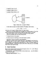
What Is an algorIthm? The word algorithm comes from the name of a Persian author Abu Ja’far Muhammad ibn Musa al-Khwarizmi who wrote a textbook on mathematics. This word has taken on a special significance in computer science, where ‘algorithm’ has come to refer to a method that can be used by a computer for the solution of a problem. Definition: An algorithm is a finite set of instructions that accomplishes a particular task. All algorithms must satisfy the following criteria: 1. Input. Zero or more quantities are externally supplied. 2. Output. At least one quantity is produced. DOI: 10.1201/9781003355403-1

1

2

Algorithm and Design Complexity



FIGURE 1.1

The notion of the algorithm

3

Algorithm Analysis

Example 1 gcd(60, 24) = gcd(24, 60 mod 24) = gcd(24, 12) = gcd(12, 24 mod 12) = gcd(12, 0) = 12 Euclid’s algorithm for computing gcd (m, n): Step 1: If n = 0, return the value of m as the answer and stop; otherwise, proceed to step 2. Step 2: Divide m by n and assign the value of the remainder to r. Step 3: Assign the value of n to m and the value of r to n. Go to step 1. Algorithm (Euclid(m,n)) in a pseudo code: // Compute gcd (m,n) by Euclid’s algorithm // Input: Two nonnegative and nonzero integers m and n //Output: Greatest common divisor of m and n. while n ≠ 0 do r ← m mod n m←n n←r return m How do we know that Euclid’s algorithm eventually comes to a stop? This follows from the observation that the second integer of the pair gets smaller with each iteration and that it cannot become negative. Indeed, the new value of n on the next iteration is m mod n, which is always smaller than n (why?). Hence, the value of the second integer eventually becomes 0, and the algorithm stops. 2. Consecutive Integer Checking Algorithm for Computing gcd(m, n) A common divisor cannot be greater than the smaller of the two numbers, which will denote by t = min {m, n}. So we can check whether t divides both m and n. If it does t is the answer; If it does not, we simply decrease t by 1 and try again. We have to follow this method until it reaches the answer. Step 1: Assign the value of min{m, n} to t. Step 2: Divide m by t. If the remainder of this division is 0 go to step 3; otherwise, go to step 4. Step 3: Divide n by t. If the remainder of this division is 0, return the value of t as the answer and stop; otherwise, proceed to step 4. Step 4: Decrease the value of t by 1. Go to step 2.

4

Algorithm and Design Complexity

Let us understand this algorithm with the help of some examples. Consider m = 12, n = 8 t = min(12, 8) We will set a value of t = 8 initially. Check whether we get m mod t = 0 as well as n mod t = 0. If not, then decrease t by 1, and again, with this new t value, check whether m mod t = 0 and n mod t = 0. Then we go on checking whether m mod t and n mod t both result in 0 or not. Thus, we will repeat this process each time by decrementing t by 1 and performing m mod t and n mod t. 12 mod 8 = 4 So set t = t − 1 12 mod 7 = 5 12 mod 6 = 0 8

8 mod 8 = 0

12 mod 8 is not equal to zero. So 8 is not a gcd. that is, t = 8 − 1 = 7 8 mod 7 = 1 Both 12 mod 7 and 8 mod 7 are not equal to 0. So 7 is not a gcd. So set new t = t − 1, that is, t = 7 − 1 = 6. mod 6 = 2 8 mod 6 is not equal to zero. So 6 is not a gcd.

So t = 6 − 1 = 5. 12 mod 5 = 7 8 mod 5 = 3 12 mod 4 = 0

8 mod 4 = 0

Both 12 mod 5 and 8 mod 5 are not equal to 0. So 5 is not a gcd. So set new t = t − 1, that is, t = 5 − 1 = 4. Both 12 mod 4 and 8 mod 4 are equal to 0. So 4 is a gcd.

gcd(12, 8) = 4 3. Middle School Procedure for Computing gcd(m, n) Step 1: Find the prime factors of m. Step 2: Find the prime factors of n. Step 3: Identify all the common factors in the two prime expansions found in steps 1 and 2. Step 4: Compute the product of all the common factors and return it as the gcd of the numbers given. Thus, for the numbers 120 and 72, we get 120 = 2 × 2 × 2 × 3 × 5 72 = 2 × 2 × 2 × 3 × 3 gcd(120, 72) = 2 × 2 × 2 × 3 = 24.

Algorithm Analysis

FIGURE 1.2

5

Algorithm design and analysis process

Fundamentals oF algorIthm Problem-solvIng In computer science, developing an algorithm is an art or skill. Before the actual implementation of the program, designing an algorithm is a very important step. We can consider algorithms to be procedural solutions to problems. These solutions are not answers but specific instructions for getting answers. It is this emphasis on precisely defined constructive procedures that makes computer science distinct from other disciplines. In particular, this distinguishes it from theoretical mathematics, whose practitioners are typically satisfied with just proving the existence of a solution to a problem and, possibly, investigating the solution’s properties. We now list and briefly discuss a sequence of steps one typically goes through when designing and analyzing an algorithm as shown in Figure 1.2. A Sequence of Steps in Designing and Analyzing an Algorithm • Understanding the problem • Ascertaining the capabilities of a computational device • Choosing between exact and approximate problem-solving • Deciding the appropriate data structures • Reviewing algorithm design techniques • Designing the algorithm

6

Algorithm and Design Complexity

• Proving the correctness of the algorithm • Analyzing the algorithm • Coding the algorithm Understanding the Problem • From a practical perspective, first of all, the step we need to understand completely is the problem statement. To understand the problem statements, read the problem description carefully and ask questions to clarify the doubts about the problem. • After understanding the problem statements, find out what the necessary inputs for solving that problem are. Use a known algorithm for solving it. • If there is no readily available algorithm, then design your own. • An input to the algorithm is called the instance of the problem. It is very important to decide the range of inputs so that the boundary values of an algorithm get fixed. • The algorithm should work correctly for all valid inputs. Ascertaining the Capabilities of a Computational Device Once you completely understand a problem, you need to ascertain the capabilities of the computational device the algorithm is intended for. We can classify an algorithm according to its execution point of view as a sequential algorithm and a parallel algorithm. • Sequential algorithm: The sequential algorithm runs on the machine in which the instructions are executed one after another. Such a machine is called a random-access machine. Algorithms designed to be executed on such machines are called sequential algorithms. • Parallel algorithm: Some newer computers can execute operations concurrently, that is, in parallel. Algorithms designed to be executed on machines that execute operations concurrently are known as parallel algorithms. Choosing Between Exact and Approximate Problem-Solving The next decision is to choose between solving the problem exactly or solving the problem approximately. • An algorithm that solves the problem exactly is called an exact algorithm. • An algorithm that solves the problem approximately is called an approximation algorithm. Reasons for Using an Approximation Algorithm • There are important problems that cannot be solved exactly. • Available algorithms for solving a problem exactly can be unacceptably slow because of the problem’s intrinsic complexity. • An approximation algorithm can be a part of a more sophisticated algorithm that solves a problem exactly. Deciding on appropriate data structures: The efficiency of an algorithm can be improved by using an appropriate data structure. The data structure is important for

7

Algorithm Analysis

both the design and the analysis of an algorithm. The data structure and the algorithm work together, and these are interdependent. Hence, choosing the proper data structure is required before designing the actual algorithm. Algorithm design techniques: An algorithm design technique is a general approach to solve problems algorithmically. These problems may belong to different areas of computing. Various algorithm design techniques are • Divide and conquer: In this strategy, the problem is divided into smaller subproblems; the subproblems are solved to obtain the solution to the main problem. • Dynamic programming: The problem is divided into smaller instances, and the results of smaller reoccurring instances are obtained to solve the problem. • Greedy technique: From a set of obtained solutions, the best possible solution is chosen each time to obtain the final solution. • Backtracking: In this method, in order to obtain the solution, a trial-anderror method is followed. Methods of Specifying an Algorithm Once you have designed an algorithm, you need to specify it in some fashion. There are different ways by which we can specify an algorithm: 1. Using natural language 2. Pseudo code 3. Flowchart 1. Using natural language: It is very simple to specify an algorithm using natural language. For example: Write an algorithm to perform the addition of two numbers. Step 1: Read the first number, say, ‘a’. Step 2: Read the second number, say, ‘b’. Step 3: Add the two numbers and store the result in a variable. Step 4: Display the result. 2. Pseudo code: In pseudo code, English-like words are used to represent the various logical steps. The pseudo code is a mixture of natural language and programming language–like constructs. For example: ALGORITHM Sum(a,b) //Problem Description: This algorithm performs addition of two numbers //Input: Two integers a and b // Output: Addition of two integers c←a+b return c. 3. Flowchart: A flowchart is a visual representation of the sequence of steps for solving a problem. Instead of descriptive steps, we use pictorial

8

Algorithm and Design Complexity

FIGURE 1.3

Flowchart for the addition of two numbers

representation for every step. A flowchart is a set of symbols that indicates various operations in the program. For example, a flowchart for the addition of two numbers is shown in Figure 1.3. Proving the Correctness of the Algorithm • Once an algorithm has been specified, you have to prove its correctness. That is, you have to prove that the algorithm yields a required result for every legitimate input in a finite amount of time.

Algorithm Analysis

9

• A common technique for proving correctness is to use mathematical induction because an algorithm’s iterations provide a natural sequence of steps needed for such proofs. • But in order to show that an algorithm is incorrect, you need just one instance of its input for which the algorithm fails. • If the algorithm is found to be incorrect, you need to redesign it under the same decisions regarding the data structures, the design techniques, and so on. Analyzing the Algorithm After correctness, by far the most important is efficiency. While analyzing an algorithm, we should consider the following factors: • • • •

Time efficiency Space efficiency Simplicity Generality

Time efficiency: Time efficiency indicates how fast the algorithm runs. Space efficiency: Space efficiency indicates how much extra memory the algorithm needs to complete its execution. Simplicity: Simplicity of an algorithm means generating a sequence of instructions that are easy to understand. Generality: The generality of the problem is what the algorithm solves and the range of inputs it accepts. If you are not satisfied with the algorithm’s efficiency, simplicity, or generality, you must return to the drawing board and redesign the algorithm. Coding the Algorithm The implementation of an algorithm is done through a suitable programming language. The validity of programs is still established by testing. Test and debug your program thoroughly whenever you implement an algorithm.

study oF algorIthms The study of algorithms includes many important areas, such as • • • •

how to devise algorithms, how to validate algorithms, how to analyze algorithms, and how to test a program.

How to devise algorithms: Creating an algorithm is an art. By mastering the design strategies, it will become easier to devise new and useful algorithms.

10

Algorithm and Design Complexity

How to validate algorithms: Once an algorithm is devised, it is necessary to show that it computes the correct answer for all possible legal inputs. This process is algorithm validation. The purpose of the validation is to assure that this algorithm will work correctly. Once the validity of the method has been shown, a program can be written, and a second phase begins. This phase is referred to as program proving or sometimes as program verification. A proof of correctness requires that the solution be stated in two forms. One form is usually a program that is annotated by a set of assertions about the input and output variables of the program. These assertions are often expressed in the predicate calculus. The second form is called a specification, and this may also be expressed in the predicate calculus. How to analyze algorithms: This field of study is called the analysis of algorithms. As an algorithm is executed it uses the computer’s central processing unit to perform operations and its memory to hold the program and data. An analysis of algorithms, or a performance analysis, refers to the task of determining how much computing time and storage an algorithm requires. How to test a program: Testing a program consists of two phases: • Debugging • Profiling Debugging is the process of executing programs on sample data sets to determine whether faulty results occur and, if so, to correct them. Profilingor Performance measurement is the process of executing a correct program on data sets and measuring the time and space it takes to compute the results.

ImPortant Problem tyPes Let us see some of the most important problem types: 1. 2. 3. 4. 5. 6. 7.

Sorting Searching String processing Graph problems Combinatorial problems Geometric problems Numerical problems

1. Sorting: Sorting is nothing but arranging a set of elements in increasing or decreasing order. The sorting can be done on numbers, characters, strings, or employee records. As a practical matter, we usually need to sort lists of numbers, characters from an alphabet, character strings, and, most important, records similar to those maintained by schools about their students, libraries about their holdings, and companies about their employees. In the case of records, we need to choose a piece of information to guide sorting. For example, we can choose to sort student records

Algorithm Analysis

11

in alphabetical order of names or by student number or by student gradepoint average. Such a specially chosen piece of information is called a key. Computer scientists often talk about sorting a list of keys even when the list’s items are not records but, say, just integers. Furthermore, sorting makes many questions about the list easier to answer. The most important use of sorting is searching; it is why dictionaries, telephone books, class lists, and so on are sorted. 2. Searching: Searching is an activity by which we can find out the desired element from the list. The element which is to be searched is called a search key. There are many searching algorithms such as sequential search, binary search, and many more. They range from the straightforward sequential search to a spectacularly efficient but limited binary search and algorithms based on representing the underlying set in a different form more conducive to searching. For searching, there is no single algorithm that fits all situations best. Some algorithms work faster than others but require more memory. Some are very fast but applicable only to sorted arrays. Unlike sorting algorithms, there is no stability problem, but different issues arise. Specifically, in applications in which the underlying data may change frequently relative to the number of searches, searching has to be considered in conjunction with two other operations: an addition to and deletion from the data set of an item. In such situations, data structures and algorithms should be chosen to strike a balance among the requirements of each operation. Also, organizing very large data sets for efficient searching poses special challenges with important implications for real-world applications. 3. String processing: A string is a sequence of characters from an alphabet. Strings of particular interrupt are text strings, which comprise letters, numbers, and special characters, and bit strings, which comprise zeros and ones. It should be pointed out that string-processing algorithms have been important for computer science for a long time in conjunction with computer languages and compiling issues. 4. Graph problems: A graph can be thought of as a collection of points called vertices, some of which are connected by line segments called edges. Basic graph algorithms include graph traversal algorithms, shortest path algorithms, and topological sorting for graphs with directed edges. Graphs are an interesting subject to study, for both theoretical and practical reasons. Graphs can be used for modeling a wide variety of applications, including transportation, communication, social and economic networks, project scheduling, and games. Studying different technical and social aspects of the internet in particular is one of the active areas of current research involving computer scientists, economists, and social scientists. 5. Combinatorial problems: Combinatorial problems are related to problems like computing permutations and combinations. Combinatorial problems are the most difficult problems in computing areas because of the following causes:

12

Algorithm and Design Complexity

• As problem size grows, the combinatorial objects grow rapidly and reach to a huge value. • There is no algorithm available that can solve these problems in a finite amount of time. • Many of these problems fall in the category of unsolvable problems. 6. Geometric problems: Geometric algorithms deal with geometric objects such as points, lines, and polygons. Today, people are interested in geometric algorithms with quite different applications such as applications to computer graphics, robotics, and topography. 7. Numerical problems: Numerical problems are problems that involve mathematical objects of continuous nature, solving equations and systems of equations, computing definite integrals, evaluating functions, and so on. A majority of such mathematical problems can be solved only approximately.

abstract data tyPes • The abstract data type (ADT) is a mathematical model which gives a set of utilities available to the user but never states the details of its implementation. • In object-oriented programming, the class is an ADT, which consists of data and functions that operate on the data. • Various visibility labels in object-oriented languages are used to restrict data access only through the functions of the object. That is, the data are secured by hiding the data. Difference Between ADT and Data Types Data type is an implementation or computer representation of an ADT. Once the ADT is defined, programmers can use the properties of the ADT by creating instances of the ADT. For example, a programming language provides several built-in data types. Example Integer is an ADT. The implementation of an integer may be through any one of the several forms like unsigned, signed, and others. The instance of this is used in programs. In C++, the instance of the data type int is created by declaring int i; Here, the programmer simply uses the properties of the int by creating an instance without seeing how it has been implemented. Therefore, int can be said to be an INTEGER ADT. • We cannot always expect all necessary ADTs to be available in the form of built-in data types. Sometimes, the user may want to represent the data type, both logically and physically, in a specified manner. This is the concept of the user-defined data type.

Algorithm Analysis

13

• In many situations, communication between data structures becomes mandatory, such as restricting one data structure to access the data of other without its knowledge. • In programming languages, the concepts of classes permit this by communicating through the member functions. • Structured programming languages do not have the properties of data hiding. This creates damage to the data. Example As an example, let us take the data structure stack. The stack is implemented using arrays, then, it is possible to modify any data in the array without going through the proper rule, LIFO (last in, first out). Figure 1.4 demonstrates this. The data’s of this kind is not possible in an object-oriented approach. Figure 1.4 shows the direct access of data in the non-object-oriented approach. This is an illegal operation, but no program error occurs. Performance Analysis: The analysis of an algorithm deals with the amount of time and space consumed by it. An efficient algorithm can be computed with minimum requirement of time and space. Space Complexity:Most of what we will be discussing is going to be how efficient various algorithms are in terms of time, but some forms of analysis could be done based on how much space an algorithm needs to complete its task. This space complexity analysis was critical in the early days of computing when storage space on a computer (both internal and external) was limited. When considering space complexity, algorithms are divided into those that need extra space to do their work and those that work in place. It was not unusual for programmers to choose an algorithm that was slower just because it worked in place, because there was not enough extra memory for a faster algorithm. The space complexity of an algorithm is the amount of memory it needs to run to completion. Looking at software on the market today, it is easy to see that space analysis is not being done. Programs, even simple ones, regularly quote space needs in a number of megabytes. Software companies seem to feel that making their software space efficient is not a consideration because customers who don’t have enough computer

FIGURE 1.4

Example of a stack

14

Algorithm and Design Complexity

memory can just go out and buy another 32 megabytes (or more) of memory to run the program or a bigger hard disk to store it. This attitude drives computers into obsolescence long before they really are obsolete. Reasons for the Space Complexity of a Program • If the program is to be run on a multi-user computer system, then the amount of memory to be allocated to the program needs to be specified. • For any computer system, know in advance whether there is sufficient memory is available to run the program. • A problem might have several possible solutions with different space requirements. • Use the space complexity to estimate the size of the largest problem that a program can solve. Components of Space Complexity The space needed by each algorithm is the sum of the following components: 1. Instruction space 2. Data space 3. Environment stack space 1. Instruction space: The space needed to store the compiled version of the program instructions 2. Data space: The space needed to store all constant and variable values 3. Environment stack space: The space needed to store information to resume execution of partially completed functions The total space needed by an algorithm can be simply divided into two parts from the three components of space complexity: 1. Fixed 2. Variable Fixed Part A fixed part is independent of the characteristics (e.g., number, size) of the inputs and outputs. This part typically includes the instruction space (i.e., space for the code), space for simple variables and fixed-size component variables (also called aggregate), space for constants, and so on. Variable Part A variable part that consists of the space needed by component variables whose size is dependent on the particular problem instance being solved, the space needed by referenced variables (to the extent that this depends on instance characteristics), and the recursion stack space (insofar as this space depends on the instance characteristics).

Algorithm Analysis

15

The space requirement S(P) of any algorithm P may therefore be written as S(P) = c + Sp(instance characteristics), where c is a constant that denotes the fixed part of the space requirement. Sp—This variable component depends on the magnitude (size) of the inputs to and outputs from the algorithm. When analyzing the space complexity of a program, we concentrate solely on estimating Sp(instance characteristics). For any given problem, we need first to determine which instance characteristics to use to measure the space requirements. Examples Find the space complexity of the following algorithms: 1. Algorithm abc computes a + b + b × c + 4.0. Algorithm abc (a,b,c) { return a+b+b x c+ 4.0; } For algorithm abc, the problem instance is characterized by the specific values of a, b, and c. Assume that one word is adequate to store the values of each a, b, and c, and the result, which is the space needed by abc, is independent of the instant characteristics, Sp(instance characteristics) = 0. 2. Algorithm abc computes a + b + b * c + (a + b − c)/(a + b) + 4.0; float abc (float a, float b, float c) { return (a + b + b*c + (a+b-c)/(a+b) + 4.0); } The problem instance is characterized by the specific values of a, b, and c. Making the assumption that one word is adequate to store the values of each of a, b, and c, and in the result, we see that the space needed by abc is independent of the instance characteristics. Consequently, Sp(instance characteristics) = 0. 3. Iterative function for sum float Sum(float a[], int n) { float s = 0.0; for (int i=1; i (n + 3) (n for a[ ], one each for n, i, and s). Time Complexity The time complexity of an algorithm is the amount of computer time it needs to run to completion. Reasons for the Time Complexity of a Program • Some computer systems require the user to provide an upper limit on the amount of time the program will run. Once this upper limit is reached, the program is aborted. • The program might need to provide a satisfactory real-time response. • If there are alternative ways to solve a problem, then the decision on which to use will be based primarily on the expected performance difference among these solutions. The time T(P) taken by a program P is the sum of the compile time and the run (or execution) time. The compile time does not depend on the instance characteristics. A compiled program will run several times without recompilation. The run time is denoted by tp (instance characteristics). Because many of the factors tp depends on are not known at the time a program is conceived, it is reasonable to attempt only to estimate tp, If we knew the characteristics of the compiler to be used, we could proceed to determine the number of additions, subtractions, multiplications, divisions, compares, loads, stores, and so on that would be made by the code for P. So, we could obtain an expression for tp(n) of the form tp(n) = Ca ADD(n) + CsSUB(n) + Cm MUL(n) + CdDIV(n)+ . . . . . . . , where n denotes the instance characteristics. Ca, Cs, Cm, Cd, and so on, respectively, denote the time needed for addition, subtraction, multiplication, division, and so on, and ADD, SUB, MUL, DIV, and so on are functions whose values are the numbers of additions, subtractions, multiplications, divisions, and so on that are performed when the code for P is used on an instance with characteristic n. In a multi-user system, the execution time depends on such factors as system load, the number of other programs running on the computer at the time program P is run, the characteristics of these other programs, and so on. To overcome the disadvantage of this method, we can go one step further and count only the number of ‘program steps’, where the time required by each step is relatively independent of the instance characteristics.

Algorithm Analysis

17

A program step is defined as a syntactically or semantically meaningful segment of a program for which the execution time is independent of the instance characteristics. The program statements are classified into three types depending on the task to be performed, and the number of steps required by the unique type is given as follows: a. Comments—zero step b. Assignment statement—one step c. Iterative statement—finite number of steps (for, while, repeat–until) The number of steps needed by a program to solve a particular problem instance is done using two different types of methods. Method 1 A new global variable count is assigned with an initial value of zero. Next, introduce into the program statements to increment the count by the appropriate amount. Therefore, each time a statement in the original program or function is executed, the count is incremented by the step count of that statement. Method 2 To determine the step count of an algorithm a table is built in which we list the total number of steps contributed by each statement. The final total step count is obtained by consecutive three steps: • Calculate the number of steps per execution (s/e) of the statement. • Determine the total number of times each statement is executed (i.e., frequency). • Multiply (s/e) and frequency to find the total steps of each statement and add the total steps of each statement to obtain a final step count (i.e., total). Example for Method 1 Introduce a variable count in the algorithm sum computes a[i] iteratively, where the a[i]’s are real numbers. Algorithm sum (a, n) { s:= 0.0; count = count + 1; //count is global; it is initially zero. for i: = 1 to n do { count: = count + 1; // For for loop s: = s+ a[i]; count: = count + 1; //For assignment } count: = count +1; //For last time of for

18

Algorithm and Design Complexity

count: = count +1; // For the return; return s; } Step Count The change in the value of count by the time this program terminates is the number of steps executed by the algorithm sum. 1. 2. 3. 4. 5.

Count in the for loop—2n steps For assigning s value to zero—1 step For last time for execution—1 step For return statement—1 step That is, each invocation of sum executes a total of 2n + 3 steps.

Example for Method 2 Find the total step count of the summation of n numbers using the tabular method. Statement 1. 2. 3. 4. 5. 6. 7.

Algorithm sum(a,n) { s=0.0; for i=1 to n do s:=s+a[i]; return s; }

s/e

Frequency

Total steps

0 0 1 1 1 1 0

– – 1 n+1 n 1 –

0 0 1 n + 1 n 1 0

Total

1.2

2n + 3

TIME–SPACE TRADE-OFF

Time and space complexity can be reduced only to certain levels, as later on a reduction of time increases the space and vice versa; this is known as time–space trade-off. Consider the following example shown in Figure 1.5, where we have an array of n numbers that are arranged in ascending order. Our task is to get the output as an array that contains these numbers in descending order. • The first method is by taking two arrays, one for the input and the other for the output. • Now, read the elements of the first array in reverse linear order and place them in the second array linearly from the beginning. The code for such an operation is as follows: int ary1 [n]; int ary2[n];

Algorithm Analysis

19

FIGURE 1.5 (a) Reversing array elements using two arrays. (b) Reversing array elements using the swap method.

for(int i=0;i 10n2. So f(n) = Ω(n2). Also, 3n + 2 > 1, so f(n) = Ω(1). 10n2 + 4n + 2 > n. So f(n) = Ω(n). Big-theta notation (θ ): This notation is used to define the exact complexity in which the function f(n) is bound both above and below by another function g(n).

FIGURE 1.7

Big-omega notation: f(n) ∈ Ω(g(n))

23

Algorithm Analysis

FIGURE 1.8

deFInItIon

Big-theta notation: f (n) ∈ Θ(g(n))

Let f and g be two functions defined from a set of natural numbers to a set of nonnegative real numbers. That is, f, g: N → R ≥ 0. It is said that the function f(n) = θ (g(n)) (read as ‘f of n is theta of g of n’), if there exists three positive constants C1, C2 ∈ R and n0 ∈ N such that C1g(n) ≤ f(n) ≤ C2 g(n) for all n, n ≥ n0. The definition is illustrated in Figure 1.8. Example Consider f(n) = 3n + 2. 4n ≥ 3n + 2 ≥ 3n 3n ≤ 3n + 2 ≤ 4n C1 g(n) ≤ f(n) ≤ C2 g(n) C1 = 3 C2 = 4 Therefore, 3n + 2 = θ (n). Little-oh notation (o): This notation is used to describe the worst-case analysis of algorithms and is concerned with small values of n. The function f(n) = o(g(n)) (read as ‘f of n is little oh of g of n’) iff lim

naa

f ( n) a 0. g( n)

Little-omega notation (ω): This notation is used to describe the best-case analysis of algorithms and is concerned with small values of n.

24

Algorithm and Design Complexity

The function f(n) = ω (g(n)) (read as ‘f of n is little omega of g of n’) iff lim

n aa

1.4

g( n) a 0. f ( n)

PROPERTIES OF BIG-OH NOTATIONS

statement 1 O(f(n)) + O(g(n)) = O(max{f(n),g(n)}) Proof Let f(n) ≤ g(n). L.H.S = C1g(n) + C2f(n) ≤ C1g(n) + C2g(n) = (C1 + C2)g(n) = O(g(n)) = O(max{f(n),g(n)})

statement 2 f(n) = O(g(n)) and g(n) ≤ h(n) implies f(n) = O(h(n)).

statement 3 Any function can be said as an order of itself. That is, f(n) = O(f(n)). Proof Proof of this property trivially follows from the fact that f(n) ≤ 1 × f(n).

statement 4 Any constant value is equivalent to O (1). That is C = O (1), where C is a constant. The asymptotic notations are defined only in terms of the size of the input. For example, the size of the input for sorting n numbers is n. So, the constants are not directly applied to the stated facts to obtain the results. For instance, suppose we have the summation 12 + 22 +. . . . . . . . . . . . . . .+ n2. By using the property explained in statement 1 directly, we get 12 + 22 +. . . . . . . . . . . . . . .+ n2 = O (max{12, 22, . . . . . , n2}) = O(n2), which is wrong. Actually, the asymptotic value of the sum is O(n3) and is obtained as follows:

25

Algorithm Analysis

12 + 22 +. . . . . . . . . . . . . . .+ n2 = n(n + 1)(2n + 1)/6 = (2n3 + 3n2 + n)/6 = O(n3) + O(n2) + O(n) = O(max{n3,n2,n }) = O(n3)

statement 5 If lim a f a n a / g a n aa a R a 0 then f a n a a a a g a n a a . n aa

statement 6 aa f a n a aa If lim a a a 0 then f a n a a O a g a n a a but f a n a a a a g a n a a . n aa g a n a a a That is O a f a n a a a O a g a n a a ,

which also implies f a n a a O a g a n a a and g a n a a O a f a n a a .

statement 7 If lim a f a n a / g a n aa a a a aa f a n a a a a g a n a a butf a n a a a a g a n a a. n aa

That is, O a f a n a a a O( g a n a . Sometimes, the L’Hospital’s rule is useful in obtaining the limit value. The rule states that lim

n aa

f ana

g ana

a lim

n aa

f aana , ga a n a

where f′ and g′ are the first derivatives of f and g, respectively.

Problem Prove that log n a O( n ) but n a O(log n). Proof lim

n aa

log n n

a lim

1 n

n aa 1 2

a lim

n aa

n a21

2 n n

[By L-Hospital’s rule]

26

Algorithm and Design Complexity

a lim

n aa

2 n

a0 Therefore, by statement 6, log n a O( n )but n a O(log n). • The asymptotic values of certain functions can be easily derived by imposing certain conditions. • For example, if the function f(n) is recursively defined as f(n) = sf(n/2) + n, f(1) = 1. Suppose n is the power of 2. That is, n = 2k for some k. f(2k) = 2f(2k−1) + 2k = 22f(2k−2) + 2k + 2k = 22f(2k−2) + 2(2k) . . . . . . . . . . . . . . . . . . . . . . . . . . = 2kf(1) + k2k, which is equal to n + n log n, and so, O (n log n), where n = 2k.

1.5

CONDITIONAL ASYMPTOTIC NOTATIONS

Many algorithms are easier to analyze if we impose conditions on them initially. Imposing such conditions, when we specify an asymptotic value, is called conditional asymptotic notation.

condItIonal bIg-oh notatIon Let f,g: N → R ≥ 0. It is said that f(n) = O(g(n)|A(n)), read as g(n) when A(n), if there exist two positive constants C ∈ R and n0 ∈ N such that A(n) ⇒ [f(n) ≤ Cg(n)] for all n ≥ n0.

condItIonal bIg-omega notatIon Let f,g: N → R ≥ 0. It is said that f(n) = Ω(g(n)|A(n)), read as g(n) when A(n), if there exist two positive constants C ∈ R and n0 ∈ N such that A(n) ⇒ [f(n) ≥ Cg(n)] for all n ≥ n0.

condItIonal bIg-theta notatIon Let f,g: N → R ≥ 0. It is said that f(n) = θ (g(n)|A(n)), read as g(n) when A(n), if there exists two positive constants C1, C2 ∈ R and n0 ∈ N such that A(n) ⇒ [C1g(n) ≤ f(n) ≤

27

Algorithm Analysis

C2 g(n)] for all n ≥ n0. We know that f(n) = 2f(n/2) + n = O(n log n| n is a power of 2), which is the conditional asymptotic value. That is, f(n) = O(n log n) an a n0 for some n0 ∈ N . A function f: N → R ≥ 0 is eventually nondecreasing if an0 a N such that f(n) ≤ f(n + 1), an a n0.

theorem Let p ≥ 2 be an integer. Let f, g: N → R ≥ 0. Also, f be an eventually nondecreasing function and g be a p-smooth function. If f(n) ∈ O(g(n)| n is a power of p), then f(n) ∈ O(g(n)). Proof Apply the theorem for proving f(n) = O(n log n), ∀n. To prove this, we have to prove that f(n) is eventually nondecreasing and n log n is 2-smooth. Claim 1: f(n) is eventually nondecreasing. Using mathematical induction, the proof is as follows f(1) = 1 ≤ 2(1) + 2 = f(2). Assume for all m < n, f(m) ≤ f(m + 1). In particular, f(n/2) ≤ f((n + 1)/2). Now, f(n) = 2 f(n/2) + n ≤ 2f((n + 1)/2) + (n + 1) = f(n + 1). Therefore, f is eventually nondecreasing. Claim 2: n log n is 2-smooth. 2n log 2n = 2n(log 2 + log n) = O(n log n), which implies n log n is 2-smooth. Therefore, f(n) = O(n log n). The preceding function f(n) is simple in obtaining the asymptotic value by recursively applying the function.

1.6

RECURRENCE EQUATIONS

A recurrence is an equation or an inequality that describes a function in terms of its values on the smallest inputs.

28

Algorithm and Design Complexity

derIvIng recurrence relatIons To derive a recurrence relation, • figure out what ‘n’, the problem size, is. • see what value of n is used as the base of the recursion. It will usually be a single value but may be multiple values suppose it is n0. • figure out what T (n0) is, you can usually use ‘constant C’, but sometimes a specific number will be needed. • the general T(n) is usually a sum of various choices of T(m) (for the recursive calls) plus the sum of the other work done. Usually, the recursive calls will be solving subproblems of the same size f(n), giving a term ‘a.T(f(n))’ in the recurrence relation. Cifn a n0 a T ana a a , aa.T a f a n a a a g a n a otherwise where C = running time for base, n0 = base of recurrence, a = the number of times a recursive call is made, n = the size of the problem solved by a recursive call, and g(n) = all other processing not counting recursive calls. Recurrence equations can be classified into homogeneous and inhomogeneous. In algebra, there are easy ways to solve both homogeneous and inhomogeneous equations. Suppose T(n) is the time complexity of our algorithm for the size of the input n. Assume that T(n) is recursively defined as T a n a a b1T a n a 1a a b2T a n a 2 a aaa bk T a n a k a a0 T a n a a a1T a n a 1a aaa ak T a n a k a a 0 .

(1)

The constants, which are bis, are now converted to ais for simplicity. Let us denote T(i) as xi. Hence, the equation becomes a0 X n a a1 X n a1 aaa ak X n a k a 0,

(2)

which is a homogeneous recurrence equation. One of the trivial solutions for Equation 2 is x = 0. After removing common x terms from Equation 2, we get a0 X k a a1 X k a1 aaa ak a 0. The preceding equation is known as a characteristic equation and can have k roots. Let the roots be r1, r2, . . . . . , rk. The roots may not be the same.

29

Algorithm Analysis

Case 1: Suppose all the roots are distinct. Then, the general solution is k

T a n a a aci ri n, where ci’s are some constants. i a1

For example, suppose the characteristic equation is x2 − 5x + 6 = 0. Then x2 – 5x + 6 = 0 ⇒ (x − 3)(x − 2) = 0 ⇒ the roots are 3 and 2. Therefore, the general solution is T(n) = c13n + c22n. Case 2:Suppose some of the p roots are equal and the remaining are distinct. Let us assume that the first p roots are equal to rl. Then, the general solution can be stated as p

T a n a a aci ni a1r1n a i a1

k

acr

i i

n

.

i a p a1

For example, suppose the characteristic equation is (x − 2)3 (x − 3) = 0. Then the roots of this equation are 2, 2, 2, and 3. Therefore, the general solution is T(n) = c12n + c2n2n + c3n22n + c43n. Case 2 can be extended to cases like p roots are equal to r1, q roots are equal to r2, and so on.

Inhomogeneous recurrence equatIon The general form is as follows a0tn + a1tn−1 + . . . . . . . . . . + ak tn−k = b1nP1(n) + b2nP2(n) +. . . . , where ai’s and bi’s are constants. Each Pi(n) is a polynomial in n of degree di. Here the characteristic equation tends to be (a0xk + a1xk−1 + . . . . . . . . . . + ak)(x − b1)d1+1(x − b2)d2+1 . . . = 0 ⇒ a0x  + a1xk−1+ . . . . . . . . . . + ak = 0 (x − b1)d1+1 = 0 (x − b2)d2+1 = 0 . . . . . . . . . . . . . . . k

30

Algorithm and Design Complexity

These are a set of homogeneous equations, and hence, the general solution can be obtained as before. Let the general solutions for the earlier equations be S1, S2, . . . Then the general solution of the inhomogeneous equation is given by T(n) = S1 + S2 + . . . Example The recurrence equation of the complexity of merge-sort algorithm f(n) = 2f(n/2) + n, f(1) = 1

(1)

Let n = 2k. For simplicity, we say f(2k) = tk. Therefore, Equation 1 ⇒ tk − 2tk−1 = 2k

(2)

Equation 2 is an inhomogeneous equation. The characteristic equation of the recurrence Equation 2 is (x − 2) (x − 2) = 0 ⇒ (x − 2)2 = 0 The roots are 2 and 2. Now the general solution is tk = c12k + c2k2k ⇒ f(n) = c1n + c2n logn Given that f(1) = 1 ⇒ 1 = c1, similarly, f(2) = 2f(1) + 2 = 2 + 2 = 4. From Equation 3,

(3)

4 = c12 + c22 ⇒ 4 = 2 + c22 ⇒ c2 = 1.

Therefore, Equation 3 becomes f(n) = n + n log n = O (n log n| n is a power of 2). As we have already proved that n log n is 2-smooth and that (n) is eventually nondecreasing. So we say f(n) = O(n log n).

31

Algorithm Analysis

1.7

SOLVING RECURRENCE EQUATIONS

There are three methods of solving recurrence relations: • Substitution • Iteration • Master

substItutIon method In the substitution method, make intelligent guesswork about the solution of a recurrence and then prove by induction that the guess is correct. Given a recurrence relation T(n), • • • •

substitute a few times until you see a pattern. write a formula in terms of n and the number of substitutions i. choose I so that all references to T() become references to the base case. solve the resulting summation.

Example Multiplication for all n > 1 T(n) = T(n − 1) + d Therefore, for a large enough n, T(n) = T(n − 1) + d T(n − 1) = T(n − 2) + d . . T(2) = T(1) + d T(1) = c. Repeated substitution T(n) = T(n − 1) + d = (T(n − 2) + d) + d = T(n − 2) + 2d = (T(n − 3) + d) + 2d = T(n − 3) + 3d There is a pattern developing. It looks like after i substitutions, T(n) = T(n − i) + id

32

Algorithm and Design Complexity

Now choose i = n − 1, then T(n) = T(n − (n − 1)) + (n − 1)d = T (n − n + 1) + (n − 1)d = T(1) + (n − 1)d = c + nd − d T(n) = dn + c − d Iteration Method In the iteration method, the basic idea is to • expand the recurrence, • express it as a summation of terms dependent only on n and the initial conditions, and • evaluate the summation. Example: Consider the recurrence T(n) = T(n − 1) + 1, and T(1) = θ(1). Solution T(n) = T(n − 1) + 1 T(n − 1) = T (n − 2) + 1 T(n) = (T(n − 2) + 1) + 1 = T(n − 2) + 2 T(n − 2) = T(n − 3) + 1 Thus, T(n) = (T(n − 3) + 1) + 2 = T(n − 3) + 3 T(n) = T(n − k) + k k = n − 1 T(n − k) = T(n − (n − 1)) = T(n − n + 1) = T(1) T(n) = T(1) + k = T(1) + k T(n) = θ(n) Master Method The master method is used for solving the following type of recurrence: T(n) = aT(n/b) + f(n), with a ≥ 1 and b > 1. In the preceding recurrence, the problem is divided into a subproblem each of size almost (n/b). The subproblems are solved recursively each in T(n/b) time. The cost of splitting the problem or combining the solutions of subproblems is given by function f(n). It should be noted that the number of leaves in the recursion tree is n E with E= (log a/b log b).

33

Algorithm Analysis

Master Theorem Let T(n) be defined on the nonnegative integers by the recurrence. T(n) = aT(n/b) + f(n), where a ≥ 1 and b > 1 are constants, f(n) is a function, and n/b can be interpreted as [n/b]. Then T(n) can be bound asymptotically as follows:

a a Case 2: If f a n a a a a n a, then T a n a a a a f a n a .logn a. Case 3: If f a n a a a a n a for some e > 0 and f a n a a O a n

Case 1: If f a n a a O n E a e for some e > 0, then T a n a a a (n E ). E

E ae

then T a n a a a aaa f a n a a aa .

E

a

a a for some δ  ≥ e,

Example Consider the following recurrence T(n) = 4T(n/2) + n. Using the master method, a = 4, b = 2, and f(n) = n nE = n(log a/logb), where E =

log a . log b

= n logba = n log24 = n2 Since f(n) = n ∈ O(n2−e), thus, T(n) ∈θ (n2). Problem 1: Solve the recurrence equation T(n) − 2T(n − 1) = 3n subject to T(0) = 0. Proof The characteristic equation is (x − 2)(x − 3) = 0. Therefore, the roots are 2 and 3. Now the general solution is T(n) = c12n + c23n. Since T(0) = 0, T(1) = 3. Thus, from the general solution, we get c1 = −3 and c2 = 3. So, T(n) = −3 × 2n + 3 × 3n = O(3n) Problem 2: Solve the recurrence equation T(n) − 2T(n − 1) = 1 subject to T(0) = 0. Proof The characteristic equation is (x − 2)(x − 1) = 0. Therefore the roots are 2 and 1.

34

Algorithm and Design Complexity

Now the general solution is T(n) = c11n + c22n. Since T(0) = 0, T(1) = 1. Thus, from the general solution, we get c1 = −1 and c2 = 1. So, T(n) = 2n − 1 = θ (2n). Problem 3: Solve the recurrence equation T(n) = 2T(n − 1) + n2n + n2. Proof The characteristic equation is (x − 2)(x − 2)2(x − 1)3 = 0. (x − 2)3(x − 1)3 = 0 Therefore the roots are 2, 2, 2, 1, 1, and 1 Now the general solution is T(n) = c12n + c2n2n + c3n22n + c41n + c5n1n + c6n21n. So T(n) = O (n22n).

1.8

ANALYSIS OF LINEAR SEARCH

• Algorithms are analyzed to get best-case, worst-case, and average-case asymptotic values. • Each problem is defined on a certain domain. From the domain, we can derive an instance for the problem. • In the example of multiplying two integers, any two integers become an instance of the problem. • So, when we go for analysis, it is necessary that the analyzed value will be satisfiable for all instances of the domain. • Let Dn be the domain of a problem, where n be the size of the input. • Let I ∈ Dn be an instance of the problem taken from the domain Dn. • T(I) be the computation time of the algorithm for the instance I ∈ Dn.

best-case analysIs • The best-case efficiency of an algorithm is its efficiency for the best-case input of size n, which is an input of size n for which the algorithm runs fastest among all possible inputs of that size. • Determine the kind of inputs for which the count c(n) will be the smallest among all the possible inputs of size n. • This gives the minimum computed time of the algorithm with respect to all instances from the respective domain. Mathematically, it can be stated as B(n) =min{T (I) | I ∈ Dn}. • If the best-case efficiency of an algorithm is unsatisfactory, we can immediately discard it without further analysis.

Worst-case analysIs • The worst-case efficiency of an algorithm is its efficiency for the worst-case input of size n, which is an input of size n for which the algorithm runs the longest among all possible inputs of that size.

35

Algorithm Analysis

• Analyze the algorithm to see what kind of inputs yield the largest value of basic operation’s count c(n) among all the possible inputs of size n and then compute this worst-case value Cworst(n). • This gives the maximum computation time of the algorithm with respect to all instances from the respective domain. • Mathematically, it can be stated as • W(n) = max{T(I) | I ∈ Dn}.

average-case analysIs • It is neither the worst-case analysis nor its best-case counterpart yields the necessary information about an algorithm’s behavior on a ‘typical’ or ‘random’ inputs. • To analyze the algorithm’s average-case efficiency, make some assumptions about possible inputs of size n. • Mathematically, the average case value can be stated as A ana a

a P a I a T a I a.

I aDn

• P(I) is the average probability with respect to instance I. Example • Take an array of some elements as shown in Figure 1.9. The array is to be searched for the existence of an element x. • If the element x is in the array, the corresponding location of the array should be returned as an output. • The element may or may not be in the array. If the element is in the array, it may be in any location, that is, in the first location, the second location, anywhere in the middle, or at the end of the array. • To find the location of the element x, we use the following algorithm, which is said to be the linear search algorithm. int linearsearch(const char A[ ], const unsigned int size, char ch) { for(int i=0;i bk

a a T a N a aa a N a T a N a a a N logb

a

log24

if a a b k if a a b k

a a

T a N a aa N 2

2. T(n) = 4T(n/2) + n2 T(1) = 1 Compare with T(n) = aT(n/b) + f(n). We get a = 4, b = 2, f(n) = n2. θ(nk) = n2 bk = 22 = 4 a = bk T a N a a a N k logN if a a b k

a

a

T a N a a a ( N log N ) 2

48

Algorithm and Design Complexity

3. T(n) = 4T(n/2) + n3 T(1) = 1 Compare with T(n) = aT(n/b) + f(n). We get a = 4, b = 2, f(n) = n3. θ(nk) = n3 bk = 23 = 8 a < bk T a N a aa N k if a a b k

a a T a N a aa a N a 3

Divide-and-Conquer Examples • Binary search • Sorting: merge sort and quick sort • Binary tree traversals • Matrix multiplication: the Strassen algorithm • Closest-pair algorithm • Convex-hull algorithm • Tower of Hanoi • Exponentiation

2.2

BINARY SEARCH

A binary search is an efficient search method based on the divide-and-conquer algorithm. The binary search technique determines whether a given element is present in the list of sorted arrays. If we compare the target with the element that is in the middle of a sorted list, we have three possible results: the target matches, the target is less than the element, or the target is greater than the element. In the first and best case, we are done. In the other two cases, we learn that half of the list can be eliminated from consideration. When the target is less than the middle element, we know that if the target is in this ordered list, it must be in the list before the middle element. When the target is greater than the middle element, we know that if the target is in this ordered list, it must be in the list after the middle element. These facts allow this one comparison to eliminate one-half of the list from consideration. As the process continues, we will eliminate from consideration one-half of what is left of the list with each comparison. Let an array a[i], 1 ≤ i ≤ n be a list of elements that are sorted in nondecreasing order (ascending order). The problem is to find whether the given element x is present in the list. • If x is present then return the index ‘j’ such that a[j] = x. • If x is not in the list, then j is to be set to zero. Let P = (n, ai, ai+1, . . . , al, x) denote an arbitrary instance of this search problem. Here n = number of elements in the list ai, ai+1, . . . ; al = list of elements; and x = the element to be searched for. Divide and conquer can be used to solve this problem.

Divide and Conquer

49

case 1 Let Small(P) be true if n = 1. In this case, S(P) will take the value i if x = ai. Otherwise, it will take the value 0. Then, g(n)= θ(1).

case 2 If P has more than one element, it can be divided (or reduced) into new subproblems as follows. Pick an index q in the range [i, l] and compare x with a[q]. There are three steps: 1. If x = a[q], then the problem P is immediately solved. 2. If x < a[q], then search x in the sub list a[i], a[I + 1], a[i + 2], . . . . . . a[q − 1]. Now the problem P was reduced to (q-i, ai, . . . , aq−1, x) 3. If x > a[q], then search x in the sublist a[q + 1], a[q + 2], . . . . . . , a[l]. Now the problem P is reduced to (l − q, aq+1, . . . , a1, x) Any given problem P gets divided (reduced) into one new subproblem. After a comparison with a[q], the instance remaining to be solved (if any) can be solved by using this divide-and-conquer scheme again. If q is always chosen such that a[q] is the middle element (i.e., q a a n a 1a / 2 or q a a first a last a / 2), then the resulting search algorithm is known as binary search. Now the answer to the new subproblem is also the answer to the original problem ‘P’, so there is no need for any combining. int BinSrch(Type a[], int i, int 1, Type x) // Given an array a[i:l] of elements in nondecreasing order, l 13. So K is present in the right sub-array. 14, 18, 20 ↑ Middle term 5. Compare K with the middle element, K = 18. Yes. The element is present in the array.

analysIs oF bInary search algorIthm Worst-Case Analysis 1. The search key is not in the sorted array. 2. The search key is in the last position. Here the key comparison is done with half the size of the array. Let T(n) be the worst-case number of comparisons used by procedure search on an array of n numbers. Suppose n is the power of 2: a 0 T ana a a aT a n / 2 a a 1

if n a 1 otherwise

This recurrence is solved as T(n) = T(n/2) + 1 = (T(n/4) + 1) + 1 = T(n/4) + 2 = (T(n/8) + 1) + 2 = T(n/8) + 3 . . = T(n/2i) + i . = T(1) +log n (i.e., i = log2 n)

52

Algorithm and Design Complexity

= 0 + log2n Tw(n) = log2n T(n) = θ(log n) Average-Case Analysis The number of key comparisons in an average case is slightly smaller than that in the worst case. To obtain the average-case efficiency of a binary search, we will consider some samples of input n. Input n 1 2 4 8 16 . . . 128

Total comparison C 1 2 3 4 5 . . . 8

Observing the given table, we can write log2n + 1 = C. For instance if n = 2, then log22 = 1. Then, C = 1 + 1 = 2. Similarly, n = 16; then, C = log216 + 1. C = 4 + 1 = 5 Thus, we can write Tavg(n) = log2n + 1 T(n) = θ(log2n). Best-Case Analysis The number of comparisons used by procedure search on an array of n numbers is only one. Tbest(n) = 1 T(n) = θ(1)

theorem Function BinSearch (a, n, x) Works Correctly. Proof int BinSearch(Type a[], int n, Type x) // Given an array a[l:n] of elements in nondecreasing order, n>=0, determine whether

53

Divide and Conquer

// x is present, and if so, return j such that x == a[j]; else return 0. { int low = 1, high = n; while (low a[mid]) low = mid + 1; else return(mid); } return(0); } We assume that all statements work as expected and that comparisons such as x > a [mid] are appropriately carried out. Initially, low=l, high=n, n>=0, and a [1] 25 max = 30 i = 5, a[5] > 30 max = 35 Here we need four comparisons (n − 1). The function StraightMaxMin requires 2(n − 1) element comparisons in the best, average, and worst cases. An immediate improvement is possible by realizing that the comparison a [i] < min is necessary only when a [i] > max is false. Hence, we can replace the contents of the loop by if (a[i] > max) max = a[i]; else if (a[i] < min) min = a[i]; Now the best case occurs when the elements are in increasing order. The number of element comparisons is n − 1. The worst case occurs when the elements are in decreasing order. In this case, the number of element comparisons is 2(n  − 1).

a dIvIde-and-conquer algorIthm For thIs Problem Would Proceed as FolloWs Steps 1. Divide the array into sub-arrays of sizes 1 or 2. 2. Find their maximum and minimum. 3. Do it recursively to find the maximum and minimum of the given array. Let P = (n, a[i], . . . , a[j]) denote an arbitrary instance of the problem. Here n is the number of elements in the list a[i], . . . , a[j]. We are interested in finding the maximum and minimum of this list. • Let Small (P) be true when n ≤ 2. In this case, the maximum and minimum are a[i] if n = l. • If n = 2, the problem can be solved by making one comparison. • If the list has more than two elements, P has to be divided into smaller instances. For example, divide the problem P into two instances P1 = ( n/2 , a [1], . . . , a [ n/2 ]) and P2= (n- n/2 , a [ n/2 +1] . . . a[n]). After subdividing the problem into smaller subproblems, we can solve them by recursively invoking the same divide-and-conquer algorithm, and finally, the results can be combined to give the main solutions. If MAX (P) and MIN (P) are the maximum and minimum of the elements in P, then MAX (P) = larger value of MAX (P1) and MAX (P2). Also, MIN (P) = smaller value of MIN (P1) and MIN (P2).

58

Algorithm and Design Complexity

void MaxMin(int i, int j, Type& max, Type& min) // a[l:n] is a global array. Parameters i and j are integers, 1