A Short Course in Technical Trading (Wiley Trading) 0-471-26848-8

Citation preview

A Short Course in Technical Trading

PERRY J. KAUFMAN

John Wiley & Sons, Inc.

A Short Course in Technical Trading

Founded in 1807, John Wiley & Sons is the oldest independent publishing company in the United States. With offices in North America, Europe, Australia, and Asia, Wiley is globally committed to developing and marketing print and electronic products and services for our customers’ professional and personal knowledge and understanding. The Wiley Trading series features books by traders who have survived the market’s ever changing temperament and have prospered—some by reinventing systems, others by getting back to basics. Whether a novice trader, professional, or somewhere in-between, these books will provide the advice and strategies needed to prosper today and well into the future.

For a list of available titles, visit our Web site at www.WileyFinance.com.

A Short Course in Technical Trading

PERRY J. KAUFMAN

John Wiley & Sons, Inc.

This book is printed on acid-free paper. Copyright © 2003 by Perry J. Kaufman. All rights reserved. Published by John Wiley & Sons, Inc., Hoboken, New Jersey. Published simultaneously in Canada. No part of this publication may be reproduced, stored in a retrieval system, or transmitted in any form or by any means, electronic, mechanical, photocopying, recording, scanning, or otherwise, except as permitted under Section 107 or 108 of the 1976 United States Copyright Act, without either the prior written permission of the Publisher, or authorization through payment of the appropriate per-copy fee to the Copyright Clearance Center, Inc., 222 Rosewood Drive, Danvers, MA 01923, 978-750-8400, fax 978-750-4470, or on the web at www.copyright.com. Requests to the Publisher for permission should be addressed to the Permissions Department, John Wiley & Sons, Inc., 111 River Street, Hoboken, NJ 07030, 201-748-6011, fax 201-748-6008, e-mail: [email protected]. Limit of Liability/Disclaimer of Warranty: While the publisher and author have used their best efforts in preparing this book, they make no representations or warranties with respect to the accuracy or completeness of the contents of this book and specifically disclaim any implied warranties of merchantability or fitness for a particular purpose. No warranty may be created or extended by sales representatives or written sales materials. The advice and strategies contained herein may not be suitable for your situation. You should consult with a professional where appropriate. Neither the publisher nor author shall be liable for any loss of profit or any other commercial damages, including but not limited to special, incidental, consequential, or other damages. For general information on our other products and services, or technical support, please contact our Customer Care Department within the United States at 800-762-2974, outside the United States at 317-572-3993 or fax 317-572-4002. Wiley also publishes its books in a variety of electronic formats. Some content that appears in print may not be available in electronic books. For more information about Wiley products, visit our web site at www.wiley.com. ISBN 0-471-26848-8 Printed in the United States of America. 10 9 8 7 6 5 4 3 2 1

Contents

Preface

vii

Acknowledgments

ix

1. Timing Is Everything

1

2. Charting the Trend

18

3. Breakout Trends

36

4. Calculating the Trend

51

5. The Trading Game

78

6. Channels and Bands

91

7. Event-Driven Trends

107

8. Controlling the Risk of a Trade

118

9. One-Day Chart Patterns and Reversals

130

10. Continuation Patterns

145

11. Top and Bottom Formations

153

12. Retracements, Reversals, Fibonacci Numbers, and Gann

167

13. Volume, Breadth, and Open Interest

180

14. Momentum and MACD

199

15. Overbought/Oversold Indicators and Double Smoothing

213

v

vi

CONTENTS

16. Managing Your Entry and Exit

235

17. Volatility and Portfolio Management

243

18. Dow Theory

262

Review Questions

275

Answers to Chapter Questions

287

Review Answers

307

Index

317

Preface

rading is all about making money. Technical trading uses chart patterns, indicators, some simple math, and clear rules to make money. There are many successful traders who use instinct, but I believe they’ve got a computer going inside their heads, looking for patterns and signals that tell them prices are going to surge ahead or stop and reverse. Experience teaches you what works and what doesn’t work. In this course we’re going to take some simple ideas and turn them into successful trading. If you can’t turn an idea into profitable returns, then you’re wasting your time. Trading is really all about making money. I was fortunate to have stumbled into this industry in 1970. As far as I know, no one studies to be a trader—it just happens. You watch stock or gold prices going up or down because of a series of front-page news events, and somehow you decide that here is a profit opportunity. You open a brokerage account and make a trade. Win or lose, you can’t stop. It can be the fastest way to making or losing a fortune. When you start out, you have the overwhelming feeling of participating in the ideal of Free Trade. You are making the price and you are trying to beat the market—the collective action of all the other buyers and sellers. It’s exhilarating. When I was asked to teach a graduate course in technical analysis at Baruch College in the spring of 2002, my first thought was, “Technical analysis just isn’t enough.” The students need to come away with a skill that they can use and build on in the future. We were still immersed in the Enron collapse, and the press was exposing the conflicts of interest between the market analysts and the investment banking departments inside the major brokerage houses. All of a sudden, we couldn’t trust the information that was basic to making a buy or sell decision. Using technical analysis is an unbiased way of evaluating a stock, index, or futures market. If the price is going down, it doesn’t matter if the analyst is reporting that the company is undervalued, or that the pro forma performance shows a potential profit in six months—the timing is not right to buy.

T

vii

viii

PREFACE

However, technical analysis isn’t enough. It doesn’t tell you how to trade. There is a big gap between analyzing the market and trading, and it is filled with trading losses. How can you bridge that gap without making every mistake yourself? You can learn from someone with experience. Good advice moves you along faster, but making mistakes yourself is an important and unavoidable way to learn. This course is intended to do both—teach you what works and give you a chance to make mistakes without costing you anything. You’ll find traditional instruction alternating with “words of wisdom,” a series of trading games that I encourage you to play, and comments on what is likely to go wrong when you trade. Those comments are the result of reviewing the trading of other ambitious students. We can learn from their mistakes in order to make fewer mistakes of our own. I’ve been developing trading systems for 30 years, traded them myself, and directed others while they were being traded. I’ve profited from their successes and lost when they failed. By now I have a good understanding of what works and what doesn’t work, and why. This course is an effort to pass on that knowledge to you. In case you’re thinking that this is a magical method for profitable trading, you’re wrong. There are no secrets in this course, just sensible methods and hard work. You should be able to take what you learn and use it as a solid foundation for moving forward, or you can trade successfully using only what you learned in this course.

OTHER READING This course is based on experience; however, there are other books that can be used to expand each lesson. John Murphy’s Technical Analysis of the Financial Markets (New York Institute of Finance, 2000) is always a good place to start. Jack Schwager’s Schwager on Futures: Technical Analysis (Wiley, 1996) covers charting step-by-step and adds another level of understanding. Perry Kaufman’s Trading Systems and Methods, 3rd edition (Wiley 1998), my own book, has much more extensive coverage and evaluation of trading techniques. The last lesson in this course is based on a fine article by Ralph Acampora and Rosemarie Pavlick, “A Dow Theory Update,” originally published in the MTA Journal, January 1978, reprinted in the MTA Journal, Fall-Winter 2001. PERRY J. KAUFMAN Redding, Connecticut May 2003

Acknowledgments

y thanks to the students of Baruch College Graduate Course in Finance, FIN 9790, Spring 2002, for their enthusiastic participation, and to Bill Abrams, the best student of all, who never stops learning. Bill has been a constant supporter of my efforts and an invaluable aid in reviewing the manuscript. My appreciation to David Krell, who motivated this effort and continues to help facilitate education and knowledge in the financial industry. I would like to acknowledge the gracious help of TradeStation Technologies, Inc., and Janette Perez for providing their systems. Since their inception, I have found their programmable platform an indispensable tool for implementing many of my strategies. The charts in this book were all produced using the TradeStation Platform. My warmest thanks to my mother for, besides other things that mothers do to make things work, her very astute comments when reviewing the manuscript. Of course, the most important and extensive help came from my wife, Barbara, who worked along with me every weekday and every weekend reviewing the constant flow of hundreds of orders in the Trading Game. It was an effort far beyond the call of duty. And, to all the dedicated teachers who give so much to future generations.

M

P. J. K.

ix

CHAPTER 1

Timing Is Everything

This course is about how to trade, not how to hold a position. It’s about being on the right side of the hill. It will teach you when to buy, when to sell, and how to take losses before they affect your net worth. There are some basic market truths that everyone needs to know before trading. One of the most important things to learn is that things change. Because things change, you need to ground yourself with trading facts. After all, you are going to be immersed in stock prices, interest rates, and the barrage of information that floods the news. You will need to know some of the terms used in trading and in analyzing price patterns. You’ll also want to know what works and what doesn’t work—mostly what works—and why. For the answer to this last question, you will need to work your way through the lessons. By the end of this course, you will understand why a technical approach to trading makes sense.

THE MARKET CHANGES The stock market is evolving. It is not the same as it was 10 years ago, or even 5 years ago. That’s good news for those of you starting now because you won’t be burdened by unnecessary and incorrect ideas about the way the market should act. Consider the obvious things that have changed: • • • •

The equipment is faster. The people who are trading are more knowledgeable. More people are using the markets—there is more competition. Exchanges are becoming electronic. 1

2

A SHORT COURSE IN TECHNICAL TRADING

FIGURE 1.1a Unprecedented trends. S&P 500 trends 1993–1997. The mid-1990s had an unprecedented bull market. Nearly any purchase was highly profitable. From 1995 through 1997 the S&P gained 50 percent.

• A lot of the order entry is computerized. • Commissions are so low that they no longer force you to hold a trade for a long time just to break even. • Improved communications technology has caused globalization. • New trading vehicles, such as trusts, Fed funds rates, single stock futures, and derivatives have changed the way institutions and individuals use the markets • Everyone reacts to news faster than ever before. • We’ve discovered recently that the recommendations of stock analysts often were biased. How could prices move in the same way now, when the basic structure of the market is in constant change? The importance of these changes is that what was successful trading in the past is unlikely to work as well today—if at all. During the 1990s we saw an unprecedented bull market trend in stocks that stretched around most of the world. That was followed by an equally dramatic, highly volatile drop in prices and an erratic sideways price period. In Figure 1.1a, we see the S&P

Timing Is Everything

3

Unprecedented trends. Microsoft trends 1995–1997. Much like the S&P, Microsoft moved steadily higher from 1995 through 1997, gaining 260 percent, a remarkable 86 percent per year.

FIGURE 1.1b

500 index from 1993 through 1997, and in Figure 1.1b, Microsoft from late 1995 through 1997. The trends are remarkable. During the last three years of that period, the S&P 500 gained 50 percent, and Microsoft gained 260 percent. We see how quickly these markets can change in Figure 1.2. The S&P (Figure 2.1a) loses 50 percent of its value during 2000 and 2001, with very sharp drops and mild rallies. Microsoft (Figure 1-2b) loses half of its value, changing to an erratic, volatile sideways pattern before dropping half its value in one month. As if global warming affected the markets, we are seeing one extreme after another.

HOLDING ON FOR THE BIG PROFIT Of course, you can still profit from a buy-and-hold approach, given enough time. You also can profit from a sustained policy of the Federal Reserve to lower interest rates and stimulate growth—a plan that can last two years or more and create trends in everything from stocks to real estate and art. But when you hold a position for a long time, you are exposed to more price fluctuations

4

A SHORT COURSE IN TECHNICAL TRADING

and more risk. With the exception of the mid-1990s, there haven’t been many periods of high profitability for investors and long-term traders. Beginning in 1999 anyone holding equity positions found out that the stock market doesn’t just keep going up. It’s been three years of downward, sideways, and volatile price movement; trying to keep losses to a minimum isn’t easy. Investors are now looking at the market with the eye of the trader, trying to hold a position when it’s doing the right thing and getting out when it’s not. There’s nothing wrong with that approach. In fact, there’s a lot that’s right with it.

EXTRA BENEFITS OF TRADING When you actively trade a stock or a futures contract, you are not holding a position all of the time. That’s very important because stocks spend a lot of time doing nothing, or doing the wrong thing. To offset these sometimes prolonged periods of aggravation or boredom, we get an occasional price shock, such as September 11, 2001, the U.S. invasion of Kuwait, a presidential

Changing markets. 2001 and 2002 show a completely different picture for the S&P, dominated by volatile downward price moves and erratic sideways periods. Trading techniques that worked for the strong trends in the mid-1990s do not work from 2000 to 2002.

FIGURE 1.2a

Timing Is Everything

5

election, or a surprise interest rate increase by the Federal Reserve. A price shock causes an unpredictable, large jump in prices. Note that the term unpredictable means that you can’t plan to make a profit, no matter how clever you are. When you are always in the market, you will always be tossed around by price shocks, most of them small, a few of them very big. We’re going to spend some time throughout this course looking back at price shocks. They are the rare random events that cause the greatest losses among traders. The longer you trade, the more you’ll see price shocks. You don’t ever want to make the mistake of thinking that it was skill that netted a big profit from a price shock. It was luck. Next time, or the time after, you won’t be lucky. It’s a 50-50 chance.

WHAT IS TECHNICAL TRADING? Technical trading is the process of making trading decisions based on clear, objective, predetermined rules. Those rules apply only to price data, volume, and for futures markets, open interest. You could include other economic

FIGURE 1.2b After its historic bull market, Microsoft’s price turned volatile and sideways before dropping half its value in April 2000.

6

A SHORT COURSE IN TECHNICAL TRADING

data, such as unemployment and the Consumer Price Index (CPI), but that’s not necessary and we won’t do it here. Besides, it’s not clear that using all these facts will improve our profits. The techniques used in technical trading include trendlines, moving averages, chart patterns, and a few indicators based on simple mathematical formulas. None of it is complicated, but it takes practice to do it right. Some people call this systematic trading. The way to be sure that the indicators are done correctly is to enter them into a spreadsheet, or program them into a software trading program that helps us get results quickly. Charting and pattern recognition remain special skills, but ones that are not very difficult to master.

CHOOSING THE SYSTEMATIC WAY It is not a choice between “which is better,” investing based on fundamentals or technical trading. They are two very different methods chosen for completely different reasons. The fundamental investor may be looking for a cheap price or good value on a piece of merchandise with the idea of holding it until it returns to value, or appreciates in value. You don’t want to overpay for real estate or stocks because it cuts into your returns. The systematic trader is foremost a trader. A trader doesn’t hold a position based on value, but decides whether the price is relatively too high or too low, whether it is in a long-term or short-term trend, extremely volatile or quiet. For each of these technical qualities, the systematic trader has a clear rule to follow. The rules are based on common sense and then tested using historical data to be sure they actually work. We will learn how a spreadsheet or special computer program may be used to validate the rules. You will find that many of the rules that are based on charting methods have been handed down from one generation to another.

TECHNICAL TRADING AND VALUE A technical trader may also be influenced by fundamentals. A long-term trend follower—one who buys a stock when the trend is rising—is really tracking the increase in the value of the stock in an objective way. If Mrs. Hathaway was long Cinergy (a public utility) in 1997 based on a 100-day

Timing Is Everything

7

trend, she would be taking advantage of the Fed policy of lowering rates even though the reason for rising prices might not be important to her, and she may not have seen the close relationship between Cinergy’s stock price and interest rates. The fast systematic trader could even profit if the stock or futures market were above value. He or she could be in a trade for a few hours or a few days. The value of a stock isn’t very important for a fast trader, only its volatility and short-term direction. Even when stocks were trending higher, as they were in 1997, the impact of the long-term trend on a one-day trade was very small. You could buy or sell and still return a profit. Value, or fundamental information, is of minor importance for short-term traders. We choose systematic trading because • It provides discipline. • We can backtest (check the rules using historic prices) to see if the trades would have been profitable. • We have confidence by knowing what results to expect both risk and return. • We can monitor current performance to decide if the method is still working as we expected.

USING A METHOD WE UNDERSTAND By using trading rules based on prices, we are going to avoid some important problems. For example, • We don’t know how to find out if a stock is undervalued. In fact, we’re not sure that the experts can find the right value. We’ve found out the hard way that those who try to assess value may not have all the facts. • We don't need to watch a stock price drop by 90 percent before being told by an expert that its value has changed. • We are concerned that news, opinions of others, or just a bad day can change the opinion of a fundamental or value trader. • We don’t know if using fundamentals can produce consistent profits. We will let the market tell us that prices are rising or falling and not rely on the advice of broker. A trend follower needs a Yogi Berra type of philosophy: “It’s not going up until it’s going up!”

8

A SHORT COURSE IN TECHNICAL TRADING

Basic Questions You Must Always Ask Whether you’re managing your own personal money or you’re a professional money manager, you need to ask the same questions: Which method of trading is more consistent? Which one has more integrity? Which one can be influenced by outside factors? Which one can give you a fair assessment of expected returns and risks? Which one is most likely to make money?

What’s the Downside to Technical Trading? Every method has its problems. To use systematic trading, you also need to know what can go wrong. • You can’t find a method that works. • You may take a position opposite to what is being said on CNBC. • It may seem stupid to take another long position after just posting two losses in a row. • It started working great, but now something’s gone wrong. • The risk is too high. Each one of these problems has a reasonable solution. The purpose of this course is to show you some of the methods that are most likely to work, and

Why Technical Trading Works Let’s be realistic. Not all trading systems work, but many systems do work. Those are the ones based on a sound premise. Once you understand how to follow the rules, systematic trading works because • It identifies price trends and patterns objectively and applies clear rules. • It will profit from a fundamental or seasonal trend—if one exists. • It controls losses using stops. • It takes profits, based on predefined values. • It easily allows diversification. • It can be adjusted to personalized risk levels. • It is not affected by news or opinion. • It generates profits when continuously applied over time.

Timing Is Everything

9

help you get comfortable with their good and bad parts. If you can’t find a simple method that works, you won’t find a complicated one.

WHAT ARE THE OTHER GUYS DOING? Let’s take a few minutes to look at how man.y fundamental traders decide on what stock to buy, and when they will enter and exit the position.

How Do We Normally Decide to Buy a Stock? • We make a qualitative decision: Is it a good company? • Is it profitable? Has it paid dividends regularly? Is the stock rising? Does it have a lot of debt? Is the P/E ratio high or low? In other words, is the company a good value? • Is the company healthy? Is it in good strong hands? Is the management competent? Is there a large employee turnover? Are salaries reasonable? • Is the company likely to be competitive in the future? • Add to these concerns some new questions, such as: Does the CEO have a sensible exit package? Are there any accounting irregularities? All of these questions and answers are important. They try to reach the vital areas that determine whether a company is sound and likely to remain that way. The problem is whether you can get answers to these questions, and whether those answers are reliable. Even when they appear to be answered, what is your level of confidence in a decision based on so many complex issues?

Reliability of Information Let’s look at the most outrageous event of the past 10 years—the collapse of Enron. Briefly, Enron was a powerhouse in energy trading. It had assets in the form of a pipeline, and a large trading “book” in electricity. It was thought of as innovative and highly successful, a business model for the future. It was a substantial component of the S&P. We see now that much of that was done with mirrors. It appears that Enron had off-balance-sheet deals that were not reflected in their numbers, and the company was said to have generated artificial trades to make it appear that their trading volume was higher. Enron closed out trades before producing its monthly risk report, and then reset them the next day. The

10

A SHORT COURSE IN TECHNICAL TRADING

company did everything it could to inflate the Enron stock price and with the apparent blessing of their accountants. With the full benefit of hindsight, how reliable is the information that we use to base our value decisions?

Pro Forma Results—What Are They? Amazon.com has made an art of publishing pro forma company performance. What is that? It’s not the net earnings of the company, or its profitability. It’s a statement of “what company earnings would be if . . . ,” where “if” can be • If we didn’t need to write off a one-time loss due to a mistake in starting a new product • If we didn’t need to pay out debt that was obligated when we began the company • If we didn’t have to pay our employees a salary The problem is that pro forma results can be anything, as long as you explain what you’ve done. As remarkable as it seems, the stock price will rally after good pro form results—why would a pro forma report be anything but good?

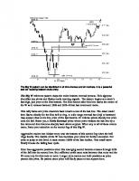
What Happens When Public Confidence Changes? Returning to Enron, we need to remember how fast public confidence eroded. In Figure 1.3 we see the stock quickly drop from $30 to nothing in the final days, but Enron prices had peaked a year earlier. Even before the offbalance-sheet transactions became public and problems became obvious, prices had declined from $90 to $60. What is most upsetting is that the major brokerage firms did not issue a sell signal until Enron was in the throws of death, a decline of nearly 90 percent of the stock price.

How Would You Have Done? Look at Figure 1.3 again. During all of 2000 and the first part of 2001, Enron held above $60, peaking at $90. In early 2001 it dropped from about $70 to $60, then to $50 within a few weeks. That was an unprecedented decline, leaving prices well off the highs by 40 percent. Traditional thinking declares a bear market when prices decline 20 percent. At least we need to recognize that something has changed. Why would the price drop 40 percent unless there was a problem?

Timing Is Everything

11

Was the fast collapse of Enron (ENE) the result of a sudden lack of confidence by the public or insider selling in excess of $1 billion? Did you care about the insider selling before the collapse? Did you think about it when accounting irregularities were announced?

FIGURE 1.3

HOW DO YOU DECIDE THAT YOU SHOULD NO LONGER OWN THE STOCK? The decision to sell a stock is at least as important as the one to buy. Ask yourself • What is the opposite of a buy decision when using only fundamental information? • How long does it take to realize that the quality is no longer there? • How far down does a stock price need to fall from the highs before you sell? • One major retail broker waited until Cisco had declined 75 percent before taking it off their hold list. What would you have done? Do you remember that the public was told (on CNBC) that the major houses had shifted from a buy recommendation to a neutral when Enron hit $10? Let’s look at other examples to get an idea of some of the recent price

12

A SHORT COURSE IN TECHNICAL TRADING

FIGURE 1.4 Cisco’s clear bull market and subsequent dramatic drop is easy to see in hindsight, but would you have closed out your long position at 60 when you still had a 300 percent profit in your original position?

patterns. If you were holding these stocks from 1997, consider whether you could have made an objective decision to sell them before the major price drop. If you did not actually get out while you still had profits, then you need to learn some things about technical trading.

Cisco Cisco (Figure 1.4) moved higher for three years, along with all of technology, with very little retracement. At the beginning of 2000 it dropped more than one-third in two weeks, a sign that something had dramatically changed. Prices tried to rally, but by the third quarter of that year they began falling to new lows. There was still a 300 percent profit in the original position. Would you have gotten out?

General Electric General Electric (GE), the flagship of the Dow, had a steadier rise and a less volatile fall than Cisco (see Figure 1.5). You may have exited at $40, or even $45, as prices fell, and then regretted that decision when prices moved back over $50. General Electric certainly doesn’t look like Cisco, but a decline

Timing Is Everything

13

from $60 to $30 is an unnecessarily large loss to absorb when you easily could have done better.

American Airlines It was not possible to be prepared for the price shock in American Airlines that came in mid-1998 (see Figure 1.6), when price turned from a perfect bull market to fall 35 percent in a few days. You might have been lucky when the second shock hit, at the beginning of 2000, because prices were already heading lower. You might even have escaped the third shock on September 11, 2001, because prices were still looking weak. The first shock should have been a lesson in itself.

Amazon.com Amazon is a remarkable investment story. We all believe in the future of the Internet, and Amazon was up front taking advantage of that promise. However, expectations and profits are different, and Amazon has not been able to deliver quarterly profits. Instead, it feeds the hopes of the investors by releas-

FIGURE 1.5 General Electric (GE), the flagship of the Dow, is down one-third from it’s highs. Would you still be holding it? Would you have gotten out at $40 and then gotten back in at $50 because it looked as though it was heading back up? If not, where would you get in again?

14

A SHORT COURSE IN TECHNICAL TRADING

American Airlines is different from the other examples because of a series of price shocks. Would you have been on the correct side of the market? Would you be correct next time?

FIGURE 1.6

Amazon.com lost $50 million each quarter yet continued higher through 1999. It was the product of dreams. Fortunes were made and lost. Does the extreme volatility in 1999 tell you anything?

FIGURE 1.7

Timing Is Everything

15

ing pro forma financial statements showing that profits are likely if everything goes according to projections. So far, that hasn’t happened. We are still hoping. The volatility of Amazon (see Figure 1.7), much greater than many other stocks, is based on overspeculation, constant promotion by the company, and a lack of any basis for valuing the stock price. How do you price the stock when the company posts a loss every quarter since inception?

IF YOU CAN’T HELP LOOKING AT THE CHART PATTERNS THEN YOU’RE GOING TO BE A GOOD TECHNICAL TRADER It’s fun to look at chart patterns and trends and imagine what trades you could have made. In technical trading we’re going to learn rules about price patterns and apply them in the same way to all of the stock and futures markets. Before you move on to the next lesson and see these rules, think about what you already know about price patterns.

Can You Apply the Same Buy-Sell Principles to All Stocks? • Can you write down the rules you’ve used to buy and sell a stock, any stock? Can you write down the rules for when you would have exited the long positions in the previous stock charts? If so, you’re a systematic trader. • When you look at a chart, do you see it in terms of continuous price moves? Do you look at the highs and lows of price swings? Do you draw conclusions, make up rules, and imagine that you can capture large profits? Looking at a historic chart is frustrating and deceiving. It makes you think that you could have profited from the price moves. It’s much harder when you can’t see the future. However, high-tech display equipment lets you see the past price movement of any stock. It has brought many new traders to the table who think they can profit from future price moves because they can see the past.

THE IMPORTANCE OF TIMING A few thoughts about timing are important before we move forward. We would like to think that we can profit from the news if we act faster than others. It’s not true.

16

A SHORT COURSE IN TECHNICAL TRADING

• The market moves on anticipation. “Buy the rumor, sell the fact.” If you bought on every piece of good news published in the Wall Street Journal, you would be broke. • The market responds to the difference between the actual news and what was expected. The unemployment rate could have dropped 0.2 percent, and the market falls because it expected a drop of 0.4 percent. • Action does not always mean immediate reaction. When did the Fed start lowering interest rates? When did the market start to respond? In the case of interest rates, it always takes more than one move by the Fed before you see a reaction in the economy.

EVOLVING MARKETS The market is dynamic. It is not the same as it was, yet it is driven by the same underlying economic forces.

What Has Changed? • The equipment has changed, allowing instantaneous analysis, program trading, electronic orders (smart order entry), high-momentum trading, and unreasonable expectations. • Methods have changed, with far more systematic traders, especially professional fund managers. • Participants have changed, with a larger influence from pensions, designer funds, and institutional investors. Day traders are common because commissions are low. • Electronic exchanges and side-by-side trading are new. You can beat your competition by creating an electronic order the instant a system “signal” is triggered. • Globalization has changed the way world markets move, with alternating leaders and followers. • There are more trading vehicles, including ETFs for index and sector investing, and single stock futures. • Markets are noisier because of more participation. Sometimes they have irrational swings because of piggy-backed orders. The frequency of extreme moves is increasing, causing greater volatility. Will a system that worked in 1990 work in 2002? Probably not. Will the people who made money in the 1990s make money now? If they change, too.

Timing Is Everything

17

WORDS OF ADVICE Throughout this course there will be trading tips, trading insights, and some old-fashioned advice. Take some time to think about all of it.

Don’t Confuse Luck for Skill In a prolonged bull market, all buyers are eventually right. They buy all dips, regardless of size, because it has always worked. As they gain confidence, they may add leverage by buying on margin. At the end of the bull market they are usually wiped out. • • • • •

It’s a business, not a casino. It’s all about risk. Learn how to take a loss. Don’t turn a profit into a loss. Anticipation is the key to success.

CHAPTER 2

Charting the Trend The trend is your friend.

I

n this chapter you will learn about the trend. The trend is simply the direction of prices over some time period. No matter how much you learn, you will always want to know the trend of the market.

TRENDS Trends are very easy to see on a chart. They are seen best over a long time period—weeks, months, and years. If prices are going up, the trend is up; if prices are going down, the trend is down. Here we get to the first problem. If prices go up and then down, is the trend up or down? Look at Figure 2.1, the S&P weekly chart. Is the price going up or down? The answer is “yes.” It’s going up in the long term, over the period of the entire chart, but down in the shorter term, the last two years.

The Trend Depends on Your Time Frame If you’re a very, very long-term investor, the trend will always be up because inflation and economic growth eventually will cause the stock index to make new highs. If you’ve been holding Merck from 1994 through 2002, you’ve watched the price rise from $5 to $60, a gain of 1,100 percent. If you bought Merck at the beginning of 2001 and held it through 2002, you watched the price go from $90 down to $60, a loss of 33 percent. The trend is always a matter of time interval. Even over a few days, two traders may see the same market as going in different directions. Each one can make money or lose money within the same period by correctly or incorrectly deciding where to buy and where to sell. 18

Charting the Trend

19

What Creates Trends? • Government policy. When economic policy is to target a growth rate of 3 percent, then the Federal Reserve (the Fed) raises and lowers interest rates to accomplish this. Lowering rates encourages business activity. Raising rates controls inflation by dampening activity. • International trade. When the United States imports goods, it pays for it in dollars. That is the same as selling the dollar. It weakens the currency. A country that increases its exports strengthens its currency. • Expectations. If investors think that stock prices will rise, they buy, causing prices to rise. Consumer confidence is a good measure of how the public feels about buying. • Supply and demand. A shortage, or anticipated shortage, of any product will cause its price to rise. Too much of a product results in declining prices. These trends develop as news makes the public aware of the situation.

The Trend Is Always Easier to See Afterward Look again at the S&P chart in Figure 2.1. You can easily see the upward trend. But after an uptrend, how far down do prices need to fall before you say that the trend is down? That’s a difficult question, and we’ll answer it in

FIGURE 2.1 S&P weekly 1996–2001. Is it going up or down? Yes. It was going up, and it’s now going down. If you’re a long-term trader, then you can still say that it’s going up.

20

A SHORT COURSE IN TECHNICAL TRADING

this chapter. Part of the answer depends on your time frame, but most of it depends on the market itself.

What It Means to Be a Trend Follower A trend follower buys when the price trend is up and sells when the price trend is down. A trend follower believes that, if the trend is up then it will continue to go up; therefore, trend followers make the assumption that trends persist. If everything works as expected, the trend continues long enough to yield a profitable trade.

Why Should the Trend Continue? There’s a good reason why the trend persists. Most trends are the result of government economic policy. In the U.S. the Federal Reserve (Fed) targets an economic growth of 3 percent. In order to accomplish that in a bad economy, they will lower interest rates. First they lower rates by 0.5 percent to see how the economy reacts. Then they lower rates by another 0.5 percent and watch (see Figures 2.2 and 2.3). This process of ratcheting down interest

Interest rates drive the stock market. Top: 10-year notes continuation series. Bottom: S&P 500 Index. There’s a clear relationship between interest rates and the stock market but it’s not always the same. Interest rates always lead, but the market doesn’t always respond. T-note prices begin going up in January 2000 (interest rates declining), but the stock market has not yet reacted.

FIGURE 2.2

Charting the Trend

21

rates causes a trend in all of the markets that depend on rates and all companies that have debt—which is pretty nearly all of them. The biggest trends usually begin with a change in interest rates. Sometimes, the beginning can be a change in the value of the U.S. dollar. The dollar can drop when the U.S. imports much more than it exports. When you buy foreign products, you buy their currency as well. Expectation also drives prices. Will a hot summer cause a shortage of electricity, or a shortage of water? Will a weakening economy reduce the number of airline passengers and shorten hotel stays? Will the economy strengthen or weaken? These events don’t occur overnight; they evolve gradually. Prices rise and fall in anticipation.

The Reason for Shorter Trends There are other trends besides long-term interest rates and currency. You’ll find seasonal trends in many businesses that focus on travel and leisure, such as airlines or hotels. The agricultural products are seasonal because they have a clear growing and harvest period. Heating oil is used during the winter

FIGURE 2.3 Cause and effect: good news versus bad news. When the stock market falls (S&P, center panel), short-term interest rates (Eurodollars, bottom panel) are lowered to start a recovery. When the stock market moves higher too quickly, rates rise to slow it down. The Fed manages growth using interest rates; policy lasts for 6 months to 2 years. At the same time, a cheaper dollar (Dollar index, top panel) stimulates trade and encourages foreign investment into stocks.

22

A SHORT COURSE IN TECHNICAL TRADING

Summer rally in corn. The summer growing season provides more than one opportunity to expect a problem with the corn crop. In 1990 prices began to rise before the crop was planted and continued through the middle of the summer based on lack of rainfall and news reports of devastation to land in some states. But technology won in the end, and the crop was much larger than expected. Price fell to levels lower than the previous year. (Prices shown are an adjusted continuous series of futures contracts.)

FIGURE 2.4

and gasoline is consumed in larger amounts during the summer. These patterns can cause extreme trends that last about three months. There are always unexpected events that cause a surge in prices: a cold spell that could affect the orange juice crop in Florida or a good chance that a new cancer drug will be approved for a medical research company. Shorter trends can also be caused by expectation. The public expects earnings to improve because interest rates are dropping. The public expects the cost of wheat to be higher because there’s been very little rain in the Midwest. As the news confirms their opinion, prices move steadily higher. You really don’t know how the corn crop is affected by rain until it is harvested in October. Any rise in prices over the summer is expectation, not fact (see Figure 2.4).

FINDING THE TREND ON A CHART What is the trend in Figure 2.5? It’s down because prices at the end of the chart are lower than prices at the beginning. Simple enough. There are periods when prices are rising, but the overall picture is a downward trend.

Charting the Trend

23

FIGURE 2.5 S&P daily, September 2000–December 2001. Is it an uptrend or downtrend? Are you influenced by how much of the chart is visible? Try to keep your long-term perspective.

The Trend Is Seen Best Using Weekly or Monthly Charts Everything looks smoother when you see it at a distance. You can’t see the details. That’s especially true with price charts. A monthly chart looks smoother than a weekly chart, a weekly chart is smoother than a daily chart, and a daily chart is smoother than an hourly chart. You can see the trend best on a weekly or monthly chart. You see more market “noise” on a daily or intraday chart. Market noise is the erratic up and down movement that occurs over a period of a few days.

CHARTING THE TREND It’s time to draw classic trendlines on a chart in order to get a relatively objective assessment of the trend direction. It’s relative because you can change the trend by choosing a longer or shorter trendline, or a daily, weekly, or monthly chart. There’s usually a way to make the chart say what you want if you’re determined to force your opinion on your analysis. We’ll try to avoid that approach. To begin, you’ll need to know that:

24

A SHORT COURSE IN TECHNICAL TRADING

• An uptrend (a support line) is formed by connecting the lowest rising prices. • A downtrend (a resistance line) is formed by connecting the highest declining prices

Where Do You Start? You can start a major upward trendline at a low price and then draw the trendline up and to the right, touching the lowest price or prices. Using Cisco as an example (see Figure 2.6) the upward trendline, A, starts at the low in October 1998 and touches the two lows in the third and fourth quarters of 1999. After that, prices move quickly away from the trendline and only cross it on the way down. The major downward trendline, B, was started at the high of the move. Of course, you don’t know the high until after prices have dropped significantly. At that point we can draw the line B from the peak, touching the high of the right shoulder where a second rally ended.

Do wn

wa Right shoulder rd Tr en dl in e B

Re n Tre ne

dli C

r wa

Up

wn dra

eA

lin

d ren dT

Intermediate Trendline

Trendlines drawn on the Cisco weekly chart. This company shows a clear major upward trend and a major downward trend. Lines can be redrawn to keep current with the price move.

FIGURE 2.6

Charting the Trend

25

Redrawing the Trendlines Price patterns change and so should the trendlines. They need to be redrawn from time to time in order to stay current with the price move. When Cisco prices begin to drop quickly in late 2000, we can redraw the downward trendline, C, at a sharper angle. Later, we might find that both lines, the original one and the new one, are both helpful for trading. After a while, your chart will look like a “work in progress” with redrawn lines everywhere.

How Many Points Should the Trendline Touch? You can draw a trendline with two points, but three or four are even better. The more points that lie on the same line, the more confidence we have that we’ve drawn the correct trendline. However, you can’t expect the lows to fall exactly on the same line—the market is just not that precise. If you can see a clear trend, even though the bottom is a little ragged, then draw the trendline anyway. In Figure 2.6, a shorter, intermediate trendline (the broken line) was drawn across the six bottoms during 1999. The first two low prices and the last low price fall right on the line but the middle three go through the trendline by small amounts. You should still see it as a trend. A price that penetrates a trendline and then corrects itself is considered a strong confirmation of that trendline.

More on Redrawing Trendlines Redrawing the trendline is a normal part of tracking the direction of prices. In the S&P chart shown in Figure 2.7 the first trendline is drawn from the October 1998 low to the October 1999 low (line A), then redrawn to touch the lows of February after a new high is made in March 2000 (line B), and redrawn a third time along the lows of April, May, and June (line C ). We can stop redrawing the upward trendline after the downward trend begins.

Which Trendlines Are More Important? If an upward trendline is drawn from one long-term low to another, it is more important than a line connecting two intermediate lows. If a trendline can be drawn across three or more lows (even though one point might poke through the line by a small amount), it is more important than a line through two lows. If a trendline is not violated, it gains in importance.

26

A SHORT COURSE IN TECHNICAL TRADING

A

B

C

Weekly S&P futures continuation chart. Upward trendlines are redrawn after new highs and then stop after the downtrend begins.

FIGURE 2.7

Charting the Trend on Daily Prices Up to now the charts used in the examples have been weekly and monthly because they show the trend more clearly, but daily charts will be used for our trading. We need to learn what to expect. In Figure 2.8 trendlines are drawn on an S&P daily chart. The first downward trendline, A, is perfect. It touches three points and crosses the final upward move as prices gap through the trendline. However, trendlines on daily charts can be confused by market noise. The upward move in October and November does not provide a third point for the trendline. You can redraw the upward trendline a number of times, and none of them will look as good as the downtrend line. Because of the increased noise, daily prices won’t line up as clearly as weekly prices and the trends won’t be as easy to draw. When you’re trading, be prepared for frustrating periods where you get in and out of the market because of noise. You need to hang on through those periods until the clear trends return.

The Evolving Trend of Enron One of the best recent examples of the benefits of charting is the demise of Enron. As the news tells it, a well-paid analyst continued to recommend the

27

Charting the Trend

Tr

en

dli

ne

A

FIGURE 2.8 Trendlines on a daily S&P chart. The downtrend is very clear, but the initial uptrend doesn’t fit very well. The redrawn uptrend seems to be better, but market noise that shows up on a daily chart makes it difficult to find a clear pattern.

purchase of Enron while prices were falling to $10 (see Figure 2.9). Was it a conflict of interest or simply bargain hunting? Now that you’ve been introduced to charting trendlines, when would you have sold your Enron shares? For certain, there is a major upward trendline that connects the lows during the summer of 1998 with the lows of December 2000. If that line is continued, it crosses the price decline in May 2001 at about $55. The fast break in March 2001 that took prices from just under $70 to the low $50s gives us

Tip: Real Market Conditions Real market conditions are never perfect for the technical trader. Each stock or futures market has its own personality. Instead of a bull market correction stopping at the trendline, it will stop a little above or below the trendline before starting back up. It’s smart to give a little room for a false break of the trendline. After all, this isn’t an exact science—prices are moved by news, emotion, and occasionally facts that create a public opinion. Exactly How Much Do You Let Prices Penetrate the Trendline? About 10 percent of the current price volatility. Let’s say that IBM has been moving in swings of $5. Allow an extra 50¢ for excessive movement.

28

A SHORT COURSE IN TECHNICAL TRADING

FIGURE 2.9 Enron during its best and worst times. How would you have traded it using classic trendline charting?

the idea that there was an intermediate trendline across the lows of the topping formation from the first quarter of 2000 until the break in May 2001. Whenever you question why you’ve decided to trade technically, think of Enron. Any chartist or technician would have been safely out before the worst of the news caused the final collapse of the stock price. How could any rational person recommend holding Enron down to $10?

TREND TRADING RULES FOR TRENDLINES It may seem clear from the charting examples that the trendlines show where to buy to enter a trade and sell to exit; however, traders place their orders in a few different ways:

Entry Rules • Buy when the price closes above the downtrend line (conservative). • Buy when the intraday price penetrates the downtrend line (aggressive). • Buy in an upward trend when prices decline to near the upward trendline.

Charting the Trend

29

Exit Rules • Sell when the price closes below the upward trendline (conservative). • Sell when the intraday price penetrates the upward trendline (aggressive). Notice that the aggressive trader buys during the day when prices cross through the trendline. A more conservative trader will wait to see if the closing price is going to be above the trendline. Price action during the day can be very volatile and the direction of prices can change, and often does, from midday to the close. On the other hand, if important news reaches the market during the earlier trading hours, the first one that buys gains the most profit. You can only decide your style from practice. Start with the closing price as a measure of direction until you are confident that another way is better.

Getting Out of the Trade When the upward trend is finished, prices will move down through the trendline. At that point you sell, closing out your trade, hopefully with a profit. However, not all trades are profitable. About two-thirds of all trend trades lose money, and yet trend trading is still a reliable, profitable way to trade. Profits Through Persistence. The majority of times, a change of direction does not turn into a trend; however, when prices do continue in one direction, they produce good profits. Success is a matter of numbers. You can expect 6 to 7 out of 10 trend trades to be losses, some small, some a little larger. Of the 3 or 4 good trades you can expect one small profit, two medium-size profits, and one large profit. On average, a profitable trend trade should be about 2.5 times the size of a loss. With enough trades, that should result in a net profit in your trading account. As an example, say we lose $100 on each of the 6 losing trades, for a total loss of $600. On the four profitable trades we get an average of $250 per trade for a total profit of $1,000. The individual profits are most likely $100, $200, $200, and $500. That’s a $400 gross profit less some slippage for entering and exiting and commissions on 10 trades. If instead of 6 losses there were 7 losses and 3 profits, we would net only $50. Expect the real results to be somewhere in between $50 and $400. As a trend trader, you should expect mostly small losses, some small profits, and a few large profits.

30

A SHORT COURSE IN TECHNICAL TRADING

What Can You Expect Your Trading Results to Look Like? • Most trades will be small losses • About 25 percent of the trades will be small or medium-size profits. • About 10 percent of the trades will be larger profits. • A small number of trades will be very large profits. Trend trading is successful because of the occasional very large profit.

The Fat Tail Trend trading is successful because losses are kept small and profits are allowed to grow. That technique is called conservation of capital. What makes trend trading profitable in the long run is the unusually large number of big profits compared to what is expected in a normal distribution. For example, in a normal distribution of 1000 coin tosses, half of them would be single runs of heads or tails. Half of those, 25 percent, would be a sequence of either two heads or two tails. Half of the remaining, 12.5 percent, would be sequences of three in a row, and so on. Therefore, in 1,000 coin tosses you can expect only one run of 10 heads or tails in a row. Apply that to prices. In 1,000 days of trading (about four years) you would expect only one time that prices would go up or down 10 days in a row. However, that happens much more often than once; therefore, price movement is not normally distributed, and not random. It has a fat tail distribution. There are fewer days where prices turn from up to down, or down to up, and more longer runs. That’s what makes trend trading profitable.

IMPACT OF THE TIME HORIZON Before leaving trendlines, think about the importance of the length of the trendline and the use of daily, weekly, or monthly data: • Using major tops and bottoms to draw a trendline identifies the most important trends; monthly and weekly charts will show these points clearly. • Longer time horizons put the points where the trend changes farther away, causing a longer delay, or larger lag, in your decisions. • Longer time horizons allow larger price swings; therefore those trades have larger risk.

Charting the Trend

31

• Longer time horizons are more reliable because they allow prices more freedom of movement. Even in a trending market, prices do not go straight up or straight down. These features show a trade-off between reliability and risk. You need to accept more risk to have better results. All trading has choices between risk and return. You can never have both large profits and low risk.

A Computerized Approach: Finding the Points Automatically for Drawing Trendlines Most analysts will look at a chart and pick the low prices that will be used to draw an uptrend line. However, you also can find those points automatically. Anyone who enjoys working with a spreadsheet or writing a computer program might find the rules for finding those points a good first step toward automating a trading method. In Figure 2.10 the dots above the price peaks mark the swing highs, and the dots below the bottoms are the swing lows. They are called swing highs

FIGURE 2.10 Finding the tops and bottoms automatically. The points showing the tops and bottoms of this S&P chart are separated by price swings of at least 5 percent.

32

A SHORT COURSE IN TECHNICAL TRADING

For Computer Mavens: Finding the Swing Points Automatically Using a Spreadsheet Set A B C D C3

up your columns with the following data: Date High price Low price Closing price Put the minimum swing percentage value in cell C3 (for example, 5% = .05)

Put the following formulas in the corresponding cells. Row 6 initializes the process. E6 = B6 (the current swing high) F6 = C6 (the current swing low) G6 = IF (D6 > (E6 + F6) / 2,−1,1) (where −1 is a downswing and +1 is an upswing) Row 7 is the beginning of the repeated process. Row 7 can be copied down. E7 = IF($G6 = −1#AND#B7 > E6,B7,IF($G6 = 1,B7,E6)) (the new current low) F7 = IF($G6 = 1#AND#C7 < F6,C7,IF($G6 = −1,C7,F6)) (the new current high) G7 = IF($G6 = −1,IF(C7 < E7 − $C$3× D7,1,$G6),IF(B7 > F7 + $C$3× D7,−1,$G6)) (test high or low) H7 = IF($G7 = 1#AND#G6 = −1,E7,H6) (the new swing high) I7 = IF($67 = −1#AND#G6 = 1,F7,I6)) (the new swing low)

and lows because they are separated by at least a 5 percent price move in this example. You can choose any percentage. A larger percentage identifies major points, while smaller percentages show minor points. Major points are more reliable. When we use the dots in Figure 2.10, we draw an upward trendline only when the bottom dots are rising and a downward trendline when the top dots are falling. The trendlines do not need to be formed by connecting consecutive dots.

EVOLUTION OF A TREND The trend is constantly being redrawn based on new highs and lows. In Figure 2.11, only the automatically calculated swing highs and lows are used to give you an idea of how your chart will look as time creates new patterns. Some of the main features of this Amazon chart are: • The highest point, 1, on the left remains the highest throughout this period.

33

Charting the Trend

1 E C

D 2 F

A

3

4

B

5

G

H

Evolution of a trend. In this Amazon chart we see how trendlines need to be redrawn as price patterns develop. This chart used only swing highs and lows computed automatically. The result shows that these trendlines clearly mark the changes in price direction.

FIGURE 2.11

• The downward trendline, A, beginning at point 1, is redrawn each time prices move above the existing downward trendline (B, C, D, and E), creating a new swing high. • An intermediate downward trendline, E, may be drawn beginning from another high (see mid-April 2001). • Other downtrend lines (G and H ) begin in July 2001 at point 4 after prices drop. • Good lines are confirmed by the market, often with a price gap. • The major downward trendline, E, formed by connecting points 1 and 4, seems to hold after the rally to point 5 at the far right.

MAKING THE TREND WORK It is easier to see a trend using a weekly chart instead of a daily chart, but trading using a weekly chart is very slow and exposes you to larger price swings and larger risk. Many professional traders will use the weekly chart to

34

A SHORT COURSE IN TECHNICAL TRADING

draw the major trend, but a daily chart to decide where to get in and out. It is easier to find the trend on a weekly chart, and this assures us that we don’t loose sight of the correct trend.

Questions 1. What is the reason for drawing a trendline? 2. What is the intended relationship between interest rate changes and stock market changes? 3. If you wanted to see the trend on a chart more clearly, would you use a daily, weekly, or monthly chart? Why? 4. How could you have a chart where the trend was both up and down? 5. In the S&P monthly chart shown in Figure 2.12, draw the major uptrend lines as they develop. Is there a point (or points) at which you would have gone short?

The S&P futures monthly continuation series shows the sustained bull market of the 1990s and the peak in 2000.

FIGURE 2.12

Charting the Trend

35

6. Using the chart of Cisco during 1998 shown in Figure 2.13, draw the trendlines and outline the (ideal) trades you would have made based on the price penetration of the trend.

Daily Cisco prices from February through October 1998. A strong uptrend followed by a difficult, volatile period makes finding the trendlines more challenging but makes trading more exciting.

FIGURE 2.13

CHAPTER 3

Breakout Trends

pward and downward trendlines, or angled trendlines, are not the only way of finding the trend. Although they are the classic method, there is a simpler way of identifying the trend that many think is more practical for trading. It’s called a breakout.

U

BREAKOUTS The start of a trend can be recognized by a price breakout. A breakout is simply a new high price or new low price after a sideways pattern. The longer the sideways pattern, the more important is the breakout. In Figure 3.1 we see a sideways pattern in General Electric (GE) from November 1996 through April 1997. The breakout occurs near the end of April when prices move over the previous highs of $18. They move quickly higher before stabilizing. Not all sideways breakouts are as clear as GE. The AOL chart in Figure 3.2 has three different sideways patterns, all overlapping. The shortest period from October to November 1996 is broken by a sharply higher move that begins at $1.75 and ends at $2.80 in 7 days. A larger sideways pattern from July to November 1996 is ended with the same breakout. Following that move, we see another sideways period from December 1996 ending at the beginning of March 1997 with a break above $2.75. Notice that the support line for the first two sideways patterns did not include the two lows in October. They can be considered false breakouts. When you ignore them, the support line for the sideways pattern is very clear. 36

37

Breakout Trends

Breakout

FIGURE 3.1 An upward breakout from a sideways pattern in GE. After six months of sideways price movement, GE prices break out to the upside in April 1997.

It is an advantage to smooth out the patterns with your eyes. Very few patterns are perfect.

Why Do Breakouts Look So Good? A breakout is a sure sign that something has changed. If GE has been trading between $45 and $55 for 3 months and then makes a new low, something has changed. There are expectations of bad news. When you draw a classic upward trendline, as we did in Chapter 2, you are imposing the expectation that prices should continue higher at the same rate, or faster, in order to keep above the trendline. That may not be realistic. As long as prices go higher rather than lower, it doesn’t matter how long they take between new highs. By looking only at new highs and new lows, we can recognize the trend without placing as many conditions on price movement.

Pinpointing the Breakout with Horizontal Support and Resistance Lines In order to recognize a breakout we draw two horizontal lines on a chart, one beginning at the highest high of the most recent sideways period and the

38

A SHORT COURSE IN TECHNICAL TRADING

3

2

1

FIGURE 3.2 Multiple breakouts from sideways patterns in AOL. Three clear sideways patterns can be found in AOL. The fast price move through the resistance line, especially in pattern 1, is a confirmation that traders recognized this pattern.

other from the lowest low of the same period. If today’s high price crosses the resistance line, we have a new upward trend breakout; if the low crosses the support line, we have a new downward trend. In Figure 3.2 the horizontal lines cross through some of the highs and lows. That’s good if it makes the sideways pattern clearer. The trend remains the same until prices cross the support or resistance lines going in the other direction (see Figure 3.3). Cisco is an interesting example. It breaks above a sideways pattern in July 1998. It drifts sideways for three months and then starts up, and it doesn’t consolidate and move sideways until it forms a broad top in 2000. To show that support is a real phenomenon, look at the number of times the price bars had a low of $50. Someone must have been buying large quantities at that price in order to have stopped prices from going lower. Finally, at the end of 2000 the market wins (as it always does), and prices break through support. Whoever was buying has been stopped out or is very unhappy.

39

Breakout Trends

Support

Breakout Resistance

Breakouts can be used to identify major trends. In this chart of Cisco, a breakout to the upside at the beginning of 1998 is followed by a downside breakout at the end of 2000. Note the number of times the price touches $50 during all of 2000 before finally breaking down.

FIGURE 3.3

Trading Rules for Breakouts Breakouts are the easiest of all methods to trade. • You buy when prices make a new high above the previous resistance level. • You sell when prices make a new low below the previous support level. • You do nothing in between.

Placing Your Sell Order after Buying a Breakout When there is an upward breakout from a sideways pattern, the sell order goes below the bottom of the sideways pattern. Prices must be allowed to flop around before they continue their upward pattern. We would like them to go straight up after we buy, but it usually doesn’t happen that way. The beginning of a trend can be sloppy, and prices usually fall before moving higher. By placing your initial sell order below the original sideways pattern, you are saying that you’ll only exit the trade if the breakout was false. That is, if prices now make a new low, then something was wrong and the market wants to go lower.

40

A SHORT COURSE IN TECHNICAL TRADING

Later, we’ll show how to use support levels to set a stop-loss order. We don’t want to turn a profitable trade into a loss. Enron is another good example of breakouts (see Figure 3.4). At the beginning of 1998 it moves above its previous high. Something new has happened. It gets more volatile but moves steadily higher until the summer of 1999 when it takes a setback before surging above $70. Now prices seem to form a sideways market with clear lows between $63 and $64. If you were watching for a change of direction based on breakouts, you would be short on a break of $60. It would seem clear that something had changed.

False Breakouts A false breakout occurs when the resistance level ( previous high) is penetrated during the day but prices close back inside the range. There are volatile days in which prices are pushed to new highs on expectations that fail to develop. By the end of the day those higher prices could not be reinforced by fact and so prices return to previously lower levels inside the range. Although we can now redraw the top of the range to include the new higher high, it is best not to consider a breakout unless the closing price confirms the direction by staying above the high of the sideways range.

Support

Short-term breakout Long-term breakout

Breakout

FIGURE 3.4

Enron upward breakouts and impending downward break.

Breakout Trends

41

The Risk of Using the Breakout Method If a new upward trend occurs with a new high and a downward trend with a new low, then the risk of trading using the breakout method is the difference between the high price and the low price. Looking back at Figure 3.2, we can see the risk in the sideways pattern 1 is about one-third of the risk of pattern 2. During volatile periods the risk significantly increases; while during quiet times the risk is small. The strongest feature of the breakout method is that the risks and the trends adjust to market conditions. You also may think of the larger risk as a problem, but it can be corrected simply by trading a smaller position.

THE ROLLING BREAKOUT We normally find a sideways period and the corresponding breakout levels by looking at the chart. However, computerized programs have taken a different approach by always looking backward by the same number of days. If we always use the highest high and lowest low over the past 20 days, we call that a 20-day rolling breakout or simply a 20-day breakout system. For each new day we drop off the oldest day and find the highest high and lowest low of the new 20-day period.

Is the “Rolling Breakout” Better Than the Old-Fashioned Method? No, but it can be very profitable, and it can be tested on a computer. It has the same profit and risk characteristics as the handdrawn lines but sometimes gets fooled into using the wrong highs and lows. It’s a lot more practical than drawing lines on each of a large number of charts each day. A computer can calculate the breakout trends of all the markets in a few seconds. If you like the diversification of trading a number of markets, the rolling breakout is a good method to use. Example of Trading Results of a 30-Week Breakout. Table 3.1 shows the Enron trades using a 30-week rolling breakout system. This calculation period gives results similar to those in Figure 3.4. The trades can be seen in Figure 3.5 with the words buy and sell below and above with an arrow pointing to the day of the trade. Figure 3.6 gives the Excel code and a small piece of an Excel worksheet that can calculate the breakout trends, including buy and sell signals. Using a spreadsheet greatly simplifies the problem.

42

A SHORT COURSE IN TECHNICAL TRADING

TABLE 3.1 Trade No.

1 2 3 4 5 6 7 8

Enron Trades Using a 30-Week Breakout System Type

Units

Price

Signal Name

Trade P/L

Cumulative P/L

6/17/1994 11/25/1994

Buy Exit

1 1

17.313 14.438

Buy Sell

−2.875

−2.875

11/25/1994 2/24/1995

Sell Exit

1 1

14.438 16.438

Sell Buy

−2.000

−4.875

2/24/1995 4/4/1997

Buy Exit

1 1

16.438 18.500

Buy Sell

2.062

−2.813

4/4/1997 1/23/1998

Sell Exit

1 1

18.500 20.813

Sell Buy

−2.313

−5.126

1/23/1998 9/4/1998

Buy Exit

1 1

20.813 21.719

Buy Sell

.906

−4.220

9/4/1998 12/25/1998

Sell Exit

1 1

21.719 29.156

Sell Buy

−7.437

−11.657

12/25/1998 12/1/2000

Buy Exit

1 1

29.156 65.500

Buy Sell

36.344

24.687

12/1/2000

Sell

1

65.500

Sell

Date

There were a lot of breakout systems that would have made money on both the rise and fall of Enron. This one went short on December 1, 2000, and would still be short.

−1 Sell

−1 Sell

−1 Sell

Buy −1 Buy

FIGURE 3.5 Enron rolling breakout trades. Buy and sell signals for a 30-week rolling breakout system are shown at the point of the breakout.

43

Breakout Trends

Calculating the Rolling 10-Day Breakout System Using a Spreadsheet Set up your columns with the following data: A Date B High price C Low price D Closing price Repeat (copy down) the following lines. There are no constants and no initialization. For a 10-day calculation the data begins in row 1 and the calculations begin in row 11. E11 = MAX(B1:B10) the 10-day high through the previous day F11 = MIN(C1:C10) the 10-day low through the previous day G11 = IF(B11>E11#AND#D11>D10,1,IF(C110,"L","S") "NDB=if(B13>max(B3:B12),"L", " if(C13 0, then OBV = OBV + today’s volume If today’s price change < 0, then OBV = OBV − today’s volume Once we have created the OBV line, we interpret the OBV to make trading decisions instead of using the price. In Figure 13.5 the OBV is plotted along with the volume at the bottom of the chart. You’ll notice that it looks very much like the price chart rather than the volume chart, even though it is created from volume. The obvious difference between the price chart and the OBV line is that the peak is shifted from the end of 1999 to the end of March 2000. On the OBV line, the low in November is more significant than it appears in the prices, and it shows a breakout of the lows at an early point.

Volume Accumulator The Volume Accumulator (VA), created by Mark Chaiken, uses buying or selling strength as a way to assign volume to the buyers or sellers. If the

Volume, Breadth, and Open Interest

187

On-Balance Volume. On-Balance Volume (OBV) is created by adding the volume when prices rise and subtracting the volume when prices fall. You then use the OBV line to make trading decisions, rather than price.

FIGURE 13.5

close is above the middle of the trading range, then the percentage above the middle determines how much volume goes to the buyers; if it is below the middle of the range, then that percentage of volume goes to the sellers: VA = ((close − low) / (high − low) − .50) × 2 × volume If close = high, then all volume goes to the buyers. If close = low, then all volume goes to the sellers. If close = middle of the range, then no volume is added. If you want to check your arithmetic, when prices close three-fourths of the way up in today’s range (for example, a high, low, and close of 44, 40, and 43), then 50 percent of the volume is added to the indicator VA.

An Unexpected Comparison between On-Balance Volume and the Volume Accumulator We should expect the OBV and VA lines to be very different because the calculations of the VA are so much more complex. In Figure 13.6 it seems

188

A SHORT COURSE IN TECHNICAL TRADING

Comparison of the On-Balance Volume and Volume Accumulator. On-Balance Volume (gray line) and the Volume Accumulator (dark line) are remarkably the same, even though the calculations seem different. Both are intended to be used for trading instead of price.

FIGURE 13.6

remarkable that there should be so little difference between the two indicators. Sometimes we can be fooled into thinking that two apparently different methods yield different results. Our first hint of this was when we looked at the difference in performance of four trending methods. The conclusion was that, if the market trended, any of the methods would work. We’ll see many more examples where we can simplify our trading by using only one method. Further Comparisons. It’s not always the case that the Volume Accumulator is the same as On-Balance Volume. In Figure 13.7, On-Balance Volume starts higher, drops lower, and then stays lower than the Volume Accumulator. Across the entire chart, the Volume Accumulator shows an upward trend, while On-Balance Volume shows a break in June 1994. Look at the chart carefully and try to decide how you would use either of these indicators to your advantage.

Volume, Breadth, and Open Interest

189

Recent-Exxon Mobil volume patterns. In this example, the OBV and VA show very different patterns. OBV shows a sell in January 1994, while VA holds an uptrend throughout the entire interval. Neither is better than a simple price trend for this one-year interval.

FIGURE 13.7

September 11 It is always interesting to see how indicators performed on September 11, 2001. In the charts of XOM (Figure 13.8) and the S&P (Figure 13.9) we see slightly different pictures. On September 10 XOM was trading at $41.42 on volume of about 10 million shares. Markets were closed September 11 and reopened on September 17 to a rapid sell-off. The bottom came on September 21 when XOM traded at a low of $35.01 with volume of 21 million shares. The spike in Figure 13.8 shows the day. By October 11, prices were back at $41.77, up 19 percent, erasing the entire decline that began September 11. Other spikes in Figure 13.8 mark local turning points, except in mid-December. The S&P 500 show a slightly different picture of building volume from the reopening of the New York Stock Exchange until the bottom on September 21. Volume in Figure 13.9 comes from the total futures contracts traded. The S&P index doesn’t trade; therefore, there is no volume.

190

A SHORT COURSE IN TECHNICAL TRADING

XOM on September 11, 2001. Prices fell sharply when the NYSE reopened on September 17, hitting a low on September 21 with a volume spike. By October 11, prices had fully recovered the 19 percent drop that occurred from September 11 to September 21.

FIGURE 13.8

S&P on September 11, 2001. When dealing with a broad index, the volume spike following the September 11 attack is clearly the major event on the chart and signals a reversal. Although the volume spike was an accurate signal, you would need nerves of steel and deep pockets to buy on September 21.

FIGURE 13.9

Volume, Breadth, and Open Interest

191

Because the S&P represents a much broader market than XOM, volume after September 11 is clearly much higher than any other time. The entire market was swept away by selling over five days, only to bounce back to a price higher than before the attack on the World Trade Center. Volume Indicators on September 11. How did the OBV and VA indicators perform during the crisis? On the XOM chart they both rally when the market reopens after September 11, but the VA continues higher and then falls while OBV drops and rebounds. The OBV actually has the same pattern as the prices. The indicators move in opposite directions, proving that they are not the same indicator in disguise as it appeared at first. On the S&P chart, the OBV drops after September 11 and doesn’t recover. The VA follows the price pattern. Prudence. Volume spikes tend to be an accurate indicator of price reversals and September 11 was no exception. Afterward, it looks as if it was a lost opportunity; the chart clearly shows a buy signal. Don’t fool yourself. You could only buy between September 17 and September 21 if you had nerves of steel and deep pockets. There was enormous risk. Try to remember that when you’re looking back at this chart in five years.

The Crash of 1987 As you gain experience, you’ll suffer through other extreme events. The crash of October 1987 seems to have been pushed aside by the more recent bull market of the 1990s, but it was devastating at the time. In Figure 13.10 we see a volume spike on the day of the crash, but it doesn’t rise above the other volume bars as far as we would expect. Would you have taken it as a buy signal? On-Balance Volume gained credibility during the 1987 crash by turning down ahead of prices. The Volume Accumulator didn’t react soon enough and hardly reacted during the crash. We would prefer an indicator that worked in extreme price moves.

Automatically Identifying a Volume Outlier A volume outlier is the statistician’s name for a spike. If you are trying to automate your trading rules in order to test them, it’s easy to recognize an outlier: 1. Calculate the average volume over 20 days (call that N days), beginning

five days ago. You will not be using the last five days to avoid volume that is creeping higher.

192

A SHORT COURSE IN TECHNICAL TRADING

The crash of 1987. The volume spike is on the right day, but may not be as clear as we need to buy. The OBV indicator (gray) gains credibility by turning down ahead of the crash. The VA doesn’t seem to respond.

FIGURE 13.10

2. Compare today’s volume with your average volume from 6 to 25 days ago. 3. If today’s volume is 2 to 3 times higher than the average for a stock, or 11⁄2

to 2 times higher for an index, you have a volume spike. Notice that individual stocks will show spikes that are far above the average, but a broadly traded index market has consistently high volume; therefore, spikes are not as extreme.

MARKET BREADTH INDICATORS Market breadth measures the imbalance between the number of advancing and declining stocks on a given day. In general, more advancing issues should add confidence to an upward price move. A net increase in the S&P 500 while more issues are declining should generate concern that the upward move is poorly supported.

193

Volume, Breadth, and Open Interest

The information for advances and declines is published along with stock prices each day. You also may want the volume of advancing issues and the volume of declining issues. Both of these values can be found in the Wall Street Journal under “Trading Activity.” Market breadth indicators are best used as a confirmation of price direction. The table below shows that the interpretation of market breadth is the same as the relationship between volume and price. Market Breadth

Price

Rising Falling Falling Rising

Rising Falling Rising Falling

Interpretation

Breadth Breadth Breadth Breadth

confirms price rise confirms price drop does not confirm price rise does not confirm price drop

Advance-Decline Index The most well-known and simplest of the market breadth indicators is the advance-decline (AD) index. It is a running count of the number of advancing issues minus the number of declining issues at the end of each day: AD(today) = AD(previous day) + advances(today) − declines(today)

Sibbett’s Demand Index The volume of stocks advancing compared to the volume of stocks declining may be considered more a “robust” measurement than simply the number of issues advancing and declining. Throughout technical analysis we’ll see indicators that are equally weighted and their counterparts that use relative value. Sibbett’s Demand Index, (DI), uses the sum of the past 10 days’ upside and downside volume because these volume numbers, just as with total market volume, can jump around quite a bit. A 10-day sum is really the same as a 10-day average, only the numbers are 10 times as large: DI =

sum(upside volume, 10 days) sum(downside volume, 10 days)

where upside volume and downside volume are found in the Wall Street Journal under “Trading Activity.”

194

A SHORT COURSE IN TECHNICAL TRADING

Arm’s Index—TRIN The Arm’s Index, called TRIN, combines the number of advancing and declining issues with the volume of the advances and declines. Its value is often quoted on television and has gained popularity among technicians:

TRIN =

(number of advancing issues / number of declining issues) (volume of advancing issues / volume of decline issues)

Bolton-Tremblay Index The Bolton-Tremblay Index (BT) recognizes that there are also unchanged issues each day. Without including the unchanged issues, we have an incomplete picture. This index also takes the square root of the change value, a familiar technique that reduces the importance of a few extremely large changes: BT =

(advancing issues − declining issues ) unchanged issues

where if BT > 0, then BT = BT + BT if BT < 0, then BT = BT − BT

Schultz A /T Index Schultz takes the same advancing, declining, and unchanged data and represents it as a “bullish index.” By putting the advancing issues in the numerator, the Schultz A/T Index (SAT) would be 100 if all issues advanced:

SAT =

advancing issues (advancing issues + declining issues + unchanged issues)

Is One Breadth Index Better Than Another? These five breadth indicators show some of the ways data can be massaged into an index. There are dozens of others that have not been mentioned. There is no doubt that we should be more confident of a price rally when a large number of issues are advancing, or the total number of shares traded is much greater for the advancing issues. We should be concerned when market breadth drops, as we would when volume drops, during any price move up or down.

195

Volume, Breadth, and Open Interest

Does it make a difference whether we include the unchanged issues in the index? Is the total volume traded on advancing issues a better picture than simply the number of advancing issues? Does the square root used in the BT Index make the result more accurate? To find the answer, we should remember the charts that compared the On-Balance Volume with the Volume Accumulator. Sometimes one looks better than the other, and sometimes they look the same. Neither seemed to be perfect. Breadth is an interesting measurement, but don’t expect it to solve too many problems. Most often, it will simply confirm the current price move. When it does stand out by conflicting with rising prices, volume and other indicators also should show weakness.

OPEN INTEREST IN FUTURES The stock market has a fixed number of shares that can be traded, the amount issued by each company. In futures markets the concept is different. When a new buyer trades with a new seller, they create a contract between themselves. That contract is one unit of open interest. Each buy or sell in futures may create or liquidate a unit of open interest. If a new buyer finds a new seller, then a new contract is added to the total open interest. If a new buyer finds an old seller, then his unit of open interest (his outstanding obligation) is transferred to the new buyer and there is no change in open interest. When those contracts are liquidated, they are removed from the open interest. The larger the open interest, the more outstanding contracts exist and the larger the participation in the market. A day trader who buys and sells but holds no positions overnight does not affect the open interest, which is calculated at the end of the day. The table summarizes these relationships. Buyer

Seller

New New Old Old

New Old New Old

Change in Open Interest

Increase in open interest No change in open interest No change in open interest Decrease in open interest

A new buyer (seller) is a trader with no market posiition seeking to be long (short); an old buyer (seller) is a trader who had previously entered a short (long) position and seeks to exit.

Futures contracts, as with stock options, are traded for a specific delivery month, such as March, June, September, and December. When we

196

A SHORT COURSE IN TECHNICAL TRADING

use futures volume and open interest data, we must always use the total of all contracts for that market, not the volume or open interest for the nearest or most active contract. Total volume and total open interest are interpreted as follows: Volume

Open Interest

Rising Rising Falling Falling

Rising Falling Rising Falling

Interpretation

Confirmation of trend Position liquidation (the end of a trend) Slow accumulation of a position Congestion phase, denies a trend

An increase in open interest means greater participation in a move. It is possible to have high volume during the day because of day trading activity, but more open interest means that traders are going home with their position. High open interest during a trend means that the market is in strong hands and the trend is likely to persist. When it is in weak hands, it is likely to fail.

ARE THERE TOO MANY INDICATORS? There is an underlying theme in the interpretation of volume, breadth, and open interest. Increasing values confirm price direction, and decreasing values deny that direction. That is a valuable concept. However, which of these indicators should we use? Does a volume indicator tell you more than a simple volume spike or a sharp drop in volume at the top of a move? If we look back at the OBV and VA in Figure 13.7, the final results don’t seem to be as good as simply using a moving average price trend. The VA implies that you should be holding the long position throughout, while the OBV is late exiting a long and entering a short. In the final analysis, when volume spikes or drops sharply lower during a rising market, we get a reliable indicator of a change of direction. None of the indicators seem to improve on this simple interpretation.

Become Familiar with One Indicator The most important part of any indicator is the way you use it. When we looked at different moving average techniques, we concluded that they all worked when prices trended. All of these indicators will show the same result in slightly different ways. Pick one that seems most sensible to you,

Volume, Breadth, and Open Interest

197

watch it, and become familiar with it. Most often, it will simply confirm price movement, but once in a while it will show you that the direction of prices is not supported by much activity. If it helps only a few times, it’s valuable.

ADVANCED TOPICS How Do You Recognize an Extreme Volume Day Using Excel? An extreme volume day is one that has a much wider range, from high to low, than previous days. You can recognize an extreme day if Today’s volume > factor × average(volume from t − 6 to t − N) where factor should be at least 2.0 and N should be at least 20. Therefore, today’s volume is extreme if it is 3 times greater than the average volume of the 15 days from 6 days ago to 20 days ago. This satisfies the idea that today’s volume is much higher than normal. It also avoids using the most recent five days in the average. Sometimes the volume increases gradually until it reaches an extreme. If you measure each day against the previous day, you might not recognize an extreme, so we don’t look at the most recent few days.

Low-Volume Periods Low volume is important because it is associated with lack of direction for prices. To recognize a low-volume period we need to have the average volume over the past few days below a threshold value. That threshold varies with the individual stock. Therefore, a low-volume day occurs when Average volume over the past N days < threshold where the average might be 250,000 shares and N should be at least 5.

Questions 1. What interpretation do you place on falling prices and falling volume? 2. Would you say that volume trends are (a) clear and easy to interpret or

(b) require smoothing to avoid erratic values?

198

A SHORT COURSE IN TECHNICAL TRADING

3. If volume was high and prices closed unchanged, would you consider the

risk of trading (a) low, (b) normal, or (c) high? 4. A volume spike usually corresponds with what price pattern? 5. How do you calculate On-Balance Volume? 6. Of all the volume patterns and indicators, which appears to be the most

definitive? 7. If prices are falling, what would the market breadth need to do in order to

confirm the decline? 8. In futures trading, if a new buyer meets an old seller, what happens to the

open interest?

C H A P T E R 14

Momentum and MACD

n this chapter we’ll focus on momentum, the speed of the price. Changes in the speed can be seen in different momentum indicators. Momentum indicators make up a very valuable set of tools. The most well-known variation of a momentum indicator is the moving average convergencedivergence (MACD), which gives extremely reliable forecasts of price changes.

I

MOMENTUM Momentum is speed. Then the momentum value M is the change of price over a specific time period, such as a week: M = price(today) − price(N days ago) If N is 5, then we have the weekly momentum, the price change over a oneweek period. An important feature of momentum is that its value can be as large the biggest price move over the N days used in the calculation. A momentum indicator plotted below the prices in Figure 14.1 shows that momentum is smoother than price. The more days used in the momentum calculation, the smoother the line. A 5-day or 20-day momentum has the same effect as looking at weekly or monthly prices instead of daily prices. The weekly prices appear smoother than the daily and the monthly smoother than the weekly.

199

200

A SHORT COURSE IN TECHNICAL TRADING

FIGURE 14.1 Momentum. In this chart of AOL the prices are on the top and the 20- and 40-day momentum lines on the bottom. The 40-day momentum is smoother and has peaks and valleys at about the same place as the price series. The 20-day momentum (gray) reaches its peak sooner than prices because the price swings last more than 20 days.

Interpreting Momentum The momentum line doesn’t lag as we saw with a moving average. A 10-day momentum simply answers the question, “How high or low is today’s price compared to 10 days ago?” In Figure 14.1 the scale to the right of the momentum lines shows that the momentum was as high as 20 and slightly below −10. For both the 20 and 40-day momentum lines that means prices over any 20- or 40-day interval never gained more than $20 or fell more than $15. The thinner gray line is a 20-day momentum. It peaks at the place where the largest move occurs over a 20-day period. The heavier line, a 40-day momentum, peaks at the largest move of a 40-day period. The scale on the right measures the net price change over 20 or 40 days. Steadily Increasing Prices. One special feature of momentum that must be understood is that if prices continue higher at the same rate after 40 days, the 40-day momentum indicator will go sideways. Therefore, prices could be increasing, but the momentum line is not increasing.

Momentum and MACD

201

For example, the price of International Widgets starts at $10 and increases by $1 every day. After 40 days it is $50 and the 40-day momentum is 40 (50 − 10 = 40). On the next day it again increases by $1. The price is $51 and the 40-day momentum is 40 (51 − 11 = 40). As long as the price increases by the same amount, the momentum remains the same. It’s the same as driving a car. As long as you hold the accelerator at the same pressure, the car moves forward at the same speed. If the speed is unchanged, the momentum value is unchanged. Acceleration. If the speed is the same when the momentum line is moving sideways, then prices must be accelerating (increasing in speed) when the momentum line is rising. It will also be accelerating to the downside when momentum is falling below zero. We will refer to speed and acceleration throughout our study of momentum.

Momentum as a Trend Indicator Momentum can be used as a trend indicator. We showed in Figure 14.1 that the longer the momentum calculation, the smoother the momentum line. It’s not as smooth as a moving average, but it is smoother than the actual prices. When the momentum moves above zero, the trend is up. When it moves below zero, the trend is down. If a 20-day momentum line moves above zero, then the price today is higher than the price 20 days ago, a legitimate reason for saying that prices are rising. You may notice that the momentum lines show a lot of small, erratic moves. When using momentum to decide the trend, you may want to use a small buffer zone, a filter, around zero so that a little erratic movement does not cause you to change position unnecessarily. For example, you can go long AOL when the momentum goes above 2 and short when it goes below –2. That will prevent jumping in and out if the value gets stuck around zero, as it might if prices are going sideways.

Comparing Momentum to a Moving Average To be sure that momentum really acts as a trend, we should compare it with a moving average. In Figure 14.2 20-day and 40-day moving averages are plotted along with prices on the top of the chart, and the previous 20-day and 40-day momentum indicators are shown at the bottom. To compare the slower moving average with the slower momentum (the thicker lines), we look at where the moving average changes direction and

202

A SHORT COURSE IN TECHNICAL TRADING

FIGURE 14.2 Comparing momentum with moving averages. To compare the trends of momentum with a moving average, we match the point where the moving average changes direction with the point where the momentum crosses the zero line.

where the momentum crosses zero. In April 2001 the moving average turns up at about $42; the momentum crosses the zero line moving higher at just about the same day. When the moving average turns down in July, the momentum falls below zero at about the same time. You’ll find that the same is true of the faster 20-day trends. We concluded at the end of Chapter 4, Calculating the Trend, that if the market is trending, any of the trend calculations would be profitable. We can now add the momentum trend to that list.

Detrending a Price Series Using Momentum Momentum can be used to remove the trend from a price series. A detrended series allows us to see the cyclic or oscillating patterns clearly. It is a method used by economists. If we create a one-day momentum, we are looking at the one-day price changes by subtracting today’s price from the previous price. In mathematics this is called the first difference in price. The first difference also gives you the speed. In Figure 14.3 the first differences of AOL are shown in the center panel. It is easy to see the daily volatility of price changes, but the overall

Momentum and MACD

203

FIGURE 14.3 The detrended AOL price series. Classic detrending is simply the one-day price changes (center panel), but you can also detrend AOL by subtracting the 40-day momentum from the current price (the bottom panel). Both methods remove the downtrend. The bottom panel using momentum shows the cyclic pattern clearly, while the one-day changes show volatility.

trending pattern is sideways. The trend has been removed. We can also detrend the AOL series by subtracting a longer momentum value. In Figure 14.3 the bottom panel shows the new series when a 40-day momentum is subtracted from the original price series. By using a longer momentum calculation, we also remove the trend bias but keep the cyclic pattern. By subtracting a momentum line of a different speed, we can choose to see specific patterns in AOL that were not as obvious in the original series. We will use this technique to create the well-known indicator, MACD.

MOVING AVERAGE CONVERGENCE-DIVERGENCE The moving average convergence-divergence (MACD) indicator is a smoothed difference between two smoothed trendlines. It is formed by creating a faster and slower smoothed trendline from the original price series, subtracting the slower one from the faster one, and finally applying another smoothing to the new series. If we choose the slow calculation period as 40 days, the

204

A SHORT COURSE IN TECHNICAL TRADING

fast period as 20 days, and the final smoothing as the 9-day equivalent, the MACD is calculated as follows: Step 1. Choose the two calculation periods, for example, slow = 40 and

fast = 20. Calculate the percentage smoothing values using 2 / (N + 1), where N is 40 or 20. Step 2. Calculate the slow trendline using the smoothing value .0243. Step 3. Calculate the fast trendline using the smoothing value .0476. Step 4. The MACD line, the slower oscillating line in the bottom panel of

Figure 14.4, is calculated as the fast trendline minus the slow trendline. When the market is moving up quickly, the fast smoothing will always be above the slow and the difference will be positive. This is done so that the MACD line goes up when prices go up. Step 5. The signal line is the 9-day smoothing (using a percentage of .10) of

the MACD line. The signal line is slower than the MACD; therefore, it can be seen in the bottom panel of Figure 14.4 as the lower line when prices are moving higher.

MACD. The MACD line is the faster of the two trendlines (gray) in the bottom panel; the signal line is the slower (dark). The histogram is created by subtracting the slower signal line from the MACD line. This histogram shows the relative strength or weakness of the MACD compared to the signal line.

FIGURE 14.4

Momentum and MACD

205

Reading the MACD Indicator We normally see the MACD as it appears in the bottom panel of Figure 14.4. The MACD line is higher in an uptrend and lower in a downtrend. The histogram is created by subtracting the slower signal line from the MACD line. When the histogram is above zero, it confirms the uptrend. The 40/20 MACD line is similar to the 40-day momentum line. We can compare the MACD in the lower panel with the 20- and 40-day momentum in the center panel and see that the peaks and valleys are in about the same place, but the MACD line is much smoother. The MACD is a variation of momentum because it is the difference between two trendlines.

Trading the MACD The most common use of the MACD is as a trend indicator. For that purpose, we use only the MACD and signal lines in the following way: Buy when the MACD line (faster) crosses above the signal line (slower). Sell when the MACD line crosses below the signal line. We can look at the bottom panel of Figure 14.4 to see that the buy signals that occur right after a bottom, in April and October 2001, generated large gains. Unfortunately, there were a lot of other crossings that generated losses. It is clear that we need to be more selective about these signals. One easy way to pick the good trades is to say that we only take the sell signals that occur after the MACD goes above 2.00, and only the buy signals after the MACD has fallen below −2.00. That gives us a very nice buy signal in April, a sell in May, and a buy in October. However, if someone were looking over our shoulder, we would be accused of “fitting” the data. We looked to see what worked for this chart and made up a rule to profit from it. Using +2.00 and −2.00 works for this chart, but some other charts will have peaks that may be as high as +10. What looks as if it’s a top on this chart will turn out to be the middle of another chart. If you have some other way of deciding that prices are near a top, then you can select the signal crossover as your point to sell. One likely method is to look for a strong resistance level on your price chart. If prices slow as they rise into resistance, then you have a good chance that the MACD sell signal will work. Using a much longer time period for your chart will also give you a better view of the possible range of MACD values.

206

A SHORT COURSE IN TECHNICAL TRADING

DIVERGENCE Divergence is one of the great concepts in technical analysis. Divergence shows when prices are about to change direction. It is easier to show divergence in an illustration than in words. In Figure 14.5 there is a bearish divergence in Amazon formed in October through December 2000. It is bearish because it anticipates a drop in prices. To see this divergence on the Amazon.com chart, follow the rules: 1. Find the swing highs on the chart. This can be done simply by looking

at the highest peaks. In Figure 14.5 there are five significant peaks, the largest in April and December 1999, medium peaks in October 1999 and February 2000, and a small peak in July 1999. 2. Find two consecutive peaks that are rising. They are July, October, and

December. 3. Draw a line connecting the October and December peaks.

Divergence: Prices are rising

Indicator is falling

FIGURE 14.5 MACD divergence. In this divergence, prices are rising sharply while the MACD is falling. Sell the next crossover of the MACD line and signal line.

Momentum and MACD

207

4. Look at the MACD line directly below the October–December line that

you drew in the upper part of the chart. There always will be a peak in the MACD corresponding to a peak in prices. Connect the two peaks in the MACD line. 5. The line drawn across the price highs is rising sharply. The line across the

MACD peaks is falling slightly. Whenever these lines are angling in opposite directions, you have divergence. Bearish divergence occurs when the price moves higher and the indicator moves lower. This divergence is important because the MACD is not confirming the upward move, but indicating that prices want to go down. Prices drop from $110 to $60 in a few weeks. Bullish divergence is the opposite formation. Prices are dropping, but the MACD is rising. Prices want to change direction. Figure 14.5 has an equally successful bullish divergence. Can you find it? The bullish divergence has lower price lows in June and August with clearly rising lows in the MACD at the same time. The August price low marks the bottom of the move, and a substantial rally follows. Divergence is one of the most successful of all indicators. When you study it closely, you find that the divergence is formed when the new high price peaks get farther and farther apart. Although not as apparent, a bearish divergence also is recognizing an irregular but rounded top formation. Divergence is most profitable when it is very clear, as it is in the bullish divergence example. If the price peaks are nearly at the same height, the peaks are not very big, or the MACD line is nearly horizontal, then the success of the divergence is doubtful. Unfortunately, the clear divergence signals never occur as often as we would like them, but they have a high degree of success. Watch for them.

Another Amazon Example of Divergence Earlier in 1999 Amazon shows another clear bearish divergence (see Figure 14.6). Prices show peaks in January and April 1999. At the same time the MACD peaks are clearly declining. Note that Amazon had a test of the January highs three weeks before the major peak. At the time the second MACD peak was much lower and a divergence seemed likely, but prices didn’t quite move above the first peak. As it turned out, this was not the

208

A SHORT COURSE IN TECHNICAL TRADING

Rising prices Not a divergence

Falling MACD gives strong divergence signal

Another example of divergence in Amazon. In this bearish divergence, the MACD is much weaker on the second peak, indicating a strong divergence signal. Before the actual divergence, there is another peak that may be taken as a divergence; however, prices did not make a new high.

FIGURE 14.6

top of the market, and the divergence signal would have been premature. Once the second price peak has been made in the bearish divergence, we look for the MACD line crossing the signal line heading down. We can now sell.

Anticipating the Divergence As you become more comfortable with recognizing a divergence, you’ll want to trade it as early as possible. So far, we enter a bearish divergence after we see the second MACD peak form and recognize that it is lower than the previous MACD peak. We can do better than that. When a current price rally moves above the high of the previous rally (which happened about December 1 in Figure 14.5), we look at the MACD. The MACD value is less than 4.0 when prices break out to the upside. The previous MACD high was above 6.0. If prices were to turn now, we would

Momentum and MACD

209

have a strong divergence (the new MACD peak being much lower than the previous peak). We should start selling now. Don’t sell everything at one time. Divide your capital into three parts: 1. Sell the first third when prices make a new high and the MACD is much

lower. 2. Sell the second part when the MACD line gets to within 15 to 20 percent

of the previous MACD high. 3. Sell the third part when the MACD line crosses the signal line heading

down. If you only have one choice, you are better taking the second signal. If you have two choices, take the first and second. If you look at the price when the MACD crossed the signal line, the third sell signal, you’ll see that your fill would have been disappointing. Prices already had dropped significantly.

Exiting a Divergence Trade A bearish divergence is a special case of prices being overbought. Prices have reached new highs but have slowed down and give every sign of wanting to reverse direction. As with other overbought situations, once prices have returned to a neutral position, the trade is over. For divergence, that happens when the value of the MACD reaches zero. It is a mistake to think that prices will go from overbought to oversold. The Divergence Disappears. Not all trades are profitable. Although a divergence signal is reliable, it is not perfect. If you’ve sold a bearish divergence and prices start back up and the MACD value goes above the previous MACD peak, then the divergence formation has disappeared. The MACD peaks are now rising, and you must exit your trade. Take your loss and look for the next divergence trade. Combining Divergence with a Trend. One very effective strategy is to combine divergence with a trend. If you use a trend for you basic positions, watch for the formation of both bullish and bearish divergence patterns. If you are long, then sell if a bearish divergence forms and watch the trend to see if it also reverses. The best case is that when the MACD reaches zero, the trend has turned down and you can hold your short position and continue to follow the trend.

210

A SHORT COURSE IN TECHNICAL TRADING

HIGH-MOMENTUM TRADING— A GAME PLAYED BY PROFESSIONALS We started this chapter looking at momentum. Momentum is the change in price over some time interval, a number of days or hours. Momentum is strongest as prices gain speed in a clear uptrend, or as they gain speed during a dramatic drop. We saw that momentum has peaks based on the span of the momentum calculation. If we use a 10-day momentum, the peaks show the largest 10-day net moves; if we use a 20-day momentum, the peaks will be higher than the 10-day peaks and will show the largest 20-day moves. One quirk about using a short momentum period, for example, 10 days, is that the momentum line will remain high if prices continue rising for more than 10 days. If there is a 20-day rally, then the last 10 days will all post high momentum values. In Figure 14.7, a chart of AOL, the 10-day momentum is shown along the bottom, and two horizontal lines have been drawn at +15 and −15 to show the extremely high and low momentum values. It would be possible, although

Trading high-momentum periods. Professional traders will buy when prices are moving fast and hold the trade for a short time. High-momentum periods, when the momentum value is above the horizontal line, show where prices are rising quickly and accelerating.

FIGURE 14.7

Momentum and MACD

211

risky, to sell when momentum crosses the upper band and buy when it crosses the lower band. We saw in previous charts that momentum usually doesn’t remain at a high level for long.

Trading above the Threshold Some professional traders have made a business of trading in the direction of the trend only when momentum exceeds a high threshold level (for example, +15) rather than looking for a change of direction. There is a lot of money to be made because prices are moving fast. There is also a great deal of risk. High-momentum trades are held for only a short time—a few minutes or a few hours for day traders, two or three days for longer-term traders. Price patterns have changed over the past five years. There are many more day traders. When one stock breaks out above a previous high, everyone sees it as an opportunity for profit. Buy orders start to flow and volume increases. Stocks that are normally ignored can attract large volume when prices make a new high. Traders ride the rising price for as long as possible, watching to see when volume begins to drop, and then they exit. They may just target a modest profit and get out. It’s a fast game that requires tools that allow you to scan a wide range of stocks looking for one that has made a new high after a long, quiet period. You need to stay glued to your screen, enter fast, and exit fast. It’s a business for the professional trader, and it’s not easy.

TRADING GAME TIPS Gold shares and gold prices. Is there a relationship between gold shares and gold prices? Yes, if the company is not so diversified that the mining operation is only a small part of its revenue. You can then watch the cash price of gold and look for support and resistance levels that occur at the same place for both the share price and the physical gold price (see Figure 14.8). General Electric and electricity prices. Don’t think for a moment that the price of GE has anything to do with the price of electricity. GE is a massive financial company. Light bulbs and electricity round off the end of its balance sheet.

Questions 1. If the last five prices of IBM were $40.25, $40.75, $41.25, $40.75, and

$41.50, what is the value of the five-day momentum?

212

A SHORT COURSE IN TECHNICAL TRADING

Barrick Gold (ABX) compared to physical gold prices. You can gain extra insight, as well as confirmation of technical signals, by comparing gold stocks with the price of physical gold.

FIGURE 14.8

2. Which one of the 20-day or 40-day momentum lines can potentially have

the highest value? 3. When two consecutive momentum values are 1.50 and 1.50, are prices

(a) increasing, (b) unchanged, or (c) decreasing? 4. When two consecutive momentum values are 2.50 and 1.50, are prices

(a) increasing, (b) unchanged, or (c) decreasing? 5. If you are using momentum as a trend indicator, at what point does the

trend turn up? 6. If you are using the MACD as a trending indicator, when do you get a sell

signal? 7. How would you improve the reliability of a standard MACD trending sell

signal? 8. Describe an MACD bearish divergence. 9. What would make you consider one bullish divergence as stronger than

another? 10. If you were anticipating a bearish divergence and planned to make two

sales, when would you sell?

C H A P T E R 15

Overbought/Oversold Indicators and Double Smoothing

W

hen we watch the way a stock price moves, we form expectations. When the price breaks out above a previous high, we expect continued higher movement because something new has happened. When prices move up exceptionally fast, we expect them to stop and reverse. Prices can’t accelerate upward forever. We call a market that has gone up unusually far or unusually fast overbought. A stock that has dropped in the same way is called oversold. We can decide that a stock or index is overbought or oversold in two ways. The “quants” will statistically measure the fluctuations in price movement over the past, create a profile, and then say that the current move is extreme. Before mathematical analysis was so easily done on a computer, overbought and oversold conditions were decided by market sentiment. Market sentiment is still popular and just as valid today.

MARKET SENTIMENT—OPINION AND CONTRARY OPINION Market sentiment is the driving force of the market. Prices don’t go up unless investors believe they will go up and are willing to back up their opinion with money. Although there is a constant flow of funds into pension plans, which works its way into the market, investors will draw money out if they see a gloomy forecast for the next six months. We might conclude at first that if consumer confidence is rising, then we should buy and if it is falling, we should sell. Is the public always right? We expect prices to rise if the general public is comfortable putting their pension money into the market in large numbers, 213

214

A SHORT COURSE IN TECHNICAL TRADING

allocating a larger percentage to stocks and putting less into fixed income, such as bonds. What happens when prices have been rising steadily, as in the mid-1990s, and the public becomes enamored by the returns of the stock market, when they expect to get more than 20 percent each year? Isn’t that an overbought situation?

Contrary Opinion Contrary opinion is a theory that when the public is overly confident in its belief that the market will continue higher, it is time to sell or, at least, time to get out of your long stock holdings and look for a place to sell. Extreme cases justify this approach. The most famous of all events in which the public was wrong are documented in Charles Mackay’s Extraordinary Popular Delusions and the Madness of Crowds (originally published in 1932 but available in a Noonday Press paperback). It’s a bit scary to think that the rise and fall of the Internet stocks, still an incomplete story, may qualify as another great financial bubble. The contrarian is the investor who believes in doing the opposite of the majority of investors. Some of the qualities of contrarian investors are: • They are value investors. • They look for undervalued stocks or opportunities where prices are away from value. • They are attracted to prices after a sustained run up or down. • Once they identify an opportunity, they use other technical tools for timing; being undervalued does not mean the stock price will rise any time soon. • After they buy, they wait patiently for prices to turn from down to up. To be successful, contrarians must not act in the same way as everyone else.

Bullish Consensus One of the tools for measuring public opinion is the Bullish Consensus by Earl Hadady. The Bullish Consensus assesses the impact of the opinions of professional market analysts and brokerage houses by ranking the bullishness of their analyses and weighting the results by the circulation of each one’s market letter:

Overbought/Oversold Indicators and Double Smoothing

215

Interpretation of the Bullish Consensus. (With permission from Figure 6.1, p. 69, R. Earl Hadady, Contrary Opinion, New York, John Wiley, 2000).

FIGURE 15.1

Bullish Consensus = sum of (each source × relative weight × bullish opinion) sum of (each source × relative weight × 100) Bullish Consensus values range from 0 to 100 percent. It is considered neutral at 55 percent because of the bullish bias in the stock market that has resulted in a 5 percent rise over the long term. In Figure 15.1, an imminent downtrend is expected when the Bullish Consensus is greater than 90 percent, and an imminent uptrend when it is below 10 percent. Positions are never entered without confirmation. The obvious problem with the Bullish Consensus is timeliness. First, the analysts must evaluate the individual stocks and write their reports; the reports are then published and distributed. They are usually sent by mail. The

216

A SHORT COURSE IN TECHNICAL TRADING

elapsed time must be no less than two weeks. Then the reports must be ranked for bullish content.

OSCILLATORS: OVERBOUGHT/OVERSOLD INDICATORS Oscillators are the best tools for identifying contrary options without reading through all the available market letters—and a much more definitive and timely solution. Some oscillators measure the current price relative to previous highs and lows, while others try to extract a more complex “quality” of the price. We’ll look carefully at the two most important of these indicators, the stochastic and the Relative Strength Index.

The Stochastic Not to be confused with the stochastic random process, this stochastic was created by George Lane and is a widely used technical indicator for determining overbought and oversold conditions. The basic calculation, called the raw stochastic (also called %K), gives the relative position of the closing price within the range of the previous N days. Raw stochastic = %K(today) = 100 ×

close(today) − lowest low of past N days (high − low) range of past N days

where range is the highest high of the past N days (not including today) minus the lowest low of the past N days (not including today). Dividing by the range creates a value from 0 to 100. For example, if we are using the past 10 days (called a 10-day stochastic), the raw stochastic has the value: • 100 if today’s close is higher than the high of the past 10 days. • 0 if today’s close is lower than the low of the past 10 days. • 0 < %K < 100 if today’s close is between the high and low of the past 10 days. Calculating the 10-Day Stochastic for Nokia. Using an Excel spreadsheet, we can calculate a smoothed version of the raw stochastic called %K-slow (or %D), and an even smoother version called %D-slow. In Figure 15.2, the historic prices for Nokia are imported into columns A to D. We are then ready for the calculation of the raw stochastic:

217

Overbought/Oversold Indicators and Double Smoothing

A

B

C

D

Date 1/2/1996 1/3/1996 1/4/1996 1/5/1996 1/8/1996 1/9/1996 1/10/1996 1/11/1996 1/12/1996 1/15/1996 1/16/1996 1/17/1996 1/18/1996 1/19/1996 1/22/1996 1/23/1996 1/24/1996 1/25/1996 1/26/1996 1/29/1996 1/30/1996 1/31/1996 2/1/1996 2/2/1996 2/5/1996 2/6/1996 2/7/1996 2/8/1996

High 2.50 2.55 2.39 2.30 2.23 2.20 2.20 2.27 2.26 2.21 2.25 2.30 2.30 2.33 2.37 2.37 2.37 2.40 2.35 2.36 2.41 2.38 2.45 2.45 2.45 2.48 2.44 2.39

Low 2.45 2.41 2.29 2.19 2.19 2.14 2.07 2.15 2.18 2.10 2.12 2.18 2.23 2.25 2.27 2.31 2.34 2.30 2.26 2.30 2.37 2.30 2.35 2.38 2.39 2.45 2.31 2.31

Close 2.50 2.44 2.34 2.21 2.19 2.19 2.16 2.27 2.19 2.12 2.25 2.20 2.29 2.30 2.37 2.34 2.37 2.30 2.35 2.35 2.37 2.34 2.43 2.41 2.45 2.45 2.36 2.34

E F 10-day 10-day High Low

2.55 2.55 2.39 2.30 2.33 2.37 2.37 2.37 2.40 2.40 2.40 2.41 2.41 2.45 2.45 2.45 2.48 2.48 2.48

2.07 2.07 2.07 2.07 2.07 2.07 2.07 2.10 2.10 2.10 2.12 2.18 2.23 2.25 2.26 2.26 2.26 2.26 2.26

G 10-day Range

H 10-day Stochastic %K

0.48 0.48 0.32 0.23 0.26 0.30 0.30 0.27 0.30 0.30 0.28 0.23 0.18 0.20 0.19 0.19 0.22 0.22 0.22

10.4 37.5 40.6 95.7 88.5 100.0 90.0 100.0 66.7 83.3 82.1 82.6 61.1 90.0 78.9 100.0 86.4 45.5 36.4

I

J

%K-slow %D-

29.5 57.9 74.9 94.7 92.8 96.7 85.6 83.3 77.4 82.7 75.3 77.9 76.7 89.6 88.4 77.3 56.1

54.1 75.8 87.5 94.7 91.7 88.5 82.1 81.1 78.5 78.6 76.6 81.4 84.9 85.1 73.9

Excel example of 10-day stochastic. The stochastic has three variations, the raw calculation, %K, a three-day smoothing of %K, called %K-slow or %D, and a three-day smoothing of that called %D-slow. The raw values, %K, fluctuate faster between 0 and 100 percent, while the slowest, %D-slow, fluctuate the least.

FIGURE 15.2

1. In column E find the 10-day high, not including today, using the function

@Max. 2. In column F find the 10-day low, not including today, using the function

@Min. 3. Calculate the high-low range by subtracting column F from column E

and putting it in column G in the same row. 4. The raw stochastic %K, in column H, is = (close − 10-day low) × 100 / range. 5. In column I, the %K-slow is the three-day average of K. 6. In column J, %D-slow is the three-day average of column I.

218

A SHORT COURSE IN TECHNICAL TRADING

If we look at the raw stochastic in column H of the spreadsheet, we see that values reach 100 percent three times. This means that prices are at the highest level, or higher than prices during the past 10 days. For the first occurrence of 100 percent on January 22, 1996 the closing price of $2.37 was the high of that day and higher than the highs of the past 10 days. On January 24, 1996 the same high of 2.37 was equal to the high of the past 10 days. When calculating the stochastic, today’s close is compared to the range of the previous 10 days; the range does not include today’s values. The smoother values in columns I and J will reach 0 or 100 percent less often but will also lag because of the smoothing. Charting the Stochastic. The stochastic is an interpretation of the price chart that removes the trend and scales the prices between 0 and 100. In Figure 15.3, the price of AOL appears on the top and the raw and smoothed stochastic values appear on the bottom. You should first notice that the stochastic peaks and valleys fall at about the same place as prices, but the stochastic values run sideways while AOL prices first go up and then down.

Charting the stochastic. The 20-day raw stochastic %K is the thicker gray line along the bottom. The 3-day average %K-slow is the thinner dark line that appears smoother.

FIGURE 15.3

Overbought/Oversold Indicators and Double Smoothing

219

Two horizontal lines have been drawn at 20 percent and 80 percent to indicate an oversold and overbought levels. Whenever prices approach the lows of the past 20 days, the stochastic falls below the 20 percent line. When it nears the highs, it moves above the 80 percent line. Most analysts use the two slower stochastic values and avoid the raw stochastic because the raw value tends to jump around. On the other hand, because it is not smoothed, you can react quickly to current market action, rather than waiting a day or two for a lagged confirmation. Trading the Stochastic. The smoothed stochastic trading signal is similar to the signal line used with the MACD. If you look back to Chapter 14, you will see that the MACD smoothed signal line was created in order to get a buy or sell signal. As with the MACD, the best signals follow after the stochastic reaches an extreme: 1. After the smoothed stochastic %K-slow has moved above the 80 percent

line, sell when the %K-slow line crosses the %D-slow line moving down. 2. After the smoothed stochastic %K-slow has moved below the 20 percent

line, buy when the %K-slow line crosses the %D-slow line moving up. In Figure 15.4 we see an example of the slow (%D, the heavier line) and slower (%D-slow, the thinner line) stochastics applied to the S&P from the beginning of 2002. At the beginning of 2002 the S&P was mostly sideways, and the stochastic shows swings from below 20 to over 80. During this period the peaks are easier to trade than the valleys because the stochastic moves above the 80% line and turns down quickly. Stochastic peaks correspond to price peaks. The oversold points are a problem. As prices decline, the stochastic tends to stay below 20 percent, occasionally moving higher but rarely reaching 50 percent. This is the typical pattern of the stochastic during a downtrend. As prices make new lows, the stochastic value must near zero. Because these two stochastic lines are smoothed, they don’t touch zero as often as the raw stochastic. Clearing Up the Confusing Signals. The stochastic works best in a sideways market, where prices are not reaching new highs or new lows. During a upward-trending market the stochastic will usually remain above 50 and during a downtrend below 50. Traders will use the stochastic with a trendline (a moving average or breakout) to decide which stochastic signals are good.

220

A SHORT COURSE IN TECHNICAL TRADING

FIGURE 15.4 Sell signals using the stochastic. The stochastic generates good signals during a sideways market, but will stay at low values during a downtrend and high values during an uptrend. To trade the stochastic successfully, you’ll need to use a trend to find the direction of prices and then use the stochastic to time your entry.

If the price is trending down, as the S&P in Figure 15.4, you want to sell when the stochastic moves below 80 after being higher, or when the faster stochastic line crosses the slower line heading lower the first time after the faster line has been above 80. During March 2002 the S&P stochastic reached about 90 and both stochastic lines crossed twice above 80. The proactive trader will take the first crossing as a sell signal. The more conservative trader will wait until the faster or slower stochastic crosses below 80. If you take the first signal, then you have the advantage of selling while prices are rising—you get a good price—-but with greater risk. If you wait for a confirmation, you are safer but prices are already heading down and your entry could be much lower. You’ll need to try both ways and decide for yourself. Comparing the 20-Day Stochastic with a 20-Day Momentum. When you plot the faster stochastics (%K and %D) along with momentum, the peaks and valleys occur at the same points (see Figure 15.5). Neither the stochastic nor the momentum indicators have a lag; that is, neither is the result of

Overbought/Oversold Indicators and Double Smoothing

221

smoothing or averaging. They tend to peak where prices peak and are therefore more responsive to price change than averages. The main difference between the stochastic and momentum is that the stochastic is be scaled between 0 and 100. Even though the AOL rally in November 2001 was much smaller than the previous one in May, the stochastic values reached the same levels near 100 percent. This makes it easier to say the prices are overbought. When you look at the way momentum shows the same two rallies, the one in November peaks at about 7 percent and the May rally touches above 15 percent. Because momentum is more variable, it is not a good candidate for an overbought/oversold indicator. A Brief Review of the Stochastic. The stochastic will be an important tool for timing, but it has three different calculations and some confusing names, used differently throughout the industry: 1. The raw stochastic is the fastest. It is called %K, %FastK, and %K-fast.

It is the only stochastic called fast.

Comparing the 20-day stochastic with a 20-day momentum. The peaks and valleys of both indicators fall at about the same point, but the stochastic is scaled between 0 and 100; therefore, it has the ability to show when it is overbought and oversold using simple 80–20 lines.

FIGURE 15.5

222

A SHORT COURSE IN TECHNICAL TRADING

Fast and slow stochastics. The center panel shows the raw (%K) and slow stochastic (%D). The bottom panel shows the slow (%D) and slowest (%D-slow) stochastics.

FIGURE 15.6

2. The next slower stochastic is %SlowK, which is simply a three-day aver-

age of %K. It is also called %D and %K-slow. 3. The slowest stochastic is called %SlowD or %D-slow. It is a three-day

average of %D and it is used as the signal line. Figure 15.6 shows the faster stochastics in the middle panel and the slower ones along the bottom. When trading, use the stochastics as follows: 1. Sell in a downtrend when the stochastic crosses the signal line above 80

percent, or when the stochastic moves back below 80 after being higher. 2. Buy in an uptrend when the stochastic crosses the signal line below 20

percent, or when the stochastic moves back above 20 percent after being lower. 3. In a sideways market use both buy and sell signals.

An Example of Stochastic Timing. Although the AOL charts showed periods where the stochastic indicator was confusing, the stochastic has gained

223

Overbought/Oversold Indicators and Double Smoothing

popularity because it also can have extended periods where the signals are very clear. These tend to be sideways patterns, and prices often go sideways. In Figure 15.7 we see AOL in the last part of 2000, where prices had only a slight downward bias. We trade by combining the trendline and the fastest stochastic line (the thinner of the two). During the sideways period from June into October we sell when the stochastic falls below 80 after being higher and buy when it moves above 20 after being lower. When the downtrend becomes clear in mid-October, the stochastic is used only to enter shorts. When the stochastic falls below 20, the trade is closed out. Stochastic Divergence. We used divergence with the MACD when we found that there were too many signals and they were not always reliable. Divergence selects those patterns that are likely to forecast a turn in prices. Divergence is associated with a broadening pattern, or a rounded top or bottom. It shows when prices are rising but at a slower rate. Divergence works well with the stochastic. The fastest stochastic line is best because it has less lag. The raw stochastic line (the thinner one at the

Downtrend New sell

Sideways market Reverse to short

Reverse to short?

Downtrend Uptrend

New short New short

Buy back

New buy

Reverse to long

Close out short

Close out short

Close out short

Combining the stochastic and a trendline. The stochastic is a very good indicator for timing but needs a trendline to select which signals are best. During the sideways period both buys and sells are used. When the downtrend becomes clear in mid-October, only the sell signals are taken.

FIGURE 15.7

224

A SHORT COURSE IN TECHNICAL TRADING

Bearish divergence #1

Bearish divergence #2

Bullish divergence #1 Bullish divergence #2

Bullish divergence #3

Is this a valid stochastic divergence?

FIGURE 15.8 Stochastic divergence with AOL. A bearish divergence occurs when prices are rising and the stochastic is falling. In this chart there are two bearish and three bullish divergences, all profitable trading signals.

bottom of Figure 15.8) must always be in the extreme zone before there can be a divergence. A sell signal (a bearish divergence) occurs when there are two declining stochastic peaks at the same time that prices are rising. In August and October 2000, the raw stochastic indicator first peaked near 100 and then peaked again at about 80. When you connect the two peaks with a straight line, the line clearly angles down. If you look above the two stochastic peaks, you see prices rising. Prices peak at about the same place as the stochastic peaks (because the raw stochastic doesn’t lag) and if you connect those peaks, you see that prices are rising. The combination of rising prices and a falling stochastic creates a divergence. The sell signal occurs when the raw stochastic line crosses the slower stochastic line after the second peak. In this example prices are falling quickly at the same time as the sell signal, but there is still room for profit. In Figure 15.8 there are two bearish divergences (sell) signals and three bullish divergence (buy) signals. All of them are profitable.

Overbought/Oversold Indicators and Double Smoothing

225

Stronger and Weaker Divergence Signals. A bearish divergence is stronger when the angle between the rising prices and the falling stochastic is greater, that is, when prices are rising faster and/or the stochastic is falling faster. Divergence only works when the prices and the stochastic are moving in opposite directions. It is not enough to have a strong relative difference, where prices are declining slightly and the stochastic is declining sharply. One must be going up and the other down. Bearish Divergence Rules. There are specific rules for recognizing a divergence signal (this describes a bearish signal, but the bullish signal is just the reverse): 1. The first stochastic peak must be greater than 80. 2. The second stochastic peak should be at least a 15 percent lower (but no

less than 5 percent lower). For example, if the first peak is at 90, the second should be at 70 or 75. 3. The price peaks that occur at the same time as the stochastic peaks must

be clearly rising. Using Faster and Slower Stochastics for Divergence. Do we get better divergence signals when we use a faster or slower calculation period for the stochastic? In Figure 15.9 a 10-day and a 20-day fast stochastic are shown along the bottom, the 10-day above the 20-day. Because the 10-day calculation causes the stochastic to change faster, it creates clear and frequent peaks and valleys on the chart. The angles are clearer. In May 2001, the 20-day stochastic has a rounded formation with a very small dip in value, while the 10-day stochastic shows a drop to 60 in between two peaks of 90. In this case the faster stochastic works better and is likely to give us more trading opportunities.

Relative Strength Index Created by Wells Wilder in 1978, the Relative Strength Indicator (RSI) is used more often than the stochastic. It is most often used the same way as the stochastic, but has some extra features. The RSI is a ratio of the upward price movements to the total price movement over 14 days. It has a slight smoothing feature, and is a little more difficult to calculate. The way to calculate the RSI is:

226

A SHORT COURSE IN TECHNICAL TRADING

Bearish divergence #1

Bearish divergence #2

Bullish divergence #1

Bullish divergence #2

Bullish divergence #3

Is this a valid stochastic divergence?

Comparing the divergence signals for a 10-day and a 20-day stochastic. A faster 10-day stochastic is more sensitive and gives a clearer picture. The bullish divergence in December 2000 can be seen and the one in May 2001 is now clear.

FIGURE 15.9

SumU = sum of price changes for all those days closing higher (positive numbers) SumD = sum of price changes for all those days closing lower (positive numbers) Then RS =

SumU (the ratio of up changes to down changes) SumD

and RSI (first calculation) = 100 −

100 1RSR × 100 × 1 + RS 1 + RS

Once the first calculation has been made, the following values of SumU and SumD use the average off method, requiring only the previous values of SumU and SumD, and the current price change: SumU(today) = SumU(previous) −

SumU(previous) + today’s upward change 14

SumD(today) = SumD(previous) −

SumD(previous) + today’s downward change 14

227

Overbought/Oversold Indicators and Double Smoothing

Date 1/2/1996 1/3/1996 1/4/1996 1/5/1996 1/8/1996 1/9/1996 1/10/1996 1/11/1996 1/12/1996 1/15/1996 1/16/1996 1/17/1996 1/18/1996 1/19/1996 1/22/1996 1/23/1996 1/24/1996 1/25/1996

Close 2.50 2.44 2.34 2.21 2.19 2.19 2.16 2.27 2.19 2.12 2.25 2.20 2.29 2.30 2.37 2.34 2.37 2.30

FIGURE 15.10

Changes −0.06 −0.10 −0.13 −0.02 0.00 −0.03 0.11 −0.08 −0.07 0.13 −0.05 0.09 0.01 0.07 −0.03 0.03 −0.07

10-day SumU 0.000 0.000 0.000 0.000 0.000 0.000 0.000 0.110 0.110 0.110 0.240 0.216 0.284 0.266 0.309 0.278 0.281 0.253

10-day SumD 0.000 0.060 0.160 0.290 0.310 0.310 0.340 0.340 0.420 0.490 0.490 0.491 0.442 0.398 0.358 0.352 0.317 0.355

RS

RSI

0.49 0.44 0.64 0.67 0.86 0.79 0.89 0.71

32.9 30.6 39.2 40.1 46.4 44.2 47.0 41.6

Initial Iterative Iterative Iterative Iterative Iterative Iterative Iterative

RSI spreadsheet example.

If the current change is up then SumD is reduced by 1⁄14. If the current change is down then SumU is reduced by 1⁄14. The RSI calculation seems like a lot of numbers, but it is easily done on a spreadsheet. Figure 15.10 gives an example that you can test yourself. The formulas that go into the key cells are (for 10-day calculation period): Iterative SumU = IF($C14>0,D13 − (D13/10) + $C14, D13 − D13/10) Iterative SumD = IF($C14